THE ASIAN FINANCIAL CRISIS AND NATURAL RATE OFUNEMPLOYMENT: ESTIMATES FROM A STRUCTURAL VAR FOR THE

NEWLY INDUSTRIALIZING ECONOMIES OF ASIA*

By

Nicolaas GroenewoldDepartment of Economics

University of Western AustraliaCrawley, WA 6009

Australiangroenew@ecel.uwa.edu.au

and

Sam Hak Kan Tang #

Department of EconomicsChinese University of Hong Kong

Shatin, Hong Kongsamtang@cuhk.edu.hk

June 2002

* The paper has benefited greatly from the challenging comments by two anonymousreferees. We are grateful to the Department of Economics at UWA and ChineseUniversity of Hong Kong for financial support for this research and to Paul Branstonfor enthusiastic research assistance.# Corresponding author. Tel: (852) 2609-8005. Fax: (852) 2603-5805.

1

1. Introduction

The “natural rate of unemployment” is an important concept in

macroeconomics. Not only does it assume a central role in macroeconomic theory,

policy-makers also explicitly employ such a concept in their implementation and

evaluation of public policies. For example, the former financial secretary of Hong

Kong, Mr. Donald Tsang Yam-kuen, recently commented that full employment in

Hong Kong would be achieved if the unemployment rate reaches approximately 3

percent, as he reassured the people of Hong Kong that the economy was recovering

from the Asian financial crisis of 1997-98.1

The newly industrializing economies (NIEs) of Asia have made a remarkable

recovery from the crisis of 1997-98. As shown in Table 1, their real GDP growth is

estimated to recover to their average pre-crisis levels by 2000. However, despite the

rapid recovery in their growth rates, there has been a growing concern that the

unemployment rates of these so-called “dragon” economies is unlikely to return to

their pre-crisis levels soon. For example, Hong Kong’s unemployment rate remains at

4.6 percent in April 2001, which is much higher than the level of 2.4 percent in 1997

(see Table 1). Further, both South Korea (Korea) and Singapore still experience a rate

of unemployment that is roughly two percentage points higher in 2000 than their

historical levels. On the other hand, Taiwan’s unemployment did not worsen

significantly over the crisis period, but has been gradually increasing since the early

1990s.

Table 1: Real GDP Growth and Unemployment Rates (percent p.a.)

1997 1998 1999 2000Country 1970-96AverageGDP

GDP U GDP U GDP U GDPe U

HongKong

7.5 5.3 2.4 -5.1 4.7 3.0 6.1 8.2 5.1

Korea 8.4 5.0 2.6 -6.7 6.9 10.7 6.2 8.6 4.2Singapore 8.2 8.0 1.8 0.4 3.3 5.4 3.5 9.1 3.5

Taiwan 8.3 6.3 2.7 4.6 2.7 5.7 2.9 7.0 2.2Sources: Figures for 1970-96 are taken from The Economist (1998), ‘Frozen Miracle’, 7March. Figures for other years are taken from The Economist Intelligence Unit, ‘LatestCountry Analysis’, various issues. An “e” denotes estimates.

1 His remark was reported on the HKTV evening news. Mr. Tsang predicted in late August 2000 thatthe unemployment rate would drop from five percent to three percent by the end of 2001. However,the unemployment rate in Hong Kong rose by 0.1 of a percent point to 4.6 percent in March 2001(South China Morning Post, April 27 2001).

2

What accounts for the different labor market experiences in these countries

over the crisis period? Why has the unemployment rate failed to return to pre-crisis

levels despite the strong growth recovery? Is the rise in the unemployment rate a

temporary phenomenon or has there been a longer-term effect? Can we expect the

unemployment rates to return to their previous “natural” rates or have these natural

rates themselves been affected by the crisis? Models of hysteresis in the

unemployment rate predict that there may be permanent effects of at least some

shocks to the unemployment rates. Examples of models generating hysteresis in the

unemployment rate are the insider-outsider theory and the hypothesis that there are

scarring effects on the long-term unemployed during prolonged increases in the

unemployment rate.

In this paper, we address the above questions by estimating time series for the

natural rates of unemployment for the four Asian NIEs.2 We then examine the

natural-rate estimates for the presence of long-term shifts at the time of the crisis and

evaluate the differences between the actual and natural rates. Our method for

estimating the natural rates is based on the structural vector autoregressive (SVAR)

model of Blanchard and Quah (1989). It involves estimating a two-variable VAR and

restricting it to allow us to identify supply and demand shocks. Within this

framework we define the natural rate as the rate of unemployment that would have

prevailed had there been no demand shocks.

The structure of the paper is as follows. In the next section we provide a brief

discussion of the way in which the NIEs have been affected by the crisis in order to

provide a background against which to interpret our empirical results later in the

paper. The following section (section 3) will discuss and justify our definition of the

natural rate of unemployment and set out the model we use to implement our

definition. The data we use are reported and evaluated in section 4 and estimated

model is presented in section 5. The estimated natural rate series are presented and

discussed in section 6 and conclusions are presented in the final section.

2 We have been able to find very little empirical research on the natural rate of unemployment for thefour Asian NIEs. Wong, Liu and Siu (1991) report estimates of the natural rate of unemployment forHong Kong using Okun’s Law that relates the output gap to cyclical unemployment. They estimatedthe natural rate of unemployment for Hong Kong at 2.6 percent. This, however, is only a singleestimate and therefore not able to tell us whether the natural rate has shifted in response to the crisis.

3

2. Financial crisis and labor markets in Asian NIEs

i. Hong Kong3

The contagion effect of the financial crisis caught Hong Kong off-guard when

currency speculators attacked the Hong Kong dollar on 23 October 1997. While other

Asian economies such as Korea, Malaysia, Indonesia, Taiwan and Thailand

depreciated their currency by as much as 79 percent of the original value, Hong Kong

maintained its link with the US dollar at 7.75 HKD/USD. This brought about a

sudden and substantial loss of competitiveness vis-à-vis its neighbours in competing

goods and services. Moreover, the Currency Board System in use in Hong Kong

caused the interest rate to rise sharply each time the Hong Kong dollar was under

speculative attack. Although the interest rate eventually fell, it stayed at a relatively

high level even after the attack receded, leading to severe contractions in domestic

demand for goods and services.

Property and retail were the two hardest hit sectors that catered mainly to local

demand. Prices of residential property fell by more than 50 percent in 1998. Prices of

commercial properties fell even more sharply. 4 It was obvious then that the bubble

economy leading up to Hong Kong’s changeover had burst. In 1998, Hong Kong’s

GDP growth fell to a negative growth (-5.1 percent) for the first time in its history.

The unemployment rate soared to 4.7 percent at the same time. Interestingly, unit

labour costs did not fall in response to the increase in the unemployment rate. They

actually increased by 8.5 percent in 1998, as shown in Table 2 below.

Table 2: Changes in Unit Labor Costs (percentage)

Country 1996 1997 1998 1999 2000 2001

Hong Kong 5.6 5.1 8.5 -3.1 -1.0 2.5Korea 5.1 -8.2 -7.8 -6.2 1.4 1.7

Singapore 0.6 -0.2 -0.6 -10.8 1.3 -4.4Taiwan -5.4 -5.9 -13.5 -3.9 0.9 -6.8

Sources: Figures are taken from The Economist Intelligence Unit, ‘Latest Country Analysis’, various issues.

3 A concise discussion of the impact of the financial crisis on Hong Kong’s economy and thechallenges that Hong Kong faces after the crisis can be found in Liu Pak-wai (1998). Edward K. Y.Chen (2000) provides a summary of Hong Kong’s economic development leading up to the financialcrisis.4 Property prices also fell because of the government’s proposal to sharply increase the supply of landafter the changeover in order to bring down the extraordinarily high prices of properties at the time.

4

ii. Singapore5

Singapore weathered well the financial crisis of 1997-98, although it could not

completely escape the contagion. GDP growth slowed down from 8 percent in 1997

to 0.4 percent in 1998. The unemployment rate rose from 1.8 percent to 3.3 percent

for the same period. However, unlike its close neighbors such as Malaysia, Thailand

and Indonesia, Singapore did not suffer extreme disruptions to its capital flows mainly

because of its better financial position and regulations. For example, Singapore’s M2

to foreign reserves ratio (1.1 in 1996), an indicator of the vulnerability of the financial

system to external shocks, was much lower than that of Malaysia (3.3), Thailand (5.7)

and Indonesia (4.7) [International Monetary Fund, 1997]. As such, although the

Singapore dollar depreciated 16 percent against the US dollar, it appreciated by about

20 percent against the ringgit and baht, and 60 percent against the rupiah (Siriwardana

and Schulze, 2000, p. 234).

Much of Singapore’s economic slowdown was caused by contagion of the

crisis through trade linkages (Chia, 1998).6 Singapore accounts for around half of all

intra-ASEAN trade. Its exports of communication, financ ial, transportation and

tourism services are mostly to its ASEAN neighbors. Moreover, Singapore is a major

source of direct foreign investment in the ASEAN countries. Given this unique role

played by Singapore in the region, the financial crisis had a rippling effect on its

economy. First, the income effect directly lowered the demand for Singapore’s goods

and services. Second, Singapore’s international competitiveness was eroded by the

increase of its prices relative to those of its trading partners in competing goods and

services. The crisis, therefore, had both demand and supply effects on the

Singaporean economy.

iii. Korea7

5 For a concise evaluation of Singapore’s performance during the financial crisis, the reader is referredto Siriwardana and Schulze (2000).6 We thank the second anonymous referee for pointing out that in addition to trade linkage, financiallinkage is also important in spreading the crisis to other countries. One source of financial linkage isthe common lender effect, which arises when countries compete intensively for funds from bankshighly exposed to crises countries. If banks are confronted with losses in their securities portfolio or arise of non-performing loans in one country, they are likely to try to reduce their overall value at riskby reducing their exposure in markets that have historically been correlated.7 Much of the discussion in this section is borrowed from a recent OECD study (2000) that looks at thechanges in the labor market in Korea after the financial crisis. Dipak Mazumbar (1994) provides adiscussion of Korea’s development, its labor market structure and wage determination.

5

The financial crisis has severely shaken Korea’s economy. Its GDP fell by 6.7

percent in 1998 despite a financial support package negotiated with IMF in December

1997. In retrospect, the weaknesses that exposed the country to the crisis can be

identified as low profitability and high debt levels of the corporate sector, combined

with the poor functioning of the financial system and the large size of short-term

foreign debt (OECD, 1999). It has been observed that the ratio of short-term foreign

liquefiable liabilities to international reserves in Korea was dangerously high prior to

the outbreak of the crisis. When short-term liquefiable liabilities are measured as the

sum of short-term external debt, accumulated portfolio liabilities and six months’

imports, this ratio exceeds 500 percent in Korea prior to the crisis (Yan, 2002).

Furthermore, poor functioning of the financial system in Korea results in the so-called

“over-borrowing” syndrome.

Due to a large fall in nominal and real wages, unit labor costs fell by 8.2

percent in 1997, 7.8 percent in 1998 and 6.2 percent in 1999 as shown in Table 2. As

a result of flexible wages, a significant depreciation of the won and a quick response

by the government, Korea’s recovery from the crisis has been strong, with an 11

percent growth rate in GDP in 1999 followed by 8 percent in 2000. Reduced wages

and currency depreciation improved corporate profits and increased international

competitiveness, leading to an export-led recovery. The unemployment rate had

fallen to about 4.0 percent in the second quarter of 2000 and employment had

increased by about 300,000 jobs by the end of 1999.

iv. Taiwan8

Taiwan is the only NIE that has managed to escape the severe blow of the

financial crisis. Unit labor cost fell by 13.5 percent in 1998 in Taiwan, which may

explain why there was no drastic increase in the number of unemployed in Taiwan

following the onset of the crisis in 1997. Taiwan maintained a GDP growth rate of

4.6 percent in 1998, 5.7 percent in 1999 and 7.0 percent in 2000, while its

unemployment rate was relatively stable at 2.7 percent in 1998, 2.9 percent in 1999

and 2.2 percent in 2000 (Table 1).

8 Chen and Ku (2000) and Wang (2000) provide comparative studies on Taiwan and Korea relating tothe financial crisis of 1997-98. Kao (1996) studies the labor market structure in Taiwan before thefinancial crisis and Schive (1998) examines Taiwan’s economic role after the crisis. A study (inChinese) by Jiang (1997) discusses the causes of Taiwan’s increasing trend of unemployment rate sincethe early 1990s.

6

Although the unemployment rate increased only slightly, there were some

signs of contagion of the crisis in Taiwan’s labor market. The ratio of the number of

openings to job applicants dropped from 2.47 in 1997 to 1.54 in 1999, reflecting a

decreasing number of jobs available per job seeker. Taiwan’s labor force

participation rate also dropped slightly from 58.3 percent in 1997, to 58.0 percent in

1999 and 57.9 percent in 2000, implying a slight increase in the number of

discouraged workers.

3. A model of the natural rate of unemployment

Friedman was the first to introduce the concept of the natural rate of

unemployment. In his famous 1968 Presidential Address to the American Economic

Association, Friedman proposed the following definition:

“The natural rate of unemployment is the level which would be ground out by theWalrasian system of general equilibrium equations, provided that there isimbedded in them the actual structural characteristics of the labor and commoditymarkets, including market imperfections, stochastic variability in demands andsupplies, the cost of gathering information about job vacancies and laboravailabilities, the costs of mobility, and so on.” (Friedman, 1968, p. 8).

Clearly, Friedman’s definition is not operational as it stands. It poses several

difficulties. One difficulty arises from the catchall “and so on”, which appears at the

end of his definition. It points out that the definition is incomplete, but it does not give

any hint as to what the missing features might look like. Another difficulty of a more

practical nature is that producing a numerical model that mimics the hypothetical

economy underlying the definition is no easy task; and without such a model we have

no basis for the natural-rate estimation. Because of these difficulties, Friedman’s

definition has never been used as a starting-point for estimating the natural rate.

Nevertheless, there have been many reports of natural-rate estimates for the

industrialized countries. These natural-rate estimates were obtained using a wide

variety of alternative definitions, which share a common feature with Friedman’s

definition. That is, they all define the natural rate as the hypothetical unemployment

rate, which would be observed if certain conditions prevail in the economy. Among

them, two alternative definitions have been most commonly used. The first one

defines the natural rate as the unemployment rate that would have been observed over

a particular period if the economy had been continuously in equilibrium (see, for

7

example, Layard and Nickell, 1985, for the UK, Nickell and Jackman, 1991 for a

number of OECD countries and Ooi and Groenewold, 1992,for Australia). The

second one identifies the natural rate with the non-accelerating-inflation rate of

unemployment (NAIRU), which is estimated within the context of a Phillips Curve

(see, for example, Gordon, 1997, and Staiger, Stock and Watson, 1997, for the US

and Crosby and Oleklans, 1998 and Gruen, Pagan and Thompson, 1999, for Australia).

In this paper, we propose to compute the natural rate for the Asian NIEs from

a model, which uses a common feature of both the equilibrium and NAIRU

approaches without the need to choose between them. To do this we use a model with

minimal theoretical structure and argue that these two concepts of the natural rate

share a common feature: the natural rate would be observed only after shocks to

aggregate demand have completely worked their way through the economic system.

Thus, our definition of the natural rate is the unemployment rate that would have been

observed if demand shocks had been zero from time ∞− to the end of the sample

period being analyzed.9 The analytical tool we employ is a vector-autoregressive

(VAR) model on which we impose a simple identification restriction based on

Blanchard and Quah (1989). We use this structural VAR (SVAR) model to produce a

quarterly time-series natural rate for each of the four Asian NIEs using data for the

longest common sample period of 1982 to 2000.

The definition is not complete until the term, “demand shocks” is properly

defined. The precise meaning we give to this term is tied up with the procedure we

use to generate our natural-rate series from the estimated SVAR model, a matter we

now turn to.

We begin with a two-equation linear dynamic stochastic macroeconomic

model in real output and the unemployment rate:

( ) ( ) ( ) ( )( ) ( ) tptt

ptttt

ypb...yb

upb...ubbybub

112112

11111101211

1

100

ε++++

+++=+

−−

−−(1)

( ) ( ) ( ) ( )( ) ( ) tptt

ptttt

ypb...yb

upb...ubbybub

222122

21121202221

1

100

ε++++

+++=+

−−

−−

9 For an application of this definition to Australian data see Groenewold and Hagger (2000).

8

The model can be motivated in a manner similar to that of Blanchard and Quah

(1989) who motivate their model by starting with a four-equation macro model

(aggregate demand, employment, wage- and price-setting equations) plus

autoregressive processes for the money supply and productivity as well as a definition

of the unemployment rate. They reduce this model to two equations in ∆y and u and

capture the exogenous variables as well as the random error terms of the

autoregressive processes in the random variable ε1 and ε2. We identify ε1 as a demand

shock and ε2 as a supply shock. The demand shock therefore captures the effects of

both monetary and fiscal variables while the supply shock captures the effects of

variables such as labor productivity and the labor force.

To use this model to generate the natural rate according to our definition, we

estimate the model and simulate it with ε1 set at zero for all t. As it stands the model

is not identified since the two equations are observationally equivalent. We identify

the equation by making four assumptions. The first two are normalization

restrictions: the variance of each of ε1 and ε2 is set at 1. The third restriction is that

the structural errors have a zero covariance. The final restriction is based on the

assumption that the demand shock has only a temporary effect on y but that the

supply shock has a permanent effect on y. Neither shock has a permanent effect on u

since Blanchard and Quah found u to be stationary while y was found to be I(1).

Under these assumptions all the elements of equations (1) can be obtained from an

estimated version of a standard VAR in u and ∆y.10

In summary, the model uses data on just two variables – real output and the

unemployment rate – and uses the former to decompose the latter into that component

driven by supply shocks (the natural rate) and that part driven by demand shocks. The

decomposition is based on a model in which real output is non-stationary and the

unemployment rate is stationary – both of these accord with our priors since real

output is likely to be subject to a (stochastic) trend based on population and

productivity growth whereas the unemployment rate, being a percentage of the total

labor force, is bounded between 0 and 100 and, realistically, by much narrower

bounds and therefore could be expected eventually to return to a given level following

a shock, but possibly subject to structural shifts.

10 For a detailed exposition of the estimation and simulation of a two-variable SVAR of the B-Q typesee Enders (1995), Chapter 5.

9

4. The data

Data for the unemployment rate and real GDP were used for each of the four

countries. We chose the largest sample period common to all four countries. Data

were used at a quarterly frequency since generally GDP data are available only at this

frequency. The longest common sample period was 1986:1-2000:2. Singapore

unemployment rate figures were not available before 1986:1 at a quarterly frequency

although earlier data were available on an annual basis. By interpolating the annual

data for the period 1982-1986 we were able to extend the sample to start in 1982:3.

We interpolated by assuming the annual change in the unemployment rate to be

evenly spread over four quarters of the year in question. Thus, finally, our data ran

from 1982:3 to 2000:2.

All data were used in seasonally-adjusted form since we wished to abstract

from seasonal fluctuations, given our focus on the long-run underlying unemployment

rate. Where data were unavailable on a seasonally-adjusted basis from the country’s

official statistical agency, we adjusted the data using an exponential smoothing

procedure which automatically chose whether to include a trend and whether to use

additive or multiplicative seasonal factors. The series seasonally adjusted in this way

were real GDP for Hong Kong and the unemployment rate for Korea.

Before estimating the model, we tested the data for stationarity both as a

standard preliminary econometric procedure and because the model has implications

for stationarity as set out at the end of the previous section – the model’s scheme for

identifying demand and supply shocks is based on the plausible assumption that the

unemployment is stationary and that the (log) of real GDP is non-stationary.

Table 3 reports ADF tests for stationarity of the two variables for various lags

in the “ADF equation” – we felt that a maximum of four was sufficient given that

quarterly data were used.11 The results in the table show quite clearly that neither

variable is stationary using the ADF test based on conventional critical values. The

outcomes are not dependent on the lag length. This conclusion is not unexpected for y

given results for other countries and other time periods reported in the literature.

11 See Dickey and Fuller (1981).

10

Table 3: Stationarity: ADF Tests

Lags

Country Variable 0 1 2 3 4

HK u -0.9750 -1.3625 -1.3953 -2.2291 -2.4528

HK y -2.1089 -1.9242 -2.3711 -2.1461 -2.4332

Singapore u -1.1907 -1.5838 -1.8160 -2.2184 -1.9132

Singapore y -1.7675 -2.1502 -2.4775 -3.1463 -2.7293

Sth Korea u -1.3632 -2.6690 -2.8372 -2.1968 -2.4917

Sth Korea y -1.2281 -1.5255 -1.5533 -1.7271 -1.3923

Taiwan u -1.5300 -1.5457 -1.6694 -1.6563 -1.8683

Taiwan y -0.2409 -0.7394 -0.9320 -0.8583 -1.0754

Notes: (1) u = unemployment rate, y = log of real GDP;(2) the ADF equation for y includes a trend term and the equation for u does not;(3) the 5% critical value for the test statistic is –2.9048 for u and –3.4626 for y.

However, the results are somewhat surprising for the unemployment rate since,

as we have pointed out earlier, u is bounded by 0 and 1 so that it cannot wander about

completely arbitrarily. Further, other studies such as Blanchard and Quah (1989) find

that u is stationary for the US. Our finding of non-stationarity may be the result of

applying the tests for a long-run property such as stationarity to a relatively short data

series over a period where there have been major structural changes in the labor

market, a situation which Perron (1989) first argued could seriously bias the results of

standard tests for a unit root. This is especially important in the present application

since our maintained hypothesis is that there has been a structural break in the

unemployment rate due to the crisis of 1997/98. The application of the Perron test

including a structural break requires the precise identification of the break point which

may be different for different countries and, instead, we applied Zivot and Andrews’

(1992) tests for a unit root in the presence of a break in mean and/or in trend at an

indeterminate point in the sample. The results are in Table 4.

11

Table 4: Stationarity Tests for u: Zivot and Andrews (1992)

Break in mean Break in trend Break in mean and trendCountry(lag) Statistic Break Statistic Break Statistic BreakHK (1) -4.0771 1998:1 -3.7511 1997:4 -3.0728 1988:3HK (2) -4.0174 1998:1 -3.6947 1997:4 -3.0874 1988:3HK (3) -4.5028 1998:1 -4.3382 1997:4 -4.1410 1988:3HK (4) -4.7464 1998:1 -4.5787 1997:4 -4.7153 1988:3Sing (1) -3.0013 1987:1 -3.9732 1987:1 -3.7690 1987:1Sing (2) -3.0808 1987:1 -4.0135 1983:1 -3.7699 1987:1Sing (3) -3.4328 1986:4 -4.0219 1986:4 -3.7605 1986:4Sing (4) -3.2640 1987:1 -3.6352 1987:1 -3.7796 1992:1S Korea (1) -4.7904 1997:4 -6.2235 1997:4 -5.9594 1998:1S Korea (2) -5.3811 1997:4 -7.6802 1997:4 -5.7337 1998:1S Korea (3) -4.4574 1997:4 -6.9338 1997:4 -3.8781 1995:1S Korea (4) -4.7572 1997:4 -7.5611 1997:4 -4.5518 1995:4Taiwan (1) -2.4419 1995:4 -4.0011 1986:2 -3.8991 1986:2Taiwan (2) -2.5678 1995:4 -4.0111 1986:2 -3.8546 1986:2Taiwan (3) -2.5784 1995:4 -3.7887 1986:2 -3.4688 1986:2Taiwan (4) -2.7142 1995:4 -3.9498 1986:2 -3.6655 1986:2Note: The 5% critical values for the three tests are –4.80, -4.42 and –5.08 respectively.

The results reported in Table 4 indicate that the null hypothesis of non-

stationarity is clearly rejected for Korea at most lags and for all three forms of the test.

It is interesting that for almost all cases the optimal break date is at the end of 1997 or

the beginning of 1998, which coincides exactly with the onset of the crisis. The non-

stationarity null is also rejected at the 5% level for Hong Kong for the case of a shift

in trend and is also close to being rejected for a break in mean. Again, for both these

breaks the optimal break date is the end of 1997 or the beginning of 1998. There

seems, therefore, to be clear evidence for Korea and Hong Kong that a definite break

occurred in the process which generates the unemployment rate in late 1997 or early

1998 and that, once these breaks are taken into account, the unemployment rate is

stationary. The evidence for the other two countries is less clear-cut, however. In

each case there is some weak evidence of stationarity if a break in trend is allowed.

However, it is interesting that in these cases the optimal break date is in the mid-

1980s and therefore does not coincide with the crisis.

In a recent paper, Arestis and Mariscal (1999) test for unit roots while

allowing for two breaks in level and/or in trend at unspecified points, using extensions

of the Zivot and Andrews procedure proposed by Clemente, Montanes and Reyes

(1998) and Lumsdaine and Papell (1997). They found that for a majority of OECD

countries the unemployment rate was stationary when two breaks were allowed even

12

though all countries’ unemployment rates were found to be non-stationary using a

standard ADF test. We therefore applied both tests to the unemployment rates for the

four countries over our sample. The results (which we do not report12) confirm the

outcomes of the Zivot and Andrews test – for Korea there is strong evidence of

stationarity and for Hong Kong the unemployment rate is stationary in some cases.

For both these countries the dominant break coincides with the crisis. There is no

change in the conclusions we reached for Singapore and Taiwan – there is only weak

evidence of stationarity and the optimal break does not coincide with the crisis.

We conclude, on the basis of the outcomes of the range of tests described, that

in general the evidence for our four countries is not inconsistent with our theoretical

prior that the unemployment rates are stationary and real GDP is non-stationary. We,

therefore, proceed to estimate the model incorporating the Blanchard and Quah

identifying restrictions.

5. Model estimation

Before the model can be estimated, the order of the VAR needs to be chosen.

We do that on the basis of the Akaike Information Criterion (AIC), the Schwarz

Bayesian Criteriod (SBC) and a χ2 test for the appropriate lag length (from four lags,

the maximum number we entertain, to the number of lags in question). The values of

the criteria and the probability values for the χ2 test are reported in Table 5.

Table 5: Choice of VAR lag length

LagsCountry Criterion 0 1 2 3 4

HK AIC 41.1010 137.3253 138.8269 139.9592* 139.9517

HK SBC 38.8669 130.6229* 127.6564 124.3204 117.8448

HK χ2 0.000 0.038 0.135 0.483 ---

Singapore AIC 76.0818 162.3174 164.5116* 162.0506 160.9076

Singapore SBC 73.8771 155.7034* 153.4881 146.7178 141.0654

Singapore χ2 0.000 0.106 0.472 0.293 ---

S. Korea AIC 53.3857 154.3925 159.4816* 156.6960 155.5404

S. Korea SBC 51.1810 147.7784 148.4581* 141.2632 135.6981

S. Korea χ2 0.000 0.030 0.534 0.295 ---

Taiwan AIC 203.7366 296.4855 297.9382 298.0993* 269.1437

Taiwan SBC 201.7366 289.1576* 285.7249 281.0008 274.1599

Taiwan χ2 0.000 0.053 0.196 0.455 ---

Note: an * denotes a row maximum.

12 They are available from the corresponding author on request.

13

As is common in the choice of lag length, there is some conflict between the

indications given. For Hong Kong the AIC suggests a lag length of 3 while the SBC

suggests 1. A lag length of 1 is rejected by the χ2 test at the 5% significance level.

Thus possible acceptable lag lengths for Hong Kong are 1, 2 and 3. We experimented

with both 1 and 3 but report results only for lag 1 since the general characteristics of

the resulting series for the natural rate are not greatly affected by the choice,

especially at the end of the sample, which we are particularly interested in. In the

case of Singapore the main choice is between 1 and 2 lags. The χ2 test did not reject

the reduction of lags from 4 to 1 at the 5% level and we therefore estimated the model

with a single lag. For Korea all three criteria agree that a lag of 2 is appropriate and

the results reported below therefore incorporate two lags. Finally, the criterion values

reported in Table 5 for Taiwan conflict with the AIC suggesting a lag of 3 while the

SBC suggests that 1 lag is optimal. Since the χ2 test cannot reject the reduction of

lags from 4 to 1, we estimated the model for Taiwan with only a single lag.

Once the lag length had been chosen, the models were estimated by OLS with

the Blanchard and Quah restrictions imposed on them. The resulting restricted models

were then simulated to produce series for the natural rate: the unemployment rate,

which would have obtained if the demand shocks had been zero for the entire sample

period. The resulting natural rate series are reported and compared to the

unemployment rates actually observed in the following section.

6. Results and discussion

Our results are pictured in Figure 1. The behavior of the natural rates differs

considerably across countries. For two of the four countries in our sample, Hong

Kong and Taiwan, the natural rate has varied very little over the two decades despite

the substantial fluctuations in the actual unemployment rate. On the other hand, the

model findings for Korea and Singapore are that there have been significant

fluctuations in the natural rate, with the results for Singapore being most striking —

there the natural rate and the actual rate have moved very closely together.

14

Figure 1: Actual and Natural Unemployment Rates(quarterly)

(a) Hong Kong

1982 1984 1986 1988 1990 1992 1994 1996 1998 2000

0.8

1.6

2.4

3.2

4.0

4.8

5.6

6.4Natural Unemployment Rate

Actual Unemployment Rate

(c) South Korea

1982 1984 1986 1988 1990 1992 1994 1996 1998 2000

1.6

2.4

3.2

4.0

4.8

5.6

6.4

7.2

8.0Natural Unemployment Rate

Actual Unemployment Rate

(b) Singapore

1982 1984 1986 1988 1990 1992 1994 1996 1998 2000

1

2

3

4

5

6Natural Unemployment Rate

Actual Unemployment Rate

(d) Taiwan

1982 1984 1986 1988 1990 1992 1994 1996 1998 2000

1.25

1.50

1.75

2.00

2.25

2.50

2.75

3.00

3.25

3.50Natural Unemployment Rate

Actual Unemployment Rate

In Hong Kong, the natural rate has been relatively stable over the entire

sample period with, perhaps, a weak tendency for it to drift downwards over the

period as a whole. It is clear that, according to our modeling, there has been no

noticeable effect of the Asian crisis on the natural rate – the significant worsening of

the unemployment picture in the late 1990s is only a temporary deviation of the actual

rate from its natural path. For much of the decade from the mid-1980s to the mid-

1990s the actual unemployment rate was below the natural rate, suggesting

considerable demand pressure in the labor market.

Hong Kong had been facing a labor shortage since 1985. The increasingly

tight labor market caused the real wage rate to maintain a steady growth after 1984 in

all sectors, especially in business services, and continued into the later 1990s, as can

seen in Table 2. Several factors contributed to this tight market. The most important

factor is the transformation of Hong Kong’s economy from a manufacturing-oriented

to a service-oriented economy. The opening of China in late 1970s saw Hong Kong

manufacturers moving their labor-intensive, low-tech production to south China to

take advantage of the abundant cheap labor there, leaving the front-end and back-end

15

of manufacturing processes, such as sourcing, merchandizing, marketing and design

in Hong Kong. Since most of the output produced by Hong Kong manufacturers in

south China were re-exported through Hong Kong, it stimulated a fast growth in re-

export trade in Hong Kong and a demand for supporting activities including

transportation, storage, business services, insurance and trade financing (Liu, 1998, p.

2). Thus the shift of labor-intensive industry out of the country, which might have

lead to an increasing unemployment rate, was more than compensated for by the rapid

expansion of alternative sources of employment.13

A second factor in Hong Kong’s low unemployment rate in the 1980s and

1990s is that the growth of the labor force could not keep up with the growth of

demand for labor. The growth of the labor force slowed down from an annual rate of

2.5 percent between 1981-85 to less than one percent in 1986-92. One important

cause of the labor shortage was the substantial fall in the participation rate for those

who were aged between 15-19 and 20-24. Due to the rapid expansion of secondary

and tertiary education in Hong Kong in the 1980s, many youngsters deferred entry

into the labor force. Emigration also played a big role in explaining the reduction in

labor supply. The number of emigrants was between 18,000 and 22,000 throughout

the first half of the 1980s, but it increased sharply after the June 4 incident in 1989 in

Beijing and reached a peak of 66,000 in 1992. Emigration affected the service sectors

most severely since most of the emigrants were employees of the service sectors. At

the same time, the desire of the government to ease the labor shortage by introducing

a labor importation scheme in 1992 was met with considerable political resistance

(Liu, 1998, p. 9). Eventually, only about 27,000 workers were imported at the peak of

the program. The supply side of the labor market therefore seemed to experience

persistent shocks which would normally reduce the natural rate, helping to offset the

effects of industrial transformation described in the previous paragraph.

A final factor is the booming property sector and rapid growth of re-export

trade. High wage growth and high inflation were the manifestations of such a

booming economy. However, after the bubble burst in 1997 following the sudden

collapse of the property market and the slowdown in the re-export trade, downward

13 Thus, Lilien (1982), for example, built a theory of the natural rate based on the frictions caused byrapid changes in the industry mix in the economy. This theory would have predicted a rise in thenatural rate during the sustained shift in Hong Kong’s industrial composition in the 1980s and 1990s.Our results suggest that the labor market coped with this shift in composition efficiently enough toleave the natural rate unaffected.

16

cost adjustments appeared to be too small and too slow to restore full employment in

Hong Kong, a fact again clear from the date in Table 2.

What appears to have worsened Hong Kong’s unemployment situation after

the crisis is the sudden reversal of the declining growth rate of the labor force in 1996.

The growth rate of the labor force rose from less than one percent in 1986-92 to 4

percent in 1997 and to about 6 percent in the latter part of 1998. The return of the

emigrants from foreign host countries to seek jobs in Hong Kong after 1997 and the

increased number of legal immigrants from Mainland China were mainly responsible

for the rise in the growth rate of the labor force. Coupled with falling demand and a

pessimistic economic outlook following the crisis, the accelerated growth rate of the

labor force raised the unemployment rate to a peak of 6.2 percent in 1999.

The behavior of Singapore’s unemployment rate and natural unemployment

rate has been quite different to Hong Kong’s, as shown in Figure 1(b). Singapore’s

actual unemployment rate has been low and stable for most of the decade from the

late 1980s to the late 1990s. Second, the rise in the unemployment rate in the wake of

the crisis has been much smaller than Hong Kong’s. Third and most remarkably, the

natural rate and the actual rate have moved very closely together. This implies that

the model explains most of the fluctuations in Singapore’s unemployment rate as

change in the natural rate with little by way of demand-induced movements about the

natural rate. This is consistent with a strong hysteresis effect in the Singapore labor

market where shocks to demand have permanent effects, perhaps through an insider-

outside effect or through the scarring effects of unemployment. The insider-outsider

effect is supported by the information reported on labor costs in Table 2 which show

that the Singaporean wage level is not very downward sensitive to demand pressure –

despite growing unemployment in the late 1990s, it was 1999 before there was a

substantial fall in unit labor costs. Added to this was the rise in the real exchange rate

vis-à-vis its Asian competitors caused by the relatively small fall in the nominal

exchange rate.

A key factor that helped Singapore to smooth the effects of demand shocks on

unemployment during the late 1980s and 1990s and to alleviate its unemployment

situation following the onset of the crisis is the sheer size of its foreign workforce.

Foreign workers constituted about one-third of its labor-force growth between 1975

and 1979. In 1980, there were 80,293 foreign workers on employment passes (Saw,

1984, p. 26). The number increased to 150,000 in 1985 and to about 300,000 in 1990

17

or from about 12 percent of the labor force in 1985 to about 20 percent of the labor

force in 1990. The government imposes a levy on employers who import foreign

workers. The amount of levy per worker imposed is an instrument of industrial policy

as well as of keeping the wage of the foreign workers in line with that of the local

workers.

A large contingence of foreign workers often creates social unease, but it has

an advantage of keeping the unemployment rate relatively low in Singapore when

recessions hit. The majority of foreign workers are from neighboring countries such

as Malaysia or Indonesia and they can only remain in the country if their employment

passes are renewed periodically. During economic downturns when a surplus of

workers appears, the government may decide to repatriate some of the foreign

workers by not renewing their employment passes. The financial crisis of 1997-98

illustrates the effectiveness of this policy when Singapore’s unemployment rate rose

only by 2.6 percentage points from the third quarter of 1997 to the last quarter of 1998

compared to the 3.5 percentage-point increase experienced by Hong Kong and a 5.3

percentage-point by Korea for the same period. Thus, systematic changes in the labor

force have helped Singapore to virtually eliminate the effects of demand disturbances

on unemployment. However, the sheer size of the shocks associated with the Asian

crisis of the late 1990s defeated even the Singapore government and both the actual

and the natural rates increased substantially.

Figure 1(c) shows that the results for Korea fall between those of Hong Kong

and Singapore. Like Singapore’s experience, there have been substantial fluctuations

in the Korean natural rate but, in contrast, there are also been substantial and sustained

deviations of the actual rate from the natural rate, in particular in the reaction of the

Korean economy to the crisis. Here we see a modest increase in the natural rate but

most of the rise in the actual rate is explained by the actual rate moving substantially

above the natural rate.

It is clear that the Korean economy was very hard hit by the crisis. From a

relatively low unemployment rate of about 2.5% for most of the 1990s, it rose to a

level of 6.9 percent in the second quarter of 1998 to a peak of 7.8 percent in the first

quarter of 1999. The number of unemployed went up from 0.5 million before the

crisis to 1.5 million in 1998 and 1.8 million in February 1999. Offsetting this,

however, labor force participation rate fell by 1.5 percentage points in 1998, thus

ameliorating the rise in the measured unemployment rate. Further, the flexible labor

18

market and weak union sector enabled rapid labor costs adjustment to the adverse

effects of the crisis. Due to a large fall in nominal and real wages, unit labor costs fell

by 8.2 percent in 1997, 7.8 percent in 1998 and 6.2 percent in 1999 as shown in Table

2. These supply-side adjustments, together with the significant fall in the real

exchange rate ensured that the natural rate did not rise significantly during the crisis

and, as a result, Korea’s recovery from the crisis has been strong, with an 11 percent

growth rate in GDP in 1999 followed by 8 percent in 2000. It is likely, therefore, that

Korea will soon return to a natural rate of unemployment, which has been relatively

little affected by the crisis.

Finally, we consider Taiwan’s experience, as shown in the last panel of Figure

1. Like Hong Kong, Taiwan’s natural rate of unemployment has been relative stable

over the sample period, while there have been substantial fluctuations of the actual

rate about the natural rate. From the point of view of their reactions to the crisis, there

is, however, an important difference between them. We have seen that Hong Kong

suffered a significant adverse effect of the crisis in the form of a large rise of the

actual rate above the natural rate. Taiwan’s experience, however, was that the

unemployment rate started to rise well before the crisis and when the crisis hit, there

was no noticeable effect on the unemployment rate, although there is evidence of a

weak discouraged worker effect after the crisis with the participation rate falling from

58.3 in 1997 to 57.9 in 2000.

There are several factors contributing to the rise in the unemployment rate in

the mid-1990s (Kao, 1996, p. 53). The most plausible in terms of the outcome of our

modeling is that, like Hong Kong, Taiwan’s industries have been increasingly moving

their labor-intensive, assembly-line production offshore to Southeast Asian countries,

particularly to China more recently since the late 1980s. Unlike Hong Kong, however,

there has not been as rapid a rise in employment in other industries to absorb the

surplus workers, thus reducing the demand for workers and raising the unemployment

rate. This appears as a rise in the actual unemployment rate towards the relatively

constant natural rate in the mid-1990s.

7. Conclusions

This paper has set out to address the question of whether the rapid rise we

observed in the unemployment rates in three of our four Asian NIEs (Hong Kong,

Singapore, South Korea and Taiwan) in response to the Asian financial crisis of the

19

late 1990s was a reflection of a rise in the underlying structural or natural

unemployment rate or of a rise in the gap between the actual and natural rates.

We analyzed this question by estimating time series for the natural rates of

unemployment for each of the four NIEs and comparing these with the observed rates.

Our findings were that the behavior of unemployment rates differed

considerably across these economies. In particular, the dramatic rise in the

unemployment rate observed in Hong Kong and Korea was mainly the result of

demand shocks rather than structural changes, while in Singapore the unemployment

rate rise reflected almost entirely a rise in the natural rate. We offered tentative

explanations for these differences in terms of the different economic characteristics

(particularly labor market features) of the four countries. Ultimately, however, these

must remain conjectures. Our model is specifically designed to avoid the necessity of

structural modeling, the cost of which, of course, is that identification of specific

structural factors can only be obiter dicta. What we have shown is that there are

interesting differences between the countries. Identifying the factors, which

determines these differences requires a structural model of the natural rate in contrast

to the astructural approach in this paper.

20

References

Arestis, P. and I. B. F. Mariscal (1999), ‘Unit Roots and Structural Breaks in OECDUnemployment’, Economics Letters, vol. 65, pp. 149-156.

Blanchard, O.J. and D. Quah (1989),’The Dynamic Effects of Demand and SupplyDisturbances’, American Economic Review, vol. 79, pp. 655-673.

Chen, Edward K.Y. (2000). “The Economic Setting.” In The Business Environment inHong Kong, edited by Ng Sek Hong and David G. Lethbridge. Hong Kong:Oxford University Press, pp. 3-46.

Chen, T. J. and Y. H. Ku (2000). “Differing Approaches, Differing Outcomes:Industrial Priorities, Financial Markets, and the Crisis in Korea and Taiwan.” InWeathering the Storm: Taiwan, Its Neighbors and the Asian Financial Crisis,edited by Peter C. Y. Chow and Bates Gill. Washington: Brookings InstitutionPress, pp. 111-146.

Chia Siow Yue (1998), ‘The Asian Financial Crisis: Singapore Experience andResponse’, ASEAN Economic Bulletin, 15(3), pp. 297-308.

Clemente, J, A. Montanes and M. Reyes (1998), ‘Testing for a Unit Root in Variableswith a Double Change in the Mean’, Economics Letters, vol. 59, pp. 175-182.

Crosby, M. and N. Olekahns (1998), ‘Inflation, Unemployment and the NAIRU inAustralia’, Australian Economic Review, vol. 31, pp. 117-129.

Dickey, D.A. and W. A Fuller (1981), ‘Likelihood Ratio Statistics for AutoregressiveTime Series with a Unit Root’, Econometrica, vol. 49, pp. 1057-1072.

Enders, W. (1995), Applied Econometric Time Series, Wiley, New York.Friedman, M. (1968) ‘The Role of Monetary Policy’, American Economic Review, vol.

58, pp. 1-17.Gordon, R.J. (1997), ‘The Time-Varying NAIRU and its Implications for Economic

Policy’, Journal of Economic Perspectives, vol. 11, pp. 11-32.Groenewold, N. and A. J. Hagger (2000),”The Natural Rate of Unemployment in

Australia: Estimates from a Structural VAR”, Australian Economic Papers,39(2), pp. 121-137.

Gruen, D., A. Pagan and C. Thompson (1999), “The Phillips Curve in Australia”,Journal of Monetary Economics, 44(2), October, pp. 223-258.

International Monetary Fund (1997), International Financial Statistics, Washington.Jiang (1997), “The Structure of Taiwan’s Current Unemployment Problem and Its

Solution”, Taiwan Economic Forecast and Policy, 27(2), January, pp. 41-73.Kao, Y. S. Carol (1996), “Labor Force Participation and Manpower Utilization in the

Republic of China”, Industry of Free China, 86(3), September, pp. 29-54.Layard, R. and S. Nickell (1985), ‘The Causes of British Unemployment’, National

Institute Economic Review, No.111, pp. 62-85.Layard, R., S. Nickell and R. Jackman (1991), Unemployment: Macroeconomic

Performance and the Labor Market, Oxford University Press, New York.Lilien, D.M. (1982), “Sectoral Shifts and Cyclical Unemployment”, Journal of

Political Economy, 90, pp.777-794.Liu Pak-Wai (1998), The Asian Financial Crisis and After Problems and Challenges

for the Hong Kong Economy, Hong Kong: Occasional Paper No. 89, HongKong Institute of Asia-Pacific Studies, Chinese University of Hong Kong.

Lumsdaine, R.L. and D.H. Papell (1997), ‘Multiple Trend Breaks and the Unit-RootHypothesis’, Review of Economics and Statistics, vol. 79, pp. 212-218.

Mazumbar, Dipak (1994). “The Republic of Korea.” In Labor Markets in an Era ofAdjustment, Vol. 2 Case Studies, edited by Susan Horton, Ravi Kanbur andDipak Mazumdar. Washington: The World Bank, pp. 535-583.

21

Ministry of Trade and Industry (1998), Report of the Committee on Singapore’sCompetitiveness, Singapore.

OECD (1999), Economic Surveys: Korea, Paris.OECD (2000), Pushing Ahead with Reform in Korea: Labor Market and Social

Safety-Net Policies, Paris.Ooi, Soon Huay and N. Groenewold (1992), ‘The Causes of Unemployment in

Australia 1996-1987’, Australian Economic Papers, pp. 77-93.Perron. P. (1989), ‘The Great Crash, the Oil Price Shock, and the Unit Root

Hypothesis, Econometrica, vol. 57, pp. 1361-1401.Saw, Swee Hock (1984), The Labor Force of Singapore, Singapore: Census

Monograph No. 2, Department of Statistics.Schive, Chi (1998), ‘Taiwan’s Economic Role After the Financial Crisis’, Industry of

Free China, 88(12), December, pp. 107-140.Siriwardana, Mahinda and Schulze David (2000), ‘Singapore and the Asian Economic

Crisis’, ASEAN Economic Bulletin, 17(3), pp. 233-257.Staiger, D., J.H. Stock and M.W. Watson (1997),’The NAIRU, Unemployment and

Monetary Policy’, Journal of Economic Perspectives, vol. 11, pp. 33-49.Wang, J. C. (2000). “Taiwan and the Asian Financial Crisis: Impact and Response.”

In Weathering the Storm: Taiwan, Its Neighbors and the Asian Financial Crisis,edited by Peter C. Y. Chow and Bates Gill. Washington: Brookings InstitutionPress, pp. 147-168.

Wong, Richard Y. C., Pak-Wai Liu and Alan K. F. Siu (1991), Inflation in HongKong: Patterns, Causes and Policies, Research Report, Business andProfessionals Federation of Hong Kong.

Yan, Kit-Ming (2002), Predicting Currency Crises with a Nested Logit Model,Stanford Institute of Economic Policy Research, Discussion Paper No. 01-07,forthcoming.

Zivot, E. and Andrews, D. W. K. (1992),’Further Evidence on the Great Crash, theOil-Price Shock, and the Unit-Root Hypothesis’, Journal of Business andEconomic Statistics, vol. 10, pp. 251-70.

22

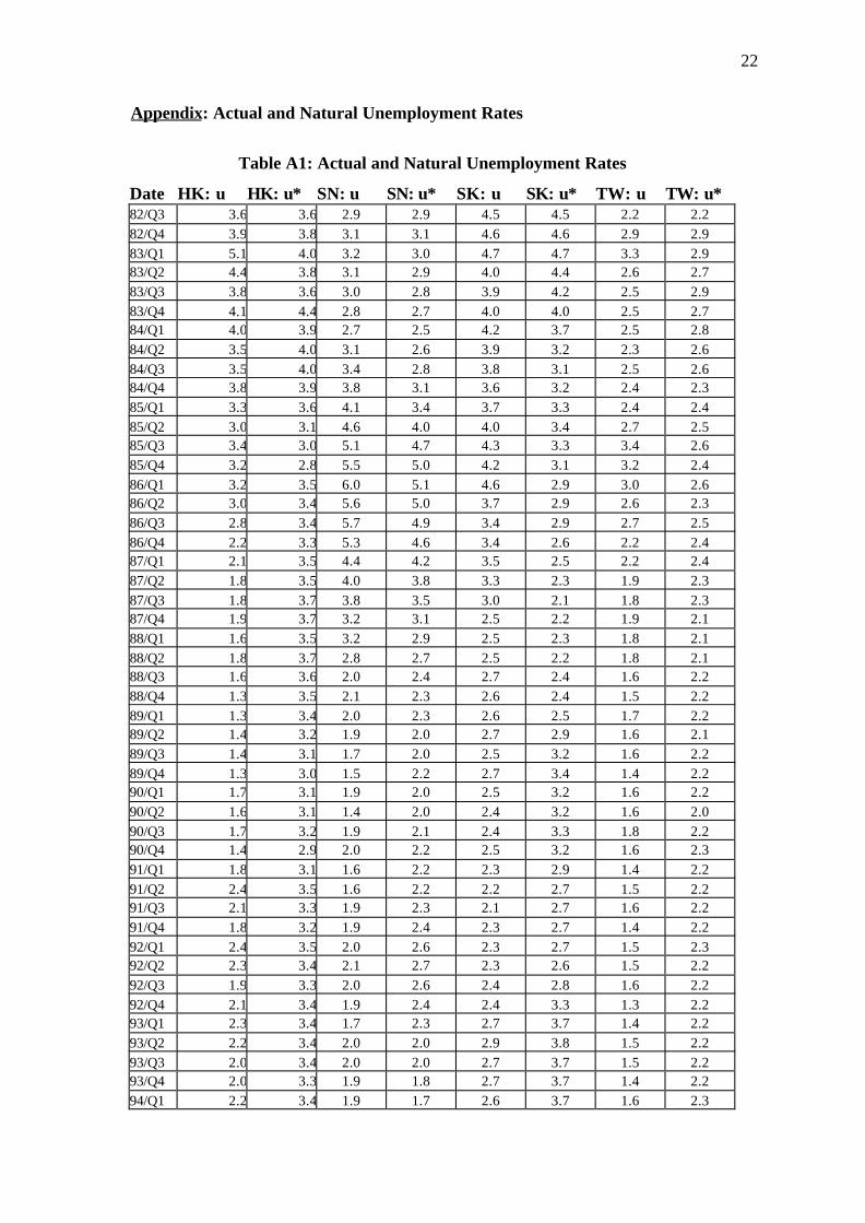
Appendix: Actual and Natural Unemployment Rates

Table A1: Actual and Natural Unemployment Rates

Date HK: u HK: u* SN: u SN: u* SK: u SK: u* TW: u TW: u*82/Q3 3.6 3.6 2.9 2.9 4.5 4.5 2.2 2.282/Q4 3.9 3.8 3.1 3.1 4.6 4.6 2.9 2.983/Q1 5.1 4.0 3.2 3.0 4.7 4.7 3.3 2.983/Q2 4.4 3.8 3.1 2.9 4.0 4.4 2.6 2.783/Q3 3.8 3.6 3.0 2.8 3.9 4.2 2.5 2.983/Q4 4.1 4.4 2.8 2.7 4.0 4.0 2.5 2.784/Q1 4.0 3.9 2.7 2.5 4.2 3.7 2.5 2.884/Q2 3.5 4.0 3.1 2.6 3.9 3.2 2.3 2.684/Q3 3.5 4.0 3.4 2.8 3.8 3.1 2.5 2.684/Q4 3.8 3.9 3.8 3.1 3.6 3.2 2.4 2.385/Q1 3.3 3.6 4.1 3.4 3.7 3.3 2.4 2.485/Q2 3.0 3.1 4.6 4.0 4.0 3.4 2.7 2.585/Q3 3.4 3.0 5.1 4.7 4.3 3.3 3.4 2.685/Q4 3.2 2.8 5.5 5.0 4.2 3.1 3.2 2.486/Q1 3.2 3.5 6.0 5.1 4.6 2.9 3.0 2.686/Q2 3.0 3.4 5.6 5.0 3.7 2.9 2.6 2.386/Q3 2.8 3.4 5.7 4.9 3.4 2.9 2.7 2.586/Q4 2.2 3.3 5.3 4.6 3.4 2.6 2.2 2.487/Q1 2.1 3.5 4.4 4.2 3.5 2.5 2.2 2.487/Q2 1.8 3.5 4.0 3.8 3.3 2.3 1.9 2.387/Q3 1.8 3.7 3.8 3.5 3.0 2.1 1.8 2.387/Q4 1.9 3.7 3.2 3.1 2.5 2.2 1.9 2.188/Q1 1.6 3.5 3.2 2.9 2.5 2.3 1.8 2.188/Q2 1.8 3.7 2.8 2.7 2.5 2.2 1.8 2.188/Q3 1.6 3.6 2.0 2.4 2.7 2.4 1.6 2.288/Q4 1.3 3.5 2.1 2.3 2.6 2.4 1.5 2.289/Q1 1.3 3.4 2.0 2.3 2.6 2.5 1.7 2.289/Q2 1.4 3.2 1.9 2.0 2.7 2.9 1.6 2.189/Q3 1.4 3.1 1.7 2.0 2.5 3.2 1.6 2.289/Q4 1.3 3.0 1.5 2.2 2.7 3.4 1.4 2.290/Q1 1.7 3.1 1.9 2.0 2.5 3.2 1.6 2.290/Q2 1.6 3.1 1.4 2.0 2.4 3.2 1.6 2.090/Q3 1.7 3.2 1.9 2.1 2.4 3.3 1.8 2.290/Q4 1.4 2.9 2.0 2.2 2.5 3.2 1.6 2.391/Q1 1.8 3.1 1.6 2.2 2.3 2.9 1.4 2.291/Q2 2.4 3.5 1.6 2.2 2.2 2.7 1.5 2.291/Q3 2.1 3.3 1.9 2.3 2.1 2.7 1.6 2.291/Q4 1.8 3.2 1.9 2.4 2.3 2.7 1.4 2.292/Q1 2.4 3.5 2.0 2.6 2.3 2.7 1.5 2.392/Q2 2.3 3.4 2.1 2.7 2.3 2.6 1.5 2.292/Q3 1.9 3.3 2.0 2.6 2.4 2.8 1.6 2.292/Q4 2.1 3.4 1.9 2.4 2.4 3.3 1.3 2.293/Q1 2.3 3.4 1.7 2.3 2.7 3.7 1.4 2.293/Q2 2.2 3.4 2.0 2.0 2.9 3.8 1.5 2.293/Q3 2.0 3.4 2.0 2.0 2.7 3.7 1.5 2.293/Q4 2.0 3.3 1.9 1.8 2.7 3.7 1.4 2.294/Q1 2.2 3.4 1.9 1.7 2.6 3.7 1.6 2.3

23

94/Q2 1.9 3.2 1.9 1.9 2.3 3.6 1.5 2.294/Q3 2.3 3.4 2.0 1.8 2.3 3.6 1.6 2.294/Q4 2.0 3.2 2.2 1.9 2.2 3.6 1.4 2.295/Q1 2.8 3.8 2.1 2.2 2.0 3.5 1.7 2.295/Q2 3.1 3.7 2.0 2.1 2.0 3.2 1.8 2.295/Q3 3.5 3.7 1.8 1.8 2.0 3.0 1.8 2.295/Q4 3.5 3.6 2.0 1.9 2.0 3.0 1.9 2.196/Q1 3.2 3.5 2.2 1.9 1.8 3.0 2.3 2.396/Q2 3.1 3.5 2.2 2.2 1.9 3.1 2.6 2.396/Q3 2.6 3.2 1.9 2.5 2.1 3.2 2.7 2.296/Q4 2.6 3.2 1.8 2.3 2.3 3.2 2.8 2.297/Q1 2.5 3.2 1.8 2.2 2.5 3.3 3.1 2.297/Q2 2.4 3.2 1.8 2.1 2.5 3.3 2.7 2.197/Q3 2.2 3.0 1.7 2.0 2.3 3.2 2.5 2.297/Q4 2.5 2.9 2.0 2.3 3.0 3.4 2.5 2.298/Q1 3.5 3.0 2.3 2.8 5.2 3.8 2.6 2.198/Q2 4.4 3.2 2.4 3.2 6.9 4.2 2.6 2.198/Q3 5.0 3.2 4.0 3.8 7.6 4.3 2.7 2.298/Q4 5.7 3.4 4.3 4.1 7.6 4.3 2.9 2.299/Q1 6.2 3.4 4.0 4.2 7.8 4.2 3.0 2.399/Q2 6.1 3.5 3.6 3.7 6.5 3.9 3.0 2.399/Q3 6.1 3.6 3.5 3.6 5.9 3.6 2.7 2.199/Q4 6.0 3.8 2.9 3.6 4.7 3.6 2.9 2.300/Q1 5.6 3.8 3.4 3.4 4.4 3.6 3.1 2.400/Q2 5.0 3.4 3.5 3.2 3.9 3.8 3.0 2.2Notes: HK = Hong Kong, SN = Singapore, SK = South Korea, TW = Taiwan, u = actualunemployment rate and u* = natural unemployment rate.