Univers

ity of

Cap

e Tow

n

THE APPLICATION OF THE SURFACE ENERGY BALANCE SYSTEM MODEL TO ESTIMATE EVAPOTRANSPIRATION IN

SOUTH AFRICA

Lesley Anne Gibson

Thesis Presented for the Degree of

DOCTOR OF PHILOSOPHY

in the Department of Environmental and Geographical Science,

Faculty of Science

UNIVERSITY OF CAPE TOWN

May 2013

The copyright of this thesis vests in the author. No quotation from it or information derived from it is to be published without full acknowledgement of the source. The thesis is to be used for private study or non-commercial research purposes only.

Published by the University of Cape Town (UCT) in terms of the non-exclusive license granted to UCT by the author.

Univers

ity of

Cap

e Tow

n

Univers

ity of

Cap

e Tow

n

i

DECLARATION

I, the undersigned, hereby declare that the work contained in this thesis is my own

original work and that this has not been previously in its entirety or in part submitted at

any university for a degree.

.

--------------------------------------------- ------------------------------

Signature Date

Univers

ity of

Cap

e Tow

n

i

ABSTRACT

In a water scarce country like South Africa with a number of large consumers of water, it

is important to estimate evapotranspiration (ET) with a high degree of accuracy. This is

especially important in the semi-arid regions where there is an increasing demand for

water and a scarce supply thereof. ET varies regionally and seasonally, so knowledge

about ET is fundamental to save and secure water for different uses, and to guarantee

that water is distributed to water consumers in a sustainable manner.

Models to estimate ET have been developed using a combination of meteorological and

remote sensing data inputs. In this study, the pre-packaged Surface Energy Balance

System (SEBS) model was used for the first time in the South African environment

alongside MODerate Resolution Imaging Spectroradiometer (MODIS) satellite data and

validated with eddy covariance data measured in a large apple orchard (11 ha), in the

Piketberg area of the Western Cape. Due to the relative infancy of research in this field in

South Africa, SEBS is an attractive model choice as it is available as open-source

freeware.

The model was found to underestimate the sensible heat flux through setting it at the

wet limit. Daily ET measured by the eddy covariance system represented 55 to 96% of

the SEBS estimate, an overestimation of daily ET. The consistent underestimation of the

sensible heat flux was ascribed to sensitivities to the land surface air temperature

gradient, the choice of fractional vegetation cover formula as well as the height of the

vegetation canopy (3.2 m) relative to weather station reference height (2 m). The

methodology was adapted based on the above findings and was applied to a second

study area (quaternary catchment P10A, near Grahamstown, Eastern Cape) where two

different approaches for deriving surface roughness are applied. It was again

demonstrated that the sensible heat flux is sensitive to surface roughness in

combination with land surface air temperature gradient and again, the overestimation of

daily ET persisted (actual ET being greater than reference ET). It was concluded that in

complex environments, at coarse resolution, it is not possible to adequately describe the

remote sensing derived input parameters at the correct level of accuracy and at the

spatial resolution required for the accurate estimation of the sensible heat flux.

Univers

ity of

Cap

e Tow

n

ii

ACKNOWLEDGEMENTS

I could not completed this thesis without the support of many individuals and

organisations. I would like to thank:

Water Research Commission for funding research projects over the years, particularly

Dr Kevin Pietersen, Dr Shafick Adams and most recently Wandile Nomquphu.

The Agricultural Research Council, my employer for the majority of this research.

Eric and Michelle Starke and Wikus Nel at Mouton’s Valley farm for allowing me to

conduct research on their property and for supplying me with weather data.

The South African Weather Service and EnviroMon Weather Service for providing

weather data.

Dr Anthony Palmer (ARC-API) and Prof Tally Palmer (Rhodes University), for their

support and encouragement.

Colleagues at ARC-ISCW: Pieter Haasbroek, Dr Thomas Fyfield, Dawie van Zyl, Terry

Newby and Dudley Rowswell

My colleagues at GEOSS for encouragement.

Lichun Wang of ITC in the Netherlands for help with SEBS in ILWIS.

Zahn Münch (University of Stellenbosch) for support and encouragement,

My supervisors Dr Frank Eckardt, UCT, Dr Caren Jarmain, UKZN and Prof Bob (Z) Su,

ITC.

To my parents for raising me to value education, to have an enquiring mind and to not

be afraid of a challenge.

And Michael, Angus and Nina.

Univers

ity of

Cap

e Tow

n

iii

TABLE OF CONTENTS

Declaration ............................................................................................................................................................ i

Abstract ................................................................................................................................................................... i

Acknowledgements .......................................................................................................................................... ii

List of Figures .................................................................................................................................................... vi

List of Tables ........................................................................................................................................................ x

List of Symbols .................................................................................................................................................. xi

List of Abbreviations .................................................................................................................................... xiv

1. Introduction ............................................................................................................................................. 1

1.1. Background to research ............................................................................................................ 5

1.2. Aims ................................................................................................................................................... 9

1.3. Thesis structure ......................................................................................................................... 10

2. Literature review ................................................................................................................................. 12

2.1. Earth observation ET studies in South Africa ................................................................ 20

2.2. SEBS in the literature ............................................................................................................... 25

2.3. SEBS formulation ....................................................................................................................... 30

3. Validation site ........................................................................................................................................ 37

4. Materials & Method ............................................................................................................................. 44

4.1. Remote sensing preprocessing ............................................................................................ 44

4.1.1. Data Selection ...................................................................................................................... 46

4.1.2. Data acquisition .................................................................................................................. 49

4.1.3. Data transformation ......................................................................................................... 49

4.1.4. Converting to radiance and reflectance.................................................................... 50

4.1.5. Atmospheric correction .................................................................................................. 51

4.2. Meteorological calculations ................................................................................................... 52

4.3. SEBS calculations ....................................................................................................................... 53

4.3.1. Albedo ..................................................................................................................................... 54

Univers

ity of

Cap

e Tow

n

iv

4.3.2. Vegetation parameters .................................................................................................... 54

4.3.3. Surface Emissivity ............................................................................................................. 55

4.3.4. Land surface temperature .............................................................................................. 56

4.3.5. Energy flux and ET calculations ................................................................................... 57

5. Results ...................................................................................................................................................... 59

5.1. Meteorology ................................................................................................................................. 59

5.2. Remotely sensed input parameters ................................................................................... 62

5.2.1. Albedo ..................................................................................................................................... 64

5.2.2. Vegetation parameters .................................................................................................... 69

5.2.3. Land surface temperature .............................................................................................. 70

5.3. Energy balance and evapotranspiration results ........................................................... 73

5.3.1. Net radiation ........................................................................................................................ 76

5.3.2. Soil heat flux ......................................................................................................................... 79

5.3.3. Sensible heat flux ............................................................................................................... 84

5.3.4. Latent heat flux ................................................................................................................... 87

5.4. Summary of results ................................................................................................................... 88

6. Model uncertainties ............................................................................................................................ 89

6.1. Study area ..................................................................................................................................... 90

6.2. Materials and methods ............................................................................................................ 92

6.3. Uncertainties in evapotranspiration estimates with SEBS....................................... 94

6.3.1. Land surface and air temperature gradient ............................................................ 95

6.3.2. Fractional vegetation cover ........................................................................................... 98

6.3.3. Zero plane displacement height ............................................................................... 102

6.3.4. Heterogeneity of the study area ............................................................................... 104

6.4. Discussion .................................................................................................................................. 109

6.5. Concluding remarks............................................................................................................... 111

7. Accounting for model uncertainties .......................................................................................... 114

7.1. Adapting the methodology ................................................................................................. 116

Univers

ity of

Cap

e Tow

n

v

7.1.1. Atmospheric effects ....................................................................................................... 116

7.1.2. Fractional vegetation cover ........................................................................................ 118

7.1.3. Reference height ............................................................................................................. 120

7.1.4. Land surface and air temperature gradient ......................................................... 120

7.1.5. Roughness lengths.......................................................................................................... 124

7.2. Results and discussion ......................................................................................................... 133

8. Application of adjusted methodology back to Mouton’s Valley field validation site .... ................................................................................................................................................................... 137

8.1. Results ......................................................................................................................................... 137

8.2. Discussion .................................................................................................................................. 141

9. Conclusions and recommendations .......................................................................................... 146

9.1. Summary of research ............................................................................................................ 146

9.2. Proposed explanations for the overestimation of ET .............................................. 151

9.3. Recommendations .................................................................................................................. 154

10. References ....................................................................................................................................... 158

Appendix 1 ...................................................................................................................................................... 170

Univers

ity of

Cap

e Tow

n

vi

LIST OF FIGURES

Figure 1: A graphical representation of the simplified surface energy balance, simplified from Su (2006)................................................................................................................................................... 4

Figure 2: Location of the study area. ...................................................................................................... 37

Figure 3: Crops grown on Mouton’s Valley farm and the location of the field validation site shown on a colour aerial photograph with field boundaries digitized from the photograph and crop information obtained from the Mouton’s Valley farm manager. .... 39

Figure 4: Recorded meteorological data for the field campaign period: a) Rainfall and radiation, b) relative humidity and air temperature and c) wind speed. ................................ 40

Figure 5: Soil water content measured at depth of 8 cm during the field campaign. ......... 41

Figure 6: Instrumentation installed at the apple orchard, a) the sonic anemometer and net radiometers clearly visible above the apple trees, b) the apple orchard from above and c) the apple orchard showing the inter-rows planted with grass and d) and e) the Moutons Valley automatic weather station (photos a-c from Jarmain & Mengistu, 2011). ................................................................................................................................................................................ 42

Figure 7: MODIS pixel footprints shown on a) an aerial photograph and b) an ASTER 321 image (22 March 2008) of the study area. ........................................................................................... 43

Figure 8: Input data, processing stages and tools required when using MOD 02 data in the SEBS model in ILWIS. ............................................................................................................................ 45

Figure 9: Flow diagram of remote sensing preprocessing steps when using MOD 02 data with numbers corresponding with section number in the text................................................... 46

Figure 10: MODIS TERRA true colour images for the dates corresponding to good quality field data. Day of year and the location of the field validation site are shown in each image. ................................................................................................................................................................... 48

Figure 11: MODIS AQUA true colour images for the dates corresponding to good quality field data. Day of year and the location of the field validation site are shown in each image8. ................................................................................................................................................................. 49

Figure 12: Example of the SEBS form in ILWIS showing all the required input data. ........ 58

Figure 13: Comparison of meteorological measurements and calculations at image capture time. ..................................................................................................................................................... 61

Figure 14: Sensor (a) and solar (b) zenith angles at time of image capture. ........................ 64

Figure 15: Sensor zenith angles against calculated albedo for a) TERRA results and b) AQUA results. .................................................................................................................................................... 64

Figure 16: Fluctuation in albedo around local noon for a vegetated area over non-bright soil (Carrer et al., 2010). .............................................................................................................................. 66

Univers

ity of

Cap

e Tow

n

vii

Figure 17: Solar zenith angles against calculated albedo. ............................................................. 67

Figure 18: Net radiation calculated for DOY 319 using MODIS AQUA data keeping all variables constant but adjusting albedo values. ................................................................................ 68

Figure 19: NDVI calculated using TERRA & AQUA data. ..................................................... 70

Figure 20: Land surface temperature calculated using TERRA & AQUA data. ...................... 70

Figure 21: Air temperature (Ta) at image capture time plotted against land surface temperature (LST) obtained from MODIS and SEVIRI. ................................................................... 72

Figure 22: SEVIRI T0 minus SEBS calculated T0 from MODIS plotted against solar and sensor zenith angles showing no correlation between zenith angles and T0. ....................... 73

Figure 23: SEBS ET plotted against field measured ET plus and minus a 30 % error. ...... 74

Figure 24: Net radiation as measured in the field for days of image capture (grey lines) with the time of each satellite image capture shown as a black square. ................................. 76

Figure 25: The MODIS TERRA (a) & AQUA (b) SEBS estimated instantaneous net radiation as a function of field measured net radiation for days on which MODIS images were acquired. ................................................................................................................................................. 78

Figure 26: The MODIS TERRA (a) and AQUA (b) SEBS calculated instantaneous radiation plotted against field validation data with 10% errors bars shown on the field validation measurements.................................................................................................................................................. 79

Figure 27: TERRA (a) & AQUA (b) SEBS soil heat flux (G0) against field measured values. ................................................................................................................................................................................ 81

Figure 28: The soil heat flux as measured in the field for days of image capture (grey lines) with the time of each satellite image capture shown as a black square. ..................... 82

Figure 29: Net radiation minus soil heat flux as calculated using SEBS with MODIS TERRA data (a), MODIS AQUA data (b,) compared with the field validation data. Ten percent error bars are shown on the field validation calculation. ............................................. 83

Figure 30: TERRA (a) & AQUA (b) SEBS sensible heat flux (H) against field measured values. .................................................................................................................................................................. 85

Figure 31: The sensible heat flux as measured in the field for days of image capture (grey lines) with the time of each satellite image capture shown as a black square. .................................................................................................................................................. 86

Figure 32: The latent heat flux as measured in the field for days of image capture (grey lines) with the time of each satellite image capture shown as a black square. ..................... 87

Figure 33: Orientation map showing the G10K catchment, the Mouton’s Valley field validation site and the weather station Piketberg: Pools-Ideal Hill (shown as Pools-Ideal Hill) situated in a dryland agricultural area which was used for experimental purposes. ................................................................................................................................................................................ 91

Univers

ity of

Cap

e Tow

n

viii

Figure 34: Sensitivity of SEBS-estimated daily ET to Δ(T0 – Ta) the Mouton’s Valley field validation site and the Piketberg: Pools-Ideal Hill site. .................................................................. 96

Figure 35: NDVI distribution for the study area for a winter wet season scene (DOY 193) and a summer dry season scene (DOY 324). ....................................................................................... 99

Figure 36: Sensitivity of SEBS-estimated ET to a range in fractional vegetation cover input values for the apple orchard field validation site. fc values resulting from specific formulae and methods are indicated. .................................................................................................. 101

Figure 37: Sensitivity of SEBS-estimated ET to d0 for the Mouton’s Valley field validation site when wind speed is measured at 2m. ......................................................................................... 103

Figure 38: SEBS derived ET from ASTER data shown in the context of two MODIS pixels for both the Mouton’s Valley site (above) and the Piketberg: Pools-Ideal Hill site (below). ............................................................................................................................................................................. 105

Figure 39: P10A study area. .................................................................................................................... 115

Figure 40: An example of top of atmosphere radiation versus surface shortwave radiation at the same location. ............................................................................................................... 117

Figure 41 Difference in sensible heat flux results when using the LAI or NDVI approach to calculate the fractional vegetation cover. The results obtained with using the NDVI approach are subtracted from the results obtained with the LAI approach (Gibson et al., 2011). ................................................................................................................................................................ 119

Figure 42: Sensible heat flux calculated using TERRA and AQUA data on the same day plotted against T0-Ta. .................................................................................................................................. 123

Figure 43: Dependence of roughness length and displacement height on height and density of roughness elements (e.g. trees) (Kipp & Zonen, 2005). ......................................... 125

Figure 44: The process of allocating z0 and d0 values in the P10A catchment (plus 1 km buffer) a. Modified land cover map, b. land cover by MODIS pixel, c. Allocated roughness lengths and d. Zero plane displacement heights. Note that the labels A, B, and C on Figure 44a indicate the locations at which photographs in Figure 45 are taken. ........................... 127

Figure 45: Land covers and assigned z0 values from the literature. a: Shrubland (South) more accurately described as grassland. b: Shrubland (North) and c: Thickets and bush clumps. ............................................................................................................................................................. 128

Figure 46: Sensitivity of sensible heat flux to z0 and T0 - Ta across the entire P10A catchment. H_1: z0 is set to 1m; H_2, z0 is set to 0.5m; and H_3, z0 is set to 0.1m. a) Summer scene DOY 017: sensitivity of H to z0 increases with increasing T0 - Ta. b) Winter scene, DOY 217: sensitivity of H to z0 is non-linear around T0 - Ta =0. c) Winter scene, DOY 185: the slope is negative in this instance indicating that the wet limit has been reached at low T0 - Ta. ................................................................................................................................ 130

Figure 47: Comparison of z0 literature values to z0 values from NDVI for DOY 185, 217 and 017. ........................................................................................................................................................... 132

Univers

ity of

Cap

e Tow

n

ix

Figure 48: Comparison of z0 literature values to z0 values derived from NDVI for H results plotted against T0 - Ta for DOY 185, 217 and 017. .......................................................... 133

Figure 49: Catchment average ET calculated for P10A using the SEBS model with AQUA and TERRA data and plotted against ET0 calculated from the Rockhurst weather station for the study period (July 2006-June2007) ...................................................................................... 134

Figure 50: AQUA SEBS ET results for each date processed for the P10A catchment plotted against T0 - Ta. ................................................................................................................................ 135

Figure 51: AQUA SEBS evaporative fraction results for each date processed for the P10A catchment plotted against T0 - Ta. .......................................................................................................... 135

Figure 52: Impact of NDVImax value in the fc calculation in daily ET estimation in SEBS for TERRA data. ................................................................................................................................................... 138

Figure 53: SEBS ET, after the methodology was adapted, plotted against field measured ET. Note: only TERRA results were processed. ............................................................................... 141

Figure 54: Daily ET calculated using NDVI derived z0m, a literature value for z0m and the field validation value, plotted against T0 – Ta. .................................................................................. 143

Figure 55: Explanation for underestimation of H in SEBS. a) Non-water stressed environment, b) Water stressed environment. ............................................................................... 145

Univers

ity of

Cap

e Tow

n

x

LIST OF TABLES

Table 1: A list of selected ET assessment methods based on earth observation techniques simplified from Verstraeten et al. (2008). ............................................................................................ 13

Table 2: Spatial, spectral and temporal characteristics of satellite sensors .......... 16

Table 3: Summary of studies conducted in South Africa. Different methods for estimating ET were assessed and their usefulness in various water resources applications and across various spatial and temporal scales were assessed in historical and operational mode. .................................................................................................................................. 21

Table 4: Chronological summary of SEBS publications. ................................................................. 26

Table 5: Validation, reported accuracies and SEBS model sensitivities. ................................. 26

Table 6: MODIS bands required for evapotranspiration estimation. ........................................ 50

Table 7: Inputs required for SMAC. ......................................................................................................... 51

Table 8: Meteorological recordings and calculations at image capture time. ....................... 60

Table 9: MODIS TERRA and AQUA pre-processing results. .......................................................... 62

Table 10: Selected typical albedo values (Brutsaert, 1982). ........................................................ 65

Table 11: T0 results from SEBS compared with the Meteosat SEVIRI T0 product. ............... 71

Table 12: MODIS AQUA & TERRA energy balance results and corresponding field measurements (# = no data). ..................................................................................................................... 75

Table 13: Sequence of SEBS processing (adapted from Su et al., 2008). ................................. 92

Table 14: Heterogeneity of Mouton’s Valley field validation site vs. Piketberg: Pools-Ideal Hill site illustrated by mean and standard deviation of DEM, NDVI and T0. ........................ 106

Table 15: Comparison of energy partitioning in MODIS pixels for more heterogeneous Mouton’s Valley field validation site: mean ASTER value per pixel vs. MODIS pixel value. ............................................................................................................................................................................. 107

Table 16: Comparison of energy partitioning in MODIS pixel for more homogeneous Piketberg: Pools-Ideal Hill site: mean ASTER value per pixel vs. MODIS pixel value. ..... 108

Table 17: Land use classes in the PELCOM land use database and associated z0 values adapted from Su (2006). ........................................................................................................................... 126

Table 18: SEBS TERRA results comparison by increasing NDVImax from 0.5 to 0.65 in fc calculation (Equation 17]). ...................................................................................................................... 138

Univers

ity of

Cap

e Tow

n

xi

Table 19: z0m, h0 and d0 for each image calculated from NDVI and NDVImax. ....................... 139

Table 20: SEBS MODIS TERRA results for the NDVI method to estimated z0m and the literature value for z0m (0.6) compared with field validation results (using adjusted NDVImax in fractional vegetation cover formula). ........................................................................... 140

APPENDIX 1

Table A1: MODIS instrument specifications (http://modis.gsfc.nasa.gov/about/design.php).............................................................................172

Table A2: MODIS data specifications (http://modis.gsfc.nasa.gov/about/design.php) …………………………………………………………………………………………………………….........................173

Table A3: MODIS reflective solar bands (RSB) key specifications (typical scene radiance, and SNR) with TERRA and AQUA MODIS on-orbit measured SNR (adapted from Xiong et al., 2002a)………………………………………………………………………………………………..…………….174

Table A4: MOD 02 and MYD 02 data used in this research………………..………………………174

Univers

ity of

Cap

e Tow

n

xii

LIST OF SYMBOLS

Surface albedo -

a1 Constant lapse rate of moist air 0.0065 K.m-1

B–1 Inverse Stanton number -

Cd Drag coefficient of the foliage elements -

Cp Specific heat capacity of air at constant pressure J.g-1

.K-1

Ct* Heat transfer coefficient of the soil -

d0 Displacement height m

E Water vapour flux density J·m−2

·s−1

Surface emissivity -

ea Actual vapour pressure kg·m−1

·s−2

es Saturated vapour pressure kg·m−1

·s−2

fc Fractional vegetation cover -

fs Complement of fractional vegetation cover -

g Acceleration due to gravity m.s-2

G0 Soil heat flux W.m-2

H Sensible heat flux W.m-2

h0 Height of the vegetation m

Hdry Sensible heat flux at the dry limit W.m-2

hs Roughness height of the soil m

Hwet Sensible heat flux at the wet limit W.m-2

k von Karman’s constant -

K↓day Daily incoming shortwave radiation W.m-2

L Obukhov length m

Lday Daily longwave radiation W.m-2

N Number of sides of the leaf to participate in heat exchange -

nec Within canopy wind speed profile extinction coefficient -

p Ambient pressure kPa

P Atmospheric pressure at elevation z kPa

P0 Atmospheric pressure at sea level kPa

Pr Prandtl number -

Pv Proportional vegetation cover -

R Specific gas constant -

Re* Reynolds number -

Univers

ity of

Cap

e Tow

n

xiii

rew External resistance at the wet limit Ω

Rlwd Downward longwave radiation W.m-2

Rn Net radiation W.m-2

Rswd Incident shortwave radiation W.m-2

T Ambient temperature K

T0 Land surface temperature K

Ta Air temperature K

TK0 Reference temperature (K) at elevation z K

u Wind speed m.s-1

u(h) Horizontal wind speed at the canopy top m.s-1

u* Friction velocity m.s-1

V Kinematic viscosity of the air m2.s

-1

Z Height above the surface m

z0 Surface roughness m

z0h Scalar height for heat transfer -

z0m Roughness height for momentum transfer m

Γ Psychrometric constant -

Γc Soil heat flux ratios for full vegetation canopy -

Γs Soil heat flux ratios for bare soil -

Δ Rate of change of saturation vapour pressure with temperature

kPa °C-1

θ0 Potential temperature at the surface K

θa Potential air temperature at height z K

θv Potential virtual temperature near the surface K

Λ Latent heat of vaporization W.m-2

Λ Evaporative fraction -

Λr Relative evaporation -

λE Latent heat flux W.m-2

λEwet

Latent heat flux at the wet limit W.m-2

Ρ Density of air kg.m-3

ρw Density of water kg.m-3

Σ Stephan–Boltzman constant -

Ψh Stability correction functions for sensible heat

Ψm Stability correction functions for momentum

Daily net radiation W.m-2

Univers

ity of

Cap

e Tow

n

xiv

LIST OF ABBREVIATIONS

ARC Agricultural Research Council

ARC-ISCW Agricultural Research Council - Institute for Soil, Climate and Water

ASTER Advanced Spaceborne Thermal Emission and Reflection Radiometer

AWS Automatic weather stations

CSIR Council for Scientific and Industrial Research

DEM Digital elevation model

DOY Day of year

EF Evaporative fraction

EMR Electromagnetic radiation

EOS Earth Observing System

ET Evapotranspiration

ILWIS Integrated Land and Water Information System

LAI Leaf area index

LST Land surface temperature

METRIC Mapping EvapoTranspiration with high Resolution and Internalised Calibration

MODIS MODerate Resolution Imaging Spectroradiometer

MSG Meteosat Second Generation

MST MODIS Swath Tool

NDVI Normalised Difference Vegetation Index

NPOESS National Polar-orbiting Operational Environmental Satellite System

NPP NPOESS Preparatory Project

PELCOM Pan-European Land Use and Land Cover Monitoring

SAWS South African Weather Service

SEBAL Surface Energy Balance Algorithm over Land

SEBI Surface Energy Balance Index

SEBS Surface Energy Balance System

SEVIRI Spinning Enhanced Visible and InfraRed Imager

SMAC Simplified method for atmospheric correction

SNR Signal-to-noise ratio

SRTM Shuttle Radar Topography Mission

SWIR Shortwave infrared

TOA Top of atmosphere

UT Universal Time

VITT Vegetation Index/Temperature Trapezoid

WetSpass Water and Energy Transfer between Soil, Plants and Atmosphere under quasi Steady State WGS84 World Geodetic System 1984

WRC Water Research Commission

Univers

ity of

Cap

e Tow

n

1

1. INTRODUCTION

With an average rainfall of less than 500mm per annum and much of the land considered semi-arid,

South Africa is a water stressed country. The country has various climatic zones from semi-desert to

tropical and is prone to erratic, unpredictable extremes in the form of droughts and floods. The average

potential evaporation is higher than the rainfall in all but a few isolated areas where rainfall exceeds

1400mm per year (Burger, 2003). This low precipitation / high evaporation rate results in low runoff

with only 8.6% of the rainfall being available as surface water. Furthermore, owing to the uneven

spatial distribution of rainfall across the country, the natural availability of water is also highly uneven

with nearly two-thirds of the country receiving less than the national average.

South Africa has well-developed commercial agriculture with the agro-industrial sector comprising

15% of the country’s gross domestic product (Burger, 2005). Subsistence farming is also practised

resulting in a dual agricultural economy. Only about 13% of South Africa’s land surface can be used for

crop production with high-potential arable land comprising only 22% of the total arable land. For

dryland agriculture to be successfully practised, 500mm of rainfall per annum is required (Turton et al.,

in NASA, 2005) so one of the limiting factor in crop production is the availability of water. The

consequence of this, coupled with the erratic nature of the country’s rainfall, is that many farmers in

South Africa rely on irrigation in order to be commercially successful. Irrigated agriculture is by far the

biggest single user of run-off water in South Africa and contributes more than 30% of the gross value of

the country’s crop production with about 90% of the country’s fruit, vegetables and grapes being

produced under irrigation (Burger, 2011).

Given this water scarce scenario, it is important for managers to have accurate information of all

aspects of water resource management including water use by crops and natural vegetation in a

catchment. Evapotranspiration (ET1) is the sum of water lost to the atmosphere from the soil surface

(including intercepted water) through evaporation and from plant tissues via transpiration and is a

vital component of the water cycle, which includes precipitation, runoff, stream flow, soil water storage

1 ET throughout this text refers to actual evapotranspiration unless specific reference is made to reference evapotranspiration in which case the abbreviation will be ET0

Univers

ity of

Cap

e Tow

n

2

and ET (Mu et al., 2007). This combined process whereby water is lost from the soil surface by

evaporation and from the plant by transpiration occurs simultaneously and it is difficult to distinguish

between the two processes. With the exclusion of water availability, evaporation is mainly a function of

the fraction of solar radiation reaching the soil surface and this is largely determined by plant canopy

(Allen et al., 1998). Water loss during transpiration through the stomata on the leaf is dependent on the

genetics and stage in growth of the plant as well as external factors such as radiation, air temperature

and humidity, and wind.

The dependency of the physical process of evaporation, whereby a liquid (water) is transformed to a

gas (water vapour), on water availability and incoming solar radiation, reflects the interactions between

surface water processes and climate (Sobrino et al., 2007). In meteorology, evaporation is usually

restricted to the change of a liquid to gas without a change in temperature. Sensible heat is that part of

the energy flux from a surface which produces a temperature change and this must be distinguished

from latent energy which is used to describe the evaporation process. Evaporation is a cooling process

since there is a removal of energy when water evaporates from a surface. Part of this energy remains

latent in the atmosphere and is released when water vapour condenses. Water vapour is therefore an

energy carrier and energy must be available to allow the water to evaporate (Savage et al., 2004).

Accurate knowledge of temporal and spatial variations in precipitation and ET is critical for improved

understanding of the interactions between land surfaces and the atmosphere (Mu et al., 2007), and

owing to increasing human consumption, climate impacts and decreasing availability, methods for

monitoring the water balance at both fine and regional scales are important in order to preserve and

manage water resources (Melesse et al., 2006). However, precipitation and ET are the most problematic

components of the water cycle to estimate accurately because of the heterogeneity of the landscape and

the large number of controlling factors involved, including climate, plant biophysics, soil properties, and

topography (Mu et al., 2007).

The accurate estimation of ET remains a challenge to researchers in the field of micrometeorology and

hydrology as well as for water resources managers and planners (Jarmain et al., 2009). ET can be

measured or estimated using empirical formulae from taking measurements in the field or more

indirectly rather than as a result of a specific evapotranspiration experiment. The field based

Univers

ity of

Cap

e Tow

n

3

measurements are generally point based and therefore not practical over a large area. Internationally it

is now recognised that remote sensing based models hold great potential for the spatial estimation of

ET at both field and catchment scale and earth observation data can be used in ET estimation methods

to extend point measurement of ET to much larger areas, even areas where measured meteorological

data may be sparse (Jarmain et al., 2009).

One method used to estimate ET is as residual in the surface energy balance. The net incoming solar

radiation at any location is converted into heat energy, heating the air above the soil surface, the plant

canopy and the soil itself, and into latent heat of evapotranspiration from the soil surface and plant

canopy. If the net incoming radiation and the energy consumed in heating the air and the soil can be

measured, then the latent heat of evaporation from the soil can be estimated and the rate of evaporation

of water deduced (Blight, 2002). These exchanges of energy or heat are called fluxes. The estimation of

these fluxes at the land surface has long been recognized as the most important process in the

determination of the exchanges of energy and mass among hydrosphere, atmosphere and biosphere

(Su, 2002).

The sources of energy in the soil-plant-atmosphere system include:

Solar energy during the day and terrestrial radiant energy at night;

Heat energy carried into the area by wind (advected energy);

Heat energy stored by vegetation and in land masses;

Heat energy stored in water bodies.

The most important of these energy sources is usually solar energy which is why the energy balance

used in this research is referred to as the simplified energy balance i.e. advected energy is excluded but

advected energy may on occasion be considerable. However, due to its complex nature, advected energy

is not routinely accounted for when using methods to estimate surface sensible heat and latent energy

flux densities (Savage et al., 2004).

Univers

ity of

Cap

e Tow

n

4

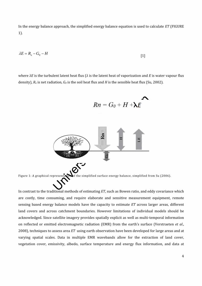
In the energy balance approach, the simplified energy balance equation is used to calculate ET (FIGURE

1).

HGRE n 0 [1]

where λE is the turbulent latent heat flux (λ is the latent heat of vaporization and E is water vapour flux

density), Rn is net radiation, G0 is the soil heat flux and H is the sensible heat flux (Su, 2002).

Figure 1: A graphical representation of the simplified surface energy balance, simplified from Su (2006).

In contrast to the traditional methods of estimating ET, such as Bowen ratio, and eddy covariance which

are costly, time consuming, and require elaborate and sensitive measurement equipment, remote

sensing based energy balance models have the capacity to estimate ET across larger areas, different

land covers and across catchment boundaries. However limitations of individual models should be

acknowledged. Since satellite imagery provides spatially explicit as well as multi-temporal information

on reflected or emitted electromagnetic radiation (EMR) from the earth’s surface (Verstraeten et al.,

2008), techniques to assess area ET using earth observation have been developed for large areas and at

varying spatial scales. Data in multiple EMR wavebands allow for the extraction of land cover,

vegetation cover, emissivity, albedo, surface temperature and energy flux information, and data at

Univers

ity of

Cap

e Tow

n

5

regional scales allow for greater spatial coverage than is possible with in situ methods (Melesse et al.,

2006). However, multiple datasets such as the abovementioned albedo, emissivity etc. must be available

or able to be generated, at appropriate spatial and temporal scales, in order to run a model based on

this approach.

Recent developments in remote sensing technologies have led to the possibility of obtaining land

surface information at spatial resolutions from 0.5m – 5km, with frequent revisit times (up to every 15

minutes). The degree of success and accuracy of that information varies; however some authors

(Bastiaanssen et al., 2006; Bastiaanssen & Bos, 1999) report that remote sensing has many advantages

such as the objectivity and repeatability of the measurements, the synoptic nature of data, and spatial

representivity of the data. With these recent advances in remote sensing have come many different

approaches and techniques for estimating evaporation using earth observation data. Some of these

approaches will be discussed in Chapter 2 in the literature review.

1.1. BACKGROUND TO RESEARCH

Accurate estimates of temporal and spatial variations in precipitation and evapotranspiration (ET) are

critical for improved understanding of the interactions between land surfaces and the atmosphere

(Mu et al., 2007). Methods for monitoring the water balance at both local and regional scales are

required to preserve and manage water resources (Melesse et al., 2006). In a water scarce country like

South Africa with a number of large consumers of water, it is important to estimate ET with a high

degree of accuracy. This is especially important in the semi-arid regions where there is an increasing

demand for water and a scarce supply thereof. ET varies regionally and seasonally, so knowledge of ET

is fundamental to save and secure water for different uses, and to guarantee that water is distributed to

water consumers in a sustainable manner.

The South African National Water Act of 1998, undertaking “some for all for always” and legislating that

ecological reserves be calculated before new water licences be granted for other uses, is aimed at

allowing for equitable distribution of water resources, including an allocation to the environment. In

order to manage this allocation process, managers and decision makers require information. Remote

Univers

ity of

Cap

e Tow

n

6

sensing technology holds great promise in this regard (Jha & Chowdary, 2006) as it can cost-effectively

provide frequent data on a relatively large scale that allow specific water resource situations to be

monitored on a long-term basis.

In the South African context, in irrigated areas, actual ET can be equated to the water usage of a crop. By

using remote sensing techniques to estimate ET, it is possible to acquire spatial estimates of actual

water use across large areas. In terms of the National Water Act this information can be used in the

validation and verification of existing lawful water use and can aid in the issuing of new licences, since

the water use at catchment scale may be estimated. Further to this, farmers may use this water use

information to analyse the water use between crops and even within fields to identify areas of high

water consumption and to better manage their water usage and irrigation efficiency.

The water use between biomes and different natural vegetation types can be assessed using spatial

estimates of ET. Catchment managers may find it useful to understand water use variation of natural

vegetation within a catchment and between, for example, indigenous vegetation and invasive alien plant

species (IAPs). This can guide planning for the removal of IAPs in terms of determining priority areas

and time frames.

Spatial estimates of ET may be used to complement the results of, or be used as input into, hydrological

models to help better understand the hydrological or geohydrological regime in an area (Münch et al,

2013). Finally the change in ET over time can be used to assess the change in water availability in a

region. This information may be useful in climate change studies and help analyse drought length and

intensity.

Given that, in South Africa, research into remote sensing ET estimation is in its infancy, together with

the legislative framework (National Water Act of 1998), it is logical that preliminary research efforts

should focus on the evaluation of existing models rather than the development of new models. Should

an existing model be found to yield accurate estimates of ET, the assimilation of these estimates into

existing monitoring programmes such as the drought monitoring programme

(http://www.amesd.org/sadc.html) will have been expedited.

Univers

ity of

Cap

e Tow

n

7

This research arose from a Water Research Commission (WRC) funded project (Gibson et al., 2009)

where earth observation data were used to determine various water fluxes. The Surface Energy Balance

System (SEBS) model was used to calculate annual ET with MODerate Resolution Imaging

Spectroradiometer (MODIS) satellite data for a quaternary catchment in the Piketberg area (Western

Cape). Through a simplified water balance (with annual ET as one of the input) the legal compliance of

water users to water use legislation was assessed. The results of the study were inconclusive as the

estimated annual catchment ET significantly exceeded the estimated annual catchment rainfall. Gibson

et al. (2009) proposed that the inaccuracies in the water use results were due to many uncertainties

and limitations with both the input data and the methodology associated with the estimation of all

water fluxes. However the largest uncertainty was attached to the ET estimate.

The lack of confidence in the annual ET estimate by Gibson et al. (2009) was due to the estimated

catchment ET from the SEBS model for the study period (a hydrological year) being nearly twice the

estimated rainfall for the same catchment for the same period. This assumed overestimation of SEBS

estimated ET was further highlighted when the results of an alternative model (Batelaan &

De Smedt, 2001), Water and Energy Transfer between Soil, Plants and Atmosphere under quasi Steady

State (WetSpass), were analyzed. In the SEBS model, the amount of ET is constrained by the available

energy with available moisture being inferred from parameters such as vegetation cover and the

differences between the land surface and air temperature. The ET estimated by the WetSpass model is

constrained by the amount of precipitation which fell in the catchment and since it is based on a water

balance, the amount of ET may not exceed the amount of precipitation. Interestingly, the results of both

methods across a hydrological year in the Gibson et al. (2009) study reflected the constraining factor of

their approaches respectively. Using the WetSpass model resulted in higher estimated ET in the winter

months where there was high water availability and using the SEBS model resulted in higher ET in the

summer months when there is high energy availability. Although it may be possible for annual ET to

exceed annual precipitation in certain instances, such as where large-scale irrigation from upstream or

groundwater resources is practised, it is believed that ET was overestimated as evidence pointed

towards there being limited water availability during the hot, dry summer months. Since irrigated

agriculture formed a small portion of the catchment (2.4%) in comparison to natural vegetation

(29.7%) and dryland agricultural (66.5%), the higher ET than precipitation at catchment scale could not

be ascribed to evaporative losses due to irrigation.

Univers

ity of

Cap

e Tow

n

8

Arising from Gibson et al. (2009) was the need to fully validate and analyse the ET results from the SEBS

model within a South African environment. Due to the complexity of the model, there are therefore

many opportunities for errors and uncertainties to be introduced. This needs to be analysed, tested and

documented in the South African environment. This research seeks to address this need. Should it be

possible to accurately model spatial estimates of ET across large areas using free software and data,

then the operational monitoring of water use for many aspect of water resource management will be

feasible.

Since the field validation funding was tied to the WRC research project by Gibson et al. (2009), the field

validation had to take place within the study area and more specifically the pilot study area selected by

Gibson et al. (2009). Furthermore, since the research has been partially funded by the Agricultural

Research Council, the validation site was required to have an agricultural land use. A large apple

orchard (11 ha) on the farm Mouton’s Valley, within the pilot study area of Gibson et al. (2009), was

chosen as the site for the field validation. This site was selected due to size of the orchard and the

location of an automatic weather station situated just outside the orchard.

The most valuable lesson learnt has been around the complexity of the ET estimation using the SEBS

model. The SEBS model is available as open-source freeware and it can be used by practitioners with

remote sensing knowledge who may not necessarily have the micrometeorological expertise to develop

a model themselves. However, the derivation of ET using the SEBS model is a complex process requiring

several sources of input data and numerous processing steps to derive intermediate output products.

The intermediate products are then combined through additional processing algorithms to derive the

final daily ET product. Whilst the open-source format of SEBS is very useful and can speed up the

research process, there are some instances where specialist knowledge is required to implement the

model correctly to derive the most accurate results. Finally, the SEBS model was initially developed for

agricultural applications and although it has been applied across many land covers (as will be shown in

Chapter 2.2), it may be that less accurate results are produced in areas of natural veld or dryland

agriculture.

Univers

ity of

Cap

e Tow

n

9

1.2. AIMS

The broad aim of this research is to implement the pre-packaged SEBS model in ILWIS in the South

African environment with MODIS TERRA and AQUA data. As a pre-packaged software is accessible to

remote sensing practitioners who may not have specific energy balance expertize, it is important for the

pre-packaged version of SEBS to be tested before large scale roll-out (for operational, research or

monitoring purposes) is implemented. Therefore the aim is to compare, analyse and validate the results

with field measured eddy covariance data, elucidate model sensitivities and make recommendations on

the future use of the pre-packaged SEBS model.

The specific objectives of this research are to:

1. Apply the pre-packaged SEBS model in ILWIS to the field validation site.

2. Compare and analyse results obtained from daily MODIS TERRA (MOD 02) and MODIS AQUA

(MYD 02) data for:

a. the calculated remotely sensed parameters (albedo, vegetation parameters, emissivity

and land surface temperature) which are required as input into the SEBS model;

b. the energy balance and ET calculations using the pre-package SEBS model in ILWIS;

3. Validate the energy balance and evapotranspiration results with field measured data;

4. Analyse and explain the results and identify potential sources of error or model sensitivities.

The above objectives are met through the course of this research. Conclusions and recommendations

regarding the future use of the pre-packaged SEBS model in South Africa are made.

Univers

ity of

Cap

e Tow

n

10

1.3. THESIS STRUCTURE

The structure of the thesis is built around fulfilling the objectives of the research. Firstly, a literature

review to set the scene and explain key concepts is set out in Chapter 2. Particular reference is made to

the current status of remote sensing ET estimation in South Africa (Chapter 2.1), SEBS references in the

literature (Chapter 2.2) and the formulation from literature of the SEBS model (Chapter 2.3).

Chapter 3 describes the validation site and methodology - conducted by the CSIR (Jarmain & Mengistu,

2011)- used to validate the results of this research.

In fulfillment of Objective 1, Chapter 4 provides a detailed method and the materials used focussing on

the remote sensing aspects, (Chapter 4.1), the meteorological requirements (Chapter 4.2) and finally

the SEBS calculations (Chapter 4.3).

In Chapter 5, the first results of the research are presented. Chapter 5.1 presents the results of required

meteorological calculations, Chapter 5.2 fulfils Objective 2a by presenting the results of the remote

sensing input parameters such as albedo, vegetation inputs and land surface temperature. Objective 2b

and Objective 3 are met in the energy balance and ET results presented in Chapter 5.3.

Objective 4 is met in Chapters 6 -8 where the sensitivity of the SEBS model to various input parameters

is explored. Chapter 6 primarily consists of a paper (published in Hydrological and Earth Systems

Sciences) where model uncertainties and sensitivities are explored. This paper has been edited in this

thesis to improve it. Chapter 7 accounts for model sensitivities by describing adaptions to the

methodology and the results when the SEBS model was applied to a different catchment in the Eastern

Cape. The study area for Chapter 7 is different to the rest of the thesis as it was important to test the

SEBS model under different environmental conditions in light of the model uncertainties and

sensitivities which are uncovered.

Univers

ity of

Cap

e Tow

n

11

To bring the research to a close, the factors which may affect the accuracy of the results are taken into

account and the original research methodology is adapted and applied back to the field validation site at

Mouton’s Valley. The results of the adapted methodology are presented in Chapter 8 where it is shown

that despite the changes in the methodology, the estimated ET remains higher than the field validation

measurements.

The thesis is concluded in Chapter 9 with a summary of research finding (Chapter 9.1), conclusions

(Chapter 9.2) and recommendations for the use of SEBS and ET estimation in South Africa (Chapter 9.3).

Univers

ity of

Cap

e Tow

n

12

2. LITERATURE REVIEW

For the past few years, there has been interest in the scientific community in estimating ET by remote

sensing, since it is a unique way to retrieve ET at several temporal and spatial scales (Sobrino et al.,

2007). There have been many techniques published but this review will focus on the techniques used in

this research, that is, the energy balance approach and specifically the Surface Energy Balance System.

However reference is made to various review papers (Courault et al., 2005; Overgaard et al., 2006;

Gowda et al., 2007; Kalma et al., 2008; Verstraeten et al., 2008; Petropoulos et al. 2009) where the

status of earth observation ET models and broad descriptions of the various techniques are given.

Courault et al. (2005) provide an overview of work done in the international community over the last

25 years related to evapotranspiration estimation from earth observation data; Overgaard et al. (2006)

review the different types of energy-based land-surface models and the potential of linking these to

distributed hydrological models; Kalma et al. (2008) focus on the use of remotely sensed surface

temperatures in ET estimation; Petropoulos et al. (2009) examine surface temperature/ vegetation

indices methods in retrieving land surface energy fluxes; and Verstraeten et al. (2008) assess

evaporation methods across different scales of observation, from leaf scale (e.g. porometry) or point

scale (e.g. lysimetry), to field scale (e.g. eddy covariance and scintillometry), landscape/ catchment scale

(e.g. mass water balance and energy balance) and finally continental scale where only the earth

observation energy / mass water balance is possible.

ET estimation methods based on earth observation techniques can be classified according to the

concept on which they are based. Verstraeten et al. (2008) identify four concepts and classify the

various models (Table 1) according to these concepts which are identified as:

(i) the parameterization of the surface energy balance;

(ii) the Penman-Monteith equation;

(iii) the water balance approach, or;

(iv) relationships between vegetation indices and land surface temperature assessed with earth

observation data.

Univers

ity of

Cap

e Tow

n

13

Table 1: A list of selected ET assessment methods based on earth observation techniques simplified from Verstraeten et al. (2008).

Concept Method Parameters Selected references

EO Other

Parameterisation of the energy balance

SEBAL (Surface Energy Balance Algorithm for Land)

T0, , NDVI

Ta, u, , RH, z0 Bastiaanssen et al, (1998), Bandara (2006), Timmermans et al. (2007)

SEBS (Surface Energy Balance System)

T0, , NDVI

Ta, u, , LAI, ea

& esat,, z0 Su (2002), Jia et al (2003)

S-SEBI (Simplified- Surface Energy Balance Index) iNOAA (ET of European forests from NOAA-imagery)

T0, , NDVI

Ta, , (RH) Roerink et al. (2000)

Penman-Monteith (PM) based

Trapezoidal Shape (Relationship between land surface temperature and vegetation indices used to estimate ET)

T0,

SAVI Ta, , vpd, LAI Moran et al. (1994), Moran et al. (1997)

Wang (Combination of day and night land surface temperatures with NDVI)

T0,, VI

Meteorological data Wang et al. (2006)

Cleugh (remote sensing inputs into PM equation)

, VI Meteorological data Cleugh et al. (2007)

Water balance based SWAP (Soil, water, atmosphere, plant)

, VI Meteorological, soil, groundwater table data

Santhi et al. (2005), Kaur et al. (2003)

VI/LST based Jackson (Relationship between VI and Land surface

temperature)

T0, VI Ta, u, calibration coeff. Jackson et al (1977) (In Verstraeten et al. (2008)

Univers

ity of

Cap

e Tow

n

14

According to Verstraeten et al. (2008), with the exception of the parameterization of the surface energy

balance which is based entirely on earth observation derived parameters and meteorological data,

other approaches are based on a combination of the water balance approach, remotely sensed surface

temperature and vegetation indices. In Table 1, the classification method of Verstraeten et al. (2008) is

used to identify remote sensing ET techniques and the data input requirements of each method.

In terms of the accuracies of the methods, Verstraeten et al. (2008) state that factors (e.g. data

requirements, complexity of data assimilation, temporal and spatial scale effects) other than the ET

estimates must be considered before drawing conclusions since these factors may affect the accuracy

assessments.

In Su (2006), it is stated that from a remote sensing perspective, there are two principles which need to

be considered when attempting to calculate ET: the conservation of energy, and the effect of turbulent

transport. The conservation of energy states that ET is a change in state of water by demanding a supply

of energy for vaporisation and if all sources and sinks for energy can be determined, ET will remain the

only unknown. The effect of turbulent transport acknowledges the role of the wind in transporting

vapour away from an evaporating surface (Su, 2006). This is the basis of the energy balance approach in

the estimation of evaporation using earth observation data.

Different methods have been developed recently to derive surface fluxes from remote sensing

observations in order to estimate ET. Remote sensing energy balance methods use empirical

relationships and physical modules from remotely sensed and meteorological data. The Surface Energy

Balance Index (SEBI) model (Menenti & Choudhury, 1993) was the foundation for the remote sensing

based surface energy balance approach (Badola, 2009). Models such as Surface Energy Balance

Algorithm over Land (SEBAL) (Bastiaanssen et al., 1998) and SEBS (Su, 2002) use earth observation

data directly to estimate input parameters and ET. Badola (2009) points out that each algorithm

developed for energy balance closure over land has its own advantages and disadvantages. The SEBAL

model, which is probably the widely published remote sensing ET model uses surface temperature,

surface reflectance and Normalised Difference Vegetation Index (NDVI) together with their

interrelationships to deduce surface fluxes (Bastiaanssen et al., 1998). Threshold values are extracted

from wet and dry surfaces on the studied area. The sensible heat flux is computed by inverting the

sensible heat flux expression over both dry (λE = 0) and wet (H = 0) land with latent heat flux being

Univers

ity of

Cap

e Tow

n

15

computed as the residual of the energy balance. The major advantage of SEBAL is that it demands few

input variables but it can only be applied to areas which have both wet and dry land pixels available

(Bastiaansen et al., 1998). SEBAL is protected by intellectual property and may not be used without the

developer’s permission, however the original algorithms were presented in the formulation publication

(Bastiaansen et al., 1998) so it is possible to reconstruct the original model. However subsequent

improvements to the model remain largely unpublished.

In contrast to SEBAL, SEBS is available as part of the free open-source software ILWIS. SEBS is scale

independent in that the wet and dry limits are not set by the range of conditions present across a scene.

SEBS was proposed by Su (2002) for the estimation of atmospheric turbulent fluxes and evaporative

fraction2 using satellite earth observation data, in combination with meteorological information.

Reflectance and radiance measured by the satellite are used to calculate land surface parameters -

albedo, emissivity, surface temperature, fractional vegetation cover and leaf area index (LAI). Other

inputs are temperature, air pressure, humidity and wind speed at reference height which are obtained

from a weather station. The third input is the radiation component which can be measured directly or

can be modelled. The instantaneous values are used to calculate the daily value because evaporative

fraction tends to be constant during daytime hours, although the H and E fluxes vary considerably

(Ahmad et al., 2005).

Although there are many potential advantages to using remote sensing techniques to estimate ET, there

are some limitations. The shortcomings of using remote sensing based ET models are succinctly

presented by Jarmain et al. (2009) as being the limited availability of high resolution thermal infrared

imagery which is essential when using an energy balance approach, the scattering and absorption of

radiation by clouds, and insufficient attention given to the spatial interpolation of weather station data

across a larger area. The limited availability of high spatial and temporal resolution thermal infrared

imagery persists (Table 1). Further, the temporal and spatial scales, in combination, of earth

observation data from the existing set of earth observing satellite platforms are not sufficiently high for

use in the estimation of spatially distributed ET for on-farm irrigation management purposes (Gowda et

al., 2008).

2 The evaporative fraction is the proportion of energy available to evaporate water. It is considered an instantaneous estimation. Evaporative fraction is estimated as a function of the other components of the simplified energy balance and the equation used to calculate this is given in Equation 17

Univers

ity of

Cap

e Tow

n

16

Table 2: Spatial, spectral and temporal characteristics of satellite sensors

SENSOR SPATIAL & SPECTRAL CHARACTERISTICS TEMPORAL

RESOLUTION

V & NIR SWIR TIR

Landsat TM 4 bands, 30 m 2 bands, 30 m 1 band, 120 m 16 days

3Landsat ETM+ 4 bands, 30 m 2 bands, 30m 1 band, 60 m 16 days

SPOT V 4 bands, 30 m - - 2 – 3 days

MODIS 2 bands at 250 m,

14 bands at 500 m

3 bands at 500 m,

10 band at 1 000 m

6 bands at 1 000 m Daily

ASTER 3 bands, 15 m 45 bands, 30 m 5 bands, 90m 5Variable

Lower resolution imagery such as MODIS with a nominal 1km resolution is often too coarse for many

applications although the high temporal (daily) resolution is advantageous. Conversely, high spatial

resolution imagery such as Landsat or ASTER does not provide adequate temporal resolution for

certain applications such as irrigation scheduling where daily data is desirable. These resolution issues

will be further magnified if the thermal sensors on future Landsat satellites are abandoned (Gowda et

al., 2007). Thermal infrared images from the current Landsat suite are no longer viable due to the scan-

line correction problem experienced by Landsat ETM+ (Jarmain et al., 2009) and the current limited

image acquisition of Landsat TM contribute to difficulties in conducting contemporary studies with this

dataset, however this remains an option for historic studies.

Kalma et al. (2008) report that errors associated with using surface temperatures to estimate sensible

heat flux are significant due to 1) significant inaccuracies in radiometric temperature estimation and

the inequality between radiometric and aerodynamic surface temperature, 2) the temporal and spatial

3 On May 31, 2003, the Scan Line Corrector (SLC), which compensates for the forward motion of Landsat 7, failed. Subsequent efforts to recover the SLC were not successful, and the failure appears to be permanent. Without an operating SLC, the Enhanced Thematic Mapper Plus (ETM+) line of sight now traces a zig-zag pattern along the satellite ground track. As a result, imaged area is duplicated, with width that increases toward the scene (USGS, 2007). 4 ASTER shortwave infrared data acquired since April 2008 are not useable, and show saturation of values and severe striping (JPL, 2009)

5 ASTER is not routinely acquired in the same way as other imagery. However, data acquisition requests can be submitted and if successful, images will be supplied. Each day the ASTER Ground Data System (GDS) in Japan analyzes the database of requests for ASTER data acquisitions and develops a schedule for 27 hours of observations (NASA, 2007).

Univers

ity of

Cap

e Tow

n

17

variability in the difference between land surface and air temperature, 3) errors in estimating the

available energy, 4) errors in ground based meteorological data and finally 5) errors in model

assumptions.

Data continuity is an important consideration when contemplating studies where long data records are

required. Landsat with a 30 year history is a particularly valuable image source. The Landsat Data

Continuity Mission was launched in late 2012 (http://landsat.usgs.gov/about_project_descriptions.php)

and this will allow for the continued collection of data at high (30 m) resolution and will include two

thermal infrared bands (http://landsat.usgs.gov/LDCM_DataProduct.php). The MODIS TERRA sensor

has been operating for over a decade and data continuity for MODIS data is also a concern. However the

National Polar-orbiting Operational Environmental Satellite System (NPOESS) is the next generation of

low earth orbiting environmental satellites (http://www.ipo.noaa.gov/index.php) due to be launched in

2013 which should provide continuous MODIS equivalent data. Furthermore the NPOESS Preparatory

Project (NPP), was due to be launched6 in October 2011 in order to extend the TERRA and AQUA

measurement series by providing a bridge between NASA's EOS missions and NPOESS.

The irregular, non-systematic capture of ASTER imagery makes on-going ET estimates with this image

source highly problematic and historic studies are unlikely to be possible due to large temporal gaps in

image acquisitions over most areas, as was reported by Gibson et al. (2009). Furthermore, the problems

experienced by ASTER with saturated values in the shortwave infrared wavelengths

(http://asterweb.jpl.nasa.gov/swir-alert.asp) add to these challenges when using this particular image

source.

When remote sensing based estimates are compared with ground based measurements of ET, from

approximately 30 validation studies, Kalma et al. (2008) note that the more complex physical and

analytical methods are not necessarily more accurate than statistical or empirical methods. However

the availability of training data for some of the empirical methods may be a limitation. However it was

observed that ground based measurements of ET have reported uncertainties of 10–15% whereas the

6 The Obama Administration has since terminated the NPOESS program. A new Joint Polar Satellite System (JPSS), jointly developed by NASA and NOAA has become the new focus of climate-related remote-sensing observations (http://www.climatesciencewatch.org/2012/07/10/jpss-satellite-delays-risk-loss-of-global-climate-data-continuity/).

Univers

ity of

Cap

e Tow

n

18

uncertainties associated with various earth observation techniques are 15–30% (Kalma et al., 2008).

However if the available energy (Rn - G0) is taken from ground based observations, the earth

observation techniques improve in accuracy with a decrease in the relative error from 30% down to

17% (Kalma et al., 2008).

Land surface temperature is a key parameter in energy budget models, ET models, estimating soil

moisture, forest detection and forecasting, monitoring the state of the crops, studying land and sea

breezes and nocturnal cooling (Batatia & Bessaih, 2009). It has been reported in the literature that ET

estimation has been achieved using high spatial but low temporal resolution satellite data such as that

obtained from the Landsat and ASTER sensors. These sensors provide data relevant for field scale

estimation of ET (Kustas et al., 2004) however the temporal resolution of this data does not allow for

operational ET estimation. Contrary to this, ET can be routinely estimated using coarse resolution

satellite data such as that from the MODIS and AVHRR sensors. However due to the resolution of

especially the thermal bands, the spatial scale at which these estimations can occur are not always

useful (Table 2). Referring to MODIS data specifically, the resolution in the reflective bands ranges from

250 – 500m with it being possible to calculate NDVI at 250m resolution. If the higher resolution of the

reflective bands could be used to downscale the radiometric surface temperature (derived from the

thermal infrared bands), then it may be possible for routine ET estimates to be carried out daily to

every second day at a spatial scale that is useful for assessing water use at catchment scale. The

functional relationship between the radiometric surface temperature (TR) and vegetation indices

(generally available at higher spatial resolutions than thermal band data) is reported in the literature

(Agam et al., 2007) where empirically derived NDVI-TR relationships are used to disaggregate TR to the

vegetation index resolution. Successful application of such a technique allows for high temporal and

spatial resolution ET estimates from satellite.

Before highlighting remote sensing ET research in South Africa, it is of interest to briefly focus on the

current state of research in Australia. Like South Africa, Australia has a higher potential evaporation

than precipitation in most areas (Glenn et al., 2011) and the two countries face similar challenges on

competing uses of water (Adreen, 2011). Furthermore, remote sensing technologies are particularly

suited to both the South African and the Australian landscape due to the vast scale, diverse landscapes

and the favourable climate (with the absence of cloud a necessity for optical remote sensing

applications). In addition, water legislation in South Africa and Australia is similar in that both the South

African National Water Act (1998) and Australia’s Commonwealth Water Act (2007) attempt to balance

Univers

ity of

Cap

e Tow

n

19

human and environmental demands for water (Adreen, 2011). Finally, given the advancement of

remote sensing ET research in Australia, it would be prudent to briefly take cognisance of what is taking

place in the Australian research arena.

A review paper by Glenn et al. (2011) on the status of Australian ground based and remote sensing

estimates of ET describes advances in the Australian research scene. According to Glenn et al. (2011)

reflective-band remote sensing and ground data have been combined to project ET at the regional and

continental scales in Australia for nearly 20 years. The early studies were based on vegetation indices

obtained from satellite imagery which were then combined with meteorological data and

biogeochemical modelling to arrive at ET. The availability of MODIS data in 1999 and 2002 with the

successful launch of the TERRA and AQUA satellites respectively meant that remote sensing

applications for ET began to take a new direction.

The 2007 legislation resulted in the Bureau of Meteorology being delegated the mandate to develop a

range of up-to-date water information services. This legislation appears to have created momentum for

the development of remote sensing ET methods in Australia with Cleugh et al. (2007) developing a

vegetation index model for predicting ET using MODIS remote sensing data and ground meteorological

(through the Penman-Monteith) data (Glenn et al., 2011). Cleugh et al. (2007) report that an

aerodynamic resistance-surface energy balance approach failed because small errors in the surface

temperature resulted in large errors in the sensible heat flux. Glenn et al. (2011) describe the

alternative approach taken by Cleugh et al. (2007) as setting a fixed daily value for leaf-level stomatal

conductance, derived from tower data, and, if leaf-level stomatal conductance is known, ET can be

calculated from a combination of LAI (derived from MODIS) and potential evapotranspiration equation

from meteorological data. Similar approaches - in that they use potential evapotranspiration derived

from meteorological data combined with a satellite derived vegetation index of some description - have

been proposed by Leuning et al. (2008), Zhang et al. (2008) and Guerschman et al. (2009). Mu et al.

(2011) have improved on the Cleugh et al. (2007) model.

Univers

ity of

Cap

e Tow

n

20

2.1. EARTH OBSERVATION ET STUDIES IN SOUTH AFRICA

Reviews in the South African literature on remote sensing ET techniques have been carried out by

Gibson et al. (2009) and Jarmain et al. (2009). Jarmain et al. (2009) present the algorithms for four

remote sensing ET models: Surface Energy Balance Algorithm for Land (SEBAL) model (Bastiaanssen et

al., 1998), Surface Energy Balance System (SEBS) model (Su, 2002), Mapping EvapoTranspiration with

high Resolution and Internalised Calibration (METRICtm) model (Allen et al., 2007) and Vegetation

Index/Temperature Trapezoid (VITT) model based on Moran et al. (1994). Furthermore, a number of

studies have been conducted in South Africa where ET has been estimated from earth observation data.

The differing spatial scales at which remote sensing estimation of ET has been carried out in South

Africa from field scale through to catchment and regional scale are categorized (Table 3). Further to the

review by Jarmain et al. (2009), field-scale studies assessing the application of remote sensing data to

water use efficiency have been carried out using the SEBAL model with high resolution (predominantly

Landsat) imagery (Klaasse et al., 2008; Klaasse et al., 2011; Jarmain et al., 2011a; Jarmain et al., 2011b;

Hellegers et al., 2011; Jarmain and Klaasse, 2012; WE Consult, 2011). A benefit of conducting field-scale

studies is that in situ validation, although expensive, is achievable and was indeed achieved for a

number of the aforementioned projects.

Various remote sensing data applications at catchment scale (Table 3) have been investigated for

catchment hydrology (Kongo & Jewitt, 2006), water use estimation (Gibson et al., 2009; Hellegers et al.,

2011) and most recently operational water planning and allocation purposes (WE Consult, 2012).

Kongo & Jewitt (2006) investigate the use of remote sensing data to estimate ET in South Africa at

catchment level, investigating a catchment’s response to rainwater harvesting. Proper validation was

lacking but on comparing ET for a pixel with ET calculated from the pixel containing the weather

station, it was found that for that day, SEBAL overestimated ET by 1.3mm.

Univers

ity of

Cap

e Tow

n

21

Table 3: Summary of studies conducted in South Africa. Different methods for estimating ET were assessed and their usefulness in various water resources applications and across various spatial and temporal scales were assessed in historical and operational mode.

Type Study focus Parameters Temporal scale Spatial scale /

resolution Reference

Review Methodology ET, Energy balance Instantaneous, day,

week, month Field / 30 m

Jarmain et al. (2009)

Historic Catchment Water

use ET, Rain, Runoff,

Groundwater recharge Day, month, year for

1 year Catchment / 1 km

Gibson et al. (2009)

Historic Catchment Water

use efficiency ET

Day, two-weekly for 3 years

Field, catchment / 250 m

Hellegers et al. (2011)

Historic Natural veld Water

use ET Day, season, annual Regional / 1 km

Palmer & Weideman

(2011)**

Historic IAP, Natural veld

Water use ET, Rain, Rain-ET

Day, two-weekly for 3 years

Provincial / 250 m Jarmain & Meijninger

(2012)

Historic Catchment hydrology

ET, Energy balance 90 days Catchment / 250 m Kongo & Jewitt

(2006)

Historic Agricultural Water

use efficiency ET 3 years

Field, regional / 30 m

Klaasse et al. (2008)

Operational Agricultural Water

use efficiency ET, Soil moisture, Energy

balance

Weekly, 8 months (grape growing

season)

Field, regional / 30 m

Klaasse et al. (2011); Jarmain

et al. (2011a)

Operational Agricultural Water

use efficiency ET, Energy balance

Weekly, for a period of 12 months

Field, farm, region / 30 m

Jarmain et al. (2011b)

Operational Agricultural water

management ET, Soil moisture, Energy

balance

Weekly, 8 months (grape growing

season)

Field, regional / 30 m

Jarmain & Klaasse (2012)

Operational Catchment scale

Planning and water allocation

ET, Rain, Rain-ET Weekly for a period

of 12 months Field, catchment,

region / 30 m WE Consult

(2011)

**This study did not apply the energy balance approach for estimating ET.

Gibson et al. (2009) use the SEBS model to calculate annual ET for a quaternary catchment in the

Western Cape, to assess the compliance of water users to water use legislation. The results of the study

are inconclusive as the estimated annual catchment ET significantly exceeds the estimated annual

catchment rainfall. Finally, Hellegers et al. (2011) use SEBAL estimates of ET to assist in assessing

competing claims on water resources in the transboundary Incomati catchment shared between South

Africa, Swaziland and Mozambique.

Univers

ity of

Cap

e Tow

n

22

At a provincial scale, Jarmain & Meijninger (2012), using SEBAL, assess the impact of Invasive Alien

Plant species (IAPs) and the clearing thereof by the Working for Water (WfW) programme, on ET and

the availability of water resources in the Western Cape and KwaZulu-Natal provinces. They conclude

that this approach (combining spatial ET data with information on land use) can be used to determine

the ET of IAPs. Although the 250m resolution SEBAL data can be used, higher resolution data (<30m)

would better assess the impact of IAPs on ET across a wider range of invasion densities and water

regimes including riparian zones. Suited to regional ET estimation but differing from the energy balance

methods, a parsimonious spatial ET method based on leaf area index (LAI) and the Penman-Monteith

equation (Palmer & Weideman, 2011) has been used with good success in several areas in South Africa.

This method uses the MODIS LAI to convert reference evapotranspiration (ET0) from the Penman-

Monteith equation to actual ET for each pixel. A LAI ratio is calculated by dividing the LAI of a pixel by

the maximum LAI retrieved at the site over 10 consecutive years of MODIS data and this is in turn

multiplied by an optimized scaling factor which relates leaf-level conductance to canopy conductance

This method has been found to be particularly suited to natural vegetation with specific application to

determining the water use efficiency (WUE) of rangelands.

The methods having proved their usefulness in historic studies have evolved into operational

applications in a number of instances (Table 3). Two SEBAL studies (Klaasse et al., 2008) using high

resolution Landsat imagery, determined the ET, biomass production and biomass WUE of table and

wine grapes in the main production areas of the Western Cape for three grape seasons. The interest

generated by this study led to the initiation of an operational project where remote sensing-based data

maps and other information were made available at a weekly timestep via a GrapeLook website

(Klaasse et al., 2011) for table and wine grape producing areas of the Western Cape. Grapelook was the

first African example where ET and related data maps (biomass, WUE, nitrogen content) as well as

satellite data-derived irrigation advice were determined and made available to users. This approach

was subsequently extended to include deciduous fruit producing areas of the Western Cape (Jarmain

and Klaasse, 2012) for the growing season of 2011-12. This operational approach is being replicated in

two studies to assess the WUE of sugarcane and grain crops. Weekly data maps are disseminated

though the website viewers SugarcaneLook (Jarmain et al., 2011b) and GrainLook (Jarmain et al., 2013).

Following on from the study conducted in the Incomati catchment (Hellegers et al., 2011), the European

Union-funded project WATPLAN was launched. WATPLAN aims to develop a web-based, operational

tool (www.watplan.com) where water balance information (rainfall, ET, Rain-ET) for the entire

Incomati catchment is disseminated weekly. Information provided through WATPLAN will be

Univers

ity of

Cap

e Tow

n

23

integrated with the operational water resources management system of the Incomati catchment

management agency (CMA).

Arising from past and current operational projects, has been the realisation that field validation of

remotely sensed ET estimates is a necessary component of these operations to allow for data products

to be used with confidence. In addition, the need to find further users of and uses for the data products

has become apparent. The presentation of the end product and its usability differs from historic studies

where a map may be an acceptable deliverable. For operational applications of remote sensed ET

estimates to be adopted, there is a need to integrate the ET data products into other systems such as

irrigation scheduling, allowing for ease of use and interpretation.

In terms of the chronology, Kongo & Jewitt (2006) were the first to use remote sensing to estimate ET in

South Africa. In 2009, besides the WRC report published by Gibson et al. (2009) which has already been

discussed in Chapter 1.1, a number of publications with different applications appeared. Jarmain et al.

(2009) evaluated the accuracy of models that estimate evaporation spatially using earth observation

data in a variety of environments including an open water surface, forestry plantation, wetlands, and

native vegetation under semi-arid environments varying in vegetative cover. The models evaluated

include the Surface Energy Balance Algorithm for Land (SEBAL), Mapping EvapoTranspiration with

High Resolution and Internalized Calibration (METRIC), Vegetation Index / Temperature Trapezoid

(VITT) and Surface Energy Balance System (SEBS) models. Jarmain et al. (2009) reported that SEBAL,

METRIC and SEBS quite easily simulated net radiation accurately, but the accuracy of soil heat flux and

heat storage of a water body was more variable. Similarly, for the sensible heat flux density (H) at the

time of satellite overpass for various land uses and with different models, accurate estimates of

simulated H were not always achieved. Evaporative fraction (EF) estimates were simulated accurately

in many cases. The VITT model generally yielded the least accurate evaporation estimates.

In 2010, a technique to determine reference crop evapotranspiration based on a modification of the

FAO56 reference crop evapotranspiration as part of a soil moisture modelling process was developed

Univers

ity of

Cap

e Tow

n

24

(Sinclair & Pegram, 2010). ET07 was computed using forecast field meteorological variables from the

Unified Model runs done by the South African Weather Service (SAWS) with Meteosat data being used

to estimate hourly radiation data. Once ET0 has been calculated, MODIS NDVI, together with the

TOPKAPI (Todini & Ciarapica, 2001) distributed hydrological model are used to calculate a water stress

and a crop factor which are used to model ET from ET0.

In 2011, a spatial ET method was developed based on LAI, particularly suited to natural vegetation, with

specific application to determining the water efficiency of rangelands (Palmer & Weideman, 2011). In

the latest publication of remote sensing ET in South Africa, Münch et al. (in press) use the results of the

Palmer & Weideman (2011) model and the MOD16 data product to successfully contextualize the

hydrogeology of a catchment in the Sandveld.

Finally, it should also be mentioned that a number of freely downloadable ET data products exist, for

example the Landsaf data and MODIS 16 ET product. Jarmain et al. (2009) refer to a number of others.

The MOD16 ET product specifically has generated interest. The MODIS Science Team, in 2011, released

a MODIS ET data product (MOD16) available freely for download. The MOD16 ET products are regular

1-km2 global land surface ET datasets for vegetated land areas at 8-day and monthly intervals (Mu et

al., 2011). The MOD16 ET product is created using MODIS global land cover (MOD12Q1), a daily

meteorological reanalysis dataset from NASA's Global Modelling and Assimilation Office, and MODIS

biophysical parameters (albedo, Leaf Area Index and Enhanced Vegetation Index) as input into the

Penman-Monteith equation. The algorithm performance has been validated against 46 flux tower

measurements across seven biomes but validation in Africa has not been published to date.

Besides Jarmain et al. (2009) and Gibson et al. (2009), the use of the SEBS model in South Africa has

been limited.

7 ET0 being reference crop evapotranspiration where: the reference surface is a hypothetical grass reference crop with an assumed height of 0.12m, a fixed surface resistance of 70 s m-1 and an albedo of 0.23. The reference surface closely resembles an extensive surface of green well-watered grass of uniform height, actively growing and shading the ground. It should be noted that ET0 is thus not the same as actual ET.

Univers

ity of

Cap

e Tow

n

25

2.2. SEBS IN THE LITERATURE

The SEBS model was developed by Prof Z. Su, at the ITC in the Netherlands, and the formulation

publication (Su, 2002) describes the model and provides the required equations. The environments in

which the SEBS model has been applied range from forests (Badola, 2009) to wetlands (Alvarez, 2007),

irrigated agriculture (Jia et al., 2003) to sparsely vegetated and barren land (Xin, 2006). SEBS

publications outside of South Africa by: type of publication, study area, scale, environments, purpose of

research and the sensors used, are summarized in Table 4. and SEBS publications by: source of

information on land surface physical parameters, fractional vegetation cover method, the validation

method and reported accuracies are summarized in Table 5.

It is difficult to properly assess the accuracy of the results from the SEBS model from the literature as

there does not appear to be a standard method for presenting the results and validation methods and

their associated accuracies vary from study to study. Published results of the SEBS model have been

validated with a variety of field and/or complementary methodologies such as the lysimeter (Lin,

2006), flux tower measurements using eddy covariance or Bowen Ratio methods (Su, 2002; Su et al.,

2005; Timmermans et al., 2005; McCabe & Wood, 2006; Badola, 2009; van der Kwast et al., 2009) and

the large aperture scintillometer (Jia et al., 2003; Timmermans et al., 2005). Additionally, results have

been compared to hydro-meteorological equations (Hailegiorgis, 2006; Lin, 2006; Gebreyesus, 2009)

and the water balance or by examining hydrological consistency with other datasets (Su & Roerink,

2004; Alvarez, 2007; McCabe et al., 2008; Pan et al., 2008).

The accuracies in the evapotranspiration and energy flux estimates as determined using the SEBS

model are comparable with validation measurements as shown by Alvarez (2007), Gebreyesus (2009),

Hailegiorgis (2006), Jia et al. (2003), Lin (2006), McCabe & Wood (2006), McCabe et al. (2008), Su

(2002), Su et al. (2005), Timmermans et al. (2005) and Van der Kwast et al. (2009). Reported

inaccuracies are in the overestimation of the latent heat flux such as was found in the studies by McCabe

& Wood (2006) and Su & Roerink (2004). Prior to 2011, the only author to report extreme inaccuracies

is Badola (2009) who found that latent heat flux was severely overestimated and sensible heat flux

severely underestimated in a forested area. Since the SEBS model was originally developed for

agriculture, the inference may be that the inaccuracies were due to the model being applied to non-

agricultural land

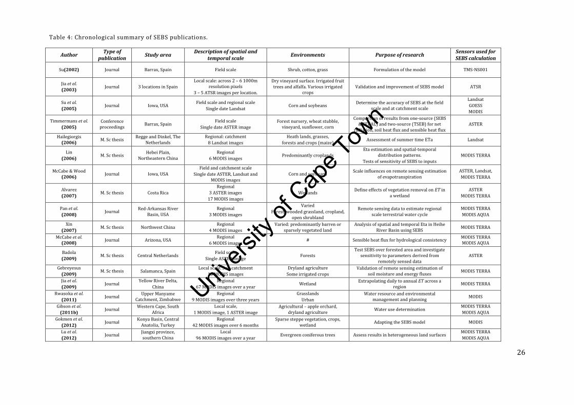
Univers

ity of

Cap

e Tow

n

26

Table 4: Chronological summary of SEBS publications.

Author Type of

publication Study area

Description of spatial and temporal scale

Environments Purpose of research Sensors used for SEBS calculation

Su(2002) Journal Barrax, Spain Field scale Shrub, cotton, grass Formulation of the model TMS-NS001

Jia et al.

(2003) Journal 3 locations in Spain

Local scale: across 2 – 6 1000m resolution pixels

3 – 5 ATSR images per location.

Dry vineyard surface. Irrigated fruit trees and alfalfa. Various irrigated

crops Validation and improvement of SEBS model ATSR

Su et al.

(2005) Journal Iowa, USA

Field scale and regional scale

Single date Landsat Corn and soybeans

Determine the accuracy of SEBS at the field scale and at catchment scale

Landsat

GOESS

MODIS

Timmermans et al.

(2005)

Conference proceedings

Barrax, Spain Field scale

Single date ASTER image

Forest nursery, wheat stubble, vineyard, sunflower, corn

Comparison of results from one-source (SEBS & SEBAL) and two-source (TSEB) for net

radiation, soil heat flux and sensible heat flux ASTER

Hailegiorgis (2006)

M. Sc thesis Regge and Dinkel, The

Netherlands

Regional: catchment

8 Landsat images

Heath lands, grasses,

forests and crops (maize) Assessment of summer time ETa Landsat

Lin

(2006) M. Sc thesis

Hebei Plain, Northeastern China

Regional

6 MODIS images Predominantly croplands

Eta estimation and spatial-temporal distribution patterns.

Tests of sensitivity of SEBS to inputs

MODIS TERRA

McCabe & Wood (2006)

Journal Iowa, USA

Field and catchment scale

Single date ASTER, Landsat and MODIS images

Corn and soybeans Scale influences on remote sensing estimation

of evapotranspiration

ASTER, Landsat,

MODIS TERRA

Alvarez

(2007) M. Sc thesis Costa Rica

Regional

3 ASTER images

17 MODIS images

Wetlands Define effects of vegetation removal on ET in

a wetland

ASTER

MODIS TERRA

Pan et al.

(2008) Journal

Red-Arkansas River Basin, USA

Regional

3 MODIS images

Varied

Forest, wooded grassland, cropland, open shrubland

Remote sensing data to estimate regional scale terrestrial water cycle

MODIS TERRA

MODIS AQUA

Xin

(2007) M. Sc thesis Northwest China

Regional

4 MODIS images

Varied: predominantly barren or sparsely vegetated land

Analysis of spatial and temporal Eta in Heihe River Basin using SEBS

MODIS TERRA

McCabe et al. (2008)

Journal Arizona, USA Regional

6 MODIS images # Sensible heat flux for hydrological consistency

MODIS TERRA MODIS AQUA

Badola

(2009) M. Sc thesis Central Netherlands

Field scale

Single ASTER image Forests

Test SEBS over forested area and investigate sensitivity to parameters derived from

remotely sensed data ASTER

Gebreyesus

(2009) M. Sc thesis Salamanca, Spain

Local scale. Sub-catchment

13 MODIS images

Dryland agriculture

Some irrigated crops

Validation of remote sensing estimation of soil moisture and energy fluxes

MODIS TERRA

Jia et al.

(2009) Journal

Yellow River Delta,

China

Regional

67 MODIS images over a year Wetland

Extrapolating daily to annual ET across a region

MODIS TERRA

Rwasoka et al.

(2011) Journal

Upper Manyame Catchment, Zimbabwe

Regional

9 MODIS images over three years

Grasslands

Urban

Water resource and environmental management and planning

MODIS

Gibson et al.

(2011b) Journal

Western Cape, South Africa

Local scale,

1 MODIS image, 1 ASTER image

Agricultural – apple orchard, dryland agriculture

Water use determination MODIS TERRA

MODIS AQUA

Gokmen et al.

(2012) Journal

Konya Basin, Central Anatolia, Turkey

Regional

42 MODIS images over 6 months

Sparse steppe vegetation, crops, wetland

Adapting the SEBS model MODIS

Lu et al.

(2012) Journal

Jiangxi province, southern China

Local

96 MODIS images over a year Evergreen coniferous trees Assess results in heterogeneous land surfaces

MODIS TERRA

MODIS AQUA

Univers

ity of

Cap

e Tow

n

27

Table 5: Validation, reported accuracies and SEBS model sensitivities.

Authors Source of information on land surface physical parameters

Method used to calculate fractional vegetation

cover Validation method Reported accuracies

Alvarez (2007) LIDAR and derived from ASTER Choudhary et al., 1994 Compared to measured water levels Within 10% of ET (from water level determination of storage)

Badola

(2009) Empirically derived from ASTER data

Baret et al., 1995; Carlson & Ripley, 1997; Gutman &

Ignatov, 1998 & Jiang et al., 2006.

Three flux towers Severe overestimation of latent heat flux and underestimation of sensible heat

flux in forested areas.

Gebreyesus

(2009) Land cover classifications

SEBS in ILWIS- assumed Carlson & Ripley, 1997

Crop coefficients and ET0 r2 of 0.86 and 0.91 when compared with complimentary approach

Gokmen et al.

(2012) Empirically derived from MODIS data Not specified Bowen ratio

For H: RMSE of 142.7 prior to algorithm adjustment, RMSE of 103.9 post algorithm adjustment

Hailegiorgis (2006)

Empirically derived from Landsat data Choudhary et al., 1994 Compared to results of hydrometeorological

equations over grassland ETa reported to be satisfactory when compared with ET0

Jia et al.

(2003) Empirically derived from ATSR data Baret et al., 1995 Large aperture scintillometer

RMSD for dry vineyard = 24.2 W.m-2, Irrigated fruit trees and alfalfa = 36.5W.m-

2, Mixed irrigated crops = 8.5 W.m-2

Jia et al.

(2009)

Land cover classification, MODIS LAI, field measurements

Not specified ET0 (ETa for a wetland should be very close

to ET0)

ETa reported to be acceptable when compared with ET0

RMSE for “Suaeda heteroptera” = 0.88mm

“reed swamp” = 1.3mm

Lin

(2006) Empirically derived from MODIS data Gutman & Ignatov, 1998

Lysimeter

Pan evaporation, Crop ET (ETc) Good agreement reported between SEBS ETa and lysimeter values

Lu et al.

(2012) Empirically derived from MODIS data Pridhodko & Goward, 1997 Eddy covariance flux measurements For evaporative fraction, r2 of between 0.552 and 0.557

McCabe & Wood

(2006)

Empirically derived from ASTER and Landsat and Landsat land cover

classifications Baret et al., 1995 Eddy covariance flux measurements

Tendency for over prediction with SEBS but good correlation to field measured values: r2 = 0.71 for ASTER and r2 = 0.74 for Landsat.

McCabe et al. (2008)

MODIS data products and land classifications

Xavier & Vettorazzi, 2004 Hydrological consistency with other remote

sensed variables For soil moisture anomalies from AMSR-E there is considerable agreement with

available sensible heat flux predictions

Pan et al. (2008) MODIS data products and land

classifications Not specified

Hydrological consistency with other remote sensed variables

SEBS retrieved ET values are higher than Variable Infiltration Capacity based predictions

Rwasoka et al.

(2011) Empirically derived from MODIS data Sobrino & Raissouni, 2000 Advection-aridity ET and ET0

Urban: between -1.5 and 0.4 mm.d-1

Grassland: between 0.6 and 3.8 mm.d-1

Su

(2002) Empirically derived from TMS data Not specified

Flux towers: eddy covariance and Bowen ratio

Mean error of SEBS is estimated to be around 20% relative to the mean sensible heat flux.

Su & Roerink (2004)

Not specified Not specified Flux towers: eddy covariance and Bowen

ratio Overestimation of Rn and LE. G0 and H results are better. Too few observations

to draw conclusions

Su et al. (2005) Field measured and empirically

derived from Landsat data Chen & Cihlar, 1995 Ten flux towers: eddy covariance

Five corn sites: relative root-mean-square error = 13.32% and root mean absolute error = 9.73%

3 soybean sites root-mean-square error = 14.02% root mean absolute error = 10.72%

Timmermans et al. (2005)

Empirically derived from ASTER data Choudhary et al., 1994 Flux towers: eddy covariance. Large aperture

scintillometer, TSEB & SEBAL Slight underestimation of Rn, G0 slightly underestimated for low vegetation

cover, underestimated H of up to 140 W.m-2

Van der Kwast et al.

(2009)

Empirically derived from ASTER data and field observations

Not specified Flux towers: eddy covariance. Large aperture

scintillometer

Standard deviations of SEBS estimated H similar to field measured values. SEBS estimated H good when the footprint of the measurements covers only one land

cover type.

Xin (2007) MODIS land cover product Choudhary et al., 1994 # #

Univers

ity of

Cap

e Tow

n

28

covers. However authors of other studies outside of irrigated agriculture have not reported the same

inaccuracies.

When looking at the use of different resolution sensors at a smaller scale or catchment scale, there

tends to be good agreement between the results obtained by using high and coarse resolution sensors.

For a wetland, Alvarez (2007) finds that the ET estimates from MODIS are within 5% of the results

obtained from ASTER with better results being obtained where the vegetation is less fragmented.

Similarly McCabe & Woods (2006) find that at field scale, the ASTER values are not regularly within

10% of MODIS values but at a catchment scale, results for ASTER, Landsat and MODIS are within 10% of

each other. From the literature it is therefore clear that the SEBS model has been used with varied

success to model energy fluxes and ET in a range of environments with an emphasis on agriculture and

with a variety of sensors.

Several authors attribute the sensitivity of the SEBS model to various input parameters including:

roughness length (Lin, 2006; Alvarez, 2007; Van der Kwast et al., 2009, Gebreyesus, 2009), zero plane

displacement height (Lin, 2006), land surface temperature (Badola, 2009; Van der Kwast et al., 2009),

wind speed and wind direction (Van der Kwast et al., 2009), fractional vegetation cover (Badola, 2009;

Lin, 2006), surface emissivity (Badola, 2009; Van der Kwast et al., 2009; Lin, 2006), albedo (Badola,

2009; Van der Kwast et al., 2009), NDVI (Badola, 2009; Van der Kwast et al., 2009), shortwave incoming

radiation (Van der Kwast et al., 2009) and the height of the planetary boundary layer (Van der Kwast et

al., 2009).

In the formulation publication of SEBS (Su, 2002), the sensitivity of the sensible heat flux to parameters8

used in its calculation are found to be around 40 W.m-2 when the various terms are assumed

independent of each other. Since in reality at least some of the terms are correlated, the expected

sensitivity can then be estimated in the order of 20 W.m–2, which is around 20% relative to the mean

sensible heat flux (Su, 2002). Of the reported sensitivities since the work of Su (2002), Badola (2009)

and Van der Kwast et al. (2009) report SEBS to be most sensitive to land surface temperature. However,

Lin (2006) reports that the SEBS model is most sensitive to roughness length and according to Van der

8 land surface temperature and air temperature gradient, friction velocity, excess resistance to heat transfer, and stability correction function for heat transfer.

Univers

ity of

Cap

e Tow

n

29

Kwast et al. (2009), sensitivity to aerodynamic parameters (roughness length, zero plane displacement

height and canopy height) and the method used to derive these parameters should be considered

depending on the heterogeneity of the image footprint.

Lin (2006) demonstrates the sensitivity of the SEBS model to zero plane displacement height especially

at high zero plane displacement heights and high NDVI. SEBS modelled evaporative fraction decreases

slightly with increasing displacement height at lower NDVI, but when the zero plane displacement

height reaches a certain threshold, the evaporative fraction begins to decrease rapidly with increasing

displacement height. Lin (2006) concludes that evaporative fraction is a function of not only

displacement height but also of NDVI. Areas that have high green leaf biomass (and therefore high

NDVI) normally have a relatively lower evaporative fraction but are more sensitive to the displacement

height (Lin, 2006).

Lin (2006) further demonstrates the sensitivity of evaporative fraction to aerodynamic roughness

length particularly at lower NDVI and concludes that the larger the NDVI, the more ET will take place

and the less sensitive the outputs will be to aerodynamic roughness height changes. It was also

illustrated that at NDVI of around 0.6, the SEBS model is most sensitive to change in aerodynamic

roughness.

Lin (2006) and Badola (2009) differ in their findings regarding the sensitivity of the SEBS model to

fractional vegetation cover. Lin (2006), who uses coarse resolution MODIS imagery, reports the SEBS

model to be relatively insensitive to change in fractional vegetation cover whereas Badola (2009), using

high resolution ASTER imagery finds a great sensitivity of sensible heat flux to change in fractional

vegetation cover. Badola (2009) motivates this sensitivity by the use of the fractional vegetation cover

and its complement in the calculation of the sensible heat flux (see Equations [12], [13] and Equations

[6], [7] & [8] in Chapter 2.3). The differing land covers under study by Lin (2006) and Badola (2009)

should be noted, in that the former’s object of study is predominantly cropland whereas the latter’s

object of study is forested areas with tall canopies.

In criticism of the literature around the application of the SEBS model, prior to 2010 much of the

available literature was published in the so-called grey literature with a limited peer review process.

Univers

ity of

Cap

e Tow

n

30

Due to this limitation, it would be specious to draw firm conclusions around the reported accuracies.

However, post 2010; journal papers (Gibson et al., 2011b; Rwasoka et al., 2011; Gokmen et al., 2011; Lu

et al., 2011) on the application of the SEBS model have been more critical in establishing the accuracy of

the model. Rwasoka et al. (2011) report an overestimation of ET at a grassland site which they ascribe

to the heterogeneity of the landscape. Heterogeneity is further put forward as a reason for inaccuracies

by Gibson et al. (2011b) Lu et al. (2012) and Gokmen et al. (2012). Further, Lu et al. (2011) state that

lack of energy balance closure leads to inaccuracies in results.

2.3. SEBS FORMULATION

According to Su (2006), it is possible to estimate the latent heat flux as a residual of the surface energy

balance algorithm after the sensible heat flux has been derived (Equation 1). However, because the

sensible heat flux is not constrained by the available energy but is determined solely by surface

temperature and the meteorological conditions at the reference height, there is an associated

uncertainty in the derived latent heat flux and therefore also in the evaporative fraction. However, in

SEBS this uncertainty is limited by considering the sensible heat flux at both the wet and dry limit and

the actual sensible heat flux is constrained to this range. The sensible heat flux at the wet limit is

derived from a combination equation and the sensible heat flux at the dry limit is set by the available

energy. In SEBS, the daily ET is determined from the total daily available energy by assuming the

evaporative fraction is constant throughout the day.

Instantaneous net radiation is estimated based on radiative energy balance:

4

01 TRRR lwdswdn [2]

where α is broadband albedo in the visible and near-infrared band; ε is broadband emissivity in the

thermal infrared band; Rswd is incident shortwave radiation; Rlwd is downward longwave radiation; T0 is

surface temperature and σ is Stephan–Boltzman constant (Su et al., 2005).

Univers

ity of

Cap

e Tow

n

31

The other component comprising the available energy is the soil heat flux. In the absence of observed

soil heat flux measurements, as in satellite applications, empirical formulations of the soil heat flux

based on net radiation and the vegetation fraction are used to estimate the total soil heat flux for the

area.

cscno fcRG 1 [3]

where Γc (0.05) (Monteith, 1973 in Su, 2002) and Γs (0.315) (Kustas & Daughtry, 1989 in Su, 2002) are

the soil heat flux ratios for full vegetation canopy and for bare soil respectively and fc is the fractional

vegetation cover (Su et al., 2005).

At the wet and dry limits, the equations used to calculate the sensible heat flux (Equations [4] & [5]

respectively) differ from the sensible heat flux equations which are used when the wet or dry limit has

not been reached (Equations [6], [7] & [8]) (Su, 2002).

1

0

ee

r

CGR

H

s

ew

p

n

wet [4]

where e and es are actual and saturation vapour pressure respectively; γ is the psychrometric constant,

rew is the external resistance at the wet limit and Δ is the rate of change of saturation vapour pressure

with temperature.

0GRH ndry [5]

Univers

ity of

Cap

e Tow

n

32

L

z

L

dz

z

dz

k

uu m

mm

m

00

0

0* ln [6]

L

z

L

dz

z

dz

Cku

H h

hh

hp

a

00

0

0

*

0 ln

[7]

kgH

uCL

vp 3

* [8]

where z is the height above the surface, u* is the friction velocity, k = 0.4 is von Karman’s constant, d0 is

zero plane displacement height, z0m is the roughness height for momentum transfer, θ0 is the potential

temperature at the surface, θa is the potential air temperature at height z, z0h is the scalar height for heat

transfer, Ψm and Ψh are the stability correction functions for momentum and sensible heat respectively,

L is the Obukhov length, Cp is the specific heat capacity of air at constant pressure, g is acceleration due

to gravity and θv is the potential virtual temperature near the surface (Su, 2002). The friction velocity,

the sensible heat flux and the Obukhov stability length are obtained by solving the system of non-linear

Equations [6], [7] and [8] using the method of Broyden (Press et al., 1997 in Su, (2002)). Derivation of

the sensible heat flux therefore requires only the wind speed and temperature at the reference height as

well as the surface temperature and is independent of other surface energy balance terms.

If H calculated from Equations [6], [7] and [8] exceeds Hdry calculated from Equation [5], then the dry

limit is said to have been reached and Equation [5] is used to determine H. If Hwet calculated from

Equation [4] exceeds H calculated from Equations [6], [7] and [8], then the wet limit is said to have been

reached and Equation [4] is used to determine H.

In the derivation of H, aerodynamic and thermal dynamic roughness parameters are required. The

aerodynamic roughness parameter can vary in space and time for two different reasons: variations in

surface roughness and variations in atmospheric stability. The first is the dominant cause of variations

in space (at a specific time of a satellite overpass), whereas the second is the dominant cause of

Univers

ity of

Cap

e Tow

n

33

variations in time (at a specific field site) (Van der Tol et al., 2009). Su (2002) advises using the within-

canopy turbulence model proposed by Maasman (1997) to estimate aerodynamic parameters d0 and

z0m, if near surface wind speed, the height of the vegetation (h0) and the leaf area index are known. If

only the height of the vegetation is available, the relationships proposed by Brutsaert (1982) can be

used:

136.0

0

0

mzh [9]

003

2hd

[10]

If a detailed land use map is available, tabulated values for aerodynamic parameters can be used.

However, the first method is recommended since the aerodynamic parameters depend not only on

surface characteristics but also wind speed and direction (Su, 2002). It should be noted that estimates

of aerodynamic resistance based on optical remote sensing contain a large degree of uncertainty

(Van der Tol et al., 2009). However if none of the above data is available, the aerodynamic parameters

can be related to remote sensing vegetation inputs, and the normalized difference vegetation index

(NDVI) is used (Su & Jacobs, 2001, in Hailegiorgis, 2006):

5.2

max

0 5.0005.0

NDVI

NDVIz m [11]

The roughness height for heat transfer, z0h, which changes with surface characteristics, atmospheric

flow and thermal dynamic state of the surface, can be derived from z0m:

1

0

0exp

kB

zz m

h

[12]

where B–1 is the inverse Stanton number, a dimensionless heat transfer coefficient. For vegetated areas,

an extended model is used to estimate the kB–1 value (Equation [13]):

Univers

ity of

Cap

e Tow

n

34

21

*

0*

2

2*

1 2

1)(

4s

t

m

sccn

t

d fkBC

hz

huu

kfff

ehu

uC

kCkB

ec

[13]

Where fc is the fractional canopy cover and fs is its complement. Ct is the heat transfer coefficient of the

leaf and in most conditions is bounded as 0.005N<Ct<0.075N where N is the number of sides of the leaf

to participate in heat exchange. Ct* is the heat transfer coefficient of the soil and is given by Ct* = Pr-2/3

Re*-1/2, where Pr is the Prandtl number Re* is the roughness Reynolds number (Re* = hsu*/v, with hs the

roughness height of the soil. The kinematic viscosity of the air is v = 1.327∙10-5(p0/p)(T/T0)1.81 with p and

T the ambient pressure and temperature and p0 = 101.3 kPa and T0 = 273.15 K. nec is the within canopy

wind speed profile extinction coefficient is formulated as a function of the cumulative leaf drag area at

the canopy top:

22

*2 huu

LAICn d

ec

[14]

where Cd is the drag coefficient of the foliage elements (assumed = 0.2), LAI is the one-sided leaf area

index defined for the total area, u(h) is the horizontal wind speed at the canopy top.

kB–1 required in Equation [12] is calculated using Equation [13] for vegetated areas while for bare soil

the model proposed by Brutsaert (1982) is used:

4.7lnRe46.2 41

*

1 kB [15]

According to formulations by Su (2002), the relative evaporation is derived from the sensible heat flux

and the sensible heat flux calculated at the wet and dry limits.

Univers

ity of

Cap

e Tow

n

35

wetdry

wetr

HH

HH

1 [16]

where r is relative evaporation, H is the sensible heat flux and Hwet and Hdry are the sensible heat flux

at the wet and dry limits respectively. The relative evaporation is, in turn, used together with Rn, G0 and

the latent heat flux at the wet limit to estimate the evaporative fraction:

00 GR

E

GR

E

n

wetr

n

[17]

where is the evaporative fraction and E and wetE are the latent heat flux and the latent heat flux

at the wet limit respectively.

In SEBS it is assumed that the daily value of evaporative fraction is approximately equal to the

instantaneous value, since the difference between the instantaneous evaporative fraction at satellite

overpass and the evaporative fraction derived from the 24-hour integrated energy balance is marginal

and may be neglected (Ahmad et al. 2005) as the evaporative fraction generally remains constant

throughout the day. From this, the daily ET can be determined as:

w

nRET

71064.8 [18]

where ET is the actual evaporation on daily basis (mm.d-1), λ is the latent heat of vaporization (J.kg), ρw

is the density of water (kg.m-3) and nR is the daily net radiation flux (Lin et al., 2008):

daydayn LKcR )1( 1 [19]

Univers

ity of

Cap

e Tow

n

36

where c1 is a conversion factor of 1.1 for instantaneous to broad band albedo, α is broad band albedo

and used in the instantaneous net radiation flux calculation in SEBS, K↓day is incoming shortwave

radiation (measured or modelled) and Lday is daily longwave radiation (Hailegiorgis, 2006). It is clear

from Equations [18] and [19] that aside from evaporative fraction itself, albedo is the sole remote

sensing derived variable used in the upscaling from instantaneous evaporative to daily ET.

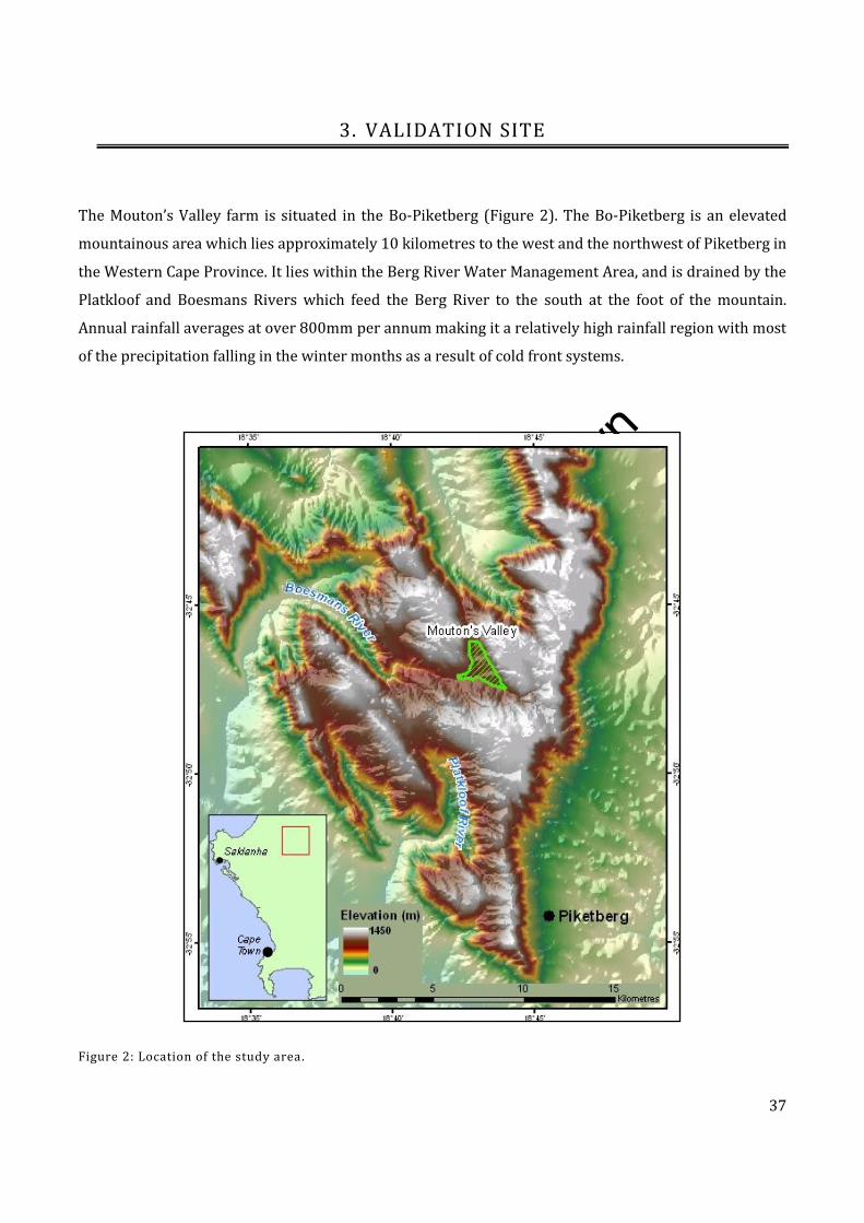
Univers

ity of

Cap

e Tow

n

37

3. VALIDATION SITE

The Mouton’s Valley farm is situated in the Bo-Piketberg (Figure 2). The Bo-Piketberg is an elevated

mountainous area which lies approximately 10 kilometres to the west and the northwest of Piketberg in

the Western Cape Province. It lies within the Berg River Water Management Area, and is drained by the

Platkloof and Boesmans Rivers which feed the Berg River to the south at the foot of the mountain.

Annual rainfall averages at over 800mm per annum making it a relatively high rainfall region with most

of the precipitation falling in the winter months as a result of cold front systems.

Figure 2: Location of the study area.

Univers

ity of

Cap

e Tow

n

38

The Bo-Piketberg is made up of a variable thickness of the Table Mountain Group rocks, which are

dominated (73%) by quartzose sandstone (quartz arenite). In the study area, the Peninsula Formation

is the most represented formation consisting of thickly bedded quartzitic sandstone with the Nardouw

Formation also having a significant presence. Basement rock of the Malmesbury Group appears in the

southeast of the study area at the base of the mountain and Quaternary alluvial deposits are found in

the southwest.

The land use is predominantly farming (fruit – deciduous and citrus, flowers and buchu) while the

steeper terrain is undeveloped and uncultivated consisting of natural vegetation however,

encroachment by invasive alien vegetation species is a reported problem. Cultivated land is irrigated

mainly using surface water from farm dams but boreholes do exist and are in operation.

The farm Mouton’s Valley is situated in the Mouton’s Valley with the cultivated fields being nestled

between the north bank of the Boesmans River, the large dam at The Hermitage to the north, and steep

mountain slopes to the east (Levant Hill, 1146 m) and the west (790 m). The cultivated land on the

farm Mouton’s Valley covers an area of approximately 150 ha and has an elevation of between 500 and

540 m above sea level (Figure 2). Mouton’s Valley is a fruit farm with both deciduous (apples,

nectarines, persimmons, peaches and pears) and citrus fruits (oranges and lemons) being grown

(Figure 3). Irrigation is predominantly from the large dam at The Hermitage and the owners report that

this contains sufficient water for their irrigation requirements. There is an Enviromon agroclimatology

weather station situated on the farm and rainfall, temperature, relative humidity, solar radiation, sun

hours and leaf wetness are recorded at hourly intervals.

The field validation took place in an apple orchard (11 ha) which was made up of three different apple

cultivars – 11 rows of Braestarr, 16 rows of Royal Gala and 15 rows of Redchief. At the time of the

energy balance and total evaporation measurements from 7 November to 1 December 2008 (DOY 315 –

326), the average canopy height was 3.2 m. The apple trees did not cover the soil surface completely,

rather by about 75 %. The inter-row areas were planted with grass (Jarmain & Mengistu, 2011). Good

quality data was available from 10 to 21 November 2008 (Day of year (DOY) 315 to 326) and this is the

time period studied in this research.

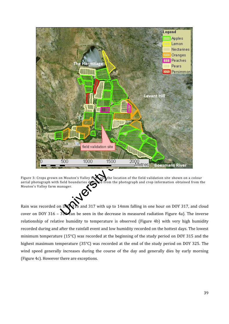
Univers

ity of

Cap

e Tow

n

39

Figure 3: Crops grown on Mouton’s Valley farm and the location of the field validation site shown on a colour aerial photograph with field boundaries digitized from the photograph and crop information obtained from the Mouton’s Valley farm manager.

Rain was recorded on DOY 316 and 317 with up to 14mm falling in one hour on DOY 317, and cloud

cover on DOY 316 – 319 can be seen in the decrease in measured radiation Figure 4a). The inverse

relationship of relative humidity to temperature is observed (Figure 4b) with very high humidity

recorded during and after the rainfall event and low humidity recorded on the hottest days. The lowest

minimum temperature (15°C) was recorded at the beginning of the study period on DOY 315 and the

highest maximum temperature (35°C) was recorded at the end of the study period on DOY 325. The

wind speed generally increases during the course of the day and generally dies by early morning

(Figure 4c). However there are exceptions.

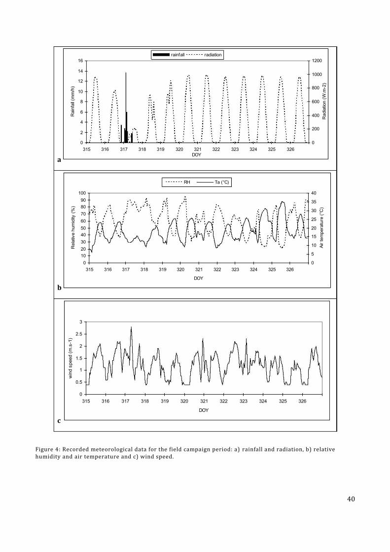
Univers

ity of

Cap

e Tow

n

40

a

b

c

Figure 4: Recorded meteorological data for the field campaign period: a) rainfall and radiation, b) relative humidity and air temperature and c) wind speed.

0

2

4

6

8

10

12

14

16

315 316 317 318 319 320 321 322 323 324 325 326DOY

Rai

nfal

l (m

m/h

)

0

200

400

600

800

1000

1200

Rad

iatio

n (W

.m-2

)

rainfall radiation

0102030405060708090

100

315 316 317 318 319 320 321 322 323 324 325 326

DOY

Rel

ativ

e hu

mid

ity (%

)

0

5

10

15

20

25

30

35

40

Air t

empe

ratu

re (°

C)

RH Ta (°C)

0

0.5

1

1.5

2

2.5

3

315 316 317 318 319 320 321 322 323 324 325 326

DOY

win

d sp

eed

(m.s

-1)

1- ....... I

.. "

. ."

I· ...... - I

1- ....... I

.. "

. ."

I· ...... - I

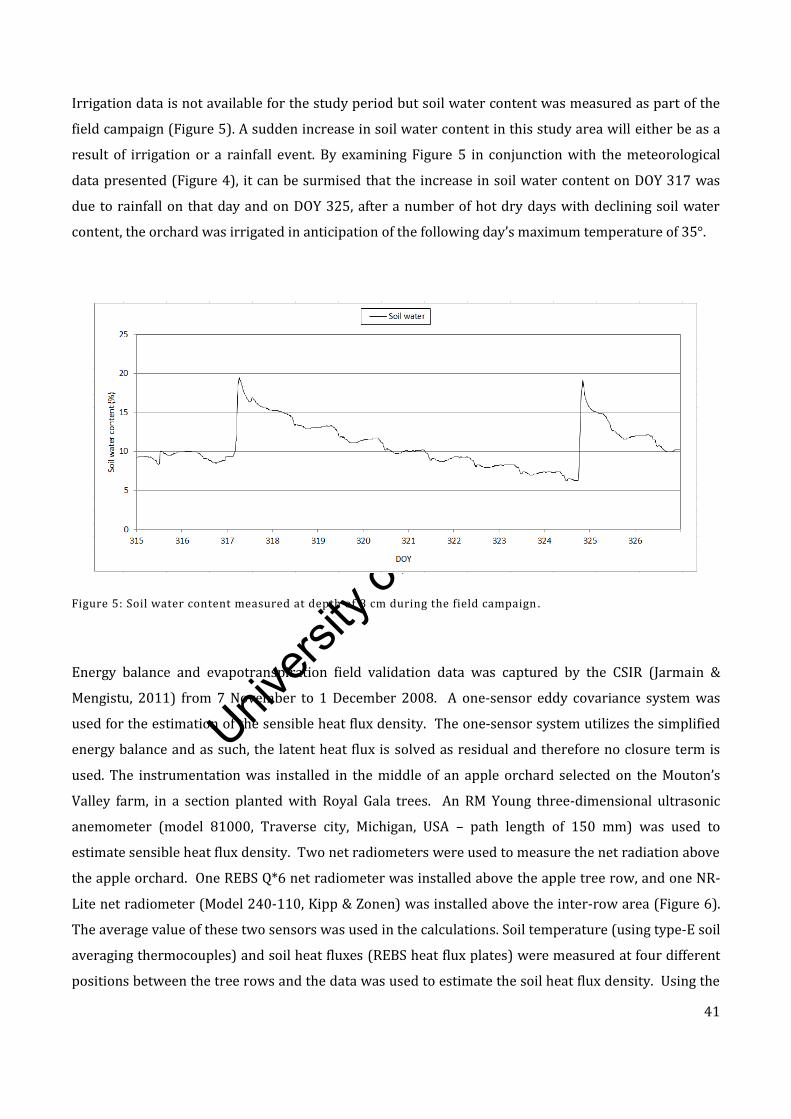
Univers

ity of

Cap

e Tow

n

41

Irrigation data is not available for the study period but soil water content was measured as part of the

field campaign (Figure 5). A sudden increase in soil water content in this study area will either be as a

result of irrigation or a rainfall event. By examining Figure 5 in conjunction with the meteorological

data presented (Figure 4), it can be surmised that the increase in soil water content on DOY 317 was

due to rainfall on that day and on DOY 325, after a number of hot dry days with declining soil water

content, the orchard was irrigated in anticipation of the following day’s maximum temperature of 35°.

Figure 5: Soil water content measured at depth of 8 cm during the field campaign .

Energy balance and evapotranspiration field validation data was captured by the CSIR (Jarmain &

Mengistu, 2011) from 7 November to 1 December 2008. A one-sensor eddy covariance system was

used for the estimation of the sensible heat flux density. The one-sensor system utilizes the simplified

energy balance and as such, the latent heat flux is solved as residual and therefore no closure term is

used. The instrumentation was installed in the middle of an apple orchard selected on the Mouton’s

Valley farm, in a section planted with Royal Gala trees. An RM Young three-dimensional ultrasonic

anemometer (model 81000, Traverse city, Michigan, USA – path length of 150 mm) was used to

estimate sensible heat flux density. Two net radiometers were used to measure the net radiation above

the apple orchard. One REBS Q*6 net radiometer was installed above the apple tree row, and one NR-

Lite net radiometer (Model 240-110, Kipp & Zonen) was installed above the inter-row area (Figure 6).

The average value of these two sensors was used in the calculations. Soil temperature (using type-E soil

averaging thermocouples) and soil heat fluxes (REBS heat flux plates) were measured at four different

positions between the tree rows and the data was used to estimate the soil heat flux density. Using the

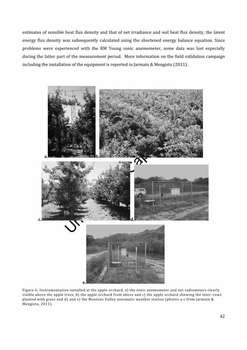
Univers

ity of

Cap

e Tow

n

42

estimates of sensible heat flux density and that of net irradiance and soil heat flux density, the latent

energy flux density was subsequently calculated using the shortened energy balance equation. Since

problems were experienced with the RM Young sonic anemometer, some data was lost especially

during the latter part of the measurement period. More information on the field validation campaign

including the installation of the equipment is reported in Jarmain & Mengistu (2011).

a. b.

c. d.

e.

Figure 6: Instrumentation installed at the apple orchard, a) the sonic anemometer and net radiometers clearly visible above the apple trees, b) the apple orchard from above and c) the apple orchard showing the inter -rows planted with grass and d) and e) the Moutons Valley automatic weather station (photos a-c from Jarmain & Mengistu, 2011).

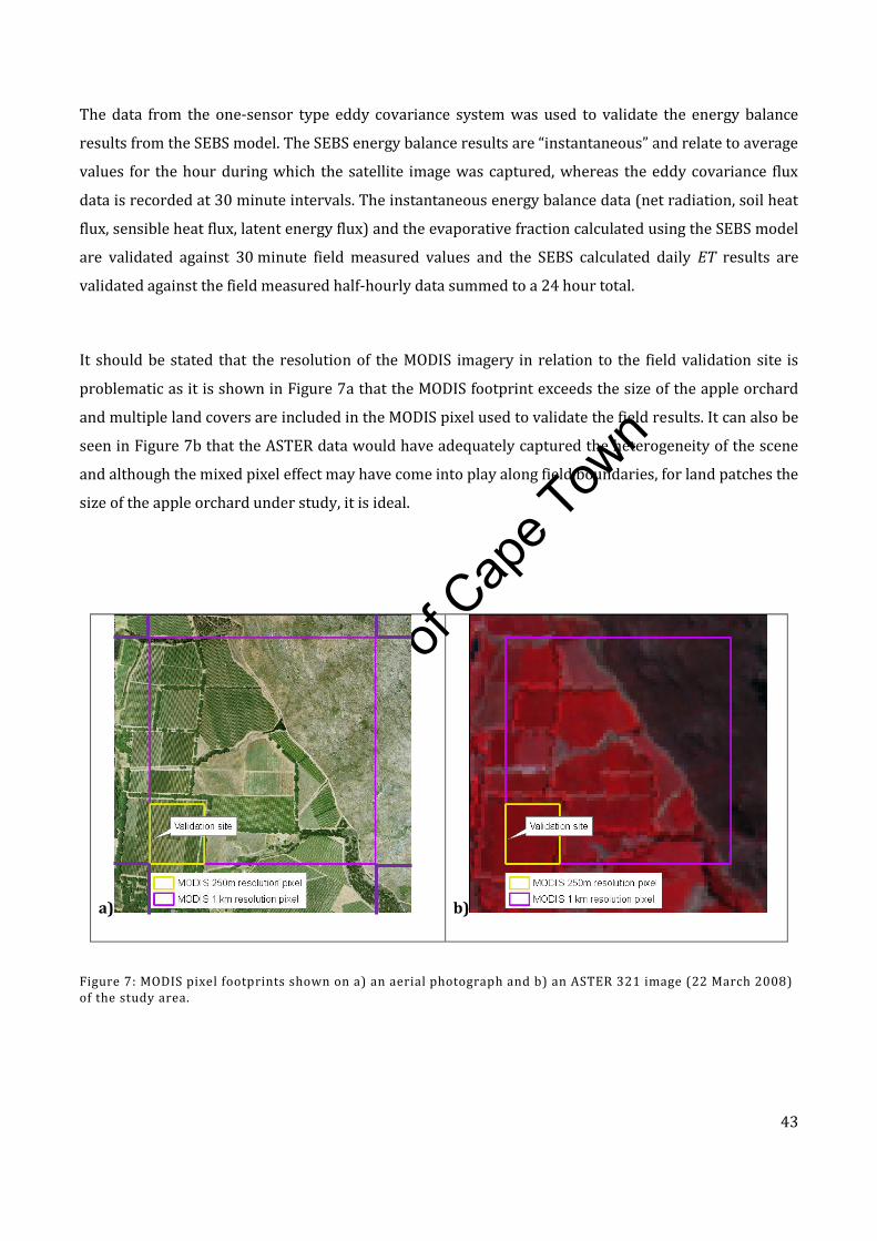
Univers

ity of

Cap

e Tow

n

43

The data from the one-sensor type eddy covariance system was used to validate the energy balance

results from the SEBS model. The SEBS energy balance results are “instantaneous” and relate to average

values for the hour during which the satellite image was captured, whereas the eddy covariance flux

data is recorded at 30 minute intervals. The instantaneous energy balance data (net radiation, soil heat

flux, sensible heat flux, latent energy flux) and the evaporative fraction calculated using the SEBS model

are validated against 30 minute field measured values and the SEBS calculated daily ET results are

validated against the field measured half-hourly data summed to a 24 hour total.

It should be stated that the resolution of the MODIS imagery in relation to the field validation site is

problematic as it is shown in Figure 7a that the MODIS footprint exceeds the size of the apple orchard

and multiple land covers are included in the MODIS pixel used to validate the field results. It can also be

seen in Figure 7b that the ASTER data would have adequately captured the heterogeneity of the scene

and although the mixed pixel effect may have come into play along field boundaries, for land patches the

size of the apple orchard under study, it is ideal.

a) b)

Figure 7: MODIS pixel footprints shown on a) an aerial photograph and b) an ASTER 321 image (22 March 2008) of the study area.

Univers

ity of

Cap

e Tow

n

44

4. MATERIALS & METHOD

The SEBS model methodology will be discussed under the headings: Remote sensing preprocessing

(Chapter 4.1), Meteorological calculations (Chapter 4.2) and SEBS calculations (Chapter 4.3). Remote

sensing preprocessing includes data selection (Chapter 4.1.1), acquisition (Chapter 4.1.2),

transformation (Chapter 4.1.3), converting to radiance or reflectance (Chapter 4.1.4) and atmospheric

correction (Chapter 4.1.5). Meteorological calculations (Chapter 4.2) pertain to the meteorological data

and calculations required for the SEBS model. SEBS calculations section (Chapter 4.3) details the

calculation of the remote sensing derived input parameters required which are albedo (Chapter 4.3.1),

vegetation parameters (Chapter 4.3.2), surface emissivity (Chapter 4.3.3) and land surface temperature

(Chapter 4.3.4) Ultimately under SEBS calculations, the energy fluxes and evapotranspiration within the

SEBS model (Chapter 4.3.5) is described. The general flow and the complexity of some of the SEBS

methodology is illustrated in Figure 8 which shows the input data, processing stages and tools which

are used in this research using MOD 02 data by way of example..

4.1. REMOTE SENSING PREPROCESSING

The SEBS model will be used to estimate evapotranspiration and energy balance components using data

from two sensors MODIS TERRA & MODIS AQUA. The methodology is identical for both TERRA and

AQUA data, however, for simplicity in the text, only MODIS TERRA will be referred to unless the

reference is specific to MODIS AQUA. Note that the prefix MOD refers to MODIS TERRA and the prefix

MYD refers to MODIS AQUA. A flowchart of the preprocessing methodology is shown in Figure 9.

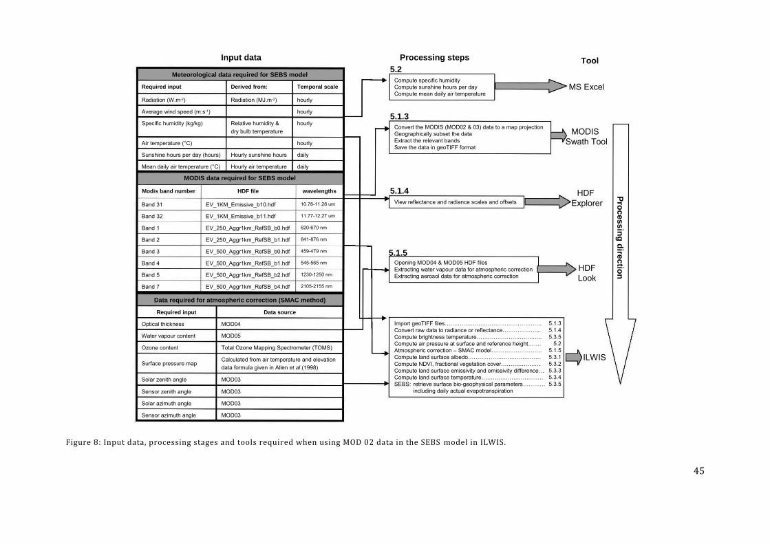
Univers

ity of

Cap

e Tow

n

45

Figure 8: Input data, processing stages and tools required when using MOD 02 data in the SEBS model in ILWIS.

Convert the MODIS (MOD02 & 03) data to a map projection Geographically subset the dataExtract the relevant bandsSave the data in geoTIFF format

View reflectance and radiance scales and offsets

Opening MOD04 & MOD05 HDF filesExtracting water vapour data for atmospheric correctionExtracting aerosol data for atmospheric correction

Import geoTIFF files…………………………………………….Convert raw data to radiance or reflectance………………...Compute brightness temperature……………………………..Compute air pressure at surface and reference height…….Atmospheric correction – SMAC model………………………

Compute land surface albedo…………………………………

Compute NDVI, fractional vegetation cover…………………

Compute land surface emissivity and emissivity difference…Compute land surface temperature……………………………

SEBS: retrieve surface bio-geophysical parameters…………

including daily actual evapotranspiration

Compute specific humidityCompute sunshine hours per dayCompute mean daily air temperature

Meteorological data required for SEBS model

dailyHourly sunshine hoursSunshine hours per day (hours)

dailyHourly air temperatureMean daily air temperature (°C)

hourlyAir temperature (°C)

hourlyRelative humidity & dry bulb temperature

Specific humidity (kg/kg)

hourlyAverage wind speed (m.s-1)

hourlyRadiation (MJ.m-2)Radiation (W.m-2)

Temporal scaleDerived from:Required input

MODIS data required for SEBS model

2105-2155 nmEV_500_Aggr1km_RefSB_b4.hdfBand 7

1230-1250 nmEV_500_Aggr1km_RefSB_b2.hdfBand 5

545-565 nmEV_500_Aggr1km_RefSB_b1.hdfBand 4

459-479 nmEV_500_Aggr1km_RefSB_b0.hdfBand 3

841-876 nmEV_250_Aggr1km_RefSB_b1.hdfBand 2

620-670 nmEV_250_Aggr1km_RefSB_b0.hdfBand 1

11.77-12.27 umEV_1KM_Emissive_b11.hdfBand 32

10.78-11.28 umEV_1KM_Emissive_b10.hdfBand 31

wavelengthsHDF fileModis band number

Data required for atmospheric correction (SMAC method)

MOD03Sensor azimuth angle

MOD03Solar azimuth angle

MOD03Sensor zenith angle

MOD03Solar zenith angle

Calculated from air temperature and elevation data formula given in Allen et al.(1998)

Surface pressure map

Total Ozone Mapping Spectrometer (TOMS)Ozone content

MOD05Water vapour content

MOD04Optical thickness

Data sourceRequired input

MS Excel

ToolInput data Processing steps

MODIS Swath Tool

HDF Explorer

HDFLook

ILWIS

Pro

cess

ing

dire

ctio

n

5.2

5.1.3

5.1.4

5.1.5

5.1.35.1.45.3.5

5.25.1.55.3.15.3.25.3.35.3.45.3.5

'-1 1 > r F>

"I > .

> v

-

-I 1 >

---. =>

I >

~

>

'---+

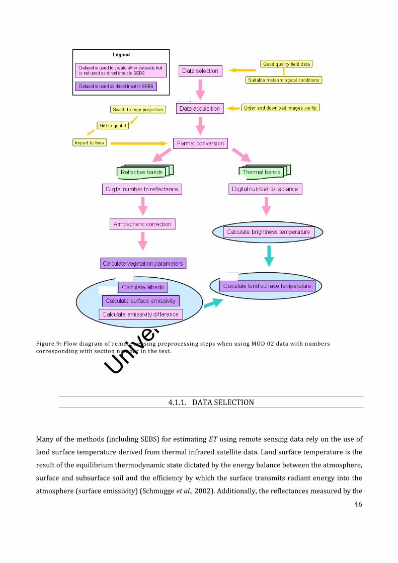
Univers

ity of

Cap

e Tow

n

46

Figure 9: Flow diagram of remote sensing preprocessing steps when using MOD 02 data with numbers corresponding with section number in the text.

4.1.1. DATA SELECTION

Many of the methods (including SEBS) for estimating ET using remote sensing data rely on the use of

land surface temperature derived from thermal infrared satellite data. Land surface temperature is the

result of the equilibrium thermodynamic state dictated by the energy balance between the atmosphere,

surface and subsurface soil and the efficiency by which the surface transmits radiant energy into the

atmosphere (surface emissivity) (Schmugge et al., 2002). Additionally, the reflectances measured by the

Univers

ity of

Cap

e Tow

n

47

satellite are used to calculate other land surface parameters i.e. albedo and NDVI which are then used to

respectively: empirically derive net radiation, and estimate other inputs for the calculation of the soil

heat flux and the sensible heat flux. For this reason, a satellite sensor which captures electromagnetic

radiation in the visible, near infrared and thermal infrared is critical in order to use a model such as

SEBS.

A caveat in the research should be stated upfront. It was originally proposed that high resolution ASTER

imagery would be used in combination with MODIS imagery. Due to cloud cover during the field

validation period and in field instrument failure, only one ASTER image was available for the field

validation period. Since there would be little value in using a single ASTER image, MODIS data alone was

selected to correspond with the field validation period. With the benefit of hindsight it became apparent

that due to study area heterogeneity and the coarse resolution of the MODIS pixel, despite the large size

of the orchard, the SEBS results from the MODIS data represent a mixed pixel effect and not only the

fluxes from the apple orchard itself. Despite the limitations to the research, it was still possible to obtain

valuable insight into the workings of the SEBS model. The field validation data allowed the results from

the SEBS model to be benchmarked if not directly compared and important conclusions and

recommendations could be made regarding the use of the SEBS model in South Africa.

MODIS is a key instrument aboard both the TERRA (EOS AM) and AQUA (EOS PM) satellites, in orbit at

705 km above the earth. TERRA successfully launched on 18 December 1999 while AQUA was

successfully launched on 4 May 2002 (http://modis.gsfc.nasa.gov/about/design.php). The direction of

the satellites differ in that TERRA orbits the Earth, north to south, and it is timed to pass over the

equator in the morning (10:30 am). AQUA orbits the Earth, south to north, and it is timed to pass over

the equator in the afternoon (1:30 pm). Together, TERRA MODIS and AQUA MODIS view the entire

Earth's surface every 1 to 2 days, acquiring data in 36 spectral bands

(http://modis.gsfc.nasa.gov/about/). Further information on the MODIS instrument is given in

Appendix 1.

During a field campaign conducted in the study area, the energy fluxes and total evaporation of an apple

orchard were measured by the Council for Scientific and Industrial Research (Jarmain & Mengistu,

2011). A one-sensor type eddy covariance system was used to collect the data from 7 November to 1

December 2008. Due to sensor problems, good quality data was only available from 10 to 21 November

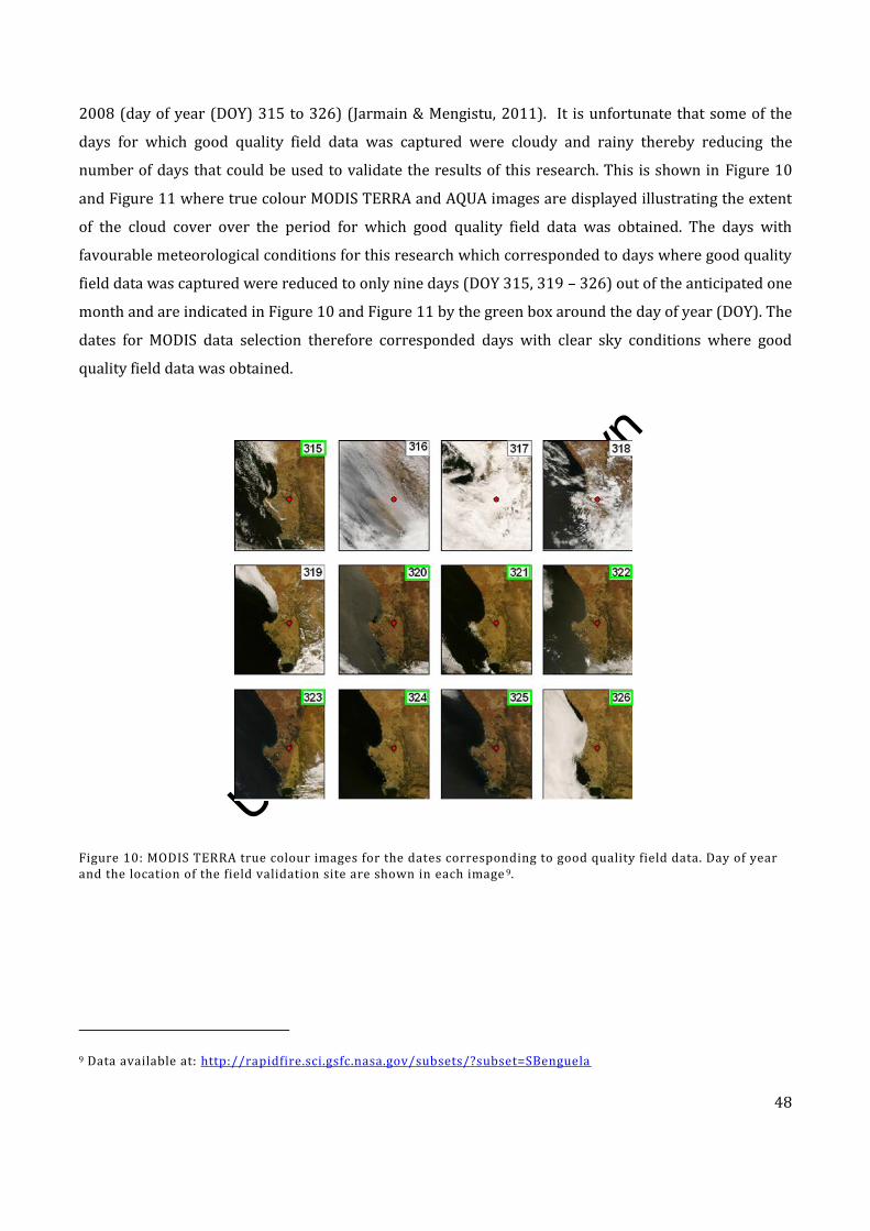
Univers

ity of

Cap

e Tow

n

48

2008 (day of year (DOY) 315 to 326) (Jarmain & Mengistu, 2011). It is unfortunate that some of the

days for which good quality field data was captured were cloudy and rainy thereby reducing the

number of days that could be used to validate the results of this research. This is shown in Figure 10

and Figure 11 where true colour MODIS TERRA and AQUA images are displayed illustrating the extent

of the cloud cover over the period for which good quality field data was obtained. The days with

favourable meteorological conditions for this research which corresponded to days where good quality

field data was captured were reduced to only nine days (DOY 315, 319 – 326) out of the anticipated one

month and are indicated in Figure 10 and Figure 11 by the green box around the day of year (DOY). The

dates for MODIS data selection therefore corresponded days with clear sky conditions where good

quality field data was obtained.

Figure 10: MODIS TERRA true colour images for the dates corresponding to good quality field data. Day of year and the location of the field validation site are shown in each image 9.

9 Data available at: http://rapidfire.sci.gsfc.nasa.gov/subsets/?subset=SBenguela

Univers

ity of

Cap

e Tow

n

49

Figure 11: MODIS AQUA true colour images for the dates corresponding to good quality field data. Day of year and the location of the field validation site are shown in each image 8.

4.1.2. DATA ACQUISITION

MODIS reflectance and radiance bands are required for the SEBS model and were selected for clear sky

days which corresponded to dates for which field validation data was available. The required data, the

scientific data contained within each dataset and where they are used in the methodology are

illustrated in the flow diagram in Figure 8. Further information on the datasets is contained in

Appendix 1, including the MOD 02 and MYD 02 files which were selected and downloaded.

4.1.3. DATA TRANSFORMATION

The MODIS Swath Tool (MST) is used to process the MOD 02 and MOD 03 hdf files. First of all the

images were converted to a map projection, then to geographically subset the image, extract the

relevant bands and finally save the image in geoTIFF format (further information is given in

Appendix 1). Not all 86 bands contained within the hdf are required for evapotranspiration estimation

Univers

ity of

Cap

e Tow

n

50

so the MST is used to extract the relevant eight bands (Table 6). The data is finally imported into ILWIS

and saved in the ILWIS file format. All processing from this point on is carried out in ILWIS using

functions, the command line or scripts.

Table 6: MODIS bands required for evapotranspiration estimation.

Band name in hdf format MODIS band number

EV_1KM_Emissive_b10 B31

EV_1KM_Emissive_b11 B32

EV_250_Aggr1km_RefSB_b0 B1

EV_250_Aggr1km_RefSB_b1 B2

EV_500_Aggr1km_RefSB_b0 B3

EV_500_Aggr1km_RefSB_b1 B4

EV_500_Aggr1km_RefSB_b2 B5

EV_500_Aggr1km_RefSB_b4 B7

4.1.4. CONVERTING TO RADIANCE AND REFLECTANCE

The data in the original hdf is recorded in digital numbers (DN). The data for each band must be

converted to reflectance (bands 1 -5, 7) or radiance (bands 31 & 32) in order to be of use in quantitative

remote sensing studies. For MODIS Level 1B data, the reflectance scales and reflectance offsets are

computed from the calibration parameters in such a way that the reflectance product can be found

directly from the digital numbers (Toller & Isaacman, 2002).

offsetcereflecDNscalecereflecceflec _tan_tantanRe [20]

Similarly, reflectance values can be calculated for the thermal bands using radiance scale and offset

values.

Univers

ity of

Cap

e Tow

n

51

offsetradianceDNscaleradianceRadiance __ [21]

4.1.5. ATMOSPHERIC CORRECTION

The accurate retrieval of surface reflectance and temperature is very important in deriving land surface

biophysical parameters and in determination of fluxes. In mapping the surface physical properties, the

surface information is highly affected by atmospheric components (scattering by aerosols and

absorption by gases, such as oxygen, water vapour and ozone) and their magnitude (Hailegiorgis,

2006). The simplified method for atmospheric correction (SMAC) proposed by Rahman & Dedieu

(1994) has been programmed into ILWIS to correct for the effects of the atmosphere on MODIS visible,

near infrared and shortwave infrared data. SMAC is a radiative transfer model and therefore requires a

description of the components in the atmospheric profile in order to correct for these effects. The

required inputs into SMAC are shown in Table 7 along with the unit of measurement, the valid range

and the source of the data.

Table 7: Inputs required for SMAC.

General Requirement Specific requirement

Source

Band-by-band top of atmospheric reflectance

Each spectral band measured in reflectance

MOD 02 with digital numbers converted to reflectance

Coefficient file for the sensor

MODIS file http://www.cesbio.ups-tlse.fr/fr/serveurs4.htm and loaded in Ilwis

Atmospheric parameters: optical thickness (nm)

MOD 04

http://ladsweb.nascom.nasa.gov/data/search.html.

Water vapour content (g.cm-2)

MOD 05

http://ladsweb.nascom.nasa.gov/data/search.html.

Ozone content (g.atm.cm)

Total Ozone Mapping Spectrometer (TOMS) http://toms.gsfc.nasa.gov/

Surface pressure (hPa) Empirical formula (Allen, 1998) and DEM from MOD 03

Sun/satellite angle data: Solar zenith angle (degrees)

MOD 03 scaled using 0.01 scale factor

Solar azimuth angle (degrees)

MOD 03 scaled using 0.01 scale factor

Sensor zenith angle (degrees)

MOD 03 scaled using 0.01 scale factor

Sensor azimuth angle (degrees)

MOD 03 scaled using 0.01 scale factor

Each of the reflective bands (bands 1- 5, 7) is atmospherically corrected using SMAC. There are many

pixels of missing data in the MOD 04 and MOD 05 products so to overcome this, mean values across the

Univers

ity of

Cap

e Tow

n

52

study area are used for MOD 05. A default optical depth value of 0.05 was used for each image based on

the findings of Gibson et al. (2009), where for the same study area, over an entire year (30 images), the

mean aerosol optical depth from MOD 04, exceeded 0.05 on only three occasions.

4.2. METEOROLOGICAL CALCULATIONS

It has already been stated in Chapter 2 that SEBS is a scale independent model proposed by Su (2002)

for the estimation of atmospheric turbulent fluxes and evaporative fraction using satellite earth

observation data in combination with meteorological information. The meteorological inputs required

in SEBS are radiation10 (W.m-2), temperature10 & 11 (°C), air pressure10 (Pa) at surface and at reference

height, specific humidity10 (kg.kg-1) wind speed10 (m.s-1) at reference height and sunshine duration10

(hours). This data can all be obtained directly from automatic weather stations (AWS) or indirectly

using empirical formulae and data from the AWS. Hourly recordings from the Mouton’s Valley AWS

(ideal because of its on site location) were made available for this research.

The satellite images were not all captured at exactly the same time every day. The time had to be

converted from Universal Time (UT) to local time by adding 2 hours. The local time was used to select

the appropriate meteorological record by using the data that was collected at the same time as the

satellite image was captured. For example, if an image was captured at 10:30 am local time, the

meteorological data recorded at 11 am will be used as that is most representative of the weather

conditions at the time of satellite image capture since it is the average weather conditions of the

previous hour which is recorded at the weather station.

The units which are recorded at the AWS are not necessarily in the units which are required in the SEBS

model and the following data conversions are performed:

1) Radiation data from MJ to W.m-2 using: MJ = 277.777 W.m-2

10 Instantaneous i.e. hourly average at time of satellite overpass

11 Daily average

Univers

ity of

Cap

e Tow

n

53

2) Average daily temperature (°C) by summing the hourly values for the 24 hour period

(calendar date) and averaging for the day.

3) Air pressure (P) at the surface and reference height (height of the AWS) using dry bulb

temperature, elevation and the formula given by Burman et al. (1987) cited in Allen et al.

(1998)

R

K

Ko

T

zzTPP

1

0

01

0

[22]

where P is atmospheric pressure at elevation z (kPa), P0 is atmospheric pressure at sea level

(101.3 kPa), z is elevation (m), z0 elevation at reference level (m), g is gravitational acceleration

= 9.807 (m.s-2), R is the specific gas constant (287 J.kg-1.K-1), a1 is the constant lapse rate moist

air (0.0065 K.m-1), TK0 is the reference temperature (K) at elevation z0 given by TK0 = 273.16 + T

where T is the mean air temperature for the time period of calculation (°C)

4) Specific humidity (kg.kg-1 using a conversion formula (courtesy ARC-ISCW) with dry bulb

temperature and relative humidity as inputs.

5) Daily sunshine duration (hours) by summing the hourly values for the 24 hour period

(calendar date).

4.3. SEBS CALCULATIONS

The remote sensing inputs for the SEBS model will be described followed by the energy flux and ET

calculations within the SEBS model. Remote sensing inputs to the SEBS model are calculated from

MODIS reflectance bands and the flow of the methodology can be tracked using Figure 8 and Figure 9 as

a guide: albedo (Chapter 4.3.1), vegetation parameters (Chapter 4.3.2) and emissivity (Chapter 4.3.2),

and thermal bands: land surface temperature (Chapter 4.3.4).

Univers

ity of

Cap

e Tow

n

54

4.3.1. ALBEDO

Land surface albedo (α) is determined using the narrow to broadband albedo MODIS specific

calculation formulated by Liang (2001).

0015.0081.0112.0116.0243.0291.0160.0 754321 [23]

where α1, α2, α3, α4, α5 and α7 are surface reflectance derived from MODIS bands 1- 5 & 7.

4.3.2. VEGETATION PARAMETERS

The required vegetation parameters for SEBS are the NDVI, proportion of vegetation (used to assign

surface emissivity values) and fractional vegetation cover. The NDVI is defined as:

RNIR

RNIRNDVI

[24]

where NIR is the near infrared reflectance and R is the visible red reflectance (Mather, 1999).

In the version of the SEBS model used in this research, when using MODIS data, proportional vegetation

cover is calculated according to the formula which Sobrino & El Kharraz (2003) derived from Carlson &

Ripley’s (1997) fractional vegetation cover formula.

Univers

ity of

Cap

e Tow

n

55

2

minmax

2

min

NDVINDVI

NDVINDVIPv

[25]

where NDVImin is taken to be 0.2 and NDVImax is taken to be 0.5.

2

minmax

2

min

NDVINDVI

NDVINDVIfc

[26]

where NDVImin is taken to be 0.2 and NDVImax is taken to be the lowest NDVI value calculated for field

validation site for the study period. The apple orchard is reported as having 75% canopy cover in the

form of apple trees and the inter-row areas are planted with grass (Jarmain & Mengistu, 2011). This

should equate to a full vegetation cover and hence the assignment of the lowest NDVI value for the

study period to equal NDVImax., in order to force the fractional vegetation cover to equal 1. 12

4.3.3. SURFACE EMISSIVITY

The land surface emissivity and the emissivity difference are calculated by considering the NDVI value

for individual pixels. The NDVI value is used to distinguish between bare soil pixels, mixed pixels and

vegetated pixels and emissivity is calculated accordingly (Sobrino & El Kharraz, 2003). Albedo of less

than 0.035 is used to identify water pixels and a constant emissivity of 0.995 is assigned.

1. Bare soil pixels are identified where NDVI < 0.2, then

1051.09825.0 Emissivity

reddifferenceEmissivity *041.00001.0

12 The calculation of fc is explored later in the thesis (Chapter 6.3.2),

Univers

ity of

Cap

e Tow

n

56

2. Vegetation pixels are identified where NDVI > 0.5

Emissivity = 0.990

Emissivity difference = 0

3. Mixed pixels are identified where 0.2 =< NDVI <= 0.5

PvEmissivity *018.0997.0

)1*006.0 PvdifferenceEmissivity [27]

4.3.4. LAND SURFACE TEMPERATURE

The brightness (blackbody) temperatures of bands 31 & 32 are one of the inputs needed in the

calculation of land surface temperature. The radiance values of bands 31 & 32 are converted to

brightness temperature by applying Plank’s equation.

The land surface temperature (T0) is calculated with brightness temperatures, surface emissivity,

emissivity difference, and water vapour content using a split window method (Sobrino & Raissouni,

2000) in application to MODIS data in the SEBS model. The split window method makes use of the

observation that the transmission of a path through a moist atmosphere at one wavelength is closely

correlated with the transmission through the same path at a second nearby wavelength (Batatia &

Bessaih, 2009).

dWW

WbtmbtmWbtmbtmWbtmT

**4.20110)1(**35.75.64

*67.02.0**08.026.0**2.097.1 121220

[28]

Univers

ity of

Cap

e Tow

n

57

where btm1 is brightness temperature for MODIS band 31, btm2 is brightness temperature for MODIS

band 32, W is water vapour content, ε is surface emissivity and dε is surface emissivity difference. If the

water vapour content of the atmosphere is not known, it can be estimated using the formula by Li et al.

(2003).

11

1266.1373.13

W [29]

where τ12/τ11 is the ratio of the two split-window channel transmittance from bands 31 and 32

respectively in the case of MODIS (Mao et al., 2005).

4.3.5. ENERGY FLUX AND ET CALCULATIONS

Following the data preparation and preprocessing, the data is input into the SEBS model (Figure 12)

and run for each MODIS dataset. For this research, this entailed repeating the process 18 times (nine

times for MOD02 and nine times for MYD 02). It can be seen in Figure 12 that it is possible to include

land use maps with associated surface roughness, canopy height and displacement height but where

these data sets are not available these parameters can be modelled within the SEBS algorithm using

Equations [9], [10] & [11]. This approach was taken in this research.

The instantaneous energy fluxes calculated in the SEBS model include: the soil heat flux (Equation [3]),

sensible heat flux at the wet limit (Equation [4]), sensible heat flux at the dry limit (Equation [5]),

sensible heat flux (Equations [4] – [8]), latent energy flux (Equation [17]), net radiation (Equation [2]),

evaporative fraction (Equation [17]) and relative evaporation (Equation [16]). The single daily flux

output is daily actual evaporation (Equation [18]).

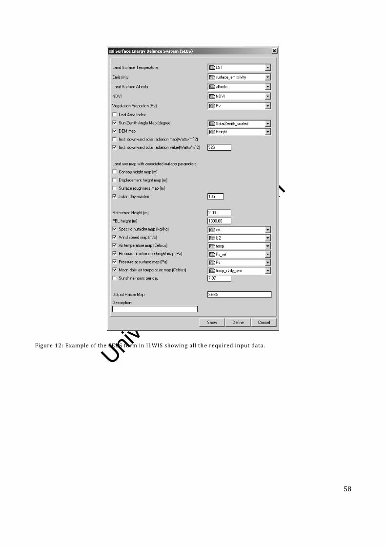
Univers

ity of

Cap

e Tow

n

58

Figure 12: Example of the SEBS form in ILWIS showing all the required input data.

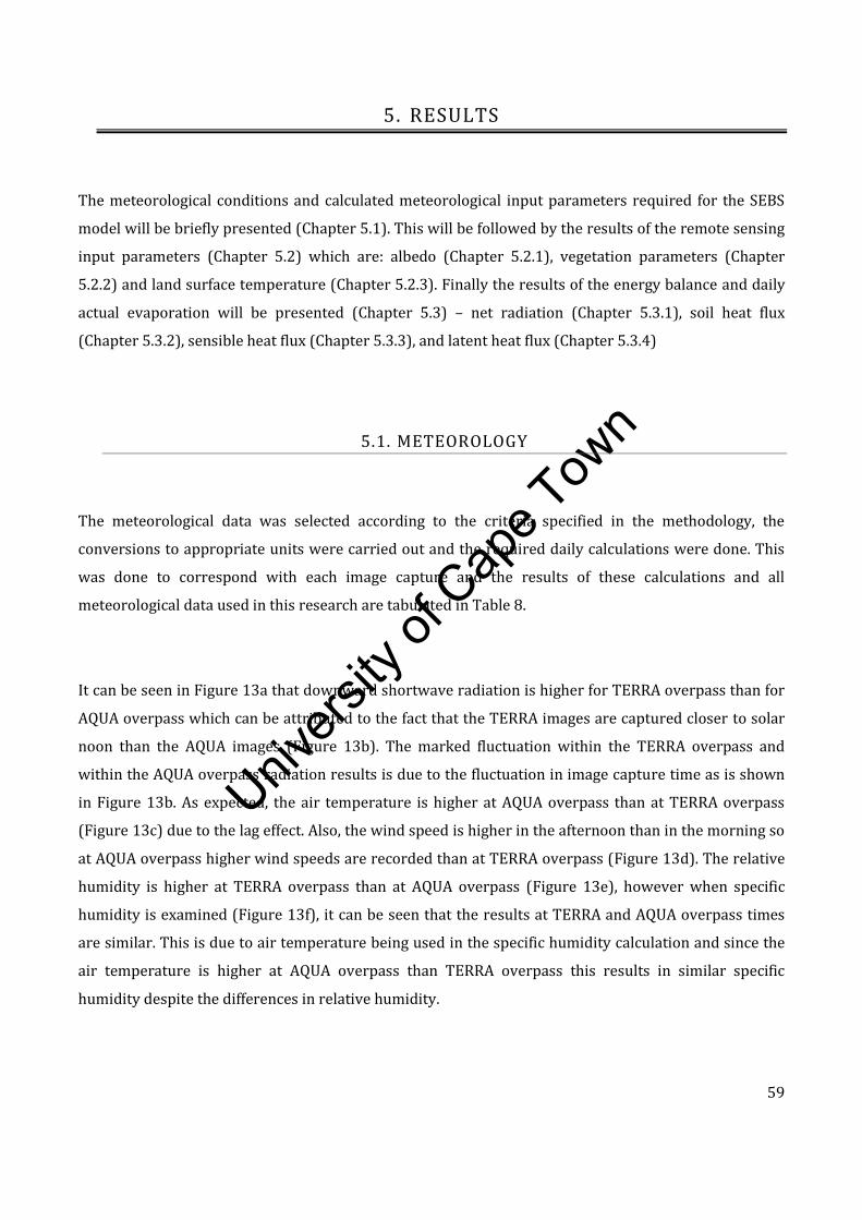
Univers

ity of

Cap

e Tow

n

59

5. RESULTS

The meteorological conditions and calculated meteorological input parameters required for the SEBS

model will be briefly presented (Chapter 5.1). This will be followed by the results of the remote sensing

input parameters (Chapter 5.2) which are: albedo (Chapter 5.2.1), vegetation parameters (Chapter

5.2.2) and land surface temperature (Chapter 5.2.3). Finally the results of the energy balance and daily

actual evaporation will be presented (Chapter 5.3) – net radiation (Chapter 5.3.1), soil heat flux

(Chapter 5.3.2), sensible heat flux (Chapter 5.3.3), and latent heat flux (Chapter 5.3.4)

5.1. METEOROLOGY

The meteorological data was selected according to the criteria specified in the methodology, the

conversions to appropriate units were carried out and the required daily calculations were done. This

was done to correspond with each image capture and the results of these calculations and all

meteorological data used in this research are tabulated in Table 8.

It can be seen in Figure 13a that downward shortwave radiation is higher for TERRA overpass than for

AQUA overpass which can be attributed to the fact that the TERRA images are captured closer to solar

noon than the AQUA images (Figure 13b). The marked fluctuation within the TERRA overpass and

within the AQUA overpass radiation results is due to the fluctuation in image capture time as is shown

in Figure 13b. As expected, the air temperature is higher at AQUA overpass than at TERRA overpass

(Figure 13c) due to the lag effect. Also, the wind speed is higher in the afternoon than in the morning so

at AQUA overpass higher wind speeds are recorded than at TERRA overpass (Figure 13d). The relative

humidity is higher at TERRA overpass than at AQUA overpass (Figure 13e), however when specific

humidity is examined (Figure 13f), it can be seen that the results at TERRA and AQUA overpass times

are similar. This is due to air temperature being used in the specific humidity calculation and since the

air temperature is higher at AQUA overpass than TERRA overpass this results in similar specific

humidity despite the differences in relative humidity.

Univers

ity of

Cap

e Tow

n

60

Table 8: Meteorological recordings and calculations at image capture time.

DOY Sensor

overhead Local Time

Radiation

W.m-2

Temperature

°C

Windspeed

m.s-1

Specific humidity

kg.kg-1

Daily average

temperature °C

Daily sunshine duration

315 TERRA 11:00 866.66 19.45 1.6 0.009

15.27 10.6 AQUA 16:00 550 22.94 2 0.008

319 AQUA 15:00 816.66 24.91 1.7 0.009 18.17 9.61

320 TERRA 12:00 961.11 24.35 1.2 0.009

18.26 10.7 AQUA 16:00 625 25.45 1.7 0.009

321 TERRA 11:00 886.11 22.09 1.4 0.009

17.68 10.9 AQUA 15:00 800 23.25 1.8 0.009

322 TERRA 11:00 863.89 18.46 1.7 0.008

15.66 10.6 AQUA 16:00 619 22.12 2.1 0.008

323 TERRA 12:00 955.55 22.66 1.4 0.008

19.14 10.8 AQUA 15:00 791.66 25.97 1.4 0.007

324 TERRA 11:00 877.78 27.66 1.2 0.007

23.62 10.9 AQUA 16:00 633.33 31.02 1.4 0.008

325 TERRA 12:00 950 33.16 1.1 0.008

23.83 10.8 AQUA 15:00 780.55 35.02 1.4 0.009

326 TERRA 11:00 855.55 23.15 1.6 0.011

19.07 10.6 AQUA 15:00 800 27.76 1.7 0.010

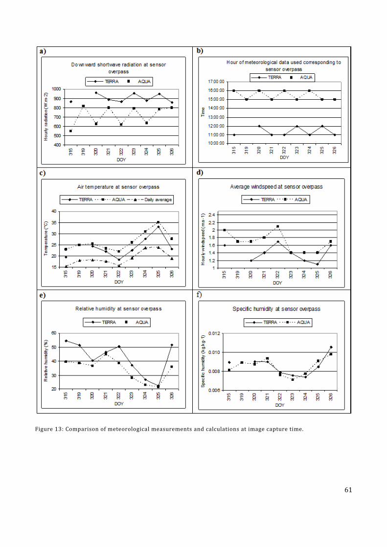
Univers

ity of

Cap

e Tow

n

61

Figure 13: Comparison of meteorological measurements and calculations at image capture time.

Univers

ity of

Cap

e Tow

n

62

5.2. REMOTELY SENSED INPUT PARAMETERS

At 1km resolution, no single complete pixel was contained within the apple orchard where the field

validation took place but rather four pixels were partially contained within the orchard. The pixel value

used for the validation was the pixel with the largest proportion contained within the orchard and also

directly on the site of the field validation equipment. It was shown in Figure 7 that the pixel footprint of

a MODIS scene for this area at 1 km resolution exceeds the boundaries of the orchard in which the field

validation is taking place, Multiple tree crops (apples, oranges, peaches, nectarines and pears, (Figure 3)

and the west facing slope of Levant Hill with natural vegetation all are contained within the 1 km pixel

resolution. For this reason, it is expected that the results obtained from the SEBS model will represent

this multitude of land covers and not exclusively represent the evapotranspiration of the apple orchard

where the field validation was conducted. The parameters required for SEBS were calculated from each

of the TERRA and AQUA datasets as per the prescribed methodology. The results of these calculations

extracted for the field validation site are shown in Table 9.

Table 9: MODIS TERRA and AQUA pre-processing results.

DOY SENSOR LOCAL TIME SOLAR

ZENITH

ANGLE (°)

SENSOR

ZENITH

ANGLE (°)

ALBEDO EMISSIVITY NDVI fc T0 (K)

315 TERRA 10:50 27 3 0.11 0.99 0.54 1 301.1

AQUA 15:10 40 46 0.11 0.99 0.53 1 302.6

319 AQUA 14:45 34 7 0.08 0.99 0.60 1 300.2

320 TERRA 11:10 23 32 0.08 0.99 0.60 1 299.7

AQUA 15:30 43 62 0.10 0.99 0.63 1 299.6

321 TERRA 10:15 33 56 0.11 0.99 0.59 1 299.3

AQUA 14:35 31 18 0.08 0.99 0.59 1 302.2

322 TERRA 10:55 25 10 0.11 0.99 0.53 1 297.9

AQUA 15:15 40 52 0.12 0.99 0.57 1 298.1

323 TERRA 11:40 17 64 0.08 0.99 0.63 1 295.4

AQUA 14:20 28 38 0.07 0.99 0.62 1 301.7

324 TERRA 10:45 27 15 0.12 0.99 0.56 1 304.9

AQUA 15:05 37 38 0.11 0.99 0.60 1 307.3

325 TERRA 11:25 19 54 0.08 0.99 0.57 1 303.9

AQUA 14:10 26 53 0.08 0.99 0.63 1 305.8

326 TERRA 10:30 29 36 0.12 0.99 0.58 1 302.4

AQUA 14:50 34 19 0.09 0.99 0.53 1 306.8

Univers

ity of

Cap

e Tow

n

63

By examining results in Table 9, a number of observations can be made and the results for each remote

sensing parameter will be discussed further under the appropriate section:

1 There is a high variation in sensor zenith angle (from 3 to 64°) and to a lesser extent in solar

zenith angle (from 17 to 43°)

2 There is a fluctuation in albedo from 0.07 to 0.12

3 NDVI ranges from 0.53 to 0.63

4 Fractional vegetation cover remains a constant 1

5 Emissivity remains a constant 0.99

6 Land surface temperature a) T0 fluctuates from 295.4K – 307.3K, a range of 11.9K b) T0

almost always higher in afternoon than in the morning and c) the fluctuation in T0 from

TERRA overpass to AQUA overpass ranges from -0.1 to 4.4 K

It is usual to consider the sensor zenith angle when selecting appropriate satellite images with low

sensor zenith angles recommended. For example, Tasumi et al. (2008) noted that images having large

view angles cause substantial smearing of the final product (with reference to the 16-day MODIS albedo

product) so that the effective resolution increases from the assumed 1 km pixel resolution to around 2 –

3 km in reality. However due to the short period for which field validation data was available, this was

not considered and all cloud free images corresponding to good quality field data were used in this

research. It can be seen in Figure 14a that the sensor zenith angle for the field validation site ranges

from 3 to 64° for TERRA and from 7 to 62° for AQUA; with TERRA generally having lower sensor zenith

angles for the period of the field campaign. The solar zenith angle (Figure 14b) is directly dependent on

the time at which the image was captured and since TERRA overpass is generally closer to solar noon,

the solar zenith angles reflect this.

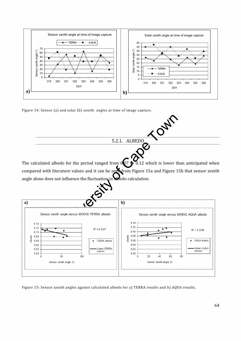
Univers

ity of

Cap

e Tow

n

64

a) b)

Figure 14: Sensor (a) and solar (b) zenith angles at time of image capture.

5.2.1. ALBEDO

The calculated albedo for the period ranged from 0.07 to 0.12 which is lower than anticipated when

compared with literature values and it can be seen from Figure 15a and Figure 15b that sensor zenith

angle alone does not influence the fluctuation in albedo calculation.

a)

b)

Figure 15: Sensor zenith angles against calculated albedo for a) TERRA results and b) AQUA results.

Sensor zenith angle at time of image capture

010203040506070

315 320 321 322 323 324 325 326

DOY

Sens

or z

enith

ang

le (°

)

TERRA AQUA

Solar zenith angle at time of image capture

05

1015202530354045

315 320 321 322 323 324 325 326

DOY

Sola

r zen

ith a

ngle

(°)

TERRA

AQUA

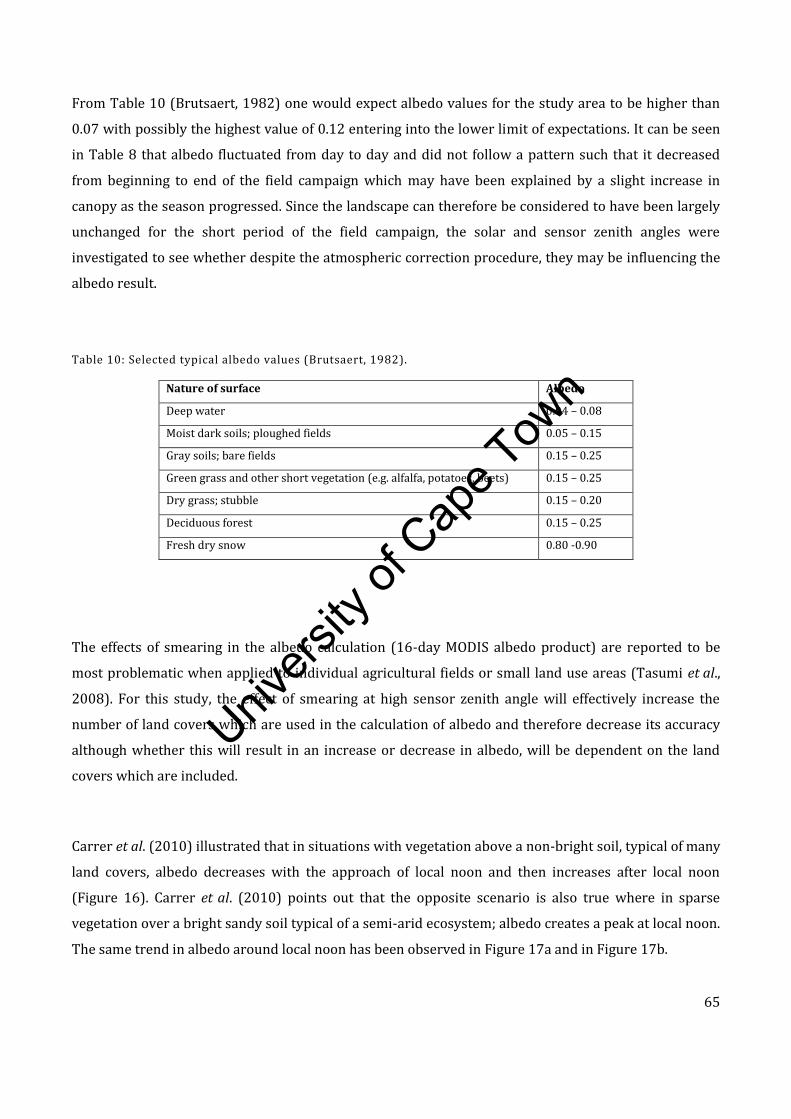
Univers

ity of

Cap

e Tow

n

65

From Table 10 (Brutsaert, 1982) one would expect albedo values for the study area to be higher than

0.07 with possibly the highest value of 0.12 entering into the lower limit of expectations. It can be seen

in Table 8 that albedo fluctuated from day to day and did not follow a pattern such that it decreased

from beginning to end of the field campaign which may have been explained by a slight increase in

canopy as the season progressed. Since the landscape can therefore be considered to have been largely

unchanged for the short period of the field campaign, the solar and sensor zenith angles were

investigated to see whether despite the atmospheric correction procedure, they may be influencing the

albedo result.

Table 10: Selected typical albedo values (Brutsaert, 1982).

Nature of surface Albedo

Deep water 0.04 – 0.08

Moist dark soils; ploughed fields 0.05 – 0.15

Gray soils; bare fields 0.15 – 0.25

Green grass and other short vegetation (e.g. alfalfa, potatoes, beets) 0.15 – 0.25

Dry grass; stubble 0.15 – 0.20

Deciduous forest 0.15 – 0.25

Fresh dry snow 0.80 -0.90

The effects of smearing in the albedo calculation (16-day MODIS albedo product) are reported to be

most problematic when applied to individual agricultural fields or small land use areas (Tasumi et al.,

2008). For this study, the effect of smearing at high sensor zenith angle will effectively increase the

number of land covers which are used in the calculation of albedo and therefore decrease its accuracy

although whether this will result in an increase or decrease in albedo, will be dependent on the land

covers which are included.

Carrer et al. (2010) illustrated that in situations with vegetation above a non-bright soil, typical of many

land covers, albedo decreases with the approach of local noon and then increases after local noon

(Figure 16). Carrer et al. (2010) points out that the opposite scenario is also true where in sparse

vegetation over a bright sandy soil typical of a semi-arid ecosystem; albedo creates a peak at local noon.

The same trend in albedo around local noon has been observed in Figure 17a and in Figure 17b.

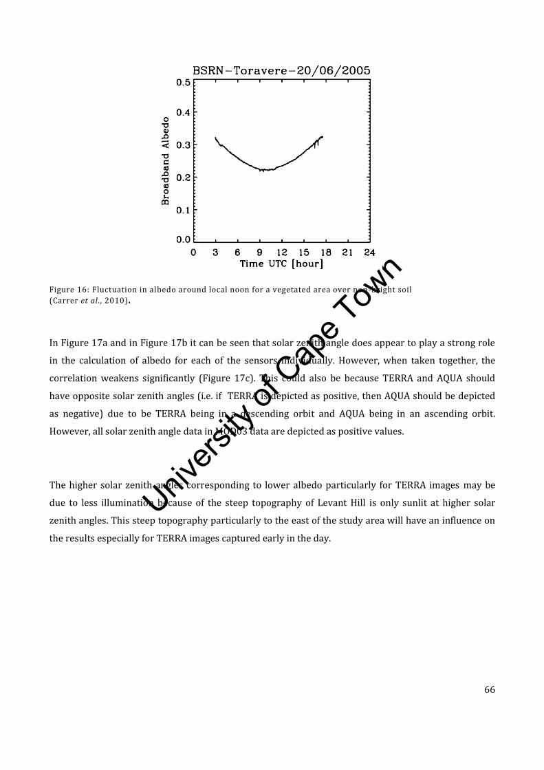
Univers

ity of

Cap

e Tow

n

66

Figure 16: Fluctuation in albedo around local noon for a vegetated area over non-bright soil

(Carrer et al. , 2010).

In Figure 17a and in Figure 17b it can be seen that solar zenith angle does appear to play a strong role

in the calculation of albedo for each of the sensors individually. However, when taken together, the

correlation weakens significantly (Figure 17c). This could also be because TERRA and AQUA should

have opposite solar zenith angles (i.e. if TERRA is depicted as positive, then AQUA should be depicted

as negative) due to be TERRA being in a descending orbit and AQUA being in an ascending orbit.

However, all solar zenith angle data in MOD03 data are depicted as positive values.

The higher solar zenith angles corresponding to lower albedo particularly for TERRA images may be

due to less illumination because of the steep topography of Levant Hill is only sunlit at higher solar

zenith angles. This steep topography particularly to the east of the study area will have an influence on

the results especially for TERRA images captured early in the day.

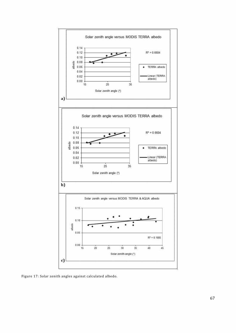
Univers

ity of

Cap

e Tow

n

67

Figure 17: Solar zenith angles against calculated albedo.

SOlar zenith angle versus MODIS TERRA al.>OOo

... '" R' _ 0.6604

" . • • • • 00 • • 00. •

rr __

00.

00' _ ....... (l'ERAA

.0> " tleOO)

" " " Sol .... _ ongIt (')

.J

Solar zenith angle versus MODIS TERRA abedo

... '" R' _ 0 6604

0.10 • • • ... • • • ... •

rr __

0,0. .. , _ Unn.(T£RRA

.0> ""'00)

" " " Sol ... . OMh or>gIt (')

bJ

Solo< .- ¥IgIo __ UOOIS TERRA 3. ~ _

." • • • • • . '" • , • • •

i • • • ... f\> _ OIAS

00.

" • .. • " " .. --""11'«')

oj

SOlar zenith angle versus MODIS TERRA alb&do

". '" R' · O.6604

", • • • , .. • • ". • "--,,.

,,, _ u.. .. (TERAA

", "tleOOI .. " " Sol ... _ "'lIlt r)

.j

Solar zenith anglo versus MODIS TERRA abedo

,,, '" R' • 0 66(l.I

0.10 • • • 0.08 • • • ... • "--0,04 .. , _ Uno .. (1'£RRA .., .... 001

" " " 901., .ondh 0I'IQ11 M

bj

Sol..- .- ""IJIe __ UOO1S Tt:RRA 3. NJ'JA _

'" • • • • • ... •

I • • • • • • .. , fI' . o 1m .. , .. , " • " .. ..

--""'JIO("

oj

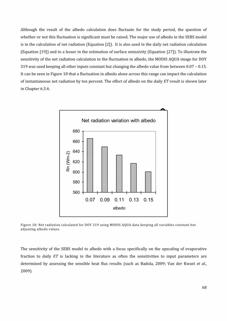
Univers

ity of

Cap

e Tow

n

68

Although the result of the albedo calculation does fluctuate for the study period, the question of

whether or not this fluctuation is significant must be raised. The major use of albedo in the SEBS model

is in the calculation of net radiation (Equation [2]). It is also used in the daily net radiation calculation

(Equation [19]) and to a lesser in the estimation of surface emissivity (Equation [27]). To illustrate the

sensitivity of the net radiation calculation to the fluctuation in albedo, the MODIS AQUA image for DOY

319 was used keeping all other inputs constant but changing the albedo value from between 0.07 – 0.15.

It can be seen in Figure 18 that a fluctuation in albedo alone across this range can impact the calculation

of instantaneous net radiation by ten percent. The effect of albedo on the daily ET result is shown later

in Chapter 6.3.4.

Figure 18: Net radiation calculated for DOY 319 using MODIS AQUA data keeping all variables constant but adjusting albedo values.

The sensitivity of the SEBS model to albedo with a focus specifically on the upscaling of evaporative

fraction to daily ET is lacking in the literature as often the sensitivities to input parameters are

determined by assessing the sensible heat flux results (such as Badola, 2009; Van der Kwast et al.,

2009).

Net radiation variation with albedo

560

580

600

620

640

660

680

0.07 0.09 0.11 0.13 0.15albedo

Rn

(Wm

-2)

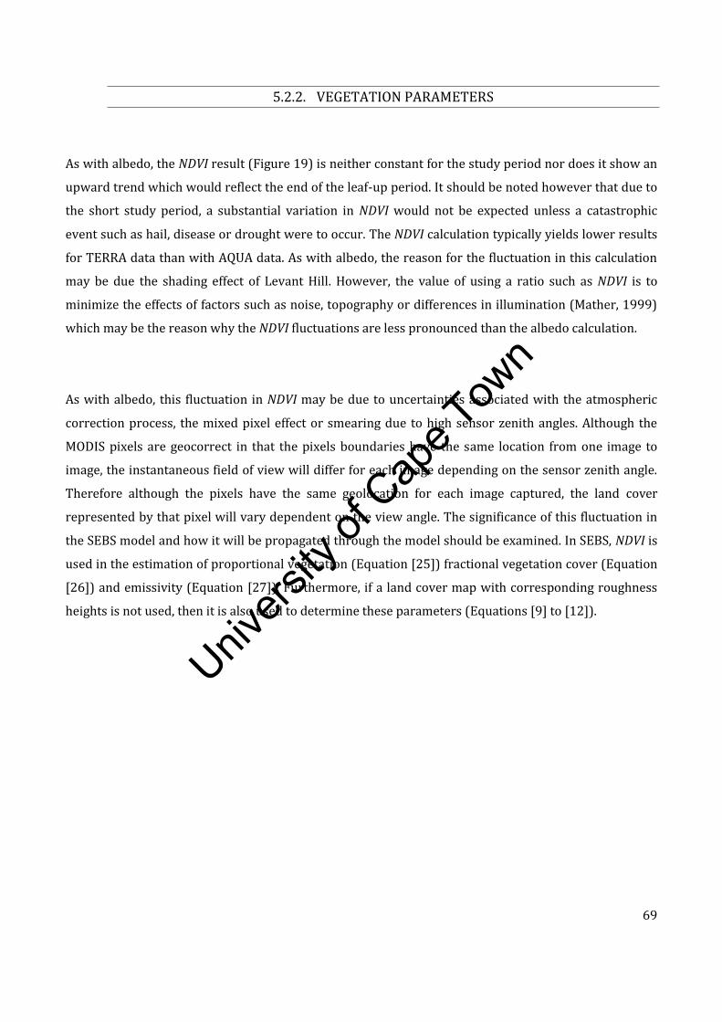
Univers

ity of

Cap

e Tow

n

69

5.2.2. VEGETATION PARAMETERS

As with albedo, the NDVI result (Figure 19) is neither constant for the study period nor does it show an

upward trend which would reflect the end of the leaf-up period. It should be noted however that due to

the short study period, a substantial variation in NDVI would not be expected unless a catastrophic

event such as hail, disease or drought were to occur. The NDVI calculation typically yields lower results

for TERRA data than with AQUA data. As with albedo, the reason for the fluctuation in this calculation

may be due the shading effect of Levant Hill. However, the value of using a ratio such as NDVI is to

minimize the effects of factors such as noise, topography or differences in illumination (Mather, 1999)

which may be the reason why the NDVI fluctuations are less pronounced than the albedo calculation.

As with albedo, this fluctuation in NDVI may be due to uncertainties associated with the atmospheric

correction process, the mixed pixel effect or smearing due to high sensor zenith angles. Although the

MODIS pixels are geocorrect in that the pixels boundaries have the same location from one image to

image, the instantaneous field of view will differ for each image depending on the sensor zenith angle.

Therefore although the pixels have the same geolocation for each image captured, the land cover

represented by that pixel will vary dependent on the view angle. The significance of this fluctuation in

the SEBS model and how it will be propagated through the model should be examined. In SEBS, NDVI is

used in the estimation of proportional vegetation (Equation [25]) fractional vegetation cover (Equation

[26]) and emissivity (Equation [27]). Furthermore, if a land cover map with corresponding roughness

heights is not used, then it is also used to determine these parameters (Equations [9] to [12]).

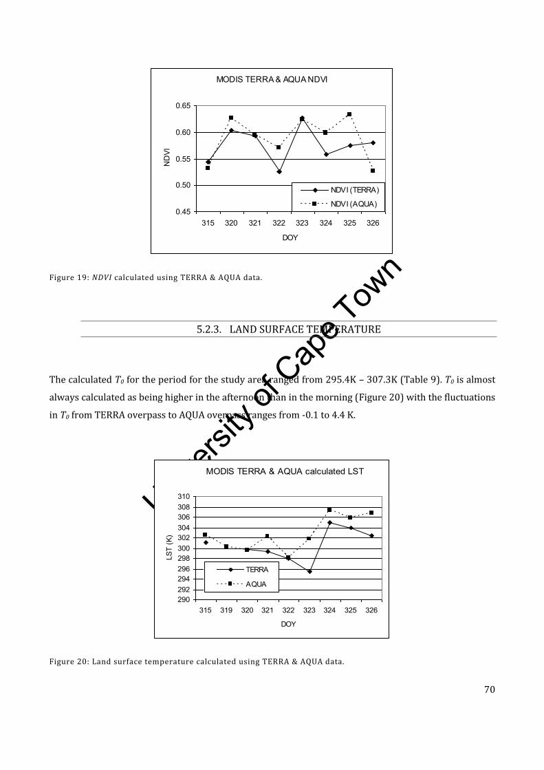
Univers

ity of

Cap

e Tow

n

70

Figure 19: NDVI calculated using TERRA & AQUA data.

5.2.3. LAND SURFACE TEMPERATURE

The calculated T0 for the period for the study area ranged from 295.4K – 307.3K (Table 9). T0 is almost

always calculated as being higher in the afternoon than in the morning (Figure 20) with the fluctuations

in T0 from TERRA overpass to AQUA overpass ranges from -0.1 to 4.4 K.

Figure 20: Land surface temperature calculated using TERRA & AQUA data.

MODIS TERRA & AQUA NDVI

0.45

0.50

0.55

0.60

0.65

315 320 321 322 323 324 325 326

DOY

ND

VI

NDVI (TERRA)

NDVI (AQUA)

MODIS TERRA & AQUA calculated LST

290292294296298300302304306308310

315 319 320 321 322 323 324 325 326

DOY

LST

(K)

TERRA

AQUA

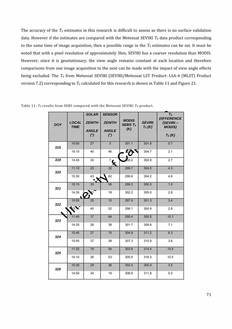
Univers

ity of

Cap

e Tow

n

71

The accuracy of the T0 estimates in this research is difficult to assess as there is no surface validation

data. However if the estimates are compared with the Meteosat SEVIRI T0 data product corresponding

to the same time of image acquisition, then a possible range in the T0 estimates can be set. It must be

noted that with a pixel resolution of approximately 3km, SEVIRI has a coarser resolution than MODIS.

However, since it is geostationary, the view angle remains constant at each location and therefore

comparisons from one image acquisition to the next can be made with the impact of view angle effects

being excluded. The T0 from Meteosat SEVIRI (SEVIRI/Meteosat LST Product: LSA-4 (MLST) Product

version 7.2) corresponding to T0 calculated for this research is shown in Table 11 and Figure 21.

Table 11: T0 results from SEBS compared with the Meteosat SEVIRI T0 product.

DOY LOCAL

TIME

SOLAR

ZENITH

ANGLE

(°)

SENSOR

ZENITH

ANGLE

(°)

MODIS

SEBS T0

(K)

SEVIRI

T0 (K)

T0

DIFFERENCE

(SEVIRI –

MODIS)

T0 (K)

315

10:50 27 3 301.1 301.8 0.7

15:10 40 46 302.6 304.7 2.1

319 14:45 34 7 300.2 302.9 2.7

320

11:10 23 32 299.7 304.0 4.3

15:30 43 62 299.6 304.2 4.6

321

10:15 33 56 299.3 300.3 1.0

14:35 31 18 302.2 305.0 2.8

322

10:55 25 10 297.9 301.3 3.4

15:15 40 52 298.1 300.9 2.8

323

11:40 17 64 295.4 305.5 10.1

14:20 28 38 301.7 308.8 7.1

324

10:45 27 15 304.9 311.2 6.3

15:05 37 38 307.3 310.9 3.6

325

11:25 19 54 303.9 314.4 10.5

14:10 26 53 305.8 316.3 10.5

326

10:30 29 36 302.4 305.9 3.5

14:50 34 19 306.8 311.8 5.0

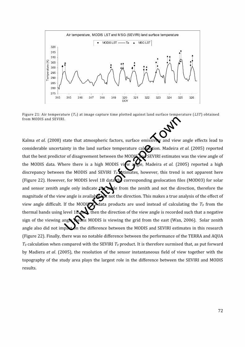
Univers

ity of

Cap

e Tow

n

72

Figure 21: Air temperature (Ta) at image capture time plotted against land surface temperature ( LST) obtained from MODIS and SEVIRI.

Kalma et al. (2008) state that atmospheric factors, surface emissivity and view angle effects lead to

considerable uncertainty in the land surface temperature calculation. Madeira et al. (2005) reported

that the best predictor of disagreement between the MODIS and SEVIRI estimates was the view angle of

the MODIS data. Where there is a high MODIS view angle, Madeira et al. (2005) reported a high

discrepancy between the MODIS and SEVIRI T0 estimates, however, this trend is not apparent here

(Figure 22). However, for MODIS level 1B data the corresponding geolocation files (MOD03) for solar

and sensor zenith angle only indicate the angle from the zenith and not the direction, therefore the

magnitude of the view angle is available but not the direction. This makes a true analysis of the effect of

view angle difficult. If the MODIS T0 data products are used instead of calculating the T0 from the

thermal bands using level 1B data, then the direction of the view angle is recorded such that a negative

sign of the viewing angle means MODIS is viewing the grid from the east (Wan, 2006). Solar zenith

angle also did not impact on the difference between the MODIS and SEVIRI estimates in this research

(Figure 22). Finally, there was no notable difference between the performance of the TERRA and AQUA

T0 calculation when compared with the SEVIRI T0 product. It is therefore surmised that, as put forward

by Madiera et al. (2005), the resolution of the sensor instantaneous field of view together with the

topography of the study area plays the largest role in the difference between the SEVIRI and MODIS

results.

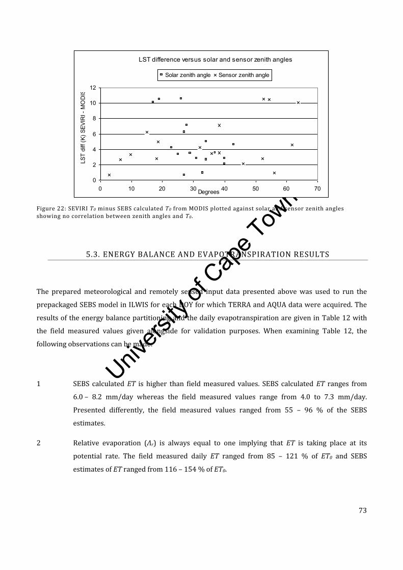
Univers

ity of

Cap

e Tow

n

73

Figure 22: SEVIRI T0 minus SEBS calculated T0 from MODIS plotted against solar and sensor zenith angles showing no correlation between zenith angles and T0.

5.3. ENERGY BALANCE AND EVAPOTRANSPIRATION RESULTS

The prepared meteorological and remotely sensed input data presented above was used to run the

prepackaged SEBS model in ILWIS for each DOY for which TERRA and AQUA data were acquired. The

results of the energy balance partitioning and the daily evapotranspiration are given in Table 12 with

the field measured values given alongside for validation purposes. When examining Table 12, the

following observations can be made:

1 SEBS calculated ET is higher than field measured values. SEBS calculated ET ranges from

6.0 – 8.2 mm/day whereas the field measured values range from 4.0 to 7.3 mm/day.

Presented differently, the field measured values ranged from 55 – 96 % of the SEBS

estimates.

2 Relative evaporation (Λr) is always equal to one implying that ET is taking place at its

potential rate. The field measured daily ET ranged from 85 – 121 % of ET0 and SEBS

estimates of ET ranged from 116 – 154 % of ET0.

LST difference versus solar and sensor zenith angles

0

2

4

6

8

10

12

0 10 20 30 40 50 60 70Degrees

LST

diff

(K) S

EVIR

I - M

OD

ISSolar zenith angle Sensor zenith angle

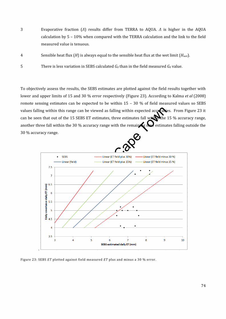
Univers

ity of

Cap

e Tow

n

74

3 Evaporative fraction (Λ) results differ from TERRA to AQUA. Λ is higher in the AQUA

calculation by 5 – 10% when compared with the TERRA calculation and the link to the field

measured value is tenuous.

4 Sensible heat flux (H) is always equal to the sensible heat flux at the wet limit (Hwet).

5 There is less variation in SEBS calculated G0 than in the field measured G0 value.

To objectively assess the results, the SEBS estimates are plotted against the field results together with

lower and upper limits of 15 and 30 % error respectively (Figure 23). According to Kalma et al (2008)

remote sensing estimates can be expected to be within 15 – 30 % of field measured values so SEBS

values falling within this range can be viewed as falling within expected accuracies. From Figure 23 it

can be seen that out of the 15 SEBS ET estimates, three estimates fall within the 15 % accuracy range,

another three fall within the 30 % accuracy range with the remaining nine estimates falling outside the

30 % accuracy range.

.

Figure 23: SEBS ET plotted against field measured ET plus and minus a 30 % error.

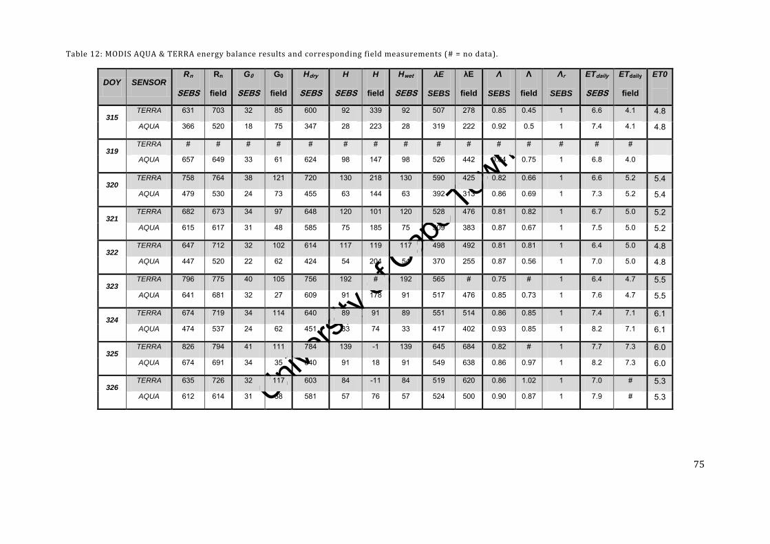
Univers

ity of

Cap

e Tow

n

75

Table 12: MODIS AQUA & TERRA energy balance results and corresponding field measurements (# = no data).

DOY SENSOR Rn

SEBS

Rn

field

G0

SEBS

G0

field

Hdry

SEBS

H

SEBS

H

field

Hwet

SEBS

λE

SEBS

λE

field

Λ

SEBS

Λ

field

Λr

SEBS

ETdaily

SEBS

ETdaily

field

ET0

315 TERRA 631 703 32 85 600 92 339 92 507 278 0.85 0.45 1 6.6 4.1 4.8

AQUA 366 520 18 75 347 28 223 28 319 222 0.92 0.5 1 7.4 4.1 4.8

319 TERRA # # # # # # # # # # # # # # #

AQUA 657 649 33 61 624 98 147 98 526 442 0.84 0.75 1 6.8 4.0

320 TERRA 758 764 38 121 720 130 218 130 590 425 0.82 0.66 1 6.6 5.2 5.4

AQUA 479 530 24 73 455 63 144 63 392 313 0.86 0.69 1 7.3 5.2 5.4

321 TERRA 682 673 34 97 648 120 101 120 528 476 0.81 0.82 1 6.7 5.0 5.2

AQUA 615 617 31 48 585 75 185 75 509 383 0.87 0.67 1 7.5 5.0 5.2

322 TERRA 647 712 32 102 614 117 119 117 498 492 0.81 0.81 1 6.4 5.0 4.8

AQUA 447 520 22 62 424 54 204 54 370 255 0.87 0.56 1 7.0 5.0 4.8

323 TERRA 796 775 40 105 756 192 # 192 565 # 0.75 # 1 6.4 4.7 5.5

AQUA 641 681 32 27 609 91 178 91 517 476 0.85 0.73 1 7.6 4.7 5.5

324 TERRA 674 719 34 114 640 89 91 89 551 514 0.86 0.85 1 7.4 7.1 6.1

AQUA 474 537 24 62 451 33 74 33 417 402 0.93 0.85 1 8.2 7.1 6.1

325 TERRA 826 794 41 111 784 139 -1 139 645 684 0.82 # 1 7.7 7.3 6.0

AQUA 674 691 34 35 640 91 18 91 549 638 0.86 0.97 1 8.2 7.3 6.0

326 TERRA 635 726 32 117 603 84 -11 84 519 620 0.86 1.02 1 7.0 # 5.3

AQUA 612 614 31 38 581 57 76 57 524 500 0.90 0.87 1 7.9 # 5.3

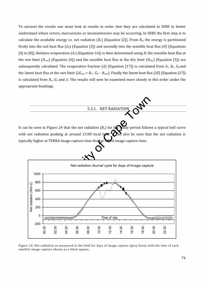
Univers

ity of

Cap

e Tow

n

76

To unravel the results one must look at results in order that they are calculated in SEBS to better

understand where errors, inaccuracies or inconsistencies may be occurring. In SEBS the first step is to

calculate the available energy i.e. net radiation (Rn) (Equation [2]). From Rn, the energy is partitioned

firstly into the soil heat flux (G0) (Equation [3]) and secondly into the sensible heat flux (H) (Equations

[4] to [8]). Relative evaporation (Λr) (Equation 16]) is then determined using H, the sensible heat flux at

the wet limit (Hwet) (Equation [4]) and the sensible heat flux at the dry limit (Hdry) (Equation [5]) are

subsequently calculated. The evaporative fraction (Λ) (Equation [17]) is calculated from Λr, Rn, G0 and

the latent heat flux at the wet limit (λEwet = Rn - G0 - Hwet). Finally the latent heat flux (λE) (Equation [17])

is calculated from Rn, G0 and Λ. The results will now be examined more closely in this order under the

appropriate headings.

5.3.1. NET RADIATION

It can be seen in Figure 24 that the net radiation (Rn) for the study period follows a typical bell curve

with net radiation peaking at around 13:00 local time. It can also be seen that the net radiation is

typically higher at TERRA image capture time than at AQUA image capture time.

Figure 24: Net radiation as measured in the field for days of image capture (grey lines) with the time of each satellite image capture shown as a black square.

Net radiation diurnal cycle for days of image capture

-200

0

200

400

600

800

1000

00:3

0

02:3

0

04:3

0

06:3

0

08:3

0

10:3

0

12:3

0

14:3

0

16:3

0

18:3

0

20:3

0

22:3

0

Time of day

Net

radi

atio

n (W

m-2

)

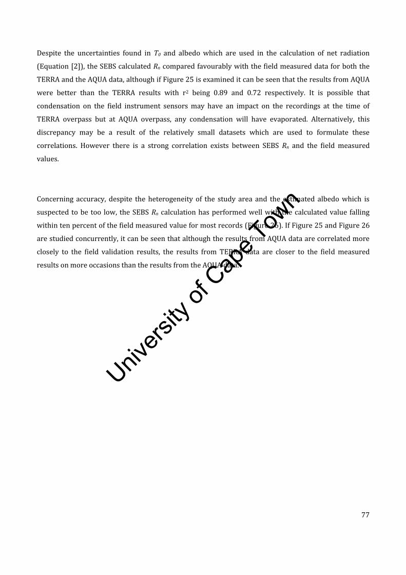
Univers

ity of

Cap

e Tow

n

77

Despite the uncertainties found in T0 and albedo which are used in the calculation of net radiation

(Equation [2]), the SEBS calculated Rn compared favourably with the field measured data for both the

TERRA and the AQUA data, although if Figure 25 is examined it can be seen that the results from AQUA

were better than the TERRA results with r2 being 0.89 and 0.72 respectively. It is possible that

condensation on the field instrument sensors may have an impact on the recordings at the time of

TERRA overpass but at AQUA overpass, any condensation will have evaporated. Alternatively, this

discrepancy may be a result of the relatively small datasets which are used to formulate these

correlations. However there is a strong correlation exists between SEBS Rn and the field measured

values.

Concerning accuracy, despite the heterogeneity of the study area and the estimated albedo which is

suspected to be too low, the SEBS Rn calculation has performed well with the calculated value falling

within ten percent of the field measured value for most records (Figure 26). If Figure 25 and Figure 26

are studied concurrently, it can be seen that although the results from AQUA data are correlated more

closely to the field validation results, the results from TERRA data are closer to the field measured

results on more occasions than the results from the AQUA data.

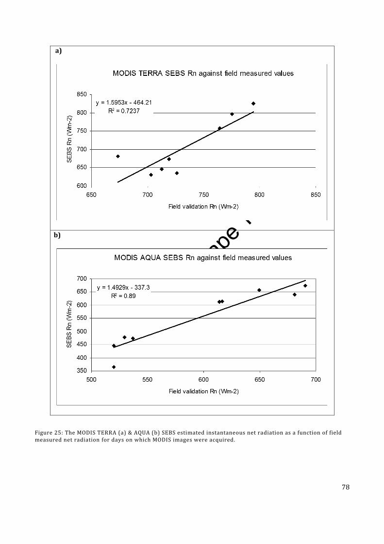
Univers

ity of

Cap

e Tow

n

78

a)

b)

Figure 25: The MODIS TERRA (a) & AQUA (b) SEBS estimated instantaneous net radiation as a function of field measured net radiation for days on which MODIS images were acquired.

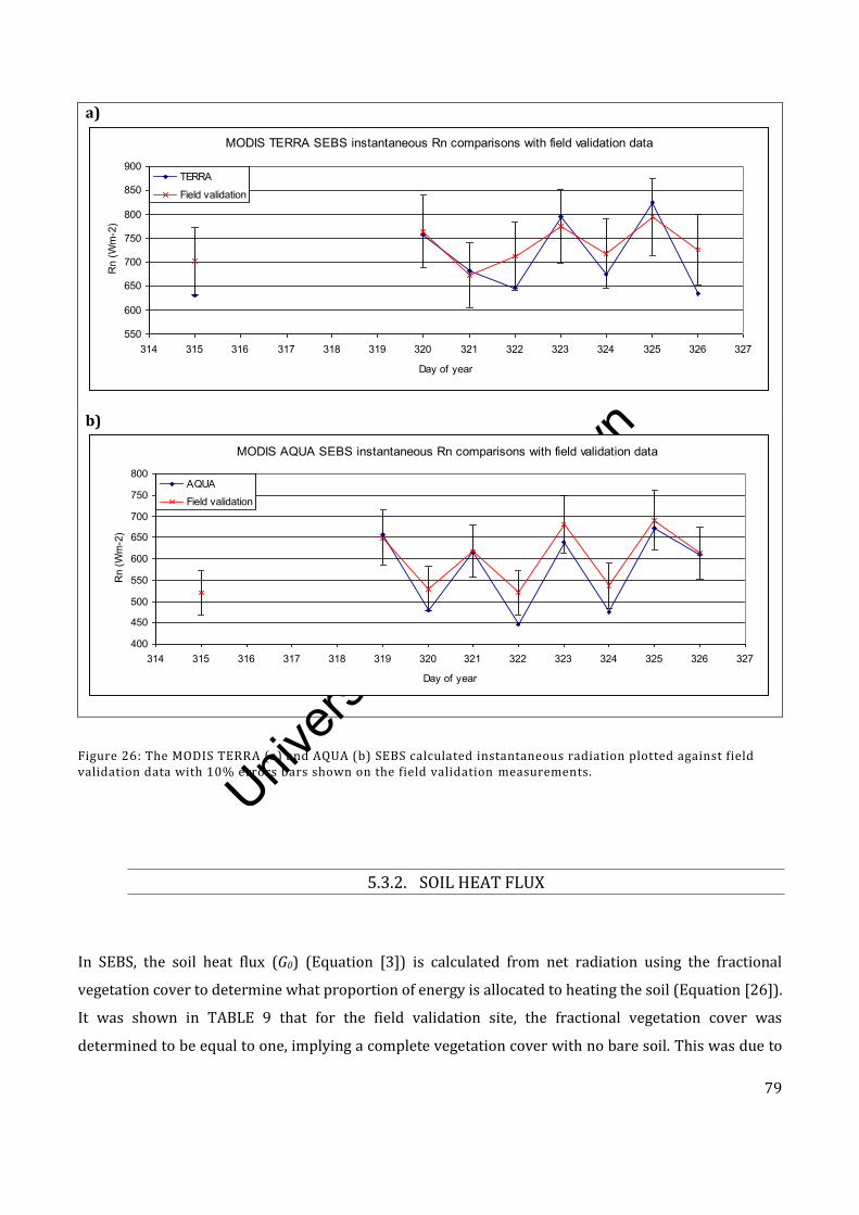
Univers

ity of

Cap

e Tow

n

79

a)

b)

Figure 26: The MODIS TERRA (a) and AQUA (b) SEBS calculated instantaneous radiation plotted against field validation data with 10% errors bars shown on the field validation measurements.

5.3.2. SOIL HEAT FLUX

In SEBS, the soil heat flux (G0) (Equation [3]) is calculated from net radiation using the fractional

vegetation cover to determine what proportion of energy is allocated to heating the soil (Equation [26]).

It was shown in TABLE 9 that for the field validation site, the fractional vegetation cover was

determined to be equal to one, implying a complete vegetation cover with no bare soil. This was due to

MODIS TERRA SEBS instantaneous Rn comparisons with field validation data

550

600

650

700

750

800

850

900

314 315 316 317 318 319 320 321 322 323 324 325 326 327

Day of year

Rn

(Wm

-2)

TERRA

Field validation

MODIS AQUA SEBS instantaneous Rn comparisons with field validation data

400

450

500

550

600

650

700

750

800

314 315 316 317 318 319 320 321 322 323 324 325 326 327

Day of year

Rn

(Wm

-2)

AQUA

Field validation

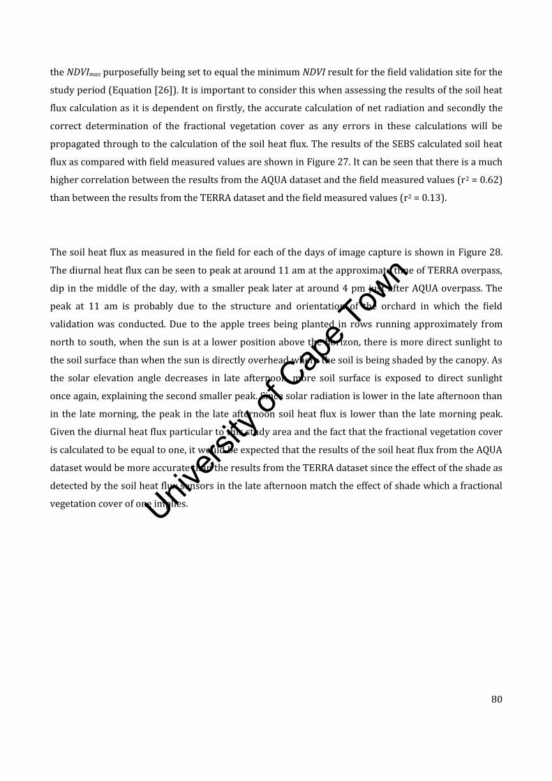
Univers

ity of

Cap

e Tow

n

80

the NDVImax purposefully being set to equal the minimum NDVI result for the field validation site for the

study period (Equation [26]). It is important to consider this when assessing the results of the soil heat

flux calculation as it is dependent on firstly, the accurate calculation of net radiation and secondly the

correct determination of the fractional vegetation cover as any errors in these calculations will be

propagated through to the calculation of the soil heat flux. The results of the SEBS calculated soil heat

flux as compared with field measured values are shown in Figure 27. It can be seen that there is a much

higher correlation between the results from the AQUA dataset and the field measured values (r2 = 0.62)

than between the results from the TERRA dataset and the field measured values (r2 = 0.13).

The soil heat flux as measured in the field for each of the days of image capture is shown in Figure 28.

The diurnal heat flux can be seen to peak at around 11 am at the approximate time of TERRA overpass,

dip in the middle of the day, with a smaller peak later at around 4 pm just after AQUA overpass. The

peak at 11 am is probably due to the structure and orientation of the orchard in which the field

validation was conducted. Due to the apple trees being planted in rows running approximately from

north to south, when the sun is at a lower position above the horizon, there is more direct sunlight to

the soil surface than when the sun is directly overhead where the soil is being shaded by the canopy. As

the solar elevation angle decreases in late afternoon, more soil surface is exposed to direct sunlight

once again, explaining the second smaller peak. Since solar radiation is lower in the late afternoon than

in the late morning, the peak in the late afternoon soil heat flux is lower than the late morning peak.

Given the diurnal heat flux particular to this study area and the fact that the fractional vegetation cover

is calculated to be equal to one, it would be expected that the results of the soil heat flux from the AQUA

dataset would be more accurate than the results from the TERRA dataset since the effect of the shade as

detected by the soil heat flux sensors in the late afternoon match the effect of shade which a fractional

vegetation cover of one implies.

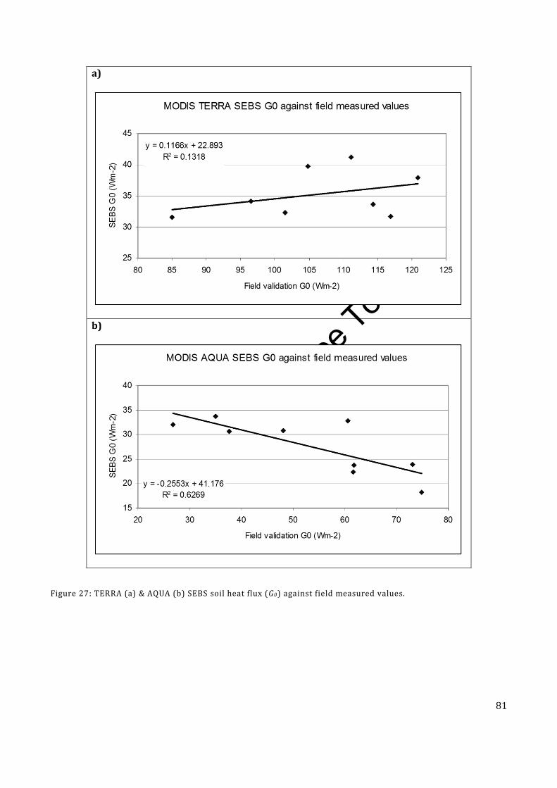
Univers

ity of

Cap

e Tow

n

81

a)

b)

Figure 27: TERRA (a) & AQUA (b) SEBS soil heat flux (G0) against field measured values.

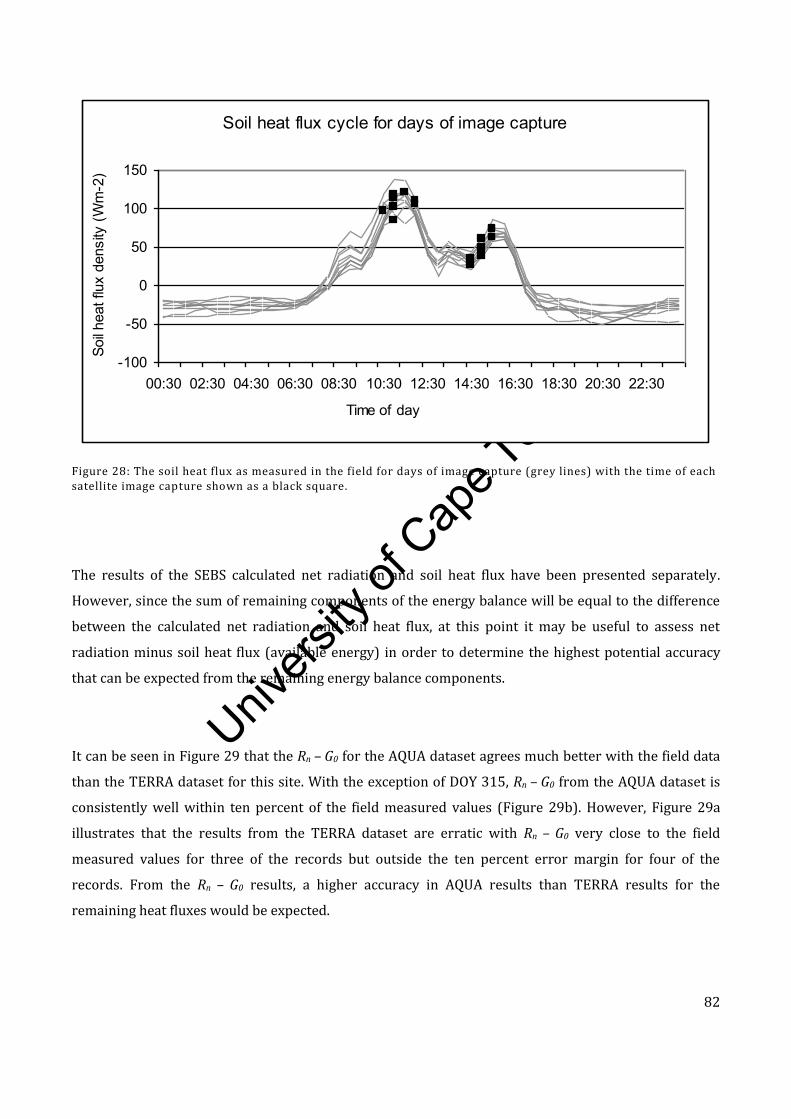
Univers

ity of

Cap

e Tow

n

82

Figure 28: The soil heat flux as measured in the field for days of image capture (grey lines) with the time of each satellite image capture shown as a black square.

The results of the SEBS calculated net radiation and soil heat flux have been presented separately.

However, since the sum of remaining components of the energy balance will be equal to the difference

between the calculated net radiation and soil heat flux, at this point it may be useful to assess net

radiation minus soil heat flux (available energy) in order to determine the highest potential accuracy

that can be expected from the remaining energy balance components.

It can be seen in Figure 29 that the Rn – G0 for the AQUA dataset agrees much better with the field data

than the TERRA dataset for this site. With the exception of DOY 315, Rn – G0 from the AQUA dataset is

consistently well within ten percent of the field measured values (Figure 29b). However, Figure 29a

illustrates that the results from the TERRA dataset are erratic with Rn – G0 very close to the field

measured values for three of the records but outside the ten percent error margin for four of the

records. From the Rn – G0 results, a higher accuracy in AQUA results than TERRA results for the

remaining heat fluxes would be expected.

Soil heat flux cycle for days of image capture

-100

-50

0

50

100

150

00:30 02:30 04:30 06:30 08:30 10:30 12:30 14:30 16:30 18:30 20:30 22:30

Time of day

Soil h

eat f

lux

dens

ity (W

m-2

)

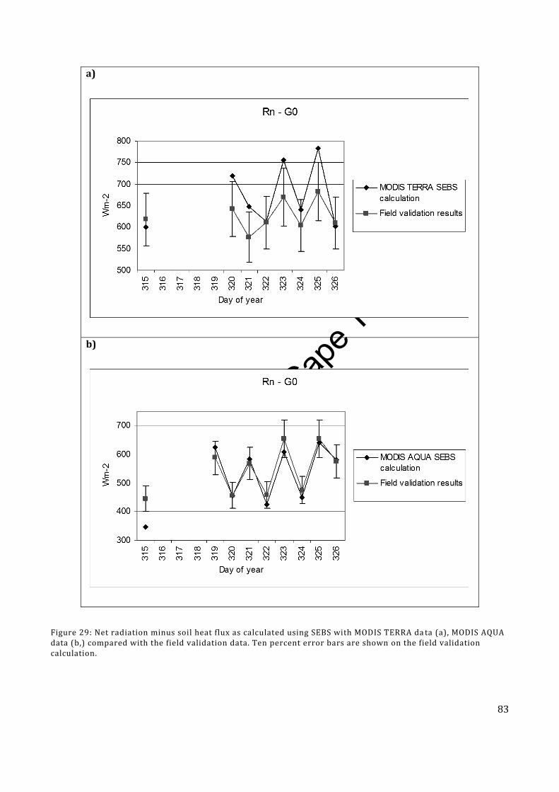
Univers

ity of

Cap

e Tow

n

83

a)

b)

Figure 29: Net radiation minus soil heat flux as calculated using SEBS with MODIS TERRA da ta (a), MODIS AQUA data (b,) compared with the field validation data. Ten percent error bars are shown on the field validation calculation.

Univers

ity of

Cap

e Tow

n

84

5.3.3. SENSIBLE HEAT FLUX

The sensible heat flux (H) is calculated in SEBS independently of the other surface energy balance terms

by solving Equations [4] to [8] using, wind speed, temperature at reference height and at the surface,

and roughness lengths for heat and momentum transfer. The roughness lengths in this research are

calculated from remotely sensed vegetation indices (Equations [9] to [12]) and the advice by Su (2002)

regarding this method was noted.

If the results of the field measured values of H and the SEBS calculated values for H in Table 12 are

examined in conjunction with Figure 30, it can be seen that there is no agreement between the SEBS

calculated values and the field measured values with r2 values of 0.01 and 0.03 for the TERRA and AQUA

dataset respectively. This is contrary to the previous good agreement between SEBS calculated Rn and

G0 at least for the AQUA dataset and the results should therefore be examined more closely. It can be

seen in Table 12 that for every record H is equal to Hwet. Since SEBS constrains H to the range set by Hwet,

and Hdry, H was calculated to be less than or equal to Hwet for every data record and H was therefore

assigned the value of Hwet. Although the field validation site is in an irrigated apple orchard at almost

complete canopy cover where it would be expected that the sensible heat flux would be tending

towards the wet limit, it is unlikely that for every record the calculated heat flux would be exactly at the

wet limit.

The sensible heat flux as measured in the field for each of the days of image capture is shown in Figure

31. Generally, the diurnal sensible heat flux can be seen to peak just after midday. Contrary to the soil

heat flux trend where the flux was measured as significantly higher at TERRA overpass time than at

AQUA overpass time, there is no such trend with the field measured sensible heat flux data.

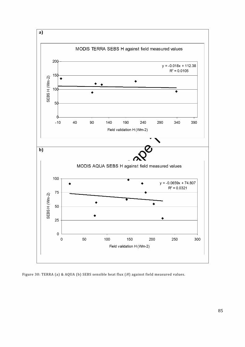
Univers

ity of

Cap

e Tow

n

85

a)

b)

Figure 30: TERRA (a) & AQUA (b) SEBS sensible heat flux (H) against field measured values.

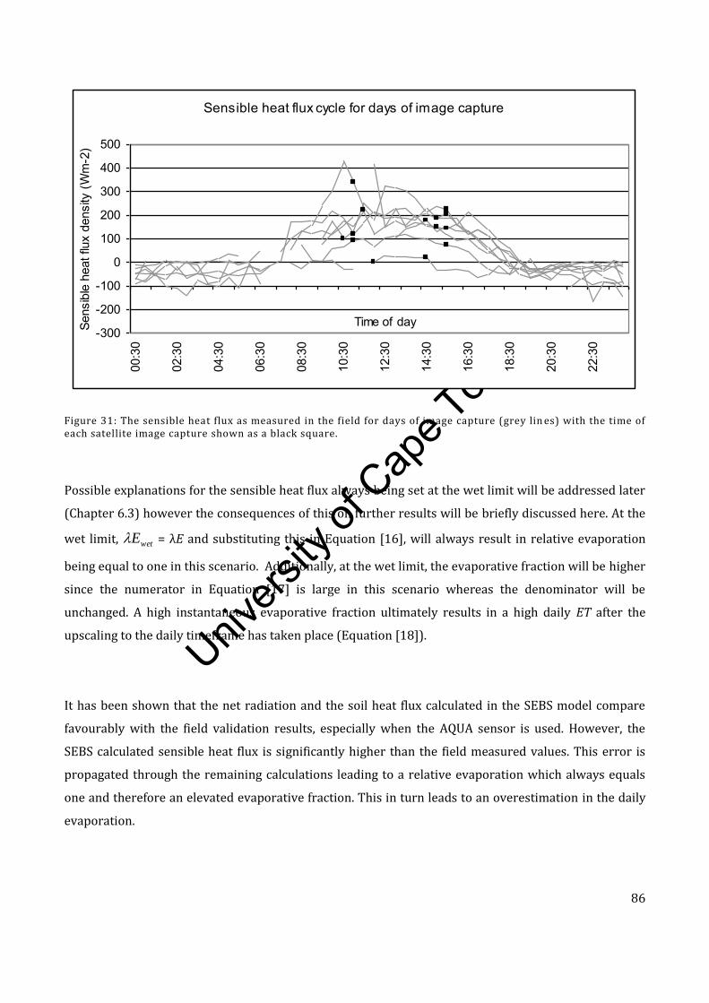
Univers

ity of

Cap

e Tow

n

86

Figure 31: The sensible heat flux as measured in the field for days of image capture (grey lin es) with the time of each satellite image capture shown as a black square.

Possible explanations for the sensible heat flux always being set at the wet limit will be addressed later

(Chapter 6.3) however the consequences of this on further results will be briefly discussed here. At the

wet limit, wetE = λE and substituting this in Equation [16], will always result in relative evaporation

being equal to one in this scenario. Additionally, at the wet limit, the evaporative fraction will be higher

since the numerator in Equation [17] is large in this scenario whereas the denominator will be

unchanged. A high instantaneous evaporative fraction ultimately results in a high daily ET after the

upscaling to the daily timeframe has taken place (Equation [18]).

It has been shown that the net radiation and the soil heat flux calculated in the SEBS model compare

favourably with the field validation results, especially when the AQUA sensor is used. However, the

SEBS calculated sensible heat flux is significantly higher than the field measured values. This error is

propagated through the remaining calculations leading to a relative evaporation which always equals

one and therefore an elevated evaporative fraction. This in turn leads to an overestimation in the daily

evaporation.

Sensible heat flux cycle for days of image capture

-300

-200

-100

0

100

200

300

400

50000

:30

02:3

0

04:3

0

06:3

0

08:3

0

10:3

0

12:3

0

14:3

0

16:3

0

18:3

0

20:3

0

22:3

0

Time of daySens

ible

hea

t flu

x de

nsity

(Wm

-2)

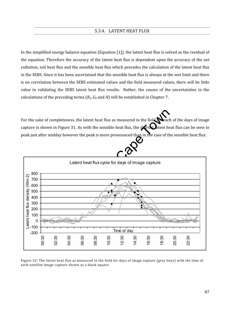
Univers

ity of

Cap

e Tow

n

87

5.3.4. LATENT HEAT FLUX

In the simplified energy balance equation (Equation [1]), the latent heat flux is solved as the residual of

the equation. Therefore the accuracy of the latent heat flux is dependent upon the accuracy of the net

radiation, soil heat flux and the sensible heat flux which precedes the calculation of the latent heat flux

in the SEBS. Since it has been ascertained that the sensible heat flux is always at the wet limit and there

is no correlation between the SEBS estimated values and the field measured values, there will be little

value in validating the SEBS latent heat flux results. Rather, the causes of the uncertainties in the

calculations of the preceding terms (Rn, G0 and H) will be established in Chapter 7.

For the sake of completeness, the latent heat flux as measured in the field for each of the days of image

capture is shown in Figure 31. As with the sensible heat flux, the diurnal latent heat flux can be seen to

peak just after midday however the peak is more pronounced than in the case of the sensible heat flux.

Figure 32: The latent heat flux as measured in the field for days of image capture (grey lines) with the time of each satellite image capture shown as a black square.

Latent heat flux cycle for days of image capture

-200-100

0100200300400500600700800

00:3

0

02:3

0

04:3

0

06:3

0

08:3

0

10:3

0

12:3

0

14:3

0

16:3

0

18:3

0

20:3

0

22:3

0

Time of day

Late

nt h

eat f

lux

dens

ity (W

m-2

)

Univers

ity of

Cap

e Tow

n

88

5.4. SUMMARY OF RESULTS

In summary, the results have shown that:

1) Despite the uncertainties found in the T0 and albedo which are used in the calculation of net

radiation, the SEBS calculated Rn compared favourably with the field measured data for both the

TERRA and the AQUA data, with the results from AQUA being better than the TERRA results

with r2 being 0.89 and 0.72 respectively.

2) The results of the SEBS calculated soil heat flux from the AQUA dataset have a higher correlation

(r2 = 0.62) than the results from the TERRA dataset (r2 = 0.13), probably due to the view angle

(and thus viewed fractional vegetation cover) at AQUA overpass time.

3) .The SEBS calculated sensible heat flux is significantly higher than the field measured values.

This error is propagated through the remaining calculations leading to a relative evaporation

which always equals one and therefore an elevated evaporative fraction. This in turn leads to an

overestimation in the daily evaporation.

The structure of the remainder of the thesis is now outlined to enable the reader to follow the direction

of the proceeding text. Model uncertainties (excluding roughness parameters) particular to the study

area are explored in Chapter 6. Adaptations to processing methods which are expected to lead to

improved results are described and applied to a new study area in Chapter 7. Finally in Chapter 8,

changes to the methodology are applied back to the Mouton’s Valley field validation site.

Univers

ity of

Cap

e Tow

n

89

6. MODEL UNCERTAINTIES

The pressure on water resources in South Africa creates a need for water resource managers to have

accurate information on all aspects of water resource occurrence and use. To quantify the various

components involved in calculating water use by means of field-based observations would be a difficult

and time consuming process, providing only point-based measurements at a specific point in time. This

problem is compounded when one considers that several measurements over time would be needed to

accurately measure or monitor water use. To address these problems, Gibson et al. (2009) investigated

the usefulness and applicability of remote sensing technologies as a tool for water resource assessment

and specifically for the quantification of water use at farm level. Their approach relied on a simplified

equation in which each component of the water balance equation was calculated for a hydrological year

using mostly remote sensing techniques or products where possible.

To derive the remote sensing datasets for input into water balance equations, several complex models

were applied to the input data. Although all of the components quantified by remote sensing data were

subject to uncertainties and limitations, Gibson et al. (2009) were alerted to the possibility of

uncertainties through the calculation of ET. The calculation of ET revealed that the total annual ET

calculated using the Surface Energy Balance System (SEBS) model for the study area exceeded the total

rainfall for the same area and time period. Although it may be possible for annual actual

evapotranspiration to exceed annual precipitation in certain instances, such as where large scale

irrigation from groundwater resources is practised, in this particular study, it is believed that actual

evapotranspiration was overestimated. Since irrigated agriculture forms a small portion of the

catchment (2.4%) in comparison to natural vegetation (29.7%) and dryland agricultural (66.5%), the

higher actual evapotranspiration than precipitation at catchment scale cannot be ascribed to

evaporative losses due to irrigation. As a consequence, the origins of uncertainties with regard to the

accuracy of the final results were explored using the estimation of ET as an example.

The derivation of ET is a complex process requiring several sources of input data and numerous

processing steps to derive intermediate output products. The intermediate products are then combined

through additional processing algorithms to derive the final daily ET product. The SEBS model is

available as part of the open source freeware ILWIS (available at www.52north.org), therefore it can be

Univers

ity of

Cap

e Tow

n

90

used by practitioners with remote sensing knowledge who may not necessarily have the

micrometeorological expertise to develop a model themselves to estimate ET. Whilst the open-source

format of SEBS is very useful and can speed up the research process, there are some instances where

specialist knowledge is required to implement the model correctly to derive the most accurate results.

Furthermore, the complexity of the SEBS model together with the inherent uncertainty in using remote

sensing derived products as input implies that a large number of sources of uncertainty may exist and

should be properly understood.

This chapter attempts to highlight some of the uncertainties encountered when using the SEBS model in

a heterogeneous area in South Africa. Several authors have addressed issues related to sensitivity of the

SEBS model to various input parameters (most notably Van der Kwast et al., 2009). This paper differs in

that it focuses on the pre-packaged version of SEBS in ILWIS and the sensitivity of SEBS to some

parameters over which the user has some control when using this version of the model, so informed

choices can be made at various stages in the processing chain, in order to limit the introduction of

unnecessary uncertainties. Furthermore, in this paper the sensitivities of SEBS to input parameters is

related to daily ET rather than energy flux results since this is of interest to water managers and other

users. This chapter will describe some of the uncertainties introduced by the sensitivity of the SEBS

model to a) land surface temperature and air temperature gradient, b) the choice of fractional

vegetation formula, c) displacement height and the height at which wind speed is measured, and d)

study area heterogeneity.

6.1. STUDY AREA

The study area, situated in the Piketberg region in the Western Cape Province of South Africa (Figure

33), encompasses a quaternary catchment (G10K) in which commercial agriculture plays an important

role. The area experiences winter rainfall (May to October), has a diverse topography and is drained by

the perennial Berg River which enters the Atlantic Ocean at Velddrif on the West Coast.

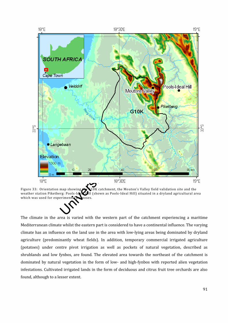
Univers

ity of

Cap

e Tow

n

91

Figure 33: Orientation map showing the G10K catchment, the Mo uton’s Valley field validation site and the weather station Piketberg: Pools-Ideal Hill (shown as Pools-Ideal Hill) situated in a dryland agricultural area which was used for experimental purposes.

The climate in the area is varied with the western part of the catchment experiencing a maritime

Mediterranean climate whilst the eastern part is considered to have a continental influence. The varying

climate has an influence on the land use in the area with low-lying areas being dominated by dryland

agriculture (predominantly wheat fields). In addition, temporary commercial irrigated agriculture

(potatoes) under centre pivot irrigation as well as pockets of natural vegetation, described as

shrublands and low fynbos, are found. The elevated area towards the northeast of the catchment is

dominated by natural vegetation in the form of low- and high-fynbos with reported alien vegetation

infestations. Cultivated irrigated lands in the form of deciduous and citrus fruit tree orchards are also

found, although to a lesser extent.

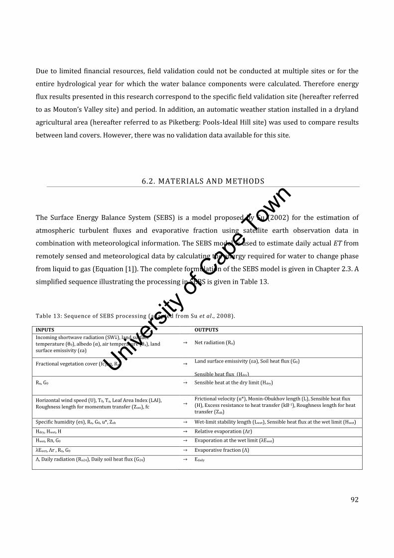
Univers

ity of

Cap

e Tow

n

92

Due to limited financial resources, field validation could not be conducted at multiple sites or for the

entire hydrological year for which the water balance components were calculated. Therefore energy

flux results presented in this research correspond to the specific field validation site (hereafter referred

to as Mouton’s Valley site) and period. In addition, an automatic weather station installed in a dryland

agricultural area (hereafter referred to as Piketberg: Pools-Ideal Hill site) was used to compare results

between land covers. However, there was no validation data available for this site.

6.2. MATERIALS AND METHODS

The Surface Energy Balance System (SEBS) is a model proposed by Su (2002) for the estimation of

atmospheric turbulent fluxes and evaporative fraction using satellite earth observation data in

combination with meteorological information. The SEBS model is used to estimate daily actual ET from

remotely sensed and meteorological data by calculating the energy required for water to change phase

from liquid to gas (Equation [1]). The complete formulation of the SEBS model is given in Chapter 2.3. A

simplified sequence illustrating the processing in SEBS is given in Table 13.

Table 13: Sequence of SEBS processing (adapted from Su et al ., 2008).

INPUTS OUTPUTS

Incoming shortwave radiation (SW↓), land surface temperature (θ0), albedo (α), air temperature (θa), land surface emissivity (εa)

→ Net radiation (Rn)

Fractional vegetation cover (fc), α, Rn → Land surface emissivity (εa), Soil heat flux (G0)

Sensible heat flux (Hdry)

Rn, G0 → Sensible heat at the dry limit (Hdry)

Horizontal wind speed (U), T0, Ta, Leaf Area Index (LAI), Roughness length for momentum transfer (Zom), fc

→ Frictional velocity (u*), Monin-Obukhov length (L), Sensible heat flux (H), Excess resistance to heat transfer (kB-1), Roughness length for heat transfer (Zoh)

Specific humidity (es), Rn, G0, u*, Zoh → Wet-limit stability length (Lwet), Sensible heat flux at the wet limit (Hwet)

Hdry, Hwet, H → Relative evaporation (Λr)

Hwet, Rn, G0 → Evaporation at the wet limit (λEwet)

λEwet, Λr , Rn, G0 → Evaporative fraction (Λ)

Λ, Daily radiation (Rn24), Daily soil heat flux (G24) → Edaily

Univers

ity of

Cap

e Tow

n

93

According to Su (2006), it is possible to estimate the latent heat flux as a residual after the sensible heat

flux has been derived. However, because the sensible heat flux is not constrained by the available

energy but is determined solely by surface temperature and the meteorological conditions at the

reference height, there is an associated uncertainty in the derived latent heat flux and therefore also in

the evaporative fraction. However, in SEBS this uncertainty is limited by considering the energy balance

at the limiting cases since the actual sensible heat flux is constrained to the range set by the sensible

heat flux at the wet limit (derived from a combination equation), and the sensible heat flux at the dry

limit (set by the available energy).

According to formulations by Su (2002), the relative evaporation is derived from the sensible heat flux

and the sensible heat flux calculated at the wet and dry limits. The relative evaporation (Equation [16])

is, in turn, used together with Rn, G0 and the latent heat flux at the wet limit to estimate the evaporative

fraction (Equation 17]). In SEBS it is assumed that the daily value of evaporative fraction is

approximately equal to the instantaneous value, and from this, the daily evaporation is given in

Equation [18]. The daily net radiation flux is given in Equation [19].It can be seen from Equations [18]

and [19] that aside from evaporative fraction itself, albedo is the sole remote sensing derived variable

used in the upscaling from instantaneous evaporative to daily ET.

For the purpose of calculating ET in this research, MODIS TERRA and AQUA data (MOD021KM _

Level 1B Calibrated Radiances – 1 km: Collection 5) were used. MODIS images are captured daily or

every second day and therefore it is possible, in South Africa, to obtain a good coverage throughout the

year. MOD02 and MYD02 data were selected for the field validation period. Single date (28 February

2008) ASTER level 1B - Registered Radiance at the Sensor, and ASTER level 2 – AST08 Surface Kinetic

Temperature, were used to compare the results of the higher resolution sensor to those of the same

date coarser resolution MODIS sensor. The required meteorological data (air temperature, wind speed,

radiation, sunshine duration) can be obtained directly from an automatic weather station (AWS) or

indirectly (air pressure, specific humidity) using empirical formulae and data from the AWS. Weather

data from the Mouton’s Valley and the ARC-ISCW, Piketberg: Pools-Ideal Hill AWSs were used.

Univers

ity of

Cap

e Tow

n

94

6.3. UNCERTAINTIES IN EVAPOTRANSPIRATION ESTIMATES WITH SEBS

Overgaard et al. (2006) put forward the argument that there is a mismatch between the scale for which

the theory behind developed models is assumed valid (typically point scale), and the scale of the typical

application. For this reason, the parameters in physically-based models are in reality conceptual, and

that even when mean parameters are available, the highly non-linear behaviour of most land-surface

models cannot be expected to simulate the mean response of a particular area (Overgaard et al., 2006).

Furthermore, the complex interaction of different sources of uncertainty in the modelling process

means that a good model driven by poor input data will not necessarily produce acceptable results

(Beven, 2008) and trying to separate the different sources of error is difficult since they interact in

complex non-linear ways (Beven, 2006).

Further, the analysis of remote sensing and GIS products usually results in maps of discrete or

continuous variables (Dungan et al., 2002), which can be associated with several sources of error or

uncertainty. These include: (1) errors or uncertainties associated with the specific remote sensing data

obtained; (2) errors or uncertainties introduced with the processing and analysis of image and field

data; (3) errors or uncertainties associated with the specific model; and (4) errors or uncertainties

associated with positional aspects (including image resolution). Wang et al. (2005) identify additional

sources of errors including sampling and measurement error of ground truth data, errors of spectral

values and radiometric calibration of images, errors from the leap from spectral measurements to

interpretation of a categorical variable, modelling errors due to misunderstanding the relationship

between spectral and thematic variables, and errors from GIS operations.

Errors and sensitivities in the derivation of ET for this study were identified as (but are by no means

limited to): (1) land surface and air temperature gradient; (2) the choice of fractional vegetation cover

formula; (3) zero plane displacement height and the height of wind speed measurement in relation to

displacement height; and (4) study area heterogeneity.

Univers

ity of

Cap

e Tow

n

95

6.3.1. LAND SURFACE AND AIR TEMPERATURE GRADIENT

The calculation of ET using the SEBS model relies on two temperature sources: air temperature (Ta) and

land surface temperature (T0). Su (2002) reported on the sensitivity of sensible heat flux to the gradient

between land surface temperature and air temperature hourly and Badola (2009) reported that of all

remotely sensed input parameters, SEBS was most sensitive to change in (T0 – Ta). T0 plays a role in the

determination of net radiation (Rn) (Table 13) and therefore soil heat flux (G0), but its main

contribution (together with the aerodynamic resistance) is in the calculation of the sensible heat flux.

To quantify the uncertainty associated with T0 estimates for the field validation site, the T0 retrieved

from MODIS data was compared with the Meteosat SEVIRI T0 data product (SEVIRI/Meteosat LST

Product: LSA-4 (MLST) Product version 7.2) corresponding to the same time of image acquisition. The

motivation for using Meteosat SEVIRI T0 data was to try to set a realistic uncertainty range in T0 in this

particular heterogeneous environment. It was found that there were differences of up to 10 K between

MODIS T0 and SEVIRI T0 with SEVIRI T0 being consistently higher than MODIS T0 which is in agreement

with the findings by Madeira et al. (2005). This large range in T0 can be ascribed to the topographically

rough nature of the terrain in the vicinity of the field validation site.

In addition to the SEBS model sensitivity to T0, the near-surface air temperature (Ta), as measured by

weather stations) has a direct influence on the evaporation process and inaccuracies in measurements

can lead to distorted reference ET measurements and actual ET estimates. For this reason, accuracy in

air temperature measurements is needed at the weather stations themselves. Additionally, the

heterogeneity of the study area implies that spatially distributed air temperature across the study area

is needed. This is because the spatial variations of surface characteristics (including topography and

land cover) have a large influence on the near-surface weather conditions (Voogt, 2006). Increasing the

accuracy of air temperature inputs will increase the likelihood of accurate ET estimates.

The sensitivity of daily ET calculated by SEBS to Δ(T0 – Ta) for the Mouton’s Valley site was assessed by

varying T0 by up to 10 K around the estimated T0 and keeping the Ta constant. The results (FIGURE 34

34) indicated that for the Mouton’s Valley site (where the estimated T0 is 301 K, the estimated Ta is

293 K and T0 – Ta equals 8 K), daily ET can vary by up to 1.5 mm in this 10 K Δ(T0 – Ta) range. Adjusting

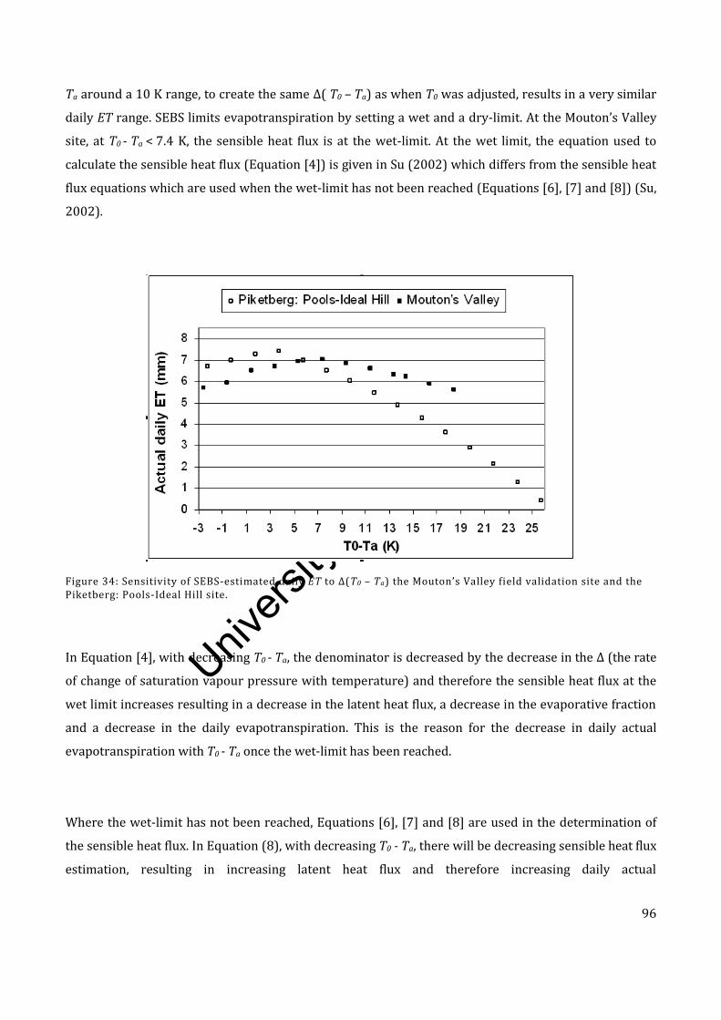
Univers

ity of

Cap

e Tow

n

96

Ta around a 10 K range, to create the same Δ( T0 – Ta) as when T0 was adjusted, results in a very similar

daily ET range. SEBS limits evapotranspiration by setting a wet and a dry-limit. At the Mouton’s Valley

site, at T0 - Ta < 7.4 K, the sensible heat flux is at the wet-limit. At the wet limit, the equation used to

calculate the sensible heat flux (Equation [4]) is given in Su (2002) which differs from the sensible heat

flux equations which are used when the wet-limit has not been reached (Equations [6], [7] and [8]) (Su,

2002).

Figure 34: Sensitivity of SEBS-estimated daily ET to Δ(T0 – Ta) the Mouton’s Valley field validation site and the Piketberg: Pools-Ideal Hill site.

In Equation [4], with decreasing T0 - Ta, the denominator is decreased by the decrease in the Δ (the rate

of change of saturation vapour pressure with temperature) and therefore the sensible heat flux at the

wet limit increases resulting in a decrease in the latent heat flux, a decrease in the evaporative fraction

and a decrease in the daily evapotranspiration. This is the reason for the decrease in daily actual

evapotranspiration with T0 - Ta once the wet-limit has been reached.

Where the wet-limit has not been reached, Equations [6], [7] and [8] are used in the determination of

the sensible heat flux. In Equation (8), with decreasing T0 - Ta, there will be decreasing sensible heat flux

estimation, resulting in increasing latent heat flux and therefore increasing daily actual

Univers

ity of

Cap

e Tow

n

97

evapotranspiration. This explains why the daily actual evapotranspiration increases with decreasing

T0 - Ta until the wet-limit is reached. At the wet-limit Equation [4] is used and the daily

evapotranspiration decreases with decreasing T0 - Ta due to decreasing saturation vapour pressure.

The modelling of the sensitivity of ET to T0 in a dryland agriculture environment at Piketberg: Pools-

Ideal Hill (where the estimated T0 is 311 K, the measured Ta is 295 K and T0 – Ta is 16 K) is also shown

in Figure 34. It can be seen that the sensitivity of daily ET to Δ( T0 – Ta) is greater than the Mouton’s

Valley site with a range of 7 mm across the same Δ( T0 – Ta) where T0 is increased and decreased by 10

K. In the case of the Piketberg: Pools-Ideal Hill site, the wet-limit is not reached when using similar T0 -

Ta values as is used for the Mouton’s Valley scenario. This is possibly due to the calculated lower

roughness lengths of the Piketberg: Pools-Ideal Hill site (in combination with different atmospheric

conditions) when compared with the Mouton’s Valley site, resulting in a higher sensible heat flux for the

same T0 – Ta as observed at the Mouton’s Valley site. In the selected T0 - Ta range (10 K), the sensible

heat flux is not forced to the wet limit. However when T0 - Ta is lowered further, the wet-limit drop off in

evapotranspiration (which occurs at T0 - Ta ~3 K in this particular instance) is reached.

It can therefore be said that the sensitivity of daily ET to Δ(T0 – Ta) is dependent on the land cover being

studied and may also be dependent on the calculated (T0 – Ta) itself. It should, however, be noted that

the uncertainty related to T0 in the dryland agricultural area is almost certainly lower than the 10 K

range found at the Mouton’s Valley site since the dryland agricultural at Piketberg: Pools-Ideal Hill is

topographically flat and relatively homogeneous. However, it is useful to note the differences in

sensitivity to Δ(T0 – Ta) on the same day, for two land covers in close proximity to each other, therefore

re-emphasizing the care that should be taken (particularly regarding the accuracy of input data) when

using SEBS in a heterogeneous environment.

Furthermore, the calculated sensitivity of the sensible heat flux at the Piketberg: Pools-Ideal Hill site to

Δ(T0 – Ta) was found to be in close agreement with the sensitivity of ΔH=10•Δ(T0 –Ta) reported by Su

(2002) for cotton, when the wet limit has not been reached. At the wet-limit, the sensitivity of the

sensible heat flux to Δ(T0 – Ta) was found to be ΔH=-8.32•Δ(T0 –Ta). For the Mouton’s Valley site, it was

found that calculated sensitivity of the sensible heat flux to Δ(T0 – Ta), is ΔH = -8.68•Δ(T0 – Ta) where the

wet limit has been reached and of ΔH = 6.09•Δ(T0 – Ta) where the wet limit has not been reached. It can

Univers

ity of

Cap

e Tow

n

98

therefore be seen that the sensitivity of H (and therefore daily ET) to Δ(T0 – Ta) is dependent on the land

cover type, T0, and whether the wet limit has been reached.

The uncertainties in the interpolation of Ta together with the uncertainties related to T0 estimates

create ambiguity with regard to the accuracy of the results. This is particularly prohibitive since these

parameters are used in the initial stages of SEBS model implementation, meaning that erroneous input

data would be translated through the entire processing sequence and eventually be reflected in the final

calculation of actual ET.

6.3.2. FRACTIONAL VEGETATION COVER

Fractional vegetation cover (fc) and its complement are used in the calculation of the roughness length

for heat transfer (Su et al., 2005) which, in turn, is used in the calculation of the sensible heat flux. In

addition, fc is used in the estimation of the soil heat flux (Su, 2002) and in the preprocessing stages to

assign surface emissivity values (Sobrino & El Kharraz, 2003) which are used to derive land surface

temperature. Fractional vegetation cover is a user defined input into the pre-packaged version of SEBS

in ILWIS and different formulations of fc are intentionally utilized in SEBS for different purposes.

Therefore, the effect of the choice of formula, and its calibration, on resulting ET should be noted.

Several methods for the calculation of fc are described in the literature. These methods generally make

use of leaf area index (LAI) (Choudhury, 1987, cited in French et al., 2003) as input or require pixel

NDVI together with a minimum and maximum NDVI value (Carlson & Ripley, 1997; Gutman & Ignatov,

1998). These minimum and maximum NDVI values are either constant (Sobrino & El Kharraz, 2003) or

can be derived directly from the scene or from a time series.

For example, if fractional vegetation cover is calculated according to the formula for vegetation

proportion (Sobrino & El Kharraz, 2003) (Equation [25]). In contrast with NDVImin and NDVImax values

as defined by Sobrino & El Kharraz (2003), Figure 35 shows the distribution of NDVI values across the

entire study area for a winter wet season and summer dry season scene. It can be seen that the range of

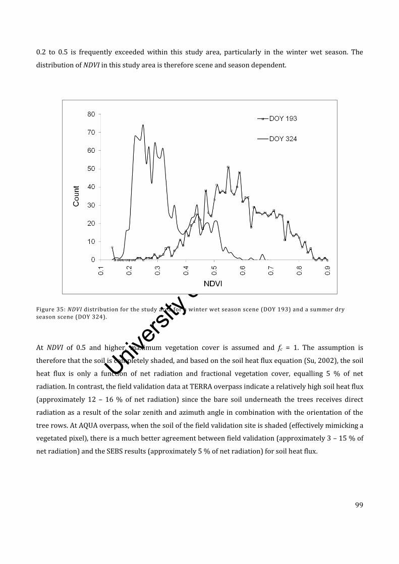
Univers

ity of

Cap

e Tow

n

99

0.2 to 0.5 is frequently exceeded within this study area, particularly in the winter wet season. The

distribution of NDVI in this study area is therefore scene and season dependent.

Figure 35: NDVI distribution for the study area for a winter wet season scene (DOY 193) and a summer dry season scene (DOY 324).

At NDVI of 0.5 and higher, maximum vegetation cover is assumed and fc = 1. The assumption is

therefore that the soil is completely shaded, and based on the soil heat flux equation (Su, 2002), the soil

heat flux is only a function of net radiation and fractional vegetation cover, equalling 5 % of net

radiation. In contrast, the field validation data at TERRA overpass indicate a relatively high soil heat flux

(approximately 12 – 16 % of net radiation) since the bare soil underneath the trees receives direct

radiation as a result of the solar zenith and azimuth angle in combination with the orientation of the

tree rows. At AQUA overpass, when the soil of the field validation site is shaded (effectively mimicking a

vegetated pixel), there is a much better agreement between field validation (approximately 3 – 15 % of

net radiation) and the SEBS results (approximately 5 % of net radiation) for soil heat flux.

Univers

ity of

Cap

e Tow

n

100

The fractional vegetation cover calculation can be tested using the field validation data at Mouton’s

Valley and by rearranging the soil heat flux equation (Equation [3]):

1

0

cs

c

nc

R

G

f [30]

Where Γc (0.05) (Monteith, 1973 in Su, 2002) and Γs (0.315) (Kustas and Daughtry, 1989 in Su, 2002)

are the soil heat flux ratios for full vegetation canopy and for bare soil respectively. Solving Equation

[30] by substituting the field measured G0 values, fractional vegetation cover is calculated to range from

0.58 – 0.73 at TERRA overpass and at AQUA overpass from 0.67 – 1. If this is taken to be a true

reflection of fractional vegetation cover of the apple orchard at image acquisition time, the NDVI

minimum and maximum values should be adjusted as a fractional vegetation cover of 1 is not a realistic

result especially at TERRA acquisition time.

Considering fc calculated above, the need for calibrating NDVI by defining an appropriate NDVImax for the

study area is apparent. Substituting this fc and the corresponding NDVI for the Mouton’s Valley site for

each MODIS TERRA and AQUA acquisition and keeping the NDVImin = 0.2 as suggested by Sobrino & El

Kharraz (2003) in Equation [25] results in an average NDVImax = 0.65, which is more appropriate for the

study area during the field validation period.

The benefits of using a set minimum and maximum NDVI should be weighed up against using scene-

specific estimates especially for scenes which do not contain a full range of vegetation cover as this will

skew the results of the fractional vegetation calculation. The sensitivity of daily ET to choice of fc

formula and the calibration of NDVImin and NDVImax are shown in Figure 36 for the Mouton’s Valley site.

The curve in Figure 36 was created by repeatedly varying fc and recomputing daily ET. The points on

the curve show that for the same pixel, a different formula would produce a different fc result: it can be

seen that in this instance, the calculated daily ET can vary by up to 0.7 mm depending on the fc input.

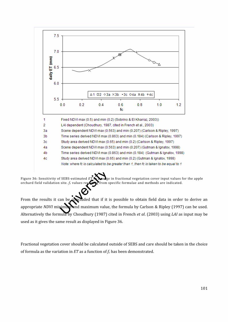
Univers

ity of

Cap

e Tow

n

101

Figure 36: Sensitivity of SEBS-estimated ET to a range in fractional vegetation cover input values for the apple orchard field validation site. fc values resulting from specific formulae and methods are indicated.

From the results it can be concluded that if it is possible to obtain field data in order to derive an

appropriate NDVI minimum and maximum value, the formula by Carlson & Ripley (1997) can be used.

Alternatively the formula by Choudhury (1987) cited in French et al. (2003) using LAI as input may be

used as it gives the same result as displayed in Figure 36.

Fractional vegetation cover should be calculated outside of SEBS and care should be taken in the choice

of formula as the variation in ET as a function of fc has been demonstrated.

Univers

ity of

Cap

e Tow

n

102

6.3.3. ZERO PLANE DISPLACEMENT HEIGHT

The objective of this section is to highlight that the type of weather station and the reference height at

which wind speed is measured is critical to the correct implementation of the SEBS model particularly

in tall canopies.

Zero plane displacement height (d0) values are used in combination with the reference height at which

wind speed is measured (z) in the process of determining the sensible heat flux (H). d0 can be obtained

from the literature or can be empirically derived from the remote sensing vegetation inputs via the

calculation of roughness length (the methodology adopted by Su, 2002; Timmermans et al., 2005; and

Van der Kwast et al., 2009). Alternatively the combination approach of Jia et al. (2009) can be used.

Using the empirical model, NDVI and NDVImax are used to determine roughness length for momentum

transfer (z0m) with the method described by Su & Jacobs (2001) as reported in Hailegiorgis (2006).

Next, the vegetation height is calculated from z0m followed by d0 using the method of Brutsaert (1982)

as reported in Hailegiorgis (2006).

In South Africa, the installation of automatic agrometeorological weather stations complies with

standards set by the World Meteorological Organisation except in the height measurement of wind

speed and direction. South African agrometeorological standards state that wind speed and wind

direction are measured at 2 m above the surface (ARC-ISCW, 2010) in contrast to the South African

Weather Service (SAWS) which measures wind speed and direction at 10 m above the surface.

A problem arises when using data from agrometeorological weather stations in canopies of 3 m or

higher (where d0 ≥ 2), as is the case with orchards in the study area. To derive the sensible heat flux (Su,

2002) the calculation of z – d0 is required, where z is the reference height at which wind speed is

measured (2 m, in the case of an agrometeorological weather station). When measuring wind speed at 2

m, and solving for H using the equations defined by Su (2002) and given in Equations [6], [7] and [8], a

situation arises where z ≤ d0, and the ln of a negative number needs to be solved.

Univers

ity of

Cap

e Tow

n

103

In this study, the average canopy height at the Mouton’s Valley site was reported to be 3.2 m in the

apple orchard (Jarmain & Mengistu, 2011) and therefore d0 > 2 m so the condition where z ≤ d0 is

reached using agrometeorological weather stations. The alternative would be to use weather data from

the SAWS which would allow for the sensible heat flux to be calculated for much higher canopies than

for the above scenario. However, it is agrometeorological weather stations which are installed in

agricultural areas where this and other studies of this nature take place. Should only

agrometeorological weather station data be available, the upscaling of the available meteorological data

to a higher reference height should be investigated based on radiosonde observations (Ershadi, 2010).

The effect on d0 in high canopies is shown by using the Mouton’s Valley site as an example, and testing

for the sensitivity of daily ET to d0 (Figure 37) At approximately d0 = 1.8 m, a rapid decrease in daily ET

estimation is noted as d0 approaches 2 m. It can be surmised therefore (although this should be tested

in different environments and under different meteorological conditions) that when using wind speed

measured at 2 m above the surface, the SEBS model should not be used in canopies of 2.7 m and higher

as it is at this point that the model becomes highly sensitive to changes in d0.

The uncertainty in the calculation of the sensible heat flux introduced when the displacement height

approaches the height of wind speed measurement should be carefully considered and addressed since

errors in the calculation of the sensible heat flux will be propagated through the model and will

eventually influence the final ET calculation as demonstrated in this study.

Figure 37: Sensitivity of SEBS-estimated ET to d0 for the Mouton’s Valley field validation site when wind speed is measured at 2m.

Univers

ity of

Cap

e Tow

n

104

6.3.4. HETEROGENEITY OF THE STUDY AREA

Heterogeneity as related to the concept of the spatial variability of a landscape plays an important role

in the application of remote sensing data to the calculation of ET, especially in the selection of the

spatial resolution of the particular sensor. Various studies have shown that, for complex heterogeneous

landscapes, there is lower confidence in variables derived using low resolution sensor data (Moran et

al., 1997; Kustas et al., 2004; Garrigues et al., 2006; McCabe & Wood, 2006; Li et al., 2006; Li et al., 2008;

Lakhankar et al., 2009) as intra-pixel spatial heterogeneity is lost due to the integration of the

radiometric signal.

The effect of heterogeneity on SEBS derived ET can be illustrated by comparing the results from a single

date (28 February 2008) ASTER image at 90 m resolution with the results of the same date MODIS

image at 1 km resolution for the Mouton’s Valley site and for the Piketberg: Pools-Ideal Hill site in

Figure 38. When the SEBS model was run on the ASTER image, it was apparent that the albedo

estimation for both the homogeneous and heterogeneous sites was unrealistically low when compared

with literature values. When the albedo calculation was carried out on the ASTER image which had not

been atmospherically corrected, the albedo values more closely matched literature values. Since the

ASTER and MODIS sensors are on board the same platform (TERRA) and the images were captured

simultaneously and therefore under exactly the same atmospheric conditions with identical sensor and

solar zenith angles, the SEBS model was rerun on the MODIS and ASTER data without applying

atmospheric correction, in order to remove any bias that this low albedo may be introducing in the

ASTER results. This approach is justified since the results are used for comparative purposes only and

results are not being assessed relative to field values or images from other dates. The uncorrected

images were only used in this section to analyze the impact of heterogeneity and all other results

reported on in this chapter are derived from images that have been atmospherically corrected.

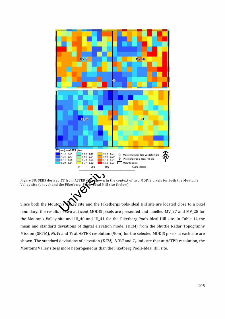
Univers

ity of

Cap

e Tow

n

105

Figure 38: SEBS derived ET from ASTER data shown in the context of two MODIS pixels for both the Mouton’s Valley site (above) and the Piketberg: Pools-Ideal Hill site (below).

Since both the Mouton’s Valley site and the Piketberg:Pools-Ideal Hill site are located close to a pixel

boundary, the results of two adjacent MODIS pixels are presented and labelled MV_27 and MV_28 for

the Mouton’s Valley site and IH_40 and IH_41 for the Piketberg:Pools-Ideal Hill site. In Table 14 the

mean and standard deviations of digital elevation model (DEM) from the Shuttle Radar Topography

Mission (SRTM), NDVI and T0 at ASTER resolution (90m) for the selected MODIS pixels at each site are

shown. The standard deviations of elevation (DEM), NDVI and T0 indicate that at ASTER resolution, the

Mouton’s Valley site is more heterogeneous than the Piketberg:Pools-Ideal Hill site.

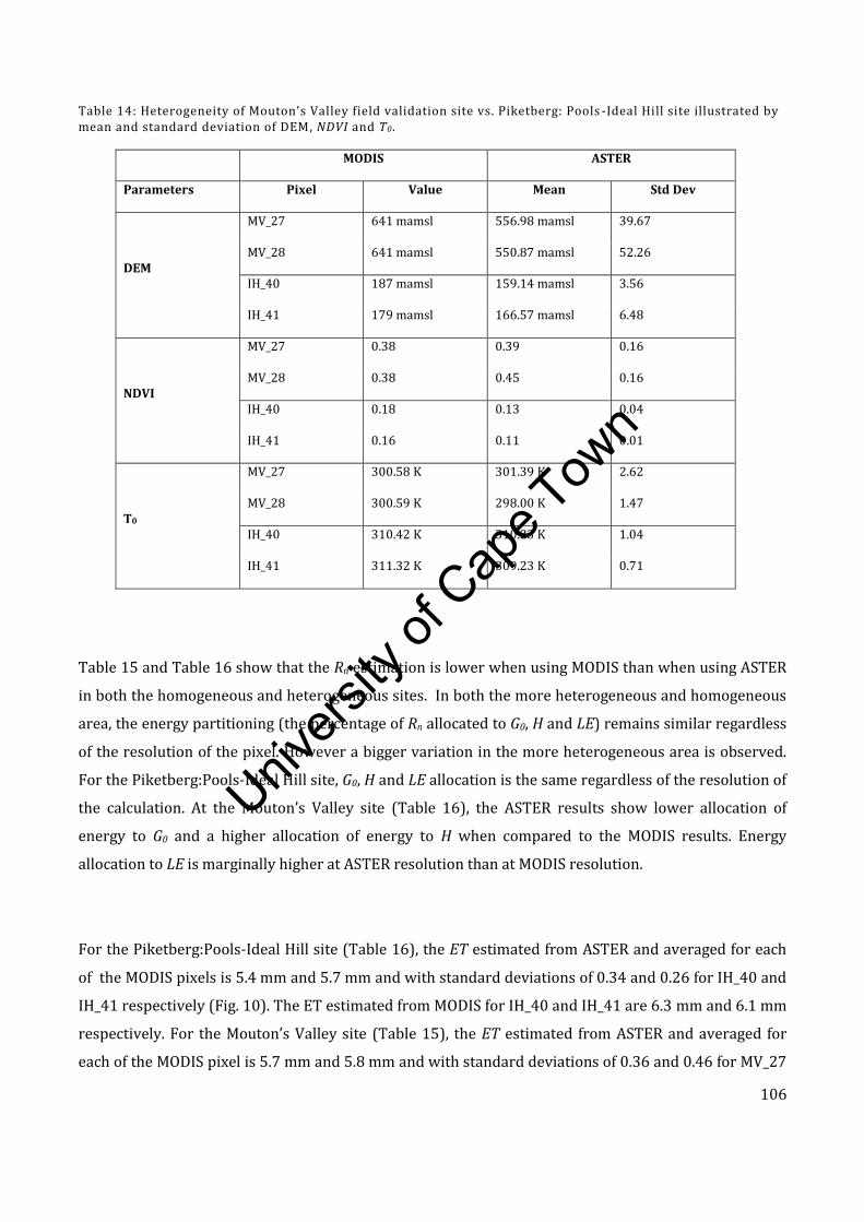
Univers

ity of

Cap

e Tow

n

106

Table 14: Heterogeneity of Mouton’s Valley field validation site vs. Piketberg: Pools -Ideal Hill site illustrated by mean and standard deviation of DEM, NDVI and T0.

MODIS ASTER

Parameters Pixel Value Mean Std Dev

DEM

MV_27 641 mamsl 556.98 mamsl 39.67

MV_28 641 mamsl 550.87 mamsl 52.26

IH_40 187 mamsl 159.14 mamsl 3.56

IH_41 179 mamsl 166.57 mamsl 6.48

NDVI

MV_27 0.38 0.39 0.16

MV_28 0.38 0.45 0.16

IH_40 0.18 0.13 0.04

IH_41 0.16 0.11 0.01

T0

MV_27 300.58 K 301.39 K 2.62

MV_28 300.59 K 298.00 K 1.47

IH_40 310.42 K 310.23 K 1.04

IH_41 311.32 K 309.23 K 0.71

Table 15 and Table 16 show that the Rn estimation is lower when using MODIS than when using ASTER

in both the homogeneous and heterogeneous sites. In both the more heterogeneous and homogeneous

area, the energy partitioning (the percentage of Rn allocated to G0, H and LE) remains similar regardless

of the resolution of the pixel. However a bigger variation in the more heterogeneous area is observed.

For the Piketberg:Pools-Ideal Hill site, G0, H and LE allocation is the same regardless of the resolution of

the calculation. At the Mouton’s Valley site (Table 16), the ASTER results show lower allocation of

energy to G0 and a higher allocation of energy to H when compared to the MODIS results. Energy

allocation to LE is marginally higher at ASTER resolution than at MODIS resolution.

For the Piketberg:Pools-Ideal Hill site (Table 16), the ET estimated from ASTER and averaged for each

of the MODIS pixels is 5.4 mm and 5.7 mm and with standard deviations of 0.34 and 0.26 for IH_40 and

IH_41 respectively (Fig. 10). The ET estimated from MODIS for IH_40 and IH_41 are 6.3 mm and 6.1 mm

respectively. For the Mouton’s Valley site (Table 15), the ET estimated from ASTER and averaged for

each of the MODIS pixel is 5.7 mm and 5.8 mm and with standard deviations of 0.36 and 0.46 for MV_27

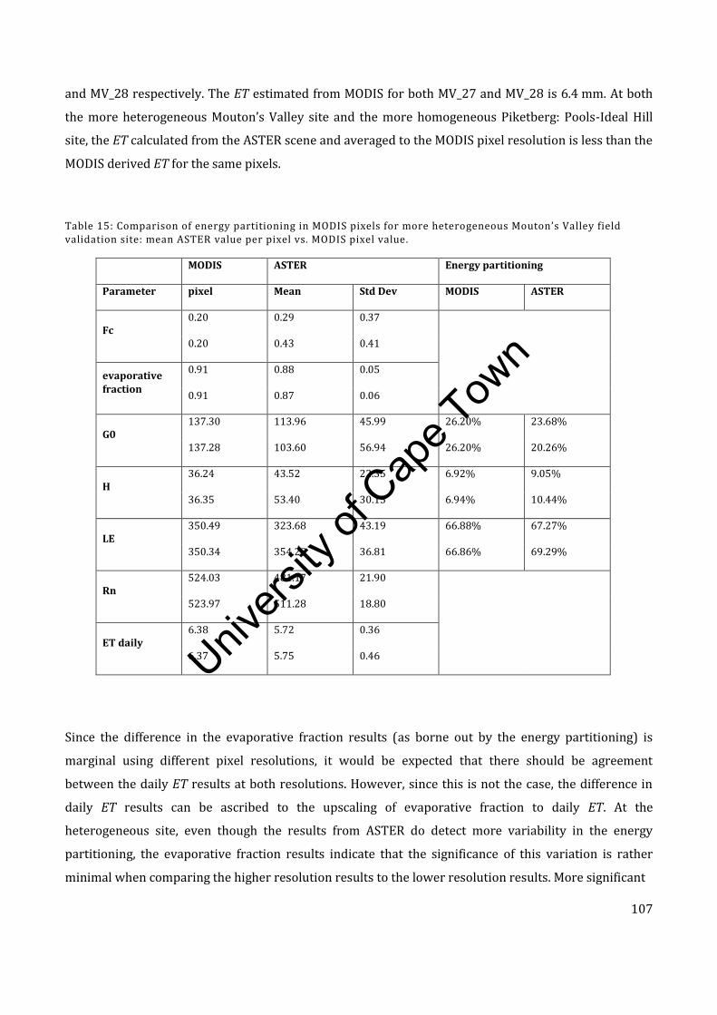
Univers

ity of

Cap

e Tow

n

107

and MV_28 respectively. The ET estimated from MODIS for both MV_27 and MV_28 is 6.4 mm. At both

the more heterogeneous Mouton’s Valley site and the more homogeneous Piketberg: Pools-Ideal Hill

site, the ET calculated from the ASTER scene and averaged to the MODIS pixel resolution is less than the

MODIS derived ET for the same pixels.

Table 15: Comparison of energy partitioning in MODIS pixels for more heterogeneous Mouton’s Valley field validation site: mean ASTER value per pixel vs. MODIS pixel value.

MODIS ASTER Energy partitioning

Parameter pixel Mean Std Dev MODIS ASTER

Fc 0.20 0.29 0.37

0.20 0.43 0.41

evaporative fraction

0.91 0.88 0.05

0.91 0.87 0.06

G0 137.30 113.96 45.99 26.20% 23.68%

137.28 103.60 56.94 26.20% 20.26%

H 36.24 43.52 22.35 6.92% 9.05%

36.35 53.40 30.15 6.94% 10.44%

LE 350.49 323.68 43.19 66.88% 67.27%

350.34 354.28 36.81 66.86% 69.29%

Rn 524.03 481.17 21.90

523.97 511.28 18.80

ET daily 6.38 5.72 0.36

6.37 5.75 0.46

Since the difference in the evaporative fraction results (as borne out by the energy partitioning) is

marginal using different pixel resolutions, it would be expected that there should be agreement

between the daily ET results at both resolutions. However, since this is not the case, the difference in

daily ET results can be ascribed to the upscaling of evaporative fraction to daily ET. At the

heterogeneous site, even though the results from ASTER do detect more variability in the energy

partitioning, the evaporative fraction results indicate that the significance of this variation is rather

minimal when comparing the higher resolution results to the lower resolution results. More significant

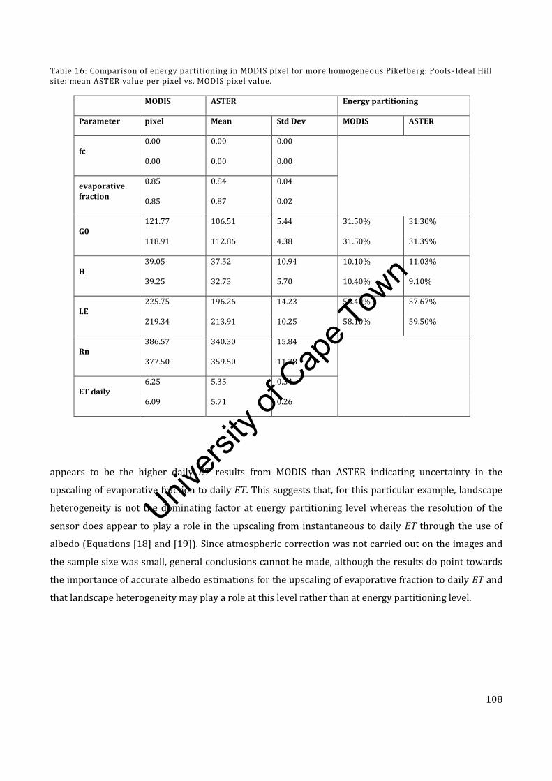
Univers

ity of

Cap

e Tow

n

108

Table 16: Comparison of energy partitioning in MODIS pixel for more homogeneous Piketberg: Pools -Ideal Hill site: mean ASTER value per pixel vs. MODIS pixel value.

MODIS ASTER Energy partitioning

Parameter pixel Mean Std Dev MODIS ASTER

fc 0.00 0.00 0.00

0.00 0.00 0.00

evaporative fraction

0.85 0.84 0.04

0.85 0.87 0.02

G0 121.77 106.51 5.44 31.50% 31.30%

118.91 112.86 4.38 31.50% 31.39%

H 39.05 37.52 10.94 10.10% 11.03%

39.25 32.73 5.70 10.40% 9.10%

LE 225.75 196.26 14.23 58.40% 57.67%

219.34 213.91 10.25 58.10% 59.50%

Rn 386.57 340.30 15.84

377.50 359.50 11.38

ET daily 6.25 5.35 0.34

6.09 5.71 0.26

appears to be the higher daily ET results from MODIS than ASTER indicating uncertainty in the

upscaling of evaporative fraction to daily ET. This suggests that, for this particular example, landscape

heterogeneity is not the dominating factor at energy partitioning level whereas the resolution of the

sensor does appear to play a role in the upscaling from instantaneous to daily ET through the use of

albedo (Equations [18] and [19]). Since atmospheric correction was not carried out on the images and

the sample size was small, general conclusions cannot be made, although the results do point towards

the importance of accurate albedo estimations for the upscaling of evaporative fraction to daily ET and

that landscape heterogeneity may play a role at this level rather than at energy partitioning level.

Univers

ity of

Cap

e Tow

n

109

6.4. DISCUSSION

The complexities associated with the derivation of ET and the uncertainties described in this chapter

imply that potential errors will be introduced at various stages of ET derivation. These errors are

related to error production and error propagation as defined by Veregin (1989). Error production

refers to a situation where errors in output products are attributed mainly to the specific operations

applied to the data, thereby producing errors in the output products while no errors were present in

the original data used as input. On the other hand, error propagation refers to the process where

potentially erroneous input data is passed through certain processing sequences and errors accumulate

in output products. In the case of deriving ET, errors will be compounded if intermediate error-bearing

output products are used in additional processing sequenced to derive the final result.

The opportunity for error production is introduced when it is considered that the SEBS model is

complex in itself as it consists of three tools (Su, 2006), namely:

a set of tools to determine physical parameters of the land surface;

an extended model to derive roughness length for heat transfer; and

a model to determine evaporative fraction on the basis of the energy balance.

An example of error production was illustrated in the case of deriving fractional vegetation cover using

ill-defined NDVI limits. An error in the calculation of fractional vegetation cover would be propagated to

soil and sensible heat flux calculations. This in turn will be propagated to the calculation of the latent

heat flux and therefore ET. Prior to adjusting for the study area, ET was set at the wet limit, although

this was not the case after NDVImax was adjusted. In the absence of known suitable NDVI maximum and

minimum values a priori, a fractional vegetation cover formula, such as proposed by Choudhury (1987)

cited by French et al. (2003), which makes use of LAI rather than NDVI may be used.

The opportunity for error propagation is introduced at the initial stages of ET derivation when it is

considered that remote sensing data together with standard meteorological data are required by the

SEBS model. Due to uncertainties associated with remote sensing and the interpolation of

meteorological data, potential errors will propagate throughout the processing sequence. An additional

Univers

ity of

Cap

e Tow

n

110

opportunity for error propagation is introduced when considering land surface temperature, air

temperature and their gradient (T0 – Ta) since T0 values derived from two different sources differed by

up to 10 K for the field validation site. The sensitivity of SEBS to T0 – Ta appears to vary between land

covers and the sensitivity may be dependent on the estimated T0 value itself. This implies that an error

in the input data would propagate through the model and cause uncertainty in the final derivation of ET.

However, the range in uncertainty cannot be modelled as it appears to vary between land cover types.

Furthermore, the use of air temperature from weather stations interpolated across a study area

introduces more opportunities for error propagation, especially in a heterogeneous environment where

Ta may vary over a short distance dependent on inter alia land cover. This will be compounded in areas

with limited weather station coverage in a heterogeneous environment due to the influence of

topography on near-surface weather conditions.

From the data presented here it can be seen that the study area comprises a spatially diverse landscape

with a high level of heterogeneity. In order to successfully estimate ET and capture the full range of

variability in fluxes, the choice of spatial resolution of remote sensing data is crucial. Kustas et al.

(2004) and Li et al. (2006) found that when the spatial resolution exceeds 500 m, mixed pixels

containing large contrasts in surface temperature and vegetation cover could cause significant errors

(Li et al., 2008). Flores et al. (2009) also demonstrated the impact of topographic heterogeneity on

near-surface soil temperature. McCabe & Wood (2006) found that MODIS has limited capacity in

capturing the spatial variability in fluxes at field level but estimates for the spatial average flux at large

scales may be accurate (McCabe & Wood, 2006). The results presented here differ from those reported

in the listed literature in that it was found that although the absolute values for the various energy

fluxes differ from MODIS to ASTER, the proportional partitioning of energy compared well between the

MODIS and ASTER results at both the more homogeneous site and the more heterogeneous site.

However, it is in the upscaling of evaporative fraction to daily ET where the uncertainty appears to be

introduced when working at varying resolutions. The sensitivity of the SEBS model to albedo with a

focus specifically on the upscaling of evaporative fraction to daily ET is lacking in the literature as often

the sensitivities to input parameters are determined by assessing the sensible heat flux results (such as

Badola, 2009; Van der Kwast et al., 2009). Mariotto & Gutschick (2010) proposed that since most

vegetation canopies are non-Lambertian reflectors, the assumption of a horizontally homogeneous

Lambertian surface reflecting energy equally in all directions affects the calculations of albedo and

vegetation index. They show that if the spatial variation of non-Lambertian reflectance can be

formulated, the accuracy of the estimation and discrimination of ET among different land cover types

Univers

ity of

Cap

e Tow

n

111

can be improved. This is particularly true in a heterogeneous environment. It is possible that the

assumption of Lambertian reflectance in a heterogeneous environment may be the reason for lower

than anticipated albedo values at ASTER resolution.

The zero plane displacement height (and therefore the height of the canopy) has been highlighted as

being an important factor to consider in combination with the reference height at which the wind speed

is measured. It was shown in Figure 37 that as the displacement height tends to the reference height at

which wind speed is measured, there is a rapid drop-off in ET estimates. Since wind speed is routinely

measured at 2, 5 and 10m above the surface, when using these models in taller canopies, the user

should ensure use of a weather station measuring wind speed at 10 m above the surface. By

implication, the same models will not be suitable for use in canopies of taller than 15 m.

In this chapter, the sensitivities of SEBS estimated daily ET to various parameters have been shown. The

sensitivities have always been related back to daily ET rather than the sensible heat flux since it is the

daily ET which is of interest to water managers and other users of the results of the SEBS model.

Generalizations regarding the magnitude of errors produced by uncertainties in the input data have not

been made as the dependence on study area and the interaction of various input parameters in the

model was not the objective of this study. However, it has been shown that users should consider which

input parameters can be calculated outside of the prepackaged version of SEBS and a decision as to

which is the most appropriate methodology should be taken.

6.5. CONCLUDING REMARKS

The results presented here can be used to improve on the project by Gibson et al. (2009) to determine

the usefulness and applicability of using remote sensing technologies as a tool for resource assessment

and determination of water use. Although promising, uncertainties in estimating the various

parameters were encountered. These uncertainties could broadly be classified as 1) errors in input

data, 2) uncertainties related to spatial heterogeneity of the study area and resolution of input data, and

3) processing errors resulting in either error production or error propagation or both.

Univers

ity of

Cap

e Tow

n

112

In this chapter some of these uncertainties are described by using the example of the derivation of

evapotranspiration using the SEBS model. Uncertainty related to input data was demonstrated through

investigating problems related to land surface and air temperature as well as in the derivation of

displacement height. Uncertainty related to the heterogeneity of the study area in terms of land cover

and topography in relation to the spatial resolution of input data was also demonstrated. Finally,

uncertainty in data processing was demonstrated using the case of determining fractional vegetation

cover as example. These uncertainties and potential errors are compounded when considering that

applying the SEBS model for calculating ET is a complex process, requiring several image processing

sequences that are combined to produce the final result. This may lead to a situation where errors may

be propagated and compounded through the processing chain, eventually affecting the final output

product.

The various uncertainties and potential errors of propagation and production are associated with the

accuracy of the final output product. Ideally, sources of uncertainty will need to be identified and the

accumulation and propagation of errors will need to be modelled. This will enable the quantification of

error or uncertainty originating either from source data or through processing errors. Simultaneous

multi-parameter sensitivity analysis of inputs which are used in the SEBS model would help in

determining to which parameters the SEBS model is most sensitive and under which conditions these

sensitivities are the most pronounced. This would begin to address the uncertainties highlighted in this

research and may lead to greater confidence in using SEBS generated ET results.

Although illustrating uncertainty using ET as an example, the derivation of all the components of the

water balance equation using remote sensing data was influenced by similar uncertainties and the

actual water consumption of individual agricultural fields could not be calculated. However,

methodologies untested in South Africa were applied to the study area with many challenges

encountered at both a data and skills capacity level. If the uncertainties and limitations encountered in

the course of the research project are considered and acted upon it may be possible that at least parts of

the methodology may be relevant at a later stage for water use determination.

In conclusion, users of the pre-packaged version of SEBS in ILWIS are offered the following advice:

Univers

ity of

Cap

e Tow

n

113

1. Since SEBS is sensitive to the T0 - Ta gradient, care should be taken when estimating T0 in

a topographically diverse area as retrievals are less accurate in this setting. In particular,

SEBS should not be used in mountainous areas with coarse resolution sensors since the

heterogeneity of the T0 cannot be captured at the appropriate scale. Furthermore, the

sensitivity to T0 – Ta is also dependent on whether the wet-limit has been reached.

2. Care should be taken when selecting a fractional vegetation cover formula as this should

be appropriate for the study area, especially if NDVI min and max values need to be

defined. In particular, it is advised that if a LAI product is available at the appropriate

scale, that it be used to estimate fractional vegetation cover according to the formula by

Choudhury (1987).

3. The reference height of the weather station should be considered in relation to the

canopy height of the study area. In an area where field crops with a low canopy height

predominate, the use of an agrometeorological weather station is appropriate. However,

where tree crops and natural vegetation with a canopy height exceeding 2.7 m are

found, weather stations which measure wind speed at 10 m are probably more

appropriate.

4. The scale at which the evapotranspiration results are required must be considered in

relation to the choice of sensor and therefore pixel resolution and the heterogeneity of

the study area. When working at a catchment scale a coarse resolution sensor may be

appropriate for energy partitioning, whereas, for farm or field scale results a higher

pixel resolution will be required to detect inter-field or inter-farm variations. The

influence of albedo on the accurate upscaling of evaporative fraction to daily ET should

be considered and this may also be a function of landscape heterogeneity.

Univers

ity of

Cap

e Tow

n

114

7. ACCOUNTING FOR MODEL UNCERTAINTIES

From the conclusions drawn in Chapter 6, implementing the recommended changes to the methodology

and validating the results in the Moutons Valley validation site would have little value for the following

reasons: 1) The topography of the field validation site lends itself to uncertainties in T0 and Ta due to the

close proximity of the mountain on either side of the field validation site. 2) The reference height at

which wind speed is measured cannot be changed retrospectively for the field validation period. 3) The

heterogeneity in the environs of the field validation site implies that the results may be valid at

catchment scale but at field or farm scale, the MODIS pixel resolution is not suitable. 4) The short field

campaign period required that all available MODIS images be selected and processed to achieve the

maximum number of SEBS derived energy flux results for comparison with the field validation results.

Therefore single MODIS images were used rather than 8-day or 16-day products and atmospheric

correction is required for these daily products and at times, high solar and sensor zenith angles are

inevitable.

However, the research would not be complete without testing the advice given in Chapter 6 to users of

the prepackaged SEBS model. Since some of the proposed changes would be impossible to apply to the

Moutons Valley validation site retrospectively, a new study area was selected. The changes to the

methodology are described in Chapter 7.1 with some analysis and discussion given around each of

these modifications. In Chapter 7.2, the results of having adapted the methodology in a new study area

are presented along with a discussion.

The attention to ensuring the highest accuracy and suitability of input data involved: the preselection of

a homogeneous catchment at MODIS pixel resolution, use of an already atmospherically corrected

MODIS data product, the adjustment of the NDVI maximum value for use in the fractional vegetation

cover formula, the use of a South Africa Weather Services weather station data to measure the wind

speed at 10m rather than at 2m, the use of literature values and a land cover map to assign roughness

length and displacement height estimates and finally the use of both TERRA and AQUA images to

determine the impact of land surface air temperature gradient and time of day at which the satellite

image was captured. The selection process for the two quaternary catchments (Gibson et al., 2011)

considered the homogeneity of quaternary catchments and the availability of data to ensure the most

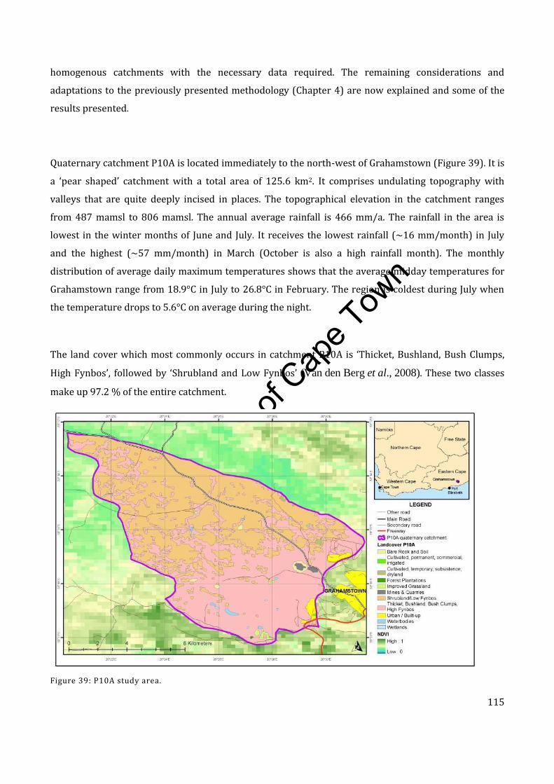
Univers

ity of

Cap

e Tow

n

115

homogenous catchments with the necessary data required. The remaining considerations and

adaptations to the previously presented methodology (Chapter 4) are now explained and some of the

results presented.

Quaternary catchment P10A is located immediately to the north-west of Grahamstown (Figure 39). It is

a ‘pear shaped’ catchment with a total area of 125.6 km2. It comprises undulating topography with

valleys that are quite deeply incised in places. The topographical elevation in the catchment ranges

from 487 mamsl to 806 mamsl. The annual average rainfall is 466 mm/a. The rainfall in the area is

lowest in the winter months of June and July. It receives the lowest rainfall (~16 mm/month) in July

and the highest (~57 mm/month) in March (October is also a high rainfall month). The monthly

distribution of average daily maximum temperatures shows that the average midday temperatures for

Grahamstown range from 18.9°C in July to 26.8°C in February. The region is coldest during July when

the temperature drops to 5.6°C on average during the night.

The land cover which most commonly occurs in catchment P10A is ‘Thicket, Bushland, Bush Clumps,

High Fynbos’, followed by ‘Shrubland and Low Fynbos’ (Van den Berg et al., 2008). These two classes

make up 97.2 % of the entire catchment.

Figure 39: P10A study area.

Univers

ity of

Cap

e Tow

n

116

7.1. ADAPTING THE METHODOLOGY

The methodology presented in Chapter 4 was modified and applied to the P10A catchment over the

period July 2006 to June 2007. The aspects are discussed are: atmospheric effect (Chapter 7.1.1),

fractional vegetation cover (Chapter 7.1.2), reference height (Chapter 7.1.3), land surface and air

temperature gradient (Chapter 7.1.4) and roughness lengths (Chapter 7.1.5).

7.1.1. ATMOSPHERIC EFFECTS

The accurate retrieval of surface reflectance and temperature is very important in deriving land surface

biophysical parameters and in the determination of fluxes. In mapping the surface physical properties

the surface information is highly affected by atmospheric components (scattering by aerosols and

absorption by gases, such as oxygen, water vapour and ozone) and their magnitude (Hailegiorgis,

2006). The simplified method for atmospheric correction (SMAC) proposed by Rahman & Dedieu

(1994) has been programmed into the prepackaged SEBS model in ILWIS to correct for the effects of the

atmosphere on MODIS visible, near infrared and shortwave infrared data. SMAC is a radiative transfer

model and therefore requires a description of the components in the atmospheric profile in order to

correct for these effects.

Each of the reflective bands (bands 1-5 & 7) is atmospherically corrected using SMAC. Due to many

pixels of missing data in the MODIS atmospheric products over the Gibson et al. (2009) study area,

mean values were used to correct for the entire study area leading to some doubt as to the accuracy of

the method. To negate the need for atmospherically correcting MODIS level 1B images as was the

approach of Gibson et al. (2009), the MCD 43 - Surface Reflectance BRDF/Albedo Product – specifically

MCD43A4 was used. The models used in creating this product best describe the differences in radiation

due to the scattering (anisotropy) of each pixel and rely on multi-date, atmospherically corrected,

cloud-cleared input data measured over 16-day periods. Both Terra and Aqua data are used in the

generation of this product, providing the highest probability for quality input data (http://modis-

land.gsfc.nasa.gov/brdf.htm). This corrected data can then be used for the calculation of all input

parameters derived from the MODIS reflective bands on the assumption that parameters such as

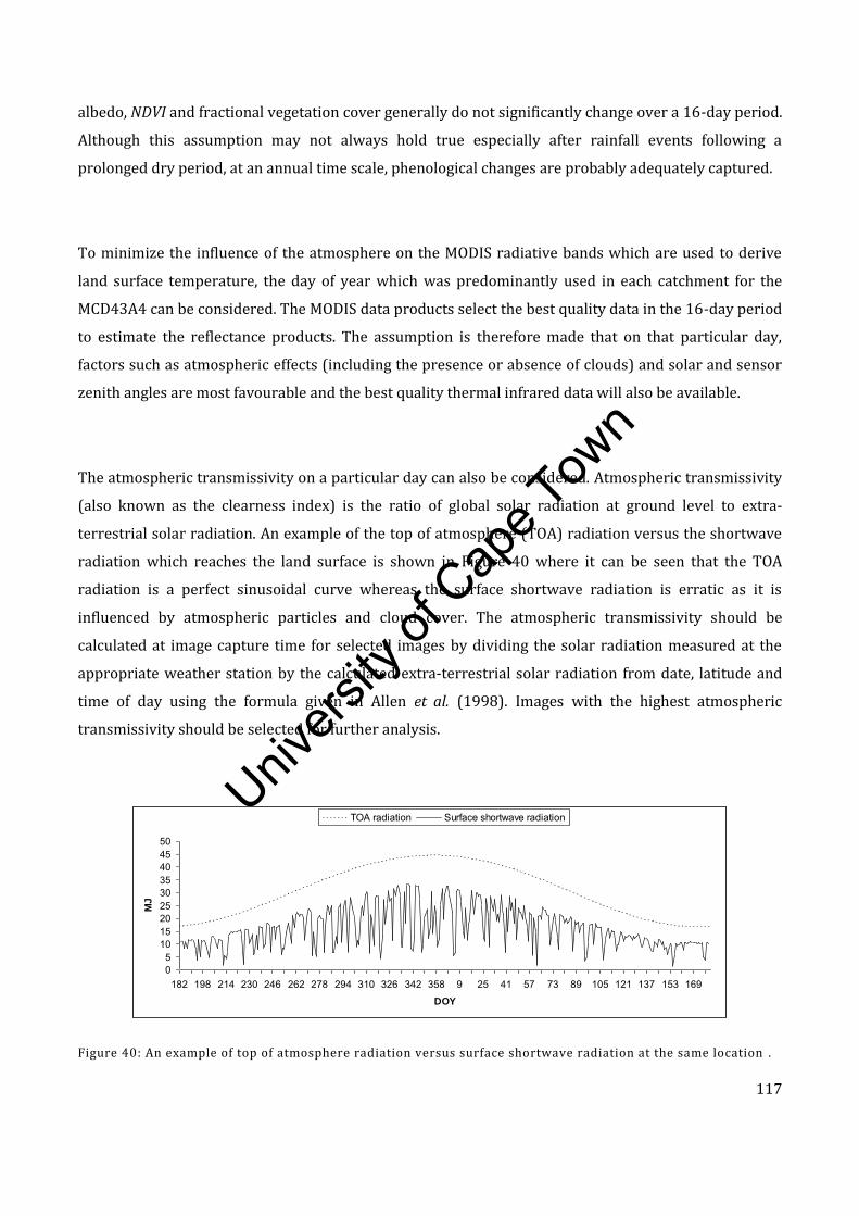
Univers

ity of

Cap

e Tow

n

117

albedo, NDVI and fractional vegetation cover generally do not significantly change over a 16-day period.

Although this assumption may not always hold true especially after rainfall events following a

prolonged dry period, at an annual time scale, phenological changes are probably adequately captured.

To minimize the influence of the atmosphere on the MODIS radiative bands which are used to derive

land surface temperature, the day of year which was predominantly used in each catchment for the

MCD43A4 can be considered. The MODIS data products select the best quality data in the 16-day period

to estimate the reflectance products. The assumption is therefore made that on that particular day,

factors such as atmospheric effects (including the presence or absence of clouds) and solar and sensor

zenith angles are most favourable and the best quality thermal infrared data will also be available.

The atmospheric transmissivity on a particular day can also be considered. Atmospheric transmissivity

(also known as the clearness index) is the ratio of global solar radiation at ground level to extra-

terrestrial solar radiation. An example of the top of atmosphere (TOA) radiation versus the shortwave

radiation which reaches the land surface is shown in Figure 40 where it can be seen that the TOA

radiation is a perfect sinusoidal curve whereas the surface shortwave radiation is erratic as it is

influenced by atmospheric particles and cloud cover. The atmospheric transmissivity should be

calculated at image capture time for selected images by dividing the solar radiation measured at the

appropriate weather station by the calculated extra-terrestrial solar radiation from date, latitude and

time of day using the formula given in Allen et al. (1998). Images with the highest atmospheric

transmissivity should be selected for further analysis.

Figure 40: An example of top of atmosphere radiation versus surface shortwave radiation at the same location .

05

101520253035404550

182 198 214 230 246 262 278 294 310 326 342 358 9 25 41 57 73 89 105 121 137 153 169

DOY

MJ

TOA radiation Surface shortwave radiation

Univers

ity of

Cap

e Tow

n

118

7.1.2. FRACTIONAL VEGETATION COVER

Fractional vegetation cover (fc) is a user defined input into the pre-packaged version of SEBS in ILWIS

and different formulations of fc are used in SEBS for different purposes. Fractional vegetation cover and

its complement are used in the calculation of the roughness length for heat transfer (Su et al., 2005)

which, in turn, is used in the calculation of the sensible heat flux. In addition, fc is used in the estimation

of the soil heat flux (Su, 2002).

It has already been stated that care should be taken when selecting fractional vegetation cover formula

as this should be appropriate for the study area, especially if NDVI minimum and maximum values need

to be defined. For the P10A catchment, the formula by Carlson & Ripley (1997) was used with a scene

specific NDVImax value defined. The NDVI maximum values over the study period were analyzed and the

98th percentile value of NDVImax (0.756) was assigned (Gibson et al., 2011).

In Chapter 6.3.2, several methods for the calculation of fc which are described in the literature are

highlighted.. These methods generally make use of LAI (Choudhury, 1987) as input or require pixel

NDVI together with a minimum and maximum NDVI (Carlson & Ripley, 1997; Gutman & Ignatov, 1998).

These minimum and maximum NDVI are either constant (Sobrino & El Kharraz, 2003) or can be derived

directly from the scene or from a time series. For example, if fractional vegetation cover is calculated

according to the formula for vegetation proportion (Sobrino & El Kharraz, 2003), then NDVI minimum

is defined to be 0.2 and NDVI maximum is 0.5, where pixels with NDVI values of 0.5 or higher are

considered to be fully vegetated and pixels with values of 0.2 or lower to be bare soil. The values

between NDVI minimum and maximum represent the mixed vegetation cover with differing degrees of

sparse vegetation.

It was earlier (Chapter 6.3.2) concluded that if it is possible to obtain field data in order to derive an

appropriate NDVI maximum value, the formula by Carlson & Ripley (1997) can be used. Alternatively

the formula by Choudhury (1987) using LAI as input may be used.

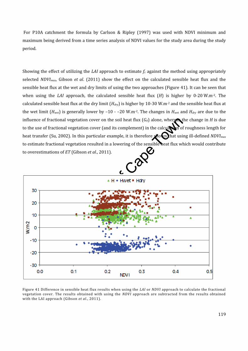
Univers

ity of

Cap

e Tow

n

119

For P10A catchment the formula by Carlson & Ripley (1997) was used with NDVI minimum and

maximum being derived from a time series analysis of NDVI values for the study area during the study

period.

Showing the effect of utilizing the LAI approach to estimate fc against the method using appropriately

selected NDVImax, Gibson et al. (2011) show the effect on the calculated sensible heat flux and the

sensible heat flux at the wet and dry limits of using the two approaches (Figure 41). It can be seen that

when using the LAI approach, the calculated sensible heat flux (H) is higher by 0-20 W.m-2. The

calculated sensible heat flux at the dry limit (Hdry) is higher by 10-30 W.m-2 and the sensible heat flux at

the wet limit (Hwet) is generally lower by –10 - –20 W.m-2. The changes in Hwet and Hdry are due to the

influence of fractional vegetation cover on the soil heat flux (G0) alone, whereas the change in H is due

to the use of fractional vegetation cover (and its complement) in the calculation of roughness length for

heat transfer (Su, 2002). In this particular example, it is therefore shown that using ill-defined NDVImax

to estimate fractional vegetation resulted in a lowering of the sensible heat flux which would contribute

to overestimations of ET (Gibson et al., 2011).

Figure 41 Difference in sensible heat flux results when using the LAI or NDVI approach to calculate the fractional vegetation cover. The results obtained with using the NDVI approach are subtracted from the results obtained with the LAI approach (Gibson et al., 2011).

Univers

ity of

Cap

e Tow

n

120

To contextualize this, it should be stated that this calculation was done for a January image where the

net radiation is over 600 W.m-2. Therefore 0 – 20 W.m-2 differences in the sensible heat flux only

accounts for a very small difference in the overall energy balance. Therefore although the calculation of

fractional vegetation cover either through the choice of NDVImax or through the LAI approach should be

chosen appropriately (as it is important to reduce all sources of uncertainty from the modelling), the

effect of using one method rather than the other was shown not to be the major source of

underestimation of the sensible heat flux, in this research.

7.1.3. REFERENCE HEIGHT

The sensitivity of the SEBS model to the reference height at which wind speed is measured, particularly

in areas with tall canopies, has been discussed (Chapter 6.3.3). For tall vegetation the 2 m reference

height from ARC-ISCW weather stations may not suitable. For this reason SAWS weather station data

was used since wind speed is measured at 10 m above the surface and it may be more appropriate in

study areas which include tall canopies.

7.1.4. LAND SURFACE AND AIR TEMPERATURE GRADIENT

The calculation of ET using the SEBS model relies on two temperature sources: air temperature (Ta) and

land surface temperature (T0). Su (2002) reported on the sensitivity of sensible heat flux to the gradient

between land surface temperature and air temperature and Badola (2009) reported that of all remotely

sensed input parameters, SEBS was most sensitive to change in T0-Ta. T0 plays a role in the

determination of net radiation and therefore soil heat flux, but its main contribution (together with the

aerodynamic resistance) is in the calculation of the sensible heat flux.

It can be seen from Equations [4] and [5] that at the wet and dry limits, the land surface and air

temperature gradient is not considered in the calculation of the sensible heat flux. For this reason, T0-Ta

does not play a role in the calculation of ET if the wet or dry limits have been reached. However, T0-Ta is

used to determine whether or not the limits are reached (Equations [6], [7] and [8]) and therefore

should not be completely discounted in these instances. The sensitivity of the sensible heat flux Δ(T0-Ta)

Univers

ity of

Cap

e Tow

n

121

for two different environments was calculated in Chapter 6.3.1 and it was concluded that the sensitivity

of H (and therefore daily ET) to Δ(T0-Ta) is dependent not only T0 but also on the land cover type (and

therefore associated roughness parameters), and whether the wet limit has been reached. It can be seen

in Figure 34 that in two different environments, the sensitivity of SEBS calculated daily ET is dependent

on both the land cover and T0-Ta. For each scenario in Figure 34, the wet limit occurs at the apex of the

respective curve. Where the wet limit has been reached, the daily ET increases with increasing T0-Ta;

however, where the wet limit has not been reached, the daily ET decreases with increasing T0-Ta. It was

concluded that SEBS should not be used in mountainous areas or topographically diverse areas as T0

retrievals are less accurate in this setting and particularly with coarse resolution sensors since the

heterogeneity of the T0 cannot be captured at the appropriate scale. Topographical analysis of potential

study areas should be done to minimize the uncertainties that inaccurate T0 calculations will contribute

to the ET results.

However, should the uncertainties associated with T0-Ta be reduced and T0-Ta is assumed to be correct,

H has been shown to be sensitive to fluctuations in this term especially in unstable conditions and in the

transition phase where T0-Ta moves from negative to positive and back again (Su, 2002). According to

Su (2002), this sensitivity is suspected to be caused by the current stability correction functions used in

SEBS not adequately describing this transition. This was found to be particularly true in the shrubs and

grasslands experiments and more accurate results for agricultural areas were found (Su, 2002). In the

similarity theory used in the formulation of the sensible heat flux (Equations [6], [7] and [8]), steady

state and horizontally homogeneous conditions are assumed (Gellens-Meulenberghs, 2000) which may

not always be good descriptors of natural vegetation and topography in South Africa. It should also be

noted that many of the agrometeorological theories and formulae were developed for agricultural crops

and not for natural vegetation and perhaps additional parameterization should be considered for those

land uses which fall outside of agricultural crops.

Furthermore, since the lag effect of the heating of land differs to the heating of the air and therefore T0-

Ta, the time of day of image acquisition may be important and the choice of satellite sensor (such as

TERRA which captures images in the morning versus AQUA which captures images in the afternoon)

should be considered in this context. Further considerations are the superior functioning of the AQUA

MODIS over the TERRA MODIS sensor. The difference in launch dates allowed for some improvements

to be made to the AQUA instrument. Xiong et al. (2002b) report on the differences between AQUA and

Univers

ity of

Cap

e Tow

n

122

TERRA signal-to-noise ratios (SNR) and on-orbit noise equivalent temperature differences. The

reported results on both these parameters are that AQUA performs better than TERRA; however,

TERRA is performing within the prelaunch standards (with the exception of band 7).

Since the aim of this research was to minimize uncertainties as far as possible, the selection of

homogeneous catchments (particularly with respect to topography but also considering land cover),

should minimize the uncertainties associated with T0 estimation in the chosen catchments. For this

reason P10A was chosen as being homogeneous (Gibson et al, 2011). To minimize the uncertainties for

the thermal bands, data from the AQUA sensor was used for the majority of the processing, however,

TERRA data was also used for comparative purposes and to indicate the influence of the time of day on

ET results due to differing meteorological conditions and differing T0-Ta due to the differential heating

of the land surface and the air.

It has already been stated that T0-Ta is used in the calculation of the sensible heat flux and it should be

noted once again that H is inversely related to ET. As the energy allocated to heating the air increases, so

the energy available to evaporate water decreases. This in turn leads to a decrease in evaporative

fraction and a decrease in ET. The effect of using TERRA data versus using AQUA data is illustrated in

Figure 42. It can be seen that when using TERRA data which is captured in the morning, T0-Ta is lower

than T0-Ta calculated using AQUA data which is captured in the afternoon. It can also be seen by the

negative slope of the TERRA results in Figure 42 that the sensible heat flux is always calculated to be at

the wet limit when using TERRA data. An indication of the wet limit having been reached is the decrease

in sensible heat flux with increase in T0-Ta whereas the positive slope indicates that the wet limit has

not been reached and H is calculated using combination equations (Equations [6], [7] and [8]). It

appears that at TERRA overpass, the transition phase where T0-Ta moves from negative to positive is

not complete, unstable conditions exist and the stability correction functions in SEBS are not suitable.

Paradoxically, the fact that the wet limit has been reached does not necessarily mean that the daily

estimated ET calculated from using TERRA data will be higher than the AQUA results due to the inverse

relationship between H and ET and the fact that AQUA results are generally close to the wet limit and

therefore clustered around the wet limit transition.

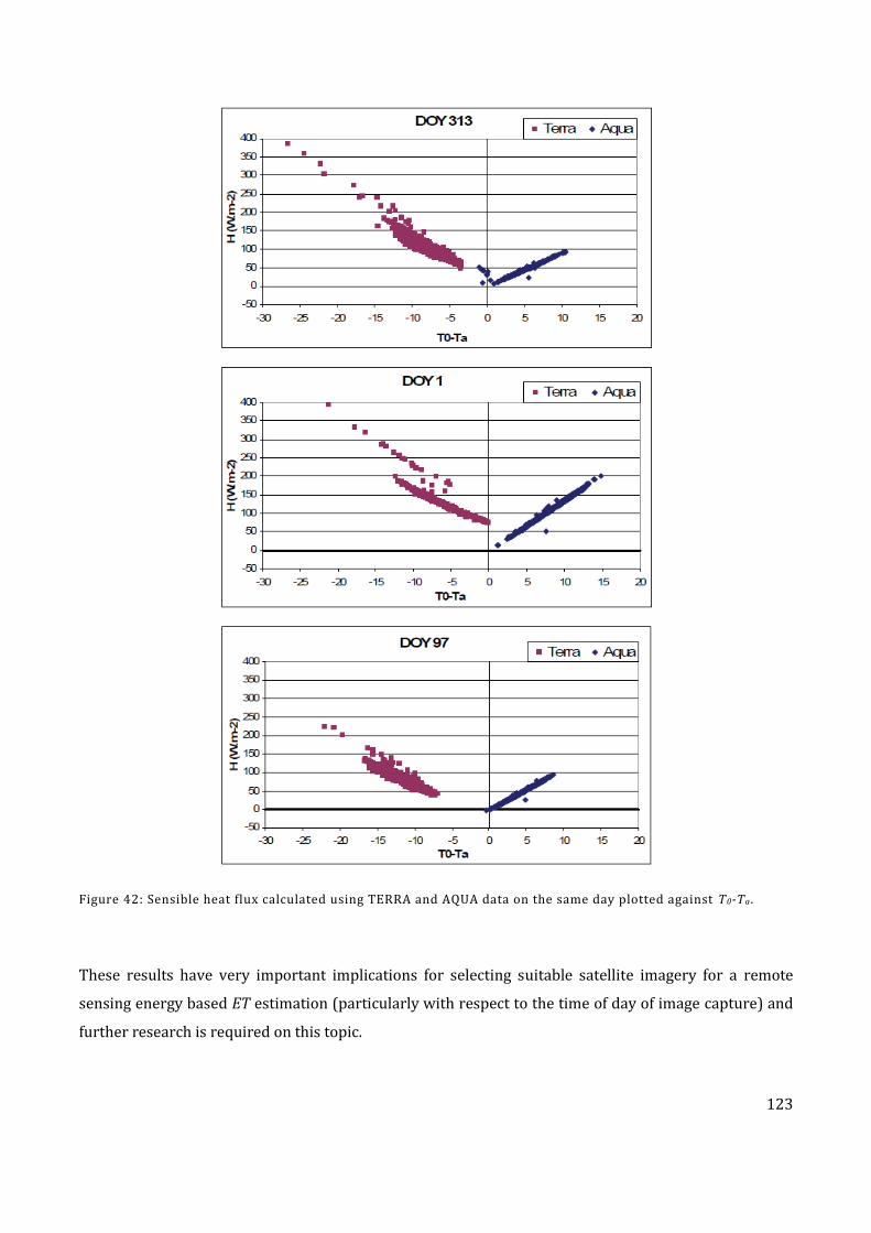
Univers

ity of

Cap

e Tow

n

123

Figure 42: Sensible heat flux calculated using TERRA and AQUA data on the same day plotted against T0-Ta .

These results have very important implications for selecting suitable satellite imagery for a remote

sensing energy based ET estimation (particularly with respect to the time of day of image capture) and

further research is required on this topic.

Univers

ity of

Cap

e Tow

n

124

According to Allen et al (2010), in a paper on the status and continuing challenges in operational

remote sensing of ET, errors in surface temperature (T0) retrievals from many satellite systems can

range from 3 – 5K. This is due to uncertainty in atmospheric conditions, surface emissivity, view angle,

and shadowing. Allen et al. (2010) report that Hook and Prata (2001) suggested that T0 retrievals from

modern satellites could be as accurate as 0.5K. However since surface temperature gradients used in

energy balance models are often in the order of 1 to 5K Allen et al (2010) state that even this amount of

error together with large uncertainties in the air temperature measurements, makes the use of models

based on differences in absolute estimates of surface and air temperature cumbersome.

7.1.5. ROUGHNESS LENGTHS

The roughness length for momentum transfer, or momentum roughness (z0m), is an important

parameter for the wind profile calculations contained within Equations [7] and [8] and also for the

calculation of roughness length for heat transfer, or heat roughness (z0h) (Equation [12]). The earth’s

surface is usually rough and for a rough surface, z0m is taken to equal the surface roughness length (z0)

(Brutsaert, 1982).

Roughness length (z0) is a measure of the aerodynamic roughness of a surface and is related to but not

equal to the height of the roughness elements. Many studies have been conducted to relate z0 with

measurable characteristics of the surface and the simplest and most obvious method is to relate it to the

mean height of the roughness obstacles (h0) (Brutsaert, 1982). Studies relating z0 to h0 report h0 / z0 of

between 7.35 and 8 (Brutsaert, 1982). In reality, the matter is not as simple as relating height of

obstacles to roughness height since h0 / z0 is a fairly complicated function of other surface

characteristics too (Brutsaert, 1982). z0 is also a function of the shape and density distribution of the

roughness elements. For example, a grassy plain has a lower roughness than an area with many trees

and buildings (Kipp & Zonen, 2005) and an additional term, zero plane displacement height (d0) is

defined as the height above the ground at which zero wind speed is achieved due to friction caused by

roughness elements. In Figure 43 it can be seen that the height of the roughness obstacles is identical in

both images and if a simple h0 / z0 were to be used, the z0 value would be identical for both images.

However, the distribution and density of the roughness elements have a profound influence on

roughness length.

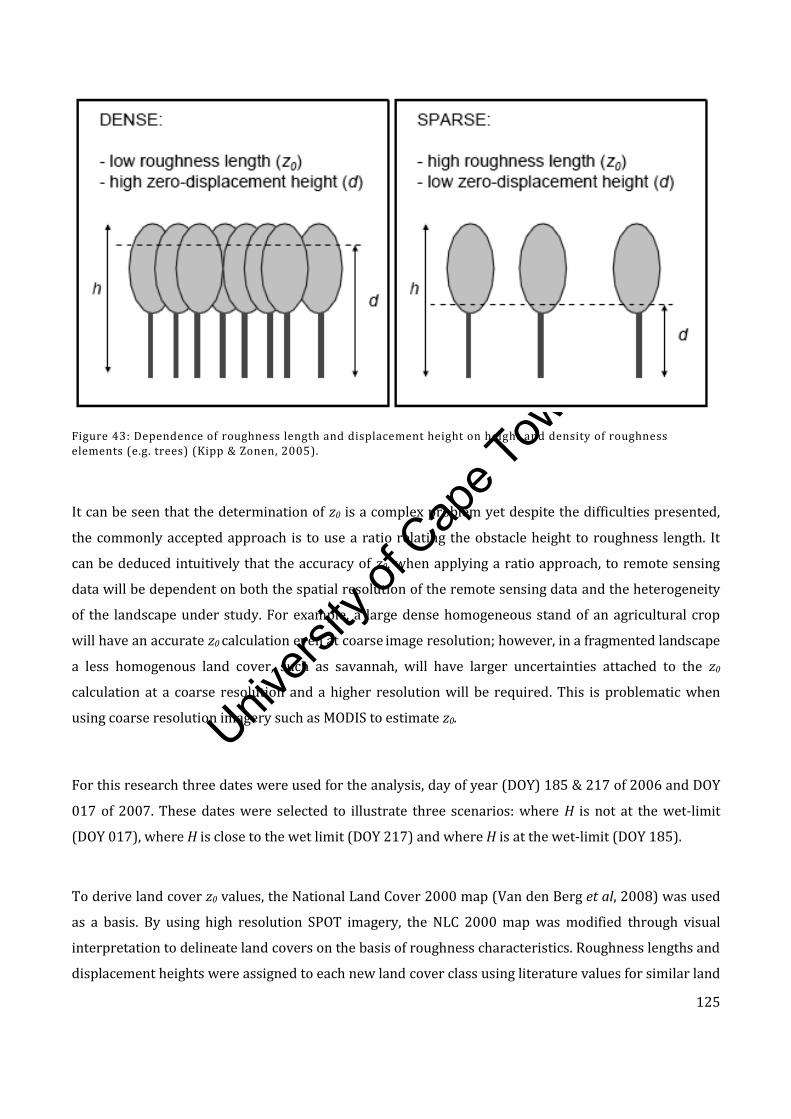
Univers

ity of

Cap

e Tow

n

125

Figure 43: Dependence of roughness length and displacement height on height and density of roughness elements (e.g. trees) (Kipp & Zonen, 2005).

It can be seen that the determination of z0 is a complex problem yet despite the difficulties presented,

the commonly accepted approach is to use a ratio relating the obstacle height to roughness length. It

can be deduced intuitively that the accuracy of z0, when applying a ratio approach, to remote sensing

data will be dependent on both the spatial resolution of the remote sensing data and the heterogeneity

of the landscape under study. For example, a large dense homogeneous stand of an agricultural crop

will have an accurate z0 calculation even at coarse image resolution; however, in a fragmented landscape

a less homogenous land cover, such as savannah, will have larger uncertainties attached to the z0

calculation at a coarse resolution and a higher resolution will be required. This is problematic when

using coarse resolution imagery such as MODIS to estimate z0.

For this research three dates were used for the analysis, day of year (DOY) 185 & 217 of 2006 and DOY

017 of 2007. These dates were selected to illustrate three scenarios: where H is not at the wet-limit

(DOY 017), where H is close to the wet limit (DOY 217) and where H is at the wet-limit (DOY 185).

To derive land cover z0 values, the National Land Cover 2000 map (Van den Berg et al, 2008) was used

as a basis. By using high resolution SPOT imagery, the NLC 2000 map was modified through visual

interpretation to delineate land covers on the basis of roughness characteristics. Roughness lengths and

displacement heights were assigned to each new land cover class using literature values for similar land

Univers

ity of

Cap

e Tow

n

126

covers. The footprint of the MODIS pixel was then overlaid on the land cover map and the land cover

class covering the largest area within each MODIS pixel was assigned to each MODIS pixel. This process

can be seen in Figure 44. It must be noted that this process is highly subjective and there are some flaws

in selecting a roughness parameter for a pixel purely based on the majority land cover within the pixel.

This highlights the influence of the resolution of the satellite imagery and the heterogeneity of the

landscape on SEBS results.

Land cover labelled Shrubland (South) can more accurately be described as grassland (Figure 44a). A z0

value from Table 17 of 0.034 m corresponding to the z0 value for grass was assigned. Land cover

labelled Shrubland (North) as shown in (Figure 44b was assigned a value of 0.0408 m from Table 17, a

value assigned to heather. Thickets and bush clumps ((Figure 44c) were found mostly in the central

portion of the catchment and were assigned a z0 value of 0.2 m for 1 – 2 m high vegetation (Brutsaert,

1982).

Table 17: Land use classes in the PELCOM land use database and associated z0 values adapted from Su (2006).

LAND USE CLASS Z0M (M)

Fresh water, salt water 0.0002

Bare soil in built-up areas, bare soil in natural areas 0.0012

Main roads and railways 0.0035

Grass in built-up area 0.0334

Grass 0.0340

Heather, other open spaces in natural areas 0.0408

Potatoes, Beets, other crops, bulbs 0.0639

Greenhouses 0.4066

Cereal, maize 0.4966

Built-up area in rural area, buildings in rural areas 0.5488

Orchards 0.6065

Continuous urban area 1.1058

Deciduous forest, coniferous forest, deciduous and coniferous forest in urban area, built-up area with dense forest

1.2214

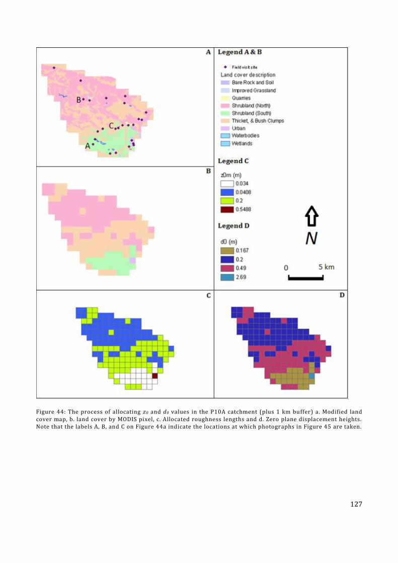
Univers

ity of

Cap

e Tow

n

127

Figure 44: The process of allocating z0 and d0 values in the P10A catchment (plus 1 km buffer) a. Modified land cover map, b. land cover by MODIS pixel, c. Allocated roughness lengths and d. Zero plane displacement heights. Note that the labels A, B, and C on Figure 44a indicate the locations at which photographs in Figure 45 are taken.

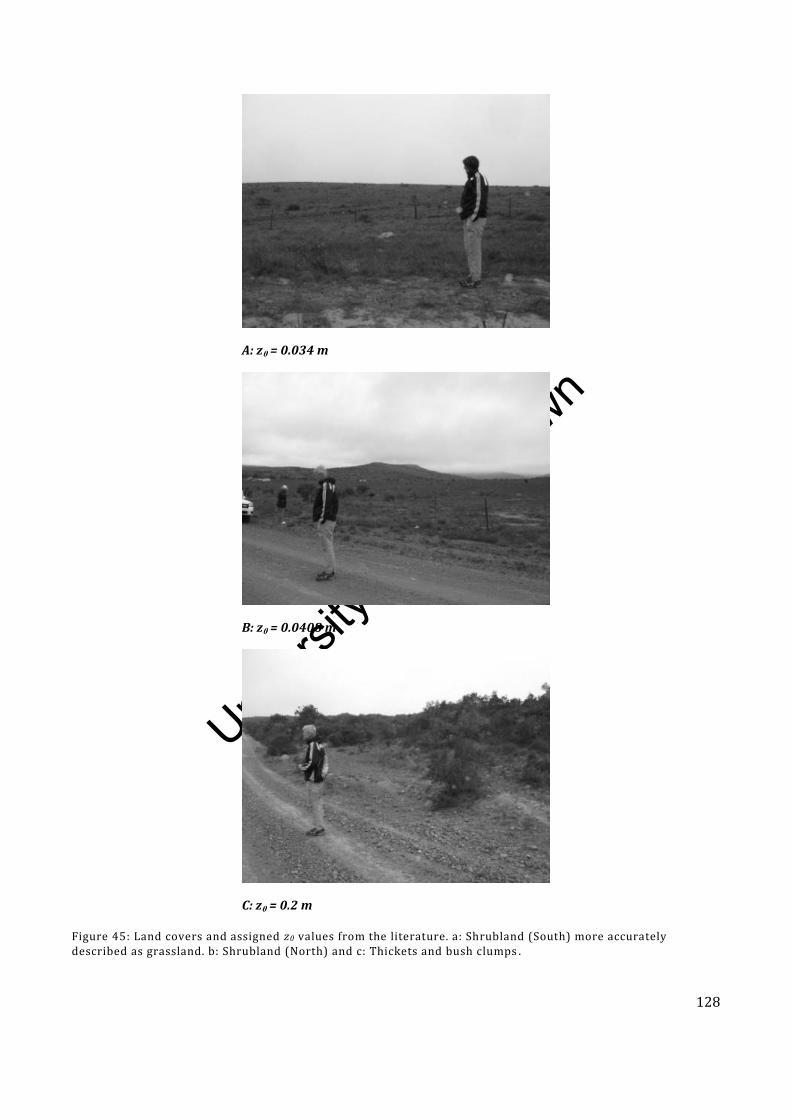
Univers

ity of

Cap

e Tow

n

128

A: z0 = 0.034 m

B: z0 = 0.0408 m

C: z0 = 0.2 m

Figure 45: Land covers and assigned z0 values from the literature. a: Shrubland (South) more accurately described as grassland. b: Shrubland (North) and c: Thickets and bush clumps .

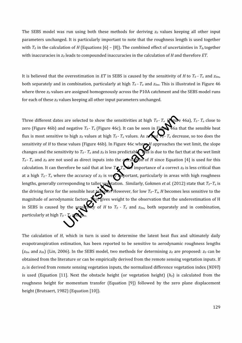
Univers

ity of

Cap

e Tow

n

129

The SEBS model was run using both these methods for deriving z0 values keeping all other input

parameters unchanged. It is particularly important to note that the roughness length is used together

with T0 in the calculation of H (Equations [6] – [8]). The combined effect of uncertainties in T0, together

with inaccuracies in z0 leads to compounded inaccuracies in the calculation of H and therefore ET.

It is believed that the overestimation in ET in SEBS is caused by the sensitivity of H to T0 - Ta and z0m,

both separately and in combination, particularly at high T0 - Ta and z0m. This is illustrated in Figure 46

where three z0 values are assigned homogenously across the P10A catchment and the SEBS model runs

for each of these z0 values keeping all other input parameters unchanged.

Three different dates are selected to show the sensitivities at high T0 - Ta (Figure 46a), T0 - Ta close to

zero (Figure 46b) and negative T0 - Ta (Figure 46c). It can be seen in Figure 46a that the sensible heat

flux is most sensitive to high z0 values at high T0 - Ta values. As z0 and T0 - Ta decrease, so too does the

sensitivity of H to these values (Figure 46b). In Figure 46c where H approaches the wet limit, the slope

changes and the sensitivity to T0 - Ta and z0 is less predictable. This is due to the fact that at the wet limit

T0 - Ta and z0 are not used as direct inputs into the calculation of H since Equation [4] is used for this

calculation. It can therefore be said that at low T0 - Ta, the importance of a correct z0 is less critical than

at a high T0 - Ta where the accuracy of z0 is very important, particularly in areas with high roughness

lengths, generally corresponding to taller vegetation. Similarly, Gokmen et al. (2012) state that T0−Ta is

the driving force for the sensible heat transfer. However, for low T0−Ta, H becomes less sensitive to the

magnitude of aerodynamic factors. This gives weight to the observation that the underestimation of H

in SEBS is caused by the sensitivity of H to T0 - Ta and z0m, both separately and in combination,

particularly at high T0 - Ta and z0m.

The calculation of H, which in turn is used to determine the latent heat flux and ultimately daily

evapotranspiration estimation, has been reported to be sensitive to aerodynamic roughness lengths

(z0m and z0h) (Lin, 2006). In the SEBS model, two methods for determining z0 are proposed: z0 can be

obtained from the literature or can be empirically derived from the remote sensing vegetation inputs. If

z0 is derived from remote sensing vegetation inputs, the normalized difference vegetation index (NDVI)

is used (Equation [11]. Next the obstacle height (or vegetation height) (h0) is calculated from the

roughness height for momentum transfer (Equation [9]) followed by the zero plane displacement

height (Brutsaert, 1982) (Equation [10]).

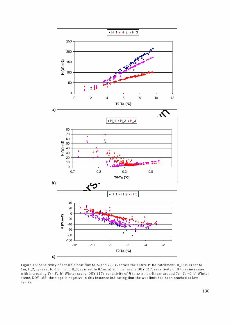
Univers

ity of

Cap

e Tow

n

130

a)

b)

c)

Figure 46: Sensitivity of sensible heat flux to z0 and T0 - Ta across the entire P10A catchment. H_1: z0 is set to 1m; H_2, z0 is set to 0.5m; and H_3, z0 is set to 0.1m. a) Summer scene DOY 017: sensitivity of H to z0 increases with increasing T0 - Ta . b) Winter scene, DOY 217: sensitivity of H to z0 is non-linear around T0 - Ta =0. c) Winter scene, DOY 185: the slope is negative in this instance indicating that the wet limit has been reached at low T0 - Ta.

0

50

100

150

200

250

0 2 4 6 8 10 12

T0-Ta (°C)

H (

W.m

-2)

H_1 H_2 H_3

01020304050607080

-0.7 -0.2 0.3 0.8

T0-Ta (°C)

H (

W.m

-2)

H_1 H_2 H_3

-100-80

-60-40

-200

2040

-12 -10 -8 -6 -4 -2

T0-Ta (°C)

H (

W.m

-2)

H_1 H_2 H_3

Univers

ity of

Cap

e Tow

n

131

It is apparent that if Equations [9] - [11] are used to calculate z0 and d0, then areas which have a low

NDVI will be assigned a low roughness length, a low canopy height and a low displacement height.

Although this assumption may generally hold true in certain irrigated agricultural regions, it does not

allow for the case of semi-arid environments where shrubs and fynbos type vegetation have a low NDVI

during the hot dry summer but the canopy height does not follow a seasonal curve in the way that NDVI

does. In this scenario, the roughness length, canopy height and displacement height are independent of

NDVI and should not vary as much as NDVI throughout the year.

An alternative method for obtaining roughness length is using look-up tables such as the Pan-European

Land Use and Land Cover Monitoring (PELCOM) land use database with associated z0 values (Su, 2006).

It can be seen in Table 17 that not all land covers in South Africa are contained within this type of

database so a large amount of guesswork is required to match South African land covers to existing

databases. Additionally, the phenological stage of the vegetation is not reflected here which will be

particularly important for land covers where the height of the vegetation changes dramatically during

the course of a growing season.

It is postulated that should it be possible to obtain a more accurate measure of z0 which can be used as

input into the SEBS model, then the calculation of the H will be more accurate in turn leading to a more

accurate ET value rather than reported overestimations (Gibson et al, 2009; Gibson et al, 2011).

The z0 values generated from NDVI are compared with the literature assigned z0 values for DOY 185,

217 and 017 in Figure 47. In the southern portion of the catchment where literature assigned z0 values

are low (0.034 m), the NDVI derived values significantly exceed the literature values for each selected

DOY and a clear seasonal influence is not apparent. It is possible that the small number of pixels in this

class did not allow for a trend to develop. The greenness of the vegetation is apparent in Figure 45a

even though at that particular time of year the vegetation was short. The greenness of the vegetation

implies that the NDVI will be high and the z0 derived from NDVI would not be expected to return

realistic z0 values.

For the northern portion of the catchment where the very low shrubland occurs and a z0 value of 0.0408

m was assigned, there is once again a higher z0 value returned for the NDVI values for each of the

selected DOY. A clearer seasonal trend can be discerned here with the summer scenes returning lower

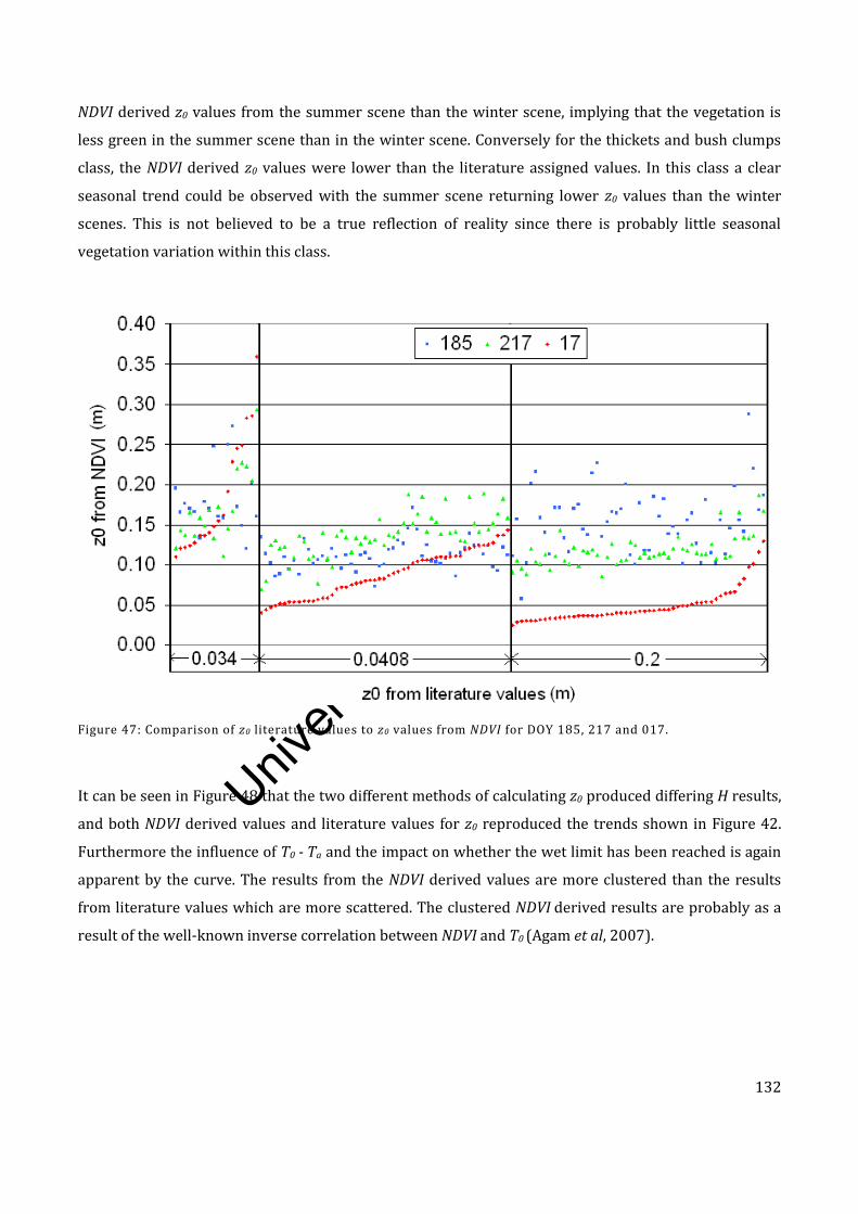
Univers

ity of

Cap

e Tow

n

132

NDVI derived z0 values from the summer scene than the winter scene, implying that the vegetation is

less green in the summer scene than in the winter scene. Conversely for the thickets and bush clumps

class, the NDVI derived z0 values were lower than the literature assigned values. In this class a clear

seasonal trend could be observed with the summer scene returning lower z0 values than the winter

scenes. This is not believed to be a true reflection of reality since there is probably little seasonal

vegetation variation within this class.

Figure 47: Comparison of z0 literature values to z0 values from NDVI for DOY 185, 217 and 017.

It can be seen in Figure 48 that the two different methods of calculating z0 produced differing H results,

and both NDVI derived values and literature values for z0 reproduced the trends shown in Figure 42.

Furthermore the influence of T0 - Ta and the impact on whether the wet limit has been reached is again

apparent by the curve. The results from the NDVI derived values are more clustered than the results

from literature values which are more scattered. The clustered NDVI derived results are probably as a

result of the well-known inverse correlation between NDVI and T0 (Agam et al, 2007).

Univers

ity of

Cap

e Tow

n

133

Figure 48: Comparison of z0 literature values to z0 values derived from NDVI for H results plotted against T0 - Ta for DOY 185, 217 and 017.

Apparent from the results is that although there are differences in estimated H when different methods

for estimating z0 are used, H remains low for both winter (DOY 185 & 217) and summer (DOY 017)

scenes. This implies that the ET estimate will be high for each of the days represented in this research.

Although the SEBS model has been shown to be sensitive to z0 (particularly in combination with T0 - Ta),

the results from this research showed no significant changes in the calculation of H when two different

methodologies were used for z0 determination.

7.2. RESULTS AND DISCUSSION

This component of the research was an iterative process as the importance of addressing some of the

items above was only discovered through selecting images, running the model, analyzing the results

and then adapting the methodology and input data. Due to the iterative nature and the volume of data

involved, it is very difficult (and not particularly helpful) to present the results of all iterations but

rather to present results after all the adaptations to input data, image selection, as described in

Chapter 7.1 had been made.

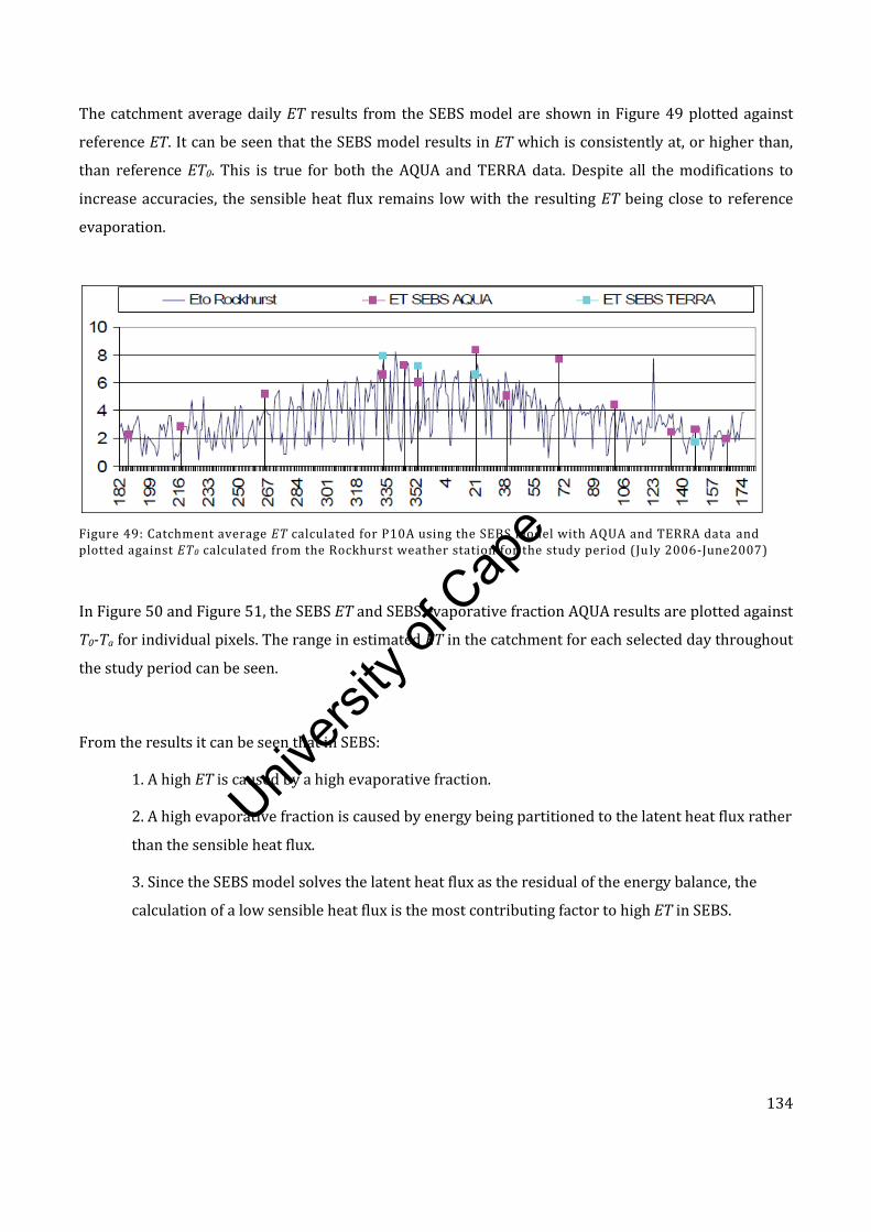
Univers

ity of

Cap

e Tow

n

134

The catchment average daily ET results from the SEBS model are shown in Figure 49 plotted against

reference ET. It can be seen that the SEBS model results in ET which is consistently at, or higher than,

than reference ET0. This is true for both the AQUA and TERRA data. Despite all the modifications to

increase accuracies, the sensible heat flux remains low with the resulting ET being close to reference

evaporation.

Figure 49: Catchment average ET calculated for P10A using the SEBS model with AQUA and TERRA data and plotted against ET0 calculated from the Rockhurst weather station for the study period (Ju ly 2006-June2007)

In Figure 50 and Figure 51, the SEBS ET and SEBS evaporative fraction AQUA results are plotted against

T0-Ta for individual pixels. The range in estimated ET in the catchment for each selected day throughout

the study period can be seen.

From the results it can be seen that in SEBS:

1. A high ET is caused by a high evaporative fraction.

2. A high evaporative fraction is caused by energy being partitioned to the latent heat flux rather

than the sensible heat flux.

3. Since the SEBS model solves the latent heat flux as the residual of the energy balance, the

calculation of a low sensible heat flux is the most contributing factor to high ET in SEBS.

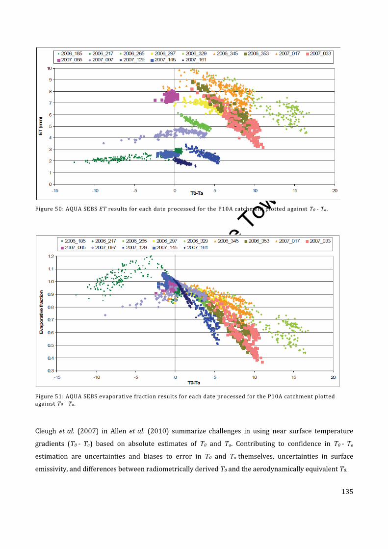
Univers

ity of

Cap

e Tow

n

135

Figure 50: AQUA SEBS ET results for each date processed for the P10A catchment plotted against T0 - Ta .

Figure 51: AQUA SEBS evaporative fraction results for each date processed for the P10A catchment plotted against T0 - Ta.

Cleugh et al. (2007) in Allen et al. (2010) summarize challenges in using near surface temperature

gradients (T0 - Ta) based on absolute estimates of T0 and Ta. Contributing to confidence in T0 - Ta

estimation are uncertainties and biases to error in T0 and Ta themselves, uncertainties in surface

emissivity, and differences between radiometrically derived T0 and the aerodynamically equivalent T0.

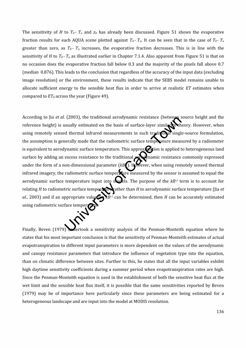
Univers

ity of

Cap

e Tow

n

136

The sensitivity of H to T0 - Ta and z0 has already been discussed. Figure 51 shows the evaporative

fraction results for each AQUA scene plotted against T0 - Ta. It can be seen that in the case of T0 - Ta

greater than zero, as T0 - Ta increases, the evaporative fraction decreases. This is in line with the

sensitivity of H to T0 - Ta as illustrated earlier in Chapter 7.1.4. Also apparent from Figure 51 is that on

no occasion does the evaporative fraction fall below 0.3 and the majority of the pixels fall above 0.7

(median 0.876). This leads to the conclusion that regardless of the accuracy of the input data (excluding

image resolution) or the environment, these results indicate that the SEBS model remains unable to

allocate sufficient energy to the sensible heat flux in order to arrive at realistic ET estimates when

compared to ET0 across the year (Figure 49).

According to Jia et al. (2003), the traditional aerodynamic resistance (between source height and the

reference height) is usually estimated on the basis of surface-layer similarity theory. However, when

using remotely sensed thermal infrared measurements in such traditional single-source formulation,

the assumption is generally made that the radiometric surface temperature measured by a radiometer

is equivalent to aerodynamic surface temperature. This approximation is applied to heterogeneous land

surface by adding an excess resistance to the traditional aerodynamic resistance commonly expressed

under the form of a non-dimensional parameter (kB-1). However, when using remotely sensed thermal

infrared imagery, the radiometric surface temperature measured by the sensor is assumed to equal the

aerodynamic surface temperature input into models. The purpose of the kB-1 term is to account for

relating H to radiometric surface temperature rather than H to aerodynamic surface temperature (Jia et

al., 2003) and if an appropriate value for kB-1 can be determined, then H can be accurately estimated

using radiometric surface temperature.

Finally, Beven (1979) undertook a sensitivity analysis of the Penman-Monteith equation where he

states that his most important conclusion is that the sensitivity of Penman-Monteith estimates of actual

evapotranspiration to different input parameters is more dependent on the values of the aerodynamic

and canopy resistance parameters that introduce the influence of vegetation type into the equation,

than on climatic difference between sites. Further to this, he states that all the input variables exhibit

high daytime sensitivity coefficients during a summer period when evapotranspiration rates are high.

Since the Penman-Monteith equation is used in the establishment of both the sensitive heat flux at the

wet limit and the sensible heat flux itself, it is possible that the same sensitivities reported by Beven

(1979) may be of importance here particularly since these parameters are being estimated for a

heterogeneous landscape and are input into the model at MODIS resolution.

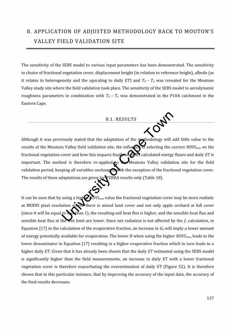
Univers

ity of

Cap

e Tow

n

137

8. APPLICATION OF ADJUSTED METHODOLOGY BACK TO MOUTON’S

VALLEY FIELD VALIDATION SITE

The sensitivity of the SEBS model to various input parameters has been demonstrated. The sensitivity

to choice of fractional vegetation cover, displacement height (in relation to reference height), albedo (as

it relates to heterogeneity and the upscaling to daily ET) and T0 – Ta was revealed for the Moutons

Valley study site where the field validation took place. The sensitivity of the SEBS model to aerodynamic

roughness parameters in combination with T0 – Ta was demonstrated in the P10A catchment in the

Eastern Cape.

8.1. RESULTS

Although it was previously stated that the adaptation of the methodology will add little value to the

results of the Moutons Valley field validation site, the influence of selecting the correct NDVImax on the

fractional vegetation cover and how this impacts finally on SEBS calculated energy fluxes and daily ET is

important. The method is therefore re-applied to the Moutons Valley validation site for the field

validation period, keeping all variables unchanged with the exception of the fractional vegetation cover.

The results of these adaptations are given for TERRA results only (Table 18).

It can be seen that by using a higher NDVImax value the fractional vegetation cover may be more realistic

at MODIS pixel resolution where there is mixed land cover and not only apple orchard at full cover

(since it will be equal to less than 1), the resulting soil heat flux is higher, and the sensible heat flux and

sensible heat flux at the wet limit are lower. Since net radiation is not affected by the fc calculation, in

Equation [17] in the calculation of the evaporative fraction, an increase in G0 will imply a lower amount

of energy potentially available for evaporation. The lower H when using the higher NDVImax, leads to the

lower denominator in Equation [17] resulting in a higher evaporative fraction which in turn leads to a

higher daily ET. Given that it has already been shown that the daily ET estimated using the SEBS model

is significantly higher than the field measurements, an increase in daily ET with a lower fractional

vegetation cover is therefore exacerbating the overestimation of daily ET (Figure 52). It is therefore

shown that in this particular instance, that by improving the accuracy of the input data, the accuracy of

the final results decreases.

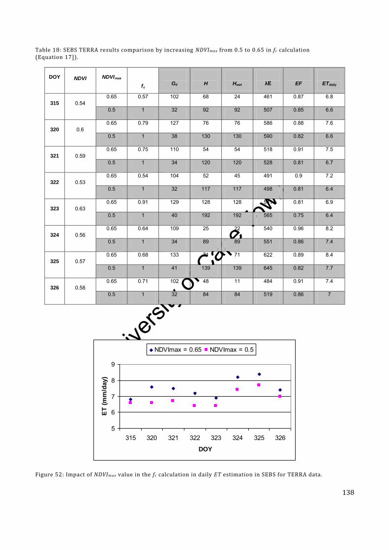
Univers

ity of

Cap

e Tow

n

138

Table 18: SEBS TERRA results comparison by increasing NDVImax from 0.5 to 0.65 in fc calculation (Equation 17]).

DOY NDVI NDVImax

fc

G0

H

Hwet

λE

EF

ETdaily

315 0.54 0.65 0.57 102 68 24 461 0.87 6.8

0.5 1 32 92 92 507 0.85 6.6

320 0.6 0.65 0.79 127 76 76 586 0.88 7.6

0.5 1 38 130 130 590 0.82 6.6

321 0.59 0.65 0.75 110 54 54 518 0.91 7.5

0.5 1 34 120 120 528 0.81 6.7

322 0.53 0.65 0.54 104 52 45 491 0.9 7.2

0.5 1 32 117 117 498 0.81 6.4

323 0.63 0.65 0.91 129 128 128 541 0.81 6.9

0.5 1 40 192 192 565 0.75 6.4

324 0.56 0.65 0.64 109 25 22 540 0.96 8.2

0.5 1 34 89 89 551 0.86 7.4

325 0.57 0.65 0.68 133 71 71 622 0.89 8.4

0.5 1 41 139 139 645 0.82 7.7

326 0.58 0.65 0.71 102 48 11 484 0.91 7.4

0.5 1 32 84 84 519 0.86 7

Figure 52: Impact of NDVImax value in the fc calculation in daily ET estimation in SEBS for TERRA data.

5

6

7

8

9

315 320 321 322 323 324 325 326

DOY

ET

(m

m/d

ay)

NDVImax = 0.65 NDVImax = 0.5

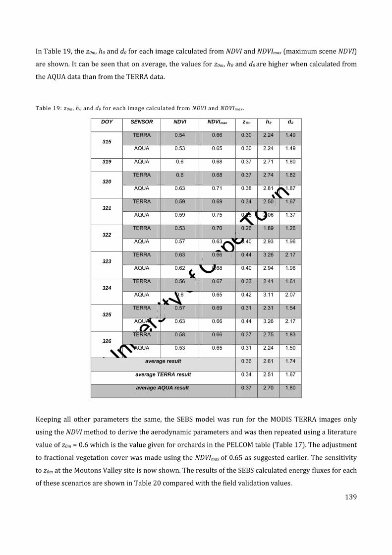
Univers

ity of

Cap

e Tow

n

139

In Table 19, the z0m, h0 and d0 for each image calculated from NDVI and NDVImax (maximum scene NDVI)

are shown. It can be seen that on average, the values for z0m, h0 and d0 are higher when calculated from

the AQUA data than from the TERRA data.

Table 19: z0m, h0 and d0 for each image calculated from NDVI and NDVImax .

DOY SENSOR NDVI NDVImax z0m h0 d0

315

TERRA 0.54 0.66 0.30 2.24 1.49

AQUA 0.53 0.65 0.30 2.24 1.49

319 AQUA 0.6 0.68 0.37 2.71 1.80

320

TERRA 0.6 0.68 0.37 2.74 1.82

AQUA 0.63 0.71 0.38 2.81 1.87

321

TERRA 0.59 0.69 0.34 2.50 1.67

AQUA 0.59 0.75 0.28 2.06 1.37

322

TERRA 0.53 0.70 0.26 1.89 1.26

AQUA 0.57 0.63 0.40 2.93 1.96

323

TERRA 0.63 0.66 0.44 3.26 2.17

AQUA 0.62 0.68 0.40 2.94 1.96

324

TERRA 0.56 0.67 0.33 2.41 1.61

AQUA 0.6 0.65 0.42 3.11 2.07

325

TERRA 0.57 0.69 0.31 2.31 1.54

AQUA 0.63 0.66 0.44 3.26 2.17

326

TERRA 0.58 0.66 0.37 2.75 1.83

AQUA 0.53 0.65 0.31 2.24 1.50

average result 0.36 2.61 1.74

average TERRA result 0.34 2.51 1.67

average AQUA result 0.37 2.70 1.80

Keeping all other parameters the same, the SEBS model was run for the MODIS TERRA images only

using the NDVI method to derive the aerodynamic parameters and was then repeated using a literature

value of z0m = 0.6 which is the value given for orchards in the PELCOM table (Table 17). The adjustment

to fractional vegetation cover was made using the NDVImax of 0.65 as suggested earlier. The sensitivity

to z0m at the Moutons Valley site is now shown. The results of the SEBS calculated energy fluxes for each

of these scenarios are shown in Table 20 compared with the field validation values.

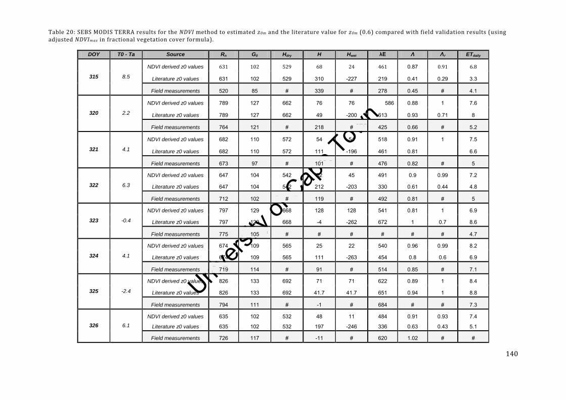
Univers

ity of

Cap

e Tow

n

140

Table 20: SEBS MODIS TERRA results for the NDVI method to estimated z0m and the literature value for z0m (0.6) compared with field validation results (using adjusted NDVImax in fractional vegetation cover formula).

DOY T0 - Ta Source Rn G0 Hdry H Hwet λE Λ Λr ETdaily

315 8.5

NDVI derived z0 values 631 102 529 68 24 461 0.87 0.91 6.8

Literature z0 values 631 102 529 310 -227 219 0.41 0.29 3.3

Field measurements 520 85 # 339 # 278 0.45 # 4.1

320 2.2

NDVI derived z0 values 789 127 662 76 76 586 0.88 1 7.6

Literature z0 values 789 127 662 49 -200 613 0.93 0.71 8

Field measurements 764 121 # 218 # 425 0.66 # 5.2

321 4.1

NDVI derived z0 values 682 110 572 54 54 518 0.91 1 7.5

Literature z0 values 682 110 572 111 -196 461 0.81 6.6

Field measurements 673 97 # 101 # 476 0.82 # 5

322 6.3

NDVI derived z0 values 647 104 542 52 45 491 0.9 0.99 7.2

Literature z0 values 647 104 542 212 -203 330 0.61 0.44 4.8

Field measurements 712 102 # 119 # 492 0.81 # 5

323 -0.4

NDVI derived z0 values 797 129 668 128 128 541 0.81 1 6.9

Literature z0 values 797 129 668 -4 -262 672 1 0.7 8.6

Field measurements 775 105 # # # # # # 4.7

324 4.1

NDVI derived z0 values 674 109 565 25 22 540 0.96 0.99 8.2

Literature z0 values 674 109 565 111 -263 454 0.8 0.6 6.9

Field measurements 719 114 # 91 # 514 0.85 # 7.1

325 -2.4

NDVI derived z0 values 826 133 692 71 71 622 0.89 1 8.4

Literature z0 values 826 133 692 41.7 41.7 651 0.94 1 8.8

Field measurements 794 111 # -1 # 684 # # 7.3

326 6.1

NDVI derived z0 values 635 102 532 48 11 484 0.91 0.93 7.4

Literature z0 values 635 102 532 197 -246 336 0.63 0.43 5.1

Field measurements 726 117 # -11 # 620 1.02 # #

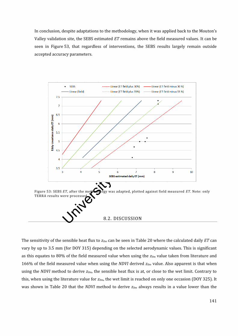
Univers

ity of

Cap

e Tow

n

141

In conclusion, despite adaptations to the methodology, when it was applied back to the Mouton’s

Valley validation site, the SEBS estimated ET remains above the field measured values. It can be

seen in Figure 53, that regardless of interventions, the SEBS results largely remain outside

accepted accuracy parameters.

Figure 53: SEBS ET, after the methodology was adapted, plotted against field measured ET. Note: only TERRA results were processed.

8.2. DISCUSSION

The sensitivity of the sensible heat flux to z0m can be seen in Table 20 where the calculated daily ET can

vary by up to 3.5 mm (for DOY 315) depending on the selected aerodynamic values. This is significant

as this equates to 80% of the field measured value when using the z0m value taken from literature and

166% of the field measured value when using the NDVI derived z0m value. Also apparent is that when

using the NDVI method to derive z0m, the sensible heat flux is at, or close to the wet limit. Contrary to

this, when using the literature value for z0m, the wet limit is reached on only one occasion (DOY 325). It

was shown in Table 20 that the NDVI method to derive z0m always results in a value lower than the

Univers

ity of

Cap

e Tow

n

142

literature value of 0.6 m. In Figure 54, the daily ET for each method to derive z0m and the field validation

value is plotted against T0 – Ta. Here it can be seen that when using a literature value for z0m, the daily ET

decreases with increasing T0 – Ta with a total range in daily ET of 5.5 mm per day. When using the NDVI

method, the daily ET does not reflect the same fluctuation with change in T0 – Ta and a total range of

1.6 mm is seen. Furthermore, the NDVI method tracks the field validation values better than when using

a fixed literature value for z0m. The increasing sensitivity of daily ET (via H) with increasing T0 – Ta to the

selected aerodynamic values is apparent with the exception being where T0 – Ta is negative. When using

the wet-limit equation (Equation [5]), the sensible heat flux decreases with increasing T0 – Ta resulting

in increasing ET with increasing T0 – Ta. The downward trend in daily ET with T0 – Ta is therefore more

apparent with the literature z0m values since there is consistent use of Equations [6] - [8] whereas with

the NDVI derived method, the wet limit is reached on many occasions thereby eliminating the

downward trend in ET with increasing T0 – Ta. This leads to the conclusion that the SEBS model is

sensitive to T0 – Ta in combination with z0m.

Should the uncertainties associated with T0 – Ta be reduced and T0 – Ta is assumed to be correct, H has

been shown to be sensitive to fluctuations in this term especially in unstable conditions and in the

transition phase where T0 – Ta moves from negative to positive and back again (Su, 2002). According to

Su (2002), this sensitivity is suspected to be caused by the current stability correction functions used in

SEBS not adequately describing this transition. This was found to be particularly true in the shrubs and

grasslands experiments and more accurate results for agricultural areas were found (Su, 2002). The lag

effect of the heating of land differs to the heating of the air and therefore T0 – Ta, and the time of day of

image acquisition may be important and the choice of satellite sensor (such as TERRA which captures

images in the morning versus AQUA which captures images in the afternoon) should be considered in

this context. Further, Beven (1979) documents the diurnal variation in canopy resistance illustrating

that differing land covers have different diurnal ranges and since it has been shown that the SEBS model

is sensitive to T0 – Ta in combination with vegetation parameters, this challenges the assumption of a

constant evaporative fraction which is used in remote sensing energy balance models for the upscaling

of instantaneous energy fluxes to daily ET.

In a recent publication, Lu et al. (2012) have reported a significant overestimation of the evaporative

fraction (and hence ET) using the SEBS model. This is the first set of authors apart from Gibson et al.

(2009), (2011) to report such a large overestimation of ET using SEBS. According to Lu et al. (2012),

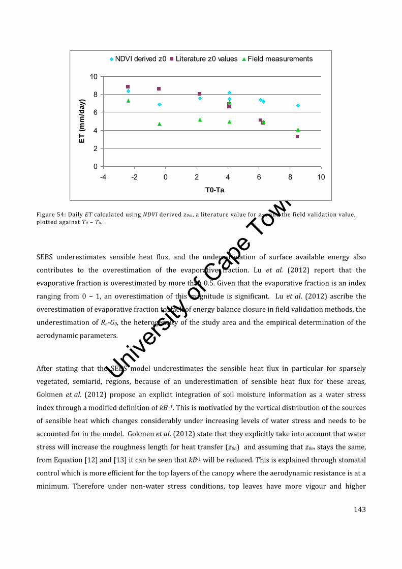
Univers

ity of

Cap

e Tow

n

143

Figure 54: Daily ET calculated using NDVI derived z0m, a literature value for z0m and the field validation value, plotted against T0 – Ta.

SEBS underestimates sensible heat flux, and the underestimation of surface available energy also

contributes to the overestimation of the evaporative fraction. Lu et al. (2012) report that the

evaporative fraction is overestimated by more than 0.5. Given that the evaporative fraction is an index

ranging from 0 – 1, an overestimation of this magnitude is significant. Lu et al. (2012) ascribe the

overestimation of evaporative fraction to: lack of energy balance closure in field validation methods, the

underestimation of Rn-G0, the heterogeneity of the study area and the empirical determination of the

aerodynamic parameters.

After stating that the SEBS model underestimates the sensible heat flux in particular for sparsely

vegetated, semiarid, regions, because of an underestimation of sensible heat flux for these areas,

Gokmen et al. (2012) propose an explicit integration of soil moisture information as a water stress

index through a modified definition of kB−1. This is motivatied by the vertical distribution of the sources

of sensible heat which changes considerably under increasing levels of water stress and needs to be

accounted for in the model. Gokmen et al. (2012) state that they explicitly take into account that water

stress will increase the roughness length for heat transfer (z0h) and assuming that z0m stays the same,

from Equation [12] and [13] it can be seen that kB-1 will be reduced. This is explained through stomatal

control which is more efficient for the top layers of the canopy where the aerodynamic resistance is at a

minimum. Therefore under non-water stress conditions, top leaves have more vigour and higher

0

2

4

6

8

10

-4 -2 0 2 4 6 8 10

T0-Ta

ET

(m

m/d

ay)

NDVI derived z0 Literature z0 values Field measurements

Univers

ity of

Cap

e Tow

n

144

stomatal conductance values. Top leaves therefore have a higher potential water loss rate than leaves

lower down the canopy indicating that stomata exert increasingly greater control over water use from

the bottom to the top of the canopy. Therefore under water-stressed conditions stomata of leaves will

close the closer to the top of the canopy they are found. There will be an associated increase in T0

toward the top of the canopy since the available energy is higher near the top. Finally, lower canopy

layers are expected to have less fluctuation in T0 – Ta, which means that as plant water stress increases

the source of heat will increasingly move towards the top of the canopy, thereby increasing z0h and

reducing kB−1.

This is illustrated in Figure 55. In Figure 55a, it can be seen that in non-water stressed environments,

the T0 – Ta will remain relatively stable from the soil surface to the top of canopy. The water loss

potential of the leaves increases towards the top of the canopy as does stomatal conductance and plant

vigour. This results in the roughness length for heat transfer remaining low, kB-1 being high and a

resulting low sensible heat flux. In the water stressed scenario in Figure 55b, it can be seen that T0 – Ta

increases towards the top of the canopy, resulting in water stress. Increased stomatal control towards

the top of the canopy occurs due to the environmental stress imposed on the plant. As a result, the

roughness height for heat transfer is high although the roughness of the surface between the water

stressed and non-water stressed scenario remains constant. In order to account for a high roughness

length for heat transfer in the water stressed scenario, Gokmen et al. (2012) propose the adjustment of

kB-1.

In the formulation of the water stress index by Gokmen et al. (2012), and in the testing and field

validation of the method, field measured values were used to integrate the soil moisture into the

calculation of H. However, Gokmen et al. (2012) took this a step further by using passive microwave

measurements of soil moisture to achieve operational application of the mapping of daily ET. This may

represent an improvement to the SEBS model changing it conceptually from a one layer-source model

to a multilayer source model (where the soil surface is considered separately to the vegetation) through

the spatial parameterization of the soil moisture through passive remote sensing.

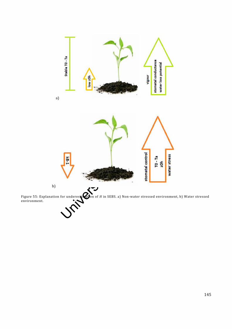
Univers

ity of

Cap

e Tow

n

145

a)

b)

Figure 55: Explanation for underestimation of H in SEBS. a) Non-water stressed environment, b) Water stressed environment.

Univers

ity of

Cap

e Tow

n

146

9. CONCLUSIONS AND RECOMMENDATIONS

In Chapter 9.1, a summary of the research findings is presented. In Chapter 9.2, proposed explanations

for the overestimation of ET, despite the many adjustments to the methodology, are put forward. Final

conclusions and recommendations are made in Chapter 9.3 with particular application to the South

African environment

9.1. SUMMARY OF RESEARCH

The broad aim of this research was to implement the pre-packaged SEBS model in ILWIS in the South

African environment with MODIS TERRA and AQUA data. As a pre-packaged software is accessible to

remote sensing practitioners who may not have specific energy balance expertize, it is important for the

pre-packaged version of SEBS to be tested before large scale roll-out (for operational, research or

monitoring purposes) is implemented (Chapter 1.1). Therefore the aim (Chapter 1.2) was to compare,

analyse and validate the results with field measured eddy covariance data, elucidate model sensitivities

and make recommendations on the future use of the pre-packaged SEBS model.

The specific objectives were given as, for the field validation site, to:

1. Apply the pre-packaged SEBS model in ILWIS.

2. Compare and analyse results obtained from daily MODIS TERRA (MOD 02) and MODIS

AQUA (MYD 02) data for:

a. the calculated remotely sensed parameters (albedo, vegetation parameters,

emissivity and land surface temperature) which are required as input into the SEBS

model;

b. the energy balance and evapotranspiration calculations using the pre-packaged

SEBS model in ILWIS;

3. Validate the energy balance and evapotranspiration results with field measured data;

Univers

ity of

Cap

e Tow

n

147

4. Analyse and explain the results and identify potential sources of error or model

sensitivities.

It had been initially anticipated that ASTER imagery corresponding to the field validation period would

be available for the study area. However due to difficulties with field equipment and the presence of

cloud, only one ASTER image was available. Since there would be little value in using a single ASTER

image, only MODIS data was used. The resolution of the MODIS imagery in relation to the field

validation site resulted in a mixed pixel effect leading to some difficulties in assessing the validity of the

validation process. Nevertheless, the SEBS model was applied, the various modules of the algorithm

were unpacked and explained, and the sensitivities to various inputs were explored.

In fulfillment of Objective 1, the remote sensing parameters which were calculated using the pre-

packaged SEBS model in ILWIS and then used in the estimation of the surface energy fluxes were

presented in Chapter 5. The results (Objective 2a) for albedo were low when compared with literature

values and may be due to inadequacies in the data used in the atmospheric correction process. Various

factors were investigated to ascertain the major influences on the albedo calculation and it was found

that the solar zenith angle played the biggest role in the albedo calculation. The NDVI calculation

typically yields lower results for TERRA data than with AQUA data, however no trend could be detected.

T0 was almost always calculated as being higher in the afternoon than in the morning. However there

appears to be a high uncertainty associated with this calculation when compared with the T0 obtained

from MSG/SEVERI.

The results of the energy flux calculations were mixed. SEBS calculated daily ET was higher than field

measured values (Objective 2b) implying an overestimation of ET using the SEBS model. When

analysing the results of the individual energy fluxes it was found that despite the uncertainties

associated with T0 and albedo which are used in the calculation of net radiation, the SEBS calculated Rn

compared favourably with the field measured data for both the TERRA and the AQUA data with the

AQUA results being superior to the TERRA results. The soil heat flux result corresponded better to the

field validation results for the AQUA results than the TERRA results with the TERRA results

underestimating the soil heat flux when compared with the field validation results.. This was due to the

Univers

ity of

Cap

e Tow

n

148

structure and orientation of the orchard in relation to the sensor view angle allowing an fc of lower than

one whereas if viewed at nadir, an fc of equal to one would be more appropriate for the orchard.

The results for the sensible heat flux showed no agreement between the SEBS calculated values and the

field measured values for both the TERRA and AQUA results. Furthermore, for every data record, the

sensible heat flux was calculated to be at the wet limit. Since the sensible heat flux is always at the wet

limit, λEwet = λE and therefore relative evaporation is always equal to one, therefore the evaporative

fraction is higher leading to a high daily ET calculation. The overestimation of daily ET can therefore be

ascribed to the underestimation of the sensible heat flux.

The sensitivity of SEBS to parameters over which the user has some control when using this version of

the model, was explored in Chapter 6 (Objective 4). It was shown that SEBS is sensitive to land surface

temperature and air temperature gradient and the magnitude of this sensitivity depended on the land

cover and whether or not the wet-limit had been reached. The choice of fractional vegetation cover

formula was shown to influence the daily ET results by up to 0.7 mm. It was shown that the height of

the vegetation canopy should be considered in relation to the weather station reference height to avoid

the sensible heat flux from becoming unsolvable due to a negative ln calculation. Finally the study area

was shown to be heterogeneous although the resolution at which fluxes were calculated did not

significantly impact on energy partitioning results. The differences in the upscaling from evaporative

fraction to daily ET at varying resolutions observed implies that the heterogeneity may play the biggest

role in the upscaling and the influence of albedo on this calculation should be studied.

In using different resolution satellite imagery (ASTER and MODIS) it was shown that landscape

heterogeneity is not the dominating factor at energy partitioning level whereas the resolution of the

sensor does appear to play a role in the upscaling from instantaneous to daily ET through the use of

albedo. These results point towards the importance of accurate albedo estimations for the upscaling of

evaporative fraction to daily ET and that, in SEBS, landscape heterogeneity may play a role at this level

rather than at energy partitioning level.

Univers

ity of

Cap

e Tow

n

149

Four points of advice were presented for users of the pre-packaged SEBS model:

1) Since SEBS is sensitive to the T0 - Ta gradient, care should be taken when estimating T0 in a

topographically diverse area as retrievals are less accurate in this setting. In particular, SEBS

should not be used in mountainous areas with coarse resolution sensors since the

heterogeneity of the T0 cannot be captured at the appropriate scale. Furthermore, the

sensitivity to T0 – Ta is also dependent on whether the wet-limit has been reached.

2) Care should be taken when selecting a fractional vegetation cover formula as this should be

appropriate for the study area, especially if NDVI min and max values need to be defined. In

particular, it is advised that if a LAI product is available at the appropriate scale, that it be

used to estimate fractional vegetation cover according to the formula by Choudhary (1987).

3) The reference height of the weather station should be considered in relation to the canopy

height of the study area. In an area where field crops with a low canopy height predominate,

the use of an agrometeorological weather station is appropriate. However, where tree crops

and natural vegetation with a canopy height exceeding 2.7 m are found, weather stations

which measure wind speed at 10 m are probably more appropriate.

4) The scale at which the evapotranspiration results are required must be considered in

relation to the choice of sensor and therefore pixel resolution and the heterogeneity of the

study area. When working at a catchment scale a coarse resolution sensor may be

appropriate for energy partitioning whereas, for farm or field scale results a higher pixel

resolution will be required to detect inter-field or inter-farm variations. The influence of

albedo on the accurate upscaling of evaporative fraction to daily ET should be considered

and this may also be a function of landscape heterogeneity.

From the model sensitivities and uncertainties raised and the four points of advice given above,

implementing the recommended changes to the methodology and validating the results in the Moutons

Valley study area would have little value. For this reason, a separate research project at quaternary

catchment scale (Chapter 7) for the P10A catchment near Grahamstown in the Eastern Cape, acting on

these points of advice, was presented. The attention to ensuring the highest accuracy and suitability of

input data involved: the pre-selection of a homogeneous catchment at MODIS pixel resolution, use of an

Univers

ity of

Cap

e Tow

n

150

already atmospherically corrected MODIS data product, the adjustment of the NDVI maximum value for

use in the fractional vegetation cover formula, the use of a South Africa Weather Services weather

station data to measure the wind speed at 10 m rather than at 2 m, the use of literature values and a

land cover map to assign roughness length and displacement height estimates and finally the use of

both TERRA and AQUA images to determine the impact of land surface air temperature gradient and

time of day at which the satellite image was captured.

Further in Chapter 7, the sensitivity of the SEBS model to the roughness length was presented in the

P10A catchment. In the SEBS model, two methods for determining z0 are possible: z0 can be obtained

from the literature or can be empirically derived from the remote sensing vegetation inputs. It was

postulated that should it be possible to obtain a more accurate measure of z0 which can be used as input

into the SEBS model, then the calculation of the H will be more accurate, in turn leading to a more

accurate ET value rather than reported overestimations. The results in P10A illustrated that although

the SEBS model was shown to be sensitive to z0 (particularly in combination with T0 - Ta), no significant

changes in the calculation of H was found when two different methodologies were used for z0

determination.

Finally, parameters which could be changed for the study area and which may have an impact on the

energy flux results were made (Chapter 8). The two changes made were in the choice of NDVImax (and

therefore the calculation of fractional vegetation cover) and z0m. The SEBS energy flux results were

compared with the field validation data. It was shown that by using a higher NDVImax value the fractional

vegetation cover may be more realistic at MODIS pixel resolution where there is mixed land cover.

Despite the more realistic soil heat flux results, the sensible heat flux is in fact calculated to be lower

when using this adjusted NDVImax and therefore the overestimation of daily ET with the SEBS model is

exacerbated. The sensitivity of the sensible heat flux to z0m was shown and the calculated daily ET can

vary by up to 3.5 mm depending on the selected aerodynamic values. The NDVI method to derive z0m,

resulted in the sensible heat flux being at, or close to the wet limit. Contrary to this, when using the

literature value for z0m, the wet limit was reached on only one occasion. Finally the SEBS model was

shown once again to be sensitive to T0 – Ta in combination with z0m.

Univers

ity of

Cap

e Tow

n

151

9.2. PROPOSED EXPLANATIONS FOR THE OVERESTIMATION OF ET

Despite much attention being given to the accuracy of the remote sensing input parameters in this

research, the SEBS model consistently underestimated the sensible heat flux resulting in an

overestimation of the daily ET.

In the SEBS formulation publication (Su, 2002), an extended model for the determination of the

roughness length for heat transfer is described. However, according to Timmermans et al. (2011), the

roughness height for heat transfer is only valid for short vegetation. The SEBS model has been shown to

be sensitive to z0m. Errors in the estimation of z0m will be propagated through to the calculation of z0h.

z0m and z0h are used together with T0 – Ta to estimate the sensible heat flux. Furthermore, the sensitivity

of calculations for the roughness height for heat transfer has been shown to be more sensitive in sparse

canopies (Su et al., 2001), which is a landscape descriptor very appropriate to the South African

environment.

McCabe & Wood (2006) found that at field scale, SEBS energy flux values calculated using ASTER are

not regularly within 10% of values calculated using MODIS, but at a catchment scale, results for ASTER,

Landsat and MODIS are within 10% of each other. In another study, aggregating input data was found to

result in an underestimation of ET with the aggregated result being 15% lower than that obtained at

original image resolution (Ershadi et al., 2013). Contrary to this, the results presented in this thesis

indicate that the partitioning of the energy balance is not affected by the image resolution

(Chapter 6.3.4). However in the upscaling of evaporative fraction to daily ET, the albedo affected the

daily ET result.

Further, subpixel heterogeneity at MODIS resolution has been shown by Li et al. (2008) to impact on the

accuracy of surface flux estimates. Scaling techniques can address some of these issues but aggregation

rules for scaling will differ depending on the environment (Kalma et al., 2008). Furthermore, applying

models to large areas is hindered by the lack of high resolution ground measurements (i.e.

meteorological observations), therefore despite the possibility of obtaining higher spatial resolutions of

Univers

ity of

Cap

e Tow

n

152

satellite images, the spatial resolution of other input data into models remains a limitation

(Kalma et al., 2008).

In complex environments, it is not possible to describe the remote sensing derived input parameters

(NDVI, fc, z0m, T0) at the correct level of accuracy and spatial resolution required for the accurate

estimation of the sensible heat flux. The method used in this research to determine roughness length for

momentum transfer was limited by the availability of data at appropriate scale, and aggregation rules

for mixed pixels such as those proposed by Shuttleworth et al. (1997) were not considered in this

research. The uncertainty in the T0 observations (Kalma et al., 2008) combined with the uncertainties

introduced in the roughness length estimates, results in error production and propagation through to

the sensible heat flux. Therefore, in complex environments, an accurate daily ET is unlikely due to:

1. the inadequate spatial resolution and precision of remote sensing derived input

parameters,

2. the sensitivity of the SEBS model to aerodynamic and temperature parameters (largely

derived from remote sensing data),

3. the assumptions made at a micrometeorological level in the calculation of kB–1 , and

4. the uncertainties associated with the stability functions in the calculation of the sensible

heat flux (Gellens-Meulenberghs, 2005).

Supporting the finding that the SEBS model is unable to allocate enough energy to the sensible heat flux,

Lu et al. (2012) report a significant overestimation of the evaporative fraction using the SEBS model.

The overestimation of evaporative fraction is ascribed to heterogeneous study areas and the empirical

determination of the aerodynamic parameters. Gokmen et al. (2012) report on the underestimation of

the SEBS derived sensible heat flux, particularly in sparsely vegetated, semiarid regions. Gokmen et al.

(2012) propose an integration of soil moisture information as a water stress index for these regions.

This will modify kB−1 in order to correct for an underestimation of the sensible heat flux.

The Australian example has shown that an aerodynamic resistance-surface energy balance approach

failed because small errors in the surface temperature resulted in large errors in the sensible heat flux

(Cleugh et al., 2007). An alternative approach of setting a fixed daily value for leaf-level stomatal

conductance to calculate ET has been proposed (Cleugh et al., 2007). Similar to the approach being

Univers

ity of

Cap

e Tow

n

153

implemented in South Africa by Palmer & Weiderman (2011), ET is calculated from a combination of

leaf area index (derived from MODIS) and potential evapotranspiration (from meteorological data).

The following statement by Overgaard et al. (2006) summarizes in essence the findings of this thesis:

“The more of the physical processes involved in the generation of land-surface fluxes we can

parameterise, the more likely it is that we can predict the behaviour of the land surface under different

conditions. This is, of course, only true if we can measure or realistically estimate all parameters in such

detailed models, preferably at the scale of application.” This statement was made in a discussion as to

the choice of land-surface flux model, particularly whether a simple model is more desirable than a

complex model.

Overgaard et al. (2006) refer to Raupach & Finnigan (1988) who stated that the choice of model in any

given situation is a trade-off between the desirable but incompatible traits of realism and simplicity.

Overgaard et al. (2006) argue that realism is desirable from the point of view that realistically

structured, and consequently very detailed models, will provide realistic results. On the other hand,

simplicity is desirable from the point of view that simple models will require fewer parameters, which

will extend the applicability of the model outside the intensely monitored experimental areas

(Overgaard et al., 2006).

Parsimony is often mentioned in the question of what physics to include and loosely put, a

parsimonious model includes just enough elements to explain: not more, but not less either (Kleinhans

et al., 2010). The dilemma of model selection and the choice between parsimonious and complex

physically based models is also a challenge for researchers tackling the remote sensing estimation of ET.

In the view of Savenije (2009), scientists should realize that all models are wrong and if this is accepted

(to a greater or lesser extent), then with a close enough examination, it will always be possible to find

some observations that will not be matched by model predictions (Beven, 2008). Furthermore, there

may be multiple models that perform within some limits of acceptability (Beven, 2008). The role of the

scientist is therefore to understand where models are wrong, and especially why they are wrong. This is

the process of scientific discovery (Savenije, 2009) which will allow for the formulation of alternative

and possibly better models.

Univers

ity of

Cap

e Tow

n

154

The results of this research have shown that using the SEBS model as it is currently programmed in

ILWIS, did not yield accurate daily evaporation results when compared with the field validation data for

this particular study. Some limitations in the field validation approach are noted, such as measurements

of LAI and irrigation not being taken and the mixed pixel effect due to the size of the apple orchard in

relation to a MODIS pixel. Despite adaptations to the methodology to address model sensitivities there

was not a significant improvement in the daily ET results. The recent paper by Gokmen et al. (2012)

highlights shortcomings in the original SEBS model. However, the new parameterization which may

contribute towards improved results with the modified SEBS model, adds to the complexities of the

model. Thus the potential for further uncertainties and sensitivities to the new parameters would need

to be investigated.

The complexity of the SEBS model and its assumptions at micrometeorological level, make the realistic

estimation of energy fluxes improbable at field and catchment scale. Due to the complexity of the model

with many input parameters, numerous errors may be introduced and propagated through the model.

The model is sensitive to remote sensing parameters which ideally should be estimated at high spatial

resolution. However, satellite imagery at a daily timescale is captured at a coarse spatial resolution.

Therefore, it is difficult to deduce, at an appropriate spatial scale, the input parameters to which the

model is sensitive.

Finally, the SEBS model is available as part of the open-source freeware ILWIS and can therefore be

freely used by remote sensing practitioners without micrometeorological expertise. However, it is

necessary for the user to have a good understanding of micrometeorological concepts in order to

understand model sensitivities and to assess the accuracy of the results.

9.3. RECOMMENDATIONS

Whilst the original motivation for this research was to estimate water use of crops in order to

determine the legal compliance of water users to water use legislation, there are many other potential

applications for a spatial representation of ET. A particular drive should be towards the implementation

of an operational system of managing water resources such as has been implemented in Australia

Univers

ity of

Cap

e Tow

n

155

(albeit in an experimental phase to date). As in Australia, the selection of a suitable method for

estimating ET from remote sensing should consider the accuracy of the method but pragmatism

dictates that computational load and robustness, reliability of data sources, and the degree of

automation achievable should be considered (Glenn et al., 2011).

The attraction of the SEBS model has been that it is available as part of the open-source freeware ILWIS

and can be used “off the shelf” without detailed micrometeorological expertise required. Should this

research have shown that accurate results could be obtained from using this version of the SEBS model,

then the wide scale use of the model may have been recommended in South Africa. It could be advised

that topographic roughness and aggregating data for a mixed pixel effect be incorporated into the

methodology before making a final recommendation for or against the use of the SEBS model. However

given the heterogeneity and sparse canopy cover of much of the South African landscape, and the

further complexities that this would introduce to the methodology, higher accuracies are not

anticipated and therefore adapting the methodology further is not recommended.

Whilst other authors using the SEBS model in previous studies have reported ET estimates within an

acceptable range, this was not found to be the case in the two study areas presented in this research.

Because of this discrepancy, it is recommended that should further research be carried out on the SEBS

model in South Africa, it should be limited to agricultural areas where accurate vegetation parameters

can be obtained, where high resolution imagery with low sensor zenith angles is available and where

canopy cover is complete.

It is recommended that the research effort in estimating actual ET for vast tracts of natural vegetation,

rangeland and dryland agriculture in South African be directed in two avenues. Firstly, the development

and/or improvement of existing parsimonious models should be explored. Secondly the validation of

the recently released MODIS evapotranspiration data product, MOD16

(http://modis.gsfc.nasa.gov/data/dataprod/dataproducts.php?MOD_NUMBER=16), should be

addressed as a matter of urgency. Both these methods bypass the use of thermal imagery. This is

advantageous given the reported sensitivities of the SEBS model to T0 – Ta coupled with associated

uncertainties in the T0 estimation. For high spatial resolution water use efficiency and crop water use

studies, the SEBAL model appears to be delivering acceptable levels of accuracy however the lack of

Univers

ity of

Cap

e Tow

n

156

local capacity development is of concern and should be addressed since the data processing is carried

out in the Netherlands without advancing the knowledge of South African scientists.

The use of more parsimonious models such as the model reported by Palmer & Weiderman (2011)

should not be overlooked. This is of particular importance given the spatial resolution restrictions of

the available satellite imagery together with the complexity of the landscape which characterises much

of South Africa. Furthermore, it is a vegetation index coupled with meteorological data (Guerschman et

al., 2009) which has been found to be the best performing method in Australia and given the parallels

drawn between the two countries, lessons from Australia should be applied in South Africa. Finally, this

represents an opportunity for skill development and capacity building for South African scientists.

Concurrent to this, research is required, as a matter of priority, into the validation of the recently

released MODIS evapotranspiration data product, MOD16 developed by Mu et al. (2011), in the South

African environment. Since it is anticipated that MOD16 will generate considerable interest in South

Africa, it is important that the accuracy of the product is ascertained across South African conditions in

order to determine the potential constraints and possible errors of the ET estimates. To date, the

MOD16 data have not been validated locally. Scientists wishing to employ the data in modelling

activities are thus unable to determine any confidence intervals or indeed accuracies of the data.

Although the SEBS model was found to produce overestimates of ET when implemented as described in

the methodology of this research, many valuable lessons have been learnt through the course of this

research. Perhaps the most valuable lesson has been around the difficulties in applying complex models

to heterogeneous environments. However, the use of the SEBS model to estimate water use in forested

areas has not yet been tested in South Africa. This remains an avenue for future research.

A final recommendation would be to consider research funding for a heterogeneity mapping project for

South Africa to update similar research by Tanser & Palmer (1999). The purpose of such a dataset

would be to allow for the selection of the appropriate level of complexity of models based on a priori

knowledge on the complexity of the landscape under study.

Univers

ity of

Cap

e Tow

n

157

Despite the overestimations of ET using the methodology described in this research, the

recommendations which have arisen from the research determine that the research project has been

successful in that the South African research agenda into remote sensing estimation of ET can be said to

have been significantly advanced as a result.

Univers

ity of

Cap

e Tow

n

158

10. REFERENCES

Adreen W, 2011. ‘Towards environmental flows: comparing water law in four countries’, available at

URL: http://www.globalwaterforum.org/2011/06/01/towards-environmental-flows-comparing-

water-law-in-four-countries/, date accessed 8 Sept 2011.

Agam N, Kustas WP, Anderson MC, Li F & Neale CMU, 2007. ‘A vegetation index based technique for

spatial sharpening of thermal imagery’, Remote Sensing of Environment, vol. 107, no. 4, pp. 545-558.

Ahmad M, Bastiaanssen WGM & Feddes RA, 2005. ‘A new technique to estimate net groundwater use

across large irrigated areas by combining remote sensing and water balance approaches, Rechna

Doab, Pakistan’, Hydrogeology Journal, vol.13, pp.653-664.

Allen RG, Pereira LS, Raes D & Smith M, 1998. ‘Crop evapotranspiration: guidelines for computing crop

water requirements’ FAO Irrigation and Drainage Paper 56, Rome, 300 pp.

Allen RG, Tasumi M, Morse A, Trezza R, Wright JL, Bastiaanssen W, Kramber W, Lorite I, & Robison CW,

2007. ‘Satellite-Based Energy Balance for Mapping Evapotranspiration with Internalized Calibration

(METRIC)—Applications’, Journal of Irrigation and Drainage Engineering, vol. 133, no. 4, pp. 395-407.

Allen RG, Hendrickx J, Bastiaanssen W, Kjaersgaard J, Irmak A & Huntington J, 2010. ‘Status and

continuing challenges in operational remote sensing of ET’. In: Proceedings of: 5th National Decennial

Irrigation Conference, December 5 - 8, 2010, Phoenix, Arizona.

Alvarez JAG, 2007. ‘Effects of land cover changes on the water balance of the Palo Verde Wetland, Costa

Rica’, M.Sc. thesis, International Institute for Geo-information Science and Earth Observation, The

Netherlands.

ARC-ISCW, 2010. Technical manual for the AgroClimatology Weather Station Network. ARC-ISCW

internal report, Agricultural Research Council-Institute for Soil, Climate and Water, South Africa,

Report No. GW/A/2008/60, 2010.

Badola A, 2009. ‘Validation of Surface Energy Balance System (SEBS) over forest land cover and

sensitivity analysis of the model’, M.Sc. thesis, International Institute for Geo-information Science

and Earth Observation, The Netherlands.

Bandara KMPS, 2006. ‘Assessing irrigation performance by using remote sensing’, Ph.D. thesis,

International Institute for Geo-information Science and Earth Observation, The Netherlands.

Univers

ity of

Cap

e Tow

n

159

Baret F, Clevers JGPW, Stevens MD, 1995. ‘The robustness of canopy gap fraction estimations from red

and near-infrared reflectances: A comparison of approaches’. Remote Sensing of Environment, vol 54,

pp 141 – 151.

Bastiaanssen WGM, Menenti M, Feddes RA & Holtslag AAM, 1998. ‘The Surface Energy Balance

Algorithm for Land (SEBAL): Part 1 formulation’, Journal of Hydrology, vol. 212 , no.213, pp.198-212.

Bastiaanssen WGM, Chavez RG, Alsulamain A & Ahmad M, 2006. ‘Estimation of groundwater extraction

on irrigated lands in arid zones from thermal infrared satellites’. Unpublished report 16pp.

Bastiaanssen WGM & Bos MG, 1999. ‘Irrigation performance indicators based on remotely sensed data:

a review of literature’, Irrigation and Drainage Systems, vol. 13, no. 4, pp. 291-311.

Batatia H & Bessaih N, 2009. ‘Satellite land surface temperature for Sarawak area’, Geospatial World,

available at URL: http://www.geospatialworld.net/index.php?option=com_content&view=article&id

=15188%3Asatellite-land-surface-temperature-for-sarawak-area&catid=123%3Aenvironment-

overview, date accessed 12 May 2011.

Batelaan O & De Smedt F, 2001. ‘WetSpass: a flexible, GIS based, distributed recharge methodology for

regional groundwater modelling’. In: Gehrels, H., Peters, J., Hoehn, E., Jensen, K., Leibundgut, C.,

Griffioen, J., Webb, B. & Zaadnoordijk, W-J. (eds). Impact of Human Activity on Groundwater

Dynamics. IAHS Publ. no. 269, Wallingford UK, pp.11-17.

Beven K, 1979. ‘A sensitivity analysis of the Penman-Monteith actual evapotranspiration estimates’,

Journal of Hydrology, vol. 44, pp. 169 – 190.

Beven K, 2006. ‘On undermining the science?’, Hydrological Processes, vol. 20, pp. 3141-3146.

Beven K, 2008. ‘On doing better hydrological science’, Hydrological Processes,vol. 22, pp. 3549-3553.

Blight GE, 2002. ‘Measuring evaporation from soil surfaces for environmental and geotechnical

purposes’, Water SA, vol. 28, no. 4, pp. 381-394.

Brutsaert W, 1982. ‘Evaporation into the atmosphere’, Reidel, Dordrecht, The Netherlands.

Burger D (ed), 2003. ‘South African Yearbook 2002/3’, Published by Government Communications

(GCIS).

Burger D (ed), 2005. ‘South African Yearbook 2004/5’, Published by Government Communications

(GCIS).

Univers

ity of

Cap

e Tow

n

160

Burger D (ed), 2011. ‘South African Yearbook 2010/11’, Published by Government Communications

(GCIS).

Carlson TN & Ripley DA, 1997. ‘On the Relation between NDVI, Fractional Vegetation Cover, and Leaf

Area Index’, Remote Sensing of Environment, vol. 62, no. 3, pp. 241-252.

Carrer D, Roujean JL & Meurey C, 2010. ‘Comparing Operational MSG/SEVIRI Land Surface Albedo

Products From Land SAF With Ground Measurements and MODIS’, IEEE Transactions on Geoscience

and Remote Sensing, vol. 48, no. 4, pp 1714-1728.

Cleugh HA, Leuning R, Mu QZ & Running SW, 2007. ‘Regional evaporation estimates from flux tower and

MODIS satellite data’, Remote Sensing of Environment, vol. 106, no. 3, pp. 285-304.

Courault D, Seguin B & Olioso A, 2005. ‘Review on estimation of evapotranspiration from remote

sensing data: From empirical to numerical modeling approaches’, Irrigation and Drainage Systems,

vol. 19, pp. 223-249.

Dungan JL, Kao D & Pang A, 2002. ‘The uncertainty visualization problem in remote sensing analysis’, in:

Proceedings of International Geoscience & Remote Sensing, Toronto, Canada, June 2, 2002, pp. 729-

731.

Ershadi A, 2010. ‘Land-atmosphere interactions from canopy to troposphere’, M.Sc. thesis, International

Institute for Geo-information Science and Earth Observation, The Netherlands, 2010.

Ershadi A, McCabe, Evans & Walker JP, 2013. ‘Effects of spatial aggregation on the multi-scale

estimation of evapotranspiration’, Remote Sensing of Environment, vol. 131, pp. 51–62.

Flores AN, Ivanov VY, Entekhabi D & Bras RL, 2009. ‘Impact of hillslope-scale organization of

topography, soil moisture, soil temperature, and vegetation on modelling surface microwave

radiation emission’, IEEE Transactions on Geoscience and Remote Sensing, vol. 47, no. 8, pp 2557-

2571.

French AN, Schmugge TJ, Kustas WP, Brubaker KL & Prueger J, 2003. ‘Surface energy fluxes over El

Reno, Oklahoma, using high-resolution remotely sensed data’, Water Resources Research, vol. 39, no.

6, pp. 1164-1176.

Garrigues S, Allard D, Baret F & Weiss M, 2006. ‘Quantifying spatial heterogeneity at the landscape scale

using variogram models’, Remote Sensing of Environment, vol. 103, no. 1, pp. 81-96.

Gebreyesus MG, 2009. ‘Validation of RS approaches to model surface characteristics in hydrology: a

case study in Guareña Aquifer, Salamanca, Spain’, M.Sc. thesis, International Institute for Geo-

information Science and Earth Observation, The Netherlands.

Univers

ity of

Cap

e Tow

n

161

Gellens-Meulenberghs F, 2000. ‘Evapotranspiration and surface heat fluxes over Belgium: outcome and

perspectives’, Agronomie, vol. 20, no. 8, pp. 857-868.

Gellens-Meulenberghs F, 2005. ‘Sensitivity Tests of an Energy Balance Model to Choice of Stability

Functions and Measurement Accuracy’, Boundary Layer Meteorology, vol. 115, no. 3, pp. 453-471.

Gibson LA, Münch Z, Engelbrecht J, Petersen N & Conrad JE, 2009. ‘Remote sensing as a tool towards

resource assessment and determination of the legal compliance of surface and groundwater use’,

Research Report 1960/1/09, Water Research Commission, Pretoria, South Africa.

Gibson LA, Münch Z, Carstens M & Conrad JE, 2011. ‘Remote sensing evapotranspiration (SEBS)

evaluation using water balance’, Consultancy Report K8/929/1. Water Research Commission,

Pretoria, South Africa.

Glenn EP, Doody TM, Guerschman JP, Huete AR, King EA, McVicar TR, Van Dijk AIJM, Van Niel TG, Yebra

M & Zhang YQ, 2011. ‘Actual Evapotranspiration Estimation by Ground and Remote Sensing

Methods: The Australian Experience’, Hydrological Processes, vol. 25, no. 26, pp. 4103 – 4116.

Gokmen M, Vekerdy Z, Verhoef A, Verhoef W, Batelaan O & van der Tol C, 2012. ‘Integration of soil

moisture in SEBS for improving evapotranspiration estimation under water stress conditions ‘,

Remote Sensing of Environment, vol. 121 , pp. 261–274.

Gowda PH, Chavez JL, Colaizzi PD, Evett SR, Howell TA, & Tolk JA, 2007. ‘Remote sensing based energy

balance algorithms for mapping ET: current status and future challenges’, Transactions of the

American Society of Agricultural and Biological Engineers, vol. 50, no. 5, pp.1639-1644.

Gowda PH, Chavez JL, Colaizzi PD, Evett SR, Howell TA & Tolk JA, 2008. ‘ET mapping for agricultural

water management: present status and challenges’, Irrigation Science, vol. 26, pp. 223-237.

Guerschman JP, Van Dijk AIJM, Mattersdorf G, Beringer J, Hutley LB, Leuning R, Pipunic RC & Sherman

BS, 2009. ‘Scaling of potential evapotranspiration with MODIS data reproduces flux observations and

catchment water balance observations across Australia’, Journal of Hydrology, vol. 369, no 1-2, pp.

107-119.

Gutman G & Ignatov A, 1998. ‘The derivation of the green vegetation fraction from NOAA/AVHRR data

for use in numerical weather prediction models’, International Journal of Remote Sensing, vol. 19, no.

8, pp. 1533-1543.

Hailegiorgis WS, 2006. ‘Remote sensing analysis of summer time evapotranspiration using SEBS

algorithm: a case study in Regge and Dinklel, The Netherlands’, M.Sc. thesis, International Institute

for Geo-information Science and Earth Observation, The Netherlands.

Univers

ity of

Cap

e Tow

n

162

Hellegers PJGJ, Jansen HC & Bastiaanssen WGM, 2011. ‘An interactive water indicator assessment tool to

support land use planning’, Irrigation and Drainage (DOI: 10.1002/ird.641).

Jackson R.D, Reginato RJ & Idso SB, 1977. ‘Wheat canopy temperature: a practical tool for evaluating

water requirements’, Water Resources Research 13, 651-656.

Jarmain C, Mengitsu M, Jewitt GPW, Kongo V & Bastiaanssen W, 2009. ‘A methodology for near-real time

spatial estimation of evaporation’, Research Report 1751-1-09, Water Research Commission,

Pretoria, South Africa.

Jarmain C & Mengistu MG, 2011. ‘Validating energy fluxes estimated using the surface energy balance

system (SEBS) model for a small catchment’, WRC Consultancy Report K8/824, Water Research

Commission, Pretoria, South Africa.

Jarmain C, Klaasse A, Basson FC, Meininger W, Wilmink S & Bastiaanssen W, 2011a. ‘Developing an

operational remote sensing system for monitoring of efficient crop water and nitrogen use of

grapes’, Western Cape Province, Final report to the Western Cape Provincial Department of

Agriculture.

Jarmain C, Singels A, Obando E, Paraskevopoulos A & Mthembu I, 2011b. ‘Water use efficiency of

irrigated agricultural crops determined with satellite imagery’, Progress Report. K5/2079//4. Water

Research Commission, Pretoria.

Jarmain C, Singels A, Obando E, P Paraskevopoulos A, Olivier F, Münch Z, van der Merwe B, Walker S,

van der Laan M, Messehazion M, Savage M, Pretorius C, Annandale J & Everson C, 2013. ‘Water use

efficiency of irrigated agricultural crops determined with satellite imagery’. K5/2079//4.

Deliverable 6, Water use efficiency Report 2012/13. Water Research Commission, Pretoria.

Jarmain C & Klaasse A, 2012. ‘Fruitlook: An operational service to improved crop water and nitrogen

management in grapes and other deciduous fruit trees using satellite technology for the season of

2011-12’, Progress Report, Western Cape Provincial Department of Agriculture.

Jarmain C & Meijninger WL, 2012. ‘Assessing the impact of Invasive Alien Plants on South African water

resources using remote sensing techniques’. IAHS publication no. 352, pp. 388-392.

Jha MK & Chowdary VM, 2006. ‘Challenges of using remote sensing and GIS in developing nations’,

Hydrogeology Journal, vol. 15, no. 1, pp. 197-200.

Jia L, Su Z, van den Hurk B, Menenti M, Moene HAR, Baselga Yrisarry JJ, Ibanez M & Cuesta A, 2003.

‘Estimation of sensible heat flux using the Surface Energy Balance System (SEBS) and ATSR

measurements’, Physics and Chemistry of the Earth, vol. 28, no.1-3, pp. 75-88.

Univers

ity of

Cap

e Tow

n

163

Jia L, Xi G, Liu S, Huang C, Yan Y, & Liu G,.2009. ‘Regional estimation of daily to annual regional

evapotranspiration with MODIS data in the Yellow River Delta wetland’. Hydrology and Earth System

Sciences, vol. 13, no. 10, pp 1775 - 1787.

JPL, 2009. SWIR- ASTER User Advisory. [online]. Available at URL:http://asterweb.jpl.nasa.gov/swir-

alert.asp [Accessed 30 March 2009]

Kalma JD, McVicar TR & McCabe MF, 2008. ‘Estimating Land Surface Evaporation: A Review of Methods

Using Remotely Sensed Surface Temperature Data’, Surveys in Geophysics, vol. 29, no. 4-5, pp. 421-

469.

Kaur R, Srinivasan R, Mishra K, Dutta D, Prasad D & Bansal G, 2003. ‘Assessment of a SWAT model for

soil and water management in India’, Land Use and Water Resources Research, vol. 3, pp. 1-7.

Kipp & Zonen, 2005. ‘Large Aperture Scintillometer instruction manual’, Delft, Holland.

Klaasse A, Bastiaanssen W, Jarmain C & Roux A, 2008. ‘Water use efficiency of table and wine grapes in

Western Cape, South Africa’, WaterWatch report, Wageningen, the Netherlands, 68 pp.

Klaasse A, Jarmain C, Roux A, Becu O & Ginati A, 2011. ‘GrapeLook: space based services to improve

water use efficiency of vineyards in South Africa’. Proceedings of: 62nd International Astronautical

Congress, 3-7 October 2011, Cape Town.

Kleinhans MG, Bierkens MFP & van der Perk M, 2010. ‘On the use of laboratory experimentation:

“Hydrologists, bring out shovels and garden hoses and hit the dirt”’, Hydrology and Earth System

Science, HESS Opinions, vol. 14, no. 2, pp. 369–382.

Kongo VM & Jewitt GPW, 2006. ‘Preliminary investigation of catchment hydrology in response to

agricultural water use innovations: A case study of the Potshini catchment – South Africa’, Physics

and Chemistry of the Earth, vol. 31, no. 15-16, pp. 976-987.

Kustas WP, Li F, Jackson TJ, Prueger JH, MacPherson JI & Wolde M, 2004. ‘Effects of remote sensing pixel

resolution on modelled energy flux variability of croplands in Iowa’, Remote Sensing of Environment,

vol. 92, no. 4, pp. 534-547.

Lakhankar T, Ghedira H, Temimi M, Azar AE & Khanbilvardi R, 2009. ‘Effect of land cover heterogeneity

on soil moisture retrieval using active microwave remote sensing data’, Remote Sensing, vol. 1, no. 2,

pp. 80-91.

Leuning R, Zhang YQ, Rajaud A, Cleugh H & Tu K, 2008. ‘A simple surface conductance model to estimate

regional evaporation using MODIS leaf area index and the Penman-Monteith equation’, Water

Resources Research, vol. 44, 10419.

Univers

ity of

Cap

e Tow

n

164

Li Z, Jia L, Su Z, Wan Z & Zhang R, 2003. ‘A new approach for retrieving precipitable water from ATSR2

split-window channel data over land area’, International Journal of Remote Sensing, vol. 24, no. 24,

pp. 5095-5117.

Li Z, Yu G, Li Q, Fu Y & Li Y, 2006. ‘Effect of spatial variation on areal evapotranspiration simulation in

Haibei, Tibet plateau, China’, International Journal of Remote Sensing, vol.27, no. 16, pp. 3487-3498.

Li F, Kustas WP, Anderson MC, Prueger JH & Scott RL, 2008. ‘Effect of remote sensing spatial resolution

on interpreting tower-based flux observations’, Remote Sensing of Environment, vol. 112, no. 2, pp.

337-349.

Liang S, 2001. ‘Narrowband to Broadband Conversions of land surface albedo I: Algorithms’, Remote

Sensing of the Environment, vol. 76, no. 2, pp. 213-238.

Lin W, 2006. ‘Satellite based regional scale evapotranspiration in the Hebei Plain, Northeastern China’,

M.Sc. thesis, International Institute for Geo-information Science and Earth Observation, The

Netherlands.

Lin W, van de Velde R & Su Z, 2008. ‘Satellite based regional-scale evapotranspiration in the Hebei Plain,

Northeastern China’, in: Proceedings of Dragon 1 Programme Final Results 2004–2007, 21– 25 April

2008, Beijing, China.

Lu J, Li Z-L, Tang R, Tang B-H, Wu H, Yang F, Labed F & Zhou G, 2012. ‘Evaluating the SEBS-estimated

evaporative fraction from MODIS data for a complex underlying surface’, Hydrological Processes, doi:

10.1002/hyp.9440.

Madeira C, Dash P, Olesen F & Trigo I, 2005. ‘Intercomparison of Meteosat-8 derived LST with MODIS

and AATSR similar products’, in: Proceedings of 2005 EUMETSAT Meteorological Satellite Conference,

19 - 23. September 2005, Dubrovnik, Croatia.

Mao K, Qin Z, Shi J & Gong P, 2005. ‘A practical split window algorithm for retrieving land-surface

temperature from MODIS data’, International Journal of Remote Sensing, vol.26, no. 15, pp. 3181-

3204.

Mariotto I & Gutschick VP, 2010. ‘Non-lambertian corrected albedo and vegetation index for estimating

land evapotranspiration in a heterogeneous semi-arid landscape’, Remote Sensing, vol. 2, no. 4, pp.

926-938.

Mather P, 1999. ‘Computer Processing of Remotely Sensed Images: An Introduction’, Wiley, Chichester.

McCabe MF & Wood EF, 2006. ‘Scale influences on the remote estimation of evapotranspiration using

multiple satellite sensors’, Remote Sensing of Environment, vol. 105, no. 4, pp. 271-285.

Univers

ity of

Cap

e Tow

n

165

McCabe MF, Wood EF, Wójcik R, Pan M, Sheffield J, Gao H & Su H, 2008. ‘Hydrological consistency using

multi-sensor remote sensing data for water and energy cycle studies’, Remote Sensing of

Environment, vol. 112, no. 2, pp. 430-444.

Melesse AM, Oberg J, Nangia V, Beeri O & Baumgartner D, 2006. ‘Spatiotemporal dynamics of

evapotranspiration at the Glacial Ridge prairie restoration in northwestern Minnesota’, Hydrological

Processes, vol. 20, no. 7, pp. 1451-1464.

Menenti M & Choudhury BJ, 1993. ‘Parameterization of land surface evapotranspiration using a location

dependent potential evapotranspiration and surface temperature range’. In: Proceedings of

Exchange Processes at the Land Surface for a Range of Space and Time Scales, 13-16 July 1993,

Yokohama, Japan.

Moran MS, Clarke TR, Inoue Y & Vidal A, 1994. ‘Estimating crop water deficit using the relation between

surface-air temperature and spectral vegetation index’, Remote Sensing of Environment, vol. 49, no. 2,

pp. 246–263.

Moran MS, Humes KS & Pinter PJ, 1997. ‘The scaling characteristics of remotely-sensed variables for

sparsely-vegetated heterogeneous landscapes’, Journal of Hydrology, vol. 190, no. 3-4, pp. 337-362.

Mu Q, Heinsch FA, Zhao M & Running SW, 2007. ‘Development of a global evapotranspiration algorithm

based on MODIS and global meteorology data’, Remote Sensing of Environment, vol. 111, no. 4, pp.

519-536.

Mu QZ, Zhao MS & Running SW, 2011. ‘Improvements to a MODIS global terrestrial evapotranspiration

algorithm’, Remote Sensing of Environment, vol. 115, pp. 1781-1800.

Münch Z, Conrad, JE, Gibson LA, Palmer AR & Hughes D, 2013. ‘Satellite earth observation as a tool to

conceptualize hydrogeological fluxes in the Sandveld, South Africa’, Hydrogeology Journal, vol. 21(5), pp

1053-1070.

NASA Earth Science Enterprise, Earth Science Applications Directorate, University of South Carolina

Affiliated Research Center, 2005. ‘Remote Sensing Crop Type for Sustainable Development by the

Department of Water Affairs & Forestry, Republic of South Africa’, Project by Department of Water

Affairs & Forestry Pretoria, South Africa and NASA Affiliated Research Center, University of South

Carolina.

NASA, 2007. Advanced Spaceborne Thermal Emission and Reflectance Radiometer. [online]. Available

at: http://asterweb.jpl.nasa.gov/schedule.asp. [Accessed 23 October 2007]

Overgaard J, Rosbjerg D & Butts MB, 2006. ‘Land-surface modelling in hydrological perspective – a

Univers

ity of

Cap

e Tow

n

166

review’, Biogeosciences, vol. 3, no. 2, pp. 229-241.

Palmer AR & Weideman CI, 2011. ‘Exploring trends in evapotranspiration in the KNP: towards a water

use efficiency model for rangeland production in semi-arid savannas’, In: Proceedings of IXth

International Rangeland Congress, 2-8 April 2011, Rosario, Argentina.

Pan M, Wood EF, Wójcik R & McCabe MF, 2008. ‘Estimation of regional terrestrial water cycle using

multi-sensor remote sensing observations and data assimilation’, Remote Sensing of Environment,

vol. 112, no. 4, pp. 1282–1294.

Petropoulos G, Carlson TN, Wooster MJ & Islam S, 2009. ‘A review of Ts/VI remote sensing based

methods for the retrieval of land surface energy fluxes and soil surface moisture’, Progress in Physical

Geography, vol. 33, no. 2, pp. 224–250.

Rahman H & Dedieu G, 1994. ‘SMAC: a simplified method for the atmospheric correction of satellite

measurements in the solar spectrum’, International Journal of Remote Sensing, vol. 15, no. 1, pp. 123-

143.

Roerink GJ, Su Z & Menenti M, 2000. ‘S-SEBI: A simple remote sensing algorithm to estimate the surface

energy balance’, Physics and Chemistry of the Earth (B), vol, 25, no. 2, pp.147-157.

Rwasoka DT, Gumindoga W & Gwenzi J, 2011. ‘Estimation of actual evapotranspiration using the

Surface Energy Balance System (SEBS) algorthim in the Upper Manyame catchment in Zimbabwe’,

Physics and Chemistry of the Earth, vol 36, pp. 736–746.

Santhi C, Muttiah RS, Arnold JG & Srinivasan R, 2005. ‘A GIS−based regional planning tool for irrigation

demand assessment and savings using SWAT’, Transactions of the American Society of Agricultural

Engineers, vol. 48, no. 1,, pp. 137−147.

Savage MJ, Everson CS, Odhiambo GO, Mengistu MG & Jarmain C, 2004. ‘Theory and practice of

evaporation measurement, with special focus on SLS as an operational tool for the estimation of

spatially-averaged evaporation’, Research Report 1335/1/04, Water Research Commission, Pretoria,

South Africa.

Savenije HHG, 2009. ‘“The art of hydrology”’, Hydrology and Earth System Science, HESS Opinions, vol. 13,

no. 2, pp. 157–161.

Schmugge TJ, Kustas WP, Ritchie JC, Jackson TJ, & Rango A, 2002. ‘Remote sensing in hydrology’,

Advances in Water Resources, vol. 25, no. 8-12. pp. 1367-1385.

Shuttleworth WJ, Yang ZL & Arain MA, 1997.’ Aggregation rules for surface parameters in global

models’, Hydrology and Earth System Science, vol 1, no. 2, pp. 217-226.

Univers

ity of

Cap

e Tow

n

167

Sinclair S & Pegram GGS, 2010. ‘A comparison of ASCAT and modelled soil moisture over South Africa,

using TOPKAPI in land surface mode’, Hydrology and Earth System Sciences, vol. 14, no. 4, pp. 613-

626.

Sobrino JA & Raissouni N, 2000. ‘Toward remote sensing methods for land cover dynamic monitoring:

Application to Morocco’, International Journal of Remote Sensing, vol. 21, no. 2, pp. 353 – 366.

Sobrino JA & El Kharraz J, 2003. ‘Surface temperature and water vapour retrieval from MODIS data’,

International Journal of Remote Sensing, vol. 24, no. 24, pp. 5161-5182.

Sobrino JA, Gómez M, Jiménez-Muñoz JC & Olioso A, 2007. ‘Application of a simple algorithm to estimate

daily evapotranspiration from NOAA–AVHRR images for the Iberian Peninsula’, Remote Sensing of

Environment, vol. 110, no. 2, pp. 139–148.

Su Z, Schmugge TJ, Kustas WP & Massman WJ, 2001. ‘An evaluation of two models for estimation of the

roughness height for heat transfer between the land surface and the atmosphere’, Journal of Applied

Meteorology, vol. 40, no. , pp. 1933-1951.

Su Z, 2002. ‘The surface energy balance system (SEBS) for estimation of turbulent heat fluxes’,

Hydrology and Earth System Sciences, vol. 6, no. 1, pp. 85-99.

Su Z & Roerink GJ (eds), 2004. ‘Drought Risk Reduction’, Alterra-rapport 1135, Wageningen, The

Netherlands.

Su H. McCabe MF & Wood EF, 2005. ‘Modeling Evapotranspiration during SMACEX: Comparing Two

Approaches for Local- and Regional-Scale Prediction’, Journal of Hydrometeorology, vol. 6, no. 6, 910-

922.

Su Z, 2006. ‘An introduction to the surface energy balance system (SEBS)’, Lecture notes, ESA TIGER

Capacity Building Facility 1st Training Course on “Advanced optical remote sensing”, 22-25

November 2006, Cape Town, South Africa.

Su Z, Wang L & Parodi GN, 2008. ‘SEBS for ILWIS Open Source: A Practical Tool for Surface Energy

Balance Estimates from Remote Sensing Data, Surface Energy Balance Models of Agricultural Areas

from Earth Observation Data’, 13 March 2008, Lima, Perú.

Tanser FC & Palmer AR, 1999. ‘The application of a remotely-sensed diversity index to monitor

degradation patterns in a semi-arid heterogeneous, South African landscape’, Journal of Arid

Environments, vol. 43, no 4, pp. 477-484.

Tasumi M, Allen RG & Trezza R, 2008. ‘At-surface reflectance and albedo from satellite for operational

calculation of land surface energy balance’, Journal of Hydrologic Engineering, vol. 13, no. 2, pp. 51-63.

Univers

ity of

Cap

e Tow

n

168

Timmermans J, Van der Tol C, Verhoef A, Verhoef W, Su Z, van Helvoirt M & Wang L, 2011. ‘Quantifying

the uncertainty in estimates of surface- atmosphere fluxes through joint evaluation of the SEBS and

SCOPE models’, Hydrology and Earth System Sciences Discussion, vol. 8, no. 2, pp. 2861-2893.

Timmermans WJ, Van der Kwast J, Gieske ASM, Su Z, Olioso A, Jia L & Elbers J, 2005. ‘Intercomparison of

energy flux models using ASTER imagery at the SPARC 2004 site, Barrax, Spain’, in: Proceedings of

the ESA WPP-250 : SPARC final workshop, 4-5 July 2005, Enschede, The Netherlands.

Timmermans WJ, Kustas WP, Anderson MC & French AN, 2007. ‘An intercomparison of the surface

energy balance algorithm for land (SEBAL) and the two-source energy balance (TSEB) modeling

schemes’, Remote Sensing of Environment, vol. 108, no. 4, pp. 369-384.

Todini E & Ciarapica L, 2001. ‘The TOPKAPI model. (Chapter 12). In: Mathematical models of large

watershed hydrology, VP Singh et al. (Eds). Water Resources Publications, Littleton, Colorado, USA.

Toller GN & Isaacman A, 2002. ‘MODIS Level 1B Product User’s Guide’, Available at URL:

http://mcst.gsfc.nasa.gov/uploads/files/M1054.pdf , date accessed: 16 May 2011.

USGS, 2007. SLC-off Products: Background. [online]. Available at URL:

http://landsat.usgs.gov/data_products/slc_off_data_products/slc_off_background.php.[Accessed 23

October 2007]

Van den Berg EC, Plarre C, Van den Berg HM & Thompson MW, 2008. ‘The South African National Land

Cover 2000’, Report GW/A/2008/86, Agricultural Research Council-Institute for Soil, Climate and

Water, Pretoria, South Africa.

Van der Kwast J, Timmermans W, Gieske A, Su Z, Olioso A, Jia L, Elbers J, Karssenberg D &

De Jong S, 2009. ‘Evaluation of the Surface Energy Balance System (SEBS) applied to ASTER imagery

with flux-measurements at the SPARC 2004 site (Barrax, Spain)’, Hydrology and Earth System

Sciences, vol. 13, no. 7, pp. 1337-1347.

Van der Tol C, Van der Tol S, Verhoef A, Su Z, Timmermans J, Houldcroft C & Gieske A, 2009. ‘A Bayesian

approach to estimate sensible and latent heat over vegetated land surface’, Hydrology and Earth

System Sciences, vol. 13, no. 6, pp. 749-758.

Veregin H, 1989. ‘Error modelling for the map overlay operation’, In: Goodchild MF & Gopal S. (eds),

Accuracy of Spatial Databases, Taylor and Francis, London.

Verstraeten WW, Veroustraete F & Feyen J, 2008. ‘Assessment of evapotranspiration and soil moisture

content across different scales of observation’, Sensors, vol 8, no. 1, pp. 70-117.

Univers

ity of

Cap

e Tow

n

169

Voogt MP, 2006. ‘Meteolook, a physically based regional distribution model for measured

meteorological variables’, MSc. Thesis TU Delft, The Netherlands. Abstract available at:

http://www.citg.tudelft.nl/live/pagina.jsp?id=50e40a94-07c2-4ccc-a3e9-

849c85ecbfd0&lang=en&binary=/doc/Voogt2006.pdf. Accessed 19 May 2011.

Wan Z, 2006. ‘MODIS land surface temperature products users' guide’, Available at:

http://g.icess.ucsb.edu/modis/LstUsrGuide/MODIS_LST_products_Users_guide.pdf. Accessed 19

May 2011.

Wang G, Gerther GZ, Fang S & Anderson AB, 2005. ‘A methodology for spatial uncertainty analysis of

remote sensing and GIS products’, Photogrammetric Engineering & Remote Sensing, vol. 17, no. 12,

pp.1423-1432.

Wang K, Li Z & Cribb M, 2006. ‘Estimation of evaporative fraction from a combination of day and night

land surface temperatures and NDVI: A new method to determine the Priestley–Taylor parameter’,

Remote Sensing of Environment, vol. 102, no. 2-4, pp 293-305.

WE Consult, 2011. ‘Operational Monitoring Product for Planning and Water Allocation in the International Incomati Basin (WATPLAN)’. Stakeholder analysis report. 53 pp.

Xin S, 2006. ‘Regional evapotranspiration over the arid inland Heihe River Basin in northwest China’, M.Sc. thesis, International Institute for Geo-information Science and Earth Observation, The Netherlands.

Xiong X, Chiang K, Guenther B & Barnes WL, 2002a. ‘MODIS Reflective Solar Bands Calibration

Algorithm and On-orbit Performance’ , In: Proceedings of SPIE — Optical Remote Sensing of the

Atmosphere and Clouds III, October 2002, Hangzhou, China.

Xiong X, Sun J, Esposito J, Guenther B & Barnes WL, 2002b. ‘MODIS Thermal Emissive Bands Calibration

Algorithm and On-orbit Performance’ , In: Proceedings of SPIE — Optical Remote Sensing of the

Atmosphere and Clouds III, October 2002, Hangzhou, China.

Zhang YQ, Chiew FHS, Zhang L, Leuning R, Cleugh HA. 2008. ‘Estimating catchment evaporation and

runoff using MODIS leaf area index and the Penman-Monteith equation’, Water Resources Research,

vol. 44: W10420

Univers

ity of

Cap

e Tow

n

170

APPENDIX 1

The required MODIS data products, MOD 02 level 1B calibrated radiances, aggregated to 1km resolution

and the MOD 03 geolocation files can be selected and ordered online at

http://ladsweb.nascom.nasa.gov/data/search.html. Once an order is placed, the user is notified by

e-mail and directed to an ftp site where the data can be downloaded.

The MOD021KM-Level 1B calibrated radiances -1KM data set contains calibrated and geolocated

at-aperture radiances, in W/(m-2µm-1sr), for 36 bands generated from MODIS Level 1A sensor counts

(Toller & Isaacman, 2002) in Hierarchical Data Format (hdf), with an aggregated pixel resolution of

1000m. Also required are the MOD 03-Geolocation files corresponding to each MOD021KM file ordered.

The geolocation file contains geodetic coordinates, ground elevation, and solar and satellite zenith and

azimuth angle for each MODIS 1-km sample and should be ordered together with its corresponding

Level 1B calibrated radiance as this is needed for further processing.

The MODIS instrument (Table A1 & Table A2) captures 36 spectral bands ranging in wavelength from

0.4 µm to 14.4 µm with a high radiometric sensitivity (12 bit) and provides very low out-of-band

response. The resolution varies from two bands which are imaged at a nominal resolution of 250 m at

nadir, five bands at 500 m, and the remaining 29 bands at 1 km.

It should be noted that although the instruments on board TERRA and AQUA are both MODIS sensors,

the difference in launch dates allowed for some improvements to be made to the AQUA instrument.

Xiong et al. (2002a) report on the reflective solar bands on-orbit calibration and give the signal-to-noise

ratios (SNR) for each of the bands for TERRA and AQUA. TERRA MODIS which has been in orbit since

1999 initially used the A-side electronics and then B-side electronics. However, after the failure of the

B-side power supply, the instrument reverted to the A-side electronics. For the shortwave infrared

(SWIR) bands, the second A-side configuration (A-II) electronics are used. The signal-to-noise ratios

(SNR) differ for each set of electronics (Xiong et al., 2002a). The SNR is given in Table A3 for each of the

reflective bands used in this research for MODIS TERRA and AQUA along with the original

specifications. For MODIS TERRA, only the SNR for the electronics used, is given. It is clear from Table

Univers

ity of

Cap

e Tow

n

171

A3 that for all bands, the SNR for AQUA is superior to that of TERRA. It should also be noted that the

SNR for TERRA band 7 is out of specification. This was determined pre-launch.

Xiong et al. (2002b) reported on the on-orbit calibration of the MODIS thermal emissive bands used

primarily for surface temperature retrieval (bands 31 and 32, used in this research for land surface

temperature retrieval). The results showed that bands 31 and 32 on both TERRA and AQUA are

performing better than design requirements with on-orbit noise equivalent temperature differences of

AQUA in band 32 being marginally superior to that of TERRA.

The MODIS Swath Tool (MST) can be downloaded from

http://lpdaac.usgs.gov/landdaac/tools/mrtswath/index.asp. The MST is used to project the images to

the appropriate map projection: Transverse Mercator, central meridian 19°, WGS84 datum. The MST is

also used to subset the image so that the image processing time is reduced and processing of all images

is carried out over the same geographical space (top left corner: -32.5°S, 18°E; bottom right corner: -

33.25°S, 19°E). The MST is used to convert the selected bands - cropped by geographical area and

transformed to the required map projection – to geoTIFF format. The output is eight geoTIFF files. In a

similar process the Height, SensorZenith, SensorAzimuth, SolarZenith and SolarAzimuth hdf files are

extracted from the MOD 03 geolocation file using the MST. Note that the geolocation data (SensorZenith,

SensorAzimuth, SolarZenith and SolarAzimuth) originally contained within in the MOD 03 hdf files are

scaled values and therefore must be corrected by the scale factor 0.01.

Toller & Isaacman (2002) details the calibration of digital number in MODIS Level 1B data. For each

band, the reflectance/radiance scales and offsets are obtained from original hdf file. The freeware HDF

Explorer can be used to do this and can be downloaded from: www.space-

research.org/explorer_download.html.

Univers

ity of

Cap

e Tow

n

172

Table A1: MODIS instrument specifications (http://modis.gsfc.nasa.gov/about/design.php).

Orbit: 705 km, 10:30 a.m. descending node (TERRA) or 1:30 p.m. ascending node (AQUA), sun-synchronous, near-polar, circular

Scan Rate: 20.3 rpm, cross track

Swath Dimensions: 2330 km (cross track) by 10 km (along track at nadir)

Telescope: 17.78 cm diam. off-axis, afocal (collimated), with intermediate field stop

Size: 1.0 x 1.6 x 1.0 m

Weight: 228.7 kg

Power: 162.5 W (single orbit average)

Data Rate: 10.6 Mbps (peak daytime); 6.1 Mbps (orbital average)

Quantization: 12 bits

Spatial Resolution: 250 m (bands 1-2) 500 m (bands 3-7) 1000 m (bands 8-36)

Design Life: 6 years

Univers

ity of

Cap

e Tow

n

173

Table A2: MODIS data specifications (adapted from http://modis.gsfc.nasa.gov/about/design.php).

Band Bandwidth

(nm)

Spectral Radiance

(W/m2 sr-1µm-1)

Required signal to

noise ratio

1 620 - 670 21.8 128

2 841 - 876 24.7 201

3 459 - 479 35.3 243

4 545 - 565 29.0 228

5 1230 - 1250 5.4 74

6 1628 - 1652 7.3 275

7 2105 - 2155 1.0 110

8 405 - 420 44.9 880

9 438 - 448 41.9 838

10 483 - 493 32.1 802

11 526 - 536 27.9 754

12 546 - 556 21.0 750

13 662 - 672 9.5 910

14 673 - 683 8.7 1087

15 743 - 753 10.2 586

16 862 - 877 6.2 516

17 890 - 920 10.0 167

18 931 - 941 3.6 57

19 915 - 965 15.0 250

Band Bandwidth

(μm)

Spectral Radiance

(W/m2 sr-1µm-1)

Required noise-equivalent temperature difference

20 3.660 - 3.840 0.45(300K) 0.05

21 3.929 - 3.989 2.38(335K) 2.00

22 3.929 - 3.989 0.67(300K) 0.07

23 4.020 - 4.080 0.79(300K) 0.07

24 4.433 - 4.498 0.17(250K) 0.25

25 4.482 - 4.549 0.59(275K) 0.25

26 1.360 - 1.390 6.00 150(SNR)

27 6.535 - 6.895 1.16(240K) 0.25

28 7.175 - 7.475 2.18(250K) 0.25

29 8.400 - 8.700 9.58(300K) 0.05

30 9.580 - 9.880 3.69(250K) 0.25

31 10.780 - 11.280 9.55(300K) 0.05

32 11.770 - 12.270 8.94(300K) 0.05

33 13.185 - 13.485 4.52(260K) 0.25

34 13.485 - 13.785 3.76(250K) 0.25

35 13.785 - 14.085 3.11(240K) 0.25

36 14.085 - 14.385 2.08(220K) 0.35

Univers

ity of

Cap

e Tow

n

174

Table A3: MODIS reflective solar bands (RSB) key specifications (typical scene radiance, and SNR) with TERRA and AQUA MODIS on-orbit measured SNR (adapted from Xiong et al ., 2002a).

Band SNR SNR SNR SNR

Specifications TERRA (B) TERRA (A-II) AQUA (B)

1 128 177 201

2 201 483 536

3 243 317 325

4 228 314 323

5 74 133 154

7 110 95 156

Table A4: MOD 02 and MYD 02 data used in this research.

Date Day of year and time

(UT) of image capture File name (.hdf)

10-Nov-08 2008-315 08:50

13:10

MOD021KM.A2008315.0850.005.2008315184056

MYD021KM.A2008315.1310.005.2008316161211

14-Nov-08 2008-319

12:45

No Terra data selected due to cloud cover over validation site

MYD021KM.A2008319.1245.005.2008320172158

15-Nov-08 2008-320 09:10

13:30

MOD021KM.A2008320.0910.005.2008320195807

MYD021KM.A2008320.1330.005.2008321191815

16-Nov-08 2008-321 08:15

12:35

MOD021KM.A2008321.0815.005.2008321203349

MYD021KM.A2008321.1235.005.2008325065751

17-Nov-08 2008-322 08:55

13:15

MOD021KM.A2008322.0855.005.2008325020549

MYD021KM.A2008322.1315.005.2008325074230

18-Nov-08 2008-323 09:40

12:20

MOD021KM.A2008323.0940.005.2008325023554

MYD021KM.A2008323.1220.005.2008325030004

19-Nov-08 2008-324 08:45

13:05

MOD021KM.A2008324.0845.005.2008324231943

MYD021KM.A2008324.1305.005.2008325192215

20-Nov-08 2008-325 09:25

12:10

MOD021KM.A2008325.0925.005.2008325215559

MYD021KM.A2008325.1210.005.2008326174322

21-Nov-08 2008-326 08:30

12:50

MOD021KM.A2008326.0830.005.2008326174202

MYD021KM.A2008326.1250.005.2008327190054