The application of simple methods using remote sensing data for the regional validation of a...

www.elsevier.com/locate/pce

Physics and Chemistry of the Earth 30 (2005) 575–587

The application of simple methods using remote sensing datafor the regional validation of a semidistributed

hydrological catchment model

Martin Wegehenkel *, Hubert Jochheim, Kurt Christian Kersebaum

Institute of Landscape System Analysis, Centre of Agricultural Landscape and Land Use Research, Eberswalder Street 84,

D-15374 Muncheberg, Germany

Received 5 July 2004; received in revised form 10 February 2005Available online 24 August 2005

Abstract

Simulation runs of a semidistributed hydrological conceptual catchment model were performed using a spatial data set from amesoscale catchment located at the moraine landscape of North–East Germany. The simulation quality of the model was estimatedby comparing measured daily actual evapotranspiration rates, soil water contents and discharge rates with the corresponding sim-ulated model outputs. Additionally, six Landsat-TM5-subsets covering the catchment were used to calculate the Normalized Dif-ference Vegetation Index (NDVI). These NDVI-distributions were compared with the corresponding simulated regionaldistributions of actual evapotranspiration (ETr) rates. A visual analysis of the spatial distribution patterns of the NDVI and ofthe simulated ETr-rates shows some correspondences. However, the spatial variability of the NDVI-patterns was distinctly higherin comparison with the variability of the ETr-rates calculated by the model. We analyzed the coefficients of correlation R betweenthe patterns of the NDVI and the simulated ETr-rates separately for the land cover classes arable land, meadows, coniferous, decid-uous and mixed forests. For arable land R ranged within 0.77 and 0.10, for meadows within 0.79 and 0.10, for coniferous forestsbetween 0.73 and 0.10, for deciduous forests between 0.88 and 0.10 as well as for mixed forests between 0.67 and 0.10. The spatialdistributions of simulated high and low ETr-rates were mainly correlated with the spatial distributions of forest areas, arable land,water bodies and settlements.� 2005 Elsevier Ltd. All rights reserved.

Keywords: Hydrological modelling; THESEUS; Validation; Remote sensing; Evapotranspiration; NDVI

1. Introduction

One essential component of the catchment water bal-ance is the spatial distribution of the soil water storageand the corresponding actual evapotranspiration. Spa-tial and temporal heterogeneity of vegetation type anddifferences in available energy and water can cause ahigh spatial variability of the actual evapotranspiration.The use of appropriate methods to estimate this spatial

1474-7065/$ - see front matter � 2005 Elsevier Ltd. All rights reserved.doi:10.1016/j.pce.2005.07.011

* Corresponding author. Tel.: +49 33432 82275; fax: +49 3343282334.

E-mail address: [email protected] (M. Wegehenkel).

variability of evapotranspiration rates is a need to im-prove the description and prediction of the hydrologicprocesses in catchments. This enables also a better esti-mation of the impact of potential land cover changes onthe water balance of hydrologic catchments. Moreover,this estimation is essential for a sustainable catchmentmanagement. Optical remote sensing data obtainedfrom satellite sensors like Landsat-TM5 or Spot wereused to evaluate input data such as the spatial distribu-tion of land cover and of vegetation parameters such asthe Normalized Difference Vegetation Index (NDVI).Furthermore, the NDVI can also be used to estimatethe spatial distribution of the evapotranspiration. For

mailto:[email protected]

Fig. 1. Hydrotopes and land cover, Stobber catchment (adapted fromWegehenkel and Steidl, 2000).

Fig. 2. Subbasins, river network and location of weather station andgauging station in the Stobber catchment (adapted from Wegehenkeland Steidl, 2000).

576 M. Wegehenkel et al. / Physics and Chemistry of the Earth 30 (2005) 575–587

this purpose, remote sensing data were used in a largeamount of studies (e.g. Hall, 1992; Kustas and Norman,1996; Mauser and Schadlich, 1998; Mo et al., 2004;Moran and Jackson, 1991; Nemani and Running,1989; Sun et al., 2004). Remotely sensed observationsfrom Landsat-TM5 or Spot have not the temporal reso-lution which is needed to measure certain changes inhydrological processes. For example, the 16-day-repeti-tion time of Landsat orbits can only provide unrelatedsnapshots of an area�s hydrology. Therefore for longerterm monitoring, the estimation of the spatial distribu-tions of evapotranspiration rates by means of remotesensing with satellites like Landsat and Spot have tobe combined with other methods such as the use of spa-tial distributed simulation models. However, new satel-lite sensors such as the Moderate Resolution ImagingSensor (MODIS) on NASA�s Terra or Aqua satellitesprovide now a temporal resolution of one day and a spa-tial resolution between 250 m · 250 m and 1000 m ·1000 m per pixel. Some first new applications of this sen-sor for the estimation of the spatial distribution of ac-tual evapotranspiration are described e.g. in Rodriguezet al. (2004) and Venturini et al. (2004).

The first objective of our study was the calculationof regional distributions of water balance componentsusing a simple semidistributed conceptual hydrologicalcatchment model. Some results as well as data prepro-cessing and calibration procedures were publishedin Wegehenkel and Steidl (2000) and Wegehenkel(2002). The main objective of the recent paper was toanalyse a combination of two validation proceduresof the model used in our study. Within the first valida-tion procedure, we compared measured with simulatedmodel outputs. Within the second validation proce-dure, we used time series of Landsat-TM5 opticalremote sensing data for the calculation of theNDVI. The spatial distributions of NDVI were com-pared with the corresponding simulated patterns of ac-tual evapotranspiration rates. These comparisons wereanalyzed using visual interpretation and simplegeostatistics.

2. Material and methods

2.1. GIS database of the catchment

The Stobber-catchment with an area of 220 km2 islocated about 35 km east of Berlin in the morainelandscape of Brandenburg, North–East Germany. Theelevation range is from 5 m up to 139 m above sea level.The regional database in the Geographical InformationSystem (GIS) consists of a land cover map (Fig. 1), a soilmap, a digital elevation model (DEM) with a grid reso-lution of 50 m · 50 m and a map of the river network inthe catchment (Fig. 2).

The actual land cover of the Stobber catchment is51% arable land and 34% forests. The remaining 15% in-clude meadows, settlement areas and water bodies. Mostsoils in the catchment are of sand texture indicating rel-atively high infiltration and percolation rates. The meanchannel slope of the river network is 60.1% andthe main flow direction is north-east draining into theOdra-River (Fig. 2). A more detailed overview of thedatabase for the Stobber-catchment as well as datapreprocessing procedures and additional studies aboutthe application of hydrological catchment models canbe found in Steidl et al. (1999), Wegehenkel andSteidl (2000), Wegehenkel (2002) and Jochheim et al.(2004).

M. Wegehenkel et al. / Physics and Chemistry of the Earth 30 (2005) 575–587 577

2.2. Simulation model THESEUS

In our study, we used the simple conceptual semidis-tributed hydrological simulation model THESEUS (Wege-henkel, 2002). A general overview of this model isgiven in Table 1.

THESEUS is coupled to a GIS and needs three data setsor coverages for the spatially distributed calculation ofthe water balance and discharge of catchments asfollows:

• Hydrotopes (Fig. 1): this coverage results from theoverlay of the land cover map, the soil map withgroundwater level categories as well as subbasinsmap and consists of information about soil type, landcover class or crop type, corresponding subbasin andmean elevation in the GIS-database.

• Subbasins (Fig. 2): this coverage was delineated fromthe DEM using GIS operations and consists of infor-mation about the mean elevation and the subsoil ofeach subbasin.

• River net (Fig. 2): this coverage results from the over-lay of the subbasins map with the DEM and the rivernet. Furthermore, this data set includes informationabout the crossprofile and the elevation of the rivernodes as well as a reference to the correspondingdownstream river section.

For each hydrotope, water balance and runoff is cal-culated on daily time steps. The approach for these cal-culations consists of a semiempirical plant model, amodified Holtan approach for determining infiltrationinto the topsoil layer, and a multiple layer capacitancemodel for computing soil water storage, movementand drainage out of the root zone.

The semiempirical plant model for transpiration,interception and evaporation calculates the daily rateof potential reference evapotranspiration PET accordingto Wendling et al. (1991) as a function of global radia-tion, saturation deficit of air and wind speed. The parti-

Table 1General characteristics of the model THESEUS (from Wegehenkel, 2002)

Spatial discretizationof the catchment

Hydrotopes, subbasins, river sections

Time discretization 1 dayCharacterization Conceptual, semidistributedEvapotranspiration PENMAN, HAUDE, TURC, WENDLING,

PENMAN-MONTEITH

Vegetation cover Semiempirical plant modelling approachInterception Single linear storageSnowmelt Degree-day approachInfiltration Modified Holtan approachOverland-channel flow Linear storage routing of river sectionsUnsaturated zone Multiple layer capacitance modelSaturated zone Single linear storage—routed

over subbasins

tioning of PET in transpiration, interception andevaporation is based on simple crop specific seasonaltime courses for rooting depth, plant height and soilcover, which depend on crop phenological stages(Koitzsch and Gunther, 1990). Heat accumulation isused to establish crop emergence and initialization ofthese functions for actual climate conditions. Intercep-tion of the canopy Int (mm d�1) is calculated empiricallyas a function of maximum interception capacity Scmax

(mm d�1) of the canopy and relative canopy soil coverSCD (0–1).

Int ¼ Scmax � SCD for forests

Int ¼ Scmax � SCD � PLH for cropsð1Þ

Here, PLH means the plant height of crops in m. Poten-tial transpiration of the plant covered fraction of the soilsurface TPOT (mm d�1) and potential evaporation PE(mm d�1) for uncovered soil are given by

TPOT ¼ PET � FðtÞPE ¼ PET

ð2Þ

where F(t) is a conversion factor (0.1 6 F(t) 6 1.4, . . . ,1.6) depending on crop or forest type and phenologicalstage. For agricultural crops, F(t) is calculated empiri-cally from the actual PLH. For forests, F(t) is a seasonaltime course like rooting depth. Two examples for theseseasonal time courses of crop parameters are presentedin Fig. 3.

Actual evapotranspiration is determined by TPOTand PE, by the relative crop soil cover SCD and by aroot density function, which establishes the potentialwater extraction from various soil layers. Dependingupon available water, the contribution of water fromeach layer to actual evapotranspiration decreases line-arly from a given threshold to zero at the wilting point.

In the soil water balance module, the infiltration ofthroughfall (precipitation minus interception) into thetopsoil layer and the generation of surface runoff is cal-culated by a modified, semiempirical approach accord-ing to Holtan (1961). The original Holtan model isbased on a time step of one hour using the saturatedhydraulic conductivity and soil moisture deficit of thetop soil layer. This modification is based on a reductionof the saturated conductivity for the time step of oneday. More information can be obtained from Wegehen-kel (2002). The actual soil water content and the waterfluxes of each soil layer per modelling time step are cal-culated using a plate theory approach in connectionwith a nonlinear storage routing technique accordingto Glugla (1969). The water flux across the lower bound-ary of the soil profile is defined as groundwater recharge.In the presence of groundwater in the soil profile, capil-lary rise is calculated according to German Soil Classifi-cation rules (Ag Boden, 1994) depending on soil texture,bulk density, distance from the soil layer to groundwater

Fig. 3. Seasonal time courses for rooting depth (RD), soil cover(SCD), and conversion factor F(t) for coniferous forest (data obtainedfrom Ernstberger, 1987), upper three graphs, and for rooting depth(RD), soil cover (SCD) and plant height (PLH) for sugar beet, lowerthree graphs (adapted from Wegehenkel, 2002).


table and soil water content in the layer. The soil type ofeach hydrotope in the GIS-database is described by acorresponding representative 1-D vertical soil profile.Based on texture and bulk density of each soil layer ob-tained from these representative soil profiles, soil param-eters like field capacity and wilting point for the soilwater model were evaluated for each layer of the corre-sponding soil profile according to German Soil Classifi-cation rules (Ag Boden, 1994). The soil map of theStobber catchment was derived from the MesoscaleAgricultural Mapping program (MMK) with a scale of1:100.000 and from a forest soil map (Schmidt and Die-mann, 1991; Kopp and Schwanecke, 1995).

Land cover parameters like soil cover and rootingdepth for each land cover or crop type in the GIS-data-base are also stored in a separate vegetation data table.An additional, more detailed description of the GIS-database and the model can be obtained from Wegehen-kel and Steidl (2000) and Wegehenkel (2002).

For stream flow routing, surface runoff and ground-water recharge rates are computed separately for eachsingle hydrotope and accumulated for the correspondingsubbasin per modelling time step. For each subbasin,accumulated surface runoff is routed by a fast linearstorage and accumulated groundwater recharge is rou-ted by a slow linear storage for base flow. A linear stor-age is defined as

qDt ¼ sDt �1� expðdÞ

dtð3Þ

where qDt is the outflow in mm per time step Dt, sDt is thestorage in mm per time step Dt and d is the linear storagecoefficient in days, dt gives the modelling time step inhours. The discharge per subbasin comprised of the out-flows of these two linear storages is assigned to the cor-responding river section of the subbasin (Fig. 2). Thestream flow through the river net is simulated by a linearstorage cascade of all river sections down to the outlet ofthe catchment (Fig. 2).

2.2.1. Modelling proceduresFor the period from 1993 to 1997, daily values of pre-

cipitation, air temperature, saturation deficit of air, windspeed and solar radiation were available from a meteo-rological station in Muncheberg located within thecatchment (Fig. 2). Furthermore, daily precipitationrates obtained from four additional precipitation sta-tions located within and in the neighbourhood of thecatchment were available. These stations are operatedby the Germany�s National Meteorological Service(DWD). The spatial distribution of the measured dailyprecipitation rates within the catchment were estimatedusing a simple inverse-distance interpolation procedure.For the period 1993–1995, a survey of the actual croprotation was available. For the period 1996–1997, croprotation were estimated using data and methods fromWurbs et al. (2000). Measured precipitation rates showerrors in order of 10–20% and are in general too low(e.g. Disse, 1995). Therefore, daily rates of measuredprecipitation were corrected within the model multiply-ing the precipitation rates with a factor of 1.1. Accord-ing to Koitzsch and Gunther (1990), the maximuminterception capacity of crops Scmax is set at 2.5 mm.The maximum interception capacity of forests dependsmainly on the age and type of forests and in our case,Scmax was set to 6 mm for coniferous, and to 4 mm formixed and deciduous forests (Raissi et al., 2001). Theinitial soil water contents in the catchment were setequal to field capacity.

2.3. Remote sensing data

Six Landsat-TM5-subsets from 29th June 1992, 02ndJuly 1993, 21st July 1994, 09th August 1995, 1st June

Fig. 4. Simulated (ETa (THESEUS)) and measured (ETa (Bowen)) dailyrates of actual evapotranspiration in mm d�1 obtained from 5 fieldplots, 1994 and 1997, Muncheberg (adapted from Eulenstein et al.,1999).


1996 and 22nd July 1997 were analyzed. For this analy-sis, geometric correction using a set of 10 referencepoints located in the catchment with a second orderpolynomial and atmospheric corrections using ATCOR2-Module (Richter, 2000) within the Software ERDAS-IMAGINE were applied to the Landsat thematic mapper(TM5) multispectral data with seven spectral bands.These data were processed to the Normalized DifferenceVegetation Index (NDVI), which is defined as (Rouseet al., 1973)

NDVI ¼ Tm� Band4� Tm� Band3

Tm� Band4þ Tm� Band3ð4Þ

The methods using satellite systems for evapotranspi-ration modelling show a broad range of complexity.There exist empirically derived relationships, physicallybased analytical approaches, numerical models, andthe exploitation of observed relationships between radi-ant surface temperatures and spectral vegetation indexeslike the Normalized Difference Vegetation Index(NDVI) (e.g. Kustas and Norman, 1996). In our study,we tried to use very simple empirical models. For exam-ple, regional patterns of daily transpiration Trans or ac-tual evapotranspiration rates ETr in mm d�1 can beestimated using the following relationships accordingto Running and Hunt (1993) and Sawamoto and Shin(1997) or Wei and Sado (1994):

Trans ¼ f e � ðNDVI � PARÞ ð5ÞETr ¼ a �NDVIþ b ð6Þ

Here, PAR represents the photosynthetic active radia-tion in J cm2 d�1 and fe means the transpiration effi-ciency of the corresponding vegetation type inmm J�1; the parameter fe depends on the vegetationtype of the corresponding area and can range from 0.5up to 3.9 (Running and Hunt, 1993); a and b are con-stants (Sawamoto and Shin, 1997; Wei and Sado,1994). Such relationships as presented in Eqs. (5) and(6) have to be calibrated for the conditions in the corre-sponding catchment. In our study, we decided to useEq. (6) for a first analysis of the relationship NDVI ver-sus simulated ETr in our catchment. For this purpose,the NDVI-patterns were compared with the correspond-ing spatial distributions of simulated daily evapotrans-piration rates for the Stobber-catchment and analysedwith a simple correlation analysis. These comparisonsand correlation analysis were carried out separatelyfor the land cover classes arable land, meadows,deciduous, coniferous and mixed forests. Water bodies,settlements and fallow were excluded from this correla-tion analysis. The results of this correlation analysis en-abled an estimation of the quality of the calibration ofEq. (6) for these selected five land cover classes in theStobber-catchment.

3. Results and discussion

3.1. Local-scale validation of the model using data from

field plots in the catchment

At the test site of Muncheberg located in the south ofthe catchment (Fig. 2), daily evapotranspiration rateswere calculated using the Bowen ratio method on 5 dif-ferent field plots with sandy soils (Eulenstein et al., 1999;Olejnik et al., 2001). These evapotranspiration rateswere compared with those simulated by THESEUS and thiscomparison resulted in a coefficient of correlation of0.90 (Fig. 4).

From three other field plots with a crop rotationexperiment located also at the test site of Muncheberg,a period of 6 years with continuous data of soil watercontents measured by Time-Domain-Reflectometry(TDR) in layers from to 0–30 cm, 30–60 cm and 60–90 cm depth were available. The TDR-system was cali-brated in the field using gravimetrically determined soilwater contents and show an accuracy of ±0.025cm3 cm�3. A detailed overview about this experimentaldata set and the TDR-calibration procedure is given inWegehenkel (2005). Using this data, the approach forcalculating soil water dynamics of arable land was testedby a comparison between simulated and observed soilwater contents (Fig. 5).

Here, the coefficient of correlation was at 0.71 and thecorresponding root mean squared error RMSE =0.031 cm3 cm�3.

3.2. Regional validation

3.2.1. Comparison of observed with simulated discharge

rates

The model THESEUS was calibrated against dailydischarge measurements from 1995 to 1997 in a

Fig. 5. Daily precipitation rates (Prc) in mm d�1 and simulated as well as measured soil water contents in 0–30 cm, 30–60 cm and 60–90 cm depth(Swc30, Swc60, Swc90) in cm3 cm�3, test site Muncheberg plot No. 2, 1993–1997.


former study (Wegehenkel, 2002). The gauging stationis located within the catchment and not at the outletof the catchment (Fig. 2). Therefore, validation dataare related only to the upper, about 65% part of thetotal catchment area (Fig. 2). Within this calibrationprocedure, the coefficients of the two linear storagesfor runoff and baseflow according to Eq. (3) werecalibrated. The comparison between simulated andobserved discharges can be obtained from Fig. 6.

The analysis of the goodness of fit between simulatedand observed discharge rates resulted in a coefficient ofcorrelation r = 0.79 and a RMSE = 0.1 m3 s�1 and aNash-Sutcliffe Index of 0.65 (Wegehenkel, 2002).

Fig. 6. Simulated and measured discharge rates in m3 s�1, Stobbercatchment, 1995–1997 (adapted from Wegehenkel, 2002).

3.3. Regional validation of the model output

evapotranspiration using NDVI obtained from

Landsat-TM data

In Fig. 7, the six Landsat-TM5-subsets with the origi-nal spatial resolution of 30 m · 30 m per pixel and theNDVI obtained from these Landsat TM5-subsets areshown. In Fig. 8, the corresponding simulated patternsof the actual evapotranspiration (ETr) rates based onthe hydrotopes are presented.

Within these hydrotopes, the simulated soil waterstorage and the corresponding evapotranspiration ratesare homogenous. The areas of these hydrotopes in theStobber-catchment are within 0.20 and 3.11 km2 and,therefore, much higher than the spatial resolution ofthe Landsat-TM5-subsets with an area of 900 m2

(30 m · 30 m) � 0.0009 km2 per pixel. Therefore, to sim-plify a first comparison of the NDVI-patterns with thesimulated ETr-patterns, we decided to reduce the spatialresolution of the TM-data. Taking into account therange of the areas of the hydrotopes between 0.20 and3.11 km2, we decided to transform the simulation resultsand the NDVI-patterns into grids with a spatial resolu-tion of 500 m · 500 m � 0.25 km2, which was near to thesmallest area of all hydrotopes. This transformation al-lows a direct comparison of the simulated ETr-patternswith the NDVI-patterns. The effects of this change in thespatial resolution of the NDVI-grids were estimatedusing simple grid statistics such as mean, maximum,minimum, standard deviation and experimental vario-grams. These experimental variograms c(h) for the spa-tial distributions of the NDVI-values are defined as

Fig. 7. RGB-composites of the Landsat-TM5-subsets (upper row) and spatial distributions of NDVI from 29th June 1992, 02nd July 1993, 21st July1994, 09th August 1995, 01st June 1996 and 22nd July 1997 for the Stobber catchment.

Fig. 8. Spatial distribution of daily ETr-rates simulated by THESEUS from 29th June 1992, 02nd July 1993, 21st July 1994, 09th August 1995, 01st June1996 and 22nd July 1997 for the Stobber catchment.


cðhÞ ¼ 1

2NðhÞXNðhÞ

i¼1

½AiðxiÞ � Aiðxi þ hÞ�2 ð7Þ

in which N means the number of pixels, h means the lag(between-sample distance) in m, · is the pixel or samplelocation and Ai(xi) and Ai(xi + h) means the neigh-boured NDVI values. The plots c(h) versus h, calledvariograms, describe the spatial structure and the spatialvariation in terms of magnitude, scale and pattern. Forthe NDVI-grids obtained from the 02nd July 1993, 01stJune 1996 and 22nd July 1997, the upscaling from

30 m · 30 m up to 500 m · 500 m per pixel showed onlysome small impacts on the mean values, but reduced therange between minimum and maximum and the stan-dard deviation (Table 2). For the other NDVI-grids ob-tained from 29th June 1992, 22nd July 1994 and 9thAugust 1995, the upscaling from higher to lower spatialresolution increased the standard deviations.

However, the comparison of all experimental vario-grams showed distinctly, that the upscaling of theNDVI-grids from 30 m · 30 m to 500 m · 500 m perpixel increased the maximum variance (Fig. 9).

Table 2Statistics of the NDVI-grids with the different spatial resolutions

Spatial resolution Minimum Maximum Mean Standard deviation

29 June 1992 30 m · 30 m 0.006 0.836 0.511 0.16129 June 1992 500 m · 500 m 0.048 0.834 0.501 0.16202 July 1993 30 m · 30 m 0.032 0.986 0.730 0.15202 July 1993 500 m · 500 m 0.124 0.924 0.730 0.14121 July 1994 30 m · 30 m 0.006 0.786 0.444 0.18421 July 1994 500 m · 500 m 0.000 0.738 0.429 0.20009 August 1995 30 m · 30 m 0.004 1.000 0.683 0.29109 August 1995 500 m · 500 m 0.000 1.000 0.655 0.31101 June 1996 30 m · 30 m 0.032 0.945 0.741 0.16301 June 1996 500 m · 500 m 0.092 0.919 0.740 0.15122 July 1997 30 m · 30 m 0.000 1.000 0.611 0.32522 July 1997 500 m · 500 m 0.000 1.000 0.606 0.296

Fig. 9. Comparison of the experimental variograms of the NDVI-grids with 30 m · 30 m with those with 500 m · 500 m per pixel.

Table 3Mininum, maximum and mean of the standard deviations r of theNDVI-values in the upscaled grids with 500 m · 500 m per pixel

Date Minimum r Maximum r Mean r

29 June 1992 0.000 0.251 0.03202 July 1993 0.000 0.317 0.02921 July 1994 0.000 0.188 0.02809 August 1995 0.000 0.221 0.02901 June 1996 0.000 0.068 0.02422 July 1997 0.000 0.327 0.030


This indicates that the differences between neighbour-hood pixels are higher in the upscaled NDVI-grids incomparison with those with the original spatial resolu-tion. Within this upscaling procedure, a mean valuefor each 500 m · 500 m pixel in the upscaled NDVI-grids was calculated from the corresponding amountof 30 m · 30 m pixels of the NDVI-grids with the origi-nal spatial resolution. Each upscaled 500 m · 500 mpixel corresponds to an amount of about 278 pixels withthe original 30 m · 30 m resolution. The correspondingstandard deviations of the NDVI-values for each500 m · 500 m pixel resulting from this upscalingcan be used as a first measure of uncertainty of theseupscaled pixels. The mean values of for the pixels inthe upscaled NDVI-grids ranged within 0.024 and0.032 (Table 3).

Taking into account the mean values of the upscaledNDVI-grids ranging from 0.501 up to 0.740 (Table 2),

the corresponding mean values of r resulted in mean rel-ative errors of the upscaled pixels between 3.2% and6.6%. However, taking into account the maximum val-ues of r within 0.068 and 0.327 (Table 3), the maximumrelative errors can range within 9% and 65%.

In Figs. 10–12, the comparisons of the spatial distri-butions of daily ETr-rates simulated by THESEUS with

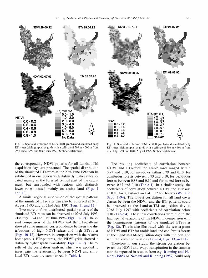
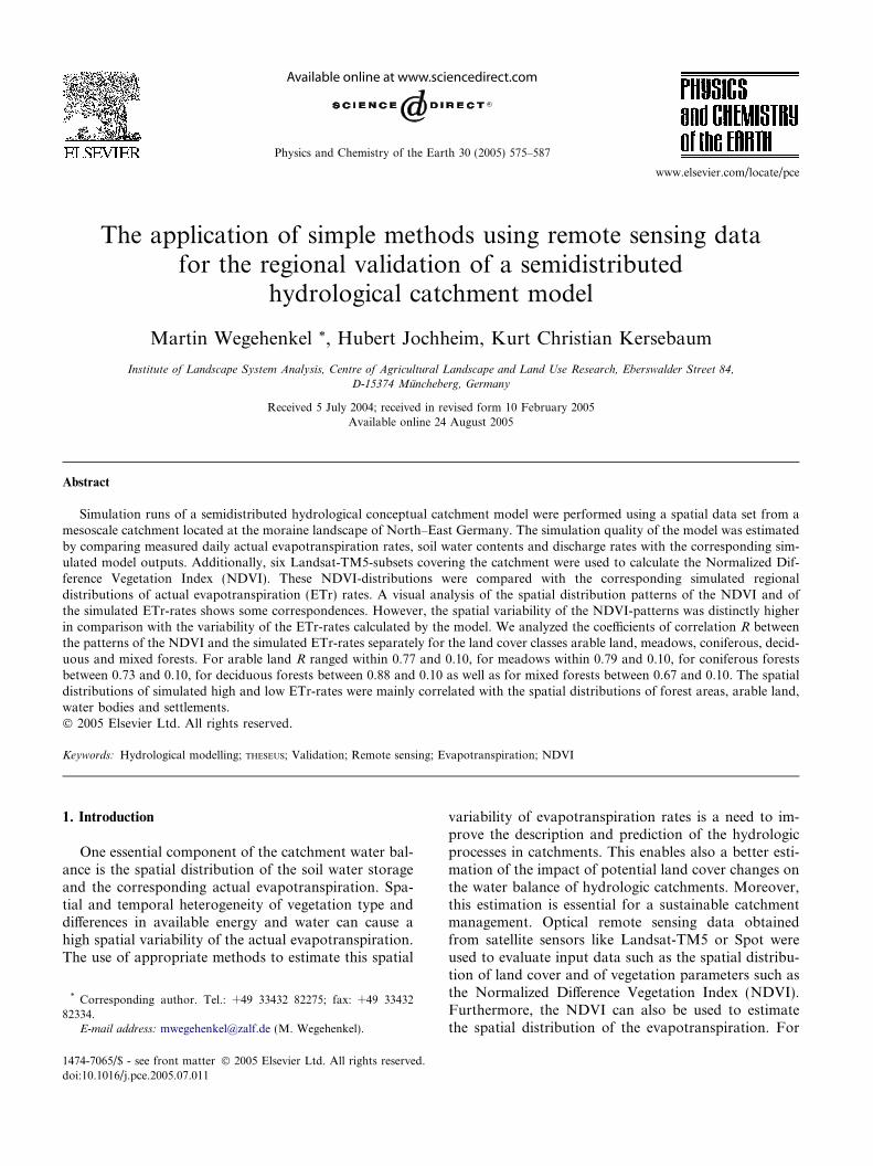
Fig. 10. Spatial distribution of NDVI (left graphs) and simulated dailyETr-rates (right graphs) as grids with a cell size of 500 m · 500 m from29th June 1992 and 02nd July 1993, Stobber catchment.

Fig. 11. Spatial distribution of NDVI (left graphs) and simulated dailyETr-rates (right graphs) as grids with a cell size of 500 m · 500 m from21st July 1994 and 09th August 1995, Stobber catchment.


the corresponding NDVI-patterns for all Landsat-TMacquisition days are presented. The spatial distributionof the simulated ETr-rates at the 29th June 1992 can besubdivided in one region with distinctly higher rates lo-cated mainly in the forested central part of the catch-ment, but surrounded with regions with distinctlylower rates located mainly on arable land (Figs. 1and 10).

A similar regional subdivision of the spatial patternsof the simulated ETr-rates can also be observed at 09thAugust 1995 and at 22nd July 1997 (Figs. 11 and 12).

Two more uniform distributed spatial patterns of thesimulated ETr-rates can be observed at 02nd July 1993,21st July 1994 and 01st June 1996 (Figs. 10–12). The vi-sual comparison of the NDVI- and the ETr-patternsshowed some minimal correspondence between the dis-tributions of high NDVI-values and high ETr-rates(Figs. 10–12). However, in comparison with the relativehomogenous ETr-patterns, the NDVI-grids showed adistinctly higher spatial variability (Figs. 10–12). The re-sults of the correlation analysis, which was applied toinvestigate the relationship between NDVI and simu-lated ETr-rates, are summarized in Table 4.

The resulting coefficients of correlation betweenNDVI and ETr-rates for arable land ranged within0.77 and 0.10, for meadows within 0.79 and 0.10, forconiferous forests between 0.73 and 0.10, for deciduousforests between 0.88 and 0.10 and for mixed forests be-tween 0.67 and 0.10 (Table 4). In a similar study, thecoefficients of correlation between NDVI and ETr wasat 0.80 for grassland and at 0.12 for forests (Wei andSado, 1994). The lowest correlation for all land coverclasses between the NDVI- and the ETr-patterns couldbe observed at the Landsat-TM acquisition day at22nd July 1997 with coefficients of correlation below0.10 (Table 4). These low correlations were due to thehigh spatial variability of the NDVI in comparison withthe homogenous patterns of the simulated ETr-rates(Fig. 12). This is also illustrated with the scattergramsof NDVI and ETr for arable land and coniferous forestsat the Landsat-TM-acquisition days with the best andwith the lowest correlation (Table 4, Figs. 13 and 14).

Therefore in our study, the strong correlation be-tween the NDVI and evapotranspiration in the summermonths reported in studies from e.g. Running and Ne-mani (1988) or Nemani and Running (1989) could only

Fig. 12. Spatial distribution of NDVI (left graphs) and simulated dailyETr-rates (right graphs) as grids with a cell size of 500 m · 500 m from01st June 1996 and 22nd July 1997, Stobber catchment.

Fig. 13. Scattergram NDVI versus ETr from 21st July 1994 and from22nd July 1997, arable land.


be observed in single cases (Table 4). Due to these differ-ent correlations, an overall sufficient calibration of thesimple relationship NDVI versus ETr-rate for all datasets defined in Eq. (6) was not possible in our study.

Furthermore, we compared also experimental vario-grams c(h) for the spatial distributions of the NDVI-val-ues and the ETr-rates. These variograms obtained eitherfrom the NDVI-grids or from the simulated ETr-ratesare similar (Fig. 15).

This indicates that the spatial structure of the NDVI-and the ETr-patterns is comparable. However, the anal-ysis of the simulated ETr-patterns showed, that themodel was only able to simulate those patterns, which

Table 4Coefficient of correlation between NDVI and simulated ETr-rates for differeLandsat-TM-acquisition days

Date Arable land Meadows Conifero

29 June 92 0.56 0.66 0.6402 July 93 0.49 0.79 0.73

21 July 94 0.77 0.61 0.6709 August 95 0.60 0.41 0.5301 June 96 0.45 0.61 0.1022 July 97 0.10 0.10 0.10

were controlled by the spatial distribution of forestareas, arable land, water bodies and buildings (Figs. 1,10–12). The spatial variability within these simulatedhomogenous ETr-areas indicated by the observedNDVI-patterns was not simulated sufficiently by themodel. For these discrepancies, potential reasons mightbe the spatial resolution and the contents of the digitalland cover and soil data base used in our study. The ob-served differences between NDVI and ETr-rates of thearable land may be due to discrepancies between the

nt vegetation classes (best results in bold, badest results in italic) at the

us forests Deciduous forests Mixed forests

0.52 0.620.72 0.430.61 0.100.88 0.67

0.6 0.250.10 0.10

Fig. 14. Scattergram NDVI versus ETr from 21st July 1994 and from22nd July 1997, coniferous forests.

Fig. 15. Experimental variograms of the NDVI-grids and the simulated ETAugust 1995, 01st June 1996 and 22nd July 1997.


virtual crop rotations with their corresponding seedingand harvest dates in the GIS-database used for themodel calculations and the real crop rotations with theactual seeding and harvest dates due to senescence.These differences between the virtual and actual harvestdates can cause discrepancies between the simulatedETr- and the observed NDVI-patterns. Furthermore,different age classes of forest stands in coniferous, decid-uous and mixed forests are also not supported by theland cover data base used in our study. These differentage classes can also contribute to the higher spatial var-iability of the NDVI in comparison to the homogenousareas of simulated ETr-rates. Differences between theactual distributions of soil types and soil properties suchsoil water storage capacity in the landscape and the spa-tial distributions of soils and soil properties representedby the digital soil map used in our study are additionalpotential reasons for the observed discrepancies betweenthe simulated ETr- and the observed NDVI-patterns.Furthermore, small scale variabilities in the meteorolog-ical input data for the calculation of PET such as satu-ration deficit of air and wind speed are additionalpotential reasons. However, especially these small scalevariabilities are difficult to take into account by semidis-tributed conceptual models.

4. Conclusions and outlook

The comparison of the measured and simulated watercontents as well as evapotranspiration rates at localscale showed a sufficient agreement. This is an indication

r-patterns from 29th June 1992, 02nd July 1993, 21st July 1994, 09th


that the process description for modelling evapotranspi-ration and soil water balance within the model is alsosufficient if a good data base for soil and crop data isavailable. Semidistributed catchment models are oftenvalidated comparing simulated with observed dischargerates of the total catchment or some subbasins. In ourstudy, this validation leads also to satisfactory results.To improve these classical validation strategies, we com-pared the spatial patterns of ETr-rates simulated by themodel with those of the NDVI to test our semidistrib-uted model at regional scale. However, in our study, itwas not possible to carry out a sufficient calibration ofthe simple relationship NDVI versus ETr for all landcover classes and all Landsat-TM acquisition days dueto the wide range of the coefficients of correlation be-tween 0.88 and 0.10 (Table 4). This was due to the dis-tinctly higher spatial variability of the NDVI-grids incomparison with the simulated ETr-patterns.

Therefore, as a first essential step to take into accountthe higher actual spatial variability of ETr-rates indicatedby the NDVI-patterns, the model has to be improvedwith more sophisticated vegetation models such physio-logically based crop, grassland and forest evapotranspi-ration models. However, this have to be combined witha higher spatial resolution andmore detailed informationespecially in the land cover data base This will lead to ahigher spatial discretization of the model for a furtherimprovement of the model calculations and, therefore,to a higher spatial variability in the model outputs.

As a second step, more complex and physically basedrelationships have to be used to estimate the spatial dis-tribution of actual ETr-rates from NDVI combined withother data such as surface temperature and energy bal-ance terms derived from remote sensing data. Suchmethods and relationships are described e.g. in Basti-aansen (2000) and Kustas et al. (2003).

Acknowledgements

The work was funded by the Germany Federal Min-istry of Consumer Protection, Food and Agriculture(BMVEL) and the Ministry of Agriculture, Environ-mental Protection and Landscape Planning (MLUR),Brandenburg. The authors also wish to thank the Ger-many�s National Meteorological Service (DWD) forproviding precipitation data from four weather stations.Furthermore, the authors have to thank the anonymousreviewers for their constructive comments and recom-mendations for an improvement of the manuscript.

References

Ag Boden, 1994. Bodenkundliche Kartieranleitung.-3. Aufl. Schweiz-erbart Stuttgart.

Bastiaansen, W.G.M., 2000. Sebal-based sensible and latent heat fluxin the irrigated Gediz Basin, Turkey. J. Hydrol. 2229, 87–100.

Disse, M., 1995. Modellierung der Verdunstung und der Grundwass-erneubildung in ebenen Einzugsgebieten. IHW, Universitat Kar-lsruhe (TH), Heft 53, p. 145.

Ernstberger, H., 1987. Einfluss der Landnutzung auf Verdunstung undWasserbilanz. Beitrage zur Hydrologie, Kirchzarten, p. 189.

Eulenstein, F., Werner, A., Olejnik, J., 1999. THESEUS—the model forwater balance estimation in different scale. Roczniki AkademiiRolniczej w Poznaniu CCCX, 475–485.

Glugla, G., 1969. Berechnungsverfahren zur Ermittlung des aktuellenWassergehaltes und Gravitationsabflusses. Albrecht-Thaer-Archiv13, 371–376.

Hall, F.G., 1992. Satellite remote sensing of surface energy balance:success, failures and unresolved issues in FIFE. J. Geophys. Res.97, 19061–19090.

Holtan, H.N., 1961. A concept for infiltration estimates in watershedengineering. US Department ARS, 41–51.

Jochheim, H., Luttschwager, D., Wegehenkel, M., 2004. Simulation ofthe water and nitrogen balances of forests within a catchment in thenortheastern lowlands. Eur. J. Forest Res. 123, 53–61.

Koitzsch, R., Gunther, R., 1990. Modell zur ganzjahrigen Simulationder Verdunstung und der Bodenfeuchte landwirtschaftlicher Nut-zflachen. Arch. Acker-Pflanzenbau Bodenkd. 24, 717–725.

Kopp, D., Schwanecke, W., 1995. Standortlich-naturraumlicheGrundlagen okologiegerechter Forstwirtschaft—Grundzuge vonVerfahren und Ergebnissen der forstlichen Standortserkundung inden funf neuen deutschen Bundeslandern. Deutscher Land-wirtschaftsverlag, Berlin.

Kustas, W.P., Norman, J.M., 1996. Use of remote sensing forevapotranspiration monitoring over land surfaces. Hydrol. Sci. 41(4), 495–516.

Kustas, W.P., Norman, J., Anderson, M.C., French, A.N., 2003.Estimating subpixel surface temperatures and energy fluxes fromthe vegetation index radiometric temperature relationship. RemoteSens. Environ. 85, 429–440.

Mauser, W., Schadlich, St., 1998. Modelling the spatial distribution ofevapotranspiration on different scales using remote sensing data. J.Hydrology 212–213, 250–267.

Mo, X., Liu, S., Lin, Z., Zhao, W., 2004. Simulating temporal andspatial variation of evapotranspiration over the Lushi basin. J.Hydrol. 285, 125–142.

Moran, M.S., Jackson, R.D., 1991. Assessing the spatial distributionof evapotranspiration using remotely sensed inputs. J. Environ.Quality 20, 725–737.

Nemani, R.R., Running, S.W., 1989. Estimation of regional surfaceresistance to evapotranspiration from NDVI and thermal IR-AVHRR data. J. Appl. Meteorol. 28, 276–284.

Olejnik, J., Eulenstein, F., Kedziora, A., Werner, A., 2001. Evaluationof a water balance model using data for bare soil and crop surfacesin middle Europe. Agricul. Forest Meteorol. 106, 105–116.

Raissi, F., Muller, U., Meesenburg, H., 2001. Ermittlung der effektivenDurchwurzelungstiefe von Forststandorten. Geofakten Nr. 9,NFLB Hannover.

Richter, R., 2000. Atmospheric correction for flat terrain: ModelATCOR2. DLR-IB 564-02/00 DLR, Wessling, Germany.

Rodriguez, J.C., Duchemin, B., Hadria, R., Watts, C., Garatuza, J.,Chehbouni, A., Khabba, S., Boulet, G., Palacios, E., Lahrouni, A.,2004. Wheat yield estimation using remote sensing and the STICSmodel in the semiarid Yaqui valley. Agronomie 26 (6–7), 295–304.

Rouse, J.W., Haas, R.H., Schell, J.A., Deering, J.A., 1973. Monitoringvegetation systems in the Great Plains ERTS. In: Third Symp. onsignificant Results obtained with ERTS-1, NASA, SP-351, pp. 309–317.

Running, S.W., Hunt Jr., E.R., 1993. Generalization of a forestecosystem process model for other biomes, BIOME-BGC, and anapplication for global-scale models. In: Ehleringer, J.R., Field, C.


(Eds.), 2000, Scaling Processes Between Leaf and LandscapeLevels. Academic Press, pp. 141–158.

Running, S.W., Nemani, R.R., 1988. Realing seasonal patterns of theAVHRR vegetation index to simulated photosynthesis and tran-spiration of forests in different climates. Remote Sens. Environ. 24,347–367.

Sawamoto, M., Shin, S., 1997. Water balance evaluation in the KoreanPeninsula through vegetation monitoring. J. Remote Sens. Soc.Jpn. 17 (3), 220–231.

Schmidt, R., Diemann, R., 1991. Erlauterungen zur Mittelmaßstabi-gen Landwirtschaftlichen Standortkartierung. FzB Muncheberg,Bereich Bodenkunde/Fernerkundung Eberswalde, p. 78.

Steidl, J., Merz, Chr., Dannowski, R., 1999. GIS-gestutzte Paramet-risierung hydrogeologischer Datenmodelle fur die Grundwasser-modellierung in jungpleistozanen Einzugsgebieten. In: Fohrer, N.,Doll, P. (Eds.), Modellierung des Wasser- und Stofftransports ingroßen Einzugsgebieten. Kassel University Press, pp. 197–205.

Sun, R., Chen, J.M., Zhu, Q., Zhou, Y., Liu, J., Li, J., Liu, S., Yan, G.,Tang, S., 2004. Spatial distribution of net primary productivity andevapotranspiration in Changbaishan Natural Reserve, China,using Landsat ETM+ data. Can. J. Remote Sens. 30 (5), 731–742.

Venturini, V., Bisht, G., Islam, S., Jiang, L., 2004. Comparison ofevaporative fractions estimated from AVHRR and MODIS

sensors over South Florida. Remote Sens. Environ. 93 (1-2), 77–86.

Wegehenkel, M., 2002. Estimating the impact of landuse changes usingthe conceptual model THESEUS—a case study. Phys. Chem. Earth 27(9–10), 631–641.

Wegehenkel, M., 2005. The validation of a soil water balance modelusing soil water content and pressure head data. Hydrol. Process.19, 1139–1164.

Wegehenkel, M., Steidl, J., 2000. Simulation des Wasserhaushaltes ineinem Einzugsgebiet der glazial gepragten nordostdeutschen Mora-nenlandschaft. Zeitschrift f Kulturtechnik und Landentwicklung 41(2), 57–61.

Wei, Y., Sado, K., 1994. Estimation of areal evapotranspiration usingLandsat-TM data alone. Available from: <http://www.gisdevelop-ment. net/aars/acrs/1994/ps1/ps1002pf.htm>.

Wendling, U.H., Schellin, G., Thoma, M., 1991. Bereitstellung vontaglichen Informationen zum Wasserhaushalt des Bodens fur dieZwecke der agrarmeteorologischen Beratung. Z. Metereol. 41 (6),1–16.

Wurbs, A., Kersebaum, K.C., Werner, A., 2000. Stickstoffaustrag beiintegrierter und okologischer Bewirtschaftung – Szenariorechnun-gen zur Abschatzung standortlicher Risiken. Zeitschrift f. Kultur-technik und Landentwicklung 41, 241–246.

http://www.gisdevelopment.net/aars/acrs/1994/ps1/ps1002pf.htm

http://www.gisdevelopment.net/aars/acrs/1994/ps1/ps1002pf.htm

The application of simple methods using remote sensing data for the regional validation of a...

Documents

Transcript of The application of simple methods using remote sensing data for the regional validation of a...