L SCHQOn

NPS55Rh74071A

NAVAL POSTGRADUATE SCHOOL//

Monterey, California

COMPUTER SOFTWARE: TESTING, RELIABILITY

MODELS, AND QUALITY ASSURANCE

by

F. Russell Richards

July 1974

Technical Report

Approved for public release; distribution unlimited,

Prepared for:nor>uty Commander

rational Test and Evaluation Force, Pacific

feddocs J l Air Station, North Island

D 208.14/2:NPS-55Rh74071A Diego, CA 92135

NAVAL POSTGRADUATE SCHOOLMonterey, California

Rear Admiral Isham Linder Jack R. BorstingSuperintendent Provost

The work reported herein was supported primarily by DeputyCommander, Operational Test and Evaluation Force under Job Order 55730.Partial support was provided by the Navy Fleet Material Support Officeunder Job Order 55753.

Reproduction of all or part of this report is authorized.

This report was prepared by:

UNCLASSIFIEDSECURITY CLASSIFICATION OF THIS PAGE (When Data Entered)

REPORT DOCUMENTATION PAGE1 REPORT NUMBER

NPS55Rh74071A

2. GOVT ACCESSION NO

READ INSTRUCTIONSBEFORE COMPLETING FORM

3. RECIPIENT'S CATALOG NUMBER

4. TITLE (and Subtitle)

COMPUTER SOFTWARE: TESTING, RELIABILITY

MODELS, AND QUALITY ASSURANCE

5. TYPE OF REPORT & PERIOD COVEREDTechnical ReportJuly 1973 - July 1974

6. PERFORMING ORG. REPORT NUMBER

7. AUTHORfsj

F. Russell Richards

8. CONTRACT OR GRANT NUMBERS

9. PERFORMING ORGANIZATION NAME AND ADDRESS

Naval Postgraduate SchoolMonterey, California

10. PROGRAM ELEMENT. PROJECT. TASKAREA a WORK UNIT NUMBERSNC 2053P0-3-0001Job Order 55730

II. CONTROLLING OFFICE NAME AND ADDRESS

Deputy Commander, Operational Test andEvaluation Force, PacificNAS North Island. San Diego, Califnrnis

12. REPORT DATE

July 197413 NUMBER OF PAGES

8614. MONITORING AGENCY NAME & ADDRESSfU different from Controlling Office) 15. SECURITY CLASS, (of thta report)

15a. DECLASSIFl CATION/ DOWN GRADINGSCHEDULE

16. DISTRIBUTION ST ATEMEN T (of this Report)

17. DISTRIBUTION STATEMENT (of the abstract entered In Block 20, If different from Report)

Approved for Public Release; Distribution Unlimited

18. SUPPLEMENTARY NOTES

19. KEY WORDS (Continue on reverse side II necessary and Identity by block number)

SoftwareReliabi lityTesting Methodology

Quality AssuranceReliability Growth

20. ABSTRACT (Continue on reverse side If necessary and Identify by block number)

A study of the problems of measuring and assuring the qualityof computer software is made. A quantitative measure of softwarequality is defined, and various mathematical models for estimatingthat measure of effectiveness are presented.

Software testing methodology, data requirements and data col-lection procedures are discussed. Also included is a discussion ofthe customer's role in software quality assurance.

DD | JAN 73 1473 EDITION OF 1 NOV 65 IS OBSOLETES/N 0102-014- 6601

|

UNCLASSIFIEDSECURITY CLASSIFICATION OF THIS PAGE (When Data Bntarad)

COMPUTER SOFTWARE: TESTING, RELIABILITY

MODELS, AND QUALITY ASSURANCE.

I. INTRODUCTION 2

II. SOFTWARE RELIABILITY

2.1 Measure of Performance 5

2.2 Definitions. 5

2.3 Classification of Errors 7

2.4 Analogy with a Hardware Reliability Program 8

2.5 The Random Nature of Software Failures . .10

2.6 Restrictions on the Mathematical Reliability Models. . . .11

III. SOFTWARE TESTING AND DATA COLLECTION

3.1 Introduction 12

3.2 Stages of Software Testing 12

3.3 Test Methodology ......... . 16

3.4 Data Collection. .19

IV. MATHEMATICAL MODELS

4.1 Introduction 234.2 A Hardware Oriented Approach .25

4.3 Error Counting Models 32

4.4 An Error Seeding Model ................. .40

4.5 A Simple Reliability Model for Qualitative Data. .... .47

4.6 A Reliability Growth Model for Qualitative Data. .... .50

4.7 Bayesian Reliability Models. . .57

V. GUIDELINES FOR SOFTWARE QUALITY ASSURANCE

5.1 Introduction ........ .63

5.2 Design for Reliability . . . 645.3 The User's Role in Software Development. ........ .66

VI. CONCLUSIONS 70

BIBLIOGRAPHY. 72

APPENDIX. ............ . . .75

I . INTRODUCTION

Computer systems are becoming more and more complex as faster and

more versatile computer hardware evolves. The resultant sophisticated

uses of the computer systems demand that programmers develop reliable

instructions to drive the computer systems. Nowhere is this more evident

than in the military where computers are being used increasingly as the

heart of sophisticated weapons systems such as real-time command control

systems which actually control their environments by receiving data,

processing data and returning results fast enough to affect the functioning

of their environments.

It is now the case that software costs (those costs related to

developing, testing, correcting and integrating all computer programs and

data descriptions used to operate, test, monitor and maintain the hard-

ware system) now exceed the hardware costs in most complex systems. We

now see huge programs with perhaps over a million words of code.

The technical literature abounds with articles about quality control

procedures, test methodologies and techniques for measuring and predicting

reliabi lity—most applied to the hardware systems. Though not complete,

the theory is certainly developed to such a state that highly reliable hard-

ware can be achieved. Unfortunately, the same cannot be said about computer

software. Until recently the software has received only modest attention

and, as a result, software development is still more an art than a science.

This is the case despite the fact that the influence of the software may

well dominate the hardware when- considering overall system reliability .

Consider, for example, the possible consequences if a real-time military

command control system crashes because of a software deficiency while enemy

units are being tracked. Even a few moments delay to restore the targets

on a video output display could be vital. In this case a software deficiency,

just like a hardware failure, could incapacitate a key component of our de-

fense structure at a critical time.

The lack of attention given to software quality control has resulted,

predictably, in products which are characteristically laden with software

errors even after they have been released to customers for operational use.

The failure of the software product to perform as required results in the

loss of customer confidence for the entire system.

How can software quality be improved so that the customer's confidence

in the software subsystem can be restored? We seek to provide at least a

partial answer to this question in this report. As with hardware, a quanti-

tative measure for evaluating software must be used if a meaningful assess-

ment of software quality is to be made. More is needed than a subjective

assessment of program performance and program deficiencies if quality is to

be described in other than general terms such as "acceptable" or "unacceptable.

This report defines a quantitative measure of software quality^and mathema-

tical models for estimating that measure of effectiveness are presented in

Chapter 4. The data requirements and data collection procedures are discussed

in Chapter 3.

A numerical measure of software quality will enable us to evaluate a

software subsystem, but, by itself, the measure will do nothing to improve

the quality of the software delivered to the customer. To accomplish this,

more effort and resources must be expended in the design, development and

integration phases of the software. The causes of "software unreliability"

must be determined, and steps must be taken to alleviate the contributions

of the identified causes of software problems.

Certainly, the software contractor must accept much of the blame for

a poor quality software product. The contractor is responsible for the

code that is created, and he must exercise management control over the pro-

duct. Nevertheless, the customer can assume a more active participation in

the development of the software which should help assure that his delivered

software is acceptable. This can be accomplished by completely spelling out

exactly what the software must be able to do and by requiring that sufficient

software testing be carried out to demonstrate adequately that the software

conforms to its performance specifications. In addition the customer can

require strict management control of the software during its development. In

Chapter 5 we discuss the role the customer can play to improve the quality

of the software which is delivered to him.

Finally, we point out the need for further work in the area of software

quality control to validate the mathematical models and to improve the test

procedures.

II. SOFTWARE RELIABILITY

2. 1 Measu re of Performance

In order to provide a meaningful assessment of software quality,

quantitative methods of evaluating software must be developed. Tradition-

ally, quality assessments have been mere subjective evaluations of soft-

ware based on the frequency of program deficiencies. However, subjective

evaluations for software do not seem consistent with the use of the rather

sophisticated methodologies used to measure the quality of interacting

hardware. For complex computer systems, consisting of the hardware, soft-

ware and human operator subsystems, the most widely accepted and most

meaningful measure of performance is total system reliability , defined as

the probability that every subsystem performs within specification limits

for the time and under the conditions of intended customer use. Thus there

is an obvious need to measure the reliability of the software subsystem.

If no software reliability specification is explicitly stated, one must be

determined from the specification for the total system. A study of the cost-

benefit trade-offs would then determine the reliability apportionment.

2.2 De finitions

Although software reliability appears to be the most appropriate mea-

sure of performance, there are definitional problems because the meanings

of such words as software reliability and software failures are not entirely

obvious by analogy with the corresponding hardware reliability concepts.

Our software reliability study will therefore begin with definitions of these

basic terms.

Definition 1: A software failure occurs when an input is made or a command

is given and the software subsystem does not respond as required.

It is generally obvious when a program has failed to function as re-

quired. The failure may be manifest in many ways. A complete stoppage of

the system may occur; output values may fail to lie within acceptable tol-

erance limits of the true values; or troubles with interactive hardware,

e.g., erroneous video displays or incorrect navigation, may be experienced.

On the other hand, there will surely be some cases of controversy as to

whether or not a failure has occurred, and some failures will go undetected.

Detection of failures is, to a large extent, a subjective decision which

must be made by the operators or the test personnel, hopefully on the basis

of objective criteria such as performance specifications In actual practice,

failure detection depends on an operator's observation, so, in effect, a soft-

ware failure is what an operator says is a failure.

After failures are detected some programmer must inspect the program

and locate the causes of the failure. Logical or clerical errors in coding

may be found to be guilty of producing the incorrect results. When software

errors are located, action should be taken to correct the errors to prevent

recurrence of the failures. Obviously, the correspondence between software

errors uncovered and software failures detected is not necessarily one-to-one.

Many errors may occur without a failure being detected, and a single detected

failure may be a result of several software errors. Also, a software failure

may be reported that is in fact no software failure at all, but rather an

operator or hardware deficiency.

Because of the difficulties involved with determining a correspondence

between the number of software failures and the number of errors, we choose

not to define software reliability as a probability of error-free performance

Instead, we opt for definitions (depending on the type of data observed)

based on the observed diffi culties--fai lures . We offer two different

definitions of software reliability depending on whether the observed data

are quantitative, such as times between failures, or qualitative, such as

"run success" or "run failure."

Definition 2 (Quantitative Data): Software reliability is the probability

that the software subsystem will operate without a single failure for a

specified length or time under given conditions.

Definit ion 3 (Qualitative Data): Software reliability is the probability

that the software subsystem will perform without failure for an entire run

under given conditions.

The latter definition requires further comment about the definition

of the word "run." In some cases a run might be taken to mean the operation

of the software under a particular set of input combinations. Alternatively,

it may mean an operation of the software subsystem for a fixed length of

time, or it may take some other meaning. Although admittedly somewhat vague

at this juncture, the meaning of the word "run" should be clear in a given

application from the context in which it is used.

2.3 Classification of Errors

The definition of software reliability fails to distinguish between

different classifications of failures. No doubt, software failures differ

with respect to their impact on the system. The more severe failures may

result in the failure of a mission, while less critical failures may only

cause nuisances or limitations which have little effect on a mission's

success. It may be appropriate to classify failures according to their

impact on the system and to define reliability in terms of a particular

class of failures, or perhaps to apply some weighting scheme to failures

so that the more critical failures are weighted more heavily than are the

minor failures. Although appealing, such an approach is not entirely satis-

factory because of the subjective nature of the assignment of weights. In

this paper we make no distinction between failures. One can still apply

the models that we present to a particular category of failures by simply

redefining a software failure in terms of a given failure classification.

2.4 Analogy with a Hardware Reliability P rogram

Because the theory of hardware reliability is developed to a relatively

advanced state, it is natural to try to learn about software reliability by

borrowing from the hardware reliability theory. There are certainly many

similarities between the two, but a few important differences have prevented

a simple direct application of the hardware techniques to software. Never-

theless, much insight can be obtained as to what kinds of things should be

done with software by studying the areas of a hardware reliability program.

MacWilliams [17] summarizes those areas as follows:

1. Define, observe and record failures at the system, subsystem

and component levels.

2. Determine the statistical behavior of failures and develop a

mathematical model for failures.

3. Isolate the principal causes of failure.

4. Determine the quantitative dependence of component failure

rates.

5. Determine achievable limits of component reliability as a

function of the variables which can be controlled in the

devel opment.

6. Develop a theory to combine component reliabilities into sub-

system or system reliability.

7. Optimize the distribution of unreliability by considering the

component reliabilities as a function of cost and by considering

the abilities to compound component reliabilities into sub-

system and system reliabilities. Apportion the overall

system reliability among subsystems in such a way as to achieve

the most economical attainment of the desired system reliability.

These same steps are desired for a software reliability program. Cer-

tainly we require a quantitative knowledge of software failure statistics,

including causes and dependencies, and a mathematical model of the failures.

Also, a method of compounding the reliabilities of software modules into a

"total software reliability" would be desirable, as would a theory for appor-

tioning effort among software modules. Unfortunately, difficulties result

when one tries to apply all steps of a hardware reliability program to soft-

ware. Even when one attempts to apply the first few steps, basic differences

between hardware and software failures create a need for new mathematical

models. Let us examine those differences.

2.5 The Random Nature of Software Failures

Hardware failures occur randomly with time as the hardware deterio-

rates. However, there is no degradation of software, and there is no

physical mechanism which generates software failures. Once all errors are

removed, the software is 100 per cent reliable and will remain so forever,

provided no program changes are made. What then accounts for the random-

ness of software failures?

Different input combinations result in different requirements of the

software. The paths traversed within a software program depend on the part-

icular input combinations, and each path can be thought of as containing

possible software bugs waiting to be discovered. Without correction, the

same errors will occur each time a specific logic path is traversed. If

the errors result in an observable software failure, the given failure can

be reproduced at will, or it can be avoided by operator control of the input

combinations. Therefore, software failures are functions of the input com-

binations—not random functions of time. However, in practice, input combin-

ations are chosen in a somewhat random fashion, and the resultant effect is

that errors are uncovered and failures are observed at random. It is in this

sense that we talk about the random occurrence of software failures. Thus,

although there are conceptual differences between software failures and

hardware failures, software failures are surely the analog of hardware fail-

ures that we should use to measure software reliability.

10

2_i 6 __Res trictions on the Mathematical Reliability Models

In Chapter 4 we present several mathematical models for software

reliabi lity--all based on software failure data. Because of the absence

of degradation of software and the "find and fix" actions that are taken

when errors are discovered, the models assume a reliability growth as a

function of total test time. The models consider the reliability of the

software subsystem alone. No attempt is made to model the interactions

of hardware-software, operator-software or hardware-software-operator.

These are all important considerations, but software reliability being

in the embryonic stage that it is requires us to focus singly on it at

this time. This does not preclude the combination of software reliability

with hardware and operator reliabilities to obtain an estimate of overall

system reliabi lity

.

Our models treat the software subsystem pretty much as a black box

in the sense that the internal structure of the software is completely

ignored. Again, better reliability models could probably be developed if

that structure were considered. This is a refinement that would probably

follow once a good understanding of software reliability is obtained and

expertise is developed.

11

III. SOFTWARE TESTING AND DATA COLLECTIONS

3.1 Introduction

A numerical estimate of software quality can be no better than the

data from which it is determined. To estimate software reliability, de-

tailed information about the frequency of failures, the times that

failures occur and the severity of the failures is needed. Furthermore,

if there is to be reliability growth, the causes of the failures must be

identified, and corrective action must be taken. Only through good,

representative failure data can reasonably accurate mathematical models

of software reliability be developed and reliable predictions about soft-

ware quality be made.

The software test effort has already become the single most costly

step in most software production processes. The high cost of testing

combined with the high reliability requirements of complex systems demands

that efficient test methodologies be developed. It also requires that the

data reporting system be established early in a software test program so

as not to lose valuable information.

3.2 Stages of Software Testing

The development of software is a "bottom-up" procedure. First,

modules are coded. These are then combined to form functional groups

(processes) which, in turn, are integrated into the software subsystem.

The "total system" is then formed by integrating the software, hardware and

operator subsystems. This development procedure is depicted in Figure 1.

12

STAGES OF SOFTWARE DEVELOPMENT

Module 1

Process 1

CODING OF MODULES

<a <=>

HardwareSubsystem

Module n

MODULE INTEGRATION

Process i C> c> o Process k

PROCESS INTEGRATION

SoftwareSubsystem

OperatorSubsystem

SUBSYSTEM INTEGRATION

Fiqure 1

13

Software testing should be conducted throughout each stage of devel-

opment. At the lowest level, the primary purpose of testinq is to discover

the crude errors such as compilation errors and syntactical errors. Debug-

ging at this level is certainly much simpler than at the process or subsystem

levels. Because modules are usually of manageable size, having perhaps only

a few functions, module check-out which is nearly exhaustive would be pos-

sible in many cases. The module failure data are useful for determining

statistical estimates of quality which could be employed to establish addi-

tional test requirements for the module.

When several modules are integrated to form a process, or when several

processes are integrated to form the software subsystem, problems surface

which had previously gone undetected. This occurs because the complex inter-

actions between modules could not have been tested previously as the indivi-

dual modules were separately checked out. Unfortunately, the complexity of

the module interactions precludes the direct use of module reliability esti-

mates to determine the software subsystem reliability, or even the process

reliabilities. The multitude of branching possibilities in a typical process

or software subsystem and the complex interactions seem, at this time, to

make infeasible a computation of subsystem reliability from a knowledge of

module reliabilities as is done with hardware systems in a "series/parallel"

sort of analysis. For these reasons, tests must be run, and failure data

must be collected during and after the integration stages.

At the beginning of the integration stage many bugs will likely be

experienced and frequent failures will occur. As with the module failure

data, this information is what is needed to estimate present reliability and

14

to provide guidance as to the extent of testing which must be performed.

Later in the integration stage, after the program has been debugged

to a point that it will run for some time before failing, the software

should be subjected to some sort of simulation test by a functional test

program to make sure that a software subsystem which may perform without

failure does indeed do the job for which it was designed. This provides

an opportunity to test the software in a complete system with hardware

and operator interfaces. It is an ideal time to collect failure data and

to measure the reliability of the software subsystem. At this stage, pro-

per design of test plans and rational methods for validating programs be-

come critical. Anything like exhaustive testing is virtually impossible

because the number of possible cases may total in excess of several million.

Finally, after the software subsystem has been judged to be acceptable

and all performance requirements have been demonstrated, it is turned over

to the user for field tests. If usual experience prevails, the supposedly

good software now suffers a completely new set of failures induced by the

unique characteristics of actual operation not considered in previous tests.

The closer the test environment simulates the operational environment, the

more accurate will be the reliability estimate made at the end of the inte-

gration stage.

It is the reliability estimate of the system in the operational en-

vironment that is of interest to the user. An estimate of this reliability

is needed to determine if the software is of sufficient quality to allow

user access. If the field tests are unsatisfactory, the software may have

to be returned to the developer for corrective work and more testing. The

15

release of an unreliable product will result in the loss of users' confi-

dence.

3.3 Test Methodology

We have discussed the importance of the test effort, and we have men-

tioned that software testing is becominq the single most costly element in

the development of software for complex systems. Because of the importance

and expense of software testing, efficient test procedures must be used.

Despite the need, no general systematic test methodology is available which

can be applied to test each program to determine whether or not all software

components perform as required.

There have been some recent attempts (see, for example, London [16] and

King [12]) to develop procedures for actually proving the correctness of

programs. Presently, these procedures are only applicable to relatively

small programs written in special languages. There seems to be little hope

that generally applicable methods for formally proving programs logically

correct can be developed for large complex programs.

With the large number of input combinations that need to be examined,

it would be desirable to have a computer program that could be used to check

out a software subsystem by exercising all options and all branches within

the subsystem through all the feasible ranges of values. The tester would

only have to supply parameters to such a program and the automatic computer

test program would do the rest of the work. Jelinski and Moranda [10] point

out that this is not possible because even with our latest generation of com-

puters with a nanosecond cycle the number of possible input combinations in-

23volved in an average-size software program exceeds 10 , and, consequently,

16

14the processing time exceeds the astronomical limit of 10 seconds of

computer time. Thus, a completely automatic computer test program does

not appear to offer a feasible solution to the software testing problem.

Certainly, software checkout could be improved if assistance could be pro-

vided by some sort of computer program tester. Jelinski and Moranda [10]

report of such a tool, called a "program testing translator", under deve-

lopment at McDonnell Douglas Company. The translator, currently designed

to run only with FORTRAN programs, when exercised with a software program

will count the number of times each branch in the program was executed by

a given set of input conditions. It also performs a number of counts on

various types of statements. These counts provide a good indication of

which branches have been checked out for a given range of values, thus

providing assistance toward achieving reliability. Such a "program testing

translator" does not completely solve the test problem, even for FORTRAN

programs, but it is certainly a useful tool for testing software.

The question of how a set of input conditions should be selected to

test a software program remains to be answered. The answer depends on many

factors such as:

(1) the size of the program being tested,

(2) the number of tests that can be run,

(3) the frequency of use of the various functions comprising

the program, and

(4) the criticality of the functions to mission success.

Because failures do not occur randomly with time, but rather they occur be-

cause of the traversals of different paths through the program, the tests

must include enough cases to exercise as many paths as possible consistent

17

with the resources available for testing and the reliability objectives.

><o doubt, many of the software errors would probably be detected if input

combinations were selected at random. In fact, such a procedure is often

used in the early stages of a test program to detect the crude errors

which account for a large percentage of all of the errors. However, if

the tests are to demonstrate that all functions perform as required and

that each performance specification is satisfied, random selection of tests

is not satisfactory. Furthermore, if the test data are to be useful for

estimating software reliability, the test cases must consider the criti-

cality of the various functions and the frequency of occurrence of the func-

tions during program operation. Otherwise, the testing would not be repre-

sentative of actual operation. This would result in a bias in the estima-

tion of software reliability.

In summary, the input combination sequences selected for testing soft-

ware should be determined by analysis of the performance criteria, the

frequency of use and the impact of the functions on mission success. The

tests should be conducted in an environment which simulates as closely as

is economically feasible the conditions that would be experienced in actual

operational use. Efficient testing requires that the tester be knowledgeable

about the use of the system and be cognizant of all performance specifica-

tions, both implicitly and explicitly stated. Keezar [11] suggests that a

sufficient, though cost-effective number and variety of input messages must

be examined in order to exercise the critical system limits, interface areas,

timing factors and storage allocations. Also, a number of likely occurrences

of illegal system inputs should be used in an attempt to make the system fail

18

Finally, the tests must be strictly controlled, reproduceable and documented

in depth.

3.4 Data Collection

In order that maximum information be acquired from each test run, good

detailed data must be collected. Although everyone expresses interest in

software reliability, very few people seem interested in documenting software

failures. At least it has been historically true that very little software

failure data have been collected that are useful for an analysis of software

reliability. This want for useful data is partially responsible for the

poor quality of delivered software. It has also handicapped the theoretical

development of mathematical models of software reliability. What software

models that exist have been developed primarily on the basis of what appear

to be plausible assumptions about failures or errors. The real test--the

scrutiny of a model in light of actual data--is yet to be made in most cases.

All too often, the reliability analyst has been asked to work in a virtual

vacuum without any usable data.

In addition to the reliability analysis, data are required for the

detection and correction of errors. Certainly, one objective of running

software tests is to uncover bugs so that the reliability of the software

will grow as cumulative test time increases. Without complete documentation

of failures this reliability growth may not take place. The data also pro-

vide a measure of the extent to which the software performs as required, and

it provides us with a measure of the amount of additional testing that is

requi red.

19

What data should be collected? If the data are to be useful for all

of the above purposes--reliabi lity estimation, error detection and correc-

tion, and software validation—the necessary information includes the

following:

(1) a description of the test run (including the input data),

(2) the date and time of the run start,

(3) the date and time of the failure incident,

(4) the date and time of the system restart,

(5) the date and time of the normal termination of a run,

(6) the impact of the failure on system performance,

(7) the traffic load and possible environmental influences, and

(8) a detailed description of the problem.

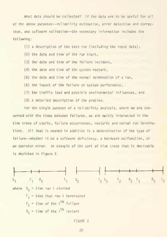
For the single purpose of a reliability analysis, where we are con-

cerned with the times between failures, we are mainly interested in the

time trace of starts, failure occurrences, restarts and normal run termina-

tions. All that is needed in addition is a determination of the type of

fai lure--whether it be a software deficiency, a hardware malfunction, or

an operator error. An example of the sort of time trace that is desirable

is depicted in Figure 2.

I-H—I-

T S'2 3

H h

F2

R2

F3

R3

T3

where S- = time run i started

T. = time that run i terminated

F. = time of the i failure

R. = time of the i restart

FIGURE 2

20

The following information can be constructed from a time trace:

(1) the distribution of the time between failures,

(2) the mean time between failures,

(3) the probability of operation for a given interval of time

without failure,

(4) the mean time to restore,

(5) the probability of a successful run, and

(6) software availability.

Since we define software reliability as the probability of a failure-free

run for a given time interval when data are times between failures, this

information is exactly what we are interested in.

In some cases we may wish to ignore some of the characteristics of

the data and use it solely to classify a given test as a success or a fail-

ure. This may be necessary if it is too costly to install automatic re-

cording equipment, or if it is impractical to have an observer make the

continuous observations required to provide a time trace. We then must be

satisfied with simply counting the number of failures at the ends of discrete

periods of time or to count the number of failures in a given number of test

runs

.

The remainder of the information that we record is that needed to vali-

date the software and to classify, detect and correct errors. When collecting

data, we must keep in* mind that any information that would enable a programmer

to recreate the problem, to locate the cause of the problem or to correct the

problem should be provided. This requires a complete description of the test

run, the manner in which the problem was manifest and the impact of the pro-

blem on system performance. A statement about the recovery or bypass procedures

21

and a computer core dump would also be useful for the subsequent examination

and corrective action that must take place. The failure report should be

followed by a supplementary report of the remedial action that was taken to

patch the program. The documentation associated with a given failure should

be considered complete only after the remedial action report has been issued

We have implied that failure data are useful for debugging the soft-

ware, for validating the software and for estimating software reliability.

We concentrate on the latter item in the next chapter. Several mathematical

models for software reliability are presented, some of which require quanti-

tative data and some which require only qualitative data.

22

IV. MATHEMATICAL MODELS

4.1 Introduction

Quantitative criteria are needed to assess the duality of software.

We have remarked that the software failure data provide the most important

indication about the duality of the software. It is rarely, if ever, the

case that any large complex software, subsystem is completely debugged.

Therefore, the strongest statement that can usually be made is a statement

about the probability of a failure-free operation - a reliability statement.

In this chapter we present several mathematical models, each of which

attemnts to provide an estimate of the reliability of the software sybsystem,

In most cases reliability specifications for the total system are

established in advance of software development. Sometimes the software

subsystem reliability specification is stated explicitly; other times

it must be determined from the overall system reouirement. In all cases,

it is handy to have some reliability specification against which to measure

progress and to determine test reouirements . We must have some realistic

goal to shoot for so that we can judge when the software is of sufficient

duality to allow user access. The difference between the attained re-

liability and the reliability objective should be the feedback information

which is used to determine the extent of the testing which must follow.

Because of the magnitude and complexity of some software sub-

systems it mav be desirable to apportion the software reliability specifica-

tion into module or nrocess reliability reouirements. There is a relatively

well developed theory for the reliability apportionment with regard to

hardware, but, as yet, little work in this area has been done with soft-

ware. We do not address the nroblem of reliability apportionment, nor do

23

we comment about what the reliability specification should be. These are

imnortant areas which depend primarily on the user's needs, the criticality

of the system and economic considerations. We will assume that explicit

nrovisions for software reliability have been established.

In the work that follows we assume that the software development

is at a noint where configuration control has been instituted so that

all subseouent changes incorporated into the software must be formally

approved and documented. This should occur by the time that the processes

are integrated to form the software subsystem. During earlier stages the

failure behavior of software will probably be so erratic that no meaningful

mathematical model could be developed. For the purpose of predicting

operational reliability, the appropriate stage of testing over which

failure data should be collected is the period of actual system operation.

However, reliability estimation is needed prior to that stage so that

nroaress can be measured and test criteria established.

We make no distinction between software failures as to criticality.

Certainly, a failure which yields the system inoperable is more important

than one which merely causes a nuisance. Nevertheless, classification

of software failures according to severity reauires, to a large degree,

a subjective assessment. We prefer to restrict our attention to the

problem of estimating reliability where all failures are weighted eaually.

If failures were classified as to severity, nothing would prevent one

from using the models that we present for the case where a software failure

has been redefined to include only those failures of a given criticality

or worse.

24

The primary data that we reouire is the time trace of software

operation discussed in the previous chapter. In some cases the actual

times between failures will not be necessary. Instead, qualitative data

such as "success" or "failure" may suffice.

We assume that the reader has some familiarity with the terminology

used in reliability analysis. Consequently , many standard reliability

terms will be used without definition or elaboration. A review of the

basic theory of reliability is presented in ADpendix A.

4.2 A Hardware-Oriented Approach

We consider first an approach towards developing procedures for

estimating software reliability which borrows heavily from the techniques

of hardware reliability analysis. It is natural that we should try to

exploit the vast reservoir of reliability theory already well established

and validated for hardware systems (especially since we have observed

analogies between software and hardware failures). When applied to

software, many of the ideas of hardware reliability theory carry over

without change. There are, however, some differences which reouire that

some caution be taken. For example, we have already discussed the

differences in the nature in which we speak of the random occurrence of

failures. Furthermore, unlike hardware, there is no degradation of

software due to age. If all bugs were removed from the software, it

would have a reliability of one thereafter. Finally, because of the

debugging that takes place as failures occur and errors are detected,

there is a natural reliability growth that accompanies testing and

operation. This reliability growth results in changes in the dis-

tribution of times between failure and conseauently changes in the

25

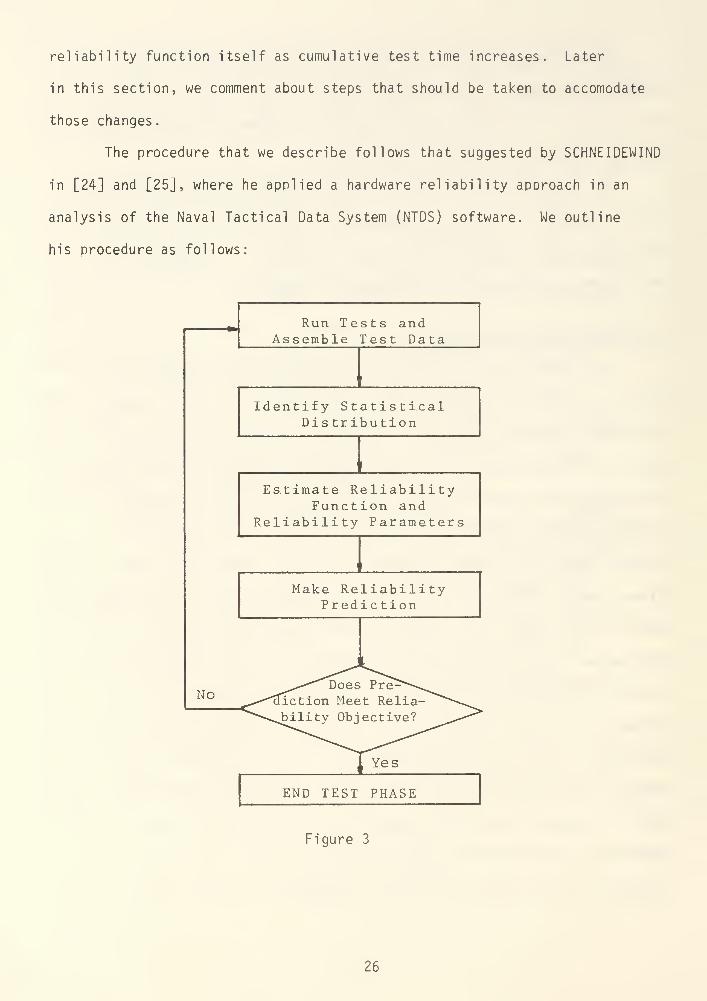
reliability function itself as cumulative test time increases. Later

in this section, we comment about steps that should be taken to accomodate

those changes.

The procedure that we describe follows that suggested by SCHNEIDEWIND

in [24] and [25], where he applied a hardware reliability approach in an

analysis of the Naval Tactical Data System (NTDS) software. We outline

his procedure as follows:

Run Tests andAssemble Test Data

'

f

Identify StatisticalDis tr ibution

'

1

Estimate ReliabilityFunction and

Reliability Parameters

1

Make ReliabilityPrediction

No^,—"Does

^^"cfiction MeePre^-^^

t Relia-^^\^lility Objective'

Yes

Figure 3

26

As indicated by Figure 3, the first step is to run tests and assemble

the failure data. The failures must be classified as to cause; whether they

be operator, hardware, software or unknown. In addition, if there is to be

a distinction as to severity, the software troubles are to be divided into

groups according to criticality. This step yields a set (or several sets)

of times at which software failures were observed, say A = {t , t ,...,t }

(or, A. = {t.-J

,t-2

,. . . ,t. } for each level of severity i ) .

For the identification phase of the procedure, the reliability analyst

relies on theoretical principles, physical considerations, and previous ex-

periments to rationalize the nature of software failures. Furthermore, the

analyst should arm himself with plots of various empirical functions to

provide clues as to the type of probability functions that might be appro-

priate. The shapes of the relative frequency function for the times between

failures, the empirical reliability function and the empirical failure rate

function, combined with the theoretical considerations and studies of fail-

ures of other software, should suggest an hypothesis about the theoretical

reliability function. That hypothesis must then withstand further statisti-

cal examination. (For a good discussion of the empirical functions, the

reader is directed to GiMEDENKO [9, pp. 78-95].)

Once the analyst has formulated an hypothesis about the reliability

function, or, equivalantly , the probability density of time between failures

or the failure rate function, he must then obtain estimates for the para-

meters of the appropriate functions. For example, if the exponential law,

R(t) = exp(-at) , is suggested, the analyst must obtain an estimate of the

single parameter a . In other cases like the Weibull law, he may have to

27

estimate two or more parameters. He is thus led to consider the basic

oroblems of mathematical statistics: (1) the estimation of the values of

unknown distribution parameters and (2) the verification of statistical

hypotheses. The statistical techniaues reauired to solve these problems

can be found in most books on statistical inference or in reliability

books such as LLOYD and LIPOW [15] or GNEDENKO [9].

Once the parameters have been estimated, a test of the hypothesis

is performed. The Kolmogorov-Smirnov (K-S) test is one of the simpler

and more powerful tests that can be employed to measure the goodness of

fit of the assumed theoretical distribution to the empirical distribution.

If the hypothesis is not rejected by the statistical test, the analyst

then proceeds to estimate the reliability function and to make a prediction

of the software reliability. On the other hand, if the hypothesis is

rejected, another is formulated, and the procedure is repeated.

The "acceptance" of the hypothesis completely determines the

reliability function, for the reliability parameters ) will have already

been obtained. Because statistical estimates of the unknown parameter(s)

are being used, the reliability analyst should provide a confidence interval

for the value(s) of the narameter(s) of the reliability function. To be

conservative, the lower confidence limit on the reliability function

should be utilized in the reliability predictions. On comparing the

predicted reliability with the specified or desired reliability, the analyst

determines whether additional testing and debugging is reauired. The

magnitude of the difference between predicted and specified values should

serve as an indicator about the extent of additional testing (see, for

example, SCHNEIDEWIND [26]).

28

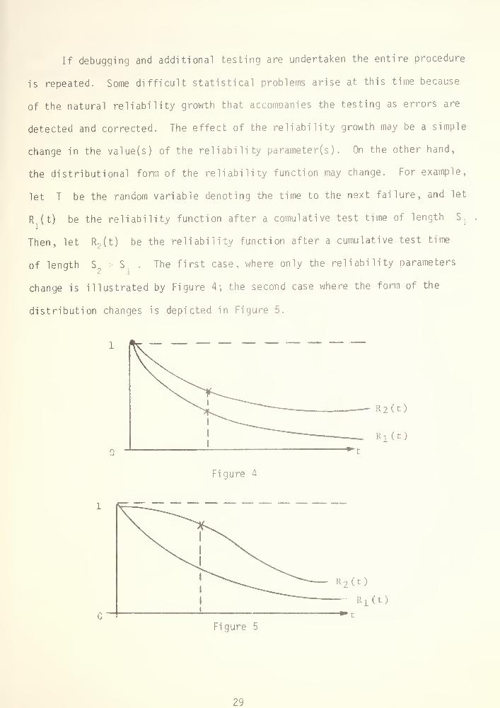
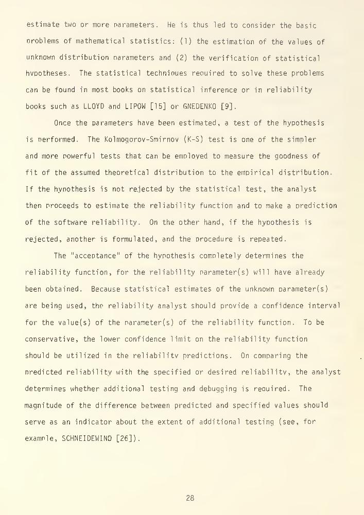
If debugging and additional testing are undertaken the entire procedure

is repeated. Some difficult statistical problems arise at this time because

of the natural reliability growth that accompanies the testing as errors are

detected and corrected. The effect of the reliability growth may be a simple

change in the value(s) of the reliability parameter(s) . On the other hand,

the distributional form of the reliability function may change. For example,

let T be the random variable denoting the time to the next failure, and let

R (t) be the reliability function after a comulative test time of length Sj

Then, let R2(t) be the reliability function after a cumulative test time

of length S S . The first case, where only the reliability parametersJ 2 [

change is illustrated by Figure 4; the second case where the form of the

distribution changes is depicted in Figure 5.

Figure 4

Figure 5

29

In both figures we observe that the reliability has grown, i.e. R2(t) > R-(t)

for all t . This is certainly the objective of additional testing, but the

growth does make the problem of estimating reliability more difficult. The

difficulty arises when the analyst tries to determine what data is to be

used as a basis for the estimation of the "new" reliability function. Because

of the changes with respect to cumulative test time, some of the data set

will probably not be representative of the current state of the process

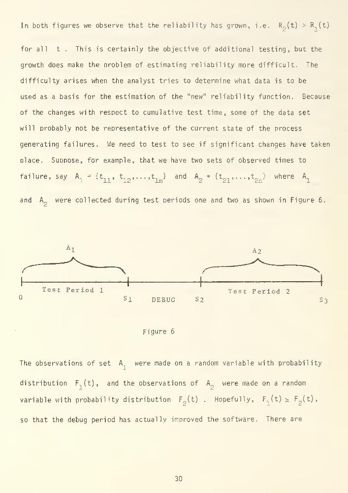
generating failures. Vie need to test to see if significant changes have taken

place. Suppose, for example, that we have two sets of observed times to

failure, say A_L

= {t^, t12

>---> tim

} and A2

= ^21" " * ft2x?where A

i

and A were collected during test periods one and two as shown in Figure 6.

A 2

Test Period 1

Si DEBUG S2Test Period 2

S3

Figure 6

The observations of set A were made on a random variable with probability

distribution F (t), and the observations of A were made on a random

variable with probability distribution F2(t) . Hopefully, F

1(t) s F

?(t),

so that the debug period has actually improved the software. There are

30

several easy-to-apply statistical tests that can be used to test the

hypothesis that no improvement has taken place; i.e.,

HQ

: F^t) = F2(t)

against the alternative

Ha

: F1U) a F

2(t)

The nonparametric tests such as the sign tests, Wilcoxon's test and Smirnov's

test are all useful for testing the given hypothesis.

If the statistical tests fail to reject the hypothesis that F (t) = F (t),

all the data can be pooled together to obtain our revised estimate of reliability.

*

However, if there are indications that a change has indeed taken place, we

certainly want to weight the latest data more heavily. If the earlier data are

ignored entirely, the result is a reduced sample size. On the other hand,

if nonrepresentative data areused the resultant reliability predictor may

not be accurate. Research is needed in the area of developing smoothing

techniques for weighting the different sets of failure data.

When the reliability function is revised and the reliability pre-

diction is updated, the prediction is again compared with the desired reliability.

This procedure continues until the predicted reliability reaches the specified

value.

Based on its application to NTDS data, the "hardware-oriented" reliability

approach described in this section appears feasible, (see SCHNEIDEWIND [24].)

31

However, the methodology reauires validation against other sets of data

before any general conclusions about the apnroach can be made.

4.3 Error-Counting Models

In the preceding section we pointed out some difficulties which result

from the possible non-homogeneous (time variant) nature of the data collected

over different test periods as software errors are detected and removed. What

is needed is a mathematical model for software reliability which is tailored to

the SDecial characteristics of software failures and which exDlicitly accounts

for the natural growth of software reliability as a function of cumulative

test time. The models presented in this section attempt to fill this need.

Assume that the total number of errors in the software program at the

start of the test period (preferably the integration test period) decreases

directly as errors are corrected. If the cumulative number of errors cor-

rected during debugging is recorded, then the number of remaining errors is

simply the difference between the initial number of errors and the number

corrected. This assumes that no new errors are introduced during debugging.

Let N be the (unknown) initial error count, d the cumulative debugging

time since the start of the test, C(d) the total number of errors corrected

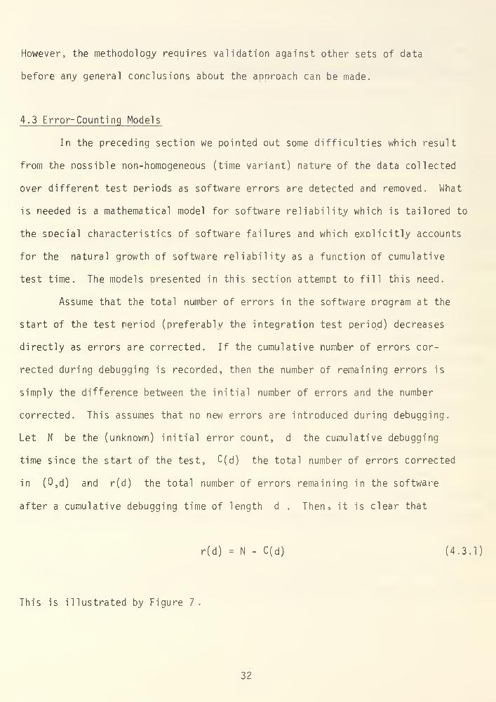
in (0,d) and r(d) the total number of errors remaining in the software

after a cumulative debugging time of length d . Then, it is clear that

r(d) = N - C(d) (4.3.1)

This is illustrated by Figure 7.

32

N

Errors

Debug t ime

ERROR MODEL

Figure 7

33

The reliability model that we present is basically that developed by

both SHOOMAN [27], [28] and JELENSKI and MORANDA [10]. Their models assume

that the probability of an error being encountered in a small interval of time

of length At after t hours of successful operation (the failure rate

Z,(t)) is proportional to the number of remaining errors. Mathematically,d

Zd(t) = K • r(d) (4.3.2)

for some constant of proportionality K . The proportionality constant may

vary from program to program depending perhaps on such factors as the total

number of machine language instructions, the rate of processing instructions,

the software structure and/or the type of test procedure.

We can then write the reliability function (see Appendix) as

t

R(t) = exp( - / Z (X)dX) (4.3.3)

On substituting (4.3.1) and (4.3.2) into (4.3.3) and writing the reliability

function as R(t,d) to indicate its dependence on both t and the debug

time d , we get

R(t,d) = exp( -K(N - C(d)t) (4.3.4)

34

We note that (4.3.4) is the exponential reliability model with reliability

parameter a(d) = K(N - C(d)) . Conseauently , the mean time between failures

(as a function of d ) is

MTBF(d) = l/a(d) = 1/K(N - C(d)) (4.3.5)

Since C(d) is assumed known, we must determine only the constants K and

N.

Using the approach of SHOOMAN [28], suppose that out of n total test

runs there are s successful runs and n - s unsuccessful runs. Let T, , T_,...,T1 d s

represent the hours of success for the s successful runs and t_ , t ,...,t1 d n-s

the run hours before failure for the n-s unsuccessful runs. Then the

cumulative run hours is

s n-sH = I T. + It.

1=1 1=1

An estimate of the mean time between failures is then obtained from

the ratio of total run hours to the number of failures

MTBF = 1/a = H/(n-s) (4.3.6)

35

The unknown constants N and K can be evaluated by looking at the

estimate (4.3.6) after two different debugging times d < d chosen so

that C(d ) < C(d ) . Using the method of moments, we eauate (4.3.6) for

debug times d and d to get:

H1/X

1= 1/^ = 1/K(N - C(d

i)) (4.3.7)

and

H2/X

2= 1/S

2= 1/K(N - C(d

2)) (4.3.8)

where X and X are the number of software failures detected in H and

H hours, respectively, of total run time. The ratio of (4.3.7) to (4.3.8)

gives an estimate of N :

•\ /\

N = (a2

C(d1

) - a1C(d

2))/(a

2- a

J

(4.3.9)

We can then obtain an estimate of K by substituting (4.3.9) into (4.3.8)

This gives

/s nK = a

2/(N - C(d

2)) (4.3.10)

The "hats" above the parameters a, N and K indicate that they are

estimates of the parameters. The estimates (4.3.9) and (4.3.10) are simple

functions of the cumulative errors corrected and the sample means 1/a,

and l/a2

. However, the statistical properties of estimates obtained

36

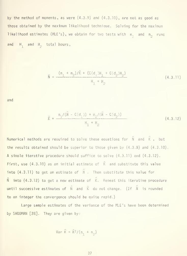
by the method of moments, as were (4.3.9) and (4.3.10), are not as good as

those obtained by the maximum likelihood technique. Solving for the maximum

likelihood estimates (MLE's), we obtain for two tests with n and n runs

and H and H total hours,

(n + n?)/K + (C(d

n)H

n+ C(d

p )HjN = ± i l_l 2_2_

(4.3.11)H1

+ H2

and

n./(N - C(d_)) + n_/(N - C(O)K = —

-

- (4.3.12)H1

+ H2

Numerical methods are reouired to solve these eouations for N and K , but

the results obtained should be superior to those given by (4.3.9) and (4.3.10).

A single iterative procedure should suffice to solve (4.3.11) and (4.3.12).

First, use (4.3.10) as an initial estimate of K and substitute this value

into (4.3.11) to get an estimate of N . Then substitute this value for

/\ ^

N into (4.3.12) to get a new estimate of K. Repeat this iterative procedure

until successive estimates of N and K do not change. (If N is rounded

to an integer the convergence should be quite rapid.)

Large sample estimates of the variance of the MLE's have been determined

by SH00MAN [28]. They are given by:

Var K = K 2 /(n1

+ ng

)

37

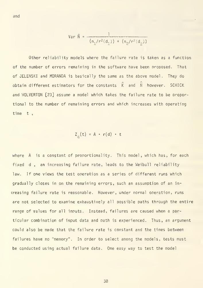
and

Var N = ! —

-

(n1/r 2 (d

1)) + (n

2/r 2 (d ))

Other reliability models where the failure rate is taken as a function

of the number of errors remaining in the software have been proposed. That

of JELENSKI and MORANDA is basically the same as the above model. They do

obtain different estimators for the constants K and N however. SCHICK

and WOLVERTON [23] assume a model which takes the failure rate to be propor-

tional to the number of remaining errors and which increases with operating

time t ,

Z (t) = A • r(d) • t

where A is a constant of proportionality. This model, which has, for each

fixed d , an increasing failure rate, leads to the Weibull reliability

law. If one views the test operation as a series of different runs which

gradually closes in on the remaining errors, such an assumption of an in-

creasing failure rate is reasonable. However, under normal operation, runs

are not selected to examine exhaustively all possible paths through the entire

range of values for all inputs. Instead, failures are caused when a par-

ticular combination of input data and oath is experienced. Thus, an argument

could also be made that the failure rate is constant and the times between

failures have no "memory". In order to select among the models, tests must

be conducted using actual failure data. One easy way to test the model

38

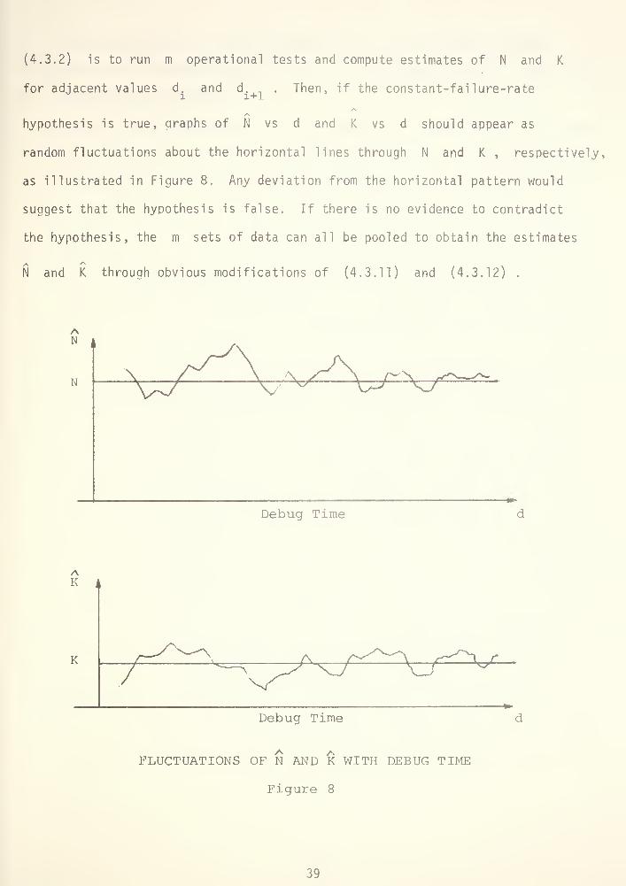
(4.3.2) is to run m operational tests and compute estimates of N and K

for adjacent values d. and d. in . Then, if the constant-failure-ratei 1+1

hypothesis is true, graphs of N vs d and K vs d should appear as

random fluctuations about the horizontal lines through N and K , respectively,

as illustrated in Figure 8. Any deviation from the horizontal pattern would

suggest that the hypothesis is false. If there is no evidence to contradict

the hypothesis, the m sets of data can all be pooled to obtain the estimates

N and K through obvious modifications of (4.3.11) and (4.3.12) .

AK k

K

Debug Time

Debug Time

FLUCTUATIONS OF N AND K WITH DEBUG TIME

Figure 8

39

Implicit in Model (4.3.4) is the assumption that all time periods of

equal length represent equal intensities of testing and debuggino. In reality,

this is rarely the case because of varying manpower assignments and different

types of testing. JELENSKI and MORANDA [10] and SH00MAN [27] offer refinements

to the basic model to adjust for unequal intensities of testing and debugging.

Their refinements require basically that the previous results be normalized

with respect to manpower and that the time to failure observations be nor-

malized to account for variable exposure rates. The refinements may improve

on the basic model, but, for the most part, the additional data required are

just not available. Consequently, their implementation would require a great

deal of subjectivity by some decision maker.

4.4 An Error-Seeding Model

The preceding reliability models rely strongly on the estimation of

the number of errors remaining in the computer program after various stages

of the testing process. MILLS [19] suggests a rather novel approach for

estimating that quantity. He proposes that software errors be intentionally

introduced at random into a program. The "seeded" errors would then be used

to calibrate the testing process and to estimate the number of remaining

"indiaenous" errors. Althouah it may seem a paradox to introduce errors in

an effort to remove eventually all indigenous errors, such a procedure does

have a firm statistical basis.

Suppose that the software contains n. indigenous errors, and

n errors (seeded errors) are deliberately inserted randomly into the software.

Suppose, further, that a testing process to find and remove errors is undertaken

and that each remaining error - indigenous or seeded - is equally likely to

40

be discovered at any point of the testing process. Then, after removing a

total of r errors, the probability that s are seeded errors and r - s

are indigenous errors is given by

/n. + n,

q (n. + n ) = — £^

—

(4.4.1)s 1 s

'/ n . + n

for s <. n and r <, n. + n . The problem is that n. is unknown.S 1 S r

1

Let us now see how the probabilities (4.4.1) can be used to give a

simple estimate of n. . First, intuitively, it seems logical that the ratio

of r - s to s should be approximately the same as the ratio of n. to

n because of the assumption that errors are equally likely to be discovered

That is,

r-s q, _is n

s

or n. ^ III . n (4.4.2)

FELLER [6] provides statistical support for the estimate (4.4.2). He shows

that the maximum likelihood estimate of n. is the integer part of (4.4.2)

That is,

\ - [^ • nB] (4.4.3)

41

Example: Suppose that 100 errors are inserted into the software and, in

the ensuing testing, 15 errors, consisting of 10 seeded errors and 5 in-

digenous errors, are found. Then n = 100 , s = 10 and r = 15 . The

maximum likelihood estimate of n. is

ni

= [IT^ ' 100] = 50

Being only a statistical estimate, the actual number of indigenous errors

may be more or less than 50. We can test the hypothesis H • n. = 50

against the alternative that n. > 50 by using the probability function

(4.4.1) . We would want to reject H only if the number of seeded errors

among the 15 discovered errors were "too small." For example, suppose the

15 discovered errors included only five seeded errors. Then, assuming H

is true, the probability of obtaining five or fewer seeded errors is given

by,

p = q (150) + qjOSO) + ... + q (150)

The probability p is difficult to calculate exactly, but, using the binomial

approximation, we find that p is approximately 0.01 . With such a small

probability, we would be inclined to believe that the number of indigenous

errors is larger than 50.

42

In the example, we see that we can obtain the MLE for the number

of indigenous errors, and we can also use the probability function (4.4.1)

to test hypotheses about the magnitude of n. . The test of hypothesis is

complicated, however, by the mathematical difficulties experienced when working

with (4.4.1) . The binomial or normal approximations are only good when

r is small compared to n. + n , but in cases of practical interest we would

like that r be nearly as large as n. + n . Consequently, other procedures

for testing the hypothesis about the number of indigenous errors are desirable.

MILLS discusses a simple procedure for testing the hypothesis that the

number of indigenous errors is less than or equal to k . We outline his

procedure, called the Assert, Insert and Test (AIT) process .

(1) Assert that n. <: k .v

i

(2) Insert n seeded errors.s

(3) Test until all n seeded errors are found and record thes

number of indigenous errors found, say i .

(4) Compute C(n ,k)> the confidence with which the assertion

n. ^ k is rejected, as

if i > k

C(n ,k) =s

ns

I n + k + 1 if i £ ks

(4.4.4)

The confidence C(n ,k) is the probability that an AIT process will correctly

reject a false assertion and is conservative in the sense that C(n ,k) is the

43

powe r of the test evaluated at n. = k + 1 . On observing (4.4.4) it is

obvious that our confidence increases with larger values of n and decreases

with increasing values of k . This is illustrated in Table 1 .

\ks \ 1 2 3 4

1 .50 .33 .25 .20 .17

2 .67 .50 .40 .33 .29

3 .75 .60 .50 .43 .38

4 .80 .67 .57 .50 .46

5 .83 .71 .62 .56 .50

10 .91 .83 .77 .71 .67

AIT Confidence (i <; k)

Table 1

44

MILLS suagests that an AIT chart be maintained to provide a visual

progress report. The chart gives a chronological record of both the maximum

likelihood estimate of the number of indigenous errors and the actual number

of indiaenous errors found. The example below illustrates an AIT chart.

Suppose that the null hypothesis (assertion) is HQ

: n. = 4 and

8 errors are seeded Then, if the number of indigenous errors found is greater

than 4 (the total number of errors found is greater than ns

+ k = 12), HQ

can

be rejected with certainty. Let us now suppose that the AIT process produces

the fullowing sequence of errors: S, S, I, S, S, I, I, S, S, S, S where S

represents a seeded error and I an indigenous error. The AIT chart for this

test is shown below.

6 -I

n-

3 -

2 _

1 -

ERROR

AIT Chart (ns= 8, k = 4, Confidence = 0.62)

Figure 9

45

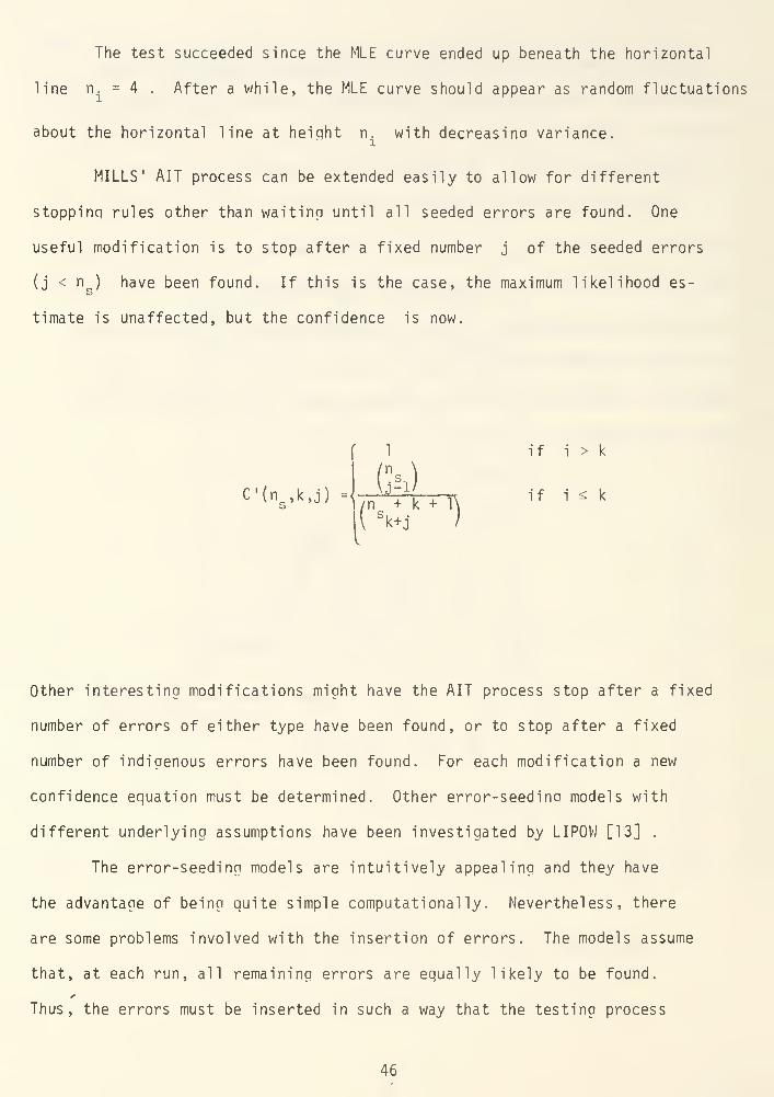
The test succeeded since the MLE curve ended up beneath the horizontal

line n. = 4 . After a while, the MLE curve should appear as random fluctuations

about the horizontal line at heiqht n. with decreasina variance.i

MILLS' AIT process can be extended easily to allow for different

stoppinq rules other than waitinp until all seeded errors are found. One

useful modification is to stop after a fixed number j of the seeded errors

(j < n ) have been found. If this is the case, the maximum likelihood es-

timate is unaffected, but the confidence is now.

i1

C'(ns,k,j) ={

(a)7n + k + 1\

(

sk+j )

if i > k

if i ^ k

Other interesting modifications might have the AIT process stop after a fixed

number of errors of either type have been found, or to stop after a fixed

number of indigenous errors have been found. For each modification a new

confidence equation must be determined. Other error-seedina models with

different underlying assumptions have been investigated by LIPOW [13] .

The error-seeding models are intuitively appealing and they have

the advantage of being quite simple computationally. Nevertheless, there

are some problems involved with the insertion of errors. The models assume

that, at each run, all remaining errors are equally likely to be found.

Thus, the errors must be inserted in such a way that the testing process

46

is not biased toward either the seeded errors or the indigenous errors. This

is a nontrivial problem in itself because the nature of the indigenous errors

is unknown. If substantive error data existed the seeded errors could be set

to reflect actual experience. Much research must be done before a methodology

for introducing software errors satisfying the assumptions of the error-

seeding model can be developed. If that problem can be solved, the error-

seedina program offers a powerful tool for validating computer programs.

4.5 A Simple Reliability Model for Qualitative Data

Up to this point we have assumed that data are in the form of times

between failures. Occasionally the data is not of that type, or the time-to-

failure data (quantitative data) has been used solely for the purpose of

classifying a test run as a success or a failure. Such a classification may

be necessary because the form of the mathematical model which describes times-

to-failureis unknown or intractable. Another reason may be that it is costly

or simply not feasible to install the recording equipment or hire observers

to monitor the software continuously as needed to obtain the variable data.

Thus, we may have to be satisfied with counting the number of failures in

a given number of test runs or the number of failures during test intervals

of a given length of time.

If we are reasonably confident that the quantitative data follow a

known, simple, mathematical form, we should use the quantitative data for

estimating reliability. The quantitative data allow for more precise ob-

servation and make more efficient use of the information available. This

efficient use of data is of increasing importance as experimentation becomes

more and more costly. Nevertheless, if the quantitative data is not available,

we must make do with what we can get. Reliability can still be demonstrated when

47

qualitative data is used. Suppose, for example, that the required failure-

free time of operation is T and several runs are made for T units of time

noting only whether each run was a success or a failure. Then, the simple

binomial distribution can be used to estimate the reliability. Other reliability

models depending on qualitative data will be described in this section.

We allow some flexibility in the classification of a run as a success

or a failure. A success may mean zero software failures of any type; it may

mean no software failures of a given critical ity or worse; it may mean that

the total number of failures is not greater than some given number; or it

may be taken to mean whatever the user desires. We assume that the user

has settled on a definition of success and on a definition of "test run".

We now describe some reliability models which make use of qualitative

data. They are somewhat heuristic models which, in some cases, require a

subjective assessment of the test runs. First, we describe a ^jery general

model proposed by Mac WILLIAMS [17] . Then we look at some special cases.

Suppose that N test runs are conducted and let n. be the number

of failures observed in test i . Let E.(n.) be a measure of the performance11 r

f"h

durina the i test and let W.(n.) be a weiohtino factor which reflects11+ h

seriousness of the errors observed in the i test. We require that

and

£ E.(n.) ^ 1 , E (0) = 1

< W.(n.) <; 1 , W.(0) = 1ii i

(4.5.1)

48

and we take

i

N

R = A I E (n .) • W.(n.) (4.5.2)

to be an estimate of the reliability.

If we take E.(n) = for all n > and W.(n) =1 for n * ,

we obtain the special case where reliability is estimated to be the frac-

tion of successful runs. For example, if in 100 test runs 85 were successful,

we would estimate the reliability to be R = 0.85 .

As another example, suppose that failures have been classified according

to severity as low, medium and high. Let E.(n.) = 1 for all n. , and

let the weights given to low, medium and high severity errors be 0.9, 0.1

and respectively. Define W.(n.) to be the product of the weights assigned

to the n. errors and W.(0) = 1 . For example, if test i results in

2 low severity errors and 1 medium severity error, then n. = 3 and

W.(n.j) = (0.9)(0.9)(0.1) = .081 . In this case the reliability model (4.5.2)

lets the user weight errors according to their impact on the performance of

the software.

The flexibility of (4.5.2) makes it particularly attractive. Test

personnel are not "locked" into complete objectivity. Instead, they are

allowed to interject their subjective assessment of software performance.

This allows personnel to adapt the model to their particular needs. The

model (4.5.2) could even be used when quantitative data are available if

49

it were desirable to weinht subjectively the quality of each test run

in a series of runs.

4.6 A Reliability Growth Model for Qualitative Data

The reliability qrowth model (4.3.4) which utilized times-to-failure

data allowed us to account for the natural growth of reliability that takes

place as errors are detected and corrected. We now discuss a model which

relies on qualitative data and which explicitly accounts for the reliability

growth. The model is one developed for hardware systems by BARLOW and

SCHEUER [1 ], but it appears to be adaptable to software.

We consider a trial to be a test run of length T . Imagine a testing

J. L.

program which consists of K stages with n. trials at the i stage.

Both K and the n. 's are completely arbitrary, therefore, no control over

the length of a sampling interval is required. Each trial is considered to

be a success or a failure. At the end of each of the k stages, an effort

is made to determine the cause of each failure and to correct the software

so that the failure will not reoccur. We allow for the possibility that

the causes of some failures may escape our detection. Consequently, those

failures might reappear. Using the terminology of BARLOW and SCHEUER, we

classify failures as "assignable-cause" or "inherent" failures depending

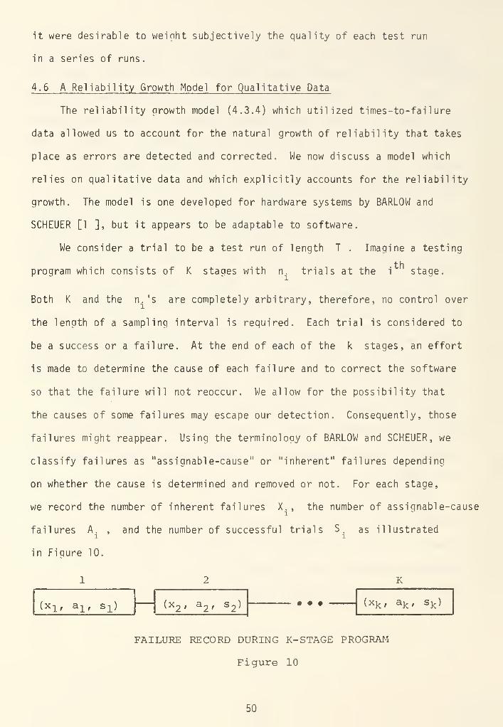
on whether the cause is determined and removed or not. For each stage,

we record the number of inherent failures X., the number of assignable-cause

failures A. , and the number of successful trials S. as illustratedi i

in Figure 10.

(x x , alf s±) \ X^ r 3.-j iS ^ ;

K

Uk , ak , sk )

FAILURE RECORD DURING K-STAGE PROGRAM

Figure 10

50

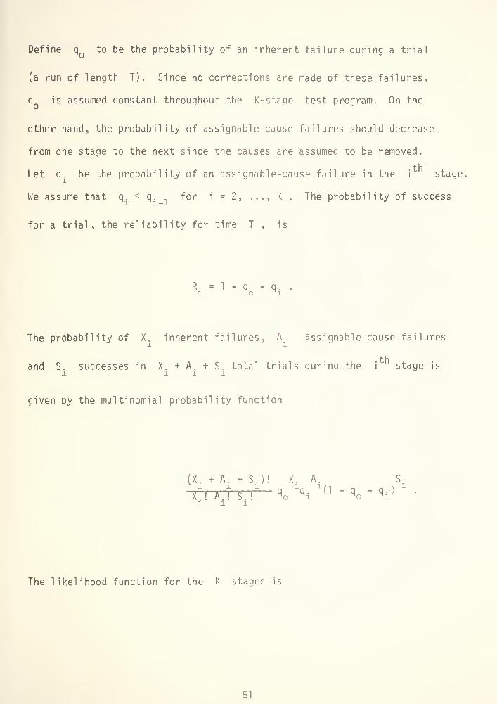
Define q to be the probability of an inherent failure during a trial

(a run of length T) . Since no corrections are made of these failures,

q is assumed constant throughout the K-stage test program. On the

other hand, the probability of assignable-cause failures should decrease

from one stage to the next since the causes are assumed to be removed.

Let q. be the probability of an assignable-cause failure in the i stage

We assume that q. ^ q for i = 2, ..., K . The probability of success

for a trial, the reliability for time T , is

R. = 1 - q - q. .

1no n

i

The probability of X. inherent failures, A. assignable-cause failures

+ h

and S. successes in X. + A. + S. total trials durina the i stage isi ill

given by the multinomial probability function

(X. + A. + S.)! X. A. S.1 1 1 1„ 1/1 n « N 1

X.! A,! S.! q o \ (1 " q o " q i}

'

The likelihood function for the K stanes is

51

L(X . A. S ;...;XKi AK

. S,)

K (X + A + S )! X As

From (4.6,1) the maximum likelihood estimators of qn

and q. are easily

shown to be

K K

6 = [ X./ j (X. + A. + S.) (4.6.2)i = l

1i = l

]"•

'

and

q. = (1 - q )A./(A. + S.) (4.6.3)H ^0 111

for i = 1, 2,... , K .

Instead of the estimates q. we want the maximum likelihood estimates of

th e q. 's subject to the restriction that q ^ q„ ^ . . . s: q^ . Let q.

be the MLE of q. subject to this condition. Then, BARLOW and SCHEUER

show that

A +. . .+ A

q .= (1 - q ) max min -j^^j-^^i (A + ^j (4.6.4)

u z i r <; lv

r r vu u'

52

Equation (4.6.4) gives an explicit expression for q. . However, in

practice one would probably want to determine the q". 's using the following

equivalent procedure. If q ^ q s . . . ;> q then q~. = q . for i = 1, 2,

. .., K . If q. < q 4j _ for some j , then combine the observations inJ J +1

the j and (j + 1) stages and compute the NILE of the q.'s by

(4.6.3) for the K - 1 stages thus formed. Continue this procedure until

the estimates of the q.'s form a non-increasing sequence. These estimates

are the maximum likelihood estimates of the q.'s subject to q n s q~ ;>

i 1 2

...* qK •

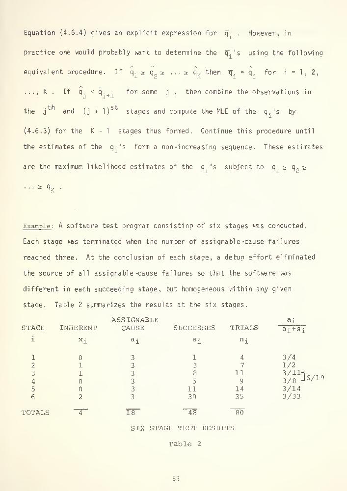
Example : A software test program consisting of six stages was conducted.

Each stage was terminated when the number of assignable-cause failures

reached three. At the conclusion of each stage, a debug effort eliminated

the source of all assignable -cause failures so that the software was

different in each succeeding stage, but homogeneous within any given

staqe. Table 2 summarizes the results at the six staqes.

INHERENTASSIGNABLE

CAUSE SUCCESSES TRIALSai

STAGE a i +s i

i xi a i s i ni

1

2

3

4

5

6

1

1

2

3

3

3

3

3

3

1

3

8

5

1130

4

7

119

1435

3/41/2

3/143/33

TOTALS 4 18 Tr 80

SIX STAGE TEST RESULTS

Table 2

53

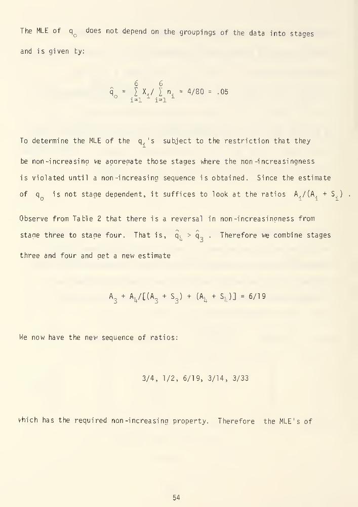
The MLE of q Qdoes not depend on the groupings of the data into stages

and i s given by:

6 6

q o- I X / I n = 4/80 = .05

i=l i=l

To determine the MLE of the q.'s subject to the restriction that they

be non -increasing we agaregate those stages where the non -increasingness

is violated until a non -increasing sequence is obtained. Since the estimate

of q is not staae dependent, it suffices to look at the ratios A. /(A. + S.)^0 r 111Observe from Table 2 that there is a reversal in non-increasingness from

staae three to stage four. That is, q, > q . Therefore we combine stages

three and four and aet a new estimate

A + AU/[(A + S ) + (A

u+ S

u)] = 6/19

We now have the new sequence of ratios:

3/4, 1/2, 6/19, 3/14, 3/33

which has the required non -increasing property. Therefore the MLE's of

54

the q-'s , subject to the non-increasinn condition, are

q^ = (.95)(3/4) = .713 q^ = (.95)(6/19) = .300

q"

2= (.95)0/2) = .475 q

5= (.95)(3/14) = .202

q"

3= (.95)(6/19) = .300 q 6

= (.95) (3/33) = .086

The MLE of the reliability of the software in its last test stage is

R6

1 - qo- q 6

= 0.864

If all test staces were incorrectly assumed to be homogeneous and all

data pooled together, the estimate of reliability, makina no distinction

between assianable-cause failure and inherent failure, vould be

6 6

K = I S./ [ n. = 48/80 = 0.60i=l i=l

We see that consideration of the reliability growth has a substantial

impact on the estimate of reliability.

55

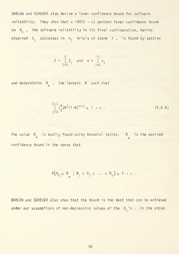
BARLOW and SCHEUER also derive a lower confidence bound for software

reliability. They show that a 100(1 -a) percent lower confidence bound

on R.. , the software reliability in its final configuration, havina

observed S. successes in n. trials at staoe i , is found by settinoi i

- J -

K KS = y S. and n = 7 n..i u

i=l i=l

and determinino R , the larqest R such that

I (")R j (l-R)n" j * 1 -a . (4.6.6)

The value R is easily found using binomial tables. R is the desired* *

confidence bound in the sense that

P[RK

;> R| R s R ss . . . * iy * 1 - a .

BARLOW and SCHEUER also show that the bound is the best that can be achieved

under our assumptions of non -decreasing values of the R.'s . In the a tove

56

examDle, the 95% lower confidence interval for R^ is given by

R = 0.803

In this reliability growth model we have allowed for the possibility

that some errors may go uncorrected. There is, of course, no requirement

that any "inherent" failures occur. Indeed, it is to be expected that most

causes can be determined and the source of the troubles removed. Most

likely, if any inherent errors do exist, they are those rare objects which

are not observed until most assignable-cause errors have been removed.

4.7 Bayesian Reliability Models

We complete our treatment of software reliability models with a brief

discussion of Bayesian reliability models. The Bayesian approach has been

widely used to develop reliability models for hardware systems. The approach

would also seem to be applicable for software reliability.

Suppose we have collected the data t , t , ... , t representing the

times between failures for the first n observed software failures. We

want to make an inference about the distribution of the time to the (n + 1)

f"h

failure. Let the random variable T. be the run time between the (i - 1)

and the i failures and let T. and T. be independent for all i f j .

Let f(t|\(i)) be the probability density function for T. with parameter

A(i) . We write the parameter as a function of i to allow for changes

that may occur as errors are removed. If one supposes that x(i) is a

57

failure-rate parameter and the software is debugged after each failure occurs,

then one would expect that A(i) ;> A(i + 1) (the failure rate is non -increasing)

Let a(ji|i,6) be the probability density function for the random variable

A(i), where 3 is a parameter (or vector of parameters). The Bayesian

approach treats the parameter 3 as though it were a random variable. The

analyst begins with a "prior" distribution for 3 , expressed by the density

function h (3) and then uses the failure data to update the prior and

obtain a "posterior" distribution hA&) . Using the Bayes' Theorem, the

relationship between the prior and the posterior is given by

h1(B) :

J\ J f(t.|A)g(A|i,3)dA • h (3)_ i=± i o

I lit J f(ti|A)g(A|i,3)dA • h

Q(3)]d3

i=l

Ha ving obtained the posterior probability function h (3) , the probability

density function of A(n+1) and T . are then found to beJ ' n+l

g(£|n + 1) = /g(£|n + 1,3)^(3^3

and

58

f(tn+1

|X(n+l)) = / f(tn+1

|£)a(£|n + l)d£

The integrals above (all taken to range over the interval (-°°,

°°) )

appear to be rather awesome mathematically. Indeed, the mathematical

difficulties and the problem of choosing an appropriate prior distribution for

3 have impeded the acceptance of the Bayesian approach. Nevertheless, for

some special cases of practical interest, the mathematics works out quite

nicely. For example, LITTLEWOOD and VERRALL [14] obtain tractable results

for the case

f(t|A) = Ae-At

t >

gU|i,e)^(i)^(iHj e-V* (l)£

r(3)

i > o

£ =

Where ip(i) is assumed to be a known monotonically .increasing function.

(Software repairs are undertaken after each observed failure). Assuming

a uniform prior distribution for 3 , they derive the following:

59

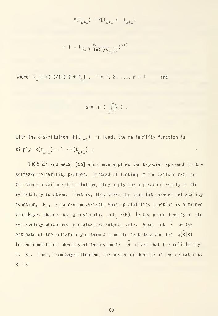
n+1 n+1 n+1

_ -I _ / a N n+1a + ln(l/k j)

*here k. = ^(i)/(ip(i) + t.) , i = 1, 2, ..., n + 1 and

a = In ( ITUi=l

n

"k

i

With the distribution F(t _) in hand, the reliability function isn+1 J

simply R(tn+1

) - 1 - F(tn+1

) .

THOMPSON and WALSH [2 9] also have applied the Bayesian approach to the

software reliability problem. Instead of looking at the failure rate or

the time-to-failure distribution, they apply the approach directly to the

reliability function. That is, they treat the true but unknown reliability

function, R , as a random variable whose probability function is obtained

from Bayes Theorem using test data. Let P(R) be the prior density of the

reliability which has been obtained subjectively. Also, let R be the

estimate of the reliability obtained from the test data and let g(R|R)

be the conditional density of the estimate R given that the reliability

is R . Then, from Bayes Theorem, the posterior density of the reliability

R is

60

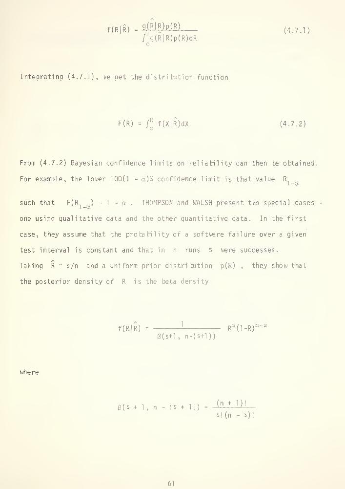
f(R |R) = 9(R|R)pCR)(4>7J)

/1g(R|R)p(R)dR

Integratinq (4.7.1), ve pet the distri bution function

F(R) = /R

f(X|R)dX (4.7.2)

From (4.7.2) Bayesian confidence limits on reliability can then be obtained

For example, the lower 100(1 - a)% confidence limit is that value R nr l-a

such that F( Ri )

=1 - a . THOMPSON and WALSH present two special cases

one using qualitative data and the other quantitative data. In the first

case, they assume that the probability of a software failure over a given

test interval is constant and that in n runs s were successes.

Taking R = s/n and a uniform prior distribution p(R) , they show that

the posterior density of R is the beta density

r>S/T n\n-Sf(R|R) = ! R

b(l-R)

$(s+l, n-(s+l))

where

3(s + 1, n - (s+ 1)) -(n + ]

)!

s!(n - s)!

61

In the second case they assumed a constant failure rate and used as their

estimate of reliability

R(t) = exp(- rt/T)

where T is the total run time and r is the number of failures. Again

using a uniform prior, they show that

f(R(t)|R(t)) = J±±JJ±)^L- R

f/t(ln 1/R)

r

r(l + r)

At present, the Bayesian approach seems to suffer in comparison to

the simplicity of the other approaches we have presented. In addition, it

requires the subjective assessment of the analyst in determining the prior

distributions. The Bayesian models require more structure than do the

other models. For these reasons, the Bayesian models do not appear to be

as useful as some of the others we have considered.

62

V. GUIDELINES FOR SOFTWARE QUALITY ASSURANCE

5 .1 Introduction

We have discussed testing, and several methods for estimating software

reliability have been presented. For the most part, these methods are most

useful for the operational tests which are conducted by the user or some

independent test agency after the integration stage of software development.

However, they are also appropriate for use at the earlier stages where it

may be desirable to estimate module or process reliability or to give guide-

lines on the amount of additional testing that should be given a certain

portion of the software. Nevertheless, it is usually the case in actual

practice that the software delivered to the customer is full of bugs. This

is true even though the software developer may have been required to demon-

strate through some sort of formal qualifying test that his product performs

as specified.

The delivery of unreliable software to the customer results in his loss

of confidence in the product. The customer finds himself forced to conduct

extensive testing to increase its reliability, or to put the unreliable soft-

ware into use and correct the errors in the time-honored fashion of fixing

them as they appear. Neither of these alternatives is satisfactory to the

user. He feels that the developer is better equipped to correct software

errors and that it is the developers job to release a reliable product. It

is not unreasonable for the user to feel this way.

What is needed is that more effort be tunneled in the direction of

ensuring that proper management techniques be performed early in the devel-

opment of the software so that the user is not forced to accept less than

63

what he bought. Since part of the problem results from poor programming

practices, research is also needed in the development of tools which enable

a programmer to write better software.

5.2 Design for Reliability

One way to improve the quality of software is to expend more effort

and resources in its design. If causes of software unreliability can be

determined, then steps can be taken to alleviate the contributions of those

causes. Testing and debugging alone cannot ever guarantee completely

reliable software for hidden errors can sometimes violate the system with-

out ever giving a warning (no failures are observed). DIJKSTRA [4] has

remarked, "Testing can be used to show the presence of bugs but never to

show their absence." What, then, can be done in the design area that will

reduce the number of errors written into the software?

TSICHRITZIS and BALLARD [31] suggest that the software can be struc-

tured in such a way as to enhance its reliability. First, a study of the

relative frequencies of different types of errors in programs could identify

the most frequent characteristic errors. This information would then, in

turn, be used to determine the program structures and languages which are

most reliable. Those structures which are unreliable should be avoided,

when possible, by programmers. Next, the software could be structured so

as to allow easier and more complete testing. This could be accomplished

by building up the software from modules and using protection mechanisms

which establish boundaries and rules to restrict communication between the

various modules. The object of the protection mechanism is to minimize

64

interface problems. By controlling the interactions between the various

parts of the software, the protection system would tend to isolate errors

so that an error which occurs in one part cannot damage the other parts.

The system would create "fire walls" which would facilitate the recovery

from failures. In addition, the protection system would aid in the dis-

covery and location of errors. This would happen because of the failures

that result from an attempt to violate some protection mechanism.

Software testing at the lowest level of the software hierarchy can

often be nearly exhaustive in the sense that all logic paths of control

can (and should) be checked at least once. Testing the individual paths

with sample inputs covering the extreme values in the domain of the vari-

ables will provide a good start on assuring good quality. Historically,

the trouble with modular test approach has been that problems result when

the modules (processes) are integrated so that they must interact with other-

modules (processes). However, if a good protection system could be devel-

oped the interaction problems would be minimized and modular testing would

be feasible. Then, the software could be designed and structured so that

the modules can be verified independently of the higher levels and then

used without further testing to verify the next level. Because of the re-

duction in the number of tests that would be required, huge savings in both

time and dollars could be achieved if validation could be accomplished by

testing modules independently. For example, suppose module i has n paths

to test and module i is called from m places in module j . If the

modules can be tested independently, we need only test n paths in module i

and m paths in module j , a total of m + n paths. However, if they

65

must be combined for testing, n x m paths must be checked. When one

considers that n and m may range upwards into the hundreds or thou-

sands, the potential savings are obvious.

Since its inception, programming has been considered an art rather

than a science. Much work is needed to develop a set of conceptual and

operational principles that constitute good programming practice so that

programming can be placed under tighter control. Considering the current

high cost of reliability, concentration in this area may offer the highest

ratio of benefits to cost.

5.3 The User's Role in Software Development

Unless programming becomes more of a science, the user will have lit-

tle control over actual programming practice. However, there is much that

the user can do to improve the quality of the software he receives. As

more and more large software subsystems are developed and lessons learned

from the successes and failures of the development programs, practices

which constitute good software control are evolving. Software acquirers

are recognizing the value of their practical experience with software devel-

opment and have begun to share their experiences, both good and bad, in the

open literature (see, for example, BUCKLEY [2] , KEEZER [11], COUTINHO [3],

or ELLINGSON [5]). In the time-honored fashion of trial and error many

guidelines have developed.

Official guidelines for government agencies involved as acquirers in

the software development process are given by two documents, MIL-STD-490

( Specification Practices) and MIL-STD-483 ( Configuration Management Practices

of Sys terns , Equipment , Munitions and Computer Programs ). The Specification

66

Practices document establishes the detailed format and content of speci-

fications for computer programs. It includes both a Computer Program

Development Specification and a Product Specification. The development

specification describes the performance requirements necessary to design

and verify the computer program in terms of performance criteria. The

product specification is the document representation of the computer pro-

gram; it consists of the flow charts and narrative that logically describe

the computer program, the coding and the data. The Configuration Management

standard expands on the documentation requirements and provides uniform

procedures for preparing, formating and processing changes to computer pro-

grams once a configuration is fixed.

Although certainly deserving of much attention, we shall not attempt

to discuss extensively the steps a software acquirer can and should take

to assure receipt of a quality product. Such an important subject is

better discussed by people who have practical experience such as those

cited above. Nevertheless, we shall focus on a few areas which fall under

the responsibility of the software acquirer and which have a potentially

large impact on the quality of the software.

Many of the problems that result can be traced to the very outset

of the software development program. Too often the customer, who is res-

ponsible for establishing detailed performance specifications, will write

vague statements as to what he wants. This forces the contractor to guess

at what is wanted or allows him too much freedom for personal interpreta-

tion of what is desired. The performance specifications should be much

more than mere expressions of good intentions. They must describe exactly

67

those functions that must be performed, and they must contain enough infor-

mation to enable a contractor to transform an operational need or system

requirement into a design specification. At the same time, overall soft-

ware test plans must be written at the same level of detail. These form

the basis for the development of future test plans and procedures. T he

test plans should require that each performance requirement of each compu-

ter program configuration end-item be verified in some appropriate manner,

and they should specify the acceptance criteria. Detailed and complete

test plans not only give the contractor something to shoot for, but they

also provide the contractor's personnel with specific tests against which

they can check their work as they progress with the coding.

In order to improve visibility, the customer must require configura-

tion management control and detailed documentation. This allows the custo-

mer to monitor the progress in the development of the product and to iden-

tify and control changes to be made to an already approved specification.

Further, it enables management to see what they are managing. The documen-

tation requirement is necessary because it fosters better communication,

and documentation is itself an important part of the software end product.

We have already discussed some of the problems experienced by test

personnel during operational testing caused by the lack of an overall ac-

cepted methodology of software testing. The same problems thwart the suc-

cess of the verification testing conducted by the contractor. Traditionally,

contractors have attempted to verify that the software performs according to

specifications by demonstrating its performance using "canned" tests with

exactly-prescribed inputs. The problem is that the software passes the formal

68

verification tests, but it often will fail to process properly other inputs

under varying load conditions. Consequently, when the entire system under-

goes operational testing numerous problems surface. A partial solution to

this problem reverts to the proper writing of performance specifications

and test plans and procedures. Much thought needs to be given to the accep-

tance criteria that are written into the software contract. The customer

must state explicitly how the contractor must verify each performance speci-

fi cation.

Because software is a much less tangible product than is hardware,

the customer must obtain visibility into the contractor's efforts from the

very beginning of the contract. Although there is little that can be ob-

served or inspected in order to assess intermediate progress, the customer

should strive to actively participate in the development by furnishing

guidance to the contractor during design reviews and software testing. The

customer should obtain sufficient visibility to enable him to ensure that

the contractor establishes and enforces good management control and proce-

dures.

Lastly, even with active participation by the customer and the best

management, the delivered software will not be perfect. Therefore, the

customer must expect to require some maintenance after he accepts the product,

and he should provide for the contractor to be kept on the job for some

period after acceptance to correct problems as they occur.

69

VI. CONCLUSIONS

In this paper we have looked at some of the problems experienced in

the computer software development process. We have pointed out the impor-

tance of software quality assurance and the necessity for keeping close

tabs on the software quality. Using the natural analogies between software

and hardware, we have defined a measure of effectiveness. Test procedures

and data collection requirements have been described.

Several mathematical models which convert the raw software failure

data into estimates of software reliability have been presented. The mathe-

matical models cover different types of failure data and, in some cases,

yield not only point estimates of reliability, but also estimates of the

number of errors remaining in the software subsystem (or a part of that sub-

system) and confidence intervals for reliability. The models represent a

survey of the state of the art in reliability estimation. With only a few

exceptions, they have not been validated with actual software failure data.

They are presented here because they appear to the author to be mathemati-

cally plausible and intuitively appealing. Nevertheless, they have not yet

passed the "acid test" -- good performance in actual use. Consequently,

much work remains to be done before any particular one can be recommended

strongly. We do recommend that software data of the form described in this

report be collected and the various models be tested against real data.

In addition to the need for a validation effort on the reliability

models, we have identified other areas related to the software problem which

cry out for further work. For example, work needs to be done to identify

70

unreliable program structures and to develop a set of operational princi-

ples that constitute good programming practice, so that better software

will be written. Also, there is a need for the development of a method-

ology for software testing. This is critical when one considers the huge

portion of total software development costs which are consumed by the test

effort.

Finally, we have pointed out some "management" responsibilities of

the software customer which can have a significant impact on the quality

of the product he is delivered. At the outset he is responsible for the

writing of contractual performance specifications, test plans and proce-

dures, and acceptance criteria. Much work needs to be done in this area

to head off those problems which result because specifications, plans and

requirements contain too little detail. After the customer has written

down exactly what he wants and requires, his function is primarily one of

vigi lance.

71

BIBLIOGRAPHY

1. Barlow, Richard and Ernest Scheuer, "Reliability Growth During a

Development Testing Program," Technometrics , Feb 1966, Vol. 8

Jo. 1 , p. 53.

2. Buckley, F. J., "Software Testing - A Report From the Field," Proc.

1973 IEEE Symposium Comp uter Software Reliabi lity , BrooklynPolytechnic Institute, April" 1973, pp. 102-106.

3. Coutinho, J., "Software Reliability Growth," Proc. 1 973 IEEE Symp.Comp uter Software Reliabil ity, Brooklyn Poly, Inst., April 1973,

pp. 58-64.

4. Dijkstra, E. W. , "Notes on Structured Programming," Report EWD249,Technische Hogeschool Eindhoven, 1969.

5. Ellingson, 0. E. , "Computer Program and Change Control," Pro c. 1973

IEEE Symposium Computer Software Reliabi lity , Brooklyn Polytechnic"Institute, April 1973, pp. 82-89.

6. Feller, W. , An Introduction to Probabi lity Theory and Its Applications ,

Vol. 1, Second Edition, John Wiley and Sons, Inc., New York, 1957,

pp. 43-44.

7. Floyd, R. W., "Assigning Meanings to Programs," Proc. Symp. in App.

Math. , Vol. 19, American Math Society, Providence, R.I., 1967,

pp. 19-32.

8. Girard, E. and J. C. Rault, "A Programming Technique for SoftwareRe 1 i abi 1 i ty

," Proc . 1973 IEEE Symp. Computer Software Reliabi lity ,

Brooklyn Poly. Inst., April 1973, pp. 44-50.

9. Gnedenko, B. V., Y. K. Belyayev and A. D. Solovyev, MathematicalMethods of Reliabili ty Theory, Academic Press, New York, 1969.

10. Jelenski, Z. and P. Moranda, "Software Reliability Research," in

Statistical Computer Performance Evaluation, Ed. by Walter Freiberger,Academic Press, New York, 1972, pp. 465-484.

11. Keezer, E. I., "Practical Experiences in Establishing Software QualityAssurance," Proc. 1973 IEEE Symp. Computer Software Reliability ,

Brooklyn Poly, Inst., April 1973, pp. 132-135.

12. King, J. C, A Program Verifier, Ph.D. Thesis, Carnegie-Mellon University,

Pittsburgh, 1969.

13. Lipow, M., "Estimation of Software Package Residual Errors," TRW Report

2260. 4B. 72-2, Redondo Beach, Calif. 1973.

72

14. Littlewood, B. and J. L. Verrall , "A Bayesian Reliability Growth Modelfor Computer Software," Journal of the Royal Statistical Society ,

Series C, Applied Statistics , 1973.

15. Lloyd, D. and M. Lipow, Reliabi li ty : Management Methods, and Mathematics

,

Prentice-Hall, Englewood Cliffs , New Jersey, 196T!

16. London, R. L. "Certification of the Algorithm Treesort," Comm

.

ACM

.

Vol. 13, No. 6, 1970, pp. 371-373.

17. MacWilliams, W. , "Reliability of Large Real-Time Control SoftwareSystems," Proc. 1973 IEEE Symp. Computer Software Reliability , BrooklynPoly. Inst., April 1973, pp. 1-6.

18. Miller, I. and J. Freund, Probability and Statistics for Engineers ,

Prentice-Hall, Englewood Cliffs, New Jersey, 1965.

19. Mills, H. D., "On the Statistical Validation of Computer Programs," IBMReport FSC-72-6015, July 1970.

20. MIL-STD-483, Configuration Management Practices erf Systems, Equipment ,

Munitions and Computer Programs .

21. MIL-STD-490, Specification Practices .

22. Naur, P., "Proof of Algorithms by General Snapshots," BIT, Vol. 6, No. 4,

1966, pp. 310-316.

23. Schick, G. and Wolverton, R. , "Assessment of Software Reliability,"Presented to the 11th Annual Meeting, German Operations Research

Society, Hamburg, September 1972.

24. Schneidewind, N., "A Methodology for Software Reliability Prediction

and Quality Control," Naval Postgraduate School Technical Report

NPS55SS72111A, November 1972.

25. , "An Approach to Software Reliability Prediction and

Quality Control," Fall Joint Computer Conference, 1972, pp. 837-847.

26. , A Model for the Analysis of Software Reliability and

Quality Control," Presented at the 43rd National Meeting of ORSA,

May 1973.

27. Shooman, M. , "Probabilistic Models for Software Reliability Prediction,"

in Statistical Computer Performance Evaluation, Ed. by W. Freiberger,

Academic Press, New York, 1972, pp. 485-502.

28. , "Operational Testing and Software Reliability Estimation

During Program Development," Proc. 1973 IEEE Symp. Computer Software

Reliability , Brooklyn Poly, Inst., April 1973, pp. 51-57.

73

29. Thompson, W. ana D. Walsh, "Reliability and Confidence Limits forComputer Software," General Research Corporation Report.

30. Trauboth, H., "Guidelines for Documentation of Scientific SoftwareSystems," Proc. 1973 I_E_Ej[ Symp. Computer Software Reliabi lity ,

Brooklyn Poly. Inst., April 1973, pp. 124-131.

31. Tsichritzis, D. and A. Ballard, "Software Reliability," IN FOR , Vol.11,No. 2, June 1973, pp. 113-124.

32. Weiss, H., "Estimation of Reliability Growth in a Complex System withPoisson Failure," Operations Research , Vol. 4, 1956, pp. 532-545.

74

APPENDIX

A brief summary of the more important terms associated with mathe-

matical reliability theory is presented in the following for those readers

unfamiliar with that theory.

Reliability .

The reliability of a product is defined as the probability that the

product will function within specified limits for at least a specified

period of time under specified environmental conditions.

Various probability distributions are required for the study of re-

liability. Of fundamental importance is the probability distribution of

the time to fai lure.

Time-to-Fai lure Distribution,

Let f(t) be the probability density of the time to failure of the

product, that is the probability that the product will fail between times

t and t + At is given by f(t) • At . The probability that the product

will fail sometime before time t is given by

ftF(t) = f(s)ds

J

which is sometimes called the "unreliability" function.

Reliability Function .

The probability that the product will survive to time t is given by

75

the reliability function

R(t) = 1- F(t)

Note the relationships between f(t) , F(t) and R(t) . In particular

f(t) = dF(t)/dt = - dR(t)/dt

Instantaneous Failure Rate

.

Another probability function which is convenient for use in relia-

bility studies is the conditional probability that the product will fail

in the interval (t,t+AtJ given that the product has survived to time t .

Mathematically, this probability is given by

(F(t+At) - F(t))/R(t)

On dividing by the length of the interval, At , and taking the limit as

At goes to zero we get the instantaneous failure rate or hazard rate

7(+\ = lim F(t+At) - F(t) 1 dF(t)/dtL[Z)

At->0 At * ~R(tT R[tT

Using the identities involving f(t) , F(t) and R(t) we get the following

equivalent expressions for Z(t) :

Z(t) = f(t)/R(t)

- - dR(t)/dt

RTtT~

= " ^ln[R(t)]

This differential equation can be solved for R(t) to yield

76

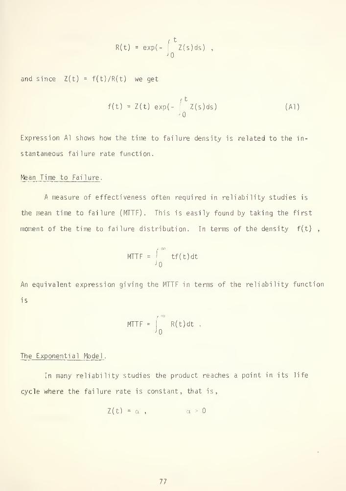
R(t) = exp(- Z(s)ds),

JO

and since Z(t) = f(t)/R(t) we get

f(t) = Z(t) exp(- Z(s)ds) (Al)

Expression Al shows how the time to failure density is related to the in-

stantaneous failure rate function.

Mea n Time to Failure.

A measure of effectiveness often required in reliability studies is

the mean time to failure (MTTF). This is easily found by taking the first

moment of the time to failure distribution. In terms of the density f(.t) ,

MTTF = tf(t)dt

An equivalent expression giving the MTTF in terms of the reliability function

is

r°°

MTTF = R(t)dt .

The Exponential Model

.

In many reliability studies the product reaches a point in its life

cycle where the failure rate is constant, that is,

Z(t) = a , a >

77

On substituting into equation Al we get the time-to-failure density

f( t) = a exp(-ut) t >

which is the well known exponential probability density. Simple calcula-

tions show that

R(t) = exp(-at)

and

MTTF = 1/a

An important property of the exponential model is its "loss of memory."

In woras, this means that the probability that the product will survive an

additional tQ

units of time does not depend on the amount of time the pro-

duct has already been in operation. Mathematically, if T is the time-to-

failure random variable, then

P[T > tQ

+s|

T > s] = P[T > tQ

] = R(tQ

)= exp(-at

Q) .

The exponential model is easily the most widely applied model in relia-

bility analyses. There are several reasons for its acceptability. First,

its theoretical properties such as constant failure rate and loss of memory

often seem appropriate for describing the probabilistic characteristics of

the failures of some products. Indeed, many theoretical investigations and

experimental verifications have shown that, for some products, the time-to-

failure density is f(t) = a exp(-at) . In the second place, the popularity

of the exponential model is often due to its simplicity. It has only a

single parameter, and many problems can be solved in explicit form using

78

simple equations

.

Recently, the exponential model has been the subject of criticism

because it is being accepted uncritically. Analysts must attempt to jus-

tify its use on the basis of the nature of the failures of the product

under consideration. In many cases failures are described quite well by

the exponential model, but there are also many cases where it is not

appropriate.

The Wei bull Model

.

While the assumption of a constant failure rate is often appropriate

for describing chance failures, it is not always sufficient. This particu-

larly true during the early "burn-in" stage and the late "wear-out" stage.

Nor would the constant failure rate be appropriate during a period of re-

liability growth due to improvements in the product. Thus, other mathema-

tical functions are required so that increasing or decreasing failure rates

can be considered. A versatile function often used to approximate such

failure rates is

Z(t) = aBt3 "

1

; t > ; a,3 > .

When 3 < 1 the failure rate decreases with time; if 3 > 1 it increases

with time; and if 3=1 the failure rate is constant. Solving for the

time-to-failure density gives

f(t) = a3t3-1

exp(-at 6) t >

This density is called the Weibull density. The reliability function is

79

given by

R(t) = exp(-at3 ) .

Like the exponential model, the Weibull enjoys widespread use. It

can also be justified on theoretical grounds, for it has been shown that

the limiting distribution (as n-*") of the time to failure of the mini-

mum of n independent random variables each having the same distribution

is described by the Weibull law. Perhaps more than any other reason, the

Weibull model has been used because it is so versatile. The Weibull faimly

is so rich that some member of the family can usually be found to describe

the nature of failures for most products.

Other Models.

Other probability functions which have been found useful for describing

the random nature of failures are the gamma and the lognormal. These func-

tions are represented by:

Gamma: f(t) = J^BL^l; a6 >

r(a)sa

and

Lognormal: f(t) = — exp(-ln (t-a) 2/26

2); 6 >

2i\ 8t

For appropriate choices of parameters, these functions can be made to repre-

sent either increasing or decreasing failure rates.

80

INITIAL DISTRIBUTION LIST

Defense Documentation Center (DDC)Cameron StationAlexandria, Virginia 22314

Library, Code 0212Naval Postgraduate SchoolMonterey, California 93940

Library, Code 55

Naval Postgraduate SchoolMonterey, California 93940

Defense Logistics Studies InformationExchange (DLSIE)

Fort Lee, Virginia 23801

Dean of Research, Code 023Naval Postgraduate SchoolMonterey, California 93940

Dr. K. T. WalleniusDepartment of Mathematical SciencesCI ems on UniversityClemson, South Carolina 29631

Dr. Tom VarleyCode 434Office of Naval ResearchArlington, Virginia 22217

Deputy Commander, Operational Testand Evaluation Force, Pacific

Naval Air Station, North IslandSan Diego, California 92135

Lyle McNeeleyUltrasystems, Inc.

500 Newport Center DriveNewport Beach, California

No. of Copies

2

10

92660

John Rau

Ultrasystems, Inc.

500 Newport Center DriveNewport Beach, California 92660

INITIAL DISTRIBUTION LIST

No. of Copies

Tom Eason, Manager System 1

Engineering DepartmentPRC System Sciences Company1 TOO Glendor AvenueLos Angeles, California 90024

Dr. James A. Chisman 1

CI ems on UniversityCI ems on, South Carolina 29631

Dr. Richard Oberle 1

C0M0PTEVF0RNorfolk, Virginia 23511

Naval Electronics Laboratory 1

Center Library271 Catalina BoulevardSan Diego, California 92152

Fleet Material Support OfficeMechanicsburg, Pennsylvania 17055

Commanding Officer 1

Mr. Edward Lukanuski 1

Commander Stephan Ruth (Code 0451) 1

Department of NavySupply Systems CommandWashington, D. C. 20376

Stanford Research InstituteMenlo Park, California 94025

Mr. D. B. Parker 1

Mr. R. E. Keirstead 1

Naval Air Development CenterWarminster, Pennsylvania 18974

Mr. H. Stuebing 1

Mr. R. Pariseau 1

Fleet Combat Direction SystemsSupport Activity

200 Catalina BoulevardSan Diego, California 92147

Commanding Officer 1

Mr. M. Griswold 1

Mr. J. Hi 1 Hard 1

INITIAL DISTRIBUTION LIST

No. of Copies

Mr. Marvin Denicoff 1

Office of Naval ResearchDepartment of the NavyArlington, Virginia 22217

Library 3

Department of Operations Research

and Administrative SciencesNaval Postgraduate School

Monterey, California 93940

Professor F. Russell Richards 5

Department of Operations Research

and Administrative SciencesNaval Postgraduate School

Monterey, California

U 164246

DUDLEY KNOX LIBRARY - RESEARCH REPORTS

5 6853 01060334 3