Testing fluvial erosion models using the transient response of bedrock rivers to tectonic forcing in...
17
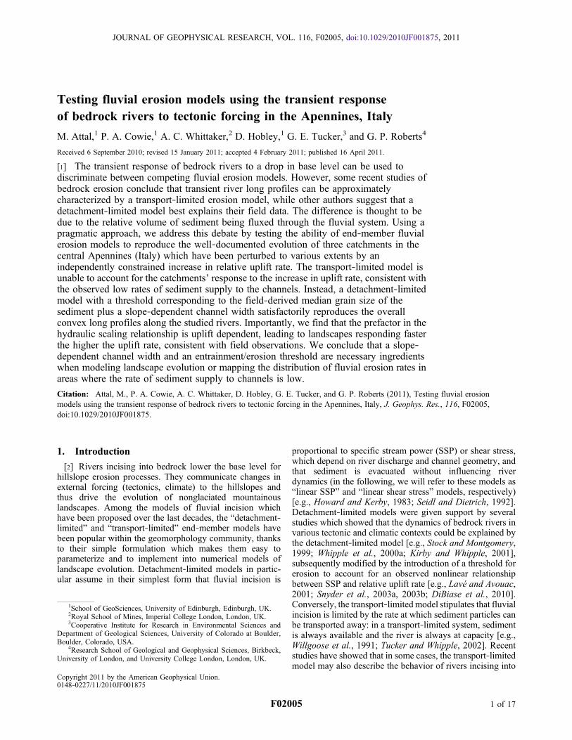
Testing fluvial erosion models using the transient response of bedrock rivers to tectonic forcing in the Apennines, Italy M. Attal, 1 P. A. Cowie, 1 A. C. Whittaker, 2 D. Hobley, 1 G. E. Tucker, 3 and G. P. Roberts 4 Received 6 September 2010; revised 15 January 2011; accepted 4 February 2011; published 16 April 2011. [1] The transient response of bedrock rivers to a drop in base level can be used to discriminate between competing fluvial erosion models. However, some recent studies of bedrock erosion conclude that transient river long profiles can be approximately characterized by a transport‐limited erosion model, while other authors suggest that a detachment‐limited model best explains their field data. The difference is thought to be due to the relative volume of sediment being fluxed through the fluvial system. Using a pragmatic approach, we address this debate by testing the ability of end‐member fluvial erosion models to reproduce the well‐documented evolution of three catchments in the central Apennines (Italy) which have been perturbed to various extents by an independently constrained increase in relative uplift rate. The transport‐limited model is unable to account for the catchments’ response to the increase in uplift rate, consistent with the observed low rates of sediment supply to the channels. Instead, a detachment‐limited model with a threshold corresponding to the field‐derived median grain size of the sediment plus a slope‐dependent channel width satisfactorily reproduces the overall convex long profiles along the studied rivers. Importantly, we find that the prefactor in the hydraulic scaling relationship is uplift dependent, leading to landscapes responding faster the higher the uplift rate, consistent with field observations. We conclude that a slope‐ dependent channel width and an entrainment/erosion threshold are necessary ingredients when modeling landscape evolution or mapping the distribution of fluvial erosion rates in areas where the rate of sediment supply to channels is low. Citation: Attal, M., P. A. Cowie, A. C. Whittaker, D. Hobley, G. E. Tucker, and G. P. Roberts (2011), Testing fluvial erosion models using the transient response of bedrock rivers to tectonic forcing in the Apennines, Italy, J. Geophys. Res., 116, F02005, doi:10.1029/2010JF001875. 1. Introduction [2] Rivers incising into bedrock lower the base level for hillslope erosion processes. They communicate changes in external forcing (tectonics, climate) to the hillslopes and thus drive the evolution of nonglaciated mountainous landscapes. Among the models of fluvial incision which have been proposed over the last decades, the “detachment‐ limited” and “transport‐limited” end‐member models have been popular within the geomorphology community, thanks to their simple formulation which makes them easy to parameterize and to implement into numerical models of landscape evolution. Detachment‐limited models in partic- ular assume in their simplest form that fluvial incision is proportional to specific stream power (SSP) or shear stress, which depend on river discharge and channel geometry, and that sediment is evacuated without influencing river dynamics (in the following, we will refer to these models as “linear SSP” and “linear shear stress” models, respectively) [e.g., Howard and Kerby, 1983; Seidl and Dietrich, 1992]. Detachment‐limited models were given support by several studies which showed that the dynamics of bedrock rivers in various tectonic and climatic contexts could be explained by the detachment‐limited model [e.g., Stock and Montgomery, 1999; Whipple et al., 2000a; Kirby and Whipple, 2001], subsequently modified by the introduction of a threshold for erosion to account for an observed nonlinear relationship between SSP and relative uplift rate [e.g., Lavé and Avouac, 2001; Snyder et al., 2003a, 2003b; DiBiase et al., 2010]. Conversely, the transport‐limited model stipulates that fluvial incision is limited by the rate at which sediment particles can be transported away: in a transport‐limited system, sediment is always available and the river is always at capacity [e.g., Willgoose et al., 1991; Tucker and Whipple, 2002]. Recent studies have showed that in some cases, the transport‐limited model may also describe the behavior of rivers incising into 1 School of GeoSciences, University of Edinburgh, Edinburgh, UK. 2 Royal School of Mines, Imperial College London, London, UK. 3 Cooperative Institute for Research in Environmental Sciences and Department of Geological Sciences, University of Colorado at Boulder, Boulder, Colorado, USA. 4 Research School of Geological and Geophysical Sciences, Birkbeck, University of London, and University College London, London, UK. Copyright 2011 by the American Geophysical Union. 0148‐0227/11/2010JF001875 JOURNAL OF GEOPHYSICAL RESEARCH, VOL. 116, F02005, doi:10.1029/2010JF001875, 2011 F02005 1 of 17
-
Upload
independent -
Category
Documents
-
view
1 -
download
0
Transcript of Testing fluvial erosion models using the transient response of bedrock rivers to tectonic forcing in...
Testing fluvial erosion models using the transient responseof bedrock rivers to tectonic forcing in the Apennines, Italy
M. Attal,1 P. A. Cowie,1 A. C. Whittaker,2 D. Hobley,1 G. E. Tucker,3 and G. P. Roberts4
Received 6 September 2010; revised 15 January 2011; accepted 4 February 2011; published 16 April 2011.
[1] The transient response of bedrock rivers to a drop in base level can be used todiscriminate between competing fluvial erosion models. However, some recent studies ofbedrock erosion conclude that transient river long profiles can be approximatelycharacterized by a transport‐limited erosion model, while other authors suggest that adetachment‐limited model best explains their field data. The difference is thought to bedue to the relative volume of sediment being fluxed through the fluvial system. Using apragmatic approach, we address this debate by testing the ability of end‐member fluvialerosion models to reproduce the well‐documented evolution of three catchments in thecentral Apennines (Italy) which have been perturbed to various extents by anindependently constrained increase in relative uplift rate. The transport‐limited model isunable to account for the catchments’ response to the increase in uplift rate, consistent withthe observed low rates of sediment supply to the channels. Instead, a detachment‐limitedmodel with a threshold corresponding to the field‐derived median grain size of thesediment plus a slope‐dependent channel width satisfactorily reproduces the overallconvex long profiles along the studied rivers. Importantly, we find that the prefactor in thehydraulic scaling relationship is uplift dependent, leading to landscapes responding fasterthe higher the uplift rate, consistent with field observations. We conclude that a slope‐dependent channel width and an entrainment/erosion threshold are necessary ingredientswhen modeling landscape evolution or mapping the distribution of fluvial erosion rates inareas where the rate of sediment supply to channels is low.
Citation: Attal, M., P. A. Cowie, A. C. Whittaker, D. Hobley, G. E. Tucker, and G. P. Roberts (2011), Testing fluvial erosionmodels using the transient response of bedrock rivers to tectonic forcing in the Apennines, Italy, J. Geophys. Res., 116, F02005,doi:10.1029/2010JF001875.
1. Introduction
[2] Rivers incising into bedrock lower the base level forhillslope erosion processes. They communicate changes inexternal forcing (tectonics, climate) to the hillslopes andthus drive the evolution of nonglaciated mountainouslandscapes. Among the models of fluvial incision whichhave been proposed over the last decades, the “detachment‐limited” and “transport‐limited” end‐member models havebeen popular within the geomorphology community, thanksto their simple formulation which makes them easy toparameterize and to implement into numerical models oflandscape evolution. Detachment‐limited models in partic-ular assume in their simplest form that fluvial incision is
proportional to specific stream power (SSP) or shear stress,which depend on river discharge and channel geometry, andthat sediment is evacuated without influencing riverdynamics (in the following, we will refer to these models as“linear SSP” and “linear shear stress” models, respectively)[e.g., Howard and Kerby, 1983; Seidl and Dietrich, 1992].Detachment‐limited models were given support by severalstudies which showed that the dynamics of bedrock rivers invarious tectonic and climatic contexts could be explained bythe detachment‐limited model [e.g., Stock and Montgomery,1999; Whipple et al., 2000a; Kirby and Whipple, 2001],subsequently modified by the introduction of a threshold forerosion to account for an observed nonlinear relationshipbetween SSP and relative uplift rate [e.g., Lavé and Avouac,2001; Snyder et al., 2003a, 2003b; DiBiase et al., 2010].Conversely, the transport‐limitedmodel stipulates that fluvialincision is limited by the rate at which sediment particles canbe transported away: in a transport‐limited system, sedimentis always available and the river is always at capacity [e.g.,Willgoose et al., 1991; Tucker and Whipple, 2002]. Recentstudies have showed that in some cases, the transport‐limitedmodel may also describe the behavior of rivers incising into
1School of GeoSciences, University of Edinburgh, Edinburgh, UK.2Royal School of Mines, Imperial College London, London, UK.3Cooperative Institute for Research in Environmental Sciences and
Department of Geological Sciences, University of Colorado at Boulder,Boulder, Colorado, USA.
4Research School of Geological and Geophysical Sciences, Birkbeck,University of London, and University College London, London, UK.
Copyright 2011 by the American Geophysical Union.0148‐0227/11/2010JF001875
JOURNAL OF GEOPHYSICAL RESEARCH, VOL. 116, F02005, doi:10.1029/2010JF001875, 2011
F02005 1 of 17
bedrock [Loget et al., 2006; Cowie et al., 2008; Valla et al.,2010].[3] Identifying which of these models best describes the
evolution of a fluvial system is important for understandingand modeling geomorphic processes and rates, since dif-ferent models will predict contrasted landscape responses toa perturbation [e.g., Tucker and Whipple, 2002]. It is alsoessential for extracting tectonic information from river longprofiles [e.g., Kirby and Whipple, 2001; Kirby et al., 2003;Wobus et al., 2006a], as different models will make differentpredictions of how channel slope relates to spatial andtemporal variations in relative rock uplift rate. Tucker andWhipple [2002] showed theoretically that the transientresponse of a landscape provides potentially the best meansto discriminate between and test the different fluvial incisionmodels. Early attempts at objectively testing and calibratingthe different models using statistical methods producedmixed results, either due to lack of transient features[Tomkin et al., 2003] or lack of temporal constraints on thetransient evolution [van der Beek and Bishop, 2003]. Morerecent studies of the transient response of real bedrock rivershave led to apparently contradictory results, that is, that insome cases the response may be approximated by a trans-ported‐limited model [Loget et al., 2006; Cowie et al., 2008;Valla et al., 2010] while in other cases the detachment‐limited model approximately describes the response docu-mented in the field [Whittaker et al., 2008; Attal et al., 2008;Boulton and Whittaker, 2009].[4] In this debate over which fluvial incision model
should be used to model landscape evolution, the sedimentissue is central [Cowie et al., 2008; Johnson et al., 2009;Valla et al., 2010]. In addition to the detachment‐limited andtransport‐limited models, many sediment‐flux‐dependentfluvial incision models have been formulated over the last20 years, based on the early realization by Gilbert [1877]that sediment particles can be tools for bedrock erosionwhen they move and impact the river’s bedrock, but canalso provide a protective cover when they are resting,motionless, on the bed [e.g.,Kooi and Beaumont, 1994; Sklarand Dietrich, 1998, 2001, 2004, 2006; Turowski et al., 2007].However, use and testing of such models remains extremelychallenging at present because many of the sediment‐relatedparameters are difficult to constrain, in particular grain sizeand lithology which strongly influence fluvial erosion rates[Sklar and Dietrich, 2001, 2004; Gasparini et al., 2006,2007; Johnson et al., 2009] and are expected to evolve alongactively incising rivers under the effect of abrasion, selectivetransport and lateral supply from hillslopes and tributaries[e.g., Sklar et al., 2006; Attal and Lavé, 2006, 2009].[5] The detachment‐limited and transport‐limited models
are simple to parameterize using easily acquired field dataand here we investigate how far they can be applied. Thesemodels have been implemented into models of landscapeevolution such as the Channel‐Hillslope Integrated Land-scape Development (CHILD) model [Tucker et al., 2001]and have proven successful at describing the evolution ofbedrock rivers in the past (see above). We assess the extentto which these end‐member fluvial incision models are ableto replicate the exceptionally well constrained response ofcatchments in the central Apennines (Italy) to an increase inrelative uplift rate. Unlike previous tests of fluvial erosionmodels which tend to focus on one single catchment [e.g.,
Attal et al., 2008], this study is unique in that we simulta-neously model the evolution of three monolithologicalcatchments of different sizes (28 to 62 km2) in the footwallof active normal faults which increased their throw rates tovalues ranging between 0.25 and 1.5 mm yr−1 around0.75 Ma ago (Figure 1) [Roberts and Michetti, 2004]. Inthese catchments, channel and catchment morphology, thecharacteristics of the sediment supplied to and transportedby the rivers, and the tectonic history of the faults have beenextensively documented in the field [Roberts and Michetti,2004; Whittaker et al., 2007a, 2007b, 2008, 2010]. Thewealth of constraints on the morphological and tectonichistories of these catchments as well as the differences incatchment size and bounding fault throw rates make themthe ideal objects to test and calibrate fluvial erosion models,since a successful model should be able to replicate theevolution of the three catchments using a similar set of inputparameters.[6] We use the CHILD model [Tucker et al., 2001] to
simulate the evolution of the three catchments in response toan increase in fault throw rate. We include a slope‐dependentchannel width [Finnegan et al., 2005] and calibrate thehydraulic scaling coefficients against field data to account forthe channel narrowing which has been documented in thefield as rivers steepen [Whittaker et al., 2007a]. We performtests using different values of a sediment entrainment (anderosion) threshold calibrated against field‐derived fluvialsediment grain size to analyze the potential effect of sedi-ment on landscape’s response time and style [Snyder et al.,2003a, 2003b; Tucker, 2004; Lague et al., 2005]; in par-ticular, we assess whether such a threshold could explainsome of the key observations derived from field data such asa faster response with increasing relative uplift rate[Whittaker et al., 2008]. After presenting the studied catch-ments and the modeling procedure, we present the results inthe transport‐limited and detachment‐limited cases. We thendiscuss how these results improve our understanding of theresponse of the studied catchments in the Apennines andprovide more generic guidelines on how to choose the bestmodel to simulate the evolution of a given area and how toextract erosional and tectonic information from topography.
2. Study Area: Transient Catchmentsin the Apennines, Italy
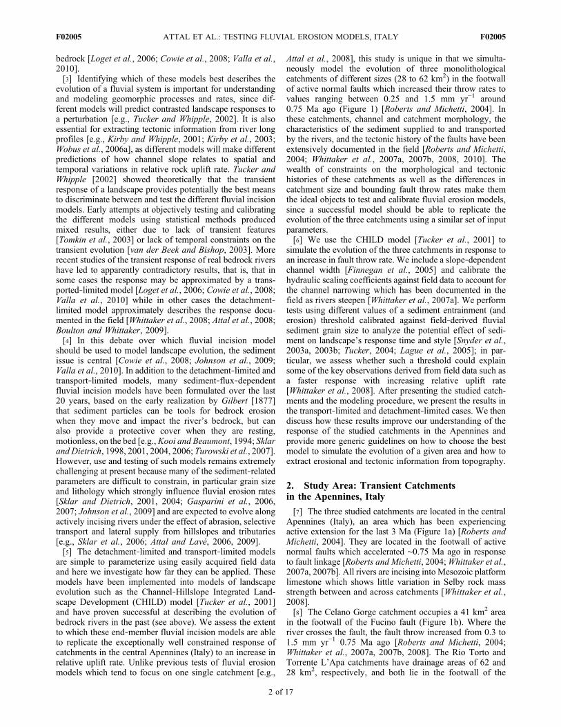
[7] The three studied catchments are located in the centralApennines (Italy), an area which has been experiencingactive extension for the last 3 Ma (Figure 1a) [Roberts andMichetti, 2004]. They are located in the footwall of activenormal faults which accelerated ∼0.75 Ma ago in responseto fault linkage [Roberts and Michetti, 2004;Whittaker et al.,2007a, 2007b]. All rivers are incising into Mesozoic platformlimestone which shows little variation in Selby rock massstrength between and across catchments [Whittaker et al.,2008].[8] The Celano Gorge catchment occupies a 41 km2 area
in the footwall of the Fucino fault (Figure 1b). Where theriver crosses the fault, the fault throw increased from 0.3 to1.5 mm yr−1 0.75 Ma ago [Roberts and Michetti, 2004;Whittaker et al., 2007a, 2007b, 2008]. The Rio Torto andTorrente L’Apa catchments have drainage areas of 62 and28 km2, respectively, and both lie in the footwall of the
ATTAL ET AL.: TESTING FLUVIAL EROSION MODELS, ITALY F02005F02005
2 of 17
Fiamignano fault (Figures 1c and 1d). The Rio Torto crossesthe fault in its center and experienced an increase in throwrate from 0.3 to 1 mm yr−1 ∼0.75 Ma ago; the Torrentel’Apa crosses the fault near its eastern tip and experiencedan increase in throw rate from 0.05 to 0.25 mm yr−1
∼0.75 Ma ago [Roberts and Michetti, 2004; Whittaker et al.,2007a, 2007b, 2008]. The response of these catchments tofault acceleration is characterized by the development of asteepened, convex reach in the river long profile upstream ofthe fault (Figure 1e) while the upper part of the catchment isprogressively uplifted and back tilted [Whittaker et al.,2007a, 2007b, 2008; Attal et al., 2008]. In the upper partof the catchments, channel slope is gentle and valleys arebroad and open, with soil‐mantled hillslopes. The lower partof the catchments exhibits steep channels, narrow gorgesand steep coupled hillslopes near the angle of repose scarredby landslides delivering coarse material to the channel(Figure 1) [Whittaker et al., 2007a, 2007b, 2008, 2010]. Thetwo domains are separated by a prominent break in slope onthe hillslope (Figures 1b–1d) and a major long‐profileconvexity along the rivers (Figure 1e). Downstream of themain long‐profile convexity, river steepening is accompa-
nied by a narrowing of the channel, leading to a breakdownof the typical square root relationship between discharge (ordrainage area) and channel width [Whittaker et al., 2007a].Such channel adjustment has been shown to occur in manyplaces worldwide in response to spatial or temporal varia-tions in relative uplift rate and is now widely accepted[Finnegan et al., 2005; Stark, 2006; Wobus et al., 2006b;Amos and Burbank, 2007; Whittaker et al., 2007a; Attalet al., 2008; Snyder and Kammer, 2008; Turowski et al.,2009; Valla et al., 2010, Yanites et al., 2010a; Yanites andTucker, 2010]. Along the steepened reaches of the threechannels, the width shows no clear downstream trend and isroughly constant: mean width values for the Celano Gorge,Rio Torto, and Torrente l’Apa are 7.4 ± 1.5, 9.5 ± 2.0, and13.1 ± 2.8 m, respectively. The channel morphology alongthe steepened reaches is characterized at the reach scale bymore or less prominent steps and pools alternating withrelatively steep bedrock reaches with discontinuous sedi-ment cover; bedrock exposure is high, typically >50%[Whittaker et al., 2007b]. Bedrock is often exposed on thechannel bed and its morphology (smooth surfaces, flutes,
Figure 1. (a) Location map; box shows location of the central Apennines. Shaded topography of the (b)Celano Gorge, (c) Rio Torto, and (d) Torrente l’Apa catchments; mapped landslides, main long‐profileconvexities along the studied channels, and break in slope in topography delineating steepened landscapeare shown. (e) River profiles extracted from the 20 m resolution DEM. Modified after Whittaker et al.[2010].
ATTAL ET AL.: TESTING FLUVIAL EROSION MODELS, ITALY F02005F02005
3 of 17
potholes) demonstrates that abrasion is the dominant bed-rock erosion process.
3. Modeling the Transient Responseof the Studied Catchments
3.1. Model Setup
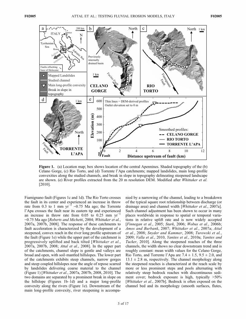
[9] The CHILD model [Tucker et al., 2001] is used tomodel the evolution of the Italian catchments. The procedureis similar to that used by Attal et al. [2008] to investigatethe impact of channel width adjustment on the evolution ofthe Rio Torto catchment and readers are referred to thatpaper for a full treatment of the approach. In brief, thetopography of the three catchments was extracted from a20 m resolution digital elevation model (DEM) and trans-formed into a Triangulated Irregular Network (TIN) with anaverage node spacing of 200 m (Figure 2). The use of the
block‐tilting model (rather than an elastic dislocation model[e.g., Ellis et al., 1999]) is justified in the central Apenninesby the small spacing between faults [Anders et al., 1993], onaverage 10 km [Roberts and Michetti, 2004]. We applied arock uplift rate to the catchments which was greatest at thefault and decreased linearly to zero from fault to fulcrum, thelatter being positioned 10 km away from the fault to reflectthe average fault spacing [Attal et al., 2008].[10] In CHILD, rainfall is uniform over the modeled
landscape and is generated according to a Poisson rectan-gular pulse rainfall model [Eagleson, 1978; Tucker andBras, 2000]. The values used for mean storm precipitationrate (0.75 mm h−1), mean storm duration (22 h) and meaninterstorm duration (260 h) are typical of a Mediterranean‐style climate, based on data from the U.S. west coast [Hawk,1992; Attal et al., 2008]. In the absence of detailed con-straints on the changes to these specific climate parametersover the Quaternary, the parameters were kept constantduring all runs.[11] Field data show a clear correlation between channel
width and gradient: channels tend to narrow as they steepen,leading to channels along the steepened reaches that arenarrower than predicted by the conventional hydraulicscaling relationship (section 2). Finnegan et al. [2005]proposed a relationship which accounts for such a channeladjustment
W ¼ kwQ3=8S�3=16; ð1Þ
where W is channel width, kw is a constant, Q is dischargeand S is channel slope. This relationship significantlyimproves the prediction of channel width along the studiedrivers [Whittaker et al., 2007a; Attal et al., 2008] and issupported by a simple physically based models of self‐formed bedrock channels [Wobus et al., 2006b; Turowskiet al., 2009; Yanites and Tucker, 2010]. We thereforeuse equation (1) to calculate channel width across themodeled landscapes.[12] Whittaker et al. [2007b] estimated that ∼2 Ma would
be required for catchments in the Apennines to achievesteady state. Fault initiation occurred 3 Ma ago and faultacceleration 0.75 Ma ago: this implies that the catchmentshad achieved steady state with respect to the uplift fieldprior to fault acceleration. In this study, we assume that thedrainage patterns and catchment boundaries have notchanged since fault acceleration. For all runs, the modernTINs of the three catchments were entered into CHILD andthe model was run with the uplift field prior to fault accel-eration (fault throw = 0.3 mm yr−1 for Celano Gorge andRio Torto, 0.05 mm yr−1 for Torrente l’Apa) until steadystate was reached. Starting from these steady state topo-graphies (Figure 2), the morphological response of thecatchments to fault acceleration (fault throw = 1.5, 1.0, and0.25 mm yr−1 for Celano Gorge, Rio Torto, and Torrentel’Apa, respectively) was then analyzed.[13] Note that field and DEM observations show that the
upper part of the Celano Gorge catchment was an internallydrained basin which has been captured by the main river(Figure 1b). We chose to include the previously internallydrained basin into the modeled catchment because fieldevidence indicates that capture happened before faultacceleration and that this basin should thus be contributing
Figure 2. Modeled topographies in steady state with theuplift rate prior to fault acceleration for the three studiedcatchments. Uplift rate decreases linearly from fault to thefulcrum located 10 km away from the fault. Node spacingis ∼200 m. In this case, tc = 0 Pa (see text).
ATTAL ET AL.: TESTING FLUVIAL EROSION MODELS, ITALY F02005F02005
4 of 17
water to the Celano Gorge in our modeling of the catch-ment’s response to fault acceleration. Evidence for an earlycapture includes: the fact that the prominent rock ridgewhich was breached, probably through regressive erosion, is∼3 kmupstreamof themain long‐profile convexity (Figure 1b)and that the channel slope between the ridge and this con-vexity is extremely low, <0.002 (Figure 1e). Previous mod-eling work [Attal et al., 2008] showed that once faultacceleration has commenced, capture by the low gradientreaches upstream of the migrating long‐profile convexity isunlikely. In the following, we will focus our comparison ofcatchment morphology and river profiles to the part down-stream of the prominent ridge located ∼9 km upstream of thefault (Figure 1e).
3.2. Fluvial Erosion Models
[14] In the detachment‐limited model, fluvial erosion E iscalculated at all points in the modeled landscape accordingto
E ¼ kb � � �ceð Þp for � > �ce; ð2aÞ
E ¼ 0 for � � �ce; ð2bÞ
where kb is the erodibility coefficient, p is a constant, t is thefluvial shear stress and tce is a threshold representing theshear stress that must be exceeded for erosion to happen. Weconsider that the rate of incision is proportional to the rate ofenergy dissipation per unit bed area and set p to 3/2 [Seidl andDietrich, 1992; Howard et al., 1994; Whipple and Tucker,1999, Attal et al., 2008]. By assuming steady, uniform flowin a relatively wide channel and applying Manning’sroughness formula, we calculate the cross‐section averagedboundary shear stress as
� ¼ �gn3=5m Q=Wð Þ3=5S7=10; ð3Þ
where Q is the water discharge, W is the channel width(calculated following equation (1)), S is channel slope, r isthe water density (1000 kg m−3), g is the gravitationalacceleration and nm is the Manning’s roughness coefficient,fixed to 0.03 in this study, a common value used for riverstransporting sediment up to cobble size (for derivation, see,e.g., Howard [1994]). Note that when tce = 0, equation (2) isequivalent to the linear SSP model. When in addition theexponent p is set to 1, equation (2) is equivalent to the linearshear stress model. For simplicity and in the absence ofconstraint on the amount of water intercepted by vegetation,lost by evaporation, and on the infiltration capacity of thesoils in the study area, we calculate the discharge Q as theproduct of the precipitation rate by the drainage area. Thiswill tend to overestimate Q but should not affect the com-parison between catchments and models since the samecalculation method was applied to all runs.[15] In the transport‐limited model, erosion at any point in
the landscape is calculated following:
E ¼ 1
W
@Qs
@~x; ð4Þ
where Qs is the sediment flux and~x represents the distance inthe downstream direction. The ratio ∂Qs/∂~x thus representsthe divergence of the sediment flux in the downstreamdirection: if the amount of sediment exiting a given point ishigher than the amount of sediment entering this point, thisterm is positive and the river erodes; in the opposite case,deposition occurs. In a transport‐limited system, the river is“at capacity”: sediment is always available and the sedimentflux Qs equals the transport capacity Qc. Transport capacityis calculated following:
Qc ¼ kf W � � �ctð Þp′; ð5Þ
where kf is a free transport efficiency coefficient, p′ is aconstant (set to 3/2), t is the fluvial shear stress calculatedfollowing equation (3) and tct is a threshold representing theshear stress that must be exceeded for sediment transport tohappen (Qc = 0 if t < tct). Previous studies showed that athreshold is required to produce realistic transport‐limitedlandscapes characterized by concave up river profiles [e.g.,Tucker and Whipple, 2002; Tucker, 2004]. In this study wetherefore set tct > 0 for all transport‐limited runs.
3.3. Calibration
[16] The data collected in the field allows the calibrationof three constants: the channel width prefactor kw (equation(1)), the erodibility coefficient kb (equation (2)) and thethresholds for erosion and sediment transport tce and tct(equations (2) and (5)). The threshold for erosion tce can beinterpreted in two ways: it can represent the shear stressvalue that must be exceeded either for bedrock detachmentto occur (bedrock‐controlled threshold) or for setting toolsin motion and exposing bedrock (sediment‐controlledthreshold) [e.g., Howard, 1994; Lavé and Avouac, 2001;Sklar and Dietrich, 2004]. Progress has been made recentlyon the quantification of the shear stress required for pluckingblocks from heavily jointed bedrock [e.g., Whipple et al.,2000b; Chatanantavet and Parker, 2009]. However, Sklarand Dietrich’s [2001] experiments suggest that the “bedrock‐controlled” threshold “can be neglected in the case of bedload abrasion because even the relatively low‐impact energyof fine sand moving as bed load is sufficient to causemeasurable bedrock wear” [Sklar and Dietrich, 2004].Because field observations in the studied catchments indi-cate that abrasion by bed load is the dominant bedrockerosion process [Whittaker et al., 2007b], we focus on the“sediment‐controlled” threshold. This threshold can beestimated using the Shields criterion (see Buffington andMontgomery [1997] for a review on the application of thismethod) and the grain size of the sediment transported byrivers. Note that this type of threshold for bedrock erosiontce has the same significance that the threshold for sedi-ment transport tct: in the former case, the threshold mustbe exceeded for sediment to be put in motion, thus exposingbedrock and providing tools for erosion; in the later case,the threshold must be exceeded for sediment transport tohappen. In the following, we will thus refer to both erosionand transport thresholds using a single “sediment‐controlled”threshold term tc.
ATTAL ET AL.: TESTING FLUVIAL EROSION MODELS, ITALY F02005F02005
5 of 17
[17] The critical shear stress for particle entrainment canbe calculated using
�c ¼ �c*:D�gD; ð6Þ
where tc* is the dimensionless critical shear stress (Shieldsstress) commonly assumed to be ∼0.045 for turbulentrough flows [Buffington and Montgomery, 1997], Dr is thedifference in density between the fluid and the sediment(1650 kg m−3 for typical crustal rocks) and D is a grain sizerepresentative of the sediment, usually taken as the mediangrain size. Along the steepened reaches of the three studiedrivers, the grain size distributions are roughly similar[Whittaker et al., 2007b, 2010]. In particular, sieving of
volumetric samples yielded median grain sizes D50 of∼50 mm and minimum D84 (84th percentile characterizingthe coarse fraction) of ∼100 mm. The threshold shearstresses calculated using these two grain sizes are tc = 38and 76 Pa, respectively. Whereas this simplistic approachignores the imbrication and hiding effects that exert animportant control on sediment’s incipient motion in moun-tain rivers [e.g., Yager et al., 2007], we believe that the shearstress to mobilize grains of diameter D = D84 calculatedusing equation (6) (tc = 76 Pa) represents in first approxi-mation the upper limit for the shear stress that would berequired to put the sediment in motion in the studiedcatchments. In the following, we present the results ofdetachment‐limited runs using tc = 0, 38 and 76 Pa, andtransport‐limited runs using tc = 38 and 76 Pa.[18] Equation (1) implies that the channel width coeffi-
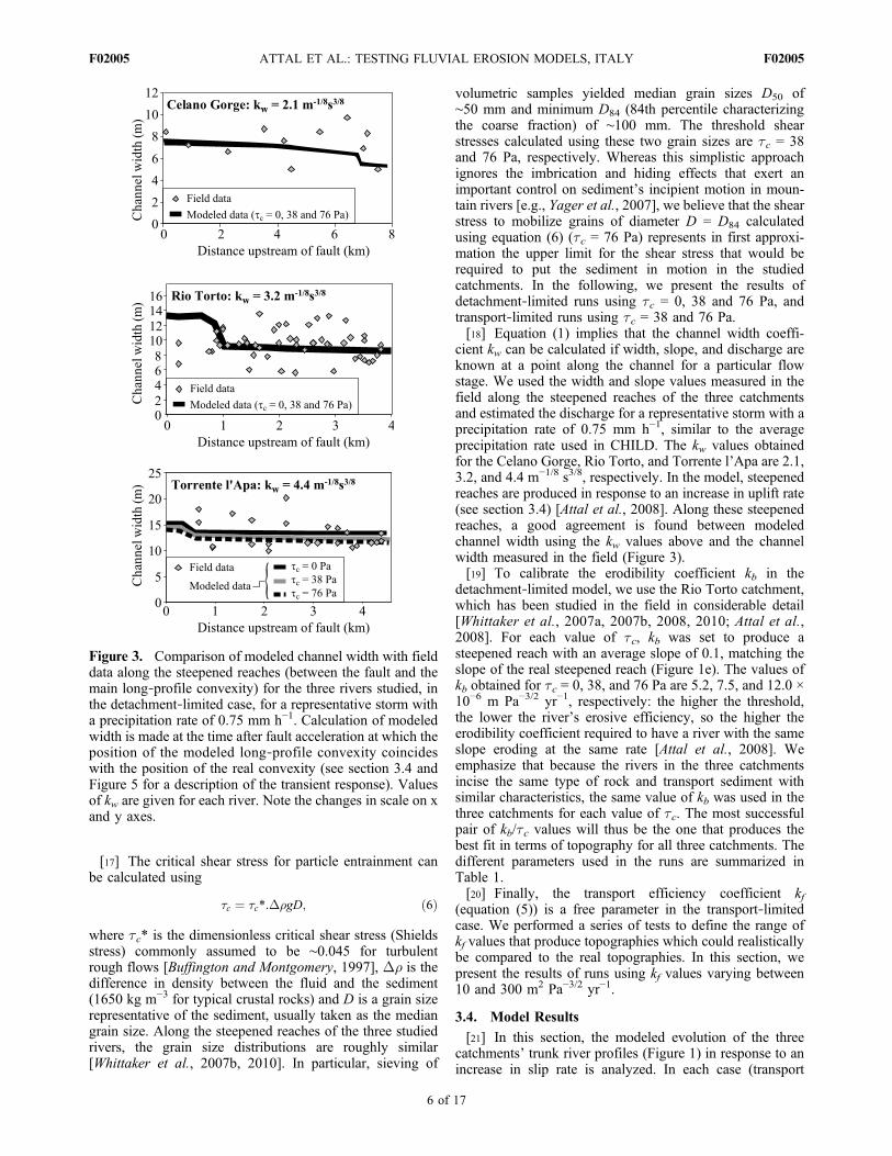
cient kw can be calculated if width, slope, and discharge areknown at a point along the channel for a particular flowstage. We used the width and slope values measured in thefield along the steepened reaches of the three catchmentsand estimated the discharge for a representative storm with aprecipitation rate of 0.75 mm h−1, similar to the averageprecipitation rate used in CHILD. The kw values obtainedfor the Celano Gorge, Rio Torto, and Torrente l’Apa are 2.1,3.2, and 4.4 m−1/8 s3/8, respectively. In the model, steepenedreaches are produced in response to an increase in uplift rate(see section 3.4) [Attal et al., 2008]. Along these steepenedreaches, a good agreement is found between modeledchannel width using the kw values above and the channelwidth measured in the field (Figure 3).[19] To calibrate the erodibility coefficient kb in the
detachment‐limited model, we use the Rio Torto catchment,which has been studied in the field in considerable detail[Whittaker et al., 2007a, 2007b, 2008, 2010; Attal et al.,2008]. For each value of tc, kb was set to produce asteepened reach with an average slope of 0.1, matching theslope of the real steepened reach (Figure 1e). The values ofkb obtained for tc = 0, 38, and 76 Pa are 5.2, 7.5, and 12.0 ×10⁻⁶ m Pa−3/2 yr−1, respectively: the higher the threshold,the lower the river’s erosive efficiency, so the higher theerodibility coefficient required to have a river with the sameslope eroding at the same rate [Attal et al., 2008]. Weemphasize that because the rivers in the three catchmentsincise the same type of rock and transport sediment withsimilar characteristics, the same value of kb was used in thethree catchments for each value of tc. The most successfulpair of kb/tc values will thus be the one that produces thebest fit in terms of topography for all three catchments. Thedifferent parameters used in the runs are summarized inTable 1.[20] Finally, the transport efficiency coefficient kf
(equation (5)) is a free parameter in the transport‐limitedcase. We performed a series of tests to define the range ofkf values that produce topographies which could realisticallybe compared to the real topographies. In this section, wepresent the results of runs using kf values varying between10 and 300 m2 Pa−3/2 yr−1.
3.4. Model Results
[21] In this section, the modeled evolution of the threecatchments’ trunk river profiles (Figure 1) in response to anincrease in slip rate is analyzed. In each case (transport
Figure 3. Comparison of modeled channel width with fielddata along the steepened reaches (between the fault and themain long‐profile convexity) for the three rivers studied, inthe detachment‐limited case, for a representative storm witha precipitation rate of 0.75 mm h−1. Calculation of modeledwidth is made at the time after fault acceleration at which theposition of the modeled long‐profile convexity coincideswith the position of the real convexity (see section 3.4 andFigure 5 for a description of the transient response). Valuesof kw are given for each river. Note the changes in scale on xand y axes.
ATTAL ET AL.: TESTING FLUVIAL EROSION MODELS, ITALY F02005F02005
6 of 17

limited and tc = 38, 76 Pa; detachment limited and tc = 0,38, 76 Pa), the initial profiles in steady state with the sliprate prior to fault acceleration and the transient profiles aredisplayed. The modeled profiles are compared to the realprofiles extracted from the DEM (Figures 4 and 5).3.4.1. Transport‐Limited Case[22] In all transport‐limited cases (tc = 38, 76 Pa) and for
all three catchments, the response of the topography to anincrease in uplift rate is characterized by a general steep-ening of the whole catchment, irrespective of the uplift rateafter fault acceleration or the kf value used. This behavior isconsistent with the transient response documented byWhipple and Tucker [2002] in their numerical modelingstudy (Figure 4a). As expected, the threshold tc influencesthe steepness of both initial steady state profiles and tran-sient profiles (Figures 4b and 4c): the higher the threshold,the steeper the slope required to move a given amount ofsediment. Similarly, the transport efficiency coefficient kfalso affects the landscape’s steepness (Figures 4b and 4c): thehigher the transport efficiency, the lower the slope required tomove a given amount of sediment. Initial steady state profilesare concave up for all values of kf (gray zone in Figures 4band 4c). For most values of kf (40 to 300 m2 Pa−3/2 yr−1),channel steepening after fault acceleration is modest: theprofiles generated 1 Ma after fault acceleration are concaveup and are at steady state with respect to the new uplift field(Figures 4b and 4c). Their slopes are far from matching theslope along the steepened reach of the real catchment. Forthe lowest values of kf however (10–20 m2 Pa–3/2 yr−1), theincrease in uplift rate leads to a substantial steepening of theprofiles: 1 Ma after fault acceleration, the general slope ofthe profile produced with kf = 10 m2 Pa−3/2 yr−1 is similar tothe slope along the steepened reach of the real profile(Figures 4b and 4c). For both values of kf, steady state is notreached and the channels carry on steepening 1 Ma afterfault acceleration. The transient response is accompanied bythe development of a gentle convexity in these runs simu-lating a landscape where rivers are not very efficient attransporting sediment. However, this convexity is muchmore subdued than the one observed in the real catchment.Similar observations were made in the two other studiedcatchments. These results indicate that the transport‐limited
model does not provide a good fit to the real data, even withthe inclusion of an appropriate threshold (see discussion).3.4.2. Detachment‐Limited Case3.4.2.1. River Profiles[23] In the detachment‐limited case, profiles in steady
state with the uplift rate prior to fault acceleration (thinlines) are all concave up. An increase in rock uplift rateleads to the development of a long‐profile convexity prop-agating upstream [Whipple and Tucker, 2002; Attal et al.,2008]: downstream of the convexity, the steepened land-scape has adjusted to the new uplift field; upstream of theconvexity, the landscape has not “felt” yet the change inuplift rate and is progressively uplifted and back tilted [Attalet al., 2008]. Below, we compare the best fit profiles obtainedin terms of location of the long‐profile convexity upstreamof fault (Figure 5). To locate the main convexity, the cur-vature was calculated along the real and modeled profiles:the main long‐profile convexity was assumed to correspondto the point of maximum curvature along the profile.[24] In all three catchments, increasing the threshold for
erosion tc leads to steeper landscapes, prior to and after faultacceleration (Figure 5) [Attal et al., 2008]. The erodibilitycoefficient kb was calibrated for each tc value to produce asteepened reach matching the steepened reach of the RioTorto (section 3.3 and Figure 5b). For this catchment, thebest fit in terms of location of long‐profile convexity isobtained 0.45 Ma after fault acceleration for tc = 0. In thisscenario, the modeled profile also fits the shape of the realprofile upstream of the convexity [Attal et al., 2008].Increasing the threshold tc leads to an oversteepening of theprofile upstream of the convexity and a best fit profile (interms of location of the convexity) produced earlier, 0.35and 0.25 Ma after fault acceleration for tc = 38 and 76 Pa,respectively. Such change in timing is partly due to the factthat the propagation rate of long‐profile convexities is afunction of bedrock erodibility [Rosenbloom and Anderson,1994; Attal et al., 2008] and that the higher the threshold,the higher the erodibility coefficient required to have the rivereroding at the same rate with similar slopes (section 3.3).[25] The introduction of a threshold for erosion has only a
modest effect on the modeled profile of the Celano Gorge(Figure 5a) because this catchment is experiencing thehighest uplift rate of all three catchments: shear stress alongthe river has to be relatively high to produce erosion ratesmatching the uplift rate and the likelihood of floods withshear stresses in excess of the threshold for erosion alongthis river is thus relatively high compared to catchmentsexperiencing low uplift rates such as the Torrente l’Apa. Inthis latter catchment, varying tc has little impact on thetiming of the response (best fit obtained 0.75–0.8 Ma afterfault acceleration for all values of tc) but leads to markedlydifferent profiles (Figure 5c). In the Celano Gorge, thelocation of the long‐profile convexity is quite well predictedin terms of distance from fault but also elevation, for allvalues of tc (Figure 5a). However, the best fit profiles forthe Celano case are produced between 0.35 and 0.5 Ma afterfault acceleration for all values of tc. Downstream of theconvexity, the predicted steepened reach has a roughlyconstant slope, in contrast to the real profile which showssecondary convexities. Upstream of the convexity, thepresence of a previously internally drained basin (“old
Table 1. Summary of the Parameters Used in the Model
Parameter Value
Average node spacing 200 mMean precipitation rate 0.75 mm h−1
Mean storm duration 22 hMean interstorm duration 260 hManning’s bed roughness coefficient
nm0.03
Channel width coefficient kw, CelanoGorge
2.1 m−1/8 s3/8
Channel width coefficient kw, RioTorto
3.2 m−1/8 s3/8
Channel width coefficient kw,Torrente l’Apa
4.4 m−1/8 s3/8
Erodibility coefficient kb, tc = 0 Pa 5.2.10−6 m Pa−3/2 yr−1
Erodibility coefficient kb, tc = 38 Pa 7.5.10−6 m Pa−3/2 yr−1
Erodibility coefficient kb, tc = 76 Pa 12.10−6 m Pa−3/2 yr−1
ATTAL ET AL.: TESTING FLUVIAL EROSION MODELS, ITALY F02005F02005
7 of 17
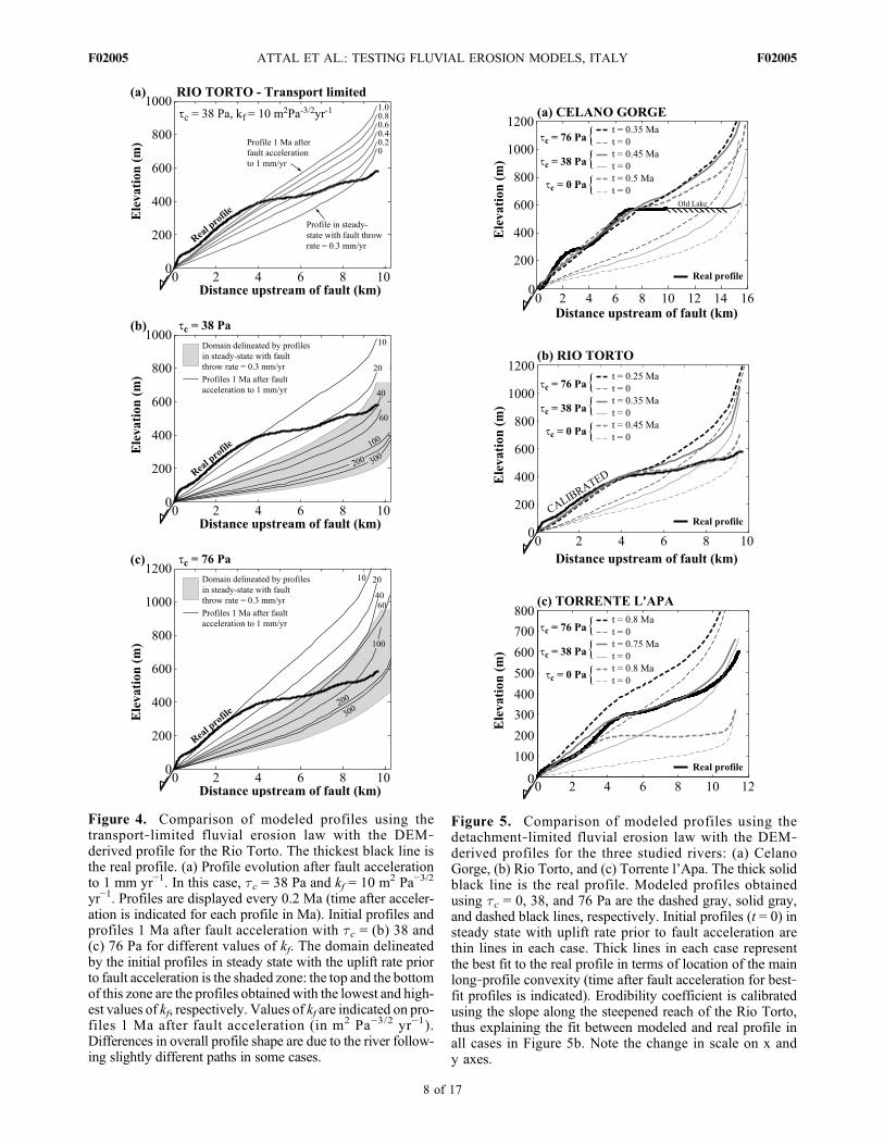
Figure 4. Comparison of modeled profiles using thetransport‐limited fluvial erosion law with the DEM‐derived profile for the Rio Torto. The thickest black line isthe real profile. (a) Profile evolution after fault accelerationto 1 mm yr−1. In this case, tc = 38 Pa and kf = 10 m2 Pa−3/2
yr−1. Profiles are displayed every 0.2 Ma (time after acceler-ation is indicated for each profile in Ma). Initial profiles andprofiles 1 Ma after fault acceleration with tc = (b) 38 and(c) 76 Pa for different values of kf. The domain delineatedby the initial profiles in steady state with the uplift rate priorto fault acceleration is the shaded zone: the top and the bottomof this zone are the profiles obtained with the lowest and high-est values of kf, respectively. Values of kf are indicated on pro-files 1 Ma after fault acceleration (in m2 Pa−3/2 yr−1).Differences in overall profile shape are due to the river follow-ing slightly different paths in some cases.
Figure 5. Comparison of modeled profiles using thedetachment‐limited fluvial erosion law with the DEM‐derived profiles for the three studied rivers: (a) CelanoGorge, (b) Rio Torto, and (c) Torrente l’Apa. The thick solidblack line is the real profile. Modeled profiles obtainedusing tc = 0, 38, and 76 Pa are the dashed gray, solid gray,and dashed black lines, respectively. Initial profiles (t = 0) insteady state with uplift rate prior to fault acceleration arethin lines in each case. Thick lines in each case representthe best fit to the real profile in terms of location of the mainlong‐profile convexity (time after fault acceleration for best‐fit profiles is indicated). Erodibility coefficient is calibratedusing the slope along the steepened reach of the Rio Torto,thus explaining the fit between modeled and real profile inall cases in Figure 5b. Note the change in scale on x andy axes.
ATTAL ET AL.: TESTING FLUVIAL EROSION MODELS, ITALY F02005F02005
8 of 17
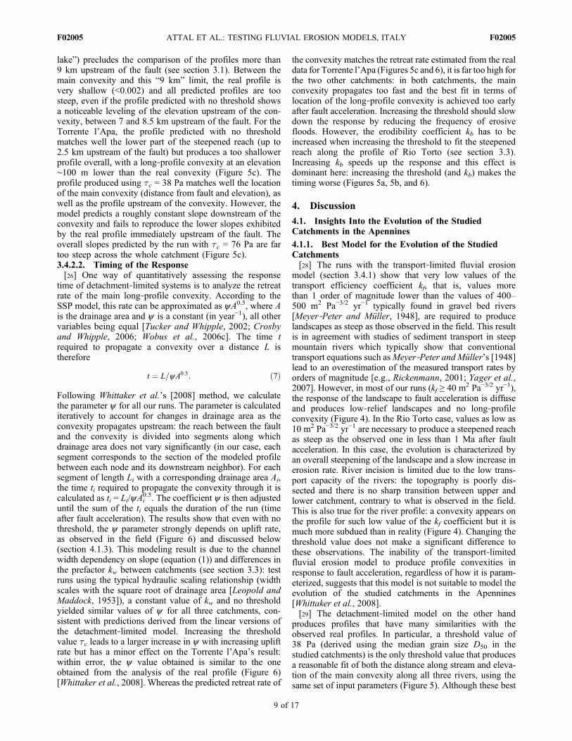
lake”) precludes the comparison of the profiles more than9 km upstream of the fault (see section 3.1). Between themain convexity and this “9 km” limit, the real profile isvery shallow (<0.002) and all predicted profiles are toosteep, even if the profile predicted with no threshold showsa noticeable leveling of the elevation upstream of the con-vexity, between 7 and 8.5 km upstream of the fault. For theTorrente l’Apa, the profile predicted with no thresholdmatches well the lower part of the steepened reach (up to2.5 km upstream of the fault) but produces a too shallowerprofile overall, with a long‐profile convexity at an elevation∼100 m lower than the real convexity (Figure 5c). Theprofile produced using tc = 38 Pa matches well the locationof the main convexity (distance from fault and elevation), aswell as the profile upstream of the convexity. However, themodel predicts a roughly constant slope downstream of theconvexity and fails to reproduce the lower slopes exhibitedby the real profile immediately upstream of the fault. Theoverall slopes predicted by the run with tc = 76 Pa are fartoo steep across the whole catchment (Figure 5c).3.4.2.2. Timing of the Response[26] One way of quantitatively assessing the response
time of detachment‐limited systems is to analyze the retreatrate of the main long‐profile convexity. According to theSSP model, this rate can be approximated as yA0.5, where Ais the drainage area and y is a constant (in year−1), all othervariables being equal [Tucker and Whipple, 2002; Crosbyand Whipple, 2006; Wobus et al., 2006c]. The time trequired to propagate a convexity over a distance L istherefore
t ¼ L=yA0:5: ð7Þ
Following Whittaker et al.’s [2008] method, we calculatethe parameter y for all our runs. The parameter is calculatediteratively to account for changes in drainage area as theconvexity propagates upstream: the reach between the faultand the convexity is divided into segments along whichdrainage area does not vary significantly (in our case, eachsegment corresponds to the section of the modeled profilebetween each node and its downstream neighbor). For eachsegment of length Li with a corresponding drainage area Ai,the time ti required to propagate the convexity through it iscalculated as ti = Li/yAi
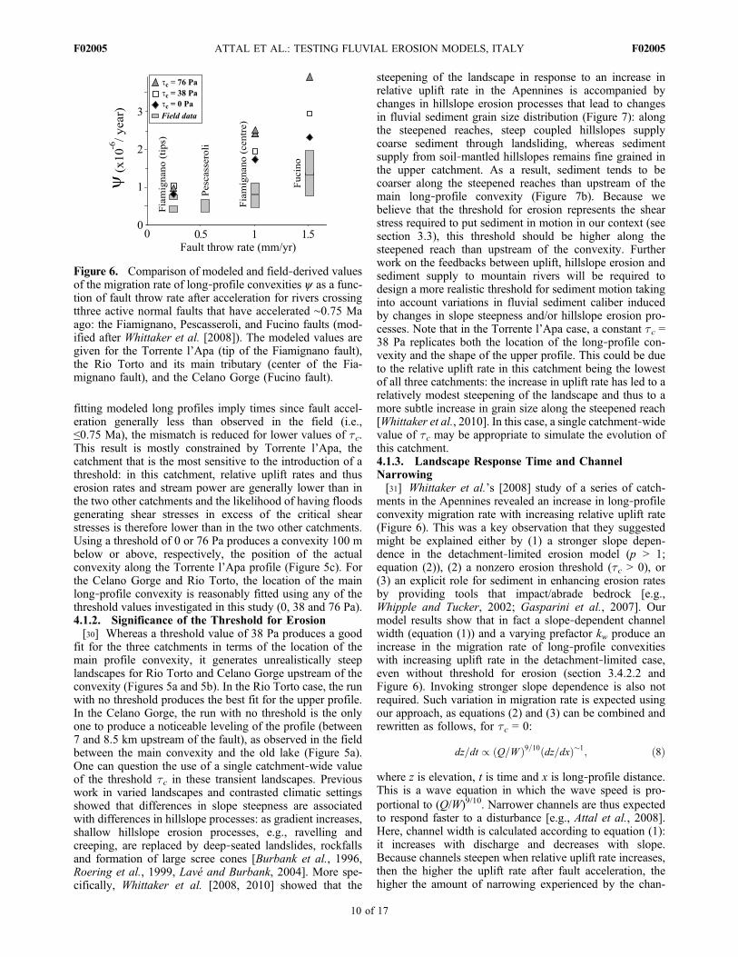
0.5. The coefficient y is then adjusteduntil the sum of the ti equals the duration of the run (timeafter fault acceleration). The results show that even with nothreshold, the y parameter strongly depends on uplift rate,as observed in the field (Figure 6) and discussed below(section 4.1.3). This modeling result is due to the channelwidth dependency on slope (equation (1)) and differences inthe prefactor kw between catchments (see section 3.3): testruns using the typical hydraulic scaling relationship (widthscales with the square root of drainage area [Leopold andMaddock, 1953]), a constant value of kw and no thresholdyielded similar values of y for all three catchments, con-sistent with predictions derived from the linear versions ofthe detachment‐limited model. Increasing the thresholdvalue tc leads to a larger increase in y with increasing upliftrate but has a minor effect on the Torrente l’Apa’s result:within error, the y value obtained is similar to the oneobtained from the analysis of the real profile (Figure 6)[Whittaker et al., 2008]. Whereas the predicted retreat rate of
the convexity matches the retreat rate estimated from the realdata for Torrente l’Apa (Figures 5c and 6), it is far too high forthe two other catchments: in both catchments, the mainconvexity propagates too fast and the best fit in terms oflocation of the long‐profile convexity is achieved too earlyafter fault acceleration. Increasing the threshold should slowdown the response by reducing the frequency of erosivefloods. However, the erodibility coefficient kb has to beincreased when increasing the threshold to fit the steepenedreach along the profile of Rio Torto (see section 3.3).Increasing kb speeds up the response and this effect isdominant here: increasing the threshold (and kb) makes thetiming worse (Figures 5a, 5b, and 6).
4. Discussion
4.1. Insights Into the Evolution of the StudiedCatchments in the Apennines
4.1.1. Best Model for the Evolution of the StudiedCatchments[28] The runs with the transport‐limited fluvial erosion
model (section 3.4.1) show that very low values of thetransport efficiency coefficient kf, that is, values morethan 1 order of magnitude lower than the values of 400–500 m2 Pa−3/2 yr−1 typically found in gravel bed rivers[Meyer‐Peter and Müller, 1948], are required to producelandscapes as steep as those observed in the field. This resultis in agreement with studies of sediment transport in steepmountain rivers which typically show that conventionaltransport equations such asMeyer‐Peter and Müller’s [1948]lead to an overestimation of the measured transport rates byorders of magnitude [e.g., Rickenmann, 2001; Yager et al.,2007]. However, in most of our runs (kf ≥ 40 m2 Pa−3/2 yr−1),the response of the landscape to fault acceleration is diffuseand produces low‐relief landscapes and no long‐profileconvexity (Figure 4). In the Rio Torto case, values as low as10 m2 Pa−3/2 yr−1 are necessary to produce a steepened reachas steep as the observed one in less than 1 Ma after faultacceleration. In this case, the evolution is characterized byan overall steepening of the landscape and a slow increase inerosion rate. River incision is limited due to the low trans-port capacity of the rivers: the topography is poorly dis-sected and there is no sharp transition between upper andlower catchment, contrary to what is observed in the field.This is also true for the river profile: a convexity appears onthe profile for such low value of the kf coefficient but it ismuch more subdued than in reality (Figure 4). Changing thethreshold value does not make a significant difference tothese observations. The inability of the transport‐limitedfluvial erosion model to produce profile convexities inresponse to fault acceleration, regardless of how it is param-eterized, suggests that this model is not suitable to model theevolution of the studied catchments in the Apennines[Whittaker et al., 2008].[29] The detachment‐limited model on the other hand
produces profiles that have many similarities with theobserved real profiles. In particular, a threshold value of38 Pa (derived using the median grain size D50 in thestudied catchments) is the only threshold value that producesa reasonable fit of both the distance along stream and eleva-tion of the main convexity along all three rivers, using thesame set of input parameters (Figure 5). Although these best
ATTAL ET AL.: TESTING FLUVIAL EROSION MODELS, ITALY F02005F02005
9 of 17
fitting modeled long profiles imply times since fault accel-eration generally less than observed in the field (i.e.,≤0.75 Ma), the mismatch is reduced for lower values of tc.This result is mostly constrained by Torrente l’Apa, thecatchment that is the most sensitive to the introduction of athreshold: in this catchment, relative uplift rates and thuserosion rates and stream power are generally lower than inthe two other catchments and the likelihood of having floodsgenerating shear stresses in excess of the critical shearstresses is therefore lower than in the two other catchments.Using a threshold of 0 or 76 Pa produces a convexity 100 mbelow or above, respectively, the position of the actualconvexity along the Torrente l’Apa profile (Figure 5c). Forthe Celano Gorge and Rio Torto, the location of the mainlong‐profile convexity is reasonably fitted using any of thethreshold values investigated in this study (0, 38 and 76 Pa).4.1.2. Significance of the Threshold for Erosion[30] Whereas a threshold value of 38 Pa produces a good
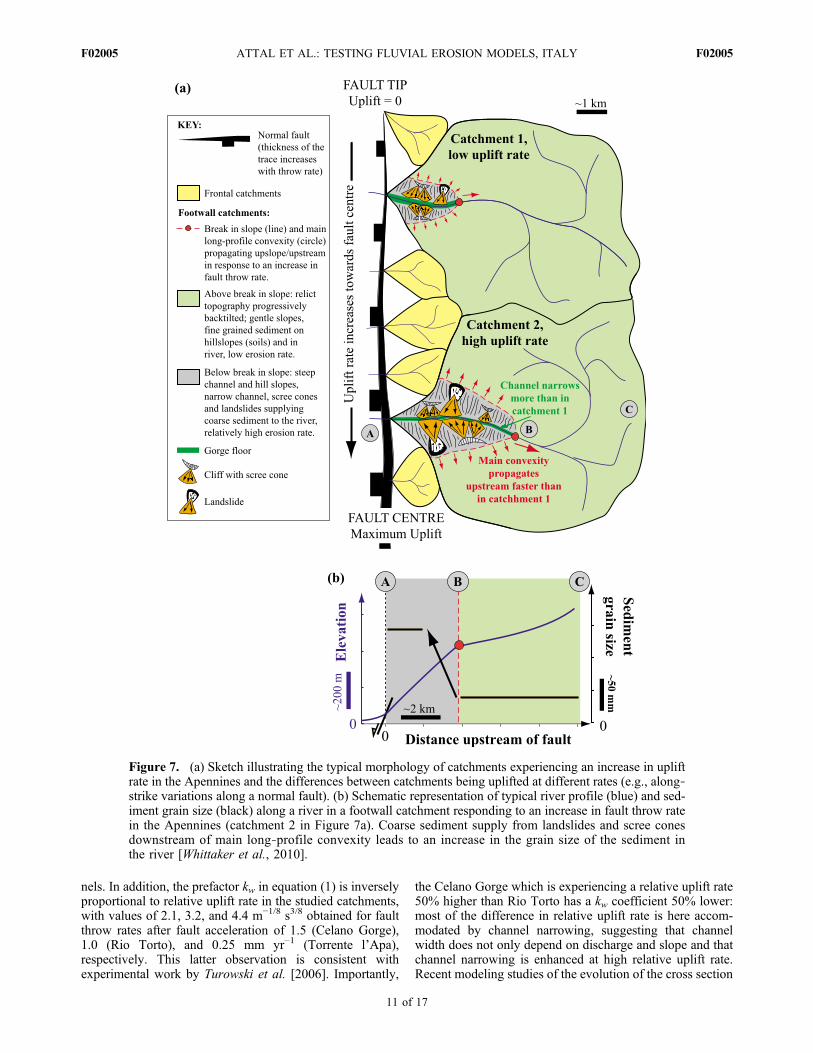
fit for the three catchments in terms of the location of themain profile convexity, it generates unrealistically steeplandscapes for Rio Torto and Celano Gorge upstream of theconvexity (Figures 5a and 5b). In the Rio Torto case, the runwith no threshold produces the best fit for the upper profile.In the Celano Gorge, the run with no threshold is the onlyone to produce a noticeable leveling of the profile (between7 and 8.5 km upstream of the fault), as observed in the fieldbetween the main convexity and the old lake (Figure 5a).One can question the use of a single catchment‐wide valueof the threshold tc in these transient landscapes. Previouswork in varied landscapes and contrasted climatic settingsshowed that differences in slope steepness are associatedwith differences in hillslope processes: as gradient increases,shallow hillslope erosion processes, e.g., ravelling andcreeping, are replaced by deep‐seated landslides, rockfallsand formation of large scree cones [Burbank et al., 1996,Roering et al., 1999, Lavé and Burbank, 2004]. More spe-cifically, Whittaker et al. [2008, 2010] showed that the
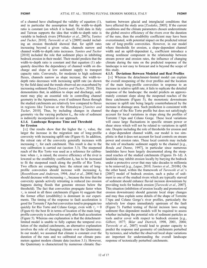
steepening of the landscape in response to an increase inrelative uplift rate in the Apennines is accompanied bychanges in hillslope erosion processes that lead to changesin fluvial sediment grain size distribution (Figure 7): alongthe steepened reaches, steep coupled hillslopes supplycoarse sediment through landsliding, whereas sedimentsupply from soil‐mantled hillslopes remains fine grained inthe upper catchment. As a result, sediment tends to becoarser along the steepened reaches than upstream of themain long‐profile convexity (Figure 7b). Because webelieve that the threshold for erosion represents the shearstress required to put sediment in motion in our context (seesection 3.3), this threshold should be higher along thesteepened reach than upstream of the convexity. Furtherwork on the feedbacks between uplift, hillslope erosion andsediment supply to mountain rivers will be required todesign a more realistic threshold for sediment motion takinginto account variations in fluvial sediment caliber inducedby changes in slope steepness and/or hillslope erosion pro-cesses. Note that in the Torrente l’Apa case, a constant tc =38 Pa replicates both the location of the long‐profile con-vexity and the shape of the upper profile. This could be dueto the relative uplift rate in this catchment being the lowestof all three catchments: the increase in uplift rate has led to arelatively modest steepening of the landscape and thus to amore subtle increase in grain size along the steepened reach[Whittaker et al., 2010]. In this case, a single catchment‐widevalue of tc may be appropriate to simulate the evolution ofthis catchment.4.1.3. Landscape Response Time and ChannelNarrowing[31] Whittaker et al.’s [2008] study of a series of catch-
ments in the Apennines revealed an increase in long‐profileconvexity migration rate with increasing relative uplift rate(Figure 6). This was a key observation that they suggestedmight be explained either by (1) a stronger slope depen-dence in the detachment‐limited erosion model (p > 1;equation (2)), (2) a nonzero erosion threshold (tc > 0), or(3) an explicit role for sediment in enhancing erosion ratesby providing tools that impact/abrade bedrock [e.g.,Whipple and Tucker, 2002; Gasparini et al., 2007]. Ourmodel results show that in fact a slope‐dependent channelwidth (equation (1)) and a varying prefactor kw produce anincrease in the migration rate of long‐profile convexitieswith increasing uplift rate in the detachment‐limited case,even without threshold for erosion (section 3.4.2.2 andFigure 6). Invoking stronger slope dependence is also notrequired. Such variation in migration rate is expected usingour approach, as equations (2) and (3) can be combined andrewritten as follows, for tc = 0:
dz=dt / Q=Wð Þ9=10 dz=dxð Þ�1; ð8Þ
where z is elevation, t is time and x is long‐profile distance.This is a wave equation in which the wave speed is pro-portional to (Q/W)9/10. Narrower channels are thus expectedto respond faster to a disturbance [e.g., Attal et al., 2008].Here, channel width is calculated according to equation (1):it increases with discharge and decreases with slope.Because channels steepen when relative uplift rate increases,then the higher the uplift rate after fault acceleration, thehigher the amount of narrowing experienced by the chan-
Figure 6. Comparison of modeled and field‐derived valuesof the migration rate of long‐profile convexities y as a func-tion of fault throw rate after acceleration for rivers crossingtthree active normal faults that have accelerated ∼0.75 Maago: the Fiamignano, Pescasseroli, and Fucino faults (mod-ified after Whittaker et al. [2008]). The modeled values aregiven for the Torrente l’Apa (tip of the Fiamignano fault),the Rio Torto and its main tributary (center of the Fia-mignano fault), and the Celano Gorge (Fucino fault).
ATTAL ET AL.: TESTING FLUVIAL EROSION MODELS, ITALY F02005F02005
10 of 17
nels. In addition, the prefactor kw in equation (1) is inverselyproportional to relative uplift rate in the studied catchments,with values of 2.1, 3.2, and 4.4 m−1/8 s3/8 obtained for faultthrow rates after fault acceleration of 1.5 (Celano Gorge),1.0 (Rio Torto), and 0.25 mm yr−1 (Torrente l’Apa),respectively. This latter observation is consistent withexperimental work by Turowski et al. [2006]. Importantly,
the Celano Gorge which is experiencing a relative uplift rate50% higher than Rio Torto has a kw coefficient 50% lower:most of the difference in relative uplift rate is here accom-modated by channel narrowing, suggesting that channelwidth does not only depend on discharge and slope and thatchannel narrowing is enhanced at high relative uplift rate.Recent modeling studies of the evolution of the cross section
Figure 7. (a) Sketch illustrating the typical morphology of catchments experiencing an increase in upliftrate in the Apennines and the differences between catchments being uplifted at different rates (e.g., along‐strike variations along a normal fault). (b) Schematic representation of typical river profile (blue) and sed-iment grain size (black) along a river in a footwall catchment responding to an increase in fault throw ratein the Apennines (catchment 2 in Figure 7a). Coarse sediment supply from landslides and scree conesdownstream of main long‐profile convexity leads to an increase in the grain size of the sediment inthe river [Whittaker et al., 2010].
ATTAL ET AL.: TESTING FLUVIAL EROSION MODELS, ITALY F02005F02005
11 of 17
of a channel have challenged the validity of equation (1),and in particular the assumption that the width‐to‐depthratio is constant (on which it is based). Field data in Italyand Taiwan supports the idea that width‐to‐depth ratio isvariable in bedrock rivers [Whittaker et al., 2007a; Yanitesand Tucker, 2010]. Turowski et al.’s [2009] model includ-ing an erosion threshold showed that, for uplift ratesincreasing beyond a given value, channels narrow andchannel width‐to‐depth ratio increases. Yanites and Tucker[2010] included the role that sediment plays in inhibitingbedrock erosion in their model. Their model predicts that thewidth‐to‐depth ratio is constant and that equation (1) ade-quately describes the dependency of channel width on dis-charge and slope at low sediment supply to transportcapacity ratio. Conversely, for moderate to high sedimentfluxes, channels narrow as slope increase, the width‐to‐depth ratio decreases with increasing uplift rate (as shownby the field data) and the trends observed are exacerbated byincreasing sediment fluxes [Yanites and Tucker, 2010]. Thisdemonstrates that, in addition to slope and discharge, sedi-ment may play an essential role in controlling channelgeometry in the Apennines, even if sediment fluxes throughthe studied catchments are relatively low compared to fluxesin regions like Taiwan or the Himalayas [Yanites andTucker, 2010]. Thus, by including changes in channelgeometry via the varying prefactor kw, the role of sedimentis indirectly incorporated in our approach.4.1.4. Landscape Response Time and Thresholdfor Erosion[32] Our results show that the higher the tc value, the
larger the increase in the migration rate of long‐profileconvexity with increasing uplift rate (Figure 6). In addition,the retreat rate of the convexity generally increases withincreasing tc for each catchment. This result is due to theway calibration is carried out (section 3.3). The steepenedreach of the Rio Torto was used as a reference for calibra-tion: when tc is raised, the erosive efficiency of the river islowered so the erodibility coefficient kb has to be increasedto fit the steepened reach along the profile of Rio Torto.Two effects are competing here: the retreat rate of long‐profile convexities should increase with increasing kb[Rosenbloom and Anderson, 1994; Attal et al., 2008] but itshould decrease with increasing tc, because the time that theconvexity spends actively retreating is reduced (no erosionhappens during floods that generate stresses below thethreshold). The fact that convexities propagate faster whentc is raised in all three catchments (Figure 6) suggests thatthe former effect (erodibility) is dominant in our experi-ments. The timing of the response to fault acceleration isgood for Torrente l’Apa but convexities tend to propagate tooquickly for Rio Torto and Celano Gorge, even with tc = 0(Figure 6): the best fit in terms of location of the main long‐profile convexity is achieved too early after fault acceleration(Figure 5). Whereas one explanation is that the detachment‐limited model is unable to fully capture the temporal evo-lution of the studied catchments, an alternative explanationinvolves the role of changing climate over the Quaternary.In our model, we assumed that climate is constant over theduration of the runs and we calibrated our climate para-meters against modern climate data (section 3.1). However,the Quaternary is characterized by numerous climatic fluc-
tuations between glacial and interglacial conditions thathave affected the study area [Tzedakis, 2005]. If the currentconditions and the climate parameters chosen underestimatethe global erosive efficiency of the rivers over the durationof the runs, then the erodibility coefficient may have beenoverestimated, with potential impact on the predicted retreatrate of long‐profile convexities. However, in our modelwhere thresholds for erosion, a slope‐dependent channelwidth and an uplift‐dependent kw coefficient introduce astrong nonlinear component in the relationship betweenstream power and erosion rates, the influence of changingclimate during the runs on the predicted response of thelandscape is not easy to forecast and is beyond the scope ofthis study.4.1.5. Deviations Between Modeled and Real Profiles[33] Whereas the detachment‐limited model can explain
the overall steepening of the river profiles and the locationof the main long‐profile convexities in response to anincrease in relative uplift rate, it fails to replicate the detailedresponse of the landscape: the model predicts an approxi-mately constant slope along the steepened reaches of thethree catchments (Figure 5), the monotonic downstreamincrease in uplift rate being largely counterbalanced by theincrease in drainage area. Such prediction is consistent withthe shape of the Rio Torto profile but does not satisfyinglyaccount for local variations in slope along the profiles ofTorrente l’Apa and Celano Gorge. These local variationswill cause large fluctuations in specific stream power orshear stress which will not be related to variations in upliftrate. Despite including the role of thresholds for erosion anda slope‐dependent channel width, our model is too sim-plistic in that it does not account for local controls on streampower and erosion rates. These local controls may includethe role of stochastic sediment supply to the channel [e.g.,Benda and Dunne, 1997], in particular since numerouslandslides have been largely documented along the steep-ened reaches of the studied catchments (Figures 1b–1d). Alandslide may inhibit erosion locally by burying the bedrockunder a protective cover that may take decades to millenniato be removed [e.g., Lague, 2010; Yanites et al., 2010b]. Onthe other hand, within the framework of Turowski et al.’s[2007] model of bedrock erosion, such a pulse of sedi-ment to one of the studied rivers which are typically starvedof sediment should enhance fluvial incision downstream byproviding tools for bedrock erosion [Turowski et al., 2007].This situation (inhibition of erosion locally and promotion oferosion downstream) should generate local slope changesand may thus explain some details of the shape of Torrentel’Apa and Celano Gorge’s river profiles, particularly therelatively low slopes immediately upstream of the fault(Figure 5). Further testing of fluvial incision laws usingsediment‐flux‐dependent models will be required to assesswhether including the potential role of sediment particles astools and/or cover with respect to bedrock erosion [e.g.,Gilbert, 1877; Sklar and Dietrich, 1998, 2001, 2004;Turowski et al., 2007] would lead to greater capacity topredict the response and geometry of catchments perturbedby tectonics, and whether the observed local slope variationsare important for understanding the overall landscaperesponse of tectonically perturbed catchments.
ATTAL ET AL.: TESTING FLUVIAL EROSION MODELS, ITALY F02005F02005
12 of 17
4.2. Implications for Modeling Landscape Evolutionand Extracting Tectonic Signals From Topography
4.2.1. Field Observations and Model Comparison[34] Based on the response of three catchments of dif-
ferent sizes which have been perturbed tectonically to var-ious extents, this work suggests that the detachment‐limitedmodel, with the addition of an appropriate threshold and aslope‐dependent channel width, adequately describes theoverall shape of the studied landscape. Lavé and Avouac[2001] came to a similar conclusion with their study ofrivers at the active front of the Himalayas. Based on theanalysis of landscapes in Northern and Southern California,Snyder et al.’s [2003a, 2003b] and DiBiase et al.’s [2010]studies, respectively, also gave some support to thedetachment‐limited model including a threshold for erosion.[35] Clearly, our results and conclusions differ markedly
from those of Loget et al. [2006] and Valla et al. [2010],where the transient response was found to be diffusive andquite well described by a transport‐limited model, in con-trast to the wave‐like response of a detachment‐limitedsystem that we observe. Both Loget et al. [2006] and Vallaet al. [2010] document bedrock incision for rivers where thechange in base level is sudden and not sustained (as a resultof lowering of the Mediterranean sea level during theMessinian salinity crisis and deglaciation, respectively),causing large convexities and substantial steepened reachesto appear almost instantly (geologically speaking) in thelower part of the river profiles. Such situation seems topromote a progressive degradation of the main profileconvexity that the detachment‐limited model is unable toaccount for. The mechanisms responsible for this behaviorin this particular setting are unknown but probably involvefeedbacks between gorge formation along the steep reaches,sediment supply into the gorge from steep hillslopes and thenecessity for the river to mobilize significant amounts ofsediment during floods to erode its bedrock [Valla et al.,2010]. Furthermore, a diffuse transient response to faultacceleration has been documented in a catchment drainingacross an active fault in Greece, even though the tectonichistory and bedrock geology of this catchment is verysimilar to that of the present study [Cowie et al., 2008]. Themain difference between the Greek example and the studiedrivers in the Italian Apennines is that the limestone which isactively incised by the Xerias River in Greece is shroudedby a layer of Plio‐Pleistocene fluvial conglomerates whichare poorly consolidated [Cowie et al., 2008]. These con-glomerates supply perfectly rounded and potentially mobilepebbles (with diameter rarely exceeding 100 mm) which areactively transported all along the river, leading to very poorbedrock exposure (the bed is typically blanketed with sed-iment and bed exposure never exceeds 20%). The presenceof a quasi‐continuous sediment cover in the Xerias Riverand the absence of long‐profile convexities upstream of theactive fault along the actively incising river suggest thatsediment transport is the main control on the gradient of theriver, thus leading to a diffuse response to an increase in faultthrow rate. Specifically, moving sediment during floods leadsto changes in the degree of bed cover which thus modulatesbedrock erosion, allowing the river to keep pace with theuplift rate at the fault.
4.2.2. Selecting Landscape Evolution Models[36] Based on our results and discussion (section 4.2.1),
we suggest that basic field observations and measurementscan help constrain the models that should be used to sim-ulate the landscape evolution of a given area or to mapspatial variations in fluvial erosion rates (Table 2). Thescarcity or absence of bed exposure along a river seems topreclude the use of the detachment‐limited model, even ifthe river is actively incising into bedrock [Cowie et al.,2008]. In the presence of moderate or low amounts ofsediment however, using a detachment‐limited modelincluding a threshold for erosion would be appropriate: thismodel explains best the evolution of the studied catchments(Table 2 and see section 4.2.2) and patterns of fluvial ero-sion at the front of the Himalayas [Lavé and Avouac, 2001]and across mountain ranges in California [Snyder et al.,2003a, 2003b; DiBiase et al., 2010]. Snyder et al. [2003a,2003b] and DiBiase et al. [2010] showed that typicalhydraulic scaling relationships can account for the evolutionof channel width through catchments in quasi‐equilibriumexperiencing quasi‐uniform uplift. However, if the responseof the landscape to a perturbation is to be predicted and/or ifthe uplift field across the studied catchment is nonuniform[Lavé and Avouac, 2001], we suggest that a slope‐dependentchannel width should be included in the model, e.g., usingequation (1). Even if such an equation does not incorporatethe additional potential controls on channel width (e.g., roleof sediment), it accounts for the now widely documentedphenomenon that channel slope cannot adjust withoutchanging the width and vice versa [Stark, 2006;Wobus et al.,2006b; Turowski et al., 2007, 2009; Yanites and Tucker,2010]. Ideally, the threshold value tc as well as the pre-factor kw in equation (1) would be calibrated against fielddata (Table 2). The threshold value should be calculatedusing the median grain size of the fluvial sediment D50
[Lavé and Avouac, 2001; this study]. We highlight that var-iations in the grain size of the sediment along the river wouldlead to changes in the threshold value (see section 4.1.2 andFigure 7) and that further work is needed to constrain spatialand temporal variations in sediment caliber (and thus ero-sion threshold) induced by changes in hillslope erosion ratesand processes as landscapes respond to changes in boundaryconditions (tectonics, climate) [e.g., Whittaker et al., 2010].4.2.3. Tectonics From Topography?[37] Steepness indices are commonly used in the literature
to assess tectonics from topography using remotely senseddata [e.g., Kirby et al., 2003; Wobus et al., 2006a; Miller etal., 2007]. They are usually calculated using a referenceconcavity index of 0.45–0.5 which is the typical concavityof steady state channels in uniformly uplifted landscapes(for methods, see Wobus et al. [2006a]); differences insteepness index along a river or between adjacent rivers thusrepresent deviations from the typical steady state profile andcould be interpreted in terms of spatially variable uplift ortransient response of the landscape to a perturbation.However, care must be taken when interpreting such databecause changes in channel width and the existence of athreshold for erosion can also affect the steepness of riversby modulating their erosive efficiency [Snyder et al., 2003b;Whittaker et al., 2008]. We believe that maps showing
ATTAL ET AL.: TESTING FLUVIAL EROSION MODELS, ITALY F02005F02005
13 of 17
specific stream power or shear stress in excess of thethreshold for erosion [Snyder et al., 2003a, 2003b; Lagueet al., 2005] that also account for potential channel widthadjustment [Finnegan et al., 2005; Stark, 2006;Wobus et al.,2006b; Turowski et al., 2007;Whittaker et al., 2007a; Yaniteset al., 2010a] would give a more accurate representation ofvariations in fluvial erosion rates – and thus potential var-iations in uplift rates – across landscapes than maps ofsteepness indices (Table 2). Ideally, thresholds for erosionwould be calibrated against field data (using fluvial sedi-ment D50), while using channel width values measured inthe field or extracted from a DEM (if its resolution is goodenough) would yield more accurate values of specific streampower or shear stress, whether channels are adjusting or not.4.2.4. Limitations[38] We emphasize that the detachment‐limited model
would not be suitable for modeling the evolution of land-scapes dissected by rivers transporting large amounts ofsediment (sections 4.2.1 and 4.2.2). Similarly, maps ofspecific stream power or shear stress along such riverswould provide a poor picture of the distribution of erosionrates along the rivers (Table 2). Care must therefore be takenwhen using such approaches to compute numerically theevolution of a landscape or to estimate relative fluvial ero-sion rates in an area, as a river which transports relativelylow amounts of sediment at the present‐day may have beenchoked with sediment in the past, possibly because ofchanges in the type of supply from hillslopes: for example,the characteristics of glacially derived sediment differ fromthose of hillslope‐derived sediment [e.g., Attal and Lavé,2006]; a change in the lithology exposed in the catchment(e.g., through the exhumation of different rock types) mayalter the bed load to total load ratio, because of a differentratio at the source and/or different abrasion rates [Attal andLavé, 2006, 2009]; climate change can alter vegetation andrunoff on the hillslopes and may potentially lead to largealluviation events in mountain rivers [e.g., Pratt‐Sitaula et al.,
2004]. In addition to temporal changes in sediment fluxes,the model outcomes will also be affected by spatial varia-tions in sediment fluxes, in particular at the downstreamtransition from detachment‐limited to transport‐limitedbehavior which has been documented along the course ofincising rivers, in theory [Whipple and Tucker, 2002] and inthe field [Brocard and van der Beek, 2006].[39] Sediment fluxes which are ignored in the approaches
described in this paper may also be responsible for changesin channel geometry that the equation used to calculatechannel width (equation (1)) fails to predict. Our data clearlyshows that channel width in the studied area is not depen-dent solely on discharge and slope and that channel isenhanced as uplift rate increases, an effect that we replicatedby adjusting the prefactor kw in equation (1) (section 4.1.3).Yanites and Tucker’s [2010] model demonstrates that despitesediment fluxes being relatively low in the studied catch-ments, they may be responsible for this enhanced narrowingand for the changes in width‐to‐depth ratio which have beendocumented in the field‐derived data [Whittaker et al.,2007a; Yanites and Tucker, 2010].[40] Finally, whereas the detachment‐limited model with
threshold for erosion and a slope‐dependent channel widthreproduces the overall shape of the studied catchments in theApennines, it fails to account for local variations in slopethat cause fluctuation in specific stream power which are notrelated to changes in uplift rates (see section 4.1.5 andFigure 5). We thus emphasize that the predictions of themodel, in terms of landscape evolution or quantification offluvial erosion rates in a given area, are valid on the largescale (i.e., at suprakilometric scale), and that local deviationsfrom the general trend in the data derived from the reallandscape (e.g., real river profile, maps of fluvial incisionrates) may result from processes which affect fluvial inci-sion rates locally and that the model does not account for,such as stochastic sediment supply from the hillslopes [e.g.,Benda and Dunne, 1997; Yanites et al., 2010b]. Further
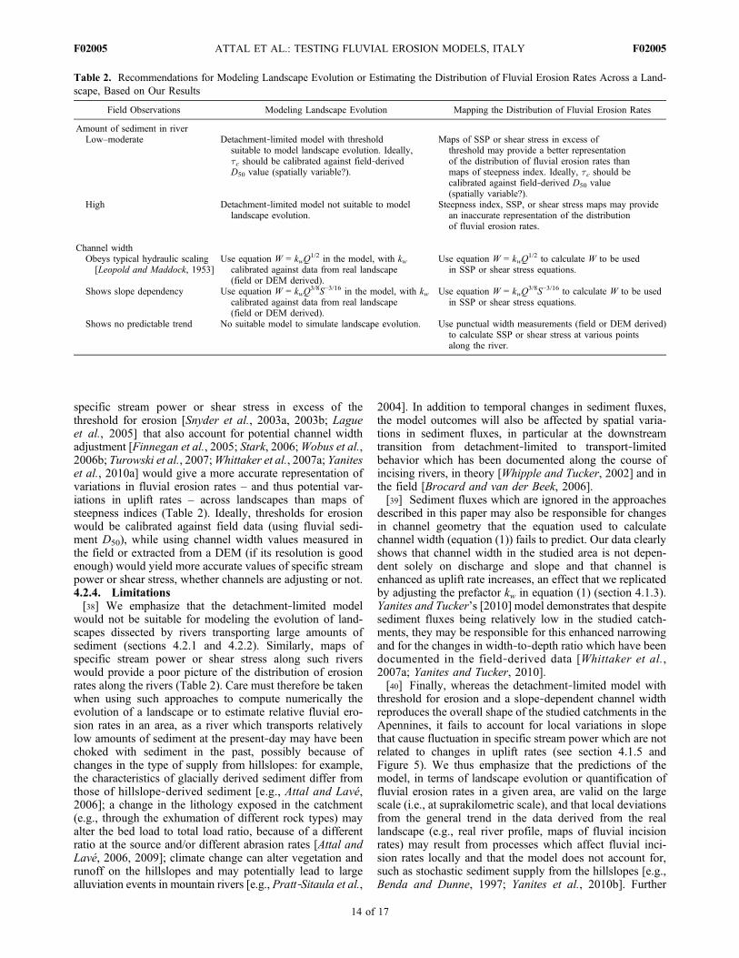
Table 2. Recommendations for Modeling Landscape Evolution or Estimating the Distribution of Fluvial Erosion Rates Across a Land-scape, Based on Our Results
Field Observations Modeling Landscape Evolution Mapping the Distribution of Fluvial Erosion Rates
Amount of sediment in riverLow–moderate Detachment‐limited model with threshold
suitable to model landscape evolution. Ideally,tc should be calibrated against field‐derivedD50 value (spatially variable?).
Maps of SSP or shear stress in excess ofthreshold may provide a better representationof the distribution of fluvial erosion rates thanmaps of steepness index. Ideally, tc should becalibrated against field‐derived D50 value(spatially variable?).
High Detachment‐limited model not suitable to modellandscape evolution.
Steepness index, SSP, or shear stress maps may providean inaccurate representation of the distributionof fluvial erosion rates.
Channel widthObeys typical hydraulic scaling[Leopold and Maddock, 1953]
Use equation W = kwQ1/2 in the model, with kw
calibrated against data from real landscape(field or DEM derived).
Use equation W = kwQ1/2 to calculate W to be used
in SSP or shear stress equations.
Shows slope dependency Use equation W = kwQ3/8S−3/16 in the model, with kw
calibrated against data from real landscape(field or DEM derived).
Use equation W = kwQ3/8S−3/16 to calculate W to be used
in SSP or shear stress equations.
Shows no predictable trend No suitable model to simulate landscape evolution. Use punctual width measurements (field or DEM derived)to calculate SSP or shear stress at various pointsalong the river.
ATTAL ET AL.: TESTING FLUVIAL EROSION MODELS, ITALY F02005F02005
14 of 17
studies are required to better understand the links betweenclimate, tectonics, sediment generation on the hillslopes,sediment supply to river, channel geometry adjustment,fluvial sediment transport and bedrock erosion, and thusdesign and test better fluvial erosion models that will makeaccurate predictions of fluvial erosion rates and landscapeevolution at all scales, from river reaches to mountain ranges.
5. Conclusion
[41] This test of fluvial erosion models using three tran-sient catchments in the Apennines favors a detachment‐limited model with a threshold for erosion and a slope‐dependent channel width. Unlike the transport‐limitedmodel and the basic detachment‐limited model (no thresh-old for erosion, channel width is a simple function of drainagearea), this model reproduces the overall shape of the riverprofiles as well as both the location and height of the mainlong‐profile convexity that formed in response to an inde-pendently constrained increase in relative uplift rate∼0.75 Ma ago. The hydraulic scaling equation proposed byFinnegan et al. [2005] (equation (1)) which includes a slopedependency to express channel width was used in this study.The prefactor kw in equation (1) calibrated against field datais strongly dependent on relative uplift rate, showing thatequation (1) tends to underestimate the amount of narrowingthat a river can undergo as it steepens. Our results show thatchanges in channel geometry exert an important control onlandscape response time: the dependency of channel widthon slope and the uplift‐dependent prefactor kw are respon-sible for a substantial increase in the migration rate of long‐profile convexities with increasing uplift rate (Figure 6),which has been observed in the study area [Whittaker et al.,2008]. A threshold of 38 Pa corresponding to the shearstress required to move sediments with a grain size of50 mm, similar to the median grain size of the fluvial sedi-ment along the steepened reaches in the study area, is requiredto fit the location and height of the main long‐profile con-vexities in the three catchments. The modeled response timesvary (0.35–0.75Ma) for a threshold of 38 Pa (Figure 5), andare somewhat younger that the field observations indicate(∼0.75 Ma), but are broadly consistent given the un-certainties in long‐term climatic controls that we are not ableto include in our approach.[42] Based on these results, we suggest that maps of
specific shear stress or stream power in excess of an erosionthreshold that also account for dynamic channel adjustmentwould bring more precise information on the spatial distri-bution of fluvial erosion rates than maps of steepness indiceswhich rely solely on slope and drainage area to highlight thedeviations from the typical steady state concave up profileof rivers incising into uniformly uplifted landscapes. Addi-tionally, we suggest that basic field observations and mea-surements of channel geometry and sediment characteristicscan help choose and calibrate the best fluvial erosion modelto predict the evolution of a given landscape (Table 2).Grain size data can be used to calibrate the threshold for adetachment‐limited model to predict the evolution of alandscape incised by rivers transporting low to moderateamounts of sediments. In all cases, a slope‐dependentchannel width should be included in the model to accountfor the now widely accepted fact that channels narrow as
they steepen [e.g., Yanites and Tucker, 2010]. Our resultsdemonstrate that simple detachment‐limited models aresuitable to reproduce the evolution of catchments, such asthose in the Apennines, with a reasonable degree of fidelity.However, assessing the extent to which local sedimentsupply variations need to be included in the models in orderto make high‐resolution predictions of landscape evolutionremains an outstanding challenge for the future.
[43] Acknowledgments. This project was funded by the NERCResearch grants NE/B504165/1 (Cowie, Roberts, Attal, and Tucker),NER/S/A/2002/10359 (Whittaker), and GR9/02995 (Roberts, Michetti)and by NSF and ARO (EAR‐0643240 and 47033‐EV; Tucker). We aregrateful to Nicole Gasparini, Jens Turowski, and the editor and associateeditor for detailed comments and suggestions which notably improved thismanuscript. We thank Eutizio Vittorio (APAT) for the DEM from whichwe derived the triangulated irregular network used in the numerical model.
ReferencesAmos, C. B., and D. W. Burbank (2007), Channel width response to differ-ential uplift, J. Geophys. Res., 112, F02010, doi:10.1029/2006JF000672.
Anders, M. H., M. Spiegelman, D. W. Rodgers, and J. T. Hagstrum (1993),The growth of fault‐bounded tilt blocks, Tectonics, 12, 1451–1459,doi:10.1029/93TC01547.
Attal, M., and J. Lavé (2006), Changes of bedload characteristics along theMarsyandi River (central Nepal): Implications for understanding hill-slope sediment supply, sediment load evolution along fluvial networks,and denudation in active orogenic belts, Spec. Pap. Geol. Soc. Am.,398, 143–171, doi:10.1130/2006.2398(09).
Attal, M., and J. Lavé (2009), Pebble abrasion during fluvial transport:Experimental results and implications for the evolution of the sedimentload along rivers, J. Geophys. Res., 114, F04023, doi:10.1029/2009JF001328.
Attal, M., G. E. Tucker, A. C. Whittaker, P. A. Cowie, and G. P. Roberts(2008), Modeling fluvial incision and transient landscape evolution:Influence of dynamic channel adjustment, J. Geophys. Res., 113,F03013, doi:10.1029/2007JF000893.
Benda, L., and T. Dunne (1997), Stochastic forcing of sediment supply tochannel networks from landsliding and debris flow, Water Resour. Res.,33, 2849–2863, doi:10.1029/97WR02388.
Boulton, S. J., and A. C. Whittaker (2009), Quantifying the slip rates, spa-tial distribution and evolution of active normal faults from geomorphicanalysis: Field examples from an oblique‐extensional graben, southernTurkey, Geomorphology, 104, 299–316, doi:10.1016/j.geomorph.2008.09.007.
Brocard, G. Y., and P. A. van der Beek (2006), Influence of incision rate,rock strength, and bedload supply on bedrock river gradients and valley‐flat widths: Field based evidence and calibrations from western Alpinerivers (southeast France), Spec. Pap. Geol. Soc. Am., 398, 101–126.
Buffington, J. M., and D. R. Montgomery (1997), A systematic analysis ofeight decades of incipient motion studies, with special reference togravel‐bedded rivers, Water Resour. Res., 33, 1993–2029, doi:10.1029/96WR03190.
Burbank, D. W., J. Leland, E. Fielding, R. S. Anderson, N. Brozovic, M. R.Reid, and C. Duncan (1996), Bedrock incision, rock uplift and thresholdhillslopes in the northwestern Himalayas, Nature, 379, 505–510,doi:10.1038/379505a0.
Chatanantavet, P., and G. Parker (2009), Physically based modeling of bed-rock incision by abrasion, plucking, and macroabrasion, J. Geophys.Res., 114, F04018, doi:10.1029/2008JF001044.
Cowie, P. A., A. C. Whittaker, M. Attal, G. P. Roberts, G. E. Tucker, andA. Ganas (2008), New constraints on sediment‐flux‐dependent river inci-sion: Implications for extracting tectonic signals from river profiles,Geology, 36, 535–538, doi:10.1130/G24681A.1.
Crosby, B. T., and K. X. Whipple (2006), Knickpoint initiation and distri-bution within fluvial networks: 236 waterfalls in the Waipaoa River,North Island, New Zealand, Geomorphology, 82, 16–38, doi:10.1016/j.geomorph.2005.08.023.
DiBiase, R. A., K. X. Whipple, A. M. Heimsath, and W. B. Ouimet (2010),Landscape form and millennial erosion rates in the San Gabriel Moun-tains, CA, Earth Planet. Sci. Lett., 289, 134–144, doi:10.1016/j.epsl.2009.10.036.
Eagleson, P. S. (1978), Climate, soil, and vegetation: 2. Distribution ofannual precipitation derived from observed storm sequences, WaterResour. Res., 14, 713–721, doi:10.1029/WR014i005p00713.
ATTAL ET AL.: TESTING FLUVIAL EROSION MODELS, ITALY F02005F02005
15 of 17
Ellis, M. A., A. L. Densmore, and R. S. Anderson (1999), Development ofmountainous topography in the Basin Ranges, USA, Basin Res., 11,21–41, doi:10.1046/j.1365-2117.1999.00087.x.
Finnegan, N. J., G. Roe, D. R. Montgomery, and B. Hallet (2005), Controlson the channel width of rivers: Implications for modeling fluvial incisionof bedrock, Geology, 33, 229–232, doi:10.1130/G21171.1.
Gasparini, N. M., R. L. Bras, and K. X. Whipple (2006), Numericalmodeling of non‐steady state river profile evolution using a sediment‐flux‐dependent incision model, Spec. Pap. Geol. Soc. Am., 398, 127–141.
Gasparini, N. M., K. X. Whipple, and R. L. Bras (2007), Predictions ofsteady state and transient landscape morphology using sediment‐flux‐dependent river incision models, J. Geophys. Res., 112, F03S09,doi:10.1029/2006JF000567.
Gilbert, G. K. (1877), Report on the geology of the Henry Mountains: Geo-graphical and geological survey of the rocky mountain region, report,160 pp., Dep. of the Inter., Washington D. C.
Hawk, K. L. (1992), Climatology of station storm rainfall in the continentalUnited States: Parameters of the Bartlett‐Lewis and Poisson rectangularpulses models, M.S. thesis, Mass. Inst. of Tech., Cambridge, Mass.
Howard, A. D. (1994), A detachment‐limited model of drainage‐basin evo-lution, Water Resour. Res., 30, 2261–2285, doi:10.1029/94WR00757.
Howard, A. D., and G. Kerby (1983), Channel changes in badlands, Geol.Soc. Am. Bull., 94, 739–752, doi:10.1130/0016-7606(1983)94<739:CCIB>2.0.CO;2.
Howard, A. D., W. E. Dietrich, and M. A. Seidl (1994), Modeling flu-vial erosion on regional to continental scales, J. Geophys. Res., 99,13,971–13,986, doi:10.1029/94JB00744.
Johnson, J. P. L., K. X. Whipple, L. S. Sklar, and T. C. Hanks (2009),Transport slopes, sediment cover, and bedrock channel incision in theHenry Mountains, Utah, J. Geophys. Res., 114, F02014, doi:10.1029/2007JF000862.
Kirby, E., and K. Whipple (2001), Quantifying differential rock‐uplift ratesvia stream profile analysis, Geology, 29, 415–418, doi:10.1130/0091-7613(2001)029<0415:QDRURV>2.0.CO;2.
Kirby, E., K. X. Whipple, W. Q. Tang, and Z. L. Chen (2003), Distributionof active rock uplift along the eastern margin of the Tibetan Plateau:Inferences from bedrock channel longitudinal profiles, J. Geophys.Res., 108(B4), 2217, doi:10.1029/2001JB000861.
Kooi, H., and C. Beaumont (1994), Escarpment evolution on high‐elevationrifted margins: Insights derived from a surface processes model thatcombines diffusion, advection, and reaction, J. Geophys. Res., 99,12,191–12,209, doi:10.1029/94JB00047.
Lague, D. (2010), Reduction of long‐term bedrock incision efficiency byshort‐term alluvial cover intermittency, J. Geophys. Res., 115, F02011,doi:10.1029/2008JF001210.
Lague, D., N. Hovius, and P. Davy (2005), Discharge, discharge variability,and the bedrock channel profile, J. Geophys. Res., 110, F04006,doi:10.1029/2004JF000259.
Lavé, J., and J. P. Avouac (2001), Fluvial incision and tectonic uplift acrossthe Himalayas of central Nepal, J. Geophys. Res., 106, 26,561–26,591,doi:10.1029/2001JB000359.
Lavé, J., and D. Burbank (2004), Denudation processes and rates in theTransverse Ranges, Southern California: Erosional response of a transi-tional landscape to external and anthropogenic forcing, J. Geophys.Res., 109, F01006, doi:10.1029/2003JF000023.
Leopold, L. B., and T. Maddock (1953), The hydraulic geometry of streamchannels and some physiographic implications, U.S. Geol. Surv. Prof.Pap., 252, 57 pp.
Loget, N., P. Davy, and J. Van Den Driessche (2006), Mesoscale fluvialerosion parameters deduced from modeling the Mediterranean sea leveldrop during the Messinian (late Miocene), J. Geophys. Res., 111,F03005, doi:10.1029/2005JF000387.
Meyer‐Peter, E., and R. Müller (1948), Formulas for bed‐load transport, inProceedings of the 2nd Meeting of the International Association forHydraulic Structures Research, pp. 39–64, Int. Assoc. Hydraul. Res.,Delft, Netherlands.
Miller, S. R., R. L. Slingerland, and E. Kirby (2007), Characteristics ofsteady state fluvial topography above fault‐bend folds, J. Geophys.Res., 112, F04004, doi:10.1029/2007JF000772.
Pratt‐Sitaula, B., D. W. Burbank, A. Heimsath, and T. Ojha (2004), Land-scape disequilibrium on 1000–10,000 year scales, Marsyandi River,Nepal, central Himalaya, Geomorphology, 58, 223–241, doi:10.1016/j.geomorph.2003.07.002.
Rickenmann, D., (2001), Comparison of bed load transport in torrents andgravel bed streams, Water Resour. Res., 37, 3295–3305, doi:10.1029/2001WR000319.
Roberts, G. P., and A. M. Michetti (2004), Spatial and temporal variationsin growth rates along active normal fault systems: An example from The
Lazio‐Abruzzo Apennines, central Italy, J. Struct. Geol., 26, 339–376,doi:10.1016/S0191-8141(03)00103-2.
Roering, J. J., J. W. Kirchner, and W. E. Dietrich (1999), Evidence for non-linear, diffusive sediment transport on hillslopes and implications forlandscape morphology, Water Resour. Res., 35, 853–870, doi:10.1029/1998WR900090.
Rosenbloom, N. A., and R. S. Anderson (1994), Hillslope and channel evo-lution in a marine terraced landscape, Santa Cruz, California, J. Geophys.Res., 99, 14,013–14,029, doi:10.1029/94JB00048.
Seidl, M. A., and W. E. Dietrich (1992), The problem of channel erosioninto bedrock, Catena, 23, suppl., 101–124.
Sklar, L. S., and W. E. Dietrich (1998), River longitudinal profiles and bed-rock incision models: Stream power and the influence of sediment sup-ply, in Rivers Over Rock: Fluvial Processes in Bedrock Channels,Geophys. Monogr. Ser., vol. 107, edited by K. Tinkler and E. E. Wohl,pp. 237–260, AGU, Washington, D. C.
Sklar, L. S., and W. E. Dietrich (2001), Sediment and rock strength controlson river incision into bedrock, Geol. Soc. Am. Bull., 29, 1087–1090.
Sklar, L. S., and W. E. Dietrich (2004), A mechanistic model for river inci-sion into bedrock by saltating bed load,Water Resour. Res., 40, W06301,doi:10.1029/2003WR002496.
Sklar, L. S., and W. E. Dietrich (2006), The role of sediment in controllingsteady state bedrock channel slope: Implications of the saltation–abrasionincision model, Geomorphology, 82, 58–83, doi:10.1016/j.geomorph.2005.08.019.
Sklar, L. S., W. E. Dietrich, E. Foufoula‐Georgiou, B. Lashermes, andD. Bellugi (2006), Do gravel bed river size distributions record channelnetwork structure?, Water Resour. Res., 42, W06D18, doi:10.1029/2006WR005035.
Snyder, N. P., and L. L. Kammer (2008), Dynamic adjustments in channelwidth in response to a forced diversion: Gower Gulch, Death ValleyNational Park, Calif. Geol., 36, 187–190.
Snyder, N. P., K. X. Whipple, G. E. Tucker, and D. J. Merritts (2003a),Channel response to tectonic forcing: Field analysis of streammorphologyand hydrology in the Mendocino triple junction region, northern Califor-nia, Geomorphology, 53, 97–127, doi:10.1016/S0169-555X(02)00349-5.
Snyder, N. P., K. X. Whipple, G. E. Tucker, and D. J. Merritts (2003b),Importance of a stochastic distribution of floods and erosion thresholdsin the bedrock river incision problem, J. Geophys. Res., 108(B2),2117, doi:10.1029/2001JB001655.
Stark, C. P. (2006), A self‐regulating model of bedrock river channelgeometry, Geophys. Res. Lett., 33, L04402, doi:10.1029/2005GL023193.
Stock, J. D., and D. R. Montgomery (1999), Geologic constraints on bed-rock river incision using the stream power law, J. Geophys. Res., 104,4983–4993, doi:10.1029/98JB02139.
Tomkin, J. H., M. T. Brandon, F. J. Pazzaglia, J. R. Barbour, and S. D.Willett (2003), Quantitative testing of bedrock incision models for theClearwater River, NW Washington state, J. Geophys. Res., 108(B6),2308, doi:10.1029/2001JB000862.
Tucker, G. E. (2004), Drainage basin sensitivity to tectonic and climaticforcing: Implications of a stochastic model for the role of entrainmentand erosion thresholds, Earth Surf. Processes Landforms, 29, 185–205,doi:10.1002/esp.1020.
Tucker, G. E., and R. L. Bras (2000), A stochastic approach to modelingthe role of rainfall variability in drainage basin evolution, Water Resour.Res., 36, 1953–1964, doi:10.1029/2000WR900065.
Tucker, G. E., and K. X. Whipple (2002), Topographic outcomes predictedby stream erosion models: Sensitivity analysis and intermodel compari-son, J. Geophys. Res., 107(B9), 2179, doi:10.1029/2001JB000162.
Tucker, G. E., S. T. Lancaster, N. M. Gasparini, R. L. Bras, and S. M.Rybarczyk (2001), An object‐oriented framework for distributed hydro-logic and geomorphic modeling using triangulated irregular networks,Comput. Geosci., 27, 959–973, doi:10.1016/S0098-3004(00)00134-5.
Turowski, J. M., D. Lague, A. Crave, and N. Hovius (2006), Experimentalchannel response to tectonic uplift, J. Geophys. Res., 111, F03008,doi:10.1029/2005JF000306.
Turowski, J. M., D. Lague, and N. Hovius (2007), Cover effect in bedrockabrasion: A new derivation and its implications for the modeling of bed-rock channel morphology, J. Geophys. Res., 112, F04006, doi:10.1029/2006JF000697.
Turowski, J. M., D. Lague, and N. Hovius (2009), Response of bedrockchannel width to tectonic forcing: Insights from a numerical model, theo-retical considerations, and comparison with field data, J. Geophys. Res.,114, F03016, doi:10.1029/2008JF001133.
Tzedakis, P. (2005), Towards an understanding of the response of southernEuropean vegetation to orbital and suborbital climate variability, Quat.Sci. Rev., 24, 1585–1599, doi:10.1016/j.quascirev.2004.11.012.
Valla, P. G., P. A. van der Beek, and D. Lague (2010), Fluvial incision intobedrock: Insights from morphometric analysis and numerical modeling
ATTAL ET AL.: TESTING FLUVIAL EROSION MODELS, ITALY F02005F02005
16 of 17
of gorges incising glacial hanging valleys (Western Alps, France),J. Geophys. Res., 115, F02010, doi:10.1029/2008JF001079.
van der Beek, P., and P. Bishop (2003), Cenozoic river profile developmentin the Upper Lachlan catchment (SE Australia) as a test of quantitativefluvial incision models, J. Geophys. Res., 108(B6), 2309, doi:10.1029/2002JB002125.
Whipple, K. X., and G. E. Tucker (1999), Dynamics of the stream‐powerriver incision model: Implications for height limits of mountain ranges,landscape response timescales, and research needs, J. Geophys. Res.,104, 17,661–17,674, doi:10.1029/1999JB900120.
Whipple, K. X., and G. E. Tucker (2002), Implications of sediment‐flux‐dependent river incision models for landscape evolution, J. Geophys.Res., 107(B2), 2039, doi:10.1029/2000JB000044.
Whipple, K. X., N. P. Snyder, and K. Dollenmayer (2000a), Rates andprocesses of bedrock incision by the upper Ukak River since the 1912Novarupta ash flow in the Valley of Ten Thousand Smokes, Alaska,Geology, 28, 835–838, doi:10.1130/0091-7613(2000)28<835:RAPO-BI>2.0.CO;2.
Whipple, K. X., G. S. Hancock, and R. S. Anderson (2000b), River incisioninto bedrock: Mechanics and relative efficacy of plucking, abrasion andcavitation, Geol. Soc. Am. Bull., 112, 490–503, doi:10.1130/0016-7606(2000)112<490:RIIBMA>2.0.CO;2.
Whittaker, A. C., P. A. Cowie, M. Attal, G. E. Tucker, and G. P. Roberts(2007a), Bedrock channel adjustment to tectonic forcing: Implications forpredicting river incision rates, Geology, 35, 103–106, doi:10.1130/G23106A.1.
Whittaker, A. C., P. A. Cowie, M. Attal, G. E. Tucker, and G. P. Roberts(2007b), Contrasting transient and steady state rivers crossing active nor-mal faults: New field observations from the central Apennines, Italy,Basin Res., 19, 529–556, doi:10.1111/j.1365-2117.2007.00337.x.
Whittaker, A. C., M. Attal, P. A. Cowie, G. E. Tucker, and G. P. Roberts(2008), Decoding temporal and spatial patterns of fault uplift using tran-sient river long profiles, Geomorphology, 100, 506–526, doi:10.1016/j.geomorph.2008.01.018.
Whittaker, A. C., M. Attal, and P. A. Allen (2010), Characterising the origin,nature and fate of sediment exported from catchments perturbed by activetectonics, Basin Res., 22, 809–828, doi:10.1111/j.1365-2117.2009.00447.x.
Willgoose, G., R. L. Bras, and J. Rodriguez‐Iturbe (1991), A coupledchannel network growth and hillslope evolution model: 1. Theory, WaterResour. Res., 27, 1671–1684, doi:10.1029/91WR00935.
Wobus, C., K. X. Whipple, E. Kirby, N. Snyder, J. Johnson, K. Spyropo-lou, B. Crosby, and D. Sheehan (2006a), Tectonics from topography:Procedures, promise, and pitfalls, Spec. Pap. Geol. Soc. Am., 398, 55–74.
Wobus, C. W., G. E. Tucker, and R. S. Anderson (2006b), Self‐formedbedrock channels, Geophys. Res. Lett., 33, L18408, doi:10.1029/2006GL027182.
Wobus, C. W., B. T. Crosby, and K. X. Whipple (2006c), Hanging valleysin fluvial systems: Controls on occurrence and implications for landscapeevolution, J. Geophys. Res., 111, F02017, doi:10.1029/2005JF000406.
Yager, E. M., J. W. Kirchner, and W. E. Dietrich (2007), Calculating bedload transport in steep boulder bed channels, Water Resour. Res., 43,W07418, doi:10.1029/2006WR005432.
Yanites, B. J., and G. E. Tucker (2010), Controls and limits on bedrockchannel geometry, J. Geophys. Res., 115, F04019, doi:10.1029/2009JF001601.
Yanites, B. J., G. E. Tucker, K. J. Mueller, Y.‐G. Chen, T. Wilcox, and S. Y.Huang (2010a), Incision and channel morphology across active structuresin the Peikang River, central Taiwan: Implications for the importance ofchannel width, Geol. Soc. Am. Bull., 122, 1192–1208, doi:10.1130/B30035.1.
Yanites, B. J., G. E. Tucker, K. J. Mueller, and Y.‐G. Chen (2010b), Howrivers react to large earthquakes: Evidence from central Taiwan, Geology,38, 639–642, doi:10.1130/G30883.1.
M. Attal, P. A. Cowie, and D. Hobley, School of GeoSciences,University of Edinburgh, Drummond Street, Edinburgh EH8 9XP, UK.([email protected])G. P. Roberts, Research School of Geological and Geophysical Sciences,
Birkbeck, University of London, and University College London, GowerStreet, London WC1E 6BT, UK.G. E. Tucker, Cooperative Institute for Research in Environmental
Sciences, University of Colorado at Boulder, Boulder, CO 80309, USA.A. C. Whittaker, Royal School of Mines, Imperial College London,
South Kensington Campus, London SW7 2AZ, UK.
ATTAL ET AL.: TESTING FLUVIAL EROSION MODELS, ITALY F02005F02005
17 of 17