Test vector decomposition-based static compaction algorithms for combinational circuits

Test Vector Decomposition Based StaticCompaction Algorithms for Combinational Circuits

Aiman H. El-Maleh and Yahya E. Osais

King Fahd University of Petroleum and Minerals

Testing system-on-chips involves applying huge amounts of test data, which is stored in the testermemory and then transferred to the chip under test during test application. Therefore, practicaltechniques, such as test compression and compaction, are required to reduce the amount of testdata in order to reduce both the total testing time and memory requirements for the tester. In thispaper, a new approach to static compaction for combinational circuits, referred to as test vectordecomposition (TVD), is proposed. In addition, two new TVD based static compaction algorithmsare presented. Experimental results for benchmark circuits demonstrate the effectiveness of thetwo new static compaction algorithms.

Categories and Subject Descriptors: B.6.2 [Logic Design]: Testing—static compaction; B.7.3[Integrated Circuits]: Testing—static compaction; J.6 [Computer-Aided Engineering]:computer-aided design (CAD)

General Terms: Theory, Algorithms

Additional Key Words and Phrases: Static compaction, combinational circuits, taxonomy, testvector decomposition, independent fault clustering, class-based clustering

1. INTRODUCTION

Advances in the VLSI technology paved the way for System-on-Chips (SoCs). Tra-ditional IC design, in which every circuit is designed from scratch and reuse islimited only to standard cell libraries, is more and more replaced by the SoC designmethodology. However, this new design methodology has its own challenges. Amajor challenge is how to reduce the increasing volume of test data. Basically,there are two approaches: compression and compaction. In the first approach, testdata is kept compressed while it is stored in the tester memory and transferred tothe Chip Under Test (CUT). Then, it is decompressed on the CUT. This reducesthe memory and transfer time requirements. In the second approach, however,the objective is to reduce the size of a test set while maintaining the same faultcoverage.

Test compaction techniques are classified into two categories. The first categoryincludes algorithms that can be integrated into the test generation process. Suchalgorithms are referred to as dynamic compaction algorithms. On the other hand,

Authors’ addresses: Aiman H. El-Maleh, KFUPM, P.O. Box 1063, Dhahran 31261, Saudi Arabia;email: [email protected]; Yahya E. Osais, KFUPM, P.O. Box 983, Dhahran 31261, SaudiArabia; email: [email protected] to make digital/hard copy of all or part of this material without fee for personalor classroom use provided that the copies are not made or distributed for profit or commercialadvantage, the ACM copyright/server notice, the title of the publication, and its date appear, andnotice is given that copying is by permission of the ACM, Inc. To copy otherwise, to republish,to post on servers, or to redistribute to lists requires prior specific permission and/or a fee.c© 2003 ACM 1084-4309/2003/0400-0001 $5.00

ACM Transactions on Design Automation of Electronic Systems, Vol. V, No. N, July 2003, Pages 1–29.

2 · El-Maleh and Osais

the second category includes algorithms that are applied after the test sets aregenerated. Such algorithms are referred to as static compaction algorithms. Thereare several approaches to static compaction of a given test set as will be shown inthe next section.

Since test application time is proportional to the length of the test set thatneeds to be applied, it is desirable to apply shorter test sets that provide thesame fault coverage at reduced test application time. Although static compactionalgorithms do not typically produce test sets of sizes equal to those generatedusing dynamic compaction, interests in developing more efficient static compactionalgorithms have increased [Miyase et al. 2002]. Static compaction has the followingadvantages over dynamic compaction. First, generating smaller test sets usingdynamic compaction is time consuming because many attempts to modify partiallyspecified test vectors to detect additional faults often fail [Miyase et al. 2002].Secondly, dynamic compaction does not take advantage of random test patterngeneration. Thirdly, static compaction is independent of ATPG.

Given a test set T with single stuck-at fault coverage FCT for a combinationalcircuit, the static compaction problem can be formulated as to find another testset, T ∗, for the same circuit such that FCT∗ ≥ FCT and |T ∗| < |T | [Chang and Lin1995]. It should be pointed out that in the above definition, there is no constrainton the individual fault coverage of each test vector and the proximity between thetest vectors of T and T ∗. That is, the fault coverage of each test vector needs notremain intact and T ∗ needs not be a subset of T .

This paper is structured as follows. First, we give a taxonomy of static com-paction algorithms for combinational circuits. In this section, we review the exist-ing static compaction algorithms and show how they fit in our taxonomy. Besides,we introduce and motivate the new concept of test vector decomposition. Then, wedescribe two new static compaction algorithms based on test vector decomposition.After that, we present and discuss the experimental results. Finally, we concludeby summarizing the results of the paper and their significance.

2. TAXONOMY OF STATIC COMPACTION ALGORITHMS

In this section, we give a taxonomy of static compaction algorithms for combina-tional circuits. We first start with an overview of the taxonomy. Then, we give adescription of every class in the taxonomy with examples from the literature.

2.1 Overview

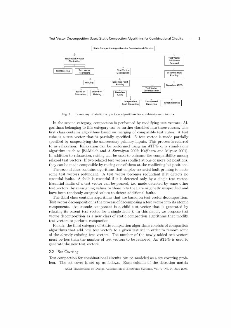
Static compaction algorithms for combinational circuits can be divided into threebroad categories: (1) Redundant Vector Elimination, (2) Test Vector Modification,and (3) Test Vector Addition and Removal. Figure 1 shows our proposed taxon-omy. In the first category, compaction is performed by dropping redundant testvectors. A redundant test vector is a vector whose faults are all detectable byother test vectors. Static compaction algorithms falling under this category canbe further classified into two classes. The first class contains algorithms based onset covering in which faults are to be covered using the minimum possible numberof test vectors. On the other hand, the second class contains algorithms based ontest vector reordering in which reordering, fault simulation, fault distribution, anddouble detection are used to identify redundant test vectors and then drop them.ACM Transactions on Design Automation of Electronic Systems, Vol. V, No. N, July 2003.

Test Vector Decomposition Based Static Compaction Algorithms for Combinational Circuits · 3

Static Compaction Algorithms for Combinational Circuits

Set Covering

Redundant VectorElimination

Test VectorAddition &Removal

Test VectorReordering

Test VectorModification

Merging

Based onRaising

Based onRelaxation

Essential FaultPruning

Based onATPG

Essential faultPruning

Based on ATPGTest Vector

Decomposition

Class-basedClustering

Graph ColoringIndependent

Fault Clustering

Fig. 1. Taxonomy of static compaction algorithms for combinational circuits.

In the second category, compaction is performed by modifying test vectors. Al-gorithms belonging to this category can be further classified into three classes. Thefirst class contains algorithms based on merging of compatible test cubes. A testcube is a test vector that is partially specified. A test vector is made partiallyspecified by unspecifying the unnecessary primary inputs. This process is referredto as relaxation. Relaxation can be performed using an ATPG or a stand-alonealgorithm, such as [El-Maleh and Al-Suwaiyan 2002; Kajihara and Miyase 2001].In addition to relaxation, raising can be used to enhance the compatibility amongrelaxed test vectors. If two relaxed test vectors conflict at one or more bit positions,they can be made compatible by raising one of them at the conflicting bit positions.

The second class contains algorithms that employ essential fault pruning to makesome test vectors redundant. A test vector becomes redundant if it detects noessential faults. A fault is essential if it is detected only by a single test vector.Essential faults of a test vector can be pruned, i.e. made detected by some othertest vectors, by reassigning values to those bits that are originally unspecified andhave been randomly assigned values to detect additional faults.

The third class contains algorithms that are based on test vector decomposition.Test vector decomposition is the process of decomposing a test vector into its atomiccomponents. An atomic component is a child test vector that is generated byrelaxing its parent test vector for a single fault f. In this paper, we propose testvector decomposition as a new class of static compaction algorithms that modifytest vectors to perform compaction.

Finally, the third category of static compaction algorithms consists of compactionalgorithms that add new test vectors to a given test set in order to remove someof the already existing test vectors. The number of the newly added test vectorsmust be less than the number of test vectors to be removed. An ATPG is used togenerate the new test vectors.

2.2 Set Covering

Test compaction for combinational circuits can be modeled as a set covering prob-lem. The set cover is set up as follows. Each column of the detection matrix

ACM Transactions on Design Automation of Electronic Systems, Vol. V, No. N, July 2003.


Test Faults

t1 f1,f4

t2 f2,f4

t3 f2,f3

Fig. 2. Test vectors and their associated faults.

Fault Test

f1 t1f2 t2f3 t3f4 t1

Fig. 3. First test vector that detects every fault.

corresponds to a test vector and each row corresponds to a fault. If a test vectorj detects fault i, then the entry (i, j) is one; otherwise, it is zero. In this setup,the total amount of memory required for building the detection matrix is O(nf),where n is the number of test vectors and f is the number of faults.

Static compaction procedures based on set covering were described in [Floreset al. 1999; Boateng et al. 2001; Hochbaum 1996]. It should be pointed out thatthis approach has not been used much in the literature due to the huge memoryand CPU time requirements.

2.3 Test Vector Reordering

Identification of redundant test vectors in a test set is an order dependent process.Given any order, redundant test vectors can be identified using fault simulation,fault distribution, or double detection. There are four variations of Test VectorReordering (TVR) based static compaction algorithms.

2.3.1 TVR with Fault Dropping Simulation. Fault simulation of a test set in anorder different from the order of generation is used as a fast and effective method todrop redundant test vectors. Under Reverse Order Fault simulation (ROF) [Schulzet al. 1988; Pomeranz and Reddy 2001], a test set is fault simulated with droppingin reverse order of generation. That is, a test vector that was generated later isfault simulated earlier. When it is simulated, a test vector that does not detect anynew faults is removed from the test set.

The intuitive reason for this phenomenon is simply that test vectors which arefurther down the list detect faults which are most difficult to detect. Therefore,if we first fault simulate a test vector which is at the end of the list, it not onlydetects a hard fault right away, it also detects many others by pure chance. Thisway hard faults are out of the way early.

2.3.2 TVR with Forward-Looking Fault Simulation. The forward-looking faultsimulation is an improved version of ROF [Pomeranz and Reddy 2001]. It is basedon the idea that information about the first test vector that detects every fault canbe used to drop test vectors that would not be dropped by ROF. That is, the yetundetected faults have lower indexed test vectors that detect them. So, some testvectors are skipped over and consequently dropped from the test set.

Let us consider the following example. Let the test set T be {t1, t2, t3} and theACM Transactions on Design Automation of Electronic Systems, Vol. V, No. N, July 2003.


fault set F be {f1, f2, f3, f4}. Figure 2 shows the test vectors with their associatedfaults and Figure 3 shows the first test vector that detects every fault. ConventionalROF first simulates t3. This test will be retained in the test set to detect f2 andf3. Next, t2 is simulated. Since it detects the new fault f4, it is retained in the testset. Finally, t1 is simulated and retained in the test set since it detects a new fault,which is f1. No tests are dropped by ROF in this case.

Now, let us start ROF again taking into account the information given in Figure 3.ROF starts by simulating t3. This test is retained in the test set to detect f2 andf3. Next, t2 is simulated. t2 detects the new fault f4. However, f4 is first detectedby t1. Therefore, we conclude that t2 is not necessary for the detection of any yetundetected fault and we drop it from the test set. Finally, when t1 is simulated, theremaining undetected faults f1 and f4 become detected and the detection processcompletes. In this case, one test vector is dropped from the test set.

2.3.3 TVR with Fault Distribution. In TVR with fault distribution, a test vectoris fault simulated without fault dropping. Faults detected by every test vector arerecorded. Besides, the number of test vectors that detect every fault is recorded.After that, given any order, a test vector whose number of essential faults is zero,i.e. the faults it detects can be distributed among other test vectors, is consideredredundant and thus can be dropped. After a test vector is dropped, the number oftest vectors that detect every one of its faults is reduced by one.

In [Hamzaoglu and Patel 1998], compaction based on fault distribution was usedto compact test sets as a part of a dynamic compaction algorithm. The motivebehind the proposed algorithm is the fact that ROF cannot identify a redundanttest vector if some of the faults detected by it are only detected by the test vectorsgenerated earlier. ROF can only identify a redundant test vector if all the faultsdetected by it are also detected by the test vectors generated later.

2.3.4 TVR with Double Detection Fault Simulation. Double Detection (DD)was first proposed in [Kajihara et al. 1995] as a dynamic compaction algorithm.Basically, when generating a new test vector, a yet undetected fault, called a pri-mary target fault, is selected and a test vector t is generated to detect it. Next,other faults, called secondary target faults, are selected one at a time and the un-specified values in t are specified appropriately to detect the secondary target faultsuntil no unspecified values remain in t or no additional secondary target faults canbe detected. In choosing the secondary target faults, faults that are not detectedare first considered and then faults detected at most once by earlier generated testvectors are considered. Faults are dropped from the list of target faults when theyare detected twice. Test vectors that detect faults which are detected only once,i.e. essential test vectors, are marked. After the test generation is complete (whenall the faults are detected at least once or aborted or proved to be untestable),the following static compaction procedure is used to reduce the test set size. Thegenerated test vectors are fault simulated with dropping in the following order.First, all the essential test vectors are simulated in the order they were generated.The essential test vectors are followed by the non-essential test vectors in the orderopposite to the order in which they were generated. During the fault simulationprocess, a test vector that does not detect any new fault is dropped. It should be



Table I. Definition of themerging operation.

◦ 0 1 x

0 0 φ 01 φ 1 1x 0 1 x

pointed out that essential test vectors cannot be dropped and thus simulating themfirst maximizes the ability to drop other test vectors.

DD can be used in static compaction procedures, e.g. [Lin et al. 2001]. However,since most test generators do not attempt to target faults for a second detection anddo not use non-fault dropping simulation, they do not collect all the informationnecessary for static compaction based on DD. Therefore, the necessary informationmust be collected in a preprocessing step.

2.4 Merging

Static compaction algorithms in this class can be divided into two groups. Thefirst group contains algorithms based on the very simple and efficient approachof merging compatible test cubes. A test cube is a relaxed test vector. A testvector is relaxed by unspecifying the unnecessary primary inputs. A test vectorcan be relaxed using an ATPG or a stand-alone algorithm, such as [El-Maleh andAl-Suwaiyan 2002; Kajihara and Miyase 2001]. A merging procedure employingrelaxation proceeds as follows. Given a test set T , test vectors in T are all relaxed.Then, an iterative search is performed for pairs of compatible test vectors. Twotest vectors ti and tj are compatible if they do not specify complementary values inany bit position. If any two vectors, say ti and tj , are compatible, they are replacedby the vector ti ◦ tj , where ◦ represents the merging operation (see the definitionin Table I). The new test vector ti ◦ tj has all the binary values of both ti andtj . Hence, by a repetitive application of the above compaction operation, manytest vectors (two or more) can be combined into fewer test vectors. As a result thetotal number of test vectors that need to be applied with the same fault detectioncapabilities is reduced. Examples of this approach can be found in [El-Maleh andAl-Suwaiyan 2002; Ayari and Kaminska 1994; Miyase et al. 2002].

In the second group, algorithms employ in addition to the relaxation operationa raising operation. For a test vector t, the raising operation raise(t, i) tries to setthe ith bit of t to x while preserving the coverage of the essential faults of t. Theraising operation was proposed in [Chang and Lin 1995]. Raising is used to enhancecompatibility among relaxed test vectors. For example, if two relaxed test vectors,say ti and tj , conflict at one or more bit positions, they can be made compatibleby raising one of them at the conflicting bit positions. Typically, raising is used toresolve conflicts when a test set contains no compatible test vectors.

2.5 Test Vector Decomposition

Test Vector Decomposition (TVD) is the process of decomposing a test vector intoits atomic components. An atomic component is a child test vector that is generatedby relaxing its parent test vector for a single fault f . That is, the child test vectorcontains the assignments necessary for the detection of f . Besides, the child testvector may detect other faults in addition to f . For example, consider the test vectorACM Transactions on Design Automation of Electronic Systems, Vol. V, No. N, July 2003.


tp = 010110 that detects the set of faults Fp = {f1,f2,f3}. Using the relaxationalgorithm in [El-Maleh and Al-Suwaiyan 2002], tp can be decomposed into threeatomic components, which are (f1,01xxxx), (f2,0x01xx), and (f3,x1xx10). Everyatomic component detects the fault associated with it and may accidentally detectother faults. An atomic component cannot be decomposed any further because itcontains the assignments necessary for detecting its fault.

Static compaction based on merging is a very simple and efficient technique.However, it has the following problems. First, for a highly incompatible test set,merging achieves little reduction. Secondly, raising is a costly operation. Thirdly, atest vector must be processed as a whole. Therefore, we propose that a test vectorbe decomposed into its atomic components before it is processed. In this way, atest vector that is originally incompatible with all other test vectors in a given testset can be eliminated if its components can be merged with other test vectors.

By decomposing a test vector into its atomic components, a merging based com-paction algorithm will have more degree of freedom. This is because of the fact thatthe number of unspecified bits in an atomic component is much larger than that ina parent test vector. Thus, the probability of merging a component is higher thanthat of merging its parent test vector.

The problem of static compaction based on TVD can be modeled as a graphcoloring problem. Basically, given a test set T with single stuck-at fault coverageFCT , the set of atomic components CT is first obtained. Then, a graph G is built.In G, every node corresponds to a component and an edge exists between twonodes if their corresponding components are incompatible. Now, our objective isto partition CT into k subsets such that k is as small as possible and no adjacentnodes belong to the same subset. The fault coverage of the new test set T ∗ whosesize is k should be greater than or equal to FCT .

It is well known that graph coloring is an NP-hard problem [Garey and John-son 1979]. Thus, efforts of researchers are devoted to heuristic methods, ratherthan exact ones. Heuristic methods are simple schemes in which nodes are coloredsequentially according to some criteria.

2.6 Essential Fault Pruning

Generally speaking, pruning a fault of a test vector decreases the number of itsfaults by one. A test vector becomes redundant if all of its faults are pruned. FaultPruning (FP) is implemented as follows. Given a test vector t, an attempt is madeto detect each of its faults by modifying the other test vectors in the test set. Afault of t is said to be pruned if it becomes detected by another test vector afterthe modification. If all the faults of t are pruned, then t can be removed from thetest set.

The above operation of modifying a test vector, say t′, to further detect an

additional fault f of another test vector t is basically achieved by generating a newtest vector t

′′such that DET(t

′′) = DET(t

′) ∪ f , where DET(t) is the set of faults

detected by t. Multiple Target Faults Test Generation (MTFTG) is used for thispurpose. In MTFTG, a test vector is to be found for a set of target faults. MTFTGwill fail if there exists at least two independent faults in the set of target faults.Two faults are independent if they cannot be detected by a single test vector.

The run time of an FP based static compaction procedure can be greatly improvedACM Transactions on Design Automation of Electronic Systems, Vol. V, No. N, July 2003.


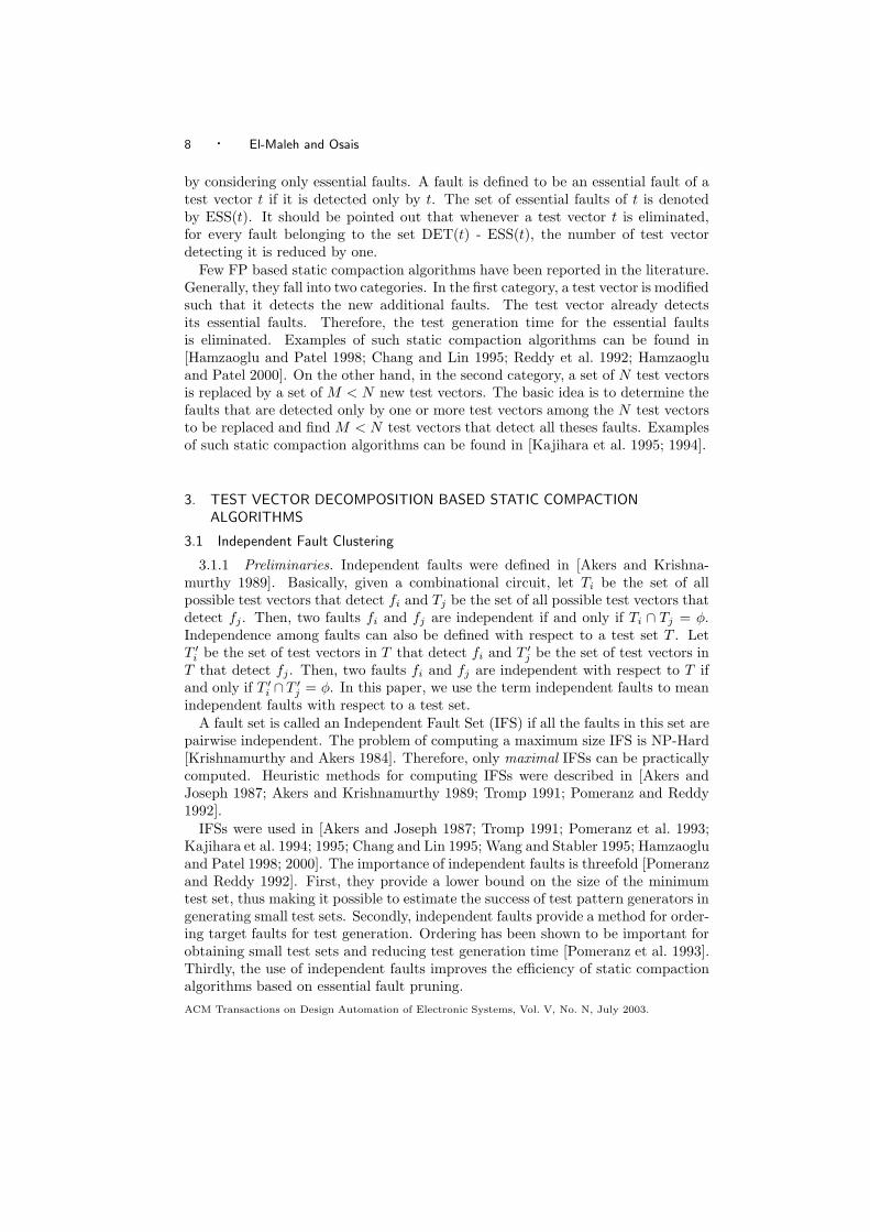
by considering only essential faults. A fault is defined to be an essential fault of atest vector t if it is detected only by t. The set of essential faults of t is denotedby ESS(t). It should be pointed out that whenever a test vector t is eliminated,for every fault belonging to the set DET(t) - ESS(t), the number of test vectordetecting it is reduced by one.

Few FP based static compaction algorithms have been reported in the literature.Generally, they fall into two categories. In the first category, a test vector is modifiedsuch that it detects the new additional faults. The test vector already detectsits essential faults. Therefore, the test generation time for the essential faultsis eliminated. Examples of such static compaction algorithms can be found in[Hamzaoglu and Patel 1998; Chang and Lin 1995; Reddy et al. 1992; Hamzaogluand Patel 2000]. On the other hand, in the second category, a set of N test vectorsis replaced by a set of M < N new test vectors. The basic idea is to determine thefaults that are detected only by one or more test vectors among the N test vectorsto be replaced and find M < N test vectors that detect all theses faults. Examplesof such static compaction algorithms can be found in [Kajihara et al. 1995; 1994].

3. TEST VECTOR DECOMPOSITION BASED STATIC COMPACTIONALGORITHMS

3.1 Independent Fault Clustering

3.1.1 Preliminaries. Independent faults were defined in [Akers and Krishna-murthy 1989]. Basically, given a combinational circuit, let Ti be the set of allpossible test vectors that detect fi and Tj be the set of all possible test vectors thatdetect fj. Then, two faults fi and fj are independent if and only if Ti ∩ Tj = φ.Independence among faults can also be defined with respect to a test set T . LetT ′

i be the set of test vectors in T that detect fi and T ′j be the set of test vectors in

T that detect fj. Then, two faults fi and fj are independent with respect to T ifand only if T ′

i ∩ T ′j = φ. In this paper, we use the term independent faults to mean

independent faults with respect to a test set.A fault set is called an Independent Fault Set (IFS) if all the faults in this set are

pairwise independent. The problem of computing a maximum size IFS is NP-Hard[Krishnamurthy and Akers 1984]. Therefore, only maximal IFSs can be practicallycomputed. Heuristic methods for computing IFSs were described in [Akers andJoseph 1987; Akers and Krishnamurthy 1989; Tromp 1991; Pomeranz and Reddy1992].

IFSs were used in [Akers and Joseph 1987; Tromp 1991; Pomeranz et al. 1993;Kajihara et al. 1994; 1995; Chang and Lin 1995; Wang and Stabler 1995; Hamzaogluand Patel 1998; 2000]. The importance of independent faults is threefold [Pomeranzand Reddy 1992]. First, they provide a lower bound on the size of the minimumtest set, thus making it possible to estimate the success of test pattern generators ingenerating small test sets. Secondly, independent faults provide a method for order-ing target faults for test generation. Ordering has been shown to be important forobtaining small test sets and reducing test generation time [Pomeranz et al. 1993].Thirdly, the use of independent faults improves the efficiency of static compactionalgorithms based on essential fault pruning.ACM Transactions on Design Automation of Electronic Systems, Vol. V, No. N, July 2003.


Algorithm IFCInput: A test set T of size |T | and fault coverage FCT .Output: A new test set T ∗ such that |T ∗| ≤ |T | and FCT∗ ≥ FCT .

1. Fault simulate T without fault dropping.2. For every essential fault f that is detected by a test vector t:

2.1. Extract the atomic component cf from t.2.2. If the number of compatibility sets is zero, create a new compatibility set,map cf to it, and then go to Step 2.2.3. Map cf to an existing compatibility set, if possible, and then go Step 2.2.4. Create a new compatibility set and map cf to it.

3. Find sets of independent faults.4. Sort sets of independent faults in decreasing order of their sizes.5. For every fault in an IFS, sort the test vectors that detect the fault indecreasing order of the number of faults they detect.6. For every fault f , where f belongs to an IFS:

6.1. For every test vector t that detects f :6.1.1. Extract the atomic component cf from t.6.1.2. If the number of compatibility sets is zero, create a new compatibilityset, map cf to it, and then go to Step 6.6.1.3. Map cf to an existing compatibility set, if possible, and go to Step 6.

6.2. Create a new compatibility set and map cf to it.7. Return T ∗.

Fig. 4. The IFC algorithm.

3.1.2 Algorithm Description. In Independent Fault Clustering (IFC) algorithms,IFSs are first derived. Then, a fault matching procedure is used to find sets of com-patible faults, i.e. faults that can be detected by a single test vector. In the IFSderivation phase, independent faults are identified with respect to a test set. On theother hand, in the fault matching phase, compatible components, corresponding tocompatible faults, are mapped to the same compatibility set. Whenever a compo-nent is mapped to a compatibility set, it is merged with the partial test vector ofthat compatibility set. At the end, every compatibility set represents a single testvector.

Our IFC algorithm is shown in Figure 4 and proceeds as follows. First, the giventest set T is fault simulated without fault dropping. This step is performed tofind the number and set of test vectors that detect every fault. Secondly, essentialfaults are matched. In this step, for every essential fault f detected by t, the atomiccomponent cf corresponding to f is extracted from t. Then, for every compatibilityset CSi, if cf is compatible with the partial test vector in CSi, cf is mapped to CSi.On the other hand, if the number of compatibility sets is zero or cf is incompatiblewith all partial test vectors in the existing compatibility sets, a new compatibilityset is created and cf is mapped to it.

It should be observed that an essential fault has a single component while non-essential faults have more than one. Therefore, if a component of a non-essentialfault f is incompatible with all the partial test vectors in the existing compatibilitysets, the other components of f will be tried before creating a new compatibilityset. On the other hand, if the component of an essential fault is incompatible withall the partial test vectors in the existing compatibility sets, a new compatibility



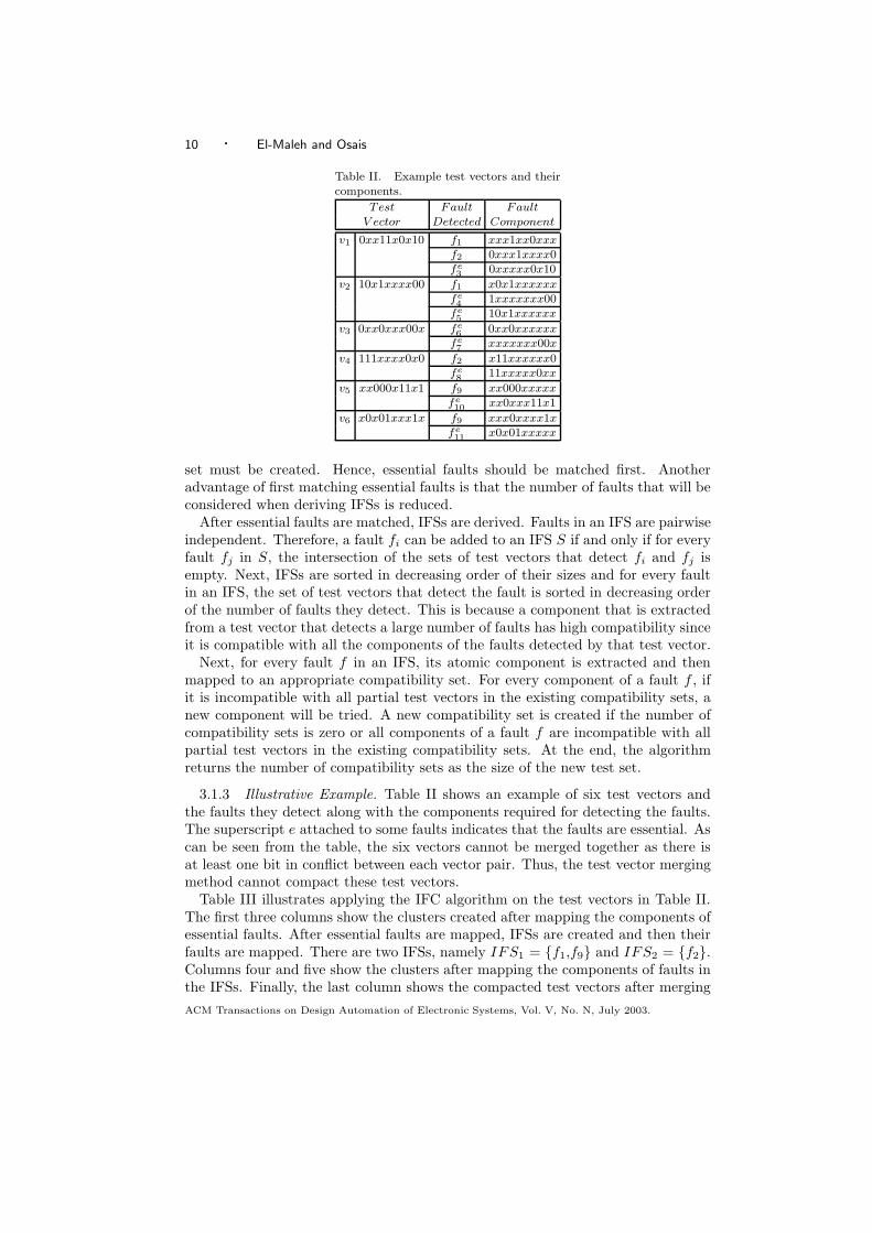
Table II. Example test vectors and theircomponents.

Test Fault FaultV ector Detected Component

v1 0xx11x0x10 f1 xxx1xx0xxxf2 0xxx1xxxx0fe3 0xxxxx0x10

v2 10x1xxxx00 f1 x0x1xxxxxxfe4 1xxxxxxx00

fe5 10x1xxxxxx

v3 0xx0xxx00x fe6 0xx0xxxxxx

fe7 xxxxxxx00x

v4 111xxxx0x0 f2 x11xxxxxx0fe8 11xxxxx0xx

v5 xx000x11x1 f9 xx000xxxxxfe10 xx0xxx11x1

v6 x0x01xxx1x f9 xxx0xxxx1xfe11 x0x01xxxxx

set must be created. Hence, essential faults should be matched first. Anotheradvantage of first matching essential faults is that the number of faults that will beconsidered when deriving IFSs is reduced.

After essential faults are matched, IFSs are derived. Faults in an IFS are pairwiseindependent. Therefore, a fault fi can be added to an IFS S if and only if for everyfault fj in S, the intersection of the sets of test vectors that detect fi and fj isempty. Next, IFSs are sorted in decreasing order of their sizes and for every faultin an IFS, the set of test vectors that detect the fault is sorted in decreasing orderof the number of faults they detect. This is because a component that is extractedfrom a test vector that detects a large number of faults has high compatibility sinceit is compatible with all the components of the faults detected by that test vector.

Next, for every fault f in an IFS, its atomic component is extracted and thenmapped to an appropriate compatibility set. For every component of a fault f , ifit is incompatible with all partial test vectors in the existing compatibility sets, anew component will be tried. A new compatibility set is created if the number ofcompatibility sets is zero or all components of a fault f are incompatible with allpartial test vectors in the existing compatibility sets. At the end, the algorithmreturns the number of compatibility sets as the size of the new test set.

3.1.3 Illustrative Example. Table II shows an example of six test vectors andthe faults they detect along with the components required for detecting the faults.The superscript e attached to some faults indicates that the faults are essential. Ascan be seen from the table, the six vectors cannot be merged together as there isat least one bit in conflict between each vector pair. Thus, the test vector mergingmethod cannot compact these test vectors.

Table III illustrates applying the IFC algorithm on the test vectors in Table II.The first three columns show the clusters created after mapping the components ofessential faults. After essential faults are mapped, IFSs are created and then theirfaults are mapped. There are two IFSs, namely IFS1 = {f1,f9} and IFS2 = {f2}.Columns four and five show the clusters after mapping the components of faults inthe IFSs. Finally, the last column shows the compacted test vectors after mergingACM Transactions on Design Automation of Electronic Systems, Vol. V, No. N, July 2003.


Table III. Example test vectors and their components.

AfterMapping AfterMapping AfterMergingEssentialFaults IndependentFaultSets Components

Cluster Fault Fault Component Fault Fault Component Test V ector

1 f3 0xxxxx0x10 f3 0xxxxx0x10 00x01x0x10f6 0xx0xxxxxx f6 0xx0xxxxxxf11 x0x01xxxxx f11 x0x01xxxxx

f2 0xxx1xxxx0

2 f4 1xxxxxxx00 f4 1xxxxxxx00 10x1xx0000f5 10x1xxxxxx f5 10x1xxxxxxf7 xxxxxxx00x f7 xxxxxxx00x

f1 xxx1xx0xxx

3 f8 11xxxxx0xx f8 11xxxxx0xx 11000xx0xxf9 xx000xxxxx

4 f10 xx0xxx11x1 f10 xx0xxx11x1 xx0xxx11x1

Algorithm Iter IFCInput: A test set T of size |T | and fault coverage FCT .Output: A new test set T ∗ such that |T ∗| ≤ |T | and FCT∗ ≥ FCT .

1. Randomly fill the unspecified bits in T .2. T ∗ = IFC(T)3. If |T ∗| < |T |, copy T ∗ to T and go to Step 1.

Else If |T ∗| == |T |, return T ∗.Else return T .

Fig. 5. The iterative IFC algorithm.

the components in each cluster. Since the number of clusters obtained is four, thecompacted test set is of size four. Hence, two test vectors were eliminated.

3.1.4 Iterative IFC. The level of compaction achievable by our IFC algorithmcan be improved in two ways. First, after a component is generated for a fault, thecomponent is fault simulated and the faults detected by it are marked as detected.In this way, a large portion of the faults will not be considered subsequently sincethey are already detected. Based on our experimental investigations, we noticedthat this extra step increases the runtime and improves the results very little.Secondly, the IFC algorithm can be called on a test set iteratively. Basically, thenew test set generated is treated as the test set to be compacted. Therefore, IFC iscarried out iteratively until the length of the test set cannot be reduced any more.This process is called iterative IFC and is shown in Figure 5. Unspecified bits inthe test set T are assigned random values before every call to the IFC algorithm.

It should be pointed out that any static compaction algorithm can be used afterour IFC algorithm. In fact, given a test set T , the IFC algorithm will generate a newtest set T ∗ whose characteristics are different from the characteristics of T . Thus,a static compaction algorithm that cannot compact T may manage to compact T ∗.

3.2 Class-based Clustering

3.2.1 Preliminaries. Given the set of components of every test vector in a testset, a test vector can be eliminated if its components can be all moved to othertest vectors. Moving a component to a test vector is implemented by merging the



component with the destination test vector. Even though the idea is very simple,it is not always possible to move a component to a new test vector. This is becauseof two problems: (1) blocking and (2) conflicting components. In the former, acomponent ci is blocked from being moved to a test vector t when it becomesincompatible with it. ci becomes incompatible with t when another component cj

that is incompatible with ci is moved to t. In the latter, however, a test vectoris uneliminatable if it contains at least one conflicting component. A conflictingcomponent cannot be moved to any other test vector in the given test set.

Definition 1. (Conflicting Component). A component c of a test vector t be-longing to a test set T is called a Conflicting Component (CC) if it is incompatiblewith every other test vector in T .

The number of CCs in a test vector determines its degree of hardness. The degreeof hardness of a test vector is basically a measure of how much hard a test vectoris to eliminate. Test vectors can be classified based on their degree of hardness.

Definition 2. (Degree of Hardness of a Test Vector). A test vector is at the nth

degree of hardness if it has n CCs.

Definition 3. (Class of a Test Vector). A test vector belongs to class k if itsdegree of hardness is k.

A CC can be moved to a test vector t if the characteristics of t are changed. Thatis, a CC ci is movable to a test vector t, if the components in t incompatible withci can be moved to other test vectors. The set of test vectors to which ci can bemoved is referred to as the set of candidate test vectors of ci. A test vector whoseCCs are all movable is referred to as a potential test vector.

Definition 4. (Movable CC). Let ci be a CC in a test vector ts, β be a set ofcomponents in a test vector td such that ci is incompatible with every componentcj in β, Sj be the set of test vectors compatible with cj . Then, ci is movable to tdif and only if Sj �= φ for every cj in β.

Definition 5. (Set of Candidate Test Vectors of a CC). The set of candidate testvectors of a CC ci, denoted by Scand(ci), contains all test vectors to which ci canbe moved.

Definition 6. (Potential Test Vector). Let α be the set of CCs in a test vectort. t is a potential test vector that belongs to class |α| if and only if for every CC ci

in α, ci is movable.

3.2.2 Algorithm Description. After stating the necessary definitions, we nowdescribe our Class-Based Clustering (CBC) algorithm. The CBC algorithm is basedon the idea of dividing test vectors into classes and then heuristically processingtest vectors of every class. A test vector is eliminated if its components can beall moved to other test vectors. Eventually, in the final test set, every test vectorrepresents a cluster whose components originally belong to test vectors in differentclasses. This is why the technique is called CBC.

The CBC algorithm is shown in Figure 6 and proceeds as follows. First, thegiven test set is fault simulated without fault dropping. This step is performedACM Transactions on Design Automation of Electronic Systems, Vol. V, No. N, July 2003.


Algorithm CBCInput: A test set T of size |T | and fault coverage FCT .Output: A new test set T ∗ such that |T ∗| ≤ |T | and FCT∗ ≥ FCT .

1. Fault simulate T without fault dropping.2. Sort test vectors in increasing order of their number of faults.3. Generate atomic components (see Figure 7).4. Sort test vectors in decreasing order of their number of components.5. Remove redundant components using fault dropping simulation.6. For every test vector, merge its components together.7. Classify test vectors.8. Process class zero test vectors (see Figure 8).9. For every test vector, merge its components together.10. Reclassify test vectors.11. Process class one test vectors (see Figure 9).12. For every test vector, merge its components together.13. Reclassify test vectors.14. Process class i test vectors, where i > 1 (see Figure 11).

Fig. 6. The CBC algorithm.

Algorithm Gen Comp1. For every test vector t:

1.1. For every fault f detected by t:1.1.1. If f is essential:

a. Extract the atomic component cf

from t.Else

b. Decrement the number of test vectorsdetecting f by one.

Fig. 7. Algorithm for generating components.

to find the number and set of test vectors that detect every fault. Secondly, testvectors are sorted in increasing order of their number of faults. Then, atomiccomponents of test vectors are generated. Component generation is performedsuch that components are extracted from essential test vectors. An essential testvector is a test vector that detects at least one essential fault. The componentgeneration algorithm is shown in Figure 7 and proceeds as follows. For every faultf detected by t, if the number of test vectors that detect f is one, i.e. f is anessential fault, the component of f is extracted from t; otherwise, the number oftest vectors that detect f is reduced by one. Therefore, a test vector that detectsno essential faults is eliminated. The sorting step preceding component generationimproves the number of eliminated test vectors. Note that a component of a faultis extracted from a test vector that detects a large number of faults.

After obtaining the set of components of every test vector, test vectors are sortedin decreasing order of their number of components. This helps maximize the num-ber of redundant components. Redundant components are dropped using faultsimulation with dropping. After that, every test vector is reconstructed by mergingits components together. Then, test vectors are classified and processed.

Class zero test vectors are processed as shown in Figure 8. First, test vectors areACM Transactions on Design Automation of Electronic Systems, Vol. V, No. N, July 2003.


Algorithm Proc Class 0 TVs

1. Sort class zero test vectors in increasing order of their numberof components.2. For every class zero test vector, compute its blockage value.3. For every class zero test vector t whose blockage value is zero:

3.1. Move components of t to appropriate test vectors.3.2. Eliminate t.3.3. Update Scomp of components belonging to other class zerotest vectors.3.4. Update the blockage values of other class zero testvectors.

4. Sort class zero test vectors in increasing order of their numberof components.5. For every remaining class zero test vector t:

5.1. If components of t can be all moved:5.1.1. Move components of t to appropriate test vectors.5.1.2. Eliminate t.5.1.3. Update Scomp of components belonging to otherclass zero test vectors.

Fig. 8. Algorithm for processing class zero test vectors.

sorted in increasing order of their number of components. This way a test vectorwith a small number of components has a higher chance of getting eliminated. Afterthat, for every test vector, its blockage value is computed. The blockage value of atest vector t, denoted by TVB(t), can be defined as the sum of the blockage valuesof the individual components making up t. This can be shown mathematically asfollows.

TV B(t) =NumComp∑

i=1

CB(ci),

where CB(ci) is the blockage value of component ci belonging to the set of compo-nents of t and NumComp is the number of components making up t.

CB(ci) is mathematically defined as follows.

CB(ci) = Min{CB(ci, tj)},where CB(ci, tj) is the number of class zero test vectors that will be blocked whencomponent ci is moved to test vector tj , tj belongs to Scomp(ci), and Scomp(ci) isthe set of test vectors compatible with ci. Note that when computing CB(ci, tj)only components ck ∈ tj such that Scomp(ck) = 1 and ck is in conflict with ci needsto be considered.

Components of a test vector whose blockage value is zero can be moved withoutblocking any class zero test vector. Therefore, for any class zero test vector whoseblockage value is zero, its components are moved to appropriate test vectors andthen it is eliminated. A component ci is moved to a test vector tj in Scomp(ci)such that CB(ci, tj) = 0. If there is more than one test vector, a test vector withthe smallest number of components is selected. This is based on the assumptionthat a test vector with a small number of components has a smaller probability ofACM Transactions on Design Automation of Electronic Systems, Vol. V, No. N, July 2003.


Table IV. Example test vectors show-ing that although v1 has a zero blockagevalue, it blocks v2.

Test Component Set of CompatibleV ector Test V ectors

v1 c11 {v3}c12 {v4}

v2 c21 {v3, v4}

conflicts with other components. The blockage values of the other class zero testvectors must be updated after merging the components of a class zero test vector.Note that the blockage value of a class zero test vector t needs to be updated ift has at least one component ci whose Scomp has been modified or t receives newcomponents. Besides, the blockage value needs to be updated if t has at least onecomponent ci in conflict with another component cj such that Scomp(cj) has beenmodified and Scomp(cj) = 1.

Next, remaining class zero test vectors, having non-zero blockage value, are sortedin increasing order of their number of components. A remaining test vector t canbe eliminated if for every component ci in t, Scomp(ci) �= φ. A component isheuristically moved to a test vector with the smallest number of components. Scomp

of every component must be updated after eliminating every test vector.It is worth mentioning that the technique we use for computing the blockage

value of a class zero test vector is not exact. Consider for example the two testvectors shown in Table IV. Both vectors are in class zero. Suppose that c21 is inconflict with both c11 and c12. Our technique will compute the blockage value ofv1 as zero although it will block v2. The correct blockage value of v1 is one.

After processing class zero test vectors, every test vector is reconstructed bymerging its components together. Then, test vectors are reclassified. After that,class one test vectors are processed as shown in Figure 9. Basically, for every classone test vector, Scand of the CC is found and potential test vectors are marked.Then, for every test vector in Scand, the number of class one potential test vectorswhose CCs can be moved to it is found. Besides, test vectors in Scand of every classone potential test vector are sorted according to their types, i.e. a non-potentialtest vector should come before a potential test vector. If two test vectors have thesame type, they are sorted in decreasing order of the number of CCs that can bemoved to every one of them.

After processing the Scand of the CC of every class one potential test vector,class one potential test vectors are sorted in decreasing order of the number ofnon-potential test vectors in Scand. This is done to reduce the number of CCs thatmay be moved to potential test vectors. After that, for every class one potentialtest vector t1p, its CC is moved to a test vector selected from Scand, call it td,remaining components making up t1p are moved to appropriate test vectors, andtest vectors are reclassified (see Figure 10). Before moving a remaining component,test vectors in its Scomp are sorted in decreasing order of their degree of hardness.This is to avoid increasing the number of components of test vectors having lowerdegrees of hardness since they have better chances of getting eliminated. After t1pis eliminated, for every test vector t2p whose CC can be moved to td, t2p is processedin the same way as t1p.



Algorithm Proc Class 1 TVs

1. For every class one test vector t:1.1. Find Scand of the CC.1.2. If Scand �= φ, mark t as potential.

2. For every class one potential test vector t:2.1. For every test vector in Scand, find the number of classone potential test vectors whose CCs can be moved to it.2.2. Sort test vectors in Scand according to their types.

3. Sort class one potential test vectors in decreasing order of thenumber of non-potential test vectors in Scand.4. For every unprocessed class one potential test vector t1p:

4.1. Merge t1p (see Figure 10). Denote by td the test vector to

which the CC of t1p has been moved.

4.2. If t1p has been eliminated, then for every class one potential

test vector t2p whose CC can be moved to td, merge t2p.

Fig. 9. Algorithm for processing class one test vectors.

Algorithm Merge Class 1 Potential TVInput: A class one potential test vector tp.

1. If the CC in tp is movable:1.1. Move the CC to an appropriate test vector selected fromScand.1.2. Move the remaining components to appropriate test vectors.

2. Reclassify test vectors.

Fig. 10. Algorithm for merging class one potential test vectors.

After processing class one test vectors, test vectors are reconstructed and thenreclassified. Next, test vectors in class i, where i > 1, are processed as shown inFigure 11. Basically, for every class, if the number of potential test vectors is greaterthan zero, potential test vectors are marked. Then, if all the CCs of a potentialtest vector t can be moved, t is marked eliminated and its components are movedto other test vectors. If at least one CC of t cannot be moved, t is skipped. Severalheuristics can be tried when moving a component. In our case, before moving aCC ci, test vectors in Scand(ci) are sorted in decreasing order of the number ofcomponents incompatible with ci. Besides, before moving a component cj that isnot CC, test vectors in Scomp(ci) are sorted in decreasing order of their degree ofhardness. Note that test vectors are reclassified after moving every CC and set ofremaining components.

3.2.3 Illustrative Example. We now illustrate the application of the CBC algo-rithm on the example given in Table II. Table V shows the test vectors and theircomponents after the component generation phase. In the example, redundantcomponents are not dropped for simplicity. The second column shows the class ofeach test vector. The third and fourth columns show the faults detected by eachtest vector and their components, respectively. The last column shows the set ofcompatible test vectors with each component.

We first consider test vectors in class zero with the smallest number of compo-ACM Transactions on Design Automation of Electronic Systems, Vol. V, No. N, July 2003.


Algorithm Proc Remaining Classes

1. For every class i, where i > 1:1.1. Find the set of class i potential test vectors.1.2. For every class i potential test vector tp:

1.2.1. For every CC in tp:a. Move the CC to an appropriate test vector;otherwise, go to Step 1.2.b. Reclassify test vectors.

1.2.2. If all CCs in tp have been moved:a. Move remaining components.b. Reclassify test vectors.

Fig. 11. Algorithm for processing remaining classes.

Table V. Test vectors and their generated components.

Test Class Fault Component Set of CompatibleV ector Test V ectors

v1 0 f3 0xxxxx0x10 {v6}v2 0 f1 x0x1xxxxxx {v1, v5}

f4 1xxxxxxx00 {v4}f5 10x1xxxxxx {v5}

v3 0 f6 0xx0xxxxxx {v1, v5, v6}f7 xxxxxxx00x {v2, v4}

v4 1 f2 x11xxxxxx0 {v1, v3}f8 11xxxxx0xx {}

v5 0 f10 xx0xxx11x1 {v6}v6 0 f9 xxx0xxxx1x {v1, v4, v5}

f11 x0x01xxxxx {v1, v3, v5}

Table VI. Test vectors and their components after elim-inating v1.


v2 0 f1 x0x1xxxxxx {v5}f4 1xxxxxxx00 {v4}f5 10x1xxxxxx {v5}

v3 0 f6 0xx0xxxxxx {v5, v6}f7 xxxxxxx00x {v2, v4}

v4 1 f2 x11xxxxxx0 {v3}f8 11xxxxx0xx {}

v5 1 f10 xx0xxx11x1 {}v6 1 f9 xxx0xxxx1x {v4, v5}

f11 x0x01xxxxx {v3, v5}f3 0xxxxx0x10 {}

nents. We choose to eliminate v1 by moving its component to v6. Table VI showsthe test vectors and their components after eliminating v1. We next eliminate v3 bymoving the component of f6 to v6 and the component of f7 to v4. Table VII showsthe test vectors and their components after eliminating v3. We next eliminate v2

by moving the components of f1 and f5 to v5 and the component of f4 to v4. TableVIII shows the test vectors and their components after eliminating v2.



Table VII. Test vectors and their components aftereliminating v3.


v2 0 f1 x0x1xxxxxx {v5}f4 1xxxxxxx00 {v4}f5 10x1xxxxxx {v5}

v4 2 f2 x11xxxxxx0 {}f8 11xxxxx0xx {}f7 xxxxxxx00x {v2}

v5 1 f10 xx0xxx11x1 {}v6 1 f9 xxx0xxxx1x {v5}

f11 x0x01xxxxx {v5}f3 0xxxxx0x10 {}f6 0xx0xxxxxx {v5}

Table VIII. Test vectors and their components aftereliminating v2.


v4 4 f2 x11xxxxxx0 {}f8 11xxxxx0xx {}f7 xxxxxxx00x {}f4 1xxxxxxx00 {}

v5 3 f10 xx0xxx11x1 {}f1 x0x1xxxxxx {}f5 10x1xxxxxx {}

v6 4 f9 xxx0xxxx1x {}f11 x0x01xxxxx {}f3 0xxxxx0x10 {}f6 0xx0xxxxxx {}

At this stage, none of the test vectors can be eliminated. So, the resultingcompacted test set is obtained by merging the components in each test vector. Thefinal test set is of size three and is {111xxxx000,1001xx11x1,00x01x0x10}.

3.3 Worst-Case Analysis

We analyze here the worst-case storage and runtime requirements of our algorithms.In the analysis, we assume that the test set, fault list, and circuit structure are givenas inputs. Therefore, their memory and time requirements are not considered.Throughout the analysis, the number of test vectors in a test set will be denotedby NT , size of a test vector will be denoted by NPI , and the number of faults andgates in a circuit will be denoted by NF and NG, respectively.

3.3.1 Space Complexity. The space complexity of the IFC algorithm is analyzedas follows. In Step 1, a memory space of size O(NF NT ) is required for storingthe indexes of test vectors detecting every fault. In Step 2, a memory space ofsize O(NPI) is required for storing a component when it is generated. Besides, amemory space of size O(NT NPI) is required for storing test vectors of compatibilitysets. In Step 3, the memory space required for building IFSs is O(NF ). Finally, inStep 6, a memory space of size O(NPI) is required for storing a component when itACM Transactions on Design Automation of Electronic Systems, Vol. V, No. N, July 2003.


is generated. Besides, a memory space of size O(NT NPI) is required for storing testvectors of compatibility sets. Hence, the IFC algorithm has the space complexityO(NT (NF + NPI)).

The space complexity of the CBC algorithm is analyzed as follows. In Step 1,a memory space of size O(NF NT ) is required for storing the set of faults detectedby every test vector. In Step 3, a memory space of size O(NF NPI) is required forstoring all the components. For every component, a list of size O(NT ) is requiredfor storing the indexes of compatible/candidate test vectors. The complexity ofthis step is O(NF NT ). Furthermore, for every component belonging to class zerotest vector, a list of size O(NT ) is required for storing the blockage values. Thecomplexity of this step is O(NF NT ). Hence, the CBC algorithm has the spacecomplexity O(NF (NT + NPI)).

3.3.2 Time Complexity. The analysis of time complexity is based on the follow-ing two assumptions. First, logic simulation of a test vector requires O(NG) basicoperations. Secondly, fault simulation of a test vector for a single fault requiresO(NG) basic operations.

The time complexity of the IFC algorithm is analyzed as follows. In Step 1, thecost of fault simulation without fault dropping is O(NF NT NG). In Step 2, thecost of finding essential faults is O(NF ). Besides, the costs of extracting a singlecomponent and mapping it are O(NG) and O(NT NPI), respectively. Therefore,the overall complexity of Step 2 is O(NF (NT NPI + NG)). In Step 3, the cost ofcomputing IFSs is O(N2

F N2T ). In Steps 4 and 5, the costs of sorting IFSs and test

vectors detecting every fault are O(NF log2NF ) and O(NF NT log2NT ), respectively.In Step 6, the complexity of component extraction is O(NF NT NG). This is becausea component is extracted a number of times O(NT ) if it is incompatible with existingcompatibility sets. However, from our experimental results the average number oftimes a component is extracted for a fault is one. The complexity of mappingcomponents of remaining faults to existing compatibility sets is O(NF N2

T NPI).Therefore, the overall complexity of Step 6 is O(NF NT (NT NPI + NG)).

Based on our experimental analysis of the different phases of IFC (see Table XI),we noticed that most of the runtime of IFC is spent in computing the IFSs andmatching the remaining faults. Hence, Steps 3 and 6 are the dominating sources oftime consumption.

The time complexity of the CBC algorithm is computed as follows. In Step 1,the cost of fault simulation without fault dropping is O(NF NT NG). The cost ofsorting test vectors in Step 2 is O(NT log2NT ). In Step 3, the cost of componentgeneration is O(NF NG). The cost of sorting test vectors in Step 4 is O(NT log2NT ).In Step 5, the cost of dropping redundant components using fault simulation withdropping is O(N2

F NG). The cost of merging components in Step 6 is O(NF ). InStep 7, the cost of classifying test vectors is O(NF NT NPI).

Computing the cost of processing class zero test vectors involves the follow-ing steps (see Figure 8). In Step 1, the cost of sorting class zero test vectors isO(NT log2NT ). In Step 2, the cost of computing blockage values for all class zerotest vectors is O(N2

F NT NPI). In Step 3, the cost of moving components to appro-priate test vectors is O(NF NT ) and the cost of updating Scomp for all componentsbelonging to class zero test vectors is O(NF NT NPI). Note that only components



whose Scomp contains eliminated and/or modified test vectors should be updated.The cost of updating blockage values for all class zero test vectors is O(N2

F N2T NPI).

The cost of sorting test vectors in Step 4 is O(NT log2NT ). Finally, the cost of pro-cessing remaining class zero test vectors is O(NF N2

T NPI).Based on our experimental analysis of the class zero algorithm (see Table XV), we

noticed that most of the runtime of the algorithm is spent in computing class zerotest vector blockage values and updating Scomp and blockage values of components.Hence, Steps 2, 3.3, and 3.4 are the dominating sources of time consumption.

After processing class zero test vectors, components of test vectors are mergedand test vectors are reclassified. The costs of merging components and reclassifyingtest vectors are O(NF ) and O(NF NT NPI), respectively. After that, class onetest vectors are processed as shown in Figure 9. In Step 1, the complexity offinding class one test vectors is O(NT ). Besides, the complexity of computingScand of a CC belonging to class one test vector is O(NF NPI). This process costsO(NT NF NPI) for all CCs. Thus, the complexity of Step 1 is O(NF NT NPI). InStep 2, the cost of finding class one potential test vectors is O(NT ). Furthermore,the cost of Step 2.1 is O(N3

T ). The cost of sorting test vectors in Step 2.2 isO(N2

T log2NT ). Therefore, the time complexity of Step 2 is O(N3T ). In Step 3,

the cost of sorting class one potential test vectors is O(NT log2NT ). Computingthe complexity of merging a class one potential test vector in Step 4 involves thefollowing steps. First, the complexity of moving the CC to an appropriate testvector is O(NT ). Secondly, the complexity of moving remaining components toappropriate test vectors is O(NF NT ). Thirdly, the complexity of reclassifying testvectors is O(NF NT NPI). Therefore, the complexity of Step 4 is O(NF N2

T NPI).Hence, from the above analysis, it can be seen that the complexity of processingclass one test vectors is O(NF N2

T NPI).After processing class one test vectors, components of test vectors are merged and

test vectors are reclassified. The costs of merging components and reclassifying testvectors are O(NF ) and O(NF NT NPI), respectively. After that, class i test vectors,where i > 1, are processed. As can be seen from the algorithm in Figure 11, thecomplexity of processing remaining classes is O(NF N2

T NPI).Based on our experimental analysis of the different phases of CBC (see Table XV),

we noticed that the CBC algorithm spends most of its runtime in the componentgeneration, component elimination, and blockage value computation phases. Hence,Steps 3 and 5 in Figure 6 and Step 2 in Figure 8 are the dominating sources of timeconsumption.

4. EXPERIMENTAL RESULTS

In order to demonstrate the effectiveness of the IFC and CBC algorithms, we haveperformed experiments on a number of the ISCAS85 and full-scanned versions ofISCAS89 benchmark circuits. The experiments were run on a SUN Ultra60 (Ul-traSparc II-450 MHz) with a RAM of 512 MB. We have used test sets generatedby HITEC [Niermann and Patel 1991]. In addition, we have used the fault simula-tor HOPE [Lee and Ha 1996] for fault simulation purposes and the test relaxationalgorithm in [El-Maleh and Al-Suwaiyan 2002] for component generation.

Table IX summarizes the features of benchmark circuits we have used in ourACM Transactions on Design Automation of Electronic Systems, Vol. V, No. N, July 2003.


Table IX. Benchmark circuits.

Cct # Inputs # Outputs # Gates # TV s # CFs # DFs FC

c2670 233 140 1193 154 2747 2630 95.741

c3540 50 22 1669 350 3428 2895 84.452

c5315 178 123 2307 193 5350 5291 98.897

s13207.1f 700 790 7951 633 9815 9664 98.462

s15850.1f 611 684 9772 657 11725 11335 96.674

s208.1f 18 9 104 78 217 217 100

s3271f 142 130 1572 256 3270 3270 100

s3330f 172 205 1789 704 2870 2870 100

s3384f 226 209 1685 240 3380 3380 100

s38417f 1664 1742 22179 1472 31180 31004 99.436

s38584f 1464 1730 19253 1174 36303 34797 95.852

s4863f 153 120 2342 132 4764 4764 100

s5378f 214 228 2779 359 4603 4563 99.131

s6669f 322 294 3080 138 6684 6684 100

s9234.1f 247 250 5597 620 6927 6475 93.475

Table X. Results by the RM, GC, and IFC algorithms.

Cct ROF RM GC IFC# # # # T ime (sec.) # T ime (sec.)

TV s TV s Comp TV s Total TV s Total

c2670 106 100 761 99 8.03 96 6.95

c3540 83 80 657 83 9.08 83 8.98

c5315 119 106 1491 117 34.95 103 31

s13207.1f 476 252 3516 248 339.93 243 169

s15850.1f 456 181 4135 169 463.95 144 249

s208.1f 33 33 94 33 0.009 32 0.93

s3271f 115 76 1212 69 14.97 61 7.02

s3330f 277 248 1263 233 11.01 208 9

s3384f 82 75 1048 73 15.01 72 7.97

s38417f 822 187 12215 173 5327.3 145 2072

s38584f 819 232 16086 210 9250 145 2590

s4863f 65 59 607 52 24.01 49 25.96

s5378f 252 145 1460 130 34.95 123 23

s6669f 52 42 1286 40 60.01 35 37.91

s9234.1f 375 202 2093 185 104.01 172 68.06

experiments. The first column gives the circuit name. Columns two through eightgive the number of primary inputs, number of primary outputs, number of gates,number of Test Vectors (TVs), number of Collapsed Faults (CFs), number of De-tected Faults (DFs), and Fault Coverage (FC), respectively.

In Table X, we report the results of applying the Random Merging (RM), GraphColoring (GC), and IFC algorithms on the test sets after they are compacted byROF. The first column gives the circuit name. The second and third columns givetest set sizes after applying ROF and RM, respectively. Columns four through sixgive the results of the GC algorithm. The number of components obtained afterdropping redundant ones is given under the column headed #Comp. Test set sizesare given under the column headed #TV s. The total time required by the GCalgorithm is given under the column headed Total. Columns seven to eight givethe results of the IFC algorithm. Test set sizes are given under the column headed



Table XI. Analysis of the different phases of IFC.

Cct # # CSs # Size Avg. # TV s Max. # T ime (sec.)EFs After IFSs of Per Tried TV s FS Mat. Build. Mat.

Mat. Max. Fault Per Tried Per ND EFs IFSs Rem.EFs IFS Fault Fault Faults

c2670 269 91 787 26 22.2 1 2 0.95 0.06 1.96 3.96

c3540 343 74 665 22 13.62 1.1 3 0.95 0.07 0.97 7

c5315 302 85 1206 19 18.6 1.2 10 1.93 1.03 4 24.1

s13207.1f 1153 208 2906 63 106.8 1.03 12 15 10.06 61.97 75

s15850.1f 982 125 3301 62 95.61 1.04 16 23 15 56.05 151

s208.1f 59 32 64 7 7.48 1.01 2 0.005 0.9 0.003 0.01

s3271f 170 49 985 19 22.3 1.07 8 0.05 0.93 1.06 5

s3330f 358 198 730 37 51.6 1.04 4 1.04 0.96 3 3.94

s3384f 135 70 1221 10 25.93 1 4 0.95 0.02 1.97 5

s38417f 1913 106 9466 107 176 1.1 51 87 74 753 1133

s38584f 1670 126 10405 129 189.23 1.02 51 89.04 66 1212 1189

s4863f 227 36 1473 14 15.16 1.16 6 0.96 0.98 2.05 21.95

s5378f 320 109 1341 37 55.32 1.02 9 2.04 1.01 5.96 14

s6669f 100 23 2340 12 15.94 1.1 6 0.96 0.95 8.02 27.04

s9234.1f 722 157 1439 66 61.33 1.03 18 9 5.06 11 42.02

Table XII. Results by the Iter IFC algorithm.

Cct IFC Iter IFC# TV s # TV s # Iterations T ime (sec.)

c2670 96 85 6 42.07

c3540 83 75 3 26.95

c5315 103 86 4 88.04

s13207.1f 243 238 2 473.12

s15850.1f 144 129 1 374.95

s208.1f 32 32 1 0.01

s3271f 61 60 2 18.98

s3330f 208 196 3 30.02

s3384f 72 72 1 7.07

s38417f 145 120 2 3775.06

s38584f 145 124 3 8217.08

s4863f 49 42 3 70.88

s5378f 123 117 6 109

s6669f 35 30 4 175.01

s9234.1f 172 155 4 200.93

#TV s. The total time required by the IFC algorithm is given under the columnheaded Total.

The GC algorithm is called the Brelaz Color-Degree algorithm and is explainedin [Mchugh 1990]. It proceeds as follows. First, an incompatibility graph is built.In this graph, nodes correspond to components and an edge exists between twonodes if their corresponding components are incompatible. Secondly, as long as thenumber of uncolored nodes is not zero, a node n∗ is selected such that it has themaximum number of adjacent nodes. Now, n∗ is colored with the current color ck.Then, for every node ni that is compatible with n∗ and can be colored with ck, itis colored with ck. After that, the incompatibility graph is updated.

As can be seen from Table X, for most of the circuits, the GC algorithm is ableACM Transactions on Design Automation of Electronic Systems, Vol. V, No. N, July 2003.


to compute test sets whose sizes are smaller than the sizes of the test sets obtainedby RM. This observation reveals the potential of the TVD technique. Test setscomputed by the GC algorithm are as much as 11.9% smaller than those computedby RM, e.g. 1% smaller for c2670, 9.5% smaller for s38584f, and 11.9% smaller fors4863f.

It can be seen that the results obtained by the IFC algorithm are better thanthose obtained by the RM and GC algorithms. The percentage improvement overthe RM algorithm varies between 3% for s208.1f and 37.5% for s38584f. On theother hand, the percentage improvement over the GC algorithm varies between1.4% for s3384f and 31% for s38584f. The runtime of the IFC algorithm is betterthan that of the GC algorithm.

In Table XI, we provide a detailed analysis of the IFC algorithm. The firstcolumn gives the circuit name. The second and third columns give the numberof essential faults in the test set and the number of compatibility sets createdafter matching essential faults, respectively. The fourth and fifth columns give thenumber of independent fault sets and the maximum size of an independent faultset, respectively. The sixth column gives the average number of test vectors thatdetect a fault. The seventh and eighth columns give the average and maximumnumber of components generated per fault during the process of fault matching.Columns nine to twelve indicate the time taken by the different phases of the IFCalgorithm. Column nine gives the time taken by fault simulation without dropping.Column ten gives the time taken for matching essential faults. Column eleven givesthe time taken for building independent fault sets. Finally, column twelve gives thetime taken for matching remaining faults.

The following observations can be made from the information in Table XI. First,an average of five essential faults are mapped to a compatibility set. Secondly, theaverage number of components generated for a fault is one. This indicates that onaverage, a component is mapped successfully to a compatibility set from the firsttrial. Thirdly, the most time consuming phases in the IFC algorithm are the phasesof building the independent fault sets and the phase of matching the non-essentialfaults.

Our implementation of building the independent fault sets has a complexity ofO(N2

F N2T ). However, a more efficient implementation can be achieved by finding

pairwise independent faults and then solving a clique partitioning problem. Findingpairwise independent faults can be implemented efficiently using appropriate datastructures. This will be investigated in future work.

The step of matching non-essential faults is time consuming mainly due to thegeneration of components. This step can be speeded up by reducing the number ofcomponents that need to be generated. This can be achieved by fault simulatingthe test vectors resulting from matching essential faults and dropping the detectednon-essential faults. This will also be investigated in future work.

For large circuits with large number of faults, fault simulation without droppingcan be also time consuming. The speed of fault simulation without dropping can beimproved by employing the X-algorithm [Akers et al. 1990]. The X-algorithm, basedon logic simulation and value justification, can significantly reduce the number offaults that need to be injected. Furthermore, double detection fault simulation



Table XIII. Results of applying CBC on test sets first com-pacted by ROF+RM.

Cct RM CBC# TV s # TV s T ime (sec.)

After After After TotalClass Class Remaining

0 1 Classes

c2670 100 94 94 94 10

c3540 80 78 78 78 13.02

c5315 106 96 96 95 29.03

s13207.1f 252 243 243 243 443

s15850.1f 181 147 145 145 476.02

s208.1f 33 33 33 33 0.01

s3271f 76 66 65 65 15.95

s3330f 248 226 223 223 27

s3384f 75 72 72 72 11.02

s38417f 187 146 143 143 5750

s38584f 232 159 153 153 8813

s4863f 59 52 52 52 24.04

s5378f 145 122 117 116 52

s6669f 42 37 37 37 50.1

s9234.1f 202 168 166 163 136

can be used to speed up fault simulation without dropping. The impact of doubledetection on the quality of the compacted test sets will be investigated in futurework.

Critical Path Tracing (CPT) [Abramovici et al. 1984; Abramovici et al. 1990]can also be used to speed up fault simulation without dropping. CPT deals withfaults implicitly. Therefore, fault simulation, fault collapsing, fault partitioning,fault insertion, and fault dropping are not needed. Furthermore, although CPT isan approximate method, it was experimentally shown in [Abramovici et al. 1984]that the impact of approximation is negligible. CPT can be implemented to be asfast as concurrent fault simulation [Abramovici et al. 1990].

In Table XII, we give the results of applying the iterative IFC algorithm ontest sets first compacted by ROF. The first column gives the circuit name. Thesecond column gives the test set sizes after running IFC for one iteration. The thirdcolumn gives the test set sizes after applying IFC iteratively until no improvementis noticed. The fourth column gives the number of iterations that were run. Finally,the fifth column gives the time taken by the iterative IFC algorithm.

It can be seen that Iter IFC improves over both RM and IFC. The percentageimprovement over RM varies from 3% to 46.6%, e.g. 3% for s208.1f, 35.8% fors38417f, and 46.6% for s38584f. On the other hand, the percentage improvementover IFC varies from 1.6% to 17.2%, e.g. 1.6% for s3271f, 14.5% for s38584f, and17.2% for s38417f.

In Table XIII, we give the results of applying the CBC algorithm on test setsfirst compacted by ROF+RM1. The unspecified entries in test vectors are randomlyfilled. The first column gives the circuit name. The second column gives the test setsizes after applying RM. Columns three to five give the test set sizes after processing

1ROF+RM is an abbreviation for ROF followed by RM.



Table XIV. Statistics about the test sets compacted by ROF+RM.

Cct # Elim. # TV s Maximun Degree ofComp. Class 0 Class 1 Class 1 Potential Hardness

c2670 1869 12 46 0 18

c3540 2263 0 12 0 23

c5315 3758 77 21 0 29

s13207.1f 6219 252 150 0 49

s15850.1f 7283 180 63 4 39

s208.1f 123 0 22 0 15

s3271f 2090 76 39 1 7

s3330f 1595 194 134 5 21

s3384f 2363 3 24 0 3

s38417f 19055 186 24 24 70

s38584f 20386 232 10 10 41

s4863f 4173 58 17 0 9

s5378f 3085 144 17 16 14

s6669f 5426 41 15 0 13

s9234.1f 4414 194 64 2 28

Table XV. Analysis of some phases of CBC.

Cct T ime (sec.)

FS Comp. Comp. TV TV TV Proc. P roc.ND Gen. Elim. Recons. Classif. Block. Class 0 Class 1

c2670 0.05 3 5.03 0.002 0.93 0.001 0.002 0.01

c3540 0.96 5.03 7.02 0.001 0.002 0 0 0.0001

c5315 1.01 7.05 16.94 0.004 0.04 1 1.96 0.004

s13207.1f 8.01 26.92 123.01 0.04 9 173.97 257 0.99

s15850.1f 9.01 73.93 177.07 0.92 3.09 115.92 200 6.91

s208.1f 0.001 0.003 0.002 0.00004 0.0002 0 0.00001 0.0001

s3271f 0.94 2.05 6.93 0.002 0.02 4 5.02 0.03

s3330f 1.02 2.03 5.92 0.003 0.06 7.03 14.01 2

s3384f 0.94 2.06 6.97 0.003 0.03 0.0005 0.001 0.01

s38417f 20 588 1102 72.06 34.95 2310 2919 119

s38584f 25.04 730.06 1369.02 79 87 4029 5340 256

s4863f 0.06 10.92 12 0.001 0.008 0.1 1.03 0.0003

s5378f 1.92 5 19.03 0.004 0.96 10.04 19.03 2.05

s6669f 0.06 18.03 25.96 0.006 0.03 4.93 6 0.002

s9234.1f 4 12 54.02 0.007 1.93 24.02 48.03 2.01

test vectors belonging to class zero, class one, and remaining classes, respectively.The runtime of the CBC algorithm is given under the column headed Total.

In Table XIV, we give some statistics about the test sets compacted by ROF+RM.The statistics are generated while the CBC algorithm processes the test sets. Thesecond column gives the number of eliminated components dropped by fault simu-lation. The third, fourth, and fifth columns indicate the size of class 0, size of class1 after processing class 0, number of class one potential test vectors, respectively.The maximum degree of hardness computed before processing remaining classes isgiven under the column headed Maximun Degree of Hardness.

The following observations can be made from the results in Table XIII and in-formation in Table XIV. For circuits c3540 and s208.1f, the size of class zero iszero. This indicates that every test vector has at least one CC. However, for the



circuit c3540, although it does not have class zero test vectors, some improvementis noticed after processing class zero test vectors. This is because some test vectorsare eliminated in the component generation phase since they do not detect essentialfaults. Another interesting observation is that not all class zero test vectors can beeliminated. This is because while processing class zero test vectors, the Scomp ofsome components will become empty which makes their parent test vectors becomenon-class zero test vectors. In addition, Scomp may contain only class zero testvectors.

It is also observed that although the size of class one is large, the number of classone potential test vectors is very small. In fact, the number of class one potentialtest vectors is zero for most of the circuits. In general, if the size of class i, wherei > 0, is greater than zero and the number of class i potential test vectors is zero,this indicates that every class i test vector has at least one CC whose Scand is empty.It should also be observed that not all potential test vectors can be eliminated. Thisis because potential test vectors can be damaged. A potential test vector is saidto be damaged if the Scand of one or more of its CCs become empty. In addition,a potential test vector is damaged if one or more of its components become CCsand/or if it receives one or more CCs from other potential test vectors.

As can be seen from the results in Table XIII, the CBC algorithm reduces thetest sets by as much as 34%, e.g. 2.5% for c3540, 23.5% for s38417f, and 34% fors38584f. It should be observed that the improvements achieved after processingclass one are very small. This is due to the reasons explained above.

In Table XV, we give a detailed analysis of some phases of the CBC algorithm.The first column gives the circuit name. Column two gives the time taken byfault simulation without dropping. Columns three and four give the time takenfor generating components and dropping redundant ones, respectively. Columnsfive and six give the time taken for reconstructing and reclassifying test vectors,respectively. Column seven gives the time taken for computing the initial blockagevalues for all class zero test vectors (see Step 2 in Figure 8). It should be pointedout that the computation of test vector blockage is part of the phase of processingclass zero test vectors. Finally, columns eight and nine give the time taken forprocessing class zero and class one test vectors, respectively.

As can be seen from the table, most of the runtime of the CBC algorithm isspent in the component generation, component elimination, and blockage valuecomputation phases. Component generation can be speeded up by first generatingthe components for essential faults and fault simulating them to drop all detectednon-essential faults. Hence, the number of components that need to be generatedfor remaining faults will be reduced. Furthermore, the time requirement of thecomponent elimination phase is reduced since less components are generated. Othertechniques for speeding up the component elimination phase will be investigated infuture work.

Another interesting observation that can be seen from the table is that our currentimplementation of the blockage value computation phase is time consuming. Moreefficient techniques for computing test vector blockage and other heuristics will beinvestigated in future work.

Table XVI shows the results of applying the CBC algorithm on test sets com-ACM Transactions on Design Automation of Electronic Systems, Vol. V, No. N, July 2003.


Table XVI. Results of applying CBC on test sets compacted by ROF+IFC andROF+Iter IFC.

Cct ROF + IFC ROF + IFC + CBC ROF + Iter IFC ROF + Iter IFC + CBC# TV s # TV s T ime (sec.) # TV s # TV s T ime (sec.)

c2670 96 93 10 85 83 9.97

c3540 83 78 13.95 75 73 13

c5315 103 78 31.96 86 70 33.02

s13207.1f 243 239 174.02 238 236 180.93

s15850.1f 144 134 248.01 129 126 250.05

s208.1f 32 32 0.01 32 32 0.01

s3271f 61 59 9.98 60 58 10

s3330f 208 201 11.93 196 188 7.01

s3384f 72 72 11.04 72 72 11.96

s38417f 145 122 4684 120 111 3433

s38584f 145 129 5322 124 121 3563

s4863f 49 44 24.01 42 42 25.96

s5378f 123 113 37.96 117 112 26.97

s6669f 35 35 43 30 30 44.03

s9234.1f 172 156 82 155 143 72

pacted by ROF+IFC and ROF+Iter IFC. The unspecified entries in test vectorsare randomly filled. The first column gives the circuit name. The second and thirdcolumns give the test set sizes for ROF+IFC and ROF+IFC+CBC, respectively.The fourth column gives the runtime of applying CBC on test sets compacted byROF+IFC. The fifth and sixth columns give the test set sizes for ROF+Iter IFCand ROF+Iter IFC+CBC, respectively. The last column gives the runtime of ap-plying CBC on test sets compacted by ROF+Iter IFC.

From Table XVI, it can be seen that the CBC algorithm reduces the test setscompacted by ROF+IFC by as much as 23.5%, e.g. 3% for c2670, 16% for s38417f,and 23.5% for c5315. It can also be seen that the CBC algorithm reduces the testsets compacted by ROF+Iter IFC by as much as 18.6%, e.g. 2.7% for c3540, 7.7%for s9234.1f, and 18.6 c5315.

The improvement of ROF+IFC+CBC over ROF+RM+CBC varies from 1.1% to18%. ROF+Iter IFC+CBC improves over both ROF+RM+CBC and ROF+IFC+CBC. The improvement over ROF+RM+CBC varies from 3% to 26.3%. On theother hand, the improvement over ROF+IFC+CBC varies from 1.3% to 14.3%.Therefore, we propose a hybrid static compaction algorithm that is composed ofROF, Iter IFC, and CBC. Given a test set, by first running ROF, redundant testvectors are dropped quickly. Then, Iter IFC is used to compact the test set. Finally,CBC is used to optimize the size of the test set as much as possible.

5. CONCLUSIONS AND FUTURE WORK

In this paper, we have introduced the concept of Test Vector Decomposition (TVD).Using TVD, a test vector can be decomposed into its atomic components. Then,it is eliminated if its components can be all moved to other test vectors. Basedon this approach, we have proposed two new static compaction algorithms. Theyare Independent Fault Clustering (IFC) and Class-Based Clustering (CBC). In IFC,independent faults are found and then compatible faults are matched together. Twoindependent faults can be mapped to the same compatibility set if their components



are compatible. On the other hand, in CBC, classes of test vectors are formed andthen test vectors are processed in increasing order of their degree of hardness. Atthe end, every test vector represents a cluster whose components originally belongto test vectors in different classes. Experimental results are reported to demonstratethe effectiveness of the two algorithms. In general, the IFC algorithm has achievedan improvement of as much as 37.5% over random merging. Besides, the iterativeversion of IFC has achieved an improvement of as much as 46.6% over randommerging and 17.2% over IFC. Furthermore, the CBC algorithm has achieved a testset reduction of as much as 34%.

In the future, we will investigate the impact of the critical path tracing and dou-ble detection algorithms on the quality of compacted test sets. Besides, we willconsider reducing the complexity of non-essential fault matching in the IFC algo-rithm by fault simulating test vectors resulting from essential fault matching andthen dropping the detected non-essential faults. Furthermore, we will consider im-proving the current implementation of building the independent fault sets. Finally,we will consider improving the time consuming phases in CBC.

ACKNOWLEDGMENT

The authors would like to thank King Fahd University of Petroleum & Minerals forsupport.

REFERENCES

Abramovici, M., Bruer, M. A., and Friedman, A. D. 1990. Digital Systems Testing andTestable Design. IEEE, Piscataway, NJ.

Abramovici, M., Menon, P. R., and Miller, D. T. 1984. Critical Path Tracing – An Alternativeto Fault Simulation. IEEE Design and Test , 83–92.

Akers, S. B. and Joseph, C. 1987. On the Role of Independent Fault Sets in the Generation ofMinimal Test Sets. In Proc. of the International Test Conference. IEEE, Washington, D.C.,USA, 1100–1107.

Akers, S. B., Krishamurthy, B., Park, S., and Swaminathan, A. 1990. Why Is Less Infor-mation From Logic Simulation More Useful in Fault Simulation? In Proc. of the InternationalTest Conference. IEEE, 786–800.

Akers, S. B. and Krishnamurthy, B. 1989. Test Counting: A Tool for VLSI Testing. IEEEDesign and Test of Computers 6, 5 (Oct.), 58–73.

Ayari, B. and Kaminska, B. 1994. A New Dynamic Test Vector Compaction for Automatic TestPattern Generation. IEEE Transactions on Computer-Aided Design of Integrated Circuits andSystems 13, 3 (March), 353–358.

Boateng, K. O., Konishi, H., and Nakata, T. 2001. A Method of Static Compaction of TestStimuli. In Proc. of the Asian Test Symposium. IEEE, Kyoto, Japan, 137–142.

Chang, J.-S. and Lin, C.-S. 1995. Test Set Compaction for Combinational Circuits. IEEETransactions on Computer-Aided Design of Integrated Circuits and Systems 14, 11 (Nov.),1370–1378.

El-Maleh, A. and Al-Suwaiyan, A. 2002. An Efficient Test Relaxation Technique for Com-binational and Full-Scan Sequential Circuits. In Proc. of the VLSI Test Symposium. IEEE,Monterey, CA, 53–59.

Flores, P. F., Neto, H. C., and Marques-Silva, J. P. 1999. On Applying Set Covering Modelsto Test Set Compaction. In Proc. of the Ninth Great Lakes Symposium on VLSI. IEEE,Ypsilanti, MI, USA, 8–11.

Garey, M. R. and Johnson, D. S. 1979. Computers and Intractability: A Guid to the Theoryof NP-Completeness. W.H. Freedman, San Francisco.



Hamzaoglu, I. and Patel, J. H. 1998. Test Set Compaction Algorithms for Combinational

Circuits. In Proc. of the International Conference on Computer-Aided Design. IEEE, SanJose, CA, USA, 283–289.

Hamzaoglu, I. and Patel, J. H. 2000. Test Set Compaction Algorithms for Combinational Cir-cuits. IEEE Transactions on Computer-Aided Design of Integrated Circuits and Systems 19, 8(Aug.), 957–963.

Hochbaum, D. S. 1996. An Optimal Test Compression Procedure for Combinational Circuits.IEEE Transactions on Computer-Aided Design of Integrated Circuits and Systems 15, 10(Oct.), 1294–1299.

Kajihara, S. and Miyase, K. 2001. On Identifying Don’t Care Inputs of Test Patterns forCombinational Circuits. In IEEE/ACM Int’l Conference on Computer-Aided Design. IEEE,San Jose, CA, USA, 364–369.

Kajihara, S., Pomeranz, I., Kinoshita, K., and Reddy, S. M. 1994. On Compacting Test Setsby Addition and Removal of Test Vectors. In VLSI Test Symposium. IEEE, Cherry Hill, NJ,USA, 25–28.

Kajihara, S., Pomeranz, I., Kinoshita, K., and Reddy, S. M. 1995. Cost Effective Generationof Minimal Test Sets for Stuck-At Faults in Combinational Logic Circuits. IEEE Transactionson Computer-Aided Design 14, 12 (Dec.), 1496–1504.

Krishnamurthy, B. and Akers, S. B. 1984. On the Complexity of Estimating the Size of a TestSet. IEEE Transactions on Computers C-33, 8 (Aug.), 750–753.

Lee, H. K. and Ha, D. S. 1996. HOPE: An Efficient Parallel Fault Simulator for SynchronousSequential Circuits. IEEE Transactions on Computer-Aided Design of Integrated Circuits andSystems 15, 9 (Sept.), 1048–1058.

Lin, X., Rajski, J., Pomeranz, I., and Reddy, S. M. 2001. On Static Test Compaction and TestPattern Ordering for Scan Designs. In Proc. of the Int’l Test Conference. IEEE, Baltimore,MD, USA, 1088–1098.

Mchugh, J. 1990. Algorithmic Graph Theory. Prentice Hall, NJ.

Miyase, K., Kajihara, S., and Reddy, S. M. 2002. A Method of Static Test Compaction Basedon Don’t Care Identification. In Proc. of the First IEEE Int’l Workshop on Electronic Design,Test, and Application. IEEE, Christchurch, New Zealand, 392–395.

Niermann, T. M. and Patel, J. H. 1991. HITEC: A Test Generation Package for SequentialCircuits. In Proc. of the European Conference on Design Automation. IEEE, Amsterdam,

Netherlands, 214–218.

Pomeranz, I., Reddy, L. N., and Reddy, S. M. 1993. Compacttest: A Method to GenerateCompact Test Sets for Combinational Circuits. IEEE Transactions on Computer-Aided Designof Integrated Circuits and Systems 12, 7 (July), 1040–1049.

Pomeranz, I. and Reddy, S. M. 1992. Generalization of Independent Faults for TransitionFaults. In Proc. of the VLSI Test Symposium. IEEE, Atlantic City, NJ, USA, 7–12.

Pomeranz, I. and Reddy, S. M. 2001. Forward-Looking Fault Simulation for Improved StaticCompaction. IEEE Transactions on Computer-Aided Design of Integrated Circuits and Sys-tems 20, 10 (Oct.), 1262–1265.

Reddy, L. N., Pomeranz, I., and Reddy, S. M. 1992. ROTCO: A Reverse Order Test Com-paction Technique. In Proc. of the EURO-ASIC Conference. IEEE, Paris , France, 189–194.

Schulz, M. H., Trischler, E., and Sarfert, T. M. 1988. SOCRATES: A Highly EfficientAutomatic Test Pattern Generation System. IEEE Transactions on Computer-Aided Designof Integrated Circuits and Systems 7, 1 (Jan.), 126–137.

Tromp, G.-J. 1991. Minimal Test Sets for Combinational Circuits. In Proc. of the InternationalTest Conference. IEEE, 204–209.

Wang, J. C. and Stabler, E. P. 1995. Collective Test Generation and Test Set Compaction.In Proc. of the International Symposium on Circuits and Systems. IEEE, Seattle, WA, USA,2008–2011.


Test vector decomposition-based static compaction algorithms for combinational circuits

Documents

Transcript of Test vector decomposition-based static compaction algorithms for combinational circuits