Temporal logic for process specification and recognition

Intel Serv Robotics (2013) 6:5–18DOI 10.1007/s11370-012-0122-2

SPECIAL ISSUE

Temporal logic for process specification and recognition

Arne Kreutzmann · Immo Colonius ·Diedrich Wolter · Frank Dylla ·Lutz Frommberger · Christian Freksa

Received: 30 March 2012 / Accepted: 8 October 2012 / Published online: 2 November 2012© Springer-Verlag Berlin Heidelberg 2012

Abstract Acting intelligently in dynamic environmentsinvolves anticipating surrounding processes, for example toforesee a dangerous situation by recognizing a process andinferring respective safety zones. Process recognition is thuskey to mastering dynamic environments including surveil-lance tasks. In this paper, we are concerned with a logic-basedapproach to process specification, recognition, and interpre-tation. We demonstrate that linear temporal logic (LTL) pro-vides the formal grounds on which processes can be specified.Recognition can then be approached as a model checkingproblem. The key feature of this logic-based approach is itsseamless integration with logic inference which can sensiblysupplement the incomplete observations of the robot. Fur-thermore, logic allows us to query for process occurrencesin a flexible manner and it does not rely on training data. Wepresent a case study with a robotic observer in a warehouselogistics scenario. Our experimental evaluation demonstratesthat LTL provides an adequate basis for process recognition.

Keywords Knowledge representation ·Linear temporal logic (LTL) · Process recognition

This paper is a significantly extended and improved version of [18]presented at ECMR 2011. We have improved the interpretation ofrobot observations and we present a new experimental evaluation,based on an enhanced model checker implementation..

A. Kreutzmann · I. Colonius (B) · D. Wolter · F. Dylla ·L. Frommbe rger · C. FreksaSFB/TR 8 Spatial Cognition, University of Bremen,Cartesium, Enrique-Schmidt-Str. 5, 28359 Bremen, Germanye-mail: [email protected]

D. Woltere-mail: [email protected]

1 Introduction

Mastering dynamic environments is a demanding challengein autonomous robotics, involving recognition and under-standing processes in the environment. Recent advances insimultaneous localization and mapping in dynamic envi-ronments build the basis for sophisticated navigation, butunderstanding processes goes even beyond. The ability torecognize and to understand processes allows a robot to inter-act with its environment in a goal-oriented fashion. For exam-ple, in processes that involve dangerous situations like theviolation of safety zones, process understanding enables arobot to avoid dangerous situations in an anticipatory man-ner. But first of all, processes need to be represented in a waythat fosters process understanding. Moreover, the represen-tation should be seamlessly integrated with other high-levelrobot control tasks to ease the control flow.

We approach process understanding with linear temporallogic (LTL) ([29], see Sect. 3) which allows us to representprocesses as logic formulas in a declarative manner. LTL is aslender knowledge representation language that recently hasreceived increasing attention from the autonomous roboticscommunity. The use of LTL in robotics has been advocatedmuch earlier though [1]. For example, LTL has been usedto specify controllers in a correct-by-construction manner[17]. LTL is widely used for motion planning from high-levelspecifications (e.g. [15,32,19]). Kloetzer and Belta [16]demonstrate the applicability to real robotic systems. Ourmotivation of using LTL is twofold. Firstly, we wantto demonstrate that LTL specifications also provide anadequate basis for process recognition and understanding,supplementing existing approaches to robot control. Sec-ondly, LTL allows a domain expert to describe processesof interest in a way that does not require knowledgeabilityof robot technology. LTL further provides an excellent basis

123

6 Intel Serv Robotics (2013) 6:5–18

for flexibly querying the observations of the robot. It is thenthe task of the robotic system to turn a query into an effectiveobservation and reasoning strategy.

In this paper, we focus on spatio-temporal processes,i.e., processes that are characterized by temporal patternsof movements in space. Spatio-temporal aspects are at thecore of any process description and so this study achievesa high degree of generality. As scenario for our experimen-tal evaluation we have selected warehouse logistics whichis an interesting and relevant domain for studying spatio-temporal processes. In a warehouse, there is a steady flowof goods which are moved through space, establishing func-tional zones that are connected with certain types of storageprocesses (for example, admission of goods into a warehousemakes use of buffer zones to temporarily store goods). Notethat these functional zones are not necessarily known a priori.Hildebrandt et al. [14] argue for use of autonomous robotsas a minimally invasive means to recognize in-warehouseprocesses which, in turn provides the knowledge for opti-mizing the warehouse. The task of the robot is to recognizethe storage processes that occur. However, a robot is gen-erally not able to gather all potentially relevant informationabout a process and therefore needs to infer missing piecesof information, in particular identifying functional zones andtheir whereabouts.

The first contribution of this paper is to show that LTLoffers adequate means for declaratively specifying processesin a way that fosters process recognition from robot observa-tions. We demonstrate how a mobile observer can recognizevarious processes in a warehouse based on sensor percep-tion backed up by a formal process specification. The sec-ond contribution of this work is to show that logic reasoningcan be performed with the declarative process specificationsand observations, enabling the robot sensibly to supplementmissing pieces of information.

This paper is organized as follows: we first point out con-nections to existing work and we discuss reasons for choosinga logic-based formalism (Sect. 2). In Sect. 3, we briefly intro-duce LTL and summarize its important features. Thereafter,we describe our formalization of in-warehouse processes(Sect. 4) which consists of a domain axiomatization and anappropriate grounding of logic primitives. Section 5 presentsour system realization, followed by an experimental evalua-tion (Sect. 6). We discuss our results (Sect. 7) and concludewith some final remarks (Sect. 8).

2 Related work

Many approaches have been used to tackle process recog-nition, which can roughly be categorized into learningapproaches, probabilistic process descriptions, and logic-based declarative approaches.

Machine learning approaches such as Markov networks[5,20], Bayesian networks [36], supervised learning [3], orinductive logic programming [9] require a training phasebefore deployment. By contrast, we are particularly inter-ested in mastering contexts in which no training data areavailable beforehand. Our aim is to enable querying therobot’s observations using a flexible formal language forspecifying process descriptions. Thus, any process to berecognized could be specified on the fly and does not needto be known beforehand; also queries to the system can bechanged flexibly without need of relearning.

Declarative, logic-based formalisms enable us to posequeries flexibly. Utilizing logics in robotics dates back to thefirst appearances of AI robotic research (recall, for example,seminal work related to Shakey [28]). More recently, Mastro-giovanni et al. [25] have been using a logic-based approachintegrating ontologies to recognize contexts in a ubiquitousrobotics setting, which relates to our process recognition task.Mastrogiovanni et al. [24] introduced a new formal languageto specify these contexts. In their framework, time is rep-resented by a series of discrete time steps such that a for-mula holds at a given time instant. Computing time thenincreases exponentially with the number of time steps con-sidered, such that only a limited number of time steps canbe maintained. In the approach we present in this paper, weavoid this shortcoming by representing time explicitly on thelevel of the chosen logic formalism, namely linear temporallogics (LTL). This reduces the complexity and yields linearcomplexity with respect to the number of time steps as wewill show in Sect. 3.2.

Moreover, formalisms based on LTL or its extensionsneatly integrate into other LTL-based approaches to robotcontrol such as motion planning or construction of controllers.Kress-Gazit et al. [17] propose a method for constructingcontrollers from an LTL formula and they determine thatmastering state explosion is a key challenge, i.e., to developtechniques that avoid generating more states than feasible.This problem arises as LTL formulas are naturally eval-uated over infinite time sequences, hence they potentiallyinvolve infinitely many states. One practical approach is toemploy a receding horizon ([35,34,17], e.g.) which aims tocut off irrelevant future states. In our work we use a simi-lar approach to interpret queries over the finite sequence ofobservations available to the robot. Ding et al. [8] proposea method to transform LTL specifications of processes intoa control policy for Markov decision process, taking intoaccount probabilities of successful action execution. This isaccomplished in a way similar to model checking with aprobabilistic temporal logic. Putting this into a more gen-eral context, probabilistic extensions of LTL, such as proba-bilistic temporal logic [7], are interesting. However, processdetection with probabilistic logics requires the probabilitiesof process occurrence to be specified beforehand. In settings

123

Intel Serv Robotics (2013) 6:5–18 7

like ours where no training data are available to determinethe required probabilities, probabilistic logics are hence notsuitable.

Model checking is widely used in software verification,but it has important applications in robotics, as well. Forexample, planning can be posed as a model checking task([6,10,16], e.g.). Consider φ to be the specification of a planto be fulfilled and M to be the set of all possible states a robotcan be in. In this setting, verifying that M models φ meansthat we find a time linear sequence of robot states that meetsthe requirements of the specified plan. As we will show later,the same principle can be applied to process detection: theset of worlds M is then derived from sensor observations ofthe robot.

3 Linear temporal logic (LTL) for process detection

In classical propositional logic, formulas are evaluated withrespect to a single fixed interpretation called world. Thus,a formula is either true or false. In order to acknowledgedynamic environments in which a proposition may hold forsome limited time only, temporal logics utilize a set of worldsover which formulas are evaluated. Formulas may be satisfiedin some worlds, but not in others. Linear temporal logic is amodal logic that extends propositional logic by a sequentialnotion of time. A formula φ in LTL is defined over a finite setof propositions with the usual logic operators (∧, ∨,¬,→).The temporal component is established by an accessibilityrelation R that connects the individual worlds (also calledstates with LTL) over which formulas are interpreted. In lin-ear temporal logic, the relation R is a discrete linear ordering.We say that a world W is a future world of V if (V, W ) ∈ R,i.e., W is reachable from V by R. LTL defines three unarymodal operators on the basis of R:

◦φ (next) φ holds in the following world�φ (always) φ holds in the current world and in

all future worlds♦φ (eventually) φ holds in some future world

(♦φ ↔ ¬�¬φ)

One important reasoning task in logic is model checking:given a specification φ and a model which valuates the logicprimitives, does the model satisfy φ?

3.1 Process recognition as model checking

We describe a process by an LTL formula φ. Then, a processis said to be recognized if a model derived from the observa-tions of the robot satisfies φ. Thus, model checking matcheslogic predicates with observations. Usual techniques for LTLmodel checking are based on translation of the formulas toeither ω-automata or Büchi-automata. These automata are

then used to process an infinite model. However, in processdetection we are involved with finite models. For any giventime point one can decide whether a complete process hasbeen observed or not.

3.2 Computational complexity of model checking

Sistla and Clarke [31] show that the model checking prob-lem of LTL is PSPACE-complete, but various fragments havea significantly lower complexity. Bauland et al. [4] inves-tigated various fragments of LTL and found tractable sub-sets with time complexity as low as NLOGSPACE-complete.Efficient subclasses either exclude the eventually operator orthey do not allow the Boolean and. However, both operatorsadd important expressiveness to process descriptions. Ourformalization of warehouse processes detailed in Sect. 4.6involves both operators. The resulting subclass of modelchecking which involves only ♦,∧, and ¬ is NP-complete[4,31].

In a survey about complexity of temporal logic modelchecking, Schnoebelen [30] describes the influence of var-ious factors. If the length of formulas is fixed, complexityof model checking is in NLOGSPACE with respect to modelsize |M |. By contrast, if the model is fixed, then the complex-ity is in PSPACE with respect to varying length of the formu-las. Lichtenstein and Pnueli [21] show that model checkingcan be done in 2O(|φ|)O(|M |), i.e., model checking is linear-time with respect to the size of the model. This is an importantresult since in applications like process detection the modelsize grows with the amount of observations, but the length ofthe query formulas is fixed, assuming fixed process descrip-tions. In other words, the exponential growth with respect toformula length does not apply.

We consider an important variety of model checking. Con-sider formulas which disjunctively combine sub-formulaswhich only vary in one atom, i.e., formulas which can bewritten

∨a∈A φ(a), whereby A denotes a set of atoms. If

all φ(a) are within an NP-complete fragment of LTL modelchecking, the complete formula is also in NP as one cannon-deterministically select a clause from the disjunctionin polynomial time and then continue with model check-ing. Morgenstern and Schneider [27] pursue a similar ideaby introducing oracle variables which “[. . .] may represent‘angelic’ nondeterminism that may be resolved in favor tosatisfy the specification”.

We can thus apply LTL model checking to formulas thatinvolve an extensional quantifier ranging over a set of atomswithout increasing computational complexity further. Thisobservation is important in our context since we are inter-ested in querying for process occurrences and queries nat-urally involve unknowns. For example, one would ratherquery whether a good was moved to some place withinthe storage area, rather than querying whether a specific

123


Fig. 1 A warehouse, itsfunctional zones, and typicalmovements of different goods(G, G ′)

buffer zone (B)enozgnikcip(P)

storage zone (S)

entrance zone (E)

buffer zone (B)

storage zone (S)

outlet zone (O)

outlet zone (O)

outlet zone (O) G

G

G

G

G

G'

G'

GG

good G was moved to a specific location L . With respectto computational complexity of querying we note that theprocedure can be carried out in NP given that the set ofatoms to consider is fixed, i.e., our domain is not expand-ing. Considering our warehouse domain we naturally havea fixed set of locations but a potentially growing set ofgoods. However, within a limited amount of time the amountof goods visiting a warehouse can be regarded to remainconstant.

4 Specification and interpretation of in-warehouseprocesses

In the following, we describe a case study of warehouse logis-tics in which a mobile robot observes processes in a ware-house. The robot can later be queried by a logistic expert whois involved with improving storage strategies. We use LTLto describe relevant storage processes and their functionalcomponents. Both temporal and spatial primitives used inthe logic are grounded in the observations of the robot. Weconclude this section by a small example.

4.1 Scenario

We address the problem of understanding so-called chaotic orrandom-storage warehouses, characterized by a lack of pre-defined spatial structures, that is, there is no fixed assignmentof storage locations to specific goods. Thus, storage processesare solely under the responsibility of the warehouse opera-tors and basically are not predictable: goods of the same typemay be distributed over various locations and no databasekeeps track of these locations. This makes it a hard problemfor people aiming to improve the internal storage processes.We are interested in representing the spatio-temporal changethat occurs in the warehouse, but we are not interested intracking individual movements. Therefore, we can assumethe environment to be piecewise static.

On a conceptual level, storage processes are defined by aunique pattern [33]: on their way into and out of the ware-house, goods are (temporarily) placed into functional zoneswhich serve specific purposes (see Fig. 1). All goods arrivein an entrance zone (E). From there, they are picked upand temporarily moved to a buffer zone (B) before theyare finally stored in the storage zone (S). This process iscalled ‘admission’. Within the storage zone ‘redistribution’of goods can occur arbitrarily. When ‘taking out’ goods, theyare first moved from the storage zone to the picking zone (P)from where they are taken to an outlet zone (O), before beingmoved out of the warehouse.

A mobile robot observing such a warehouse is not ableto perceive these zones directly, as they are not marked. Forall zones we know that they exist (that is, that such regionsare used within the storage operations), but neither their con-crete spatial extents nor the number of their occurrences isknown. This information solely depends on the dynamic in-warehouse storage processes. The robot can detect and iden-tify goods and it can estimate their position. We thus facethe challenge that for detecting concrete storage processeswe need to rely on knowledge about functional zones whichis not yet available. For example, if a robot perceives a goodat three different locations the process interpretation largelydepends on the zones of the locations. If all locations are in thestorage zone, a redistribution may have occurred, whereas ifall locations are in different zones an admission or a take-outprocess may have occurred.

4.2 Formalizing the warehouse scenario

In this section we explain the formalization of processes andgeneral background knowledge in terms of spatio-temporalintegrity constraints like, for instance, the fact that objectscan only be at one location at a time. To this end we need tocompose LTL formulas which capture the characteristics ofspatio-temporal processes. These formulas serve as axioms

123


and are used to enforce a sensible interpretation of the obser-vations of the robot. To begin with, observations are mappedin a spatio-temporal grounding process to primitives of ourlogic. Our formalization is based on the following set of prim-itives:

Goods: a set G = {G1, . . . , Gn} of goods constitutesthe entities that move in space over time and determinethe dynamics of the scenario. They are observable by therobot and their position can be estimated.Locations: a location is a property of a good whichremains the same when a good is not moved. Dur-ing spatio-temporal grounding, position estimates areabstracted to a discrete set of locations. For a spatiallyrestricted scenario the set of locations L = {L1, . . . , Lm}is finite.Zones: the warehouse scenario involves functional zonesZ = {E, B, S, P, O} as described in Sect. 4.1. The extentof a zone is defined by the set of locations it contains.Zones are considered to be fixed in our scenario, but theirextent is a priori unknown to the reasoning system.

4.3 Atomic propositions for spatio-temporal processes

Modeling with LTL involves devising a finite set of atomicpropositions which capture relevant facts about the state ofthe world. Atomic propositions can either be determinedby interpreting observations of the robot or by logic infer-ence. We utilize the following atomic propositions which wedenote in a predicate style for ease of readability, i.e., theatom at(G, L) stands for |G| · |L| atoms, one per combina-tion of good G and location L .

– at(G, L) ⇔ good G is at a location L .This type of atom is data-driven, that is, its value candirectly be obtained from sensor observations of therobot. Proposition at(G, L) holds if and only if a goodG is known to be at location L . Truth of this propositioncan thus change over time if a good is moved.

– in(L , Z) ⇔ location L is contained in a zone Z .As the set of locations is generated at runtime, in(L , Z)

also depends on sensor perceptions. The interpretation ofin(L , Z) remains constant over time.

– close(L1, L2) ⇔ two locations L1, L2 are close to oneanother.We use closeness as a central concept to distinguish dif-ferent zones. close(L1, L2) remains constant over time.

4.4 Spatio-temporal grounding

In LTL, time is represented as a sequence of independentworlds. A temporal interpretation can thus be achieved by

sampling the observations of the robot. To this end, we makeuse of the perception loop of the robot. During each cycle,sensors are read and localization and mapping are updated.The updated information is then used to determine which ofthe atomic propositions currently holds. Since our domaindoes not require us to state that nothing has changed, we canreduce the set of worlds emitted by temporal grounding. Anew world is only generated if the interpretation of at leastone atomic proposition changes.

One central task of spatio-temporal grounding is the robustinterpretation of position estimates (x, y) ∈ R

2 to discretelocations Li ∈ L. Naturally, position estimates are subjectto noise and may vary over time even if an object does notmove. Additionally, by keeping the size of the set of loca-tions minimal, we can minimize the set of atomic proposi-tions and thereby limit the size of our formulas. This canbe accomplished by updating the set of locations at runtime,adding new locations only if necessary. In our implementa-tion we apply a clustering approach that takes uncertainty ofestimates into account (see Sect. 5.2). It provides us with acompact and robust interpretation, but other methods wouldbe possible too. A requirement is, however, that the mappingfrom positions to locations is stable over time, i.e., if a goodG is said to be located at Li then this interpretation shall notbe revised when observations are integrated into the local-ization procedure. With L available, at(G, L) can be directlyderived for every time step. Furthermore, close(L1, L2) isvaluated by applying a metric and checking whether the dis-tance between L1 and L2 is below a certain threshold (inthe experiments in this paper, we use an Euclidean distanceof 1 m). The propositions in(L , Z) can be set if knowledgeabout zones is available a priori, otherwise they need to beinferred by reasoning.

4.5 Spatio-temporal integrity constraints

Commonsense knowledge about spatio-temporal processesin our domain is captured by the following set of axiomswhich enforce a sensible interpretation of data available.While processes and related queries can be freely specified,axioms remain the same over any process detection task.Explicating this knowledge in axioms separately allows usto keep the process specification simple and intuitive. Wedefine the following four axioms:

– Locations are fixed, i.e., if two locations are close to oneanother they are always close to one another.

A1Li ,L j = close(Li , L j ) → �close(Li , L j ) (A1)

– A good G can only be at one location at a time.

A2G = �∧

Li =L j

¬(at(G, Li ) ∧ at(G, L j )

)(A2)

123


Axioms (A1) and (A2) describe common-sense spatio-temporal constraints. Their fulfillment is guaranteed by thespatio-temporal grounding process and therefore can beomitted in the reasoning process. The next two axioms needto be addressed explicitly during model checking:

– A location L ∈ L always belongs to the same zone andis exactly in one zone Z ∈ Z . In other words, zones arestatic and do not overlap.

A3L =∨

Z∈Z�

(in(L , Z) ∧ ( ∧

Z ′∈Z\{Z}¬in(L , Z ′)

))

(A3)

– Locations in different zones are not close to one another,that is, zones are at least some minimum distance apart.We note that it is still possible that two locations whichare not close to one another can belong to the same zone(multiple occurrences of zones).

A4Li ,L j = �(close(Li , L j )

→∨

Z∈Z(in(Li , Z) ∧ in(L j , Z))

)(A4)

In the following we use A′ to refer to axioms (A3)–(A4) thatare essential for process recognition. In conduction with allpropositions ‘close’ and ‘in’ which are static over all worlds[also constituted by (A1) and (A3)] this forms the set

B = A′ ∪⋃

Li ,L j ∈Lclose(Li , L j ) ∪

⋃

L∈L,Z∈Zin(L , Z) (1)

that we call the background knowledge of the warehousedomain.

In situations where further knowledge about zones is avail-able, the axioms can be modified to accommodate such apriori knowledge, for example by adding appropriate propo-sitions in(L , Z) to the set of axioms. In our evaluation wemake use of such modifications to B in order to study theeffectiveness of inferring zone membership by reasoning.

4.6 In-warehouse processes

We now formalize in-warehouse processes. In particular, wedefine admission, take-out, and redistribution of goods. Allprocesses are specified using the following schema:

start condition ∧ ♦(next state condition ∧ ♦(. . .)). (2)

The schema solely captures the characteristic states of aprocess. This ensures a robust detection of processes whichcan vary in the level of detail.

– Admission: a good G is delivered to the warehouse’sentrance zone E and moved to the storage zone S via thebuffer zone B. For all G ∈ G and Li , L j , Lk ∈ L:

AdmissionG,Li ,L j ,Lk = at(G, Li ) ∧ in(Li , E)

∧♦(

at(G, L j ) ∧ in(L j , B)

∧♦(at(G, Lk) ∧ in(Lk, S)

))

(3)

– Take-out: a good G is moved from the storage zone S tothe outlet zone O via a picking zone P . For all G ∈ Gand Li , L j , Lk ∈ L:

TakeoutG,Li ,L j ,Lk = at(G, Li ) ∧ in(Li , S)

∧♦(

at(G, L j ) ∧ in(L j , P)

∧♦(at(G, Lk) ∧ in(Lk, O)

))

(4)

– Redistribution: a good G is moved within the storagezone S. For all G ∈ G and Li , L j ∈ L, i = j :

RedistributionG,Li ,L j = at(G, Li ) ∧ in(Li , S)

∧♦(at(G, L j ) ∧ in(L j , S)

)

(5)

4.7 Inferring functional zones

The axioms and the process specifications make use of func-tional zones like entrance or buffer. While some zones maybe known beforehand, others are not known and need to beinferred. Zones are characterized by the functional role theytake, for example, an outlet zone is the set of locations inwhich a good can be seen last before it is taken out of thewarehouse. Thus, identifying zones is the task of identifyinga set of locations close to one another which all take the samefunctional role in the storage processes observed. This taskcan be viewed as model checking: do the observations pro-vide a model for a hypothesis that a set of locations takes aspecific functional role? During model checking variables ina process description are instantiated with observations. Thisincludes that the locations involved in process descriptionsare assigned to zones. In other words, inference of functionalzone happens naturally during model checking. For example,if trying to verify that an admission has taken place, at leastone location Le is required to belong to an entrance zone.Axiom (A4) further enforces that all locations close to eachother belong to the same zone. Technically speaking, zonemembership is ruled by the transitive closure of the close

123


relation on locations. This leads to an interpretation that isconsistent with all processes detected.

4.8 Histories and complex process queries

One piece of good can participate in many processes. Goodsenter a warehouse in an admission process, they possibly getredistributed a couple of times before they eventually leavethe warehouse in a takeout process. We call the sequence ofprocesses a good participates in the history of the good. Inour domain histories naturally begin with an admission andend with a takeout. Analogous to process detection, historiescan also be detected in an atomic manner, i.e., LTL allowsus to pose complete histories as a single query. This canbe accomplished by using the same basic schema as shownin Eq. (2). We give three examples of complex queries tohighlight the generality of the LTL-based approach to processdetection by model checking:

– Has a good G been moved back and forth?

Q1 = at(G, Li ) ∧ ♦(at(G, L j ) ∧ ♦at(G, Li )

)

∧Li =L j

︷︸︸︷¬(at(G, Li ) ∧ at(G, L j )) (6)

– Has a good G been redistributed k or more times?

Q2 = φLi,1 ∧ ♦(φLi,2 ∧ ♦(φLi,3 ∧ ♦(· · · )))︸︷︷︸

k nestings

(7)

with

RedistributionG,Lk ,Ll ==φLi, j

︷︸︸︷at(G, Lk) ∧ in(Lk, S)

∧♦

=φLi, j+1︷︸︸︷(at(G, Ll) ∧ in(Ll , S))

– Do two goods Gi , G j with Gi = G j that have beenobserved together once remain co-located?

Q3 = (at (Gi , Lk) ∧ at (G j , Ll) ∧ close(Lk, Ll)

)

→ �(

Gi ,G j are observed together...︷︸︸︷∨

Lm ,Lnclose(Lm ,Ln )

(at(Gi , Lm) ∧ at(G j , Ln)

)

∨¬∨

Lo

(at(Gi , Lo) ∨ at(G j , Lo)

)

︸︷︷︸...or neither is observed

)

(8)

By conjunctively joining process specifications, arbitrar-ily complex queries can be stated. Prefixing a process in aconjunctive query by the eventual operator (♦) states, thatthe process may happen any time, independent of the otherprocesses. Joint queries are important to enable reasoningacross histories. By conjunctively combining several historyqueries and prefixing them by ♦ we obtain a single query forthe existence of a model that satisfies all processes involved(joined histories). In particular, this leads to a jointly compat-ible interpretation of functional zones. For example, duringindividual queries in one of the solutions a location might beinterpreted to be a buffer area while during querying for adifferent good it is interpreted as part of an entrance. In thecase of jointly querying for both histories, the same locationcannot be part of different zones as of axiom (A3). There-fore, we only obtain histories as a result that satisfy a processspecification using the same interpretation of location-zonemembership. This results in more robust interpretation butcomes at the cost of higher computing time due to increasedformula size.

4.9 Example

A good G enters the warehouse and is stored in the entrancezone E at position L1 at time t0. Between t1 and t2 the goodis moved to a location L2 and between t2 and t3 the goodis moved further to L3. Let us assume that this process isobserved as follows: we perceive G to be at L1 at t1, at L2

at t2 and at L3 at t4. Furthermore, all these locations arenot close to one another. See Fig. 2 for a depiction and thelogic interpretations—to ease understanding the worlds arelabeled by time points. These observations constitute a modelthat satisfies (3), i.e., the observed process is an admissionthat starts in world t1 and ends in world t4. By inference itfollows that location L2 is contained in the buffer zone andL3 is contained in a storage zone. Note that detected startand end times differ from the real admission times: whilethe admission takes place from t0 to t3, we detect it fromobservations t1 to t4; this is due to incomplete observation ofthe world.

5 System realization

Our implementation of logic-based process recognitionessentially consists of three parts: perceptions by the robot,their symbolic interpretation and process understandingusing the high-level process model. The system architectureis shown in Fig. 3. The first part, perception, is integratedwith our robot control software and its main objective isto localize the robot and to provide an up-to-date map ofthe changing warehouse. Essentially, we utilize a feature-based SLAM to map the environment, using tag-based good

123


Fig. 2 Example: model checking for an admission process of good G(only the relevant assertions for each world t1...4 are shown). in(L1, E)

is background knowledge, also it is known that locations L2 and L3 areeither part of the buffer zone (B) or the storage zone (S) but not close to

one another so that they do not have to belong to the same zone. Fromthis admission refined knowledge about the buffer and storage zonescan be inferred: in(L2, B) ∧ in(L3, S)

identification. Perceptions are then lifted to the symboliclevel. By evaluating the posterior probability of changes inlandmark positions at each time step we determine whether agood was moved and can update the map accordingly, keep-ing track of all re-locations. During symbolic grounding theposition estimates obtained from the robot map are also clus-tered to discrete qualitative locations that are then employedto describe the trajectory of good movements. We refer tothe output of the symbolic grounding stage as qualitativeobservations. Process recognition is realized by the symbolicreasoning component that matches qualitative observationsagainst the process descriptions or process queries, supple-menting the qualitative observations by inferred knowledge.

5.1 Perception: localizing and mapping goods

Localization and mapping of goods is realized as a feature-based SLAM using visual tags attached to both goods and theenvironment (see Fig. 5). We use the ARToolKit software1 foridentifying tags in camera images. This toolkit provides uswith a tag identifier and with a 3D projection matrix that esti-mates the tag position and its orientation relative to the cam-era. We project this transformation to the 2D ground plane inorder to obtain a bearing-and-distance estimate that is usedwith the SLAM system. To this end, we determine a mea-surement model for our camera. This model is coarsened tomimic RFID-scanners that would be typical in an industrialcontext. By only working with tags positioned in the sameheight, a simple projection suffices to calculate the 3D to 2Dtransformation. ARToolKit also provides a quality of recog-nition which we use to gate tag recognition, discarding anyidentifications with less than 80 % quality.

1 http://www.artoolkit.sourceforge.net/

Fig. 3 System architecture of robotic platform and reasoning

Feature-based SLAM is accomplished by a modified ver-sion of the TreeMap system [11] for simultaneous local-ization and mapping in static environments. TreeMap esti-mates the position of 2D landmarks by a least squareapproach, assuming a Gaussian noise model for odometryand observations. Originally, TreeMap does not grant accessto covariances. We extended TreeMap to provide us withcovariances for position estimates of landmarks. This allowsmovement detection in an uncertainty-sensitive manner bydetermining the Mahalanobis distance between the positionof an observed landmark and its position given by the map,using both covariance of observations according to the mea-surement model and covariance of the position estimate. Amovement is said to be detected if the Mahalanobis distanceexceeds a fixed threshold of 1.9. Moved goods are re-enteredinto the SLAM system using a new identifier. By keepingtrack of the different identifiers used to refer to a single land-mark we can reconstruct its trajectory.

5.2 Symbol grounding: from perception to qualitativeobservations

Position estimates in the robot map are clustered immediatelybefore the logic-based process detection is invoked in order

123


EntranceBuffer

StoragePicking

Outlet

22

16

15

1412 1113

9

10

8

5

7

6

18

17

23

21

20

(a) (b)

Fig. 4 Experimental setup: warehouse in the lab (6.12 × 7 m). a Warehouse layout with positions of static landmarks. b SLAM map for experimentalrun I consisting of four trajectories for goods (0,1,2,3) and static landmarks (5..23)

to obtain a small and robust set of locations which describepositions of goods in LTL. We use a straightforward cen-troid clustering that iteratively processes position estimatesgenerated by the SLAM system. A new cluster is generatedwhenever a position does not fit into any cluster already estab-lished. For every cluster we generate a location L and valuatethe atoms at(G, L) and close(L , L ′) (distance between loca-tions less than 1 m) accordingly. Clusters are limited in sizeto a circle of 0.25 m radius as they represent single qual-itative locations only. The iterative clustering method maynot yield the most sensible interpretation of locations, but itensures that the assignment from positions to clusters andthus locations will not be revised if new observations areavailable. This avoids detection of spurious movements andensures monotony of the reasoning process (cp. Sect. 4.4). Tostudy the effects of the autonomous clustering method, weemploy an additional method that uses pre-defined centroidsand allows us to test ground truth data for the centroids.

All in all, we obtain a time-discrete sequence of obser-vations, e.g., t0 : {at(a, l1), at(b, l2)}, t1 : {at(b, l1)}, andso on. To construct the sequence of qualitative observations,repetitive time points are collapsed into a single qualitativestate, i.e., we omit all observations which share the same setof at(·) atoms as the preceding observation.

5.3 Symbolic reasoning: process understanding withqualitative observations

For performing process recognition we utilize the mod-eling language of answer set programming (ASP). Based

Fig. 5 Warehouse mockup equipped with AR-tags and a Pioneer 2-DX(see also Fig. 4a)

on its roots in logic-based knowledge representation andnon-monotonic reasoning, databases, satisfiability testingand logic programming, ASP offers high-performance toolswhile providing us with a rich yet simple modeling language.The semantics of ASP is based on the stable model semantics[22,23].

Linear temporal logic semantics can easily be achievedwith ASP. First, qualitative observation atoms are attributedwith the world in which they hold, for example at(G, L)

becomes at(W, G, L). Second, the modal operators are real-ized. The next operator is realized as a preposition on worlds,i.e., we add next(Wi , Wi+1) if Wi+1 directly follows Wi .

123


Table 1 Scenarios evaluated,their characteristics with respectto problem size, andcomputation time for thesymbolic process recognition

1Averaged over varying zoneknowledge: full, partial, and noprevious knowledgeFor a definition of joined historysee Sect. 4.8

Scenario #Goods (histories) #Processes Duration (m:s) #Observations Largest joined history1

A 1 2 5:24 5 0.0 s (±0.0)

B 4 8 8:08 70 1.0 s (±0.1)

C 4 8 10:42 125 8.5 s (±0.8)

D 4 8 11:56 188 41.1 s (±4.3)

E 4 8 13:08 192 55.2 s (±6.8)

F 4 8 14:35 71 0.8 s (±0.5)

G 4 8 15:48 95 3.5 s (±0.5)

H 4 10 10:35 197 71.8 s (±11.1)

I 4 10 18:03 107 3.5 s (±1.6)

J 4 10 18:38 177 37.1 s (±6.5)

K 11 24 29:00 326 23.7 s (±2.4)

L 12 32 34:06 473 152.7 s (±21.7)

Future is realized as a recursively defined preposition uti-lizing the next operator. Then, process specifications andqueries are rewritten accordingly. Axioms are modeled asconstraints and free variables occurring in queries are repre-sented by choice rules in ASP. We use gringo for groundingand clasp as ASP solver [12,13].2

In general, one set of observations can be interpreted dif-ferently in terms of which histories could have occurred. Con-sider the example of moving a good from A to B and furtherto C. This clearly satisfies the model RedistributionG,A,B ∧RedistributionG,B,C, but it also satisfies RedistributionG,A,C.The latter interpretation ignores the observation that the goodvisited location B. In such cases we select the maximalmodel in the sense of selecting the history that involves thelargest number of processes—this can also be performedby the ASP solver. The example is thus interpreted as tworedistributions.

6 Experiments and evaluation

In our experimental setting we simulate warehouse processesin our lab. We measure how many histories, i.e., chains ofprocesses per good, can be identified correctly. The numbersare further detailed to study the ability of the symbolic com-ponent to counteract absence of process knowledge. Also,we analyze the computing time of the symbolic reasoningcomponent.

6.1 Experimental setup

Our experimental robot platform consists of an ActiveMedia Pioneer 2-DX (differential drive) controlled by a

2 As provided at http://www.potassco.sourceforge.net

top-mounted laptop and equipped with a SONY DFW SX900(approximately 160◦ FOV) camera that delivers 7.5 framesper second.

We simulate a warehouse that consists of five dedicatedzones (entrance, buffer, storage, picking, outlet) as depictedin Figs. 1 and 4a. Each good is labeled with a unique visual tagas shown in Fig. 5 (rectangular shapes on paper sheets). Fortag identification, we rely on the ARToolKit. We distribute17 tags as static landmarks over the environment in order toease robot localization.

One run of the experiment consists of a series of move-ments of goods between the zones while our robot ismonitoring the environment. The location of all tags isdetermined and we record which processes happen to obtainground truth data for evaluation. For each of the 12 sce-narios performed, the robot was manually driven aroundthe test environment until each landmark has been seenat least once to ensure a robust localization. Then, westeered the robot in random courses, while we moved boxesthrough the lab, simulating the previously defined logis-tic processes (Sect. 4.6). The duration of a single run wasbetween approximately 5 and 34 min in which we movedone to 12 goods through the warehouse, resulting in twoto 32 detectable processes (admission, redistribution, take-out) per run. Details are shown in Table 1. Goods weremoved between zones while not covered by sensor sur-veillance to comply with Axiom (A2) in Sect. 4.2. Datagathered by the robot are processed as described aboveto obtain good trajectories (see Fig. 4b for an exam-ple depicting the movement of our goods) that are theninterpreted in terms of qualitative observations and passedto the symbolic process recognition to recognize histo-ries of all goods. We say that a history is correct if alldetected processes and their temporal order matches with theground-truth.

123


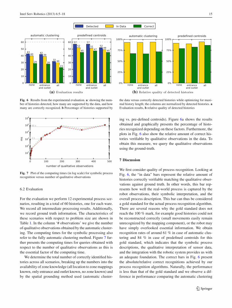
(a) (b)

Fig. 6 Results from the experimental evaluation. a: showing the num-ber of histories detected, how many are supported by the data, and howmany are correctly recognized. b Percentage of histories supported by

the data versus correctly detected histories while optimizing for maxi-mal history length; the columns are normalized by detected histories. aEvaluation results, b relative quality of detected histories

Fig. 7 Plot of the computing times (in log scale) for symbolic processrecognition versus number of qualitative observations

6.2 Evaluation

For the evaluation we perform 12 experimental process sce-narios, resulting in a total of 60 histories, one for each ware.We record all intermediate processing results. Additionally,we record ground truth information. The characteristics ofthese scenarios with respect to problem size are shown inTable 1. In the column ‘# observations’ we give the numberof qualitative observations obtained by the automatic cluster-ing. The computing times for the symbolic processing alsorefer to the fully automatic clustering method. Figure 7 fur-ther presents the computing times for queries obtained withrespect to the number of qualitative observations as this isthe essential factor of the computing time.

We determine the total number of correctly identified his-tories across all scenarios, breaking up the numbers into theavailability of zone knowledge (all location to zone mappingsknown, only entrance and outlet known, no zone known) andby the spatial grounding method used (automatic cluster-

ing vs. pre-defined centroids). Figure 6a shows the resultsobtained and graphically presents the percentage of histo-ries recognized depending on these factors. Furthermore, theplots in Fig. 6 also show the relative amount of correct his-tories verifiable by qualitative observations in the data. Toobtain this measure, we query the qualitative observationsusing the ground-truth.

7 Discussion

We first consider quality of process recognition. Looking atFig. 6, the “in data” bars represent the relative amount ofhistories correctly verifiable matching the qualitative obser-vations against ground truth. In other words, this bar rep-resents how well the real-world process is captured by therobot observations, their symbolic interpretation, and theoverall process description. This bar can thus be considereda gold standard for the actual process recognition algorithm.There are several reasons why the gold standard does notreach the 100 % mark, for example good histories could notbe reconstructed correctly (small movements easily remainunrecognized by the mapping component), or the robot mayhave simply overlooked essential information. We obtainrecognition rates of around 61 % in case of automatic clus-tering and 84 % in case of predefined centroids for thisgold standard, which indicates that the symbolic processdescriptions, the qualitative interpretation of sensor data,and the integration with the robotic system provides us withan adequate foundation. The correct bars in Fig. 6 presentthe absolute/relative correct recognitions achieved by ourprocess recognition algorithms. Naturally, the performanceis less than that of the gold standard and we observe a dif-ference in performance comparing the automatic clustering

123


method against clustering with pre-defined centroids. Thisdifference indicates the importance of a sensible spatialgrounding and motivates further research to obtain moresophisticated automated methods. As expected, we observethat with increased background knowledge the relative num-ber of histories matching the ground truth increases whilethe total number of detectable processes decreases. The rea-son for this is due to the fact that providing more backgroundinformation restricts the way the data can be interpreted, lead-ing to fewer interpretations that meet a process description.

In some scenarios when all regions are known it occurredthat some locations are not within any zone, thereby violatingAxiom (A3) and hence inhibiting recognition at all. This isespecially true in the case of the automatic clustering as canbe seen by the drop in the case when all regions are known.Overall the increase in background knowledge reduces theamount of false positives while having little impact on thenumber of correctly detected histories.

The most important observation is however that the rela-tive number of correctly identified histories, i.e., how manyfrom the detected histories are correct, is hardly affected bythe amount of background knowledge available about zonemembership. In case of pre-defined cluster centers the aver-age relative recognition rate is 83 % whereas for the case ofautomatic clustering the average relative recognition is 69 %.Missing zone membership information is compensated forby logic reasoning during model checking which determinesthe unknown variables sensibly. In other words, the infer-ence process is capable of supplementing all missing zonemembership information to the process recognition process.This demonstrates that a logic-based approach is a valuablecontribution to process recognition methods.

We note that these results confirm a previous study withrespect to the overall conclusion, absolute recognition rateshave improved though (cp. [18]), in the case of pre-definedclusters from 68 % achieved previously to about 76 % inthis study (for automatic clustering from 42 to 44 %). Therelative recognition rates, i.e., how many of the detected his-tories are correct ones, have improved even more: in case ofpre-defined clusters from 73 to 83 % and in case of automaticclustering from 57 to 69 %. This improvement is due to threechanges: first, we changed the robot hardware from a Pioneer3-AT (four wheel skid steering drive) to a Pioneer 2-AT (dif-ferential drive) as slip and drift for the 3-AT robot are veryhigh on the lab floor. Second, we changed the visual tags forlandmarks and goods as we have previously been sufferingfrom mixups in tag detection. Last but not least we extendedthe TreeMap SLAM algorithm3 to provide uncertainty esti-mates. By exploiting covariances for position estimates frommap and observation we are able to detect movements morerobustly which increases the overall map quality too.

3 As provided at http://www.openslam.org/TreeMap.html

8 Conclusion

In this paper, we propose an approach to process detectionbased on a specification of processes as temporal logic formu-las in LTL. We demonstrate the applicability of our approachby an evaluation with real sensory data from a mobile robot.In our case study of warehouse logistics, the observationsof a robot can be queried for process occurrences using anabstract process description. This allows a domain expert toobtain valuable information.

The evaluation demonstrates usefulness of the LTL-basedapproach to process description and recognition. With LTLone takes a declarative approach that is accessible to anydomain expert as the declarative formulas abstract from thedetails of underlying algorithms. The performance of thegold standard clearly demonstrates feasibility of the sym-bolic approach to process specification and recognition, con-firming the first claim of this paper. The claim is furthersupported by the actual recognition rates of the autonomousprocess recognition. Let us now consider the second claimof this paper, namely that the declarative approach enableslogic reasoning to supplement observations of the robot, sen-sibly filling in missing pieces of information. Indeed, theexperimental setting in which no information about zonemembership is available a priori resembles a chicken-and-egg problem: on the one hand, zones need to be known inorder to identify processes. On the other hand, the processesneed to be known to identify zones. Approaching processrecognition as a model checking problem allows us tojointly recognize processes and zones using the well-definedsemantics of answer set programming. Naturally, the lessinformation is available the poorer the recognition rate. Fig-ure 7 however shows that the declarative approach effectivelycounteracts the loss of information, showing only a smalldecline despite loss of zone information. This demonstratesa key benefit of a logic-based approach: the seamless inte-gration of inference processes into the robot control architec-ture. Last but not least, the approach is sufficiently efficientto handle real-world data. Two factors are the essential con-tributors: the qualitative representation cuts down compre-hensive experimental runs to few observations (see Table 1)and the ASP solver exhibits a low-degree polynomial growthof computing time.

In a real-world warehouse we expect the robot to onlyobserve a relative small amount of processes occurring, as arobot’s perception is limited in range. Nevertheless, an analy-sis of the overall warehouse processes is still possible if theprocesses and histories detected are prototypical for the over-all warehouse. This requires a high degree of correct recogni-tions though. As our approach meets this requirement we areconfident that the approach will also scale to a large setting.

While the focus of this paper was to present an LTL-based approach to process recognition and understanding,

123


we aim to extend this approach to a comprehensive LTL-based control strategy. An interesting next step is to automat-ically derive an observation strategy that generates a sensiblesurveillance behaviour. In particular, we aim to use tempo-ral logic to incorporate so-called search control knowledgeand perform high-level planning [2], i.e., we shift to activeprocess detection in the sense of planning which places toobserve in order gather most valuable information.

For some complex queries it would be helpful to addressall knowledge gathered during observations, in particularinformation about goods we have observed before and whichare included in the map, but which we are unable to per-ceive at the very moment. Currently, we take a conserva-tive approach that only explicates knowledge that is certain.However, for such objects we still have a strong belief oftheir existence and position in the warehouse, but this beliefcan—according to the actual observation—not be validated.A possibility to include reasoning on such beliefs is to use alogic that provides a modal belief operator, such as the logicfor BDI agents presented in [26]. Another source of infor-mation for more complex queries could be provided by anontology, as shown in [25].

Acknowledgments This paper presents work carried out in the projectR3-[Q-Shape] of the Transregional Collaborative Research CenterSFB/TR 8 Spatial Cognition. Financial support by the German ResearchFoundation (DFG) is gratefully acknowledged. We like to thank UdoFrese for his valuable comments and his support in extending theTreeMap-algorithm. We also thank the anonymous reviewers for theirhelpful comments.

References

1. Antoniotti M, Mishra B (1995) Discrete event models + temporallogic = supervisory controller: automatic synthesis of locomotioncontrollers. In: Proceedings of the IEEE conference on roboticsand automation (ICRA), Nagoya, vol 2, pp 1441–1446

2. Bacchus F, Kabanza F (2000) Using temporal logics to expresssearch control knowledge for planning. Artif Intell 116(1–2):123–191

3. Balcan MF, Blum A (2010) A discriminative model for semi-supervised learning. J ACM (JACM) 57(3):1–46

4. Bauland M, Mundhenk M, Schneider T, Schnoor H, Schnoor I,Vollmer H (2011) The tractability of model checking for LTL: thegood, the bad, and the ugly fragments. ACM Trans Comput Log12(2):13

5. Bennewitz M, Burgard W, Cielniak G, Thrun S (2005) Learningmotion patterns of people for compliant robot motion. Int J RobotRes (IJRR) 24(1):39–41

6. Cimatti A, Giunchiglia F, Giunchiglia E, Traverso P (1997) Plan-ning via model checking: a decision procedure for AR. In: Steel S,Alami R (eds) European conference on planning (ECP), Lecturenotes in computer science. Springer, Berlin, vol 1348, pp 130–142

7. Dianco A, Alfaro LD (1995) Model checking of probabilistic andnondeterministic systems. In: Foundations of software technologyand theoretical computer science. Springer, LNCS, vol 1026, pp499–513

8. Ding XC, Smith SL, Belta C, Rus D (2011) Ltl control in uncertainenvironments with probabilistic satisfaction guarantees. Technicalreport accompanying IFAC 2011 (math.OC, arXiv: 1104.1159v2)

9. Dubba K, Bhatt M, Dylla F, Cohn A, Hogg D (2011) Interleavedinductive–abductive reasoning for learning event-based activitymodels. In: Inductive logic programming (lecture notes in com-puter science), 21st international conference, ILP-2011, WindsorGreat Park

10. Edelkamp S, Jabbar S (2006) Action planning for directed modelchecking of petri nets. Electron Notes Theor Comput Sci 149(2):3–18

11. Frese U (2004) An O(log n) algorithm for simultaneous localiza-tion and mapping of mobile robots in indoor environments. PhDthesis, University of Erlangen-Nürnberg, Bavaria

12. Gebser M, Kaufmann B, Neumann A, Schaub T (2007) Conflict-driven answer set solving. In: Veloso M (ed) Proceedings of the 20thinternational joint conference on artificial intelligence (IJCAI’07),AAAI Press/MIT Press, pp 386–392

13. Gebser M, Kaminski R, König A, Schaub T (2011) Advances ingringo series 3. In: Delgrande J, Faber W (eds) Proceedings ofthe 11th international conference on logic programming and non-monotonic reasoning (LPNMR’11), lecture notes in artificial intel-ligence, vol 6645, Springer, Berlin, pp 345–351

14. Hildebrandt T, Frommberger L, Wolter D, Zabel C, Freksa C,Scholz-Reiter B (2010) Towards optimization of manufacturingsystems using autonomous robotic observers. In: Proceedings ofthe 7th CIRP international conference on intelligent computationin manufacturing engineering (ICME)

15. Kloetzer M, Belta C (2006) LTL planning for groups of robots. In:Proceedings of the IEEE international conference on networking,sensing and control (ICNSC), Fort Lauderdale, pp 578–583

16. Kloetzer M, Belta C (2010) Automatic deployment of distributedteams of robots from temporal logic motion specifications. IEEETrans Robot 26(1):48–61

17. Kress-Gazit H, Wongpiromsarn T, Topcu U (2011) Correct, reac-tive robot control from abstraction and temporal logic specifica-tions. Spec Issue IEEE Robot Autom Mag Form Methods RobotAutom 18(3):65–74

18. Kreutzmann A, Colonius I, Frommberger L, Dylla F, Freksa C,Wolter D (2011) On process recognition by logical inference. In:Proceedings of the 5th European conference on mobile robots(ECMR), Orebro, pp 7–12

19. Lahijanian M, Andersson SB, Belta C (2011) Temporal logicmotion planning and control with probabilistic satisfaction guar-antees. IEEE Trans Robot 99:1–14

20. Liao L, Patterson DJ, Fox D, Kautz H (2007) Learning and inferringtransportation routines. Artif Intell 171(5–6):311–331

21. Lichtenstein O, Pnueli A (1985) Checking that finite state concur-rent programs satisfy their linear specification. In: Proceedings ofthe 12th ACM SIGACT-SIGPLAN symposium on principles ofprogramming languages (POPL ’85), ACM, New York, pp 97–107

22. Lifschitz V (1996) Foundations of logic programming. In: BrewkaG (ed) Principles of knowledge representation. CSLI Publications,Stanford, pp 69–128

23. Lifschitz V (2002) Answer set programming and plan generation.Artif Intell 138:39–54

24. Mastrogiovanni F, Scalmato A, Sgorbissa A, Zaccaria R (2009a)On situation specification in context aware robotics applications.In: Proceedings of the 4th European conference on mobile robots(ECMR), Mlini/Dubrovnik, Croatia, pp 265–270

25. Mastrogiovanni F, Sgorbissa A, Zaccaria R (2009b) Context assess-ment strategies for ubiquitous robots. In: IEEE international con-ference on robotics and automation (ICRA) , pp 2717–2722

26. Meyer JJ, Veltman F (2007) Intelligent agents and common sensereasoning. In: Blackburn P, Benthem JV, Wolter F (eds) Handbook

123


of modal logic, studies in logic and practical reasoning, vol 3. Else-vier, New York, pp 991–1029 (chapter 18)

27. Morgenstern A, Schneider K (2011) Program sketching via CTL*model checking. In: Groce A, Musuvathi M (eds) Model checkingsoftware (SPIN), vol 6823. Springer, LNCS, Snowbird, pp 126–143

28. Nilsson NJ (1984) Shakey the robot. Technical report 323, AI Cen-ter, SRI international, Menlo Park

29. Pnueli A (1977) The temporal logic of programs. In: Proceedingsof the 18th annual symposium on foundations of computer science(FOCS), pp 46–57

30. Schnoebelen P (2003) The complexity of temporal logic modelchecking. In: Balbiani P, Suzuki NY, Wolter F, Zakharyaschev M(eds) Selected papers from the 4th workshop on advances in modallogics (AiML’02). King’s College Publication, Toulouse, pp 393–436

31. Sistla AP, Clarke EM (1985) The complexity of propositional lineartemporal logics. J Assoc Comput Mach 32(3):733–749

32. Smith SL, Tumová J, Belta C, Rus D (2010) Optimal path planningunder temporal logic constraints. In: Proceeding of the IEEE/RSJinternational conference on intelligent robots and systems (IROS),Taipei, pp 3288–3293

33. Ten Hompel M, Schmidt T (2010) Management of warehouse sys-tems. Springer, Berlin, pp 13–63 (chapter 2)

34. Wongpiromsarn T, Topcu U, Murray R (2009) Receding horizontemporal logic planning for dynamical systems. In: Proceedingsof the 48th IEEE Conference on decision and control, 2009 heldjointly with the 28th Chinese control conference. CDC/CCC 2009,pp 5997–6004

35. Wongpiromsarn T, Topcu U, Murray RM (2010) Receding horizoncontrol for temporal logic specifications. In: Proceedings of the13th ACM international conference on hybrid systems: computa-tion and control, ACM, New York, HSCC’10, pp 101–110

36. Yang Q (2009) Activity recognition: linking low-level sensorsto high level intelligence. In: Proceedings of the 21st interna-tional joint conference on artificial intelligence (IJCAI), Pasadena,pp 20–25

123

Temporal logic for process specification and recognition

Documents

Transcript of Temporal logic for process specification and recognition