Tectonics, erosion, and sedimentation in an overthrust system: A numerical model

Pergamon

Computers & Gmsciences Vol. 22, No. 2, pp. 117-l 38, 1996

oo!W3004(!%)00086-0 Copyright Q 1996 Elsevier Science Ltd

Printed in Great Britain. All rights reserved 0098-3004/96 $15.00 + 0.00

TECTONICS, EROSION, AND SEDIMENTATION IN AN OVERTHRUST SYSTEM: A NUMERICAL MODEL

EDOUARD CHALARON’,3, JEAN LOUIS MUGNIER’, WILLIAM SASSI’, and GEORGES MASCLE’

‘Laboratoire de GCodynamique des Chaines Alpines (U.R.A. C.N.R.S. No. 69) Universite Joseph Fourier, 15 rue M. Gignoux, 38031 Grenoble, France, 21nstitut FranGais du P&role, 1 i 4 Avenue de Bois-Prkau, 92506 Rueil Malmaison. France, and ‘Current address: INRS GCoressources. 2535 Boulevard Laurier.

CP 7500, Sinte Foy, Quibec, Canada GlV4C7 (e-mail: [email protected])

(Received 29 July 1994; accepted 2 February 1995)

Abstract-The frontal overthrust structures of a collision ridge and its foreland basin together form an area where the movement of imbricated overthrust structure, erosion, sedimentation, and substratum subsidence occur simultaneously. These various phenomena interact and lead to a subsequent sequence of exhumations and burying of the sheets forming these structures. Separate models have been developed in Turbo Pascal for each of these phenomena (imbricate movement, erosion, sedimentation, differential subsidence of the bedrock) and these models are coupled in a general algorithm. By changing the values of the geometrical and mechanical parameters, it is possible to study and quantify the effect of various phenomena on the development and tectonic history of the collision ridge front. Ancillary programs for reconstructing the geometry of the sedimentary bodies of the transported basins and the series of cross sections also were developed and are used to analyze the geometry predicted by the models and to compare them with natural examples.

Key Words: Foreland basins, Transported basins, Overthrust structures, Erosion, Sedimentation, Turbo Pascal.

INTRODUCTION

Foreland basins and the imbricated structures cover- ing them can be likened to accretion wedges by their geometry and evolution mode. These geological formations also have a high oil-bearing potential. However, owing to their complex structures and the numerous interfering phenomena, these formations are difficult to explore. As far as mother rock matu- ration is concerned, sedimentation encourages burying, erosion is conducive to exhumation, and a tectonic sheet alternately may promote exhumation or burying.

These phenomena have been modeled in three dimensions (Chalaron and Mugnier, 1993; Chalaron, 1994; Chalaron, Mugnier, and Mascle, in press) and the finite deformation geometry is obtained in the form of topographical blocks (Fig. 1) or cross sections (Fig. 2). For this purpose, the values of the various parameters (Table 1) are introduced in an algorithm based on a geometrical model of imbricated overthrusts in flats and ramps; a mechanical balanced wedge model, drawn from the work of Dahlen, Suppe, and Davis (1984); a kinematic simple vertical shear model (Jones and Linsser, 1986); and a model of surface diffusion of material simulating

erosion and sedimentation phenomena (Beaumont, Fullsack, and Hamilton 1992; Moretti and Turcotte, 1985).

The programming language used here is Turbo Pascal (0 Borland). The elementary processes are programmed independently in the form of modules which interact in a main algorithm around a procedural architecture. With this procedural programming method, modules can be created to answer macro-commands, thereby increasing their call potential. The discretization grids of the phenomena are allocated memory space up to the 640 kb of basic RAM in MS-DOS, and certain parts of the program, used only at the beginning of the numerical experiments, are placed in overlay. This algorithm (Table 1) takes into account tectonic, erosion, and sedimentation aspects and provides a large volume of data for quantifying the phenomena and for defining the limits of the tectonic history of these overthrusting structures. The originality of the work described here lies in the influence of erosion and sedimentation on the activation and reactivation of faults in a balanced wedge and the final objective is to assess the effect of variations in parameters on the finite deformation geometry of such systems.

117

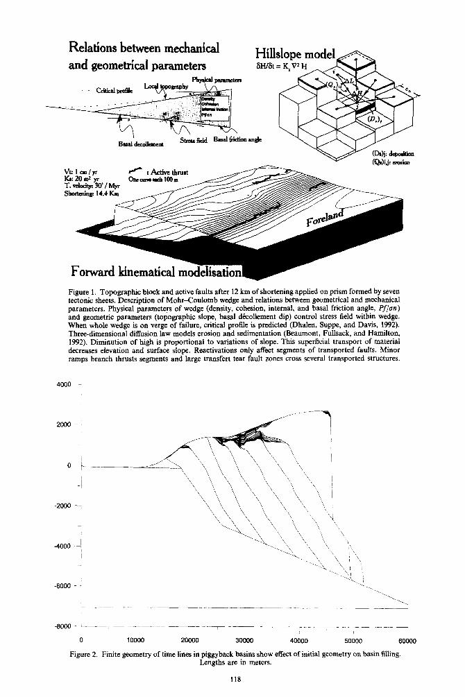
Relations between mechankal

and geometrical parameters

Figure 1. Topographic block and active faults after 12 km of shortening applied on prism formed by seven tectonic sheets. Description of Mohr-Coulomb wedge and relations between geometrical and mechanical parameters. Physical parameters of wedge (density, cohesion, internal, and basal friction angle, Pfiun) and geometric parameters (topographic slope, basal decollement dip) control stress field within wedge. When whole wedge is on verge of failure, critical profile is predicted (Dhalen, Suppe, and Davis, 1992). Three-dimensional diffusion law models erosion and sedimentation (Beaumont, Fullsack, and Hamilton, 1992). Diminution of high is proportional to variations of slope. This superficial transport of material decreases elevation and surface slope. Reactivations only affect segments of transported faults. Minor ramps branch thrusts segments and large transfert tear fault zones cross several transported structures.

4000 ~-

-6000 -

0 10000 20000 30000 40000 50000 60000

Figure 2. Finite geometry of time lines in piggyback basins show effect of initial geometry on basin filling. Lengths are in meters.

118

Tectonics, erosion, and sedimentation in an overthrust system 119

Table 1. List of parameters used in model. First part defines geometric parameters, second one defines physical properties of sediments and basal dicolle- ment of wedge. Third one is for time

dependent parameters.

Definition of parameters Run number

Geometric parameters B Dip of basal

decollement in degrees G( Topographic slope 6 Dip of ramps in degrees L Length of wedge in km

Mechanical parameters P Density of sediments

in kg me3

S0 Cohesion of sediments in MPa

a. Fluids pressure/ normal constraint

p basal friction coefficient

4 Internal friction coefficient of sediments

Time parameters Shortening velocity in cm an-’ Transport capacity in rn? an’ Tilting velocity of the basement in degrees/Myr

MODEL PRINCIPLES

This section gives a brief description of the physical principles governing the phenomena studied.

Physical principles of balanced wedges

The study of mechanical equilibrium conditions of wedges (Davis, Suppe, and Dahlen, 1983; Dahlen, Suppe, and Davis, 1984) shows that their tectonic evolution is affected (Fig. 1) by: (1) the surface topography, (2) the decollement surface geometry, and (3) the mechanical properties of the wedge and basal dtcollement rock. The following relationship between the mechanical parameters and the geometrical parameters defines the critical balanced profile of a subaerial wedge (Fig. 1) (after Dahlen, Suppe, and Davis, 1984):

tl + B = D + (1 - i)P, - e(%lPgr)cot($) l+(l-1)K ’

(1)

where CI and fi are respectively the slopes of the topography and the regional decollement surface, 1 is the ratio of fluid pressure (P,) to normal stress (en) in a subaerial wedge, So, p, and 4 are, respectively, the cohesion, the density and the internal friction angle of the sediments, g is the acceleration as a result of

gravity, p,, is the coefficient of friction of the decollement surface at the base of the wedge, and

r = H/(a + ,I?) where H is the equilibrium thickness of the wedge in meters.

K z Q z 2/(csc $J - 1).

In this analysis, the wedge is in an aerial medium considered to be continuous in terms of physical properties. Moreover, deformation is not located preferentially along the faults.

Principles of d@ision

The intracontinental accretion wedges are subjected continually to superficial phenomena (i.e. erosion/sedimentation) as shown by field studies, especially at the Himalayan front (Delcailau, Herail, and Mascle, 1987; Mascle and Herail, 1982; Mugnier, Mascle, and Faucher, 1992; Mugnier and others, 1994; Chalaron, 1994; Chalaron, Mugnier, and Mascle, in press). In order to model these phenomena, the three-dimensional diffusion law is used in the form proposed by Beaumont, Fullsack, and Hamilton, (1992). This method represents the cumu- lative effect of the slope sliding processes, and surface and subsurface leaching. This module is based on local diffusion in a homogeneous environment in relation to the level difference separating two cells (Fig. 1) and obeys the following equation:

6h/& = KS V’h,

where KS is the transport capacity (m2/yr’, h is the altitude of the points considered (in meters) and t the time (in yr).

Behavior of the underlying basement

The tectonic and superficial phenomena interfere with basement movements. Several models of bedrock response to a vertical load have been proposed. The elastic model is based on a constant flexural rigidity and depends on the elastic thickness of the lithosphere (Karner and Watts, 1983). A flexural elasticity model can be used to describe the geometry of the lithosphere having a high degree of flexural rigidity similar to a curvature of several hundred kilometers wavelength. By limiting the size of the model (60 x 60 km), the effect of lithospheric flexure can be considered to induce tipping of the basement only.

MODULES AND PROCEDURES

This section describes the translation of physical principles into algorithms.

General algorithm

The geometry files are ASCII format files compatible with the SURFER software (0 Golden Software). They consist of a header and a sequenced series of points corresponding to the vertical axis

E. Chalaron and others

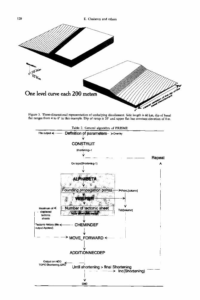
One level curve each 200

Figure 3. Three-dimensional representation of underlying d&collement. Side length is 60 km, dip of basal flat ranges from 4 to 6” in this example. Dip of ramp is 20” and upper flat has constant elevation of 0 m.

Table 2. General algorithm of PRISME

File output f--- Deflnitlon of parameters+oday 4

CONSTRUIT !

Shortening= 1

4 ___. -~-

I On topo(Shortening-1)

I

Repeat

Maximum off - displaced

tectonic

+Provi.[column]

:

Tab[column]

I sheets

6 ~

Tectonic history (file <Pm CHEMINDEF output Append)

$ -~~-------+ MOVE-FORWARD +

I

4 ADDITIONNECDEP

Output on HDD < TOPOShwtening.GRD I

Until shortening > final Shortening c--------_, Inc(Shortening)

s

Tectronics, erosion, and sedimentation in an overthrust system 121

value of the points considered (elevation or thickness). The header consists of five lines representing the format, the number of lines and columns, and successively, the minimum and maximum length, with and elevation values of the model. The rest of the file then consists of a sequence of elevations

Z x(I+ I),y(l).. Z, x(1+ ILyu+ I)” zx(i + I),y(imax$

Z x(max),y(l)” Z x(max),yD + 1)” Zx(imax)JQnaxJ~

Each file of the model corresponds to a grid of 125 x 125 regularly spaced points. The general algorithm produces a series of files respecting this format. These files represent the successive topographies of the model subjected to incremental shortening. The rate and direction of movement applied to the rear of the system are assumed to be constant. This system consists of a decollement surface upon which several tectonic sheets move. In order to represent the topographies generated, the SURFER graphics software is used (0 Golden Software).

Each of the main procedures simulating the phenomena to be modeled uses a file read and write procedure (Appendix 1). As all the files used have the same structure, these read and write procedures can be applied without distinction in all the algorithms simulating the natural phenomena.

Geometry of the dtkollement und tectonic sheet

surfaces

The successive decollement surfaces are defined by their elevation at the various grid nodes. A flat-ramp- flat geometry is used in the numerical experiments

presented (Fig. 3). The dip of the lower flat changes laterally (from “penteprox” to “pentedist”).

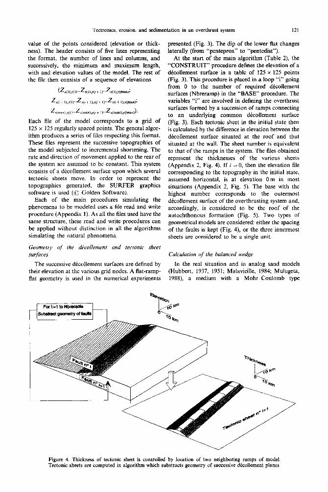
At the start of the main algorithm (Table 2) the “CONSTRUIT” procedure defines the elevation of a decollement surface in a table of 125 x 125 points (Fig. 3). This procedure is placed in a loop “i” going from 0 to the number of required dtcollement surfaces (Nbreramp) in the “BASE” procedure. The variables “i” are involved in defining the overthrust surfaces formed by a succession of ramps connecting to an underlying common dtcollement surface (Fig. 3). Each tectonic sheet in the initial state then is calculated by the difference in elevation between the dtcollement surface situated at the roof and that situated at the wall. The sheet number is equivalent to that of the ramps in the system. The files obtained represent the thicknesses of the various sheets (Appendix 2, Fig. 4). If i = 0, then the elevation file corresponding to the topography in the initial state, assumed horizontal, is at elevation Om in most situations (Appendix 2, Fig. 5). The base with the highest number corresponds to the outermost decollement surface of the overthrusting system and, accordingly, is considered to be the roof of the autochthonous formation (Fig. 5). Two types of geometrical models are considered: either the spacing of the faults is kept (Fig. 4) or the three innermost sheets are considered to be a single unit.

Calculation of the balanced wedge

In the real situation and in analog sand models (Hubbert, 1937, 1951; Malavieille, 1984; Mulugeta, 1988), a medium with a Mohr-Coulomb type

Figure 4. Thickness of tectonic sheet is controlled by location of two neighboring ramps of model. Tectonic sheets are computed in algorithm which substracts geometry of successive d6collement planes.


0

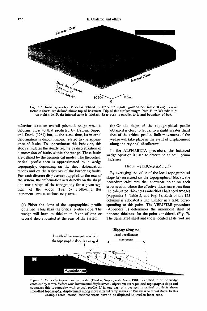
Figure 5. Initial geometry. Model is defined by 125 x 125 regular gridded box (60 x 60 km). Several tectonic sheets are defined above top of basement. Dip of this surface ranges from 4” on left side to 6”

on right side. Right internal zone is thickest. Rear push is parallel to lateral boundary of bof.

behavior takes an overall prismatic shape when it deforms, close to that predicted by Dahlen, Suppe, and Davis (1984) but, at the same time, its internal deformation is discontinuous, related to the appear- ance of faults. To approximate this behavior, this study simulates the steady regime by discretization of a succession of faults within the wedge. These faults are defined by the geometrical model. The theoretical critical profile then is approximated by a wedge topography, depending on the sheet deformation modes and on the trajectory of the bordering faults. For each discrete displacement applied to the rear of the system, the deformation acts directly on the shape and mean slope of the topography for a given segment of the wedge (Fig. 6). Following this increment, two situations may arise:

(a) Either the slope of the topographical profile obtained is less than the critical profile slope. The wedge will have to thicken in favor of one or several sheets located at the rear of the system.

Length of the segment on which

the topographic slope is averaged I I

V

(b) Or the slope of the topographical profile obtained is close to (equal to a slight greater than) that of the critical profile. Bulk movement of the wedge will take place in the event of displacement along the regional dtcollement.

In the ALPHABETA procedure, the balanced wedge equation is used to determine an equilibrium thickness

By averaging the value of the local topographical slope (a) measured on the topographical blocks, the procedure calculates the innermost point on each cross section where the effective thickness is less than the calculated thickness (subcritical balanced wedge) (Appendix 3, Table 2, and Fig. 6). Each of the 125 columns is allocated a line number in a table corresponding to this point. The VERIFIER procedure (Appendix 3) determines the innermost sheet of nonzero thickness for the point considered (Fig. 7). The designated sheet and those located at its roof are

Slippage along the

basal decollement

< may occur

+,

Figure 6. Critically tapered wedge model (Dhalen, Suppe, and Davis, 1984) is applied to brittle wedge cross-cut by ramps. Before each incremental displacement, algorithm averages local topographic slope and compares this topography with critical profile. If in one part of cross section critical profile is above smoothed topography, displacement along more internal ramp makes up thickness of thrust stack. In this

example three internal tectonic sheets have to be displaced to thicken inner zone.


topographic map

3

F Recorded as testonic history

/

Tectonic shortening of X increments

Test of the equilibrium thickness on 125-X nodes of the grid

Way of test

Number of the innermost node which verifies the condition of equilibrium

Number of the uppermost tectonic sheet where the thickness of the equilibrium point

is different from zero

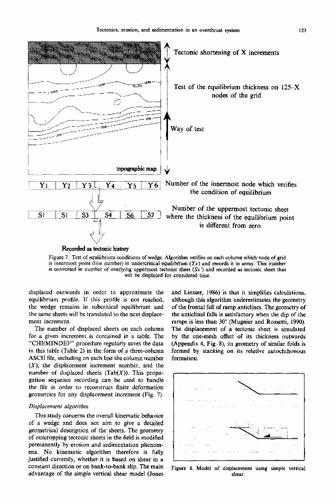
Figure 7. Test of equilibrium conditions of wedge. Algorithm verifies on each column which node of grid is innermost point (line number) in undercritical equilibrium (Yx) and records it in array. This number is converted in number of overlying uppermost tectonic sheet (Sx’) and recorded as tectonic sheet that

will be displaced for considered time.

displaced outwards in order to approximate the equilibrium profile. If this profile is not reached, the wedge remains in subcritical equilibrium and the same sheets will be translated to the next displacement increment.

The number of displaced sheets on each column for a given increment is contained in a table. The “CHEMINDEF” procedure regularly saves the data in this table (Table 2) in the form of a three-column ASCII file, including on each line the column number (X), the displacement increment number, and the number of displaced sheets (Tab(X)). This propagation sequence recording can be used to handle the file in order to reconstruct finite deformation geometries for any displacement increment (Fig. 7).

Displacement algorithm

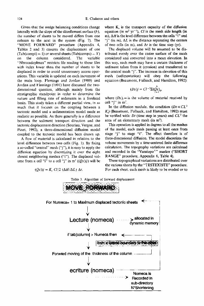
This study concerns the overall kinematic behavior of a wedge and does not aim to give a detailed geometrical description of the sheets. The geometry of outcropping tectonic sheets in the field is modified permanently by erosion and sedimentation phenomena. No kinematic algorithm therefore is fully justified currently, whether it is based on shear in a constant direction or on bank-to-bank slip. The main advantage of the simple vertical shear model (Jones

and Linsser, 1986) is that it simplifies calculations, although this algorithm underestimates the geometry of the frontal fall of ramp anticlines. The geometry of the anticlinal falls is satisfactory when the dip of the ramps is less than 30” (Mugnier and Rossetti, 1990). The displacement of a tectonic sheet is simulated by the one-mesh offset of its thickness outwards (Appendix 4, Fig. 8), its geometry of similar folds is formed by stacking on its relative autochthonous formation.

Figure 8. Model of displacement using simple vertical shear.

124 E. Chalaron and others

Given that the wedge balancing conditions change laterally with the slope of the decollement surface (b), the number of sheets to be moved differs from one column to the next in the system (Fig. 7). The “MOVE FORWARD” procedure (Appendix 4, Tables 2 and 3) ensures the displacement of one (Tab(compt) = 1) or several sheets (Tab(compt) = X) on the column considered. The variable “Nbrecadeplmax” restricts file reading to those files with index lower than the number of sheets to be displaced in order to avoid unnecessary access oper- ations. This variable is updated on each increment of the main loop. Flemings and Jordan (1989) and Jordan and Flemings (1991) have discussed the two- dimensional question, although mainly from the stratigraphic standpoint in order to determine the nature and filling rate of sediments in a foreland basin. This study takes a different partial view, in as much that it focuses on the coupling between a tectonic model and a sedimentation model made as realistic as possible. As there generally is a difference between the sediment transport direction and the tectonic displacement direction (Souriau, Vergne, and Pinet, 1992), a three-dimensional diffusion model coupled to the tectonic model has been drawn up.

where K, is the transport capacity of the diffusion equation (in m* yr-‘), Cl is the mesh side length (in m), AH is the level difference between the cells ‘5” and “j” (in m), AL is the distance separating the centers of two cells (in m), and At is the time step (yr).

The displaced volume will be assumed to be distributed evenly over the entire surface of the mesh considered and converted into a mean elevation. In this way, each mesh may have a certain thickness of sediment taken from it (erosion) and transferred to the central mesh “j”. The increase in elevation of this mesh (sedimentation) will obey the following equation (Beaumont, Fullsack, and Hamilton, 1992):

where (OS), = is the volume of material received by cell “j” in m3.

In the diffusion module, the condition (Dt <<CL* KS) (Beaumont, Fullsack, and Hamilton, 1992) must be verified with: Dt (time step in years) and CL2 the area of an elementary mesh (in m2).

A flow of material is calculated in relation to the level difference between two cells (Fig. 1). By fixing a so-called “central” mesh (‘j”), it is easy to apply the diffusion equation by discretizing it over the eight closest neighboring meshes (“i”). The displaced volume from a cell “i” to a cell “j” in m3 ((Qs)~) will be

This operation is applied in degrees to all the meshes of the model, each mesh passing at least once from stage “j” to stage “i”. The effect therefore is of three-dimensional diffusion. The model discretizes the volume movements by a time-centered finite difference calculation. The topography variations are calculated and recorded in the “Varatopo”” marker (“SHORT RANGE” procedure, Appendix 6, Table 4).

(Qs)ij = K, Cl/2 (AH/AL) At,

These topographical variations are distributed over the various sheets by the “TESTEXISTE” procedure. For each sheet, each mesh is likely to be eroded or to

(Dslj = Cl-“z(Q?&:

Table 3. Algorithm of forward displacement

For Numeca= 1 to Maximum displaced tectonic sheets -

Lecture (nomeca) $~~~~~e~ov

4 if tab[column] > Numeca then

Forward moving of the thickness of the column /

j,

ecrituye (nomeca) ___ Nomeca is

-> Recorded in sub-directory NOShortening


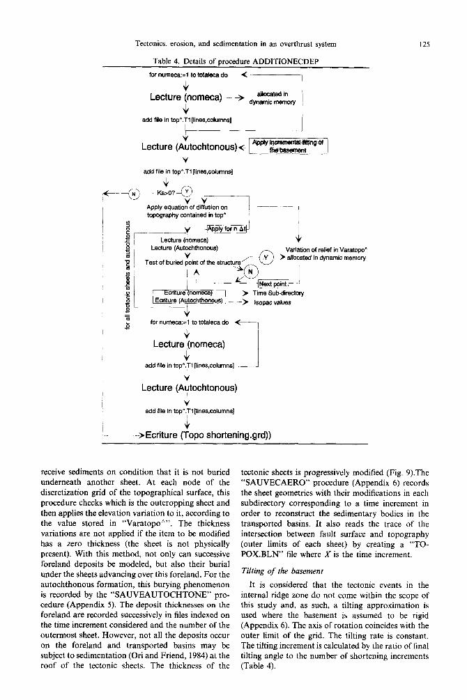
Table 4. Details of procedure ADDITIONECDEP

for numeca:=l to totaka do

Lecture (nomeca) - -> d$$f~~ow

4 add file in top^.Ti [lines,columns]

j +

Lecture (Autochtonous) f- w

add file in top^.Ti ginescolumns]

Apply equation of diffusion on topography contained in top* I

Variation of relief in Varatopo^ allocated in dynamic memory

* ‘m e’

for numeca:=t to totaleca do -

+

Lecture (nomeca)

4 add file in top^.Ti [lines,columns] 1

4

Lecture (Autochtonous)

J add file in top^.Ti [lines,columns]

-+Ecriture sop0 shortening.grd))

receive sediments on condition that it is not buried underneath another sheet. At each node of the discretization grid of the topographical surface, this procedure checks which is the outcropping sheet and then applies the elevation variation to it, according to the value stored in “Varatopo”“. The thickness variations are not applied if the item to be modified has a zero thickness (the sheet is not physically present). With this method, not only can successive foreland deposits be modeled, but also their burial under the sheets advancing over this foreland. For the autochthonous formation, this burying phenomenon is recorded by the “SAUVEAUTOCHTONE” procedure (Appendix 5). The deposit thicknesses on the foreland are recorded successively in files indexed on the time increment considered and the number of the outermost sheet. However, not all the deposits occur on the foreland and transported basins may be subject to sedimentation (Ori and Friend, 1984) at the roof of the tectonic sheets. The thickness of the

tectonic sheets is progressively modified (Fig. 9).The “SAUVECAERO” procedure (Appendix 6) records the sheet geometries with their modifications in each subdirectory corresponding to a time increment in order to reconstruct the sedimentary bodies in the transported basins. It also reads the trace of the intersection between fault surface and topography (outer limits of each sheet) by creating a “TO- POX.BLN” file where X is the time increment.

Tilting of the basement

It is considered that the tectonic events in the internal ridge zone do not come within the scope of this study and, as such, a tilting approximation is used where the basement is assumed to be rigid (Appendix 6). The axis of rotation coincides with the outer limit of the grid. The tilting rate is constant. The tilting increment is calculated by the ratio of final tilting angle to the number of shortening increments (Table 4).


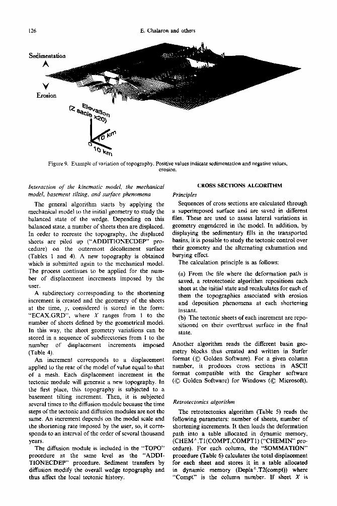
Figure 9. Example of variation of topography. Positive values indicate sedimentation and negative values, erosion.

Interaction of the kinematic model, the mechanical model, basement tilting, and surface phenomena

The general algorithm starts by applying the mechanical model to the initial geometry to study the balanced state of the wedge. Depending on this balanced state, a number of sheets then are displaced. In order to recreate the topography, the displaced sheets are piled up (“ADDITIONECDEP” procedure) on the outermost decollement surface (Tables 1 and 4). A new topography is obtained which is submitted again to the mechanical model. The process continues to be applied for the number of displacement increments imposed by the user.

A subdirectory corresponding to the shortening increment is created and the geometry of the sheets at the time, y, considered is stored in the form: “ECAX.GRD”, where X ranges from 1 to the number of sheets defined by the geometrical model. In this way, the sheet geometry variations can be stored in a sequence of subdirectories from 1 to the number of displacement increments imposed (Table 4).

An increment corresponds to a displacement applied to the rear of the model of value equal to that of a mesh. Each displacement increment in the tectonic module will generate a new topography. In the first place, this topography is subjected to a basement tilting increment. Then, it is subjected several times to the diffusion module because the time steps of the tectonic and diffusion modules are not the same. An increment depends on the model scale and the shortening rate imposed by the user, so, it corresponds to an interval of the order of several thousand years.

The diffusion module is included in the “TOPO” procedure at the same level as the “ADDI- TIONECDEP” procedure. Sediment transfers by diffusion modify the overall wedge topography and thus affect the local tectonic history.

CROSS SECTIONS ALGORITHM

Principles

Sequences of cross sections are calculated through a superimposed surface and are saved in different files. These are used to assess lateral variations in geometry engendered in the model. In addition, by displaying the sedimentary fills in the transported basins, it is possible to study the tectonic control over their geometry and the alternating exhumation and burying effect.

The calculation principle is as follows:

(a) From the file where the deformation path is saved, a retrotectonic algorithm repositions each sheet at the initial state and recalculates for each of them the topographies associated with erosion and deposition phenomena at each shortening instant. (b) The tectonic sheets of each increment are repositioned on their overthrust surface in the final state.

Another algorithm reads the different basin geometry blocks thus created and written in Surfer format (0 Golden Software). For a given column number, it produces cross sections in ASCII format compatible with the Grapher software (0 Golden Software) for Windows (0 Microsoft).

Retrotectonics algorithm

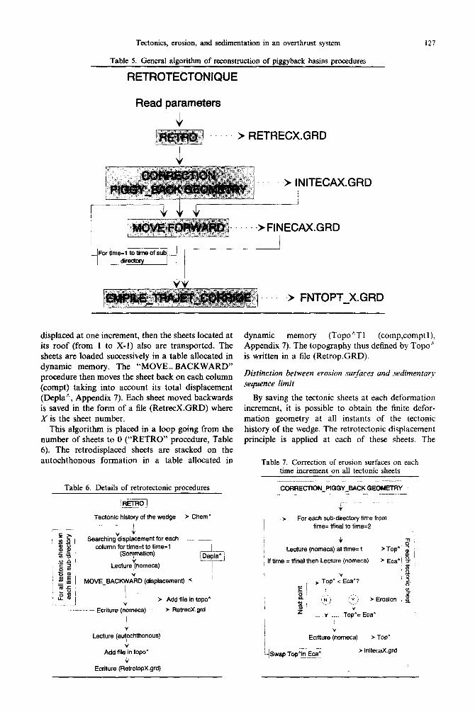
The retrotectonics algorithm (Table 5) reads the following parameters: number of sheets, number of shortening increments. It then loads the deformation path into a table allocated in dynamic memory, (CHEM” .Tl(COMPT,COMPTl) (“CHEMIN” procedure). For each column, the “SOMMATION” procedure (Table 6) calculates the total displacement for each sheet and stores it in a table allocated in dynamic memory (Depla * .T2(compt)) where “Compt” is the column number. If sheet X is


Table 5. General algorithm of reconstruction of piggyback basins procedures

RETROTECTONIQUE

Read parameters

~> RETRECX.GRD

-> INITECAX.GRD I

->FINECAX.GRD

w -> FNTOPT_X.GRD

displaced at one increment, then the sheets located at its roof (from 1 to X-l) also are transported. The sheets are loaded successively in a table allocated in dynamic memory. The “MOVE- BACKWARD” procedure then moves the sheet back on each column (compt) taking into account its total displacement (Depla ‘, Appendix 7). Each sheet moved backwards is saved in the form of a file (RetrecX.GRD) where X is the sheet number.

This algorithm is placed in a loop going from the number of sheets to 0 (“RETRO” procedure, Table 6). The retrodisplaced sheets are stacked on the autochthonous formation in a table allocated in

dynamic memory (TopoAT (comp,comptl), Appendix 7). The topography thus defined by Topo’ is written in a file (Retrop.GRD).

Distinction between erosion surfaces and sedimentary sequence limit

By saving the tectonic sheets at each deformation increment, it is possible to obtain the finite deformation geometry at all instants of the tectonic history of the wedge. The retrotectonic displacement principle is applied at each of these sheets. The

Table 7. Correction of erosion surfaces on each time increment on all tectonic sheets

Table 6. Details of retrotectonic procedures

!_R_ETRo

Tectonic history of the wedge > Chem^ , L

.E p !

coo .Searchingvdisp&ament for each .__. ZB z .g

column for time=1 to time=1 1 ua%

5 I .$ 2 (sor7mation) @pZj

/ ov), Lecture Jnomeca) T- i MOVt_BACKWARD (displacement) (’

!

V > Add file in topo^

~~ .- Ecriture (nomeca) P RetrecX.grd

V

Lecture (au$chthonous)

V Add file in topo^

+ Ecrtture (RetrotopX.grd)

I---- I.CORR~O!:!G v

, ____~_,

I For each sub-directory time from

time= tfinal to time=2

I i 21 I Lecture (nomeca) at time= t >Top^’ ;

If time = tfinal then Lecture (nomeca) 8 i

> Eca^l =7 ,f

I %

V

Ecrtture (nomeca) > TofY

i!Swap Top’% Eca^ > InitecaX.grd


Table 8. List of parameters values used in run nos 1 and 2

Geometrical parameters 4 to 6 Dip of basal decollement

(degrees) 20” Dip of ramps (degrees) 60 Length of the model in

kilometers

2500

15

0.85

0.8 0.95

Mechanical parameters Density of sediments in kg m3 Cohesion of sediments in Mpa Internal friction coefficient of sediments Basal friction coefficient Fluids pressure/normal constraint

Time parameters 0.5-l Shortening velocity cm yr-’ 10-100 Transport capacity in

m2 yr-’ 15-30 Tilting velocity of the

basement in minute m yr-’

“SOMMATION” procedure is used so that the tectonic history is considered only for the increments TX, TX-,, . . . TI. In each subdirectory, from Tsnal to T,, the sheets will be displaced until the initial state. To distinguish between erosion surface and time lines in the transported basins, a loop compares the geometry of sheet X at increment T, and of sheet X at increment T,_ I (CORRECTION PIGGY-BACK

GEOMETRIE procedure, Table 7). Each geometry is stored in a table allocated in dynamic memory (Topo” for the sheet at time (T,) and Eta” for the sheet at time (T, _ ,)). Thickness tests are performed in order to determine erosion zones and sedimentation zones. The values contained in Eta ’ are saved in their respective subdirectory (Ti) in a file InitecaX.GRD where X is the number of the sheet considered. The values of Topo A are transferred into Eta A in order to check the erosion surfaces of the previous time increment. This retrotectonics principle is applied to all the sheets at all the time increments. The corrected sheet geometry files (INITCAX.GRD) are used to reconstruct the incremental retrotectonic topographies. Thus, RETROTOP.GRD files exist in each of these subdirectories.

Calculation of the finite geometry of piggyback basins

In each subdirectory Ti, the modified geometries of the tectonic sheets are repositioned forwards by an identical value to that used for their backward movement. They are stored in each subdirectory T, and renamed FINECAX.GRD, where X is the number of the tectonic sheet considered. The finite deformation geometry of the transported basins at stage Ttid is obtained by summating the succession from the tectonic sheet thicknesses at the various stages to the finite fault geometry at time T,,. In practice, the sheet thicknesses (FINECAX.GRD) at time T, are added to an autochthonous formation consisting of the finite geometry of the decollement surface and

0 T.nloclly:lS'/yLr

crustal basement

0 T. dodQzso’/Myr

Crustal basement

-loo00 1 I I I I I I

0 loo00 3oom 4oooo 5woo 6amo

Fig. 10A. (Caption opposite.)


Crustal basement

-10 ’ I I I I I ,

0 loa 3wQo 4oooo 5ao1w) 6mm

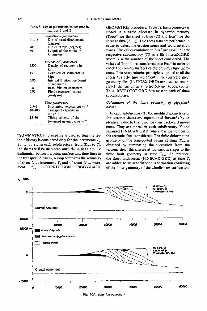
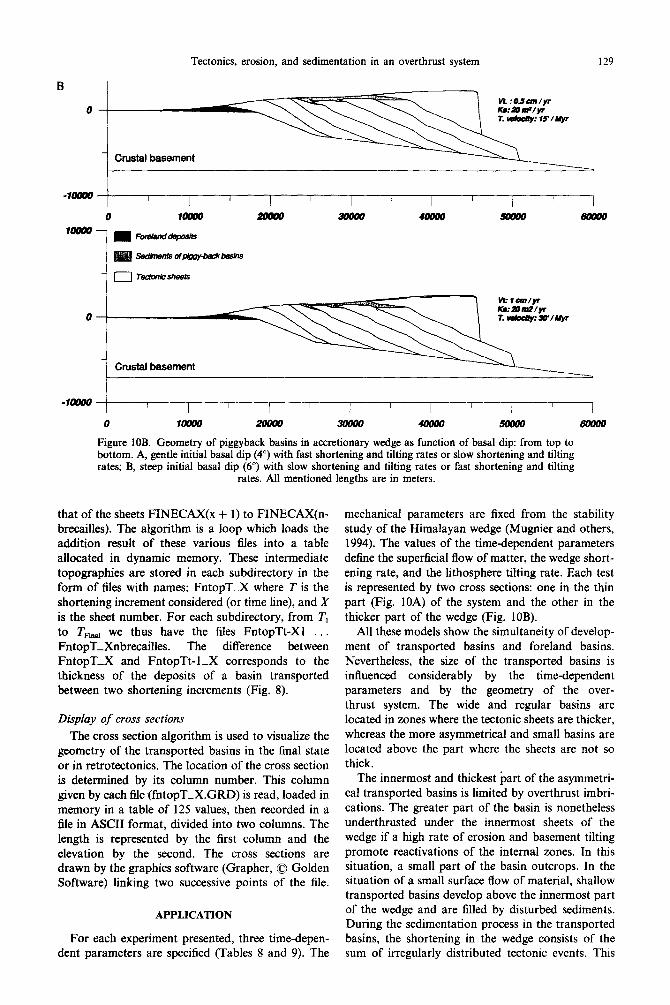
Figure 10B. Geometry of piggyback basins in accretionary wedge as function of basal dip: from top to bottom. A, gentle initial basal dip (4”) with fast shortening and tilting rates or slow shortening and tilting rates; B, steep initial basal dip (6”) with slow shortening and tilting rates or fast shortening and tilting

rates. All mentioned lengths are in meters.

that of the sheets FINECAX(x + 1) to FINECAX(n- brecailles). The algorithm is a loop which loads the addition result of these various files into a table allocated in dynamic memory. These intermediate topographies are stored in each subdirectory in the form of files with names: FntopT-X where T is the shortening increment considered (or time line), and X is the sheet number. For each subdirectory, from T,

to TFimal we thus have the files FntopTt-Xl . . FntopT-Xnbrecailles. The difference between FntopT-X and FntopTt-1-X corresponds to the thickness of the deposits of a basin transported between two shortening increments (Fig. 8).

Display of cross sections

The cross section algorithm is used to visualize the geometry of the transported basins in the final state or in retrotectonics. The location of the cross section is determined by its column number. This column given by each file (fntopT_X.GRD) is read, loaded in memory in a table of 125 values, then recorded in a file in ASCII format, divided into two columns. The length is represented by the first column and the elevation by the second. The cross sections are drawn by the graphics software (Grapher, 0 Golden Software) linking two successive points of the file.

APPLICATION

For each experiment presented, three time-dependent parameters are specified (Tables 8 and 9). The

mechanical parameters are fixed from the stability study of the Himalayan wedge (Mugnier and others, 1994). The values of the time-dependent parameters define the superficial flow of matter, the wedge shortening rate, and the lithosphere tilting rate. Each test is represented by two cross sections: one in the thin part (Fig. 10A) of the system and the other in the thicker part of the wedge (Fig. 10B).

All these models show the simultaneity of development of transported basins and foreland basins. Nevertheless, the size of the transported basins is influenced considerably by the time-dependent parameters and by the geometry of the overthrust system. The wide and regular basins are located in zones where the tectonic sheets are thicker, whereas the more asymmetrical and small basins are located above the part where the sheets are not so thick.

The innermost and thickest part of the asymmetrical transported basins is limited by overthrust imbri- cations. The greater part of the basin is nonetheless underthrusted under the innermost sheets of the wedge if a high rate of erosion and basement tilting promote reactivations of the internal zones. In this situation, a small part of the basin outcrops. In the situation of a small surface flow of material, shallow transported basins develop above the innermost part of the wedge and are filled by disturbed sediments. During the sedimentation process in the transported basins, the shortening in the wedge consists of the sum of irregularly distributed tectonic events. This


the piggy back basin

Q Foreland

1 -3 4

First and second increment of deformation: Example of a backward fault propagation

8

1oKm

Transfer of mass sediments

y Active thrust L 0

1oKm

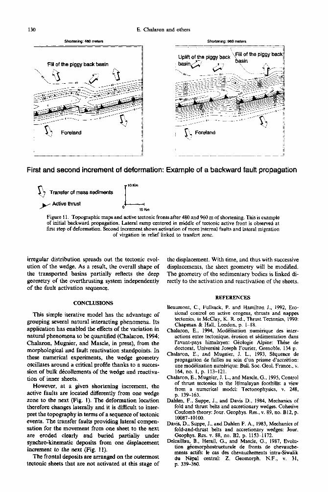
Figure 11. Topographic maps and active tectonic fronts after 480 and 960 m of shortening. This is example of initial backward propagation. Lateral ramp centered in middle of tectonic active front is observed at first step of deformation. Second increment shows activation of more internal faults and lateral migration

of virgation in relief linked to tranfert zone.

irregular distribution spreads out the tectonic evolution of the wedge. As a result, the overall shape of the transported basins partially reflects the deep geometry of the overthrusting system independently of the fault activation sequence.

CONCLUSIONS

This simple iterative model has the advantage of grouping several natural interacting phenomena. Its application has enabled the effects of the variation in natural phenomena to be. quantified (Chalaron, 1994; Chalaron, Mugnier, and Mascle, in press), from the morphological and fault reactivation standpoints. In these numerical experiments, the wedge geometry oscillates around a critical profile thanks to a succession of bulk d&ollements of the wedge and reactivation of inner sheets.

However, at a given shortening increment, the active faults are located differently from one wedge zone to the next (Fig. 1). The deformation location therefore changes laterally and it is difficult to inter- pret the topography in terms of a sequence of tectonic events. The transfer faults providing lateral compen- sation for the movement from one sheet to the next are eroded clearly and buried partially under synchro-kinematic deposits from one displacement increment to the next (Fig. 11).

The frontal deposits are arranged on the outermost tectonic sheets that are not activated at this stage of

the displacement. With time, and thus with successive displacements, the sheet geometry will be modified. The geometry of the sedimentary bodies is linked directly to the activation and reactivation of the sheets.

REFERENCES

Beaumont, C., Fullsack, P. and Hamilton J., 1992, Ero- sional control on active orogens, thrusts and nappes tectonics, in McClay, K. R. ed., Thrust Tectonics, 1990: Chapman & Hall, London, p. I-18.

Chalaron, E., 1994, Modelisation num&ique des inter- actions entre tectonique, trosion et kdimentation dans l’avant-pays himalayen: GBologie Alpine: Tl&e de doctorat, Universitk Joseph Fourier, Grenoble, 134 p.

Chalaron, E., and Mugnier, J. L., 1993, S6quence de propagation de failles au sein d’un prisme d’acc&tion: une modClisation numkrique: Bull. Sot. Geol. France., v. 164, no. 1, p. 113-121.

Chalaron, E., Mugnier, J. L., and Mascle, G., 1995, Control of thrust tectonics in the Himalayan foothills: a view from a numerical model: Tectonophysics, v. 248, p. 139-163.

Dahlen, F., Suppe, J., and Davis D., 1984, Mechanics of fold and thrust belts and accretionary wedges. Cohesive Coulomb theory: Jour. Geophys. Res., v. 89, no. B12, p. 10087-10100.

Davis, D., Suppe, J., and Dahlen F. A., 1983, Mechanics of fold-and-thrust belts and accretionary wedges: Jour. Geophys. Res. v. 88, no. B2, p. 1153-1172.

Delcaillau, B., Herail, G., and Mascle, G., 1987, Evolu- tion g6omorphostructurale de fronts de chevauchements actifs: le cas des chevauchements intra-Siwalik du N&al central: Z. Geomorph. N.F., v. 31, p. 339-360.


Flemings, P. B.. and Jordan, T., 1989, A synthetic stratigraphic model of foreland basin development: Jour. Geophys. Res.. v. 94, no. 84, p. 3851-3866.

Hubbert. M. K., 1937, Theory of scale models as applied to the study of geological structures: Geol. Sot. America Bull., v. 48, no. IO, p. 1459-1519.

Hubbert, M. K.. 1951, Mechanical basis for certain familiar geologic structures: Gcol. Sot. America Bull., v. 62, no. 4. p. 365.-372.

Jones, P. B.. and Linsscr, H.. 1986, Computer synthesis of balanced cross sections by forward modelling (abst.): Am. Assoc. Petroleum Geologists Bull.. v. 70, no. 5, p. 605.

Jordan, T. E.. and Flemings P. B.. 1991, Large-scale stratigraphic architecture. custatic variation and unsteady tectonism: a theorical evaluation: Jour. Geophys. Res., v. 96. no. 84. p. 6681 669.

Karner. G. D., and Watts. A. B., 1983. Gravity anomalies and flexure of the lithosphere, Jour. Geophys. Res.. v. X8. no. BII, p. 10449-10477.

Malavieille. J., 1984. Modelisation experimentale des chcvauchements imbriques: application aux chaines de montagnes: Bull. Sot. Geol. France, v. 26, no. I, p. 139 -150.

Mascle. G.. and Hcrail. Cr., 19X2. Les Siwalik: le prisme d’accretion tectoniquc associe a la subduction intracon- tinentale Himalayenne: Giologie Alpine. v. 58. p. 95 104.

Moretti, I., and Turcotte, D. L., 1985, A model for erosion, sedimentation, and flexure with application to New Caledonian: Jour. Geodynamics, v. 3, no. I-2, p. 155-168.

Mugnier, J. L., Huyghe, P., Chalaron, E., and Mascle. G., 1994, Recent movements along the Main Boundary Thrust of the Himalayas. Normal faulting in an over-critical thrust wedge?: Tectonophysics, v. 238, no. l-4. p. 199-215.

Mugnier, J. L., Mascle, G., and Faucher, T.. 1992. La structure des Siwahk de I’Ouest Nepal: un prisme d’accretion intracontinental: Bull. Sot. Geol. France, v. 163, no. 5, p. 585-595.

Mugnier, J. L., and Rossetti, J. P., 1990, The effects of simplifying assumptions on balanced cross-sections: a view from the Chartreuse massif, in Letouzey, J., ed., Petroleum and tectonics in mobile belts: Editions Technip, Paris. p. 167-180.

Mulugetta, G., 1988. Modelling the geometry of Coulomb thrust wedges: Jour. Struct. Geology, v. IO, no. 8. p. 847 -860.

Ori. G. G., and Friend, P. F., 1984, Sedimentary basins formed and carried piggyback on active thrust sheets: Geology, v. 12, no. 8, p. 475-478.

Souriau, M.. Vergne, M., and Pinet P.. 1992, Hydrographie fluviale et relief comme dontrees pour modeliser erosion et tectonique: Colloque D.B.T., Toulon, Decembre 1992. unpaginated.

APPENDIX 1

Procedures Jar writing and reading Jices

PKOCLIDURI: I.ECTl!RT.(nomrca.strinf):

Heqn

new(point).

assign(l:nomecn).

rmn: for compt:= I 10 5 do readIn(

for compr- I IO lignes do

begm

for compr I:- I lo colonnes do

hegm

read( f.poinr”.T I (compt.compt I]). ~fcompt I mod( IO)=0 then readln(Q:

end:

readln(n.

end:

close(II

End:

PROCEDURE ECRITURE(nomefa:srring):

Begm

3ssign(g,nomeca);

rewrite(g):

wteln(g.fbrma):

writeln(g,colonnes.’ ‘.lignes):

writeln(g.xmin.’ ‘.xmax):

writeln(g.ymin.’ ‘.ymax):

wrireln(g.zmin.’ ‘.zmax):

for compt:= I 10 lignes do

begin

for compt I := I to colonnes do

hegin

~rite(g.pomt”.TI [comptxompf I ]:5:2.“):

ifcomptl mod( IO)=0 then writeIn(

end:

writein(

end:

writeln(g.’ ‘):

close(g):

End:


APPENDIX 2

Definition of the geometrical model

PROCEDURE CONSTRUIT: Begin

for compt: = I IO ligneb do

beg!”

for compt I I to cchlnes do bL’gm

Ifcompf 1’ -~colonnes then

beta:=-((p”teprox~(((compr I-I )‘(~ntepro~-pentedibt)),l~gn~~))

else beta:-pntedist:

point, rl [compt.compt I I:--rap*compt’tang(kta~.

Ilmlt~:--llgnesii:~*3*tallle*ta”g(beta):rap):

If compt:,limite then

If((limite-cc~mpt)*rap’ta”g(alpha)~: --point I I jcompt.compt I ] then

pomr’ ‘7’1 [comptsompt I ].-I hmitc-compt)‘rap’tang(alpha).

It’comptc -limite then point’. fl[compt.compt I ] -4.0: end.

end.

End.

PROCEDlJRE RASt.

BegI”

new(point):

for i:=O to nbreramp do

begin

CONSTRIIIT:

,tr(i.fg).

nomeca.=concat(‘base’.fg.‘.grd’l

lXRlTlJRE(n”mecak

end:

Dispose(point):

End:

PROCEDURE CALCECAILLES.

Begin

str(nhreramp.fx):

writeln(‘CALCUL DE(S)‘.Fx.’ ECAILLb(S) EN COIJRS’):

for i:=O to nbreramp-I do

begin

>tr(i.fg):

Nom:= concat(‘BASE’.fg*‘(;RD’).

str(i- I .fg).

Nom”:= concat(‘BASE’*fg-’ GRD’):

Nomeca:-concat(‘ECA’.fg.‘CRD’):

LECTURE (Nom).

LECTURE (Nom”):

DIFFERENCE (Nomn-Nom);

ECRITURE (Nomeca):

end:

dispose(p&t);

End;

APPENDIX 3

Test qf balanced wedge

PRDCEDlJRE ALPIIABETA:

const gra-9.8 I : Begin

for i:= I to colonnes do

begI”

clrscr:

writeln(‘CALCUL EN COURS SL’R COLONNE N “.i). if i<>colonnes then beta:=((penteprox)-(((i-l )*(penteprox-pentedist)):lignes))*pi/l80 else

beta:=pentedist’pi!l80:

compt2: = I:

repeat

begin

calcul_.eqwlibrium _thickness:

ifThick_tew Thick-wedge then

Provi(i]:=comptZ:

inc(compt2);


end: until compt2= l&es-increl:

end:

End:

PROCEDURE VERIFIER:

Begin

For y:=Nbrecaille+ I downto I do

begin

Ify=Nbrecaille+l then

begin

str(y- I .I&: nom:=concat(‘BASE’,fg.‘.GRD’)

end

else

begin

S1tiy.fg);

nom:=concat(‘ECA’.fg.‘.GRD’);

end:

I.ECTURE(nom):

for compt I := I to colonnes do

begin

IIgnes))*pi/lSO else

if compt I <> I3 then beta:=((penteprox)-(((compt I - I )*(penteprox- pentedist)):

beta:=pentedist*pill80;

ifyunbrecaille+l then ifpoint”Tl[Provi[comptI j,comptI ] ; 0 then tab[comptl]:-y-l:

if y=nbrecaille~ I then if point”.TI [Pmvi[compt I Ixompt I I >(- np*prow[compt I ]*tang(beta)) then tab(comptl]:=y-I:

if provi[comptI]=lignes-increl then tab[compt I I:- I:

end:

end:

End:

APPENDIX 4

Movement of tectonic sheets

PROCEDURE DEPLACELIG:

Begin

for compt:= I to lignes- I do

begin

for comptl:-I to colonnes do

begin

if i+ tab[compt I] then compt2:=compt+ I else compt2:-compt:

point’,.TI [compwompt I I:-point”.TI [compt2.compr I]: end:

compt2:=0:

end:

for comptl := I to colonnes do point”.TI [lignexompt I J:=O:

End:

PROCEDURE MOVE_FORWARD:

Begin

for i:= I to nbrecadeplmax do

begin

LECTURE (nomecaj;

DEPLACELIG:

ECRITIJRE(nomeca):

end;

dispose(point):

End:

APPENDIX 5

Erosion, mod$cation of the topography, backup of tectonic sheets geometry and deposits on the autochthonous

PROCEDURE SHORT_RANGE(temps.paIemps:single);

Begin

New(Ds):

New(Qs):

New(VaraTopo);

DeltaT:-0:test I :=O;testz:=O:

for compt:= I to ligncs do

for compt I := I to colonnes do vararopoA.Tl [compt,compt I]:=O:


Repeat begin

for compt:= I to lignes do for compt I := I to colonnes do begin

Qs”.TI [compt.comptl]:=O: Ds^.T 1 [compt.compt I I:=&

end: DeltaT:=DeltaT+Pastemps; CITSCK

writ&(’ EROSION TOP0 N”‘.num); writeln(‘Temps &x~ulC: ‘.trunc(Deltat)); writeln(‘Temps pour un incrkment de dtplacement: ‘,trunc(temps).’ am’); writeln(‘lncr6ment de temps: ‘,trunc(pastemps)); for compt:=lignes-increl downto I do for compt I := I to colonnes do begin

Val I :=- I: Val2:= I ; if ((compt=l) or (compt l=I)) then vail :=O; if ((compt=lignes - increl) or (compt I= colannes )) then val2:=0: for test I := val I to 42 do for test2:= WI I to val2 do begin

if top”.T I [compt,compt I]< top”.T I [compt+test I .compt I +test2] then begin

deltah:=(top”.T I [compt+test I .compt I +test2]- top”.Tl [compt.compt I J)/(rap*sqrt(sqr(test I )+sqr(test2))); Qstemp:=Pastemps*Ks*deltaH*rap/2: Ds^.T I [compt.compt I ]:=Ds”.T I [compt,compt I ]+QStemp;

Qs”.T I [compt+test 1 .compt I +testZ]:=Qs”.T I [compt+test I .compt I +testZ]+QStemp; end:

end: end; for compt:= I to colonnes do for compt I := I to lignes do begin

Varatopo”.T I [compt,compt I ]:=Varatopo”.T I [compt,compt I ]+((Ds".T I [compt.compt I ]-Qs”.T I [compt,compt I])/

sqr(rap)): top”.TI [compt,comptl]:= top”.Tl[compt,comptl]+((Ds”.TI[compt,comptl]- Q9.T I [compfcompt I ])/sqr(rap));

end; end until deltat=temps; dispose(top); dispose(ds); dispose(Qs);

End:

PROCEDURE TESTEXISTE(n:byte); Begin

test:=true: writeln( ’ REPARTITION DES SEDIMENTS); New (eta); new (ecapred); For compt I := I to colonnes do for compt:=I to lignes do begin

Ecapred^.Tl [compt,comptl]:=O: Eca”.Tl [compt.compt I ]:=O;

end; for i:=l to n+l do begin

str(i,fg);

if i=n+l then begin

str(i-I ,fg); nom:=concat(‘BASE’.fg,‘.GRD’);

end else nom:=concat(‘ECA’.fg,‘.GRD’); LECTURE (nom); for compt I := I to colonnes do for compt:=l to lignes do begin

if i=n+ I then


if Ecapred^.TI [compt$omptl]=O then

Eca”.T I [compt.compt I]:=Eca^.T I [compt.compt I ]+Varatopo^.T I [compt.co+npt I]: if i<n+ I then

begin

if((Eca”.TI [compt.compt I]>O) and (Ecapred”.TI Icompt.compt I]=O)) then

Eca”.TI[compt.compt I ]:=Eca^.TI [compt.comptI]+Varatopo”.TI[compuomptl]:

if Eca^.TI [compt.comptI]<O then

begin

Varatopo^.T I [compt.compt I ]:=Varatopo”.T I (compt.compt I ]+abs(Eca^.TI [compuompt I]):

End:

Eca^.Tl[compt,comptI]:=O:

end:

end:

Ecapred^.TI [compt.comptl]:=EcapredA.TI [compt.comptI]+Eca^.TI [compt.compt I]:

end:

SAUVECAERqnom):

end;

disposz(Varatopo):

dispose(Eca):

PROCEDURE SAUVEAUTOCHTONE;

Var

fgnum:string;

Begin

SMnum.fgnum);

nomautoch:=concat(‘BAS’.t%.‘_‘.fgnum.’.GRD’):

assign(k,nomautoch):

rewrite(k);

titeln(k,forma):

writeln(k,colonnes.’ ‘.lignes):

writeln(k.xmin.’ ‘.xmax);

writeln(k.ymin,’ ‘.ymax);

writeln(k.0.’ ‘.zmax-zmin):

for compt:- I to lignes do

begin

for comptl := I to colonnes do

begin

if(eca”.TI[compt.compt I ]>=-compt*rap*tang(tilt*num)) then

write(k.abs(-compt~~*tang(tilt~num))+eaA.Tl~compt.compt I ]:4:3.“)

else write(k.O.’ 9;

if compt I mod( IO)=0 then writeIn(

end:

writeIn(

end:

writeln(k.’ ‘):

close(k):

End:

PROCEDURE SAUVECAERO(nom:string);

Begin

if((test=true) and (i<nbrecaille+I )) then

begin

strtnum.fg);

nomlim:=concat(TOPO’,fg,‘.BLN’):

assign(g.nomlim):

rewrite(g);

writeln(g.’ I?5 0’):

end else if i<nbrecaille- I then begin

append(g);

writeln(g,‘l?S 0’):

end:

ECRITURE(nom):

if kso 0 then ifl(num mod(pas)=O) and (nom=nomstock)) then SAUVEAUTOCHTONE:

for compt I : = I to colonnn do

begin

interupt :=true:

for compt:= I to lignes do

begin

if ((interupt-rme) and (eca^.T I [compt.compt I ]>o)) then

begin

interupt:=false:

if i<nLwecaille+l then

witeln(&60000-trunc(-(compt I -colonnes)*rap).’ ‘.trunc((compt-lignes)*rap)):


end: end:

end: if i<nbrecaille* t then clotig):

tesc:=false. End:

APPENDIX 6

Retrotectonic procedure PROCEDURE CHEMIN: Begin

assign(f.‘CHEMIN.DAT’): rese1(fj: for compt I := I IO raccourci do for compt:= I 10 I25 do readln(f.x.y.chem,‘.T I [comptxompt I]); close(f):

End:

PROCEDURE SOMMATION(nbre. tempsinteger): Begin

for compt:=l to ) 25 do depla”.l2[compt]:;O; for compt:=l to I25 do for compt I := I to temps do If chem”.TI[compt.comprI ]>=nbre then inc(Depl~‘:fZ(comptI):

End:

PROCEDURE MOVE .BACKWARD. Begm

for compr I : = I25 dowto 1 do for compt:= I2S downto I do ecaYT I [compt.compt I ]:=eca^.T I [comptdeplaA.T2[compt I ).compt I I: for compt I := I to I25 do for compt:=l to 125 do ifeca” Tl[compt.comptI]CO then ec&TI [comptxompt I ].=O:

End.

PROCEDtiRE RETROTECTO: Begin:

new(depla): new(eca): new(topo): for compt:- I to I25 do for comptl:=l to I25 do topo”.‘TI(compt.comprI 1:-O: for nbre:-0 to nbrccaille do bcgm

if nbre <>O then if nbre <> 0 then SOMMATION(nbre.raccourci); CHARGE(nbre); if nbre <> 0 then MOVE-BACKWARD; ADDITION: ifnbreo Othen ECRITURE:

end: End.

APPENDIX 7

Computation of the piggyback basins

PROCEDURE ECRITURE_INTER(test2:bc&an:n:integer): Begin

iftest2= false then nom:=Concat (“FINECA”.fz.‘.GRD’) else nom:-Concat (“INITECA”.fz’.GRD’); ECRITURE(nom):

End;

PROCEDURE LECTURE_INTERMEDIAIRE(test:boolean:mteger): Begin

srrtn.fz); if test = false then nom:=concat(“ECA”.fi’.GRD’)

else nom:=concat(“lNITECA”.fr.‘.GRD’): LECTURE(nom1:

End:

Tectonics, erosion, and sedimentation in an overthrust system

PROCEDURE CORRECTION_PIGGY~BACK_GEOMETRIE;

Begin

for boucle2:=l to nbrecaille do

begin

test:=true:

for bouclel:=raccourci downto 2 do

begin

str(bouclel.fx);

str(boucle2.corpig):

Chdir(fx);

nom:=concat(“lNITECA”.corpig.‘.GRD’);

iftest = true then LECTURE(nom):

tert:=false:

Chdir(“C:\PRISME”);

str(bouclel-l,fx);

Chdir(fx);

LECTURE(nom);

writeln(“CORRECTION DES ECAILLES”);

writeln(“NO de I”‘kaille: “,corpig);

writeln(“lncrkment: “.bouclel-I);

for compt:= I to I25 do

forcomptl:=l to l25do

begin

if eca’.TI [compt.compt I]>=topo^.Tl [compt.compt I] then

eca”.TI [compt,compt I]:=topo^.Tl [compt.compt I]; topo”.T I [compt.compt I]:=eca”.T I [compt,compt I]:

end;

ECRITURE INTER(true.boucle2):

Chdir(.‘c:\p&me”):

end:

end;

End;

PROCEDURE EMPlLE_TRAJET_CORRIGE:

Begin

for boucle I :=raccourci downto I do

begin

for boucle2:=nbrecaille downto I do

begin

writeln(” EMPILAGE DE L”‘ECAILLE N” “.boucle7);

writelnc INCREMENT “,bouclel);

str(boucle I .fx):

str(boucle2.corpig);

CHARGE(O);

ADDITION:

for boucle3:==nbrecaille downto boucle2+1 do

begin

CHARGE(boucle3);

ADDITION:

end:

Chdir(fx);

nom:=concat(“FINECA”,cwpig,‘.GRD’):

LECTURE(Nom)

ADDITION:

TOPOFIN(True);

Chdir(“c:‘prisme”):

end:

end:

End:

PROCEDURE DEPLACEMENT_TRAJET_CORRIGE:

Begin

for boucle2:=nbrecaille downto I do

begin

SOMMATION(boucle2. raccourci):

for bouclel :=raccourci downto I do

begin

writeln(” DEPLACEMENT DE L”‘ECAILLE N” “.boucle?):

writeln(” INCREMENT “,boucle I);

str(bouclel ,fx):

Chdir(fx);

CHARGE_INTERMEDIAIRE(True,boucle2);

DEPLACELIG;

ECRITURE INTER(false.boucle2);

Chdir(“c:\prke”):

137


end; end; EMPILE_TRAJET_CORRIGE:

End:

PROCEDURE PIGGY-BACK; Begin

str(nbrecaille,fg): for boucle I := I to raccourci do begin

for compt:= I to I25 do for comptl:=l to I25 do topo”.TI[compt,comptl]:=O: str(boucle I ,fx); ChDir(fx): for boucle2:=l to nbrecaille do begin

SOMMATION_INITIAL_PIGGY(boucle2.boucleI): LECTURE_INTERMEDlAIRE(false,boucle?): DEPLACEMENT: ECRlTURE_INTER(true,boucle2);

end: Chdir(“C:\prisme”)

end: End:

Tectonics, erosion, and sedimentation in an overthrust system: A numerical model

Documents

Transcript of Tectonics, erosion, and sedimentation in an overthrust system: A numerical model