Tax Incentives and the Demand for Private HealthInsurance

Olena StavrunovaUniversity of Technology, Sydney

Oleg YerokhinUniversity of Wollongong

December 2013

Abstract

We analyze the effect of an individual insurance mandate (Medicare Levy Sur-charge) on the demand for private health insurance (PHI) in Australia. With adminis-trative income tax return data, we show that the mandate has several distinct effects ontaxpayers’ behavior. First, despite the large tax penalty for not having PHI coveragerelative to the cost of the cheapest eligible insurance policy, compliance with mandateis relatively low: the proportion of the population with PHI coverage increases by6.5 percentage points (15.6%) at the income threshold where the tax penalty startsto apply. This effect is most pronounced for young taxpayers, while the middle agedseem to be least responsive to this specific tax incentive. Second, the discontinuousincrease in the average tax rate at the income threshold created by the policy gen-erates a strong incentive for tax avoidance which manifests itself through bunchingin the taxable income distribution below the threshold. Finally, after imposing someplausible assumptions, we extrapolate the effect of the policy to other income levelsand show that this policy hasn’t had a significant impact on the overall demand forprivate health insurance in Australia.

1 Introduction

Many countries actively intervene in the market for private health insurance (PHI) using

some combination of community ratings, price subsidies and insurance mandates. While

the community rating (group insurance) regulation ensures that high risk sub-groups of the

population are not priced out of the market, it reduces the value of insurance for low risk

individuals, creating a potential for adverse selection. To overcome this problem, mandates

and subsidies typically are used to increase participation in the health insurance market.

The main challenge for the policy makers is implementing the correct mix of these policies

to ensure equitable access to health care while minimizing the inefficiency associated with

1

regulation. This is not an easy task, as evidenced by the debates surrounding the Affordable

Care Act of 2010 in the United States, which envisions introduction of all three policies in

2014 (Gruber, forthcoming).

Knowing how subsidies and mandates will affect the demand for PHI is essential to

implementing the optimal policy mix. Although there exists a large literature on the effects

of price subsidies on the demand for health insurance, few studies look at the effect of

insurance mandates. This is because mandates seem to be less popular than subsidies among

policymakers. Also, in the few national health systems with mandates (e.g. Netherlands,

Switzerland) there is no legal op-out option such as paying a tax penalty which makes those

countries unsuitable for studying tax based insurance mandates.

In Australia the market for private health insurance is heavily regulated by the govern-

ment. As in some other countries (e.g. UK, Ireland, and Spain), Australia has a universal

tax financed health care system (Medicare) with the private health sector playing a duplicate

role. Specifically, all Australians have access to free public hospital treatments automati-

cally, but treatments in private sector settings require out-of-pocket expenses. The private

hospital sector is large: e.g. about 2/3 of elective surgeries were performed in the private

sector in the period 2006-2011 (Surgery in Australian Hospitals 2010-2011). The advantages

to patients of being treated in private hospitals, or as private patients in public hospitals,

include the possibility of avoiding long waiting times for elective surgery in the public sector

(Johar et al. (2011)), the ability to nominate a treating doctor, or to have private or better

quality accommodations, etc. Although the costs of private treatment can be substantial,

they can be greatly reduced by purchasing private health insurance coverage.

Since the introduction of public health insurance in the mid-1980s, the proportion of

the Australian population covered by private insurance has been declining steadily, a fact

commonly attributed to adverse selection caused by the community rating (Butler, 2002).

In an attempt to slow this trend, the Australian government introduced several measures

at the end of the 1990s aimed at increasing the take-up of private health insurance. These

measures included a 30% price subsidy, a system of premium loadings designed to encourage

the take-up of PHI coverage at a younger age (Life Time Health Cover) and a means-tested

insurance mandate, known as the Medicare Levy Surcharge (MLS). Under the MLS, which

is the focus of this paper, a tax penalty at the rate of 1% of total taxable income is imposed

on those with reported incomes above a specified threshold who do not have eligible PHI

coverage.

We use the administrative income tax returns data collected by the Australian Taxation

2

Office to study the effect of the MLS on the demand for PHI. The MLS policy creates

a discontinuous change in the average tax rate for those at a specified income threshold

without PHI coverage. In theory, this should create strong incentives to purchase insurance

for all taxpayers above the threshold. Moreover, taxpayers just below the MLS threshold

should constitute a suitable control group which could be used to estimate of the treatment

effect of the policy. However, this strategy is not appropriate if reported taxable income

can be manipulated (McCrary, 2008). Because reported taxable income responds to changes

in marginal tax rates (Saez, 2010; Chapman and Leigh, 2006), the MLS might produce a

similar response: facing a significant change in the average tax rate, taxpayers with incomes

just above the threshold and a low willingness to pay for health insurance might choose

to manipulate their taxable incomes to avoid paying the tax. We empirically verify this

intuition and document bunching in the taxable income distribution just below the MLS

threshold. This implies that estimation of the MLS effect on PHI coverage relying on a

simple comparison of the insurance rates just below and just above the income threshold

will be misleading.

We develop a novel approach to estimating the effect of the mandate in the presence

of tax avoidance using the observation that income shifting is limited to a certain interval

around the MLS threshold. First, we estimate the boundaries of the bunching interval in

the income tax returns data using similar methods to those recently applied in the income

taxation literature (Chetty et al., 2011). Second, we obtain the policy effect at the MLS

threshold by estimating the relationship between income and the PHI coverage rate outside

of the bunching interval; we then can predict the values of the counterfactual probability

of PHI coverage within the bunching interval that would obtain if income shifting were not

possible. To implement this empirical strategy we use taxable income and PHI coverage data

for single individuals in the fiscal year 2007-8. After implementing various robustness checks,

we find that the MLS has increased private health insurance coverage at the threshold by

6.5 percentage points (15.6%). Given that the tax penalty at the threshold in 2006-7 was

approximately equal to the price of the cheapest MLS eligible insurance policy, this effect

is relatively small. It suggests that even if the value of PHI for the marginal individual

was close to zero, many taxpayers either made dominated choices or faced large transaction

costs of obtaining PHI coverage. Our estimates of the treatment effect for different age

groups suggest that older households are the least responsive to the monetary incentives

created by the MLS; the majority of tax income from the surcharge comes from younger

cohorts of taxpayers. Finally, we extrapolate the MLS effect estimated at the threshold

3

to other income levels, assuming a constant treatment effect per dollar of the tax. This

counterfactual analysis implies that the MLS overall increased PHI coverage rate among

singles from 34% to 36.6%.

This study contributes to the existing literature on the effect of monetary incentives on

the demand for health insurance. The extensive literature investigating the effect of subsidies

on the demand for health insurance includes, among others: Gruber and Poterba (1994),

Finkelstein (2002), Emerson et al. (2001) and Rodriguez and Stoyanova (2004) for the cases

of US, Canada, UK and Spain, respectively. In addition, Chandra, Gruber and McKnight

(2011) study the impact of an individual mandate on the characteristics of the insurance

pool in the presence of large subsidies to premiums in the Massachusetts’ Commonwealth

Care program. We focus here on the effectiveness of mandates in Australia, which has a

rather different health care system. Therefore, our main policy implications are relevant for

other countries with public health care systems in which private insurance largely plays a

supplementary role. This study also contributes to a growing literature in public economics

on the behavioral responses to taxation, which uses discontinuous changes in tax rates as a

source of exogenous variation: see e.g. Saez (2010), Chetty et al. (2011) and Kleven and

Waseem (2013). This literature is primarily concerned with using the observed responses

to kink points in the income tax schedule to estimate the elasticity of taxable income with

respect to the tax rate, the magnitude of which is informative about the excess burden of

income taxes. Similar to the evidence presented in Kleven and Waseem (2013), we document

a pattern of sharp bunching at the MLS notch; this implies that this type of tax incentives

likely lead to tax avoidance behavior on a relatively large scale.

2 Medicare Levy Surcharge

When introduced in 1997, the MLS was meant to be an insurance mandate targeted towards

the high income uninsured, with separate income thresholds for single and married individ-

uals. Until fiscal year 2008-9, the annual household income threshold was $50,000 for singles

and $100,000 for families/couples. The families’ threshold also applied to single parents with

dependent children. For families and single parents, the threshold increased by $1,500 for

each child after the first.1 To avoid the MLS, an individual must have been covered during

the preceding fiscal year by the insurance policy with the front-end deductible or excess no

1In fiscal year 2008-9 these thresholds were increased to $73,000 and $150,000 respectively and annualindexation of the thresholds was introduced. Starting in mid-2012 the Fairer Private Health InsuranceIncentives Bill introduced means testing of the 30% PHI subsidy and a tiered structure of the MLS.

4

greater than a specified limit ($500 for singles and $1,000 for families/couples). Figure 1

illustrates how the MLS policy would work with the income threshold set at $50,000 for a

single individual without dependent children, assuming that the marginal tax rate is equal to

30% throughout this income range: upon reaching the MLS threshold, a person without PHI

coverage will experience a discontinuous drop in after-tax income of $500 ($50, 000 · 0.01);

someone with eligible health insurance coverage will not be affected by the surcharge.

PLACE FIGURE 1 HERE

The tax notch created by the MLS provides strong incentives to purchase insurance or

to reduce your taxable income (i.e. engage in income shifting), either through tax evasion

or tax avoidance. The relative magnitude of either response depends on the price of PHI

coverage offered by the insurance funds. Existing evidence suggests that insurance funds take

advantage of the MLS policy by designing low priced insurance policies that still satisfy the

eligibility requirements; the cost of the cheapest plans approximately equals the surcharge

that a person without PHI at the MLS income threshold would face.2 For some taxpayers

this implies that the MLS is likely to result in a situation in which consumption can be

increased by purchasing PHI coverage even if they put no value on the insurance itself,

provided that their search cost is sufficiently low. On the other hand, taxpayers just above

the MLS threshold can increase their consumption and leisure by lowering their earnings

below the threshold or by engaging in tax avoidance (provided that the cost of avoidance is

relatively low). Such responses would manifest themselves via the bunching in the income

distribution near the MLS threshold.

The MLS was one of three policies introduced at the end of the 1990s to increase the

2The insurance intermediary website www.iselect.com.au provides pricing information on various insur-ance products in Australia. Among other contracts, it advertises PHI policies designed specifically forconsumers whose primary reason for buying insurance is to avoid the Medicare Levy Surcharge. In March2012 the cheapest eligible policy for a single 40 y.o. male offered at this site was priced at around $840 peryear. With the 30% insurance premium rebate, the effective cost of this policy was $588, lower than the2011-12 MLS liability of $800 at the MLS income threshold for singles of $80,000. At the same time PHIregulations require that in order to avoid the MLS charges, taxpayers must have a plan providing hospitalcoverage with an excess no greater then $500 for singles and $1,000 for couples. This prevents insurancecompanies from offering plans with little or no benefit to consumers. For example, in November 2013 thecheapest eligible policy fully covers treatments as a private patient in a public hospital in a shared room,with the choice of doctor, for most procedures where in-hospital Medicare benefits are payable, excludingdialysis, joint replacements, cataract-related procedures, obstetrics and assisted reproductive services. Thisplan should be attractive to younger patients who prefer to have a choice of doctor and a possibility ofavoiding waiting lists in public sector. The most expensive policy fully covers all of the above treatments ina private hospital, in a private or shared room.

5

proportion of the population covered by private health insurance. The other two policies

were: a 30% price subsidy to PHI coverage for those under the age of 65, increasing to

40% for those aged 70 and over (introduced January 1999); and the Life Time Health Cover

(LTHC) policy, providing monetary incentives for buying PHI before one’s 30th birthday

(introduced July 2000). The combined effect of these policies was to increase the proportion

of the population covered by PHI by approximately 50%: from 31% of the population in early

1999 to 45.3% in mid-2001. Because this set of policies was introduced with an explicit goal

of alleviating the burden on the public health system by shifting the demand for care to the

private sector, one important remaining policy question is whether the cost of PHI incentives

is exceeded by the cost savings in the public system. This is especially pertinent because the

three incentive schemes differ vastly in terms of the burden they place on public finances:

the MLS and LTHC come at no cost to the government, but the subsidy component of the

policy is quite expensive, costing more than $3 billion annually (Butler, 2002). Therefore

the relative impact of each measure on the demand for health insurance is of considerable

practical importance. Ideally, one would like to conduct a comprehensive analysis of all three

policies taking into account that they can interact in complex ways (Ellis and Savage, 2008),

but this task is beyond the scope of this paper. Instead, we attempt to isolate the effect of

the MLS conditional on the presence of the other two policies.

3 Data and Preliminary Analysis

The data used in this paper were provided by the Australian Taxation Office (ATO) and are

based on the population of individual income tax returns in the fiscal year 2007-8. The main

dataset includes counts of taxpayers with private health insurance as well as total counts of

individuals within narrow income bins (with the size of each bin set at $250) for the single

childless population and for the total population, stratified by three age groups. Because

of the difficulties of inferring total household income and the number of children in a given

household (which affects the MLS threshold for families) from the individual income returns

data, we focus on the effect of the MLS on single childless individuals only. In the main

part of the paper, we focus on the behavior of single individuals overall and then present a

similar analysis for different age groups.

The administrative data used in the paper in general is of high quality and is free from

measurement error in income, but one potential concern is that the marital status might

be misreported. In particular, because the income tax in Australia is administered on an

6

individual basis, declaration of marital status is only required to calculate MLS liability.

As a result, married individuals without PHI might have a stronger incentive to report

their marital status correctly if their income exceeds the MLS threshold for singles, thus

preventing the MLS tax being applied to them erroneously. This may create an upward bias

in the number of uninsured singles at income levels below the MLS threshold for singles,

leading to an increase in the proportion of individuals with PHI among singles above this

threshold, even if the true MLS policy effect on PHI is zero.

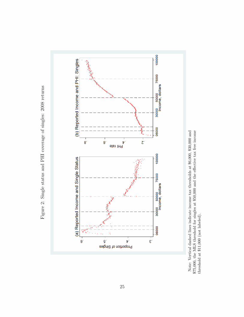
Panel (a) of Figure 2 presents the relationship between income and the proportion of

self-reported singles in the total population of tax returns. One notable feature of this graph

is a discontinuous drop in the proportion of singles above the MLS threshold which was set

at $50,000 in 2007-8; this supports our reasoning about changes in incentives for reporting

single status correctly once individuals cross the MLS threshold for singles. In order to

account for this potential sample selection bias, the estimation strategy (described in detail

in Section 4) combines the income distribution and PHI coverage data for all individuals

with the data on singles. Specifically, an increase in the PHI coverage at the MLS threshold

for singles is estimated from the data on PHI coverage for the total population. Then this

number is divided by the proportion of singles in the total population at the MLS threshold

for singles. Assuming that the PHI coverage of families does not change significantly at the

MLS threshold for singles, this will give us an estimate of the effect of the MLS policy on

single childless individuals at their MLS threshold.

Although we will not use the ATO data on PHI coverage of singles for estimation of the

MLS policy effect (for reasons discussed above), it is still useful to examine these data to

form an expectation about the final results. Panel (b) of Figure 2 presents the relationship

between taxable income and the proportion of individuals with private health insurance

coverage in 2007-8 in the single population. The PHI coverage increases with income from

0.10 at the lowest income levels to about 0.8 for incomes close to $100,000. There is a clear

discontinuous increase of about 7 percentage points in the proportion of individuals with

PHI at the MLS threshold for singles. However, as discussed above, this increase can in

part be an artifact of different incentives to report marital status correctly on the two sides

of the threshold. The probability of PHI coverage never reaches unity despite the strong

incentives to purchase PHI that are created by the MLS. There are 1,489,825 self-reported

single individuals with incomes exceeding the MLS threshold for singles, of whom 1,014,430

(68%) have an eligible health insurance coverage. The remaining 475,395 individuals are

subject to the MLS tax, and their MLS tax contributions amount to 321.4 million dollars in

7

2007-8.

PLACE FIGURE 2 HERE

To estimate the MLS policy effect on the PHI coverage of singles, we use the data

on the taxable income distribution and PHI coverage in the total population (single and

coupled) in 2007-8. The distribution of taxable income in the total population is plotted

in Panel (a) of Figure 3. There are 12.8 million individual tax returns in these data, with

the average of 30,068 individuals per $250 income bin. The largest income income bin,

with 234,043 individuals corresponds to yearly reported taxable income of $250 or less.

The smallest income bin, with 5,246 individuals, has a midpoint of $99,375. For privacy

reasons incomes exceeding $100,000 are grouped in a single bin with the midpoint of $100,125

containing 804,652 individuals. In the distribution obtained by weighting the $250 bins by

their respective number of observations the average income is 39.4 thousand dollars, the

standard deviation is $ 30,000, the median is equal to 34 thousand dollars, and the skewness

is 0.65.

The bracket cutoffs of the income tax schedule (kink points) in this period were $6,000,

$30,000 and $75,000. Although the nominal tax free threshold was set at $6,000, the low

income tax offset policy in place during this time resulted in effective tax free income thresh-

olds being set at $11,000. The taxable income distribution shows clear evidence of bunching

at the kink points of the income tax schedule in this period. Consistent with the evidence

from other countries, we find that the pattern of bunching at all of the kink points is diffuse,

with the excess mass on both sides of the kink points. Another notable feature of this in-

come distribution is the existence of bunching at the MLS threshold for singles. The pattern

of bunching at the MLS threshold is qualitatively different from that observed at the kink

points of the income tax schedule. Like the patterns of bunching at the tax notches docu-

mented by Kleven and Waseem (2013), the bunching at the MLS threshold is sharp, with

excessively high density below the threshold and excessively low density above the threshold.

These distinct patterns of bunching can be explained by the different incentives created by

the increases in the marginal tax rate as opposed to the MLS policy. In particular, for MLS

tax avoidance to be profitable reported taxable income must be strictly below the threshold.

Panel (b) of Figure 3 shows the relationship between taxable income and the proportion

of individuals with private health insurance coverage in 2007-8 in the total population. The

PHI coverage rate increases with income, from about 0.2 at the lower end of the income

distribution to approximately 0.75 at the income level of $100,000. The effect of the MLS

8

manifests itself as a discontinuous increase in the coverage rate at the MLS threshold for

singles. As expected, this increase is smaller than that in Panel (b) of Figure 2 because only

a fraction of individuals shown in this graph is affected by the MLS threshold for singles.

PLACE FIGURE 3 HERE

Despite the highly visible discontinuous jump at the MLS threshold for singles in the

relationship between income and PHI coverage rate, the behavior of the coverage rate is

non-monotonic in the vicinity of the threshold. In particular, the proportion of taxpayers

with insurance coverage is excessively low just below the threshold and excessively high

immediately above the threshold. This pattern is simply an artifact of income shifting

caused by the MLS: those above the threshold who do not wish to purchase PHI policy

end up with reported taxable incomes just below the threshold, simultaneously depressing

the coverage rate below the threshold and increasing it above the threshold. Importantly,

this implies that the causal effect of the insurance mandate cannot be estimated simply by

comparing coverage rates below and above the threshold. In the next section we develop an

estimation approach that allows us to correct for the consequences of bunching.

4 Empirical Analysis

In this section, we present our strategy for estimation of the MLS effect at the MLS threshold,

then apply this strategy to the data described earlier. We will use the following notation:

Y is true taxable income level (different from the reported taxable income Yr near the MLS

threshold where individuals engage in income shifting); T is the MLS income threshold; t is

the MLS tax rate; I is an indicator of private health insurance status (i.e., I = 1 in individual

has PHI and I = 0 otherwise); E is the amount of income shielded from taxation; P (I = 1)

is the probability of PHI coverage.

4.1 Estimation Strategy

In this study the main effect of interest is the difference between the probability of PHI

coverage with and without the MLS tax, i.e. P (I = 1|Y, t = 0.01) − P (I = 1|Y, t = 0)

for all income levels Y above the MLS threshold. However, the counterfactual probability

P (I = 1|Y : Y > T, t = 0) is not observable. If data on the true taxable incomes rather

than the reported incomes were available, one could attempt to estimate the MLS effect at

9

the threshold by comparing the insurance rates of individuals with incomes just above and

just below the threshold. This strategy would yield a consistent estimate of the effect of the

policy at the threshold if the densities of all other determinants of the insurance status were

continuous around the threshold; this is a standard assumption of the regression discontinuity

identification methodology. However, as discussed above, only the reported taxable income

is observed in our data, and it is likely to be different from the true income for individuals

without PHI and with true incomes exceeding the MLS threshold. Moreover, this strategy

will underestimate the full effect of the policy because individuals near the threshold can

avoid the MLS tax by misreporting their income rather than purchasing the PHI.

Our approach to estimation is based on the following arguments which are formally

developed in the Appendix. Suppose that it is costly to shield income from taxation and

that the marginal cost of tax avoidance is increasing in E.3 Then there will be income level

Y > T after which it will be more costly to shield excess income from taxation than to

either pay the MLS tax or purchase PHI coverage. Individuals with true incomes in the

interval (T, Y ) who do not have PHI will report incomes slightly less than T . Hence there

will be a shortage of mass in the distribution of the reported income between T and Y and

an excess mass in a small interval to the left of T . Let Y denote the lower boundary of

this interval.4 Because only uninsured individuals engage in misreporting, the PHI rate will

be excessively low in the reported taxable income interval (Y , T ) and excessively high in

the reported taxable income interval [T, Y ). Outside of the bunching interval (Y , Y ), true

incomes are reported and the relationship between income and the PHI rate is the same as

where tax avoidance is not possible for any income level. The MLS tax will have its full

intended effect on individuals with incomes above Y because they no longer have an option

of avoiding the MLS tax by engaging in income shifting.5 If there were no income gradient in

PHI coverage, this full effect could be estimated as the difference between the PHI coverage

rate at Y and at Y . However, there is a strong positive income gradient in PHI coverage

in our data, so this approach will produce an upward biased estimate of the MLS effect.

Therefore, we will attempt instead to estimate how much the PHI rate would have increased

at the MLS income threshold if tax avoidance was not possible, i.e. E = 0. In this case, the

3The following arguments will still apply when the marginal cost of tax avoidance is constant and greaterthan the MLS tax rate, t.

4In theory we would expect that all individuals who engage in income shifting will report $49,999 income,but in reality it is not always possible to attain this number precisely when filing a tax return, hence therewill be an interval of excess mass to the left of T rather than a single peak at $49,999.

5All of these predictions are derived formally in the Appendix, using a theoretical model of tax avoidance/health insurance choice.

10

MLS policy would produce a discontinuous increase in PHI coverage at the MLS threshold

if consumers are rational and utility maximizing. We denote this increase as ∆P |(Y = T ):

∆P |(Y = T ) ≡ P (I = 1|Y = T, t = 0.01, E = 0)− P (I = 1|Y = T, t = 0, E = 0).

To estimate ∆P |(Y = T ), we extrapolate the relationship between income and PHI for

income levels Y : Y < Y and Y : Y > Y to T and take the difference between the latter

and the former predictions. The accuracy of this estimator depends on the shape of the

relationship between income and PHI rate outside of the bunching interval (e.g., a linear

relationship will be more accurately extrapolated than a non-linear one) and on the distance

between T and Y and Y (i.e., a larger distance leads to poorer quality of extrapolation). It

turns out that in our data, ∆P |(Y = T ) can be estimated rather accurately. To estimate

∆P |(Y = T ) we do the following:

1. Estimate the boundaries of the bunching interval Y and Y using the distribution of

the reported taxable income.

2. Estimate P (I = 1|Y = T, t = 0, E = 0) by extrapolating the conditional probability

of PHI coverage P (I = 1|Y : Y < Y ) to income level Y = T .

3. Estimate P (I = 1|Y = T, t = 0.01, E = 0) by extrapolating the probability of PHI

P (I = 1|Y : Y > Y ), to income level Y = T .

4. Estimate ∆P |(Y = T ) by subtracting the result obtained in step 2 from that obtained

in step 3.

In principle,we should apply this strategy to the income tax returns and PHI coverage

of the individuals who are directly affected by the policy, i.e. single individuals with no

children. However, as discussed earlier, in our data the self-reported single status may

be an unreliable indicator of belonging to this group, and the propensity to report single

status correctly can change as one crosses the MLS threshold. Therefore, we use data on

the total population (single and married individuals) to estimate the policy effect on all

individuals, ∆PAll|(Y = T ), performing the four steps just discussed. After imposing the

assumption that the effect on married individuals (who are not affected by the policy at

the MLS income threshold for singles) is equal to zero, we can express the total effect as

∆PAll|(Y = T ) = P (S|Y = T ) ·∆P S|(Y = T ), where P (S|Y = T ) is the probability of being

in the treatment group (i.e single without children) and ∆P S|(Y = T ) is the policy effect

11

on the treated group. After estimating the probability of being single at the MLS income

threshold P (S|Y = T ) using data plotted on Panel (a) of Figure (2), we can compute the

effect on the treated group as ∆P S|(Y = T ) = ∆PAll|(Y=T )P (S|Y=T )

.

4.2 Estimation of the bunching interval

As outlined in the previous section, the first step of the empirical analysis is to find the lower

and upper bounds Y and Y of the income interval in which bunching behavior distorts the

densities of reported taxable income and the PHI rate. We follow the methodology used in

other studies of bunching behavior (e.g. Chetty et al. (2011); Kleven and Waseem (2013)).

In particular, we use data on all individuals (single and married) to fit the following flexible

polynomial model to the empirical density of reported taxable income:

Ci = β0 +3∑j=1

βjYjri +

5∑k=1

γk · ι(T − 250 · k < Yri < T − 250 · (k − 1))

+15∑k=1

αk · ι(T + 250 · (k − 1) < Yri < T + 250 · k) + εi (1)

where Ci is counts of individuals in income bin i; Yri is the mid-point of the reported taxable

income bin i; β0 +∑3j=1 βjY

jri is the (counterfactual) distribution of the reported taxable

income in the absence of tax avoidance; γk measures the excess mass of individuals in the

income bins immediately to the left of the MLS threshold; and αk measures a shortage of mass

in the income bins immediately to the right of the MLS threshold. As long as individuals

with true incomes above T and without PHI engage in income shifting, we expect that some

γk closest to T will be positive and statistically significant, and some αk closest to T will

be negative and statistically significant. Because the excess mass in the distribution of the

reported income to the left of T should be equal to the shortage of mass on the interval [T, Y ]

we impose an adding-up constraint requiring that the coefficients γk and αk in equation (1)

sum to zero:∑5k=1 γk +

∑15k=1 αk = 0.

We define Y as the midpoint of the income bin closest to T on the left whose corresponding

coefficient γ is not statistically significant. That is, Y ≡ T − 125 − (k∗ − 1) · 250 where

k∗ ≡ mink : γk = 0. Similarly, Y is defined as the midpoint of the income bin closest to T

on the right whose corresponding α coefficient is not statistically significantly different from

zero. That is, Y ≡ T + 125 + (k∗ − 1) · 250 where k∗ ≡ mink : αk = 0.Table 5 presents the results from fitting equation (1). In going from Model 1 to Model 2

we have removed dummies corresponding to income bins whose coefficients γk and αk are not

12

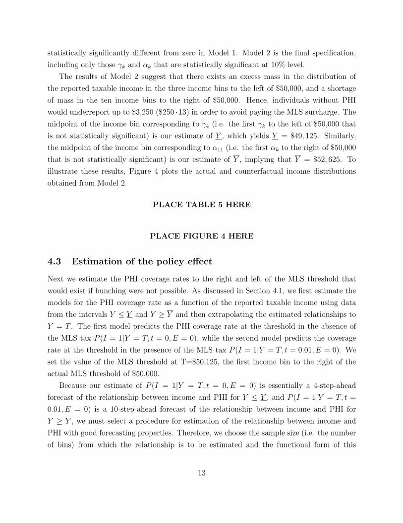
statistically significantly different from zero in Model 1. Model 2 is the final specification,

including only those γk and αk that are statistically significant at 10% level.

The results of Model 2 suggest that there exists an excess mass in the distribution of

the reported taxable income in the three income bins to the left of $50,000, and a shortage

of mass in the ten income bins to the right of $50,000. Hence, individuals without PHI

would underreport up to $3,250 ($250 ·13) in order to avoid paying the MLS surcharge. The

midpoint of the income bin corresponding to γ4 (i.e. the first γk to the left of $50,000 that

is not statistically significant) is our estimate of Y , which yields Y = $49, 125. Similarly,

the midpoint of the income bin corresponding to α11 (i.e. the first αk to the right of $50,000

that is not statistically significant) is our estimate of Y , implying that Y = $52, 625. To

illustrate these results, Figure 4 plots the actual and counterfactual income distributions

obtained from Model 2.

PLACE TABLE 5 HERE

PLACE FIGURE 4 HERE

4.3 Estimation of the policy effect

Next we estimate the PHI coverage rates to the right and left of the MLS threshold that

would exist if bunching were not possible. As discussed in Section 4.1, we first estimate the

models for the PHI coverage rate as a function of the reported taxable income using data

from the intervals Y ≤ Y and Y ≥ Y and then extrapolating the estimated relationships to

Y = T . The first model predicts the PHI coverage rate at the threshold in the absence of

the MLS tax P (I = 1|Y = T, t = 0, E = 0), while the second model predicts the coverage

rate at the threshold in the presence of the MLS tax P (I = 1|Y = T, t = 0.01, E = 0). We

set the value of the MLS threshold at T=$50,125, the first income bin to the right of the

actual MLS threshold of $50,000.

Because our estimate of P (I = 1|Y = T, t = 0, E = 0) is essentially a 4-step-ahead

forecast of the relationship between income and PHI for Y ≤ Y , and P (I = 1|Y = T, t =

0.01, E = 0) is a 10-step-ahead forecast of the relationship between income and PHI for

Y ≥ Y , we must select a procedure for estimation of the relationship between income and

PHI with good forecasting properties. Therefore, we choose the sample size (i.e. the number

of bins) from which the relationship is to be estimated and the functional form of this

13

relationship so as to minimize the mean squared difference between the out-of-sample and

in-sample forecasts obtained from a very flexible model, with the regression’s R-squared

close to 0.99.6 We find that the linear model estimated using 23 income bins yields the best

forecast for the relationship between income and PHI for Y ≤ Y , while the linear model

estimated using 18 income bins gives the best out-of-sample forecast for Y ≥ Y . To estimate

∆PAll|(Y = T ), we first use the data on all individuals (single and married) to fit the model:

PHIi = (β01 + β0

2Yri)ι(Yri <= Y ) + (β11 + β1

2Yri)ι(Yri >= Y ) + εi (2)

where PHIi is the proportion of individuals with PHI in income bin i and Yri is the mid-

point of the reported taxable income bin i. The midpoint of the smallest income bin in the

estimation sample is $43, 625; the midpoint of the largest income bin is $56, 875; Y = $49, 125

and Y = $52, 625. The estimate of ∆PAll|(Y = T ) is given by

∆PAll|(Y = T ) = (β11 + β1

2 · 50, 125)− (β01 + β0

2 · 50, 125) (3)

To estimate equation (2) we use a two-step feasible GLS method described in detail in

the Appendix. This method yields estimates which are equivalent to those from the linear

probability model estimated from individual data on PHI status and income (assuming that

individuals’ incomes are equal to the midpoint of their corresponding income bin) for the

part of population with incomes between $43, 625 and $56, 875. Table 2 presents the results

of the GLS estimation of equation 2 and the GLS standard errors. In the estimation sample

the number of individuals within each bin varies between 26,010 and 37,324, which results

in the total of 1,322,409 individual observations. Figure 5 shows the in- and out-of-sample

fit of this model to the data. The dashed vertical lines around 50,000 indicate the bunching

interval, that is ($49,125,$52,625), within which the PHI coverage is forecasted out-of-sample

using the estimates in Table 2.

PLACE TABLE 2 HERE

PLACE FIGURE 5 HERE

6In the Appendix we discuss in detail how the specification was selected.

14

We then substitute the estimates from Table 2 into equation (3) to obtain:

∆PAll|(Y = T ) = (.0125840 + .0092023 · 50.125)− (0.0914307 + .0070741 · 50.125) = 0.0278

(4)

Hence, our estimate of the MLS effect at the threshold for singles in the absence of tax

avoidance ∆PAll|(Y = T ) is equal to 0.0278 and its standard error is equal to 0.00297. This

makes the estimate statistically significantly different from zero at any significance level. It

implies that the probability of having a PHI coverage in the population increases by 2.8

percentage points at the MLS threshold for singles. This is the size of the vertical distance

between the dashed and solid lines at the income of $50,125 in Figure 5.

As a robustness check, we also estimate the placebo MLS effect using income tax returns

data from 2009-10. In this period one would not expect to see discontinuity at the 2007-8

MLS threshold of $50,000, because the threshold for singles had been increased to $73,000

in 2008-9.8 We find that the estimated effect of the MLS is equal to -.005 with a standard

error of .003. The p-value associated with the null hypothesis, that this effect is equal to

zero, is 0.073. These results suggest, that using our estimation approach, we are unlikely to

obtain a positive policy effect of a magnitude and statistical significance similar to what we

obtain using the 2007-8 data.

To obtain the MLS effect on the treated population, we divide the total effect by the

proportion of single individuals with no dependent children in the total population at the

MLS threshold for singles. Self-reported single status available in the ATO data and plotted

on Panel (a) of Figure 2 can be used to estimate the proportion of singles at this threshold.

The irregularities in these data, where the proportion of singles is artificially low in the

reported taxable income bins just to the right of the threshold and is artificially high just

to the left of the threshold, are limited to the bunching interval Y , Y . Therefore, to predict

the proportion of singles at the MLS threshold we use the forecasting technique described

earlier. We estimate a linear model specified in equation (2) with the proportion of singles

in the income bin i as the dependent variable, using data outside of the bunching interval,

and then forecast this proportion to the MLS threshold for singles using the relationship

estimated for income levels Y > Y . We choose the forecast to the right of the threshold as

an estimate of single status at the threshold because, as discussed above, individuals have a

7This standard error was computed using the lincom Stata command.8We did not attempt to estimate the MLS effect in 2010 at the new threshold because the income tax

threshold was very close to the MLS threshold. This made it difficult to obtain reliable out-of-samplepredictions of the coverage at the threshold. Visual inspection suggests that the effect is even smaller thanat the 2007-8 threshold.

15

stronger incentive to report their true marital status to the right of the MLS threshold for

singles. The estimation results are presented in the Appendix. The estimated proportion of

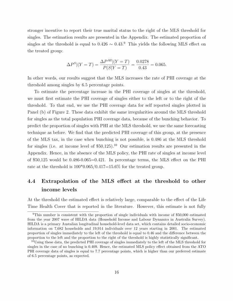
singles at the threshold is equal to 0.426 ∼ 0.43.9 This yields the following MLS effect on

the treated group:

∆P S|(Y = T ) =∆PAll|(Y = T )

P (S|Y = T )=

0.0278

0.43= 0.065.

In other words, our results suggest that the MLS increases the rate of PHI coverage at the

threshold among singles by 6.5 percentage points.

To estimate the percentage increase in the PHI coverage of singles at the threshold,

we must first estimate the PHI coverage of singles either to the left or to the right of the

threshold. To that end, we use the PHI coverage data for self reported singles plotted in

Panel (b) of Figure 2. These data exhibit the same irregularities around the MLS threshold

for singles as the total population PHI coverage data, because of the bunching behavior. To

predict the proportion of singles with PHI at the MLS threshold, we use the same forecasting

technique as before. We find that the predicted PHI coverage of this group, at the presence

of the MLS tax, in the case when bunching is not possible, is 0.486 at the MLS threshold

for singles (i.e. at income level of $50,125).10 Our estimation results are presented in the

Appendix. Hence, in the absence of the MLS policy, the PHI rate of singles at income level

of $50,125 would be 0.486-0.065=0.421. In percentage terms, the MLS effect on the PHI

rate at the threshold is 100*0.065/0.417=15.6% for the treated group.

4.4 Extrapolation of the MLS effect at the threshold to other

income levels

At the threshold the estimated effect is relatively large, comparable to the effect of the Life

Time Health Cover that is reported in the literature. However, this estimate is not fully

9This number is consistent with the proportion of single individuals with income of $50,000 estimatedfrom the year 2007 wave of HILDA data (Household Income and Labour Dynamics in Australia Survey).HILDA is a primary Austalian longitudinal household-level data set, which contains detailed socio-economicinformation on 7,682 households and 19,914 individuals over 12 years starting in 2001. The estimatedproportion of singles immediately to the left of the threshold is equal to 0.46 and the difference between theproportion to the left and the proportion to the right of the threshold is highly statistically significant.

10Using these data, the predicted PHI coverage of singles immediately to the left of the MLS threshold forsingles in the case of no bunching is 0.409. Hence, the estimated MLS policy effect obtained from the ATOPHI coverage data of singles is equal to 7.7 percentage points, which is higher than our preferred estimateof 6.5 percentage points, as expected.

16

informative about how much total coverage in the treatment group is affected by the policy.

In order to estimate the total effect of the policy, we will assume that the MLS effect per

dollar of the tax is constant. In this case, the treatment effect of the MLS at any income

level, Y, is proportional to the dollar amount of the payable MLS tax. In other words,

the change in the PHI rate at income Y due to the MLS tax t, ∆PHI|Y, t, is equal to

∆PHI|Y, t = α · t · Y , where α is the per dollar effect of the policy. The estimated effect at

the MLS threshold suggests that α = 0.065/501.25 (recall that with an MLS tax rate of 0.01,

the MLS tax of someone whose income is $50,125 but who has no PHI is $501.25). To obtain

the counterfactual PHI rates for singles (i.e. PHI rate in the absence of the MLS policy),

we use the observed PHI rates and compute PHICFi = PHIi − [0.01 · Yi] · 0.065501.25

for each

income bin above the threshold. The estimated total policy effect then can be interpreted as

an upper bound on the actual effect, because one would expect that taxpayers with higher

incomes might be less responsive to the tax of a given size than those in the middle of the

income distribution.

Figure 6 shows actual and counterfactual PHI coverage obtained after imposing these

assumptions for single individuals with reported taxable income above $50,000. Table 3

summarizes the numerical results. In particular, we compute how much the total coverage

in this group increased because of the policy, taking into account the number of individuals

in each income bin. We find that the total number of people with PHI increases by approx-

imately 146,459 as a result of the MLS policy, that is equivalent to a 7.2% increase in the

number of insured singles. The aggregate PHI rate for this group increases from 34.2% to

36.6%. These results suggest that the MLS policy had at best a modest effect overall on

the PHI coverage rate (among singles) in the sample period. This is consistent with other

circumstantial evidence of the weak effect of the MLS. In particular, the MLS had no effect

on the aggregate PHI coverage rate at the time of its introduction in 1997. There were

also no significant changes in the PHI coverage rate after substantial increases in the MLS

thresholds for singles and married taxpayers in 2009.

We also compute the additional cost of the 30% private health insurance premium rebate

that was induced by the MLS. We do not know which policies are chosen by individuals

driven into the PHI coverage by the MLS, so we consider three scenarios. In the first,

individuals are assumed to purchase the cheapest eligible policy. The costs of these policies

typically are close to the MLS tax liability. Hence, we assume that the PHI price P in the

first scenario is equal to $500. In the second scenario, we assume that individuals purchase

a policy with out-of-pocket costs (after the 30% subsidy rebate) exactly equal to their MLS

17

tax liability, i.e. P = 0.1 · Y/0.7. Finally, we assume that all individuals purchase the policy

with the most comprehensive coverage. For a 40 year old male in 2013, that would cost

$ 2,718 according to the iSelect.com.au. This gives an approximate cost of $2,283, for a

similar policy in 2008 after CPI deflation. Table 3 presents the cost to the budget under

each of these scenarios. In all three, budget revenue from the MLS far exceeds the added

costs associated with the premium rebate.

PLACE FIGURE 6 HERE

PLACE TABLE 3 HERE

4.5 The effect of the MLS for different age groups

We also estimate the effect of the MLS tax on PHI coverage for single individuals in three

age groups: ”young” (between 15 and 32 years old); ”middle-aged” (between 33 and 50

years old); and ”old” (older than 50 years old). The details of this estimation are in the

Appendix. Our results suggest that there are important heterogeneities in how taxpayers

in the different age groups respond to the tax incentives. In particular, the old taxpayers

exhibit the strongest reaction to the tax incentives: their coverage rate increases by 9.2

percentage points from a relatively high baseline of 58% (67%-9.2%) at the MLS threshold,

which implies a 15.9% increase. The coverage rate of the young taxpayers increases by 7.4

percentage points from the baseline of 32.6% (40%-7.4%), a 22.5% increase. The middle aged

group appears to be the least sensitive to the incentives created by the MLS policy, with

their coverage rate increasing by 5 percentage points or 11%. Taxpayers in the oldest age

group also exhibit the highest increase in their overall rate of PHI coverage: it goes up by 4

percentage points as a result of the policy. Intuitively, the policy seems to affect the most

that segment of the population with the highest expected benefit from having PHI, namely

older people. In absolute terms, young taxpayers account for the largest fraction of budget

revenue from the MLS. This group also has the largest percentage of taxpayers (among those

liable to pay the tax) who choose not to comply with the MLS mandate: 44% compared to

30% in the middle age group and 21% in the old age group. However, their average MLS

tax liability is slightly lower than that of the two other age groups because that younger

taxpayers tend to have relatively lower incomes. The large number of non-compliers among

the young may reflect their lower valuation of the benefits of the private health insurance,

or a lack of knowledge about PHI tax incentives.

18

5 Conclusion

In this paper, we study the effect of an individual insurance mandate, the Medicare Levy

Surcharge (MLS), on the demand for PHI within the Australian national health care system.

Using administrative income tax returns data for the entire population of Australian taxpay-

ers in 2007-08 allows us to estimate the effect of the policy at the MLS income threshold for

single individuals. We find that the policy has resulted in an increase in the PHI coverage

rate of 6.5 percentage points or 15.6% at the threshold. Overall, this policy has increased

the total number of insured singles by 7.2% and increased the PHI rate of singles by 2.4

percentage points. Our results suggest that the MLS has had at best a modest effect on

the demand for private health insurance in Australia during the study period. The effect of

the policy seems to be the strongest among older taxpayers. Also, a significant number of

individuals choose not to comply with the mandate and pay the MLS tax instead. This is

especially true for younger people: 44% of taxpayers below the age of 30 with incomes above

the MLS threshold choose not to comply with the mandate. To interpret these results, we

must consider the supplementary role that PHI coverage plays in the Australian mixed pub-

lic/private health care system. That is, with a tax financed Medicare system guaranteeing

free treatment in the public sector, the attractiveness of private insurance is greatly reduced.

As a result a large proportion of younger individuals may have low willingness to pay for

PHI coverage. At the same time, this supplementary role of the PHI cannot be the only

explanation for the limited effectiveness of the mandate. Clearly, many of the uninsured high

income taxpayers would be able to purchase PHI cover at the cost lower than their MLS

tax liability. Thus, these individuals either face significant transaction costs of purchasing

insurance or they make dominated choices. Because these frictions appear to significantly

influence the effectiveness of the policy, understanding them remains an important topic for

future research.

19

References

[1] Butler, J. (2002) ”Policy change and private health insurance: did the cheapest policy

do the trick?” Australian Health Review, 25(6), 33 - 41.

[2] Chandra A, Gruber J. and R. McKnight. 2011. ”The Importance of the Individual Man-

date - Evidence from Massachusetts” New England Journal of Medicine, 364, January

27, 2011, 293-295.

[3] Chapman B. and A. Leigh (2006) ”Do Very High Tax Rates Induce Bunching? Im-

plications for the Design of Income Contingent Loan Schemes.” Economic Record, 85,

276-289.

[4] Chetty, R., J. Friedman, T. Olsen, and L. Pistaferri (2011). ”Adjustment Costs, Firm

Responses, and Micro vs. Macro Labor Supply Elasticities: Evidence from Danish Tax

Records.” Quarterly Journal of Economics, 126 (2): 749-804.

[5] Emmerson C., Frayne C. and A. Goodman (2001) ”Should private medical insurance

be subsidised?” The King’s Fund Review of Health Policy 2001. Health Care UK 51(4):

49-65.

[6] Ellis R. and E. Savage (2008) ”Run for cover now or later? The impact of premiums,

threats and deadlines on private health insurance in Australia,” International Journal of

Health Care Finance and Economics, 8(4), 257-277.

[7] Finkelstein A. (2002) ”The effect of tax subsidies to employer-provided supplementary

health insurance: evidence from Canada,” Journal of Public Economics, 84, 305-339.

[8] Gruber, J. and J. Poterba (1994) ”Tax incentives and the decision to purchase health

insurance: Evidence from the self-employed,” Quarterly Journal of Economics, August,

701-733.

[9] Gruber, J. ”The Impacts of the Affordable Care Act: How Reasonable Are the Projec-

tions?,” National Tax Journal, forthcoming.

[10] Gujarati, D. and Porter D. (2009) ”Basic Econometrics”. McGraw-Hill/Irwin, 5th ed.

[11] Hahn, J., Todd, P., and W. Van der Kalauw (2001) ”Identification and Estimation

of Treatment Effects with a Regression-Discontinuity Design,” Econometrica, 69(1):

201:209.

20

[12] Johar, M., Jones, G., Keane, M., Savage, E., and O. Stavrunova (2011) ”Waiting Times

for Elective Surgery and the Decision to Buy Private Health Insurance,” Health Eco-

nomics 20(S1), 2011: pp. 68-86.

[13] Kleven H. and M.Waseem (2013) ”Using Notches to Uncover Optimization Frictions

and Structural Elasticities: Evidence from Pakistan,” Quarterly Journal of Economics,

128, 669-723.

[14] Martin, S and Smith, P.C (1999). ”Rationing by waiting lists: an empirical investiga-

tion,” Journal of Public Economics, 41:141-164.

[15] McCrary, J. (2008). ”Manipulation of the Running Variable in the Regression Discon-

tinuity Design: A Density Test,” Journal of Economerics, 142 (2).

[16] Palangkaraya, A. and Yong, J. (2005), ”Effects of Recent Carrot and Stick Policy Initia-

tives on Private Health Insurance Coverage in Australia,” Economic Record, 81, 262-72.

[17] Porter, J. (2003) ”Estimation in the Regression Discontinuity Model”, Unpublished

manuscript, Harvard University.

[18] Rodriguez M., and A. Stoyanova (2004) ”Changes in the demand for private medical

insurance following a shift in tax incentives,” Health Economics, 17(2), 185-202.

[19] Saez, E. (2010) ”Do Taxpayers Bunch at Kink Points?” American Economic Journal:

Economic Policy, 2, 180-212.

[20] Australian Institute of Health and Welfare. Surgery in Australian hospitals 201011.

Available at http://www.aihw.gov.au/hospitals/surgery-2010-11/.

Tables and Figures

21

Table 1: Estimation of Y and YModel 1 Model 2

Variable Coefficient P-value Coefficient P-value

Y 1636.73 0 1745.413 0Y 2/1002 -516401.715 0 -537159.815 0Y 3/1003 350569.776 0 363457.612 0

γ1 11599.627 0 11494.594 0γ2 3025.017 0 2919.442 0γ3 1304.348 0 1198.252 0.001γ4 479.637 0.184γ5 463.93 0.199

α1 -3675.88 0 -3780.354 0α2 -2377.506 0 -2481.402 0α3 -1663.303 0 -1766.605 0α4 -1401.311 0 -1504.006 0α5 -1294.542 0 -1396.615 0α6 -1004.043 0.006 -1105.482 0.003α7 -830.839 0.022 -931.633 0.011α8 -914.968 0.012 -1015.107 0.006α9 -749.455 0.039 -848.93 0.021α10 -683.348 0.059 -782.152 0.033α11 -414.677 0.25α12 -572.459 0.113α13 –645.746 0.075α14 -265.553 0.461α15 -378.928 0.293

const 35795.864 0 33948.618 0

N 131 131R2 0.998 0.998

Y $49,125Y $52,625

Note: The dependent variable is counts of individuals in the reported taxableincome bin with width of $250. The reported taxable income Y is measured inthousands of dollars. Estimation sample includes income bins between $39,125and $71,625. The counts of individuals within income bins varies between 16,771and 44,279 in the estimation sample.

22

Table 2: Relationship between income and PHI coverage, equation (2)

Coefficient Estimate St.err P-value

β01 .0914307 .0150 0.000β02 .0070741 .0003 0.000β11 .0125840 .0298 0.673β12 .0092023 .0005 0.000

Note: The dependent variable is the proportion of individuals with PHI inthe reported taxable income bin with width of $250. The explanatory variable(reported taxable income Y ) is measured in thousands of dollars. Estima-tion sample includes income bins between $43,625 and $49,125, and between$52,625 and $56,875. R2 is close to unity.

Table 3: Extrapolating the MLS effect to income levels above the MLS threshold1 Total counts, singles 5,948,2902 Total counts with PHI, actual 2,175,6803 Total counts with PHI, counterfactual 2,029,2214 ∆ (2-3) 146,4595 ∆, percent (100%*4:3) 7.2%6 Overall PHI rate, actual (2:1) 36.57%7 Overall PHI rate, counterfactual (3:1) 34.1%8 Budget revenue, mln. 321.49 Budget cost of 30% premium rebate, mln, P = $500 2210 Budget cost of 30% premium rebate, mln, P = 0.1 · Y/0.7 4811 Budget cost of 30% premium rebate, mln, P = $2283 100

Note: Budget revenue is computed as 1% of the total reported taxable income ofsingle population without PHI with reported incomes exceeding $50,000

23

Figure 1: How the MLS works: single individuals, no children, 2008

47 48 49 50 51 52 5333

34

35

36

37

Before Tax Income, thousand dollars

Afte

r Tax

Inco

me,

thou

sand

doll

ars

Before Tax Income-tYWith PHI (Before Tax Income-tY)

Without PHI (0.99*Before Tax Income-tY)

50000 dollars

$500

Note: In the Figure tY denotes income tax liability, i.e. tY = Y · t, where Y isbefore tax income and t is the income tax (set to 0.30 in the Figure).

24

Fig

ure

2:Sin

gle

stat

us

and

PH

Ico

vera

geof

singl

es:

2008

retu

rns

Not

e:V

erti

cal

das

hed

lin

esin

dic

ate

inco

me

tax

thre

shold

sat

$6,0

00,

$30,0

00

an

d$7

5,00

0,th

eM

LS

thre

shol

dfo

rsi

ngl

esat

$50,

000

an

dth

eeff

ecti

ve

tax

free

inco

me

thre

shol

dat

$11,

000

(not

lab

eled

).

25

Fig

ure

3:R

epor

ted

taxab

lein

com

edis

trib

uti

onan

dP

HI

cove

rage

:to

tal

pop

ula

tion

,20

08re

turn

s

Not

e:V

erti

cal

das

hed

lin

esin

dic

ate

inco

me

tax

thre

shold

sat

$6,0

00,

$30,0

00

an

d$7

5,00

0,th

eM

LS

thre

shol

dfo

rsi

ngl

esat

$50,

000

an

dth

eeff

ecti

ve

tax

free

inco

me

thre

shol

dat

$11,

000

(not

lab

eled

).

26

Figure 4: Reported taxable income distributions: total population, 2008 returns

Figure 5: Reported taxable income and PHI coverage if bunching was not possible: totalpopulation, 2008 returns

Note: The dashed and solid sloped lines are fitted values from equation (2).The dashed vertical lines around 50,000 indicate the bunching interval (i.e.($49,125,$52,625)) within which the PHI coverage is forecasted out of sample usingestimates in Table 2.

27

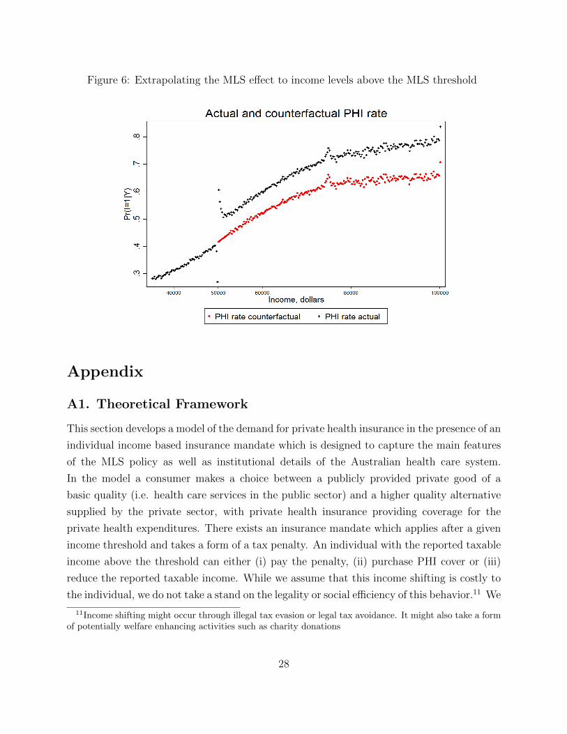
Figure 6: Extrapolating the MLS effect to income levels above the MLS threshold

Appendix

A1. Theoretical Framework

This section develops a model of the demand for private health insurance in the presence of an

individual income based insurance mandate which is designed to capture the main features

of the MLS policy as well as institutional details of the Australian health care system.

In the model a consumer makes a choice between a publicly provided private good of a

basic quality (i.e. health care services in the public sector) and a higher quality alternative

supplied by the private sector, with private health insurance providing coverage for the

private health expenditures. There exists an insurance mandate which applies after a given

income threshold and takes a form of a tax penalty. An individual with the reported taxable

income above the threshold can either (i) pay the penalty, (ii) purchase PHI cover or (iii)

reduce the reported taxable income. While we assume that this income shifting is costly to

the individual, we do not take a stand on the legality or social efficiency of this behavior.11 We

11Income shifting might occur through illegal tax evasion or legal tax avoidance. It might also take a formof potentially welfare enhancing activities such as charity donations

28

show that this conceptual framework is capable of reproducing the main patterns observed

in the data as described in the previous section. We also show that it can be used to develop

an intuitive approach to the estimation of the treatment effect of the MLS policy in the

presence of income shifting.

A1.1 Model Setup

Consider an individual who faces a given probability π of becoming ill and experiencing

a disutility of health restoring treatment, whose preferences are defined over a composite

consumption good. The treatment can be obtained either from public or private health

care sector. As is typically assumed in these type of models (e.g. Martin and Smith, 1999)

the disutility of treatment is lower in the private sector, reflecting the fact that private

treatment as a rule involves shorter waiting times, ability to choose the treating doctor and

other quality enhancements. However, treatment in the private sector commands a higher

price. An individual can purchase private health insurance to cover the cost of treatment in

the private sector. To simplify exposition we assume that (i) insurance provides full coverage,

implying that insured individual will always choose private treatment; and (ii) the price of

private treatment is sufficiently high to induce someone without insurance to always choose

public sector treatment. Under these assumptions the choice of insurance status completely

determines the choice of the health care sector, resulting in the expected utility function

defined over the composite consumption good and insurance status given by

u(c, I) = m(c)− π(I · τpr + (1− I) · τpb)− I · ξ

Here m(c) denotes individual’s consumption utility, I is private health insurance indicator,

τpb and τpr are the disutilities of treatment in a public and private sectors, respectively, and

ξ denotes an additive psychic search cost associated with purchasing a private insurance. In

what follows the price of treatment in the public sector and the disutility of treatment in

the private sector τpr will be both normalized to zero.

The MLS policy stipulates that if the individual’s income is greater than a given threshold

T , they must pay a Medicare Levy Surcharge of t percent of the total reported taxable

income. Let Y denote the true taxable income earned by the individual. The reported

taxable income Yr can be lower than Y if an individual decides to engage in income shifting.

We assume that the cost of underreporting is linear in the amount of the underreported

income E = Y − Yr and is given by C(E) = aE. Because MLS is the only reason to engage

29

Table 4: Utility function

Y < T Y ≥ T

I = 0 m(Y )− π · τpb m(Y − t · (Y −E) · ι(Y −E ≥ T )− aE)− π · τpbI = 1 m(Y − P )− ξ m(Y − P )− ξ

in income shifting, an individual might have E > 0 only if the true income exceeds the MLS

threshold (Y ≥ T ). Throughout the analysis we assume that the marginal cost of avoidance

is higher than the surcharge rate, a > t.12 This guarantees that there exists a threshold level

of income above which no avoidance takes place. Under these assumption the individual’s

utility maximization problem amounts to choosing c, I and the amount of underreported

income E to maximize the expected utility function u(c, I) subject to the following budget

constraint

c ≤ Y − I · P − (1− I) · t · (Y − E) · ι(Y − E ≥ T )− aE,

where ι(.) is an indicator function equal to 1 if the expression in parenthesis is true, and is

equal to zero otherwise and P denotes the insurance premium. Note, that apart from the

insurance premium P , the costs of health care do not enter the budget constrain because it

is assumed that (i) treatment is free in the public sector; (ii) insurance covers fully the cost

of treatment in the private sector; (iii) it is never optimal for a person without PHI to choose

private treatment. Using this budget constraint one can substitute for consumption in the

utility function, which reduces maximization problem to the choice of insurance status and

amount of income shifting. Table (4) shows utilities of insured and uninsured individuals

with incomes below and above the MLS threshold after imposing the normalization τpr = 0.

If the individual’s true income is below the threshold, the utility maximization problem

reduces to the choice of the insurance status, which is affected by the disutility of treatment

in the public sector, insurance premium and the search cost of insurance. On the other hand,

a person with income above the MLS threshold decides whether to buy insurance as well as

how much income to underreport if no insurance is purchased.

The insurance choice problem can be further simplified by solving for the optimal amount

of income shifting chosen by a person with income above the threshold conditional on not

12Without this assumption it will always be optimal for individuals with true incomes exceeding T andwithout PHI to report incomes less than T, resulting in PHI coverage rate of unity above the MLS threshold.This pattern is not consistent with the observed data. It is easy to show that a linear cost function with therestriction a > t results in similar model predictions as a quadratic cost function C(E) = E2. Although thequadratic cost function is perhaps more realistic, we chose the linear specification because it is much easierto analyze.

30

having insurance. First note that the structure of MLS implies that a person engaged in

underreporting will need to report income below the MLS threshold to avoid paying the

tax. Because underreporting is costly, the optimal reported taxable income, conditional on

engaging in income shifting, must be strictly below but as close as possible to the MLS

threshold T . In practice such exact manipulation of income will be difficult to implement,

and one would expect that underreported incomes will fall into some small interval below

the threshold. To formalize this intuition, let ε > 0 denote the length of the interval and

assume that by choosing the target level of reported income equal to T −ε a person engaging

in income shifting can guarantee that the actual realization of the reported income is a draw

of random variable distributed uniformly on [T − ε, T ). Under this assumption the optimal

amount of underreporting is given by Y − T + ε. Next note that because the marginal cost

of underreporting, a, is higher than the MLS rate t, not everyone who is not insured will

engage in income shifting. In particular, there exists a threshold level of income Y such

that for income levels satisfying T < Y ≤ Y it would be optimal to underreport income by

exactly Y −T+ε, while for income levels Y > Y it is optimal to report income truthfully and

pay the tax. An individual with the income level Y must be indifferent between reporting

the income level just below the MLS threshold and reporting truthfully. The value of Y is

determined by the following equality:

Y − a · (Y − T + ε) = Y − tY

Solving this equation for Y we get

Y =a(T − ε)a− t

. (5)

The above arguments taken together imply that the structure of the individual’s insurance

choice problem will depend on the individual’s true taxable income Y as follows.

Case 1: Y < T . True taxable income is reported. Utility without insurance is u(I =

0) = m(Y )− π · τpb. Utility with insurance is u(I = 1) = m(Y − P )− ξ.Case 2: T ≤ Y ≤ Y . True taxable income is reported if insured, and Y − T + ε is

reported otherwise. The actual realization of the reported taxable income for those without

insurance follows uniform distribution on [T − ε, T ). Utility without insurance is u(I = 0) =

m(Y − a(Y − T + ε))− π · τpb. Utility with insurance is u(I = 1) = m(Y − P )− ξ.Case 3: Y > Y . True taxable income is reported. Utility without insurance is u(I =

0) = m(Y − t · Y )− π · τpb. Utility with insurance is u(I = 1) = m(Y − P )− ξ.

31

A1.2 Model Predictions

The model outlined above can be used to derive predictions about taxpayers’ responses to

the incentives embedded in the MLS policy. In this section we impose assumptions on the

functional forms and parameter distributions to illustrate graphically model’s predictions,

while the analytical results are derived in the Appendix. We start by describing the rela-

tionship between the distribution of the true income, the probability of having insurance

conditional on the true income (both of which are not fully observed in the data), on the

one hand, and the distribution of the reported taxable income and the probability of having

insurance conditional on the reported income (both are fully observed in the data). We then

discuss how the data on the reported taxable income and insurance rates can be used to

estimate (i) the amount of income shifting caused by MLS; and (ii) the treatment effect of

MLS on the PHI coverage rate.

Let η ≡ π · τpb − ξ denote the expected net psychic benefit of private health insurance.

Since π, τpb and ξ are all non-negative, η can take any value on the real line. Suppose that

η and Y are identically and independently distributed in the population.13 Let G(η) denote

the cumulative distribution function (cdf) of η. The cdf of η can be used to compute the

probability that an individual is insured, conditional on the reported income Yr, as well as

conditional on the true income Y . Let py(Y ) denote the probability density function of Y

and pr(Yr) denote the probability density of Yr.

The predictions of the model obtained under these assumptions are illustrated in Figure 7.

The graphs in this figure are constructed for the income range from $49,000 to $51,000 under

the following parameterization: Y is distributed uniformly on this interval, the consumption

utility is assumed to be linear, m(Y ) = Y , η has a standard normal distribution independent

of Y , a = 0.8 and ε = $100. The solid line in the leftmost panel of the figure shows the

relationship between actual income Y and probability of having insurance coverage obtained

from the model with income shifting. Note that because only the reported (and not actual)

income is observed, this relationship cannot be compared to what is observed in the data. The

dashed line in the same panel depicts the same relationship for the case when income shifting

is not possible (for example because the marginal cost a is too high). The probability of

coverage jumps discontinuously at the MLS threshold, with the size of the jump representing

the treatment effect of the MLS at the threshold. On the other hand, when the income

shifting is possible insurance coverage increases gradually after the threshold, and the policy

effect reaches it’s full magnitude only at Y , when income shifting is no longer profitable

13This assumption can be relaxed without affecting main results.

32

Fig

ure

7:M

odel

Pre

dic

tion

s

4.95

55.

055.

1

x 10

4

0

0.1

0.2

0.3

0.4

0.5

0.6

0.7

0.8

0.91

Y; T

ens

thou

sand

dol

lars

p(I|Y)

Pro

babi

lity

of P

HI,

cond

. on

inco

me

(Y)

Yba

rT p(

I|Y)

p(I|Y

,E=0

)

4.95

55.

055.

1

x 10

4

-50510x

10-4

Y, Y

r; Ten

s th

ousa

nd d

olla

rs

p(Y), p(Yr)

Dis

tribu

tion

of in

com

e (Y

) and

taxa

ble

inco

me

(Yr)

p(Y

)p(

Yr)

Yba

rT

4.95

55.

055.

1

x 10

4

0

0.1

0.2

0.3

0.4

0.5

0.6

0.7

0.8

0.91

Yr; T

ens

thou

sand

dol

lars

p(I|Yr)

Pro

babi

lity

of P

HI,

cond

. on

taxa

ble

inco

me

(Yr)

p(I|Y

r)

Yba

rT

33

for the taxpayers. Note also that in both cases (with and without income shifting) the

relationship between income and the PHI coverage rate is the same when income is below T

or above Y .

The middle panel of Figure 7 plots the probability densities of Y and Yr. The density

of the reported income illustrates the phenomenon of bunching observed in the data: this

density is excessively high (compared to that of Y ) in the interval below the threshold

T , and is excessively low in the interval to the right of T (these two intervals are defined

as Region 2 and Region 3, respectively, in the analytical derivations presented in section

8.2). Finally, the rightmost panel of the Figure plots the relationship between the reported

income Yr and PHI coverage rate. As discussed above, there is a dip in the coverage rate

below the threshold in Region 2, while the coverage rate rises to 100 percent to the right of

the threshold in Region 3. This pattern is an artifact of the income shifting by the taxpayers

who choose not to buy the insurance. The behavior of the density of the reported income and

the insurance conditional on the reported income predicted by the model mirrors closely the

patterns observed in the data (Figure3).14 Also note that in the rightmost panel of Figure

7, the relationships between insurance coverage and reported income Yr and actual income

Y are the same when Yr < Tε or Yr > Y , because these are the intervals where the behavior

of individuals is not distorted by income shifting. This observation forms the basis for our

estimation strategy, described in section 4.1.

A.2 Choosing an Econometric Model for Forecasting PHI Coverage

at the MLS Threshold

To select the model for the relationship between income and PHI for Y ≤ Y for forecasting

P (I = 1|Y = T, t = 0, E = 0) using the data on the PHI coverage rate in the total population

we compare various combinations of the estimation sample size and functional forms in

their ability to forecast out-of-sample 8 PHI rates corresponding to 8 income bins closest to

T=$50,125 on the left that are not contaminated by the bunching behavior.15 Similarly, we

choose the specification for the relationship between income and PHI rate for Y ≥ Y for

forecasting P (I = 1|Y = T, t = 0.01, E = 0) by comparing the out-of-sample forecasting

14An obvious exception is that the observed insurance coverage rate in the Region 3, while excessivelyhigh, is not 100% as predicted by the model. This is the result of the simplifying assumption that everyonehas the same marginal cost of income shifting. Introducing heterogeneity in this parameter will result insome taxpayers without insurance reporting incomes above the MLS threshold, as observed in the data.

15In particular, we are forecasting for the 8 income bins with the mid-points between $47,375 and $49,125,with the increment of $250. Note that $49,125 is our estimate of Y .

34

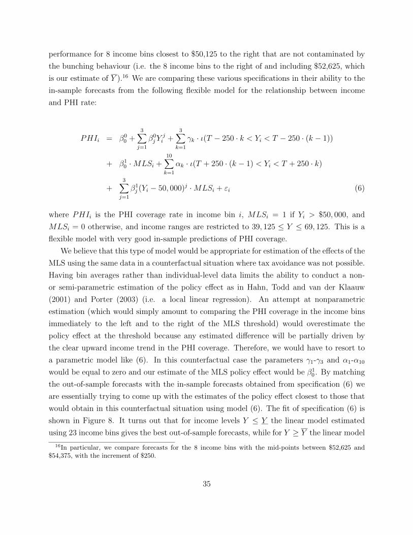
performance for 8 income bins closest to $50,125 to the right that are not contaminated by

the bunching behaviour (i.e. the 8 income bins to the right of and including $52,625, which

is our estimate of Y ).16 We are comparing these various specifications in their ability to the

in-sample forecasts from the following flexible model for the relationship between income

and PHI rate:

PHIi = β00 +

3∑j=1

β0jY

ji +

3∑k=1

γk · ι(T − 250 · k < Yi < T − 250 · (k − 1))

+ β10 ·MLSi +

10∑k=1

αk · ι(T + 250 · (k − 1) < Yi < T + 250 · k)

+3∑j=1

β1j (Yi − 50, 000)j ·MLSi + εi (6)

where PHIi is the PHI coverage rate in income bin i, MLSi = 1 if Yi > $50, 000, and

MLSi = 0 otherwise, and income ranges are restricted to 39, 125 ≤ Y ≤ 69, 125. This is a

flexible model with very good in-sample predictions of PHI coverage.

We believe that this type of model would be appropriate for estimation of the effects of the

MLS using the same data in a counterfactual situation where tax avoidance was not possible.

Having bin averages rather than individual-level data limits the ability to conduct a non-

or semi-parametric estimation of the policy effect as in Hahn, Todd and van der Klaauw

(2001) and Porter (2003) (i.e. a local linear regression). An attempt at nonparametric

estimation (which would simply amount to comparing the PHI coverage in the income bins

immediately to the left and to the right of the MLS threshold) would overestimate the

policy effect at the threshold because any estimated difference will be partially driven by

the clear upward income trend in the PHI coverage. Therefore, we would have to resort to

a parametric model like (6). In this counterfactual case the parameters γ1-γ3 and α1-α10

would be equal to zero and our estimate of the MLS policy effect would be β10 . By matching

the out-of-sample forecasts with the in-sample forecasts obtained from specification (6) we

are essentially trying to come up with the estimates of the policy effect closest to those that

would obtain in this counterfactual situation using model (6). The fit of specification (6) is

shown in Figure 8. It turns out that for income levels Y ≤ Y the linear model estimated

using 23 income bins gives the best out-of-sample forecasts, while for Y ≥ Y the linear model

16In particular, we compare forecasts for the 8 income bins with the mid-points between $52,625 and$54,375, with the increment of $250.

35

Figure 8: Fit of specification (6)

estimated using 18 income bins gives the best out-of-sample forecasts. Below we describe in

detail how these specifications were chosen.

Tables 5 and 6 detail how the out of sample forecasting performance of various models

was evaluated. Table 5 details this procedure for forecast of the PHI coverage from below

the MLS threshold, while Table 6 does it for forecasting for above the MLS threshold. In

these tables PHI denotes the in-sample prediction of PHI rate from the model in equation

(6),PHIj denotes out-of-sample forecasts of PHI rate, where j = lin for a model that

is linear in income Y , j = quad for a model quadratic in Y and j = cub for a model

cubic in Y . RMSEj is the root mean squared error computed using PHI andPHIj:

RMSEj =

√18

∑8i=1(PHI i −

PHIji)2, where the summation is taken over the 8 income bins

for which the forecasts are obtained. ˜RMSEj is the root mean squared error computed

using actual PHI rate andPHIj: ˜RMSEj =

√18

∑8i=1(PHIi −

PHIji)2.

For example, the first 8 rows of Table 5 show the performance of the linear, quadratic

and cubic in income models estimated on the sample of 46 income bins in their ability to

forecast PHI coverage in 8 income bins just to the left of and including Y . In particular, we

are forecasting for the income bins with the following mid-points: $47,375, $47,625, $47,875,

$48,125, $48,375, $48,625, $48,875, and $49,125. These income bins are listed in Table 5

in the column labeled ”income”. The 46 income bins estimation sample for obtaining the

36

4-steps ahead out-of sample forecast of PHI coverage in the income bin with the midpoint

of $47,375 starts with the bin with the midpoint of $35,125 and ends with the bin with

the midpoint of $46,375. The actual PHI coverage of the income bin with the midpoint of

$47,375 is 0.427 (column PHI), the in-sample prediction of this coverage rate obtained from

model (6) is 0.427 (column PHI), while the 4-step ahead forecasts obtained from the linear,

quadratic and cubic in income forecasting models are 0.422, 0.429 and 0.423, respectively

(columnsPHI lin,

PHIquad,

PHIcub). To obtain the 4-steps ahead out-of-sample forecast of

PHI coverage in the income bin with the midpoint of $47,625 we have to shift the 46 bin

estimation window to the right by one bin: the new estimation sample starts at $35,375 and

ends at $46,625. The estimation windows are successively shifted by one bin to the right

to obtain the out-of-sample forecasts for the remaining income bins in the column labeled

”income”. The reported RMSEj and ˜RMSEj in row 9 are taken over the 8 forecasts

reported in rows 1-8. Among the models estimated on 46 income bins the quadratic model

has the lowest RMSE of 0.0018. Similarly, the first estimation window of the estimation

sample consisting of 45 income bins which are used to obtain the PHI prediction for the

income bin with midpoint of $47,375 starts at 35,375 and ends at 46,375. The second

estimation window of the estimation sample consisting of 45 income bins which are used to

obtain the PHI prediction for the income bin with midpoint of $47,625 starts at 35,625 and

ends at 46,625, and so on. Again, the quadratic model produces the smallest RMSE among

the three competing models for the estimation sample of 45 income bins.

Figure 9 plots the RMSE computed over the predictions for 8 income bins to the left of

and including Y against the number of income bins in the estimation sample of the prediction

model, for the linear, quadratic and cubic polynomial specifications. It is easy to see that

the linear model estimated on the sample of 23 income bins results in the lowest RMSE.

For this reason we are using the estimation sample consisting of 23 income bins and a linear

model to predict the PHI rate at the absence of the MLS tax for income of $50,125.

The assessment of the goodness of the out-of-sample forecasting performance of different

specifications and sample sizes for PHI rate in the presence of the MLS tax (to the right of

the MLS threshold) is detailed in Table 6 and Figure 10. It turns out that the linear model

estimated on 37 income bins produces the lowest out-of-sample RMSE, and we adopt this

specification in section 4.3 to obtain the prediction of PHI rate in the presence of the MLS

tax and at the absence of bunching for income level of $50,125.

The sizes of the forecast errors allow us to estimate lower and upper bounds on the MLS

effect. In the interval below the threshold the largest negative and positive forecast errors

37

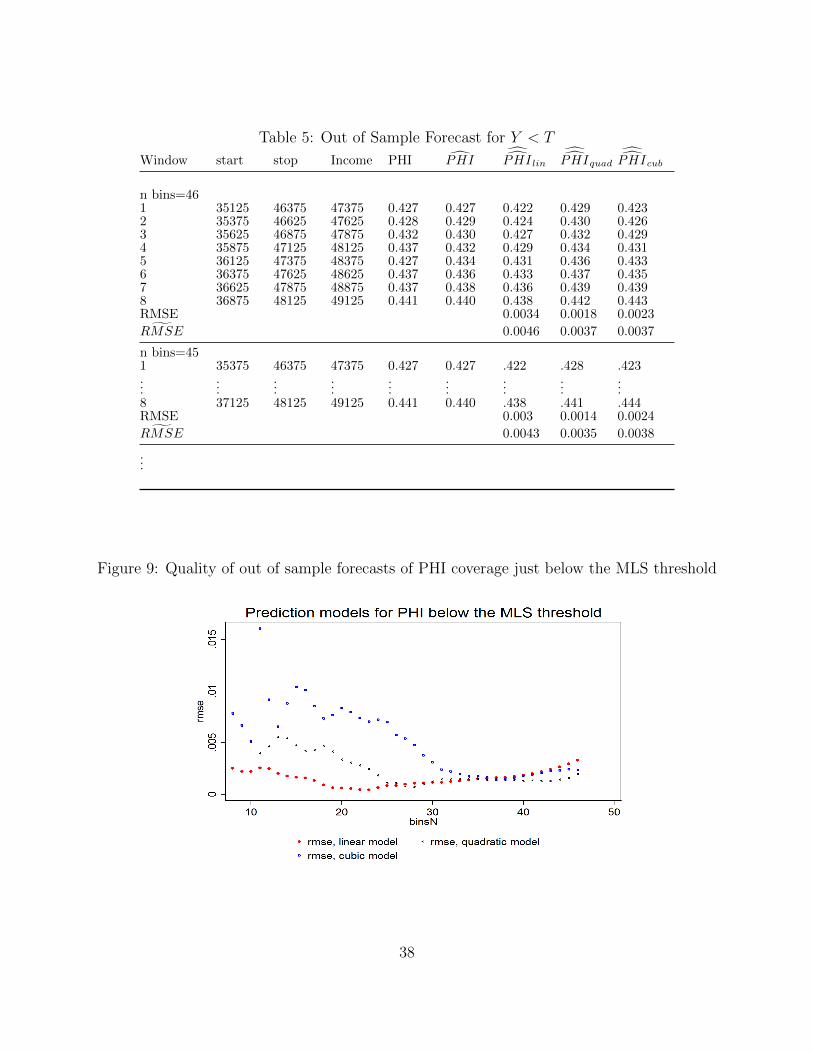
Table 5: Out of Sample Forecast for Y < T

Window start stop Income PHI PHIPHI lin

PHIquad

PHIcub

n bins=461 35125 46375 47375 0.427 0.427 0.422 0.429 0.4232 35375 46625 47625 0.428 0.429 0.424 0.430 0.4263 35625 46875 47875 0.432 0.430 0.427 0.432 0.4294 35875 47125 48125 0.437 0.432 0.429 0.434 0.4315 36125 47375 48375 0.427 0.434 0.431 0.436 0.4336 36375 47625 48625 0.437 0.436 0.433 0.437 0.4357 36625 47875 48875 0.437 0.438 0.436 0.439 0.4398 36875 48125 49125 0.441 0.440 0.438 0.442 0.443RMSE 0.0034 0.0018 0.0023˜RMSE 0.0046 0.0037 0.0037

n bins=451 35375 46375 47375 0.427 0.427 .422 .428 .423...

......

......

......

......

8 37125 48125 49125 0.441 0.440 .438 .441 .444RMSE 0.003 0.0014 0.0024˜RMSE 0.0043 0.0035 0.0038

...

Figure 9: Quality of out of sample forecasts of PHI coverage just below the MLS threshold

38

Table 6: Out of Sample Forecast for Y > T

Window start stop Income PHI PHIPHI lin

PHIquad

PHIcub

n bins=661 73125 56875 54375 0.513 0.513 0.518 0.512 0.5082 72875 56625 54125 0.510 0.511 0.516 0.510 0.5083 72625 56375 53875 0.511 0.509 0.514 0.507 0.5054 72375 56125 53625 0.505 0.507 0.511 0.504 0.5035 72125 55875 53375 0.506 0.505 0.509 0.500 0.5016 71875 55625 53125 0.498 0.503 0.506 0.497 0.4977 71625 55375 52875 0.501 0.501 0.503 0.494 0.4938 71375 55125 52625 0.497 0.499 0.500 0.491 0.490RMSE 0.0037 0.0049 0.0059˜RMSE 0.0047 0.0043 0.0052

n bins=651 72875 56875 54375 0.513 0.513 .518 512 .508...

......

......

......

......

8 71125 55125 52625 0.497 0.499 .500 .491 .490RMSE 0.0036 0.0051 0.0057˜RMSE 0.0047 0.0044 0.0050

...

Figure 10: Quality of out of sample forecasts of PHI coverage just above the MLS threshold

39

among the 8 forecasts (i.e. PHI i −PHI i, where PHI i is the in-sample forecast from the

equation 6, whilePHI i is the four steps ahead out-of-sample forecasts from the linear model

estimated on 23 income bins) were −0.0007 and 0.0008. Similarly, in the interval above

the threshold the largest negative and positive forecast errors among the 8 ten steps ahead

forecasts were −0.0009 and 0.0014. Because our prior belief based on observing the data

is that the MLS effect is relatively small, we want to obtain an upper bound of this effect

at the MLS threshold. We know that we either over or underestimate the PHI coverage at

the threshold. To obtain the upper bound on the effect we have to adjust the estimated

total population effect at the MLS threshold for singles of 2.78 percentage points so that it

reflects the most optimistic estimate. This can be done by adding the maximum by which the

coverage is likely to be overestimated from below the threshold (0.0007) and the maximum

by which the coverage is likely to be underestimated from above the threshold (0.0014) to

0.0278 to obtain the upper bound of 0.0299. Similarly, we can obtain the lower bound on

the MLS effect as 0.0278-0.0008-0.0009=0.0261.

A3. Generalized least squares

To estimate equation (2) we use a two-step feasible GLS method. In the first step we obtain

estimates of β01 , β0

2 , β11 and β1

2 as bw = (X′Ω−1X)−1X′Ω−1I, where X is the matrix of

covariates from equation (2), I is the vector of PHI rates corresponding to the income bins in

the estimation sample, and Ω is a diagonal matrix with the diagonal element ωii equal to the

inverse of the total number of individuals in the income bin i, i.e. ωii = 1Ci

. It is easy to show

that this estimate is equivalent to that of the linear probability model (LPM) obtained from

the individual-level data on PHI status and income, where all individuals in income bin i

are assigned an income level equal to the midpoint of their $250 bin. However, the variance-

covariance matrix of this weighted least squares estimator, (X′Ω−1X)−1 will underestimate

the true variance of the coefficients in the LPM model, because the dependent variable used

to obtain bw is equal to the within-bin proportion of individuals with PHI, rather than to

the actual realizations of the binary PHI status. However, the available data does allow

computation of the efficient GLS variance of the coefficients in the LPM model estimated

from individual-level data, even though actual realizations of the individual PHI status are

not known. Assuming that all individuals in the income bin i are assigned income levels

equal to the midpoint of the income bin, the efficient GLS variance of the LPM coefficients

estimated from the individual-level data is given by VGLS = (X′Ω−1X)−1. Here Ω is a

diagonal matrix with the diagonal elements ωii = Pi(1−Pi)Ci

and Pi is the probability of PHI

40

coverage of individual with income equal to the midpoint of the income bin i (see e.g.

Gujarati and Porter, p. 545). In the second step, we estimate Pi as Pi = Xbw and then

compute estimates of β01 , β0

2 , β11 and β1

2 as βGLS = (X′Ω−1X)−1X′Ω−1I after replacing Pi

with Pi in Ω. The variance-covariance matrix VGLS is computed similarly. As expected,

weighted least squares estimates bw and GLS estimates βGLS are practically identical, while

the standard errors obtained from (X′Ω−1X)−1 are about 200 times smaller than the standard

errors obtained from VGLS.

A4. Placebo analysis using 2010 data

As a robustness check we also estimated the placebo effect using the income tax returns data

for the total population from 2009-10, in which one would not expect to see a discontinuity

at the 2007-08 MLS threshold of $50,000 because the threshold has been increased to $73,000

in 2008-09. We use the same approach to selection of specification of the model to be used

to forecast PHI rate at the income of $50,125 from the left of the MLS threshold (4-steps

ahead forecast) and from the right of the threshold (10 steps ahead forecast) for 2010 data.

Interestingly, for the 2010 PHI data the quadratic model which uses 34 income bins for

Y < 50, 000 and 60 income bins for Y > 50, 000 was found to produce the best out of

sample forecasts for the sixteen income bins described above. Hence, the estimation sample

consisting of the income bins between $40,875 and $49,125 was used to obtain the 4-step

ahead forecast from below the threshold, while the estimation sample consisting of income

bins between $52,625 and $67,375 is used to obtain a 10-step ahead forecast from above.

Using this specification we find that the estimated effect of the MLS is equal to -.005 with

the standard error of .003, implying that this effect is not statistically significantly different

from zero at 5% or lower significance levels. The p-value associated with the null hypothesis

that this effect is equal to zero is 0.073. The fit of the prediction models used to estimate

the MLS effect from 2010 data is shown on Figure 11. These results suggest that using our

estimation approach we are unlikely to obtain a positive policy effect of a magnitude and

statistical significance that we obtain using the 2008 data from the data in which this effect

is not present.

41

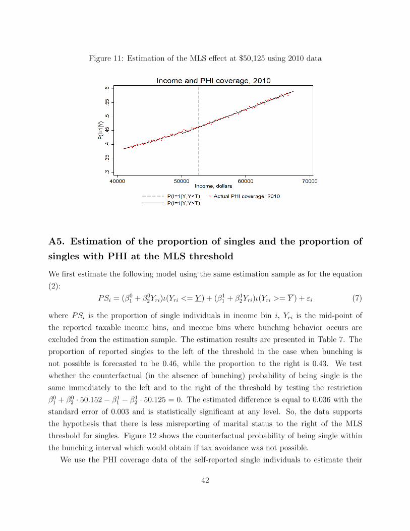
Figure 11: Estimation of the MLS effect at $50,125 using 2010 data

A5. Estimation of the proportion of singles and the proportion of

singles with PHI at the MLS threshold

We first estimate the following model using the same estimation sample as for the equation

(2):

PSi = (β01 + β0

2Yri)ι(Yri <= Y ) + (β11 + β1

2Yri)ι(Yri >= Y ) + εi (7)

where PSi is the proportion of single individuals in income bin i, Yri is the mid-point of

the reported taxable income bins, and income bins where bunching behavior occurs are

excluded from the estimation sample. The estimation results are presented in Table 7. The

proportion of reported singles to the left of the threshold in the case when bunching is

not possible is forecasted to be 0.46, while the proportion to the right is 0.43. We test

whether the counterfactual (in the absence of bunching) probability of being single is the

same immediately to the left and to the right of the threshold by testing the restriction

β01 + β0

2 · 50.152− β11 − β1

2 · 50.125 = 0. The estimated difference is equal to 0.036 with the

standard error of 0.003 and is statistically significant at any level. So, the data supports

the hypothesis that there is less misreporting of marital status to the right of the MLS

threshold for singles. Figure 12 shows the counterfactual probability of being single within

the bunching interval which would obtain if tax avoidance was not possible.

We use the PHI coverage data of the self-reported single individuals to estimate their

42

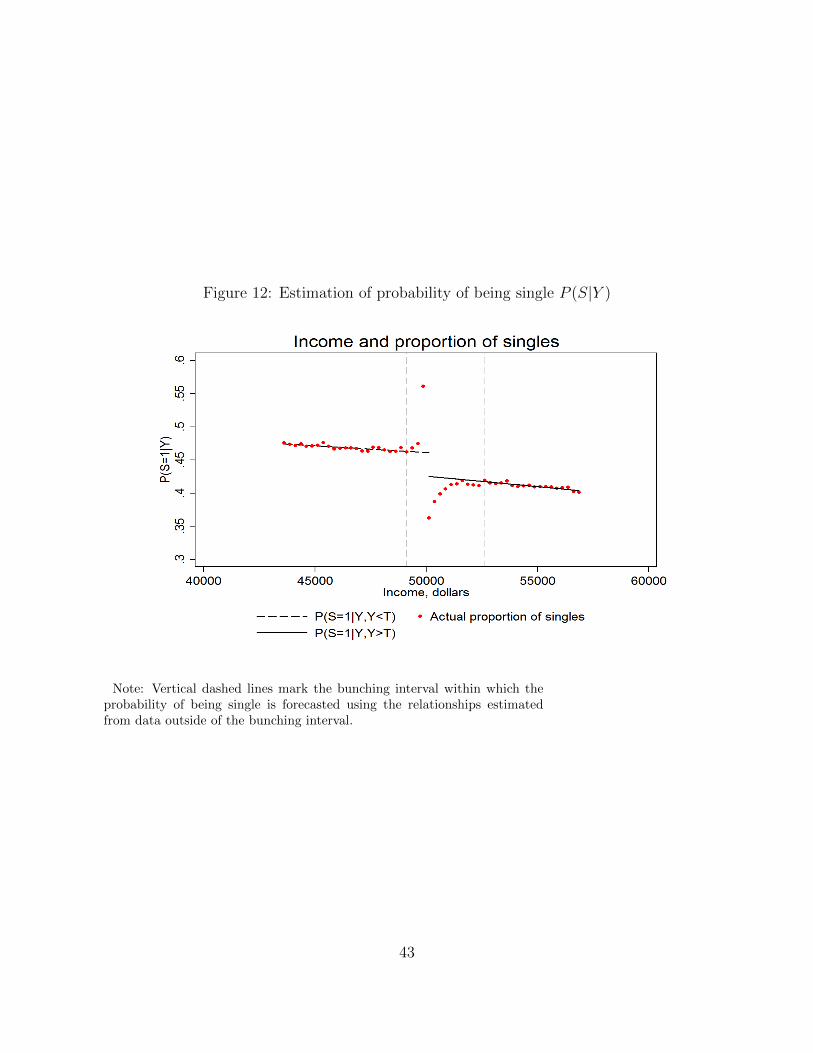
Figure 12: Estimation of probability of being single P (S|Y )

Note: Vertical dashed lines mark the bunching interval within which theprobability of being single is forecasted using the relationships estimatedfrom data outside of the bunching interval.

43

Table 7: Relationships between probability of being single, PHI coverage rate of singles, andincome

Coefficient Estimate St.err P-value

Dependent variable: Proportion of singles

β01 .5620822 .0154167 0.000β02 -.0020114 .0003326 0.000β11 .5850878 .029325 0.000β12 -.0031834 .000536 0.000

Dependent variable: Proportion of singles with PHI

β01 -.0751433 .0232281 0.000β02 .0096474 .0005015 0.000β11 -.1273144 .0461804 0.009β12 .0122267 .000844 0.000

Table 8: *Note: The dependent variables are: (i) the proportion of single indi-viduals in the reported taxable income bin with width of $250; (ii) theproportion of single individuals with PHI in the reported taxable in-come bin with width of $250;. The explanatory variable reported tax-able income Yr is measured in thousands of dollars. Estimation sampleincludes income bins between $43,625 and $49,125, and between $52,625and $56,875. Both R2’s are near unity.

PHI coverage to the right of the MLS threshold, as we believe that self-reported single status

is likely to be free of misreporting to the right of the MLS threshold for the reasons discussed

above. Using specification (7), but with the PHI rate of self-reported single individuals as a

dependent variable we find that the predicted PHI coverage of this group (in the case of no

bunching) at the income level of $50,125 is 0.486. The in- and out-of sample fit of model 2

to the PHI rate of self-reported singles is shown in Figure 13.

A6. Heterogeneity of the policy effect by age

We estimate the effect of the MLS tax on PHI coverage for the three age groups of single

individuals: ”young” (between 15 years old and 32 years old), ”middle-aged” (between 33

and 50 years old) and ”old” (older than 50 years old). To estimate the MLS effect for

each age group we use the methodology developed in section 4. In particular, for each of

the three groups we first estimate the MLS effect at the threshold for all individuals (both

married and single) which would obtain in the absence of bunching using the m-steps ahead

forecasts. The number of steps in the forecasts, the specification of the prediction model

and the estimation sample for the prediction model were chosen for each group separately.

44

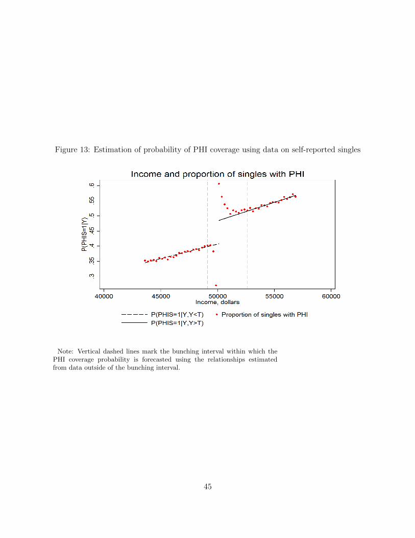
Figure 13: Estimation of probability of PHI coverage using data on self-reported singles

Note: Vertical dashed lines mark the bunching interval within which thePHI coverage probability is forecasted using the relationships estimatedfrom data outside of the bunching interval.

45

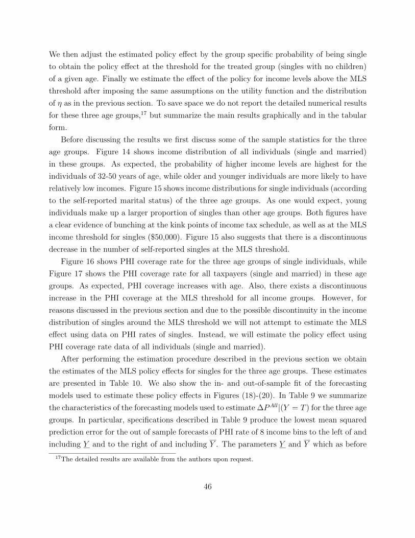
We then adjust the estimated policy effect by the group specific probability of being single

to obtain the policy effect at the threshold for the treated group (singles with no children)

of a given age. Finally we estimate the effect of the policy for income levels above the MLS

threshold after imposing the same assumptions on the utility function and the distribution

of η as in the previous section. To save space we do not report the detailed numerical results

for these three age groups,17 but summarize the main results graphically and in the tabular

form.

Before discussing the results we first discuss some of the sample statistics for the three

age groups. Figure 14 shows income distribution of all individuals (single and married)

in these groups. As expected, the probability of higher income levels are highest for the

individuals of 32-50 years of age, while older and younger individuals are more likely to have

relatively low incomes. Figure 15 shows income distributions for single individuals (according

to the self-reported marital status) of the three age groups. As one would expect, young

individuals make up a larger proportion of singles than other age groups. Both figures have

a clear evidence of bunching at the kink points of income tax schedule, as well as at the MLS

income threshold for singles ($50,000). Figure 15 also suggests that there is a discontinuous

decrease in the number of self-reported singles at the MLS threshold.

Figure 16 shows PHI coverage rate for the three age groups of single individuals, while

Figure 17 shows the PHI coverage rate for all taxpayers (single and married) in these age

groups. As expected, PHI coverage increases with age. Also, there exists a discontinuous

increase in the PHI coverage at the MLS threshold for all income groups. However, for

reasons discussed in the previous section and due to the possible discontinuity in the income

distribution of singles around the MLS threshold we will not attempt to estimate the MLS

effect using data on PHI rates of singles. Instead, we will estimate the policy effect using

PHI coverage rate data of all individuals (single and married).

After performing the estimation procedure described in the previous section we obtain

the estimates of the MLS policy effects for singles for the three age groups. These estimates

are presented in Table 10. We also show the in- and out-of-sample fit of the forecasting

models used to estimate these policy effects in Figures (18)-(20). In Table 9 we summarize

the characteristics of the forecasting models used to estimate ∆PAll|(Y = T ) for the three age

groups. In particular, specifications described in Table 9 produce the lowest mean squared

prediction error for the out of sample forecasts of PHI rate of 8 income bins to the left of and

including Y and to the right of and including Y . The parameters Y and Y which as before

17The detailed results are available from the authors upon request.

46

Figure 14: Income distribution by age group

Note: Counts of individuals in the first income bin ($0-$250) and in thelast income bin (>$100,000) are not shown on the graph.

47

Figure 15: Income distribution by age group, single individuals

Note: Counts of individuals in the first income bin ($0-$250) and in thelast income bin (>$100,000) are not shown on the graph.

48

Figure 16: PHI coverage rate by age group, singles

Note: PHI rates in the first income bin ($0-$250) and in the last incomebin (>$100,000) are not shown on the graph.

49

Figure 17: PHI coverage rate by age group, all individuals

Note: PHI rates in the first income bin ($0-$250) and in the last incomebin (>$100,000) are not shown on the graph.

50

Table 9: Characteristics of the forecasting models for the three age groups.Characteristic Young age Middle age Old age

Y 49,125 48,875 49,375Y 51,375 52,875 50,625Steps ahead from below 4 5 3Steps ahead from above 5 11 2Forecasting model from below $50,000 linear linear linearForecasting model from above $50,000 linear linear quadraticEstimation sample from below $50,000 18 bins;

44,875-49,12539 bins;39,375-48,875

22 bins;44,125-49,375

Estimation sample from above $50,000 33 bins;59,375 -51,375

41 bins;62,875 - 52,875

23 bins;56,125-50,625

Table 10: The MLS effects by age groupsYoung age Middle age Old age

1 ∆PAll|(Y = T ) 0.047 0.015 0.0352 P (S|(Y = T )) 0.63 0.31 0.383 ∆PS |(Y = T ) (1:2) 0.074 0.050 0.0924 P (PHIS = 1|Y = T, t = 0.01) 0.40 0.49 0.675 %∆PS |(Y = T ) (3:(4-3)) 22.5% 11% 15.9%

6 Total counts of singles 3,042,050 1,451,460 1,505,7257 Total counts of singles with PHI, actual 752,135 625,555 807,3658 Total counts of singles with PHI, counter-

factual704,755 581,715.1 747,129.3

9 ∆ (7-8) 47,380 43,839.88 60,235.7510 ∆, percent (9:8) 6.7% 7.5% 8.06%11 Overall PHI rate, actual (7:6) 24.7% 43% 53.6%12 Overall PHI rate, counterfactual (8:6) 23.2% 40% 49.6%

13 MLS budget revenue, millions. 133 123 6314 Number of MLS non-compliers 204,240 177,705 91,15515 Average MLS amount paid, $ 651 692 69116 Percent of MLS non-compliers 44% 30% 21%

denote the boundaries of the bunching interval around the MLS threshold were estimated

separately for each age group.

51

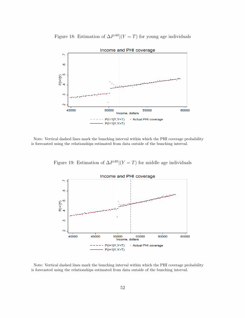
Figure 18: Estimation of ∆PAll|(Y = T ) for young age individuals

Note: Vertical dashed lines mark the bunching interval within which the PHI coverage probabilityis forecasted using the relationships estimated from data outside of the bunching interval.

Figure 19: Estimation of ∆PAll|(Y = T ) for middle age individuals

Note: Vertical dashed lines mark the bunching interval within which the PHI coverage probabilityis forecasted using the relationships estimated from data outside of the bunching interval.

52

Figure 20: Estimation of ∆PAll|(Y = T ) for old age individuals

Note: Vertical dashed lines mark the bunching interval within which the PHI coverage probabilityis forecasted using the relationships estimated from data outside of the bunching interval.

53