Grades, Course Evaluations, andAcademic Incentives

By

Matthew J. KotchenDepartment of Economics

Williams Collegemkotchen@williams.edu

and

David A. LoveDepartment of Economics

Williams Collegedlove@williams.edu

This draft: November 13, 2004

Grades, Course Evaluations, andAcademic Incentives

Abstract

We construct a model that identi�es a range of new and somewhat counterintuitive resultsabout how the incentives created by academic institutions a¤ect student and faculty be-havior. The model provides a theoretical basis for grade in�ation and demonstrates how itdiminishes student e¤ort. Comparative statics are used to analyze the e¤ects of institutionalexpectations placed on faculty. The results show that placing more emphasis on course eval-uations exacerbates the problems of grade in�ation and can even unintentionally decrease aprofessor�s teaching e¤ort. Increased emphasis on research productivity also decreases teach-ing e¤ort and provides a further incentive for grade in�ation. We �nd that many predictionsof the model are consistent with empirical trends within and between academic institutions.We then use the model to analyze how grade targets can serve as an e¤ective policy forcontrolling grade in�ation. We also discuss implications of the model for hiring, promotion,and tenure.

JEL Classi�cation Numbers: A20, A22, I20.

1 Introduction

At the end of an academic term, students �ll out course evaluations and faculty assign

grades. The proximity of these events raises the question of whether they are independent.

In particular, can professors improve evaluations with lenient grading? And if so, what are

the implications for faculty, students, and academic institutions? We argue in this paper that

the answer to the �rst question is �yes�� grades in�uence evaluations. We then construct

a theoretical model to show that this relationship not only contributes to grade in�ation; it

also leads to diminished student e¤ort and a disconnect between institutional expectations

and faculty incentives.

The perspective that grades do not bias evaluations might be overly optimistic. It views

students as dispassionate judges of teaching e¤ectiveness who refuse to reciprocate the rating

practices of the professor, whether strict or lax. Professors, in turn, are considered to be

oblivious of the potential for bias, or at least incorruptible. This point of view invites

scepticism. After all, academic promotion depends on both teaching and research, and time

is scarce. If lenient grading o¤ers a low cost means of boosting evaluations without sacri�cing

time for research, the temptation to in�ate grades is obvious.

From the students�perspective, lower grades, like higher prices, limit options. College

campuses are rife with competing activities and obligations, and students must choose among

them. While studying might improve grades, it also costs time that could be spent on

athletics, volunteer work, or socializing. When a professor makes students work harder

for the same grade, it e¤ectively taxes time spent away from coursework. This makes the

students worse o¤, and it would be surprising if they did not convey their displeasure on

course evaluations.

Academic institutions and individual departments establish the incentives for faculty by

choosing how much to emphasize teaching and research in promotion and tenure decisions.

Faculty, in turn, set incentives for students in the form of a syllabus and an approximate

grade distribution. If instructors use grades to a¤ect evaluations, the two groups of incentives

become linked, opening up the possibility for perverse responses to institutional policies. As

1

an example, suppose that a college attempts to raise its educational quality (measured by

course evaluations) without sacri�cing research. Assume further that the college succeeds.

Was there a free lunch? Not necessarily. Professors might simply have in�ated their grades,

thereby boosting evaluations without increasing teaching e¤ort. The potential for perverse

results arises because instructors have two levers to control evaluations: teaching e¤ort and

grades. When one lever is more costly� such as teaching e¤ort when research expectations

are high� the other can serve as a substitute.

Most research �nds a positive correlation between expected grades and course evaluations,

and recent studies (e.g., Johnson 2003) demonstrate that the relationship is causal; that is,

lenient grading buys higher evaluations. This empirical relationship provides the starting

point for the theoretical model that we develop in this paper. We consider a simple setup

involving a student and a professor. The student faces a tradeo¤ between time spent on

studying and time spent on other activities. The professor allocates time between teaching

preparation and research by trading o¤concern for the student�s education with institutional

expectations regarding course evaluations and research productivity.

The model is useful for identifying a range of new and somewhat counterintuitive results

about how the incentives created by academic institutions a¤ect student and faculty behav-

ior. The interaction between student and professor provides a theoretical basis for grade

in�ation and shows how a consequence is diminished student e¤ort. Comparative statics

are used to analyze the e¤ects of institutional expectations placed on faculty. The results

show that placing more emphasis on course evaluations exacerbates the problems of grade

in�ation and can even unintentionally decrease teaching e¤ort. Increased emphasis on re-

search productivity also decreases teaching e¤ort and provides a further incentive for grade

in�ation. We �nd that many predictions of the model are consistent with empirical trends

within and between academic institutions. We then use the model to analyze how grade

targets can serve as an e¤ective policy for controlling grade in�ation. Finally, we discuss

implications of the model for hiring, promotion, and tenure.

2

2 Background

In this section we review literature that provides the background for motivating the theoret-

ical model. After establishing that grade in�ation exists, we discuss why it is a concern, with

an important reason being that higher grades can reduce student incentives to learn. We

then review empirical evidence on the correlation between grades and student evaluations of

teachers (SETs). With this evidence, we conclude that some degree of causation is at play,

whereby higher grades can produce more favorable SETs.

2.1 Grade In�ation

Grade in�ation began in the 1960s and continued unabated through the 1990s. One way to

measure grade in�ation is to look at the change in the composition of grades. A study by

Levine and Cureton (1998) �nds that from 1967 to 1993, the number of A�s increased from

7 to 26 percent, while the number of C�s fell from 25 to 9 percent. Another way to measure

grade in�ation is to compare GPAs through time. In a study using the Colleges Student

Experiences Questionnaire (CSEQ), Kuh and Hu (1999) �nd that GPAs rose on average

from 3.07 in the mid-1980s to 3.34 in the mid-1990s� almost 9 percent over the decade.

Both of these studies look at a broad spectrum of academic institutions, and while nearly

all of them experienced grade in�ation, the elite institutions are in a league of their own.

Average grades at Duke, Northwestern, and the University of North Carolina, for example,

have increased an average of .18 to .24 points on a 4.0 scale per decade (Rojstaczer 2004).

Figure 1 plots average GPA over time for �ve representative institutions. With the

exception of the University of Washington, all of the schools experienced substantial grade

in�ation during the 1990s. Given that average grades cannot rise above a 4.0, it is perhaps

surprising that grade in�ation in the two schools with the highest grades proceeded at rates

equal to or faster than those of institutions with much lower grades. Perhaps this explains

why in 1999 only 9 percent of Harvard undergraduates did not graduate with Latin Honors.

It is clear that grade in�ation exists, but why does it matter? As with prices, one might

3

1950 1960 1970 1980 1990 2000 20102.2

2.4

2.6

2.8

3

3.2

3.4

3.6

3.8

Aver

age

GPA

on

a 4.

0 sc

ale

Williams College

Harvard Univ ersity

University of Washington

Univ ersity of North Carolina

Georgia Institute of Technology

Figure 1: Grade in�ation trends for selected schools

imagine that a steady growth in grades could be accommodated by simply drawing a dis-

tinction between real and nominal measures. The trouble is that, unlike prices, grades are

bounded above (e.g., a 4.0 on a 4-point scale), so grade in�ation leads to grade compression.

As grades become compressed at the upper end of the distribution, their role as a signal of

ability weakens. This a¤ects both the external signal to employers and graduate schools, as

well as the internal signal to the students themselves. When employers read an applicant�s

transcript, they must interpret whether grades re�ect genuine ability or simply grade in�a-

tion. By weakening this external signal, grade compression makes it harder to discern ability

among candidates.1

While the external signal of grades can a¤ect the matching of students with employers

and graduate schools, the internal signal can in�uence what �elds students pursue. Grades

1Chan, Hao, and Suen (2002) model grades as external signals and argue that universities can exploit thenoisiness of the signal to improve the job prospects of weaker students. They then show that this incentiveleads to grade in�ation.

4

serve as relative prices, allocating students toward their comparative advantage. As it be-

comes harder to di¤erentiate grades, the allocation of students across �elds becomes less

e¢ cient. Sabot and Wakeman-Linn (1991) study the e¤ect of grades on enrollments across

departments at Williams College. They predict that if grades in introductory courses in

Math were distributed the same as those in introductory courses in English, there would be

an 80 percent increase in the number of students taking more than one Math course.

Perhaps equally or more troubling is the e¤ect grade in�ation can have on student in-

centives to learn. During their years in college, students construct a portfolio of grades and

extracurricular accomplishments that can serve as a foundation for resumes and graduate

school applications. In addition, students just want to have fun. When grading is lax, stu-

dents have an incentive to shift their time toward extracurricular activities and leisure. This

does not, of course, imply that a reallocation away from academics is undesirable. Com-

bining academics with participation in music, sports, and volunteer work may represent an

improvement over a strictly curricular vision of college education. But whatever the optimal

mix of curricular and extracurricular activities, colleges and universities ought to be aware

that grade in�ation changes the relative costs and bene�ts that students face when deciding

how to allocate their time.

2.2 Grades and Student Evaluations of Teachers (SETs)

Grades are the means by which teachers evaluate students, but students also evaluate teach-

ers. Studies investigating the validity and biases of SETs abound in the education literature.

Here we brie�y discuss observational and experimental studies on the e¤ect of expected

grades on SETs.

The preponderance of observational studies �nds a positive correlation between grades

and student ratings.2 The mean correlation reported in the Stumpf and Freedman (1979)

survey of the literature, for example, is approximately 0.31, and almost all of the correlations

2Detailed surveys of this literature can be found in Johnson (2003), Greenwald and Gillmore (1997),Stumpf and Freedman (1979), and Feldman (1976).

5

are positive and statistically signi�cant. But this alone does not imply a causal relationship.

Many researchers accept the evidence on correlation, but are skeptical that it represents a

bias. Instead, they appeal to one of several theories positing a third intervening variable

that a¤ects the other two. These theories typically involve some variation of the teacher

e¤ectiveness theory.3

The teacher e¤ectiveness theory argues that students learn more from e¤ective teachers

and are deservedly rewarded with higher grades. In this case, good course evaluations ac-

company higher grades but do not indicate a bias. Instead, they capture exactly what they

are intended to� good teaching. In one version of this theory, an e¤ective teacher enables

students to learn material more e¢ ciently, thereby lowering the price of e¤ort. In another

variant, e¤ective teachers motivate students to work harder, and the increased student e¤ort

rationalizes the higher grades.

While the teacher e¤ectiveness theory may explain some of the correlation between grades

and SETs, it cannot explain it all. Many studies have found a positive correlation between

grades and SETs within a given college class (e.g., Gigliotti and Buchtel 1990). Since these

classes are taught by a single professor, it is not clear why students in the same class tend to

give better evaluations when they receive, or expect to receive, better grades. In addition,

Greenwald and Gillmore (1997) �nd that higher grades correlate negatively with student

workload, an observation that is incompatible with the teacher e¤ectiveness theory unless

one believes that e¤ective teachers actually reduce student e¤ort.

Experimental studies, in which professors arti�cially manipulate the grades of some por-

tion of the class, con�rm the causal relationship between expected grades and student eval-

uations.4 In the Chacko (1983) experiment, for example, two sections of the same course

taught by the same professor were graded according to di¤erent distributions. Students in

the section with more lenient grades rated the professor on average 0.6 points higher on a 7

point scale. Since the only factor that was di¤erent between the sections was the grading,

3For examples see McKeachie (1997) and Costin, Greenough, and Menges (1971).4For examples see Holmes (1972), Worthington and Wong (1979), and Chacko (1983).

6

Chacko concludes that higher grades caused higher SETs.

One of the few explanations that is consistent with the evidence above is the grade-

leniency theory, in which students reward professors who reward them with easier grades

(McKensie 1975). Despite the common sense appeal of this idea, it has fallen into disfavor

among education researchers, perhaps because of its cynical �avor. A more charitable version

of the theory invokes attribution bias� the tendency to attribute success to ourselves but

failure to others� to explain the e¤ect of expected grades on SETs.

Both the grade-leniency and attribution-bias theories receive empirical support from

Johnson�s (2003) exhaustive study of grade in�ation. Using a comprehensive data set from

Duke University SETs, Johnson controls for student grades, prior interest, instructor grading

practices, the average rating practices of each student, and a consensus variable capturing

the average rating of all students in the class. Results from random e¤ects regressions in-

dicate that the standardized relative grade is roughly half as important in determining the

SET rating as the class consensus variable. This contradicts the teacher-e¤ectiveness theory.

If the teacher-e¤ectiveness theory were right, relative grades would have only a negligible

impact because the consensus rating variable controls for the teacher�s e¤ectiveness. John-

son then conducts a second analysis where he reports the odds that a student who expects

a particular grade will rate a professor higher than a given level. He �nds that expected

grades have a substantial impact on the odds a student rates a professor �good�or better.

For example, the odds that students rate a professor as �good�or better are nearly twice as

high for those expecting an A than for those expecting a B.

The evidence clearly suggests that grades in�uence SETs. We conclude, therefore, that

it is possible for professors to improve course evaluations by assigning more lenient grades.

In the analysis that follows, this relationship plays a role in our model of the interaction

between students, professors, and academic institutions.

7

3 The Model

We consider a simple model in which a student is taking a professor�s course. We start

with the student�s problem of allocating time, and then turn to the professor�s problem

of allocating time and assigning grades. After solving the model, we consider institutional

e¤ects on student and professor behavior. The model�s setup is the simplest possible to

demonstrate the important interactions between students, professors, and institutions.

3.1 The Student

The student�s well-being depends on his grade, the quality of the professor�s instruction, and

the time he has available for other activities. Two factors a¤ect the student�s grade: the

amount of time he spends studying t, and the professor�s choice of the average grade �g for

the course. We write the student�s grade g as a function of these two arguments:

g = g (�g; t) ,

where g is strictly increasing, concave, and additively separable.

The student values time spent on other activities as well. These activities may include

other courses, athletics, or simply leisure. We denote time spent on all other activities as l.

Normalizing the time available to the student to one yields the constraint

t+ l = 1.

The student�s preferences are represented by a utility function of the form

us = us (g; l; e) ,

where e is the quality of the professor�s instruction measured in terms of preparation e¤ort.

We assume that us is strictly increasing, strictly concave, and additively separable.

8

The student�s utility maximization problem can be written as

maxtus (g (�g; t) ; 1� t; e) . (1)

Assuming an interior solution, the �rst order condition for this problem is

usggt = usl ,

where subscripts denote corresponding partial derivatives. This expression shows that the

student chooses his study time such that the marginal bene�t from increasing his grade is

equal to the marginal opportunity cost of time spent on other activities. The unique solution

to this problem can be written as a function of the professor�s choice of the average grade:5

t� = t (�g) .

How does the student�s choice of t� change with a change in �g? Applying the implicit

function theorem, we have

t��g =�usggg�ggt

usggg2t + u

sggtt + u

sll

< 0: (2)

Thus, the student�s study time is a decreasing function of the professor�s choice of the average

grade. The intuition is that a boost to the student�s grade substitutes for study time and

causes a shift toward activities other than studying. An important implication of this result,

which we revisit later, is that grade in�ation causes a reduction in the time the student

spends studying.

5The solution t� does not depend on the professor�s level of e¤ort because of the simplifying assumptionthat us is additively separable. We include e in the student�s utility function to recognize that better teachingcan increase the student�s well-being. This provides the basis for the evaluation function de�ned in equation(3).

9

3.2 The Professor

The professor�s well-being depends on her course evaluation, her research productivity, and

the education of the student. The student enters the professor�s utility function through

two channels: concern for the student�s education and concern for the student�s evaluation

of her course. The professor can in�uence the student�s education (measured in terms of

study time) with her choice of the average grade �g, as shown in (2). She also knows that her

choice of �g as well as e will a¤ect the student�s level of satisfaction and therefore her course

evaluation. We assume the student�s course evaluation is determined by the function

v = v (�g; e) , (3)

where v is strictly increasing, concave, and additively separable.6

Beyond the professor�s interaction with the student, she also cares about her research

productivity, denoted r. There is a tradeo¤, however, between the professor�s time spent on

research and time spent on course preparation. Normalizing the work time available to the

professor to one, she faces the constraint

e+ r = 1.

The professor�s preferences are represented by a utility function of the form

up = up (v; r; t;�; �) .

This function is assumed to be strictly increasing, strictly concave, and additively separable

in v, r, and t. The parameters � and � characterize the institution where the professor is

employed. Speci�cally, � is an indicator of the institution�s teaching expectations, and � is

an indicator of the institution�s research expectations.

6One possible form of the evaluation function that satis�es these properties is simply the student�s max-imized utility function.

10

We specify the relationship between the institution�s expectations and the professors

preferences as follows:

upv� > 0 and upr� > 0.

If the professor is at an institution with higher teaching expectations, her marginal utility

from the course evaluation is greater. In parallel fashion, if the professor is at an institution

with higher research expectations, her marginal utility from research productivity is greater.

Note that di¤erences in both � and � can be used to characterize institutions along two

dimensions.7 We will exploit this feature of the model after considering the professor�s

problem.8

Nesting the student�s problem within the professor�s utility maximization problem yields

max�g;e

up (v (�g; e) ; 1� e; t� (�g) ;�; �) . (4)

The �rst order conditions (assuming an interior solution) are

�g : upvv�g = �upt t��g and e : upvve = u

pr.

The �rst condition shows how the professor chooses the average grade such that the marginal

bene�t from an improved course evaluation equals the marginal cost of diminishing the

student�s incentive to work. The second condition shows how the professor chooses her level

of teaching preparation such that the marginal bene�t from an improved course evaluation

equals the marginal cost of lower research productivity. Together, the �rst order conditions

implicitly de�ne the professor�s optimal choices as a function of the institutional parameters:

�g� = �g (�; �) and e� = e (�; �) .

7This would not be possible with one parameter that solely determined the relative weighting on teachingand research.

8In section 6.3 we discuss the implications of interpreting � and � in the context of either institutionalexpectations or professorial heterogeneity.

11

With negative de�niteness of the Hessian matrix, which we assume, the solutions �g� and e�

will be unique and guaranteed to maximize (4).

4 Institutional E¤ects

How do institutional characteristics a¤ect the way the professor assigns grades? What about

the allocation of time between teaching and research? And how do academic institutions

a¤ect the way students allocate time between studying and other activities? We address

these questions in this section.9

4.1 The Professor�s Behavior

Let us �rst consider how the professor�s optimal behavior depends on institutional teaching

expectations. A change in � will a¤ect the professor�s choice of the average grade according

to@�g�

@�= upv� (u

pvvee + u

prr) > 0,

where is de�ned in the Appendix as the inverse of the determinant of the Hessian matrix.

The sign of this expression is positive since upv� > 0, both terms in the parentheses are

negative, and < 0 by negative de�niteness of the Hessian matrix. Thus, an increase

in institutional teaching expectations creates an incentive for the professor to increase the

average grade� that is, greater teaching expectations result in grade in�ation.

What about the e¤ect of changing teaching expectations on the professor�s e¤ort? Intu-

ition would suggest that the professor would spend more time preparing. While this may in

fact occur, it is interesting to note that it need not be the case. Consider the comparative

static

@e�

@�= upv�ve

�upvv�g�g + u

pttt�2�g + u

pt t��g�g

�. (5)

9While we report and discuss comparative static results in the text, the technical derivations can be foundin the Appendix.

12

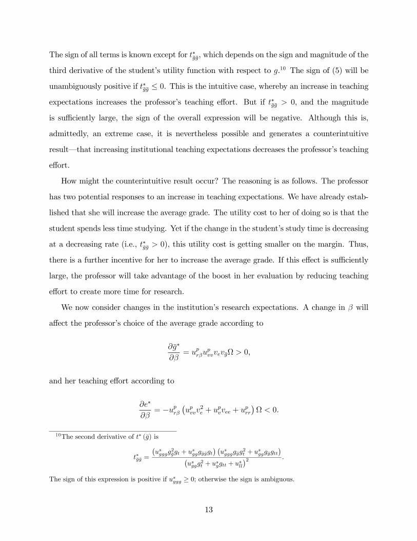
The sign of all terms is known except for t��g�g, which depends on the sign and magnitude of the

third derivative of the student�s utility function with respect to g.10 The sign of (5) will be

unambiguously positive if t��g�g � 0. This is the intuitive case, whereby an increase in teaching

expectations increases the professor�s teaching e¤ort. But if t��g�g > 0, and the magnitude

is su¢ ciently large, the sign of the overall expression will be negative. Although this is,

admittedly, an extreme case, it is nevertheless possible and generates a counterintuitive

result� that increasing institutional teaching expectations decreases the professor�s teaching

e¤ort.

How might the counterintuitive result occur? The reasoning is as follows. The professor

has two potential responses to an increase in teaching expectations. We have already estab-

lished that she will increase the average grade. The utility cost to her of doing so is that the

student spends less time studying. Yet if the change in the student�s study time is decreasing

at a decreasing rate (i.e., t��g�g > 0), this utility cost is getting smaller on the margin. Thus,

there is a further incentive for her to increase the average grade. If this e¤ect is su¢ ciently

large, the professor will take advantage of the boost in her evaluation by reducing teaching

e¤ort to create more time for research.

We now consider changes in the institution�s research expectations. A change in � will

a¤ect the professor�s choice of the average grade according to

@�g�

@�= upr�u

pvvvev�g > 0,

and her teaching e¤ort according to

@e�

@�= �upr�

�upvvv

2e + u

pvvee + u

prr

� < 0.

10The second derivative of t� (�g) is

t��g�g =

�usgggg

2�ggt + u

sggg�g�ggt

� �usgggg�gg

2t + u

sggg�ggtt

��usggg

2t + u

sggtt + u

sll

�2 .

The sign of this expression is positive if usggg � 0; otherwise the sign is ambiguous.

13

The signs of these expressions are unambiguously positive and negative, respectively. The

intuition is straightforward. In response to greater research expectations, the professor wants

to spend more time doing research. The only way she can accomplish this is by spending less

time on teaching preparation. As a result, she increases the average grade to compensate

for the negative e¤ect of diminished teaching e¤ort on her course evaluation. Note that

these results identify an additional cause of grade in�ation: holding teaching expectations

constant, institutions with greater research expectations will have both more research and

more grade in�ation.

4.2 The Student�s Behavior

We now consider how changes in an institution�s teaching and research expectations will

a¤ect the student�s behavior. Referring back to the student�s problem, we established that

the student�s choice of t� will depend on the average grade. But since the professor�s choice

of the average grade �g� will depend on the institutional parameters � and �, the student�s

choice of t� is an implicit function of these parameters as well:

t� = t (�g� (�; �)) .

We can now di¤erentiate this expression to determine how the student�s optimal study

time changes with changes in the institutional parameters. First consider a change in �:

@t�

@�= t��g�

@�g�

@�< 0. (6)

The sign of this expression is negative because the �rst term is negative and the second term

is positive. The implication is that increasing teaching expectations of an institution results

in less academic e¤ort on the part of the student. The reason is that the professor will in�ate

grades and thereby diminish the student�s incentive to work hard.

14

Table 1: Institutional e¤ects on professor and student behavior

Professor StudentAverage Teaching Study

Institutional policy grade (�g�) e¤ort (e�) time (t�)Teaching emphasis (�) + + or � �Research emphasis (�) + � �

The result of a change in � follows an identical pattern:

@t�

@�= t��g�

@�g�

@�< 0. (7)

Increasing the research expectations of an institution also results in less student e¤ort. The

reason, once again, is that the professor responds by in�ating grades, which diminishes the

student�s incentive to spend time studying.

4.3 Summary

Table 1 summarizes the comparative static results of the model. Looking at the results

for �g� and t�, we see that increasing institutional expectations will always result in more

grade in�ation and less student e¤ort. With greater teaching expectations, the professor

attempts to boost evaluations by in�ating grades. Increasing research expectations has a

similar e¤ect. The professor spends less time on teaching preparation and increases grades

in order to o¤set the consequent drop in teaching evaluations. Both changes in institutional

expectations result is grade in�ation, and the student responds by studying less and spending

more time on other activities.

A particularly counterintuitive result is that an increase in the emphasis on course eval-

uations can potentially decrease teaching e¤ort. Presumably, the primary motivation for

institutions to place greater emphasis on course evaluations is to improve teaching quality

and therefore student education. Despite this intent, our results suggest that the opposite

may occur because of the added incentive for grade in�ation.

15

5 A Simple Example

In this section we demonstrate the setup and results of the model with a simple example.

The intent is to facilitate intuition, so we have chosen functional forms to make the analysis

as straightforward as possible.

5.1 Student and Professor

The student�s utility function is given by

us (g; l; e) = ln g + ln l + ln e.

Grades are a function of the average grade for the course and student time spent studying

such that

g (�g; t) = 2�g + t� 1.

Substituting in the student�s time constraint t + l = l, solving the student�s maximization

problem, and assuming an interior solution yields the optimal time spent studying:

t� = 1� �g. (8)

The professor�s utility function is given by

up (v; r; t;�; �) = � ln v + � ln r + ln t.

Course evaluations are a function of the professor�s choice of the average grade and teaching

e¤ort such that

v (�g; e) = �g + e� 1.

Substituting in for the professor�s time constraint e+ r = 1, solving the professor�s problem,

and assuming an interior solution yields the professor�s optimal choices for the average grade

16

01

23

45

0

1

2

3

4

50

0.2

0.4

0.6

0.8

1

alphabeta

aver

age

grad

e

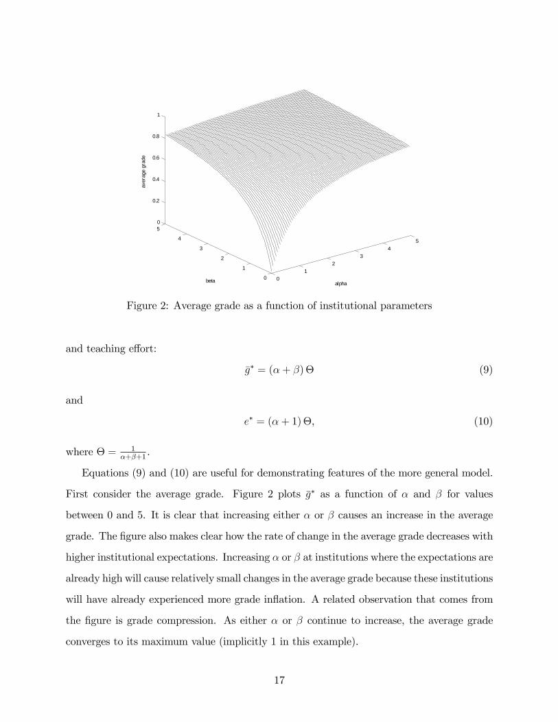
Figure 2: Average grade as a function of institutional parameters

and teaching e¤ort:

�g� = (�+ �)� (9)

and

e� = (�+ 1)�, (10)

where � = 1�+�+1

.

Equations (9) and (10) are useful for demonstrating features of the more general model.

First consider the average grade. Figure 2 plots �g� as a function of � and � for values

between 0 and 5. It is clear that increasing either � or � causes an increase in the average

grade. The �gure also makes clear how the rate of change in the average grade decreases with

higher institutional expectations. Increasing � or � at institutions where the expectations are

already high will cause relatively small changes in the average grade because these institutions

will have already experienced more grade in�ation. A related observation that comes from

the �gure is grade compression. As either � or � continue to increase, the average grade

converges to its maximum value (implicitly 1 in this example).

17

01

23

45

0

1

2

3

4

50.1

0.2

0.3

0.4

0.5

0.6

0.7

0.8

0.9

1

alphabeta

teac

hing

effo

rt

Figure 3: Teaching e¤ort as a function of institutional parameters

Figure 3 plots teaching e¤ort e� as a function of the same institutional parameters. Teach-

ing e¤ort is increasing in �, which is the intuitive case, as increasing teaching expectations

via course evaluations causes the professor to spend more time on course preparation.11 Note

that the responsiveness of e� to changes in � is greater for intermediate values of �. The

intuition follows from considering extreme values of �. When � is high, the opportunity

cost of increasing teaching e¤ort is greater because of the emphasis on research. When � is

low, teaching e¤ort is already high so there is little room to further increase e�. From the

�gure we can also see that the responsiveness to changes in � is greater for lower levels of

�. This re�ects the fact that increasing time spent on research is less costly when teaching

expectations are low.

The e¤ect of institutional expectations on student e¤ort is also straightforward to see in

11Recall that @e�

@� > 0 if t��g�g � 0. This condition is satis�ed in this example because t� is a linear function

of �g�.

18

this example. Substituting equation (9) into equation (8) yields

t� = 1� (�+ �)�.

Since �g� = (�+ �)�, the plot of t� is simply Figure 2 turned upsidedown. Student e¤ort

in decreasing in institution expectations, and the rate of the decline is greatest from start-

ing points where institutional expectations are relatively low. Moreover, as expectations

continue to increase, student e¤ort converges the minimum of spending zero time study-

ing. These relationships underscore the results in the last column of Table 2, which state

that a consequence of increasing institutional expectations is that students spend less time

studying.

6 Discussion

We now consider how predictions of the model compare with average GPAs across academic

institutions. In our discussion of the model we also consider two straightforward extensions.

The �rst examines a policy of grade targeting as a means to control in�ation. The second

explores professor heterogeneity and its implications for hiring, promotion, and tenure.

6.1 GPAs Across Institutions

All academic institutions care about teaching and research, but the values they place on

these two activities can di¤er substantially. The results of our model suggest that these

di¤erences in emphases should produce corresponding variation in grading behavior across

institutions. A casual look at the evidence con�rms the predictions of our model.

Table 2 lists selected academic institutions by their average GPAs over a three year period

from 1997 to 1999. The top schools on the list have something in common� they are elite.

Of the �rst 15, for instance, only one college did not make the top 20 in the U.S. News &

World Report rankings. These institutions are either renowned research universities, such

19

as Harvard and Stanford, or elite liberal arts colleges, such as Pomona and Williams. A

characteristic of these schools is that while they may care an extraordinary amount about

either research or teaching, they do not focus on one to the exclusion of the other. In terms

of the model, these are the schools that have either very high ��s and moderately high ��s,

or very high ��s and moderately high ��s. Since they have a high combined value of � and

�, these are exactly the type of institutions that our model predicts will have the highest

average grades.

Moving down the table, the next group of institutions is dominated by a large number

of top public research universities, such as Illinois, Wisconsin, California, North Carolina,

and Washington. These institutions produce a substantial amount of research, but arguably

place a lower value on teaching evaluations relative to the elite private universities. So even

if their ��s are high, their lower ��s should, according to the model, generate lower average

grades.12

The institutions further down the list are primarily lower-ranked public universities�

schools with comparatively lower ��s and ��s. The model predicts that these schools will

have low average grades since their opportunity cost of increasing student e¤ort is relatively

small. Universities such as Kent State, Auburn, and Alabama may produce less research

than elite public universities, but the model predicts their students will work harder for

the same grades. The Georgia Institute of Technology, a school with both a high ranking

and low average grades, appears to be an exception but is still consistent with the model.

Technical schools focus on science, where successful grant writing tends to play a signi�cant

role in promotion decisions. To the extent that grants substitute for course evaluations in

faculty promotion, these schools are likely to have lower ��s, and therefore lower grades, than

non-technical peer institutions.

12Our model does not explain why private institutions might choose higher ��s than public institutions.One possibility is that private universities tend to rely more heavily on tuition and alumni donations thanpublic universities, and, as a consequence, they may place more emphasis on course evaluations as a measureof student satisfaction.

20

Table 2: Average GPA between 1997 and 1999 for selected schools

School GPA School GPA School GPA

Brown (13) 3.47 Wisconsin (32) 3.11 UC Santa Barbara (45) 2.90

Wesleyan (9*) 3.46 U Washington (46) 3.10 Central Michigan U 2.89

Stanford (5) 3.44 Arizona (98) 3.10 Ohio U 2.89

Harvard (1) 3.40 Florida (50) 3.09 Nebraska, Kearny 2.88

Pomona (5*) 3.37 U Miami (58) 3.05 UNC Greensboro 2.85

Wheaton (51*) 3.37 Utah (111) 3.04 Colorado State (117) 2.84

Northwestern (11) 3.34 Eastern Oregon 3.04 Montana State 2.83

Princeton (1) 3.33 Southern Illinois 3.01 CSU Sacramento 2.82

Duke (5) 3.32 CSU Hayward 2.98 Georgia Tech (41) 2.82

Williams (1*) 3.32 Western Michigan 2.96 Ohio State (62) 2.81

Carleton (5*) 3.28 Minnesota (66) 2.95 Kent State 2.80

Chicago (14) 3.26 Missouri (86) 2.95 Dixie State 2.79

Harvey Mudd (16*) 3.26 CSU San Bernadino 2.94 Purdue (62) 2.77

Penn (4) 3.25 Northern Iowa 2.94 Auburn (90) 2.76

Swathmore (2*) 3.24 UC Irvine (43) 2.94 Alabama (86) 2.74

Kenyon (29*) 3.18 UNC Chapel Hill (29) 2.93 Northern Michigan 2.69

W. Washington 3.13 Texas (46) 2.93 Hampton-Sydney 2.68

U of Illinois (37) 3.12 Iowa State (84) 2.92 Houston 2.59

Notes: The institutions listed are all those for which GPA data are available from Rojstaczer(2004). Numbers in parentheses are 2005 U.S. News & World Report rankings. Asterisksindicate that rankings are for liberal arts colleges.

21

6.2 Grade Targets

One way academic institutions have attempted to deal with grade in�ation is by impos-

ing grade targets that suggest� or even require� grade distributions for individual classes.

Consider the actual policy for an institution that we leave unnamed:

In 2000, the faculty passed legislation mandating regular reporting to the faculty of themean grades in their courses. In consequence, at the end of the semester, every facultymember receives from the Registrar a grade-distribution report for each course he orshe has taught. This report places the mean grade for each course in the context of a setof suggested maximum mean grades: 100-level courses, 3.2; 200-level courses, 3.3; 300-level courses, 3.4; 400-level courses, 3.5; where A=4.0, B=3.0, C=2.0, D=1.0. Thesesuggested maximum mean grades re�ect the averages that prevailed at [institutionname] during the mid-1990s. The intent of the guidelines is to recommend upperlimits for average grades, so that faculty can aim to avoid grade in�ation in the normalcourse of their grading.

How do such grade targets a¤ect the results of the model? Assuming the policy is binding,

the professor�s choice of the average grade is constrained to equal the target. We write this

constraint as �g = �gT . Rewriting the professors problem in (4) with this constraint yields

maxeup�v��gT ; e

�; 1� e; t�

��gT�;�; �

�.

Now the the professor has lost a degree of freedom and must maximizes utility by choosing

only her level of teaching e¤ort. Assuming an interior solution, the optimal level of e¤ort

continues to satisfy the same �rst order condition, but the solution is conditional on the

grade target �gT . The professors choice of teaching e¤ort now depends on three exogenous

parameters:

e� = e��; �; �gT

�.

With this function, we can analyze the e¤ects of changing the institutional parameters

�, �, and �gT . Applying the implicit function theorem, we have the following results:

@e�

@�= upv�ve� > 0;

@e�

@�= �upr�� < 0; and

@e�

@�gT= upvvvgve� < 0,

where � = � (upvvv2e + upvvee + uprr)�1> 0. These results are all intuitive: increasing teaching

22

expectations increases teaching e¤ort; increasing research expectations increases research

and therefore decreases teaching e¤ort; and relaxing the grade-target constraint enables the

professor to in�ate grades, keep evaluations high, and spend more time on research and less

time on teaching. These results di¤er qualitatively from those we encountered previously.

The e¤ect of a change in � is now unambiguously positive; that is, with grade targets in

place, the institution can unambiguously increase the professor�s teaching e¤ort by increasing

its emphasis on course evaluations.

Grade targeting also implies di¤erent responses in the student�s behavior. The student�s

problem remains unchanged, since study time is still a function of only the average grade.

But now the average grade is set by the grade target, so t� = t��gT�. It follows that with a

grade target in place @t�

@�= @t�

@�= 0. Thus, a grade-target policy enables the institution to

a¤ect the professor�s allocation of time, without a¤ecting the student�s allocation of time. It

appears, therefore, that grade targeting can be an e¤ective policy not only because it limits

grade in�ation, but also because institutions can set expectations to improve teaching and

research productivity without the cost of diminishing student e¤ort.

6.3 Professor Heterogeneity

Thus far we have considered heterogeneity regarding institutions but not regarding profes-

sors. It is not only that institutions vary in the emphases they place on teaching and research;

the faculty across these institutions also di¤er in their preferences for teaching, research, and

student education. These di¤erences may arise through sorting during faculty recruitment

or selection during promotion. In either case, it is straightforward to reinterpret the model

to account for both institutional and professorial heterogeneity.

To accomplish this, we need only reinterpret the parameters � and � as functions

of institutional expectations and the professor�s preferences. Speci�cally, we can de�ne

� = max f�I ; �pg and � = max��I ; �p

, where parameters subscripted with I denote the

institution�s preferences and those with p denote the professor�s preferences. This formula-

tion demonstrates that if the institutional expectations exceed the professor�s preferences,

23

then the institution will in�uence behavior; otherwise, behavior is determined by the profes-

sor�s preferences alone. For example, a professor for whom �I � �p and �I � �p will feel no

external pressure to improve her course evaluation or increase her research productivity.

The speci�ed relationship between institutional expectations and faculty preferences pro-

vides two further insights of the model. The �rst relates to faculty recruitment. While

individual departments may have little in�uence on their institution�s overall expectations,

they have greater control over their hiring decisions. Accordingly, they can a¤ect teaching

and research productivity by recruiting candidates according to �p and �p. In practice, of

course, there is the problem of asymmetric information, yet the institutional expectations of

�I and �I provide insurance in the form of a lower bound for promotion and tenure.

The second insight that comes from modeling professor heterogeneity relates to the e¤ect

of promotion and tenure. To the extent that being promoted or receiving tenure makes a

professor less concerned with institutional expectations, we can think of these changes as

causing a reduction in �I , �I , or both. It follows that in the case where �I � �p and �I � �p,

promotion or tenure will have no e¤ect on the professor�s behavior, as her own expectations

are equal to or exceed those of the institution. If, however, either or both of these inequalities

do not hold� in which case � = �I , � = �I , or both� then promotion or tenure will a¤ect

behavior. While it is unclear whether we would expect better teaching or more research, it

is clear that we would expect tougher grading and more student e¤ort.

7 Conclusion

This paper set out to identify a range of new and somewhat counterintuitive results about

how the incentives created by academic institutions can a¤ect student and faculty behavior.

The model provides a theoretical basis for grade in�ation and shows how an important con-

sequence can be diminished student e¤ort. The results show that institutional emphasis on

teaching evaluations can exacerbate the problems of grade in�ation and inadvertently lower

faculty teaching e¤ort. It is also the case that increased emphasis on research productivity

24

decreases teaching e¤ort and provides a further incentive for grade in�ation. We �nd that

grade targets can be an e¤ective policy not only because they limit grade in�ation, but

also because institutions can set expectations to improve teaching and research productivity

without the cost of diminishing student e¤ort. These same objectives can be accomplished

with careful attention to hiring, promotion, and tenure decisions.

Finally, while this paper is useful for understanding behavioral responses to institutional

incentives, it is important to recognize that the normative questions remain unanswered. As

institutions change their expectations, we can use the model to predict how students and

faculty will respond. But how should institutions set their expectations? Why should some

institutions emphasize teaching while others emphasize research? How might competition

between institutions a¤ect their choice of grade targets? What, if any, are the �nancial

consequences of emphasizing one or the other? Such questions get at the important issue of

how to de�ne an institution�s objective function. While this topic is well beyond the scope

of this paper, an improved understanding of student and faculty behavior is essential for

evaluating the tradeo¤s that are inherent to the mission of all academic institutions.

25

8 Technical Appendix

In this Appendix we derive the comparative-static results for the professor�s behavior. TheHessian matrix of the professor�s utility function is written as

H =

�up�g�g up�geupe�g upee

�=

�upvvv

2�g + u

pvv�g�g + u

pttt�2�g + u

pt t��g�g upvvvev�g

upvvvev�g upvvv2e + u

pvvee + u

prr

�.

Negative de�niteness of H implies that up�g�g < 0 and detH > 0. By the concavity assump-tions, we also know that all of the other elements of H have signs that are strictly negative.Now using the general implicit function theorem, we can write the comparative-static resultsfor the professor�s problem as"

@�g�

@�@�g�

@�@e�

@�@e�

@�

#= �H�1

�upv�v�g 0upv�ve �upr�

�= �adjH

detH

�upv�v�g 0upv�ve �upr�

�= � 1

detH

�upv�

�upeev�g � u

p�geve

�upr�u

p�ge

upv��up�g�gve � upe�gv�g

��upr�u

p�g�g

�.

Now letting = � 1detH

and substituting in for the elements of H yields

@�g�

@�= upv� (u

pvvee + u

prr)

@e�

@�= upv�ve

�upvv�g�g + u

pttt�2�g + u

pt t��g�g

�

and

@�g�

@�= upr�u

pvvvev�g

@e�

@�= �upr�

�upvvv

2e + u

pvvee + u

prr

�.

26

References

Chan, W., L. Hao, and W. Suen. 2002. �Grade In�ation.�Working paper, The Universityof Hong Kong.

Chacko, T.I. 1983. �Student Ratings of Instruction: A Function of Grading Standards.�Educational Research Quarterly. Vol. 8, No. 2: pp. 19-25.

Costin, F., W.T. Greenough, and R.J. Menges. 1971. �Student Ratings of College Teaching:Reliability, Validity, and Usefulness.�Review of Educational Research. Vol. 41: pp. 511-535.

Feldman, K.A. 1976. �Grades and College Students� Evaluations of Their Courses andTeachers.�Research in Higher Education. Vol. 4: pp. 69-111.

Gigliotti, R.J. and F.S. Buchtel. 1990. �Attributional Bias and Course Evaluations.�Journalof Educational Psychology. Vol. 82: pp. 341-351.

Greenwald, A.G. and G.M. Gillmore. 1997. �Grading Leniency is a Removable Contaminantof Student Ratings.�American Psychologist. Vol. 52, No. 11: pp. 1209-1217.

Johnson, V.E. 2003. Grade In�ation: A Crisis in College Education. New York, NY:Springer-Verlag.

Holmes, D.S. 1972. �E¤ects of Grades and Discon�rmed Grade Expectancies on Students�Evaluation of Their Instructor.�Journal of Educational Psychology. Vol. 63: pp. 130-133.

Kuh, G. and S. Hu. 1999. �Unraveling the Complexity of the Increase in College Gradesfrom the Mid-1980s to the Mid-1990s.�Educational Evaluation and Policy Analysis. Vol.21, No. 3: pp. 297-320.

Levine, A. and J.S. Cureton. 1998. When Hope and Fear Collide: A Portrait of Today�sCollege Student. San Francisco, CA: Jossey-Bass.

McKeachie, W.J. 1997. �Student Ratings: Validity of Use.�American Psychologist. Vol. 52,No. 11: pp. 1218-1225.

McKenzie, R.B. 1975. �The Economic E¤ects of Grade In�ation on Instructor Evaluations:A Theoretical Approach.�The Journal of Economic Education. Vol. 6, No. 2: pp. 99-105.

Rojstaczer, S. 2004. �Grade In�ation at American Colleges and Universities.�<http://www.gradein�ation.com>.

Sabot, R. and J. Wakeman-Linn. 1991, �Grade In�ation and Course Choice.� Journal ofEconomic Perspectives. Vol. 5, No. 1: pp. 159-170.

Stumpf, S.A. and R.D. Freedman. 1979. �Expected Grade Covariation with Student Ratingsof Instruction: Individual versus Class E¤ects.�Journal of Educational Psychology. Vol.71: pp. 293-302.

27

Worthington, A.G. and P.T. Wong. 1979. �E¤ects of Earned and Assigned Grades on Stu-dent Evaluations of and Instructor.� Journal of Educational Psychology. Vol. 71: pp.764-775.

28