Incentives for Quality Through Endogenous Routing

Incentives for Quality through Endogenous RoutingLauren Xiaoyuan Lu · Jan A. Van Mieghem · R. Canan Savaskan

Kellogg School of Management, Northwestern University

August 16, 2006

Abstract

We study how rework routing together with piece rate compensation can improve incentives for

quality. When a worker generates a defect, rework is conventionally assigned to the originating

worker (in a self routing scheme) or to another worker dedicated to rework (in a dedicated

routing scheme). In contrast, a novel cross routing scheme allocates a worker’s defects to a

parallel worker performing both new jobs and rework. The worker who passes quality inspection

or completes rework receives the piece rate paid per job. We compare the incentives of these

rework allocation schemes in a principal-agent model with embedded quality control and routing

in a multi-class queueing network. We show that conventional self routing of rework can never

induce first-best effort. Dedicated routing and cross routing, however, improve incentives for

quality by imposing an implicit punishment for quality failure. In addition, cross routing leads

to workload allocation externalities and a prisoner’s dilemma between the two parallel workers,

thereby creating the highest incentives for quality. Firm profitability depends on revenues,

quality costs, and compensation costs. In general, cross routing generates the highest profit rate

when appraisal, internal failure, or external failure costs are high, while self routing performs

best when gross margins or disutilities of effort are high.

Key words: queueing networks; routing; Nash equilibrium; quality control; piece rate.

1 Introduction

This paper investigates how rework routing together with piece rate compensation can induce effort

and improve a firm’s quality and profits. It is motivated by the practice of a service operations

firm, Memphis Auto Auction, which is a wholesale automotive liquidator of used vehicles that

employs two teams of workers to clean and detail vehicles in parallel. The workers are paid piece

rate while the quality control leader is paid salary plus a bonus based on overall work quality. The

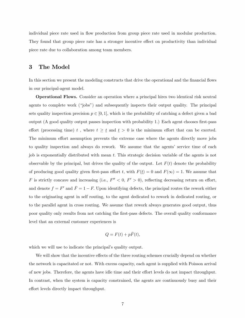
firm ties worker pay to quality through an unconventional rework routing scheme illustrated in

Figure 1C that we will call cross routing. If the vehicle passes quality inspection, the team earns

1

A: Self Routing

Agent 1

Agent 2

rework

rework

Z1

Z2

C: Cross Routing

Agent 1

λ12

Z3

Agent 2

λ21Z4

rework

rework

Z1

Z2

Agent 1

λ12

Agent 2

Z2

reworkZ1

B: Dedicated RoutingA: Self Routing

Agent 1

Agent 2

rework

rework

Z1

Z2

A: Self Routing

Agent 1

Agent 2

rework

rework

Z1

Z2

Agent 1

Agent 2

rework

rework

Z1

Z2

Z1

Z2

C: Cross Routing

Agent 1

λ12

Z3

Agent 2

λ21Z4

rework

rework

Z1

Z2

C: Cross Routing

Agent 1

λ12

Z3

Agent 2

λ21Z4

rework

rework

Z1

Z2

Agent 1

λ12

Agent 2

Z2

reworkZ1

B: Dedicated Routing

Agent 1

λ12

Agent 2

Z2Z2

reworkZ1


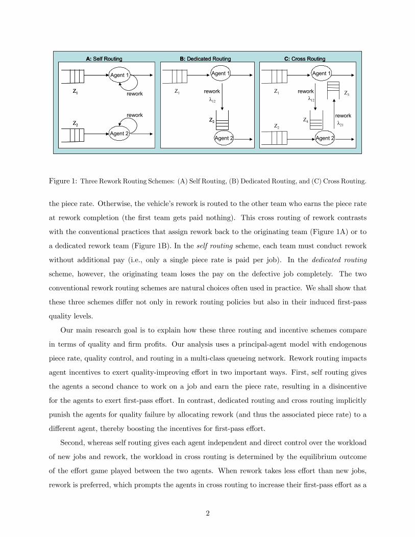
Figure 1: Three Rework Routing Schemes: (A) Self Routing, (B) Dedicated Routing, and (C) Cross Routing.

the piece rate. Otherwise, the vehicle’s rework is routed to the other team who earns the piece rate

at rework completion (the first team gets paid nothing). This cross routing of rework contrasts

with the conventional practices that assign rework back to the originating team (Figure 1A) or to

a dedicated rework team (Figure 1B). In the self routing scheme, each team must conduct rework

without additional pay (i.e., only a single piece rate is paid per job). In the dedicated routing

scheme, however, the originating team loses the pay on the defective job completely. The two

conventional rework routing schemes are natural choices often used in practice. We shall show that

these three schemes differ not only in rework routing policies but also in their induced first-pass

quality levels.

Our main research goal is to explain how these three routing and incentive schemes compare

in terms of quality and firm profits. Our analysis uses a principal-agent model with endogenous

piece rate, quality control, and routing in a multi-class queueing network. Rework routing impacts

agent incentives to exert quality-improving effort in two important ways. First, self routing gives

the agents a second chance to work on a job and earn the piece rate, resulting in a disincentive

for the agents to exert first-pass effort. In contrast, dedicated routing and cross routing implicitly

punish the agents for quality failure by allocating rework (and thus the associated piece rate) to a

different agent, thereby boosting the incentives for first-pass effort.

Second, whereas self routing gives each agent independent and direct control over the workload

of new jobs and rework, the workload in cross routing is determined by the equilibrium outcome

of the effort game played between the two agents. When rework takes less effort than new jobs,

rework is preferred, which prompts the agents in cross routing to increase their first-pass effort as a

2

result of the workload allocation externality arising in the effort game. This interesting effect stems

from the strategic interaction between the agents and the flow dynamics of the queueing network.

In a capacity constrained system, both agents are continuously busy working on either new jobs or

rework. To receive more rework, agent 1 increases first-pass effort and sends less rework to agent 2.

Keeping his effort unchanged, agent 2 automatically processes more new jobs and would send more

rework to agent 1. Suffering from reduced pay rate due to low rework inflow, agent 2 increases

first-pass effort to counteract. Consequently both agents exert high effort and receive low rework

allocation in equilibrium. This equilibrium exhibits a prisoner’s dilemma, where each agent has

an incentive to exert high effort when the other agent exerts low effort, even though both agents

would jointly benefit from an cooperative outcome of both exerting low effort. Nevertheless, the

agents are compensated with higher piece rates for their increased effort.

While higher first-pass effort produces fewer internal and external defects, it does not always

lead to higher profits for the principal. Inducing first-pass effort benefits the principal by improving

quality and reducing three of the four quality costs in Juran’s cost-of-quality framework (Juran &

Gryna (1993)): internal failure costs, external failure costs, and appraisal costs. On the other hand,

higher first-pass effort implies higher piece rate compensation and lower throughput of the system

as the agents spend more effort (processing time) per job on average. Since piece rate compensation

cost can be deemed as a form of prevention costs, our model covers all of the four dimensions of the

cost-of-quality framework. It predicts that the principal would strive for the optimal defect rate

(which has a one-to-one relationship with the induced first-pass effort) to achieve the lowest cost

by balancing the costs of non-conformance with appraisal and prevention costs. Built on this cost

minimization view of quality management, our model adds an additional dimension: throughput

and thus revenues also impact a firm’s quality control decisions. Since high effort leads to low

throughput in a capacitated system, the principal must trade-off quality with revenue.

Given that quality output and inspection are imperfect, endogenous probabilistic routing of

rework is a central feature of our model. Because the agents’ actual workload allocation of new

jobs and rework is endogenously determined by their effort, the only available tool we are aware of

to characterize the effort equilibrium arising in the flow system is queueing theory. A deterministic

model cannot capture the inherent variability and flow dynamics of the system. The endogeneity

of rework routing also has a second aspect: The principal compares the financial performance of

the three routing schemes and chooses the most profitable one.

Using an analytical model we establish the following results. Conventional self routing of rework

3

can never induce agents to exert first-best effort. Dedicated routing and cross routing, however,

offer some remedy by inducing higher effort and quality, which can lead to higher profits for the

principal. As a result, piece rates paid in these two schemes are higher. Financial performance

crucially depends on revenues, quality costs, and compensation costs. In general, cross routing of

rework generates the highest profit rate when appraisal, internal failure, or external failure costs

are high, i.e., when it is important to induce high first-pass effort. On the other hand, self routing

performs best when gross margins or agent disutilities of effort are high, i.e., when throughput is

important or labor is costly.

The remainder of the paper is organized as follows. Section 2 reviews related literature while

Section 3 lays out the main model. Sections 4 and 5 analyze the networks with excess capacity and

excess supply, respectively. In each of the two sections, we first derive the first-best benchmark

and then analyze the three rework routing schemes, and finally compare their performance. In the

rest of the paper, we will use superscripts S, D, and C to denote self, dedicated, and cross routing,

respectively. In addition, we will use superscript FB to denote the first-best solutions.

2 Related Literature

This paper contributes to three streams of literature. The first stream is the economics literature

on compensation and job design, which studies the moral hazard problem that arises when a

worker’s effort is imperfectly observed. Worker compensation is thus often based on output instead

of effort. Holmstrom & Milgrom (1991) explain the trade-offs between inducing effort towards

quantity vs. quality with a multitask principal-agent model. In their model, producing high volume

and good quality output is viewed as two dimensional tasks of a worker’s job. They argue that it

would be costly, if not impossible, to achieve good quality with piece rate compensation if quality

were poorly measured. Instead of taking a multitask approach, we manifest the intrinsic trade-off

between quantity and quality by a single dimensional decision variable, i.e., the average processing

time spent on each job. Moreover, we provide theoretical support that smart routing of rework is

capable of inducing quality-improving effort even under piece rate compensation. Lazear (2000)

provides empirical evidence that piece rate compensation significantly improves productivity. In

Lazear’s real-world example, rework is assigned to the originating worker (i.e., self routing) and

quality does not deteriorate after the firm implements piece rate compensation scheme. He argues

that workers have incentives to get it right in the first time because rework is costly. In contrast,

4

we will show that workers always exert system suboptimal quality effort in the self routing scheme.

Holmstrom & Milgrom (1991) also demonstrate that job design is an important instrument

for the control of incentives. They find that tasks should be grouped such that easily measured

tasks are assigned to one worker and hard-to-measure tasks to the other worker. Though we use a

one-dimensional principal-agent model, there are two tasks in our model that differ in their mea-

surability: first-pass work is monitored imperfectly by quality inspection while rework is assumed

to have no uncertainty in quality. Supporting Holmstrom & Milgrom (1991)’s theory that tasks

should be separated according to their measurability characteristics, we show that the dedicated

routing scheme achieves advantageous incentive power over the self routing scheme.

The second relevant stream of literature is on the economics of quality control and inspection in

a game-theoretic setting. Note that these papers consider quality-related contractual issues between

firms and are only tangentially related to our work. For example, Reynier & Tapiero (1995) study

the effect of contract parameters and warranty costs on the choice of quality by a supplier and the

quality control policy by a buyer. Baiman, Fischer & Rajan (2000) focus on how contractibility of

quality-related information impact the product quality and profits of a supplier and a buyer. Our

work studies how rework routing and costs of quality affect the workers’ choice of quality-improving

effort and the firm’s quality inspection policy.

Third, from a methodological perspective, we combine the two previous literatures on principal-

agent models and quality management with that of queueing networks. Much of agency theory seeks

contracts that maximize a principal’s objective subject to an agent’s post-contractual opportunis-

tic behavior. However, little is known about quality control policies, i.e., how precisely should

performance be measured? Queueing network models can capture system dynamics and quality

inspection levels and allow us to draw operational insights that are largely missing in the existing

agency literature. We endogenize quality control policy by allowing the principal to set the qual-

ity inspection precision level. In addition, by considering capacity-constrained systems, we allow

agents’ effort levels (i.e., processing times) to directly impact system throughput, i.e., productiv-

ity. Similar work can be found in the literature that studies the impact of decentralized decision

making on process performance in queueing systems. Seminal work by Naor (1969) studies how

pricing can achieve social optimum and prevent performance degradation as a result of customers’

self-interested behavior. Many followers (e.g., Mendelson & Whang (1990), Van Mieghem (2000),

Ha (2001), etc.) also design pricing mechanisms to achieve system optimal performance, but none

of these works model quality inspection and rework.

5

Principal-agent models in queueing systems have been explored in the operations management

literature. A sample of recent papers include Gilbert & Weng (1998), Plambeck & Zenios (2000),

Shumsky & Pinker (2003), and Gunes & Aksin (2004). Gilbert & Weng (1998) study the incentive

effects of common vs. separate queue allocation schemes on self-interested operators’ capacity

decisions in a principal-agent model. Plambeck & Zenios (2000) study incentives in a dynamic

setting where an agent’s effort influences the transition probabilities of a system. Similarly in

our model, probabilistic routing is determined by agents’ effort. But, our model captures system

dynamics resulting from the strategic interaction between agents, which is not present in Plambeck

& Zenios (2000). Our paper is closely related to Shumsky & Pinker (2003) in that the principal

designs incentives to induce effort in steady state. Our work differs from Shumsky & Pinker (2003)

in two important ways. First, we explicitly model the queueing network dynamics and also consider

the case where the system is capacity constrained. Second, the principal in our model hires two

agents whose expected utility rates are interdependent. Therefore, we need to investigate the

strategic interactions between the agents and derive the effort Nash equilibrium. Gunes & Aksin

(2004) model the interaction of market segmentation, incentives, and process performance of a

service-delivery system using a single-server queue embedded in a principal-agent framework. Out

of these papers, only Gilbert & Weng (1998) consider two servers, thus a network setting, which is

the closest to our queueing network model. The novelty of our model in terms of incorporating a

queueing system in a principal-agent framework lies in that we model two endogenous queues, i.e.,

the rework queues that are generated by the agents and the arrival rate of rework is endogenously

determined by the agents’ effort.

Examples of games in queueing systems can be found in Cachon & Harker (2002) and Parlak-

turk & Kumar (2004). Cachon & Harker (2002) investigate the competition dynamics between two

service providers in a queueing game when outsourcing is allowed. Parlakturk & Kumar (2004) pro-

pose a scheduling rule that achieves first-best system performance in the presence of self-interested

routing of customers. The queueing games in our model is distinct because the players are two

agents whose effort directly impacts the capacity and quality output of the system, which in turn

affects the principal’s profit.

In our motivating example, Memphis Auto Auction employed teams to complete jobs. In this

paper, we will treat teams as agents and ignore the team incentive issues that may arise due to

free riding and collaboration. A relevant reference for team incentives is Hamilton, Nickerson &

Owan (2003), which empirically investigates the impact of teams on productivity. They distinguish

6

individual piece rate used in flow production from group piece rate used in modular production.

They found that group piece rate has a stronger incentive effect on productivity than individual

piece rate due to collaboration among team members.

3 The Model

In this section we present the modeling constructs that drive the operational and the financial flows

in our principal-agent model.

Operational Flows. Consider an operation where a principal hires two identical risk neutral

agents to complete work (“jobs”) and subsequently inspects their output quality. The principal

sets quality inspection precision p ∈ [0, 1], which is the probability of catching a defect given a badoutput (A good quality output passes inspection with probability 1.) Each agent chooses first-pass

effort (processing time) t , where t ≥ t and t > 0 is the minimum effort that can be exerted.

The minimum effort assumption prevents the extreme case where the agents directly move jobs

to quality inspection and always do rework. We assume that the agents’ service time of each

job is exponentially distributed with mean t. This strategic decision variable of the agents is not

observable by the principal, but drives the quality of the output. Let F (t) denote the probability

of producing good quality given first-pass effort t, with F (t) = 0 and F (∞) = 1. We assume thatF is strictly concave and increasing (i.e., F 00 < 0, F 0 > 0), reflecting decreasing return on effort,

and denote f = F 0 and F̄ = 1−F. Upon identifying defects, the principal routes the rework eitherto the originating agent in self routing, to the agent dedicated to rework in dedicated routing, or

to the parallel agent in cross routing. We assume that rework always generates good output, thus

poor quality only results from not catching the first-pass defects. The overall quality conformance

level that an external customer experiences is

Q = F (t) + pF̄ (t),

which we will use to indicate the principal’s quality output.

We will show that the incentive effects of the three routing schemes crucially depend on whether

the network is capacitated or not. With excess capacity, each agent is supplied with Poisson arrival

of new jobs. Therefore, the agents have idle time and their effort levels do not impact throughput.

In contrast, when the system is capacity constrained, the agents are continuously busy and their

effort levels directly impact throughput.

7

For tractability, we assume that rework takes r units of time on average, where r is common

knowledge. Since defects have to be corrected as instructed by the principal, we assume rework

effort is observable, i.e., no moral hazard problem in rework. We argue that even if agents may

exhibit opportunistic behavior in performing rework, the effect is limited because identified defects

have to be corrected completely. We assume that rework time is exponentially distributed with

mean r. Furthermore, rework has preemptive priority over new jobs. This priority rule is adopted

because of two considerations. First, in a capacitated system, the agents can be always engaged

in new jobs. Without the priority rule, defects may never be reworked. Second, the priority rule

simplifies analytics of the model. Finally, we assume that rework takes less time than the minimum

first-pass processing time:

r ≤ t. (A1)

This assumption allows us to focus on the interesting range of parameter values that highlight the

moral hazard problem and the efficacy of “smart” rework routing in inducing effort. We will discuss

the implications of this assumption when we compare the performance of the three rework routing

schemes in Section 4.5.

Financial Flows and Incentives. Each agent earns piece rate w when completing a new

job that passes quality inspection or when completing a rework. The agents’ disutility of effort

per unit time is α. Without loss of generality, we normalize the agents’ reservation utility to be 0.

In a competitive labor market, α can also be interpreted as the outside wage rate. The principal

earns gross margin v per completed job that passes quality inspection, pays agents, and incurs

three quality costs classified as in Juran’s cost-of-quality framework: (1) an appraisal cost per

new job denoted by CA(p). We assume CA(0) = C 0A(0) = 0 and C 0A(1) = ∞, which implies thatin equilibrium the principal chooses an interior inspection policy, i.e. p ∈ (0, 1). In addition,C 0A > 0, C 00A > 0. Note that these are standard assumptions used in the quality management

literature (e.g., Baiman et al. (2000)). (2) an expected internal failure cost per new job, denoted

by CI(p, t) = pF̄ (t)cI , where cI is the cost per defect when internally detected; (3) an expected

external failure cost per new job, denoted by CE(p, t) = (1 − p)F̄ (t)cE, where cE is the cost perdefect when externally detected. (External failure costs are typically larger than internal failure

costs: cE > cI . Otherwise, the principal would have no incentives to fix defects internally.) We

assume that the principal maximizes her long-run average profit rate, denoted by V, while the

agents maximize their long-run average utility rate, denoted by U .

8

The incentive contract offered by the principal consists of two elements: the quality inspection

precision p and the piece rate w. It is worth noting that we intentionally restrict the principal’s

choice of contract to piece rate. This modeling choice is motivated by the fact that piece rate has

been empirically demonstrated effective in improving productivity. Moreover, consistent with the

personnel economics literature, piece rate is often used when productivity is important and quality

monitoring is possible. Our objective is to evaluate real-world practices that involve both piece

rate compensation and quality inspection.

4 Case I: Excess Capacity

Excess capacity implies that the principal maintains a sufficient staffing level to complete all jobs

and the agents have idle time in steady state. Hence, the throughput of the system is driven by

the exogenous market demand, which is represented by the arrival rate of jobs (denoted by 2λ).

The principal focuses on reducing internal and external failure costs through quality inspection and

inducing first-pass effort, while controlling for appraisal costs and agent compensation costs. Let

ρi denote the utilization of agent i. Throughout this section, we assume the system is stable in

steady state. The stability condition for the system is maxi∈{1,2}

ρi < 1.

4.1 The First-Best Benchmark

When effort is observable, the principal’s problem is independent of whether rework is performed

by the originating agent or a different agent. For expositional convenience, we derive the first-best

benchmark using the self routing scheme. The agents spend on average t + pF̄ (t)r time units per

job. Since the job arrival rate is λ per agent, renewal theory yields that the agents’ long-run average

utility rate is λ[w−α(t+ pF̄ (t)r)]. Though the principal hires two agents, the contracting problem

of each agent is independent and identical. The principal maximizes her long-run average profit

rate:

V FB = max0≤p≤1,w≥0,t≥t

2λ[v − w − F̄ (t)(pcI + (1− p)cE))− CA(p)],subject to λ[w − α(t+ pF̄ (t)r)] ≥ 0 (IR).

The individual rationality (IR) constraint specifies the agents’ outside option. Note that we define

only one IR constraint because it is the same for the two identical agents. Since the principal’s profit

rate is monotonically decreasing in the piece rate w, the IR constraint must bind, simplifying the

9

principal’s problem to an optimization problem of two variables: t and p. Let {tFB, pFB} denote thefirst-best solution to the above optimization problem1. Since ρi = λ(tFB+pF̄ (tFB)r), the stability

condition becomes λ < 1tFB+pF̄ (tFB)r

. For a stable system, Lemma 1 characterizes the first-best

solution (all proofs are relegated to the Appendix2).

Lemma 1 If cE > cI + αr > αf(t) , there exists an interior first-best solution {tFB, pFB}, which is

characterized by

f(tFB) =1

pFBr + 1α(p

FBcI + (1− pFB)cE), (1)

C 0A(pFB) = F̄ (tFB)(cE − cI − αr). (2)

It is simple to show that ∂2V∂t∂p < 0, i.e., t and p are strategic substitutes. Since the principal is

the Stackelberg leader and the agent earns zero utility rate in equilibrium, the principal’s objective

is identical to a central planner’s. Therefore, the first-best solution achieves the Pareto optimum

for the entire system. Moreover, the resulting first-best piece rate wFB = α(tFB + pFBF̄ (tFB)r).

4.2 Self Routing

When effort t is not observable and the rework is routed back to the originating agent, the principal’s

problem becomes

V S = max0≤p≤1,w≥0

2λ[v − w − F̄ (t)(pcI + (1− p)cE))− CA(p)],subject to λ[w − α(t+ pF̄ (t)r)] ≥ 0 (IR),

t ∈ argmaxt0≥ t

λ[w − α(t0 + pF̄ (t0)r)] (IC).

The additional incentive compatibility (IC) constraint describes the agents’ post-contractual opti-

mization behavior. Since the two agents are completely independent and symmetric, we only need

a single IR and IC constraint. Let tS denote the agents’ best response to the incentive contract

{p,w}. The first-order condition is equivalent to

f(tS) =1

pr, (3)

which can be rewritten as tS(p) = f−1( 1pr ). Hence, the stability condition becomes λ <1

tS+pF̄ (tS)r.

1We ignore the issue of uniqueness of solution as all of our subsequent results hold for any interior optimum.2Available by contacting Erica Plambeck, the Chair of 2006 MSOM Student Paper Competition.

10

Lemma 2 If tS(p) ≥ t, then tS(p) is a unique global maximum and is the agents’ best response to

the incentive contract {p,w}.

Since the agents have sufficient time to complete all jobs and always earn the piece rate of

each job, the agents’ optimal effort is not impacted by the job arrival rate λ and the piece rate w.

However, the first-pass effort increases when the principal raises the quality inspection precision or

when rework is costly to the agents.

4.3 Dedicated Routing

Under dedicated routing, rework is assigned to an agent dedicated to rework. Without loss of

generality, we assign new jobs to agent 1 and rework to agent 2. To keep the system’s supply of

jobs unchanged, agent 1 is assigned with job arrival rate 2λ. The principal maximizes her long-run

average profit rate:

V D = max0≤p≤1,w≥0

2λ[v − w − F̄ (t)(pcI + (1− p)cE))− CA(p)],subject to 2λ[(1− pF̄ (t))w − αt] ≥ 0 (IR1), 2λpF̄ (t)(w − αr) ≥ 0 (IR2)

t ∈ argmaxt0≥t

2λ[(1− pF̄ (t0))w − αt0] (IC1).

Since agent 2’s effort is fully observable as he only performs rework, only IC1 is needed. Let tD

denote agent 1’s best response to the incentive contract {p,w}. Then, tD satisfies

f(tD) =α

pw,

which can be rewritten as tD(p,w) = f−1( αpw ). Agent 1 and 2’s utilizations are ρ1 = 2λtD and

ρ2 = 2λpF̄ (tD)r, respectively. The stability condition becomes λ < min{ 1

2tD, 12pF̄ (tD)r

}.

Lemma 3 If tD(p,w) ≥ t, tD(p,w) is a unique global maximum and is agent 1’s best response to

the incentive contract {p,w}.

Now agent 1’s best response depends on both p and w. Therefore, the principal can induce

higher first-pass effort not only by increasing the quality inspection precision but also by raising

the piece rate.

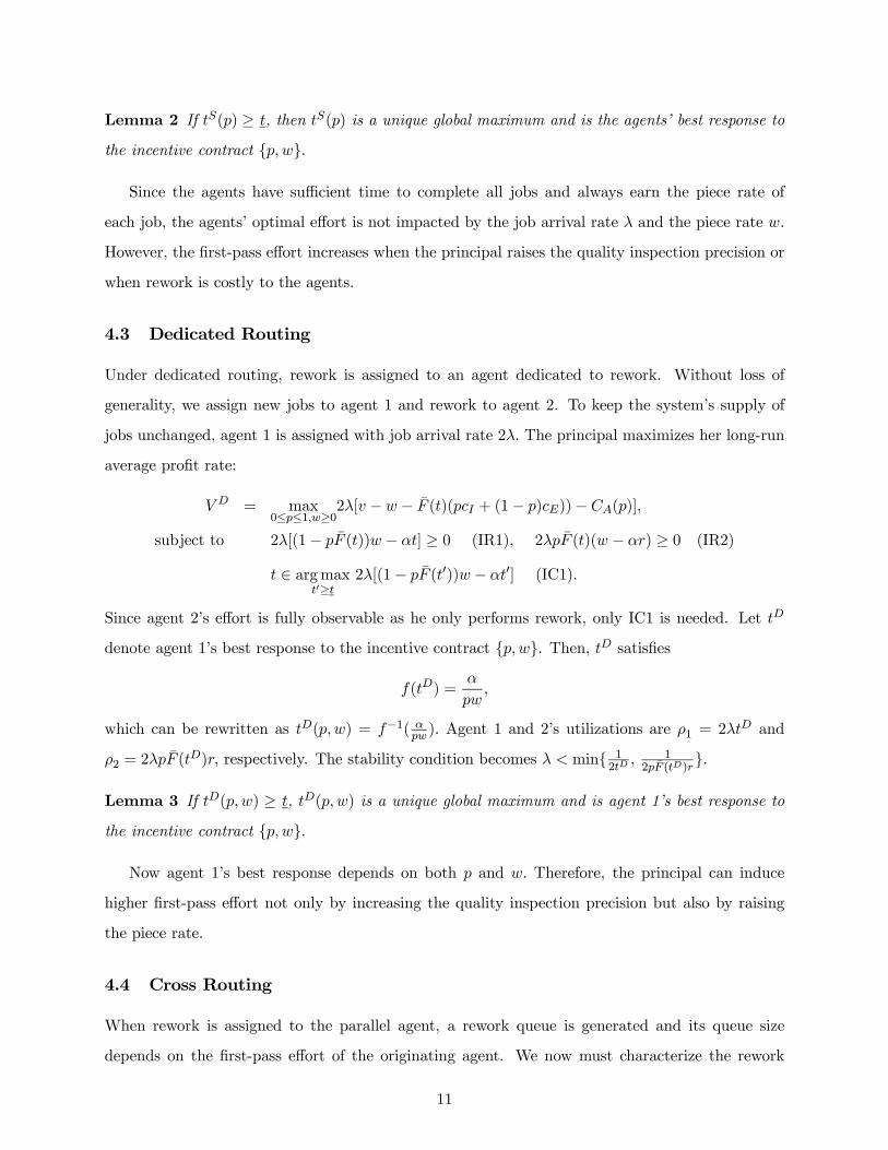
4.4 Cross Routing

When rework is assigned to the parallel agent, a rework queue is generated and its queue size

depends on the first-pass effort of the originating agent. We now must characterize the rework

11

equilibrium queues as part of the principal-agent incentive problem. For the multi-class queueing

network illustrated in Figure 1C, we define the following rates for i, j ∈ {1, 2} and i 6= j:

• Agent i0s new job service rate µni = 1ti

• Agent i0s rework service rate µri = 1r

• Agent i0s defect generation rate (or agent j0s rework arrival rate) λij = pF̄ (ti)ti

Let a four-dimensional vector (Z1, Z2, Z3, Z4) represent the state of the four queues of the system

(two new job queues and two rework queues). The detailed balance equations are too complex to be

solved analytically in closed form. Luckily, we do not need the limiting distribution of every single

state to compute the utility rate of the agents. We only need to know the aggregate probabilities

of the agents being idle π0i , working on new jobs πni , and working on rework πri . In steady state,

the queueing network must satisfy

π0i + πni + πri = 1 (Law of total probability),

λ = µni πni (Balance of agent i0s new job queue),

λjiπnj = µ

riπri (Balance of agent i0s rework queue),

for i, j ∈ {1, 2} and i 6= j. Solving the above equations yields

π0i = 1− λti − λpF̄ (tj)r, πni = λti, πri = λpF̄ (tj)r

Thus, agent i0s long-run average utility rate

Ui(ti, tj) = πni ×(1− pF̄ (ti))w − αti

ti+ πri ×

w − αr

r

= λ[(1− pF̄ (ti))w − αti] + λpF̄ (tj)(w − αr).

Notice that the first term is agent i’s average reward rate from working on new jobs, while the second

term is his average reward rate from completing rework generated by agent j. Let tCi denote agent

i0s best response. Solving the first-order condition of the agents’ problem yields that f(tCi ) =αpw .

Because f(tCi ) = f(tCj ), we drop the subscript from now on:

f(tC) =α

pw,

which can be rewritten as tC(p,w) = f−1( αpw ). Since agent i’s utilization ρi = λ(ti + pF̄ (tj)r), the

stability condition becomes λ < 1tC+pF̄ (tC)r

.

12

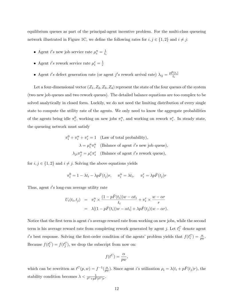
Table 1: The Agents’ Best Response Functions Assuming Constant Rework Time

Excess Capacity Capacity Constrained

Self f−1( 1pr ) f−1( 1pr )

Dedicated f−1( αpw ) f−1(1−pF̄ (t

D)ptD

)

Cross f−1( αpw ) f−1( 1−ρ(tC)2

ptC(1+ρ(tC)(1− r

tC))− F̄ (tC)

tC)

Lemma 4 If tC(p,w) ≥ t, (tC(p,w), tC(p,w)) is a unique effort equilibrium.

Surprisingly, the agents’ optimal effort in equilibrium is independent of each other’s effort and is

solely determined by the principal’s quality inspection and incentive decisions. Because the agents

have idle time in steady state, performing rework simply reduces idle time, but does not impact

their workload of new jobs. Therefore, cross routing imposes no additional effect on the agents’

incentives other than taking away the second opportunity to work on a job, which is the effect also

present in dedicated routing. As a result, the agents have the same best response function as agent

1 in dedicated routing and thus have no strategic interactions. The principal’s problem becomes

V C = max0≤p≤1,w≥0

2λ[v − w − F̄ (t)(pcI + (1− p)cE))− CA(p)],subject to λ[(1− pF̄ (t))w − αt] ≥ 0 (IR),

t = tC(p,w), t ≥ t (IC).

In the next subsection, we compare V S , V D, and V C and identify which rework routing scheme

achieves the highest profit rate.

4.5 Performance Comparison of Three Networks: Implicit Punishment

Comparing equation (1) with (3) allows us to illustrate the importance of the assumption (A1).

Notice that when r is large, the difference between f(tFB) and f(tS) becomes small and thus even

the self routing scheme performs close to first best. This supports the intuition that agents have

incentives to get it right in the first time when rework is costly. Therefore, assumption (A1) allows

us to restrict our attention to the range of parameter values where agents’ opportunistic behavior

is prominent. For a summary of the best response functions, please refer to Table 1. To facilitate

our comparison, we introduce a notation tFB (p) to represent the first-best effort at any fixed p.

Further, let w∗ = αpFBf(tFB)

, which we will show attains first best under certain conditions.

13

Proposition 1 Self routing can never implement first best. Furthermore, tS(p) < tFB(p) for all

p ∈ (0, 1). In contrast, dedicated routing implements first best with a unique contract {pFB, w∗}if and only if w∗ ≥ αtFB

1−pFBF̄ (tFB) , while cross routing implements first best with a unique contract

{pFB, w∗} if and only if w∗ ≥ α[tFB + pFBF̄ (tFB)r].

Proposition 1 reflects the weakness of the conventional self routing scheme: Because the agent

has a second chance to work on a job and earn the piece rate, he has a disincentive to exert first-pass

effort and takes his chance at quality inspection. This gaming behavior leads to a lower first-pass

quality level, incurring higher internal and external failure costs to the principal. In contrast, both

dedicated routing and cross routing can attain first best under a mild condition on w∗.

From a central planner’s point of view, dedicated routing and cross routing are superior because

the effort and quality inspection are set at the system optimal level. However, implementing

{tFB, pFB} in the dedicated and cross routing schemes does not guarantee that the IR constraintsbind, i.e. the principal may need to pay a piece rate that leaves the agents with non-zero utility3.

This implies that it may not be optimal for the principal to implement the effort-inducing contracts

specified in Proposition 1. To address this issue, next we compare the three routing schemes based

on the principal’s profit rate. To this end, we first introduce three new notations. Let w(p) be the

optimal piece rate for the principal at any fixed p. This allows us to further define t(p) := t(p,w(p))

and quality output Q(p) := Q(t(p)).

Lemma 5 For all p ∈ (0, 1), min{tC(p), tD(p)} > tS(p). Therefore, min{QC(p), QD(p)} > QS(p).

We have shown previously that dedicated routing and cross routing share the same best response

functions, which implies that the two schemes have the same incentive effects on effort. Lemma

5 further compares these two schemes with self routing in their ability to induce effort: dedicated

routing and cross routing induce higher first-pass effort than self routing at any inspection precision,

leading to a higher quality output. Dedicated routing and cross routing provide stronger incentives

for quality because assigning rework to a different agent imposes an implicit punishment on the

agents for their quality failure. This punishment is derived from the fact that in these two schemes

the agents lose the effort spent on each job that fails quality inspection.

Lemma 6 For all p ∈ (0, 1), min{wC(p), wD(p)} > wS(p).3 If an additional lump sum transfer is allowed, the principal can extract all the surplus and let the agents earn

zero utility in equilibrium.

14

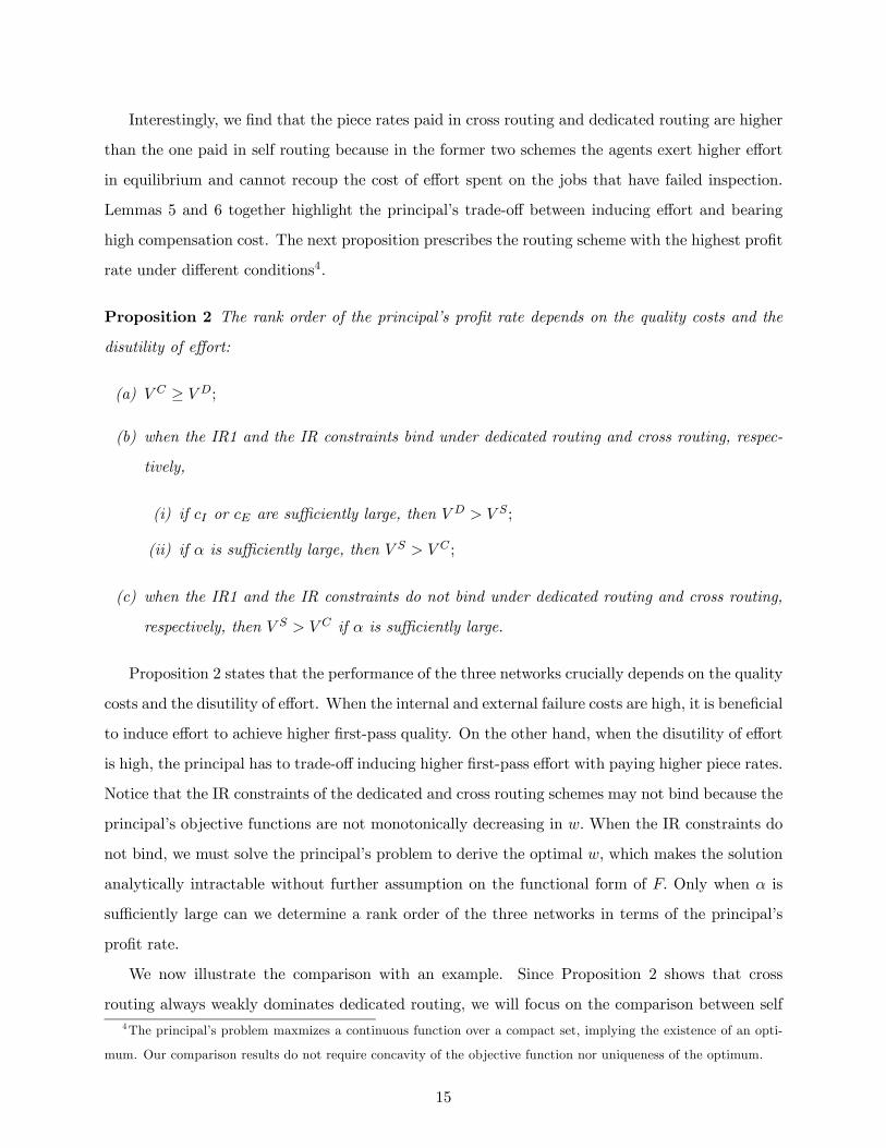
Interestingly, we find that the piece rates paid in cross routing and dedicated routing are higher

than the one paid in self routing because in the former two schemes the agents exert higher effort

in equilibrium and cannot recoup the cost of effort spent on the jobs that have failed inspection.

Lemmas 5 and 6 together highlight the principal’s trade-off between inducing effort and bearing

high compensation cost. The next proposition prescribes the routing scheme with the highest profit

rate under different conditions4.

Proposition 2 The rank order of the principal’s profit rate depends on the quality costs and the

disutility of effort:

(a) V C ≥ V D;

(b) when the IR1 and the IR constraints bind under dedicated routing and cross routing, respec-

tively,

(i) if cI or cE are sufficiently large, then V D > V S;

(ii) if α is sufficiently large, then V S > V C ;

(c) when the IR1 and the IR constraints do not bind under dedicated routing and cross routing,

respectively, then V S > V C if α is sufficiently large.

Proposition 2 states that the performance of the three networks crucially depends on the quality

costs and the disutility of effort. When the internal and external failure costs are high, it is beneficial

to induce effort to achieve higher first-pass quality. On the other hand, when the disutility of effort

is high, the principal has to trade-off inducing higher first-pass effort with paying higher piece rates.

Notice that the IR constraints of the dedicated and cross routing schemes may not bind because the

principal’s objective functions are not monotonically decreasing in w. When the IR constraints do

not bind, we must solve the principal’s problem to derive the optimal w, which makes the solution

analytically intractable without further assumption on the functional form of F. Only when α is

sufficiently large can we determine a rank order of the three networks in terms of the principal’s

profit rate.

We now illustrate the comparison with an example. Since Proposition 2 shows that cross

routing always weakly dominates dedicated routing, we will focus on the comparison between self4The principal’s problem maxmizes a continuous function over a compact set, implying the existence of an opti-

mum. Our comparison results do not require concavity of the objective function nor uniqueness of the optimum.

15

A: Agent Effort t B: Quality Inspection Precision p

C: Piece Rate w D: Principal Profit Rate V

5 10 15 201.1

1.2

1.3

1.4

1.5

1.6

cE

5 10 15 200.92

0.94

0.96

0.98

1

cE

SelfCross

SelfCross

5 10 15 201.15

1.2

1.25

1.3

1.35

cE

5 10 15 208.5

8.55

8.6

8.65

8.7

cE

SelfCross

SelfCross



5 10 15 201.1

1.2

1.3

1.4

1.5

1.6

cE

5 10 15 200.92

0.94

0.96

0.98

1

cE

SelfCross

SelfCross

5 10 15 201.1

1.2

1.3

1.4

1.5

1.6

cE

5 10 15 200.92

0.94

0.96

0.98

1

cE

SelfCross

SelfCross

5 10 15 201.15

1.2

1.25

1.3

1.35

cE

5 10 15 208.5

8.55

8.6

8.65

8.7

cE

SelfCross

SelfCross

5 10 15 201.15

1.2

1.25

1.3

1.35

cE

5 10 15 208.5

8.55

8.6

8.65

8.7

cE

SelfCross

SelfCross

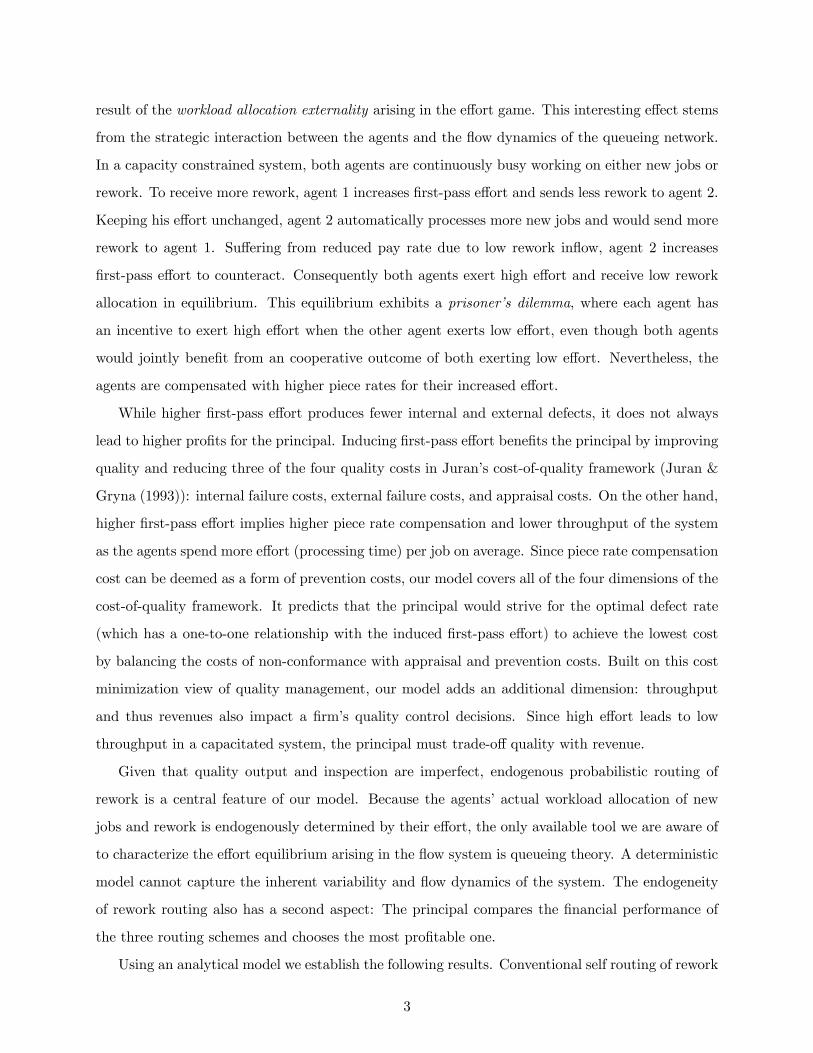
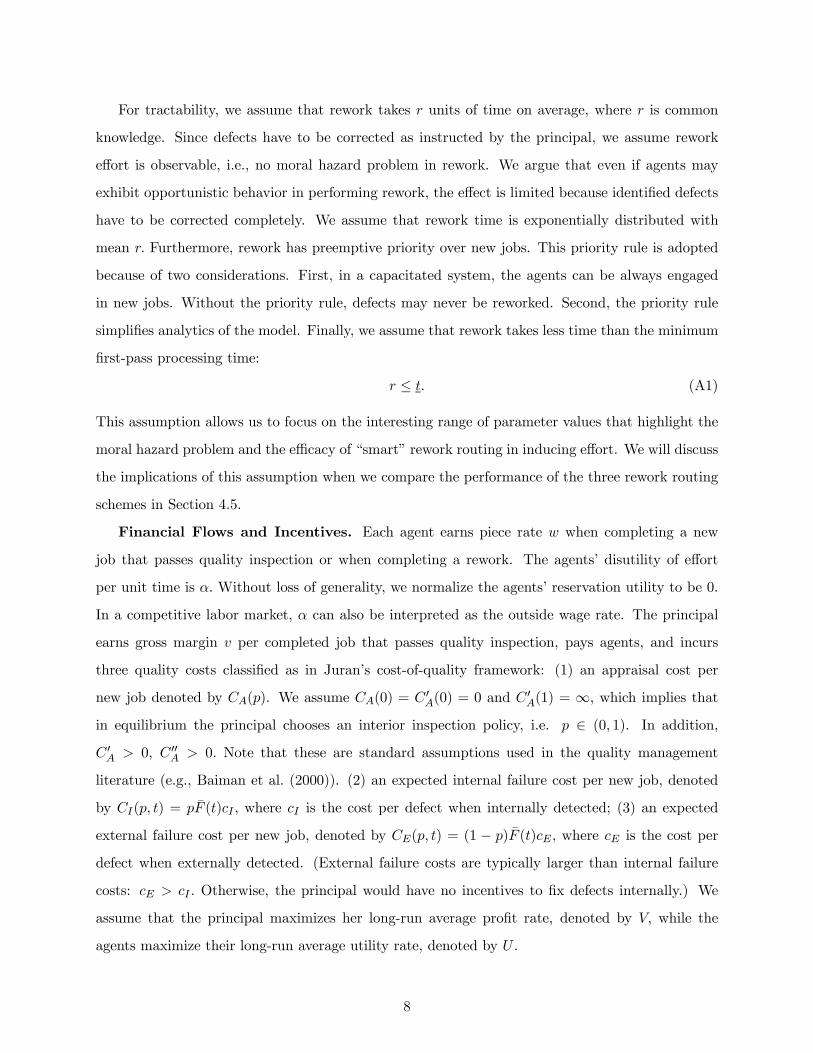
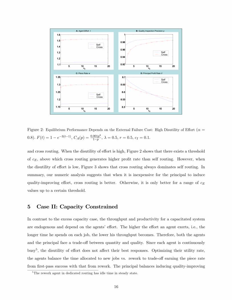
Figure 2: Equilibrium Performance Depends on the External Failure Cost: High Disutility of Effort (α =

0.8). F (t) = 1− e−3(t−1), CA(p) = 0.001p2

1−p , λ = 0.5, r = 0.5, cI = 0.1.

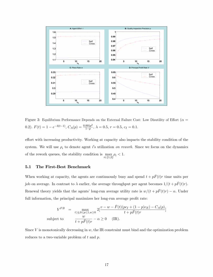
and cross routing. When the disutility of effort is high, Figure 2 shows that there exists a threshold

of cE, above which cross routing generates higher profit rate than self routing. However, when

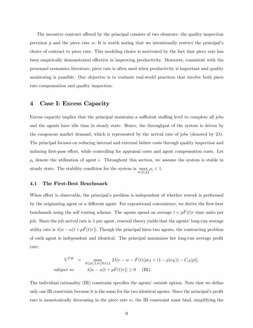
the disutility of effort is low, Figure 3 shows that cross routing always dominates self routing. In

summary, our numeric analysis suggests that when it is inexpensive for the principal to induce

quality-improving effort, cross routing is better. Otherwise, it is only better for a range of cE

values up to a certain threshold.

5 Case II: Capacity Constrained

In contrast to the excess capacity case, the throughput and productivity for a capacitated system

are endogenous and depend on the agents’ effort. The higher the effort an agent exerts, i.e., the

longer time he spends on each job, the lower his throughput becomes. Therefore, both the agents

and the principal face a trade-off between quantity and quality. Since each agent is continuously

busy5, the disutility of effort does not affect their best responses. Optimizing their utility rate,

the agents balance the time allocated to new jobs vs. rework to trade-off earning the piece rate

from first-pass success with that from rework. The principal balances inducing quality-improving5The rework agent in dedicated routing has idle time in steady state.

16



E E

5 10 15 201.1

1.2

1.3

1.4

1.5

1.6

c5 10 15 20

0.94

0.95

0.96

0.97

0.98

0.99

1

c

SelfCross

SelfCross

5 10 15 20

0.29

0.3

0.31

0.32

0.33

cE5 10 15 20

9.4

9.45

9.5

9.55

9.6

9.65

cE

SelfCross

SelfCross





E E

5 10 15 201.1

1.2

1.3

1.4

1.5

1.6

c5 10 15 20

0.94

0.95

0.96

0.97

0.98

0.99

1

c

SelfCross

SelfCross

E E

5 10 15 201.1

1.2

1.3

1.4

1.5

1.6

c5 10 15 20

0.94

0.95

0.96

0.97

0.98

0.99

1

c

SelfCross

SelfCross

5 10 15 20

0.29

0.3

0.31

0.32

0.33

cE5 10 15 20

9.4

9.45

9.5

9.55

9.6

9.65

cE

SelfCross

SelfCross

5 10 15 20

0.29

0.3

0.31

0.32

0.33

cE5 10 15 20

9.4

9.45

9.5

9.55

9.6

9.65

cE

SelfCross

SelfCross

Figure 3: Equilibrium Performance Depends on the External Failure Cost: Low Disutility of Effort (α =

0.2). F (t) = 1− e−3(t−1), CA(p) = 0.001p2

1−p , λ = 0.5, r = 0.5, cI = 0.1.

effort with increasing productivity. Working at capacity also impacts the stability condition of the

system. We will use ρi to denote agent i0s utilization on rework. Since we focus on the dynamics

of the rework queues, the stability condition is maxi∈{1,2}

ρi < 1.

5.1 The First-Best Benchmark

When working at capacity, the agents are continuously busy and spend t + pF̄ (t)r time units per

job on average. In contrast to λ earlier, the average throughput per agent becomes 1/(t+ pF̄ (t)r).

Renewal theory yields that the agents’ long-run average utility rate is w/(t + pF̄ (t)r) − α. Under

full information, the principal maximizes her long-run average profit rate:

V FB = maxt≥t,0≤p≤1,w≥0

2[v − w − F̄ (t)(pcI + (1− p)cE)−CA(p)

t+ pF̄ (t)r]

subject tow

t+ pF̄ (t)r− α ≥ 0 (IR).

Since V is monotonically decreasing in w, the IR constraint must bind and the optimization problem

reduces to a two-variable problem of t and p.

17

Lemma 7 Assume an interior first-best solution {tFB, pFB} exists. Then it must satisfy

f(tFB) =1

pFBr + 1A(tFB ,pFB)

(pFBcI + (1− pFB)cE),

C 0A(pFB) = F̄ (tFB)(cE − cI −A(tFB, pFB)r),

where A(tFB, pFB) = v−F̄ (tFB)(pFBcI+(1−pFB)cE)−CA(pFB)tFB+pFBF̄ (tFB)r

.

Notice that the first-order conditions resemble Equations 1 and 2. The only difference is that

the disutility of effort α is replaced by A(tFB, pFB).

5.2 Self Routing

When effort is not observable, the principal’s objective function becomes

V S = max0≤p≤1,w≥0

2[v − w − F̄ (t)(pcI + (1− p)cE))− CA(p)

t+ pF̄ (t)r],

subject tow

t+ pF̄ (t)r− α ≥ 0 (IR),

t ∈ argmaxt0≥t

{ w

t0 + pF̄ (t0)r− α} (IC).

The first-order condition of the agents’ problem is equivalent to f(tS) = 1pr .

Lemma 8 If tS ≥ t, then tS is a unique global maximum and is the agents’ best response to the

incentive contract {p,w}.

Notice that the agents have the same best response function as in the excess capacity case. In

both cases, the agents maximize their average payoff by minimizing the total expected time spent

on each job, i.e.,

tS = argmint0≥t

{t0 + pF̄ (t0)r}

Doing so is optimal for the agents because the piece rate of each job is a guaranteed income given

the opportunity of rework. Consequently, the agents’ optimal effort only depends on the inspection

precision p and the slope of F, thus independent of whether the agents are continuously busy or

have idle time.

18

5.3 Dedicated Routing

Without loss of generality, we assign new jobs to agent 1 and rework to agent 2. The principal

maximizes

V D = max0≤p≤1,w≥0

1

t1[v − w − F̄ (t1)(pcI + (1− p)cE))− CA(p)],

subject to(1− pF̄ (t1))w

t1− α ≥ 0 (IR1),

w

r− α ≥ 0 (IR2),

t1 ∈ argmaxt0≥t

{ (1− pF̄ (t0))w

t0− α} (IC1).

Let tD denote agent 1’s best response. The first-order condition U 01(t) = 0 is equivalent to

f(tD) =1− pF̄ (tD)

ptD.

Given agent 1’s best response, agent 2’s utilization ρ2 =pF̄ (tD)rtD

. The stability condition ρ2 < 1 is

automatically satisfied because r ≤ tD and p < 1.

Lemma 9 If tD ≥ t, then tD is a unique global maximum and is agent 1’s best response to the

incentive contract {p,w}.

Different from the excess capacity case, agent 1’s optimal effort does not depend on w. Since

agent 1 is continuously busy in the capacitated system, he does not face the trade-off between

earning piece rate and having idle time. He only cares about the expected time spent on each job,

and thus his successful throughput, represented by (1− pF̄ (t))/t.

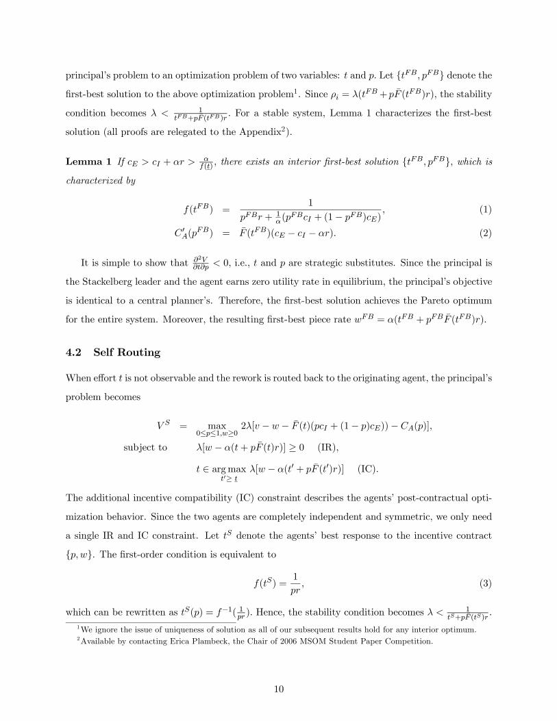
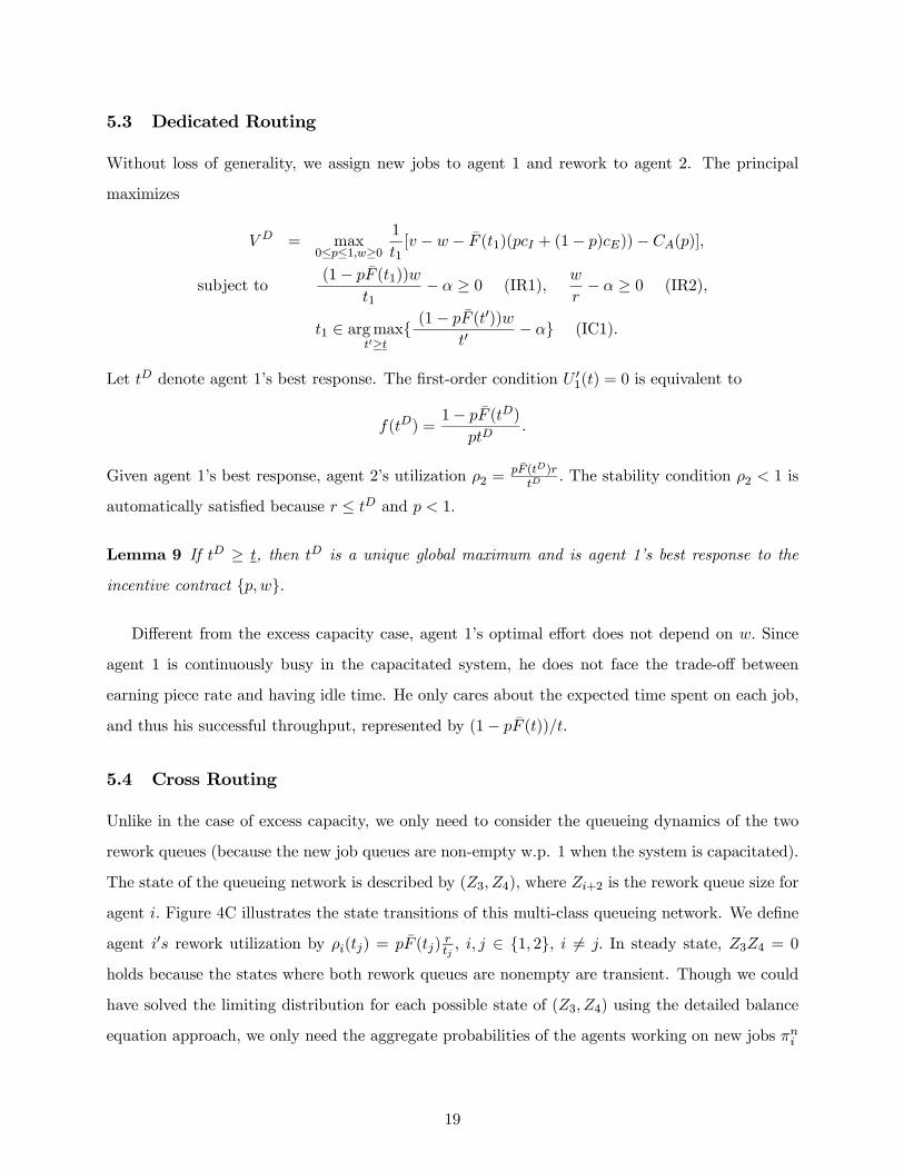
5.4 Cross Routing

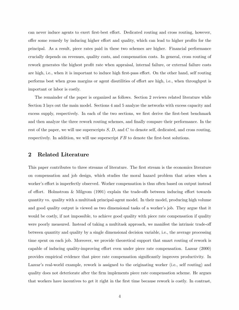
Unlike in the case of excess capacity, we only need to consider the queueing dynamics of the two

rework queues (because the new job queues are non-empty w.p. 1 when the system is capacitated).

The state of the queueing network is described by (Z3, Z4), where Zi+2 is the rework queue size for

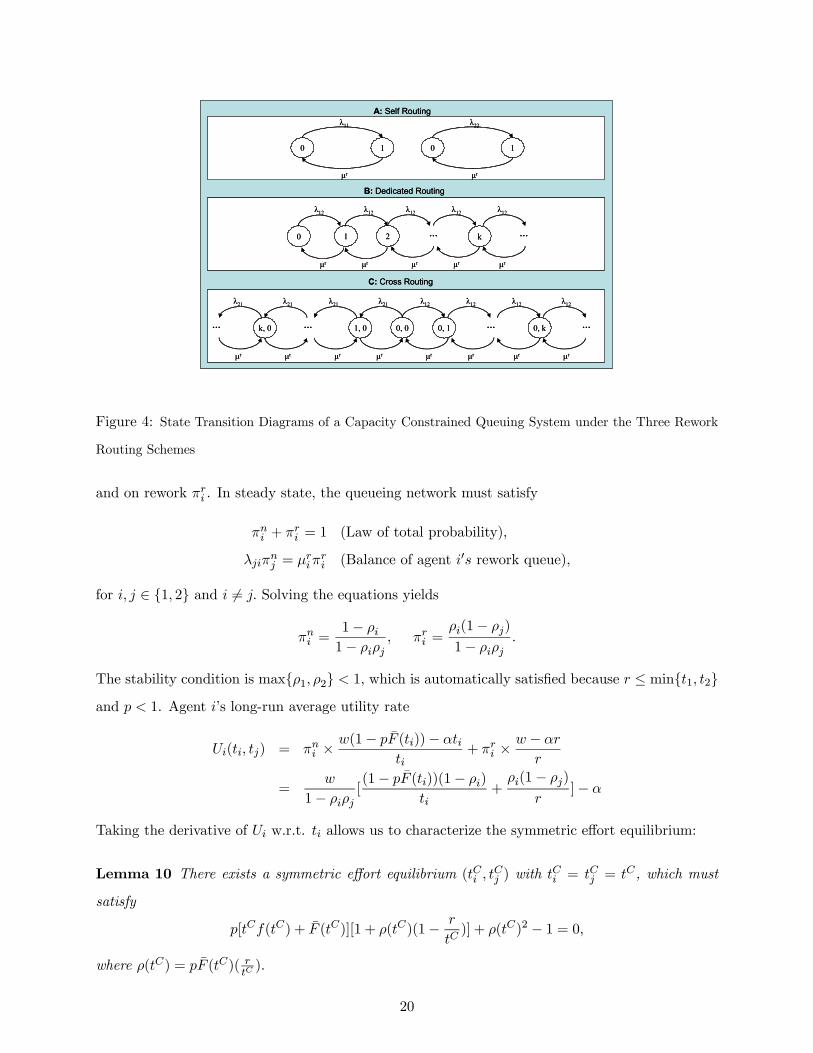
agent i. Figure 4C illustrates the state transitions of this multi-class queueing network. We define

agent i0s rework utilization by ρi(tj) = pF̄ (tj)rtj, i, j ∈ {1, 2}, i 6= j. In steady state, Z3Z4 = 0

holds because the states where both rework queues are nonempty are transient. Though we could

have solved the limiting distribution for each possible state of (Z3, Z4) using the detailed balance

equation approach, we only need the aggregate probabilities of the agents working on new jobs πni

19

1, 0 0, 0 0, 1k, 0 0, k… … … …

λ12 λ12 λ12 λ12λ21λ21λ21λ21

µr µr µr µr µr µr µr µr

C: Cross Routing


µr µr µr µr µr

1 2 k …

λ12 λ12 λ12λ12λ12

0 …

0 1

λ22

µr

A: Self Routing

0 1

λ11

µr

1, 0 0, 0 0, 1k, 0 0, k… … … …

λ12 λ12 λ12 λ12λ21λ21λ21λ21


C: Cross Routing

1, 0 0, 0 0, 1k, 0 0, k… … … …

λ12 λ12 λ12 λ12λ21λ21λ21λ21


1, 0 0, 0 0, 1k, 0 0, k… … … …

λ12 λ12 λ12 λ12λ21λ21λ21λ21


C: Cross Routing


µr µr µr µr µr

1 2 k …

λ12 λ12 λ12λ12λ12

0 …


µr µr µr µr µr

1 2 k …

λ12 λ12 λ12λ12λ12

0 …

µr µr µr µr µr

1 2 k …

λ12 λ12 λ12λ12λ12

0 …

0 1

λ22

µr

A: Self Routing

0 1

λ11

µr

0 1

λ22

µr

0 1

λ22

µr

A: Self Routing

0 1

λ11

µr

0 1

λ11

µr

Figure 4: State Transition Diagrams of a Capacity Constrained Queuing System under the Three Rework

Routing Schemes

and on rework πri . In steady state, the queueing network must satisfy

πni + πri = 1 (Law of total probability),

λjiπnj = µ

riπri (Balance of agent i0s rework queue),

for i, j ∈ {1, 2} and i 6= j. Solving the equations yields

πni =1− ρi1− ρiρj

, πri =ρi(1− ρj)

1− ρiρj.

The stability condition is max{ρ1, ρ2} < 1, which is automatically satisfied because r ≤ min{t1, t2}and p < 1. Agent i’s long-run average utility rate

Ui(ti, tj) = πni ×w(1− pF̄ (ti))− αti

ti+ πri ×

w − αr

r

=w

1− ρiρj[(1− pF̄ (ti))(1− ρi)

ti+

ρi(1− ρj)

r]− α

Taking the derivative of Ui w.r.t. ti allows us to characterize the symmetric effort equilibrium:

Lemma 10 There exists a symmetric effort equilibrium (tCi , tCj ) with t

Ci = tCj = tC, which must

satisfy

p[tCf(tC) + F̄ (tC)][1 + ρ(tC)(1− r

tC)] + ρ(tC)2 − 1 = 0,

where ρ(tC) = pF̄ (tC)( rtC).

20

Similar to dedicated routing, the equilibrium effort only depends on p. The principal’s problem

becomes

V C = maxw,0≤p≤1

2[(v − w)(1− pF̄ (t)) + F̄ (t)(pcI + (1− p)cE)−CA(p)

t+ pF̄ (t)r],

subject tow

t+ pF̄ (t)r− α ≥ 0 (IR),

t = tC(p), t ≥ t (IC).

5.5 Comparing Three Networks: Externality and Prisoner’s Dilemma

We compare the performance of the three networks. In Section 4, we have shown that dedicated

routing and cross routing impose an implicit punishment for quality failure. Here, we will highlight

two additional incentive effects of cross routing: workload allocation externalities and a prisoner’s

dilemma.

Proposition 3 The first-best solution {pFB, tFB} can never be achieved by the three rework routingschemes. Furthermore, tS(p) < tFB(p) for all p ∈ (0, 1).

The conventional self routing scheme induces lower effort than the first-best situation at any

inspection precision p. As a result, self routing can never achieve first best. Dedicated routing

and cross routing cannot attain first best either. Next we determine the performance of the three

routing schemes in terms of effort, quality, and profit rate.

Lemma 11 For all p ∈ (0, 1), tC(p) > tD(p) > tS(p) and therefore, QC(p) > QD(p) > QS(p).

Similar to the excess capacity case, self routing induces the least effort. However, cross routing

induces even higher effort than dedicated routing. Under cross routing, the two parallel agents

impact each other in two ways: they both generate and perform rework for each other. Since

rework is favorable, each agent would like the other one to send him more rework. Because rework

has priority, agent i has an incentive to pass less rework to agent j so that agent j has more time

to work on new jobs and pass more rework back to agent i.

Externality. The strategic interaction in the effort game results in workload allocation exter-

nalities between the agents. Whenever agent i increases effort, he not only improves his first-pass

success probability, but also forces agent j to spend more time on new jobs and thus generate more

rework for agent i, keeping agent j0s effort unchanged. Analytically,

∂πnj∂ti

= − 1− ρi(1− ρiρj)

2

∂ρj∂ti

> 0,∂πri∂ti

= − ρi(1− ρi)

(1− ρiρj)2

∂ρj∂ti

> 0.

21

∂πnj /∂ti > 0 illustrates the workload externality imposed on agent j when agent i increases his first-

pass effort. Since πri is the fraction of time agent i spends on rework in steady state, ∂πri /∂ti > 0

implies that agent i has more rework allocation when he increases his first-pass effort. For the

same reason, agent j increases his first-pass effort to respond to agent i0s action. In the effort

Nash equilibrium, both agents exert higher first-pass effort than in the dedicated routing scheme,

resulting in a lower defect rate. Therefore, the workload allocation externalities in the effort game

give cross routing superiority in inducing quality-improving effort.

Lemma 12 For all p ∈ (0, 1), min{wC(p), wD(p)} > wS(p).

Lemma 12 states that the principal pays a higher piece rate to compensate for the higher effort

that agents exert in cross routing and dedicated routing. More interestingly, using this piece rate

ranking, we can show that the effort equilibrium arising in the cross routing scheme exhibits a

prisoner’s dilemma.

Prisoner’s Dilemma. Notice that cooperative agents would exert tS because it minimizes

the total expected time spent on each job. This cooperative outcome gives agents strictly positive

utility rate because wC(p) > wS(p), thus a better outcome for both agents than the equilibrium

outcome that renders zero utility rate for both agents. Since f(tS) = 1/pr,

∂Ui(ti, tS)

∂ti|ti=tS =

w(1− ρ(tS))

[(1− ρ(tS)2)tS ]2[p(tSf(tS) + F̄ (tS))(1 + ρ(tS)(1− r

tS)) + ρ(tS)2 − 1]

=w(1− ρ(tS))

[(1− ρ(tS)2)tS ]2[tS

r(1 + ρ(tS))(1 + ρ(tS)(1− r

tS)) + ρ(tS)2 − 1]

> 0.

The last inequality follows from the fact that ρ(tS) < 1 and r ≤ tS . Therefore, agent i has an

incentive to unilaterally deviate from the cooperative outcome. (Section 6.2 elaborates on this

strategic behavior and discusses incentives for collusion.) This prisoner’s dilemma works in favor

of the principal because it induces higher first-pass effort and thus leads to higher quality output.

We now compare the principal’s profit rate in cross routing and self routing6.

6We shall not compare the profit rate of dedicated routing to the other two schemes because it has lower utilization

of agent 2 by design. Notice that in dedicated routing, agent 2 is not continuously busy because the rework queue

generated by agent 1 has positive probability of being empty under the stability condition of the system. In contrast,

both agents are fully utilized in the other two schemes. This renders dedicated routing incomparable with the other

two schemes.

22



0.05 0.1 0.15 0.21

1.1

1.2

1.3

1.4

1.5

cA

0.05 0.1 0.15 0.2

0.65 0.7

0.75 0.8

0.85 0.9

0.95

cA

SelfCross

SelfCross

A

0.05 0.1 0.15 0.20.7

0.72

0.74

0.76

0.78

0.8

c0.05 0.1 0.15 0.2

9.5

10

10.5

11

11.5

12

cA

SelfCross

SelfCross





0.05 0.1 0.15 0.21

1.1

1.2

1.3

1.4

1.5

cA

0.05 0.1 0.15 0.2

0.65 0.7

0.75 0.8

0.85 0.9

0.95

cA

SelfCross

SelfCross

0.05 0.1 0.15 0.21

1.1

1.2

1.3

1.4

1.5

cA

0.05 0.1 0.15 0.2

0.65 0.7

0.75 0.8

0.85 0.9

0.95

cA

SelfCross

SelfCross

A

0.05 0.1 0.15 0.20.7

0.72

0.74

0.76

0.78

0.8

c0.05 0.1 0.15 0.2

9.5

10

10.5

11

11.5

12

cA

SelfCross

SelfCross

A

0.05 0.1 0.15 0.20.7

0.72

0.74

0.76

0.78

0.8

c0.05 0.1 0.15 0.2

9.5

10

10.5

11

11.5

12

cA

SelfCross

SelfCross

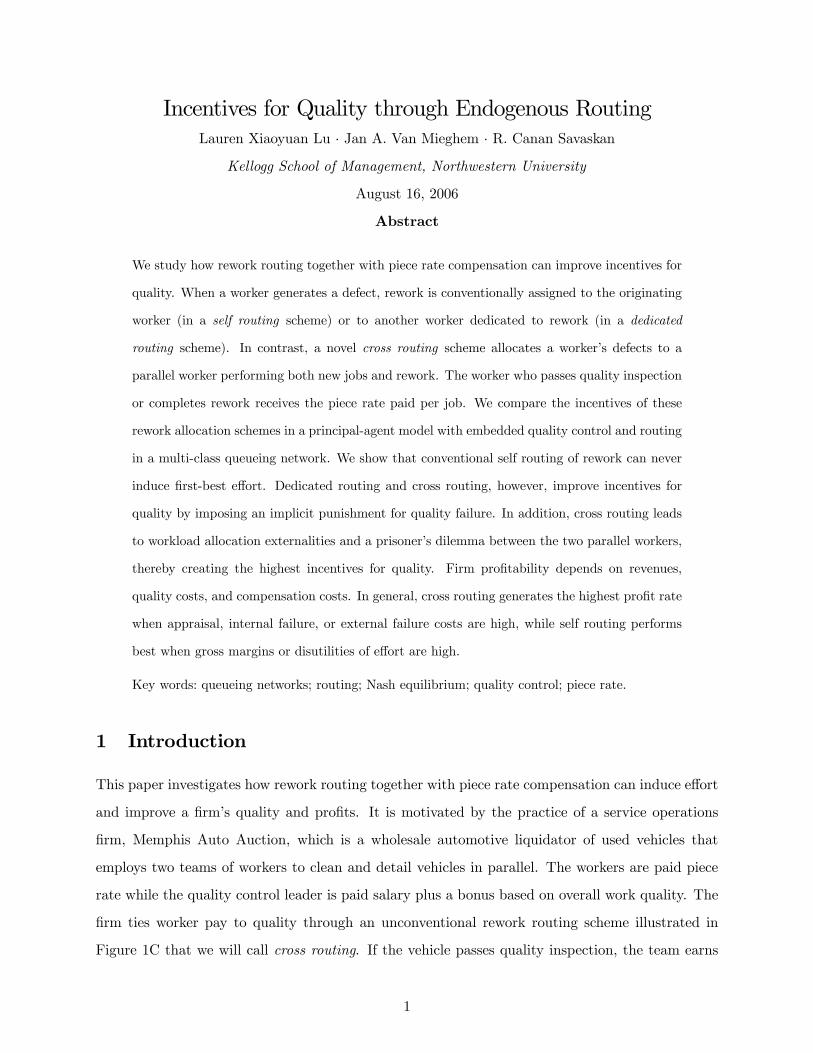
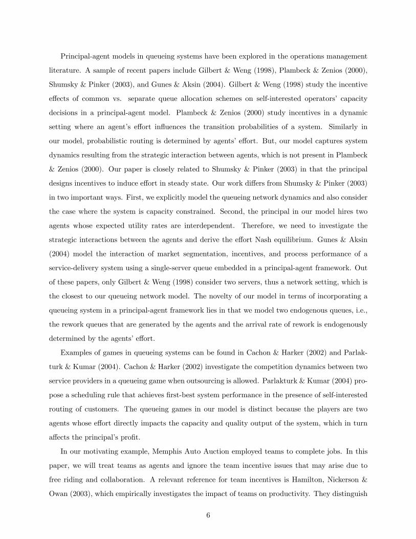
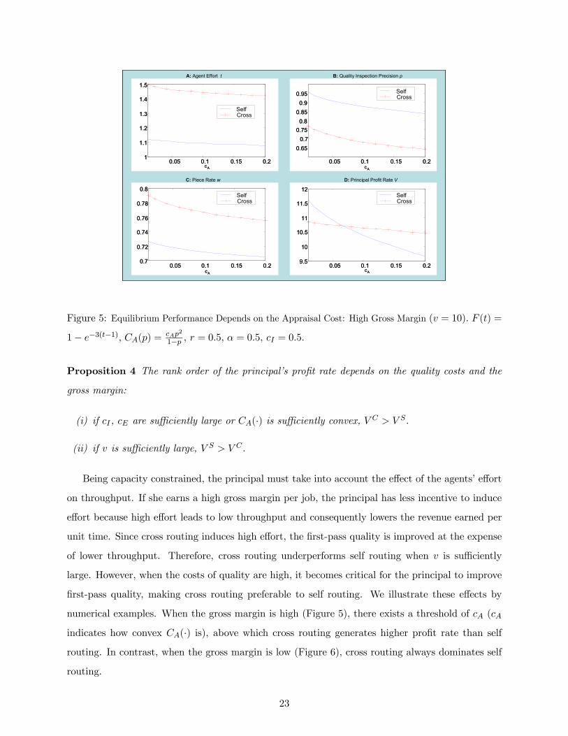
Figure 5: Equilibrium Performance Depends on the Appraisal Cost: High Gross Margin (v = 10). F (t) =

1− e−3(t−1), CA(p) = cAp2

1−p , r = 0.5, α = 0.5, cI = 0.5.

Proposition 4 The rank order of the principal’s profit rate depends on the quality costs and the

gross margin:

(i) if cI , cE are sufficiently large or CA(·) is sufficiently convex, V C > V S .

(ii) if v is sufficiently large, V S > V C .

Being capacity constrained, the principal must take into account the effect of the agents’ effort

on throughput. If she earns a high gross margin per job, the principal has less incentive to induce

effort because high effort leads to low throughput and consequently lowers the revenue earned per

unit time. Since cross routing induces high effort, the first-pass quality is improved at the expense

of lower throughput. Therefore, cross routing underperforms self routing when v is sufficiently

large. However, when the costs of quality are high, it becomes critical for the principal to improve

first-pass quality, making cross routing preferable to self routing. We illustrate these effects by

numerical examples. When the gross margin is high (Figure 5), there exists a threshold of cA (cA

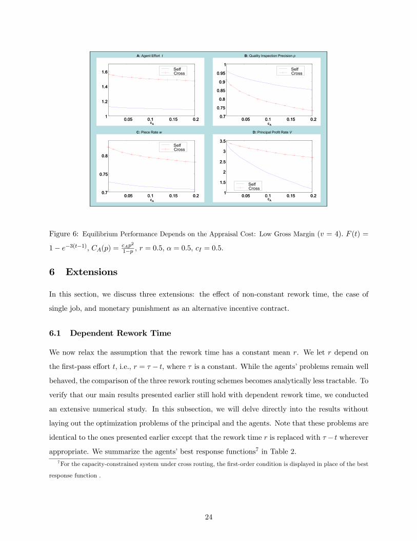
indicates how convex CA(·) is), above which cross routing generates higher profit rate than selfrouting. In contrast, when the gross margin is low (Figure 6), cross routing always dominates self

routing.

23



0.05 0.1 0.15 0.21

1.2

1.4

1.6

cA0.05 0.1 0.15 0.2

0.7

0.75

0.8

0.85

0.9

0.95

1

cA

SelfCross

SelfCross

0.05 0.1 0.15 0.20.7

0.75

0.8

cA

0.05 0.1 0.15 0.21

1.5

2

2.5

3

3.5

cA

SelfCross

SelfCross





0.05 0.1 0.15 0.21

1.2

1.4

1.6

cA0.05 0.1 0.15 0.2

0.7

0.75

0.8

0.85

0.9

0.95

1

cA

SelfCross

SelfCross

0.05 0.1 0.15 0.21

1.2

1.4

1.6

cA0.05 0.1 0.15 0.2

0.7

0.75

0.8

0.85

0.9

0.95

1

cA

SelfCross

SelfCross

0.05 0.1 0.15 0.20.7

0.75

0.8

cA

0.05 0.1 0.15 0.21

1.5

2

2.5

3

3.5

cA

SelfCross

SelfCross

0.05 0.1 0.15 0.20.7

0.75

0.8

cA

0.05 0.1 0.15 0.21

1.5

2

2.5

3

3.5

cA

SelfCross

SelfCross

Figure 6: Equilibrium Performance Depends on the Appraisal Cost: Low Gross Margin (v = 4). F (t) =

1− e−3(t−1), CA(p) = cAp2

1−p , r = 0.5, α = 0.5, cI = 0.5.

6 Extensions

In this section, we discuss three extensions: the effect of non-constant rework time, the case of

single job, and monetary punishment as an alternative incentive contract.

6.1 Dependent Rework Time

We now relax the assumption that the rework time has a constant mean r. We let r depend on

the first-pass effort t, i.e., r = τ − t, where τ is a constant. While the agents’ problems remain wellbehaved, the comparison of the three rework routing schemes becomes analytically less tractable. To

verify that our main results presented earlier still hold with dependent rework time, we conducted

an extensive numerical study. In this subsection, we will delve directly into the results without

laying out the optimization problems of the principal and the agents. Note that these problems are

identical to the ones presented earlier except that the rework time r is replaced with τ − t whereverappropriate. We summarize the agents’ best response functions7 in Table 2.

7For the capacity-constrained system under cross routing, the first-order condition is displayed in place of the best

response function .

24

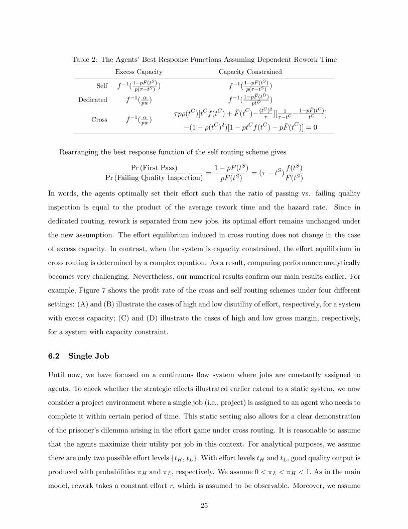
Table 2: The Agents’ Best Response Functions Assuming Dependent Rework Time

Excess Capacity Capacity Constrained

Self f−1(1−pF̄ (tS)

p(τ−tS) ) f−1(1−pF̄ (tS)

p(τ−tS) )

Dedicated f−1( αpw ) f−1(1−pF̄ (t

D)ptD

)

Cross f−1( αpw )

τpρ(tC)[tCf(tC) + F̄ (tC)− (tC)2τ ][ 1

τ−tC−1−pF̄ (tC)

tC]

−(1− ρ(tC)2)[1− ptCf(tC)− pF̄ (tC)] = 0

Rearranging the best response function of the self routing scheme gives

Pr (First Pass)Pr (Failing Quality Inspection)

=1− pF̄ (tS)pF̄ (tS)

= (τ − tS) f(tS)

F̄ (tS)

In words, the agents optimally set their effort such that the ratio of passing vs. failing quality

inspection is equal to the product of the average rework time and the hazard rate. Since in

dedicated routing, rework is separated from new jobs, its optimal effort remains unchanged under

the new assumption. The effort equilibrium induced in cross routing does not change in the case

of excess capacity. In contrast, when the system is capacity constrained, the effort equilibrium in

cross routing is determined by a complex equation. As a result, comparing performance analytically

becomes very challenging. Nevertheless, our numerical results confirm our main results earlier. For

example, Figure 7 shows the profit rate of the cross and self routing schemes under four different

settings: (A) and (B) illustrate the cases of high and low disutility of effort, respectively, for a system

with excess capacity; (C) and (D) illustrate the cases of high and low gross margin, respectively,

for a system with capacity constraint.

6.2 Single Job

Until now, we have focused on a continuous flow system where jobs are constantly assigned to

agents. To check whether the strategic effects illustrated earlier extend to a static system, we now

consider a project environment where a single job (i.e., project) is assigned to an agent who needs to

complete it within certain period of time. This static setting also allows for a clear demonstration

of the prisoner’s dilemma arising in the effort game under cross routing. It is reasonable to assume

that the agents maximize their utility per job in this context. For analytical purposes, we assume

there are only two possible effort levels {tH , tL}.With effort levels tH and tL, good quality output isproduced with probabilities πH and πL, respectively. We assume 0 < πL < πH < 1. As in the main

model, rework takes a constant effort r, which is assumed to be observable. Moreover, we assume

25

A: Excess Capacity: High Disutility of Effort α B: Excess Capacity: Low Disutility of Effort α

C: Capacity Constrained: High Gross Margin v D: Capacity Constrained: Low Gross Margin v

5 10 15 208.5

8.55

8.6

8.65

8.7

cE

SelfCross

0.05 0.1 0.15 0.210

10.5

11

11.5

cA

SelfCross

5 10 15 209.45

9.5

9.55

9.6

9.65

cE

SelfCross

0.05 0.1 0.15 0.22

2.5

3

3.5

cA

SelfCross





5 10 15 208.5

8.55

8.6

8.65

8.7

cE

SelfCross

5 10 15 208.5

8.55

8.6

8.65

8.7

cE

SelfCross

0.05 0.1 0.15 0.210

10.5

11

11.5

cA

SelfCross

0.05 0.1 0.15 0.210

10.5

11

11.5

cA

SelfCross

5 10 15 209.45

9.5

9.55

9.6

9.65

cE

SelfCross

5 10 15 209.45

9.5

9.55

9.6

9.65

cEcE

SelfCross

0.05 0.1 0.15 0.22

2.5

3

3.5

cA

SelfCross

0.05 0.1 0.15 0.22

2.5

3

3.5

cA

SelfCross

Figure 7: The Principal’s Profit Rate in Systems with Excess Capacity (A: α = 0.8. B: α = 0.2. λ = 0.5,

cA = 0.001) and with Capacity Constraint (C: v = 10. D: v = 4. cE = 10). F (t) = 1 − e−3(t−1),CA(p) =

cAp2

1−p , τ = 2, cI = 0.5.

rework is relatively less costly, specifically, r < tL. Here we can allow a more general disutility8

of effort g(t), with g(0) = 0, g0 > 0 and g00 > 0. Further more, we assume that it is optimal for

the principal to induce high effort. This is the more interesting case as quality is crucial to the

principal.

6.2.1 Self Routing

In self routing, agent i’s utility depends on his effort:

UH = w − g(tH)− p(1− πH)g(r), UL = w − g(tL)− p(1− πL)g(r).

The IC constraint for inducing high effort is UH ≥ UL. Equivalently,

p ≥ p̄S = g(tH)− g(tL)(πH − πL)g(r)

.

To ensure high effort is implementable using the self routing scheme, we need p̄S < 1 and thus

assume g(r) > g(tH)−g(tL)πH−πL . This is the more interesting case because the self routing scheme would

8 In our main model, a linear disutility of effort is assumed because long-run analysis of the agents’ utility rate

requires additivity of disutility.

26

otherwise be immediately inferior. Since the throughput is limited to one unit, the principal’s

problem becomes a cost minimization:

CS = min0≤p≤1,w≥0

w + (1− πH)(pcI + (1− p)cE) + CA(p)subject to w − g(tH)− p(1− πH)g(r) ≥ 0 (IR), p ≥ p̄S (IC).

6.2.2 Dedicated Routing

In dedicated routing, agent 1’s utility depends on his effort:

UH = (1− p(1− πH))w − g(tH), UL = (1− p(1− πL))w − g(tL).

The IC constraint for inducing high effort is UH ≥ UL. Equivalently,

p ≥ p̄D = g(tH)− g(tL)(πH − πL)w

.

The principal’s problem becomes

CD = min0≤p≤1,w≥0

w + (1− πH)(pcI + (1− p)cE) + CA(p)subject to (1− p(1− πH))w − g(tH) ≥ 0 (IR1), p ≥ p̄D (IC1),

p(1− πH)(w − g(r)) ≥ 0 (IR2).

Since p̄D is dependent on w, high effort is always implementable as long as the piece rate w is set

high enough. Similar to the excess capacity case of the main model, dedicated routing gives the

principal an additional lever, i.e., w, to induce quality-improving effort.

6.2.3 Cross Routing

In cross routing, agent i’s utility depends on agent j0s effort:

UHH = w − g(tH)− p(1− πH)g(r), ULH = (1− p(πH − πL))w − g(tL)− p(1− πH)g(r),

ULL = w − g(tL)− p(1− πL)g(r), UHL = (1 + p(πH − πL))w − g(tH)− p(1− πL)g(r),

where the first and second subscripts denote agent i’s and j’s effort level, respectively. The IC

constraint for inducing {H,H} equilibrium outcome is UHH ≥ ULH . Equivalently,

p ≥ p̄C = g(tH)− g(tL)(πH − πL)w

27

Similar to dedicated routing, high effort is always implementable as long as the piece rate w is set

high enough. The principal’s problem becomes

CC = min0≤p≤1,w≥0

w + (1− πH)(pcI + (1− p)cE) + CA(p)subject to w − g(tH)− p(1− πH)g(r) ≥ 0 (IR), p ≥ p̄C (IC).

6.2.4 Comparing Three Schemes: Prisoner’s Dilemma and Collusion

We first compare the lower bound on the quality inspection precision required to achieve high effort.

It is simple to show that p̄C = p̄D < p̄S. The inequality follows from w > g(r), which is true because

of the IR constraint and the assumption that r < t. Further notice that when p̄C < p < p̄S , the

Nash equilibrium induced between the two agents in cross routing exhibits a prisoner’s dilemma.

This follows from

UHL − ULL = p(πH − πL)w − g(tH) + g(tL) > 0UHH − ULL = g(tL)− g(tH) + pg(r)(πH − πL) < 0

In other words, even though strategy profile {L,L} let both agents enjoy a higher payoff thanthe equilibrium payoff, agents will make unilateral deviation to high effort, resulting in a prisoner’s

dilemma. Interestingly, the existence of the prisoner’s dilemma hinges on the condition that p < p̄S.

If to the contrary p ≥ p̄S , then self routing can implement high effort and thus have the same

incentive effects as cross routing. Therefore, cross routing has stronger incentives for quality only

when the optimal p under this scheme is strictly less than p̄S.

The equality between p̄C and p̄D implies that cross assignment of rework and assigning rework

to a dedicated agent have equivalent incentive effects on the agents’ effort. In cross routing, though

the agents could have exhibit more opportunistic behavior, it is curbed by the prisoner’s dilemma.

In dedicated routing, separating the rework task completely from the new job task alleviates the

moral hazard problem. Consistent with the result of the main model, self routing is disadvantageous

in inducing effort as it requires a higher inspection precision.

Proposition 5 The rank order of the principal’s cost depends on the quality costs:

(i) if cI is sufficiently large or CA(·) is sufficiently convex, then CC = CD < CS ;

(ii) if cE is sufficiently large, then CC = CD = CS.

28

The above results differ from the main results (i.e., Propositions 2 and 4) in two ways: (1)

self routing is weakly dominated by the other two schemes; (2) cI and cE play different roles in

determining the rank order. These differences result from the assumption that high effort is always

desirable in the current model, while the principal is allowed to choose optimal effort in the main

model.

Finally, we caution that the superior performance of cross routing relies on the restriction that

the agents do not have future interactions. According to the Nash Reversion Folk Theorem (see

Mas-Colell, Whinston & Green (1995)), a collusive outcome {L,L} can be supported with Nashreversion strategies and a sufficiently large discount factor in a repeated game. This suggests that

in practice, it may be beneficial for the principal to maintain a certain level of staff turnover to

prevent collusion.

6.3 Punishment as an Alternative Incentive Scheme

Assigning rework to a different agent implicitly punishes the agent for shirking. In dedicated

routing and cross routing, the agents are punished because they cannot recoup the cost of effort

spent on a job that fails quality inspection. Such punishment could be replicated by a modified self

routing scheme where the principal executes a monetary punishment whenever a defect is identified.

Consider the case of excess capacity. Suppose the principal specifies a penalty x for each defect

identified, the agents’ problem becomes

maxt≥t

λ[w − α(t+ pF̄ (t)r)− pF̄ (t)x].

The first-order condition is equivalent to f(t) = 1pr+ 1

αpx. Recalling Equation (1), we set x =

cI +1−pFBpFB

cE to allow the principal to achieve the first-best effort level. Different from the first-

best outcome, the principal needs to compensate the agent with a higher piece rate: w = wFB +

pFBF̄ (tFB)x. Similarly, we could also design a piece rate plus a bonus that is paid whenever a job

passes quality inspection in the first pass. This contract also enables the principal to achieve first

best, but requires a higher piece rate than wFB as well. Since positive rents need to be paid to

the agents to attain tFB and pFB, it may not be profitable for the principal to implement such

contracts.

While these incentive schemes are powerful, it is difficult in practice for a principal to “force”

rework without or with negative pay. Moreover, the principal may face a limited liability constraint

29

that withholds him from using the punishment compensation scheme9. In contrast, cross routing

of rework is a more “fair” contract in the sense that the principal always pays the full piece rate

but chooses to pay the parallel agent for his rework. Rather than designing a more complex

contract, we take piece rate, a commonly used incentive scheme, as given, and try to design rework

routing schemes that improve quality. We believe doing so has rather practical implications as the

cross routing scheme can be implemented without modifying the existing pay scheme, though the

magnitude of piece rate may be changed.

7 Conclusions

This paper investigates how incentives and judicious rework routing can improve quality and prof-

itability of a firm using a principal-agent model integrated into a multi-class queueing network.

We demonstrate that conventional self routing of rework is always suboptimal in terms of inducing

quality-improving effort. In contrast, dedicated routing and cross routing perform better in induc-

ing effort. However, financial performance depends not only on the first-pass effort induced, but

also on revenues, quality costs, and compensation costs. The more novel cross routing scheme is

applicable in both manufacturing and service operations environment. The merit of this scheme

lies in that the agents influence each other’s workload allocation of new jobs and rework in a way

that leads to higher equilibrium first-pass effort as a result of a prisoner’s dilemma. This works in

favor of the principal when quality is important, i.e., when quality costs are high.

We have made two methodological contributions to the agency and operations management

literature. First, we study a multi-agent principal-agent model in a multi-class queueing network

with endogenous queues (recall the job arrival rate of the rework queues is endogenously determined

by the agents’ first-pass effort). To the best of our knowledge, this is the first attempt at modeling

endogenous queueing dynamics in a principal-agent framework10. Second, we embed the quantity-

quality trade-off in a single dimensional decision variable, i.e., the average processing time per job.

We think this is a more realistic way to model the trade-off because quantity and quality output

are often inseparable tasks of a worker’s job.

Our model has limitations. First, due to the inherent variability in queueing networks, risk9For a detailed discussion of limited liability constraint, see Sappinton (1983) that illustrates limited liability in a

risk-neutral agent setting.10Gilbert & Weng (1998) model a two-server queuing network in a principal-agent framework, but only consider

queues with exogenous arrival rate.

30

aversion cannot be easily incorporated given that we conduct long-run analysis. Second, we assume

that agents commit to a single first-pass effort level even though in reality they can adjust effort from

time to time and thus play a dynamic game. Third, our model does not capture customer waiting

costs and inventory holding costs, though they can be incorporated. When customer waiting costs

are considered, pricing of the goods or services sold by the principal will depend on the agents’

effort. Customer waiting also affects the principal’s decision on capacity, i.e., whether to acquire

adequate staffing to provide good service or maintain high utilization of resources to minimize

cost. Inventory holding costs can be incorporated straightforwardly. We believe this will change

our result in one direction: the principal will have less incentives to induce effort because higher

first-pass effort leads to longer flow time, and thus higher inventory holding costs. Fourth, the

nonobservability of effort is a key assumption for the existence of the moral hazard problem here.

Though it is a standard assumption11 in the principal-agent literature, we acknowledge that the

principal is able to infer (still imperfectly) the agents’ effort from their output after a long period of

interaction. Finally, our model does not cover a few important aspects of manufacturing and service

operations. From the perspective of lean operations, self routing enables quality at the source and

allows the workers to learn from their own mistakes. Since the utilization of agents is not balanced

in dedicated routing, cross routing may be preferred even though the two routing schemes have the

same incentive effects. However, cross routing loses the worker specialization benefit of dedicated

routing.

Acknowledgements

We thank Kevin Wilson (Memphis Auto Auction) for bringing cross routing to our attention. We

also greatly benefited from the encouraging suggestions from James Dana and Martin Lariviere.

References

Avriel, M., Diewert, W. E., Schaible, S. & Zang, I. (1988), Generalized Concavity, Plenum Press, New York.

Baiman, S., Fischer, P. E. & Rajan, M. V. (2000), ‘Information, contracting, and quality costs’, Management

Science 46(6), 776—789.

Cachon, G. & Harker, P. T. (2002), ‘Competition and outsourcing with scale economies’, Management

Science 48(10), 1314—1333.11Plambeck & Zenios (2000) assume that the production rate of the agent is not observable by the principal.

31

Gilbert, S. M. & Weng, Z. K. (1998), ‘Incentive effects favor nonconsolidating queues in a service system:

The principal-agent perspective’, Management Science 44(12), 1662—1669.

Gunes, E. D. & Aksin, O. Z. (2004), ‘Value creation in service delivery: Relating market segmentation, incen-

tives, and operational performance’, Manufacturing and Service Operations Management 6(4), 338—357.

Ha, A. Y. (2001), ‘Optimal pricing that coordinates queues with customer-chosen requirements’,Management

Science 47(7), 915—930.

Hamilton, B. H., Nickerson, J. A. & Owan, H. (2003), ‘Team incentives and worker heterogeneity: An em-

pirical analysis of the impact of teams on productivity and participation’, Journal of Political Economy

111(3), 465—497.

Holmstrom, B. & Milgrom, P. (1991), ‘Multitask principal-agent analyses: Incentive contracts, asset owner-

ship, and job design’, Journal of Law, Economics, and Organization 7, 24—52.

Juran, J. M. & Gryna, F. M. (1993), Quality Planning and Analysis: from product development through use,

McGraw-Hill, New York.

Lazear, E. P. (2000), ‘Performance and productivity’, American Economic Review 90(5), 1346—1361.

Mas-Colell, A., Whinston, M. D. & Green, J. R. (1995), Microeconomic Theory, Oxford University Press,

New York.

Mendelson, H. & Whang, S. (1990), ‘Optimal incentive-compatible priority pricing for the m/m/1 queue’,

Operations Research 38(5), 870—883.

Naor, P. (1969), ‘The regulation of queue size by levying tolls’, 37, 15—24.

Parlakturk, A. K. & Kumar, S. (2004), ‘Self-intereted routing in queueing networks’, Management Science

50(7), 949—966.

Plambeck, E. L. & Zenios, S. A. (2000), ‘Performance-based incentives in a dynamic principal-agent model’,

Manufacturing and Service Operations Management 2(3), 240—263.

Reynier, D. J. & Tapiero, C. S. (1995), ‘The delivery and control of quality in supplier-producer contracts’,

Management Science 41(10), 1581—1589.

Sappinton, D. (1983), ‘Limited liability contracts between principal and agent’, Journal of Economic Theory

29, 1—21.

Shumsky, R. A. & Pinker, E. J. (2003), ‘Gatekeepers and referrals in services’, Management Science

49(7), 839—856.

Van Mieghem, J. A. (2000), ‘Price and service discrimination in queuing systems: Incentive compatibility of

gcu scheduling’, Management Science 46(9), 1249—1267.

32

Appendix

PROOF OF LEMMA 1. We only need to show that the optimum exists and is an interior solution. Notice

that when t ≥ vα , V < 0. Therefore, we are maximizing a continuous function over a compact set: t

FB ∈[t, vα ] and p

FB ∈ [0, 1], which implies the existence of an optimum. Moreover, C 0A(1) =∞ implies pFB < 1.

V ( vα , p) < 0 implies that tFB < v

α . Since the IR constraint must bind, substitute w = α(t+ pF̄ (t)r) into

the objective function and derive the Kuhn-Tucker conditions:

∂V (tFB, pFB)

∂t= 2λ[−α(1− pFBf(tFB)r) + f(tFB)(pFBcI + (1− pFB)cE)]= 2λ[−α+ f(tFB)(pFB(αr + cI) + (1− pFB)cE)] ≤ 0,

∂V (tFB, pFB)

∂p= 2λ[F̄ (tFB)(cE − cI − αr)− C 0A(pFB)] ≤ 0.

Since C 0A(0) = 0, we must have pFB > 0 because the assumption that cE−cI > αr leads to∂V (t

FB ,0)∂p > 0.

pFB ∈ (0, 1) implies that (pFB(αr+cI)+(1−pFB)cE) ∈ (αr+cI , cE). If αf(t) < αr+cI , then

∂V (t,p)∂t > 0

for any p ∈ (0, 1). Therefore, tFB > t. ¥PROOF OF LEMMA 2. The second-order condition (SOC) is λαprF 00(t) < 0. ¥

PROOF OF LEMMA 3. The SOC is 2λwpF 00(t) < 0. ¥

PROOF OF LEMMA 4. The SOC is λwpF 00(t) < 0. Therefore, tC uniquely maximizes both agents’

utility rate and thus (tC , tC) is a unique effort equilibrium. ¥

PROOF OF PROPOSITION 1. (Self Routing) Substituting tS(p) into the FOC of tFB gives 2λ[−α(1−pf(tS(p))r) + f(tS(p))(pcI + (1 − p)cE)] = 2λ[f(tS(p))(pcI + (1 − p)cE)] > 0. Since ∂2V (t,p)

∂t2=

2λF 00(t)(p(αr + cI) + (1 − p)cE) < 0 for the first-best problem, it follows that tS(p) < tFB(p) for all

p ∈ (0, 1). Therefore, first best can never be achieved. (Dedicated Routing) Since tD = f−1( αwp), the

principal can set p = pFB and w∗ = αpFBf(tFB)

to induce tFB. Further, if w∗ ≥ αtFB

1−pFBF̄ (tFB) , then the

IR1 and IR2 constraints are satisfied. The “only if” part is immediate because the IR1 constraint must be

satisfied to implement the first-best solution. Similarly we prove the results for cross routing. ¥

PROOF OF LEMMA 5. The IR1 constraint requires that w(p) > αt ≥ αr, which implies αpw(p) <

1pr .

Since F 00(·) < 0, it follows that tD(p) = f−1( αpw(p)) > f

−1( 1pr ) = tS(p). Similarly, tC(p) > tS(p). ¥

PROOF OF LEMMA 6. Since the principal’s objective function under self routing is monotonically

decreasing in w, the IR constraint must bind, i.e., wS(p) = α[tS(p) + prF̄ (tS(p))]. However, wC(p)

33

≥ α[tC(p) + prF̄ (tC(p))]. It follows that

wC(p)− wS(p) ≥ α[tC(p)− tS(p) + pr(F̄ (tC(p))− F̄ (tS(p)))]= α(tC(p)− tS(p))(1− prF (t

C(p))− F (tS(p))tC(p)− tS(p) )

> α(tC(p)− tS(p))(1− prf(tS(p))) = 0.

The last inequality follows from the fact that F (·) is strictly concave and tC(p) > tS(p). Since wD(p) ≥αtD(p)

1−pF̄ (tD(p)) ,

wD(p)− wS(p) ≥ αtD(p)

1− pF̄ (tD(p)) − α[tS(p) + prF̄ (tS(p))]

>αtD(p)

1− pF̄ (tD(p)) − α[tD(p) + prF̄ (tD(p))]

=α

1− pF̄ (tD(p))pF̄ (tD(p))[tD(p)− (1− pF̄ (tD(p)))r] > 0.

The second inequality follows from the fact that tS = argmint

{t+ prF̄ (t)}. ¥PROOF OF PROPOSITION 2. Let pS denote the optimal p under self routing. Similarly, we define

pD and pC . Since p ∈ [0, 1] and w ∈ [0, v], we are maximizing a continuous function over a compactset, implying existence of an optimum. (Part a) Because the IR2 constraint of dedicated routing is always

nonbinding and fD(t) = fS(t) = αpw , the principal’s problems of dedicated and cross routing are identical

except that the IR constraints are different. Under dedicated routing w ≥ αt1−pF̄ (t) , while under cross routing

w ≥ α(t + pF̄ (t)r). For any t ≥ t, αt1−pF̄ (t) − α(t + pF̄ (t)r) = αpF̄ (t)[t−(1−pF̄ (t))r]

1−pF̄ (t) > 0. Therefore, the

optimization problem in the dedicated routing has a more stringent IR constraint. Hence, V C ≥ V D.(Part b) We start by comparing the principal’s profit rate at any p,

V C(p)− V S(p) = λ[−α((tC(p) + pF̄ (tS(p))r) + α(tS(p) + pF̄ (tS(p))r)

+(pcI + (1− p)cE)(F̄ (tC(p))− F̄ (tS(p)))= λ[−α(tC(p)− tS(p))(1− prF (t

C(p))− F (tS(p))tC(p)− tS(p) )

+(pcI + (1− p)cE)(F (tC(p))− F (tS(p)))]

Since F (tC(p))−F (tS(p))tC(p)−tS(p) < f(tS(p)) = 1

pr , 1 − F (tC(p))−F (tS(p))tC(p)−tS(p) > 0. Therefore V C(p) < V S(p) if α is

sufficiently large. Hence, V C = V C(pC) < V S(pC) < V S(pS) = V S if α is sufficiently large. The last

inequality follows from the optimality of pS .

V D(p)− V S(p) = λ[−α( tD(p)

1− pF̄ (tD) − (tS(p) + pF̄ (tS(p))r))

+(pcI + (1− p)cE)(F̄ (tD(p))− F̄ (tS(p)))

34

Since tD(p)1−pF̄ (tD) > t

D(p)+pF̄ (tD(p))r > tS(p)+pF̄ (tS(p))r, V D(p) > V S(p) if cI and cE are sufficiently

large. Using a similar argument as before, we prove that V D > V S if cI and cE are sufficiently large.

(Part c) Since wC(p) > α[tC(p) + pF̄ (tC(p))r]

V C(p)− V S(p) < λ[−α(tC(p)− tS(p))(1− prF (tC(p))− F (tS(p))tC(p)− tS(p) )

+(pcI + (1− p)cE)(F (tC(p))− F (tS(p)))] < 0 if α is sufficiently large

Using a similar argument as before, we prove that V C < V S if α is sufficiently large.¥

PROOF OF LEMMA 7. Since tFB ∈ [t, vα ] and pFB ∈ [0, 1], we are maximizing a continuous functionover a compact set, implying the existence of an optimum. Assuming an interior optimum exists, optimum

{tFB, pFB} is then given by the FOCs. ¥PROOF OF LEMMA 8. Evaluating the second derivative of U(t) at tS using f(tS) = 1/pr yields that

U 00(tS) =wprF 00(tS)

(tS + pF̄ (tS)r)2+2w(1− prf(tS))(tS + pF̄ (tS)r)3

=wprF 00(tS)

(tS + pF̄ (tS)r)2< 0.

Because U(t) is strictly concave at any interior critical point, U(t) is strictly pseudoconcave (Avriel, Diewert,

Schaible & Zang (1988)) and thus tS is a unique global maximum if tS ≥ t. ¥PROOF OF LEMMA 9. Evaluating the second derivative of U1(t1) at tD using f

¡tD¢= 1−pF̄ (tD)

ptD

yields that

U 001 (tD) = w[

pF 00(tD)tD

− 2

(tD)3(ptDf(tD) + pF̄ (tD)− 1)] = wpF 00(tD)

tD< 0.

Because U1(t1) is strictly concave at any interior critical point, U1(t1) is strictly pseudoconcave (Avriel

et al. (1988)) and thus tD is a unique global maximum if tD ≥ t.PROOF OF LEMMA 10. The FOC is

∂Ui(ti, tj)

∂ti=w(1− ρi)

(1− ρiρj)2

1

t2i[p(tif(ti) + F̄ (ti))(1 + ρi(1−

r

ti)) + ρiρj − 1] = 0.

Equivalently, p[tif(ti) + F̄ (ti)][1 + ρi(1 − rti)] + ρiρj(ti) − 1 = 0. Let t̂i be the critical point satisfying

the above FOC. The SOC evaluated at t̂i is

∂2Ui(ti, tj)

∂t2i|ti=t̂i =

w(1− ρi)

(1− ρiρj(t̂i))2

1

t̂2i[pt̂iF

00(t̂i)(1 + ρi(1−r

t̂i))

+p(t̂if(t̂i) + F̄ (t̂i))ρir

t̂2i+ ρi

∂ρj(t̂i)

∂ti]

+w(1− ρi)∂[ 1(1−ρiρj)2

1t2i]

∂ti[p(t̂if(t̂i) + F̄ (t̂i))(1 + ρi(1−

r

t̂i)) + ρiρj(t̂i)− 1]

35

Substituting∂ρj(t̂i)

∂ti= −pr

t̂2i[t̂if(t̂i)+F̄ (t̂i)] and the FOC into the SOC gives

∂2Ui(t̂i,tj)

∂t2i= w(1−ρi)

(1−ρiρj(t̂i))21t̂2i[pt̂iF

00(t̂i)(1+

ρi(1− rt̂i))] < 0. The inequality follows from the fact that F 00(·) < 0 and that (1 + ρi(1− r

t̂i)) > 0. Be-

cause it is strictly concave at any interior critical point, Ui(ti, tj) is strictly pseudoconcave in ti (Avriel

et al. (1988)), implying t̂i is a unique global maximum. If we further assume a symmetric equilibrium, i.e.,

t̂i = t̂j = tC , then we get the equilibrium equation. ¥

PROOF OF PROPOSITION 3. Let A(t, p) = v−w−F̄ (t)(pcI+(1−p)cE)−CA(p)t+pF̄ (t)r

and B(t, p) = t+pF̄ (t)r.

Substituting tS(p) into the first-best FOC of tFB(p) gives

f(tS(p))(pcI + (1− p)cE))B(tS(p), p)

− (1− prf(tS(p)))A(p, tS(p))

B(p, tS(p))

=f(tS(p))(pcI + (1− p)cE))

B(tS(p), p)> 0

Claim: At any fixed p, V FB is uniquely maximized at tFB.

∂V 2(tFB)

∂t2=

F 00(tFB)(pcI + (1− p)cE)B(tFB, p)

− (1− prf(tFB))f(tFB)(pcI + (1− p)cE)

B(tFB, p)2

+prF 00(tFB)A(tFB, p)

B(tFB, p)− (1− prf(tFB))f(t)(pcI + (1− p)cE)

B(p, tFB)2

+2[1− prf(tFB)]2 A(tFB, p)

B(tFB, p)2

=F 00(tFB)(pcI + (1− p)cE)

B(tFB, p)+ prF 00(tFB)

A(tFB, p)

B(tFB, p)2

−2(1− prf(tFB))

B(tFB, p)2[f(t)(pcI + (1− p)cE)− (1− prf(tFB))A(tFB, p)]

=F 00(tFB)(pcI + (1− p)cE)

B(tFB, p)+ prF 00(tFB)

A(tFB, p)

B(tFB, p)< 0

Since V (t) is strictly concave at any interior critical point, V (t) is strictly pseudoconcave (Avriel et al.

(1988)), and tFB(p) is a unique, global maximum. It follows that tS(p) < tFB(p). Therefore, the self

routing scheme can never achieve first best. Since the agents’ best response functions in dedicated and cross

routing only depend on p and are different from the FOC of tFB, first best cannot be implemented by these

two schemes. ¥

PROOF OF LEMMA 11. To show tS(p) < tD(p), substituting tS(p) into the FOC of tD(p) yields

that wtS(p)

[ptS(p)f(tS(p)) + pF̄ (tS(p))− 1] = wtS(p)

[ tS(p)r + pF̄ (tS(p)− 1] > 0. We show tD(p) < tC(p)

by contradiction. Suppose tD(p) ≥ tC(p) and it follows from the FOC of tD(p) that ptC(p)f(tC(p)) +

pF̄ (tC(p))− 1 ≥ 0. Then,

p[tC(p)f(tC(p)) + F̄ (tC(p))][1 + (1− r

tC(p))ρ(tC(p))] + ρ(tC(p))2 − 1

≥ 1 + (1− r

tC(p))ρ(tC(p)) + ρ(tC(p))2 − 1 = ρ(tC(p))

tC(p)(tC(p) + pF̄ (tC(p)r − r) > 0,

36

contradicting the FOC of tC(p). ¥

PROOF OF LEMMA 12. Since the principal’s objective function is monotonically decreasing in w in

three routing schemes, all the IR constraints must bind except IR2 under dedicated routing. Therefore,

wS(p) = α(tS(p) + pF̄ (tS(p)r), wD(p) = αtD(p)1−pF̄ (tD(p)) , and w

C(p) = α(tC(p) + pF̄ (tC(p)r). The rest of

the proof is omitted due to similarity to that of Lemma 6. ¥

PROOF OF PROPOSITION 4. First we compare the principal’s profit rate at any p,

V C(p)− V S(p)=

v − F̄ (tC(p))(pcI + (1− p)cE)− CA(p)tC(p) + pF̄ (tC(p))r

− v − F̄ (tS(p))(pcI + (1− p)cE)−CA(p)tS(p) + pF̄ (tS(p))r

= (tC(p)− tS(p))(v − CA(p))(prF (t

C(p))−F (tS(p))tC(p)−tS(p) − 1)

(tC(p) + pF̄ (tC(p))r)(tS(p) + pF̄ (tS(p))r)

+(pcI + (1− p)cE)(tCF̄ (tS(p))− tSF̄ (tC(p)))(tC(p) + pF̄ (tC(p))r)(tS(p) + pF̄ (tS(p))r)

(i) Since tC(p) > tS(p), it follows that F (tC(p))−F (tS(p))tC(p)−tS(p) < f(tS(p)) = 1

pr and tCF̄ (tS(p)− tSF̄ (tC(p) >

0. Therefore, V C(p) − V S(p) > 0 when pcI + (1 − p)cE is large enough or when v − CA(p) is smallenough, i.e., if cI or cE are sufficiently large or if CA(·) is sufficiently convex. Hence, V C = V C(pC) >V C(pI) > V S(pI) = V S. The first inequality follows from the optimality of V C . (ii) V C(p)− V S(p) < 0if v is large enough. Hence, V C = V C(pC) < V S(pC) < V S(pI) = V S. The last inequality follows from

the optimality of V S. ¥

PROOF OF PROPOSITION 5. Since IR1 implies IR2, the principal’s problems under dedicated and

cross routing are identical, implying CD = CC . We will next compare CC with CS. First notice that the

two optimization problems are identical except that cross routing has a less stringent IC constraint than self

routing. This immediately implies that CC ≤ CS. We next find conditions under which the inequality isstrict. Let p̂ be the solution to the unconstrained optimization problem:

min0≤p≤1,w≥0

g(tH) + p(1− πH)g(r) + (1− πH)(pcI + (1− p)cE) + CA(p)

The FOC is C 0A(p̂) = (1−πH)(cE − cI − g(r)). Since the objective function is monotonically increasing inw under self routing, the IR constraint must bind. Therefore, finding pS boils down to comparing p̄S with

p̂ :

pS =

p̂ if p̂ > p̄S

p̄S if p̂ ≤ p̄S.

37

Similarly if the IR constraint under cross routing binds, then

pC =

p̂ if p̂ > p̄C

p̄C if p̂ ≤ p̄C.

We have shown that in the main text that p̄C < p̄S . Consider three possibilities: 1) If p̄C < p̄S < p̂, then

pC = pS = p̂, which implies CC = CS ; 2) If p̄C < p̂ ≤ p̄S , then pC = p̂ and pS = p̄S, which implies

CC > CS; 3) If p̂ ≤ p̄C , then pC = p̄C and pS = p̄S, which implies CC > CS. From the first-order

condition of p̂, we conclude that case 1 will occur if cE is sufficiently large and case 2 & 3 will occur if cI is

sufficiently large or CA(·) is sufficiently convex.Now we suppose the IR constraint under cross routing does not bind. Consider the Lagrangian of the

constrained optimization problem:

L = w + (1− πH)(pcI + (1− p)cE) + CA(p)− φ[w − g(tH)− p(1− πH)g(r)]

−σ[p− g(tH)− g(tL)(πH − πL)w

].

Taking the derivative yields

∂L

∂p= (1− πH)(cI − cE) + C 0A(p) + φ(1− πH)g(r)− σ = 0,

∂L

∂w= 1− φ− σ

g(tH)− g(tL)(πH − πL)w2

= 0.

Nonbinding IR constraint implies φ = 0. From ∂L∂w = 0, we infer that σ > 0. Complimentary slackness

implies that IC must bind i.e., w = g(tH)−g(tL)(πH−πL)p . Substituting into the objective function yields

min0≤p≤1

g(tH)− g(tL)(πH − πL)p

+ (1− πH)(pcI + (1− p)cE) + CA(p).

Taking the derivative yields − g(tH)−g(tL)(πH−πL)p2 + (1− πH)(cI − cE) +C 0A(p) = 0. The SOC is 2g(tH)−g(tL)(πH−πL)p3 +

C00A(p) > 0. Substituting p̂ into the above FOC gives

− g(tH)− g(tL)(πH − πL)p̂2

+ (1− πH)(cI − cE) + C 0A(p̂) = −g(tH)− g(tL)(πH − πL)p̂2

− (1− πH)g(r) < 0,

which implies p̂ < pC due to strict convexity of the objective function. In addition, binding IC constraint

implies pC = p̄C < p̄S . Therefore, pS = p̄S . Then,

CC − CS =g(tH)− g(tL)(πH − πL)p̄C

− g(tH)− (1− πH)g(tH)− g(tL)(πH − πL)

+(1− πH)(p̄S − p̄C)(cE − cI) + CA(p̄C)− CA(p̄S).

If cI is sufficiently large or CA(·) is sufficiently convex, then CC − CS < 0. Otherwise, CC = CS . ¥

38

Incentives for Quality Through Endogenous Routing

Documents

Transcript of Incentives for Quality Through Endogenous Routing