Electronic copy available at: http://ssrn.com/abstract=1773175

Securitization rating performance and agency

incentives

Daniel Rosch a Harald Scheule b 1

aInstitute of Banking & Finance, Leibniz University of Hannover, Konigsworther

Platz 1, 30167 Hannover, Germany, Phone: +49-511-762-4668, Fax:

+49-511-762-4670. mailto: Daniel.Roesch@finance.uni-hannover.de

bDepartment of Finance, Faculty of Economics and Commerce, University of

Melbourne, Victoria 3010, Australia, Phone: +61-3-8344-9078, Fax:

+61-3-8344-6914, mailto: hscheule@unimelb.edu.au

1 We would like to thank Louis Ederington, Bruce Grundy, Harrison Hong, Marty Subrahmanyam,Klaus Dullmann and Hans Genberg for valuable suggestions. We would also like to thank theparticipants of financial seminars at Deakin University, Deutsche Bundesbank, Global Associationof Risk Professionals, Leibniz University Hannover, Hong Kong Institute for Monetary Research,Macquarie University, Melbourne Centre for Financial Studies, The University of Melbourne,University of Innsbruck, University of St. Gallen and University of Technology Sydney as wellas the discussants of various conferences for valuable comments.The paper was presented at C.R.E.D.I.T. 2009, the Asian Finance Conference 2009, theInternational Risk Management Conference 2009, the Australasian Finance and Banking Conference2009, the 20th Asia Pacific Futures Research Symposium, the 59th Midwest Finance Conference,the 2010 Global Finance Conference, the 2010 FMA European Conference, the 2010 FMA AsianConference, the 17th Annual Conference of the Multinational Finance Society, Finlawmetrics 2010,the Fourth Annual NUS Risk Management Conference, the Joint BIS/ECB/World Bank PublicInvestors’ Conference 2010, the 2010 Annual Meeting of the German Finance Association, the18th Conference on Theories and Practices of Securities and Financial Markets, the InternationalResearch Forum of the Hong Kong Polytechnic University and the University of Texas at Dallas,the 2010 NTU International Conference on Finance - Risk in Globalized Financial Markets, and theFifth Annual Conference on Asia-Pacific Financial Markets of the Korean Securities Association,Seoul, Korea, 2010.The paper received the Australian Securities Exchange’s Best Paper Award on Derivatives andQuantitative Finance in 2009, the 2009 Korea Development Bank Outstanding Paper Award andthe Research Award of the 18th Conference on Theories and Practices of Securities and FinancialMarkets. The support of the Melbourne Centre for Financial Studies, the Hong Kong Institute forMonetary Research and the Thyssen Krupp Foundation is gratefully acknowledged.

Preprint submitted to Working Paper 15 February 2011

Electronic copy available at: http://ssrn.com/abstract=1773175

Securitization rating performance and agency

incentives

Abstract

This paper provides an empirical study, which assesses the historical performance ofcredit rating agency (CRA) ratings for securitizations before and during the financialcrisis. The paper finds that CRAs do not sufficiently address the systematic risk ofthe underlying collateral pools as well as characteristics of the deal and tranchestructure in their ratings. The paper also finds that impairment risk is understatedduring origination years and years with high securitization volumes when CRA feerevenue is high.

The mismatch between credit ratings of securitizations and their underlying riskshas been suggested as one source of the Global Financial Crisis, which resulted inthe criticism of models and techniques applied by CRAs and misaligned incentivesdue to the fees paid by originators.

Key words: Asset-backed Security, Credit Rating Agency, Collateralized DebtObligation, Economic Downturn, Fee Revenue, Forecasting, Global FinancialCrisis, Home Equity Loans, Impairment, Mortgage-backed Security, Rating,Securitization

JEL classification: G20, G28, C51

2

Electronic copy available at: http://ssrn.com/abstract=1773175

1 Introduction

This paper compares and analyzes cross-sectional and time-series characteristics of credit

rating agency (CRA) ratings, implied impairment rate estimates and realized impairment

rates of asset portfolio securitizations. Two distinct hypotheses are analyzed, which provide

empirical evidence on the role of ratings for securitizations during the Global Financial Crisis

(GFC). 2 This is of highest importance as shortcomings may have been instrumental to past,

current and future loss rates of investors in relation to structured finance transactions, which

are generally called securitizations. Structured finance ratings and associated fee revenue have

experienced an unprecedented growth in past years and until the GFC were the dominant

rating category – both in terms of numbers of ratings issued as well as CRA fee revenue. 3

The Global Financial Crisis led to an unprecedented and unexpected increase of impairment

rates for securitizations. The disappointment of investors resulted in the criticism of models

applied by credit rating agencies. Examples are VECTOR from Fitch rating agency (see

Fitch Ratings 2006), CDOROM from Moody’s rating agency (see Moody’s Investors Service

2006) and CDO Evaluator from Standard and Poor’s rating agency (see Standard & Poor’s

2005). A similar critique was ventured after the South East Asian Crisis of 1997 in relation to

corporate bond issuer and bond issue credit ratings. For example, Leot et al. (2008) find that

ratings follow rather than predict the crisis as systematic downgrades occurred subsequent

to the crisis.

Securitizations involve the sale of asset portfolios to bankruptcy-remote special purpose vehi-

cles, which are funded by investors of different seniorities (tranches). Based on the nature of

the securitized asset portfolios, important transaction types include asset-backed securities

(ABSs), collateralized debt obligations (CDOs), home equity loan-backed securities (HELs)

and mortgage-backed securities (MBSs). Securitizations are generally over-the-counter in-

struments. Information is available to measure the risk of securitizations and includes credit

ratings, impairment histories and proxies for the asset portfolio risk, such as asset value in-

dices or cash flow indices. The evaluation of individual risks, their dependence structure and

2 Namely, the Impairment Risk and Agency Incentive hypotheses, compare Section 2.3 Rating fee revenue peaked in 2007. According to Table 1, CRA Moody’s Investors Services hasgenerated in 2007 a fee revenue of $873 million for structured finance ratings, $412 million forcorporate issuer and issue ratings, $274 million for financial institution issuer and issue ratings and$221 million for public project and infrastructure ratings. The relative fee revenues in 2007 (1998)were 49% (32%) for structured finance ratings, 23% (33%) for corporate issuer and issue ratings,15% (20%) for financial institution issuer and issue ratings and 12% (15%) for public project andinfrastructure ratings.

3

derivatives is complicated by the low liquidity of the underlying assets, the unavailability of

secondary markets and the recent origination of such transactions.

Various streams exist in literature on the measurement of financial risks of securitizations

and – with regard to the risk exposure – similar credit derivatives. A first stream focuses

on the pricing, where the central issue is to explain observed prices such as credit spreads

of credit default swap indices. The most prominent examples are the CDX North America

and iTraxx Europe indices, which reference the default events in relation to bond portfolios.

These indices were originated in 2003 and 2004. Credit spreads for the indices as well as

tranches are generally available daily. Longstaff & Rajan (2008) and Hull & White (2004)

apply a risk-neutral pricing framework to develop pricing techniques for these spreads. A

central point of these risk models is the specification of the dependence structure for the

portfolio assets.

Another stream is concerned with the modeling and estimation of risk characteristics of the

underlying asset portfolio without relying on market prices. The focus is on the derivation

of the distribution of future asset values (or losses) based on individual risk parameters. In

the case of a loan portfolio, the relevant parameters are default probabilities, loss rates given

default, exposures at default and dependence parameters such as correlations or more gen-

eral copulas. Merton (1974), Leland (1994), Jarrow & Turnbull (1995), Longstaff & Schwartz

(1995), Madan & Unal (1995), Leland & Toft (1996), Jarrow et al. (1997), Duffie & Single-

ton (1999), Shumway (2001), Carey & Hrycay (2001), Crouhy et al. (2001), Koopman et al.

(2005), McNeil & Wendin (2007) and Duffie et al. (2007) address the default likelihood. Di-

etsch & Petey (2004) and McNeil & Wendin (2007) model the correlations between default

events. Carey (1998), Acharya et al. (2007), Pan & Singleton (2008), Qi & Yang (2009),

Grunert & Weber (2009) and Bruche & Gonzalez-Aguado (2010) develop economically mo-

tivated empirical models for recoveries using explanatory co-variables. Altman et al. (2005)

model correlations between default events and loss rates given default.

Within this stream, credit ratings are often used to explain credit risk. Ratings aim to mea-

sure the credit risk of corporate bond issuers, corporate bond issues, sovereigns and structured

finance issues. In the contemporary climate of the Global Financial Crisis, the role and im-

portance of ratings to all market participants (e.g., issuers, investors and regulators), while

controversial, is acknowledged. Previous research focuses on the degree to which corporate

credit rating changes introduce new information. For example, Radelet & Sachs (1998) find

that rating changes are pro-cyclical. This suggests that they provide only a limited amount

of new information to the market. Ederington & Goh (1993), Dichev & Piotroski (2001)

4

and Purda (2007) find that corporate credit rating downgrades provide news to the market.

Loeffler (2004) finds that the default prediction power of ratings is low. Poon et al. (2009)

analyze solicited and unsolicited bank credit ratings and show that solicitation is a significant

explanatory variable between both groups. Jorion et al. (2005) show that after Regulation

Fair Disclosure, the market impact of both downgrades and upgrades is significant and of

greater magnitude compared to that observed in the pre-Regulation Fair Disclosure period.

The relative roles of different CRAs have also been studied. For example, Miu & Ozdemir

(2002) examine the effect of divergent Moody’s and S&P’s ratings of banks and Becker &

Milbourn (2008) analyze the link between information efficiency of ratings and competition

after the market entry of CRA Fitch. Guettler & Wahrenburg (2007) find that bond ratings

by Moody’s and Standard & Poor’s are highly correlated and Livingston et al. (2010) find

that the impact of Moody’s ratings on market reactions is stronger compared to Standard

& Poor’s.

With regard to the GFC, Demyanyk et al. (2010) find that updated credit score next to

credit score at origination is an important predictor of mortgage default. Rajan et al. (2008)

show that the omission of soft information in ratings can lead to substantial model risk.

Mayer et al. (2008) find that the decline of housing prices was responsible for increasing

sub-prime mortgage delinquency rates. Benmelech & Dlugosz (2009) show empirically that

rating inflation was an issue in the GFC and they argue that one of the causes of the crisis

was overconfidence in statistical models. The authors use rating migration statistics and

analyze up- and downgrades around the crisis. Ashcraft et al. (2009) find that CRA ratings

for mortgage-backed securities provide useful information for investors, show significant time

variation and become less conservative prior to the GFC. Griffin & Tang (2009) compare

CRA model methodologies with CRA ratings for collateralized debt obligations and find that

the models are more accurate than the ratings. Coval et al. (2009) argue that model risk

and the exposure to systemic risk of securitization may explain the increase of impairment

rates during the GFC. Crouhy et al. (2008) point out that CRAs’ fee revenues depend on the

number of ratings and may be linked to ratings quality. Similarly, Franke & Krahnen (2008)

argue that incentive effects in relation to rating shopping have played an important role in

the GFC, particularly associated with the allocation of equity tranches of securitizations.

Hull (2009) and Hellwig (2008) identify deficient CRA models as a cause of the GFC. Bolton

et al. (2009) show that the fraction of naive investors is higher, and the reputation risk for

CRAs of getting caught understating credit risk is lower during economic booms, which gives

CRAs the incentive to understate credit risk in booms.

5

Other authors focus on strategic mortgage default. 4 Krainer et al. (2009) develop an equi-

librium valuation model that incorporates optimal default to show how mortgage yields and

lender recovery rates on defaulted mortgages depend on initial loan-to-value ratios. Their

empirical findings confirms the presence of strategic default. Bajari et al. (2008) model the

drivers of traditional and strategic default and find that the US decrease in home prices as

well as deterioration in loan quality led to increases in mortgage default rates. Guiso et al.

(2009) use survey data to analyze the likelihood for strategic default if the debt value exceeds

the value of the collateralized house value. Important drivers of this likelihood are relocation

costs, moral and social considerations as well as the proportion of foreclosures in the same

region. 5

This paper identifies two gaps in the existing literature. Firstly, important contributions

analyze rating migrations with regard to informativeness of securitization credit ratings. 6

This paper extends the literature by analyzing the ability of credit ratings to reflect impair-

ment risk and collects a unique database of 13,072 impairment events and fee revenue for a

CRA. The analysis of impairment events as the realization of impairment risk provides new

insights. The analysis of rating changes is important but partially limited as it assumes the

accuracy of credit ratings which is the main testable hypotheses.

Secondly, this paper finds new evidence on incentive miss-alignments and extends the above

theoretical literature empirically. The paper is first of its kind to show that CRAs collect

the majority of fee revenue at origination. Following this observation, the paper compares

ratings at origination with ratings at monitoring years as well as total securitization volume at

origination. The paper finds that ratings under-reflect risk in periods when CRA fee revenue

is high and offers an alternative theoretical explanation for the observation by Bolton et al.

(2009) who relate rating inflation (i.e., the underestimation of risk by ratings) to the fraction

of naive investors.

Please note, that this paper does not argue that CRA fee revenue has led to inaccurate

4 A strategic default is the decision by a borrower to default despite having the financial abilityto make loan payments. In relation to the recent financial crisis, strategic default may have beenencouraged by large drops in real estate (collateral) values and interest rates.5 There is a related literature which focuses on the mortgage asset class, the GFC and lendingstandards. Demyanyk & Hemert (2009) and Dell’Ariccia et al. (2008) analyze US loan-level dataand find that the quality of loans deteriorated for six consecutive years before the GFC. Thesefindings are consistent with Rajan et al. (2008) who argue that lenders have an incentive to originateloans that rate high based on characteristics that are reported to investors which may lead to adeterioration of loan quality.6 Examples are Benmelech & Dlugosz (2009) and Ashcraft et al. (2009).

6

ratings but rather argues that current incentive structures may give rise to inaccurate credit

ratings and that the elimination of such incentives may support more meaningful external

ratings for securitizations in the future. To date, investors and prudential regulators assume

the existence of a link between impairment risk and credit ratings by acknowledging CRAs

and assigning credit spreads and regulatory capital risk weights to CRA rating categories.

The remainder of this paper is organized as follows. Section 2 develops the main hypotheses,

consistent with the current literature in relation to the risk and uncertainty of CRA assess-

ments. A framework to test the hypotheses is presented. Section 3 describes the data used in

the study and analyzes the hypotheses. Various robustness checks are conducted. Section 4

discusses the major ramifications of the empirical results for securitization risk models and

provides suggestions in relation to a new stability framework for financial markets, institu-

tions and instruments.

7

2 Hypotheses and Testing Approach

2.1 Development of Hypotheses

Rating agencies have been charged for the failure to measure the impairment risk of secu-

ritizations i.e., the risk that investors may experience losses. The papers aims to provide

empirical insights into CRA securitization ratings and their information content relative to

the inherent risks.

CRAs address various elements of the asset and liability side of securitizations when designing

and implementing a securitization rating model. Rajan et al. (2008) find that securitization

risk models omit ‘soft’ information. This implies that CRA ratings, relying on such incom-

plete models omit important risk factors and hence misevaluate the average credit quality of

the asset portfolio. Crouhy et al. (2008) suggest that CRAs did not monitor raw data and

were tardy in recognizing the implications of the declining state of the sub-prime market and

support the argument by Rajan et al. (2008) that other asset portfolio characteristics, such

as soft facts, may be important drivers of asset portfolio risk.

Our Impairment Risk Hypotheses distinguish missing information on the asset (H1a) and

liability side (H1b) of securitizations. H1a addresses characteristics of the asset portfolio and

is stated as follows:

H1a: Ratings contain all information about the average asset quality of the asset portfolio

relevant for impairment risk such as asset class, resecuritization status and transaction size.

H1b addresses the tranching structure of securitizations and the discussion on the appropriate

specification of the dependence structure of the asset portfolio (compare Hull 2009, Hellwig

2008). The probability distribution and hence the percentiles of losses associated with the

pool are particularly sensitive to the correlations in the underlying asset pool (compare Coval

et al. 2009). Thus, the level of subordination may be a key driver and should explain tranche

impairments after controlling for credit ratings if correlations are mis-specified in the CRA

model. H1b is therefore:

H1b: Ratings contain all information about the characteristics of securitizations relevant for

impairment risk, such as subordination level and tranche thickness.

Furthermore, the rating agencies may have an incentive to bias the measures of impairment

8

risk. Crouhy et al. (2008) argue generally that CRA fees are paid by issuers and that CRA

competition is limited by regulation. This may imply that the credit quality measured by

a CRA and CRA fee revenue are positively correlated. However, CRAs publish default and

rating migration tables, which are used to calibrate ratings to metric risk measures. Thus, a

systematic ‘rating for fee’ policy would be noticed and priced by investors when analyzing the

financial risk in relation to ratings. Two Agency Incentive Hypotheses address two potential

ways in which rating agencies may ‘circumvent’ this rating-performance mechanism.

The first incentive problem (H2a) relates to the assumption that investors do not differenti-

ate the risk with regard to origination and monitoring years. Rating performance measures

are generally calculated as an average per rating class and/or observation year. The fee rev-

enue of rating agencies is high when the first rating is generated (origination year) and low

in later years when ratings are revisited (monitoring years). Figure 1 shows the origination

volume and outstanding volume of the analyzed tranches as well as the CRA fee revenue. 7

It is apparent and insightful that despite the fact that CRAs provide origination and mon-

itoring ratings, CRA fee revenue corresponds with the origination volume rather than the

outstanding volume. 8 Thus, H2a is:

H2a: Rating-implied impairment risk and time since origination are positively correlated.

The reason for this finding is that origination fees exceed the monitoring fees in absolute

terms. 9 In addition, the fees in relation to origination and monitoring years are often paid

upfront despite their lagged recognition as accounting income. As a result, CRAs may have

an incentive to assign i) too low risk ratings in origination years to increase fee revenue and

ii) too high risk ratings in monitoring years to maintain stable default and rating migration

performance measures. In other words, this hypothesis tests whether the underestimation of

risk decreases over time since origination.

The second incentive problem (H2b) relates to a critique by Bolton et al. (2009) who suggest

that the fraction of naive investors is higher, and the reputation risk for CRAs of getting

caught understating credit risk is lower during economic booms, which gives CRAs the

7 Please note that outstanding volume as well as fee revenue relate to origination years and moni-toring years while the origination volume relates to origination years only.8 A similar conclusion can be drawn for count data instead of volume data.9 In financial year 2007, CRA Moody’s Investors Service generated 77% of fee revenue for orig-ination of ratings and 23% for monitoring of ratings. The empirical data suggests that 37% ofstructured finance ratings relate to an origination year and 63% of structured finance ratings relateto a monitoring year. These numbers imply that an origination rating generates approximately 5.7times more fee revenue than monitoring a rating for one year.

9

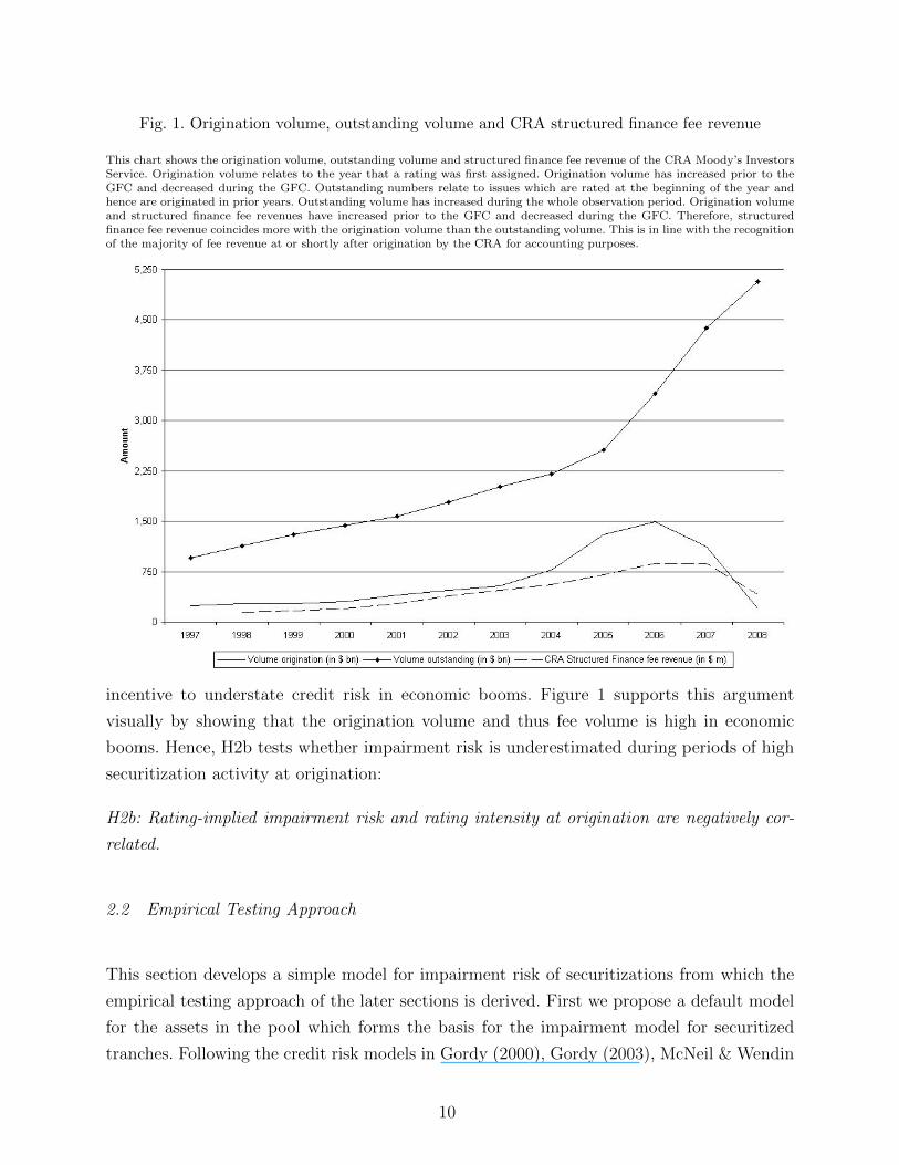
Fig. 1. Origination volume, outstanding volume and CRA structured finance fee revenue

This chart shows the origination volume, outstanding volume and structured finance fee revenue of the CRA Moody’s InvestorsService. Origination volume relates to the year that a rating was first assigned. Origination volume has increased prior to theGFC and decreased during the GFC. Outstanding numbers relate to issues which are rated at the beginning of the year andhence are originated in prior years. Outstanding volume has increased during the whole observation period. Origination volumeand structured finance fee revenues have increased prior to the GFC and decreased during the GFC. Therefore, structuredfinance fee revenue coincides more with the origination volume than the outstanding volume. This is in line with the recognitionof the majority of fee revenue at or shortly after origination by the CRA for accounting purposes.

incentive to understate credit risk in economic booms. Figure 1 supports this argument

visually by showing that the origination volume and thus fee volume is high in economic

booms. Hence, H2b tests whether impairment risk is underestimated during periods of high

securitization activity at origination:

H2b: Rating-implied impairment risk and rating intensity at origination are negatively cor-

related.

2.2 Empirical Testing Approach

This section develops a simple model for impairment risk of securitizations from which the

empirical testing approach of the later sections is derived. First we propose a default model

for the assets in the pool which forms the basis for the impairment model for securitized

tranches. Following the credit risk models in Gordy (2000), Gordy (2003), McNeil & Wendin

10

(2007), and Gupton et al. (1997), let Rkt denote the asset return of borrower k in time period

t (k = 1, ..., K; t = 1, ..., T ) which is generated by the following process

Rkt =√ρ ·Xt +

√1− ρ · εkt (1)

where Xt and εkt are standard normally distributed systematic and idiosyncratic risk factors

and ρ is a parameter denoting the correlation between asset returns which measures the

strength of association between borrowers. The factors are assumed to be serially and cross-

sectionally independent.

A default event occurs if the asset return Rkt falls below a threshold ckt, that is

Dkt = 1⇔ Rkt < ckt (2)

where Dkt is an indicator variable with

Dkt =

1 borrower k defaults in t

0 otherwise(3)

Under the normality assumption of the model the probability of default is πkt = Φ(ckt) where

Φ(.) is the standard normal cumulative distribution function. Now, assume that K assets are

pooled to an asset portfolio j. 10 The default rate of the pool is the average over the default

indicators of its assets and defined as

Pjt =1

K

K∑k

Dkt (4)

A common approximation of the probability density f(pjt) of the default rate of the pool uses

the assumptions of an infinite large number and homogeneity of assets with ckt = cjt for all k.

The density converges against the ‘Vasicek’-density under these assumptions (see Vasicek

1987, 1991, Gordy 2000, 2003):

f(pjt) =

√1− ρ√ρ· exp

(1

2(Φ−1(pjt))

2 − 1

2ρ(cjt −

√1− ρ · Φ−1(pjt))

2

)(5)

10 Please note that it is common to refer to the asset portfolio with terms such as deal or transaction.

11

where Φ−1(.) is the inverse standard normal cumulative distribution function. The default

rate has the cumulative distribution function (see e.g., Bluhm et al. 2003)

F (pjt) = P (Pjt < pjt) = Φ

(√1− ρΦ−1(pjt)− cjt√

ρ

)(6)

Pjt in Equation (5) and Equation (6) can also be interpreted as the loss rate (rather than

the default rate) of the portfolio when loss rates given default are deterministic and equal

to unity.

Next, consider the structuring of a pool (or transaction) into several tranches. A tranche i

(i = 1, ..., Ij) of pool j experiences a loss and therefore an impairment if the default rate Pjt

in the portfolio exceeds the relative subordination level (or attachment level) ALijt

Dijt = 1⇔ Pjt > ALijt (7)

where Dijt is an indicator variable with

Dijt =

1 tranche i of asset pool j is impaired in t

0 otherwise(8)

The relative attachment level is calculated by the ratio of the attachment level (in $) and the

deal principal (in $) of period t. As a result of this definition, impaired tranches of previous

years have reduced both the attachment level as well as the deal principal. The probability

of a tranche impairment is thus

P (Dijt = 1) = P (Pjt > ALijt) (9)

The attachment probability (i.e., the propensity of being exposed to a loss in the underlying

asset pool) for a tranche i of asset pool j in period t (i = 1, ..., Ij; j = 1, ..., J ; t = 1, ..., T ) is

12

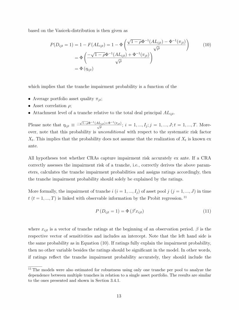
based on the Vasicek-distribution is then given as

P (Dijt = 1) = 1− F (ALijt) = 1− Φ

(√1− ρΦ−1(ALijt)− Φ−1(πjt)√

ρ

)(10)

= Φ

(−√

1− ρΦ−1(ALijt) + Φ−1(πjt)√ρ

)= Φ (ηijt)

which implies that the tranche impairment probability is a function of the

• Average portfolio asset quality πjt;

• Asset correlation ρ;

• Attachment level of a tranche relative to the total deal principal ALijt.

Please note that ηijt ≡ −√

1−ρΦ−1(ALijt)+Φ−1(πjt)√ρ

; i = 1, ..., Ij; j = 1, ..., J ; t = 1, ..., T . More-

over, note that this probability is unconditional with respect to the systematic risk factor

Xt. This implies that the probability does not assume that the realization of Xt is known ex

ante.

All hypotheses test whether CRAs capture impairment risk accurately ex ante. If a CRA

correctly assesses the impairment risk of a tranche, i.e., correctly derives the above param-

eters, calculates the tranche impairment probabilities and assigns ratings accordingly, then

the tranche impairment probability should solely be explained by the ratings.

More formally, the impairment of tranche i (i = 1, ..., Ij) of asset pool j (j = 1, ..., J) in time

t (t = 1, ..., T ) is linked with observable information by the Probit regression. 11

P (Dijt = 1) = Φ (β′xijt) (11)

where xijt is a vector of tranche ratings at the beginning of an observation period. β is the

respective vector of sensitivities and includes an intercept. Note that the left hand side is

the same probability as in Equation (10). If ratings fully explain the impairment probability,

then no other variable besides the ratings should be significant in the model. In other words,

if ratings reflect the tranche impairment probability accurately, they should include the

11 The models were also estimated for robustness using only one tranche per pool to analyze thedependence between multiple tranches in relation to a single asset portfolio. The results are similarto the ones presented and shown in Section 3.4.1.

13

information as specified in Equation (10).

However, if a rating omits information, then additional information besides the rating may

explain the tranche impairment probability. Examples may relate to the asset portfolio qual-

ity, the securitization structure as well as observable information with regard to the business

cycle as stated in our hypotheses. Consider an error in assigning one or more of the pool

parameters made by the CRA resulting in ηijt 6= ηijt. Using ηijt instead of ηijt will provide

erroneous impairment probability assessments P (Dijt = 1) = Φ (ηijt) 6= P (Dijt = 1) and

therefore misclassification into wrong rating grades. The true impairment probability can

then be written as

P (Dijt = 1) = Φ (ηijt + ∆ijt) (12)

with ∆ijt ≡ ηijt − ηijt denoting the measurement error in variables which may refer to

characteristics of the pool, the tranche or time. Model (12) will provide the basis for the

empirical tests in the following section. 12

Please note that this paper focuses on the ability of ratings and other risk factors to explain

the binary impairment risk. Thus, the above probit analysis is appropriate to compare ratings

and impairment events as it links the probability of impairment with explanatory variables.

Krahnen & Weber (2001) argue that such a link is a necessity under generally accepted rating

principles. These types of models have also been employed in other studies for analyzing

corporate bond issue and issuer ratings or a bank’s loan credit ratings (compare e.g., Grunert

et al. 2005). 13 However, it may be argued that the above model is oversimplified and therefore

the empirical approach is not valid and robust with respect to model mis-specification. For

example, the above model in Equation (10) assumes homogeneity, large pools, and normally

distributed risk factors whereas literature has found that Student’s t-distributions or copulas

explain credit spreads of CDOs better than Gaussian copulas (compare e.g., Hull & White

2004). We analyze the impact of the assumptions and the robustness of results in Section

3.4.

12 This approach is consistent with Ashcraft et al. (2009) who distinguish between the case thatratings partially explain risk (Informativeness) and the case where other variable are additionallysignificant (Information Efficency).13 The research question is slightly different to the analysis of rating standard dynamics. Oneimportant study in this area is by Blume et al. (1998) who analyze corporate rating standards andfind that such rating standards have become more stringent from 1978 to 1995. Rating standardis defined in this study as the propensity to assign a certain rating category and thus an orderedProbit models is estimated where the ratings grades are the dependent variables. Another examplefor such an approach is Becker & Milbourn (2008).

14

3 Empirical analysis

3.1 Structured finance data

This paper analyzes a comprehensive panel data set of structured finance transactions rated

by CRA Moody’s Investors Service. The data covers characteristics of asset portfolios (which

are also known as collateral portfolios), characteristics of tranches, ratings of tranches as well

as occurrences of impairment events for tranches.

This paper focuses on the CRA Moody’s as Moody’s unique corporate structure implies that

fee revenues are published. Please note that Standard & Poor’s is a subsidiary of McGraw-

Hill and FitchRatings is a subsidiary of Fimalac. Both parent firms do not publish fee

revenues for securitizations. We have checked the consistency of structured finance ratings 14

across three CRAs. We hand-collect the initial ratings of 1,000 randomly selected tranches

and assigned numbers from 1 (rating Aaa for Moody’s and rating AAA for Standard &

Poor’s and Fitch respectively) to 21 (rating C). Of the 1,000 tranches rated by Moody’s,

680 are rated by Standard & Poor’s and 356 are rated by Fitch. We find extremely high

Spearman correlations 15 coefficients in excess of 90%: between Moody’s and Standard &

Poor’s: 0.9339, between Moody’s and Fitch: 0.9584 and between Standard & Poor’s and

Fitch: 0.9855. Moody’s and Standard & Poor’s differ in 88 of 680 cases. Moody’s and Fitch

differ in 49 of 356 cases and Standard & Poor’s and Fitch differ in 11 of 163 cases. This

implies that the empirical likelihood of a rating deviation is between 6.7% and 13.8%. Please

note that the majority of ratings difference relates to a single notch. These findings suggest

that results based on Moody’s can be generalized to other major rating agencies.

This is also consistent with Guettler & Wahrenburg (2007), who find that bond ratings

by Moody’s and Standard & Poor’s are highly correlated. Our empirical findings, industry

experience and interviews with employees of the three CRAs support our conjecture that the

ability to predict default or impairment risk is similar for the three major CRAs. In addition,

Livingston et al. (2010) find that the impact of Moody’s ratings on market reactions is

somewhat stronger compared to Standard & Poor’s and supports the use of Moody’s ratings

further.

14 Please note that starting August 2010 such ratings require the ’SF’ designation to be differentiatedfrom bond an other ratings.15 We chose to report this measure for the relationship as ratings are ordinal in nature. We obtainsimilar results for Bravais-Pearson correlation coefficients.

15

The focus of the present study is on the performance of CRA ratings, which involves a

comparison of CRA ratings with the likelihood of occurrence of impairment events. An

impairment event is defined as (compare Moody’s Investors Service 2008):

“[...] one of two categories, principal impairments and interest impairments. Principal

impairments include securities that have suffered principal write-downs or principal losses

at maturity and securities that have been downgraded to Ca/C, even if they have not yet

experienced an interest shortfall or principal write-down. Interest impairments, or interest-

impaired securities, include securities that are not principal impaired and have experienced

only interest shortfalls.”

Our model suggests that impairment risk is measured by CRAs ex ante and unconditional on

the macroeconomic factor. However, the realization of impairments is measured conditional

on the economy. To control for the unanticipated realization of the economy we include rating

years, or alternatively, proxies for the economy in the regression models. Moreover, to check

for structural breaks and to control for the increasing number of defaults we additionally

divide our data into the sub-periods before and during the GFC.

Alternative measures for rating performance have been proposed in literature (compare Sec-

tion 1). Firstly, ratings may be compared to the performance of the asset portfolios. The

approach may be reasonable for asset portfolios such as mortgage-backed securities where

information on the default rates of the underlying portfolios is available. We chose not to

follow this approach for two reasons: i) we focus on the securitization market rather than

mortgage-backed securities only and find distinct differences between various asset portfo-

lios; and ii) credit ratings are issued for individual securities (tranches) and a key element

in credit ratings is the credit enhancement (subordination) of these securities.

Secondly, ratings may be compared to the propensity of occurrence of rating downgrades.

We chose not to follow this approach as our research question aims to analyze the accuracy

of credit ratings with regard to the ex ante prediction of impairment risk. Analyzing rating

downgrades limits the interpretation of results as the link between downgrades and losses to

investors is less transparent as it assumes the accuracy of credit ratings which is the main

testable hypotheses.

Structured finance transactions are very heterogeneous by definition. The authors are aware

of potential prudential policy implications of this study. Seven filter rules to generate a

homogeneous data set are applied and the following observations are deleted:

16

(1) Transaction observations which can not be placed into the categories ABS, CDO, CMBS,

HEL or RMBS. These are mainly asset-backed commercial paper, structured covered

bonds, catastrophe bonds, and derivative product companies. 22.0% of the original

number of observations are deleted;

(2) Transaction observations where the monetary volume and therefore relative credit en-

hancement and thickness of individual tranches could not be determined without setting

additional assumptions due to i) multiple currency tranches and ii) missing senior un-

funded tranche characteristics. 13.5% of the original number of observations are deleted

after the application of Filter Rule (1);

(3) Transaction observations which are not based on the currency USD or transaction obser-

vations which are not originated in the USA. 5.0% of the original number of observations

are deleted after the application of Filter Rule (1) and Filter Rule (2);

(4) The time horizon is 1997-2008. Tranche observations which relate to years prior to 1997

due to a limited number of impairment events. Impairment events are the focus of this

paper and years prior to 1997 have experienced few impairment events. Years after 2008

are not yet available at the time of writing this paper. 7.3% of the original number of

observations are deleted after the application of Filter Rule (1) to Filter Rule (3);

(5) Tranche observations which have experienced an impairment event in prior years. 0.2%

of the original number of observations are deleted after the application of Filter Rule

(1) to Filter Rule (4).

The resulting data comprises 325,443 annual tranche observations. The number of impaired

tranche observations is 13,072. 16 The data set is one of the most comprehensive data sets

on securitization collected and analyzed to date.

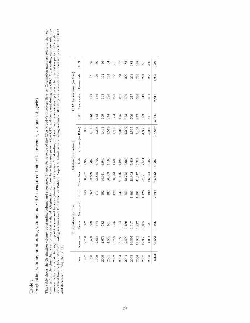
Table 1 shows various proxies for origination 17 and outstanding volume of the data: number

of tranches, number of deals and volume. The variables cover CRA ratings at origination and

the beginning of a year, asset pool and securitization characteristics, impairment events as

well as systematic variables. In addition, rating fee revenues of the CRA Moody’s Investors

Service is shown. The outstanding number relates to issues which are rated at the beginning

of the year and hence originated in prior years. Outstanding volume has increased during

the whole observation period. Origination volume and structured finance fee revenues have

increased prior to the GFC and decreased during the GFC. Therefore, structured finance

fees coincide more with the origination volume which is in line with the recognition of the

16 The original data set included 15,083 impairment events before the application of filtering rules.17 Origination volume relates to the year starting from the time that a rating was first assigned.

17

majority of fee revenue at or shortly after origination by the CRA. 18

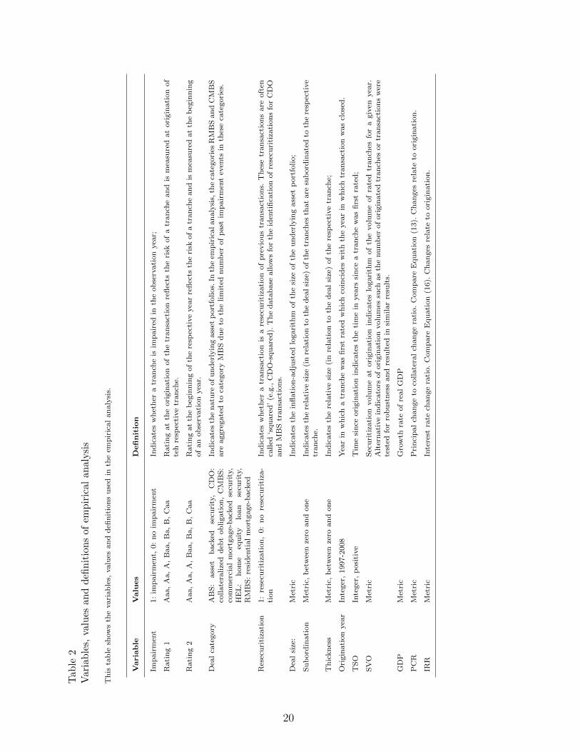
Table 2 describes the co-variables used in the empirical analysis. The table is consistent with

Figure 1.

18 Compare Footnote 3.

18

Tab

le1

Ori

gin

atio

nvo

lum

e,ou

tsta

nd

ing

volu

me

and

CR

Ast

ruct

ure

dfi

nan

cefe

ere

venu

e,va

riou

sca

tego

ries

Th

ista

ble

show

sth

eO

rigin

ati

on

volu

me,

ou

tsta

nd

ing

volu

me

an

dst

ruct

ure

dfi

nan

cefe

ere

ven

ue

of

the

CR

AM

ood

y’s

Inves

tors

Ser

vic

e.O

rigin

ati

on

nu

mb

ers

rela

teto

the

yea

rst

art

ing

from

the

tim

eth

at

ara

tin

gw

as

firs

tass

ign

ed.

Ori

gin

ati

on

nu

mb

ers

have

incr

ease

dp

rior

toth

eG

FC

an

dd

ecre

ase

dd

uri

ng

the

GF

C.

Ou

tsta

nd

ing

nu

mb

ers

rela

teto

issu

esw

hic

hare

rate

dat

the

beg

inn

ing

of

the

yea

ran

dh

ence

ori

gin

ate

din

pri

or

yea

rs.

Ou

tsta

nd

ing

nu

mb

ers

have

incr

ease

dd

uri

ng

the

wh

ole

ob

serv

ati

on

per

iod

.S

Fst

an

ds

for

stru

ctu

red

fin

an

ce(s

ecu

riti

zati

on

)ra

tin

gre

ven

ues

an

dP

PI

stan

dfo

rP

ub

lic,

Pro

ject

&In

frast

ruct

ure

rati

ng

reven

ues

.S

Fra

tin

gfe

ere

ven

ues

have

incr

ease

dp

rior

toth

eG

FC

an

dd

ecre

ase

dd

uri

ng

the

GF

C.

Ori

gin

ati

on

volu

me

Ou

tsta

nd

ing

volu

me

CR

Afe

ere

ven

ue

(in$

m)

Yea

rT

ran

ches

Dea

lsV

olu

me

(in$

bn

)T

ran

ches

Dea

lsV

olu

me

(in$

bn

)S

FC

orp

ora

teF

inan

cials

PP

I

1997

2,7

04

582

243

10,9

57

2,9

58

959

1998

2,5

01

559

269

12,8

39

3,3

60

1,1

30

143

144

90

65

1999

2,6

65

574

271

13,8

55

3,7

02

1,2

98

172

166

105

60

2000

2,6

74

582

302

14,9

41

3,9

44

1,4

41

199

163

112

46

2001

4,5

33

761

402

16,3

09

4,1

93

1,5

79

274

226

131

64

2002

5,7

27

855

477

18,8

14

4,5

36

1,7

82

384

228

155

81

2003

6,7

83

1,0

14

537

21,4

16

4,8

88

2,0

12

475

267

181

87

2004

9,5

99

1,1

89

781

22,7

28

5,0

65

2,2

02

553

300

209

82

2005

16,5

97

1,6

17

1,3

01

28,3

02

5,4

38

2,5

65

709

277

214

185

2006

19,9

29

1,8

27

1,4

91

41,2

47

6,3

12

3,4

01

873

336

233

198

2007

12,9

58

1,4

05

1,1

26

57,6

61

7,5

11

4,3

80

873

412

274

221

2008

1,0

14

231

199

66,3

74

8,4

53

5,0

67

411

301

263

230

Tota

l87,6

84

11,1

96

7,3

99

325,4

43

60,3

60

27,8

16

5,0

66

2,8

17

1,9

67

1,3

19

19

Tab

le2

Var

iab

les,

valu

esan

dd

efin

itio

ns

ofem

pir

ical

anal

ysi

s

Th

ista

ble

show

sth

evari

ab

les,

valu

esan

ddefi

nit

ion

su

sed

inth

eem

pir

ical

an

aly

sis.

Varia

ble

Valu

es

Defi

nit

ion

Imp

air

men

t1:

imp

air

men

t,0:

no

imp

air

men

tIn

dic

ate

sw

het

her

atr

an

che

isim

pair

edin

the

ob

serv

ati

on

yea

r;

Rati

ng

1A

aa,

Aa,

A,

Baa,

Ba,

B,

Caa

Rati

ng

at

the

ori

gin

ati

on

of

the

tran

sact

ion

refl

ects

the

risk

of

atr

an

che

an

dis

mea

sure

dat

ori

gin

ati

on

of

teh

resp

ecti

ve

tran

che.

Rati

ng

2A

aa,

Aa,

A,

Baa,

Ba,

B,

Caa

Rati

ng

at

the

beg

inn

ing

of

the

resp

ecti

ve

yea

rre

flec

tsth

eri

skof

atr

an

che

an

dis

mea

sure

dat

the

beg

inn

ing

of

an

ob

serv

ati

on

yea

r.

Dea

lca

tegory

AB

S:

ass

etb

ack

edse

curi

ty,

CD

O:

collate

ralize

dd

ebt

ob

ligati

on

,C

MB

S:

com

mer

cial

mort

gage-

back

edse

curi

ty,

HE

L:

hom

eeq

uit

ylo

an

secu

rity

,R

MB

S:

resi

den

tial

mort

gage-

back

ed

Ind

icate

sth

en

atu

reofu

nd

erly

ing

ass

etp

ort

folios.

Inth

eem

pir

icalan

aly

sis,

the

cate

gori

esR

MB

San

dC

MB

Sare

aggre

gate

dto

cate

gory

MB

Sd

ue

toth

elim

ited

nu

mb

erof

past

imp

air

men

tev

ents

inth

ese

cate

gori

es.

Res

ecu

riti

zati

on

1:

rese

curi

tiza

tion

,0:

no

rese

curi

tiza

-ti

on

Ind

icate

sw

het

her

atr

an

sact

ion

isa

rese

curi

tiza

tion

of

pre

vio

us

tran

sact

ion

s.T

hes

etr

an

sact

ion

sare

oft

enca

lled

‘squ

are

d’

(e.g

.,C

DO

-squ

are

d).

Th

ed

ata

base

allow

sfo

rth

eid

enti

fica

tion

of

rese

curi

tiza

tion

sfo

rC

DO

an

dM

BS

tran

sact

ion

s.

Dea

lsi

ze:

Met

ric

Ind

icate

sth

ein

flati

on

-ad

just

edlo

gari

thm

of

the

size

of

the

un

der

lyin

gass

etp

ort

folio;

Su

bord

inati

on

Met

ric,

bet

wee

nze

roan

don

eIn

dic

ate

sth

ere

lati

ve

size

(in

rela

tion

toth

ed

ealsi

ze)

of

the

tran

ches

that

are

sub

ord

inate

dto

the

resp

ecti

ve

tran

che.

Th

ickn

ess

Met

ric,

bet

wee

nze

roan

don

eIn

dic

ate

sth

ere

lati

ve

size

(in

rela

tion

toth

ed

eal

size

)of

the

resp

ecti

ve

tran

che;

Ori

gin

ati

on

yea

rIn

teger

,1997-2

008

Yea

rin

wh

ich

atr

an

che

was

firs

tra

ted

wh

ich

coin

cid

esw

ith

the

yea

rin

wh

ich

tran

sact

ion

was

close

d.

TS

OIn

teger

,p

osi

tive

Tim

esi

nce

ori

gin

ati

on

ind

icate

sth

eti

me

inyea

rssi

nce

atr

an

che

was

firs

tra

ted

;

SV

OM

etri

cS

ecu

riti

zati

on

volu

me

at

ori

gin

ati

on

ind

icate

slo

gari

thm

of

the

volu

me

of

rate

dtr

an

ches

for

agiv

enyea

r.A

lter

nati

ve

indic

ato

rsof

ori

gin

ati

on

volu

mes

such

as

the

nu

mb

erof

ori

gin

ate

dtr

an

ches

or

tran

sact

ion

sw

ere

test

edfo

rro

bu

stn

ess

an

dre

sult

edin

sim

ilar

resu

lts.

GD

PM

etri

cG

row

thra

teof

real

GD

P

PC

RM

etri

cP

rin

cip

al

chan

ge

toco

llate

ral

chan

ge

rati

o.

Com

pare

Equ

ati

on

(13).

Ch

an

ges

rela

teto

ori

gin

ati

on

.

IRR

Met

ric

Inte

rest

rate

chan

ge

rati

o.

Com

pare

Equ

ati

on

(16).

Ch

an

ges

rela

teto

ori

gin

ati

on

.

20

Table 3 and Table 4 describe the number of observations over time. The overall number of

rated securitizations has increased at an increasing rate over time. 19

Table 3 shows the relative frequency of rating categories at origination (Panel A) and at

the beginning of the observation year (Panel B). In both Panels, the average rating quality

deteriorates over time as the relative frequency of the rating category Aaa declined. This may

reflect i) a deterioration of the average asset portfolio quality, ii) a higher average risk level

induced by the securitization structure (e.g., subordination or thickness), or iii) a change of

the CRA rating methodology. 20

Table 4 shows the relative frequency of asset portfolio (Panel A) and securitization char-

acteristics (Panel B). Asset portfolio characteristics are the asset portfolio category, the

resecuritization status and the asset portfolio size. The asset portfolio categories are asset

backed security (ABS), collateralized debt obligation (CDO), commercial mortgage-backed

security (CMBS), home equity loan security (HEL) and residential mortgage-backed security

(RMBS). The asset portfolio size is categorized into Small (asset portfolio size less than or

equal to $500 million), Medium (asset portfolio size greater than $500 million and less than

or equal to $1,000 million) and Big (asset portfolio size greater than $1,000 million).

The number of rated tranches has increased at an increasing rate. The relative frequency

of CDO and HEL has increased. The relative frequency of resecuritizations has generally

decreased. The inflation-adjusted asset portfolio size has increased.

Securitization characteristics are the subordination level, thickness and origination year. The

subordination level Junior indicates that a tranche attaches between 0% and 5%, Mezzanine

indicates that a tranche attaches between 5% and 30% and Senior indicates that a tranche

attaches between 30% and 100%.

The relative frequency of mezzanine and thin tranches has increased while the relative fre-

quency of the various origination years (OY) depends on the origination as well as the

maturity and impairment of securitizations.

Generally speaking, the validation of credit ratings is complicated as the use of ratings

involves two steps: firstly the ordinal assessments of the financial risk of issuers or issues by

19 All tables weight individual transactions equally and the findings are robust for the value ofsecuritizations.20 This finding is consistent with Ashcraft et al. (2009) who analyze AAA fractions for MBS andHEL securities over time.

21

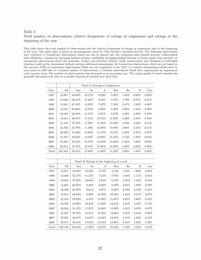
Table 3Total number of observations, relative frequencies of ratings at origination and ratings at thebeginning of the year

This table shows the total number of observations and the relative frequencies of ratings at origination and at the beginningof the year. The panel data is based on securitizations rated by CRA Moody’s Investors Service. The following observationswere excluded: i) transaction observations which can not be placed into the categories asset-backed security, collateralizeddebt obligation, commercial mortgage-backed security, residential mortgage-backed security or home equity loan security; ii)transaction observations where the monetary volume and therefore relative credit enhancement and thickness of individualtranches could not be determined without setting additional assumptions; iii) transaction observations which are not based onthe currency USD or transaction observations which are not originated in the USA; iv) tranche observations which relate toyears prior to 1997 due to a limited number of observations, v) tranche observations which have experienced an impairmentevent in prior years. The number of rated tranches has increased at an increasing rate. The rating quality of rated tranches hasgenerally decreased over time as a smaller fraction of tranches are rated Aaa.

Panel A: Rating at Origination

Year All Aaa Aa A Baa Ba B Caa

1997 10,957 69.66% 16.72% 6.20% 5.04% 1.58% 0.80% 0.00%

1998 12,839 69.41% 15.02% 6.82% 5.97% 1.79% 0.97% 0.01%

1999 13,855 67.10% 13.95% 7.87% 7.28% 2.41% 1.34% 0.04%

2000 14,941 64.86% 12.76% 8.96% 8.49% 3.00% 1.84% 0.09%

2001 16,309 62.50% 12.17% 9.91% 9.67% 3.59% 2.06% 0.10%

2002 18,814 60.31% 11.45% 10.73% 11.04% 4.26% 2.10% 0.10%

2003 21,416 57.49% 11.26% 11.95% 12.16% 4.70% 2.32% 0.11%

2004 22,728 53.78% 11.39% 13.38% 13.89% 4.90% 2.55% 0.11%

2005 28,302 51.08% 12.06% 14.12% 15.21% 4.98% 2.47% 0.07%

2006 41,247 50.04% 13.48% 13.88% 15.43% 5.14% 1.99% 0.04%

2007 57,661 47.43% 15.07% 14.48% 15.86% 5.46% 1.66% 0.03%

2008 66,374 47.25% 16.18% 14.38% 14.89% 4.99% 2.02% 0.29%

Total 325,443 58.41% 13.46% 11.06% 11.25% 3.90% 1.84% 0.08%

Panel B: Rating at the beginning of a year

Year All Aaa Aa A Baa Ba B Caa

1997 10,957 72.09% 13.50% 6.74% 4.74% 1.93% 1.00% 0.00%

1998 12,839 72.57% 11.37% 7.24% 5.76% 1.94% 1.11% 0.01%

1999 13,855 70.70% 10.04% 8.05% 6.79% 2.79% 1.52% 0.10%

2000 14,941 68.04% 9.46% 9.02% 8.33% 2.94% 1.93% 0.28%

2001 16,309 65.95% 9.01% 9.97% 8.92% 3.78% 2.13% 0.25%

2002 18,814 63.03% 9.00% 10.76% 10.28% 4.44% 2.21% 0.27%

2003 21,416 58.92% 9.51% 11.88% 11.67% 4.89% 2.68% 0.44%

2004 22,728 53.96% 10.35% 13.20% 13.21% 5.31% 3.24% 0.74%

2005 28,302 51.24% 11.25% 13.86% 14.39% 5.34% 3.05% 0.87%

2006 41,247 50.70% 12.81% 13.56% 14.66% 5.31% 2.34% 0.62%

2007 57,661 48.61% 14.61% 14.00% 14.91% 5.51% 1.93% 0.44%

2008 66,374 48.23% 15.63% 12.12% 12.68% 6.16% 3.89% 1.29%

Total 325,443 60.34% 11.38% 10.87% 10.53% 4.19% 2.25% 0.44%

22

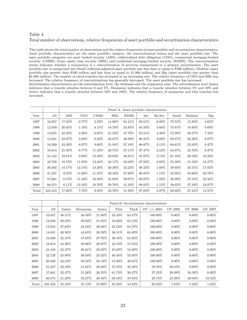
Table 4Total number of observations, relative frequencies of asset portfolio and securitization characteristics

This table shows the total number of observations and the relative frequencies of asset portfolio and securitization characteristics.Asset portfolio characteristics are the asset portfolio category, the resecuritization status and the asset portfolio size. Theasset portfolio categories are asset backed security (ABS), collateralized debt obligation (CDO), commercial mortgage-backedsecurity (CMBS), home equity loan security (HEL) and residential mortgage-backed security (RMBS). The resecuritizationstatus indicates whether a transaction is a resecuritization of previous transactions or a primary securitization. The assetportfolio size is categorized into Small (inflation-adjusted asset portfolio size less than or equal to $500 million), Medium (assetportfolio size greater than $500 million and less than or equal to $1,000 million) and Big (asset portfolio size greater than$1,000 million). The number of rated tranches has increased at an increasing rate. The relative frequency of CDO and HEL hasincreased. The relative frequency of resecuritizations has generally decreased. The asset portfolio size has increased.Securitization characteristics are the subordination level, the thickness and the origination year. The subordination level Juniorindicates that a tranche attaches between 0 and 5%, Mezzanine indicates that a tranche attaches between 5% and 30% andSenior indicates that a tranche attaches between 30% and 100%. The relative frequency of mezzanine and thin tranches hasincreased.

Panel A: Asset portfolio characteristics

Year All ABS CDO CMBS HEL RMBS Sec. Re-Sec. Small Medium Big

1997 10,957 17.03% 0.77% 2.92% 14.88% 64.41% 93.01% 6.99% 79.55% 15.80% 4.65%

1998 12,839 20.05% 1.16% 4.15% 18.70% 55.94% 94.34% 5.66% 75.91% 18.40% 5.69%

1999 13,855 22.29% 2.36% 6.05% 21.52% 47.78% 95.51% 4.49% 72.39% 20.27% 7.34%

2000 14,941 23.97% 4.69% 8.28% 22.07% 40.99% 96.31% 3.69% 69.47% 22.46% 8.07%

2001 16,309 24.29% 6.97% 9.60% 21.94% 37.19% 96.87% 3.13% 68.61% 22.92% 8.47%

2002 18,814 21.95% 8.77% 11.43% 20.75% 37.11% 97.47% 2.53% 64.87% 25.76% 9.37%

2003 21,416 19.91% 9.96% 12.49% 20.83% 36.81% 97.87% 2.13% 61.16% 28.52% 10.32%

2004 22,728 18.73% 11.83% 13.24% 24.17% 32.03% 97.95% 2.05% 55.39% 31.34% 13.27%

2005 28,302 14.17% 12.14% 13.20% 28.26% 32.23% 98.32% 1.68% 49.68% 33.31% 17.02%

2006 41,247 9.53% 11.00% 11.35% 30.42% 37.69% 98.85% 1.15% 43.58% 35.66% 20.76%

2007 57,661 6.75% 11.40% 10.38% 31.80% 39.67% 98.97% 1.03% 39.99% 37.45% 22.56%

2008 66,374 6.11% 12.10% 10.70% 29.76% 41.33% 98.85% 1.15% 39.65% 37.29% 23.07%

Total 325,443 17.06% 7.76% 9.48% 23.76% 41.93% 97.03% 2.97% 60.02% 27.43% 12.55%

Panel B: Securitization characteristics

Year All Junior Mezzanine Senior Thin Thick OY <= 2004 OY 2005 OY 2006 OY 2007

1997 10,957 30.51% 38.49% 31.00% 35.43% 64.57% 100.00% 0.00% 0.00% 0.00%

1998 12,839 28.23% 39.82% 31.95% 34.88% 65.12% 100.00% 0.00% 0.00% 0.00%

1999 13,855 27.82% 42.24% 29.94% 35.22% 64.78% 100.00% 0.00% 0.00% 0.00%

2000 14,941 26.56% 44.85% 28.59% 36.51% 63.49% 100.00% 0.00% 0.00% 0.00%

2001 16,309 25.19% 47.05% 27.76% 38.18% 61.82% 100.00% 0.00% 0.00% 0.00%

2002 18,814 24.26% 48.86% 26.87% 42.18% 57.82% 100.00% 0.00% 0.00% 0.00%

2003 21,416 24.47% 49.61% 25.92% 45.60% 54.40% 100.00% 0.00% 0.00% 0.00%

2004 22,728 24.98% 49.50% 25.52% 46.44% 53.56% 100.00% 0.00% 0.00% 0.00%

2005 28,302 24.24% 50.58% 25.19% 51.09% 48.91% 100.00% 0.00% 0.00% 0.00%

2006 41,247 22.10% 51.01% 26.89% 57.52% 42.48% 59.76% 40.24% 0.00% 0.00%

2007 57,661 22.47% 51.28% 26.25% 61.73% 38.27% 37.35% 28.09% 34.56% 0.00%

2008 66,374 21.28% 52.27% 26.44% 62.16% 37.84% 29.14% 23.29% 28.04% 19.52%

Total 325,443 25.18% 47.13% 27.69% 45.58% 54.42% 85.52% 7.64% 5.22% 1.63%

23

CRAs and secondly the calibration of these ordinal ratings to metric credit risk measures such

as default rates, loss rates given default or unconditional loss rates. This calibration step is

generally opaque and investors rely on impairment rate tables which are periodically updated

by CRAs. These tables are generally univariate and aggregate over various dimensions. The

data set enables the estimation of impairment risk based on the most detailed information

level, i.e., the individual transaction in a given observation year. Table 5 and Table 6 show

the impairment rates over time for all tranches as well as per rating category, asset portfolio

and securitization characteristics.

US securitizations have experienced two economic downturns during the observation period:

the first one in 2002 subsequent to the US terrorist attacks (a period characterized by large

bankruptcies such as Enron, WorldCom and various US airlines) and the Global Financial

Crisis. With regard to the GFC, the impairment rate has increased by a factor of approxi-

mately 80 within two years between 2006 and 2008. Approximately 81% of all impairment

events relate to 2008. 21

Table 5 shows the impairment rates for rating categories at origination (Panel A) and at the

beginning of the observation year (Panel B). In both Panels, the impairment rate increases

for lower rating categories (i.e., from rating Aaa-A to rating Caa) and fluctuates over time

with a dramatic increase during the GFC for all rating classes. The relative increase de-

creases during the GFC with the rating quality (i.e., from rating Caa to rating Aaa-A). 22

Ironically, investors were most surprised by the increase of impairment rates of highly rated

securitizations.

Table 6 shows the impairment rates for asset portfolio (Panel A) and securitization char-

acteristics (Panel B). Impairment rates are high in 2002 and 2007/2008. Impairment rates

per rating category fluctuate over time. Impairment rates per asset portfolio type increased

in 2002 for CDOs and in 2008 especially for CDOs, MBSs and HELs. HELs include sub-

prime mortgage loans and the impairment risk increased to a larger degree than the one of

21 This number underlines the severity of the GFC and the importance of this study. However,it also raises the concern of imbalances in the data set. We address the issue of robustness by i)controlling for rating years, ii) analyzing the data for the period prior to the GFC and the GFCand iii) focusing on relative differences within these controlled environments.22 Please note that inconsistencies may reflect the accuracy as well as the stochastic nature ofimpairment events. The latter is particularly relevant if the number of observations is low for agiven category. One example is the impairment rate for the rating classes Ba (16.49%) and B(4.68%) in 2007 in Panel B of Table 5 as one would expect the impairment rate of rating Ba tobe lower than rating B. These inconsistencies are in line with reports by the data-providing CRA(compare Moody’s Investors Service 2008).

24

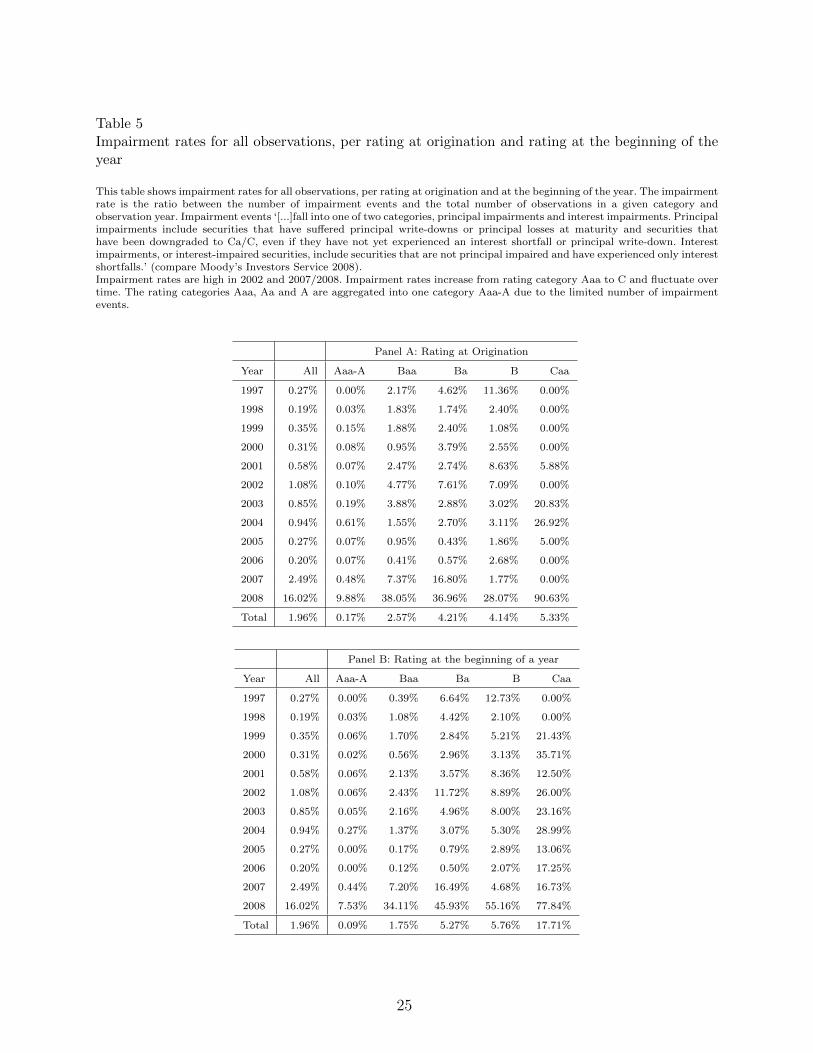
Table 5Impairment rates for all observations, per rating at origination and rating at the beginning of theyear

This table shows impairment rates for all observations, per rating at origination and at the beginning of the year. The impairmentrate is the ratio between the number of impairment events and the total number of observations in a given category andobservation year. Impairment events ‘[...]fall into one of two categories, principal impairments and interest impairments. Principalimpairments include securities that have suffered principal write-downs or principal losses at maturity and securities thathave been downgraded to Ca/C, even if they have not yet experienced an interest shortfall or principal write-down. Interestimpairments, or interest-impaired securities, include securities that are not principal impaired and have experienced only interestshortfalls.’ (compare Moody’s Investors Service 2008).Impairment rates are high in 2002 and 2007/2008. Impairment rates increase from rating category Aaa to C and fluctuate overtime. The rating categories Aaa, Aa and A are aggregated into one category Aaa-A due to the limited number of impairmentevents.

Panel A: Rating at Origination

Year All Aaa-A Baa Ba B Caa

1997 0.27% 0.00% 2.17% 4.62% 11.36% 0.00%

1998 0.19% 0.03% 1.83% 1.74% 2.40% 0.00%

1999 0.35% 0.15% 1.88% 2.40% 1.08% 0.00%

2000 0.31% 0.08% 0.95% 3.79% 2.55% 0.00%

2001 0.58% 0.07% 2.47% 2.74% 8.63% 5.88%

2002 1.08% 0.10% 4.77% 7.61% 7.09% 0.00%

2003 0.85% 0.19% 3.88% 2.88% 3.02% 20.83%

2004 0.94% 0.61% 1.55% 2.70% 3.11% 26.92%

2005 0.27% 0.07% 0.95% 0.43% 1.86% 5.00%

2006 0.20% 0.07% 0.41% 0.57% 2.68% 0.00%

2007 2.49% 0.48% 7.37% 16.80% 1.77% 0.00%

2008 16.02% 9.88% 38.05% 36.96% 28.07% 90.63%

Total 1.96% 0.17% 2.57% 4.21% 4.14% 5.33%

Panel B: Rating at the beginning of a year

Year All Aaa-A Baa Ba B Caa

1997 0.27% 0.00% 0.39% 6.64% 12.73% 0.00%

1998 0.19% 0.03% 1.08% 4.42% 2.10% 0.00%

1999 0.35% 0.06% 1.70% 2.84% 5.21% 21.43%

2000 0.31% 0.02% 0.56% 2.96% 3.13% 35.71%

2001 0.58% 0.06% 2.13% 3.57% 8.36% 12.50%

2002 1.08% 0.06% 2.43% 11.72% 8.89% 26.00%

2003 0.85% 0.05% 2.16% 4.96% 8.00% 23.16%

2004 0.94% 0.27% 1.37% 3.07% 5.30% 28.99%

2005 0.27% 0.00% 0.17% 0.79% 2.89% 13.06%

2006 0.20% 0.00% 0.12% 0.50% 2.07% 17.25%

2007 2.49% 0.44% 7.20% 16.49% 4.68% 16.73%

2008 16.02% 7.53% 34.11% 45.93% 55.16% 77.84%

Total 1.96% 0.09% 1.75% 5.27% 5.76% 17.71%

25

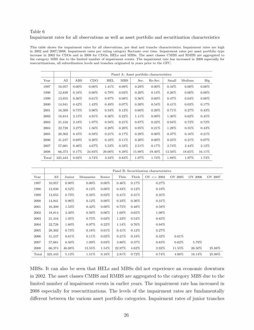
Table 6Impairment rates for all observations as well as asset portfolio and securitization characteristics

This table shows the impairment rates for all observations, per deal and tranche characteristics. Impairment rates are highin 2002 and 2007/2008. Impairment rates per rating category fluctuate over time. Impairment rates per asset portfolio typeincrease in 2002 for CDOs and in 2008 for CDOs, HELs and MBSs. The asset classes CMBS and RMBS are aggregated tothe category MBS due to the limited number of impairment events. The impairment rate has increased in 2008 especially forresecuritizations, all subordination levels and tranches originated in years prior to the GFC.

Panel A: Asset portfolio characteristics

Year All ABS CDO HEL MBS Sec. Re-Sec. Small Medium Big

1997 10,957 0.00% 0.00% 1.41% 0.09% 0.29% 0.00% 0.34% 0.00% 0.00%

1998 12,839 0.16% 0.00% 0.79% 0.03% 0.20% 0.14% 0.26% 0.00% 0.00%

1999 13,855 0.36% 0.61% 0.97% 0.08% 0.36% 0.00% 0.47% 0.04% 0.00%

2000 14,941 0.42% 1.43% 0.49% 0.07% 0.30% 0.54% 0.41% 0.03% 0.17%

2001 16,309 0.73% 3.96% 0.34% 0.12% 0.60% 0.20% 0.71% 0.27% 0.43%

2002 18,814 2.15% 4.91% 0.36% 0.22% 1.11% 0.00% 1.36% 0.62% 0.45%

2003 21,416 2.18% 1.97% 0.58% 0.21% 0.87% 0.22% 0.94% 0.72% 0.72%

2004 22,728 3.27% 1.56% 0.20% 0.20% 0.95% 0.21% 1.28% 0.55% 0.43%

2005 28,302 0.45% 0.58% 0.21% 0.17% 0.28% 0.00% 0.37% 0.16% 0.21%

2006 41,247 0.69% 0.26% 0.16% 0.11% 0.20% 0.00% 0.25% 0.21% 0.07%

2007 57,661 0.46% 4.67% 5.53% 0.33% 2.51% 0.17% 2.74% 2.44% 2.12%

2008 66,374 0.17% 24.93% 29.00% 8.39% 15.98% 19.40% 13.50% 18.65% 16.11%

Total 325,443 0.92% 3.74% 3.34% 0.83% 1.97% 1.74% 1.89% 1.97% 1.73%

Panel B: Securitization characteristics

Year All Junior Mezzanine Senior Thin Thick OY <= 2004 OY 2005 OY 2006 OY 2007

1997 10,957 0.90% 0.00% 0.00% 0.46% 0.17% 0.27%

1998 12,839 0.52% 0.12% 0.00% 0.33% 0.12% 0.19%

1999 13,855 0.73% 0.32% 0.02% 0.41% 0.31% 0.35%

2000 14,941 0.96% 0.12% 0.00% 0.33% 0.30% 0.31%

2001 16,309 1.53% 0.42% 0.00% 0.75% 0.48% 0.58%

2002 18,814 3.40% 0.50% 0.06% 1.68% 0.65% 1.08%

2003 21,416 1.95% 0.75% 0.02% 1.23% 0.54% 0.85%

2004 22,728 1.60% 0.97% 0.22% 1.14% 0.76% 0.94%

2005 28,302 0.73% 0.18% 0.01% 0.41% 0.12% 0.27%

2006 41,247 0.61% 0.11% 0.02% 0.21% 0.18% 0.32% 0.01%

2007 57,661 8.56% 1.09% 0.03% 3.80% 0.37% 0.83% 0.62% 5.79%

2008 66,374 40.08% 13.55% 1.54% 22.97% 4.62% 2.92% 11.55% 26.50% 25.88%

Total 325,443 5.13% 1.51% 0.16% 2.81% 0.72% 0.74% 4.06% 16.14% 25.88%

MBSs. It can also be seen that HELs and MBSs did not experience an economic downturn

in 2002. The asset classes CMBS and RMBS are aggregated to the category MBS due to the

limited number of impairment events in earlier years. The impairment rate has increased in

2008 especially for resecuritizations. The levels of the impairment rates are fundamentally

different between the various asset portfolio categories. Impairment rates of junior tranches

26

increased to a greater degree than impairment rates of senior tranches. Impairment rates of

thin tranches increased more than impairment rates of thick tranches and the ones of more

recent vintage (with regard to the GFC) more so than the ones of older vintage. This result is

consistent with findings by Demyanyk & Hemert (2009) for securitized sub-prime mortgage

loans and Ashcraft et al. (2009) for mortgage-backed securities.

3.2 H1 – Impairment Risk Hypotheses

Table 7 presents Probit models linking the impairment events with CRA ratings. Model 1

takes the dummy-coded ratings (reference category: Aaa-A) into account. As measures for in-

sample accuracy of the models the Pseudo-R2, re-scaled R2, and the area under the receiver

operating characteristic curve (AUROC) are calculated (see Agresti 1984). 23 The parameter

estimates increase from rating Aaa-A to rating Caa and are significant. This demonstrates

that the ratings imply higher impairment risk from Aaa to Caa as one would expect. Model

1 shows that CRA ratings explain the credit risk.

Model 2 includes the ratings as well as the dummy-coded rating years (reference category:

1997). The rating years are significant which implies that the realized impairment rates dif-

fer between the years. This has been pointed out by previous studies on corporate ratings

(compare e.g., Loeffler 2004) which conclude that ratings average the risk over the business

cycle. 24 In other words, Model 2 shows that CRA ratings do not explain the increased level

of impairment risk especially during economic downturns. This might be due to omitted

macroeconomic factors in the credit rating or due to unexpected and unpredictable system-

atic random shocks in the year following the rating. If an explanatory variable is correlated

with the systematic risk, it might be possible to obtain results, which are spuriously signifi-

cant and capture the economy in the observation year partially. Therefore, we include rating

year fixed effects in all subsequent models.

In addition, we include various macroeconomic variables and find that the results are robust

with regard to these control variables. Therefore, Model 3 includes the growth rate of real

GDP as a proxy for the US economy. The impact is highly significant and and GDP growth

and impairment risk are negatively related.

In Table 8 we additionally include asset portfolio characteristics (Model 4, 6, 7 and 8) such as

23 All measures are bounded between zero (lowest fit) and one (highest fit).24 Such models are also known as through-the-cycle models.

27

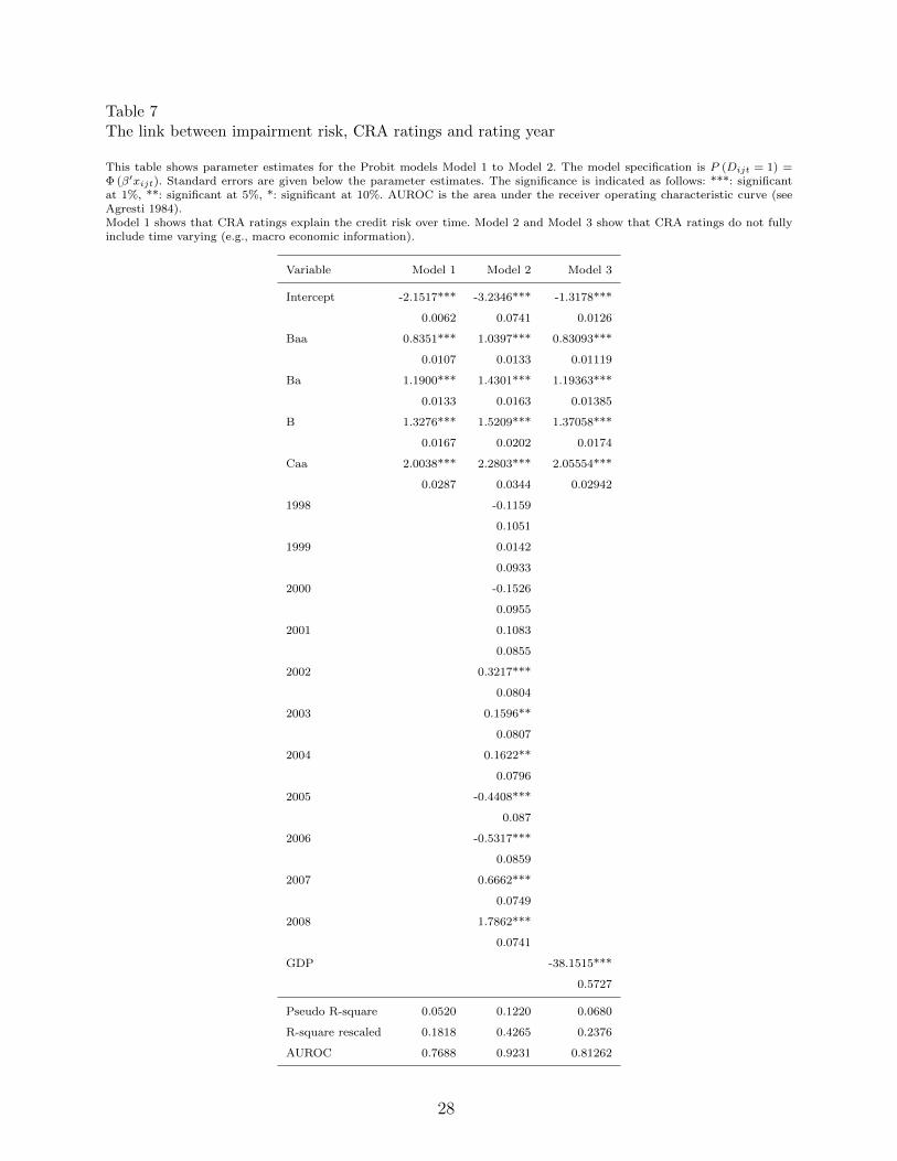
Table 7The link between impairment risk, CRA ratings and rating year

This table shows parameter estimates for the Probit models Model 1 to Model 2. The model specification is P (Dijt = 1) =Φ (β′xijt). Standard errors are given below the parameter estimates. The significance is indicated as follows: ***: significantat 1%, **: significant at 5%, *: significant at 10%. AUROC is the area under the receiver operating characteristic curve (seeAgresti 1984).Model 1 shows that CRA ratings explain the credit risk over time. Model 2 and Model 3 show that CRA ratings do not fullyinclude time varying (e.g., macro economic information).

Variable Model 1 Model 2 Model 3

Intercept -2.1517*** -3.2346*** -1.3178***

0.0062 0.0741 0.0126

Baa 0.8351*** 1.0397*** 0.83093***

0.0107 0.0133 0.01119

Ba 1.1900*** 1.4301*** 1.19363***

0.0133 0.0163 0.01385

B 1.3276*** 1.5209*** 1.37058***

0.0167 0.0202 0.0174

Caa 2.0038*** 2.2803*** 2.05554***

0.0287 0.0344 0.02942

1998 -0.1159

0.1051

1999 0.0142

0.0933

2000 -0.1526

0.0955

2001 0.1083

0.0855

2002 0.3217***

0.0804

2003 0.1596**

0.0807

2004 0.1622**

0.0796

2005 -0.4408***

0.087

2006 -0.5317***

0.0859

2007 0.6662***

0.0749

2008 1.7862***

0.0741

GDP -38.1515***

0.5727

Pseudo R-square 0.0520 0.1220 0.0680

R-square rescaled 0.1818 0.4265 0.2376

AUROC 0.7688 0.9231 0.81262

28

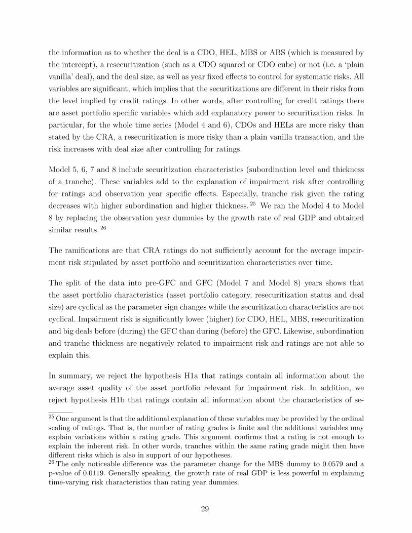
the information as to whether the deal is a CDO, HEL, MBS or ABS (which is measured by

the intercept), a resecuritization (such as a CDO squared or CDO cube) or not (i.e. a ‘plain

vanilla’ deal), and the deal size, as well as year fixed effects to control for systematic risks. All

variables are significant, which implies that the securitizations are different in their risks from

the level implied by credit ratings. In other words, after controlling for credit ratings there

are asset portfolio specific variables which add explanatory power to securitization risks. In

particular, for the whole time series (Model 4 and 6), CDOs and HELs are more risky than

stated by the CRA, a resecuritization is more risky than a plain vanilla transaction, and the

risk increases with deal size after controlling for ratings.

Model 5, 6, 7 and 8 include securitization characteristics (subordination level and thickness

of a tranche). These variables add to the explanation of impairment risk after controlling

for ratings and observation year specific effects. Especially, tranche risk given the rating

decreases with higher subordination and higher thickness. 25 We ran the Model 4 to Model

8 by replacing the observation year dummies by the growth rate of real GDP and obtained

similar results. 26

The ramifications are that CRA ratings do not sufficiently account for the average impair-

ment risk stipulated by asset portfolio and securitization characteristics over time.

The split of the data into pre-GFC and GFC (Model 7 and Model 8) years shows that

the asset portfolio characteristics (asset portfolio category, resecuritization status and deal

size) are cyclical as the parameter sign changes while the securitization characteristics are not

cyclical. Impairment risk is significantly lower (higher) for CDO, HEL, MBS, resecuritization

and big deals before (during) the GFC than during (before) the GFC. Likewise, subordination

and tranche thickness are negatively related to impairment risk and ratings are not able to

explain this.

In summary, we reject the hypothesis H1a that ratings contain all information about the

average asset quality of the asset portfolio relevant for impairment risk. In addition, we

reject hypothesis H1b that ratings contain all information about the characteristics of se-

25 One argument is that the additional explanation of these variables may be provided by the ordinalscaling of ratings. That is, the number of rating grades is finite and the additional variables mayexplain variations within a rating grade. This argument confirms that a rating is not enough toexplain the inherent risk. In other words, tranches within the same rating grade might then havedifferent risks which is also in support of our hypotheses.26 The only noticeable difference was the parameter change for the MBS dummy to 0.0579 and ap-value of 0.0119. Generally speaking, the growth rate of real GDP is less powerful in explainingtime-varying risk characteristics than rating year dummies.

29

Table 8The link between impairment risk, CRA ratings, asset portfolio and securitization characteristics,with rating year fixed effects

This table shows parameter estimates for the Probit model Model 4 to Model 8. The model specification is P (Dijt = 1) =Φ (β′xijt). Standard errors are given below the parameter estimates. The significance is indicated as follows: ***: significantat 1%, **: significant at 5%, *: significant at 10%. AUROC is the area under the receiver operating characteristic curve (seeAgresti 1984).The inclusion of asset portfolio (Model 4 and 6) and securitization (Model 5 and 6) characteristics after controlling for creditrating and rating year explains impairment risk. The ramifications are that CRA ratings do not sufficiently account for theimpairment risk stipulated by asset portfolio and securitization characteristics for given rating years. The division of the datainto pre-GFC and GFC years shows that the asset portfolio characteristics (asset portfolio category, resecuritization status anddeal size) are cyclical as the parameter sign changes while the securitization characteristics are not cyclical. CRAs are unableto measure both relationships.

Variable Model 4 Model 5 Model 6 Model 7 (prior GFC) Model 8 (GFC)

Intercept -5.6417*** -2.8000*** -4.5874*** 0.2176*** -7.0547***

0.1575 0.0750 0.1694 0.3047 0.2006

Baa 0.9849*** 0.6949*** 0.5668*** 0.8263*** 0.5472***

0.0138 0.0143 0.0152 0.0481 0.0169

Ba 1.4267*** 1.0748*** 0.9934*** 1.4125*** 0.9244***

0.0170 0.0172 0.0183 0.0510 0.0208

B 1.6326*** 1.1510*** 1.2224*** 1.8561*** 1.0900***

0.0216 0.0212 0.0228 0.0558 0.0268

Caa 2.3478*** 1.9833*** 1.9779*** 2.5822*** 1.7801***

0.0365 0.0356 0.0382 0.0665 0.0495

CDO 0.5059*** 0.5925*** -0.3066*** 2.1625***

0.0263 0.0274 0.0428 0.0801

HEL 0.5885*** 0.4660*** -0.4728*** 1.9970***

0.0245 0.0252 0.0419 0.0789

MBS -0.2606*** -0.4380*** -1.1824*** 1.0394***

0.0253 0.0262 0.0475 0.0791

Resecuritisation 0.2355*** 0.3450*** -0.0909 0.3954***

0.0528 0.0561 0.1530 0.0634

Deal size 0.1220*** 0.0994*** -0.1383*** 0.1657***

0.0071 0.0077 0.0151 0.0090

Subordination -2.6234*** -3.4892*** -1.4095*** -4.0653***

0.0602 0.0792 0.1708 0.0935

Thickness -0.5138*** -0.6260*** -0.5851*** -0.5317***

0.0388 0.0454 0.0893 0.0538

Year Dummies Yes Yes Yes Yes Yes

Pseudo R-square 0.1355 0.1328 0.1476 0.0246 0.2231

R-square rescaled 0.4735 0.4643 0.5159 0.4048 0.4729

AUROC 0.9427 0.9416 0.9540 0.9507 0.9171

curitizations relevant for impairment risk. CRAs do not take all available asset portfolio

and securitization information into account, which is relevant for explaining impairment

risk. Important ramifications are that i) CRAs may have to include such characteristics into

the rating models or ii) users such as investors or prudential regulators should apply asset

30

portfolio specific impairment rates to ratings when interpreting CRA ratings.

31

3.3 H2 – Agency Incentive Hypotheses

Figure 1 provides empirical evidence that CRAs collect the majority of fee revenue at origina-

tion. Commercial CRAs may have a monetary incentive to bias the measures of impairment

risk to generate fee revenue, which is tied to the origination rather than the monitoring

process of securitizations. Following this argumentation, the paper compares ratings at orig-

ination with ratings at monitoring years as well as other macroeconomic conditions repre-

sented by the securitization volume at origination. The analyzed incentive hypotheses test

whether a CRA may underestimate the risk in general at origination (as fee revenue is high

at origination) or during economic booms (as origination volumes and therefore fee revenue

is high during economic booms). 27

Please note that the panel data set looks at origination and monitoring years, i.e., years

between origination and maturity of securitizations. The impact of the vintage, i.e., the year

of origination is shown in Table 9. Model 9 shows the same parameter estimates as Model

2. Model 10 shows that the origination years (also known as vintages) differ in risk and that

ratings are unable to explain the risk of the different vintages.

Model 11 includes two variables which capture the strategic default of borrowers due to the

relation between outstanding loan amounts and loan repayment/service rates. The results

show that ratings do not reflect vintage risk (i.e., origination year dummies) in general and

strategic default characteristics in particular.

The two variables are constructed following Demyanyk et al. (2010) for every securitization,

origination and observation period. 28 Firstly, the principal collateral adjustment ratio (PCR)

is calculated, which accounts for changes in the outstanding loan amount as well as collateral

under the assumption of a fixed-rate asset portfolio:

PCRt =PV Rt

CV Rt

(13)

PV Rt is the principal value ratio of current to origination principal value: 29

27 Please note that Bolton et al. (2009) provide the complementary argument that investors arenaive and reputation risk is low.28 Please note that by including PVR (see below) we extend the approach by Demyanyk et al.(2010) by accounting for the loan amortization.29 As we have only access to legal maturities which are significantly longer than real maturity,we assume a loan maturity of 10 years. The results are robust with regard to variations in this

32

PV Rt =1−

(1

1+r0

)T−t1−

(1

1+r0

)T (14)

With 0 as the origination date, t the observation date and T the loan maturity date. The

loan maturity date is approximated by the median maturity of the respective loan portfolio.

r0 is the interest rate at origination and is approximated by the federal funds rate. 30

CV Rt is the collateral value ratio of current to origination real estate value proxied by the

Standard & Poor’s Case-Shiller 10 index (SPCS10):

CV Rt =CStCS0

(15)

SPCS10 is a composite index of the top 10 US metropolitan statistical areas. Other proxies

(asset indices) for the collateral value may exist. We chose the the Standard & Poor’s Case-

Shiller 10 index as the majority of securitizations are backed by mortgage portfolios.

In addition, we construct an interest rate ratio (IRR) to measure the serviceability of the

asset portfolio. IRR indicates the degree to which new or floating rate loans become more

serviceable due to interest changes:

IRRt =rtr0

(16)

PCR and IRR reflect changes in the underlying loans since origination which may change the

incentives of borrowers to strategically default on their loans in relation to the outstanding

loan amount to collateral value and the serviceability.

In order to test the hypotheses H2a and H2b, we replace the origination year fixed effects by

the time since origination (TSO) and the securitization volume at origination (SVO). TSO

is equal to one in the origination year and greater than one in monitoring years. 31

parameter.30 Please note that we also modeled the discount rate by the federal fund rate plus a lending spreadand confirmed the robustness of the results.31 High SVO indicates that a tranche was originated in a high securitization volume year (i.e.,especially 2002 and later). Low SVO indicates that a tranche was originated in a low securitizationvolume year (i.e., especially before 2002).

33

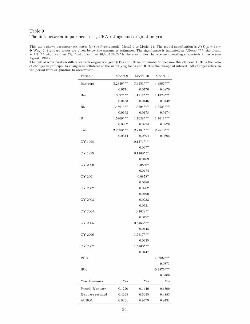
Table 9The link between impairment risk, CRA ratings and origination year

This table shows parameter estimates for the Probit model Model 9 to Model 11. The model specification is P (Dijt = 1) =Φ (β′xijt). Standard errors are given below the parameter estimates. The significance is indicated as follows: ***: significantat 1%, **: significant at 5%, *: significant at 10%. AUROC is the area under the receiver operating characteristic curve (seeAgresti 1984).The risk of securitization differs for each origination year (OY) and CRAs are unable to measure this element. PCR is the ratioof changes in principal to changes in collateral of the underlying loans and IRR is the change of interest. All changes relate tothe period from origination to observation.

Variable Model 9 Model 10 Model 11

Intercept -3.2346*** -3.3453*** -4.3966***

0.0741 0.0770 0.0879

Baa 1.0397*** 1.1717*** 1.1329***

0.0133 0.0146 0.0142

Ba 1.4301*** 1.5794*** 1.5525***

0.0163 0.0178 0.0174

B 1.5209*** 1.7628*** 1.7611***

0.0202 0.0224 0.0220

Caa 2.2803*** 2.7181*** 2.7570***

0.0344 0.0394 0.0395

OY 1998 0.1171***

0.0477

OY 1999 0.1160***

0.0469

OY 2000 0.0866*

0.0474

OY 2001 -0.0878*

0.0488

OY 2002 0.0282

0.0490

OY 2003 -0.0233

0.0521

OY 2004 0.1029**

0.0497

OY 2005 0.8465***

0.0445

OY 2006 1.5317***

0.0435

OY 2007 1.5700***

0.0447

PCR 1.5902***

0.0371

IRR -0.2879***

0.0106

Year Dummies Yes Yes Yes

Pseudo R-square 0.1220 0.1440 0.1399

R-square rescaled 0.4265 0.5035 0.4883

AUROC 0.9231 0.9479 0.9431

34

Table 10 shows that the negative parameter estimate (panel for all years) for the time since

origination (TSO) implies that the level of impairment risk (given the rating) decreases over

time. The relative fee revenue is high at origination and low thereafter. The implication is

that the impairment risk given ratings (i.e., which is not explained by ratings) decreases over

time. This confirms that CRAs may have an incentive to assign i) too low risk ratings in

origination years to increase fee revenue and ii) too high risk ratings in monitoring years to

maintain stable default and rating migration performance measures. The second and third

panel show that this effect is mainly driven by the occurrence of the GFC. In summary, we

reject the hypothesis H2a that rating-implied impairment risk and time since origination are

positively correlated.

35

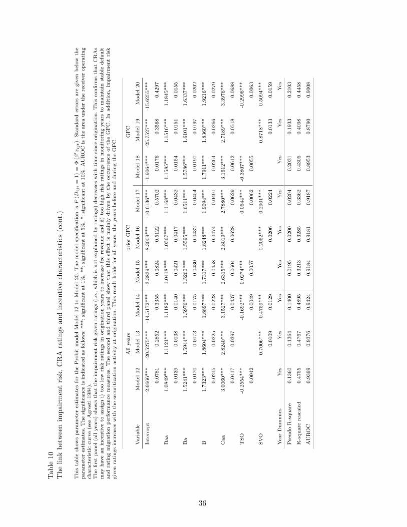
Tab

le10

Th

eli

nk

bet

wee

nim

pai

rmen

tri

sk,

CR

Ara

tin

gsan

din

centi

vech

arac

teri

stic

s(c

ont.

)

Th

ista

ble

show

sp

ara

met

eres

tim

ate

sfo

rth

eP

rob

itm

od

elM

od

el12

toM

od

el20.

Th

em

od

elsp

ecifi

cati

on

isP

(Dij

t=

1)

=Φ

(β′ x

ijt).

Sta

nd

ard

erro

rsare

giv

enb

elow

the

para

met

eres

tim

ate

s.T

he

sign

ifica

nce

isin

dic

ate

das

follow

s:***:

sign

ifica

nt

at

1%

,**:

sign

ifica

nt

at

5%

,*:

sign

ifica

nt

at

10%

.A

UR

OC

isth

eare

au

nd

erth

ere

ceiv

erop

erati

ng

chara

cter

isti

ccu

rve

(see

Agre

sti

1984).

Th

efi

rst

pan

el(a

llyea

rs)

show

sth

at

the

imp

air

men

tri

skgiv

enra

tin

gs

(i.e

.,w

hic

his

not

exp

lain

edby

rati

ngs)

dec

rease

sw

ith

tim

esi

nce

ori

gin

ati

on

.T

his

con

firm

sth

at

CR

As

may

have

an

ince

nti

ve

toass

ign

i)to

olo

wri

skra

tin

gs

inori

gin

ati

on

yea

rsto

incr

ease

fee

reven

ue

an

dii)

too

hig

hri

skra

tin

gs

inm

on

itori

ng

yea

rsto

main

tain

stab

led

efau

ltan

dra

tin

gm

igra

tion

per

form

an

cem

easu

res.

Th

ese

con

dan

dth

ird

pan

elsh

ow

that

this

effec

tis

main

lyd

riven

by

the

occ

urr

ence

of

the

GF

C.

Inad

dit

ion

,im

pair

men

tri

skgiv

enra

tin

gs

incr

ease

sw

ith

the

secu

riti

zati

on

act

ivit

yat

ori

gin

ati

on

.T

his

resu

lth

old

sfo

rall

yea

rs,

the

yea

rsb

efore

an

dd

uri

ng

the

GF

C.

All

yea

rsp

rior

GF

CG

FC

Vari

ab

leM

od

el12

Mod

el13

Mod

el14

Mod

el15

Mod

el16

Mod

el17

Model

18

Mod

el19

Mod

el20

Inte

rcep

t-2

.6666***

-20.5

275***

-14.5

172***

-3.3

839***

-8.3

009***

-10.6

136***

-1.9

064***

-25.7

527***

-15.6

255***

0.0

781

0.2

852

0.3

355

0.0

824

0.5

122

0.5

702

0.0

176

0.3

568

0.4

297

Baa

1.0

849***

1.1

121***

1.1

182***

1.0

418***

1.0

367***

1.1

168***

1.1

585***

1.1

516***

1.1

845***

0.0

139

0.0

138

0.0

140

0.0

421

0.0

417

0.0

432

0.0

154

0.0

151

0.0

155

Ba

1.5

241***

1.5

944***

1.5

976***

1.5

260***

1.5

595***

1.6

511***

1.5

786***

1.6

101***

1.6

337***

0.0

170

0.0

173

0.0

175

0.0

430

0.0

432

0.0

454

0.0

197

0.0

197

0.0

202

B1.7

323***

1.8

604***

1.8

897***

1.7

317***

1.8

248***

1.9

094***

1.7

911***

1.8

360***

1.9

216***

0.0

215

0.0

225

0.0

228

0.0

458

0.0

474

0.0

491

0.0

264

0.0

266

0.0

279

Caa

3.0

060***

2.8

240***

3.1

527***

2.6

315***

2.8

019***

2.7

880***

3.1

612***

2.7

189***

3.3

976***

0.0

417

0.0

397

0.0

437

0.0

604

0.0

628

0.0

629

0.0

612

0.0

518

0.0

688

TS

O-0

.2554***

-0.1

692***

0.0

274***

0.0

644***

-0.3

807***

-0.2

996***

0.0

042

0.0

049

0.0

057

0.0

062

0.0

055

0.0

063

SV

O0.7

006***

0.4

759***

0.2

062***

0.2

901***

0.8

718***

0.5

094***

0.0

109

0.0

129

0.0

206

0.0

224

0.0

133

0.0

159

Yea

rD

um

mie

sY

esY

esY

esY

esY

esY

esY

esY

esY

es

Pse

ud

oR

-squ

are

0.1

360

0.1

364

0.1

400

0.0

195

0.0

200

0.0

204

0.2

031

0.1

933

0.2

103

R-s

qu

are

resc

ale

d0.4

755

0.4

767

0.4

895

0.3

213

0.3

285

0.3

362

0.4

305

0.4

098

0.4

458

AU

RO

C0.9

399

0.9

376

0.9

424

0.9

184

0.9

181

0.9

187

0.8

953

0.8

790

0.9

008

36

In addition, a high securitization volume at origination (when absolute fee revenue is high)

implies high impairment risk after controlling for rating. This result holds for the years before

and during the GFC. Thus we reject the hypothesis H2b that rating-implied impairment risk

and rating intensity at origination are negatively correlated. 32

Both hypothesis tests suggest that impairment risk is under-represented by ratings when

fee revenue is high, which is the case at origination and during an economic boom when

origination volume is high.

3.4 Robustness Tests

3.4.1 Dependence across Tranches within a Deal

The empirical Probit regression model assumes independence of the tranches. However, the

impairment events may exhibit dependence between the tranches of the same deal. 33

Therefore, we repeat the model estimations using only one tranche per deal. The tranches

are selected randomly per deal. The reduced data set contains 60,360 observations. We show

the modified results for the key results of Table 8 in Table 11 and of Table 10 in Table 12

respectively.

In summary, the results are consistent. Very few variables become insignificant in the models

for data before GFC while the variables stay significant for GFC data. The implication is

that the findings remain but at a slightly lower statistical confidence level.

32 High securitization volume (SVO) may coincide with periods of high collateral value and thereforereflect strategic default rather than inaccuracies due to securitization volumes. We have re-estimatedthe models controlling for PCR and IIR and obtained similar results for this parameter.33 We would like to thank our conference discussants of the paper for raising this concern.

37

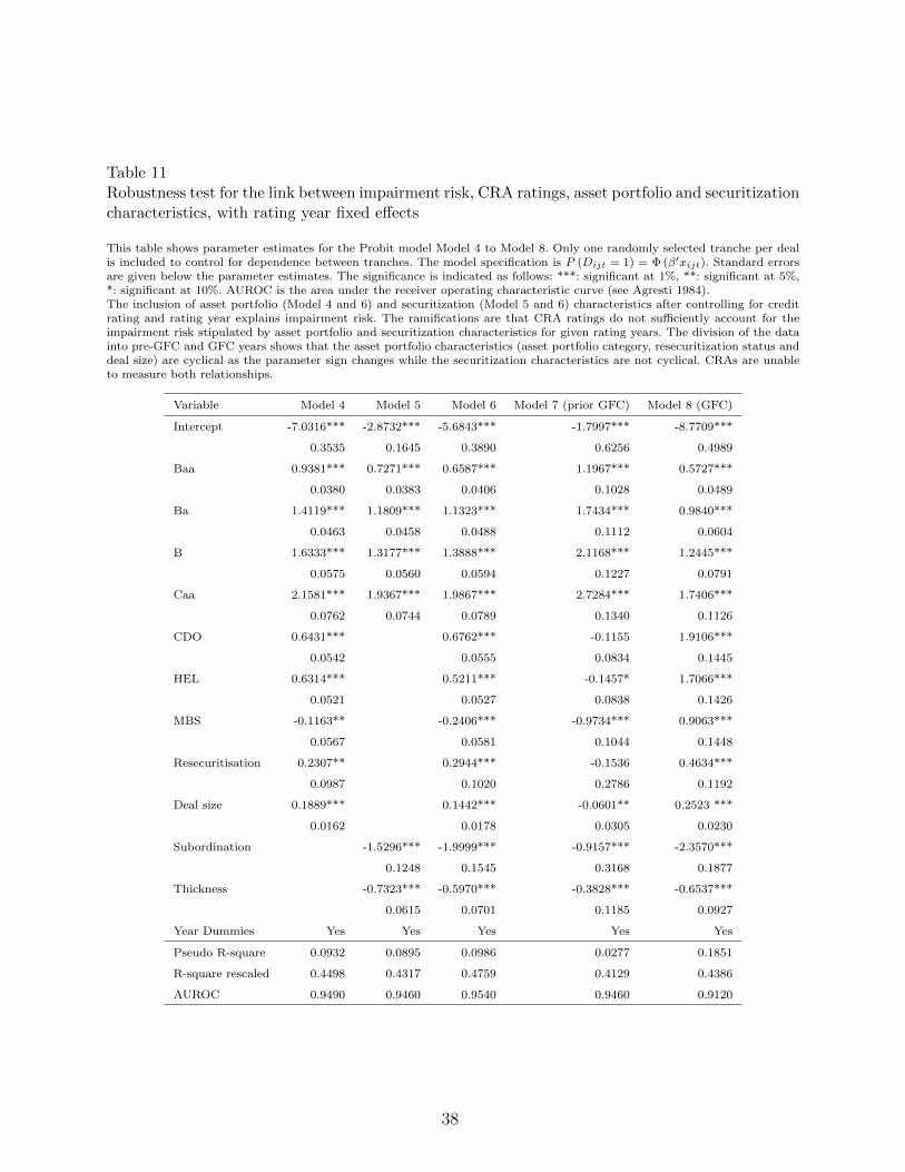
Table 11Robustness test for the link between impairment risk, CRA ratings, asset portfolio and securitizationcharacteristics, with rating year fixed effects

This table shows parameter estimates for the Probit model Model 4 to Model 8. Only one randomly selected tranche per dealis included to control for dependence between tranches. The model specification is P (Dijt = 1) = Φ (β′xijt). Standard errorsare given below the parameter estimates. The significance is indicated as follows: ***: significant at 1%, **: significant at 5%,*: significant at 10%. AUROC is the area under the receiver operating characteristic curve (see Agresti 1984).The inclusion of asset portfolio (Model 4 and 6) and securitization (Model 5 and 6) characteristics after controlling for creditrating and rating year explains impairment risk. The ramifications are that CRA ratings do not sufficiently account for theimpairment risk stipulated by asset portfolio and securitization characteristics for given rating years. The division of the datainto pre-GFC and GFC years shows that the asset portfolio characteristics (asset portfolio category, resecuritization status anddeal size) are cyclical as the parameter sign changes while the securitization characteristics are not cyclical. CRAs are unableto measure both relationships.

Variable Model 4 Model 5 Model 6 Model 7 (prior GFC) Model 8 (GFC)

Intercept -7.0316*** -2.8732*** -5.6843*** -1.7997*** -8.7709***

0.3535 0.1645 0.3890 0.6256 0.4989

Baa 0.9381*** 0.7271*** 0.6587*** 1.1967*** 0.5727***

0.0380 0.0383 0.0406 0.1028 0.0489

Ba 1.4119*** 1.1809*** 1.1323*** 1.7434*** 0.9840***

0.0463 0.0458 0.0488 0.1112 0.0604

B 1.6333*** 1.3177*** 1.3888*** 2.1168*** 1.2445***

0.0575 0.0560 0.0594 0.1227 0.0791

Caa 2.1581*** 1.9367*** 1.9867*** 2.7284*** 1.7406***

0.0762 0.0744 0.0789 0.1340 0.1126

CDO 0.6431*** 0.6762*** -0.1155 1.9106***

0.0542 0.0555 0.0834 0.1445

HEL 0.6314*** 0.5211*** -0.1457* 1.7066***

0.0521 0.0527 0.0838 0.1426

MBS -0.1163** -0.2406*** -0.9734*** 0.9063***

0.0567 0.0581 0.1044 0.1448

Resecuritisation 0.2307** 0.2944*** -0.1536 0.4634***

0.0987 0.1020 0.2786 0.1192

Deal size 0.1889*** 0.1442*** -0.0601** 0.2523 ***

0.0162 0.0178 0.0305 0.0230

Subordination -1.5296*** -1.9999*** -0.9157*** -2.3570***

0.1248 0.1545 0.3168 0.1877

Thickness -0.7323*** -0.5970*** -0.3828*** -0.6537***

0.0615 0.0701 0.1185 0.0927

Year Dummies Yes Yes Yes Yes Yes

Pseudo R-square 0.0932 0.0895 0.0986 0.0277 0.1851

R-square rescaled 0.4498 0.4317 0.4759 0.4129 0.4386

AUROC 0.9490 0.9460 0.9540 0.9460 0.9120

38

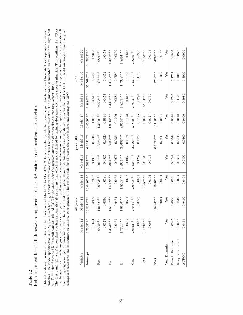
Tab

le12

Rob

ust

nes

ste

stfo

rth

eli

nk

bet

wee

nim

pai

rmen

tri

sk,

CR

Ara

tin

gsan

din

centi

vech

arac

teri

stic

s

Th

ista

ble

show

sp

ara

met

eres

tim

ate

sfo

rth

eP

rob

itm

od

elM

od

el12

toM

od

el20.

On

lyon

era

nd

om

lyse

lect

edtr

an

che

per

dea

lis

incl

ud

edto

contr

ol

for

dep

end

ence

bet

wee

ntr

an

ches

.T

he

mod

elsp

ecifi

cati

on

isP

(Dij

t=

1)

=Φ

(β′ x

ijt).

Sta

nd

ard

erro

rsare

giv

enb

elow

the

para

met

eres

tim

ate

s.T

he

sign

ifica

nce

isin

dic

ate

das

follow

s:***:

sign

ifica

nt

at

1%

,**:

sign

ifica

nt

at

5%

,*:

sign

ifica

nt

at

10%

.A

UR

OC

isth

eare

au

nd

erth

ere

ceiv

erop

erati

ng

chara

cter

isti

ccu

rve

(see

Agre

sti

1984).

Th

efi

rst

pan

el(a

llyea

rs)

show

sth

at

the

imp

air

men

tri

skgiv

enra

tin

gs

(i.e

.,w

hic

his

not

exp

lain

edby

rati

ngs)

dec

rease

sw

ith

tim

esi

nce

ori

gin

ati

on

.T

his

con

firm

sth

at

CR

As

may

have

an

ince

nti

ve

toass

ign

i)to

olo

wri

skra

tin

gs

inori

gin

ati

on

yea

rsto

incr

ease

fee

reven

ue

an

dii)

too

hig

hri

skra

tin

gs

inm

on

itori

ng

yea

rsto

main

tain

stab

led

efau

ltan

dra

tin

gm

igra

tion

per

form

an

cem

easu

res.

Th

ese

con

dan

dth

ird

pan

elsh

ow

that

this

effec

tis

main

lyd

riven

by

occ

urr

ence

of

the

GF

C.

Inad

dit

ion

,im

pair

men

tri

skgiv

enra

tin

gs

incr

ease

sw

ith

the

secu

riti

zati

on

act

ivit

yat

ori

gin

ati

on

.T

his

resu

lth

old

sfo

rall

yea

rs,

the

yea

rsb

efore

an

dd

uri

ng

the

GF

C.

All

yea

rsp

rior

GF

CG

FC

Vari

ab

leM

od

el12

Mod

el13

Mod

el14

Mod

el15

Mod

el16

Mod

el17

Mod

el18

Mod

el19

Mod

el20

Inte

rcep

t-2

.7695***

-16.8

314***

-10.9

480***

-3.5

097***

-6.1

942***

-6.4

569***

-1.8

889***

-25.7

616***

-14.7

603***

0.1

694

0.6

352

0.7

887

0.1

913

0.8

705

1.0

051

0.0

517

0.9

420

1.2

060

Baa

0.9

605***

1.0

082***

0.9

933***

1.2

990***

1.3

226***

1.3

309***

0.9

593***

0.9

786***

0.9

860***

0.0

378

0.0

376

0.0

381

0.0

925

0.0

920

0.0

934

0.0

453

0.0

452

0.0

458

Ba

1.4

578***

1.5

151***

1.5

039***

1.7

804***

1.8

230***

1.8

314***

1.4

051***

1.4

197***

1.4

263***

0.0

460

0.0

464

0.0

468

0.0

977

0.0

984

0.1

000

0.0

581

0.0

580

0.0

590

B1.7

701***

1.8

030***

1.8

565***

1.9

924***

2.0

497***

2.0

544***

1.8

243***

1.7

369***

1.8

874***

0.0

585

0.0

591

0.0

602

0.1

050

0.1

074

0.1

078

0.0

817

0.0

795

0.0

842

Caa

2.6

612***

2.4

474***

2.6

958***

2.7

356***

2.7

905***

2.7

850***

2.7

892***

2.3

359***

2.8

239***

0.0

847

0.0

793

0.0

856

0.1

257

0.1

272

0.1

275

0.1

292

0.1

123

0.1

337

TS

O-0

.1960***

-0.1

272***

-0.0

122

0.0

071

-0.3

194***

-0.2

163***

0.0

087

0.0

104

0.0

113

0.0

127

0.0

130

0.0

159

SV

O0.5

496***

0.3

270***

0.1

090***

0.1

186***

0.8

762***

0.4

775***

0.0

244

0.0

304

0.0

349

0.0

394

0.0

352

0.0

447

Yea

rD

um

mie

sY

esY

esY

esY

esY

esY

esY

esY

esY

es

Pse

ud

oR

-squ

are

0.0

942

0.0

936

0.0

961

0.0

242

0.0

244

0.0

244

0.1

742

0.1

701

0.1

805

R-s

qu

are

resc

ale

d0.4

547

0.4

519

0.4

639

0.3

617

0.3

648

0.3

648

0.4

128

0.4

030

0.4

277

AU

RO

C0.9

460

0.9

440

0.9

490

0.9

390

0.9

400

0.9

400

0.8

980

0.8

930

0.9

090

39

3.4.2 Regression link function

The Probit regression is based on the assumption of a Probit link function in the regression.

Other assumptions are homogeneity, large pool size and normality of risk factors. 34

We test the robustness of our approach in relation to violations of these assumptions. 35 We

conduct several Monte-Carlo simulation studies which are carried out as follows:

(1) For the simulations we specify the unconditional default probability π = Φ(c) and the

asset return correlation ρ.

(2) K Borrowers are pooled and each pool is tranched into five tranches (with attachment

levels 1%, 3%, 5%, 10%, and 30%). According to the decreasing tranche risk we assign

ratings from 1 to 5 for the five tranches. 36

(3) We generate default events for the assets in the pool. Firstly we randomly draw realiza-

tions of the common risk factors Xt for the pools. The conditional probability of default

(CPD) of each borrower within asset pool j is computed given Xt as

CPDjt(Xt) = Φ

(cjt −

√ρXt√

1− ρ

)(17)

cjt is the default threshold which equals c in the case where the model is correctly

specified by the rating agency. To control for macroeconomic distortions we add a ran-

domly generated time specific variable ξt to c such that cjt = c + ξt varies the default

threshold. Hence, the default probability of the pools simultaneously changes over time

and introduces a dependence structure between the pools. The results are reported in

Table 13. In Table 14, we also include pool specific heterogeneity by adding a distortion

variable ϕj leading to cjt = c + ϕj + ξt. ξt and ϕj are normally distributed with mean

zero.

(4) The number of defaults in pool j (j = 1, ..., J) is randomly drawn from a (conditional)

binomial distribution with K assets and probability equal to the CPD. The default rate

is computed by dividing the number of defaults by the number of assets in the pool.

(5) For the realized default rate of each pool we note if a tranche in a pool is impaired.

34 The normality assumption and large pool size assumptions are checked for robustness in Section3.4.3. The impact of heterogeneity is analyzed by the inclusion of the instrument (distortion)variable in Section 3.4.2 to 3.4.4.35 Please note that the regression results may be spurious, biased, or inconsistent if the approachis not robust with respect to these types of mis-specification.36 Please note that these thresholds were chosen in line with standard subordination levels of secu-ritizations.

40

(6) We run the Probit regression of tranche impairments on ratings, fixed year effects (which

act as control for the distortions ξt), and additional variables.

(7) Steps 3 to 6 are repeated 1,000 times for varying pool sizes, varying numbers of pools,

and various parameter settings. The parameter estimates are summarized and reported.

The default probabilities of the assets in the pool are set to π = 5% and the asset return

correlation is set to ρ = 0.2. Unless noted otherwise, the number of portfolio assets in each

pool is K = 10, 000. The number of pools is J = 1, 000 and number of years is T = 10 per

simulation run.

The empirical analysis is based on a Probit link function between impairment probabilities

and explanatory variables. A frequently used alternative to the Probit function is the Logit

function which exhibits wider tails. We therefore run the simulations generated under the

above model and estimate the model i) under the default generating Probit link function

and ii) under a mis-specified logistic regression with Logit function.

The results from 1,000 Monte-Carlo simulations are shown in Table 13. The left part contains

in Column 1 the averages of the 1,000 estimates for the intercept, fixed effects for Year 2

to 10 (t2 to t10), rating grades 2 to 5 (r2 to r5) for the Probit specification. Additionally

we include a randomly generated distortion or instrumental variables ϕj in the regression

to test whether an effect which should not be significant is detected to be significant under

our model mis-specifications. Column 2 provides the empirical standard deviation of the

simulated sample of the 1,000 estimates. Column 3 shows the average of the 1,000 estimated

standard deviations for each parameter estimate. Column 4 gives the fraction of rejections

of the null hypothesis that the respective parameter equals zero at a significance level of 5%.

Thus, we expect the true null hypothesis to be rejected in about 5% of all iterations.

The table shows that most of the year fixed effects are significant (rejection rates between 20%

and 100%). The business cycle effect is correctly detected, and the coefficients for the ratings

are increasing with decreasing credit quality. The average coefficient for the instrument is

close to zero as expected and the true null is rejected in about 5% of all cases. The right

hand side of the table contains in Columns 1 to 4 the analogous estimation results if a

Logit specification is used in the estimation. The coefficients and the standard deviations

of the Logit model are on an absolute scale larger throughout. However, the percentages of

rejections of the null hypotheses are quite similar to the Probit model. We therefore conclude

that the specification of the linking function of the regression model does not qualitatively

alter the results. This is particularly important for the instrumental variable which is included

41

as it should be significantly different from zero in no more than about 5% of all cases. Thus,

a true null is not rejected in more cases than given by the size of the test. A variable which

does not explain the risk of the tranches is not spuriously identified to do so by the test as

it does not enter the default generating process of Equation (17).

The previous examples considered significance of the instrumental variable when it does not

have an effect on the ‘true’ risk, i.e., it is included in the empirical regression model but not

in the model which generated the defaults according to Equation (17). To check the power

of the test (i.e., to see whether a variable is detected to be significant when it should be

significant because it is also included in the default generating process) we include the pool

specific distortion parameter ϕj in Equation (17) and in the regressions. That is, it should

be detected to explain default risk in addition to the ratings as it now enters the default

generating process. Table 14 shows the results for this case. While the coefficients for the

time and the rating effects show similar behavior as before, the instrumental variable is now

different from zero in 100% of all regressions with an average coefficient of -2.41 (Probit)

and -3.99 (Logit). This shows that a variable which is driving defaults in addition to ratings

is detected to be significant with a large probability (e.g., subordination in our empirical

analysis). This holds for the true model (Probit) and for a mis-specified model (Logit).

42

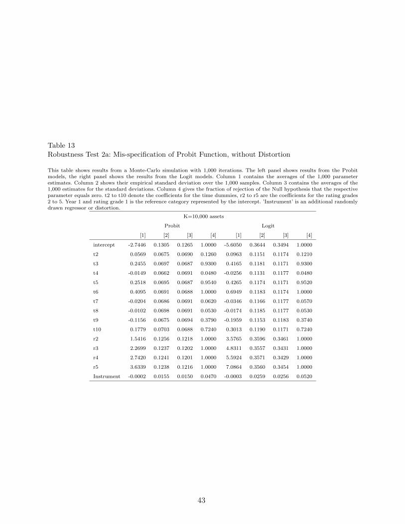
Table 13Robustness Test 2a: Mis-specification of Probit Function, without Distortion

This table shows results from a Monte-Carlo simulation with 1,000 iterations. The left panel shows results from the Probitmodels, the right panel shows the results from the Logit models. Column 1 contains the averages of the 1,000 parameterestimates. Column 2 shows their empirical standard deviation over the 1,000 samples. Column 3 contains the averages of the1,000 estimates for the standard deviations. Column 4 gives the fraction of rejection of the Null hypothesis that the respectiveparameter equals zero. t2 to t10 denote the coefficients for the time dummies, r2 to r5 are the coefficients for the rating grades2 to 5. Year 1 and rating grade 1 is the reference category represented by the intercept. ’Instrument’ is an additional randomlydrawn regressor or distortion.

K=10,000 assets

Probit Logit

[1] [2] [3] [4] [1] [2] [3] [4]

intercept -2.7446 0.1305 0.1265 1.0000 -5.6050 0.3644 0.3494 1.0000

t2 0.0569 0.0675 0.0690 0.1260 0.0963 0.1151 0.1174 0.1210

t3 0.2455 0.0697 0.0687 0.9300 0.4165 0.1181 0.1171 0.9300

t4 -0.0149 0.0662 0.0691 0.0480 -0.0256 0.1131 0.1177 0.0480

t5 0.2518 0.0695 0.0687 0.9540 0.4265 0.1174 0.1171 0.9520

t6 0.4095 0.0691 0.0688 1.0000 0.6949 0.1183 0.1174 1.0000

t7 -0.0204 0.0686 0.0691 0.0620 -0.0346 0.1166 0.1177 0.0570

t8 -0.0102 0.0698 0.0691 0.0530 -0.0174 0.1185 0.1177 0.0530

t9 -0.1156 0.0675 0.0694 0.3790 -0.1959 0.1153 0.1183 0.3740

t10 0.1779 0.0703 0.0688 0.7240 0.3013 0.1190 0.1171 0.7240

r2 1.5416 0.1256 0.1218 1.0000 3.5765 0.3596 0.3461 1.0000

r3 2.2699 0.1237 0.1202 1.0000 4.8311 0.3557 0.3431 1.0000

r4 2.7420 0.1241 0.1201 1.0000 5.5924 0.3571 0.3429 1.0000

r5 3.6339 0.1238 0.1216 1.0000 7.0864 0.3560 0.3454 1.0000

Instrument -0.0002 0.0155 0.0150 0.0470 -0.0003 0.0259 0.0256 0.0520

43

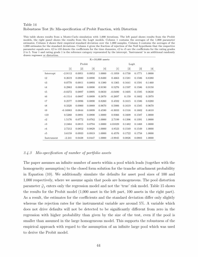
Table 14Robustness Test 2b: Mis-specification of Probit Function, with Distortion

This table shows results from a Monte-Carlo simulation with 1,000 iterations. The left panel shows results from the Probitmodels, the right panel shows the results from the Logit models. Column 1 contains the averages of the 1,000 parameterestimates. Column 2 shows their empirical standard deviation over the 1,000 samples. Column 3 contains the averages of the1,000 estimates for the standard deviations. Column 4 gives the fraction of rejection of the Null hypothesis that the respectiveparameter equals zero. t2 to t10 denote the coefficients for the time dummies, r2 to r5 are the coefficients for the rating grades2 to 5. Year 1 and rating grade 1 is the reference category represented by the intercept. ’Instrument’ is an additional randomlydrawn regressor or distortion.

K=10,000 assets

Probit Logit

[1] [2] [3] [4] [1] [2] [3] [4]

Intercept -2.9112 0.0951 0.0952 1.0000 -5.1959 0.1730 0.1771 1.0000

t2 0.2619 0.0880 0.0890 0.8400 0.4663 0.1581 0.1586 0.8380

t3 0.0770 0.0911 0.0893 0.1380 0.1365 0.1641 0.1591 0.1460

t4 0.2963 0.0888 0.0890 0.9190 0.5276 0.1597 0.1586 0.9150

t5 -0.0272 0.0897 0.0895 0.0650 -0.0490 0.1605 0.1595 0.0630

t6 -0.1514 0.0887 0.0899 0.3870 -0.2697 0.159 0.1602 0.3970

t7 0.2577 0.0896 0.0890 0.8260 0.4592 0.1615 0.1586 0.8280

t8 0.3320 0.0900 0.0889 0.9670 0.5906 0.1619 0.1585 0.9670

t9 -0.16983 0.0844 0.0899 0.4590 -0.3033 0.1516 0.1602 0.4610

t10 0.5260 0.0891 0.0890 1.0000 0.9366 0.1609 0.1587 1.0000

r2 1.5176 0.0772 0.0762 1.0000 2.7199 0.1396 0.1391 1.0000

r3 2.2464 0.0815 0.0794 1.0000 4.01029 0.1482 0.1468 1.0000

r4 2.7212 0.0852 0.0829 1.0000 4.8523 0.1549 0.1549 1.0000

r5 3.6159 0.0933 0.0919 1.0000 6.4576 0.1722 0.1758 1.0000

Instrument -2.241 0.0438 0.0447 1.0000 -3.9945 0.0826 0.0883 1.0000

3.4.3 Mis-specification of number of portfolio assets

The paper assumes an infinite number of assets within a pool which leads (together with the

homogeneity assumption) to the closed form solution for the tranche attachment probability

in Equation (10). We additionally simulate the defaults for asset pool sizes of 100 and

1,000 respectively, where we assume again that pools are homogeneous. The pool distortion

parameter ϕj enters only the regression model and not the ‘true’ risk model. Table 15 shows

the results for the Probit model (1,000 asset in the left part, 100 assets in the right part).

As a result, the estimates for the coefficients and the standard deviation differ only slightly

whereas the rejection rates for the instrumental variable are around 5%. A variable which

does not drive defaults will not be detected to be significantly different from zero in the

regression with higher probability than given by the size of the test, even if the pool is

smaller than assumed in the large homogeneous model. This supports the robustness of the

empirical approach with regard to the assumption of an infinite large pool which was used

to derive the Probit model.

44

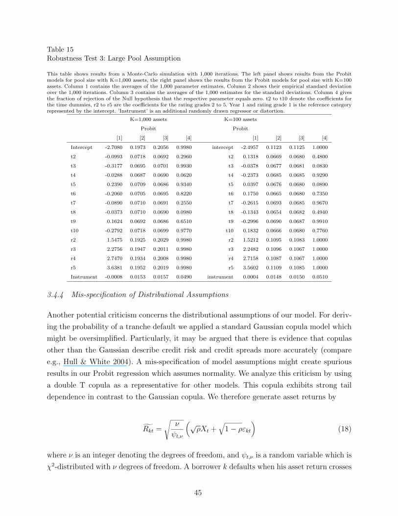
Table 15Robustness Test 3: Large Pool Assumption

This table shows results from a Monte-Carlo simulation with 1,000 iterations. The left panel shows results from the Probitmodels for pool size with K=1,000 assets, the right panel shows the results from the Probit models for pool size with K=100assets. Column 1 contains the averages of the 1,000 parameter estimates, Column 2 shows their empirical standard deviationover the 1,000 iterations. Column 3 contains the averages of the 1,000 estimates for the standard deviations. Column 4 givesthe fraction of rejection of the Null hypothesis that the respective parameter equals zero. t2 to t10 denote the coefficients forthe time dummies, r2 to r5 are the coefficients for the rating grades 2 to 5. Year 1 and rating grade 1 is the reference categoryrepresented by the intercept. ’Instrument’ is an additional randomly drawn regressor or distortion.

K=1,000 assets K=100 assets

Probit Probit

[1] [2] [3] [4] [1] [2] [3] [4]

Intercept -2.7080 0.1973 0.2056 0.9980 intercept -2.4957 0.1123 0.1125 1.0000

t2 -0.0993 0.0718 0.0692 0.2960 t2 0.1318 0.0669 0.0680 0.4800

t3 -0.3177 0.0695 0.0701 0.9930 t3 -0.0378 0.0677 0.0681 0.0830

t4 -0.0288 0.0687 0.0690 0.0620 t4 -0.2373 0.0685 0.0685 0.9290

t5 0.2390 0.0709 0.0686 0.9340 t5 0.0397 0.0676 0.0680 0.0890

t6 -0.2060 0.0705 0.0695 0.8220 t6 0.1750 0.0665 0.0680 0.7350

t7 -0.0890 0.0710 0.0691 0.2550 t7 -0.2615 0.0693 0.0685 0.9670

t8 -0.0373 0.0710 0.0690 0.0980 t8 -0.1343 0.0654 0.0682 0.4940

t9 0.1624 0.0692 0.0686 0.6510 t9 -0.2996 0.0690 0.0687 0.9910

t10 -0.2792 0.0718 0.0699 0.9770 t10 0.1832 0.0666 0.0680 0.7760

r2 1.5475 0.1925 0.2029 0.9980 r2 1.5212 0.1095 0.1083 1.0000

r3 2.2756 0.1947 0.2011 0.9980 r3 2.2482 0.1096 0.1067 1.0000

r4 2.7470 0.1934 0.2008 0.9980 r4 2.7158 0.1087 0.1067 1.0000

r5 3.6381 0.1952 0.2019 0.9980 r5 3.5602 0.1109 0.1085 1.0000

Instrument -0.0008 0.0153 0.0157 0.0490 instrument 0.0004 0.0148 0.0150 0.0510

3.4.4 Mis-specification of Distributional Assumptions

Another potential criticism concerns the distributional assumptions of our model. For deriv-

ing the probability of a tranche default we applied a standard Gaussian copula model which

might be oversimplified. Particularly, it may be argued that there is evidence that copulas

other than the Gaussian describe credit risk and credit spreads more accurately (compare

e.g., Hull & White 2004). A mis-specification of model assumptions might create spurious

results in our Probit regression which assumes normality. We analyze this criticism by using

a double T copula as a representative for other models. This copula exhibits strong tail

dependence in contrast to the Gaussian copula. We therefore generate asset returns by

Rkt =

√ν

ψt,ν

(√ρXt +

√1− ρεkt

)(18)

where ν is an integer denoting the degrees of freedom, and ψt,ν is a random variable which is

χ2-distributed with ν degrees of freedom. A borrower k defaults when his asset return crosses

45

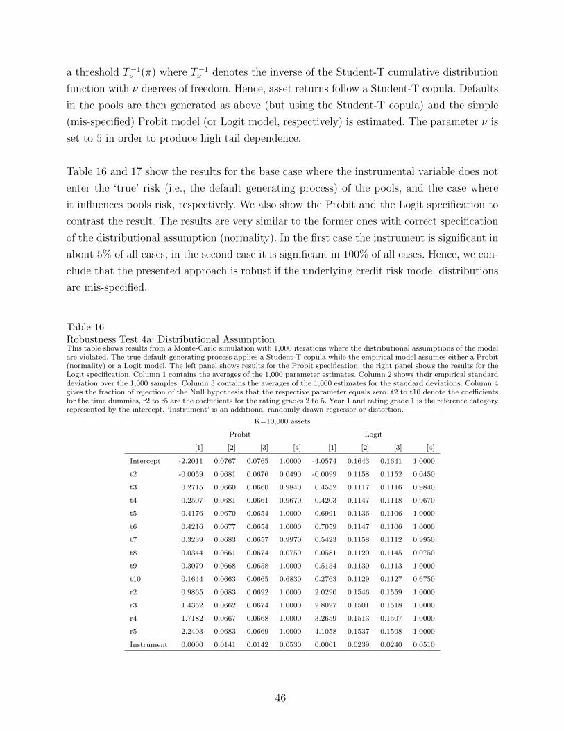
a threshold T−1ν (π) where T−1

ν denotes the inverse of the Student-T cumulative distribution

function with ν degrees of freedom. Hence, asset returns follow a Student-T copula. Defaults

in the pools are then generated as above (but using the Student-T copula) and the simple

(mis-specified) Probit model (or Logit model, respectively) is estimated. The parameter ν is

set to 5 in order to produce high tail dependence.

Table 16 and 17 show the results for the base case where the instrumental variable does not

enter the ‘true’ risk (i.e., the default generating process) of the pools, and the case where

it influences pools risk, respectively. We also show the Probit and the Logit specification to

contrast the result. The results are very similar to the former ones with correct specification

of the distributional assumption (normality). In the first case the instrument is significant in

about 5% of all cases, in the second case it is significant in 100% of all cases. Hence, we con-

clude that the presented approach is robust if the underlying credit risk model distributions

are mis-specified.

Table 16Robustness Test 4a: Distributional AssumptionThis table shows results from a Monte-Carlo simulation with 1,000 iterations where the distributional assumptions of the modelare violated. The true default generating process applies a Student-T copula while the empirical model assumes either a Probit(normality) or a Logit model. The left panel shows results for the Probit specification, the right panel shows the results for theLogit specification. Column 1 contains the averages of the 1,000 parameter estimates. Column 2 shows their empirical standarddeviation over the 1,000 samples. Column 3 contains the averages of the 1,000 estimates for the standard deviations. Column 4gives the fraction of rejection of the Null hypothesis that the respective parameter equals zero. t2 to t10 denote the coefficientsfor the time dummies, r2 to r5 are the coefficients for the rating grades 2 to 5. Year 1 and rating grade 1 is the reference categoryrepresented by the intercept. ’Instrument’ is an additional randomly drawn regressor or distortion.

K=10,000 assets

Probit Logit

[1] [2] [3] [4] [1] [2] [3] [4]

Intercept -2.2011 0.0767 0.0765 1.0000 -4.0574 0.1643 0.1641 1.0000

t2 -0.0059 0.0681 0.0676 0.0490 -0.0099 0.1158 0.1152 0.0450

t3 0.2715 0.0660 0.0660 0.9840 0.4552 0.1117 0.1116 0.9840

t4 0.2507 0.0681 0.0661 0.9670 0.4203 0.1147 0.1118 0.9670

t5 0.4176 0.0670 0.0654 1.0000 0.6991 0.1136 0.1106 1.0000

t6 0.4216 0.0677 0.0654 1.0000 0.7059 0.1147 0.1106 1.0000

t7 0.3239 0.0683 0.0657 0.9970 0.5423 0.1158 0.1112 0.9950

t8 0.0344 0.0661 0.0674 0.0750 0.0581 0.1120 0.1145 0.0750

t9 0.3079 0.0668 0.0658 1.0000 0.5154 0.1130 0.1113 1.0000

t10 0.1644 0.0663 0.0665 0.6830 0.2763 0.1129 0.1127 0.6750

r2 0.9865 0.0683 0.0692 1.0000 2.0290 0.1546 0.1559 1.0000

r3 1.4352 0.0662 0.0674 1.0000 2.8027 0.1501 0.1518 1.0000

r4 1.7182 0.0667 0.0668 1.0000 3.2659 0.1513 0.1507 1.0000

r5 2.2403 0.0683 0.0669 1.0000 4.1058 0.1537 0.1508 1.0000

Instrument 0.0000 0.0141 0.0142 0.0530 0.0001 0.0239 0.0240 0.0510

46

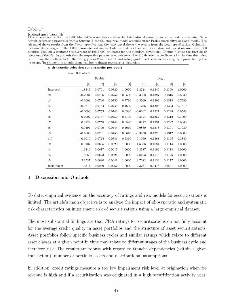
Table 17Robustness Test 4bThis table shows results from 1,000 Monte-Carlo simulations when the distributional assumptions of the model are violated. Truedefault generating process is from a Student-T copula, empirical model assumes either Probit (normality) or Logit model. Theleft panel shows results from the Probit specification, the right panel shows the results from the Logit specification. Column[1]contains the averages of the 1,000 parameter estimates. Column 2 shows their empirical standard deviation over the 1,000samples. Column 3 contains the averages of the 1,000 estimates for the standard deviations. Column 4 gives the fraction ofrejection of the Null hypothesis that the respective parameter equals zero. t2 to t10 denote the coefficients for the time dummies,r2 to r5 are the coefficients for the rating grades 2 to 5. Year 1 and rating grade 1 is the reference category represented by theintercept. ’Instrument’ is an additional randomly drawn regressor or distortion.

with tranche selection (one tranche per pool)

N=10000 assets

Probit Logit

[1] [2] [3] [4] [1] [2] [3] [4]

Intercept -1.8443 0.0701 0.0720 1.0000 -3.2244 0.1249 0.1300 1.0000

t2 -0.2284 0.0756 0.0752 0.8590 -0.3988 0.1327 0.1316 0.8540

t3 -0.2003 0.0740 0.0750 0.7710 -0.3500 0.1305 0.1313 0.7580

t4 -0.0719 0.0754 0.0745 0.1630 -0.1256 0.1325 0.1303 0.1610

t5 -0.0096 0.0753 0.0743 0.0580 -0.0162 0.1321 0.1298 0.0540

t6 -0.1902 0.0767 0.0750 0.7130 -0.3324 0.1352 0.1312 0.7090

t7 0.0122 0.0758 0.0742 0.0590 0.0212 0.1337 0.1297 0.0640

t8 -0.0497 0.0749 0.0744 0.1010 -0.0869 0.1318 0.1301 0.1030

t9 -0.1806 0.0781 0.0750 0.6610 -0.3150 0.1373 0.1312 0.6600

t10 -0.1010 0.0774 0.0746 0.2810 -0.1760 0.1361 0.1305 0.2840

r2 0.9107 0.0605 0.0620 1.0000 1.6036 0.1084 0.1114 1.0000

r3 1.3440 0.0617 0.0617 1.0000 2.3587 0.1102 0.1113 1.0000

r4 1.6260 0.0623 0.0621 1.0000 2.8493 0.1116 0.1126 1.0000

r5 2.1537 0.0630 0.0641 1.0000 3.7682 0.1139 0.1177 1.0000

Instrument -1.3314 0.0259 0.0262 1.0000 -2.3261 0.0478 0.0501 1.0000

4 Discussion and Outlook

To date, empirical evidence on the accuracy of ratings and risk models for securitizations is

limited. The article’s main objective is to analyze the impact of idiosyncratic and systematic

risk characteristics on impairment risk of securitizations using a large empirical dataset.

The most substantial findings are that CRA ratings for securitizations do not fully account

for the average credit quality in asset portfolios and the structure of asset securitizations.

Asset portfolios follow specific business cycles and similar ratings which relate to different

asset classes at a given point in time may relate to different stages of the business cycle and

therefore risk. The results are robust with regard to tranche dependencies (within a given

transaction), number of portfolio assets and distributional assumptions.

In addition, credit ratings measure a too low impairment risk level at origination when fee

revenue is high and if a securitization was originated in a high securitization activity year.

47

Generally speaking, this underestimation of risk coincides with periods of high fee revenue.

In the broader context, CRA ratings as well as many other commercial vendor solutions

may have to be interpreted in relation to the invested resources. Please note that the major

CRAs cover a large number of rated debt issuers and issues per year 37 with a limited

number of financial analysts 38 . Despite this criticism, this paper has also shown that ratings

are informative with regard to the average idiosyncratic impairment risk over the business

cycle.

Consequences from the findings of the papers relate to establishment of rating standards

for CRA’s and higher transparency of their employed approaches, models and parameters,

along with more prudential supervision. This paper has shown that the ‘paid-by-originator’

approach is a source for misaligned incentives. This may be addressed i) ex ante by switching

to a ‘paid-by-investors’ approach or ii) ex post by a tax for risk under-representation.

CRAs publish histories of their financial risk measures as well as the respective realizations.

Little is known of the quality of models of other vendors as well as financial institution inter-

nal models as the respective information is kept private. However, recent negative earnings

announcements of financial institutions suggest that other models applied in industry share

similar properties to CRA assessments. Model outputs should be used with caution and a

formal validation of such models is important.

37 For instance, in 2007, Moody’s Investors Service rated 100 sovereigns; 12,000 corporate issuers;29,000 public finance issues; and 96,000 structured finance obligations.38 For instance, in 2007, Moody’s Investors Service employed approximately 1,000 analysts.

48

References

Acharya, V. V., Bharath, S. T. & Srinivasan, A. (2007), ‘Does industry-wide distress affect

defaulted firms? - Evidence from creditor recoveries’, Journal of Financial Economics

85, 787–821.

Agresti, A. (1984), Analysis of Ordinal Categorical Data, Wiley, New York.

Altman, E., Brady, B., Resti, A. & Sironi, A. (2005), ‘The link between default and recovery

rates: Theory, empirical evidence and implications’, Journal of Business 78, 2203–2227.

Ashcraft, A., Goldsmith-Pinkham, P. & Vickery, J. (2009), ‘Mbs ratings and the mortgage

credit boom’, Working Paper, Federal Reserve Bank of New York and Harvard University

.

Bajari, P., Chu, C. & Park, M. (2008), ‘An empirical model of subprime mortgage default’.

Becker, B. & Milbourn, T. (2008), ‘Reputation and competition: Evidence from the credit

rating industry’, Harvard Business School Working Paper, No. 09-051, October 2008 .

Benmelech, E. & Dlugosz, J. (2009), ‘The alchemy of CDO credit ratings’, Journal of Mon-

etary Economics 56, 615–634.

Bluhm, C., Overbeck, L. & Wagner, A. (2003), An Introduction to Credit Risk Modeling,

Chapman/CRC, London.

Blume, M., Lim, F. & MacKinlay, A. (1998), ‘The declining credit quality of U.S. corporate

debt: Myth or reality?’, Journal of Finance 53, 1389–1413.

Bolton, P., Freixas, X. & Shapiro, J. (2009), ‘The credit ratings game’, Working Paper 14712,

National Bureau of Economic Research .

Bruche, M. & Gonzalez-Aguado, C. (2010), ‘Recovery rates, default probabilities, and the

credit cycle’, Journal of Banking and Finance 34, 713–723.

Carey, M. (1998), ‘Credit risk in private debt portfolios’, Journal of Finance 53, 1363–1387.

Carey, M. & Hrycay, M. (2001), ‘Parameterizing credit risk models with rating data’, Journal

of Banking and Finance 25, 197–270.

Coval, J., Jurek, J. & Stafford, E. (2009), ‘The economics of structured finance’, Journal of

Economic Perspectives 23, 3–25.

Crouhy, M., Galai, D. & Mark, R. (2001), ‘Prototype risk rating system’, Journal of Banking

and Finance 25, 47–95.

Crouhy, M., Jarrow, R. & Turnbull, S. (2008), ‘The Subprime Credit Crisis of 07’, Working

Paper, University of Houston, Natixis and Cornell University .

Dell’Ariccia, G., Igan, D. & Laeven, L. (2008), ‘Credit booms and lending standards: Evi-

dence from the subprime mortgage market’, Working Paper .

Demyanyk, Y. & Hemert, O. V. (2009), ‘Understanding the subprime mortgage crisis’, forth-

49

coming Review of Financial Studies .

Demyanyk, Y., Koijen, R. & Hemert, O. V. (2010), ‘Determinants and consequences of

mortgage default’, Working Paper Federal Reserve Bank of Cleveland .

Dichev, I. & Piotroski, J. (2001), ‘The long-run stock returns following bond ratings changes’,

Journal of Finance 56, 173–203.

Dietsch, M. & Petey, J. (2004), ‘Should SME exposures be treated as retail or corporate

exposures? a comparative analysis of default probabilities and asset correlations in French

and German SMEs’, Journal of Banking and Finance 28, 773–788.

Duffie, D., Saita, L. & Wang, K. (2007), ‘Multi-period corporate default prediction with

stochastic covariates’, Journal of Financial Economics 83, 635–665.

Duffie, D. & Singleton, K. (1999), ‘Modeling term structures of defaultable bonds’, Review

of Financial Studies 12, 687–720.

Ederington, L. H. & Goh, J. C. (1993), ‘Is a bond rating downgrade bad news, good news,

or no news for stockholders?’, Journal of Finance 48, 2001–2008.

Fitch Ratings (2006), ‘Exposure draft: Introducing the Fitch VECTOR Default Model Ver-

sion 3.0’.

Franke, G. & Krahnen, J. (2008), ‘The future of securitization’, Working Paper, Frankfurt

Center for Financial Studies .

Gordy, M. (2000), ‘A comparative anatomy of credit risk models’, Journal of Banking and

Finance 24, 119–149.

Gordy, M. (2003), ‘A risk-factor model foundation for ratings-based bank capital rules’,

Journal of Financial Intermediation 12, 199–232.

Griffin, J. M. & Tang, D. (2009), ‘Did subjectivity play a role in CDO credit ratings?’,

Working Paper, University of Texas at Austin and University of Hong Kong .

Grunert, J., Norden, L. & Weber, M. (2005), ‘The role of non-financial factors in internal

credit ratings’, Journal of Banking and Finance 29, 509–531.

Grunert, J. & Weber, M. (2009), ‘Recovery rates of commercial lending: Empirical evidence

for German companies’, Journal of Banking and Finance 33, 505–513.

Guettler, A. & Wahrenburg, M. (2007), ‘The adjustment of credit ratings in advance of

defaults’, Journal of Banking and Finance 31, 751–767.

Guiso, L., Sapienza, P. & Zingales, L. (2009), ‘Moral and social constraints to strategic

default on mortgages’, NBER Working Paper 15145 .

Gupton, G., Finger, C. & Bhatia, M. (1997), ‘CreditMetrics technical document’.

Hellwig, M. (2008), ‘Systemic risk in the financial sector: An analysis of the Subprime-

Mortgage Financial Crisis’, Working Paper, Max Planck Institute for Research on Collec-

tive Goods.

50

Hull, J. (2009), ‘The credit crunch of 2007: What Went Wrong? Why? What Lessons Can

Be Learned?’, Journal of Credit Risk 5, 3–18.

Hull, J. & White, A. (2004), ‘Valuation of a CDO and nth to default CDS without monte

carlo simulation’, Journal of Derivatives 12, 8–23.

Jarrow, R., Lando, D. & Turnbull, S. (1997), ‘A Markov model for the term structure of

credit risk spreads’, Review of Financial Studies 10, 481–523.

Jarrow, R. & Turnbull, S. (1995), ‘Pricing derivatives on financial securities subject to credit

risk’, Journal of Finance 50, 53–85.

Jorion, P., Liu, Z. & Shi, C. (2005), ‘Informational effects of regulation fd: Evidence from

rating agencies’, Journal of Financial Economics 76, 309–330.

Koopman, S., Lucas, A. & Klaassen, P. (2005), ‘Empirical credit cycles and capital buffer

formation’, Journal of Banking and Finance 29, 3159–3179.

Krahnen, J. & Weber, M. (2001), ‘Generally accepted rating principles: a primer’, Journal

of Banking and Finance 25, 3–23.

Krainer, J., LeRoy, S. & O, M. (2009), ‘Mortgage default and mortgage valuation’.

Leland, H. (1994), ‘Corporate debt value, bond covenants and optimal capital structure’,

Journal of Finance 49, 1213–1252.

Leland, H. & Toft, K. (1996), ‘Optimal capital structure, endogeneous bankruptcy, and the

term structure of credit spreads’, Journal of Finance 51, 987–1019.

Leot, P., Arber, D. & Schou-Zibell, L. (2008), ‘Securitisation in east asia’, Asian Development

Bank Working Paper Series on Regional Economic Integration .

Livingston, M., Wei, J. & Zhou, L. (2010), ‘Moodys and S&P ratings: Are they equivalent?

conservative ratings and split rated bond yields’, Journal of Money, Credit and Banking

42, 1267–1293.

Loeffler, G. (2004), ‘An anatomy of rating through the cycle’, Journal of Banking and Finance

28, 695–720.

Longstaff, F. & Rajan, A. (2008), ‘An empirical analysis of the pricing of collateralized debt

obligations’, Journal of Finance 63, 529–563.

Longstaff, F. & Schwartz, E. (1995), ‘A simple approach to valuing risky fixed and floating

rate debt’, Journal of Finance 50, 789–819.

Madan, D. & Unal, H. (1995), ‘Pricing the risk of recovery in default with apr violation’,

Journal of Banking and Finance 27, 1001–1218.

Mayer, C., Pence, K. & Sherlund, S. (2008), ‘The rise in mortgage defaults: Facts and myths’,

forthcoming in Journal of Economic Perspectives .

McNeil, A. & Wendin, J. (2007), ‘Bayesian inference for generalized linear mixed models of

portfolio credit risk’, Journal of Empirical Finance 14, 131–149.

51

Merton, R. C. (1974), ‘On the pricing of corporate debt: The risk structure of interest rates’,

Journal of Finance 29, 449–470.

Miu, P. & Ozdemir, B. (2002), ‘Rating banks, risk and uncertainty in an opaque industry’,

American Economic Review 92, 874–888.

Moody’s Investors Service (2006), ‘CDOROM v2.3 user guide’.

Moody’s Investors Service (2008), ‘Default & loss rates of structured finance securities: 1993-

2007’.

Pan, J. & Singleton, K. (2008), ‘Default and recovery implicit in the term structure of

sovereign CDS spreads’, Journal of Finance 68, 2345–2384.

Poon, W., Lee, J. & Gup, B. (2009), ‘Do solicitations matter in bank credit ratings? results

from a study of 72 countries’, Journal of Money, Credit and Banking 41, 285–314.

Purda, L. (2007), ‘Stock market reactions to anticipated versus surprise rating changes’,

Journal of Financial Research 30, 301–320.

Qi, M. & Yang, X. (2009), ‘Loss given default of high loan-to-value residential mortgages’,

Journal of Banking and Finance 33, 788–799.

Radelet, S. & Sachs, J. (1998), ‘The East Asian Financial Crisis: Diagnosis, remedies,

prospects’, Brookings Papers 28, 1–90.

Rajan, U., Seru, A. & Vig, V. (2008), ‘The failure of models that predict failure: distance,

incentives and defaults’, Working paper, University of Michigan, University of Chicago

and London Business School .

Shumway, T. (2001), ‘Forecasting bankruptcy more accurately: a simple hazard-rate model’,

Journal of Business 74, 101–124.

Standard & Poor’s (2005), ‘CDO Evaluator Version 3.0: Technical document.’.

Vasicek, O. (1987), Probability of loss on loan portfolio, Working paper, KMV Corporation.

Vasicek, O. (1991), Limiting loan loss probability distribution, Working paper, KMV Cor-

poration.

52