Task Scheduling Strategies for Dynamic Reconfigurable Processors inDistributed Systems

M. Faisal Nadeem, S. Arash Ostadzadeh, Stephan Wong, and Koen BertelsComputer Engineering Laboratory, Delft University of Technology, The Netherlands

{M.F.Nadeem, S.A.Ostadzadeh, J.S.S.M.Wong, K.L.M.Bertels}@TUDelft.nl

ABSTRACT

Reconfigurable processors in distributed grid systems canpotentially offer enhanced performance along with flexi-bility. Therefore, grid systems, such as TeraGrid, are uti-lizing reconfigurable computing resources next to general-purpose processors (GPPs) in their computing nodes. Ingeneral, the application task scheduling largely affects thenear-optimal performance of resources in distributed gridsystems. The inclusion of reconfigurable nodes in suchsystems requires to take into account reconfigurable hard-ware characteristics, such as, area utilization, reconfigu-ration time, and time to communicate configuration bit-streams, execution codes, and data. Generally, many ofthese characteristics are not taken into account by tradi-tional task scheduling systems in distributed grids. In thispaper, we present a simulation framework for applicationtask distribution among different nodes of a reconfigurablecomputing grid. Furthermore, we propose three differenttask scheduling strategies, namely Optional Closest Match(OCM), Exact Match Priority (EMP), and Sufficient-AreaPriority (SAP). The simulation results are presented basedon the average scheduling steps required by the scheduler toaccommodate each task, the total scheduler workload, andthe average waiting time per task. We compare the impactsof the three scheduling strategies on these metrics. In ad-dition, we present a thorough discussion of the results. Inparticular, the results show that the two key metrics averagescheduling steps per task and average waiting time per taskare reduced for the EMP and the SAP when compared tothe OCM.

KEYWORDS: Distributed systems; Reconfigurable com-puting; Simulation framework; Task scheduling; Resourcemanagement.

1. INTRODUCTION

Distributed Computational grids provide inexpensive anddependable access to high-end computational resources that

are geographically dispersed over the world [1]. Somenotable worldwide projects in grid computing are Globus[2], Legion [3], and Unicore [4]. In the recent years,reconfigurable computing is utilized more commonly inhigh-performance computing, such as, multimedia process-ing, bioinformatics, and cryptography [5]. The reasonis that reconfigurable devices provide both increased per-formance without expensing on flexibility, i.e., allowingquick changes between the supported applications. Conse-quently, distributed computing networks (such as TeraGrid[6]) have incorporated reconfigurable computing resourcesnext to general-purpose processors (GPPs) in their comput-ing nodes. Proposals to better exploit the characteristics ofreconfigurable computing merged with the requirements ofcomputational grids have been suggested, e.g., Collabora-tive Reconfigurable Grid Computing (CRGC) in [7].

Scheduling algorithms have been thoroughly studied in con-ventional parallel and distributed systems. Various state-of-the-art scheduling algorithms for traditional grids havebeen proposed in [8] and [9]. The near-optimal utilizationof grid resources predominately depends on application taskscheduling onto the computing nodes. Therefore, schedul-ing algorithms are of paramount significance for compu-tational grids and new ones must be developed when thenode characteristics are changed. The inclusion of recon-figurable processors in the computational nodes requires therethinking of existing scheduling techniques in order to takeinto account reconfigurable processor characteristics, suchas, area utilization, reconfiguration time, (possible) perfor-mance increase, and the time required to transfer configura-tion bitstreams, execution codes, and data.

In this work, we present the design of a simulation frame-work for the application task scheduling for reconfigurableprocessors in a distributed grid system. The proposed de-sign can model complex reconfigurable computing nodes,processor configurations, and tasks along with GPPs. Theprocessor configurations can be modeled using a number ofdifferent reconfiguration parameters, such as, area required,reconfiguration time delay, network delay, etc. Various pa-rameters (e.g., node area range, task arrival rate, reconfigu-

978-1-61284-383-4/11/$26.00 ©2011 IEEE 90

ration time range, etc.) can be set according to the require-ments of a particular simulation. The simulation frameworkgenerates a report on different result statistics at each simu-lation run.

Using our simulation framework, we propose and imple-ment three different task scheduling strategies, namely Op-tional Closest Match (OCM), Exact Match Priority (EMP),and Sufficient-Area Priority (SAP). The scheduling strate-gies are described in detail and the results show the impactsof each scheduling strategy on three different system met-rics total scheduling steps required by the scheduler to ac-commodate each task, average waiting time per task andthe total workload of the scheduler. In particular, the resultsshow that the two key metrics average scheduling steps pertask and average waiting time per task are reduced for theEMP and the SAP when compared to the OCM.

The remainder of the paper is organized as follows. Sec-tion 2 provides related work. The background and scopeare discussed in Section 3. We discuss the design of the oursimulation framework in Section 4. Three different schedul-ing strategies are proposed and discussed in Section 5. Thesimulation environment and results are explained in Section6. Finally, we provide our conclusions and future work inSection 7.

2. RELATED WORK

Many state-of-the-art simulators for task scheduling in dis-tributed systems are proposed. Few examples are Sim-Grid [10], MicroGrid [11], and GridSim [12]. These sim-ulators can model computational resources composed ofGPPs and there is no specific simulator to take into ac-count the behavior of reconfigurable nodes in distributedcomputing environment. In [7], CRGridsim has been pro-posed by extending Gridsim [12] to add reconfigurable ele-ments in grids. However, it only considers speedup factor ofa reconfigurable processor over a GPP, as the reconfigura-tion parameter. Other important parameters, such as recon-figurability, reconfiguration delay, reconfiguration method(partial or full), area utilization, and hardware technologyhave not been taken into account. Most of the work [8] [9]on scheduling algorithms has been proposed for traditionalgrid networks with processors of heterogeneous computingcapacity, but they are not reconfigurable processors.

3. BACKGROUND AND SCOPE

Task scheduling in grids is defined as scheduling n taskswith a given execution time onto m resources. In this sec-tion, we formulate the scheduling problem and discuss themodels for task, processor configuration, and nodes. A typ-

ical reconfigurable node is represented by the following tu-ple:

Nodei (NID,Area,Cexisting, state) (1)

Where NID represents the node number, Area the totalreconfigurable area of node i and Cexisting the current pro-cessor configuration on the node. Initially, no configura-tion is assumed on a computing node and, therefore, setto Cblank. Furthermore, state represents the status of thenode i; whether it is busy or idle. Subsequently, the generalconfiguration of a processor to be configured on a node, isrepresented as:

Ci (CID,Area, Ptype, parameters) (2)

WhereCID represents the configuration number andAreais the total reconfigurable area required by configuration i. Ptype represents the processor type required by tasks inthe system. parameters is a list of attributes of a particularprocessor which provide the details of the Ptype processorrequired by tasks. Typical examples of Ptype are soft-coreprocessors, digital signal processors (DSPs), custom com-puting units (CCUs), etc. For instance, a soft-core ρ-VEXVLIW processor (specified by Ptype) implemented on anFPGA, can be adopted to several parameters such as, thenumber of issue slots, cluster cores, the number and types offunctional units, or the number of memory units [13]. Sim-ilarly, the following tuple represents an application task:

Taski (TID, trequired, Cpref ) (3)

Where TID represents the task number and trequired isthe execution time required by task i if it is processed onits preferred processor configuration (Cpref ). Cpref is thepreferred processor configuration demanded by task i. Thisconfiguration can be a specific processor that can be imple-mented on a reconfigurable node. Based on above defini-tions, we formulate the problem as follows.

Given a set of reconfigurable nodes represented by (1) anda set of tasks defined by (3), find a scheduling algorithmto map all tasks onto nodes, following a particular strategyto minimize key system metrics, such as waiting time, totalreconfigurable area waste, and scheduling workload etc. Inthis work, we discuss three different scheduling strategiesto investigate their effects on these metrics.

In a distributed system with reconfigurable computingnodes, each node consists of a reconfigurable processor offixed area and it is configured with a particular processorconfiguration Ci. Furthermore, the network contains a Re-source Management System (RMS) which takes in user ap-plication tasks and implements a scheduling algorithm to

91

Grid Information System

Task Scheduling

System

BitstreamRepository

Tasks Queue

Scheduling Decisions

ConfigurationBitstreams

Execution Codes & data

Resource Management System

Node status updates

Application tasks

New node registration

requests

Inputs Outputs

(a)

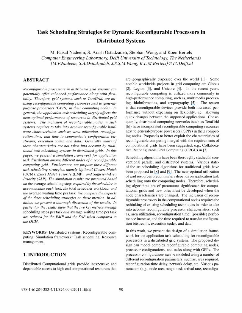
Figure 1: The Resource Management System for a Distrib-uted System with Reconfigurable Nodes.

map tasks onto nodes. The RMS, depicted in Figure 1a,consists of a Grid Information Service (GIS), which is a dy-namically changing module. It contains information aboutthe current states of all the nodes in the network. This in-formation consists of current state (busy or idle) of a par-ticular node, its current Ci configuration and its availablereconfigurable area. The status information of each node isupdated each time the current state of that node is changed.The core of the RMS is a task scheduler which implementsa scheduling algorithm to assign tasks onto nodes. More-over, the RMS contains a bitstream repository which con-sists of a set of bitstreams of different configurations ofCi. These bitstreams are already synthesized, implementedand tested on all the nodes and are considered as valid bit-streams for the system. Each application task in the gridrequires a preferred processor configuration (Cpref ) withspecific parameters. The parametrization characteristicsof Ci processor can be exploited by the grid system by ei-ther sending the required parameters of theCpref of a taskor by sending the corresponding bitstream of the Cpref tothe respective reconfigurable computing nodes.

4. SIMULATION FRAMEWORK DESIGN

In this section, we present the design of the proposed sim-ulation framework. We briefly discuss the proposed datastructures and different modules in the framework.

4.1. Data Structures

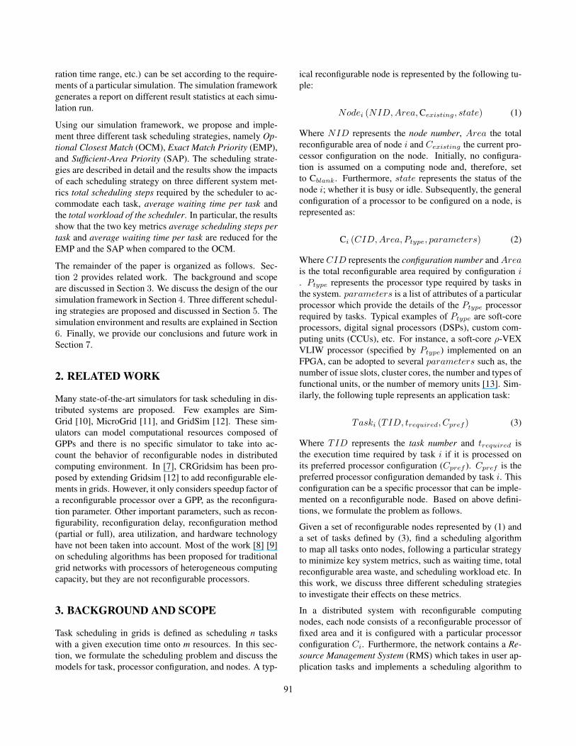
Here we discuss the required data structures developed forresource management in our proposed simulation frame-work. These proposed data structures are used to maintainthe states of the nodes in the resource management system,depicted in Figure 1a. All possible configurations in thegrid are stored in a data structure which is called the con-figurations list depicted in Figure 2a. Each entry in this listcorresponds to the data structure to provide the details ofCi configuration and its parameters as shown in tuple (2).Furthermore, it contains two pointers Idle start and Busy

Configuration Index 0 1 2 3 4 …. n

Configuration C0 C1 C2 C3 C4 …. Cn

Configurations Data Structure

ObjectPtype0

AREA

Idle start

Busy start

Parameter 0

Parameter n

Parameter 1

Ptype1

AREA

Idle start

Busy start

Parameter 0

Parameter n

Parameter 1

Ptypen

AREA

Idle start

Busy start

Parameter 0

Parameter n

Parameter 1

(a) The Configurations List.

Node Index 0 1 2 3 4 …. k

Current Configuration Cexisting Cexisting Cexisting Cexisting Cexisting …. Cexisting

Node Data Structure

ObjectC

AREA

Inext

Bnext

CAREA

Inext

Bnext

CAREA

Inext

Bnext

CurTask CurTaskCurTask

(b) The Nodes List.

Figure 2: The Proposed Data Structures.

start. The Idle start points to the first node of the linked listof the idle nodes with the corresponding configuration of aparticular node. Similarly, the Busy start points to the firstnode of the linked list of busy nodes with the correspondingconfiguration of a particular node. Similarly, Figure 2b de-picts the Node data structure which represents a typical gridnode. It contains the current or the existingCi configurationof the node, reconfigurable area, pointers to the next nodein the idle list with the same configuration (Inext), pointerto the next node in the busy list with the same configuration(Bnext), and a pointer to the current task being executed onthe node (CurTask). The node structure is represented bytuple (1). In the following sections, we describe how thesedata structures are utilized by the simulation framework andthe scheduling module.

4.2. The Simulation Framework

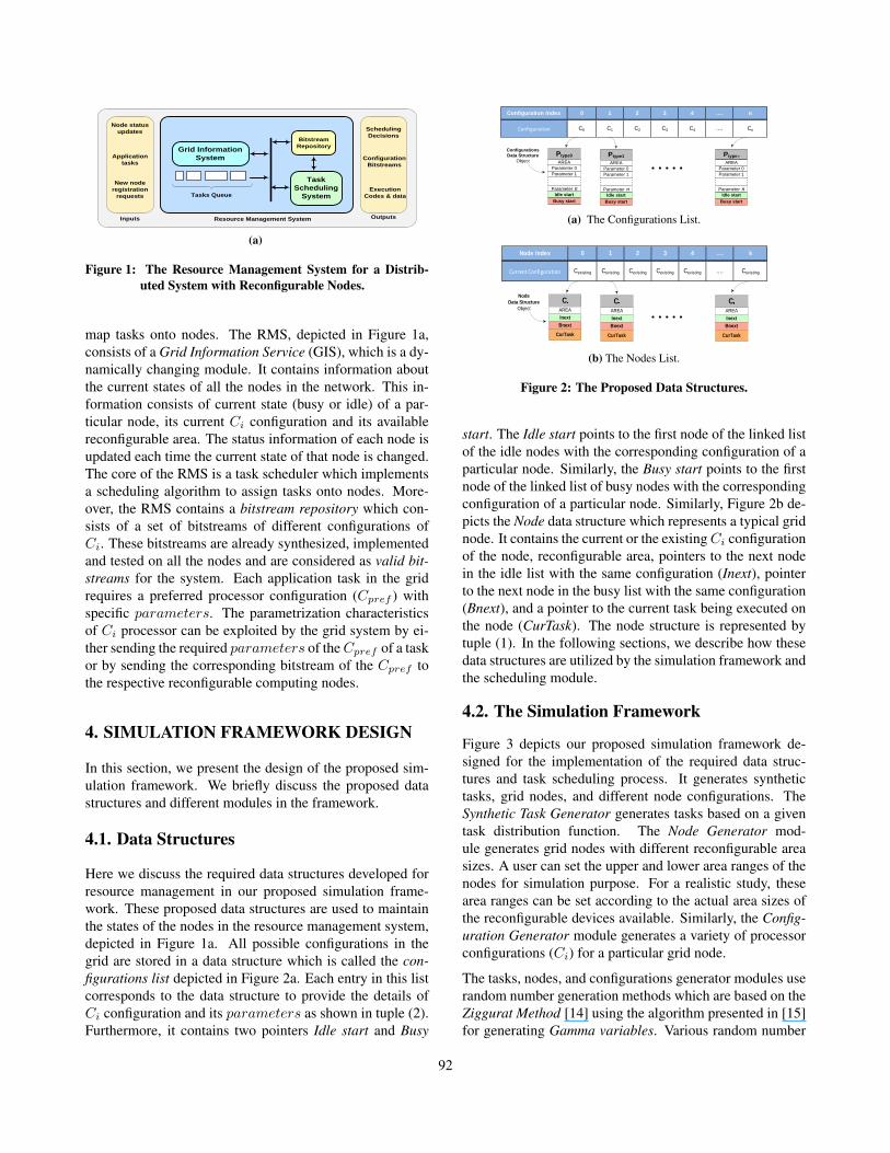
Figure 3 depicts our proposed simulation framework de-signed for the implementation of the required data struc-tures and task scheduling process. It generates synthetictasks, grid nodes, and different node configurations. TheSynthetic Task Generator generates tasks based on a giventask distribution function. The Node Generator mod-ule generates grid nodes with different reconfigurable areasizes. A user can set the upper and lower area ranges of thenodes for simulation purpose. For a realistic study, thesearea ranges can be set according to the actual area sizes ofthe reconfigurable devices available. Similarly, the Config-uration Generator module generates a variety of processorconfigurations (Ci) for a particular grid node.

The tasks, nodes, and configurations generator modules userandom number generation methods which are based on theZiggurat Method [14] using the algorithm presented in [15]for generating Gamma variables. Various random number

92

Synthetic Task Generator

CoreScheduling

ModuleCurrent Busy ListCurrent Idle List

Suspended Tasks Queue

Configurations Generator

Node Generator

Simulation Report

Generator

Configurations List

Node List

Figure 3: The Simulation Framework.

distributions, such as Poisson, Binomial, Gamma, Uniformrandom etc., are provided by a random number generatorclass. The tasks arrival times correspond to the statisticaldistributions available in the class. The core of the simu-lation framework implements a scheduling module whichimplements different scheduling strategies, as discussed inthe Section 5. Furthermore, the framework implements thedata structures described in Section 4.1. The user-definedconfigurations are stored in the Configuration list and thelinked lists are implemented accordingly. The SuspensionQueue holds TIDs of the tasks which can not be accom-modated by any node upon their arrivals. This particularsituation occurs, when all the nodes with Cpref are busyand no blank or idle nodes (with sufficient area) are avail-able for executing the current task. The suspension queue ischecked automatically after the completion of each runningtask to find a potential replacement. The Core SchedulingModule implements different scheduling strategies and themethods required to interact with the node and configura-tion data structures.

Finally, the Simulation Report Generator module stores thestatistics gathered during the simulation process. It re-ports on different performance metrics, such as number ofscheduling steps required by the scheduler to accommodateeach task, total scheduler workload, average task waitingtime, average task running time, reconfiguration count pernode, reconfiguration time per task, etc. The average num-ber of scheduling steps required per task is an indication ofthe total number of search links explored by the schedulerbefore a task can be assigned to a proper node in the system.This metric closely reflects the quantitative value of the timetaken by the scheduler to accommodate a task. The totalscheduler workload provides an estimate of the workloadrequired by the scheduler to assign a task to a proper nodeand to perform various housekeeping jobs, such as initial-ization of node and configuration lists, updating the linkedlists during task assignments, suspension queue checking,etc. These performance metrics are important because theyare proportional to the system time of a host executing thescheduler, hence, critical in comparing different schedulingstrategies. The average waiting time per task provides the

Algorithm 1 The Optional Closest-Match SchedulingInitialize the configs listInitialize the nodes listBegin TaskSchedule (Task CT)Phase-I- If possible, allocate the CT to the best-match node config-ured with its Cpref .- Otherwise if possible, allocate CT to a blank node afterconfiguring it with Cpref of CT.- Otherwise, allocate CT to any idle node (currently config-ured with a Cexisting) after reconfiguring it with Cpref ofCT.Phase-II- If CT required a Cpref not available in the configs list,if possible, allocate CT to any available node with closest-match (of Cpref ) configuration.- Otherwise, put CT in suspension queue if at least one busynode with sufficient area is available.- Otherwise, discard CT.

average time elapsed from the time a task is submitted to thesystem until the time it is assigned to a node to be executed.

5. SCHEDULING STRATEGIES

In this section, we describe the three different schedulingstrategies used in the core scheduling module in the simu-lation framework. The scheduling module takes tasks, con-figurations, and nodes as inputs and assigns the tasks ontodifferent nodes, based on a particular scheduling strategy.

5.1. Optional Closest-Match (OCM) Strategy

An incoming task (current task-CT) is assumed to have itspreferred configuration (Cpref ) as shown in the tuple (2).The algorithm assigns the CT onto a grid node of its Cpref ,if possible. Initially, the Cpref of the CT is matched in theconfigurations list depicted in Figure 2a. If the Cpref isfound in the list, then the algorithm looks for a suitable idlenode of the same configuration by traversing the list of idlenodes of that particular configuration.

If idle nodes are available, the CT is allocated to the best-match node. The node with the best-match is one whichmakes minimum reconfiguration area waste among all thenodes in the linked list. On the other hand, if Cpref isfound in the configurations list, but there is no idle nodeavailable, then the scheduler searches for the list of blanknodes (which are not yet configured). If neither idle norblank nodes are available with the Cpref , then the schedulersearches for any potential idle node of any other configura-tion, by traversing the configurations list. Subsequently, anode with the minimum sufficient area is selected and the

93

task is allocated to it after making it a blank node and re-configuring it with Cpref of the CT.

In case the Cpref of the CT is not found in the configura-tions list (phase-II in Algorithm 1), the scheduler searchesfor a node with the closest-match configuration to the Cpref

of CT. The closest-match processor configuration is the onewhich can still execute the CT but takes more time forprocessing than the exact-match configuration. Once theclosest-match configuration is found, the scheduler looksfor suitable idle nodes with that configuration. If not found,it looks for blank nodes with sufficient area to configurethe closest-match configuration and accommodate the CT.If blank nodes are also not found, then the scheduler putsthe task in the suspension queue to wait for any busy nodewith sufficient area to become idle. Finally, a task is dis-carded if no node with sufficient reconfigurable area can befound to accommodate the current task.

5.2. Exact-Match Priority (EMP) Strategy

The EMP strategy is described in Algorithm 2. At the endof Phase-I, if the scheduler can not find a suitable node toaccommodate the CT, we prefer to wait for a potential nodewith Cpref to be idle than to go for a closest-match configu-ration. Therefore, the scheduler puts the task in the suspen-sion queue. When the queue is checked, the CT is assignedto the first recently released node which is configured withCpref of the CT.

Algorithm 2 The Exact-Match Priority SchedulingInitialize the configs listInitialize the nodes listBegin TaskSchedule (Task CT)Perform Phase-I in the Algorithm-1- If there is at least one busy node with Cpref configurationand sufficient area, put the CT in the suspension queue.Perform Phase-II in the Algorithm-1

5.3. Sufficient-Area Priority (SAP) Strategy

Algorithm 3 describes the SAP scheduling strategy. Themain difference between EMP and SAP is that in SAP,we relaxed the restriction of accommodating the suspendedtasks on the queue with the nodes of the same configura-tion. In other words, the scheduler may select any node re-gardless of its configuration to accommodate a task on thesuspension queue provided that there is enough area. At theend of Phase-I, if the scheduler can not find a suitable node,it puts the CT in the suspension queue. When the queue ischecked, the allocation of CT is made to the first recentlyreleased node with sufficient area to accommodate the task.

If the node is already configured with Cpref , the task is al-located to it. Otherwise, the node is first configured withCpref and then CT is allocated to it.

Algorithm 3 The Sufficient-Area Priority SchedulingInitialize the configs listInitialize the nodes listBegin TaskSchedule (Task CT)Perform Phase-I in the Algorithm-1- If there is at least one busy node with sufficient area, putthe CT in suspension queue.Perform Phase-II in the Algorithm-1

During the scheduling process in all strategies, the corre-sponding busy or idle lists are updated accordingly whenthe CT is allocated to a certain node. If the scheduler selectsa blank node to accommodate the CT, the node is removedfrom the blank list and is attached to the list of busy nodes.

6. SIMULATION ENVIRONMENT AND EX-PERIMENTAL RESULTS

The main simulation parameters used in our experimentsare presented in Table 1. The experiments were con-ducted on different sets of tasks consisting of 103 to 106

tasks. Completion time required by tasks ranges between[100...10000] timeticks. Similarly, the Cpref for any giventask requires area within range [100...2500] area units (e.g.,area slices or FPGA LUTs). For 10 % of the total tasks,we assign a preferred configuration (Cpref ) that can not befound in configurations list. Therefore, these tasks are as-signed to the reconfigurable nodes with closest-match con-figuration by the scheduler at run time.

Table 1: The Main Simulation Parameters.

Parameter ValueTotal number of tasks generated [103...106]Total number of nodes 64, 128Total number of configurations 10, 20, 30, 40, 50Next task arrival interval [1...50]Configurations required area range [100...2500]Node available area range [1000...5000]Task required timeslice range [100...10000]Reconfiguration time range [1...5]

6.1. Results Discussion

All the experiments were performed on Intel Core 2 DuoCPU E8400@3.00GHz, 64-bit machine running Linuxv.2.634. Simulation experiments were conducted for all 3scheduling strategies, in order to compute the total sched-uler workload, average number of scheduling steps re-quired per task, and average waiting time per task. In the

94

103

104

105

10640

50

60

70

80

90

Number of tasks

Avg

. sch

edul

ing

step

s pe

r tas

k

conf10−nodes64conf20−nodes64conf30−nodes64conf40−nodes64conf50−nodes64

(a) Avg. scheduling steps per task.

103

104

105

10610

6

107

108

109

1010

1011

Number of tasks

Tota

l sch

edul

er w

orkl

oad

conf10−nodes64conf20−nodes64conf30−nodes64conf40−nodes64conf50−nodes64

(b) Total scheduler workload (y-axis on log scale).

103

104

105

106

102

103

104

105

106

Number of tasks

Avg.

waitin

g tim

e per

task

conf10−nodes64conf20−nodes64conf30−nodes64conf40−nodes64conf50−nodes64

(c) Avg. task waiting time (y-axis on log scale).

(A) Total Number of Nodes=64.

103

104

105

10640

60

80

100

120

140

Number of tasks

Avg

. sch

edul

ing

step

s pe

r tas

k

conf10−nodes128conf20−nodes128conf30−nodes128conf40−nodes128conf50−nodes128

(d) Avg. scheduling steps per task.10

310

410

510

6106

107

108

109

1010

1011

Number of tasks

Tota

l sch

edul

er w

orkl

oad

conf10−nodes128conf20−nodes128conf30−nodes128conf40−nodes128conf50−nodes128

(e) Total scheduler workload (y-axis on log scale).

103

104

105

10610

2

103

104

105

106

Number of tasks

Avg.

sche

dulin

g st

eps p

er ta

sk

conf10−nodes128conf20−nodes128conf30−nodes128conf40−nodes128conf50−nodes128

(f) Avg. task waiting time (y-axis on log scale).

(B) Total Number of Nodes=128.

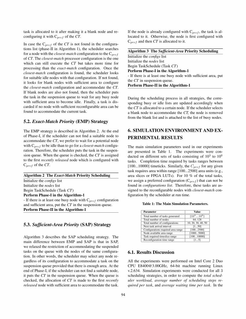
Figure 4: The OCM Scheduling Strategy with a Fixed Set of Configurations. (A) Total nodes=64 and (B) Total nodes=128.

following sections, we discuss results for each schedulingstrategy in detail. Since we used the uniform random num-bers to generate large number of tasks, the average valuesremain the same for several run of simulations for each ex-perimental setup.

The OCM strategy. Figure 4 depicts simulation results forthe OCM scheduling strategy. Figures 4 (A) and 4 (B) giveaverage scheduling steps per task, total scheduler work-load, and average task waiting time results for 64 and 128nodes, respectively.

Figures 4a and 4d compare the average scheduling stepsper task for 64 and 128 nodes, respectively. The schedul-ing steps in both cases are less for smaller number of tasks(104 or less) and then, they reach to a steady-state. Thisoccurs because, initially, the corresponding linked-lists forconfigurations are not formed. Consequently, the numberof scheduling steps are less. Later, when the linked-listsare populated with corresponding configurations and due tomore workload stress on the system, the lists most likelyare searched completely to accommodate an incoming task.Although an option of sending a particular task to a closest-match configuration node is available, but still the numberof nodes are too scarce to make use of closest-match option,resulting in putting more tasks in the suspension queue. Inthe case of 128 nodes, the average scheduling steps per taskare relatively high (around 120) due to more blank nodesbeing searched initially for an exact-match configuration.As depicted in Figures 4b and 4e, the total scheduler work-

load in both cases, increases exponentially (y-axis are inlogarithmic scale) as the number of tasks grow showing theworkload burden on the scheduler. Due to rapid arrival rateand insufficient nodes, the tasks are put more frequently intosuspension queue, which increases scheduler burden. It isslightly more for lesser number of nodes (64 nodes) due tomore congestion in the suspension queue. Similarly, due tomore frequent use of the suspension queue, the average taskwaiting time is also very high (see figures 4c and 4f).

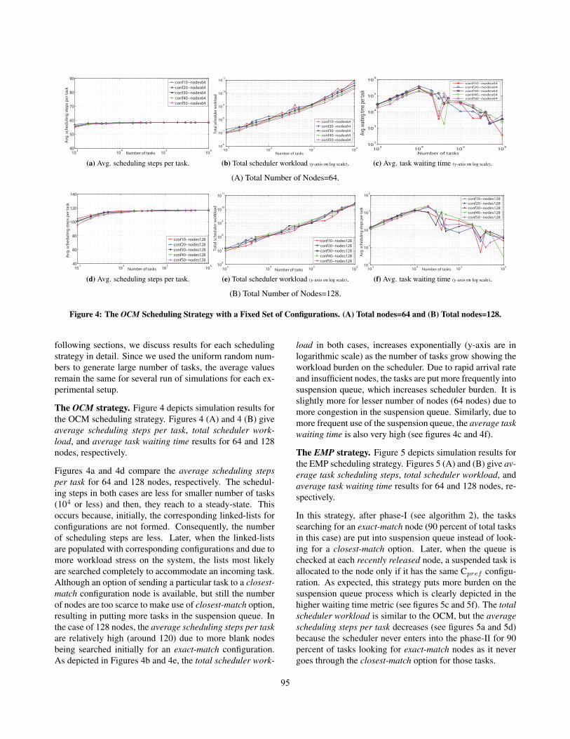
The EMP strategy. Figure 5 depicts simulation results forthe EMP scheduling strategy. Figures 5 (A) and (B) give av-erage task scheduling steps, total scheduler workload, andaverage task waiting time results for 64 and 128 nodes, re-spectively.

In this strategy, after phase-I (see algorithm 2), the taskssearching for an exact-match node (90 percent of total tasksin this case) are put into suspension queue instead of look-ing for a closest-match option. Later, when the queue ischecked at each recently released node, a suspended task isallocated to the node only if it has the same Cpref configu-ration. As expected, this strategy puts more burden on thesuspension queue process which is clearly depicted in thehigher waiting time metric (see figures 5c and 5f). The totalscheduler workload is similar to the OCM, but the averagescheduling steps per task decreases (see figures 5a and 5d)because the scheduler never enters into the phase-II for 90percent of tasks looking for exact-match nodes as it nevergoes through the closest-match option for those tasks.

95

103

104

105

1060

5

10

15

20

25

30

Number of tasks

Avg

. sch

edul

ing

step

s pe

r tas

k

conf10−nodes64conf20−nodes64conf30−nodes64conf40−nodes64conf50−nodes64

(a) Avg. scheduling steps per task.

103

104

105

10610

6

107

108

109

1010

1011

Number of tasks

Tota

l sch

edul

er w

orkl

oad

conf10−nodes64conf20−nodes64conf30−nodes64conf40−nodes64conf50−nodes64

(b) Total scheduler workload (y-axis on log scale).

103

104

105

10610

3

104

105

106

107

108

Number of tasks

Avg

. wai

ting

time

per t

ask

conf10−nodes64conf20−nodes64conf30−nodes64conf40−nodes64conf50−nodes64

(c) Avg. task waiting time (y-axis on log scale).

(A) Total Number of Nodes=64.

103

104

105

1060

5

10

15

20

25

30

Number of tasks

Avg.

sche

dulin

g st

eps p

er ta

sk

conf10−nodes128conf20−nodes128conf30−nodes128conf40−nodes128conf50−nodes128

(d) Avg. scheduling steps per task.

103

104

105

10610

6

107

108

109

1010

1011

Number of tasks

Tota

l sch

edul

er w

orkl

oad

conf10−nodes128conf20−nodes128conf30−nodes128conf40−nodes128conf50−nodes128

(e) Total scheduler workload (y-axis on log scale).

103

104

105

10610

3

104

105

106

107

108

Number of tasks

Avg.

wai

ting

time

per t

ask

conf10−nodes128conf20−nodes128conf30−nodes128conf40−nodes128conf50−nodes128

(f) Avg. task waiting time (y-axis on log scale).

(B) Total Number of Nodes=128.

Figure 5: The EMP Scheduling Strategy with a Fixed Set of Configurations. (A) Total nodes=64 and (B) Total nodes=128.

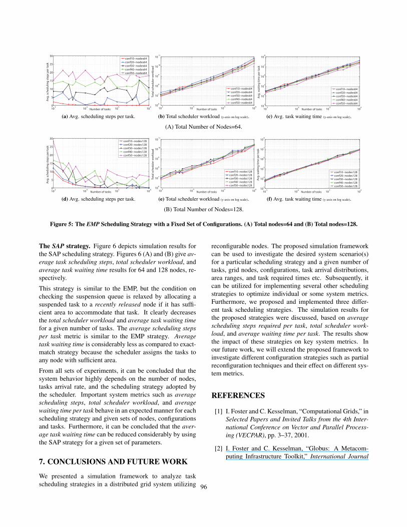
The SAP strategy. Figure 6 depicts simulation results forthe SAP scheduling strategy. Figures 6 (A) and (B) give av-erage task scheduling steps, total scheduler workload, andaverage task waiting time results for 64 and 128 nodes, re-spectively.

This strategy is similar to the EMP, but the condition onchecking the suspension queue is relaxed by allocating asuspended task to a recently released node if it has suffi-cient area to accommodate that task. It clearly decreasesthe total scheduler workload and average task waiting timefor a given number of tasks. The average scheduling stepsper task metric is similar to the EMP strategy. Averagetask waiting time is considerably less as compared to exact-match strategy because the scheduler assigns the tasks toany node with sufficient area.

From all sets of experiments, it can be concluded that thesystem behavior highly depends on the number of nodes,tasks arrival rate, and the scheduling strategy adopted bythe scheduler. Important system metrics such as averagescheduling steps, total scheduler workload, and averagewaiting time per task behave in an expected manner for eachscheduling strategy and given sets of nodes, configurationsand tasks. Furthermore, it can be concluded that the aver-age task waiting time can be reduced considerably by usingthe SAP strategy for a given set of parameters.

7. CONCLUSIONS AND FUTURE WORK

We presented a simulation framework to analyze taskscheduling strategies in a distributed grid system utilizing

reconfigurable nodes. The proposed simulation frameworkcan be used to investigate the desired system scenario(s)for a particular scheduling strategy and a given number oftasks, grid nodes, configurations, task arrival distributions,area ranges, and task required times etc. Subsequently, itcan be utilized for implementing several other schedulingstrategies to optimize individual or some system metrics.Furthermore, we proposed and implemented three differ-ent task scheduling strategies. The simulation results forthe proposed strategies were discussed, based on averagescheduling steps required per task, total scheduler work-load, and average waiting time per task. The results showthe impact of these strategies on key system metrics. Inour future work, we will extend the proposed framework toinvestigate different configuration strategies such as partialreconfiguration techniques and their effect on different sys-tem metrics.

REFERENCES

[1] I. Foster and C. Kesselman, “Computational Grids,” inSelected Papers and Invited Talks from the 4th Inter-national Conference on Vector and Parallel Process-ing (VECPAR), pp. 3–37, 2001.

[2] I. Foster and C. Kesselman, “Globus: A Metacom-puting Infrastructure Toolkit,” International Journal

96

103

104

105

1060

10

20

30

40

50

60

Number of tasks

Avg.

sche

dulin

g st

eps p

er ta

sk

conf10−nodes64conf20−nodes64conf30−nodes64conf40−nodes64conf50−nodes64

(a) Avg. scheduling steps per task.

103

104

105

10610

6

107

108

109

1010

Number of tasks

Tota

l sch

edul

er w

orkl

oad

conf10−nodes64conf20−nodes64conf30−nodes64conf40−nodes64conf50−nodes64

(b) Total scheduler workload (y-axis on log scale).10

310

410

510

6102

103

104

105

106

107

Number of tasks

Avg.

wai

ting

time

per t

ask

conf10−nodes64conf20−nodes64conf30−nodes64conf40−nodes64conf50−nodes64

(c) Avg. task waiting time (y-axis on log scale).

(A) Total Number of Nodes=64.

103

104

105

1060

10

20

30

40

50

60

Number of tasks

Avg.

sche

dulin

g st

eps p

er ta

sk

conf10−nodes128conf20−nodes128conf30−nodes128conf40−nodes128conf50−nodes128

(d) Avg. scheduling steps per task.10

310

410

510

6106

107

108

109

1010

Number of tasks

Tota

l sch

edul

er w

orkl

oad

conf10−nodes128conf20−nodes128conf30−nodes128conf40−nodes128conf50−nodes128

(e) Total scheduler workload (y-axis on log scale).

103

104

105

10610

2

103

104

105

106

107

Number of tasks

Avg.

wai

ting

time

per t

ask

conf10−nodes128conf20−nodes128conf30−nodes128conf40−nodes128conf50−nodes128

(f) Avg. task waiting time (y-axis on log scale).

(B) Total Number of Nodes=128.

Figure 6: The SAP Scheduling Strategy with a Fixed Set of Configurations. (A) Total nodes=64 and (B) Total nodes=128.

of Supercomputer Applications, vol. 11, pp. 115–128,1996.

[3] S. J. Chapin, et. al, “The Legion Resource Manage-ment System,” in Proceedings of the 5th Workshopon Job Scheduling Strategies for Parallel Processing,pp. 162–178, 1999.

[4] D. Erwin, “UNICORE - A Grid Computing Envi-ronment,” in Lecture Notes in Computer Science,pp. 825–834, 2001.

[5] K. Compton and S. Hauck, “Reconfigurable Comput-ing: A Survey of Systems and Software,” ACM Com-puter Survey, vol. 34, no. 2, pp. 171–210, 2002.

[6] TeraGrid, “FPGA Resources in Purdue University.”http://www.rcac.purdue.edu/teragrid/userinfo/fpga.

[7] S. Wong and M. Ahmadi, “Reconfigurable Archi-tectures in Collaborative Grid Computing: An Ap-proach,” in Proceedings of the 2nd International Con-ference on Networks for Grid Applications (GridNets),2008.

[8] F. Dong and S. G. Akl, “Scheduling Algorithms forGrid Computing: State of the Art and Open Prob-lems,” Technical report no. 2006-504, 2006.

[9] H. Topcuoglu, S. Hariri, and M.-Y. Wu, “TaskScheduling Algorithms for Heterogeneous Proces-sors,” in Proceedings of the 8th Heterogeneous Com-puting Workshop (HCW), pp. 3–17, 1999.

[10] H. Casanova, “Simgrid: a Toolkit for the Simula-tion of Application Scheduling,” in Proceedings of theFirst IEEE/ACM International Symposium on Clus-ter Computing and the Grid (CCGrid), pp. 430–437,2001.

[11] H. J. Song, et. al, “The MicroGrid: a Scientific Toolfor Modeling Computational Grids,” Journal of Scien-tific Programming, vol. 8, no. 3, pp. 127–141, 2000.

[12] R. Buya and M. M. Murshed, “GridSim: A Toolkitfor the Modeling and Simulation of Distributed Re-source Management and Scheduling for Grid Com-puting,” Concurrency and Computation: Practice andExperience, vol. 14, no. 13-15, pp. 1175–1220, 2002.

[13] S. Wong, T. V. As, and G. Brown, “p-VEX: A Re-configurable and Extensible Softcore VLIW Proces-sor,” in IEEE International Conference on Field-Programmable Technology (ICFPT), 2008.

[14] G. Marsaglia and W. W. Tsang, “The Ziggurat Methodfor Generating Random Variables,” Journal of Statis-tical Software, vol. 5, no. 8, pp. 1–7, 2000.

[15] G. Marsaglia and W. W. Tsang, “A Simple Method forGenerating Gamma Variables,” ACM Transactions onMathematical Software, vol. 26, no. 3, pp. 363–372,2000.

97