Szymko-S-2006-PhD-Thesis.pdf - Spiral – Imperial College ...

Imperial College

The development of an eddy current dynamometer

for evaluation of steady and pulsating turbocharger

turbine performance

By Shinri Szymko

January 2006

This thesis is submitted for the Doctor of Philosophy Degree of the University of London and The Diploma of Membership of Imperial College

Abstract

Most modern diesel vehicles are fitted with a turbocharger that increases power output, hand-in-hand with a small overall engine efficiency increase. The turbine in a turbocharger operates under pulsating flow conditions, the optimisation of this device is a difficult task due to the highly unsteady flow that feeds it. It operates

at off-design conditions for most of the engine cycle. This thesis presents the experimental performance results of a mixed flow tur-

bocharger turbine under steady and pulsating flow using a new high speed perma-nent magnet eddy current (PMEC) dynamometer. The dynamometers research and

development is described in detail with the overall aim of increasing the load range and measurement accuracy under both steady and pulsating flow. The dynamo-meter allows a reaction torque measurement and has been tested over the full speed

range of 0 - 60,000 RPM. The dynamometer has a power absorption range of 0.3 -

62.2 kW. The steady flow performance results are presented for a mixed-flow turbine pre-

viously developed at Imperial College over a non-dimensional speed range of 0.833 -1.666. The tests have been carried out over a velocity ratio range of 0.375 to 1.068 which is well beyond other testing methodologies commonly used in turbocharger research and it illustrates the usefulness of the dynamometer at enlarging the tur-bine map. The maximum total-to-static efficiency of the turbine was measured to be 74.3 % at a velocity ratio of 0.663. The results demonstrate a reduction in opti-mum velocity ratio for this mixed-flow turbine compared to a typical radial inflow

turbine. The importance of the instrumentation has been highlighted, with particular

emphasis placed on the measurement of the instantaneous quantities. To achieve

the response rate required under pulsating flow, a technique has been developed which allows the simultaneous measurement of the temperature and mass flow rate using a dual hot-wire technique. Significant improvements have been made to the measurement accuracy of the instantaneous mass flow and torque measurements in

relation to previous investigations.

2

The pulsating flow performance of the same mixed flow turbine are presented for a pulse frequency range of 20 - 80 Hz over the non-dimensional speed range of 0.833 - 1.666 with a maximum obtained pressure ratio of 3.27. The results show that the turbine stage does not exhibit quasi-steady behaviour but instead a hysteresis of the performance parameters is recorded. Two types of behaviour has been seen; a 'filling and emptying' regime occurring a lower frequencies and a 'wave action'

regime occurring at the higher frequencies. The introduction of the normalised Strouhal numbers (St.*, S t (p)* ) have proved

consistent for inferring the onset of the above flow regimes and suggests its use as

a tool for the appropriate selection of modelling codes, that is quasi-steady St.* <

0.1, filling-and-emptying S t .(p)* < 0.1 < St.* or wave action S t (p)* > 0.1.

The use of an energy weighted time average has allowed an equivalent quasi-

steady efficiency to be calculated and compared against the true cycle averaged efficiency for the first time. The results show a 6 % mean reduction in the cy-cle averaged efficiency at a pulse frequency of 20 Hz; this reduction reduces with

increasing pulse frequency.

3

Acknowledgment

I wish to thank my supervisors Dr. R.F. Martinez-Botas and Dr. K.R. Pullen. My old office mates Dean Palfreyman, Jae Yoon, and Kaokanya Sudaprasert. I wish also to thank Keith Buffard, Niall McGlashan, Harminder Flora, John Laker and

the many people who have helped and befriended me during this time. Special thanks goes to both my parents and to Joanne Davies who have supported

me during the last few years.

4

This thesis is dedicated to my parents.

5

Contents

Abstract 2

Acknowledgment 4

Dedication 5

Contents 6

List of Tables 12

List of Figures 14

Nomenclature 19

1 Introduction 25 1.1 Automotive Turbochargers 25

1.1.1 General Principles 25 1.1.2 Turbocharging Systems 26

1.2 Project Background 27 1.2.1 Motivation 28 1.2.2 Turbocharger Turbine 29 1.2.3 Permanent Magnet Eddy-Current Dynamometer 31

1.3 Thesis Objectives 33 1.4 Thesis Outline 34

2 Literature Survey 36 2.1 Synopsis 36 2.2 Dynamometers 36 2.3 Turbine Pulsating Flow Performance 45 2.4 Survey Summary 54

3 Dynamometer 55 3.1 Synopsis 55

3.1.1 Objectives and General Specification 55

6

3.2 Initial Prototype - Mk I Dynamometer 56 3.2.1 Rig Layout 56 3.2.2 Instrumentation 59 3.2.3 Experimental Evaluation 60 3.2.4 Mkt Dyno: Summary 64

3.3 Prototype - Mk II Dynamometer 65 3.3.1 Dynamometer Layout 65 3.3.2 Instrumentation 68 3.3.3 Experimental Evaluation 69 3.3.4 Mkt Dyno: Summary 77

3.4 Final Design - Mk III Dynamometer 78 3.4.1 Layout 78 3.4.2 Bearing Module 79 3.4.3 Dynamometer Module 96 3.4.4 Instrumentation 102 3.4.5 Experimental Evaluation 102 3.4.6 Summary 110

4 Magnetic Analysis 111 4.1 Synopsis 111 4.2 Introduction 111 4.3 Governing Equations 112

4.3.1 Boundary Conditions 114 4.3.2 Low Frequency Simplification 115 4.3.3 Potential Formulisation 116

4.4 Finite Element Approach 117 4.4.1 Geometry, Properties and Equation Restrictions 117 4.4.2 Analysis Type and Solvers 119 4.4.3 Post Processing 120

4.5 2D Finite Element Analysis 121 4.5.1 2D Model Transformation 121 4.5.2 Solution Domain 121 4.5.3 Properties and Assumptions 122 4.5.4 Variables 124 4.5.5 Results and Discussion 125 4.5.6 2D Analysis Summary 142

4.6 3D Finite Element Analysis 142 4.6.1 Solution Domain 142 4.6.2 Boundary Conditions 143

7

4.6.3 Properties and Assumptions 145

4.6.4 Variables 147

4.6.5 Results and Discussion 147

4.6.6 3D Model Summary 152

4.7 2D Dynamometer Approximation 152

4.7.1 2D and 3D Model Compatibility 152

4.7.2 Mk3 Dynamometer Model 153

4.7.3 Results 155

4.8 Summary 156

5 Test Facility 157

5.1 Synopsis 157

5.2 Dimensional Analysis 157

5.2.1 Dimensionless Parameters 157

5.2.2 Equivalent Design Conditions 159

5.3 Test Facility 159

5.3.1 Test Facility Layout 160

5.3.2 Air Supply and Heater System 161

5.3.3 Pulse Generator 161

5.3.4 Instrumented Volume 162

5.3.5 Turbine Stage 163

5.3.6 Dynamometer 163

5.3.7 Control System 164

5.3.8 Safety Systems 164

5.4 Instrumentation and Technique 165

5.4.1 Air Mass Flowrate 166

5.4.2 Temperature 170

5.4.3 Pressure 174

5.4.4 Rotational Speed 176

5.4.5 Turbine Torque 177

5.4.6 Miscellaneous 179

5.5 Calibration 181

5.5.1 Air Mass Flowrate Calibration 181

5.5.2 Temperature Calibration 183

5.5.3 Pressure Calibration 185 5.5.4 Rotational Speed Calibration 185

5.5.5 Turbine Torque Calibration 186

5.6 Data Acquisition - Hardware 187

5.6.1 Steady Flow 187

8

5.7

5.8

5.6.2 Unsteady Flow Uncertainty Analysis

5.7.1 Individual Variables

5.7.2 Propagation of Uncertainty

Summary

188 189 189 190 191

6 Steady Flow Experiments 192

6.1 Synopsis 192

6.2 Performance Parameters 192

6.2.1 Efficiency - Velocity Ratio Characteristic 193

6.2.2 Mass Flow rate - Pressure Ratio Characteristic 196

6.3 Experimental Test 196

6.3.1 Test Conditions 196

6.3.2 Data Logging 197

6.4 Experimental Results and Discussion 198

6.4.1 Efficiency Characteristic 198

6.4.2 Mass Flow rate Characteristic 202

6.5 Uncertainty Analysis 203

6.5.1 Independent Variables 204

6.5.2 Parameters 207

6.6 Summary 210

7 Unsteady Flow Experiments 212

7.1 Synopsis 212

7.2 Performance Parameters 212

7.2.1 Efficiency Characteristic 213

7.2.2 Mass Flowrate Characteristic 214

7.3 Experimental Method 214

7.3.1 Test Conditions 214

7.3.2 Data Logging 214

7.4 Data Refinement and Processing 216

7.4.1 Spline Resampling 218

7.4.2 Ensemble Average 218

7.4.3 Filter/Smoothing 220

7.4.4 Phase Shifting 226

7.5 Analysis Parameters 227

7.5.1 Engine Cycle Simulation 227

7.5.2 Cycle-Average Efficiency & Energy Weighted Average 228

7.5.3 Strouhal Number 229

9

7.6 Experimental Results and Discussion 232

7.6.1 Mass Flow Rate Correction 232

7.6.2 Instantaneous Temperature Measurement 234

7.6.3 Inlet and Exit Static Pressure 236

7.6.4 Mass Flow rate 239

7.6.5 Temperature 240

7.6.6 Speed 241

7.6.7 Torque 241

7.6.8 Isentropic and Actual Power 242

7.6.9 Performance Characteristics 243

7.7 Uncertainty Analysis 254

7.7.1 Independent Variables 254

7.7.2 Parameters 258

7.8 Summary 267

8 Conclusions 268

8.1 Synopsis of Achievements 268

8.2 Conclusions 269

8.2.1 PMEC Dynamometer 269

8.2.2 Steady Flow Experimentation 270

8.2.3 Pulsating Flow Experimentation 270

8.3 Suggestions for Further Work 272

8.3.1 Dynamometer Power 272

8.3.2 Experimental Investigation 272

8.4 Epilogue 273

Bibliography 274

Appendices 281

A Introduction 281

A.1 Aerodynamic Dynamometers 282

A.2 Hydraulic Dynamometers 283

A.3 Eddy Current Dynamometers 285

B Dynamometer 286

B.1 Load Cell Calibration 287

B.2 1D Stator Temperature Distribution 287

B.2.1 Boundary Conditions 287

B.3 Fatigue Life 289

10

B.4 Mk III Dyno: Dyno Module Features 290

C Magnetic Analysis 292

C.1 Materials 293 C.1.1 Magnetic Materials 293 C.1.2 Non-Permeable Materials 294 C.1.3 Permeable Materials 294

C.2 Skin Depth 295

D Test Facility and Calibration 296 D.1 Test Facility 297

D.1.1 Pulse Generator 297 D.1.2 Mass Flow Leakage 297

D.2 Calibration 298 D.2.1 Pressure 298 D.2.2 Torque - Load Cell 299 D.2.3 Thermocouple Recovery Factor 299

E Steady Flow Experiments 300 E.1 Uncertainty Analysis 301

E.1.1 Efficiency 301 E.1.2 Velocity Ratio 302 E.1.3 Mass Flow Parameter 303 E.1.4 Pressure Ratio 304 E.1.5 Equivalent Design Speed 305

F Unsteady Flow Experiments 306

11

List of Tables

3.1 MK1 DYNO: ROTOR-STATOR HEAT LOSS PARAMETER VALUES 61

3.2 MK2 DYNO: STATOR MATERIAL PROPERTIES 66

3.3 MK3 DYNO: BEARING SPEED CORRECTION FACTORS 82

3.4 ROTOR DYNAMIC MODEL: PROPERTY VALUES 88

3.5 ROTOR DYNAMIC MODEL: RESULTS 89

3.6 MAGNETIC ROTOR: COMPARISON 91

3.7 MAGNETIC ROTOR: PLASTIC STRESS-STRAIN DATA FOR 7075-T6 92

3.8 MAGNETIC ROTOR: PROPERTIES 92

3.9 MAGNETIC ROTOR: RADIUS CHANGE AFTER ASSEMBLY 94

4.1 2D MODEL: MATERIAL PROPERTIES 124

4.2 2D MAGNETIC REYNOLDS NUMBER: PERMEABLE 136

4.3 3D MODEL: MATERIAL PROPERTIES 146

4.4 3D STATOR FORCE COMPONENTS 148

4.5 MK3 3D COMPARISON MODEL: MATERIAL PROPERTIES 155

4.6 SHAPE FACTOR DETERMINATION MODEL 155

5.1 EQUIVALENT DESIGN CONDITIONS 160

5.2 GEOMETRIC DETAIL OF TURBINE 'D' 164

5.3 AUTOMATED SAFETY LOOP 165

5.4 TEMPERATURE MEASUREMENT TYPE AND LOCATION 170

5.5 PRESSURE MEASUREMENT TYPE AND LOCATION 175

5.6 CTA HOT-WIRE TEMPERATURE SPECIFICATION 181

6.1 TURBINE 'D' STEADY STATE TEST CONDITIONS 196

6.2 STEADY FLOW PERFORMANCE PARAMETER RANGE 202

6.3 STEADY MASS FLOW - INDEPENDENT VARIABLE UNCERTAINTY . . . 204

7.1 TURBINE 'D' MEAN PULSATING FLOW TEST CONDITIONS 215

7.2 MSER: 50 COMPLETE DATA CYCLES 219

7.3 GAS VELOCITY STROUHAL NUMBER: EXPERIMENTAL AVERAGE . . 231

7.4 ACOUSTIC STROUHAL NUMBER: EXPERIMENTAL AVERAGE 231

7.5 PRESSURE STROUHAL NUMBER: EXPERIMENTAL AVERAGE 231

12

7.6 HOT-WIRE CORRECTION: CYCLE AVERAGED COMPARISON 233

7.7 PULSATING FLOW RESULTS: TEMPERATURE COMPARISON 235

7.8 STEADY LIMIT STROUHAL NUMBER: PULSE FREQUENCY 245

7.9 PULSATING FLOW: CYCLE AVERAGE EFFICIENCY 250

7.10 PULSATING FLOW: ISENTROPIC SPECIFIC WORK AND POWER . . 251

7.11 PULSATING FLOW: TRI-FILAR UNCERTAINTY 258

7.12 PULSATING FLOW: UNCERTAINTY FRACTIONAL IMPORTANCE . . 259

7.13 PULSATING FLOW: CYCLE AVERAGE UNCERTAINTY - EFFICIENCY . 262

7.14 PULSATING FLOW: CYCLE AVERAGE UNCERTAINTY - U21C,s 263

7.15 PULSATING FLOW: CYCLE AVERAGE UNCERTAINTY - MFP 264

7.16 PULSATING FLOW: CYCLE AVERAGE UNCERTAINTY - PR 265

7.17 PULSATING FLOW: CYCLE AVERAGE UNCERTAINTY - EQUIV. SPEED 266

C.1 SKIN DEPTH FIELD AND POWER DENSITIES 295

13

List of Figures

1.1 SIMPLE SCHEMATIC OF A TURBOCHARGED ENGINE 26

1.2 IDEAL SUPERCHARGED LIMITED PRESSURE 4-STROKE CYCLE 27

1.3 RADIAL AND MIXED FLOW TURBINES 30

1.4 ISENTROPIC POWER AND VELOCITY RATIO 31

1.5 EDDY CURRENT PRINCIPLE 32

1.6 ORIGINAL EPSRC DYNAMOMETER PROPOSAL, GR/M47812/01 33

2.1 EARLY NASA RADIAL TURBINE AERODYNAMIC DYNAMOMETER . 37

2.2 UMIST RADIAL TURBINE OIL HYDRAULIC DYNAMOMETER 39

2.3 OPERATING RANGE OF VARIOUS DYNAMOMETERS 40

2.4 McDONNELL RADIAL TURBINE OIL HYDRAULIC DYNAMOMETER . 40

2.5 IMPERIAL COLLEGES EDDY CURRENT DYNAMOMETER 43

2.6 OPERATING RANGE OF IMPERIAL COLLEGES EC DYNAMOMETER 44

2.7 STEADY FLOW RESULTS, [25] 46

2.8 STEADY AND PULSATING FLOW RESULTS, [25] 46

2.9 PULSATING FLOW RESULTS, [61] 48


2.11 STEADY AND PULSATING FLOW RESULTS, [4] 50


2.13 TEST SECTION AND PHASE SHIFT, [42] [75] 53

2.14 TRAVERSE GRID AND K-FACTOR, [42] 53

3.1 MK1 DYNO: LAYOUT 57

3.2 MK1 DYNO: ASSEMBLY 58

3.3 MK1 DYNO: MAIN COMPONENTS 58

3.4 MK1 DYNO: EXPERIMENTAL LAYOUT 59

3.5 MK1 DYNO: 4 AND 8-POLE ROTOR RESULTS 62

3.6 MK1 DYNO: VIBRATIONS 63

3.7 MK2 DYNO: LAYOUT 65

3.8 MK2 DYNO: ASSEMBLY 66

3.9 MK2 DYNO: GIMBAL SCHEMATIC 68

3.10 MK2 DYNO: PHOTOGRAPH EXPERIMENTAL LAYOUT 69

14

3.11 MK2 DYNO: RESULTS 70

3.12 MK2 DYNO: RSS MEASUREMENT UNCERTAINTY 72

3.13 MK2 DYNO: RESULTS - STATOR PLATES 74

3.14 MK2 DYNO: VIBRATIONS 76

3.15 MK3 DYNO: GENERAL LAYOUT 78

3.16 MK3 DYNO: BEARING MODULE 81

3.17 MK3 DYNO: BEARING ARRANGEMENT 83

3.18 MK3 DYNO: BEARING UNIT 84

3.19 MK3 DYNO: BEARING MODULE EXPLODED VIEW 86

3.20 MK3 DYNO: ROTOR DYNAMIC SOLUTION DOMAIN 88

3.21 MK3 DYNO: IDEAL AND ACTUAL 14-POLE ROTOR 90

3.22 MK3 DYNO: 14 POLE DOUBLE ROW MAGNETIC ROTOR PHOTOGRAPH 90

3.23 MK3 DYNO: 14 POLE MAGNETIC ROTOR: SOLUTION DOMAIN 92

3.24 MK3 DYNO: CONTACT ANALYSIS - MCL AND SCL RESULTS 95

3.25 MK3 DYNO: 14 POLE MAGNETIC ROTOR 95

3.26 MK3 DYNO: DYNAMOMETER MODULE 96

3.27 MK3 DYNO: DYNAMOMETER MODULE 97

3.28 MK3 DYNO: FLOW ANALYSIS, [67] 99

3.29 MK3 DYNO: DYNAMOMETER MODULE EXPLODED VIEW 100

3.30 MK3 DYNO: OVERALL SCHEMATIC 103

3.31 MK3 DYNO: OVERALL PHOTOGRAPH 104

3.32 MK3 DYNO: RESULTS - VARIOUS GAPS 105

3.33 MK3 DYNO: INTERPOLATED RESULTS - VARIOUS SPEEDS 106

3.34 MK3 DYNO: RSS MEASUREMENT UNCERTAINTY 107

3.35 MK3 DYNO: RESULTS - STATOR PLATES 108

3.36 MK3 DYNO: RESULTS - VIBRATIONS 109

4.1 MK1, MK2 AND MK3 DYNAMOMETER LAYOUT 111

4.2 GENERAL MAGNETIC MODEL DOMAIN 114

4.3 2D MODEL TRANSFORMATION 121

4.4 2D MODEL: SOLUTION DOMAIN & MODEL VARIABLES 122

4.5 2D MODEL: PERIODIC BOUNDARY ASSIGNMENT 123

4.6 2D FLUX LINES: SKIN DEPTH DEVELOPMENT, NON-PERMEABLE 126

4.7 2D TOTAL FLUX PLOT: NON-PERMEABLE 127

4.8 2D MAGNETIC FLUX DENSITY PLOTS: NON-PERMEABLE 127

4.9 2D CURRENT DENSITY PLOT: NON-PERMEABLE 127

4.10 2D JOULE HEAT PLOT: NON-PERMEABLE 128

4.11 2D ACTIVITY AREA FLUX PLOT: NON-PERMEABLE 128

4.12 2D LORENTZ FORCE X-COMPONENT PLOT: NON-PERMEABLE 129

15

4.13 2D LORENTZ FORCE Y-COMPONENT PLOT: NON-PERMEABLE . 129

4.14 2D LORENTZ FORCE: NON-PERMEABLE 130

4.15 2D NON-PERMEABLE: POWER VS STATOR THICKNESS & RESISTIVITY 131

4.16 2D NON-PERMEABLE: POWER VS STATOR THICKNESS AND SPEED . . 132

4.17 2D NON-PERMEABLE: POWER VS POLE NUMBER FOR VARIOUS GAPS 133

4.18 2D NON-PERMEABLE: POWER VS RESISTIVITY & STATOR THICKNESS 133

4.19 2D FLUX LINES: SKIN DEPTH DEVELOPMENT, PERMEABLE 134

4.20 2D MAGNETIC FLUX DENSITY PLOTS: PERMEABLE 135

4.21 2D MAGNETIC REYNOLDS NUMBER PLOT: PERMEABLE 135

4.22 2D PERMEABILITY PLOT: PERMEABLE 136

4.23 2D CURRENT DENSITY PLOT: PERMEABLE 137

4.24 2D JOULE HEAT PLOT: PERMEABLE 137

4.25 2D LORENTZ FORCE X-COMPONENT GRAPH: PERMEABLE 138

4.26 2D PERMEABLE: POWER VS STATOR THICKNESS AND RESISTIVITY 140

4.27 2D PERMEABLE: POWER VS STATOR THICKNESS AND SPEED . . . . 140

4.28 2D PERMEABLE: POWER VS POLE NUMBER FOR VARIOUS GAPS . . . 141

4.29 2D PERMEABLE: POWER VS RESISTIVITY AND STATOR THICKNESS . 141

4.30 3D MODEL: MK1 AND MK2 SOLUTION DOMAIN 143

4.31 3D MODEL: MK2 DYNO ELEMENT DOMAIN & BOUNDARY CONDITIONS 144

4.32 3D MODEL: CYCLIC BOUNDARY NODE ROTATION 145

4.33 3D STATOR SURFACE FORCE PLOT: COPPER STATOR, 60 kRPM 148

4.34 3D STATOR SURFACE PLOT: COPPER STATOR, 60 kRPM 150

4.35 3D 1 MM STATOR DEPTH PLOT: COPPER STATOR, 60 kRPM 150

4.36 3D 2 MM STATOR DEPTH PLOT: COPPER STATOR, 60 kRPM 150

4.37 3D MODEL: EXPERIMENTAL COMPARISON 151

4.38 MK3 ROTOR MAGNET SWEPT WIDTH 153

4.39 MK3 2D MODEL: SOLUTION DOMAIN 154

4.40 MK3 3D MODEL: SOLUTION DOMAIN & MESH 154

4.41 MK3 DYNO: 2D COMPARISON TO EXPERIMENTAL - STEEL 156

5.1 GENERAL TEST FACILITY LAYOUT 160

5.2 PULSE GENERATOR - ROTATION 162

5.3 INSTRUMENTED VOLUME 163

5.4 MODEL OF MIXED-FLOW TURBINE 'D' 164

5.5 36-POINT HOT-WIRE TRAVERSE GRID 169

5.6 HOT-WIRE CALIBRATION: OVERALL CORRELATION 183

5.7 INSTANTANEOUS TEMPERATURE CALIBRATION 184

5.8 TURBINE SPEED: TOOTHED ENCODER CORRECTION 186

5.9 NORMAL DISTRIBUTION: BIAS AND PRECISION UNCERTAINTIES 189

16

6.1 TURBINE H-S DIAGRAM 193

6.2 DATA LOGGING: DAQ MODULES 197

6.3 DYNAMOMETER POWER VERSUS VELOCITY RATIO 199

6.4 STEADY FLOW RESULTS 201

6.5 STATIC TAPPING ERROR, BENEDICT, 1984 [6] 205

6.6 STEADY FLOW: OVERALL RSS UNCERTAINTY 211

7.1 INSTANTANEOUS DATA REFINEMENT PROCEDURE 217

7.2 INSTANTANEOUS DATA REFINEMENT EXAMPLE 221

7.3 INSTANTANEOUS SPEED DATA - FFT 223

7.4 VOLUTE MEAN FLOW PATH 225

7.5 INSTANTANEOUS PRESSURE DATA - FFT 225

7.6 PHASE SHIFT: LENGTH SCALES 227

7.7 STROUHAL NUMBER: SCALE DEFINITIONS 230

7.8 PULSATING FLOW: TINST 70 % SPEED, MASS FLOW CORRECTION 233

7.9 PULSATING FLOW: TINST 70 % SPEED, TEMPERATURE COMPARISON 235

7.10 PULSATING FLOW: TINST 70 % SPEED, MEASURED PARAMETERS . . . 237

7.11 PULSATING FLOW: TINST 70 % SPEED, PRESSURE & POWER 238

7.12 PULSATING FLOW: TINST 70 % SPEED, PERFORMANCE PARAMETERS 244

7.13 PULSATING FLOW: MEASURED, QUASI STEADY EFFICIENCY 252

7.14 PULSATING FLOW: RSS UNCERTAINTY - EFFICIENCY 262

7.15 PULSATING FLOW: RSS UNCERTAINTY - VELOCITY RATIO 263

7.16 PULSATING FLOW: RSS UNCERTAINTY - MASS FLOW PARAMETER . 264

7.17 PULSATING FLOW: RSS UNCERTAINTY - PRESSURE RATIO 265

7.18 PULSATING FLOW: RSS UNCERTAINTY - EQUIVALENT SPEED 266

A.1 MIYASHITA ET AL RADIAL TURBINE AERODYNAMIC DYNAMOMETER 282

A.2 WONG AND NUSBAUM AERODYNAMIC DYNAMOMETER 282

A.3 DAS RADIAL TURBINE OIL HYDRAULIC DYNAMOMETER 283

A.4 HIETT AND JOHNSTON HYDRAULIC DYNAMOMETER 283

A.5 NASA RADIAL TURBINE WATER HYDRAULIC DYNAMOMETER 284

A.6 WALLACE'S RADIAL TURBINE OIL HYDRAULIC DYNAMOMETER 284

A.7 NASA RADIAL TURBINE EDDY CURRENT DYNAMOMETER 285

A.8 SASAKI'S AC GENERATOR BASED DYNAMOMETER 285

B.1 MK2 DYNO: LOAD CELL CALIBRATION 287

B.2 STATOR TEMPERATURE: FOURIER LAW OF CONDUCTION 288

C.1 MAGNETIC PROPERTIES: CRUMAX 4014 293

C.2 GENERAL MATERIAL PROPERTIES 294

C.3 STEEL PROPERTIES 294

17

C.4 SKIN DEPTH PENETRATION 295

PULSE GENERATOR: FLOW AREA 297

MASS FLOW LEAKAGE : PIPEWORK 297

STEADY FLOW: PRESSURE TRANSDUCER CALIBRATION 298

PULSATING FLOW: PRESSURE TRANSDUCER CALIBRATION 298

LOAD-CELL TORQUE CALIBRATION

299

THERMOCOUPLE RECOVERY FACTOR 299

CONSTITUENT EFFICIENCY UNCERTAINTY 301

CONSTITUENT VELOCITY RATIO UNCERTAINTY 302

CONSTITUENT MFP UNCERTAINTY 303

CONSTITUENT PRESSURE RATIO UNCERTAINTY 304

CONSTITUENT EQUIVALENT SPEED UNCERTAINTY 305

F.1

PULSATING F LOW: 50 % SPEED, MEASURED PARAMETERS 307

F.2

PULSATING F LOW: 50 % SPEED, PRESSURE & POWER 308

F.3

PULSATING F LOW: 50 % SPEED, PERFORMANCE PARAMETERS 309

F.4


F.5


F.6


F.7


F.8


F.9


F.10 PULSATING F LOW: 80 % SPEED, MEASURED PARAMETERS 316

F.11 PULSATING F LOW: 80 % SPEED, PRESSURE & POWER 317

F.12 PULSATING F LOW: 80 % SPEED, PERFORMANCE PARAMETERS 318

F.13 PULSATING F LOW: 90 % SPEED, MEASURED PARAMETERS 319

F.14 PULSATING F LOW: 90 % SPEED, PRESSURE & POWER 320

F.15 PULSATING F LOW: 90 % SPEED, PERFORMANCE PARAMETERS 321

F.16 PULSATING FLOW: 100 % SPEED, MEASURED PARAMETERS 322

F.17 PULSATING FLOW: 100 % SPEED, PRESSURE & POWER 323

F.18 PULSATING FLOW: 100 % SPEED, PERFORMANCE PARAMETERS 324

F.19 PULSATING FLOW: 20 - 80 Hz, PRESSURE, MASS FLOW 325

F.20 PULSATING FLOW: 20 - 80 Hz, TEMPERATURE, EXIT PRESSURE 326

F.21 PULSATING FLOW: 20 - 80 Hz, TORQUE, EFFICIENCY 327

F.22 PULSATING FLOW: 20 - 80 Hz, POWER 328

F.23 PULSATING FLOW: 20 - 80 Hz, PERFORMANCE PARAMETERS 329

D.1

D.2

D.3 D.4

D.5

D.6

E.1

E.2

E.3

E.4

E.5

18

Alternating Current Data AcQuisition Dynamometer Electro-Magnetic Force Fast Fourier Transform Internal Combustion Laser Doppler Velocimetry Magnet Centre Line

Number of Pulse Cycles Pressure Ratio Root Mean Square Revolution Per Minute Spider Centre Line Velocity Ratio

DC DOF EC FS HTD LCD MSER NDP PC PPR RSS RPS TTL VGT

Direct Current Degree of Freedom Eddy Current Full Scale High Torque Drive Liquid Crystal Display

Mean Square Error Ratio Number of Data Points

Personal Computer Pulses Per Revolution

Root-Sum-Square Revolution Per Second Transistor-Transistor Logic Variable Geometry Turbine

Nomenclature

Abbreviations

AC DAQ Dyno EMF FFT IC LDV MCL NPC PR RMS RPM SCL VR

A/R CFD CTA EPSRC FIR MFP NASA NdFeB PCI PMEC M Nu Gr Pr

Area Radius Ratio Computational Fluid Dynamics Constant Temperature hotwire Anemometer Engineering and Physical Sciences Research Council

Finite Impulse Response (non-recursive) Pseudo-non-dimensional mass flow rate parameter National Aeronautics and Space Administration Neodymium-Iron-Boron Peripheral Component Interconnect Permanent Magnet Eddy Current

Mach Number Nusselt Number Grashof Number Prandtl Number

M E

Nu= Gr = L3gi3°T 2

Pr ='-' = uCP

19

cf.r, Re Reynolds Number Re = p 1-, NpD2 Reo Rotational Reynolds Number Re4, = 27 il

St.* Normalised Strouhal Number St.* = —fU L jr- 20

St.(a)* Acoustic Normalised Strouhal Number St.(a)* = St*M

St.(p)* Presssure Normalised Strouhal Number St.(p)* = St* M+1

.75 Flow coefficient 0 — c,,, u2 0 Loading coefficient 0 = 6'h2 U 2

English

a* Hot-wire: Overheat ratio

a Hot-wire: geometric/resistance constant

a Speed of sound m/s

b Hot-wire: geometric/resistance constant

Intercept Specific heat capacity J/kgK

d Turbine mean diameter, orifice diameter

f Fraction Frequency Hz

h Heat transfer coefficient Wlm2 K h FIR filter coefficient

Specific enthalpy J/kg i Integer, no. of load sharing bearings

Incidence angle degrees j Imaginary

Thermal conductivity W/mK k Generic constant

m slope, gradient Hot-wire: Temperature loading factor

sic Mass flow rate kg/s

n Hot-wire: constant Sample number

ndm Speed factor RPM.mm q Charge

r Recovery factor

t Time

t Student's t multiplier

x Generic variable

20

V x V.

A A [A] B [B]

CO C33

Cd Cis

Co C D [D] E E

[E] F

H He [H] I

[J] L L

Llo Liar

Mo N N, P

P33

Q Q.;

Curl operator Divergence operator

Area Hot-wire: fluid property constant Magnetics: Magnetic vector potential

Hot-wire: fluid property constant Magnetics: Magnetic flux density vector Static bearing load capacity Dynamic bearing load capacity Discharge coefficient Isentropic expansion velocity Tangential gas velocity

Cylinder number Orifice upstream internal diameter Electric flux density vector Young's modulus Hotwire: CTA probe voltage Magnetics: Electric field intensity vector

Force Shear modulus No. of cylinder groups Hot-wire: generic geometric constant

Isentropic specific work, total-to-total Magnetics: Coercive Force Magnetics: Magnetic field intensity vector

Polar mass moment of inertia Magnetics: Current density vector

Angular momentum Length Bearing fatigue life, 90% survival Bearing fatigue life, varying speeds, 90% survival Magnetics: Remanent intrinsic magnetisation vector Turbine rotational speed

Turbine specific speed Pressure Equivalent dynamic bearing load

Volume flow rate Magnetics: Joule heat

m/s

Tm

T N N

m/s m/s

CITO GPa V Vim N GPa

J/kg Alm Alm kgm2

kg — m21 sec

hrs hrs Alm RPS radians Pa N

m3/s J

21

Q Heat flux W

R Gas Constant J/kgK

S Speed encoder: No. of tooth-gap segments

S Standard sample deviation (n-1)

T Temperature °K

U Linear velocity, air velocity m/s

W Power W

X Generic variable —

Greek

a Angular acceleration rads/s2

a Absolute gas flow angle degrees

0 Orifice area ratio = d/D

i3 Thermal expansion coefficient 1/K

0 Relative gas flow angle degrees

X Shape factor

6 Skin depth m

6 Expansion factor

0 Duty cycle (Pulse period fraction)

.13 Hot-wire: Mach number influence on Nu

7 Specific heat ratio —

71 Turbine stage efficiency —

k Thermal diffusivity 771,2/s

A Air pulse frequency Hz

11 Dynamic viscosity Ns/m2

is Coefficient of friction —

Po Magnetics: Permeability of free space: 47r x 10-07 Hlm

PT Magnetics: Relative permeability

v Poisson's ratio

0 Degrees

e Radians Rads

P Density kg/m3

P Magnetics: Resistivity am a Standard deviation —

r Turbine torque Nm

w Angular velocity rads' s

Derivation: Pressure Ratio

V) Bandwidth tolerance factor

22

Subscripts

a abs amb arm B2 bearing cal equiv fa

f re f

h is in inst i m mrotor msw offset ori f out pl p2 ref RS S s stator t — s w w 0 1 2

3 4

Recovery value Absolute quantity

Ambient Load cell lever arm Blade inlet angle

Bearing Calibration value Equivalent Hot-wire: property value

T fa = 1/2(T„, — Ta )

Hot-wire: property value

temperature. Tf„f = 1/2(Ta, — T„ f )

Heat loss Isentropic Inner limb, inlet value

Instantaneous Index/integer value Hot-wire: temperature loading factor Magnetic rotor Magnetics: magnet swept width

Offset value

Orifice outer limb, outlet value Hot-wire: probe 1 Hot-wire: probe 2 Hot-wire: calibration value

Root-Sum-Square Static condition Stator variable Total-to-static Water Hot-wire: wire Stagnation condition

Volute inlet Turbine mean inlet

Turbine exit Volute exit

deg

at mean film temperature

at mean calibration film

23

Superscripts

Mean quantity Fluctuating quantity Fluctuating transfered quantity

* Approximate calculated value * Normalised or non-dimensional quantity

24

Chapter 1

Introduction

Turbochargers are a successful means of increasing the power output of a recipro-

cating engine and are used extensively on marine, locomotive, land-based industrial and commercial automotive diesel engines.

Over the last 20 - 30 years energy and environmental concern has become more important due in part to legislation and is one of the significant driving forces in development. In the diesel automotive sector, manufacturers strive to improve per-formance from their engines whilst reducing emissions which has led to virtually all modern heavy diesels being fitted with a turbocharger. At the turn of the millen-nium around one million turbocharged vehicles were on British roads with nearly

all major car manufacturers offering a turbo-diesel model.

1.1 Automotive Turbochargers

1.1.1 General Principles

Turbocharging is a form of supercharging, which is the pressurised air induction of an IC engine. A turbocharger is a machine which is mechanically separate from the IC engine and consists of an air compressor driven by the exhaust gases of the engine instead of being mechanically driven as with a supercharger. In the case

of an automotive turbocharger the compressor is directly coupled to a radial or mixed-flow turbine which is driven by the otherwise wasted exhaust gases. The turbine stage consists of a volute and turbine rotor. The purpose of the volute is to direct the incoming flow uniformly around the periphery of the rotor where energy can be extracted from the gas. The compressor increases the air density entering the combustion chamber of the IC engine; this greater mass allows more fuel to be injected and burnt per power stroke. Figure 1.1 shows a simple schematic of an

automotive turbocharged engine.

25

Figure 1.1: SIMPLE SCHEMATIC OF A TURBOCHARGED ENGINE, [28]

1.1.2 Turbocharging Systems

Figure 1.2 shows the idealised energy available to the turbine of a supercharged 4-stroke limited pressure cycle. In practice not all this energy can be utilised but two main methods are employed to try to harness this, the 'constant pressure system'

and the 'pulse pressure system'. The latter is suited to automotive applications.

Constant Pressure/Steady-flow System The pulsating flow exiting the IC engine is fed through short pipes into a single exhaust manifold with sufficient volume

to damp out the pressure pulsations. The turbine stage acts as a restriction and is driven by the constant pressure reservoir. The available turbine energy can be seen by the P-V diagram bounded by 7-8-10-11, Figure 1.2. The 'constant pressure

system' is unsuitable for automotive applications due to its slow transient response and large space requirements resulting from the pressure reservoir. This type of system is ideal for large marine diesels, locomotives and power generation units.

Pulse Pressure/Unsteady-flow System In the 'pulse pressure system' an at-

tempt is made to harness the energy associated with the high-pressure pulses exiting the exhaust valve as well as the energy associated with the 'constant pressure sys-tem'. This is achieved by connecting the exhaust ports of the engine to the turbine through narrow short pipes, largely preserving the exhaust pulse. The additional energy available at the turbine is largely held by the pressure wave and to a smaller extent the preservation of the kinetic energy leaving the exhaust port. Ideally for the 'pulse pressure system' the available energy for the turbine can be seen on a P-V

diagram bounded by 5-8-10-11-1, Figure 1.2.

26

Pe

2

T C V

till*" of • a sr ZAira..-

KnahltennegiSSOSSVAVaaseiftwows....

Figure 1.2: IDEAL SUPERCHARGED LIMITED PRESSURE 4-STROKE CYCLE, [83]

The complexities arise in the interactions of the pressure pulses with the turbine stage and with the engine performance itself. The pressure pulsations result in a large variance in the operating conditions seen by the turbine rotor, Karamanis,

2001 [43] which will ultimately impact the overall stage performance. The pres-sure pulsations can also reflect from the turbine and interact with the scavenging process of the engine in a positive or negative way. These interactions become more complicated with the addition of multiple-cylinders as pulses from one cylinder can adversely effect the scavenging of another. The manifold design is crucial in order for the engine and the turbocharger to work well, which due to the engine valve timing typically result in a maximum of three cylinders connected to a common manifold on a 4-stroke engine. A single turbine can generally support up to six cylinders by using a split volute with two separate passageways to inhibit interference.

1.2 Project Background

The strive towards reduced exhaust emissions and greater fuel economy has increased the importance of turbine design and turbocharger matching to the automotive engine, the large speed and load range of the engine increases this difficulty. Within one pulse cycle the operating point of the turbine will swing from one extreme to the other further increasing the difficulty in optimising and understanding the turbine

and its subsequent match. The automotive research group at Imperial College has actively been involved in

the development and understanding of pulsed flow turbines since the 1980's. The turbocharger test facility was originally developed by Dale and Watson, 1986 [24]

27

and extended by Baines et al, 1994 [4]. The facility was modified to accommodate the mixed-flow turbine research programme of Abidat, 1991 [1] with pulse flow

experimental work presented by Arcoumanis et al, 1995 [3] and Hakeem, 1995 [36]. Further researchers Su, 1999 [75] and Karamanis, 2000 [42] extended the research

into LDV inlet and exit flow measurements of the turbine rotor.

1.2.1 Motivation The range of the turbine steady state performance map that can be obtained exper-

imentally is limited by the loading range of the power absorption device used. The accuracy of the experiments are limited by the instrumentation and the measure-

ment methodology employed. The loading device typically used in industry and previously in this test facility

is a centrifugal compressor. The disadvantage of this is a narrow window in which the performance of the turbine can be found; the compressor must work within its surge and choke limits. The experimental results obtained by Karamanis, 2000 [42] found that the steady state performance maps of a mixed-flow turbine' were limited

to a velocity ratio (U2/Cis) range of 0.2 - 0.1 at the turbine design speed of 50 -100 % respectively. To obtain a good engine match, simulation codes are frequently used and require a large range performance map to achieve accurate results; this is generally not available when using a compressor as the loading device. Extrapolation

of the turbine map is therefore necessary which may result in significant errors and

make code validation limited. Improvements to the measurement systems particularly in pulsating flow are ad-

dressed in this thesis and are briefly outlined at this stage. The calculation of the steady and unsteady performance parameters necessitates the accurate measurement of both the mean and instantaneous turbine torque. The previous test facility ther-modynamically measured the mean turbine torque from the power consumed by the compressor and bearings. This required the measurement of 14 physical quantities, 9 of these being thermodynamic; this results in significant uncertainties particularly

at the high velocity ratios regions, Hakeem, 1995 [36]. To measure the instantaneous torque, it is useful if the angular inertia of the

rotational assembly has a known and low value, this requirement imposes restrictions on the suitable choice of dynamometer, discussed in Section 2.2. Additional to this, the previously available data refinement techniques has resulted in a damped resolution of the instantaneous torque data where only the primary features are seen, Dale and Watson, 1986 [24], Nikpour, 1990 [61], Hakeem, 1995 [36], Su, 1999 [75]

and Karamanis, 2000 [42].

'Prototype turbine 'D'

28

Further to the unsteady torque, the instantaneous mass flux, pressure ratio and inlet temperature are required in order to assess the unsteady performance of the

turbine. The measurement of the instantaneous mass flow rate is the dominant factor in assessing the isentropic power of the gas and has been measured by hot-wire anemometry. The refinement process of the raw signal is dependent on many correction factors, which have to be estimated appropriately; this will be shown later

on in the thesis. Finally the difficulty in measuring the instantaneous turbine inlet temperature

has meant that this has not been measured simultaneously with the other required

quantities. In order to account for its influence various assumptions have been made, the appropriateness of not measuring the instantaneous temperature is described in

the thesis. An improved measurement accuracy and resolution of the instantaneous per-

formance parameters will better quantify the turbines instantaneous behaviour and allow a true comparison of the turbines cycle average efficiency and equivalent quasi-

steady efficiency. Further to this, information can be obtained to quantify the tran-sition of the turbine stage from true quasi-steady behaviour to a hysteresis style 'filling and emptying' mode and then finally into a wave action mode. This type of information is particularly useful in engine simulations where the correct treatment

and losses of the turbine stage is essential.

1.2.2 Turbocharger Turbine

There are two main types of turbine rotor associated with automotive turbochargers; the radial and mixed-flow type. Although this thesis is not primarily concerned with the advantages of either type it seems appropriate to offer a short discussion

indicating some advantages of mixed-flow turbines given that a fourth generation mixed-flow turbine has been extensively mapped within this thesis.

To provide a good engine-turbocharger match a well performing turbine would

have a relatively flat efficiency and mass flow rate curve, from a quasi-steady stand-point this would allow a better utilisation of the available exhaust energy. To achieve

this, the designer has a number of design issues to overcome. For both a radial and mixed-flow turbine at any location in or on the turbine

blade surface if a path is followed radially towards the central bore, the material follows a radial direction. This is done to eliminate bending stresses caused by the high centrifugal forces imposed on the blades during their rotation. This results in geometric inflexibility and for a radial turbine dictates that the blade inlet angle is

zero, Figure 1.3. This geometric limitation sets the optimum velocity ratio of the

turbine to be equal to approximately \/1/2.

29

MIXED-FLOW

LEADING EDGE LEADING EDGE

SIDE VIEW RADIAL AND MIXED-FLOW

MIXED-FLOW

SHAFT

RADIAL

. ..... ROTOR

PLANE OF BLADE

PLANE OF BLADE RADIAL

Figure 1.3: RADIAL AND MIXED FLOW TURBINES, [42]

The velocity ratio is a non-dimensional quantity U2/Cis , where U2 is the turbine

mean tip velocity and Cis is the isentropic expansion velocity, the velocity that would be theoretically achieved by an ideal expansion over the turbine pressure ratio. For a radial turbine the optimum velocity ratio is approximately fixed and for a particular turbine speed and inlet temperature also fixes the optimum pressure

ratio (VR oc 11PR). This does not give the designer much scope to optimise the

turbine to better match the pressure pulses from the engine. The mixed-flow turbine has an inclined leading edge and can accepts flow that

has both a radial and axial component of velocity, Figure 1.3. This allows the use of a non-zero inlet blade angle whilst still maintaining structural integrity by maintaining the radial fibres and allows the designer an extra degree of freedom to geometrically optimise the turbine. A positive blade angle will also lower the

optimum value of the velocity ratio (U2/Cis) hence increasing the optimum pressure

ratio. This is advantageous in pulsating flow as a large proportion of the available energy from the exhaust is held within the high-pressure pulse, Figure 1.4.

High instantaneous mass flow rates occur in the exhaust manifolds due to the

exhaust pressure pulses, the turbine must be appropriately sized in order to accept this flow. An important criterion for an automotive turbocharger is to have a low rotating inertia to improve transient response; this implies a small radius turbine

and compressor. Increasing the swallowing capacity of a turbine is beneficial as this will allow a smaller diameter and hence inertia turbine to be used resulting in better turbocharger response. To achieve this, the blockage to the flow must be reduced; this can be done by increasing the turbine inlet area or by decreasing the

aerodynamic blockage. A radial turbine has some disadvantages in attaining a higher mass flow rate for

a fixed diameter. To achieve this, the inlet and exit area could be increased but this will increase the curvature of the shroud, which may lead to flow separation and

30

0.5

0

1.5

Vel

ocity

Rat

io (U

2/C

is)

80 MIXED FLOW TURBINE

PEAK EFFICIENCY VELOCITY RATIO

ISENTROPIC POWER

R 6

40 2

'I" 20 RADIAL TURBINE: PEAK EFFICIENCY

60 120 180 240 300 360

Phase Angle (Degrees)

Figure 1.4: ISENTROPIC POWER AND VELOCITY RATIO: 70 % DESIGN SPEED, 20 HZ PULSE FREQUENCY

poor internal flow in the turbine, Chou and Gibbs, 1989 [20], Ikeya et al., 1992 [40], Tsujita et al., 1993 [79], Minegishi et al., 1995 [56]. A consequence of this is excessive kinetic energy at the turbine exit due to the reduced flow area caused by the flow separation blocking the main stream flow. An advantage of the mixed-flow turbine is that as the flow enters the turbine it already has an axial component of velocity and hence the shroud curvature is less pronounced allowing a larger inlet area to be used before poor internal flow is encountered. A mixed flow turbine can reduce aerodynamic blockage, Chou and Gibbs, 1989 [20], which decreases the passage loss, Japikse and Baines, 1994 [41], and a decrease in the exit kinetic energy loss, Rohlik, 1968 [70], and increase in the total-to-static efficiency. For the same mass flow rate a smaller radius mixed-flow turbine could be used compared to a radial turbine resulting in a reduced inertia and stress.

1.2.3 Permanent Magnet Eddy-Current Dynamometer

This thesis initially concerns the research and development of a high-speed perma-nent magnet eddy current dynamometer (PMEC dynamometer) in order to improve the accuracy and range of the current test facility.

Eddy Currents

If a conductor is exposed to a changing magnetic field caused by the relative motion of a permanent magnet translating above its surface, eddy-currents are induced within the conductor. These eddy-currents generate their own magnetic field that will oppose the source field and the magnet will experience reactionary forces. These reactionary forces manifest themselves as both a repulsion and a retardation force.

31

Repulsion Force

00i > Magnet Velocity Braking Force

Induced Eddy Currents Stationary Metallic Plate

Figure 1.5: EDDY CURRENT PRINCIPLE

It is the latter force that is utilized by the dynamometer; the retardation force multiplied by the relative velocity yields the power absorbed by the conductor. This power is also equal to the heat generated by Ohmic losses and must be removed in order to maintain a stable system. Figure 1.5 shows a simplified model of the

eddy-current principle.

PMEC Dynamometer - Initial Proposal

In the past, permanent magnet technology could not meet the requirements of tur-bocharger dynamometers and other such devices because of the high demagnetisa-tion field generated by the eddy currents. With the advent of rare-earth magnets such as Neodymium-iron-boron magnets with their high resistance to demagnetisa-

tion, their use has become practical in dynamometers, permanent magnet couplings,

electricity generators and other similar applications. Typically in rotary PMEC dynamometers and brakes the permanent magnets are

held stationary whilst the conductor rotates, this is for engineering simplicity but

greatly limits the maximum power absorption of these kinds of devices due to the difficulties in removing the generated heat from the rotating conductor. To improve the heat transfer characteristics of this type of machine, the proposed dynamometer will incorporate a rotating permanent magnet rotor attached to the turbine shaft. This will spin coaxially to a metallic disk, where induced eddy currents will gen-

erate a reactionary torque on the magnetic rotor equal to the torque produced by the turbine. Within the conductor heat will be generated equal to the power de-veloped by the turbine, and is cooled by water passing over the disk surface. This conducting disk is referred to as the 'stator' as it is the stationary component whilst the permanent magnet disk is referred to as the 'rotor'. Increasing or decreasing the gap between the rotor and the stator can change the amount of power that the stator dissipates; a decreasing gap increases the amount of power generated within the stator due to the increased magnetic flux seen by the conductor.

32

Carbon fibre

Magnets

MAGNETIC ROTOR

FRONT VIEW

Matpetic rotor

Water Inlet Actuator motor

Ball lead screw

Turbocharger turbine. rotor

Metallic disc (internal water

cooled)

Water outlet

111 1:111111 151111 lavirje-To

14. ) 6 R.,11111111Pre •

re

Gimbal bearings

Figure 1.6: ORIGINAL EPSRC DYNAMOMETER PROPOSAL, GR/M47812/01

A schematic of the initial EPSRC grant proposal, GR/M47812/01 for the dyna-mometer can be seen by Figure 1.6.

1.3 Thesis Objectives

1. Numerical modelling of the PMEC dynamometer : To develop electromag-netic models that can accurately predict the global performance of the PMEC dynamometer and give insight into the local electromagnetic behaviour within

the conductor.

2. PMEC dynamometer : To design, analyse and manufacture a PMEC dynamo-meter suitable for medium sized turbocharger turbine testing. To commission the dynamometer, meeting the requirements of Section 3.1.1 and the following main requirements:

(a) Load range: > 0.5 - 50 kW

(b) Speed range: > 30,000 - 60,000 RPM

(c) Reaction torque measurement with low known inertia.

33

3. Steady flow turbine performance : To measure the steady state performance

of a mixed flow turbine over a large load and speed range. To minimise and

assess the uncertainty of the performance parameter measurement.

4. Pulsating flow performance : To measure the instantaneous performance of

the mixed flow turbine over a large speed and pulse frequency range. To significantly increase the accuracy of the measured parameters and to assess the uncertainty in the performance parameter measurement. To compare the

cycle average efficiency against a true quasi-steady value.

1.4 Thesis Outline

Chapter One Introduces the topic of turbocharging followed by the background and motivations behind this thesis. A brief introduction to PMEC dynamometers is

given prior to the statement of the thesis objectives. This chapter is concluded with a literature survey covering the topics of turbocharger dynamometers and pulsating

flow experimentation.

Chapter Two Develops the PMEC dynamometer from prototype to final rig. Two prototype dynamometers are described with the subsequent experimental data.

This is followed by the detailed design of the final PMEC dynamometer covering the bearing and dynamometer design. The chapter concludes with the commissioning of the dynamometer and the resultant load and speed range are presented with the

experimental uncertainties.

Chapter Three Develops the magnetic analysis of the PMEC dynamometer and was conducted in parallel to the development of the prototype dynamometers. A 2-D parametric study is performed giving both global power predictions and local electromagnetic effects for an extensive set of variables. A geometrically correct 3-D model of the PMEC dynamometer is developed with the subsequent discussion of

the results. The outcome of this chapter is an optimised set of variables to which

the final PMEC dynamometer was designed to.

Chapter Four States the non-dimensional parameters of importance and de-scribes the test facility and its components. This is followed by a detailed description of the instrumentation and the calibration techniques utilised to improve the accu-racy of measurements. This chapter concludes with a description of the uncertainty

techniques employed throughout this thesis.

34

Chapter Five Describes the calculation of the steady flow performance para-meters and the experimental results are presented and discussed. The chapter is concluded with a detailed uncertainty analysis showing the individual influence of the measured parameters over the full range of test conditions.

Chapter Six Describes the pulsating flow performance parameters and the de-tailed description of the procedures required to obtain the accurate processed data.

Particular emphasis is placed on the importance of the data refinement procedures. The is followed by the introduction of various analysis parameters before the full

set of instantaneous performance results are presented and discussed. The chapter

concludes with a detailed uncertainty analysis.

Chapter Seven Concludes the thesis with a review of the findings giving recom-

mendations for the future.

35

Chapter 2

Literature Survey

2.1 Synopsis

The following literature survey consists of two sections. The first section contains a discussion of the alternative types of dynamometers that have been employed for the testing of turbocharger style turbines. The important features and the individual

advantages and disadvantages are described. The second section reviews the recent experimental advances in the measurement and understanding of pulsating flow

performance data.

2.2 Dynamometers

The three main types of dynamometers that have been used in turbocharger turbine testing are discussed below. Szanca and Schum, 1975 [76] gave an earlier description of all these types of dynamometers in a NASA Special publication on turbine design

and application. Nikpour, 1990 [61], Dale, 1990 [25] and McDonnell, 1999 [53] have

given more recent reviews.

Radial compressor and aerodynamic dynamometers The radial compressor

is a common choice of dynamometer for the turbocharger turbine, this naturally arises since it is the actual loading device of the turbocharger and therefore requires few modifications in order to achieve test results. As the inertia of the rotating components have not been altered, under pulsating conditions the turbine speed fluctuations are what may be expected in a real situation.

The disadvantage is due to the small loading range in which the compressor can operate, attempts at Imperial College to throttle both the compressor inlet and out-let have resulted in a 54 % load reduction from the full load value for a fixed turbine speed, Pullen, 1991 [68] and similar results have been seen by Hakeem, 1995 [36], Su, 1999 [75] and Karamanis, 2000 [42]. For a fixed load the power absorbed by

36

ttbes Qva' "9,••

I

Throttle valve -' Inlet collet or -J

bel hrrL'i rigs t a a s r

- s•-• Straighteners f- Flan

Figure 2.1: EARLY NASA RADIAL TURBINE AERODYNAMIC DYNAMOMETER, [76]

the compressor is proportional to its speed cubed. This is quite limiting in experi-mental testing as a wide speed and load range is often required. By using different

diameter compressors one can vary the load-speed characteristics as accomplished by Scrimshaw, 1981 [73] using 5 different compressor wheels, this can upset the

consistency of the experiments and practically is very time consuming. Specifically designed aerodynamic dynamometers have also been used such as

the aerodynamic dynamometer developed by NASA for its radial turbine program,

refer Szanca and Schun, 1975 [76]. This dynamometer uses an axial flow rotor as the loading device attached to the test turbines shaft, refer to Figure 2.1. Stator blades are used to generate air spinning in a direction opposed to the test turbines rotation, this air was impinged against the axial rotor to create the load. The load

was measured using a reaction technique, which utilises the principle of conservation of angular momentum (L) of the rotating components. The rate of change of angular

momentum dL/dt of the fluid flowing through the test turbine exerts a torque on the rotating components, for steady state conditions to be satisfied this torque must be matched by an equal but opposite external torque so that the angular momentum of the rotating components are conserved dL/dt = 0.

If the loading air flowing into and out of the test rig is maintained in a purely axial direction, the torque produced by the turbine must be transferred to the dy-namometers casings. This torque transfer occurs through fluid friction, impulse of the loading air and through friction in the turbine bearings. By mounting the dyna-mometer and bearings so that they are free to rotate on low friction gimbal bearings,

37

in this case air bearings, the test turbines torque can be assessed by reacting the dynamometer casing against a load cell. In the NASA aerodynamic dynamometer flow straighteners were used on the inlet and outlet air flow to avoid significant an-gular momentum loss and throttling was used in order to control power absorption. This dynamometer was able to separately measure the bearing and seal friction

losses as well as the windage losses of the turbine. This was achieved by driving the axial flow rotor using the swirl velocity generated by the stator blades without the test turbine attached and the torque measured as before. NASA extensively used

this dynamometer for testing turbines up to 19 kW.

An aerodynamic dynamometer developed by Miyashita et al, 1974 [57] has also been developed. Similar in principle to the NASA developed dynamometer but instead using a radial rotor to load the test turbine, a schematic of this dynamometer can be found by Figure A.1. Like a radial compressor this dynamometer suffered from choke at full load and required multiple rotors to achieve a larger test window, the speed range for this dynamometer was narrow for the test turbine concerned at

15,000 - 45,000 RPM over a total-to-static pressure ratio of 3.1.

Hydraulic dynamometer The hydraulic dynamometer has been successfully

used for measuring turbocharger turbine power up to a few hundred kilowatts in daily industrial use. Its operating principles are similar to that of the aerodynamic dynamometer except that the working fluid is a liquid. Typically synthetic oil is used as the high speeds of operation can cause cavitation problems with liquids such

as water and necessitates the use of a closed oil system in which the oil is cooled

and re-circulated. A number of researchers have successfully developed hydraulic dynamometers

with sufficient load and speed range, recently these are Nikpour under D.E Win-terbone, 1990 [61] and McDonnell under D.W Artt, 1998 [53]. Nikpour, 1990 [61] was the first to develop a hydraulic dynamometer specifically for turbocharger re-search, this was done in collaboration with Holset Engineering Company Ltd using a modified design of an existing Holset hydraulic dynamometer, refer to Figure 2.2.

Similar in layout to the Miyashita et al, 1974 [57] aerodynamic dynamometer,

the loading rotor consists of a radial impeller, in this case an 8 bladed rotor directly attached to the test turbines shaft, oil is directed axially into the rotor which imparts

its angular momentum onto the fluid. The dynamometer including the test turbines bearings are freely floated in air

bearings so a reaction measurement of torque can be made. The reaction measure-ment of torque has proved to be successful with a reported error of + 0.04 Nm which is approximately 0.5 % of the maximum dynamometer torque, Winterbone, 1990 [86]. The stated operating speed range for this dynamometer and its corre-

38

Rom 10: Absorption rotor

Item 1: Eod cover (fixed)

Item 2: Bmb (fine to torte)

Item 3: Oil inlet port (fixed to item 4)

Item 4: Load absorption body (motmkd on air headman tree

to rotate against load cell)

7: Turbine beating housing (fixed to Rao 4)

zItem ft: Tibiae horsing

"TL

Item 9: Radial dabble wheel

I 6: Air bearings (fixed)

out Pi>

Exhaust pa in

Rem 5: Central body (fixed to base)

Figure 2.2: UMIST RADIAL TURBINE OIL HYDRAULIC DYNAMOMETER, [61], [87]

sponding test rig set up is 5,000 - 70,000 RPM with a maximum pressure ratio of 2, and was originally used to test a radial inflow turbine of 97 mm diameter. The power absorption of this dynamometer was controlled by adjusting the oil flow rate into the hydraulic rotor through a stepper motor controlled needle valve. It was found that accurate control of the oil flow rate was essential in order to achieve fine and reliable control of the test turbines speed; this dynamometer has a speed step change of 50 RPM, with a stated speed resolution of 100 - 200 RPM.

Early in the development of this dynamometer erratic running was encountered and was found to be due to air entrainment (aeration of the oil), this problem was

solved by using synthetic oil with additives to minimise the air entrainment (Esso XD-3). To further reduce this, within the oil tank strategically placed baffles were

used to aid in the extraction of residual dissolved air. In order to absorb the required

power the dynamometer oil flow rates were up to 3 It/s and required an oil tank

with a capacity of 450 litres, this was equivalent to a 2.5 minute oil circulation time. Extracted from the steady state performance graphs of the tested radial turbine

Nikpour, 1990 [61] an approximate operating range of this dynamometer is given by Figure 2.3 and indicates a maximum power absorption of approximately 25 kW.

39

McDonnell, 1999 Phd. Thesis

Nikpour, 1990 Phd. Thesis

0

20 40 60

80

100

Turbine Speed (krpm)

Figure 2.3: OPERATING RANGE OF UMIST (NIKPOUR) AND QUEENS UNIVERSITY (McDONNELL) OIL HYDRAULIC DYNAMOMETERS, [61], [54]

More recently McDonnell et al, 1998 [54] developed a drum style hydraulic dyna-mometer in conjunction with Garrett Engine Boosting Systems then named Al-

liedSignal Turbochargers. This dynamometer is capable of absorbing between 0.15 - 1.3 Nm in a speed range of between 30,000 - 100,000 RPM, extracted data is given by Figure 2.3. The range covered by this dynamometer is different to that

of Nikpour, 1990 [61] and is suitable for smaller (passenger car sized) turbines and was originally used to test a 47 mm diameter Garrett T02 radial inflow turbine. A

schematic of this dynamometer is given by Figure 2.4 although this does not show

the air bearing used.

elff... All , Id a .,t.t.,, ;,...

0,4 c wit di $11. ....„, .1-- -• A r- .:•,,7.1s, NEM:. 4tagi

A s.. 'orVirAmmar.i..- 0

BEARING HOUSING LEAD

0.14.19,11

INTERCHANGABLE SLEEVE

Et,

OIL FLOW TUBE

SCREW —\

OIL DRAIN

DRUM SLEEVE ADJUSTER

Figure 2.4: McDONNELL RADIAL TURBINE OIL HYDRAULIC DYNAMOMETER, [53]

40

McDonnell based various design features on a turbocharger bearing dynamo-meter, the design of which was made available to Queens University by AlliedSig-nal, see Flaxington, 1994 [34]. Their initial design used a 2-D radial impeller as the loading device and air bearings supporting the dynamometer so that a reaction measurement of torque could be made. An oil control valve on the outlet of the dynamometer was used to prevent cavitation and vary the load absorption but this arrangement proved to be limiting. At a fixed pressure ratio it was found that the dynamometers speed range varied from 26,600 RPM at minimum load to 22,000 RPM at full load. After several attempts at redesigning their impeller with limited success McDonnell revised their impeller design to follow a technique used by Hi-

ett and Johnston, 1964 [39]. The new design used a cylindrical drum rotating in an oil filled sleeve in which viscous drag was used to absorb the torque produced

by the test turbine. The power absorption on this dynamometer was altered by either changing the oil flow rate or by changing the over lap between the rotating drum and the oil filled sleeve. This design has the advantage of allowing near zero power absorption from the drum so alleviating the problem of the previous design.

It was noted by McDonnell et al, 1998 [54] that the maximum torque that could be absorbed by the dynamometer remained largely constant with speed rather then proportional as would be expected from their equations. It was thought that this was due to a reduction in viscosity of the oil due to the viscous heating. A bulk

oil temperature rise of approximately 50 K was seen at 100,000 RPM and a milky

appearance of the oil indicating significant aeration. The infrastructure required to run the turbine test rig used a 600 litre capacity

oil tank, although typically only 300 litres of SAE 10W/40 oil at 313 K was used to

allow settling of the aerated oil in the tank. The screw compressors used to supply

air to the turbine is capable of supplying 0.5 kg/s of air at 298 K. Appendix A.2 illustrates four other hydraulic dynamometer designs used to test

radial turbines. Nikpour, 1990 [61] describes an oil hydraulic dynamometer origi-nally reported by Das, 1966 [26] and tested by Farashkhalvat, 1979 [32], Figure A.3. This design uses a smooth loading disk in which oil is directed to the central shaft and is thrown outwards by the motion of the disc. To vary the power absorbed the amount of immersion of the disk in the oil can be altered. A rolling element bearing is used to freely support the dynamometer so that a reaction torque measurement can be made. This dynamometer was found to be unstable except in the fully loaded

(fully immersed in oil) or in the fully unloaded (no oil) state, this instability was thought to be due to the aeration of the oil and its general design.

Similarly to the Das, 1966 [26] dynamometer, a smooth loading disk was used by the Szanca and Schun, 1975 [76] hydraulic dynamometer but water was used as

the working fluid, Figure A.5.

41

The Wallace, 1969 [81] dynamometer similarly uses a simple disk where oil is

directed into the absorption disk compartment and the depth of immersion and viscosity of the oil regulates the power. This dynamometer was operated up to 90,000 RPM under no load conditions but a substantial gap in data exists in the

partially immersed state due to instability, thought to occur for the same reasons

as the Das dynamometer, Figure A.6. To test over a large load range McDonnell, 1999 [53] reports that Ziarati, 1979 [90]

used twin absorption discs in their design. Five sizes of discs were used in order to map the turbine, but gaps in the data still existed. The oil supply used to load the discs shared the supply used for the bearings and hence were limited by the

minimum bearing housing oil pressure. The previously referred to Hiett and Johnston, 1964 [39] dynamometer, see Fig-

ure A.4, uses the viscous drag technique in which a cylinder attached to the turbine rotates separated from a stationary sleeve by a film of oil being fed axially into this gap and angular contact bearings were used to allow a reaction torque measurement. The load absorbed by the dynamometer was adjusted by varying either the oil flow

rate, the overlap between the cylinder and the sleeve or by changing the cylinder diameter. This dynamometer reached speeds of up to 80,000 RPM using a 5 inch turbine rotor, with a pressure ratio of between 1.2 and 2.5. A 6 inch cylinder was used for speeds below 46,000 RPM whilst a 4.25 inch cylinder was used to test at

speeds above this. With all hydraulic dynamometers a drawback occurs with the evaluation of the

instantaneous torque of the turbine. The difficulty in measuring the instantaneous torque directly, typically requires an indirect method of measuring the sum of the mean and the fluctuating component of torque separately, the latter can be estimated from the angular acceleration of the turbine and the known angular inertia of the

rotating components. The angular inertia of the assembly includes that of the oil trapped in the impeller and hence an estimate of the position and volume of oil in the rotor is required which can lead to measurement uncertainties with hydraulic

dynamometers.

Induction eddy current & generator dynamometers The induction eddy current (EC) dynamometer absorbs power through the reactive torque generated by eddy currents. Stationary windings sandwiched within a conductive stator are positioned circumferentially around an axially slotted steel rotor. The windings are energized by an external DC current and produce a magnetic field which is fluctuated by the slotted rotor as it rotates past the stator, where the eddy currents are produced. Through Ohmic losses heat is produced in both the rotor and the stator and must be removed in order to stop overheating.

42

electrical cooling water windings passages

• C)

1 a U El

a rat U

Figure 2.5: IMPERIAL COLLEGES EDDY CURRENT DYNAMOMETER., [24]

The maximum power absorption for a particular size of machine is generally

limited by the heat transfer rate available. It is difficult to achieve a high cooling rate on the moving rotor and to sufficiently cool the stator windings.

One such device was developed at Imperial College by Dale and Watson, 1986 [24] and was designed to absorb 40 kW at 70,000 RPM, but suffered from dynamic and bearing problems resulting from the heavy rotor and did not achieve this. Figure 2.5 shows a schematic of their induction EC dynamometer, which was a modified com-mercial unit from Vibro-meter, 1983 [71] capable of absorbing 0 - 12 kW with a speed

range from 0 - 50,000 RPM. This came with the option of an increased maximum speed of 70,000 RPM if the rolling element bearings were oil mist lubricated rather then grease packed. This dynamometer obtained its maximum rated power of 12 kW at a speed of 5730 RPM and could maintain this up to its upper speed limit; the power level is limited by the heat transfer rate available to cool the stator. To increase the power absorption further a radial compressor was used to supplement the EC dynamometer, this compressor could be directly attached to the free end

of the dynamometer, Dale, 1990 [25]. The results indicate this combination could

absorb 33 kW at 50,000 RPM. Due to the high rotational speeds of the turbine, the rotor diameter was small

such that to achieve the desired torque the rotors axial length was comparatively large. This resulted in rotor dynamic problems most notably the first critical speed occurring between 19,000 - 24,000 RPM and combined with the fragility of the high speed bearing ultimately limited the usefulness of the dynamometer. It should be noted that the load range within its safe operating speed was large. Added to this Dale and Watson, 1986 [24] states that two EC dynamometer could be used in tandem to increase the load range further.

43

Tandem EC Dynamometer with Compressor Limit

EC Dynamometer with / Compressor Limit

EC Dynamometer Absorption Limit

0

45

40

35

30

25

20

15

10

5

0

AO.

/ Dale, 1990 Phd. Thesis

r.

Shaded Area = Known 0 eratin• Rance

10 20 30 40

50

60

70

Turbine Speed (krpm)

Figure 2.6: OPERATING RANGE OF IMPERIAL COLLEGES (DALE) EDDY CURRENT DYNAMOMETER, [25]

The published results indicate a further reduction in maximum speed, with their test results limited to 42,000 RPM, which could be due to further rotor dynamic problems caused by the coupling of the two dynamometers. The load range of the dynamometer can be seen by Figure 2.6, the shaded area indicating the known operating range whilst the dashed lines indicating the theoretical operating range in which a tandem EC dynamometer with loading compressor could be used.

With this design similarly to the hydraulic dynamometer a drawback arises with the assessment of the instantaneous torque of the turbine. The heavy rotor sig-

nificantly reduces the angular acceleration associated with the pressure pulses and hence a reduction in sensitivity to speed changes, this increases the uncertainties

associated with the subsequent calculations of the instantaneous acceleration.

Another form of dynamometer used for turbine testing is the AC generator. An early example of this was given by Kosuge et al, 1976 [46] in which the test turbines output shaft speed was reduced with a 12:1 ratio gear train and subsequently cou-pled to a low speed AC generator. The minimum power absorption of this kind of dynamometer can be considerable due to the inefficiency of the gear train. A later example of this type of dynamometer is given by Najjar, 1994 [60] in which a free power turbine with a maximum speed of 36,000 RPM was geared down with a 4.5:1 ratio toothed pulley system to drive an AC generator. This dynamometer calculated the net turbine power through the electrical output of the generator; this resulted

in the calculated value including the losses of the pulley system, bearing and other electrical losses.

44

A high speed AC generator reported by Sasaki, 1983 [72] was used for testing a small single shaft gas turbine engine. This dynamometer did not use a reduction

gearbox and was capable of absorbing 3.3 Nm of torque at 90,000 RPM with an error of less then ± 0.01 Nm. Its layout is similar to that of the Dale and Watson, 1986 [24] dynamometer except that AC power is generated and then rectified into DC to be

externally absorbed rather then absorbed, a schematic of this dynamometer is given

by Figure A.8. This dynamometer is also freely floated in bearings so that a reaction torque measurement can be obtained, but it is noted by Mcdonnell, 1999 [53] that this device does not allow the user to control the power absorbed by the generator

so the load range is limited.

2.3 Turbine Pulsating Flow Performance

The following section gives a brief overview primarily focused on experimental re-search conducted in the measurement of pulsating flow performance of either a radial or mixed-flow turbine. Detailed surveys have been conducted by several investiga-tors covering various eras of research: Dale, 1990 [25], Nikpour, 1990 [61], Chen, 1990 [18], Hakeem, 1995 [36], Su, 1999 [75] and Karamanis, 2000 [42]. The most

recent from Palfreyman, 2004 [63] who chronologically reviewed in detail the state of research of both radial and mixed-flow turbines from an experimental and numerical

view considering both the local flow field and the global performance. This survey will focus on experimental pulsating flow performance data and the

range of conditions they were obtained under. The general form of the performance parameters and the cycle averaged values are described. The techniques and im-

provements in the measurement instruments are also discussed.

The first systematic investigation of pulsating flow performance of radial tur-bines was conducted by Wallace and Blair, 1965 [82] and Benson and Scrimshaw, 1965 [8]. Further research followed by Wallace et al., 1969 [81], Miyashita et al.,

1974 [57], Benson, 1974 [7] and Kosuge, 1976 [46]. The experimental side of this early research was limited by the available instrumentation; only the instantaneous pressure could be measured. The mass flow rate, temperature, speed and torque were recorded as time-averaged values. Later research by Capobianco et al, 1989, 1990 [16] [17] focused on developing correlations between equivalent steady flow and quasi-steady flow assessed from the instantaneous pressure measurement. Three in-fluence parameters were defined, although across the large range of pulse frequencies tested (25 - 140 Hz) were found not to be definitive.

45

70 , 0603• —..„......\\

—0974 o . . ON.

-0-417.. 8.0

, 0.417 terror N.,. In .7.

0974 07 04 u 0-6 08 10

-E-

Figure 2.7: STEADY FLOW RESULTS, DALE, 1990 [25]

20

0/74

w e 40Hz — 60Hz

2.0

--- steady flow results 5 15

N.D R.T. • 0/74

w 60Hz — 60Hz -

— steady flow results SO

60

ox 04 u

06 08 1

(a) Efficiency Vs Velocity ratio

2,000• if ..rg 4000 . 6,000

1,

(b) Pressure ratio Vs MFP

Figure 2.8: STEADY AND PULSATING FLOW RESULTS, DALE, 1990 [25]

It was not until Dale and Watson, 1986 [24] that the first complete set of in-

stantaneous parameters1 were measured for a radial inflow turbine. A specifically

built test facility at Imperial College2 enabled the turbine performance to be mea-

sured with steady or pulsating flow under full or partial admission. Dale, 1990 [25] presented results for a 75 mm radial inflow turbine for a pulse frequency of 40 and

60 Hz, a non-dimensional speed of 0.42 - 0.97 (27rd2NNToi • R) (18,000 - 42,000

RPM), a mean total inlet temperature of 400 K and a maximum instantaneous pres-sure ratio of 1.8. Steady flow performance results were additionally obtained given by Figure 2.7. An eddy current dynamometer was used to absorb the power of the

turbine and a disk type pulse generator was used to create the required pressure pro-files. The instantaneous mass flow rate was measured using a constant temperature hot-wire anemometer whilst the torque was assessed from the angular acceleration of

the rotating assembly added to the mean torque value as described in Section 5.4.5.

lWith the exception of the instantaneous temperature which could not be measured 2lmperial College of Science, Technology and Medicine. London, UK

46

50•

Its (%)

30

10

These techniques have been used by all subsequent researchers that have mea-sured instantaneous mass flow rate and torque; Nikpour, 1990 [61], Baines et al.,

1994 [4], Hakeem, 1995 [36], Su, 1999 [75] and Karamanis, 2000 [42]. Dale and Watson, 1986 [24] was the first to measure the characteristic hysteresis loops that

typify the turbine stage under pulsating flow. In Dale, 1990 [25] later data is presented showing the narrow hysteresis loops

with a maximum instantaneous deviation from the steady state data of - 11 to + 2 % for a 40 Hz pulse frequency and a non-dimensional speed of 0.974, Figure 2.8. No cycle average results were presented although it is evident from the results that the cycle average is below the equivalent quasi-steady efficiency. Additionally no time-history data were presented for the measured parameters in either raw or refined form. To give some indication of the loss of information in the transformation of the raw data to the performance parameters the low pass filter cut-off frequencies were stated; these were 204 - 323 Hz for the speed signal and 500 Hz for the pressure and mass flow signal. This work represents a significant step.

The test facility developed at UMIST3 by Nikpour, 1990 [61] and Winterbone et

al., 1990 [86] had similar instrumentation capabilities to Dale and Watson, 1986 [24]. The measurement of mass flow rate was processed differently, Nikpour, 1990 [61]

measured the flow velocity using the hot-wire and then converted this into a mass flow rate by calculating an instantaneous density. A hydraulic dynamometer was used to absorb the power produced by the radial inflow nozzleless turbine whilst a drum type pulse generator created a sinusoidal pressure waveform. Nikpour, 1990 [61] presented results for a 97 mm radial inflow turbine for a pulse frequency of 35 Hz, a non-dimensional speed of 0.5 - 0.9 (27d2NNToi • R) (14,800 - 26,000

RPM), a mean total inlet temperature of 300 - 320 K and a maximum instantaneous

pressure ratio of 2. Figure 2.9 illustrates a typical set of results which usefully shows the raw and

processed data. Of particular interest is the conversion of the speed signal into the

fluctuating torque component, a polynomial curve was used to fit to the data such that it could be smoothly differentiated. This has resulted in a loss of information as the higher harmonics of the original speed signal are not seen in the torque trace. The instantaneous efficiencies showed a much greater degree of variation through a pulse cycle then Dale, 1990 [25] with infinite values being recorded. These values are a result of their particular test facility design which due to wave action can result in the the pressure ratio becoming unity. The mass flow parameter results show a true departure away from the quasi-steady performance curve such that the loop of the hysteresis curve does not always encapsulate the steady state curve.

3The University of Manchester Institute of Science and Technology. Manchester, UK

47

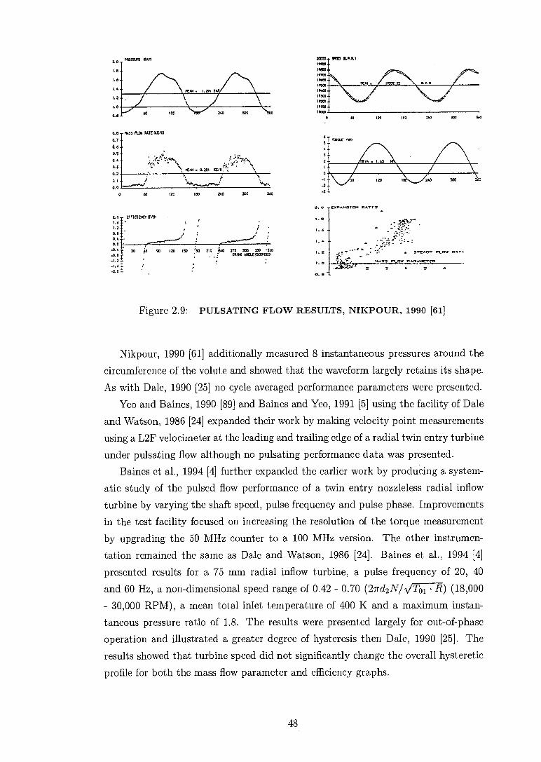
2)000 18400 1800 18700 111100 14300 IWO 19303 moo iota) 10000

WES P.11.

CXPwH9TOH CIATT3

PRESSLRE 1DA21 2 0 1.e

1.6

I. 4

1.2

1.0 0.e

0.e — nkss FUN RATE 11KG/51

O. 7 — O. a —

0.5- 0.1 — O. 3 — MEAN . 0.204 38.411.•":

a 1 — a.

0 60 120 180 240 SOO 360

2 0 — EFFICIENCY (1/3) 1. d • 1. 2 — MO 0. 4 0.0 •

-0. .0.1 30 jo 911 120 i so

t00 o QAO 270 300 330 1 360

CRAW OGLE SIEGAESS1 -1.21 •

• -I, is -2C-

.32 • ••• 0.2 •

' ;

Figure 2.9: PULSATING FLOW RESULTS, NIKPOUR, 1990 [61]

Nikpour, 1990 [61] additionally measured 8 instantaneous pressures around the

circumference of the volute and showed that the waveform largely retains its shape. As with Dale, 1990 [25] no cycle averaged performance parameters were presented.

Yeo and Baines, 1990 [89] and Baines and Yeo, 1991 [5] using the facility of Dale and Watson, 1986 [24] expanded their work by making velocity point measurements using a L2F velocimeter at the leading and trailing edge of a radial twin entry turbine

under pulsating flow although no pulsating performance data was presented. Baines et al., 1994 [4] further expanded the earlier work by producing a system-

atic study of the pulsed flow performance of a twin entry nozzleless radial inflow turbine by varying the shaft speed, pulse frequency and pulse phase. Improvements in the test facility focused on increasing the resolution of the torque measurement by upgrading the 50 MHz counter to a 100 MHz version. The other instrumen-tation remained the same as Dale and Watson, 1986 [24]. Baines et al., 1994 [4] presented results for a 75 mm radial inflow turbine, a pulse frequency of 20, 40

and 60 Hz, a non-dimensional speed range of 0.42 - 0.70 (27rd2N/VToi • R) (18,000

- 30,000 RPM), a mean total inlet temperature of 400 K and a maximum instan-taneous pressure ratio of 1.8. The results were presented largely for out-of-phase operation and illustrated a greater degree of hysteresis then Dale, 1990 [25]. The results showed that turbine speed did not significantly change the overall hysteretic

profile for both the mass flow parameter and efficiency graphs.

48

0

0

E C)

0

rn 111

30

2.5

2.0

15

ID

as 0.0

ID

.5

2.0

0.5

0.0 ID

12 1.6

Pressure ratio

12

o-c refer 10 'outer entry, e-9 10 inner crdry

16

tE 2D

20

o 10 0-

° 0.5

0

3 S0 E

2.5 to

2.0

OA 10 i. t.

Pulse feno2ky = E.0 Nr

•

15 ----- • - t

0.0 10 1 14 1,4 20

Pressure ratio

20

Figure 2.10: PULSATING FLOW RESULTS, BAINES et al., 1994 [4]

Whilst a significant increase in the enclosed area occurred for a change in pulse frequency from 20 to 40 Hz for the mass flow parameter and pressure ratio, Fig-ure 2.10. Figure 2.11 gives the performance results for an in-phase condition of 60 Hz and 30,000 RPM, the results show the instantaneous efficiency varies between

0.2 - 1.35, with the highest efficiency being seen at the lowest pressure ratio. It was stated that this was due to the fly-wheel effect which maintains the torque during

the periods of low pressure ratios. The mass averaged cycle efficiencies were pre-sented for a pulse frequency of 20 Hz and were 0.322, 0.370 and 0.423 for a turbine

speed of 18,000, 24,000 and 30,000 RPM respectively. Arcoumanis et al., 1995 [3] extended the work of Abidat et al., 1991 [1] who

modified the test facility of Dale and Watson, 1986 [24] to accept a mixed-flow turbine and presented its instantaneous pulsating performance. This followed from the doctorial thesis of Hakeem, 1995 [36]. The eddy current dynamometer was replaced by a radial compressor to enable the increased power of the new larger turbine to be absorbed. This had an additional benefit of providing a low and known inertia of the rotating assembly which aids in the measurement accuracy of the instantaneous torque. Hakeem, 1995 [36] presented results for a 84 mm mixed-

flow turbine, a pulse frequency of 40 and 60 Hz, a non-dimensional speed range of

0.83 - 1.17 (271-d2 NNToi • R) (29,130 - 40,770 RPM), a mean total inlet temperature

of 326 K and a maximum instantaneous pressure ratio of 2.1.

49

o 3.0

0 2.5

2.0

Tota

l—st

atic

eff

icie

ncy

14

1,2

10

0.8

06

04

0.2

0.0 10

h phaSe

0.0 12 14 1.6 18 20

Pressure ratio 10 14 16 t.8 20

Pressure ratio

(a) Efficiency Vs Pressure ratio (b) MFP Vs Pressure ratio

Figure 2.11: STEADY AND PULSATING FLOW RESULTS, BAINES et al., 1994 [4]

The instrumentation was similar to Baines et al., 1994 [4] except the method of instantaneous speed measurement which now utilised an opto-diffusive sensor triggered 10 times per revolution from the back of the compressor wheel. Hakeem, 1995 [36] presented a comprehensive set of results for two mixed-flow turbines('

inclusive of the measured parameters and demonstrated a larger hysteresis loop then Baines et al., 1994 [4]. Hakeem, 1995 [36] calculated the true cycle averaged

efficiencies obtained by integrating the instantaneous isentropic power over a pulse cycle and dividing this by the integrated actual turbine power. This was compared against the steady flow peak efficiency of the turbine but no conclusive trends in behaviour was seen, cycle mean efficiencies varied from - 6 to + 3 % points from the steady peak efficiency value; a true comparison of the equivalent quasi-steady

efficiency was not made. The cycle mean velocity ratio and mass flow parameter was assessed from the time-average of the instantaneous measured quantities.

Su, 1999 [75]4 and Karamanis, 2000 [42]4 inherited the test facility from and

repeated the measurements of Hakeem, 1995 [36]. Additionally Laser Dopplier Ve-locimetry (LDV) point measurements were made at the leading and trailing edge of the turbine rotor. Performance measurements were taken for all turbines following

the techniques of Hakeem, 1995 [36] and were the latest measurements of either a radial or mixed-flow turbine under pulsating flow, Figure 2.12. Karamanis, 2000 [42] presented results for four 84 mm mixed-flow turbines, a pulse frequency of 40 and 60

Hz, a non-dimensional speed range of 0.83 - 1.17 (27rd2NR/Toi • R) (29,400 - 41,300

RPM), a mean total inlet temperature of 333 K and a maximum instantaneous

pressure ratio of 2.7.

4Hakeem, 1995 [36]: Tested prototype turbines A and B, Su, 1999 [75]: A, B and C and Karamanis, 2000 [42]: A, B, C and D.

50

1.5 POI PL

1. 5 25

o Beady A — A —B —C — 17 70% - 1.401-k

1.5 P„

25

o Steady A —A — — C —13 70% - 1.-601k

1.5 25 3

4

Tota

l-to

-sta

tic

t 1.

o Steady A — A — B — C —D 50% " 1-401k

.-. 5

O

3

7

5

3

-z

7

-2 25 3 0.3

Figure 2.12: PULSATING FLOW RESULTS, KARAMANIS, 1994 [42]

51

0.6u , 0 9 q,

o St Cady A — A — B — C —

0.3 7

12

4

Tota

l-to

-sta

tic

,>;‘

la 1

70% - 1-4011r -2

06 a 9 U / q,

o Steady A — A —B —C —D

70% 1-601-k

0. 6/

0.9 -2

0. 3

1. 2

I. 2

0. 3 7

4

0

a t)

7

4

,W. 1

7

8 5

s-g 3

7

o Steady A — A — B

C — 13

50Z " 1-401-k

0. 6 0 9 u/ q, 1.2

o Steady A — A -- B — C — D 50% - 1..601k

o Steady A — A —B

C — D

50% " 1-601k

The results indicate a further increase in the area of the hysteresis loop compared to Baines et al., 1994 [4] although similarly high efficiency values were seen at

the low velocity ratio regions and were attributed to the fly-wheel effect stated by Baines et al., 1994 [4]. The true cycle average efficiency was computed and the results indicated that it was always less then the peak steady state efficiency. The difference reduced with increasing turbine speed and pulse frequency. The cycle

averaged efficiency varied from - 25 to - 4 % points below the peak steady state efficiency for 50 % speed, 40 Hz and 70 % speed and 60 Hz respectively, Karamanis, 2001 [43]. Again no comparison of the equivalent quasi-steady efficiency was made and to date no researcher has presented the comparison of the true cycle average

efficiency against the calculated quasi-steady efficiency. The measurement of the isentropic power and the turbine torque represent a

different phase in the pulse cycle. A finite amount of time is required for the energy associated with the flow at the measurement plane to travel to the rotor and impart

its energy to be measured as a torque; an appropriate phase shift can be applied to align these quantities. The phase shift techniques of Dale and Watson, 1986 [24]

who used the sonic velocity of the gas and Baines et al., 1994 [4] who used the bulk flow velocity were compared, by Hakeem, 1995 [36], Su, 1999 [75] and Karamanis, 2000 [42]. The isentropic and actual power traces were compared and the results indicated that the phase shift should be based on the sonic speed of the gas, Fig-ure 2.13. The smoothness of the instantaneous torque can be seen by Figure 2.13 and does not follow the higher harmonics of the isentropic power. This suggests that the resolution of this parameter has not improved significantly since Dale and

Watson, 1986 [42]. The most recent and advanced measurement of the instantaneous mass flow rate,

Karamanis, 2000 [42] was assessed using a constant temperature hot-wire anemome-

ter from a point measurement taken at the central location of the duct. The calibra-tion was performed firstly under steady state conditions to obtain the calibration

constants and then under pulsating conditions where the probe was manually tra-versed over a 36-point grid and the results integrated to obtain the mass flux for the entire duct, Figure 2.14(a). A comparison is made between between the two measurements where a power law fit is used to find a correlation factor, K of the measured and true duct flow rate; noting this is only an estimate of the true corre-lation, Figure 2.14(b). Additionally no corrections are made to the hot-wire mea-surement to account for variations away from the calibration conditions, such as the fluid properties, temperature and Mach number. This has important implications on the measurement of the mass flow rate.

52

60 120 180 240 300 360

— isentropic power — actual power output

25000

20000

15000

t 10000

5000

—5000

25000

20000 -

15000 a

1000D

5000

5000

Angle (degree)

(a) Test Sections [42]

(b) Zero Phase Shift [75]

180 240 300 360

60 120 180 240

SOO 360

Angle (degree)

Angle (degree)

(c) Sonic Phase Shift [75]

(d) Bulk Flow Phase Shift [75]

Figure 2.13: TEST SECTION AND PHASE SHIFT: 50 % DESIGN SPEED, 40 HZ, KARAMANIS, 2000 [42], SU, 1999 [75]

Outer limb

3

25

2

1-5

1

05

0

o 5:PAciAgiv44311

)Pco 0

0 00

°.°

'0.. 0

0 °o 0

0 00 ct)

111.111 .11.! 1,.11111.1 .11 11.

Inner limb

0 10) 15) 7:o 35)

36-point grid

CieriralpitmsfluK

(a) Traverse Grid: Mass Flux (b) K Factor: Mass Flux

Figure 2.14: TRAVERSE GRID AND K-FACTOR,: 50 % DESIGN SPEED, 40 HZ, KARAMANIS, 2000 [42]

53

2.4 Survey Summary

A number of successful dynamometers have been designed and tested in the past. It is apparent to achieve a large power range over the high operating speeds of a

typical turbocharger turbine is difficult. This difficulty greatly increases when the load range is required in a low and known inertia dynamometer which is suitable for pulsating flow; this has been discussed in relation to Dale, 1990 [25] and Nikpour, 1990 [61]. These authors have also shown the successful measurement of the mean torque through use of a reaction torque measurement and would suggest this is a

suitable choice of technique.

The measurement of the instantaneous performance of a turbocharger turbine

has been measured for two decades. These measurements show that a characteristic

hysteresis loop is present between the performance parameters and is due to the volumes between the measurement location and the turbine. The results suggest that the cycle average efficiency is always less than the peak steady efficiency and this discrepancy reduces with increasing pulse frequency and turbine speed. The compounded maximum range of test conditions presented in literature cover a pulse frequency range between 20 - 60 Hz, a non-dimensional speed range between 0.42 -1.17 (14,800 - 42,000 RPM) and a maximum pressure ratio of 2.7.

The true cycle average efficiency has not been compared against the quasi-steady efficiency, it is therefore not known whether the turbine rotor (with volute losses)

behave in a quasi-steady manner. Additionally, in order to accurately calculate the quasi-steady efficiency, a large range steady state turbine map is required.

It is evident from these results that the measurements of the instantaneous per-formance parameters are not sufficient in accuracy and still warrant further research; this is apparent when considering the instantaneous mass flow rate and torque. In the literature no corrections have been applied to the hot-wire data to account for changes in the fluid properties, temperature and Mach number. These are extremely important and can result in a large discrepancy between the true and measured val-ues. Further to this the single point measurement and the use of the K-factor results in additional errors. Universally the measurement of the instantaneous torque has resulted in a smooth curve which principally follows only the main feature of the isentropic power pulse, the secondary features are ignored and this can result in a large discrepancy in instantaneous efficiency.

54

Chapter 3

Dynamometer

3.1 Synopsis

This chapter describes the experimental development of the Permanent Magnet

Eddy-Current (PMEC) Dynamometer. Verification of this concept was made us-

ing an initial prototype and was developed through an improved second prototype. Following this, a description of the design and analysis of the final PMEC dyna-

mometer is given along with experimental results illustrating the available load and

speed range.

3.1.1 Objectives and General Specification

The dynamometer is required for the steady, pulsating and transient testing of a medium sized turbocharger turbine, a suitable specification for such a dynamometer

is given below:

1. SPEED RANGE: > 30, 000 — 60, 000 RPM The dynamometer should be able to continuously operate over the minimum speed range given. For the mixed-flow turbine under investigation, turbine 'D', this speed range is the 50 - 100 % equivalent design speed of the turbine.

2. LOAD RANGE: > 0.5 — 50 + kW It is estimated from previous investigation that turbine 'D' has a peak efficiency point at 40 kW at 100 % design speed and as such the power range given is a minimum required in order to characterise the turbine.

3. Low KNOWN INERTIA:.,:-..-, 4.262 x 10-04 kg.m2

A low known inertia is important for pulsating flow measurements as discussed in Section 5.4.5. It is difficult to design such a dynamometer, the ideal aim would be to design a dynamometer with an rotational inertia similar to that

of a standard turbocharger assembly.

55

This would give representative speed variation under pulsating flow conditions. The value of the rotational inertia given is that of the previously used standard

turbocharger assembly.

4. REACTION TORQUE MEASUREMENT: The accuracy of the measurement of turbine power is important particularly

at low pressure ratios, Section 6.5.

5. MODULAR CONSTRUCTION: To increase the usability and reduce the down time of the dynamometer.

6. ELECTRONIC CONTROL: To allow the automation of the controls and monitoring systems for the dyna-

mometer.

7. REPLACEABLE STATOR UNIT: To allow the future development of the PMEC dynamometer by allowing sim-

ple replacement of the stator unit.

8. TRANSIENT OPERATION: For future work, to be able to change power absorption from its minimum

value to its maximum value in < 1 second.

3.2 Initial Prototype - Mk I Dynamometer

The prototype rig was originally developed as an undergraduate project at Imper-ial College London by Kidwai et al, 1999 [44] and was mechanically developed by

McGlashan, 1999 [55] into a working prototype. This initial prototype was used to demonstrate the proof of concept of a high speed permanent magnet dynamometer and to identify issues regarding its mechanical design and also to obtain experimen-

tal data for use as a comparison to future numerical predictions. This prototype was manufactured and tested prior to the numerical analysis described in Chapter 4.

3.2.1 Rig Layout The two main components of the dynamometer are the magnetic rotor and the single copper stator, Figure 3.1. The magnetic rotor consists of 8 magnets and the rotor is directly attached to the turbine shaft. The stationary copper stator is the volume

in which the eddy-currents are produced, this generates heat which is dissipated through water cooling. The bearing assembly used was a HOLSET H3 automotive turbocharger unit, whilst the turbine was a prototype mixed-flow turbine known as

turbine 'B', Abidat, 1991 [1].

56

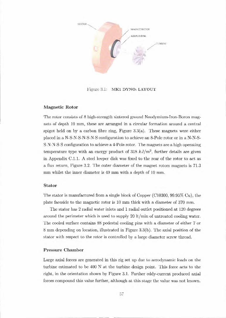
STATOR

MAGNET ROTOR

KEEPER DISK

TURBINE

Figure 3.1: MK1 DYNO: LAYOUT

Magnetic Rotor

The rotor consists of 8 high-strength sintered ground Neodymium-Iron-Boron mag-

nets of depth 10 mm, these are arranged in a circular formation around a central spigot held on by a carbon fibre ring, Figure 3.3(a). These magnets were either placed in a N - S-N-S-N-S-N-S configuration to achieve an 8-Pole rotor or in a N-N-S-

S-N-N-S-S configuration to achieve a 4-Pole rotor. The magnets are a high operating temperature type with an energy product of 318 kJ/m3 , further details are given in Appendix C.1.1. A steel keeper disk was fixed to the rear of the rotor to act as

a flux return, Figure 3.2. The outer diameter of the magnet rotors magnets is 71.3 mm whilst the inner diameter is 40 mm with a depth of 10 mm.

Stator

The stator is manufactured from a single block of Copper (C10300, 99.95% Cu), the plate faceside to the magnetic rotor is 10 mm thick with a diameter of 370 mm.

The stator has 2 radial water inlets and 1 radial outlet positioned at 120 degrees around the perimeter which is used to supply 20 It/min of untreated cooling water. The cooled surface contains 88 pedestal cooling pins with a diameter of either 7 or 8 mm depending on location, illustrated in Figure 3.3(b). The axial position of the

stator with respect to the rotor is controlled by a large diameter screw thread.

Pressure Chamber

Large axial forces are generated in this rig set up due to aerodynamic loads on the turbine estimated to be 400 N at the turbine design point. This force acts to the

right, in the orientation shown by Figure 3.1. Further eddy-current produced axial forces compound this value further, although at this stage the value was not known.

57

TURBOCHARGER SHAFT

WEAL ADJUSTMENT SCREW THREAD [3,

COOLANT

INLET

COI-II ANT

OUTLET

TURBACHARCER BLARING NUDGING

Al IGNMENT PITS

LABYRINTH SEAL

ST AT SP 1.1

PRESSURE ClIAMBt

COOLANT

INLET

FFPFR DISK

ECTIDN n

TURBECHARGER SwF- KU

=LIRE PEDESTALS

MASNFT TE ROTOR

BACKLASi I SPRINCS

Figure 3.2: MKI DYNO: ASSEMBLY

(a) Mkl Dyno: 8-Pole Rotor (b) Mkl Dyno: Copper stator

Figure 3.3: MK1 DYNO: MAIN COMPONENTS

The turbine force alone exceeds the capacity of the bearing since it is normally

balanced by a near equal and opposite force on the compressor, now replaced by the magnetic rotor. In order to equalise this force a pressure chamber on the rear

of the rotor was used to create an opposing force of approximately equal magnitude using a chamber pressure of 1 Barg, Figure 3.2. This positive pressure was also used to reduce oil leakage from the journal bearings as it mimics the action of the compressor.

58

COOLANT (WATER)

— u

STATOR

TURBINE VOLUTE

VELOWTOR

Figure 3.4: MKI DYNO: EXPERIMENTAL LAYOUT

3.2.2 Instrumentation

A brief description of the main instrumentation required to assess the performance of the dynamometer is given below. The instrumentation in relation to the final dynamometer is described in detail in Chapter 5. A photograph of the Mkl dyno can be seen by Figure 3.4.

Turbine Speed: The speed of the rotor was measured using a magnetic pick-up positioned close to the turbocharger shaft. The pick-up produces two pulse signals per revolution sensed from two flat bottomed holes machined diametrically opposite on the turbine shaft. The quality of the output signal was monitored with an oscilloscope, whilst the speed value was manually recorded from a digital display. It is estimated that the accuracy of the speed measurement is ± 2 RPS.

Temperature Measurement: The temperature of the coolant water entering and exiting the stator was measured using K-Type thermocouples. Of the two inlet pipes only one was used to measure the water inlet temperature as it was reasonable to assume the temperature in each pipe would be of similar value as they originate from the same source pipe. A thermocouple was positioned in the single outlet pipe of the stator to monitor the exit water temperature. Additionally, air was entrained past the magnetic rotor and measured with a K-Type thermocouple, to give an indication of the rotor temperature.

59

The thermocouples have an absolute temperature accuracy stated by the manu-facturers of + 1.5 K, although the importance in these experiments is the accuracy of the difference of the two coolant measuring thermocouples, this was found by

comparison to be + 0.2 K.

Water Flow-rate: The mass flow-rate of coolant water into the stator was mea-sured and controlled using a manufacturer calibrated water rota-meter and valve.

The rota-meter has an accuracy of + 2 % FS, a repeatability of ± 0.25 % FS and is rated up to 83 It/min.

Vibration Sensor: The rotor dynamics of the rig were assessed by monitoring

the vibration levels using a linear velocity sensing transducer of type Bently-Nevada, Velomitor PN 330500. The position of which can be seen by Figure 3.4. The output from the transducer was processed into the frequency domain using Fast Fourier

Transformation and displayed on a LCD output.

Miscellaneous Measurement: The rotor-to-stator gap was measured directly using a digital vernier gauge. The pressure chamber pressure was monitored from a pressure tapping fed to a dial pressure gauge with pneumatic tubing.

3.2.3 Experimental Evaluation

Power Absorption

The factor of interest in these tests was the power absorbed by the dynamometer with respect to the turbine speed and rotor-to-stator gap in steady state conditions. By measuring the temperature rise of the stator cooling water an estimate of this power was obtained. This estimate is conservative as there is heat loss from the stator which is not measured.

The power absorbed by the dynamometer, Q can be estimated by Equation 3.1, where Mt, is the mass flow-rate of the water, cp,„ is the specific heat of water, AT is the temperature rise of the coolant and Qh is the stray heat loss of the stator.

Q = fnwep,„,AT + (3.1)

Stray Heat Loss Estimation

The sources of stray heat loss are through convection caused by the motion of the magnetic rotor (windage), the natural convection from the stator surface and conduction to the rig stand.

GO

Table 3.1: MK1 DYNO: ROTOR-STATOR HEAT LOSS PARAMETER VALUES

Parameter: (at 400°K, 1.01325 Bar) Value Unit

Air density p 0.875 kg/m3

Rotational speed N 1000 RPS

Rotor diameter dutrotor 0.071 71-1

Dynamic viscosity t 2.21 x 10' Ns/m.2

Magnet swept area A 2.74 x 10' 77.0

Thermal conductivity k 3.31 x 10-02 W/m.K

Temperature difference AT 150 K

Free stream temperature Too 323 K

An estimate of the natural convection and conduction term suggested that this was negligible compared to the motion induced term. An estimate of this loss was performed using a particular heat transfer correlation applicable to a rotor and stator system, the correlation of Cobb and Saunders, 1956 [21] as given by Owen,

1989 [62], Equation 3.2, where the parameters are defined in the Nomenclature. An estimate of the heat transfer from the stator was made at a limiting operating

point of the Mkl dyno using the parameters given in Table 3.1. This results in an overall heat loss of 140 W and an average heat transfer coefficient, h of 340 W/m2K.

This gives a maximum estimation of the stray heat loss from the stator for the 18

kW test presented later and accounts for < 0.8 % of the power.

N7100 = 0.015 • Re:15 (3.2)

Experimental Results

The experimental results are given in Figure 3.5(a) - 3.5(b) and show the variation of dynamometer power is approximately linear with turbine speed for a fixed rotor-to-stator gap over the speed range concerned. The highest power measured in the

experiment was 18.86 kW at 50,000 RPM for an 8-Pole rotor with a gap of 0.75 mm, this would suggest approximately 22 kW could be achieved at 60,000 RPM, Figure 3.5(b). It was decided to limit the 4-pole test to a maximum power of 10 kW, this was due to a thrust bearing failure which occurred in the high-power test of the 8-pole rotor. The maximum power achieved with the 4-pole rotor was 10.34 kW at 51,000 RPM with a gap of 1.47 mm. For the same operating conditions the

8-pole rotor would achieve approximately 13.5 kW.

61

40 50 60 30 20 10 60 20 30 40 50 Turbine Speed (kRPM) Turbine Speed (kRPM)

(b) Mkl Dyno: Results 8-Pole (a) Mkl Dyno: Results 4-Pole

Rotor-to-Stator Gap (mm) Rotor-to•Stator Gap (mm)

• 30 kRPM • 40 kRPM A 50 kRPM • 54 kRPM

2 0

0 5 1 1.5 2 2.5 3 3.5 4 0 5 1 1.5 2 2.5 3

o gap 2.75 • gap 1.94 A gap 1.37 • gap 0.96 x gap 0.75

0

12

10

8 o.

6 0 E

i. 4

2

• gap 3.49 • gap 2.97 a gap 2.5 • gap 2 x gap 1.47

25

F 20

15 o.

E 10- 0

E a, 5

8 - a.

t: 6 E

4 -a

15

E 10 0 E

g. 5 a

• 25 • 30 kRPM • 40 kRPM A 50 kRPM F 20

• 54 kRPM

(c) Mk1 Dyno: Interpolated Results 4-Pole (d) Mkl Dyno: Interpolated Results 8-Pole

Figure 3.5: MK1 DYNO: 4 AND 8-POLE ROTOR RESULTS

For fixed conditions the dynamometer absorbed a greater amount of power us-ing the 8-pole rotor compared to the 4-pole rotor. To allow a direct comparison

between the rotors, the results of Figure 3.5(a) - 3.5(b) have been interpolated giv-ing Figure 3.5(c) - 3.5(d). These graphs illustrate the variation of dynamometer power for a change of rotor-to-stator gap for a fixed speed. An increase in power occurs non-linearly by reducing the rotor-to-stator gap. For the 18 kW test a water

temperature rise of 13.5 K occurred. A temperature measurement of the rotor entrained air was carried out at 10 kW,

a measured value of 343 K was recorded. Although this is not a direct measurement

of the rotor temperature, it gives an indication of its value. The measured value is considered high, both structurally and magnetically for the rotor to experience. The epoxy bonding within the carbon fibre sleeve of the rotor will degrade from a

temperature of around 363 K, which could result in a catastrophic failure of the

rotor. This high temperature will partially but reversibly demagnetise the mag-netic rotor, from the information supplied by the magnet manufacturers Crucible Magnetics, [52] this reversible reduction of the magnetic field will have a value of

approximately -0.110 % per K (293 K to 423 K, Reversible Temperature Coefficient

of Induction), resulting in a 5.5 % reduction in field strength strength at 343 K.

62

Limit for short term operation

Limit of continuous safe operation

RM

S V

ibra

tion

(mm

/s) 4

3

2

0

10

20

30

40

50

60

Turbine Speed (kRPM)

Figure 3.6: MK1 DYNO: RESULTS - VIBRATIONS

Rig Observations

The stator surface after the 18 kW test was seen to be heat affected. This manifested

itself as a white layer of approximately the same swept area as the magnetic rotor, suggesting localised heating and inadequate cooling. It is estimated from a 1D Fourier law calculation that the surface of the stator was at approximately 567 K,

the calculations and plots for this can be found in Appendix B.2. During the high power 8-pole test, a thrust bearing failed. The bearing damage

suggested an axial force in the direction of the turbine, this axial force is due to the eddy currents and the turbine pressure loading. It was estimated that the pressure-chamber would balance the turbine forces, which indicates that the bearing damage was caused by a large eddy-current force. Although at this stage the value was not known, a later estimate from a finite element model indicated a value of 500 N would

occur in the 18 kW test. It was also noted that the vibrations levels were high during the experiment.

The RMS vibration results are given by Figure 3.6. The rig vibrations are discussed in more detail in consideration of the Mk2 and Mk3 Dyno of Section 3.3.3 and

Section 3.4.5.

Design Criticism and Evaluation

It was evident from the layout of the stator that it had a poor cooling design. The pedestals used for cooling are positioned nearly all outside the projected area of the

magnetic rotor.

63

The localised heating seen on the stator surface would indicate the pedestals are redundant. Another key area of the stator design is the large volume in which the coolant can by-pass the localised heated zone. The stator design would have benefited from smaller channels that direct the entire coolant flow over the localised

heated zone. The distance a magnetic field can penetrate into the surface of the conductor

can be estimated by the calculation of the skin depth, this is further discussed in Chapter 4. A calculation of the skin depth gives a depth range from 1.5 - 1.1 mm for a speed of 30 - 60 kRPM respectively for the 8-pole rotor, the details of this calculation

can be found in Appendix C.2. This suggests that the stator thickness of 10 mm

is excessive and will not increase the power of the dynamometer but simply impede the cooling due to the large temperature drop across the stator plate, Appendix B.2.

The high surface temperature of the stator, estimated up to 567 K would impact

on the temperature of the rotor. To reduce the rotor temperature an improved stator cooling design and direct cooling of the rotor would be beneficial as this would reduce the reversible demagnetisation of the magnets and maintain the structural integrity

of the carbon fibre. The failing of the thrust bearing indicates that the eddy-current forces are sig-

nificant and must be taken into account. The results of the Mkl dyno demonstrated a high-speed PMEC dynamometer

was a viable concept, but required extensive development and optimisation. At this stage a numerical approach was chosen to magnetically optimise the design for the Mkt dyno, utilising the test data of the Mkl dyno to verify the models. The

numerical approach is described in detail by Chapter 4.

3.2.4 Mkl Dyno: Summary

The concept of the high-speed PMEC dynamometer was demonstrated experimen-tally. A maximum power of 18.86 kW at 50,000 RPM for an 8-Pole rotor and a gap of 0.75 mm was achieved. The variation of power with speed for a fixed rotor-to-stator gap was linear and the power increased non-linearly with decreasing rotor-to-stator gap. For fixed conditions the dynamometer absorbed a greater amount of power

using the 8-pole rotor then the 4-pole rotor. A number of design issues have been highlighted by the Mkl prototype, the main

issues that require attention in order of importance are: 1) Reduction of axial forces

2) Increase in power output through magnetic optimisation 3) Increase in rotor and

stator cooling.

64

3.3 Prototype - Mk II Dynamometer

The Mk2 dyno was a development of the Mkl dyno and addressed the main magnetic and design issues identified with its predecessor. This dynamometer was designed to experimentally test the numerical optimisations and identify further design im-provements. The mechanical design and cooling system was designed by McGlashan,

2000 [55] and built on a pre-adapted gimbaled turbocharger housing. The manufac-ture of the Mk2 prototype dynamometer took place in parallel with the numerical

analysis of Chapter 4.

STATOR PLATES

TURBINE

MAGNETIC ROTOR

Figure 3.7: MK2 DYNO: LAYOUT

3.3.1 Dynamometer Layout This dynamometer consists of two small stators, positioned either side of the 8-Pole rotor, Figure 3.7. The stator nearest the turbine is fixed in position due to a lack

of available space whilst the other can translate axially. The design permitted the stators to be changed so that different materials could be tested.

The stator cooling design directs the coolant through smaller passageways di-

rectly past the localised heated zone, so allowing a much greater proportion of the water to be in intimate contact with the heated surfaces. To aid in the rotor cooling compressed air is supplied to both sides of the rotor.

The turbocharger housings are mounted on a gimbal, which allows a reaction torque measurement of the turbine to be made. As a comparison the temperature rise of the coolant water is also used to calculate the power. The turbine and turbocharger housings of the Mk2 dyno employed that of the Mkl dyno.

65

AXIAL ADJUSTMENT SCREW THREAD

STATOR PLATE (II

TURBOCHARGER BEARING HOUSING

TURBOCHARGER SHAFT

MAGNETIC ROTOR

ALIGNMENT PINS

WATER FLOW OUT

STATOR PLATE (2

COOLING AIR IN

WATER FLOW IN

BACKLASH SPRINGS

SECTION ON

Figure 3.8: MK2 DYNO: ASSEMBLY

Rotor

The 8-pole magnetic rotor used for the Mk2 dyno is the same as the for Mkl dyno except the keeper disk has been removed due to the presence of the second stator,

refer Figure 3.7.

Stator Plates

The stators are small diameter plates that can be interchanged to allow a variety of materials to be tested. As a result of the numerical analysis of Chapter 4, the chosen materials were Copper, Aluminium Alloy and Steel. The basic properties of interest are given in Table 3.2, whilst more detailed information are held in Appendix C.1.3 and Appendix C.1.2. The stator plates had an outer diameter of a 100 mm, the copper and aluminium alloy stators were 2 mm thick and the steel stator 1 mm thick, a compromise between thermal conductivity and the power absorption.

Table 3.2: MK2 DYNO: STATOR MATERIAL PROPERTIES

MATERIAL

Resistivity (Stan) x In-0'

Therm. Conductivity (W/mK)

Rel. Permeability

293 K 473 K 293 K 473 K 293 K 473 K Copper 2.0 3.28 365 327.1 0.9999888 - Aluminium Alloy 2.39 5.36 236.8 239.3 1.00000819 - Steel (070M20) 16 29.2 58 52 1-1200 -

66

The steel stator has a lower thermal conductivity then the copper and aluminium

stators, this makes it more difficult to cool. In order to improve the cooling of the steel stator, a set of radial cooling fins was employed. Additionally the thinner stator thickness helps reduce the outer surface temperature. The copper and aluminium stators did not employ cooling fins as this was deemed unnecessary from the results of the Mkl dyno and the improved cooling system of the Mkt dyno.

To assess the outer surface temperature of the stators, a 1D Fourier law estima-

tion was performed. If the stators inner surface is held at 373 K due to boiling heat

transfer and the heat flow rate is 25 kW, this results in a outer surface temperature

of 414 K, 433 K and 480 K for the copper, aluminium and steel stators respectively.

Although the steel stator has the thinnest section its outer surface temperature is

66 K hotter then the copper. The detailed description of this calculation can be

found in Appendix B.2. Two copper and aluminium stators were manufactured, whilst due to time and

financial constraints only one steel stator was made. This was used as the variable gap stator, whilst for the fixed gap stator an aluminium one was used.

Cooling System

Stator Cooling: The stator has two water inlets and two outlets positioned alter-nately on the stator as shown in Figure 3.10, these enter and exit the stator axially so that they do not impose a torque on the gimbal. The water enters from the inner radius of the stator plate and exits at the outer radius, a diagram of the flow passages can be seen by Figure 3.8. The overall water flow-rate has been uprated from the Mk1 dyno to 70 It/min of untreated water, 35 It/min per stator.

Rotor Cooling: The rotor is cooled by high-pressure air injected past its surface,

this adds an insulating layer between the rotor and the stator plate. This air is also used to supply positive pressure to the turbochargers journal bearing to reduce oil leakage. The mass flow rate of the cooling air is estimated to be 5 - 10 g/s.

Gimbal

The turbochargers main body is mounted on two large diameter bearings, this allows the turbocharger housing to rotate about its central axis, Figure 3.9. The stator and cooling assembly are attached to the bearing housing so that any torque applied to them will also rotate the bearing housing. The bearing housing is reacted against a load-cell through a lever arm which can then be used to directely measure the turbine torque. This reaction technique of measuring torque is further described in

Section 2.2 and 5.4.5.

67

GIMBLE BEARINGS TURBINE

VOLUTE

OIL - DRAIN

JOURNAL BEARINGS

Figure 3.9: MK2 DYNO: GIMBAL SCHEMATIC


The instrumentation required for the Mk2 dyno is identical to the Mkl dyno except for an additional measurement of turbine torque. A photograph of the Mk2 dyno

can be seen by Figure 3.10.

Torque: A lever arm linked to the freely rotating bearing housing is reacted

against a strain-gauge load cell and measures the turbine torque. The torque is measured from the lever arm length (0.11 m) and the load-cell force, this is con-verted to power by the turbine speed, refer Equation 3.3.

Wait = F La, • 27N (3.3)

The load-cell is a cantilever beam of type Tedea Huntleigh 1040-1-20 and is

identical to that used in the steady and unsteady turbine performance measurements

of Chapter 6 and 7 and as such is fully described in Section 5.4.5. The calibration curve for the load cell is given in Appendix B.1 and was performed in a similar way to that described in Section 5.5.5. The location of the load cell for the Mk2 dyno can be seen by Figure 3.10.

68

STATOR ASSEMBLY

vELomfroR

COOLANT WATER

Figure 3.10: MK2 DYNO: PHOTOGRAPH EXPERIMENTAL LAYOUT


The main factor of interest was the power absorbed by the dynamometer as well as

power produced by the turbine with respect to the speed for various rotor-to-stator

gaps in steady state. Of particular interest was the comparison of the three different

stator materials.

As used in the Mkl experiments, the water temperature rise and flow-rate can

be used to calculate the power absorbed by the dynamometer. The turbine power

is assessed using the load cell data, as per Equation 3.3.

Results and Discussion

The results show that the Mk2 dyno demonstrates an approximately linear variation

of dynamometer power with a variation of turbine speed and a fixed rotor-to-stator

gap, Figure 3.11(a)-3.11(c), these results are consistent with the Mkl dyno. The

linear variation is seen for the different materials tested copper, aluminium and steel.

The highest power measured in the Mk2 test was achieved with the steel and

aluminium stator combination, which obtained 49 kW at 54,000 RPM. The steel

stator was set at a rotor-to-stator gap of 0.55 mm, whilst the fixed aluminium

stator was set at 0.41 mm. This would extrapolate to give approximately 54 kW

at 60,000 RPM. The twin aluminium stators achieved a maximum of 38.6 kW at

55,000 RPM with the rotor-to-stator gaps set at 0.41 mm and 0.60 mm and would

extrapolate to give approximately 41.6 kW at 60,000 RPM.

69

VARIOUS tiAPS

90

.98

rf

_ TURN. POWER TIERMAL POWER

50 1

VARIOUS OA.(nsm)

. •

9 90 1.49 ___--- ....2 2.1

W ORIP : 1_ .

..14.../041,,,,1111001 4.99"

. . . ojAl _ ..,,,,g , i . --:,....,.,......mm rt----- - TL-ROM POWER

- TIIIT,L,L POWER

30

20

10

40

Eu 30

20

10

45 30 35 40 45 50

55

60 25

30

35 40 45 50 55

60



(a) Mk2 Dyno: Steel

(b) Mk2 Dyno: Aluminium

0.0)

504*

- TURBINE POW. - THERMAL POWER

30 35 40 45 50

55

60


(c) Mk2 Dyno: Copper

Figure 3.11: MK2 DYNO: RESULTS

The twin copper stators achieved a maximum of 27.12 kW at 53,400 RPM with the rotor-to-stator gaps set at 0.50 and 0.56 mm and would extrapolate to give approximately 29.5 kW at 60,000 RPM.

The Mk2 copper stators gave an increase of approximately 27 % for the equivalent gap and speed setting as compared to the Mkl dyno. Although the number of stators

doubled the power levels did not follow this and was a result of a number of known causes. The Mkl rotor employed a steel keeper disk on one side of the rotor which allows a greater magnetic flux to be developed by the magnets and this sequentially results in a greater amount of power that can be absorbed by the dynamometer, the quantification of which was given in Chapter 4.

Additionally the smaller thickness of the Mk2 stators results in a lower stator surface temperature. The consequence of this is a lower resistivity value which as

demonstrated by the test results and the magnetic analysis of Chapter 4 gives a

lower power absorption capability. Ignoring the temperature effect, it should be noted that the difference in physical thickness of the Mkl and Mk2 stator plays little part in the comparison, a simple skin depth analysis suggests the Mk2 stator losses approximately 1.5 % of the available power due to the reduced thickness, Appendix C.2.

70

30

25

20

15

10

When the copper stators were replaced with the aluminium alloy stators a power increase of approximately 40 - 44 % was observed. Magnetically the only difference between these two different stator materials is their respective resistivity values and demonstrates the beneficial effect of an increase in resistivity. Such behaviour is

confirmed by the magnetic analysis of Chapter 4. The single steel stator was used to replace one of the aluminium stators and

the resultant combination produced the highest power from the Mk2 tests. From

these results it is not possible to deduce the power that would be absorbed by a combination of two steel stators, this is a result of a coupling effect that occurs between the steel and aluminium stators. The steel stator produces a keeper disk effect which increases the magnetic flux developed by the magnets, this results in

the aluminium stator absorbing a greater amount of power then it would with a

double aluminium stator combination. It can be seen from Figure 3.11(a) - 3.11(c) that the minimum power absorption

of the dynamometer was large, for the steel stator it was approximately 18 kW at 30,000 RPM. This large minimum value would greatly limit the usefulness of the

dynamometer as it is important that the dynamometer is able to act passively when required. For the turbine under investigation the dynamometer is required to absorb less then 0.5 kW at 30,000 RPM, refer Chapter 6 so that a large load range turbine map can be obtained. The majority of this high minimum load is a result of the fixed

gap stator which is set at 0.5 mm due to restricted space available. The remaining

is due to the limited movement of the variable gap stator. The gimbal measurement of power was reasonably close to the thermodynamic

measurement, at maximum power the results were within 2 %. It was evident that the gimbal technique should give a higher power output then the thermodynamic approach as the former includes the measurement of bearing losses. It was found that the thermodynamic technique had values both above and below the gimbal technique, an uncertainty analysis was therefore performed.

Uncertainty Analysis

The uncertainty of the two different power measurement techniques can be assessed

using the first order method of Kline and McClintock, 1953 [45] and the develop-ments of Moffat, 1982 [58]. This method is later described in detail in Section 5.7.

The resultant equation for the uncertainty in power measurement using the ther-modynamically calculated technique is given by Equation 3.4, whilst the uncertainty in power measurement using the gimbal technique is given by Equation 3.5. This procedure computes the uncertainty propagation of the measured independent quan-

tities into the calculated power.

71

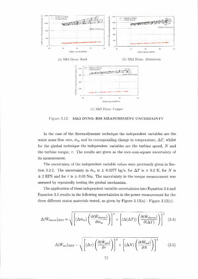
sure

men

t Unc

erta

inty

(W

)

1600

1200

1100

400

RSS

Pow

er M

easu

rem

ent U

ncer

tain

ly (

V)

1500

1200

900

600

300

— THERMAL POWER — GIMBAL POWER 0.60,90 THERMAL POWER

GIMBAL POWER 24.449

4.99 2.98

VARIOUS GAPS (mm)

— THERMAL POWER _L — GIMIIAL POWER " 09

1.41 2.50

VARIOSiS GAPS (mm)

•

20 30 40 50

60

Furbim Speed (kRPM)

20 30 40 50

60


(a) Mk2 Dyno: Steel (b) Mk2 Dyno: Aluminium

40

50 60

Turbm Speed (kRPM)

(c) Mk2 Dyno: Copper

Figure 3.12: MK2 DYNO: RSS MEASUREMENT UNCERTAINTY

In the case of the thermodynamic technique the independent variables are the water mass flow rate, frt,i, and its corresponding change in temperature, AT, whilst for the gimbal technique the independent variables are the turbine speed, N and the turbine torque, T. The results are given as the root-sum-square uncertainty of its measurement.

The uncertainty of the independent variable values were previously given in Sec-tion 3.2.2. The uncertainty in rh„, is + 0.0277 kg/s, for AT is + 0.2 K, for N is ± 2 RPS and for T is ± 0.03 Nm. The uncertainty in the torque measurement was assessed by repeatedly testing the gimbal mechanism.

The application of these independent variable uncertainties into Equation 3.4 and Equation 3.5 results in the following uncertainties in the power measurement for the three different stator materials tested, as given by Figure 3.12(a) - Figure 3.12(c).

>. 1200

400

600

ij 300

0 30

A(Wtherm)RSS [ (Arhtv ) a(Wtherm) 2

2 + (A(AT)) a(Wtherm) (3.4 )

I ariii,,, 0(AT)

A(*act)RSS 2 2 [(AT) (a(waract) )1 + [(AN) ( a(aWNact ) )1 (3.5)

72

It can be seen from these figures that there is a marked difference in the magni-tude of the uncertainty between the thermal power and gimbal technique. Typically

for these tests the uncertainty in the thermal technique ranged from 3 - 6 % whilst

for the gimbal technique ranged from 0.4 - 0.7 %. In the thermal technique the influence on the overall uncertainty due to the mea-

surement of the water mass flow rate and the temperature change were of approxi-mately equal importance. Whilst for the gimbal technique the torque measurement accounted for about 70 % of the uncertainty, the speed measurement accounting for the remainder. The large uncertainties associated with the thermal technique would make it difficult to accurately assess the dynamometer performance especially with a large coolant flow rate where the temperature rise of the fluid is small. It is likely to be the inaccuracy in this measurement which has resulted in the thermal technique recording both a greater and lesser power then the gimbal technique.

Rig Observations

After testing, the stator plates were inspected and photographed as shown in Fig-ure 3.13. The variable gap copper stator was inspected after 60 minutes of run time and showed only modest signs of heating on the rotor side and slight calcium scaling on the coolant side. The fixed gap stator after 100 minutes of run time showed

increased signs of heating and scaling, the photographs of this stator are given in Figure 3.13(c). Throughout the duration of the test, this stator was positioned at a rotor-to-stator gap of 0.5 mm and as such was running at its maximum power absorption capability resulting in the increased heating effects. The scale on this stator showed signs of cracking and peeling and occurred at a radius similar to that of the rotor magnets. It is thought this cracking and peeling is due to the large temperature gradient across the scale and the expansion and contraction of the sta-tor throughout a test cycle. A consequence of the scale is a lower heat transfer

coefficient and hence a higher stator temperature. Additionally this stator shows slight evidence of hotspots on the stator surface through the discolouration of the

copper occurring at 90 degree intervals around the stator. The variable gap aluminium stator was inspected after 60 minutes of run time

and showed no visible heating effects or scaling. Instead an unknown black tacky residue was seen on the coolant side of the stator, Figure 3.13(b). It is estimated from 1D Fourier law of conduction that the average surface temperature of the copper

stator was approximately 395 K when operating at its maximum power, whilst the

aluminium stator reached 420 K, the calculations and plots for this can be found in

Appendix B.2.

73

•

•

•

•

•

(a) Steel Stator

(b) Aluminium Stator

•

• • •

•

•

• • •

• •

(c) Copper Stator

Figure 3.13: MK2 DYNO: RESULTS - STATOR PLATES

74

The variable gap steel stator was inspected after 100 minutes of run time, and showed distinct heat colouration, Figure 3.13(a). The development of hotspots on

the steel stator is clearly seen to occur at 90 degree intervals and is due to the design of the cooling system. The coolant passageways of the present design have entry and exit ports at 90 degree intervals and this is likely to limit the coolant flow to the matching hotspot areas of the stator. An accurate estimation of the maximum surface temperature of the steel can be made from the colour of the oxide layer present. This suggests that the majority of the stator surface reached a maximum

operating range of 503 - 528 K. The hotspots typically ranged from 553 - 573 K

whilst at the hottest parts reached approximately 593 K. It is estimated from 1D Fourier law of conduction that the average surface tem-

perature of the steel stator reached 478 K, the calculations and plots for this can

be found in Appendix B.2. The cooling fins on the steel stator are not included in this analysis and as such this method would under predict the surface temperature

of the stator, in this case an estimated 30 K. This increase in surface temperature

has negative affects on the power absorption capabilities of the dynamometer, an

increase in temperature results in a greater amount of reversible demagnetisation of the rotor magnets resulting in lower power absorption. Additionally this puts the carbon fibre ring at greater risk of de-bonding.

A maximum coolant temperature rise of 10 K occurred for a dynamometer power

of 49 kW. This temperature rise is lower then that of the Mkl dyno due to the larger flow rate used. The power levels were also much higher but no problems with the thrust bearings were encountered, suggesting the double stator technique has

balanced the main axial force.

Vibrations

In order to assess the rotor dynamics of the Mk2 dyno, the vibration levels were recorded against turbine speed, Figure 3.14. Typically a measure of casing velocity is used to assess the vibration levels of a rigid rotor system as it can be related to

the vibrational energy. The British Standard BS 7854-1: 1996, [12] gives a guideline for acceptable vibration levels, a value of 1.8 mm/s is typically chosen as the upper limit for continuous vibration levels for this type of high-speed machinery. The rig vibrations and rotor dynamics is further discussed in Section 3.4.2.

It is evident from Figure 3.14 that there are three resonant frequencies within the operating range of the dynamometer. In these regions the vibration levels become large and it was considered unsafe to continuously run at these speeds. Significantly the shaft bend mode occurs at the maximum operating speed of the dynamometer and is marked on Figure 3.14. This mode is a major limitation of the Mk2 dyno.

75

RM

S V

ibra

tion

Lev

el (m

m/s

)

4

3

2

0

Limit for short Bend Mode

term operation

Bounce Mode Rock Mode

imit of continuous/ operationsafe

0

10

20

30 40 50

60



To adapt the Mk2 dyno to enable both stators to have a variable gap would require the extension of the shaft length. This would result in a reduction of the bend mode frequency into the operating range of the dynamometer and was not an acceptable approach. The bend mode frequency is a strong function of the rotor/turbine mass

and the shaft geometry and as such can not be significantly raised using a standard

turbocharger bearing housing and shaft assembly.

Design Criticism and Evaluation

The two major interrelated concerns of the Mk2 dyno were the high minimum power absorption and the rotor dynamics of the rig. In order to reduce the high minimum power absorption of the dynamometer the rotor-to-stator gap must be increased. It is difficult to achieve this whilst maintaining the standard turbocharger assembly and suggests that the occurrence of the bend mode is an inherent problem in its present design. In the Mk2 dyno the diameter of the standard turbocharger shaft

is 011 mm which coupled with the overhanging masses results in a low bend mode

frequency. The overall cooling of the stators did not present a problem, but localised

hotspots on the stator occurred due to the cooling system design. To reduce scaling and rusting of the stators, a closed-loop water system can be implemented with ad-ditives to increase heat transfer and reduce rusting. This will allow the heat transfer coefficient to stay at a high constant value.

Additionally, a gap actuation method should be developed so that the gap can be changed remotely and whilst the dyno is in use.

76

3.3.4 Mk2 Dyno: Summary

The Mk2 twin-stator design is beneficial over the Mkl single-stator design in ab-sorbing the turbine power. It has been shown that an increase in power absorption

can be obtained by an increase in stator resistivity. A steel and aluminium stator set produced the greatest power, this may suggest a steel stator is most beneficial although this is not conclusive from the test. The use of the twin-stator design can counterbalance the axial forces caused by the magnetic rotor.

A major concern of the dynamometer design is the rotor dynamics, the Mk2 dyno is limited in range due to the occurrence of three resonant frequencies including

the bend mode occurring within the 30,000 RPM test window. The dynamometer additionally has a high minimum power absorption, which is also a consequence of

limited space available.

77

DYNAMOMETER MODULE

ROTOR BEARING MODULE

ACTUATION I STATOR GIMBAL SHAFT UNIT UNITS UNIT BEARING

L UNIT

3.4 Final Design - Mk III Dynamometer

The Mkl and Mk2 prototypes were principally used to develop the power absorption

capabilities of this style of dynamometer, but were not in themselves suitable for mapping the performance of a turbine. The final Mk3 dyno was a purpose designed dynamometer which amalgamated the findings of the Mkl and Mk2 dyno into a useable PMEC dynamometer which was designed to be suitable for medium sized

turbocharger turbine testing under steady, pulsating and in the future transient flow

conditions.

3.4.1 Layout

The Mk3 dyno was based on the layout of the Mk2 dyno and similarly can be separated into two main and separate modules, these are the bearing and the dyna-mometer module. Each of these modules are made up of further smaller units as

illustrated by Figure 3.15. The modular construction gives advantages both in the rigs final usability and in

the design and construction process. The dynamometer is assembled from just five

units. These units are: the 1) Shaft bearing unit 2) Gimbal unit 3) Magnetic rotor

4) Stator units and 5) Actuation unit. Each unit is made up from a series of smaller parts but once these units are assembled they will not need to be disassembled for the medium term use of the dynamometer. This allows quick disassembly and assembly of the units without additional set-up time, the important set-ups and referencing are performed within the individual units themselves.

The advantages within the design and construction process arise as each unit can be designed as separate entities, the boundary conditions for the designs are the common assembly points between the units. This style of design allowed the bearing module to be manufactured before the design of the dynamometer module

was complete.

Figure 3.15: MK3 DYNO: GENERAL LAYOUT

78

3.4.2 Bearing Module

The bearing module consists of three units, the 1) Shaft bearing unit 2) Gimbal unit

and the 3) Magnetic rotor. The shaft bearing unit employs three oil fed angular

contact bearings, which are large diameter, robust bearings and are capable of speeds of over 60,000 RPM. The magnetic rotor is bolted to the opposing end of the shaft to the turbine and consists of 28 high-strength Neodymium-Iron-Boron magnets arranged in a 14-Pole axial flux rotor. The gimbal unit consists of two large diameter opposing angular contact bearings. All other units are assembled to the freely rotating section of the gimbal unit which allows them to be reacted against a load-cell giving a turbine torque measurement. An assembly of the bearing module is

given in Figure 3.16(a) and a photograph in Figure 3.16(b).

General Features

A summary of the main design features and data values are given for the bearing module below, important parameters are further discussed in the following sections:

• Bearing Type

— 025 mm bore, low profile, 15° angular contact, ceramic balled, oil fed through upper race. Bearing of type SNFA VEB25/NS/H1 9CE1 TD. Maintains precision alignment and hence constant tip clearance.

• Bearing Arrangement

— Tandem back-to-back arrangement: Allows high-speed operation whilst

allowing axial loads to be accepted in both directions. The tandem bear-ing set is orientated to accept the axial load generated by the turbine inlet flow pressure, the axial forces caused by the dynamometer are generally

balanced.

• Bearing Life

— The predicted fatigue life of the bearings running equally at the turbines

test conditions of 30,000 - 60,000 RPM is 5600 hours.

• Spring Pre-load

— Spring pre-load of 50 N, applied axially in either direction.

• Bearing Oil Supply

— A single oil bus supplies lubricant to the three bearings via a hole through the upper bearing race, which injects oil adjacent to the ball contact area.

79

• Air Supply and Seals

— A single air bus supplies compressed air to the air-blown labyrinth seals.

This directs oil to the central oil sump.

— Air-blown labyrinth seals to reduce oil leakage. Labyrinth seal clearance 0.1 mm, Brass/lead inserts for labyrinth seal rubbing.

• Bearing Unit Housing

— Aluminium alloy construction and steel inserts for bearing seating - min-

imum weight for rotor dynamic reasons.

• 0-Ring Soft Mounts

Bearing unit radially soft-mounted in o-rings. Provides damping and a low stiffness mounting that lowers the bounce and rock mode frequencies

allowing a safer operating range, refer Section 3.4.2.

— Bearing unit axially soft-mounted in o-rings and provides damping to axial vibrations. Rotor dynamics can be altered by changing the number

of o-rings or material used.

• Safe Operating Range

— Operating range 0 - 60,000 RPM.

• Gimble Bearings

— 095 mm bore, low profile, 25° angular contact, ceramic balled, periodi-cally oil lubricated. Bearing of type SNFA SEB95/NS 7CE3 DD.

— Solid pre-load, back-to-back arrangements offer high moment stiffness.

• Magnetic Rotor

— 14-Pole, double row rotor with 28 high-strength Neodymium-Iron-Boron button magnetics, 12 mm thick rotor with carbon fibre containment ring.

— Square drive for transferring torque and angular alignment of rotor.

— Shaft attachment axially displaced from main rotor body allowing rotor to grow under high speed rotation.

• Modular Construction

— Bearing module designed as three units (sub-assemblies).

— Allows balancing of the rotating assembly within its own bearing housing.

— Once units are assembled they do not need to be disassembled except for

maintenance.

80

DYNAMOMETER MODULE ATTACHMENT

GIMBAL BEARINGS

SPRING PRE-LOAD

BEARING OIL FEED VOLUTE

AIR BLOWN LABYRINTH SEALS

ENiViocAT MIXED FLOW TURBINE

"\\ = ,".....L- \

A . . ., q . ,— whir ,s AMEN k.k xN

' Ilir

14 POLE MAGNETIC ROTOR

ANGULAR 0-RING SOFT CONTACT BEARING MOUNTS

OIL DRAIN COMPRESSED AIR FEED

LABYRINTH DUMMY HEAT SEALS SHIELD

AXIAL SOFT MOUNT 0-RINGS

(a) 2d Annotated Assembly

(b) Photograph

Figure 3.16: MK3 DYNO: BEARING MODULE

81

Bearing Selection

The bearing selection is an important consideration for high-speed machine design.

The choice of bearing will depict the maximum working speed, the load, bearing life and additionally influences the rotor dynamics of the machine. The choice of bearing size specifies the shaft diameter, which influences stiffness and hence the

natural frequencies of the system.

Bearing Type and Size: The bearings for the dynamometer are required to withstand high-speeds and intermediate value axial loading; a typical bearing choice for this type of situation are angular contact bearings. A speed factor, ndm may

be used to estimate the maximum bearing size appropriate for a given rotational

speed. The speed factor is calculated by multiplying the limiting speed of the bear-ing (RPM) by the bearings bore diameter (mm). For oil lubricated high precision

angular contact bearings the speed factor has a value generally between 1.5 - 2.5

x 106 RPM.mm. In order to give a safety margin in the operating speed, a limiting speed of 66,000 RPM was chosen, a 10 % increase from the required 60,000 RPM.

The speed factor range given above are for a single spring-loaded bearing arrange-ment, the range shown is a result of the differing make-up and quality of the bearing. Factors which affect this are the bearing profile, contact angle, precision, lubrication technique and ball material. To increase the speed factor high precision ABEC 9, low profile, ceramic balled bearings were chosen. Additionally these bearings are oil fed through small holes drilled through the bearing races which supplies oil close to the contact area of the ball/race and further increases the speed rating through

better bearing lubrication. Additionally, the speed factor will generally need to be adjusted to take into

account the in-service conditions which effect the bearing performance. These con-ditions are the axial and radial loading, the bearing arrangement, the cooling and the lubrication method. The speed factor correction factors appropriate for the

dynamometer are given in Table 3.3.

Table 3.3: MK3 DYNO: BEARING SPEED CORRECTION FACTORS

Ceramic Balled

1-11 Lubrication

Tandem Configuration

Axial Loading

ABEC 9 Precision

15° Contact Angle

Kl

1.15

K2

1.1

K3

0.9

K4

0.8 - 1

K5

1

K6

1

82

OIL FEED HOLE

TANDEM BACK TO BACK

Figure 3.17: MK3 DYNO: BEARING ARRANGEMENT

As well as sizing the bearings it is also necessary to consider the quantity and arrangement of the bearings in order to cope with the applied loading, refer to the Fatigue Life Calculation in Apendix B.3. The shaft assembly will generally have an axial load in one direction, this is as a result of the turbine pressure load. In order to cope with this reasonable sized load two bearings may be used in a 'tandem' configuration hence sharing the load, as illustrated by Figure 3.17. Although for the

dynamometer the axial load is generally in one direction in certain circumstances the load may change directions due to the magnetic rotor . In order to cope with a dual direction axial load a typical bearing arrangement is the 'back-to-back' configuration, as illustrated by Figure 3.17. This is the chosen bearing arrangement for the Mk3

dyno.

The chosen high-precision angular contact bearing has a base speed factor, ndm

of 1.83 x106 RPM.mm. Applying the correction factors of Table 3.3 gives an appro-

priate bearing size of 025 mm. The rotor dynamic analysis in the following sections

suggests this is an acceptable size of bearing.

Bearing Housing Design

The bearing module was developed as three units, the Bearing, Gimbal and rotor units, these are highlighted in Figure 3.19.

Bearing Unit: The key issues in the design of the bearing system are: 1) Bearing,

shaft and pre-loading 2) Oil supply and sealing 3) Soft mounting and .4) Balancing.

1) The tandem back-to-back bearing arrangement is located on a high strength alloyed steel shaft, EN24-T (BS. 817M40) whilst the bearing housing was manufac-tured from a high strength aluminium alloy, 7075-T6. The bearings are positioned such that the tandem thrust taking bearings are on the rotor side, refer Figure 3.18.

83

0-RING SOFT MOUNTS PRE-LOAD

BEARING UPPER RACE

B EARI NG LOWER RACE SPACER

GROUND SPACER

0 15 mm--I

SPARE 0-RING SOFT PRE-LOAD BEARING SPRING HOUSING

0-RING SOFT MOUNT MOUNT GROVE & DAMPER

LABYRINTH PRESSURE PLENUM

TANDEM ANGULAR HI OIL FEED CONTACT BEARING HOLES — 0.4 MM

AIR-BLOWN LABYRINGTH SEALS OIL FEED

bra/ 410,

A " 1cI1 1111'

OLUIPAAO yr ArA.

01.10.

wAIN "S.

0-RING SEALS OIL SUPPLY RING

PRE-LOAD SRING PLUNGER

LABYRINTH SEALS

0.1 ran— COMPRESSES AIR INLET 5 BAR AT GAUGE

SPRING PLUNGER

(a) 2d Annotated Assembly

(b) Photograph

Figure 3.18: MK3 DYNO: BEARING UNIT

84

This has two main benefits: the thrust results in heat generation within the bearings, the location of these bearings are further away from the heated turbine air so are less effected by heat conduction; bearing temperature is a major limitation to speed. Additionally, the overhanging rotor results in greater radial loading on the

rotor side bearings, which the tandem set have a greater capacity to cope with. Angular contact bearings require an specific direction axial load in order to avoid

ball skidding, this is achieved by pre-loading. For high-speed machinery this pre-load is often supplied by form of a spring, which allows a constant pre-load regardless of the thermal expansion of the shaft and housing. The pre-load design used on the bearing unit is shown by Figure 3.18(a). A series of compression springs apply a pre-load force of 50 N to the single bearing through a plunger and spacer as shown.

The bearing design allows axial load to be accepted in either direction. For

opposite loading, the single bearing axially presses against the bearing housing whilst the spring plunger pre-loads the tandem bearing set in the other direction. In order for the axial movement of the rig to be a minimum, tight tolerance of the spacer

clearance gap is required. Taking into account the differing thermal expansion of the shaft and housing a clearance of 0.05 mm has been set.

2) The oil is fed to the bearings through holes drilled through the outer race, as shown by Figure 3.18(a). A central oil bus supplies all three bearings, it is vital

that good sealing between the bearing and housing occur in order to maintain the oil pressure. This is achieved using o-ring seals for each individual bearings allowing

the oil to flow through the 0 0.4 mm holes. The bearings were located on the shaft sandwiched between two sets of labyrinth

seals, these seals are used to stop oil leakage to the surroundings. These high-speed seals are non-contact which results in a possible leakage path for the oil to flow. In

order to minimise this, compressed air was supplied to the labyrinth seals as shown by Figure 3.18. A seal pressure greater then the bearing chamber pressure results in a positive air flow into the chamber so restricting the oil leakage. The labyrinths knives are manufactured from high-strength steel whilst the adjacent surface which has a design clearance of 0.1 mm was manufactured from a soft leaded-bronze.

3) The rotor dynamics suggest that soft mounting the bearing housing is ben-eficial, refer Section 'Rotor dynamics' below. One form of soft mounting which additional gives some degree of damping, Vance, 1988 [801 is the soft mounting of the bearing housings on o-rings. For benefit the bearing housings design should be as light as possible and hence the use of aluminium in its construction. The position of the o-ring soft mounts can be seen by Figure 3.18. Spare grooves were included in the design so that a variation in stiffness and damping can be achieved.

85

ROTOR UNIT GIMBAL UNIT BEARING UNIT

HEAT SHIELD SLIDES BACK TO GIVE ACCESS TO BALANCING PLANE

1NIBELIM

BEARING UNIT SLIDES OUT OF GIMBAL UNIT TO ALLOW BALANCING

\ LC

YAW

BALANCING PLANES

Figure 3.19: MK3 DYNO: BEARING MODULE EXPLODED VIEW & BALANCING PLANES

4) To achieve a high level of balance of the rotating components it is necessary

to perform the balance within its own bearing system, refer British Standard on balancing quality requirements of rigid rotors, BS 6861, 1987 [11]. To achieve this the bearing unit was designed to be removed from the gimbal unit as one piece, illustrated by Figure 3.19. The removal of the magnetic rotor is still required before the bearing unit can be removed, this is a result of the dynamometer stator unit,

but is reattached before balancing using the square drive to angularly align it.

Gimbal Unit: The gimbal unit is required to have a high resistance to moment bending whilst package size requires a compact form. The moment bending forces originate largely from the dynamometer which over hang from the the gimbal bearings, it is estimated that the dynamometers mass is 12 kg which results in a bending moment of 11 Nm on the gimbal bearings. Additionally it is important that

the gimbal unit has a small axial length, this is so the shaft length is a minimum which is beneficial for the rotor dynamics.

In order to achieve these requirements a pair of angular contact bearings were used in back-to-back configuration as shown by Figure 3.19. To create a stiff assem-bly, a solid pre-load was applied to the bearings of magnitude 450 N.

86

Rotor Dynamics

This subsection gives a brief overview of the rotor dynamic analysis which was used to estimate the natural frequencies of the rotor assembly. It was seen by the Mk2 dyno that the first three natural frequencies and particularly the third frequency is

of direct concern for the dynamometer, Figure 3.14. The aim of the rotor dynamic analysis was to raise the third natural frequency,

the shaft bend mode above the maximum running speed of the dynamometer and to lower the first two natural frequencies, the rock and bounce modes to frequencies

where less energy is available to excite them. The design procedure involved an iteration between the mechanical design and

the rotor dynamic analysis in order to produce a design most likely not to suffer

from rotor dynamic problems.

Background: In a overhung mass system, such as the system employed in this

facility, the rock and bounce modes are the first natural frequencies to be encoun-tered, whilst the first shaft bend mode is the third. The rock and bounce modes are rigid body modes as they involve little shaft bending whilst the bend modes predominantly involves shaft bending. It was found in the analysis that the natural

frequencies above the third mode have values much greater then the operating range

of the turbocharger. These natural frequencies are excited largely by the out-of-balance of the rotating

assembly, this type of excitation results in a synchronous whirl of the rotating com-ponents at the frequency of rotation (1X). Super-synchronous whirl occur at frequen-cies greater then this and may arise due to shaft mis-alignment producing a whirl frequency typically twice that of the synchronous frequency (2X). Sub-synchronous whirl occur at lower frequencies and may arise due to oil whip or labyrinth seal rubs,

Vance, 1988 [80]. The rotating assembly may whirl in either direction, forward or backward. Generally forward whirl, which is in the direction of rotation is impor-tant as backward whirl is generally only excited by an anisotropic system without

sufficient damping. As well as the material and geometric properties which depict the natural fre-

quencies of the system, a gyroscopic effect is also present. As the rotor starts spin-ning, the natural frequencies split into two components, one component excited by forward whirl and one by backward whirl. An apparent gyroscopic stiffening of the rotating components occur due to forward whirl whilst a increase in apparent com-pliance occur due to backward whirl. Typically this type of data is displayed on a

Campbell diagram of frequency versus rotational speed, with various lines indicating the natural frequencies excited by the forward and backward whirl.

87

SHAFT TURBINE

BEARING STIFFNESS

BEARING HOUSING 0-RING STIFFNESS

TURBINE BLADES MAGNET ROTOR

Table 3.4: ROTOR DYNAMIC MODEL: PROPERTY VALUES

Density Youngs Poisson's Spring Modulus Ratio Stiffness

Material (p) (E) (v) (K)

kg/m3 GPa iVINIm Steel 7850 207 0.3 Aluminium 2720 69 0.3 - Magnet 7000 147 0.3 Carbon Fibre 1600 300 0.1 Bearing - - 100 0-ring - - - 25

Finite Element Model: In order to model the shaft and bearing housing as-sembly an un-damped linear elastic axi-symmetric modal analysis was performed using a commercial finite element package, ANSYS 5.7 [2]. This followed the work of Lee, 2000 [49] and Buffard, 2005 [15].

The solution domain of the model is given by Figure 3.20, which highlights the main components of the model. The material properties are given by Table 3.4. The turbine blades are modelled under plane stress conditions and a representative density is used to maintain the overall mass of the turbine.

The axi-symmetric model does not include the effects of gyroscopics and as such predicts the natural frequencies at zero speed. This would suggest that the results would under predict the forward whirl bend mode frequency and to a lesser extent the rigid body modes, these are less affected by gyroscopic motion. This means with regard to the bend mode frequency the results are likely to be conservative so giving an additional safety margin in design.

Figure 3.20: MK3 DYNO: ROTOR DYNAMIC SOLUTION DOMAIN

88

Results: Table 3.5 gives the results of the numerical analysis for the final iter-

ated geometric design of the bearing module. Included in this table is the free -free natural frequency, this is the natural frequency of the shaft and rotor system unsupported in free space. This frequency is often used in design, as it gives the lowest bend mode frequency that the system could have, as can be seen a 20 % safety margin occurs between the maximum operating speed and the free - free frequency, Table 3.5. By adding supports to the system results in an increase in the bend mode frequency and also gives rise to the rigid body modes. A typical design strategy is to have soft supports which are damped whilst remaining within the limits of the tip

clearance tolerance. This keeps the energy available to excite the rigid body modes

low. Table 3.5 also gives the natural frequencies of the rotating components supported

by the bearing system with and without o-ring soft mounts. The o-rings reduce the stiffness of the system which lowers the natural frequencies of the rigid body modes whilst providing additional damping to limit the amplitude of the resonant vibrations. The chosen design employs two o-ring supports. The experimental rotor

dynamic test results are shown later in Section 3.4.5.

Table 3.5: ROTOR DYNAMIC MODEL: RESULTS

Vibrational Mode Free - Free

Natural Frequency (Hz) Bearings Only With 0-rings

Rock Mode Bounce Mode Bend Mode

0

0 1246

516

945 1944

296

590 1715

Rotor Design

The magnetic analysis of Chapter 4 specifies a 14-pole rotor as the optimum choice for the dynamometer. Ideally the magnet coverage would be similar to Figure 3.21 but was not possible as the cost, time and structural constraints required a cheaper and structurally safer design to be sort. The final design of the 14-pole double row rotor is given by Figure 3.21 with a front and rear photograph given by Figure 3.22.

This design utilises 14 x 012x12 mm and 14 x 08x12 mm button magnets of type Neodymium-Iron-Boron (NdFeB), Crumax 4014 with an energy product of 318

kJ/m3. The magnets are arranged in an alternative pole configuration evenly spaced around an aluminium spider. The spider is manufactured from an aluminium alloy 7075-T6 which is a good electrical conductor and so does not generate excessive heating caused by stray eddy current generation.

89

Figure 3.21: MK3 DYNO: IDEAL (LEFT) AND ACTUAL (RIGHT) 14-POLE ROTOR

Figure 3.22: MK3 DYNO: 14 POLE DOUBLE ROW MAGNETIC ROTOR PHOTOGRAPH

The high rotational speeds of the rotor results in high centripetal forces imposed

on the magnets. In order to contain the magnets in the spider a high strength carbon-fibre composite ring surrounds it and holds the rotor in a high state of compression. This compression is required for two reasons, the first is to maintain

the integrity of the rotor magnets due to their poor tensile properties and the second is to limit the movement of the magnets under high speed rotation as this could set the rotor out-of-balance. This compression is achieved in the fabrication process where the rotor is pre-stressed by having an interference fit between the magnets and the spider. The high strength carbon-fibre ring is used to limit the expansion of the spider so maintaining the high compression state of the rotor.

The fabrication of the rotor required the design of a specialised jig in order to pre-stretch the magnet holes in the spider to accept the button magnets. The pre-

stretching of the spider required a force of 27 tonnes achieved through a hydraulic press, each individual magnet was then pushed into place creating the finished rotor.

90

In order to reduce the bore stresses, the inner bore of the rotor was allowed to grow under centripetal forces. This was achieved by having this bore hollow, the attachment of the rotor to the turbine shaft was offset away from the edge of the

rotor disk by 7 mm. A comparison can be made between the effective magnet area of the 8-pole, 14-

pole and the ideal 14-pole rotor, the results of which can be found in Table 3.6. This shows that the magnetic area of the new 14-pole rotor is similar to that of the

8-pole rotor. The difference in the two designs magnetically is largely controlled by the difference in the fill factor of the two rotors, the fill factor is defined as the ratio of the magnet area over the effective swept area. The new 14-pole rotor has a

fill factor 81 % of the 8-pole rotor and 71 % of the ideal rotor this results in a less then optimum magnetic design for the new rotor but with sufficient magnet area to achive an increased power absorption level.

Table 3.6: MAGNETIC ROTOR: COMPARISON

Parameter Magnetic Rotor Type

8-Pole 14-Pole 14-Pole IDEAL

Magnet Area (mm2) 2228 2287 3178 Swept Area (mm2) 2732 3463 3463 Fill Factor 0.816 0.660 0.918

Contact Analysis: In order to assess the mechanical integrity of the magnetic rotor it was necessary to perform a finite element analysis. The pre-stressing of the rotor and the centripetal loading caused by the high speed rotation results in considerable stress within the rotor. It was necessary to determine whether this stress was within the required safety margin.

This analysis followed the work of Toh, 2001 [77] and Toh, 2003 [78] who per-formed computational and experimental investigations into strains within a compos-

ite rotor. Toh, 2001 [77] as part of a contract job performed an analysis on a 14-pole single row version of this rotor. The following work uses the techniques determined by Toh, 2001 [77] to extend the analysis to a double row magnetic rotor.

The aim of this work was to determine the most appropriate interference fit to apply between the magnet and spider and also to determine the stress levels within the rotor.

91

MAGNET NdFcB CRUMAX 4014

CONTACT SURFACE — INTERFERENCE — FRICTION

L

MAGNET CENTER LINE (MCL)

CARBON-FIBRE COMPOSITE RING

SPIEDER CENTER LINE (SCL)

SYMMETRY B.C.

CONTACT SURFACE — FRICTION

SPIDER ALUMINIUM 7075-T6

CONTACT SURFACE — INTERFERENCE — FRICTION

Figure 3.23: MK3 DYNO: 14 POLE MAGNETIC ROTOR: SOLUTION DOMAIN

Table 3.7: MAGNETIC ROTOR: PLASTIC STRESS-STRAIN DATA FOR 7075-T6

Stress (MPa) Plastic Strain

500.0 0 502.5 0.0002 520.5 0.0059 538.4 0.0169

Table 3.8: MAGNETIC ROTOR: PROPERTIES

Parameter NdFeB 7075-T6

Material

CFCR Density, (p) (kg / 770) 7550 2800 1400 Coeff. Friction, (p) (—) 0.3 0.3 0.3 Shear Modulus, (G) (G Pa) - 10 Young's Modulus, (E) (G Pa) 160 69 6.67 r, 164 0, 9 z Poisson's Ratio, (v) (—) 0.3 0.3 0.054 rO, 0.24 Oz, 0.24 rz

92

Finite Element Model: A non-linear two-dimensional contact analysis was

performed using a commercial finite element package, ANSYS 5.7 [2]. The solution domain of the model is given by Figure 3.23, which highlights

the main components and conditions specified in the model. The various material

properties which have been used in this analysis are given by Table 3.7 and Table 3.8,

these were determined by Toh, 2001 [77]. Due to the symmetric nature of the rotor, one magnet sector was modelled,

25.71°. The rotor analysis employed a 2D model under plane strain with symmetry conditions applied to the boundaries as shown by Figure 3.23. Contact surfaces were specified for all mating surfaces, this included a specification of the coefficient

of friction and also an interference fit for the case of the magnets. The interference fit of the magnets results in localised yielding of the aluminium alloy. This was taken into account in the analysis by including stress - strain data for plastic flow, Table 3.7. Noting that data outside this range is held constant.

A comparison model was constructed of a 14-pole single row rotor. This model was used to compare against the three dimensional model of Toh, 2001 [77] and

demonstrated a close match between results, with the maximum hoop stress varying by < 2 %. This model also verified the plane strain assumption with similar Z-axis

stress levels being seen.

Results: Various interference fit values were modelled in order to arrive at the optimum choice for the magnets. The final values chosen were for a radial inter-ference of 0.08 mm for the 08 mm magnets and a radial interference of 0.04 mm for the 012 mm magnets. For brevity only the final results are presented in this

section. Hoop and radial stress results are given for the magnet center line (MCL) and

spider center line (SCL) by Figure 3.24(a) and Figure 3.24(b), the definition of which

is given in Figure 3.23. The maximum hoop stress occur at the rotors maximum speed of 60 kRPM,

the location of which is the inner edge of the carbon fiber ring as this resists the growth of the rotor due to an increase in speed and the pre-stressing of the rotor. The maximum hoop stress has a value of 950.7 MPa and occurs at the MCL due to the close proximity of the 012 mm magnet which results in localised yielding of the aluminium in between the magnet and the carbon fiber. The corresponding SCL hoop stress has a value of 838.1 MPa, which is lower as it is less influenced by the

012 mm magnet. The corresponding 0 RPM values for the hoop stress are 731.8 MPa and 626.1 MPa for the MCL and SCL respectively and illustrate the change

in stress caused by the centripetal forces as the rotor speed is increased.

93

After assembly the magnets and the aluminium spider are predominantly in com-pression due to the containment of the carbon fibre ring. As the speed is increased this compression is reduced and in some locations becomes positive most noticeably at the bore. The 012 mm magnet at 60,000 RPM has a positive hoop stress with a maximum value of 25.2 MPa, this is deemed acceptable as the tensile strength of the magnet is 132 MPa. Within the aluminium spider positive hoop stresses are evident most noticeably in between the 012 mm and 08 mm magnets, this is due

to the action of the interference fit and the round button magnets. The results show that the 08 mm magnets are under a higher compression then

the 012 mm magnets, this is due to the more constrained location and the higher

interference fit used. The radial stress is less changeable and is largely negative except in between the magnets where the interference fit has resulted in the radial loading. In between the 08 mm magnets the interference fit has resulted in localised

yielding of the aluminium. Figures 3.25(a) - 3.25(b) shows the contour plots of the von Mises stress distri-

bution for the rotor after assembly at 0 kRPM and at 60 kRPM. This shows the areas of the aluminium that have yielded and how the stress increases as the rotor speed is increased. Test results given by Toh, 2003 [78] show that the carbon fibre

ring typically fails between 1900 - 2100 MPa, giving a safety margin of two. The strains induced by the interference fit and also the rotor speed result in the

rotor changing shape, the radius change of the rotor is given in Table 3.9. After construction it can be seen that the outer diameter of the rotor increases by 0.280

mm and further increases to 0.376 mm at 60 kRPM. Figure 3.25(c) - 3.25(d), shows the occurrence of separation between the magnets

and the spider as the speed is increased. It shows a maximum separation of 0.012 mm on the sides of the 012 mm magnets and a small maximum separation of 0.005 mm on the bottom of the 08 mm magnets. Although the 012 mm magnet separates from the spider at high speed, it is held in location by contact on the top and bottom surfaces. The bottom surface would have shown a high degree of separation if the smaller 08 mm magnets where not included, this allowed a lower interference fit of

the 012 mm magnets enabling lower stresses in the rotor.

Table 3.9: MAGNETIC ROTOR: RADIUS CHANGE AFTER ASSEMBLY

Location 0 kRPM 60 kRPM

MCL SCL MCL SCL

Outer Radius Change (mm) +0.140 +0.133 +0.188 +0.175

Bore Radius Change (mm) -0.0090 -0.0088 +0.050 +0.049

94

1 tuu

ISO

ioo

!SO

150

100

— RADIAL STRESS ' — HOOP STRESS 60 kRPM

60 kRPM 0 IMPM

-*."--- .rRPM °-

0 k •

(..'-

ow

750

500

250

250

son

— RADIAL STRESS — HOOP STRESS

I • ,60k/iPM

`,.....,

—..___,_."" 0 kRPM

0 kRPM

\

10 15 20 25 30 35 40 45 10 15 20 25 30 35

40

45

Magnetic Rotor Radius (noo)

(a) Mk3 Dyno: MCL

Magnetic Rotor Radius (nisn)

(b) Mk3 Dyno: SCL

Figure 3.24: MK3 DYNO: CONTACT ANALYSIS - MCL AND SCL RESULTS

rnrrS: N/In'

(a) Von Mises Stress: 0 kRPM (b) Von Mises Stress: 60 kRPM UNITS: of

(c) Gap Results: 0 kRPM (d) Gap Results: 60 kRPM

Figure 3.25: MK3 DYNO: 14 POLE MAGNETIC ROTOR

95

—A-

0-RING SEALS

WATER INLET

STEPPER MOTOR

BALL BALL SCREW NUT

BELLOWS COUPLING

TIMING PULLEYS

SOFT MOUNT WATER PIPES

WATER OUTLET

BEARING MODULE ATTACHMENT

0

FRONT STATOR —

BACK STATOR

COOLING AIR INLET

THERMALLY INSULATED PLATE

COOLING AIR INLET

LABYRINTH SEALS

3.4.3 Dynamometer Module

The dynamometer module consists of two main units 1) the stator units and 2)

the Actuator unit. An annotated assembly of the dynamometer module is given by

Figure 3.26 and a photograph and cross-section by Figure 3.27. The dynamometer module is designed to attach directly to the bearing module. Each stator unit consists of two stator plates in which the eddy currents are generated whilst the

magnetic rotor is located between the two front stator plates. The stator units employ three axial water inlets and equivalent outlets offering

a much greater flow area then the previous prototype dynamometers. The stators are positioned by the actuation unit and their rotor-to-stator gap is electronically controlled by stepper motor actuated ball screws. Each stator is independently controlled by an intelligent stepper motor drive. This is integrated with the control and data acquisition system described in Section 5.3.7 allowing automated control.

RADIAL ACTUATOR DOUBLE ROW ANGULAR BEARING PLATES CONTACT BEARINGS

Figure 3.26: MK3 DYNO: DYNAMOMETER MODULE

96

(a) Mk3 Dyno: Photograph

(b) Mk3 Dyno: X-Section

Figure 3.27: MK3 DYNO: DYNAMOMETER MODULE

General Features

A summary of the main design features and data values are given for the dynamo-meter module below. An extended list of features is given in Appendix B.4 whilst important design parameters are further discussed in the following sections:


— Actuator unit, Stator units


maintenance.

• Stepper Motor Controlled

— Three ball screw shaft for low backlash of stator positioning.

• HTD Belt/Pulley

— Used to synchronize the three ball screws per stator unit.

• Movement Limits

— Two limit switches per stator unit send stop signals to stepper motors

— Six mechanical stops per stator unit physically prevent impact of the

stator unit to the rotor.

97

• Stators

— Material: EN2 Steel

— Front stator 1 mm thick, rear stator 2 mm thick.

— Limit switches for automated rotor-to-stator calibration.

• Three Water Inlet/Outlet

— Greater symmetric water flow then the Mk2 dyno.

— Increased inlet pipe area: Mk3 dyno is 681 mm2, Mk2 dyno is 226 mm2.

• Air Cooling

— Stator front surfaces and rotor are cooled using compressed air.

Stator Units

There are two stator units, which consist of the stator plate and the cooling system

which are located either side of the magnetic rotor.

Stator Plate: The front and back stator plates in which the eddy currents are

generated are located either side of the magnetic rotor and are manufactured from EN2 steel. To avoid oxidation of the steel, the stator plates were coated using an

electroless Nickel-Phosphorous technique to a thickness of 30 ,um. An electroless

process gives an even coating thickness on all the surfaces of the component. The

effects of oxidation are later described in Section 3.4.5. The double stator plate per side configuration was found from the magnetic

analysis of Chapter 4 to increase power absorption, a schematic of the plates can be seen by Figure 3.26. This type of configuration results in less loading on the cooling system as the back stator plate can absorb some of the turbine power whilst also acting as a keeper disk increasing the available magnetic flux. The front stator plate

is 1 mm thick whilst the back stator plate is 2 mm thick. To increase the initiation points for the boiling heat transfer process the front stator plates were machined

such that a rough, slightly grooved surface was the result.

Water Cooling System: The cooling system is based on the Mk2 dyno, and consists of two stator units of similar design as illustrated by Figure 3.29. These units are linked by a common water supply bus and are designed to be dismantled from the actuator unit without disassembly, this required the outer diameter of each unit to be necessarily different. Floating o-ring connection tubes allow the transmission of water between the two stator units whilst still allowing dynamic movement to occur through tube misalignment.

98

PROSTAR 3.10

06-Sep-02 VELOCITY MAMITUDE MIS ITER • 1007 LOCAL MX• 4276 LOCAL MN. 51277E-01

4 976 4621 4.267 3912 asse 3203 2 819 2.494 2.140 1743 1.431 1 076 01210 0.3673 01277E-01

(a) Mk3 Dyno: CFD Flow Analysis (b) Mk3 Dyno: Flow Visualisation

Figure 3.28: MK3 DYNO: FLOW ANALYSIS, PINTOSSI [67]

To improve the symmetry in water flow over the stator plate surface and to increase the overall flow-rate through the cooling system, three water inlets and three outlets were used. This was to avoid the hotspots which were found on the Mk2 dyno. Additionally the reduction in flow area from the inlet to the stator plate results in back pressure allowing increased equalisation of water flow over the stator plate. A masters research project in which the flow through the stator units were examined both experimentally and numerically showed the flow was indeed uniform over the stator plates, Pintossi, 2003 [67]. This can be seen by Figure 3.28 which shows the CFD flow velocity results over the stator surface and the experimental flow visualisation results using an injected dye to highlight the streaklines.

To further increase the water flow-rate, the pipe work leading to the dynamo-meter was uprated to a larger diameter. The summation of these changes has allowed an increase in the flow-rate from 70 It/min in the Mk2 dyno to approximately 200 It/min in the Mk3 dyno. To decrease the heat transfer from the hot fluid to the cold fluid within the stator system, the aluminium separating wall was insulated, as shown by Figure 3.29.

Air Cooling System: As with the Mk2 dyno compressed air was used to cool the magnetic rotor. This air was fed from the inner radius of each stator unit, the location shown in Figure 3.26. Due to the turbine shaft penetrating through Stator Unit One, labyrinth seals of working gap 0.15 mm were used to create the necessary pressure plenum, this can be seen more clearly by Figure 3.29.

99

STATOR I UNIT STATOR 2 UNIT ACTUATION UNIT

[L • IZZ 01. kuratemarmILL—

FLOATING TUBES

CIRCLIP

FLOATING TUBE.

HOUSING

AIR INLET: LABYRINTH

WATER PASSAGEWAYS — —2.0 nn

rnrn

MISCELLANEOUS

INSULATED PLATE

—3.5 nn

L.

ROTOR UNIT

0.15

COMPRESSED -AIR INLET

LABYRINTH -SEALS

Figure 3.29: MK3 DYNO: DYNAMOMETER MODULE EXPLODED VIEW

Actuator Unit

The actuation unit consists of the main casing which links the dynamometer module

to the bearing module. Within this case are the actuator plates which locate the stator units in their correct positions either side of the magnetic rotor. The actuator plates are controlled by a stepper motor system which can independently control

the plates.

Ball Screw Setup: Each actuator plate is held in position by three ball screw shafts, additionally a slide fit between the actuator plates and casing is utilised to radially position the stator unit to maintain the correct labyrinth seal gaps around the turbine shaft, Figure 3.26. The three ball screws are linked together using a HTD timing belt which can be seen by Figure 3.27(a). Idler timing pulleys are used on alternate shafts to give clearance of the HTD belt so the stator units can be removed without effecting the actuator unit set up.

The ball screws are axially positioned by a solid pre-loaded, back-to-back config-uration, as shown by the right-hand side bearing units of Figure 3.26. This allows dual directional axial loading whilst offering very little bearing play. The left hand bearing is a single radial bearing giving good radial stiffness whilst allowing the ball

shaft to axially equilibrate.

100

The ball nuts themselves also offer low friction and very little axial play (± 0.035 mm) which results in an axially stiff system, giving repeatable position versus power

absorption results from the dynamometer. Once the initial set-up of the actuation plates have been performed, the stator

units can be removed and reattached without any additional set-up.

Stator Movement Limits: To stop the movement of the stator plates from

impacting the rotor three mechanisms are used. The first mechanism is through

software control, which does not allow movement of the stator beyond specified limits. The second mechanism is the use of two limit switches per stator unit, for safety the default for these switches are ON. When the actuator plate reaches the chosen minimum rotor-to-stator gap of 0.6 mm or the maximum chosen rotor-to-stator gap, the switches are turned off sending a signal to the stepper motor indexer to stop movement. These limit switches gave repeatable results to within 10

am with respect to the shaft encoder output. The final mechanism consists of six mechanical stops per stator unit which physically prevent impact of the stator on the rotor, these are set up to a rotor-to-stator gap of 0.5 mm.

Stepper Motor System: Two hybrid stepper motors with integrated 500 pulses per revolution (ppr) shaft encoder are used to axially move each stator unit. The stepper motor is controlled by an intelligent indexer unit with on-board memory,

this allows both digital input and output signals to be received and transmitted and also serial cable control from a PC. The automation of most processes was achieved through storage of programming sequences in the on-board memory, these were then activated through simple serial communication trigger commands or manual control via an in lab keypad. Additionally the PC interface has allowed the stepper motor system to be integrated with the control and data acquisition systems of the test

facility. An optical shaft encoder is used to monitor relative position from a reference

point and dictates the rotor-to-stator gap. For additional safety the estimated po-sition from the pulses sent to the stepper motor is compared to that of the position sensed by the encoder, if the two signals are not within the specified dead-band the system halts and outputs the associated error signal.

In order to calibrate the reference position, an automated rotor-to-stator cali-bration sequence was programmed such that the stepper motor indexer would be able to self calibrate to establish the absolute gap following a power off situation. This sequence additionally allowed a physical check to make sure the stator would

not impact the rotor.

101

For the experiments described in this thesis the stepper motor is operated with a low peak linear velocity of 1 mm/s equivalent to approximately 12 seconds for the stator unit to move from the maximum to minimum rotor-to-stator gap. The torque output of the stepper motor is able to move the stator unit from the maximum to minimum rotor-to-stator gap in approximately 0.5 second with a 100 % safety margin on the stepper motor torque, this may be useful for transient experiments

in the future.


The instrumentation used for the final Mk3 dyno was similar to the Mk2 dyno except for the additional temperature measurements used to monitor the bearing and rotor temperatures. A brief overview of the instrumentation is given below and an overall

schematic shown by Figure 3.30 with a photograph shown by Figure 3.31.

Instrumentation Overview: The torque was measured using the same strain-gauge load cell as the Mk2 dyno, later discussed in detail in Section 5.4.5. The turbine speed was measured differently and uses an optical slotted sensor that was triggered from a 10-toothed wheel mounted on the turbine shaft. This enables both steady and instantaneous speed measurements to be made, later discussed in

Section 5.4.4. The rotor-to-stator gap was measured using the shaft encoder attached to the

stepper motor shaft. This has a measurement accuracy of ± 25 pm and a repeata-

bility as previously stated of ± 10 hum. The vibrations were monitored similarly to

the Mk2 dyno using the Velomitor transducer. Finally, to monitor the health of the rig the three turbine bearing temperatures

were measured individually. This was achieved using K-Type thermocouples po-sitioned 1 mm above the outer bearing race. Additionally to monitor the rotor temperature two K-Type thermocouples were positioned 5 mm above the rotor, one at each stator cooling air outlet. These temperatures were recorded using a low

speed data acquisition as described in Section 5.6.


The primary factors of interest were the power absorbed by the dynamometer with respect to the turbine speed for the full design speed and rotor-to-stator gap range

of the dynamometer.

102

RIG MOUNT CLAMP BALL NUT

TIMING PULLEY BALLSCREW SHAFT BELLOWS COUPLING STEPPER MOTOR lTfnf Z.ZZ- .01

tuttlit% 'tikitvm

—,gos

r 'NR.7

god-...sh rorrio

GIMBLE BEARINGS 0-RING SOFT MOUNTS h. VOLUTE

BEARING SPRING PRELOAD

SOFT MOUNT WATER PIPES --- HEAT SHIELD

WATER OUTLET LABRINTH SEALS AIR SUPPLY

OIL DRAIN

OIL SUPPLY

STATORS MAGNETIC ROTOR

ROTOR MR COOLING

MIXED FLOW TURHINT

LABRINTH SEALS

LOAD CELL RIG MAIN CLAMP

ALTERNATIVE STEPPER MOTOR LOCA DON

CALIBRATION LOADING ARM

LOAD ARM ------ LLL

• •-cecLE:LILL LLLLLLLLLLLLLLLL LLLLLLLLLLLLLLLL

0.—LL LLILLELL

LLLLyLLLLLLLL

LLLLLLLLL

VOLUTE MOUNTING FACE

LI—LI—LLI—L.1-1—L1-1—LLL

1 ALL LEEEELELL:EEEEELHZ " rEE ' ILLLULLLLWId±1;131.11;j. .1{±11.1J

(a) SIDE CROSS-SECTION

(b) FRONT

Figure 3.30: MK3 DYNO: OVERALL SCHEMATIC

103

Figure 3.31: MK3 DYNO: OVERALL PHOTOGRAPH

Results

The absorbed power results of the dynamometer are given by Figure 3.32 with the equivalent interpolated results for constant speeds given by Figure 3.33.

The highest power measured by the Mk3 dyno was 62.2 kW at 60,000 RPM with a rotor-to-stator gap of 0.60 mm, a modest 27 % increase compared to the Mk2 dyno. The largest improvements are in the power range and to a lesser extent the speed range. It was estimated that the minimum power absorption of the Mk2 dyno at 60,000 RPM would be 33 kW, whilst the Mk3 dyno absorbed 1.7 kW, a 95 % reduction in minimum power absorption. A increase of 2.9 times that of the Mk2 dyno at the test turbines 100 % equivalent design speed.

A similar comparison at 30,000 RPM, the test turbines 50 % equivalent speed. The Mk3 dynos absorption range was 0.3 - 23.3 kW, whilst the Mk2 dynos range was 18 - 26 kW. Again this gives a power range increase of 2.9 times as compared to the Mk2 dyno. The compressor previously used as the loading device had a range of 1.60 - 4.95 kW and 22.4 - 39.5 kW at the equivalent speed of 50 % and 100 % respectively. This equates to an increase in range of the Mk3 dyno of 6.87 times and 3.54 times respectively. The consequence of this increase in range will be shown in Chapter 6.

104

It may be noted that the maximum power absorbed by the Mk3 dyno was 2.7 kW less then the Mk2 dyno at 30,000 RPM. This was a result of the thicker aluminium

alloy stator plate used on the Mk2 dyno giving good low speed absorption. The Mk3 dyno was a compromise between the heat transfer rate at the higher powers

and the loss of power at the lower speeds. Figure 3.32 shows an approximately linear variation of power with speed for a

fixed rotor-to-stator gap over the turbines test speed range of 30,000 - 60,000 RPM.

This is similar to that observed in the Mkl and Mk2 tests. Figure 3.33 shows how the power varies with changing rotor-to-stator gap for

a fixed speed. The power increases with reducing rotor-to-stator gap in a positive non-linear way. Particularly for gaps over 6 mm the decay in power absorption is slow, it is important that this power can be reduced a much as practical as a small reduction in power can have a significant change in the range of the turbine

performance map as demonstrated in Chapter 6. The heat transfer rate may be estimated by considering the heat affected zone

on the stator surface, this suggests a maximum average heat transfer rate of 11.4

MW/m2. Alternatively by considering the magnet swept area this value is reduced

to 9.0 MW/m2 . Both values of heat flux are considered extremely high and demon-strates the ability to achieve these high rates using a simple flat plate with boiling

heat transfer.

VARIOUS BOTH STATORS

GAPS (mm)

0.60 0.80 1.00

1.50 x.00

2.50 -.rid ' 00

-:-.."-: .-- -....:.--:.-:- . ....._....„4„,....,

----. Ammi ldi - J .00 5.00 *---4•

12.0+,*

10 20 30 40 50

60 70


Figure 3.32: MK3 DYNO: RESULTS - VARIOUS GAPS

70

60

50

40

30

20

10

0 0

105

70 60

VARIOUS SPEEDS (kRPM)

60

50

0

50

0 2

4

6

8

10

12

Rotor-to-Stator Gap (mm)

Figure 3.33: MK3 DYNO: INTERPOLATED RESULTS - VARIOUS SPEEDS

Uncertainty Analysis

As with the Mk2 dyno the uncertainty in the power measurement has been calculated

using the first order method of Kline and McClintock, 1953 [45]. This is described

later in Section 5.7. This analysis technique results in Equation 3.6, which is the root-sum-square

uncertainty of the turbine actual power, Wait and is equivalent to Equation 3.5 given

previously. The procedure computes the uncertainty propagation of the measured

independent quantities, the turbine speed, N and the turbine torque, T into the

actual turbine power.

A(Wact)RSS = VRAT) (27r • N)]2 + [(AN) (27r • T )]2 (3.6)

The uncertainty associated with the independent variables are later described in Section 6.5. It was found that the general uncertainty in the torque measurement was

+ 0.025 Nm throughout the range of measurements undertaken. The uncertainty associated with the speed measurement was ± 2 RPS.

The uncertainty in the turbine power measurements are given by Figure 3.34 and the proportional influence of the measured quantities by Figure 3.34(d). Fig-ure 3.34(a) shows the large uncertainties at low turbine powers, this corresponds to large rotor-to-stator gaps. In this situation the proportion of the uncertainty asso-ciated with the torque measurement becomes large, for a 12 mm gap, the torque measurement uncertainty accounts for approximately 98 % of the uncertainty, whilst at a 0.6 mm gap, accounts for about 50 % of the uncertainty.

106

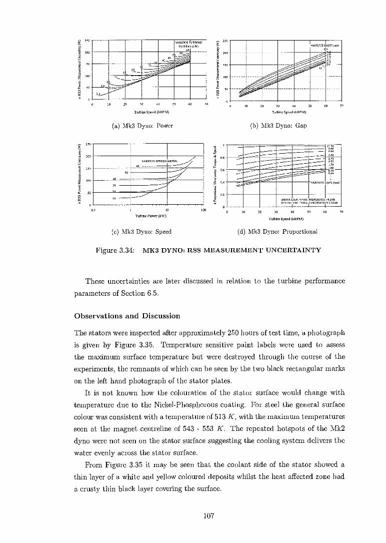
RSS

Pow

er M

easu

rem

ent l

iner

tain

ty (W

) 50

200

150

100

50

Prop

ortio

nal U

nerta

inty

: Tor

que &

Spe

ed

0.0

0.(6

0.4

0.2

0

70 60

VARIOUS TURBINE POWERS (kW)

60

150

100

50

0 10 20 30 40 50

250

200

30

ID

VARIOUS SPEEDS ORM) /

40

60

12 51

60 70

200 VARIOUS GAPS (mm)

06 6.RI(1

in 25

10 20 30 40 50 0

0

200

150

100

11

0


(a) Mk3 Dyno: Power


(h) Mk3 Dyno: Gap

...... 15 00

., 10.3

.00 NM 3.00

2 50 2.00

—4.41M111011.1111111.1111_11111111.11101010111 Il0"0 0.80 _........ ......,014( 0160

....4-4-•"---- VARIOUS GAPS (6=1

AHOY> LINE :SPERO PROPORTION ERROR BELOW LINE : TORULE PROPORTION ERROR

01

10

100 0 10 20 30 40 50

60

70

Turbkie Power (kW) Turbine Speed (kRPM)

(c) Mk3 Dyno: Speed (d) Mk3 Dyno: Proportional

Figure 3.34: MK3 DYNO: RSS MEASUREMENT UNCERTAINTY

These uncertainties are later discussed in relation to the turbine performance

parameters of Section 6.5.

Observations and Discussion

The stators were inspected after approximately 250 hours of test time, a photograph

is given by Figure 3.35. Temperature sensitive paint labels were used to assess the maximum surface temperature but were destroyed through the course of the experiments, the remnants of which can be seen by the two black rectangular marks

on the left hand photograph of the stator plates. It is not known how the colouration of the stator surface would change with

temperature due to the Nickel-Phosphorous coating. For steel the general surface

colour was consistent with a temperature of 513 K, with the maximum temperatures

seen at the magnet centreline of 543 - 553 K. The repeated hotspots of the Mkt

dyno were not seen on the stator surface suggesting the cooling system delivers the water evenly across the stator surface.

From Figure 3.35 it may be seen that the coolant side of the stator showed a thin layer of a white and yellow coloured deposits whilst the heat affected zone had a crusty thin black layer covering the surface.

107

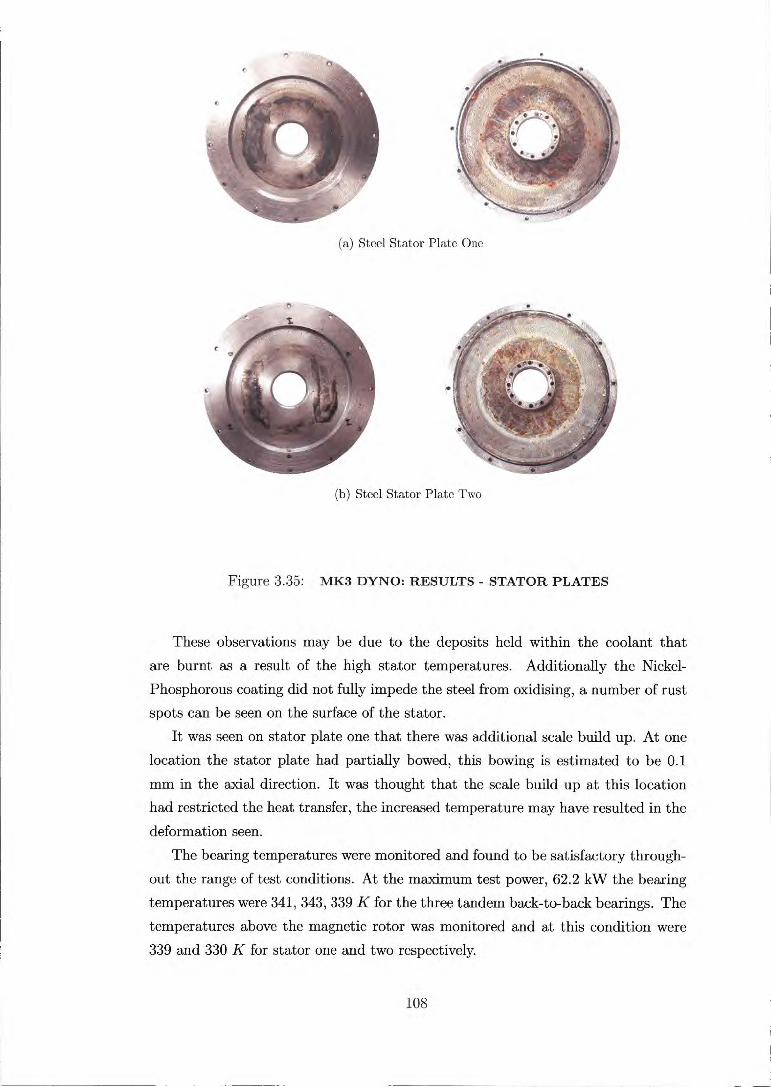
(a) Steel Stator Plate One

(b) Steel Stator Plate Two

Figure 3.35: MK3 DYNO: RESULTS - STATOR PLATES

These observations may be due to the deposits held within the coolant that are burnt as a result of the high stator temperatures. Additionally the Nickel-

Phosphorous coating did not fully impede the steel from oxidising, a number of rust spots can be seen on the surface of the stator.

It was seen on stator plate one that there was additional scale build up. At one

location the stator plate had partially bowed, this bowing is estimated to be 0.1

mm in the axial direction. It was thought that the scale build up at this location had restricted the heat transfer, the increased temperature may have resulted in the

deformation seen. The bearing temperatures were monitored and found to be satisfactory through-

out the range of test conditions. At the maximum test power, 62.2 kW the bearing temperatures were 341, 343, 339 K for the three tandem back-to-back bearings. The temperatures above the magnetic rotor was monitored and at this condition were 339 and 330 K for stator one and two respectively.

108

Limit of continuous safe operation

Rock t

Mode

Rotating Assembly Without Dynomometer

- n Bounce Mode

Rotating With Dynamometer

Assembly -

ilk Nip

2

0

These temperatures are high and are a result of the high power levels and the close proximity of the stator to the rotor. It was found that this temperature dramatically reduced as the rotor-to-stator gap was increased, as this allowed a greater mass flow of coolant air to flow.

An oil leakage problem through the labyrinth seal on the magnetic rotor side of the bearing housing was encountered at speeds over 55,000 RPM. It was known that the labyrinth seal gap was out of specification at approximately 0.25 mm, this increased gap reduces the sealing capabilities. This problem was alleviated by increasing the air pressure within the air blown seals to overcome the additional air loss.

Vibrations

The RMS vibration levels were recorded and a real-time FFT analysis performed and frequency domain monitored. The RMS vibration levels are given by Fig-ure 3.36. Two vibration traces are shown, the red trace illustrates the vibrations levels measured with the bearing housings and rotating assembly attached, whilst the black traces illustrates a later vibration trace measured additionally with the dynamometer assembly attached running under moderate loading. Overall the rotor dynamics of the Mk3 dyno were satisfactory such that the dynamometer was within the British Standard BS 7854-1:1996, [12] limit of 1.8 mm/s over the full range of turbine speed, 0 - 60,000 RPM. The low vibration levels are indicative of a good degree of balance, this was made possible by the modular design of the bear-ing housing allowing the rotating assembly to be balanced within its own bearing housings.

0 10 20 30 40 50 60

70



109

Evaluation

Overall the dynamometer has proved successful with no major problems encoun-tered. The general specifications of Section 3.1.1 have been met. The available speed range of the dynamometer is 0 - 60,000 RPM, whilst for the turbine equiva-

lent design speeds of 50 - 100 % the load range is 0.35 - 62.2 kW. The dynamometers polar mass moment of inertia was measured to be 4.5626 x

10'4 kg — m2, this is only 7.1 % higher then the previously employed turbocharger assembly and hence the test rig is deemed acceptable at mimicking the dynamic

behaviour of a commercial turbocharger. A reaction torque measurement has allowed an accurate measurement of turbine

torque with an accuracy of ± 0.025 Nm. The accuracy was limited by mechanical

hysteresis of the system which is therefore open to improvement. The modular design of the dynamometer has proved valuable at increasing the

usability of the test rig. The bearing module allows simple and accurate balancing of the rotating assembly and quick reassembly of the rig. The actuator unit requires the set-up of the rotor-to-stator gaps only once, the stator units can then be removed

and reattached without need of further set-up time. The dynamometer has integrated PC control and monitoring which allows control

and automated monitoring of the test rigs health, which is further discussed in

Section 5.3.8. The stator plates are simple in design and allows the dynamometer to be up-

graded by a simple replacement of the stator plates with an improved design.

3.4.6 Summary

The Mk3 dynamometer has proved successful at increasing the load range available in which to performance test turbocharger turbines. The concept of using permanent magnets in a high-speed dynamometer has allowed a compact, low inertia and stable power absorption device to be developed. This has allowed a load range of 1.7 - 62.2

kW to be absorbed at 60,000 RPM.

110

Chapter 4

Magnetic Analysis

4.1 Synopsis

This chapter describes the numerical analysis employed in order to understand and

optimise the magnetic circuit of the dynamometer. A 2D parametric model is de-scribed and the local and global results are presented. The Mkl, Mk2 and Mk3 dynamometers are modelled in 3D with comparisons given against experimental

data.

4.2 Introduction

The numerical analysis presented in this chapter was performed after the develop-

ment and testing of the Mkl dyno and during the development of the Mk2 and Mk3 dynos of Chapter 3. The basic layouts of these dynamometers are given by

Figure 4.1.

STATOR

TURBINE

(a) Mkl Dynamometer (b) Mk2 & Mk3 Dynamometers

Figure 4.1: MK1, MK2 AND MK3 DYNAMOMETER LAYOUT

111

The magnetic circuit of these dynamometers consist of two main components, the magnetic rotor and the conductive stator plates in which the eddy currents are

generated, Figure 4.1. This simple layout lends the dynamometer to be numerically modelled both in 2D and 3D. The majority of the simulations were conducted using a 2D finite element model. These computationally inexpensive models allow a broad

and generalised parametric study to be conducted with the optimisation of the numerous variables giving a better understanding of their effects. To give an accurate comparison against the experimental results a 3D finite element model specific to the dynamometers were used to validate that all fundamental parameters were being

accurately modelled.

4.3 Governing Equations

Electromagnetism is governed by the Maxwell equations, where a suitable form for the dynamometer is given by Equations 4.1 - 4.3. The general low frequency approximation is used in which the displacement current term is neglected, Equa-tion 4.1. By employing a relative frame of reference approach the time varying field of Equation 4.2 can also be neglected. These simplifying assumptions are discussed

in Section 4.3.2.

[D] v x [1-1] = [J] +a at --,,--- 0

V x [E] = a [B]at .._.,.._, 0

V • [B] = 0 (4.3)

(4.1)

(4.2)

Where : V x = V • --= [H] =

[B] =

[J1 = [E] = [D] = t=

curl operator divergence operator magnetic field intensity vector (A/m) magnetic flux density vector (T) (free) current density vector (A/m2) electric field intensity vector (V/m)

electric flux density vector (C/m2) time (s)

112

Equation 4.1 is Ampere's law for the case of a static electric field, the low fre-quency assumption. It relates the line integral of the magnetic field around a closed

loop to the electric current flowing through the loop, fc,[1/] • dl = f s[J] • da. Where

the area 'S' is enclosed by the closed curve 'C'.

Equation 4.2 is Faraday's law of induction. It relates the line integral of the

electric field around a closed loop which by definition is the induced EMF, to the negative rate of change of magnetic flux through the area enclosed by the loop,

fc[E] • dl = —1 f s[B] • da. For the dynamometer, the change in relative reference plane, the magnetic flux is static and therefore its rate of change is equal to zero.

Equation 4.3 is Gauss's law of magnetism. It is the conservation of magnetic flux, where the net magnetic flux out of any closed surface is zero, which presumes

only magnetic dipoles exist, fc[B] • da = 0.

The governing equations can not be directly solved without the constitutive equations which relates the field quantities to the physical properties of the materials

and are given by Equations 4.4 - 4.5.

[J] = {1/p} ([E] + [U] x [B]) (4.4)

[B] = {p} [H] +po[mc] (4.5)

Where : = velocity vector (m/s) = remanent intrinsic magnetisation vector (A/m)

= electrical resistivity matrix (n.m) = magnetic permeability matrix (H/m) = magnetic permeability of free space (H/m)

Equation 4.4 describes the relation between the current density [J] and the elec-

tromagnetic fields [E] and [B] and physical properties [U] and {p}. A current can

occur directly as a result of an electric field and/or due to the cross product of the

velocity and the magnetic flux density. Equation 4.5 describes the relation between the magnetic flux density [B] and the

magnetic and magnetisation field [H] and [M], which is related to the permeability

{u}, a property of the medium.

Domain Areas

There are three basic domain areas which are required to magnetically model the dynamometer given by Figure 4.2. All the domains are within the general non-

permeable region in this case air (no) which is confined by a boundary condition

that depicts the boundary of the overall model.

113

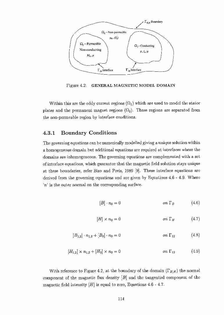
Boundary

SI, —Non-permeable

Flo > (.1)

1'20 Interface Flo Interface

Figure 4.2: GENERAL MAGNETIC MODEL DOMAIN

Within this are the eddy current regions (C-21) which are used to model the stator

plates and the permanent magnet regions (p2). These regions are separated from

the non-permeable region by interface conditions.

4.3.1 Boundary Conditions

The governing equations can be numerically modelled giving a unique solution within

a homogeneous domain but additional equations are required at interfaces where the domains are inhomogeneous. The governing equations are complemented with a set

of interface equations, which guarantee that the magnetic field solution stays unique at these boundaries, refer Biro and Preis, 1989 [9]. These interface equations are

derived from the governing equations and are given by Equations 4.6 - 4.9. Where

'n' is the outer normal on the corresponding surface.

[B] • no = 0 on FB (4.6)

[H] x no = 0 on FH (4.7)

[B1,2] • n1,2 + [Bo] • no = 0 on F12 (4.8)

[H1,2] X n1,2 + [Ho] x no = 0 on 1'12 (4.9)

With reference to Figure 4.2, at the boundary of the domain (FB,H) the normal

component of the magnetic flux density [B] and the tangential component of the

magnetic field intensity [H] is equal to zero, Equations 4.6 - 4.7.

114

At the interfaces between different materials (F12 ), the normal component of

the magnetic flux density [B] and the tangential component of the magnetic field

intensity [H] is continuous, Equation 4.8 - 4.9.

4.3.2 Low Frequency Simplification

Displacement Current

The displacement current (0[D] I at]) can usually be neglected in the context of a

mechanical system, as its current contribution is many magnitudes smaller then the

conduction current [J]. This may be seen by consideration of a harmonic time variation of the displace-

ment current (jw) Hammond, 1994 [38], which allows the ratio of the free current

density and the displacement current to be simply assessed, Equation 4.10. For a

good conductor the resistivity is in the order of 3 x 10-08 am and the permittivity

(c) which is equal to the free space permittivity (€c ) of 8.85 x 10' Flm.

_ ( 11 P)[E] 1 x 1018 la[Duati jw€[E]

(4.10)

The conduction current [J] is many order of magnitude larger then the displace-

ment current ( a [ D ]/at ]) and justifies its omission from Equation 4.1. Typically the

upper limit to this simplification is 10 - 50 MHz for a mechanical system, Perry,

1985 [64].

Relative Frames of Reference

Equation 4.4 is derived from the Lorentz Force, which gives the force on a charge,

Equation 4.11.

[F] = q ([E] {U} x [B]) (4.11)

A charged particle 'q' moving with a velocity U through a magnetic field [B],

produces a force on the particle, [F] = q {U} x [B] . Now consider a frame of reference

stationary to the particle, [U] = 0, the force is still present, the transformation of the frame of reference of this system causes an electric field to appear such that

E = {U} x [B] . For the low speed simplification, the classical Galilean frame of

reference transformation is correct. This allows the dynamometer to be modelled with stationary magnets and with

motion on the stator.

115

4.3.3 Potential Formulisation

The governing equations are solved using the potential formulisation. The main

benefit of using potentials is to reduce the number of DOFs to be solved. The use of

potentials transforms the field variables such as [B] and [H] "away from a physical

problem into a mathematically abstract problem" Krawczyk, 1993 [48]. Within the 2D environment this transforms the vectorial problem into a Scalar problem.

The potential formulation implemented in the finite element method is the A, V — A formulation, based upon Biro and Preis, 1989 [9]. Where [A] is the Magnetic

Vector Potential, and 'V' is the Electric Scalar Potential. The A, V — A formulation

obtains its name from its applicability; within the eddy current regions both the [A] and 'V' potentials are required to solve the problem whilst outside only [A] is required. The magnetic vector potential is defined by Equation 4.12 and the electric

scalar potential defined by Equation 4.13.

[B] = V x [A] (4.12)

Oat ] [E] =

vv (4.13)

Equation 4.12 - 4.13 are consistent with Maxwell equations and also contains

two of them, this can be seen by the following derivation. By taking the divergence of Equation 4.12 results in Equation 4.14, which is

identical to Equation 4.3, Gauss's law of magnetism.

V • [B] = V • (V x [A]) = 0 (4.14)

By taking the curl of Equation 4.13 results in Equation 4.15, which is equal to

Equation 4.2, Faraday's law of induction.

V x [E] = -V x (VV) - a —at v x [A] = o a [B] at (4.15)

The uniqueness of [A] is not insured by the potential formulations. Typically

this is achieved by specifying the divergence of [A], known as gauging. In a closed

region this is not enough to attain uniqueness and it is required that the boundary conditions are imposed directly on [A]. Biro and Preis, 1989 [9] offer a detailed discussion on this topic. The gauge that is used is the Coulomb gauge, given by

Equation 4.16.

116

V • [A] = 0 (4.16)

Two of the Maxwell equations have been satisfied, the third equation Ampere's law is satisfied using the constitutive Equations 4.4 - 4.5 and the implication from Ampere's law that the current density is divergence free. The difficulty arises with

the fulfilment of the Coulomb gauge to ensure uniqueness of the equations, although beyond the scope of this thesis the inclusion of an additional term —VW/4V • [A]

ensures this, a discussion is given by Biro and Preis, 1989 [9]. This results in the

following differential equations that are numerically solved by the employed finite

element package, Equations 4.17 - 4.19.

V x {1/u}V x [A] — V{1/0V • [A]+

{l/p}VV — [U] x {1//i}V x [A] = 0 in Qi (4.17)

o (—{1/OVV [U] x 0./i4V x [A]) = 0 in, Qi (4.18)

V x {1/11}V x [A] — V {11 it}V • [A] = V x u0{1/0[Ma] in 170,2 (4.19)

This formulisation requires that the normal component of the magnetic vector

potential [A] must be continuous across interfaces and with inhomogeneous materials this is not the case . This does not effect the 2D model, as the normal components

of the Vector Potential are zero, only a z-component exists.

4.4 Finite Element Approach

The finite element analysis employed used a commercial package, ANSYS 5.7, [2]. A brief discussion on the general procedures and restrictions of this finite element package are given before the specific 2D and 3D models are described.

4.4.1 Geometry, Properties and Equation Restrictions

The finite element package is not able to model all situations and restrictions apply.

These restrictions within ANSYS 5.7 requires bodies with motion must be spatially invariant in the direction of motion and motion must be constant in value.

117

A frame of reference transformation allows the magnetic rotor to be modelled as stationary with an implied velocity on the stator plate requiring the geometric

model of the stator to be invariant in the direction of motion. An additional restriction for the 3D model is that non-linear motional effects

cannot be analysed, such that steel stators with non-linear magnetic properties are not permitted.

Property Restrictions

For magnetic materials, non-linear orthotropic magnetic properties may be specified with a combination of a B — H curve and linear relative permeability. ANSYS does not permit the modelling of magnetic hysteresis losses as only an initial (virgin) magnetisation curve can be used as a input with respect to a permeable steel stator

used in the Mk2 and Mk3 dyno.

Skin Depth

A useful non-dimensional number is the skin depth, 6m. It is a measure of the depth

an oscillating field can penetrate into the surface of a conductor. The skin depth gives the depth at which the field has decreased to 1/e or about 37 % of its surface value, Equation 4.20.

Where w is the angular frequency of the field, given by Equation 4.21, Npotes is the number of alternative pole magnets in the rotor and RPM is the revolutions per minute of the rotor. An accompanying Phase Lag can also be specified. As the depth into the material increases the phase of the field lags the surface field, such that at one skin depth the phase lag is 57° (one radian).

6m = 2p V it0PrW

(4.20)

7r.N ) w Rpm po es

60 (4.21)

This motional effect is of direct importance in assessing an appropriate minimum element size. The conductor within one skin depth contains approximately 89 % of the available power and hence it is important that there are at least 1 - 2 elements within this depth in order to capture its effect.

An estimate of the element size can be made considering an extreme case, for a resistivity of 2 x10-08 it.m, a permeability of 47r x 10-°7 H/m, a 24-pole rotor and a rotational speed of 60 kRPM. This gives a skin depth of 0.65 mm, suggesting a appropriate element size of 0.33 - 0.65 mm perpendicular to the motion direction.

118

Magnetic Reynolds Number

The numerical accuracy of problems with motional effects depends on various fac-tors, which depict the appropriate mesh refinement. A magnetic Reynolds' number

can be defined to characterise the problem, Equation 4.22. Where L is equal to

half the element length in the direction of motion, Pop, is the permeability, p the

resistivity and U the imposed velocity. Typically motional effects are accurately modelled for low values of magnetic

Reynolds number of order 1. In order to investigate its effects a mesh sensitivity

analysis was conducted in Section 4.5.5.

Rem = lloPrUL (4.22) p

4.4.2 Analysis Type and Solvers

The dynamometer model may be solved using a quasi-static analysis in 2D, whilst

it is required to be solved as a harmonic or a transient analysis in 3D. There are three solvers that may be used for the dynamometer problem and are:

• Frontal Solver: Direct Elimination Solver

• JCG (Jacobi Conjugate Gradient) Solver: Iterative Solver

• ICCG (Incomplete Cholesky Conjugate Gradient) Solver: Iterative Solver

The Frontal Solver uses a direct Cholesky factorization algorithm. This method

does not suffer from convergence problems and has low memory requirements, but the formation of the triangular matrix requires heavy disk usage. This solver was

used for all linear and non-linear analysis < 50,000 DOFs. The JCG and ICCG are iterative techniques where instead of eliminating de-

pendent DOFs the full global matrix is formed and the solution found by iteration.

These methods have low disk usage but the memory requirements are large. This solver was used for solution domains that were prohibitive for the frontal solver,

50,000 to 1,000,000 DOFs. The computation was performed with a desktop PC 700 MHz, 500 MB of RAM

and 3 GB disk space.

'This has no physical resemblance to the fluid Reynolds number.

119

4.4.3 Post Processing

The primary data calculated by ANSYS 5.7 are the DOFs of the problem. In a 2D

analysis this will consist of just one component of the magnetic vector potential, Az ,

whilst for a 3D problem this will consist of all three components Ax , Ay and Az and

the electric scalar potential V. Derived from the primary DOFs are the relevant magnetic vector results such as

the Magnetic Flux Density [B], Magnetic Field Intensity [H], Current Density [J],

Lorentz Forces [Fib], Maxwell Forces [Fm], Torque [Tjb] and the scalar Joule Heat,

Qi. These quantities are derived in the following hierarchy, where the previous

hierarchy is used to define the next.

• PRIMARY data:

• FIRST derived data:

• SECOND derived data:

• THIRD derived data:

[A], V [B] [H], [J]

- [F b], [Fm], [Ti1 b„ b,, Qj

Derived Power

There are two inter-related techniques used to calculate the power absorbed by the stator. The power may be derived from the forces acting on the stator or from the

Joule heating occurring within the stator. For a 2D analysis, the power (W) may be assessed from the velocity (U) and

forces (F) acting on the stator, in vector notation this is given by Equation 4.23.

It is only the x-component of force which can contribute to power absorbed by the

dynamometer.

= [F] • [U] (4.23)

In 3D the process is similar but the forces are replace by torque [Tit) ] and the

linear velocity is replaced by angular speed [w].

The Joule heat, which is a function of the current density [J] may also be used

to assess the power absorbed by the stator. The derived Joule heat data is per unit volume and may be transformed into an overall power using Equation 4.24, where 'v' is the element volume and 'n' is the number of elements within the stator.

= (Qi • v)i (4.24) i=1

120

Y-AXIS: INTO PAGE Z-AXIS: OUT OF PAGE

S STATOR

MAGNET -

STATOR S

x

3-D POLAR COORDINATES 2-D CARTESIAN COORDINATES z (UNIT DEPTH)

0

3-D POLAR COORDINATES 2-D CARTESIAN COORDINATE

MEAN DIAMETER (BASED ON MAGNET VOLUME)

x

DOUBLE STATOR (MK2 & MK3 RIG)

4.5 2D Finite Element Analysis

A parametric analysis was performed to study the effects of various parameters on

the performance of the dynamometer. The model layout matches the Mk2 and Mk3 dyno of Chapter 3 which utilise a double stator configuration given by Figure 4.1.

4.5.1 2D Model Transformation

The 3D polar coordinates which best describe the geometry of the dynamometer may be approximated in 2D cartesian coordinates. For the Mk2 and Mk3 dyno this is achieved by unwrapping the magnetic rotor and stator in the circumferential

direction '0' to form an infinite linear array of magnets between an infinite pair of stator plates, refer Figure 4.3. This transformation is valid assuming the following

geometrical assumptions apply: 1) curvature effects are neglected 2) the stator

geometry is homogeneous in the z-axis 3) the magnets are represented by sectors.

Please note the coordinate change as the following discussion uses the 2D format,

where 0 —> x and z --> y.

4.5.2 Solution Domain

Due to the cyclic symmetric nature of the dynamometer in the x-direction and the symmetric nature in the z-direction, it is sufficient to model one half of a magnet sector and one stator. The solution domain is illustrated by Figure 4.4, which

simulates the Mk2 dyno layout. The dynamometer model is meshed with quadratic

elements and a mesh size of 0.25 mm.

Figure 4.3: 2D MODEL TRANSFORMATION

121

OD

D P

ERIO

DIC

BO

UN

DA

R Y

MAGNET

AIR GAP

STATOR

AIR GAP

FLUX PARALLEL

FLUX NORMAL

OD

D PE

RIO

DIC

BO

UN

DA

RY

1/2 MAGNET GAP

MAGNET LENGTH

1/2 MAGNET DEPTH

ROTOR-TO-STATOR GAP

STATOR THICKNESS

POLE LENGTH

Figure 4.4: 2D MODEL: SOLUTION DOMAIN & MODEL VARIABLES

Boundary Conditions

The boundary conditions are shown by Figure 4.4. A flux normal condition is used on the top face of the magnet. This is a naturally occurring condition and

constrains the DOF Az to be normal to the boundary plane and is therefore a

symmetry boundary. A flux parallel condition is applied to the bottom face of the solution domain, this

constrains the DOF Az to be zero at the boundary plane. This boundary condition

has little effect on the solution output when the stator has an imposed velocity due to the shielding effect created by the eddy currents. In a stationary stator the flux lines are influenced by the boundary but this is of little interest in this analysis.

With respect to the period boundary condition, the flux density is a vector quan-

tity therefore it is necessary to consider its direction when enforcing this condition.

The choice of either odd or even boundary conditions can be specified dependent on

whether one or both of the alternative pole magnets are being modelled. With reference to Figure 4.5, to enforce the boundary condition it is necessary

to constrain the opposite nodes on the boundary as follows: For an odd boundary

condition Azl = —Az2, whilst for an even boundary condition Azl = Az3.

4.5.3 Properties and Assumptions

The main simplifying assumption of the real multi-physics problem is that only a magnetic analysis is performed. The solution is open loop such that the material property are independent of the non-magnetic environment. In the context of a parametric study this is not a simplification, the analysis is not simulating a specific problem but giving a general result which can be used appropriately to optimise a

design.

122

Periodic Boundary (Even)

Periodic Boundary (Odd) -►

Node 1 Node 2 Node 3

Figure 4.5: 2D MODEL: PERIODIC BOUNDARY ASSIGNMENT

There are three main types of materials used in this analysis, these are: 1) air

2) permanent magnetic material and 3) the stator material which can be either

permeable or non-permeable.

Material Properties

The material properties that are used in the analysis are given in Table 4.1.

Air Properties: Magnetically air is inert, therefore it is only required to specify

the airs relative permeability, fir . The value of its absolute permeability is equal to

that of free space, iii: 4ir x 10' H/m.

Magnet Properties: The properties used to simulate the rotor magnets were

supplied by Crucible Magnetics of type Crumax(D4014, [52]. These magnets were

used in the all the magnetic rotors tested in the Mkl - Mk3 dynos, additional properties can be found in Appendix C.1.1. For generality, the 293 K curve data is

used which demonstrates linearity throughout its range.

Stator Properties: There were two types of stator materials specified in the

parametric study, permeable and non-permeable conductors. Non-Permeable: Non-permeable conductors are materials with a relative perme-

ability, uT of 1, such as copper and aluminium. The analysis covered a range of resistivity values, 2 - 32 x 10' am, which encompasses most available materials.

Permeable: Permeable conductors have relative permeabilities greater then one, such as steel. A single common class of permeable steel was analysed of type AISI 1021 (070M20), this being the material used in the Mkt dyno. The range of resis-

tivity values analysed was 2 - 32 x10-08 am. The detailed characteristics of AISI

1021 steel including its B — H curve may be found in Appendix C.1.1.

123

Table 4.1: 2D MODEL: MATERIAL PROPERTIES

Material Properties Air Permanent

Magnet

Stator Non-permeable Permeable

Relative Permeability, GO 1 1.049 1 Variable

Coercive Force, (He ) A/rn - 979,000 - -

Resistivity, ( x 10-4)8) am - - 2 - 32 2 - 32

4.5.4 Variables

With reference to Figure 4.4, the variables which control the models behaviour are:

• NUMBER OF POLES (N poies ): 4, 8, 12, 16 and 24

The number of poles is the number of alternative pole magnets in the rotor. A 4-pole rotor will have a N - S - N - S configuration. An increase in the

number of poles reduces the pole length (Lpoie) as the mean magnet volume

radius (Rmean) of the rotor is constant: Lpoie = an-Rmean /N poies •

• STATOR THICKNESS (Lstator): 1, 2, 4 and 6 mm

The stator thickness is the perpendicular distance between its two outer sur-

faces.

• ROTOR-TO-STATOR GAP (Gap): 0.5, 1, 3, 4 and 6 mm

The rotor-to-stator gap is the perpendicular distance between the magnetic rotor surface and the stator surface.

• RESISTIVITY OF STATOR (pstator ): 2, 4, 8, 16 and 32 x 10-°8 S-2.m

The stator resistivity range has been chosen to provide a realistic range of material resistivity values. A resistivity of 2 x10-08 Q.m is that of copper,

whilst 32 x10-08 am is of nickel silver or a AISI 1021 steel at 513 K.

• VELOCITY OF STATOR2 : 20, 40 and 60 kRPM

The linear velocity of the stator was assessed from the the mean magnet vol-ume radius of the rotor, Rn,„7, of 0.033 m. Giving 69.12, 138.23, 207.35 m/s

respectively for the kRPM.

• RELATIVE PERMEABILITY OF STATOR (itr,stator): 1, variable

The non-permeable stators have a relative permeability of 1, whilst the steel stator has a variable permeability according to its B — H curve,

refer Appendix C.1.1.

2h was subsequently found from the 3D analysis that these linear velocities were over estimates of the dynamometer speeds, a multiplication factor of 0.85 may be used to reduce the calculated power to approximate the MK Mk2 and Mk3 dynamometers directly from these results.

124

• MAGNET GAP (Lg,magnet): 2 mm, special case

The magnet gap is the perpendicular distance between adjacent magnets. This is of secondary importance in the analysis and a value of 2 mm was assigned.

The magnet length, Li,magnet = Lpole — Lg,magnet•

• MAGNET DEPTH (Ld,magnet): 10 mm

The magnet depth is the distance measured perpendicular from the stator

surface between the two magnet outer surfaces.

4.5.5 Results and Discussion

In order to obtain an understanding of the processes that occur within the magnetic circuit an analysis was conducted that studied the resultant effects at a local level. This enables appropriate decisions to be made in the optimisation and design of the

rotor and stator system.

Non-Permeable Stators - Local Results

The development of the skin depth has been shown by Equation 4.20 and may be seen graphically by Figure 4.6. This figures shows two alternate pole magnets with a small rotor-to-stator air gap and a thick non-permeable stator, the lines are of constant magnetic flux and illustrate the influence of the stator velocity.

In the stationary case, Figure 4.6(a) the flux lines are unaffected by the presence of the stator which is magnetically invisible when no motion is imposed. With

motion the development of the skin depth can be seen by Figures 4.6(b) - 4.6(c). As the stator passes through the magnetic field, eddy currents are induced within

the stator. These currents have their own magnetic field which oppose the original and results in the skewing of the overall field seen. These flux lines become further constrained to the surface as the speed is increased, such that the stator acts as a

magnetic shield.

To provide consistency in the following sections a single case is discussed, the chosen case replicates the Mkt dyno experiments of Section 3.3. An 8-Pole rotor is

modelled with a rotational speed of 60,000 RPM (207.35 m/s), a magnet thickness of 10 mm, a magnet gap of 2 mm, a rotor-to-stator gap of 0.5 mm, a stator thickness

of 2 mm and a resistivity of 2 x10-08 am. To aid visualisation the results have been

extended to show two alternate pole magnets. The total flux density contour plot of Figure 4.7 illustrates the magnetic shielding

effect as a consequence of the development of the skin depth. It may be seen that the magnetic flux density has a maximum value at the corners of the magnet where the neighbouring alternative pole magnet provides a desirable path for the flux.

125

1

(b) 10 RPM

Figure 4.8 gives the individual components of the magnetic flux density, Bx and By. The importance of these plot becomes apparent in the following discussion.

It may be seen from Equation 4.1 or Equation 4.4 that in a 2D x - y analysis only

a z-component of current density, J, will exist and is proportional to one variable, the

y-component of the magnetic flux density, By. The general form can be simplified

giving Equation 4.25 and the current density contour plot is given by Figure 4.9.

1 (4.25)

1 Qj = p • 4 = — • Ux2 B (4.26)

Figure 4.10 illustrates the Joule heat generated within the stator. For the 2D

model the Joule heat is related to the current density by Equation 4.26. It can be seen from these equations that the current density and Joule heat is

directly related to the y-component of the magnetic flux density, By and therefore

it is important to maximise this component.

jl illii ) )))1

,__--'

(a) 0 RPM

(c) 60 RPM

Figure 4.6: 2D FLUX LINES: SKIN DEPTH DEVELOPMENT, NON-PERMEABLE

126

x UNITS: T

.713E-05 MN .196251

UNITS: T MIII .392494

.58E1737

.784981 MIN .981224 I 1 1.177

1.374 I I 1.57

1.766

(a) 0 RPM .714E-04

K UNITS: T m, (b) 60 RPM

Figure 4.7: 2D TOTAL FLUX PLOT: NON-PERMEABLE

-1.927 ▪ -1.5

-1.072 - -.644434

- mmo -.216775

.210883

.638542 ▪ 1.066

- 1.494 1.922

(a) X-COMPONENT, B, -1.139

lili -.886208 Mil -.633006 IM -.379803 MI -.126601 Ell .126601 ME .379003 = .633006

.886208 - 1.139

(c) Y-COMPONENT, By

Figure 4.8: 2D MAGNETIC FLUX DENSITY PLOTS: NON-PERMEABLE

UNITS: Alm2„

INN NMI 111111

I

-.145E+10 -.112E+10 -.604E+09 -.483E+09 -.163E+09 .156E+09 .470E+09 .799E+09 .112E+10 .144E+10

Figure 4.9: 2D CURRENT DENSITY PLOT: NON-PERMEABLE

127

- 111.1.452019 -

=.903966 - 1.13 1.356

= 1.562 1.000

- 2.034

54627 .691E+10 .138E+11 .207E+11 MIII .276E+11

MIN .395E+11 11% UNITS: J/m2 .415E+11

.484E+11

.553E+11 Ell .622E+11

Figure 4.10: 2D JOULE HEAT PLOT: NON-PERMEABLE

These plots indicate that the majority of the activity (J., and Q.j ) occur in a localised region at the surface of the stator just offset from the gap separating the magnets. Visually this offset can be seen from the flux line plots. Figure 4.11 is an enlarged view of the earlier plot, noting that this plot shows constant vector potential lines, Az and by definition By = —(a.Az/ax). A high value of By and the corresponding high values of Jz and Qi are indicated when the iso-potential lines are densely packed in the x-direction.

An alternative derivation of power given previously in Section 4.4.3 is through the assessment of forces on the stator. In a non-permeable stator the Lorentz force contribution is due to the [J] x [B] term as given by Equation 4.11. It may be seen that this equation results in two components of force, a braking force, Fx and a repulsive force, Fy. As the current density [J] is proportional to [B], the Lorentz force is also proportional to [B] and gives Equation 4.27 for the x-component of force and Equation 4.28 for the y-component of force. It can be seen that the differing techniques for the assessment of stator power are derived from the fundamental elec-tromagnetic relations and will therefore yield identical results. The corresponding contour plots of these forces are given by Figures 4.12 - 4.13.

1 = Ux By2

STATOR VELOCITY DIRECTION

MAIN ACTIVITY AREA (AREA OF LARGEST By)

Figure 4.11: 2D ACTIVITY AREA FLUX PLOT: NON-PERMEABLE

128

(4.27)

1111 -19.885 -17.676 -15.467 -13.257 1111 -11.048 111 1 1 -8.838

MN UNITS: N/m -6.629 -4.419 -2.21 1111 -.6106-04

Figure 4.12: 2D LORENTZ FORCE X-COMPONENT PLOT (ELEMENT/M): NON-PERMEABLE

EX IN UNITS: N/m

-101.267 -89.041 -76.814 -64.588 -52.361 -40.135 -27.909 -15.682 -3.456 0.771

Figure 4.13: 2D LORENTZ FORCE Y-COMPONENT PLOT (ELEMENT/M): NON-PERMEABLE

Fy = 1 — • UxB xB y (4.28)

The x-component of force will always be in a negative sense to the velocity and will therefore always resist motion, it is proportional to the square of By, Equa-tion 4.27. In order to visualise the process within the stator, the x-component of force can be plotted at various positions within the stator, Figure 4.14(a). This figure illustrates the localised nature of the braking force and its migration and reduction in the direction of motion as the depth within the stator is increased. The x-component of force at the surface of the stator peaks below the corner of the leftward magnet due to the high flux density occurring at this location. This is a consequence of the influence of the induced current skewing the source field and resulting in the migration of the peak location as the depth within the stator is increased. The localised nature of the braking force suggests that an increase in the number of poles would be beneficial in power absorption for the dynamometer, such that a reduction in the unused area of the stator can be obtained.

The y-component of force is illustrated for various positions within the stator by Figure 4.14(b) and demonstrates a similar trend to the x-component braking force. Both attractive and repulsive forces occur within the stator although the overall repulsive force is a magnitude larger then the attractive force and larger then the braking force.

129

MAGNET n MAGNET

I

____...,....‘

} DISTANCE INTO (0 mm = STATOR

— 0.125 — 0.375

STATOR SURFACE)

mm mm

0.625 mm 0.875 mm

1.125 mm — 1.375 mm — L625

1.875 mm mm Geometry STATOR VELOCITY — Rotor

-25 -15 -5 5 15 25

Stator X-Direction (mm)

(a) X-Component

MAGNET n MAGNET

--. irs.---

if-.... DISTANCE

(0 nun = STATOR INTO STATOR

SURFACE) — 0.125 mm — 0.375 tom 0.625 mm

0.875 mm — 1.125 mm — 1.375 mm — 1.625 mm

1.875 mm — Rotor Geometry STATOR VELOCITY

-25 -15 -5 5

15 25

Stator X-Direction (mm)

(b) Y-Component

Figure 4.14: 2D LORENTZ FORCE: NON-PERMEABLE

The y-component of force is proportional to both Bx and By, Equation 4.28. It may be seen an attractive force is produced when the two components BB and By are of similar sign such that the flux direction is in the first or third quadrant.

The repulsive forces occur when the flux direction is in the second or fourth quadrant, this is the dominant direction due to the skewing of the magnetic flux resulting from the induced current. The attractive forces occur in localised regions largely on the surface of the stator where the flux exiting the stator has not been sufficiently skewed. The large value of the y-component of force is due to its de-pendency on both components of the magnetic flux, Bs and By. At the peak force point, the Bx flux is approximately 6 times larger then the By flux which results in the repulsive force being of similar magnitude larger then the peak breaking force.

X-D

irect

ion

Forc

e (N

/m)

5

0

-5

-10

-15

-20

-25

Y-D

irect

ion

Forc

e (N

/m)

25

0

-25

-50

-75

-100

-125

130

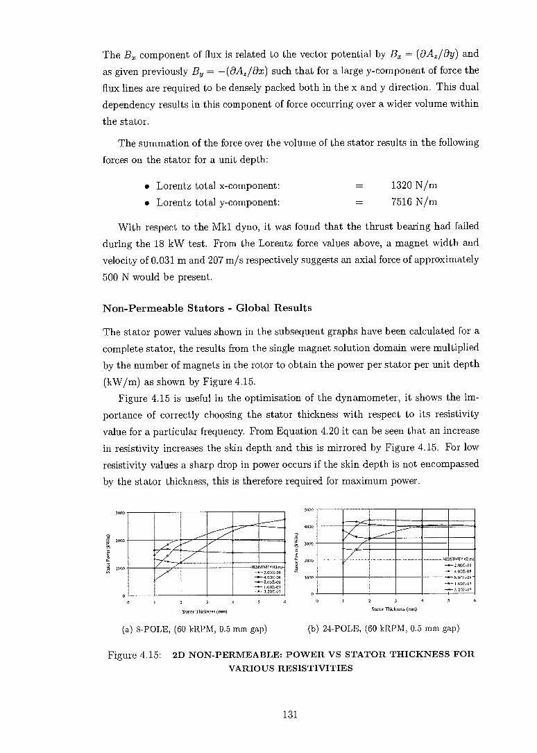
5000

40130

Stat

or P

ow e

r (kW

/m)

3000

2000

1000

a

The Bx component of flux is related to the vector potential by Bx (DA,/ay) and

as given previously B y = —(aA.,10x) such that for a large y-component of force the

flux lines are required to be densely packed both in the x and y direction. This dual dependency results in this component of force occurring over a wider volume within

the stator.

The summation of the force over the volume of the stator results in the following

forces on the stator for a unit depth:

• Lorentz total x-component: 1320 N/m

• Lorentz total y-component: 7516 N/m

With respect to the Mkl dyno, it was found that the thrust bearing had failed during the 18 kW test. From the Lorentz force values above, a magnet width and velocity of 0.031 m and 207 m/s respectively suggests an axial force of approximately

500 N would be present.

Non-Permeable Stators - Global Results

The stator power values shown in the subsequent graphs have been calculated for a complete stator, the results from the single magnet solution domain were multiplied by the number of magnets in the rotor to obtain the power per stator per unit depth

(kW/m) as shown by Figure 4.15. Figure 4.15 is useful in the optimisation of the dynamometer, it shows the im-

portance of correctly choosing the stator thickness with respect to its resistivity value for a particular frequency. From Equation 4.20 it can be seen that an increase

in resistivity increases the skin depth and this is mirrored by Figure 4.15. For low resistivity values a sharp drop in power occurs if the skin depth is not encompassed by the stator thickness, this is therefore required for maximum power.

:_j'A.'...'---'------'------'-.

RES STIVITY (11.ml- --.- 1000-08 —.— 4.00E-05 --.-- 8.000-04 --.— 1.600-07 —W--1.20E-07

5

6

1

RESISTIVITY (Sim) —•-2.00E-08 —.— 4.00E-08 —..— 5.00E-08 - -4.— 1.600-07 —.,,— 3.70E-07

0 3 4

6

Stator Thickness (mm)

3000

2000

ct'

a 1000

0 0 2 3 4

Stator Thilmess (min)

(a) 8-POLE, (60 kRPM, 0.5 mm gap) (b) 24-POLE, (60 kRPM, 0.5 mm gap)

Figure 4.15: 2D NON-PERMEABLE: POWER VS STATOR THICKNESS FOR VARIOUS RESISTIVITIES

131

1000

0

f 500

1500

L.

ROTOR 1kRPM) 20

—4-40 —4^ 60

ROTOR (kRPM) —4-20 —4-40 —4-61,

3000

5000

C 1000

2 3 4 0 2

Stator thickness (lien) Stator Thickness (min)

(a) 2x10-°8 arn, (8-Pole, 0.5 mm gap) (b) 32x10-" am, (8-Pole, 0.5 mm gap)

Figure 4.16: 2D NON-PERMEABLE: POWER VS STATOR THICKNESS FOR VARIOUS SPEEDS

It is clear from Equation 4.20 that the skin depth is also governed by the fre-quency of the magnets: this is a function of both the rotor speed and the number of magnetic poles on the rotor. Figure 4.15 additionally illustrates that the opti-mum resistivity is dependent on the pole number, where an increase in pole number

decreases the optimum resistivity. The skin depth is dynamic in nature and will change with the speed of the

dynamometer. The requirements of the dynamometer must be considered before the correct choice of stator thickness can be assigned. It is prudent to have the

stator thickness as thin as practical as this will aid the heat transfer. The copper and aluminium stators of the Mkt dyno have a thickness of 2 mm and a resistivity

value of less then 8 x 10-08 fl.m. From Figure 4.15 this would suggest that the stator

thickness for the 8-pole rotor is optimum. Although the resolution is low an electromagnetic phenomenon is visible in Fig-

ure 4.15, that of wave reflection and interference. This occurs when the skin depth approaches the stator thickness and allows the magnetic flux oscillations to interact with the boundaries. The subsequent positive interference can result in a peak of the maximum obtainable power above that of the infinitely thick stator, this has been analytically predicted by Perry, 1985 [64]. It is difficult to take advantage of this phenomenon in a variable speed device due to the changing skin depth, a com-promise is necessary balancing the low speed torque obtainable with a larger stator

thickness and the high speed torque where stator cooling becomes important. Figure 4.16 illustrates the stator thickness optimisation with respect to the work-

ing speeds of the dynamometer. For low resistivity materials given by Figure 4.16(a) the skin depth is encompassed within the stator at all useful speeds and the wave re-flection phenomenon can be taken advantage of. For a high resistivity material given by Figure 4.16(b) a high power can potentially be obtained but this is restricted at lower speeds as the skin depth is now not encompassed within the stator.

132

3000

‘000

i Don GAPS (MM) -+-0s _._1 -*-

2 -A- 6 -*-4 ,--''''-'-----.--------.

Stat

or P

ower

(kW

fm)

35 30 I 0 20 25 30 35

ResiSlivily (00'0111m in)

0 10 IS 20 25

Resistivity (x I 0." 0 hm-m)

5000

4000

3000

2000 •

1000

STATOR THICKNESS

(MM) - 1 -4- 1.5 -A - 2 -5-4 - A- 6

3000

2500

2000

3 1500 6°.

1000 tr,

500 .5 STATOR

2 -THICKNESS 4 (MM)

-A- 6

10 15 20

25 10 15

20

25

No. of Poles No. of Poles

(a) 2 x10-°8 arn, (6 mm 1,,,t ator , 60 kRPM) (b) 32x10-08 am, (6 mm Lst ator , 60 kri.PM))

Figure 4.17: 2D NON-PERMEABLE: POWER VS POLE NUMBER FOR VARIOUS GAPS


Figure 4.18: 2D NON-PERMEABLE: POWER VS RESISTIVITY FOR VARIOUS STATOR THICKNESS

Figure 4.17 shows that an optimum pole number exists with respect to the rotor-to-stator gap for a particular set of conditions. For larger gaps a small pole number is beneficial due to the required coupling of the magnetic field to that of the stator.

These figures re-illustrate that the optimum pole number is co-dependant on the other variables, such as the resistivity values affecting the optimum pole number. To reach its optimum value a highly conductive material will require a larger pole number as this skin depth is smaller. The magnets must be sufficiently small so that the stator is not dominated by the unproductive B, component of flux, giving

higher aspect ratio magnets. Figure 4.18 illustrates the effect of the skin depth and wave interference to the

power absorption. The bunching of the lines indicate the skin depth is encompassed by the stator thickness, whilst the lack of true coincidence indicate the effect of the wave reflection power peak. As the skin depth increases with the resistivity to a greater value compared to the stator thickness the lines diverge and the power

absorption reduces.

133

Permeable Stators - Local Results

In this section a specific case is discussed which mimics the steel stator used in the

Mkt dyno, Section 3.3. An 8-Pole rotor travelling at 60,000 RPM (207.35 m/s) with a magnet thickness of 10mm, a gap between the magnets of 2 mm, a stator to rotor gap of 0.5 mm, with a stator thickness of lmm and a resistivity 32 x10-08 am.

The flux lines are illustrated by Figure 4.19, where the highly permeable steel stator offers a low reluctance path for the flux to travel through. This results in the

flux taking the most direct route from the magnet into the stator and results in a more constant distribution of flux exiting the magnet with an average magnetic flux density [B] greater then that of a non-permeable stator.

Figure 4.19(a) demonstrates that the flux lines once within the stator run parallel to its surface, the lowest reluctance path for the flux is through the highly permeable steel to the neighbouring alternate pole magnet. For the stationary stator case, due to the highly permeable steel, the magnetic flux has increased by about 20 % com-pared to the non-permeable case. As motion is imposed as given by Figures 4.19(b) - 4.19(c), the skin depth forms and the density of the flux lines are seen to have a

greater degree of uniformity compared to the non-permeable stator, this indicates that the power generation occurs over a wider volume of the stator.

1)11 I , Li t IL ,_:_:::_,L,„_-_,,„/

, (a) 0 RPM

NW)] \R\ \!

(b) 10 RPM

(c) 60 RPM

Figure 4.19: 2D FLUX LINES: SKIN DEPTH DEVELOPMENT, PERMEABLE

134

-3.171 -2.462 -1.754 -1.045 -.336016 .372762 1.082 1.79 2.499 3.208

-1.208 -.939861 -.671329 -.402797 -.134265

LJ .134267 .402799 .671331 .939063 1.206

I I

X UNITS: T

I I

(a) X-COMPONENT, B,

(b) Y-COMPONENT, B y

Figure 4.20: 2D MAGNETIC FLUX DENSITY PLOTS: PERMEABLE

Figure 4.20 illustrates the components of the magnetic flux density. The flux values are higher then the non-permeable case with peak values approximately 5 times greater. Slight irregularities occur in Figure 4.20(a) in the low flux area of the stator which would not be expected in a real situation. It is thought that this is due to an increase in magnetic Reynolds number in this localised region, shown by Figure 4.21. The increased magnetic Reynolds number is a result of the high stator permeability shown by Figure 4.22. In these areas only trivial eddy current generation occur and the irregularities do not significantly effect the power absorption results.

A sensitivity analysis was performed in order to investigate both the effect of the magnetic Reynolds number and the element size used in the general parametric study, Table 4.2 summarises the results. The results indicate that the force calcula-tion is robust in relation to the chosen element size with a difference of < 1 % seen for the x-component of force for an element size reduction of 16 times. In response to these results the element size chosen for the general parametric study was 0.25 mm.

.296374 1111 3.287

6.278 9.269

1111 12.26 15.25 18.241

UNITS: - NN 21.232 24.223

In 27.214

Figure 4.21: 2D MAGNETIC REYNOLDS NUMBER PLOT: PERMEABLE

135

MN UNITS:

3.115 33.474

1111 63.833 94.191 124.55 154.909 185.268 215.627 245.986 276.345 MI

Figure 4.22: 2D PERMEABILITY PLOT: PERMEABLE

The magnetic Reynolds number results suggests that its effect is localised to only the low flux regions within the stator and as such does not significantly contribute to the assessment of force.

With permeable materials, the Lorentz force calculation does not take into ac-count the additional forces that arise due to the polarisation of the steel; this causes an attractive force between the steel and the magnet. It was found that the Lorentz force calculation was accurate for the assessment of the x-component of force (brak-ing) but not for the y-component. The Maxwell stress tensor technique was em-ployed to calculate this force as it includes the polarisation effect. It is a statement of energy-momentum conservation, where a surface integral of the rate of change of field momentum is performed over the surface of the stator and equated to the external forces applied to the stator. This approach is accurate for the global force on the stator but not local values as the location of internal momentum exchange is not specified within the technique.

A comparison was made between the x-component of Lorentz force and the Maxwell stress tensor approach. The results are given below for a 2-magnet model of unit depth which demonstrates the comparability of the methods with a difference of 0.05 %.

Table 4.2: 2D MODEL: MAGNETIC REYNOLDS NUMBER (8 - pole, 60 kRPM, 32 x 10-08 S2.7n, 0.5 mm gap, 1- magnet model): PERMEABLE

Physical Element Size mm

X-Force Nlm

Y-Force Nlm

Magnetic Reynolds Number (Max)

1 - 891 + 620 30 0.5 - 925 + 603 35 0.25 - 927 + 637 31 0.125 - 930 + 636 27 0.0625 - 934 + 637 19 0.03125 - 933 + 634 16

136

-.305E+09 -.237E+09 -.169E+09 -.102E+09 -.342E+08 .334E+08

1 .101E+09 . 169E+09 .236E+09 .304E+09

x

UNITS: A/M ' IIN MX 1

MI

Figure 4.23: 2D CURRENT DENSITY PLOT: PERMEABLE

I

I= IIII MI MI IIII

.385E+07

.310E+10

.619E+10

.9281E+10

.124E+11

1 .155E+11 .186E+11 .216E+11 .247E+11 .278E+11

UNITS: J/m2 1 = IM

Figure 4.24: 2D JOULE HEAT PLOT: PERMEABLE

The Lorentz force can be employed to analyse the local variations in braking force, whilst the Maxwell stress tensor approach can be employed to analyse the global repulsion or attractive forces.

• Lorentz total x-component: = - 1855 N/m • Maxwell stress tensor total x-component: = - 1854 N/m

For completeness the current density, Jiz and Joule heat, Q j plots are given by Figure 4.23 - 4.24 showing the close relation between these two parameters.

Figure 4.25 gives the Lorentz force at various locations within the stator volume for one magnet sector. To aid explanation the previously given flux lines and mag-netic flux density, By plots are overlaid. The results show some numerical rippling but this has been found to be a localised event and does not change the explanation. The results show that the x-direction force is produced over a larger area compared to the non-permeable stator in which the flux was directed towards the corners of the magnets, thereby leaving only a small section of the stator to develop the force.

By considering the overlaid figures, the mechanisms behind the force development can be explained, noting that the plots contain part of two separate cycles, the end of the previous cycle and the start of the next.

137

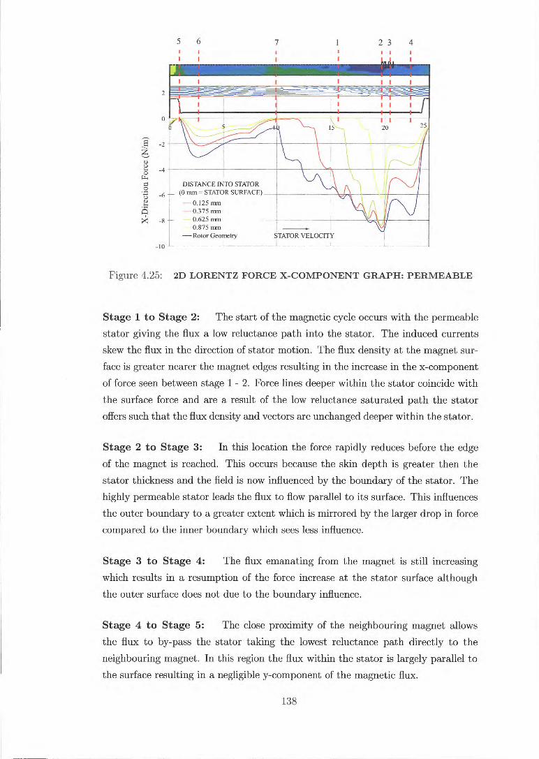
5 6 7 23 4

I I I I I 1 1 — _- -,-- - - _ _ _ _ _ _ _ __ _ . — _ - - ---------- ---- - - - - -," a i . _-_ - 4 .,- - ..1__ri- . . .- •- ... L-• : -____.- - A . . . -- --. , . . _ _--,....-ii...--_ _- .. „_„...---,--.-

lik, ....as lli

I 20 25,

11010--

111

DISTANCE INTO (0 mm = STATOR —0.125 rim —03775 mm — 0.625 mm

0.875 mm —Rotor Geometry

STATOR SURFACE) I kl

vr Tim

STATOR 'VELOCITY

Figure 4.25: 2D LORENTZ FORCE X-COMPONENT GRAPH: PERMEABLE

Stage 1 to Stage 2: The start of the magnetic cycle occurs with the permeable

stator giving the flux a low reluctance path into the stator. The induced currents

skew the flux in the direction of stator motion. The flux density at the magnet sur-

face is greater nearer the magnet edges resulting in the increase in the x-component

of force seen between stage 1 - 2. Force lines deeper within the stator coincide with

the surface force and are a result of the low reluctance saturated path the stator

offers such that the flux density and vectors are unchanged deeper within the stator.

Stage 2 to Stage 3: In this location the force rapidly reduces before the edge

of the magnet is reached. This occurs because the skin depth is greater then the

stator thickness and the field is now influenced by the boundary of the stator. The

highly permeable stator leads the flux to flow parallel to its surface. This influences

the outer boundary to a greater extent which is mirrored by the larger drop in force

compared to the inner boundary which sees less influence.

Stage 3 to Stage 4: The flux emanating from the magnet is still increasing

which results in a resumption of the force increase at the stator surface although

the outer surface does not due to the boundary influence.

Stage 4 to Stage 5: The close proximity of the neighbouring magnet allows

the flux to by-pass the stator taking the lowest reluctance path directly to the

neighbouring magnet. In this region the flux within the stator is largely parallel to

the surface resulting in a negligible y-component of the magnetic flux.

138

X-D

irect

ion

Forc

e (N

/m)

2

0

-2

-4

-6

-8

-10

Stage 5 to Stage 6: The proximity of the neighbouring magnet allows the flux to exit the stator directed towards the alternative pole magnet, which necessitates

a y-component of flux resulting in the increase in braking force.

Stage 6 to Stage 7: The flux lines become less dense and a reduction in the

y-component of flux reduces the braking force.

Stage 7 to Stage 1: The flux remaining in the stator are influenced by the

induced currents from the neighbouring cycle which skews the flux and increases the y-component of flux and braking force. The separate cycles are seen to merge.

By considering the difference between the y-component of force of the Maxwell stress tensor approach and the corresponding Lorentz force gives an estimation of

the polarisation force.

• Lorentz total y-component: - 4826 N/m

• Maxwell stress tensor total y-component: + 1274 N/m

• Polarisation total y-component: + 6100 N/m

It can be seen that the force due to the magnetic field (Lorentz force) is opposed

to the polarisation force of the steel resulting in an overall force that is lower then would occur for a non-permeable stator. For the Mk2 dyno, this would translate to a maximum force per stator < + 76 N. This is significantly lower then the non-permeable stator of the Mkl dyno which had an estimated force of - 500 N in the

18 kW test. At zero speed the force per stator is attractive and high but reduces

with increasing speed.

Permeable Stators - Global Results

The power values shown in the subsequent graphs have been calculated for a com-plete stator, the results from the single magnet solution domain have been multiplied by the number of magnets in the rotor to obtain the power per stator per unit depth

(kW/m). Particular emphasis has been placed on the higher resistivity values of 16 - 32 x10' Q.m, these are the typical values that may be experienced by a steel stator over the previously experienced working temperatures of 423 - 523 K.

The results of the permeable analysis show similar trends to that of the non-permeable analysis, the differences arise through the influence of the permeability which decreases the skin depth seen. This allows the previously given discussion on the non-permeable stator to apply directly to the permeable case; a brief summary

will only be given.

139

..... 0100 1611PM)- - 20 - 40

60

/.-- i 11E515TR/130 (am).

^.— 2000-08 —.1-4.00E-08 —4 0.000-00 —.-- 1.60E-07 ---111— 1200-07

3 2 4

Stater Thickness (1211)

I r.

,

0051571011'0(1.m) —•--- 2.000-08 _ —.--- 4 00E-08 —,1,— 8.000.-0/1 —.— 1.60E-07 —..— 3.200-07

▪ 4 2

Stator Thickness (am)

8000

6000

00 4000

2000

0

Stat

or P

ower

(k \W

m)

10000

7500

5000

2500

5 6

(a) 8-POLE, (60 kRPM, 0.5 nun gap) (b) 24-POLE, (60 kRPM, 0.5 mm gap)

Figure 4.26: 2D PERMEABLE: POWER VS STATOR THICKNESS FOR VARIOUS RESISTIVITIES

2 3 4

Stator Thickness (inn)

7

• Jr --•

—ROTOR (kRP —.-20 --.-40 --•-60

1 — —

2 3 4 6

Stator Thickness (nan)

8000

6000

4000

1, 2000

0

Stat

or P

OW

[1(k

W1m

)

8000

6000

4000

2000

(a) 8-Pole, (32x10-08 arn, 0.5 mm gap) (b) 24-Pole, (32x10-°8 arn, 0.5 mm gap

Figure 4.27: 2D PERMEABLE: POWER VS STATOR THICKNESS FOR VARIOUS SPEEDS

Figure 4.26 gives the stator power versus thickness for various resistivity values.

The choice of stator thickness depends heavily on the material resistivity and pole number. This would suggest the Mkt dyno stator of 1 mm thick was less than opti-mum. The Lorentz force plot of Figure 4.25 showed the skin depth was greater then the stator thickness and caused a premature drop in the x-component of force. An increase in thickness would be beneficial although a consequence would be a higher stator surface temperature which negatively impacts on the rotor temperature.

The skin depth estimations using Equation 4.20 become erroneous for perme-able materials such as steel. The difficulty arises in the estimation of the stator permeability, for steel this may change by two magnitudes dependent on the applied magnetic field and hence the saturation state of the steel. This results in an esti-mated skin depth that is much smaller then is found numerically but its usefulness

in depicting trends is still apparent. In the permeable analysis the largest skin depth obtained was 4 mm at 20 kRPM, with a resistivity of 32 x 10-08 Q.m for a 4-pole

rotor.

140

•

GAPS lt.AMI

—0— 0.5

4 —0.-6

000

500 ....---*--- •—________

----___ —

000 •

-..

GAPS 0.4M)

500 —..— 0.5 —

—.— 2 —0-4

n —.— 6

6000

4000 0

20(10

10

5

2

la IS 20 25 0 15 20

No. or roles No. of Pots

(a) 2x10-0$ Si. n (6 mm Lstator, 60 kRPM) (b) 32x10-08 /2.m, (6 mm L stator , 60 kRPM))

Figure 4.28: 2D PERMEABLE: POWER VS POLE NUMBER FOR VARIOUS GAPS

Sta

tor

Pow

cr

(1W

irn )

5000

6000 _—.

4000

2000 — —.— t —.0.— 1.5 STATOR

,--______.

—6— 2 THICKNESS

n —.-- 4 —00— 6 PAM)

0000

7500

5000 STATOR

THICKNESS MM)

25.11. -• --. —0-1.5 —6— 2 —H— 4

n

5 IS 20 25

30

35 10 IS 2$ 30 35

Resistivity (x1 0'0111n-m) Resistivity (xi 0-'Ohm-m)


Figure 4.29: 2D PERMEABLE: POWER VS RESISTIVITY FOR VARIOUS STATOR THICKNESS

Figure 4.27 demonstrates the differing skin depths for various speeds and resis-tivities. A low pole number suggests a large skin depth and the requirement for a large stator thickness, although in comparison to the non-permeable stator the skin depths are lower. The turbine steady and unsteady experiments are required to be performed between 30 - 60 kRPM, this suggests that to achieve sufficient low speed power absorption the pole number of the stator is required to be larger then 8-pole.

Figure 4.28 suggest a pole number of approximately 14 is suitable to achieve optimum power absorption for a high resistivity material. Figures 4.26, 4.27 and 4.29 suggest an optimum stator thickness of between 1.5 - 2 mm although due to high stator surface temperatures, the chosen value was reduced to 1 mm.

141

4.5.6 2D Analysis Summary

A 2D investigation has been conducted focusing on both the local and global effects of eddy current generation in both a permeable and non-permeable stator material. It has been shown that for the range of single homogeneous materials analysed under high speed operation, the permeable stator offers greater power absorption capabil-

ities compared to the non-permeable stator. The optimum balance of parameters for the dynamometer appears to be a 14-pole rotor and a 1 mm thick steel stator.

The main variables associated in the magnetic design of the circuit are the stator thickness, resistivity, pole number, magnet speed and permeability. Improved mag-

netic design requires the increase of the y-component of magnetic flux throughout

an increased volume coverage of the stator.

4.6 3D Finite Element Analysis

The 3D model allows the geometry of the Mkl and Mk2 dynos to be modelled accurately and allows a direct comparison with the experimentally obtained data. These models allow insights into the performance effects of the 3D geometry of the dynamometers and gives an improved estimation of the axial forces imposed on

them. The analysis conducted simulates the experimental results of the Mkl and Mk2

dyno with copper and aluminium alloy stators for varying speeds and gaps.

4.6.1 Solution Domain

The solution domains for the Mkl and Mk2 dyno are given by Figure 4.30. The

Mkl dyno requires two magnet sectors to be modelled in order to analyse the 4-pole rotor as sequentially the magnet poles are N-N-S-S-N-N-S-S. A flux return keeper disk is additionally modelled on the rear face of the rotor, shown by Figure 4.30(a). The Mk2 dyno employs an 8-pole rotor which allows a single magnet sector to be modelled. This dynamometer model requires both stators to be included as one has

a fixed gap whilst the other is variable, shown by Figure 4.30(b).

• No. of elements 20,000

• No. of nodes per element 8

• DOF Ax, Ay, Az, Volt

• Active DOFs 65,000

142

ROTOR-TO-STATOR GAP

■ MR

DOMAIN MESH

SOLUTION DOMAIN EXCLUDING AIR ELEMENTS

STATOR PLATE

. KEEPER DISK

111 ROTOR SPIDER

(a) Mkl Dynamometer DOMAIN MESH SOLUTION DOMAIN

EXCLUDING AIR ELEMENTS

MAGNET SHAPE

k.(

■ FIXED GAP STATOR

■ VARIABLE GAP STATOR

▪ ROTOR SPIDER

■ AIR

ROTOR-TO-STATOR GAPS

(b) Mk2 Dynamometer

Figure 4.30: 3D MODEL: MK1 AND MK2 SOLUTION DOMAIN

4.6.2 Boundary Conditions

The solution domain is bounded by flux parallel conditions to all surfaces except those that are cyclic symmetric in nature. The flux parallel condition is appropriate following the arguments of the 2D model and are illustrated for the Mk2 dyno by Figure 4.31.

The flux parallel condition was applied by constraining all the in-plane compo-nents of the vector potential [A] to zero, an asymmetric condition. For a Cartesian coordinate system this is applied to a surface whose normal component is in the x-direction by constraining the Ay and A, components to zero, which implies the Bx component is also zero. The final boundary condition required is the Cyclic Sym-metric or Asymmetric condition. The Mkl dyno uses a cyclic symmetric condition to model the 8-pole rotor and a cyclic asymmetric condition to model the 4-pole

143

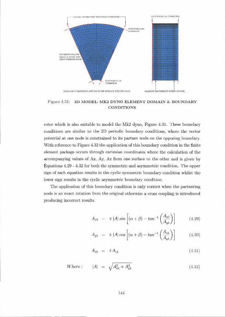
CYCLIC ASYMMETRIC BOUNDARY CONDITION

• FLUX PARALLEL CONDITION

ELEMENTS FOLLOW MAGNET SHAPE AND EDDY CURRENT FLOW

FLUX PARALLEL CONDITION

FLUX PARALLEL CONDITION

1

. L 1 111111111111111111:

1111u111111101111 ' 1111111111111111111 [ 1111111 1111M11111, 1111111g, „, ' L. 'HI 1101111 Ill

111111111M IN 11111110111111 1111111 NN® 1111111111 NC 111111110111111MIL

j 111111- 11111111111.

inierilej: 41111MomMINI=IMEN

. 111111111111111-901, -moquismial, IIIIIIMEIN ._, ..

BOUNDARY CONDITIONS APPLIED TO THE SURFACE INTO THE PAGE

ELEMENT REFINEMENT WITHIN STATOR

Figure 4.31: 3D MODEL: MK2 DYNO ELEMENT DOMAIN & BOUNDARY CONDITIONS

rotor which is also suitable to model the Mk2 dyno, Figure 4.31. These boundary

conditions are similar to the 2D periodic boundary conditions, where the vector

potential at one node is constrained to its partner node on the opposing boundary.

With reference to Figure 4.32 the application of this boundary condition in the finite

element package occurs through cartesian coordinates where the calculation of the

accompanying values of Ax, Ay, Az from one surface to the other and is given by

Equations 4.29 - 4.32 for both the symmetric and asymmetric condition. The upper

sign of each equation results in the cyclic symmetric boundary condition whilst the

lower sign results in the cyclic asymmetric boundary condition.

The application of this boundary condition is only correct when the partnering

node is an exact rotation from the original otherwise a cross coupling is introduced

producing incorrect results.

(4.29)

(4.30)

Where : AlJ = I + A2 Y1 (4.32)

144

Axe

=

lAl sin

f lAl cos

[(a + fi) tan-1 (tii)]

Aye tan-1 [(a +0) (1,44:)]

Az2 = ±Az1 (4.31)

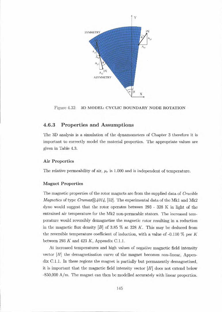
rAl

Figure 4.32: 3D MODEL: CYCLIC BOUNDARY NODE ROTATION

4.6.3 Properties and Assumptions

The 3D analysis is a simulation of the dynamometers of Chapter 3 therefore it is

important to correctly model the material properties. The appropriate values are

given in Table 4.3.

Air Properties

The relative permeability of air, it,. is 1.000 and is independent of temperature.

Magnet Properties

The magnetic properties of the rotor magnets are from the supplied data of Crucible Magnetics of type Crum,axC).4014, [52]. The experimental data of the Mkl and Mk2

dyno would suggest that the rotor operates between 293 - 328 K in light of the

entrained air temperature for the Mk2 non-permeable stators. The increased tem-

perature would reversibly demagnetise the magnetic rotor resulting in a reduction

in the magnetic flux density [B] of 3.85 % at 328 K. This may be deduced from the reversible temperature coefficient of induction, with a value of -0.110 % per K between 293 K and 423 K, Appendix C.1.1.

At increased temperatures and high values of negative magnetic field intensity

vector [H] the demagnetisation curve of the magnet becomes non-linear, Appen-

dix C.1.1. In these regions the magnet is partially but permanently demagnetised,

it is important that the magnetic field intensity vector [H] does not extend below

-850,000 A/m. The magnet can then be modelled accurately with linear properties.

145

The true magnet temperature is unknown, for generality, the 293 K curve data is

used where the coercive force is 979,000 A/m and a relative permeability, it, of 1.049.

No significant eddy current generation occurs within the magnetic rotor itself as the eddy currents are synchronous to the rotor and the resistivity of the magnets is

large with a value of 150 x 10' am. The magnet keeper disk shown in Figure 4.30(a) is modelled with a linear relative

permeability, it, of 500.

Stator Properties

The relative permeability, it, of the copper and aluminium alloy stators is 1.000, with no appreciable temperature effect. The principal source of error in the material

properties arises with the specification of the resistivity value. It is known from previous analysis that the resistivity plays a key role in the magnitude of eddy

current generation and therefore the power absorbed by the stator. Within the stator the resistivity value varies throughout the material volume,

with its highest value seen in the hottest regions, it is these regions in which the eddy currents are generated. It was seen by the 2D analysis that the majority of power generation occurs in the first millimetre of the stator, from the 1D Fourier law of conduction calculation, Appendix B.2 suggests a temperature difference of less then 15 K within this region. It is reasonable to specify a single value of resistivity based on the expected eddy current region temperatures. This will allow some generality

to results which will identify mechanisms which are not correctly modelled. The resistivity values employed for the Mkl dyno are 2.0 x am and for

the Mkt dyno are 2.5 x 10-°8 Cl.m for the copper stator and 5 x 10' S-2.m for the

aluminium stator.

Table 4.3: 3D MODEL: MATERIAL PROPERTIES


Magnet Keeper

Disk

Stator Copper Alum.

Relative Permeability, (ur) - 1 1.049 500 1 1

Coercive Force, (He ) A/m - 979,000 -- -

Mkl: Resistivity, ( x 10'8) am - - - 2.0 -

Mk2: Resistivity, ( x 10'8) Qin - - - 2.5 5.0

146

4.6.4 Variables

The following variables are used to simulate the Mk2 dyno experiments.

• ROTOR-TO-STATOR GAP (Gap):

— Mkl: 4-pole:

- Mkl: 8-pole:

— Mk2: Fixed gap stators:

— Mk2: Variable gap copper stator:

— Mk2: Variable gap aluminium stator:

1.47, 2.0, 2.5, 2.97, 3.49 mm

0.75, 0.96, 1.37, 1.94, 2.75 mm

0.5 mm

0.5, 1.41 and 2.5 mm

0.5, 2.0 and 5.0 mm

• VELOCITY OF STATOR : 20, 40 and 60 kRPM

3D analysis allows direct specification of rotational speed in RPS.

4.6.5 Results and Discussion

To gain greater insights into the eddy current mechanism a discussion of the local results is given for a specific case before the global comparisons are made with

respect to the experimental results.

Local Results

The results given are for the Mk2 dyno model with a copper stator, 2 mm thick,

60,000 RPM and a rotor-to-stator gap of 0.5 mm. The 3D model allows the assess-ment of the end-effects caused by the magnet geometry.

Figure 4.33(a) is a vector plot of the current density for the stators surface el-ements. The stator is rotating in a clockwise direction with the magnetic rotor positioned behind the plot, an outline of the position of the rotor magnet is shown. The current density follows the trends of the 2D analysis. Within the 3D environ-ment the planar current flow circulates a path depicted by the influence and shape of the magnets. Due to its close proximity, the stator surface current flow is largely constant in direction over the projected area of the magnet. This direction depends

on whether the opposing magnet is a north or south pole. The 2D analysis demonstrates the direction of the current flow is the cross prod-

uct of the stator velocity and the magnetic flux density, Equation 4.25. This pro-duces a motional EMF which can drive the eddy currents around the stator circuit.

The three components of magnetic force imposed on the stator surface is illus-

trated by Figure 4.33 and the overall values given by Table 4.4. The braking torque on the rotor is a result of only the circumferential component

of force, the radial and axial components of force are by-products and must simply be absorbed mechanically by the dynamometer.

147

-- -- -

\ \\\‘

..j71rrn‘)IYilzt fly

IIII1

I

L. CURRENT 0055110

(Nrtel .395E+07

— .147E+09 = .2908+09 -- .4348+09

. 577E+09 - .7208+09 EFEE7 .8638+09

.]..ne.3.0

. 1158+10

.129E+10

L. RADIALFORCE

(8161

- -. 602E+08 - 455E+08

310E+08 — 164E+08 - -.1796+07

.1208+00

.2742+08

.420E+06

.566E+06 MO .713E+06

(a) Current Density (b) Radial Force

L. Rxim -FORCE

(tOn'l -.1068+09

— .3738+08 .181E+09 .325E+09

- .969E+09 . 613E+09

R". .7568+09 .9008+09 .2.o4E+3.o .1198+10

(c) Circumferential Force (d) Axial Force

- -

- - -------------

Figure 4.33: 3D STATOR SURFACE FORCE PLOT: COPPER STATOR, 60 kRPM

Table 4.4: 3D STATOR FORCE COMPONENTS

Force Component Per Sector

(N)

Per Stator (N)

Radial Circumferential Axial

0.266 - 12.17 57.27

0 -97.4 458

The radial component of force results largely from the current flow that is parallel to the stator velocity direction, Figure 4.33(b) and is a result of the (Jz Bx — Jx ./3,)

term. These forces are small compared to the circumferential and axial components and do not impose a net force on the stator as opposing sectors cancel each other out. Table 4.4 suggests a radial force per sector of 0.266 N but no net force. The axial component of force is the largest and potentially the most damaging component, Figure 4.33(d) and is a result of the (JsB y — J yBx ) term. Similar to the 2D analysis an isolated area of attractive force is seen in the area above the magnet.

148

This attractive force is limited to the surface of the stator whilst deeper within this force becomes repulsive. The net axial force is the summation of each magnet sector and from Table 4.4 suggests a repulsive force on a single sector of 57.27 N and a net stator repulsive force of 458 N. This is consistent with the 2D analysis

of Section 4.5.5. The circumferential component of force is localised and is largely located along the radial edge of the magnet, Figure 4.33(c). It is a result of the

(J yB, — J,B y ) term and its position is similar to that of the 2D analysis although now a modest propulsive force is evident along the top and bottom surfaces of the stator. This is detrimental to the performance of the dynamometer and reduces the net braking force by approximately 6 %.

Figure 4.34 - 4.36 show the current density and the Joule heating at different depth within the stator. As with the 2D analysis there is a migration of the main area of activity with increasing depth due to the skewing of the field lines as a result of the induced currents. The plots illustrate the strong influence of the rotor magnets on the surface of the stator producing the localised high peak current density and Joule heating and how this influence diminishes with depth.

Experimental Comparison

The results presented are a comparison against the experimental results obtained in the Mk1 and Mkt dyno for the non-permeable copper and aluminium alloy stators.

Figures 4.37(a) - 4.37(b) show the comparison of the Mkl dyno for the 4-pole and 8-pole rotor. These results indicate that all important parameters are being adequately modelled by the analysis and suggests the simplistic specification of constant resistivity and magnet properties are acceptable.

For the 8-pole comparison, the slope of the data is correctly predicted for the full range of rotor-to-stator gaps tested with an absolute maximum discrepancy in power of 7 %. The 4-pole rotor shows a greater variance in result but still predicts resonably the slope and absolute power values. For these low power conditions it is difficult to determine the cause of these discrepancy as the experimental uncertainty

in the power measurement is large. The two important property variables are the stator resistivity and the magnet

[B] — [H] variation. From a single value of these, it would be expected the slope of the power curve would show some discrepancy. An increase in speed would increase the power absorption of the dynamometer, resulting in a raised stator temperature and consequently its resistivity which would suggest the model would under predict the slope of the curve. The higher temperatures would raise the magnet temperatures

thereby reducing its flux output suggesting an over prediction of the slope. These two opposing effects may partially compensate for each other giving slope seen.

149

.. . ,

\ \ '

• -t-- ;;;;;;;::;;',1 ,i'lVi`‘)1)/1"

. • ........

_______________ •

CURRENT DENSITY JAJJW)

. 395E i-07 11110 . 147E409

.290E+09 - .434E+09

- .577E+09

. 720E-J09 Egn . 8 6.3E+ 0 9

.101E+10

.1155+10

.1295+10

Y x

JOULE HEAT OW)

277513 - .445E+10

- .890E+10

.134E+11 - 178E+11 LE2 .223E+11

.267E+11 I=1 .312E+11

- EMI .356E+11

. 401E+11

JOULE HEAT (1M3)

709834 - .777E+09 flEM. 155E+10 - .233E+10

- .311E+10

.388E+10

.466E+10

.544E+10

- 621E+10

. 6990.10

(a) Current Density (b) Joule Heat

JOULE HEAT (Hue)

277513 .2248+09

111.▪ .948E+09 - .6710+09

- .8950+09

• .1120+10 O .1340+10 • .1570+10

- .▪ 179E+ 10

.201E+10


Figure 4.34: 3D STATOR SURFACE PLOT: COPPER STATOR, 60 kRPM


Figure 4.35: 3D 1 MM STATOR. DEPTH PLOT: COPPER STATOR, 60 kRPM

Figure 4.36: 3D 2 MM STATOR DEPTH PLOT: COPPER STATOR, 60 kRPM

150

60 70 10 20 30 40 50

50 VARIOUS GAPS (mm)

— NUMERICAL EXREIUMENTAL

2.01-4

4.99'

40

30

a 20

10

0

VARIOUS L474

GAPS (mm)

200 2.594

ffIl 2.97'. '440111 249'

........... ,-- 11.--

— NUMERICAL — EXEERIMENTAL

0.75 „,.....- m— 0 .96

L3

00. 0...r...1 .1 ..1- app.p.,--- 1.94

111101111111P --

2.7

VARIO S GAPS (mm)

NUMERICAL — ERIMENTAL

12

9

6

3

_4

18

12

10 20 30 40 50

60 70 10 20 30 40 50

60

70

Turbine Speed (IcliPM)

(a) Mkl 4-Pole Model

VARIOUS

/0. A504 ,

GAPS (mm)

_...0,00...0 1w SO IA1 2.

1000WIPm- 1001.1311."— 2.50

— NUMERICAL EXPERIMENTAL

20 30 40

60

70

Turbine Speed (6RPM)

(c) Mk2 Copper Stator Model

Turbine Speed (6RPM)

(b) Mkl 8-Pole Model

Turbine Speed (kRP11,1)

(d) Mk2 Aluminium Stator Model

40

30

0 20 P

10

0 I

Figure 4.37: 3D MODEL: EXPERIMENTAL COMPARISON

The results of the Mk2 dyno show greater variability, Figures 4.37(c) - 4.37(d). The copper stator results over predict the experimental data with an off-set of ap-proximately 4 kW, whilst the aluminium stator results would appear to be accurate magnitudes although an over prediction of the slope is apparent. The copper stator results suggest that the resistivity and/or the magnet strength may be specified too large. With consideration of the aluminium alloy stator results, the copper results are consistent with a to high specification of resistivity. The copper grade used for the Mk2 stator was unspecific and its resistivity value may be lower then applied. The over prediction of the slope for the aluminium alloy stator may be due to the increased heating of the Mk2 dyno compared to the Mkl dyno as both sides of the of the magnetic rotor are now adjacent to a hot stator surface. This increased tem-perature would cause a reversible demagnetisation of the rotor magnets, reducing its flux output especially at the high power conditions. A 2 -3 % reduction in the Coercive force, HCU of the magnet would account for the difference seen between the numerically predicted and the experimental performance of the aluminium stator.

The general agreement between the numerical and experimental results would suggest the 2D analysis would also correctly predict the trends of the various para-meters. This allows the 2D analysis to be used parametrically in order to optimise the magnetic design.

151

4.6.6 3D Model Summary

The Mkl and Mkt dynamometers have been magnetically modelled in 3D and com-

pared to the experimentally obtained result. The results show that all important parameters have been adequately modelled by the analysis and suggests the use of the 2D analysis would correctly predict the trends associated with the various pa-rameters allowing its use for the parametric study. The use of a constant resistivity and magnet properties has been found to give adequate results, although the accu-

rate assessment of these properties are required in order to obtain accurate absolute power values.

4.7 2D Dynamometer Approximation

The use of the 3D analysis gives a realistic representation of the dynamometers performance although this restricts the models to linear analysis , such that the permeable non-linear steel stator of the Mk3 dyno may not be modelled in ANSYS 5.7 [2]. A simple technique may be used to transform the results of the generic 2D model to give an estimate of the Mk3 dyno performance.

The performance estimate may be achieved by the comparison of the results

of the 3D model with a comparable 2D model. A suitable shape factor may be found which broadly encompasses the effects of curvature, magnet shape and end effects. This may be used to transform the results of the 2D analysis into realistic performance estimates of the dynamometer.

4.7.1 2D and 3D Model Compatibility

All material properties between the 2D and 3D model are kept consistent. It is necessary to correctly specify a comparable linear speed (U2d ) for the 2D model. This is obtained from the 3D model by equating the summation of the Joule heat (W) to the overall circumferential force (F& ) and average velocity (U0 ,,,,9 ), Equation 4.33.

W3d E(Qi • oi = E(F0) ' UOg (4.33)

Where: U2d = U8,avg•

The absorbed power is assessed using the previous techniques given in Sec-tion 4.4.3. The 2D results are calculated for a unit depth, therefore an appropriate magnet swept width is specified, its definition and values are illustrated by Figure 4.38 for the Mk3 dyno rotor. The 2D power excluding the shape factor cor-rection is calculated from the multiplication of the power per unit depth and the magnet swept width, Equation 4.34.

152

DIMENSIONS IN MM

Figure 4.38: MK3 ROTOR MAGNET SWEPT WIDTH

W2d = (W I 712 )2d • Lmsw (4.34)

The 2D and 3D calculated stator powers can thus be used to obtain the shape

factor, x, Equation 4.35.

Wad X = T i

vr 2d (4.35)

4.7.2 Mk3 Dynamometer Model

2D Model: The Mk3 dyno 2D model was set up similarly to the Mk2 model described in Section 4.5. The Mk3 dyno utilises twin stators on each side of the rotor

which is included in this model, Figure 4.39. The comparable 2D model simulates a non-permeable stator and the 14-pole double row rotor of the Mk3 dyno.

3D Model: The Mk3 3D dyno model was set up similarly to the Mk2 model

described in Section 4.6. The analysis simulates a non-permeable stator and a 14-pole double row rotor of the Mk3 dyno for single speed and gap setting.

The cyclic symmetric nature of the dynamometer geometry similarly allows a single magnet sector to be modelled illustrated by Figure 4.40. A further reduction in model size may be obtained as the Mk3 dyno employs equal rotor-to-stator gaps on each side of the rotor, which allows only one side of the dynamometer to be modelled. A symmetry condition is applied on the cutting surface shown in Figure 4.40.

153

FLUX NORMAL \ili

'( / IfMAGNET

Ih\

\ \ \\ NI

RONTI .TGAAPApt-LORIII: N- \.

AIR

BACK STATOR

AIR GAP

FLUX PARALLEL

Figure 4.39: MK3 2D MODEL: SOLUTION DOMAIN

DOMAIN MESH

SOLUTION DOMAIN

O U

0

O OD

D PE

RIO

DIC

BOU

ND

ARY

MAGNETS

STATOR PLATES

■ ROTOR SPIDER

■ AIR

ROTOR-TO- STATOR GAP

SYMMETRIC BOUNDARY X 2

(FLUX NORMAL CONDITION) APPLIED TO SURFACE

Figure 4.40: MK3 3D MODEL: SOLUTION DOMAIN & MESH

• No. of elements 22,000 • No. of nodes per element 8 • DOF

Ax, Ay, Az, Volt

Base Model Properties and Parameters

The material properties for the Mk3 3D comparison model are given in Table 4.53. A single speed value and gap setting was found to be sufficient to ascertain the shape factor, x and this was chosen to be the highest power setting of the dynamometer.

'Non-linear models can not be modelled in ANSYS 5.7. The shape factor is assessed for the Mk3 dyno from a non-permeable material with a similar resistivity value to steel.

154

Table 4.5: MK3 3D COMPARISON MODEL: MATERIAL PROPERTIES


Magnet

Stator Steel

Rel. Permeability, (Pr) - Coercive Force, (He ) A/rn

Resistivity, ( x 10') Q.m

1 - -

1.049 979,000

-

1

- 30.0

• STATOR 1 mm, steel

• VELOCITY OF STATOR 60 kRPM

• ROTOR-TO-STATOR GAP (Gap)

0.5 mm

4.7.3 Results

The results from the analysis are given by Table 4.6 with the corresponding shape factor. The results are for the complete double twin stator assembly of the dyna-mometer, where the results have been multiplied by the number of sectors to form a complete stator and by the number of stators. It was noted in the analysis that

the shape factor decreased with increasing stator resistivity.

Table 4.6: SHAPE FACTOR DETERMINATION MODEL

Parameter Steel

2D 3D

Stator power, (W) kW 128.7 40.38

Braking force, (Fr , F9 ) N -700.5 -219.8

Velocity, MO mis 183.7

Shape factor, (X.) 0.3138

A 2D simulation of the Mk3 dyno was performed employing the shape factor

to include the 3D effects, the results are given by Figure 4.41 in comparison to the experimental data of Section 3.4.5. The results demonstrate a good representation

of the power versus speed and gap trends, although absolute power values are over predicted. At maximum power the 2D model predicted the Mk3 dyno would absorb a value of 73.5 kW whilst 62.2 kW was achieved experimentally, a 18 % over prediction.

There are various reasons which may contribute to this over prediction. The magnet strength throughout the numerical studies have employed for generality a consistent value, it is likely from the experimental findings of the Mk3 dyno that the magnet temperature at maximum power would be within the range 323-353 K.

155

At 353 K the coercive force of the magnets is reduced by 5 % to 928,000 A/m

resulting in a 7.2 kW reduction in maximum power which would result in an over

prediction of only 6.5 %. It is thought that the true stator resistivity and the

permeability effects of the stator that are not taken into account with the 3D non-

permeable shape factor contribute to the additional discrepencies.

- 2D NUMERICAL - EXPERIMENTAL

VARIOUS S

0.60 .a

_Ad 1.50

.411.01,1.H11101111:111 2.50_0

1 . I. I. l• j

--1.1001000-01••••ever01010000V 4.00

_ 12.

0

10 20 30 40 50 60 70


Figure 4.41: MK3 DYNO: 2D NUMERICAL COMPARISON TO EXPERIMENTAL - STEEL

4.8 Summary

The results of the numerical models suggest that all governing parameters are being

modelled adequately which gives confidence in both the usefulness of the 2D and

3D models. A 2D local and parametric study has allowed the understanding and

optimisation of the relevant magnetic variables. For the range of single homogeneous

materials analysed under high speed operation, the permeable stator offers greater

power absorption capability with the optimum balance of parameters resulting in a

14-pole rotor and a 1 mm thick steel stator.

The 3D analysis has allowed the Mkt and Mkt dynamometers to be geometri-

cally modelled. The results have shown good comparison with experimental results

generally within 10 %.

A shape factor has been estimated which allows the transformation of the 2D

results into realistic dynamometer performance of the Mk3 dyno.

80

60

40 0

20

0

156

Chapter 5

Test Facility

5.1 Synopsis

This chapter describes the use of dimensional analysis and similitude in defining the performance of the turbine. The test facility is described with particular emphasis placed on the turbine performance instrumentation and its calibration. The tech-niques used to obtain the uncertainty in the performance results are also outlined.

5.2 Dimensional Analysis

Dimensional analysis can used to represent the performance characteristics of a tur-bine in an efficient manner. This method groups the relevant independent variables

into a smaller number of non-dimensional groups that describe a physical problem.

5.2.1 Dimensionless Parameters

The dependent parameters of relevance to radial and mixed-flow turbine perfor-mance and their corresponding independent parameters are given by Equation 5.1,

Watson and Janota, 1982 [83].

= f P01 T01 N, d2, R, -11 11 )

(5.1)

Where rim is the mass flow rate, is the total-to-static efficiency, P01 is the

total inlet pressure, P4 is the static exit pressure, T01 is the total inlet temperature,

N is the turbine rotational speed, d2 is the turbine mean inlet diameter, R is the

gas constant, -y is the specific heat ratio and u is the dynamic viscosity of the gas.

The principle of Buckingham PI theorem, Glassman, 1972 [35], Watson and

Janota, 1982 [83] can be employed to transform Equation 5.1 into a reduced set of dimensionless parameters constructed from the independent variables, Equation 5.2.

157

Th .VRT01 Nd2 P01 rh D

Old2 2 Th-s = f

A RT0 1' P4 11C12)

It is desirable to reduce the number of non-dimensional parameters still further

by excluding the terms of lesser importance. The Reynolds number term', 7h/µd2

is difficult to scale and generally is of secondary importance to that of the other dimensionless groups, Glassman, 1972 [35], Hiett and Johnson, 1964 [39], Scrimshaw, 1981 [73]. With the present test facility it was not possible to control the Reynolds number term whilst maintaining control of the primary non-dimensional groups and as such this group has not been compared in the present analysis. The 7 group for the typical range of test conditions is predominantly constant and again may be omitted from the comparison. In respect to the similitude between the hot on engine

conditions and the cold-flow test rig conditions, it is described by Dale, 1990 [25] that the effect of -y is usually included in the Reynolds number term which suggests

it is of secondary importance. Equation 5.2 can be further simplified when considering a specific turbine wheel

and a known gas. The independent variables d2 , R for this situation are constant

and can be omitted. Now not all the groups are dimensionless, giving Equation 5.3.

riz,VITll N Poi > 71t-s = f ( , —D Poi v / 01 1 4

An additional group, the velocity ratio is useful in aiding the compressor-turbine matching process and can be seen to be a substitution for the pressure ratio by

Equation 5.4, Watson and Janota, 1982 [83]. Where U2 is the turbine inlet mean

tip speed and Cis is the isentropic expansion velocity; which is the velocity attained

with an isentropic expansion over the total-to-static pressure ratio of the turbine.

N d2 Poi U21Cis = f(( ), -Y) 0131 fr? P4 (5.4)

The resultant non-dimensional/pseudo-dimensionless groups and their transfor-mation values are given below. The transformation values are used to convert the

pseudo-dimensionless groups back into their dimensionless form.

'Various definitions are in use for the Reynolds number term, such as Hiett and Johnson,

1964 [39], uz#: Where U is the rotor tip speed, h is the tip width and v is the kinematic viscosity.

(5.2)

(5.3)

158

Mass flow parameter (MFP): ri-t0/TH/Poi Speed parameter (SP): N/0—'01

Pressure ratio (PR): Poi/P4 Total-static efficiency: 77t-s Velocity ratio (VR)

MFP dimensionless transformation, V.T?/4 2425

SP dimensionless transformation, d2/0i 4.933 x 10-03

The useful non-dimensional/pseudo-dimensionless groups which characterise the turbine are usually plotted on two graphs. Typically the first graph plots rh.

versus P01/P.4 with lines of constant NI OTH , relating the mass flow rate, pressure

ratio and turbine rotational speed. The second performance graph plots rit_s ver-

sus U2/C29 with lines of constant NR /771, relating efficiency, turbine loading and

rotational speed.

5.2.2 Equivalent Design Conditions

A cold flow gas stand facility was used for the present study and this required scal-ing of the hot flow on engine turbine conditions to that of the cold flow conditions obtainable on the gas stand. The non-dimensional nature of the performance pa-

rameters allows the use of Similitude to scale the conditions, Glassman, 1972 [35].

In order to scale to the equivalent design conditions it is common to keep the pres-

sure ratio constant, hence P01 is the same for both the actual and equivalent design

conditions, Equation 5.5 - 5.6. The hot flow design point for the turbine, supplied by Holset Engineering Co.

Ltd. can be found in Table 5.1 with the corresponding scaled cold flow design point.

rhA/1'01

\s. P01 rig

rh,V2Ti ) P01 ) act

nirig = matt TOLact

Tol,rig (5.5)

(

N NiTTn.) rig (0/TO act

N Nrig = Nact

TO1,rig

T01,act (5.6)

5.3 Test Facility

The test facility has the capabilities for the single-stage testing of radial or mixed-flow turbines under either single or twin-entry flow conditions. Further to this the control valves allow either full or partial flow admission to the turbine and a pulse generator allows either steady or pulsating flow to drive the turbine.

159

Electric heaters 9 kW

2x 36 kW

Inner limb

Limb Pulse generatorf. orifice plates

Instrumented section

Oil in (Ps)inst r T

rr :16

(POinst 77' Ps =Rtrn Turbine.exit

ynamometer rt

Oil out

Turbine

Turbocharger

Table 5.1: EQUIVALENT DESIGN CONDITIONS

Parameter Design Equivalent

Inlet temperature K 923 344

Mass flow rate kgls 0.414 0.678

Rotational speed Rpm 98,000 59,800

Pressure ratio 2.91 2.91

Velocity ratio 0.616 0.616

Reynolds number - 1.22 x 105 3.90 x 105

The facility set up for the present study uses a single-stage, mixed-flow turbine

running single entry conditions under both steady and pulsating flow.

5.3.1 Test Facility Layout

The layout and main components of the test facility are illustrated in Figure 5.1. These components consist of a compressed air supply, electrical heater stack, pulse generator, instrumented volume, mixed-flow turbine and an eddy current dynamo-meter. These components are monitored and controlled through a semi-automated

control system as described in the following sections.

Figure 5.1: GENERAL TEST FACILITY LAYOUT, MODIFIED [36]

160

5.3.2 Air Supply and Heater System

Pressurised air is supplied to the test facility from three Ingersoll Rand screw com-

pressors. A combined mass flow rate of 1.2 kg/s can be supplied at room temperature at a pressure of 5 bar absolute. The air enters the test facility and is filtered through

a three-stage cyclonic filter and a subsequent 60 pm paper filter; see Dale, 1990 [25]. Immediately downstream of the filters is the main flow valve, which is remotely controlled and used to regulate the air flow entering the test facility. An additional controlled valve is situated adjacent to the main valve and is used for safety with a

toggled open-close action. Downstream of the control valves is an 81 kW heater stack; this consists of one

9 kW and two 36 kW electrical heaters arranged in series. These heaters are used to heat the incoming air to the desired turbine test conditions, 333 - 343 K. This

temperature is sufficient to avoid water vapour forming in the expansion process within the turbine. The master 36 kW heater is linked to a PID control system of

type West 4200 and is used to regulate the turbine inlet temperature in response

to an output signal from a chosen thermocouple. The secondary 36 kW and 9 kW heaters are manually switched on when required. The heaters and subsequent pipework are lagged and additionally covered with aluminium foil to reduce heat

loss. Directly downstream of the heaters the flow is branched into two separate 081.40

mm pipes, known as the inner and outer limbs. Each limb has a remotely controlled

valve to allow partial admission research to be conducted and a 059.85 mm orifice plate, located prior to the pulse generator in accordance with BS 5167-1:1997 [13].

5.3.3 Pulse Generator

The pulse generator consists of two counter rotating chopper plates, one for each

limb. These plates have specifically shaped cut outs to enable the desired pulse

shape and period to be obtained which replicates a realistic engine pulse form. The pulse is generated through a linear area opening and closing of the flow area, which occurs over a 120 degree period. Figure 5.2 illustrates the pulse generator and the various chopper plate positions whilst Appendix D.1.1 illustrates the flow area versus

phase angle for a complete revolution. A DC motor is used to belt drive the plates to achieve a pulse frequency of 0

- 80 Hz. For the present study the plates were driven in phase simulating a single entry flow system with a pulse frequency of 20, 40, 60 and 80 Hz. This corresponds to a twin turbocharged, four stroke, six cylinder engine running at 800, 1600, 2400

and 3200 RPM respectively.

161

(a) Chopper plate - 30° partially open (b) Chopper plate - 60° fully open

(c) Chopper plate - 90° partially closed (d) Chopper plates

Figure 5.2: PULSE GENERATOR - ROTATION: a, b, c [42]

Using a digital magnetic pick-up, the pulse generator was used to create an

electrical pulse once per revolution, from which the data acquisition system could

be triggered.

5.3.4 Instrumented Volume

The steady and pulsating inlet flow conditions were measured within the instru-

mented volume; this is situated 0.755 m downstream of the pulse generator and

0.337 m upstream of the volute inlet, Figure 5.3. A separate discussion of the in-

strumentation is given in Section 5.4.

Upstream of the instrumented volume is a solenoid-actuated guillotine valve

which is used to provide a rapid shut-down of the air flow in case of an emergency.

This can be triggered either manually from an emergency stop button or automati-

cally through the software safety systems as described in Section 5.3.8.

162

INSTANTANEOUS

STEADY FLOW: INSTANTANEOUS

PRESSURE TRANSDUCER

PRESSURE, TEMPERATURE

PRESSURE TRANSDUCER

CTA INSTANTANEOUS CTA INSTANTANEOUS

CTA TRAVERSE

DIFFUSER MASS-FLUX TEMPERATURE

Figure 5.3: INSTRUMENTED VOLUME

5.3.5 Turbine Stage

The turbine rotor employed in this investigation known as turbine 'D' was a medium sized mixed-flow turbine suited for heavy goods vehicles. A fourth generation turbine designed by Karamanis, 2000 [42] as a development of Abidat's turbines, 1991 [1].This prototype turbine was machined from aluminium alloy and hard an-odised to improve its durability. A solid model is given in Figure 5.4 and the dimen-sions by Table 5.2. The turbine rotor is housed in a single entry nozzle-less volute where the flow exits the turbine directly to atmosphere through a short diffuser shown in Figure 5.3. The A/R ratio of this volute is 34.7 mm (1.37 inch).

5.3.6 Dynamometer

In order to load the turbine a purpose built permanent magnet eddy current dyna-mometer is employed, as described in detail in Chapter 3. The dynamometer is used to control the operating point of the turbine by the variation of power absorption, such that for a fixed speed a large variation in velocity ratio can be achieved.

Typically, a turbocharger compressor is used as the loading device but due to the compressors surge and choke limits, the performance maps that can be obtained in this manner are narrow. In an engine simulation where the turbine is modelled in a quasi-steady manner, the pulsating flow conditions within the engine manifold result in wide ranging conditions at the turbine inlet, hence the requirement for a wide performance map.

163

Figure 5.4: MODEL OF MIXED-FLOW TURBINE 'D'

Table 5.2: GEOMETRIC DETAIL OF TURBINE 'D'

Turbine 'D' Geometric Feature Value Number of Blades — 12 Leading Edge Mean Diameter mm 83.58 Leading Edge Span Height mm 18.00 Trailing Edge Tip Diameter mm 78.65 Trailing Edge Hub Diameter mm 31.10 Cone Angle (from horizontal) Deg 40° Axial Cord mm 40 Inlet Mean-line Blade Angle Deg 20° (Constant incidence)

5.3.7 Control System

The turbocharger test facility was controlled remotely through software control de-veloped by Pesiridis et al, 2004 [66]. This allows many automated safety features to be incorporated into the control systems, as described in Section 5.3.8.

5.3.8 Safety Systems

Due to the high rotational speeds associated with performance testing of turbines a number of automated safety systems have been implemented. These systems monitor various parameters and in the event of the preset limits being breached the software responds, as per Table 5.3.

164

Table 5.3: AUTOMATED SAFETY LOOP

Parameter Limits

Min Max Action

Turbine Speed rps - 1,050 Rig Shut-down Turbine Bearing Temperatures K - 373 Rig Shut-down Magnetic Rotor Temperatures K - 323 Rig Shut-down Heater Air Temperature K - 373 Heater disabled Vibration Level. mm/s — 1.5 Rig Shut-down Cooling Water Flow Rate ltImin 150 - Rig Shut-down Bearing Oil Flow Rate It/hr 11 - Rig Shut-down Air Mass Flow Rate kg/s 0.05 - Heater disabled

When the response is a 'Rig Shut-down' the following actions occur:

• Guillotine valve released • Limb valves closed

• Safety valve closed • Heaters disabled

• Main air valve closed • Pulse generator disabled

5.4 Instrumentation and Technique

The instruments required to measure the steady and unsteady performance of the turbocharger turbine are described in the following sections, the various parameters

measured are given below.

Mass flow rate (kg's) P7, Turbine torque (Nm) T

Inlet static pressure (Pa) P1 Recovery factor r Inlet recovery temperature (K) Tr 1 Rotor mean inlet diameter (m) d2 Outlet static pressure (Pa) P4 Inlet flow area (m2) Al Turbine speed (RPS) N Air gas constant (J/kgK) R

Rotor mean inlet diameter (d2) = 0.08376 m Inlet flow area per limb (A1) = 0.001232 m2 Air gas constant (R) = 287.0 J/kgK

165

5.4.1 Air Mass Flowrate

Steady Flow

The air mass flow rate was measured by means of a sharped edged orifice plate with

D and D/2 tappings, located on each limb in accordance with the British Standard, BS 5167-1:1997 [13]. In order to determine the mass flow rate it was necessary to

measure the static pressure and temperature upstream of the orifice plate in order to determine the air density and to measure the pressure drop across it. These

quantities were measured using the instrumentation described in Section 5.4.2 -5.4.3. This allows Equation 5.7 to iteratively compute the mass flow rate.

Sliding surfaces of the instrumented volume and the emergency guillotine valve create a small leakage flow as these components can not be fully sealed. This leakage was measured as a function of pipe pressure and the mass flow rate was adjusted

accordingly. The calibration of the leakage can be found in Section 5.5.1.

Cd m = EAorif -V2APorif POTif — 04

(5.7)

Unsteady Flow

A suitable technique for measuring the instantaneous mass flux of the turbine is the Constant Temperature hot-wire Anemometer (CTA). It has been used by a number of researchers in the past for measuring the pulsating inlet flow of a turbine to various degrees of accuracy viz. Dale, 1990 [25], Nikpour, 1990 [61] and Karamanis, 2000 [42]. Its suitability for pulsating flow is due to the high frequency response but

achieving an accurate mass flux measurement is difficult. The instantaneous mass flux was measured only on the outer-limb using a Con-

stant Temperature hot-wire Anemometer (CTA), the hot-wire probe was located on an automated 2D traverse mechanism within the instrumented volume. A commer-

cial CTA system, Dantec Dynamics [30] was used to provide a conditioned output

voltage signal, this being a function of the mass flux. This output signal is connected

to an analogue channel in the data acquisition system. Hot-wire anemometry is based on the measurement of the convective heat loss

from a sensing element. The heat loss is a function of various parameters such as the geometrical shape, size and temperature of the wire and the temperature, pressure, density, velocity and the thermal properties of the fluid. For a variation of one parameter the heat loss from the sensing element is a direct representation of that parameter. The set-up and usage of a CTA system is described in literature such as

Brunn, 1995 [14] and Lomas, 1986 [51].

166

The choice of hot-wire material and diameter is a compromise between wire durability and its frequency response. The chosen hot-wire material was tungsten

with a wire diameter of 10 µm and a length of 1.25 mm. Tungsten is a suitable choice as it has the highest tensile strength of all the typical materials used. The

frequency response of the hot-wire system was measured using a standard square wave test, where the time constant of the instruments reaction is measured and gave

a typical frequency response of 7.7 kHz. For general usage it is convenient to represent the heat transfer from the probe

by a non-dimensional relationship. For the moderate Mach number flow of the present study the following non-dimensional relationship was deemed appropriate,

Nu = f (M, Pr, Re, T*, k* ,G*) 2 . Where M is the Mach number, Pr the Prandtl

number, Re the Reynolds number, T the temperature, k the thermal conductivity

and G represents a generic geometric constant. In order to obtain a relationship for this expression it was required to combine

two correlations, these were chosen to be the correlation of Kramers, 1946 [47] to

represent the effect of Nu = f (Pr, Re, T*, k* ,G*) and Dewey, 1965 [27] to repre-

sent the effect of Nu = f (Re, M). Kramers equation is a commercially used heat

transfer relationship where a suitable representation for CTA usage has been given by Brunn, 1995 [14] and Lomas, 1986 [51]. The Dewey equation' is the measure of departure of the test condition from the Mach number independent region of M >> 1. The combined relationship of Kramers, 1946 [47] and Dewey, 1965 [27] is given

by Equation 5.8 and has been presented in terms of the mass flux rather then the

velocity. Equation 5.11 is a generalised form, where a and b are constants related to

the sensor geometry and circuit resistances, A and B are constants related to the

fluid properties, n is a hot-wire calibration constant and the subscripts 'w' refer to

the hot-wire values, 'a' refers to the free stream recovery value and 'f a' refers to the

fluid properties being evaluated at the mean film temperature, Tf a = (T„ — Ta). A

description of the remaining symbols is given in the Nomenclature.

E 2 = (Tu, — Ta ) • [k faPr°f2 • a + kfa.Pr(f).:3 pr

aU ) • b] • (1). (Re fa) M)

f a

Where:

(5.8)

Rel.109 43.(Re fa, M) = 1 + A(M) •

fa 1.834 — 1.634 (

2.765 + Re fa

• [1 + (0.300 0.065) C4 +R

fa (5.9) 1.670

0

fa 4 + f a )

2The superscript * represents the non-dimensional representation of the quantity. 3The utilised correlation is presented in terms of the mean film properties, fa which differs from

the original correlation of Dewey, 1965 [27] where free stream values were used.

167

0.6039 A(M) = + 0.5701

Mfa M 1 222 — 1 ' '"fa

(5.10) M1 222 ) 1.569

.`"-` fa

E2 = aA + bB (pf aU)n (5.11)

Kramers - valid in the ranges: 0.01 < Re < 10,000 and 0.71 < Pr < 1000. Dewey - valid in the ranges: 0.02 < Re < 1,000 and 0.2 < M.

A difficulty and often the cause of error in CTA measurements is the heat transfer from the hot-wire probe is related to many different parameters. A change of any of these away from the calibration condition will result in an error in the apparent mass flux reading and is particularly important in pulsed flow measurements where

the variations are significant. In pulsed turbocharger measurements the parameters that have the greatest

influence on the hot-wires output voltage (E) are the velocity, Mach number, density

and the temperature of the air flow. All four parameters change significantly through a pulse cycle and must be accurately accounted for. The parameters which have a

lesser influence are the Prandtl number (Pr) and the thermal conductivity of the

fluid (k fa ). These are also accounted for in this analysis. To reduce the number of dominant variables in Equation 5.8 it is therefore pru-

dent to combine the density and velocity term together, which is conveniently the

output quantity required, the mass flux term, pU. The temperature and Mach number, the remaining primary influence are taken

into account with the fluid properties by applying temperature and property correc-tions, as given by Equations 5.12 - 5.13. The correction factors for Kramers equation have been previously presented by Dantec Dynamics, [29] in terms of velocity mea-

surements. Where subscripts 'ref' refers to the value obtained at the calibration

condition, 'fref' refers to the fluid properties being evaluated at the mean film cali-

bration temperature, Tf„f = z (Tin — T„f) whilst the parameter 'm' is a temperature

loading factor.

Acorn

1±771 0.2 T„ — Ta ( /chi ( Pr fa 1C'fa Aref L - Tref J \,kfref ) \sPrfref ) \,(1) fref

(5.12)

Bcorr [

T,,, — Ta r' Ti„ — Tref

k f a ( Pr f a )0' 33 \s k f re f \ ,. Pr f re f

tlfa n l'jfa

fre f f ref B„f (5.13)

168

(2.50, Y) (10.62, Y) (17.79, Y) (25.90,

COORDINATE DIMENSIONS

Y) (MM)

3 (X,40.49) 32-33 34---3

213---29-30 (X, 30.79) 25-26-27

20-2 22-23-24 (X, 24.15)

(X,17.52) 14-15-16-17-1R

10-11 12 7-8 (X, 7.82)

4 (X,3.65)

(0.0)

(3.45,Y)

(24.95, Y)

Figure 5.5: 36-POINT HOT-WIRE TRAVERSE GRID

Typically a calibration condition is chosen and the coefficients aA and bB of

Equation 5.11 are evaluated. In order to account for conditions away from this point, temperature, Mach number and property corrections are made using Equations 5.12 - 5.13, which modify the original constants to take into account the new conditions.

To improve accuracy the exponent of the temperature correction can be modified with a temperature loading factor, m. For Ta > T„ f , m should be added and for

Ta < T, f , m should be subtracted. The value of M. is ascertained experimentally and

was found to be 0.25, which is consistent with the findings of Dantec Dynamics [29].

The CTA system measures the mass flux at a single point so it is necessary to traverse the hot-wire probe over the duct area and numerically integrate to obtain the total duct flow. The hot-wire was automatically traversed over a 36-point grid for each performance test point and the resultant mass flux was numerically integrated following the British Standard guidelines, BS 1042:2.1, 1983 [10]. An illustration of the traverse grid and the point coordinates are given in Figure 5.5.

A small mass flow leakage occurs due to the traverse mechanism, this leakage was measured as a function of pipe pressure and the mass flow rate was accordingly adjusted. The calibration of the CTA system and the leakage can be found in

Section 5.5.1.

169

5.4.2 Temperature

The measurement of temperature for steady and unsteady flow is assessed using

a number of different intrusive techniques, the use of these techniques results in a temperature measurement in a moving fluid that is neither a static (T) nor a total

temperature (T0 ), the relation between these temperatures is given by the isentropic

flow relation, Equation 5.14.

-77;0 = 1 +

-2 1

) M 2 (5.14)

The stationary probe causes the fluid to stagnate ahead of it and through the combined effects of the aerodynamic stagnation, kinetic impact and viscous shear, a temperature rise in the probe boundary layer occurs. This rise is opposed by heat

transfer away from the probe through fluid thermal conduction and the diabatic nature of the probe itself, which conducts heat away through its stem/wires and

radiates heat to the surroundings. The temperature indicated by the probe is known as the recovery temperature,

(Ta) and is related to the static and total temperature by the recovery factor (r) given by Equation 5.15. The recovery factor can be obtained through calibration, refer Section 5.5.2 and is found to be a weak function of the Mach number (M).

To, = T + r(To — T)

(5.15)

Table 5.4: TEMPERATURE MEASUREMENT TYPE AND LOCATION

Location Unit Type

STEADY Inner Limb: Upstream 3" Orifice 1 E-Type Thermocouple

Outer Limb: Upstream 3" Orifice 1 E-Type Thermocouple

Inner Limb: Turbine Inlet 1 T-Type Thermocouple (Shrouded)

Outer Limb: Turbine Inlet 1 T-Type Thermocouple (Shrouded)

UNSTEADY Inner Limb: Turbine Inlet 1 T-Type Thermocouple (Shrouded)

Outer Limb: Turbine Inlet 1 T-Type Thermocouple (Shrouded) OR Dual CTA Hot-wire Probe

170

Steady Flow

The recovery temperatures, Ta were measured using mineral insulated stainless steel

E and T-Type thermocouples, their locations are given in Table 5.4. The output

of each thermocouple was connected by shielded extension cable to a thermocouple

channel on the data acquisition system. The turbine inlet temperature was measured using T-Type thermocouples which

are particularly suited to the temperature range expected. The uncalibrated static accuracy of these thermocouples are ±0.5 K and a repeatability of ±0.1 K. These thermocouples had exposed junctions to reduce stem conduction and were partially shrouded to create a stable stagnation zone around the thermocouple junction.

Due to the relatively high gas velocity at the turbine inlet M > 0.22, compress-

ibility effects become important. The recovery factor for these thermocouples were determined experimentally and are discussed in Section 5.5.2.

The orifice plate inlet temperature was measured using exposed junction E-Type thermocouples. In this location the gas velocity is much lower then at the turbine inlet and remains essentially incompressible throughout the range of turbine

test conditions, M < 0.22, where To is within 1 % of T. The measured recovery

temperature, Ta differs little from the true static temperature, T and so are taken

as equal, the recovery factor was not measured for these thermocouples. All thermocouples were statically calibrated to improve measurement accuracy,

a brief description is given in Section 5.5.2.

Unsteady Flow

Two techniques were used to assess the instantaneous temperature of the gas flow. The first technique is an indirect method which calculates the instantaneous static temperature by assuming an adiabatic compression or expansion of an ideal gas, Benson, 1974 [7]. An approximate relationship can be formed linking the measured time averaged values denoted with a bar to the instantaneous values, Equation 5.164.

This technique has been used by Su, 1999 [75] and Karamanis, 2000 [42].

i=1 T* T (-1j ) .7 (5.16)

Numerical studies were conducted and suggest for an isentropic gas, the use of

the time averaged values of the static temperature, T and pressure, P results in a

under prediction of the mean isentropic static temperature. For modest variations in pressure Equation 5.16 is accurate and generally follows the rule of Equation 5.17.

4The superscript * denotes an approximate value.

171

1 —

4-1 T* (Within 1 %)

n,

2 c—,n X Z-il i When 1.35

n (5.17)

Where x = If <1) Then (x = 13) Else (x =

Noting the parameter 'n' is the number of measurements taken in the pulse cycle with a fixed sample rate. The time averaged static temperature, T is measured using the steady state instrumentation and assessed in the same way. The slow

response of the thermocouple does not allow an instantaneous measurement to be made and the steady state data logging software results in a time average result being

recorded. The instantaneous static pressure, P is measured using the fast response

pressure sensor of Section 5.4.3 and the time averaged pressure, P is assessed from

the instantaneous measurement. This now allows the solution of Equation 5.16 using

the instantaneous mean values of the specific heat ratio, In pulsed turbocharger performance measurements, the instantaneous tempera-

ture has not yet been measured together with the other instantaneous parameters required to determine the turbines instantaneous performance. This due to the

difficulty in reaching the fast response rates required in the harsh environment. The second technique is a direct measurement of the instantaneous temperature.

This technique utilises two hot-wire probes, the dual probe technique was first pro-posed by Corrsin, 1949 [23] and various simplified solutions described by Brunn,

1995 [14]. In order to measure the instantaneous temperature two CTA hot-wire probes are

operated in close proximity so they are exposed to the same mass flux and temper-ature field. The two probes are set up to have different sensitivities to temperature so that the voltage output of the probes can be correlated to resolve for tempera-ture. In order to achieve the differing temperature sensitivities each probe is set to operate at a different wire temperature, this procedure is described in Section 5.5.1.

172

Ta

W here :

Tp2

=

=

Tam]. — (Tw,p1 — Tref,p1)

1±mr2 Tw,p2 Ta

Cpl [

Cp11 ((Cp2/Tp2)

Uw,p2 — Tref ,p2

Cp 22) nP2

0) 0.33

Pfref ) ) n b • B„ f

p11,p22

0.2

Pr ) a • Aref f re f (5.19) Cp11,p22

The proposed solution is particularly suited to pulsating flow measurements as all corrections and variables are included in the solution. Combining Equations 5.11 -

5.13, the response of each hot-wire probe can be described by Equation 5.18.

2Epl aplAcorr,pi + bpi B corr,p1 (p f a UrP1

Ep22 ap2Acorr,p2 bp2Bcorr,p2 (p faU)T1P 2 (5.18)

Eliminating the mass flux from these equations allows a solution to be found

for the hot-wire recovery temperature, Ta , Equation 5.19. This equation was solved

numerically for each instantaneous set of data points throughout the pulse cycle.

k f „ (cf„f) (Prr f f r"

E2

( 12-fifref) —n (4 frea f)

Cpl,p2 b • B„ f

pl,p2

For the measurements presented in this thesis, two standard hot-wire probes were used. One probe was mounted in the automated traverse mechanism and was also used simultaneously to measure the mass flux as described in Section 5.4.1 whilst the second probe was fixed in a location close to the traverse grid point number 16 in Figure 5.5. The location of this probe is highlighted in Figure 5.3. The consequence of using a fixed probe is that the instantaneous temperature could only be measured at grid point 16; a single location'. The future accuracy of this technique can be

improved by using a single probe with two parallel hot-wires.

5Equation 5.19 may only be solved when the traverse probe is also positioned at grid point 16.

173

The temperature measured using this hot-wire technique as given by Equa-

tion 5.19 is a recovered temperature, Ta. In order to transform this into a static

temperature the same procedure as used in the steady state transformation can be applied, where the recovery factor was defined previously by Equation 5.15. A typi-

cal range for the recovery factor is 0.75 - 0.80, refer Stainback, 1993 [74] and Dantec Dynamics [30], the recovery factor was not measured experimentally. The chosen

fixed value for the recovery factor of the hot-wire was 0.80, this is consistent with

the Dantec Dynamics CTA system being used.

A brief calibration description can be found in Section 5.5.2.

5.4.3 Pressure

Atmospheric pressure was measured using a mercury barometer situated within the lab. The barometer has a scale resolution of 0.1 mmHg, approximately 13 Pa.

A brief calibration description of the pressure transducers can be found in Sec-

tion 5.5.3.

Steady Flow

Static wall pressures were measured using an automated 24-channel Scanivalve sys-

tem. Two strain-gauge pressure transducers, one rated for high pressure, the other

rated for low pressure are available within this system. A rotary switch is used to automatically select the appropriate transducer to use, dependent on the measured

pressure. These are of type Druck PDCR 23D and PDCR 22, which are rated at

0 — 3.5 Bar gauge and 0 — 0.35 Bar gauge respectively. All wall pressure tappings are linked through pneumatic tubing to the Scanivalve

system. The output of the transducers are connected to individual modules to

condition and amplify the signal, Flyde FE-492-BBS Mini-Bal bridge conditioner

and Fylde FE-351-UA Uni-Amp universal amplifier. This signal is then connected

to an analogue channel on the data acquisition system.

Unsteady Flow

Static wall pressures were measured using individual rapid response strain-gauge

pressure transducers. The transducers are of type Schaevitz P704-0001, rated at

0-3.45 Bar gauge. To reduce damping effects the transducers were directly mounted to the wall of the duct. The output of these transducers, as with the steady state

pressure transducers are connected to a Fylde FE-492-BBS Mini-Bal bridge condi-

tioner and Fylde FE-351-UA Uni-Amp universal amplifier and then to an analogue

channel in the data acquisition system.

174

Table 5.5: PRESSURE MEASUREMENT TYPE AND LOCATION

Location Unit Type

STEADY Inner Limb: Upstream 4" Orifice 1 Wall Static Tapping (Piezometer)

Inner Lirrib: Differential 4" Orifice 4 Triple-T Ring, Wall Static Tap-ping (Piezometer)

Outer Limb: Upstream 4" Orifice 1 Wall Static Tapping (Piezometer)

Outer Limb: Differential 4" Orifice 4 Triple-T Ring, Wall Static Tap-

ping (Piezometer)

Inner Limb: Turbine Inlet 1 Wall Static Tapping (Piezometer)

Outer Limb: Turbine Inlet 1 Wall Static Tapping (Piezometer)

UNSTEADY Inner Limb: Turbine Inlet 1 Wall Static Tapping (Diaphragm)

Outer Limb: Turbine Inlet 1 Wall Static Tapping (Diaphragm)

Turbine Exit 1 Wall Static Tapping (Diaphragm)

By directly mounting the sensor onto the duct wall results in significant heat conduction from the air flow into the transducer. The duct wall mean temperature varies between 333 — 343 K and required the cooling of the transducer to keep the operating temperature of its diaphragm within limits. Water cooled inserts were

placed between the transducer and the duct to achieve the required cooling. The cooled insert and subsequent pipe fittings result in a small connecting pas-

sage between the transducers diaphragm and the duct. Any passage volume causes a degradation of transducer response and hence it is important to minimise this. The

degradation occurs due to the damping effect caused by the volume of air within the passageway and the amplification of the duct pressure signal when its dynamic

frequency approaches that of the passage resonant frequency. The passage resonant frequency can be estimated from the fundamental standing

wave frequency of the passage, Equation 5.20. Based on the speed of sound, c gives

an approximate resonant frequency, fri of 2800 Hz for a passage length, L of 0.033

m. Typically the measurement frequency should be < 1/5 of the resonant frequency, giving a value of 540 Hz. Although this value is much greater then the fundamental air pulse frequency of 20 - 80 Hz, care must be taken when considering higher

harmonics.

r jn 4L

(5.20)

175

5.4.4 Rotational Speed

The turbine rotational speed was measured using a slotted infra-red sensor creating a digital gating pulse triggered by a 10-toothed encoder wheel mounted on the turbine

shaft. The infra-red sensor is a slotted transmissive optical switch of type Omron EE-

SX4101 with integrated amplifier. The transmissive sensor was chosen for reliability of its signal strength in an environment which may contain oil mist. As a bi-product of the dynamometer stator cooling, the sensor is supplied with compressed air which

maintains a constant temperature and keeps the sensor free from debris build up. A 10-toothed encoder wheel, which is screw mounted on the end of the magnetic

rotor, is used to break the sensors infra-red beam creating the digital output signal. The toothed wheel is manufactured with 10 equal tooth and gap segments and has an outer diameter of 17 mm. These segments due to fabrication tolerances are not exact and a mechanical correction factor can be used to account for this, a discussion

is given on this in Section 5.5.4.

The turbine speed is evaluated from the measurement of the time required by the turbine to rotate a known angle, Equation 5.21. A description of the calibration

procedure of the speed sensor is given in Section 5.5.4.

Aeinst 27 ' At9inst 1 Winst A

LAtinst 360 Atinst (5.21)

Steady Flow

In steady state flow a time-average turbine speed is correct for performance analysis and allows the use of a low-speed data acquisition system. In order to produce a signal that is appropriate for this system the optical switch output is electronically de-rated to produce a single pulse per revolution. This pulse is then converted into

a DC voltage, which is inversely proportional to the turbine speed. This conversion is achieved through a 16-bit counter gated by the de-rated pulse. This measures the time for one revolution by counting the number of pulses from a high speed reference clock, 16 MHz and representing this value as a DC voltage. This voltage is then connected to an analogue channel on the data acquisition system.

176

Unsteady Flow

It is necessary to have a resolution able to capture the turbine speed changes through an air pulse cycle. Its accuracy is important as its differential is proportional to the fluctuating component of torque. It was found that 10 measurements per revolution is adequate for this purpose and can be achieved by directly connecting the optical

switch output to a counter channel in the high-speed data acquisition system. The turbine speed is evaluated through Equation 5.21. The period measurement

is performed by a 32-bit counter which is gated by the rising edge of the speed sensor output. This measures the period between the start of each teeth of the encoder

wheel by counting the number of pulses from a high speed reference clock, 20 MHz. The appropriate angle obtained from the encoder wheel, refer Section 5.5.4 is used with the period measurement to calculate the instantaneous speed of the turbine. A similar measurement is performed to measure the pulse generator frequency, the

period measurement is assessed once per revolution.

5.4.5 Turbine Torque

An accurate measurement of turbine torque is essential for the performance measure-ment of the turbine efficiency, as this quantity appears directly in its formulation.

A brief description of the calibration procedure is given in Section 5.5.5.

Steady Flow

The turbine torque was measured directly using a strain-gauge load cell that reacts against the dynamometer and bearing housing by means of a gimbal. As discussed

in Section 2.2, the rate of change of angular momentum dL/dt of the fluid flowing

through the test turbine exerts a torque on the rotating components. For steady

state conditions to be satisfied this torque must be matched by an equal but op-posite external torque so that the angular momentum of the rotating components

is conserved dL/dt = 0. It is this torque that is produced by the reaction against the load cell. Due to small random fluctuations caused by vibration and electrical noise, the time-averaged torque was evaluated from the instantaneous signal.

The load cell is a cantilever beam of type Tedea Huntleigh 1040-1-20. The output

of the load cell is connected to Fylde FE-492-BBS Mini-Bal bridge conditioner

and Flyde FE-351-UA Uni-Amp universal amplifier modules. This signal is then

connected to an analogue channel on the low-speed data acquisition system.

177

Unsteady Flow

In pulsating flow it is not possible to measure the instantaneous torque using a

reaction method, as the angular momentum of the turbine is not conserved due to its

changing rotational speed. The torque fluctuates cyclically resulting in a variation of turbine speed throughout the pulse cycle. The measurement of torque is split into two components, the mean component (7f) and the fluctuating component (T) of torque, as given by Equation 5.22.

rinst = I- + '1- (5.22)

The mean or time-averaged torque is evaluated using the reaction technique as described in the steady flow measurement. The output of the conditioning and amplification modules were in this case connected to an analogue channel on the high-speed data acquisition system.

The fluctuating component of torque is defined by Equation 5.23 and is the sum of the fluctuating component of the transferred reaction torque (0 and the torque required to accelerate the rotating turbine assembly (It) as given by Equation 5.24.

1

Jo A i dt = 0 (5.23)

dL i-- = i- + dt

= ,7,. + I —du) dt (5 . 24)

The fluctuating transferred torque component is the fluctuating dynamometer torque and occurs as a direct result of the load - speed characteristics of the dyna-mometer. This would ideally be measured from the load-cell output but was not possible as the rig vibrations were at the same base frequency as the torque signal and were superimposed on top of its small magnitude. The approach chosen was to utilise the measured relationship of the turbine speed against the dynamometer torque to directly compute the fluctuating transferred torque component. This com-ponent is typically ±0.2 % and ±1 % of the mean torque value for a pulse frequency of 80 Hz and 20 Hz respectively.

178

The rate of change of angular momentum of the rotating components represent the final component of torque (it) that is required and at its peak this value constitutes the largest component of turbine torque. This is an indirect measure of the fluctuating torque component and is the favoured method used viz. Dale, 1990 [25], Nikpour, 1990 [61] and Karamanis, 2000 [42].

The first derivative of the angular speed (c4.)) represents the angular acceleration

(a) of the rotating components. It is calculated discretely by the first central dif-

ference technique as given by Equation 5.25. Where n is the number of samples in

w(t) and At is the time interval between successive data points.

Ow) (wi+i — wi-1)12

dt ) At for i = 2, 3, 4, ... n — 1 (5.25)

The sensitivity of the angular acceleration to a noisy speed signal is evident in Equation 5.25. This requires the speed signal to be appropriately processed and is

later described in detail in Section 7.4. A measure of the polar mass moment of inertia (I) around the rotating axis is re-

quired to scale the angular acceleration into a torque value. An uncertainty analysis described in Section 7.7 demonstrates the importance of an accurate measurement of this parameter. To aid in the assessment of the instantaneous torque, the design

of the dynamometer specifically resulted in a low and measurable inertia. This also allows the test turbines response to pulsations to realistically mimic a commercial turbocharger unit, the inertia of the dynamometers rotating components was only

7.1 % higher then the previously used turbocharger assembly.

5.4.6 Miscellaneous

Rotating Inertia

The polar mass moment of inertia of the rotating components is measured using a

Tri-filar suspension rig, Wilson, 1967 [85], Hakeem and Khezzar, 1994 [37]. The polar mass moment of inertia of the rotating components including the

bearing races were 4.563 x 10'4 + 1.55 x 10-05 kg.m2 , whilst the turbine 'D' had

an inertia of 9.858 x 10-'5 kg.m2 and the magnetic rotor of 2.671 x 10' kg.m2 .

Water and Oil Flow Rates

The mass flow of coolant water was monitored using a hall effect paddle wheel

sensor of type Burkert 8030, typically this flow rate was 200 It/min. The bearing oil

flow rate was also monitored with a hall effect paddle wheel sensor of type Farnell

178-923, with a typical flow rate of 20 It/hr.

179

Vibration

The vibration levels were monitored using a linear velocity sensing transducer of type Bently-Nevada, Velomitor PN 330500. These sensors use piezoelectric accelerome-ters with embedded integration electronics in order to give the velocity output. The

sensor is mounted radially on the casing of the dynamometer in order to be sensitive to the radial vibrations of the rig which are due mainly to the out-of-balance of the rotating assembly. The sensor has a rated frequency response of 4.5 Hz to 5 kHz +3.0 dB and it able to capture up to the 5th harmonic of the maximum rotating

frequency of the dynamometer. The RMS of the output was automatically monitored using the data acquisition

system and could initiate an automatic shut-down of the rig if vibration levels outside the preset levels were present, refer Section 5.3.8. A real time FFT analysis of the output signal was performed to allow the frequency domain to be monitored. The vibration frequencies and magnitudes are an indication of the health of the rotating

system.

Balancing

The rotating components of the bearing unit were dynamically balanced in two planes to reduce both the static and couple unbalance of the system. In overhung rotor systems this couple unbalance becomes an important consideration. The bal-

ancing was performed to meet the British standard BS 6861-1, 1987 [11J to a balance level of G2.5. This balance level is typical for various turbomachinery devices.

To achieve this level of balance requires a maximum overall out-of-balance of 0.48 g.mm for the rotating assembly, this is equivalent to approximately 0.08 g.mm

on each balancing plane.

Air Leakage

The air leakage was assessed by the pressurisation of the system. The outlet was

sealed and the pressure within the pipework was monitored with respect to time. With knowledge of the volume within the pipe system (0.1712 m3) the leakage mass flow rate can be assessed.

The leakage curve for both the steady flow and pulsating flow experiments can be found in Appendix D.1.2

180

5.5 Calibration

5.5.1 Air Mass Flowrate Calibration

Steady Flow

No additional calibration was performed on the orifice plate mass flow rate measure-

ment, the uncertainty associated with the measurement are outlined in the British

Standard, BS 5167-1:1997 [13]. Further discussion is given in Chapter 6, Section 6.5.

Unsteady Flow

The main steps associated with the CTA calibration are outlined below:

CTA probe set-up: There is no direct control of the probes wire temperature, this is specified indirectly by the various parameters given in Table 5.6 and depicts the wire temperature by Equation 5.26. For the given values, this results in a hot-wire temperature of 527.1 K for an overheat ratio of 0.85 and 471.6 K for an overheat ratio of 0.65. The second value is used to measure the instantaneous temperature of the fluid as described further in Section 5.4.2 and Section 5.5.2.

71 a*

, = + Tama (5.26)

Table 5.6: CTA HOT-WIRE TEMPERATURE SPECIFICATION

Parameter Value Unit

Hot-wire Resistance — 1.0306 it Ambient Temperature Tanta 291.006 °K. Temp. Coeff. Resistance a 0.36 VA" Overheat Ratio (instan. mass flux) a* 0.85 - Overheat Ratio (instan. temp) a* 0.65 -

The calibration of the hot-wire probe was performed in two stages. The first stage, a commercial calibration unit Dantec Dynamics of type Streamline 90H10 [30] was used to perform the initial calibration. Compressed air is supplied to the cali-bration unit which contains a set of control valves, a settling chamber, absolute and differential pressure transducers, a temperature transducer and a set of nozzles used to create a free jet reference flow with low turbulence and a flat velocity profile.

°Typical input values

181

A 10-point calibration of the probe was performed for a velocity range of 5 - 300 m/s, the velocity measurement has a typical accuracy of < ± 0.5 %. The resultant probe output voltage (E), free-jet velocity (U), static pressure (P), recovery tem-perature (Tr) and the wire temperature (T.,„) were used to correlate the mean-film mass flux (p faU) against the probe voltage. A Levenberg-Marquardt algorithm was used to determine the least squares coefficients aA, bB and n of Equation 5.11 that best fit the set of calibration points. These coefficients must be further corrected as the calibration module accelerates the air from a fixed stagnation temperature and results in the recovery temperature varying by up to 10 K. The temperature cor-rection procedure described in Section 5.4.1 was applied to the original coefficients to obtain a set of calibration coefficients (Ares, B„ s, n) at a fixed chosen reference temperature, 293 K.

The second stage, the hot-wire probe was calibrated in situ over a range of representative steady state conditions using the orifice plate reading as the reference

mass flow rate. This was to avoid systematic errors which may occur away from the calibration condition and also to determine the value of the temperature loading factor, m. For each calibration condition the probe was automatically traversed over the 36-point grid, at each grid point the voltage was converted into a mass flux using Equations 5.8 - 5.13 and the previously obtained calibration coefficients.

These were then integrated using BS 1042:2.1, 1983 [10] and resulting duct mass flow rate was directly compared against the orifice plate reading.

The calibration was performed for each turbine equivalent speed 50 % to 100 % in 10 % increments. For each speed the calibration was performed for a range of fixed turbine inlet temperatures representative of the values seen under pulsating

flow conditions and are 303, 323 and 343 K. The maximum temperature was limited to 343 K due to the fragility of the heater system.

For each design speed and fixed inlet temperature, the hot-wire was subjected to a 7-point calibration that covered the full range of pressure and mass flow rate variation obtainable from the dynamometer. This range is much greater then could be achieved using a radial compressor as the loading device, refer Section 6.4. This increased range becomes important under pulsating flow as the hot-wire probe is subjected to a large variation in the mass flow rate, pressure and temperature throughout the pulse cycle which would otherwise require a large extrapolation of the calibration curve with the inevitable errors.

The following procedure is used to obtain the value of the temperature loading

factor, m. For a fixed design speed the three different temperature calibration curves are plotted for a fixed m, this is then varied until all three curves collapse onto the same line. The temperature loading factor, m was found to be constant over the full range of design speeds tested, a value of 0.25 was found to be appropriate.

182

CTA

Mas

s Flu

x

200

400

300

100

0

0

100

200

300

400

Orifice Mass Flux

Figure 5.6: HOT-WIRE CALIBRATION: OVERALL CORRELATION

The results of all the in situ calibrations of the orifice plate reading plotted against the hot-wire corrected readings can be seen by Figure 5.6. From the com-

bined set of calibration data the uncertainty given in the measurement is +4.8 % throughout the calibration range to a 95 % probability.

5.5.2 Temperature Calibration

Steady Flow

A three point calibration was performed on all the performance measuring thermo-couples at temperatures of 373.15 K, 273.15 K and nominally 293 K. A steam bath was used to fix the 373.15 K point with the appropriate modifications made to the boiling point temperature in order to account for the local pressure variation. An ice bath was used to fix the 273.15 K point, this is largely insensitive to pressure so no modifications were made to the ice point temperature. The final third point was fixed by using a water bath at equilibrium temperature with the surroundings.

The temperature of this point was measured using a liquid-in-glass thermometer of resolution 0.1 K, no stem corrections were necessary on this thermometer due to the equilibrium conditions. The procedure is outlined in greater detail by Hakeem and Khezzar, 1994 [371.

These experiments were repeated and gave an error for all three temperature points of < +0.4 K.

183

390

Prob

e V

olta

ge (V

)

5.5

4.5

365

340

315

Res

ulta

nt R

ecov

ery

Tem

pera

ture

(K)

4

290

0 60 120 180 240 300

360

Pulse Phase Angle (Degrees)

Figure 5.7: INSTANTANEOUS TEMPERATURE CALIBRATION

Unsteady Flow

The dual probe hot-wire calibration was performed both under steady and unsteady

representative conditions. The hot-wire signal was processed as described in Sec-

tion 5.4.2 and compared against the time averaged turbine inlet thermocouple read-

ing. The unsteady temperature data was time averaged to enable a comparison

against the measured thermocouple reading. From the combined set of calibration

data gave an uncertainty of + 3 K.

Figure 5.7 gives a 20 Hz pulse cycle and illustrates the different sensitivities of

the CTA probes to temperature. The red trace shows the resultant temperature

data extracted from the voltage signals.

Temperature Recovery Factor Calibration

The evaluation of the recovery factor was performed on a wind tunnel calibration

rig which can replicate conditions within the measurement plane. The procedure

to determine the recovery factor is described in detail by Hakeem and Khezzar,

1994 [37].

The recovery factor was assessed by measuring the total pressure (P0 ) and tem-

perature (T0) of the air flow within a plenum before the flow was accelerated through

a test section where the recovery temperature (Tr) and static pressure (P,) can be

measured. This allows the determination of the recovery factor (r) using Equa-

tion 5.15. The recovery factor calibration curves for the two T-type thermocouples

are given in Appendix D.2.3.

184

5.5.3 Pressure Calibration

The calibration of both the steady and unsteady pressure transducers was carried out

using a commercial pressure calibration unit, Druck DPI 610. The data acquisition

voltage was monitored both on rising and falling fixed pressures, typically a 20-point calibration was performed. The calibration curves for the transducers can be seen in Appendix D.2.1 and demonstrates the high degree of linearity of the transducers.

A discussion of the uncertainty of the pressure measurements can be found for

steady flow in Section 6.5 and for pulsating flow in Section 7.7.

5.5.4 Rotational Speed Calibration

The speed measurement was calibrated by testing the individual components of the

instrumentation separately, described as follows.

Steady Flow

The frequency-to-voltage conversion and the subsequent software algorithm was tested by replacing the sensor output signal with a 5 kHz square wave calibration

signal equivalent to a turbine speed of 500 RPS (30,000 RPM). The speed reading obtained was 500 +0.017 RPS; the accuracy of the 16-bit conversion. Next the quality of the sensors output signal was monitored with an oscilloscope at various turbine speeds; a clean TTL signal was seen with no electrical noise. Finally the system was verified by independent speed readings obtained by monitoring the out

of balance of the rotating components of the rig, the 1X vibration frequency.

Unsteady Flow

A 5 kHz calibration signal was used to test the counter and its high-speed reference clock. The results were consistently within +1 clock count of the measured signal. Next the sensor signal quality was monitored with an oscilloscope and again a clean

TTL signal was seen. A comparison between the low-speed data acquisition and the time-averaged reading of the high-speed data acquisition system was made. The results matched within the pre-stated accuracies of the different systems.

Due to fabrication tolerances, the encoder wheel does not consist of 10 equal spaced tooth-gap segments. To measure the turbines instantaneous speed, the angle of each segment must be known accurately as this minimises the error propagation associated with this parameter, refer Section 7.7. The angle of each segment is measured by an indirect method achieved by operating the turbine in steady flow conditions and recording the instantaneous speed values from the high-speed data

acquisition system.

185

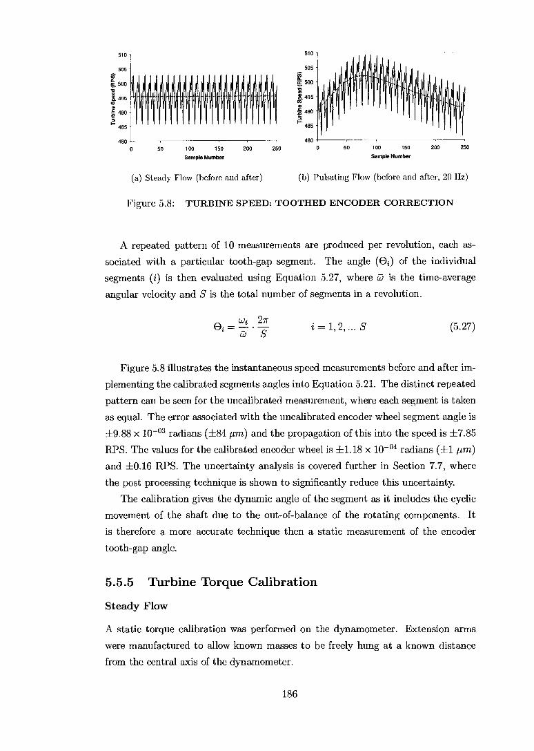
505 Ce C. ix 500 -a

200 250

505 - a re 500 -

. S. 495 -m

490 f2

485 -

480 200 250 0 50 100 150

Sample Number 50 100 150

Sample Number

510

S, 495 (i)

2 490

485

480 0

510

(a) Steady Flow (before and after) (b) Pulsating Flow (before and after, 20 Hz)

Figure 5.8: TURBINE SPEED: TOOTHED ENCODER CORRECTION

A repeated pattern of 10 measurements are produced per revolution, each as-sociated with a particular tooth-gap segment. The angle (ei ) of the individual segments (i) is then evaluated using Equation 5.27, where Co is the time-average angular velocity and S is the total number of segments in a revolution.

coi 27r ei •S

i = 1, 2, ... S (5.27)

Figure 5.8 illustrates the instantaneous speed measurements before and after im-plementing the calibrated segments angles into Equation 5.21. The distinct repeated pattern can be seen for the uncalibrated measurement, where each segment is taken as equal. The error associated with the uncalibrated encoder wheel segment angle is +9.88 x 10' radians (+84 pm) and the propagation of this into the speed is ±7.85 RPS. The values for the calibrated encoder wheel is +1.18 x 10' radians (+1 pm) and +0.16 RPS. The uncertainty analysis is covered further in Section 7.7, where the post processing technique is shown to significantly reduce this uncertainty.

The calibration gives the dynamic angle of the segment as it includes the cyclic movement of the shaft due to the out-of-balance of the rotating components. It is therefore a more accurate technique then a static measurement of the encoder tooth-gap angle.

5.5.5 Turbine Torque Calibration

Steady Flow

A static torque calibration was performed on the dynamometer. Extension arms were manufactured to allow known masses to be freely hung at a known distance from the central axis of the dynamometer.

186

The location of the extension arm in relation to the load-cell is shown in Fig-ure 3.30. The data acquisition voltage was monitored against the applied torque for both rising and falling values, typically a 28-point calibration was performed.

The influence of the water coolant and the bearing air-oil flow was also monitored and found to result in an off-set from the no flow condition. It was also noted that the slope of the calibration curve also changed resulting in a difference in torque measurement of up to 1.5 %. To over come these influences the dynamometer was calibrated with all systems running, the resulting calibration curves are given in

Appendix D.2.2.

Unsteady Flow

The unsteady torque is the sum of the mean component (I-) and the fluctuating com-

ponent (i-) of torque. The mean component is calibrated by the steady flow method,

no direct calibration was performed for the fluctuating component of torque. A dis-cussion on the uncertainty of the torque measurement can be found in Section 7.7.

5.6 Data Acquisition - Hardware

Two separate data acquisition systems were employed in this study, a low-speed system was used for steady flow performance and rig monitoring purposes, whilst a

high-speed system was used for pulsating flow performance.

5.6.1 Steady Flow

The low-speed data acquisition hardware was based on National Instruments Field-

Point Ethernet network interface modules. This system was located adjacent to the test rig and communication to a PC was provided by a 10/100 Ethernet connection. The communication was provided by a main interface module of type NI FP-1600,

the individual function modules were connected directly to this module.

THERMOCOUPLE MODULE - NI FP-TC-120: This module was used to monitor and measure the various thermocouple temperatures with an inbuilt conversion into

degrees. Each module has 8 differential inputs with 16-bit resolution. These modules were combined with an isothermal base of type NI FP-TB-3 to give a cold junction

accuracy of typically +0.25 K. The update rate for all 8 channels is 0.8 seconds.

COUNTER MODULE - NI FP-CTR-502: This module was used to monitor and measure the water coolant and bearing oil flow rate of the dynamometer. Each

module has 8 counter inputs, 4 gate inputs with 16-bit resolution and a 32 kHz

internal clock.

187

The counter module has 4 digital output sources which are independently used as part of the safety control system to enable the guillotine switch, servo valves,

heater system and pulse generator.

ANALOGUE INPUT MODULE - NI FP-AI-110: This module was used to moni-

tor and measure the Scanivalve pressures, turbine speed, load-cell output and RMS vibration. These modules were additionally used as part of the safety and control system to monitor the positions of the varies emergency stop buttons and the guil-lotine valve. Each module has 8 differential inputs with 16-bit resolution and a typical gain error of 0.03 %. The update rate for all 8 channels is 0.17 - 1.5 seconds

depending on the choice of input filters.

ANALOGUE OUTPUT MODULE - NI FP-AO-210: This module was used to con-trol the position of the servo valves which control the air flow through the rig. It

was also used to control the speed of rotation of the pulse generator and for control of the heater system which sets the temperature of the gas flow. This module has 8 voltage output channels of 12-bit resolution with a typical gain error of 0.2 %.

DIGITAL INPUT MODULE - NI FP-DI-330: This module was used to monitor

the Scanivalve channel number which depicts what pressure was being monitored. The module has 8 sinking or sourcing channels with an update rate of 1 kHz and

input range of 3 - 250 VDC, 15 - 250 VAC.

DIGITAL OUTPUT MODULE - NI FP-DO-401: This module was used to control the Scanivalve channel number which depicts what pressure was being measured by the Scanivalve. This module has 16 sourcing channels of voltage range 5 - 30 VDC.

5.6.2 Unsteady Flow

The high-speed data acquisition system comprised of a multifunctioned PCI DAQ

card of type NI 6034-E and a high speed PCI counter/timer card of type NI 6062.

The multi-function DAQ card is used to measure the instantaneous inlet/outlet pressures, the CTA hot-wire voltages and the load-cell torque reading. This card has 8 differential analogue input channels with 16-bit resolution and 8 digital I/O

lines and a overall sample rate of 200 kHz. The counter/timer card is used to measure the instantaneous speed and chopper

plate frequency. This card has 8 counter/timer channels with a 32-bit resolution and a clock frequency of either 0.1, 20 or 80 Mhz. The card may function under

buffered operation with 3 DMA channels. The time averaged inlet temperature and orifice plate mass flow readings are

required for analysis and are measured using the steady flow instrumentation.

188

5.7 Uncertainty Analysis

This section describes the principles of the uncertainty analysis which is applied to both the steady and pulsating flow experiments. The overall uncertainty of the turbine performance parameters is computed through the propagation of the uncertainties of the independent variables. These are the measured quantities such as the static pressure and the recovery temperature.

The chosen bases for the propagation of the uncertainty was originally proposed by Kline and McClintock, 1953 [45] and developed by Moffat, 1982 [58] - 1988 [59].

The true value, Xtrue of a parameter will lie within a range represented by its measured value, xi and an uncertainty interval, +Ax i given with its probability, Equation 5.28. All uncertainties within this thesis are specified to have a 95 % probability that the true value lies within the uncertainty interval. For a normal distribution this represents 1.960 standard deviations.

Xtrue = xi + AXi (95 %) (5.28)

5.7.1 Individual Variables

The uncertainty in a measurement consists of two parts, the precision error and the bias error, an illustrative definition of which may be found in Figure 5.9.

MEASURED SINGLE POINT TRUE VALUE MEAN VALUE MEASURED VALUE

PRECISION UNCERTAINTY (GIVEN IN STANDARD DEVIATIONS)

Figure 5.9: NORMAL DISTRIBUTION: BIAS AND PRECISION UNCERTAINTIES

189

The precision uncertainty can be estimated from a multiple sample experiment by Equation 5.29. Where 'n' is the number of samples, 'S' is the standard sample deviation, 't' is the Student's t multiplier7, is the measured mean value of the variable and the subscript 'cal' represents the calibration obtained values.

Heal

2 teal tealS ±AXi,precistion =

'N/71 \ E (Xi,cal cal)2 n(ncai —1) i,cal=1

(5.29)

The bias error may be deduced by calibration to the accuracy of the calibration instruments but this uncertainty may not be reduced by multiple measurements as this error is systematic to the experiment unlike the precision error.

During a typical instrument calibration, the variation of the instrument trans-ducer with respect to the calibration measured quantity can be represented by a straight line using the least-squares fit technique. If each point is sampled with

sufficient quantity the precision uncertainty becomes negligible and the resultant measured non-linearity is the bias error. The sample standard deviation of the bias error can then be assessed by Equation 5.30. Where 'm' is the gradient of the linear

slope, 'b' is the intercept and 'X' is the input quantity.

[

±AXi,bias = +tcalS = ± \ t2 a

2 E (xi - (mx, + b))2 (5.30) i=1 cal

Importantly the single point bias error can now be represented by a bias uncer-tainty interval which covers the range of calibration conditions.

The precision and bias uncertainty are combined using the Root-Sum-Square method (RSS), which results in the combined uncertainty having approximately the same probability as the individual uncertainties, Equation 5.31.

±Axi = (AXi,precision)2 (AXi,bias)2

(5.31)

5.7.2 Propagation of Uncertainty

A derived parameter, 'P' can be expressed as a function of 'n' independent variables 'xi', Equation 5.32. These independent variables have an associated uncertainty, ±Axi, ±Ax2, ±Ax3, ±Ax„, which result in an uncertainty of the derived parameter, P of ±AP.

P = f (xi , x2 , x3 , ...,xn ) (5.32)

7The Student's t multiplier are statistical values used to inflate the standard sample deviation,

S to account for the underestimation of the true standard deviation, Q. For a < DC, to;; > 1.960.

190

+APabs = E i=,

Ax• z axi

(5.33) aP

The propagation of the uncertainties of the independent parameters may be combined using either of two techniques. The absolute uncertainty or the worst-case uncertainty may be obtained using Equation 5.33. The probable uncertainty or the constant-odds uncertainty can be obtained using Equation 5.34. This results in approximately the same degree of probability that the true value of the derived parameter, P lies within the derived uncertainty interval, +AP as given to the independent variables, x„ Kline and McClintock, 1953 [45]. The constant-odds combination is derived using the Root-Sum-Square, RSS of the individual variables, it is this method that is used throughout this thesis.

±APRSS = Axi) 2

, axi

(5.34)

For Equation 5.34 to assess the uncertainty of the derived parameter with the same probability, it is required that each independent variable are given to the same probability and that A4 is its variance.

This uncertainty method is applied to the steady and pulsating performance

parameters and the resultant equations and discussions are given in Section 6.5 for steady flow and Section 7.6 for pulsating flow.

5.8 Summary

The dimensionless parameters that describe the performance of a radial or a mixed-flow turbine have been stated, with the similitude conditions that make it applicable to cold-flow testing. A description of the test facility and a detailed description of the instrumentation and calibration procedures have been outlined. In particular a method to significantly improve the mass flow rate measurement and a method to measure the instantaneous temperature of the pulsating flow have been described.

A generic technique to quantify the uncertainty in the computed parameters have been described with applicability to the dynamometer and turbine performance.

191

Chapter 6

Steady Flow Experiments

6.1 Synopsis

This chapter describes the method used to transform the measured quantities into the non-dimensional performance parameters given in Section 5.2. The experimental performance results of mixed-flow turbine 'D' are presented for an equivalent speed range of 50 - 100 % . Finally an uncertainty analysis is presented discussing the relative importance of the different parameters.

6.2 Performance Parameters

The following section describes the procedure to evaluate the non-dimensional per-formance parameters, which describe the turbine characteristics, Section 5.2.1. It

is assumed that the following parameters have been measured or are known as de-scribed in Section 5.4:

Mass flow rate (kg/s) Inlet static pressure (Pa) Inlet recovery temperature (K) Outlet static pressure (Pa) Turbine speed (RPS)

Th

P81 Tr1

P84 N

Turbine torque (Nm) Recovery factor Rotor mean inlet diameter (m) d2 Inlet flow area (m2) Al Air gas constant (J/kgK)

The measurement volume consists of two limbs which are smoothly merged to-gether before entering the volute, known as the inner and outer limbs. This requires the physical parameters to be measured for each limb and as such must be appro-priately averaged in order to calculate the performance of the turbine stage. The pressure measurements are area averaged whilst the mass flow rate, and temperature measurements are mass averaged.

192

6.2.1 Efficiency - Velocity Ratio Characteristic

The aerodynamic total-to-static efficiency (rit _s) of the turbine stage undergoing an adiabatic process is defined by Equation 6.1 and schematically shown in Figure 6.1.

The change in total enthalpy over the stage (h01 — h04) is therefore the turbine work

output and the total-to-static isentropic work (hot — h4,$ ) is the available energy

between the stage inlet and outlet assuming the exit kinetic energy is not recovered. This is true for turbines without an exit diffuser where the turbine exhausts directly to the atmosphere.

Wact hol — T„.• V V t—s,is h01 — h4,is adiabatic process (6.1)

h

Vd2

Figure 6.1: TURBINE H-S DIAGRAM

The turbine work output (Wact ) is derived from the reaction measurement of

torque, which is described in Section 5.4.5 and the measured turbine speed, Equa-

tion 6.2.

Wact = T • W = T • 27rN (6.2)

The total-to-static isentropic work (Wt,,is ) can be derived using the h-s diagram

and the isentropic flow equations and is given by Equation 6.3.

193

= [1 r (-r12-1)

Tia (6.6)

= Th• (h01 h4,is)

rn [f

1 C p • dT +

2 -1 Ud

4,i s

= cis

The isentropic expansion velocity (Qs ) is the velocity equivalent to that of the total-to-static isentropic enthalpy drop across the turbine, see Section 5.2.1. By

inspection of Figure 6.1, the h-s diagram and Equation 6.3, it can be seen that

the isentropic expansion velocity is related to the total-to-static isentropic work by

Equation 6.4. For the isentropic work to be evaluated the parameters within the

isentropic expansion velocity (Ci s ) need also to be determined, this is achieved using the following steps:

For an ideal gas the specific heat capacity at constant pressure (cp) for air is a

function of the static temperature and can be represented in polynomial form by

Equation 6.5, Zucrow and Hoffman, 1977 [91]. Where T is measured in Kelvin (K)

and the coefficients A0 to A5 are given below:

cmair = Ao + AiT + A2T 2 A3T 3 A4T 4 A5T 5 (6.5)

Ao = 0.10831165 x 104

A3 = -0.11323656 x 10-5 Al = -0.68388122 x 10°

A4 = -0.82943324 x 10-9

A2 = 0.17875137 x 10-2

A5 = 0.11100191 x 10-11

Through an iterative process the static temperature (T1 ) can be derived from the measured recovery temperature (T21), the recovery factor (r), which is a function of the Mach number, Equation 6.6. Subsequently the total temperature (T01) can

be found, Equation 6.7. This temperature is an effective mean total temperature

across the measurement plane.

(6.3)

(6.4)

T01 =T1 1+ 71 - Mi 1 2

194

(6.7)

Similarly an effective mean total pressure across the measurement plane can be

assessed by Equation 6.8.

Toil T1

P01 P1 —1.y

(6.8)

T • — T' [ I

4,zs — 01

p / p4

'Y(1-4) -1

1(1-4) (6.9)

Through an iterative process the isentropic exit static temperature can be com-puted from knowledge of the total inlet pressure and temperature and the exit static

pressure using the isentropic flow equations, Equation 6.9. An iterative process is

required because the isentropic exit specific heat ratio (y4,i8) is not known and is

required to calculate the mean specific heat ratio (1(1_4) ). The specific heat ratio

is a function of the constant-pressure specific heat capacity (cr ) and the gas con-

stant for air (R) and hence is a function of the isentropic exit static temperature,

cpAcp — R). The inlet velocity (U1) or more precisely the inlet dynamic enthalpy (W?) can

be found using Equation 6.10 or through the previously calculated Mach number, which finally allows a solution for the isentropic expansion velocity (Cis). The total-

to-static isentropic work ( can then be evaluated using Equation 6.4. This

allows the evaluation of the total-to-static efficiency of Equation 6.1.

1 r 2 —2

u i (Toi — (6.10)

The Velocity Ratio (U2/Cis) can now also be evaluated using Equation 6.11, with

reference to the definition of the isentropic expansion velocity of Equation 6.4.

U2 cis

ird2 N (6.11)

(2 f41,is cp . dT U?)

195

6.2.2 Mass Flow rate - Pressure Ratio Characteristic

The mass flow rate parameter (pseudo-non-dimensional, MFP) and the total-to-static pressure ratio can be evaluated once the total inlet pressure and temperature, mass flow rate and exit static pressure are known, Equations 6.12 and 6.13. The evaluation of the input quantities are described in Section 6.2.1.

ri/V7rn MFP.Poi

PR. = Poi P4

(6.12)

(6.13)

6.3 Experimental Test

6.3.1 Test Conditions

The aim was to assess the performance parameters that govern the characteristics of the turbine. In order to achieve this, the turbine was subjected to various tightly controlled steady state conditions that allow a large range turbine map to be con-structed.

The turbine was tested over six different equivalent speeds varying from 50 % -100 % in 10 % increments. These speeds can be found in Table 6.1, which also gives the equivalent non-dimensional speed, the turbine total inlet temperature and the range of powers that the turbine was subjected to. For each equivalent speed the turbine total inlet temperature was held constant.

In order to varying the operating point of the turbine, the turbine load was varied by the dynamometer through its entire range whilst the inlet pressure was adjusted to obtain the desired speed.

Table 6.1: TURBINE 'D' STEADY STATE TEST CONDITIONS

Equivalent Speed

(%)

Turbine Speed (RPM)

Non-dimensional Speed

Turbine Inlet Temperature

(K)

Wad Min (kW)

VT et Max (kW) (2ird2N/IToi - R)

50 29,461 0.833 333 0.29 23.3 60 35,458 1.000 335 0.52 30.3 70 41,491 1.167 337 0.80 39.6 80 47,559 1.333 339 0.96 47.6 90 53,661 1.500 341 1.37 53.2 100 59,798 1.666 343 1.70 62.2

196

r4 4 E

Pori Tr,

T„ T„,. no,

Ton,,n tin

— ePoricin an

Tb...g -

Thearing 2

Tb...8 3

T

T tore TURBINE

6'Porifout Tr 1,out

Pori Coo P Lout T (NM) N (rps)

Tnrif,out Toffs.

The r

moc

oupl

e M

odul

e

6.3.2 Data Logging

The low speed data acquisition program was developed by Pesiridis, 2000 [65]. This was used to log the measured steady state parameters. For each measurement point a total of 19 parameters' were logged, 12 were for turbine performance eval-uation and 7 were for rig monitoring purposes. The 12 turbine performance pa-rameters are: P - orif,inl Porif,outl L\Porif,inl Porif,out, Pl,in, Tarif,in, Torif,out,

Tri ,cmt , N (rps) and r (Nm). The 7 rig monitoring parameters are: Tbearing 1,

Tbearing 2, Tbearing 33 Tmrotor 1, Tmrotor 2, 7-;„,ir, and Two parameters were manually recorded these were the ambient static pressure, P4 and the torque offset, roff „t which was used to reduce the hysteresis measurement error, refer Section 6.5. To adjust for voltage drift on the pressure sensors the offset voltage was entered directly into the data acquisition program and was corrected for automatically, refer Section 6.5.

The run time for the data acquisition program is approximately 100 seconds, in this time the measured parameters except the pressure data were sampled 433 times, with an time-average being calculated. The nature of the Scanivalve meant that the pressure data was sampled sequentially, each pressure parameter was sampled 67 times with a time-average also being calculated.

The time-averaged data was then written to a file for further processing into the performance parameters.

ORIFICE PLATES PULSE GENERATOR MEASUREMENT DYNAMOMETER DAQ MODULES PLANE

Figure 6.2: DATA LOGGING: DAQ MODULES

'The symbols are given in the nomenclature.

197

6.4 Experimental Results and Discussion

This section presents the steady flow experimental performance of mixed-flow tur-bine 'D', loaded using the new PMEC dynamometer. The data presented in the following section is for the dynamometer range previously given by Figure 3.32. The turbine performance is presented for the equivalent speed range of 50 - 100 % in 10 % speed increments.

6.4.1 Efficiency Characteristic


The efficiency characteristics of mixed-flow turbine 'D' are given by Figure 6.4(a) -6.4(b) and in tabular form by Table 6.2. These give the turbine stage total-to-static aerodynamic efficiency against the velocity ratio and pressure ratio for the range of equivalent speeds.

The results show a large range turbine map with a measured velocity ratio range of 0.375 - 1.068, demonstrating the capabilities of the dynamometer. This has allowed the peak efficiency of the turbine to be well represented at all equivalent speeds giving a more complete picture of turbine performance compared to a map

obtained using a radial compressor as the loading device. Steady state data for turbine 'D' has been obtained previously by its designer Karamanis, 2000 [42] using a radial compressor as the loading device. The bounds of this data can be seen highlighted on Figure 6.4(b).

The maximum peak efficiency was measured to be 74.3 % at a velocity ratio of 0.663 and an equivalent speed of 80 %. The efficiency trends of the different speeds were found to be similar in shape with the variation in magnitude particularly for the higher speeds being relatively small. For an equivalent speed range of 60 - 100 % the peak efficiency remained within 3.3 % points of the maximum obtained efficiency value whilst the 50 % equivalent speed was lower by 5.9 % points.

The measured velocity ratio range reduces with increased speed as shown in Table 6.2. This reduction is a consequence of the increase in power requirements of the turbine as the speed increases. For 50 % equivalent speed the velocity ratio range is 0.375 - 0.974 whilst for 100 % equivalent speed is 0.613 - 1.068. By plotting the turbine power at a 100 % equivalent speed for various velocity ratios, it is estimated to measure the turbine performance at a velocity ratio of 0.567 would require a further 66 % increase in the power absorption capabilities of the dynamometer. This would result in only a 10 % increase in the turbine map and demonstrates the

difficult task faced by the dynamometer.

198

100

Dyn

amom

eter

Pow

er (k

W)

10 .

04 05 06 07 08 09

1

11

12

Velocity Ratio

Figure 6.3: DYNAMOMETER POWER VS VELOCITY RATIO AT 100% SPEED

No conclusive trend in the variation of the optimum velocity ratio and speed was seen. The variation of velocity ratio at measured peak efficiency varied between 0.644 - 0.686 with a mean value of 0.672, Table 6.2. Regardless of the chosen measurement technique it is difficult to accurately pinpoint the optimum velocity ratio, this uncertainty is due to the flat efficiency curve and the finite number of measurements which results in a sensitivity to the efficiency measurement. In order to improve the accuracy, repeated measurements were taken and a curve fit was

applied to the data. This suggests the optimum velocity ratio at 50 % equivalent speed of 0.648 rather then the measured point of 0.678. The difference of the curve fit efficiency between these velocity ratio locations is < 0.2 % points which equates to an

estimated power difference of just 9 W, this highlights the difficulty in assessment. The overall results show that the optimum velocity ratio for this mixed-flow

turbine is lower then for a radial inflow turbine, which typically has a value of 0.7. A lower optimum velocity ratio is beneficial under pulsed flow conditions as a larger proportion of the available energy is held in these regions, this is further discussed in Chapter 7. The reduction in optimum velocity ratio is thought to be caused by the positive inlet blade angle of the mixed-flow turbine viz., Hakeem, 1995 [361. The blade angle of a radial turbine is fixed at zero degrees whilst mixed-flow turbine 'D' has a positive blade angle of + 20 degrees at the midspan, refer Table 5.2.

A mean line estimate of the likely reduction in velocity ratio of the turbine can be obtained from Equation 6.14. This can quantify whether the average reduction of 0.03 is a likely result of the change in inlet blade angle.

199

U2 2 ,e-y mean—line 2 1/

UO2U2 t-,e3U3 (6.14)

U2 mean—line

cis

1 tan (13B2 + iopt)) 2 tan a2

no exit swirl

(6.15)

At the optimum operating condition a first estimate of the velocity ratio can be obtained by assuming a turbine efficiency of one with zero exit swirl. The equation can be solved with knowledge of the absolute gas flow angle, a2 and the optimum incidence angle, i0 t . The absolute gas flow angle was experimentally measured using LDV by Su, 1999 [75] for the volute under investigation. This remained predominantly constant at 75 degrees and confirmed that it is primarily a function of the volute geometry, Whitfield and Baines, 1990 [84]. An estimate of the optimum incidence angle was made using the values given by Rodgers, 1987 [69], Baines and Yeo, 1991 [5] and Rohlik, 1968 [70] of - 20, - 30 and - 40 degrees respectively; an amalgamation of - 30 degrees was chosen. A simplified form of the Equation 6.14 is given by Equation 6.15 where the exit swirl has been omitted. This results in an

optimum velocity ratio of 0.760 and 0.724 for a radial and mixed-flow turbine 'D' respectively, a difference of 0.036.

It can be seen from Equation 6.14 that the inclusion of a realistic efficiency decreases the optimum velocity ratio point whilst the inclusion of the exit swirl increases this point. Using the peak efficiency of 74.3 % and an exit swirl of 20 m/s2

a better estimate of the optimum velocity ratio can be made giving 0.689 and 0.653 respectively for a radial and mixed-flow turbine, a difference of 0.036.

This simple analysis gives sensible results compared to the present experimental findings and suggests that a positive inlet blade angle will give a moderate reduc-

tion in the optimum velocity ratio with respect to a radial turbine. The scope for this reduction is limited to < 0.04 points for a + 20 degree bladed turbine. This is beneficial under pulsed flow conditions were the energy content of the gas is biased towards the lower velocity ratios. With reference to Equation 6.15, as turbine effi-ciencies improve, the optimum velocity ratio will increase but it is likely the velocity ratio gap between the mixed-flow and the radial turbine will remain similar.

2This has been measured using LDV by Su, 1999 [75] on turbine 'A' at the 70 % equivalent speed.

200

• 50% Speed • 60% Speed • 70% Speed • 80% Speed • 90% Speed • 100% Speed

PREVIOUS DATA RANGE - BARS KARAMANIS, 2000

- . ____ ...........„All"-•

Al...." 410'

,

Aeiki

/

I Ar

A' . r 4,.. • 50% Speed 0

PREVIOUS DATA RANGE 2000

I KARAMANIS,

-BARS

I

• 60% Speed • 70% Speed • 80% Speed • 90% Speed • 100% Speed 50% 70% 1 100%

7

6

2

0.8

U 0.6

C g 0.4

01

• 50% Speed _ • 60% Speed • 70% Speed • 80% Speed • 90% Speed • 100% Speed

1.5

2

2.5 3

Pressure Ratio (total-static)

0.8

• 0.6

09 u • 0.4

0.2

(a) EFF t—s Vs PR t—s

0.2

0.4 0.6 0.8

1

1.2

Velocity Ratio (U2/Uis)

(b) EFF t—s Vs U2/Cis

1.5 2 2.5 3


(c) MFP Vs PR t—s

Figure 6.4: STEADY FLOW RESULTS

201

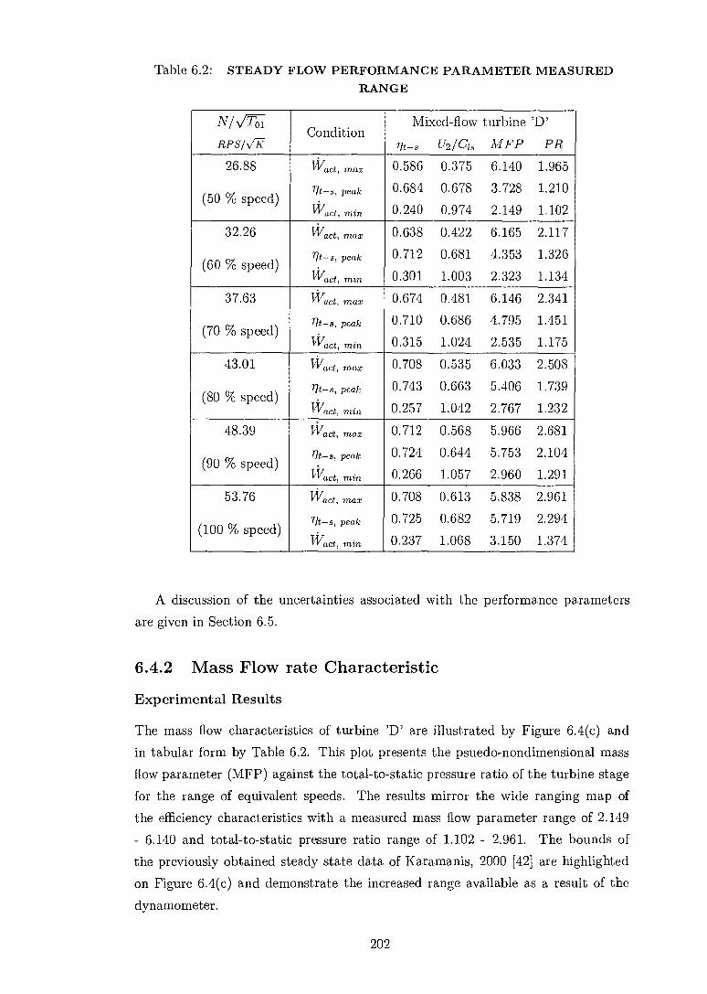
Table 6.2: STEADY FLOW PERFORMANCE PARAMETER MEASURED RANGE

N/ N/To i RPS/Vif

Condition Mixed-flow turbine 'D'

lit-8 U2/ Cis MFP PR

26.88 Wad, max 0.586 0.375 6.140 1.965

71t-8, peak 0.684 0.678 3.728 1.210 (50 % speed)

Wact, min, 0.240 0.974 2.149 1.102

32.26 Wact, max 0.638 0.422 6.165 2.117

(60 % speed) 77t-s, peak 0.712 0.681 4.353 1.326

Wact, min 0.301 1.003 2.323 1.134

37.63 Wact, max 0.674 0.481 6.146 2.341

(70 % speed) 11t-s, peak 0.710 0.686 4.795 1.451

Wact, min 0.315 1.024 2.535 1.175

43.01 Wad, max 0.708 0.535 6.033 2.508

(80 % speed) qt ' -s peak 0.743 0.663 5.406 1.739

Wact, min 0.257 1.042 2.767 1.232

48.39 Wact, max 0.712 0.568 5.966 2.681

7 ]t-,s, peak 0.724 0.644 5.753 2.104 (90 % speed)

T'7 act, min 0.266 1.057 2.960 1.291

53.76 Wact, max 0.708 0.613 5.838 2.961

(100 % speed) 71t-s, peak 0.725 0.682 5.719 2.294

"tact, rain 0.237 1.068 3.150 1.374

A discussion of the uncertainties associated with the performance parameters

are given in Section 6.5.

6.4.2 Mass Flow rate Characteristic


The mass flow characteristics of turbine 'D' are illustrated by Figure 6.4(c) and

in tabular form by Table 6.2. This plot presents the psuedo-nondimensional mass

flow parameter (MFP) against the total-to-static pressure ratio of the turbine stage

for the range of equivalent speeds. The results mirror the wide ranging map of

the efficiency characteristics with a measured mass flow parameter range of 2.149

- 6.140 and total-to-static pressure ratio range of 1.102 - 2.961. The bounds of

the previously obtained steady state data of Karamanis, 2000 [42] are highlighted

on Figure 6.4(c) and demonstrate the increased range available as a result of the

dynamometer.

202

The trends seen by Figure 6.4(c) are typical of a radial or mixed-flow nozzle-less turbine stage. It can be seen that the change in mass flow parameter with pressure ratio is non-linear and negative in value. As the pressure ratio is increased the mass flow parameter reaches an asymptotic limit where further increases in pressure ratio will not result in any further increase in mass flow parameter, in this region the turbine is choked. This is due to the gases relative acceleration through the turbine rotor and the additional aerodynamic blockage caused by separation of the flow, which results in the flow reaching sonic velocity at the exducer section of the turbine. An additional trend which is evident is the reduction in mass flow parameter with increasing speed. A centrifugal pressure field caused by the rotation of the turbine is responsible for the drop in the mass flow parameter with increasing speed viz.,

Hakeem, 1995 [36] and Su, 1999 [75]. The specific speed, N, given by Equation 6.16 has been computed for mixed-flow

turbine 'D' at the peak efficiency using the definition given by Rohlik, 1968 [70].

Where Q4 is the exit volume flow rate and H is the total-to-total isentropic specific work. The peak efficiency which occurred at 80 % equivalent speed has a specific speed of 1.05 whilst for the 50 - 100 % equivalent speed range the specific speed varied between 0.99 - 1.14 respectively. The corresponding flow coefficient, 0 and loading coefficient '0 at the peak efficiency point was 0.50 and 0.85 respectively, the definition of these parameters are given in the nomenclature. The specific speed is

a general indication of the swallowing capacity relative to the work output of the device, where larger values are associated with greater swallowing capacity. The specific speed for a radial inflow turbine such as the one tested by Dale, 1990 [25] typically has a lower specific speed in Dale's case a value of 0.86 was computed. These values suggest turbine 'D' has a larger flow rate then would be expected for a typical radial inflow turbine; this is beneficial for transient response as a smaller

turbine can be used.

27N VT4 N., =

Hi (6.16)


This section applies the uncertainty analysis given in Section 5.7 to the steady flow performance results of turbine 'D'. The overall aim is to arrive at the uncertainty of the five performance parameters, the total-to-static efficiency, velocity ratio, mass flow parameter, pressure ratio and equivalent speed value. Additionally the influ-ence of the propagation of the main independent variables into the performance parameters are assessed and discussed in the following sections.

203

6.5.1 Independent Variables

The independent variables are the parameters that must be known in order to calcu-late the performance parameters of the turbine. The variables of greatest influence are the mass flow rate (n7,), inlet static pressure (P1), inlet recovery temperature (Tri ), turbine speed (N) and turbine torque (r). These parameters and their asso-ciated uncertainty will be discussed in the following subsections. The independent variables which have minor influence are the outlet static pressure (P4), recovery fac-tor (r), rotor mean inlet diameter (d2), inlet flow area (A1) and the air gas constant (R). These are not discussed further.

Mass Flow Rate

Although strictly speaking the mass flow rate is not an independent variable as it is derived from the pressure and temperature measurements at the orifice plate. In relation to the turbine performance parameters it may be considered indepen-

dent as the measured quantities do not influence any other part of the performance parameter calculation.

The uncertainty associated with the measurement of the steady mass flow rate are outlined in the British Standard, BS 5167-1:1997 [13]. This follows the same uncertainty propagation technique as given in Section 5.7 and results in the Root-Sum-Square (RSS) error of the mass flow rate to a confidence level of 95% or two standard deviations (2(7). The overall uncertainties of the mass flow rate varied between 1 to 2 %, the lower uncertainties representing the higher mass flow rates.

The uncertainty of the measured independent quantities of the mass flow rate

are given in Table 6.3.

Table 6.3: STEADY MASS FLOW - INDEPENDENT VARIABLE UNCERTAINTY

INDEPENDENT VARIABLES Value

Pipe Diameter rn ±0.001 Orifice Diameter in ±0.0001 Upstream Static Temperature K ±0.67 Upstream Static Pressure Pa ±470 Orifice Differential Pressure Pa ±85

204

0. aa

O

D. 0.6

iJ 0.4

0.2

0

1.4

1.2

= 0.10

0.05

0.02 0.01

Inlet Recovery Temperature

The uncertainty associated with the turbine stage inlet recovery temperature is assessed through the thermocouple calibration procedure as given in Section 5.5.2. The maximum static error found by calibration through a temperature range of 273 - 373 K is +0.4 K which is largely attributed to bias error.

Inlet Static Pressure

The uncertainty associated with the inlet static pressure measurement arise from various sources. The pressure tapping geometry, transducer non-linearity, calibra-tion transducer non-linearity and the bridge drift error, these uncertainties may all be deduced.

The uncertainty caused by the pressure tapping geometry is generally small and arise due to aerodynamic interaction with the tapping hole. A description of these uncertainties are given in Benedict, 1984 [6], where an estimation of the error may be deduced with reference to Figure 6.5. It is estimated from the steady state results that the maximum error due to the geometric influence will be < 0.5 % of the

dynamic head. For the high pressure transducer (Druck PDCR 23D) this will not exceed 100 Pa at the most extreme point. The error in the low pressure transducer

(Druck PDCR 22) is deemed negligible.

1°4 2 5 106 2 5 106 2 5 107 Pipe Reynolds Na., RD

Figure 6.5: STATIC TAPPING ERROR, BENEDICT, 1984 [6]

From the calibration of the pressure transducers the non-linearity can be esti-mated. The high pressure transducer gave a maximum deviation of ± 0.066 % FS (230 Pa) whilst the low pressure sensor gave a maximum deviation of + 0.10 % FS (35 Pa). The calibration units transducer (Druck DPI 610) rated from - 1 to 3.5 Bar gauge has an associated uncertainty and is certified to give a maximum deviation

< 0.025 % FS .

205

The calibration certificate for the transducer showed a higher degree of accuracy throughout the full scale range and particularly at the lower pressures. A conser-vative uncertainty of 0.02 % FS was applied for the high pressure transducer and an uncertainty of 0.008 % FS was applied for the low pressure transducer in line with the calibration certificate. This gives an uncertainty of ± 90 Pa for the high pressure transducer and ± 36 Pa for the low pressure transducer.

It was found that both transducers showed some voltage drift. It was estimated that a maximum voltage drift of 0.0015 V may occur within a single test point. This gives an uncertainty of + 50 Pa for the high pressure transducer and ± 15 Pa for the low pressure transducer.

These above uncertainty are bias errors and as such the worst case combination has been chosen to represent the overall uncertainties:

Overall High Pressure Transducer Uncertainty ±470 Pa Overall Low Pressure Transducer Uncertainty ±86 Pa

Turbine Speed

The heater system used to keep the turbine inlet temperature constant produces a pulsed heat input into the air flow, this resulted in a low amplitude and low frequency

oscillation of the turbine speed. The uncertainty for the speed measurement was taken as the maximum acceptable peak-to-peak variation of the test point, this was taken as + 2 RPS.

Turbine Torque

The torque measurement is the most influential parameter in the assessment of the turbines efficiency. The uncertainty in measurement arise from various sources, the largest source due to external torque and friction. Other sources are the transducer linearity and bridge drift voltage. The friction in the system occurs due to the gimbal bearings and the external torque occurs due to various external attachments to the test rig. These attachments are the water coolant pipes, instrumentation-control cabling and the tubing for the bearing air-oil system. It was essential that these were carefully arranged to offer the least external torque to the freely floated dynamometer/turbine assembly. To reduce the hysteresis and voltage drift errors, a torque reading was taken at zero speed and was used to zero the load cell output

for each test condition point. The uncertainty associated with the transducers linearity from the manufacturers

full scale limits gave an accuracy of < + 0.005 Nm. By calibration and through turbine runs the overall uncertainty in the torque measurement was assessed to

have a value of ± 0.025 Nm.

206

Future improvements in the accuracy of the torque measurement can be made through better arrangement of the external attachments as previously listed. This will help reduce the uncertainties allowing better accuracy in assessing the turbine efficiency particularly in the high velocity ratio regions.

6.5.2 Parameters

The propagation of the individual parameters can be calculated using the procedures of Section 5.7. The resultant equations for the RSS uncertainty of the turbine performance parameters are given by Equations 6.17 - 6.20.

The overall RSS uncertainties are illustrated by Figures 6.6(a) - 6.6(e) for the five performance parameters of the turbine: efficiency (qt ,), velocity ratio (VR.), mass flow parameter (MFP.), pressure ratio (PR.) and the equivalent speed. Equa-tions 6.17 - 6.20 show the overall uncertainties are an RSS summation of the influence each independent variable has on the performance parameters. The influence these independent variables are graphically illustrated for the full range of the turbine test conditions by Figures E.1 - E.5 and can be found in Appendix E.1.

It should be noted the uncertainties presented do not take into account the reduction in the precision uncertainty as a consequence of repeated measurements at the test conditions and best fit slopes.

Total-Static Aerodynamic Efficiency

A (17t--, [(Orin) (°(77arhLIt-s)\ 1 2

+ [(AT1r) (3

(Ti(74-5) )] 2

r ±

[(AP1) ( aelaitAs) )] 2 + [(AT) t

(8(11 S))]

2 al_ + [( AN) (a(17t-aN

s)) ] 2

(6.17)

The uncertainty in efficiency varies substantially with both velocity ratio and

equivalent speed, the latter is due to the energy content of the gas. An increase in uncertainty is seen with increasing velocity ratio and a decrease in speed as shown by Figure 6.6(a). The variance in the efficiency uncertainty above the minimum plateau seen is predominantly a result of the change in the relative uncertainty of the torque measurement. The overall uncertainty levels vary from ± 0.9 - 7.0 % points in efficiency, this is dependent on the velocity ratio and speed.

At high velocity ratios the uncertainty is dominated by the torque measurement as the turbine power in these regions is extremely low. At the maximum velocity ratio this accounts for 85 % of the overall uncertainty.

207

The secondary influence in uncertainty is the mass flow rate measurement whilst the remaining variables of pressure, speed and temperature do not contribute a large proportion of the uncertainty. At low velocity ratios the torque does not dominate the uncertainty and accounts for 13 % of the overall uncertainty at minimum velocity ratio. The dominating factor is the mass flow rate measurement and it is this that sets the apparent minimum plateau in the overall uncertainty of about ± 1 % point in efficiency. The uncertainty in the mass flow accounts for 55 - 63 % of the overall uncertainty for the range of speeds, the other independent variables approximately share the remaining uncertainty.

In consideration of the optimum velocity ratio point, at 50 % equivalent speed the torque and mass flow are both important factors whilst at 100 % equivalent speed the uncertainty is dominated by the mass flow measurement. The independent variables

influence on the uncertainty can be found in Appendix E by Figures E.1.

Velocity Ratio

A(V R. — a(V R.) 1 2 [(Arii) ( afrt ) + [(ATir) (a(V

aT„ ) jR1 .))

2

+ [ (Api) ( a(

ap 1 )] vR.))] 2 + [(AN) ( a(vR.)

ON )] 2

(6.18)

The overall uncertainty in velocity ratio is low throughout the full range of test conditions < ± 0.7 %. An increase in uncertainty is seen with increasing velocity ratio and a decrease in equivalent speed, Figure 6.6(b). The overall uncertainty levels vary from + 0.23 - 0.62 % dependent on the velocity ratio and speed value.

The dominant uncertainty is largely from the speed measurement, although at high velocity ratios the pressure measurement becomes increasingly important. It may be seen indirectly by the overall RSS uncertainties of Figures 6.6(b) and 6.6(d) and directly by the constituent uncertainties of Figures E.1 - E.5, that the uncer-tainty in the pressure can change suddenly. This is a result of the Scanivalve selec-tion of either the high or low pressure transducer, it is their associated difference in accuracy which results in the sudden change in uncertainty.

In consideration of the optimum velocity ratio point, the relative proportions can vary due to the switching of the transducers but at 50 % equivalent speed, the speed measurement accounts for about 50 % of the uncertainty whilst the pressure and the mass flow rate account for about 20 % each and the temperature the remainder. The constituent uncertainties can be found in Appendix E by Figures E.2.

208

Pseudo-non-dimensional Mass Flowrate

A(MFP.) = [(Ath)(a(mFp.) ) J -12

thi-b +

[(ATIT) ("FP.)/

1

2

+ [( Apo \( a(-1

aPi11FP))]

2 (6.19)

\ aTir -I

The overall RSS uncertainty in mass flow parameter (MFP) range from 1.9 -0.87 % and is dependent on the value of the MFP, Figure 6.6(c). The uncertainty does not show significant sensitivity to changes in equivalent speed. Above a MFP of 3.5, the uncertainty plateaus at just < 1 %, this uncertainty increases to about 2 % as the MFP reduces to a value of 2. The MFP is dominated by the uncertainty

in the mass flow rate measurement which accounts for between 72 - 93 % of the overall value for the range of conditions. The remaining uncertainty is associated

with the pressure and temperature measurement, the temperature value is typically constant at 0.04 % of the MFP value. The constituent uncertainties can be found in Appendix E by Figures 6.6(c).

Pressure Ratio

A(PR.) = [(Aril) (.9(aPr4R.))1 2 ±

[( ATir ) (a(oPTR:))] 2 +[( Api ) (a(PR.aPi

))] 2 (6.20)

The overall RSS uncertainty in the pressure ratio is low and range from 0.08 -0.33 %, refer Figure 6.6(d). It is dependent on the value of the pressure ratio and the equivalent speed to a lesser extent. The magnitude of the pressure ratio value results in two effects. For a fixed pressure transducer there is a slight decline in the percentage uncertainty with increasing pressure ratio. The largest effect is due to the switching of the transducers, for the low-pressure transducer the uncertainty is about 0.1 % which increases three fold when the Scanivalve switches to the high-pressure transducer. The constituent uncertainties can be found in Appendix E by Figures E.4.

209

Equivalent Speed

(Neqww) [(Am) (a(Nalniv))1 2 + [(ATir) a(Nequiv))1 2 +

\ aTir a(N„„iv ) 1 2 a(Nequiv ) M 2

oP1 ± [(AN) h (6.21)

The overall RSS uncertainty in the equivalent speed measurement is low and ranges from 0.21 - 0.42 %, refer Figure 6.6(e). The absolute RSS uncertainty is largely constant with a value of ± 0.205, a small equivalent speed dependence is ex-hibited. The uncertainty is dominated by the speed measurement which contributes approximately 77 - 86 % of the uncertainty, whilst the remainder of the uncertainty is due to the temperature measurement. The constituent uncertainties can be found in Appendix E by Figures E.5.

6.6 Summary

A large range turbine map of mixed-flow turbine 'D' has been produced utilising the PMEC dynamometer demonstrating its capabilities with a measured velocity ratio

range of 0.375 - 1.068. It was found that the peak efficiency point and the velocity ratio trends were

similar, with peak efficiencies generally varying by 3 % points. At optimum condi-tions a peak total-to-static efficiency of 74.3 % was measured and occurred at the

turbines 80 % equivalent speed with a velocity ratio of 0.663. A simple analysis has shown that a 0.036 point reduction in optimum velocity ratio is feasible by a + 20 degree inlet blade angle compared to a typical radial inflow turbine, this is consistent with the experimental findings.

A specific speed assessment of the turbine giving a value of 1.05 suggests the mixed-flow turbine has a larger flow capacity then would be expected from a typical radial inflow turbine.

The overall uncertainty in efficiency ranges from 0.9 - 7.0 % points. The main source of measurement uncertainty is the torque measurement, this becomes limiting at low turbine powers. The mass flow rate measurement is the main source of uncertainty in the assessment of the mass flow parameter. All other performance parameters have a relative uncertainty of less then ± 1 % throughout the entire test range.

210

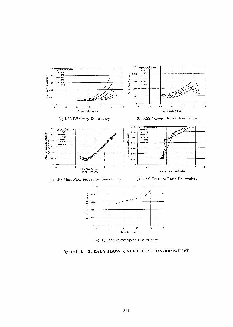
3 35 U 5 I I 5 2 25

EQUIVALENT -6-50%

- -4-60 -.- 70%

_0_ 900. - -6-100%

SPEED

A ...li. .a.AY

/

1


EQUIVALENT SPEED -43- 50%

- -4-60% -6-70%

_ 0)4'. - 90% -6- 100%

0.03 a 2 3 4

Mass Flow Parameter fkgisi IC:Bar (abs)

6

1 5 0.045

7 -4 0.04 0.035

0.06

0.055

0.05 4-;

0.007

0.006

0.005 S

0.004

0.003

0.007

0.001

EQUIVALENT SPEED -6- 50% -6-60% -6-70% -6- 8044

- -.-90% -1.-100%

EQUIVALENT -6- 50%

--..-- 80%

SPEED

-.

-34-90% -6-100% _......----

0.1

220.08

0.04

1E 4, 0.02

0.01

0.005

0.006

0.004

4' 0.012

0

132

04 06 (18

12 0

02

04 0 6 08

12

Velocity Rata (412/(7)

Velocity Ratio (4f2/Cis)

(a) RSS Efficiency Uncertainty (h) RSS Velocity Ratio Uncertainty

(c) RSS Mass Flow Parameter Uncertainty (d) RSS Pressure Ratio Uncertainty

20 40 60 80

100 120

Equivalent Speed (%)

(e) RSS equivalent Speed Uncertainty

Figure 6.6: STEADY FLOW: OVERALL RSS UNCERTAINTY

211

0.21

▪ 0.208

2) 0.206

0.204

0.202

0.2

Chapter 7

Unsteady Flow Experiments

7.1 Synopsis

This chapter describes the method used for data collection and refinement of the measured quantities and their transformation into the non-dimensional performance parameters. The instantaneous performance results of Mixed-Flow Turbine `D' are

presented for an equivalent design speed range of 50 to 100 %. A discussion is given on the individual measured parameters and the instantaneous performance parameters. Finally an uncertainty analysis is presented discussing the relative

importance of the parameters.

7.2 Performance Parameters

The required performance parameters of section 5.2 are computed similarly to the steady flow experiments given in Section 6.2 although now instantaneous quantities

are required.

Mass flow rate (kg Is) rhinst Turbine torque (Nm) Tinst

Inlet static pressure (Pa) Pl,inst Recovery factor rinst

Inlet recovery temp. (K) Trl,inst Turbine speed (RPS) Ninst

Outlet static pressure (Pa) P4,inst

The same test facility was employed as with the steady state experiments. This facility consists of two limbs, the inner and outer limbs which would ideally require the measurement of the relevant instantaneous quantities within each limb. This was not possible for all measurements: 1) the instantaneous mass flow measurement,

rizinst was measured only on the outer limb and an approximation of the inner limb values were made in consideration of the steady state values, refer to Section 7.4.

212

2) the instantaneous inlet recovery temperature, Trl,inst was measured on the

outer limb in synchronisation with the mass flow measurement and a similar ap-proximation was made for its application to the inner limb. Additionally the in-stantaneous static temperature was independently calculated using the isentropic

compression assumption of Section 5.4.2, this was implemented on each limb. The limb pressure measurements were area averaged whilst the mass flow rate,

and temperature measurements were mass averaged.

7.2.1 Efficiency Characteristic

The instantaneous aerodynamic total-to-static efficiency, n ( \ -,t-s i tnst of the turbine

stage undergoing an adiabatic process is defined by Equation 7.1.

(rIt-s)inst (Wact)inst (7.1)

1/1/ t-s,is)inst

The instantaneous turbine work output, (Wact)inst is defined by Equation 7.2.

The measurement of instantaneous turbine speed and torque are described in Sec-

tion 5.4.4 and Section 5.4.5.

(Wact)inst = 271- • (NT)inst = 2irNinst • (7 + i") (7.2)

The instantaneous isentropic total-to-static available work of the turbine,

(Wt-s,is)inst is defined by Equation 7.3. It is assessed following the procedures of

Section 6.2 using the measured instantaneous quantities, Thinsi , Trl ,inst , Pl,inst and

P4,inst •

1

1 (Wt-s,is)inst "' (4inst{(1,is inst " C p • dT + 0 ,inst

4

C i2s inst = •"Inst 2

The instantaneous Velocity Ratio, (U2/Ci s)inst is evaluated using Equation 7.5.

(7.3)

(7.4)

( U2

\ C73) inst =

7d2Ninst (7.5)

(111, Cr • cIT)qinst ) inst

213

7.2.2 Mass Flowrate Characteristic

The pseudo-non-dimensional instantaneous mass flow parameter, M F Pinst and in-

stantaneous total-to-static pressure ratio, P Rinst is evaluated using Equation 7.6

and Equation 7.7 respectively.

rhinst VT01,inst (MPP)inst

P01,inst (PR)inst

7.3 Experimental Method

For brevity the subscript `inst' of the parameters given above are generally omitted from the notation for the remainder of this chapter. These quantities are instanta-

neous unless otherwise stated.

7.3.1 Test Conditions

The turbine was tested over four different pulse frequencies, 20 to 80 Hz with incre-ments of 20 Hz and for six different equivalent speeds varying from 50 to 100 % with increments of 10 percentage points. A single test condition was chosen for each pulse frequency and test speed, this unweighted time-average operating point corresponds to approximately the turbine peak steady efficiency point. The mean turbine test conditions are summarised by Table 7.1 which also gives the mean turbine speed, the mean non-dimensional speed and the mean turbine total inlet temperature.

7.3.2 Data Logging

The development of a high speed data acquisition program was required for the acquisition of the instantaneous data. This was used in conjunction with the low

speed system to log the measured instantaneous and steady parameters. For each test point the low speed data acquisition program was looped three times

logging the parameters and following the procedures described in Section 6.3.2. To obtain the time-averaged parameters necessary to process the instantaneous data: the time averaged mass flow rates for each limb, Thin and Mout obtained from Ps ,„Ti ,

Ps,orif,out, APs,orif,out, Ts,orif,in and Ts,orif,out and the time-averaged mea-

surement plane recovery temperatures Tri,in and Trl,out. The importance of these

parameters are described in Section 7.4.

214

P4,inst

P01,inst (7.6)

(7.7)

Table 7.1: TURBINE 'D' MEAN PULSATING FLOW TEST CONDITIONS

Equivalent Speed

(%)

Turbine Speed (RPM)

Non-dim. Speed

(271-NNTol)(d2/R)

Turbine Inlet Temperature

(K)

Pulse Frequency

(Hz)

Test point

U2/Cis (Tirne-avg)

50 29,461 0.833 333 20 - 80 0.69

60 35,458 1.000 335 20 - 80 0.70

70 41,491 1.167 337 20 - 80 0.68

80 47,559 1.333 339 20 - 80 0.72

90 53,661 1.500 341 20 - 80 0.69

100 59,798 1.666 343 20 - 80 0.72

The high speed data acquisition program was used to obtain two channels of time measurements and six channels of analogue measurements required for the instanta-neous assessment of turbine performance. These measurements were obtained from the two separate high speed data acquisition cards described in Section 5.6 which were both hardware triggered from the digital pulse emitted by the pulse generator,

refer Section 5.3.3 which allows synchronous data acquisition between the cards. For each test condition, data was obtained for 50 complete pulse cycles at each

hot-wire traverse point. This results in an overall data collection of (50 x 36 = 1800)

complete cycles for each test condition. The total run time for the 36-point traverse and data acquisition has a range of

200 to 300 seconds dependent on the pulse frequency with the individual logging

duration of each traverse point ranging from 0.69 to 2.75 seconds for the 80 Hz to 20 Hz pulse cycles respectively. The raw data was then written to a file for further processing into the performance parameters, described in Section 7.4.

Counter/Timer Acquisition

The two time measurements previously described in Section 5.4.4 were used to de-

termine the turbines instantaneous speed (N) and the air pulse frequency (f). The

number of data points (NDP) sampled by the data acquisition system is given by

Equation 7.8 for the turbine speed and Equation 7.9 for the pulse frequency. Where

NPC is the number of air pulse cycles required (50), '1.1' is a factor to ensure NPC

is achieved, N% is the turbines equivalent speed (50 - 100 %), the factor 10 converts

this to frequency (Hz) and S is the number of tooth-gap segments in the encoder

wheel (10), refer Section 5.5.4.

215

NDPI N = 110N% • S NPC 1.11 fapprox

(7.8)

NDP I f = NPC (7.9)

This gives the range of NDP logged for each test condition between (3, 438 x 36 =

123, 800) and (27, 500 x 36 = 990, 000) samples for the 50 % speed, 80 Hz and the

100 % speed, 20 Hz cycle respectively.

Analogue Acquisition

The analogue measurements previously described in Section 5.4 were used to deter-mine the following instantaneous quantities of the turbine: the static inlet pressures

for each limb (-P1,in, PLout), the static exit pressure (P4), the outer limb mass flow

rate (riii,out), the outer limb recovery temperature (Tal,out) and the time-averaged

(mean) turbine torque (f). The number of data points sampled for each channel is given by Equation 7.10,

where F, is the sampling rate. For the measurements conducted within this thesis,

the sampling rate, F, is constant at 20 kHz.

NPC 1.1

1 N D Planalogue

fapprox (7.10)

This gives the range of NDP logged for each test condition between (13, 750 x 36 = 495, 000) and (55, 000 x 36 = 1, 980, 000) samples for the 80 Hz and 20 Hz cycle

respectively. To adjust for voltage drift/hysteresis, the offset voltages from the pressure trans-

ducer and load-cell were recorded and used to adjust the measured values.

7.4 Data Refinement and Processing

In order to obtain the instantaneous performance parameters of the turbine it is necessary to refine and process the raw data, the main stages are given by Figure 7.1. The most computationally intensive process is the refinement of the raw voltage

data into the required parameters comprising of the individual limb pressure, mass flow rate and temperature and the singular exit pressure, speed and torque of the turbine. The resultant 36 refined data files are then further collated and the required phase shifts are applied from which the performance parameters can subsequently be calculated.

216

RPS CONVERT

CORRECTION

• RESAMPLE

• ENSEMBLE

MULTIPLE

I FILTER

DEGREES

• TORQUE

dkat

I CONVERT I

RPS

PRESSURE CONVERT

OFFSET

I ENSEMBLE

I MULTIPLE I

FILTER I

DEGREES

•

44 144. TORQUE PRESSURE TEMPERATURE MASS FLOW

36 FILE ENSEMBLE 36-PT DUCT INTEGRATION

PHASE SHIFT TURBINE PERFORMANCE REFINED DATA FILE PERFORMANCE )

FILE

HOTWIRE 1

HOTW IRE CORRECTION

PROPERTY

TEMPERATURE

MACH NO. ITER ALTERNATIVE

INSTANTANEOUS TEMPERATURE

ENSEMBLE

MULTIPLE I

FILTER

I DEGREES I

TEMPERATURE INSTANTANEOUS

Ta OR Ts

Ts,Ta ITER

The acquired raw data contains aerodynamic, electrical and mechanical noise

and non-pulse cyclic events. It is necessary to refine the raw data to remove these unwanted effects whilst still maintaining the relevant pulse information. The choice and application of the refinement techniques ultimately impact the quality of the

calculated turbine performance parameters. The main source of noise in the speed measurement is due to the 1X vibration

of the rotating assembly and its higher harmonics effecting the apparent measured tooth-gap distance of the speed encoder wheel. The pressure measurement noise is largely created by the acoustic resonance of the small connecting passageway be-tween the pressure transducer and duct inner wall which results in an amplification of high frequency noise. The hot-wire noise is thought to be due not only to tur-

bulence in the air flow but due to cyclic high-frequency noise from vortex shedding from various components upstream of the measurement plane.

36 RAW DATA FILES

36 FILE LOOP

Figure 7.1: INSTANTANEOUS DATA REFINEMENT PROCEDURE

217

7.4.1 Spline Resampling

A refinement stage which was specific to the speed measurement was the resampling of its raw data. The data acquisition records the rotation time of the turbine over a nominally fixed angular distance in order to compute the rotational speed. This

results in the speed data having a variable sample rate, which makes it more difficult to numerically manipulate and is additionally mismatched to the pressure, mass flow

rate and temperature measurements. In order to resolve these issues the speed data was resampled to match the con-

stant sample rate of the other measured quantities. This was achieved by fitting a cubic spline through each non-uniformly spaced data point and subsequently inter-polating the resultant spline at the constant sample rate of 20 kHz.

The cubic spline is constructed from a series of cubic polynomials given by Equa-

tion 7.11. Where t is the time, a, b, c, d are the curve coefficients and st (t) is the ith cubic polynomial that constructs the overall spline curve s(t). The interior splines

have implicitly defined boundary conditions whilst the external splines require their free end point to have an additional explicitly defined constraint; a natural spline was specified. This artificially constrains the second derivative to equal zero which in respect to the number of recorded pulse cycles results in an insignificant error.

si(t) = at +bi(t—tt)+ct (t—tt )2 +dt (t—tt )3 for t E [ti, ti+1], i = 0,1...n (7.11)

7.4.2 Ensemble Average

The ensemble average is a simple but powerful technique for the attenuation of noise without the loss of the cyclic information and was utilised in the data reduction of all the measured instantaneous quantities. The ensemble average reduces the non-cyclic variations in the pulse cycle by approximately 1/ \Ft but is unable to fully remove these variations due to the finite number of averaged pulse cycles.

For each of the measured instantaneous quantities, 50 complete data cycles were ensemble averaged. This process utilised the once per revolution electronic trigger

from the pulse generator to signify the start of the first pulse cycle whilst the aver-age pulse frequency of the 50 cycles were used to average the data. Typically the standard sample deviation, S of the pulse generator frequency was < ±0.05 Hz.

The resultant ensemble averaged data were subsequently further processed fol-lowing the stages of Figure 7.1 to give the final single traverse point refined data file.

218

This procedure was repeated for each of the 36 hot-wire traverse points resulting

in 36 files for the single test condition. The mass flux was then numerically integrated using the 36 files to give the overall mass flow rate of the duct, refer Section 5.4.1, whilst the remaining instantaneous quantities were further ensemble averaged over the 36 traverse points giving a total ensemble of 1800 pulse cycles.

Cycle-to-Cycle Variation

The cycle-to-cycle variations were monitored and were found to be generally in-significant. This may be quantified by the consideration of the 'mean square error ratio', MSER. The MSER is the normalised form of the 'mean square error'and may be defined by Equation 7.12 - 7.13. Where n is the number of samples per pulse

cycle, xi is the instantaneously measured value, xi is the equivalent ensemble aver-

age value, --max is the ensemble average maximum value and -±- min is the ensemble

average minimum value per pulse cycle.

MSER 1—cycle — _ -1 1 E7

2. 2 2_ (xi - ti )

2 n (-max-min)

1 NPC MSER 50—cycle = NPC

E [MSER1—cycle]j j=1 3=1

(7.12)

(7.13)

The MSER 50— cycle encompasses the effects of per cycle noise, pulse phase fluc-

tuations and the mean cycle variations. This suggests its usefulness as a measure of the overall cycle-to-cycle variation although gives no indication of the importance of the individual components. These components may be deduced by plotting the

MSER 1-cycle for each of the 50 cycles and from the resultant graph the impor-tance of the individual components can be found. Table 7.2 gives the measured MSER 50— cycle values for the peripheral range of the test conditions.

Table 7.2: MSER: 50 COMPLETE DATA CYCLES

Parameter ( x 10-03) 50 % Equiv. Speed

20 Hz 80 Hz 100 % Equiv. Speed

20 Hz 80 Hz Inlet Static Pressure, outer limb 0.14 1.09 0.17 0.73 Inlet Static Pressure, inner limb 0.35 2.20 0.33 1.01 Exit; Static Pressure 13.6 3.42 5.58 8.45 Hot-wire, outer limb 1.40 1.98 9.99 3.41 Turbine Speed 3.60 6.32 0.32 6.00

219

In Table 7.2 the inlet static pressure measurements show little cycle-to-cycle variation over the full range of test conditions. This is in contrast to the exit static pressure which show the highest cycle-to-cycle variation of all measured quantities,

the position of the transducer is close to the trailing edge of the turbine rotor and is therefore prone to high-frequency aerodynamic noise emanating from the turbine blades. The exit pressure MSER is particularly sensitive to noise due to the small

variation in exit pressure during a pulse cycle, typically for the full range of test

conditions the exit pressure variation was between 0.03 and 0.1 Bar. The hot-wire voltage exhibits similar high values of MSER, this is a result of the

turbulent air flow. The large random fluctuations of the hot-wire signal rapidly at-tenuates with increased ensemble averaging which suggests true random fluctuations

and therefore the larger values of MSER are not of concern. The MSER of the speed signal does not show a consistent trend, the graphing of

MSER1-cyde demonstrates there is little cycle-to-cycle noise and the MSER value is

due to gradual increase of speed within the measurement period, typically 1 - 2 RPS. This type of increase can be tolerated as the importance of the speed measurement is

for the calculation of the acceleration torque which depends solely on the shape

of the speed trace and not its absolute value. The change in the mean absolute value

of speed is insignificant for the calculation of the turbines performance parameters. To illustrate the effects of the ensemble average the static inlet pressure, hot-wire

voltage and turbine speed data are given for a test condition of 100 % equivalent speed and 20 Hz pulse frequency for a mid hot-wire traverse point by Figure 7.2. This test condition represents the highest peak turbine power measured in the ex-

periments and hence gives largest variation of the measured quantities.

7.4.3 Filter/Smoothing

Sequentially after the ensemble average it was necessary to further attenuate the

remaining noise in the cycle. This was required as the ensemble average is unable to attenuate pulse cyclic and to fully attenuate the non-cyclic noise. The significance of removing superfluous high frequency noise becomes apparent in the consideration

of the instantaneous turbine performance parameters and is discussed in relation to the instantaneous speed and pressure measurements in the following sections.

A low-pass digital Finite Impulse Response filter known as non-recursive or FIR filter was employed in the data reduction of all the measured instantaneous quanti-ties. The operation of this filter is given by Equation 7.14, where x is the raw input

data, y is the filtered output data, i is the sample number, n is the total number of

the filter coefficients h and w is the windowing coefficient.

220

0 60 120 180 240 300 360

• Single Cycle Raw Data —50 Cycle Ensemble Average Filtered Ensemble Average

1.5 St

atic P

ress

ure (

Bar)

3.5

3

2.5

2

5.1

0 240 60 120 180 300 360

6 • Single Cycle Raw Data

— 50 Cycle Ensemble Average Filtered Ensemble Average

4.8

CTA

Vol

tage (

V) 5.7

5.4

1025

Turb in

e Spe

ed ( R

PS)

1000

975

• Single Cycle Raw Data —50 Cycle Ensemble Average Filtered Ensemble Average

950 60 120 180 240 0 300 360


(a) INLET STATIC PRESSURE, OUTER LIMB


(b) II0T-WIRE VOLTAGE


(c) TURBINE SPEED

Figure 7.2: INSTANTANEOUS DATA REFINEMENT EXAMPLE: 100% EQUIVALENT SPEED, 20 HZ PULSE FREQUENCY

221

By employing the standard symmetric filter coefficients, no phase distortion of

the filtered data occurs, this makes this filter a suitable choice for the refinement of the pulse signal. Due to the required number of input samples, the filtering process results in a time-delay of the output data, this necessitates that it is shifted back to match its original phase. The time delay may be calculated directly by

Equation 7.15, where F3 is the sampling frequency and At is the resultant filter

time delay. The chosen number of filter coefficients, h depict the steepness of the transition

from the passband to the stopband. From consideration of the frequency domain of the measured signals a value of 201 'taps' was found appropriate for the test conditions and used exclusively throughout this thesis. To reduce the ripple of the

filtered data caused by the finite number of coefficients used (Gibbs phenomenon) a windowing scheme was utilised. The chosen scheme was the Blackman Window which offers the lowest passband ripple and stopband attenuation of all the classic

windows, although at the expense of the transition bandwidth. These values are

0.0015 dB, -74 dB and 550 Hz respectively.

n-1

yi = E tokhkxi, k=0

At =n — 1 1

2 F,

(7.14)

(7.15)

Turbine Speed

The derivation of the instantaneous torque component, described in Section 5.4.5 relies on the numerical differentiation of the speed signal and is consequently sen-sitive to its noise content. The noise components are removed from the raw signal

using the procedures described below. Figure 7.3 illustrates the various magnitudes of the frequency components in

the speed signal and presents the components in terms of their peak amplitudes

at various stages in the data refinement process. It is evident from the raw data that the out-of-balance of the rotating assembly and the manufacturing tolerances of the speed sensor's encoder wheel produce fallacious high frequency components which occur at various harmonics of the turbine speed. The major source of noise in the speed signal occurs at the first harmonic of the turbine speed and has a peak-to-peak magnitude of approximately 14 RPS. The noise content is a large fraction of the overall variation in turbine speed (36 RPS) and its reduction is therefore

important using the techniques given below.

222

10 - RAW 50 CYCLE

ENSEMBLE DATA

STATIC ENCODER CORRECTION


ALL

0 60 120 180 240 300 360

- DYNAMIC ENCODER CORRECTION

1040

- DYNAMIC CORRECTION x 1010 AND FILTER

980 -e

950 60 120 180 240 300 360

Phase Arvle (Degrtes)

10

0

0 1000 2000 3000 4000 5000

Frequency (Hz)

(a) RAW AND STATIC ENCODER CORRECTION

0 1000 2000 3000

4000

5000

Frequency (Hz)

(b) DYNAMIC ENCODER CORRECTION AND FILTERED

Figure 7.3: INSTANTANEOUS SPEED DATA - PEAK AMPLITUDE FFT: 50 CYCLE ENSEMBLED 100% EQUIVALENT SPEED, 20 HZ PULSE FREQUENCY

A static encoder wheel correction estimated by a low-speed dynamic calibration, refer Section 5.5.4, results in the reduction of the higher harmonics of the turbine speed shown by Figure 7.3(a). A significant reduction of the first harmonic requires a high-speed dynamic correction as this includes the effects of the out-of-balance of the rotating assembly. This reduces the noise of the first harmonic of the speed by 50 times and illustrates the importance of dynamically correcting the speed signal. Although the reduction in noise is significant the remaining high frequency perturbations still influence the calculation of torque and are removed using the FIR low-pass filter. This is shown by Figure 7.3(b) where the remaining harmonics of the turbine speed are eliminated by employing the filter.

223

Pressure and Mass Flux

The pressure and mass flow rate are also filtered to remove high frequency noise although the intent behind this differs from the speed measurement. The MSER values given by Table 7.2 suggest the cycle-to-cycle variations are small, an inspec-

tion of the higher pulse frequencies reveal a pulse cyclic high frequency resonance occurring at a frequency of about 2800 Hz, Figure 7.5. The cause is consistent with the fundamental frequency of a standing wave in the pressure transducers connect-

ing passage, as previously calculated in Section 5.4.3. It is most noticeably excited at the higher turbine speeds and pulse frequencies but is evident in all test data.

The pressure associated with this and surrounding frequencies would give an amplified measurement compared to the true duct value and is subsequently removed by filtering. The amplification factor may be estimated from the typical damping

coefficient (() of a diaphragm pressure transducer, Kulite, [50]. A value of 0.02 gives a resonant amplification of 25 times. The raw 50 cycle ensemble average pressure

trace and the resonance filtered trace are shown by Figure 7.5. Further processing of the resultant pressure trace is required for the calculation

of the turbine performance parameters. The inlet quantities are required to estimate the isentropic energy across the rotor which are discretely measured with respect to time. The rotor accepts this incoming energy through 360 degrees of its axis and hence the energy entering the rotor is associated with a finite fraction of this discrete waveform. The measured turbine power is associated with the mean energy transfer of this finite fraction, the turbine acts to partially smear the discretely measured

waveform. It is this smeared isentropic power that is required to compare against the turbines actual power in order to obtain an undistorted estimation of the instan-

taneous efficiency. It is difficult to measure this energy directly and therefore some assumptions are required in order to transform the discretely measured isentropic power into a comparable waveform to the measured turbine power.

A low pass filter was used to simulate the turbines smearing of the high-frequency information of the isentropic power waveform. This requires an effective bandwidth of the turbine rotor to be known and may be estimated by Equation 7.16. The bandwidth estimates the limiting frequency at which the rotor will significantly react to the incoming energy pulse, such that frequencies above this value are increasingly ignored by the turbine from a global perspective. In Equation 7.16 L„t„ is the

mean flow path around the volute, refer Figure 7.4, Uenergy is the corresponding

mean velocity of the energy wave and V) is a bandwidth tolerance factor. From numerical simulations a value of -\/ was found suitable. Using a mean flow path of

0.4 m and an estimated typical wave velocity around the rotor of 500 m/s gives a

rotor bandwidth of approximately 880 Hz.

224

VOLUTE MEAN FLOW PATH (0.4 m)

300 360 60 120 180 240


0.5

0.25

0 5

-a 0 1_5

rn

Iti ,AL AA. A. .

— RAW DATA — RESONANCE FILTERED — EFFECTIVE PRESSURE

• "

Figure 7.4: VOLUTE MEAN FLOW PATH

1 Uenergy Bandwidth rotor = Lrotor (7.16)

The mass flow rate is similarly processed although this does not result in signifi-cant change of the measured waveform. Figure 7.5 illustrates the consequence of the additional rotor bandwidth filter applied to the pressure signal in relation to the raw and resonance filtered trace. The test condition with the greatest measured high frequency excitation is given and shows the rotor bandwidth does not greatly smear the discrete trace with respect to the resonance filtered case but it does quantify the choice of filter frequency.

0

1000 2000 3000 4000 5000

Frequency (Hz)

Figure 7.5: INSTANTANEOUS PRESSURE DATA - PEAK AMPLITUDE FFT: 50 CYCLE ENSEMBLED 100% EQUIVALENT SPEED, 80 HZ PULSE

FREQUENCY

225

7.4.4 Phase Shifting

The final stage before the instantaneous performance parameters can be calculated involves the phase shifting of measured quantities so as to ensure that a common time frame is used. The occurrence of the phase difference may be illustrated by

the difference in the location used for the measurement of the isentropic and actual turbine powers. The instantaneous quantities required for the calculation of the isentropic power with the exception of the exit pressure are recorded upstream of the rotor wheel at the measurement plane, whilst the quantities required for the turbines actual power are recorded at the rotor wheel itself, hence the mentioned

time delay or phase difference. There is finite time required for the energy asso-ciated with the inlet quantities to travel to the rotor wheel where its energy can be imparted onto the rotor. A second effect is the unsteady nature of the flow

and the associated volumes of the volute and pipework, a filling and emptying of these volumes occur throughout the pulse cycle. The rate of this effect is limited by the inertial gas velocity and results in a hysteresis of the inlet quantities, shown previously in Section 2.3. Thirdly, as the frequency increases the pulse form will alter shape between the measurement plane and the rotor wheel, this is due to wave

dynamics and might result in a different isentropic power being seen at the rotor

wheel compared to the measurement plane. The first consequence may be estimated and therefore corrected but the latter

two consequences are experimentally presented as the performance of the stage and associated pipework for the particular test condition. A further discussion of the latter two consequences is given in regards to the Strouhal number in Sections 7.5.3

and Section 7.6. In order to account for the above mentioned time lag, two approaches are com-

monly used as described in greater detail by Karamanis et al, 2001 [43]. The first

approach is to time shift based on the gas travel time using the bulk flow velocity, Baines and Hajilouy-Benisi, 1994 [4], the second is to base the travel time on the sonic velocity of the gas, Dale, 1990 [25] and Karamanis, 2000 [42].

To assess the choice of approach, velocity measurements of the isentropic energy pulse were made at each test condition between the measurement plane and rotor

wheel. The results suggest that the pulse travels at the local sonic velocity added to the local flow velocity, typically 430 - 480 m/s for the test conditions, this is consistent with the velocity of an isentropic pressure wave. In order to calculate the velocity an apparent length is required, the quantity chosen was the rotor entry point at 180 degrees from the volute tongue, this location corresponds to the design mean flow entry point of the rotor. In this test set-up the measurement plane to the

mean rotor inlet has a value of 0.7 m, Figure 7.6.

226

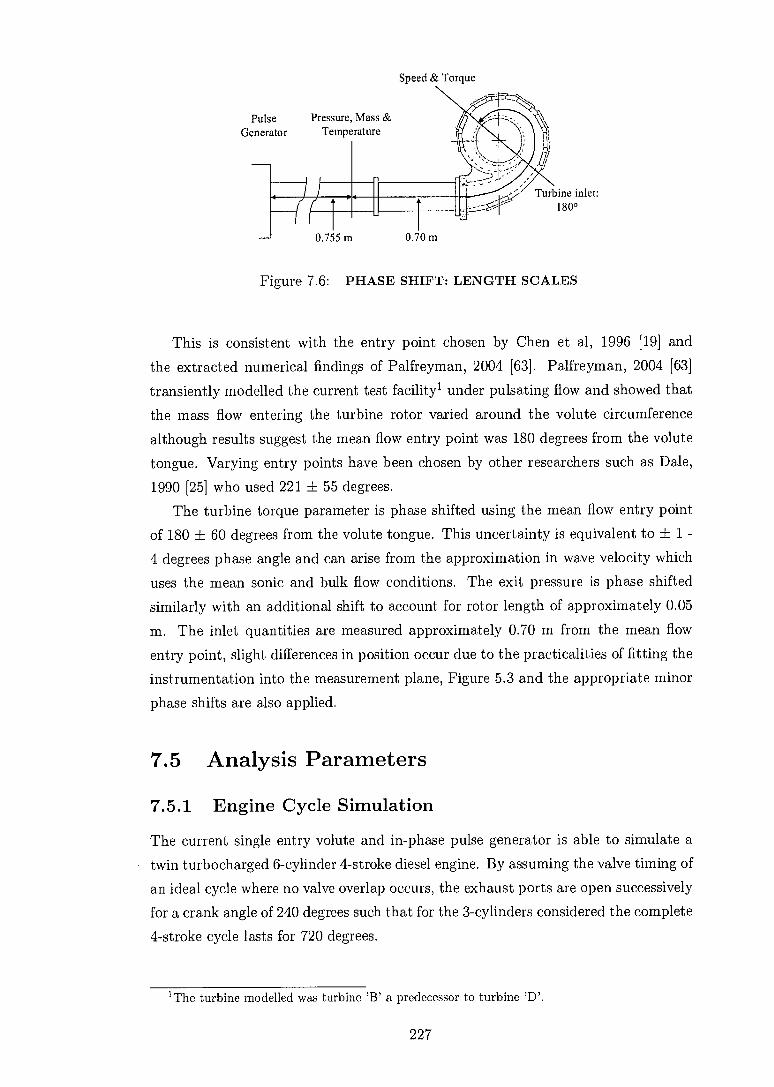
Pulse Pressure, Mass & Generator Temperature

Turbine inlet: 180°

0.755 m 0.70 m

Speed & Torque

Figure 7.6: PHASE SHIFT: LENGTH SCALES

This is consistent with the entry point chosen by Chen et al, 1996 [19] and the extracted numerical findings of Palfreyman, 2004 [63]. Palfreyman, 2004 [63]

transiently modelled the current test facilityl under pulsating flow and showed that

the mass flow entering the turbine rotor varied around the volute circumference although results suggest the mean flow entry point was 180 degrees from the volute tongue. Varying entry points have been chosen by other researchers such as Dale,

1990 [25] who used 221 ± 55 degrees. The turbine torque parameter is phase shifted using the mean flow entry point

of 180 ± 60 degrees from the volute tongue. This uncertainty is equivalent to + 1 -4 degrees phase angle and can arise from the approximation in wave velocity which uses the mean sonic and bulk flow conditions. The exit pressure is phase shifted similarly with an additional shift to account for rotor length of approximately 0.05

m. The inlet quantities are measured approximately 0.70 m from the mean flow entry point, slight differences in position occur due to the practicalities of fitting the

instrumentation into the measurement plane, Figure 5.3 and the appropriate minor

phase shifts are also applied.

7.5 Analysis Parameters

7.5.1 Engine Cycle Simulation

The current single entry volute and in-phase pulse generator is able to simulate a twin turbocharged 6-cylinder 4-stroke diesel engine. By assuming the valve timing of

an ideal cycle where no valve overlap occurs, the exhaust ports are open successively for a crank angle of 240 degrees such that for the 3-cylinders considered the complete

4-stroke cycle lasts for 720 degrees.

1. The turbine modelled was turbine 'B' a predecessor to turbine 'D'.

227

The equivalent engine speed Nengine (RPM) can be deduced in relation to the

pulse generator frequency, f (Hz) by Equation 7.17. Where n is the number of strokes (4-stroke), G is the number of groups (1 group), C is the number of cylinders in a group (3-cylinders). The frequencies at which the experimental tests were performed are 20, 40, 60 and 80 Hz giving an equivalent engine speed of 800, 1600, 2400 and

3200 RPM respectively.

n f Nengine = 60 • —

2 CG (7.17)

7.5.2 Cycle-Average Efficiency & Energy Weighted Average

It is possible to calculate a cycle-averaged isentropic efficiency viz. Karamanis et al., [43] that is independent of phase shifting, Equation 7.18. It represents the ratio of energy extracted by the turbine per pulse cycle divided by the isentropic energy

flowing into the system per pulse cycle.

(qt-s)avg fBOBo Wcict(t) • dt r •

io Wt-s,is(t) • dt (7.18)

A method to estimate the corresponding cycle-averaged velocity ratio (U2/Cis) has not been given in literature. This is required not only to determine the operating point of the turbine but also to determine the equivalent quasi-steady cycle-averaged efficiency. The method presented weights the velocity ratio in a similar manner

to Equation 7.18 and hence is compatable. The averaging technique is given by

Equation 7.19, where x(t) is the generic variable to be averaged which is weighted

in terms of the instantaneous isentropic power. This more appropriately weights such variables by relating the importance of the discrete variable measurement to the available energy associated with that point; this is a combination of mass flow

rate, pressure ratio and temperature.

fo9 [x(t) • Wi,,i8 (t)] • dt xis ,avg = re •

Jo Wt-8,13(t) • dt (7.19)

The averaging technique given by Equation 7.19 can be shown to be equivalent to Equation 7.18 when averaging efficiency, illustrated by Equation 7.20, where the

generic variable x(t) is replaced by the instantaneous efficiency 7/t_s. This shows

that Equation 7.19 may be used to weight a generic variable and in particular the velocity ratio to give a corresponding value to the cycle-averaged efficiency.

228

( 71t—s)avg f: [nt_s(t) • • dt

foe Wt-8,is(t) • dt

f09 Wact(t) • dt = r

joe t-8,is(t) • dt (7.20)

The use of Equation 7.19 allows the corresponding quasi-steady cycle-averaged

efficiency to be estimated. From this it may be determined how the turbine stage efficiency varies under pulsating flow in comparison to its steady flow performance.

In order to calculate the quasi-steady cycle-averaged efficiency, at each instant in time the measured instantaneous velocity ratio is used to determine the equivalent steady state efficiency from the measured performance maps. These instantaneous quasi-steady efficiencies can then be averaged over a pulse cycle using Equation 7.19 giving the corresponding quasi-steady efficiency to Equation 7.18.

7.5.3 Strouhal Number

In order to assess the importance of flow unsteadiness of a system, when a reduced frequency analysis is carried out, the level of unsteadiness is represented by a di-mensionless number: the Strouhal number. It relates the significance of the gas

dynamic frequency to the frequency of the unsteady event, for us the frequency of the pulse. A normalised Strouhal number (St.*) can be defined for this work as shown by Equation 7.21. Where f is the frequency of oscillation, L a characteristic

length, U the mean gas velocity, 0 the pulse period as a fraction of the cycle period

and the factor 1/2 is used to normalise the frequency such that the pulse period constitutes half the cycle period. The definition of 0 may be seen more clearly in reference to Figure 7.7 noting the pulse period is based on the pulse generator open-ing and not the measured period as this may contain wave reflections. The present pulse generator is open for 120 degrees per revolution giving a pulse fraction, 0 of

1/3.

St.* = f_L 1

U 20 (7.21)

The Strouhal number is normally used in relation to the driving gas velocity but it was found useful to have a similar parameter based on the mean speed of an acoustic wave ̀ Ei', the acoustic normalised Strouhal number (St.(a)*). This can give information to the onset of unsteady effects in relation to the acoustic travel time.

229

fL 1 St.(a)* = St*M = a 20 (7.22)

Cycle Period 4 p

Pulse Period

Time

Figure 7.7: STROUHAL NUMBER: SCALE DEFINITIONS

The definition of which is given by Equation 7.22, where St.* is scaled by the Mach

number, M to give St.(a)*. An acoustic Strouhal number has been employed by Fatsis et al., 1995 [33] and

Engeda et al., 2003 [31] to determine the importance of pressure wave propagation within compressors. For uni-directional wave propagation, the acoustic Strouhal number can be extended to include the mean flow velocity to give a Strouhal num-ber based on the mean velocity of an isentropic pressure wave, the pressure wave normalised Strouhal number St.(p)*, Equation 7.23. Where again St.* is scaled by the Mach number to give St.(p)*. Experimentally this parameter was found help-ful in assessing the unsteady influence in the measurement of the point-by-point instantaneous efficiency.

M fL 1 St.(p)* = St*

M +1 U + a 20 (7.23)

Traditionally a St. of 0.1 has been used as the limit of steadiness where unsteady effects become increasingly more significant with increasing value. The scaling of St.* with the Mach number to give the St.(a)* and St.(p)* allows a single number to be used to depict the onset of various unsteady modes with consistency as shown later in Section 7.6. Tables 7.3 - 7.5 illustrates the typical Strouhal numbers for the various length and frequency scales of importance to the present test conditions.

With reference to Section 7.5.1, the Strouhal number for a generic engine con-figuration can be found by combining Equations 7.17 and the required normalised Equation 7.21 - 7.23, where 0 is equal to x/3. The symbols have been defined previously in Section 7.5.1 and noting: For CG < 3 —). x = C else x = 3.

230

2 N 1 L 1 St.* = CG engzne

n 60 2 U x/3

1 CG L 1 = Nengine 20 n

(7.24)

Table 7.3: GAS VELOCITY STROUHAL NUMBER: EXPERIMENTAL AVERAGE

Pulse

Frequency

(Hz)

Pulse Generator

to Rotor Inlet

(1.45 m)

Measurement Plane

to Rotor Inlet

(0.7 m)

Volute Inlet

to Rotor Outlet

(0.4 in)

Turbine

Blade Passage

(0,05 m)

20 0.70 0.23 0.11 0.011

40 1.40 0.47 0.23 0.022

60 2.10 0.70 0.34 0.033

80 2.80 0.93 0.46 0.044

Table 7.4: ACOUSTIC STROUHAL NUMBER: EXPERIMENTAL AVERAGE

Pulse

Frequency

(Hz)

Pulse Generator

to Rotor Inlet

(1.45 m)

Measurement Plane

to Rotor Inlet

(0.7 in)

Volute Inlet

to Rotor Outlet

(0.4 m)

Turbine

Blade Passage

(0.05 m)

20 0.12 0.057 0.033 0.004

40 0.24 0.11 0.065 0.008

60 0.36 0.17 0.098 0.012

80 0.47 0.23 0.13 0.016

Table 7.5: PRESSURE STROUHAL NUMBER: EXPERIMENTAL AVERAGE

Pulse

Frequency

(Hz)

Pulse Generator

to Rotor Inlet

(1.45 m)

Measurement Plane

to Rotor Inlet

(0.7 m)

Volute Inlet

to Rotor Outlet

(0.4 m)

Turbine

Blade Passage

(0.05 m)

20 0.10 0.046 0.025 0.003

40 0.20 0.092 0.051 0.006

60 0.30 0.14 0.076 0.009

80 0.41 0.18 0.10 0.012

231

7.6 Experimental Results and Discussion

In this section the results of the experimental investigation are presented and dis-

cussed. Due to the large number of graphs associated with each test condition a brief outline of their presentation order and format is given.

For each turbine test speed 50 to 100 % equivalent speed, the measured data and the processed data are presented for the range of pulse frequencies 20 to 80 Hz. The measured data are presented for a single pulse cycle, this is plotted against

the phase angle of the pulse generator, where zero degrees is designated the start of the area opening of the pulse generator. The measured data are the static inlet

pressure, temperature, mass flow rate, static exit pressure, turbine torque, speed and for comparison the efficiency is also given. This is followed by the comparison of the inlet and exit static pressures and the comparison of the isentropic and actual turbine powers for each pulse frequency, similarly this is plotted against phase angle. Finally, the performance parameters of the turbine are presented, these are given

in a similar format to that of the steady state experiments of Section 6.4, where the total-to-static efficiency is plotted against the velocity ratio and the mass flow

parameter is plotted against the pressure ratio for each pulse frequency. After the complete set of data is presented for the fixed turbine test speeds, a compressed set of data is presented which illustrated the effect of a fixed pulse frequency and

varying turbine speed. For compactness the data from only the instantaneously measured temperature

test condition of 70 % equivalent speed, 20 - 80 Hz pulse frequency are plotted within this chapter in Figures 7.10 - 7.12, the remaining test condition plots are given in Appendix F in Figures F.1 - F.23.

7.6.1 Mass Flow Rate Correction

The effect of the temperature, property and Mach number hot-wire correction can be seen by Figure 7.8 for a equivalent speed of 70 %, noting the calibration ref-erence temperatures for the hot-wire is the time-averaged flow temperature. The corresponding cycle average values and percentage difference from the fully corrected measurement is given by Table 7.6.

It is evident that without temperature correction the hot-wire under predicts the mass flow rate at peak conditions and over predicts at the low flow regions due in large to the temperature effect. The overall cycle average values of the uncorrected signals show little deviation from the true corrected value with a maximum deviation of < ± 10 %, Table 7.6. The local deviations are much greater, at 20 Hz the mass flow rate is under predicted up to 37 % and over predicted up to 49 %, the equivalent for 80 Hz is 24 % and 54 % respectively.

232

2 0.6

SI 0.5

0.4 c.

j 0.3

0.2

0.1

360 300 300 360 0 60 120 180 240 0 60 120 180 240

0.8

Mas

s Flo w

Rat

e (K

O)

Phase Angk (Degrees)

(b) 40 HZ

— With Temperature Correction

No Tempereare Correction

— No Mach number or Temp Correctoin

0.7 -

0.6

0.5

0.4 -

0.3

Mas

s Flo

w R

ate (

Kg/

s)

0.2

0.8

0.1

0 60 120 180 240 300 360 60 120 180 240 300 360


(a) 20 HZ

Mas

s Flo

w R

ate

(Kg/

s)

— With Temperature Correction

— No Terrperature Correction

— No Mach Number or Temp Correction

0.9

0.8 -

0.7

These results indicate that temperature, property and Mach number corrections

are important for hot-wire pulsed flow measurements. Without correction large

instantaneous errors can occur whose presence may be masked by accurate cycle

averaged values.

Phase Angle (Degrees) Phase Angle (Degrees)

(c) 60 HZ

(d) 80 HZ

Figure 7.8: PULSATING FLOW RESULTS: TINST 70 % EQUIVALENT SPEED, 20 - 80 Hz, MASS FLOW RATE CORRECTION

Table 7.6: HOT-WIRE CORRECTION: TINST 70 % EQUIVALENT SPEED, CYCLE AVERAGED COMPARISON

Parameter 20 Hz

Mean %

(kg/s) Diff

40 Hz

Mean %

(kg/s) diff

60 Hz

Mean %

(kg/s) diff

80 Hz

Mean %

(kg/s) diff

Fully Corrected

No Temp, Property

Correction

No Temp, Property,

Mach No. Correction

0.348

0.318

0.341

-

-9.1

-2.0

0.354

0.339

0.375

-

-4.2

+5.6

0.370

0.361

0.395

-

-2.4

+6.8

0.372

0.365

0.408

-

-1.9

+9.7

233

7.6.2 Instantaneous Temperature Measurement

The results demonstrate that the dual probe hot-wire technique of Section 5.4.2 is able to measure the instantaneous temperature of a realistic cold flow turbocharger

pulse cycle. A comparison between an isentropic calculated temperature, Equa-tion 5.16 and that measured using the dual probe hot-wire technique is given by Figure 7.9 and Table 7.7. These results show that the minima and maxima temper-ature values of the two techniques correlate well although the calculated temperature has greater local fluctuations. The smoother measured signal is not thought to be

due to the response rate of the hot-wire as its ability to respond has been demon-

strated by the square wave test which gave a response of 7.7 kHz. A significant difference occurs in the assessment of temperature at 20 Hz, Fig-

ure 7.9(a). The measured temperature departs from the isentropic compression assumption and peaks 18 degrees earlier in the pulse cycle at a phase angle of 60 degrees. This change in peak position has a significant influence on the correction

of the hot-wire data and hence for the calculated energy content of the gas. The measured temperature is assessed from the mass flux data and results in a true in phase measurement of both the temperature and mass flow rate, which allows the

hot-wire data to be accurately corrected. For large variations in temperature these phase differences become important,

at an equivalent speed of 100 % and a pulse frequency of 20 Hz the overall static temperature variation is 91 K. The influence of the calculated temperature may be seen in the mass flow measurement of Figure F.16(c) where an artificial offset occurs in the rising region of the mass flow rate, which is not seen by the other measure-ments. This effect is cascaded to the assessment of isentropic power, Figure F.17(e)

and the performance parameters, Figure F.18(a) and Figure F.18(e). The results have shown the importance of accurately assessing the temperature

as its variation can be large over a pulse cycle. If the instantaneous temperature can not be measured directly, the results of Figure 7.9 have indicated that the isen-tropic compression assumption, Equation 5.16 is a reasonable approach. The general

trends, the maxima and minima values are well predicted although an appreciation

of the possible errors must be considered.

234

Measured To - Measured Ts - Calcuksted Ts

Table 7.7: PULSATING FLOW RESULTS: MEASURED AND ISENTROPIC TEMPERATURE COMPARISON

Speed 20 Hz

Temperature (K)

40 Hz 60 Hz 80 Hz

Mean 332.6 334.5 334.2 334.3

70 % Isentropic Max 373.5 363.3 357.2 357.9

(Outer Limb) Min 314.2 312.0 313.1 314.7

Diff. 59.3 51.3 44.1 43.2

Mean 331.5 332.4 333.0 332.4

70 % Measured Max 375.6 362.2 361.8 362.2

(Outer Limb) MM 312.7 316.4 315.9 311.6 Diff. 62.8 45.8 45.9 50.6

400 400

- Measured To

-Measured Ts 380 - Ca

380 - Calculated Ts

• 360

FL' 15 340

3 320 -

300 300

0 60 120 180 240 300 360 0 60 120 180 240 300

360

Phase Angle (Degees)


(a) 20 HZ

(b) 40 HZ

1 360

X 340

320

60 120 180 240


(c) 60 HZ

400

380

1 360

0

X 340

320

300

300 360 60 120 180 240 300 360


(d) 80 HZ

400

380

0

0 360

0

340

- Measured To

- Measured Ts

- Cakolated Ts

(AV\- Spj"

320

300

Figure 7.9: PULSTATING FLOW RESULTS: TINST 70 % EQUIVALENT SPEED, 20 - 80 Hz, MEASURED INSTANTANEOUS TEMPERATURE

COMPARISON

235

7.6.3 Inlet and Exit Static Pressure

The pulse generator allows flow between the reference angle of 0 - 120 degrees with

a peak area opening at 60 degrees. The general trends show that pulse frequency has a large effect on the resultant pulse shape, the measured inlet pressure is a

superposition of the original pulse and the numerous pressure wave reflections from

the turbine and other components of the pipe work, Figure 7.10(a)2. It may be seen

that the pulse wave form changes significantly between a pulse frequency of 20 and 80 Hz. As the pulse frequency increases a reduction in the pressure wavelength occurs

which allows the various components of the wave to become separated and visible. The cycle wavelength based on the acoustic velocity of the gas gives a value of 18.3, 13.7, 9.2 and 4.6 m for the pulse frequencies of 20, 40, 60 and 80 Hz respectively; noting the generated pulse width is a 1/3 this value. At the higher pulse frequencies

the fluctuation of free stream conditions is reduced which may be beneficial for the turbine performance as this may result in reduced excursion from the turbines peak

efficiency point. Due to the simple pulse form produced by the pulse generator the St.(a)* is

a useful approach to infer for a simple wave when the left and right travelling

pressure waves may become separated. The St.(a)* is the ratio of a characteristic

length divided by the pulse wavelength. The characteristic length in this instance is between the pulse generator and the rotor inlet (1.45m). Considering a simple wave reflecting back and forth over this length, as the frequency of this pulse increases the

wavelength reduces and the St.(a)* increases. When this ratio becomes significant

the left and right travelling waves may become more significantly separated. The

St.(a)* given in Table 7.4 for a pulse frequency of 20 Hz has a value of 0.12. Using

0.1 as the apparent limit of steadiness would seem consistent as the experimental

observations of Figure 7.10(a)2 illustrates that the 20 Hz pulse encompasses a larger phase angle then provided by the pulse generator. A further increase in pulse

frequency allows the individual pressure peaks to become further apparent. The combined influence of the pulse amplitude and turbine speed for a fixed pulse

frequency may be seen by Figure F.19. The general shape of the pulse waveform show similar trends with increasing amplitude and equivalent speed, although it is seen that the pulse width of the pressure pulse becomes larger. This results from the influence of the reflected portions of the pressure pulse which due to the larger flow rates do not get so rapidly damped by the turbine and can superimpose on the original pulse resulting in a migration of the peak pressure for the 20 and 40 Hz pulse and an increase in amplitude of the reflected pressure peaks of the 60 and 80 Hz pulse which now become a more dominant feature of the pulse.

2Additional graphs: Pressure results of Figures F.1 - F.23

236

380

S2 360 -

N 320

300

.0 e, 0.98 -

0.96 -

0.94

1.08

1.06 -

1.04

1.02

—20 Hz —40 Hz — 60 Hz 110 Hz

— 2014. 40 Hz — 60 Hz —80 Hz

0.5

1 0.4

0.3

0.2 -

0.1

0

0.9

0.8 -

0.7

0.6

10 -

12

2 Effic

ie ncy

(Tot

al-St

atic)

-3

665 688

698

696 ES

694

692

680 696

0. 694 675

-§ 692

670 1

'.666 ,2 690

710

700 an 44.

-§ 690

680

670

—20 Hz 40 Hz

— 20 Hz

40 Hz

— 60 Hz 80 Hz

O 60 120 180 240

300

360 60 120 180 240 300 360



(a) STATIC PRESSURE

(b) STATIC TEMPERATURE

O 60 120 180 240

300 360 0 60 120 180 240 300 360

Phase .Angle (Degrees)


(c) MASS FLOW RATE

(d) EXIT STATIC PRESSURE

60 120 180 240 300 360 0 60 120 180 240

300

360



(e) TURBINE TORQUE

(f) EFFICIENCY

O 60 120 180 240 300 360 0 60 120 180 240

300

360



(g) TURBINE SPEED: 20, 40 Hz (h) TURBINE SPEED: 60, 80 Hz

Figure 7.10: PULSATING FLOW RESULTS: TINST 70 % EQUIVALENT SPEED, 20 - 80 Hz, INSTANTANEOUS MEASURED PARAMETERS

237

0 60 120 180 240 300 360

60 120 180 240

300

360



1.03 1.9

1.8

17 1.01

E 1.6

1 a IS :_d

0.99 X 1.4

0.98 N 1.3

1.2

0.97 1.1

0.96 1

1.02

- Inkl Exit

X 1.6

-2, 1.4

1.2

Stat

ic E

xit P

ress

ure

(Bar

)

0.97

▪ 1.6

• 1.5

1.4 E • 3

114 1.2

1.7

1.8

1.1

60 120 180 240 300 360

Static

Exi

t Pre

ssur

e (B

ar)

60 120 180 240 300 360

- lokt 1.07

- 1.06

- 1.05

- 1.04

- 1.03

1.02

1.01

- Stat

ic E

xit P

ress

ure

(Bar

)

0.99

- 0.98

0.97

1.7

1.6

tt 1.5

1.4

1 1.3

H

- Wel

- Exit

1.06

1.05

- 1.04

- 1.03

- 1.02

- 1.01

jr\- 1

0.99

- 0.98

0.97

60

50 - Want (kW) -

Wen (kW)

40

20

1 0 -

60 120 180 240


-10

300 360 60 120 180 240


300 360

(a) INLET/EXIT STATIC PRESSURE: 20 HZ (b) INLET/EXIT STATIC PRESSURE: 40 HZ


(c) INLET/EXIT STATIC PRESSURE: 60 HZ (d) INLET/EXIT STATIC PRESSURE: 80 HZ

80

70 - Want (kW)

- Wisen (kW) 60

50

• 40 -

1 30

20

10

0

-10 -10

60 120 180 240 300 360 60 120 180 240 300 360

Phase Angie (Degrees) Phase Angle (Degrees)

(e) ISENTROPIC/ACTUAL POWER: 20 HZ (f) ISENTROPIC/ACTUAL POWER: 40 HZ

(g) ISENTROPIC/ACTUAL POWER: 60 HZ (h) ISENTROPIC/ACTUAL POWER: 80 HZ

Figure 7.11: PULSATING FLOW RESULTS: TINST 70 % EQUIVALENT

SPEED, 20 - 80 Hz, STATIC PRESSURES AND POWERS

238

For the range of turbine speeds, the 20 Hz plot of Figure F.19(a) exhibits a plateau in minimum stable pressure, 1.08 and 1.3 Bar respectively for the equivalent

speed of 50 % and 100 %. These values are a similar in magnitude to the centrifugal pressure head that would be developed due to radial equilibrium. Using the mean turbine radii would give approximate values of 1.04 and 1.15 Bar respectivly for the

equivalent speed of 50 % and 100 %. The measured minimum values are larger then predicted by radial equilibrium and may be due in part to mass flow leakage through

the pulse generator whilst in the fully closed position. The exit pressure measurement is located 9.5 mm downstream of the turbine

trailing edge. The results show a similar change in trend with increased pulse fre-quency for all measured speeds, Figure F.20. An initial spike in pressure occurs at

the start of the pulse with a subsequent sharp reduction to sub-atmospheric condi-tions which follows an approximately inverted shape of the upstream pulse. Typical minimum values seen were sub-atmospheric by about 4 % of the peak upstream

gauge pressure pulse, ranging between - 0.015 to - 0.12 Bar for the 20 Hz pulse and 50 to 100 % equivalent speed respectively. This type of behaviour have been seen previously by Nikpour, 1990 [61], Karamanis, 2000 [42] and numerically by

Palfreyman, 2004 [63], noting that the numerical results showed a greater degree of damping of the exit pulse which was suggested to be due to the close proximity of

the outlet boundary condition.

7.6.4 Mass Flow rate

The mass flow rate exhibits a damped behaviour similar to the pressure trace with all

the main features being mirrored, Figure 7.10(c)3. For these results the arrival of the

pressure pulse coincides with the arrival of the mass flow pulse, which is consistent with the choice of phase shift given in Section 7.4.4, where the isentropic energy for these measurement conditions is transported with the speed of the pressure wave.

The results show a much greater fluctuation is mass flow rate then previously

measured on this test facility under similar operating conditions, Hakeem, 1995 [36], Chen, 1996 [19], Su, 1999 [75] and Karamanis, 2000 [42]. It is thought that this is

directly due to the improvements made in the measurement accuracy of the hot-wire by the application of the temperature, property and Mach number corrections and the automated 36-point grid which was applied for each test condition. This results in the mass flow rate that better mirrors the pressure trace.

The minimum and maximum mass flow rates seen in the experimental test con-ditions both occurred for the 20 Hz pulse with a minimum value of 0.045 kg/s at 50

% speed and 1.38 kg/s at 100 % equivalent speed.

`Additional graphs: Mass flow rate results of Figures F.1 - F.23

239

A higher minimum was seen for the higher pulse frequencies which is attributed

to the turbine having insufficient time to consume the air mass within the pipe work

before the next pulse cycle, Dale, 1990 [25]. It may be seen from Figure F.19(f) that at 40 Hz pulse frequency and 90 - 100

% equivalent speed the mass flow rate does not directly mirror the pressure trace. An additional peak is apparent in the mass flow rate trace occuring at a phase angle

of 200 degrees. This type of behaviour has also been seen by Hakeem, 1995 [36], Su, 1999 [75] and Karamanis, 2000 [42] at lower speeds and mass flow rates but at a similar pulse frequency. It has been suggested that this may be due to back flow coupled with the hot-wires inability to distinguish flow direction. The present

results show similar trends but at higher mass flow rates which would suggest that back flow is unlikely to be the explanation; for back flow to occur the mass flow rate would be required to reduce to zero prior to reversing which from the fast response of the hot-wire probe, 7.7 kHz would be seen as a rapid decrease to zero before a

rapid increase to its required value, this type of behaviour has not been seen. With reference to the 100 % equivalent speed, back flow would require a rapid change of mass flow rate of 1 kg/s without the hot-wire responding, this is unlikely to be the case as there is no driving force of sufficient magnitude to cause such a phenomenon.

By additional consideration of the 60 Hz and 80 Hz pulse frequencies of Fig-ures F.13(c) - F.16(c) it may be seen that the peak observed for the 40 Hz curve follows in sequence the wave reflection peaks of the 60 Hz and 80 Hz plot which

follow the pressure trace. Although no conclusive explanation may be given for the 40 Hz peak it is likely to be related to the flow induced by a similar driving force as

the 60 Hz and 80 Hz plot.

7.6.5 Temperature

The temperature waveforms presented by Figures F.1 - F.23 are calculated using the isentropic compression assumption, Equation 5.16 whilst Figure 7.10(b) is in-stantaneously measured using the dual probe technique. The isentropic compression assumption results follow the trends of the pressure trace due to their direct rela-tionship. The largest variation in temperature occurs for the 20 Hz pulse, due to the greatest variation in pressure, for a 100 % speed the temperature varies between

303 - 394 K, whilst at 50 % speed varies between 322 - 357 K, a 91 and 35 K varia-tion respectively. These variations generally decrease with pulse frequency although some special cases exist where local pressure reflections such as the 60 Hz pulse that exhibits a marginally lower temperature variation then the 80 Hz curve.

240

7.6.6 Speed An accurate measure of instantaneous speed is crucial in obtaining an accurate

torque measurement. Figures 7.10(g) - 7.10(h)4 shows the effect of pulse frequency

on turbine speed, where the amplitude of speed fluctuation reduces with increased pulse frequency following the combined effects of the mass flow rate, pressure and temperature. The turbine speed fluctuations associated with the pulsed air flow are all small. For the 20 Hz pulse the speed variation is approximately 13.2 - 40.4 RPS for 50 - 100 % equivalent speed respectively and equivalent to 2.6 % and 4.1 % of the mean speed. Whilst for the 80 Hz pulse the speed variation is reduced to 2.3 - 7.0 RPS for 50 - 100 % equivalent speed respectively and equivalent to 0.45 % and 0.70

% of the mean speed. Due to the variation in total temperature through the pulse cycle the equivalent speed fluctuations are greater. This becomes important in the consideration of the equvialent steady state working point of the turbine discussed in Section 7.6.9. These variations in equivalent speed for 20 Hz and 80 Hz respectively

are 4.1 - 14.3 % and 3.4 - 7.7 % for 50 - 100 % equivalent speed. It has been possible to capture small fluctuations in speed by ensembling over a

sufficiently large number of cycles which subsequently allows a non-aggressive filter to be used to smooth out high-frequency noise as described in greater detail in Sec-tion 7.4.3. At 50 % equivalent speed and 80 Hz pulse frequency, Figure F.1(h) shows the occurance of 0.07 RPS amplitude fluctuations at a frequency of 800 Hz which directly match the observed features of the isentropic power trace, Figure F.2(h) which use independent measuring instruments and this demonstrates the quality of the measurements. These results would suggest the apparent speed sensor resolution

is < 0.02 RPS at 1000 Hz, this being the lowest value of the filter cut-off point at

80 Hz pulse frequency.

7.6.7 Torque The speed data can be differentiated and multiplied by the moment of inertia to give the acceleration torque under pulsating flow conditions; when added to the mean and fluctuating transferred torque components, Section 5.4.5 enables the cal-culation of the instantaneous actual torque, Figure 7.10(e)5. In general the torque plots follow that of the mass flow rate and to a lesser extent the pressure and tem-perature variations, the weighting of these are consistent with the isentropic power, Equation 7.3.

4Additional graphs: Speed results of Figures F.1 - F.23 "Additional graphs: Torque results of Figures F.1 - F.23

241

A pulse frequency of 20 Hz, Figure 7.10(e) although seemingly uneventful can be used to demonstrate some important features. In the latter half of the pulse cycle the derived torque value is constant with a value of approximately zero. In order to derive this constant torque value the deceleration of the turbine must be linear suggesting there is no additional driving force on the system. More importantly to

derive a torque of zero the negative torque calculated from the turbines deceleration must equal the transferred torque measured by the load cell, demonstrating that the turbine is purely acting as a flywheel. More exacting the turbine consumes work to produce a centrifugal pressure head which results in a marginally sub zero torque measurement, discussed in Section 7.6.9.

7.6.8 Isentropic and Actual Power

The actual and isentropic work plots for the various frequencies are shown by Fig-

ure 7.117, the isentropic work has been phased shifted according to the method described in Section 7.4.4. The instrumentation required to measure these quanti-ties are independent of each other and show that the turbines actual work output

generally follows the variations in isentropic work. The improvements in the post processing techniques most noticeably with the

torque and mass flux measurements have resulted in not only primary but sec-ondary features being mirrored in both the isentropic and actual power graphs as it

has already been indicated earlier. This should allow an improved estimate of the instantaneous efficiency and clarifies the phase shift techniques of Section 7.4.4.

In the measurement of a point-by-point instantaneous efficiency of the turbine rotor it is important to note that the energy measured upstream is eventually seen by the rotor, but with some time delay due to travelling of the pressure wave and the bulk flow. The energy waveform may change shape between the measurement plane and the rotor inlet, the St.* and S t (p)* are useful in estimating how important this effect is. The Strouhal numbers for the various test conditions are given by Table 7.3 and Table 7.5 where the length scale of interest is between the measurement plane

and rotor inlet (0.7 m). Using a St.* value of 0.1 as the limit to steadiness would suggest that unsteadiness is present in all the test conditions, that is the turbine stage is not quasi-steady. The influence of the St.* number is not visually obvious in these results and is therefore discussed in Section 7.6.9 with reference to the performance parameters.

6A typical value for the minimum plateau is - 0.23 Nm, the reasons for this reduced value are given in Section 7.6.9

7Additional graphs: Isentropic and actual power results of Figures F.1 - F.23

242

The St.(p)* is useful for estimating when the shape change of the waveform trav-elling between the measurement plane and the rotor inlet will become significant by

a movement of the various peaks and troughs. The importance of this will be further discussed in Section 7.6.9. Using a limit to steadiness of 0.1 would suggest above 40 Hz some change in the waveform may occur between the measurement plane and rotor inlet, this can be seen most evidently by the 80 Hz curve of Figure 7.11 where

the St.(p)* number is 0.18. The location of the secondary peak of the isentropic

power curve is slightly out of phase with the actual power curve.

7.6.9 Performance Characteristics

The pulsating flow performance graphs for unsteady flow are presented in the similar

format to the steady state graphs of Section 6.4.

Mass Flow Characteristic

The instantaneous psuedo-nondimensional mass flow parameter (MFP) and the total-to-static pressure ratio of the turbine stage for fixed equivalent equivalent

speeds of 50 - 100 % are given by Figure 7.128. These demonstrate the filling and

emptying of the volute as shown by the hysteresis loop surrounding the steady state curve. There are three main modes of behaviour of the mass flow rate with respect to the pressure as the pulse frequency increases. The first mode occurs when the oscillation in pressure is sufficiently slow so that the mass flow has time to fill the

volute volume incrementally with pressure and quasi-steady state conditions are ob-served. Although not seen experimentally this is thought to occur when the St.* is below a value of approximately 0.1. The second mode occurs in Figures 7.12(e) - 7.12(f), where the pulse frequency is 20 and 40 Hz, the pulse is sufficiently rapid that the volute volume is not filled incrementally with pressure and a hysteresis between the mass flow and pressure is observed at the measurement plane. In such modes the filling and emptying of the volute and associated pipe work is limited by the gas velocity as a finite amount of time is required for the gas to accumulate and

subsequently be consumed by the turbine. The second mode may be seen by considering the St.* and St.(p)* numbers

of Table 7.3 and Table 7.5. The length scale of concern is 0.7 m, which gives

at 20 Hz a St.* and St.(p)* number of 0.23 and 0.046 respectively. Using 0.1 as

the limit of steadiness would suggest unsteady effects are significant (St.*), whilst

the variation of the pressure wave over the characteristic length is not significant. These observations are consistent with Figure 7.12(e) where the unsteady curve encapsulates the steady state curve, a filling and emptying behaviour.

'Additional graphs: MFP and PR results of Figures F.1 - F.23

243

Effic

ienc

y (T

otal

-Sta

tic)

0.5

Velocity Ratio (U2/Cis)

(a) EFF t _s Vs U21C2s : 20 HZ

-2

0 0.5

15

0

g 1,, Steady State

—a-- 40 Hz


(b) EFF t_s Vs U2/Cis: 40 HZ

-2

0.5

15

0.5

15


Velocity Ratio (112C is)

(c) EFF t_ s Vs U2IC28 : 60 HZ

(d) EFF t_ s Vs U2ICts: 80 HZ

10

0

1.5 2

25

1.5 2

25

Pressure Ratio (Total-Static)


(e) MFP Vs PR t_s : 20 HZ

(f) MFP Vs PR t_s : 40 HZ

1.5

2

25

1.5

2

25

Pressure Ratio (Total-Stade)


(g) MFP Vs PR t_ s : 60 HZ

(h) MFP Vs PR t_s : 80 HZ

Figure 7.12: PULSATING FLOW RESULTS: TINST 70 % EQUIVALENT SPEED, 20 — 80 Hz, INSTANTANEOUS PERFORMANCE PARAMETERS

244

Table 7.8: STEADY LIMIT STROUHAL NUMBER (0.1): PULSE FREQUENCY

Pulse Generator

to Rotor Inlet (1.45 m)

Measurement Plane

to Rotor Inlet (0.7 m)

Volute Inlet to Rotor Outlet

(0.4 m)

Turbine

Blade Passage (0.05 m)

St.* St.(a)*

2.9 20

8.6

43

18

79

180

670

At 40 Hz the St.* and St.(p)* number is 0.47 and 0.092 respectively and suggests

that the pressure variations within the characteristic length are becoming significant. The third mode occurs in Figures 7.12(g) - 7.12(h), where the pulse frequency is 60 and 80 Hz. In such modes the filling and emptying of the volute and pipe work is influenced by the variation in the gas velocity within the volute. This is driven by the pressure wave which now significantly changes within the volute. Again considering

the St.* and St.(p)* numbers of Table 7.3 and Table 7.5 give a value of 0.70 and 0.14 respectively at 60 Hz. Both numbers suggest unsteady effects are present. By comparison of Figures 7.12(e) - 7.12(h) the effect of the unsteadiness of the pressure

wave can be seen, the steady state curve is no longer encapsulated by the unsteady

curve. Table 7.8 gives the frequencies for the limit of steadiness for various length scales.

Efficiency Characteristic

The instantaneous total-to-static efficiencies for a complete pulse cycle are given by Figure 7.10(f) and also plotted against velocity ratio in Figure 7.129. The latter figure illustrates the large variance in the operating point of the turbine through

a pulse cycle. The largest velocity ratio range occurs for a pulse frequency of 20 Hz and decreases with increasing frequency following the decreasing range of the pressure ratio as per Equation 7.5.

The velocity ratio range at 20 Hz varies between 0.42 - 1.17 and 0.48 - 1.08

for 50 and 100 % equivalent speed respectively, whilst at 80 Hz this range reduces to 0.46 - 1.02 and 0.60 - 0.91 respectively'. The reduction in velocity ratio range is most evident at the higher equivalent speeds where greater mass accumulation occurs within the volute and associated pipework such that the turbine is unable to fully consume the available mass flow rate within a single pulse cycle. At the lower equivalent speeds the mass is better consumed and a larger variance in velocity ratio range occurs.

9Additional graphs: Efficiency and Velocity ratio results of Figures F.1 - F.23 19The range given encompass 95 % of the isentropic power of the pulse cycle.

245

As the pulse frequency increases the form of the measured instantaneous effi-ciency curve changes from a largely smooth trace to a highly fluctuating trace illus-trating the increasing importance of unsteady effects on the instantaneous turbine stage performance. There are three requirements in order to achieve an accurate measurement of instantaneous performance; firstly the phase shift between the ac-tual and isentropic power trace should be appropriate, secondly the hysteresis caused

by the filling and emptying of the volute and associated pipework should be small and thirdly the isentropic power waveform seen at the measurement plane remains

unchanged upto the rotor inlet. The first requirement is satisfied with consideration of the actual and isentropic

power traces presented in Section 7.6.8 which suggest the choice of phase shift veloc-ity and length scale are appropriate. The second requirement concerning the system

hysteresis is difficult to meet due to the inevitable volumes created by the volute and the associated pipe work leading to the measurement plane. The filling and

emptying of the volumes have been described previously in Section 7.6.9 and can not be avoided. The effect these volumes have on the instantaneous efficiency can be seen most clearly for a 20 Hz pulse frequency where the additional effects caused by the third requirement are small. At higher pulse frequencies the third requirement is more difficult to meet, this may be seen by the actual and isentropic power traces of Section 7.6.8 where an increase in phase shift occurs with the secondary peaks.

With particular reference to the measured instantaneous temperature test con-

dition of 70 % equivalent speed and 20 Hz pulse frequency, Figure 7.12. The large hysteresis loop seen in the mass flow parameter results in a relatively small range

hysteresis loop in the efficiency curve with a maximum efficiency variation of ap-

proximately 14 percentage points at a velocity ratio of 0.5 with the remainder of the pulse cycle following the trend of the steady state curve. There is a reduction in the value of efficiency of about 4 percentage points, the mechanism for these apparent

losses are not known. The observations seen in the efficiency trace are consistent with the previous dis-

cussion given in Section 7.6.9 in consideration of the St.* and St.(p)*, refer Table 7.3

and Table 7.5. Where the values indicate that the unsteady effects due to St.* are al-

ready significant at 20 Hz whilst the pressure wave influence on the velocity becomes increasingly significant above 40 Hz for the length scale between the measurement plane and the rotor inlet. The use of the Strouhal number has shown consistency in

these results and would suggest its use as a simple criteria for the suitable selection of a simulation code to capture the performance of the turbine stage under pulsating flow. It is suggested that for a St.* < 0.1 a zero dimensional quasi-steady model is

adequate, for a St.(p)* < 0.1 < St.* a 'filling and emptying' model is more suitable

and above this a 'wave action' model becomes more appropriate.

246

This criteria allows broader application and is idealised by a generic long pipe system such as an exhaust manifold where the choice of the suitable simulation code

can be assessed in a similar way. The length scale in the assessment of the Strouhal

number is based on the length of the pipe work. The various engine simulation codes used in industry universally model the tur-

bine rotor on a quasi-steady bases. This would seem reasonable in light of the St.*

number for an individual rotor passageway, refer Table 7.8 where the limiting fre-quency for quasi-steady flow is above the typical operating speed of an engine. The present results would indicate additional losses occur in the turbine stage under

pulsating flow. The St.* number suggests these losses are not directly attributed

to isolated loss mechanisms that occur within individual rotor passageways but are more likely the result of the gas dynamic effects that occur within the turbine stage.

Various models have been used to simulate the turbine stage, such as the 'filling and emptying' model of Baines et al, 1994 [4], the 'wave action' model of Chen

et al, 1996 [19] and the combination model of Conner and Swain, 1994 [22]. It is acknowledged that the turbine rotor and volute volume are an important part of the modelling process of turbocharger turbine systems, but the lack of experimental data has meant these models employ loss coefficients based on steady state correlations.

Further investigation is required to ascertain these unsteady loss mechanisms and

allow integration into the numerical models.

The variation in efficiency on a time basis is given by Figure 7.10(f)11. Negative

efficiencies may arise particularly at the lower equivalent speeds and pulse frequen-cies where a large proportion of the cycle can exhibit negative efficiency. Again with particular reference to the measured instantaneous temperature test condition of 70 % equivalent speed and 20 Hz pulse frequency, Figure 7.12. This shows that approximately 50% of the cycle has negative efficiency and this accounts for less

then 4% of the available isentropic power and hence minimises the impact on the overall efficiency. The negative efficiencies are a consequence of the negative torque measurements shown in Figure 7.10(e)12 . Experimentally Karamanis, 2000 [42] and

numerically Palfreyman, 2004 [63] have recorded negative torque values. These occur due to momentum transfer from the rotor to the gas as it passes through the rotor. This situation may arise at low pressure ratios where the tangential component of velocity at the turbine inlet is low. The high rotational speed of the turbine blades imparts momentum to the fluid such that the exit energy is greater then the inlet energy resulting in the negative efficiency, the Euler turbomachinery, Equation 7.25.

11Additional graphs: Efficiency versus phase angle results of Figures F.1 - F.23 12Additional graphs: Torque results of Figures F.1 - F.23

247

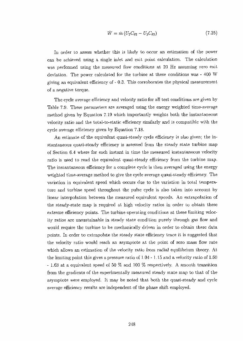
W = rh, (U2Co2 — U3Co3) (7.25)

In order to assess whether this is likely to occur an estimation of the power can be achieved using a single inlet and exit point calculation. The calculation was performed using the measured flow conditions at 20 Hz assuming zero exit

deviation. The power calculated for the turbine at these conditions was - 400 W giving an equivalent efficiency of - 0.3. This corroborates the physical measurement

of a negative torque.

The cycle average efficiency and velocity ratio for all test conditions are given by

Table 7.9. These parameters are averaged using the energy weighted time-average method given by Equation 7.19 which importantly weights both the instantaneous velocity ratio and the total-to-static efficiency similarly and is compatible with the

cycle average efficiency given by Equation 7.18. An estimate of the equivalent quasi-steady cycle efficiency is also given; the in-

stantaneous quasi-steady efficiency is assessed from the steady state turbine map of Section 6.4 where for each instant in time the measured instantaneous velocity ratio is used to read the equivalent quasi-steady efficiency from the turbine map. The instantaneous efficiency for a complete cycle is then averaged using the energy

weighted time-average method to give the cycle average quasi-steady efficiency. The variation in equivalent speed which occurs due to the variation in total tempera-ture and turbine speed throughout the pulse cycle is also taken into account by linear interpolation between the measured equivalent speeds. An extrapolation of the steady-state map is required at high velocity ratios in order to obtain these extreme efficiency points. The turbine operating conditions at these limiting veloc-ity ratios are unsustainable in steady state condition purely through gas flow and would require the turbine to be mechanically driven in order to obtain these data points. In order to extrapolate the steady state efficiency trace it is suggested that the velocity ratio would reach an asymptote at the point of zero mass flow rate which allows an estimation of the velocity ratio from radial equilibrium theory. At

the limiting point this gives a pressure ratio of 1.04 - 1.15 and a velocity ratio of 1.60 - 1.63 at a equivalent speed of 50 % and 100 % respectively. A smooth transition from the gradients of the experimentally measured steady state map to that of the asymptote were employed. It may be noted that both the quasi-steady and cycle

average efficiency results are independent of the phase shift employed.

248

Table 7.9 also presents the equivalent time-average cycle efficiency and velocity ratio. These parameters are calculated directly from the unweighted time-average

of the measured quantities'. It may be noted that the (unweighted) time-average velocity ratio remains largely constant for each equivalent speed test condition, this is because it was directly used in order to set up the individual test conditions given

in Table 7.9. The corresponding energy weighted time-average velocity ratios exhibit signifi-

cantly lower values then the unweighted velocity ratios with a difference of up to 0.2. The large difference which occurs particularly at low pulse frequencies shows that the unweighted time-average velocity ratio is unsuitable for determining the useful average working point of the turbine under pulsating flow conditions. In a commer-

cial situation, an inappropriate estimate of the average velocity ratio may lead to

an unoptimised specification of the turbine for the operating conditions concerned. The measurement of efficiency based on the (unweighted) time-averaged data

results in an over estimation of the true cycle averaged efficiency and occurs due

to the underestimation of the isentropic power available in the pulse. Although the isentropic power of a pulse is larger than the equivalent steady one, it may be shown that a pulse pressure wave contains less specific isentropic work; this is contrary to Chen, 1996 [19]. These results are shown experimentally by Table '7.10 and the proof given in the following subsection.

The increase in isentropic power of a pulse cycle is due to the cumulative differ-ence in the weighting effect of the mass flow rate and to a much lesser extent the pressure and temperature on the isentropic power for the pressures above and below the cycle mean pressure ratio. It is this weighting that is required in generic form

to allow direct use of time-averaged data under pulsating flow.

The energy weighted time-average efficiencies exhibit significantly lower values

compared to the time-averaged efficiencies with differences of up to 40 percentage points being seen, Table 7.9. This demonstrates the deficiencies of the time-averaged quantities to correctly measure the true energy conversion of the turbine. In order to discern whether the turbines performance suffers under pulsating flow it is necessary

to compare its performance against the equivalent quasi-steady performance. The difference between the true cycle average and the quasi-steady results are

given by Table 7.9 and plotted graphically by Figure 7.13; these show a loose trend between the turbine performance and the pulse frequency. For a pulse frequency of 20 Hz, the turbines performance under pulsating flow is reduced on average for the six equivalent speeds by - 6.3 % points.

13Equivalent to the efficiency and velocity ratio that would be obtained from using slow response instrumentation.

249

Table 7.9: PULSATING FLOW RESULTS: CYCLE AVERAGE EFFICIENCY

Equivalent

Speed

Pulse

Frequency

Isentropic Power Averaged

U2/Cis alt-s, (mac ilt-s, quasi-s

Time Averaged

U2/Cis 77t-s, cycle

20 Hz 0.509 0.508 0.544 0.696 0.849

40 Hz 0.516 0.510 0.518 0.682 0.799 50 %

60 Hz 0.555 0.546 0.549 0.685 0.755

80 Hz 0.567 0.509 0.579 0.685 0.679

20 Hz 0.536 0.597 0.584 0.711 0.947

40 Hz 0.562 0.613 0.600 0.706 0.884 60 %

60 Hz 0.596 0.676 0.620 0.706 0.882

80 Hz 0.596 0.653 0.628 0.701 0.842

20 Hz 0.529 0.566 0.622 0.676 0.838

40 Hz 0.565 0.620 0.641 0.670 0.810 70 %

60 Hz 0.614 0.677 0.663 0.683 0.795

80 Hz 0.617 0.723 0.672 0.681 0.842

20 Hz 0.531 0.577 0.620 0.678 0.947

70 % 40 Hz 0.563 0.623 0.639 0.669 0.884

Tinst 60 Hz 0.606 0.658 0.663 0.679 0.882

80 Hz 0.603 0.687 0.671 0.675 0.842

20 Hz 0.577 0.555 0.646 0.714 0.783

40 Hz 0.624 0.626 0.672 0.721 0.791 80 %

60 Hz 0.653 0.691 0.683 0.720 0.805

80 Hz 0.662 0.711 0.689 0.723 0.819

20 Hz 0.579 0.538 0.653 0.680 0.694

40 Hz 0.629 0.656 0.684 0.689 0.752 90 %

60 Hz 0.663 0.699 0.698 0.697 0.752

80 Hz 0.654 0.758 0.705 0.687 0.818

20 Hz 0.607 0.547 0.657 0.703 0.691

40 Hz 0.666 0.682 0.681 0.715 0.759 100 %

60 Hz 0.691 0.737 0.693 0.720 0.782

80 Hz 0.697 0.776 0.694 0.726 0.826

250

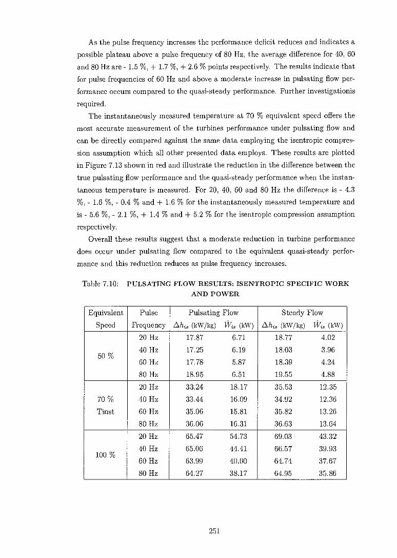
As the pulse frequency increases the performance deficit reduces and indicates a possible plateau above a pulse frequency of 80 Hz, the average difference for 40, 60 and 80 Hz are - 1.5 %, + 1.7 %, + 2.6 % points respectively. The results indicate that for pulse frequencies of 60 Hz and above a moderate increase in pulsating flow per-formance occurs compared to the quasi-steady performance. Further investigationis

required. The instantaneously measured temperature at 70 % equivalent speed offers the

most accurate measurement of the turbines performance under pulsating flow and can be directly compared against the same data employing the isentropic compres-

sion assumption which all other presented data employs. These results are plotted in Figure 7.13 shown in red and illustrate the reduction in the difference between the

true pulsating flow performance and the quasi-steady performance when the instan-taneous temperature is measured. For 20, 40, 60 and 80 Hz the difference is - 4.3 %, - 1.6 %, - 0.4 % and + 1.6 % for the instantaneously measured temperature and is - 5.6 %, - 2.1 %, + 1.4 % and + 5.2 % for the isentropic compression assumption

respectively. Overall these results suggest that a moderate reduction in turbine performance

does occur under pulsating flow compared to the equivalent quasi-steady perfor-

mance and this reduction reduces as pulse frequency increases.

Table 7.10: PULSATING FLOW RESULTS: ISENTROPIC SPECIFIC WORK AND POWER

Equivalent

Speed

Pulse

Frequency

Pulsating Flow

Ahi, (kW/kg) Wis (kW) Steady Flow

Ahis (kW/kg) 1,i7i, (kW)

20 Hz 17.87 6.71 18.77 4.02

40 Hz 17.25 6.19 18.03 3.96 50 %

60 Hz 17.78 5.87 18.39 4.24 80 Hz 18.95 6.51 19.55 4.88

20 Hz 33.24 18.17 35.53 12.35

70 % 40 Hz 33.44 16.09 34.92 12.36 Tinst 60 Hz 35.06 15.81 35.82 13.26

80 Hz 36.06 16.31 36.63 13.64 20 Hz 65.47 54.73 69.03 43.32 40 Hz 65.06 44.41 66.57 39.93

100 % 60 Hz 63.99 40.00 64.74 37.67 80 Hz 64.27 38.17 64.95 35.86

251

( Mea

sure

d - Q

uasi St

eady

) Effi

c ien

cy D

iffer

ence

-12%

12%

-6%

6%

0%

- 50% —0— 60%

—0— 70% —9-- 70% Tinst

—e— 80% -- 90% - 100% — Average

20

40 60

80

Pulse Frequency (Hz)

Figure 7.13: PULSATING FLOW RESULTS: MEASURED - QUASI STEADY EFFICIENCY DIFFERENCE

Isentropic Specific Work: Proof

It may be proved that a pulse pressure wave contains less specific isentropic work

then an equivalent steady one based on the mean pressure ratio. This result is

contrary to the proof given by Chen, 1996 [19] which although mathematically

correct is based on the cycle mean inverse pressure ratio. The following proof adapts

the steps outlined by Chen, 1996 [19] in terms of the true cycle mean pressure ratio.

Ahis = hoi — h4,is

7(1-4)-1 ) 1 7(1-4)

Cp(i_4)701 (1 [ I-01/ P4

N 6N1_4)1'n (1 - (7.26)

Where: A 70-0-1 -741-4) and =Poi/P4

Representing the pressure ratio as the sum of the cycle average and a fluctuating

component, Equation 7.27. Expanding and integrating the term as a power

series of 474 over a complete pulse cycle, Equation 7.28.

252

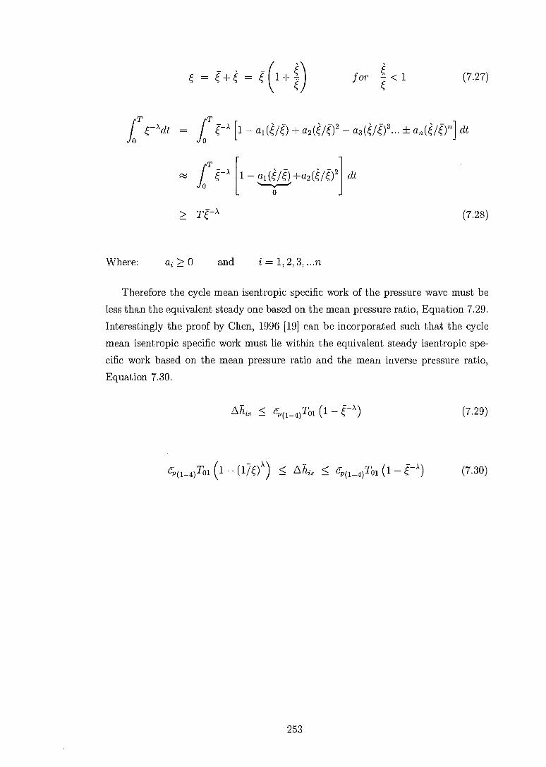
_+_ e(1+9 for <1 (7.27)

foT e-Adt

T — al(g) a2(g)2 a3(/e)3••• f an(g)n] dt

pT

1 — ai() +a2(/02 0

> 7rA (7.28)

Where: ai > 0 and i = 1, 2, 3, ...n

Therefore the cycle mean isentropic specific work of the pressure wave must be

less than the equivalent steady one based on the mean pressure ratio, Equation 7.29.

Interestingly the proof by Chen, 1996 [19] can be incorporated such that the cycle

mean isentropic specific work must lie within the equivalent steady isentropic spe-

cific work based on the mean pressure ratio and the mean inverse pressure ratio,

Equation 7.30.

/his < ep(1_4)Toi (1 — C-A ) (7.29)

Cp(i_joi (1 — (1/)1 < Ahis < ep(i_joi (1 — c-A ) (7.30)

dt

253


This section applies the uncertainty analysis given in Section 5.7 to the pulsating

flow performance results of Turbine 'D' and follows the procedures discussed in the steady flow chapter. The overall aim is to arrive at the uncertainty of the five performance parameters, the total-to-static efficiency, velocity ratio, mass flow parameter, pressure ratio and equivalent speed value.

7.7.1 Independent Variables

The independent variables are the parameters that are required to calculate the

performance parameters of the turbine. The variables of greatest influence are the

mass flow rate (gin), inlet static pressure (PO, outlet static pressure (P4), inlet static

temperature (T1), turbine speed (N) and turbine torque (r). These parameters and their associated uncertainty will be discussed in the following subsections. The independent variables which have minor influence are the recovery factor (r), rotor

mean inlet diameter (d2), inlet flow area (A1) and the air gas constant (R). These

are not discussed further.

Mass Flow Rate

The uncertainty associated with the measurement of the unsteady mass flow rate are dependent on numerous parameters and sources which have been discussed in

Section 5.4.1 and Section 7.4. It is not practical to isolate the individual uncertainties and therefore these are combined and assessed directly from experimental calibration as described in Section 5.5.1. From the combined set of 230 calibration points the Root-Sum-Square (RSS) uncertainty of the mass flow rate to a confidence level of 95 % or two standard deviations (2o) is ± 4.8 %.

Inlet Temperature

The uncertainty associated with the dual probe instantaneous recovery temperature measurement are dependent on similar parameters to the mass flow rate measure-ment and therefore are assessed directly from calibration. As the true instantaneous temperature is not known the calibrations compare the time-averaged temperature measured by the probe. This gives a Root-Sum-Square (RSS) uncertainty of ± 3 K to a confidence level of 95 %.

It is difficult to adequately prescribe the uncertainty associated with the calcu-lated temperature from the isentropic compression assumption. A direct compari-

son against the measured instantaneous temperature does not result in a usable or unique uncertainty band.

254

The results illustrate local discrepancies, phase shifts, differing secondary fea-tures but does demonstrate similar time-average values as the dual probe temper-

ature measurement. Although the measured time-averaged temperature is used directly in the isentropic compression assumption, Equation 5.16 the resultant cal-culated time-average value differs following approximately Equation 5.17 and hence may differ from the measured value with a similar uncertainty as the dual probe

technique. For this reason the uncertainty has also been prescribed at ± 3 K.

Inlet Static Pressure

The uncertainty associated with the inlet static pressure measurement have many similar sources to that of the steady flow measurement described in detail in Sec-tion 6.5. Additional unsteady effects are present in the raw signal such as acoustic resonance and are described in Section 5.4.3. These unsteady effects are reduced

through the ensemble averaging of 1800 cycles and the appropriate application of fil-ters to attenuate resonance signals. The reduction of unsteady effects are described

in detail in Section 7.4. From the calibration of the inner and outer limb unsteady pressure transducers

the non-linearity can be estimated. The outer limb transducer gave a maximum deviation of ± 0.067 % FS (235 Pa) whilst the inner limb transducer gave ± 0.051 % (177 Pa) and the exit transducer gave + 0.009 % FS (32 Pa). The transducer

bridge conditioner, amplifier and the calibration transducer (DRUCK DPI 610) are unchanged from the steady flow experiment such that similar uncertainties are applied. The uncertainty associated with the calibration transducer is ± 90 Pa for this inner and outer limb transducers and ± 15 Pa for the exit transducer whilst the uncertainty associated with the voltage drift of the bridge is + 50 Pa, refer

Section 6.5. A comparison of the time-averaged pressure from the steady and unsteady pres-

sure transducers was carried out over the test condition pulses. The unsteady flow transducer indicated a time-average value greater then the steady flow transducer, typically this was 3 % based on the overall pressure fluctuation range. The steady

flow transducer has greater accuracy in obtaining a time-average value as it less prone to resonant excitation and offers good signal damping due to the large length of pneumatic tubing between the transducer and measurement location.

The overall uncertainties for the inlet pressure transducers are + (346 + 3 %) Pa and for the exit transducer is ± (97 + 3 %) Pa; the percentage is based on the pressure pulse peak-to-peak amplitude.

255

Turbine Speed

The uncertainty associated with the speed measurement can be assessed directly by employing the uncertainty analysis described in Section 5.7. The two independent variables required for the speed measurement is the time, t required for the encoder wheel to rotate a known angle, e refer Section 5.4.4 and Section 5.5.4. The accu-racy of the time measurement is related directly to the reference clock frequency of the counter which runs at 20 MHz giving a uncertainty of ± 5 x 10-08 seconds. The known angle is replaced by a dynamic angle discussed in Section 5.5.4 which includes the effects of vibration and reduces the associated uncertainty. Typically after calibration the uncertainty in the angle is ± 1.18 x 10—°4 radians approximately fpm.

The uncertainty in the speed measurement is given by Equation 7.31, where n is the number of ensembled cycles.

1 ( [(Ae) ("1

2

1 ± [(At) (") 2 )] n ae at

(7.31)

This gives an approximate single point uncertainty of ± 0.004 - 0.013 RPS for 50 to 100 % equivalent speed respectively, which is consistent with the observations given in Section 7.6.6 suggesting that cyclic speed variations of < 0.02 RPS can be

isolated at 1000 Hz. Equation 7.31 does not account for the beneficial effects of high frequency noise attenuation through digital filtering.

Turbine Torque

The torque measurement is a significant source of uncertainty in the turbine perfor-mance parameters and comprises of two main components, the uncertainty of the mean component and the fluctuating component of torque. The uncertainty in the mean component has been described in Section 6.5 and has a value of ± 0.025 Nm.

The fluctuating component of torque results in the most significant uncertainty

in the torque measurement. The two measurement uncertainties which propagate into the uncertainty of the fluctuating torque component is the uncertainty in the measurement of angular acceleration and the polar mass moment of inertia of the rotating assembly. Dale, 1990 [25] gives a solution for the propagation of the time measurement uncertainty into the angular acceleration and fluctuating torque com-ponent. The solution given below additionally includes the propagation of the un-certainty in the angular distance and inertia measurement. For the present test facility this constitutes a significant proportion of the uncertainty in the fluctuating torque component.

256

The relation between the fluctuating torque component caused by the angular

acceleration and the rotational inertia is given by Equation 7.32 with the corre-

sponding uncertainty given by Equation 7.33.

= IC)

(7.32)

[(Al) (a( ))] 2 + [A(e) (n 2 (7.33)

The angular acceleration, e experimentally determined typically ranged from -

3,000 to 7,000 and - 11,000 to 17,500 rails/s2 for 50 and 100 % equivalent speed

respectively and translates into an uncertainty in angular acceleration of + 52 and

+ 354 rads/s2 inclusive of the time measurement uncertainty. The uncertainties in

the angular acceleration are calculated from Equation 7.34 and Equation 7.35. An additional smoothing factor, G has been included in the assessment of A(6.6) which

is used to take into account the effect of the low pass filter, experimentally this has

been determined to be <

=- 62 56 t1 - t2 St (7.34)

2 2 [A(je) a(Se + [ A(15t) a (())1) a(st) (7.35)

Where: Abi = A62 , At1 = At2 A(SO), ±VIAAG, A(St) = ±\dAt

The measurement of the polar mass moment of inertia is measured using a Tri-filar rig, refer Section 5.4.6. The rotational inertia is calculated by Equation 7.36 from the geometric and physical parameters given by Table 7.11 whilst the resultant uncertainty is given by Equation 7.37. The polar mass moment of inertia of the rotating assembly and corresponding uncertainty is 4.563 x10-'4 ± 1.55 x 10-°5

kg.m2 .

= 2 gr2m 27r) L (7.36)

257

2

A(/) = \/[6,(T) (gli 2 ±[°(r)

(V)] +

EA(m) ca(mili 2 + [A(L) (am)] 2 )]

(7.37)

Table 7.11: PULSATING FLOW RESULTS: TRI-FILAR UNCERTAINTY

Parameter Value

x

Uncertainty ±Ax

Oscillation Period, T (s) 1.5865 0.0025

Disk Radius, r (m) 0.0300 0.00025

Oscillation Mass, m (kg) 1.211 0.0005

Suspension Length, L (m) 1.494 0.0005

Gravity, g (m/s2) 9.81 -

The propagation of the acceleration and inertia uncertainties into the fluctuating torque component results in a uncertainty of + 0.024 to ± 0.111 Nm and ± 0.161

to ± 0.316 Nm for 50 and 100 % equivalent speed respectively for zero acceleration and for the maximum typical acceleration. At zero acceleration the uncertainty in fluctuating torque is a result of the uncertainty in acceleration, whilst at maximum acceleration approximately 2/3 of the uncertainty is related to the uncertainty in

inertia measurement. This results in an overall uncertainty in the torque measurement of ± 0.0347

to + 0.114 Nm and + 0.163 to ± 0.317 Nm for 50 and 100 % equivalent speed respectively for zero and the maximum typical acceleration.

7.7.2 Parameters The propagation of the individual parameters were calculated using the procedures of Section 5.7. The resultant equations for the RSS uncertainty of the turbine performance parameters are given by Equations 7.38 - 7.42.

The instantaneous RSS uncertainties are illustrated by Figures 7.14 - 7.18 for the five performance parameters of the turbine': efficiency (7)t _,), velocity ratio (VR.),

mass flow parameter (MFP.), pressure ratio (PR.) and the equivalent design speed

(Nequtv)•

14The instantaneous uncertainties presented do not take into account the effect of phase shift.

258

The tabulated overall RSS isentropic power averaged uncertainties are given by Table 7.13 - 7.17 and are the RSS summation of the influence of each independent variable on the performance parameters. The typical fractional influence is given by

Table 7.12 and discussed in the relevant sections below.

Table 7.12: PULSATING FLOW RESULTS: TYPICAL UNCERTAINTY FRACTIONAL IMPORTANCE OF VARIABLE

Parameter Efficiency U2/Cis MFP PR Acqui„

RPS (Nequiv) 0.00 0.00 - 0.00

Torque ('r) 0.30 - - -

Inlet Temperature (T31) 0.07 0.16 0.06 0.03 0.72

Mass Flow Rate (rh) 0.44 0.28 0.72 0.39 0.21

Inlet Pressure (-P.51) 0.15 0.45 0.21 0.44 0.06

Exit Pressure (Ps4) 0.04 0.12 - 0.13 -

Total-Static Aerodynamic Efficiency

6•07t-s)inst =

[(Ariz)

(a(ann-i 3) )]2 [(ATi) ( a(01177t-is) )] 2

[(AP1) (a(011-1"))]2 + [(sr) (a@latT79) )] 2 + [(AN) ( a(3711\7111 2 (7.38)

The variation in the instantaneous uncertainties show similar trends and expla-nations to the steady state results of Section 6.5. The absolute values are larger and can vary between + 2.8 to 200+ % points in efficiency; this is dependent mainly on the velocity ratio, Figure 7.14. At the higher velocity ratios > 1, the uncertainties become large > 10 % points, although the influence on the overall cycle average ef-ficiency is minimal due to the low isentropic power content of the gas. This may be

seen by Table 7.13 where the isentropic power averaged uncertainty for all test con-ditions lies between ± 4.9 to 8.2 % points in efficiency. These values are reasonable considering the difficulty in measurement.

Table 7.12 gives the typical fractional influence of the independent parameters on the uncertainty in efficiency. The mass flow rate measurement is the largest

uncertainty and accounts for approximately 2/5 the overall uncertainty with the

torque measurement accounting for 1/3 the uncertainty. Future improvements in measurement accuracy should focus on these instruments.

259

Velocity Ratio

A(VR.)inst [(Arh) (a( avthR

)J

i 2 + { (6,7,1) ( a(vR.N 2 aT, )

a(OP1 )1 vR))] 2

+ [(AN) ( a(

aN vR.N

) J 2

(7.39)

As with the efficiency the variation in the instantaneous uncertainties show sim-ilar trends and explanations to the steady state results of Section 6.5. The instanta-

neous values are approximately a magnitude larger then steady state conditions and is due to the difficulty in accurate measurement under pulsating conditions. The uncertainty can vary between + 0.006 to 0.5 dependent on the velocity ratio; the excessive values occur at the high velocity ratios which correspond to the low pres-

sure ratios. The influence of the large uncertainties are again minimised by the low power content of the gas with overall cycle average uncertainties varying between ±

0.0088 to 0.019, Table 7.14. The fractional influence, Table 7.12 suggests 1/2 the uncertainty is a result of the

inlet pressure measurement and 1/4 due to the mass flow measurement, the remain-ing being spread between the inlet temperature and exit pressure measurement.

Pseudo-non-dimensional Mass Flowrate

A(MFE)inst = [(Aro ( Fp.)m

[(63,0 ( a(MTP.)yi 2 + [(Apo (a(MFP.))] (7. 40) 2

0T1 )] a/31

The variation in the instantaneous uncertainties show similar trends and expla-nations to the steady state results of Section 6.5. The instantaneous values are approximately 5 times larger then steady state which is again related to the accu-racy of the measurement instruments. The various equivalent speed lines are seen to be coincident although at high equivalent speeds and low pulse frequencies the overall uncertainties increase in value. This is due to the larger variation in pulse amplitude resulting in a increased uncertainty of inlet pressure measurement.

The uncertainty can vary between ± 0.039 to 0.29 [kg I s]/k !Bar (abs) depen-dent on the mass flow parameter with the overall cycle average uncertainties having value between ± 0.209 to 0.274 [kg1s]V—KIBar (abs), Table 7.15.

260

The fractional influence, Table 7.12 suggests approximately 3/4 of the uncer-tainty is due to the measurement of the mass flow rate with the inlet pressure measurement accounting for the majority of the remainder. The uncertainty in the mass flow parameter is significant, typically ± 4.5 % which is similar to the accuracy of the mass flow measurement. The continuing importance of the mass flow mea-

surement would suggest further improvement in its accuracy is appropriate to yield the most significant improvement in the accuracy of pulsating flow measurements.

Pressure Ratio

A(PR.)inst [(Aril) (a(aPri7R.))] 2

2 [(AT1 )( a(PR* ) )1 2 +[(Ap1)(

(PR. ap1 1.]

) )1 (7.41) aT,

The variation in the instantaneous uncertainties of the pressure ratio are depen-dent on both the equivalent speed and pulse frequency. The instantaneous values

are a magnitude larger then steady state conditions and vary between + 0.015 to 0.089, typically 2 - 3 % of the pressure ratio. The overall cycle average uncertainties varying between ± 0.0179 to 0.0741, Table 7.16. The increased uncertainty at low

pulse frequencies occur due to the increased pulse amplitude. The fractional influence, Table 7.12 suggests just under 1/2 the uncertainty is

due to the inlet pressure measurement with 2/5 due to the mass flow measurement and the remainder largely due to the exit pressure measurement.

Equivalent Speed

A (N equiv)inst [(Aril) (N 2

a(Nequiv))] 2 + a(equiv)) + [(AT1) ( ath,

2 a(Nequiv) )1 (7.42) a(Nequiv))1 2

+ [(AN) aN [(AN( api

The equivalent speed uncertainty is equivalent speed dependent, its value in-creases from ± 0.22 to 0.47 between 50 and 100 % equivalent speed, Table 7.17. The fractional influence, Table 7.12 suggest 3/4 of the uncertainty is due to the inlet temperature measurement and 1/5 is the mass flow measurement with the re-maining due to the inlet pressure measurement. The measurement of the turbine speed results in a negligible effect on the uncertainty of the equivalent speed.

261

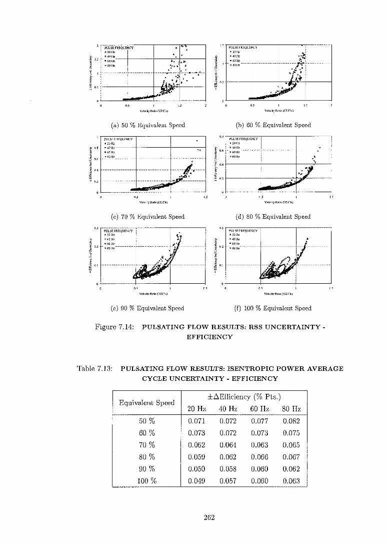
1.5

PULSE. FREQUENCY • 20 Hz

40 Hz • 60 Ilz . /10 Hz

PULSE FREQUENCY • 20 Ilz * 40 Hz • 60 Hz . 80 Hz

PULSE FREQUENCY • 20 Hz 0 40 Hz • 60 Hz * SO I lz ----- —

0.3

1.5 S

PULSE FREQUE • 20110 040 Hz

iiICY •

• o

• .

• 6011z o 130 Hz

-. ..._

A* ii* o li

• i—iti • 44

0 q° i

. o - . • • •

ii?" aMinal100414.1WPa

PULSE 10E00E6 • 20110 0 40 Hz • 60 Hz 00.0(5

CY

*. A

P. nti 1 5 0

2 )441

. .- . . 7 05 15

0 5

15

Velocity Ratio (1120Ci0

(a) 50 % Equivalent Speed

Velociya.k. (zario

(b) 60 % Equivalent Speed

• *

PULSE FREQUENCY 2011z 40 Ilz •

— --- _

• 8015 .11

N -..,-

.., •::;1

0.8

.0 0.6

0.4

(1

Z. 0.8

S 0.6

04

LL1 0.2

E 0.2

0.1

11 5 1 5 05 Velncity Ratio (U21riiii) Velnciry Ratio (U2,'Cis)

(c) 70 % Equivalent Speed

(d) 80 % Equivalent Speed

05 05 15

Velocity Ratio (1.12,Cia) Velnetry OIL is)

(e) 90 % Equivalent Speed

(f) 100 % Equivalent Speed

Figure 7.14: PULSATING FLOW RESULTS: RSS UNCERTAINTY - EFFICIENCY

Table 7.13: PULSATING FLOW RESULTS: ISENTROPIC POWER AVERAGE CYCLE UNCERTAINTY - EFFICIENCY

Equivalent Speed 20 Hz

+AEfficieney (% Pts.)

40 Hz 60 Hz 80 Hz

50 % 0.071 0.072 0.077 0.082

60 % 0.073 0.072 0.073 0.075

70 % 0.062 0.064 0.063 0.065

80 % 0.059 0.062 0.066 0.067

90 % 0.050 0.058 0.060 0.062

100 % 0.049 0.057 0.060 0.063

262

0h

S 144

0.2

8

0.3 17,

PULSE FREQUENCY • 20 Hz 0 40 Hz • 60 Hz 0 80 Hz i

• a

•

PULSE FREQUENCY A 20 Hz ^40 Hz • 60Hz 080 He

fg. 0.1

0

0

0 5

1 1

0

00

Velocity Rata:. (1.12/Ca)

(a.) 50 % Equivalent Speed

PULSE. FREQUENCY • 20 Hz.

60- - . 4011, • 60112. 0 80 Hz

0 if

- --

_

- -

0*

4/115).

iall' . t'le S .o ''

Veluciry Ratio (1.42/C6)


PULSE FREQUENCY • 20 Hz 0 40 li

lz

i '

0

• 60 Hz °60 Hz

1f

At

11/2151Z•

0.25

02

tai 0.15

5 0.1

0.05 II

0.12

.E

0.09

Q 0.06

2 0.03

0 0.5

15

05

0.1

(1.00 S

0.06

2 0.04

ti 11.02

Velocity Ratio (1.121Cia)


PUI,SF, FREQUENCY • 20 Hz

• 60 Hz Hz - 0 80

ell • 0

I i

t

Voboky Rmb (LI20Cia)


PULSE FREQUENCY • 20 Ilz

- 0 40 Hz • 60 Hz • 80 Hz

aR

...di

•

0.08

2

;IT 0.06

2 0.04

Ta 0.02

0'

0.5

15

0.5

Vakicky Ratio (1.12.1Cis)

Velma), Ratio (U2/Cit)



Figure 7.15: PULSATING FLOW RESULTS: RSS UNCERTAINTY - VELOCITY RATIO

Table 7.14: PULSATING FLOW RESULTS: ISENTROPIC POWER AVERAGE CYCLE UNCERTAINTY - VELOCITY RATIO


±AVelocity Ratio (-)

40 Hz 60 Hz 80 Hz

50 % 0.0149 0.0154 0.0179 0.0190

60 % 0.0143 0.0139 0.0153 0.0160

70 % 0.0132 0.0132 0.0124 0.0117

80 % 0.0124 0.0118 0.0118 0.0114

90 % 0.0110 0.0104 0.0097 0.0091

100 % 0.0106 0.0099 0.0091 0.0088

263

• E • 20 Hz 0 40 Hz • 60 Hz 080Hz

EQUENCY

do°

CY PULSE FREQUEN • 20 Hz • 40 Hz • 60 HE

O 80 Hz

0.3 PULSE FREQUENCY • 20 Hz • 40 11, • 60 Hz

80 Hz

• Le

PULSE FREQUEN • 20 Hz • 40 Hz • 60 Hz

:Y •

• 80 Hz .4,0

af°

2

4

6

Mss Flow Parameter (kg's) (abs)

PULSE FREQUENbY 0 1) Hz • 40 Hz • 60 Hz • SO Hz

4 6

Mass Flow Parameter [kg's] \ K/Bor (abs)

0.3

0.2 N 1 0.

0 0

0.3

0.3

2

S

PULSE FREQUENCY • 20 Hz • 40 Hz • 60 Hz _ • 80 Hz --

0. 2

0 1 4 7

N ass Flow Parameter Miss Flow Parametcr

[les] \ K/Flar (aim)

[kg/s] ,IUBar (ab3)

(a) 50 % Equivalent Speed (b) 60 % Equivalent Speed

2 6

4

fi

Mass Flow Parameter Mass Plow Parameter

[kg/s] (abs)

[Ices] (abs)

(c) 70 % Equivalent Speed (d) 80 % Equivalent Speed

(e) 90 % Equivalent Speed (f) 100 % Equivalent Speed

Figure 7.16: PULSATING FLOW RESULTS: RSS UNCERTAINTY - MASS FLOW PARAMETER

Table 7.15: PULSATING FLOW RESULTS: ISENTROPIC POWER AVERAGE CYCLE UNCERTAINTY - MFP

Equivalent Speed ±AMFP Okyls]\/.TIBar (abs) )

20 Hz 40 Hz 60 Hz 80 Hz

50 % 0.230 0.222 0.210 0.217

60 % 0.230 0.222 0.209 0.212

70 % 0.252 0.241 0.232 0.234

80 % 0.256 0.243 0.234 0.229

90 % 0.270 0.250 0.242 0.237

100 % 0.274 0.255 0.245 0.239

264

PULSE EREQUELNCY • 20 Hz o 40 11, • 60 Hz

. ..d.,, ,,.• rt,,,,o, 4k44, ° v....es

030 Hz es oviii,,...s0000

INIMILMILL a • 4

o ,,,,,,i58,1 ,• " Al.' Ir.

0.1Ult 4"

41'4 ' . • •:, 0

:%.,

PULSE FREQUENCY • 20 Hz . au 1h • 60 Hz A ••4

IIMAAMAAWAil A

o SO Hz ••••t

A 4. • •6• *•0 • 4, ig

•

.11,....00100:0 IniniMillrf..tt%

0 461),31 M I°

0

0.025

fi 002

.;1

al 0.015

001

Pres

stne R

atio

Unce

rtaint

y

0.03

0.025

0.02

0.015 14 16 I8 1.25 1.75

Pressure Ratiu Prossura Ratio

002


PULSE FREQUENCY • 20 Hz 040 Hz • 60>1, a o NO Hz • •

•o

♦A•

• d1

*

'*.

--A..."""'"*"-" "tedLI 000e

• • o oIn.P7 1 *

jr9L

. .

-rneurr.r:.


PULSE FREQUENCY i • 20 Hz 1

° 40 Hz I • 60 Hz •

As• Ai' •''''

1•'46

*SO Hz 1 i • .846 0 .

alasiamaliamal••• • " ay • Stk7

684 6 ,,

of 46.0..° . e 6

1 ,

• 4,4 „...........6.17 0 0 • 000

.....8.-TV..a

0.05

g 0.04

0

0.03

005

g 0.04

0 F.. 0.03

0.02 15 25 1.5 2 25

Pressure Rata, Pre..ere Ram

0.06

S 'St 0.04

0.08

0.02


PULSE FREQUENCY • 20 Hz 46

• Ck 040 Hz •̀ •8 • 60 Hz I•k

' *8011z A• i..4`. . ...,,e

db. ° . .,,.:d.,..°:160,.

" ' . ° •••=e nir.


PULSE FREQUE • 20 Hz

• 60 Hz 080 Hz

A

CY

• t , t ,,, • •0411 0

00" • 60°S" CO

• '

0.1

08 0.06

0

0.02 2 4 3 4

['restore Ratio Pressure Ratio



Figure 7.17: PULSATING FLOW RESULTS: RSS UNCERTAINTY - PRESSURE RATIO

Table 7.16: PULSATING FLOW RESULTS: ISENTROPIC POWER AVERAGE CYCLE UNCERTAINTY - PRESSURE RATIO


+APressure Ratio (-) 40 Hz 60 Hz 80 Hz

50 % 0.0206 0.0186 0.0179 0.0200

60 % 0.0238 0.0214 0.0203 0.0215

70 % 0.0370 0.0309 0.0268 0.0270

80 % 0.0412 0.0338 0.0294 0.0280

90 % 0.0640 0.0466 0.0382 0.0362

100 % 0.0741 0.0540 0.0427 0.0405

265

62 58 60

PULSE FREQUENCY • 20 Hz 0 40 - Hz • 6011z 9 80 Hz

•

•

41$,,,*:19,67pek

A 0 09 •

f .t• ° A....•.• :•*1 o

,%9,4441*

o

, EquivaLnt Speed (%)

56 56 54 0.21

46 40 50 52

Equivalent Speed (7s)

1 0.24

0.23

ti 0.22 eirA•

0.27 PULSE FRED

- • 20 Hz ° 40 Hz

. • 60 Hz o 80 Hz

UENCY

a g. 0.26

0.25 '

0.3

.t11 0.29

0.28

ti E 0.27

e7- 4. 0.26

0.25

(1.42

0.32


PULSE FREQUE • 20 Hz

• 60 Hz

4..Y

*80 Hz • Jo

ao08 1 ••°: 1,9**

&.: 4* A

t.h.....0;::/ ie


PIA SF FREQUENCY

• 0 Hz

-040 Hz • 60 Hz *80 Hz _ ° P

kerl °

:1 • •

'.4W'

88, 9 o 0° 4,1%.

ietee

0.16

0,34

0.32

74; 0.3

0,28 60 64 68

72

76

72

76 80 84

Equivaknt Speed

Equivalent Speed

0.5 0.56


PULSE PRE( • 20 Hz

UENCY

*40Hz 4 • • 60 Hz

o 1'. 4.1.. o : 0 00 Ile o 7, bk.. :Poi

• P. ...itoV

80 64 00 92 96

100

Equivalent Speed



PULSE FRE( • 20 Hz * 40 Hz

UENCY

o

• 60 Hz •

080 Hz g .4.: * • 4

.41:1 SA . 8. ".°:::' aP , ree°

,111•Pr .,:i. A. me. 8 ,•,•1-,..• ti° -.11,

• • "8 a d. . ' 6 60,r' ii*VI ° . • ,..V.,,,,..

140 92 96 100

104

108

EAluiyulent Speed


0.45

0.4

0.15 H

0.3

0.52

0.48

'd 0.44 •

0.4

Figure 7.18: PULSATING FLOW RESULTS: RSS UNCERTAINTY - EQUIVALENT SPEED

Table 7.17: PULSATING FLOW RESULTS: ISENTROPIC POWER AVERAGE CYCLE UNCERTAINTY - EQUIVALENT SPEED


±AEquiv. Speed (% )

40 Hz 60 Hz 80 Hz

50 % 0.230 0.223 0.229 0.238

60 % 0.259 0.263 0.266 0.267

70 % 0.309 0.308 0.317 0.321

80 % 0.351 0.365 0.365 0.369

90 % 0.408 0.412 0.425 0.419

100 % 0.444 0.466 0.470 0.469

266

7.8 Summary

The instantaneous stage performance map of mixed-flow turbine 'D' has been pre-

sented for 50 - 100 % equivalent speed and 20 - 80 Hz pulse frequency. A significant improvement in the measurement of the mass flow rate and turbine torque combined with the first instantaneous inlet temperature measurement has allowed a consider-able improvement in the accuracy of the performance parameters to be made.

The use of the isentropic power average has shown its importance in assessing the true turbine performance under pulsating flow. This technique better weights the significance of each individual measurement which allows a meaningful discussion of

the overall turbine performance and the uncertainties. The results have shown that the pulsating flow causes a hysteresis in performance

parameters which makes it fundamentally difficult to disseminate the performance of the volute volume from the turbine rotor (inclusive of stage losses). This was possible

at a pulse frequency of 20 Hz and demonstrates the turbine follows the trends of

the quasi-steady performance albeit with a moderate reduction in efficiency; this is thought to lie in the region of 0 to - 6 percentage points. The cycle average results

indicate that as the pulse frequency increases the reduction in efficiency reduces and plateaus to a constant value thought to be equal to the steady state performance of the turbine.

The introduction of the normalised and pressure normalised Strouhal number has also proved a useful concept to infer the onset of unsteadiness of the system due

to either the gas velocity or the pressure wave velocity. This suggests its usefulness as a tool for the selection of appropriate modelling codes; quasi-steady, filling and

emptying or wave action.

267

Chapter 8

Conclusions

8.1 Synopsis of Achievements

A unique permanent magnet eddy current dynamometer with reaction torque mea-surement has been developed which has increased the power absorption capabilities of this turbocharger test facility by a minimum of 3.5 times. The dynamometer

has a power absorption range of 0.3 - 62.2 kW, a speed range of 0 - 60,000 RPM

and is suitable for measuring the performance of a turbine under both steady and pulsating flow conditions due to its low rotating inertia.

The magnetics of the dynamometer has been successfully modelled in 2D and 3D. This has enabled the influence of the important parameters to be mapped allowing the dynamometer to be optimised for maximum power output.

The steady flow performance results have been obtained for a mixed-flow turbine over the velocity ratio range of 0.375 to 1.068. This has increased the data range available for this turbine by a minimum of 3.2 times over previous investigations

and illustrates the usefulness of the dynamometer. Under pulsating flow conditions, the measurement of the instantaneous temper-

ature has been made and a significant improvement in the accuracy of the instan-

taneous mass flow rate and torque measurement has been achieved in relation to previous investigations.

The pulsating flow performance results have been obtained for the same mixed-

flow turbine over a pulse frequency range of 20 - 80 Hz and a non-dimensional speed range of 0.833 - 1.666 which has extended the data range available in literature. The use of an energy weighted time-average has allowed an equivalent quasi-steady efficiency to be calculated and compared against the true cycle averaged efficiency for the first time. This has shown a 6 % point mean reduction in cycle average efficiency at a pulse frequency of 20 Hz; this reduction reduces with increasing pulse frequency.

268

8.2 Conclusions

8.2.1 PMEC Dynamometer

Dynamometer

The development of a unique permanent magnet eddy current dynamometer has been successfully accomplished and has highlighted the difficulties involved in meet-ing the performance and speed requirements of a turbocharger turbine.

The characteristics of the PMEC dynamometer are stable with respect to power' absorption and rotor dynamics, this allows operation over the full speed range of 0 - 60,000 RPM. The dynamometer has a power absorption range of 1.7 - 62.2

kW at 60,000 RPM; equating to a 3.5 times increase in power range for this speed over the previously used radial compressor. The accurately measurable polar mass moment of inertia of the dynamometer has remained similar to the previous standard turbocharger assembly, representing only a 7.1 % increase in value. This allows the turbocharger to respond to pulsed flow mimicing the behaviour of a standard assembly but with the increased range available. The style, load range and inertia

of this dynamometer makes this a unique machine.

Magnetics

A 2D parametric study has shown the variables of importance are the rotor-to-

stator gap, relative velocity, resistivity, permeability, stator thickness and number of poles; these have been used to optimise the energy transfer of the dynamometer. The numerical results suggest that all dominant parameters have been included in the analysis and highlights the power absorption benefit achieved by a permeable stator over a non-permeable stator for the materials modelled. This has also been experimentally verified and occurs as the eddy current generation is over a larger volume which outweighs the lower local power densities as compared to a non-permeable stator. The dynamometer has been modelled in 3D and its predicted power absorption is nominally within 10 % of the experimentally obtained value. The 2D results over predicted the experimentally obtained maximum power by 18 %. Whilst this absolute accuracy is not high, it is considered satisfactory for the

optimisation process.

269

8.2.2 Steady Flow Experimentation

The steady flow performance results have been obtained for mixed-flow turbine 'D'

over a non-dimensional speed range of 0.833 - 1.666. A maximum measured velocity ratio range of 0.375 - 1.068 has been obtained which has significantly increased the turbine map range over previous investigations by 3.2 and 5.1 times for the turbine speeds of 30,000 and 60,000 RPM respectively. This increase has allowed the peak turbine efficiency to be clearly represented and suggests the optimum velocity ratio for this mixed flow turbine is lower then for a typical radial inflow turbine by 0.037.

This reduction is consistent with that calculated due to a + 20 degree inlet blade angle. The maximum measured total-to-static efficiency of mixed-flow turbine 'D' was 74.3 % which occurred at the turbines 80 % design speed and a velocity ratio of 0.663. A specific speed assessment of 1.05 at maximum efficiency suggests that

the swallowing capacity for this mixed-flow turbine is larger then for a typical radial inflow turbine.

8.2.3 Pulsating Flow Experimentation

Instrumentation

The dual probe hot-wire technique has been shown suitable to measure the instan-taneous temperature of the pulsating flow as the required response rate can be

achieved (> 1kHz). The importance of this measurement is greater than its contri-bution within the performance parameter equations as the mass flow measurement

is highly dependent upon this quantity. The use of an isentropic compression assumption to estimate the instantaneous

temperature has been shown to reasonably predict the maxima and minima tem-

perature variations during a pulse cycle. The accuracy is to within 4 K with respect to the measured temperature over a 60 K cycle variation. Instantaneous differences of up to 15 K where found and this can significantly effect the calculation of the mass flow rate. If the instantaneous temperature can not be measured directly the

isentropic compression assumption is a reasonable approach to choose, although the consequences must be considered.

The uncertainties associated with the performance parameters propagate largely from the mass flow measurement. The importance of the hot-wire fluid property, temperature and Mach number correction factors is therefore apparent. The omis-sion of these can result in an instantaneous error in excess of 50 %. This effect is masked by the smaller deviation in the time-averaged value which was found to be

as little as 2 %.

270

The importance of the data refinement techniques in order to retain the informa-tion of the speed signal has been shown. This is important to retain the secondary features of the turbine power which has now demonstrated that the turbine follows closely the isentropic power trace.

Experimentation

The results have shown that the turbine stage does not exhibit quasi-steady behav-iour for the pulse frequencies of 20 - 80 Hz. Instead a hysteresis of the performance parameters occur exhibiting two types of behaviour; at the lower pulse frequencies a regime exhibiting 'filling and emptying' behaviour dominates whilst at the higher

frequencies a regime exhibiting 'wave action' dominates. The introduction of the

normalised Strouhal numbers (St.*, St.(p)*) has proved consistent for inferring the

onset of the above flow regimes and suggests its use as a simple tool to depict the

dominating flow regime: quasi-steady St.* < 0.1, 'filling and emptying' St.* > 0.1

> St.(p)* and 'wave action' St.(p)* > 0.1. The importance of the energy weighted time-average has been demonstrated. It

allows the equivalent quasi-steady efficiency to be calculated and compared against the true cycle average efficiency; the weighting of the instantaneous measurements

are the same. The results show a 6 % mean reduction in the cycle averaged efficiency at a pulse frequency of 20 Hz; this reduction reduces with increasing pulse frequency.

From the instantaneous efficiency results at low pulse frequencies it is clear that

the instantaneous efficiency follows the general trends of the steady flow performance with a reduction in efficiency. At 20 Hz pulse frequency, 70 % equivalent speed a constant reduction of 4 percentage points is seen throughout the operating range. This reduction is larger at the higher turbine speeds where the pulse amplitudes are

higher. The results have shown that at low pressure ratios, the fly-wheel effect results in

negative turbine efficiency. This is attributed to the momentum transfer from the turbine rotor into the gas in these high negative incidence regions.

Finally, the cycle averaged specific isentropic power of a pulse cycle has been shown both mathematically and experimentally to be less than the equivalent steady one based on the mean pressure ratio. Experimentally it was shown that the isen-tropic power under pulsating flow is larger than the steady one.

271

8.3 Suggestions for Further Work

8.3.1 Dynamometer Power

It is possible to achieve significant improvements in the power absorption capabilities of the dynamometer. Although it is important to be aware of the present limitations in heat transfer; the stator design is specifically conservative to avoid such problems. Before the power absorption characteristics can be improved it would be necessary

to address these issues: 1) the heat transfer from the stator surface to the magnetic rotor, 2) the heat transfer from the stator to the coolant.

An increase in stator thickness is the simplest approach to increase the power

absorption of the dynamometer. This can give significant increases in power but could lead to excessive stator surface temperatures which must be monitored. Al-though not presented in this thesis a dual material approach has been modelled, incorporating both permeable and non-permeable materials. This has numerically given the highest power densities but is likely to be more susceptible to heat transfer

problems. Finally, a re-design of the magnetic rotor to better reproduce the ideal rotor

schematic of Figure 3.21 would offer significant improvements in the power density.

Careful assessment using contact analysis would be required in order to avoid magnet separation at high speed.

8.3.2 Experimental Investigation

Instrumentation

The dominant uncertainty under steady flow conditions and high velocity ratios is the measurement of torque. The improvements should focus on reducing the mechanical hysteresis in the gimbal bearings, water coolant pipes and the various instrumentation cabling. The dominant uncertainty under pulsating flow conditions is the instantaneous mass flow measurement. A specific calibration rig would be useful to vary individually the pressure, temperature and Mach number over the entire range of conditions to be encountered under pulsating flow.

The accuracy and ease of use of the instantaneous temperature measurement would benefit from a specific dual wire hot-wire probe. This will ensure the hot-

wires experience the same flow field, decrease the calibration time and allow the traversing of the measurement duct to measure the temperature profile of the flow. This will consequently improve the measurement of the instantaneous mass flow rate. Finally the robustness of the speed measurement can be improved by increasing the diameter of the encoder wheel so it is less affected by rig vibrations.

272

Experimentation

Steady Flow: For further increases in dynamometer performance the turbine map can be extended to cover the new range; an increase in the speed range would

also be beneficial. In order to quantify the possible extrapolation error of a small range turbine map, the PMEC dynamometer map can be cropped to simulate a typical range and then extrapolated using the standard techniques. The resultant map can be compared against the original or applied to an engine simulation code

to quantify the error.

Pulsating Flow: A useful investigation would be the systematic comparison of the quasi-steady and cycle-averaged efficiency for a large range of conditions.

This should allow the losses under pulsating flow to be evaluated. In order to further investigate the applicability of the Strouhal number the pulse frequency

should be reduced to investigate the reduction in the hysteresis loop and whether the quasi-steady turbine performance coincides with a St.* < 0.1. This type of

investigation is also suited to 1-d wave action codes which can disseminate and identify the parameters of importance.

8.4 Epilogue

It is hoped that this work has provided some additional insight into the behaviour of the turbine stage under pulsating flow conditions and has highlighted the im-portance of the instrumentation and its accuracy to the experimental investigation required to answer the key questions. I look forward to the continuing development of experimental and numerical techniques to further increase our understanding of this subject.

The aims of the thesis objectives have been fulfilled.

273

Bibliography

[1] M Abidat. Design and testing of a highly loaded mixed flow turbine. Ph.d thesis,

Imperial College, London, UK, 1991.

[2] INC ANSYS. Ansys 5.7, finite element analysis package, 2001.

[3] C Arcoumanis, I Hakeem, L Khezzar, R.F Martinez-Botas, and N Baines. Per-

formance of a mixed flow turbocharger turbine under pulsating flow conditions.

ASME International gas turbine and aeroengine congress and exposition, (95-

GT-210), June 1995. .

[4] N.0 Baines, A Hajilouy-Benisi, and J.H Yeo. The pulse flow performance and

modelling of radial inflow turbines, c484/006/94. IMechE, pages 209-219, 1994.

[5] N.0 Baines and J.H Yeo. Flow in a radial turbine under equal and partial

admission conditions, c423/002. IMechE, pages 103-112, 1991.

[6] R.P Benedict. Fundamentals of temperature, pressure and flow measurements.

John Wiley and sons, 3 edition, 1984. pages 340.

[7] R.S Benson. Nonsteady flow in a turbocharger nozzleless radial gas turbine.

SAE National combined farm, construction and industrial machinery and pow-

erplant meeting, 9 - 12 September 1974.

[8] R.S Benson and K.H Scrimshaw. An experimental investigation of non-steady

flow in a radial gas turbine. In Proceedings, Institute of mechanical engineers,

volume 180 of 3J, 1965-1966. .

[9] 0 Biro and K Preis. On the use of the magnetic vector potential in the finite element analysis of three-dimensional eddy currents. IEEE transactions on

magnetics, 25(4):3145-3159, July 1989.

[10] British Standards. BS 1042: Section 2.1: Measurement of fluid flow in closed

conduits IS03966-1977, 1983.

[11] British Standards. BS 6861-1:1987 - ISO 1940-1:1986: Balance quality require-ments of rigid rotors, Part 1: Method for determination ofpermissible residual

unbalance., 1987.

274

[12] British Standards. BS 7854-1:1996 - ISO 10816-1:1995 - Mechanical vibration

Evaluation of machine vibration by measurements on non-rotating parts - Part

1: General guidelines, 1996.

[13] British Standards. BS EN ISO 5167-1:1997: Measurement of fluid flow by

means of pressure differential devices, Part 1., 1997.

[14] H.H Brunn. Hot-wire anemometry - Principles and signal analysis. Oxford

university press, 1995. pages 20, 220 - 223, 306.

[15] K Buffard. The design and development of a novel intercooled compressor for a

highly efficient microturbine generator. Phd, Imperial College, London, 2005.

[16] M Capobianco, A Gambarotta, and G Cipolla. Influence of the pulsating flow operation on the turbine characteristics of a small internal combustion engine

turbocharger, c372/019. IMechE, pages 63-69, 1989.

[17] M Capobianco, A Gambarotta, and G Cipolla. Effect of inlet pulsating pres-

sure characteristics on turbine performance of an automotive wastegated tur-

bocharger, 900359. SAE special publications, (818):97-108, Feburary 1990.

[18] H Chen. Steady and unsteady performance of vaneless casing radial-inflow tur-

bines. Ph.d thesis, UMIST, Manchester, UK, November 1990.

[19] H Chen, I Hakeem, and R.F Martinez-Botas. Modelling of a turbocharger

turbine under pulsating inlet conditions, a04695. Proceedings IMechE, Part A:

Journal of power and energy, 210:397-408, 1996.

[20] C Chou and C.A Gibbs. The design and testing of a mixed-flow turbine for turbochargers, paper 890644. SAE, 1989.

[21] E.0 Cobb and 0.A Saunders. Heat transfer from a rotating disk. Proceedings

Royal Society A, 236:343 —351, 1956.

[22] W.A Connor and E Swain. Extension of the filling and emptying engine perfor-mance simulation method to include gas dynamic effects, c484/042/94. IMechE,

pages 1-12, 1994.

[23] S Corrsin. Extended applications of hot-wire anemometer. NA CA technical

note 1864, 1949.

[24] A Dale and N Watson. Vaneless radial turbocharger turbine performance, c110/86. Turbocharging and turbochargers, IMechE, 3rd:65-76, 1986. .

[25] A.P Dale. Radial, vaneless, turbocharger turbine performance. Ph.d thesis, Imperial College, London, UK, 1990.

275

[26] S.K Das. An investigation of the aerodynamic loss in the rotor of a radial gas

turbine at design point. M.sc. thesis, UMIST, 1966. .

[27] C.F Dewey. A correlation of convective heat transfer and recovery temperature data for cylinders in compressible flow. Internation journal of heat and mass

transfer, Vol 8:pages 245-252, 1965.

[28] DieselNet. http://www.dieselnet.com/, 2003.

[29] Dantec Dynamics. Improved temperature correction in streamware®. Techni-

cal report.

[30] Dantec Dynamics. Streamline 'cta' system, 2003.

[31] A Engeda, Y Kim, R Aungier, and G Direnzi. The inlet flow structure of a centrifugal compressor stage and its influence on the compressor performance.

Journal of Fluids Engineering, 125(5):779-785, September 2003.

[32] M Farashkhalvat. Experimental and theoretical investigation of a radial inflow

turbine in unsteady flow. Ph.d thesis, UMIST, Manchester, UK, 1979. .

[33] A Fatsis, S Pierret, and R Van den Braembussche. 3-d unsteady flow and forces in centrifugal impellers with circumferential distortion of the outlet static

pressure. ASME, (95-GT-33), 1995.

[34] D Flaxington, C.S Cooper, D.A Green, and S.W.S McCloy. A turbocharger

bearing dynamometer, c484/037/94. Turbocharging and turbochargers, IMechE,

5th:321-330, 1994. .

[35] A.J Glassman. Basic turbine concepts. In Turbine design and application, SP-290, volume 1, chapter 2. NASA, 1972. .

[36] I Hakeem. Steady and unsteady performance of mixed-flow turbines for auto-motive turbochargers. Ph.d thesis, Imperial College, London, UK, 1995.

[37] I Hakeem and L Khezzar. The turbocharger aerodynamic test facility: de-

scription and operation - tf/94/37. Internal report, Imperial College London, 1994.

[38] P Hammond and J.K Sykulski. Engineering electromagnetism: Physical processes and computation. Oxford University Press, 1994. pages 85, 124.

[39] G.F Hiett and I.H Johnston. Experiments concerning the aerodynamic perfor-mance of inward radial turbines. Proceedings of IMechE, 178(Pt.3I(i0):28-42, 1963-64. .

276

[40] N Ikeya, H Yamaguchi, K Mitsubori, and N Kondoh. Development of advanced

model of turbocharger for automotive engines, paper 920047. SAE, 1992.

[41] D Japikse and N.0 Baines. Introduction to turbomachinery. Concepts ETI, Inc.

and Oxford University press, 1994.

[42] N Karamanis. Inlet and exit flow characteristics of mixed flow turbines in

advanced automotive turbocharging. Ph.d thesis, Imperial College, London, UK,

2000.

[43] N Karamanis, R.F Martinez-Botas, and C.0 Su. Mixed flow turbines: inlet and

exit flow under steady and pulsating conditions. Journal of Turbomachinery,

123:359-371, April 2001. .

[44] S Kidwai, D Tabrah, S Wilkins, and N Winder. High speed turbocharger

dynamometer. Undergraduate project, Imperial College, 1999.

[45] S.J Kline and F.A McClintock. Describing uncertainties in single-sample ex-

periments. Mechanical Engineering, 75:3-8, January 1953.

[46] H Kosuge, N Yamanaka, I Ariga, and I Watanabe. Performance of radial flow

turbines under pulsating flow conditions. Journal of engineering for power,

Transactions of the ASME, pages 53-59, January 1976.

[47] H Kramers. Heat transfer from spheres to flowing media. Physica, 12:61-80,

1946.

[48] A Krawczyk and J.A Tegopoulos. Numerical modelling of eddy currents. Claren-

don Press, Oxford, 1993. Chapter 2.

[49] S-U Lee. Dynamics of high-speed rotating machines. Phd, Imperial College,

London, 2000.

[50] Kulite Sensors Limited. Measurement of dynamic pressures. Course 4a5001,

KTH Energy Center, Department of energy technology.

[51] C.G Lomas. Fundamentals of hot-wire anemometry. Cambridge university press, 1986. pages 63.

[52] (Morgan) Crucible Magnetics. Elizabethtown, Kentucky, USA.

[53] G.T McDonnell. The design, development and testing of a turbine hydraulic dynamometer. Ph.d thesis, Queen's university, Belfast, UK, 1999.

277

[54] G.T McDonnell, D.W Artt, and S.W.T Spence. The design, development, and

testing of a hydraulic turbine dynamometer, c554/025/98. Turbocharging and

air management systems, IMechE, 6th:145-156, 1998. .

[55] N McGlashan. Research officier, 1999-2000. Imperial College.

[56] H Minegishi, H Matsushita, M Sakaida, and T Koike. Development of a small

mixed-flow turbine for automotive turbochargers, paper 95-gt-53. ASME in-

ternational gas turbine and aeroengine congress and exposition, June 5-8 1995.

[57] T Miyashita, T Tomita, and D Ishihara. Performance of inward radial flow

turbines under unsteady flow conditions. IHI engineering review, 7(1), 1974. .

[58] R.J Moffat. Contributions to the theory of single-sample uncertainty analysis.

Transactions of ASME, Journal of fluid engineering, 104:250-260, 1982.

[59] R.J Moffat. Describing the uncertainties in experimental results. Experimental

thermal and fluid science, 1(1):3 — 17, 1988.

[60] Y.S.H Najjar. Performance of simple cycle gas turbine engines in two modes of

operation. Energy conversion and management, 35(5):433-441, 1994. .

[61] B Nikpour. Measurement of the performance of a radial inflow turbine. Ph.d

thesis, UMIST, Belfast, UK, 1990.

[62] J.M Owen and R.H Rogers. Flow and heat transfer in rotating-disk systems,

rotor-stator systems, volume 1. Research studies press LTD and John Wiley

and Sons INC, 1989. pages 122, 194.

[63] D Palfreyman. Aerodynamics of a mixed flow turbocharger turbine under steady

and pulse flow conditions: A numerical study. Phd, Imperial College London,

2004.

[64] M.P Perry. Low frequency electromagnetic design. Marcel Dekker, INC., 1985.

pages 6.

[65] A Pesiridis. Research assistant, 2000 -. Imperial College London.

[66] A Pesiridis, S Rajoo, S Szymko, and R Martinez-Botas. Development of active flow control mixed-flow turbine on eddy-current dynamometer for automotive

application. IMECH, 2004.

[67] F Pintossi. Investigation into the heat transfer and pressure losses in a high

speed dynamometer. Master thesis, Imperial College, London, 2003.

278

[68] K.R Pullen. The design and development of a small gas turbine and high speed

generator. Ph.d thesis, Imperial College, London, UK, 1991.

[69] C Rodgers. Small high pressure ratio radial turbine technology - presentation 1: High pressure ratio radial turbine design constraints. 1987-07. .

[70] H.E Rohlik. Analytical determination of radial inflow turbine design geometry

for maximum efficiency. Technical Report TN D-4384, NASA, 1968.

[71] Vibro-Meter S.A. 0-12kw, 1983. Switzerland.

[72] S Sasaki. A high speed dynamometer developed to measure a small gas turbine's

output, 830432. SAE technical paper series, 1983. .

[73] K.H Scrimshaw. Scale effects in small geometrically similar radial gas turbines,

with particular reference to bladeless volute phenomenon. Ph.d thesis, Univer-

sity of London, London, UK, 1981. .

[74] P.0 Stainback and K.A Nagabushana. Review of hot-wire anemometry tech-niques and the range of their applicability for various flows. Journal of fluids

engineering, Transactions of the ASME, 167:93 — 133, 1993.

[75] C Su. Flow characteristics and performance of mixed-flow turbines. Ph.d thesis,

Imperial College, London, UK, 1999.

[76] E.M Szanca and H.J Schun. Experimental determination of aerodynamic per-

formance. In Turbine design and application, SP-290, chapter 12. NASA, 1975.

[77] E.L.R Toh. Axial flux permanent magnet rotor. Contract report: Elrt01,

Imperial College London, 2001.

[78] E.L.R Toh. A computational and experimental investigation of strains within a

composite rotor. Ph.d, Imperial College London, 2003.

[79] M Tsujita, S Niino, T Ishizuka, A Kakinai, and A Sato. Advanced fuel economy in hino new pl lc turbocharged and charge-cooled heavy duty diesel engine,

paper 930272. SAE International congress and exposition, March 1-5 1993. .

[80] J.M Vance. Rotordynamics of turbomachinery. John Wiley & Sons, 1988. pages

40.

[81] F.J Wallace, J.M Adgey, and G.P Blair. Performance of inward flow turbines

under unsteady flow conditions. IMechE Proceedings, 184(1), 1969-1970.

279

[82] F.J Wallace and G.P Blair. The pulsating-flow performance of inward radial-

flow turbines, 65-gtp-21. ASME, pages 1-19, 1965.

[83] N Watson and M.S Janota. Turbocharging the internal combustion engine. The

Macmillan Press LTD, 1982.

[84] A Whitfield and N.C. Baines. Design of radial turbomacines. Longman, 1990.

[85] W Wilson. Practical solution of torsional vibration problems, volume 1. Chap-

man and Hall, 3rd revised edition. pages 532 - 537.

[86] D.E Winterbone, B Nikpour, and G.I Alexander. Measurement of the per-formance of a radial inflow turbine in conditional steady and unsteady flow,

c405/015. Turbocharging and turbochargers, IMechE, 4th:153-162, 1990. .

[87] D.E Winterbone and R.J Pearson. Turbocharger turbine performance un-der unsteady flow - a review of experimental results and proposed models,

c554/031/98. Turbocharging and air management systems, IMECHE, 6th:193-

206, 1998.

[88] R.Y Wong and W.J Nusbaum. Air performance evaluation of a 4.0 inch mean diameter single stage turbine at various inlet pressures from 0.14 to 1.88 at-mospheres and corresponding reynolds numbers from 2500 to 50000. Technical Report D-1315, NASA Lewis research centre, 1962. .

[89] J.H Yeo and N.0 Baines. Pulsating flow behaviour in a twin-entry vaneless radial-inflow turbine. Turbocharging and turbochargers, IMechE, 4th, 1990.

[90] M.R Ziarati. Mathematical modelling and experimental testing of variable geom-etry inward radial flow turbines. Ph.d thesis, University of Bath, Bath, UK, 1979. .

[91] M.J Zucrow and J.D Hoffman. Gas dynamics, volume 1. John Wiley and sons, inc., 1977.

280

Appendix A

Introduction

281

A.1 Aerodynamic Dynamometers

Torque ',waste n8 bcotion

Figure A.1: MIYASHITA ET AL RADIAL TURBINE AERODYNAMIC DYNAMOMETER, [57]

Figure A.2: WONG AND NUSBAUM AERODYNAMIC DYNAMOMETER, [88]

282

A.2 Hydraulic Dynamometers

1 - Turbine rotor

2 - Turbine shaft

3 - Dynamometer disc

4 - Plain bearings

5 - Free end plate

6 - Inner block 7 - Outer ring

8 - Ball bearings

9 - Oil inlet chamber

10 - Oil inlet passages

11 - Oil flinger

Figure A.3: DAS RADIAL TURBINE OIL HYDRAULIC DYNAMOMETER, [26]

Figure A.4: HIETT AND JOHNSTON HYDRAULIC DYNAMOMETER, [39]

283

Water inlet Shaft Packing bearing gland -,\

Mater inlet r Packing r Shall / gland / bearing

Pedestal bearing

Pedestal bearing

Disk

Figure A.5: NASA RADIAL TURBINE WATER HYDRAULIC DYNAMOMETER, [76]

1. Absorption disc. 3. Row beatings. 4. Torque measuring cylinder. 5. Air bzarinc.,i, 6. Servo oil supply for loading Michell

thrust p.h..!:‘,:niat used). 7. Brakins and bearing oil supply. 8. Oil outlet.

Figure A.6: WALLACE'S RADIAL TURBINE OIL HYDRAULIC DYNAMOMETER, [81]

284

r stal:r

,- Water passacies—, r stalcf

Scale OC the

FIELD COIL ARMATURE WINDING ARMATURE CORE

/ ROTOR

OIL.

A.3 Eddy Current Dynamometers

Figure A.7: NASA RADIAL TURBINE EDDY CURRENT DYNAMOMETER, [76]

Figure A.8: SASAKI'S AC GENERATOR BASED DYNAMOMETER, [72]

285

Appendix B

Dynamometer

286

B.1 Load Cell Calibration

15

10

0 5

0 0

0.5

1

1.5

2 Voltage (V)

Figure B.1: MK2 DYNO: LOAD CELL CALIBRATION

B.2 1D Stator Temperature Distribution

To estimate the temperatures within the stator, the 1D Fourier's law with internal

power generation was solved.

4 kA—OT Ox

(B.1)

B.2.1 Boundary Conditions

It is assumed heat transfer occurs only from the coolant side of the stator, boiling heat transfer occurs resulting in a constant surface temperature of 373 K and heat

generation within the stator occur homogeneously within the first 1 mm of the stator

surface. The copper, aluminium and steel stator has a thermal conductivity, k of

340, 230 and 44 W/mK respectively and a surface area, A of 0.002287 m2 for the

Mkl - Mk2 rotor and 0.003463 m2 for the Mk3 rotor.

287

0 0.0005 0.001 0.0015 0.002 Stator Distance (m)

(b) Mk2 Copper Stator: 13.5 kW (a) Mkl Copper Stator: 19 kW

393

E • 388

383

r 378

373 0.002 0 0.002 0.0005 0.001 0.0015

Stator Distance (m)

(c) Mk2 Aluminium Stator: 19 kW

0.0005 0.001 0.0015 Stator Distance (in)

(d) Mk2 Steel Stator: 24.5 kW

0

0 0.0002 0.0004 0.0006 0.0008 Stator Distance (ni)

(e) 11,1k3 Steel Stator: 31.25 kW

Figure B.2: STATOR TEMPERATURE: FOURIER LAW OF CONDUCTION

0.001

288

c.,1 423 •

0.004 0.006 Stator Distance (m)

373 0 0.002 0.01 (I.( 08

623

573

0 523

473

.5 Vt 393

373

493

473

e 453 •

I433

413

398

398

eg 393

• 388

F-1 383

cn • 378

373

398

<4 378

373

ci• 393

388

Is 383

B.3 Fatigue Life

An estimate of the fatigue life of the bearing under constant load and speed condi-

tions can be obtained from Equation B.2 and an equivalent estimate for a machine running under varying conditions can be obtained from Equation B.3.

Where L10 , Lior is the bearing life for 90% survival probability (hrs) under constant load/speed and varying load/speed conditions respectively, i is the number of load sharing bearings, C33 is the dynamic load capacity (N), P33 is the equivalent

dynamic bearing load (N), N is the rotational speed (RPS) and Li, is the fractional

time the bearings are running at a particular load and speed giving bearing life

calculation L10,.

L10 = ( 106 (i 07.6'33 )3

3600.N) P33 )

Liar + f3 fn L10-1 L10_2 L10-3 • • • L10-n

The test turbine typically operates between 30,000 and 60,000 RPM, equivalent to the 50 and 100 % design speed conditions. For the bearing life calculations it was

assumed that the dynamometer is used equally at each of the turbine test speeds, given in Chapter 6, Table 6.1. An intermediate axial load, Fa of 250 N was used including a 50 N pre-load force and an out-of-balance of 2 g.mm was used to calculate

the radial centrifugal force, Fr . A tandem bearing set reacts the axial force hence i is equal to two and the dynamic load capacity, C33 for the chosen bearings is 5400 N and for completeness the static load capacity, Co is 2400 N.

The equivalent dynamic load, P33 is a function of both the radial and axial load,

the static load capacity of the bearings, C0 and the number of load sharing bearings, i. This is normally assessed from the bearing manufacturers equations, and for the

given conditions is given by Equation B.4.

P33 = 0.44.Fr + 1.33.F, (B.4)

This gives a estimated fatigue life of 5600 hours, which is satisfactory for a laboratory dynamometer.

1

(B.2)

(B.3)

289

B.4 Mk III Dyno: Dyno Module Features

General Features

A summary of the main design features and data values are given for the dyna-mometer module below, important design parameters are further discussed in the

following sections:


— Actuator unit, Stator units


maintenance.

• Actuator System

— Once rotor-to-stator gaps are set, stator units can be removed and at-

tached without effecting set up calibration.

• Stepper Motor

— Stepper Motor of type Mclennan 23HSX-306E with 500 ppr encoder

— Stepper motor torque of 1 Nm, 100 % safety margin on motor torque due to its safety critical nature.

• Stepper Motor Drive

— Stepper Motor indexer and 5A drive of type Parker Automation L50i.

— Intelligent indexer with 10 digital inputs, 8 digital outputs, serial com-munication.

— Integrated computer control

• Ball screw and nut

— Three ball screw shafts and nuts per stator.

— Ball nut of type SKF SH8x2.5R: low friction and a maximum axial play of 0.07 mm.

— Accurate and repeatable stator positioning.

— Ball screw, 08 mm, pitch 2.5 mm.

• Ball Screw Bearings

— Solid pre-load, back-to-back configuration (right-hand side): accepts bidi-rectional axial load

290

— Free floating shaft (left-hand side)

• HTD Belt/Pulley

— Used to synchronize the three ball screws per stator unit.

— Timing pulley of type HPC 21T 5-15PT, 21 tooth, 5 mm pitch.

— Timing belt of type HPC BT5/990 10, length 990 mm.

• Slide Fit Actuator Plate

— Provides radial positioning of the stator units, which is important for the air labyrinth seal.

• Movement Limits

— Two limit switches per stator unit send stop signals to stepper motors

— Six mechanical stops per stator unit physically prevent impact of the stator unit to the rotor.

• Stators

— Material: EN2 Steel

— Front stator 1 mm thick, rear stator 2 mm thick.

— Rear stator additionally acts as keeper disk.

— Limit switches for automated rotor-to-stator calibration.

• Water Passage

— Thin water passageway past stator surfaces offering high coolant contact area, 1 mm depth.

• Three Water Inlet/Outlet

— Greater symmetric water flow then the Mk2 dyno.

— Increased inlet pipe flow area: Mk3 dyno is 681 mm2, Mk2 dyno is 226 mm2.

• Floating 0-Ring Tubes

— Accommodates axial misalignment of stators.

• Air Cooling

— Stator front surfaces and rotor are cooled using compressed air.

291

Appendix C

Magnetic Analysis

292

VIOV xvturuD :4aDqS v4va

1116

.09.

(004

).4 M

al's.

40f

)..14

Te

ar sm

arone

u ton

omna

nntra

an

:v.3

4.aq

nil

*WA

Y*

al41

.0 o

otstm

a ll

9

r o

50 t

a a

rBoSo

!ME 3

I

MAGNETIC PROPERTIES: CRUMAX 4014

fir

Cru

cibl

e Cr

umax

° ilh

al M

agne

tics

4014

N

OM

INAL

MAG

NE

7IC

PR

OPE

RTI

ES

a,

(Res

idua

l lod

octie

n) —

3230

0 Ckr

steds

12

0(10

Goe

s )2

90 ra

Tesla

97

4 kN

iti

>140

)0 O

crsta

s ta'

3 115

kA.no

,

Ort

uina

acC

oerc

iste

Fec

tx)

—

..

uric,

(MaX

ireor

n F-tt

erLY

Prod

. -0

.....

40x1

O.C.

Oe

310

it.lh

e Op

erati

ng P

oint

for M

axio

mm

F-n

erts

Pand

uct

tr.

„ Pe

nnea

nee C

oeffi

cient

at 1

1./

Sten

eraibl

e Perr

n.,,L

titity

.. (R

ecoi

l Per

mea

bilit

y, SA

M)

-.III

ffiet

t (SE

C to

1)0

'1.1

Re

versi

ble T

ompa

ratio

n CoH

lizien

t of I

nduc

tion

.-5.5

061"

C (2

0--C

to 16

0*C)

Re

na/n

it& T

empe

ranc

e Coe

fficie

nt o

f Coe

rciv

e Fea

r

Tvre

m.ri

tym

cm. P

RO

PER

TIES

.769

koe

',AO

Wro

te De

nsity

—

...

°F

9±c

iC

Rman

ameo

ckff

Mai

m=

Ono

lineE

Tita

cura

nu

- 102

W

150

1110

s 10

'PC

.1. nn

Orie

ntati

on

Coe f

rioc

nt of

Lin

n. FX

pmisi

no

- 45

8* I4

4°C

II h

l Osio

ntali

on

„.:,

, 15

0 si C

crtm

c 10

myi

ern'

Corro

sion

Resis

tance

MEC

OA

FFIC

AL

PRO

PERT

IES

• Ra

cker

s Har

dnes

s .

676 H

Y Co

rnpr

esoi

ve &

mar

k 4.

39;1

0' di

sibst1

, 6.

47 x

10'

NAV

M

onte

Sw

arth

1.

92x

ItY it

ahn=

1,

32 I

T W

m'

Flex

ural

Stre

ngth

3.

61 x

IV %

she

2,40

0 0

0' W

ri -0

You

ng's

Mar

tel.

215

, 10'

l%'io

' I A

l x tO

tt Hite

Mos

t per

man

ent m

agne

ts ar

ea cl

ass o

f mate

rial&

that

lack

Hum

ility

and

am in

bcre

ntly

!oin

k. It

ch

mate

rials

shou

ld no

t he d

esig

ned a

s stru

etwal

com

pone

nts i

o a ci

rcui

t Th

ese p

rope

rties

ate f

or m

anes

ope

ratin

g m

at M

oan,

. In

addi

tion

they

arc s

ot li

ntar

sad

thew

shou

ld be

used

only

AS

a go

1del

ine.

F. am

igo

assis

rate

e, W

itte?

Crit

elble

154a

setet

ia.

The n

omin

al ro

asne

ric on

opec

hes s

hown

abov

e .re

rerre

seni

atme o

f tra

nsve

rse l

ISOS

taric

Void

pe

nsio

n. Th

e aqu

a! no

min

al Hi

in ri

epen

dem

moo

s the

size

and

ahns

te o

f 11.

mar

e tol

e pro

duce

d,

The 1

114.1

Sroo

m op

erati

ng te

mpe

ratu

re o

f any

isdi

aidui

d =p

ct in

depe

nden

t apa

rt its

mag

netic

circ

uit. 1w

,

eody

tniu

rn-lr

on-B

oron

6150

G2s

iss

6200

°mat

e&

005 r

eTes

la 49

4 kA

o,

1.04

1.6

8 - 1.

10

SI1T.104U1A1

smaaTew 3Ilau2PIAT

(a) Thermal Conductivity

673 5-3 273 373 473

—0— DS Copper

- Akuninium

- Copper 0.Ei 00

1.0-07

8.E-08

6.E-08

4.0-08

2.0-08

E lectri

cal R

esist

ivity

(II i

n)

Temperature (K)

(b) Electrical Resistivity

400

I 350

1 300

,"3 250 73'

E. 200

150 273

373

473

573

673 Temperature (K)

° DS Copper • Ahmaniim • Durahanta

". 0

10090 -10000 -5000 0 5000

Mmartic Intensity (Alm) 873 773 273 373 473 573 673

Temperature (K)

273 373 673 573 473 Temperature (K)

(a) Major Hysteresis Loop (b) Thermal Conductivity

65

60

55

a 50

45

40

E. 35

30

O

-1

-2

— Steel (0.1 % C)

C.1.2 Non-Permeable Materials

Figure C.2: GENERAL MATERIAL PROPERTIES PROPERTIES

C.1.3 Permeable Materials

(c) Electrical Resistivity

Figure C.3: STEEL PROPERTIES

294

--a— I6 Palos 12 Poles

- 8 Poles —a— 4 PoLs - 2 Poles

C.2 Skin Depth

The skin depth, SAI is a measure of the depth an oscillating field can penetrate

into the surface of a conductor. The skin depth gives the depth at which the field has decreased to 1/e or about 37 % of its surface value, Equation C.1. Where w is the angular frequency, p is the resistivity, /to is the permeability of free space (47r x 10-°7 H/m), /27. is the relative permeability, Npoies is the number of alternative

pole magnets in the rotor and RPM is the rotational speed in revs per minute.

8m = \I 2p

Polirw 7r.N )

w =RPM po es

60 (C.1)

This motional effect is of direct importance in assessing an appropriate minimum stator thickness to encompass the available field energy. Table C.1 gives the nor-malised field density in respect to the surface value and the normalised encompassed

power in respect to the maximum available power for various multiples of the skin depth. Figure C.2 gives the penetration for one skin depth for various rotational speeds and magnetic rotor configuration.

Table C.1: SKIN DEPTH FIELD AND POWER DENSITIES

Skin depth Normalised Field Density Normalised Encompassed Power

0.25 0.779 0.502 0.5 0.607 0.699 1 0.368 0.890 2 0.135 0.985 3 0.050 0.997 4 0.018 0.998

■

—a-16 Poles --a-12 Poles --a— il Naha —8-4 Poles

Poles --a-2

4

3

2

8

T, 4

2

0 10000

20000 30000 40000 50000 60000

70000 10000 20000 30000 40000 50000 60000 70000

Rotational Speed (RPM)

Rotational Speed (RPM)

(a) COPPER STATOR p = 1.72 x 10-marn (b) ALUMINIUM STATOR p = 5.00 x 10-08stm Figure C.4: SKIN DEPTH PENETRATION

295

Appendix D

Test Facility and Calibration

296

D.1 Test Facility

D.1.1 Pulse Generator

4000

Are

a Ope

ning

(mm

2 ) 3000

2000

1000

Mas

s Flo

w L

eaka

ge (k

g/s)

0.006

0.004

0.002

1 3 2 0 4

0.008

STEADY FLOW

UNSTEADY FLOW

0

60 120 180 240

300

360


Figure D.1: PULSE GENERATOR: APPROXIMATE FLOW AREA

D.1.2 Mass Flow Leakage

Gauge Pressure (Bar)

Figure D.2: MASS FLOW LEAKAGE : PIPEWORK

297

4

3

Gau

ge P

ress

ure

(Bar

)

2

2 4

D.2 Calibration

D.2.1 Pressure

0.50

2 3 4

Voltage (V)

040

0.30

020 •

0.10

0.00 0

Gau

ge P

ress

ure

(Bar

)

3

Voltage (V)

(a) Low Pressure - PDCR 22 (b) High Pressure - PDCR 23D

Figure D.3: STEADY FLOW: PRESSURE TRANSDUCER CALIBRATION

12 2 4 6 8

Voltage (V)

(a) Schaevitz P704 - Outer Limb 1.2

0 0.8

14

24

E' 0.4

8

Voltage (V)

(b) Schaevitz P704- Inner Limb

10 12

0

2

3

¶2

0

0

0.0 0 2 4 6 10 12

Voltage (V)

(c) Schaevitz P704- Turbine Exit

Figure D.4: PULSATING FLOW: PRESSURE TRANSDUCER CALIBRATION

298

D.2.2 Torque - Load Cell

12

9 -

Ez

6 O —

3 RISING TORQUE

FALLING TORQUE 0

4 6

Voltage (V) 0 8

10 12

Figure D.5: LOAD-CELL TORQUE CALIBRATION

D.2.3 Thermocouple Recovery Factor

u

on

0 a Ns ii. 01 "al lb • ea tin domp• miagio e MN CI 0

• M.

0 Il INNER LIMB

OUTER LIMB

0.2 0.4 0.6 0.8 1

Mach Number

Figure D.6: THERMOCOUPLE RECOVERY FACTOR

Rec

over

y Fa

ctor

1

0.8

0.6

0.4

0.2

0 0

299

Appendix E

Steady Flow Experiments

300

0.05

Effic

ienc

y (t

-s) U

ncer

tain

ty

0.04

0.03

0.02

0.01

2 02 04 06 00


-a- Overall Rss -a-Speed -re-Torque _ -a-Muss -+-Pressure -a- Temperature

[ --r-"------

04 0.6 0 8


0 02

0.04 Overall Rss

- Speed -a- Torque -a-Mass - Pressure -a-Temperable

0.03 'Yr

0.02

.0

co • 0.01

E.1 Uncertainty Analysis

E.1.1 Efficiency

0.1 Ef

ficie

ncy

(t-s)

Unc

ertain

ty

Overall Rss - Speed

0.08 _ Torque - Mass

Pressure -a- Temperature

0.06

0 02

0.06

0 02

-*-- Overall !Ms -a- Speed --a-Torque -e- my,, -4.- Pressure -.- Temperature

r

0.4 0.6 0 8

Velociy Ratio (U2/Cis)

004

0.02

04 06 08 12


0.05 .5 ft. 0.04

:1 0.03

.m • 0.02

0.01

(a) 50% EQUIVALENT SPEED

(b) 60% EQUIVALENT SPEED

0 02

(c) 70% EQUIVALENT SPEED

-0- Overall Rst -a-Speed -a, Torque -a-Mass -a-Pressure -a-Temperature

02 04 06 08

12


(e) 90% EQUIVALENT SPEED

(d) 80% EQUIVALENT SPEED

-a- Overoilliss -a-Speed -a-Torque -e-Mass -.- Pressure -a- Tcurpmadure

Ilk 04 06 0

Velocity Ratio (172/C is)

(f) 100% EQUIVALENT SPEED

Effic

ienc

y (t

.) U

ncer

tain

ty

0.025

0.02

0.015

0.01

0.005

0.04

003

0.02

5 0.01

Figure E.1: CONSTITUENT EFFICIENCY UNCERTAINTY

301

-4- OvcrulIR. -4- Speed -a-Torque -4-Muss -4- Preasure -4-Teroptratore

+t0.'

um

005

004

-4-Ova-a R. -4-Speed _,.._.,-..q,, _._ max, -0.--p,, -a-Thrum-Mum

003

002

1101

• --'74 br a 4

0.006

0.005 .0 .11 0.004

. g 0.003 . .1 0.002

2- 0.001

0

Vel

ocity

Ra t

io U

ncer

tain

ty

0.

0.

0.

E.1.2 Velocity Ratio

-.- Overall R. -.- Speed -a-Torque -4-Mu. -4-Pressure -0,--Temperatr

• .------ .-....

X X

0.4 0 6 0.8 12



Ull3

mi

-4-Overall R. -+-Speed

_ -4-Toolue -4-Muss -4.- pre,....

003 --a-Temperature

002

4----4."-L

001 •

34 a ..,

n

-4- 0,0,0811. -0-Speed -a-Torque -4-Mass

_ -4- Pressure -a-Ten:T..1.r

04 06 08



lAl9

,

002

001

-4- Overan R. --a-Speed -.4- Torquc -4-Mass -4-Pressure -a-Teovcruhrc

•""

Aiii k.41111101

--.-

0.6106

0.005

0.004

0.003

0.002

0.001

Vel

ocity

Rat

io U

ncer

tain

ty

0.

0.

0.

± V

eloc

ity- R

atio

Unc

erta

inty

0.008

0.006

0.004

0.002

0 0.2

00 2

02 04 06 08 12 02 04 06 08 1 2

Velocity Ratio (132/Cis) Velocity Ratio (U21Cis)



02 0.4 06 08 12 02 04 06 08 12





Figure E.2: CONSTITUENT VELOCITY RATIO UNCERTAINTY

302

4.08

006

•-77'. t 4

o

;-4 °Am „4--s,

0.02

0.05

0.06

g §M0.04

; `SI 0.02

008

0.06

Y O.04

0.02

-4-Overall Ras -4,- Speed - Torque -a-Mass -0-Pressure -6-Temperature

I 1

-4- Overall Rss -a-Speed -6-Torque

-4-Pressure -6-Tempersrtre

z

E.1.3 Mass Flow Parameter

2 3 4

5

6 Mass Flow Parioneta Errur

N1̀113.(8b8)


-4- Overall Rss -•-Speed -6-Torque

— -6-Mass - pressure -6-Temperature

2 3 4 5 Mass Flow Parameter Error

[kg's] „Kil3ar abs)


-4- Overall Stss -S.-Speed -6-Torque 1 - -mass -4-Pressure

s—•------'..-' ______..,...ar--e----.""

11

--t

irl e

6

7


2 3 4

5

6 Mass Flow Parametw Error

[rgis] (abs)


Rae -4-Speed -a-Torque

— Ma. -4-Pmssure -6-Temperaturc

I I 2 3

4

5

6 Mass Flow Parameter Error

[kg's] ,./C/Bar (abs)


0

2 3

6 Mass Flow Parameter Error

[kg's] ,K/Bar labs)


0.08

0.06

g 0.04

lag 0.02

0

0.08

0.06 ;

I ,2." 0.04

o sr

3 0.02

0

0.08

a _0.06

10.04

R ags g

fl fl

0 7 0

0 0 I 2 3 4 5

Mass Flow Parameter Error [kg/s) .,K/Bar (abs)

Figure E.3: CONSTITUENT MASS FLOW PARAMETER UNCERTAINTY

303

0

Pres

sure

Rat

io (

t-s) U

nue

- Overal Rss Speed

-a- Torque -a-Mus � Pressure -a- Temperature

E.1.4 Pressure Ratio

-4- Speed -49- Torque -a-Mass -4-Pressure -a- Temperanac

-4.- OvesolRss

A _Ili

/n

008

-4-DveralRss -4- Speed

_ -a-Torque -.- Mass -9- Pressue --TerrpereOrre a ___--4. 0n6

004

002 .-•-` -

IS ■ 4

0.01

11.1100

0.006

0.004

Z3 0.002

1 2 14 16 2 22 I2 14 16 2 22

0

a • 0 13

. • 0

Pressure Ratio (tolal-static)


Pressure Rata (total-static)


Lu 1

008

-.- Oven] Rss -e- Speed -se- Torque -4-4,i,... -4- Pressure

006 -a-Teroperuture

__--4----------------.

004

002

d *

Pres

sure

Rat

io (t

-s) l

Jnee

rlain

ty

0.01

0.008

0.006

0.004

0.002

12 14 16 I8 2 22 24 26 13 16 19 22 25

• 0.

0

0 44

Pressure Ratio (totai-statk)


1.111 -4- Overs3Rss -a- Speed

008 _ -a-Torque -a-Mass -9- Pressure -a- Temperanse

006

004

..-

002

n 111 5



--*-- fovea -.- Speed

_ -a-Torque -11- Mass -4-Pressure -14- Terrperoure

R.

-...-

ra-aL A

Pres

sure

Rat

io (t

-s) U

ncer

tain

ty

0.01

0.008

0.006

0_004

0.002

0 13 16 19 22

25

28

15 2 25

3

35

Pressure Ratio (total-Malin) Pressure Ratio (total-static)



Figure E.4: CONSTITUENT PRESSURE RATIO UNCERTAINTY

304

101 100_5

-•- Overad1Rss -.4- Speed -4- Torque -4-Mass -.-Pressure -x- Temperature • 41

• _ •

- - -,

9(1.5 88.5 89 89.5 90


0.3 Overs1 Rss

-4- -Torque -4- Maxi -4- Pressure -x- Temper.. -•

98.5 99 99.5 100 98


0.3

5'

2 0.2

0.1

ci

E.1.5 Equivalent Design Speed

0.3

.5

0.2

1. 0.1

0 58

-0- Overall Rss -4- Speed -4- Torque -4- Moss -•- Pressure • - Telepersure

49 50

51

52 Equivalent Speed (%)


-•- Chcrall Rss -0-Speed -4- Torque -4- Moss - Pressure - Temperate° •

•

-.- Overall Itss -4- Speed -.--.4417' -r.-reopen tut .

• -a

x

58.5 59 59.5 60 60.5 6



-,- ONCra Rss -0-Speed -4- Tondue -4-64m -4-Pressre -8-Temperature

0.3

0.2

iEq

uiva

lent S

peed

Unc

erta

inty

0.3

0.2

0.1

0

+ Eq

uiva

lent

Spe

ed U

ncer

tain

ly

0.25

OAS

.05

68 683 69 69.5 70 70.5 71 71.5 78.5 79 79.5 80 80.5


Equivalent speed (55)





Figure E.5: CONSTITUENT EQUIVALENT SPEED UNCERTAINTY

305

Appendix F

Unsteady Flow Experiments

306

60 120 180 240 300 360 60 120 180 240 300 360


(a) STATIC PRESSURE



360 300 60 120 180 240

360

Stat

ic In

let Pr

essu

re (

Bar

)

E 340

0

`,.", 320

300


(c) MASS FLOW RATE

9 2

H

O 60 120 180 240 300 360


(e) TURBINE TORQUE

500

20 Hz -4011z

495

530

63.

520 -x

4 510 490

500 485 O 60 120 180 240 300 360


(g) TURBINE SPEED: 20, 40 Hz

Phase Angle (Mgr..)

(4) EXIT STATIC PRESSURE


(f) EFFICIENCY

(h) TURBINE SPEED: 60, 80 Hz

Turb

ine

Spee

d 40 H

z (RP

S)

- 516.5

516

515.5

- 515

0 60 120 180 240

300


514.5

360

360 300

106

1.04

1.02

0.98

60 120 180 240 300 360 0 60 120 180 240

0.6

• 501-

•E • 500

Si

4 499 -

498

-10

50

-60 Hz - 80 Hz -

517.5

- 517

4 -

12

5.6

Figure F.1: PULSATING FLOW RESULTS: 50 % EQUIVALENT SPEED, 20 - 80 Hz, INSTANTANEOUS MEASURED PARAMETERS

307

1.05

- EA, - 1.04

1.01

- Wact (kW)

Wisen (kW)

15

‘6.

- Wact (kW)

- When (kW)

15

5

25

1.6

5

1.4

1.3

.0 1.2 S

1.03

1.025

1.02

1.015

1.01

1.005

0.995

Stat

ic E

xit P

ress

ure

(Bar

)

Stat

ic in

let P

ress

ure

(Bar

)

1.5

1.4

1.3

1.1

60 120 180 240 300 360 0 60 120 180 240

300

360

Phase Merle (Degas) Phase Angle (Degrees)


1.5

1.4

1.5

1.4

1.06

1.04

Static

Exi

t Pre

ssur

e (B

ar)

15 Ia g 1.3

1.2

e, 1.1

Static

Exi

t Pre

ssur

e (B

ar)

g 1.3

:g .g 1.2

02

0.99

0.98

60 120 180 240

300 360 0 60 120 180 240

300

360




30

- Waa (kW) 25 - Wnen (kW)

20

E 15

0 10

20

15

10

4

5

60 120 180 240 300 360 0 60 120 180 240 300 360




60 120 180 240

300

360 60 120 180 240

300 360




Figure F.2: PULSATING FLOW RESULTS: 50 % EQUIVALENT SPEED, 20 - 80 Hz, STATIC PRESSURES AND POWERS

308

-4 -

-8

-10 2 1.5 0.5 1


(b) EFF t_s Vs U21C2s : 40 HZ

(d) EFF t_s Vs U2IC2s: 80 HZ

(a) EFF t—s Vs U2/C2s: 20 HZ


(c) EFF t_s Vs U2/C2s: 60 HZ

Effi

cien

cy (

Tota

l-Sla

ne)

1.8 2 1.2 1.4 1.6

Pressure Ratio (Total-Stafic)

vir o Steady State —0— 60 Hz

1.8 2 1.2 1.4 1.6


1R 1.2 1.4 1.6

Pressure Ratio (Total-Staik)

1.8 2 1.2 1.4 1.6


to

0

(e) MFP Vs PR t _s: 20 HZ

(g) MFP Vs PR t_s: 60 HZ

(f) MFP Vs PR t,: 40 HZ

(h) MFP Vs PR 5-8: 80 HZ

10 10

'-';"?' 5

0

o Steady State —0— 80 Hz

-2

-4

-6

Sleady State

—6— 20

-10 0 0.5 0.5 1

1.5


Effi

c ienc

y (T

otal

-S

-4

0 1.5 2 0


Figure F.3: PULSATING FLOW RESULTS: 50 % EQUIVALENT SPEED, 20 - 80 Hz, INSTANTANEOUS PERFORMANCE PARAMETERS

309

300 0

60 120 180 240 300 360 60

120 180

240

300

360

—20 Hz — 40 Hz

— 20 Hz 4011z — 60 Hz 80 Hz

0.4 -

0.3

0.2

0.1

07

0.6

0.

z

2

2

b

-6

—20 Hz

— 20 Hz — 40 Hz — 60 Hz — 80 Hz

590

585 .1

F 586 - -e

—60 — 587 — 80 Hz

- 586.5 E a

— 586

— 585.5

— 585

-e — 584.5 12

— 584

1.7

380

6

1-! 1.4

L3

,j 1.2

1.1

Mas

s Fl

uw

Rat

e (K

g/s)


(a) STATIC PRESSURE



1.08

1.06 O

K 1.04

4 1.02 0

0.98

60 120 180 240

300 360 0 60 120 180 240

300

360

Phase Angle (Degrees) Phase A* (Degrees)

(c) MASS FLOW RATE (d) EXIT STATIC PRESSURE

60 120 180 240 300 360


(e) TURBINE TORQUE

60 120 180 240 300 360


(f) EFFICIENCY

595 592

587.5 600 — 20 Hz — 40 Hz

590

r9

580 -E

570 580 584 60 120 I80 240 300 360 0 60 120 180 240

583.5


300

360



310

1.1

0.995

1.05

1.045

1.04

1.035

1.025

1.02

1.015

1 .01

1.005

Static

Exi

t Pre

ssur

e (B

ar)

- Inlet - Exit

1.03 I - Mkt - Exit - 1.025

- 1.02

- 1.015

- 1.01

- 1.005

0.995

Stat

ic E

xit

Pres

sure

(Bar

)

1.4

1.3

Stat

ic I

nlet

Pre

ssur

e ( B

ar)

0.99 0.99

0.98 0.98

1.5

1.6 - lnki - Fork

300 360 60 120 180 240 300 360 0 60 120 180 240


1 4 -

1.3

1.1

.6

5

1.06

1.05

1.04

1.03

1.02

1.01

Stat

ic E

xit

Pres

sure

(Bar

)

Stat

ic In

let P

ress

ure

(Bar

)

1.07

- 1.06

- 1.05

- 1.04

- 1.03

- 1.02

- 1.01

Stat

ic E

xit P

ress

ure

(Bar

)

- Wact (kW) - Witen (kW)

60 120 180 240 300 360 0 60 120 180 240

300

360




40

35

30

- Wact (kW) - Wiscn (kW)

35

30

25

- Wact (kW) - Wiscn (kW)

25

20

15 c?- 10

a

5

0

-5

5

0

-5

60 120 180 240


300 360 60 120 180 240 300 360



30

25

20

E 15

13

0 2

20

a 15

g 10

0 60 120 180 240 300 360 60 120 180 240

300

360




311

2 0 1_5 03

o Steady State

60 Hz

1.5 2 I

Vebeity Ratio (112/Cis)

0

Steady State

-x-40 Hz

0 0.5 1.5 2 1.5 2

1.2 1.4 1.6 1.8

Pressure Rat. (Total-Static)


2 22 2 22 1.2 1.4 1.6 1.8


(f) MFP Vs PR t_s: 40 HZ

1.2 1.4 1.6 1.8 2 22 1.2 1.4 1.6 1.8 2 2.2


(g) MFP Vs PR t— s: 60 HZ

Pressure Rtio (Total-Static)

(h) MFP Vs PR t— s: 80 HZ


(a) EFF t _s Vs U2 /Cis : 20 HZ

0.5 1


(c) EFF t_s Vs U2IC,s : 60 HZ

(b) EFF t_s Vs U2/Cts : 40 HZ


(d) EFF t— s Vs U2/Cis: 80 HZ

l0

Effic

ienc

y (T

otal

-

,

10 10


312

envy

(To

tal-S

tatic

)

Steady State

--a-- 20 I-1z

-6 -

0

-2

-4

-6

-8

2.2 380

0 60 120 180 240 300 360

Phase .Ange (Degrees)

300 360 60 120 180 240


360 300 360 0 60 120 180 240 300 60 120 180 240

0 60 120 180 240 300 360


300 360 0 60 120 180 240


(f) EFFICIENCY (e) TURBINE TORQUE

300 360 0 60 120 180 240


(g) TURBINE SPEED: 20, 40 Hz

360 300 0 60 120 180 240

Phase An* (Degrees)

(h) TURBINE SPEED: 60, 80 Hz

— 20 Hz —40 Hz

60 Hz 80 Hz

X_ 360 0 rs1) r 340 -

[—

i 320

300

(a) STATIC PRESSURE (b) STATIC TEMPERATURE


(c) MASS FLOW RATE



— 20 Hz —40 Hz — 60 Hz 80 Hz

10

X 4

2 Effic

iency

(Tot

al-S

tatic)

-3

700

690

rr) 680

670 665 688

698

697

696

695 -2

a 694 .4

693

692

680 696

5 694 675

:o? lot 692

690 -

0

1.08

1.06

1.04

0 1.02 0 0.

0.98

0.96

0.94

Mas

s Flu

w R

ate (

Kg/

s)

0.9

0.8

0.7

0.6

0.5

0.4

0.3

0.2

0.1


313

- Inlet Exit

1.03

1.02

S

1

0.99

0.97

((.96

S a i.s S

1.6

..t1 1.4

1.2

1.05 - Inlet Exit - 1.04

1.03

a - 1.02

S 1.01 2

t - 0.99

0.98

0.97

1.06 1.8 - Inlet

- 1.05 1.7

1.6 - 1.03 a

- 1.02 g

Stati

c Exi

t Pre

ssur

e (Ba

r)

S -- 1.01 1A

-2 ▪ 1.3

1.2

1.1 1.1 - 0.97

0.96

- Inlet EH

1.07

- 1.06

- 1.05

- 1.04

- 1.03

1.02

- 0.99

- 0.98

0.97

50

-10

60 120 180 240 300 360 60 120 180 240 300 360

60 120 180 240 300 360 60 120 180 240 300 360




60 120 180 240

300

360

60 120 180 240 300 360 60 120 180 240 300 360 60 120 180 240 300 360




80

70 - Wact (kW)

- Wisen (kW) 60

50

3 40-

30 0.

20

10 -

0

-10

50

30

g 20

10

- Wad (kW) - Wisen (kW)

-10

0 60 120 180 240 300 360

0 60 120 180 240

300 360




60 120 180 240 300

360 60 120 180 240 300 360 60 120 180 240 300 360 60 120 180 240 300 360

Phase Angle (Degrees) Phase Angle (Degrees) Phase Angle (Degrees) Phase Angle (Degrees)

(g) ISENTROPIC/ACTUAL POWER: 60 HZ (h) ISENTROPIC/ACTUAL POWER: 80 HZ (g) ISENTROPIC/ACTUAL POWER: 60 HZ (h) ISENTROPIC/ACTUAL POWER: 80 HZ


314

0

0.5

15

0.5 1

15 Velocity Ratio (U2/Cis)


(c) EFF t _ s Vs U2IC23 : 60 HZ

(d) EFF t_s Vs U2/Cgs: 80 HZ

10

S

5 s_ .

1 . 5

2

25

1.5

2

25


Preu-ure Ratio (Total-Static)


(f) MFP Vs PR t_ s: 40 HZ

to

3j 5 5

0 Steady State 80 I lz

S S

E

-2

ency

(Tot

al-S

infic

)

Effi

c ienc

y ( T

otal

-Sta

tic)

-2

Strady State

20 Hz

0 0.5 15

0 0.5

15


Velociry Ratio (U2/Cis)

(a) EFF t _s Vs U2/CCs : 20 HZ

(b) EFF t_s Vs U2/CCs : 40 HZ

1.5 2 25

1.5 2



(g) MFP Vs PR t—s: 60 HZ

(h) MFP Vs PR t_s: 80 HZ


315

400

300

A 1

1, 1.4

380

g 360

I- 340

a

320

— 20 Hz 40 Hz — 60 Hz

— 80 Hz

— 20 Hz 40 Hz — 60 Hz —80 Hz

12

l0

a 0

b • 6

• 4

2

300 360 360 300

. . ,

60 120 180 240


O 60 120 180 240


810

700 770 0

782 60 120 180 240 300 360 60 120 180 240 300 360

800 790

800 - - 795

790 - - 790 77.,

$

El 780 - - 785 g

ria-' 788 S

786

784

rfh- — 60 Hz 80 Hz

—20 Hz —40 Hz

0.8

• 0.6

A 0.4 0

0.2

0 60 120 180 240 300 360


(a) STATIC PRESSURE

O 60 120 180 240 300 360



1.06

1.04

0 FS 1.02

0.98

0.96

0.94

0 60 120 180

240 300 360 0 60 120 180 240 300 360



(c) MASS FLOW RATE


(e) TURBINE TORQUE

(f) EFFICIENCY

792

790 1,31,

788 -r▪ a,

786

784




Figure F.10: PULSATING FLOW RESULTS: 80 % EQUIVALENT SPEED, 20 -80 Hz, INSTANTANEOUS MEASURED PARAMETERS

316

60 120 180 240 300

1.05

- 1.04

- 1.03

- 1.02 a

-Inkt - Exit

1.01 5,

0.99 ;Ps

0.98 A. 0.97

- 0.96

0.95 360

- Wact (kW) - Wiser] (kW)

50 -

20 -

10 -

0

70

60

40

• 30 6

2.2 1.05

La. 1

• 1.4

e 1.8 414

12

1.02

.6

0.98

01 .9091

t '77

1 004 ;3

- Exit

0.97 O 60 120 180 240 300 360

60 120 180 240

300 360


Phase Angie (Degrees)





-10 60 120 180 240 300 360

60 120 180 240

300 360




O 60 120 180 240

300 360 0 60 120 180 240 300

360




Figure F.11: PULSATING FLOW RESULTS: 80 % EQUIVALENT SPEED, 20 -80 Hz, STATIC PRESSURES AND POWERS

317

2.4

2.2

▪ 2

N 1.8

a.

1.03

1.02

- 1.01

- 1

- 0.99

- 0.98

- 0.97

1 0.96

0.95

- Inlet - >t

Stati

c Ex

it Pr

essu

re, P

s4

1.05 -Inlet - Exit 1.04

- 1.03 S

▪ 1.6 4) 0.

1.4

2

S - 4.02 e -1.01

0

- 10

0.99

- 0.98

- 0.97

0.96

O 60 120 180 240 300 360

90

80 -Wact (kW)

70 - Wisen (kW)

60

50

30 -

20 -

10

0

-10 -

Effic

ienc

y (T

otal

-Sta

tic)

Effic

ienc

y (T

otal

-Sta

tic)

Steady State —.-40 Hz

10

5

0

0.5

15

0

0.5

15



(a) EFF t_s Vs U21Ci3: 20 HZ

(b) EFF t—s Vs U21C23: 40 HZ

0.5 1

l5

0.5

)5 Velocity Ratio (112/Cis)


(c) EFF t_s Vs U2/Cis: 60 HZ

(d) EFF t_s Vs £12/Ci s: 80 HZ

1.5

2

23

3

1.5 2 2.5

Press= Ratio (Total-Scat c)


(e) MFP Vs PR t_s: 20 HZ

(f) MFP Vs PR t _ s: 40 HZ

ICI

1.5 2 2.5

3 1.5 2 2.5



(g) MFP Vs PR t— s: 60 HZ

(h) MFP Vs PR t—s: 80 HZ

Figure F.12: PULSATING FLOW RESULTS: 80 % EQUIVALENT SPEED, 20 -80 Hz, INSTANTANEOUS PERFORMANCE PARAMETERS

318

Stat

ic Inl

et P

ress

ure

(Bar

)

3.5

2.5 0

1; 340

0 360

400

380

320

300

— 20 Hz — 40 Hz — 60 lb 80 Hz

18

16 -

14

12 -

• 10 -

8

'(3, 6

4 -

2

0

-2 60 120 180 240 300 360


-2 0

0 60 120 180 240 300 360 O 60 120 180 240 300 360


0 0

(a) STATIC PRESSURE

60 120 180 240 300 360


(c) MASS FLOW RATE

(e) TURBINE TORQUE


1.06

1.04

1.02

g 1

2 0.98

W 0.96 — 20 Hz

0.94 — 40 Hz

0.92 60 Hz —80 Hz

0.9 O 300 360 60 120 180 240



60 120 180 240 300 360 Phase Angle (Degrees)

(f) EFFICIENCY

12 -

fa' 1

0.8 -

0.6

± 0.4

0.2

1.4

— 20 Hz — 40 1-12

930

920 -

F.' e5-• 910 - -la

7, 900 - '8. ces .§ 890 -

H 880 -

900 905

- 895 r-:

9- S 900 '' 4 .

890 -V,

itt 13 k ..•.a..' -9 0 .9 895

885 -,

890 60 120 180 240 300 360


870 0

880

886

— 60 Hz 80 Hz

884 E

882

880

878 0 60 120 180 240 300 360




319

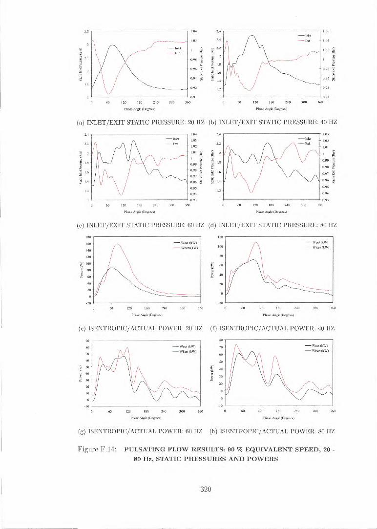
-Inlet -Exit 1.04

- 1.02 l.

1 g 0 0.

- 0.98 I0

- 0.96 g,

0.94

Stat

ic E

xit P

ress

ure

(Bar

)

-

Exit

1.03

1.02

- 1.01

-

2.4

2.2 -

2

1.8 0 X 1.6

Stat

ic E

xit P

ress

ure

(Bar

)

1.4

1.2

0.99

0.98

0.97

0.96

0.95

- 0.94

0.93 60 120 180 240 360 300


- Wact (kW) - Wisen (kW)

i .

120 180 240


-20

300 360 0 60 120 180 240 300 360

Phase A* (Degrees)

60

180

160

140

120

100

80

60

40

20

0 -20

120

100

80

g 60

4° 20


90

80

70

- watt (kW) - Wisen (kW)


60

-10

40 0

30

20

0

0

-10

60 120 180 240 300 360 0 60 120 180 240 300 360

80

70

60

50

- 0.99

- 0.98

- 0.97

0.96

0.95

0.94

0.93 360

2.4 1.04

0 60 120 180 240

Phase A* (Degrees)

300

- Inlet 1.03 - Exit

1.02

- 1.01

-Z---'

2.2

8 1.8 -

ef. 1.6

.4 1.4 -

1.2

1.04 2.6

1.02

- 1 Exit

- 0.98

0.96

- 0.94

0.92

0.9 0 60 120 180 240 300 360


1.06

0.92 60 120 180 240

300

360


3.5

fL g 2.5 0

a

1.5

2.4

Stat

ic Ex

it Pr

essu

re (E

ar)

8 1.8

4 1.6

9" 1.4

1.2

2.2

el 2 -






320

Eff i

cien

cy (To

tal-S

tatic

)

0

0.5

15

0.5

t5


Velocity Ratio (U2iCis)

(a) EFF t_s Vs U2/Ci s : 20 HZ

(b) EFF t_ s Vs U21C2s: 40 HZ

Effic

ienc

y (T

otal-S

tatic

)

O Steady State 60 Hz

-2

0 0.5

15

0.5

15

Velocity Ratio (C/2/Cis)

Velociy Ratio (U2/Cis)

(c) EFF t_s Vs U2/C23 : 60 HZ

(d) EFF t_ s Vs U2/CC s : 80 HZ

10

5

2

3

4

2 3

4




(1) MFP Vs PR t,: 40 HZ

5 g

10

2 3

4

2 3

4

Pressure Ratio (Total-State)


(g) MFP Vs PR t_ s: 60 HZ



321

3.5 400

20 Hz — 40 Hz —60 Hz 130 lIz

2.5 -

• 2

3 •

1.5

380

a • 360

.1.1 340

8 320

300

Mas

s F low

Rat

e (K

O)

0.

0.6

0.4

0.2

1.6

1.4

1.2

0

▪ 0.94 0.3 2 0.92

0.9

10.98

0.96 0

0.86

0.88

1.04

1.02

— 20 Hz — 40 Hz — 60 Hz — 80 Hz

• 1000

1.. • 990

• g 980

1010

1020

970 0 60 120 180 240 300 360

1000

995

II of

990

985

980 980

1005 992

990 -

RIC 988 '

986

984 - -6

982 -

0 60 120 180 240 300 360

1000

998

996

994

992

990

Turb

ine

Speed

80 H

z (R

PS)

— 20 Hz —40 Hz

0 60 120 180 240 300 360 0 60 120 180

240

300

360



(a) STATIC PRESSURE


60 120 180 240

300 360 0 60 120 180 240

300

360


(c) MASS FLOW RATE



18

16

14

12

10

'F2 6

4

2

0

-2 60 120 180 240

300

360 60 120 180 240 300 360 Phase Angle (Degrees)


(e) TURBINE TORQUE

(f) EFFICIENCY




Figure F.16: PULSATING FLOW RESULTS: 100 % EQUIVALENT SPEED, 20 -80 Hz, INSTANTANEOUS MEASURED PARAMETERS

322

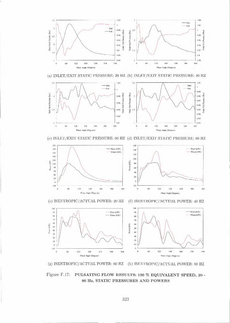
O 60 120 180 240


300 360 300 360 0 60 120 180 240

Phase An* (Degrees)

Wet ad. 0.98 .5

- 0.96 E - 0.94 k,

0.92 "'

- 0.9 1.5

0.88

0.86

tic In

Stat

ic Ex

it Pre

ssure

(Bar

)

1.04

Exit - 1.02

- 0.98

0.96

0.94

- 0.92

- 0.9

0.88

1.02

1

3.5

2

0

360 O 60 120 180 240 300 360 0 60 120 180 240 300

2.5

I

Stati

c Ex it P

ress

ure (

Bar)

6 S 2

11

0.92

1.01

1 Exit

- 0.99

0.98

- 0.97

- 0.96

0.95

0.94

- 0.93

1.02 2.5 - Inlet - Exit

5. 6 - 0.98 e.

- 0.96

0.94 -2 .2 1-5 e, - 0.92

0.9


360 60 120 180 240 300


60 -


60 120 180 240 300 360

160

140 -

(20

100 -

88 -

-20 0


-20

- Want (kW) Wisen (kW)

200

180 -

160 -

140

20 1100

300 360 0 60 120 180 240 300 360 O 60 120 180 240


100

- Want (kW) Wisen (kW)

100

90

80

70

60

▪ 50

40

30

20

10

0 -10

90

80

70

F 60

40

30

20






323

Effic

ienc

y (T

otal

-Sta

tic)

0

0

2

2

0.5

15

0.5

15

Velocity Ratio (U./Cis)

Vckicity Ratio (Ur)Cis)

(a) EFF t_s Vs U21C,s : 20 HZ

(b) EFF t, Vs U2/Cis : 40 HZ

0.5

15

0.5

15 Velocity Ratio (U2/Cis)


(c) EFF t, Vs U2 /Cis: 60 HZ

(d) EFF t _„ Vs U21C,s : 80 HZ

10

Sal

;15

2 3

4

2 3

4




(f) MFP Vs PR t_s: 40 HZ

2 3

4

3

4




(h) MFP Vs PR t_s : 80 HZ


324

2

2.5

—50 % — 60% 70 %

80 % 90%

100%

j

1.5

2.5

2

Stati

c In

let P

ress

ure

(Bar

)

1.5

—50% — 60 % — 70 %

80 % — 90 %

100%

0.8

2 g '1 0.6 -

0 0.4

— 50 % 60 %

— 70

— 90% 100%

— 50 % — 60 % — 70 % — 80 % 90%

100%

0 60 120 180

240 300 360 0 60 120 180 240 300 360



(a) STATIC PRESSURE: 20 Hz (b) STATIC PRESSURE: 40 Hz

1.5

— 50 % — 60 % — 70 % 80 % 90% 100%

— 50 % — 60%

70 % 80 %

90%

\ r 100%

2.5 1-

60 120 180 240 300 360

60 120 180 240

300

360

1.4

Name Angle (Degrees)

(c) STATIC PRESSURE: 60 Hz


(d) STATIC PRESSURE: 80 Hz

1A

1.2

2 0.8

0.6

OA

.2

Mas

s Fl

ow R

ate

(KO

)

1.2 -

0.8 -

0.6

0.4 -

0.2

0 60 120 180 240 300

360

0

60 120 180 240

300

360



(e) MASS FLOW: 20 HZ

1.2

0

(f) MASS FLOW: 40 HZ

Mas

s Fl

ow R

ate

(Kg /

s)

0 0

0.2

60 120 180 240

300 360 60 120 180 240

300

360


(g) MASS FLOW: 60 HZ

(h) MASS FLOW: 80 HZ

Figure F.19: PULSATING FLOW RESULTS: 20 - 80 Hz, PRESSURE AND MASS FLOW

325

3.5

5

2.5

11 )7;

1.5

400

380 57

A 8 360

• 340

A 320

300

380

2 360 -

A

▪ 340

1-;

N 320 •

300

— 50 % — 60 — 70 %

80 % 90% 100%

—50 % — 60 — 70 % — 80 % 90% 100%

1.05

t" 0.95

A

0.9

0.85

0.9 -

— 50 % 60

— 70 % — 80 %

90% - 100%

0.85

1.05

le • 1 A

1: 0.95

A

60 120 180 240

300

360

60 120 180 240

300

360


(a) STATIC TEMPERATURE; 20 Hz (b) STATIC TEMPERATURE: 40 Hz

300 0 60 120 180 240

300

360


60 120 180 240 300 360


380

-2 360

A

340

ffl, • 320

300

380

ae 360

2 340

2 eg 320

(c) STATIC TEMPERATURE: 60 Hz (d) STATIC TEMPERATURE: 80 Hz

' A

1.05

0.85 0 60 120 180 240


— 50 % — 60 % — 70 % 0.9 — 80 %

90% — 100%

0.85 300 360 0 60 120 180 240 300 360


0.95 -

w a

1.05

0. 0.95

3

— 50 % — 60 — 70 % — 80 %

90% — 100%

(e) EXIT STATIC PRESSURE: 20 HZ (f) EXIT STATIC PRESSURE: 40 HZ

60 120 180 240

300 360 0 60 120 180 240 300 360


Phase Aegis (Degrees)

(g) EXIT STATIC PRESSURE: 60 HZ (h) EXIT STATIC PRESSURE: 80 HZ

Figure F.20: PULSATING FLOW RESULTS: 20 - 80 Hz, TEMPERATURE AND EXIT PRESSURE

326

18

16

4

12

1. 10

ff" l 6

4

0

12

10

▪ 8

E 6

—50 % — 60% —70 % — 80 % -90 %

100 %

—50% — 60 % — 70 % — 80 %

90 % 100

300 360 . . .

60 120 180 240

Phase Angle (Degees)

-2 300 360 0 60 120 180 240


-2

—50% — 60% — 70% — 80 % --- 90 %

—100 %

14

10

• 8

8 • 6 a.

—50% — 60% — 70 %

80% - 90%

100%

300 360 0 60 120 180 240


300 360 60 120 180 240


Effic

ienc

y (T

otal

-Stat

ic)

-6 0

-4

E ffic

iency

(Toi

al-S

tatic)

— 50 % — 60 % — 70 % — 80 %

90% — 100%

2

.incy

(Tot

al-S

tatic)

-2

Effi ci

ency

(Tot

al-S

tatic

)

-2 -2

0 6U 120 180 240 300 360 0 60 120 180 240 300 360

Phase Angk (Degrees)


(a) TORQUE: 20 Hz (b) TORQUE: 40 Hz

(c) TORQUE: 60 Hz (d) TORQUE: 80 Hz

(e) EFFICIENCY: 20 HZ

60 120 180 240


(g) EFFICIENCY: 60 HZ

(f) EFFICIENCY: 40 HZ

—50 % 60 %

— 70 % -- 80 %

90% — 100•!

-6 60 120 180 240

300

360


(h) EFFICIENCY: 80 HZ

300

360

0

Figure F.21: PULSATING FLOW RESULTS: 20 - 80 Hz, TORQUE AND INSTANTANEOUS EFFICIENCY

327

0 60 120 180 240 300 360


(d) ISENTROPIC POWER: 80 Hz (c) ISENTROPIC POWER: 60 Hz

— 50 % — 60 — 70 % 80 % 90% 100%

-20 0 60 120 180 240 300 360 0 60 120 180 240 300 360


(e) ACTUAL POWER: 20 HZ


(f) ACTUAL POWER: 40 HZ

90 90

300 360

120

100

80

60 6 ag 40

— 50 % — 60 % — 70 % 80 % 90% 100%

80

70

60

50

0

0

Act

ual P

ower

(kW

)

20

10

300

-10

60 120 180 240 300 360 0 60 120 180 240


(g) ACTUAL POWER: 60 HZ


(h) ACTUAL POWER: 80 HZ

(a) ISENTROPIC POWER: 20 Hz

60 120 180 240 300 360


(b) ISENTROPIC POWER: 40 Hz

— 50 % — 60 % — 70 % — 80 % — 90% — (00%

—50 % — 60 % — 70 % 80 %

90% — MO%

Isent

ropi

e Pow

er (kW

)

140

120 -

100

80 -

60

40 -

20 -

140

120 -

60 120 180 240 300 360


0

0

. .

60 120 180 240

Phase Angle (Degrees) A

ctual P

ower

(kW)

ao -

80 -

70

60 -

50 -

30 -

20 -

10

— 50 % 60 70 % 80 % 90%

00%

0

-10

360

140

120

100

0

Isent

ropi

c Pow

er (kW

)

60

40

20

200

150

ri 100 -5

50

0

—509 — 60 % — 709 -- 80 %

90% 100%

— 50 % — 60% — 70 % 80 %

90% — 100%

Figure F.22: PULSATING FLOW RESULTS: 20 - 80 Hz, ISENTROPIC AND ACTUAL POWER

328

Eftle

tt:my

(Toa

d-St

atic)

Effic

iency

(Tot

al-S

tatic)

/ 114.040 \ •

—50% 60 70%

-- 80%

— 100%

— 50 % 60

— 70 % -- 80 %

— 90 % -- 100 %

0 0.5 1

1.5

2

0

0.5 I

1.5

Velocity Rath (U2/Cis)

Velocity Ratio (U2/Cs)

(a) EFF t_s Vs U2/Ci3 : 20 HZ

(b) EFF t_s Vs U2 /C29 : 40 Hz

0 0.5 1

Velocity Ratio (U2/C6)

0

-2 0 0.5 1

1.5


1.5

2

10

(c) EFF t_s Vs U2/Cis : 60 Hz

— SO % — 60 % — 70 % — 80 % -- 90%

100 %

(d) EFF t_s Vs U2/C1s: 80 Hz

10

Ti

9

LT. 11 7

1.5 2 2.5 3 3.5

4

45 1.5 2 2,5 3

3.5

4

Pressure Ratio (Total-Statist

Pressure Ratio (Total-Static/


(f) MFP Vs PR t—s: 40 HZ

1.5 2 2.5

3

35

1.5 2 2.5





Figure F.23: PULSATING FLOW RESULTS: 20 - 80 Hz, PERFORMANCE PARAMETERS

329

Szymko-S-2006-PhD-Thesis.pdf - Spiral – Imperial College ...

Documents

Transcript of Szymko-S-2006-PhD-Thesis.pdf - Spiral – Imperial College ...