IFPRI Discussion Paper 01454

August 2015

Supply-side Dynamics of Chickpeas and Pigeon Peas in India

Kalimuthu Inbasekar

Devesh Roy

P. K. Joshi

South Asia Office

INTERNATIONAL FOOD POLICY RESEARCH INSTITUTE

The International Food Policy Research Institute (IFPRI), established in 1975, provides evidence-based policy solutions to sustainably end hunger and malnutrition and reduce poverty. The Institute conducts research, communicates results, optimizes partnerships, and builds capacity to ensure sustainable food production, promote healthy food systems, improve markets and trade, transform agriculture, build resilience, and strengthen institutions and governance. Gender is considered in all of the Institute’s work. IFPRI collaborates with partners around the world, including development implementers, public institutions, the private sector, and farmers’ organizations, to ensure that local, national, regional, and global food policies are based on evidence. IFPRI is a member of the CGIAR Consortium.

AUTHORS

Kalimuthu Inbasekar is a scientist in the Division of Agricultural Economics at the Indian Agricultural Research Institute, New Delhi.

Devesh Roy (d.roy@cgiar.org) is a research fellow in the Markets, Trade and Institutions Division of the International Food Policy Research Institute (IFPRI), New Delhi.

P. K. Joshi is the director of the South Asia Office of IFPRI, New Delhi.

Notices 1. IFPRI Discussion Papers contain preliminary material and research results and are circulated in order to stimulate discussion and critical comment. They have not been subject to a formal external review via IFPRI’s Publications Review Committee. Any opinions stated herein are those of the author(s) and are not necessarily representative of or endorsed by the International Food Policy Research Institute. 2. The boundaries and names shown and the designations used on the map(s) herein do not imply official endorsement or acceptance by the International Food Policy Research Institute (IFPRI) or its partners and contributors.

Copyright 2015 International Food Policy Research Institute. All rights reserved. Sections of this material may be reproduced for personal and not-for-profit use without the express written permission of but with acknowledgment to IFPRI. To reproduce the material contained herein for profit or commercial use requires express written permission. To obtain permission, contact the Communications Division at ifpri-copyright@cgiar.org.

iii

Contents

Abstract v

Acknowledgments vi

1. Introduction 1

2. Data 4

3. Stylized Facts about Pulses in India: A State-level Analysis 5

4. Relative Performance of Pulses across Time Clusters: Cereals versus Pulses 10

5. Zone wise—Spatial and Temporal Variations 12

6. Determinants of Relative Area Allocation: A State-level Panel Data Analysis 20

7. Results for Chickpea Relative Area Allocation 21

8. Possible Drivers Influencing Production of Pulses in India 25

9. Conclusions and Policy Implications 26

Appendix: Supplementary Figures 27

References 30

iv

Tables

1.1 Share of different pulses in production in India, 2009–2010 1

1.2 Area shares of different crops by size categories of farms, in percentages, 2003 2

4.1 Comparative performance of cereals and pulses (percentage increase) 10

5.1 Decadal change in chickpea area and production 12

5.2 Decadal change in pigeon pea area and production 16

5.3 Major states for pulses area and production 19

7.1 Determinants of chickpea area allocation with respect to competing crops 21

7.2 Spatial variations in chickpea area allocation 22

7.3 Temporal variations in chickpea area allocation 22

7.4 Determinants of pigeon pea area allocation with respect to competing crops 23

7.5 Spatial variations in pigeon pea area allocation 24

Figures

3.1 Evolution of zone wise pulses production across states in India 6

5.1 Chickpea yield variations in various zones 14

5.2 Pigeon pea yield variations in various zones 17

A.1 Pulses areas, by states 27

v

ABSTRACT

This study was undertaken to analyze the dynamics of production for pulses in India, one of the most important crops in India from the perspective of nutrition as well as environmental sustainability. India has been persistently deficient in pulses in spite of significant investment by the government over time. Using secondary data for a long period of time, from 1950 to 2011, we study how production of pulses has changed across regions and over time in India. Realizing the role of pulses in the cereals complex, the study shows the changing scenario in pulses production as it was crowded out by cereals with the advent of Green Revolution technologies. We create typologies of different phases in the evolution of production in India. Results show that there have been pronounced movements in pulses, with production centers shifting regionally from north to south and east to west and some concentration in central India. Notwithstanding the turnaround in pulses in the past three to four years, pulses have been moving increasingly to marginal unirrigated areas. The econometric results based on fixed-effects estimation establish that as irrigation becomes available there is a switch away from pulses toward competing crops. Recent advances in technology with short- to extra-short-duration varieties that fit into cereal-based systems have opened up new avenues for pulses reflected in increasing production. Also, we find no evidence of crowding out of domestic production because of liberalized trade, which has been the case in pulses for a long period of time.

Keyword: pulses, green revolution, pigeon pea, chickpea, competing crops

vi

ACKNOWLEDGMENTS

The authors gratefully acknowledge the support of the CGIAR Research Program on Agriculture for Nutrition and Health led by IFPRI for partial funding of this project. The authors thank John McDermott for his interest in promoting the study of pulses in India and also the government of India for supporting part of the study. Researchers from the National Agricultural Research System in India provided many helpful comments on prioritizing the main issues to cover in this research. Reviews from participants in the workshop, “Pulses for Nutrition in India: Changing Patterns form Farm-to-Fork”, hosted by IFPRI are also duly acknowledged. The comments received from this workshop also validated our findings. This paper has not gone through IFPRI’s standard peer-review procedure. The opinions expressed here belong to the authors, and do not necessarily reflect those of A4NH, IFPRI, or CGIAR.

1

1. INTRODUCTION

The Green Revolution during the 1960s in India—while it benefited rice and wheat farmers—failed to distribute the benefits evenly among states and among small and medium farmers. It has been indicted by some for having led to the emergence of a new wealthy class of farmers (Sebby 2010). Moreover, the Green Revolution had a deleterious impact on several other crops. One crop group in this context has been pulses. The adoption of irrigation and consequent increase in the preference of paddy and wheat diverted the pulses area to these crops.

Yet India continues to be the largest producer (23 percent share in production and 32 percent of area under cultivation) and consumer (27 percent of global consumption) of pulses in the world (Akibode and Maredia 2011). India also grows and consumes several pulses owing to preference heterogeneity across regions. Major pulses grown in India include pigeon peas, chickpeas, black grams, green grams, and lentils. The minor pulse crops include kidney beans, cow peas, and other beans. About 72 percent of the total global area of pigeon peas, 68 percent of chickpeas, and around 37 percent of lentils are in India. These crops account for 61, 68, and 20 percent of global production, respectively (FAO 2012).1 Table 1.1 provides the relative importance of different pulses in India.

Table 1.1 Share of different pulses in production in India, 2009–2010 Pulse crop Production Share Gram 7.4 51.0 Arhar (pigeon pea) 2.4 16.7 Masur (lentil) 1.0 7.0 Urad (black matpe) 1.2 8.3 Moong (green bean) 0.6 4.7 Total pulses 14.6 100.0

Source: India, MoA (2012).

In spite of being the leading producer in different pulses, the situation over time has turned into one of persistent demand-supply gaps, several policy measures by the government to promote pulses notwithstanding. In spite of revived policy focus on pulses and several domestic and external changes with significant bearings on the pulses sector, the evolution of this sector in India remains largely underresearched. Among the few existing studies, Reddy and Mishra (2009) study growth and instability of chickpea production in India and attributes part of the increase in area-yield variances to increased price variability, erratic rainfall patterns, and fluctuations in supply of modern inputs like pesticides. Sadavatti (2007) studies the supply side of pulses in a regression framework at the regional and national level, based on the time series data covering the period from 1965/1966 to 1998/1999. The findings suggest that rainfall and farm harvest prices are significant determinants of area allocation to chickpeas and pigeon peas. Further, irrigation coverage of all crops negatively affects area allocation to pulses. Another study, Srivastava, Sivaramane, and Mathur (2010), uses total pulses area, production, and yield data from 1970 to 2006 for the state level and concludes that the growth rate of area and production is negligible and that there exists wide variability in yields across states. Using a Markov model, they conclude that area substitution coupled with the biased revenue terms of trade led to greater preference for cereals and oilseeds compared to pulses even though pulses were preferred to coarse cereals.

Pulses have traditionally played a subordinate role to other crops, mainly cereals. Table 1.2, based on the situation assessment survey of the National Sample Survey, shows the relative importance of pulses vis-à-vis other crops in terms of area shares disaggregated by farm size categories. Clearly, cereals are many times more important in terms of cropping area vis-à-vis pulses.

1 Different types of pulses in India can be grouped into seven main categories, namely, peas, pigeon peas, chickpeas,

green gram, black matpe, lentils, and beans. Peas include yellow peas, yellow split peas, green peas, and dry peas. Pigeon pea includes whole peas as well as ones with minor processing, that is, split pigeon pea. Chickpeas comprise desi chana, kala chana, and white peas. Green gram or moong include green as well as yellow moong, both whole and split varieties. The combined beans category includes kidney beans, black-eyed beans, cow peas, lablabbeans, and green beans.

2

Across all farm size categories, allocation of land to pulses is roughly of the same order as another crop crowded out by cereals, that is, oilseeds.

Table 1.2 Area shares of different crops by size categories of farms, in percentages, 2003 Crop groups Marginal Small Medium Large Total Share in landholdings 63.09 19.26 11.46 6.18 100.00 Rice 38.09 31.14 24.76 15.13 26.67 Wheat 20.90 17.21 15.83 14.16 16.92 Maize 5.66 5.45 4.38 2.89 4.50 Other cereals 9.26 12.85 14.76 17.69 13.82 Total cereals 73.90 66.64 59.73 49.87 61.90 Pulses 6.58 9.53 10.96 16.01 11.04 Oilseeds 6.20 8.31 12.13 15.44 10.78 Fibers 2.01 3.64 5.05 6.87 4.51 Sugar crops 2.20 3.30 3.47 2.88 2.93 Fruits 1.12 1.20 1.37 1.06 1.18 Vegetables 4.03 3.08 2.06 1.24 2.54 Spices 1.05 1.00 1.24 1.13 1.11 Plantation 0.98 0.70 0.52 0.49 0.67 Flowers 0.09 0.05 0.13 0.03 0.07 Medicinal and narcotic plants 0.20 0.27 0.39 0.16 0.25 High-value crops 7.46 6.29 5.71 4.11 5.81 Other crops 1.65 2.28 2.96 4.82 3.03

Source: India, MSPI (2005).

In relation to these existing studies, in this paper we map out the dynamics of pulses across states and within states, that is, at the district level (for frontline states), using a long time period beginning in the 1950s. With the long panel of states we are able to create phases in the evolution of pulses into four categories, namely, pre–Green Revolution period, post–Green Revolution period, postliberalization period, and a period following the trade spike from 2000. There were several phase-specific factors that would have a bearing on the supply side of pulses. During the Green Revolution period, the reduction in the variability of paddy and wheat yields coupled with unabated risks in pulses could have led to the substitution of the pulses area by the paddy and wheat area. Even though farmers are price responsive and farm harvest prices of pulses are much higher than those of competing crops like cereals, farmers do not realize reasonable returns for their outputs because of lower and also unstable yields of chickpeas and pigeon peas (Savadatti 2007). The price policy and procurement support of the government in favor of paddy, wheat, cotton, and sugarcane would further affect the choice of farmers to grow pulses.

An extensive mapping of the movement of pulses area and production across space and time allows us to create clusters where we can place the different states into specific groups. These clusters comprise states of gaining ground, losing ground, and being in between or status quo. Those with secular upward trends in pulses production are clubbed into gaining-ground states, with a secular downward trend into losing-ground states and those with in between and no clear patterns as status quo states.

Further, while studying the evolution of the pulses sector we disaggregate the analysis by variety (focusing mainly on pigeon peas and chickpeas) across zones, states, and districts in leading states. Chickpeas and pigeon peas constitute 60 percent of the pulses area and production. With state and some district-level analysis we study how pulses have moved in response to several changes such as the Green Revolution, economic reforms of 1991, and trade spikes since 2000. Overall, pulses seem to have been confined to marginal environments as comparatively resource-rich farmers have tended to prefer crops like paddy, wheat, cotton, and sunflower. Pulses continue to be produced mostly by small and marginal farmers under rainfed conditions. Our findings suggest that this characteristic of confinement to comparatively marginal environments is in spite of the inter-regional movement of pulses production that has become quite pronounced in the past two decades.

After mapping the production/area allocation we go a step further and test econometrically for the factors affecting area allocated to pulses relative to competing crops using robust fixed-effects

3

estimation. The rich specification controls for several observed as well as state- and time-specific unobserved factors thereby mitigate the omitted variables problem to a large extent. Inclusion of the state and time fixed effects is a significant improvement over the methodologies followed in the few studies that exist. Also, in terms of variables that we control for, apart from state and year fixed effects we include time-specific rainfall such as September and October rainfall for chickpeas and June and July rainfall for pigeon peas. In terms of main variables of interest, the empirical model focuses on conditions such as rain dependence, improvements such as mechanization, and economic availability of labor.

Further, the outcome variable in our regression analysis is distinct from that in other papers on related topics. We invoke regionwise differences in crops competing with pulses to get a more accurate picture of land allocation. We believe that the right metric for intensity of pulses cultivation is land put to it vis-à-vis the competing crops rather than absolute allocation. Using state-level data, we show that for a long period since 1950, the overall scenario in pulses has been characterized by sluggishness in area as well as in production. Important to note, pulses consumption is characterized by significant spatial preference heterogeneity. Chickpeas, for example, are more popular in the north, while black matpe is a staple in south India. Until the last two decades, the data showed congruence between area of production and consumption.

Over time, as infrastructure developed, incomes rose, and India opened up for liberalized imports in pulses, having a significant effect on pulses production. Changes over time resulted in significant reallocation across space in terms of production and area even within states. Increasingly the production and area allocated to pulses moved from eastern India to the west and from north to south. Moreover, geographically production and consumption of pulses in India got increasingly decoupled, a tendency reinforced because of imports of different types of pulses. Amid all these changes, for a large part until the middle of the 1990s, the yields in pulses remained stagnant owing to lack of technological progress in pulses. Studies have attributed low yield per hectare to various factors, mainly lack of high-yielding and short-duration varieties and competition with other crops. Inadequate irrigation, cultivation in inferior lands, absence of fertilizer use, frequent attacks of pests and diseases, dearth of extension services, and poor infrastructure and slow transfer of technology have also disadvantaged the pulses sector (Banerjee and Palke 2010).

Our regression results reinforce only some of these findings. The results show that even across states, mechanization and irrigation are strongly associated with allocation of less land to pulses vis-à-vis the state-specific competing crops. In other words as these amenities become available they draw land away from pulses to other remunerative crops. In the case of chickpeas there is robust evidence of negative association with wage rates as well.

The paper is organized as follows. Section 2 presents a summary of data sources, explaining the methods for creating the variables for analysis. Subsequently, section 3 presents some stylized facts about pulses in India as a whole and across states. Section 4 brings up a synopsis of the comparative performance of pulses vis-à-vis cereals during different periods and in different zones. In section 5 we present a detailed picture of spatial and temporal variations in pulses area and production with special reference to chickpeas and pigeon peas. Section 6 concludes and draws some policy implications.

4

2. DATA

This study focuses on area, production, and yields for two pulses, namely, chickpeas and pigeon peas. The state-level analysis is conducted for the period from 1950 to 2011 based primarily on secondary data published in 2012 from various sources such as the Directorate of Economics and Statistics (DES) and Ministry of Agriculture (MoA). To study the spatial movement of pulses over time, we group the states into six zones based on geographical location. The northern zone comprises Haryana, Himachal Pradesh, Punjab, Jammu and Kashmir, and Uttar Pradesh. The southern zone comprises Andhra Pradesh, Karnataka, and Tamil Nadu. The eastern and western zones consist of Assam, Bihar, Odisha, West Bengal and Rajasthan, Gujarat, and Maharashtra, respectively. Only two states lie in the central zone, namely, Madhya Pradesh and Chhattisgarh. Finally, the northeast zone is made up of Manipur, Meghalaya, Nagaland, Sikkim, Tripura, and Mizoram.

The data pertain to area, production, and yield from triennium ending (TE) 1960 to TE 2010. The data used for regression analysis belong to the period 1981 to 2010. The ratio of chickpea area to area of its competing crops is calculated by taking the chickpea area and dividing it by the sum of areas of all competing crops. The set of competing crops varies across states. Similarly, the land allocation variable is constructed in case of pigeon peas.

Among the other variables used in the analysis, road density is expressed as a percentage of length of road in kilometers to total area of the state in square kilometers. These road density data were obtained from the Ministry of Road Transport and Highways. Fertilizer per hectare is calculated dividing total fertilizer consumption by gross cropped area in the state. These fertilizer data have been obtained from various issues of Fertilizer Association of India. Market density has been calculated as the number of markets per hundred square kilometer area. Urbanization is the percentage of urban population to total population in the state.

September and October rainfall is calculated as monthly mean rainfall based on data from the Indian Meteorological Department. It is available at the district level. We averaged it to the state level by averaging across districts for that time period. Smallholder density refers to the percentage of smallholders in the total agrarian population. Tractor intensity is expressed as the number of tractors per thousand square kilometers of gross cropped area. Similarly, irrigation intensity obtained from the DES and MoA (2012) is calculated as a percentage of area under irrigation to total cropped area. Per capita income is calculated as national income at factor cost divided by the total population of the state. It was collected from the Reserve Bank of India at 2004/2005 constant prices. The wage rate, collected from the DES and MoA (2012). represents the mean annual wage in rupees for the state.

5

3. STYLIZED FACTS ABOUT PULSES IN INDIA: A STATE-LEVEL ANALYSIS

Broadly the evolution of pulses in India can be summarized in terms of the following stylized facts: 1. The area under pulses moved from northern to southern regions and from eastern to

western regions, and central India emerged as the hub of pulses production. This trend was accentuated after 1990.

2. The area, production, and yield of major crops including pulses show an increasing trend in the post–trade spike period (beginning 2000).

3. Over time Madhya Pradesh, Andhra Pradesh, Karnataka, and Maharashtra have become the leading states in pulses production and area. Maharashtra has consistently maintained its position, whereas others like Andhra Pradesh have leapfrogged to be among the leading pulse states. Further, the emerging spatial patterns in pulses production have become more pronounced since 1990. These patterns leading to regional specialization are also characterized by geographical continuity (that transcends state boundaries).

4. In the northeast, Nagaland and Manipur show increasing trends in pulses area and production. Other states in the region have maintained the status quo.

5. Further, compact yield distributions imply reflection of area on production by cluster, that is, high production area overlap with high output of pulses.

6. Nationally, across varieties, in the pre– and post–Green Revolution period, pigeon peas show an increasing trend in area and production, while the opposite holds true for chickpeas. In the postliberalization and pre–trade spike period (1991–2000) chickpeas show significant increases in area, production, and yield. In the same period, pigeon peas show a decreasing trend for these indicators.

7. In the post–trade spike period (2001–2010) both chickpeas and pigeon peas show increasing trends.

These facts are summarized in Figure 3.1. In plotting the pulses production over time, bifurcations of states that have happened at different points in time have been accounted for. Given the differences in area and production among the states in the north zone with mountain states like Jammu and Kashmir, Himachal Pradesh, and newly formed Uttarakhand, having much smaller area and production, we divided these states into a separate category. There has been a stark change in the area and production of pulses in the frontline agricultural states of Punjab, Haryana, and Uttar Pradesh. In the two states, namely, Haryana and Punjab, the land allocated to pulses and production has been driven almost to zero. Uttar Pradesh has more or less maintained its production of pulses during a period of more than 60 years.

6

Figure 3.1 Evolution of zone wise pulses production across states in India

0

1000

2000

3000

4000

500019

50-5

119

53-5

419

56-5

719

59-6

019

62-6

319

65-6

619

68-6

919

71-7

219

74-7

519

77-7

819

80-8

119

83-8

419

86-8

719

89-9

019

92-9

319

95-9

619

98-9

920

01-0

220

04-0

520

07-0

820

10-1

1

'000

tons

North zone-I pulses production

Haryana Punjab Uttar Pradesh

0102030405060

1950

-51

1953

-54

1956

-57

1959

-60

1962

-63

1965

-66

1968

-69

1971

-72

1974

-75

1977

-78

1980

-81

1983

-84

1986

-87

1989

-90

1992

-93

1995

-96

1998

-99

2001

-02

2004

-05

2007

-08

2010

-11

'000

tons

North zone-II pulses production

Himachal Pradesh Jammu & Kashmir Uttarakhand

0200400600800

10001200140016001800

1950

-51

1953

-54

1956

-57

1959

-60

1962

-63

1965

-66

1968

-69

1971

-72

1974

-75

1977

-78

1980

-81

1983

-84

1986

-87

1989

-90

1992

-93

1995

-96

1998

-99

2001

-02

2004

-05

2007

-08

2010

-11

'000

tons

South zone pulses production

Andhra Pradesh Karnataka Tamil Nadu

7

Figure 3.2 Continued

.

05

101520253035

1950

-51

1953

-54

1956

-57

1959

-60

1962

-63

1965

-66

1968

-69

1971

-72

1974

-75

1977

-78

1980

-81

1983

-84

1986

-87

1989

-90

1992

-93

1995

-96

1998

-99

2001

-02

2004

-05

2007

-08

2010

-11

'000

tons

Keral pulses production

Kerala

0200400600800

100012001400

1950

-51

1953

-54

1956

-57

1959

-60

1962

-63

1965

-66

1968

-69

1971

-72

1974

-75

1977

-78

1980

-81

1983

-84

1986

-87

1989

-90

1992

-93

1995

-96

1998

-99

2001

-02

2004

-05

2007

-08

2010

-11

'000

tons

East zone pulses production

Bihar Orissa West Bengal Jharkhand

0500

100015002000250030003500

1950

-51

1953

-54

1956

-57

1959

-60

1962

-63

1965

-66

1968

-69

1971

-72

1974

-75

1977

-78

1980

-81

1983

-84

1986

-87

1989

-90

1992

-93

1995

-96

1998

-99

2001

-02

2004

-05

2007

-08

2010

-11

'000

tons

West zone pulses production

Gujarat Maharashtra Rajasthan

8

Figure 3.3 Continued

. Source: India, DES and India, MoA (various years).

What is happening to the frontline agrarian states in the north zone is the opposite of the case in south India. Big southern states such as Karnataka and Andhra Pradesh have experienced secular growth in pulses production particularly in the postliberalization period. Further, the pattern in Uttar Pradesh is mimicked by that in Tamil Nadu. Kerala in the south had comparatively low levels of pulse production throughout, and whatever little it had, like Punjab and Haryana, has descended toward zero since the mid-1990s. In this movement of pulses from north to south, particularly to Andhra Pradesh and Karnataka, the 1990s seemed to be the time of the structural break.

Similar to the migration of pulses from north to south, there is a distinctive shift in pulses production from east to west, albeit in a more pronounced fashion. Barring the new state of Jharkhand, other eastern states such as Bihar, Odisha, and West Bengal have been losing ground in pulses. Only recently (post-2000), Odisha has begun to come up in pulses production. At the same time Maharashtra and Rajasthan have expanded their pulses production over time. Akin to the case of Tamil Nadu or Uttar Pradesh, Gujarat has maintained the status quo during a long period of time.

0500

100015002000250030003500400045005000

1950

-51

1953

-54

1956

-57

1959

-60

1962

-63

1965

-66

1968

-69

1971

-72

1974

-75

1977

-78

1980

-81

1983

-84

1986

-87

1989

-90

1992

-93

1995

-96

1998

-99

2001

-02

2004

-05

2007

-08

2010

-11

'000

tons

Central zone pulses production

Madhya Pradesh Chhatisgarh Linear (Madhya Pradesh)

0

10

20

30

40

50

1950

-51

1953

-54

1956

-57

1959

-60

1962

-63

1965

-66

1968

-69

1971

-72

1974

-75

1977

-78

1980

-81

1983

-84

1986

-87

1989

-90

1992

-93

1995

-96

1998

-99

2001

-02

2004

-05

2007

-08

2010

-11

'000

tons

North east zone pulses production

Manipur Meghalaya Nagaland

Sikkim Tripura Mizoram

9

The northeast zone mostly comprises states with little changes in pulses production over time but at a low level given their small land areas. The exceptions are Manipur and Nagaland, more so the latter, which experienced a sharp increase in pulses production. In a relative sense, the orders of magnitude are still quite small even for Nagaland. At its peak the production in Nagaland equaled merely 40,000 tons.

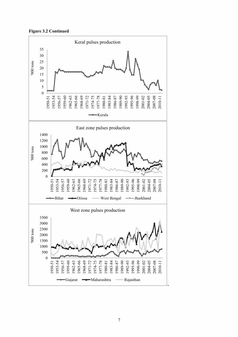
Amid all these changes, the region that has kept its engagement with pulses on a consistent upward trajectory is central India. Comprising the two states of Madhya Pradesh and Chattisgarh, there have been continued increases in pulses production (given modest yield improvements in area, see Figure A.1 in the appendix). The only perceptible dip in Madhya Pradesh is associated with the bifurcation of the state after 2000, which when combined with figures for Chattisgarh keeps the pattern intact for the region as a whole.

The discussion above presents the dynamics of pulses production across regions in India. The increase or decrease in production/area of pulses comes from changes in competing crops. Most commonly cereals constitute the crops with which pulses compete.

10

4. RELATIVE PERFORMANCE OF PULSES ACROSS TIME CLUSTERS: CEREALS VERSUS PULSES

Table 4.1 summarizes the relative performance of pulses over time (vis-à-vis cereals) in terms of area, production, and yield measures. The time clusters with which these indicators are summarized are the ones listed above.

Pre–Green Revolution Period (1960–1970) During this period nationally chickpea area and production declined by 21.64 and 9.73 percent, respectively, while pigeon pea area and production increased by 8.26 and 10.68 percent. Overall the pulses area declined by 8 percent. Concomitantly, wheat area and production gained momentum and increased shares (Table 4.1). All over India during this period paddy area and production increased by nearly 12 and 34 percent, respectively. The highest yield increase was observed in wheat (55.13 percent), followed by paddy (19.72 percent). While the chickpea yield increased by about 15 percent, the pigeon pea yield increased marginally. However, the total pulses yield during this period increased by 8 percent—a remarkably inferior performance vis-à-vis cereals.

Table 4.1 Comparative performance of cereals and pulses (percentage increase) Crop Particulars Pre–Green

Revolution period (1960–1970)

Post–Green Revolution period (1970–1990)

Postliberalization period (1991–2000)

Post–trade spike period (2000 onward)

Chickpea Area –21.6 –18.4 17.6 6.4

Production –9.73 –18.0 39.1 12.3

Yield 14.9 0.5 19.0 5.1

Pigeon pea Area 8.2 32.5 –1.8 3.3

Production 10.6 42.6 –5.8 7.6

Yield 2.4 7.3 –3.9 3.9

Total pulses Area –8.0 3.3 –0.9 2.2

Production –0.8 10.3 2.1 14.0

Yield 7.9 6.7 3.6 11.2

Wheat Area 26.1 48.5 15.6 3.1

Production 95.5 171.5 42.5 12.1

Yield 55.1 83 23.3 8.7

Paddy Area 11.8 10.5 8.7 –1.5

Production 33.7 70.6 28.5 10.3

Yield 19.7 54.0 18.5 12.0

Source: India, DES and India, MoA (various years).

Post–Green Revolution Period (1970–1990) The government of India implemented a pulses development scheme during this period in its fourth 5-year plan. However, the chickpea yield increase was merely 0.5 percent. Consequently, the 18 percent decrease in chickpea area was accompanied by a 18 percent decrease in production. On the other hand, the pigeon pea area and production increased, and its yield showed more than a 7 percent increase in this period. However, the total pulses area and production increased by 3.31 and 10.34 percent, respectively. In comparison, wheat area, production, and yield increased by more than 48 and 83 percent, respectively, while paddy area, production, and yield increased by 10, 70, and 54 percent.

11

Post liberalization Period (1991–2000) In this period there was a remarkable increase in chickpea area, production, and yield by nearly 18, 39, and 19 percent, respectively, while pigeon peas showed a marginal decrease. Overall the pulses area declined (Table 4.1); while wheat area increased by 15 percent, the paddy area increased by less than 9 percent. The yield of both wheat and paddy increased during this period as well. During the beginning of the 1990s, short-duration chickpea varieties were introduced in Andhra Pradesh and Karnataka. This could be the reason chickpea area, production, and yield increased significantly.

Post–Trade Spike Period (2000 Onward) After 2001 there was a spike in trade, with a 36 percent increase in pulses imports. During this period chickpeas, pigeon peas, wheat, and paddy all showed increases in area, production, and yield. For the first time the total pulses yield increased by more than 11 percent. The success of the technology mission in oilseeds induced the government to restructure the program into the Integrated Scheme on Oilseeds, Pulses, Oil Palm and Maize (ISOPOM) by including pulses and maize in it in 2004.

Under the ISOPOM scheme, financial assistance is provided for the production and distribution of certified seeds, seed mini kits, sprinkler sets, rhyzobium cultures and Phosphate Solubilising Bacteria, gypsum/pyrite, plant protection chemicals, and biofertilizers. Integrated Pest Management demonstrations are organized through the State Department of Agriculture on a large scale. Provision for the crash program for quality seed production of pulses has also been made in the scheme to meet the need for quality seeds. The accelerated pulses production program under the National Food Security Mission was implemented in 468 districts of 16 states.

12

5. ZONE WISE—SPATIAL AND TEMPORAL VARIATIONS

The analysis above has focused on the evolution of pulses by the four time clusters. Below we summarize the behavior of the pulses sector across zones (and states within zones for the four time clusters) (Table 5.1).

Table 5.1 Decadal change in chickpea area and production Percentage change

State Pre–Green Revolution

Post–Green Revolution

Postliberalization Post–trade spike

Northern zone Haryana –34.1 (–13.6) –54.5 (–54.4) –40.7 (–51.6) –61.3 (–63.2) Himachal Pradesh –47.7 (–60.7) –59.3 (–70) –64.92 (–22.7) –56.7 (–74.07) Punjab –53.1 (–52.3) –85.4 (–87.1) –83 (–80.3) –73.4 (–65.09) Uttar Pradesh –15.2 (4.9) –40.6 (–35.5) –35.5 (–28.2) –35.2 (–37.05)

Southern zone Andhra Pradesh –24.2(–33.3) –33.5 (35.3) 189.7 (288.05) 313.1(729.9) Karnataka 34.2 (124) 4.4 (–14.5) 54.5 (105.9) 127.5 (172.3) Tamil Nadu 37.5 (50) 64.5 (86.6) 33.1 (35.7) –12.4 (–11.1)

Eastern zone Assam — 73.3 (30) –23.08 (–23) –31.2 (30) Bihar –50.06 (–27.6) –38.02 (–27.3) –34.31 (–70.8) –42.9 (–40.5) Odisha 19.3 (156.2) 98.09 (109.02) –26.8 (–37.4) 23.3 (57.2) West Bengal –14.5 (19.3) –74.4 (–76.4) –41.05 (–32.4) –9.02 (23.1)

Western zone Gujarat –65.7 (–60.2) 95.6 (28.3) 42.7 (94) 54.5(92.4) Maharashtra –13.1 (–17.1) 60.6 (186.5) 37.5 (49.5) 48.4 (106.7) Rajasthan –20.7 (–3.49) –13.6 (–14.0) 93.1 (123.8) –43.7 (–55.3)

Central zone Madhya Pradesh 3.1 (1.07) 34.4 (74.6) 21.6 (66.6) 6.9 (5.1) India –21.6 (–9.7) –18.4 (–18) 17.6 (39.1) 6.4 (12.3)

Source: India, DES and India, MoA (various years). Note: Terms in parentheses are for production. Dash indicates missing data.

Table 5.1 shows that all over India, the chickpea area decreased during pre– and post–Green Revolution periods. However, it increased during the postliberalization period and during the post–trade spike period. Underlying these changes are significant regional differences. In the northern zone (principal area for consumption) the chickpea area declined continuously from the pre–Green Revolution period to the present. This is a salient feature of the transition in pulses where the production and consumption nodes begin to get decoupled from each other (Table 5.1).

In the southern zone Andhra Pradesh showed significant expansion in the chickpea area during the postliberalization period with a major spurt in the post–trade spike period. The chickpea area in Karnataka increased quite significantly as well during this period to the extent of 128 percent. However, Tamil Nadu showed a decrease in the chickpea area during the post–trade spike period.

In the eastern region, Odisha showed about a 23 percent increase in the chickpea area during the post–trade spike period. Earlier, during the post–Green Revolution period Odisha and Assam increased their respective chickpea areas. In western India, the overall chickpea area increased by more than 90 percent during the postliberalization period. Gujarat and Maharashtra are the two states in western India that showed a continuous increase in the chickpea area from the post–Green Revolution period.

13

There could be several demand- and supply-side factors explaining the regional dynamics in pulses including chickpeas. Since 1990, three improved chickpea varieties—ICCC 37, ICCV 2, and ICCC 10—were released in Andhra Pradesh. These were developed by the International Crop Research Institute for Semi-Arid Tropics in collaboration with the national program, such as the Andhra Pradesh Agricultural University (Joshi, Asokan, and Bantilan 2005).

Apart from the introduction of new technology in terms of varieties, more labor-intensive crops like cotton, chilies, and other cash crops were substituted by the less labor-intensive chickpea crop. Crops like cotton are prone to pests and diseases, and prices are usually subject to high fluctuations; chickpea, a low-risk crop, is found to be a suitable alternative to varied dry land agroclimatic conditions in Andhra Pradesh. Low pest and disease attack compared to other crops, storability, and lower price fluctuations triggered the adoption of chickpeas by farmers in Andhra Pradesh (Suhasini et al. 2009). In most of the northern and eastern states that show a declining trend in the chickpea area, the decrease might be attributable to extended irrigation facilities and nonavailability of inputs responsive to high-yielding varieties.

During the pre– and post–Green Revolution periods, chickpea production showed a decreasing trend, while during the postliberalization period, chickpea production increased by 39 percent. In the northern zone all states show a decreasing trend in chickpea production. This is because of substitution by cereals. In the southern zone, Andhra Pradesh has shown a 700 percent increase in production in the post–trade spike period. Karnataka and Maharashtra have shown 172 and 107 percent increases in production during the same period. In the central zone Madhya Pradesh showed only a little more than a 5 percent increase in the post–trade spike period, but this has to do with the consistent upward trajectory in pulses.

In the western zone Maharashtra and Gujarat are the emerging states in chickpea production. In the central zone Madhya Pradesh showed a remarkable increase during the post–Green Revolution and postliberalization periods (Table 5.1). This variation in chickpea production is due to increased price variability, more erratic rainfall patterns, and fluctuations in supply of modern inputs like pesticides (Reddy and Mishra 2009).

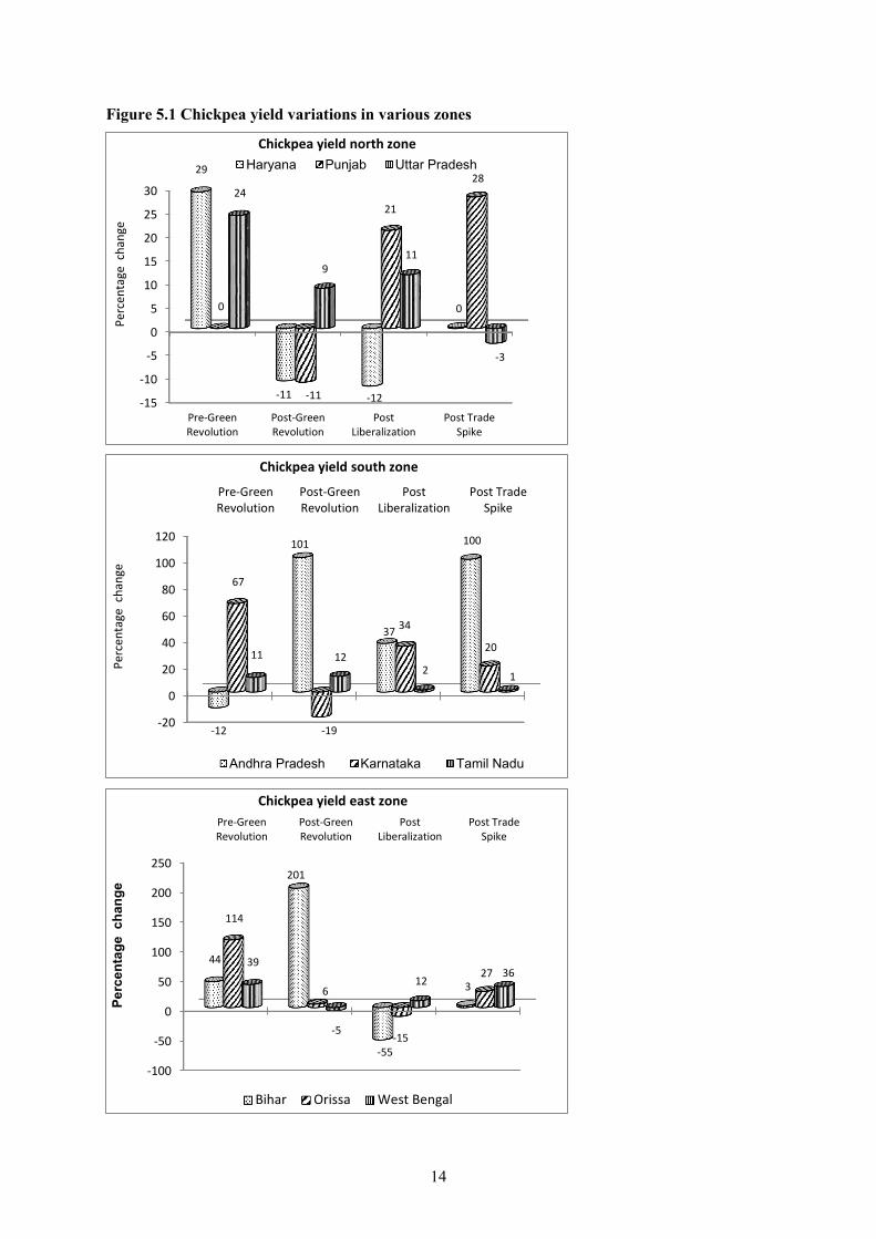
The yield patterns in chickpeas across regions are presented in Figure 5.1. In both the northern and southern zones, the yields have increased considerably in some states in the postliberalization period. In Andhra Pradesh the spurt in yields is striking in the past decade, that is, the period subsequent to the trade spike. In terms of yields growth, both the eastern and western zones have not fared well over time even when portions of the north and particularly south India took off with yield spurts. Madhya Pradesh experienced a significant yield growth of more than 37 percent in chickpeas, which owing to a high base effect culminated in no growth in the post–trade spike period.

14

Figure 5.1 Chickpea yield variations in various zones

-15

-10

-5

0

5

10

15

20

25

30

Pre-GreenRevolution

Post-GreenRevolution

PostLiberalization

Post TradeSpike

29

-11 -12

00

-11

21

2824

911

-3

Perc

enta

ge c

hang

e

Chickpea yield north zoneHaryana Punjab Uttar Pradesh

-20

0

20

40

60

80

100

120

Pre-GreenRevolution

Post-GreenRevolution

PostLiberalization

Post TradeSpike

-12

101

37

100

67

-19

34

2011 12

2 1

Perc

enta

ge c

hang

e

Chickpea yield south zone

Andhra Pradesh Karnataka Tamil Nadu

-100

-50

0

50

100

150

200

250

Pre-GreenRevolution

Post-GreenRevolution

PostLiberalization

Post TradeSpike

44

201

-55

3

114

6

-15

2739

-5

1236

Perc

enta

ge c

hang

e

Chickpea yield east zone

Bihar Orissa West Bengal

15

Figure 5.1 Continued

Source: India, MoA and India, DES (various years).

-100

-50

0

50

100

150

200

250

300

350

Pre-GreenRevolution

Post-GreenRevolution

Post Liberalization Post Trade Spike

26

349

-67

34

-5

76

84121

-1

16

-20

Per

cent

age

cha

nge

Chickpea yield west zone

Gujarat Maharashtra Rajasthan

-5.00.05.0

10.015.020.025.030.035.040.0

Pre-GreenRevolution

Post-GreenRevolution

PostLiberalization

Post TradeSpike

-1.4

30.0

37.0

-3.2

Perc

enta

ge c

hang

e

Chickpea yield in Madhya Pradesh

Madhya Pradesh

0.0

5.0

10.0

15.0

20.0

Pre-GreenRevolution

Post-GreenRevolution

PostLiberalization

Post TradeSpike

15.0

0.5

19.0

5

Perc

enta

ge c

hang

e

Chickpea yield in India

India

16

In summary, all over India, chickpea yields increased prior to the Green Revolution but stagnated during the post–Green Revolution period. The yields in chickpeas staged a comeback during the postliberalization period, increasing by as much as 19 percent. Most salient of the yield increase has been the state of Andhra Pradesh during the post–Green Revolution and post–trade spike periods. Karnataka also showed an increasing trend in chickpea yields from the postliberalization period. In Bihar the chickpea yield increased 200 percent during the post–Green Revolution period. In Gujarat, the post–Green Revolution period witnessed a 348 percent increase in the chickpea yield.

Dynamics of Pigeon Peas over Time Table 5.2 presents the dynamics of pigeon peas across regions in India. In this case, area increased drastically after the Green Revolution to the tune of 30.4 percent. Subsequently, the area allocation to pigeon pea production has moderated and decreased by 1.89 percent during the postliberalization period, followed by a reversal in the post–trade spike period, resulting in a 3.37 percent increase in the pigeon pea area. In the post–Green Revolution period Punjab and Haryana showed remarkable increases in pigeon pea areas. In the northern zone, from the postliberalization period onward, the pigeon pea area has been showing a decreasing trend.

Table 5.2 Decadal change in pigeon pea area and production Percentage change State Pre–Green

Revolution Post–Green Revolution

Postliberalization Post–trade spike

Northern zone Haryana ---- 411.6(853.8) -30.1(-19.4) -5.9(-7.9) Punjab ----- ------ -60.5(-63.1) -41.7(27.8) Uttar Pradesh -5.2(-0.3) -17.5(-7.5) -13.0(-18.3) -24.4 (-46.2) Southern zone Andhra Pradesh 12.1 (62.6) 93.4 (–24.9) 12.1 (97.8) 19.5 (85.1) Karnataka –1.9 (23.2) 70.2 (53.5) –2.5 (11.8) 33.9 (77.5) Tamil Nadu –6.5 (–16.2) 187.7 (416.1) –48.8 (–48.2) –63.05 (–65.5) Eastern zone Assam 83.3 (60) 119.09 (112.5) –11.6 (–11.1) –17.3 (–19.2) Bihar –7.8 (37.5) –59.9 (–44.07) –7.4 (5.9) –54.2 (–58.4) Odisha 163.4 (181.8) 307.3 (437.1) –4.09 (–25.9) –3.1 (39.5) West Bengal 26.8 (62.5) –83.5 (–78.2) 26.8 (62.5) –73.1 (67.7) Western zone Gujarat 15.9 (16.9) 276.9 (419.8) 6.6 (36.5) –28.4 (–14.1) Maharashtra 11.9 (–3.4) 41.9 (92.6) 16.1 (10.2) 7.3 (28.3) Rajasthan 11.2 (38.8) 4.4 (80) 33.7 (88.6) –42.6 (–55.9) Central zone Madhya Pradesh 30.6 (21.1) –9.6 (44.6) –19.8 (–37.6) –6.7 (–10.3) India 8.2 (10.6) 32.5 (42.6) –1.8 (–5.8) 3.3 (7.6)

Source: India, MoA and India, DES (various years). Note: Terms in parentheses are for production. Dashes indicate missing values

Elsewhere, Andhra Pradesh and Maharashtra have experienced a continuous increase in the pigeon pea area. Not a marked story in pulses by any yardstick, Gujarat witnessed a staggering increase in pigeon pea production and area in the post–Green Revolution period, but the area decreased during the post–trade spike period. In the central zone Madhya Pradesh had a continuous decrease in the pigeon pea area. In the postliberalization period the pigeon pea area declined 19.8 percent in Madhya Pradesh.

In India, pigeon pea production increased by 10.68 and 42.6 percent during the pre– and post–Green Revolution periods, respectively. However, it declined 5.81 percent during the postliberalization period. In the northern zone, Punjab and Haryana showed remarkable increases in the pigeon pea yield, but they started to decline during the postliberalization and post–trade spike periods. In the southern zone Karnataka has shown a continuous increase in pigeon pea production. In fact Karnataka has become the leading state in pigeon pea production. In the south, as Andhra Pradesh rose up the ranks in chickpeas, pigeon pea production decreased by 25 percent during the post–Green

17

Revolution period. In the eastern zone Odisha showed a nearly 40 percent increase in production during the post–trade spike period, while in the western zone, Gujarat and Rajasthan experienced decreases in pigeon pea production—more so the latter.

Figure 5.2 plots the evolution of yields in pigeon peas across states over time. At an all-India level there was a 4 percent decrease in pigeon pea yield during the postliberalization period. Compared with chickpeas there has been no substantial increase in the pigeon pea yield in India. Uttar Pradesh showed a decrease in yield during the postliberalization and post–trade spike periods. In the southern zone Andhra Pradesh and Karnataka showed 61.24 and 10.31 percent decreases in pigeon pea yields in the post–Green Revolution period but reversed the trend thereafter in the postliberalization and post–trade spike periods (Figure 5.2).

Figure 5.2 Pigeon pea yield variations in various zones

.

-40

-20

0

20

40

60

80

Pre-GreenRevolution

Post-GreenRevolution

Post Liberalization Post Trade Spike

77.14

8.764.13

-19.03

-8.67

29.99

5.7611.83

-5.76

-29.67

Per

cent

age

cha

nge

Pigeon pea yield south zone

Haryana Punjab Uttar Pradesh

-80

-60

-40

-20

0

20

40

60

80

Pre-GreenRevolution

Post-GreenRevolution

PostLiberalization

Post Trade Spike

44.53

-61.24

71.0659.73

26.9

-10.31

11.37

34.47

-10.36

79.73

-1.53 -1.24

Per

cent

age

cha

nge

Pigeon pea yield south zone

Andhra Pradesh Karnataka Tamil Nadu

18

Figure 5.3 Continued

.

.

. Source: India, MoA and India, DES (various years).

-40

-30

-20

-10

0

10

20

30

40

50

60

Pre-GreenRevolution

Post-GreenRevolution

Post Liberalization Post Trade Spike-13.33

-2.35

0.56

-2.24

50.26

39.42

14.65

-8.11

7.17

30.81

-22.23

43.91

Per

cent

age

cha

nge

Pigeon pea yield south zone

Assam Bihar Orissa West Bengal

-30-20-10

01020304050607080

Pre-GreenRevolution

Post-GreenRevolution

Post Liberalization Post Trade Spike

1.27

35.3930.77 19.56

-13.07

34.66

-5.23

18.67

26.87

44.95

71.38

-25.38

Perc

enta

ge c

hang

e

Pigeon pea yield south zone

Gujarat Maharashtra Rajasthan

-4

-2

0

2

4

6

8

Pre-GreenRevolution

Post-GreenRevolution

Post Liberalization Post Trade Spike

2.4

7.32

-3.99

3.91

Perc

enta

ge c

hang

e

Pigeon pea yield India

India

19

Based on the discussion above we create a typology of states in terms of their patterns of pulses production. In particular we enlist states into respective clusters of gaining-ground, losing-ground, and in between (status quo) states based on the observed secular trends in pulses production. Table 5.3 presents the typology for chickpeas, pigeon peas, and total pulses. Notably, the number of gaining-ground states is lower than the number of losing-ground states, depicting the overall decline in prominence of pulses.

Table 5.3 Major states for pulses area and production Chickpea Pigeon pea Total pulses

Area Production Area Production Area Production

Gai

ning

gr

ound

Andhra Pradesh Karnataka Madhya Pradesh Maharashtra

Andhra Pradesh Karnataka Madhya Pradesh Maharashtra

Andhra Pradesh Karnataka Madhya Pradesh Maharashtra

Andhra Pradesh Karnataka Madhya Pradesh Maharashtra

Andhra Pradesh Karnataka Madhya Pradesh Maharashtra

Andhra Pradesh Karnataka Madhya Pradesh Maharashtra

Losi

ng g

roun

d

Assam Bihar Haryana Punjab West Bengal Uttar Pradesh Himachal Pradesh Odisha

Assam Bihar Haryana Punjab West Bengal Uttar Pradesh Himachal Pradesh Odisha

Assam Bihar Gujarat Himachal Pradesh Haryana Punjab West Bengal Uttar Pradesh Tamil Nadu Odisha

Assam Bihar Gujarat Himachal Pradesh Haryana Punjab West Bengal Uttar Pradesh Himachal Pradesh Tamil Nadu Odisha

Assam Bihar Gujarat Himachal Pradesh Haryana Punjab West Bengal Uttar Pradesh Tamil Nadu Odisha

Assam Bihar Gujarat Himachal Pradesh Haryana Punjab West Bengal Uttar Pradesh Himachal Pradesh Tamil Nadu Odisha

Stat

us

quo

Gujarat, Rajasthan, Tamil Nadu

Gujarat, Rajasthan Tamil Nadu

— — — —

Source: India, DES and India, MoA (various years). Note: Dashes indicate – no existing cases.

For chickpeas as well as pigeon peas, Andhra Pradesh, Karnataka, Madhya Pradesh, and Maharashtra can be treated as gaining-ground states. Important to note, states from the north are missing among gaining-ground states. Further, the eastern and northeastern regions are conspicuous for their absence. The losing-ground states are mostly in the northern and eastern zones. Finally, the status quo states, which show fluctuating and stagnant area and production during a period of time, included in the case of chickpea are Gujarat, Rajasthan, and Tamil Nadu. Incidentally no state is classified in the in-between state in the case of pigeon peas.

20

6. DETERMINANTS OF RELATIVE AREA ALLOCATION: A STATE-LEVEL PANEL DATA ANALYSIS

The descriptive analysis above presents significant across-states and over-time variation in pulses area, production, and yields. Beset with substantial within-state changes over time, this section presents the results from fixed-effects estimation for panel data on states for the case of chickpeas and pigeon peas.

The fixed-effects regression equation for state-level analysis is specified as follows:

𝑅𝑅𝑖𝑖𝑖𝑖 = 𝛼𝛼𝑖𝑖 + 𝛽𝛽𝑖𝑖 + 𝜃𝜃 ∗ 𝑆𝑆𝑚𝑚𝑖𝑖𝑖𝑖 + 𝛾𝛾𝑋𝑋𝑖𝑖𝑖𝑖 + 𝛿𝛿 ∗ 𝑑𝑑𝑖𝑖𝑖𝑖 + 𝜀𝜀𝑖𝑖𝑖𝑖 (1)

In equation (1), the dependent variable 𝑅𝑅𝑖𝑖𝑖𝑖 is the ratio of area allocated to either chickpea or pigeon pea in state 𝑖𝑖 at time 𝑡𝑡 to the state specific competing crops. The coefficients of interest are those on states of agricultural development such as irrigation facilities and mechanization in agriculture (included in 𝑋𝑋𝑖𝑖𝑖𝑖) and proportion of smallholders in the state at different points in time denoted 𝑆𝑆𝑚𝑚𝑖𝑖𝑖𝑖. The variable 𝑆𝑆𝑚𝑚𝑖𝑖𝑖𝑖 captures the effect of state level share of smallholders in total holdings.

Further, taking frontline states in production or area as the benchmark we also are interested in assessing which states (averaged over time) exceed the model prediction and which fall below it conditional on the other explanatory variables. The coefficients of the state dummies can be used to make this assessment. Similarly the coefficient of time fixed effects can be used to assess common mark-up and mark-down years (averaged across states).

The panel contains data from 1981-2010. In equation (1), we account for several supply side factors for example water availability, labor availability, access to credit) that could affect relative land allocation to pulses diversification and that vary with time and state. Similarly, there are demand side factors like state’s GDP and the degree of urbanization that could affect 𝑅𝑅𝑖𝑖𝑖𝑖.

The control variables thus include road density, fertilizer per hectare, market density, urbanization, September and October rainfall, percentage of smallholders, no of tractors per 1000 hectare of gross cropped area, per-capita income, wage and percentage of irrigated area. In case of pigeon pea, June and July rainfall has been taken along with other above mentioned variables. 𝛼𝛼𝑖𝑖,𝛽𝛽𝑖𝑖 denote state and time fixed effects respectively. Hence, the identification in the model comes from within-state changes in relative land allocation over time.

21

7. RESULTS FOR CHICKPEA RELATIVE AREA ALLOCATION

Table 7.1 presents the results of fixed-effects estimation for chickpeas. Our preferred specification corresponds to the results in the last column that control for both state and time fixed effects. Results provide evidence that the proportion of smallholders in a state on average is negatively associated with relative area allocation to chickpeas. Since the results are based on within variation, it implies that on average as the share of smallholders within a state increases over time, the relative land allocation to chickpeas is reduced.

Table 7.1 Determinants of chickpea area allocation with respect to competing crops Dependent variable: Relative chickpea area with respect to competing crops

Explanatory variable Linear Year fixed State fixed Year and state fixed

Road density 0.00208*** (0.0002)

0.00175*** (0.0002)

0.00190*** (0.0005)

0.000814 (0.0006)

Fertilizer per hectare 0.000874* (0.0004)

–3.56e-05 (0.0004)

0.000383 (0.0005)

9.37e-05 (0.0005)

Market density –0.00967 (0.006)

–0.00150 (0.006)

0.0137 (0.01)

0.00893 (0.01)

Urban –0.00560*** (0.001)

–0.00607*** (0.001)

0.00590 (0.007)

0.00218 (0.007)

September Rainfall

–0.000174* (9.05e-05)

–8.56e-05 (9.01e-05)

8.21e-06 (9.00e-05)

9.02e-05 (9.33e-05)

October Rainfall

6.77e-05 (0.0001)

3.12e-05 (0.0001)

0.000107 (0.0001)

6.56e-05 (0.0001)

Smallholders % –0.0103*** (0.001)

–0.0120*** (0.0009)

–0.00769** (0.003)

–0.00736** (0.003)

Tractors per 1,000 hectare of gross cropped area

–0.000331 (0.001)

–0.00428*** (0.001)

–0.00248* (0.001)

–0.00426*** (0.001)

Per capita income –5.50e-06** (2.17e-06)

–7.26e-06*** (2.05e-06)

6.24e-07 (4.14e-06)

–7.66e-06* (4.21e-06)

Wage –0.00172* (0.0009)

–0.00309*** (0.0009)

–0.000604 (0.0009)

–0.00228** (0.0009)

Irrigated area % –0.00199** (0.0008)

0.000991 (0.0009)

–0.00380* (0.002)

–0.00338* (0.002)

Observations 347 347 347 347 R-squared .433 .551 .656 .711 Root mean square error 0.140 0.129 0.111 0.106

Source: Authors’ regression estimates. Notes: * denotes significant at 10 percent level, ** denotes significance at 5 percent level and *** denotes significance at 1

percent level.

The marginality element in pulse production is clearly revealed by the findings for irrigation and mechanization. More mechanization, increase in per capita income, increase in wage, and increase in irrigated area are all associated with significantly less relative land allocation to chickpeas.

Further, as Madhya Pradesh accounts for 36 percent of the area for chickpeas in India, it has been taken as a benchmark state with which other states are to be compared with respect to relative area allocation to chickpeas (Table 7.2). Odisha, compared to Madhya Pradesh, does not allocate less land to chickpeas relative to shares predicted by the model. When compared to Madhya Pradesh, the relative chickpea areas in Maharashtra, Gujarat, Tamil Nadu, and Karnataka are predicted to be less by 0.48, 0.41, 0.42, and 0.31, respectively. Ratios in Andhra Pradesh, Assam, Punjab, and West Bengal are 0.2 unit less when compared to Madhya Pradesh, controlling for other independent variables (Table 7.2).

22

Table 7.2 Spatial variations in chickpea area allocation State Chickpea state fixed effect—base state: Madhya Pradesh Andhra Pradesh

–0.260*** (0.07)

Assam

–0.277** (0.13)

Gujarat

–0.415*** (0.07)

Karnataka

–0.310*** (0.06)

Maharashtra

–0.488*** (0.10)

Odisha

0.0663 (0.10)

Punjab

–0.298** (0.12)

Rajasthan

–0.112*** (0.04)

Tamil Nadu

–0.424*** (0.12)

West Bengal

–0.275** (0.11)

Source: Authors’ regression estimates. Notes: * denotes significant at 10 percent level, ** denotes significance at 5 percent level and *** denotes significance at 1

percent level.

In the postliberalization period there was a significant increase in chickpea area and production in India. This significant increase was reinstated by the regression results. The year dummies from 1994 to 2002 show a significant increase in relative allocation of area to chickpeas when compared to 1981, controlling for all other independent variables (Table 7.3).

Table 7.3 Temporal variations in chickpea area allocation Year Chickpea year fixed effect—base year: 1981 1994

0.0955** (0.04)

1995

0.113** (0.04)

1996

0.122** (0.04)

1997

0.163*** (0.05)

1998

0.182*** (0.05)

1999

0.169*** (0.05)

2000 0.153*** (0.05) 2001 0.203*** (0.05) 2002 0.212*** (0.05)

Source: Authors’ regression estimates. Notes: * denotes significant at 10 percent level, ** denotes significance at 5 percent level and *** denotes significance at 1

percent level.

23

Determinants of Area Allocation—Pigeon Pea Table 7.4 presents the results (for pigeon peas) of similar fixed-effects regressions as in the case of chickpea. There are some significant differences in the results from the chickpea regression. Controlling for all other independent variables at the state level during a period of time, an increase in the percentage of smallholders has the opposite significant effect for pigeon peas. Again, an increase in irrigated area weans away land from pulses, in this case pigeon peas. Further, July rainfall is negatively associated with allocation of area to pigeon peas.

Table 7.4 Determinants of pigeon pea area allocation with respect to competing crops Dependent variable: Relative pigeon pea area with respect to competing crops

Explanatory variable Linear Year fixed State fixed Year and state fixed

Road density –1.40e-05 (6.01e-05)

–4.91e-05 (6.45e-05)

–1.99e-05 (3.99e-05)

3.13e-05 (5.00e-05)

Fertilizer per hectare 0.000263*** (9.01e-05)

0.000240** (0.0001)

–1.87e-05 (3.62e-05)

1.99e-05 (3.94e-05)

Market density –0.00306*** (0.001)

–0.00306*** (0.001)

0.000777 (0.0007)

0.00106 (0.0008)

Urban 0.00133*** (0.0002)

0.00130*** (0.0002)

–0.000941* (0.0004)

–0.000504 (0.0005)

June rainfall –5.17e-06 (1.55e-05)

–6.47e-06 (1.66e-05)

–4.27e-06 (7.01e-06)

–6.90e-06 (7.52e-06)

July rainfall –5.50e-06 (1.36e-05)

7.10e-06 (1.57e-05)

–1.28e-05** (5.22e-06)

–1.39e-05** (6.21e-06)

Smallholders % –0.00112*** (0.0001)

–0.00121*** (0.0001)

0.000285 (0.0002)

0.000851*** (0.0003)

Tractor per 1,000 hectare of gross cropped area

–0.000243 (0.0002)

–0.000514* (0.0002)

–1.90e-05 (0.0001)

–4.41e-05 (0.0001)

Per capita income 5.36e-07 (3.87e-07)

5.91e-07 (4.03e-07)

4.31e-07 (2.89e-07)

4.96e-07 (3.04e-07)

Wage –0.00126*** (0.0001)

–0.00137*** (0.0001)

–0.000112 (7.09e-05)

–0.000108 (7.44e-05)

Irrigated area % –0.000353** (0.0001)

–0.000154 (0.0002)

–0.000450*** (0.0001)

–0.000359** (0.0001)

Observations 330 330 330 330 R-squared .575 .588 .956 .959 Root mean square error 0.023 0.024 0.007 0.007

Source: Authors’ regression estimates. Notes: * denotes significant at 10 percent level, ** denotes significance at 5 percent level and *** denotes significance at 1

percent level.

We found by conducting a similar relative-to-benchmark analysis that Maharashtra is a major state for pigeon peas with a share of 31 percent in India and therefore constitutes a reference state. Controlling for other independent variables, Assam, Bihar, Himachal Pradesh, Odisha, Rajasthan, and West Bengal show less relative area allocation to pigeon peas compared to Maharashtra (Table 7.5). In the case of pigeon peas, there were no statistically significant temporal variations observed.

24

Table 7.5 Spatial variations in pigeon pea area allocation State Pigeon pea state fixed effect—base state:

Maharashtra Andhra Pradesh

–0.0796*** (0.008)

Assam –0.142*** (0.01)

Bihar –0.121*** (0.01)

Gujarat

–0.0455*** (0.004)

Haryana

–0.0877*** (0.01)

Himachal Pradesh

–0.153*** (0.01)

Karnataka

–0.0448*** (0.005)

Madhya Pradesh

–0.0635*** (0.007)

Odisha

–0.109*** (0.01)

Punjab

–0.0899*** (0.01)

Rajasthan

–0.121*** (0.008)

Tamil Nadu

–0.0844*** (0.008)

Uttar Pradesh

–0.0532*** (0.01)

West Bengal

–0.128*** (0.01)

Source: Authors’ regression estimates. Notes: * denotes significant at 10 percent level, ** denotes significance at 5 percent level and *** denotes significance at 1

percent level.

25

8. POSSIBLE DRIVERS INFLUENCING PRODUCTION OF PULSES IN INDIA

After the introduction of short-duration varieties, production went up in many states like Andhra Pradesh and Maharashtra. As the area under irrigation increases or when water is available in plenty, farmers prefer wheat in the northern zone and paddy in the southern zone. The system of minimum support prices and ensured institutional procurement of wheat has made farmers shift to this crop rather than pulses. In southern India, less remunerative and more labor-intensive crops like cotton and tobacco are being replaced by chickpeas. The introduction of short-duration and wilt-resistant chickpea varieties also expedited the increase in the chickpea area. Thus, the primary reason for the declining pulses area in the northern zone could be an increase in irrigated area and ensured minimum support prices and procurement of wheat (push factors).

A conspicuous reason for the increase in pulses production in Andhra Pradesh and Maharashtra may be that farmers are substituting cotton and tobacco areas with chickpea area. Incessant rain during July, which leads to waterlogging, severely limits and drastically affects the pigeon pea crop in Bihar, Gujarat, Madhya Pradesh, Uttar Pradesh, Maharashtra, Andhra Pradesh, and Karnataka. Proper agronomic and soil and water conservation measures must be developed to address this problem.

Thus, the relative profitability, risk aversion, and differential impact of technologies like fertilizer and irrigation, the government’s policy prejudice in increasing price-supportive measures in favor of cereals, and inherent low yield potential of pulses are the major reasons pulses production has not increased substantially in India.

26

9. CONCLUSIONS AND POLICY IMPLICATIONS

Pulses predominantly cultivated in the marginal and rainfed region under resource-starved conditions need an entirely different approach to increasing area, production, and productivity. Pulses show remarkable diversity in production and consumption. Although traditional pulses production areas switched to other crops, pulses moved to nontraditional areas. Pulses moved from north to south and east to west, with central India becoming a hub for pulses.

Technology played a crucial role in this shift in allocation of area in favor of pulses in these nontraditional areas. The introduction of short-duration varieties of chickpeas resulted in an increase in area and production. The increasing farm fragmentation and consequent increase in percentage of smallholders will likely reduce area allocation to chickpeas. The July rainfall is negatively associated with area allocation to pigeon peas. So proper soil and water conservation measures need to be taken to ensure flooding does not affect pigeon peas during the July rainfall.

There is regional specialization and geographical continuity in pulses areas and production. This trend also is visible at the macro level; regional specialization turned out to be an important factor in deciding pulses areas. Common things to observe in these districts are rainfed conditions, absence of irrigation, and absence of alternative profitable crops. So the sustainability of pulses production in India depends heavily on these areas. Although it is important to address problems of rainfed areas, policymakers must ensure they will not lead to displacement of pulses from these regions.

The impacts and separate ramifications of the pulses trade require careful study to ensure efficient resource allocation either for domestic production or import of pulses based on comparative advantage. The findings in this study show no crowding out of domestic production because of increased import penetration.

27

APPENDIX: SUPPLEMENTARY FIGURES

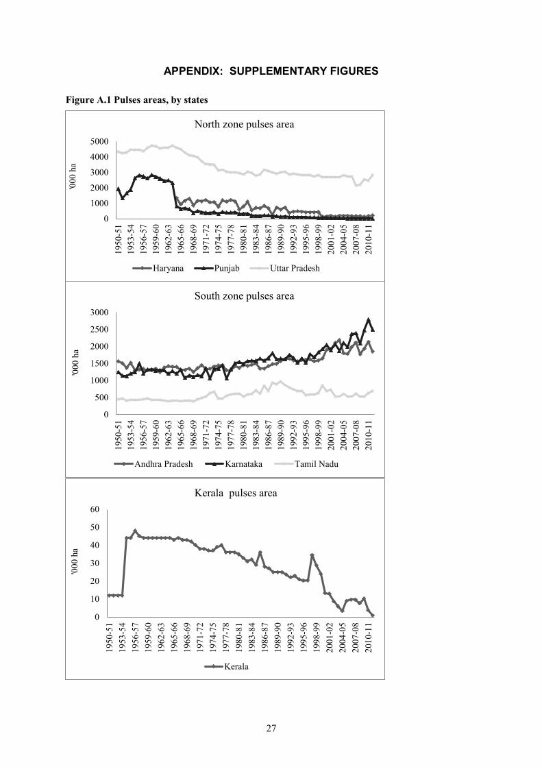
Figure A.1 Pulses areas, by states

0

1000

2000

3000

4000

5000

1950

-51

1953

-54

1956

-57

1959

-60

1962

-63

1965

-66

1968

-69

1971

-72

1974

-75

1977

-78

1980

-81

1983

-84

1986

-87

1989

-90

1992

-93

1995

-96

1998

-99

2001

-02

2004

-05

2007

-08

2010

-11

'000

ha

North zone pulses area

Haryana Punjab Uttar Pradesh

0

500

1000

1500

2000

2500

3000

1950

-51

1953

-54

1956

-57

1959

-60

1962

-63

1965

-66

1968

-69

1971

-72

1974

-75

1977

-78

1980

-81

1983

-84

1986

-87

1989

-90

1992

-93

1995

-96

1998

-99

2001

-02

2004

-05

2007

-08

2010

-11

'000

ha

South zone pulses area

Andhra Pradesh Karnataka Tamil Nadu

0

10

20

30

40

50

60

1950

-51

1953

-54

1956

-57

1959

-60

1962

-63

1965

-66

1968

-69

1971

-72

1974

-75

1977

-78

1980

-81

1983

-84

1986

-87

1989

-90

1992

-93

1995

-96

1998

-99

2001

-02

2004

-05

2007

-08

2010

-11

'000

ha

Kerala pulses area

Kerala

28

Figure A.1 Continued

.

0

500

1000

1500

2000

2500

300019

50-5

119

53-5

419

56-5

719

59-6

019

62-6

319

65-6

619

68-6

919

71-7

219

74-7

519

77-7

819

80-8

119

83-8

419

86-8

719

89-9

019

92-9

319

95-9

619

98-9

920

01-0

220

04-0

520

07-0

820

10-1

1

'000

ha

East zone pulses area

Bihar Orissa West Bengal Jharkhand

0500

100015002000250030003500400045005000

1950

-51

1953

-54

1956

-57

1959

-60

1962

-63

1965

-66

1968

-69

1971

-72

1974

-75

1977

-78

1980

-81

1983

-84

1986

-87

1989

-90

1992

-93

1995

-96

1998

-99

2001

-02

2004

-05

2007

-08

2010

-11

'000

ha

West zone pulses area

Gujarat Maharashtra Rajasthan

29

Figure A.1 Continued

. Source: India, DES and India, MoA (various years). Note: ha = hectare; NE = northeast.

0

1000

2000

3000

4000

5000

600019

50-5

119

53-5

419

56-5

719

59-6

019

62-6

319

65-6

619

68-6

919

71-7

219

74-7

519

77-7

819

80-8

119

83-8

419

86-8

719

89-9

019

92-9

319

95-9

619

98-9

920

01-0

220

04-0

520

07-0

820

10-1

1

'000

ha

Central zone pulses area

Madhya Pradesh Chhattisgarh Linear (Madhya Pradesh)

05

10152025303540

1950

-51

1953

-54

1956

-57

1959

-60

1962

-63

1965

-66

1968

-69

1971

-72

1974

-75

1977

-78

1980

-81

1983

-84

1986

-87

1989

-90

1992

-93

1995

-96

1998

-99

2001

-02

2004

-05

2007

-08

2010

-11

'000

ha

NE zone pulses area

Manipur Meghalaya Nagaland

Sikkim Tripura Mizoram

30

REFERENCES

Akibode, S., and M. Maredia. 2011. Global and Regional Trends in Production, Trade and Consumption of Food Legume Crops. Report Submitted to SPIA. March. Accessed August 5, 2015. http://impact.cgiar.org/sites/default/files/images/Legumetrendsv2.pdf.

Banerjee, G., and L. M. Palke. 2010. Economics of Pulses Production and Processing of India. Mumbai, India. Department of Economic Analysis and Research, National Bank for Agriculture and Rural Development.

FAO (Food and Agriculture Organization of the United Nations). 2012. FAOSTAT Statistical Database. Accessed August 5, 2015. http://faostat.fao.org/site/339/default.aspx.

Fertilizer Association of India. 2012. Statistics. Accessed August 5, 2015. www.faidelhi.org/statistics.htm.

Joshi, P. K., M. Asokan, and M. C. S. Bantilan. 2005. “Chickpea in Nontraditional Area: Evidence from Andhra Pradesh.” In Impact of Agricultural Research: Post–Green Revolution Evidence from India, edited by P. K. Joshi, S. Pal, P. S. Birthal, and M. C. S. Bantilan, 115–129. New Delhi, India: National Centre for Agricultural Economics and Policy Research; Andhra Pradesh, India: International Crops Research Institute for the Semi-Arid Tropics.

India, DES (Directorate of Economics and Statistics). 2012. Agricultural Statistics at a Glance. Accessed December 2014. http://eands.dacnet.nic.in/latest_2012.htm.

India, MoA (Ministry of Agriculture). 2012. Agricultural Statistics at a Glance. Accessed August 5, 2015. http://eands.dacnet.nic.in/Publication12-12-2012/Agriculture_at_a_Glance%202012/Pages85-136.pdf.

India, Ministry of Road Transport and Highways. 2012. Basic Road Statistics in India. Accessed http://www.indiaenvironmentportal.org.in/files/file/basic%20road%20statistics%20of%20india.pdf.

India, MSPI (Ministry of Statistics and Program Implementation). 2005. Situation Assessment Survey of Farmers - Some Aspects of Farming, NSS Report 496. New Delhi: National Sample Survey Organization.

Indian Meteorological Department. 2012. Rainfall Statistics. Accessed August 5, 2015. www.imd.gov.in/section/hydro/dynamic/rfmaps/datamain.html.

Reddy, A. and D. Mishra 2009. “Growth and Instability in Chickpea Production in India: A State Level Analysis.” Agricultural Situation in India November 2009: 230–145. http://papers.ssrn.com/sol3/ papers.cfm?abstract_id=1499577

Reserve Bank of India. 2014. Handbook of Statistics on Indian Economy. Available at https://rbi.org.in/Scripts/AnnualPublications.aspx?head=Handbook%20of%20Statistics%20on%20Indian%20Economy

Savadatti, P. 2007. “An Econometric Analysis of Demand and Supply Response of Pulses in India.” Karnataka Journal of Agricultural Sciences 20 (3): 545–550.

Sebby, K. 2010. “The Green Revolution of the 1960’s and Its Impact on Small Farmers in India.” Undergraduate student thesis. Lincoln, NE, US: University of Nebraska–Lincoln. Environmental Studies Program.

Srivastava, S. K., N. Sivaramane, and V. C. Mathur. 2010. “Diagnosis of Pulses Performance of India.” Agricultural Economics Research Review 23:137–148.

Suhasini, P., V. R. Kiresur, G. D. N. Rao, and M. C. S. Bantilan. 2009. Adoption of Chickpea Cultivars in Andhra Pradesh: Pattern, Trends and Constraints. Andhra Pradesh, India: International Crops Research Institute for the Semi-Arid Tropics.

RECENT IFPRI DISCUSSION PAPERS

For earlier discussion papers, please go to www.ifpri.org/pubs/pubs.htm#dp. All discussion papers can be downloaded free of charge.

1453. Measuring women’s decisionmaking: Indicator choice and survey design experiments from cash and food transfer evaluations in Ecuador, Uganda, and Yemen. Amber Peterman, Benjamin Schwab, Shalini Roy, Melissa Hidrobo, and Daniel Gilligan, 2015.

1452. The potential of farm-level technologies and practices to contribute to reducing consumer exposure to aflatoxins: A theory of change analysis. Nancy Johnson, Christine Atherstone, and Delia Grace, 2015.

1451. How will training traders contribute to improved food safety in informal markets for meat and milk? A theory of change analysis. Nancy Johnson, John Mayne, Delia Grace, and Amanda Wyatt, 2015.

1450. Communication and coordination: Experimental evidence from farmer groups in Senegal. Fo Kodjo Dzinyefa Aflagah, Tanguy Bernard, and Angelino Viceisza, 2015.

1449. The impact of household health shocks on female time allocation and agricultural labor participation in rural Pakistan. Gissele Gajate-Garrido, 2015.

1448. The biophysical potential for urea deep placement technology in lowland rice production systems of Ghana and Senegal. Cindy Cox, Ho-Young Kwon, and Jawoo Koo, 2015.

1447. The Impact of investment in agricultural research and development and agricultural productivity. Nicostrato D. Perez and Mark W. Rosegrant, 2015.

1446. Agricultural diversification and poverty in India. Pratap S. Birthal, Devesh Roy, and Digvijay S. Negi, 2015.

1445. Peer effects in the valuation of attributes and practices for food safety: Findings from the study of dairy consumers in India. Raj Chandra, Abdul Munasib, Devesh Roy, and Vinay Kumar Sonkar, 2015.

1444. The Bali Agreement: An assessment from the perspective of developing countries. Eugenio Díaz-Bonilla and David Laborde, 2015.

1443. Rural and agricultural mechanization: A history of the spread of small engines in selected Asian countries. Stephen Biggs and Scott Justice, 2015.

1442. Investigating public financial accounts and coding system in Malawi and measuring agricultural expenditures within the system. Chance Mwabutwa, 2015.

1441. The effects of political competition on rural land: Evidence from Pakistan. Katrina Kosec, Hamza Haider, David J. Spielman, and Fatima Zaidi, 2015.

1440. Heterogeneous preferences and the effects of incentives in promoting conservation agriculture in Malawi. Patrick S. Ward, Andrew R. Bell, Gregory M. Parkhurst, Klaus Droppelmann, Lawrence Mapemba, 2015.

1439. The cooling effect of pulse imports on price: The case of pigeon pea in India. Akanksha Negi and Devesh Roy, 2015.

1438. Financial constraints and international trade with endogenous mode of competition. Antoine Bouët and Anne-Gaël Vaubourg, 2015.

1437. Understanding men’s and women’s access to and control of assets and the implications for agricultural development projects: A case study in rice-farming households in Eastern Uttar Pradesh, India. Thelma Paris, Valerien Pede, Joyce Luis, Raman Sharma, Abha Singh, Jeffrey Stipular, and Donald Villanueva, 2015.

1436. Gender, assets, and agricultural development: Lessons from eight projects. Nancy L. Johnson, Chiara Kovarik, Ruth Meinzen-Dick, Jemimah Njuki, and Agnes Quisumbing, 215.

1435. A framework for physical growth and child development. Harold Alderman, Jere R. Behrman, and Paul Glewwe, 2015.

1434. Filling the legal void? Experimental evidence from a community-based legal aid program for gender-equal land rights in Tanzania. Valerie Mueller, Lucy Billings, Tewodaj Mogues, Amber Peterman, and Ayala Wineman, 2015.

1433. Agricultural intensification in Africa: A regional analysis. Alejandro Nin-Pratt, 2015.

1432. Inputs, productivity, and agricultural growth in Africa south of the Sahara. Alejandro Nin-Pratt, 2015.

1431. When expectations become aspirations: Reference-dependent preferences and liquidity Constraints. Berber Kramer, 2015.

1430. Demand for complementary financial and technological tools for managing drought risk. Patrick S. Ward, David J. Spielman, David L. Ortega, Neha Kumar, and Sumedha Minocha, 2015.

INTERNATIONAL F OOD POLICY RESEARCH INSTITUTE

www.ifpri.org

IFPRI HEADQUARTERS 2033 K Street, NW Washington, DC 20006-1002 USA Tel.: +1-202-862-5600 Fax: +1-202-467-4439 Email: ifpri@cgiar.org

IFPRI SOUTH ASIA OFFICE NASC, DPS Road, Opp Todapur, Pusa New Delhi 110-012 India Tel.: 91 11 2584-6565 Fax: 91 11 2584-8008 / 2584-6572 Email: ifpri-newdelhi@cgiar.org