TECHNICAL REPORT STANDARD TITLE PAGE

I. Report No. 2. Government Accession No. 3. Recipient's Catalog No.

FHWA/TX-90/1212-1F

4. Title and Subtitle 5. Report Date October 1990

Study for a Comprehensive Bridge Management System for Texas

July 1991/Revised 6. Performing Organization Code

7. Author(s) 8. Performing Organization Report No.

George Stukhart, Ray W. James, Alberto Garcia-Diaz, Roger P. Bligh, John Sobanjo, and W. Frank McFarland

Research Report 1212-1F

9. Performing Organization Name and Address

Texas Transportation Institute The Texas A&M University System College Station, Texas 77843-3135 12. Sponsoring Agency Name and Address

Texas State Department of Highways and Public Transportation Transportation Planning Division P. O. Box 5051 Austin, Texas 78763 15. Supplemental)' Notes

Research performed in cooperation with DOT, FHWA

10. War!< Unit No.

11. Contract or Grant No.

Study No. 2-4-89/0-1212 13. Type of Report and Period Covered

Final- April 1989 October 1990

14. Sponsoring Agency Code

Research Study Title: Study for a Comprehensive Bridge Management System 16. Abstract

This report covers a two-year study of the feasibility and development of specific recommendations for a comprehensive bridge management system for Texas SDHPT. The study identified the problems which could advantageously be addressed by a BMS and recommends a scope for a proposed BMS which is believed to be appropriate for application at district and state level. The study also included review of BMS proposed, developed, and used in other states and reviews of theory and technology relevant to the sub-problems comprising the overall bridge management problem. Finally, the study addresses the problem of identifying the data required for the application of a BMS in Texas.

17. Kq< Words

BMS, bridge management systems, bridges

18. Distribution Statement

No restrictions. This document is available to the public through the National Technical Information Service 5285 Port Royal Road Springfield, Virginia 22161

19. Security Classit (of this report) 20. Security Classif. (of this page) 21. No. of Pages 22. Price

Unclassified Unclassified 224 r'orm DOT t' 1700.7 (8-69)

STUDY FOR A COMPREHENSIVE BRIDGE MANAGEMENT SYS1EM

FOR 1EXAS

by

George Stukhart

RayW. James

Alberto Garcia-Diaz

Roger P. Bligh

John Sobanjo

and

W. Frank McFarland

Research Report 1212·1F Research Study No. 2-4-89/0-1212

Study for a Comprehensive Bridge Management System

Sponsored by the

Texas State Department of Highways and Transportation

in cooperation with

U .5. Department of Transportation Federal Highway Administration

TEXAS TRANSPORTATION INSTITUTE The Texas A&M University System College Station, Texas n843·3135

July 1991

METRIC (SI*) CONVERSION FACTORS

APPROXIMATE CONVERSIONS TO SI UNITS .,.... ...... Yo. Know MuIIIpIf By To find

In ft yd ml

oz Ib T

Inches teet yants miles

square IncheI aquarefeet aqusre yarda aqusremlles seres

LENGTH

2.54 centfmetres 0.3048 metres 0.,"4 metres 1.e1 kilometres

AREA

145.2 0.0929 0.838 2.51 0.395

centfmelr .. aquared metres squared metres squared kilOmetres squared hectares

MASS (weIght)

ounces 28.35 grama kilograms meg80rama

pounds 0.454 shott tons (2000 Ibt 0.907

VOLUME

" oz flutd ounces 21.57 mllllinres 081 oallons 3.785 II .... ft- cubfc .... 0.0328 met .... cubed yd' cOble yards 0.0785 metres cubed

NOTE: Volumes greater than 1000 L shall be shown In mi.

TEMPERATURE (exact)

Of Fahre"helt 511 (after Celsius temperature aubtractlng 32) temperature

• SI Is the symbol for the International System of Measurements

em m m km

km' ha

g kg Mg

mL L m' ml

.. -

. -

.. -

...

...

...

=-­==

=­=

.. .. .. .. .. ..

.. • .. ..

...

..

APPROXIMATE CONVERSIONS TO SI UNITS Symbol When You Know To FIftd

mm m m km

mm' m'

kml

ha

mllllmet,ea metres metrea kilometres

mlllimetrea squared metres aquared kilometres squared hectorea (10 000 m,

LENGTH

0.039 3.28 1.09 0.821

AREA

0.0018 10.784 0.39 2.53

Inches feet yards miles

square Inches square feet square miles Icres

MASS (weight)

g grams 0.0353 kg kllograma 2.205 Ma megagrams (1 000 kg) 1.103

mL mllltlitres L IItrea mt metres cubed m' metres cubed

VOLUME

0.034 0.2&4 35.315 1.308

ounces pounds shott tons

fluid ounces gallons cubic feet cubic yards

TEMPERATURE (exact)

OC Cefalua 9/5 (then Fahrenheit temperature add 32t temperature

Of' "F 32 .... 212

-~, t! ~!' ~~, •• !!O, h:'~! t ,'!'O. , .~J , r' r , , , i f -~ -~ 0 ~ • ~ ~ ~ ~ ~

These factors conform to the requirement of FHWA Order 5190.1A.

Sytftbol

In It yd ml

Inl

ft' ml' ac

oz Ib T

fI OZ

gal ft' yd'

TABLE OF CONTENTS

SUMMARY .....................................................•.............. v

SUMMARY STATEMENT ON RESEARCH IMPLEMENTATION ......•................... v

ACKNOWLEDGEMENTS ......................................................... v

DISClAIMER . . . . . . . . . . . . . . . . . . . . . . . . . . . . . . • • . . • . . . . . • . . . . . . . . . . . . . . . . . . . . . . . . .. v

LIST OF FIGURES . . . . . . . . . . . . . . . . . . . . . . . . . . . . . . . . . . . . . . . . . . . . . . . . . . . . . . . • . . . . . .. vi

LIST OF TABLES . . . . . . . . . . . . . . . . . . . . . . . . . . . . . . . . . . . . . . . . . . . . . . . . . . . . . . . . . . . . . . .. vii

INTRODUCTION . . . . . . . . . . . . . . . . . . . . . . . . . . . . . . . . . . . . . . . . . . . . . . . . . . . . . . . . . . . . . . .. 1 Significance of the Problem at the Federal Level . . . . . . . . . . . . . . . . . . . . . . . . . . . . . . . . . . .. 1

The Status of the Nation's Bridges ........ . . • . . . . . . . . . . . . . . . . . . . . . . . . . . . .. 1 Federal Funding and Support for Bridge Management ......................... 1

Significance of the Problem in Texas . . . . . . . . . . . . . . . . . . • . . . . . . . . . . . . . . . . . . . . . . . . .. 4

LITERATURE REVIEW .......................................................... 7 Pennsylvania .............................................................. 7 North Carolina ............................................................ 8 NCHRP 300 .............................................................. 10 Indiana .................................................................. 11 FHWA's Bridge Needs Improvement Process (BNIP) ................................ 13 New York City Preventive Maintenance Management System .......................... 14 Other Recent Studies . . . . . . . . . . . . . . . . . . . . . . . . . . . . . . . . . . . . . . . . . . . . . . . . . . . . . . .. 15

BRIDGE MANAGEMENT PRACTICES IN TEXAS. . . . . . . . . . . . . . . . . . . . . . . . . . . . . . . . . . . . .. 19 Decentralization . . . . . . . . . . . . . . . . . . . . . . . . . . . . . . . . . . . . . . . . . . . . . . . . . . . . . . . . . . .. 19 The Federal and State Budgetary Processes ....................................... 19 Bridge Funding Priorities ... . . . . . . . . . . . . . . . . . . . . . . . . . . . . . . . . . . . . . . . . . . . . . . . . .. 20 Role of the FHW A and the Sufficiency Rating ..................................... 21 Maintenance Management Information System (MMIS) .............................. 22 Maintenance Practices and Priorities . . . . . . . . . . . . . . . . . . . . . . . . . . . . . . . . . . . . . . . . . . . .. 23 Bridge Maintenance Inspections ................................................ 25 Routine Maintenance Specifications ............................................. 25 Bridge Maintenance Needs and Priorities .......•................................. 25 FHW A Recommendations on Bridge Maintenance .............•.................... 26

SCOPE OF THE BRIDGE MANAGEMENT STUDY. . . . . . . . . . . . . . . . . . . . . . . . . . . . . . . . . . . .. 29 Defmition ...................................•............................ 29 The Benefits of a Comprehensive Bridge Management System . . . . . . . . . . . . . . . . . . . . . . . . .. 29 Scope of the Present Study . . . . . . . . . . . . . . . . . . . . . . . . . . . . • . . . • • . . . . . . . . . . . . . . . . .. 30

Phase 1 Tasks ........................•.............................. 30 Phase 2 (Continuation) .........................•..•.............•..... 31 Summary of Accomplishments ................•.......................... 32

APPLICATION OF BMS TO TEXAS SDHPT . . . . . . . . . . . • . . . . . . . . . . . . . • . . . . . . . . . . . . . . . .. 35 Identification of District Needs . . . . . . . . . . . . . . . . . . . . . . . . . . . . . . . . . . . . . . . . . . . . . . . .. 35

jj

Current Data Management ............................................. 35 Maintenance ........................................................ 36 Personnel and Training ................................................ 36 General Observations ................................................. 37

Determination of Needs That Can be Met by a BMS ................................ 38 Data Requirements and Availability ...............•...............•............. 39

Database Requirements of Other BMS .........•.................•........ 39 Bridge Needs and Investment Process (BNIP) ......................... 39 North Carolina's Bridge Management System . . . . . . . . . . . . . . . . . . . . . . . . .. 40 NCHRP 300 . . . . . . . . . . . . . . . . . . . . . . . . . . . . . . . . . . . . . . . . . . . . . . . . .. 40

Data Availability ......................•.............................. 42 Bridge Inventory and Condition Data . . . . . . . . . . . . . . . . . . . . . . . . . . . . . . .. 42 Maintenance Management Data ................................... 43 Unit Cost Data . . . . . . . . . . . . . . . . . . . . . . . . . . . . . . . . . . . . . . . . . . . . . . .. 44 Bridge Improvement Activities Data ................................ 45

RECOMMENDATIONS FOR BMS FOR TEXAS ................•..................... " 47 Overview . . . . . . . . . . . . . . . . . . . . . . . . . . . . . . . . . . . . . . . . . . . . . . . . . . . . . . . . . . . . . . . .. 47 Identification of Suitable Models ............................................... 49

Level-of-Service Concept ............................................... 49 Feasible Improvements Model ........................................... 51 Classification of Deterioration Models ..................................... 52

Mechanistic Models ............................................ 52 Regression Models ............................................. 54 Stochastic Bridge Deterioration Models . . . . . . . . . . . . . . . . . . . . . . . . . . . . .. 55

Deterioration Models Based on BRINSAP Data . . . . . . . . . . . . . . . . . . . . . . . . . . . . .. 56 Correlation Analyses of Bridge Condition Versus Age ................... 57 Regression Analysis of Bridge Condition Data ..................... . . .. 58 Analyses of Multiple-Year Bridge Records ............................ 66 Piecewise Linear Regression Model (Wisconsin Approach) ................ 66 Nonlinear Regression-Based Deterioration Models ...................... 74

The Probabilistic Approach - Frequency Analysis. . . . . . . . . . . . . . . .. 80 Models Based on Expert Opinions ........................... 81

Life-Cycle Costs Models ......................................•........ 85 FHW A LCC Model ............................................ 87 Generalized Life-Cycle Costs for Multi-Period Optimization ............... 92

Fixed Budgets and Discounting of Agency Costs ................. 92 Length of Planning (or Optimization) Period and Sub-periods ....... 93 Calculation of Life-Cycle Costs and User Costs ................ .. 94 The Overall Do-Nothing Alternative and Costs for Alternatives ...... 96

Agency Benefits Model ................................................ 97 Extension in Bridge Service Life ......................•............ 97

User Benefits Model .........•....•........ . . . . • . . . . . . . . . . . . . • . . . . . .. 100 Accident Costs .......•....................................... 100 Time and Vehicle Operating Costs Associated With Detours ............. 101 Time and Vehicle Operating Costs Associated With Narrow Bridges ........ 101

Optimization Model. . . . . . . . . . . . . . . . . . . . . . . . . . . . . . . . . . . • • • . . . . • . . . . . .. 102 Incremental Benefit/Cost Analysis . . . . . . . . . . . . . . . . . . . . . . . . . . . . . . . .. 104 Integer Programming .••..........•............................ 104 INCBEN Algorithm ........................................... 105 Long and Medium Range Planning Horizons ...•.. . . . . . . . . . . . . . . . . . .. 106 Dynamic Programming Solution Procedure .......................... 108

ill

CONCLUSIONS

Computational Requirements •.•.............••.................. 111 Single-Period Planning Horizons •.. . . . . . . • . . . . . . . . . . . . . . • • .. 111 Multi-Period Planning Horizons ...•........................ 114

117

RECOMMENDED FURTHER WORK. . . . . . . . . . . . . . . . . . . . . . . . . • . . . . . . . . . . . . . . . . . . . .. 119

REFERENCES ................................................................. 121

APPENDIX A. BRIDGE MAINTENANCE CASE STUDY ............................... 127

APPENDIX B. QUESTIONNAIRE ON BRIDGE DETERIORATION AND REHABILITATION .. 147

APPENDIX C. ANALYSIS OF BRIDGE DETERIORATION AND REHABILITATION ......... 167

APPENDIX D. INTERVIEWS WITH SDHPT PERSONNEL .............................. 183

APPENDIX E. REVIEW OF THE BRINSAP DATABASE ............................... 203

APPENDIX F. QUESTIONNAIRE ON MAINTENANCE EFFECTIVENESS ................. 209

APPENDIX G. ANALYSIS OF MAINTENANCE EFFECTIVENESS . . . . . . . . . . . . . . . . . . . . . . .. 215

IV

SUMMARY

This report covers two years' study of the feasibility and development of specific recommendations for a comprehensive bridge management system for Texas SDHPT. The study identified the problems which could advantageously be addressed by a BMS, and recommends a scope for a proposed BMS which is believed to be appropriate for application and district and state level. The study also included review of BMS proposed, developed, and used in other states, reviews of theory and technology relevant to the sub-problems comprising the overall bridge management problem. Finally, the study addresses the problem of identifying the data required for the application of a BMS in Texas.

SUMMARY STATEMENT ON RESEARCH IMPLEMENTATION

Implementation is anticipated through a study to develop a BMS based on the recommendations of this report. Development and coding of the models and procedures identified in the present study will require a significant effort. Prompt initiation of such a follow-up study is recommended. Initial implementation of the final product will probably be best attempted at district level, to reduce the scale of the implementation and evaluation problems.

ACKNOWLEDGEMENTS

The researchers appreciate the support provided by the Department of Highways and Public Transportation. A study of this type must draw on the expertise and judgement of the experienced bridge managers of the SDHPT. This study could not have been productive without the close involvement of Ralph Banks, who served as Technical Coordinator. In addition to his valuable personal contributions, Ralph was instrumental in assembling an experienced and energetic committee of Technical Advisors, including Larry Buttler (D-18), Gene Day (Dist. 12), Van McElroy (Dist. 18), Morgan Prince (Dist. 11), Don Shipman (Dist. 4), and LeRoy Surtees (Dist. 15). The assistance and advise of Joe Graff CD-18) and Clark Titus (D-18) is also acknowledged and appreciated.

DISCLAIMER

The contents of this report reflect the views of the authors, who are responsible for the facts and accuracy of the data presented herein. The contents do not necessarily reflect the official views or policies of the Texas State Department of Highways and Public Transportation of the Federal Highway Administration. This report does not constitute a standard, specification, or regulation.

v

LIST OF FIGURES

FIgUre 1. Cost Impact of Full (100%) and Reduced Maintenance [NYC Consortium 1990) .......... 16 Figure 2. Schematic Flow Chart for Recommended BMS . . . . . . . . . . . . . . . . . . . . . . . . . . . . . . . . . .. 48 Figure 3. Equivalent HS Rating vs. Time of 6()..ft Span [Kayser and Nowak 1989] ................. 53 FJgUre 4. Washington State DOT Bridge Deck Management System Deck Deterioration Model ...... 56 FJgUre 5. Regional Classification of Texas Bridges . . . . . . . . . . . . . . . . . • . . . . . . . . . . . . . . . . . . . . .. 63 Figure 6. General Form of a Piecewise-Linear Model .........................•........... 67 FJgUre 7. Piecewise Linear Deterioration Model for Reinforced Concrete Decks by Highway Class .... 73 Figure 8. Piecewise Linear Deterioration Model for Superstructures By Highway ................. 73 Figure 9. Piecewise Linear Deterioration Models for Substructures by Highway Class .............. 78 Ftgure 10. Nonlinear Deterioration Models for Reinforced Concrete Decks by Highway . . . . . . . . . . . .. 78 Figure 11. Nonlinear Deterioration Models for Steel Superstructures by Highway ................. 79 Figure 12. Nonlinear Deterioration Models for Steel Superstructures . . . • . . . . . . . . . . . . . . . . . . . . . .. 79 Figure 13. State Probability Plot for Steel Superstructure on FM Highway . . . . . . . . . . . . . . . . . . . . . .. 81 Figure 14. AnnuaJ Maintenance Effort Model Due to Spalling on Two Classes of Bridge Decks

(WSDOT) .....................................•.......................... 86 Figure 15. Life-Cycle Costs for Replacement Case ........................................ 88 Figure 16. Life-Cycle Costs for Rehabilitation Case ....................................... 88 Figure 17. Stream of Life-Cycle Costs ................................................. 90 Figure 18. Equivalent Single-Cost Representation of Maintenance Cost Gradients ................. 91 Figure 19. Present Worth of Perpetual Service ........................................... 91 Figure 20. Future Cost Assuming Rehabilitation . . . . . . . . . . . . . . . . . . . . . . . . . . . . . . . . . . . . . . . . .. 91 Figure 21. Dynamic Programming Process for Stages 1,2,3 ................................. 110 Figure 22. Dynamic Programming Process for Stage 4 .................................... 111 Figure 23. Comparison of INCBEN and INTPROG for 1000 Bridges ......................... 112 Figure 24. Time Comparison of INCBEN and INTPROG .................................. 113 Figure 25. Run Time Differential Between INCBEN and INTPROG . . . . . . . . . . . . . . . . . . . . . . . . .. 113 Figure 26. INTPROG Analysis for up to 5000 Bridges .................................... 114 Figure 27. Computer Time Estimates . . . . . . . . . . . . . . . . . . . . . . . . . . . . . . . . . . . . . . . . . . . . . . . .. 115

vi

LIST OF TABLES

Table 1. Bridge Fiscal Requirements (Constant Dollars) ................................... 4 Table 2. Highway System FIScal Requirements (Constant Dollars) ............................ 5 Table 3. Correlation Analysis on Substructures by Material and Highway Classification . . . . . . . . . . . .. 59 Table 4. Correlation Analysis on Major Bridge Components for All Highway Classifications ......... 60 Table 5. Correlation Analysis on Bridge Decks by Material and Highway . . . . . . . . . . . . . . . . . . . . . .. 61 Table 6. Correlation Analysis on Superstructures by Material and Highway Classification ........... 62 Table 7. Regression Analyses on Coastline Bridge Substructures .••.......................... 64 Table 8. Regression Analyses on Bridge Substructures by Region for All Highway Classifications ..... 65 Table 9. Data Screening. Futering, and Merging of Bridge Records ........................... 67 Table 10. Data Breakdown Summary of Bridge Superstructure Records . . . . . . . . • . • . . . . . . . . . . . . .. 68 Table 11. Piecewise Linear Deterioration Models for Bridge Decks By Highway Classification . . . . . . .. 70 Table 12. Piecewise Linear Deterioration Models for Bridge Superstructures by Highway

Classification ....................••.............•.••....................... 71 Table 13. Piecewise Linear Deterioration Models for Bridge Substructures by Highway

Classification ................................................ . . . . . . . . . . . . .. 72 Table 14. Nonlinear Deterioration Models (2-Parameter Exponential) for Superstructures ........... 76 Table 15. Nonlinear Deterioration Models (2-Parameter Exponential) for Superstructures ........... 77 Table 16. Simple Linear Deterioration Models for Bridge Decks (Expert Opinion) ................ 82 Table 17. Simple Linear Deterioration Models for Bridge Superstructures (Expert Opinion) ......... 83 Table 18. Simple Linear Deterioration Model for Bridge Substructures (Expert Opinion) ............ 84 Table 19. Bridge Expert's Estimate of Bridge Improvement's Effectiveness ...................... 99

vii

INTRODUCTION

Significance or the Problem at the Federal Level

The Status of the Nation's Bridges

In 1989 the Department of Transportation issued its annual report to the Congress on The Status of the

Nation's Hi&hways and Bri<J&es: Condjtions and Performance and HiahwAY Bridae Rt;placement and

Rt;habilitation Proaram [U.S. Congress 1989]. According to this report, the number of structurally deficient and

functionally obsolete bridges in the federal-aid category rose within the last six years from 69,645 to n,I92. This

is 32.9 percent of the total bridge inventory. The total number of deficient bridges has declined, however,

because the number of off-system deficient bridges has dropped due primarily to removal and nonreplacement.

Based on the Federal Highway Authority (FHWA)'s sufficiency rating, a bridge is deficient and in need of

rehabilitation or replacement if it has a rating (discussed below) of 80 or less.

A report by the U.S. Department of Transportation (USDOT)/Federal Highway Administration

(FHW A) - the Bridge Needs Improvement Process (BNIP) - shows an estimated cost of $31.1 billion to bring

all deficient bridges in the federal-aid category up to acceptable standards and another $19.6 billion for off-system

bridges [FHWA 1989]. This includes federal and state shares. Investment by all units of government to

eliminate existing and accruin& bridge deficiencies from 1987 through year 2005 total $93 billion, or $4.9

billion/year [FHWA 1989]. Of this total, $67.6 billion is needed to eliminate backlog/existing deficiencies and

$25.3 billion is needed for accruing deficiencies. The cost estimate to replace all existing bridges has remained

relatively stable over several years, but is expected to increase as the bridges constructed during the SO's and 60's

become of age.

The BNIP shows a forecast of the number of deficient bridges and corresponding rehabilitation or

replacement cost in the categories of Interstate, Primary, Secondary, Fed-Aid Urban, and Non Fed-Aid for

funding periods 1989-1993 and 1994-1998. In order to evaluate the practical application of the BNIP, six states,

including Texas, are in the process of testing and validating the model. While the BNlP calculates total bridge

needs, it does not prescribe alternative improvements for individual bridges or groups of bridges. The model

includes onJy replacement and rehabilitation costs - excluding new construction - as the federal government does

not fund maintenance.

FeiJem/ Funding and Support for Bridge Management

The Federal-Aid Highway and Bridge Replacement and Rehabilitation Program (HBRRP) is the

primary means of providing federal funds to the states for highway improvements. The Surface Transportation

and Uniform Relocation Act of 1987 (STURAA) extended the original HBRRP and the current authorization

is approximately $1.63 billion per year for years 1987-1991. After certain deductions for other requirements, the

1

actual apportionment to the states is $1.37 billion. Thus. nationwide the funds available annually from the federal

government for bridge replacement and rehabilitation are really only about 28 percent of the total requirement

($4.9 billion). If the BNIP's estimate of the requirements is correct, the HBRRP amount is not only insufficient

presently but would be of even less help in the future as bridge requirements increase.

Section 162 of the STURAA (Public Law 100-17) required the Secretary of Transportation to make a

full and complete investigation and study of state bridge management programs for purposes of determining

whether or not those states participating in the Federal Bridge Replacement and Rehabilitation program need

to establish comprehensive bridge management programs. Further, the Secretary was required to make

legislative and administrative recommendations concerning the establishment of comprehensive bridge

management programs. as wen as minimum requirements of such programs which the Secretary considers

appropriate. FHW A responded to this with a study in April 1988 [FHW A 1988]. drawing the following

conclusions regarding the need for comprehensive bridge management systems by states participating in the

HBRRP:

1. Nearly all states have expressed an interest in improving their present bridge programs. Some 40

percent of the states appear to be headed in the direction of developing a BMS. This interest stems

primarily from the concern for current and impending bridge problems. although the FHW A

promotional efforts have had some effect.

2. There is consensus among the states that comprehensive bridge management systems are needed.

3. The status of development varies widely between states. Most states are in the early phase, and only

a few have what could be called a comprehensive bridge management system (BMS).

4. Widespread implementation of BMSs win take years and will require a multi-disciplinary approach

and careful planning. Further, states have unique social, economic, political, and mobility

considerations that affect their system. Past weaknesses in tbe databases of many states will delay

full implementation of their systems.

S. Developing a BMS will require a substantial commitment of state resources.

6. FHWA has not yet specified minimum federal requirements for bridge management systems.

However. current drafts of proposed federal legislation do define some minimum requirements for

a bridge management system.

2

Current FHW A recommendations [FHW A 1990] indicate that apportioned funds may be used to develop

a BMS, and that regulations establishing minimum requirements for a BMS should be available by January I,

1992. These requirements are:

1. A BMS will have formal procedures for selecting projects and strategies for bridge maintenance,

repair, rehabilitation, and replacement.

2. The BMS will consider network needs as well as funding constraints. It will minimize agency and

user costs and enhance the state's ability to develop and substantiate funding proposals based on

short and long-term predictions. It will determine yearly funding requirements to attain level-of­

service goals at least cost, and the backlog that would accrue if sufficient funds are not available

3. The BMS will include all essential engineering and management functions that are necessary Cor a

bridge program. These include:

(a) Suitable analytical tools for objectively assessing bridge needs

(b) Procedures and algorithms for selecting and prioritizing bridge projects, including

maintenance, rehabilitation, improvement, and replacement.

(c) Formal procedures for coordinating inspection, maintenance, design, and construction.

4. The social, economic, political, and mobility considerations of each state must be given latitude in

developing a BMS. BMS regulations should specify what is required, and be flexible in terms of how

it is to be done.

5. The FHW A may approve federal-aid participation in bridge projects on the National Highway

System (NHS) which have been selected in accordance with an approved BMS. The FHW A will not

have to determine if the bridge work to be done (replacement or rehabilitation) is eligible for

federal-aid funds, since projects selected through a state's BMS will be eligible. This would include

all bridges not just those on the NHS.

The FHW A believes that using HBRRP funds will have long-term benefits far exceeding the reductions

in funds available for other uses in the HBRRP program.

3

The FHW A has taken a number of steps to encourage better bridge management in the states. They

have published a demonstration project [FHW A 1987] which contains much of the essentials of a BMS and

conducted regional seminars to discuss the subject. The FHW A is now funding, through the California

Transportation Agency (CALTRANS). a study on Network Optimization for Bridge Management Systems; this

could provide a common model for other states to use in their BMS. This 27-month study due in early 1992 will

use data and bridge engineering experience from CAL TRANS and five other states. CAL TRANS is proposing

this project as AASHTO-sponsored computer software. If sponsored by AASHTO. member states will be able

to pool resources on a voluntary basis to produce enhancements.

SignJOcance or the Problem in Texas

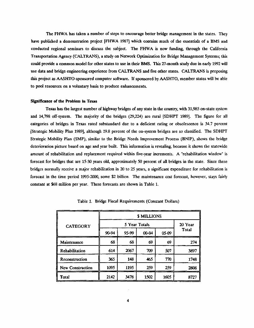
Texas has the largest number of highway bridges of any state in the country, with 31,985 on-state system

and 14,798 off-system. The majority of the bridges (29,224) are rural [SDHPT 1989]. The figure for all

categories of bridges in Texas rated substandard due to a deficient rating or obsolescence is 34.7 percent

[Strategic Mobility Plan 1989], although 19.8 percent of the on-system bridges are so classified. The SDHPT

Strategic Mobility Plan (SMP), similar to tbe Bridge Needs Improvement Process (BNIP). shows the bridge

deterioration picture based on age and year built. This information is revealing, because it shows tbe statewide

amount of rehabilitation and replacement required within five-year increments. A "rehabilitation window" is

forecast for bridges that are 15-30 years old, approximately 50 percent of all bridges in the state. Since these

bridges normally receive a major rehabilitation in 20 to 25 years, a significant expenditure for rehabilitation is

forecast in the time period 1995-2000, some $2 billion. The maintenance cost forecast. however, stays fairly

constant at $68 million per year. These forecasts are shown in Table 1.

Table 1. Bridge F'lSCal Requirements (Constant Dollars)

$ MILLIONS

CATEGORY 5 Year Totals 20 Year

I 90-94 95-99

Total 00-04 05-09

Maintenance 68 68 69 69 274

Rehabilitation 614 2067 709 507 3897

Reconstruction 365 148 465 770 1748

New Construction 1095 1195 259 259 2808

Total 2142 3478 1502 1605 8727

4

Table 2. Highway System Fiscal Requirements (Constant Dollars)

$ MILLIONS

FUNCTION 5 Year Totals 20 Year Total

*9()..94 95·99 00-04 05.09

Roadways 22338 11314 10549 10509 54260

Bridges 2142 3478 1502 1605 8727

Roadside 527 535 551 575 2188

Traffic Operations 1154 1208 1335 1380 5077

Ferries and Tunnels 68 61 64 63 256

ROW Acquisition 2286 1329 754 476 4845

Transportation Research 84 89 95 95 363

Highway System Mgt I 122 626 590 590 2528

Highway System Totals I 29321 I 18640 I 15440 I 148431 782441

* Includes Backlog

Table 1 shows bridge fiscal requirements for a 2Q..year planning horizon. Table 2 compares the bridge

fiscal requirements with the other highway system totals. Comparing the two tables, bridge rehabilitation will

consume 11 percent of the SDHPT budget, in the period 1995-1999, a considerable increase over the current

situation. For example, in 1988 total bridge spending is $160 million/year; Table 2 shows that more than $400

million per year will be needed. These figures do not include the effects of deterioration rates or the increases

in traffic volume requiring substantial increases in capacity. It is estimated that 90 percent of the bridge

rehabilitation in urban areas is due to this capacity increase. When the Texas SDHPT completes the evaluation

of the BNIP, using available data, it will be possible to compare total Texas needs in the next 20 years against

federal projections. The implications of these forecasts for bridge management are that Texas must evaluate

other more cost effective means of managing the bridge inventory, not only because the federal government is

very concerned with bridge management, but also because means must be found to keep the extensive inventory

of bridges in the state maintained.

One would suspect that greater expenditures for maintenance would reduce the deterioration rate

causing other expenditures. Postponing rehabilitation five or ten years would provide considerable savings. To

demonstrate that more conservative strategies are possible, the life·C,)rcle cost approach can be used, as well as

suitable deterioration models. These considerations lead also to the need for methods to model the agency costs

and user costs over the life cycle of a bridge, and account for these costs to fmd the most cost-effective

5

alternatives for one bridge or for a network of bridges. This combination of analytical tools is a significant part

ofa BMS.

6

LITERATURE REVIEW

While all states practice some form of bridge management, very few have implemented a comprehensive,

systematic approach to the problem. Many states prioritize their bridges needs based on the mw A sufficiency

rating or a similar ranking system. However, several parallel efforts are currently underway as states recognize

the benefits of a BMS. Through HP&R funds, states are adapting current knowledge to their individual needs

and, where appropriate, advancing into state-of-the-art bridge management. Described below are some of the

major studies which have helped defme the general scope and current state of knowledge for bridge management

systems.

Pennsylvania

The Pennsylvania Department of Transportation (Penn DOT) developed and implemented a bridge

management system that has now been in use since March 1987. Its development is documented in reports

mwA-PA-86-Q36 [Bridge Management Work Group 1987] and FHWA-PA-87-005 [Van Horn 1987]. This

system uses a ranking scheme to systematically prioritize bridge activities at a regional or statewide level, based

upon the structural and functional needs for each highway classification. The bridge activities include

maintenance, rehabilitation, and replacement. The system is also capable of predicting present and future needs

for all bridges using various levels of service scenarios.

Penn DOT's computerized Structure Inventory Records System (SIRS) was substantially enhanced and

expanded to form the basic part of their Bridge Information Database (BIDB). The former SIRS database

consisted of 15 segments and 235 data elements including the 88 data items mandated by the Federal Highway

Administration (FHWA). The new BlOB contains an additional 190 elements of data for a total of 28 segments

and 425 data items. The expanded BIDB was designed to accommodate multiple inspection recordings,

prioritization/deficiency point assignments, bridge maintenance needs, and cost data storage. The other two

databases that are essential to the BMS are the BMS Tables Database and the BMS Activity Database which

stores transaction history. The Tables Database consists of computerized tables which store relatively fixed

system items such as geometric and loading goals, costs of major improvements, condition rating constants,

maintenance activity descriptions, units and costs, remaining life, and other similar items. A total of 41 different

tables are included in this database.

The actual bridge management system can be separated into two distinct parts--the Bridge Rehabilitation

and Replacement System (BRRS) and the Bridge Maintenance System (BMTS). In the Pennsylvania BMS, the

prioritization of bridges for rehabilitation and replacement is based upon the degree to which a bridge is

deficient. The deficiencies are evaluated in three general categories: level-of-service capability, bridge condition,

and other related characteristics. The deficiencies are combined to yield a total deficiency rating (TOR) on a

7

scale from zero to 100. The TOR index was patterned after parts of the federal Sufficiency Rating System and

parts of the system developed by North Carolina State University for use by the North Carolina DOT.

The level-of-service deficiencies are based on four characteristics: load capacity, clear deck width,

vertical clearance for traffic carried by the bridge, and vertical clearance for traffic passing under the bridge.

These criteria were set at three levels: minimum acceptable, minimum design, and desirable design. They are

primarily dependent upon functional classification of the highway with some dependence on average daily traffic

(ADT).

All the bridges on the highway system are ranked in decreasing order of TOR, resulting in a prioritized

listing based on degree of deficiency. In addition to the TOR, other factors are utilized in determining indexes

which enable comparative evaluation of the bridges, as weD as comparison between replacement and

rehabilitation options for each bridge. These factors include cost of replacement, cost of rehabilitation, and

ADT. Notably absent from the evaluation is consideration of life-cycle costing, estimates of economic benefits,

and costjbenefit or optimization procedures.

Another important component of the overall BMS is the Bridge Maintenance Management Subsystem

(BMTS). This portion of the BMS uses standardized bridge maintenance activities and costs, and stored bridge

activity needs, to rank activities and prioritize bridges for maintenance programming. In addition, it transfers

programmed projects to the Maintenance Division's programming and scheduling system and stores the cost of

completed work.

The method of prioritization for bridge maintenance was based on a deficiency point concept as is the

BRRS. The components of the procedure include: activity ranking, activity urgency, bridge criticality, and bridge

adequacy. The SIRS, as it originaDy existed, had a very limited capability for defining maintenance needs of

bridges. It was determined that the data was totally inadequate for either costing or programming purposes.

The database was therefore modified to included a listing of nine approach roadway and 67 bridge maintenance

activities which forms the basis of the maintenance portion of the BMS as well as a new Maintenance Needs

Reporting Form for bridge inspectors to follow.

In summary, although Penn DOT's BMS has very complete inventory, maintenance, and cost data, and

the system is very complex in many respects, it relies on a ranking procedure to prioritize bridges rather than

optimization. Although life-cycle costing and optimization were proposed as future work items, they have not

been included in the BMS to date. For this reason, it is often considered to be more of a bridge information

management system rather than a comprehensive BMS.

North Carolina

A BMS has been developed for the North Carolina Department of Transportation (NCDOT) through

a series of studies conducted by researchers at North Carolina State University (NCSU). Although a BMS has

already been implemented in North Carolina as a result of this research. NCDOT continues to work

8

cooperatively with NCSU to expand and improve upon the existing system. The system is documented in

research reports FHW A/NC/88-003 [Nash and Johnston, 19851, FHW A/NC/88-004 [Chen and Johnston, 1987),

and FHW A/NC/89-002 [AI-Subhi, Johnston, and Farid, 1989].

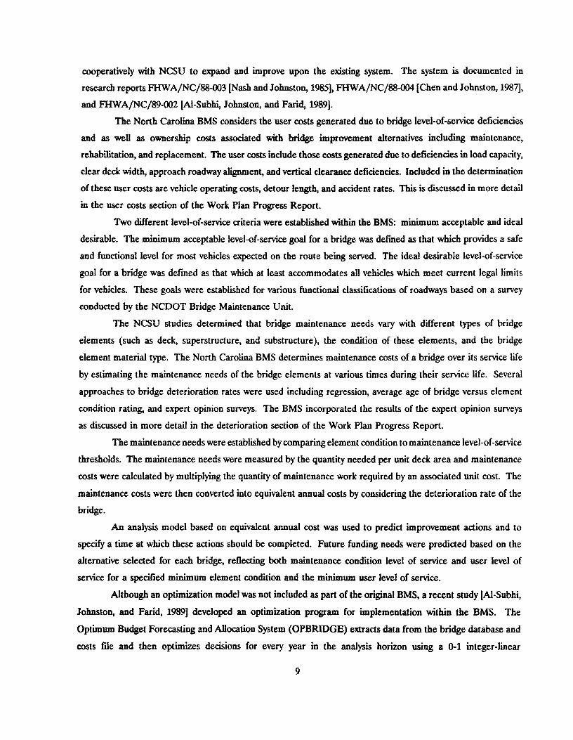
The North Carolina BMS considers the user costs generated due to bridge level-of-service deficiencies

and as wen as ownership costs associated with bridge improvement alternatives including maintenance,

rehabilitation, and replacement. The user costs include those costs generated due to deficiencies in load capacity,

clear deck width, approach roadway alignment, and vertical clearance deficiencies. Included in the determination

of these user costs are vehicle operating costs, detour length, and accident rates. This is discussed in more detail

in the user costs section of the Work Plan Progress Report.

Two different level-of-service criteria were established within the BMS: minimum acceptable and ideal

desirable. The minimum acceptable level-of-service goal for a bridge was defmed as that which provides a safe

and functional level for most vehicles expected on the route being served. The ideal desirable level-of-service

goal for a bridge was defmed as that which at least accommodates all vehicles which meet current legal limits

for vehicles. These goals were established for various functional classifications of roadways based on a survey

conducted by the NCDOT Bridge Maintenance Unit.

The NCSU studies determined that bridge maintenance needs vary with different types of bridge

elements (such as deck, superstructure, and substructure), the condition of these elements, and the bridge

element material type. The North Carolina BMS determines maintenance costs of a bridge over its service life

by estimating the maintenance needs of the bridge elements at various times during their service life. Several

approaches to bridge deterioration rates were used including regression, average age of bridge versus element

condition rating, and expert opinion surveys. The BMS incorporated the results of the expert opinion surveys

as discussed in more detail in the deterioration section of the Work Plan Progress Report.

The maintenance needs were established by comparing element condition to maintenance level-of-service

thresholds. The maintenance needs were measured by the quantity needed per unit deck area and maintenance

costs were calculated by multiplying the quantity of maintenance work required by an associated unit cost. The

maintenance costs were then converted into equivalent annual costs by considering the deterioration rate of the

bridge.

An analysis model based on equivalent annual cost was used to predict improvement actions and to

specify a time at which these actions should be completed. Future funding needs were predicted based on the

alternative selected for each bridge, reflecting both maintenance condition level of service and user level of

service for a specified minimum element condition and the minimum user level of service.

Although an optimization model was not included as part of the original BMS, a recent study [AI-Subhi,

Johnston, and Farid, 1989] developed an optimization program for implementation within the BMS. The

Optimum Budget Forecasting and Allocation System (OPBRIDGE) extracts data from the bridge database and

costs file and then optimizes decisions for every year in the analysis horizon using a 0-1 integer-linear

9

programming formulation. In the algorithm of OPBRIDGE a bridge manager inputs the analysis horizon,

minimum performance requirements, and policies as well as granted budget, maximum allowable budget, or

unlimited budget for each year in the horizon. At the end of every year, OPBRIDGE ages the bridges one year

and predicts condition ratings, ADT, and other variables.

With the inclusion of this optimization scheme, the North Carolina BMS can be categorized as a BMS.

The work implemented in North Carolina has gained national recognition and clearly demonstrates that a

comprehensive BMS is feasible.

NCHRP300

The main goal of project NCHRP 12-28(2) was to develop a model Bridge Management System (BMS),

for small sized states and local transportation agencies, capable of operation on both network and project levels.

The fmdings of the first phase of this project, as revealed in the NCHRP Report 300, defined six basic elements

that are necessary for an effective bridge management system.

These six essential modules are: 1) database module; 2) network level major maintenance, rehabilitation

and replacement (MR&R) selection module; 3) maintenance module; 4) historical data analysis module; 5)

project level interface module; and 6) reporting module. The database module, being the core module of the

system, provides information through collection and storage of bridge inventory, condition, and MR&R data.

Of the six modules, the network MR&R selection module is the analytical component of the BMS; it assists

bridge managers in making decisions related to programming and budgeting. Tasks carried out in this module

include ranking of bridges or required MR&R activities, selection of specific MR&R activity, life-cycle costing,

and optimization. The maintenance module estimates minor maintenance needs for bridges which are not

selected for major MR&R actions, while the historical data analysis module uses historical data to estimate

parameters such as MR&R costs, MR&R action effectiveness, region-to-region expenditure, and life-cycle

activity profiles. For project level applications, such as bridge structural analysis, the model BMS project level

interface module will provide a medium for exchange of data between the BMS database and this application.

Finally, the reporting module serves as the communication link between the model BMS and the user, producing

reports such as data lists, summary reports, graphs, charts, and maps.

While the model BMS of NCHRP Project 12-28(2) is impressive, it should be noted that it is very

conceptual and enormously comprehensive; it has not yet been determined whether the intended users have the

resources and capabilities to implement such a system. One of the specific objectives of this project was to assist

bridge managers to seJect optimum cost-effective improvement alternatives, within the limitations of available

funds. However, the fmdings state that out of the four tasks required for the network MR&R selection module,

optimization was the least important in terms of having a true BMS. Contrary to this conclusion, an optimization

mode~ as described in the optimization section of the Work Plan Progress Report, is considered by many to be

an essential component of a comprehensive BMS.

10

Because the computerized BMS demonstration software was coded in dBASEIII + language, there may

be limitations in the number of bridges it can efficiently handle. This could present a problem when

implementing the BMS in larger states and transportation agencies.

Indiana

The Indiana Bridge Management System (IBMS) is the result of a r~nt research project undertaken

by the School of Civil Engineering at Purdue University and sponsored by the Indiana Department of

Transportation. The main objective of the research was to develop a framework for managing bridge

maintenance, rehabilitation, and replacement activities in Indiana.

The proposed IBMS is similar to the comprehensive bridge management system developed by in

NCHRP 300, but instead of the NCHRP 300 six major modules, the IBMS consists of eight major modules.

These are the Database module, Condition Rating Assistance Module, Bridge Safety Evaluation Module,

Improvement Activity Module, Impact Identification Module, Project Selection Module, Activity Recording and

Monitoring Module, and the Reporting Module. The modules perform the following:

1. Database Module: Contains all information necessary for other modules to perform tasks on a

network of state-owned bridges.

2. Condition Rating Assistance Module: Consists of a computer program to fIlter out inconsistencies

in ratings, to assist bridge inspectors, to train new inspectors, and to predict the condition rating after

certain improvements.

3. The Bridge Traffic Safety Evaluation Module computes a bridge safety index using fuzzy set theory

applied to a bridge inspector's subjective ratings of traffic safety on various bridge components.

4. The Improvement Activity Identification Module provides information on the types of improvement

activities that may be recommended at certain condition ratings.

5. The Impact Identification Module is designed to identify the costs and consequences of structurally

deficient and/or functionally obsolete bridges on the highway agency, the user, and the surrounding

community.

6. The Project Selection Module is a set of decision-making tools that can be used to select and

program the most economical options for bridge improvement projects. There are three submodels:

Life-cycle Cost, Ranking, and Optimization.

11

7. The Activity Recording and Monitoring Module tracks maintenance, rehabilitation, and replacement

of bridges in the network, in addition to accumulating historical data on cost, timing, and sequence

of bridge-related activities.

8. The Reporting module would produce summary reports on bridge condition and characteristics,

maintenance needs, improvement activity, network level impact, life-cycle cost analysis, priority

ranking, optimal activity programming, and bUdget.

It should be noted that the condition rating assistance, traffic safety evaluation, and improvement activity

identification modules are used by the inspector, to assign appropriate ratings annually, and by the bridge

manager to select improvement alternatives. Candidate bridge projects are developed in a series of meetings

at the district level.

The study catalogs the effectiveness of various improvement alternatives on condition ratings; for

example, an improvement strategy may cause a change in the condition rating of the deck from a 4 to an 8 and

also increase the service life an average of 21 years (or a range of 16-27 years). This information is used in the

impact identification module and translated into agency cost. Bridge maintenance is not seriously considered

as an alternative, however, and the study states that impacts on the user have not been identified.

The project selection process uses the life-cycle activity profile; unit costs and timing of activities must

be estimated. The study uses the Equivalent Uniform Annual Cost to compare alternatives, rather than the Net

Present Value used in the FHWA Demonstration Project (FHWA 1987). Since the FHWA compares bridges

with an infinite series of replacements, the EUAC and NPV yield the same results. The Indiana study states

that comparisons of alternatives for a single bridge using only the least (life-cycle) agency cost criterion are valid

if the benefits are the same for each option. However, even for a single bridge user costs can yield different

results than would be derived from agency costs alone. For a network there are other variables, such as bridge

geometry and ADT.

The ranking submodel is discussed and recognized as not being optimum but useful to compare projects

on the basis of objectives, in addition to economic desirability; however, it does provide the bridge manager a

means to use some expert judgment to select or eliminate certain alternatives. The optimization method uses

a combination of integer and dynamic programming to select rehabilitation and replacement projects. Integer

programming seJects alternatives in a single-period planning horizon, and dynamic programming selects an

optimal policy over a given planning horizon.

The Indiana study uses a deterioration model to compute the effectiveness of improvement alternatives

in the optimization model and to weigh the objective function such that improvement is selected when

deterioration is the steepest. A third-order polynomial which is a function of bridge age is selected to predict

12

deterioration for various groups of bridges. In the dynamic programming model condition ratings are updated

using a Markovian analysis. A transition matrix was developed for every six year interval.

In summary, the Indiana study is a major contribution to the study of bridge management systems and

represents the most sophisticated analytical tools developed and publisbed to date on the SUbject.

FHWA's Bridge Needs Improvement Process (BNIP)

The Bridge Needs Improvement, developed by FHWA [FHWA 1989], is currently in draft stage and

scheduled for release later this year. BNIP is designed to do two levels of analysis, a needs assessment of the

nation's bridges and an investment analysis of the effects of various budget levels on the condition of those

bridges. It is in effect an additional analysis tool to complement the Highway Performance Monitoring System

(HPMS) [FHW A 1986], which performs a similar analysis on the nation's highways, but does not explicitly

analyze bridge needs.

The BNIP takes the National Bridge Inventory data furnished by the states as the basic input data. The

analysis frrs! identifies current bridge deficiencies in three categories; structural deficiency, functional deficiency,

and functionally adequate but with some condition falling below one or more minimum tolerable condition

parameters. The minimum tolerable conditions cover the deck condition, superstructure condition, the

substructure condition, and culvert and retaining walls.

If a deficiency is identified for a bridge, a set of criteria is applied to an array of improvement types.

These criteria are used to select an improvement to correct that deficiency. It also has a feature to check if other

deficiencies will occur within a given future time period (default is 10 years), so that the simulated improvement

will satisfy current as well as future deficiencies. The cost of the improvement is also estimated within the

analysis.

In the needs analysis the improvements are simulated by appropriate changes to the bridge data and

then cycles forward over the analysis period deteriorating the bridges, identifying deficiencies, and simulating

improvements. The investment analysis uses the needs analysis framework but checks a funding level before

improvements are simulated. If insufficient funds are available to correct all the deficiencies for that period the

analysis uses a priority system to determine the bridges to improve. The deficient bridges that are not improved

are carried into the next funding period and further updated. This may result in a more serious deficiency which

would need correction. Up to four funding periods may be specified over a twenty-year period. The summary

output gives the aggregated condition of the bridges so that the effects of tbe budget constraints can be assessed

and compared to the current conditions.

The Bridge Needs Improvement Process is designed as a type of "expert system," in terms of the criteria

for defming deficiencies and selecting improvements. This decision process defines the appropriate improvement

alternative for a given set of conditions. Some of the important parts of these criteria can also be adjusted to

changing expert opinion and data by changing the default parameters.

13

As a needs assessment model, the Bridge Needs Improvement Process seems to be adequate in terms

of its general structure. However, it is deficient in several areas for use as a bridge management system. First,

it does not consider maintenance strategies. The improvement types considered include combinations of

rehabilitation and replacement, not any combination strategy that would allow a maintenance strategy to alter

or delay a major rehabilitation or replacement. BNIP also does not have any optimization strategy to select the

improvements for a given funding period or mUltiple funding periods. It does have a ranking procedure which

includes a number of factors, but it does not optimize over a single factor or group of factors, nor does it

evaluate other alternatives or the timing of the improvements. It also does not explicitly consider the benefits

to the users of the bridge. Some of the deficiency criteria and ranking criteria take into account some of the

important factors that may affect user costs, but they are not considered explicitly.

In summary, the general logical structure of BNIP may be useful in performing the need assessment

portion of a comprehensive BMS. The short-term funding analysis would require incorporation of maintenance

strategies, generation of mUltiple improvement alternatives, and an optimization procedure to select the alternates

and the timing of those alternatives.

New York City Preventive Maintenance Management System

A consortium of Civil Engineering Departments of New York City Colleges and Universities has

published a technical report for the New York City Department of Transportation Bureau of Bridges that

develops a Preventive Maintenance Management System for bridges in the city. (New York City 1990). It

includes New York City, New York State, and railroad bridges.

The study establishes the following essential activities:

1. Debris removal and sweeping

2. Maintenance of drainage systems

3. Cleaning of abutment and pier tops

4. Cleaning of open-grating decks

5. Maintenance of expansion joints

6. Washing of deck and salt splash zone

7. Painting of steel bridges

8. Spot painting of steel

9. Painting of salt splash zone

10. Crack sealing in pavement and curbline sealing

11. Patching of sidewalks

12. Replacement of wearing surfaces

13. Special needs for moveable and cable bridges

14

The study develops the annual cost of preventive maintenance for each of these work items; included

in the cost is the number of work crews and crew sizes. The total annual cost for a 100 percent maintenance

program is a sizeable $52 million. This is not the entire picture, however. The study shows that annual costs

are at a minimum at 100 percent maintenance and reach a maximum of $600 million if no maintenance is done

as shown in Figure 1; this cost is for repairs and replacement. In addition to the above results, the study

provides the following items of general use to any state or city:

1. A summary of literature on the subject, including maintenance practices of 30 agencies and private

contractors.

2. A bridge classification scheme which classifies bridges by type, condition, service required, physical

location and other factors and includes a listing/inventory of functional components.

3. An analysis of preventive maintenance activities required for various components by type and

condition.

4. A bridge maintenance management system, which although developed for New York City, serves as

a guide for other organizations.

5. A discussion of bridge maintenance requirements, with a technical discussion of techniques and

materials, such as patching, sealing, and painting techniques.

6. A model for evaluating alternatives.

In summary, this study is of value because it is the most comprehensive effort to date on bridge

maintenance. Even though many of the costs and maintenance requirements are not applicable to other areas

of the country, this study illustrates the need for and value of a preventive maintenance program in a situation

where bridges are rapidly deteriorating and extremely hazardous conditions can exist. Such conditions could

eventually occur in many areas of the country.

Other Recent Studies

Other recent studies which have influenced this study are:

1. A paper by the Pennsylvania Transportation Institute [West et at 1989] which provides a nonlinear

regression model of deterioration. This model is discussed in detail in the section on deterioration.

15

$600~----~-----.------.---~~-----,

500~-----+------+-----~------~----TI

$5.2M MAINTENANCE I

$ 400M CAPITAL ff)

z 400 ~----~-------+------~------T-~~~ o -.l -.l

~ -

t) 300 l----Jf.-----t----+---:ff--r-~ o u -.l

~ TOTAL COST

Z z 200 1--------iI-----1-----::;;",.,e:::...~::..----r--r--1 <{

152 '------1"-

100~~~-4----~~------~------~--+__1

REPLACEMENT COST

100 80 60 40 20 10 o MAINTENANCE LEVEL. '0

Figure 1. Cost Impact of Full (100%) and Reduced Maintenance [NYC Consortium 1990)

2. Two papers by Resource International [Harper et aI. 1990) describe the prediction and optimization

modules of a stochastic network level BMS. Maintenance and Repair work is selected based on

condition states.

16

3. Saito and Sinha [1990] have papers that discuss the timing, cost prediction, and condition ratings.

These papers are included in the Indiana Study discussed earlier.

4. The OPBRIDGE decision support system [Al-Subbi et aI. 1990] and • A Resource Constrained

Capital Budgeting Model for Bridge Maintenance, Rehabilitation, and Replacement" are optimization

models developed by North Carolina State University which expand on their previous research.

17

18

BRIDGE MANAGEMENT PRACTICES IN TEXAS

Decentralization

As noted, the problem of bridge management within Texas is unique in several respects. Most notably,

the scale of the problem is different. Texas has more bridges than any other state, both on and off the state

highway system. This fact in itself is not thought to be a significant problem, since adequate computing power

can be brought to bear to satisfactorily handle bridge management problems of the scale anticipated. The more

important distinction of bridge management within the SOHPT is the fact that the highway management

responsibilities are very decentralized. The district engineer is essentially autonomous in all decisions regarding

management of highways within the district. While many potential problems can exist in such management

systems, this decentralized system has served the state well for many years, and it is not likely that changes

resulting in more centralized management responsibility will occur in the near future. Any proposed bridge

management system must work with tbe existing decentralized management structure.

It is not necessarily more difficult to design a bridge management system which can be successful in such

a decentralized management system; in fact the smaller scale of the district level management problem allows

faster computation times with smaller and less expensive computers. The difficulty lies in developing a BMS

which can fmd acceptance with the bridge managers in the various districts, whose management styles and

philosophies may vary significantly across the state. The key to making a system acceptable to bridge managers

with different management philosophies lies in designing a BMS with enough flexibility to allow customizing of

the various features and default data to reflect the various practices of the various districts.

Comparison of the needs of the various districts is made difficult by the wide range of population

densities, and therefore ADT levels, of the mostly urban and mostly rural districts. Climatic and geological

variations are also more extreme than in most other states, and these variations are partly responsible for the

differences in bridge management philosophies within the various districts.

The Federal and State Budgetary Processes

The earlier discussion emphasized the variability in bridge management throughout the nation. Bridge

management practice varies from state to state because of the physical, geographic, political, and economic

factors influencing decisions. In spite of the regional differences, there exist certain common characteristics.

One of these is the budgetary process. There are seven categories of highway work funding that account for

more than 90 percent of the federal-aid highway funds. These are discussed below as they relate to Texas.

Bridges on the federal·aid primary system and state systems are the maintenance responsibility of SOHPT;

federal-aid urban and off-system bridges are usually the responsibility oflocal governments [SOHPT 1989]. The

10-Year Development Plan is based on the following categories of funds:

19

Cate&OO'-Road Class

1. Interstate Highway

2a. Interstate Highway

3. Primary, Secondary & State

4. Interstate, Primary,

Secondary, & State System

5. Farm to Market & Ranch/

Market Road System

6. Urban System/Principal

Arterial Street System

7. Preventive Maintenance

8. Bridges On & Off System

9. Miscellaneous

Tme Projects

Construction

4R

Added Capacity

Rehabilitation

Construction &

Rehabilitation

Construction

Construction

Replacement &

Rehabilitation

Hazard Elim.,

Safety,

Discretionary,

& Other

Fundini

90% Fed ..

75% Fed

..

100% State

75% Fed

100% State

80% Fed

Varies

The most important of these categories for bridge management purposes is Category 8, which is funded

from the annual apportionment from the Federal Highway Bridge Replacement and Rehabilitation Program, to

be matched by state contribution of 20 percent [Banks 1988]. In the 1987 STURAA, Congress authorized this

apportionment over five years, 1987-1991. Currently the federal apportionment to Texas is approximately $55

million/year, although the federal government does not guarantee this sum in advance. This includes funding

of both on-system bridges and off-system bridges. The state and local government contributions of 20 percent

provides a total of approximately $70 million for bridges in this category. The BRRP apportionment factors for

Texas have averaged approximately 4.1 percent of the federal total [Banks 1988]. On-system bridge work can

also be funded in most of the other categories, in the form of new construction and 4R on interstates, primary,

secondary, farm to market, or urban systems. The total spending for bridges in 1988 was approximately $150

million, but had been as high as $300 million/year in 1984-85.

Bridge Funding Priorities

Within Category 8, bridge funding priorities are determined initially using the Texas Eligible Bridge

Selection System (TEBSS), developed by the University of Texas' Center for Transportation Research. This

system uses five characteristics of a structure: the sufficiency rating, discussed beloW; the cost per vehicle; the

average daily traffic (ADT); the minimum of deck, superstructure, and substructure condition ratings; and the

20

ratio of bridge roadway width to standard width considering ADT. These are weighted according to criticality

and a score calculated which gives a prioritization total for a bridge from 0 up to 100, on a statewide basis. The

TEBSS score is calculated for all eligible bridges and arranged in descending order until the statewide program

total is reached. The estimated cost for each district is a subtotal, and the district's apparent allocations are

reviewed by the SDHPT Administration to determine the final district allocations.

Maintenance of bridges is funded under Category 7, Preventive Maintenance, and under separate state

funding based on considerations of miles of roadway, previous maintenance history, and other considerations

established by SDHPT. Category 7 includes $100 million/year for "Safety and Betterment", and the support

necessary for certain types of work, such as seal coating, overlay, bridge painting, and deck repair. Generally

an additional S30-35 million/year is allocated for these last items. These projects are classified as contract

preventive maintenance or CPM; recently the state legislature mandated that a minimum of 25 percent of all

maintenance be contracted.

The other source of maintenance funds, for routine roadway maintenance, has not as a rule included

significant amounts of bridge work, except when the district engineer believes that it is essential to perform repair

or replacement of items such as railings for reasons of safety. Bridge maintenance expenditures now constitute

approximately 1% of the total routine maintenance budgets or $5 million/year. In the Strategic Mobility Plan,

bridge maintenance totals $274 million, or $13 million per year. This figure is barely 2 percent of the total

maintenance costs shown in the plan. There are few comparisons available; North Carolina reported annual

direct expenditures for bridge maintenance as $9.5 million on 16,800 bridges [Nash and Johnston 1985]. New

York State reported that annual bridge maintenance prior to 1988 was accomplished with 400 state workers at

$8.5 million, with $2.5 million in materials, as well as $13 million in contracts [Thomas and DiFabio 1988]. The

study prepared for remedying New York city's deteriorating bridges [New York City 1990], discussed earlier,

recommends a optimum preventive maintenance program for 2,026 structures costing $52 million per year and

an absolute minimum estimated maintenance cost of $5.6 million per year needed for safety.

Role of the FHW A and the Sufficiency Rating

The TEBSS process is based on five characteristics discussed above, one of which is the FHW A

Sufficiency Rating for bridges (SR)[FHWA 1988]. The Sufficiency Rating has been revised several times and

is calculated by the states and FHW A from the data elements in the National Bridge Inventory (NBI) database.

the data for which is reported by the states to FHWA. States are encouraged to use the SR in determining

eligibility for bridge replacement or rehabilitation funds under HBRRP. The use by the state is optional,

however, and each state may use its own rating scheme. From the state's inventory data the FHWA compiles

an eligibility list for each state using an SR of 80 as a threshold for rehabilitation, and 50 as a threshold for

replacement. The rating is on a scale of 1 to 100 and is determined by the following formula:

21

where

SR = SI + S2 + S3 - S4,

SI = Structural Adequacy and Safety (weighted 55 percent),

S2 = Serviceability and Functional Obsolescence (30 percent),

S3 = Essentiality for Public Use (15 percent), and

S4 = Special Reductions: Detour, Safety, etc. (max 13 percent)

S4 is only applied if the sum of the other variables is greater than or equal to SO. Details of calculating the

Sufficiency Rating are in the BRINSAP manual.

The Sufficiency Rating has certain drawbacks even though it serves the purpose of an eligibility sorting

for funding. The main drawback is that the rating is determined on the basis of a singJe standard for load

capacity and deck width which may not be appropriate for all classes of roads in the state [FHW A 1987]. TEBSS

takes four other characteristics into account, and other states have adopted other priority ranking formulas. The

FHW A is studying other priority ranking, and potential HBRRP criteria which would be based on required levels

of service on various classes of highways [US. Congress 1989]. Nortb Carolina uses a formula tbat calculates

deficiency points from four need functions, wbere 0 is no deficiency, tbus

where

DP = CP + WP + VP + LP

CP is Single Vehicle Load Capacity Priority,

WP is Clear Deck Width Priority,

VP is Vertical Roadway Clearance Priority, and

LP is Estimated Remaining Life.

This formula is mentioned only because some variations of it are used by several states as alternatives to the

Sufficiency Rating. A full discussion is found in the FHWA Demonstration Project [FHWA 1987].

Maintenance Management Information System (MMIS)

Actual bridge maintenance costs in Texas are difficult to estimate. This difficulty is largely because so

much of the work is done by contract; records show only the average low bid prices for the last twelve months,

and do not always distinguish between bridge maintenance items and roadway maintenance items. In an effort

to determine bridge maintenance costs, the following seven bridge maintenance work items were added to the

Maintenance Management Information System functions, as of September 1, 1989:

22

~ 625 630 640 650 660 670 971

Function Channel Rail Repair Joint Repair Deck Repair Superstructure Repair Substructure Repair Bridge Routine inspection - non-BRINSAP

It is important that these tasks will be tracked directly to the structure rather than by milepost as is currently

planned.

The Department is currently developing a new Bridge Maintenance Manual, and a Maintenance

Management Information System (MMIS). While in the infancy stage of its implementation, the MMIS was

developed to provide statistics primarily on road maintenance activities, accounting for 21 maintenance functions

with no function specifically designated for bridges [SDHPT 1988]. Although there are limited funds for bridge

maintenance, there is no means of monitoring or measuring the effectiveness of the many maintenance activities

associated with bridges. It will be beneficial to add a few bridge-related maintenance functions to MMIS in

order to monitor the activities. The MMIS is designed to be capable of monitoring both contract and

noncontract maintenance activities.

The annual bridge maintenance expenditures and work effort can then be tallied at the end of each fiscal

year, and then compared to the level of service achieved on the bridges. This will be a good measure of

maintenance effectiveness, and also a good tool for future planning.

Maintenance Practices and Priorities

Bridge maintenance activities at SDHPT may be classified as either preventive or routine. Preventive

maintenance is any maintenance action which is scheduled at more or Jess regular intervals, intervals which are

sometimes extended or shortened after inspection. On the other hand, a routine maintenance activity is one

which is triggered by inspection or reported problems. Examples of preventive maintenance activities include

bridge painting, seal coat, overlay, cold milling, deck cleaning, and cleaning expansion joints. Routine

maintenance involves activities such as repair of bridge railings or joints, illumination work, sign repairs,

drainagejriprap minor repairs, channel cleaning and alignment, and repair of protection devices. In terms of

highway maintenance budgeting, preventive maintenance is coded Activity 204 (Contract and Noncontract

Preventive Maintenance), while routine maintenance is coded Activity 202. Depending on the availability of

resources: material, equipment, and labor, bridge maintenance activities are carried out using either state-force

or by contract. Usually, state forces are employed for routine bridge maintenance work.

23

While it is customary to schedule most highway system maintenance activities ahead of time, it was

observed from a review of the Department's maintenance practices that most bridge maintenance activities are

done on an "as·neededff basis. During visits in 198&-1989 and in telephone conversations

with five selected districts in 1990 the following was learned:

1. The SDHPT has initiated a Preventive Maintenance program as an offshoot of the old SDHPT

Safety and Betterment Program. In at least one district (District 4) a separate program for bridge

maintenance has been in operation for two years. The full report of the visit to this district can be

found in Appendix A.

2. A survey of bridge maintenance practices in the state is shown in Appendices B and C. This shows

the following:

(a) Bridge deck: The most frequent application is linseed oil, followed by deck widening and

surface overlay. Strictly speaking, deck widening is usually classified as rehabilitation.

Patching, crack sealing, and joint cleaning and sealing are the next most important

preventive maintenance items.

(b) Bridge superstructure: Although repairing damage was the most frequent work, cleaning

and painting was by far the most effective preventive maintenance work item.

(c) Bridge substructure: Again repairs to damage was the most frequent operation, replacing

steel piling was judged to be the most effective.

3. Most of tbe bridge personnel interviewed were concerned about maintenance problems due to deck

joints, especially sealed joints. The presence of dirt and debris in the joint can eventually result in

bridge defects which will require considerable expense.

4. In the northern portions of the state, problems due to use of deicing salts on tbe bridge decks were

considered serious. In one of the districts visited, semi·annual preventive bridge cleaning was

reported to be effective and economical. Two annual cleanings are usually scheduled to clean caps,

beam ends, flanges, bearings, etc., using air or water jets. In addition to cleaning, waterproofmg of

concrete surfaces and spot painting are also carried out as preventive maintenance.

5. Altbough not one of the major maintenance problems indicated on the survey, repairs to the

abutments due to cavities in the riprap and lateral movement caused by debris in joints is also a

major problem cited by individual districts.

24

6. The MMIS bridge maintenance items should provide some method of capturing cost of maintenance

for a particular structure. Maintenance crews are charging their time to the roadway.

Bridge Maintenance Inspections

Maintenance-related inspection of the bridge is usually done twice a year as suggested by the

Maintenance Manual. This type of inspection is different from that required by the Bridge Inventory, Inspection,

and Appraisal Program (BRINSAP) where closer attention is paid to serious defects on the bridge but the

maintenance-related inspection regulations are not as formal or as organized in the BRINSAP inspection. The

main objective of bridge maintenance inspection is to determine the preventive maintenance and immediate

repair requirements of the bridge. In the past, maintenance inspectors have rilled out the BRINSAP Inspection

Form 1085 to document their rmdings, but the results were not always meaningful because these inspectors were

sometimes not completely trained. The documentation of these important findings was often insufficient and

not adequately addressed by BRINSAP. There may be a need for separate bridge maintenance inspection and

recommendation forms for use by bridge inspectors and maintenance foremen. Also, bridge maintenance

inspections should be closely coordinated with regular BRINSAP inspections.

It was a common consensus among most bridge management personnel that BRINSAP does not

adequately address bridge maintenance needs since it was designed to detect the possibility of catastrophic

failure, and to aid decisions on rehabilitation and replacement of bridges.

Routine Maintenance Specifications

The SDHPT Highway Routine Maintenance Specifications Manual identifies only three bridge-related

maintenance items: Item 9611 - Repairing Damaged Steel Bridge Members; Item 9631 - Bridge Joint Cleaning;

Item 9632 • Cleaning and Painting Bridge Rail and/or Metal Beam Guard Rail [SDHPT 1988b]. It might be

necessary to add the specifications of more routine bridge maintenance items to this manual; some might already

exist in form of special provisions.

Bridge Maintenance Needs and PrIorities

What is actually desired by the SDHPT district bridge managers is a form that serves as a decision­

support. It would not be intended to perform the entire bridge maintenance management by itself, but to aid

the bridge and maintenance engineers in making decisions. It is also important that maintenance considerations

be emphasized during the design phase of bridge projects.

It seems that several bridge maintenance activities are of highest priorities at the present time, and that

the number of work items in the MMIS need to be expanded to include not only repair. There is a need for

a prescribed periodic maintenance system that includes the most significant work items. A study of all the

25

referenced state and city preventive maintenance practices indicates that the foUowing work items must be

accomplished on a periodic basis:

Debris removal Clean openings Seal or waterproof joints Crack Sealing Replace or overlay wearing surfaces Patching Spot painting Painting Clean, repair abutments and ret.walls Clean, adjust,lubricate bearings Lubrication of movable parts Channel maintenance, including rip rap

APPROXIMATE FREOUENCY

Monthly Annually Every 3-5 years Every 3 years Every 5-10 years Every 5 years Every 3-5 years Every 8-10 years Quarterly Annually Quarterly Every 5 years

A system is required to address bridge maintenance needs, not only to require periodic maintenance, but also

to determine how effective the activities are in terms of reducing the costs of rehabilitation and replacement.

A good bridge management strategy will be to retard the bridge deterioration through a proper and effective

maintenance program, thus reducing long-term capital expenditures on bridge rehabilitation or replacement

projects.

FHW A Recommendations on Bridge Maintenance

Based on interviews, literature search, and assessment of the state of the practice and the experience

of many, a recent nation-wide bridge maintenance study by the Federal Highway Administration (FHW A)

suggested the fonowing recommendations [Kruegler et aI. 1986]:

1. Develop a bridge inventory database which identifies each bridge on the system and the major

elements of each bridge.

2. Develop and implement a comprehensive bridge maintenance inspection program which will identify

the condition of each bridge and the condition of major elements of each bridge.

3. Develop and adopt achievable and measurable bridge maintenance program objectives which are

consistent with the agency goals.

26

4. Develop and adopt general bridge maintenance strategies which reflect the varying degrees of level

of service.

5. Obtain a policy decision on what percentage of the annual budget is to be targeted for each general

maintenance strategy to ensure a reasonable and fair distribution of maintenance funds. This is

particularly important in the case of pr~ventive maintenance.

6. Identify specific maintenance activities which are being performed or that should be performed.

Determine relative cost-effectiveness.

7. Categorize the specific maintenance activities under each of the maintenance strategies.

8. Using the results of the maintenance inspections, identify the bridge maintenance requirements for

each bridge.

9. Match the maintenance requirements to the maintenance activities.

10. Develop unit costs for each of the maintenance activities based on historical data, if available;

otherwise, estimate unit costs. Establish a procedure to capture appropriate cost data.

11. Develop added service-life data related to specific maintenance activities. Use historic data, if

available. Otherwise, use a group estimating technique. Develop a procedure to capture service-life

data.

12. Prioritize the maintenance requirements/activities on each bridge based on the physical needs of

each bridge. Prioritize the bridges on the system, one against another.

13. Utilizing the funding allocated for each strategy, develop a beginning bridge maintenance program

using cost estimates for each maintenance activity and the priority list developed. This is sometimes

called "pre-legislative budgeting."

14. Refme the annual program by checking work schedules and defming costs in more detaiL sometimes

called "post-legislative budgeting."

27

15. Implement the work program. Perform quality assurance inspections and provide feedback on the

results.

The term strategies as used in these recommendations means a set of specific maintenance activities

assigned to each bridge according to an established bridge maintenance program. While this study is of a

national scope, some of the recommendations are already in practice in the State of Texas. Based on an

approach similar to the research study 1212, some of the other recommendations are found to be appropriate

and they could be implemented in Texas, depending on the availability of resources and how elaborate a bridge

maintenance program is desired by the SDHPT bridge managers.

28

SCOPE OF THE BRIDGE MANAGEMENT STUDY

Definition

A Bridge Management System may be defmed to be a series of engineering actions necessary to manage

a bridge program [FHWA 1987]. The specific actions which are taken by virtually all managers of bridges consist

of:

• Inventorying and inspecting bridges.

• Evaluating priorities.

• Selecting and programming projects.

• Improving bridges.

• PIanning Scheduled Maintenance Activities

Although each district has well-defined procedures to set priorities for projects for rehabilitation and

replacement, the state will be increasingly concerned with obtaining the most efficient use of limited funds to

manage a growing inventory of aging bridges. As a result, Texas, with the nation's largest inventory of bridges,

must consider whether it will adopt a BMS. A BMS is a more formal, analytical program, having the following

additional attributes:

• A database which permits selecting the most cost-effective bridge treatments, considering both

agency and user costs.

• Analytical tools for objective assessment of alternatives.

• Integration of all possible alternatives occurring over the life cycle of a bridge.

• A means of evaluating systemwide or network improvements, as opposed to individual projects.

The Benefits or a Comprehensive Bridge Management System

A BMS provides a rational means of predicting present and future needs and associated costs for

maintenance, rehabilitation, and replacement of bridges or groups of bridges. It relies on the judgement of the

bridge engineer or manager in selecting bridges for consideration, in selecting a range of possible improvements,

and in making the fmal judgments as to whether to proceed with funding proposals. In that sense a bridge

management system is like any other engineering system. It must treat the correct problem and contain the

correct alternatives. The bridge management ~ is a representation of a bridge life cycle in mathematical

form. This model is used only to estimate the consequences of preselected courses of action, and calculate the

costs and benefits associated with each alternative. The model cannot substitute for expert opinion nor anticipate

29

alternatives, which are not known or feasible. It merely provides additional tools, generally in the form of

computer programs, to assist in decision making in a rational manner.

A BMS study differs from either the BNIP or the SDHPI' Strategic Mobility Plan. The latter two

documents are used for estimating funding requirements at the federal and state level using aggregated bridge

deterioration rates. For example, the SMP uses 50 years as the average bridge design life and 25-30 years as

the average time before rehabilitation. The SMP does not consider added capacity requirements although the

BNIP does. The BNIP also uses the Sufficiency Rating, detour length, and ADT to determine a ranking for

funding for rehabilitation, widening, and replacement. The major difference between these two systems and a

bridge management system is their objectives. The BNIP and SMP are designed to show the long-range needs

for certain levels of requirements, with no constraints on budget, although the BNIP does show levels of

investments. However, neither is a model of the real world where difficult choices must be made; in other words

they are not optimization programs. A BMS should have an optimization program, in which the user can be

assisted in making choices between conflicting requirements. In addition to the alternatives of rehabilitation and

replacement, the BMS choices must include maintenance, limited rehabilitation, or doing nothing.

Last year it was reported that at least nine states say that they have bridge management systems, eleven

states are developing a BMS, and six are planning to do so [Saito and Sinha, 1988]. This same report revealed

that the majority of the states are not satisfied with their current bridge management practices and seek a BMS.

Scope or the Present Study

This study was performed in the years 1988-1990 and was divided into two phases. Phase 1, completed

in 1988-1989, responds to the problem statement "Study for a Comprehensive Bridge Management System for

Texas." This problem statement proposed two research goals to be achieved in a one-year study:

"Ascertain top management's goals and objectives for a BMS, and

articulate an outline for the development of a comprehensive BMS based on these goals and objectives."

Phase 2, a continuation of Phase 1, was completed in 1989-1990.

Phase 1 Tasks

In response to the original 1988 problem statement TIl submitted a proposal which included the

following work items:

1. Identifying district and departmental needs that can be met by a BMS.

30

2. Identifying the specific data required for the BMS database, and determining the extent to which

the BRINSAP, FIMS, nCIS, and MMIS databases can be used to provide the required data. Data

requirements that cannot be met within existing databases were also identified as part of this work

item.

3. Identifying existing algorithms and studying additional algorithms to develop a decision-aiding

module for a comprehensive BMS.

4. Articulating an outline for a recommended comprehensive BMS.

5. Preparing a fmal report with recommendations for further research and development of BMS

components.

Phase 2 (Continuation)

Phase 2 included the following work items:

1. Further development of a bridge deterioration model, which takes into account the variability of

factors influencing deterioration in Texas.

2. Conducting case studies. This task would use whatever historical data is available in the state or

elsewhere to determine which maintenance or rehabilitation work items have proven to have the

greatest effects under various conditions. It is believed that this information will serve to educate

users and to further demonstrate the need for an organized approach to bridge management.

3. Evaluating the proposed work breakdown structure to determine which items of agency cost can be

feasibly collected and organized for maintenance, rehabilitation, replacement, engineering, and new

construction. This list of feasible work items will also serve as a basis for any recommendations for

data requirements listed below.

4. Computerizing and testing an optimization model, using actual bridge data derived from BRINSAP

and other databases. This should be the most revealing of the tasks, because it will require the use

of the same actual field data that is currently used to prepare priorities for funding. This

experiment should take place using sample data from one or more districts that are selected by or

from the Advisory Committee.

31

5. Recommending extensions and modifications to existing reporting systems. The tasks above will

almost certainly indicate the need for development of some data not currently available, or in a

form not readily extractible for a bridge management system. If such data is found to be essential

for operation of the system, this task will develop recommendations to restructure existing reporting

systems and indicate whether new data is needed.

Although not specified in the original proposal, it is the intent of the research to concentrate on on-system

bridges. It is the opinion of the research team, as discussed in several meetings, that many of the methods of

managing on-system bridges will be applicable to off-system; however, for the initial phase of the study it is

believed that the problems of getting complete inventory data for off-system bridges would detract from this

effort.

Summary of Accomplishments

The following is a summary of work accomplished in the two years of the study:

1. An extensive literature search was made and discussions were held with other state researchers and

with Federal Highway Administration personnel to acquire all possible information on the status

of Bridge Management Systems in other states and by the federal government. As a result, the ITI

research team is confident that recommendations being provided in this study are feasible.

2. Meetings were held with representatives of the SDHPT Bridge Division and Safety and Maintenance

Division to form an Advisory Team. The purpose of this advisory committee is to obtain feedback

on various ideas and to obtain expert advice on the needs and problems at the district level.

Meetings were held with this team in 1989 and 1990 to obtain feedback for this study. Their

recommendations are included in this report.

3. In late 1988 visits were made to each of the districts and the SDHPT divisions which are

represented on the Advisory Committee to determine the needs that can be met by a BMS.

Reports of these visits are summarized in the next section of this report and in Appendix D.

4. Visits were made and interviews conducted with individuals in the Planning and Policy Division

SDHPT, the local FHWA office, and the Bridge Division of FHWA to gain insight into bridge

planning, and the background on bridge management.

32

5. Bridge cost and bridge management practice information was obtained from various states and New

York City. These data are discussed in the Literature Review section of this report.

6. Single-period optimization models were developed and computerized. Tentative runs of the

optimization models were conducted to compare their computer time requirements and the

feasibility of running them in a microcomputer environment. An additional objective of this task

was to determine whether computer time is a limiting factor at the district level.

7. Presentations were made to senior management of the SDHPT and at the SDHPT Area IV annual

meetings in 1989 and 1990.

8. A correlation analysis of bridge condition versus age and ADT was completed in which records on

the BRINSAP tape were generated for years 1978, 1983, and 1988. Bridges were classified by

component - deck, superstructure, and substructure, type of highway. type of structure, and by five

regions of Texas. This study is discussed in more detail in the deterioration section of this report.

9. A questionnaire was developed and sent to all districts. This questionnaire elicited information on

maintenance practices and effectiveness, bridge deterioration rates, and estimated remaining lives

of bridge components at various deterioration rates. The results of this questionnaire are discussed

in the sections of this report on Maintenance and Deterioration.

10. Development of an experimental expert system for the synthesizing of feasible alternatives for each

bridge. Existing logic such as that in TEBS, two sets of expert system rules and the California DOT

procedure are being evaluated. Expert systems to evaluate the rules have been written, and a

DBASE format database has been developed using a portion of the BRINSAP rue.

11. An informal survey of bridge maintenance practices and costs at five selected districts was

conducted to determine the status of actual work being performed on bridge scheduled and

corrective maintenance. Visits were made to two districts to determine the type of preventive

maintenance, the effectiveness of maintenance and rehabilitation, and costs of same.

12. Optimization models were extended to include multi-period planning horizons. The recommended

multi-period optimization model uses dynamic programming and incremental benefit/cost analysis

to allow the consideration of changes in bridge condition and the effect that selecting or not

selecting improvements in one period will have on other periods.

33

34

APPLICATION OF BMS TO TEXAS SDHPT

Identification of District Needs

The task of determining district needs was achieved through the formation of the Technical Advisory

Committee (TAC). visits with those committee members, through visits and interviews with selected departments,

and meetings of the TAC. The questions that were used in the district interviews and the memoranda of these

visits are in Appendix D. There were four major areas discussed; these were selected to determine the feasibility

of using a comprehensive BMS at the district level. The topics are current data management, maintenance,

training and manpower, and a general discussion of the need, if any, for a BMS. There are also many comments

by district personnel that are of general interest and they are so identified.

Current Data Management

Various information systems are available Co the Department, but the Bridge Inventory, Inspection, and

Appraisal Program (BRINSAP) file is the most widely used source for bridge information. Other systems that

can provide data for a BMS are the Design and Construction Information System (DCIS), the Financial

Information Management System (FIMS) and the Maintenance Management Information System (MMIS). These

are discussed in more detail under Task 3, below. Districts and the state use CICS and ROSCOE as the two

mainframe operating systems. Districts can access the mainframe computers with PCs or terminals. Districts

update their bridge files weekly.

While the BRINSAP file is useful for determining the Sufficiency Rating (SR), it does not completely

qualify as a database management system. Some modification to meet current demands may be needed,

especially in indicating immediate maintenance needs. Basically, the BRINSAP file is used to comply with federal

requirements, as a planning tool, and to secure information for various other needs. It can be used on a daily

basis, even though the information is not designed for this purpose. One of the problems encountered at districts

is the lack of use of the BRINSAP file by maintenance personnel. The BRINSAP file is used for the selection

of a candidate list of bridges in need of major rehabilitation or replacement, but the original inspection reports

contain more information on maintenance needs than is actually entered into the BRINSAP file. These reports

can show more detail, including photographs.

The MMIS does not currently track bridge maintenance functions. Starting September 1, 1989 the seven

new bridge maintenance work items, previously identified, will be added to the MMIS. Although these new

functions will be present within MMIS, their units will not be tracked until some future date. Before these

functions are implemented, a new numbering system that will track to the structure instead of mileposts is

needed.

35

The Sufficiency Rating (SR) is not always an adequate means of evaluating bridge deficiencies. Because

some bridges with low SRs are functioning wen and several with high SR need work, bridges with high district

priority are not usually considered in the federal bridge programs especially if they have a high SR. Deck

functions are not weighted properly. It is possible for a deck to have an extremely low rating and the SR still be

greater than SO. New formulas or methods are needed and the SDHPT headquarters office should give more

weight to district priorities.

Maintenance

The section on Maintenance Practices and Priorities above discusses much of the information gathered

on this subject during interviews. Preventive and routine maintenance are both used, but currently another form

of "emergency maintenance," is also used. Maintenance is almost always managed at the district level or lower,

with little Austin office involvement. In several districts maintenance was almost always unplanned; preventive

maintenance was sometimes accomplished only when possible, but was frequently not done. There is a need for

an intermediate-range bridge maintenance plan and more information on maintenance history, such as the

effectiveness of maintenance effort. There is insufficient bridge maintenance data at all levels of management,

and there is no quick way of making decisions on the most economical and efficient expenditure of funds on

bridges. Incidental maintenance work is very costly, so it must be programmed.

There is not enough communication between the Maintenance and Design Divisions. It is important

to have maintenance considerations in designs. For example, the number of joints should continue to be reduced;

it is expensive to maintain them. Many maintenance problems are due to design and construction. There should

be some way to track these problems on an historical basis, but this currently does not exist. Case studies would

be of help if state and federal agencies used the information in them as a basis for maintenance funding.

Otherwise case studies are useful only on a one-time basis.

In order to expand the number of reporting fields for maintenance tracking such as is done in

Pennsylvania, significant extra effort and personnel would be required. Such a maintenance tracking system may

be useful for bridges with ratings below a certain level. North Carolina has expanded the number of fields in

their maintenance system from 25 to 43. Of this number, 30-35 fields would appear to be appropriate for use

in Texas.

Personnel and Training

The number of inspectors in a major urban area can be considerable; in Houston there are about 150

consultant bridge inspectors used almost fun time, with sometimes 15 different contracts for inspection services.

Some districts said that since the use of consultants is limited by available funding, there may not be adequate

manpower . Inspection by contract appears to be the only solution where there is a huge work load and a shortage

of qualified inspectors. Inspection by contract appears to work wen.

36

At present the training program of in-house and consultant personnel is good, and consultant inspectors

should continue to take state training courses. Consistency is very important to any rating system. Training should

be continuous and needs to be expanded to include bridge maintenance training, especially if new forms are

prepared to record maintenance needs. Inspectors should continue to be trained by the Department, but state

training courses shou1d address particular district needs as appropriate.

General Observations

Major deficiencies in bridge management today include inadequate maintenance, cost-effective

rehabilitation and lack of consistency in funding. Districts often make decisions based on personal philosophy

and intangibles; they do not generally use life-cycle cost analysis. A bridge management program must be

automated for quick identification of maintenance needs versus rehabilitation work. The system should be able

to track costs of repairs and yield benefits as well. The BMS should not be used to monitor and control funding,

but should be used to support funding decisions. A major advantage of such a system would be more objective

decisionmaking and the incorporation of user costs into the decision process. The level of service attained should

be as important as the first costs. The BMS would be very helpfuJ in analyzing maintenance effectiveness.

Keeping historical cost records in the BMS would be of benefit, to indicate cost overruns and decisions

as to when to rehabilitate/replace bridges. Traffic data will have to be tied to the structure to be meaningful.

The major disadvantage of a BMS is the expense, primarily in manpower, to maintain the quantity and

reliability of data needed on All bridges. The BMS must be evolutionary and training programs must accompany

the introduction of the system.

Off-system bridges and many Federal-Aid Urban on-system bridges pose a difficult time-consuming

problem for the districts, and there is a lack of complete BRINSAP data on off-system bridges. There is a

problem in selecting candidate structures for funding, because the Off-System category requires concurrence of

the local government. There is also a problem getting funds for low-volume bridges, because the rating system

seldom gives them high priority.

Traffic control is a major problem in urban areas, especially for fracture-critical inspection. Underwater

inspections are very difficult and require specially trained inspectors.

Theoretically, a bridge should be replaced only when its service life expires. In urban areas bridges are

usually replaced due to functional deficiency, not structural deterioration. Some districts say rehabilitation should

be considered before replacement primarily because of the detour costs (also rehabilitation is usually cheaper).

Other districts say replacement is cheaper in the long run, at least in terms of allocation of federal funds, because

the federal government only considers first costs. There is a shortage of funds in virtually all bridge programs.

Funds are sometimes spent on projects that could be used more efficiently elsewhere. Part of the

problem is the mix of state and federal funds; that is, where a federal contribution is possible the district and

state will sometimes allocate money for that project even though other projects may be more deserving.

37

Counties can often build a small, inexpensive, short ·lived bridge that will meet their immediate needs for less

money than they would have to contribute to federal programs for a durable, 10Dg·lived bridge. These programs

may require several years to get funds. A related situation arises when districts are faced with the immediate

need to widen bridges, knowing that the bridge may soon have to be replaced.

Determination of Needs nat Can be Met by a BMS

In reviewing the needs expressed by the districts, it appears that some are directly related to the concept

of a comprehensive bridge management system, while others are indirectly but not directly relevant. The

following is a summary of the key needs expressed in the interviews above. Those marked with an asterisk can

be aided by the introduction of a comprebensive BMS.

*1. A common database tbat the districts and the Austin office can access for current bridge

maintenance and other bridge management information.

*2. A supplement to the Sufficiency Rating system for setting planning priorities.

*3. An intermediate-range plan for scheduled maintenance to accompany the replacement and

rehabilitation funding programs.

4. Use of maintenance data feedback by agencies responsible for design and construction.

S. Revision to the maintenance data now being reported on specific bridges. This is planned by the

department in future revisions to tbe MMIS.

·6. Greater consistency, currency, and detail in reporting maintenance inspection data.

7. Methods to expedite approval of programs involving severa1 sources of funds.

·8. Consideration of the life-cycle cost in programming activities at the state and federal levels.

*9. Consideration of user benefits and level of service in making funding decisions.

*10. An incentive and method for districts to use funds more efficiently, regardless of source, and to

make the funding tradeoffs.

38

·11. A method of gauging the effectiveness of maintenance.

·12. A method of evaluating alternatives, including maintenance, over a network as well as for single

bridges.

·13. An analytical approach to identification of bridge needs.

Data Requirements aod Availability

Database Requirements of Other BMS

The database requirements depend on the requirements of the deterioration modeJ. Some of these

requirements will be found in the BRINSAP file. Two important observations are apparent:

1. It is highly desirable to work with existing electronic data, such as the BRINSAP file, as collection

of additional data represents a very significant burden on the department.

2. Restricting the available data to that contained in the BRINSAP file, or any other existing data set,

essentially restricts the degree of "detail" in any bridge management plans which may be based on

the data.

Obviously, there may be data not presently stored in electronic form that could be of use in a BMS.

However, it is important to determine, for each data item under consideration, whether the cost of collection

and processing is outweighed by the usefulness of the data item. It is difficult to assess the usefulness of the data

items without trials of the existing models and data. With these two points in mind, the databases used by

several reported bridge management programs or bridge data management programs are reviewed.

Bridge Needs and Investment Process (BNIP)

The FHW A's Planning Analysis Division, with cooperation of the Structures Division, prepared the

Bridge Needs and Investment Process (BNIP) [FHWA 1989). The BNIP, originally referred to as the Bridge

Analytic Process (BAP), is a system of several programs and data sets based on the successful Highway

Performance Monitoring System (HPMS). While not a BMS according to the definition used in this report,

BNIP may be caJJed a bridge data management system. The distinction here is that BNIP analyzes bridge data

to produce reports of bridge needs, without producing formal recommendations of bridge management actions.

The prototype codes were provided to seven states, including Texas, for trial implementation, along with the

necessary data sets.

39

All data requirements for the BNIP are taken from the NBI data set as described by the SI&A guide.

In the prototype codes, special data sets are provided by FHW A, however differences in these sets and the NBI

data are not significant. In addition to these items from the NBI data, certain factors are used by the process

to provide for the prediction of future deficiencies. These include the deterioration coefficients, traffic growth

rates, and traffic K factors, used for calculating the design hour volume from the design year AADT

(DHV =AADT·K). In the BNIP, the traffic growth rates and K factors are estimated from data contained in

the HPMS (Highway Performance Monitoring System) sample section data by functional class. The traffic

growth rates are brought in from the GROWFACf data set, and the K factors are contained in the KFACf data

set. The coding necessary to produce these data sets from the NBI data is presumably available from FHW A,

and could be adapted to other efforts.

Whether the BNIP will ultimately become a useful too) for the states is nol yet determined, however

it is considered after TTl's review that the BNIP, which represents a "broad brush" approach to the bridge

management problem, may represent a significant contribution to the long-term (5 yr to 40 yr) budget needs

planning problem, and yet may not be of particular value on the short-term (1-2 yr) specific management process.

Whether this perceived shortcoming could be overcome without the addition of additional data is not yet clear.

North Carolina's Bridge Management System

Research accomplished by North Carolina State University, in cooperation with NCDOT has led to the

NCDOT's implementation of a bridge management system which has gained national recognition as a significant

contribution.

Data items used include:

Deck Condition Rating

Superstructure Condition Rating

Substructure Condition Rating

Paint Rating

Sufficiency Rating--this is calculated from the more fundamental condition ratings

NCHRP300

Approximately 56 bridge condition variables, essentially a rating of those variables reported on SDHPT's

Form 1085-1, plus a more detailed estimate of the extent and cause of any observed problems, is proposed in

NCHRP 300. This list includes eight items from the SI&A guide and is reproduced below. Numbers in

parenthesis refer to the corresponding item number in the SI&A guide, and the coded letters R/E/D refer to

the recommended level of consideration in the database; i.e., R means it is recommended that the item be rated

on a scale of 0-9, E means it is recommended that the extent of the item be estimated, and D means it is

40

recommended that the actual distress causing the problem be specified. The procedure for quantifying

descriptions corresponding to the various codes is not specified, however, except for those eight items which are

taken from the SI&A guide.

J. Roadway Condition Rating (58) Jl. Deck R/E/D J2. Wearing surface R/E/D J3. Joints R/E J4. Drainage system R J5. Curbs, sidewalks, and parapets R/E J6. Median barrier R/E J7. Railings R/E J8. Delineation (striping and curve markers) R

K. Superstructure Condition Rating (59) Kl. Main members R/E/D K2. Main member connections R/E/D K3. Floor system members R/E/D K4. Floor system connections R/E/D KS. Secondary members R/E K6. Secondary member connections R/E K7. Expansion bearings R/E K8. Fixed bearings R/E K9. Steel protective coating R/E

L. Substructure Rating (67) LL Abutments RjE/D

Lt.l. Caps Ll.2. Above ground Ll.3. Below ground

L2. Intermediate supports R/EjD L2.1. Caps L2.2. Above ground L2.3. Below ground

1..3. Collision protection system R LA. Steel protective coating R/E L5. Retaining walls (62) R/E/D L6. Culverts

L6.1. Damage to pipe L6.2. Debris L6.3. Damage to walks

L7. Concrete protective system R/E/D

M. Channel and Channel Protection Rating (61) MI. Banks R M2. Bed R M3. Rip rap R/E M4. Dikes & Jetties R MS. Substructure foundation erosion (scour) R/E

41

N. Approaches Rating (65) NI. Embankments R/E N2. Pavement R/E N3. Relief joints R/E N4. Drainage R/E N5. Guard Fence R/E N6. Delineation markers R

O. Estimated Remaining Life (63)

P. Inspection Information Pl. Date of last inspection (90) P2. Unusual inspection features P3. Frequency of unusual inspections P4. Date of last unusual inspection P5. Inspector

Including the R/E/D-type information, this list of variables represents a much larger set of data than is presently

stored electronically by Texas SDHPT. While some of this information is presently collected during scheduled

bridge inspections, and some might be of benefit for future decision makers if electronically stored, the costs of

such data storage are significant.

Data Availability

There are basically four major types of data required to implement a comprehensive bridge management

system (BMS): bridge inventory data, condition and rating data, cost data, and improvement activity

(rehabilitation and maintenance) data.

At present, the main database utilized by the Texas State Department of Highways and Public

Transportation (SDHPT) for its bridge-management-related activities is the BRINSAP file--established by the

agency to execute its Bridge Inventory, Inspection and Appraisal Program. Other SDHPT-maintained databases

that are relevant to a BMS include the Design and Construction Information System (DCIS). the Financial

Information Management System (FlMS). and the newly developed Maintenance Management Information

System (MMIS).

Bridge Inventory and Condition Data

These are data items identifying the bridge type, location, general description, age, functional

classification, etc. A review of the BRINSAP file revealed its adequacy to serve as a bridge inventory database

for a comprehensive BMS (see Appendix E). The BRINSAP file allows the bridge inspector to record the

condition rating after condition assessment of the bridge, allocating a rating out of possible values 0 - 9 as

stipUlated by the National Bridge Inventory Coding Guide [FHWA 1988]. The condition rating of a major

component (SI & A Item) is derived by selecting the lowest rating of any element of that component, as

42

illustrated in Form 1085-1 of the BRINSAP me. In addition to the ratings, the inspector may also record

important comments on the condition of the component or its elements. While these comments and the ratings

are both useful for detailed bridge analyses, only the overall component condition ratings are stored on the

computerized BRINSAP database; the remaining information can be accessed only manually, through the

individual bridge folders maintained by the districts.

Since any form of network analysis requires computer accessibility to the data required, the level of

details of any analysis conducted using the current data in the BRINSAP me will be limited to a consideration

at the bridge's component level only. To illustrate this point, consider the SI & A Item 58, Roadway. The

condition performance of seal joints, railings, etc., which are elements of this component, cannot be monitored

on a network basis, because the data required (condition rating of the joint or railing) has been overridden by

the available single overall rating of the Roadway component. In order to improve the current level of details

in network analyses, the element's specific condition ratings should be included in the BRINSAP me. Since these

data are collected at the time of the on-site bridge inspection, there is no additional cost incurred; only a slight

modification of the BRINSAP database structure is needed to accommodate this change. Moreover, these

additional data will give a more complete picture of the bridge condition and the maintenance and rehabilitation

needs. The need for such data was identified during one of the research team's interviews with the SDHPT

district bridge personnel.

Maintenance Management Data

The only formal system for monitoring maintenance activities on the Texas Highway System is the newly

developed Maintenance Management Information System (MMIS). In its original form, the MMIS was designed

to monitor 21 highway maintenance functions, with none specifically designated for bridge maintenance [SDHPT

1988], but efforts are underway to add seven bridge maintenance functions to the system.

The MMIS should provide data and statistics on work performed and costs expended on various

maintenance activities. It will also be a useful tool in analyzing, hence improving the productivity and efficiency

of bridge maintenance programs. Since the system is designed to track activities on highway by milepost location,

it might be necessary to modify the MMIS database structure slightly in order to track bridge maintenance

activities. This problem is apparent in the case of two adjacent bridges on a divided highway--different structures

at the same milepost. A possible solution will be to use the bridge's structure number instead of the milepost,

or try the new idea of using milemarkers instead of mileposts. The MMIS seems flexible enough that such slight

changes and the addition of maintenance functions could be accommodated. In the future, it might be necessary

to add to these seven bridge maintenance functions because there are many activities to be monitored. For

instance, existing bridge maintenance management systems in use at Pennsylvania and North Carolina DOTs

track 71 and 40 bridge maintenance activities lAmer et al. 1986, Chen and Johnston 1988], respectively.

43

In addition to its link with three other SDHPT-maintained databases, Salary and Labor Distribution

(SLD), Equipment Operating System (EOS), and Material Supply and Management System (MSMS), it would

be beneficial to bridge managers if MMlS could be linked to other pertinent SDHPT systems such as the

BRINSAP fIle, the DCIS, the FIMS, and the Roadway Information System (RIS). This form of integrated

system has been successfully implemented by the Pennsylvania Department of Transportation [FHW A 1987].

The MMIS is also designed to capture data on contract maintenance activities (Contract Preventive Maintenance

- CPM); this information could be tied to other databases through the use of the contract project number.

After collecting these data on a historical basis, it will then be feasible to conduct various case studies

on bridge maintenance expenditures. This will facilitate the future calibration, or fine tuning, of a comprehensive

bridge management system for the state of Texas.

Unit Cost Data

For a comprehensive Bridge Management System to function properly, it is necessary to develop unit

costs for each of the bridge improvement activities. This could be done through statistical analyses of historical

data if available; else the costs could be estimated from «scratch," that is, preliminary cost estimate. Sources of

available data on bridge-related expenditures at the SDHPT include the BRINSAP fIle, Construction Projects'

Average Low Bid Listings, Bridge Projects' Bid Listings, the DCIS, the FIMS, and MMIS.

BRINSAP contains five data items for costs on proposed bridge improvement projects: total cost of

improvement (Item 84), preliminary engineering cost (Item 85), demolition cost (Item 86), substructure cost

(Item 87), and superstructure cost (Item 88). These data are either supplied by the districts or as a default,

generated by the computer.

Preliminary cost estimates of bridge replacement or major rehabilitation projects are usually obtained

through the aggregation of unit costs of different work items as retrieved from previous similar projects' low bid

listings. The total project unit cost, or major component's unit costs (deck, superstructure, substructure) can be

estimated using the bridge deck area as a unit of measurement. Despite the appropriateness of using a unit cost,

it will be unwise to use a general unit cost value for all the bridges, even for the same type of improvement

activity. This is simply because bridge improvement projects are often unique to specific classes of bridges,

especially substructure rehabilitation projects. It will therefore be necessary to categorize these project unit costs

by bridge type) improvement activity type, and also by geographic location. In a similar fashion, unit costs for

each bridge maintenance activity can be estimated as preliminary cost estimates.

It will be necessary to establish a procedure and framework to capture appropriate cost data as they are

actually expended during the service life of the bridge. Hopefully, the MMIS will be modified to be capable of

capturing bridge maintenance cost data on a regular and historical basis.

44

Bridge Improvement Activities Data

This class of data identifies bridge specific rehabilitation or maintenance activities carried out, or are

required to be performed. BRINSAP's Items 73 - 78: Proposed Improvement Data, contain information related

to bridge improvement activities.

A review of these BRINSAP Items is as follows:

1. Item 73 - 78: Proposed Improvement Data: Using a Sufficiency Rating of 80 as a threshold, the

required bridge improvement activities along with the cost and time data are listed. The data is

computer-generated, but could be overridden by user-supplied data.

2. Item 73 - Year Needed: This field contains the last two digits of the year improvements are

needed. The default, as generated by the computer is the addition of estimated remaining life of

bridge (Item 63) to the date of last inspection (Item 90). This information could be better predicted

using recently developed deterioration and needs prediction models.

3. Item 74 - Type of Service: Type of service to be provided over or under the proposed bridge, that

is, highway, railroad, waterway, etc.

4. Item 75 - Type of Work: Type of work proposed to improve the bridge. The first two digits of this

coded item indicate proposed work, while the third digit indicates whether the proposed work is to

be done by contract or by owner's (SDHPT) forces. The coded list of possible improvement works

could be expanded from the current short list in BRINSAP to include more work items and also

to increase the level of details (i.e. seal joints, replace deck, overlay, etc.). The third digit provides

information that is very vital to tracking bridge maintenance and rehabilitation costs. For instance,

contract projects will have a project number (Item 23.2) which could be used to retrieve related cost

information from the DCIS. Improvement activities carried out by the state forces could also be

identified through a linkage of the BRINSAP me with the MMIS as mentioned earlier, using the

Control-Section-Structure number field.

5. Item 76 - Length of Improvement: Not necessarily the full length of the structure. This information

is useful for cost estimating purposes.

6. Item 77 - Proposed Design Loading of Improvement: An indication of the desired level of service.

7. Item 78 - Proposed Roadway Width: Useful for cost estimating purposes.

45

The FHWA's stock of BRINSAP data tapes (1978 - present) on Texas bridges may be a good source

of historical data, especially on bridge inventory and condition. These data will be more informative if there is

a means of incorporating the change in condition rating of the bridge element or component after the

performance of a particular bridge improvement activity. In addition to being a measure of effectiveness, the

results could be used to predict the service life associated with specific bridge rehabilitation and maintenance

activities.

RECOMMENDATIONS FOR BMS FOR TEXAS

Overview

In Texas, bridge management, at least the maintenance part, is largely accomplished by the district staff

under the direction of the district engineer. Bridge design is accomplished mainly by 0-5, the Bridge Division

in Austin, but most other bridge engineering tasks, i.e., almost all "bridge management,ft is accomplished at the

district level. Thus, a bridge management system to serve a Texas district needs to handle only approximately

2000-400O bridges at the present time. The lower number represents the maximum number of on-system (state

maintained) bridges in any district, while the larger number represents the total of both on- and off-system

(maintained by counties or other jurisdictions) bridges.

The proposed BMS is described generaUy by the flowchart shown in FtgUre 2. The system consists of

several submodels which perform essentiaUy independent tasks. The system is entered with the selection of

either a minimum level-of-service proftle or a known level offunding with a predetermined planning horizon and

with a specified subset of bridges. The system may be used in the short term (1-2 yr, for instance) for

determination of the optimum projects to obtain the greatest benefits for a fIXed level of funding--the important

general short-term problem faced by bridge managers. On the other hand the system may be used to determine

and justify, for longer planning horizons (5, 10 or 20 yrs, for example), the required level of funding necessary

to satisfy a desired level-of-service proftle. The subset of bridges analyzed may be chosen in many different ways.

In the case when a one-year schedule is needed and a known budget constraint exists, the subset chosen may

be the set of all bridges on the system within the region or within the state. In the case of other uses, the subset

could be chosen to be all the bridges on the interstate highways, aU bridges on a certain specified network, all

steel bridges older than 45 years, all bridges over salt water, or even a single bridge.

Once the above three parameters have been specified, the system considers the bridges in the specified

subset, one bridge at a time. All available data is read from a database, called here OBI, which contains

appropriate data from the state's existing databases, such as the BRINSAP ftle and other inventory data, and

which may be modified by user input. User input is important when it is known that some factor affecting the

future of a bridge is not represented by the electronic data in the database. For instance it may be known that

future plans for a certain bridge include widening or replacement in 5-6 years, in which case such knowledge

must be made known to anyone planning any maintenance activities which are intended to extend the bridge's

service life longer than such a period. The database OBI must be developed, and it is expected that the database

DBI will be developed primarily from existing electronic data with limited recommendation for additional data

collection. It is further expected that the database OBI will be generated in an automated fashion from existing

electronic meso

With the knowledge represented by the data described above, along with any other runtime data input

by the user for specific bridges, the feasible improvements submodel will synthesize a list of several feasible

47

BRIDGE MANAGEMENT SYSTEM

Pre/rost Processor BRINSAP, LiMIS. (future GIS)

DCIS. etc. • SElECT BRIDGE

I INV. & CONDo READ BRIDGE DATA

OBI from Database DB 1

I DETERIORATION fl.JSER INPUT MODEL

I FEASIBLE IMPROVEMENTS

Generate Alternatives

I UNIT COSTS INITIAl COST

DB2 of Each Alternative

I IUSER BENEFITS I AGENCY/USER BENEFITS

DB3 I -I for Each Alternative

I AlL BRIDGES CONSIDERED? llID

t YES I OPTIMIZATION

t RECOMMENDED ACTIVITIES

Figure 2. Schematic Flow Chart for Recommended BMS

48

alternative bridge management activities. The feasible improvements submodel will be a knowledge based

system, denoted here KBS1, which will function much like a panel of experts who are presented with all the

available data and asked for feasible alternatives. This list may be supplemented by user·generated alternatives

in the case where the user desires to force economic consideration of some specific activity for a selected bridge

that may not be considered properly by KBSl.

For each of the synthesized alternatives, an initial cost and a life·cycle cost are generated. The

improvement costs submodel is used to estimate the agency costs, or initial cost of implementation of each

alternative. This submodel will be a straightforward application of unit costs data stored in a unit costs database,

termed here DB2. The database DB2 will be built from existing data, historical data and case studies. It is

proposed to consider only first costs of the alternatives in this submodel. It is essential to consider the life·cycle

costs in the optimization, however. The effects of changes in life·cycle costs will be addressed in the user costs

submodel. This approach allows application of budgetary constraints directly to the cumulative costs resulting

from the improvement costs submodel.

It should be pointed out that funds for bridge maintenance, repair, rehabilitation, and replacement may

come from a variety of sources, in many cases depending on the exact nature of the project. The various funding

sources involve a complicated set of mixtures of federal aid monies and state monies, as well as funds from other

agencies in some instances. While it is presently considered inappropriate to optimize the selection with respect

to minimization of Texas' state funds costs, due consideration must be given to the various funding formulas to

assure that projects eligible for various fractions of federal aid funds are identified. This is best accomplished

by post· processing, either manual or automated.

The user costs submodel will be used to estimate life·cycle user costs and benefits of each alternative.

For optimization purposes, the benefits of an alternative will be determined to be the reduction in the annualized

life·cycle costs of the alternative relative to a standardized life· cycle cost, much in the fashion of FHW A Demo

Project DP·71·010

Once all bridges have been considered and a number of alternative activities have been synthesized for

each alternative, the costs and benefits, including relative life·cycle costs reductions associated with each

alternative will be considered by an optimization submodel.

Identification or Suitable Models

Level--of·Service Concept

Most existing BMS use a level·of·service (LOS) concept as the primary basis for expressing policies and

evaluating needs. A LOS submodel typically consists of a LOS proftle consisting of LOS goals for various

attributes of bridges in service under each of several functional classifications. The LOS goals are predefined

during the development of the BMS for various predetermined highway functional classifications, similar to those

49

suggested by NCDOT, FHWA DP·71, and BNIP. The following functional classifications indicate one possible

means of derIDing functional classifications of bridge service:

Class No. Function ADT 1. Local O-Lt 2. Lt·L2 3. L2. 4. CoUector O-Cl 5. CI·C2 6. C2. 7. Arterial O-Al 8. Al·A2 9. A2. 10. Interstate O-U 11. 11·12 12. 12·

The ADT limits Lt, etc., are defined by predetermined default values but should be user·adjustable to allow for

possible differences in the LOS philosophies of the various districts in Texas. One suggested choice for these

default limits is

~ Limit

1 2

Local 250 1500

~ollector 750 2500

arterial 1500 4500

Interstate 1500 4500

The LOS goals are dermed for numerous attributes related to geometry and structural condition, such as:

Geometric Characteristics: Number of lanes carried Lane width (ft) Left shoulder width (ft) Right shoulder width (ft)

Clearances (ft) Vertical

On structure Beneath structure

Lateral

50

Structural Condition: Design load capacity Current load capacity

Inventory rating Operating rating

Condition ratings Deck Superstructure Substructure Sufficiency Rating

Note that some attributes may be defmed as functions of other more fundamental attributes, such as the

sufficiency rating which is a function of the component condition ratings and the current load capacity. For each

defmed attribute. there should be two predefmed but user-adjustable WS goals:

Minimum ACC«ptable: That value of the attribute considered in expert opinion to be the minimum value

of that attribute acceptable commensurate with the functional classification.

Desirable: The value of the attribute considered in expert opinion to be desirable for all structures with

similar functional classifications across the network under consideration.

Note that these LOS goals are slightly different from the "should replacejrehabilitateff and "must

replacejrehabilitate"levels of service defined by some other BMS planners. The difference is subtle, but these

LOS goals reflect levels of service which the State desires to achieve, while the more common approach

represents trigger points in a decision process. The minimum acceptable WS will closely correspond with the

"must replace/rehabilitate" level, but there may not be such close correlation between the "desirable" and "should

replace/rehabilitate" categories. It is emphasized that due to the different problems associated with different

climates, terrains, geologies. and possibly management philosophies in the various SDHPT districts, there is a

need for user-adjustable values for each of these two predefined WS goals. These WS goals can be predefined

in the form of a matrix of real number values. A preprocessor can be provided to allow modification of any of

these default values to produce a user-modified matrix of WS goals.

Feasible Improvements Model

The feasible improvements submodel will be a knowledge-based system, denoted here KBSI. KBSl will

evaluate the data from the database DBl for each bridge in tum, and synthesize alternative maintenance

strategies and treatments called for purposes of this discussion, alternatives. KBSl will function much like a

panel of experts who are presented with all the available data, DBl and any user input data, and asked for

feasible alternatives. When a known budget constraint option has been chosen at the initiation of the system.

51

the knowledge-based system will synthesize alternatives ranging from "do nothing" to "replace the bridge;

depending on the circumstances. When a level-of-service profIle has been selected and a specific budgetary

constraint has not been entered, the alternatives will each be constrained by the level-of-service constraints. That

is, "do nothing", for instance, may not be a feasible alternative if it does not provide a level of service consistent

with the level-of-service profde constraints. All synthesized alternatives will provide at least the required level

of service. User input is required in this submodel to account for factors that may not be considered properly

by the KBSI. In some circumstances it may be important for the bridge engineer to override the KBSI

submodel. This application of knowledge-based systems has been discussed with the bridge management branch

of FHWA (O'Connor and Wentworth 1989), and it is believed to be a practical and promising approach for the

solution of the alternative synthesis problem. One incidental advantage of using knowledge-based systems for

this submodel over ordinary coded algorithms is ease of modification of the database upon which interpretation

of the rules is based without the necessity of changing the coded algorithms.

Exploratory knowledge based systems have been built using the shell VP-EXPERT, and evaluation of

specific rules is still in progress. Existing rules, in expert system format, are suggested by Zuk (1987) and

Harper, et al. (1990). Both of these rules have been coded in a form compatible with a prototype database

prepared using DBase III and data on 50 bridges selected arbitrarily from the 1989 BRINSAP data fIle. In

addition, rules are being developed from the Jogic used by Texas SDHPT TEBSS routine (Boyce et al. 1987),

and from the logic used by the California Department of Transportation for the rehabilitation/replacement

decisions. Both the Texas and California rules are limited to index prioritization of rehabilitation/replacement

options according to formulas which incorporate knowledge about economics, cost-effectiveness, and safety. The

anticipated decision about adoption of specific rules will be based on trials of these rules on sample data sets

from the Texas inventory, keeping in mind the purpose of the alternative synthesis process--the generation of

a set of feasible alternatives with high confidence that the optimal solution is contained in the set.

Classification of Deterioration Models

Several models have been proposed and used to study the deterioration process of bridge structural

components. These models fall into the following categories: mechanistic models, regression models, and

stochastic models.

Mechanistic Models

Mechanistic models are models that are based on some specific deterioration mechanism, and therefore

are aesthetically satisfying, although sometimes more difficult to develop for practical application. A good

example is presented by Kayser and Nowak [1989). This mechanistic model is based on the observation that

corrosion loss in steel superstructure members follows an exponential law,

52

where,

C the average corrosion penetration in microns,

t the time in yr, and

A and B are parameters determined from observations.

From these models can be developed predictions of bridge girder rating vs. time, i.e., a rating deterioration

model. Figure 3 presents the results of an example calculation by Kayser and Nowak of a 6O-ft span simple

girder bridge.

L­o

+-.! U (IJ

LL

+-.! CD

cr: (j)

4

3

2

1

o

Bearing with stiffeners

Shear

1---"=------=::::::::::::------- tv'ome nt

o 10 20 30 Year

40

Bearing w/o stiffenerS

so

Equivalent H Rat ng v Time

for 60 ft simple span

Figure 3. Equivalent HS Rating vs. Time of 6O-ft Span [Kayser and Nowak 1989]

Using this exponential law, and making certain assumptions about the relative susceptibly of various portions of

bridge girders to corrosion, models of remaining capacity to resist moment, shear, and web buckling are

generated.

Mechanistic deterioration models require only fundamental data, such as age of the structure in the

example considered here. Other mechanistic deterioration models might conceivably require data such as

53

number of design loadings experienced, number of thermal cycles, number of deicing agent applications, painting

or protective coating history, etc.

Regression Models

Deterioration models developed empirically from regression of field service data for various measures

of condition of bridge components are by far the most common models in use in bridge management systems

at present. These models lack the generality of the mechanistic models, however they make up for this

shortcoming with practicality-.models can be readily developed for any desired condition rating given suitable

field performance data. A more significant criticism of the use of regression models is that the resulting models

may be region-specific, and additional analysis is required to apply the models to use in other regions where for

numerous reasons deterioration may not proceed at the same rates.

A regression model may represent either simple linear, piecewise-linear, or a nonlinear relationship

between a designated dependent variable such the bridge condition rating, and independent variable(s) such as

the age of bridge or the Average Daily Traffic on the bridge. FHWA Demonstration Project DP-71-01 [FHWA

1987] identified several regression models, including those developed by the Transportation Systems Center

(TSC) in Cambridge, Massachusetts (Busa, et aI' 1985a], the Massachusetts Institute of Technology (MIT) (Busa,

et aI. 1985b], the Wisconsin Department of Transportation (WISDOT) [Hyman et al. 1983], and the New York

State Department of Transportation (NYSDOT) [Fitzpatrick et al. 1981].

In the TSC study, a linear regression analysis was performed to determine the relationship between a

bridge condition rating and the following seven independent variables: 1) Age, 2) Average Daily Traffic (ADT),

3) Geographical Location (State or County), 4) Main Structure Type, 5) Degree of skew, 6) Number of Main

Spans, and 7) Custodian (Ownership). Based on the degree of correlation with the dependent variable (condition

rating), age and ADT were selected as the most significant independent variables with age having the highest

correlation and ADT the next.

Typical linear regression equations for the bridge condition, in terms of its deck, superstructure, and

substructure were given as:

DECK

SUBSTRUCTURE

SUPERSTRUCTURE

where ADTAGE

= 9 - 0.119 (AGE) - 2.158 E -6 (ADTAGE)

= 9 - 0.105 (AGE) - 2.105 E -6 (ADT)

= 9 - 0.103 (AGE) - 1.982 E -6 (ADT)

= (ADT)(AGE)

10

54

The regression coefficients indicate that the condition rating of a new bridge is assumed to be nine, and that the

deck deteriorates faster than the other two bridge components. These deterioration models are recommended

as default models by Hudson et aI. [1987]. Chen and 10hnston [1987] and Hyman et aI. [1983] also describe

piecewise-linear models of substructure, superstructure and deck deterioration, which are dependent on the

design, the materials, and the environment of the bridge. More recently, West et aI. [1989] and Sinha et aI.

[1989] proposed nonlinear models for bridge deterioration. In their effort on the development of a

comprehensive bridge management system for the State of Indiana, Sinha [1989] formulated a third-order

polynomial form of regression function relating the bridge condition rating to its age. West et aI. [1989] on the

other hand, proposed a set of exponential decay curves as a regression model of the bridge deterioration process.

Also, Babaei [1988] describes a nonlinear regression mode~ shown in rtgW'e 4, which is used by Washington state

DOT to simulate the deterioration of a condition index I of any newly constructed or reconstructed bridge deck.

The relation between the condition index and the age of the deck, A is

I = 100 - m Ab

where m and b are parameters determined by fitting historical condition index data to the equation.

Stochastic Bridge Deterioration Models

Based on the stochastic nature of the bridge deterioration process, there are two applicable techniques

for modeling bridge deterioration: the Markov chain approach [Bhat 1984]. and the use of simulation techniques

[Pristker 1986J.

The Markov chain approach is based on the concept that, given the present condition of a bridge and

a known probability of the change in its condition over a specified time period, the future condition of the bridge

can be reasonably predicted [Bhat 1984]. This approach has already been proposed for use in bridge

management [Sinha and Jiang 1989] and in pavement management [Smith and Monismith 1976]. A Markovian

model is presently being used to update bridge deteriorated condition in the optimization module of Indiana's

bridge management system [Sinha 1989]. The probabilities of changes in bridge condition can be assembled in

a matrix called the transition probability matrix. By performing mathematical operations on the transition matrix

[Bhat 1984], the future condition of a bridge or its component can be reasonably predicted - a direct application

as a bridge deterioration model. Also, if any improvement is done to correct defects on the bridge, the Markov

Chain model can be used to update the effect of this improvement project, in terms of increase in the bridge

condition rating.

The second applicable process is the use of deterioration simulation modeling. Since bridge

deterioration is a complex process, the stochastic anaJysis of the system can be achieved most advantageously

by means of a simulation model of bridge performance over time. Metaphorically, the condition of a bridge can

55

Deterioration Model Wash. OOT BtJ,AS

100

90

80

70 x • 'F 60

c;

~ 50 ... '0 C

<40 0

" t 30 ~

20

10

0

0 .. e 12 16 20 24 28

Age (yr)

Figure 4. Washington State DOT Bridge Deck Management System Deck Deterioration Model

be imagined as a tourist passing through different states in a country. The bridge condition is usually rated 9

when newly built, so, the bridge "departs" from "State-9" (condition rating 9). Then, as it deteriorates, it "travels"

down through the other "states" (condition ratings) 8,7 •.... 4. But, if there is an effective improvement done to

the bridge along the "trip" (bridge service life), it may "travel" back to a relatively higher condition rating. If the

statistics on transition times is available, then the entire deterioration process can be simulated. The output of

the simulation will be a probabilistic deterioration profde in terms of time lengths taken by the bridge condition

to change from one rating to the other.

Any of the three models--the mechanistic models, the linear regression-based deterioration models, or

the stochastic deterioration models 09tlined in this section--have the potential for being effective and reliable

tools for reasonably predicting a bridge's future condition. Generally, regression models are most often

employed because of their simplicity, and perhaps because the other models require. In the case of the

mechanistic models, a better understanding of the nature of the mechanics and chemistry of deterioration or,

in the case of the stochastic models, more precise data than is usually available.

Deterioration Models Based on BRINSAP Data

As noted above, the most common method currently used to model bridge deterioration process is

statistical linear regression [Busa et aI. 1985a, 1985b, Chen and Johnston 1987, Fitzpatrick et aI. 1981, Hyman

et aI. 1983. West et aI. 1989, Sinha et aI. 1989]. While there are limitations to the statistical regression technique,

it is still a good practical descriptive model of the bridge deterioration process; by proper classification into

56

bridge material types, and Average Daily Traffic (ADT) carried by the bridge, the generality nature of this

technique can be reasonably reduced. An attempt was therefore made using statistical techniques in the form

of correlation analyses and regression analyses, to study and model the deterioration process of on-system bridges

in the State of Texas.

Using a cross section of inventory data (dated 1988) of bridges on the BRINSAP database, an

investigation was made into the possible relationships between the bridge condition rating as the dependent

variable and independent variables such as the age of bridge, and the traffic volume carried by the bridge -- data

variables which are readily available from the BRINSAP rue. An investigation was further made, using instead

of the one-year bridge data, a merged data made up of three years of bridge inspection and condition records

(1978, 1983, and 1988) kept by the FHW A. Statistical analyses were done to fit bridge condition data to simple

linear models, piecewise linear models, and nonlinear models (exponential decay curves) of deterioration. In

addition to the correlation and regression analyses performed on the bridge condition data, a frequency

distribution of the condition ratings and the age of the bridge were determined. All the data used in these

statistical analyses were screened such as to remove any bridge with an indication of rehabilitation in its service

life; the objective is to model the "natural" deterioration of the bridge. Finally, to complement the results

obtained using the historical data, expert opinions of bridge engineers in the various districts of the Texas

SDHPT, were elicited to formulate an approximate simple linear model of bridge deterioration.

Correlation Analyses of Bridge Condition Versus Age

Initially, 31,933 bridge records on the BRINSAP file 1988 computer tape were screened, in order to

eliminate records with miscoded or missing data; to remove any records with an indication of historical

rehabilitation activity (using for example BRINSAP Item 27b - Year last rehabilitated); and to restrict data to

only bridge-classified structures (no culverts). The bridge components - deck, superstructure, and substructure -

were classified by bridge material types (steel, reinforced concrete, etc.), and also by the highway system on

which the bridge is located. Separate correlation analyses were accomplished and plots of condition ratings

versus Age, were generated for each classification category. The categories include such groups of bridges like

steel superstructures on Interstate Highways, reinforced concrete decks on United States (US) highways, timber

substructures on Farm or Ranch to Market (FM) roads, etc. A summary of the results of these analyses are

shown in Table 3 • Table 6. The statistical parameters in the outputs included the Pearson correlation

coefficients, in addition to the means, standard deviations, and ranges of the variables.

Correlation analysis is used as a statistical tool to assess the nature or strength of relationship between

two designated variables. Positive correlation coefficients always indicate that high values of one variable is

associated with high values of the other variable while negative coefficients associates high values of one variable

with the low values of the other. The latter situation seems to be more applicable to the case of a bridge

deterioration process - the bridge condition ratings should decrease as the bridge ages. Pearson correlation

57

coefficients normally range from -1 to + 1; the closer a coefficient is to + 1, the more positive is their correlation,

while a coefficient close to -1 implies strong negative correlation. A correlation coefficient of zero means there

is no correlation between the two variables. Looking at Table 3 - Table 6, negative values of the Pearson

correlation coefficients obtained from the analyses revealed that there is some form of relationship between the

bridge condition ratings and the age of bridge, but the low values of these coefficients suggest that given the

nature of the bridge records used, the relationship is not very strong.

Regression Analysis of Bridge Condition Data

Using the 1988 BRINSAP data, the bridge condition rating was modeled against the age of the bridge

and the Average Daily Traffic (ADT). Further classification of the bridge data was done in terms of bridge

geographical location. It was decided that the geographical location of a bridge might influence the deterioration

process, for instance, application of deicing salts in the northern parts of the State or corrosive water effects on

substructures in the eastern parts of the State, etc. Five regions were created based upon factors considered

unique only in each of these five regions:

Coastline Region

East Texas Region

Inland Region

West Texas Region -

Panhandle Region

SDHPT Districts 12, 13, 16,20, and 21.

SDHPT Districts 1, 10, 11, 17, 18, and 19.

SDHPT Districts 2, 8, 9, 14, 15, and 23.

SDHPT Districts 6,7, and 24.

SDHPT Districts 3, 4, 5, and 25.

These regions are identified on the attached map of Figure 5. Using STEPWISE Procedure for

regression analysis on the Statistical Analysis System (SAS) package, the following set of independent variables -

AGE, AGE2, AGE3

, and AGE*ADT, were modeled against the dependent variable -Substructure Condition

Rating (SBCD), and their respective influences on the variation of SBCD were determined. Selecting the best

possible combinations among these independent variables, regression-based models were developed for the bridge

substructures. The results of these analyses are shown in Table 7 and Table 8. Again, it could be observed that

some reasonable dependence or relationship exists, but the strength of these relationships are low. The values

of R2 obtained from the analyses are low. Rv the coefficient of determination, being a square of the correlation

coefficient, can be interpreted as the proportionate reduction of the total variation of bridge condition rating

which can be accounted for by the independent variables AGE and ADT in the regression model.

Thus, the regression-based models developed so far indicate that, based on the nature of available bridge

data, there is a weak relationship between the bridge deteriorated state and its age, its present Average Daily

Traffic (ADT).

58

Table 3. Correlation Analysis on Substructures by Material and Highway Classification

(a) Steel Substructures

Highway Number Condition Rating AGE Pearson of (CR) Corr. Coeff

Bridges Mean Std Dev Mean Std Dev Min Max (CR vs AGE)

IH (Prin. Arterial) 47 7.17 0.84 19.13 10.84 0 49 -0.541

US (Minor Arterial) 133 6.76 1.11 26.41 10.62 0 .56 -0.397

SH (Minor Arterial) 144 6.49 1.45 33.46 12.58 0 57 -0.491

PM (Collectors) 738 6.41 1.23 32.52 6.68 2 64 -0.123

Other 52 6.44 1.14 28.90 10.79 1 .56 -0.292

(b) Concrete Substructures

Highway Number Condition Rating AGE Pearson of (CR) Corr. Coeff

Bridges Mean Std Dev Mean Std Dev Min Max (CR vsAGE)

IH (Prin. Arterial) 4542 7.36 0.83 20.22 8.93 0 86 -0.3.56

US (Minor Arterial) 2820 7.30 0.98 22.39 13.19 0 87 -0.406

SH (Minor Arterial) 2531 7.34 1.05 23.51 15.34 0 74 -0.460

FM (Collectors) 3873 6.96 1.34 27.73 11.72 0 68 -0.426

Other 932 7.16 1.17 22.24 16.73 0 88 -0.390

(c) Timber Substructures

Highway Number Condition Rating AGE Pearson of (CR) Corr. Coeff

Bridges Mean Std Dev Mean Std Dev Min Max (CR vs AGE)

IH (Prin. Arterial) 4 6.50 1.29 27.25 21.16 5 .56 -0.153

US (Minor Arterial) 13 5.38 2.02 42.00 15.75 7 .56 -0.649

SH (Minor Arterial) 65 5.54 1.63 47.98 10.50 6 57 -0.336

PM (Collectors) 347 4.96 1.72 38.20 5.85 15 68 +0.049

Other 45 6.33 1.75 32.34 16.31 1 61 -0.330

59

Table 4. Correlation Analysis on Major Bridge Components for All Highway Classifications

(a) Substructures (All Highways)

Number Condition Rating AGE Pearson Bridge of (CR) Corr. Coeff Material Bridges Mean Std Dev Mean Std Dev Min Max (CR\SAGE)

Steel 1114 6.49 1.24 31.18 9.19 0 64 ..0.291

Concrete 14693 7.23 1.08 2331 12.68 0 88 ..0.421

Timber 473 5.20 1.77 39.01 952 1 68 ..0.123

(b) Superstructures (All Highways)

Number Condition Rating AGE Pearson Bridge of (CR) Corr. Coeff Material Bridges Mean Std Dev Mean Std Dev Min Max (CR \SAGE)

Steel 2939 6.78 0.98 29.38 12.68 0 87 -0.283

Reinf. Cone. 7453 7.32 0.98 27.66 11.94 0 88 ..0.225

Prestr. Cone. 5088 7.75 0.69 14.07 8.38 0 85 -0.384

Timber 57 6.40 1.60 37.54 16.38 1 61 -0.268

(c) Decks (AU Highways)

Number Condition Rating AGE Pearson Bridge of (CR) Corr. Coeff Material Bridges Mean Std Dev Mean Std Dev Min Max (CR \SAGE)

Steel 12 6.25 1.29 26.67 13.81 8 58 ..0.348

Reinf. Cone. 15713 7.07 0.84 23.84 11.94 0 88 -0.305

Prestr. Cone. 115 7.64 0.84 7.33 6.31 0 30 -0364

Timber 60 5.95 1.67 33.61 19.47 0 67 -0.369

60

Table 5. Correlation Analysis on Bridge Decks by Material and Highway

(a) Reinforced Concrete Decks

Highway Number Condition Rating AGE Pearson of (CR) Corr. Coeff

Bridges Mean Std Dev Mean Std Dev Min Max (CR '.sAGE)

m (Prin. Arterial) 4197 7.04 0.78 20.74 9.21 0 86 -0.319

US (Minor Arterial) 2850 7.04 0.85 22.48 13.10 0 87 -0.340

SH (Minor Arterial) 2639 7.10 0.88 24.56 15.59 0 74 -0.364

PM (Collectors) 4278 7.17 0.84 28.26 12.02 0 87 -0.333

Other 1154 6.87 0.88 22.02 16.71 0 88 -0.315

(b) Prestressed Concrete Decks

Highway Number Condition Rating AGE Pearson of (CR) Corr. Coeff

Bridges Mean Std Dev Mean Std Dev Min Max (CR '.sAGE)

IH (Prin. Arterial) 26 7.38 0.50 6.31 5.38 1 30 -0.391

US (Minor Arterial) 21 7.42 0.51 13.29 8.06 1 28 +0.091

SH (Minor Arterial) 36 8.03 0.97 4.36 4.04 0 15 -0.674

PM (Collectors) 24 7.58 0.97 7.50 5.34 0 21 -0.384

Other 8 7.50 0.93 7.88 5.22 2 16 -0.015

61

Table 6. Correlation Analysis on Superstructures by Material and Highway Classification

(a) Steel Superstructures

Highway Number Condition Rating AGE Pearson of (CR) Corr. Coeff

Bridges Mean Std Dev Mean Std Dev Min Max (CR "\SAGE)

IH (Prin. Arterial) 1191 6.84 0.82 23.25 7.80 0 86 -0.303

US (Minor Arterial) 666 6.76 1.01 31.17 13.10 0 87 -0.270

SH (Minor Arterial) 534 6.75 1.12 35.93 14.18 0 73 -0321

FM (Collectors) 373 6.73 1.13 35.45 12.19 0 87 -0.282

Other 177 6.60 1.02 31.31 14.96 0 86 -0.263

(b) Reinforced Concrete Superstructures

Highway Number Condition Rating AGE Pearson of (CR) Corr. Coeff

Bridges Mean Std Dev Mean Std Dev Min Max (CR "\SAGE)

IH (Prin. Arterial) 1349 7.21 0.90 24.92 8.06 0 58 -0.227

US (Minor Arterial) 1057 7.21 1.04 26.52 12.94 0 67 -0.339

SH (Minor Arterial) 1153 7.31 1.03 28.51 14.26 0 74 -0.336

FM (Collectors) 3338 7.41 0.96 29.11 10.77 0 77 -0.269

Other 561 7.24 1.01 26.01 16.73 0 88 -0.330

(e) Prestressed Concrete Superstructures

Highway Number Condition Rating AGE Pearson of (CR) Corr. Coeff

Bridges Mean Std Dev Mean Std Dev Min Max (CR \SAGE)

IH (Prin. Arterial) 2268 7.66 0.69 16.27 7.92 0 83 -0316

US (Minor Arterial) 1162 7.71 0.67 13.83 7.36 0 73 -0.352

SH (Minor Arterial) 976 7.89 0.68 11.46 8.06 0 63 -0.476

FM (Collectors) 354 7.89 0.68 11.83 9.71 0 63 -0.445

Other 329 7.86 0.75 9.86 9.68 0 85 -0.342

62

CoeS~iine Region - OIS~~IC~S 12~ 13~ 16, 2Q~ ono 21

East Tex~. Region - Ois~ricta 1~ 10~ 11~ 1i~ 19. end

Inland ReOlon - Ots~rIC~~ 2~ 8~ 9~ 1~~ 15. ana 23

Wes~ Texas ReQ[on - Districts S* 7~ end 24

Panhandle Region - Oistric~s 3. 4, 5~ and 25

Figure 5. Regional Classification of Texas Bridges

63

Table 7. Regression Analyses on Coastline Bridge Substructures

Highway Regression Model Equations R2

Interstate (III) SBCD = 7.80 - O.022{AGE] 0.065

SBCD = 7.98 - O.036[AGE] + 3.89E-4{AGE12 - 8.00E-8[AGE*ADT] 0.085

US SBCD = 7.81 - O.OI7[AGE] 0.089

SBCD = 7.94 - O.028[AGE] + 2.02E-4[AGE12 - 6.00E-8[AGE*ADT] 0.097

SII SBCD = 8.12 - O.025[AGE] 0.170

SBCD = 8.47 - O.064[AGE] + 7.45E-4(AGE]2 - 2.20E-7[AGE*ADT] 0.229

FM SBCD = 8.11 - O.028[AGE] 0.125

SBCD = 8.18 - 0.032[AGE] + 1.84E-6[AGE]3 0.126

Other SBCD = 7.93 - O.034[AGE] 0.217

64

Table 8. Regression Analyses on Bridge Substructures by Region for All Highway Classifications

Region Regression Model Equations R2

Coastline SBCD == 7.97 • 0.024[AGE] 0.121

SBCD == 8.14· O.04O[AGE] + 331E.4fAGE]2 - 9.00E-8[AGE·ADT] 0.135

SBCD == 8.22 - 0.057[AGE] + 1.0SE-3[AGE]2 - 8.25E-6[AGEf - 9.00E-8[AGE· ADT] 0.137

East Texas SBCO == 8.20 - O.037[AGE] 0.159

SBCD = 8.20 - O.OI2[AGE] - I.58E-3[AGEY + 2.24E-5[AGEf 0.174

Inland Texas SBCD = 7.93 - O.015[AGE] 0.067

SBCD = 8.05 - O.028[AGE] - 4.40E-4[AGEf + 3.76E-6[AGE]3 - 6.00E-8[AGE* ADT] 0.071

West Texas SBCD == 7.85 - O.015[AGE] 0.069

SBCD = 8.27 - 0.059[AGE] - 1.22E_3[AGE]2 + 9.00E-6[AGEt • 4.40E-7[AGE* ADT] 0.112

Panhandle SBCD == 7.72 - O.015[AGEJ 0.027

SBCD == 8.56 - O.I09[AGEJ - 2.52E-3[AGEf + 1.62E-5[AGEJ3 - 3.60E-7[AGE* ADT] 0.091

All Regions SBCD = 7.98 - O.023[AGE] 0.097

SBCD == 8.21 - O.043[AGE] - 3.68E-4[AGEY - 5.00E-8[AGE*ADT] 0.108

65

Analyses of Multiple-Year Bridge Records

In an attempt to improve over the limitations due to the use of a cross-section data (one-year BRINSAP

data) in the previous deterioration analyses, bridge inventory and condition data records for Texas bridges were

obtained from the FHW A's National Bridge Inventory (NBI) for the years 1978 and 1983. These two data sets

were then merged together with that of the year 1988; the combined data then filtered as described earlier for

the 1988 data. All records with an indication of rehabilitation (indicated by Item 27b of the BRINSAP),

miscoded data entries, and records for off-system bridges or non bridge-cl.assified structures were removed. The

resulting data was further restricted to only those bridges with records in each of these three separate data sets

(1978, 1983, and 1988) - same set of bridges being monitored over the three inspection years. A summary of

the screening and filtering process is shown in Table 9.

The combined data set contained 34,248 records, that is, three-period records for 11,416 bridges. The

records were then classified, first by highway on which the bridges were located (a measure of the traffic

volume), and also by the material type of the bridge components. A summary of the breakdown of this

classification for the bridge superstructures is shown in Table 10.

A classification of the geographical region of bridge locations, was also modified based on a previous

study on pavement deterioration conducted on Texas highways [Garcia-Diaz 1988] The new region classifications

are:

Coastline Region

East Texas Region

Inland Region

West Texas Region

Panhandle Region

SDHPT Districts 12, 13, 16, 20, and 21.

SDHPT Districts 1, 10, 11, and 19.

SDHPT Districts 2, 9, 14, 15, 17, 18, and 23.

SDHPT Districts 6,7,8, and 24.

SDHPT Districts 3, 4, 5, and 25.

Piecewise Linear Regression Model (Wisconsin Approach)

Based on the concept that bridge deterioration rate is not constant over the entire bridge service life,

a study by the Wisconsin Department of Transportation [Hyman et al. 1983] developed a piecewise linear

regression model of the bridge deterioration process. Connecting segments of straight lines (usually of different

slopes) were fitted to bridge data to represent the bridge deterioration rates during periods of the bridge service

life. As shown in Figure 6, a dependent variable - condition rating or appraisal ratings, is assumed to be related

to the independent variable - age of the bridge - with a particular relation in some range of age, but follow a

different relation in other ranges. The two break points thus signify a change in the deterioration rate.

Adopting the Wisconsin approach in a preliminary study of the deterioration process of Texas bridges,

the break points of 25 years and 45 years were chosen. These points are based partly on a frequency distribution

of the on-system bridges with respect to year built [Tascione et aI1987]. Also, a similar study by Wisconsin DOT

66

9 Condition Rating

8

7

6

5

4

3

2

1

o o

~ ~ ~

20

~ ~

'" ~

40 60

Age of Bridge (yrs)

Figure 6. General Form of a Piecewise-Linear Model

Table 9. Data Screening, Filtering, and Merging of Bridge Records

NBI Data Year Original No. of Records

1978 29,178

1983 47,165'

1988 31,933

Total No. of Records 108,276

No. of Records After Initial Screening

13,645

27,975

23,4U

65,032

~ ~

80

Final No. of Records After Futering

11,416

11,416

11,416

34,248

• Combined data for on-system and off-system bridges.

100

{Hyman et al1983] and Pennsylvania DOT [West et al 1989] used 2S years, 45 years, and 60 years as their

breaking points. A frequency distribution for Texas bridges in the Tascione's report, is trimodal, with the two

"valley" points corresponding to 25 years and 45 years ago. This implies that three peaks of bridge construction

67

Table 10. Data Breakdown Summary of Bridge Superstructure Records

Highway Bridge Material No. of Bridge Type Records

Interstate Prestressed Concrete 4,508

Reinforced Concrete 3,655

Steel 2,903

State / Farm to Market Prestressed Concrete 1,874

Reinforced Concrete 11,864

Steel 2,592

United States Prestressed Concrete 2,048

Reinforced Concrete 2,812

Steel 1,837

activities occurred; the first period ended just after the second world war (circa 1945), the second period ended

at about 1965 to 1970, while the last period is consist of about the recent 25 years. The bridge data thus consist

of bridges in three age groups, separated by the two break points of AGE = 25 years, and AGE =45 years. The

Wisconsin and Pennsylvania studies [Hyman et al. 1983, West at al. 1989] further justified the selection of similar

break points based upon the average age of bridge at repairs, and historical changes in design and maintenance

practices.

A general mathematical model of the piecewise linear regression technique is as follows:

CR(AGE) = Bo + B1[AGE] + BJAGE. 25]11 + B)[AGE - 45]lz

where

CR(AGE) "" Condition rating at a specified age of the bridge,

AGE = Age of the bridge,

Bo "" Intercept of the curve at AGE"" 0,

BI • Bz, B3 = Regression coefficients, and

68

I, = Indicator variable

12 = Indicator variable

JI if AGE> 25

= to, otherwise

JI if AGE> 45

= 10, otherwise

Case 1: AGE < = 25 ; II = 0 ; 12 = 0 ;

CR(AGE) = Bo + BI[AGE]

Thus, the intercept is Bo while the slope of the curve is B1-

Case 2: AGE > 25 ; 11 ;:: 1 ; 12 = 0 ;

CR(AGE);:: Bo + BI[AGE] + B2[AGE - 25]

CR(AGE);:: (Bo - 25*B2) + (Bl + B2)[AGE]

Thus, the slope of the curve in this range is (Bl + B2).

Case 3: AGE > 45 ; II = 0 ; 12 = 1 ;

CR(AGE);:: Bo + BllAGE] + B3[AGE - 45]

CR(AGE);:: (Bo - 45*B3) + (Bl + B3)[AGE]

Thus, the slope of the curve in this range is (B1 + B3).

Based on the piecewise-linear regression technique, models were fitted using the three-year data on

bridge superstructure, substructure, and deck condition ratings as the dependent variables, and age of the bridge

as the independent variable (Table 11 - Table 13, rtgW'e 7 - Figure 9).

69

Table 11. Piecewise Linear Deterioration Models for Bridge Decks By Highway Classification

(a) Interstate Highways

Bridge Material Regression Model Equations Type INTERCEPT SLOPElb SLOPEr

Reinf. Conc. 8.17 - 0.051 + 0.003

Other 8.18 - 0.025 + 0.004

(b) State / FM Highways

Bridge Material Regression Model Equations Type INTERCEPT" SLOPElb SLOPE2c

Reinf. Cone. 8.04 - 0.029 - 0.016

Other 8.06 - 0.012 - 0.004

(c) US Highways

Bridge Material Regression Model Equations Type INTERCEPT" SLOPElb SLOPEX'

Reinf. Conc. 8.25 - 0.056 + 0.018

Steel 8.08 - 0.016 + 0.004

• - Expected Average Condition Rating of a New Bridge Superstructure b _ Expected Deterioration Rate for AGE < '" 25 yrs. e _ Expected Deterioration Rate for 25 < AGE < '" 45 yrs. d _ Expected Deterioration Rate (or AGE > 45 yrs.

70

SLOPE3d

- 0.046

- 0.063

SLOPE3d

- 0.034

- 0.032

SLOPE3d

- 0.134

- 0.040

R2

0.18

0.06

R2

0.11

0.05

R2

0.20

0.03

Table 12. Piecewise Linear Deterioration Models for Bridge Superstructures by Highway Classification

(a) Interstate Highways

Bridge Material Regression Model Equations Type INTERCEPT SLOPElb SLOPE2"

Prestr. Conc. 8.23 - 0.029 - 0.132

Reinf. Conc. 8.27 - 0.036 - 0.036

Steel 8.16 - 0.056 + 0.002

(b) State / FM Highways

Bridge Material Regression Model Equations Type INTERCEPT· SLOPElb SLOPE2c

Prestr. Cone. 8.33 - 0.033 - 0.027

Reinf. Cone. 8.08 - 0.016 - 0.026

Steel 8.08 - 0.035 - 0.016

(c) US Highways

Bridge Material Regression Model Equations Type INTERCEPr SLOPElb SLOPE2"

Prestr. Cone. 8.34 - 0.038 - 0.038

Reinf. Cone. 8.25 - 0.034 - 0.002

Steel 8.17 - 0.053 - 0.016

• - Expected Average Condition Rating of a New Bridge Superstructure b _ Expected Deterioration Rate for AGE < = 25 yrs. c _ Expected Deterioration Rate for 25 < AGE < = 45 yrs. d _ Expected Deterioration Rate for AGE > 45 yrs.

71

SLOPE3d R2

- 0.184 0.15

- 0.036 0.11

- 0.050 0.16

SLOPE3d R2

+ 0.084 0.17

- 0.013 0.08

- 0.056 0.11

SLOPE3d R2

+ 0.004 0.20

- 0.125 0.15

- 0.147 0.12

Table 13. Piecewise linear Deterioration Models for Bridge Substructures by Highway Classification

(a) Interstate Highways

Bridge Material Regression Model Equations Type INTERCEP'I" SLOPElb SLOPE2c

Concrete 8.23 - 0.039 - 0.018

Steel 8.46 - 0.066 - 0.066

Other 8.30 - 0.029 - 0.029

(b) State / FM Highways

Bridge Material Regression Model Equations Type INTERCEP'I" SLOPElb SLOPEZC

Concrete 8.32 - 0.039 - 0.039

Steel 7.87 - 0.028 - 0.048

Other 8.23 - 0.032 - 0.032

(c) US Highways

Bridge Material Regression Model Equations Type INTERCEP'I" SLOPElb SLOPE2c

Concrete 8.34 - 0.046 + 0.007

Steel 8.08 - 0.033 - 0.063

Other 8.43 - 0.040 + 0.009

• - Expected Average Condition Rating of a New Bridge Superstructure b _ Expected Deterioration Rate for AGE < = 2S yrs. C _ Expected Deterioration Rate for 2S < AGE < = 45 yrs. d _ Expected Deterioration Rate for AGE > 45 yrs.

72

SLOPE3d R2

- 0'()04 0.15

- 0.066 0.26

- 0.029 0.13

SLOPE3d R2

+ 0.020 0.15

- 0.094 0.12

- 0.032 0.06

SLOPE3d R2

- 0.118 0.18

- 0.063 0.22

- 0.109 0.22

9

8

7

6

5

4

3

2

o

Condition Ratill(

...... ~ -- --....

o 20

J.

~ .....

"'" ----~ ~

"

40 60 80

Age of Bridge (yrs)

"""*- (SH/FM)* -+- (IH)* -er- (US)*

• NUl Data

100

Figure 7. Piecewise Linear Deterioration Model for Reinforced Concrete Decks by Highway Class

9

8

7

6

5

4

3

2

1

o

Condition Raling

~ r-.c.

o 20

~~

'" ~ "" ~

"" '" 40 60 80

Age of Bridge (yrs)

I -&- Steel ([8)' -+- Steel (SHIrK)' -tr- Steel (US)'

* NUl Data

Figure 8. Piecewise Linear Deterioration Model for Superstructures By Highway

73

100

Nonlinear Regression-Based Deterioration Models

To further investigate the notion that the bridge deteriorated "state" (or condition rating) varies in a linear

fashion with the age of bridge, an approach recently proposed by West et al. [19891 was tried on a data set of

Texas on-system bridges. This approach developed a nonlinear deterioration model in the form of exponential

decay curves, that is, exponential functions relating the bridge condition ratings to the age of the bridge. Three

types of models were proposed by West. Fust, the most basic of the models, a two-parameter model, which can

be expressed as:

where

CR(t) = Bridge component condition rating,

= Age of the bridge (yr),

e = 2.7183 ... , base of natural logarithms,

fJI = Average estimate of initial bridge CR, and

fJ2 = Exponential decay coefficient.

The second model is a four-parameter model which allows the incorporation of bridge rehabilitation

activity in the form of a ·spike" or abrupt increase in the condition rating, at any specific age during the bridge

service life. This model is of the form:

where

tf ::: Age of bridge at the time of major rehabilitation (yr),

fJI = Average estimate of initial bridge condition rating,

fJ2>fJ4 == Exponential decay coefficients,

fJ3 == "Spike" due to bridge rehabilitation, and

x = Indicator variable; 1 if rehabilitated, 0 otherwise.

The third model proposed by West is a six-parameter model. This model is very similar to tbe four­

parameter mode~ except that the it allows for tbe incorporation of two possible "spikes" -- for minor

74

rehabilitation or major rehabilitation (reconstruction), depending on the timing of these improvement activities.

A general form of the six-parameter model can be expressed as:

where

tr

PI P2 P4 P3 Ps

CR{t) = (l-x)(I-Y)Il,e -tIP2 + x{ll,e -t,lP2 +1l3 ) e -(t-tr)/P4

+ Y (Il, e -t,lP2 +/Js) e -(t-tr)/l3e

= Age of bridge at the time of major reconstruction (yr),

= Average estimate of initial bridge condition rating,

= Exponential decay coefficient before a rehabilitation,

= Exponential decay coefficient after rehabilitation; associated with B3,

= "Spike" due to bridge reconstruction at an age less than or equal to 25 years,

= "Spike" due to bridge reconstruction at an age greater than 25 years,

P6 Exponential decay coefficient after rehabilitation; associated with Bs,

x = Indicator variable; 1 if tf:S 25 yr, 0 otherwise, and

y = Indicator variable; 1 if tf :S 25 yr, 0 otherwise.

Due to the nature of bridge inventory data available for Texas bridges, only the first type of model

discussed above - the two-parameter model - were considered in this study. The BRINSAP provides information

only on the latest rehabilitation done to the bridge, so there is no convenient way of logically justifying any

estimates of the rehabilitation "spikes· or their timings as required in the other two types of models. Using the

SAS statistical package, the NUN procedure (for nonlinear regression modeling), was applied to the available

multi-year bridge data, and the regression coefficients Bl and Bz were estimated to produce the best fitting

deterioration equations in the form of exponential decay curves. Results, showing the models developed for

bridge decks and superstructures, classified by highway and material type are presented in Table 14 and Table 15,

and Figure 10 - rtgUI'e 12.

75

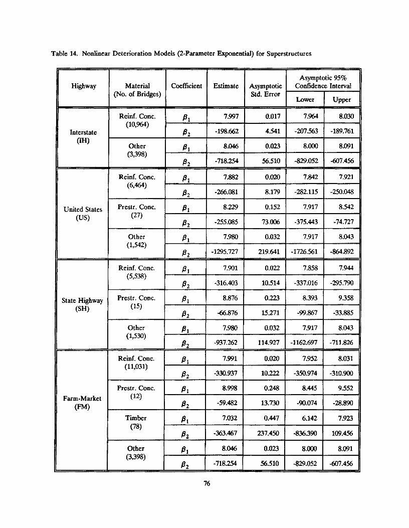
Table 14. Nonlinear Deterioration Models (2-Parameter Exponential) for Superstructures

Asymptotic 95% Highway Material Coefficient Estimate Asymptotic Confidence Interval

(No. of Bridges) Std. Error Lower Upper

Reinf. Cone. PI 7.997 0.017 7.964 8.030 (10,964)

Interstate Pl -198.662 4.541 -207.563 -189.761 (IH)

Other PI 8.046 0.023 8.000 8.091 (3,398)

Pl -718.254 56.510 -829.052 -607.456

Reinf. Cone. PI 7.882 0.020 7.842 7.921 (6,464)

-250.048 Pl -266.081 8.179 -282.115

United States Prestr. Cone. PI 8.229 0.152 7.917 8.542

(US) (27) P2 -255.085 73.006 -375.443 -74.727

Other PI 7.980 0.032 7.917 8.043 (1,542)

P2 -1295.727 219.641 -1726.561 -864.892

Reinf. Cone. PI 7.901 0.022 7.858 7.944 (5,538)

P2 -316.403 10.514 -337.016 -295.790

State Highway Prestr. Cone. PI 8.876 0.223 8.393 9.358

(SH) (15) P2 -66.876 15.271 -99.867 -33.885

Other (1,530)

PI 7.980 0.032 7.917 8.043

112 -937.262 114.927 -1162.697 -711.826

Reinf. Cone. PI 7.991 0.020 7.952 8.031 (11,031)

P2 -330.937 10.222 -350.974 -310.900

Prestr. Cone. PI 8.998 0.248 8.445 9552

Farm-Market (12)

(FM) {32 -59.482 13.730 -90.074 -28.890

Timber (78)

PI 7.032 0.447 6.142 7.923

{32 -363.467 237.450 -836.390 109.456

Other PI 8.046 0.023 8.000 8.091 (3,398)

{32 -718.254 56.510 -829.052 -607.456

76

Table 15. Nonlinear Deterioration Models (2·Parameter Exponential) for Superstructures

Asymptotic 95% Highway Material Coefficient Estimate Asymptotic Confidence Interval

(No. of Bridges) Std. Error Lower Upper

Reinf. Cone. PI 8.177 0.033 8.113 8.241 (3,656)

P2 -256.504 12.395 -280.806 -232.202

Interstate Prestr. Cone. PI 8.269 0.018 8.233 8.306

(IH) (4,509)

P2 ·247.523 9.156 -265.472 -229.573

Steel PI 7.938 0.040 7~1 (2,904)

P2 -184.626 8.815 -201.

Reine. Cone. (2,813)

PI 8.155 0.031 8.093 8.217

P2 -302.925 14.773 -331.893 -273.958

United States Prestr. Cone. PI 8.356 0.024 8.308 8.405

(US) (2,049) P2 ·204.955 9.062 -222.727 -187.182

Steel (1,838)

PI 7.630 0.051 7.531 7.729

P2 -371.819 30.640 -431.913 -311.724

Reine. Cone. PI 8.186 0.034 8.119 8.252 (2,805)

P2 -332.936 16.683 -365.648 -300.224

State Highway Prestr. Cone. PI 8.373 0.029 8.315 8.430

(SH) (1,377) P2 -217.760 12.195 -241.593 -193.748

Steel PI 7.929 0.067 7.798 8.059 (1,491)

P2 -291.797 21.229 -333.440 -250.154

Reine. Cone. - 8.194 0.024 8.146 8.242 1 (9,060) -2 -352.926 13.931 -380.235 -325.618

Farm-Market Prestr. Cone. PI 8.187 0.041 8.106 8.269

(FM) (498) P2 -410.558 54.529 -517.697 -303.419

Steel (1,092)

PI 7.957 0.080 7.800 8.114

P2 -289.826 26.125 ·341.087 -238.565

77

9

8

7

6

5

4

3

2

1

a

Condition Rating

Ie:",

~ ~

~ ~

~"~

a 20 40 60 80

Age of Bridge (yrs)

~ Concrete (IH)- -+- Steel (SH/FM)· -6- Steel (US)-

• NSI Data

Figure 9. Piecewise Linear Deterioration Models for Substructures by Highway Class

9

8

7

6

5

4

3

2

1

o

Condition Rating

~

o

~ -r-:;::::::::

" 'i ~ ---=::: --~"," ~ ~~ ~

'" "' "'l~

" ~ 20 40 60 60

Age of Bridge (yrs)

-+- Expert (PeA) .... Expert (UkeJy)~ Expert (Optim)

• NSI nata (Exponential Cu"e.)

100

Figure 10. Nonlinear Deterioration Models for Reinforced Concrete Decks by Highway

78

100

-

120

9

8

7

6

5

" 3

2

1

o

Condition Rating

~

~ ----.:::: ~

~ ~ -----",", ~ ,,~ ~

"" "'~ , " ~ "" o 20 40 60 80

Age of Bridge (yrs)

IH* -+- us- --- FII--*- Expert OpUm ~ Expert Pess ...... Expert Likely

• NOI nata (ExponenUaJ Curves)

100

~ SH-

Figure 11. Nonlinear Deterioration Models for Steel Superstructures by Highway

120

Condition Rating 9r-------~~------~~------_,--------~--------~--------_,

:~ ..... . ~~ .. 6 ....... : ..... .

. ~~~~ .......... . 5~------~---------r--------~------~~~~~~~------~ ...... ~~ ...... -........... .

•· .. ~·· .. • .. t ." ................. ~

4~------~~------~~-------;--------~--------~----~~~

3~------~~------~~------~--------~--------~--------~ o 20 40 60 80 100 120

Age of Bridge (yrs)

- Steel (IH) NBI Data -t::.: .. Upper Umit 95% C.1. ....... Lower Umlt 95% C.1.

Figure 12. Nonlinear Deterioration Models for Steel Superstructures

79

The Probabilistic Approach - FreQuency Analysis

Another approach taken to model the bridge deterioration process was by examining the frequency

distributions of the condition ratings, at various ages of a bridge classification category. In addition, the

frequency distribution was determined for bridge ages at specific condition ratings. Using the frequency

procedure on SAS, a cross-table frequency distribution of condition ratings and ages of bridges was approximated

into conditional probability density distributions. While condition ratings are discrete variables, their distributions

are actually bar graphs or relative frequency polygons, but these plots were approximated into continuous

distributions in order to clearly emphasize the variation, and also, this enhances some practical application of

the results. Since the bridge data used in the analysis indicated no rehabilitation history, these distributions will

give estimates of conditional probabilities and state probability vectors such that:

P[CR I AGE] = P(CR=X I AGE=Y] , the probability of a bridge component being in condition

rating X when it is Y years old.

P[CR I AGE] in its discrete form, can be interpreted as the state probability vector for a specified age

Y. Since there are eight possible condition ratings (2 - 9), a row vector indicating the probabilities of finding

the bridge components in each of these states (i) is a state probability vector.

Also,

P[AGE I CR] P[AGE = Y I CR = Xl, the probability that the age of bridge is Y years, given its

current condition rating X.

This estimate could also be interpreted as the probability distribution of the time (years) it takes a

bridge component from its newly built condition (AGE = 0) to reach the specified condition rating X. It should

be noted however that there is no adequate time series data available on bridge condition ratings, in terms of

time length, that would provide information on how long the bridges have been in the various states (sojourn

times).

While this a simplistic approach to modeling bridge deterioration, it revealed some valuable findings.

It was observed that the bridge records indicate most bridges tend to be rated at one particular condition ratings

regardless of their age. In other words, the P[CR I AGE] seems to peak at a particular condition rating. For

example, in the plot for steel superstructures on PM roads (Figure 13), the peak of most curves is at condition

rating of 7, irrespective of age. This might be due to undocumented bridge maintenance and rehabilitation

masking the natural deterioration process of the bridge. It might also be due to inconsistencies on the inspector's

part, during bridge field inspection.

80

State Probability 1 ~----~----T-----~--~r---~----~----~----~----_

O.8+-----+-----+-----~----~--~~--~----~----++~--H

O.6~----+-----+-----r_----r_--~----~----~~_r_+~~~

o 1 2

-• At.e ot Brid,e

3 4 5 6 Condition Rating

-e- 5 yrs*

-+- 40 yrs*

...- 10 yrs*

.. -6 ... 50 yn*

FJ.gUfe 13. State Probability Plot for Steel Superstructure on FM Highway

7 8 9

-+ .. 20 yr8-

-.-If.. 60 yr.-

The next task taken to solve this problem was to supplement the statistical data from the BRINSAP

tape, with expert judgmental opinion of the bridge engineers at Texas SDHPT. While the deterioration rates

estimated purely based on the statistical data may be used for analyses within the BMS, they may have to be

modified by the user to reflect his or her expert judgmental opinion on the bridge deterioration process.

Models Based on Expert Opinions

Due to uncertainty present in the bridge deterioration process, coupled with the inadequacy of the

information available for modeling, a judgmental forecasting approach was used to supplement the statistical

regression-based modeling done on the historical data earlier. By eliciting information from bridge engineers

and managers based upon their experience and expertise, service-life data, specifically, the remaining service lives

of bridges, were estimated. The remaining service life of a bridge component is the number of years estimated

by the bridge engineer, that it will take for the component's condition rating to drop from its current value to

the value 2, assuming no maintenance or rehabilitation is done on the bridge within this time period. The

condition rating of 2 is assumed to be the end of a bridge component's service life, a critical condition at which

the bridge is recommended closed.

81

Through a devised package of questionnaires (see Appendix B), information in the form of a triplet

(minimum, most likely, maximum) on the estimates of remaining service lives were elicited from bridge experts

from the Texas SDHPT. The statistics of the responses - averages and standard deviations - are shown in

Appendix C. These estimates were further utilized to fit simple linear deterioration curves by computing the

time interval of change in the values of the condition ratings. A sample of these approximated deterioration

curves is shown in Figure 11 while the estimates of deterioration rates, in condition rating points per year, are

included with the summary of responses on the remaining services lives (Appendix C). The formulated

regression models are shown in Table 16 - Table 18. The estimated deterioration rates corresponding to each

parameter of the triplet (minimum, most likely, maximum) of information on service lives, can be considered

to be the bridge experts' pessimistic, most likely, and optimistic estimates respectively.

Table 16. Simple Linear Deterioration Models for Bridge Decks (Expert Opinion)

Bridge Regression Equations Material Type Level of Confidence (t -statistics) R2

Reinforced Pessimistic" 7.560 - O.145[AGE] 0.581 Concrete (36.522) (-11.159)

Most LikelY' 7.758 - 0.115[AGE] 0.670 (41.300) (-13.509)

OptimisticC 7.655 - 0.083[AGE] 0.641 (39.815) (-12.682)

• -- Based on the experts' minimum estimates of bridge component's expected remaining service life. b __ Based on the experts' "most likely" estimates of bridge component's expected remaining service life. e _ Based on the experts' maximum estimates of bridge component's expected remaining service life.

82

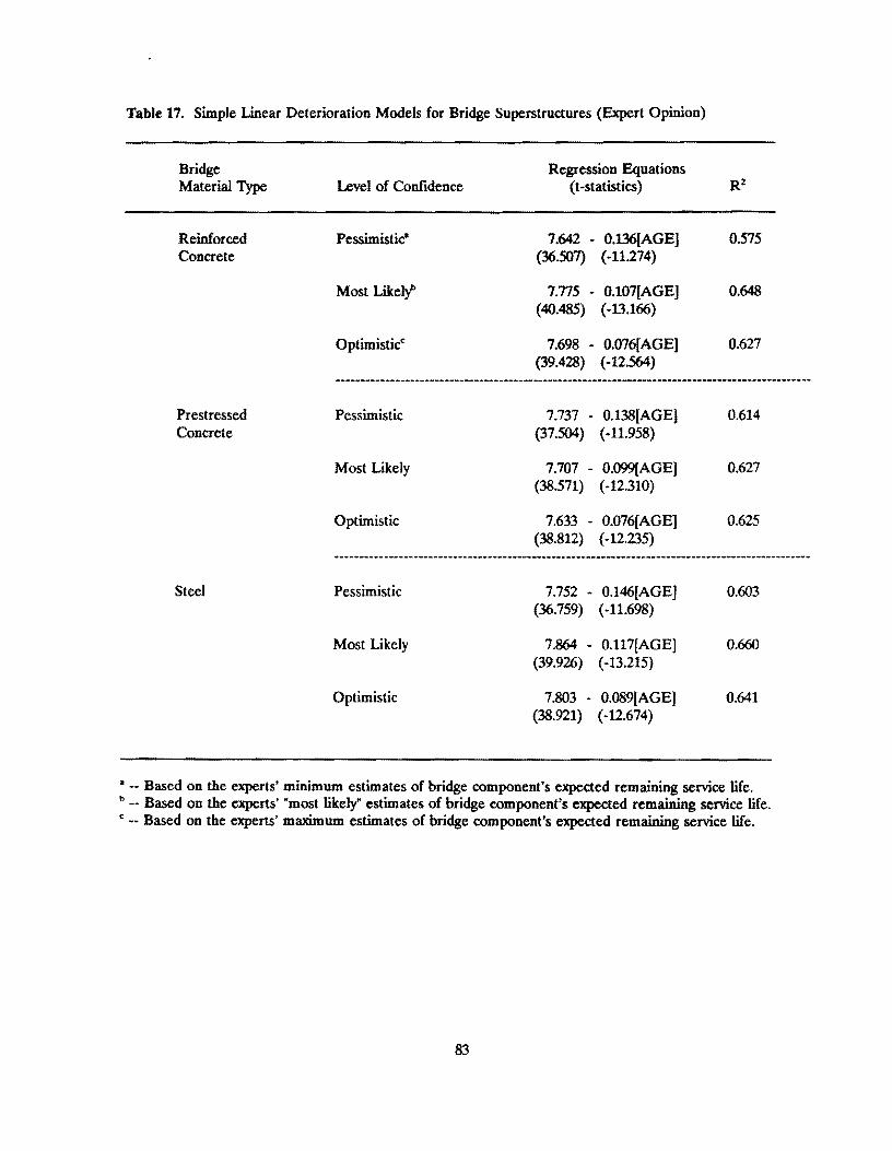
Table 17. Simple Linear Deterioration Models for Bridge Superstructures (Expert Opinion)

Bridge Regression Equations Material Type Level of Confidence (t -statistics) R2

Reinforced PessimistiC- 7.642 - O.136[AGEJ 0.575 Concrete (36.507) (-11.274)

Most likelY' 7.775 - 0.107[AGE] 0.648 (40.485) (-13.166)

Optimistic" 7.698 - O.076[AGE] 0.627 (39.428) (-12.564)

Prestressed Pessimistic 7.737 - O.I38[AGEJ 0.614 Concrete (37.504) (-11.958)

Most Likely 7.707 - O.099[AGE] 0.627 (38.571) (-12.310)

Optimistic 7.633 - 0.076[AGEJ 0.625 (38.812) (-12.235)

Steel Pessimistic 7.752 - 0.146[AGE] 0.603 (36.759) (-11.698)

Most Likely 7.864 - 0.117[AGE] 0.660 (39.926) (-13.215)

Optimistic 7.803 - 0.089[AGEJ 0.641 (38.921) (-12.674)

• -- Based on the experts' minimum estimates of bridge component's expected remaining service life. \> -- Based on the experts' "most likely" estimates of bridge component's expected remaining service life. C __ Based on the experts' maximum estimates of bridge component's expected remaining service life.

83

Table 18. Simple Linear Deterioration Model for Bridge Substructures (Expert Opinion)

Simple Linear Deterioration Model for bridge Substructures (Expert Opinion) ---------------------------------------------------------------

Bridge Regression Equations Material Type Level of Confidence (t-statistics) R2

Reinforced Pessimistic" 7.654 - O.I44{AGE] 0.604 Concrete (38.187) (-11.968)

Most Likely" 7.740 - 0.107[AGE] 0.650 (40.831) (-13.218)

OptimisticC 7.701 - 0.081[AGE] 0.630 (39.609) (-12.643)

Prestressed Pessimistic 7.710 - 0.131[AGE] 0.623 Concrete (34.711) (-IU)66)

Most Likely 7.739 - 0.097(AGE] 0.657 (36.666) (-11.899)

Optimistic 7.723 - 0.073[AGE] 0.646 (36.064) (-11.627)

Steel Pessimistic 7.881 - O.I77[AGE] 0.644 (36.000) (-11.875)

Most Likely 7.866 - O.l38[AGE] 0.663 (37.386) (-12.392)

Optimistic 7.883 - 0.105[AGEJ 0.680 (38.487) (-12.865)

Timber Pessimistic" 7.535 - O.202[AGE] 0.513 (30.769) (-9.056)

Most Likely" 7.846 - 0.174[AGE] 0.629 (35.222) (-11.489)

OptimisticC 7.992 - 0.14O(AGE] 0.680 (37.918) (-12.880)

• -- Based on the experts' minimum estimates of bridge component's expected remaining service life. b __ Based on the experts' "most likely" estimates of bridge component's expected remaining service life.

84

Life-Cycle Costs Models

Babaei [1988] reports algorithms used for estimating bridge deck maintenance rehabilitation and

maintenance costs for various types of bridge decks. Maintenance costs for patching of deck spalling are

estimated by the following equations:

Annual Spalling Rate = S/(1+el 2-A)

for latex modified concrete (LMC) overlaid decks, and

Annual Spalting Rate = S/(1+e7•A

)

for asphalt concrete membrane (ACM) overlaid decks. The parameter S is the maximum annual spalling rate

expected, and A is the age of the deck in years. The maximum expected spall rate S is given in terms of the

observed cumulative spalls caused by debonding and delamination. These two curves are shown in Figure 14.

The relationship between observed cumulative spalls by debonding and delamination is assumed to be

where

CS1 is the cumulative spalls caused by debonding, in percent, and

CSz is the cumulative spalls caused by delamination, in percent.

For LCM overlaid decks, CS1 and CS2 can be taken to be one-third of the observed debonding at 20 yrs

and one-fourth the magnitude of delamination at 20 yrs, respectively. For ACM overlaid decks, these parameters

may be taken to be one-half the magnitude of debonding at 15 yrs and 1/3 the magnitude of delamination at

15 yrS, respectively. The appropriate magnitUde of distress (MD) is estimated from prior inspection data by

assuming a linear rate of accumulation of distress:

where

r = (MDL-MDF)/(AcAF) is an average rate of distress increase,

A = age, and

the subscripts F and L denote "fmal" times, and times of "latest" survey, respectively.

85

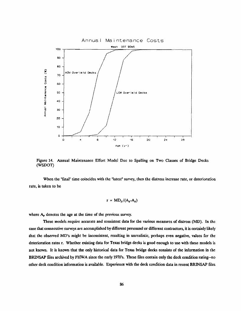
Annual Maintenance Costs Was.h DOT BOlAS

100

90

eo 1"\ IR \.J

CI> 70

oJ CI> 0 \J 60 .. u c: f3 SO c: <I> oJ c: - 40 §

Ci 30 :l c: c «

20

10

0

0 4 8 12 16 20 24 28

Age (yr)

Figure 14. Annual Maintenance Effort Model Due to SpaDing on Two Classes of Bridge Decks (WSDOT)

When the "fmal" time coincides with the "latest" survey, then the distress increase rate, or deterioration

rate, is taken to be

where A, denotes the age at the time of the previous survey.

These models require accurate and consistent data for the various measures of distress (MD). In the

case that consecutive surveys are accomplished by different personnel or different contractors, it is certainly likely

that the observed MD's might be inconsistent, resulting in unrealistic, perhaps even negative, values for the

deterioration rates r. Whether existing data for Texas bridge decks is good enough to use with these models is

not known. It is known that the only historical data for Texas bridge decks consists of the information in the

BRINSAP flIes archived by FHW A since the early 1970's. These files contain only the deck condition rating--no

other deck condition information is available. Experience with the deck condition data in recent BRINSAP flIes

86

suggests that this data would not be "precise" enough to use successfully with the models used in the WSDOT

bridge deck management system.

FHWA Lee Model

In order to evaluate the alternative improvement strategies for every bridge on a network system, it is

necessary to consider the corresponding costs to be incurred by the highway agency. These costs include the frrst

or initial one-time cost, periodic maintenance costs, and possibly a rehabilitation or replacement cost as the

bridge approaches the end of its service life.

While most of the current bridge project selection methods consider only the frrst or initial construction

costs [FHWA 1987]. it seems more appropriate that the entire life-span costs or simply, the life-cycle costs

associated with each alternative be considered. Life-cycle cost analysis is particularly suitable for evaluating

mUltiple alternatives which have unequal life expectancy and maintenance costs. Based on the expected

deterioration rate, costs required to bring bridge back to a desired level of service are utilized to generate a life­

cycle profile.

For the purpose of presenting the fundamental concepts of the life-cycle cost analysis, it will be assumed

that each bridge replacement alternative may have two courses of action: (1) rehabilitation and maintenance to

postpone eventual replacement into the future by, say, e years; or (2) immediate replacement of the bridge.

For a life-cycle cost comparison of the two courses of action, the following information is needed:

e = extended life of bridge due to rehabilitation and maintenance,

Lee;, = present worth of life-cycle costs for the replacement case, and

Lee) = present worth of life-cycle costs for the extended life case.

A graphical representation of the replacement and rehabilitation cases is given in Figure 15 and

Figure 16, respectively. The agency net benefit B. associated with the extended service life case is computed as

the difference between the two life-cycle costs involved, that is,

87

A

o

A

SL = Service Life

SL Future Years

Replace at SL intervals

A = Present WOrth (one I ife cycle)

Figure 15. Life-Cycle Costs for Replacement Case

A

B

Extended SL Service Life Life e

o e Future Years

A = Present Worth Cone life cycleJ

B = Rehab! I itation Cost

FIgUre 16. Life-Cycle Costs for Rehabilitation Case

A

I

Replace at SL intervals

e ... SL

The following are the fundamental equations used in the life-cycle cost analysis. The notation used in

these equations is shown below:

= interest/discount rate,

n number of time periods,

F = future value,

A = annuity,

G = gradient. or rate at which costs are expended, and

p = present worth.

Basically, the economic analysis equations can be classified into two groups: (A) present worth

calculations, and (B) future value calculations. The present worth calculations refer to four cases: single

payment, uniform series, gradient, and perpetual series.

88

A. Present worth calculated by discounting:

Single payment:

P = F(l+i)"fl

Uniform Series:

Uniform Gradient:

p - G [l-(l~i)" - n 1 i 7 (1 +i)"

Perpetual Series:

P = A (1+i)" 1 (1+i)"-1

B. Future Value of Investments:

F = P (1 +i)"

An example that illustrates the present worth calculation of a stream of life-cycle costs is given in

Figure 17. The discount rate used in the example is 6 percent. Here we consider a bridge experiencing the

following sequence of actions:

• Replacement in the base year (year 0).

• Rising maintenance costs increasing from zero in the frrst year to 2 percent of the replacement cost

at the end of the service life of the bridge which, for this example, is taken as 40 years.

89

• Rehabilitation in year 40 and a sequence of rising maintenance costs beginning in year 41, and

following the same growth as the previously dermed gradient out to year 70.

• Replacement in year 70 after which time the same stream of life-cycle costs repeat itself.

Replace Fut.ure Action

1 0 Rehab iIi tate 1.0

0.1

Mel j ntenance Mel i nt.enance

. 2

o 1 39 ~o ~1 6970

Figure 17. Stream of Life-Cycle Costs

As indicated before, the present worth of a uniform gradient is given by the following relationship:

Using the above relationship and the data shown in Figure 17, the following results are obtained for the

two gradient series associated with the maintenance activity:

Po == 0.02/40 t1-( 1. 06) .. 0 40 ] = 0.093

0.06 0.06 (1. 06 )40

P40 == 0.02/40 t 1 -( 1. 06).... - 30 ] = O. 071

0.06 0.06 (1.06)30

As shown in Figure 18 can be seen, one of the series will be the present worth of the first gradient in

the base year and the other wiU be the single cost or payment in year 40, equivalent to the rising maintenance

costs from year 40 through year 70. The next step is to bring all single payments to a present worth value. This

gives a present worth cost for one life cycle of 1.17, as indicated below:

90

Po :: 1 + 0.093 + (0.7+0.071)(1.06)~o = 1.17

Future Act ion

t' 0,093 I' , 0,071 I

o , 394041 6970

Figure 18. Equivalent Single-Cost Representation of Maintenance Cost Gradients

Future Act ion

1 17

o

Life cycle costs recurring at 70 year intervals indefinitely

Figure 19. Present Worth of Perpetual Service

1,17

70

If the future action every 70 years is another replacement, we need to fmd the present worth of a

perpetual service. As shown in Figure 19, the present worth of the life-cycle cost for the replacement case,

assuming perpetual service is given by:

Rehabi I itatlon

o 771

:: 1. 17 ( 1. 06) 70 1 = 1. 19 (1.06) 70_1

Replacement

1 19

Rehab iii tat Ion

Extends life 30 years

~ 70 o ~

Figure 20. Future Cost Assuming Rehabilitation

To illustrate life-cycle cost comparisons, refer to FIgure 18. Assume that 40 years have elapsed since

the bridge illustrated in the cost profUe was replaced, and that a major improvement action is now necessary.

If the bridge is rehabilitated as originally proposed, the future costs profUe shown in FIgure 20 is obtained.

There are 30 years of life remaining in the bridge if it is rehabilitated at the cost indicated. The cost of

rehabilitation plus maintenance costs for 30 years is 0.771. The bridge would then need to be replaced. The

91

replacement life-cycle cost, taken to perpetuity, is 1.19, as shown in Figure 18. This would be the cost if the

replacement option were selected. For the rehabilitation option, the present worth of the life-cycle prof!.le,

assuming perpetual service, is calculated as shown below.

Lec, = 0.771 + 1.19(1.06r~o = 0.98

Finally, the agency benefit of rehabilitating the bridge is the difference in life-cycle costs between the

replacement option and the rehabilitation option:

Ba = 1. 19 - O. 98 = O. 21

Thus, even though the cost of rehabilitation is more than two-thirds of the replacement cost, the life-cycle cost

comparison shows that extending the life of the bridge with the rehabilitation alternative would provide a net

savings to the agency equivalent to 21 percent of the replacement cost in current dollars. Of course, the amount

of savings will vary with the interest rate and the amount of life extension provided by the rehabilitation. A lower

discount rate or less life extension would result in less cost savings and vice versa.

Generalized Life-Cycle Costs for Multi-Period Optimization

FIXed Budaets and Discountina of A~ncy Costs

In the multiple-period optimization situation, budgets typically are assumed to be fIXed for each sub­

period of the analysis period. Because the budget for each period is fIXed at the time of the sub-period, there

is no discounting of costs to time zero. Costs that occur in a particular period simply are subtracted from the

budget for that period when an alternative is chosen. That is, since the sub-period budgets are faxed, the

optimization problem can be stated as having the objective of choosing the set of projects (with total cost for

alternatives chosen for improvement in each sub-period not exceeding each sub-period's budget, not discounted)

over time that will maximize the present value of future benefits (or reductions in user and possibly agency costs

other than capital costs). It typically is assumed that all funds must be spent as they become available and that

they cannot be invested and carried over to future years as a strategy (possibly with investment in future periods

when needs are greater) even though this assumption can be changed if desired. Therefore, in the multi-period

92

optimization problem, it is reasonable to not discount future agency costs, and in fact, such discounting is not

compatible with the assumption of absolutely fIXed budgets in the multi-period optimization problem.

If the fixed budget for each sub-period is assumed to cover all types of agency costs, including

maintenance costs, then these costs should be considered without discounting since they subtract fully from future

money available for rehab or rebuild alternatives. This point is critical to recognize in going from a standard

life-cycle cost analysis to a true fixed-budget, multi-period optimization problem. A way of simplifying the

problem, however, is to assume that the budget being considered is for major capital costs only and to include

reductions in maintenance costs in benefits; this possibility is considered in more detail later in this discussion.

Lenath of Plannine (or Optimization) Period and Sub-periods

In developing an optimization routine, several considerations should be recognized in developing the

optimization structure. The true optimal solution for the fIXed-budget, multi-period problem cannot be obtained

by analyzing only a short budgeting or planning period (for example, considering only ten successive one-year

sub-periods to obtain the 10-year budget optimization). One reason this is the situation is that there are needs

that are coming due in years after ten years that can now be predicted and should be taken into account in the

first ten years. For example, assume that annual budgets are somewhat below needs in the frrst ten years, and

are expected to be greatly below needs in the foUowing ten years. This might be the case if for example, a state

has a large number of Interstate bridges that wiU need to be rehabilitated or rebuilt in the second ten years.

The true long-term optimal solution might entail rebuilding some of these bridges in the frrst ten years while not

rebuilding some minor bridges that would be scheduled if we did not look beyond ten years. Therefore, the ten­

year optimal solution depends on budgets beyond ten years. In a broader framework, including the possibility

of increased funding, the true global optimal solution might be to increase funding so that more funds would be

available in the first ten years and in the second ten years and in the second ten years. This could be tested by

running the program with different budget levels.

Having a large number of periods considerably complicates optimization solutions through increasing

the number of alternatives. One possibility for simplifying the problem is for the optimization problem for fIXed

budgets to be structured in a way that includes a fairly long planning period (say 20 to 30 years) so that

important trade-offs (both types of alternatives chosen and timing of alternatives) are considered. Using a

planning period of this length would considerably increase the complexity of the optimization problem if one-year

budgets are considered. However, this can be simplified by dividing the planning period into sub-periods that

are longer than one year for purposes of optimization. One possibility, for example would be to use sub-periods

of five years in length and allow initial optimization to choose at most one major improvement alternative within

each five-year period. The budget for each fIVe years would simply be the sum of the five one-year budgets

within the five-year period.

93

Use of a 2O-year planning (or optimization) period with four five year sub-periods, or possibly a 3O-year

planning period with six sub-periods probably would greatly improve the true, global optimization (as opposed

to a narrow, but perhaps more accurate technically, optimization) with little loss in the accuracy of the within

period optimization. There are two reasons wby there would be little loss in accuracy: (1) most (if indeed not

all) of the major alternatives that would be considered in the optimization would have a life of more than five

years, so there would not be a problem of wanting to do two major improvements within one S-year period, and

(2) given the accuracy of the deterioration estimates, the short -term changes in scheduling in practice. and the

length of time needed to construct major improvements, five years is probably a more reasonable budget

optimization period.

Even if a five-year sub-period is used in this way for optimization, deterioration can still be modeled on

a one year basis. Moreover, the person using could stiD use the five-year list as a starting point and could use

judgment and/or decision rules for setting priorities within each five-year sub-period. (It might even be possible

to do a successive sub-optimization within each five year period using an approach similar to the twenty (or

thirty) year optimization, by checking alternative timings for the chosen alternatives within the period. Some

rules for determining the effects of the specific timing of decisions in earlier periods on future periods must be

developed, and this may mean that the solution only approximates a true optimum. If the fIXed budget solution

is being worked out for ten one-year budgets combined into two five-year budgets, but using a twenty planning

or optimization period, this effect will tend to be small if most major alternatives last at least ten years and will

be almost nonexistent if most improvements last at least twenty years.) This would be especially true for the first

five-year period where the decision maker would want to use judgment in scheduling and coordinating work.

Judgment also could be used in selecting some bridges from later five-year sub-periods if they are good projects

that need to be coordinated with other work in the first five years. The model is a tool to be used by the

decision maker. Even the best model will not include all of the important factors that should be considered in

practice, not only impacts but factors affecting scheduling.

Calculation of Life-Cycle Costs and User Costs

In the single-period, life-cycle cost model developed by the Federal Highway Administration, the base

alternative is the most expensive alternative, bridge replacement. Alternatives are compared to this alternative

and reductions in cost are considered as benefits in the single-period optimization problem.

This simple life-cycle cost model is not adequate for the multiple period optimization problem. Several

assumptions are made to simplify the optimization problem.

1. It is assumed that a maintenance and inspection strategy is defmed so that for each capital

investment strategy, the maintenance and inspection costs can be calculated with certainty for each

year to the point in time where a major capital expenditure is made beyond the analysis period.

94

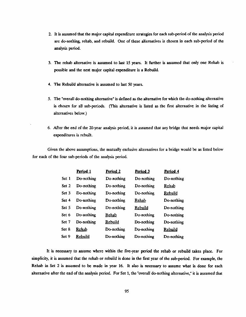
2. It is assumed that the major capital expenditure strategies for each sub-period of the analysis period

are do-nothing, rehab, and rebuild. One of these alternatives is chosen in each sub-period of the

analysis period.

3. The rehab alternative is assumed to last 15 years. It further is assumed that only one Rehab is

possible and the next major capital expenditure is a Rebuild.

4. The Rebuild alternative is assumed to last 50 years.

5. The "overall do-nothing alternative" is defmed as the alternative for which the do-nothing alternative

is chosen for all sub-periods. (This alternative is listed as the first alternative in the listing of

alternatives below.)

6. After the end of the 2O-year analysis period, it is assumed that any bridge that needs major capital

expenditures is rebuilt.

Given the above assumptions, the mutually exclusive alternatives for a bridge would be as listed below

for each of the four sub-periods of the analysis period.

Period 1 P~riod 2 fCriod 3 Period 4

Set 1 Do-nothing Do-nothing Do-nothing Do-nothing

Set 2 Do-nothing Do-nothing Do-nothing &haQ

Set 3 Do-nothing Do-nothing Do-nothing R~build

Set 4 Do-nothing Do-nothing Rehab Do-nothing

Set 5 Do-nothing Do-nothing Rebuild Do-nothing

Set 6 Do-nothing Rehab Do-nothing Do-nothing

Set 7 Do-nothing Rebuild Do-nothing Do-nothing

Set 8 &haQ Do-nothing Do-nothing Rebuild

Set 9 B~build Do-nothing Do-nothing Do-nothing

It is necessary to assume where within the five-year period the rehab or rebuild takes place. For

simplicity. it is assumed that the rehab or rebuild is done in the fust year of the sub-period. For example, the

Rehab in Set 2 is assumed to be made in year 16. It also is necessary to assume what is done for each

alternative after the end of the analysis period. For Set I, the "overall do-nothing alternative," it is assumed that

95

the bridge is rebuilt at the first time that it does meet tolerable conditions; if it deteriorates to the point where

it does should be replaced during the analysis period, it is assumed that it will be rebuilt at year 21.

Set 1 Rebuild at year 21 (and rebuild year 71, year 121, year 171, etc.)

Set 2 The Rehab during last period takes place at year 20 and lasts 15 years, so a Rebuild is

scheduled at years 35, 85, 135, etc.

Set 3 The Rebuild during the analysis period is assumed to occur at year 20 so there are additional

rebuilds at years 70, 120, 110, etc.

Set 4 The Rehab during the analysis period is assumed to occur at year 15 so there are Rebuilds at

years 30, SO, 130, etc.

Set 5 The Rebuild during the analysis period is assumed to occur at year 15 followed by Rebuilds at

years 65, 115, 165, etc.

Set 6 The Rehab during the analysis period is assumed to occur at year 10 so there are Rebuilds at

years 25, 15, 125, etc.

Set 1 The Rebuild during the analysis period is assumed to occur at year 10 followed by Rebuilds at

years 60, 110, 160, etc.

Set 8 The Rehab during the analysis period is assumed to occur at year 5 so there are Rebuilds at

years 20, 10, 120, etc.

Set 9 The Rebuild during the analysis period is assumed to occur at year 5 followed by Rebuilds at

years 55, 105, 155, etc.

The OVerall Do-Nothina: Alternative and Costs for Alternatives

Set 1, the overall do-nothing alternative, has the following characteristics:

1. It has zero capital costs during the analysis period.

96

2. It will have relatively high maintenance costs during the analysis period, if these are made a function

of the level of deterioration, since the bridge may need to have major capital expenditure on it, but

these are not made during the analysis period.

3. It will have the highest user costs of all alternatives since no major capital expenditures are made

with this alternative. (If the bridge is in very good condition, user costs may be low for all

alternatives; at a minimum, the overall d<rnothing alternative should have user costs that are at least

as great as any other alternative.)

4. It has high capital costs for the time period beyond the optimization period, since it is assumed that

the needed capital expenditure is made immediately after the optimization period (if minimum

tolerable conditions justify such expenditure).

Two types of costs are calculated: (1) capital costs during the analysis period and (2) "other costs."

Other costs include aU of the following and are calculated for each set, or alternative: user costs, maintenance

costs, and capital costs beyond the end of the analysis period. Benefits are calculated for each alternative except

Set 1, the overall d<rnothing alternative and are defined as reductions in ·other costs· relative to the "other costs"

for Set 1, which will have the highest other costs, since no capital improvements are made during the analysis

period. After capital costs and benefits are calculated for each alternative for all bridges, an optimization

procedure can then be used to determine the best choice of alternatives for the multiple-period fIXed budget

problem.

Agency Benefits Model

The life-cycle cost model will consider the two types of benefits discussed in the FHW A Demonstration

Project [FHW A 1987], agency benefits and user benefits. Agency benefits are defined as reductions in life-cycle

cost resulting from actions of the agency, such as preventive maintenance, certain types of rehabilitation, and any

other actions that effectively extend the life of the bridge.

Extension in Bridge Service Life

A bridge service life is defined as the time remaining till the bridge deteriorates to a specified condition

at which it is dosed to the public. Bridge rehabilitation effort is expected to halt the deterioration process and

improve the bridge condition. This action will ultimately extend the original bridge remaining service life. It

has been recognized by most bridge engineers that the service life of a bridge is a very important criterion in

making decisions related to bridge management. This is apparent in the case of priority ranking systems where

the remaining service life of a bridge is considered as an attribute in assessing the ~urgency" or priority of funding

97

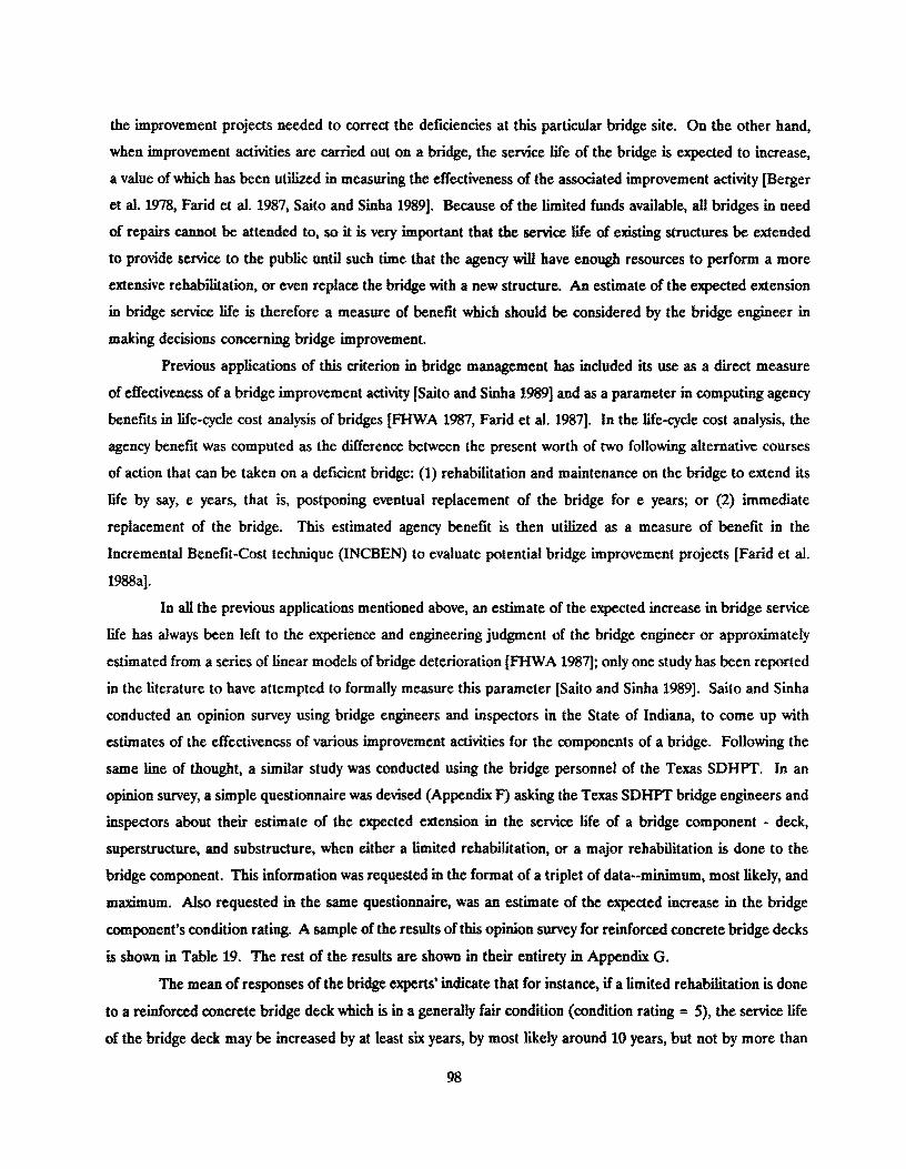
the improvement projects needed to correct the deficiencies at this particular bridge site. On the other hand,

when improvement activities are carried out on a bridge, the service life of the bridge is expected to increase,

a value of which has been utilized in measuring the effectiveness of the associated improvement activity [Berger

et al. 1978, Farid et al. 1987, Saito and Sinha 1989]. Because of the limited funds available, all bridges in need

of repairs cannot be attended to, so it is very important that the service life of existing structures be extended

to provide service to the public until such time that the agency will have enough resources to perform a more

extensive rehabilitation, or even replace the bridge with a new structure. An estimate of the expected extension

in bridge service life is therefore a measure of benefit which should be considered by the bridge engineer in

making decisions concerning bridge improvement.

Previous applications of this criterion in bridge management has included its use as a direct measure

of effectiveness of a bridge improvement activity [Saito and Sinha 1989] and as a parameter in computing agency

benefits in life-cycle cost analysis of bridges [FHWA 1987, Farid et al. 1987]. In the life-cycle cost analysis, the

agency benefit was computed as the difference between the present worth of two following alternative courses

of action that can be taken on a deficient bridge: (1) rehabilitation and maintenance on the bridge to extend its

life by say, e years, that is, postponing eventual replacement of the bridge for e years; or (2) immediate

replacement of the bridge. This estimated agency benefit is then utilized as a measure of benefit in the

Incremental Benefit-Cost technique (INCBEN) to evaluate potential bridge improvement projects [Farid et al.

1988a].

In all the previous applications mentioned above, an estimate of the expected increase in bridge service

life has always been left to the experience and engineering judgment of the bridge engineer or approximately

estimated from a series of linear models of bridge deterioration [FHW A 1987]; only one study has been reported

in the literature to have attempted to formally measure this parameter [Saito and Sinha 1989]. Saito and Sinha

conducted an opinion survey using bridge engineers and inspectors in the State of Indiana, to come up with

estimates of the effectiveness of various improvement activities for the components of a bridge. Following the

same line of thought, a similar study was conducted using the bridge personnel of the Texas SDHPT. In an

opinion survey, a simple questionnaire was devised (Appendix F) asking the Texas SDHPT bridge engineers and

inspectors about their estimate of the expected extension in the service life of a bridge component • deck,

superstructure, and substructure, when either a limited rehabilitation, or a major rehabilitation is done to the

bridge component. This information was requested in the format of a triplet of data--minimum, most likely, and

maximum. Also requested in the same questionnaire, was an estimate of the expected increase in the bridge

component's condition rating. A sample of the results of this opinion survey for reinforced concrete bridge decks

is shown in Table 19. The rest of the results are shown in their entirety in Appendix G.

The mean of responses of the bridge experts' indicate that for instance, if a limited rehabilitation is done

to a reinforced concrete bridge deck which is in a generally fair condition (condition rating = 5), the service life

of the bridge deck may be increased by at least six years, by most likely around 10 years, but not by more than

98

Table 19. Bridge Expert's Estimate of Bridge Improvement's Effectiveness

(a) Reinforced Concrete Deck (Limited Rehabilitation) - [No. of responses = 19].

Expected Extension in Bridge Service Life (yr) Initial Final

Condition Minimum Most likely Maximum Condition

(Rating) Rating

Mean Std Mean Std Mean Std Mean Std Dev Dev Dev Dev

Gen. Fair (5) 5.6 4.2 9.8 7.8 13.4 9.9 6.6 0.9

Marginal (4) 4.2 4.2 7.9 8.2 10.2 10.1 5.4 1.2

Poor (3) 2.8 4.4 5.5 8.6 7.3 10.7 4.3 4.1

Critical (2) 1.9 4.5 4.2 8.9 5.8 11.1 GU 1.7

(b) Reinforced Concrete Deck (Major Rehabilitation) - [No. of responses = 19].

Expected Extension in Bridge Service Life (yr) Initial Final

Condition Minimum Most Likely Maximum Condition (Rating) Rating

Mean Std Mean Std Mean Std Mean Std Dev Dev Dev Dev

Marginal (4) 17.0 9.5 25.8 14.1 33.3 17.4 7.7 1.0

Poor (3) 17.3 11.5 26.6 17.8 34.7 22.9 7.6 1.2

Critical (2) 17.7 12.3 25.9 18.3 35.1 23.5 7.4 1.3

13 years. There will also be an improvement of two units in the condition rating, resulting in an expected rating

of 7 (Table 19). Also, if a major rehabilitation is applied to the bridge deck, say this time, the deck is in a

critical condition (condition rating = 2). the service life will increase by at least 18 years, by most likely around

26 years, but not by more than 35 years. The major rehabilitation will also result in a expected fmal condition

rating of 7. A similar study by Saito and Sinha [1989] produced comparable results. In their study, Saito and

Sinha reported that an application of deck reconstruction (major rehabilitation) on a bridge deck which is in a

very poor condition (condition rating = 3) will increase its service life by seven years at minimum. by 10 years

on the average, and by 15 years at the maximum [Saito and Sinha 1989]. The expected final condition rating is

7. If a limited rehabilitation such as resurfacing by asphalt overlay is applied to the bridge deck which is in a

99

fair condition (condition rating = 5), Saito and Sinha reported that there will be an expected increase in service

life of six years on the minimum, nine years on the average, and a maximum of 12 years. The expected fmal

condition rating is 1.

Judging from the standard deviations of the values in Table 19, there is a large variation in the

responses; it can be seen that these are rough estimates, but they nonetheless provide an estimate along with a

quantified imprecision. The expected extension in bridge service life is a difficult parameter to estimate. Until

actual real-life data of bridge improvement activities and their associated extensions in life is recorded historically

and analyzed, such estimates as derived from the opinion survey conducted in this study, will serve as a reliable

guide in estimating the expected extension in the bridge service life when a bridge improvement project is carried

out.

User Benefits Model

User benefits are the benefits to the public, represented by reductions in user costs. User costs can be

generated due to narrow width, low clearance, poor alignment, and low load capacity. Included in this category

are three primary benefits:

• Reduction in accident costs,

• Savings in vehicJe operating costs, and

• Reduction in travel times.

Accident Costs

Savings in accident costs result from bridge improvements that eliminate width restrictions and poor

approach geometry. Several studies have shown that bridge width, roadway width, bridge rail design, roadway

marking and signing, and roadway geometry are important in determining accident rates and severity. One of

the fust reviews of bridge studies showed how several studies had emphasized the importance of bridge and

roadway width in determining tbe accident rate [Jorgenson et al. 1966]. Vehicles tend to strike the bridge rail

when the bridge is narrow, either absolutely or relative to the roadway width. More recent literature confirms

this. A study by TTl of a large number of bridge accidents shows accidents with the bridge rail tend to be more

severe if the rail tends to cause severe deceleration or causes vehicles to spin out on the bridge [Brinkman and

Mak 1986]. Other research has developed improved estimates of bridge-related accident costs [Rollins and

McFarland 1985]. This research showed that fatality and injury rates for bridge-related accidents were among

the highest cost accidents. The annual accident benefits or bridge widening are calculated as follows:

Annual Accident Benefits = (Change in Accident Rate)(ADT)(365)(Cost/Accident)

100

Time and Vehicle Operating Costs Associated With Detours

The cost of detouring vehicles when the load capacity or size of a bridge requires a detour includes the

extra time and vehicle operating costs of traveling the alternative route instead of using the preferred route. The

benefit of not having to detour is equal to this cost (saving) and is calculated with the following two formulas

[FHWA 1987]:

Annual Vehicle Operating Cost Savings From Not Detouring

Savings = (ADT) (365) (Change in Fraction of Trucks Detoured) (Change in Distance Traveled

by Trucks Detoured, in Miles) (Operating Cost Per Mile).

Annual Value of Time Savings

Savings = (ADT) (365) (Change in Fraction of Trucks Detoured) (Change in Distance Traveled

by Trucks Detoured in Miles) (Value of Time Per Hour)/ (Speed in Miles Per Hour)

The FHW A manual uses vehicle operating costs developed in a New York study in 1981 and a driver

time value of $14.02 per hour. Truck and passenger values of time have also recently been developed by TTl

[McFarland and Chui 1987]. Very detailed procedures for estimating the number of trucks that will be detoured

for load limits and size restrictions have been developed by North Carolina [Farid et al. 1988], and it is proposed

that these estimation procedures, or similar, be used in the proposed next phase of this study. These procedures

for calculating the vehicle operating and time costs associated with detours use average values and are rough

approximations of the expected costs of detours. It is proposed that this simple procedure be used, with certain

research being added to the program where costs are especially significant, or special situations need to be

investigated. For example, the TTl procedure can be used to model the effects of closing one or more lanes,

the effects of intersections, or the estimation of user cost savings if a new bridge is being built in a different

location while the old one is kept open during construction.

Time and Vehicle Operating Costs Associated With Narrow Bridges

Although the existing North Carolina and FHW A procedures for estimating user costs does not include

time and vehicle operating costs for vehicles traveling over narrow bridges, there is evidence that vehicles slow

down and move toward the center of the highway on narrow bridges. Previous research by TTl treats this issue

and should be used if bridges are less than 22 feet wide. In this case the cost can affect the choice of

alternatives.

101

Optimization Model

The bridge rehabilitation/replacement model is actuaUy a special case of discrete optimization

models. Discrete optimization problems abound in all situations concerning the management and efficient

use of scarce resources to increase productivity. In the last few years meaningful applications of discrete

optimization models have been possible. as a result of significant theoretical developments. as well as the

availability of powerful microcomputers and sophisticated database management procedures.

The proposed bridge project selection model uses a level-or-service measure of effectiveness subject

to budget availability constraints for a group of bridges in each period of a specified planning horizon. The

model is flexible enough to provide the most cost-effective way to achieve a specified level of service, or the

maximum level of service that can be generated with a specified budget for a given bridge system. This

bridge system could be an entire state, a district, or part of a district. For each bridge, several corrective

actions (involving maintenance, various degrees of rehabilitation, and replacement) can be specified along

with their associated level of benefit (service) and cost.

For a successful application of the optimization model the following information is needed:

(a) Group of bridges to be considered,

(b) Set of feasible alternatives for each bridge, and

(c) Cost and benefit associated with each alternative.

There are two basic scenarios for the bridge alternative selection model: (a) benefit maximization,

and (b) cost minimization. The mathematical models for these two cases are formulated as follows:

(a) Benefit Maximization Case

n

Maximize Z = E :E bijXij i.., j~si

102

subject to

E Xij = 1 for each bridge i jfs j

n

E E CijXij ~ 8 i.., jUj

Xij =0,1 fora11 i andj

where the following notation is used:

n - number of bridges,

Si - set of alternatives (including do-nothing alternative) for bridge ~

bij - benefits associated with the selection of alternative j for bridge i,

Ctj - Cost of choosing alternative j for bridge i,

B - Specified budget for a given planning horizon, and

x,j - 1 if alternative j is chosen for bridge i, or 0 Otherwise.

The objective function of the model maximizes the benefits resulting from a set of budget-feasible

bridge alternatives. The frrst set of constraints allows only one alternative to be selected for each bridge.

The last constraint ensures that the total budget available is not exceeded.

(b) Cost Minimization Case

In this case the basic model is formulated as a minimization problem where it is desired to find the

most cost-effective way to achieve a specified cumulative level of benefits from the selected bridge projects.

n

Minimize Z = E I: cijXij i.., jU j

103

subject to

L Xij = 1 for each bridge i jfl l

n

L L b;jXij ~ 8 1=1 jfl l

Xij = 0, 1 for all i and j

where R is a specified minimum level of benefits to be achieved in the most cost-effective manner.

The basic mathematical model is an Integer Programming model. A computationally efficient

solution for the model can be obtained from a branch-and-bound integer programming procedure due to

Nauss [1978] or a special-purpose methodology based on a systematic analysis of incremental costs and

benefits due to McFarland et al. [1983a]. These procedures have been computerized in FORTRAN and are

referred to as INTPROG and INCBEN, respectively.

Incremental Benefit/Cost Analysis

Simple benefit-cost analysis typically is used to study several alternatives for performing a specific

project, such as that of maintaining, rehabilitating, or replacing a given bridge.

The alternatives are developed in such a way that they are mutually exclusive, and the analysis entails

calculating benefit/cost ratios for all alternatives and choosing the one associated with the largest ratio.

The incremental benefit/cost ratio is defmed as the ratio of the additional benefit to additional cost

when two alternatives representing bridge improvements are considered. The purpose of the analysis is to

determine the highest level of improvement associated with incremental benefits exceeding incremental costs

without exceeding a specified budget.

McFarland et al. [1979,1985] deVeloped the INCBEN Program to investigate the cost-effectiveness of a

number of alternative safety projects considered for possible implementation in a highway network.

Integer Programming

The computer program INTPROG uses an integer programming optimization technique to analyze

the cost-effectiveness of various highway safety improvement projects. The TTl research team has used this

procedure successfully with hypothetical data to identify bridge alternatives (maintenance, rehabilitation,

replacement) for a large number of bridges.

104

The algorithm used in INTPROG to solve the budget allocation problem is a ()"1 knapsack

algorithm, with mu1tiple choice constraints, developed by Nauss [1978]. BasicalJy, it is a type of generalized

upper bound (GUB) algorithm solved using branch-and-bound procedures. This solution procedure deals

with choosing one alternative from each of a group of projed:s in a combination which maximizes the total

benefits while acting under a budgetary constraint. The program is explained and documented by McFarland

et al. [1983,1985].

INCBEN Algorithm

The INCBEN program was originally developed for allocating highway safety budgets and evaluating

the cost-effectiveness of various highway accident countermeasures. Since this time, its flexibility has lent

itself to other applications including the allocation of limited budgets to bridge improvement alternatives at

the network level. The analysis also provides a listing of increments of expenditures from best to worst. The

procedure is documented in FHWA Report RD-79-53 [McFarland et a1. 1979] and FHWA Report RD-84-

011 [McFarland et al. 1985].

The basic procedure of the INCBEN algorithm is summarized below. This algorithm ensures that

the optimal set of bridge alternatives will be chosen for any cumulative cost:

Step 1.

Step 2.

Step 3.

Step 4.

Step S.

For each bridge arrange aU alternatives in increasing order of cost.

If there are several alternatives having the same cost for the same bridge, delete all

alternatives except the one resulting in the largest benefit

Calculate the ratio of incremental benefit to incremental cost for each nondeleted

alternative for each bridge.

Delete any alternative for which the incremental benefit-ratio is less than one.

For each bridge, compare the incremental benefit -cost ratio of the flfst alternative to that

of the second one. If the second ratio is larger than the flfst ratio, combine the two

increments to form a mariPnal benefit -cost ratio. Leave the flfst alternative in the array

in case that budget limitations exclude the second alternative but allow the first one.

Then compare the marginal benefit-cost ratio of the flfst and second alternatives against

the benefit -cost ratio of the third alternative, and repeat this basic procedure. This will

yield an "average" benefit-cost ratio.

105

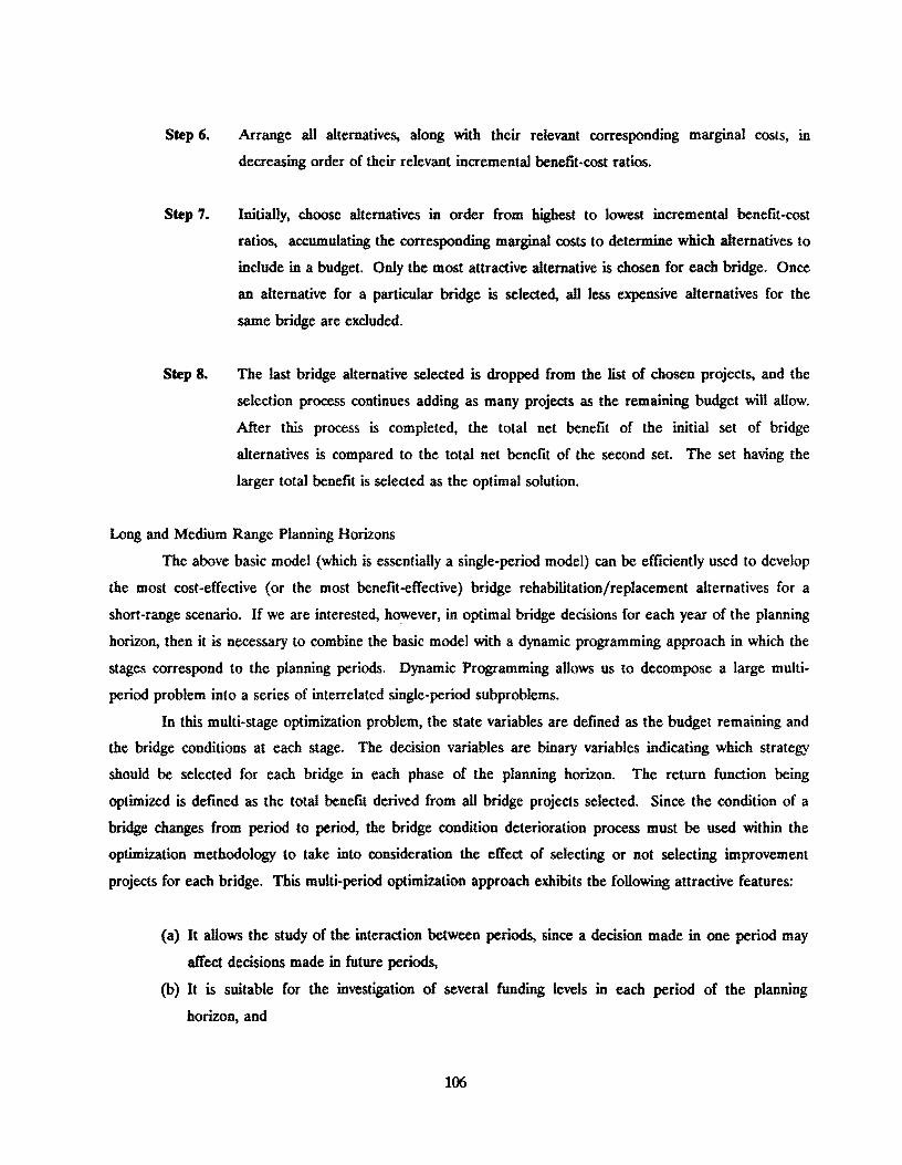
Step 6.

Step 7.

Step 8.

Arrange all alternatives, along with their relevant corresponding marginal costs, in

decreasing order of their relevant incremental benefit-cost ratios.

Initially, choose alternatives in order from highest to lowest incremental benefit-cost

ratios, accumulating the corresponding marginal costs to determine which alternatives to

include in a budget. Only the most attractive alternative is chosen for each bridge. Once

an alternative for a particular bridge is selected, all less expensive alternatives for the

same bridge are excluded.

The last bridge alternative selected is dropped from the list of chosen projects, and the

selection process continues adding as many projects as the remaining budget will allow.

After this process is completed, the total net benefit of the initial set of bridge

alternatives is compared to the total net benefit of the second set. The set having the

larger total benefit is selected as the optimal solution.

Long and Medium Range Planning Horizons

The above basic model (which is essentially a single-period model) can be efficiently used to develop

the most cost·effective (or the most benefit-effective) bridge rehabilitation/replacement alternatives for a

short-range scenario. If we are interested, however, in optimal bridge decisions for each year of the planning

horizon, then it is necessary to combine the basic model with a dynamic programming approach in which the

stages correspond to the planning periods. Dynamic Programming aUows us to decompose a large multi·

period problem into a series of interrelated single-period subproblems.

In this multi-stage optimization problem, the state variables are defined as the budget remaining and

the bridge conditions at each stage. The decision variables are binary variables indicating which strategy

should be selected for each bridge in each phase of the planning horizon. The return function being

optimized is defined as the total benefit derived from all bridge projects selected. Since the condition of a

bridge changes from period to period, the bridge condition deterioration process must be used within the

optimization methodology to take into consideration the effect of selecting or not selecting improvement

projects for each bridge. This multi-period optimization approach exhibits the following attractive features:

(a) It allows the study of the interaction between periods, since a decision made in one period may

affect decisions made in future periods,

(b) It is suitable for the investigation of several funding levels in each period of the planning

horizon, and

106

(c) It ac:.cepts input from the bridge deterioration process for each intermediate period of the

planning horizon.

The following notation will be used in the formulation of the dynamic programming recursive

relationship for the analysis of a multi-period planning horizon:

~ = amount available at the beginning of period t,

~ = set of projects to choose from in period t.

b(~) = total benefit for period t,

c(~) = total cost for period t,

Ile = bridge conditions at the beginning of period t, and

PI = set of feasible projects for period t, P, = d(Ile).

Using the above notation, the subproblem for period t can be formulated as follows:

• First Period (t=l)

gl(AI ) = maximize bl(Xl )

Subject to

• Subsequent Periods (t=2, •••• T)

&(B,) = maximize {fl(~) + &-l(~ + C(X·I_l)}

o <A,.s.B,

where X·I _l indicates the most benefit-effective decision at period t-l, and

~(~) = maximize b(~)

subject to

In the above formulation. f(~) can be determined in one pass of the INCBEN algorithm for all

desirable values of ~.

107

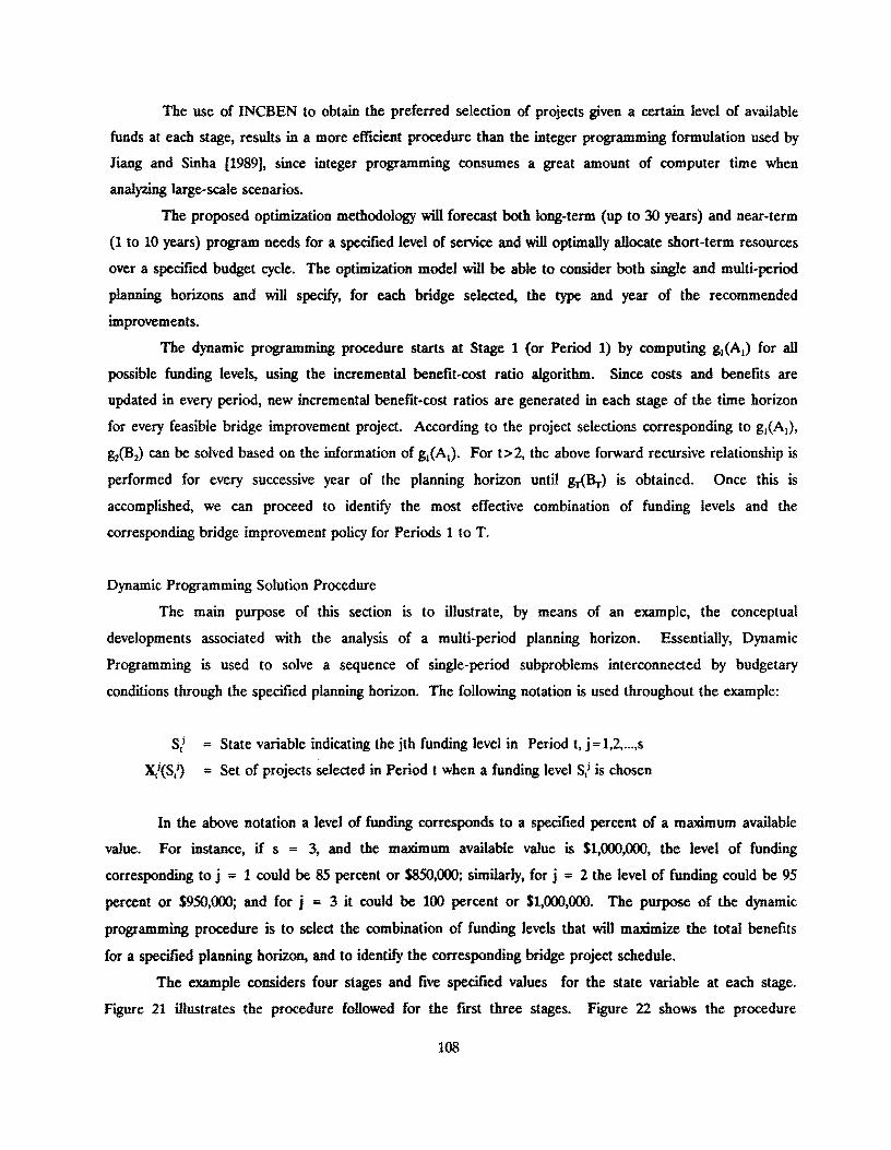
The use of INCBEN to obtain the preferred selection of projects given a certain level of available

funds at each stage, results in a more efficient procedure than the integer programming formulation used by

Jiang and Sinha [19891, since integer programming consumes a great amount of computer time when

analyzing large-scale scenarios.

The proposed optimization methodology will forecast both long-term (up to 30 years) and near-term

(1 to 10 years) program needs for a specified level of service and will optimally allocate short-term resources

over a specified budget cycle. The optimization model will be able to consider both single and multi-period

planning horizons and will specify, for each bridge selected, the type and year of the recommended

improvements.

The dynamic programming procedure starts at Stage 1 (or Period 1) by computing gl(AI ) for all

possible funding levels, using the incremental benefit-cost ratio algorithm. Since costs and benefits are

updated in every period, new incremental benefit-cost ratios are generated in each stage of the time horizon

for every feasible bridge improvement project. According to the project selections corresponding to gj(Al ),

g2(B2) can be solved based on the information of gl(Al ). For t > 2, the above forward recursive relationship is

performed for every successive year of the planning horizon until g"(Br) is obtained. Once this is

accomplished, we can proceed to identify the most effective combination of funding levels and the

corresponding bridge improvement policy for Periods 1 to T.

Dynamic Programming Solution Procedure

The main purpose of this section is to illustrate, by means of an example, the conceptual

developments associated with the analysis of a multi-period planning horizon. Essentially, Dynamic

Programming is used to solve a sequence of single-period subproblems interconnected by budgetary

conditions through the specified planning horizon. The following notation is used throughout the example:

S(i = State variable indicating the jlh funding level in Period t, j = 1,2, ... ,s

X/(Sli) = Set of projects selected in Period t when a funding level Sli is chosen

In the above notation a level of funding corresponds to a specified percent of a maximum available

value. For instance, if s = 3, and the maximum available value is $1,000,000, the level of funding

corresponding to j = 1 could be 85 percent or $850,000; similarly, for j = 2 the level of funding could be 95

percent or $950,000; and for j = 3 it could be 100 percent or $1,000,000. The purpose of the dynamic

programming procedure is to select the combination of funding levels that will maximize the total benefits

for a specified planning horizon, and to identify the corresponding bridge project schedule.

The example considers four stages and five specified values for the state variable at each stage.

Figure 21 illustrates the procedure followed for the fust three stages. Figure 22 shows the procedure

108

followed for the last stage, that is, Stage 4. Each project set ~i selected in Period t, under the jth G = 1,2, ... ,s)

funding level, is associated with a number indicating the rank in magnitude (that is, the number 1,2,3,4 or 5)

of the funding level selected in the precedini perio(i. This selection number for each stage can be organized

into a vector which will be referred to as the "Summary Vector".

The procedure starts at Stage 1 where a set of projects is selected for each of the five different

values of the state variable, in such a way that the benefit is maximized. Assume that for state value SII, the

set of projects XII was chosen. Similarly, for state value S12, the set of projects XI2 was chosen, and so on.

Each of these selected projects has its corresponding cost and benefit.

As indicated in Figure 21, the preferred selections are organized into a summary vector containing

numbers 1,2, ... ,5. These numbers are shown in the last column of the decision table. In subsequent stages a

similar analysis is repeated.

In Stage 2, a set of projects is also selected for each one of the five different values of the state

variable, in such a way that the combined benefit from Period 1 and Period 2 is maximized. In this case, the

Xi sets are selected considering all possible choices for XI It (k = 1, .. .5) in the preceding stage. Of all the five

different sets Xi selected for each value of S2i G = 1, .. .5) the one that yields the maximum benefit is chosen as

the best selection of projects, and the corresponding value of the index k is stored in the summary vector.

To facilitate the discussion of Stage 2, the summary vector of the preceding stage is placed across

the top of the decision table, as shown in Figure 21. The row corresponding to the first funding level in the

decision table for Stage 2 indicates that the best selection of projects for the state value S21 is that

corresponding to k = 2. The procedure is repeated for the remaining values of Si as well, and the results

are stored in the summary vector. As illustrated, the summary vector for Stage 2 contains selection numbers

k = 2, 3, 5, 1, and 1.

The first value k = 2 indicates that the selection of projects X21(S/) in Period 2 corresponds to a

funding level Silt = S/ in Period 1. Similarly, from the second entry k = 3 in the summary vector, we can

determine that the selection of projects X/(S/) corresponds to a funding level S/ in Period 1, and so on.

In the analysis of the following stages, and based on the principle of optimality of dynamic

programming, the procedure considers for each funding level only the solutions corresponding to the

summary vector of the previous stage. After considering these solutions, the one maximizing total combined

benefits is selected. The methodology described above is then applied to the current stage and a new

summary vector is obtained. ragure 21 shows that the summary vector for Stage 3 contains the selection

numbers k = 1,4,5, 1, and 2. This means that the selection of projects X31(S31) in Period 3 corresponds to a

funding level S21 in Period 2. Similarly, the selection of projects X32(S/) that yields maximum benefit is

obtained with S24, The same discussion applies to the remaining values of S3i .

As shown in Figure 22 for this example, in Stage 4 only the value of S/ is considered, assuming that

all the available budget must be spent at the end of the planning horizon. Thus, state values S41, S/, S/, and

109

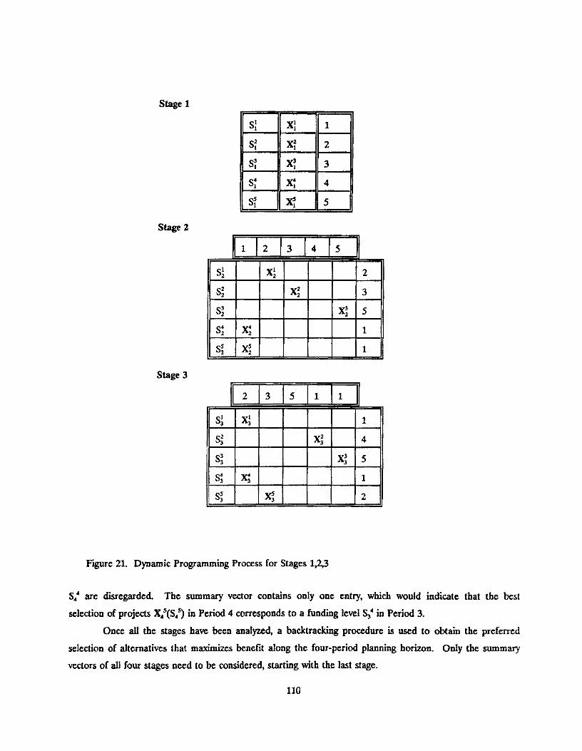
Stagel

S! Xl I 1

Sf Xi 2

S~ X3 1 3

51 Xi 4

S~ X1 5

Stage 1

II 1 12 13 I 4 15 II

I Si Xl 2: 2

S2 2 X2

2 3

S3 2 X3

2 5 Si Xi 1

si Xi 1

Stage 3

1\ 2 3 5 1 II

SI 3 Xj 1

S2 3 X2

3 4

~ X3 3 5

S; X; 1

S; Xi 2

FJgUl'e 21. Dynamic Programming Process for Stages 1,2,3

S44 are disregarded. The summary vector contains only one entry, which would indicate that the best

selection of projects X/(S/) in Period 4 corresponds to a funding level ~ 4 in Period 3.

Once all the stages have been analyzed, a backtracking procedure is used to obtain the preferred

selection of alternatives that maximizes benefit along the four-period planning horizon. Only the summary

vectors of all four stages need to be considered, starting with the last stage.

110

Stage 4

1 4 15 11 I 2 I S!

S;

S;

s: S! X! 4

rlgUre 22. Dynamic Programming Process for Stage 4

Since the best selection of projects in Stage 4, X/(S"s), was computed from state value S34 of Stage

3, X34(S;') is chosen as the best selection of projects for Stage 3. Since X,l"(S34) was selected for a state value

S21 in Stage 2, X/(S21) is chosen as the best selection of projects for Stage 2. rmally, since X/(S21) was

selected for a state value S12 in Stage 1, X/(S/) is chosen as the best selection of projects for Stage 1. In

summary, the preferred selection of alternatives that yields the maximum benefit on a time horizon of four

periods, given five possible values for the state variable is the following:

In Stage 1 select projects X12(SI2)

In Stage 2 select projects X21(S21)

In Stage 3 select projects X34(S3")

In Stage 4 select projects X/(S/)

Computational Requirements

A. Sin&1e-Period Plannin& Horizons

As part of this study, the feasibility of utilizing INCBEN and/or INTPROG for the optimization of

bridge-improvement alternatives for single-period problems involving both constrained and unconstrained

budgets was investigated. The objective of this effort was to determine the suitability of these programs for

implementation within a comprehensive BMS for Texas which is capable of handling a large number of

bridges at the district level. Both programs were used successfully with hypothetical bridge data to identify

an optimal set of bridge-improvement alternatives for up to 5,000 bridges with up to seven alternatives each.

A comparison of the optimality of the solutions was accomplished, as well as a comparison of the

computation time and hardware requirements for the two methods. It appears that the incremental benefit­

cost and integer programming models both offer distinct advantages for application within a BMS. For all

111

practical purposes, the accuracy of the solution sets were essentially identical for the data sets and budget

constraints used in the investigation. This is illustrated in an example with 1,000 bridges as shown in

rIgW'e 23. It should be noted, however, that although INTPROG guarantees an optimal solution, such is not

the case for INCBEN. INCBEN will always select the optimal set of alternatives under an unlimited budget,

but the solution may be sub-optimal for certain cases under a constrained budget.

9

r--. 8 ~

s::: 0 7 .,-j

...-1

...-1 1000 Bridges

.,-j

:c: '-' INCBEN • (f) .....,

INTPROG .,-j 5 + ...... OJ s::: OJ

a:l

1 2 Budget (Mllllon $)

3

Figure 23. Comparison of INCBEN and INTPROG for 1000 Bridges

Although the programs produce nearly identical results, there are distinct time differences between

the two programs. As shown in Figure 24, the INCBEN program runs considerably faster than INTPROG,

especially for large data sets. In fact, for certain data sets, INCBEN ran up to two times faster than

INTPROG. The run-time differential between the two programs is further illustrated in Figure 25.

On the other hand, although INCBEN runs faster, it requires 1.5 times the memory storage capacity

of INTPROG. While this fact may be inconsequential for operation of the programs on a mainframe

computer, it is a significant factor when considering implementation in a micro-computer environment.

Under the DOS operating system, INTPROG can analyze up to 1,000 bridges with seven alternatives each,

whereas INCBEN can only handle approximately 500 bridges with the same number of alternatives. Since

some of the larger districts have up to 2,000 on-system bridges, use of these programs in their current forms

may not be practical under a DOS environment.

A micro-computer with an 80386 processor operating under the OS/2 operating system can provide

increased speed and memory capacity. Unlike the DOS operating system, OS/2 is not limited to 640

kilobytes of RAM and a 20 megahertz machine with an 80386 processor runs approximately 4.5 times as fast

112

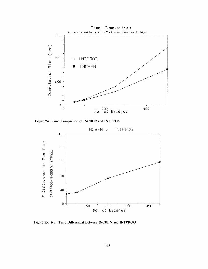
Time Compar-ison for optimization with 1-7 alternatives per bridge

300 ~---------------------------------------------,

"""' u Q) (/\

'--'

Q) 200 + INTPROG a

• INCBEN .::: 0

,.-; ..., co 100 ..., ;::5

o +---------r--------,--------,---------,-------~ o 200 400

No of Bridges

Figure 24. Time Comparison of INCBEN and INTPROG

INCBEN v INTP 100 ,---------------------------------------------,

Q)

9 . .-1 80 8

8 s:: cr ;::5 n. p;:: I-

Z 60 s:: ,.-;

Q)

u s:: 40 OJ >-< I Q) Q ..... 0

I4-l a: ,.-I n. 20 Q I-

Z

~ u

0 50 150 250 3 0 450

No. of Bridges

FtgUre 25. Run Time Differential Between INCBEN and INTPROG

113

as an 80286 based AT computer. Shown in Figure 26 is an example using INTPROG to analyze up to 5,000

bridges using a PS/2 Model 70 computer running under the OS/2 operating system. As evident from this

figure, this environment can handle a sufficient number of bridges to accommodate any district in the state of

Texas.

s::: ..... s

ill S ..... Eo-

s::: 0 ...... .., <t) .., :;:I p... s 0 u ill tTl <t) l-I Q.)

> <:

90

80

70

60

50

40

30

20

10

0 0

INTPROG Run Time using PS/2 Hodel 70 Computer

1000 2000 3000 No. of Bndges

Figure 26. INTPROG Analysis for up to 5000 Bridges

B. Multi-Period Planning Horizons

4000 5000

The fundamental purpose of this section is to explore the computational requirements of the

proposed optimization model when used to investigate a planning horizon consisting of mUltiple periods. In

this section, we first show microcomputer time requirements when the model is used under small-scale and

middle-scale scenarios. After this is accomplished, we present a summary of the results obtained when

running the model for five different funding levels per period on large-scale scenarios using a VAX 8650

mainframe computer.

The following comparison considers a five-period analysis and five different funding levels per period

in each run of the program. Three small-scale scenarios including 40, 80 and 160 bridges were first

considered. The corresponding run times for these scenarios were 8, 25 and 89 seconds, respectively. Two

middle-scale scenarios including 320 and 450 bridges, were considered next. The run times were 5.67

minutes, and 11.1 minutes, respectively. F"mally, a large-scale application with 999 bridges was tried, and the

corresponding run time was equal to 51.52 minutes. As illustrated in Figure 27, the computer running time

increases exponentially, as the number of bridges is increased. For this reason, scenarios including more

114

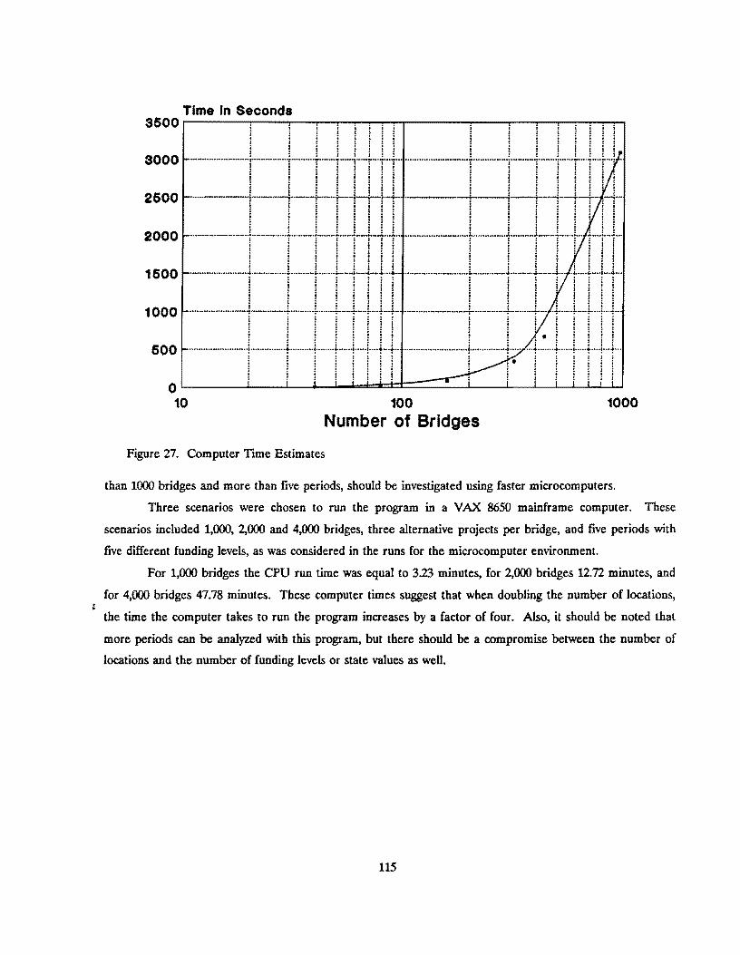
3000

2600

2000

1600

1000

600

100 1000 Number of Bridges

Figure 27. Computer Time Estimates

than 1000 bridges and more than five periods, should be investigated using faster microcomputers.

Three scenarios were chosen to run the program in a VAX 8650 mainframe computer. These

scenarios included 1,000, 2,000 and 4,000 bridges, three alternative projects per bridge, and five periods with

five different funding levels, as was considered in the runs for the microcomputer environment.

For 1,000 bridges the CPU run time was equal to 3.23 minutes, for 2,000 bridges 12.72 minutes, and

for 4,000 bridges 47.78 minutes. These computer times suggest that when doubling the number of locations,

the time the computer takes to run the program increases by a factor of four. Also, it should be noted that

more periods can be analyzed with this program, but there should be a compromise between the number of

locations and the number of funding levels or state values as well.

115

116

CONCLUSIONS

The following conclusions are offered:

1. A comprehensive bridge management system for Texas is feasible. The bridge management

system developed and used in North Carolina is the best evidence for this observation and the

best existing model for such a system. The NCDOT system has been implemented with reported

success, although perhaps not enough experience has been acquired to pass final judgment. This

system uses limited bridge condition data and simple but workable models to produce suggested

specific bridge management strategi:'" Much of this procedure could be adapted to Texas' needs.

Other evidence of the feasibility is the Bridge Needs and Investment Process (BNIP), developed

by FHW A, which uses similar bridge condition data and models. The BNIP is not a BMS

according to the definition of a BMS followed in this report, but is more accurately described as a

bridge information management system. The BNIP does however use much of the same logic and

data needed by a comprehensive BMS to predict deterioration of structures and life-cycle costs of

management alternatives. While the BNIP has not been formally implemented by any state DOT,

it has been field-tested by several states, and appears to have promise. The bridge management

system outlined in NCHRP 300, and that used by Pennsylvania DOT utilize more detailed

condition data than do the earlier mentioned systems. Pennsylvania's system primarily manages

data, rather than providing recommended bridge management actions. Additional cost and

complication is associated with the use of more detailed data, and it remains to be determined

whether the benefits of a more detailed system justify the additional complexity.

2. To be most useful, a bridge management system for Texas should be implemented at district level.

Different management philosophies, climates, traffic densities, etc., result in bridge management

needs which vary to some extent regionally across the state. The decentralized nature of Texas'

bridge management practices at present, along with the fact that some of Texas' districts are as

large as some states, further justifies this recommendation.

3. Bridge management decisions should be made with due consideration of life-cycle cost analyses.

and by comparison of the costs and benefits of proposed alternatives, rather than being based on

empirical measures of need, such as the sufficiency rating in the question of rehabilitation or

replacement. Optimization techniques should be employed to guarantee most cost-effective

solutions. It is recognized that the present ranking procedures used by FHW A to determine

eligibility and relative need is based on the SR, but numerous weaknesses in this ranking system

are perceived by SDHPT district personnel. It is anticipated that as bridge management systems

117

become more widely used by the various states, the present system of ranking projects will be

changed to reflect the use of bridge management decision aids based more closely on engineering

economics.

4. Preventive and routine maintenance efforts should be included in bridge management activities

included in a bridge management system, since levels of maintenance affects the other bridge

management activities. A comprehensive system should encompass all such bridge management

activities in order to accurately consider trade-offs among the various activities.

5. A determination of the level of complexity or the level of detail associated with the data used by

the BMS, which would be most useful to the SDHPT, cannot be satisfactorily accomplished

without actually implementing, at least in a rudimentary form, the basic models and logic

available.

118

RECOMMENDED FURTHER WORK

Development and implementation of a comprehensive bridge management system, for primary

application at the district level, is recommended. Recommended major components of the BMS include the

following submodels:

1. The Level-or-Service Submodel is useful for determining needs and improvement priorities.

Present priorities for rehabilitation and replacement are established by the TEBSS process, which

incorporates a form of level~of~service criteria. A similar level of service for maintenance has

been developed by NCSU and is discussed by Nash and Johnston [1985].

2. The Feasible Improvements Submodel, designed to generate the list of alternatives for

maintenance, rehabilitation, or replacement. This relies on the judgment of experts such a bridge

engineers.

3. The Deterioration Submodel. As the previous discussion in the Workplan indicated, there are

several procedures which have been developed, most of which are linear models. This part of the

problem is very fundamental to developing a BMS. The recently proposed nonlinear model

described by West [1989] can be adapted to reflect the regional variations in deterioration in

bridges in Texas. Most of the deterioration models do not consider the scientific use of expert

opinion, which may be important in supplementing inadequate data.

4. The Agency Cost Submodel consists of unit costs of work items, which can be developed in a

work breakdown structure analogous to the work items in the BRINSAP file. Such a proposed

work hierarchy is necessary to develop a life~cyde cost database. Such a work breakdown

structure (WBS) should be used in all operations: engineering, new construction or replacement,

inspection, reporting, maintenance, and limited rehabilitation. At this stage, it is not known

whether such a WBS is feasible for districts; part of the continuation study would investigate the

use of such a WBS in case studies. Information on bridge costs must be gathered from various

databases; consequently, the ability to use these sources is a major requirement of future studies.

5. The User Cost Submodel can be used to determine the user benefits or savings in user costs for a

preselected range of feasible improvements. The types of user benefits to be considered are

savings in accident costs, savings in vehicle operating costs, and savings in travel time. As in the

119

case of agency costs, the collection of these costs in a statewide or district database is a difficult

task, and sometimes this task must be supplemented with expert opinion.

6. The Optimization Submodel. Various algorithms are being tested in computer simulations, as

discussed earlier. In order to proceed with the development of a bridge management system,

these models should use some actual data for comparison purposes. Recommended work

alternatives, e.g., tbose derived under INCBEN or INTPROG, should be compared with choices

arrived at using the Sufficiency Rating, TEBSS, or other selection procedures.

120

REFERENCES

Al-Subhi, K., D. Johnston, and F. Farid (1989). "Optimizing System-Level Bridge Maintenance,

Rehabilitation, and Replacement Decisions: Executive Summary," Report No. FHWA/NC/89-OO2, Federal

Highway Administration, Washington, DC

Babae~ K. (1988). "Development of a Bridge Deck Management System for Washington State Department

of Transportation," F'mal Report on Contract Y 3399, Task 19, Washington State Transportation Center

(TRAC), University of Washington, Olympia, WA 98195.76 pp.

Banks, R. K. (1988). "Bridge Inspection and Apportionment of Federal Funds," Presentation to the FHWA

Fort Worth Remon Bridge Conference, Texas State Department of Highways and Public Transportation,

Austin, TX.

Berger, R. H., T. Byrd, MacDonald, L. S. Gordon (1978). "Extending the Service Life of Existing Bridges,"

Bridge Engineering Vol I, Transportation Research Record 664, Transportation Research Board,

Washington DC, Sept.

Bhat, N. U. (1984). Elements of Applied Stochastic Process 2nd ed., John Wiley and Sons, Inc., NY

Boyce, C, W. R. Hudson, and N. H. Burns (1987). "Improvements in On-System Bridge Project

Prioritization", Report CTR 3-5-86-439-1, Center for Transportation Research, The University of Texas,

Austin. TX.

Bridge Management Work Group (1987). "The Pennsylvania Bridge Management System; Report No.

FHWA-PA86-036+ 84-28A, Bureau of Bridge and Roadway Technology, Pennsylvania Department of

Transportation, Harrisburg, P A.

Brinkman, C, and K. Mak (1986). "Accident Analysis of Highway Narrow Bridge Sites," Public Roads,

49(4), Federal Highway Administration, Washington, DC, pp 127-133.

Busa, G., M. Cassella, S. Gazda, and R. Hom (1985a). "A National Bridge Deterioration Model,"

Transportation Systems Center (SS-42-o5-26), U.S. Department of Transportation, Cambridge, MA.

121

Busa, G., M. Ben-Akhiva, and O. Buyukoztuk (1985b). "Modelling Concrete Deck Deterioration,"

Department of Civil Engineering, Massachusetts Institute of Technology, Cambridge, MA.

California Department of Transportation (CALTRANS) (1989). "Network Optimization Model for Bridge

Management Systems,« Request for Pro.posa1s RF 89=017. RFf DOT -8044, Sacramento, CA.

Chen, C., and D. W. Johnston (1987). "Bridge Management Under A Level-of-Service Concept Providing

Optimum Improvement Action, Time, and Budget Prediction," Center for Transportation Engineering

Studies, North Carolina State University, Raleigh, NC.

Consortium of Civil Engineering Departments of New York City (1990). "Preventive Maintenance

Management System for New York City Bridges," Technical Report No 90-1. New York City DOT Bureau of

Bridges.

Farid, F., D. W. Johnston, C. Chen, M. A. Laverde, and B. S. Riham, (1988a). "Feasibility of Incremental

Benefit-Cost Analysis for Optimal Allocation of Limited Budgets to Maintenance, Rehabilitation and

Replacement of Bridges," Report No. FHWA-DP-71-02, Federal Highway Administration, Washington, DC.

Farid, F., etal. (1988b). "Feasibility of Incremental Benefit-Cost Analysis for Optimal Allocation of Limited

Budgets to Maintenance, Rehabilitation, and Replacement of Bridges NC-07," Report No. FHWA-DP-71-02,

Center for Transportation Engineering Studies, North Carolina State University, Raleigh, NC.

Federal Highway Administration (FHWA), (1986). "Highway Performance Monitoring System, Volume II:

Technical Manual,· Washington, DC.

Federal Highway Administration (FHWA), (1987). "Bridge Management Systems,· Report No. FHWA DP-

71-01, Washington, DC.

Federal Highway Administration (FHWA), (1988a). "State Bridge Program Management; Special Study

Required by Section 162 of P.L. 100-17 STURM of 1987. Washington, DC.

Federal Highway Administration (FHWA). (l988b). "Recording and Coding Guide for the Structure

Inventory and Appraisal of the Nation's Bridges," Report No. FHWA-ED-89-044, Washington, DC.

122

Federal Highway Administration (FHWA), (1989). "Bridge Needs and Investment Process; Executive

Summary, Version 1.2, U.S. Department of Transportation, Federal Highway Administration, Office of

Planning, Planning analysis Division, Highway Performance Analysis Branch, Washington, DC.

Federal Highway Administration (FHWA), (1990a). "Bridge Management System," (Draft legislative

proposal furnished to state highway departments), Washington DC.

Federal Highway Administration (FHWA), (l990b). "Level-of-Service Criteria, Highway Bridge Replacement

and Rehabilitation Program (HBRRP) Apportionment, Memorandum from Director, Office of Structures,

FHWA Fort Worth, TX.

Fitzpatrick, M., D. Law, and W. Dixon (1981). "Deterioration of New York State Highway Structures,"

Bridge and Pavement Maintenance, Transportation Research Record No. 800, Transportation Research

Board, National Research Council, Washington, DC.

Garda-Diaz, A. (1988). "A Model for Estimating Rehabilitation Costs Associated with The Elimination of

Load Zones in the PM System,· Research Report 1132-F, Texas Transportation Institute, Texas A&M

University, College Station, TX, Nov.

Harper et al. (1990a). ·Stochastic Optimization Subsystem of a Network Level Bridge Management System",

Selected Papers Related to Bridae Manasement, presented at the 1990 Transportation Research Board

Annual Meeting, Paper 890280, Washington, DC.

Harper, W. V., A. al-Salloum, S. al-Sayyari, S. al Theneyan, J. Lam, and C. Helm, (l990b) ·Selection of Ideal

Maintenance Strategies in a Network Level Bridge Management System,· Presented at the Annual Meeting

of the Transportation Research Board, Washington, DC.

Hudson, et al., (1987). "Bridge Management Systems,· National CoQperative HiShwilY Research PrQ&t'am

Report 300, Transportation Research Board, Washington DC.

Hyman, W., D. Hughes, and T. Dobson (1983). "The Least Cost Mix of Bridge Replacement and Repair

Work on Wisconsin's State Highways Over Time - A Computer Simulation," Draft Technical Report,

Wisconsin Department of Transportation, Madison, WI.

123

Jiang, Y., and K. C. Sinha (1989). "A Dynamic Optimization Model for Bridge Management Systems;

Transportation Research Board, Paper No. 88--0409, 68th Annual Meeting, Washington, DC.

Jorgenson, R., and Assoc. and Westat Research Analysis (1966). "Evaluation of Criteria for Safety

Improvements on Highways," Report No. PB-I73-822, Gaithersburg, MD.

Kayser, J. R., and A. S. Nowak (1989). "Capacity Loss due to Corrosion in Steel-Girder Bridges,' Journal of

Structural Engineering, American Society of Civil Engineers, 115(6), pp. 1525-1537.

KruegJer, J., G. Briggs, and C. McMullen (1986). ·Cost-Effective Bridge Maintenance Strategies; Vol. 1,

Executive Summary, Report No. FHW A/RD-86/109, Final Report, Federal Highway Administration

(FHW A), McLean, VA.

McFarland, W. F., et al., (1979). "Assessment of Techniques for Cost Effectiveness of Highway Accident

Countermeasures; Report FHWA/RD-79/53, Federal Highway Administration, Washington, DC.

McFarland, W. F., J. B. Rollins, and R. Dheri (1983a). "Documentation for Incremental Benefit-Cost

Technique," Technical Report prepared for Federal Highway Administration, Texas Transportation Institute,

Texas A&M University, College Station, TX.

McFarland, W. F., J. B. Rollins, and F. Harris (1983b). "Documentation for Integer Programming

Technique," Technical Report prepared for Federal Highway Administration, Texas Transportation Institute,

Texas A&M University, College Station, TX.

McFarland, W.F., and J. B. Rollins (1985). "Cost-Effectiveness Techniques for Highway Safety: Resource

Allocation," Report FHWA/RD-84/011, Federal Highway Administration, Washington, DC.

McFarland, W. F., and M. K. Chui (1987). "The Value of Travel Time: New Estimates Developed Using a

Speed-Choice Mode~" Transportation Researdl Record No. 1116, Transportation Research Board,

Washington, DC.

Nash, S. C., and D. W. Johnston (1985). "Level-of-Service Analysis for Bridge Maintenance Activities in

North Carolina, Center for Transportation Engineering Studies: North Carolina State University, Raleigh,

NC.

124

Nauss, R. M. (1978). "The 0-1 Knapsack Problem with Mu1tiple Choice Constraints,~ European Journal of

Operational Resean:b.

O'Connor, D. S., and J. Wentworth, (1989). Personal Communications with Bridge Management Branch

Personnel. Federal Highway Administration, Washington, DC.

Pritsker, A. A. (1986). Introduction to Simulation and SlAMII 3rd ed., John Wiley and Sons, Inc., NY.

Saito, M., and C. Sinha (1987). "Review of Current Practices of Bridge Management at the State Level."

Transportation Resean:b Record No. 1113, Transportation Research Board, Washington, DC.

Saito, M., and K. C. Sinha (1990). "Timing for Bridge Replacement, Rehabilitation, and Maintenance,"

Selected Papers Related to Brid&e Mana&ement, presented at the 1990 Transportation Research Board

Annual Meeting, Paper 890366, Washington, DC.

Sinha, K.C., et al, (1989). "The Development of Optimal strategies for Maintenance, Rehabilitation, and

Replacement of Highway Bridges," Final Report. The Elements of Indiana Brid&e Mana/iement System

(IBMS). FHWA/IN/JHRP-88/15, Purdue University, IN.

Texas State Department of Highways and Public Transportation (SDHPT), (1984). "Bridge Inventory,

Inspection, and Appraisal (BRINSAP) - Manual of Procedures," Austin, TX.

Texas State Department of Highways and Public Transportation (SDHPT), (1986). "10~Year Project

Development PIan," Rept. No. D-8PS-1,2a, and 3-9-86, Austin, TX.

Texas State Department of Highways and Public Transportation (SDHPT), (1988a). "Maintenance

Management Information System (MMIS): Safety and Maintenance Division, Austin, TX,

Texas State Department of Highways and Public Transportation (SDHPT), (l988b). "Routine Maintenance

Specifications," Safety and Maintenance Division, Austin, TX.

Texas State Department of Highways and Public Transportation (SDHPT), (1989). "Strategic Mobility Plan -

Identifying Transportation Requirements 1990-2009," Austin, TX.

125

Thomas, J. J., and J. J. DiFabio (1988). "A Bridge Maintenance Strategy to Greatly Reduce Bridge Capital

Expenditures." New York State Department of Transportation, Albany, Paper presented at the 74th Annual

Meeting of AASHTO, Wichita, KS.

U.S. Congress, 101st Congress. 1st Session, Committee on Public Works and Transportation (1989). "The

Status of the Nation's Highways and Bridges: Conditions and Performance and Highway Bridge Replacement

and Rehabilitation Program," Report of the Secretary of Transportation to the Congress of the United

States. U.S. Govt Printing Office, Committee Print 101-2, Washington, DC.

Van Horn, D. A. (1987). "Commentary on the Pennsylvania Bridge Management System,· Report No.

FHWA/pA-87..Q05+84-28A, Federal Highway Administration, Washington, DC.

West, H. H., et al, (1989a). "A Nonlinear Deterioration Model for the Estimation of Bridge Design Life,"

Report No. FHWA-PA-89-016-86-07, The Pennsylvania Transportation Institute, University Park, PA.

West, H. H., R. M. McClure, E. J. Gannon, H. L. Riad, and B. E. Siverling (1989b). "A Nonlinear

Deterioration Model for the Estimation of Bridge Design Life," Report No. 86-07, Pennsylvania

Transportation Institute, The Pennsylvania State University, University Park, PA.

Zimmermann, H. J., L. A. Zadeh, and B. R. Gaines, Editors (1984). FU27Y Sets and Decision Analysis.

TIMS/Studies in Management Sciences, Elsevier Science Publishers. B.V. North Holland.

Zuk, W. (1987). "Expert Systems as Applied to Bridges--Knowledge Acquisition Phase," Report No. VTRC

88-R6, Virginia Transportation Research Council, Charlottesville, NC.

126

APPENDIX A. BRIDGE MAINTENANCE CASE STUDY

127

A CASE STUDY ON BRIDGE MAINTENANCE (Texas SDHPT District 4, Amarillo)

Introduction

The main objective of this case study was to visit one of the Texas SDHPT districts, to determine if

there is any formal bridge preventive maintenance program in the district, and if so, review this program.

The specific objectives included the following:

1. Determine the most predominantly applied bridge maintenance activities (techniques) 10 the

district. Obtain a detailed description of the procedures of these activities.

2. Inquire on the district's experience with the maintenance activities: why were the activities

applied? to correct which defects? were they effective techniques?

3. Inspect some identified bridges where these maintenance activities have been applied or not

applied.

4. Study the performance of the identified bridges with respect to time.

5. Obtain estimates of cost and frequency of application of the bridge preventive maintenance

activities.

The Texas SDHPT District 4 in Amarillo was visited on July 18, 1990, and a small-scale case study

was conducted with the assistance of the following people: Don Shipman, the district maintenance engineer;

Martin Rodin, a supervising bridge engineer; and James Ford, the district's BRINSAP coordinator.

The District's Bridge Preventive Maintenance Program

As an offshoot of the SDHPT's old Safety and Betterment Program for maintenance of the highway

system (highway pavements and bridges), a new program - the Preventive Maintenance Program - has

recently been provided by the SDHPT's headquarters office in Austin. The work is accomplished by contract

and the program includes bridge maintenance work and highway pavement maintenance work such as seal

coating, light surface overlays, etc. Two years ago, District 4 started a separate program specifically for

bridge maintenance work, the Bridge Preventive Maintenance Program. In each of these two years,

preventive maintenance work has been done on 10 percent of all the bridges on the district's network,

concentrating on three major work items: clean and seal joints; concrete repairs; and painting of steel

128

superstructures, railings, bearings, etc. All the bridge preventive maintenance work on this program has been

done by contract, under the Contract Preventive Maintenance (CPM) scheme using a discretionary fund

because the money could have been used for maintenance of highway pavements.

Predominant Bridge Maintenance Activities

The following bridge maintenance work items were identified as the most predominantly applied

activities:

1. Bridge deck maintenance - surface treatment, cleaning, and removal of debris.

2. Clean and seal joints.

3. Concrete repairs

4. Seal riprap.

5. Header bank repairs.

6. Repair bearings - adjust steel shoes, replace lead sheets.

7. Paint steel superstructures, railings, bearings, etc.

District's Experience with the Bridge Maintenance Activities

1. Brid/:e deck maintenance - surface treatment. c1eanin/:. and removal of debris: Due to the

geographical location of this district (North Texas panhandle), there is seasonal accumulation of ice on the

bridge decks, and the application of deicing agents containing chloride. It has been observed that the

presence of chloride in the deck's concrete cover and its eventual penetration to the top rebar in the concrete

results in various serious defects such as delamination, break in bonding, cracks, corrosion in the rebars, etc.

In response, the district's most preferred preventive maintenance technique to protect the bridge concrete

decks is a partial-depth overlay (about 2ft dense concrete) on deck surfaces to protect the deck and its top

rebars from the defects mentioned earlier.

The first step taken in the preventive maintenance effort is core drilling on bridge concrete decks.

The cores are then tested for their chloride content - usually observed to be about 2ft - 3" deep penetration of

chloride. If a significant amount of chloride is present, then about 1" is milled off the deck surface, before a

2" dense concrete overlay is applied. The effectiveness of this techniqu~nnot be ascertained yet because it

has just been recently applied; more years ahead are needed to observe and monitor the performance of the

bridge. So far, from day-to-day experience with using the bridge, the technique seems to be effective. In

addition to testing for the chloride content, the core drilled from the deck is also tested for its compressive

strength to determine the need for any other preventive maintenance or rehabilitation work.

Linseed oil treatment on the bridge concrete deck surface is discouraged in this district; it has not

been done in the last 15 years, due to concern that this technique tends to make the deck surface slick.

129

Other alternative surface treatments used include the Texas Bridge Deck Protection System - a two course

asphaltic surface treatment with an overJay of Hot-Mix Asphaltic Concrete (HMAC) using about 1SO Ibs/sy

of deck surface. Some epoxy sealing of decks is also used. Also recently, as a form of bridge preventive

maintenance, the district has been using epoxy-coated Tebars in the top and bottom mats of their reinforced

concrete bridge decks.

2. Oean and seal joints: There is a problem due to the accumulation of dirt and debris in the

groove opening on Preformed Seal Joints (PSJ). The presence of dirt and silt deactivates the seal

performance, thereby restricting movement in the longitudinal span direction of the bridge deck. If the seal

is not cleaned in time, this has been observed to result in bridge defects such as crushing of superstructure

beam ends and lateral pressure/displacement of abutment walls. During snow clearing operations on the

bridge deck, it has been observed that the snow plows accidentally lift portions of the PSJ up eventually

dislodging the seal and creating an opening for penetration of moisture or brine solution into the vulnerable

superstructure and substructure below. This district would rather have an open expansion joint in their

bridge decks instead of the seals; if the open joints are cleaned regularly, they will be more effective.

Bridges with popped-up seals were observed during a field inspection trip.

Cleaning and sealing of bridge joints as done in the district's recent bridge preventive maintenance

program involves the use of a preformed fiber joint material. According to a recent maintenance contract

specification, the procedures can be described as follows. Joints are first cleaned of all existing materials,

dirt, siltation, aggregates, etc. by a high pressure water and air jet (filtered air) or other methods approved

by the engineer. After cleaning, the fiber joint material is installed in accordance with the details shown in

the construction plans. The work item is measured by the linear foot of cleaned or cleaned and sealed joints.

Also, as part of the recent bridge preventive maintenance program, it was necessary to remove,

furnish and install neoprene seals in existing bridge expansion joints. According to contract specifications,

the installation should be done at about 70°F temperature, with the full range of movement assumed to occur

between O"F and 1ZOOF for concrete structures. The existing steel angle is cleaned of aU remaining weld

material, paint, and rust, with the existing steel extrusion removed and replaced. The seal is then mounted

on existing angles as shown in the construction plans. Neoprene seal replacement is measured by the linear

foot of the size (minimum total movement capacity) shown on the plans, with measurement being along the

centerline of joint at the surface of the roadway and the parapet if required.

3. Concrete Repairs: After bridge inspection and location of unsound concrete members, repairs

of the spalled and chipped areas of concrete are done to remove the unsound concrete materials and replace

them with sound concrete. According to contract specifications, the materials required consist of Portland

concrete and mortar. To repair areas with depth less than r, fme aggregate grade no. 1 will be required for

130

the mortar. Concrete for repair of areas with depths of r or greater will contain grade 1 fme aggregate,

grade 7 coarse aggregate, and a minimum of seven sacks of Portland cement per cubic yard. The concrete

used for repair should have a maximum slump of 3" with a minimum 7-day design flexural strength of 600

PSI.

The concrete repair procedure is started by chipping existing concrete, to remove all loose or

defective concrete. Feather edges are avoided by saw-cutting and/or chipping a perpendicular face along the

periphery of the area to be repaired so that the minimum depth of repair is approximately one-half inch.

The area being prepared is then cleaned by sandblasting, high pressure water, or other means, to remove all

loose particles, dirt, deteriorated concrete or other substances that would impair the bond between the old

concrete and the mortar on the new concrete. Exposed reinforcing steel is cleaned of all old concrete and

corrosion, with the final cleaning being done by high pressure air blast (filtered air). Prior to the application

of new concrete or mortar, the concrete and steel surface is painted with an approved bonding agent. The

concrete or mortar is then placed at a minimum temperature of 62"F. Repaired areas are water cured, and

all repairs are done carefully to avoid voids in the concrete and also to restore the original lines and surfaces

of the structure. Concrete repair is measured on the surface of the repair, by the square foot in place.

4. Seal riprap: This bridge maintenance activity can be described as the placing of Galvanized

metal Flashing and Hot Asphalt-Rubber Sealing on concrete riprap. In this district, it has been observed

that if the construction joint between the concrete riprap and the abutment cap (or header wall) is not

properly sealed - probably due to faulty original construction - water is directed into the soil below the

riprap. Due to the unpredictable soil activities resulting from the presence of water below the riprap -

swelling, cavities, etc.- horizontal cracks and bulges are often observed on the surface of the concrete riprap.

These cavities below the concrete riprap are almost impossible to detect during a routine BRINSAP bridge

inspection; they may be detected late when the cavities are already exposed at the toe walls of the riprap.

Sealing riprap can therefore be classified as a form of bridge preventive maintenance. In addition to sealing

riprap, header bank repairs were usually done in this district to correct already-occurring defects such as the

late stages of the cavities under the riprap. Header bank repairs involves pumping a mixture of pea gravel,

Portland cement and sand to fill the cavity.

In sealing riprap, the sealant material is a blend of rubber and asphalt, suitable for sealing 1/8 inch

or larger width cracks in concrete riprap. According to the contract specifications, the sealant material

should contain no water or highly volatile matter, and it should be capable of being melted and applied by a

suitable oil jacketed kettle equipped with pressure pump, hose and nozzle at a temperature of 400F or less.

Prior to the application of Galvanized Metal Flashing and/or Hot Asphalt-Rubber Sealant, cracks are

cleaned with compressed air to remove all dust, dirt, moisture and foreign material. Sealant material is then

131

applied at a suitable weather condition. Sealing riprap is measured by the linear fool of crack cleaned and

sealed.

5. Header bank repairs; As mentioned in the previous section, when voids are detected beneath

existing concrete riprap covering header banks, the placement of pea gravel concrete in these voids is

referred to as header bank repairs. The material used for filling the voids is a pea gravel concrete mixture of

one part Portland cement, seven parts sand, and six parts gravel. Inspection holes are drilled in the concrete

riprap - holes not more than five inches in diameter or to a size to fit the hose for pumping and to a depth

sufficient to break through the concrete riprap. For small voids - voids less than 15 cubic yards - the

concrete material can be placed in one pour. In larger voids, the backftlling with pea gravel concrete is

performed in three stages. The first two-thirds of the void is ftlled with two consecutive pours. With the

final pour on the last one-third of the void, each hole is pumped with pea gravel concrete until the material

is observed to be flowing from hole to hole. Any water displaced from the void is allowed to flow freely, and

after fiUing the void, all drilled holes, existing cleaned out holes, and construction holes are sealed flush with

the concrete material. The header bank repair is measured by the cubic yard of material in place.

6. R~pair bearin&S - adjust steel shoes. replace lead sheets: It has been observed during past bridge

inspections that some of the bearings on the bridge main superstructure have "frozen" or "locked; that is,

their rocking or sliding movements are now restricted. In the case of steel shoes, the rocking movement

which is to allow for movement along the longitudinal span direction of the bridge, has become restricted

because of the accumulation of dirt, silt, and other foreign materials clogging up the bearing. As for the

bearings with lead sheets, the lead sheets are inserted between two metal shoes for sliding actions induced

due to the such bridge movements allowed by the steel shoes. When the lead sheets wear out, the metal

shoes "freeze" and the sliding movement become restricted. Inability of these bearings to transmit the bridge

longitudinal movements, puts pressure on the abutment walls and approaches, resulting in defects such as

cracks on the concrete members.

Adjusting steel shoes involves the removal of weld between the steel shoes and the girder flange,

jacking up the girder, freeing the shoe pin, adjusting, and repairing the shoe. The shoe is rewelded to the

flange, cleaned, and painted. This work is measured by each steel shoe complete in place.

Removal and replacement of lead sheets between the top and bottom portions of the bridge bearings

is done by first raising all beams simultaneously at the end of a span using a minimum of one jack for each

beam. Existing lead sheets are removed, steel surfaces of the bearings cleaned, and new lead sheets placed

between these surfaces, flush with the sides of the bearings. The beams are then lowered simultaneously.

Replacing lead sheets is measured by each of lead sheets required for the size of bearings.

132

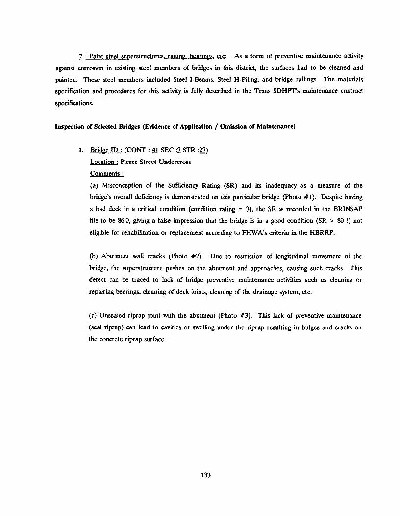
7. Paint steel superstructures. railinK. bearina.s. etc: As a form of preventive maintenance activity

against corrosion in existing steel members of bridges in this district, the surfaces had to be cleaned and

painted. These steel members included Steel I-Beams, Steel H-Piling, and bridge railings. The materials

specification and procedures for this activity is fully described in the Texas SDHPT's maintenance contract

specifications.

Inspection of Selected Bridges (Evidence of Application / Omission of Maintenance)

1. Brida.e ID : (CONT : ~ SEC :1 STR :1:1)

Location j Pierce Street Undercross

Comments:

(a) Misconception of the Sufficiency Rating (SR) and its inadequacy as a measure of the

bridge's overall deficiency is demonstrated on this particular bridge (Photo #1). Despite having

a bad deck in a critical condition (condition rating = 3), the SR is recorded in the BRINSAP

file to be 86.0, giving a false impression that the bridge is in a good condition (SR > 80 !) not

eligible for rehabilitation or replacement according to FHWA's criteria in the HBRRP.

(b) Abutment wall cracks (Photo #2). Due to restriction of longitudinal movement of the

bridge, the superstructure pushes on the abutment and approaches, causing such cracks. This

defect can be traced to lack of bridge preventive maintenance activities such as cleaning or

repairing bearings, cleaning of deck joints, cleaning of the drainage system, etc.

(c) Unsealed riprap joint with the abutment (Photo #3). This lack of preventive maintenance

(seal riprap) can lead to cavities or swelling under the riprap reSUlting in bulges and cracks on

the concrete riprap surface.

133

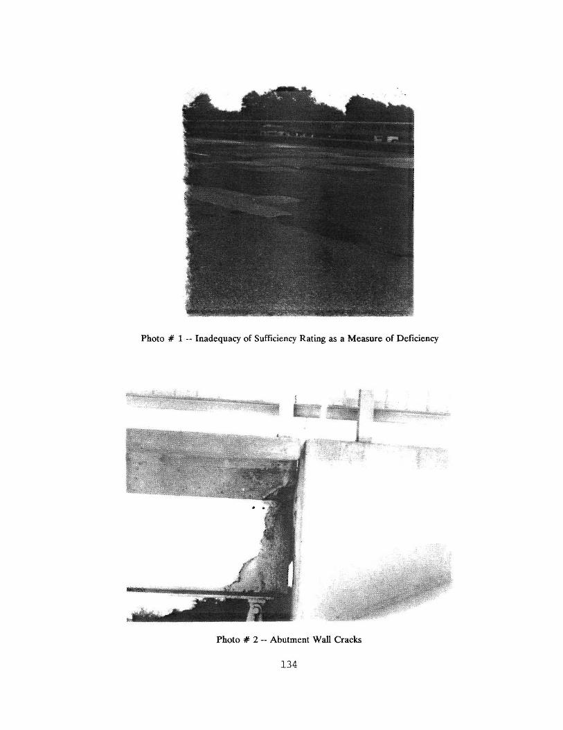
Photo # 1 -- Inadequacy of Sufficiency Rating as a Measure of Deficiency

Photo # 2 -- Abutment Wall Cracks

134

Photo tI 3 -- Unsealed Riprap

2. Bridge ID : (CONT : 90 SEC :§ STR :20) W

(CONT: 2Q SEC:2 STR :21) E

Location: NW 8 in Amarillo (US 66)

Comments: These bridges have epoxy-coated rebars in the top mat reinforcement of the bridge

deck. Photo tl4 (underside of deck) and Photo tiS (roadway surface of deck) show no

significant defects on the deck. This probably demonstrates the effectiveness of using epoxy­

coated rebars in bridge decks as a form of preventive maintenance.

135

Photo # 4 -- Underside of Bridge Deck with Epoxy-coated Rebar

Photo # 5 -- Roadway Surface of Bridge Deck with Epoxy-coated Rebar

136

3. Bridge ID : (CONT : ill SEC :1 STR :~) W

Location: I 40 MP 67.7 (IH 40 West)

Comments: Application of dense concrete overlays (done about six years ago). Photos #6 and

117 show that there is no significant defects on the deck surface, probably demonstrating the

effectiveness of this bridge preventive maintenance activity.

Photo II 6 -- Dense Concrete Overlays on Bridge Deck

137

Photo # 7 -- Dense Concrete Overlays on Bridge Deck

4. Bridge ID: (CONT: 90 SEC :~ STR :~)

Location: I 40 MP 67.7 (Hope Road)

Comments:

(a) Due to unsealed riprap joints (Photo #8), cavities are forming under concrete riprap near

the toe wall as a result of water entering the soil beneath the riprap through these joints. This

demonstrates the effect of not applying a particular preventive maintenance activity - sealing

riprap.

(b) Concrete beam end repair and seal riprap work done by the district's special job crew

(photo #9). The abutment cap was epoxy-coated about two years ago. The beam end material

(mortar?) used in the concrete repair is already flaking off. Also, the presence of vegetation

along the riprap joint indicate passage of water into the soil below the riprap. This might have

led to the cavity shown in Photo #8.

138

Photo # 8 -- Unsealed Riprap (Cavities under Riprap)

Photo # 9 -- Concrete Repair and Sealing Riprap

139

5. Bridge ID: (CO NT : 275 SEC :15 STR :72)

Location: Helium Rd. I 40 MP 63.6

Comments: Sealing riprap with a 6" Galvanized Metal Flashing and an Asphaltic-Rubber sealant

material (Photo #10). No cracks or cavities were observed on the riprap, probably

demonstrating the effectiveness of sealing riprap as a form of bridge preventive maintenance.

Photo II 10 -- Sealing Riprap

140

6. Brid~e ID: (CONT: 275 SEC :15 STR :22)

Location: 140 MP 70.2 (IH 40 West)

Comments: Preformed Seal Joints (pSJ) falling through the bridge expansion joints (Photos

#11 and #12 - underside of bridge deck). This demonstrate the ineffectiveness of PSJs and lack

of bridge preventive maintenance - cleaning and sealing joints. Salt-brine solution containing

silt, debris, etc. seeps through this open joints with the potential of causing defects on the

vulnerable superstructure and substructure below. Discoloration of these bridge members as

seen in the photographs shows an evidence of silt already getting through the open joints.

Photo # 11 -- Underside of Bridge Deck (Falling Seals)

141

Photo # 12 -- Underside of Bridge Deck (Falling Seals)

7. Brid~e ID: (CO NT : 168 SEC :2 STR :~)

Location: Tyler Street, Amarillo

Comments: Preformed Seal Joints (PSJ) covered with dirt and silt accumulation (Photos #13,

#14, and #15). This will eventually disactivate the bridge expansion joint, restricting

longitudinal movement of the bridge thereby causing various defects on the superstructure, the

abutment, and the approaches. This demonstrates a lack of cleaning seal joints as a form of

bridge preventive maintenance.

142

Photo # 13 -- Dirt Accumulation on Seal Joints

Photo # 14 -- Dirt Accumulation on Seal Joints.

143

Photo II 15 -- Dirt Accumulation on SeaJ Joints.

Performance of Bridge after Maintenance

Due to the recent initiation of the district's bridge preventive maintenance program (two years ago),

the effectiveness of these efforts or the performance of these bridges cannot be significantly ascertained at

the present time - more time is needed. But, in some cases, by omission of certain preventive maintenance

activities, e.g. seaJing riprap, the effects on bridge performance has been documented during a field

inspection.

Cost and Frequency of Application

All the work on the bridge preventive maintenance program described for this district has been done

by contract, under the SDHPT's Contract Preventive Maintenance (CPM) program. It should be noted

however that the district's special job crew do some light bridge maintenance work too but the records of

their work is not kept in any formal manner. The cost of CPM projects are available on the SDHPT 's

Design and Construction Information System (DCIS) but the costs are in the form of a combined total cost

for all the bridges, say on one particular contract - the costs are not on a bridge-by-bridge basis. The MMIS

is used to record and track costs of highway maintenance, including bridge maintenance, but the cost is

tracked by highway not by individual bridges.

144

The district does not have information on the timing frequency of application of bridge maintenance

activities because there is no tool currently available to do this. The district has a database program written

in DBASE language to assist in their bridge maintenance program. This program mainly identifies bridge

maintenance needs (manually input by the BRINSAP coordinator) and communicate this information to the

party required to do the maintenance work.

Conclusions

A small-scale case study conducted at District 4 of the Texas SDHPT, but with limited results. First

of all, a knowledge was gained of the general bridge preventive maintenance program in the district. Second,

the seven most predominantly applied bridge maintenance activities were identified as: bridge deck

maintenance; cleaning and sealing joints; concrete repairs; sealing riprap; header bank repairs; repair of

bearings; and painting of steel members. Third, a review of the district's experience revealed the justification

of applying these activities. By inspecting some identified bridges, the following bridge maintenance activities

were observed to be effective in retarding the deterioration of the bridge: bridge deck maintenance

(application of dense overlay, use of epoxy-coated rebars in the deck, cleaning drainage); cleaning and sealing

joints; concrete repairs; sealing ripraps; and cleaning or repairing bearings. On the other hand, activities

such as the use of Preformed Seal Joints (PSJ) in bridge deck joints, caused a lot of maintenance problems

and were thus found to be ineffective.

The performance of these bridge maintenance efforts could not be monitored with respect to time

because they had just been recently applied. Also, due to the current book keeping procedures of the

SDHPT, the records are not available on the cost estimates and frequency of application of the various

bridge maintenance activities.

145

146

APPENDIX B. QUESTIONNAIRE ON BRIDGE DETERIORATION AND REHABILITATION

147

SECTION I - OUESTIONNAIRE FOR STUDY ON BRIDGE DETERIORATION

A. GENERAL INFORMATION:

1. Job Responsibilities: Please circle one or more of the following duties/experience applicable to the

individuals who completed the questionnaire:

a. Bridge Maintenance and Rehabilitation

b. Bridge Design or Load Rating

c. Bridge Planning or Programming (Fund Allocation)

d. Bridge Inspection

e. Other - Please specify ____________________ _

2. Years of Experience of individuals who completed the questionnaire (Bridge-related work):

3. Types of bridges they are most familiar with (Steel Girder Bridges, Prestressed Concrete Bridges, etc.):

4. Please indicate any special effects or bridge treatments that may be unique to your district (use of

deicing salts on deck, coastal water crossing, etc.):

148

B. DETERIORATION: EXPECTED REMAINING SERVICE LIVES

Please consider the following classes of highway bridges, and estimate, based on your bridge engineering

experience, the expected remaining service lives of the bridge components - the time (years) the bridge

component will be due for replacement, given the present condition rating of the bridge. Assume no future

maintenance or rehabilitation activity is planned for the bridge, that is, the bridge is allowed to deteriorate

naturally. Each time estimate will be requested in the foUowing format:

1. At Minimum

2. Most Likely around

3. At Maximum

EXAMPLE:

_ ......... xx ....... __ years

_--LXX~ __ years

_......LXX~ __ years

Consider a reinforced concrete piling currently at a condition rating of 5 (fair condition), and this piling

is left to deteriorate without any maintenance or rehabilitation. An expert bridge engineer thinks that the

piling will certainly survive at least 12 years, that it most likely will last another 15 years, but it will certainly

have to be replaced before 20 years time. A sample time estimate of this expert's opinion as requested in

the format mentioned above will be:

1. At Minimum _ ......... 1 .... 2 __ years

2. Most Likely around _ ......... 1"""5 __ years

3. At Maximum _--=2O=--_ years

149

NOTE:

The bridge condition rating scheme currently used in the Bridge Inventory, Inspection and Appraisal

Program (BRINSAP) of the Texas State Department of Highways and Public Transportation (SDHPT) is as

follows:

Condition Rating

9

8

7

6

5

4

3

2

1

o

Condition of Bridge as Observed

New Condition

Good Condition; DO repairs needed

Generally Good Condition; potential exists for minor maintenance

Fair Condition; potential exists for major maintenance

Generally Fair Condition; potential exists for minor rehabilitation

Marginal Condition; potential exists for major rehabilitation

Poor Condition; repair or rehabilitation required immediately

Critical Condition; bridge should be closed until repairs are complete

Critical Condition; bridge closed but repairable

Critical Condition; bridge closed and beyond repair

150

1. DECK:

a. Reinforced Concrete Deck (with or without deck panels).

Initial Condition

CRatinil

New (9)

Good (7)

Fair (5)

Poor (3)

b. Timber Deck.

Initial Condition

(Rating)

New (9)

Good (7)

Fair (5)

Poor (3)

c. Steel Deck.

Initial Condition

(Ratin&)

New (9)

Good (7)

Fair (5)

Poor (3)

Expected Remaining Service Life (years)

Minimum Most Likely

Expected Remaining Service Life (years)

Minimum Most Likely

Expected Remaining Service Life (years)

Minimum Most Likely

151

Maximum

Maximum

Maximum

2. SUPERSTRUcrURE:

a. Cast-In-Place Reinforced Concrete Superstrudure.

Initial Condition

(Ratin&,)

New (9)

Good (7)

Fair (5)

Poor (3)

b. Prestressed Concrete Superstructure.

Initial Condition

(Ratini)

New (9)

Good (7)

Fair (5)

Poor (3)

c. Steel Stringer (I-Beam/plate Girder).

Initial Condition

(Ratin&,)

New (9)

Good (7)

Fair (5)

Poor (3)

Expected Remaining Service Life (years)

Minimum Most Likely

Expected Remaining Service Life (years)

Minimum Most Likelv

Expeded Remaining Service Life (years)

Minimum Most Likely

152

Maximum

Maximum

Maximum

d. Steel Truss.

e.

Initial Condition

(Ratins)

New (9)

Good (7)

Fair (5)

Poor (3)

Timber Superstructure.

Initial Condition

(Ratins)

New (9)

Good (7)

Fair (5)

Poor (3)

Expected Remaining Service Life (years)

Minimum Most Likely Maximum

Expected Remaining Service Life (years)

Minimum Most Likely Maximum

153

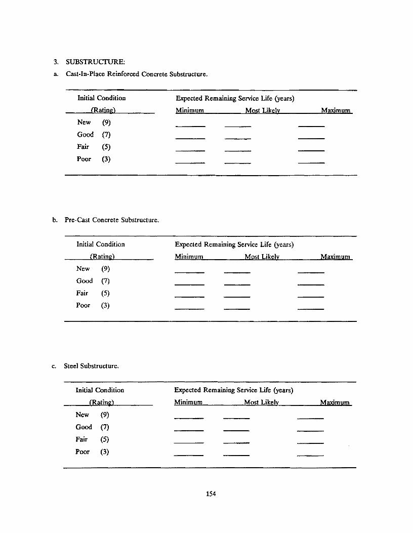
3. SUBSTRUCTURE:

a. Cast-In-Place Reinforced Concrete Substructure.

Initial Condition

(Ratin&)

New (9)

Good (7)

Fair (5)

Poor (3)

b. Pre-Cast Concrete Substructure.

Initial Condition

(Rating)

New (9)

Good (7)

Fair (5)

Poor (3)

c. Steel Substructure.

Initial Condition

(Rating)

New (9)

Good (7)

Fair (5)

Poor (3)

Expected Remaining Service Life (years)

Minimum Most Likely

Expected Remaining Service Life (years)

Minimum Most Likely

Expected Remaining Service Life (years)

Minimum Most Likely

154

Maximum

Maximum

Maximum

d. Timber Substructure.

Initial Condition

(Ratjn~)

New (9)

Good (7)

Fair (5)

Poor (3)

Expected Remaining Service Life (years)

Minimum Most Likely Maximum

Thank you very much for your opinion. We would like to visit you again and discuss the fmdings of our

study. Please provide the following information:

Name

Job Title

District -----------------------------TeJephone No.

Name --------------------------------Job Title

District

Telephone No.

Name

Job Title ----------------------------District

Telephone No.

155

SECTION II • QUESTIONNAIRE FOR STUDY ON BRIDGE REHABILITATION

A. EXPECTED INCREASE IN BRIDGE SERVICE LIVES;

Please consider the following types of highway bridges, and estimate, based on your bridge engineering

experience, the expected increase in service lives, and the expected final condition rating of the bridge

components after rehabilitation. Each time estimate will be requested in the following format:

1. At Minimum

2. Most Likely around

3. At Maximum

EXAMPLE:

_-..<.XX ........ __ years

_--£.XX~ __ years

_-..<.XX,:;:.,L __ years

Consider a reinforced concrete piling currently at a condition rating of 5 (fair condition). An expert

bridge engineer thinks that with an application of limited rehabilitation, the piling's service life will certainly

be extended by at least 10 years, that it most likely will last an ~xtra 13 years, but that the extension in life

will certainly not be more than 18 years. A sample time estimate of this expert's opinion as requested in the

format mentioned above will be:

1. At Minimum

2. Most Likely around

3. At Maximum

_---=:.1,:;:..0 __ years

_~1..::.3 __ years

_.......:.1>;<.8 __ years

156

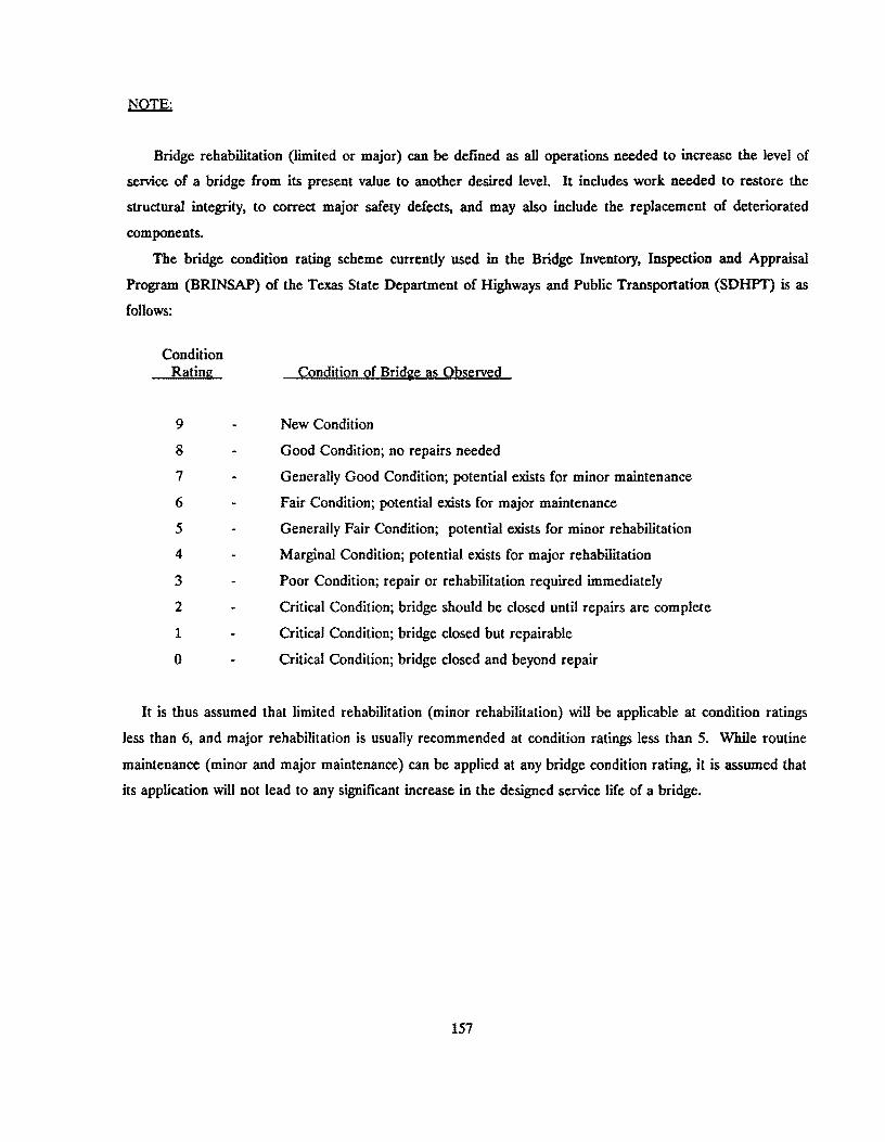
NOTE:

Bridge rehabilitation (limited or major) can be defined as all operations needed to increase the level of

service of a bridge from its present value to another desired level. It includes work needed to restore the

structural integrity, to correct major safety defects, and may also include the replacement of deteriorated

components.

The bridge condition rating scheme currently used in the Bridge Inventory. Inspection and Appraisal

Program (BRINSAP) of the Texas State Department of Highways and Public Transportation (SDHPT) is as

follows:

Condition Rating

9

8

7

6

5

4

3

2

1

o

Condition of Bridge as Observed

New Condition

Good Condition; no repairs needed

Generally Good Condition; potential exists for minor maintenance

Fair Condition; potential exists for major maintenance

Generally Fair Condition; potential exists for minor rehabilitation

Marginal Condition; potential exists for major rehabilitation

Poor Condition; repair or rehabilitation required immediately

Critical Condition; bridge should be closed until repairs are complete

Critical Condition; bridge closed but repairable

Critical Condition; bridge dosed and beyond repair

It is thus assumed that limited rehabilitation (minor rehabilitation) will be applicable at condition ratings

less than 6, and major rehabilitation is usually recommended at condition ratings less than 5. While routine

maintenance (minor and major maintenance) can be app1ied at any bridge condition rating, it is assumed that

its application wiD not lead to any significant increase in the designed service life of a bridge.

157

1. DECK:

a. Reinforced Concrete Deck:

(i) Limited Rehabilitation (repair of joints, thin overlay, etc.)

Initial Condition

matinal

Gen. Fair (5)

Marginal (4)

Poor (3)

Critical (2)

Expected Increase in Service Life (years)

Minimum Most Likely Maximum

(ii) Major Rehabilitation (deck widening, deck replacement, etc.)

Initial Condition

(Rating)

Marginal (4)

Poor (3)

Critical (2)

b. Timber Deck:

Expected Increase in Service Life (years)

Minimum Most Likely Maximum

(i) Limited Rehabilitation (creosote treatment, thin overlay, etc.)

Initial Condition

(Rating)

Gen. Fair (5)

Marginal (4)

Poor (3)

Critical (2)

Expected Increase in Service Life (years)

Minimum Most Likely Maximum

158

Expected Final

Rating

Expected Final

Rating

Expected Final

Rating

(ii) Major Rehabilitation (deck widening, partial replacement, etc.)

Initial Condition

<Rating)

Marginal (4)

Poor (3)

Critical (2)

c. Steel Deck:

Expected Increase in Service Life (years)

Minimum Most Likely Maximum

(i) Limited Rehabilitation (repair of wearing surface, repair of joints, etc.)

Initial Condition

(Ratins)

Gen. Fair (5)

Marginal (4)

Poor (3)

Critical (2)

Expected Increase in Service Life (years)

Minimum Most Likely Maximum

(ii) Major Rehabilitation (deck widening, deck partial replacement, etc.)

Initial Condition

(Rating)

Marginal (4)

Poor (3)

Critical (2)

Expected Increase in Service Life (years)

Minimum Most Likely Maximum

159

Expected Final

Rating

Expected Fmal

Rating

Expected Final

Rating

2. SUPERSTRUcruRE:

a. Prestressed Concrete Superstructure:

(i) Limited Rehabilitation (repair of beam ends, repair of cracks, etc.)

Initial Condition

(Ratin~

Gen. Fair (5)

Marginal (4)

Poor (3)

Critical (2)

Expected Increase in Service Life (years)

Minimum Most Likely Maximum

(ii) Major Rehabilitation (partial replacement, repair of collision damage, etc.)

Initial Condition Expected Increase in Service Life (years)

(Rating) Minimum Most Likely Maximum

Marginal (4)

Poor (3)

Critical (2)

b. Cast-In-Place Concrete Superstructure:

(i) Limited Rehabilitation (repair of beam ends, repair of cracks, etc.)

Initial Condition

(Ratin~

Gen. Fair (5)

Marginal (4)

Poor (3)

Critical (2)

Expected Increase in Service Life (years)

Minimum Most Likely Maximum

160

Expected rmal

Ratin&,

Expected Final

Rating

Expected Final

Rating

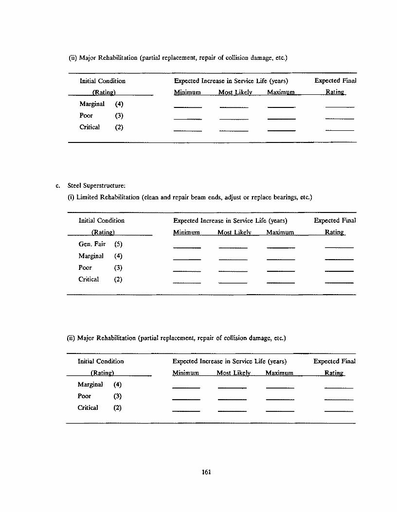
(il) Major Rehabilitation (partial replacement, repair of collision damage, etc.)

Initial Condition

(Ratina)

Marginal (4)

Poor (3)

Critical (2)

c. Steel Superstructure:

Expected Increase in Service Life (years)

Minimum Most Likely Maximum

(i) Limited Rehabilitation (dean and repair beam ends, adjust or replace bearings, etc.)

Initial Condition

(Rating)

Gen. Fair (5)

Marginal (4)

Poor (3)

Critical (2)

Expected Increase in Service Life (years)

Minimum Most Likely Maximum

(0) Major Rehabilitation (partial replacement, repair of collision damage, etc.)

Initial Condition

(Rating)

Marginal (4)

Poor (3)

Critical (2)

Expected Increase in Service Life (years)

Minimum Most Likely Maximum

161

Expected FInal

Ratina

Expected Final

Rating

Expected rmal

Rating

d. Steel Truss Superstructure:

(i) Limited Rehabilitation (clean and repair members, adjust or replace bearings, etc.)

Initial Condition

(Rating)

Gen. Fair

Marginal

Poor

(5)

(4)

(3)

Critical (2)

Expected Increase in Service Life (years)

Minimum Most Likely Maximum

(ii) Major Rehabilitation (partial replacement, repair of collision damage, etc.)

Initial Condition

(Rating)

Marginal (4)

Poor (3)

Critical (2)

e. Timber Superstructure:

Expected Increase in Service Life (years)

Minimum Most Likely Maximum

(i) Limited Rehabilitation (creosote treatment, repair of connections, etc.)

Initial Condition

(Ratinli'

Gen. Fair (5)

Marginal (4)

Poor (3)

Critical (2)

Expected Increase in Service Life (years)

Minimum Most Like]y Maximum

162

Expected Final

Ratin~

Expected Final

Rating

Expected F'mal

Ratina

(ii) Major Rehabilitation (partial replacement, repair of collision damage, etc.)

Initial Condition

(Ratins)

Marginal (4)

Poor

Critical

(3)

(2)

Expected Increase in Service Life (years)

Minimum Most Likely Maximum

163

Expected Final

Rating

2. SUBSTRUcrURE:

a. Reinforced Concrete Substructure:

(i) Limited Rehabilitation (repair of cracks, etc.)

Initial Condition

(Ratins)

Gen. Fair (5)

Marginal (4)

Poor (3)

Critical (2)

Expected Increase in Service Life (years)

Minimum Most Likely Maximum

Expected Final

Rating

(ii) Major Rehabilitation (partial replacement, encasement, repair of collision damage, etc.)

Initial Condition

(Ratins)

Marginal (4)

Poor (3)

Critical (2)

b. Steel Substructure:

Expected Increase in Service Life (years)

Minimum Most Likely Maximum

(i) Limited Rehabilitation (splicing, repair of cap spalls, etc.)

Initial Condition

(Rating)

Gen. Fair (5)

Marginal (4)

Poor (3)

Critical (2)

Expected Increase in Service Life (years)

Minimum Most Likely Maximum

164

Expected Final

Rating

Expected Final

Rating

(n) Major Rehabilitation (partial replacement, concrete encasement, etc.)

Initial Condition

(Ratin~

Marginal (4)

Poor (3)

Critical (2)

c. Timber Substructure:

Expected Increase in Service Life (years)

Minimum Most Likely Maximum

(i) Limited Rehabilitation (creosote treatment, etc.)

Initial Condition

(Rating)

Gen. Fair (5)

Marginal (4)

Poor (3)

Critical (2)

Expected Increase in Service Life (years)

Minimum Most Likely Maximum

(n) Major Rehabilitation (partial replacement, strengthening etc.)

Initial Condition

(RatinK)

Marginal (4)

Poor (3)

Critical (2)

Expected Increase in Service Life (years)

Minimum Most Likely Maximum

165

Expected Final

RatinK

Expected Final

Rating

Expected Final

RatinK

Thank you very much for your opinion. We would like to visit you again and discuss the fmdings of our

study. Please provide the following information:

Name ---------------------------------Job Title ------------------------------District -----------------------------Telephone No.

Name

Job Title ________________ _

District

Telephone No. ____________ _

Name -----------------------------Job Title _______________ _

District ---------------------------Telephone No. ______________________ _

166

APPENDIX C. ANALYSIS OF BRIDGE DETERIORATION AND REHABILITATION

167

GENERAL INFORMATION

1. Job Responsibilities: Participants were requested to circle one or more of the following duties/experience

applicable:

a. Bridge Maintenance and Rehabilitation

b. Bridge Design or Load Rating

c. Bridge Planning or Programming (Fund Allocation)

d. Bridge Inspection

e. Other - Please specify ____________________ _

2. Years of Experience of individuals who completed the questionnaire (Bridge-related work):

3. Types of bridges they are most familiar with (Steel Girder Bridges, Prestressed Concrete Bridges, etc.):

4. Participants were requested to indicate any special effects or bridge treatments that may be unique to

their district (use of deicing salts on deck, coastal water crossing, etc.)

168

SEmON I· OUESTIONNAIRE FOR STUDY ON BRIDGE DETERIORATION

Participants were requested to consider various classes of highway bridges, and estimate, based on their

bridge engineering experience, the expected remaining service lives of the bridge components - the time

(years) the bridge component will be due for replacement, given the present condition rating of the bridge.

They assumed no future maintenance or rehabilitation activity is planned for the bridge, that is, the bridge is

allowed to deteriorate naturaJly. Each time estimate was requested in tbe following format:

1. At Minimum

2. Most Likely around

3. At Maximum

EXAMPLE:

_--,,-XX=-=-__ years

_--,-XX~ __ years

_-.:..XX~ __ years

Consider a reinforced concrete piling currently at a condition rating of 5 (fair condition), and this piling

is left to deteriorate witbout any maintenance or rehabilitation. An expert bridge engineer thinks that the

piling will certainly survive at least 12 years, that it most likely will last another 15 years, but it will certainly

have to be replaced before 20 years time. A sample time estimate of this expert's opinion as requested in

the format mentioned above win be:

1. At Minimum

2. Most Likely around

3. At Maximum

_---:.1:;:.2 __ years

_---:.1""'5 __ years

_--=20><--_ years

169

NOTE:

The bridge condition rating scheme currently used in the Bridge Inventory, Inspection and Appraisal

Program (BRINSAP) of the Texas State Department of Highways and Public Transportation (SDHPT) is as

follows:

Condition Ratinz

9

8

7

6

5

4

3

2

1

o

Condition of Bridge as Observed

New Condition

Good Condition; no repairs needed

Generally Good Condition; potential exists for minor maintenance

Fair Condition; potential exists for major maintenance

Generally Fair Condition; potential exists for minor rehabilitation

Marginal Condition; potential exists for major rehabilitation

Poor Condition; repair or rehabilitation required immediately

Critical Condition; bridge should be closed until repairs are complete

Critical Condition; bridge closed but repairable

Critical Condition; bridge closed and beyond repair

170

1. DECK:

a. Reinf. Cone. Deck (with/without deck panels) • Expected Remaining Service Lives (yrs) [No. of responses = 23].

Initial Condition Minimum Most Likely Maximum

(Rating) Mean Std Dev. Mean Std Dev. Mean Std Dev.

New (9) 25.7 10.3 38.9 13.8 52.4 20.0

Good (7) 20.8 9.4 32.0 14.0 43.9 19.1

Fair (5) 10.7 6.4 18.3 9.6 25.3 11.6

Poor (3) 2.0 2.2 4.2 3.3 6.7 4.8

Est. Deterioration Rate (Pt./yr)" -0.145 -0.115 -0.083

• From simple linear regression analysis.

b. Timber Deck [Responses indicate its limited use on Texas on-system bridges].

c. Steel Deck [Responses indicate its limited use on Texas on-system bridges].

171

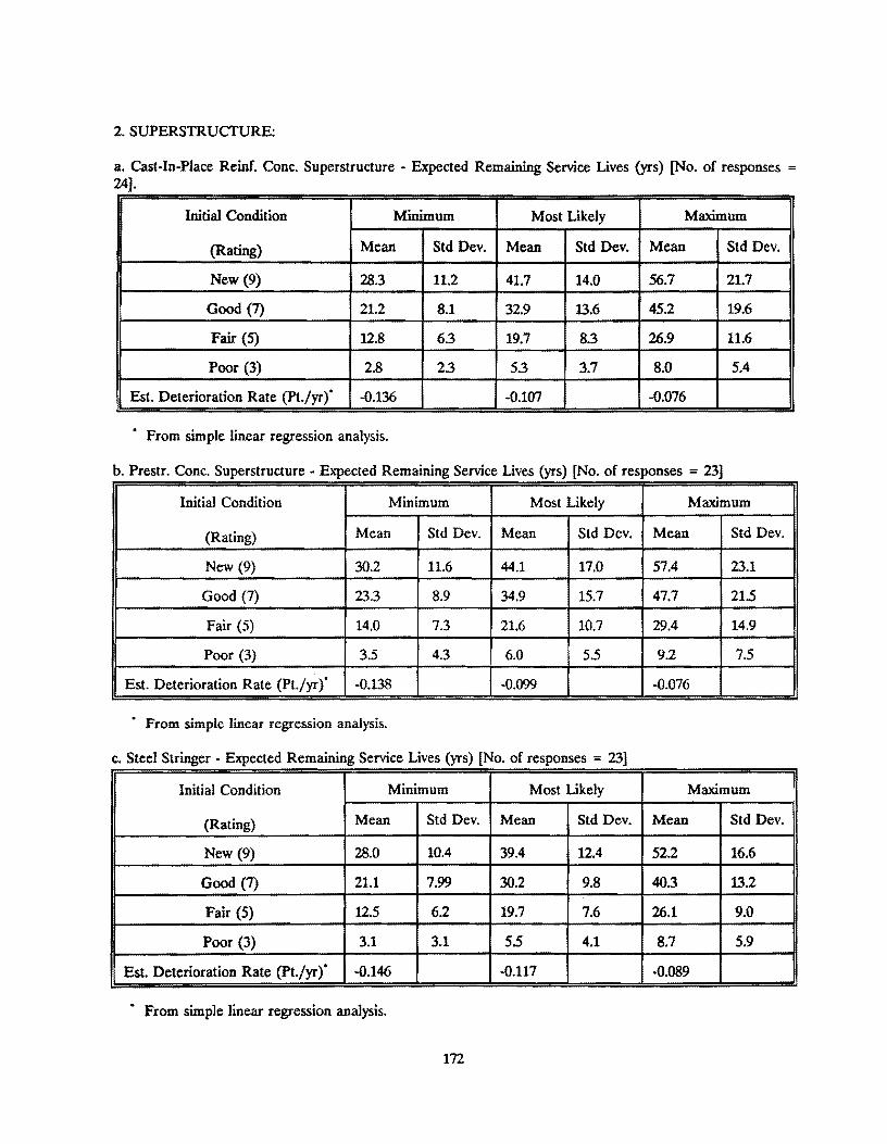
2. SUPERSTRUcrURE:

a. Cast-In-Place Reinf. Conc. Superstructure - Expected Remaining Service Lives (yrs) [No. of responses = 24].

Initial Condition Minimum Most Likely Maximum

(Rating) Mean Std Dev. Mean Std Dev. Mean Std Dev.

New (9) 28.3 11.2 41.7 14.0 56.7 21.7

Good (7) 21.2 8.1 32.9 13.6 45.2 19.6

Fair (5) 12.8 6.3 19.7 8.3 26.9 11.6

Poor (3) 2.8 2.3 5.3 3.7 8.0 5.4

Est. Deterioration Rate (Pt.fyr), -0.136 -0.107 -0.076

• From simple linear regression analysis.

b. Prestr. Conc. Superstructure - Expected Remaining Service Lives (yrs) [No. of responses = 23]

Initial Condition Minimum Most Likely Maximum

(Rating) Mean Std Dev. Mean Std Dev. Mean Std Dev.

New (9) 30.2 11.6 44.1 17.0 57.4 23.1

Good (7) 23.3 8.9 34.9 15.7 47.7 21.5

Fair (5) 14.0 7.3 21.6 10.7 29.4 14.9

Poor (3) 3.5 4.3 6.0 5.5 9.2 7.5

Est. Deterioration Rate (Pt./~)' -0.138 -0.099 ·0.076

* From simple linear regression analysis.

c. Steel Stringer - Expected Remaining Service Lives (yrs) [No. of responses = 23]

Initial Condition Minimum Most Likely Maximum I i

(Rating) Mean Std Dev. Mean Std Dev. Mean Std Dev.

New (9) 28.0 10.4 39.4 12.4 52.2 16.6

Good (7) 21.1 7.99 30.2 9.8 40.3 13.2

Fair (5) 12.5 6.2 19.7 7.6 26.1 9.0

Poor (3) 3.1 3.1 5.5 4.1 8.7 5.9

Est. Deterioration Rate (Pt./yr)* -0.146 ·0.117 -0.089

• From simp1e linear regression analysis.

172

d. Steel Truss - Expected Remaining Service Lives (yrs) [No. of responses = 20]

Initial Condition Minimum Most Likely Maximum

(Rating) Mean Std Dev. Mean Std Dev. Mean Std Dev.

New (9) 30.3 11.6 41.0 13.2 56.3 17.4

Good (7) 22.0 8.5 30.3 10.1 41.8 13.0

Fair (5) 12.5 5.8 18.2 6.8 26.1 8.6

Poor (3) 2.5 2.4 5.0 3.9 7.6 5.4

Est. Deterioration Rate (Pt./yr)" -0.135 -0.111 -0.087

• From simple linear regression analysis.

e. Timber Superstructure - Expected Remaining Service Lives (yrs) [No. of responses = 17]

Initial Condition Minimum Most Likely Maximum

(Rating) Mean Std Dev. Mean Std Dev. Mean Std Dev.

New (9) 14.7 9.3 22.2 10.2 32.4 13.9

Good (7) 11.1 6.8 16.2 7.7 243 11.7

Fair (5) 6.5 4.5 10.8 5.8 15.7 7.7

Poor (3) 1.4 1.3 3.3 3.0 5.5 4.6

Est. Deterioration Rate (Pt./yr)" -0.202 -0.188 -0.132

• From simple linear regression analysis.

173

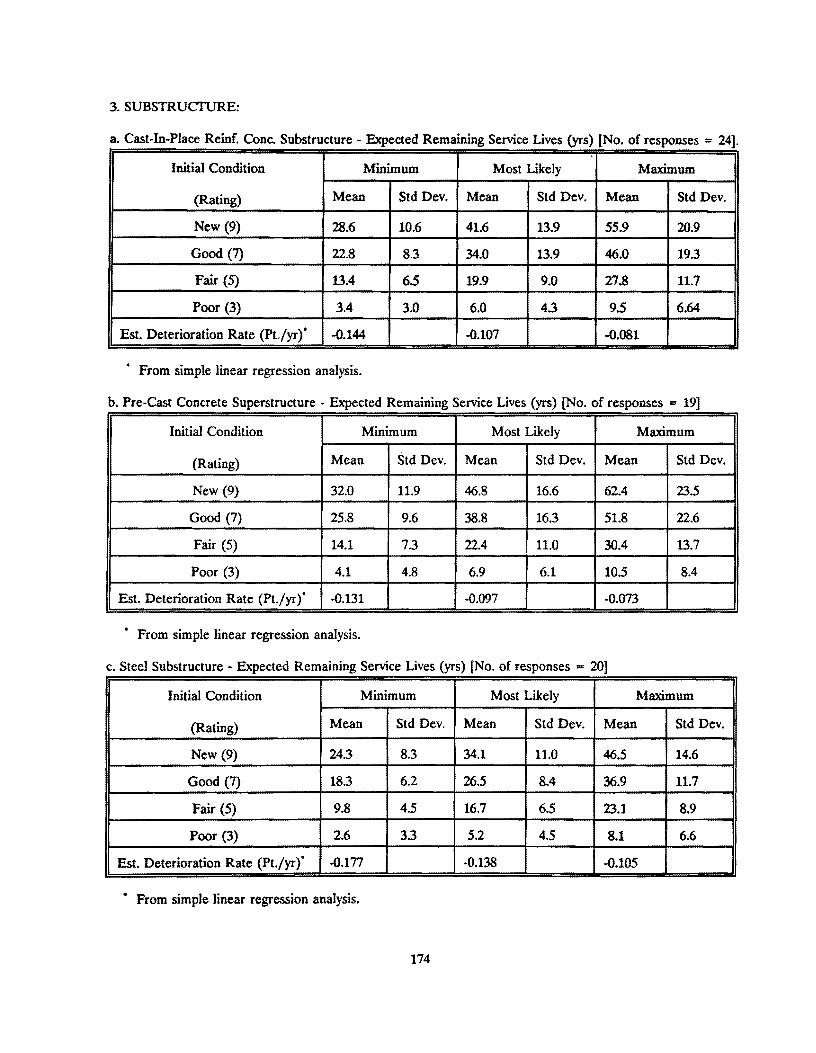
3. SUBSTRUCTURE:

a. Cast-In-Place Reinf. Cone. Substructure - Expected Remaining Service Lives (yrs) [No. of responses = 24].

Initia1 Condition Minimum Most Likely Maximum

(Rating) Mean Std Dev. Mean Std Dev. Mean Std Dev.

New (9) 28.6 10.6 41.6 13.9 55.9 20.9

Good (7) 22.8 8.3 34.0 13.9 46.0 19.3

Fair (5) 13.4 6.5 19.9 9.0 27.8 11.7

Poor (3) 3.4 3.0 6.0 4.3 9.5 6.64

Est. Deterioration Rate (Pt.jyr)" -0.144 -0.107 -0.081

• From simple linear regression analysis.

b. Pre-Cast Concrete Superstructure - Expected Remaining Service Lives (yrs) [No. of responses = 19]

Initial Condition Minimum Most Likely Maximum

(Rating) Mean Std Dev. Mean Std Dev. Mean Std Dev.

New (9) 32.0 11.9 46.8 16.6 62.4 23.5

Good (7) 25.8 9.6 38.8 16.3 51.8 22.6

Fair (5) 14.1 7.3 22.4 11.0 30.4 13.7

Poor (3) 4.1 4.8 6.9 6.1 10.5 8.4

Est. Deterioration Rate (Pt.jyr)" -0.131 -0.097 -0.073

• From simple linear regression analysis.

c. Steel Substructure - Expected Remaining Service Lives (yrs) [No. of responses = 20]

Initia1 Condition Minimum Most Likely Maximum

(Rating) Mean Std Dev. Mean Std Dev. Mean Std Dev.

New (9) 24.3 8.3 34.1 11.0 46.5 14.6

Good (7) 18.3 6.2 26.5 8.4 36.9 11.7

Fair (5) 9.8 4.5 16.7 6.5 23.1 8.9

Poor (3) 2.6 3.3 5.2 4.5 8.1 6.6

Est. Deterioration Rate (Pt.!yr)" -0.177 -0.138 -0.105

• From simple linear regression ana1ysis.

174

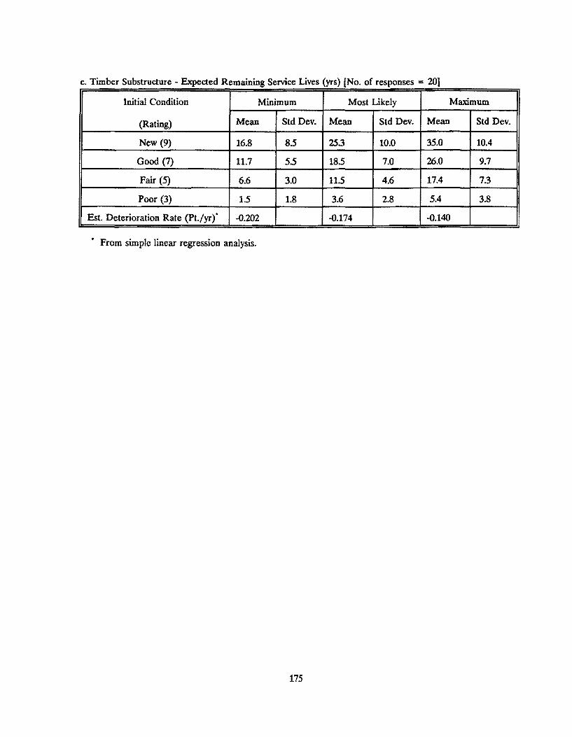
c. Timber Substructure - Expected Remaining Service Lives (yrs) [No. of responses = 201

Initial Condition Minimum Most Likely Maximum

(Rating) Mean Std Dev. Mean Std Dev. Mean Std Dev.

New (9) 16.8 8.5 25.3 10.0 35.0 10.4

Good (7) 11.7 5.5 18.5 7.0 26.0 9.7

Fair (5) 6.6 3.0 11.5 4.6 17.4 7.3

Poor (3) 1.5 1.8 3.6 2.8 5.4 3.8

Est. Deterioration Rate (Pt./yr)" -0.202 -0.174 -0.140

• From simple linear regression analysis.

175

SECTION II - OUESTIONNAIRE FOR STUDY ON BRIDGE WORK ACTMTlES

Participants were requested to consider various types of highway bridges, and estimate, based on their

bridge engineering experience, the expected increase in service lives, and the expected fmal condition rating

of the bridge components after rehabilitation. Each time estimate was requested in the following format:

1. At Minimum

2. Most Likely around

3. At Maximum

EXAMPLE:

_--'-XX~ __ years

_ ......... XX~ __ years

_--S.XX~ __ years

Consider a reinforced concrete piling currently at a condition rating of 5 (fair condition). An expert

bridge engineer thinks that with an application of limited rehabilitation, the piling's service life will certainly

be extended by at least 10 years, that it most likely will last an extra 13 years, but that the extension in life

will certainly not be more than 18 years. A sample time estimate of this expert's opinion as requested in the

format mentioned above will be:

1. At Minimum

2. Most Likely around

3. At Maximum

NOTE;

_~I~O __ years

_--",13~_ years

_---"'1 .... 8 __ years

Bridge rehabilitation (limited or major) can be defined as all operations needed to increase the level of

service of a bridge from its present value to another desired leve.. It includes work needed to restore the

structural integrity, to correct major safety defects, and may also include the replacement of deteriorated

components.

176

1. DECK:

a. (i) Reinf. Cone. Deck (Limited Rehabilitation) - [No. of responses = 19].

Expected Extension in Bridge Service Life (yr) Initial Condition Fmal Condition

(Rating) Minimum Most Likely Maximum Rating

Mean SId Dev. Mean Std Dev. Mean Std Dev Mean SId Dev.

Gen. Fair (5) 5.6 4.2 9.8 7.8 13.4 9.9 6.6 0.9

Marginal (4) 4.2 4.2 7.9 8.2 10.2 10.1 S.4 1.2

Poor (3) 2.8 4.4 S5 8.6 7.3 10.7 4.3 4.1

Critical (2) 1.9 45 4.2 8.9 5.8 11.1 35 1.7

(ii) Reinf. Cone. Deck (Major Rehabilitation) - [No. of responses = 19J.

Expected Extension in Bridge Service Life (yr) Initial Condition Final Condition

(Rating) Minimum Most Likely Maximum Rating

Mean Std Dev. Mean Sid Dev. Mean SId Dev Mean Std Dev.

Marginal (4) 17.0 95 25.8 14.1 33.3 17.4 7.7 1.0

Poor (3) 17.3 115 26.6 17.8 34.7 22.9 7.6 1.2

Critical (2) 17.7 12.3 25.9 18.3 35.1 235 7.4 1.3

177

2. SUPERSTRUcrtJRE:

a.(i) Prestressed Cone. Superstructure (Limited Rehabilitation) - [No. of responses = 18].

&peeted Extension in Bridge Service Ufe (yr) Initial Condition Final Condition

(Rating) Minimum Most Ukely Maximum Rating

Mean Sid Dev. Mean SId Dev. Mean Std Dev Mean Std Dev.

Ocn. Fair (5) 7.2 5.7 12.0 9.1 17.4 12.5 6.6 0.8

Marginal (4) 5.1 4.2 8.9 8.2 13.1 10.6 5.6 1.1

Poor (3) 3.8 4.5 7.1 8.6 10.6 11.1 4.7 1.5

Critical (2) 2.9 4.8 5.9 9.5 9.0 12.2 4.0 1.9

(n) Prestressed Cone. Superstructure (Major Rehabilitation) - [No. of responses = 18].

Expected Extension in Bridge Service ure (yr) Initial Condition Final Condition

(Rating) Minimum Most Ukely Maximum Rating

Mean Std Dev. Mean SId Dev. Mean SId Dev Mean Std Dev.

Marginal (4) 15.2 10.7 24.1 15.2 31.4 18.7 7.0 1.0

Poor (3) 15.1 12.3 24.0 18.8 31.6 24.2 6.5 1.4

Critical (2) 12.5 10.1 20.2 15.9 26.9 20.5 6.1 1.5

b. (i) Cast-In-Place Reinf. Cone. Superstructure (Limited Rehabilitation) • [No. of responses = 23].

Expected Extension in Bridge Service ure (yr) Initial Condition Final Condition

(Rating) Minimum Most Ukely Maximum Rating

Mean Std Dev. Mean SId Dev. Mean Std Dev Mean Std Dev.

Gen. Fair (5) 6.5 4.9 11.2 8.7 16.5 12.3 6.7 0.8

Marginal (4) 5.1 4.4 8.9 8.4 13.3 10.8 5.7 10.3

Poor (3) 4.2 4.5 7.4 8.7 11.1 11.2 5.0 1.4

Critical (2) 3.5 4.9 6.6 9.5 10.1 12.3 4.2 1.8

178

(ii) Cast-In-Place reinf. Conc. Superstructure (Major Rehabilitation) - [No. of responses = 23].

Expected Extension in Bridge Setvice Ufe (yr) Initial Condition Final Condition

(Rating) Minimum Most Likely Maximum Rating

Mean SId Dev. Mean SId Dev. Mean Std Dev Mean Sid Dev.

Marginal (4) 13.4 6.8 20.6 11.7 27.7 B.2 7.0 1.1

Poor (3) IV 7.3 20.8 13.2 27.1 17.3 6.5 1.4

Critical (2) 1; 8.6 20.2 14.7 26.6 19.5 6.1 1.8

c. (i) Steel Superstructure (Limited Rehabilitation) - [No. of responses = 19].

Expected Extension i:. Bridge Setviee Life (yr) Initial Condition Final Condition

(Rating) Minimum Most Likely Maximum Rating

Mean SId Dev. Mean SId Dev. Mean SId Dev Mean SId Dev.

Gen. Fair (5) 7.5 4.6 12.6 85 17.3 11.4 6.4 0.8

Marginal (4) 6.7 5.1 11.3 9.3 15.3 11.9 5.6 1.0

Poor (3) 5.4 6.3 9.1 11.1 12.2 13.2 4.7 15

Critical (2) 5.0 7.5 8.5 11.8 11.6 14.8 4.0 1.8

(ii) Steel Superstructure (Major Rehabilitation) - [No. of responses = 191.

Expected Extension in Bridge Setvice Life (yr) Initial Condition Final Condition

(Rating) Minimum Most Likely Maximum Rating

Mean Std Dev. Mean SId Dev. Mean SId Dev Mean SId Dev.

Marginal (4) 12.0 5.4 20.0 10.3 26.4 13.3 7.1 1.2

Poor (3) 12.3 7.2 20.8 12.8 27.0 16.2 6.7 15

Critical (2) 12.2 9.1 20.3 14.4 26.6 18.7 6.4 1.7

179

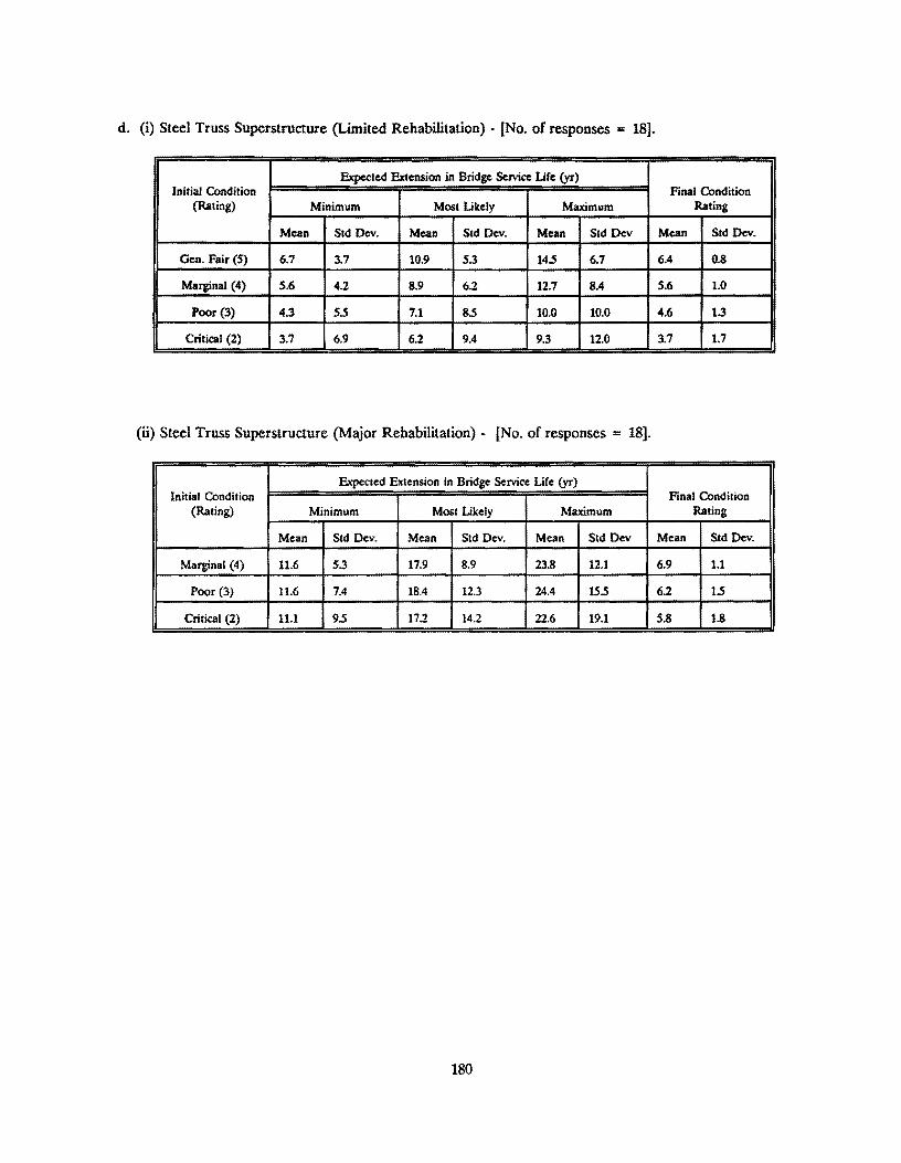
d. (i) Steel Truss Superstructure (Limited Rehabilitation) - [No. of responses = 18].

Expected Extension in Bridge Service Lift (yr) Initial Condition Final Condition

(Rating) Minimum Most Liktly Maximum Rating

Mean Std Ocv. Mean Std Ocv. Mean Std Dev Mean Std Ocv.

Otn. Fair (5) 6.7 3.7 10.9 5.3 14.5 6.7 6.4 0.8

Marginal (4) 5.6 4.2 8.9 6.2 12.7 8.4 5.6 1.0

Poor (3) 4.3 5.5 7.1 8.5 10.0 10.0 4.6 1.3

Critical (2) 3.7 6.9 6.2 9.4 9.3 12.0 3.7 1.7

(n) Steel Truss Superstructure (Major Rehabilitation) - [No. of responses = 18].

Expected Extension in Bridge Service Lift (yr) Initial Condition Final Condition

(Rating) Minimum Most Likely Maximum Rating

Mean Std Dev. Mean SId Dev. Mean SId Dev Mean Sid Ocv.

Marginal (4) 11.6 5.3 17.9 8.9 23.8 12.1 6.9 1.1

Poor (3) 11.6 7.4 18.4 12.3 24.4 15.5 6.2 1.5

Critical (2) 11.1 9.5 17.2 14.2 22.6 19.1 5.8 1.8

180

3. SUBSTRUcrURE:

a.(i) Reinforced Conc. Substructure (Limited Rehabilitation) - [No. of responses = 18].

Expected Extension in Bridge Service Ufe (yr) Initial Condition Final Condition

(Rating) Minimum Most Likely Maximum Rating

Mean Std Dev. Mean SId Dev. Mean SId Dev Mean SId Dev.

Gen. Fair (5) 6.9 4.5 U.5 8.3 16.1 10.6 6.6 0.8

Marginal (4) 4.8 4.0 8.6 8.2 11.7 10.1 5.4 1.0

Poor (3) 3.1 4.4 6.1 8.5 8.8 10.9 4.3 1.4

Critical (2) 2.5 4.8 5.3 9.3 7.8 12.0 3.5 1.7

(li) Reinforced Conc. Substructure (Major Rehabilitation). [No. of responses = 18].

Expected Extension in Bridge Service Life (yr) Initial Condition Final Condition

(Raling) Minimum Most Likely Maximum Rating

Mean Std Dev. Mean Std Dev. Mean Std Dev Mean Std Dev.

Marginal (4) 13.6 8.5 21.4 12.1 29.5 17.0 7.2 1.1

Poor (3) 13.8 11.1 21.1 16.4 28.5 22.0 6.7 1.4

Critical (2) 12.7 12.1 20.4 17.6 27.9 23.4 6.3 1.8

b. (i)Steel Substructure (Limited Rehabilitation) - [No. of responses = 18].

Expected Extension in Bridge Service Life (yr) Initial Condition Final Condition

(Rating) Minimum Most Likely Maximum Rating

Mean Std Dev. Mean Std Dev. Mean Std Dev Mean SId Dev.

Gen. Fair (5) 7.2 4.6 11.3 6.2 16.0 7.8 6.6 0.8

Marginal (4) 5.2 3.2 8.2 4.5 12.9 6.6 5.4 0.9

Poor (3) 3.2 2.7 4.9 3.6 8.1 5.4 4.4 1.1

Critical (2) 1.8 2.5 3.8 4.6 6.1 6.9 3.4 1.4

181

(li) Steel Substructure (Major Rehabilitation)· (No. of responses = 18J.

Expected Extension in Bridge Service Life (yr) Initial Condition Final Condition

(Rating) Minimum Most Likely Maximum Rating

Mean Sid Ocv. Mean Std Ocv. Mean Std Ocv Mean Std Ocv.

Marginal (4) 11.7 S.2 17.6 7.1 24.9 10.8 7.2 1.0

Poor (3) 11.7 7.0 16.7 8.6 22.9 12..7 6.3 0.8

Critical (2) 10.2 7.6 16.3 9.8 21.9 14.3 6.4 1.5

c. Timber Substructure (Limited Rehabilitation) - [No. of responses = 18J.

Expected Extension in Bridge Service Life (yr) Initial Condition Final Condition

(Rating) Minimum Most Likely Maximum Rating

Mean Sid Dev. Mean Std Dev. Mean Std Dev Mean SId Dev.

Gen. Fair (5) 5.3 2.3 8.8 3.4 11.6 5.0 6.2 0.7

Marginal (4) 3.1 1.3 5.4 2.4 8.1 3.9 5.0 0.7

Poor (3) 1.4 1.1 2.9 1.9 4.9 3.4 3.9 0.9

Critical (2) 0.8 1.1 2.2 2.1 3.3 3.0 3.1 1.1

(ii) Timber Substructure (Major Rehabilitation) - [No. of responses = 18].

Expected Extension in Bridge Service Life (yr) Initial Condition FIRal Condition

(Rating) Minimum Most Likely Maximum Rating

Mean Std Dev. Mean Std Ocv. Mean Std Ocv Mean Std Dev.

Marginal (4) 10.8 9.0 17.0 13.1 23.7 17.5 7.1 1.0

Poor (3) 9.9 10.6 16.2 15.8 22.8 21.4 6.5 1.3

Critical (2) 9.7 11.4 15.4 16.9 22.0 22..9 6.3 1.6

182

APPENDIX D. INTERVIEWS WITH SDHPT PERSONNEL

183

The comments of interviewed personnel are presented here without identification of the individual, district or division.

QUESTIONS ASKED AT DISTRICf VISITS

1. Current Data Management a. What d.b. management systems are in use for bridge information? (BRINSAP, DCIS, CIS, MMIS,

other) b. What computer systems? Is SAS used at District? c. How adequate is BRINSAP at the District level? d. How is BRINSAP used? e. Is BRINSAP effective? If not, what should be changed? f. What records are maintained at District vs State? g. What bridges are being inspected to comply with BRINSAP? h. How does BRINSAP feed into Fed SIA?

2. Maintenance a. How is maintenance managed within the District? What level of maintenance is being performed? b. Is maintenance data sufficient, insufficient, or too much? c. Would historical data be of value? (Case Studies) d. Is a policy needed to equate maintenance level with condition rating? e. Is there a need for more emphasis on preventive maintenance? Where? f. Would the Pennsylvania BMS maintenance needs be appropriate?

3. Training/manpower a. Is extra training for engineers/inspectors needed? If so, in What? (Maintenance, visual inspection,

technology-underwater, etc.) b. Is manpower adequate for getting more data, if needed? c. Where should additional training be held, if needed?

4. BMS-General a. What tasks are currently done to manage bridge MRR? b. Are there deficiencies in the overall bridge management today? If so, where? c. What could a BMS provide (within reason) that is not currently available? d. Should a BMS be used for funding? Costjbenefit analysis? Maintenance tracking? Other historical

costs? Traffic estimates?

DlSTRICf A 1. Current Data Management

a. What d.b. management systems are in use for bridge inrormation? (BRINSAP, DCIS, CIS, MMIS, other)

BRINSAP only useful tool MMIS does not track bridge maint. functions - will track cost of work - labor, materials - can include bridges

talk of going to new reference system • new numbering - will get away from milepost tracking - new system TRANSNET

b. What computer systems? Is SAS used at District?

access system in Austin to update BRINSAP 2 individuals knowledgeabJe of BRINSAP (engineer and technician. inspector)

won't inspect all bridges at once - use rotation over 2 year period will inspect several each month; system by counties (17 counties)

184

must identify bridges that need more frequent inspection o have used MARK IV; may be using SAS

c. How adequate is BRINSAP at the District level?

o SR not adequate - deck functions not weighed properly- deck can have rating of .D and not be eligible for rehab because SR > 80

o salt decks - deteriorate quickly - have had chunks of concrete falling off onto cars - cars riding on reinforcing steel

d. How is BRINSAP used?

BRINSAP just used to get sufficiency rating for bridge

o not much communication between maintenance and design o important to have feedback of mainl. to design o decks are a problem due to deicing o big problem with joints • feels all sealed joints should be eliminated • very expensive to

construct and maintain o have maint. program to clean caps, etc. o waterproof tops of caps • cast house top shapes, waterproof with epoxy "cleaning is best

preventative maintenance"

e. Is BRINSAP effective? If not. what should be changed?

BRINSAP effective for what its used for· to get SR and bridges on a program BRINSAP not a good maintenance tool - used for SR but not for maintenance

r. What records are maintained at District vs State?

2 mainl. inspections recommended per year - no formal requirements for inspectors - in past have filled out some BRINSAP form - 1085 form· got meaning less results because inspectors not properly trained

o trying to develop maint. recommendation sheet that inspector fdls out and sends to foreman o BRINSAP does not address maint. needs

Maint. follow up form in BRINSAP manual • written comment sheet - lists work recommended and work completed

Have inspector and maint. functions both involved • may be able to answer question in BRINSAP if mainl. recommendations are made and how urgent work is - can then list bridges and look at second sheet

g. What bridges are being inspected to comply with BRINSAP?

h. How does BRINSAP feed into Fed SIA?

185

2. Maintenance a. How is maintenance managed within the District? What level or maintenance is being performed?

local or section level special jobs or bridge crew contract maint. rehab/replacement· need to go to programs (Fed/State aid)

o keeping a structure clean is one of most inexpensive and effective method of maintenance early spring & prior to winter

o propose 2 cleanings a year - clear by air or water clean caps, beam ends. flanges, bearings, etc. spot painting

1. can be done by section maintenance people

2. special bridge crew used to repair joints, spatJed concrete, etc. o concrete repair above section level - 3 man crew o repair slabs, bridge rails, etc.

3. contract labor

Maint. manual suggests inspecting bridges twice a year maint. is a separate inspection - need to look for different things - need separate inspection form - individual training

have Preventative Maintenance Program - Activity 204 $7M, $1.2M on bridges Routine Maint. -Activity 202 $13M

204 - all contract seal coats, overlays, repair of bridge joints, decks, repainting

typically only bridge work done is within Fed. Aid Program

most deck/cap problems occurring around 15-20 yrs.

o good cleaning program could double life

b. Is maintenance data sufficient, insufficient, or too much? e. Would historical data be of value? (Case Studies) d. Is a policy needed to equate maintenance level with condition rating? e. Is there a need for more emphasis on preventive maintenance? Where? f. Would the Pennsylvania BMS maintenance needs be appropriate?

3. Training/manpower a. Is extra training for engineers/inspectors needed? If so, In What? (Maintenance, \'isual Inspection,

technology-underwater, etc.)

o inspectors not taught to treat bridge with different perspectives o trying to use 2 forms- one for maintenance needs, one for bridge inventory

b. Is manpower adequate for getting more data, If needed? c. Where should additional training be held, It needed?

186

4. BMS-General a. What tasks are currently done to manage bridge MRR? b. Are there deficiencies in the overall bridge management today? If so, where?

No systematic program; BRINSAP is not bridge management districts have no direction from divisions in Austin each district on their own no level of service guidelines for W maintenance functions

c. What could a BMS provide (within reason) that is not currently available?

should be automated for quick identification of maint. needs vs major rehab work; inspection tracking/monitoring o should track costs of repair; cost/benefit

187

VISIT TO SDHPT DISTRICT B INTERVIEW WITH DISTRICT MAINTENANCE ENGINEER

Current Data Management The database management system currently in use at the district is the BRINSAP (Bridge Inventory,

Inspection, and Appraisal) System. Available computer systems include the mM Mainframe and various microcomputers. While the BRINSAP is very useful, it does not completely qualify as a database management system. First, there is need for the inclusion of most crucial maintenance needs such as bridge painting. repair of bearing pads, etc. Also, descriptive information from field inspection should be included in the BRINSAP database. Presently, BRINSAP's uses include inventory of bridges in the district, bridge condition records, sufficiency rating information, rehabilitation / replacement needs on existing bridges, and FHW A's other uses.

BRINSAP is effective for its original intended purpose, but should be modified to satisfy present demands. The information on inventory, and condition of bridges, is very important, but the sufficiency rating does not adequately measure the deficiencies of the bridge; a detailed look at the condition ratings is usually needed. The BRINSAP could serve as a duplicate system or supplement bridge maintenance management tool, indicating immediate maintenance needs, may be in a coded form.

Detailed records on bridges are kept in individual folders at district level, whiJe mostly short-length coded records are kept computerized at the state level. The entire BRINSAP records are available to the FED SIA, as often as requested.

Maintenance Normally, routine bridge maintenance activities are planned ahead of time, but presently, an "emergency"

form of maintenance management is being used. There are two levels of maintenance management: maintenance foremen (lower) leve~ and district maintenance office level. The headquarters (Austin Office)is usually not involved in maintenance management except in cases of need for special expertise, for example, expert structural engineer's inspection and opinion. In most cases, the district would have taken a temporary line of action, before the arrival of the "expert". The involvement of the Austin Office is usually only at the District's request.

There are one-year, five-year, and ten-year maintenance plans, but there is a need for an extensive Five-year Bridge Maintenance Plan. There is also a need for information on maintenance requirements: when is this maintenance activity needed?, how effective was the last maintenance effort?, and the next time to maintain bridge. BRINSAP was actually designed for making decisions on major rehabilitation and replacement of bridges, not for routine bridge maintenance.

There is insufficient bridge maintenance data at management level, thus, there is no quick way of making decisions on the most economical and efficient expenditure of funds on bridges. A good data should contain prioritized list of bridges.

Defmitely, historical data would be of value, but it might be difficult to conduct case studies at the present time because of the lack of data. No proper documentation of case histories and routine maintenance operations are done on the bridge, because these information are not stored on the BRINSAP computerized mes, especially state-force maintenance operations. So, it is possible to conduct case studies, but only at district level, and it would be necessary to interview personnel familiar with the bridge inspections, and previous maintenance operations.

A maintenance rating would be very beneficia~ but it should be a "weighted" rating, that is, the maintenance level should be linked to condition ratings.

Training/Manpower At present, the training program is good but it should be conducted on a continuous basis. In some

districts, there is adequate manpower for obtaining more bridge data, but in others, the availability of manpower would depend on the number of bridges within the district's jurisdiction. The idea of hiring an outside consultant could be considered. Additional on-site training should held at or near the districts. It is better for the instructors to travel around, to the different locations, instead of the district personnel

188

scheduling trips to Austin, within each district's allocated quota. This would provide the districts with more trained bridge management personnel.

Bridge Management System (BMS) General There are deficiencies in the overall bridge management today, simply because there is no real bridge

management system. There is no systematic approach, the system is fragmented, and the districts have different approaches towards bridge management.

The Bridge Management System (BMS) could improve effectiveness of limited funding being presently expended on bridge maintenance. The BMS should not be used for funding; there is a possibility of people "tricking" the system, so the BMS should influence, not control fund. Level of service should be considered before costs. The BMS should be used for cost/benefit analysis, especially, on maintenance effectiveness of alternative operations, in order to avoid repeating an ineffective bridge improvement activity.

Maintenance operations on a bridge should be tracked to the structure, not the highway. At present, bridge maintenance activities are tracked to the roadway file by control-section of highway, and not to the particular structure. The records should also be detailed.

Keeping historical costs record on the BMS would be of benefit, indicating cost-overruns on routine maintenance, and also decisions on the rehabilitation/ replacement options. Traffic data estimates are done by roadway, but should be done by specific structure. A future estimate would also be useful.

There should be a database from which any information listing is easily accessible to users within the district and SDHPT, upon request.

General comments A bridge should be replaced only when the service life expires. Rehabilitation should always be

considered first, because of detour costs involved in bridge replacement. The present criteria for bridge replacement are:

• Sufficiency Rating

• ADT • Relevance to other structures in the location • Route consideration e.g cumulative costs on one route • Cost per vehicle mile

BRINSAP should include codes for preventive maintenance (painting, joint cleaning, etc.). If a bridge's condition becomes critical, action should be taken at that time. The level of service needed should be established, and cost estimates made. Other notes of importance are:

• BRINSAP fields' modifications needed. • Preventive maintenance program is currently accessing BRINSAP records in addition to other

records such as the Roadway Inventory File (RIF), and interviewing maintenance foremen, before making bridge management decisions

• Allocated structure numbers are sometimes out of sequence, thereby causing location problems • There is currently a problem of underfunding. Funding programs (sources) include:

1. Bridge program (State). 2. Rehab program. 3. Discretionary program. 4. Preventive maintenance program.

189

DISTRICf ~

1. Current Data Management

a. What d.b. management systems are in use for bridge inrormation? (BRINSAP, DCISt CIS, MMIS, other)

BRINSAP

DCIS - under CICS - data management done through this engineering computations under ROSCOE

two operating systems on IBM CICS

b. What computer systems? Is SAS used at District?

Use MARK IV not SAS - considered satisfactory.

can access mainframe with PC or terminals which are shared among division

c. How adequate is BRINSAP at the District level?

When bridge needs work, almost always make physical inspection BRINSAP just a staring point, but can't be used for decisions

basically keep BRINSAP updated to maintain federal aid BRINSAP never meant to help design a bridge maint. info. not included such as when overlayed, etc. maint. maint. info. should be computerized - historically, etc. have section - proposed improvements

FORM 1321-1,2 computer input sheet

changes coming within 2 years for BRINSAP

BRINSAP - often hard to locate bridge structure - use prioritization of roadways Interstate or US hwy - if two interstates - use lower number (regardless of which roadway actually has bridge)

d. How is BRINSAP used?

used in planning

e. Is BRJNSAP etTective? If not, what should be changed?

effective as planning tool

f. What records are maintained at District VI State?

records updated every thursday night; hard copy of inspection kept

190

g. What bridges are being inspected to comply with BRINSAP?

all bridges, consultants challenged to find additional bridges ·if less than 20 ft don't include

h. How does BRINSAP reed into Fed SIA?

. every two months· tape generated in Austin from BRINSAP

2. Maintenance a. How is maintenance managed within the District? What level of maintenance is being performed?

Maintenance· need better records, communication between planning, maintenance, etc.

b. Is maintenance data sufficient, insufficient, or too much?

Co Would historical data be or value? (Case Studies)

d. Is a policy needed to equate maintenance level with condition rating?

e. Is there a need ror more empbasis on preventive maintenance? Where?

no scbeduled preventative maintenance

Maintenance money is unrestricted

rehab. has strings attached

f. Would the Pennsylvania BMS maintenance needs be appropriate?

much money required to make sq. ft. estimates, etc.

- maybe use as secondary inspection for bridges with rating below certain level • may waste time and money otherwise

maintenance money used to repair components of a particular bridge, not entire bridge

- different when considering a series of bridges or network

3. Training/manpower

use consultants· works well

- independent appraisal has advantage from legal standpoint - selected based on past experience, manpower, cost - get price per bridge

traffic control a big item - especially for fracture critical inspection - steel, nonredundant members

191

a. Is extra training for engineers/inspectors needed? If so, in What? (Maintenance, visual inspection, technology-underwater, etc.)

- would like P.E.'s to attend training session - underwater inspection

b. Is manpower adequate for getting more data, if needed?

not applicable since they use consultants would require more money

BRINSAP may say 15 percent deck spalled, etc., but don't know where location is - once rehab. decided upon, need to make inspection

- BRINSAP useful for identification and planning but not decision making

• get new FHW A coding guide - Revised Recording and Coding Guide for BRINSAP

c. Where should additional training be held, if needed?

4. BMS·General a. What tasks are currently done to manage bridge MRR?

send in list of bridges; apply to Fed. aid

• cities & municipalities make up own list

- run BRINSAP- get low sufficiency rating to get recommendations then get input from cities

- use ADT, number of buses, mail trucks

- using federal money must put up 20 percent and follow all Fed. guidelines

- counties can often build a small, cheap bridge for the same 20 percent in a much shorter time

- Fed. funded bridge may take 2-3 yrs. to complete

- don't use TEBS

- must filter out which bridges are available for which funding

b. Are there deficiencies in the overall bridge management today? If so, where?

problem getting funding for low volume bridges - get pushed down list year after year

Bridges for replacement and rehab. funded every three years

- federal funding always exceeded

maintenance planning design} communication; money doesn't necessarily get to right places

o people in different sections don't have good communication o 5 or 6 design sections o maintenance and design - big gap

192

o on one particular project there were one set of plans being made to replace bridge and one set to widen

o frequently spend money on projects that could be used more efficiently elsewhere o had excess maintenance money - drew up plans for bridge rehab. o sent to Austin for approval - state felt it was a good project and it received state funds and later

Fed. funds o didn't spend almost $200,000 maint. money o need to consider future plans - how to best spend money o one bridge is structurally fme, but functionally inadequate due to restricted lanes o need to widen, but know that this would be temporary measure since there will be a 10 lane

bighway approaching in future and bridge will be replaced.

c. What could a BMS provide (within reason) that is not currently avalJable?

projects selected for mainL, rehab. money, different categories

- do eight bridges a month (one every 3 days) which are most suitable for different categories - state maint., state rehab., fed. rehab. - choice between when to replace and when to rehab.

d. Should a BMS be used for funding? Cost/benefit analysis? Maintenance tracking? Other historical costs? Traffic estimates?

i) funding - there is some prioritizing at state level already - competition among districts - everything in one pot - get list of bridges and alternatives - divide or separate list based on alternative by giving each alternative a category - print out list of maint., rehab., etc.

CRP - federal grant (can use for on/off system) FAU - Federal Aid Urban - Category 6

GENERAL COMMENTS

If bridge is deficient - do you rehab. or replace? Feds base decision on cost - can use life cycle cost comparison.

Sufficiency Rating generated out of Bridge inspection report Category 8 Fed Bridge RR - BRINSAP used

SR SO-SO eligible for rehab. SR <: SO replacement

Nine Categories for funding - set up by Slate for different types of projects almost all categories can have bridge rehab. in it .

• must apply for Fed. MR&R

Cost/Benefit analysis not really performed - use initial cost of alternative; do consider certain "intangibles"

Personal philosophy important in district

193

data collected maybe insufficient· many types of bridges can't be widened curved girder; single column BRINSAP doesn't have this info have pictures, inspectors report, etc. on hard file use consultants· don't have manpower 10 different consultants (15 different contracts) - approx. 4000 bridges 1/2 off; 1/2 on-system

approx. 150 peoples involved in inspection full time

New coding for Fed SIA inspection - out by 1st of year • adding additional info. on fracture critical inspection, underwater insp.

also want to delete some old info. will need to modify BRINSAP accordingly consultant will look for cracks using visual inspection and then if they exist then nondestructive testing will be used criteria of age and ADT used to select bridges -some measure of Fatigue

Preventative Maintenance - always a catch-up situation no formal reporting system many bridges have slope problems - erosion, sliding biggest problem - expansion joint cleaning and replacing money spent on slabs, rails, armor joints use salts 1 or 2 times a year but gets washed away, not a big corrosion problem maintenance directed toward upgrading load posted bridges firstly want to be able to pass school buses (28,000), and mail trucks most maintenance is just to keep the bridges open

BMS - databases insufficient to make decisions from communication between maintenance, future work, BRINSAP

if maint. fixed something; others may not be aware

Feds have rigid requirements, guidelines Geometry problems can disqualify bridges

funding categories can change and restrictions change accordingly

No federal maint. money; maint. is separate and handled by state

District maintenance crew - done by contract each residency has maint. crew - replace guardfence, patch roadway .

.. get copy of Bridge Insp. Report (2 sheets) 1085-1 What needs to be added to BRINSAP Bridges Inspection Record

Bridges Rating Record

194

VISIT TO SDHPT DISTRICf D

Current Data Management Bridge inspection is being performed by consultants and data in BRINSAP is fairly complete; problems

exist with off system bridges, which are largely substandard and must be load posted. There is need for a listing of these bridges but some counties are nol furnishing. BRINSAP is used constantly but inspection reports should be used directly for inputting to maintenance. Inspection data is furnished on diskettes. They are trying to get consistent programs to enter data directly into other systems at the State and local level. Resident Engineers should pay more attention to reports.

Inspection All inspection, both on and off system, is done by consultants District could use more indicators of

maintenance but doubt that extensive bridge maintenance fields would be practical. Promised to get him a copy of the Pennsylvania maintenance reporting scheme. Said that the uniform reporting of information was most important, and people must pay more attention to the inspection reports, because there is quite a lot of data already reported that is not used. In particular, photos of problems are very helpful and should trigger action.

Maintenance Management District does not do enough routine or scheduled maintenance. Maintenance that is performed is very

expensive, because it affects traffic and ties up crews for considerable periods of time. Special crews are needed. Maintenance relies on original inspection reports more than BRINSAP.

195

DISTRICf E

1. Current Data Management a. What d.b. management systems are in use ror bridge information? (BRINSAP, DCIS, CIS, MMIS,

other)

BRINSAP • not accessible enough to use on daily basis

use DCIS - used after program organized

need one database to keep up with bridges rather than entering different d.b.'s

- MMIS helpful in identifying when and where work done

would be very difficult to get enough comments in BRINSAP to determine why ratings were as given

- may only have a handful of bridges you need added info on • if too much info .• will run into manpower problem

b. What computer systems? Is SAS used at District?

use of SAS cumbersome • need to know a lot more do not use MARK IV

using DB III - more user friendly on PC and can use faster than SAS don't need to wait on computer in AUSTIN

- Will be sent disk from D-5 every two weeks - can manipulate lists for own use

- go through ROSCOE to update BRINSAP

c. How adequate is BRINSAP at the District level?

yes, is useful· good for permits to get H rating

helpful as tool

adequate for posting and closing

not adequate for maint. other than becoming aware through inspection where work is needed - no repairs scheduled by it

TEBS - only as good as how factors are weighed in formulas used for prioritization

d. How is BRINSAP used?

posting, permits, selection of bridges for program consideration

196

e. Is BRINSAP effective? If nOlt what should be changed?

problem with SR - ADT should be big factor, structural elements and decks reviewed

truck percentage? might be necessary

f. What records are maintained at District vs State?

BRINSAP, hard copy of bridge files

g. What bridges are being inspected to comply with BRINSAP?

all bridges > 20 ft in length

feds approve inspection contracts

h. How does BRINSAP feed into Fed SJA?

district updates state file - state prepares file for FEDS quarterly sent to Washington

District file updated weekly

- problem with Feds - state gives inspection data quarterly and Feds. might not have updates - time lag

- Feds. recently tied in directly to BRINSAP

2. Maintenance a. How is maintenance managed within the District? What level of maintenance is being performed?

(i) handled under resident eng., each responsible for some design and construction, and all maint. on hrs defmed area - change within dist. 1 1/2 yrs.

- previously handled within District

(ii) performed as required; some scheduled maint. (ex. clean bearings) but no scheduled program

- one problem is bridge damage from high loads - unless emergency, must go through normal letting process

emergency is collapse or life threatening event; not necessarily lane closed.

b. Is maintenance data sufficient, insufficient, or too much?

sufficient would be even more sufficient combined with MMIS

197

c. Would historical data be or value? (Case Studies)

a lot of maint. due to poor initial construction, don't necessarily need to track this work stemming from poor construction; may be helpful from passing on knowledge of problems with current practices, etc.; keeping records

- doesn't like bridge rehab. - prefer replacement • has found that life cYcle cost typically cheaper by replacing - Peds generally go on rrrst cost basis - do tend to listen to arguments supported by numbers

d. Is a policy needed to equate maintenance level with condition rating?

may use computer to pull items with CR below a certain level

- fairly specific already - just a problem of picking out which items to emphasize

e. Is there a need for more emphasis on preventive maintenance? Where?

yes, but can't within current budget

• don't need to do much more within current guidelines

- salt has been a problem • historically, sealing joints, etc. could have helped problem

• bridges replaced due to functional deficiency; none based on structural considerations

r. Would the Pennsylvania BMS maintenance needs be appropriate?

BRINSAP not used for maint. except to become aware of problem bridges

- time could be used more efficiently

• comments on specific needs taken care of during inspection using comments

if data was collected and Austin based maint. budget on it

• wouldn't be useful in finding work - already have enough - currently don't have lack of work - could use manpower to effect repairs

• would be useful at least on one time basis to make people aware of problems - if automated, could see a big need in comparing bridges

3. Training/manpower a. Is extra training ror engineers/inspectors needed? If so, in what? (Maintenance, visual inspection,

technology-underwater, etc.)

would like consultants to take training course

- get everyone on same wavelength; knowing how to fill out forms • like consistency

198

• should be mandated when contract awarded

• longer courses than are now available

b. Is manpower adequate for getting more data, if needed?

no! using consultants are limited by feds on funding

• lack of manpower to punch in data, etc .• currently have back log

Co Where should additional training be held, if needed?

if have facilities, would prefer to have in District

4. BMS· General a. What tasks are currently done to manage bridge MRR?

selection procedure described earlier

BMS would take off political pressure

h. Are there deficiencies in the overall bridge management today? If so, Where?

Sufficiency Rating

c. What could a BMS provide (within reason) that is not currently available?

d. Should a BMS be used for funding? Cost/benefit analysis? Maintenance tracking? Other historical costs? Tramc estimates?

(i) use for funding if it is all encompassing realisticaUy it should be used as a decision aiding tool

(ii) cost /benefit analysis, yes

(iii) maint. tracking· don't need info. currently

(iv) historical cost - might be interesting, but is it worth the effort - how often will it be used - what is benefit

(v) traffic estimates· no

make sure info. input into database is understood an cannot be misinterpreted.

concern over user input - how to determine proper programs and funding categories • must be input by decision maker

funding· not just state, but also federal - also private funding (developers)

199

benefits may vary from district to district

must be able to evolve, consider who will use the program

must be able to understand input; filter information from district engineer on down

GENERAL COMMENTS

Communication - not a big problem

District responsible for maint. of on-system bridges FAU - considered on system, not necessarily responsible for maint. unless state hwy • sometimes, even on state hwys, may be voluntarily taken over by city Various mainl. agreements with local gov.

Prioritize bridges using BRINSAP, submit various projects to Austin for approval

Problem selecting candidate structures because of FAU: on-system Off-system needs concurrence of city

Not considered if its privately owned

Use consultants for inspection due to manpower problem

Have been using in-house up till this year for everything except FAU off-system

On-system structures inspected yearly

Problem with SR - have bridges of low SR that are functioning fine and those with high SR that need work

Factors not weighted properly often Austin does not consider bridges with high District priority of high SR last period Austin did look at district priority had bridges with SR 60 - 70 that were high priority question on replacement or rehab.

Finding generally depends on type of structure bridges might fall within a certain program and would not be considered for bridge replacement funds

SR doesn't take hydraulics into account Identify fracture critical· D·5 will handle

- underwater handled by 0-5 adding 30 items to BRINSAP Texas only state tbat has BRINSAP, many other states don't need to use conversion Feds. now tied directly into BRINSAP - can use PC

discretionary funds

Problem - to program, needs to be cut and dry and tbe process isn't in terms of maint., program category selection

200

VISIT TO SDHPT FILE G

General Visited with the Maintenance Division to discuss the current maintenance program and to discuss what

possibilities exist to provide meaningful information on bridge maintenance.

Maintenance Reporting and Budgeting Currently the Maintenance Management Information System reports on 21 functions that comprise 70

percent of the budget. There are three line items under the Bridge Maintenance function, but none of these are reported on. Bridge maintenance is approximately (only) 1 percent of the total maintenance budget, or about $5 million a year. Maintenance funds are part of an overall allocation, not designated by the SDHPT to a particular project, until awarded to a contractor. Funds are prorated over the total length of highway except for the 21 functions reported on, which are recorded to the nearest milepost. The purpose of the MMIS is to evaluate the efficiency of operations, primarily for the Legislature.

Bridge Management Reporting Although the budgeted amounts statewide for bridge maintenance do not appear to be adequate, there is

no method for evaluating bridge maintenance effectiveness. It was further indicated that any extensive changes to the reporting system, such as that used by PennDOT would require a great deal of extra work. Changes are being recommended for the function codes to show rail repairs, joint cleaning, and painting.

Some districts have a partial bridge maintenance program; Districts 10, 13, and 14 are doing PM. A few districts are doing joint cleaning but not enough is being done. Painting is done largely by contract so only gross amounts can be reported. Judgement must be used in any rating system and a very sophisticated weighting scheme is needed; even the best would be very SUbjective.

Maintenance contracting is currently handled through design and construction. The system for collecting data would have to be modified to collect specific work items. Reports show average low bid prices for costs over the last twelve months. Tapes showing bridge costs are available through 08, Highway Design Division. Will be sent a copy of one of the more current reports on bid awards. The budget for bridge maintenance does not include funds transferred to construction for contract work.

Prototype Bridge Maintenance Reporting Program A DBASEIII maintenance reporting system was set up in D18. This was never implemented; the intent

was for each district to run a maintenance history on certain items, such as painting, sealing, etc. They will send us a copy of the program.

201

202

APPENDIX E. REVIEW OF THE BRINSAP DATABASE

203

In order to implement the National Bridge Inspection Standards as issued by the Federal Highway Administration (FHWA), a manual of procedures was prepared by the Texas State Department of Highways and Public Transportation (SDHPT 1984]. This manual assists the Department in executing its Bridge Inventory, Inspection, and Appraisal Program (BRINSAP).

The BRINSAP me is a computerized database that contains inventory, inspection, and appraisal data of each bridge and tunnel on Texas public roads. While the main database is maintained by the SDHPT's Austin Office, each district also maintain a complete, accurate. current, and more detailed record of each bridge in their district.

With the aid of BRINSAP coding guide. the records in the computerized database were interpreted and reviewed to evaluate their relevance to the development of a comprehensive Bridge Management System.

Items 5.1 • 5.6, 6.1, 6.2: Provides information on the principal route ~ route either carried by the bridge or underpasses the bridge. The records in these fields could be utilized in setting up a functional classification for the level of service criteria.

Item 10.4 • Widening: Coded historical information on the previous bridge widening projects e.g. 7 implies both sides, three widening jobs. When considered along with the present condition of the bridge or another level of service, a measure of the rehabilitation effectiveness of bridge widening can be obtained.

Item 19 • Bypass, Detour Length: Information on the shortest feasible detour. This information could be used to calculate user costs or benefits [Chen and Johnston 1988].

Item 20 • Toll: Information on tolls paid to cross the bridge. If applicable. the tolls could be used in life­cycle cost analyses.

Item 21 • Custodian: Indicates the type of agency in charge of the bridge· State Highway Department. Federal Agency, Railroad Commission, etc. This information is relevant to fund allocation or the budgetary process.

Item 23.1 - Type Project: indicates type of project, and also the type of funds (Federal, State, or Private funds) used for bridge construction or reconstruction. This information is useful for the budgetary process.

Item 23.2 • Project Number: This record could be used to link BRINSAP with other SDHPT-maintained databases such the Design and Construction Information System (DCIS).

Item 24 • Federal Aid System: Indicates the type of Federal Aid System of which the route is a part. This information is relevant to the establishment of level of service criteria.

Item 25 • Administrative Jurisdiction: Similar to Item 21.

Item 26 - Functional Classification: Very important record; useful in establishing level of service criteria, and classification of bridge types for the development of deterioration prediction models. In this field, information is provided on functional system - urban or rural classification, depending on the population.

Item 27 • Year Built: Year of construction and year of last Federal-Aid Rehabilitation (reconstruction or widening). This information is useful in modeling bridge deterioration and measuring the effectiveness of rehabilitation activities. But one drawback is: suppose the rehabilitation project is not Federal-Aid funded?

204

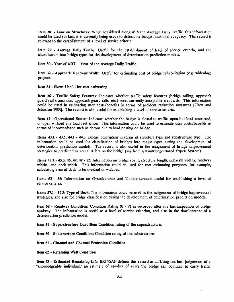
Item 28 - Lane on Structures: When considered along with the Average Daily Traffic, this information could be used (in fact, it is currently being used) to determine bridge functional adequacy. The record is relevant to the establishment of a level of service criteria.

Item 29 • Average Daily Traffic: Useful for the establishment of level of service criteria, and the classification into bridge types for the development of deterioration prediction models.

Item 30 - Year of ADT: Year of the Average Daily Traffic.

Item 32 • Approach Roadway Width: Useful for estimating cost of bridge rehabilitation (e.g. widening) projects.

Item 34 • Skew: Useful for cost estimating.

Item 36 • Traffic Sarety Features: Indicates whether traffic safety features (bridge railing, approach guard rail transitions, approach guard rails, etc.) meet currently acceptable standards. This information could be used in estimating user costs/benefits in terms of accident reduction measures [Chen and Johnston 1988]. The record is also useful for establishing a level of service criteria.

Item 41 • Operational Status: Indicates whether the bridge is closed to traffic, open but load restricted, or open without any load restriction. This information could be used to estimate user costs/benefits in terms of inconvenience such as detour due to load posting on bridge.

Items 43.1 • 43.5, 44.1 • 44.3: Bridge description in terms of structure type and substructure type. The information could be used for classification of bridges into major types during the development of deterioration prediction models. The record is also useful in the assignment of bridge improvement strategies to predicted or actual defect on the bridge (say from a Knowledge-Based Expert System).

Items 45.1 • 45.3, 46, 48. 49 • 52: Information on bridge spans, structure length, sidewalk widths, roadway widths, and deck width. This information could be used for cost estimating purposes, for example, calculating area of deck to be overlaid or widened.

Items 53 • 56: Information on Overclearance and Underclearance; useful for establishing a level of service criteria.

Items 57.1 - 57.3: type of Deck: The information could be used in the assignment of bridge improvement strategies, and also for bridge classification during the development of deterioration prediction models.

Item 58 • Roadway Condition: Condition Rating (0 - 9) as recorded after the last inspection of bridge roadway. The information is useful as a level of service criterion, and also in the development of a deterioration prediction model.

Item 59 • Superstructure Condition: Condition rating of the superstructure.

Item 60 • Substructure Condition: Condition rating of the substructure.

Item 61 • Channel and Channel Protection Condition

Item 62 • Retaining Wall Condition

Item 63 • Estimated Remaining Lire: BRINSAP defines this record as ... .'Using the best judgement of a "knowledgeable individual; an estimate of number of years the bridge can continue to carry traffic

205

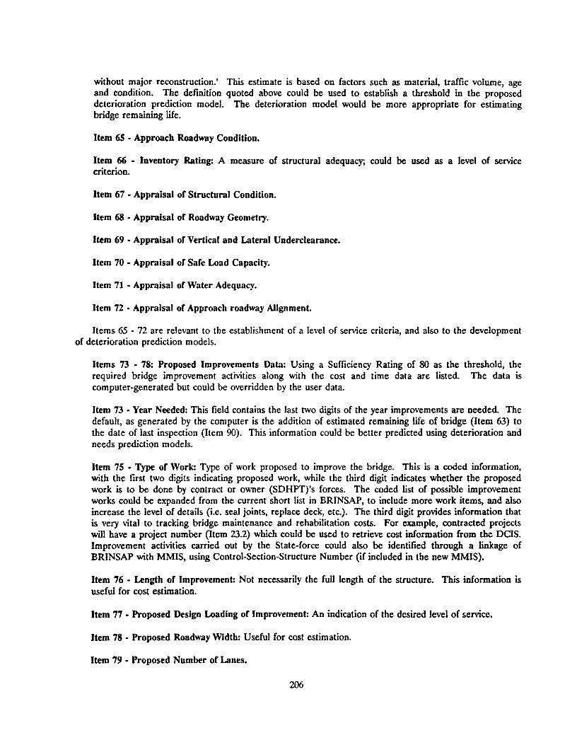
without major reconstruction.' This estimate is based on factors such as material, traffic volume, age and condition. The defmition quoted above could be used to establish a threshold in the proposed deterioration prediction model. The deterioration model would be more appropriate for estimating bridge remaining life.

Item 6S • Approach Roadway Condition.

Item 66 • Inventory Rating: A measure of structural adequacy; could be used as a level of service criterion.

Item 67 • Appraisal or Structural Condition.

Item 68 • Appraisal of Roadway Geometry.

Item 69 • Appraisal or Vertical and Lateral Underclearance.

Item 70 • Appraisal or Sare Load Capacity.

Item 71 • Appraisal or Water Adequacy.

Item 72 • Appraisal of Approach roadway Alignment.

Items 65 - 72 are relevant to the establishment of a level of service criteria, and also to the development of deterioration prediction models.

Items 73 • 78: Proposed Improvements Data: Using a Sufficiency Rating of 80 as the threshold, the required bridge improvement activities along with the cost and time data are listed. The data is computer-generated but could be overridden by the user data.

Item 73 - Year Needed: This field contains the last two digits of the year improvements are needed. The default, as generated by the computer is the addition of estimated remaining life of bridge (Item 63) to the date of last inspection (Item 90). This information couJd be better predicted using deterioration and needs prediction models.

Item 7S • Type of Work: Type of work proposed to improve the bridge. This is a coded information, with the first two digits indicating proposed work, while the third digit indicates whether the proposed work is to be done by contract or owner (SDHPT)'s forces. The coded list of possible improvement works could be expanded from the current short list in BRINSAP, to include more work items, and also increase the level of details (i.e. seal joints, replace deck, etc.). The third digit provides information that is very vital to tracking bridge maintenance and rehabilitation costs. For example, contracted projects will have a project number (Item 23.2) which could be used to retrieve cost information from the DCIS. Improvement activities carried out by the State-force could also be identified through a linkage of BRINSAP with MMIS, using Control-Sect ion-Structure Number (if included in the new MMIS).

Item 76 - Length of Improvement: Not necessarily the full length of the structure. This information is useful for cost estimation.

Item 77 • Proposed Design Loading of Improvement: An indication of the desired level of service.

Item 78 • Proposed Roadway Width: Useful for cost estimation.

Item 79 - Proposed Number of Lanes.

206

Items 82, 83 - Year and Type or Proposed Adjacent Roadway Improvement: Approaches to the bridge.

Item 84 - Total Cost or Improvements: Includes cost for approach roadway and other miscellaneous work.

Item 85 - Preliminary Engineering Cost.

Item 86 - Demolition Cost.

Item 87 - Substructure Cost.

Item 88 - Superstructure Cost.

Item 90 - Date or Last Inspection.

207

208

APPENDIX F. QUESTIONNAIRE ON MAINTENANCE EFFECTIVENESS

209

SECTION III • QUESTIONNAIRE FQR STUDY ON BRIDGE WORK ACfMTIES

Please evaluate the following bridge maintenance, rehabilitation, and replacement activities. Based on

your bridge engineering experience, indicate the importance of each activity considering its frequency of

application in terms of fraction of bridges under your jurisdiction which receive these treatments, in a typical

year, and also indicate the treatments' effectiveness in retarding the deterioration of bridges. Please use the

following scales for your assessment:

freQuens;y of Application (Fraction of all bridges)

A 0% - 5% of all bridges

B 6% - 10% of all bridges

C 11 % - 30% of all bridges

D 31 % - 50% of all bridges

E 51 % - 100% of aU bridges

1. ROADWAY

Effectiveness of Activity

1 Slightly effective

2 Effective

3 Very effective

A. DECK AND WEARING SURF8CE: Frs.9uenc): of Al2ulicatiQU Effectivel!ess

1. Washing of concrete bridge deck A B C D E 1 2

2. Linseed oil treatment A B C D E 1 2

3. Cathodic protection A B C D E 1 2

4. Partial-Depth patching A B C D E 1 2

5. fun-Depth patching A B C D E 1 2

6. Concrete overlay A B C D E 1 2

7. Widen deck A B C D E 1 2

8. Rotomill deck surface A B C D E 1 2

9. Bituminous surface overlay A B C D E 1 2

10. Crack sealing A B C D E 1 2

11. Maint. and/or rehab. of timber deck A B C D E 1 2

12. Maint. and/or rehab. of steel deck A B C D E 1 2

13. Replacement of deck A B C D E 1 2

210

3

3

3

3

3

3

3

3

3

3

3

3

3

B. JOINTS: Fregueng:: of AI!I2lication

1. Clean joint A B C D E

2. Seal or waterproof joint A B C D E

3. Replace joint A B C D E

4. Reset steel joint A B C D E

5. Misc. maint/or rehabilitation of joint A B C D E

C. DRAINAGE SYSTEM: Fregueng:: of Application

1. Clean drain opening ABC D E

2. Replace or rehabilitate drainage system ABC D E

D. CURBS, SIQEWALK, liARRIER. RAILINGS, ETC.:

1. Maint. or rehab. curb, sidewalk, parapet A B C D E

2. Paint median barrier A B C D E

3. Misc. repair of median barrier A B C D E

4. Replace median barrier A B C D E

5. Clean or paint railings A B C D E

6. Repair or rehab. bridge railings A B C D E

7. Replace railings A B C D E

Others for Roadway (Please specify): Fregyeng:: of App1i£i!tion

A B C D E

A B C D E

A B C D E

A B C D E

211

Effecliv~ne§§

1 2

1 2

1 2

1 2

1 2

Effectiveness

1

1

2

2

Eff~cliv~n~ss

1 2

1 2

1 2

1 2

1 2

1 2

1 2

Eff~ctiven£ss

1 2

1 2

1 2

1 2

3

3

3

3

3

3

3

3

3

3

3

3

3

3

3

3

3

3

2. SUPERSTRUCTURE

Fr~gys<n~ of AIU~1iS;i;ltion Eff$;;s;tivs<ne§s

1. dean steel I-Beam girder flanges A B C D E 1 2 3

2. Clean steel truss members A B C D E 1 2 3

3. Clean or paint structural steel A B C D E 1 2 3

4. Repair collision damage to steel member A B C D E 1 2 3

5. Repair connection damage in steel member A B C D E 1 2 3

6. Clean, lubricate and/or paint steel connect. A B C D E 1 2 3

7. Misc. structural repair of steel member A B C D E 1 2 3

8. Partial replacement of steel superstructure A B C D E 1 2 3

9. Repair collision damage - concrete member A B C D E 1 2 3

10. Repair concrete beam ends A B C D E 1 2 3

11. Partial replacement of concr. superstr. A B C D E 1 2 3

12. Repair timber superstructure A B C D E 1 2 3

13. Partial replacement of timber superstr. A B C D E 1 2 3

14. Reset or restore bearing A B C D E 1 2 3

15. Clean, paint, and/or lubricate bearing A B C D E 1 2 3

Others for Superstructure (Please specify): Fre!:!uenc~ of A1212licalion Effes;livens;s~

A B C D E 1 2 3

A B C D E 1 2 3

A B C D E 1 2 3

A B C D E 1 2 3

212

3. SUBSTRUCTURE

Fr~gu~nc):: Qf Aenlication sffe~iveness

1. Clean concrete pile cap A B C D E 1 2 3

2. Repair concrete pile cap A B C D E 1 2 3

3. Clean and paint steel pile cap A B C D E 1 2 3

4. Repair steel pile cap A B C D E 1 2 3

5. Repair timber pile cap A B C D E 1 2 3

6. Repair concrete piling A B C D E 1 2 3

7. Clean and paint steel piling A B C D E 1 2 3

8. Repair steel piling A B C D E 1 2 3

9. Repair timber piling A B C D E 1 2 3

10. Replace concrete piling A B C D E 1 2 3

11. Replace steel piling A B C D E 1 2 3

12. Replace timber piling A B C D E 1 2 3

13. Repair retaining wall A B C D E 1 2 3

14. Repair masonry substructure A B C D E 1 2 3

15. Repair collision protection A B C D E 1 2 3

16. Clean and paint collision protection A B C D E 1 2 3

17. Repair abutment A B C D E 1 2 3

18. Repair foundation problems A B C D E 1 2 3

19. General maintenance - substructure A B C D E 1 2 3

Others for Substructure (Please specify): Fr~guenc~ of Anl21i~Sltion sffectiv~n~~~

A B C D E 1 2 3

A B C D E 1 2 3

A B C D E 1 2 3

A B C D E 1 2 3

213

4. OTHERS (APPROACHES, BRlDGE·CLASSIFlED CULVERTS, SLOPES, CHANNEL. ETC.)

Fr!<gu~nQ: of A12121j~li!;!n Effe£tiveness

1. Erosion control A B C D E 1 2 3

2. Remove underbrush/debris from channel A B C D E 1 2 3

3. Repair approach (slab, shoulder) A B C D E 1 2 3

4. Replace approach slab A B C D E 1 2 3

5. Repair or replace slope protection A B C D E 1 2 3

6. Repair and/or reinforce embankment slope A B C D E 1 2 3

7. Repair/rehabilitate concrete culvert A B C D E 1 2 3

8. Replace concrete culvert A B C D E 1 2 3

9. Repair/rehabilitate steel culvert A B C D E 1 2 3

10. Replace steel culvert A B C D E 1 2 3

11. Remove silt from culvert A B C D E 1 2 3

12. Repair guard fence A B C D E 1 2 3

13. Repair traffic signs A B C D E 1 2 3

14. Repair illumination system A B C D E 1 2 3

15. Repair warning device A B C D E 1 2 3

16. Repair utility lines A B C D E 1 2 3

Others (Please specify): Freguenc!l of AImlis;alillD Effecliv~nes~

A B C D E 1 2 3

A B C D E 1 2 3

A B C D E 1 2 3

A B C D E 1 2 3

214

APPENDIX G. ANALYSIS OF MAINTENANCE EFFECTIVENESS

215

SECTION III • QUESTIONNAIRE FOR STUDY ON BRIDGE WQRK ACTOOTIES

Participants were requested to evaluate the a list of feasible bridge maintenance, rehabilitation, and

activity considering its frequency of application in terms of fraction of bridges under their jurisdiction which

receive these treatments, in a typical year, and they also indicated the treatments' effectiveness in retarding

the deterioration of bridges. The following scales were used for their assessment:

Frequen£)' of Application (Fraction of all bridges)

A 0% - 5% of aU bridges

B 6% - 10% of all bridges

C 11 % - 30% of all bridges

D 31% - 50% of all bridges

E 51 % - 100% of all bridges

Effectiveness of Activity

1 Slightly effective

~ Effective

J Very effective

A Rating was computed for each bridge improvement activity to reflect its importance in terms of its

frequency of application and its effectiveness, as judged by the bridge experts. The formula used in

computing these ratings is as follows:

1. Frequency of Application (using the notations in scale of assessment shown above) -

Rating = (A x 1.0) + (B x 2.0) + (C x 3.0) + (D x 4.0) + (E x 5.0)

2. Effectiveness of Activity (using the notations in scale of assessment shown above) -

Rating = ( (1 x 1.0) + (~x 2.0) + (;1 x 3.0) ) x (5.0/3.0)

216

CATEGORY I: BRIDGE ROADWAY I DECK

(i) Fraction of Responses on Annual Application of Bridge Maintenance

Bridge Maintenance Activity Apply to Apply to Apply to Apply to Apply to Computed 0-5% of 6-10% 11- 30% 31-50% > 51% Rating all bridges of all of all of all of all (1.0 - 5.0)

bridges bridges bridges bridges

1. Washing of concrete deck 0.90 0.05 0.05 - - 1.15

2. Linseed oil treatment 050 0.23 0.09 0.05 0.13 2.08

3. Cathodic protection 0.95 0.05 - - - 1.05

4. Partial-Depth patching 059 0.27 0.14 - - 155

5. Full-Depth patching 0.72 0.18 0.05 0.05 - 1.43

6. Concrete overlay 0.85 0.15 - - - 1.15

7. Widen deck 050 0.25 0.21 - 0.04 1.83

8. Rotomill deck surface 0.82 0.09 0.09 - - 1.27

9. Bituminous surface overlay 054 0.17 0.17 0.08 0.04 1.91

10 Crack sealing 0.65 0.17 0.13 0.04 - 154

11 Maint/rehab timber deck 0.94 0.06 - - - 1.06

12 Maint/rehab steel deck 1.00 - - - - 1.00

13 Replacement of deck 0.82 0.09 0.09 - - 1.27

14 Clean joint 0.61 0.09 0.17 0.13 - 1.82

15 Seal or waterproof joint 054 0.21 0.17 0.08 - 1.79

16 Replace joint 0.83 0.13 0.04 - - 1.21

17 Reset steel joint 0.95 0.05 - - - 1.05

18 Mise maint/rehab of joint 0.88 0.04 0.04 0.04 - 1.24

19 Oean drain opening 0.46 0.21 0.21 0.12 - 1.99

20 Replace/rehab drainage system 0.82 0.18 - - - 1.18

21 Maint/rehab curb, sidewalk, etc. 0.78 0.17 0.05 - - 1.27

22 Paint median barrier 0.82 0.18 - - - 1.18

23 Mise repair of median barrier 0.82 0.18 - - - 1.18

24 Replace median barrier 0.90 0.10 - - - 1.10

25 Oean or paint railings 058 0.25 0.17 - - 159

26 Repair/rehab railings 054 0.29 0.17 - - 1.63

27 Replace railings 0.67 0.21 0.08 0.04 - 1.49

217

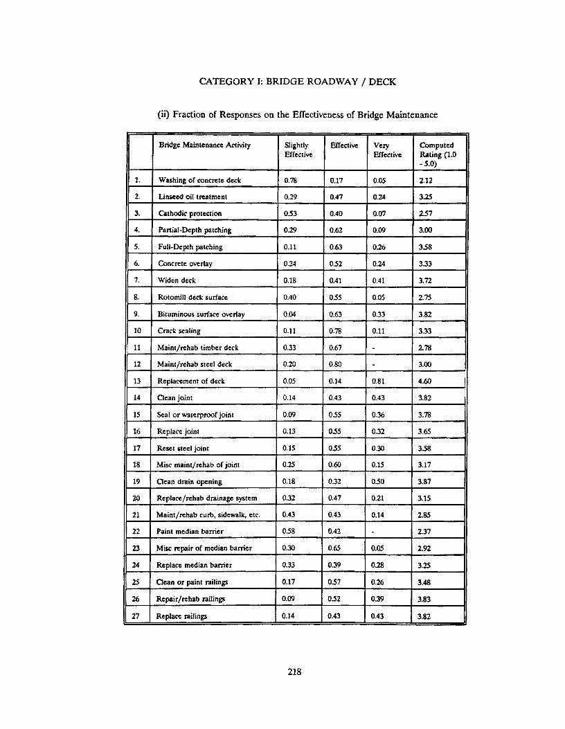
CATEGORY I: BRIDGE ROADWAY / DECK

(ii) Fraction of Responses on the Effectiveness of Bridge Maintenance

Bridge Maintenance Activity Slightly Effective Very Computed Effective Effective Rating (1.0

- 5.0)

1. Washing of concrete deck 0.78 0.17 O.OS 2.12

2. Linseed oil treatment 0.29 0.47 0.24 3.25

3. Cathodic protection 0.53 0.40 0.07 2.57

4. Partial-Depth patching 0.29 0.62 0.09 3.00

S. Full-Depth patching 0.11 0.63 0.26 3.58

6. Concrete overlay 0.24 0.52 0.24 3.33

7. Widen deck 0.18 0.41 0.41 3.72

8. Rotomill deck surface 0.40 O.5S 0.05 2.75

9. Bituminous surface overlay 0.04 0.63 0.33 3.82

10 Crack sealing 0.11 0.78 0.11 3.33

11 Maint/rehab timber deck 0.33 0.67 - 2.78

12 Maint/rehab steel deck 0.20 0.80 - 3.00

13 Replacement of deck 0.05 0.14 0.81 4.60

14 aean joint 0.14 0.43 0.43 3.82

15 Seal or waterproof joint 0.09 0.55 0.36 3.78

16 Replace joint 0.13 0.55 0.32 3.65

17 Reset steel joint 0.15 0.55 0.30 3.58

18 Mise maint/rehab of joint 0.25 0.60 0.15 3.17

19 aean drain opening 0.18 0.32 0.50 3.87

20 Replace/rehab drainage system 0.32 0.47 0.21 3.1.5

21 Maint/rehab cum, sidewalk, etc. 0.43 0.43 0.14 2.85

22 Paint median barrier 0.58 0.42 - 2.37

23 Mise repair of median barrier 0.30 0.65 0.05 2.92

24 Replace median barrier 0.33 0.39 0.28 3.25

2S aCln or paint railings 0.17 0.57 0.26 3.48

[26 Repair/rehab railings 0.09 0.52 0.39 3.83

27 Replace railings 0.14 0.43 0.43 3.82

218

CATEGORY II: BRIDGE SUPERSTRUcrURE

(i) Fraction of Responses on Annual Application of Bridge Maintenance

Bridge Maintenance Activity Apply to Apply to Apply to Apply to Apply to Computed 0-5% of 6-10% 11-30% 31-50% > 51% Rating (1.0 all bridges of all of all of all of all - 5.0)

bridges bridges bridges bridges

1 Clean steel I-Beam girder 0.81 0.14 O.OS - - 1.24

2 Clean steel truss members 0.90 O.OS O.OS · - 1.15

3 Oean or paint structural steel 0.61 0.30 0.09 · - 1.48

4 Repair collision damage (steel) 0.66 0.24 O.OS - O.OS 1.54

5 Repair connect. damage (steel) 0.76 0.14 O.OS · 0.05 1.44

6 Oean/ lubricate/ paint steel 0.81 0.14 0.05 - - 1.24 connection

7. Mise structural repair (steel) 0.86 0.09 0.05 - . 1.19

8. Partial replacement of steel 0.90 0.10 - - - 1.10 superstructure

9 Repair collision damage (cone.) 0.77 0.09 0.09 - O.OS 1.47

10 Repair concrete beams ends 0.76 0.19 - O.OS - 1.34

11 Partial replacement of concrete 0.83 0.13 0.04 - - 1.21 superstructure

12 Repair timber superstructure 0.90 0.10 - · . 1.10

13 Partial replacement of timber 0.89 0.11 - - - 1.11 superstructure

14 Reset or restore bearing 0.82 0.14 0.04 - - 1.22

15 Clean/ paint/ lubricate bearing 0.81 0.14 O.OS - - 1.24

219

CATEGORY II: BRIDGE SUPERSTRUcrURE

(ii) Fraction of Responses on the Effectiveness of Bridge Maintenance

Bridge Maintenance Activity Slightly Effective Very Computed Effective Effective Rating (1.0

- S.O)

1 Oean steel I-Beam girder 0.26 0.42 0.32 3.43

2 Oean steel truss members 0.22 0.56 0.22 3.33

3 Oean or paint structural steel 0.14 0.19 0.67 4.22

4 Repair collision damage (steel) 0.10 0.35 O.5S 4.08

S Repair connect. damage (steel) 0.15 0.35 0.50 3.92

6 Oean/ lubricate/ paint steel 0.21 0.53 0.26 3.42 connection

7. Mise structural repair (steel) 0.11 0.56 0.33 3.70

8. Partial replacement of steel 0.11 0.50 0.39 3.80 superstructure

9 Repair collision damage (cone.) 0.05 0.62 0.33 3.80

10 Repair concrete beams ends 0.35 0.30 0.35 3.33

11 Partial replacement of concrete 0.14 0.57 0.29 3.58 superstructure

12 Repair timber superstructure 0.25 0.50 0.25 3.33

13 Partial replacement of timber 0.33 0.54 0.13 3.00 superstructure

14 Reset or restore bearing 0.14 0.53 0.33 3.65

15 Oean/ paint/ lubricate bearing 0.21 0.53 0.26 3.42

220

CATEGORY III: BRIDGE SUBSTRUCfURE

(i) Fraction of Responses on Annual Application of Bridge Maintenance

Bridge Maintenance Activity Apply to Apply to Apply to Apply to Apply to Computed 0- 5% of 6-10% 11- 30% 31-50% > 51% Rating (1.0 all bridges of all of all or all of all -S.O)

bridges bridges bridges bridges

1 Cean concrete pile cap 0.76 0.19 - 0.05 - 1.34

2 Repair concrete pile cap 0.83 0.13 -. 0.04 - 1.25

3 Cean and paint steel pile cap 0.86 0.09 0.05 - - 1.19 . 4 Repair steel pile cap 0.86 0.14 - - - 1.14

5 Repair timber pile cap 0.90 0.10 - - - 1.10

6 Repair concrete piling 0.86 0.09 0.05 - - 1.19

7. Cean and paint steel piling 0.82 0.08 O.OS 0.05 - 1.33

8. Repair steel piling 0.81 0.14 0.05 - - 1.24

9 Repair timber piling 0.95 0.05 - - - 1.05

10 Replace concrete piling 0.90 O.OS - 0.05 - 1.20

11 Replace steel piling 0.80 0.15 0.05 - - 1.25

12 Replace timber piling 0.90 0.10 - - - 1.10

13 Repair retaining wall 0.74 0.22 0.04 - - 1.30

14 Repair masonry substructure 0.90 0.10 - - - 1.10

1lE- Repair collision protection 0.81 O.OS 0.09 - O.OS 1.43

16 Cean and paint collision 0.95 0.05 - - - 1.05 protection

17 Repair abutment 0.78 0.17 O.OS - - 1.27

18 Repair foundation problems 0.82 0.10 0.04 0.04 - 1.30

19 General maintenance 0.78 0.14 0.04 0.04 - 1.34

221

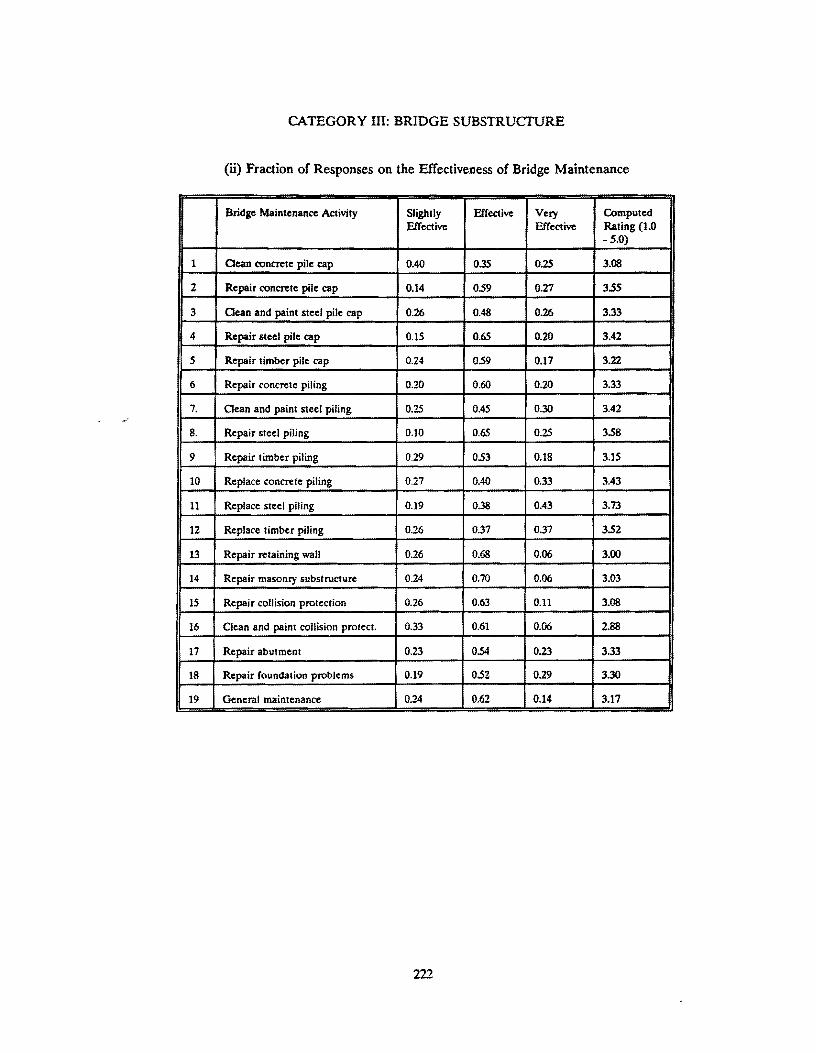
CATEGORY III: BRIDGE SUBSTRUcrURE

(ii) Fraction of Responses on the Effectiveness of Bridge Maintenance

Bridge Maintenance Activity Slightly Effective Very Computed Effective Effective Rating (1.0

-S.O)

1 Oean concrete pile cap 0.40 0.35 0.25 3.08

2 Repair concrete pile cap 0.14 0.59 0.27 3.55

3 Oean and paint steel pile cap 0.26 0.48 0.26 3.33

4 Repair steel pile cap 0.15 0.65 0.20 3.42

5 Repair timber pile cap 0.24 0.59 0.17 3.22

6 Repair concrete piling 0.20 0.60 0.20 3.33

7. Oean and paint steel piling 0.25 0.45 0.30 3.42

8. Repair steel piling 0.10 0.65 0.25 3.58

9 Repair timber piling 0.29 0.53 0.18 3.15

10 Replace concrete piling 0.27 0.40 0.33 3.43

11 Replace steel piling 0.19 0.38 0.43 3.73

12 Replace timber piling 0.26 0.37 0.37 3.52

13 Repair retaining wall 0.26 0.68 0.06 3.00

14 Repair masonry substructure 0.24 0.70 0.06 3.03

15 Repair collision protection 0.26 0.63 0.11 3.08

16 Clean and paint collision protect. 0.33 0.61 0.06 2.88

17 Repair abutment 0.23 0.54 0.23 3.33

18 Repair foundation problems 0.19 0.52 0.29 3.30

19 General maintenance 0.24 0.62 0.14 3.17

222

CATEGORY IV: OTHERS (APPROACHES, CULVERTS, SLOPES, CHANNELS, ETC.)

(i) Fraction of Responses on Annual Application of Bridge Maintenance

Bridge Maintenance Activity Apply to Apply to Apply to Apply to Apply to Computed o -5%of 6-10% 11- 30% 31- SO% > 51% Rating (1.0 all bridges of all of all of all of all - 5.0)

bridges bridges bridges bridges

1 Erosion control 0.48 0.22 0.30 - - 1.82

2 Remove debris from channel 0.36 0.36 0.23 0.05 - 1.97

3 Repair approach (slab, shoulder) 0.64 0.23 0.13 - - 1.49

4 Replace approach slab 0.90 0.10 - - - 1.10

5 Repair or replace slope protection 0.82 0.09 0.09 - - 1.27

6 Repair/ reinf. embankment slope 0.90 0.05 0.05 - - 1.15

7. Repair / rehab concrete culvert 0.90 0.05 0.05 - - 1.15

8. Replace concrete culvert 0.90 0.05 0.05 - - 1.15

9 Repair/ rehab steel culvert 1.00 - - - - 1.00

10 Replace steel culvert 0.95 0.05 - - - 1.05

11 Remove silt form culvert 0.74 0.09 0.17 - - 1.43

12 Repair guard fence 0.26 0.30 0.35 0.09 - 2.27

13 Repair traffic signs 0.33 0.14 0.38 0.10 0.05 2.40

14 Repair illumination system 0.67 0.14 0.14 - 0.05 1.62

15 Repair warning devices 0.60 0.10 0.20 0.05 0.05 1.85

16 Repair utility lines 0.79 0.16 0.05 - - 1.26

223

CATEGORY IV: OTHERS (APPROACHES, CULVERTS, SWPES, CHANNELS. ETC.)

(ii) Fraction of Responses on the Effectiveness of Bridge Maintenance

Bridge Maintenance Activity Slightly Effective Very Computed Effective Effective Rating (1.0

.S.O)

1 Erosion control 0.23 0.54 0.23 3.33

2 Remave debris (rom channel 0.24 0.48 0.28 3.40

3 Repair approach (slab, shoulder) 0.19 0.62 0.19 3.33

4 Replace approach slab 0.17 0.44 039 3.70

5 Repair or replace slope protection 0.29 0.48 0.29 3.23

6 Repair! reine. embankment slope 0.32 0.58 0.10 2.97

7. Repair ! rehab concrete culvert 0.16 0.63 0.21 3.42

8. Replace concrete culvert 0.05 0.50 0.45 4.00

9 Repair! rehab steel culvert 0.38 0.50 0.12 2.90

10 Replace steel culvert 0.19 0.44 0.37 3.63

11 Remove silt form culvert 0.33 0.57 0.10 2.95

12 I n~I"''' guard fence 0.25 0.45 I 0.30 3.42

13 Repair traffic signs 0.30 0.45 0.25 3.25

I 14 Repair illumination system 0.28 0.50 0.22 3.23

15 Repair warning devices 0.28 0.50 0.22 3.23

16 Repair utility lines 0.44 0.44 0.12 2.80

224