Comprehensive Risk Assessment for Natural Hazards

Comprehensive Risk Assessmentfor Natural Hazards

WMO/TD No. 955

Reprinted 2006

The designations employed and the presentation of material in thispublication do not imply the expression of any opinion whatsoever on thepart of any of the participating agencies concerning the legal status of anycountry, territory, city or area, or of its authorities, or concerning thedelimitation of its frontiers or boundaries.

Cover photos: Schweizer Luftwaffe, Randy H. Williams, DigitalGlobe

© 1999, World Meteorological Organization

WMO/TD No. 955

Reprinted 2006

NOTE

Page

AAUUTTHHOORRSS AANNDD EEDDIITTOORRSS . . . . . . . . . . . . . . . . . . . . . v

FOREWORD . . . . . . . . . . . . . . . . . . . . . . . . . . . . . . . . . . vii

CHAPTER 1 — INTRODUCTION . . . . . . . . . . . . . . . 1

1.1 Project history . . . . . . . . . . . . . . . . . . . . . . . . . . . . . 11.2 Framework for risk assessment . . . . . . . . . . . . . . . 2

1.2.1 Definition of terms . . . . . . . . . . . . . . . . . . . 21.2.2 Philosophy of risk assessment . . . . . . . . . . 21.2.3 Risk aversion . . . . . . . . . . . . . . . . . . . . . . . . 4

1.3 The future . . . . . . . . . . . . . . . . . . . . . . . . . . . . . . . . . 41.4 References . . . . . . . . . . . . . . . . . . . . . . . . . . . . . . . . . 5

CHAPTER 2 — METEOROLOGICAL HAZARDS . . 6

2.1 Introduction . . . . . . . . . . . . . . . . . . . . . . . . . . . . . . . 62.2 Description of the event . . . . . . . . . . . . . . . . . . . . . 6

2.2.1 Tropical storm . . . . . . . . . . . . . . . . . . . . . . . 62.2.2 Necessary conditions for tropical storm

genesis . . . . . . . . . . . . . . . . . . . . . . . . . . . . . 62.3 Meteorological hazards assessment . . . . . . . . . . . 7

2.3.1 Physical characteristics . . . . . . . . . . . . . . . . 72.3.1.1 Tropical storms . . . . . . . . . . . . . . . 82.3.1.2 Extratropical storms . . . . . . . . . . . 8

2.3.2 Wind . . . . . . . . . . . . . . . . . . . . . . . . . . . . . 82.3.3 Rain loads . . . . . . . . . . . . . . . . . . . . . . . . . . . 82.3.4 Rainfall measurements . . . . . . . . . . . . . . . . 92.3.5 Storm surge . . . . . . . . . . . . . . . . . . . . . . . . . 92.3.6 Windwave . . . . . . . . . . . . . . . . . . . . . . . . . . . 92.3.7 Extreme precipitation . . . . . . . . . . . . . . . . . 10

2.3.7.1 Rain . . . . . . . . . . . . . . . . . . . . . . . . . 102.3.7.2 Snow and hail . . . . . . . . . . . . . . . . . 102.3.7.3 Ice loads . . . . . . . . . . . . . . . . . . . . . 10

2.3.8 Drought . . . . . . . . . . . . . . . . . . . . . . . . . . . . . 102.3.9 Tornadoes . . . . . . . . . . . . . . . . . . . . . . . . . . . 102.3.10 Heatwaves . . . . . . . . . . . . . . . . . . . . . . . . . . . 11

2.4 Techniques for hazard analysis and forecasting . . . . . . . . . . . . . . . . . . . . . . . . . . . . . . . . 112.4.1 Operational techniques . . . . . . . . . . . . . . . 112.4.2 Statistical methods . . . . . . . . . . . . . . . . . . . 12

2.5 Anthropogenic influence on meteorological hazards . . . . . . . . . . . . . . . . . . . . . . . . . . . . . . . . . . . 14

2.6 Meteorological phenomena: risk assessment . . . 142.6.1 General . . . . . . . . . . . . . . . . . . . . . . . . . . . . . 142.6.2 Steps in risk assessment . . . . . . . . . . . . . . . 152.6.3 Phases of hazard warning . . . . . . . . . . . . . 15

2.6.3.1 General preparedness . . . . . . . . . . 152.6.3.2 The approach of the

phenomenon . . . . . . . . . . . . . . . . . 152.6.3.3 During the phenomenon . . . . . . . 152.6.3.4 The aftermath . . . . . . . . . . . . . . . . 16

Page

2.7 Conclusion . . . . . . . . . . . . . . . . . . . . . . . . . . . . . . . . 162.8 Glossary of terms . . . . . . . . . . . . . . . . . . . . . . . . . . 162.9 References . . . . . . . . . . . . . . . . . . . . . . . . . . . . . . . . . 16

CHAPTER 3 — HYDROLOGICAL HAZARDS . . . . 18

3.1 Introduction . . . . . . . . . . . . . . . . . . . . . . . . . . . . . 183.2 Description of the hazard . . . . . . . . . . . . . . . . . . . 183.3 Causes of flooding and flood hazards . . . . . . . . . 19

3.3.1 Introduction . . . . . . . . . . . . . . . . . . . . . . . . . 193.3.2 Meteorological causes of river floods and

space-time characteristics . . . . . . . . . . . . . 203.3.3 Hydrological contributions to floods . . . . 203.3.4 Coastal and lake flooding . . . . . . . . . . . . . 213.3.5 Anthropogenic factors, stationarity, and

climate change . . . . . . . . . . . . . . . . . . . . . . . 213.4 Physical characteristics of floods . . . . . . . . . . . . . 21

3.4.1 Physical hazards . . . . . . . . . . . . . . . . . . . . . . 213.4.2 Measurement techniques . . . . . . . . . . . . . . 21

3.5 Techniques for flood hazard assessment . . . . . . . 223.5.1 Basic principles . . . . . . . . . . . . . . . . . . . . . . 223.5.2 Standard techniques for watersheds with

abundant data . . . . . . . . . . . . . . . . . . . . . . . 233.5.3 Refinements to the standard

techniques . . . . . . . . . . . . . . . . . . . . . . . . . . . 243.5.3.1 Regionalization . . . . . . . . . . . . . . . 243.5.3.2 Paleoflood and historical data . . . 25

3.5.4 Alternative data sources and methods . . . 253.5.4.1 Extent of past flooding . . . . . . . . . 253.5.4.2 Probable maximum flood and

rainfall-runoff modelling . . . . . . . 253.5.5 Methods for watersheds with limited

streamflow data . . . . . . . . . . . . . . . . . . . . . . 263.5.6 Methods for watersheds with limited

topographic data . . . . . . . . . . . . . . . . . . . . . 263.5.7 Methods for watersheds with no data . . . 26

3.5.7.1 Estimation of flood discharge . . . 263.5.7.2 Recognition of areas subject to

inundation . . . . . . . . . . . . . . . . . . . 263.5.8 Lakes and reservoirs . . . . . . . . . . . . . . . . . . 263.5.9 Storm surge and tsumani . . . . . . . . . . . . . . 26

3.6 Flood risk assessment . . . . . . . . . . . . . . . . . . . . . . . 273.7 Data requirements and sources . . . . . . . . . . . . . . . 273.8 Anthropogenic factors and climate change . . . . 28

3.8.1 Anthropogenic contributions to flooding . . . . . . . . . . . . . . . . . . . . . . . . . . . . . 28

3.8.2 Climate change and variability . . . . . . . . . 283.9 Practical aspects of applying the

techniques . . . . . . . . . . . . . . . . . . . . . . . . . . . . . . . . 293.10 Presentation of hazard assessments . . . . . . . . . . . 293.11 Related preparedness schemes . . . . . . . . . . . . . . . 303.12 Glossary of terms . . . . . . . . . . . . . . . . . . . . . . . . . . 303.13 References . . . . . . . . . . . . . . . . . . . . . . . . . . . . . . . . . 31

CONTENTS

Page

CHAPTER 4 — VOLCANIC HAZARDS . . . . . . . . . . 34

4.1 Introduction to volcanic risks . . . . . . . . . . . . . . . . 344.2 Description and characteristics of the main

volcanic hazards . . . . . . . . . . . . . . . . . . . . . . . . . . . 364.2.1 Direct hazards . . . . . . . . . . . . . . . . . . . . . . . 364.2.2 Indirect hazards . . . . . . . . . . . . . . . . . . . . . . 37

4.3 Techniques for volcanic hazard assessment . . . . 374.3.1 Medium- and long-term hazard

assessment: zoning . . . . . . . . . . . . . . . . . . . 374.3.2 Short-term hazard assessment:

monitoring . . . . . . . . . . . . . . . . . . . . . . . . . . 384.4 Data requirements and sources . . . . . . . . . . . . . . . 39

4.4.1 Data sources . . . . . . . . . . . . . . . . . . . . . . . . . 394.4.2 Monitoring — Data management . . . . . . 39

4.5 Practical aspects of applying the techniques . . . 404.5.1 Practice of hazard zoning mapping . . . . . 404.5.2 Practice of monitoring . . . . . . . . . . . . . . . . 41

4.6 Presentation of hazard and risk assessment maps . . . . . . . . . . . . . . . . . . . . . . . . . . . 41

4.7 Related mitigation scheme . . . . . . . . . . . . . . . . . . . 414.8 Glossary of terms . . . . . . . . . . . . . . . . . . . . . . . . . . 424.9 References . . . . . . . . . . . . . . . . . . . . . . . . . . . . . . . . . 44

CHAPTER 5 — SEISMIC HAZARDS . . . . . . . . . . . . . 46

5.1 Introduction . . . . . . . . . . . . . . . . . . . . . . . . . . . . . 465.2 Description of earthquake hazards . . . . . . . . . . . 465.3 Causes of earthquake hazards . . . . . . . . . . . . . . . . 48

5.3.1 Natural seismicity . . . . . . . . . . . . . . . . . . . . 485.3.2 Induced seismicity . . . . . . . . . . . . . . . . . . . 48

5.4 Characteristics of earthquake hazards . . . . . . . . . 495.4.1 Application . . . . . . . . . . . . . . . . . . . . . . . . . . 495.4.2 Ground shaking . . . . . . . . . . . . . . . . . . . . . . 495.4.3 Surface faulting . . . . . . . . . . . . . . . . . . . . . . 495.4.4 Liquefaction . . . . . . . . . . . . . . . . . . . . . . . . . 495.4.5 Landslides . . . . . . . . . . . . . . . . . . . . . . . . . . . 495.4.6 Tectonic deformation . . . . . . . . . . . . . . . . . 49

5.5 Techniques for earthquake hazard assessment . . 505.5.1 Principles . . . . . . . . . . . . . . . . . . . . . . . . . . . 505.5.2 Standard techniques . . . . . . . . . . . . . . . . . . 505.5.3 Refinements to standard techniques . . . . 515.5.4 Alternative techniques . . . . . . . . . . . . . . . . 53

5.6 Data requirements and sources . . . . . . . . . . . . . . . 535.6.1 Seismicity data . . . . . . . . . . . . . . . . . . . . . . . 535.6.2 Seismotectonic data . . . . . . . . . . . . . . . . . . 535.6.3 Strong ground motion data . . . . . . . . . . . . 535.6.4 Macroseismic data . . . . . . . . . . . . . . . . . . . . 545.6.5 Spectral data . . . . . . . . . . . . . . . . . . . . . . . . . 545.6.6 Local amplification data . . . . . . . . . . . . . . . 54

5.7 Anthropogenic factors . . . . . . . . . . . . . . . . . . . . . . 545.8 Practical aspects . . . . . . . . . . . . . . . . . . . . . . . . . . . 545.9 Presentation of hazard assessments . . . . . . . . . . . 54

5.9.1 Probability terms . . . . . . . . . . . . . . . . . . . . . 54

Page

5.9.2 Hazard maps . . . . . . . . . . . . . . . . . . . . . . . . 545.9.3 Seismic zoning . . . . . . . . . . . . . . . . . . . . . . . 55

5.10 Preparedness and mitigation . . . . . . . . . . . . . . . . . 555.11 Glossary of terms . . . . . . . . . . . . . . . . . . . . . . . . . . 555.12 References . . . . . . . . . . . . . . . . . . . . . . . . . . . . . . . . . 59

CHAPTER 6 — HAZARD ASSESSMENT AND LAND-USE PLANNING IN SWITZERLAND FOR SNOW AVALANCHES, FLOODS AND LANDSLIDES . . . . . 61

6.1 Switzerland: A hazard-prone country . . . . . . . . . 616.2 Regulations . . . . . . . . . . . . . . . . . . . . . . . . . . . . . . . . 616.3 Hazard management . . . . . . . . . . . . . . . . . . . . . . . 62

6.3.1 Hazard identification: What might happen and where? . . . . . . . . . . . . . . . . . . . 62

6.3.2 The hazard assessment: How and when can it happen? . . . . . . . . . . . . . . . . . . 62

6.4 Codes of practice for land-use planning . . . . . . . 646.5 Concluding remarks . . . . . . . . . . . . . . . . . . . . . . . . 646.6 References . . . . . . . . . . . . . . . . . . . . . . . . . . . . . . . . . 64

CHAPTER 7— ECONOMIC ASPECTS OF VULNERABILITY . . . . . . . . . . . . . . . . . . . . . . . . . . . . . 667.1 Vulnerability . . . . . . . . . . . . . . . . . . . . . . . . . . . . . 667.2 Direct damages . . . . . . . . . . . . . . . . . . . . . . . . . . . . 67

7.2.1 Structures and contents . . . . . . . . . . . . . . . 677.2.2 Value of life and cost of injuries . . . . . . . . 68

7.3 Indirect damages . . . . . . . . . . . . . . . . . . . . . . . . . . . 717.3.1 General considerations . . . . . . . . . . . . . . . . 717.3.2 The input-output (I-O) model . . . . . . . . . 71

7.4 Glossary of terms . . . . . . . . . . . . . . . . . . . . . . . . . . 747.5 References . . . . . . . . . . . . . . . . . . . . . . . . . . . . . . . . . 76

CHAPTER 8 — STRATEGIES FOR RISK ASSESSMENT — CASE STUDIES . . . . . . . . . . . . . . . 77

8.1 Implicit societally acceptable hazards . . . . . . . . . 778.2 Design of coastal protection works in The

Netherlands . . . . . . . . . . . . . . . . . . . . . . . . . . . . . . . 788.3 Minimum life-cycle cost earthquake design . . . . 79

8.3.1 Damage costs . . . . . . . . . . . . . . . . . . . . . . . . 818.3.2 Determination of structural damage

resulting from earthquakes . . . . . . . . . . . . 828.3.3 Earthquake occurrence model . . . . . . . . . 82

8.4 Alternative approaches for risk-based flood management . . . . . . . . . . . . . . . . . . . . . . . . . . . . . . . 838.4.1 Risk-based analysis for flood-damage-

reduction projects . . . . . . . . . . . . . . . . . . . . 838.4.2 The Inondabilité method . . . . . . . . . . . . . . 85

8.5 Summary and conclusions . . . . . . . . . . . . . . . . . . 888.6 Glossary of terms . . . . . . . . . . . . . . . . . . . . . . . . . . 898.7 References . . . . . . . . . . . . . . . . . . . . . . . . . . . . . . . . . 91

Contentsiv

AUTHORS:

Chapter 1

Charles S. Melching United States of America

Paul J. Pilon Canada

Chapter 2

Yadowsun Boodhoo Mauritius

Chapter 3

Renée Michaud (Mrs) United States of America


Chapter 4

Laurent Stiltjes France

Jean-Jacques Wagner Switzerland

Chapter 5

Dieter Mayer-Rosa Switzerland

Chapter 6

Olivier Lateltin Switzerland

Christoph Bonnard Switzerland

Chapter 7


Chapter 8


EDITORS:



AUTHORS AND EDITORS

The International Decade for Natural Disaster Reduction(IDNDR), launched as a global event on 1 January 1990, isnow approaching its end. Although the decade has hadmany objectives, one of the most important has been towork toward a shift of focus from post-disaster relief andrehabilitation to improved pre-disaster preparedness. TheWorld Meteorological Organization (WMO), as the UnitedNations specialized agency dedicated to the mitigation ofdisasters of meteorological and hydrological origin, hasbeen involved in the planning and implementation of theDecade. One of the special projects undertaken by WMO asa contribution to the Decade has been the compilation andpublication of the report you are now holding in yourhands; the Comprehensive Risk Assessment for NaturalHazards.

The IDNDR called for a comprehensive approach indealing with natural hazards. This approach would thusneed to include all aspects relating to hazards, including riskassessment, land use planning, design codes, forecastingand warning systems, disaster preparedness, and rescue andrelief activities. In addition to that, it should also be com-prehensive in the sense of integrating efforts to reducedisasters resulting from tropical cyclones, storm surges,river flooding, earthquakes and volcanic activity. Using thiscomprehensive interpretation, the Eleventh Congress ofWMO and the Scientific and Technical Committee for theIDNDR both endorsed the project to produce this import-ant publication. In the WMO Plan of Action for the IDNDR,the objective was defined as “to promote a comprehensiveapproach to risk assessment and thus enhance the effective-ness of efforts to reduce the loss of life and damage causedby flooding, by violent storms and by earthquakes”.

A special feature of this report has been the involve-ment of four different scientific disciplines in its production.Such interdisciplinary cooperation is rare, and it has indeedbeen a challenging and fruitful experience to arrange for co-operation between experts from the disciplines involved.Nothing would have been produced, however, if it were notfor the hard and dedicated work of the individual expertsconcerned. I would in particular like to extend my sinceregratitude to the editors and the authors of the various chap-ters of the report.

Much of the work on the report was funded fromWMO’s own resources. However, it would not have beenpossible to complete it without the willingness of the vari-ous authors to give freely of their time and expertise and thegenerous support provided by Germany, Switzerland andthe United States of America.

The primary aim of this report is not to propose thedevelopment of new methodologies and technologies. Theemphasis is rather on identifying and presenting the variousexisting technologies used to assess the risks for natural dis-asters of different origins and to encourage theirapplication, as appropriate, to particular circumstancesaround the world. A very important aspect of this report isthe promotion of comprehensive or joint assessment of riskfrom a variety of possible natural activities that could occurin a region. At the same time, it does identify gaps wherethere is a need for enhanced research and development. Bypresenting the technologies within one volume, it is possibleto compare them, for the specialists from one discipline tolearn from the practices of the other disciplines, and for thespecialists to explore possibilities for joint or combinedassessments in some regions.

It is, therefore, my sincere hope that the publication willoffer practical and user friendly proposals as to how assess-ments may be conducted and provide the benefits ofconducting comprehensive risk assessments on a local,national, regional and even global scale. I also hope that themethodologies presented will encourage multidisciplinaryactivities at the national level, as this report demonstratesthe necessity of and encourage co-operative measures inorder to address and mitigate the effects of natural hazards.

FOREWORD

(G.O.P. Obasi)Secretary-General

1.1 PROJECT HISTORY

In December 1987, the United Nations General Assemblyadopted Resolution 42/169 which proclaimed the 1990s asthe International Decade for Natural Disaster Reduction(IDNDR). During the Decade a concerted internationaleffort has been made to reduce the loss of life, destruction ofproperty, and social and economic disruption causedthroughout the world by the violent forces of nature.Heading the list of goals of the IDNDR, as given in theUnited Nations resolution, is the improvement of the capac-ity of countries to mitigate the effects of natural disasterssuch as those caused by earthquakes, tropical cyclones,floods, landslides and storm surges.

As stated by the Secretary-General in the Foreword tothis report, the World Meteorological Organization (WMO)has a long history of assisting the countries of the world tocombat the threat of disasters of meteorological and hydro-logical origin. It was therefore seen as very appropriate forWMO to take a leading role in joining with other interna-tional organizations in support of the aims of the IDNDR.The forty-fourth session of the United Nations GeneralAssembly in December 1989 adopted Resolution 44/236.This resolution provided the objective of the IDNDR whichwas to “reduce through concerted international action,especially in developing countries, the loss of life, propertydamage, and social and economic disruption caused by nat-ural disasters, such as earthquakes, windstorms, tsunamis,floods, landslides, volcanic eruptions, wildfires, grasshopperand locust infestations, drought and desertification andother calamities of natural origin.” One of the fine goals ofthe decade as adopted at this session was “to develop mea-sures for the assessment, prediction, prevention andmitigation of natural disasters through programmes oftechnical assistance and technology transfer, demonstrationprojects, and education and training, tailored to specific dis-asters and locations, and to evaluate the effectiveness ofthose programmes” (United Nations General Assembly,1989).

The IDNDR, therefore, calls for a comprehensiveapproach to disaster reduction; comprehensive in that plansshould cover all aspects including risk assessment, land-useplanning, design codes, forecasting and warning, disaster-preparedness, and rescue and relief activities, butcomprehensive also in the sense of integrating efforts toreduce disasters resulting from tropical cyclones, stormsurges, river flooding, earthquakes, volcanic activity and thelike. It was with this in mind that WMO proposed the devel-opment of a project on comprehensive risk assessment as aWMO contribution to the Decade. The project has as itsobjective: “to promote a comprehensive approach to riskassessment and thus enhance the effectiveness of efforts toreduce the loss of life and damage caused by flooding, byviolent storms, by earthquakes, and by volcanic eruptions.”

This project was endorsed by the Scientific andTechnical Committee (STC) for the IDNDR when it met for

its first session in Bonn in March 1991 and was included inthe STC’s list of international demonstration projects. Thisproject was subsequently endorsed by the WMO ExecutiveCouncil and then by the Eleventh WMO Congress in May1991. It appears as a major component of the Organization’sPlan of Action for the IDNDR that was adopted by theWMO Congress.

In March 1992, WMO convened a meeting of expertsand representatives of international organizations to developplans for the implementation of the project. At that time theobjective of the project was to promote the concept of atruly comprehensive approach to the assessment of risksfrom natural disasters. In its widest sense such an approachshould include all types of natural disaster. However, it wasdecided to focus on the most destructive and most wide-spread natural hazards, namely those of meteorological,hydrological, seismic, and/or volcanic origin. Hence theproject involves the four disciplines concerned. Two of thesedisciplines are housed within WMO itself, namely hydrologyand meteorology. Expertise on the other disciplines wasprovided through contacts with UNESCO and with the international non-governmental organizationsInternational Association of Seismology and Physics ofthe Earth’s Interior (IASPEI) and International Associationof Volcanology and Chemistry of the Earth’s Interior(IACEI).

One special feature of the project was the involvementof four scientific disciplines. This provided a rare opportu-nity to assess the similarities and the differences betweenthe approaches these disciplines take and the technologythey use, leading to a possible cross–fertilization of ideasand an exchange of technology. Such an assessment is fun-damental when developing a combined or comprehensiverisk assessment of various natural hazards. This featureallows the probabilistic consideration of combined hazards,such as flooding in association with volcanic eruptions orearthquakes and high winds.

It was also felt that an increased understanding of therisk assessment methodologies of each discipline isrequired, prior to combining the potential effects of the nat-ural hazards. As work progressed on this project, it wasevident that although the concept of a comprehensiveassessment was not entirely novel, there were relatively few,if any, truly comprehensive assessments of all risks from thevarious potentially damaging natural phenomena for agiven location. Chapter 6 presents an example leading tocomposite hazard maps including floods, landslides, andsnow avalanches. The preparation of composite hazardmaps is viewed as a first step towards comprehensive assess-ment and management of risks resulting from naturalhazards. Thus, the overall goal of describing methods ofcomprehensive assessment of risks from natural hazardscould not be fully achieved in this report. The authors andWMO feel this report provides a good starting point forpilot projects and the further development of methods forcomprehensive assessment of risks from natural hazards.

Chapter 1INTRODUCTION

1.2 FRAMEWORK FOR RISK ASSESSMENT

1.2.1 Definition of terms

Before proceeding further, it is important to present the defin-itions of risk, hazard and vulnerability as they are usedthroughout this report. These words, although commonlyused in the English language, have very specific meaningswithin this report. Their definitions are provided by the UnitedNations Department of Humanitarian Affairs (UNDHA,1992), now the United Nations Office for Coordination ofHumanitarian Affairs (UN/OCHA), and are:

Disaster:A serious disruption of the functioning of a society, causingwidespread human, material or environmental losses whichexceed the ability of affected society to cope using only itsown resources. Disasters are often classified according totheir speed of onset (sudden or slow), or according to theircause (natural or man-made).

Hazard:A threatening event, or the probability of occurrence of apotentially damaging phenomenon within a given timeperiod and area.

Risk:Expected losses (of lives, persons injured, property dam-aged and economic activity disrupted) due to a particularhazard for a given area and reference period. Based onmathematical calculations, risk is the product of hazard andvulnerability.

Vulnerability:Degree of loss (from 0 to 100 per cent) resulting from apotentially damaging phenomenon.

Although not specifically defined within UNDHA(1992), a natural hazard would be considered a hazard thatis produced by nature or natural processes, which wouldexclude hazards stemming or resulting from human activi-ties. Similarly, a natural disaster would be a disasterproduced by nature or natural causes.

Human actions, such as agricultural, urban and indus-trial development, can have an impact on a number ofnatural hazards, the most evident being the influence on themagnitude and frequency of flooding. The project paysclose attention to various aspects of natural hazards, butdoes not limit itself to purely natural phenomena. Examplesof this include potential impacts of climate change on mete-orological and hydrological hazards and excessive miningpractices and reservoirs on seismic hazards.

1.2.2 Philosophy of risk assessment

One of the most important factors to be considered in makingassessments of hazards and risks is the purpose for which theassessment is being made, including the potential users of theassessment. Hazard assessment is important for designing

mitigation schemes, but the evaluation of risk provides asound basis for planning and for allocation of financial andother resources. Thus, the purpose or value of risk assessmentis that the economic computations and the assessment of thepotential loss of life increase the awareness of decision makersto the importance of efforts to mitigate risks from naturaldisasters relative to competing interests for public funds, suchas education, health care, infrastructure, etc. Risks resultingfrom natural hazards can be directly compared to other soci-etal risks. Decisions based on a comparative risk assessmentcould result in more effective allocation of resources for publichealth and safety. For example, Schwing (1991) compared thecost effectiveness of 53 US Government programmes wheremoney spent saves lives. He found that the programmes abat-ing safety-related deaths are, on average, several thousandtimes more efficient than those abating disease- (health-)related deaths. In essence, detailed risk analysis illustrates tosocieties that “the zero risk level does not exist”. It also helpssocieties realize that their limited resources should be directedto projects or activities that within given budgets should mini-mize their overall risks including those that result from natural hazards.

The framework for risk assessment and risk managementis illustrated in Figure 1.1, which shows that the evaluation ofthe potential occurrence of a hazard and the assessment ofpotential damages or vulnerability should proceed as parallelactivities. The hazard is a function of the natural, physicalconditions of the area that result in varying potential for earth-quakes, floods, tropical storms, volcanic activity, etc., whereasvulnerability is a function of the type of structure or land useunder consideration, irrespective of the location of the struc-ture or land use. For example, as noted by Gilard (1996) thesame village has the same vulnerability to flooding whether itis located in the flood plain or at the top of a hill. For thesesame two circumstances, the relative potential for floodingwould be exceedingly different. An important aspect ofFigure 1.1 is that the vulnerability assessment is not the secondstep in risk assessment, but rather is done at the same time asthe hazard assessment.

Hazard assessment is done on the basis of the natural,physical conditions of the region of interest. As shown inChapters 2 through 5, many methods have been developedin the geophysical sciences for hazard assessment and thedevelopment of hazard maps that indicate the magnitudeand probability of the potentially damaging natural phe-nomenon. Furthermore, methods also have been developedto prepare combined hazard maps that indicate the poten-tial occurrence of more than one potentially damagingnatural phenomenon at a given location in commensurateand consistent terms. Consistency in the application of tech-nologies is required so that results may be combined and arecomparable. Such a case is illustrated in Chapter 6 forfloods, landslides and snow avalanches in Switzerland.

The inventory of the natural system comprises basic dataneeded for the assessment of the hazard. One of the mainproblems faced in practice is a lack of data, particularly indeveloping countries. Even when data exist, a major expendi-ture in time and effort is likely to be required for collecting,checking and compiling the necessary basic information intoa suitable database. Geographic Information Systems (GISs)

Chapter 1 — Introduction2

offer tremendous capabilities in providing geo-referencedinformation for presentation of risk assessment materialsheld in the compiled database. They should be consideredfundamental tools in comprehensive assessment and form anintegral part of practical work.

Figure 1.1 shows that the assessments of hazard poten-tial and vulnerability precede the assessment of risk. Riskassessment infers the combined evaluation of the expectedlosses of lives, persons injured, damage to property and dis-ruption of economic activity. This aspects calls for expertisenot only in the geophysical sciences and engineering, butalso in the social sciences and economics. Unfortunately, themethods for use in vulnerability and damage assessmentleading to the risk assessment are less well developed thanthe methods for hazard assessment. An overview of meth-ods for assessment of the economic aspects of vulnerabilityis presented in Chapter 7. There, it can be seen that whereasmethods are available to estimate the economic aspects ofvulnerability, these methods require social and economicdata and information that are not readily available, particu-larly in developing countries. If these difficulties are notovercome, they may limit the extent to which risk assess-ment can be undertaken with confidence.

In part, the reason that methods to evaluate vulnerabilityto and damages from potentially damaging natural phenom-ena are less well developed than the methods for hazardassessment is that for many years an implicit vulnerabilityanalysis was done. That is, a societally acceptable hazard levelwas selected without consideration of the vulnerability of the

property or persons to the potentially damaging naturalphenomenon. However, in recent years a number of methodshave been proposed and applied wherein complete risk analy-ses were done and risk-mitigation strategies were enacted onthe basis of actual consideration of societal riskacceptance/protection goals as per Figure 1.1. Several exam-ples of these risk assessments are presented in Chapter 8.

The focus of this report includes up to risk assessmentin Figure 1.1. Methods for hazard assessment on the basis ofdetailed observations of the natural system are presented inChapters 2 to 6, methods for evaluating the damage poten-tial are discussed in Chapter 7, and examples of riskassessment are given in Chapter 8. Some aspects of planningmeasures for risk management are discussed in Chapters 2through 6 with respect to the particular natural phenomenaincluded in these chapters. Chapter 8 also describes someaspects of social acceptance of risk. The psychology of soci-etal risk acceptance is very complex and depends on thecommunication of the risk to the public and decision makers and, in turn, their perception and understanding of“risk”. The concept of risk aversion is discussed in section1.2.3 because of its importance to risk-management decisions.

Finally, forecasting and warning systems are among themost useful planning measures applied in risk mitigationand are included in Figure 1.1. Hazard and risk maps can beused in estimating in real-time the likely impact of a majorforecasted event, such as a flood or tropical storm. The linkgoes even further, however, and there is a sense in which ahazard assessment is a long-term forecast presented in

3Comprehensive risk assessment for natural hazards

AccountingInventory

Thematic event maps

Hazard potentialSector domain

Intensity or magnitudeProbability of occurrence

Risk assessmentRisk = function (hazard, vulnerability, value)

Planning measures

Minimization of risk through best possiblemanagement practices

> Land-use planning> Structural measures (building codes)

> Early warning systems

VulnerabilityValue (material, people)

InjuriesResiliency

Protection goals / Risk acceptance

Unacceptable risk Acceptable risk

Natural system observations

Figure 1 — Framework for risk assessment and risk management

probabilistic terms, and a short-term forecast is a hazardassessment corresponding to the immediate and limitedfuture. Therefore, while forecasting and warning systemswere not actually envisaged as part of this project, the nat-ural link between these systems is illustrated throughout thereport. This linkage and their combined usage are funda-mental in comprehensive risk mitigation and should alwaysbe borne in mind.

1.2.3 Risk aversion

The social and economic consequences of a potentiallydamaging natural phenomenon having a certain magnitudeare estimated based on the methods described in Chapter 7. Inother words, the vulnerability is established for a specific eventfor a certain location. The hazard potential is, in essence, theprobability of the magnitude of the potentially damagingphenomenon to occur. This is determined based on the meth-ods described in Chapters 2 through 5. In the risk assessment,the risk is computed as an expected value by the integration ofthe consequences for an event of a certain magnitude and theprobability of its occurrence. This computation yields thevalue of the expected losses, which by definition is the risk.

Many decision makers do not feel that high cost/lowprobability events and low cost/high probability events arecommensurate (Thompson et al., 1997). Thompson et al.(1997) note that engineers generally have been reluctant tobase decisions solely upon expected damages and expectedloss of life because the expectations can lump events withhigh occurrence probabilities resulting in modest damageand little loss of life with natural disasters that have lowoccurrence probabilities and result in extraordinary dam-ages and the loss of many lives. Furthermore, Bondi (1985)has pointed out that for large projects, such as the storm-surge barrier on the Thames River, the concept of riskexpressed as the product of a very small probability andextremely large consequences, such as a mathematical riskbased on a probability of failure on the order of approxi-mately 10-5 or 10-7 has no meaning, because it can never beverified and defies intuition. There also is the possibility thatthe probability associated with “catastrophic” events may bedramatically underestimated resulting in a potentially sub-stantial underestimation of the expected damages.

The issues discussed in the previous paragraph relatemainly to the concept that the computed expected damagesfail to account for the risk-averse nature of society and deci-sion makers. Risk aversion may be considered as follows.Society may be willing to pay a premium — an amountgreater than expected damages — to avoid the risk. Thus,expected damages are an underestimate of what society iswilling to pay to avoid an adverse outcome (excessive dam-age from a natural disaster) by the amount of the riskpremium. This premium could be quite large for what wouldbe considered a catastrophic event.

Determining the premium society may be willing to payto avoid excessive damages from a natural disaster is difficult.Thus, various methods have been proposed in the literatureto consider the trade-off between high-cost/low probabilityevents and low-cost/high probability events so that decision

makers can select alternatives in light of the societal level ofrisk aversion. Thompson et al. (1997) suggest using risk pro-files to show the relation between exceedance probability anddamages for various events and to compare among variousmanagement alternatives. More complex procedures have aswell been presented in the literature (Karlsson and Haimes,1989), but are not yet commonly used.

1.3 THE FUTURE

Each discipline has its traditions and standard practices inhazard assessment and they can differ quite widely. For thenon-technical user, or one from a quite different discipline,these differences are confusing. Even more fundamental arethe rather dramatically different definitions and connota-tions that can exist within the various natural sciences forthe same word. Those concerned with planning in the broadsense or with relief and rescue operations are unlikely to beaware of or even interested in the fine distinctions that thespecialists might draw. To these people, areas are disasterprone to varying degrees and relief teams have to knowwhere and how to save lives and property whatever the causeof the disaster. Therefore, the most important aspect of the“comprehensive” nature of the present project is the call forattempts to be made to combine in a logical and clear man-ner the hazard assessments for a variety of types of disasterusing consistent measures within a single region so as topresent comprehensive assessments. It is hoped this reportwill help in achieving this goal.

As previously discussed and illustrated in the followingchapters, the standard risk-assessment approach whereinthe expected value of risk is computed includes many uncer-tainties, inaccuracies and approximations, and may notprovide complete information for decision-making.However, the entire process of risk assessment for potentialnatural disasters is extremely important despite the flaws inthe approach. The assessment of risk necessitates an evalua-tion and mapping of the various natural hazards, whichincludes an estimate of their probability of occurrence, andalso an evaluation of the vulnerability of the population tothese hazards. The information derived in these steps aids inplanning and preparedness for natural disasters.Furthermore, the overall purpose of risk assessment is toconsider the potential consequences of natural disasters inthe proper perspective relative to other competing publicexpenditures. The societal benefit of each of these also is dif-ficult to estimate. Thus, in policy decisions, the focus shouldnot be on the exact value of the benefit, but rather on thegeneral guidance it provides for decision-making. As notedby Viscusi (1993), with respect to the estimation of the valueof life, “value of life debates seldom focus on whether theappropriate value of life should be [US] $3 million or $4million...the estimates do provide guidance as to whetherrisk reduction efforts that cost $50 000 per life saved or $50million per life saved are warranted.”

In order for the results of the risk assessment to beproperly applied in public decision-making and risk management, local people must be included in the assess-ment of hazards, vulnerability and risk. The involvement of

Chapter 1 — Introduction4

local people in the assessments should include: seekinginformation and advice from them; training those with thetechnical background to undertake the assessments them-selves; and advising those in positions of authority on theinterpretation and use of the results. It is of limited value forexperts to undertake all the work and provide the localcommunity with the finished product. Experience showsthat local communities are far less likely to believe and useassessments provided by others and the development oflocal expertise encourages further assessments to be madewithout the need for external support.

As discussed briefly in this section, it is evident thatcomprehensive risk assessment would benefit from furtherrefinement of approaches and methodologies. Research anddevelopment in various areas are encouraged, particularlyin the assessment of vulnerability, risk assessment and thecompatibility of approaches for assessing the probability ofoccurrence of specific hazards. It is felt that that societywould benefit from the application of the various assess-ment techniques documented herein that constitute acomprehensive assessment. It is hoped that such applica-tions could be made in a number of countries. Theseapplications would involve, among a number of items:• agreeing on standard terminology, notation and sym-

bols, both in texts and on maps;• establishing detailed databases of natural systems and

of primary land uses;• presenting descriptive information in an agreed format;• using compatible map scales, preferably identical base

maps;• establishing the local level of acceptable risk;• establishing comparable probabilities of occurrence for

various types of hazards; and• establishing mitigation measures.

As mentioned, the techniques and approaches should be applied, possibly first in pilot projects in one ormore developing countries. Stress should be placed on a

coordinated multidisciplinary approach, to assess the risk ofcombined hazards. The advancement of mitigation effortsat the local level will result through, in part, the applicationof technologies, such as those documented herein.

1.4 REFERENCES

Bondi, H., 1985: Risk in Perspective, in Risk: Man MadeHazards to Man, Cooper, M.G., editor, London, OxfordScience Publications.

Gilard, O., 1996: Risk Cartography for Objective Negotiations,Third IHP/IAHS George Kovacs Colloquium,UNESCO, Paris, France, 19-21 September 1996.

Karlsson, P-O. and Y.Y. Haimes, 1989: Risk assessment ofextreme events: application, Journal of Water ResourcesPlanning and Management, ASCE, 115(3), pp. 299-320.

Schwing, R.C., 1991: Conflicts in health and safety matters:between a rock and a hard place, in Risk-Based DecisionMaking in Water Resources V, Haimes, Y.Y., Moser, D.A.and Stakhiv, E.Z., editors, New York, American Societyof Civil Engineers, pp. 135-147.

Thompson, K.D., J.R. Stedinger and D.C. Heath, 1997:Evaluation and presentation of dam failure and floodrisks, Journal of Water Resources Planning andManagement, American Society of Civil Engineers, 123(4), pp. 216-227.

United Nations Department of Humanitarian Affairs(UNDHA), 1992: Glossary: Internationally AgreedGlossary of Basic Terms Related to DisasterManagement, Geneva, Switzerland, 93 pp.

United Nations General Assembly, 1989: InternationalDecade for Natural Disaster Reduction (IDNDR),Resolution 44/236, Adopted at the forty-fourth session,22 December.

Viscusi, W.K., 1993: The value of risks to life and health,Journal of Economic Literature, 31, pp. 1912-1946.


2.1 INTRODUCTION

Despite tremendous progress in science and technology,weather is still the custodian of all spheres of life on earth.Thus, too much rain causes flooding, destroying cities, wash-ing away crops, drowning livestock, and giving rise towaterborne diseases. But too little rain is equally, if not more,disastrous. Tornadoes, hail and heavy snowfalls are substan-tially damaging to life and property. But probably mostalarming of all weather disturbances are the low pressuresystems that deepen and develop into typhoons, hurricanes orcyclones and play decisive roles in almost all the regions of theglobe. These phenomena considerably affect the socio-economic conditions of all regions of the globe.

The objective of this chapter is to provide a globaloverview of these hazards; their formation, occurrence andlife-cycle; and their potential for devastation. It must, how-ever, be pointed out that these phenomena in themselves arevast topics, and it is rather difficult to embrace them all intheir entirety within the pages of this chapter. Thus, becauseof the severity, violence and, most important of all, theiralmost unpredictable nature, greater stress is laid upon trop-ical storms and their associated secondary risks such asstorm surge, rain loads, etc.

2.2 DESCRIPTION OF THE EVENT

2.2.1 Tropical storm

In the tropics, depending on their areas of occurrence, trop-ical storms are known as either typhoons, hurricanes,depressions or tropical storms. In some areas they are givennames, whereas in others they are classified according totheir chronological order of occurrence. For example, trop-ical storm number 9015 means the 15th storm in the year1990. The naming of a tropical storm is done by the warningcentre which is responsible for forecasts and warnings in thearea. Each of the two hemispheres has its own distinct stormseason. This is the period of the year with a relatively highincidence of tropical storms and is the summer of the hemisphere.

In some regions, adjectives (weak, moderate, strong, etc.)are utilized to describe the strength of tropical storm systems.In other regions, tropical storms are classified in ascendingorder of their strength as tropical disturbance, depression(moderate, severe) or cyclone (intense, very intense). Forsimplicity,and to avoid confusion,all through this chapter onlythe word tropical storm will be used for all tropical cyclones,hurricanes or typhoons. Furthermore, the tropical storm casesdealt with in this chapter are assumed to have average windspeed in excess of 63 km/h near the centre.

During the period when an area is affected by tropicalstorms, messages known as storm warnings and storm bul-letins are issued to the public. A storm warning is intendedto warn the population of the impact of destructive winds,

whereas a storm bulletin is a special weather message pro-viding information on the progress of the storm still somedistance away and with a significant probability of givingrise to adverse weather arriving at a community in a giventime interval. These bulletins also mention the occurringand expected sustained wind, which is the average surfacewind speed over a ten-minute period; gusts, which are theinstantaneous peak value of surface wind speed; and dura-tion of these.

Extratropical storms, as their names suggest, originatein subtropical and polar regions and form mostly on fronts,which are lines separating cold from warm air. Dependingon storm strength, warning systems, which are not as sys-tematically managed as in the case of tropical storms, areused to inform the public of the impending danger of strongwind and heavy precipitation.

Warnings for storm surge, which is defined as the dif-ference between the areal sea level under the influence of astorm and the normal astronomical tide level, are alsobroadcast in areas where such surges are likely to occur.Storm procedures comprise a set of clear step-by-step rulesand regulations to be followed before, during and after thevisit of a storm in an area. These procedures may vary fromdepartment to department depending on their exigencies.

Tropical storms are non-frontal systems and areas of lowatmospheric pressure. They are also known as “intense verti-cal storms” and develop over tropical oceans in regions withcertain specific characteristics. Generally, the horizontal scalewith strong convection is typically about 300 km in radius.However, with most tropical storms, consequent wind (say 63km/h) and rain start to be felt 400 km or more from the centre,especially on the poleward side of the system. Tangential windspeeds in these storms may range typically from 100 to 200km/h (Holton, 1973).Also characteristic is the rapid decreasein surface pressure towards the centre.

Vertically, a well-developed tropical storm can betraced up to heights of about 15 km although the cyclonicflow is observed to decrease rapidly with height from itsmaximum values in the lower troposphere. Rising warm airis also typical of tropical storms. Thus, heat energy is con-verted to potential energy, and then to kinetic energy.

Several UN-sponsored symposia have been organizedto increase understanding of various scientific aspects of thephenomena and to ensure a more adequate protectionagainst the destructive capabilities of tropical storms on thebasis of acquired knowledge. At the same time, attemptshave been made to harmonize the designation and classifi-cation of tropical storms on the basis of cloud patterns, asdepicted by satellite imagery, and other measurable anddeterminable parameters.

2.2.2 Necessary conditions for tropical storm genesis

It is generally agreed (Riehl, 1954; Gray, 1977) that the con-ditions necessary for the formation of tropical storms are:

Chapter 2METEOROLOGICAL HAZARDS

(a) Sufficiently wide ocean areas with relatively high sur-face temperatures (greater than 26°C).

(b) Significant value of the Coriolis parameter. This auto-matically excludes the belt of 4 to 5 degrees latitude onboth sides of the equator. The influence of the earth’srotation appears to be of primary importance.

(c) Weak vertical change in the speed (i.e. weak verticalshear) of the horizontal wind between the lower andupper troposphere. Sea surface temperatures are signif-icantly high during mid-summer, but tropical stormsare not as widespread over the North Indian Ocean,being limited to the northern Bay of Bengal and theSouth China Sea. This is due to the large vertical windshear prevailing in these regions.

(d) A pre-existing low-level disturbance and a region ofupper-level outflow above the surface disturbance.

(e) The existence of high seasonal values of middle levelhumidity.Stage I of tropical storm growth (Figure 2.1) shows

enhanced convection in an area with initially a weak low-pressure system at sea level. With gradual increase inconvective activity (stages II and III), the upper tropo-spheric high becomes well-established (stage IV). Thefourth stage also often includes eye formation. Tropicalstorms start to dissipate when energy from the earth’s sur-face becomes negligibly small. This happens when either thestorm moves inland or over cold seas.

2.3 METEOROLOGICAL HAZARDS ASSESSMENT

2.3.1 Physical characteristics

Havoc caused by tropical and extratropical storms, heavyprecipitation and tornadoes differs from region to region andfrom country to country. It depends on the configuration ofthe area — whether flatland or mountainous, whether the seais shallow or has a steep ocean shelf, whether rivers and deltasare large and whether the coastlines are bare or forested.Human casualties are highly dependent on the ability of theauthorities to issue timely warnings; to access the communityto which the warnings apply; to provide proper guidance andinformation; and, most significant of all, the preparedness ofthe community to move to relatively safer places when the situ-ation demands it.

The passage of tropical storms over land and alongcoastal areas is only relatively ephemeral, but they causewidespread damage to life and property and wreck themorale of nations as indicated by the following examples.

In 1992, 31 storm formations were detected by theTokyo-Typhoon Centre and of these, 16 reached tropicalstorm intensity. In the Arabian Sea and Bay of Bengal area,out of 12 storm formations depicted, only one reachedtropical storm intensity, whereas in the South-West IndianOcean 11 disturbances were named, and four of thesereached peak intensity.

In 1960, tropical storm Donna left strong imprints inthe Florida region. Cleo and Betsy then came in the mid-sixties, but afterward, until August 1992, this region did notsee any major storm. In 1992, Andrew came with all its

ferocity, claiming 43 lives and an estimated US $30 billionworth of property (Gore, 1993).

In 1970, one single storm caused the death of 500 000 inBangladesh. Many more died in the ensuing aftermath.

Although warnings for storm Tracy in 1974 (Australia)were accurate and timely, barely 400 of Darwin’s 8 000 mod-ern timber-framed houses were spared. This was due toinadequate design specifications for wind velocities andapparent noncompliance with building codes.

In February 1994, storm Hollanda hit the unpreparedcountry of Mauritius claiming two dead and inflicting wide-spread wreckage to overhead electricity and telephone linesand other utilities. Losses were evaluated at over US $ 100million.

In October 1998, hurricane Mitch caused utter devasta-tion in Nicaragua and the Honduras, claiming over 30 000lives, wrecking infrastructure, devastating crops and caus-ing widespread flooding.

Consequences of tropical storms can be felt monthsand even years after their passage. Even if, as in an idealizedscenario, the number of dead and with severe injuries can beminimized by efficient communication means, storm warn-ings, and proper evacuation and refugee systems, it isextremely difficult to avoid other sectors undergoing thedire effects of the hazards. These sectors are:


HIGH

WEAKHIGH

Upper-troposphericpressure and wind

RING

LOW

HIGH

RING

LOW

HIGH

RING

LOW

StageII

StageI

StageIV

StageIII

PRESSURERISE

WARMING

WARMING

WEAK LOW

PRESSURE FALL

STRONGPRESSURE FALL

EYE

VERY LOW

EYE

Figure 2.1 — Schematic stages of formation of tropical storm(after Palmen and Newton, 1969)

Chapter 2 — Meteorological hazards8

(a) Agriculture: considerable damage to crops, which sus-tain the economy and population.

(b) Industries: production and export markets becomeseverely disrupted.

(c) Electricity and telephone network: damages to poles andoverhead cables become inevitable.

(d) Water distribution system: clogging of filter system andoverflow of sewage into potable surface and under-ground water reservoirs.

(e) Cattle: these are often decimated with all the ensuing conse-quences to meat,milk production and human health.

(f) Commercial activity: stock and supply of food and othermaterials are obviously damaged and disrupted.

(g) Security: population and property become insecure andlooting and violence follow.Furthermore, often-human casualties and damage to

property result from the secondary effects of hazards: flood,landslide, storm surge and ponding (stagnant water for days)that destroy plantations and breed waterborne diseases.

2.3.1.1 Tropical storms

In assessing tropical storm hazard,it is important to consider thesubject in its global perspective, since storms, at the peak oftheir intensities, in most cases, are out over oceans.Furthermore, tropical storms may within hours change theircharacteristics depending on the type of terrain they pass overduring their lifetimes. It is, perhaps, paramount to considercases region by region, since say, the Philippines and the areassurrounding the Bay of Bengal are more prone to damage byflood and storm surges than by wind, whereas other countries,such as mountainous islands (like Mauritius and Réunion),would be more worried by the wind from tropical storms thanby rains. Therefore, storm data for each area must be carefullycompiled since the most common and comprehensible diag-nostic approach for tropical storm impact and risk assessmentis the “case-study”approach.

Furthermore, assessment of tropical storm events mustconsider the different components that actually representthe risks occurring either separately or all together. Thesecomponents are flood, landslide, storm surge, tornado andwind. The flood aspect of torrential rain will not be consid-ered in this chapter as it is discussed in detail in Chapter 3on Hydrological Hazards.

2.3.1.2 Extratropical storms

As mentioned earlier, extratropical storms originate in sub-tropical and polar regions over colder seas than do tropicalstorms. Their salient feature is that they form over a frontalsurface where air masses, with differing properties (essen-tially warm and cold), which originate in subtropical andpolar regions, meet. At this point in space with a small per-turbation on a quasistationary front, warm air encroachesslightly on the cold air, causing a pressure fall. This process,once triggered and bolstered by other elements, may accen-tuate the cyclonic circulation, with further reduction ofpressure at the storm centre.

Extratropical storms have been observed to enter the westcoast of Europe and the United States of America and Canadain the northern hemisphere, whereas in the southern hemi-sphere the southern coast of Australia and New Zealand aremostly hit in quick and fairly regular succession. These stormsare sometimes described as travelling in whole families.

Some extratropical storms are particularly violent withwinds exceeding 100 km/h. Rarely, some storms have beenreported to have winds of 200 km/h or more, but when thishappens the havoc caused can be as disastrous as with trop-ical storms. After a long lull such a storm did take place oneday in October 1987 and western Europe woke up and wascaught by surprise to see blocked roads and buildings andinfrastructures damaged by uprooted trees and swollenrivers as a result of strong winds and heavy precipitation. Asimilar scenario repeated itself in October 1998.

The comforting aspects of extratropical storms are theirfairly regular speed and direction of movement, which ren-der them relatively easy to forecast and follow by weatherprediction models.

2.3.2 Wind

Of all the damaging factors of tropical and extratropicalstorms, strong winds are perhaps the best understood andfortunately so, since the winds largely determine the otherdamaging factors. Damage caused by wind pressure on reg-ular shaped structures increases with the square of themaximum sustained wind. However, due to high gust fac-tors, the total damage may considerably increase to varywith even the cube of the speed (Southern, 1987).

With the help of satellite imagery and with aircraftreconnaissance flights, it has been possible to reconstructthe wind distribution near ground level in meteorologicalhazards. It has also been found that wind distribution on thepoleward side of the storm is stronger than on the equatorside. This is due to the increasing value of the Coriolis para-meter towards the poles.

2.3.3 Rain loads

Rain driven by strong winds and deflected from the vertical,is known as “driving rain” and represents a serious threat towalls of buildings and other structures. Walls, made ofporous material, succumb to driving rains. Door and win-dow joints which do not have to be airtight in the tropics,most often cannot withstand driving rain. This is not con-sidered as a standard storm parameter and is notsystematically measured at meteorological stations.Experimental measurements have been conducted only at afew places and because of the scarcity of such observations,driving rain values typically are computed. Kobysheva(1987) provides details of the procedures for computing val-ues of rain loads.

The same author suggests the following as being someof the basic climatic parameters of driving rain:(a) Highest amount of precipitation and corresponding

wind speed and rain intensity.

(b) Highest wind speed in rain with a given degree of con-fidence, and corresponding amount of precipitationand its intensity.

(c) Highest intensity of rainfall with a given degree of con-fidence, and the corresponding amount of precipitationand its intensity.

2.3.4 Rainfall measurements

The conventional method of observing rainfall is through araingauge network. The accuracy of these observationsdepends on the density of gauges in the network as well asthe variability of the terrain. With the advent of modernmeans, weather surveillance radars have greatly improvedthe systematic estimates of precipitation amounts. Becauseof the shape of the earth, however, weather radars have alimited range of about 400 km which implies the require-ment of a dense network of such radars. But this isfinancially out of reach of most countries. Satellite imageryand its proper analysis, i.e. for location and movement ofsquall lines, spiral bands and eyewall of storms, fronts etc.,immensely contributes in the operational techniques ofrainfall forecasting.

Remarkable events of intense rainfall over extendedperiods have led to high rain loads. These have been experi-enced during tropical storms. Such heavy rainfalls have andare likely to provoke floods and inflict heavy damages to lifeand property. Some of them are:• 3 240 mm/3 days in March 1952 at Réunion Island.• 2 743 mm/3 days in October 1967 in Taiwan.• 1 631 mm/3 days in August 1975 at Henan, China.• 1 114 mm/day in September 1976 in Japan.

In squall lines, which are located 400 to 500 km in frontof a tropical storm and which are about 200 to 300 km longand 20 to 50 km wide, the rainfall, although of relativelyshort duration (10 to 30 minutes), may total 30 to 70 mm.Extremely heavy rainfall rates almost always occur near thecentral convection region, the spiral cloud bands and nearthe eyewall.

2.3.5 Storm surge

Storm surge can result in flooding and in an abnormal risein the level of a body of water due to tropical storms andother meteorological systems moving over a continentalshelf. Flooding from storm surge occurs mainly where low-lying land partially affronts water bodies, for example, theBay of Bengal and the Gulf of Mexico, or across inland waterbodies such as estuaries, lakes and rivers. Other factorsexacerbating storm surges are a concave coastline that pre-vents the water from spreading sideways, a fast-movingstorm, the absence of coral reefs, the destruction of man-groves or other naturally occurring vegetation, siltation ofriver deltas, tampering with coastal lines, etc. Islands withsteep rising physical features and surrounded by coral reefssuffer less from storm surge. Sustained wind causes water topile up along the shoreline so that the gravitational high tiderises between 2 and 10 m or even more above normal. One

tropical storm in 1970 known as the “great cyclone” claimedhalf a million lives and left another million homeless inBangladesh, where out of a population of 100 million, 20million live in coastal areas. Here, surge heights of 2 to 10 mreturn every two to ten years accompanied by winds of 50 to200 km/h. A storm surge may affect well over 100 km ofcoastline for a period of several hours. Countries in SouthEast Asia and the South Pacific Islands suffer heavily fromstorm surges. Often, a greater number of casualties resultfrom storm surges than from cyclonic winds. Papua NewGuinea lost a considerable number of lives and sufferedheavy structural damage during the severe storm surge thatswept over the country in mid-1998.

Surge data consists of tide gauge observations, staffrecords and high water marks. Tide gauges are consideredessential for monitoring tides, and with global warming, andeventual sea-level rise, for detection of variations of the sealevel. Reliable data from tide gauges from around the globe arerequired.Until recently tide gauges were very sparse.Under thecoordination of the Intergovernmental OceanographicCommission (IOC) of UNESCO and WMO, a worldwideeffort is being deployed to install tide gauges. Out of the 300planned, approximately 250 have already been installed, whilework is currently under way on the others.

Although statistical surge forecasting techniques andsurge models exist, their applications are often hampered bylack of data. Before a surge model can be run in a given area,a thorough physical description of the “basin” is needed.This should consist of:(a) inland terrain;(b) inland water bodies such as lakes, bays and estuaries;(c) segment of the continental shelf; and(d) physical structures along the coast.

Despite vertical obstructions, high surges may overtopbarriers and water may penetrate well inland until impededby other constructed barriers or naturally rising terrain. Theutility of a storm surge model is directly linked to the accu-racy of the storm evolution (whether intensifying orweakening), storm direction and speed of movement. Theuse of surge models for evacuation planning has proven tobe of great value.

2.3.6 Windwave

In critical regions with extensive habitations and hotelsalong coastal regions and at ports, the windwave effect isimportant. Although inundation due to surge is in itselfdamaging, the pounding nature of the wave field accom-panying the storm surge is usually responsible for most ofthe damage to structures and for land erosion. A wave-height forecast in the open sea is often made from estimatedwind speed and is found to be roughly as given in Table 2.1.

The wave heights listed in Table 2.1 are determined forthe open sea. Nearer to the coast, the wave heights may bemodified depending on coastal configuration, shape of sea-bottom and depth of lagoons. Waves travel outward in alldirections from the tropical storm system centre. They canbe spotted, as long sea swells, over 1 500 km away from thecentre and their speed of propagation may be as much as


70 km/h. Since the average tropical storm displacement isonly about 20 km/h, sea swells are early indicators ofimpending danger. The distinction between waves andswells is that waves are generated by the wind blowing at thetime in the area of observation whereas swells are waveswhich have travelled into the area of observation after hav-ing been generated by previous winds in other areas.

2.3.7 Extreme precipitation

2.3.7.1 Rain

In addition to tropical and extratropical storms, heavy raininflicts considerable loss of life and damage to property.Rainfall as intense as 3.8 mm per minute has been recordedin Guadeloupe in November 1970, while over a longer timeinterval of 24 hours, 1 870 mm was recorded in March 1952in Réunion. If such intense rainfall were to fall over a flat anddry land, most of it would pond and eventually would infil-trate into the ground. But as it often happens, most terrainsare varied with mountains and valleys, buildings and roads,and surfaces of varying permeabilities. Thus, abnormallyintense rainfall causes new rivers to be formed and existingones to swell and roar downstream, flooding plains, upturn-ing rocks and causing havoc to infrastructure.

2.3.7.2 Snow and hail

Heavy snow and severe hail are other forms of meteorologi-cal hazards that are discussed, but only superficially sincethese can be considered together with heavy rain as precipi-tation. Snow surprised Tunisia in 1992, blocking roads andclaiming lives. In Turkey snow avalanches left more than 280dead. Out-of-season snow caused damage in excess ofUS $2 billion to Canadian agriculture in 1992.

Hail, although not as widespread and frequent asextreme rainfall, is also destructive to crops, plants andproperty. Thus, severe hailstorms often cause millions of USdollars worth of damage in Australia, Canada, USA andelsewhere.

It is paramount to note that examples of such havoccaused to life and property by heavy precipitation arenumerous around the world every year. Although everyeffort is deployed to mitigate the impact of these elementson life and property, most of the time humanity is a helplessspectator.

2.3.7.3 Ice loads

Ice deposits occur in the form of glaze or rime and form whensupercooled droplets are precipitated and freeze. At and nearthe ground, ice is deposited mainly on the surface of objectsexposed to the wind. The deposit is very adhesive and can onlybe removed from objects by being broken or melted.

Icing produces loading that may affect telephone andelectric power lines and other structures and trees andplants. The additional load becomes critical when thedeposited ice load exceeds the weight of the cable itselfthereby causing mechanical stress and deficiency in the per-formance of lines which may ultimately give way. Trees andplants collapse under heavy icing. Ice storms are said tooccur when accumulation of ice, the duration of the periodduring which the icing conditions prevail, and the locationand extent of the area affected become significant and athreat to life and property.

The northern winter of 1997 to 1998 witnessed a severestorm that caused serious disruption of life over some majorcities and rural communities of Canada and the USA. Thestorm left several casualties, hundreds of thousands of house-holds without power,breakdown of services,millions of brokentrees and heavy damage to telephone and electric power lines.

Computational methods for the determination of iceloads do exist and can also be performed using monograms.These will not be reproduced here but can be obtained fromKobysheva (1987).

2.3.8 Drought

The main cause of drought is a prolonged absence, deficiencyor poor distribution of precipitation. As such, drought canbe considered to be a normal part of climate variability andmay occur in any part of the world.Anthropogenic activitiesaccentuate occurrences of drought. Pressure due to an ever-increasing population on land-use and inappropriatemanagement of the agro-ecosystems (overgrazing by live-stock, deforestation for firewood and building material, andovercultivation) are substantially responsible for makingdrylands increasingly unstable and prone to rapid degrada-tion and desertification.

Although drought and desertification are at timesdescribed as a rather passive hazard — the argument beingthat their onset is gradual in time and space, thus allowingample time for mitigation measures — this does not in anyway minimize the devastating effects. Nor does it downplaythe entailing consequences — undernourishment, famine,outburst of plagues and, at times, forced migration andresettlement problems. Temporary droughts may last formonths, years or even decades like in the Sahel. In this lattercase, as can be imagined, the aspect of desertification maygradually take over.

2.3.9 Tornadoes

Usually tornadoes occur at the base of tall clouds that verti-cally extend from near-ground level to the mid-troposphere,


Wind speed Beaufort scale Probable heightof waves

56–66 7 4.0–5.568–80 8 5.7–7.582–94 9 7.0–10

96–100 10 9–12.5112–116 11 11.5–16

>128 12 >14

Table 2.1 — Wind speed (km/h) and probable wave height (m)

i.e. over 10 km. They are mainly characterized by a violentwhirl of air affecting a circle of about a hundred metres indiameter, but in which winds of over 300 km/h or moreblow near the centre. The whirl is broadest just under thecloud base and tapers down to where it meets the ground.Visually, it appears as a dark curly funnel-shaped cloud. Thedarkness is due to the presence of thick clouds, torrentialrain, dust and debris. Despite modern means at the disposalof meteorologists, tornadoes give little time for evacuationor preparation. They form in a short time and often movequickly along unpredictable tracks. Thus, for every event,lives and property could be placed in jeopardy.

Conditions favourable to the formation of tornadoesare when maritime polar air overruns maritime tropical airleading to high atmospheric instability. The most violentand frequent tornadoes have been observed to form in themiddle west and central plains of the USA, where hundredsof millions of dollars worth of damage are inflicted to prop-erty every year. They also occur in other localities mainly intemperate zones but are of a lesser intensity.

Tornadoes within tropical storms are much more com-mon than was once assumed. Jarrell (1987) suggests thattornadoes are expected for about half of the landfallingtropical storms. Analysis of proximity soundings show thatthe large-scale feature associated with tornadoes is verystrong vertical shear of the vertical wind between the sur-face and 1.5 km. This shear is estimated to be around 23 m/scompared to about half the value in tropical storms withouttornadoes.

2.3.10 Heatwaves

Temperatures where humans can live in comfort, withoutthe need for heating or artificial air conditioning, is gener-ally accepted to be in the range of 20 to 28°C. Below 20°C,the need to be dressed in warm clothes is required, whereasabove 28°C artificial cooling of the surrounding airbecomes necessary. However, the human ability to adaptprovides another two degrees of tolerance on either side ofthis range.

Temperatures above 30°C are very hard on society,especially the elderly, the sick and infants. Exposures to suchtemperatures may affect the output of people at work. Attemperatures above 35 to 40°C, human health is threatened.

Persistent occurrence of such high temperatures over aperiod of time ranging from days to a week or so is knownas a heatwave. Heatwaves have been found to be a majorthreat to human health and well-being and are most preva-lent over large land masses and megacities of the worldduring the warmer months of the year.

The threat to human health from the impact of heatstress is one of the most important climate-related healthissues facing all nations. Every year several hundreds die asa result of heatwaves, with the elderly being the most affected.This was clearly apparent in the summer of 1960, when dur-ing a heatwave event, the number of deaths in New Yorksoared well above the average.

In June 1998 at the peak of northern summer, the northof India witnessed a higher-than-usual number of deaths

linked to dehydration and the extreme heat of 45 to 50°Cwhich persisted for several days. Those who survive suchheatwaves definitely emerge affected. This is also reflected inthe economy as national production is reduced. Output ofpeople at work and yield from crops greatly suffers duringsuch events.

The phenomenon of a heatwave is not always apparent.There is a need to devise methods, which will filter the wavefrom the predicted general temperature patterns of predictedmeteorological conditions. Projects within meteorologygeared to the mitigation of the potential impacts of heat-waves would be useful.

2.4 TECHNIQUES FOR HAZARD ANALYSIS ANDFORECASTING

2.4.1 Operational techniques

As mentioned earlier, tropical storms can encompass hugeareas. Figure 2.2 shows the cloud mass and wind field asso-ciated with tropical storm Hurricane Mitch on 26 October1998 using the GOES 8 satellite. The figure shows the spi-ralling tentacles of cloud bands that cover a large portion ofthe Caribbean Sea. Different methods, depending onregions, are used to analyse and assess the “content” of suchevents. This would consist of:(a) Analysis of the central position, intensity and wind

distribution;(b) 12-, 24- and 48-hour forecasts of the central position;(c) Forecasts of intensity and wind distribution; and(d) Diagnostic reasoning and tendency assessment, if

applicable.The central position of tropical storms can be extra-

polated based on the persistence of the storm movement inthe hours immediately preceding the given moment and areliable, accurate current position. If within “reach” of aradar(s), fairly accurate positions can be obtained.Reconnaissance flight observations also provide usefulinformation for position determination. Satellite analysis isanother efficient tool, especially with geostationary satellites.

The assessment of tropical cyclone intensity can be per-formed by using the empirical relation between centralpressure and maximum wind given by the equation:

Vm = 12.4 (1010-Pc)0.644 (2.1)

Vm = maximum sustained (one minute) wind speed (km/h)Pc = minimum sea-level pressure (hectopascal).

Reconnaissance flight analysis is an additional tool forintensity assessment and consists of different types of data —eye data, drop sonde data, peripheral data and flight report.

Tropical storm intensity analyses are, in some regions,conducted using the technique described by Dvorak (1984).This technique uses pictures both in the infrared and visiblewavelengths. It considers whether or not the tropical stormhas an eye, the diameter of this eye, and cloud band widthsand spiralling length. The result of analysis culminates in a digital value (T No.) or Dvorak scale ranging from 1


(weakest) to 8 (strongest) as shown in Figure 2.3. The unitsfor the abscissa of Figure 2.3 are:1st line — T number (unitless) corresponding to the

Dvorak scale;2nd line — mean 10 minutes wind (km/h);3rd line — sustained 1 minute wind (km/h);4th line — gusts (km/h);5th line — central pressure measured in units of hec-

topascal (hPa).Perhaps the most important features to be considered

during cyclone watch are the direction and speed of move-ment. These are also the most difficult features to obtain asno specific method of estimating them has been shown tobe perfect, even in the global weather model run at WorldMeteorological Centres. This is probably due to a lack ofdata at all levels in the oceans. Some of the methods used ortried are briefly mentioned in the following.

Rules of thumb for forecasting movement using satelliteimagery indicate that, when deep convective cloud clusters(CCC) develop around the cloud system centre (CSC), whichitself is located at the centre of the eye, then the cyclone isbelieved to move towards these CCCs. Elongation of thecyclone cloud system or the extension of the cirrus shield arealso indications of direction of cyclone movement. Some ofthe other methods used by different national MeteorologicalServices (NMSs) are: persistence and climatology method;statistical-dynamic method; dynamic-space mean method;fixed and variable control-point method; analog method; andglobal prediction model. These methods are extensively dealtwith in WMO (1987) Report No. TCP-23.

For the prediction of intensity and wind distribution, areconnaissance analysis is conducted in addition to surfaceand satellite information. In several cases, real strengths oftropical storms could not possibly be gauged for several rea-sons. The obvious reason is that no direct measurement ofcentral pressure or maximum wind speed can be made as

the storms evolve mostly over oceans where surface obser-vations are inadequate. Secondly, cases have been reportedwhen anemometers gave way after having measured thehighest gust. In Mauritius, for example, the highest everrecorded gust was on the order of 280 km/h during the pas-sage of tropical storm Gervaise in February 1975. After this,the anemometer gave way.

2.4.2 Statistical methods

For the providers of storm and other meteorological hazardinformation and appropriate warning, efficient and judi-cious use of tried and tested tools is important. The primarytool in risk analysis and assessment is the application of theconcept of probability. This permits the compilation of theconsequences of various actions in view of the possible out-comes. If the probability of each possible outcome can beestimated, then an optimum action can be found that mini-mizes the otherwise expected loss. Furthermore, riskassessment of secondary effects of the hazards previouslydescribed, besides being used for operational hazard fore-casting, can also be useful for informing the public of therisks involved in developing certain areas and for long-termland-use planning purposes.

It is, therefore, important to analyse past data of themagnitude and occurrence of all the hazards and their con-stituents. One of the simplest statistical parameters utilizedin meteorology is the return period, Tr. This is defined as theaverage number of years within which a given event of a cer-tain magnitude is expected to be equalled or exceeded. Theevent that can be expected to occur, on an average, onceevery N years is the N-year event. The concepts of returnperiod and N-year event contain no implication that anevent of any given magnitude will occur at constant, or evenapproximately constant, intervals of N-years. Both terms


Figure 2.2 — Satellite picture of Hurricane Mitchon 26 October 1998

refer to the expected average frequency of occurrence of anevent over a longer period of years.

It is common practice to graphically present the data fora particular variable on specially constructed probabilitypaper. An emperical estimate of the probability of exeedanceof each ranked observation is made through use of probabil-ity plotting equations. The theoretical cumulative frequencydistribution is also plotted, and the plotted data points areoften used to visually assess the suitability of the theoreticaldistribution in fitting the data. Figure 3.2 provides an exampleof such a graph for the variable discharge.

In 1983, WMO conducted a survey of the practices forextremal analysis in precipitation and floods. The results of thesurvey (WMO, 1989) indicated that 41 per cent of respondentsused the Gumbel, also known as the Extreme value 1 (EV1),distribution for precipitation. The two most commonly usedplotting positions were the Weibull (47 per cent) and theGringorten (13 per cent).WMO (1989), Cunnane (1978) andothers argue that unbiased plotting positions should be usedin preference to biased plotting positions such as the Weibull:

Tr = (n + 1) / m (2.2)

The unbiased probability plotting equation for the Gumbeldistribution is the Gringorten:

Tr = (n + 0.12) / (m – 0.44) (2.3)

while the probability plotting position for the normal distri-bution is known as the Blom and is:

Tr = (n + .25) / (i – 3/8) (2.4)

It is evident from these equations that if a variable weretruly Gumbel, then use of the Weibull formula would

systematically underestimate the return period for the largestranked observation in a sample of size n. However, the WMOsurvey clearly indicated the continued use of the Wiebullformula, as well as the popularity of the Gumbel distribution(41 per cent) for modelling extreme precipitation. Hence, anexample is provided to illustrate the steps for the frequencyanalysis of the highest gust. Table 2.2 gives hypothetical dataand their estimated return period. The hypothetical values arefor a series of annual gust maxima. In this example, it ispresumed that the gusts will follow a Gumbel distribution.

Referring to Table 2.2, n=14, the mean speed, Vm =62,and the standard deviation is computed as:

Sd = ((1/(n-1) * (Vi–Vm)2)1/2 = (1/13 * 4404)1/2 = 18.4

Based on the inverse form of the cumulative distribu-tion function of the Gumbel distribution, and substitutingmoment relationships for its parameters, a general equationcan be used to compute the wind speed for a given returnperiod, Tr, as follows:

VTr = Vm – 0.45 Sd – 0.7797 Sd ln [–ln (F)] (2.5)

where Vm is the value of the mean wind speed, Sd is thestandard deviation of the wind speeds,VTr is the magnitudeof the event reached or exceeded on an average once in Tryears, and F is the probability of exceeding VTr or simply (1 – 1/Tr).

For the data of Table 2.2 and assuming a Gumbel distri-bution, the 50-year return period wind using equation 2.5would be:

V50 = 62 – 0.45 (18.4) – 0.7797 (18.4) ln [–ln (0.98)] = 91 km/h

Similarly, the 500-year return period wind would be:


Figure 2.3 — Graph showingstrength (T No.) with

central pressure (after Dvorak, 1984)

Very intensetropical cyclone

Intensetropical cyclone

Tropical cyclone

Severe tropicaldepression/storm

Moderate tropicaldepression/storm

Tropical depression

Km/h252

213

167

107

87

61

8252315387858

T Number (DVORAK) …………Mean wind (10’) ………………Sustained wind (1’)……………Gusts………………………….…Central pressure ..………………………

230287345879

7207259330898

180235273914

6170213256927

152189228941

5133167200954

115143172966

496

120145976

81102120934

36783

100991

526573

997

2445667

1000

374656

1374656

Mea

n w

ind

(10’

) : (

Km/h

)

V500 = 62 – 0.45 (18.4) – 0.7797 (18.4) ln [–ln (0.998)] = 124 km/h

In this example, for convenience’s sake, a short record ofonly 14 years is used. Such a record, as is known in statistics,results in a substantial sampling error (VITUKI, 1972) ofthe estimate of the Tr event, particularly when extrapolatingfor long return periods.

In the case of storms, one way of computing the returnperiod of extreme danger would be by considering the indi-vidual parameters (i.e. peak gust, most intense rainfall,strongest storm surge, etc. emanating from the storms) sep-arately depending on which parameter usually causes thegreatest damage to the country.

2.5 ANTHROPOGENIC INFLUENCE ONMETEOROLOGICAL HAZARDS

The first category of anthropogenic effects results fromhuman actions on the ecosystems, such as deforestation andurbanization. These lead to changes in the ecosystem thatmagnify the consequences of heavy precipitation, convert-ing this precipitation into floods of a greater severity thanotherwise would have resulted. Furthermore, several islandsand land masses are protected by coral reefs that arebelieved to grow at a rate of 1 to 1.5 cm per year. These reefs,which are normally a few kilometres from the coast, act aswave-breakers. Unfortunately, intense tourist and fishingactivities, as well as pollutants from terrestrial sources, notonly inhibit the growth of these coral reefs but destroy them.The ensuing result of a no-reef scenario during severestorms with phenomenal seas and wave action can be imag-ined along unprotected coasts.

The second category of anthropogenic effect on meteo-rological hazards is global warming, which presently is amatter of great debate and concern. There is no doubt, withcurrently available scientific data, that climate is changing inthe sense of global warming. Global warming, whatever bethe eventual magnitude, will very certainly affect the

location, frequency and strength of meteorological hazards.For example, a global temperature increase of only 0.5°C inthe mean may provoke increases in urban areas by severaldegrees, thus exacerbating the frequency and magnitude ofheatwaves. Furthermore, sea-level rise, a direct consequenceof global warming, will add to the problems associated withstorm surges. Rainfall patterns as well as hurricane inten-sities are also likely to undergo changes.

2.6 METEOROLOGICAL PHENOMENA:RISK ASSESSMENT

2.6.1 General

It is unfortunate to note that in several cases planning andoperation tend to be viewed primarily in economic terms.As a result, justification for disaster research or prepared-ness measures are frequently couched in some kind ofcost-benefit framework and analysis of relief. Programmesto mitigate damage resulting from meteorological hazardsare, therefore, given a dollar and cents connotation.

To fully assess the risk resulting from a hazard, it may benecessary to prepare a list of scenarios that could be reason-ably expected to occur. Otherwise, there is a possibility thatsome sections of the population will become aware of thenecessity for protective action only after they have suffereddamage. It is, therefore, necessary to remind the public ofdangers before they strike and, more particularly, after periods when the country has not suffered from such hazards.

In general, the public needs reminders of the buildingpractices required to withstand cyclonic winds and heavyprecipitation and other severe weather phenomena and theremoval of rotting or overgrown trees, of weak construc-tions, and of all loose materials likely to be blown about.Thus, it is alleged one of the reasons for the widespreaddamage by tropical cyclone Andrew to habitations during itspassage over Florida in the northern summer of 1992 is that


Year

19851986198719881989199019911992199319941995199619971998

Total

WindV

4037687756443866869270526183

870

m

1514

649

1113

7215

1083

Tr = (n+1)/m

1.251.072.503.751.671.361.152.147.50

15.003.001.501.88 5.00

V–Vm

–22–25

615–6

–18–24

424308

–10–121

(V–Vm)2

48462536

22536

32457616

57690064

1001

441

4 404

Table 2.2 — Example forthe computation of extremevalues of wind speed

building codes had not been properly enforced during therelatively quiet period preceding Andrew.

2.6.2 Steps in risk assessment

Risk is evaluated in terms of the consequences of a disasterincluding lives lost, persons injured, property damaged andeconomic activity disrupted. Risk is the product of hazardand vulnerability. Thus, risk assessment combines hazardassessment with the vulnerability of people andinfrastructure.

Assessment of meteorological hazards should invari-ably go through the following steps.(a) Forecasting and warning needs:

— Location of area at risk— Type of forecast or warning— Required lead time— Required accuracy;

(b) Data collection:— Number of satellite pictures available— Availability of other types of data such as synoptic,

aircraft-reconnaissance flight reports— Manner and timeliness of reception;

(c) Processing and analysis of data;(d) Transmission of data:

— Availability and types of transmission system— Reliability— Timeliness;

(e) Accuracy of forecast and warning.It is then considered more appropriate to divide the

exercise of risk assessment into two parts with respect to thetime horizon of the consequences of the disaster:(a) Short-term risk assessment, and (b) Medium- and long-term risk assessment.

The short-term risk assessment is concerned with:(a) Threat to human life;(b) Damage to crops and industries;(c) Damage to human settlements;(d) Disruption of transportation; and(e) Damage to power and communication services.

In addition to the short-term risk assessment, themedium- and long-term risk assessment are concernedwith:(a) Socio-economic consequences;(b) Pest and disease occurrence and propagation;(c) Cost of refurbishing or relocating human structures

and related infrastructure;(d) Number of beach areas impacted; and(e) Damage to the tourist industry.

When hazard warnings are issued by the meteorologi-cal service, a whole series of step-by-step actions isunleashed. These actions may be divided into four parts:(a) General preparedness;(b) The approach of a hazard;(c) During the hazard; and(d) The aftermath.

In all of these, the following departments will beinvolved:(a) Meteorological service;

(b) Radio and television broadcasting service;(c) Ministry of Information;(d) Ministry of Social Security;(e) Power and water utilities; and(f) Police and the army.

2.6.3 Phases of hazard warning

2.6.3.1 General preparedness

To better coordinate action plans, it is useful to form localhazard committees in each town and district. These com-mittees should liaise with the authorities and organizerefugee centres and ensure that all requirements are in placeto receive the refugees. Emergency lighting and power mustbe verified and adequate stocks of fuel must be prepared bysuch committees since power may be disrupted. At thebeginning of holiday periods or weekends, arrangementsmust be made for personnel to be available for more elabo-rate precautions.

In the long term, it is essential, so as to minimize theimpact of meteorological hazards, for the scientific commu-nity to impress upon decision makers the need to reviewplanning strategies, and to reorganize urban areas. In thiscontext, the WMO-initiated Tropical Urban ClimateExperiment (TRUCE) has consolidated the foundation forstudies of urban climates with their human and environ-mental impacts.

2.6.3.2 The approach of the phenomenon

As soon as a phenomenon starts to approach the vicinity ofa country, and danger of destructive gusts or intense precip-itation increases, warning systems are enforced. When gustsbecome frequent and reach, say, 120 km/h, overhead powerand telephone lines will start being affected. To ensure continued communication, especially between the meteoro-logical service and the radio service, the police or armyshould arrange for manned HF radio-telephone trans-ceivers to operate on their network (Prime Minister’s Office,1989). Other key points, such as the police/army headquar-ters, harbour, airport and top government officials shouldbe hooked on this emergency communication network.Instructions will be given to stop all economic, social andschool activities. Well-conditioned schools may be used asrefugee centres.

2.6.3.3 During the phenomenon

During an event (mainly tropical or extratropical storm orprolonged periods of heavy precipitation), movement ofservices outside may become very difficult. Mobility ofthose employed by essential services may be possible onlywith the help of heavy army trucks. The population will bewarned to stay in safe places and should refrain fromattempting to rescue belongings outdoors or remove or dis-mantle television aerials and other fixtures.


2.6.3.4 The aftermath

Immediately after the occurrence of an event, theemergency relief operation will be directed from a centralpoint, which could be even the office of the head ofgovernment. Liaison would be through the localcommittees that would be responsible for collectinginformation on the general situation throughout thedisaster-stricken area, such as the damage to governmentand non-government property. The local committeeswould also make recommendations and/or decide on anyrelief measures immediately required; and provide anaccessible central reporting point for Heads ofMinistries/Departments primarily concerned in the workof relief and construction.

Immediate steps will be taken to:(1) Reopen roads (for example, by the army);(2) Restore water supplies;(3) Restore essential telephones;(4) Restore power and lighting;(5) Reopen the port and the airport;(6) Assess damage to food stocks;(7) Organize scavenging services;(8) Provide and maintain sanitary arrangements at refugee

centres and throughout the country; and(9) Salvage damaged property and restore ministries/

departments to full operational efficiency.In the medium term, steps will be taken to locate and

disinfect stagnant pools of water, and reorganize industryand agriculture.

2.7 CONCLUSION

Precautions cost money and effort and must be regarded asan insurance against potential future losses from meteoro-logical events, but not as a prevention of their occurrence.Not investing in prompt and adequate measures may haveextremely serious consequences. The formation, occurrenceand movement of meteorological events and their fore-casted future state provides important hazard andrisk-management information, which may require theenhancement of existing techniques and services.

To reduce the impact of meteorological hazards, gov-ernments should actively undertake to:— uplift the living standard of the inhabitants to enable

them to acquire basic needs and some material comfort;

— consider judicious planning in human settlement andland use;

— set up efficient organization for evacuation and conve-nient shelters for refugees;

— take steps so that return periods of extreme eventsbecome a design consideration, and enforce appropri-ate specifications of design wind velocities forbuildings;

— give high priority to updating disaster plans. Thisshould be a sustained effort rather than undertakenafter the occurrence of a recent event.

2.8 GLOSSARY OF TERMS

Coriolis force is the force which imposes a deflection onmoving air as a result of the earth’s rotation. This forcevaries from a maximum at the poles to zero at the equator.

Cumulonimbus clouds, commonly known as thunderclouds,are tall clouds reaching heights of about 15 km. Theseclouds are characterized by strong rising currents insome parts and downdraft in others.

Extratropical storms are storms originating in subtropicaland polar regions.

Eye of the storm is an area of relatively clear sky and is calm.The eye is usually circular and surrounded by a wall ofconvective clouds.

Geostationary satellites: Meteorological satellites orbiting theearth at an altitude of about 36 000 km with the sameangular velocity as the earth, thus providing nearly con-tinuous information over a given area.

Heavy rain is a relative term and is better described by inten-sity, measured in millimetres or inches per hour.

Meteorological drought is commonly defined as the time,usually measured in weeks, months or years, whereinthe atmospheric water supply to a given area is cumula-tively less than climatically appropriate atmosphericwater supply (Palmer, 1965).

Squall lines are non-frontal lines with remarkably strongand abrupt change of weather or narrow bands ofthunderstorm.

Storm bulletin is a special weather message providing infor-mation on the progress of the storm still some distanceaway.

Storm procedures comprise a set of clear step-by-step rulesand regulations to be followed before, during and afterthe occurrence of a storm in a given area.

Storm surge is defined as the difference between the area sealevel under the influence of a storm and the normalastronomical tide level.

Storm warnings are messages intended to warn the popula-tion of the impact of destructive winds.

Tornadoes are strong whirls of air with a tremendous con-centration of energy and look like dark funnel-shapedclouds, or like a long rope or snake in the sky.

Tropical storms are areas of low pressure with strong windsblowing in a clockwise direction in the southern hemi-sphere and anticlockwise in the northern hemisphere.They are intense storms forming over the warm tropicaloceans and are known as hurricanes in the Atlantic andtyphoons in the Pacific.

2.9 REFERENCES

Cunnane, C., 1978: Unbiased plotting positions — a review.Journal of Hydrology, Vol. 37 No. (3/4), pp. 205-222.

Dvorak, V.F., 1984: Tropical Cyclone Intensity Analysis UsingSatellite Data. NOAA Technical Report NESDIS II, U.S.Department of Commerce, Washington D.C., 47 pp.

Gore, R., 1993: National Geographic Magazine. April.



Gray, W.M., 1977: Tropical cyclone genesis in the westernnorth Pacific. Journal of the Meteorological Society ofJapan, Vol. 55, No. 5.

Holton, J.R., 1973: An introduction to dynamic meteorology.Academic Press, New York and London.

Jarrell, J.D., 1987: Impact of tropical cyclones, a global view oftropical cyclones, Proceedings of InternationalWorkshop on Tropical Cyclones, November/December1985, Bangkok, Thailand. University of Chicago Press.

Kobysheva, N.V., 1987: Guidance Material on the Calculationof Climate Parameters Used for Building Purposes. WMOTechnical Note No. 187, (WMO-No. 665),WMO, Geneva,Switzerland.

Palmen, E. and C.W Newton, 1969: Atmospheric circulationsystems. Academic Press, New York and London.

Palmer, W.C., 1965: Meteorological Drought. Research Paper45, U.S. Weather Bureau, Washington, D.C.

Prime Minister’s Office, 1989: Cyclone and Other NaturalDisasters Procedure. Prime Minister’s Office CircularNo. 9 of 1989, Mauritius.

Riehl, H., 1954: Tropical Meteorology. McGraw-Hill BookCompany, New York, Toronto, London.

Southern, R.L., 1987: Tropical cyclone warning andmitigation systems, a global view of tropical cyclones.Proceedings of International Workshop on TropicalCyclones, November/December 1985 Bangkok,Thailand, University of Chicago Press.

Vizgazalkodasi Tudomanyos Kutatokozpont (VITUKI),1972: Lecture Notes on Observation of Water-QualityAspects in the Solution of Engineering Problems.VITUKI (Water Resources Research Centre),Budapest.

World Meteorological Organization (WMO), 1987:Typhoon Committee Operational Manual —Meteorological Component; 1987. Report No. TCP-23,WMO, Geneva, Switzerland.

World Meteorological Organization (WMO), 1989:Statistical Distributions for Flood Frequency Analysis.Operational Hydrology Report No. 33, (WMO-No.718), 131 pp.

3.1 INTRODUCTION

This chapter provides an overview of flood hazards, thecauses of flooding, methods for assessing flood hazards andthe data required for these analyses. These topics have beencovered in depth elsewhere; the purpose here is to provide asummary that will allow a comparison between assessmenttechniques for floods and assessment techniques for othertypes of natural hazards. In terms of techniques, the empha-sis is on practical methods, ranging from standard methodsused in more developed counties to methods that can beused when minimal data and resources are available. It isassumed that the motivation for such analyses is to under-stand and predict hazards so that steps can be taken toreduce the resulting human suffering and economic losses.

It should be noted that flood-related disasters do notconfine themselves exclusively or even primarily to riverinefloods. Tropical cyclones, for example, produce hazardsfrom storm surge, wind and river flooding. Earthquakes andvolcanic eruptions can produce landslides that cause flood-ing by damming rivers. Volcanic eruptions are associatedwith hazardous mudflows, and volcanic ash may causeflooding by choking river channels. From a natural hazardperspective, there are important similarities between riverflooding; lake flooding; flooding resulting from poordrainage in areas of low relief; and flooding caused by stormsurges (storm-induced high tides), tsumani, avalanches,landslides and mudflows.All are hazards controlled, to someextent, by the local topography, and to varying degrees it ispossible to determine hazard-prone locations. Mitigationand relief efforts are also similar. Nonetheless, this chapterwill focus on riverine flooding, with some discussion ofstorm surges and tsunami, and so, unless otherwise noted,the term “flood” will refer to riverine floods.

3.2 DESCRIPTION OF THE HAZARD

The natural flow of a river is sometimes low and sometimeshigh. The level at which high flows become floods is a mat-ter of perspective. From a purely ecologic perspective,floods are overbank flows that provide moisture and nutri-ents to the floodplain. From a purely geomorphicperspective, high flows become floods when they transportlarge amounts of sediment or alter the morphology of theriver channel and floodplain. From a human perspective,high flows become floods when they injure or kill people, orwhen they damage real estate, possessions or means of liveli-hood. Small floods produce relatively minor damage, butthe cumulative cost can be large because small floods arefrequent and occur in many locations. Larger, rarer floodshave the potential to cause heavy loss of life and economicdamage. A disaster occurs when a flood causes “widespreadhuman, material, or environmental losses that exceed theability of the affected society to cope using only its ownresources” (UNDHA, 1992). The physical manifestations of

floods are discussed in section 3.4; the following paragraphsdescribe the human consequences.

The human consequences of flooding vary with thephysical hazard, human exposure and the sturdiness ofstructures. Primary consequences may include:(a) death and injury of people;(b) damage or destruction of residences, commercial and

industrial facilities, schools and medical facilities,transportation networks and utilities;

(c) loss or damage of building contents such as householdgoods, food and commercial inventories;

(d) loss of livestock and damage or destruction of crops,soil and irrigation works; and

(e) interruption of service from and pollution of water-supply systems;

Secondary consequences may include:(f) homelessness;(g) hunger;(h) loss of livelihood and disruption of economic markets;(i) disease due to contaminated water supply; and(j) social disruption and trauma.

Floods are among the most common, most costly andmost deadly of natural hazards. For comparison of flooddisaster to other disasters, see Aysan (1993). Wasseff (1993)also discusses the geographical distribution of disasters.

Davis (1992) lists 118 major flood disasters from thebiblical deluge to the present, and Wasseff (1993) lists 87floods during 1947–1991 that resulted in homelessness of atleast 50 000 people. The worst recorded flood disasteroccurred in 1887 along the Yellow River in China. This floodcaused at least 1.5 million deaths and left as many as ten mil-lion homeless (Davis, 1992; UN, 1976). More recently, floodsduring 1982–1991 caused approximately 21 thousanddeaths per year and affected 73 million persons per year(Aysan, 1993). Annual crop losses from flooding have beenestimated to be on the order of 10 million acres in Asia alone(UN, 1976). Figure 3.1 shows an all too typical scene ofdamages and hardship caused by flooding.

Storm surge and tsunami can also be very destructive.On at least three occasions (in China, Japan andBangladesh) storm surges have killed at least a quarter of amillion people. There have been a number of tsunami thatindividually resulted in tens of thousands of deaths. Thetsunami caused by the Santorini eruption is reputed to havedestroyed the Minoan civilization (Bryant, 1991). As well,landslides and ice-jams can result in flooding. Rapid massmovements of materials into lakes or reservoirs can result inovertopping of structures and flooding of inhabited lands,such as in the case of Vajont dam in Italy where a landslideinto a reservoir resulted in the death of approximately 2 000.

The formation of ice jams can result in the rapid rise ofwater levels that can exceed historically high open water lev-els. Various characteristics of water, such as its stage orheight, velocity, sediment concentration, and chemical andbiological properties reflect the amount of danger and dam-ages associated with an event. In the case of ice-jams, the rise

Chapter 3HYDROLOGICAL HAZARDS

in level, sometimes historically unprecedented, results indamage and potential loss of life. Whereas, with tsunamis,the damages are related both to the height of the water col-umn and with the energy of the tsunami, the latter moreclosely conveying the destructive force of the event.

Data since 1960 (Wijkman and Timberlake, 1984;Wasseff, 1993) indicate that each passing decade sees anincrease in the number of flood disasters and the number ofpeople affected by flooding. However, Yen and Yen (1996)have shown that relative flood damages in the USAexpressed as a fraction of annual Gross National Productshow a declining trend from 1929–1993. The increases inflood damage have been attributed to increased occupancyof floodplains and larger floods due to deforestation andurbanization. Deforestation and urbanization increaseflooding because they decrease the capacity of the land toabsorb rainfall. It is widely agreed that disasters, includingflood disasters, affect developing countries more severelythan developed countries, and that the poor suffer dispro-portionately. It has been argued (Maskrey, 1993) that humanvulnerability to flooding is increasing because disadvan-taged individuals and communities do not have theresources to recover from sudden misfortunes. It is likelythat future economic and population pressures will furtherincrease human vulnerability to flooding.

Assessment of flood hazard is extremely important in thedesign and siting of engineering facilities and in zoning forland management. For example, construction of buildings andresidences is often restricted in high flood hazard areas.Critical facilities (e.g., hospitals) may only be constructed inlow-hazard areas. Extremely vulnerable facilities, such asnuclear power plants, must be located in areas where the floodhazard is essentially zero (WMO, 1981c). Care should also beexercised with the design and siting of sewage treatment aswell as land and buildings having industrial materials of a toxicor dangerous nature, due to the potential widespreadconveyance of contaminants during floods resulting in conta-minant exposure to people and the environment. Finally, forlocations where dam failure may result in massive floodingand numerous fatalities, dam spillways must be sized to passextremely large floods without dam failure.

3.3 CAUSES OF FLOODING AND FLOODHAZARDS

3.3.1 Introduction

The causes of floods and flood hazards are a complex mix-ture of meteorological, hydrological and human factors. Itmust be emphasized that human exposure to flood hazardsis largely the result of people working and living in areas thatare naturally — albeit rarely — subject to flooding.

River floods can be caused by heavy or prolonged rain-fall, rapid snowmelt, ice jams or ice break-up, damming ofriver valleys by landslide or avalanche, and failure of naturalor man-made dams. Natural dams may be composed oflandslide materials or glacial ice. High tides or storm surgecan exacerbate river flooding near the coast. Most floodsresult from rainstorms or rain/snowmelt events, and, thus,rainfall/snowmelt induced flooding is the focus of thischapter.

Under most circumstances, damaging floods are thosethat exceed the capacity of the main conveyance of the riverchannel. The main conveyance may be the primary channelof a river without levees or the area between the levees for ariver with levees. The capacity may be exceeded as a result ofexcessive flows or blockages to flow such as ice or debrisjams. There are a number of unusual circumstances whenflows that do not overtop the river banks or levees might beconsidered floods. These are: flows in channels that are usu-ally dry, high flows in deep bedrock canyons and flowscausing significant erosion. Some regions, such as inlandAustralia, contain extensive flatlands that are normally drybut are occasionally subject to shallow lake-like floodingafter exceptional rainfall. Similarly, local areas of poordrainage may be subject to shallow flooding. Flood hazardscan also result from rivers suddenly changing course as aresult of bank erosion. If sediment loads are very high or thewatershed is small and steep, mudflows (or debris flows orhyperconcentrated flows) may occur instead of waterfloods. Hazard mapping and mitigation measures are differ-ent for water floods and debris flows (Pierson, 1989; Costa,1988).


Figure 3.1 — Flooding inGuilin, China, 1995

(photo: W. Kron)

Flooding can also be exacerbated by human activities,such as failure to close flood gates, inappropriate reservoiroperations or intentional damage to flood mitigation facili-ties. These factors played a role in the damages resultingfrom the 1993 flood in the Upper Mississippi River Basin.For example, flood water from early in the flood period wasretained too long in the Coralville, Iowa, reservoir, so that noflood-storage capacity was available when later, larger floodsoccurred. This led to increases in the magnitude of floodingin Iowa City, Iowa. Also, a man attempted to cause a leveebreak near Quincy, Illinois, so that he would be trapped onone side of the river and not have to tell his wife he was latecoming home because he was visiting his girlfriend. This lat-ter point, although seemingly ludicrous, illustrates that evenwhen preventative measures have been taken, individual orgroup action could seriously jeopardize them, potentiallyresulting in loss of life and serious economic damages.

3.3.2 Meteorological causes of river floods and space-time characteristics

The meteorological causes of floods may be grouped intofour broad categories:(a) small-scale rainstorms causing flash floods;(b) widespread storms causing flooding on a regional scale;(c) conditions leading to snowmelt; and(d) floods resulting from ice jams.

There is a general correlation among storm duration,storm areal extent, the size of the watershed associated withthe flood, the duration of flooding, and the time from thebeginning of the storm to the flood peak. Much of the fol-lowing description is taken from Hirschboeck (1988), whodescribes the hydroclimatology and hydrometeorology offloods. Flash floods (WMO, 1981a; WMO, 1994) are typi-cally caused by convective precipitation of high intensity,short duration (less than two to six hours) and limited arealextent (less than 1 000 km2). Isolated thunderstorms andsquall line disturbances are associated with the most local-ized events, whereas mesoscale convective systems, multiplesquall lines and shortwave troughs are associated with flashfloods occurring over somewhat larger areas. Flash floodscan also be associated with regional storms if convectivecells are embedded within the regional system.

Regional flooding (1 000 to 1 000 000 km2) tends to beassociated with major fronts, monsoonal rainfall, tropicalstorms, extratropical storms and snowmelt. Here, the term“tropical storm” is used in the general sense as described inChapter 2 and has more specific names including tropicalcyclone, hurricane, or typhoon. Rainfall causing flooding inlarge watersheds tends to be less intense and of longer dura-tion than rain causing localized flash floods. For regionalflooding, the rainfall duration may range from several daysto a week or, in exceptional cases involving very large water-sheds, may be associated with multiple storms occurringover a period of several months, such as in the 1993 flood inthe Upper Mississippi River basin or the 1998 flood in theYangtze River basin.

Floods are often associated with unusual atmosphericcirculation patterns. Flood-producing weather may be due

to a very high intensity of a common circulation pattern anuncommon location of a circulation feature, uncommonpersistence of a weather pattern or an unusual circulationpattern. The most well-known of these anomalies is the “ElNiño” event, which represents a major perturbation inatmospheric and oceanic circulation patterns in the Pacific,and is associated with flooding, and also with droughts, indiverse parts of the world.

Snowmelt floods are the result of three factors: the exis-tence of the snowpack (areal extent and depth), itscondition (temperature and water content) and the avail-ability of energy for melting snow. Snowmelt occurs whenenergy is added to a snowpack at 0°C. In snow-dominatedregions, some of the largest floods are caused by warm rainfalling onto a snowpack at this temperature. In very large,snow-dominated watersheds, the annual peak flow is nearlyalways caused by snowmelt, whereas either snowmelt orrainstorms can cause the annual peak in small or medium-sized watersheds. In cold regions, extreme high water stagecan be caused by snow obstructing very small channels orice jams in large rivers. Church (1988) provides an excellentdescription of the characteristics and causes of flooding incold climates.

3.3.3 Hydrological contributions to floods

Several hydrological processes can lead to flooding, and sev-eral factors can affect the flood potential of a particularrainstorm or snowmelt event. Some of factors that affect thevolume of runoff include:(a) soil moisture levels prior to the storm;(b) level of shallow groundwater prior to the storm;(c) surface infiltration rate: affected by vegetation; soil tex-

ture, density and structure; soil moisture; ground litter;and the presence of frozen soil; and

(d) the presence of impervious cover and whether runofffrom the impervious cover directly drains into thestream or sewer network;

Other factors affect the efficiency with which runoff is con-veyed downstream, and the peak discharge for a givenvolume of storm runoff including:(e) the hydraulics of overland, subsurface and open-chan-

nel flow;(f) channel cross-sectional shape and roughness (these

affect stream velocity);(g) presence or absence of overbank flow;(h) plan view morphometry of the channel network; and(i) the duration of runoff production relative to the time

required for runoff to travel from the hydraulically far-thest part of the watershed to the outlet, and temporalvariations in runoff production.In general, soil moisture, the total amount of rain

(snowmelt) and the rainfall intensity (snowmelt rate) aremost important in generating flooding (WMO, 1994). Therelative importance of these factors and the other factorspreviously listed vary from watershed to watershed and evenstorm to storm. In many watersheds, however, flooding isrelated to large rainfall amounts in conjunction with highlevels of initial soil moisture. In contrast, flash floods in arid

Chapter 3 — Hydrological hazards20

or urbanized watersheds are associated with rainfall intensi-ties that are greater than the surface infiltration rate.

3.3.4 Coastal and lake flooding

The causes of lake flooding are similar to the causes of riverflooding, except that flood volumes have a greater influence onhigh water levels than do flood discharge rates. As a firstapproximation, the increase in lake volume is equal to inflowrate (sum of flow rates from tributary streams and rivers)minus outflow rate (determined by water surface elevation andcharacteristics of the lake outlet). In large lakes, either largevolumes of inflow or storm surge may cause flooding.

Coastal flooding can be caused by storm surge, tsunami,or river flooding exacerbated by high astronomical tide orstorm surge. High astronomical tide can exacerbate stormsurge or tsunami. Storm surge occurs when tropical cyclonescross shallow water coastlines. The surge is caused by a combi-nation of winds and variations in atmospheric pressure(Siefert and Murty, 1991). The nearshore bathymetry is afactor in the level of the surge, and land topography deter-mines how far inland the surge reaches. Water levels tend toremain high for several days. The Bay of Bengal is particularlyprone to severe surges; several surges in excess of 10 m haveoccurred in the last three centuries (Siefert and Murty, 1991).Surge heights of several metres are more common. Chapter 2contains more information on this phenomenon.

Tsunamis are great sea waves caused by submarineearthquakes, submarine volcanic eruptions or submarinelandslides. In the open ocean they are scarcely noticeable,but their amplitude increases upon reaching shallow coast-lines. Tsunami waves undergo refraction in the open ocean,and diffraction close to shore; coastal morphology and res-onance affect the vertical run up (Bryant, 1991). The largestrecorded tsunami was 64 m in height, but heights of lessthan 10 m are more typical (Bryant, 1991). Other factors ofimportance include velocity and shape of the wave, whichalso reflect the destructive energy of the hazard. Often asuccession of waves occurs over a period of several hours.Depending on the topography, very large waves can propa-gate several kilometres inland. At a given shoreline, tsunamimay be generated by local seismic activity or by events tensof thousands of kilometres away. Tsunamis are particularlyfrequent in the Pacific Basin, especially in Japan and Hawaii.Chapter 5 contains more information on the seismic factorsleading to the generation of a tsunami.

3.3.5 Anthropogenic factors, stationarity, and climatechange

It is widely acknowledged that people’s actions affect floodsand flood hazards. Land use can affect the amount ofrunoff for a given storm and the rapidity with which it runsoff. Human occupancy of floodplains increases theirvulnerability due to exposure to flood hazards. Dams,levees and other channel alterations affect floodcharacteristics to a large degree. These factors are discussedin section 3.8.1.

It is customary to assume that flood hazards are sta-tionary, i.e. they do not change with time. Climate change,anthropogenic influences on watersheds or channels, andnatural watershed or channel changes have the potential,however, to change flood hazards. It is often difficult to dis-cern whether such changes are sufficient to warrantreanalysis of flood hazards. The impact of climate changeon flooding is discussed in section 3.8.2.

3.4 PHYSICAL CHARACTERISTICS OF FLOODS

3.4.1 Physical hazards

The following characteristics are important in terms of thephysical hazard posed by a particular flood:(a) the depth of water and its spatial variability;(b) the areal extent of inundation, and in particular the area

that is not normally covered with water;(c) the water velocity and its spatial variability;(d) duration of flooding;(e) suddenness of onset of flooding; and(f) capacity for erosion and sedimentation.

The importance of water velocity should not be under-estimated, as high velocity water can be extremelydangerous and destructive. In the case of a flood flowinginto a reservoir, the flood volume and possibly hydrographshape should be added to the list of important characteris-tics. If the flood passes over a dam spillway, the peak flowrate is of direct importance because the dam may fail if theflow rate exceeds the spillway capacity. In most cases, how-ever, the flow rate is important because it is used, inconjunction with the topography and condition of thechannel/floodplain, in determining the water depth, vel-ocity and area of inundation.

Characteristics such as the number of rivers and streamsinvolved in a flood event, total size of the affected area, dura-tion of flooding and the suddenness of onset are related to thecause of flooding (section 3.3). Usually, these space-timefactors are determined primarily by the space-time character-istics of the causative rainstorm (section 3.3.1) andsecondarily by watershed characteristics such as area andslope. Because of the seasonality of flood-producing storms orsnowmelt, the probability of floods occurring in a given water-shed can differ markedly from season to season.

On a given river, small floods (with smaller discharges,lower stages and limited areal extent) occur more frequentlythan large floods. Flood-frequency diagrams are used to illus-trate the frequency with which floods of different magnitudesoccur (Figure 3.2). The slope of the flood-frequency relationis a measure of the variability of flooding.

3.4.2 Measurement techniques

In order to understand the characteristics and limitations offlood data, it is helpful to understand measurement techniques(WMO, 1980). Streamflow rates can be measured directly(discharge measurement) or indirectly (stage measurement orslope-area measurement). Direct measurements can be taken


by lowering a device into the water that measures water depthand velocity. These are measured repeatedly along a lineperpendicular to the direction of flow. For any reasonably-sized river a bridge, cableway or boat is necessary for dischargemeasurement. Discharge (m3/s) through each cross-section iscalculated as the product of the velocity and the cross-sectional flow area.

Most gauging stations are located such that there is aunique or approximately unique relation between flow rate,velocity and stage. The flow-rate measurements may, there-fore, be plotted against stage measurements to produce arating curve. Once the rating curve is established, continu-ous or periodic stage measurements, made eitherautomatically or manually, can be converted to estimates ofdischarge. Because measurements of discharge duringfloods are difficult to make when the water levels and flowvelocities are high, it is common to have records of onlystage measurement during major floods. Consequently, theestimation of discharges for such floods relies on extra-polating the rating curve, which may introduce considerableerror. However, recent advances in the development andapplication of acoustic Doppler current profilers for dis-charge measurement have facilitated dischargemeasurement during floods on large rivers, e.g., on theMississippi River during the 1993 Flood (Oberg andMueller, 1994). Also, stage measuring equipment often failsduring severe floods. In cases where no discharge measure-ments have been made, discharge can be estimated using theslope-area technique, which is based upon hydraulic flowprinciples and the slope of the high water line. The highwater line is usually discernable after the event in the form ofdebris lines.

The area of inundation can be measured during orimmediately after a flood event using ground surveys (localscale), aerial photographs (medium scale), or satellite tech-niques (large scale). With remote-sensing techniques, it isbest to verify the photo interpretation with ground observa-tions at a few locations. In general, it may be difficult toestablish the cause of flooding (cyclone, snowmelt, etc.) or

the suddenness of its onset due to a lack of coordinated andcomplementary systematic records for various aspects ofthe hydrological cycle. In addition, bank erosion, sedimenttransport and floodplain sedimentation are important top-ics in their own right. Quantitative prediction of sediment-related phenomena for specific floods and river reaches isvery difficult because of the complexity of the phenomenainvolved and the lack of appropriate data.

3.5 TECHNIQUES FOR FLOOD HAZARDASSESSMENT

3.5.1 Basic principles

Well-established techniques are available for the assessmentof flood hazards (WMO, 1976 and 1994). The most compre-hensive approach to hazard assessment would consider thefull range of floods from small (frequent) to large (infre-quent). Such comprehensive treatment is rarely, if ever,practical. Instead, it is customary to select one size of flood(or a few sizes) for which the hazard will be delineated. Theselected flood is called the target flood (commonly referredto as a design flood in the design of flood-mitigation mea-sures) for convenience. Often the target flood is a flood witha fixed probability of occurrence. Selection of this probabil-ity depends on convention and flood consequences. Highprobabilities are used if the consequence of the flood is light(for example, a 20-year flood if secondary roads are at risk)and low probabilities are used if the consequence of theflood is heavy (for example, a 500-year flood if a sensitiveinstallation or large population is at risk). In some countriesthe probability is fixed by law. It is not strictly necessary,however, to use a fixed probability of occurrence. The targetflood can be one that overtops the channels or levees, a historical flood (of possibly unknown return interval), orthe largest flood that could conceivably occur assuming amaximum probable precipitation for the region and conser-vative values for soil moisture and hydraulic parameters(sometimes known as the probable maximum flood). In thesimplest case, hazard estimation consists of determiningwhere the hazard exists, without explicit reference to theprobability of occurrence; but ignorance of the probabilityis a serious deficiency and every effort should be made toattach a probability to a target flood.

In terms of specific techniques, several methods andcombinations of methods are available for assessing floodhazards. What follows is, therefore, a list of possibleapproaches. In any practical application, the exact combina-tion of methods to be used must be tailored to specificcircumstances, unless the choice is prescribed by law orinfluenced by standard engineering practice. Determinationof the most suitable methods will depend on:(a) the nature of the flood hazard;(b) the availability of data, particularly streamflow mea-

surements and topographic data;(c) the feasibility of collecting additional data; and (d) resources available for the analysis.

Even with minimal data and resources, it is generallypossible to make some type of flood hazard assessment for


1.01 1.1 2 5 10 20 50 100Return period (years)

4 000

3 000

2 000

1 000

Dis

char

ge (

m3 /

s)

0.99 0.98 0.95 0.90 0.80 0.70 0.50 0.30 0.20 0.10 0.05 0.02 0.01

Annual exceedance probability

Figure 3.2 — Example of a flood-frequency diagram plottedon log-probability paper. Symbols represent data points; theline represents the cumulative probability distribution, whichhas been fitted to the data

almost any river or stream, although the quality of theassessment will vary. As a rule, it is better to examine severalsources of data and estimation methods than to rely on asingle source or method. Local conditions and experiencemust be taken into account.

3.5.2 Standard techniques for watersheds withabundant data

In rivers with abundant data, the standard method for flood-hazard analysis begins with a thorough analysis of the qualityand consistency of the available data. Upon confirming thequality of the data, the peak flow rate of the target flood, whichmay be the 100-year flood (or possibly the 20-, 50- or 200-yearfloods), is determined. The peak flow rate of the target floodwill be called the target flow rate, for convenience. The water-surface elevation associated with the target flow rate is thendetermined using hydraulic analysis techniques, whichaccount for the relation between discharge, velocity and stage,and how these quantities vary in time and space. Finally, theinundated area associated with the stage of the target flood isplotted on a topographic map.

Flood-frequency analysis is used to estimate the rela-tion between flood magnitude (peak) and frequency(WMO, 1989). The analysis can either be conducted using aseries of annual peaks or a partial duration series. The for-mer consists of one data value per year: the highest flow rateduring that year. The later consists of all peaks over a speci-fied threshold. In either case the observations are assumedto be identically and independently distributed. The discus-sion given here is restricted to analysis of the annual seriesbecause this series is used more frequently than the partialduration series.

As the flow record is almost always shorter than thereturn interval of interest, empirical extrapolation is used topredict the magnitude of the target flood. A frequency dis-tribution is most commonly used as the basis forextrapolation, and various distributions may be fitted toobserved data. These data with the theoretical distributionfitted to the data are plotted on probability paper (Figure3.2). Observed peaks are assigned probability of exceedanceusing approaches described in section 2.4.2. Commonlyused distributions in flood frequency analysis include thegeneralized extreme value, Wakeby, 3 parameter lognormal,Pearson Type III and log-Pearson Type III. Flood frequencyanalysis has been discussed extensively in the literature(Potter, 1987; NRC, 1988; Stedinger et al., 1993; InteragencyAdvisory Committee on Water Data, 1982). Recognitionthat floods may be caused by several mechanisms(snowmelt or rain on snow; convective or frontal storms)has led to the concept of mixed distributions. The mixeddistribution permits a better statistical representation of thefrequency of occurrence of processes, but is, at times, diffi-cult to apply to the problem of hazard assessment due to alack of supporting evidence allowing the categorization ofcauses of each flood event.

Once the target peak flow has been determined, thecorresponding areas of inundation can be calculated(Figure 3.3). First, the water-surface profile is determined.

The water-surface profile is the elevation of the watersurface along the river centreline. Estimation of the profile isdetermined from the target discharge (or hydrograph) andhydraulic-analysis techniques. In many cases the floodduration is sufficient to warrant the assumption that thepeak discharge is constant with time; in other cases, theassumption is made for convenience. Therefore, steady-state analysis is applied to determine, for a given discharge,how the water-surface elevation and average cross-sectionalvelocity vary along the length of the river. It is assumed thatdischarge is either constant or only gradually varying in adownstream direction. The step-backwater method is asteady-state method that is commonly used in hazardassessment. Among other factors, the method takes intoaccount the effect of channel constrictions, channel slope,channel roughness and the attenuating influence ofoverbank flow. Step-backwater and other steady-statemethods require topographic data for determining thedownstream slope of the channel bed and the cross-sectional shape of the channel at a number of locations.O’Conner and Webb (1988) and Feldman (1981) describethe practical application of step-backwater routing. Morecomplex methods may be adopted, depending on localconditions that might make estimation by these simplermethods inaccurate.

Once the water-surface profile has been determined,the associated areas of inundation are indicated on a topo-graphic map, perhaps along with the velocities that arecalculated during the hydraulic computations. In somecountries it is customary to divide the inundated area into acentral corridor, which conveys the majority of the dis-charge (the floodway) and margins of relatively stagnantwater (the flood fringe). To obtain accurate estimates ofvelocity, more complex hydraulic modelling procedures areemployed.

All or part of the above techniques are unsuitable undercertain conditions, such as: river sections downstream frommajor reservoirs, alluvial fans, lakes, areas of low relief andfew channels subject to widespread shallow flooding, areassubject to mudflows, water bodies subject to tidal forces andfloods related to ice jam. In the case of reservoirs, the targetflow must be estimated on the basis of expected reservoiroutflows, rather than natural flows. Even though reservoirsfrequently serve to reduce downstream flooding by storingfloodwaters, it is customary to conduct flood analyses underthe assumption that the target flood will occur while thereservoir is full. On active alluvial fans, one must considerthe possibility that sedimentation and erosion will cause thechannel to suddenly change position. For small lakes, thewater surface is assumed to be horizontal; the change in lakevolume is computed as the difference between flood inflowsand lake outflow. In the case of rivers that flow into lakes,reservoirs or oceans, the water-surface elevation of thedownstream water body is used as the boundary conditionfor hydraulic calculations. In principle, the joint probabilityof high river discharge and high downstream boundarycondition should be considered, but this is difficult inpractice. In the case of oceans, mean high tide is often usedas the boundary condition, but it is better to use arepresentative tidal cycle as a time-variable downstream


boundary condition in the unsteady-flow analysis. Undercertain conditions, it may be necessary to include surgeeffects.

3.5.3 Refinements to the standard techniques

Estimation of infrequent floods on the basis of short obser-vation periods has obvious limitations. It is thereforedesirable to examine supplemental data.

3.5.3.1 Regionalization

Several regionalization techniques are available, but theindex approach as described by Meigh et al. (1993) istypical. This approach is based on the assumption that,within a homogenous region, flood-frequency curves atvarious sites are similar except for a scale factor that isrelated to hydrological and meteorological characteristics ofindividual sites (Stedinger et al., 1993). In essence, data fromseveral sites are pooled together to produce a larger sample

than is available at a single site, although the advantage maybe offset by correlation between sites. As a rule, however,regional flood-frequency analysis produces results that aremore robust than flood-frequency analysis at a single site(Potter, 1987).

In the index approach, the first task is to (subjectively)identify the homogeneous region and compile data from allsites in this region. From these data, a regional equation isdeveloped that relates the mean annual peak to watershedcharacteristics such as area. Flood-frequency curves aredeveloped for each watershed; the curves are normalized bydividing by the mean annual peak. Finally, the normalizedcurves from all watersheds are averaged to find a regionalcurve. For gauged watersheds, the mean annual peak iscalculated from observed data, and the regional curve isused to estimate the magnitude of the flood of interest. Forungauged watersheds (those without streamflow data), theprocedure is the same, except that the regional equation alsois used to estimate the mean annual peak. Regional flood-frequency curves have already been developed for severalareas of the world (Farquharson et al., 1987, 1992; Instituteof Hydrology, 1986).


200 0 400 800 1200 1600 FEET

H

F

F

G

E

D

E

H

SU

T

ST

U

V

V

BROAD

RIVER

SHORT LYMAN AVENURIVERVIEW

DRIVE

HAYW

OO

D

LOG

AN

LOGAN

DEPOTSTREET

REYNOLDS

CIR

CLE

HU

NTE

RS

CREEK

FRENCH

148

1

2

3

9

87

6

FLOODWAY BOUNDARY

FLOODWAY FRINGE

100 YEAR FLOOD BOUNDARY

500 YEAR FLOOD BOUNDARY

CROSS-SECTION LOCATION

Figure 3.3 — Example of a flood hazard map from the USA. Three hazard zones are indicated: The floodway (white area cen-tred over the river) is the part of the 100-year floodplain that is subject to high velocity flow. The flood fringe (shaded area) is

the part of the 100-year floodplain that has low velocity flow. The floodplain with a very low probability of inundation is locat-ed between the 100-year flood boundary (dotted line) and the 500-year flood boundary (solid line). Also shown are the

locations where channel cross-sections were surveyed (source: United States Federal Insurance Administration (Department ofHousing and Urban Development, Washington D.C., Borough of Sample, No. 02F, Exhibit B). After UN (1976)

3.5.3.2 Paleoflood and historical data

Paleoflood data (Kochel and Baker, 1982) are derived fromgeological or botanical evidence of past floods. High-quality data can be obtained only in suitable geologicalenvironments such as bedrock canyons. Certain types ofpaleoflood data (paleostage indicators from slackwaterdeposits) can yield the magnitudes and dates of large floods,up to about 10 000 years before present.

Historic data refer to information on floods thatoccurred before the installation of systematic streamgaug-ing measurements, or after discontinuation of systematicmeasurements. This information may be in the form of aspecific stage on a specific date, or the knowledge that floodshave exceeded a certain level during a certain time.

Paleoflood and historic data can be used to augmentmodern systematic flood data, providing that they are ofacceptable quality and are relevant to future floods. Subtleclimate changes are unlikely to make these data irrelevant, butthe likely causes of past and future flooding must be consid-ered. There are statistical techniques for drawing on thestrengths of both modern systematic data and historic or pale-oflood data in flood-frequency analysis (Stedinger and Baker,1987; Chen, 1993; Pilon and Adamowski, 1993). Two dataformats can be used for historic and paleoflood data:(a) a list of dates and associated magnitudes; or (b) the number of times during a given period that floods

have exceeded a threshold.Statistically, historic and paleoflood data may be con-

sidered censored data (data above a threshold), althoughone cannot be sure that all data above the threshold havebeen recorded.

3.5.4 Alternative data sources and methods

3.5.4.1 Extent of past flooding

Ground observations taken after flooding, aerial pho-tographs taken soon after flooding, geomorphic studies andsoil studies can be used to delineate areas that have beenflooded in the past. These data sources are listed in increas-ing order of expense; all offer the advantage of simplicityand directness. The disadvantage is that it may not be poss-ible to determine a recurrence interval. Also, it may bedifficult to adjust the result to take account of changes suchas new levees. Geomorphic and soil studies give a longer-term view and can provide detailed information. Thesemethods are reviewed and summarized in UN (1976). Oye(1968) gives an example of geomorphic flood mapping; andCain and Beatty (1968) describe soil flood mapping.

3.5.4.2 Probable maximum flood and rainfall-runoffmodelling

One approach to flood prediction is to identify hypotheticalsevere storms and predict the flooding that would resultfrom these storms using a rainfall-runoff model. A rainfall-runoff model is a mathematical model that predicts the

discharge of a certain river as a function of rainfall. To gainconfidence in predictions obtained from a particular model,it should be calibrated using observed sequences of rainfalland runoff data. The rainfall-runoff approach recognizes theseparate contributions of hydrological and meteorologicalprocesses, and capitalizes on the strong spatial continuity ofmeteorological processes for large storms. Rainfall-runoffapproaches tend to be used for return intervals greater than100 years or for sites where there are less than 25 years ofstreamflow records.

Three main types of hypothetical storms are used:(a) storms derived from the probable maximum precipita-

tion;(b) storms synthesized from precipitation frequency-

depth-duration relations; and (c) observed storms that are transposed in space within the

same (homogenous) region.The last type of storm is used in the Storm

Transposition Method.Precipitation depth-duration-frequency (ddf) curves

are similar to flood-frequency curves except that the proba-bility of a given rainfall intensity, averaged over a given timeduration, decreases with increasing time duration (WMO,1981b and 1994). Also, the probability of a given rainfallintensity, averaged over an area, is less for large areas thanfor small areas.

The probable maximum precipitation (PMP) repre-sents the largest amount of rainfall that is conceivable in agiven location for a given time duration (WMO, 1986). Theprobable maximum flood (PMF) results from the PMP andrepresents the largest flood that is conceivable in a givenwatershed. PMF techniques are often used in designing damspillways. Both the PMP and PMF should be regarded asuseful reference values that cannot be assigned a probabilityof occurrence.

It is possible to assign a probability to storms that arederived from precipitation frequency-depth-duration rela-tions that have been developed from observed data. It iscommonly assumed that the runoff hydrograph computedfrom the selected storm has the same occurrence prob-ability as the storm, but this is only a rough approximation.Hiemstra and Reich (1967) have demonstrated a high vari-ability between rainfall return period and runoff returnperiod. Because soil-moisture conditions affect the floodpotential of a given storm, it is necessary to consider thejoint probability of soil moisture and rainfall to obtain amore accurate estimate of runoff return period.Nevertheless, the selection of a design soil-moisture condi-tion and the assumption that rainfall return period equalsrunoff return period, dominate flood-mitigation analysisfor many small basin projects in many countries.

The effects of a snow pack are not considered withinthis approach. One common version of this philosophy iscaptured within the Rational Method that is a very simplerainfall-runoff model in which the peak flow is assumed tobe directly proportional to rainfall intensity. This methoduses precipitation frequency data to estimate peak flows forthe design of road culverts and storm sewers. Use of theRational Method is usually restricted to small watershedsless than 13 km2 (ASCE and WPCF, 1970, p. 43).


3.5.5 Methods for watersheds with limited streamflowdata

Use of regional, historic or paleoflood data, along with evi-dence of the extent of past flooding, is especially importantwhen assessing flood peaks in watersheds that have a limitednumber of systematic streamgauge measurements. Alsorainfall-runoff models for which parameter values may beestimated on the basis of watershed characteristics or cali-bration results for hydrologically similar watersheds maybe used to estimate the target flood using precipitationddf-curve data. The regional flood-frequency and envelope-curve methods discussed in section 3.5.7 may also be usefulfor watersheds with limited streamflow data.

3.5.6 Methods for watersheds with limitedtopographic data

Without adequate topographic data, it is difficult or imposs-ible to predict the area that is to be inundated by a particularflow rate. Section 3.7 discusses sources of topographic dataand the types of topographic data necessary for floodrouting and hazard assessment. If adequate topographicdata are impossible to obtain, then see sections 3.5.4.1 and3.5.7.2.

3.5.7 Methods for watersheds with no data

3.5.7.1 Estimation of flood discharge

If sufficient regional discharge data are available, regionalflood-frequency curves (section 3.5.3.1) or regional regres-sion equations can be used for ungauged watersheds.Regional regression equations relate peak flow (perhaps at aspecified return interval) to watershed physiographic char-acteristics such as area and slope (Eagleson, 1970; Stedingeret al., 1993; WMO, 1994). Equations developed from data atgauged sites are then applied to ungauged watersheds. Asimilar approach is based on the observation that, for manystreams, bankfull discharge (the flow capacity of the chan-nel) has a return interval of two to three years. Bankfulldischarge at an ungauged site can be estimated from a fewquick field measurements; discharge for a specified returninterval T can then be estimated from an assumed ratio ofQT/Qbankfull that has been determined on the basis ofregional flood-frequency relations.

Flood envelope curves show the relations betweenwatershed area and the largest floods ever observed in theworld or, preferably, in a certain region. These curves can beused to place an upper bound on the largest flood that canbe expected for an ungauged watershed of a certain size.This value should be used cautiously, however, because theclimate and hydrological conditions that led to the extremefloods defining the envelope may not be present in otherwatersheds.

The rainfall-runoff modelling methods described insection 3.5.5 may also be applied on watersheds for whichno or little data are available.

3.5.7.2 Recognition of areas subject to inundation

An observant person who knows what to look for can oftenrecognize flood-prone areas. Flat ground adjacent to a riveris flat because repeated floods have deposited sediment.Alluvial fans are composed of flood sediment. Vegetationmay give clues as to high water levels or areas subject toshallow flooding. Oxbow lakes or abandoned watercoursesadjacent to a meandering river show that the river haschanged its course in the past and may do so again. Riverstend to erode the outer bank of a bend or meander.Common sense, attention to the lay of the land, andattention to the past flooding history can go a long waytowards estimation of flood hazards. Long-time farmers orresidents near rivers may recall past flooding, or haveknowledge of flooding in previous generations. Simple,inexpensive surveys of this nature may be used to assessflood hazards for a community. Historic flood data may alsobe available. If topographic maps are not available for plotting the results, a road map or sketch map may beused as the base map on which flood-prone areas areindicated.

3.5.8 Lakes and reservoirs

In general, the volumes and temporal variations of floodrunoff are of greater significance for lakes and reservoirsthan for rivers. Unsteady routing techniques must be used toconsider the inflow and outflow characteristics of the lake orreservoirs. The flood elevation for small lakes with horizon-tal surfaces may be calculated from the mass-balanceequation, utilizing the flood hydrographs of rivers flowinginto the lake, a relation describing lake outflow as a functionof lake elevation, and bathymetric data describing the vol-ume-elevation relation for the lake (Urbonas and Roesner,1993). In very large lakes, both storm surge and large vol-umes of storm runoff flowing into the lake must beconsidered. Hazard assessment for reservoirs is similar tothat for lakes, especially for dams with passive outlet works.In many large reservoirs, the outflow rate can be controlledto a greater or lesser extent, and the policy for controllingoutflow under flood conditions must be taken into account.It is customary in hazard assessments to assume thatextreme floods will occur while the reservoir is full.

3.5.9 Storm surge and tsumani

Flood-hazard estimation for storm surge may take the fol-lowing factors into account (WMO, 1976 and 1988; Siefertand Murty, 1991; Murty, 1984):(a) the probability of a cyclone (or hurricane or typhoon)

occurring in a region;(b) the probability that the cyclone will cross inland at a

particular location along the coast;(c) the configuration of wind speeds and pressure fields;(d) the resulting wind set up (height of surge) for a partic-

ular coastal bathymetry. Mathematical models are usedto calculate the setup;


(e) the probability distribution of storm strength, andtherefore of surge height;

(f) possible coincidence of storm-induced surge and astro-nomical high tide; and

(g) the propagation of the surge over the land surface. Thiscan be calculated using two-dimensional routing models.For large shallow lakes, storm surge may be more easily

computed based on maximum sustained wind speed anddirection and the corresponding fetch length.Assessment oftsunami hazards is particularly difficult because thecausative event may occur in numerous places, far or near.Coastal morphology has a significant effect on run-up, butthe effect can be different for tsunami arriving fromdifferent directions. In the Pacific basin there is aprogramme for detecting tsunami, predicting theirpropagation, and warning affected coastal areas (Bryant,1991).

3.6 FLOOD RISK ASSESSMENT

Assessment of flood risk, which is the expected flood losses,is important both for planning mitigation measures and forknowing how to cope with an emergency situation.Mitigation measures are designed to reduce the effect offuture hazards on society. Risk assessment can also be usedto evaluate the net benefits of a proposed flood-mitigationprogramme. For example, expected losses would be calcu-lated with and without the proposed dam, or with andwithout the flood-forecasting programme. Risk assessmentsare rarely undertaken, however, because of their particularrequirements for data and the fact that many countries haveselected target flood return periods assuming an implicitvulnerability level for the surrounding land. This maychange in the near future in the USA because the US ArmyCorps of Engineers has mandated that a risk-basedapproach must be applied to all flood-damage reductionstudies as described in section 8.4.1. Petak and Atkisson(1982) give an example of a multi-hazard risk analysis per-formed for the entire USA; many of the following methodsare drawn from their example.

Risk assessment includes four basic steps:(a) Estimation of the hazard: this includes location, fre-

quency and severity;(b) Estimation of the exposure: this includes the number of

people, buildings, factories, etc. exposed to the hazard:these are sometimes called “elements at risk”;

(c) Estimation of the vulnerability of the elements at risk:this is usually expressed as percentage losses of people,buildings, crops, etc.; and

(d) Multiplication of the hazard, exposure and vulner-ability to obtain the expected losses.Up-to-date census data on the geographic distribution

of the population are essential for accurate estimation of theexposure. Aerial photographs or satellite images may behelpful in updating older information or determining thedensity of housing or factories. Economic data are neededto transform the building count into an economic value asdescribed in Chapter 7. Some risk analyses attempt to esti-mate the cost of indirect flood damages such as

unemployment and disruption of economic markets alsodiscussed in Chapter 7.

Experience from previous floods has been used to con-struct curves of percentage losses versus flood depth. Griggand Helweg (1975) developed such loss curves for the USA.Such information is not readily transferable to otherregions, however, due to differences in construction prac-tices, lifestyles and economic factors.

In the risk assessment performed by Petak andAtkisson (1982), the flood-frequency curve was trans-formed into a depth-frequency curve. Monte Carlosimulation (repeated random selection of a flood depthfrom the frequency distribution) was used to find theexpected losses. Estimation of losses over a time horizonwas obtained using projections of the future population andfuture economic variables.

3.7 DATA REQUIREMENTS AND SOURCES

The types of data that are potentially useful in flood-hazardassessment are listed in this section. The list begins with thetypes of data used in data-intensive methods, and ends withless commonly used types of data or types of data that areused in data-poor watersheds. Therefore, it is not necessaryto have all these types of data for every flood-hazard assessment.(a) Systematic streamflow measurements. For flood-fre-

quency analysis, only peaks are needed. The water stageassociated with these peaks may also be useful.Whereas it is preferable to use streamflow data col-lected continuously in time, it is also possible to usedata from peak-flow gauges. These devices measure thehighest stage, but not the entire hydrograph or the timeof occurrence. Streamflow data are normally obtainedfrom the national hydrological services, or from agen-cies operating reservoirs or managing water-supplysystems.

(b) Topographic data. These data are used for four purposes:(i) to determine the width and location of the flooded

area for a given water-surface elevation;(ii) to determine the longitudinal (downriver) profile

of the water-surface elevation for a given dischargerate;

(iii) to determine watershed size; and (iv) to display results of the hazard analysis. The

required spatial resolution of the topographic datawill vary with how they are to be used and the sizeof the river. It is therefore difficult to specify apriori the required scale of the topographic data.

For detailed studies in developed countries, it is com-mon to supplement ordinary topographic data (at scales of1:25 000 to 1:250 000) with specialized data (1:5 000 andcontour intervals of 0.5 metres) obtained specifically forflood studies in selected watercourses. Ground surveys con-ducted by trained surveyors are used to determine the slopeof the channel bed and the shape of the channel cross-section at a number of sections. High-resolution topo-graphic data may also be produced from specialized datataken from low-elevation aircraft flights. Very coarse


resolution digital terrain models (computerized topograph-ic data) are currently available for the world, and newsatellite data are likely to improve the resolution.

It is important that maps be up to date and fieldchecked in critical locations, because new highway and rail-way embankments and other man-made topographicchanges can alter drainage areas and drainage patterns.

If topographic data are lacking or the available resolu-tion is completely inadequate, sketch maps can be drawnfrom mosaics of aerial photographs or satellite images. Suchmaps cannot be used for flood routing, but can be used todisplay areas of known or suspected flood hazard.(c) For locations downstream of major reservoirs, infor-

mation on the dam operating policy, reservoirflood-control policy, etc.

(d) Data on drainage alterations and degree of urbaniza-tion. Up-to-date aerial photographs can be excellentsources of information. Drainage alterations includelevees, breaks in levees for roads and railways, small andlarge dams, etc.

(e) Historical flood data, that is, oral or written accounts offloods occurring before systematic streamflow mea-surements begin or after they end. Data sources includefloodmarks on buildings; old newspaper reports;records and archives of road and rail authorities andother businesses; municipalities; and churches, temples,or other religions institutions that have recorded flooddamage.

(f) Maps showing the aerial extent of a flood based on aerial photographs or ground information gatheredafter the event.

(g) Specialized geologic, geomorphic or soils studiesdesigned to provide data on previous floods. Unlessscholarly studies have already been performed, it will benecessary to engage specialists to conduct these studies.

(h) Streamflow measurements (annual peaks) from riversin the same region as the river for which hazard assess-ment is desired; see item (a) above.

(i) Rainfall frequency data for the region of interest orrainfall data from exceptional storms. These data can beused as inputs to a rainfall-runoff model; see section3.5.4.2.

(j) Envelope curves showing the largest observed floods asa function of drainage area. Curves are available for theworld (Rodier and Roche, 1984) and selected regions.

3.8 ANTHROPOGENIC FACTORS AND CLIMATE CHANGE

3.8.1 Anthropogenic contributions to flooding

In the case of rainfall or snowmelt flooding, natural processescan be exacerbated by watershed changes that enhance runoffproduction, cause flows to move more rapidly into the chan-nel or cause flows to move more slowly or more quickly withinthe channel. Thus, deforestation, overgrazing, forest or bushfires, urbanization and obstruction or modification ofdrainage channels can be so extensive or severe as to have asignificant effect on flooding. Deforestation, in particular, has

been credited with causing important increases in thefrequency and severity of flooding.

Typically flood plain risk management is directed towaterways and neighbouring lands within large basins,while local urban drainage systems are geared to smallerbasins. Flooding in an urban environment may result fromrunoff of local precipitation and melting snow or may resultfrom vulnerable urban areas located in floodplains of near-by streams and rivers. The majority of flooding depicted inthis report is directed towards the latter cause of flooding.However, aspects of local municipal drainage systems mustbe considered in a comprehensive assessment of the vulner-ability and risk of urban centres from extreme precipitationevents. The hydrological characterization of urban and ruralor natural basins is exceedingly different. Urbanizationtends to increase the responsiveness of an area to a rainfallevent, usually leading to flash flooding and increased maxi-mum rates of streamflow. Infrastructure planning andimplementation, usually as part of a regional master plan forthe development of an urban area, contribute greatly to themitigation of damages from such events.

Some observers note that while dams reduce flooddamage from small and medium floods, they are less likelyto affect catastrophic floods and likely to produce a falsesense of security. Dam failures can cause catastrophic flood-ing; average failure rates are about one failure per 1 000dam-years (Cheng, 1993). Levees also can cause a false senseof security on the part of the public. As noted by Eiker andDavis (1996) for flood-mitigation projects, the question isnot if the capacity will be exceeded, but what are the impactswhen the capacity is exceeded. Thus, land-managementplanners and the public must be fully informed of the con-sequences when the levee or dam fails.

In the next several decades, it is expected that land-use changes will exacerbate flood hazards in a great manywatersheds. Deforestation, overgrazing, desertification,urbanization and drainage /channel alterations will con-tinue to a greater or lesser degree all over the world.

3.8.2 Climate change and variability

Scientific recognition is increasing that, in general, climate isnot constant but fluctuates over time scales ranging fromdecades to millions of years. For example, modern floodregimes are undoubtedly different than they were 18 000years ago during glacial conditions. Some regions haveexperienced discernible climate shifts during the last 1 000years. European examples are the medieval warm periodand the little ice age. In terms of flood-hazard assessment,however, it has usually been considered impractical to takeclimate fluctuations into account. It is generally difficult todescribe the exact effect of climate on the flood-frequencyrelation of a given river, and even more difficult to predictfuture climate fluctuations.

There is a growing body of scientific opinion that a sig-nificant possibility exists that hydrological regimesthroughout the world will be altered over the next severalcenturies by climate warming associated with increased lev-els of anthropogenically produced greenhouse gases. Global


warming may also lead to sea-level rises that will, in addi-tion to flooding coastal regions, backflood low gradientrivers that empty into the sea and aggravate the impact ofmajor rainfall-induced flooding in the lower reaches ofrivers.

It is particularly difficult to predict the changes inregional precipitation, flood-producing rainfall andsnowmelt rates that may be associated with global warming.There are potential increases to the natural variability fromclimate change, which may be reflected in the magnitude ofextreme events and in shifting seasonality. It is even moredifficult to predict the climate-induced vegetation changesand agricultural changes and that will also affect runoff andfloods. However, two effects can be deduced from basicprinciples. First, global warming may produce earlier melt-ing of seasonal snowpacks in certain areas. Second, theincidence and severity of extreme rainfall may increasebecause higher temperatures may produce a more vigoroushydrological cycle and because the precipitable water con-tent of the atmosphere increases with temperature.Assessment of the impact of projected global warming onregional hydrology is an active research topic. It should beemphasized that while current studies support these deduc-tions (Lettenmaier et al., 1994; Karl et al., 1996), theuncertainties in the regional predictions are very large.General circulation models (GCMs), which are used to pre-dict future climate change, predict precipitation morepoorly than other atmospheric variables and were neverintended to simulate regional climates. Future precipitationpredictions should improve, however, as the spatial resolu-tion of GCMs improves, and as modelling of individualprocesses (clouds and land hydrology) improves. Betterspatial resolution should lead to improved representation ofthe synoptic atmospheric circulation features that are asso-ciated with regional climates.

3.9 PRACTICAL ASPECTS OF APPLYING THE TECHNIQUES

Flood-hazard maps range in scale from 1:2 500 to 1:100 000,although the topographic data required for the assessmentmust usually be resolved at scales finer than 1:100 000.Hazard maps at a scale of 1:250 000 would be useful forshowing hazard prone regions. Fairly detailed maps, say1:10 000 to 1:30 000, are used for delineating urban floodhazards or administering land-use restrictions.

Geographical information systems (GISs) are powerfultools for displaying and analysing flood hazards, and espe-cially for conducting risk analyses. They are expensive tools,however, typically requiring many years to enter availabledata into the database. GISs can be used most effectively ifapplied as a general management tool serving several pur-poses, including hazard management.

When conducting a flood-frequency analysis for a single site, it is recommended that recurrence intervalsshould not exceed two to four times the number of years ofavailable data, so as to avoid excessive extrapolation. In suchcases, regionalization techniques are sometimes used toreduce the effects of excessive extrapolation.

Many of the analytical techniques useful for hazardassessment can be applied using medium powered com-puters and widely available software packages, such as thoseavailable through the Hydrological OperationalMultipurpose System (HOMS) of WMO.

3.10 PRESENTATION OF HAZARD ASSESSMENTS

Maps are the standard format for presenting flood hazards.Areas subject to flooding are indicated on topographic basemaps through shading, colouring or drawing lines aroundthe indicated area. The flood-hazard areas may be dividedaccording to severity (deep or shallow), type (quiet water orhigh velocity) or frequency of flooding. Different symbols(different types of shading, colours or lines) should be usedto clearly indicate the different types of flood-hazard area,and there should be written explanations, either on the mapor in an accompanying report, as to the exact meaning ofthe symbols. The maps will be easier to read if extraneousinformation is omitted from the base maps. Maps shouldalways have a graphic scale. Numeric scales (e.g., 1:1 000)lose their validity when the map is reduced or enlarged.

Ancillary information may accompany the basic maps:flood-frequency diagrams; longitudinal profiles or channelcross-sections showing water level as a function of flood fre-quency; information on velocity; suddenness of onset;duration of flooding; the expected causes; and season offlooding. The actual maps can be prepared manually usingstandard cartographic techniques or with a GIS.

The format and scale of a hazard map will depend onthe purpose for which it is used, and it may be desirable tohave more than one type of map. High-resolution floodmaps are necessary to show the exact location of the floodhazard. Such maps may be used by individuals and author-ities to direct new construction into relatively safe areas. Forpurposes of disaster preparedness, planning and reliefefforts, it is best to have maps which depict all types of haz-ards (natural and human induced). Disaster-planning mapsshould also show population and employment centres,emergency services and emergency shelters, utilities, loca-tions of hazardous materials, and reliable transportationroutes. It is useful to show which bridges and roads are likelyto be made impassable by flooding of various magnitudes,and which are likely to be passable under all foreseeableconditions. Even if a disaster-response plan has not beenformulated, these maps can be used in the event of a disas-ter to direct relief to critical areas by the most reliable routes.

Photographs are one of the most effective ways of com-municating the consequences of a hazard. If photographsthat are appropriate to the local nature of the hazard accom-pany hazard maps then more people are likely to payattention to them. Communication of the infrequent andprobabilistic nature of the hazard is important, though dif-ficult. This is particularly important in areas protected bylevees.

Hazard maps should be made widely available in paperformat to local communities and authorities. They shouldbe distributed to:(a) those who may be involved in disaster-relief efforts;


(b) the public; and (c) those who may be in a position to implement mitiga-

tion measures.Ideally, the key organizations involved in disaster-relief

efforts will have the maps displayed permanently on a wall,and will have studied the maps and instituted disaster plan-ning. Ideally, the public, community leaders andgovernment bodies will also study the maps and appreciatethat prevention is worthwhile, and implement appropriatemitigation measures. Also, near full-scale disaster exercisesmay be conducted periodically to maintain the readiness ofdisaster relief and management organizations, and to keepthe public aware of the potential hazard.

3.11 RELATED PREPAREDNESS SCHEMES

Three main ways are available to reduce future flood dam-age to buildings and their contents:(a) reduce the flood through physical means (dams, levees,

reforestation);(b) build buildings to withstand flooding with minimal

damage, for example, elevation of buildings above theflood level; and

(c) restrict or prohibit development on flood-prone land.Realistic consideration of the costs and benefits of these

options requires hazard assessment and at least a roughassessment of the risks. Lack of data for quantitative hazardand risk assessment, however, should not preclude takingsteps to reduce future damages or disasters. Unconstrainedgrowth in a flood-prone area can be a costly mistake.

Certain types of advanced planning have the potentialto reduce social, and in some cases, physical damage in theevent of a flood:(a) public education and awareness;(b) flood forecasting (prediction of flood levels hours or

days in advance);(c) disaster response planning, including evacuation plan-

ning and preparation of emergency shelter andservices.The value of public education and awareness cannot be

overestimated. Experience has shown that many people tendto ignore flood warnings. Effective public education shouldwarn of the existence of the hazard, provide informationabout the nature of the hazard, and what individuals can doto protect their lives and possessions. For example, coastalresidents should be aware that tsunamis are a series of wavesthat may occur over a six-hour period; it is not safe to goback after the first wave has passed. Motorists should beaware that, at least in certain developed countries, most people who die in flash floods do so in their cars; theyshould never drive into a flooded area.

Flood forecasts can be made using a variety of tech-niques ranging from simple approaches to complexprocedures. The selection of the technique to be used islargely dependent on the needs of the community and thephysical setting. One approach is to use mathematically-based hydrological process models. Such models transformthe most recent conditions (e.g., rainfall, soil moisture,snowpack state and water equivalence), upstream flow

conditions, and forecasted precipitation and temperaturesinto hydrological predictions of streamflow. In larger river systems, forecasts could be made through use of mathemat-ically-based hydraulic models, wherein existing conditionsupstream are projected downstream based on the physicalconditions of the river’s channels and the specific propertiesof the flood wave. In some cases a combination of modelsmay be required. A common example results from tropicaland extratropical storms wherein high winds can causemarine waters to rise above normal levels. These samestorms can carry large amounts of rain inland, resulting indramatically increased streamflow in river systems. In low-lying areas, where the slope of the river may be very low, therising water level of the surge restricts the passage of fresh-water, combining in effect to increase the consequences andgravity of the event. In such cases, flood forecasting wouldcomprise a combination of river-runoff process modelling,river hydraulic modelling and coastal surge modelling inorder to provide projections of conditions at specific locations.

The availability of a flood-forecasting programmeenhances the opportunity for taking protective action.Protective actions include evacuation, moving possessionsto higher ground, moving hazardous materials to higherground, building temporary levees with sandbags, filling inweak spots in existing levees, and mobilizing heavy equip-ment for construction of temporary preventative measuresand for clearing flood debris.

Hazard and risk information can be used to design flood-forecasting systems that are more effective because they:(a) forecast floods for the geographic areas with the great-

est hazards and risks; and (b) are sensitive to the flow levels at which flood damage

commences.Similarly, disaster planning should take into account the

nature of the flood hazards. For example, the effect of floodingon roads and bridges should be taken into account whenselecting shelter facilities, evacuation routes and supply routes.Because floods often contaminate water supplies, plans shouldbe made to obtain a safe supply of drinking water.


* Definitions taken from (WMO/UNESCO, 1992)** Definition taken from (UNDHA, 1992)*** Definitions taken from (WMO, 1992)Annual peak: The largest instantaneous flow rate in a given

year at a given river location.Assessment:** Survey of real or potential disaster to estimate

the actual or expected damages and to make recom-mendations for prevention, preparedness and response.

Bathymetry: Underwater or submarine topography.Depth-duration-frequency curve:*** Curve showing the rela-

tion between the depth of precipitation and thefrequency of occurrence of different duration periods.

Disaster:* A serious disruption of the functioning of society,casing widespread human, material or environmentallosses which exceed the ability of the affected society tocope using only its own resources.


Discharge:* Volume of water flowing through a river (orchannel) cross-section in unit time.

Elements at risk:** The population, buildings and civil engi-neering works, economic activities, public services,utilities and infrastructure, etc. exposed to hazard.

El Niño:*** An anomalous warming of ocean water off thewest coast of South America, usually accompanied byheavy rainfall in the coastal region of Peru and Chile.

Envelope curve:* Smooth curve which represents theboundary within which all or most of the known datapoints are contained.

Flash flood:* Flood of short duration with a relatively highpeak discharge.

Flood:*(1) Rise, usually brief, in the water level in a streamto a peak from which the water level recedes ata slower rate.

(2) Relatively high flow as measured by stage heightor discharge.

(3) Rising tide.Flood forecasting:* Estimation of stage, discharge, time of

occurrence and duration of a flood, especially of peakdischarge, at a specified point on a stream, resultingfrom precipitation and/or snowmelt.

Flood plain:* Nearly level land along a stream flooded onlywhen the streamflow exceeds the water carrying capac-ity of the channel.

Flood-protection structures: Levees, banks or other worksalong a stream, designed to confine flow to a particularchannel or direct it along planned floodways; a flood-control reservoir.

Flood routing:** Technique used to compute the movementand change of shape of a flood wave moving through ariver reach or a reservoir.

Hazard:** A threatening event, or the probability of occur-rence of a potentially damaging phenomenon within agiven time period and area.

Hydrograph:* Graph showing the variation in time of somehydrological data such as stage, discharge, velocity, sed-iment load, etc. (hydrograph is mostly used for stage ordischarge).

Ice jam:* Accumulation of ice at a given location which, in ariver, restricts the flow of water.

Mean return interval:** See mean return period.Mean return period:** The average time between occur-

rences of a particular hazardous event.Mitigation:** Measures taken in advance of a disaster aimed

at decreasing or eliminating its impact on society andthe environment.

Peak flow:** The largest flow rate during a given flood (syn-onym: peak discharge).

Preparedness:** Activities designed to minimize loss of lifeand damage, to organize the temporary removal ofpeople and property from a threatened location andfacilitate timely and effective rescue, relief andrehabilitation.

Prevention:** Encompasses activities designed to providepermanent protection from disasters. It includesengineering and other physical protective measures, andalso legislative measures controlling land use and urbanplanning.

Probable maximum flood (PMF):** The largest flood thatcould conceivably occur at a given location.

Probable (possible) maximum precipitation (PMP):*** Thetheoretically greatest depth of precipitation for a speci-fic duration which is physically possible over aparticular drainage area at a certain time of the year.

Rainfall-runoff model:** A mathematical model that predictsthe discharge of given river as a function of rainfall.

Rating curve:* Curve showing the relation between stageand discharge of a stream at a hydrometric station. Ifdigitized, it is a rating table.

Recurrence interval: See mean return period.Relief:** Assistance and/or intervention during or after dis-

aster to meet life preservation and basic subsistenceneeds. It can be of emergency or protracted duration.

Risk:** Expected losses (of lives, persons injured, propertydamaged, and economic activity disrupted) due to aparticular hazard for a given area and reference period.Based on mathematical calculations, risk is the productof hazard and vulnerability.

Stage:* Vertical distance of the water surface of a stream,lake, reservoir (or groundwater observation well) rela-tive to a gauge datum.

Storm surge:** A sudden rise of sea level as a result of highwinds and low atmospheric pressure (also called stormtide, storm wave or tidal wave).

Tropical cyclone:* Cyclone of tropical origin of small diame-ter (some hundreds of kilometres) with minimumsurface pressure in some cases less than 900 hPa, veryviolent winds, and torrential rain; sometimes accompa-nied by thunderstorms.

Tsunami:* Great sea wave produced by a submarine earth-quake or volcanic eruption.

Vulnerability:** Degree of loss (from 0 per cent to 100 per cent)resulting from a potentially damaging phenomenon.

Watershed:** All land within the confines of a topographi-cally determined drainage divide. All surface waterwithin the watershed has a common outlet (synonym:catchment, drainage basin).

Water surface profile: The elevation of the water surfacealong the river centreline, usually plotted along with theelevation of the channel as a function of river distancefrom a tributary junction.

T-year flood: In each year, there is a 1/T probability on aver-age that a flood of magnitude QT or greater will occur.The 100-year flood is a commonly applied T-year floodwhere T is 100 years.

3.13 REFERENCES

American Society of Civil Engineers and Water PollutionControl Federation (ASCE and WPCF), 1970: Designand Construction of Sanitary and Storm Sewers, ASCEManuals and Reports of Engineering Practice No. 37 orWPCF Manual of Practice No. 9, ASCE, New York orWPCF, Washington, DC, 332 pp.

Aysan, Y.F., 1993: Vulnerability Assessment, in NaturalDisasters: Protecting Vulnerable Communities, ThomasTelford, London, pp. 1-14.


Bryant, E., 1991: Natural hazards, Cambridge UniversityPress, 294 pp.

Cain, J.M. and M.T. Beatty, 1968: The Use of Soil Maps inMapping Flood Hazards, Water Resources Research,4(1), pp. 173-182.

Chen, J., 1993: The Role of Flood-Extremes and DifferentApproaches in Estimating Design Floods, in ExtremeHydrological Events: Precipitation, Floods and Droughts,IAHS Publication No. 213, IAHS Press, Oxfordshire,UK, pp. 201-206.

Cheng, S-T., 1993: Statistics of Dam Failures, in Reliabilityand Uncertainty Analyses in Hydraulic Design, B.C. Yenand Y-K. Tung, editors, American Society of CivilEngineers, New York, pp. 97-105.

Church, M., 1988: Floods in Cold Climates, in FloodGeomorphology, V. Baker, C. Kochel, and P. Patton, edi-tors, John Wiley, New York, pp. 205-230.

Costa, J.E., 1988: Rheologic, Geomorphic, andSedimentologic Differentiation of Water Floods,Hyperconcentrated Flows, and Debris Flows, in FloodGeomorphology, V. Baker, C. Kochel and P. Patton, edi-tors, John Wiley, New York, pp. 113-122.

Davis, L., 1992: Natural Disasters: From the Black Plague tothe Eruption of Mt. Pinatubo, Facts on File, 321 pp.

Eagleson, P.S., 1970: Dynamic Hydrology, McGraw-Hill, NewYork.

Eiker, E.E. and D.W. Davis, 1996: Risk-based analysis for Corpsflood project studies — A status report, in Proceedings,Rivertech ’96, 1st International Conference on New/Emerging Concepts for Rivers, W.H.C. Maxwell, H.C.Preul, and G.E. Stout, editors, International WaterResources Association,Albuquerque, NM, pp. 332-339.

Farquharson, F.A.K, C.S. Green, J.R. Meigh and J.V. Sutcliffe,1987: Comparison of flood frequency curves for manydifferent regions of the world, in Regional FloodFrequency Analysis, V.P. Singh, editor, Dordrecht, TheNetherlands, Reidel, pp. 223-256.

Farquharson, F.A.K, J.R. Meigh and J.V. Sutcliffe, 1992:Regional flood frequency analysis in arid and semi-aridareas, Journal of Hydrology, 138, pp. 487-501.

Feldman, A.D., 1981: HEC Models for Water ResourcesSystem Simulation: Theory and Experience, Advance inHydroscience, 12, pp. 297-423.

Grigg, N.S. and O.J. Helweg, 1975: State-of-the-art of esti-mating flood damage in urban areas, Water ResourcesBulletin, 11, pp. 370-390.

Hiemstra, L.A.V. and B.M. Reich, 1967: Engineering judge-ment and small area flood peaks, Hydrology Paper No.19, Colorado State University.

Hirschboeck, K.K., 1988: Flood Hydroclimatology, in FloodGeomorphology, V. Baker, C. Kochel and P. Patton, edi-tors, John Wiley, New York, pp. 27-49.

Institute of Hydrology, 1986: Flood Estimates forMazwikadei Dam, Zimbabwe, Report to C.M.C. diRavenna, Italy, 1986.

Interagency Advisory Committee on Water Data, 1982:Guidelines for Determining Flood Flow Frequency,Hydrology Subcommittee Bulletin 17-b, with editorialcorrections, Office of Water Data Coordination, U.S.Geological Survey, 28 pp.

Karl, T.R., R.W. Knight, D.R. Easterling and R.G. Quayle,February 1996: Indices of Climate Change for theUnited States, Bulletin of the American MeteorologicalSociety, 77(2), pp. 279-292.

Kochel, R.C. and V.R. Baker, 1982: Paleoflood hydrology,Science, 215, pp. 353-361.

Lettenmaier, D.P., E.F. Wood and J.R. Wallis, 1994: Hydro-climatological Trends in the Continental United States,1948-1988, Journal of Climate, 7, pp. 586-607.

Maskrey, A., 1993: Vulnerability Accumulation in PeripheralRegions in Latin America: The Challenge for DisasterPrevention and Management, in Natural Disasters:Protecting Vulnerable Communities, Thomas Telford,London, 461-472, 1993.

Meigh, J.R., J.V. Sutcliff and F.A.K. Farquharson, 1993:Prediction of Risks in Developing Countries withSparse River Flow Data, in Natural Disasters: ProtectingVulnerable Communities, Thomas Telford, London, pp.315-339.

Murty, T.S., 1984: Storm surges — meteorological oceantides, Canadian Bulletin of Fisheries and AquaticScience, 212, Ottawa.

National Research Council (NRC), 1988: EstimatingProbabilities of Extreme Floods: Methods andRecommended Research, National Academy Press,Washington D.C., 141 pp.

Oberg, K.A. and D.S. Mueller, 1994: Recent application ofacoustic Doppler current profilers, in Fundamentalsand Advancements in Hydraulic Measurements andExperimentation, C.A. Pugh, editor, American Societyof Civil Engineers, New York, pp. 341-365.

O’Conner, J.E. and R.H. Webb, 1988: Hydraulic Modellingfor Paleoflood Analysis, in Flood Geomorphology, V.Baker, C. Kochel and P. Patton, editors, John Wiley, NewYork, pp. 393-402.

Oye, M., 1968: Topographical Survey Map of the KuzuruRiver Basin, Japan, Showing Classification of Flood FlowAreas, Government of Japan, Science and TechnologyAgency, Resources Bureau.

Petak, W.J. and A.A. Atkisson, 1982: Natural Hazard RiskAssessment and Public Policy: Anticipating theUnexpected, Springer-Verlag, 489 pp.

Pierson, T.C., 1989: Hazardous Hydrological Consequencesof Volcanic Eruptions and Goals for Mitigative Action:An Overview, in Hydrology of Disasters, Ö. Starosolszkyand O. Melder, editors, World MeteorologicalOrganization, James and James, London, pp. 220-236.

Pilon, P.J. and K. Adamowski, 1993: Asymptotic variance offlood quantile in log pearson type III distribution withhistorical information, Journal of Hydrology, 143, pp.481-503.

Potter, K.W., 1987: Research on Flood Frequency Analysis:1983-86, Reviews of Geophysics, 25(2), pp. 113-118.

Rodier, J.A. and M. Roche, 1984: World Catalogue of MaximumObserved Floods, IAHS-AISH Publication No. 143,International Association of Hydrologic Sciences.

Siefert, W. and T.S. Murty, 1991: Storm surges, river flow andcombined effects, state of the art report prepared for theUNESCO Workshop “Storm 91”, Hamburg, Germany,8-12 April 1991, Nationalkomitee der Bundesrepublik



Deutschland für das Internationale HydrologischeProgramem der UNESCO und das OperationalHydrologie-Program der WMO.

Stedinger, J.R. and V.R. Baker, 1987: Surface WaterHydrology: Historical and Paleoflood Information,Reviews of Geophysics 25(2), pp. 119-124.

Stedinger, J.R., R.M. Vogel, and E. Foufoula-Georgiou, 1993:Frequency Analysis of Extreme Events, Chapter 18 inHandbook of Hydrology, D. Maidment, editor, McGraw-Hill, New York.

Urbonas, B.R. and L.A. Roesner, 1993: Hydrologic Designfor Urban Draingage and Flood Control, Chapter 28 inHandbook of Hydrology, D. Maidment, editor, McGraw-Hill, New York.

United Nations (UN), 1976: Guidelines for Flood LossPrevention and Management in Developing Countries,Natural Resources / Water Resources No. 5 (ST/ESA/45),United Nations Department of Economic and SocialAffairs, United Nations Sales No. E.76.ii.a.7.

United Nations Department of Humanitarian Affairs(UNDHA), 1992: Glossary: Internationally AgreedGlossary of Basic Terms Related to DisasterManagement, United Nations, DHA-Geneva, 83 pp.

Wasseff,A.M., 1993: Relative Impact on Human Life of VariousTypes of Natural Disaster:An Interpretation of Data for thePeriod 1947-91, in Natural Disasters: Protecting VulnerableCommunities,Thomas Telford,London,pp.15-24.

Wijkman, A. and L. Timberlake, 1984: Natural Disasters:Acts of God or Acts of Man? Earthscan.

World Meteorological Organization (WMO), 1976: TheQuantitative Evaluation of the Risk of Disaster fromTropical Cyclones, Special Environmental Report No 8,(WMO-No. 455), Geneva, Switzerland, 153 pp.

World Meteorological Organization (WMO), 1980: Manualon Stream Gauging, Operational Hydrology Report, No.13, (WMO-No. 519), Geneva, Switzerland, 566 pp.

World Meteorological Organization (WMO), 1981a: FlashFlood Forecasting, Operational Hydrology Report No.18, (WMO-No. 577), Geneva, Switzerland, 47 pp.

World Meteorological Organization (WMO), 1981b:Selection of Distribution Types for Extremes ofPrecipitation, Operational Hydrology Report No. 15,(WMO-No. 560), Geneva, Switzerland, 71 pp.

World Meteorological Organization (WMO), 1981c:Meteorological and Hydrological Aspects of Siting andOperation of Nuclear Power Plants, Volume II:Hydrological Aspects, Technical Note No. 170, (WMO-No. 550), Geneva, Switzerland, 125 pp.

World Meteorological Organization (WMO), 1986: Manualfor Estimation of Probable Maximum Precipitation,Operational Hydrology Report No. 1, (WMO-No. 332),Geneva, Switzerland, 1982, rev., 297 pp.

World Meteorological Organization (WMO), 1988:Hydrological Aspects of Combined Effects of StormSurges and Heavy Rainfall on River Flow, OperationalHydrology Report No. 30, (WMO-No. 704), Geneva,Switzerland, 82 pp.

World Meteorological Organization (WMO), 1989:Statistical Distributions for Flood Frequency Analysis,Operational Hydrology Report No. 33, (WMO-No.718), Geneva, Switzerland, 124 pp.

World Meteorological Organization (WMO), 1992:International Meteorological Vocabulary (WMO-No.182) Second Edition, Geneva, Switzerland, 799 pp.

World Meteorological Organization (WMO) and UnitedNations Educational, Scientific and CulturalOrganization (UNESCO), 1992: International Glossaryof Hydrology (WMO-No. 385) Second edition, Geneva,Switzerland, 437 pp.

World Meteorological Organization (WMO), 1994: Guide toHydrological Practices (WMO-No. 168), Volume II,Fifth edition, Geneva, Switzerland, 765 pp.

Yen, C-L., and B.C. Yen, 1996: A Study on Effectiveness ofFlood Mitigation Measures, in Proceedings, Rivertech’96, 1st International Conference on New/EmergingConcepts for Rivers, W.H.C. Maxwell, H.C. Preul andG.E. Stout, editors, International Water ResourcesAssociation, Albuquerque, NM, pp. 555-562.

4.1 INTRODUCTION TO VOLCANIC RISKS

Every year several of the 550 historically active volcanoes onearth are restless and could pose a threat to mankind (seeTable 4.1); two recent examples are particularly relevant. On19 September 1994, the Vulcan and Tavurvur volcanoes inthe Rabaul Caldera, Papua New Guinea, began to erupt.Monitoring of precursors and awareness of the populationof the eruptions allowed the safe evacuation of 68 000 people.The economic damage due to ash fall was significant.On 18 July 1995, a steam blast explosion occurred on thedormant Soufrière Hills volcano, Montserrat, West Indies.This event was followed by an ongoing activity that includeda larger event on 21 August 1995, which generated an ash-cloud that menaced the capital, Plymouth. About 5 000out of 12 500 inhabitants of the island were temporarilyevacuated from the southern high hazard area towards thecentre and the north of the island. Since then, the volcanicactivity progressively developed to the point where it affectedPlymouth on 6 August 1997. Eighty per cent of the buildingswere either badly damaged or destroyed, but the previouslyevacuated population were safe, although for greater security,they were moved further north. These two cases demonstrate that with a good understanding of the haz-ardous phenomenon, appropriate information, andawareness of the population and the authorities, it is possiblein most cases to manage a difficult situation. This, ofcourse, does not alleviate all personal suffering, but con-tributes to its reduction.

Before entering into a description of volcanic hazardsand the different ways in which they can be surveyed, it isimportant to present the way in which they are integratedinto risk analyses (Tiedemann, 1992). This approach pro-vides the basis for developing sound mitigation measures.Figure 4.1 gives a global view of the problem, whilst its dif-ferent aspects will be presented later in this chapter.

Volcanic risk may be defined as: The possibility of lossof life and damage to properties and cultural heritage in anarea exposed to the threat of a volcanic eruption.

This definition can be summarized by the followingformula (UNDRO, 1980):

Risk* = f(hazard, vulnerability, value)

* See the glossary for the different definitions

The volcanic hazard, denoted Hv, can also be written inthe following form:

Hv = f (E,P) (4.1)

with E being an event in terms of intensity or magnitude,duration and P being the probability of occurrence of thattype of event. The product of the vulnerability, denoted Vu,times the value of the property, denoted Va, is a measure ofthe economic damages that can occur and is given by therelation:

D = Vu • Va (4.2)

Chapter 4VOLCANIC HAZARDS

Table 4.1 — Examples of major volcanic eruptions during the 20th Century

Year Volcano Country Type of eruption Consequences

1980 Mount St Helens USA Collapse with explosion, 57 deaths, major environmentalpyroclastic flow, debris flow destruction

1982 El Chichon Mexico Explosive, pyroclastic flow 3 500 deaths, high atmosphereeffects

1985 Nevado del Ruiz Columbia Explosive, ice melting, lahars 22 000 deaths, related mainly tothe lahar passing through Armero

1986 Oku volcanic field, Cameroon Carbon dioxide gas released 1 700 persons perished due to thelake Nyos by the lake lethal gas; 845 were hospitalized

1991 Pinatubo Luzon, Explosive, pyroclastic flow, 900 deaths, 1 000 000 peoplePhillipines ash fall and lahars affected by the devastation

1991 Unzen Kyushu, Japan Preatic eruption, extrusion 43 deaths, 6 000 people wereand growth of lava domes, evacuated; 338 houses werepyroclastic flow destroyed or damaged

1994 Rabaul Caldera Papua New Ash eruption from two Large portion of the town Rabaul(Tavurvur and Guinea volcanic cones Vulcan was destroyed by ash fall;Vulcan) and Tavurvur 50 000 people evacuated safely

from damaged areas

1995– Soufrière Hills Montserrat, Phreatic eruption, dome 19 deaths; of the 11 000 people of1998 Caribbean, (UK) growth and collapses, the island 7 000 were evacuated

explosion, pyroclastic flow,ash fall


Figure 4.1 — Flow chart for the mitigation of volcanic hazards and risk assessments

Chapter 4 — Volcanic hazards36

4.2 DESCRIPTION AND CHARACTERISTICS OFTHE MAIN VOLCANIC HAZARDS

An active volcano can produce different hazards as defined by the IAVCEI (1990). These can be subdividedinto:• Primary or direct hazards due to the direct impact of

the eruption products.• Secondary or indirect hazards due to secondary conse-

quences of an eruption.

4.2.1 Direct hazards

One can distinguish four principal types of direct volcanichazards (Holmes, 1965). These are: lava flows; pyroclasticflows; ash fulls and block falls; and gases:(a) Lava flows (Figure 4.2);(b) Pyroclastic flows such as pumice flow, nuée ardente,

base surge, … (Figure 4.3);(c) Ash falls and block falls (Figures 4.4, 4.5 and 4.6);(d) Gases (Figure 4.7).

Figure 4.2 — Hawaiian type (Type example, Hawaii, USA)

Figure 4.3 — Pelean type (Type example Mt Pelé,Martinique, French West Indies)

Figure 4.4 — Plinian type (Defined at Vesuvius, Italy)

Figure 4.5 — Vulcanian type (Defined at Vulcano, Italy)

Figure 4.6 — Strombolian type (Defined at Stromboli, Italy)Figure 4.7 — Sketch of gas emission

SO2 Sulfur dioxideCO2 Carbon dioxideHF Hydrofluoric acid, etc.

Fig. 4.10 — Sketch of a tsunami

Figure 4.9 — Sketch of a landslide

Figure 4.8 — Sketch of a lahar


4.2.2 Indirect hazards

One can distinguish three main types of indirect volcanichazards. These are lahars, landslides and tsunamis. The firsttwo are often triggered by explosive eruptions and so volca-nologists tend to classify them as primary hazards, which isa matter of debate.

(a) LaharsThey correspond to a rapidly flowing sediment-laden mix-ture of rock debris and water. One can classify themaccording to their sediment content. Hyperconcentratedflows contain between 40 and 80 per cent by weight sedi-ment and debris flows more than 80 per cent (Fisher andSmith, 1991). One can categorize these flows as debris flow,mud flow and granular flow (Figure 4.8).

(b) LandslidesLandslides are downslope movements of rocks which rangein size from small movements of loose debris on the surfaceof a volcano to massive failures of the entire summit orflanks of a volcano. They include slumps, slides, subsidenceblock falls and debris avalanches. Volcaninc landslides arenot always associated with eruptions; heavy rainfall or alarge regional earthquake can trigger a landslide on steepslopes (Figure 4.9).

(c) TsunamisTsunamis may be generated from volcanic activity whenhuge masses of water are suddenly displaced by an eruptionor an associated landslide. The explosion of the Krakatoavolcano in 1883 provoked a tsunami that killed more than34 000 people. The collapse of Mt Mayuyama in 1792 at theUnzen volcano in Japan generated a major tsunami thatkilled 15 000 people (Figure 4.10).

(d) OthersThese are other notable indirect hazards such as acid rain andash in the atmosphere (Tilling, 1989). Their consequences leadto property damage and the destruction of vegetation andpose a threat to airplane traffic.

4.3 TECHNIQUES FOR VOLCANIC HAZARDASSESSMENT

Volcanic hazards may be evaluated through two main comple-mentary approaches, which lead to their prediction (Scarpaand Tilling, 1996):• Medium- to long-term analysis; volcanic hazard

mapping and modelling, volcanic hazard zoning.• Short term; human surveillance and instrumental

monitoring of the volcano.

4.3.1 Medium- and long-term hazard assessment:zoning

In most cases, one is able to characterize the overall activityof a volcano and its potential danger from field observationsby mapping the various historical and prehistoric volcanicdeposits. These deposits can, in turn, be interpreted in termsof eruptive phenomena, usually by analogy with visuallyobserved eruptions. It is then possible to evaluatecharacteristic parameters such as explosivity, using thevolcanic explosivity index (VEI) listed in Table 4.2 (Newhalland Self, 1982), intensity, magnitude and duration. Thisallows the reconstruction of events and their quantificationin terms of, for example, plume elevation, volume of magmaemitted and dispersion of the volcanic products. Thisactivity is illustrated within Figure 4.1.

VEIGeneral Volume of Cloud column Qualitative

Historic

description tephra (m3) height (km) descriptionClassification eruptions

up to 1985

0 Non-explosive <0.1 Gentle. effusive Hawaiian 487104

1 Small 0.1–1 623106 Strombolian

2 Moderate 1–5 3 176107 Explosive

3 Moderate/Large 3–15 Vulcanian 733108 Severe,

4 Large 10–25 violent, 119109 terrific

5 Very large 25 Plinian 191010 Cataclysmic,

6 paroxismal, 51011 colossal Ultra-plinian

7 21012

8 0

Table 4.2 — Volcanic Explosivity Index (modified after Smithsonian Institution/SEAN, 1989)

Each parameter may then be sorted, classified andcompared with a scale of values, permitting the zoning of eachvolcanic hazard. This can be drawn according to: the intensity,for example the thickness or extent of the hazard, such asshown in Figure 4.11; the frequency of occurrence; or theircombination.

As a general rule, the intensity of volcanic phenomenadecreases with the distance from the eruptive centre —crater or fissure. Topographic or meteorological factors maymodify the progression of the phenomenon, such as thediversion of lava flow by morphology.

Basically the delineation of areas or zones, previouslythreatened by direct and indirect effects of volcanic eruptions,is the fundamental tool to estimate the potential danger froma future eruption. To fully use zoning maps, it is important tobe familiar with the concept of zone boundaries and assess-ment scales.

(a) Zoning boundariesBoundaries are drawn on the volcanic zoning maps usingexpert judgement based on physical conditions and the esti-mate of the nature (explosivity, intensity) of the futurevolcanic activity. They are drawn to one of two scales related to the phenomenon’s intensity and frequency ofoccurrence, where frequency is estimated from data andgeological surveys and anecdotal evidence.

(b) Zoning scalesIn vulcanological practice, each hazard may be zonedaccording to two assessment scales. The first is thefrequency scale and is comprised of four levels. The levelsare:• annual frequency → permanent hazard• decennial frequency → very high hazard• centennial frequency → high hazard• millennial frequency → low hazard

The second is the intensity scale which would coveraspects such as lava flow extension and thickness of cinders.This scale is also comprised of four levels. They are:• very high intensity → total destruction of

population, settlements,and vegetation

• high intensity → settlement, buildingspartially destroyed

→ important danger for thepopulation

• moderate intensity → partial damage ofstructures

→ population partlyexposed

• low intensity → no real danger for population

→ damage for agriculture→ abrasion, corrosion of

machinery, tools,...

The establishment of hazard maps is a fundamentalrequirement but not sufficient for appropriate mitigationaction, as their information has to be interpreted in

conjunction with the vulnerability of the exposed environ-ment in a broad sense.

4.3.2 Short-term hazard assessment: monitoring

Geophysical and geochemical observations are used to deci-pher the ongoing dynamics of a volcanic system. The maingoal is to develop an understanding sufficient to allow theforecasting of an eruption. To achieve this, a volcano mustbe monitored in different ways:• In real- or near-real-time through physical or chemical

sensors located on the volcano and connected to anobservatory by telecommunication lines such as cabletelephone, cellular phones and standard UHF or VHFradio via terrestrial or satellite links.

• In the field where operators regularly make directobservations and/or measurements.

• By laboratory analysis of freshly expelled volcanicmaterial collected in the field.The different tools commonly employed are documented

by Ewert and Swanson (1992). They are described below.

(a) Seismic activityVolcano-seismic observations allow a major contribution tobe made to the prediction of a volcanic eruption. Thisdomain is complex, not only because the seismic sources ofthe volcanoes imply the dynamics of fluids (liquids andgases) and of solids, but also because the wave propagationevolves in an heterogeneous and anisotropic medium thatcan be very absorbent. In addition, the topography can bevery irregular.

Volcano-seismic monitoring records events in ananalogue or digital manner. In a first step they areinterpreted in terms of source location, of strength(magnitude) and of frequency of occurrence. The locationand the magnitude are determined with standard computerprograms such as Hypo71 (Lee and Lahr, 1975) or SEISAN(Havskov, 1995). In a complementary step, one tries to inferwhat had initially generated the vibration, which is termedthe source type (tectonic, internal fluid movements,explosions, lava or debris flow, rock avalanches). To facilitatethis, one can use a classification based on the shape(amplitude and duration) and frequency content. It ispossible to distinguish within the seismic activity, transitorysignals, the standard earthquake and/or nearly stationaryones referred to as tremors.

The observed events may have frequencies usuallyranging from 0.1 to 20 Hz. In the classification of the eventsbased on their frequency content, two broad classes aredefined based on the source processes (see for exampleChouet, 1996). The first class has earthquakes with highfrequencies, and the second has those with low frequencies(often called long period, LP). Those in the first class areproduced by a rupture of brittle rocks and are known astectonic events. If they are directly associated with thedynamics of the volcano, they are defined as volcano-tectonic events. The low frequency, volcanic earthquakesand tremors are associated with fluid movement and rangein value between 1 to 5 Hz. Observations show that many of


these earthquakes are generally quasi-monochromatic (e.g.,1.3 Hz) and often display a high frequency onset. Chouet(1996) also demonstrates the close similarity in the sourcesof low frequency events and tremors.

The careful analysis of the changes in seismic activityand specially the recognition of the occurrence of low fre-quency swarms allow warnings to be given. An example isthe case of tephra eruptions, such as the eruption ofRedoubt Volcano, Alaska (1989-1990).

(b) Ground deformationWith the growth of a magma chamber by injection ofmagma and/or with the modification of its pressure byinternal degassing, the surface of a volcano can bedeformed (Dvorak and Dzurizin, 1997). In terms of tilting,changes can be detected with a sensitivity of 0.01 μrad(microradian). Depending on the type of volcano, anincrease of 0.2 μrad may be a precursor for a summiteruption, such as occurred in Sakurajima, Japan in 1986. Ingeneral, variations of the order of 10 μrad indicate a futureeruption (e.g., Etna, Italy, 1989), while values as large as 100μrad or more have been observed in Kilauea, Hawaii. Avariety of topographic equipment is used in deformationmonitoring, such as theodolites, electronic distance meters(EDM) and electronic tiltmeters. The recent developmentand accuracy of Global Positioning System (GPS) satellitesmake these very convenient tools to measure the inflationor deflation rate. Laser distance meters, which do not needa mirror, are also very useful for estimating the growth of adome. Deformation monitoring combined with seismicmonitoring was extremely useful in the case of predictingthe Mount St Helens eruption.

(c) Gas emissionSeveral gases are involved in eruptive processes such asH2S, HCl and HF, while H2O vapour, CO2 and SO2 are thepredominant magmatic gases. The monitoring of thesedifferent gases is the most effective diagnostic precursor ofmagmatic involvement. There are a large variety ofmethods to analyse these gases. One of the standardapproaches is to measure remotely their flux. For example,the amount of emitted sulfur dioxide is measured with thehelp of a correlation spectrometer “COSPEC” (Stoiber etal., 1983). It compares the quantity of solar ultra-violetradiation absorbed by this gas with an internal standard.The values are expressed in metric tons per day. Currentvalues depend on the volcano and vary between 100 to5 000 t/d. An increase in emission helps to forecast aneruption. In contrast, a decrease could mean the end of amajor activity, or it could also be the sign of the formationof a ceiling in the volcanic conduit system leading to anexplosion.

All gases are not volcanic in origin, but can neverthelessbe valuable indicators. Such is the case of the Radon, aradioactive gas, generated by Uranium or Thorium disinte-gration, which is freed at depth by fissuration of rocksrelated to the ascent of magma.

Gas monitoring has limited value by itself, and it shouldbe considered as an additional tool to seismic and grounddeformation monitoring. Sometimes, it is helpful in the

recognition of a very early stage of a forthcoming eruption,and it could help to evaluate the end stage of a volcanic crisis.

(d) Other geophysical methodsInjection of magma into the upper crust results in changesof density and/or volume (Rymer, 1994) and also to a loss ofmagnetization (Zlotnicki and Le Mouel, 1988), which affectthe local gravity and magnetic fields. Movements of fluidscharged with ions will generate natural electrical currentsnamed spontaneous polarization (SP). Therefore, changes inelectrical fields are an additional indicator for monitoringvolcanic activity (Zlotnicki et al., 1994). Approaches basedon these other geophysical methods are of interest in betterunderstanding of the volcanic processes, but at this stage,they remain experimental and are generally not routinelyused in operations.

(e) Remote sensingRemote sensing can be divided in two branches. The passiveone, which is purely observational, concerns the naturalradiation of the earth, while the active one, which sends sig-nals down to the earth, detects the reflected radiation.

The observational satellites such as LANDSAT’sThematic Mapper (USA) and SPOT (France) produce datathat are useful for the surveillance of poorly accessible vol-canoes. The infrared band from LANDSAT is capable ofseeing the “hot spot” on a volcano and, therefore, is of assis-tance in helping to detect the beginning of an eruption.These satellites, including those with lesser resolution (e.g.,METEOSAT), are very important after the eruption to trackthe movement and dispersion of the volcanic plume(Francis, 1994).

The use of radar equipment such as Synthetic ApertureRadar (SAR) on satellites such as ERS-1 or RADARSAT is apromising tool for the surveillance of volcanoes in anyweather, day and night. It also allows radar interferometryanalysis that gives information on the dynamic deformationof the volcano surface. Lanari et al. (1998) provide an example of such an application for the Etna volcano in Italy.


4.4.1 Data sources

Standard observational data related to volcanic activities areusually sent to the Scientific Event Alert Network(Smithsonian Institution/SEAN, 1989) of the NationalMuseum of Natural History of the Smithsonian Institutionin Washington. A monthly bulletin is available. These datacan also be accessed by Internet. Recently, many researchgroups on volcanoes and observatories are placing their dataon the World Wide Web (http://www.nmnh.si.edu/gvp).

4.4.2 Monitoring — Data management

Rapid progress in electronics, especially in microprocess-ing, has contributed most to the improvement of digital dataacquisition systems. The data are stored on various media,


such as high-density magnetic tapes, magneto-optical disksand CD ROMs. The largest database is for the volcano-seismic observations. To assist in the database management,a program named BOB has been developed at the CascadesVolcano Observatory. It allows for the treatment of multi-methods observational data and to provide graphicaldisplays of the data (Murray, 1990a and 1990b).Technologies for monitoring and evaluating volcanoes isavailable through STEND (1996).

4.5 PRACTICAL ASPECTS OF APPLYING THETECHNIQUES

The following is largely inspired by a publication “Reducingvolcanic disasters in the 1990’s” from the IAVCEI (1990).

4.5.1 Practice of hazard zoning mapping

To establish volcanic hazard maps, the minimum requiredmaterials are:• Topographic base maps preferably to the 1:50 000 scale

or more, including updated information on roads,schools and hospitals.


Figure 4.11 — Map of the 1991 eruption of the MountPinatubo volcano, Philippines, exhibiting ashfall, pyroclasticflow and lahar (mudflow) deposits (PHIVOLCS, 1992)

Figure 4.12 — Example of a volcanic risk map of MountRainier based on a hazard map from Crandell, 1973

(in NRC, 1994)

• Air photo coverage.• Geologic maps.• Stratigraphic studies.

With these, maps are drawn by hand or using comput-erized systems such as Geographic Information System(GIS) (Bonham-Carter, 1994). This allows easy updatingand the addition of newly available, relevant data.

The volcanic hazard maps must include:• Primary hazards potential (including a brief description

of each, with its range of speed and travel distance).• Secondary hazards potential (as above).• Areas likely to be affected (by each hazard or by combi-

nations of hazards).• Information on sources of data, assumptions, condi-

tions under which the map will apply, date ofpreparation and expected period of applicability.

4.5.2 Practice of monitoring

A minimum degree of continuous surveillance is required todetect volcanic unrest. It may include the following observations:• Visual: frequent observations (daily, weekly or monthly),

in consultation with local residents. Includes localreporting of felt earthquakes.

• Seismic: continuous operation of at least one seis-mometer (this equipment should be located not morethan 5 km from the vent and, if possible, on thebedrock). For crude earthquake location, a minimumof three stations is necessary).

• Ground deformation: at GPS benchmarks, a minimumof two remeasurements per year initially; thereafter at afrequency commensurate with observed changes.

• Fumarolic gases, hot spring: temperature and simplechemical analysis, a minimum of two remeasurementsper year initially; thereafter at a frequency commensu-rate with observed changes.Crisis monitoring necessitates a dense seismic network

and an expanded geodetic monitoring activity with appro-priate telemetry to a safely located observatory.

4.6 PRESENTATION OF HAZARD AND RISKASSESSMENT MAPS

Many examples of volcanic hazard maps (e.g., volcanic hazardmap from the Mount Pinatubo in the Philippines, 1991, seeFigure 4.11) have been published (Crandell et al., 1984). Theyare very useful if provided in an accessible and appropriateform, in a timely manner, to the public administration and tothe inhabitants of the concerned area. The Nevado del Ruizvolcanic crisis of 1985, which started in December 1984,provides an illustration of a process that resulted in extremeloss of life. The provisional hazard map was only presentedand available on 7 October 1985, a few weeks before the majorevent which occurred on 13 November 1985. It caused apartial melting of the ice cap, giving rise to disastrous laharsthat wiped out the locality of Armero killing more than 22 000people. The unfortunate consequences of this natural hazard

should have been averted. Voight (1990) provides a detaileddescription of the breakdown of administrative processesleading to these catastrophic consequences.

Access to the hazard map is not sufficient in itself as it onlyshows which area may be affected. It is also necessary to knowthe risk. It is, therefore, important to assess the environmental,structural and societal vulnerabilities (Blaikies et al., 1994;Blong, 1984; Cannon, 1994) in respect to the various volcanicphenomena previously described. In Table 4.3, TEPHRA(1995) enumerates in a simple manner the effects of volcanicactivity on life and property.

This combined assessment of hazards and vulnerabili-ties permits the realization of risk maps (e.g. volcanic riskmap of Mount Rainier, Washington, USA, 1993, is shown inFigure 4.12) that are an important tool in defining an appro-priate strategy for mitigation actions.

4.7 RELATED MITIGATION SCHEME

As previously mentioned the knowledge of volcanic hazardmay be approached through two complementary avenues.These are through:• Zoning maps for the medium to long-term horizon,

and• Short-term volcano monitoring.

All the field observations are used to model the futurebehaviour of the volcano. The ongoing monitoring andthese models will be integrated for the forecasting and themanagement of a crisis. In most cases, warnings may beissued to the population, as listed in Table 4.4. Consequently,lives are saved and, in some cases, the economical damagesare limited to the properties of the community.

Mitigation includes the following major activities(UNDRO, 1991):• Long term planning of human settlements.• Building codes.• Preventive information for the population.• Emergency management and evacuation plans.• Warnings and alerts.

The flow chart of Figure 4.13 outlining volcanic emer-gency planning can be of help.

Based on this knowledge and evaluation of volcanichazard and vulnerability, one may build a strategy and a policyof mitigation through planning, as shown in Figure 4.13 andsecurity measures, as listed in Table 4.4. Options for volcanicrisk reduction may be pursued in three directions:1. Hazard modification, valid only for lava flows:

— diverting (e.g., Etna, 1992–1993);— channeling;— cooling (e.g., Heimaey, 1973).These are possible but difficult to apply, as there are

many uncertainties in projecting location.2. Structural vulnerability reduction through construc-

tion code (rules):— appropriate roof slope; ash-fall protection;— use of inflammable materials;— burying vital infrastructures such as energy and

communication networks (Heiken et al., 1995);— damming; lahar protection (e.g., Pinatubo in 1991).


These are possible to achieve and are important for vitalfunctions during the crisis and for rehabilitation after thecrisis.3. Population vulnerability reduction through changing

the functional characteristics of settlements:— regulation and land-use planning in exposed areas,

depending on the type of volcanic hazards.These have a direct bearing on risk reduction.Last but not least, mitigation also includes a good level

of preparedness taking into account education and effectivemedia communications. It is important to recognize thecomplexity of the problem. Successful mitigation can onlyresult from multi- and transdisciplinary activities. Another

major factor for success is the acceptance of the approachesby the population.


* Definitions taken from IDNDR- DHA, 1992** Definitions taken from R.W.Decker and B.B.Decker,1992 Aerosol:** A suspension of fine liquid or solid particles in air.Ash flow:* Pyroclastic flow including a liquid phase and a solid

phase composed mainly of ashes.Bomb:* See ejecta.


Hazard Threat to life Threat to properties Areas affected

Lava flows Low Extremely high Local

Tephra falls Generally low, Variable, depends on Local to regionalexcept close to vent thickness

Pyroclastic flows Extremely high Extremely high Local to regionaland debrisavalanches

Gases and acid In general low Moderate Local to regionalrains

Lahars Moderate High Local to regional

Table 4.2 — Threats to lifeand property based on volcanic activity (after

TEPHRA, 1995)

Table 4.3 — Alert stagesbased on the monitoring

and the action to be taken by the public

administration and itsemergency committee (after

UNDRO-UNESCO, 1985)

Phenomenaobserved

Abnormal local seismicactivity; some grounddeformations; fumaroletemperature increases

Significant increase inlocal seismicity, rate ofdeformation, etc.

Dramatic increase inabove anomalies, locallyfelt earthquakes, milderuptive activity

Protracted seismictremor, increase oferuptive activity

Interpretation — violenteruption possible within

a period of

Years or months

Months or weeks

Weeks or days

Days or hours

Action by PublicAdministration and by its

emergency committee

Inform all responsibleofficials. Review andupdate emergency plans

Check readiness of per-sonnel and equipmentfor possible evacuation.Check stocks of materi-als and relief supplies

Public announcement ofpossible emergency andmeasures taken to dealwith it. Mobilization ofpersonnel and equip-ment from possibleevacuation. Temporaryprotective measuresagainst ash fall

Evacuation of popula-tion from risk zones

Alert stage

I

II (Yellow)

III (Orange)

IV (Red)

Debris flow:* A high-density mud flow with abundantcoarse-grained materials such as rocks, tree trunks,etc.

Dome:* Lava which is too viscous to flow laterally and there-fore forms a dome above the erupting vent.

Dormant volcano:** A volcano that is not currently eruptingbut is considered likely to do so in the future.

Ejecta:* Material ejected from a volcano, including large frag-ment (bombs), cindery material (scoria), pebbles (lapilli)and fine particles (ash).

Explosive index:* Percentage of pyroclastic ejecta among thetotal product of a volcanic eruption.

Extinct volcano:** A volcano that is not expected to eruptagain; a dead volcano.

Forecast:* Statement or statistical estimate of occurrence of afuture event. This term is used with different meanings indifferent disciplines, as well as prediction.

Fumarole: A vent or opening through which issue steam,hydrogen sulfide, or other gases. The craters of manydormant volcanoes contain active fumaroles.

GIS: A geographic information system for managing spatialdata in the form of maps, digital images and tables ofgeographically located data items such as the results ofhazards survey.


Figure 4.13 — Volcanicemergency planning(UNDRO-UNESCO, 1985)


Hazard:* A threatening event, or the probability of occurrenceof a potentially damaging phenomenon within a giventime period and area.

Lahar:* A term originating in Indonesia, designating a debrisflow over the flank of a volcano.

Lava flow:* Molten rock which flows down-slope from avolcanic vent, typically moving between a few metres toseveral tens of kilometres per hour.

Magma:* The molten matter including liquid rock and gasunder pressure which may emerge from a volcanic vent.

Magma chamber:** An underground reservoir in whichmagma is stored.

Mean return period:* The average time between occurrence ofa particular hazardous event.

Mitigation:* Measures taken in advance of a disaster aimed atdecreasing or eliminating its impact on society and envi-ronment.

Monitoring:* System that permits the continuous observation,measurement and a valuation of the progress of a processor phenomenon with a view to taking correctivemeasures.

Mud flow:* The down-slope transfer of fine earth materialmixed with water.

Nuée ardente:* A classical expression for “Pyroclastic flow”.Precursor:* Phenomena indicating a probable occurrence of an

earthquake or a volcanic eruption.Prediction:* A statement of the expected time, place and

magnitude of a future event (for volcanic eruptions).Prevention:* Encompasses activities designed to provide

permanent protection from disasters. It includes engi-neering and other physical protective measures, and alsolegislative measures controlling land use and urban plan-ning.

Pyroclastic flow:* High-density flow of solid volcanic frag-ments suspended in gas which flow downslope from avolcanic vent (at speed up to 200 km/h) which may alsodevelop from partial collapse of a vertical eruption cone,subdivided according to fragment composition andnature of flowage into: ash flow, glowing avalanche, (“nuéeardente”), pumice flow.

Repose time:** The interval between eruptions on an activevolcano.

Risk:* Expected losses (of lives, persons injured, propertydamaged, and economic activity disrupted) due to aparticular hazard for a given area and reference period.Based on mathematical calculations, risk is the product ofhazard and vulnerability.

Seismicity:* The distribution of earthquake in space and time.Swarm: A series of minor earthquakes, none of which may be

identified as the mainshock, occurring in a limited areaand time.

Tephra: A general term for all fragmented volcanic material,including blocks, pumice and volcanic ash. Fallout tephrafrom eruption columns and clouds may be called airfall,ash fall or tephra fall.

Tremor, harmonic:** Volcanic tremor that has a steadyfrequency and amplitude.

Tremor, volcanic:** A continuous vibration of the ground,detectable by seismographs, that is associated withvolcanic eruption and other subsurface volcanic activity.

Viscosity:** A measure of resistance to flow in a liquid.Volcanic eruption:* The discharge (aerially explosive) of

fragmentary ejecta, lava and gazes from a volcanic vent.

Volcanic eruption index (VEI): Relative measure of the explo-sive vigor of eruptions.VEI combines principally volumeof products and eruption cloud height. The scale rangesfrom 0 to 8, the highest value.

Volcano:* The mountain formed by local accumulation ofvolcanic materials around an erupting vent.

Vulnerability:* Degree of loss (from 0 to 100 per cent) result-ing from a potentially damaging phenomenon.

Zonation:* In general it is the subdivision of a geographicalentity (country, region, etc.) into homogenous sectorswith respect to certain criteria (for example, intensity ofthe hazard, degree of risk, same overall protection againsta given hazard, etc.).

4.9 REFERENCES

Blaikies, P., T. Cannon, I. Davis and B. Wisner, 1994: At Risk,Natural Hazards, People’s Vulnerability and Disasters.Routledge, London and New-York, 284 pp.

Blong, R.J., 1984: Volcanics Hazards, a Sourcebook on theEffects of Eruptions, Academic Press, 424 pp.

Bonham-Carter, G.F., 1994: Geographic InformationSystems for Geoscientists, Modeling with GIS.Computer Methods in the Geosciences, Vol. 13,Pergamon, 398 pp.

Cannon, T., 1994: Vulnerability Analysis and the Explanationof “Natural” Disasters in Disasters, development andenvironment, editors A.Varley, John Wiley and Sons Ltd.

CERESIS, 1989: Riesgo Volcánico, Evaluación y Mitigación enAmérica Latina, Aspectos Sociales, Institucionales yCientíficos, editor CERESIS, Lima, 298 pp.

Chouet, A.B., 1996: Long-period volcano seismicity: itssource and use in eruption forecasting, review article,Nature, 380, pp. 309-316.

Crandell, D.R., 1973: Map showing potential hazards fromfuture eruptions of Mount Rainier, Washington (withaccompanying text), U.S. Geological Survey,Miscellaneous geologic investigation, Map I-836.

Crandell, D.R., B. Booth, K. Kusumadinata, D.Shimozuru,G.P.L. Walker and D. Westercamp, 1984: Source-book forvolcanic-hazards zonation, UNESCO, Paris, 97 pp.

Decker R.W. and B.B. Decker, 1992: Mountains of Fire;the Nature of Volcanoes, Cambridge University Press,198 pp.

Dvorak, J.J. and D. Dzurizin, 1997: Volcano Geodesy: TheSearch for Magma Reservoir and the Formation ofEruptive Vents,AGU, Reviews of Geophysics, 35, pp. 343-384.

Ewert, J.W. and D.A. Swanson, 1992: Monitoring volcanoes:Techniques and strategies used by the staff of the cas-cades volcano observatory, 1980-90, U.S. GeologicalSurvey Bulletin, 1966, 223 pp.

Fisher, R.V. and G.A. Smith, 1991: Sedimentation in VolcanicSettings, SEMP (Society for Sedimentary Geology),Tulsa, Oklahoma, Special publication No 45, 257 pp.

Francis, P.W., 1994: The Role of Satellite Remote Sensing inVolcanic Hazard Mitigation, in Natural Hazards &Remote Sensing, Ed. G Wadge, Proc.of UK IDNDRConference, the Royal Society, London, pp. 39-43.

Havskov, J., 1995: The SEISAN Earthquake Analysis Softwarefor IBMPC and SUN, Institute of Solid Earth Physics,University of Bergen, 157 pp.

Heiken, H., M. Murphy, W. Hackett and W. Scott, 1995:Volcanic Hazards and Energy Infrastructure — UnitedStates — prepared for the U.S. Department of Energy,Code EH-33 (Office of Risk Analysis and Technology),LA-UR 95-1087, U.S. Government printing office 1995-0-673-029/7089, 45 pp.

Holmes,A., 1965: Principles of Physical Geology, 2nd edition,Ronald Press, New-York, 305 pp.

International Decade for Natural Disaster Reduction —Department of Humanitarian Affairs (IDNDR-DHA),1992: Glossary: Internationally Agreed Glossary ofBasic Terms Related to Disaster Management (English,Spanish and French), United Nations, Geneva, 83 pp.

International Association of Vocanology and Chemistry ofthe Earth’s Interior (IAVCEI), 1990: Reducing volcanicdisasters in the 1990’s, Task group for theInternational Decade for Natural Disaster Reduction(IDNDR), Bulletin of the Volcanological Society, Japan,ser. 2, 35, pp. 80-95.

Lanari, R. P. Lundgren and E. Sansosti, 1998: DynamicDeformation of Etna Volcano Observed by SatelliteRadar Interferometry, American Geophysical Union,Geophysical Research Letters, 25, pp. 1541-1544.

Lee, W.H.K. and J.C. Lahr, 1975: (Revised): A ComputerProgram for Determining Hypocenter, Magnitude, andFirst Motion Pattern of Local Earthquakes. USGeological Survey, Open-File Report 78-649, 113 pp.

Murray, T.L., 1990a: An Installation Guide to the PC-basedTime-series Data-management and Plotting ProgramBOB, US Geological Survey, Open-File Report 90-634,26 pp.

Murray, T.L., 1190b: A User’s Guide to the PC-based Time-series Data-management and Plotting Program BOB, USGeological Survey Open-File Report 90-56, 53 pp.

Newhall, C. and S. Self, 1982: Volcanic Explosivity Index(VEI): an estimate of explosive magnitude for historicalvolcanism. Journal of Geophysical Research, 87, pp.1231-1238.

National Research Council (NRC), 1994: Mount Rainier; anActive Cascade Volcano, Research Strategies forMitigating Risk from High, Snow-clad Volcano in aPopulous Region. National Academy Press, Washington,D.C., 114 pp.

Office of the United Nations Disaster Relief Co-ordinator —United Nations Educational, Scientific and Cultural

Organization (UNDRO-UNESCO), 1985: VolcanicEmergency Management, United Nations,New York,86 pp.

Office of the United Nations Disaster Relief Co-ordinator(UNDRO), 1980: Natural Disasters and VulnerabilityAnalysis, Report of Expert Group Meeting (9-12 July1979), United Nations, Geneva, 49 pp.

Office of the United Nations Disaster Relief Co-ordinator(UNDRO), 1991: Mitigating Natural Disasters,Phenomena, Effects and Options, A Manual for PolicyMakers and Planners, United Nations, New York, 164 pp.

PHIVOLCS, 1992: Pinatubo Volcano Wakes from 4 CenturySlumber, Editor Philippine Institute of Volcanology andSeismology, 36 pp.

Rymer, H., 1994: Microgravity change as a precursor to vol-canic activity, Journal of Volcanology and GeothermalResearch, 61, pp. 311-328.

Scarpa, R. and R.I. Tilling, 1996: Monitoring and Mitigationof Volcano Hazards, Springer Verlag, Berlin HeidelbergNew York, 841 pp.

Smithsonian Institution/SEAN, 1989: Global volcanism1975-1985, the first decade of reports from theSmithsonian Institution’s Scientific Event Alert Network,Ed. McClelland, L., T. Simkin, M. Summers, E. Nielsenand T.C. Stein, Prentice Hall, Englewood Clifts, NewJersey and American Geophysical Union, Washington,D.C., 655 pp.

Stoiber, R.E, L.L. Malinconic and S.N. Williams, 1983: Use ofCorrelation Spectrometer at Volcanoes in ForecastingVolcanic Events, Developments in Volcanology 1, Ed. H.Tazieff and J.C. Sabroux, Elsevier, Amsterdam, pp. 425-444.

System for Technology Exchange for Natural Disasters(STEND), 1996: World Meteorological Organization,http:///www.wmo.ch/web/homs/stend.html.

TEPHRA, 1995: Volcanic hazards in New Zealand, Ministryof Civil Defense, Wellington, N.-Z., 14, 33 pp.

Tiedemann, H., 1992: Earthquakes and Volcanic Eruptions, AHandbook on Risk Assessment. Swiss Re, Zurich, 951 pp.

Tilling, R.I., 1989: Volcanic Hazards and their Mitigation:Progress and Problems, American Geophysical Union,Review of Geophysics, 27, pp. 237-269.

Voight, B., 1990: The 1985 Nevado del Ruiz volcano cata-strophe: anatomy and retrospection, Journal ofVolcanology and Geophysical Research, 44, 349-386 pp.

Zlotnicki, J. and J.L. Le Mouel, 1988: Volcanomagneticeffects observed on Piton de la Fournaise volcano(Réunion Island): 1985-1987. Journal of GeophysicalResearch, 93, pp. 9157-9171.

Zlotnicki, J., S. Michel, and C.Annen, 1994: Anomalie de polar-isation spontanée et systèmes convectifs sur le volcan duPiton de la Fournaise (Ile de la Réunion, France), C.R.Academie des Sciences de Paris, 318 (II), pp. 1325-1331.


5.1 INTRODUCTION

This chapter reviews the assessment of seismic hazards, theirdifferent aspects and principle causes, and the methods anddata required. Mainly standard methods and techniques aredescribed that have been applied in many countries around theworld and have produced reliable results.

The primary hazard results from the direct effects ofearthquake motion. Earthquake triggered sea waves,avalanches, rockfalls and landslides are considered to besecondary hazards, which may be important in certainareas. These hazards, their resulting risks and how to dealwith them, are not covered in this chapter. A comprehensivedescription can be found in Horlick-Jones et al. (1995).

Earthquake hazard evaluation is the initial step in thegeneral strategy of risk assessment and disaster mitigationmeasures in seismically active areas. Seismic risk is therebyassumed to be composed of: (1) seismic hazard; (2) vulner-ability; and (3) exposure of persons and goods to primary(and secondary) hazards. The complete disaster manage-ment and risk reduction plan comprises the followingactions and professionals (SEISMED, 1990).

Seismic hazard assessment. Professionals involved areessentially seismologists, geologists and geotechnical engi-neers. Their activities are devoted to the production ofvarious types of technical maps with site-specific hazardfigures. Earthquake hazard is usually expressed in probabil-ities of occurrence of a certain natural earthquake effect(e.g., level of strong ground shaking) in a given time frame.

Vulnerability analysis. Professionals involved are mainly civil and geotechnical engineers and architectsinvestigating the interaction between soil and structuresunder seismic load and the susceptibility of structures todamage. Typical vulnerability figures are presented as thepercentage of a building type showing damage of a certaindegree due to a selected seismic ground motion level.

Exposure evaluation. The socio-geographical and eco-nomical aspects of an environment prone to earthquakesare evaluated by planners, engineers, economists andadministrators.

The results of these investigations will ultimately be theguide to adequate actions (Hays, 1990), such as:

Planning: The evaluation of the expected losses due tostrong earthquakes should lead to a revision in urban andregional planning, as well as to procedures for limiting dam-age to buildings (e.g. building codes and regulations).

Administration: The earthquake-resistant design speci-fications (e.g., zoning maps) that have been studied andproduced by the scientific and engineering communitiesbecome instruments for disaster mitigation.

Disaster preparedness: The logistical and administrativeauthorities prepare plans, measures and training facilities inanticipation of earthquake emergencies, which include res-cue, relief and rehabilitation. International organizationscompile databases containing ready-to-use scientific, tech-nical and educational tools (STEND, 1996).

Public awareness: Programmes to inform the public onearthquake risk are prepared with the participation of gov-ernments, local authorities, and the mass media includingscenarios and disaster simulation.

5.2 DESCRIPTION OF EARTHQUAKE HAZARDS

An earthquake is caused by the abrupt release of graduallyaccumulated strain energy along a fault or zone of fractur-ing within the earth’s crust. When a fault ruptures seismicwaves are propagated in all directions from the source. Asthe waves hit the surface of the earth, they can cause a var-iety of physical phenomena and associated hazards. Each ofthese hazards can cause damage to buildings, facilities andlifelines systems. Table 5.1 lists the major earthquakes since1990 that have resulted in more than one thousand deaths.In general, the effects of earthquakes at the ground surfacemay be classified into the following domains:— permanent rupturing (faults, fissures, etc.);— transient shaking (frequency, amplitude, duration, etc.);— permanent deformation (folds, settlements, etc.);— induced movement (liquefaction, landslides, etc.).

Other common effects of earthquakes are fires andfloods. Aftershocks, usually following an already disastrousearthquake, often cause additional damage by reactivatingany or all of these physical phenomena.

As a consequence of the intensity, spectral content andduration of the ground shaking, buildings and lifeline sys-tems (depending on their geometry) are forced to vibrate inthe vertical and horizontal directions. Extensive damagetakes place if the structures are not designed and built towithstand the permanent displacements and dynamicforces resulting from earthquake motions.

Evaluation of earthquake hazards and associated risksis a complex task (Hays, 1990). Scientists and engineersmust perform a wide range of technical analyses that areconducted on different scales. Regional studies establish thephysical parameters needed to define the earthquake poten-tial of a region. Local studies define the dominant physicalparameters that control the site-specific characteristics ofthe hazard. In principle, all of the studies seek answers to thefollowing technical questions:• Where are the earthquakes occurring now? • Where did they occur in the past? • Why are they occurring? • How often do earthquakes of a certain size (magnitude)

occur? • How big (severe) have the physical effects been in the

past?• How big can they be in the future?• How do the physical effects vary in space and time?

The size or severity of an earthquake is usuallyexpressed by two well-established quantities: magnitudeand (epicentral) intensity. Magnitudes are determined frominstrumental recordings (seismograms),scaled logarithmically

Chapter 5SEISMIC HAZARDS

Date Location Coordinates DeathsMagnitude

CommentsRichter scale

16/12/1902 Turkestan 40.8 N 72.6 E 4 500 6.404/04/1905 India, Kangra 33.0 N 76.0 E 19 000 8.608/09/1905 Italy, Calabria 39.4 N 16.4 E 2 500 7.931/01/1906 Colombia 1 N 81 5 W 1 000 8.917/03/1906 Formosa — — 1 300 7.117/08/1906 Chile, Santiago 33 S 72 W 20 000 8.614/01/1907 Jamaica 18.2 N 76.7 W 1 600 6.521/10/1907 Central Asia 38 N 69 E 12 000 8.128/12/1908 Italy, Messina 38 N 15.5 E > 70 000 7.5 Death from earthquake and tsunami09/08/1912 Marmara Sea 40.5 N 27 E 1 950 7.813/01/1915 Italy, Avezzano 42 N 13.5 E 29 980 7.516/12/1920 China, Gansu 35.8 N 105.7 E 200 000 8.6 Major fractures, landslides01/09/1923 Japan, Kwanto 35.0 N 139.5 E 143 000 8.3 Great Tokyo fire16/03/1925 China, Yunnan 25.5 N 100.3 E 5 000 7.107/03/1927 Japan, Tango 35.8 N 134.8 E 3 020 7.922/05/1927 China, Xining 36.8 N 102.8 E 200 000 8.3 Large fractures01/05/1929 Islamic Republic of Iran 38 N 58 E 3 300 7.423/07/1930 Italy 41.1 N 15.4 E 1 430 6.525/12/1932 China, Gansu 39.7 N 97.0 E 70 000 7.602/03/1933 Japan, Sanriku 39.0 N 143.0 E 2 990 8.915/01/1934 Bihar-Nepal 26.6 N 86.8 E 10 700 8.420/04/1935 Formosa 24.0 N 121.0 E 3 280 7.130/05/1935 Pakistan, Quetta 29.6 N 66.5 E > 30 000 7.5 Quetta almost completely

destroyed25/01/1939 Chile, Chillan 36.2 S 72.2 W 28 000 8.326/12/1939 Turkey, Erzincan 39.6 N 38 E 30 000 8.010/09/1943 Japan, Tottori 35.6 N 134.2 E 1 190 7.407/12/1944 Japan, Tonankai 33.7 N 136.2 E 1 000 8.312/01/1945 Japan, Mikawa 34.8 N 137.0 E 1 900 7.131/05/1946 Turkey 39.5 N 41.5 E 1 300 6.010/11/1946 Peru, Ancash 8.3 S 77.8 W 1 400 7.3 Landslides, great destruction20/12/1946 Japan, Tonankai 32.5 N 134.5 E 1 330 8.428/06/1948 Japan, Fukui 36.1 N 136.2 E 5 390 7.305/08/1949 Ecuador, Ambato 1.2 S 78.5 E 6 000 6.8 Large landslides, topographical

changes15/08/1950 Assam, Tibet 28.7 N 96.6 E 1 530 8.7 Great topographical changes,

landslides, floods09/09/1954 Algeria 36 N 1.6 E 1 250 6.802/07/1957 Islamic Republic of Iran 36.2 N 52.7 E 1 200 7.413/12/1957 Islamic Republic of Iran 34.4 N 47.6 E 1 130 7.329/02/1960 Morocco, Agadir 30 N 9 W > 10 000 5.9 Occurred at shallow depth22/05/1960 Chile 39.5 S 74.5 W > 4 000 9.5 Tsunami, volcanic activity, floods01/09/1962 Islamic Republic of Iran, Qazvin 35.6 N 49.9 E 12 230 7.326/07/1963 Yugoslavia, Skopje 42.1 N 21.4 E 1 100 6.0 Occurred at shallow depth19/08/1966 Turkey, Varto 39.2 N 41.7 E 2 520 7.131/08/1968 Islamic Republic of Iran 34.0 N 59.0 E > 12 000 7.325/07/1969 Eastern China 21.6 N 111.9 E 3 000 5.904/01/1970 China, Yunnan 24.1 N 102.5 E 10 000 7.528/03/1970 Turkey, Gediz 39.2 N 29.5 E 1 100 7.331/05/1970 Peru 9.2 S 78.8 W 66 000 7.8 Great rock slide, floods10/04/1972 Islamic Republic of Iran 28.4 N 52.8 E 5 054 7.123/12/1972 Nicaragua, Managua 12.4 N 86.1 W 5 000 6.206/09/1975 Turkey 38.5 N 40.7 W 2 300 6.704/02/1976 Guatemala 15.3 N 89.1 W 23 000 7.506/05/1976 Italy, northeastern 46.4 N 13.3 E 1 000 6.525/06/1976 Papua New Guinea 4.6 S 140.1 E 422 7.5 > 9 000 missing and presumed

dead27/07/1976 China, Tangshan 39.6 N 118.0 E 255 000 8.016/08/1976 Philippines, Mindan 6.3 N 124.0 E 8 000 7.924/11/1976 Islamic Republic of Iran, northwest 39.1 N 44.0 E 5 000 7.304/03/1977 Romania 45.8 N 26.8 E 1 500 7.216/09/1978 Islamic Republic of Iran 33.2 N 57.4 E 15 000 7.810/10/1980 Algeria, El Asnam 36.1 N 1.4 E 3 500 7.723/11/1980 Italy, southern 40.9 N 15.3 E 3 000 7.211/06/1981 Islamic Republic of Iran, southern 29.9 N 57.7 E 3 000 6.928/07/1981 Islamic Republic of Iran, southern 30.0 N 57.8 E 1 500 7.313/12/1982 W. Arabian Peninsula 14.7 N 44.4 E 2 800 6.030/10/1983 Turkey 40.3 N 42.2 E 1 342 6.919/09/1985 Mexico, Michoacan 18.2 N 102.5 W 9 500 8.110/10/1986 El Salvador 13.8 N 89.2 W 1 000+ 5.506/03/1987 Colombia–Ecuador 0.2 N 77.8 W 1 000+ 7.020/08/1988 Nepal to India 26.8 N 86.6 E 1 450 6.607/12/1988 Turkey–USSR 41.0 N 44.2 E 25 000 7.020/06/1990 Islamic Republic of Iran, western 37.0 N 49.4 E > 40 000 7.716/07/1990 Philippines, Luzon 15.7 N 121.2 E 1 621 7.8

Table 5.1 — Earthquakes with 1 000 or more deaths from 1900 to 1990 (Source: NEIC, 1990)


to represent the total energy release in the earthquake focus.In general, this scale is called Richter scale, but it should benoted that different magnitude scales are in use by special-ists. If not stated otherwise, the term magnitude simplyrefers to the Richter scale throughout this chapter.

On the other hand, the felt or damaging effects of anearthquake can also be used for scaling the size of an earth-quake. This scale is called seismic intensity scale, sometimesalso referred to as the Mercalli scale after one of the earlyauthors. It is common in most countries of the world to use12 grades of intensity, expressed with the Roman numerals Ito XII. Japan is an exception and uses a 7-grade intensityscale. The maximum intensity of an earthquake, usuallyfound in the epicentral areas, is called the epicentral inten-sity, and replaces or complements the magnitude whendescribing the size of historical earthquakes in catalogues.

For earthquakes with relatively shallow focal depths(about 10 km), the following approximate empirical rela-tionship holds:

Magnitude Epicentral Magnitude Epicentral(Richter) intensity (Richter) intensity

(<3)I 5 VIIII 5.5 VIII

3 III 6 IX3.5 IV X4 V (>6) XI4.5 VI XII

5.3 CAUSES OF EARTHQUAKE HAZARDS

5.3.1 Natural seismicity

The concept of large lithospheric plates migrating on theearth’s surface allows deep insight into earthquake genera-tion on a global scale. This has become known as platetectonics. Three plate boundary related mechanisms can beidentified through which more than 90 per cent of theearth's seismicity is produced. These are:(a) Subduction zones in which deep focus earthquakes are

produced in addition to the shallow ones (e.g., westcoast of South America, Japan);

(b) Midocean ridges with mainly shallow earthquakes,which are often connected with magmatic activities(e.g., Iceland, Azores); and

(c) Transform faults with mainly shallow seismicity (e.g.,west coast of North America, northern Turkey).In general, shallow-focus earthquake activity contributes

much more to the earthquake hazard in an area than the lessfrequently occurring deep earthquake activity. However, deepstrong earthquakes should not be neglected in complete seis-mic hazard calculations. Sometimes they even may dominatethe seismic hazard at intermediate and larger distances fromthe active zone, as found, for example, in Vrancea, Romania.

A smaller portion of the world’s earthquakes occurwithin the lithosphere plates away from the boundaries.These “intra-plate” earthquakes are important and some-times occur with devastating effects. They are found in theeastern USA, northern China, central Europe and westernAustralia.

5.3.2 Induced seismicity

Reservoir-induced seismicity is observed during periodswhen hydroelectric reservoirs are being filled (Gough,1978). About 10–20 per cent of all large dams in the worldshowed some kind of seismicity either during the first fillingcycle or later when the change of the water level exceeded acertain rate. A significant number of prominent cases aredescribed in the literature. Table 5.2 provides a sampling ofsuch occurrences. However, many other large reservoirssimilar in size and geologic setting to the ones listed in Table5.1 have never shown any noticeable seismic activity otherthan normal natural seismicity.

Mining-induced seismicity is usually observed in placeswith quickly progressing and substantial underground miningactivity. The magnitudes of some events have been remarkable(Richter magnitude > 5), resulting in substantial damage in theepicentral area. This type of seismicity is usually very shallowand the damaging effect is rather local. Examples of regionswith well-known induced seismic activity are in South Africa(Witwaterstrand) and central Germany (Ruhrgebiet).

Explosion-induced seismic activity of the chemical ornuclear type is reported in the literature, but this type ofseismicity is not taken into account for standard seismichazard assessment.

Chapter 5 — Seismic hazards48

Location Dam Capacity Year of Year of StrongestHeight (m) (km3) impounding largest event

event Magnitude(Richter)

Hoover, USA 221 38.3 1936 1939 5.0Hsinfengkiang, China 105 11.5 1959 1961 6.1Monteynard, France 130 0.3 1962 1963 4.9Kariba, Zambia/Zimbabwe 128 160 1958 1963 5.8Contra, Switzerland 230 0.1 1964 1965 5.0Koyna, India 103 2.8 1962 1967 6.5Benmore, New Zealand 110 2.1 1965 1966 5.0Kremasta, Greece 160 4.8 1965 1966 6.2Nurek, Tajikistan 300 10.5 1972 1972 4.5

Table 5.2 — Selected casesof induced seismicity athydroelectric reservoirs

{

{

5.4 CHARACTERISTICS OF EARTHQUAKEHAZARDS

5.4.1 Application

Dynamic ground shaking and permanent groundmovement are the two most important effects considered inthe analysis of seismic hazard, at least with respect tobuildings and lifelines. Dynamic ground shaking is theimportant factor for buildings. Permanent groundmovements such as surface fault rupture, liquefaction,landslide, lateral spreading, compacting and regionaltectonic deformation are typically more important thanground shaking with regard to extended lifeline systems. Insummary, the following effects of strong earthquakes mustbe quantitatively investigated for standard seismic hazardand risk evaluations.

5.4.2 Ground shaking

Ground shaking refers to the amplitude, frequency contentand duration of the horizontal and vertical components ofthe vibration of the ground produced by seismic wavesarriving at a site, irrespective of the structure or lifeline systems at that site. The frequency range of interest forbuildings and engineered structures is generally 0.1–20Hertz, although higher frequencies may be important forcomponents of lifelines such as switches and distributionnodes in electrical power stations. Ground shaking willcause damage to structures, facilities and lifeline systemsunless they are designed and constructed to withstand thevibrations that coincide with their natural frequencies.

The damages or other significant effects observedeither at the epicentre (usually the location of maximumeffects for that earthquake) or at locations distant to theepicentre are often used for the specification of groundmotion in terms of seismic intensity grades. This is thepreferred procedure for areas where no instrumental dataare indicated in the catalogues of historical earthquakes.Caution in comparing intensity data of different origin hasto be exercised, as various intensity scales are currently inuse in different parts of the world (see 5.11).

The spatial, horizontal and vertical distribution ofground motions are very important considerations forextended lifeline systems. Spectral velocity anddisplacement are more significant values than peakacceleration for some structures such as bridges andpipelines. Ground shaking can also trigger permanentground deformation. Buried pipelines are especiallysensitive to these displacement-controlled processes ratherthan to the force-controlled process of ground shaking,which have the most pronounced effect on buildings.

The estimation of ground motion and ground shakingis sometimes considered important for the design ofunderground structures. However, seismologicalmeasurements show that the intensity of the groundshaking decreases with increasing depth from the surface,while permanent ground motion is the dominatingparameter of concern.

5.4.3 Surface faulting

Surface faulting is the offset or rupturing of the ground surfaceby differential movement across a fault during an earthquake.This phenomenon is typically limited to a linear zone alongthe surface. Only a small fraction of earthquakes cause surfacefaulting. Faulting tends to occur when the earthquake has ashallow focus (5–10 km depth) and is relatively strong (magni-tude larger than Richter 6).Although a spectacular feature, thedirect effect of faulting does not play a major role in hazardmapping due to its very local nature.

5.4.4 Liquefaction

Liquefaction is a physical process generated by vibrationduring strong earthquakes and is generally restricted to dis-tinct localities leading to ground failure. Liquefactionnormally occurs in areas predominated by clay to sand sizedparticles and high groundwater levels. Persistant shakingincreases pore water pressure and decreases the shearstrength of the material, resulting in rapid fluidization of thesoil. Liquefaction causes lateral spreads, flow failures andloss of bearing strength. Although uncommon, liquefactioncan occur at distances of up to 150 km from the epicentre ofan earthquake and may be triggered by levels of groundshaking as low as intensity V or VI (12-grade intensityscale).A recent example of strong liquefaction was observedin the Kobe (Japan) earthquake of 1995 (EERI, 1995).

5.4.5 Landslides

Landslides can be triggered by fairly low levels of groundmotion during an earthquake if the slope is initially unstable.The most abundant types of earthquake-induced landslidesare rock falls and slides of rock fragments that form on steepslopes. The lateral extent of earthquake induced landslidesreaches from a few metres to a few kilometres depending onthe local geological and meteorological conditions. Landslidesmay produce large water waves if they slump into filled reser-voirs, which may result in the overtopping of the dam.Although not as a result of an earthquake, a landslide on 9October 1963 caused the overtopping of the Vajont dam,flooding Longarone and other villages in Italy. The floodingresulted in approximately 2 000 deaths.

Large earthquake-induced rock avalanches, soilavalanches and underwater landslides can be very destruc-tive. One of the most spectacular examples occurred duringthe 1970 Peruvian earthquake when a single rock avalanchetriggered by the earthquake killed more than 18 000 people.The 1959 Hebgen Lake, Montana, earthquake triggered asimilar but less spectacular landslide that formed a lake andkilled 26 people.

5.4.6 Tectonic deformation

Deformation over a broad geographic area covering thou-sands of square kilometres is a characteristic feature of


earthquakes having large magnitudes. In general, the fol-lowing effects can be observed in principle and have to berecognized in seismic hazard assessment for specific sites:(a) tilting, uplifting, and down warping;(b) fracturing, cracking, and fissuring;(c) compacting and subsidence;(d) creeping in fault zones.

5.5 TECHNIQUES FOR EARTHQUAKE HAZARDASSESSMENT

5.5.1 Principles

Objective of earthquake hazard assessmentThe objective of a statistical earthquake hazard analysis is toassess the probability that a particular level of groundmotion (e.g., peak acceleration) at a site is reached orexceeded during a specified time interval (such as 100years). An alternative approach is to consider the evaluationof the ground motion produced by the maximum conceiv-able earthquake in the most unfavourable distance to aspecific site.

Limits of earthquake hazard assessmentEarthquake hazard assessment in areas of low seismicity ismuch more subject to large errors than in areas with highearthquake activity. This is especially the case if the timespan of the available data is considerably smaller than themean return interval of large events, for which the hazardhas to be calculated.

Incorporation of uncertaintiesUncertainties result from lack of data or/and lack of knowl-edge. In seismic hazard computations, the uncertainties ofthe basic input data must be taken into account (McGuire,1993). This task is accomplished by developing alternativestrategies and models in the interpretation of those inputdata, for which significant uncertainties are known to exist.This applies in particular for:(a) the size, location, and time of occurrence of future

earthquakes; and(b) the attenuation of seismic waves as they propagate from

all possible seismic sources in the region to all possiblesites.

5.5.2 Standard techniques

Input models for probabilistic seismic hazard analysis:

(a) Earthquake source modelsThe identification and delineation of seismogenic sources inthe region is an important step in preparing input para-meters for hazard calculation. Depending on the quality andcompleteness of the basic data available for this task, thesesources may have different shapes and characteristics.

Faults are line sources specified by their three-dimen-sional geometry — slip direction, segmentation andpossible rupture length. A line source model is used when

earthquake locations are constrained along an identifiedfault or fault zone. All future earthquakes along this fault areexpected to have the same characteristics. A set of linesources is used to model a large zone of deformation whereearthquake rupture has a preferred orientation but a ran-dom occurrence.

Area sources must be defined, if faults cannot be identi-fied or associated to epicentres. Seismicity is assumed to occuruniformly throughout an area. An area source encompassinga collection of line sources is used when large events areassumed to occur only on identified active faults and smallerevents are assumed to occur randomly within the region.

The existing distribution of earthquakes and the seis-motectonic features can be represented by more than onepossible set of source zones leading to quite different hazardmaps for the same region (Mayer-Rosa and Schenk, 1989;EPRI, 1986).

(b) Occurrence modelsFor each seismic source (fault or area), an earthquake occur-rence model must be specified. It is usually a simplecumulative magnitude (or intensity) versus frequency dis-tribution characterized by a source-specific b-value and anassociated activity rate. Different time of occurrence modelssuch as Poissonian, time-predictable, slip-predictable andrenewal have been used in the calculation process.Poissonian models are easy to handle but do not always rep-resent correctly the behaviour of earthquake occurrence ina region. For the more general application, especially wherearea sources are used, the simple exponential magnitudemodel and average rate of occurrence are adequate to specify seismicity (McGuire, 1993).

It must be recognized that the largest earthquakes insuch distributions sometimes occur at a rate per unit timethat is larger than predicted by the model. A “characteristic”earthquake distribution is added to the exponential modelto account for these large events.

(c) Ground motion modelsThe ground motion model relates a ground motion para-meter to the distance from the source(s) and to the size ofthe earthquake. The choice of the type of ground motionparameter depends on the desired seismic hazard output.Usual parameters of interest are peak ground acceleration(PGA), peak ground velocity (PGV) and spectral velocityfor a specified damping and frequency. Effective maximumacceleration is used as a parameter when large scatter ofpeak values is a problem. All these parameters can beextracted from accelerograms, which are records producedby specific instruments (accelerometers) in the field.

In cases where the primary collection of earthquakesconsists of pre-instrumental events for which seismic inten-sities have been evaluated (see section 5.4.2), the siteintensity (specified for example either by the EMS or MMIscale) is the parameter of choice for the representation of theground motion level. However, this method includes highuncertainties and bias due to the subjectiveness of intensityestimation in general. Furthermore, information on groundmotion frequency is not explicitly considered within suchmodels.


A preferred procedure in many countries to predictphysical ground motion parameters at sites of interest is toconvert the original intensity information into magnitudevalues and to use deterministic attenuation relations foracceleration and distance.

Seismic hazard calculationThe following two approaches of probabilistic hazard calcu-lation are frequently applied:(1) The deductive method uses statistical interpretations

(or extrapolations) of the original data to describe theoccurrence of earthquakes in time and space and theirgeneral characteristics. Cornell (1968) developed themethod, while Algermissen and Perkins (1976) andMcGuire (1976) wrote its computer codes. Hays (1980)and Basham and Giardini (1993) describe the proce-dure. The handling of uncertainties is contained inMcGuire (1993). All steps from the collection of thebasic data to the application of the method is shownschematically in Figure 5.1.

(2) The historic method directly uses the historical recordof earthquakes and does not involve the definition ofdistinct seismic sources in form of faults and areas(Veneziano et al., 1984). Each historical event is treat-ed as a source for which the effect on the site iscalculated individually. Seismic hazard is assessed bysummation of the effects of all historical events on thesite.In both approaches, the probability of exceedance or

non-exceedance of a certain level of ground motion for agiven exposure time is the target result, considering earth-quakes of all possible magnitudes and distances having aninfluence on the site.

Application of the deductive methodStep 1: Definition of seismogenic sourcesFaults and area sources have to be delineated describing thegeometric (3-dimensional) distribution of earthquakeoccurrence in the investigated area. Then distance and mag-nitude distributions

fR (r) and fM (m) (5.1)

are calculated, with hypocentral distance (r) and magnitude(m).

Step 2: Definition of seismicity parametersIt is assumed that the rate of recurrence of earthquakes ingeneral follows the Gutenberg-Richter (G-R) relation

log10 n (m) = a – bm (5.2)

where n(m) is the mean number of events per year havingmagnitudes greater than m, while a and b are constantsdefined by regression analysis as described in 5.5.2b above.For a single source, the modified G-R relation for the annual mean rate of occurrence is

(5.3)

where mu and ml are the upper- and lower-bound magni-tudes, and aN is the number of events per year in the sourcehaving magnitudes m equal to or greater than ml.

Step 3: Establishing the ground motion modelThe ground motion equation is calculated for the condi-tional probability of A exceeding a* given an earthquake ofmagnitude m occurring at a distance r from a site

G(A > a* |m, r) (5.4)

where A and a* are ground motion values (acceleration).

Step 4: Probability analysisThe contribution of each source to the seismic hazard at thesite is calculated from the distributions of magnitude, dis-tance and ground motion amplitude. Following equations5.1 to 5.4, the probability that the value A of ground motionat the site exceeds a specified level a* is:

(5.5)

in which the summation is performed over all sources i,where no is the mean annual rate of occurrence for asource.

5.5.3 Refinements to standard techniques

Study of paleoseismicity Field techniques have been developed to determine thedates of prehistoric earthquakes on a given fault and toextend the historical seismicity back in time as much as10 000 years or more. These techniques involve trenchingand age dating of buried strata that immediately pre-dateand post-date a historic earthquake. The application ofthese techniques is called a “paleoseismicity”study (Pantostiand Yeats, 1993).

Study of site amplificationThese studies help to quantify the spatial variation of groundshaking susceptibility and, thus, more precisely define theengineering design parameters. Experience and data haveshown that strong contrasts in the shear-wave velocitybetween the near-surface soil layers and underlying bedrockcan cause the ground motion to be amplified in a narrowrange of frequencies, determined by the thickness of the softlayers.All relevant parameters, such as peak amplitudes, spec-tral composition and duration of shaking, are significantlychanged when the velocity contrast exceeds a factor of about2 and the thickness of the soil layer is between 10 and 200 m.Microzonation studies have been performed for a number oflarge cities in the world (Petrovski, 1978).

Study of the potential for liquefaction and landslidesLiquefaction is restricted to certain geologic and hydrologicconditions. It is mainly found in areas where sands and siltswere deposited in the last 10 000 years and the ground waterlevels are within the uppermost 10 m of the ground. As ageneral rule, the younger and looser the sediment and the

P A a n G A a m r f m f r dm droi

m R>( ) = >( ) ( ) ( )∗ ∗∑ ∫∫ ,

n ae

eo N

b m m

b m m

l

u l= −

−

−

⎡

⎣⎢⎢

⎤

⎦⎥⎥

− −

− −1

1

1

( )

( )



Str

ong

grou

nd m

otio

nda

ta (

max

imun

ampl

itude

, spe

ctra

lch

arac

teris

tics)

I. B

AS

IC G

EO

SC

IEN

CE

DA

TA

Ear

thqu

ake

para

met

ricda

ta (

latit

ude

long

itude

,de

pth,

mag

nitu

de,

mec

hani

sm)

Sei

smot

ecto

nic

and

geol

ogic

al d

ata

(act

ive

faul

ts, f

ault

mov

emen

ts,

neot

ecto

nic

feat

ures

)

Labo

rato

ry d

ata

(mec

hani

sms

offr

actu

ring,

sim

ulat

ion

ofea

rthq

uake

occ

urre

nce)

Def

initi

on o

f sou

rce

regi

ons

and

eart

hqua

keoc

curr

ence

mod

els

Isos

eism

al m

aps,

iden

tific

atio

n of

are

asw

ith s

yste

mat

ic in

tens

ityan

omal

ies

Loca

l, re

gion

al a

ndna

tiona

l eco

nom

ic fi

gure

san

d de

velo

pmen

t mod

els

Sei

smic

mic

rozo

natio

n,id

entif

icat

ion

of a

reas

with

hig

h po

tent

ial f

orda

mag

e

Str

ong

mot

ion

atte

nuat

ion

mod

els,

spec

tral

acc

eler

atio

n

Epi

cent

re a

nd e

nerg

yre

leas

e m

aps,

mag

nitu

de-f

requ

ency

dist

ribut

ions

Dev

elop

men

t of d

esig

nsp

ectr

a an

d re

leva

ntgr

ound

mot

ion

time-

serie

s

Zon

ing

map

s: e

xpec

ted

inte

nsity

, acc

eler

atio

n,ve

loci

ty fo

r sp

ecifi

c re

turn

perio

ds

Eng

inee

ring:

soi

lco

nditi

ons

Mic

rozo

ning

: loc

al s

oil

ampl

ifica

tion

Bui

ldin

gs: s

oil i

nter

actio

n,ea

rthq

uake

res

ista

ntde

sign

Dis

aste

r m

anag

emen

t:em

erge

ncy

mea

sure

sP

lann

ing:

urb

ande

velo

pmen

t, la

nd u

se

Mac

rose

ism

ic d

ata

(spa

tial d

istr

ibut

ion

ofm

acro

seis

mic

effe

cts)

II. D

AT

A P

RO

CE

SS

ING

III. Z

ON

ING

IV. A

PP

LIC

AT

ION

Fig

ure

5.1

– S

chem

atic

dia

gram

of

the

step

s (I

-IV

) an

d b

asi

c co

mpo

nen

ts o

fpr

obab

ilis

tic

eart

hqu

ake

ha

zard

ass

essm

ent

higher the water table, the more susceptible a clay to sandysoil will be to liquefaction.

Liquefaction causes three types of ground failures: lat-eral spreads, flow failures and loss of bearing strength.Liquefaction also enhances ground settlement. Lateralspreads generally develop on gentle slopes (< 3 degrees) andtypically have horizontal movements of 3–5 m. In slope ter-rain and under extended duration of ground shaking thelateral spreads can be as much as 30–50 m.

5.5.4 Alternative techniques

Although the deductive methods in seismic hazard assess-ment are well established other methods may also giveuseful results under special conditions. These include his-torical and determinate approaches, described below.

The historical methodsIn contrast to the deductive seismic source methods, non-parametric methods are often employed when the processof earthquake generation is not well known, or the distribu-tion of historical earthquakes do not show any correlationwith mapped geological features.

A historical method (Veneziano et al., 1984) is basedonly on historical earthquake occurrence and does notmake use of interpretations of seismogenic sources, seismic-ity parameters and tectonics. The method has limitationswhen seismic hazard for large mean return periods, i.e. largerthan the time span of the catalogues, are of interest. Theresults have large uncertainties. In general, to apply the his-torical method, the following steps have to be taken:(a) Compilation of a complete catalogue with all historic

events including date, location, magnitude, and/orintensity and uncertainties (Stucchi and Albini, 1991;Postpischl, 1985).

(b) Development of an attenuation model that predictsground motion intensity as a function of distance for acomplete range of epicentral intensities or magnitudes.Uncertainties are introduced in the form of distribu-tions representing the dispersion of the data.

(c) Calculation of the ground motion produced by eachhistorical earthquake at the site of interest.The summationof all effects is finally represented in a function relating thefrequency of occurrence with all ground motion levels.

(d) Specification of the annual rate of exceedance by divid-ing this function through the time-span of thecatalogue. For small values of ground motion the annualrate is a good approximation to the annual probabilityof exceedance.

The deterministic approachDeterministic approaches are often used to evaluate theground-shaking hazard for a selected site. The seismicdesign parameters are resolved for an a priori fixed earth-quake that is transposed onto a nearby tectonic structure,nearest to the building, site or lifeline system. An often-applied procedure includes the following steps:(a) Choosing the largest earthquake that has occurred in

history or a hypothetical large earthquake whose

occurrence would be considered plausible in a seismo-genic zone in the neighbourhood of the site.

(b) Locating this earthquake at the nearest possible pointwithin the zone, or on a fault.

(c) Adoption of an empirical attenuation function for thedesired ground motion parameter, preferably onebased on local data, or at least taken from anotherseismotectonically similar region.

(d) Calculation of the ground motion at the site of interest forthis largest earthquake at the closest possible location.

(e) Repetition for all seismotectonic zones in the neigh-bourhood of the site and choice of the largest calculatedground motion value.Estimations of seismic hazard using this method usually

are rather conservative. The biggest problem in this relativelysimple procedure is the definition of those critical sourceboundaries that are closest to the site and, thus, define thedistance of the maximum earthquake. Deterministic methodsdeliver meaningful results if all critical parameters describingthe source-path-site-system are sufficiently well known.


The ideal database, which is never complete and/or avail-able for all geographic regions in the world, should containthe information for the area under investigation (Hays,1980) as outlined in this section. This database correspondsto the components under “Basic Geoscience Data” inFigure 5.1.

5.6.1 Seismicity data

These data include complete and homogeneous earthquakecatalogues, containing all locations, times of occurrence,and size measurements of earthquakes with fore- and after-shocks identified. Uniform magnitude and intensitydefinitions should be used throughout the entire catalogue(Gruenthal, 1993), and uncertainties should be indicated foreach of the parameters.

5.6.2 Seismotectonic data

The data include maps showing the seismotectonicprovinces and active faults with information about theearthquake potential of each seismotectonic province,including information about the geometry, amount andsense of movement, temporal history of each fault, and thecorrelation with historical and instrumental earthquakeepicentres. The delineation of seismogenic source zonesdepends strongly on these data.

5.6.3 Strong ground motion data

These data include acceleration recordings of significantearthquakes that occurred in the region or have influence onthe site. Scaling relations and their statistical distribution for


ground-motion parameters as a function of distance have tobe developed for attenuation models.

5.6.4 Macroseismic data

These data include macroseismic observations and isoseis-mal maps of all significant historical earthquakes that haveaffected the site. Relationships between macroseismicobservations (intensities) and physical ground motion mea-surements (accelerations) have to be established.

5.6.5 Spectral data

Adequate ensembles of spectra are required for “calibrating”thenear field,the transmission path,and the local-ground response.Thus,frequency dependent anomalies in the spatial distributionof ground motions can be identified and modelled.

5.6.6 Local amplification data

These data describe seismic wave transmission characteris-tics (amplification or damping) of the unconsolidatedmaterials overlying bedrock and their correlation withphysical properties including seismic shear wave velocities,densities, shear module and water content. With these data,microzonation maps can be developed in local areas identi-fying and delineating anomalous amplification behaviourand higher seismic hazards.

5.7 ANTHROPOGENIC FACTORS

The factors that continue to put the world’s population cen-tres at risk from earthquake hazards are:— rapid population growth in earthquake-prone areas;— growing urban sprawl as a worldwide phenomenon;— existence of large numbers of unsafe buildings, vulner-

able critical facilities and fragile lifelines; and— interdependence of people in local, regional, national

and global communities.

5.8 PRACTICAL ASPECTS

The earthquake database used in seismic hazard assessmentas a basic input usually consists of an instrumentally deter-mined part and a normally much larger historical time spanwith macroseismically determined earthquake source data.

It is essential to evaluate the historical (macroseismic)part of the data by using uniform scales and methods. Forthe strongest events, well-established standard methodsmust be applied (Stucchi and Albini, 1991; Guidoboni andStucchi, 1993). Special care must be taken whenever cata-logues of historical earthquakes of different origin aremerged, e.g., across national borders.

The total time span of earthquake catalogues can varyfrom some tens to some thousands of years. In general, the

earthquake database is never homogeneous with respect tocompleteness, uniform magnitude values or location accu-racy. The completeness of catalogues must be assessed ineach case and used accordingly to derive statistical parame-ters such as the gradient of log frequency-magnituderelations.

It is inevitable that one has to extrapolate hazard from amore or less limited database. The results of hazard calcula-tions are, therefore increasingly uncertain as larger meanrecurrence periods come into the picture. This is especiallyso, if these periods exceed the entire time window of theunderlying earthquake catalogue. The user of the output ofseismic hazard assessments should be advised about theerror range involved in order to make optimal use of thisinformation.

Different physical parameters for ground shaking maybe used to describe seismic hazard. These include peakacceleration, effective (average) acceleration, ground vel-ocity, and the spectral values of these parameters. However,for practical and traditional reasons, the parameter selectedmost often for mapping purposes is horizontal peak acceler-ation (Hays, 1980).

5.9 PRESENTATION OF HAZARD ASSESSMENTS

5.9.1 Probability terms

With respect to hazard parameters, two equivalent resultsare typically calculated. These are the peak acceleration cor-responding to a specified interval of time, which is known asexposure time, or the peak acceleration having a specifiedaverage recurrence interval. Table 5.3 provides a few examples of these two methods of expressing hazard.

While recurrence intervals in the order of 100 to 500years are considered mainly for standard building codeapplications, larger recurrence intervals of 1 000 years ormore are chosen for the construction of dams and criticallifeline systems. Even lower probabilities of exceedance (e.g.,10 000 year recurrence interval or more or 1 per cent in 100years or smaller) have to be taken into account for nuclearinstallations, although the life span of such structures mayonly be 30 to 50 years. Use is made of equation 6.1 to obtainthe recurrence internal as listed in Table 5.3.

5.9.2 Hazard maps

In order to show the spatial distribution of a specific hazardparameter, usually contoured maps of different scales areprepared and plotted. These maps may be classified into dif-ferent levels of importance, depending on the requireddetail of information, as listed in Table 5.4. These scales areonly approximate and may vary in other fields of naturalhazards. Seismic hazard assessment on the local and projectlevel usually incorporates the influence of the local geologi-cal conditions. The resulting hazard maps are presentedthen in the form of so-called “Microzoning” maps showingmainly the different susceptibility to ground shaking in therange of metres to kilometres.


Figure 5.2 shows a composite of different national seis-mic hazard maps. The parameter representing groundmotion is intensity defined according to the new EuropeanMacroseismic Scale (Gruenthal, 1998). The probability ofnon-exceedance of the indicated intensities in this map is 90per cent in 50 years, equivalent to a recurrence interval ofexactly 475 years, which corresponds to the level requiredfor the new European building codes-EC8. This map in anexample for international normalization of procedures,since it was uniformly computed with the same criteria andassumptions for the three countries — Austria, Germanyand Switzerland.

5.9.3 Seismic zoning

Zoning maps are prepared on the basis of seismic hazardassessment for providing information on expected earth-quake effects in different areas. The zoned parameters are ofa different nature according to their foreseen use. The fol-lowing four types of zoning maps may serve as examples:(a) maps of maximum seismic intensity, depicting the spa-

tial distribution of the maximum observed damageduring a uniform time period, mainly used for deter-ministic hazard assessment;

(b) maps of engineering coefficients and design para-meters, mainly used for national building codespecifications;

(c) maps of maximum expected ground motion (accelera-tion, velocity, displacement, etc.) for differentrecurrence intervals, including amplification factors fordifferent ground conditions (microzonation maps);and

(d) maps of zones where different political and/or admin-istrative regulations have to be applied with respect toearthquakes, mainly used for economic and/or logisticpurposes.Typical zoning maps are those used in earthquake-

building codes (Sachanski, 1978). The specification andquantification of the different zones in terms of design para-meters and engineering coefficients is demonstrated in thetwo maps for Canada shown in Figure 5.3 (Basham et al.,1985). Shown are the peak ground motion values with 10

per cent probability of exceedance in 50 years, together withthe zoning specifications. They differ in terms of the con-toured type of the ground motion parameter, horizontalacceleration and horizontal velocity, respectively.

5.10 PREPAREDNESS AND MITIGATION

There are basically three ways to reduce the risk imposed byearthquakes (Hays, 1990). They are:(a) to reduce vulnerability of structures,(b) to avoid high hazard zones; and(c) to increase the awareness and improve the prepared-

ness of the population.The reduction of vulnerability is achieved most econom-

ically by applying established building codes.With the provenmeasures listed in such codes and developed for engineeringpractice, the desired level of protection can be achieved with agood benefit-cost ratio or the minimum expected life-cyclecost (Pires et al., 1996; Ang and De Leon, 1996). Such buildingcodes, either in rigid legal form or as a more flexible profes-sional norm, are available in almost every civilized country inthe world. However, the national codes of even neighbouringcountries are often found to differ considerably, leading todiscontinuities in the level of protection across nationalborders. For Europe a new uniform code, Eurocode 8, isexpected to improve this situation in future.

One way to also reduce the financial consequences forthe individual is by insurance (Perrenoud and Straub, 1978).However, the integral costs of a disastrous earthquake in adensely populated and industrialized area may well exceedthe insured property value and may severely affect the eco-nomic health of a region. This is beyond aspects dealingwith the human losses.

Disaster response planning and increasing prepared-ness for strong earthquakes may also reduce considerablythe extreme effects of earthquakes. Preparedness on family,community, urban and national levels is crucial in earth-quake-prone countries. Such preparedness plans have beendeveloped in many countries.

Public education and increased awareness, through attimes the involvement of the mass media, are very efficienttools in reducing risks on a personal level. Professional andeducational efforts in schools and universities provide a solidbasis for the transfer of knowledge (Jackson and Burton,1978).


Accelerogram: The recording of an instrument calledaccelerometer showing ground motion acceleration as


Probability of exceedancefor a given exposure time

10 per cent in 10 years10 per cent in 50 years10 per cent in 100 years1 per cent in 100 years

Probability or non-exceedance for a given exposure time

90 per cent in 10 years90 per cent in 50 years90 per cent in 100 years99 per cent in 100 years

Equivalent approximateaverage recurrenceinterval

100 years500 years1 000 years10 000 years

Table 5.3 — Examples ofequivalent hazard figures

Level scale Level scale

National 1:1 000 000 Local 1: 25 000Regional 1: 250 000 Project 1: 5 000

Table 5.4 — Level of importance and scales in seismic hazard mapping

a function of time. The peak acceleration is the largestvalue of acceleration on the accelerogram and veryoften used for design purposes.

Acceptable risk: A probability of occurrences of social oreconomic losses due to earthquakes that is sufficientlylow so that the public can accept these consequences(e.g., in comparison to other natural or human-maderisks). This risk is determined by authorities to repre-sent a realistic basis for determining designrequirements for engineered structures, or for takingcertain social or economic actions.

Active fault: A fault is active if, because of its present tectonicsetting, it can undergo movement from time to time inthe immediate geologic future. Scientists have used anumber of characteristics to identify active faults, suchas historic seismicity or surface faulting, geologicalrecent displacement inferred from topography orstratigraphy, or physical connection with an active fault.However, not enough is known of the behaviour offaults to assure identification of all active faults by suchcharacteristics.

Attenuation: Decrease in seismic ground motion with dis-tance. It depends generally on a geometrical spreadingfactor and the physical characteristics between sourceof energy and observation point or point of interest forhazard assessment.

b-value:A parameter in the Gutenberg-Richter relationship logN = a – b * M indicating the relative frequency of earth-quakes of different magnitudes,M,derived from historicalseismicity data.Worldwide studies have shown that theseb-values normally vary between 0.6 and 1.4.

Bedrock: Any solid, naturally occurring, hard consolidatedmaterial located either at the surface or underlying soil.Rocks have a shear-wave velocity of at least 500 m/s atsmall (0.0001 per cent) levels of strain.

Design earthquake: A specification of the ground motion ata site based on integrated studies of historic seismicityand structural geology and used for the earthquake-resistant design of a structure.

Design spectra: Spectra used in earthquake-resistant designwhich correlate with design earthquake ground motionvalues. A design spectrum is typically a spectrum


Figure 5.2 — Uniformseismic hazard map forAustria, Germany and

Switzerland (Gruenthal etal., 1995). Ground motion

parameter in seismicintensity (EMS-Scale),

with a probability of90 per cent not to be

exceeded, or recurrenceinterval of 475 years


Figure 5.3 — Typical peakhorizontal accelerationzoning map (above) andpeak horizontal velocityzoning map (below) for theprobability of exceedanceof 10 per cent in 50 years,used in the new buildingcode of Canada. Sevenzones, Za and Zv, are contoured with units infractions of gravity,g = 981 m/s2, and m/s,respectively (after Bashamet al., 1985)

g0

0.04

0.08

0.11

0.16

0.23

0.32

Za

0

1

2

3

4

5

6

m/s0

0.04

0.08

0.11

0.16

0.23

0.32

v

0

0.05

0.10

0.15

0.20

0.30

0.40

Zv

0

1

2

3

4

5

6

Peak Horiz. Acc. (g)Prob. Exc. 10% / 50 years

Peak Horiz. Vel. (m/s)Prob. Exc. 10% / 50 years

0 200 400 600

km

0 200 400 600

km

having a broad frequency content. The design spectrumcan be either site-independent or site-dependent. Thesite-dependent spectrum tends to be less broad band asit depends also on (narrow band) local site conditions.

Duration: A description of the length of time during whichground motion at a site exhibits certain characteristicssuch as being equal to or exceeding a specified level ofacceleration (e.g., 0.05 g)

Earthquakes: Sudden release of previously accumulatedstresses in the earth’s crust and thereby producing seis-mic waves.

Earthquake hazards: Probability of occurrence of naturalphenomena accompanying an earthquake such asground shaking, ground failure, surface faulting, tecton-ic deformation, and inundation which may causedamage and loss of life during a specified exposure time(see also earthquake risk).

Earthquake risk: The social or economic consequences ofearthquakes expressed in money or casualties. Risk iscomposed from hazard, vulnerability and exposure. Inmore general terms, it is understood as the probabilityof a loss due to earthquakes.

Earthquake waves: Elastic waves (body and surface waves)propagating in the earth, set in motion by faulting of aportion of the earth.

EMS-Scale 1998: Short form:I — Not felt.II — Scarcely felt, only by very few individuals at rest.III — Weak, felt indoors by a few people, light trem-

bling.IV — Largely observed, felt indoors by many people,

outdoors by very few. A few people are awak-ened. Windows, doors and dishes rattle.

V — Strong, felt indoors by most,outdoors by few.Manysleeping people are woken up. A few are fright-ened. Buildings tremble throughout. Hangingobjects swing considerably. Small objects areshifted. Doors and windows swing open or shut.

VI — Slightly damaging, many people are frightenedand run outdoors. Some objects fall. Manyhouses suffer slight non-structural damage.

VII — Damaging, most people are frightened and runoutdoors. Furniture is shifted and objects fallfrom shelves in large numbers. Many well-builtordinary buildings suffer moderate damage.Older buildings may show large cracks in wallsand failure of fill-in walls.

VIII— Heavily damaging, many people find it difficultto stand. Many houses have large cracks in walls.A few well-built ordinary buildings show seri-ous failure of walls. Weak old structures maycollapse.

IX — Destructive, general panic. Many weak con-structions collapse. Even well-built ordinarybuildings show very heavy damage, e.g., partialstructural failure.

X — Very destructive, many ordinary well-builtbuildings collapse.

XI — Devastating, most ordinary well-built buildingscollapse, even some with good earthquake resis-tant design.

XII — Completely devastating, almost all buildings aredestroyed.

Epicentre: The point on the earth’s surface vertically abovethe point where the first fault rupture and the firstearthquake motion occur.

Exceedance probability: The probability (for example 10 percent) over some exposure time that an earthquake willgenerate a value of ground shaking greater than a spec-ified level.

Exposure time: The period of time (for example, 50 years)that a structure or facility is exposed to earthquake haz-ards. The exposure time is sometimes related to thedesign lifetime of the structure and is used in seismicrisk calculations.

Fault: A fracture or fracture zone in the earth along whichdisplacement of the two sides relative to one anotherhas occurred parallel to the fracture. Often visible asfresh ground displacement at the earth’s surface afterstrong, shallow events.

Focal depth: The vertical distance between the earthquakehypocentre and the earth’s surface.

Ground motion: A general term including all aspects ofmotion; for example particle acceleration (usually givenin fractions of the earth’s gravitation (g) or in percent-age of it), velocity or displacement. Duration of themotion and spectral contents are further specificationsof ground motion. Ground acceleration, response spectra (spectral acceleration, velocity and displace-ment) and duration are the parameters used mostfrequently in earthquake-resistant design to character-ize ground motion. Design spectra are broad-band andcan be either site-independent (applicable for sites hav-ing a wide range of local geologic and seismologicconditions) or site-dependent (applicable to a particu-lar site having specific geologic and seismologicalconditions).

Hertz: Unit of the frequency of a vibration, given in cyclesper second.

Induced seismicity: Generated by human activities mainly inmining and reservoir areas. Can produce considerableor even dominating hazards. There are two likely causes for the triggering effect of a large reservoir. Thestrain in the rock is increased by the extra load of thereservoir fill, and reaches the condition for local fault-ing. However, this theory is physically not as acceptableas the second one, which involves increased pore pres-sure due to infiltrated water, thereby lowering the shearstrength of the rocks along existing fractures and trig-gering seismicity. The focal depths of reservoir-inducedearthquakes are usually shallower than 10 km.

Intensity:A numerical index describing the effects of an earth-quake on the earth’s surface, on people and on structures.The scale in common use in the USA today is theModified Mercalli Intensity (MMI) Scale of 1931. TheMedvedev-Sponheuer-Karnik (MSK) Scale of 1964 iswidely used in Europe and was recently updated to thenew European Macroseismic (EMS) Scale in 1998. Thesescales have intensity values indicated by Roman numeralsfrom I to XII. The narrative descriptions of the intensityvalues of the different scales are comparable and thereforethe three scales roughly correspond. In Japan the 7-degreescale of the Japan Meteorological Agency (JMA) is used.Its total range of effects is the same as in the 12-degreescales, but its lower resolution allows for an easier separa-tion of the effects.

Landslides: Refer to downward and outward movement onslopes of rock, soil, artificial fill and similar materials.The factors that control landsliding are those thatincrease the shearing stress on the slope and decreasethe shearing strength of the earth materials. The latter islikely to happen in periods with large rainfalls.

Liquefaction: The primary factors used to judge the poten-tial for liquefaction, the transformation ofunconsolidated materials into a fluid mass, are: grainsize, soil density, soil structure, age of soil deposit anddepth to ground water. Fine sands tend to be more sus-ceptible to liquefaction than silts and gravel. Behaviourof soil deposits during historical earthquakes in manyparts of the world show that, in general, liquefactionsusceptibility of sandy soils decreases with increasingage of the soil deposit and increasing depth to ground


water. Liquefaction has the potential of occurring whenseismic shear waves having high acceleration and longduration pass through a saturated sandy soil, distortingits granular structure and causing some of the voidspaces to collapse. The pressure of the pore waterbetween and around the grains increases until it equalsor exceeds the confining pressure. At this point, thewater moves upward and may emerge at the surface.The liquefied soil then behaves like a fluid for a shorttime rather than as a solid.

Magnitude: A quantity characteristic of the total energyreleased by an earthquake, as contrasted to intensitythat describes its effects at a particular place. C.F.Richter devised the logarithmic scale for local magni-tude (ML) in 1935. Magnitude is expressed in terms ofthe motion that would be measured by a standard typeof seismograph located 100 km from the epicentre of anearthquake. Several other magnitude scales in additionto ML are in use; for example, body-wave magnitude(mb) and surface-wave magnitude (MS). The scale istheoretically open ended, but the largest known earth-quakes have MS magnitudes slightly over 9.

Peak acceleration: The value of the absolutely highest acceler-ation in a certain frequency range taken fromstrong-motion recordings. Effective maximum accelera-tion (EMA) is the value of maximum ground accelerationconsidered to be of engineering significance. EMA isusually 20–50 per cent lower than the peak value in thesame record. It can be used to scale design spectra and isoften determined by filtering the ground-motion recordto remove the very high frequencies that may have little orno influence on structural response.

Plate tectonics: Considered as the overall governing processresponsible for the worldwide generation of earthquakeactivity. Earthquakes occur predominantly along plateboundaries and to a lesser extent within the plates. Intra-plate activity indicates that lithospheric plates are notrigid or free from internal deformation.

Recurrence interval (see return period).Response spectrum: The peak response of a series of simple

harmonic oscillators having different natural periodswhen subjected mathematically to a particular earth-quake ground motion. The response spectrum shows ingraphical form the variations of the peak spectral accel-eration, velocity and displacement of the oscillators as afunction of vibration period and damping.

Return period: For ground shaking, return period denotesthe average period of time — or recurrence interval —between events causing ground shaking that exceeds aparticular level at a site; the reciprocal of annual proba-bility of exceedance. A return period of 475 yearsmeans that, on the average, a particular level of groundmotion will be equalled or exceeded once in 475 years.

Risk: Lives lost, persons injured, property damaged and eco-nomic activity disrupted due to a particular hazard.Risk is the product of hazard and vulnerability.

Rupture area: Total subsurface area that is supposed to besheared by the earthquake mechanism.

Seismic microzoning: The division of a region into geographicareas having a similar relative response to a particular

earthquake hazard (for example, ground shaking, surfacefault rupture, etc.). Microzoning requires an integratedstudy of: 1) the frequency of earthquake occurrence in theregion; 2) the source parameters and mechanics of fault-ing for historical and recent earthquakes affecting theregion; 3) the filtering characteristics of the crust andmantle along the regional paths along which the seismicwaves are travelling; and 4) the filtering characteristics ofthe near-surface column of rock and soil.

Seismic zoning: The subdivision of a large region (e.g., acity) into areas within which have uniform seismicparameters to be used as design input for structures.

Seismogenic source: Area with historical or/and potentialearthquake activity with approximately the same characteristics.

Seismotectonic province: Area demarcating the location ofhistoric or/and potential earthquake activity with sim-ilar seismic and tectonic characteristics. The tectonicprocesses causing earthquakes are believed to be simi-lar in a given seismotectonic province.

Source: The source of energy release causing an earthquake.The source is characterized by one or more variables,for example, magnitude, stress drop, seismic moment.Regions can be divided into areas having spatiallyhomogeneous source characteristics.

Strong motion: Ground motion of sufficient amplitude to beof engineering interest in the evaluation of damageresulting from earthquakes or in earthquake-resistantdesign of structures.

Tsunami: Large sea waves caused by submarine earthquakestravelling over long distances and thereby forming dis-astrous waves on shallow-water seashores.

5.12 REFERENCES

Algermissen, S. and D. Perkins, 1976: A probabilistic estimateof maximum acceleration in rock in the contiguousUnited States, U.S. Geological Survey Open File Report,76-0416, 45 pp.

Ang,A.H-S. and D. De Leon, 1996: Determination of optimaltarget reliabilities for design and upgrading of structures.Proceedings of the 11th World Conference onEarthquake Engineering, Acapulco, Mexico.

Basham, P. and D. Giardini, 1993: Technical guidelines forglobal seismic hazard assessment, Annali di Geofisica,36, pp. 15-26.

Basham, P., D. Weichert, F. Anglin and M. Berry, 1985: Newprobabilistic strong motion maps of Canada, Bulletin ofthe Seismological Society of America, 75, pp. 563-596.

Cornell, C.A., 1968: Engineering seismic risk analysis,Bulletin of the Seismological Society of America, 58, pp.1583-1606.

Earthquake Engineering Research Institute (EERI), 1995:The Hyogo-Ken Nanbu Earthquake, 17 January 1995.Preliminary reconnaissance report, EERI, Oakland,Ca., 95-04, 116 pp.

Electric Power Research Institute (EPRI), 1986: Seismic haz-ard methodology for the central and eastern UnitedStates, Vol.1, Section 4: Methodology, 110 pp.



Gough, D.I., 1978: Induced seismicity, in Natural Hazards:The Assessment and Mitigation of Earthquake Risk.Paris: UNESCO, pp. 91-117.

Gruenthal, G., ed., 1998: European macroseismic scale 1998.Cahiers du Centre Européen de Géodynamique et deSéismologie, Vol. 15., Luxembourg, 99 pp.

Gruenthal, G., D. Mayer-Rosa and W. Lenhardt, 1995: Jointstrategy for seismic hazard assessment; application forAustria, Germany and Switzerland. Proceedings of theXXI General Assembly of IUGG, Boulder, Colorado,USA.

Guidoboni, E. and M. Stucchi, 1993: The contribution ofhistoric records of earthquakes to the evaluation ofseismic Hazard, Annali di Geofisica, 36, pp. 201-216.

Hays, W., 1980: Procedures for Estimating EarthquakeGround Motions. U.S. Geological Survey ProfessionalPaper 1114, 77 pp.

Hays, W., 1990: Opportunities to Reduce the Risk fromEarthquakes and Other Natural Hazards in theMediterranean Area (ANNEX). F. Maranzana ed., Co-operative Project for Seismic Risk Reduction in theMediterranean Region (SEISMED): Workshop I onSeismic Hazard Assessment, Santa Margherita Ligure,7-11 May 1990, I, pp. 764-769.

Horlick-Jones, T., A. Almendola, and R. Casale, ed., 1995:Natural risk and civil protection, Commission of theEuropean Communities, E & FN SPON, London, ISBN0419199705.

Jackson, E. and I. Burton, 1978: The Process of HumanAdjustment to Earthquake Risk, in Natural Hazards:The Assessment and Mitigation of Earthquake Risk.Paris, UNESCO, pp. 241-260.

Mayer-Rosa, D. and V. Schenk, ed., 1989: TERESA: TestRegions for Evaluation of Algorithms for SeismicHazard Assessment in Europe. Natural Hazards, 2,Dordrecht, The Netherlands, Kluwer AcademicPublishers, pp. 217-404.

McGuire, R., 1976: FORTRAN Computer Program forSeismic Risk Analysis. U.S. Geological Survey, Open-FileReport, 76-0067, 68 pp.

McGuire, R., 1993: Computations of Seismic Hazard. Annalidi Geofisica, 36, pp. 181-200.

National Earthquake Information Center (NEIC), 1990:Significant Earthquakes Data File, Boulder, CO., USGSNational Earthquake Information Center.

Pantosti, D. and R. Yeats, 1993: Paleoseismology of greatearthquakes of the late Holocene, Annali di Geofisica,36, pp. 203-4 and 237-257.

Perrenoud, P. and E. Straub, 1978: Insurance and EconomicConsequences of Earthquakes, in Natural Hazards: TheAssessment and Mitigation of Earthquake Risk, Paris,UNESCO, pp. 261-273.

Petrovski, J., 1978: Seismic Microzoning and RelatedProblems, in Natural Hazards: The Assessment andMitigation of Earthquake Risk. Paris, UNESCO, pp. 48-65.

Pires, J.A.,A.H-S.Ang and J.C. Lee, 1996: Target Reliabilities forMinimum Life-Cycle Cost Design: Application to a Class ofR.C. Frame-Wall Buildings. Proceedings of the 11th WorldConference On Earthquake Engineering,Acapulco,Mexico.

Postpischl, D., 1985: Catalogo dei Terremoti Italiani dall´anno 1000 al 1980, CNR: PFG, 239 p.

Sachanski, S., 1978: Buildings: Codes, Materials, Design, inNatural Hazards: The Assessment and Mitigation ofEarthquake Risk. Paris, UNESCO, pp. 157-170.

SEISMED, 1990: F. Maranzana, ed, Co-operative Projectfor Seismic Risk Reduction in the MediterraneanRegion (SEISMED): Proceedings of Workshop I onSeismic Hazard Assessment, Santa MargheritaLigure, IX-XII.

System for Technology Exchange for Natural Disasters(STEND), 1996: World Meteorological Organization,http://www.wmo.ch/web/homs/stend.html.

Stucchi, M. and P. Albini, 1991: New Developments inMacroseismic Investigations, Edited Proceedings of theMexico/EC Workshop on “Seismology and EarthquakeEngineering”, Mexico City, pp. 47-70.

Veneziano, D., C. Cornell and T. O’Hara, 1984: HistoricalMethod of Seismic Hazard Analysis. Electrical PowerResearch Institute, Report NP-3438, Palo Alto,California.

The previous chapters describe the assessment of variousnatural hazards and mitigation measures that may reducethe consequences of these natural hazards. Land-useplanning and the resulting zoning laws are among the mosteffective tools for the prevention and mitigation of disastersresulting from natural hazards. Effective planning andzoning require consideration of all the natural hazards thatcould affect a location in a commensurate and consistentmanner. In Switzerland, new Federal legislation requires theCantons to establish hazard maps and zoning for floods,snow avalanches and mass movements to restrictdevelopment on hazard-prone land. Areas highly exposedto natural hazards have to be mapped at regional or localscales. A coherent code of practice for landslides, snowavalanches and floods is now available, taking into accountthe possible threat to human life and important facilities insettled areas. The codes of practice also include somepractical criteria to establish hazard maps based onintensity and return period of events. The transposition ofthese maps for the purposes of land-use planning isproposed for planners and policy makers. This example ofcombined assessment of natural hazards in Switzerlandprovides guidance for similar combined or compositeassessments of natural hazards in other areas that are proneto multiple natural hazards.

6.1 SWITZERLAND: A HAZARD-PRONE COUNTRY

Located in the Alps, Switzerland is a small “hazard-prone”country (covering 41 300 km2 with 6.7 million inhabitants)exposed to natural disasters, such as debris flows, earth-quakes, floods, forest fires, hail storms, landslides, rockfalls,snow avalanches and wind storms.

Protection against natural disasters is incomplete andsuitable protection does not exist in many places or nolonger exists owing to changes in the use of the environ-ment. Catastrophic floods took place in the summer of 1987(damages of US $1 billion), as well as in 1990 and 1993.Floods cause damages amounting to US $150 million annu-ally. In August 1995, a debris flow (40 000 m3) cut thehighway in Villeneuve, near Montreux, destroying somehouses and vineyards (loss: US $15 million). Yearly, snowavalanches kill more than twenty-five people. In 1356, thecity of Basel was destroyed by a violent earthquake(Intensity IX on MSK scale, 1 510 victims), and this highlyindustrial area remains under the threat of future earth-quakes. More than eight per cent of the Swiss territory maybe affected by landslides, mainly in the Prealps and the Alps.The Randa rock avalanche of 1991 (30 million m3 of fallenrock debris) cut off the villages of Zermatt, Täsch and

Randa from the rest of the valley for two weeks. In 1994, aprehistoric landslide experienced a strong reactivation withhistorically unprecedented rates of displacement up to6 m/day, thus causing the destruction of the village of Falli-Hölli (41 houses, loss of US $15 million). Future climaticwarming and unfavourable development of forests couldlead to increased debris flow hazards in the periglacial belt ofthe Alps.

6.2 REGULATIONS

Switzerland is a Federal country where 26 Cantons are sovereign in principle: the central authorities only havejurisdiction in those domains determined by the FederalConstitution and all other state powers automaticallybelong to the Cantons or to the communities. Each Cantonhas its own government, constituting laws and regulationswithin the framework defined by the relevant Federal laws.The prevention and management of natural disasters followthe same rules.

The legal and technical background conditions forprotection from mass movements have undergoneconsiderable changes during the past few years. The flood of1987 prompted the federal authorities to review the criteriagoverning the protection of the habitat against naturalhazards.

A former regulation, the Federal Law for Land-usePlanning of 1979, required each Canton to elaborate aMaster Plan, including a map of scale 1:50 000, designating,among others, the hazardous territories. At the communallevel, a Local Plan, including a map of scale 1:5 000, wasrequested for apportionment of land-use (e.g., agriculture,settlements) taking into account natural hazards. Due to thelack of Federal subsidies, the Cantonal and communalauthorities didn’t support such investigations, whichrestricted the use of their own land. Therefore, in manyplaces in Switzerland, these maps are still lacking.

Two new regulations, the Federal Law on FloodProtection and the Federal Forest Law, came into force in1991. Their purpose is to protect the environment, humanlives and objects of value from the damaging effects causedby water, mass movements, snow avalanches and forest fires.Following these new regulations, the main emphasis is nowplaced on preventive measures to an increasing extent.Therefore, hazard assessment, the differentiation ofprotection objectives, the purposeful planning of measuresand the limitation of the remaining risk are of centralimportance. The Cantons are required to establish registersand maps depicting endangered areas, and to take hazardsinto account for their guidelines and for the purposes ofland-use planning. For the elaboration of the hazard

Chapter 6

HAZARD ASSESSMENT AND LAND-USE PLANNING IN SWITZERLAND FOR SNOW AVALANCHES, FLOODS AND LANDSLIDES

registers and hazard maps, the Federal government isproviding subsidies to the Cantonal authorities up to 70 percent of the costs. Land-use planning and the resultingzoning laws are among the most effective instruments toprevent substantial losses and casualties caused by naturalhazards in sensitive areas.

6.3 HAZARD MANAGEMENT

The identification of natural hazards, the evaluation of theirimpact and the general risk assessment are decisive stepstowards the selection and dimensioning of adequate protec-tive measures. Therefore, a three step procedure has beenproposed and is shown in Figure 6.1.

6.3.1 Hazard identification: What might happen andwhere?

Some recommendations for the uniform classification,representation and documentation of natural processes(e.g., snow avalanches, floods, debris flows, landslides and rockfalls) have been established by the Swiss Agency forthe Environment, Forests and Landscape, and by the Federal Office of Water Management (Kienholz andKrummenacher, 1995). From these, the elaboration of themap of phenomenon should be based on an uniformlegend. According to the scale of mapping (e.g., 1:50 000 forthe Cantonal Master Plan, 1:5 000 for the Communal LocalPlan), their legends offer, in a modular manner, a greatnumber of symbols. For the 1:5 000 scale map, moresymbols are available within an “extended legend”.However, for a hazard assessment map to be deemedadequate, it must meet certain minimum informationrequirements. These requirements are contained in the“minimum legend”. This “minimum legend” is a basic list ofinformation that is included in each map used for hazardassessment. The map of phenomenon is based uponfieldwork and can be supported by other information, ifavailable (e.g., floods records, geological maps, geodeticmeasurements, aerial photography).

The various phenomena (landslide, flood, debris flowand snow avalanche) are represented by different coloursand symbols. Additional distinction is made betweenpotential, inferred or observed events. Following therecommendations and the uniform legend, maps can beestablished exhibiting the different hazardous phenomenawithin an area of investigation. Owing to nation-wideconsistent application of procedures, maps from differentparts of the country can easily be compared.

Based on the Federal recommendations, harmonizedRegisters of Events are under development. Each registerwill include special sheets for every phenomenon (snowavalanches, landslides, rockfalls, debris flows and floods).Each Canton is responsible for its own register. Finally, theseregisters or databases will be transferred to the FederalForest Agency, allowing the agency to overview the differentnatural disasters and damages in Switzerland, according tothe standards of classification.

6.3.2 The hazard assessment: How and when can ithappen?

Hazard means the probability of occurrence of a potentiallydamaging natural phenomenon within a specific period oftime in a given area. Hazard assessment implies the determination of a magnitude or intensity over time. Massmovements often correspond to gradual (landslides) orunique events such as rock avalanches, which are extremelyrapid flows of dry debris created by large falls and slides. Itis, therefore, difficult to evaluate the return period for a mas-sive rock avalanche or to predict the reactivation of a latentlandslide. For processes like rockfalls, snow avalanches,floods or debris flows, it is much easier to evaluate theirprobability of occurrence.A rockfall is defined as a relativelyfree-falling newly detached segment of bedrock of any sizefrom a cliff or steep slope.

Some Federal recommendations for land-use planningin landslide-prone areas (Lateltin, 1997) and in flood-proneareas (Petrascheck and Loat, 1997) have been proposed tothe Cantonal authorities and to planners for the establish-ment of hazard maps using an intensity-probabilitydiagram. Similar recommendations have existed since 1984for snow (OFF and IFENA, 1984).

Hazards maps established for the Master Plan (e.g.,scale 1:50 000) display all hazard-prone zones at the Cantonallevel. The classification is made in a simple way: endangered ornot endangered areas. Based on a diagram combining inten-sity and probability, hazard mapping for the Local Plan (e.g.,scale 1:5 000) represents four classes or grades of hazard: highdanger (dark grey), moderate danger (grey), low danger (light

62 Chapter 6 — Hazard assessment and land-use planning in Switzerland for snow, avalanches, floods and landslides

1. WHAT MIGHT HAPPEN AND WHERE?(Hazard identification)Documentation:* thematic maps (e.g., topography, geology) * aerial photography* geodetic measurements* register of events* map of phenomenon

2. HOW AND WHEN CAN IT HAPPEN?(Hazard assessment)Determination:* simulation, modelling* hazard map

3. HOW CAN WE PROTECT OURSELVES?(Planning of courses of action)Transposition for:* land-use planning (code of practices)* preventive and protective measures* warning systems, emergency planning

Figure 6.1 — Procedure for collecting data on natural haz-ards and planning courses of action

grey) and no danger (white). An example of such a hazardmap for snow avalanches in the form of an intensity-probabil-ity diagram is shown in Figure 6.2.

The criteria for probability of occurrence or returnperiod are defined below:

In the above table, the probability of occurrence in 50successive years is related to the return period by thebinomial distribution assuming one or more independentoccurrences in n (= 50) years. The relation can be expressedas:

Pn = 1 – (1 – 1/Tr)n (6.1)

where Pn is the probability of at least one occurrence in nsuccessive years, and Tr is the return period in years for anevent of a particular magnitude.


Figure 6.2 — Intensity-probability diagram and an example of hazard zoning for snow avalanches

Probability of occurrence Return period(in 50 years) (in years)

high 100 to 82 % 1 to 30 medium 82 to 40 % 30 to 100low 40 to 15 % 100 to 300

The criteria for intensity can be summarized in the fol-lowing manner (OFF and IFENA, 1984; Lateltin, 1997;Petrascheck and Loat, 1997):High intensity— People endangered inside the building.— Substantial damage to the building leading to possible

destruction.Medium intensity — People endangered in the field,but not inside the building.— Slight to medium damage to the building.Low intensity— People not endangered, neither in the field nor in the

building.— Slight damage to the building.

The detailed criteria for intensity were chosen accord-ing to Table 6.1 (OFF and IFENA, 1984; Lateltin, 1997;Petrascheck and Loat, 1997):

6.4 CODES OF PRACTICE FOR LAND-USEPLANNING

Absolute safety is impossible to achieve. In the differentFederal recommendations for natural hazards of landslides,floods and snow avalanches, acceptable risks are given forthe different grades of hazard. A generally acceptable riskhas been fixed a priori, which considers only events up to areturn period of approximately 300 years. That is, the possi-bility of damages resulting from events with return periodsgreater than 300 years is considered acceptable. The Federalrecommendations are principa

l

64 Chapter 6 — Hazard assessment and land-use planning in Switzerland for snow, avalanches, floods and landslides

Phenomenon Low intensity Medium High

Rockfall E < 30 kJ 30 kJ < E < 300 kJ E > 300 kJ

Landslide V < 2 cm/year V: dm/year V > dm/day or H > 1 m/event(V > 2 cm/year)

Debris flow _____ D < 1 m D > 1 mand Vw < 1m/s and Vw > 1 m/s

Flood T < 0.5 m 0.5 m < T < 2 m or T > 2 mor Vw T < 0.5 m2/s 0.5 m2/s < Vw T < 2 m2/s or Vw T > 2 m2/s

Snow avalanche P < 3 kN/m2 3 kN/m2 < P < 30 kN/m2 P > 30 kN/m2

Table 6.1 — Criteria forintensity

E: kinetic energy

V: mean annual velocity of

landslide

P: avalanche pressure exerted

on an obstacle

H: horizontal displacement

Vw: flow velocity

D: thickness of debris front

T: water depth

de l’économie des eaux et Office fédéral de l’environ-nement, des forêts et du paysage, Diffuseur Officefédéral central des imprimés et du matériel, no de com-mande 310.023/f, 42 pp.

Office fédéral des forêts et Institut fédéral pour l’étude de laneige et des avalanches (OFF and IFENA), 1984:Directives pour la prise en compte du danger d’avalanch-es lors de l’exercice d’activités touchant à l’organisationdu territoire, Diffuseur Office fédéral central des

imprimés et du matériel, no. de commande 310.020/f,23 pp.

Petrascheck, A and Loat, R., 1997: Recommandations pour laprise en compte du danger d'inondations dans l'amé-nagement du territoire, Série dangers naturels, Officefédéral de l’économie des eaux et Office fédéral de l’en-vironnement, des forêts et du paysage, Diffuseur Officefédéral central des imprimés et du matériel, no de com-mande 804.201/f, 32 pp.


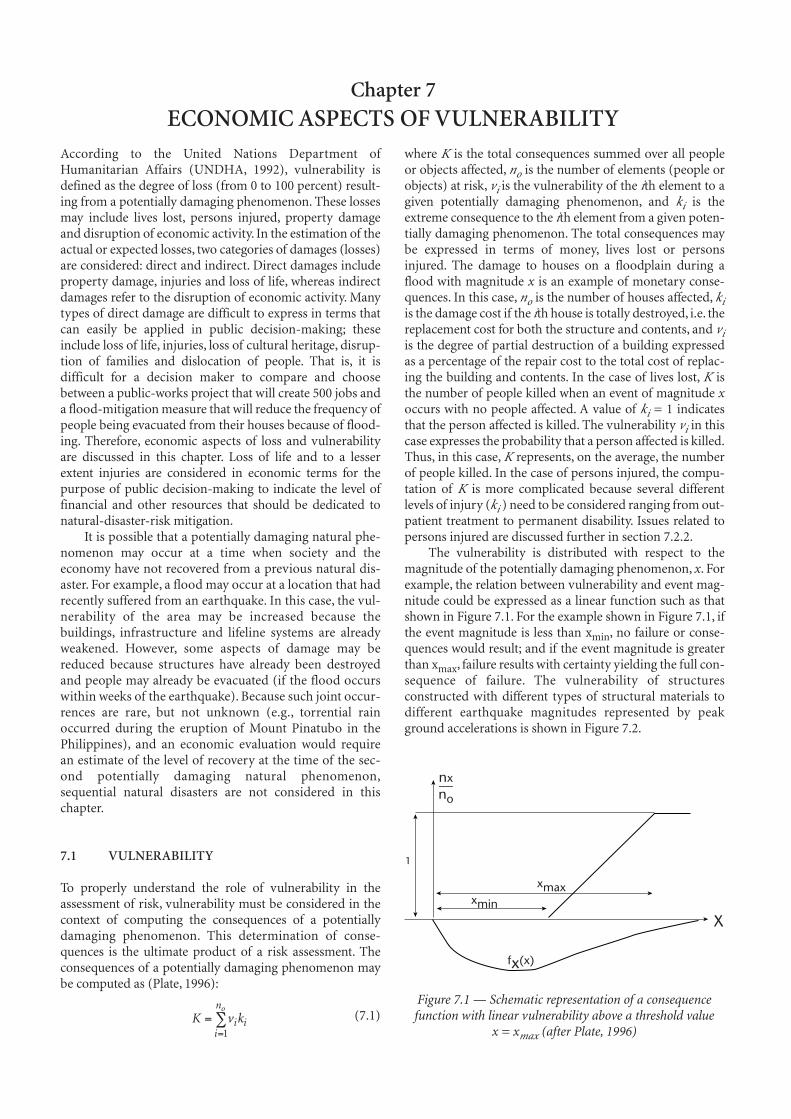
According to the United Nations Department ofHumanitarian Affairs (UNDHA, 1992), vulnerability isdefined as the degree of loss (from 0 to 100 percent) result-ing from a potentially damaging phenomenon. These lossesmay include lives lost, persons injured, property damageand disruption of economic activity. In the estimation of theactual or expected losses, two categories of damages (losses)are considered: direct and indirect. Direct damages includeproperty damage, injuries and loss of life, whereas indirectdamages refer to the disruption of economic activity. Manytypes of direct damage are difficult to express in terms thatcan easily be applied in public decision-making; theseinclude loss of life, injuries, loss of cultural heritage, disrup-tion of families and dislocation of people. That is, it isdifficult for a decision maker to compare and choosebetween a public-works project that will create 500 jobs anda flood-mitigation measure that will reduce the frequency ofpeople being evacuated from their houses because of flood-ing. Therefore, economic aspects of loss and vulnerabilityare discussed in this chapter. Loss of life and to a lesserextent injuries are considered in economic terms for thepurpose of public decision-making to indicate the level offinancial and other resources that should be dedicated tonatural-disaster-risk mitigation.

It is possible that a potentially damaging natural phe-nomenon may occur at a time when society and theeconomy have not recovered from a previous natural dis-aster. For example, a flood may occur at a location that hadrecently suffered from an earthquake. In this case, the vul-nerability of the area may be increased because thebuildings, infrastructure and lifeline systems are alreadyweakened. However, some aspects of damage may bereduced because structures have already been destroyedand people may already be evacuated (if the flood occurswithin weeks of the earthquake). Because such joint occur-rences are rare, but not unknown (e.g., torrential rainoccurred during the eruption of Mount Pinatubo in thePhilippines), and an economic evaluation would requirean estimate of the level of recovery at the time of the sec-ond potentially damaging natural phenomenon,sequential natural disasters are not considered in thischapter.

7.1 VULNERABILITY

To properly understand the role of vulnerability in theassessment of risk, vulnerability must be considered in thecontext of computing the consequences of a potentiallydamaging phenomenon. This determination of conse-quences is the ultimate product of a risk assessment. Theconsequences of a potentially damaging phenomenon maybe computed as (Plate, 1996):

(7.1)

where K is the total consequences summed over all peopleor objects affected, no is the number of elements (people orobjects) at risk, vi is the vulnerability of the ith element to agiven potentially damaging phenomenon, and ki is theextreme consequence to the ith element from a given poten-tially damaging phenomenon. The total consequences maybe expressed in terms of money, lives lost or personsinjured. The damage to houses on a floodplain during aflood with magnitude x is an example of monetary conse-quences. In this case, no is the number of houses affected, kiis the damage cost if the ith house is totally destroyed, i.e. thereplacement cost for both the structure and contents, and viis the degree of partial destruction of a building expressedas a percentage of the repair cost to the total cost of replac-ing the building and contents. In the case of lives lost, K isthe number of people killed when an event of magnitude xoccurs with no people affected. A value of ki = 1 indicatesthat the person affected is killed. The vulnerability vi in thiscase expresses the probability that a person affected is killed.Thus, in this case, K represents, on the average, the numberof people killed. In the case of persons injured, the compu-tation of K is more complicated because several differentlevels of injury (ki ) need to be considered ranging from out-patient treatment to permanent disability. Issues related topersons injured are discussed further in section 7.2.2.

The vulnerability is distributed with respect to themagnitude of the potentially damaging phenomenon, x. Forexample, the relation between vulnerability and event mag-nitude could be expressed as a linear function such as thatshown in Figure 7.1. For the example shown in Figure 7.1, ifthe event magnitude is less than xmin, no failure or conse-quences would result; and if the event magnitude is greaterthan xmax, failure results with certainty yielding the full con-sequence of failure. The vulnerability of structuresconstructed with different types of structural materials todifferent earthquake magnitudes represented by peakground accelerations is shown in Figure 7.2.

K v ki ii

no

==∑

1

Chapter 7ECONOMIC ASPECTS OF VULNERABILITY

nx__no

xmaxxmin

fx(x)

X

1

Figure 7.1 — Schematic representation of a consequencefunction with linear vulnerability above a threshold value

x = xmax (after Plate, 1996)

The vulnerability may be estimated in several waysincluding those listed below.(a) The vulnerability may be obtained from experience in

many different locations, involving many different popu-lations, with a total number of no people at risk, of whichnx would suffer the consequences of failure if an event ofmagnitude x occurs (Plate, 1996). That is, vi(x) = nx/no.

(b) The vulnerability of objects at risk also can be obtainedfrom experience in many different locations.

(c) The vulnerability of structures may be determined bycomputer simulation of structural damage resultingfrom an event of magnitude x. This approach is a cen-tral component of minimum life-cycle-cost design ofearthquake resistant structures discussed in detail insection 8.3.

The vulnerability of a structure or land use is a quality of thestructure or land use, irrespective to where it is built orlocated (UNDRO, 1991).

Usually, it is assumed that no is a known constant and Kis a deterministic function of the event magnitude x, i.e. it isassumed that for every event of magnitude x one and onlyone value of K results. However, K is actually a random vari-able because both ki and vi are subject to substantialuncertainty. For example, in standard practice the riskresulting from flooding is computed as follows (see alsoChapter 3): (1) the flood magnitude corresponding to aspecified return period is determined from frequencyanalysis; (2) the discharge is converted to a correspondingstage (flood elevation) through hydraulic analysis; (3) theflood damages corresponding to this stage is determined

from economic analysis; finally, (4) the damages corre-sponding to floods of different frequencies are integratedwith the probabilities to determine an expected risk. Steps 1and 2 determine which areas are vulnerable (vi), step 3determines the consequences (ki), and step 4 is the summa-tion of equation 7.1. However, the flood frequency-magnitude relation is subject to uncertainties because ofsample limitations, the stage-discharge relation is subject touncertainties in the hydraulic analysis, and the stage-dam-age relation is subject to uncertainties in the economicevaluation. Some of the methods discussed in Chapter 8attempt to consider the uncertainties in ki and vi explicitly.In particular, the US Army Corps of Engineers (USACE)risk-based analysis for flood-damage-reduction projects(section 8.4.1) considers uncertainties in the hydrologic,hydraulic and economic computations previouslydescribed. The minimum life-cycle cost design of earth-quake resistant structures (section 8.3) considers theuncertainties in structural strength.

7.2 DIRECT DAMAGES

7.2.1 Structures and contents

Potential damage to structures and their contents are typi-cally estimated through a combination of field surveys ofstructures in the area that would be affected by potentiallydamaging phenomena and information obtained frompost-disaster surveys of damage. The USACE (1996) hasdeveloped a detailed procedure for estimating the potentialdamages to structures and their contents resulting fromflooding.A similar procedure could be applied to determinepotential damages from other types of natural disasters:such as hurricanes, volcanoes, earthquakes, etc. Therefore,in this section, the procedure for estimating potential flooddamage provides an example on how to approach damageestimation for other types of natural disasters.

The traditional USACE procedure for estimating astage-damage function for residential structures involvesthe following steps.(1) Identify and categorize each structure in the study area

based upon its use and construction.(2) Establish the first-floor elevation of each structure

using topographic maps, aerial photographs, surveys,and (or) hand levels.

(3) Estimate the value of each structure using real-estateappraisals, recent sales prices, property tax assessments,replacement cost estimates or surveys.

(4) Estimate the value of the contents of each structureusing an estimate of the ratio of contents value to struc-ture value for each unique structure category.

(5) Estimate damage to each structure due to flooding tovarious water depths at the site of the structure using adepth-per cent damage function for the category of thestructure along with the value from step 3.

(6) Estimate damage to the contents of each structure dueto flooding to various water depths using a depth-percent damage function for contents for the structure cat-egory along with the value calculated in step 4.


Peak ground acceleration (% of gravity)

Per

cent

dam

age

100

90

80

70

60

50

40

30

20

10

00 10 20 30 40 50

Stone masonryBrick masonryStrengthened masonryReinforced concrete frame buildings

Figure 7.2 — Vulnerability of structures constructed with different materials to earthquake magnitude

(after UNDRO, 1991)

(7) Transform the depth-damage function for each struc-ture to a stage-damage function at an index location forthe flood plain using computed water-surface profilesfor reference floods.

(8) Aggregate the estimated damages for all structures bycategory for common water depths.

The aggregated stage-damage function then is integratedwith the stage-probability function, which is determinedusing hydrologic and hydraulic models, to determine thetotal flood damages or risk for various flood-mitigation scenarios.

The USACE applies a “rational planner” model and thewillingness-to-pay principle to compute the depreciatedreplacement value for a structure as per step 3. The threemost common approaches to estimate the replacementvalue are use of the Marshall and Swift Valuation Service(MSVS), real-estate-assessment data and recent sales prices.The MSVS develops a replacement construction-cost esti-mate based on information on the foundation, flooring,walls, roofing, heating system, plumbing, square footage,effective age and built-in appliances. This estimate requiresdetailed surveys of representative structures. The estimate isadjusted for depreciation. See the World Wide Web site(http://www.marshallswift.com) for more information onthe MSVS. The use of real-estate-assessment data involvesadjusting real-estate tax-assessment values for deviationsbetween assessed value and market value and subtractingthe land component of market value. It is assumed that theremainder is the depreciated replacement value of the struc-ture. The use of recent sales prices requires sufficient recentproperty sales in the area for each structure and construc-tion type for which a structure value is to be estimated. Aswith the real-estate-assessment data, the land value must besubtracted from the sales price to estimate the value of thestructure.

Typically, the value of contents is specified as a fractionof the value of the structure. This approach is similar to theapproach normally applied by residential casualty insurersin setting rates and content coverage for homeowners insur-ance. The value of contents may be determined fromdetailed surveys of representative structures. The value ofcontents also may be estimated from experience with pastfloods. The USACE (1996) has summarized the claimsrecords of the Flood Insurance Administration for variouscategories of residential structures. The ratio of the value ofcontents to the value of the residential structure is:— 0.434 for one-story structures without a basement,— 0.435 for one-story structures with a basement,— 0.402 for two-story structures without a basement,— 0.441 for two-story structures with a basement,— 0.421 for split-level structures without a basement,— 0.435 for split-level structures with a basement, and— 0.636 for mobile homes.

The value of contents found in any structure is highlyvariable because it represents the wealth, income, tastes andlifestyle of the occupants. Nevertheless, the above ratios pro-vide insight on the relative value of the contents and thestructure. Similar values of the ratio of the value of contentsto the value of the structure were applied in the minimumlife-cycle-cost design of earthquake-resistant commercial

structures described in section 8.3.1. Ratios of 0.5 and 0.4were applied for Mexico City and Tokyo, respectively. Theratio of the value of contents to the value of the structuremay be adjusted as necessary to reflect economic conditionsand cultural values of a given locality. The values given hereare examples of typical magnitudes of the ratio.

Similar information on value, damage as a function ofdepth and flood depth at a site is necessary to develop stage-damage functions for non-residential structures and otherproperty. For non-residential property, the stage-damagefunction is frequently determined from the results of post-flood surveys or through personal interviews with plantengineers, plant managers or other experts. Then, instead ofdeveloping dimensionless depth-per cent damage func-tions, damages incurred at various water-surface elevationsare directly approximated. Use of post-disaster damage sur-veys (De Leon and Ang, 1994; Lee, 1996) also have beenused to estimate structural damage resulting from earth-quakes in the minimum life-cycle-cost design of earthquake-resistant structures described in section 8.3.1.

7.2.2 Value of life and cost of injuries

Estimation of the value of human life and, thus, the value oflives saved by risk-mitigation measures used for decision-making is difficult and controversial. The reason why it isnecessary to estimate the value of human life for decision-making is described by Kaplan (1991) as follows:

“If the risk in question is a risk to human life, there is a school of

thought, often quite vocal, that says ‘You cannot put a dollar value

on human life — human life is priceless.’ True enough, but the

hitch is that when we talk about paying the price of safeguards

[reductions in vulnerability], we are not talking about dollars. We

are talking about what dollars represent, i.e., time, talent, and

resources. Time, talent, and resources are limited.What we spend

on reducing one risk is not available to spend on another.”

Schwing (1991) illustrates how these resource limita-tions may be considered as follows:

“Since we know the US GNP [Gross National Product] and the

number of deaths each year, we can calculate the willingness to

pay by long division. It turns out that if you ignore the fact that

we also value education, our homes, our mobility, the arts, and

other indices of the quality of life, each life could claim a little

over $2 million.”

The simple analysis done by Schwing is not truly repre-sentative of a means to estimate the value of human livessaved by risk-mitigation measures, but rather it highlightsthe fact that the societal resources available to save lives arelimited. Thus, in order for society to decide how it will allo-cate the available resources among the various means toprotect life, safety and regional economy, and among otherpublic goods, an estimate of the value of human lives savedmust be used.

Numerous methods have been proposed to estimate thevalue of human life including those based on the following:

68 Chapter 7 — Economic aspects of vulnerability

(1) life-insurance coverage;(2) court awards for wrongful death;(3) regulatory decisions;(4) calculations of direct out-of-pocket losses associated

with premature death (i.e. the present value of expectedfuture earnings); and

(5) examination of how much people are willing to pay toreduce their risk of death.Methods based on data derived from 4 and 5 are most

commonly applied in the literature on public decision–making.

Method 4 is commonly known as the human-capitalapproach. Rice and Cooper (1967) note that the human-capital approach had its beginnings in the 17th and 18thcenturies as economists tried to determine the value of slavelabour. The human-capital approach generally has been dis-credited for moral reasons because the value of human life ismore than just the sum of one’s future earnings. Sugden andWilliams (1978, p. 173) describe the moral problems withthe human-capital approach quite bluntly in that thisapproach “would imply that it would be positively beneficialto society that retired people be exterminated”.

The current consensus in the field of economics is thatthe appropriate way to measure the value of reducing therisk of death is to determine what people are willing to pay(Lanoie et al., 1995). The reasons for this preference are thatthe willingness-to-pay (WTP) approach (method 5) is likelyto produce estimates that are theoretically superior andpotentially more acceptable to the public than the otherapproaches (Soby et al., 1993). In the WTP approach, noattempt is made to determine the value of an actual individ-ual as is done with the human-capital approach —method 4 — and in methods 1 and 2. Rather, the value of astatistical life is estimated. That is, a safety improvementresulting in changes dpi (i = 1,...,n) in the probability ofdeath during a forthcoming period for each of n individuals,such that Σ dpi = – 1, is said to involve the avoidance of one“statistical” death or the saving of one “statistical” life(Jones-Lee et al., 1985). Thus, the willingness to pay for thesaving of one “statistical” life may be computed as

Value of statistical life = (7.2)

where mi denotes the marginal rate of substitution of wealthfor risk of death for the ith individual. In practical terms, thevalue of a statistical life represents what the whole group, inthis case society, is willing to pay for reducing the risk foreach member by a small amount (Lanoie et al., 1995). Themain requirement for practical application of the WTPapproach is empirical estimation of the marginal rates ofsubstitution of wealth for risk of death or for risk of injury(Jones-Lee et al., 1985). These estimates may be made basedon the contingent-valuation (CV) method or the revealed-preferences (RP) method.

In the CV method, questionnaires are used to elicit theactual willingness to pay for specified risk reductions fromrespondents. The primary advantage of the CV method rel-ative to the RP method, where market data are utilized, isthat the CV method is not constrained by the availability ofmarket data and, thus, may provide insight into classes of

outcomes that cannot be addressed with available marketdata. That is, the researchers can tailor the questionnaireand selection of respondents to elicit precisely the neededinformation. The primary problems with the CV methodare: (1) do those surveyed truly understand the questions?and (2) do the respondents give honest thoughtful answers?Viscusi (1993) reviewed the results of six CV studies of thevalue of life and concluded that in practice, truthful revela-tion of preferences (2) has proven to be less of a problemthan has elicitation of meaningful responses because of afailure to understand the survey task (1).

The primary difficulty is that most people have difficultydiscerning the meaning of very low probability events. Intheory, if someone was willing to pay $1 for a device thatwould reduce some risk from 2/10 000 to 1/10 000, theyshould be willing to pay $0.10 for another device that wouldreduce some other risk from 2/100 000 to 1/100 000.However, people tend to take a view that if cutting one riskin half is worth a dollar, then cutting another risk in half isworth another dollar. Viscusi (1993) further notes that “theevidence in the psychology and economics literature indi-cates that there is a tendency to overestimate the magnitudeof very low probability events, particularly those called toone’s attention” by the media.

There are two general sources of data for the RPmethod-consumer-market data and labour-market data. Ineach case, the goal is to determine from actual risk-wealthtradeoffs the amount of money people are willing to pay toreduce risk (e.g., purchase of safety devices) or willing toaccept in order to do tasks that involve greater risk (i.e. riskpremiums in pay). The primary advantage of the RPmethod is that actual tradeoffs are used to determine themarginal rate of substitution of wealth for risk of death,whereas the CV method must utilize hypothetical data. Thedisadvantages include: (1) the tradeoff values are pertinentonly in the “local range” of the workers studied and general-ization to the entire population of the society is difficult;and (2) it is difficult to properly identify the marginal rate ofsubstitution from the available data. Consumer-market dataare rarely used to determine the value of life, and so proce-dures based on these data are not discussed in detail here.Because the RP method using labour-market data is the pre-dominant method in economics, its application,assumptions and problems are discussed in detail in the fol-lowing paragraphs.

The basic approach is to identify the relation betweenwages and risk through a linear regression that considers thevarious factors that affect the wage rate and the workerswillingness to accept this rate. This “wage equation” may bedefined as (Viscusi, 1993)

(7.3)

where wi is the wage rate for worker i (or its logarithm), α is aconstant, the xim are different personal characteristic and jobcharacteristic variables for worker i (m = 1 to M), pi is the fatal-ity risk for the job of worker i, qi is the nonfatal risk for the jobof worker i, WCi reflects the workers’ compensation benefits

w x p q q WCi m imm

M

o i i i i i= + + + + +=

∑α ψ γ γ γ μ1

1 2

−=∑m dpi ii

n

1


that are payable for a job injury incurred by worker i, mi is arandom error term reflecting unmeasured factors that affectthe wage rate and Ψm,γ0,γ1, and γ2 are coefficients to be deter-mined by regression. It is important to consider that the RPmethod is not concerned with the total wage rate wi, which isa function of the strength of the national and/or regional econ-omy, but rather it is concerned with the risk premiums pi andgi the workers require to accept risk.

One of the most difficult aspects of this approach is todetermine the fatality risk and the nonfatal risk for the job of agiven worker. Typically, the job fatality risk is determined fromgovernment statistics for different job classifications. However,many inconsistencies and inaccuracies are included in thesedata as discussed by Leigh (1995) in a comparison among“value of life” estimates obtained using data from the USBureau of Labor Statistics and the National Institute ofOccupational Safety and Health. Also, if both the fatality riskand the nonfatal risk are included in the regression, the strongcorrelation between these variables may obscure the relationsto wages, whereas if the nonfatal risk is excluded, the fatalityrisk premium may be overvalued. Some of these problemsmay be mitigated by regression approaches that are lessaffected by colinearity — e.g., ridge regression and regressionof principle components. However, these approaches may be difficult to apply and may not solve all regression-relatedproblems.

The larger difficulty with the determination of the fatal-ity risk is that it should be based on the worker’s perceptionof risk of death rather than the actual risk of death fromgovernment statistics. Also, the workers must be able tofreely move to new jobs if they determine that the wealth-risk tradeoff is unacceptable. If the workers do notaccurately understand the risks they face or have limitedwork alternatives, the risk premium determined may beinaccurate in assessing society’s willingness to accept risk.

Application of the RP method using labour-market dataalso may be difficult for estimating the acceptable wealth-risktradeoff for the entire society. As noted by Jones-Lee et al.(1985) no doubt the wages of steeplejacks and deep-sea diversinclude clearly identifiable risk premiums, but it seems unlikelythat the attitudes of these individuals toward risk will be typi-cal of society. Further, as noted by Lanoie et al. (1995),risk-averse workers are probably concentrated in jobs wherethe existence of explicit risk premium is unlikely or difficult todetect. Thus, Lanoie et al. (1995) suggested that the results ofthe CV method may be more representative of the preferencesof the entire society, provided a representative sample of thepopulation is questioned.

Another difficulty with the use of labour-market data isthat the workers willingness to accept risk in return forwealth is measured. However, public decision-makingshould be based on society’s willingness to pay to reducerisks. Viscusi (1993) notes that individuals may require alarge financial inducement to accept an increase in risk fromtheir accustomed risk level that generally exceeds their will-ingness to pay for equivalent incremental reductions in risk.Thus, willingness to pay estimates of the value of lifeobtained with application of the RP method based onlabour-market data tend to be higher than society’s actualwillingness to pay.

The job characteristics considered in the regressionanalysis of equation 7.3 have included (Viscusi, 1993; Lanoieet al., 1995):• Does the job require physical exertion?• Does the job involve exposure to extreme cold, humid-

ity, heat, noise and/or dust?• Does the job require long hours?• Does the job require experienced workers?• Does the worker have supervisory or decision-making

responsibilities?• Does the job require that the worker not make mistakes?• The speed of work• Job security• Worker training

The personal characteristics of the workers consideredin the regression analysis have included (Viscusi, 1993;Lanoie et al., 1995) union membership, age, age squared (asa measure of the decrease of the rate of wage increases withage), experience, level of education, gender, martial statusand spouse’s employment, number of dependents, experi-ence and/or discounted years of remaining life. Also, anumber of industry dummies (transportation, manufactur-ing, government, etc.) may be included in the analysis toaccount for industry-specific effects (Lanoie et al., 1995;Leigh, 1995).

Application of the RP method using labour-marketdata requires a large amount of job and personal character-istic data for a representative sample of workers in the regionof interest. Viscusi (1993) states that application of the RPmethod with labour-market data using industry-wide,aggregate data sets often results in difficulties in distinguish-ing wage premiums for job risks. He notes that the relianceon aggregate industry data pools workers with heteroge-neous preferences, and firms with differing wage-offercurves, so that the estimated tradeoffs at any particular risklevel cannot be linked to any worker’s preferences or anyfirm’s wage-offer curve. The need for extensive data sets forjobs and workers limits the practical application of thisapproach. The literature search done by Viscusi (1993)revealed that the RP method using labour-market data hadonly been applied in five countries: the US (value of lifeUS $3–7 million in 1990), the UK (US $2.8 million), Canada(US $3.6 million), Australia (US $3.3 million) and Japan(US $7.6 million).

If the extensive labour-market data needed to apply theRP method are available, this method is recommended forrisk assessment for natural-disaster mitigation. Otherwise,application of the CV method to an appropriate sample ofthe affected population is recommended.

The value of injury reduction also can be computedthrough the WTP approach. However, Soby et al. (1993)reported difficulties in applying approaches used to estimatethe monetary value of life to determine the value of injuryreduction. These difficulties result because of the wide varietyof injury states: no overnight hospital stay, overnight hospitalstay, one-week hospital stay, long-hospital stay with majorrehabilitation, etc.Viscusi (1993) summarized the results of 14studies of the value of injury reduction computed by the WTPapproach with the RP method using US labour-market data.Most of the estimates considered data for all injuries regardless


of severity range and resulted in values of injury reductionfrom $25 000–50 000 (in 1990 US$). The value of injuriesrequiring at least one lost workday was approximately $50 000,or at the high end of the range of estimates for the implicitvalue of injuries. Only data for the US are available withrespect to the value of injury reduction. The ratio between thevalue of injury reduction and the value of lives saved is approx-imately 0.01 (determined from US data as $50 000/$5 000 000). This ratio could be applied as a first approxima-tion in other countries for which labour costs are not as highas in the US Therefore, if the value of lives saved in a givenregion were $1 million, then the value of injury reductionwould be $10 000.

7.3 INDIRECT DAMAGES

7.3.1 General considerations

Indirect damages are determined from the multiplier or ripple effect in the economy caused by damage to infra-structure resulting from a natural disaster. In particular,damage done to lifelines, such as the energy-distributionnetwork, transportation facilities, water-supply systems andwaste-management systems, can result in indirect financiallosses greater than the direct financial damages to these sys-tems and a long-term drain on the regional or nationaleconomy. Munich Reinsurance (1997) noted in their AnnualReview of Natural Catastrophes 1996 that numerous naturaldisasters of recent years have shown how vulnerable theinfrastructure of major cities is to minor breakdowns andhow severe shortages of supply can develop in a short time.Industry optimizes storage, production, supply of compo-nents and dispatch of goods using sophisticated controlprogrammes. Thus, industry is dependent on a perfectlyworking infrastructure. In the event of a natural disaster,lack of standby supply systems can lead to enormous lossesof revenue and profits that can mean the ruin of manufac-turers, suppliers, processors and/or wholesalers. On thebasis of the experiences of the 1995 Kobe, Japan earthquake,loss estimates for a similar or more severe earthquake in thearea of Greater Tokyo are on the order of US $1–3 trillion(Munich Reinsurance, 1997). Thus, the possible extent oflosses caused by extreme natural disasters in one of theworld’s major metropolises or industrial centres could be sogreat as to result in the collapse of the economic system ofthe country and could even bring about the collapse of theworld’s financial markets.

Wiggins (1994) described five problems affecting thedetermination of indirect economic losses (damages) as follows:(a) Any aggregated loss data from previous natural disas-

ters do not discern between how much of the loss to aparticular economic sector resulted from disruption tolifelines, and how much resulted from direct damage.

(b) Available loss data, such as gathered by a questionnairemay be inaccurate, because many companies prefer notto disclose detailed financial loss data.

(c) The ripple effects of a changing local economy are dif-ficult to measure and positively attribute to particular

disruptions, such as telephone, electricity, direct dam-age, etc.

(d) It is difficult to determine if selected short-term lossesare actually postponed rather than cancelled. That is,permanent losses result from economic activity — pur-chases, trips, use of services, etc. — that was cancelledbecause of a natural disaster, whereas other similar eco-nomic activity may be merely postponed to be “madeup” at a later time.

(e) It is difficult to define the region of impact, and haveeconomic data and models available for that regiononly. The determination of regions experiencing indi-rect financial losses is not limited to the areas sufferingphysical damage, but also include the normal deliverypoints of the affected industries. The larger the regionchosen, the more difficult it becomes to positively jus-tify that changes in economic activity solely result fromthe natural disaster, rather than other influences.These problems indicate that it is unlikely that data on

damages from previous natural disasters can be used to esti-mate indirect damages from possible future naturaldisasters. Thus, some type of macroeconomic model mustbe utilized to estimate indirect damages.

Lee (1996) reports that analyses of the indirect dam-ages resulting from earthquakes have been done withappropriate models of the regional economy that include:(1) input-output (I-O) models; (2) social accounting matrixmodels; (3) computable general equilibrium models; and(4) other macroeconomic models. The complexity of therelation between direct damages and indirect damages thatthese models must approximate is illustrated in Figure 7.3.This figure shows the facets of the macroeconomic modeldeveloped by Kuribayashi et al. (1984) to estimate indirectlosses from earthquakes in Japan. This chapter focuses onthe application of I-O models to estimate indirect damagesresulting from natural disasters because I-O models areavailable for many countries (as described in 7.3.2) and theyare generally accepted as good tools for economic planning.

7.3.2 The input-output (I-O) model

I-O models are frequently selected for various economicanalyses and are widely applied throughout the world (Lee,1996). The United Nations has promoted their use as apractical planning tool for developing countries and hassponsored a standardized system of economic accounts fordeveloping the models (Miller and Blair, 1985). More than50 countries have developed I-O models and applied themto national economic planning and analysis (Lee, 1996).Wiggins (1994) notes that I-O models may be particularlywell suited to estimation of indirect damages because it isthought that a properly applied I-O model can largelyovercome the first four problems with the estimation ofindirect economic losses listed previously. Definition of theappropriate “region of impact” for indirect losses ordamages remains a difficult problem for all macroeconomicmodels.

Input-output models constitute a substantially simpli-fied method for analysing interdependency between sectors


in the economy. As such, it is necessary to understand themagnitude of the simplifications applied in I-O models,which include the following (Randall, 1981, p. 316):(a) the industrial sector, rather than the firm, is taken to be

the unit of production;(b) the production function for each sector is assumed to

be of the constant-coefficient type;

(c) the question of the optimal level of production is notaddressed;

(d) the system contains no utility functions; and(e) consumer demands are treated as exogenous.

Further, Young and Gray (1985) note that I-O modelsare production models characterized by: the lack of anyspecified objective function; no constraining resources; lack


PERSONALINCOME

COMPOSITION OF EMPLOYEDPOPULATION

DEAD, INJURED SUSPENSION

OF WORK

COMPENSATION OF EMPLOYEES

PROPIETOR’SINCOME

CORPORATEPROFITS

PERSONALINCOME

GROSS PRODUCT OF AGRICULTURE

MANUFACTURING OUTPUT

WHOLESALE & RETAIL SALES

EMPLOYEDPOPULATION

PREFECTURALINCOME

OPTIMUM CAPITALSTOCK

SOCIALCAPITAL

MIGRATIONCHANCE

POPULATION

GOVERNMENTCONSUMPTION

CAPITALCOST

SOCIAL CAPITALDAMAGE

GOVERNMENTFIXED ASSETSFORMATION

ENTERPRISESASSETS

INVESTMENT

ENTERPRISESCAPITALSTOCK

REVENUE OFPREFECTURE &MUNICIPALITY

PREFECTURALINCOME

PERSONAL CONSUMPTION

HOUSEHOLDDAMAGE

(DIRECT LOSS)

GOVERNMENT

INVENTORYDAMAGE

DEMAND OFOUTPUT

NET PRODUCT

(ENTERPRISE)

(INCOME)

NATURALCHANGE RATE

RESIDENCEDAMAGE

PERSONALRESIDENTIAL

CONSTRUCTION

START

WORKING HOUR PER CAPITAL

ENTERPRISESASSETS

DAMAGE

(EXOGENOUSVARIABLES)

INVESTMENTDEFLATOR

CAPITAL DEFLATOR

DEPRECIATION RATE

INTEREST RATE

CORPORATION TAX RATE

MANUFACT-URING PRICE

DEFLATOR

Figure 7.3 — Economic interactions that affect the indirect economic losses (damages) resulting from a natural disaster (after Kuribayashi et al., 1984)

of choice on the production or consumption side; constantfactor and product prices; and a production functionreturning constant returns to scale. Randall (1981, p. 316)states that these are rather radical assumptions, but theseassumptions have the advantage of permitting a simpleinteractive model that may be empirically estimated withrelative ease. Thus, I-O models have become accepted,despite their rigid and somewhat unrealistic assumptions, asthe basic tool in the analysis of regional economic systems.In the application of I-O models to estimation of indirectdamages, a comparison is made between economic produc-tion with and without the occurrence of a natural disaster.Thus, because the goal is to estimate relative economic out-put and not exact economic output, the effects of some ofthe assumptions on the reliability of the estimated indirectdamages are reduced. Further, as described in the followingdiscussion, the constants in the I-O model are modified toreflect lost productivity in various sectors resulting from anatural disaster. Therefore, I-O models are more reliable forestimating indirect damages than for estimating economicoutput because some of the problems listed above do notsubstantially affect estimation of indirect damages.

As discussed previously, the approach to evaluating theindirect damages resulting from a natural disaster is to com-pare the post-disaster scenario with an estimate of what theeconomy would have looked like without the disaster. Lee(1996) presents an outstanding summary of how an I-Omodel could be applied to estimate the indirect damagesresulting from an earthquake. This summary forms thebasis for the following paragraphs.

An I-O model is a static general equilibrium model thatdescribes the transactions between the various productionsectors of an economy and the various final demand sectors.An I-O model is derived from observed economic data for aspecific geographical region (nation, state, county, etc.). Theeconomic activity in the region is divided into a number ofindustries or production sectors. The production sectorsmay be classified as agriculture, forestry, fishery, mining,manufacturing, construction, utilities, commercial busi-ness, finance and insurance, real estate, transportation,communication, services, official business, households andother sectors. In practice, the number of sectors may varyfrom only a few to hundreds depending on the context ofthe problem under consideration. For example, Wiggins(1994) utilized 39 sectors in estimating the indirect eco-nomic losses resulting from earthquake damage to threemajor oil pipelines in the USA.

The activity of a group of industries that produce goods(outputs) and consume goods from other industries(inputs) in the process of each industry producing output isapproximated with the I-O model. The necessary data arethe flows of products from each “producer” sector to each“purchaser” sector. These intersectoral flows are measuredin monetary terms for a particular time period, usually ayear. Using this information on intersectoral flows, a linearequation can be developed to estimate the total output fromany sector of the n-sector model as

(7.4)

where Yij is the value of output of sector i purchased by sec-tor j, Ci is the final consumption for the output of sector i, Yiis the value of the total output of sector i, and n is the num-ber of sectors in the economy. Thus, the I-O model may beexpressed in matrix form as:

Y = AY + C (7.5)

where Y is the vector of output values, C is the vector of finalconsumption and A is the input coefficient matrix whoseelements Aij are equal to Yij/Yi. The rows of the A matrixdescribe the distribution of the output of a producerthroughout the economy, and the columns of the A matrixdescribe the composition of inputs required by a particularindustry to produce its output. The consumption matrix, C,shows the sales by each sector to final markets, such as pur-chases for personal consumption.

Most of the I-O model coefficients that have been devel-oped at the national level or provincial/state level are based onextensive surveys of business, households and foreign trade.These detailed lists of model coefficients are very expensiveand time consuming to produce and can easily become out ofdate. The I-O model coefficients for regions within a countryor province/state generally are prepared by reducing thenational coefficients so that they match whatever economicdata are available for the particular area. Interpolation of theproduction and consumption coefficients on the basis ofpopulation also seems to provide reasonable results at anaggregated economic sector level (Wiggins, 1994).

From equation 7.5, the output of the economy if thenatural disaster does not occur may be obtained as

YN = (I – A)–1C (7.6)

where I is an n × n identity matrix, the subscript N indicatesno disaster, and the exponent –1 indicates the inverse func-tion of the matrix. The indirect loss or damage resultingfrom structural and infrastructure damage caused by a nat-ural disaster can be divided into a first-round loss and asecond-round loss. The first-round loss comes from thereduction in output related specifically to loss of functionresulting from damage to a given sector of the economy. Thesecond-round loss results as the loss of capacity in one sec-tor of the economy reduces the productivity of other sectorsof the economy that obtain inputs from the first sector.

The primary factor that drives both the first-round andsecond-round losses is the amount of time a given sector ofthe economy will be out of service because of damage froma natural disaster. The concept of a restoration function hasbeen used to describe the relation between structural dam-age to the loss of function of a facility and, ultimately, of asector of the economy. The loss of function depends on thelevel of damage to the economic sector. For a particular stateof damages, the restoration function may be expressed as atime-to-restore curve as shown in Figure 7.4, where the hor-izontal axis is the elapsed time after the event and thevertical axis is the restored functionality, FR(t). The loss offunction for the given damage state, tloss, measured in time,may be calculated as the area above the time-to-restorecurve and can be estimated as:

Y C Yij i ij

n+ =

=∑

1


(7.7)

where FR(t) is the functionality of the economic sector, and t3is the amount of time required to restore the facility to fullfunctionality. Different types of facilities and economic sectorsunder the same level of damage may experience differentlosses of functionality depending on the nature of theeconomic sector. Reasonable estimates of the loss of functionfor a given economic sector as a result of a natural disaster maybe obtained on the basis of the estimated direct damage andthe restoration time observed in previous disasters.

The production loss for a given sector, i, may be esti-mated as:

Yi,loss = (tloss /tIO) Yi,N (7.8)

where Yi,loss is the production loss from economic sector iresulting from a natural disaster, tIO is the time interval overwhich the I-O model coefficients are estimated, and Yi,N isthe total output from sector i without any disaster. For givendamage levels to the various economic sectors, the totalfirst-round loss then is obtained as

(7.9)

where CB1 is the total first-round loss, and εi is the econ-omic surplus per unit of total output of sector i in the I-Omodel.

Using the estimated change in output from the variouseconomic sectors, the new post-disaster demand is obtainedas

C* = (I – A) Y* (7.10)

where Y* = YN – Yloss. As described previously, in the appli-cation of I-O models for conventional inter-industrystudies, it is assumed that the intermediate input require-ments reflected in the A matrix are invariant. However, thiscannot be assumed after a natural disaster because of thereduction in capacity resulting from the damage to struc-tures and the interruption of service. Thus, the changingstructure of the economy must be accounted for throughchanges in the A matrix in order to adequately estimate theindirect losses or damages. In the post-disaster economy,matrix A may be approximated by assuming that the directinput requirements of sector i per unit output j are reducedin proportion to the reduction in output i (Boisvert, 1992).That is, local purchases of sector j products by sector i tomeet the reduced levels of final consumption are reduced inproportion to the damage in sector i (Lee, 1996). The post-disaster level of production is estimated as

YD = (I – A*)–1 C*= (I – A*)–1 (I – A) Y*

(7.11)

where YD is the post-disaster level of production, and A* isthe I-O model coefficient matrix for the post-disaster econ-omy whose elements Aij* = (Yi*/Yi,N)Aij. For given damage

levels to the various economic sectors, the total second-round loss is then obtained as

(7.12)

where CB2 is the total second-round loss. The total indirectloss for given damage levels resulting from a natural disasteris the sum of the first-round loss and second-round loss.

The methodology described previously in this sectiondoes not account for the redistribution effects of spending onrestoration. Such spending results in increased economicactivity as governments inject higher-than-normal amounts ofmoney in the region to aid in disaster recovery. Restorationspending takes the form of a direct increase in the construc-tion sector with subsequent ripple effects throughout theaffected regional economy. From the point of view of planningfor natural-disaster mitigation at the national level, it is reason-able to omit the effects of restoration spending on the regionaleconomy. The entire nation will experience the total economiclosses expressed by equations 5.9 and 5.12 because of theopportunity costs of the resources used for reconstruction. Itis not possible to accurately estimate how much lost produc-tion can be made up after recovery is in progress (Lee, 1996).Thus, planners may make assumptions regarding the make upof lost productivity to moderate the likely overestimate of indi-rect damages obtained as the sum of CB1 and CB2. Forexample,Wiggins (1994) assumed that 80 per cent of the time-dependent losses resulting from damage to oil pipelinesbecause of an earthquake would be recovered over time.However, such assumptions are highly dependent on theeconomic sectors involved and the magnitude of the damage.A conservative overestimate is probably most useful for plan-ning for natural-disaster mitigation.


Consequences: Property damage, injuries and loss of life that may occur as a result of a potentially damaging

C Y YB i i i Di

n

21

= ∗−( )=∑ε ,

C YB i i lossi

n

11

==∑ε ,

t F t dtloss R

t

= − ( )( )∫ 10

3


100

60

30

0

t1 t2 t3

Rest

ored

func

tiona

lity

(%)

Elapsed time

Figure 7.4 — Time-to-restore functionality of an economicsector (after Lee, 1996)

phenomenon. Computed as the product of vulner-ability and extreme consequence (replacement cost,death, etc.) summed over all elements at risk.

Contingent valuation: A method to determine the value oflives saved wherein questionnaires are used to elicit theactual willingness to pay for specified risk reductionsfrom respondents who represent the affected population.

Depreciation: The loss of value of items because of wear andtear and age.

Direct damages: Property damage, injuries and loss of lifethat occur as a direct result of a natural disaster.

Economic surplus: The value of the products made by aneconomic sector in excess of the cost of production.

Elements at risk: The population, buildings and civil engi-neering works, economic activities, public services,utilities and infrastructure, etc. exposed to hazard.

Fatality risk: The probability that someone will die whileparticipating in an activity or doing a job.

First-round loss: The indirect damage resulting from thereduction in output related specifically to loss of func-tion resulting from damage to a given sector of theeconomy.

Human capital approach: A method to determine the eco-nomic value of human life wherein the directout-of-pocket losses associated with premature death(i.e. the present value of expected future earnings) arecalculated.

Indirect damages: Economic losses resulting from themultiplier or ripple effect in the economy caused bydamage to infrastructure resulting from a naturaldisaster. Damage done to lifelines such as the energy-distribution network, transportation facilities,water-supply systems and waste-managementsystems, can result in indirect economic losses greaterthan the direct economic damage to these systems anda long-term drain on the regional or nationaleconomy.

Input-output model: A static general equilibrium model thatdescribes the transactions between the various produc-tion sectors of an economy and the various finaldemand sectors. This model is derived from observedeconomic data for a specific geographical region(Nation, State, county, etc.).

Macroeconomics: Economics studied in terms of largeaggregates of data whose mutual relationships are inter-preted with respect to the behaviour of the system as awhole.

Marginal rate of substitution: The point at which the increasein utility or benefit gained from one objective (e.g.,financial gain) from an activity is exactly equal to thedecrease in utility or benefit gained from anotherobjective (e.g., safety). Thus, if financial gain were tofurther increase, safety would unacceptably increaserelative to the individual’s overall utility preferences.

Nonfatal risk: The probability that someone will be injuredwhile participating in an activity or doing a job.

Opportunity cost: The benefits lost to society or an individ-ual because resources were expended on anotheractivity.

Restoration function: The restoration of economic sectorproductivity as a function of time after a natural disas-ter. For a particular state of damages, the restorationfunction may be expressed as a time-to-restore curve,where the horizontal axis is the elapsed time after theevent and the vertical axis is the restored functionality.

Restoration spending: The Government spends higher thannormal amounts of money in a region affected by a nat-ural disaster to aid in disaster recovery. This spendingresults in increased economic activity in the region, butan overall loss for the national economy.

Revealed preferences: A method to determine the value of livessaved wherein the amount of money people are willing topay to reduce risk (e.g.,purchase of safety devices) or will-ing to accept in order to do tasks that involve greater risk(i.e., risk premiums in pay) are used to establish the soci-etally acceptable wealth-risk tradeoff.

Risk premium: The extra amount of money a worker mustbe paid to accept a job with higher fatality risk andnonfatal risk. This depends on a worker’s perception ofthe risk posed by the job and his or her ability to selectless risky jobs.

Second-round loss: The indirect damage resulting as the lossof capacity in one sector of the economy reduces theproductivity of other sectors of the economy thatobtain inputs from the first sector.

Sectors: Subsections of the economy that produce certaintypes of goods; these include agriculture, forestry, fish-ery, mining, manufacturing, construction, utilities,commercial business, finance and insurance, real estate,transportation, communication, services, official busi-ness and households.

Value of a statistical life: A safety improvement resulting inchanges dpi (i = 1,...,n) in the probability of death dur-ing a forthcoming period for each of n individuals, suchthat Σ dpi = – 1, is said to involve the avoidance of one“statistical” death or the saving of one “statistical” life.The value of a statistical life represents what the wholegroup, in this case society, is willing to pay for reducingthe risk for each member by a small amount.

Value of injury reduction: The monetary value society placeson reducing injuries through infrastructure improve-ments, public-health programmes, land-use manage-ment and other activities.

Value of lives saved: The monetary value society places onprotecting and preserving human life through infra-structure improvements, public-health programmes,land-use management and other activities.

Vulnerability: The degree of loss (from 0 to 100 per cent)resulting from a potentially damaging phenomenon.These losses may include lives lost, persons injured,property damage and disruption of economic activity.The vulnerability is distributed with respect to themagnitude of the potentially damaging phenomenon.

Willingness to accept: The amount of money that a personmust be paid to accept increased fatality and (or) non-fatal risks; generally greater than the willingness to pay.

Willingness to pay: The amount of money that a person willpay to reduce fatality and (or) nonfatal risks; generallyless than the willingness to accept.



7.5 REFERENCES

Boisvert, R.N., 1992: Indirect losses from a catastrophicearthquake and the local, regional, and national inter-est, in Indirect Economic Consequences of a CatastrophicEarthquake, Washington, D.C., DevelopmentTechnologies, Inc., pp. 209-265.

De Leon, D. and A.H-S. Ang, 1994: A damage model forreinforced concrete buildings. Further study of the 1985Mexico City earthquake, in Structural Safety andReliability, Rotterdam, The Netherlands, A.A. Balkema,pp. 2081-2087.

Jones-Lee, M.W., M. Hammerton and P.R. Philips, 1985: Thevalue of safety: results of a national sample survey, TheEconomic Journal, 95, pp. 49-72.

Kaplan, S., 1991: The general theory of quantitative risk assess-ment, in Risk-Based Decision Making in Water ResourcesV, Haimes,Y.Y., Moser, D.A., and Stakhiv, E.Z., eds., NewYork,American Society of Civil Engineers, pp. 11-39.

Kuribayashi, E., O. Ueda and T. Tazaki, 1984: An econometricmodel of long-term effects of earthquake losses,Proceedings of the U.S.-Japan Workshop on UrbanEarthquake Hazards Reduction, Stanford, California, p.189-218.

Lanoie, P., C. Pedro and R. Latour, 1995: The value of statis-tical life: a comparison of two approaches, Journal ofRisk and Uncertainty, 10, pp. 235-257.

Lee, J-C., 1996: Reliability-based cost-effective aseismicdesign of reinforced concrete frame-walled buildings,PhD thesis, University of California at Irvine, Irvine,Calif.

Leigh, J.P., 1995: Compensating wages, value of a statistical life,and inter-industry differentials, Journal of EnvironmentalEconomics and Management, 28, pp. 83-97.

Miller, R.E., and P.D. Blair, 1985: Input-output analysis:Foundations and extensions, Englewood Cliffs, N.J.,Prentice Hall.

Munich Reinsurance, 1997: Topics: Annual review of naturalcatastrophes 1996, 16 pp.

Plate, E.J., 1996: Risk management for hydraulic systemsunder hydrological loads, Third IHP/IAHS George

Kovacs Colloquium, UNESCO, Paris, France,September 19-21, 1996.

Randall,A., 1981: Resource economics: An economic approachto natural resource and environmental policy, Columbus,Ohio, Grid Publishing, Inc., 415 pp.

Rice, D.P. and B.S. Cooper, 1967: The economic value ofhuman life, American Journal of Public Health, 57(11),pp. 1954-1966.

Schwing, R.C., 1991: Conflicts in health and safety matters:between a rock and a hard place, in Risk-Based DecisionMaking in Water Resources V, Haimes, Y.Y., Moser, D.A.,and Stakhiv, E.Z., eds., New York, American Society ofCivil Engineers, pp. 135-147.

Soby, B.A., D.J. Ball and D.P. Ives, 1993: Safety investmentand the value of life and injury, Risk Analysis, 13(3), pp.365-370.

Sugden, R. and A. Williams, 1978: The principles of practicalcost-benefit analysis, London, Oxford University Press,275 pp.

United Nations Department of Humanitarian Affairs(UNDHA), 1992: Glossary—Internationally agreedglossary of basic terms related to disaster management,83 pp.

United Nations Disaster Relief Co-ordinator (UNDRO),1991: Mitigating natural disasters, phenomena, effectsand options—A manual for policy makers and planners,UNDRO/MND/1990 Manual, United Nations, Geneva,164 pp.

U.S. Army Corps of Engineers (USACE), 1996: Risk-basedanalysis for flood damage reduction studies, EngineerManual EM 1110-2-1619, Washington, D.C.


Wiggins, J.H., 1994: Estimating economic losses due to aninterruption in crude oil deliveries following an earth-quake in the New Madrid seismic zone, Proceedings ofthe 5th U.S. National Conference on EarthquakeEngineering, Chicago, Ill., Vol. 3, pp. 1077-1086.

Young, R. and S. Gray, 1985: Input-output models, econom-ic surplus, and the evaluation of state or regional waterplans, Water Resources Research, 21(12), pp. 1819-1823.

According to the United Nations Department ofHumanitarian Affairs (UNDHA, 1992), assessment involvesa survey of a real or potential disaster to estimate the actualor expected damages and to make recommendations forprevention, preparedness and response. The survey of theexpected damages for a potential disaster essentially con-sists of a risk evaluation. Risk is defined as the expectedlosses (of lives, persons injured, property damaged and eco-nomic activity disrupted) due to a particular hazard for agiven area and reference period (UNDHA, 1992). Based onmathematical calculations, risk is the product of hazard andvulnerability (UNDHA, 1992).

Risk evaluations should be the basis of the design andestablishment of methods to prevent, reduce and mitigatedamages from natural disasters. Methods to evaluate mete-orological, hydrological, volcanic and seismic hazards areavailable and have been presented in Chapters 2 to 5,respectively. Methods also are available to develop a com-mensurate rating system for the possible occurrence ofmultiple potentially damaging natural phenomena (e.g.,landslides and floods) and to present equivalent hazard levels to land-use planners in a single map, as illustrated bythe example given in Chapter 6. Methods also have beenproposed to evaluate the economic damages resulting fromnatural disasters some of which are presented in Chapter 7.However, despite the availability of the methods to evaluatethe damages resulting from natural disasters, most societieshave preferred to set somewhat arbitrary standards on theacceptable hazard level as the basis for mitigation of risksfrom natural disasters. Without a detailed evaluation of thedamages resulting from natural disasters and the directconsideration of societally acceptable damage levels(including loss of life), society is sure to inadequately allo-cate natural-disaster risk-mitigation funds and, as a result,is guaranteed to encounter damage that is deemed unacceptable by society.

In recent years, several countries have started to applyrisk evaluations in the design and establishment of methodsto prevent, reduce and mitigate damages from natural disas-ters. This chapter includes reviews of examples of thesemethods applied to: (1) the design of coastal protectionworks in The Netherlands, earthquake resistant structuresin Mexico and Japan, and flood-protection works in theUSA; and (2) the establishment of flood mitigation vialand-use planning in France. This chapter does not includean exhaustive review of risk evaluations, but rather presentsexamples to illustrate that the methods are available andhave been successfully applied. This review provides aframework for the development and application of similarmethods for mitigation of other natural disasters, as appro-priate, to conditions in other countries. Thus, in thischapter, assessment is defined as a survey and evaluation toestimate the expected damages from a potential disaster andto recommend designs or measures to reduce damages tosocietally acceptable levels, if possible.

8.1 IMPLICIT SOCIETALLY ACCEPTABLEHAZARDS

It is valuable to review the history of the determination ofsocietally acceptable hazards in order to understand theneed for risk assessment in the design and establishment ofmitigation programmes for risks from natural disasters. Inthe design of structures and the establishment of land-usemanagement practices to prevent and/or reduce damagesresulting from natural disasters, the risk or damage assess-ment typically has been implicit. An example can be takenfrom the area of flood protection where the earliest struc-tures or land-use management practices were designed orestablished on the basis of the ability to withstand previousdisastrous floods. Chow (1962) notes that the Dun water-way table used to design railroad bridges in the early 1900swas primarily determined from channel areas correspond-ing to high-water marks studied during and after floods.Using this approach, previous large floods of unknown fre-quency would safely pass through the designed bridges.Also, after a devastating flood on the Mississippi River in1790, a homeowner in Saint Genieve, Missouri, rebuilt hishouse outside the boundary of that flood. Similar rules wereapplied in the design of coastal-protection works in TheNetherlands at the time the Zuiderzee was closed (1927-32)(Vrijling, 1993).

In some cases, rules based on previous experience workwell. For example, the house in Missouri was not floodeduntil the 1993 flood on the Mississippi River and theZuiderzee protection works survived the 1953 storm thatdevastated the southwestern part of The Netherlands.However, in most cases these methods are inadequatebecause human experience with floods and other naturalhazards do not include a broad enough range of events norcan they take into account changing conditions that couldexacerbate natural disasters. As noted by Vrijling (1993)“one is always one step behind when a policy is only basedon historical facts.”

In the early part of the twentieth century, the concept offrequency analysis began to emerge as a method to extendlimited data on extreme events. These probabilisticallybased approaches allow estimates of the magnitude of rarelyoccurring events. Frequency analysis is a key aspect of mete-orological, hydrological and seismic hazard analyses asdescribed in Chapters 2, 3 and 5, respectively. Thus, usingfrequency-analysis methods, it is possible to estimate eventswith magnitudes beyond those that have been observed.This necessitates the selection of a societally acceptable haz-ard frequency.

In the USA, the societally acceptable frequency of occur-rence of flood damage was formally set to once on average in100 years (the so-called 100-year flood) in the Flood Disasterand Protection Act of 1973. However, the 100-year flood hadbeen used in engineering design for many years before 1973.In this Act, the US Congress specified the 100-year flood as the

CHAPTER 8

STRATEGIES FOR RISK ASSESSMENT — CASE STUDIES

limit of the flood plain for insurance purposes, and this hasbecome widely accepted as the standard of hazard (Linsleyand Franzini, 1979, p. 634). This acceptable hazard frequencywas to be applied uniformly throughout the USA, withoutregard to the vulnerability of the surrounding land or people.The selection was not based on a benefit-cost analysis or anevaluation of probable loss of life. Linsley (1986) indicated thatthe logic for one fixed level of flood hazard (implicit vulner-ability) was that everyone should have the same level ofprotection. Linsley further pointed out that many hydrologistsreadily accepted the implicit vulnerability assumption becausea relatively uncommon flood was used to define the hazardlevel, and, thus,

“The probability that anyone will ever point a finger and

say ‘you were wrong’ is equally remote. If the flood is

exceeded, it is obvious that the new flood is larger than

the 10-year or 100-year flood, as the case may be. If the

estimate is not exceeded, there is no reason to think

about it.”

Comprehensive mitigation of risks resulting frompotentially damaging natural phenomena requires a morerigorous consideration of the losses resulting from the haz-ard and society’s willingness to accept these losses.

For other types of disaster, societally acceptable hazardlevels also have been selected without formal evaluation ofbenefits and costs. For example, in the USA, dam-failurerisks are mitigated by designing dams to pass the probablemaximum flood where failure may result in the loss of life.Also, in The Netherlands, coastal-protection works are nor-mally designed by application of a semi-deterministicworst-case approach wherein the maximum storm-surgelevel (10 000-year storm surge) is assumed to coincide withthe minimum interior water level. Comparison of the worst-case approach to the societally acceptable probabilistic-loadapproach (described in section 8.2) resulted in a 40 per centreduction in the design load when the actual probability offailure was considered (Vrijling, 1993). This example illus-trates that when a risk assessment is performed, a societallyacceptable level of safety can be maintained and in somecases improved, while at the same time effectively usingscarce financial resources.

The examples presented in the following sections illus-trate how risk assessment can be done to keep losses/damages resulting from potentially damaging natural phe-nomena within societally acceptable bounds. In the case ofstorm surges in The Netherlands, the loss/damage analysisconsidered only the rate of fatalities (section 8.2). In the caseof earthquakes in Tokyo and Mexico City, the loss/damageanalysis considered the cost, including the cost of fatalities,with possible additional constraints on the rate of fatalities(section 8.3). In the case of flood management in the USA,the loss/damage analysis was approached in terms of eco-nomic benefits and costs, with other consequences offlooding and the flood-management projects considered inthe decision-making (section 8.4.1). Finally, in the case offlood management in France, societally acceptableloss/damage was determined by negotiation among flood-plain land owners and local or national government

representatives. These losses/damages were transformedinto hazard units for comparison with the flood hazard at agiven location (section 8.4.2).

8.2 DESIGN OF COASTAL PROTECTION WORKSIN THE NETHERLANDS

More than one half of the land surface in The Netherlandslies at elevations below the 10 000-year storm-surge level.These areas include approximately 60 per cent of the popu-lation of the country (Agema, 1982). Therefore, protectionof coastal areas from storm surge and coastal waves is ofparamount importance to the survival of The Netherlands.These concerns are especially important in the southwest-ern coastal Province of Zeeland where the funnelling effectof the English Channel on storm surges in the North Seagreatly magnifies the height and intensity of the surges. Thefollowing discussion of design of coastal-protection worksin The Netherlands is based on Vrijling (1993) and readersare referred to this paper for further information.

Application of frequency analysis to storm-surge levelswas first proposed in The Netherlands in 1949. After a longdebate in the committee to provide coastal protection in theMaas-Rhine delta in and near Zeeland (Delta Committee),the acceptable return period for storm surges was set at onceon average in 10 000 years. This resulted in a storm-surgelevel of 5 m above mean sea level to which a freeboard forwave run-up would be added in design. This Delta Standarddesign rule has been applied in the analysis of all Dutch seadikes since 1953.

A new design method and evaluation of societallyacceptable hazard levels were needed for the design of thestorm-surge barrier for the Eastern Scheldt Estuary becauseof the structural and operational complexity of the barriercompared to those for a simple dike. Therefore, the designrules for dikes established by the Delta Committee in the1950s had to be transformed into a set of rules suitable for acomplicated structure. A consistent approach to the struc-tural safety of the barrier was unlikely if the componentssuch as the foundation, concrete piers, sill and gates weredesigned according to the rules and principles prevailing inthe various fields. Thus, the Delta Commission developed aprocedure for probabilistic design that could be consistentlyapplied for each structural component of the barrier.

The Delta Committee set the total design load on thestorm-surge barrier at the load with an exceedance proba-bility 2.5 × 10–4 per year (that is, the 4 000-year water level)determined by integration of the joint probability distribu-tion among storm-surge levels, basin levels and thewave-energy spectrum. A single failure criterion then wasdeveloped for the functioning of all major components ofthe storm-surge barrier (concrete piers, steel gates, founda-tion, sill, etc.) under the selected design load. The failurecriterion was tentatively established at 10–7 per year on thebasis of the following reasoning. Fatality statistics for TheNetherlands indicate that the average probability of deathresulting from an accident is 10–4 per year. Previous experi-ence has shown that the failure of a sea-defence system mayresult in 103 casualties. Thus, a normal safety level can be

78 Chapter 8 — Strategies for risk assessment — case studies

guaranteed only if the probability of failure of the system isless than or equal to 10–7 per year.

The joint distribution of storm-surge level, basin level andwave energy was developed for The Netherlands as follows.Frequency analysis was applied to available storm-surge-leveldata. Knowledge of the physical laws governing the storm-surge phenomenon was used to determine whether extremewater levels obtained by extrapolation were physically realis-tic.A conditional distribution between storm-surge levels andbasin levels was derived from a simple mathematical model ofwind set-up and astronomical tide applied to simulation ofdifferent strategies for closing the barrier gates. The basin levelwas found to be statistically independent of the wave energy.Aconditional distribution between storm-surge levels and waveenergy could not be derived because of lack of data. Therefore,a mathematical model was developed considering the twosources of wave energy: deep-water waves originating from theNorth Sea and local waves generated by local wind fields.

The advanced first-order second-moment reliabilityanalysis method (Ang and Tang, 1984, p. 333-433; Yen et al.,1986) was applied to determine the failure probability ofeach major system component of the storm-surge barrier.An advantage of this method is that the contribution of eachbasic variable (model parameters, input data, model correc-tion or safety factors, etc.) to the probability of failure of agiven component can be determined. Thus, problematicaspects of the design can be identified and research effortcan be directed to the variables that have the greatest effecton the probability of failure.

Application of the failure criterion of 10–7 to the designof each major component of the storm-surge barrier was asubstantial step in achieving a societally acceptable safetylevel. However, the appropriate approach is to determine thesafety of the entire barrier as a sea-defence system. Thus, theprobability of system failure was determined as a functionof the probability of component failure, and the probabilityof failure resulting from mismanagement, fire and ship col-lision through application of fault-tree analysis (Ang andTang, 1984, p. 486-498). The fault tree for determining theprobability that parts of Zeeland are flooded because of fail-ure of components of the barrier, mismanagement, and/ormalfunction of the gates is shown in Figure 8.1. By using thefault tree, the design of the barrier was refined in everyaspect and the specified safety criterion of 10–7 per year wasachieved in the most economical manner.

Through application of sophisticated probabilistictechniques, Dutch engineers were able to reduce the designload for the storm-surge barrier by 40 per cent relative totraditional design methods and still achieve a societallyacceptable failure probability or hazard level. In this case,the societally acceptable hazard was defined by setting thefatality rate equal to levels resulting from accidents in TheNetherlands. Thus, the completed structure reduced the riskresulting from storm surges to fatality rates accepted by thepeople of The Netherlands in their daily lives.

It could be considered that the application of the newdesign procedures resulted in an increase in the hazard levelresulting from storm surges faced by society relative to theapplication of the previous design standards. However, theprevious design standards were implicitly set without any

consideration of the consequences of a storm surge andsocietally acceptable hazard levels. The population in thesouthwestern region of The Netherlands to be protected bythe storm-surge barrier was already facing a substantial haz-ard. Thus, the question was to what level should the hazardbe reduced? The Dutch Government decided that people inThe Netherlands would be willing to accept a possibility ofdying because of a failure of the sea defences that was equalto the probability of dying because of an accident. Thisresulted in substantial savings relative to the use of theimplicit societally acceptable hazard level. The key point ofthis example is that when faced with the construction of alarge, complex and expensive structure for the protection ofthe public, the Dutch Government abandoned implicit soci-etally acceptable hazard levels and tried to determine real,consequence-based societally acceptable hazard levels.

8.3 MINIMUM LIFE-CYCLE COST EARTHQUAKEDESIGN

Earthquake-resistant design and seismic-safetyassessment should explicitly consider the underlyingrandomness and uncertainties in the earthquake load andstructural capacity and should be formulated in thecontext of reliability (Pires et al., 1996). Because it is notpossible to avoid damage under all likely earthquake loads,the development of earthquake-resistant design criteriamust include the possibility of damage and an evaluationof the consequences of damage over the life of thestructure. To achieve this risk assessment for structures inearthquake-prone regions, Professor A. H-S. Ang and hiscolleagues at the University of California at Irvine haveproposed the design of earthquake-resistant structures onthe basis of the minimum expected total life-cycle cost ofthe structure including initial (or upgrading) cost anddamage-related costs (Ang and De Leon, 1996, 1997; Pireset al., 1996) and a constraint on the probability of loss oflife (Lee et al., 1997).

The minimum life-cycle cost approach consists of fivesteps as follows (Pires et al., 1996; Lee et al., 1997).(1) A set of model buildings is designed for different levels

of reliability (equal to one minus the probability ofdamage, pf) or performance following the procedure ofan existing design code. For reinforced concrete build-ings, this is done by following the design code exceptthat the base-shear coefficient is varied from code values to yield a set of model buildings having differentstrengths, initial costs (construction or upgrading), andprobabilities of damage.

(2) A relation between the initial cost of the structure andthe corresponding probability of damage under all pos-sible earthquake loads is established from the designsmade in step 1.

(3) For each design, the expected total cost of structuraldamage is estimated as a function of the probability ofdamage under all possible earthquake loads and isexpressed on a common basis with the initial cost. Thedamage cost includes the repair and replacement cost,Cr, loss of contents, Cc, economic impact of structural


damage, Cec, cost of injuries resulting from structuraldamage, Cin, and cost of fatalities resulting from struc-tural damage, Cf.

(4) The expected risk of death for all designs under all likely earthquake intensities also is expressed as a func-tion of the probability of damage.

(5) A trade-off between initial cost of the structure and thedamage cost is then done to determine the target relia-bility (probability of damage) that minimizes the totalexpected life-cycle cost subject to the constraint of thesocially acceptable risk of death resulting from struc-tural damage.

Determination of the relation between damage cost andthe probability of damage in step 3 is the key component ofthe minimum life-cycle-cost earthquake-design method.The estimate of the damage cost is described mathemat-ically as given by Ang and De Leon (1997) and summarizedin the following. Each of the damage-cost components willdepend on the global damage level, x, as:

Cj = Cj(x) (8.1)

where j = r, c, ec, in and f are as previously described in item 3.If the damage level x resulting from a given earthquake with


DISCHARGE VIA558 IN

OPERATION

05 BASIN LEVEL>N.A.P. -4.3

PARTS OF ZEELAND ARE FLOODED

DISCHARGE VIA CLOSABLE PART

FG = 1.2.3.4

FG = ODISCHARGE VIA DAM SECTION

FAILURE OF 1 PIER

FAILINGFOUNDATION

FAILING OFSUBSOIL SUPP.

FAILING OFSILL CORE

1 GATE DOES NOT SLIDE

UPPER BEAM COLLAPSES

DEFORMATIONS > EXPECTED

SILL BEAM COLLAPSES

LOADS ON GATE > BEARING CAP

DISCHARGE VIA 1 FAILING GATE

FAILING GATE

GATE IS STUCK

FAILURE BED PROTECTION

FAILING OFSILL SUPPORT

DEFORMATION OF SUBSOIL >

EXPECTED

FAILING GATE BECAUSE OF COLLAPSED UPPER-

AND/OR SILLBEAM

FAILURE OF UPPER- AND/OR

SILLBEAM

FAILURE OF FOUNDATION

MATTRESS

LOADS ON FOUNDATION >

BEARING CAP

FAILING OF 4 OR MORE PIERS

CHAIN REACTIONB

CHAIN REACTIONA

SCHOJVEN AND/OR N-BEVELAND ARE

FLOODED

DISCHARGE VIACOMPLETELY FAILING 558

DISCHARGE VIAPARTIALLY

FAILING 558

DEFORMATION SUBSOIL > EXPECTED

EXCESS OF TOLERANCES

FAILING CONTROL

FAILURE GATE SLIDING SYSTEM

SHIPS COLLISION

GATE COLLAPSES

FAILURE OF SILL CORE OTHER

REASONS

FAILING GATE SLIDING SYSTEM

FAILING GATE SLIDING SYSTEM

FAILING CONTROL

DISCHARGE VIAFAILING ABUTM (FAILING TDPL)

DISCHARGE VIAFAILING ABUTM(FAILING PIER)

FAILINGMANAGEMENT

FAILURE OF MATTRESS

OTHER REASONS

FAILURE OF BED PROTECTION. OTHER REASONS THAN DISCHARGE VIA 1 FG

FAILURE OFSUBSOIL

FAILING OF DAM SECTION

LOADS ON PIERS> BEARING CAP

DISCHARGE VIA • DAM SECTION • LEAKAGE • PIPING • WAVE OVER TOPPING

FAILURE OF BEARING CONSOLE

LOADS SILL BEAM > BEARING CAP

LOADS UPPER BEAM > BEARING CAP

AND

Figure 8.1 — Fault tree for computation of the failure probability of the Eastern Schedlt storm-surge barrier in the Netherlands(after Vrijling, 1993)

a specified intensity A=a, is defined with a conditionalprobability density function (pdf), fXa(x), each of theexpected damage cost items would be

E[Cja] = Cj(x) fXa(x) dx (8.2)

The intensity of an earthquake also may be defined as a pdf,fA(a), and the total expected damage cost under all likelyearthquake intensities may be computed by integration as

E[Cj] = E[Cja] fA(a) da (8.3)

where the bounds of integration are amin and amax, whichare the minimum and maximum values of the likely range ofearthquake intensities, respectively.

The evaluation of equations 8.1 to 8.3 requires: (a)development of relations between the level of physical,structural damage and the associated damage cost and lossof life; and (b) application of a structural model to relateearthquake intensity to structural damage. Further, the timeof earthquake occurrence and the transformation of thisfuture cost to an equivalent present cost are not consideredin equation 8.3. Thus, the establishment of a probabilisticmodel to describe earthquake occurrence and an economicmodel to convert future damage cost to present cost also arekey features of the minimum life-cycle-cost earthquake-design method. These aspects of the method are describedin the following sections.

8.3.1 Damage costs

The global damage of a structure resulting from an earth-quake is a function of the damages of its constituentcomponents, particularly of the critical components. Inorder to establish a consistent rating of the damage to rein-forced-concrete structures, Prof. Ang and his colleagues(Ang and De Leon, 1996, 1997; Pires et al., 1996; Lee et al.,1997) suggested applying the Park and Ang (1985) structural-member damage index. Each of the damage costs then isrelated to the median damage index, Dm, for the structure.

The repair cost is related to Dm on the basis of availablestructural repair-cost data for the geographic region. Forexample, the ratio of repair cost, Cr, to the initial construc-tion cost, Ci, for reinforced-concrete buildings in Tokyo isshown in Figure 8.2 as determined by Pires et al. (1996) andLee et al. (1997). A similar relation was developed forMexico City by De Leon and Ang (1994) as:

Cr = 1.64 CR Dm , 0 Dm 0.5; and Cr = CR, Dm > 0.5 (8.4)

where CR is the replacement cost of the original structure,which is equal to 1.15 times the initial construction cost forMexico City.

The loss of contents cost, Cc, is typically assumed to reacha maximum of a fixed percentage of the replacement cost, CR,and to vary linearly from 0 to this maximum with Dm forintermediate levels of damage to the structure (Dm < 1). Forreinforced-concrete structures, the loss of contents wasassumed to be 50 per cent for Mexico City (Ang and De Leon,

1996, 1997) and 40 per cent for Tokyo (Pires et al., 1996). Leeet al. (1997) applied a piecewise-linear relation for the range ofDm for intermediate levels of damage.

The economic loss resulting from structural damage,Cec, may be estimated in several ways. Ideally, this lossshould be evaluated by comparing the post-earthquake eco-nomic scenario with an estimate of what the economywould be if the earthquake had not occurred. A completeevaluation of all economic factors is difficult, and simplifiedestimates have been applied. For example, Pires et al. (1996)assumed that the loss of rental revenue, if the building col-lapses or exceeds the limit of repairable damage, is equal to23 per cent of the replacement cost of the building, andvaries nonlinearly with Dm up to the limit of repairabledamage (Dm = 0.5). They developed this function on thebasis of the average rental fees per square metre per monthfor office buildings at the site, and assuming that 1.5 yearswill be needed to reconstruct the building. Lee (1996) usedan economic input-output (I-O) model to compute Cec. TheI-O model (see Chapter 7) is a static general-equilibriummodel that describes the transactions between various pro-duction sectors of an economy and the various finaldemand sectors. Lee aggregated I-O model data for 46 eco-nomic sectors from the Kanto region of Japan, whichincludes the city of Tokyo, into 13 sectors for the estimationof the economic loss resulting from structural damage. Leealso used time-to-restore functionality curves for profes-sional, technical and business-service buildings reported bythe Applied Technology Council (1985) to relate Dm to eco-nomic losses as a piecewise-linear function.

The cost of injuries, Cin, also may be estimated in sev-eral ways. Pires et al. (1996) and Lee et al. (1997) assumedthat 10 per cent of all injuries are disabling for Dm 1, andthat the loss due to a disabling injury was equal to the lossdue to fatality (as described in the following paragraph).Pires et al. (1996) estimated the cost for non-disablinginjuries to be 5 million Yen (approximately US $50 000). Anonlinear function was used to estimate the cost of injuries


Median Global Damage Index, dm

Rep

air

cost

rat

io, C

R/C

1

10.750.500.250

1.0

0.8

0.6

0.4

0.2

0

Building A

Building B

Building C

Building D

Building E

Building F

Figure 8.2 — Damage repair cost function derived from datafor reinforced-concrete structures damaged by earthquakes

in Tokyo (after Lee, 1996)

for the intermediate damage range (Dm < 1). Lee et al.(1997) estimated the cost of nonfatal accidents using labourmarket data compiled by Viscusi (1993). Lee et al. related theinjury rate to the fatality rate with the ratio of the injury rateto the fatality rate expressed in terms of Dm.

The cost of fatalities, Cf, also may be estimated in severalways as discussed in detail in Chapter 7. Ang and De Leon(1996, 1997) and Pires et al. (1996) estimated the cost offatalities on the basis of the expected loss to the nationalgross domestic product determined through the human-capital approach. Pires et al. (1996) estimated the number offatalities per unit floor area of a collapsed building on thebasis of data from the earthquake in Kobe, Japan, in 1995.For intermediate values of Dm, Ang and De Leon (1996,1997) and Pires et al. (1996) made the cost of fatalities pro-portional to the 4th power of Dm. Lee et al. (1997) estimatedthe cost of fatalities on the basis of the willingness-to-payapproach for saving a life through the revealed preferencesmethod as given in Viscusi (1993). The difference inmethodology between Pires et al. (1996) and Lee et al.(1997) results in an increase in the cost of fatalities fromapproximately US $1 million for the human-capitalapproach, to US $8 million in the willingness-to-payapproach. Lee et al. (1997) used relations between collapserate and fatality rate proposed by Shiono et al. (1991).Despite the differences in the economic-evaluationapproaches taken by Pires et al. (1996) and Lee et al. (1997),the optimal base-shear coefficients for the design of five-story reinforced-concrete buildings in Tokyo wereessentially identical.

8.3.2 Determination of structural damage resultingfrom earthquakes

Because the structural response under moderate and severeearthquake loads is nonlinear and hysteretic, the computa-tion of response statistics (e.g., the damage index) underrandom earthquake loads using appropriate random struc-tural models and capacities is an extremely complex task.Pires et al. (1996) recommended that Monte Carlo simula-tion be applied to determine the desired response statistics.The approach involves the selection of an appropriate struc-tural computer code capable of computing key structuralresponses, such as maximum displacement and hysteretic-energy dissipated. The earthquake ground motions used asinput can be either actual earthquake records or samples ofnonstationary filtered Gaussian processes with both fre-quency and amplitude modulation (Yeh and Wen, 1990). InMonte Carlo simulation, (1) a random earthquake load isselected, (2) the structural damage index is computed usingthe selected structural model considering uncertainties inthe structural properties and capacities, and (3) the damagecost is computed as per section 8.3.1. This is essentially anumerical integration of equations 8.1 to 8.3. The prob-ability of damage and the probability of death resultingfrom earthquake damage also are computed in Monte Carlosimulation. An empirical joint pdf among the response sta-tistics is obtained by performing a large number ofsimulations.

The uncertainties in the structural properties andcapacities and critical earthquake load parameters may bemodelled as lognormally distributed variables, and, thus,from the Central Limit Theorem, the distribution of thedamage response statistics also can be expected to be log-normal. Therefore, to reduce computational costs and time,a relatively small number of simulations, on the order of afew hundred, are done, and the joint lognormal pdf of theresponse statistics is fitted from the empirical results.

8.3.3 Earthquake occurrence model

The expected damage costs computed as described in sec-tions 8.3.1 and 8.3.2 are associated with structural damageor collapse resulting from future earthquakes, whereas theinitial (or upgrading) cost is normally a present value. Thus,the present worth of the respective damage costs willdepend on the times of occurrence of these earthquakes(Ang and De Leon, 1996, 1997). A suitable earthquakeoccurrence model may be derived by assuming that: (1) theprobability of occurrence of possible future damagingearthquakes at the building site constitutes a Poissonprocess; (2) earthquake occurrences and their intensity arestatistically independent; and (3) the structure is repaired toits original condition after every damaging earthquake(Pires et al., 1996). These assumptions are common inseismic-hazard evaluation, although they may not always beappropriate as discussed in Chapter 5. If earthquake occur-rences follow a Poisson process, then the occurrence time ofeach earthquake is defined by the Gamma distribution (Angand De Leon, 1996, 1997). The discount rate, q, used totransform future damage costs to present worth may be eas-ily incorporated into the gamma distribution for earthquakeoccurrences. This results in a present worth factor that ismultiplied by the damage cost computed as per sections8.3.1 and 8.3.2 to obtain the present cost of damages result-ing from possible future earthquakes. The present worthfactor for a structural design life of 50 years in Mexico City


7

5

3

10 0.025 0.05 0.075 0.1

Pw

q

L=50 years

Figure 8.3 — Present worth factor for Mexico City as a functionof the annual discount rate, q (after Ang and De Leon, 1996)

is shown as a function of the discount rate in Figure 8.3(Ang and De Leon, 1996, 1997). Lee (1996) varied the dis-count rate between 2 and 8 per cent and found that althoughthe total expected life-cycle costs decrease significantly asthe discount rate decreases, the optimal design levels andtarget reliabilities are much less sensitive to changes in dis-count rate.

8.4 ALTERNATIVE APPROACHES FOR RISK-BASED FLOOD MANAGEMENT

When considering flood-management issues, the questionthat must be answered is not if the capacity of a flood-reduction project will be exceeded, but what are the impactswhen the capacity is exceeded, in terms of economics andthreat to human life (Eiker and Davis, 1996). Therefore, riskmust be considered in flood management. Flood risk resultsfrom incompatibility between hazard and acceptable risklevels measured in commensurate units on the same plot ofland (Gilard, 1996). However, in traditional flood manage-ment in many countries, an implicit acceptable-risk level isassumed, and only the hazard level is studied in detail.

In the USA, the implicit acceptable-risk level for flood-plain delineation and other flood-management activities isdefined by the requirement to protect the public from theflood exceeded once on average in 100 years (the 100-yearflood). Linsley (1986) indicated that the logic for this fixedlevel of flood hazard (implicit acceptable risk) is that every-one should have the same level of protection. However, henoted that because of the uncertainties in hydrological andhydraulic analyses all affected persons do not receive equalprotection. He advocated that the design level for flood haz-ard should be selected on the basis of assessment of hazardand vulnerability. In this section, two approaches for riskassessment for flood management are described. These arethe risk-based approach developed by the US Army Corpsof Engineers (USACE, 1996) and the Inondabilité methoddeveloped in France (Gilard et al., 1994). These approachesoffer contrasting views of flood-risk management. The risk-based approach seeks to define optimal flood protectionthrough an economic evaluation of damages including con-sideration of the uncertainties in the hydrologic, hydraulicand economic analyses; whereas the Inondabilité methodseeks to determine optimal land use via a comparison offlood hazard and acceptable risks determined throughnegotiation among interested parties.

8.4.1 Risk-based analysis for flood-damage-reductionprojects

A flood-damage-reduction plan includes measures thatdecrease damage by reducing discharge, stage and/or dam-age susceptibility (USACE, 1996). For Federal projects inthe USA, the objective of the plan is to solve the problemunder consideration in a manner that will “... contribute tonational economic development (NED) consistent withprotecting the Nation’s environment, pursuant to nationalenvironmental statutes, applicable executive orders and

other Federal planning requirements (USA Water ResourcesCouncil, 1983).” In the flood-damage-reduction planningtraditionally done by the USACE the level of protection pro-vided by the project was the primary performance indicator(Eiker and Davis, 1996). Only projects that provided a setlevel of protection (typically from the 100-year flood)would be evaluated to determine their contribution to NED,effect on the environment and other issues. The level of pro-tection was set without regard to the vulnerability level ofthe land to be protected. In order to account for uncertain-ties in the hydrological and hydraulic analyses applied in thetraditional method, safety factors, such as freeboard, areapplied in project design in addition to achieving the speci-fied level of protection. These safety factors were selectedfrom experience-based rules and not from a detailed analy-sis of the uncertainties for the project under consideration.

The USACE now requires risk-based analysis in the for-mulation of flood-damage-reduction projects (Eiker andDavis, 1996). In this risk-based analysis, each of the alterna-tive solutions for the flooding problem is evaluated todetermine the expected net economic benefit (benefitminus cost), expected level of protection on an annual basisand over the project life, and other decision criteria. Theseexpected values are computed with explicit consideration ofthe uncertainties in the hydrologic, hydraulic, and economicanalyses utilized in plan formulation. The risk-based analy-sis is used to formulate the type and size of the optimal planthat will meet the study objectives. The USACE policyrequires that this plan be identified in every flood-damage-reduction study. This plan may or may not be therecommended plan based on “additional considerations”(Eiker and Davis, 1996). These “additional considerations”include environmental impacts, potential for fatalities andacceptability to the local population.

In the traditional approach to planning flood-damage-reduction projects, a discharge-frequency relation for theproject site can be obtained through a variety of methods(see Chapter 3). These include a frequency analysis of dataat the site or from a nearby gauge through frequency trans-position or regional frequency relations. Rainfall-runoffmodels or other methods described by the USACE (1996)can be used to estimate flow for a specific ungauged site orsite with sparse record. If a continuous hydrological simula-tion model is applied, the model output is then subjected toa frequency analysis; otherwise flood frequency is deter-mined on the basis of the frequency of the design storm.Hydraulic models are used to develop stage-discharge rela-tions for the project location, if such relations have not beenderived from observations. Typically, one-dimensional,steady flows are analysed with a standard step-backwatermodel, but in some cases, streams with complex hydraulicsare simulated using an unsteady-flow model or a two-dimensional flow model. Stage-damage relations aredeveloped from detailed economic evaluations of primaryland uses in the flood plain as described in Chapter 7.Through integration of the discharge-frequency, stage-discharge and stage-damage relations, a damage-frequencyrelation is obtained. By integration of the damage-frequencyrelations for without-project and various with-project con-ditions, the damages avoided by implementing the various


projects on an average annual basis can be computed. Theseavoided damages constitute the primary benefit of the pro-jects, and by subtracting the project cost (converted to anaverage annual basis) from the avoided damages the neteconomic benefit of the projects is obtained.

The traditional approach to planning of flood-damage-reduction projects is similar to the minimum life-cycle costearthquake-design method with the constraint of achievinga specified level of protection. That is, the flood-damage-reduction alternative that maximizes net economic benefitsand provides the specified level of protection would be therecommended plan unless it was unacceptable with respectto the “additional considerations.”

The risk-based analysis offers substantial advantagesover traditional methods because it requires that the projectresulting in the maximum net economic benefit be identi-fied without regard to the level of protection provided.Therefore, the vulnerability (from an economic viewpoint)of the flood-plain areas affected by the project is directlyconsidered in the analysis, whereas environmental, socialand other aspects of vulnerability are considered throughthe “additional considerations” in the decision-makingprocess. In the example presented in the USACE manual onrisk-based analysis (USACE, 1996), the project that resultedin the maximum net economic benefit provided a level ofprotection equivalent to once, on average, in 320 years.However, it is possible that in areas of low vulnerability, theproject resulting in the maximum net-economic benefitcould provide a level of protection less than once, on aver-age, in 100 years. A more accurate level of protection iscomputed in the risk-based analysis by including uncertain-ties in the probability model of floods and the hydraulictransformation of discharge to stage rather than acceptingthe expected hydrological frequency as the level of protec-tion. This more complete computation of the level ofprotection eliminates the need to apply additional safetyfactors in the project design and results in a more accuratecomputation of the damages avoided by the implementationof a proposed project.

Monte Carlo simulation is applied in the risk-basedanalysis to integrate the discharge-frequency, stage-discharge and stage-damage relations and their respectiveuncertainties. These relations and their respective uncer-tainties are shown in Figure 8.4. The uncertainty in thedischarge-frequency relation is determined by computingconfidence limits as described by the Interagency AdvisoryCommittee on Water Data (1982). For gauged locations, theuncertainty is determined directly from the discharge data.For ungauged locations, the probability distribution is fit tothe estimated flood quantiles, and an estimated equivalentrecord length is used to compute the uncertainty, throughthe confidence-limits approach. The uncertainty in thestage-discharge relation is estimated using differentapproaches dependent on available data and methods used.These approaches include: direct use of corresponding stagedata and streamflow measurements; calibration results forhydraulic models if a sufficient number of high water marksare available; or Monte Carlo simulation considering theuncertainties in the component input variables (Manning’sn and cross-sectional geometry) for the hydraulic model

(e.g., USACE, 1986). The uncertainty in the stage-damagerelation is determined by using Monte Carlo simulation toaggregate the uncertainties in components of the economicevaluation. At present, uncertainty distributions for struc-ture elevation, structure value and contents value areconsidered in the analysis.

The Monte Carlo simulation procedure for the risk-based analysis of flood-damage-reduction alternativesincludes the following steps applied to both without-projectand with-project conditions (USACE, 1996).(1) A value for the expected exceedance (or non-

exceedance) probability is randomly selected from auniform distribution. This value is converted into a ran-dom value of flood discharge by inverting the expectedflood-frequency relation.

(2) A value of a standard normal variate is randomly selec-ted, and it is used to compute a random value of errorassociated with the flood discharge obtained in step 1.This random error is added to the flood dischargeobtained in step 1 to yield a flood-discharge value thatincludes a crude estimate of the effect of uncertaintyresulting from the sampling error for the preselectedprobability model of floods. The standard deviation forthe standard normal variate is determined from thepreviously described confidence limits of the floodquantiles.

(3) The flood discharge obtained in step 2 is converted tothe expected flood stage using the expected stage-discharge relation.

(4) A value of a standard normal variate is randomly selec-ted, and it is used to compute a random value of errorassociated with the flood stage computed in step 3. Thisrandom error is added to the flood stage computed in


Flood hazard

Exceedance probability

Dis

char

ge (

Q)

Uncertainty in discharge

Exceedance probability

Dis

char

ge (

Q)

Uncertainty in stage

Discharge (Q)St

age

(S)

Uncertainty in damage

Stage (S)

Dam

age

($)

Figure 8.4 — Uncertainty in discharge, stage and damage asconsidered in the US Army Corps of Engineers risk-based

approach to flood-damage reduction studies (after Tseng et al., 1993)

step 3 to yield a flood stage that includes the effects ofuncertainty in the stage-discharge relation and the esti-mation of the flood quantiles. If the performance of aproposed project is being simulated, the level of protec-tion may be empirically determined by counting thenumber of flood stages that are higher than the projectcapacity and dividing by the number of simulations,provided the number of simulations is sufficientlylarge. The standard deviation of the standard normalvariate is determined from the previously describedmethods used to determine uncertainty in the stage-discharge relation.

(5) The flood stage obtained in step 4 is converted to theexpected flood damage using the expected flood-damage relation. For a particular proposed project, thesimulation procedure may end here if the simulatedflood stage does not result in flood damage.

(6) A value of a standard normal variate is randomlyselected, and it is used to compute a random value oferror associated with the flood damage obtained in step5. This random error is added to the flood damageobtained in step 5 to yield a flood-damage value thatincludes the effects of all the uncertainties considered.If the flood-damage value is negative, it is set equal tozero. The standard deviation of the standard normalvariate is determined by Monte Carlo simulation of thecomponent economic uncertainties affecting the stage-damage relation as previously described.Steps 1-6 are repeated as necessary until the values of

the relevant performance measures (average flood damage,level of protection, probability of positive net-economicbenefits) stabilize to consistent values. Typically, 5 000 sim-ulations are used in USACE projects.

The risk-based approach, summarized in steps 1 to 6,has many similarities with the traditional methods particu-larly in that the basic data and discharge-frequency,stage-discharge and stage-damage relations are the same.The risk-based approach extends the traditional methods toconsider uncertainties in the basic data and relations. Themajor new task in the risk-based approach is to estimate theuncertainty in each of the relations. Approaches to estimatethese uncertainties are described in detail by the USACE(1996) and are not trivial. However, the information neededto estimate uncertainty in the basic component variables isoften collected in the traditional methods, but not used. Forexample, confidence limits are often computed in flood-fre-quency analysis, error information is available for calibratedhydraulic models, and economic evaluations are typicallydone by studying in detail several representative structuresfor each land-use category providing a measure of the vari-ability in the economic evaluations. Therefore, an excessiveincrease in the data analysis relative to traditional methodsmay not be imposed on engineers and planners throughapplication of this risked-based analysis.

Because steps 1 to 6 are applied to each of the alterna-tive flood-damage-reduction projects, decision makers willobtain a clear picture of the trade-off among level of protec-tion, cost and benefits. Further, with careful communicationof the results, the public can be better informed about whatto expect from flood-damage-reduction projects, and, thus

can make better-informed decisions (USACE, 1996).Finally, with careful communication of the results, decisionmakers and the public may gain a better understanding ofthe amount of uncertainty surrounding the decision-mak-ing process and the impact such uncertainty may have onthe selection of the “optimal” outcome.

8.4.2 The Inondabilité method

The Inondabilité method was developed by researchers atCEMAGREF in Lyon, France (Gilard et al., 1994; Gilard,1996). The essence of this method is to: (1) develop flood-hazard maps and maps of acceptable risk in commensurateunits; (2) identify land uses with low acceptable risk locatedin high-hazard areas and land uses with high acceptable risklocated in low-hazard areas; and (3) propose changes inland-use zoning such that activities with high acceptablerisks are moved to or planned for high-hazard areas and,conversely, activities with low acceptable risks are moved toor planned for low-hazard areas. These maps are developedfor entire river basins as per recent French laws (Gilard,1996).

Gilard (1996) reasoned that the level of acceptable riskis related to the sensitivity of land use to flooding and isdependent only on the type of land use and the social per-ception of hazard (which can be different from one area toanother, even for the same land use, and can change withtime), independent of the potentially damaging naturalphenomenon. For example, the same village has the sameacceptable risk whether it is located in the flood plain or ontop of a hill. The difference in the risk for these two villagesresults from the hazard, i.e. the probability of occurrenceflooding, which is obviously different for the two locations.Conversely, hazard primarily depends on the flow regime ofthe river, which is relatively independent of the land use inthe flood plain. Land-use changes in the flood plain andwithin the basin can result in shifts in the stage-probabilityand stage-discharge relations, but as a first approximationfor land-use zoning the assumption of independencebetween hazard and land use in the flood plain may beapplied. After changes in land use in the flood plain are pro-posed, the hydraulic analysis of hazard can be repeated toensure the new land-use distribution is appropriate.Therefore, acceptable risk and hazard may be evaluated sep-arately, converted into commensurate units and comparedfor risk evaluation.

The hazard level is imposed by the physical conditionsand climate of the watershed (hydrology and hydraulics).The conditions resulting in hazard can be modified some-what by hydraulic works, but basin-wide risk mitigation isbest achieved by modifying the land use particularly withinthe flood plain thereby increasing the acceptable risk for theland use in the flood plain. The acceptable risk must beexpressed in suitable units for deciding which land usesshould be changed in order to reduce risk. In the USACE(1996) risk-based analysis for flood-damage-reductionstudies (section 8.4.1), acceptable risk is determined byminimizing the expected economic damages that are calcu-lated by integration of economic damages with the flood


probability (hazard). This approach was rejected by Frenchresearchers because of the problems of considering theprobability of each damaging event and the indirect dam-ages. In the Inondabilité method, the acceptable risk isdetermined by negotiating allowable characteristics offlooding, such as duration and frequency or duration,depth, and frequency for each type of land use. Negotiationsinclude all parties in charge of management of a portion ofthe river system, even including each riverine landowner, ifnecessary. These allowable flood characteristics are con-verted to an equivalent flood frequency or level ofprotection that can be compared with the flood hazarddetermined from flood-frequency analysis and hydraulicrouting that are done as described in the following paragraphs.

The transformation of the allowable flood characteris-tics into an equivalent flood frequency is accomplishedusing locally calibrated, regional flood discharge (Q)-dura-tion-frequency (QdF) curves. The flood regimes of mostFrench and European rivers are described by three regionalmodels and two local parameters: the 10-year instantaneousmaximum flow for a particular site and the characteristicduration of the catchment (Gilard, 1996). The characteristicduration of the catchment (D) is the width of the hydro-graph at a discharge equal to one half of the peak discharge.The value of D may be determined from gauge records, orfrom empirical equations relating D with the catchment’sphysical characteristics (Galea and Prudhomme, 1994).QdF curves have been derived for three regions in France,and the QdF curves span flood flows of 1–s to 30-day dura-tion and return periods from 0.5 to 1 000 years forwatersheds less than 2 000 km2.

Transformation of an allowable duration and frequencyof flooding into an acceptable risk in units equivalent to

those used in flood-hazard analysis using the QdF curves isillustrated in Figure 8.5. In this case, a flood duration of a little less than one day is allowed, on average, once in 100years for the type of land use under consideration. Theequivalent instantaneous peak discharge has a frequency(TOP = return period, T, of protection) between 10 and 50years (say 20 years). This means that if the type of land useunder consideration is flooded more often than once, onaverage, in 20 years (probability of flooding > 0.05), anunacceptably high probability of floods with a durationslightly less than one day results.

Specified values of an acceptable depth (pobj), duration(dobj) and frequency (Tobj) of flooding also can be trans-formed into an equivalent level of protection as shown inFigure 8.6. In general, the combination of allowable floodconditions (p=pobj, d=dobj, T=Tobj) is transformed to anequivalent condition where (p=0, d=0, T=TOP) as follows(Gendreau, 1998).(a) The elevation of the level of protection is zobj = z0 +

pobj, where z0 is the elevation of the parcel of land underconsideration.

(b) Using the local stage-discharge-rating curve, andequivalent discharge, Qobj, is determined for zobj.

(c) Using the local QdF curves, the return periodT(Qobj,dobj) can be estimated.

(d) Using the discharge corresponding to an elevation of z0,Q(p=0), at a constant return period, the equivalentduration d(p=0) for no water depth can be estimated.That is, T(Qobj,dobj) = T(Q(p=0),d(p=0)).

(e) The equivalent discharge for Tobj is estimated as Qeq =Q(Tobj,d(p=0)).

(f) The equivalent return period for the desired level ofprotection then is determined as TOP = T(Qeq,d=0).Methods to consider allowable flood duration, depth,

velocity and frequency are currently under development.If allowable frequencies, durations and/or depths of

flooding can be defined for each type of land use through-out the river basin by negotiation, then the equivalentfrequency of protection (TOP) may be determined for eacharea in the flood plain. CEMAGREF has also developed pre-liminary standards for acceptable flooding levels fordifferent types of land use in France and these are listed inTable 8.1. A map delineating areas with specific acceptablerisk levels expressed in terms of TOP in years is then drawnas shown in Figure 8.7.

The hazard level for various locations throughout theriver basin also is determined using the QdF curves. Aconsistent definition of flood hazard throughout the riverbasin is obtained by using the QdF curves to define mono-frequency synthetic hydrographs (Galea and Prudhomme,1994) for selected frequencies at key locations throughoutthe river basin (Gilard, 1996). The mono-frequency syn-thetic hydrograph is determined from the QdF curve asfollows. The peak discharge is the maximum instantaneousvalue from the QdF curve, and the duration during whichspecified smaller discharges are exceeded is thendetermined from the QdF curve. This duration isproportioned in time, as appropriate, on either side of thepeak discharge to yield a hydrograph that has theappropriate discharge and duration for the selected


T= 1 000 yearsT= 500 yearsT= 100 yearsT= 50 yearsT= 10 years

Qeq

d

10<TOP<50

Duration of discharge greater than Q (days)

Dis

char

ge,

Q(m

3 /s)

Figure 8.5 — Determination of equivalent frequency (returnperiod, T) of protection (TOP) given societally acceptable

duration and frequency of flooding applying locally calibrated discharge (Q)-duration-frequency (QdF) model

(after Gilard et al., 1994)

frequency. Thus, the mono-frequency synthetic hydrographdoes not represent actual hydrographs, but rather is anenvelope curve. The hydrographs for selected frequenciesare used as input to dynamic-wave flood routing modelsthat are applied to determine the exact location ofinundation for all areas along the river and tributaries forthe specific frequency of occurrence of the flood. Acomposite map of the flooded areas for various returnperiods is then drawn as shown in Figure 8.8.

The hazard and acceptable risk maps are then overlaidand a colour code (shown in grey-scale in this report) isused to identify protected and underprotected areas on theresulting river-basin risk map. Three types of areas aredelineated as follows.(1) The hazard level, expressed as a return period, is

undefined (larger than the simulated maximum returnperiod). That is, the area is outside of the flood plain of the simulated maximum flood and, because the frequency of protection for this area is finite,the area is protected. These areas are marked in yellow.

(2) The hazard level is larger than the acceptable risk,expressed as a return period. That is, the probability ofhazard is less than the equivalent frequency of protectionrequired for the land use under consideration. Therefore,the area is subject to flooding but not at unacceptablelevels for that land use. These areas are marked in green.

(3) The hazard level is smaller than the acceptable risk.That is, the probability of hazard is greater that theequivalent frequency of protection required for theland under consideration. Therefore, the area is subjectto more frequent flooding than is acceptable for thatland use, which is considered underprotected. Theseareas are marked in red.An example risk map is shown in Figure 8.9. The goal of

flood management then is to alter land use throughout thebasin or add hydraulic-protection works at key locations suchthat the red areas (areas with unacceptable flooding) becomegreen areas (areas with acceptable flooding). If hydraulic-protection works are implemented for areas with low accept-able risk, the hazard analysis must be redone to ensure thathazards have not been transferred from one area to another.


T= 1 000 yearsT= 500 yearsT= 100 yearsT= 50 yearsT= 10 years

QIEO

d=dobj d(p=0)

T(Qobj, dobj)Qobj

Q(p=0) Tobj

TOP=10 years

duration

QC

X (

m3 /

s)

Q(m

3 /s)

Z obj ZoPobj

2

1

65

4

3

Local mean rating curve Locally calibrated QdF model

altitudedepth

Figure 8.6 — Determinationof equivalent frequency(return period, T) of pro-tection (TOP) givensocietally acceptable depth,duration and frequency offlooding applying locallycalibrated discharge (Q)-duration-frequency (QdF)model (after Gilard, 1996)

Land use SeasonMaximal acceptable Maximal acceptable Maximal acceptableduration water depth return period

Market gardening Spring Instantaneous to 1 day 5 years

Horticulture Summer/Autumn 1 to 3 days 5 years

Vineyard Summer Instantaneous 10 yearsAutumn Instantaneous 10 yearsWinter 1 month 5 years

Forest, wood 1 week to 1 month 1 year

Home:Cellar Instantaneous –2 to 0 m 10 yearsGround Floor Instantaneous 0 to 50 cm 100 yearsFirst Floor Instantaneous 1 m 1 000 years

Industry Instantaneous 30 to 60 cm 1 to 100 years

Campsite Spring/Summer Instantaneous 50 cm 10 years

Sports ground 1 day 1 year

Table 8.1 — Preliminary standards for selection of acceptable duration, depth and frequency of flooding for different land uses in France (after Desbos, 1995)

Implementation of the Inondabilité method can belengthy because of the necessary negotiations among theaffected communities and landowners (Gilard andGivone, 1993). However, the Inondabilité method hasbeen successfully applied in several river basins inFrance ranging in area from 20 to 1 000 km2 (Gilard,1996).

8.5 SUMMARY AND CONCLUSIONS

The development of various new methods of probabilistic,economic and structural- and hydraulic-engineeringanalyses used in the risk-assessment methods described inthis chapter is impressive and noteworthy. However, thereal potential for mitigation risks from natural hazards


SITUATION INITIALE. Carte n°1 : CARTE DES OBJECTIFS DE PROTECTION.

Figure 8.7 — Example acceptable risk map derived with the Inondabilité method. Acceptable risk is expressed in terms of theequivalent frequency (return period, T) of protection (TOP) in years (after Gilard, 1996)

Carte n°1 : CARTE DES ALEAS.

Figure 8.8 — Example hazard map for use in the Inondabilité method (after Gilard, 1996)

through implementation of the methods described hereresults from the political will of legislators in France, TheNetherlands and the USA to specify actual societallyacceptable risks or processes for the establishment of theserisks and to charge local governments, engineers andplanners to meet appropriate risk criteria. Therefore,advances in the mitigation of risks from natural hazards aredependent on governments to realistically assess societallyacceptable risks establish criteria that reflect these risks andmandate their use.


Assessment: A survey of a real or potential disaster to estimatethe actual or expected damages and to make recommen-dations for prevention, preparedness and response.

Astronomical tide: Tide which is caused by the forces ofastronomical origin, such as the period gravitationalattraction of the sun and moon.

Basin level: Water level on the landward side of a sea defencestructure.

Characteristic duration of the catchment: The width of thehydrograph at a discharge equal to one half of the peakdischarge.

Damage-frequency relation: The relation between flooddamages and flood frequency at a given location alonga stream.

Discharge-duration-frequency curve: Curve showing therelation between the discharge and frequency of occur-rence for different durations of flooding.

Discount rate: The annual rate at which future costs or ben-efits should be reduced (discounted) to express theirvalue at the present time.

Earthquake-resistant design: Methods to design structuresand infrastructure such that these can withstand earth-quakes of selected intensities.

Equivalent level of protection: Acceptable duration, depth,and frequency of flooding for a given land use isexpressed in terms of the frequency of an equivalentpeak discharge for comparison with the flood hazard atlocations with that land use.

Fault-tree analysis: A method for determining the failureprobability for a system or structure where the poten-tial causes of failure are reduced to the most elementalcomponents for which failure probability informationis available or may be estimated. These component fail-ures are aggregated into the system failure through aseries of “and” and “or” operations laid out in a treeframework.

Flood-damage-reduction plan: A plan that includes mea-sures that decrease damage by reducing discharge, stageand/or damage susceptibility

Frequency analysis: The interpretation of a past record ofevents in terms of the future probabilities ofoccurrence, e.g., an estimate of the frequencies offloods, droughts, rainfalls, storm surges, earthquakes,etc.

Frequency transposition: A method for estimating flood fre-quency at ungauged locations wherein theflood-frequency relation for a gauged location isapplied at an ungauged location in a hydrologically

89Comprehensive risk assessment for natural hazardsCarte n°1 :

Figure 8.9 – Example flood risk map derived with the Inondabilité method by comparison of the flood vulnerability (Figure8.7) and flood hazard (Figure 8.8) maps (after Gilard, 1996).

similar area. This application involves the use of arearatios and possibly ratios of other physical characteris-tics to account for differences between the locations.

Hazard: A threatening event, or the probability of occur-rence of a potentially damaging phenomenon within agiven time period and area.

Human capital approach: A method to determine the eco-nomic value of human life wherein the directout-of-pocket losses associated with premature death(i.e. the present value of expected future earnings) arecalculated.

Hydraulic-protection works: Levees, banks or other worksalong a stream, designed to confine flow to a particularchannel or direct it along planned floodways.

Implicit vulnerability: When determining or selecting thesocietally acceptable hazard level and applying this inthe design and planning of measures to mitigate dam-ages from natural phenomena, the area of interest isassumed to be vulnerable without evaluating the actualvulnerability of the people, infrastructure and build-ings at risk.

Input-output model: A static general-equilibrium model thatdescribes the transactions between various productionsectors of an economy and the various final demandsectors.

Minimum life-cycle cost: The minimum value of the cost of astructure designed to withstand earthquakes computedover the life of the structure as a present value. The costincludes construction cost and damage costs, such asthe repair and replacement cost, loss of contents, eco-nomic impact of structural damage, cost of injuriesresulting from structural damage and cost of fatalitiesresulting from structural damage.

Mitigation: Measures taken in advance of a disaster aimed atdecreasing or eliminating its impact on society and theenvironment.

Mono-frequency synthetic hydrograph: A hydrographderived from the discharge-duration-frequency curvesfor a site such that the duration of discharges greaterthan each magnitude corresponds to the selected fre-quency. That is, the 50-year mono-frequency synthetichydrograph has a peak discharge equal to that for the50-year flood and a duration exceeded once on averagein 50 years for all other discharges.

Monte Carlo simulation: In Monte Carlo simulation, proba-bility distributions are proposed for the uncertainvariables for the problem (system) being studied.Random values of each of the uncertain variables aregenerated according to their respective probability dis-tributions and the model describing the system isexecuted. By repeating the random generation of thevariable values and model execution steps many timesthe statistics and an empirical probability distributionof system output can be determined.

Poisson process: A process in which events occur instanta-neously and independently on a time horizon or alonga line. The time between such events, or interarrivaltime, is described by the exponential distributionwhose parameter is the mean rate of occurrence of theevents.

Present worth factor: Factor by which a constant series ofannual costs or benefits is multiplied to obtain theequivalent present value of this series. The value of thisfactor is a function of the discount rate and the durationof the series.

Probability density function: For a continuous variable, thefunction that gives the probability (=0) for all values ofthe variable. The integral of this function over the rangeof the variable must equal 1.

Regional frequency relations: For a hydrologically homoge-neous region the frequency relations at the gaugedlocations are pooled to determine relations betweenflood frequency and watershed characteristics so thatflood-frequency relations may be estimated atungauged locations.

Reliability: Probability that failure or damage does not occuras the result of a natural phenomenon. The complementof the probability of damage or failure, i.e. one minusthe probability of damage or failure.

Revealed preferences: A method to determine the value oflives saved wherein the amount of money people arewilling to pay to reduce risk (e.g., purchase of safetydevices) or willing to accept in order to do tasks thatinvolve greater risk (i.e. risk premiums in pay) are usedto establish the societally acceptable wealth-risk trade-off.

Risk: The expected losses (of lives, persons injured, propertydamaged and economic activity disrupted) due to aparticular hazard for a given area and reference period.Based on mathematical calculations, risk is the productof hazard and vulnerability.

Societally acceptable hazards: The average frequency ofoccurrence of natural disasters that society is willing toaccept, and, thus, mitigation measures are designed andplanned to reduce the frequency of damages from nat-ural phenomena to this acceptable frequency. Ideallythis frequency should be determined by risk assess-ment, but often it is selected arbitrarily with anassumption of implicit vulnerability.

Stage-discharge relation: The relation between stage (waterlevel relative to a datum) and discharge of a stream at agiven location. At a hydrometric station this relation isrepresented by the rating curve.

Stage-damage relation: The relation between stage (waterlevel relative to a datum) and flood damages at a givenlocation along a stream.

Standard normal variate: A variable that is normally distrib-uted with a mean of zero and a standard deviation ofone.

Storm surge: A sudden rise of sea level as a result of highwinds and low atmospheric pressure.

Structural capacity: The ability of a structure to withstandloads placed on the structure. These loads might bewater levels for floods and storm surges, maximumacceleration for earthquakes, forces generated by windsfor tropical storms, etc.

Uncertainty: Future conditions or design conditions forcomplex natural or human (economic) systems cannotbe estimated with certainty. Uncertainties result fromnatural randomness, inadequate data, improper models


of phenomena, improper parameters in these models,among other sources.

Vulnerability: Degree of loss (from 0 to 100 per cent) result-ing from a potentially damaging phenomenon.

Wave energy: The capacity of waves to do work. The energyof a wave system is theoretically proportional to thesquare of the wave height, and the actual height of thewaves (being a relatively easily measured parameter) isa useful index to wave energy.

Willingness to pay: The amount of money that a person willpay to reduce fatality and (or) nonfatal risks

Wind set-up: The vertical rise in the still water level on theleeward (downwind) side of a body of water caused bywind stresses on the surface of the water.

100-year flood: The 100-year flood has a fixed magnitudeQ100 and exceedance frequency 1/100. In each year,there is a 1/100 probability on average that a flood ofmagnitude Q100 or greater will occur.

10 000-year storm surge: The 10 000-year storm surge has afixed magnitude H10 000 and exceedance frequency1/10 000. In each year, there is a 1/10 000 probability onaverage that a storm surge of magnitude H10 000 orgreater will occur.

8.7 REFERENCES

Agema, J.F., 1982: 30 years of development of the design criteria for flood protection and water-control works,in Eastern Scheldt Storm Surge Barrier, Proceedings,Delta Barrier Symposium, Rotterdam, 13-15 October1982, Magazine Cement, ’s-Hertogenbosch, TheNetherlands, pp. 6-13.

Ang, A.H-S. and D. De Leon, 1996: Determination of opti-mal target reliabilities for design and upgrading ofstructures, Proceedings of the 11th World Conference onEarthquake Engineering, Acapulco, Mexico.

Ang, A.H-S. and D. De Leon, 1997: Determination of opti-mal target reliabilities for design and upgrading ofstructures, Structural Safety, 19(1), pp. 91-103.

Ang, A.H-S., and W.H. Tang, 1984: Probabilistic concepts inengineering planning and design, Volume II: Decision,risk, and reliability, New York, John Wiley and Sons, 562pp.

Applied Technology Council, 1985: Earthquake damageevaluation data for California, Report No. ATC-13,Redwood City, Calif.

Chow, V-T., 1962: Hydrological determination of waterwayareas for the design of drainage structures in smalldrainage basins, University of Illinois, EngineeringExperiment Station Bulletin No. 462, Urbana, Ill., 104pp.

De Leon, D. and A.H-S. Ang, 1994: A damage model forreinforced concrete buildings. Further study of the 1985Mexico City earthquake, in Structural Safety andReliability, Rotterdam, The Netherlands, A.A. Balkema,pp. 2081-2087.

Desbos, E., 1995: Qualification de la vulnérabilité du terri-toire face aux inondations, Mémoire de DEA, CemagrefLyon/INSA de Lyon.

Eiker, E.E. and D.W. Davis, 1996: Risk-based analysis forCorps flood project studies — A status report,Proceedings, Rivertech 96: 1st International Conferenceon New/Emerging Concepts for Rivers, W.H.C.Maxwell, H.C. Preul, and G.E. Stout, eds., Albuquerque,N.M., International Water Resources Association, pp.332-339.

Galea, G. and C. Prudhomme, 1994: The mono frequencysynthetic hydrogram (MFSH) concept: definition,interest and construction from regional QDF modelsbuilt with threshold discharges, for little mountainousbasins with rapid runoff, Third InternationalConference on FRIEND “Flow Regimes fromInternational Experimental and Network Data”,Bratislava, Slovakia, 12-16 September 1994.

Gendreau, N., 1998: The objectives of protection in floodrisk prevention, Proceedings, International Symposiumon Hydrology in a Changing Environment, Exeter,United Kingdom, 6-10 July 1998.

Gilard, O., 1996: Risk cartography for objective negotia-tions, Third IHP/IAHS George Kovacs Colloquium,UNESCO, Paris, France, 19-21 September 1996.

Gilard, O. and P. Givone, 1993: Flood events of September1992 south of France: Reflexions about flood manage-ment, Conference of Coastal and River Engineering,Loughborough University, United Kingdom, 5-7 July1993.

Gilard, O., P. Givone, G. Oberlin and B. Chastan, 1994: Denouveaux concepts et des outils pour gerer rationnelle-ment l’occupation des sols en lit majeur, ContratEtat-Region Rhône-Alpes, Programme de Recherchesur les risques naturels, Lyon, France, 3-4 February1994.

Interagency Advisory Committee on Water Data, 1982:Guidelines for determining flood flow frequency, Bulletin17B, U.S. Department of the Interior, U.S. GeologicalSurvey, Office of Water Data Coordination, Reston, Va.

Lee, J-C., 1996: Reliability-based cost-effective aseismicdesign of reinforced concrete frame-walled buildings,PhD thesis, University of California at Irvine, Irvine,Calif.

Lee, J-C., J.A. Pires and A.H-S. Ang, 1997: Optimal targetreliability and development of cost-effective aseismicdesign criteria for a class of R.S. shear-wall structures,Proceedings International Conference on StructuralSafety and Risk ’97, Kyoto, Japan.

Linsley, R.K. 1986: Flood estimates: How good are they?Water Resources Research, 22(9), pp. 159s-164s.

Linsley, R.K. and J.B. Franzini, 1979: Water resources engi-neering, New York, McGraw-Hill, 716 pp.

Park, Y-J. and A.H-S. Ang, 1985: Mechanistic seismic dam-age model for reinforced concrete, Journal of StructuralEngineering, ASCE, 111(4), pp. 722-739.

Pires, J.A., A.H-S. Ang and J-C. Lee, 1996: Target reliabilitiesfor minimum life-cycle cost design: Application to aclass of R.C. frame-wall buildings, Proceedings of the11th World Conference on Earthquake Engineering,Acapulco, Mexico.

Shiono, K., F. Krimgold and Y. Ohta, 1991: A method for theestimation of earthquake fatalities and its applicability



to the global macro-zonation of human casualty risk,Proceedings 4th International Conference on SeismicZonation, Stanford, Calif., Vol. 3, pp. 277-284.

Tseng, M.T., E.E. Eiker and D.W. Davis, 1993: Risk anduncertainty in flood damage reduction project design,in Hydraulic Engineering ’93, Shen, H-W., Su, S-T., andWen F., eds., New York, American Society of CivilEngineers, pp. 2104-2109.

United Nations Department of Humanitarian Affairs(UNDHA), 1992: Glossary: Internationally agreed glossaryof basic terms related to disaster management, 83 pp.

U.S. Army Corps of Engineers (USACE), 1986: Accuracy ofcomputed water surface profiles, Research Document 26,Davis, Calif., Hydrological Engineering Center.

U.S. Army Corps of Engineers (USACE), 1996: Risk-basedanalysis for flood damage reduction studies, EngineerManual EM 1110-2-1619, Washington, D.C.

U.S. Water Resources Council, 1983: Economic and environ-mental principles and guidelines for water and relatedland resources implementation studies, Washington,D.C., U.S. Government Printing Office.


Vrijling, J.K., 1993: Development in probabilistic design inflood defences in The Netherlands, in Reliability andUncertainty Analyses in Hydraulic Design, New York,American Society of Civil Engineers, pp. 133-178.

Yeh, C-H., and Y-K. Wen, 1990: Modeling of nonstationaryground motion and analysis of inelastic structuralresponse, Structural Safety, 8, pp. 281-298.

Yen, B.C., S.I. Cheng and C.S. Melching, 1986: First orderreliability analysis, in Stochastic and Risk Analysis inHydraulic Engineering, Yen, B.C., ed., Littleton, Colo.,Water Resources Publications, pp. 1-36.

Comprehensive Risk Assessment for Natural Hazards

Documents

Transcript of Comprehensive Risk Assessment for Natural Hazards