STRAND: A Model for Longshore Sediment Transport in the Swash Zone
12
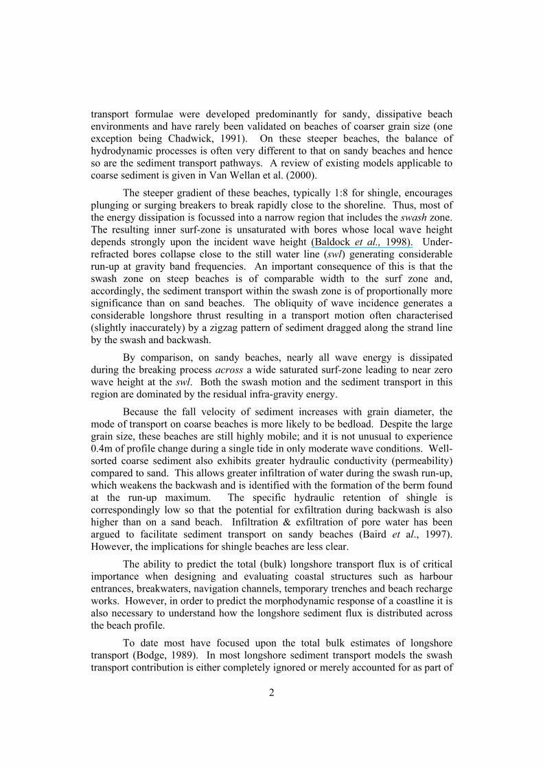
1 STRAND – a Model for Longshore Sediment Transport in the Swash Zone Eric van Wellen 1 , Tom Baldock 2 , Andrew Chadwick 3 & David Simmonds 3 . Abstract In this paper we report on the development and performance of an engineering model, STRAND which has the aim of predicting longshore movement of coarse sediment above the still water line of steep beaches. The model assumes that this transport is driven by swash run-up at the edge of an unsaturated inner surfzone and uses Nielsen's (1992) formulation for sediment transport rate. The hydrodynamic sub-model is shown to agree well with field measurements of swash run-up and swash period. We argue that consideration of interactions between subsequent swash events implies that a monotonic relationship between transport rate and incident wave period is inappropriate. Bulk longshore transport rates are shown to compare reasonably with previous estimates from field studies in the UK and accounts for up to 50% of the net longshore flux. Agreement of this simplified model with one of the best available laboratory data sets, Kamphuis (1991a,b), is very good indeed. However, new laboratory and field data are required before stronger conclusions can be drawn. Introduction Shingle or coarse grained beaches with D 50 > 2mm are common to many regions of the world including Canada, Japan, Argentina, New Zealand, Ireland and along considerable stretches of the Pacific coast of the USA. In the UK they constitute one third of the natural coastline and increasing use is being made of coarse-grained sediment to replenish eroding beaches, often in conjunction with structures such as rock and wooden groynes or offshore breakwaters. Examples in the UK include Highcliffe and Hurst Spit in Dorset, Hayling Island in Hampshire, Elmer in West Sussex and Seaford in East Sussex. These have been implemented within the last decade with others due to start e.g. at Hythe in Kent. One of the most popular analytical tools for total longshore transport rate prediction has been the CERC equation. However this and the majority of all other 1 Dredging International NV, Haven 1025, Scheldedijk 30, B2070, Zwijndrecht, Belgium. [email protected]. 2 Dept Civil Eng., Imperial College, London SW7 2BU, UK. [email protected]. 3 School Civil & Struct.Eng., Univ.Plymouth, Palace Court, PL1 2DE, UK. [email protected] & [email protected]. ++1752233664.
-
Upload
independent -
Category
Documents
-
view
4 -
download
0
Transcript of STRAND: A Model for Longshore Sediment Transport in the Swash Zone
1
STRAND – a Model for Longshore Sediment Transport in the Swash Zone
Eric van Wellen1, Tom Baldock2, Andrew Chadwick3 & David Simmonds3.
Abstract
In this paper we report on the development and performance of an engineering model, STRAND which has the aim of predicting longshore movement of coarse sediment above the still water line of steep beaches. The model assumes that this transport is driven by swash run-up at the edge of an unsaturated inner surfzone and uses Nielsen's (1992) formulation for sediment transport rate. The hydrodynamic sub-model is shown to agree well with field measurements of swash run-up and swash period. We argue that consideration of interactions between subsequent swash events implies that a monotonic relationship between transport rate and incident wave period is inappropriate. Bulk longshore transport rates are shown to compare reasonably with previous estimates from field studies in the UK and accounts for up to 50% of the net longshore flux. Agreement of this simplified model with one of the best available laboratory data sets, Kamphuis (1991a,b), is very good indeed. However, new laboratory and field data are required before stronger conclusions can be drawn.
Introduction
Shingle or coarse grained beaches with D50 > 2mm are common to many regions of the world including Canada, Japan, Argentina, New Zealand, Ireland and along considerable stretches of the Pacific coast of the USA. In the UK they constitute one third of the natural coastline and increasing use is being made of coarse-grained sediment to replenish eroding beaches, often in conjunction with structures such as rock and wooden groynes or offshore breakwaters. Examples in the UK include Highcliffe and Hurst Spit in Dorset, Hayling Island in Hampshire, Elmer in West Sussex and Seaford in East Sussex. These have been implemented within the last decade with others due to start e.g. at Hythe in Kent.
One of the most popular analytical tools for total longshore transport rate prediction has been the CERC equation. However this and the majority of all other
1 Dredging International NV, Haven 1025, Scheldedijk 30, B2070, Zwijndrecht, Belgium. [email protected]. 2 Dept Civil Eng., Imperial College, London SW7 2BU, UK. [email protected]. 3 School Civil & Struct.Eng., Univ.Plymouth, Palace Court, PL1 2DE, UK. [email protected] & [email protected]. ++1752233664.
2
transport formulae were developed predominantly for sandy, dissipative beach environments and have rarely been validated on beaches of coarser grain size (one exception being Chadwick, 1991). On these steeper beaches, the balance of hydrodynamic processes is often very different to that on sandy beaches and hence so are the sediment transport pathways. A review of existing models applicable to coarse sediment is given in Van Wellan et al. (2000).
The steeper gradient of these beaches, typically 1:8 for shingle, encourages plunging or surging breakers to break rapidly close to the shoreline. Thus, most of the energy dissipation is focussed into a narrow region that includes the swash zone. The resulting inner surf-zone is unsaturated with bores whose local wave height depends strongly upon the incident wave height (Baldock et al., 1998). Under-refracted bores collapse close to the still water line (swl) generating considerable run-up at gravity band frequencies. An important consequence of this is that the swash zone on steep beaches is of comparable width to the surf zone and, accordingly, the sediment transport within the swash zone is of proportionally more significance than on sand beaches. The obliquity of wave incidence generates a considerable longshore thrust resulting in a transport motion often characterised (slightly inaccurately) by a zigzag pattern of sediment dragged along the strand line by the swash and backwash.
By comparison, on sandy beaches, nearly all wave energy is dissipated during the breaking process across a wide saturated surf-zone leading to near zero wave height at the swl. Both the swash motion and the sediment transport in this region are dominated by the residual infra-gravity energy.
Because the fall velocity of sediment increases with grain diameter, the mode of transport on coarse beaches is more likely to be bedload. Despite the large grain size, these beaches are still highly mobile; and it is not unusual to experience 0.4m of profile change during a single tide in only moderate wave conditions. Well-sorted coarse sediment also exhibits greater hydraulic conductivity (permeability) compared to sand. This allows greater infiltration of water during the swash run-up, which weakens the backwash and is identified with the formation of the berm found at the run-up maximum. The specific hydraulic retention of shingle is correspondingly low so that the potential for exfiltration during backwash is also higher than on a sand beach. Infiltration & exfiltration of pore water has been argued to facilitate sediment transport on sandy beaches (Baird et al., 1997). However, the implications for shingle beaches are less clear.
The ability to predict the total (bulk) longshore transport flux is of critical importance when designing and evaluating coastal structures such as harbour entrances, breakwaters, navigation channels, temporary trenches and beach recharge works. However, in order to predict the morphodynamic response of a coastline it is also necessary to understand how the longshore sediment flux is distributed across the beach profile.
To date most have focused upon the total bulk estimates of longshore transport (Bodge, 1989). In most longshore sediment transport models the swash transport contribution is either completely ignored or merely accounted for as part of

3
the total sediment transport budget, generally via a calibration coefficient applied to the transport model when verified against field data. Bodge (1989) has provided a literature review of longshore sediment transport models that account for the cross-shore profile of longshore sediment flux. This concludes that the majority of these models assume a distribution that is maximum just landward of the point of wave breaking and reduces to zero at the swl. The few models that account for longshore transport in the swash zone do so by introducing set-up, which results in only an insignificant longshore flux in the swash zone. In laboratory experiments, however, Sawaragi and Deguchi (1978) observed non-zero transport rates at the swl. This was also observed in Bodge & Deans’ (1987) laboratory experiments in which a groyne was deployed to impound longshore transport and thereby allow measurements of the resulting accretion of sediment across the beach face. As wave steepness increased from spilling to plunging breakers, the observed build up of sediment changed from being concentrated in the surf-zone, to being concentrated in the swash zone. For the plunging/collapsing waves typical of steep beaches, their data suggests that up to 60% of the total longshore transport occurs in the swash zone.
A clear need exists therefore for a model to estimate the longshore transport in the swash zone, above the swl and especially for steep, coarse-grained beaches. The aim of this paper is to provide a simple engineering model that can be used in conjunction with a suitable surf-zone transport model. The model is presented and compared with the best currently available laboratory data set, Kamphuis (1991a,b).
Model Philosophy
The nature of sediment transport is undoubtedly complex, involving the interaction of many processes. The simplest parametric relationships for sediment transport require minimal input information and little computational effort but only provide the practising engineer with estimates of bulk transport rates. As outlined above, such information is not always sufficient. At the other extreme, the use of a state-of-the-art numerical model still requires a series of assumptions to be made, a varying degree of "calibration" and detailed site-specific information with which to calibrate and compare. The detail of the predictions of numerical models is often far in excess of that which can practically be expected to be found in the field measurements. As a result the benefits of using high-resolution models with less than complete data must always be questioned. Often the above requirements render such models unusable in practise or the assumptions that must be made reduce the accuracy of their predictive capability to being little better that of the simplest parametric models.
The model STRAND (Swash TRansport and Nearshore Dynamics) is aimed at a balance of these approaches. We apply Occam’s electric razor- the best solution is that which achieves the best accuracy with the least computational effort. Also we believe that the complexity of the predictions should be balanced against the complexity of the best available measurements. STRAND is conceptually easy to understand, computationally economic and uses a simplified view of the dynamics on steep beaches. The model requires minimal site-specific information and yet compares well a priori with the best available laboratory data sets. It is believed
4
this approach will be of practical use to Coastal Engineers working with steep coarse-grained beaches.
Model Overview
Here, the swash is defined simply as the area intermittently wetted above the swl. This is different to that used on a sandy beach or in the case of surging breakers where the swash is defined as the area of intermittent wetting and drying which includes often considerable run-down below the swl. The different definition comes from laboratory and field observations that on steep beaches, the swash front barely retreats below the mean the swl and indeed the swash zone appears to be well described by a continuous series of bores riding in above the mean water level. There is also a tendency for a step in the bathymetry to form just below the swl due to a subsurface rolling vortex formed by the interaction of the backwash of the previous swash with the next bore to arrive. This vortex excavates and maintains the step and prevents the swash front from moving much below this position.
STRAND proceeds by deducing the depth integrated, horizontal velocity field under a swash lens which is then used to drive sediment flux calculations over a single swash period or up until the next bore arrives. The hydrodynamic model domain effectively begins at the break point and ends at the maximum run-up during a swash event and is described by a longshore invariant beach of slope tanα.. The root-mean-square wave height at breaking Hrmsbr , the breaking wave angle θb and the peak wave period Tp, constitute the boundary conditions for the hydrodynamic calculations. Sediment transport is calculated only above the swl under the swash lens. The flux calculations require the fifty percentile grain size D50, the natural angle of repose of the bed material φ and the density of the solids and the fluid ρs and ρ.
Hydrodynamic Description
To begin with we describe the simplified view of the hydrodynamic processes that are used to drive swash sediment transport. Figure 1 shows the definition sketch in plan and side elevation of a wave breaking on a steep beach with the following sequence of events:
I. At the break point the surface wave transforms immediately into a turbulent bore of the same height.
II. The bore height attenuates towards the mean the swl in balance with the production of turbulence. Oblique bores are refracted by the change of celerity in decreasing water depth.
III. At the swl, the residual bore of attenuated but finite height collapses, rapidly recovering kinetic energy from this loss of potential energy. The swash front at this time acquires an initial velocity W0.

5
IV. The swash front sweeps up and down the beach face accelerated by gravity. With bed friction ignored, the ensuing bore front trajectory is symmetric and parabolic.
V. The depth averaged horizontal velocity under the "swash lens" between the swl and the position of the swash front are calculated along a cross-shore transect.
VI. The relationship between the period of the swash event Ts and the period of the incident waves Tp determine whether there is to be an interaction of subsequent swashes before the earlier swash retreats to the mean the swl.
Note that both friction and longshore currents are presently ignored as are the effects of infiltration. From the breakpoint, the model currently assumes a flat sloping bed
x
(0,0,0)β
θbθbore
y or t
z
Normalto theSWL
Velocityvector atborecollapse
SWL
Instantaneousshorelineposition duringswash event
Breaker line
Waveray atpoint ofbreaking
Run-upduringswash
(0,0,0)
SIDE VIEW
PLAN VIEW
x y or t
z
SWL
Sea bed
Indicative topmargin of thewater surfaceenvelope
Run-upduringswash
Figure 1: STRAND model definition sketch.

6
Figure 2: Swash lens profile evolution
and beach face and uses a simple dissipation model with depth limited breaking switched off to transform the rms wave height at breaking to the rms bore height at the swl.
dT
gH
p
3
41 . ρε = (1.)
This is Battjes & Janssen's (1978) dissipation model applied to each wave in turn. The depth limited breaking is switched off (Baldock et al 1998) so that the observed unsaturated wave heights at the swl can occur. The refraction of the wave angle following breaking is calculated using Snells law. However, in order to reproduce the "refraction lag" observed in laboratory (van Hijum and Pilarczyk, 1982, Asano et al., 1994) and field experiments (Walker et al., 1991), the water depth between the breakpoint and the swl has been artificially increased by half the breaking wave height.
The next stage is to calculate the shoreline motion of the swash front during a single cycle. The initial velocity W0 of the swash front following bore collapse at the swl is calculated by applying the classical dam-break equation as suggested by Luccio et al. (Equation 2.)
00 gHCW = (2.)
Although Luccio et al. suggested a value for C of the order 1.5, the coefficient is here set to 2 in accordance with laboratory experiments of Yeh et al. (1989) and of Baldock and Holmes (1997). Note that the coefficient C can be altered to accommodate the effects of friction. The subsequent motion of the swash front is then governed by Shen and Meyer's (1963) frictionless parabolic description of the shoreline motion in accordance with the observations of Hughes (1992). In the longshore direction the velocity V0 is constant, whilst in the cross shore the variation of position, Xs ,with time is given by Equation 3:
Figure 3: Instantaneous transport rate
7
αsin221
0 gttUX s −= (3.)
From Equation 3 the period of the swash event depends on the initial cross shore swash velocity, U0 , and the beach slope:
αsin
2 0
gU
Ts = (4.)
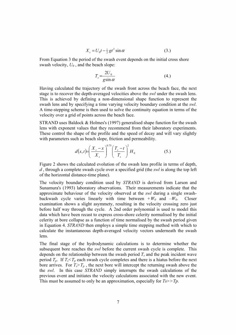
Having calculated the trajectory of the swash front across the beach face, the next stage is to recover the depth-averaged velocities above the swl under the swash lens. This is achieved by defining a non-dimensional shape function to represent the swash lens and by specifying a time varying velocity boundary condition at the swl. A time-stepping scheme is then used to solve the continuity equation in terms of the velocity over a grid of points across the beach face.
STRAND uses Baldock & Holmes's (1997) generalised shape function for the swash lens with exponent values that they recommend from their laboratory experiments. These control the shape of the profile and the speed of decay and will vary slightly with parameters such as beach slope, friction and permeability.
( ) 0
275.0
, HT
tTX
xXtxd
s
s
s
s
−
−= (5.)
Figure 2 shows the calculated evolution of the swash lens profile in terms of depth, d , through a complete swash cycle over a specified grid (the swl is along the top left of the horizontal distance-time plane).
The velocity boundary condition used by STRAND is derived from Larson and Sunamura's (1993) laboratory observations. Their measurements indicate that the approximate behaviour of the velocity observed at the swl during a single swash-backwash cycle varies linearly with time between +W0 and –W0. Closer examination shows a slight asymmety, resulting in the velocity crossing zero just before half way through the cycle. A 2nd order polynomial is used to model this data which have been recast to express cross-shore celerity normalised by the initial celerity at bore collapse as a function of time normalised by the swash period given in Equation 4. STRAND then employs a simple time stepping method with which to calculate the instantaneous depth-averaged velocity vectors underneath the swash lens.
The final stage of the hydrodynamic calculations is to determine whether the subsequent bore reaches the swl before the current swash cycle is complete. This depends on the relationship between the swash period Ts and the peak incident wave period Tp. If Ts<Tp each swash cycle completes and there is a hiatus before the next bore arrives. For Ts>Tp , the next bore will intercept the returning swash above the the swl. In this case STRAND simply interrupts the swash calculations of the previous event and initiates the velocity calculations associated with the new event. This must be assumed to only be an approximation, especially for Ts>>Tp.

8
Sediment Transport Calculations Given the difficulty of making measurements in the swash zone, it is uncertain how to best represent the physics of swash sediment transport. Field observations of Horn and Mason (1994) made on sand beaches, suggest that sediment is transported on the uprush as a combination of bedload and suspended load, whilst on the backwash bedload dominates. Such observations, however, may be artefacts of the measurement procedure rather than the processes involved (Masselink and Hughes, 1998). Hughes et al. (1997) have indicated that transport in the swash generally occurs under sheet flow conditions, yet here too there is considerable disagreement as to what this implies.
STRAND proceeds to calculate sediment transport as a function of a Shields parameter, θ, and assumes that suspended sediment is insignificant.
501 Dg s
−
=
ρρ
ρ
τθ (6.)
Here τ is the total shear stress at the bed, ρ is the fluid density, ρs is the density of the sediment and D50 is the fifty-percentile grain diameter. The bed shear stress is calculated via Wilson's (1989) friction factor, fw89, and the depth averaged velocity vectors output from the hydrodynamics calculations. Masselink and Hughes (1998) concluded that Wilson’s friction factor is the most appropriate formulation for swash conditions on the basis that it was derived specifically for sheet flow conditions. The factor is found by iteratively solving Equation 7, where, â is the peak wave orbital excursion and T is the wave period.
203
1
2 0 4 2
2 89 89
πρρ
$exp .a
g Tf fs w w−
= −
(7.)
STRAND uses Nielsen's (1992) formula for dimensionless bedload transport, Φ, which incorporates a threshold of motion term, θcr . This threshold is not necessary for lighter sediments but is important for larger grain sizes.
( )crθθθ −=Φ 12 (8.)
The threshold term, θcr, is calculated using Soulsby & Whitehouse's (1997) extension of Shields work (Equation 9) and this is also corrected for bed slope.
( )[ ]**
020.0exp1055.024.0 DDcr −−+=θ (9.)
Finally, the instantaneous volumetric bedload transport rate per unit width of beach, qb, is calculated.

9
3501 Dgq s
b
−Φ=
ρρ
(10.)
Figure 3 shows the instantaneous transport rate calculated in this way over the duration of a single swash cycle, showing the largest transport rates close to the swl at any one time, with no transport occuring in the middle of the swash cycle (the swl position is along the time axis). This transport rate can then be resolved into bulk cross-shore and long-shore transport fluxes accross the entire swash zone by integrating over cross-shore distance and time.
Model Testing
The model was subject to a series of sensitivity tests reported in Van Wellan (1999). One of the first observations to make concerns the implications of swash–wave interaction. Figure 4 shows the variation of the cross-shore and longshore fluxes calculated at the mid-swash and the swl, and the integrated rates across the swash, as the percentage ratio of the incident wave period to the natural swash period changes. The model suggests that both the cross-shore and longshore transport rates reach maximum when these two wave periods are equal; but reach a minimum when Tp is 70%-80% of Ts. At this time the following bore arrives to cancel the strong, slope assisted backwash transport resulting in zero cross-shore transport and removing a major contribution to the longshore transport. For smaller values of the ratio, the transport is increasingly dominated by the early phase of the swash cycle producing stronger onshore (and longshore) transport. For larger ratios there is an increase in the hiatus between completion of the swash event and the arrival of the next bore during which there is no transport. The point to make is that if such a model is appropriate, then a monotonic relationship between the sediment flux and the wave period is not justified.
Tran
spor
t [m
3 /m
s]
-0.0015
-0.0010
-0.0005
0.0000
0.0005
0.0010
0.0015
0.0020
qSWL
qmid swash
qmean
Tp/Ts*100 [%]0 50 100 150 200 250 300
0
2e-5
4e-5
6e-5
8e-5
Cross-shore component
Longhore component
swash interaction no swash interactionTs = 5.06s
Figure 4:Variation of transport fluxes with Tp/Ts.

10
Published laboratory data (Asano,1996, Sunamura 1984, Sawaragi & Deguchi 1978, Baldock et al.1998, Bodge & Dean, 1987) and measurements obtained at Lancing, UK in 1997 were used to test the hydrodynamics of STRAND further. A good comparison was found between the measured bore heights and those predicted by STRAND from the measured wave parameters at breaking. STRAND also demonstrated that bores arriving at the swl retain up to 70% of their height at breaking.
A less favourable comparison between predicted and measured values of maximum swash run-up was obtained though this is a difficult parameter to measure and experimental values are likely to be a underestimates. Better comparison was obtained with field observations on a steep beach at Lancing, UK, though generally STRAND overestimates this parameter. STRAND was also found to under-predict the natural swash period possibly as a result of neglecting friction.
STRAND was also used to estimate longshore transport on an open macro-tidal steep shingle beach (D50=20mm, slope≈1/7) at Shoreham in southern England. The hydrodynamic conditions and littoral drift estimates (15,00-20,000m3) at this site are well reported (Van Wellen et al., 2000). Using measurements of the conditions which appear to contribute most to the net drift at Shoreham, STRAND predicted a rate that accounted for 50%-70% of the total mean annual longshore transport estimate, thus re-emphasising the importance assigned to swash zone sediment transport.
Finally, Kamphuis (1991a,b) reported on a series of comprehensive laboratory tests that focussed on measurements of longshore sediment flux profile across both the
Measured immersed swash zone transport [kg/m*hr] (Kamphuis, 1991)0 10 20 30 40 50 60
Pre
dict
ed im
mer
sed
tota
l sw
ash
zone
tra
nspo
rt [k
g/m
*hr]
(STR
AN
D m
odel
)
-20
-10
0
10
20
30
40
50
60
Data pointsBest fit line95% confidence limits
R2 = 81.46%
Figure 5: Comparison with Kamphuis laboratory data.

11
surf and swash zone on scale beaches. The STRAND model was applied to this data using the recorded hydrodynamic parameters to predict longshore transport rates in the swash zone. The Kamphuis results show flux profiles across the surf and swash zones for a range of conditions corresponding to both sand and steeper shingle beaches. Both the observed peak values and the integrated fluxes across the entire swash zone were compared with the STRAND predictions .
A good agreement is shown for both the maximum expected transport rate and the swash zone averaged transport rate. The latter is shown in Figure 5. In general the STRAND model appears to under-predict the maximum swash transport, but this seems to be balanced by the over-prediction of the swash zone extent, resulting in a very good correlation for the mean swash zone longshore transport rate.
Conclusions
STRAND was developed to provide a simple engineering model of swash sediment transport on steep, coarse-grained beaches. The model supports observations that in such environments sediment transport above the still water line is not insignificant. Swash interaction is dealt with by the model in only a simplistic way (i.e. replacing the hydrodynamics and associated transport with those of the new incoming bore). This requires further development although this presently indicates that parametric models that assume a simple monotonic relationship between wave period and transport rate are inappropriate. The simplicity of STRAND adds to its appeal and utility. Despite this simplicity, a very good correlation between its predictions and Kamphuis's laboratory data are achieved which is particularly encouraging since the dataset is the currently the best available for validating longshore transport models.. Further testing of STRAND is necessary, and to this end new field and laboratory data sets from coarse-grained steep beach environments are needed.
Acknowledgements
The authors gratefully acknowledge funding from the UK Ministry of Agriculture, Fisheries and Food (MAFF) and the European Commission through the MAST III programme, SASME project, contract no: MAS3-CT97-0081. We are also wish to thank all participants in the MAFF shingle beach project.
References Asano T. (1994). Swash motion due to obliquely incident waves. Proc. 24th Int. Conf. on Coastal Eng., American Society of Civil Engineers, 1; 27-41.
Baird A. J., Mason T. E. and Horn D. P. (1997). Monitoring and modelling groundwater behaviour in sandy beaches as a basis for improved models of swash zone sediment transport. Proc. of Coastal Dynamics 97, Plymouth, American Society of Civil Engineers; 774-783.
Baldock T. E. and Holmes P. (1997). Swash hydrodynamics on a steep beach. Proceedings of Coastal Dynamics'97, Plymouth, American Society of Civil Engineers; 784-793.
Baldock T. E., Holmes P., Bunker S. and Van Weert P. (1998). Cross-shore hydrodynamics within an unsaturated surf zone. Coastal Engineering, Elsevier Science Publishers B.V., Amsterdam, 34; 173-196.
Battjes J. A. and Janssen J. P. F. M. (1978). Energy loss and set-up due to breaking of random waves. Proc. 16th Int. Conf. on Coastal Eng., New York, American Society of Civil Engineers; 569-587.

12
Bodge K. R. (1989). A literature review of the distribution of longshore sediment transport across the surf zone. Journal of Coastal Research, The Coastal Education and Research Foundation, 5, (2); 307-328.
Bodge K. R. and Dean R. G., (1987), Short-term impoundment of longshore transport, Proc. Coastal Sediments '87, ASCE, pp 468-483.
Chadwick A. J. (1991). An unsteady flow bore model for sediment transport in broken waves. Part 1: the development of the numerical model. Proc. Instn Civ. Engrs, Part 2, (91); 719-737.
Horn D. P. and Mason T. (1994). Swash zone sediment transport modes. Marine geology, 120; 309-325.
Hughes S. A. (1992). Application of a non-linear shallow water theory to swash following bore collapse on a sandy beach. Journal of Coastal Research, The Coastal Education and Research Foundation, 8; 562-578.
Hughes S. A., Masselink G. and Brander R. W. (1997). Flow velocity and sediment transport in the swash zone on a steep beach. Marine Geology, Elsevier Science Publishers B.V., Amsterdam, 138; 91-103.
van Hijum E. and Pilarczyk K. W. (1982). Equilibrium profile and longshore transport of coarse material under regular and irregular wave attack., Delft Hydraulics Publication no. 274.
Kamphuis J. W. (1991a). Alongshore sediment transport rate distribution. Coastal Sediments '91 Conference, American Society of Civil Engineers; 170-183.
Kamphuis J. W. (1991b). Alongshore sediment transport rate. J. Waterway, Port, Coastal and Ocean Engineering, American Society of Civil Engineers, 117; 624-640.
Larson M. and Sunamura T. (1993). Laboratory experiment on flow characteristics at a beach step. Journal of sedimentary petrology, 63, (3); 495-500.
Masselink G. and Hughes M. (1998). Field investigation of sediment transport in the swash zone. Continental Shelf Research, 18; 1179-1199.
Nielsen P. (1992). Coastal bottom boundary layers and sediment transport, Advanced series on ocean engineering, World Scientific, Singapore, 4; 324.
Sawaragi T. and Deguchi I. (1978). Distribution of sand transport rate across the surf zone. Proc. 16th Int. Conf. on Coastal Eng., Hamburg, American Society of Civil Engineers, 2; 1596-1613.
Shen M. C. and Meyer R. E. (1963). Climb of a bore on a beach; Part 3. Run-up. Journal of Fluid Mechanics, 16; 113-125.
Soulsby R. L. and Whitehouse R. J. S. (1997). Threshold of sediment motion in coastal environments. Proc. of the combined Australasian Coastal Engineering and Ports Conference, Christchurch; 149-154.
Sunamura T. (1983). Proc. 30th Japan. Conf. Coastal Eng., (in Japanese); 214-218.
Van Wellan E. , Chadwick, A.J. and Mason, T. (2000) A review and assessment of longshore sediment transport equations for coarse-grained beaches, Coastal Engineering, 40, 243-275.
Van Wellan, E. (1999). Modelling of swash zone sediment transport on coarse grained beaches. University of Plymouth PhD thesis.
Walker J. R., Everts C. H., Schmelig S. and Demirel V. (1991). Observations of a tidal inlet on a shingle beach. Coastal Sediments '91 Conference, American Society of Civil Engineers; 975-989.
Wilson K. C. (1989). Friction of Wave-Induced Sheet Flow. Coastal Engineering, Elsevier Science Publishers B.V., Amsterdam, (12); 371-379.
Yeh H. H., Ghazali A. and Marton I. (1989). Experimental study of bore run-up. Journal of Fluid Mechanics, 206; 563-578.