PHASE II INVESTIGATION OF SEDIMENT CONTAMINATION ...

PPHHAASSEE IIII IINNVVEESSTTIIGGAATTIIOONN OOFF SSEEDDIIMMEENNTT CCOONNTTAAMMIINNAATTIIOONN

IINN WWHHIITTEE LLAAKKEE

BY

DDrr.. RRiicchhaarrdd RReeddiisskkee DDrr.. MMiicchhaaeell CChhuu DDrr.. DDoonn UUzzaarrsskkii JJeeffff AAuucchh R. B. Annis Water Resources Institute Grand Valley State University 740 W. Shoreline Dr. Muskegon, MI 49441

DDrr.. GGrraahhaamm PPeeaasslleeee Chemistry Department Hope College 35 E. 12th St. Holland MI 49423

DDrr.. JJoohhnn GGaabbrroosseekk Department of Statistics Grand Valley State University 1 Campus Drive Allendale, MI 49401

GREAT LAKES NATIONAL PROGRAM OFFICE # GL975368-01-0 U. S. Environmental Protection Agency

PROJECT OFFICER:

Dr. Marc Tuchman

U. S. Environmental Protection Agency Great Lakes National Program Office

77 West Jackson Blvd. Chicago IL 60604-3590

February 2004

ACKNOWLEDGEMENTS This work was supported by grant #GL975368-01-0 from the Environmental Protection Agency Great Lakes National Program Office (GLNPO) to the Annis Water Resources Institute (AWRI) at Grand Valley State University. Project Team

EPA Project Officer

Dr. Marc Tuchman USEPA GLNPO Principal Scientists

Dr. Richard Rediske AWRI/GVSU Sediment Chemistry Dr. Michael Chu AWRI/GVSU GIS Dr. Don Uzarski AWRI/GVSU Aquatic Ecology Jeff Auch AWRI/GVSU Benthic Macroinvertebrates Dr. John Gabrosek GVSU Statistical Methods Dr. Graham Peaslee Hope College Radiochemistry Project technical assistance was provided by the following individuals at GVSU and U of M: Trace Analytical Trimatrix Laboratories

Eric Andrews Betty Doyle Gail Smythe Al Steinman

Ship support was provided by the crew of the R/V Mudpuppy (USEPA) and Captain Joe. Bonem

Disclaimer The U.S. Environmental Protection Agency through its Great Lakes National Program Office funded the project described here under Grant GL-975207 to Grand Valley State University. It has not been subjected to Agency review and therefore does not necessarily reflect the views of the Agency, and no official endorsement should be inferred. Reference herein to any specific commercial products, process or service by trade name, trademark, manufacturer or otherwise, does not necessarily constitute or imply its endorsement, recommendation, or favoring by the United States Government. The views and opinions of the authors expressed herein do not necessarily state or reflect those of the United States Government, and shall not be used for advertising or product endorsement purposes.

i

TABLE OF CONTENTS List Of Tables ................................................................................................................................ iii

List Of Figures ............................................................................................................................... vi

Executive Summary .........................................................................................................................1

1.0 Introduction...............................................................................................................................2

1.1 Summary of Anthropogenic Activities In White Lake .................................................5

1.2 Project Objectives And Task Elements ........................................................................7

1.3 Experimental Design.....................................................................................................9

1.4 References...................................................................................................................11

2.0 Sampling Locations ................................................................................................................13

3.0 Methods ..................................................................................................................................17

3.1 Sampling Methods ......................................................................................................17

3.2 Chemical Analysis Methods For Sediment Analysis .................................................18

3.3 Chemical Analysis Methods For Water Analysis.......................................................29

3.4 Sediment Toxicity.......................................................................................................29

3.5 Benthic Macroinvertebrate Analysis ..........................................................................33

3.6 Radiometric Dating.....................................................................................................33

3.7 Statistical Analysis......................................................................................................34

3.8 Contaminant Mapping ................................................................................................34

3.9 References...................................................................................................................35

4.0 Results And Discussion ..........................................................................................................36

4.1 Sediment Chemistry Results .......................................................................................36

4.2 Stratigraphy and Radiodating Results.........................................................................53

4.3 Toxicity Testing Results .............................................................................................63

4.4 Benthic Macroinvertebrate Results.............................................................................73

4.5 Chromium Uptake by Aquatic Organisms..................................................................87

ii

4.6 The Environmental Fate and Significance of Chromium and PCBs in White Lake.............................................................................................................90

4.7 Sediment Quality Triad Assessment of Contaminated sediments in White Lake...........................................................................................................100

4.8 Summary and Conclusions .......................................................................................101

4.9 References.................................................................................................................102

5.0 Recommendations.................................................................................................................106

Appendices ..............................................................................................................................107

Appendix A. Quality Assurance Review of the Project Data ..................................................108

Appendix B. Results Physical Analyses On White Lake Sediments, October 2000...............115

Appendix C. Organic Analyses On White Lake Sediments, October 2000. ...........................120

Appendix D. Results Of Metals Analyses For White Lake Sediments, October 2000. ...................................................................................................................128

Appendix E. Summary Of Chemical Measurements For The Toxicity Test With Sediments From White Lake, October 2000. .....................................................133

Appendix F. Summary Of Benthic Macroinvertebrate Results For White Lake, October 2000 ......................................................................................................150

iii

LIST OF TABLES

Table 2.1 White Lake Core Sampling Stations......................................................................15

Table 2.2 White Lake Stratigraphy Sampling Stations..........................................................16

Table 2.3 White Lake PONAR Core Sampling Stations .......................................................16

Table 3.1 Sample Containers, Preservatives, And Holding Times........................................18

Table 3.2.1 Analytical Methods And Detection Limits ............................................................19

Table 3.2.2 Organic Parameters And Detection Limits ............................................................25

Table 3.2.3 Data Quality Objectives For Surrogate Standards.................................................26

Table 3.2.4 Sediment Detection Limits for PCBs.....................................................................27

Table 3.3.1 Analytical Methods And Detection Limits For Culture Water..............................29

Table 3.4.1 Test Conditions For Conducting A Ten Day Sediment Toxicity Test With Hyalella azteca .............................................................................................31

Table 3.4.2 Recommended Test Conditions For Conducting A Ten Day Sediment Toxicity Test With Chironomus tentans................................................................32

Table 4.1.1 Results Of Sediment Grain Size Fractions, TOC, And Percent Solids For White Lake Core Samples, October 2000 .......................................................37

Table 4.1.2 Results Of Sediment Grain Size Fractions, TOC, And Percent Solids For White Lake PONAR Samples, October 2000 .................................................38

Table 4.1.3 Results Of Sediment Metal Analyses For White Lake Core Samples (mg/kg Dry Weight), October 2000.......................................................................40

Table 4.1.4 Results Of Sediment Metal Analyses For White Lake PONAR Samples (mg/kg Dry Weight), October 2000 ........................................................41

Table 4.1.5 Results of Sediment PCB and Semivolatile Analyses for White Lake Core Samples (mg/kg Dry Weight), October 2000 ...............................................42

Table 4.1.6 Results of Sediment PCB and Semivolatile Analyses for White Lake PONAR Samples (mg/kg Dry Weight), October 2000..........................................43

Table 4.1.7 Spearman Rank Order Correlations for Chemical and Physical Parameters For White Lake Sediments..................................................................52

Table 4.1.8 Concentration of Organic Chromium in White Lake Sediments...........................53

Table 4.2.1 Stratigraphy and Radiodating Results For Core WL-2S Collected From White Lake, October 2001 ...........................................................................54



iv

Table 4.2.4 Results of ICP and PIXE Analyses for Chromium in Core WL-9S Collected From White Lake, October 2001...........................................................62

Table 4.2.5 Average and Corrected Data for Stratigraphy Cores (October 2001) Compared to the Results of the Top Core Section From the Investigative Survey (October 2000) for White Lake Sediments..........................62

Table 4.3.1.1 Summary Of Hyalella azteca Survival Data Obtained During The 10 Day Toxicity Test With White Lake Sediments ....................................................64

Table 4.3.1.2 Summary Of Dunnett’s Test Analysis Of Hyalella azteca Survival Data Obtained During The 10 Day Toxicity Test With White Lake Sediments From Shallow Stations .........................................................................65

Table 4.3.1.3 Summary Of Dunnett’s Test Analysis Of Hyalella azteca Survival Data Obtained During The 10 Day Toxicity Test With White Lake Sediments From Deep Stations..............................................................................65

Table 4.3.2.1 Summary Of Chironomus tentans Survival Data Obtained During The 10 Day Toxicity Test With White Lake Sediments ...............................................67

Table 4.3.2.2 Summary Of Dunnett’s Test Analysis Of Chironomus tentans Survival Data Obtained During The 10 Day Toxicity Test With White Lake Sediments From Shallow Stations .........................................................................68

Table 4.3.2.3 Summary Of Dunnett’s Test Analysis Of Chironomus tentans Survival Data Obtained During The 10 Day Toxicity Test With White Lake Sediments From Deep Stations..............................................................................68

Table 4.3.2.4 Summary Of Chironomus tentans Dry Weight Data Obtained During The 10 Day Toxicity Test With White Lake Sediments........................................69

Table 4.3.2.5 Summary of Dunnett’s Test Analysis of Chironomus tentans Growth Data Obtained During The 10 Day Toxicity Test With White Lake Sediments From Shallow Stations .........................................................................70

Table 4.3.2.6 Summary of Dunnett’s Test Analysis of Chironomus tentans Growth Data Obtained During The 10 Day Toxicity Test With White Lake Sediments From Deep Stations..............................................................................70

Table 4.3.3.1 Summary of Results of Total Chromium, Organic Chromium, and Amphipod Survival for White Lake Sediments.....................................................71

Table 4.4.1.1 Benthic Macroinvertebrate Distribution In White Lake (#/m2), October 2000. Mean Number Of Organisms And Standard Deviation Reported For Each Station.....................................................................................................74

Table 4.4.1.2 Mean Abundance (#/m2) And Relative Densities (%) of Major Taxonomic Groups in White Lake, October 2000.................................................77

Table 4.4.2.1 Summary of Diversity And Trophic Status Metrics for the Benthic Macroinvertebrates in White Lake, October 2000.................................................80

v

Table 4.4.2.2 Spearman Rank Order Correlations for Ecological, Chemical, and Physical Parameters for White Lake......................................................................82

Table 4.4.3.1 Summary Statistics for the Analysis of Individual Benthic Macroinvertebrate Samples from White Lake, October 2000...............................84

Table 4.5.1 Chromium Concentration in Macrophytes and Zebra Mussels in Tannery Bay...........................................................................................................87

Table 4.5.2 Chromium Concentration in Chironomids from Tannery Bay ..............................88

Table 4.6.1 White Lake Chromium Data ..................................................................................90

Table 4.6.2 White Lake PCB Data............................................................................................96

Table 4.7.1 Sediment Quality Assessment Matrix for White Lake Data, October 2000. Assessment Matrix from Chapman (1992) ...............................................100

vi

LIST OF FIGURES

Figure 1.1 White Lake...............................................................................................................2

Figure 1.2 Areas Of Sediment Contamination Identified In White Lake .................................5

Figure 2.1 White Lake Core and PONAR Sampling Stations ................................................14

Figure 4.1.1 Distribution of Arsenic in Core Samples Collected in Western White Lake, October 2000................................................................................................44

Figure 4.1.2 Distribution of Chromium in Core Samples Collected in Western White Lake, October 2000.....................................................................................44

Figure 4.1.3 Distribution of Lead in Core Samples Collected in Western White Lake, October 2000................................................................................................45

Figure 4.1.4 Comparison of Arsenic Concentrations in PONAR Samples and Top Core Sections Collected in White Lake, October 2000 .........................................45

Figure 4.1.5 Comparison of Chromium Concentrations in PONAR Samples and Top Core Sections Collected in White Lake, October 2000..................................46

Figure 4.1.6 Comparison of Lead Concentrations in PONAR Samples and Top Core Sections Collected in White Lake, October 2000 .........................................46

Figure 4.1.7 Distribution of Aroclor 1248 in Core Samples Collected in Western White Lake, October 2000.....................................................................................48

Figure 4.1.8 Distribution of Chromium in PONAR Samples for White Lake, October 2000..........................................................................................................49

Figure 4.1.9 Bathymetric plot of White Lake ............................................................................50

Figure 4.1.10 PCA Analysis of White Lake Physical and Chemical Data ..................................51

Figure 4.2.1 Depth and Concentration Profiles for Chromium, Lead-210, and Cesium-137 at Station WL-2S, White Lake, October 2001. .................................55

Figure 4.2.2 Depth and Concentration Profiles for Chromium, Lead-210, and Cesium-137 at Station WL-7S, White Lake, October 2001 ..................................58

Figure 4.2.3 Depth and Concentration Profiles for Chromium, Lead-210, and Cesium-137 at Station WL-9S, White Lake, October 2001 ..................................60

Figure 4.3.3.1 Relationship Between Total Chromium and Amphipod Survival for Tannery Bay Sediments .........................................................................................71

Figure 4.3.3.2 Relationship Between Organic Chromium and Amphipod Survival for Tannery Bay Sediments .........................................................................................72

Figure 4.4.1.1 General Distribution Of Benthic Macroinvertebrates In White Lake, October 2000..........................................................................................................78

Figure 4.4.2.1 Summary Of Trophic Indices (Pollution Tolerance) For The Benthic Macroinvertebrates In White Lake, October 2000 ................................................81

vii

Figure 4.4.3.1 Canonical Correspondence Analysis of Benthic Macroinvertebrate Taxa for White Lake, October 2000 ......................................................................83

Figure 4.4.4.1 Plot of CCA Dimension 1 (Macroinvertebrate Taxa) and Chromium for White Lake Sediments, October 2000..............................................................86

Figure 4.5.1 Chromium Accumulation in Macrophytes and Zebra Mussels in Tannery Bay...........................................................................................................88

Figure 4.5.2 Chromium Accumulation in Chironomids from Tannery Bay ..............................89

Figure 4.6.1 Chromium Sampling Points in White Lake ...........................................................91

Figure 4.6.2 Chromium Sampling Points in the Vicinity of Tannery Bay.................................92

Figure 4.6.3 Chromium Concentration Contours for White Lake Surficial Sediments...............................................................................................................93

Figure 4.6.4 Generalized Circulation Pattern for White Lake ...................................................94

Figure 4.6.5 PCB Sampling Points in White Lake.....................................................................97

Figure 4.6.6 PCB Concentration Contours in the Surficial Sediments in the Vicinity of the Former Occidental/Hooker Chemical Discharge ........................................98

Figure 4.6.7 PCB Concentration Contours in the Surficial Sediments in White Lake ..............99

1

Executive Summary

A Phase II investigation of the nature and extent of sediment contamination in White Lake was performed. Sediment chemistry, solid-phase toxicity, and benthic macroinvertebrates were examined at 21 locations. Since chromium was previously identified as the major contaminant in the sediments, experiments were conducted to determine the accumulation of the metal in zebra mussels, macrophytes, and chironomids. In addition, three core samples were evaluated using radiodating and stratigraphy to assess sediment stability and contaminant deposition. High levels of chromium were found to cover a majority of the lake bottom and to extend 8 km from Tannery Bay. All locations sampled west of Tannery Bay exceeded the Probable Effect Concentration (PEC). Most of the chromium was found in the top 51 cm of the core samples. High concentrations of PCBs were found near the outfall of the former Occidental/Hooker Chemical facility. These levels also exceeded PEC guidelines. Sediment toxicity was observed in the east bay area and at the Occidental/Hooker Chemical outfall. Toxicity near the Occidental/Hooker Chemical outfall was probably due to the presence of PCBs. No obvious toxicant was present in the sediments from the east bay. While no relationship was previously observed for total chromium and amphipod toxicity, a significant correlation was found for the organically bound fraction and the metal. Elevated levels of organic chromium were found in archived sediments from Tannery Bay. Benthic macroinvertebrate communities throughout White Lake were found to be indicative of organically enriched conditions. The locations in the east bay were significantly different than reference sites, as indicated by a shift to chironomids that were predators and sprawlers. Chironomid populations in the remainder of the lake were burrowers and detritivores. Higher densities of nematodes and reduced tubificids populations were associated with the stations with elevated chromium levels (> 400 mg/kg). The metal also was correlated with an increase in the trophic status of chironomid populations. Chromium accumulation was observed in chironomid populations throughout White Lake. In addition, macrophytes and zebra mussels in Tannery Bay were observed to accumulate the metal in their tissue. All of the stratigraphy cores showed uniform levels of chromium deposition in the top 10 - 15 cm. This pattern suggested that a constant source of chromium was present in White Lake. A standard exponential decay pattern was absent in the lower sections of the cores, indicating that historical changes in sedimentation were caused by episodic events. These data coupled with chromium contour maps and the generalized circulation pattern of the lake were used to elucidate the fate and transport of the metal. The proximity to the drowned rivermouth currents at the Narrows and the wind induced resuspension in the bay provided conditions that facilitated the advection and dispersion of a sediment plume 8 km from its source. Higher concentrations of chromium were found in the three deep deposition basins (300-500 mg/kg). In contrast, the PCBs discharged by the Occidental/Hooker Chemical outfall remained within 100 m of the outfall pipe. The depth of the discharge (15 m) plus the depositional nature of the discharge zone acted to confine the contaminants to a small area. The removal of contaminated sediments in Tannery Bay and the Occidental/Hooker outfall were completed by October 2003. Both remedial actions are essential for the recovery of White Lake. Remediation at Tannery Bay removed the ongoing source of chromium contamination while dredging the Occidental/Hooker outfall reduced the amount of bioaccumulative compounds in the lake.

2

1.0 Introduction

White Lake, Michigan is a 10.2 km2 (4,150 acres) drowned river mouth lake that is directly connected to Lake Michigan by a navigation channel. The lake has a mean depth of 7.3 m and an estimated volume of 7.6×107 m3 (Freedman et al. 1979). Deep deposition zones are located at Dowies Point (17 m) and Long Point (21 m). The lake is part of the White River watershed, which has a drainage basin of 139,279 hectares (2,634 square miles). The White River originates in Newaygo County and flows through a large marsh/estuary complex before entering White Lake. A predominately western flow is maintained through the lake resulting in a residence time of 56 days. Strong currents are often noted in the region called the Narrows, where two peninsulas cause a restriction in the watercourse and produce riverine flow conditions through the passage. White Lake functions as a significant fishery and recreational area in this region of the Great Lakes and provides an important transition zone between the open waters of Lake Michigan and the estuary/riverine environments associated with the White River.

1 MILE

FIGURE 1.1 WHITE LAKE.

Tannery Bay

Dowies Point

Long Point

The Narrows

3

White Lake has a long history of environmental issues related to water quality and the discharge of toxic materials. The lake was impacted in the mid 1800s when saw mills were constructed on the shoreline during the lumbering era. During this period, a large portion of the littoral zone was filled with sawdust, wood chips, timber wastes, and bark. Large deposits of lumbering waste can still be found today in the nearshore zone of White Lake. The lumbering era was followed in the 1900s by an era of industrial expansion related to the construction of specialty chemical production facilities and a leather tanning operation. Tannery waste from Whitehall Leather was discharged directly into White Lake from 1890-1973. Effluents from Hooker Chemical’s (now Occidental Chemical) chloralkali and pesticide production were discharged from the 1950-1986 (Evans 1992 and GLC 2000). Chlorinated organic chemicals from DuPont and Muskegon Chemical (now Koch Chemical) have also entered White Lake through groundwater and surface water discharges. As a result, degraded conditions were observed in much of the lake, as well as high sediment concentrations of heavy metals and pesticide related chemicals. Evans (1992) presented a review of studies that described extensive areas of oxygen depletion, high quantities of chromium in the sediments, thermal pollution, the discharge of industrial wastes with a high oxygen demand from the tannery (sulfide and organic matter), tainted fish, frequent algal blooms, and high nutrient concentrations. Generally, oligochaetes were the dominant benthic taxa and macroinvertebrate species richness and diversity were low across the lake (Evans 1976). These factors indicated that eutrophic conditions were prevalent in 1972, especially, the southeastern portion of the lake. The International Joint Commission designated White Lake as an Area of Concern (AOC) because of severe environmental impairments related to these discharges. The AOC boundary includes the lake and several small subwatersheds. In 1973, a state of the art wastewater treatment facility was constructed and the direct discharge of waste effluents and partially treated municipal sewage to White Lake was eliminated. The new facility was constructed near Silver Creek and utilized aeration, lagoon impoundment, spray irrigation and land treatment to remove nutrients, heavy metals, and organic chemicals. While the system was very effective in reducing the point source load of nutrients to White Lake, nonpoint contributions from upstream sources increased after construction and a net reduction in loading was not observed during 1974 and 1975 (Freedman et al. 1979). Recent and historical studies have indicated extensive contamination of sediments in White Lake. Elevated levels of chromium, lead, arsenic, and mercury were detected in the northeastern section of the lake in 1982 during a U.S. Environmental Protection Agency (U.S.EPA) funded study conducted by the West Michigan Shoreline Regional Development Commission (WMSRDC 1982). This study also found evidence of heavy metal contamination in several locations along the northwest shore. In a more recent study conducted in the summer of 1994 by U.S.EPA/Michigan Department of Environmental Quality (MDEQ), elevated concentrations of these metals were detected in an area of the northeast shore of White Lake (Bolattino and Fox 1995). This area (Tannery Bay) was the historical discharge point for tannery effluent from Whitehall Leather. The chromium levels found in the sediments of this area (4,500 mg/kg) were some of the highest concentrations reported from any site in the Great Lakes. In a recent investigation, Rediske et al. (1998) determined the distribution of chromium in western White Lake and evaluated the toxicity and stability of sediments in Tannery Bay. Key findings of the investigation were as follows:

4

Sediments in Tannery Bay were acutely toxic to amphipods and midges. Chromium concentrations in Tannery Bay ranged from 1000 mg/kg to 4,500 mg/kg.

No correlation was found between solid phase toxicity and total chromium concentrations.

The highest degree of toxicity was found in the bay located to the east of Tannery Bay. Chromium levels were low (100 mg/kg - 200 mg/kg) at this location.

Benthic macroinvertebrates in Tannery Bay and the east bay were lower in diversity and contained more pollution tolerant organisms than an uncontaminated control location.

Profiles of 210Pb showed that mixing was occurring in the top 20 cm of sediment in Tannery Bay.

Chromium levels approaching 900 mg/kg were found 2.4 km (1.5 miles) down gradient of the discharge point.

High levels of PCBs (100 mg/kg) were detected in the sediments near the discharge of the former Occidental Chemical facility (Dowies Point).

The extent of chromium and PCB contamination in western White Lake was not investigated in the previous study. While we know that high levels of chromium are present in the near surface zone in many areas of eastern White Lake, the toxicity of these sediments has not been evaluated. In addition, contaminant sediment profiles, toxicity evaluations, and an assessment of the macroinvertebrate community have not been performed in section of White Lake from Dowies Point to the Lake Michigan channel. The presence of contaminated sediments and ecological impairments in the eastern half of the lake coupled with westerly flow of water through the lake underscore the importance of conducting a more comprehensive assessment of the system. This investigation expanded the historical data and addressed critical data gaps related to the distribution of chlorinated hydrocarbons and heavy metals in the western half of White Lake and the toxicity of sediments outside of Tannery Bay. The investigative sampling focused on regions of sediment contamination in areas near the shoreline and in deeper deposition zones. A series of 10 sediment cores and 20 PONAR samples were analyzed for heavy metals, semivolatiles, PCBs, and physical characteristics. PONAR samples were analyzed for benthic macroinvertebrates and sediment toxicity. Chromium levels in the benthic macroinvertebrates were also examined. In addition, three cores from deposition zones were dated using 210Pb and 137Cs. These cores were analyzed for chromium and radionuclides to determine the depositional patterns and contaminant flux in the lake. The study protocol followed the sediment quality triad approach (Canfield 1998) and focused on sediment chemistry, sediment toxicity, and the status of the in situ benthic macroinvertebrate community. The information from this investigation will be important in the determination of areas that may require further delineation and the prioritization of remedial action and habitat restoration activities. Additionally, these data will further our understanding of the ecological significance of sediments that are mobile and subject to resuspension in drowned river mouth systems.

5

1.1 Summary Of Anthropogenic Activities In White Lake

Areas and sources of contained sediments were recently inventoried as part of the Remedial Action Plan (RAP) update for White Lake (Rediske 2002). Locations and sources are shown in Figure 1.2. Wastes discharged by Whitehall Leather from 1890-1973 have impacted eastern White Lake. Wastewater and sludge from tanning operations based on a tree bark process were discharged into the east bay and Tannery Bay from 1890 to 1945. The process was changed to a chromium-based system in 1945 and wastewater containing heavy metals, hide fragments, and animal hair was discharged directly into the bay. Arsenic and mercury were added to the process as preservatives. In addition to heavy metals, the wastewater contained high levels of organic nitrogen, biological oxygen demand (BOD), and sulfide.

FIGURE 1.2 AREAS OF SEDIMENT CONTAMINATION IDENTIFIED IN WHITE LAKE

DuPont Chemical

Groundwater Plume

East Bay

Tannery Bay

Occidental Chemical Discharge

Koch Chemical

6

Solid wastes, dredged materials from the lagoons, and process sludge were disposed in landfill areas adjacent to the shore. Local residents frequently reported problems with the erosion of the solid waste materials. Recent and historical studies have indicated extensive contamination of sediments in this region of White Lake. High levels of chromium (4,000 - 60,000 mg/kg), mercury (1 -15 mg/kg), and arsenic (10 - 200 mg/kg) were reported (Bolattino and Fox 1995, Rediske et al. 1998). The sediments were found to be subject to a high degree of mixing in the bay and they also were toxic in laboratory bioassays. Internal resuspension plus the presence of high surface zone chromium concentrations 2.4 km from the discharge point suggested that the sediments were subject to transport by lake currents. Based on this information, the U.S. Army Corps of Engineers and the Michigan Department of Environmental Quality conducted a feasibility study and developed a remediation plan for Tannery Bay that involved the removal of 85,000 cubic yards of contaminated sediment. The dredging began in September 2002 and was completed in 2003. A contaminated groundwater plume exists on site and is currently being treated. The treatment system will have to remain in place to prevent future sediment contamination. A large amount of contaminated soils is also present on site and needs to stabilized or removed to prevent future sediment contamination by erosion and runoff. The sediments in the bay area east of Tannery Bay were found to be contaminated with chromium slightly above the Probable Effect Concentration (PEC) in 1997 (Rediske et al. 1998). This location is on the shoreline of the Whitehall Leather facility and is also in the discharge zone of the former City of Whitehall wastewater treatment plant. Sediments were found to be highly toxic in laboratory bioassays and the diversity and total number of benthic macroinvertebrates were reduced. The toxicant in the sediments could not be identified. In consideration of the high toxicity and the degree of impact to the benthic community, further investigation and toxicity evaluations need to be performed in the east bay. The Occidental Chemical facility discharge zone near Dowies Point received chemical production wastes from chloralkali and pesticide intermediate production operations from 1954 to 1977. Levels of chromium and lead that exceeded PEC values were found in the sediments at this location in previous investigations (West Michigan Shoreline Regional Development Commission 1982, Evans 1976). Rediske et al. (1998) determined that the deep water zone off Dowies Point functioned as a deposition area for contaminated sediments that were transported from Tannery Bay. This determination was based on the presence of high chromium concentrations and mats of animal hair in the surficial zone. A core sample collected from the area revealed the presence of high levels of PCBs (> 100 mg/kg) and chlorinated pesticide byproducts at sediment depths of 1-3 ft. Further investigations conducted by Earth Tech (2000) found a 30 x 100 m area that was contaminated with PCBs above the PEC value. The area was localized in the former effluent discharge zone and followed the prevailing lake currents to the west. The Earth Tech investigation also revealed an elliptical 30 m zone that was devoid of benthic macroinvertebrates. Because of the high level of PCBs present in the sediments and the potential for bioaccumulation in the local fish

7

populations, Occidental Chemical and the EPA have agreed to remove the contaminated sediments by dredging. The removal operations were completed in the fall of 2003. A groundwater treatment system is in place that prevents a plume of contaminants from reaching White Lake. This system will remain in operation to protect the sediments after remediation. The E.I. DuPont Chemical groundwater discharge zone is located between Long Point and the sand dunes on the Lake Michigan shore. The groundwater discharge is related to infiltration of lime wastes that contain low levels of heavy metals, high pH levels, and thiocyanate (EPA 2002). PCBs and chromium were detected at levels exceeding the PEC guidelines during an investigation in 1981 (West Michigan Shoreline Regional Development Commission 1982). These chemicals may have originated from Tannery Bay and/or Dowies Point since they are not related to the groundwater plume. The Muskegon/Koch Chemical facility is located near Mill Pond Creek. The Creek drains into an impounded area, Mill Pond, and then discharges into White Lake on the southern shore. The Muskegon/Koch Chemical facility operated from 1975-1986 and produced a variety of specialty chemicals. The facility is a Superfund Site (EPA 2002) because the area groundwater and soil are contaminated with chlorinated solvents and chlorinated ethers (several compounds are classified as carcinogenic). As part of a consent agreement, a groundwater treatment system was installed 1995 that intercepts contaminants and prevents them from reaching Mill Pond Creek. The Creek passes through a residential area and there is no information available on the presence of contaminated sediments. In consideration that some of the groundwater contaminants are carcinogenic, a more detailed assessment of the area is ranked with a high priority. Chlorinated ethers were not observed in the discharge zone of Mill Pond Creek in White Lake (Rediske et al. 1998). Mill Pond Creek and the pond were not investigated in this project. Evans (1992) summarized historical water quality and biological data for White Lake. Prior to the 1973 wastewater diversion, nuisance algal blooms, fish tainting problems, excessive macrophyte growth, winter fish kills, and oxygen depletion in the hypolimnion were common. Average sediment concentrations of total phosphorus and total nitrogen were 3,258 mg/kg and 7,180 mg/kg respectively. Benthic macroinvertebrate communities were dominated by pollution tolerant oligochaetes and chironomids. While ambient water quality improved significantly by the mid 1980s, the composition of the benthic community remained similar due to persistent sediment contamination. The only area where pollution intolerant organisms such as Hexagenia sp. were found was in the eastern section of White Lake near the river mouth (Evans 1992, Rediske et al. 1998). 1.2 Project Objectives And Task Elements

The objective of this investigation is to conduct a Category II assessment of sediment contamination in White Lake. Specific objectives and task elements are summarized below:

8

• Determine the nature and extent of sediment contamination in western White Lake.

- A Phase II investigation was conducted to examine the nature and extent of sediment contamination in western White Lake. Core samples were collected to provide a historical perspective of sediment contamination. The investigation was directed at known sources of contamination in the lake and provided expanded coverage in the area of the old Occidental Chemical facility outfall and the DuPont lime pile groundwater plume. Arsenic, barium, cadmium, chromium, copper, lead, nickel, zinc, selenium, mercury, TOC, and grain size were analyzed in all core samples.

- Surface sediments were collected from western White Lake with a PONAR to provide chemical data for the sediments used in the toxicity evaluations and for the analysis of the benthic macroinvertebrate communities. The PONAR samples were analyzed for the same parameters as the sediment cores in addition to PCBs and semivolatile organics.

- Critical measurements were the concentration of arsenic, barium, cadmium, chromium, copper, lead, nickel, zinc, selenium, mercury, PCBs, and semivolatile organics in sediment samples. Non-critical measurements were total organic carbon, and grain size.

• Evaluate the toxicity of sediments from sites in White Lake. - Sediment toxicity evaluations were performed with Hyalella azteca and Chironomus

tentans. - Toxicity measurements in White Lake sediments were evaluated and compared to

control locations. These measurements determined the presence and degree of toxicity associated with sediments from White Lake.

- Critical measurements were the determination of lethality during the toxicity tests and the monitoring of water quality indicators during exposure (ammonia, dissolved oxygen, temperature, conductivity, pH, and alkalinity).

• Determine the abundance and diversity of benthic invertebrates in White Lake. - Sediment samples were collected with a PONAR in White Lake - The abundance and diversity of the benthic invertebrate communities were evaluated

and compared to control locations. - Critical measurements included the abundance and species composition of benthic

macroinvertebrates. • Determine the bioavailability of chromium in the sediments of eastern White Lake - Sediment samples were collected with a PONAR in White Lake

- Benthic macroinvertebrates were removed from the sediment and analyzed for total chromium.

- The sediment was analyzed for total and organic chromium. - Critical measurements were the determination of total and organic chromium.

9

• Determine the uptake of chromium by aquatic macrophytes and zebra mussels (Dreissena polymorpha) in Tannery Bay.

- Benthic samples containing zebra mussels and macrophytes were collected from

Tannery bay and a control location near the mouth of the White River. - Zebra mussels and macrophytes were removed from the sediment and washed

thoroughly with lake water. - Critical measurements included the analysis of chromium in sediment and plant, and

zebra mussel tissue.

• Determine the depositional history and stability of selected sediments in White Lake. - Sediment samples were collected with a piston core in White Lake.

- The profiles of radioisotopes and chromium were determined in the sediment cores. - Critical measurements include the concentrations of total chromium and the

radioisotopes (210Pb, 214Bi, and 137Cs).

1.3 Experimental Design

This investigation was designed to examine specific sites of possible contamination as well as provide an overall assessment of the nature and extent of sediment contamination in White Lake. This bifurcated approach allowed the investigation to focus on specific sites based on historical information in addition to examining the broad-scale distribution of contamination. To determine the nature and extent of sediment contamination in western White Lake, 11 core samples were collected from locations that have been impacted by anthropogenic activity. Four cores were taken from deep depositional zones near Dowies Point, Long Point, Sylvan Beach, and Indian Bay. Seven additional cores were collected from shallow areas along the south shore (2), down gradient from Occidental Chemical (3), and the DuPont ground water plume (2). These core samples were analyzed for heavy metals (arsenic, barium, cadmium, chromium, copper, lead, selenium, and mercury), semivolatile organics, PCBs, and physical characteristics (grain size distribution, TOC, and percent solids). PONAR samples were collected at the same locations. An additional group of 10 PONARs were collected in areas of eastern White Lake. Two PONARs were collected from the cove area between Whitehall Leather and the White Lake Marina. This location had the highest level of amphipod toxicity in the NOAA/GVSU investigation (Rediske et al., 1998). Eight additional PONAR samples were collected from control sites (4) and locations outside of the Tannery Bay remediation area (4). The latter locations corresponded to Stations E-5, E-6, E-7, and E-9 in the Rediske et al. (1998) report. High levels of chromium were found in the near surface zone sediments at these locations. While we know that chromium contaminated sediments were exported from Tannery Bay, information on their toxicity was unknown. PONAR samples were analyzed for the same parameters as the cores plus sediment toxicity and organic chromium (Walsh and O'Holloran, 1996). Organic chromium complexes have been identified in sediments contaminated with tannery wastes and may exhibit a higher toxicity than inorganic chromium. Two sets of benthic macroinvertebrate

10

samples were also collected at the PONAR sites. One set was analyzed for macroinvertebrate community composition and the second was analyzed for total chromium to assess the potential for bioaccumulation. A final series of four PONAR samples was used to evaluate the uptake of chromium by zebra mussels and aquatic macrophytes in Tannery Bay. Plant material and zebra mussels were removed from the PONAR and washed on site with lake water to remove attached sediment. Three locations in Tannery Bay and one location at the control site were examined. Sediment and tissue samples from the aquatic macrophytes and zebra mussels were lyophilized and analyzed for total chromium. A complete listing of locations and sample types is provided in Section 2.0 The final location of the core and PONAR samples was determined in cooperation with the MDEQ and USEPA. Core samples at the above locations were collected by VibraCore techniques using the R/V Mudpuppy. This part of the project provided both historical and current information related to the nature and extent of sediment contamination in White Lake. The benthic macroinvertebrate and toxicity evaluations were used to support this information and for the evaluation of ecological effects and the prioritization areas for remediation. Analytical methods were performed according to the protocols described in SW-846 3rd edition (EPA 1999a). Chemistry data were then supplemented by laboratory toxicity studies that utilized standardized exposure regimes to evaluate the effects of contaminated sediment on test organisms. Standard EPA methods (1999b) using Chironomus tentans and Hyalella azteca were used to determine the acute toxicity of sediments from the PONAR samples. In addition to the above scope of work, an investigation of sediment deposition and stability was conducted using radiodating and detailed stratigraphy. Radiodating profiles were used to define annual deposition rates and directly reflect sediment stability (Appleby et al. 1983, Schelske et al. 1994). In consideration of the effluent diversions that occurred in the early 1970s, heavy metal flux into White Lake has changed dramatically over the last 25 years. If the sediments are stable and not subject to resuspension, lower levels of heavy metals should be encountered in the surface strata. To help assess the stability and deposition of sediments in White Lake, two box cores from deep deposition zones and one piston core from a near shore location were collected and dated using 210Pb and 137Cs. Each core was analyzed for a target list of heavy metals at 2 cm intervals in order to develop a detailed stratigraphic profile. Radionuclide and heavy metal profiles in the near shore areas were used to determine if the sediments are stable or mixed by wave action. Data from the deeper cores were used to assess the mobility of sediments in the lake. If the near shore sediments were subject to mixing, contaminated materials from historic discharges may be moved to the surface and result in a long term impairment of ecological conditions. These data along with the biological and toxicological studies discussed above will provide a technically sound basis for the development of remediation alternatives and restoration plans for White Lake. This project will also provide information on the fate and transport of contaminated sediments in drowned river mouth systems.

11

1.4 References

Appleby, P. G. and F. Oldfield. 1983. The assessment of 210

Pb data from sites with varying sediment accumulation rates. Hydrobiologia 103: 29-35.

Bolattino, C. and R. Fox. 1995. White Lake Area of Concern: 1994 sediment assessment. EPA Technical Report. Great Lakes National Program Office, Chicago.

Canfield, T. J., E.L Brunson, and F.J Dwyer, 1998. Assessing sediments from upper Mississippi River navigational pools using a benthic invertebrate community evaluation and the sediment quality triad approach. Arch. Environ. Contam. Toxico. 35 (2):202-212.

Earth Tech 2000. Corrective Measures Study for White Lake Sediment near Dowies Point for the Former Occidental Chemical Corporation Site Montague, Michigan. Submitted to the U.S. Environmental Protection Agency. Region V, Chicago, Illinois.

EPA 1995. White Lake Area of Concern: Division Street Outfall, 1994 sediment assessment. EPA Technical Report. Great Lakes National Program Office, Chicago. 48 pp.

EPA 1999a. Test Methods for Evaluating Solid Waste Physical/Chemical Methods. U.S. Environmental Protection Agency. SW-846, 3rd Edition.

EPA 1999b. Methods for Measuring the Toxicity and Bioaccumulation of Sediment-Associated Contaminants with Freshwater Invertebrates. 2nd Edition. EPA Publication EPA/600/R-99/064.

EPA 2002. National Priority Fact Sheets for Michigan. U.S. Environmental Protection Agency. Region V Superfund Division. Chicago, Illinois. 45 pp.

Evans, E. 1976. Final report of the Michigan Bureau of Water Management's investigation of the sediments and benthic communities of Mona, Muskegon, and White Lakes, Muskegon County, Michigan, 1972.

Evans, E.D. 1992. Mona, White, and White Lakes in White County, Michigan The 1950s to the 1980s. Michigan Department of Natural Resources. MI/DNR/SWQ-92/261. 91pp.

GLC. 2000. Assessment of the Lake Michigan monitoring inventory: A report on the Lake Michigan tributary monitoring project. Great Lakes Commission, Ann Arbor, MI

Rediske, R., G. Fahnensteil, T. Nalepa, P. Meier, and C. Schelske 1998. Preliminary Investigation of the Extent and Effects of Sediment Contamination in White Lake, Michigan. EPA-905-R-98-004.

12

Rediske, R., 2002. White Lake Area of Concern Contaminated Sediment Update. Remedial Action Plan Update for the White Lake Area of Concern. 34 pp.

Schelske, C. L., A., Peplow, M. Brenner, and C. N. Spencer. 1994. Low-background gamma counting: Applications for 210Pb dating of sediments. J. Paleolim. 10:115-128.

Walsh, A.R. and O'Halloran, J. 1996. Chromium speciation in tannery effluent - II. Speciation in the effluent and in a receiving estuary. Water Res. 30(10):2401-2412.

West Michigan Shoreline Regional Development Commission. 1982. The White County Surface Water Toxics Study. Toxicity Survey General Summary. 153 pp.

13

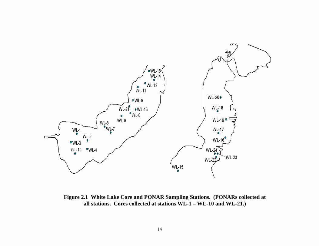
2.0 Sampling Locations

Sampling locations for the assessment of contaminated sediments in White Lake were selected based on proximity to potential point and nonpoint sources of contamination. The locations of these sites were determined by review of historical records. Sediment samples were collected in areas of fine sediment deposition. Samples from areas containing rubble and sand were excluded. A total of 10 locations were selected for the collection of core samples and 24 locations were selected for PONAR samples. The sampling locations are listed below and displayed on Figure 2.1. GPS coordinates, depths, and visual descriptions are included in Tables 2.1, 2.2, and 2.3 respectively, for sediment core, stratigraphy core, and PONAR samples.

Core and PONAR Identification Description WL-1 and WL-2 DuPont Groundwater Plume

WL-3, WL-4, WL-10, WL-13 Western White Lake Deposition Basin WL-5, WL-7, Long Point Deposition Basin

WL-6, WL-8, WL-9, WL-13, WL-21 Occidental Chemical Outfall Area WL-11, WL-12, WL-14, WL-15 Central White Lake Deposition Basin

WL-22, WL-23, WL-24 Tannery Bay WL-16 and WL-17 East Bay

WL-18, WL-19, WL-20 Control Locations

14

Figure 2.1 White Lake Core and PONAR Sampling Stations. (PONARs collected at all stations. Cores collected at stations WL-1 – WL-10 and WL-21.)

15

m cm N WWL-1 10/24/2000 15.0 183 43o 22.58' 86o 24.56'

White Lake 1 Top 0-51 Black siltWhite Lake 1 Middle 51-102 Black siltWhite Lake 1 Bottom 102-152 Brown clay

WL-1 Duplicate 10/24/2000 14.9 191 43o 22.58' 86o 24.56'White Lake 1D Top 0-51 Black silt

White Lake 1D Middle 51-102 Black siltWhite Lake 1D Bottom 102-152 Brown Black silt

WL-2 10/24/2000 20.3 229 43o 22.46' 86o 24.16'White Lake 2 Top 0-51 Black silt

White Lake 2 Middle 51-102 Black siltWhite Lake 2 Bottom 102-152 Black sand to Beach sand


White Lake 3 Middle 51-102 Black siltWhite Lake 3 Bottom 102-152 Brown silt

WL-4 10/23/2000 14.4 120 43o 22.27' 86o 24.16'White Lake 4 Top 0-51 Sand Black Silt with Hydrocarbon odor

White Lake 4 Bottom 51-102 Sandy Black siltWL-5 10/23/2000 11.9 201 43o 22.73' 86o 23.50'

White Lake 5 Top 0-51 Fine Black siltWhite Lake 5 Middle 51-102 Black siltWhite Lake 5 Bottom 102-152 Brown silt

WL-6 10/24/2000 21.5 191 43o 22.95' 86o 22.88'White Lake 6 Top 0-51 Black silt with clay

White Lake 6 Middle 51-102 Black siltWhite Lake 6 Bottom 102-152 Grey clay


White Lake 7 Middle 51-102 Black siltWhite Lake 7 Bottom 102-152 Brown silt plastic

WL-8 10/23/2000 12.32 185 43o 23.01' 86o 22.53'White Lake 8 Top 0-51 Fine Black silt no odor

White Lake 8 Middle 51-102 Black silt Brown clayWhite Lake 8 Bottom 102-152 Black silt Brown clay

WL-9 10/23/2000 9.73 170 43o 23.27' 86o 22.44'White Lake 9 Top 0-51 Fine Black silt

White Lake 9 Middle 51-102 Fine Black siltWhite Lake 9 Bottom 102-152 Brown peat plastic

WL-10 10/23/2000 14.35 196 43o 22.18' 86o 24.61'White Lake 10 Top 0-51 Fine Black silt

White Lake 10 Middle 51-102 Fine Black siltWhite Lake 10 Bottom 102-152 Fine Black silt

WL-21 10/24/2000 15.11 155 43o 23.16' 86o 22.57'White Lake 21 Top 0-51 Red, Yellow, Black chemical odor

White Lake 21 Middle 51-102 Black silt no odorWhite Lake 21 Bottom 102-152 Black silt no odor

Station Sample ID Date Depth to Core Depth of Core Latitude Longitude Description

TABLE 2.1 WHITE LAKE CORE SAMPLING STATIONS.

16

m N WWL-1-P 10/25/00 15.04 43o 22.58' 86o 24.55'WL-2-P 10/25/00 20.32 43o 22.45' 86o 24.15'WL-3-P 10/25/00 16.54 43o 22.41' 86o 24.77'WL-4-P 10/25/00 14.35 43o 22.27' 86o 24.16'WL-5-P 10/26/00 11.89 43o 22.73' 86o 23.50'WL-6-P 10/26/00 21.46 43o 22.95' 86o 22.86'WL-7-P 10/26/00 10.85 43o 22.61' 86o 23.27'WL-8-P 10/26/00 12.32 43o 23.01' 86o 22.53'WL-9-P 10/27/00 9.73 43o 23.27' 86o 22.43'

WL-10-P 10/27/00 14.35 43o 22.18' 86o 24.61'WL-11-P 10/27/00 14.30 43o 23.54' 86o 22.25'WL-12-P 10/27/00 16.15 43o 23.62' 86o 21.97'WL-13-P 10/27/00 10.90 43o 23.08' 86o 22.33'WL-14-P 10/27/00 8.76 43o 23.69' 86o 21.63'WL-15-P 10/27/00 8.48 43o 23.87' 86o 21.83'WL-16-P 10/24/00 3.43 43o 24.16' 86o 21.15'WL-17-P 10/24/00 4.14 43o 24.20' 86o 21.25'WL-18-P 10/24/00 3.18 43o 24.39' 86o 21.26'WL-19-P 10/24/00 3.78 43o 24.32' 86o 21.14'WL-20-P 10/24/00 2.74 43o 24.51' 86o 21.22'WL-21-P 10/27/00 15.11 43o 23.15' 86o 22.57'WL-22-P 10/27/00 3.66 43o 23.99' 86o 21.28'WL-23-P 10/27/00 2.44 43o 24.02' 86o 21.26'WL-24-P 10/27/00 3.20 43o 24.02' 86o 21.30'

Fine Black siltFine Black silt

Fine Black siltFine Black siltFine Black silt

Station Date Depth to Sediment Latitude LongitudeDescription

Fine Black siltFine Black siltFine Black silt

Sand Black Silt with Hydrocarbon odorFine Black siltFine Black siltFine Black siltFine Black siltFine Black siltFine Black siltFine Black siltFine Black siltFine Black siltFine Black silt

Fine Black silt

Fine Black siltFine Black siltFine Black siltFine Black silt

TABLE 2.2 WHITE LAKE STRATIGRAPHY SAMPLING STATIONS

Station Date Depth to Sediment

Latitude Longitude

M N W WL-2S 10/25/00 20.32 43o 22.45' 86o 24.15' WL-7S 10/25/00 21.46 43o 22.61' 86o 23.27' WL-9S 10/25/00 15.11 43o 23.27' 86o 22.43'

TABLE 2.3 WHITE LAKE PONAR CORE SAMPLING STATIONS

17

3.0 Methods

3.1 Sampling Methods

Sediment and benthos samples were collected using the U.S. EPA Research Vessel Mudpuppy. VibraCore methods were used to collect sediment cores for chemical analysis. A 4-inch aluminum core tube with a butyrate liner was used for collection. A new core tube and liner were used at each location. The core samples were measured and sectioned into three equal segments corresponding to top, middle, and bottom. Each section was then homogenized in a polyethylene pan and split into sub-samples. The visual appearance of each segment was recorded along with the water depth and core depth. PONAR samples were collected for toxicity testing, sediment chemistry, and benthic macroinvertebrates. For sediment chemistry and toxicity testing, a standard PONAR sample was deposited into a polyethylene pan and split into sub-samples. The PONAR was washed with water in between stations. A petite PONAR was used for the collection of benthic macroinvertebrates. Three replicate grabs were taken at each of the sites and treated as discrete samples. All material in the grab was washed through a Nitex screen with 500 µm openings and the residue preserved in buffered formalin containing rose bengal stain. GPS system coordinates were used to record the position of the sampling locations. Since the core and PONAR samples were collected on different days, some variation in the location may have occurred. 3.1.2 Sample Containers, Preservatives, And Volume Requirements Requirements for sample volumes, containers, and holding times are listed in Table 3.1. All sample containers for sediment chemistry and toxicity testing were purchased, precleaned, and certified as Level II by I-CHEM Inc.

18

TABLE 3.1 SAMPLE CONTAINERS, PRESERVATIVES, AND HOLDING TIMES

Hold Times Matrix Parameter Container Preservation Extraction Analysis

Sediment Metals 250 mL Wide Mouth Plastic

Cool to 4oC --- 6 months, Mercury-28

Days

Sediment TOC 250 mL Wide Mouth Plastic

Freeze -100C --- 6 months

Sediment Semi-Volatile

Organics 500 mL Amber

Glass Cool to 4oC 14 days 40 days

Sediment Grain Size 1 Quart Zip-Lock

Plastic Bag Cool to 4oC --- 6 months

Sediment Toxicity 4 liter Wide Mouth

Glass Cool to 4oC --- 45 days

Water Semi-Volatile

Organics and Resin Acids

1000 mL Amber Glass

Cool to 4oC 14 days 40 days

Culture Alkalinity 250 mL Wide

Mouth Plastic Cool to 4oC --- 24 hrs.

Water Ammonia

Hardness Conductivity

pH

250 mL Wide Mouth Plastic

Cool to 4oC --- 24 hrs.

3.2 Chemical Analysis Methods For Sediment Analysis

A summary of analytical methods and detection limits is provided in Table 3.2.1. Instrument conditions and a summary of quality assurance procedures are provided in the following sections.

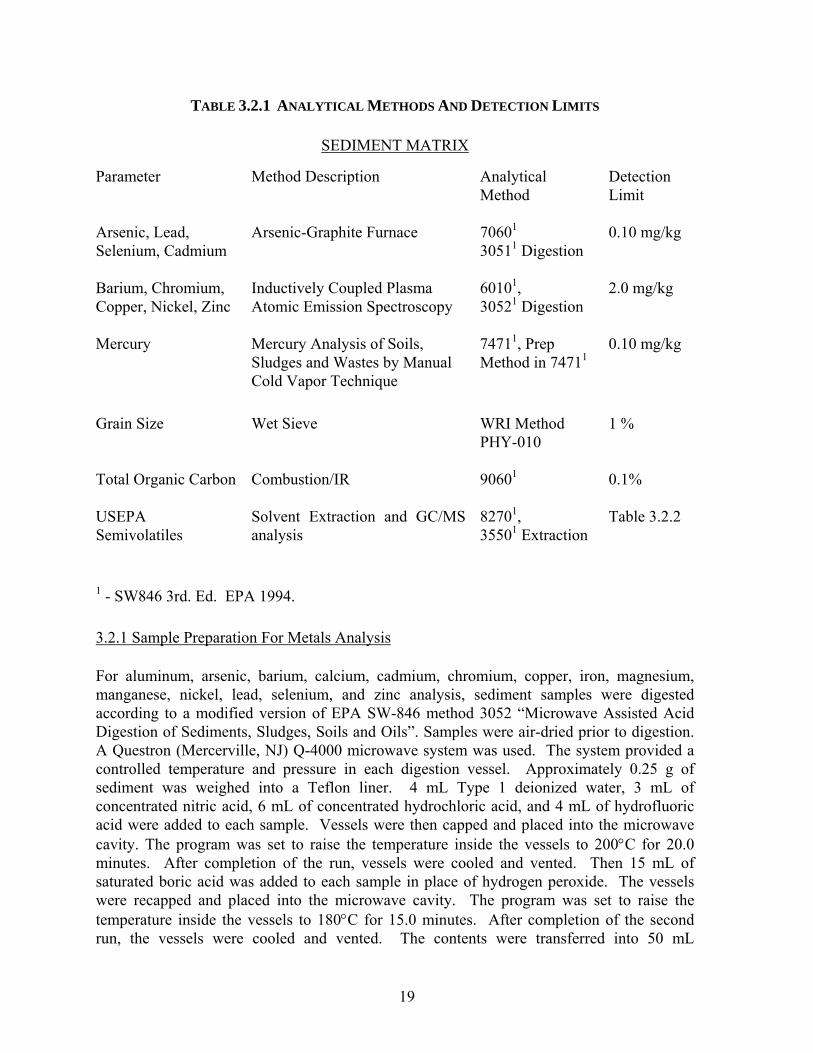
19

TABLE 3.2.1 ANALYTICAL METHODS AND DETECTION LIMITS

SEDIMENT MATRIX

Parameter Method Description Analytical Detection Method Limit Arsenic, Lead, Selenium, Cadmium

Arsenic-Graphite Furnace 70601

30511 Digestion 0.10 mg/kg

Barium, Chromium, Copper, Nickel, Zinc

Inductively Coupled Plasma Atomic Emission Spectroscopy

60101, 30521 Digestion

2.0 mg/kg

Mercury Mercury Analysis of Soils, 74711, Prep 0.10 mg/kg Sludges and Wastes by Manual Method in 74711 Cold Vapor Technique Grain Size Wet Sieve WRI Method 1 % PHY-010 Total Organic Carbon Combustion/IR 90601 0.1% USEPA Semivolatiles

Solvent Extraction and GC/MS analysis

82701, 35501 Extraction

Table 3.2.2

1 - SW846 3rd. Ed. EPA 1994. 3.2.1 Sample Preparation For Metals Analysis For aluminum, arsenic, barium, calcium, cadmium, chromium, copper, iron, magnesium, manganese, nickel, lead, selenium, and zinc analysis, sediment samples were digested according to a modified version of EPA SW-846 method 3052 “Microwave Assisted Acid Digestion of Sediments, Sludges, Soils and Oils”. Samples were air-dried prior to digestion. A Questron (Mercerville, NJ) Q-4000 microwave system was used. The system provided a controlled temperature and pressure in each digestion vessel. Approximately 0.25 g of sediment was weighed into a Teflon liner. 4 mL Type 1 deionized water, 3 mL of concentrated nitric acid, 6 mL of concentrated hydrochloric acid, and 4 mL of hydrofluoric acid were added to each sample. Vessels were then capped and placed into the microwave cavity. The program was set to raise the temperature inside the vessels to 200°C for 20.0 minutes. After completion of the run, vessels were cooled and vented. Then 15 mL of saturated boric acid was added to each sample in place of hydrogen peroxide. The vessels were recapped and placed into the microwave cavity. The program was set to raise the temperature inside the vessels to 180°C for 15.0 minutes. After completion of the second run, the vessels were cooled and vented. The contents were transferred into 50 mL

20

centrifuge tubes and brought up to 50 mL with Type I deionized water. Samples were centrifuged for 5 minutes at 3000 rpm before analysis. For every batch of 20 samples at least one set of the following quality control samples was prepared: Method Blank (4 mL of Type 1 deionized water, 3 mL of nitric acid and 6 mL of

hydrochloric acid); Laboratory Control Spike (Blank Spike); Matrix Spike; Matrix Spike Duplicate. For determining total mercury the samples were prepared by EPA SW-846 method 7471A, “Mercury in Solid and Semisolid Waste”. Approximately 0.2 g of wet sediment was weighed into a 50 mL centrifuge tube. 2.5 mL of Type I deionized water and 2.5 mL of aqua regia were then added to the tube. Samples were heated in a water bath at 95°C for 2 minutes. After cooling, the volume of the samples was brought up to 30 mL with Type I deionized water. Then 7.5 mL of 5% potassium permanganate solution was added to each sample, the samples were mixed, and the centrifuge tubes were returned to the water bath for a period of 30 minutes. Three mL of 12% hydroxylamine chloride solution was added to each sample after cooling. Finally, the samples were mixed and centrifuged for 5 minutes at 3,000 rpm. Calibration standards were digested concurrent with the samples. Quality control samples were prepared as stated previously for every batch of 10 samples or less. 3.2.2 Arsenic Analysis By Furnace Arsenic was analyzed in accordance with the EPA SW-846 method 7060A utilizing the Graphite Furnace technique. The instrument employed was a Perkin Elmer 4110ZL atomic absorption spectrophotometer. An arsenic EDL Lamp was used as a light source at a wavelength of 193.7 nm. The instrument utilized a Zeeman background correction that reduces the non-specific absorption caused by some matrix components. The temperature program is summarized below:

Time, sec. Step Temp, °C Ramp Hold

Gas Flow, mL/min

Read

1 2 3 4 5

110 130 1300 2100 2500

1 15 10 0 1

35 37 20 5 3

250 250 250 0

250

X

A Pd/Mg modifier was used to stabilize As during the pyrolysis step. The calibration curve was constructed from four standards and a blank. Validity of calibration was verified with a check standard prepared from a secondary source. This action was taken immediately after calibration, after every 20 samples, and at the end of each run. At least 1 post-digestion spike was performed for every analytical batch of 20 samples.

21

3.2.3 Cadmium Analysis By Furnace Cadmium was analyzed in accordance with the EPA SW-846 method 7060A utilizing the Graphite Furnace technique. The instrument employed was a Perkin Elmer 4110ZL atomic absorption spectrophotometer. A hollow cathode lamp was used as a light source at a wavelength of 228.8 nm. The instrument utilized a Zeeman background correction that reduces the non-specific absorption caused by some matrix components. The temperature program is summarized below:


Gas Flow, mL/min

Read

1 2 3 4 5

110 130 500 1550 2500

1 15 10 0 1

40 45 20 5 3

250 250 250 0

250

X

A Pd/Mg modifier was used to stabilize Cd during the pyrolysis step. The calibration curve was constructed from four standards and a blank. Validity of calibration was verified with a check standard prepared from a secondary source. This action was taken immediately after calibration, after every 20 samples, and at the end of each run. At least 1 post-digestion spike was performed for every analytical batch of 20 samples. 3.2.4 Lead Analysis By Furnace Lead was analyzed in accordance with the EPA SW-846 method 7060A utilizing the Graphite Furnace technique. The instrument employed was a Perkin Elmer 4110ZL atomic absorption spectrophotometer. A lead EDL Lamp was used as a light source at a wavelength of 283.3 nm. The instrument utilized a Zeeman background correction that reduces the non-specific absorption caused by some matrix components. The temperature program is summarized below:


Gas Flow, mL/min

Read

1 2 3 4 5 6

120 140 200 850 1900 2500

1 5 10 10 0 1

20 40 10 20 5 3

250 250 250 250 0

250

X

A Pd/Mg modifier was used to stabilize Pb during the pyrolysis step. The calibration curve was constructed from four standards and a blank. Validity of calibration was verified with a

22

check standard prepared from a secondary source. This action was taken immediately after calibration, after every 20 samples, and at the end of each run. At least 1 post-digestion spike was performed for every analytical batch of 20 samples. 3.2.5 Selenium Analysis By Furnace Selenium was analyzed in accordance with the EPA SW-846 method 7060A utilizing the Graphite Furnace technique. The instrument employed was a Perkin Elmer 4110ZL atomic absorption spectrophotometer. An arsenic EDL Lamp was used as a light source at a wavelength of 196.0 nm. The instrument utilized a Zeeman background correction that reduces the non-specific absorption caused by some matrix components. The temperature program is summarized below:


Gas Flow, mL/min

Read

1 2 3 4 5 6

120 140 200 1300 2100 2450

1 5 10 10 0 1

22 42 11 20 5 3

250 250 250 250 0

250

X

A Pd/Mg modifier was used to stabilize Se during the pyrolysis step. The calibration curve was constructed from four standards and a blank. Validity of calibration was verified with a check standard prepared from a secondary source. This action was taken immediately after calibration, after every 20 samples, and at the end of each run. At least 1 post-digestion spike was performed for every analytical batch of 20 samples. 3.2.6 Metal Analysis By ICP Aluminum, barium, calcium, chromium, copper, iron, magnesium, manganese, nickel, and zinc were analyzed in accordance with EPA SW-846 method 6010A using Inductively Coupled Plasma Atomic Emission Spectroscopy. Samples were analyzed on a Perkin Elmer P-1000 ICP Spectrometer with Ebert monochromator and cross-flow nebulizer. The following settings were used:

Element Analyzed Wavelength, nm Al 308.2 Ba 233.5 Ca 315.9

Element Analyzed Wavelength, nm Cr 267.7 Cu 324.8 Fe 259.9

23

Mg 279.1 Mn 257.6 Ni 231.6 Zn 213.9 RF Power: 1300 W

Matrix interferences were suppressed with internal standardization utilizing Myers-Tracy signal compensation. Interelement interference check standards were analyzed in the beginning and at the end of every analytical run and indicated absence of this type of interference at the given wavelength. The calibration curve was constructed from four standards and a blank, and was verified with a check standard prepared from a secondary source. 3.2.7 Mercury After the digestion procedure outlined in 3.2.1, sediment samples were analyzed for total mercury by cold vapor technique according to SW-846 Method 7471. A Perkin Elmer 5100ZL atomic absorption spectrophotometer with FIAS-200 flow injection accessory was used. Mercury was reduced to an elemental state using stannous chloride solution, and atomic absorption was measured in a quartz cell at an ambient temperature and a wavelength of 253.7 nm. A mercury electrodeless discharge lamp was used as a light source. The calibration curve consisted of four standards and a blank, and was verified with a check standard prepared from a secondary source. 3.2.8 Total Organic Carbon Total Organic Carbon analysis of sediments was conducted on a Shimadzu TOC-5000 Total Organic Carbon Analyzer equipped with Solid Sample Accessory SSM-5000A. Samples were air dried and then reacted with phosphoric acid to remove inorganic carbonates. Prior to analysis, the samples were air dried a final time. Calibration curves for total carbon were constructed from three standards and a blank. Glucose was used as a standard compound for Total Carbon Analysis (44% carbon by weight). 3.2.9 Grain Size Analysis Grain size was performed by wet sieving the sediments. The following mesh sizes were used: 2 mm (granule), 1 mm (very coarse sand), 0.85 mm (coarse sand), 0.25 mm (medium sand), 0.125 mm (fine sand), 0.063 (very fine sand), and 0.031 (coarse silt). After sieving, the fractions were dried at 105oC and analyzed by gravimetric methods to determine weight percentages. 3.2.10 Semivolatiles Analysis

24

Sediment samples were extracted for analysis of semivolatiles using SW-846 Method 3050. The sediment samples were dried with anhydrous sodium sulfate to form a free flowing powder. The samples were then serially sonicated with 1:1 methylene chloride/acetone and concentrated to a volume of 1 mL. The sample extracts were analyzed by GC/MS on a Hewlett Packard 5895 MSD Mass Spectrometer according to Method 8270. Instrumental conditions are itemized below:

MS operating conditions:

- Electron energy: 70 volts (nominal). - Mass range: 40-450 amu. - Scan time: 820 amu/second, 2 scans/sec. - Source temperature: 190° C - Transfer line temperature: 250°C

GC operating conditions:

- Column temperature program: 45°C for 6 min., then to 250°C at

10°C/min, then to 300°C at 20°C/min hold 300°C for 15 min.

- Injector temperature program: 250°C - Sample volume: 1 µl

A list of analytes and detection limits is given in Table 3.2.2. Surrogate standards were utilized to monitor extraction efficiency. Acceptance criteria for surrogate standards are given in Table 3.2.3. The GC/MS was calibrated using a 5-point curve. Instrument tuning was performed by injecting 5 ng of decafluorotriphenylphosphine and then adjusting spectra to meet method acceptance criteria. The MS and MSD samples were analyzed at a 5% frequency.

TABLE 3.2.2 ORGANIC PARAMETERS AND DETECTION LIMITS

Semi-Volatile Organic Compounds (8270) Sediment (mg/kg)

25

Phenol 0.33 Bis(2-chloroethyl)ether 0.33 2-Chlorophenol 0.33 1,3-Dichlorobenzene 0.33 1,4-Dichlorobenzene 0.33 1,2-Dichlorobenzene 0.33 2-Methylphenol 0.33 4-Methylphenol 0.33 Hexachloroethane 0.33 Isophorone 0.33 2,4-Dimethylphenol 0.33 Bis(2-chloroethoxy)methane 0.33 2,4-Dichlorophenol 0.33 1,2,4-Trichlorobenzene 0.33 Naphthalene 0.33 Hexachlorobutadiene 0.33 4-Chloro-3-methylphenol 0.33 2-Methylnaphthalene 0.33 Hexachlorocyclopentadiene 0.33 2,4,6-Trichlorophenol 0.33 2,4,5-Trichlorophenol 0.33 2-Chloronaphthalene 0.33 Dimethylphthalate 0.33 Acenaphthylene 0.33 Acenaphthene 0.33 Diethylphthalate 0.33 4-Chlorophenyl-phenyl ether 0.33 Fluorene 0.33 4,6-Dinitro-2-methylphenol 1.7 4-Bromophenyl-phenyl ether 0.33

26

TABLE 3.2.2 ORGANIC PARAMETERS AND DETECTION LIMITS (CONTINUED)

Semi-Volatile Organic Compounds (8270) Sediment (mg/kg) Hexachlorobenzene 0.33 Pentachlorophenol 1.7 Phenanthrene 0.33 Anthracene 0.33 Di-n-butylphthalate 0.33 Fluoranthene 0.33 Pyrene 0.33 Butylbenzylphthalate 0.33 Benzo(a)anthracene 0.33 Chrysene 0.33 Bis(2-ethylhexyl)phthalate 0.33 Di-n-octylphthalate 0.33 Benzo(b)fluoranthene 0.33 Benzo(k)fluoranthene 0.33 Benzo(a)pyrene 0.33 Indeno(1,2,3-cd)pyrene 0.33 Dibenzo(a,h)anthracene 0.33 Benzo(g,h,i)perylene 0.33 3-Methylphenol 0.33 TABLE 3.2.3 DATA QUALITY OBJECTIVES FOR SURROGATE STANDARDS CONTROL LIMITS

FOR PERCENT RECOVERY

Parameter Control Limit Nitrobenzene-d5 30%-97% 2-Fluorobiphenyl 42%-99% o-Terphenyl 60%-101% Phenol-d6 43%-84% 2-Fluorophenol 33%-76% 2,4,6-Tribromophenol 58%-96% 3.2.11 PCB Analysis

27

The sediment samples were extracted for PCBs using SW-846 Method 3050. Sediment samples were air dried for 24 hours, and then equal weights of the dried soil and anhydrous sodium sulfate were mixed together. The samples were then extracted using 50 mL of methanol and 100 mL of hexane. The samples were sonicated for 3 minutes, and then the hexane layer was removed and filtered through anhydrous sodium sulfate. The process was repeated two more times, adding 50 mL of hexane each time. The hexane extract was concentrated to 1 mL in the Turbovap, and then run through a chromatography column packed with 2% deactivated florisil and anhydrous sodium sulfate. Copper turnings cleaned with 1 M hydrochloric acid were added to remove sulfur. The eluent was concentrated to 1 mL using the Turbovap, and concentrated sulfuric acid was added as a final clean-up step. Solvent transfer to iso-octane was achieved under a flow of nitrogen gas and condensed to a final volume of 1 mL. Sample extracts were analyzed using gas chromatography with a Ni63 electron capture detector and RTX-5 capillary column. Helium and nitrogen were used as the carrier gas and makeup gas, respectively. Instrumental operating conditions were as follows:

Column temperature program: 80°C for 2 min., 10°C/min to 160°C, 1.5°C/min to 190°C, 2°C/min to 256°C and hold at 256°C for 6 min. Injector temperature: 260°C Detector temperature: 330°C Sample volume: 1 µl

Table 3.2.4 presents a list of PCB congeners and their detection limits. Two surrogate standards, tetrachloro-m-xylene and decachlorobiphenyl were used to monitor extraction efficiency. Acceptance limits for the surrogates were ± 50% for precision and accuracy.

Table 3.2.4 Sediment Detection Limits for PCBs

PCB Formulation Detection Limit (mg/kg)

Aroclor 1221 0.33 Aroclor 1232 0.33 Aroclor 1242 0.33 Aroclor 1248 0.33 Aroclor 1254 0.33 Aroclor 1260 0.33

28

3.2.12 Organic Chromium Analysis

The organic chromium fraction in sediment was extracted using 0.1 M Na2P2O7 at a 10:1 (v/m) ratio by shaking for 18 hours (Walsh and O’Halloran 1996). Twenty grams of wet sediment were extracted. The extract was centrifuged, filtered with a 0.45 µm membrane and analyzed for total chromium as described previously. Sample results were converted to a dry weight basis for reporting. 3.2.13 Proton Induced X-Ray Emission Spectroscopy (PIXE) Dried 2-cm-sections of sediment cores were homogenized by mechanical shaking. A sample of approximately 0.1 to 0.2 g of sediment was pressed into a self-supporting thin target by 10,000 psi of hydraulic pressure in a standard pellet press. The exact mass and thickness of the pellet was not critical as long as the resultant target remains thin with respect to the range of accelerated protons used in the irradiation. A current of approximately 10 nA of 2.3 MeV protons was used as an ion analysis probe for X-ray emission. The sediment samples were loaded on a target wheel in a vacuum chamber, which was subsequently evacuated to <10−5 torr. Each sample was exposed to the beam for approximately 300 seconds, or a total accumulated charge of approximately 3 µCoulomb. The incident beam current was measured with a Faraday cup immediately before and after irradiation and an average current was used to calculate the exact charge collected on each target. The resultant X-rays emitted from the irradiation were detected with a 4 cm2 Si(Li) detector located at 135° from the incident beam. There was a thin vacuum window and a piece of Be foil in front of the active detector, as well as an adjustable wheel of Kaptan® foils that was interspersed between the target and X-ray detector to attenuate the excess low-energy X-rays. A 2 mil (.002") of Kaptan® foil was used to suppress low energy X-rays on sediment sample irradiation. The X-ray energies were calibrated with a set of known metal standards (Si, Ti, In, Au) and for each run (up to a maximum of 36 samples per target wheel) a NIST standard mud pellet was used to standardize the X-ray yield calculations. We use both Buffalo River Sediment (NIST SRM 2704) and Trace Elements in Soil (NIST SRM 2586) as calibration standards for sediment samples. The X-ray spectra were acquired by standard NIM and CAMAC electronics and recorded onto a PC in binary format. The spectra were analyzed off-line by GUPIX II® a commercial PIXE analysis program1. The limits of detection vary from element to element, but typically range between the ppb - ppm level for most metals. A general review of the technique and examples of earth science applications are provided by Johanssen and Campbell (1988).

29

3.3 Chemical Analysis Methods For Water Analysis

The parameters, methods, and detection limits for the measurements performed on the culture water used in the sediment toxicity tests are listed in Table 3.3.1. All methods were performed according to procedures outlined in Standard Methods 14th Edition (1996).

TABLE 3.3.1 ANALYTICAL METHODS AND DETECTION LIMITS FOR CULTURE WATER

Parameter Method Detection Limit

Specific Conductance Standard Methods 2510 B. NA

Alkalinity Standard Methods 2320 10 mg/l Temperature Standard Methods 2550 NA

Dissolved Oxygen Standard Methods 4500-O G. 0.5 mg/l

Ammonia Electrode Standard Methods 4500-NH 3 F.

0.05 mg/l

Hardness Standard Methods 2340 C. 10 mg/l 3.4 Sediment Toxicity

The evaluation of the toxicity of the White Lake sediments was conducted using the ten-day survival test for the amphipod Hyalella azteca and the dipteran Chironomus tentans. The procedures followed are contained in EPA/600/R-94/024, Methods for Measuring the Toxicity and Bioaccumulation of Sediment-associated Contaminants with Fresh Water Invertebrates. All sediments were stored at 4°C prior to analysis. 3.4.1 Laboratory Water Supply Moderately hard well water was employed for the culture and maintenance of H. azteca and C. tentans. 3.4.2 Test Organisms The original stock of H. azteca was obtained from the Great Lakes Environmental Research Laboratory in Ann Arbor, Michigan. The H. azteca culture was maintained in four 20 L glass aquaria using maple leaves as a substrate and as a food source. The food source was supplemented with a suspension of Tetramin® fish food. The original stock of C. tentans was obtained from the University of Michigan Department of Environmental Health in Ann Arbor, Michigan. The culture of C. tentans was maintained in 36 L glass aquaria using shredded paper toweling as a substrate and was fed a suspension of Tetrafin® goldfish food.

30

3.4.3 Experimental Design For the November testing, eight replicates per sediment were set up for both H. azteca and C. tentans exposures, with the sediment from site M-15P designated as the control. In all tests, moderately hard well water was utilized as the overlying water. The experimental conditions outlined in Tables 3.4.1 and 3.4.2 were used for the toxicity evaluations. One day prior to the start of the test (day –1), the sediment from each site was mixed thoroughly and a 100 mL aliquot was transferred to each of the eight test chambers. Additionally, visual observations of the sediments were made. Moderately hard well water also was added at this time. On day 0, the overlying water was renewed once before the test organisms were introduced into each of the glass beakers. Measurement of water quality parameters also was initiated on this day. Ten, 7-14 day old H. azteca and 10 third instar C. tentans larvae were randomly added to their respective test chambers. At this time the organisms were fed 1.5 mL of Tetrafin®. The glass beakers were placed in a rack and transferred to a temperature controlled room (23 + 1oC). The light cycle was 16 hours on and 8 hours off. Temperature and dissolved oxygen measurements were taken from one randomly selected beaker for each sediment sample every 12 hours, after which the overlying water was renewed in all the beakers. Feeding with the Tetrafin® suspension occurred after the morning renewal. This procedure was repeated daily through day 10, at which point the test was terminated. On day 0, the overlying water from the beakers was composited from each sediment sample and 250 mL were retained for alkalinity, pH, conductance, hardness and ammonia analysis. On the last day the same procedure was carried out. On day 10, the sediments were sieved, and the surviving test organisms were removed and counted. The biological endpoint for these sediment tests was mortality. The validity of the test was based on EPA (1994) criteria of greater than 80% survival in the control treatment for H. azteca and greater than 70% survival in the control treatment for the C. tentans. In addition, EPA (1994) recommended that the hardness, alkalinity, pH, and ammonia in the overlying water within a treatment should not vary by more than 50% over the duration of the test. 3.4.4 Statistical Analysis Survival data for the toxicity testing were analyzed first for normality with Chi Square and then for homogeneity using Bartlett’s Test. All data passed the normality and homogeneity tests without transformation. The data were then examined using Dunnett’s Procedure to determine whether there was a significant difference in survival between the designated control sediment and those sediments containing pollutants. The TOXSTAT® 3.5 Computer Program was used for the statistical evaluations.

31

TABLE 3.4.1 TEST CONDITIONS FOR CONDUCTING A TEN DAY SEDIMENT TOXICITY TEST WITH HYALELLA AZTECA.

________________________________________________________________________

1. Test Type: Whole-sediment toxicity test with renewal of overlying water 2. Temperature (°C): ..................23 + 1°C

3. Light quality:..........................Wide-spectrum fluorescent lights

4. Illuminance: ...........................About 500 to 1000 lux

5. Photoperiod:...........................16 h light, 8 h darkness

6. Test chamber size: .................300 mL high-form lipless beaker

7. Sediment volume: ..................100 mL

8. Overlying water volume: .......175 mL

9. Renewal of overlying water: .....................................2 volume additions per day (i.e., one volume addition

every 12 hours)

10. Age of test organisms: ...........7 to 14 days old at the start of the test

11. Number of organisms per chamber:...........................10

12. Number of replicate chambers per treatment:.........8

13. Feeding: .................................Tetramin® fish food, fed 1.5 mL daily to each test chamber

14. Aeration: ................................None, unless dissolved oxygen in overlying water drops below 40% of saturation

15. Overlying water: ....................Reconstituted water

16. Overlying water quality: ........Hardness, alkalinity, conductivity, pH, and ammonia measured at the beginning and end of a test. Temperature and dissolved oxygen measured daily.

17. Test duration: .........................10 days

18. End point:...............................Survival, with greater than 80% in the control

________________________________________________________________________

Test Method 100.1. EPA Publication 600/R-94/024 (July 1994).

32

TABLE 3.4.2 RECOMMENDED TEST CONDITIONS FOR CONDUCTING A TEN DAY SEDIMENT TOXICITY TEST WITH CHIRONOMUS TENTANS.

________________________________________________________________________

1. Test Type: ..............................Whole-sediment toxicity test with renewal of overlying water

2. Temperature (°C): ..................23 + 1°C

3. Light quality:..........................Wide-spectrum fluorescent lights

4. Illuminance: ...........................About 500 to 1000 lux

5. Photoperiod:...........................16 h light, 8 h darkness

6. Test chamber size: .................300 mL high-form lipless beaker

7. Sediment volume: ..................100 mL

8. Overlying water volume: .......175 mL

9. Renewal of overlying water: .....................................2 volume additions per day (i.e., one volume addition

every 12 hours)

10. Age of test organisms: ...........Third instar larvae (All organisms must be third instar or younger with at least 50% of the organisms at third instar)

11. Number of organisms per chamber:...........................10

12. Number of replicate chambers per treatment:.........8

13. Feeding: .................................Tetrafin® goldfish food, fed 1.5 mL daily to each test chamber (1.5 mL contains 4.0 mg of dry solids)

14. Aeration: ................................None, unless dissolved oxygen in overlying water drops below 40% of saturation

15. Overlying water: ....................Reconstituted water

16. Overlying water quality: ........Hardness, alkalinity, conductivity, pH, and ammonia measured at the beginning and end of a test. Temperature and dissolved oxygen measured daily.

17. Test duration: .........................10 days

18. End point:...............................Survival, with greater than 70% in the control. Weight > 0.6 mg per midge in the control

________________________________________________________________________

Test Method 100.2. EPA Publication 600/R-94/024 (July 1994).

33

3.5 Benthic Macroinvertebrate Analysis

Samples were washed with tap water to remove formalin and extraneous debris through a USGS #30 mesh screen. The retained portion was poured into a white enamel pan from which the organisms were picked into two groups. These were oligochaetes and “other”. The worms were preserved with 4% formalin and later identified to the lowest practical level. The worms were mounted separately and examined under 100X and 400X. The “other” group was preserved in 70% ethanol. Midges were removed from this group and a head mount of each midge was made and examined under 100X and 400X. The number and taxa were reported. The remainder of the organisms were identified and enumerated utilizing a 60X dissecting microscope. 3.6 Radiometric Dating

Radiometric measurements were made using low-background gamma counting systems with well-type intrinsic germanium detectors (Schelske et al. 1994). Dry sediment from each section was packed to a nominal height of 30 mm in a tared polypropylene tube (84 mm high x 14.5 mm outside diameter, 12 mm inside diameter). Sample height was recorded and tubes were weighed to obtain sample mass. Samples in the tubes were then sealed with a layer of epoxy resin and polyamine hardener, capped, and stored before counting to ensure equilibrium between 226Ra and 214Bi. Activities for each radionuclide were calculated using empirically derived factors of variation in counting efficiency with sample mass and height (Schelske et al. 1994). Total 210Pb activity was obtained from the 46.5 keV photon peak, and 226Ra activity was obtained from the 609.2 keV peak of 214Bi. 226Ra activity was assumed to represent supported 210Pb activity. Excess 210Pb activity was determined from the difference between total and supported 210Pb activity and then corrected for decay from the coring date. The 661.7 keV photon peak is used to measure 137Cs activity. Sediments were aged using activity measurements of the above radioisotopes in the sediment samples. The method was based on determining the activity of total 210Pb (22.3 yr half-life), a decay product of 226Ra (half-life 1622 yr) in the 238U decay series. Total 210Pb represents the sum of excess 210Pb and supported 210Pb activity in sediments. The ultimate source of excess 210Pb is the outgassing of chemically inert 222Rn (3.83 d half-life) from continents as 226Ra incorporated in soils as rocks decay. In the atmosphere, 222Rn decays to 210Pb which is deposited at the earth's surface with atmospheric washout as unsupported or excess 210Pb. Supported 210Pb in lake sediments is produced by the decay of 226Ra that is deposited as one fraction of erosional inputs. In the sediments, gaseous 222Rn produced from 226Ra is trapped and decays to 210Pb. By definition, supported 210Pb is in secular equilibrium (production rate matches decay rate) with sedimentary 226Ra and is equal to total 210Pb activity at depths where excess 210Pb activity is not measurable due to decay. Because the decay of excess 210Pb activity in sediments provides the basis for estimating sediment ages, it is necessary to make estimates of total and supported 210Pb activities so excess 210Pb activity can be determined by difference. Excess 210Pb activity was calculated either by subtracting 226Ra activity from total 210Pb activity at each depth or by subtracting an estimate of supported 210Pb activity based on measurements of total 210Pb activity at depths where excess 210Pb activity was negligible.

34

Sediment ages were calculated using a CRS model (Appleby and Oldfield 1983). This model calculates ages based on the assumption that the flux of excess 210Pb to the lake was constant and therefore that variation in 210Pb activity from a pattern of exponential decrease with depth depends on variation in rate of sedimentation. The age of sediments at depth x is given by: t = (1/k) [ln (A0/A)] where t is time in yr, k is 0.03114 (the 210Pb decay constant), A0 is the total residual excess 210Pb activity in the sediment core, and A is the integrated excess 210Pb activity below depth x. Calculations for each depth provide a continuous profile of ages as a function of depth. Mass sedimentation rate (MSR) at depth x was determined by: MSR = m/t where m is dry mass of sediment (g /cm2) for the sampling interval. Errors in age and mass sedimentation rate were propagated using first-order approximations and calculated according to Binford (1990).

3.7 Statistical Analysis

Multivariate analyses were conducted using SAS version 8.0 (Cary, North Carolina). Principal Components Analysis (PCA) was conducted on the physical/chemical parameters. Correspondence Analysis (CA) was conducted on the benthic macroinvertebrate data using the individual taxa. Spearman Rank Correlation was used to determine significant relationships between individual physical and chemical parameters and the trophic status indices. Pearson correlation analysis was conducted using SYSTAT version 5.0 (Evanston, Illinois). 3.8 Contaminant Mapping

ArcView GIS and Surfer were utilized for analyzing and mapping contaminant concentrations in White Lake. ArcView was primarily used for geographic projection and spatial distribution mapping while Surfer was used for creating contour maps of chromium and PCB concentrations, in which Kriging was selected as a gridding method. The original GPS observation points were expressed in decimal degrees under the Geographic-Lat/Long system. To determine the coordinates of the station locations, ArcView GIS 3.3 and the MI DNR Projection Extension were used to project the station points to the Michigan GeoRef NAD 1983 system. Kriging was used for the interpolation of chromium concentrations at the grid points. Specific information concerning the range of X and Y

35

coordinates, grid size, as well as the variogram model, drift type, and nugget effect are shown below:

X Coordinates 465255 - 471530 meters

Y Coordinates 312504 - 317754 meters

Grid Size 876 rows × 1047 columns

Variogram Model Type: Linear

Parameters: Scale: 671000; Length: 3310

Drift Type No Drift

Nugget Effect Error Variance: 0; Micro Variance: 0

Anisotropy Ratio = 1; Angle = 0

3.9 References

Appleby, P. G. and F. Oldfield. 1983. The assessment of 210

Pb data from sites with varying sediment accumulation rates. Hydrobiologia 103: 29-35.

Binford, M. W. 1990. Calculation and uncertainty analysis of

210Pb dates for PIRLA project

lake sediment cores. J. Paleolim. 3:253-267. EPA. 1994. Methods for Measuring the Toxicity and Bioaccumulation of Sediment-

Associated Contaminants with Freshwater Invertebrates. EPA Publication 600/R-94/024.

Johanssen, S.A.E. and J. L Campbell. 1988. PIXE, A Novel Technique for Elemental

Analysis, John Wiley & Sons, Chichester, NY. 458 pp. Schelske, C. L., A. Peplow, M. Brenner, and C. N. Spencer. 1994. Low-background

gamma counting: Applications for 210

Pb dating of sediments. J. Paleolim. 10:11128. Walsh, A.R. and O'Halloran, J. 1996. Chromium speciation in tannery effluent - II.

Speciation in the effluent and in a receiving estuary. Water Res. 30(10):2401-2412.

36

4.0 Results And Discussion The results and discussion section is organized according to 6 sections that present and summarize the information related to the following topics: Section 4.1 Sediment Chemistry Results Section 4.2 Stratigraphy and Radiodating Results Section 4.3 Toxicity Testing Results Section 4.4 Benthic Macroinvertebrate Results Section 4.5 Chromium Uptake In Aquatic Organisms Section 4.6 Environmental Fate and Transport Analysis Section 4.7 Sediment Quality Triad Assesment Section 4.8 Summary and Conclusions The sediment chemistry results are presented for the core and PONAR samples (Section 4.1) and include metals, semivolatiles, and physical parameters. A discussion is also included related to the comparison of the data with published sediment quality guidelines. The stratigraphy and radiodating results are presented in Section 4.2 and include the results of radioisotopes and the target list of metals (chromium and lead). Toxicity and Benthic Macroinvertebrate results are presented in Sections 4.3 and 4.4, respectively. Statistical analyses of the data and comparisons to related chemical and biological data are also discussed. Chromium accumulation in selected aquatic organisms and the results are summarized in Section 4.5. Section 4.6 provides a discussion of the environmental fate and transport of contaminants in White Lake using the results of this investigation plus studies by Rediske et al. (1998) and Earth Tech (2001). Finally, Section 4.7 presents the investigative data in the contex of the Sediment Quality Triad. The project summary and conclusions are provided in section 4.8. The project data were reviewed for compliance with the Data Quality Objectives outlined in the Quality Assurance Project Plan. Low matrix spike recoveries were obtained on one sample for semivolatiles and one sample for metals. Acceptable recoveries were obtained in the laboratory control sample, indicating that the problem was matrix related. The data were not qualified due to the fact that the project was a preliminary investigation. The results of the Quality Assurance reviews are summarized in Appendix A. 4.1 Sediment Chemistry Results

The results of sediment grain size fractions, percent solids and TOC for the core and PONAR samples are presented in Tables 4.1.1 and 4.1.2, respectively. The sediments from most of the core samples can be characterized as having fine grain size (> 70% of particles < 63 um) and moderate to high in total organic carbon (TOC 1% - 10%) in the top 51 cm. Grain size distributions changed to include a greater sand fraction (125-500 um range) in the middle (51-102 cm) and bottom (102-152 cm) sections. This pattern is consistent with historical modification and development of the shoreline. Much of the lake shoreline was modified by

37

TABLE 4.1.1 RESULTS OF SEDIMENT GRAIN SIZE FRACTIONS, TOC, AND PERCENT SOLIDS FOR WHITE LAKE CORE SAMPLES, OCTOBER 2000. (TOP = 0-52 CM, MID = 52-102 CM, BOT = 102-152 CM)

>2000 um 2000-1000 um 1000-850 um 850-500 um 500-125 um 125-63 um <63 um TOC SolidsSample ID Weight % Weight% Weight % Weight % Weight % Weight % Weight % % % WL-1 TOP 0 0 0 0 2 6 92 3.9 12 WL-1 MID 0 0 0 0 13 9 78 11 14 WL-1 BOT 0 0 0 0 7 9 84 9.5 15 WL-2 TOP 1 0 0 0 4 4 92 6.5 11 WL-2 MID 0 0 0 0 13 9 77 10 15 WL-2 BOT 0 0 0 2 90 2 5 <1.0 67 WL-3 TOP 0 0 0 0 4 8 87 2.2 13 WL-3 MID 0 0 0 1 23 11 65 4.8 18 WL-3 TOP 0 0 0 0 7 9 84 8.1 15 WL-4 TOP 0 0 0 0 10 14 76 2.9 13 WL-4 MID 0 0 0 3 80 3 13 <1.0 53 WL-5 TOP 0 0 0 0 7 12 81 5.8 12 WL-5 MID 0 0 0 0 9 12 79 8.9 15 WL-5 BOT 0 0 0 0 6 10 84 7.2 15 WL-6 TOP 0 0 0 0 2 5 93 3.0 17 WL-6 MID 1 0 0 2 43 8 46 10 38 WL-6 BOT 0 0 0 1 8 13 78 3.0 16 WL-7 TOP 0 0 0 0 8 12 80 3.6 12 WL7 MID 0 0 0 0 11 17 72 10 16

WL-7 BOT 0 0 0 0 8 18 75 10 15 WL-8 TOP 0 0 0 0 8 16 76 6.6 12 WL-8 MID 0 0 0 0 8 11 80 1.2 15 WL-8 BOT 0 1 0 0 6 12 83 1.3 16 WL-9 TOP 0 1 0 0 9 14 76 7.5 13 WL-9-MID 0 0 0 0 9 10 81 7.1 15 WL-9 BOT 0 0 0 0 7 11 81 8.1 16 WL-10 TOP 6 0 0 0 23 6 71 5.0 14 WL-10 MID 0 0 0 0 11 10 79 9.7 15 WL-10 BOT 0 0 0 0 6 7 87 8.9 14 WL-21 TOP 0 0 0 0 10 5 84 2.7 20 WL-21 MID 0 0 0 1 10 15 74 7.1 16 WL-21 BOT 0 0 0 1 6 6 86 3.4 13

38

TABLE 4.1.2 RESULTS OF SEDIMENT GRAIN SIZE FRACTIONS, TOC, AND PERCENT SOLIDS FOR WHITE LAKE PONAR SAMPLES, OCTOBER 2000.

>2000 um 2000-1000 um 1000-850 um 850-500 um 500-125 um 125-63 um <63 um TOC Solids Sample ID Weight % Weight% Weight % Weight % Weight % Weight % Weight % % %

WL-1 P 0 0 0 0 4 5 91 8.0 7 WL-2 P 0 0 0 0 6 5 88 3.5 10 WL-3 P 0 0 0 0 4 5 90 3.0 10 WL-4 P 0 0 0 5 82 2 11 <1.0 61 WL-5 P 0 0 0 0 6 10 83 5.0 11 WL-6 P 0 0 0 0 5 7 88 4.4 10 WL-7 P 0 0 0 0 7 10 83 6.6 10 WL-8 P 0 0 0 0 8 10 82 5.5 11 WL-9 P 0 0 0 0 7 9 83 6.4 11 WL-10 P 0 0 0 0 5 5 89 2.2 10 WL-11 P 0 0 0 0 7 9 84 6.0 11 WL-12 P 1 0 0 0 6 9 84 7.1 11 WL-13 P 0 0 0 0 30 14 55 5.0 15 WL-14 P 1 0 0 0 13 10 76 18 13 WL-15 P 1 0 0 0 6 10 83 7.4 12 WL-16 P 0 0 0 0 3 7 90 10 14 WL-17 P 0 0 0 0 5 10 84 10 15

WL-18 P 0 0 0 0 8 8 84 11 16 WL-19 P 0 0 0 0 6 11 83 11 15 WL-20 P 0 0 0 0 11 17 70 8.5 16 WL-21 P 0 0 0 1 19 9 71 5.6 13 WL-22 P 6 2 0 1 12 13 65 4.6 11 WL-23 P 3 3 1 2 10 9 73 5.9 12 WL-24 P 3 1 0 1 12 7 76 8.2 15

39

logging in the 1800s and urban/industrial development in the 1900s. The subsequent erosion and runoff probably resulted in a sand layer being deposited throughout the near shore area. The presence of the finer grained material is consistent with the recent history of a more stable shoreline and eutrophic conditions present in the lake. Station WL-4 was different with respect to grain size distribution as it contained a higher sand fraction (80%) in the 52-102 cm core section. WL-4 was collected off a sloping contour with a public boat launch located to the south. Since the particle size and TOC characteristics of sediments will influence their ability to retain metals and organic chemicals, these data will be important in explaining the distribution of anthropogenic contaminants. Very little difference was noted between the grain size and TOC content of the PONAR samples (Table 4.1.2) and the top core sections (Table 4.1.1) for all samples except WL-4. The PONAR collected at this location was very high in sand fraction sediments (80%) suggesting that sediment composition is variable at this location. The variability may be due to the landscape variables discussed above or depositional patterns. Since these samples were used for chemical analysis in addition to the assessment of sediment toxicity and benthic invertebrate diversity, the influence of particle size and TOC content will also be an important factor in the evaluation of the project data. Chemical and ecological results from W-4 will be influenced to a large extent by the physical characteristics of the substrate. The results of sediment metals analyses are presented for the core and PONAR samples in Tables 4.1.3 and 4.1.4 respectively. The results of semivolatile and PCB analyses for the same sample groupings are given in Tables 4.1.5 and 4.1.6. Figures 4.1.1, 4.1.2, and 4.1.3 illustrate the distribution of arsenic, chromium, and lead respectively, in core samples collected from western White Lake. In general, arsenic concentrations in the three core sections showed little variation (±3 mg/kg) with depth (Figure 4.1.1). The same pattern was noted in the prior investigation (Rediske et al. 1998) for samples collected in eastern White Lake. These data suggest a relatively constant deposition rate of arsenic in the lake occurred over time. Uniform deposition rates over an extended period of time are usually related to regional geology and do not indicate anthropogenic pollution. Chromium and lead (Figures 4.1.2 and 4.1.3 respectively) did not follow this pattern as the highest levels of these elements were found in the top 51 cm of sediment. The sediment chemistry profiles of chromium and lead are indicative of recent anthropogenic pollution and cannot be attributed to background levels. A comparison of the results for arsenic, chromium and lead is provided in Figures 4.1.4, 4.1.5, and 4.1.6 respectively. The PONAR collects sediments to an approximate depth of 18 cm and can be used to estimate very recent deposition. The results for arsenic are again indicative of a relatively constant deposition rate, as there was little difference between PONAR and core sections (Figure 4.1.4). Chromium results follow a similar pattern indicating stable deposition rates in the more recent strata (Figure 4.1.5). In consideration that the deeper strata were considerably lower in chromium, these results suggest a relatively constant source is currently present in the lake. This is significant because the tannery ceased its discharge of chromium laden wastewater to White Lake in 1975. Chromium deposition in the western half of the lake reflects a constant loading of chromium after the wastewater diversion. These data support the hypothesis that the erosion and transport of sediments from Tannery Bay play an important role in the mobilization and deposition of contaminants in the western portion of White Lake (Rediske et al. 1998). Lead

40

TABLE 4.1.3 RESULTS OF SEDIMENT METAL ANALYSES FOR WHITE LAKE CORE SAMPLES (MG/KG DRY WEIGHT), OCTOBER 2000. (TOP = 0-52 CM, MID = 52-102 CM, BOT = 102-152 CM)

Sample Arsenic

(mg/kg) Barium (mg/kg)

Cadmium (mg/kg)

Chromium (mg/kg)

Copper (mg/kg)

Mercury (mg/kg)

Nickel (mg/kg)

Lead (mg/kg)

Selenium (mg/kg)

Zinc (mg/kg)

WL-1 Top 9.1 130 1.3 270 29 0.42 23 140 2.8 140 WL-1 Mid 6.1 130 0.87 34 18 < 0.1 16 15 2.8 75 WL-1 Bot. 6.6 160 0.74 37 21 < 0.1 18 9.8 2.6 86 WL-2 Top 9.0 160 1.6 470 33 0.42 18 190 2.6 140 WL-2 Bot 7.5 150 0.97 34 18 0.14 12 24 2.7 87 WL-3 Top 7.9 120 1.5 290 33 0.39 24 190 2.7 150 WL-3 Mid 6.2 110 0.61 33 17 0.16 14 28 2.1 80 WL-3 Bot 5.7 130 0.48 28 16 < 0.1 13 8.2 2.6 65 WL-4 Top 9.0 130 1.9 440 34 0.49 27 180 2.5 160 WL-4 Mid 1.8 18 0.15 8.1 2.3 < 0.1 U 2.1 0.47 16 WL-5 Top 8.9 140 1.4 300 31 0.52 24 110 3.6 160 WL-5 Mid 6.3 130 0.53 34 18 0.10 15 16 2.9 82 WL-5 Bot 6.1 150 < 0.1 24 17 < 0.1 12 5.9 3.1 69 WL-6 Top 6.7 180 1.3 410 23 0.38 27 340 2.1 110 WL-6 Mid 12 88 0.26 19 12 < 0.1 13 13 0.86 46 WL-6 Bot 12 110 0.19 17 13 < 0.1 14 7.7 1.5 45 WL-7 Top 8.2 130 1.6 600 34 0.62 28 180 2.6 160 WL-7 Mid 6.5 110 0.65 40 19 0.13 16 22 1.9 90 WL-7 Bot 5.5 110 0.35 33 17 < 0.1 15 7.9 < 0.1 70 WL-8 Top 7.7 140 1.4 380 32 0.58 26 180 < 0.1 160 WL-8 Mid 7.7 120 0.42 34 18 < 0.1 15 9.6 < 0.1 76 WL-8 Bot 7.3 1470 0.49 40 18 < 0.1 16 8.9 1.7 78 WL-9 Top 9.6 140 1.5 500 34 0.63 26 120 5.1 170 WL-9 Mid 7.5 120 0.6 38 18 0.12 16 18 2.6 81 WL-9 Bot 7.0 120 0.51 35 17 < 0.1 14 8.0 2.6 69

WL-10 Top 6.5 92 1.1 210 23 0.34 18 97 < 0.1 120 WL-10 Mid 5.8 110 0.47 33 16 0.11 14 18 2.0 75 WL-10 Bot 6.5 110 0.36 30 16 < 0.1 14 6.9 2.7 64 WL-21 Top 9.5 162 1.2 430 23 0.51 28 290 1.5 160 WL-21Mid 7.8 120 0.78 99 12 0.11 19 170 1.8 85

41

TABLE 4.1.4 RESULTS OF SEDIMENT METAL ANALYSES FOR WHITE LAKE PONAR SAMPLES (MG/KG DRY WEIGHT), OCTOBER 2000.

Sample Arsenic (mg/kg)

Barium (mg/kg)

Cadmium (mg/kg)

Chromium (mg/kg)

Copper (mg/kg)

Mercury (mg/kg)

Nickel mg/kg)

Lead (mg/kg)

Selenium (mg/kg)

Zinc (mg/kg)

WL-1 P 6.3 140 0.85 270 30 0.20 17 70 < 0.1 120 WL-2 P 7.5 150 0.85 300 34 0.20 18 76 < 0.1 120 WL-3 P 5.5 120 0.73 190 29 0.16 16 54 < 0.1 100 WL-4 P 1.4 12 < 0.1 18 2.2 < 0.1 1.6 8.3 < 0.1 33 WL-5 P 6.2 130 1.1 400 31 0.27 19 89 2.9 120 WL-6 P 8.4 130 1.0 360 28 0.25 18 73 3.0 120 WL-7 P 7.6 120 0.99 390 37 0.29 25 86 3.6 130 WL-8 P 8.8 130 0.93 380 27 0.25 20 75 3.7 120 WL-9 P 7.9 170 0.87 420 34 0.30 23 74 3.0 130

WL-10 P 7.0 120 0.91 270 31 0.34 19 75 < 0.1 120 WL-11 P 6.3 * 0.96 310 32 0.32 18 78 * 116 WL-12 P 5.9 * 1.03 510 30 0.28 17 70 * 118 WL-13 P 6.3 * 0.96 250 32 0.27 17 67 * 108 WL-14 P 6.3 * 1.10 480 31 0.25 17 72 * 95 WL-15 P 6.0 * 0.75 250 28 0.26 17 71 * 101 WL-16 P 5.8 * 0.84 190 27 0.27 18 75 * 105 WL-17 P 5.4 * 0.64 50 30 0.05 19 34 * 115 WL-18 P 5.3 * 0.51 29 32 0.05 20 22 * 125 WL-19 P 5.7 * 0.42 39 31 0.05 21 26 * 131 WL-20 P 6.2 * 0.61 28 28 0.05 19 21 * 124 WL-21P 6.5 * 1.00 450 31 0.24 18 65 * 132

* PONAR analyzed for target list metals. Barium and selenium not analyzed.

42

Aroclor 1248

1,3-DICHLOROBENZENE

1,4-DICHLOROBENZENE

BIS (2-ETHYLHEXYL)-

PHTHALATE

DI-N- BUTYL

PHTHALATEFLUORANTHENE HEXACHLORO

BENZENEHEXACHLORO

BUTADIENEHEXACHLOROCYCLO

PENTADIENE PYRENE

mg/kg mg/kg mg/kg mg/kg mg/kg mg/kg mg/kg mg/kg mg/kg mg/kgWL-1 Top 0.22 < 1.5 < 1.5 0.38 < 1.5 < 1.5 < 1.5 < 1.5 < 1.5 < 1.5WL-1 Top 0.49 < 1.7 < 1.7 < 1.5 < 1.7 < 1.7 < 1.7 < 1.7 < 1.7 < 1.7WL-1 Mid < 0.33 < 1.1 < 1.1 < 1.1 < 1.1 < 1.1 < 1.1 < 1.1 < 1.1 < 1.1WL-1 Mid 0.07 < 1.2 < 1.2 0.42 < 1.2 < 1.2 < 1.2 < 1.2 < 1.2 < 1.2WL-1 Bot < 0.33 < 1.2 < 1.2 .26 < 1.2 < 1.2 < 1.2 < 1.2 < 1.2 < 1.2WL-1 Bot .061 < 1.2 < 1.2 0.32 < 1.2 < 1.2 < 1.2 < 1.2 < 1.2 < 1.2WL-2 Top 0.07 < 1.7 < 1.7 0.56 < 1.7 < 1.7 < 1.7 < 1.7 < 1.7 < 1.7WL-2 Mid < 0.33 < 1.2 < 1.2 0.35 < 1.2 < 1.2 < 1.2 < 1.2 < 1.2 < 1.2WL-3 Top 0.05 < 1.4 < 1.4 0.99 < 1.4 < 1.4 < 1.4 < 1.4 < 1.4 < 1.4WL-3 Mid < 0.33 < 0.93 < 0.93 < 0.93 < 0.93 < 0.93 < 0.93 < 0.93 < 0.93 < 0.93WL-3 Bot 0.06 < 1.0 < 1.0 0.39 < 1.0 < 1.0 < 1.0 < 1.0 < 1.0 < 1.0WL-4 Top 0.17 < 1.3 < 1.3 < 1.3 1 0.10 < 1.3 < 1.3 < 1.3 < 1.3WL-4 Mid < 0.33 < 0.33 < 0.33 < 0.33 < 0.33 < 0.33 < 0.33 < 0.33 < 0.33 < 0.33WL-5 Top 0.17 < 1.3 < 1.3 < 1.3 < 1.3 0.097 < 1.3 < 1.3 < 1.3 < 1.3WL-5 Mid < 0.33 < 1.2 < 1.2 < 1.2 < 1.2 < 1.2 < 1.2 < 1.2 < 1.2 < 1.2WL-5 Bot 0.06 < 1.1 < 1.1 < 1.1 < 1.1 < 1.1 < 1.1 < 1.1 < 1.1 < 1.1WL-6 Top 0.39 < 1.1 < 1.1 0.22 < 1.1 < 1.1 < 1.1 < 1.1 < 1.1 < 1.1WL-6 Mid < 0.33 < 0.46 < 0.46 0.19 < 0.46 < 0.46 < 0.46 < 0.46 < 0.46 < 0.46WL-6 Bot < 0.33 < 0.45 < 0.45 0.14 < 0.45 < 0.45 < 0.45 < 0.45 < 0.45 < 0.45WL-7 Top 0.24 < 1.5 < 1.5 0.28 1.1 < 1.5 < 1.5 < 1.5 < 1.5 < 1.5WL-7 Mid < 0.33 < 1.1 < 1.1 0.25 0.99 < 1.1 < 1.1 < 1.1 < 1.1 < 1.1WL-7 Bot < 0.33 < 1.1 < 1.1 < 1.1 < 1.1 < 1.1 < 1.1 < 1.1 < 1.1 < 1.1WL-8 Top 0.27 < 1.3 < 1.3 0.25 < 1.3 < 1.3 < 1.3 < 1.3 < 1.3 < 1.3WL-8 Mid 0.054 < 1.1 < 1.1 < 1.1 < 1.1 < 1.1 < 1.1 < 1.1 < 1.1 < 1.1WL-8 Bot < 0.33 < 1.1 < 1.1 < 1.1 < 1.1 < 1.1 < 1.1 < 1.1 < 1.1 < 1.1WL-9 Top 0.07 < 1.4 < 1.4 < 1.4 < 1.4 < 1.4 < 1.4 < 1.4 < 1.4 < 1.4WL-9 Mid 0.06 < 1.1 < 1.1 < 1.1 0.44 < 1.1 < 1.1 < 1.1 < 1.1 < 1.1WL-9 Bot < 0.33 < 1.1 < 1.1 0.23 0.46 < 1.1 < 1.1 < 1.1 < 1.1 < 1.1

WL-10 Top 0.06 < 1.1 < 1.1 0.25 0.98 < 1.1 < 1.1 < 1.1 < 1.1 < 1.1WL-10 Mid 0.06 < 1.1 < 1.1 < 1.1 1.1 < 1.1 < 1.1 < 1.1 < 1.1 < 1.1WL-10 Bot < 0.33 < 1.2 < 1.2 < 1.2 0.84 < 1.2 < 1.2 < 1.2 < 1.2 < 1.2WL-21 Top 22 1.9 0.65 0.94 < 1.2 < 1.2 0.54 < 0.33 < 0.33 < 1.2WL-21 Mid 0.84 0.29 < 0.33 0.54 < 0.98 < 0.98 0.051 < 0.98 < 0.98 < 0.98

Sample ID

TABLE 4.1.5 RESULTS OF SEDIMENT PCB AND SEMIVOLATILE ANALYSES FOR WHITE LAKE CORE SAMPLES (MG/KG DRY WEIGHT), OCTOBER 2000. (SAMPLES AND PARAMETERS THAT WERE NOT DETECTED WERE OMITED.) (TOP = 0-52 CM,

MID = 52-102 CM, BOT = 102-152 CM)

43

Aroclor 1248

1,3-DICHLOROBENZENE

1,4-DICHLOROBENZENE

BIS (2-ETHYLHEXYL)-

PHTHALATE

DI-N- BUTYL

PHTHALATEFLUORANTHENE HEXACHLORO

BENZENEHEXACHLORO

BUTADIENEHEXACHLOROCYCLO

PENTADIENE PYRENE

mg/kg mg/kg mg/kg mg/kg mg/kg mg/kg mg/kg mg/kg mg/kg mg/kgWL-1 P < 0.33 < 1.8 < 1.8 0.92 < 1.8 < 1.8 < 1.8 < 1.8 < 1.8 < 1.8WL-2 P 0.086 < 1.7 < 1.7 < 1.7 < 1.7 < 1.7 < 1.7 < 1.7 < 1.7 < 1.7WL-3 P < 0.33 < 1.5 < 1.5 0.31 < 1.5 < 1.5 < 1.5 < 1.5 < 1.5 < 1.5WL-4 P < 0.33 < 0.33 < 0.33 < 0.33 < 0.33 < 0.33 < 0.33 < 0.33 < 0.33 < 0.33WL-5 P < 0.33 < 1.7 < 1.7 0.62 < 1.7 < 1.7 < 1.7 < 1.7 < 1.7 < 1.7WL-6 P 0.071 < 1.5 < 1.5 0.25 < 1.5 < 1.5 < 1.5 < 1.5 < 1.5 < 1.5WL-7 P 0.084 < 1.7 < 1.7 0.32 0.3 < 1.7 < 1.7 < 1.7 < 1.7 < 1.7WL-8 P 0.076 < 1.7 < 1.7 0.35 0.25 < 1.7 < 1.7 < 1.7 < 1.7 < 1.7WL-9 P < 0.33 < 1.5 < 1.5 1.3 < 1.5 < 0.33 < 1.5 < 1.5 < 1.5 < 1.5

WL-10 P < 0.33 < 1.7 < 1.7 < 1.7 < 1.7 < 1.7 < 1.7 < 1.7 < 1.7 < 1.7WL-11 P < 0.33 * * * * * * * * *WL-12 P < 0.33 * * * * * * * * *WL-13 P < 0.33 * * * * * * * * *WL-14 P < 0.33 * * * * * * * * *WL-15 P < 0.33 * * * * * * * * *WL-16 P < 0.33 < 1.2 < 1.2 1.1 < 1.2 0.18 < 1.2 < 1.2 < 1.2 0.12WL-17 P < 0.33 * * * * * * * * *WL-18 P < 0.33 * * * * * * * * *WL-19 P < 0.33 * * * * * * * * *WL-20 P < 0.33 * * * * * * * * *WL-21 P 21 < 1.3 < 1.3 0.4 < 1.3 < 1.3 < 1.3 < 1.3 < 1.3 < 1.3

Sample ID

TABLE 4.1.6 RESULTS OF SEDIMENT PCB AND SEMIVOLATILE ANALYSES FOR WHITE LAKE PONAR SAMPLES (MG/KG DRY WEIGHT), OCTOBER 2000. (SAMPLES AND PARAMETERS THAT WERE NOT DETECTED WERE OMITED.)

44

WL-1 WL-2 WL-3 WL-4 WL-5 WL-6 WL-7 WL-8 WL-9 WL-10

0-51 cm51-102 cm

102-152 cm

0.0

2.0

4.0

6.0

8.0

10.0

12.0

Ars

enic

(mg/

kg)

0-51 cm51-102 cm102-152 cm

FIGURE 4.1.1 DISTRIBUTION OF ARSENIC IN CORE SAMPLES COLLECTED IN WESTERN WHITE LAKE, OCTOBER 2000.


0-51 cm51-102 cm

102-152 cm

0

100

200

300

400

500

600

Chr

omiu

m (m

g/kg

)

0-51 cm51-102 cm102-152 cm

FIGURE 4.1.2 DISTRIBUTION OF CHROMIUM IN CORE SAMPLES COLLECTED IN WESTERN WHITE LAKE, OCTOBER 2000.

45


0-51 cm51-102 cm

102-152 cm

0

50

100

150

200

250

300

350

Lead

(mg/

kg)

0-51 cm51-102 cm102-152 cm

FIGURE 4.1.3 DISTRIBUTION OF LEAD IN CORE SAMPLES COLLECTED IN WESTERN WHITE LAKE, OCTOBER 2000.


0-51 cm0-18 cm

0.0

1.0

2.0

3.0

4.0

5.0

6.0

7.0

8.0

9.0

10.0

Ars

enic

(mg/

kg)

0-51 cm0-18 cm

FIGURE 4.1.4 COMPARISON OF ARSENIC CONCENTRATIONS IN PONAR SAMPLES (0-18 CM) AND TOP CORE SECTIONS (0-51 CM) COLLECTED IN WHITE LAKE,

OCTOBER 2000.

46


0-51 cm0-18 cm

0

50

100

150

200

250

300

350

Lead

(mg/

kg)

0-51 cm0-18 cm

FIGURE 4.1.6 COMPARISON OF LEAD CONCENTRATIONS IN PONAR SAMPLES (0-18 CM) AND TOP CORE SECTIONS (0-51 CM) COLLECTED IN

WHITE LAKE, OCTOBER 2000.

FIGURE 4.1.5 COMPARISON OF CHROMIUM CONCENTRATIONS IN PONAR SAMPLES (0-18 CM) AND TOP CORE SECTIONS (0-51 CM) COLLECTED IN

WHITE LAKE, OCTOBER 2000.


0-18 cm0-51cm

0

100

200

300

400

500

600

Chr

omiu

m (m

g/kg

)

0-18 cm0-51cm

47

follows a different depositional pattern as the PONAR samples have lower contaminant concentrations than the 0-51 cm core sections (Figure 4.1.6). Lead was removed from fuel formulations during the 70s and lower deposition rates in the more recent sediments reflect this change. With the exception of the sample collected at WL-21, high levels of PCBs and organic chemicals were not present in sediment cores (Table 4.1.5). Station WL-21 was collected near the outfall of the former Hooker/Occidental Chemical facility and contained similar PCB levels as previously reported (Rediske et al. 1998). Figure 4.1.7 shows the distribution of Aroclor 1248 in the three core sections. PCBs appear to be localized in the vicinity of the outfall and show minimal migration to areas in the western basin. Low levels of phthalate esters (bis ethylhexyl phthalate and di-n-butyl phthalate) were sporadically found in a number of core sections (Table 4.1.5). Phthalate esters are often found in plastic materials and are common laboratory contaminants. Their sporadic distribution in the samples does not point to a particular contaminant source or time period. PONAR samples (Table 4.1.6) reflect a similar deposition pattern for Aroclor 1248. The highest concentration was found at WL-21 and no significant migration of PCBs was noted in the western stations. Organic contaminants were not detected in the PONAR sample from WL-16. This station exhibited the highest degree of toxicity in the previous investigation (Rediske et al. 1998) and in this project (Section 4.3). These results strongly indicate that the heavy metals and/or the scan list of organic chemicals are not responsible for the toxicity observed at this WL-16. Chromium concentrations were analyzed in a series of PONAR samples collected in the eastern section of White Lake to provide an indication of the distribution of this contaminant throughout the entire system. The results of the PONAR samples are summarized in Figure 4.1.8. While a decreasing trend in chromium concentration is noted moving downgradient from Tannery Bay to Long Point, it is significant to note that the lowest chromium value measured in the organic sediments was 190 mg/l. The low chromium concentration observed at station WL-4 can be attributed to the physical characteristics (80% sand). Since the PONAR collects samples from the biologically active zone of 0-18 cm, the results can be compared to sediment quality guidelines to evaluate ecological effects. For this purpose, the Probable Effect Concentration (PEC) (MacDonald et al. 2000) for chromium (111 mg/kg) can be used as a reference point. Stations with concentrations above the chromium PEC are identified on Figure 4.1.8. PECs are consensus based guidelines that indicate a >75% probability that adverse ecological effects may be observed when the concentrations are exceeded. The results suggest that a majority of the organic sediments in White Lake west of the Tannery are contaminated with chromium at levels exceeding the PEC. The bathymetric plot for White Lake (Figure 4.1.9) supports this conclusion as it shows a shallow zone with an approximate depth of 4 m that is present along the perimeter west of the Narrows (white and light green contours). This shelf area consists of sandy sediments related to the native soils and has physical characteristics that limit the accumulation of chromium. Depositional organic sediments are found in the deeper areas of the lake west of Tannery Bay and in the shallow zone extending from the rivermouth to the Narrows. All of the samples collected in this depositional zone were contaminated with chromium at levels significantly above the PEC and are representative of a majority of the lake bottom.

48

FIGURE 4.1.7 DISTRIBUTION OF AROCLOR 1248 IN CORE SAMPLES COLLECTED IN WESTERN WHITE LAKE, OCTOBER 2000.

In contrast to chromium, the pattern of PCB contamination shows that it is localized in the area near the Occidental/Hooker Chemical outfall near WL-21 (Figure 4.1.7). The discharge of PCBs occurred in a deep area near the Occidental/Hooker Chemical outfall (15 m) that was not subject to wave action and currents. The stability of the sediments plus the hydrophobic nature of PCBs limited the ability of this contaminant to be transported to areas downgradient from the outfall zone. In contrast, the discharge of chromium occurred in an area of shallow sediments (< 3 m) that were subject to shoreline erosion and currents related to the flow of the drowned rivermouth and wave action. Even though chromium is very insoluble in natural water due to the formation of Cr(OH)3, the combination of resuspension by wave action and advection by lake currents resulted in contamination throughout the basin west of Tannery Bay. Factors influencing the spatial distribution of contaminants in White Lake will be discussed in Section 4.6.

WL-1 WL-2 WL-3 WL-4 WL-5 WL-6 WL-7 WL-8 WL-9 WL-10 WL-21

102-152 cm51-102 cm

0-51 cm

0

5

10

15

20

25

Aro

clor

124

8 (m

g/kg

)

Station

102-152 cm51-102 cm0-51 cm

CoreDepth

49

0

200

400

600

800

1000

1200

1400

WL-1WL-2

WL-3WL-4

WL-10 WL-5

WL-6WL-7

WL-8WL-9

WL-11WL-12

WL-13WL-14

WL-15WL-21

WL-22WL-23

WL-24WL-16

WL-17WL-18

WL-19

WL-20

Chr

omiu

m (m

g/kg

)

West of Long Point

East of Long Point

East of Dowies Point

Tannery Bay

East BayUpgradient Controls

PEC

FIGURE 4.1.8 DISTRIBUTION OF CHROMIUM IN PONAR SAMPLES FOR WHITE LAKE, OCTOBER 2000. LINE DENOTES PROBABLE EFFECT CONCENTRATION (PEC) (MACDONALD ET AL. 2000).

50

466000 467000 468000 469000 470000 471000 472000

313000

314000

315000

316000

317000

318000

0

2

4

6

8

10

12

14

16

18

20

22

24

26

Long Point

DowiesPoint

Narrows

Tannery

FIGURE 4.1.9 BATHYMETRIC PLOT OF WHITE LAKE.

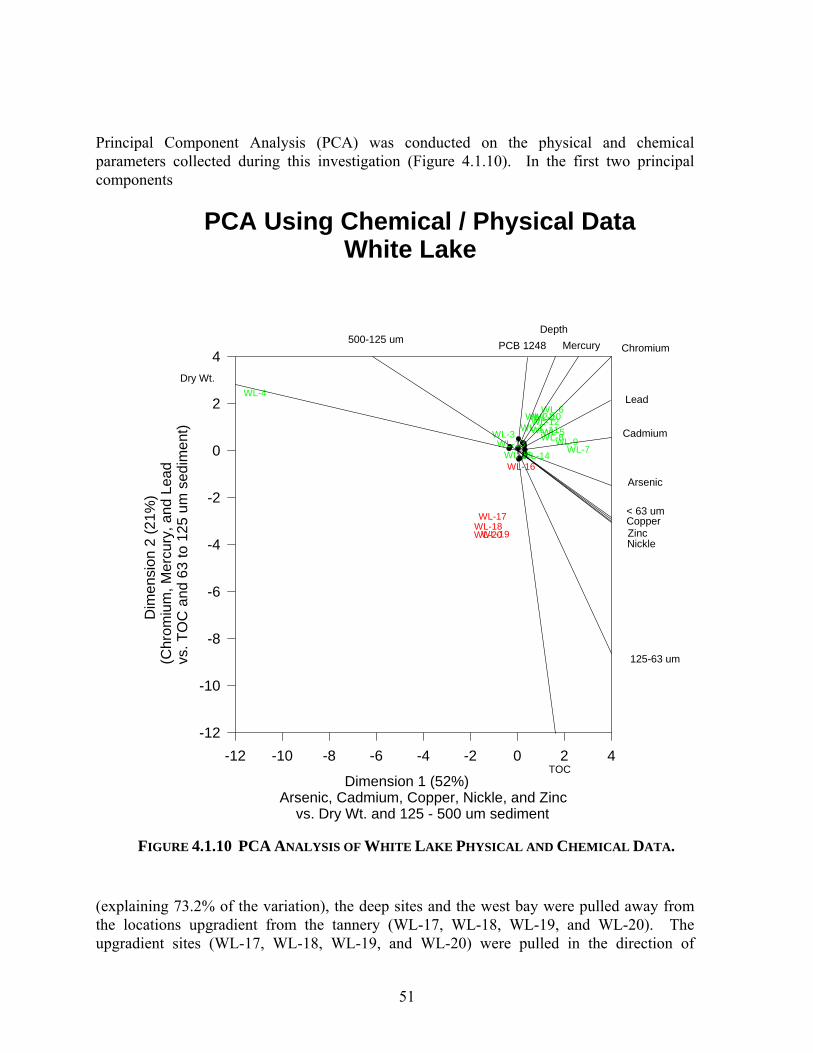
51

PCA Using Chemical / Physical Data White Lake

Dimension 1 (52%)Arsenic, Cadmium, Copper, Nickle, and Zinc vs. Dry Wt. and 125 - 500 um sediment

-12 -10 -8 -6 -4 -2 0 2 4

D

imen

sion

2 (2

1%)

(Chr

omiu

m, M

ercu

ry, a

nd L

ead

vs. T

OC

and

63

to 1

25 u

m s

edim

ent)

-12

-10

-8

-6

-4

-2

0

2

4

WL-16

WL-17WL-18

WL-19WL-20

WL-1WL-2

WL-3

WL-4

WL-5

WL-6

WL-7WL-8WL-9

WL-10WL-11WL-12

WL-13WL-14WL-15

WL-21

Dry Wt.

500-125 um PCB 1248Depth

Mercury Chromium

Lead

Cadmium

Arsenic

< 63 umCopperZincNickle

125-63 um

TOC

Principal Component Analysis (PCA) was conducted on the physical and chemical parameters collected during this investigation (Figure 4.1.10). In the first two principal components

(explaining 73.2% of the variation), the deep sites and the west bay were pulled away from the locations upgradient from the tannery (WL-17, WL-18, WL-19, and WL-20). The upgradient sites (WL-17, WL-18, WL-19, and WL-20) were pulled in the direction of

FIGURE 4.1.10 PCA ANALYSIS OF WHITE LAKE PHYSICAL AND CHEMICAL DATA.

52

physical parameters (TOC and grain size) while the remainder of the stations clustered around the contaminants chromium, mercury, and lead. Station WL-4 did not follow this pattern as it was pulled in the direction of the grain size (sand fraction) and % solids. This station had the greatest sand fraction, the highest dry weight (% solids), and was the only deep station that contained low contaminant concentrations. Spearman Rank Order Correlations were developed for chromium and the physical/chemical parameters measured in the investigation (Table 4.1.7) to further examine the relationship between the variables. Chromium showed a strong positive correlation with lead, arsenic, and mercury. In addition, chromium showed a negative correlation with % solids. Previous investigations (Bolattino and Fox. 1995, Rediske et al. 1998) established that arsenic, lead, and mercury were associated with the tannery discharge and found in high concentrations in Tannery Bay. The clustering of the deep stations in the PCA around these contaminants plus the Spearman Correlations indicate that the tannery is the predominant source of metal enrichment in western White Lake. TABLE 4.1.7 SPEARMAN RANK ORDER CORRELATIONS FOR CHROMIUM, CHEMICAL, AND

PHYSICAL PARAMETERS FOR WHITE LAKE SEDIMENTS. (VALUES IN BOLD DENOTE STATISTICALLY SIGNIFICANT CORRELATIONS)

Chromium with: r Arsenic 0.644

Cadmium 0.906 Copper 0.347

Mercury 0.63 Nickel 0.063 Lead 0.616 Zinc 0.189

Depth 0.459 <63um -0.03

Total organic carbon -0.03 % Solids -0.52

Organic chromium was analyzed in the PONAR samples by extraction with sodium pyrophosphate (Walsh and O’Halloran 1996). This fraction contains chromium bound to alkaline extractable ligands such as humic and fulvic acids. Organically bound chromium was found in sediments contaminated with tannery wastes in New Zealand (Walsh and O’Halloran 1996). The results of organic chromium determinations are given in Table 4.1.8. No detectable organic chromium was found in the stations east of Tannery Bay (WL-17, WL-18, WL-19, and WL-20) and at WL-4. The high sand content and low organic carbon would prevent this fraction of chromium from accumulating at this location. Stations west of Tannery Bay had levels of organic chromium ranging from 23-55 mg/kg. A set of archived samples that had been collected from Tannery Bay (Rediske et al. 1998) were also analyzed (Table 4.1.8). Organic chromium in these samples ranged from 40-380 mg/kg. The location with the lowest organic chromium fraction (I-6) was similar to WL-4 in that it contained a

53

high sand fraction. Samples that were previously noted to contain hide fragments, I-5 and I-3, exhibited the highest levels of organic chromium (380 and 160 mg/kg, respectively). The relationship between organic chromium and sediment toxicity will be discussed in Section 4.3.3.

TABLE 4.1.8 CONCENTRATION OF ORGANIC CHROMIUM IN WHITE LAKE SEDIMENTS.

Station Organic

Chromium (mg/kg)

Total Chromium

(mg/kg) Station

Organic Chromium

(mg/kg)

Total Chromium

(mg/kg)

WL 1 P 55 270 WL 15 P 27 250 WL 2 P 37 300 WL 16 P 24 190 WL 3 P 45 190 WL 17 P 0 50 WL 4 P 0 18 WL 18 P 0 29 WL 5 P 41 400 WL 19 P 0 39 WL 6 P 41 360 WL 20 P 0 28 WL 7 P 39 390 WL 21 P 39 450 WL 8 P 30 380 I-3* 155 934 WL 9 P 38 420 I-4* 120 1890 WL 10 P 31 270 I-5* 380 4100 WL 11 P 30 310 I-6* 40 2650 WL 12 P 54 510 I-7* 110 2560 WL 13 P 23 250 I-8* 160 515 WL 14 P 53 480 * Collected in 1996 (Rediske et al. 1998)

While discharges from the tannery and Occidental/Hooker Chemical left large areas of contaminated sediment in White Lake, samples collected near the DuPont groundwater plume (WL-1 and WL-2) did not contain elevated levels of organic compounds. Chromium and other metals were at concentrations consistent with the tannery discharge. No obvious signature related to the DuPont groundwater plume was noted in the core or PONAR samples. 4.2 Stratigraphy and Radiodating Results

Three cores were collected for radiodating and the analysis of detailed stratigraphy for chromium. Stations were selected based on bathymetry and the chromium concentrations measured in the initial cores. One core was collected from a deep depositional area and the remaining two were collected at locations that showed high accumulations of chromium in the 0-51 cm section of the initial cores. The first core (WL-2S) was collected at station WL-2 and was located in the deep basin (20.3 m) west of Long Point (Figures 2.1 and 4.1.8) and

54

near the channel to Lake Michigan. This station represented the deep depositional zone of the lake. The second core (WL-7S) was collected at WL-7 in a shallower zone (10.8 m) east of Long Point. This station had the highest level of chromium in the 0-51 cm zone of the initial set of cores (600 mg/kg). The final core (WL-9S) was collected at station WL-9 located west of Dowies Point at a depth of (9.7 m). This site is nearer to Tannery Bay than the previous cores and contained the second highest level of chromium (500 mg/kg). The results of each core are presented in the following sections. 4.2.1 Core WL-2S Stratigraphy and radiodating results for WL-2S are presented in Table 4.2.1. Station WL-2S is located at the deep point in White Lake near Long Point and within the flow path of the old river channel (Figure 2.1). Profiles of depth and concentration for chromium, 210Pb, and 137Cs are shown on Figure 4.2.1. Elevated concentrations of chromium continue beyond the estimated date of 1894, which indicates that the CRS model did not yield credible results for the deeper strata. Depositional patterns for 210Pb describe three regions in the core. The top 25 cm exhibits an exponential decay pattern for the radionuclide, which indicates stable deposition (Robbins and Herche 1993). Estimated dates within the top 19 cm of the core appear to be realistic as a peak in 137Cs activity is noted at 15cm. This peak corresponds to TABLE 4.2.1 STRATIGRAPHY AND RADIODATING RESULTS FOR CORE WL-2S COLLECTED

FROM WHITE LAKE, OCTOBER 2001.

Depth (cm) Total

Chromium mg/kg

Ra-226 Activity (dpm/g)

Cs-137 Activity (dpm/g)

Excess Pb-210

Activity (dpm/g)

Date at Given Depth

3 340 1.797 0.992 17.667 1996 7 341 2.529 1.438 8.904 1986 11 317 2.384 1.992 7.538 1977 15 347 2.359 8.801 4.637 1966 19 415 2.980 5.181 2.198 1958 23 481 2.612 2.070 5.012 1954 27 625 2.612 2.055 2.318 1947 31 688 2.090 2.384 0.970 1935 35 793 2.342 2.904 3.385 1930 39 1137 2.187 2.466 2.598 1910 43 1915 2.205 0.932 0.000 1890 47 2046 2.737 0.209 0.000 51 1846 3.260 0.437 0.000 55 1400 3.093 0.759 0.000 59 911 3.514 0.305 0.000 61 679 2.446 -0.542 0.000

55

FIGURE 4.2.1 DEPTH AND CONCENTRATION PROFILES FOR CHROMIUM , LEAD-210, AND CESIUM-137 AT STATION WL-2S, WHITE LAKE, OCTOBER 2001.

0

10

20

30

40

50

60

0 500 1000 1500 2000 2500Chromium Concentration (mg/kg)

Dep

th (c

m)

0

10

20

30

40

50

60

0.000 5.000 10.000 15.000 20.000 25.000 30.000Unsupported Pb-210 (dpm)

Dep

th (c

m)

0

10

20

30

40

50

60

-5.000 0.000 5.000 10.000 15.000

Cs-137 activity (dpm))

Dep

th (c

m)

56

the maximum deposition of the radionuclide that occurred during 1962 from atomic testing. The CRS model estimated the data of this interval to be 1966, indicating good agreement with the 137Cs peak. Chromium deposition appears to be constant in the top 15 cm of the core, which indicates a relatively constant supply of the element. Since the tannery discharge ceased in the mid 70s, the continued deposition of chromium can be attributed to the transport of contaminated sediment from Tannery Bay by lake currents. From 19 cm to 39 cm, 210Pb deposition is uniform. Chromium deposition increases from 415 mg/kg to 1915 mg/kg at the end of this interval. Excess 210Pb activity is absent in the region below 43 cm. Chromium levels peak at 47 cm (2071 mg/kg) and then decrease to 795 mg/kg at the bottom of the core (81 cm). The results of the strata below 19 cm suggest that 210Pb deposition was attenuated by dilution from excessive sedimentation. Since 226Ra inventories were relatively consistent throughout the core, it is unlikely that sediments generated by the erosion of surficial soils were responsible for the dilution of the 210Pb signal. A similar pattern of high chromium levels in strata with no 210Pb inventories was noted for sediment cores taken in Tannery Bay (Rediske et al. 1989). Dilution by the discharge of industrial waste materials was thought to have attenuated the 210Pb signal in Tannery Bay. In the deep basin where WL-2S is located, it is likely that the additional sedimentation was generated by primary productivity and/or the input of organic matter. This location is 8 km from Tannery Bay and no known source of industrial waste is present in the area. Since the historical tannery discharge also contained high levels of nitrogen and phosphorus from the processing of animal hides, the productivity of White Lake may have been greater during the years prior to 1960. Observations and data from Evans (1992) support this conclusion as the water quality in White Lake was significantly degraded during the 50s and early 60s. Excessive algal blooms, high turbidity, and degraded benthic populations were reported for this time period. A trend of increasing water quality was noted in the late 60s. The fact that a peak in chromium deposition is coupled with the absence of 210Pb suggests that the tannery was discharging high levels of metal laden waste materials into White Lake prior to the early 1960s and that organic sedimentation was elevated by primary productivity. 4.2.2 Core WL-7S Stratigraphy and radiodating results for WL-7S are presented in Table 4.2.2. Profiles of depth and concentration for chromium and lead are shown in Figure 4.2.2. This core was taken at a depth of 21.5 m in the deep basin near Dowies Point (Figure 2.1). The top 11 cm showed an exponential decay pattern for 210Pb while the remainder of the core had variable radioisotope inventories. These data suggest a recent pattern of stable deposition followed by a period of mixing and excess sedimentation from advection within the lake. Since White Lake is a drowned rivermouth, storm events and currents are capable of transporting significant amounts of sediment on an episodic basis. The layer of uniform 210Pb inventories

57

TABLE 4.2.2 STRATIGRAPHY AND RADIODATING RESULTS FOR CORE WL-7S COLLECTED FROM WHITE LAKE, OCTOBER 2001.

Depth (cm) Total

Chromium mg/kg



Excess Pb-210

Activity (dpm/g)

Date at Given Depth

3 204 4.047 1.922 30.878 1999 7 242 3.773 2.184 27.848 1996 11 273 3.056 2.244 22.008 1992 15 330 2.947 2.348 16.646 1990 19 470 2.535 2.195 18.633 1983 23 462 3.356 2.828 20.804 1977 27 397 3.531 2.183 12.293 1971 31 702 3.083 3.247 16.398 1966 35 928 3.562 4.015 11.531 1964 39 893 3.018 3.695 13.742 1957 43 1052 3.398 4.611 11.814 1951 47 1230 3.734 3.515 14.954 1947 51 1848 3.404 3.434 13.294 1939 55 1779 3.126 3.877 11.450 1928 59 1418 3.357 4.282 13.387 1918 61 1072 2.639 3.467 9.901 1900

may be due to a combination of mixing and excess deposition by episodic events. The absence of a 137Cs horizon (Figure 4.2.2) also supports the hypothesis of sediment mixing and transport, as the radionuclide profile shows a slightly increasing deposition pattern instead of the classic peak shape found in core WL-2S (Figure 4.2.1). In consideration of the atypical radioisotope at this location, the dates assigned by the constant supply model cannot be considered to be accurate. Chromium deposition patterns (Figure 4.2.2) also show the dates to be inaccurate as the highest levels of chromium were estimated to be deposited prior to the conversion of the tanning process in 1945. Chromium levels were relatively consistent in the top 11 cm and then increased to a maximum of 1848 mg/kg at 51 cm. This region of the core also contained 210Pb inventories that were more representative of exponential decay, indicating stable sediments and a constant supply of chromium. Increasing chromium deposition is evident in the deeper region where the 210Pb is variable. The presence of excess 210Pb throughout this region of the core indicates a continuous influx of sediment and frequent movement out of the location. Based on the increasing and decreasing pattern, it appears that episodic events such as storms act to remove and deposit varying amounts of sediment at this location.

58


0

10

20

30

40

50

60

0 500 1000 1500 2000

Chromium Concentration (mg/kg)D

epth

(cm

)

0

10

20

30

40

50

60

0.0 10.0 20.0 30.0 40.0 50.0

Unsupported Pb-210 (dpm)

Dep

th (c

m)

0

10

20

30

40

50

60

0.0 2.0 4.0 6.0 8.0

Cs-137 activity (dpm)

Dep

th (c

m)

59

4.2.3 Core WL-9S Stratigraphy and radiodating results for WL-9S are presented in Table 4.2.3. Profiles of depth and concentration for chromium and lead are shown in Figure 4.2.3 along with the calculated dates from the 210Pb deposition model. The radiodating results indicate that stable sediments are not accumulating at this location. The accumulation of stable sediments would result in a 210Pb profile that exhibits an exponential decay of the radioisotope (Robbins and Herche 1993) similar to core WL-2S. No exponential decay pattern is visible in core WL-2S (Table 4.2.3). Instead, a mixed layer with uniform 210Pb inventories was observed for the first 15 cm followed by a pattern of sections with increasing and decreasing 210Pb concentrations ranging from ≈ 11 - 19 dpm. The presence of excess 210Pb throughout the core indicates a continuous influx of sediment and frequent movement out of the location. Based on the increasing and decreasing pattern, it appears that episodic events such as storms act to remove varying amounts of sediment from the location. The depositional pattern of chromium also exhibits sporadic changes in concentration indicating the influence of episodic events. The relatively uniform concentrations of chromium noted in the top 11 cm correspond to a mixed sediment layer shown in the 210Pb profile. Chromium concentrations peak at 31 cm and then decline to the base of the core. Station WL-9S is closer to Tannery Bay than the two previous cores and is also located in shallower water (15.2 m). TABLE 4.2.3 STRATIGRAPHY AND RADIODATING RESULTS FOR CORE WL-9S COLLECTED

FROM WHITE LAKE, OCTOBER 2001.

Depth (cm) Total

Chromium mg/kg



Excess Pb-210

Activity (dpm/g)

Date at Given Depth

3 454 1.797 0.992 24.098 1999 7 464 2.529 1.438 23.798 1996 11 488 2.384 1.992 23.858 1991 15 606 2.359 8.801 20.499 1989 19 643 2.980 5.181 17.389 1984 23 695 2.339 3.576 16.061 1978 27 917 2.612 2.070 14.196 1972 31 1201 2.612 2.055 14.602 1967 35 849 2.090 2.384 15.705 1963 39 778 1.839 2.261 10.988 1958 43 750 2.040 2.239 15.262 1955 47 732 2.205 1.932 12.225 1947 51 678 2.272 1.759 17.246 1932 55 722 3.326 0.851 18.967 1912 59 630 3.093 0.759 19.093 1890

60


0

10

20

30

40

50

60

0 500 1000 1500

Chromium Concentration (mg/kg)

Dep

th (c

m)

0

10

20

30

40

50

60

0 10 20 30 40

Unsupported Pb-210 (dpm)

Dep

th (c

m))

0

10

20

30

40

50

60

1 2 3 4 5

Cs-137 activity (dpm)

Dep

th (c

m)

61

4.2.4 Stratigraphy and Radiodating Summary In examining the results of the three stratigraphy cores together, some important patterns in contaminant deposition are evident. All of the cores show uniform levels of chromium deposition in the top 10 - 15 cm. This pattern indicates that a relatively constant source of chromium is currently present in White Lake. These data coupled with the previous investigation (Rediske et al. 1998) suggest that the heavily contaminated sediments near the historic tannery discharge are being transported out of the bay by currents and then deposited throughout the lake. In addition, the lack of a standard exponential decay pattern in the lower sections of the core illustrates that sediments in the open waters of the lake are also mobile and influenced by currents and episodic events. Even when there is evidence of a distinct 137Cs horizon as in WL-2S, the deeper sections of the core still contain atypical 210Pb profiles that suggest mixed sediment layers. The stratigraphy cores were analyzed by PIXE while the investigative samples were evaluated by ICP. The PIXE method is a form of elemental analysis based on the characteristics of X-rays and the nature of X-ray detection (Johansson et al. 1995). The method uses beams of energetic ions, produced by an accelerator to generate a beam of protons in the 2-5 MeV range, used to create inner electron shell vacancies. As these inner shell vacancies become filled by outer shell electrons, the characteristic X-rays emitted by this cascade effect can be detected by wavelength dispersion. PIXE techniques provide a rapid screening of the samples for metals without sample preparation. The PIXE results represent a total analysis of metals due to the interaction of the proton beam with all metallic forms (Rajander et al. 1999). In contrast, the microwave digestion used for the investigative samples provides data on acid extractable metals. Comparative studies of the two techniques found that acid extractable digestions underestimate chromium concentrations by up to 40% because of the stability of chromite (Ma et al. 1997, Chen and Ma 2001). Total metal digestions involving HF are necessary to dissolve the refractory chromite. In order to compare the results of the stratigraphy cores with the investigative samples, the core from WL-9S was analyzed by PIXE and ICP methods. The results of the comparison study are shown in Table 4.2.4. With respect to White Lake sediments, there appears to be a 21% difference between the two methods (based on grand mean). Since the soils in the White River watershed consist of glacial tills that originated in the Canadian Shield, background levels of chromite can be expected in the core samples. The results also indicate that some of the chromium originating in the tannery waste may be refractory to acid digestion. The results of the top core section from the investigative samples (0-51 cm) are compared to the same depth interval of the stratigraphy cores in Table 4.2.5. When a 21% factor is applied to the PIXE results to account for the difference between total and extractable metals, the results between the methods show good agreement. There appears to be some high bias associated with the stratigraphy results that is probably related to sample collection methods. The investigative samples were collected by VibraCore methods that tend to compress flocculent sediments. It is possible that some of the deeper strata were included in the VibraCore samples. It is also interesting to note that the middle core section of the investigative samples (51-102 cm) had chromium levels that ranged from 34-38 mg/kg (Table 4.1.3). These results suggest that anthropogenic chromium contamination does not extend down into this region of the core.

62

TABLE 4.2.4 RESULTS OF ICP AND PIXE ANALYSES FOR CHROMIUM IN CORE WL-9S

COLLECTED FROM WHITE LAKE, OCTOBER 2001.

Depth (cm)

Chromium (ICP) mg/kg

Chromium (PIXE) mg/kg

% Difference

3 359 454 21 7 427 464 8 11 421 488 14 15 484 606 20 19 496 643 23 23 552 695 21 27 709 917 23 31 870 1200 28 35 678 849 20 39 627 778 19 43 611 750 19 47 540 732 26 51 564 678 17 55 564 712 20 59 359 454 21

Grand Mean 551 695 21

TABLE 4.2.5 AVERAGE AND CORRECTED DATA FOR STRATIGRAPHY CORES (OCTOBER 2001) COMPARED TO THE RESULTS OF THE TOP CORE SECTION FROM THE INVESTIGATIVE

SURVEY (OCTOBER 2000) FOR WHITE LAKE SEDIMENTS.

Station Stratigraphy Core Average

Chromium (PIXE) mg/kg

Stratigraphy Core Corrected Average Chromium (PIXE)

mg/kg*

Investigative Core Top Section Chromium (ICP)

mg/kg**

3 695 549 470 7 869 686 600 11 712 574 500

* Corrected for 21% difference between PIXIE and ICP results ** Top Core Section Results (0-51 cm)

63

4.3 Toxicity Testing Results The toxicity evaluations of the White Lake sediments were performed during November 2000. Grab sediment samples collected from 21 different sites were evaluated using the EPA (1994) solid phase testing protocol with Hyalella azteca and Chironomus tentans. Conductivity, hardness, alkalinity, ammonia, and pH were determined for the culture water at the beginning and on the tenth day of each test (Appendix E: Tables E-1, E-3). With the exception of ammonia in most of the sediments and conductivity and hardness in M10-P, these parameters remained relatively constant. Variations of less than 50% from initial to final measurements for both test species were observed. Based on the initial pH values (all < 8.00) and the fact that the overlying water was exchanged prior to adding the organisms, toxicity related to unionized ammonia was not anticipated to be a factor in these experiments. Temperature and dissolved oxygen measurements were recorded daily throughout the duration of the tests (Appendix E: Tables E-2, E-4). Very little variation was noted with respect to temperature. The dissolved oxygen remained above 40% saturation in all of the test beakers. 4.3.1 Hyalella azteca Survival data for solid phase toxicity tests with Hyalella azteca are presented in Table 4.3.1.1. The survival in the control (WL-20P and WL-4P) treatments exceeded the required 80%. In order to group the samples based on depth, WL-20P was used as the control for the shallow locations east of the Narrows and WL-4P was used as the control for the deep stations. Separate statistical analyses also were performed on the two groups of data. Un-transformed survival data were evaluated to determine whether they were consistent with a normal distribution. The Chi-Squared distribution was used to compare the expected count of data values at the 10th, 20th, …, and 90th percentiles with the observed count. The sample data from both groups were found to be consistent with those drawn from a normal population (p > 0.01). Dunnett’s Test (Table 4.3.1.2) showed a statistically significant (p < 0.05) difference for the survival data compared to control site WL-20P in 1 out of 4 shallow stations. Sediments from site WL-16P had significantly reduced survival compared to WL-20P (66% vs 90% respectively). Dunnett’s Test (Table 4.3.1.3) showed a statistically significant (p < 0.05) difference for the survival data compared to control site WL-4P in 1 out of 9 deep stations. Sediments from site WL-21P had significantly reduced survival compared to WL-4P (65% vs 88% respectively). All of the other deep and shallow locations had greater than 80% survival.

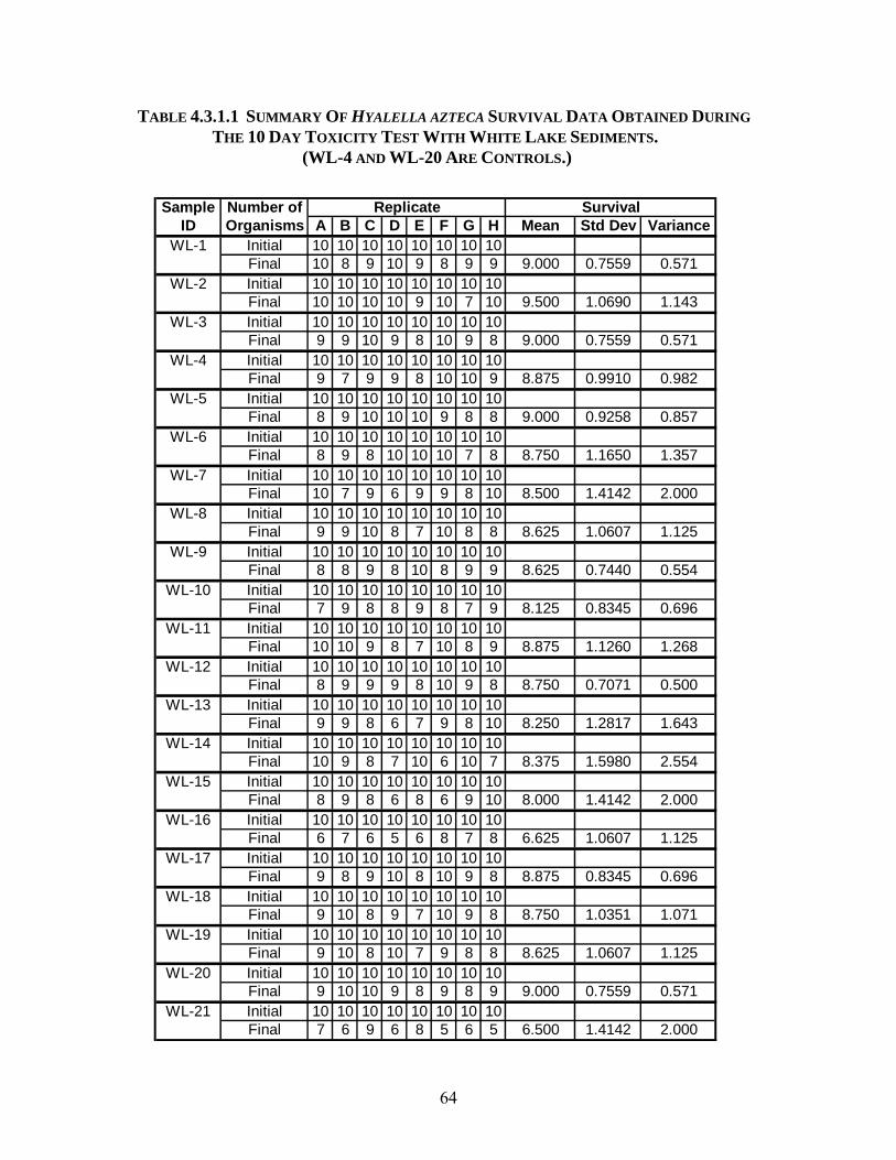
64

Sample Number ofID Organisms A B C D E F G H Mean Std Dev Variance

WL-1 Initial 10 10 10 10 10 10 10 10Final 10 8 9 10 9 8 9 9 9.000 0.7559 0.571

WL-2 Initial 10 10 10 10 10 10 10 10Final 10 10 10 10 9 10 7 10 9.500 1.0690 1.143

WL-3 Initial 10 10 10 10 10 10 10 10Final 9 9 10 9 8 10 9 8 9.000 0.7559 0.571

WL-4 Initial 10 10 10 10 10 10 10 10Final 9 7 9 9 8 10 10 9 8.875 0.9910 0.982

WL-5 Initial 10 10 10 10 10 10 10 10Final 8 9 10 10 10 9 8 8 9.000 0.9258 0.857

WL-6 Initial 10 10 10 10 10 10 10 10Final 8 9 8 10 10 10 7 8 8.750 1.1650 1.357

WL-7 Initial 10 10 10 10 10 10 10 10Final 10 7 9 6 9 9 8 10 8.500 1.4142 2.000

WL-8 Initial 10 10 10 10 10 10 10 10Final 9 9 10 8 7 10 8 8 8.625 1.0607 1.125

WL-9 Initial 10 10 10 10 10 10 10 10Final 8 8 9 8 10 8 9 9 8.625 0.7440 0.554

WL-10 Initial 10 10 10 10 10 10 10 10Final 7 9 8 8 9 8 7 9 8.125 0.8345 0.696

WL-11 Initial 10 10 10 10 10 10 10 10Final 10 10 9 8 7 10 8 9 8.875 1.1260 1.268

WL-12 Initial 10 10 10 10 10 10 10 10Final 8 9 9 9 8 10 9 8 8.750 0.7071 0.500

WL-13 Initial 10 10 10 10 10 10 10 10Final 9 9 8 6 7 9 8 10 8.250 1.2817 1.643

WL-14 Initial 10 10 10 10 10 10 10 10Final 10 9 8 7 10 6 10 7 8.375 1.5980 2.554

WL-15 Initial 10 10 10 10 10 10 10 10Final 8 9 8 6 8 6 9 10 8.000 1.4142 2.000

WL-16 Initial 10 10 10 10 10 10 10 10Final 6 7 6 5 6 8 7 8 6.625 1.0607 1.125

WL-17 Initial 10 10 10 10 10 10 10 10Final 9 8 9 10 8 10 9 8 8.875 0.8345 0.696

WL-18 Initial 10 10 10 10 10 10 10 10Final 9 10 8 9 7 10 9 8 8.750 1.0351 1.071

WL-19 Initial 10 10 10 10 10 10 10 10Final 9 10 8 10 7 9 8 8 8.625 1.0607 1.125

WL-20 Initial 10 10 10 10 10 10 10 10Final 9 10 10 9 8 9 8 9 9.000 0.7559 0.571

WL-21 Initial 10 10 10 10 10 10 10 10Final 7 6 9 6 8 5 6 5 6.500 1.4142 2.000

Replicate Survival

TABLE 4.3.1.1 SUMMARY OF HYALELLA AZTECA SURVIVAL DATA OBTAINED DURING THE 10 DAY TOXICITY TEST WITH WHITE LAKE SEDIMENTS.

(WL-4 AND WL-20 ARE CONTROLS.)

65

TABLE 4.3.1.2 SUMMARY OF DUNNETT’S TEST ANALYSIS OF HYALELLA AZTECA SURVIVAL

DATA OBTAINED DURING THE 10 DAY TOXICITY TEST WITH WHITE LAKE SEDIMENTS FROM SHALLOW STATIONS (< 4.5 M).

ID MEAN T STAT SIG 0.05

WL-20P 9.0000 0.0000 WL-19P 8.6250 0.7828 WL-18P 8.7500 0.5219 WL-17P 8.8750 0.2609 WL-16P 6.6250 4.9580 *

Dunnett's critical value = 2.2500. 1 Tailed, alpha = 0.05.

TABLE 4.3.1.3 SUMMARY OF DUNNETT’S TEST ANALYSIS OF HYALELLA AZTECA SURVIVAL

DATA OBTAINED DURING THE 10 DAY TOXICITY TEST WITH WHITE LAKE SEDIMENTS FROM DEEP STATIONS (> 4.5 M).

ID MEAN T STAT SIG

0.05 WL-4P 8.8750 0.0000

WL-2P 9.5000 -1.1832 WL-3P 9.0000 -0.2366 WL-1P 9.0000 -0.2366 WL-5P 9.0000 -0.2366 WL-6P 8.7500 0.2366 WL-7P 8.5000 0.7099 WL-8P 8.6250 0.4733 WL-9P 8.6250 0.4733 WL-21P 6.5000 4.4962 *


66

4.3.2 Chironomus tentans Survival data for solid phase toxicity tests with Chironomus tentans are presented in Table 4.3.2.1. The survival in the control treatments (WL-4P and WL-20P) exceeded the required 70%. Un-transformed survival data were evaluated as described above with the Chi-Squared distribution. The sample data were found to be consistent with those drawn from a normal population (p > 0.01). Dunnett’s Test (Table 4.3.2.2) showed a statistically significant (p < 0.05) difference for the survival data compared to control site WL-20P in 1 out of 4 shallow stations. Sediments from site WL-16P had significantly reduced survival compared to WL-20P (66% vs 90% respectively). Dunnett’s Test (Table 4.3.2.3) showed a statistically significant (p < 0.05) difference for the survival data compared to control site WL-4P in 1 out of 9 deep stations. Sediments from site WL-21P had significantly reduced survival compared to WL-4P (65% vs 88% respectively). All of the other deep and shallow locations had greater than 80% survival. Chironomus tentans growth data are presented in Table 4.3.2.4. Un-transformed growth data were found to be consistent with a Chi-Squared distribution at p > 0.01. Dunnett’s Test (Table 4.3.2.5) showed a statistically significant (p < 0.05) difference for the growth data compared to control site WL-20P in 1 out of 4 shallow stations. Sediments from site WL-16P had significantly reduced growth compared to WL-20P (0.5375 mg/individual vs 1.1522 mg/individual respectively). Dunnett’s Test (Table 4.3.2.6) showed a statistically significant (p < 0.05) difference for the growth data compared to control site WL-4P in 1 out of 9 deep stations. Sediments from site WL-21P had significantly reduced growth compared to WL-4P (0.6263 mg/individual vs 0.9834 mg/individual respectively). All of the other deep and shallow locations had average individual weights of >0.6 mg. 4.3.3 Sediment Toxicity Data Discussion Statistically significant (p < 0.05) acute toxicity effects were observed in the sediments from sites WL-16 and WL-21 for the amphipod, H. azteca. In addition, statistically significant (p < 0.05) mortality and growth rates were noted for the midge, C. tentans in sediment from the same sites. Sediment from station located in the east bay, WL-16, contained no detectable organic compounds and metals that were above PEC guidelines (MacDonald et al. 2000). The toxic agent(s) present at this location were not identified in the current protocol. Given the high level of toxicity measured in this study and the previous investigation, a more detailed assessment of east bay area is warranted. A Toxicity Identification Evaluation (TIE) protocol needs to be performed to examine the classification of the toxicant. The east bay is located adjacent to the old storage reservoir for the tree bark tanning agent used from 1890-1940. Since tannins are known to be toxic to herbivores including insects (Cowan 1999, Bernays et al. 1989, and Kubanek et al. 2001), it is possible that this class of compounds is responsible for the amphipod and midge mortality. The dark, opaque color of pyrophosphate extract from

67

Sample Number of Replicate SurvivalID Organisms A B C D E F G H Mean Std Dev Variance

WL-1 Initial 10 10 10 10 10 10 10 10Final 7 6 8 8 8 9 9 8 7.875 0.9910 0.982

WL-2 Initial 10 10 10 10 10 10 10 10Final 8 7 8 9 8 8 9 8 8.125 0.6409 0.411

WL-3 Initial 10 10 10 10 10 10 10 10Final 8 9 8 7 8 9 8 8 8.125 0.6409 0.411

WL-4 Initial 10 10 10 10 10 10 10 10Final 8 9 8 8 9 8 7 8 8.125 0.6409 0.411

WL-5 Initial 10 10 10 10 10 10 10 10Final 9 8 7 8 9 8 8 7 8.000 0.7559 0.571

WL-6 Initial 10 10 10 10 10 10 10 10Final 6 5 8 9 7 6 8 9 7.250 1.4880 2.214

WL-7 Initial 10 10 10 10 10 10 10 10Final 8 9 7 8 6 7 9 9 7.875 1.1260 1.268

WL-8 Initial 10 10 10 10 10 10 10 10Final 8 7 6 5 9 10 9 8 7.750 1.6690 2.786

WL-9 Initial 10 10 10 10 10 10 10 10Final 8 6 7 6 8 6 9 6 7.000 1.1952 1.429

WL-10 Initial 10 10 10 10 10 10 10 10Final 7 9 8 7 10 7 9 8 8.125 1.1260 1.268

WL-11 Initial 10 10 10 10 10 10 10 10Final 7 8 10 7 11 8 11 7 8.625 1.7678 3.125

WL-12 Initial 10 10 10 10 10 10 10 10Final 7 8 7 5 10 5 8 7 7.125 1.6421 2.696

WL-13 Initial 10 10 10 10 10 10 10 10Final 6 8 5 8 5 7 10 7 7.000 1.6903 2.857

WL-14 Initial 10 10 10 10 10 10 10 10Final 9 12 8 10 10 9 9 9 9.500 1.1952 1.429

WL-15 Initial 10 10 10 10 10 10 10 10Final 10 8 8 8 4 4 8 6 7.000 2.1381 4.571

WL-16 Initial 10 10 10 10 10 10 10 10Final 7 6 5 3 5 5 8 4 5.375 1.5980 2.554

WL-17 Initial 10 10 10 10 10 10 10 10Final 10 8 8 8 7 6 8 7 7.750 1.1650 1.357

WL-18 Initial 10 10 10 10 10 10 10 10Final 8 6 8 6 7 6 8 7 7.000 0.9258 0.857

WL-19 Initial 10 10 10 10 10 10 10 10Final 7 8 7 6 9 9 7 8 7.625 1.0607 1.125

WL-20 Initial 10 10 10 10 10 10 10 10Final 8 8 8 7 9 7 6 8 7.625 0.9161 0.839

WL-21 Initial 10 10 10 10 10 10 10 10Final 6 5 6 5 6 5 7 5 5.625 0.7440 0.554

TABLE 4.3.2.1 SUMMARY OF CHIRONOMUS TENTANS SURVIVAL DATA OBTAINED DURING THE 10 DAY TOXICITY TEST WITH WHITE LAKE SEDIMENTS.

(WL-4 AND W-20 ARE CONTROLS.)

68

TABLE 4.3.2.2 SUMMARY OF DUNNETT’S TEST ANALYSIS OF CHIRONOMUS TENTANS SURVIVAL DATA OBTAINED DURING THE 10 DAY TOXICITY TEST WITH WHITE LAKE

SEDIMENTS FROM SHALLOW STATIONS (<4.5 M).


WL-20P 7.6250 0.0000 WL-19P 7.6250 0.0000 WL-18P 7.0000 1.0773 WL-17P 7.7500 -0.2155 WL-16P 5.3750 3.8781 *


TABLE 4.3.2.3 SUMMARY OF DUNNETT’S TEST ANALYSIS OF CHIRONOMUS TENTANS SURVIVAL DATA OBTAINED DURING THE 10 DAY TOXICITY TEST WITH WHITE LAKE

SEDIMENTS FROM DEEP STATIONS (> 4.5 M).

ID MEAN T STAT SIG

0.05 WL-4P 8.1250 0.0000

WL-1P 7.8750 0.4585 WL-2P 8.1250 0.0000 WL-5P 8.0000 0.2292 WL-6P 7.2500 1.6047 WL-7P 7.8750 0.4585 WL-8P 7.7500 0.6877 WL-9P 7.0000 2.0632 WL-10P 8.1250 0.0000 WL-21P 5.6250 5.6250 *


69

Sample Individual Weight (mg)

Average Individual

Weight (mg)Sample Individual

Weight (mg)

Average Individual

Weight (mg)Sample Individual

Weight (mg)

Average Individual

Weight (mg)WL-1 A 0.9714 WL-8 A 1.0875 WL-15 A 1.0700WL-1 B 1.2167 WL-8 B 1.4571 WL-15 B 1.1125WL-1 C 0.9500 WL-8 C 1.9000 WL-15 C 1.0625WL-1 D 0.9875 WL-8 D 1.5800 WL-15 D 1.1875WL-1 E 1.0500 WL-8 E 0.9556 WL-15 E 1.5250WL-1 F 0.8667 WL-8 F 1.0100 WL-15 F 1.9000WL-1 G 0.9111 WL-8 G 1.0333 WL-15 G 1.9875WL-1 H 1.0625 WL-8 H 1.0500 WL-15 H 0.9000WL-2 A 0.9500 WL-9 A 1.0250 WL-16 A 0.7857WL-2 B 1.0429 WL-9 B 1.0167 WL-16 B 0.6111WL-2 C 1.2000 WL-9 C 0.9429 WL-16 C 0.4625WL-2 D 0.8444 WL-9 D 1.2667 WL-16 D 0.3667WL-2 E 0.9500 WL-9 E 0.9375 WL-16 E 0.7250WL-2 F 1.0125 WL-9 F 1.0000 WL-16 F 0.2600WL-2 G 0.8222 WL-9 G 0.8667 WL-16 G 0.7500WL-2 H 1.1250 WL-9 H 1.0000 WL-16 H 0.3250WL-3 A 1.3750 WL-10 A 0.9143 WL-17 A 0.7636WL-3 B 1.0667 WL-10 B 0.7333 WL-17 B 1.0125WL-3 C 1.0500 WL-10 C 0.9000 WL-17 C 1.0500WL-3 D 1.3571 WL-10 D 1.0714 WL-17 D 0.9500WL-3 E 1.4000 WL-10 E 0.9900 WL-17 E 1.1429WL-3 F 2.1000 WL-10 F 1.0857 WL-17 F 1.1000WL-3 G 1.8250 WL-10 G 0.8556 WL-17 G 1.0375WL-3 H 1.4375 WL-10 H 0.8625 WL-17 H 1.0000WL-4 A 0.8250 WL-11 A 0.9714 WL-18 A 0.8625WL-4 B 0.8667 WL-11 B 0.9750 WL-18 B 1.0500WL-4 C 1.1125 WL-11 C 0.8600 WL-18 C 0.9000WL-4 D 0.7750 WL-11 D 0.9143 WL-18 D 1.1500WL-4 E 1.1111 WL-11 E 0.9364 WL-18 E 1.0714WL-4 F 1.0750 WL-11 F 1.1500 WL-18 F 1.0500WL-4 G 1.0143 WL-11 G 0.9636 WL-18 G 0.9500WL-4 H 1.0875 WL-11 H 1.0714 WL-18 H 0.9429WL-5 A 1.1333 WL-12 A 0.9286 WL-19 A 1.0857WL-5 B 1.1250 WL-12 B 0.8250 WL-19 B 1.1333WL-5 C 1.0857 WL-12 C 0.8714 WL-19 C 0.8857WL-5 D 1.0750 WL-12 D 0.9600 WL-19 D 0.9333WL-5 E 0.8111 WL-12 E 0.5800 WL-19 E 0.9556WL-5 F 0.8125 WL-12 F 1.0600 WL-19 F 0.8111WL-5 G 0.7625 WL-12 G 1.0375 WL-19 G 1.0714WL-5 H 0.9429 WL-12 H 0.8571 WL-19 H 1.0714WL-6 A 1.1833 WL-13 A 1.9000 WL-20 A 1.1429WL-6 B 0.9200 WL-13 B 1.3750 WL-20 B 0.9875WL-6 C 1.1000 WL-13 C 1.3200 WL-20 C 1.1000WL-6 D 1.1556 WL-13 D 1.3875 WL-20 D 0.9571WL-6 E 1.0571 WL-13 E 0.5400 WL-20 E 1.9667WL-6 F 0.8667 WL-13 F 1.1857 WL-20 F 0.7714WL-6 G 1.1000 WL-13 G 0.9600 WL-20 G 1.1667WL-6 H 0.9444 WL-13 H 0.9143 WL-20 H 1.1250WL-7 A 1.3000 WL-14 A 1.1111 WL-21 A 0.7000WL-7 B 0.9222 WL-14 B 0.8083 WL-21 B 0.5000WL-7 C 1.2000 WL-14 C 0.9750 WL-21 C 0.6000WL-7 D 0.9125 WL-14 D 0.9600 WL-21 D 0.6600WL-7 E 1.2833 WL-14 E 1.0000 WL-21 E 0.6333WL-7 F 1.1571 WL-14 F 0.9667 WL-21 F 0.6800WL-7 G 0.9778 WL-14 G 1.1333 WL-21 G 0.6571WL-7 H 0.9667 WL-14 H 1.1444 WL-21 H 0.5800

0.9935

1.1522

0.6263

1.3431

0.5357

1.0071

0.9971

0.9685

1.0409

1.0900 1.0124

1.1978

0.8900

0.9803

1.0020

0.9934

1.4514

0.9834

0.9266

1.0069

1.2592

TABLE 4.3.2.4 SUMMARY OF CHIRONOMUS TENTANS DRY WEIGHT DATA OBTAINED DURING THE 10 DAY TOXICITY TEST WITH WHITE LAKE SEDIMENTS.

(WL-4 AND WL-20 ARE CONTROLS.)

70

TABLE 4.3.2.5 SUMMARY OF DUNNETT’S TEST ANALYSIS OF CHIRONOMUS TENTANS GROWTH DATA OBTAINED DURING THE 10 DAY TOXICITY TEST WITH WHITE LAKE

SEDIMENTS FROM SHALLOW STATIONS (<4.5 M).


WL-20P 1.1522 0.0000 WL-19P 0.9935 1.6051 WL-18P 0.9971 1.4816 WL-17P 1.0071 1.4816 WL-16P 0.5357 6.1733 *


TABLE 4.3.2.6 SUMMARY OF DUNNETT’S TEST ANALYSIS OF CHIRONOMUS TENTANS GROWTH DATA OBTAINED DURING THE 10 DAY TOXICITY TEST WITH WHITE LAKE

SEDIMENTS FROM DEEP STATIONS (> 4.5 M).

ID MEAN T STAT SIG

0.05 WL-4P 0.9834 0.0000

WL-2P 0.9934 -0.2551 WL-3P 1.4514 -4.7197 WL-1P 1.0020 0.2551 WL-5P 0.9685 -0.6378 WL-6P 1.0409 -1.1480 WL-7P 1.0900 -2.9339 WL-8P 1.2592 -0.1276 WL-9P 1.0069 0.5102 WL-21P 0.6263 3.5717 *


WL-16 provides indirect evidence of the presence of high levels of tannins due to their solubility in alkaline conditions. The toxicity observed at WL-21 was most likely due to the presence of PCBs (22 mg/kg) and/or chlorinated hydrocarbons. This area was dredged in 2003 and further toxicity evaluations are not necessary. No correlation was found between amphipod toxicity and chromium concentrations in Tannery Bay sediments in the previous investigation (Rediske et al. 1998). Table 4.3.3.1

71

R2 = 0.0004

0

10

20

30

40

50

60

70

0 500 1000 1500 2000 2500 3000 3500 4000 4500

Total Chromium (mg/kg)

% S

urvi

val (

H. a

ztec

a)

contains the 1996 data for total chromium and amphipod toxicity plus the recently measured values of organic chromium. The correlation results for amphipod toxicity and total chromium and organic chromium are displayed in Figures 4.3.3.1 and 4.3.3.2, respectively. The results clearly show that a significant correlation exists between organic chromium and TABLE 4.3.3.1 SUMMARY OF RESULTS OF TOTAL CHROMIUM, ORGANIC CHROMIUM, AND AMPHIPOD SURVIVAL FOR WHITE LAKE SEDIMENTS (REDISKE ET AL. 1998). (ORGANIC

CHROMIUM ANALYSIS PERFORMED ON ARCHIVED SEDIMENT FROM 1996.)

Total Cr

% Survival

Organic Cr Station

(mg/kg) H. azteca (mg/kg)

E-1 35 84 160 I-1 212 9 120 I-2 259 1 380 I-3 934 20 40 I-4 1890 53 110 I-5 4100 9 155 I-6 2650 60 33 I-7 2560 41 58 I-8 515 23 27

FIGURE 4.3.3.1 RELATIONSHIP BETWEEN TOTAL CHROMIUM AND AMPHIPOD SURVIVAL

FOR TANNERY BAY SEDIMENTS (REDISKE ET AL. 1998).

72

FIGURE 4.3.3.2 RELATIONSHIP BETWEEN ORGANIC CHROMIUM AND AMPHIPOD

SURVIVAL FOR TANNERY BAY SEDIMENTS (REDISKE ET AL. 1998). (ORGANIC CHROMIUM ANALYSIS PERFORMED ON ARCHIVED SEDIMENT FROM 1996.)

amphipod toxicity (r2=0.6902). No correlation was observed for total chromium and amphipod toxicity. Chromium (III) is anticipated to be the only form of the metal present in the sediments of White Lake due to their reducing nature (ENVCA 1994). While trivalent chromium compounds have low membrane permeabilities (Eisler 1986), organically bound metals exhibit increased absorption (Barnhart 1997). Once in the cell, chromium (III) has been shown to bind with DNA and induce conformational changes in bio molecules (Snow 1994). In consideration of these chemical properties and the correlation with amphipod mortality, it is possible that the organic chromium fraction in the sediments of Tannery Bay is responsible for the observed toxicity. More research would be required to link cause and effect with the organic chromium fraction. The presence of the decomposing animal hides in Tannery Bay may contribute a form of organic chromium that is more toxic than the material found in the remainder of the lake.

R2 = 0.6902

0

10

20

30

40

50

60

70

0 50 100 150 200 250 300 350 400

Organic Chromium (mg/kg)

% S

urvi

val (

H. a

ztec

a)

73

4.4 Benthic Macroinvertebrate Results

Triplicate PONAR grab samples were used to characterize the benthic macroinvertebrate populations at each of the investigative stations. The locations, depths, and physical characteristics of the sediments are given in Table 2.2. Benthic macroinvertebrate populations were assessed by three methods. These data were first analyzed for differences in taxa and total number of organisms and the results summarized in Section 4.4.1. A further analysis of these data using trophic indices and diversity metrics was then conducted and presented in Section 4.4.2. Finally, the community composition on an organismal level was statistically analyzed in Section 4.4.3 to determine if differences in community composition were associated with contaminant concentration and distribution. 4.4.1 Benthic Macroinvertebrate Results Of Individual Samples

The population composition and abundance data are summarized in Table 4.4.1.1 by mean and standard deviation for each station. The results for each replicate are presented in Appendix F, Table F-1. The general distribution of organisms is shown in Figure 4.4.1.1. Tubificids dominated the benthic macroinvertebrate assemblages at most stations. Nematodes were the dominant taxon at WL-12, WL-9, and WL-14. Chironomids also were abundant at most stations. Benthic populations show an increase in both total numbers and species compared to the historic data reported by Evans (1992) for the 1980s. A summary of total organisms and taxometric groups is presented in Table 4.4.1.2. Total density was generally high and ranged between 2,297/m2 and 34,405/m2 with 15 of 21 sites having >4000 organisms/m2. Tubificidae were the most abundant group at all but three of the sites sampled, comprising between 1,880/m2 and 30,171/m2. Fifteen of the locations had tubificid populations that accounted for 75% of the total organisms. Four species, Aulodrilus limnobius, Aulodrilus pigueti, Limnodrilus hoffmeisteri, and Ilyodrilus templetoni were found at most sites (Table 4.4.1). One of the more pollution tolerant species, L. hoffmeisteri, was found at all sites and was the dominant tubificid taxon. Howmiller and Scott (1977) and Milbrink (1983) classified benthic macroinvertebrate assemblages dominated by these species as enriched with organic (nutrient) materials. Sites with the highest chromium levels (WL-9, WL-12, and WL-14) had lower tubificid densities (45%, 23%, and 37% respectively). WL-20, the control station, was also characterized by a lower percentage of these organisms (31%) and a slightly larger abundance of amphipods (35%). The shallow depth and presence of macrophytes at this station provided an environment more conducive to the growth of amphipods.

Nematoda were the second most abundant group in White Lake with densities that ranged from 0/m2 to 7,780/ m2 (Table 4.4.1.2). Stations WL-9, WL-12, and WL-14 had nematode densities of 47%, 72%, and 55% of the total population, respectively, and the organisms were found in greater abundance than tubificids. This taxon was not found in significant quantities in the shallow stations (WL-16 - WL20) and several of the deeper locations (WL-2, WL-3, WL-4, and WL-7). Nematodes are generally considered part of the microbenthos,

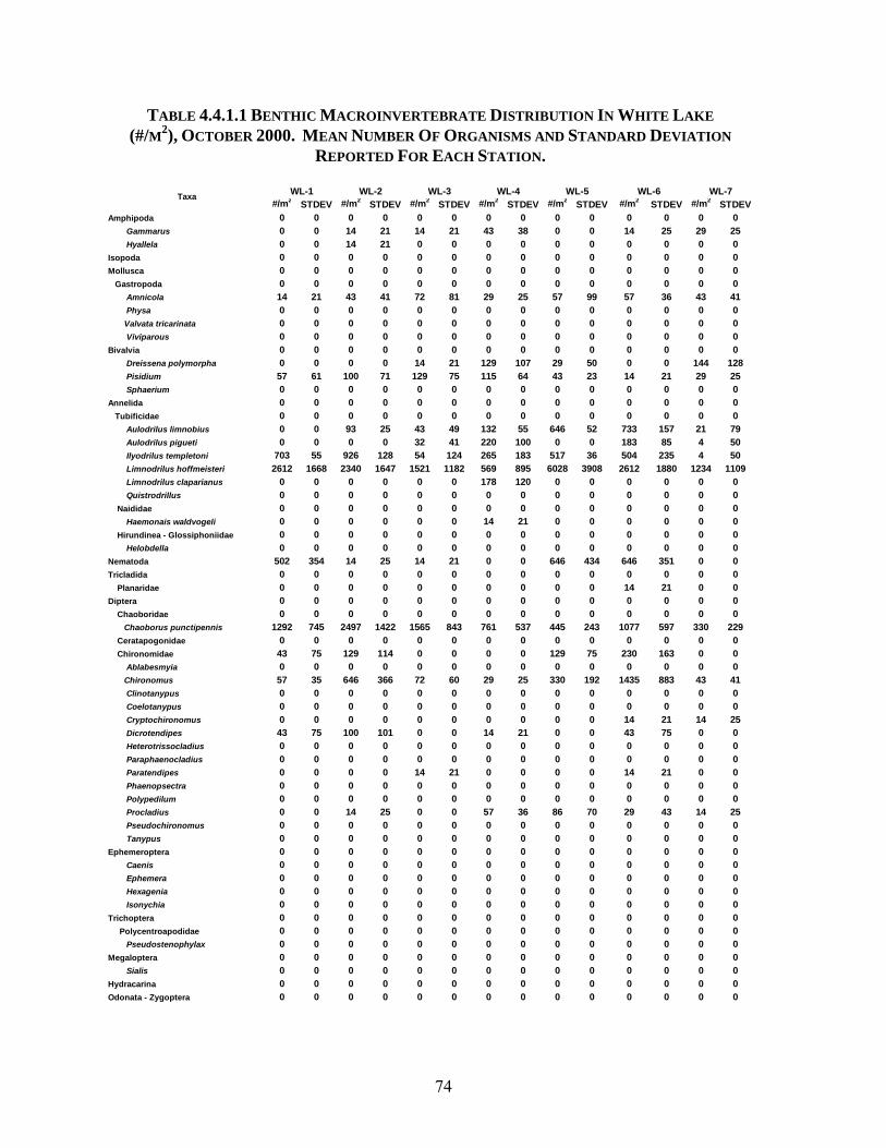
74

#/m2 STDEV #/m2 STDEV #/m2 STDEV #/m2 STDEV #/m2 STDEV #/m2 STDEV #/m2 STDEVAmphipoda 0 0 0 0 0 0 0 0 0 0 0 0 0 0 Gammarus 0 0 14 21 14 21 43 38 0 0 14 25 29 25 Hyallela 0 0 14 21 0 0 0 0 0 0 0 0 0 0Isopoda 0 0 0 0 0 0 0 0 0 0 0 0 0 0Mollusca 0 0 0 0 0 0 0 0 0 0 0 0 0 0 Gastropoda 0 0 0 0 0 0 0 0 0 0 0 0 0 0 Amnicola 14 21 43 41 72 81 29 25 57 99 57 36 43 41 Physa 0 0 0 0 0 0 0 0 0 0 0 0 0 0 Valvata tricarinata 0 0 0 0 0 0 0 0 0 0 0 0 0 0 Viviparous 0 0 0 0 0 0 0 0 0 0 0 0 0 0Bivalvia 0 0 0 0 0 0 0 0 0 0 0 0 0 0 Dreissena polymorpha 0 0 0 0 14 21 129 107 29 50 0 0 144 128 Pisidium 57 61 100 71 129 75 115 64 43 23 14 21 29 25 Sphaerium 0 0 0 0 0 0 0 0 0 0 0 0 0 0Annelida 0 0 0 0 0 0 0 0 0 0 0 0 0 0 Tubificidae 0 0 0 0 0 0 0 0 0 0 0 0 0 0 Aulodrilus limnobius 0 0 93 25 43 49 132 55 646 52 733 157 21 79 Aulodrilus pigueti 0 0 0 0 32 41 220 100 0 0 183 85 4 50 Ilyodrilus templetoni 703 55 926 128 54 124 265 183 517 36 504 235 4 50 Limnodrilus hoffmeisteri 2612 1668 2340 1647 1521 1182 569 895 6028 3908 2612 1880 1234 1109 Limnodrilus claparianus 0 0 0 0 0 0 178 120 0 0 0 0 0 0 Quistrodrillus 0 0 0 0 0 0 0 0 0 0 0 0 0 0 Naididae 0 0 0 0 0 0 0 0 0 0 0 0 0 0 Haemonais waldvogeli 0 0 0 0 0 0 14 21 0 0 0 0 0 0 Hirundinea - Glossiphoniidae 0 0 0 0 0 0 0 0 0 0 0 0 0 0 Helobdella 0 0 0 0 0 0 0 0 0 0 0 0 0 0Nematoda 502 354 14 25 14 21 0 0 646 434 646 351 0 0Tricladida 0 0 0 0 0 0 0 0 0 0 0 0 0 0 Planaridae 0 0 0 0 0 0 0 0 0 0 14 21 0 0Diptera 0 0 0 0 0 0 0 0 0 0 0 0 0 0 Chaoboridae 0 0 0 0 0 0 0 0 0 0 0 0 0 0 Chaoborus punctipennis 1292 745 2497 1422 1565 843 761 537 445 243 1077 597 330 229 Ceratapogonidae 0 0 0 0 0 0 0 0 0 0 0 0 0 0 Chironomidae 43 75 129 114 0 0 0 0 129 75 230 163 0 0 Ablabesmyia 0 0 0 0 0 0 0 0 0 0 0 0 0 0 Chironomus 57 35 646 366 72 60 29 25 330 192 1435 883 43 41 Clinotanypus 0 0 0 0 0 0 0 0 0 0 0 0 0 0 Coelotanypus 0 0 0 0 0 0 0 0 0 0 0 0 0 0 Cryptochironomus 0 0 0 0 0 0 0 0 0 0 14 21 14 25 Dicrotendipes 43 75 100 101 0 0 14 21 0 0 43 75 0 0 Heterotrissocladius 0 0 0 0 0 0 0 0 0 0 0 0 0 0 Paraphaenocladius 0 0 0 0 0 0 0 0 0 0 0 0 0 0 Paratendipes 0 0 0 0 14 21 0 0 0 0 14 21 0 0 Phaenopsectra 0 0 0 0 0 0 0 0 0 0 0 0 0 0 Polypedilum 0 0 0 0 0 0 0 0 0 0 0 0 0 0 Procladius 0 0 14 25 0 0 57 36 86 70 29 43 14 25 Pseudochironomus 0 0 0 0 0 0 0 0 0 0 0 0 0 0 Tanypus 0 0 0 0 0 0 0 0 0 0 0 0 0 0Ephemeroptera 0 0 0 0 0 0 0 0 0 0 0 0 0 0 Caenis 0 0 0 0 0 0 0 0 0 0 0 0 0 0 Ephemera 0 0 0 0 0 0 0 0 0 0 0 0 0 0 Hexagenia 0 0 0 0 0 0 0 0 0 0 0 0 0 0 Isonychia 0 0 0 0 0 0 0 0 0 0 0 0 0 0Trichoptera 0 0 0 0 0 0 0 0 0 0 0 0 0 0 Polycentroapodidae 0 0 0 0 0 0 0 0 0 0 0 0 0 0 Pseudostenophylax 0 0 0 0 0 0 0 0 0 0 0 0 0 0Megaloptera 0 0 0 0 0 0 0 0 0 0 0 0 0 0 Sialis 0 0 0 0 0 0 0 0 0 0 0 0 0 0Hydracarina 0 0 0 0 0 0 0 0 0 0 0 0 0 0Odonata - Zygoptera 0 0 0 0 0 0 0 0 0 0 0 0 0 0

WL-1 WL-2 WL-3 WL-4 WL-5 WL-6 WL-7Taxa

TABLE 4.4.1.1 BENTHIC MACROINVERTEBRATE DISTRIBUTION IN WHITE LAKE (#/M2), OCTOBER 2000. MEAN NUMBER OF ORGANISMS AND STANDARD DEVIATION

REPORTED FOR EACH STATION.

75

#/m2 STDEV #/m2 STDEV #/m2 STDEV #/m2 STDEV #/m2 STDEV #/m2 STDEV #/m2 STDEV #/m2 STDEVAmphipoda 0 0 0 0 0 0 0 0 0 0 0 0 0 0 0 0 Gammarus 0 0 29 25 29 43 14 25 0 0 43 23 57 85 14 21 Hyallela 0 0 0 0 0 0 0 0 0 0 0 0 0 0 0 0Isopoda 0 0 0 0 0 0 0 0 0 0 0 0 14 21 0 0Mollusca 0 0 0 0 0 0 0 0 0 0 0 0 0 0 0 0 Gastropoda 0 0 0 0 0 0 0 0 0 0 0 0 0 0 0 0 Amnicola 115 120 43 41 29 43 14 21 57 61 129 69 43 38 172 110 Physa 0 0 0 0 0 0 0 0 14 25 0 0 0 0 0 0 Valvata tricarinata 0 0 0 0 0 0 0 0 0 0 0 0 0 0 0 0 Viviparous 0 0 0 0 0 0 0 0 0 0 0 0 0 0 0 0Bivalvia 0 0 0 0 0 0 0 0 0 0 0 0 0 0 0 0 Dreissena polymorpha 0 0 86 101 43 41 0 0 43 64 29 43 72 74 57 35 Pisidium 57 85 100 101 86 70 0 0 0 0 0 0 0 0 0 0 Sphaerium 0 0 0 0 0 0 0 0 0 0 0 0 0 0 0 0Annelida 0 0 0 0 0 0 0 0 0 0 0 0 0 0 0 0 Tubificidae 0 0 0 0 0 0 0 0 0 0 0 0 0 0 0 0 Aulodrilus limnobius 660 55 785 87 0 0 298 60 215 25 1837 742 0 0 514 156 Aulodrilus pigueti 110 21 0 0 112 49 119 25 0 0 0 0 0 0 73 21 Ilyodrilus templetoni 220 43 349 35 419 119 1491 536 431 150 0 0 675 321 73 25 Limnodrilus hoffmeisteri 3746 2541 1270 1363 1409 748 6967 1432 1421 675 2110 1247 2770 932 1852 760 Limnodrilus claparianus 0 0 423 88 328 148 0 0 0 0 0 0 0 0 0 0 Quistrodrillus 0 0 0 0 0 0 683 81 0 0 0 0 0 0 0 0 Naididae 0 0 0 0 0 0 0 0 0 0 0 0 0 0 0 0 Haemonais waldvogeli 0 0 0 0 14 21 14 21 0 0 0 0 0 0 0 0 Hirundinea - Glossiphoniidae 0 0 0 0 0 0 0 0 0 0 0 0 0 0 0 0 Helobdella 0 0 0 0 0 0 0 0 0 0 0 0 0 0 0 0Nematoda 1177 705 3804 2569 172 163 1277 697 7780 4390 574 440 5698 3620 617 592Tricladida 0 0 0 0 0 0 0 0 0 0 0 0 0 0 0 0 Planaridae 0 0 0 0 0 0 0 0 0 0 0 0 14 21 0 0Diptera 0 0 0 0 0 0 0 0 0 0 0 0 0 0 0 0 Chaoboridae 0 0 0 0 0 0 0 0 0 0 0 0 0 0 0 0 Chaoborus punctipennis 201 129 158 126 1077 598 416 242 129 76 201 139 0 0 0 0 Ceratapogonidae 14 21 0 0 0 0 0 0 14 21 0 0 14 21 43 41 Chironomidae 72 64 0 0 0 0 301 172 43 41 72 52 72 60 115 77 Ablabesmyia 0 0 0 0 0 0 0 0 0 0 0 0 0 0 0 0 Chironomus 215 130 230 153 115 120 904 490 172 143 144 104 273 162 359 381 Clinotanypus 0 0 0 0 0 0 0 0 0 0 0 0 0 0 0 0 Coelotanypus 0 0 0 0 0 0 0 0 0 0 0 0 0 0 43 38 Cryptochironomus 14 21 0 0 0 0 0 0 0 0 0 0 57 49 72 52 Dicrotendipes 0 0 0 0 0 0 29 25 0 0 0 0 0 0 0 0 Heterotrissocladius 14 25 0 0 0 0 0 0 0 0 0 0 0 0 0 0 Paraphaenocladius 0 0 0 0 0 0 0 0 0 0 0 0 14 25 0 0 Paratendipes 0 0 14 21 0 0 0 0 0 0 0 0 0 0 0 0 Phaenopsectra 0 0 0 0 0 0 0 0 0 0 0 0 0 0 0 0 Polypedilum 14 21 0 0 0 0 0 0 0 0 0 0 0 0 0 0 Procladius 115 107 144 89 29 25 0 0 115 105 115 89 158 97 172 130 Pseudochironomus 0 0 0 0 14 21 0 0 0 0 0 0 0 0 0 0 Tanypus 0 0 0 0 0 0 0 0 0 0 0 0 0 0 0 0Ephemeroptera 0 0 0 0 0 0 0 0 0 0 0 0 0 0 0 0 Caenis 0 0 0 0 0 0 0 0 0 0 0 0 0 0 0 0 Ephemera 0 0 0 0 0 0 0 0 0 0 0 0 0 0 0 0 Hexagenia 0 0 0 0 0 0 0 0 0 0 0 0 0 0 0 0 Isonychia 0 0 0 0 0 0 0 0 0 0 0 0 0 0 0 0Trichoptera 0 0 0 0 0 0 0 0 0 0 0 0 0 0 0 0 Polycentroapodidae 0 0 0 0 0 0 0 0 0 0 0 0 0 0 0 0 Pseudostenophylax 0 0 14 21 0 0 0 0 0 0 0 0 0 0 0 0Megaloptera 0 0 0 0 0 0 0 0 0 0 0 0 0 0 0 0 Sialis 0 0 0 0 0 0 0 0 0 0 0 0 0 0 0 0Hydracarina 0 0 0 0 0 0 0 0 0 0 0 0 0 0 0 0Odonata - Zygoptera 0 0 0 0 0 0 0 0 0 0 0 0 0 0 0 0

TaxaWL-11 WL-12 WL-13 WL-14 WL-15WL-8 WL-9 WL-10

TABLE 4.4.1.1 (CONTINUED) BENTHIC MACROINVERTEBRATE DISTRIBUTION IN WHITE LAKE (#/M2), OCTOBER 2000. MEAN NUMBER OF ORGANISMS AND STANDARD DEVIATION


76

#/m2 STDEV #/m2 STDEV #/m2 STDEV #/m2 STDEV #/m2 STDEV #/m2 STDEV #/m2 STDEVAmphipoda 0 0 0 0 0 0 0 0 0 0 0 0 0 0 Gammarus 29 25 57 36 43 23 43 41 2483 2312 100 88 244 132 Hyallela 0 0 0 0 0 0 0 0 230 290 0 0 0 0Isopoda 0 0 0 0 0 0 0 0 100 101 0 0 0 0Mollusca 0 0 0 0 0 0 0 0 0 0 0 0 0 0 Gastropoda 0 0 0 0 0 0 0 0 0 0 0 0 0 0 Amnicola 43 38 72 42 14 25 57 49 144 142 86 74 43 41 Physa 0 0 29 43 0 0 0 0 14 25 0 0 0 0 Valvata tricarinata 0 0 0 0 0 0 0 0 14 21 0 0 0 0 Viviparous 0 0 0 0 14 25 0 0 0 0 0 0 0 0Bivalvia 0 0 0 0 0 0 0 0 0 0 0 0 0 0 Dreissena polymorpha 244 226 72 81 86 82 0 0 201 247 43 38 14 25 Pisidium 0 0 43 41 0 0 0 0 0 0 144 99 100 88 Sphaerium 0 0 0 0 0 0 0 0 0 0 0 0 14 25Annelida 0 0 0 0 0 0 0 0 0 0 0 0 0 0 Tubificidae 0 0 0 0 0 0 0 0 0 0 0 0 0 0 Aulodrilus limnobius 0 0 0 0 0 0 0 0 0 0 3986 1154 772 292 Aulodrilus pigueti 0 0 2411 83 115 0 165 0 0 0 996 281 114 45 Ilyodrilus templetoni 890 25 0 0 115 0 165 0 215 149 5381 1223 772 406 Limnodrilus hoffmeisteri 2225 110 1716 174 1306 0 1837 56 1521 136 18444 9279 5177 2644 Limnodrilus claparianus 0 0 0 0 0 0 0 0 0 0 0 0 0 0 Quistrodrillus 0 0 322 64 0 0 0 0 0 0 0 0 0 0 Naididae 0 0 0 0 0 0 0 0 0 0 0 0 0 0 Haemonais waldvogeli 0 0 0 0 0 0 0 0 0 0 0 0 0 0 Hirundinea - Glossiphoniidae 0 0 0 0 0 0 0 0 0 0 0 0 0 0 Helobdella 0 0 0 0 0 0 0 0 14 25 14 21 0 0Nematoda 14 21 0 0 14 21 14 21 0 0 2268 1337 330 309Tricladida 0 0 0 0 0 0 0 0 0 0 0 0 0 0 Planaridae 29 43 0 0 0 0 0 0 431 590 0 0 0 0Diptera 0 0 0 0 0 0 0 0 0 0 0 0 0 0 Chaoboridae 0 0 0 0 0 0 0 0 0 0 0 0 0 0 Chaoborus punctipennis 0 0 0 0 0 0 0 0 0 0 976 594 488 483 Ceratapogonidae 14 25 0 0 14 21 0 0 115 98 0 0 0 0 Chironomidae 86 81 0 0 187 137 172 230 560 422 258 281 187 161 Ablabesmyia 0 0 0 0 0 0 29 23 0 0 0 0 0 0 Chironomus 115 64 29 23 43 64 43 38 86 76 976 691 646 362 Clinotanypus 0 0 0 0 0 0 57 49 0 0 0 0 0 0 Coelotanypus 0 0 0 0 0 0 0 0 0 0 0 0 0 0 Cryptochironomus 0 0 144 123 0 0 129 76 57 56 14 25 14 21 Dicrotendipes 0 0 0 0 0 0 0 0 0 0 0 0 0 0 Heterotrissocladius 0 0 0 0 0 0 0 0 0 0 0 0 0 0 Paraphaenocladius 0 0 0 0 0 0 0 0 0 0 0 0 0 0 Paratendipes 0 0 0 0 0 0 0 0 0 0 0 0 14 21 Phaenopsectra 0 0 0 0 0 0 0 0 14 21 14 21 0 0 Polypedilum 0 0 0 0 0 0 0 0 0 0 0 0 0 0 Procladius 57 60 43 41 57 85 57 60 301 164 316 192 244 136 Pseudochironomus 0 0 0 0 0 0 0 0 0 0 0 0 0 0 Tanypus 0 0 29 43 0 0 0 0 0 0 0 0 0 0Ephemeroptera 0 0 0 0 0 0 0 0 0 0 0 0 0 0 Caenis 0 0 0 0 0 0 0 0 14 21 0 0 0 0 Ephemera 0 0 0 0 0 0 0 0 14 25 0 0 0 0 Hexagenia 0 0 0 0 29 23 29 43 129 129 0 0 0 0 Isonychia 0 0 0 0 0 0 0 0 14 25 0 0 0 0Trichoptera 0 0 0 0 0 0 0 0 0 0 0 0 0 0 Polycentroapodidae 0 0 0 0 0 0 0 0 14 25 0 0 0 0 Pseudostenophylax 0 0 0 0 0 0 0 0 0 0 0 0 0 0Megaloptera 0 0 0 0 0 0 0 0 0 0 0 0 0 0 Sialis 14 25 0 0 0 0 0 0 0 0 0 0 0 0Hydracarina 0 0 0 0 0 0 0 0 14 25 0 0 0 0Odonata - Zygoptera 0 0 0 0 0 0 0 0 57 99 0 0 0 0

Taxa WL-16 WL-17 WL-18 WL-19 WL-20 WL-21 WL-21 Dup

TABLE 4.4.1.1 (CONTINUED) BENTHIC MACROINVERTEBRATE DISTRIBUTION IN WHITE LAKE (#/M2), OCTOBER 2000. MEAN NUMBER OF ORGANISMS AND STANDARD DEVIATION


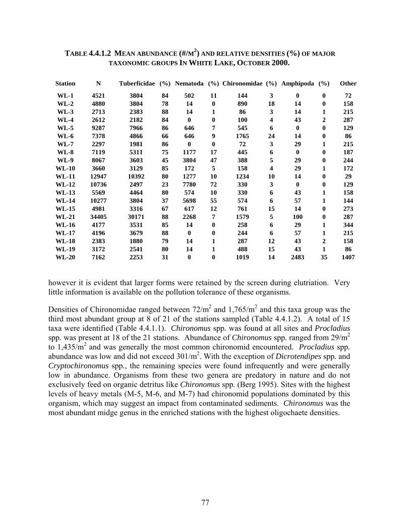
77

TABLE 4.4.1.2 MEAN ABUNDANCE (#/M2) AND RELATIVE DENSITIES (%) OF MAJOR TAXONOMIC GROUPS IN WHITE LAKE, OCTOBER 2000.

WL-1 4521 3804 84 502 11 144 3 0 0 72WL-2 4880 3804 78 14 0 890 18 14 0 158WL-3 2713 2383 88 14 1 86 3 14 1 215WL-4 2612 2182 84 0 0 100 4 43 2 287WL-5 9287 7966 86 646 7 545 6 0 0 129WL-6 7378 4866 66 646 9 1765 24 14 0 86WL-7 2297 1981 86 0 0 72 3 29 1 215WL-8 7119 5311 75 1177 17 445 6 0 0 187WL-9 8067 3603 45 3804 47 388 5 29 0 244

WL-10 3660 3129 85 172 5 158 4 29 1 172WL-11 12947 10392 80 1277 10 1234 10 14 0 29WL-12 10736 2497 23 7780 72 330 3 0 0 129WL-13 5569 4464 80 574 10 330 6 43 1 158WL-14 10277 3804 37 5698 55 574 6 57 1 144WL-15 4981 3316 67 617 12 761 15 14 0 273WL-21 34405 30171 88 2268 7 1579 5 100 0 287WL-16 4177 3531 85 14 0 258 6 29 1 344WL-17 4196 3679 88 0 0 244 6 57 1 215WL-18 2383 1880 79 14 1 287 12 43 2 158WL-19 3172 2541 80 14 1 488 15 43 1 86WL-20 7162 2253 31 0 0 1019 14 2483 35 1407

Chironomidae Amphipoda Other(%) (%) (%)(%)Station N Tuberficidae Nematoda

however it is evident that larger forms were retained by the screen during elutriation. Very little information is available on the pollution tolerance of these organisms.

Densities of Chironomidae ranged between 72/m2 and 1,765/m2 and this taxa group was the third most abundant group at 8 of 21 of the stations sampled (Table 4.4.1.2). A total of 15 taxa were identified (Table 4.4.1.1). Chironomus spp. was found at all sites and Procladius spp. was present at 18 of the 21 stations. Abundance of Chironomus spp. ranged from 29/m2 to 1,435/m2 and was generally the most common chironomid encountered. Procladius spp. abundance was low and did not exceed 301/m2. With the exception of Dicrotendipes spp. and Cryptochironomus spp., the remaining species were found infrequently and were generally low in abundance. Organisms from these two genera are predatory in nature and do not exclusively feed on organic detritus like Chironomus spp. (Berg 1995). Sites with the highest levels of heavy metals (M-5, M-6, and M-7) had chironomid populations dominated by this organism, which may suggest an impact from contaminated sediments. Chironomus was the most abundant midge genus in the enriched stations with the highest oligochaete densities.

78

FIGURE 4.4.1.1 GENERAL DISTRIBUTION OF BENTHIC MACROINVERTEBRATES IN WHITE LAKE, OCTOBER 2000.

0

5000

10000

15000

20000

25000

30000

35000#

Org

anis

ms/

m2

WL-1WL-2WL-3WL-4WL-5WL-6WL-7WL-8WL-9WL-10WL-11WL-12WL-13WL-14WL-15WL-21WL-16WL-17WL-18WL-19WL-20

Station

NTubificidaeNematodaChironomidaeAmphipodaOther

Western White Lake

EastBay

Controls

Occidental/HookerChemical

79

Station WL-20 was very different than the other stations with respect to macroinvertebrate composition as amphipods were the dominant genera (35%) along with four mayfly taxa plus odonata and trichoptera species. The latter three groups were not present in the other shallow stations. WL-20 was located in closest proximity to the mouth of the White River and away from the marinas. The absence of both physical and chemical anthropogenic disturbance at this station influenced the quality of the macroinvertebrate population at this location. 4.4.2 Analysis of Macroinvertebrate Results Using Trophic Indices and Diversity Metrics The benthic macroinvertebrate data were analyzed by a variety of trophic status indices and diversity metrics. The following indices and metrics were utilized:

• Shannon Weaver Diversity (Krebs 1989) • Margalef's Richness (Krebs 1989) • Evenness (Krebs 1989) • Pielou's J (Krebs 1989) • Oligochaete Index (Howmiller and Scott 1977, Hilsenhoff 1987) • Chironomid Index (Hilsenhoff 1987) • Oligochaete + Chironomid Index (*) • Trophic Index (Hilsenhoff 1987)

* Modified from Howmiller and Scott (1977) Tolerance values used to calculate the Trophic Index and the individual indices for Chironomids and Oligochaetes were taken from Winnell and White (1985), Lauritsen et al. (1985), Hilsenhoff (1987), Schloesser et al. (1995), and Barbour et al. (1999). The results of the population metrics are summarized in Table 4.4.2.1. Summaries of Trophic Indices for the benthic populations are shown in Figure 4.4.2.1. Shallow stations WL-20 and WL-17 had the most favorable trophic index scores for overall community structure (Hilsenhoff) and chironomids. All of the other shallow stations and the deep stations exhibited high scores for the Hilsenhoff index, indicating enriched conditions. Chironomid index values for the shallow stations WL-18, WL-19, and WL-20 were all <7.5. Deep stations had higher chironomid index values that were again representative of organic enrichment. It is interesting to note that the stations WL-4 and WL-20 had similar Shannon-Weaver scores, indicating a more balanced community structure (∼2.1). Shannon-Weaver scores for the other stations ranged from 0.8-1.5, indicating a more limited diversity. The increased diversity at WL-4 appears to be related to the lower TOC and increased sand fraction.

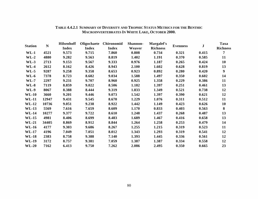
80

WL-1 4521 9.573 9.715 7.860 0.808 0.734 0.321 0.415 7WL-2 4880 9.282 9.563 8.819 1.402 1.191 0.370 0.585 11WL-3 2713 9.153 9.567 9.333 0.976 1.187 0.265 0.424 10WL-4 2612 8.162 8.426 8.943 2.100 1.602 0.628 0.819 13WL-5 9287 9.258 9.358 8.653 0.923 0.892 0.280 0.420 9WL-6 7378 8.723 8.682 9.034 1.588 1.497 0.350 0.602 14WL-7 2297 9.231 9.707 8.960 0.925 1.358 0.229 0.386 11WL-8 7119 8.859 9.022 8.506 1.182 1.397 0.251 0.461 13WL-9 8067 8.388 8.444 9.319 1.833 1.349 0.521 0.738 12

WL-10 3660 9.201 9.446 9.073 1.542 1.397 0.390 0.621 12WL-11 12947 9.431 9.545 8.670 1.229 1.076 0.311 0.512 11WL-12 10736 9.051 9.238 8.922 1.442 1.149 0.423 0.626 10WL-13 5569 7.616 7.659 8.609 1.170 0.833 0.403 0.563 8WL-14 10277 9.377 9.722 8.610 1.248 1.437 0.268 0.487 13WL-15 4981 8.406 8.699 8.483 1.689 1.467 0.416 0.658 13WL-21 34405 8.869 8.912 8.844 1.264 1.258 0.253 0.479 14WL-16 4177 9.303 9.686 8.267 1.255 1.215 0.319 0.523 11WL-17 4196 7.049 7.051 8.012 1.343 1.293 0.319 0.541 12WL-18 2383 8.758 9.388 7.140 1.393 1.445 0.336 0.561 12WL-19 3172 8.757 9.381 7.059 1.387 1.387 0.334 0.558 12WL-20 7162 6.413 9.750 7.262 2.086 2.495 0.350 0.665 23

N Margalef's Richness Evenness J Taxa

RichnessHilsenhoff

IndexOligochaete

IndexChironomid

IndexShannon- WeaverStation

TABLE 4.4.2.1 SUMMARY OF DIVERSITY AND TROPHIC STATUS METRICS FOR THE BENTHIC MACROINVERTEBRATES IN WHITE LAKE, OCTOBER 2000.

81

6.000

7.000

8.000

9.000

10.000In

dex

Valu

e

WL-1

WL-2

WL-3

WL-4

WL-5

WL-6

WL-7

WL-8

WL-9

WL-1

0W

L-11

WL-1

2W

L-13

WL-1

4W

L-15

WL-2

1W

L-16

WL-1

7W

L-18

WL-1

9W

L-20

Station

HilsenhoffOligochaeteChironomid

FIGURE 4.4.2.1 SUMMARY OF TROPHIC INDICES (POLLUTION TOLERANCE) FOR THE BENTHIC MACROINVERTEBRATES IN WHITE LAKE, OCTOBER 2000.

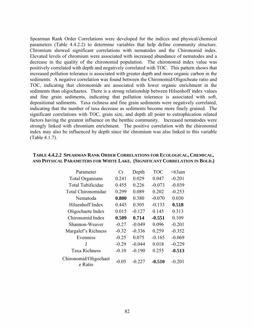
82

Spearman Rank Order Correlations were developed for the indices and physical/chemical parameters (Table 4.4.2.2) to determine variables that help define community structure. Chromium showed significant correlations with nematodes and the Chironomid index. Elevated levels of chromium were associated with increased abundance of nematodes and a decrease in the quality of the chironomid population. The chironomid index value was positively correlated with depth and negatively correlated with TOC. This pattern shows that increased pollution tolerance is associated with greater depth and more organic carbon in the sediments. A negative correlation was found between the Chironomid/Oligocheate ratio and TOC, indicating that chironomids are associated with lower organic enrichment in the sediments than oligochaetes. There is a strong relationship between Hilsenhoff index values and fine grain sediments, indicating that pollution tolerance is associated with soft, depositional sediments. Taxa richness and fine grain sediments were negatively correlated, indicating that the number of taxa decrease as sediments become more finely grained. The significant correlations with TOC, grain size, and depth all point to eutrophication related factors having the greatest influence on the benthic community. Increased nematodes were strongly linked with chromium enrichment. The positive correlation with the chironomid index may also be influenced by depth since the chromium was also linked to this variable (Table 4.1.7).

TABLE 4.4.2.2 SPEARMAN RANK ORDER CORRELATIONS FOR ECOLOGICAL, CHEMICAL, AND PHYSICAL PARAMETERS FOR WHITE LAKE. (SIGNIFICANT CORRELATION IN BOLD.)

Parameter Cr Depth TOC <63um Total Organisms 0.241 0.029 0.047 -0.201 Total Tubificidae 0.455 0.226 -0.073 -0.039

Total Chironomidae 0.299 0.089 0.202 -0.253 Nematoda 0.800 0.380 -0.070 0.030

Hilsenhoff Index 0.445 0.305 -0.133 0.518 Oligochaete Index 0.015 -0.127 0.145 0.313 Chironomid Index 0.509 0.714 -0.551 0.109 Shannon-Weaver -0.27 -0.049 0.096 -0.201

Margalef’s Richness -0.32 -0.336 0.259 -0.352 Evenness -0.25 0.075 -0.165 -0.069

J -0.29 -0.044 0.018 -0.229 Taxa Richness -0.10 -0.190 0.255 -0.513

Chironomid/Oligochaete Ratio -0.05 -0.227 -0.510 -0.201

83

4.4.3 Analysis of Macroinvertebrate Results Using Community Structure The benthic macroinvertebrate taxa were further analyzed for associations with chromium by canonical correspondence analysis (Figure 4.4.3.1). A description of the taxa abbreviations are provided in Table 4.4.3.1. Dimensions 1 and 2 accounted for 55% of the variability in the data set (31% and 24%, respectively). Four data clusters are evident. The clean site, Station WL-20, was characterized by amphipods, mayflies, and isopods. This assemblage was not

FIGURE 4.4.3.1 CANONICAL CORRESPONDENCE ANALYSIS OF BENTHIC MACRO-

INVERTEBRATE TAXA FOR WHITE LAKE, OCTOBER 2000. (LABELS INDICATE SPECIFIC TAXA AND STATIONS. SHALLOW STATIONS LISTED IN RED AND DEEP STATIONS IN GREEN.)

Dimension 1 (31%)

-2 0 2 4

Dim

ensi

on 2

(24%

)

-2

0

2

4

gam

hyaiso

amn

phy

tri

viv

drei

pis

limn

pig

temphof

clap

qui

wald

hel

nem pla

cer

chir

abla

chiron

clin

coel

cryp

dic

heter

para

par

pha

poly

pro

pseu

tany

caeephem

hex

isopolycpseudos

sia

zyg

WL-16

WL-17 WL-18 WL-19

WL-20

WL-1 WL-2 WL-3 WL-4

WL-5 WL-6 WL-7

WL-8

WL-9

WL-10 WL-11

WL-12

WL-13

WL-14

WL-15

WL-21

84

TABLE 4.4.3.1 SUMMARY STATISTICS FOR THE ANALYSIS OF INDIVIDUAL BENTHIC MACROINVERTEBRATE SAMPLES FROM WHITE LAKE, OCTOBER 2000.

Taxa Abbreviation Taxa Abbreviation

Gammarus gam Chironomus chiron Hyallela hya Clinotanypus clin Isopoda iso Coelotanypus coel Amnicola amn Cryptochironomus cryp Physa phy Dicrotendipes dic Valvata tricarinata tri Heterotrissocladius heter Viviparous viv Paraphaenocladius para Dreissena polymorpha drei Paratendipes par Pisidium pis Phaenopsectra pha Aulodrilus limnobius limn Polypedilum poly Aulodrilus pigueti pig Procladius pro Ilyodrilus templetoni temp Pseudochironomus pseu Limnodrilus hoffmeisteri hof Tanypus tany Limnodrilus claparianus clap Caenis cae Quistrodrillus qui Ephemera ephem Haemonais waldvogeli wald Hexagenia hex Helobdella hel Isonychia iso Nematoda nem Polycentroapodidae polyc Planaridae pla Pseudostenophylax pseudos Ceratapogonidae cer Sialis sia Chironomidae Chir Zygoptera zyg Ablabesmyia Abla

found in the other sites. WL-16, the site in the east bay with high solid phase toxicity, was grouped around the two tubificid taxa Quistrodrillus spp. and Aulodrilus pigueti, the gastropod Physa spp., and the midges Tanytarsus spp., Ablabesmyia spp., Cryptochironomus spp., and Clinotanypus spp. The tubificid taxa represent additional pollution tolerant organisms at this location. Tanytarsus spp. is classified as a “sprawler” because it resides on the surface and does not burrow in the sediment. Ablabesmyia spp., Cryptochironomus spp., and Clinotanypus spp. are predators and do not ingest sediment and/or detritus. The additional pollution tolerant tubificids and the shift to predatory and surface dwelling midges are indicative of adverse conditions in the sediment. Stations WL-9, WL-12, and WL-14 cluster together around Nematoda, Pseudostenophylax spp., and Paraphaenocladius spp. The latter two organisms were found in very low numbers

85

(1 organism in the triplicate PONARS) and cannot be considered as important members of the benthic assemblage. Chromium concentrations and the order Nematoda showed a strong correlation (Table 4.4.2.2). Stations WL-9, WL-12, and WL-14 had the highest concentrations of chromium (420 mg/kg, 510 mg/kg, and 480 mg/kg, respectively). Nematodes have been reported to be tolerant of heavy metal pollution (Gyedu-Ababio et al. 1999, Fiscus and Neher 2002). Some are able to produce phytochelatins that are able to detoxify heavy metals (Cobbett 2000, Vatamaniuk et al. 2001). In addition to changes in the nematode population, this group of locations also had the lowest percentage of tubificids (Table 4.4.1.2). Samples at stations WL-9, WL-12, and WL-14 contained tubificid percentages of 45%, 23%, and 37%, respectively. The tubificid percentage range for the other deep stations was 66-85%. Based on these results, the benthic macroinvertebrate populations at these stations appear to be influenced by chromium. The remainder of stations and organisms form a cluster in the middle of the CCA plot. Benthic macroinvertebrate assemblages of the remaining shallow stations (WL-17, WL-18, and WL-19) with low chromium levels are grouped with deep locations that contain high concentrations of the metal. These sites are characterized by similar TOC, % solid, and grain size values. This suggests that organic enrichment from eutrophication exerts the predominant influence on the benthic community for this cluster. 4.4.4. Benthic Macroinvertebrate Data Summary The benthic macroinvertebrate community of White Lake is characterized by organisms that are tolerant of organic (nutrient) enrichment. The presence of organic deposition from the White River, the eutrophic conditions in the lake, and the historical anthropogenic enrichment from the lumbering operations, the Tannery, and the wastewater treatment plant all act to increase the densities of pollution tolerant organisms. To this extent, detritivores such as tubificids and chironomids from the genus Chironomus should dominate the benthic populations (Winnell and White 1985). While these conditions would indicate habitat degradation in a more pristine system, organic enrichment forms the basis for structuring the benthic community in White Lake. The only sites that did not fit this characterization were the locations with high chromium levels (WL-9, WL-12, and WL-14) and the east bay site, WL-16. The most notable difference with respect to the first group of stations was a change in benthic taxa from tubificids to nematodes. WL-16 was characterized by a change in chironomid species from detritivores to predators. A shift to more opportunistic organisms has previously been attributed to contaminant impact (Dauer 1991). With respect to the influence of chromium on the benthic ecology in White Lake, a significant relationship exists between the metal and the macroinvertebrate community (Figure 4.4.4.1). When dimension 1 of the CCA (invertebrate taxa) is plotted against chromium, a strong relationship is noted (r = –0.588, p < 0.017). An increase in chromium concentration shifts the population from an assemblage dominated by tubificids to one dominated by nematodes. Changes in the benthic community in response to chromium have been previously reported (Leslie et al. 1999). The significance of this shift is unknown and would require further taxonomic resolution to identify and classify the nematode species with

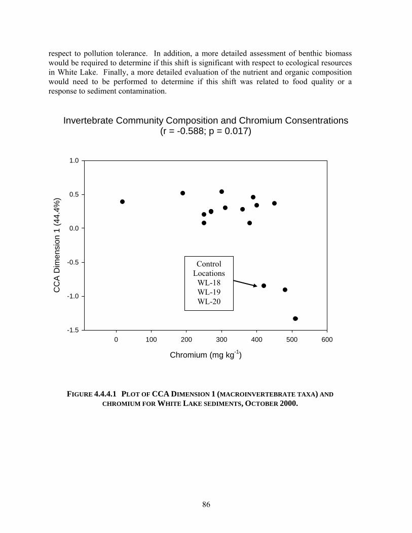
86

respect to pollution tolerance. In addition, a more detailed assessment of benthic biomass would be required to determine if this shift is significant with respect to ecological resources in White Lake. Finally, a more detailed evaluation of the nutrient and organic composition would need to be performed to determine if this shift was related to food quality or a response to sediment contamination.

Invertebrate Community Composition and Chromium Consentrations

(r = -0.588; p = 0.017)

Chromium (mg kg-1)

0 100 200 300 400 500 600

CC

A D

imen

sion

1 (4

4.4%

)

-1.5

-1.0

-0.5

0.0

0.5

1.0

FIGURE 4.4.4.1 PLOT OF CCA DIMENSION 1 (MACROINVERTEBRATE TAXA) AND CHROMIUM FOR WHITE LAKE SEDIMENTS, OCTOBER 2000.

Control Locations

WL-18 WL-19 WL-20

87

StationChromium in

Zebra Mussels (mg/kg)

Chromium in Plant Tissue

(mg/kg)22A 52 1422B 12 1122C 14 1623A 16 3623B 12 4823C 23 2324A 45 5424B 16 3624C 23 2020A 0.84 6.920B * 3.5* Insufficient organisms present for

replicates

4.5 Chromium Uptake by Aquatic Organisms

The accumulation of chromium in several aquatic organisms was examined to determine the biological fate of the metal in White Lake. The contaminated sediments in Tannery Bay contained the highest levels of chromium (1,000-4,000 mg/kg) and supported dense macrophyte and zebra mussel populations (Rediske et al. 1998). For this project, triplicate collections of macrophytes (Ceratophyllum spp.) and zebra mussels (Dreissena polymorpha) were made at three sites in Tannery Bay and at WL-20. The results are shown in Table 4.5.1 and displayed in Figure 4.5.1. Only macrophyte shoots and the attached zebra mussels were analyzed to minimize the inclusion contact with the highly contaminated sediment. The Ceratophyllum spp. tissue found in Tannery Bay contained significantly higher chromium levels than the control location (13-35 mg/kg vs. 5 mg/kg respectively). Zebra mussel tissue followed a similar trend, however the difference between the chromium concentrations in samples from Tannery Bay (16-33 mg/kg) and from the control area (2 mg/kg) were greater. Chromium accumulation in macrophytes (Vajpayee et al. 1995) and zebra mussels (Redders and Bij de Vaate 1993, LaValle et al. 1999) has been previously reported. The results from this investigation demonstrate the bioavailability of chromium in the sediments of Tannery Bay. In consideration of the dense macrophyte growth in the bay and the level of chromium accumulation, translocation and senescence would not contribute significant concentrations of the metal to the sediment. While the macrophytes would contribute organic matter and nutrients to the sediments, mixing and resuspension provide the mechanism for maintaining the high chromium levels in the surficial layers. The accumulation of chromium in zebra mussels also supports the mixing and resuspension hypothesis as these organisms are filter feeders and ingest suspended particulates.

TABLE 4.5.1 CHROMIUM CONCENTRATION IN MACROPHYTES AND ZEBRA MUSSELS IN TANNERY BAY. (STATION 20 IS THE CONTROL SITE.)

88

Station Chromium in Sediment (mg/kg)

Chromium in Chironomids (mg/kg) Station Chromium in

Sediment (mg/kg)Chromium in

Chironomids (mg/kg)

WL-1 270 59 WL-12 510 140

WL-2 300 44 WL-13 250 85

WL-3 190 41 WL-14 480 88

WL-4 18 10 WL-15 250 67

WL-5 400 84 WL-16 190 48

WL-6 360 75 WL-17 50 14

WL-7 390 92 WL-18 29 12

WL-8 380 91 WL-19 39 14

WL-9 420 99 WL-20 28 13

WL-10 270 62 WL-21 450 130

WL-11 310 69

05

10152025303540

Chr

omiu

m (m

g/kg

)

22 24 24 20

Station

Zebra MusselsPlant Tissue

FIGURE 4.5.1 CHROMIUM ACCUMULATION IN MACROPHYTES AND ZEBRA MUSSELS IN

TANNERY BAY. The accumulation of chromium was evaluated at all of the PONAR locations. Chromium concentrations in the sediment and in chironomid tissue from each station are presented in Table 4.5.2 and displayed graphically in Figure 4.5.2. The results show a significant

TABLE 4.5.2 CHROMIUM CONCENTRATION IN CHIRONOMIDS FROM TANNERY BAY.

FIGURE 4.5.2 CHROMIUM ACCUMULATION IN CHIRONOMIDS FROM TANNERY BAY.

89

R2 = 0.8833

0

20

40

60

80

100

120

140

160

0 100 200 300 400 500 600

Chromium in Sediment (mg/kg)

Chr

omiu

m in

Chi

rono

mid

s (m

g/kg

)

relationship between chromium uptake and the concentration in the sediment. The Spearman Correlation coefficient was 0.92 (p < 0.001), indicating a strong relationship between sediment and chironomid concentrations. Locations with sediment concentrations < 50 mg/kg had chromium concentrations in the chironomid populations of 10-14 mg/kg. In contrast, locations with chromium concentrations > 100 mg/kg had accumulated metal levels of 48-140 mg/kg. These data coupled with the increased chironomid index value (Table 4.4.2.2) suggest that chromium is associated with an adverse impact to this group of organisms. A more detailed evaluation of physiological response to chromium would be necessary to establish a direct link between accumulation and the increased pollution tolerance. The results of the tissue analyses showed that chromium in the sediment from White Lake was accumulated by macrophytes, chironomids, and zebra mussels. Based on the dense growth of macrophytes and the high numbers of zebra mussels in Tannery Bay, there was no obvious ecological effect apparent in these organisms. More research would be necessary to establish the linkage between chromium accumulation in chironomids and ecological impairment.

90

4.6 The Environmental Fate and Significance of Chromium and PCBs in White Lake

The results of this investigation coupled with previous studies (Rediske et al. 1998, Earth Tech 2001) provide an extensive sampling grid for chromium and PCBs in White Lake. The chromium sampling points are shown in Figure 4.6.1 for White Lake and in Figure 4.6.2 for the Tannery Bay area. Coordinates and chromium concentrations are listed in Table 4.6.1.

TABLE 4.6.1 WHITE LAKE CHROMIUM DATA. (PONAR SAMPLES FROM CURRENT INVESTIGATION AND REDISKE ET AL. 1998)

N W N WWL-1 43o 22.58' 86o 24.55' 270 WL-21 43o 23.15' 86o 22.57' 450WL-2 43o 22.45' 86o 24.15' 300 WL-22 43o 23.99' 86o 21.28' 520WL-3 43o 22.41' 86o 24.77' 190 WL-23 43o 24.02' 86o 21.26' 1200WL-4 43o 22.27' 86o 24.16' 18 WL-24 43o 24.02' 86o 21.30' 1300WL-5 43o 22.73' 86o 23.50' 400 I-1 43o 24.15' 86o 21.15' 212

WL-6 43o 22.95' 86o 22.86' 360 I-2 43o 24.11' 86o 21.27' 259

WL-7 43o 22.61' 86o 23.27' 390 I-3 43o 24.06' 86o 21.32' 934

WL-8 43o 23.01' 86o 22.53' 380 I-4 43o 24.05' 86o 21.31' 1890

WL-9 43o 23.27' 86o 22.43' 420 I-5M 43o 24.04' 86o 21.26' 4100

WL-10 43o 22.18' 86o 24.61' 270 I-6 43o 23.98' 86o 21.25' 2650

WL-11 43o 23.54' 86o 22.25' 310 I-7M 43o 23.97' 86o 21.22' 2560

WL-12 43o 23.62' 86o 21.97' 510 I-8 43o 23.97' 86o 21.36' 515

WL-13 43o 23.08' 86o 22.33' 250 E-1-P 43o 24.59' 86o 21.59' 23

WL-14 43o 23.69' 86o 21.63' 480 E-2-P 43o 21.10' 86o 21.38' 64

WL-15 43o 23.87' 86o 21.83' 250 E-3-P 43o 23.89' 86o 21.50' 43

WL-16 43o 24.16' 86o 21.15' 190 E-4-P 43o 23.93' 86o 21.69' 344

WL-17 43o 24.20' 86o 21.25' 50 E-5-P 43o 23.70' 86o 21.61' 492

WL-18 43o 24.39' 86o 21.26' 29 E-6-P 43o 23.70' 86o 21.95' 771

WL-19 43o 24.32' 86o 21.14' 39 E-7-P 43o 23.59' 86o 21.71' 541

WL-20 43o 24.51' 86o 21.22' 28 E-9-P 43o 23.13' 86o 21.59' 369

Station Latitude Longitude Chromium mg/kgStation Latitude Longitude Chromium

mg/kg

Chromium concentration contours plotted from the data using kriging are shown in Figure 4.6.3. Concentrations are plotted for the ≥ 4 m depth contours as shallower sediments in the lake are sandy and related to shoreline erosion. Organic depositional sediments are typically found at depths ≥ 4 m. The concentration map shows that the spatial extent of chromium contamination covers the area of the lake from Tannery Bay to the navigation channel. Advective transport and deposition are also evident from the reservoir of highly contaminated sediment in Tannery Bay. Moving westward from Tannery Bay, an area of low chromium concentration is present in the Narrows, where drowned rivermouth related currents would be highest. The maximum chromium concentration outside of Tannery Bay (771 mg/kg) occurs

91

FIGURE 4.6.1 CHROMIUM SAMPLING POINTS IN WHITE LAKE (CURRENT INVESTIGATION AND REDISKE ET AL. 1998). (RED LINE DENOTES THE 4 M DEPTH CONTOUR.)

N

92

FIGURE 4.6.2 CHROMIUM SAMPLING POINTS IN THE VICINITY OF TANNERY BAY . (CURRENT INVESTIGATION AND REDISKE ET AL. 1998. RED LINE DENOTES THE 4 M DEPTH CONTOUR.)

N

93

Long Point

466000 467000 468000 469000 470000 471000 472000

X (m)

313000

314000

315000

316000

317000

318000

Y (m

)

025501001502002503003253503754005006007008009001000125015001750200025003000350040004200

0 500 1000 1500 2000

Dowies Point

Narrows

FIGURE 4.6.3 CHROMIUM CONCENTRATION CONTOURS FOR WHITE LAKE SURFICIAL SEDIMENTS. (CONCENTRATIONS PLOTTED FOR DEPTHS > 4 M. TANNERY BAY AREA SHOWN IN GREATER DETAIL)

N

94

in the first depositional basin (16 m) at the midpoint between Dowies Point and the Narrows (Figures 4.1.8 and 4.6.3). The next areas of high chromium concentration occur in the depositional basins to the east (420 mg/kg) and west (400 mg/kg) of Dowies Point (6 m and 20 m, respectively). In the depositional basin west of Long Point (22 m), chromium levels decrease to 300 mg/kg and continue to decline in concentration to the channel (190 mg/kg). The plume of contaminated sediment emanating from Tannery Bay extends ≈ 8 km from the source. Depositional contours also follow the generalized circulation pattern for White Lake. Lung (1975) described a westerly flow of water from the drowned rivermouth and a wind induced countercurrent along the southern shore (Figure 4.6.4). The predominant westerly wind results in a current moving eastward until it reaches the Narrows where it is nullified by the drowned rivermouth flow. The shallow depths and sandy nature of the sediments on the southern shore of the lake are indicative of the erosional character of this current and its effect on the shoreline. The extensive shallow zone along the southern shore is the result of the erosional effects on the shoreline and the rapid depositional process resultant from the interaction of the countercurrents. The northern shoreline is protected from the prevailing

FIGURE 4.6.4 GENERALIZED CIRCULATION PATTERN FOR WHITE LAKE (LUNG 1975). wind by the high banks and shows little evidence of erosion. The morphometry of the northern shore and the two points result in the formation of two gyres that enhance sediment

N

95

and detrital deposition. Based on these flow characteristics, chromium deposition should be lower along the southern shore and higher to the north. The chromium concentration map fits the generalized flow pattern as the higher metal concentrations follow the northern shoreline of White Lake. The position of Tannery Bay in the eastern corner of the lake and morphometry associated with the Narrows would make this area a deposition and transport zone depending on the nature of the storm event. Small storm events and wind surges would cause sediment resuspension in the bay and result in a minor degree of transport out into the drowned rivermouth current. Larger storm events would result in considerable resuspension and transport as the increased wave action facilitates sediment advection out of the bay and into the main section of the lake. The 20 cm mixed layer previously reported in the Tannery Bay sediments (Rediske et al. 1998) and the influence of episodic events on chromium stratigraphy described in Section 4.2 are evidence of these phenomena. The environmental fate and transport of the PCB discharge in White Lake from the former Occidental/Hooker Chemical facility is very different from the chromium release from the tannery. The data from the extensive sampling of the Occidental/Hooker Chemical discharge zone (Earth Tech 2001) plus the results of current and previous investigations of White Lake are given in Table 4.6.2. A map of the sampling locations is provided in Figure 4.6.5. Maps of PCB concentration contours for the discharge zone and for White Lake are shown in Figures 4.6.6 and 4.6.7, respectively. The effluent pipe was located at a depth ≈ 10 m and the maximum PCB concentration occurred at ≈ 11 m (390 mg/kg). Sediment contamination is confined to a 100 m2 zone around the outfall. The discharge from this facility began in the mid 50s and the origin of the PCBs is not known. Occidental/Hooker Chemical manufactured chlorinated pesticide intermediates and the PCBs were either produced as byproducts or were released from the electrical systems on site. The discharge of chemical wastes was terminated in the mid 70s, however treated groundwater from an activated carbon system is currently released from the old outfall. Concentration contours follow the southwestern flow of the drowned rivermouth and the depth change from 10 m to 14 m. The affinity of PCBs for sediment coupled with the location of the outfall in the deep depositional basin resulted in conditions that limited the advective transport of the chemical outside the area around Dowies Point. This environment is in stark contrast to the shallow area of the tannery discharge and its proximity currents associated with the Narrows. The presence of PCBs in the surficial sediments is problematic because of the depositional nature of the discharge zone. If this location was a true depositional zone, the PCBs would have been covered by clean sediment over the last 20+ years. The groundwater treatment discharge (≈1.6 mgd) may cause turbulence in the local area and result in the resuspension and limited transport of PCBs. The complex flow pattern for this area (Figure 4.6.5) may also result in limited redistribution of sediments. The highly contaminated sediment in Tannery bay and near the former Occidental/Hooker Chemical outfall will be removed by dredging in 2003. Removing the sediments from Tannery Bay will eliminate the source that has contaminated the depositional sediments in

96

TABLE 4.6.2 WHITE LAKE PCB DATA. (PONAR SAMPLES FROM EARTH TECH 2001 AND THE CURRENT AND PREVIOUS INVESTIGATION)

Sample Aroclor 1248 (mg/kg) X Y Sample Aroclor 1248

(mg/kg) N W

SD-99-01 < 0.3 1456881.77 694618.72 WL-1 <0.05 43o 22.58' 86 o 24.55'SD-99-02 < 0.3 1456885.82 694617.08 WL-2 0.09 43o 22.45' 86 o 24.15'SD-99-03 6.3 1456882.99 694581.86 WL-3 <0.05 43o 22.41' 86 o 24.77'SD-99-05 0.55 1456903.31 694609.45 WL-4 <0.05 43o 22.27' 86 o 24.16'SD-99-06 < 0.3 1456813.09 694632.34 WL-5 <0.05 43o 22.73' 86 o 23.50'SD-99-07 < 0.3 1456928.34 694653.54 WL-6 0.07 43o 22.95' 86 o 22.86'SD-99-08 413 1456911.14 694532.07 WL-7 0.08 43o 22.61' 86 o 23.27'SD-99-09 390 1456915.93 694552.40 WL-8 <0.05 43o 23.01' 86 o 22.53'SD-99-10 110 1456934.64 694574.49 WL-9 <0.05 43o 23.27' 86 o 22.43'SD-99-11 0.58 1456959.40 694600.19 WL-10 <0.05 43o 22.18' 86 o 24.61'SD-99-12 < 0.3 1456978.93 694622.57 WL-11 <0.05 43o 23.54' 86 o 22.25'SD-99-13 0.47 1456931.41 694516.70 WL-12 <0.05 43o 23.62' 86 o 21.97'SD-99-14 9 145647.75 694562.27 WL-13 <0.05 43o 23.08' 86 o 22.33'SD-99-15 0.4 1456997.48 694604.88 WL-14 <0.05 43o 23.69' 86 o 21.63'SD-00-01 0.88 1456870.26 694582.65 WL-15 <0.05 43o 23.87' 86 o 21.83'SD-00-02 7.6 1456900.67 694552.86 WL-16 <0.05 43o 24.16' 86 o 21.15'SD-00-03 1.4 1456960.59 694507.16 WL-17 <0.05 43o 24.20' 86 o 21.25'SD-00-04 38 1456866.68 694540.53 WL-18 <0.05 43o 24.39' 86 o 21.26'SD-00-06 2.1 1456920.27 694492.04 WL-19 <0.05 43o 24.32' 86 o 21.14'SD-00-07 1.1 1456946.05 694475.87 WL-20 <0.05 43o 24.51' 86 o 21.22'SD-00-08 44 1456859.61 694495.57 WL-21 22 43o 23.15' 86 o 22.57'SD-00-09 27 1456896.51 694467.79 I-1 <0.05 43o 24.15' 86 o 21.15'SD-00-10 0.76 1456926.84 694445.57 I-2 <0.05 43o 24.11' 86 o 21.27' SD-00-11 0.35 1456801.24 694501.97 I-3 <0.05 43o 24.06' 86 o 21.32' SD-00-12 0.99 1456765.84 694363.00 I-4 <0.05 43o 24.05' 86 o 21.31' SD-00-13 0.47 1456699.94 694215.55 I-5M <0.05 43o 24.04' 86 o 21.25'SD-00-17 < 0.3 1456969.63 694297.55 I-6 <0.05 43o 23.98' 86 o 21.25' SD-00-18 0.55 1456990.59 694393.18 I-7M <0.05 43o 23.97' 86 o 21.22' SD-00-19 1.1 1456924.39 694410.49 I-8 <0.05 43o 23.97' 86 o 21.36'SD-00-20 1.3 1456868.38 694436.77 E-1-P <0.05 43o 24.59' 86 o 21.59'SD-00-21 4.3 1456828.58 694468.79 E-2-P <0.05 43o 24.10' 86 o 21.38'SD-00-22 < 0.3 1456891.26 694314.74 E-3-P <0.05 43o 23.90' 86 o 21.50' SD-00-23 < 0.3 1456819.55 694335.65 E-4-P <0.05 43o 23.93' 86 o 21.69' SD-00-34 34 1457055.22 694554.38 E-5-P <0.05 43o 23 70' 86 o 21.61' SD-00-35 < 0.3 1456846.44 694564.03 E-6-P <0.05 43o 23.70' 86 o 21.95' SD-00-38 76 1456697.60 694274.53 E-7-P <0.05 43o 23.59' 86 o 21.71'SD-00-40 50 1456894.22 694487.45 E-9-P 5.5 43o 23.13' 86 o 22.59' SD-00-41 3.3 1456927.94 694543.62SD-00-46 < 0.3 1457097.29 694530.11SD-00-47 0.35 1457050.21 694584.42SD-00-48 1.5 1457022.73 694536.46SD-00-49 0.56 1456887.74 694386.30SD-00-50 0.82 1456822.38 694388.65SD-00-51 110 1456887.81 694593.90

97

FIGURE 4.6.5 PCB SAMPLING POINTS IN WHITE LAKE (EARTH TECH 2001, CURRENT INVESTIGATION AND REDISKE ET AL. 1998. OCCIDENTAL/HOOKER CHEMICAL AREA SHOWN IN GREATER DETAIL)

N

98

0

1

2

4

6

8

10

20

40

60

80

100

120

140

160

180

200

300

400

FIGURE 4.6.6 PCB CONCENTRATION CONTOURS IN THE SURFICIAL SEDIMENTS IN THE VICINITY OF THE FORMER OCCIDENTAL/HOOKER CHEMICAL DISCHARGE.

X (m)

Y (m

)

PCBs (mg/kg)

Outfall

N

469320 469340 469360 469380 469400 469420

314980

315000

315020

315040

315060

315080

315100

15.5

15.5

15

15

15

14.5

14.5

14.5 14

14

14

13

13

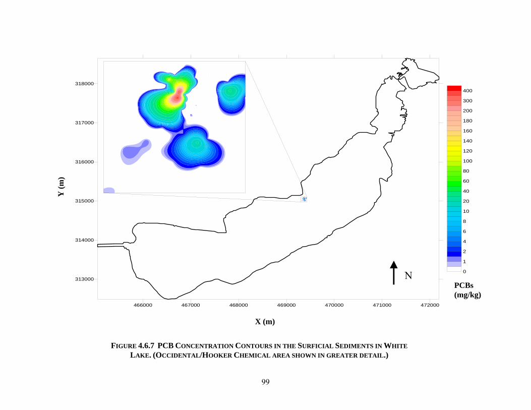
99

466000 467000 468000 469000 470000 471000 472000

313000

314000

315000

316000

317000

318000

0

1

2

4

6

8

10

20

40

60

80

100

120

140

160

180

200

300

400

Y (m

)

X (m)

PCBs (mg/kg)

FIGURE 4.6.7 PCB CONCENTRATION CONTOURS IN THE SURFICIAL SEDIMENTS IN WHITE LAKE. (OCCIDENTAL/HOOKER CHEMICAL AREA SHOWN IN GREATER DETAIL.)

N

100

90% of White Lake. The complex flow pattern of the lake will continue to redistribute the remaining contaminated sediments throughout the western basins. Even though the source has been eliminated, it will take many years to observe a significant trend of reduced chromium deposition in the surficial zone. Dredging should have a more immediate impact on the ecosystem in Tannery Bay as the toxic sediments will be removed from the environment. The removal of PCB contaminated sediment from the Occidental/Hooker Chemical outfall will also have an immediate benefit to the local ecosystem through the elimination of toxic sediment. On a broader scale, the removal of PCBs will eliminate a major area of persistent bioaccumulative toxicants from White Lake. 4.7 Sediment Quality Triad Assessment of Contaminated sediments in White Lake

In order to determine the significance of the remaining areas of sediment contamination, an assessment matrix (Chapman 1992) can be used to examine the relationship between chemistry, toxicity, and benthic macroinvertebrate data. An assessment matrix for the White Lake data is presented in Table 4.6.3. Stations exceeding the PEC (MacDonald et al. 2000)

TABLE 4.7.1 SEDIMENT QUALITY ASSESSMENT MATRIX FOR WHITE LAKE DATA, OCTOBER 2000. ASSESSMENT MATRIX FROM CHAPMAN (1992).

+ = Indicator classified as affected; as determined based on comparison to the PEC or control site - = Indicator not classified as affected; as determined based on comparison to the PEC or control site

Station Sediment Chemistry

Toxicity Test

Benthic Community Possible Conclusions

No stations fit the criteria + + +

Impact highly likely; contaminant induced degradation of sediment dwelling organisms

evident WL-17, WL-18, WL-

19, WL-20 - - - Impact highly unlikely; contaminant degradation of sediment dwelling organisms not likely

WL-1, WL-2, WL-3, WL-4, WL-5, WL-6,

WL-7, WL-8, WL-10, WL-11, WL-13. WL-15

+ - - Impact unlikely; contaminants unavailable to sediment dwelling organisms

No stations fit the criteria - + -

Impacts possible; Unmeasured contaminants or conditions exist that have the potential to cause

toxicity

No stations fit the criteria - - +

Impacts unlikely; no degradation of sediment dwelling organisms in the field apparent relative to sediment contamination; physical factors may

be influencing benthic community

WL-21 + + - Impact likely; toxic chemicals probably stressing system

WL-16 - + + Impact likely; unmeasured toxic chemicals contributing to the toxicity

WL-9, WL-12, WL-14 + - +

Impact likely; sediment dwelling organisms degraded by toxic chemical, but toxicity tests not

sensitive to chemicals present

101

were classified as having a potential impact from sediment chemistry. Toxicity and benthic community impacts were based on observing a statistically significant difference in mortality and diversity/trophic status metrics, respectively. Using this assessment methodology, the Occidental/Hooker Chemical Outfall (WL-21), the east bay (WL-16), and the high chromium sites (WL-9, WL-12, and WL-14) were likely to be impacted by contaminated sediments. None of the stations were positive for all three components of the triad. Station WL-21 had levels of chromium and PCBs that exceeded the PEC and solid phase toxicity. The benthic community at this location was not significantly different from the other deep stations in White Lake. Given the organically enriched conditions present in the sediment, it is difficult to detect a toxic response in the benthos above effects caused by eutrophication. Sediments from WL-16 exhibited solid phase toxicity and impacted benthic invertebrates. None of the chemicals however were at sufficient concentrations to produce the toxic effect. Stations WL-9, WL-12, and WL-14 had chromium levels above the PEC, no solid phase toxicity, and a marginally impacted benthic community. Nematodes were the most abundant organism at these locations while tubificids dominated the other stations. Based on the Assessment Matrix, ecological impairments exist at all of these sites due to contaminated sediments. Stations WL-17, WL-18, WL-19, and WL-20 did not exhibit solid phase toxicity, benthic impairment, or contaminant concentrations above the PEC. While the remaining stations exceeded the chromium PEC, solid phase toxicity was absent and the benthic community was similar to WL-17, WL-18, and WL-19. Because of these findings, impacts from contaminated sediments were not anticipated at these locations. In consideration of the remediation of the sediments in Tannery Bay and near the Occidental/Hooker Chemical Outfall, the source of impairments due to chromium and PCBs in White Lake should be eliminated. While dredging should remove all of the sediment containing harmful levels of PCBs, the extent of chromium contamination throughout western White Lake and the cost of remediation make removal an unfeasible alternative. Natural attenuation by the redistribution and burial of contaminated sediments appears to be the most cost effective option. 4.8 Summary And Conclusions

A Phase II investigation of the nature and extent of sediment contamination in White Lake was performed. Sediment chemistry, solid-phase toxicity, and benthic macroinvertebrates were examined at 21 locations. Since chromium was previously identified as the major contaminant in the sediments, experiments were conducted to determine the accumulation of the metal in zebra mussels, macrophytes, and chironomids. In addition, three core samples were evaluated using radiodating and stratigraphy to assess sediment stability and contaminant deposition. High levels of chromium were found to cover a majority of the lake bottom and extend 8 km from the Tannery Bay. All locations sampled west of Tannery Bay exceeded the Probable Effect Concentration (PEC). Most of the chromium was found in the top 51 cm of the core samples. High concentrations of PCBs were found near the outfall of the former Occidental/Hooker Chemical facility. These levels also exceeded PEC guidelines. Sediment toxicity was observed in the east bay area and at the Occidental/Hooker Chemical outfall. Toxicity near the Occidental/Hooker Chemical outfall was probably due to the presence of PCBs. No obvious toxicant was present in the sediments from the east bay.

102

While no relationship was previously observed for total chromium and amphipod toxicity, a significant correlation was found for the organically bound fraction. Elevated levels of organic chromium were found in archived sediments from Tannery Bay. Benthic macroinvertebrate communities throughout White Lake were found to be indicative of organically enriched conditions. Invertebrate community structure of locations in the east bay were significantly different than reference sites, as indicated by a shift to chironomids that were predators and sprawlers. Chironomid populations in the remainder of the lake were burrowers and detritivores. Higher densities of nematodes and reduced tubificid populations were associated with the stations with elevated chromium levels (> 400 mg/kg). The metal also was correlated with an increase in the trophic status of chironomid populations. Chromium accumulation was observed in chironomid populations throughout White Lake. In addition, macrophytes and zebra mussels in Tannery Bay were observed to accumulate the metal in their tissue. All of the stratigraphy cores showed uniform levels of chromium deposition in the top 10 - 15 cm. This pattern suggested that a constant source of chromium was present in White Lake. A standard exponential decay pattern was absent in the lower sections of the cores, indicating that historical changes in sedimentation were caused by episodic events. These data coupled with chromium contour maps and the generalized circulation pattern of the lake were used to elucidate the fate and transport of the metal. The proximity to the drowned rivermouth currents at the Narrows and the wind induced resuspension in the bay provided conditions that facilitated the advection and dispersion a sediment plume 8 km from its source. Higher concentrations of chromium were found in the three deep deposition basins (300-500 mg/kg). In contrast, the PCBs discharged by the Occidental/Hooker Chemical outfall remained within 100 m of the outfall pipe. The depth of the discharge (15 m) plus the depositional nature of the discharge zone acted to confine the contaminants to a small area. The removal of contaminated sediments in Tannery Bay and the Occidental/Hooker outfall was completed in October 2003. Both remedial actions were essential for the recovery of White Lake. Remediation at Tannery Bay removed the ongoing source of chromium contamination while dredging the Occidental/Hooker outfall reduced the amount of bioaccumulative compounds in the lake. 4.9 References

Barbour, M.T., J. Gerritsen, B.D. Snyder, J.B. Stribling. 1999. Rapid Bioassessment

Protocols for Use in Streams and Wadeable Rivers: Periphyton, Benthic Macroinvertebrates and Fish, Second Edition. EPA 841-B-99-002. U.S. Environmental Protection Agency; Office of Water; Washington, D.C.

Barnhart, J. 1997. Chromium chemistry and implications for environmental fate and toxicity. Journal of Soil Contamination. 6: 561-568.

103

Berg, M. H. 1995. Larval food and feeding behavior. Pages 139-168 in P. Armitage, P. S. Cranston and L. C. V. Pinder, eds. The Chironomidae: The biology and ecology of non-biting midges. Chapman and Hall, London, England.

Bernays EA, Cooper Driver G and Bilgener M. 1989. Herbivores and plant tannins. Advances in Ecological Research 19:263-301.

Chapman, P.M. 1992. Sediment quality triad approach. In: Sediment Classification Methods

Compendium. EPA 823-R-92-006. USEPA. Washington, D.C. Chen, M. and L.Q. Ma. 2001. Comparison of three aqua regia digestion methods for

analyzing 16 elements in soils. Soil Sci. Soc. Am. J. 65:491-499. Cobbett, C.S. 2000. Phytochelatins and Their Roles in Heavy Metal Detoxification. Plant

Physiology, 123: 825-832. Cowan M.J.. 1999. Plant Products as Antimicrobial Agents. Clinical Microbiology Reviews

12(4):564-582. Dauer DM. 1991. Biological criteria, environmental health, and estuarine macrobenthic

community structure: Mar. Pollut. Bull. 26:249-257. Del Valls TA and P.M Chapman. 1998. Site-specific sediment quality values for the Gulf of

Cadiz (Spain) and San Francisco Bay (USA), using the sediment quality triad and multivariate analysis: Cienc. Mar. 24:313-336.

Eisler, R. 1986. Chromium hazards to fish, wildlife, and invertebrates: a synoptic review.

U.S. Fish Wildl. Serv. Biol. Rep. 85(1.6) 60 pp. ENVCA 1994. Priority Substances List Assessment Report, Chromium and its Compounds.

Chemicals Evaluation Division, Environment Canada Quebec, Canada KIA OH3. 59 pp.

EPA 1990 Macroinvertebrate Field and Laboratory Methods for Evaluating the Biological

Integrity of Surface Waters. EPA/600/4-90/03. Evans, E.D. 1992. Mona, White, and White Lakes in White County, Michigan The 1950s to

the 1980s. Michigan Department of Natural Resources. MI/DNR/SWQ-92/261. 91pp.

Fiscus, D.A. and D.A. Neher. 2002. Distinguishing nematode genera based on

relative sensitivity to physical and chemical disturbances. Ecological Applications 12(2): 565-575.

104

Gyedu-Ababio TK, J.P. Furstenberg, D Baird, and A Vanreusel. 1999. Nematodes as indicators of pollution: A case study from the Swartkops River system, South Africa. Hydrobiologia 397: 155-169.

Hilsenhoff, W.L. 1987. An Improved Biotic Index of Organic Stream Pollution. Great Lakes Entom. 20:31-39.

Howmiller, R.P. and M.A. Scott. 1977. An environmental index based on the relative

abundance of oligochaete species. J. Water Pollut. Cont. Fed. 49: 809-815. Johansson S.A., J.L. Campbell, K.G. and Malmquist: Particle Induced X-Ray Emission

Spectrometry (PIXE). John Wiley & Sons, Chichester, New York, 1995 Krebs, C. J. (1989). Ecological methodology. New York: Harper & Row. 325 pgs Kubanek1 J., M. E. Hays, P. J. Brown, N. Lindquist, and W. Fenical1 2001. Lignoid

chemical defenses in the freshwater macrophyte Saururus Cernuus. Chemoecology 11:1-8.

Lauritsen, D.D., S.C. Mozley, and D.S. White. 1985. Distribution of oligochaetes in Lake

Michigan and comments on their use as indices of pollution. J. Great Lakes Res. 11:67-76.

LaValle, P.D., A. Brooks, Andrew, and L V. Chris. 1999. Zebra Mussel Wastes and Concentrations of Heavy Metals on Shipwrecks in Western Lake Erie J. Great Lakes Res. 25(2):330-338.

Leslie, H.A., T.I. Pavluk, A.B. de Vaate, M.H.S. Kraak, 1999. Triad assessment of the

impact of chromium contamination on benthic macro-invertebrates in the Chusovaya River (Urals, Russia). Arch. Environ. Contam. Toxicol. 37(2): 182-189.

Lung, W. S. 1975. Modeling of Phosphorus Sediment-Water Interactions in White Lake,

Michigan. Doctoral Thesis. University of Michigan. Department of Civil Engineering.

Ma, L.Q., F. Tan and W.G. Harris. 1997. Concentrations and distributions of 11 elements in

Florida soils. J. Environ. Qual. 26:769-775. MacDonald D.D., C.G. Ingersoll, and T.A. Berger. 2000. Development and Evaluation of

Consensus-Based Sediment Quality Guidelines for Freshwater Ecosystems. Arch. Environ. Contam. Toxicol. 39(1):20-31.

Merritt, R.W. and K.W. Cummins. 1996. An Introduction to the Aquatic Insects of North America. 3rd edition. Kendall/Hunt Publishing Co., Dubuque, IA. 789 pp.

105

Milbrink, G. 1983. An improved environmental index based on the relative abundance of oligochaete species. Hydrobiologia 102: 89-97.

Rajander, J., and L. Harju. 1999. Monitoring of chromium, copper and arsenic in

contaminated soils using thick-target PIXE. Nuclear Instruments and Methods in Physics Research Section B: Beam Interactions with Materials and Atoms 150: 510-515.

Reeders, H. H., and A. Bij de Vaate, 1992. Bioprocessing of Polluted Suspended Matter

from the Water Column by the Zebra Mussel(Dreissena polymorpha Pallas),” Hydrobiologia, 239:53-63.

Rediske R, G. Fahnenstiel, P. Meier, T. Nalepa, and C. Schelske, 1998. Preliminary

Investigation of the Extent and Effects of Sediment Contamination in White Lake, Michigan. U.S. Environmental Protection Agency. EPA-905-R-98-004.

Robbins, J. A., and L. R. Herche. 1993. Models and uncertainty in 210Pb dating of

sediments. Int. Ver. Theor. Angew. Limnol. Verh 25:217-222. Schelske, C. L. and D. Hodell. 1995. Using carbon isotopes of bulk sedimentary organic

matter to reconstruct the history of nutrient loading and eutrophication in Lake Erie. Limnol. Oceanogr. 40:918-929.

Schloesser, Don W., Trefor B. Reynoldson, Bruce A. Manny. 1995, Oligochaete fauna of

western Lake Erie 1961 and 1982: signs of sediment quality recovery: J. Great Lakes Res. 21(3):294-306.

Snow, E.T. 1994. Effects of Chromium on DNA Replication In Vitro. MoleculaMechanisms of Metal Toxicity and Carcinogenicity. Environmental Health Perspectives 102, Supplement 3: 41-44.

Vatamaniuk, O.K., Bucher, E.A., Ward, J.T., and Rea, P.A. 2001. A new pathway for heavy

metal detoxification in animals: phytochelatin synthase is required for cadmium tolerance in Caenorhabditis elegans. J. Biol. Chem. 276: 20817-20820.

Vajpayee, P.R., U. N., Sinha, S., Tripathi, R. D., and Chandra, P. 1995 Bioremediation of

tannery effluent by aquatic macrophytes. Bull environ contam toxicol. 55(4):. 546-553.

Walsh, A.R. and O'Halloran, J. 1996. Chromium speciation in tannery effluent - II.

Speciation in the effluent and in a receiving estuary. Water Res. 30(10):2401-2412. Winnell, M. H., D. S. White. 1985. Trophic status of southeastern Lake Michigan based on

the Chironomidae (Diptera). J. Great Lakes Res. 11:540-548.

106

5.0 Recommendations

The remediation of contaminated sediments in Tannery Bay and in the vicinity of the Occidental/Hooker Chemical outfall provide a unique opportunity monitor the restoration of these areas and effects on the ecology of White Lake. The following recommendations are based on the results of this investigation and the completion of the above sediment remediation:

1. East Bay. Solid phase toxicity and an impaired benthic community were identified in the current and previous investigations. Conventional analyses for metals and organic compounds were unable to identify a toxicant. In consideration that the east bay contains one of the few undeveloped littoral zones, it is important to identify the source of the toxicity and the benthic impairment. A Toxicity Identification Evaluation (TIE) study should be conducted to evaluate the nature of the toxicant. Tannin levels in the sediments should also be evaluated. Once the toxic agent(s) have been identified, remediation and restoration options can be developed.

2. The removal of contaminated sediments from Tannery Bay and in the vicinity of the Occidental/Hooker Chemical outfall remediated the two major source areas responsible for the Area of Concern designation for White Lake. In order to prepare for future delisting activities, it is important to initiate a lake wide monitoring program to evaluate the effectiveness of the remediation. Annual monitoring of sediment chemistry, toxicity, benthic macroinvertebrates, and the macrophyte community should be conducted in the remediated areas to determine whether the influx of contaminants has ceased and a stable benthic community is established. In addition, sediment chemistry and benthic macroinvertebrates should be examined on a lake wide scale to evaluate the effects of reduced chromium loading on the ecosystem. The stations used in this investigation will provide a solid data set that describes the condition of the lake prior to remediation. Since the sampling locations reflect a broad range of chromium concentrations and depths, the data from this investigation will provide a baseline to evaluate changes in specific areas of elevated contamination and on a lake wide scale.

3. No sediment contamination related to the DuPont groundwater plume was detected in the investigation. Based on these results, questions related to contaminated sediments should not prevent the disposition of the DuPont property west of Long Point.

4. The only remaining site with potential sediment contamination is the Mill Pond area downstream from Koch Chemical. This site should be investigated since hazardous chemicals were discharged in the creek and the area is residential.

107

Appendices

108

Appendix A. Quality Assurance Review of the Project Data.

109

QA/QC Analysis Checklist for SEDIMENT CHEMISTRY ANALYSIS

GRANT/IAG NUMBER: GL- GL975368-01-0 PROJECT NAME: Phase II Investigation of Sediment Contamination in White Lake REVIEWER: Richard Rediske DATE: 6-26-03 1. What sediment chemistry data has been collected (CHECK ALL THAT APPLY)? Total Metals ___X__ PCBs _____ pH _____ TOC _X____

Dioxins/Furans _____ PAHs ___X__Pesticides ___X__ DO _____ AVS _____ SEM Metals _____ Particle Size _X____ Other Semivolatile Organics X

2. Were the target detection limits met for each parameter? YES ____

NO X (UNACCEPTABLE) (Target Detection Limits were not met for semivolatile organics due to low % solids))

3. Were the Method Blanks less than the established MDL for each parameter? YES X

NO _____ (UNACCEPTABLE) 4. Did the results of Field Duplicate Analysis vary by less than the % RPD specified in the QAPP? YES X

NO _____ (UNACCEPTABLE) 5. Did the results of the Field Replicates Analysis vary by less than the % RPD specified in the QAPP? YES X Field replicates were not required in the QAPP

NO _____ (UNACCEPTABLE) 6. Did the surrogate spike recoveries meet the limits set forth in the QAPP? YES X

NO _____ (UNACCEPTABLE)

110

7. Did the MS/MSD recoveries meet the limits set forth in the QAPP? YES ___X__

NO _____ 8. Did the RPD (%) of the MS/MSD sample set meet the limits set forth in the QAPP? YES __X___

NO _____ 9. Did the initial calibration verification standards meet the requirements set forth in the QAPP? YES X

NO _____ (UNACCEPTABLE) 10.. Were any level of contaminants detected above the MDL for the trip blanks and storage blanks? YES _____ (UNACCEPTABLE)

NO X Trip and Storage blanks were not required in the QAPP

11. Did all required analysis take place within the required holding time protocols set forth in the QAPP? YES X

NO _____ (UNACCEPTABLE) 12. Did the laboratory duplicates vary by less than the % RPD specified in the QAPP? YES X

NO _____ (UNACCEPTABLE)

13. Are measured dry weight contaminant concentrations reported? (Note: Conversion from wet weight to dry weight concentration may occur ONLY if data on moisture or TOC are provided. Nominal concentrations are unacceptable.)

YES X NO _____ (UNACCEPTABLE)

111

14. Please provide details for all of the "UNACCEPTABLE" marked above. Include details on the specific analytes affected by any QA/QC discrepancies, and recommendations regarding usability of data. __________________________________________________________________________ Sediment samples had very low % solids that resulted in raising the detection limits for semivolatiles. The results are listed in the data tables. A larger sample volume should be used at these locations if additional assessments are made. Target detection limits were achieved on all other samples.

112

QA/QC Analysis Checklist for ACUTE AND CHRONIC WHOLE SEDIMENT TOXICITY TESTS

(10-dayC. tentans and 10-day or 28-day H. azteca) GRANT/IAG NUMBER: GL975368-01-0 PROJECT NAME: Phase II Investigation of Sediment Contamination in White Lake REVIEWER: Richard Rediske DATE: 2-26-02 1. Did toxicity tests employ appropriate procedures? [ASTM: E1367, E1611, E1706, USEPA (2000)] YES X NO _____ (UNACCEPTABLE) 2. Does sample storage time exceed the allowable storage time specified in the QAPP? Allowable Storage Days Specified in QAPP 45

Number of Storage Days Prior to Testing 14 DYAS AND 30 DAYS

YES _____ (UNACCEPTABLE) NO X

3. Was the age for H. azteca organisms between 7- to 14-days at the start of the test with an age

range less than 2-days?


4A. Were all of the C. tentans organisms second- to third-stage larvae with at least 50% at the third instar?


4B. How was the developmental stage of the C. tentans larvae measured?

Head Capsule Width _____ (See Table 10.2 of EPA/600/R-99/064, March 2000) Length X (Should fall between 4 mm to 6 mm) Weight _____ (Should fall between 0.08 to 0.23 mg/individual)

5. Do flow rates through the different test chambers differ by more than 10% at any particular time during the test?

YES _____ (UNACCEPTABLE) NO X (QAPP REQUIRED 2X DAILY RENEWAL OF OVERLYING WATER INSTEAD OF FLOW THROUGH)

113

6. Did Dissolved Oxygen remain above 2.5 mg/L? YES X NO _____ (Provide Explanation at end of Checklist) 7. Does daily mean Temperature remain at 23 ± 1oC?

YES X NO _____ (UNACCEPTABLE) 8. Does the instantaneous Temperature remain in the range of 23 ± 3ΕC?

YES X NO _____ (UNACCEPTABLE) 9. Do the Ranges of for Hardness, Alkalinity, pH, and Ammonia fluctuate more than 50% from the mean? Maximum % Difference:

DO ____30%____ Alk ____22%__ pH ____6%_____ NH3 50%

YES _____ (UNACCEPTABLE)

NO _____ 10. Was the Ammonia concentration ever greater than 20 mg/L?

YES _____ (See EPA/600/R-99/064, March 2000 to determine if ammonia contributed to toxicity of H. azteca.)

NO X 11. Was the Ammonia concentration greater than 82 mg/L?

YES _____ (See EPA/600/R-99/064, March 2000 to determine if ammonia contributed to toxicity of C. tentans)

NO X 12. Was the Mean Control Survival in the H. azteca Control Sediments greater than or equal to 80%?

YES X NO _____ (UNACCEPTABLE) 13. Was the Mean Control Survival in the C. tentans Control Sediments greater than or eqaul to 70%?


114

14. Was the mean weight per surviving C. tentans control organism greater than 0.48 mg (ash-free dry weight)?

YES X QAPP used dry weight of 0.8 mg/ individual. This was achieved. NO _____ (UNACCEPTABLE) 15. Was the overlying water renewed at a rate of 2 volumes per day?

YES X NO _____ (UNACCEPTABLE) 16. Please provide details for all of the "UNACCEPTABLE" responses marked above. Include details on the specific results that potentially may be affected by any QA/QC discrepancies, and recommendations regarding usability of data. All discrepancies were related to following methods approved in the project QAPP.

115

Appendix B. Results Physical Analyses On White Lake Sediments, October 2000

116

>2000 u m 2000-1000 u m 1000-850 u m 850-500 u m 500-125 u m 125-63 u m <63 u m TOC SolidsSample ID Weight % Weight% Weight % Weight % Weight % Weight % Weight % % %WL-1 TOP 0 0 0 0 2 6 92 3.9 12WL-1 MID 0 0 0 0 13 9 78 11 14WL-1 BOT 0 0 0 0 7 9 84 9.5 15

WL-1 TOP DUP 0 0 0 0 2 6 92 3.1 11WL-1 MID DUP 0 0 0 0 6 9 86 1.5 15WL-1 BOT DUP 0 0 0 0 12 12 75 9 14

WL-2 TOP 1 0 0 0 4 4 92 6.5 11WL-2 MID 0 0 0 0 13 9 77 10 15WL-2 BOT 0 0 0 2 90 2 5 <1.0 67WL-3 TOP 0 0 0 0 4 8 87 2.2 13WL-3 MID 0 0 0 1 23 11 65 4.8 18WL-3 TOP 0 0 0 0 7 9 84 8.1 15WL-4 TOP 0 0 0 0 10 14 76 2.9 13WL-4MID 0 0 0 3 80 3 13 <1.0 53WL-5 TOP 0 0 0 0 7 12 81 5.8 12WL-5 MID 0 0 0 0 9 12 79 8.9 15WL-5 BOT 0 0 0 0 6 10 84 7.2 15WL-6 TOP 0 0 0 0 2 5 93 3.0 17WL-6 MID 1 0 0 2 43 8 46 10 38WL-6 BOT 0 0 0 1 8 13 78 3.0 16WL-7 TOP 0 0 0 0 8 12 80 3.6 12WL7 MID 0 0 0 0 11 17 72 10 16

WL-7 BOT 0 0 0 0 8 18 75 10 15WL-8 TOP 0 0 0 0 8 16 76 6.6 12WL-8 MID 0 0 0 0 8 11 80 1.2 15WL-8 BOT 0 1 0 0 6 12 83 1.3 16WL-9 TOP 0 1 0 0 9 14 76 7.5 13WL-9-MID 0 0 0 0 9 10 81 7.1 15WL-9 BOT 0 0 0 0 7 11 81 8.1 16

WL-10 TOP 6 0 0 0 23 6 71 <1.0 14WL-10 MID 0 0 0 0 11 10 79 9.7 15WL-10 BOT 0 0 0 0 6 7 87 8.9 14WL-21 TOP 0 0 0 0 10 5 84 2.7 20WL-21 MID 0 0 0 1 10 15 74 7.1 16WL-21 BOT 0 0 0 1 6 6 86 3.4 13

TABLE B-1. RESULTS OF GRAIN SIZE, TOC, AND % SOLIDS ANALYSES ON WHITE LAKE SEDIMENT CORE SAMPLES. OCTOBER 2000.

117

TABLE B-2. RESULTS OF GRAIN SIZE, TOC, AND % SOLIDS ANALYSES ON WHITE LAKE SEDIMENT SAMPLES. OCTOBER 2000.

>2000 u m 2000-1000 u m 1000-850 u m 850-500 u m 500-125 um 125-63 u m <63 u m TOC SolidsSample ID Weight % Weight% Weight % Weight % Weight % Weight % Weight % % %

WL-1 P 0 0 0 0 4 5 91 <1.0 7WL-2 P 0 0 0 0 6 5 88 3.5 10WL-3 P 0 0 0 0 4 5 90 3.0 10WL-4 P 0 0 0 5 82 2 11 <1.0 61WL-5 P 0 0 0 0 6 10 83 5.0 11WL-6 P 0 0 0 0 5 7 88 4.4 10WL-7 P 0 0 0 0 7 10 83 6.6 10WL-8 P 0 0 0 0 8 10 82 5.5 11WL-9 P 0 0 0 0 7 9 83 6.4 11WL-10 P 0 0 0 0 5 5 89 2.2 10WL-11 P 0 0 0 0 7 9 84 6.0 11WL-12 P 1 0 0 0 6 9 84 7.1 11WL-13 P 0 0 0 0 30 14 55 5.0 15WL-14 P 1 0 0 0 13 10 76 18 13WL-15 P 1 0 0 0 6 10 83 7.4 12WL-16 P 0 0 0 0 3 7 90 10 14WL-17 P 0 0 0 0 5 10 84 10 15WL-18 P 0 0 0 0 8 8 84 11 16WL-19 P 0 0 0 0 6 11 83 11 15WL-20 P 0 0 0 0 11 17 70 8.5 16WL-21 P 0 0 0 1 19 9 71 5.6 13WL-22 P 6 2 0 1 12 13 65 4.6 11WL-23 P 3 3 1 2 10 9 73 5.9 12WL-24 P 3 1 0 1 12 7 76 8.2 15

118

Sample IDSample OC

mgMS OC

mgMatrix Spike

Conc. mg % RecoveryWL-5 Top 6.1 20.2 12.4 114WL-6 Bot 2.6 56.9 52.9 103WL-9 Top 8.0 28.7 21.0 98

WL-21 Top 2.7 22.3 18.6 106WL-5 P 5.0 26.5 23.5 91

WL-14 P 7.2 31.8 25.1 98WL-18 P 9.0 36.1 26.7 101

Sample IDSample OC

mgMSD OC

mgMatrix Spike

Conc. mg % Recovery RPD*WL-5 Top 6.1 30.9 23.4 106 8WL-6 Bot 2.6 33.1 29.1 105 2WL-9 Top 8.0 41.5 34.1 98 0

WL-21 Top 2.7 19.9 18.6 92 13WL-5 P 5.0 31.4 25.8 102 11

WL-14 P 7.2 29.8 22.7 99 8WL-18 P 9.0 30.1 21.6 98 0

* RPD was calculated using the % recoveries for the ms and msd.Different amounts (mg) of sample and spike were used for the ms and msd

Matrix Spike Data

Matrix Spike Duplicate Data

TABLE B-3. TOC MATRIX SPIKE AND MATRIX SPIKE DUPLICATE RESULTS FOR WHITE LAKE SEDIMENT SAMPLES. OCTOBER 2000.

119

>2000 u m 2000-1000 um 1000-850 um 850-500 u m 500-125 um 125-63 u m <63 u mSample ID Weight % Weight% Weight % Weight % Weight % Weight % Weight %WL-2 Bot 0 0 0 2 90 2 5

WL-2 Bot Dup 0 0 0 3 90 2 5WL-4 Mid 0 0 0 3 81 2 12

WL-4 Mid Dup 0 0 0 3 81 3 12Wl-6 Mid 1 0 0 2 43 8 46

WL-6 Mid Dup 0 1 0 2 42 7 47WL-10 P 0 0 0 0 5 5 89

WL-10 P Dup 0 0 0 0 6 5 90WL-15 P 1 0 0 0 6 11 83

WL-15 P Dup 0 0 0 0 6 10 83WL-18 P 0 0 0 0 8 8 84

WL-18 P Dup 1 0 0 1 6 11 82WL-21 P 0 0 0 1 19 9 71

WL-21 P Dup 0 0 0 1 17 9 73

TABLE B-4. QUALITY CONTROL RESULTS FOR GRAIN SIZE ANALYSES ON WHITE LAKE SEDIMENT SAMPLES. OCTOBER 2000.

120

Appendix C. Organic Analyses On White Lake Sediments, October 2000.

121

PCB-1016 < 0.33 < 0.33 < 0.33 < 0.33 < 0.33 < 0.33 < 0.33 < 0.33 < 0.33 < 0.33 < 0.33 < 0.33 < 0.33PCB-1221 < 0.33 < 0.33 < 0.33 < 0.33 < 0.33 < 0.33 < 0.33 < 0.33 < 0.33 < 0.33 < 0.33 < 0.33 < 0.33PCB-1232 < 0.33 < 0.33 < 0.33 < 0.33 < 0.33 < 0.33 < 0.33 < 0.33 < 0.33 < 0.33 < 0.33 < 0.33 < 0.33PCB-1242 < 0.33 < 0.33 < 0.33 < 0.33 < 0.33 < 0.33 < 0.33 < 0.33 < 0.33 < 0.33 < 0.33 < 0.33 < 0.33PCB-1248 0.22 < 0.33 < 0.33 0.44 < 0.33 0.06 0.06 0.07 < 0.33 0.06 < 0.33 0.06 < 0.33 < 0.33PCB-1254 < 0.33 < 0.33 < 0.33 < 0.33 < 0.33 < 0.33 < 0.33 < 0.33 < 0.33 < 0.33 < 0.33 < 0.33 < 0.33PCB-1260 < 0.33 < 0.33 < 0.33 < 0.33 < 0.33 < 0.33 < 0.33 < 0.33 < 0.33 < 0.33 < 0.33 < 0.33 < 0.33

1,2,4-TRICHLOROBENZENE < 1.7 < 1.2 < 1.2 < 1.7 < 1.2 < 1.2 < 1.7 < 1.2 < 1.4 < 0.93 < 1.0 < 1.3 < 0.331,2-DICHLOROBENZENE < 1.7 < 1.2 < 1.2 < 1.7 < 1.2 < 1.2 < 1.7 < 1.2 < 1.4 < 0.93 < 1.0 < 1.3 < 0.331,3-DICHLOROBENZENE < 1.7 < 1.2 < 1.2 < 1.7 < 1.2 < 1.2 < 1.7 < 1.2 < 1.4 < 0.93 < 1.0 < 1.3 < 0.331,4-DICHLOROBENZENE < 1.7 < 1.2 < 1.2 < 1.7 < 1.2 < 1.2 < 1.7 < 1.2 < 1.4 < 0.93 < 1.0 < 1.3 < 0.332,4,5-TRICHLOROPHENOL < 8.6 < 6.1 < 6.1 < 8.6 < 6.1 < 6.1 < 8.6 < 6.1 < 7.2 < 4.8 < 5.4 < 6.6 < 1.72,4,6-TRICHLOROPHENOL < 1.7 < 1.2 < 1.2 < 1.7 < 1.2 < 1.2 < 1.7 < 1.2 < 1.4 < 0.93 < 1.0 < 1.3 < 0.332,4-DICHLOROPHENOL < 1.7 < 1.2 < 1.2 < 1.7 < 1.2 < 1.2 < 1.7 < 1.2 < 1.4 < 0.93 < 1.0 < 1.3 < 0.332,4-DIMETHYLPHENOL < 1.7 < 1.2 < 1.2 < 1.7 < 1.2 < 1.2 < 1.7 < 1.2 < 1.4 < 0.93 < 1.0 < 1.3 < 0.332,4-DINITROPHENOL < 8.6 < 6.1 < 6.1 < 8.6 < 6.1 < 6.1 < 8.6 < 6.1 < 7.2 < 4.8 < 5.4 < 6.6 < 1.72,4-DINITROTOLUENE < 1.7 < 1.2 < 1.2 < 1.7 < 1.2 < 1.2 < 1.7 < 1.2 < 1.4 < 0.93 < 1.0 < 1.3 < 0.332,6-DINITROTOLUENE < 1.7 < 1.2 < 1.2 < 1.7 < 1.2 < 1.2 < 1.7 < 1.2 < 1.4 < 0.93 < 1.0 < 1.3 < 0.332-CHLORONAPHTHALENE < 1.7 < 1.2 < 1.2 < 1.7 < 1.2 < 1.2 < 1.7 < 1.2 < 1.4 < 0.93 < 1.0 < 1.3 < 0.332-CHLOROPHENOL < 1.7 < 1.2 < 1.2 < 1.7 < 1.2 < 1.2 < 1.7 < 1.2 < 1.4 < 0.93 < 1.0 < 1.3 < 0.332-METHYLNAPHTHALENE < 1.7 < 1.2 < 1.2 < 1.7 < 1.2 < 1.2 < 1.7 < 1.2 < 1.4 < 0.93 < 1.0 < 1.3 < 0.332-METHYLPHENOL < 1.7 < 1.2 < 1.2 < 1.7 < 1.2 < 1.2 < 1.7 < 1.2 < 1.4 < 0.93 < 1.0 < 1.3 < 0.332-NITROANILINE < 8.6 < 6.1 < 6.1 < 8.6 < 6.1 < 6.1 < 8.6 < 6.1 < 7.2 < 4.8 < 5.4 < 6.6 < 1.72-NITROPHENOL < 1.7 < 1.2 < 1.2 < 1.7 < 1.2 < 1.2 < 1.7 < 1.2 < 1.4 < 0.93 < 1.0 < 1.3 < 0.333,3'-DICHLOROBENZIDINE < 10 < 7.2 < 7.2 < 10 < 7.2 < 7.2 < 10 < 7.2 < 8.4 < 5.6 < 6.3 < 7.8 < 2.03-NITROANILINE < 8.6 < 6.1 < 6.1 < 8.6 < 6.1 < 6.1 < 8.6 < 6.1 < 7.2 < 4.8 < 5.4 < 6.6 < 1.74,6-DINITRO- 2-METHYLPHENOL < 8.6 < 6.1 < 6.1 < 8.6 < 6.1 < 6.1 < 8.6 < 6.1 < 7.2 < 4.8 < 5.4 < 6.6 < 1.74-BROMOPHENYL PHENYLETHER < 1.7 < 1.2 < 1.2 < 1.7 < 1.2 < 1.2 < 1.7 < 1.2 < 1.4 < 0.93 < 1.0 < 1.3 < 0.334-CHLORO-3-METHYLPHENOL < 1.7 < 1.2 < 1.2 < 1.7 < 1.2 < 1.2 < 1.7 < 1.2 < 1.4 < 0.93 < 1.0 < 1.3 < 0.334-CHLOROANILINE < 6.6 < 4.7 < 4.7 < 6.6 < 4.7 < 4.7 < 6.6 < 4.7 < 5.5 < 3.7 < 4.1 < 5.1 < 1.34-CHLOROPHENYLPHENYL- ETHER < 1.7 < 1.2 < 1.2 < 1.7 < 1.2 < 1.2 < 1.7 < 1.2 < 1.4 < 0.93 < 1.0 < 1.3 < 0.334-METHYLPHENOL < 1.7 < 1.2 < 1.2 < 1.7 < 1.2 < 1.2 < 1.7 < 1.2 < 1.4 < 0.93 < 1.0 < 1.3 < 0.334-NITROANILINE < 8.6 < 6.1 < 6.1 < 8.6 < 6.1 < 6.1 < 8.6 < 6.1 < 7.2 < 4.8 < 5.4 < 6.6 < 1.74-NITROPHENOL < 8.6 < 6.1 < 6.1 < 8.6 < 6.1 < 6.1 < 8.6 < 6.1 < 7.2 < 4.8 < 5.4 < 6.6 < 1.7ACENAPHTHENE < 1.7 < 1.2 < 1.2 < 1.7 < 1.2 < 1.2 < 1.7 < 1.2 < 1.4 < 0.93 < 1.0 < 1.3 < 0.33ACENAPHTHYLENE < 1.7 < 1.2 < 1.2 < 1.7 < 1.2 < 1.2 < 1.7 < 1.2 < 1.4 < 0.93 < 1.0 < 1.3 < 0.33ANTHRACENE < 1.7 < 1.2 < 1.2 < 1.7 < 1.2 < 1.2 < 1.7 < 1.2 < 1.4 < 0.93 < 1.0 < 1.3 < 0.33BENZO (A) ANTHRACENE < 1.7 < 1.2 < 1.2 < 1.7 < 1.2 < 1.2 < 1.7 < 1.2 < 1.4 < 0.93 < 1.0 < 1.3 < 0.33BENZO (A) PYRENE < 1.7 < 1.2 < 1.2 < 1.7 < 1.2 < 1.2 < 1.7 < 1.2 < 1.4 < 0.93 < 1.0 < 1.3 < 0.33BENZO (B) FLUORANTHENE < 1.7 < 1.2 < 1.2 < 1.7 < 1.2 < 1.2 < 1.7 < 1.2 < 1.4 < 0.93 < 1.0 < 1.3 < 0.33BENZO (G,H,I,) PERYLENE < 1.7 < 1.2 < 1.2 < 1.7 < 1.2 < 1.2 < 1.7 < 1.2 < 1.4 < 0.93 < 1.0 < 1.3 < 0.33BENZO (K) FLUORANTHENE < 1.7 < 1.2 < 1.2 < 1.7 < 1.2 < 1.2 < 1.7 < 1.2 < 1.4 < 0.93 < 1.0 < 1.3 < 0.33BIS (2-CHLOROETHOXY)- METHANE < 1.7 < 1.2 < 1.2 < 1.7 < 1.2 < 1.2 < 1.7 < 1.2 < 1.4 < 0.93 < 1.0 < 1.3 < 0.33BIS (2-CHLOROETHYL) ETHER < 1.7 < 1.2 < 1.2 < 1.7 < 1.2 < 1.2 < 1.7 < 1.2 < 1.4 < 0.93 < 1.0 < 1.3 < 0.33BIS (2-CHLOROISOPROPYL)- ETHER < 1.7 < 1.2 < 1.2 < 1.7 < 1.2 < 1.2 < 1.7 < 1.2 < 1.4 < 0.93 < 1.0 < 1.3 < 0.33BIS (2-ETHYLHEXYL)- PHTHALATE 0.38 < 1.2 0.26 < 1.7 0.42 0.32 0.56 0.35 0.99 < 0.93 0.06 0.17 < 0.33BUTYL BENZYL PHTHALATE < 1.7 < 1.2 < 1.2 < 1.7 < 1.2 < 1.2 < 1.7 < 1.2 < 1.4 < 0.93 < 1.0 < 1.3 < 0.33CARBAZOLE < 1.7 < 1.2 < 1.2 < 1.7 < 1.2 < 1.2 < 1.7 < 1.2 < 1.4 < 0.93 < 1.0 < 1.3 < 0.33CHRYSENE < 1.7 < 1.2 < 1.2 < 1.7 < 1.2 < 1.2 < 1.7 < 1.2 < 1.4 < 0.93 < 1.0 < 1.3 < 0.33DI-N-BUTYLPHTHALATE < 1.7 < 1.2 < 1.2 < 1.7 < 1.2 < 1.2 < 1.7 < 1.2 < 1.4 < 0.93 < 1.0 < 1.3 < 0.33DI-N-OCTYLPHTHALATE < 1.7 < 1.2 < 1.2 < 1.7 < 1.2 < 1.2 < 1.7 < 1.2 < 1.4 < 0.93 < 1.0 < 1.3 < 0.33DIBENZO (A,H) ANTHRACENE < 1.7 < 1.2 < 1.2 < 1.7 < 1.2 < 1.2 < 1.7 < 1.2 < 1.4 < 0.93 < 1.0 < 1.3 < 0.33DIBENZOFURAN < 1.7 < 1.2 < 1.2 < 1.7 < 1.2 < 1.2 < 1.7 < 1.2 < 1.4 < 0.93 < 1.0 < 1.3 < 0.33DIETHYLPHTHALATE < 1.7 < 1.2 < 1.2 < 1.7 < 1.2 < 1.2 < 1.7 < 1.2 < 1.4 < 0.93 < 1.0 < 1.3 < 0.33DIMETHYLPHTHALATE < 1.7 < 1.2 < 1.2 < 1.7 < 1.2 < 1.2 < 1.7 < 1.2 < 1.4 < 0.93 < 1.0 < 1.3 < 0.33FLUORANTHENE < 1.7 < 1.2 < 1.2 < 1.7 < 1.2 < 1.2 < 1.7 < 1.2 < 1.4 < 0.93 < 1.0 < 1.3 < 0.33FLUORENE < 1.7 < 1.2 < 1.2 < 1.7 < 1.2 < 1.2 < 1.7 < 1.2 < 1.4 < 0.93 < 1.0 < 1.3 < 0.33HEXACHLOROBENZENE < 1.7 < 1.2 < 1.2 < 1.7 < 1.2 < 1.2 < 1.7 < 1.2 < 1.4 < 0.93 < 1.0 < 1.3 < 0.33HEXACHLOROBUTADIENE < 1.7 < 1.2 < 1.2 < 1.7 < 1.2 < 1.2 < 1.7 < 1.2 < 1.4 < 0.93 < 1.0 < 1.3 < 0.33HEXACHLOROCYCLOPENTADIENE < 1.7 < 1.2 < 1.2 < 1.7 < 1.2 < 1.2 < 1.7 < 1.2 < 1.4 < 0.93 < 1.0 < 1.3 < 0.33HEXACHLOROETHANE < 1.7 < 1.2 < 1.2 < 1.7 < 1.2 < 1.2 < 1.7 < 1.2 < 1.4 < 0.93 < 1.0 < 1.3 < 0.33INDENO (1,2,3-CD) PYRENE < 1.7 < 1.2 < 1.2 < 1.7 < 1.2 < 1.2 < 1.7 < 1.2 < 1.4 < 0.93 < 1.0 < 1.3 < 0.33ISOPHORONE < 1.7 < 1.2 < 1.2 < 1.7 < 1.2 < 1.2 < 1.7 < 1.2 < 1.4 < 0.93 < 1.0 < 1.3 < 0.33N-NITROSO-DI-PHENYLAMINE < 1.7 < 1.2 < 1.2 < 1.7 < 1.2 < 1.2 < 1.7 < 1.2 < 1.4 < 0.93 < 1.0 < 1.3 < 0.33N-NITROSODI-N-PROPYLAMINE < 1.7 < 1.2 < 1.2 < 1.7 < 1.2 < 1.2 < 1.7 < 1.2 < 1.4 < 0.93 < 1.0 < 1.3 < 0.33NAPHTHALENE < 1.7 < 1.2 < 1.2 < 1.7 < 1.2 < 1.2 < 1.7 < 1.2 < 1.4 < 0.93 < 1.0 < 1.3 < 0.33NITROBENZENE < 1.7 < 1.2 < 1.2 < 1.7 < 1.2 < 1.2 < 1.7 < 1.2 < 1.4 < 0.93 < 1.0 < 1.3 < 0.33PENTACHLOROPHENOL < 8.6 < 6.1 < 6.1 < 8.6 < 6.1 < 6.1 < 8.6 < 6.1 < 7.2 < 4.8 < 5.4 < 6.6 < 1.7PHENANTHRENE < 1.7 < 1.2 < 1.2 < 1.7 < 1.2 < 1.2 < 1.7 < 1.2 < 1.4 < 0.93 < 1.0 < 1.3 < 0.33PHENOL < 1.7 < 1.2 < 1.2 < 1.7 < 1.2 < 1.2 < 1.7 < 1.2 < 1.4 < 0.93 < 1.0 < 1.3 < 0.33PYRENE < 1.7 < 1.2 < 1.2 < 1.7 < 1.2 < 1.2 < 1.7 < 1.2 < 1.4 < 0.93 < 1.0 < 1.3 < 0.33

W L-1Top Middle Bottom

W L-1 Dup W L-2Top Middle Bottom Top Middle

W L-3 W L-4Top Middle Bottom Top Middle

TABLE C-1. RESULTS OF SEMIVOLATILE ORGANIC ANALYSES ON WHITE LAKE SEDIMENTS, OCTOBER 2000. (MG/KG DRY WT)

122

PCB-1016 < 0.33 < 0.33 < 0.33 < 0.33 < 0.33 < 0.33 < 0.33 < 0.33 < 0.33 < 0.33 < 0.33 < 0.33 < 0.33 < 0.33 < 0.33PCB-1221 < 0.33 < 0.33 < 0.33 < 0.33 < 0.33 < 0.33 < 0.33 < 0.33 < 0.33 < 0.33 < 0.33 < 0.33 < 0.33 < 0.33 < 0.33PCB-1232 < 0.33 < 0.33 < 0.33 < 0.33 < 0.33 < 0.33 < 0.33 < 0.33 < 0.33 < 0.33 < 0.33 < 0.33 < 0.33 < 0.33 < 0.33PCB-1242 < 0.33 < 0.33 < 0.33 < 0.33 < 0.33 < 0.33 < 0.33 < 0.33 < 0.33 < 0.33 < 0.33 < 0.33 < 0.33 < 0.33 < 0.33PCB-1248 0.17 < 0.33 < 0.33 0.39 < 0.33 < 0.33 0.24 < 0.33 < 0.33 0.27 < 0.33 < 0.33 < 0.33 < 0.33 < 0.33PCB-1254 < 0.33 < 0.33 < 0.33 < 0.33 < 0.33 < 0.33 < 0.33 < 0.33 < 0.33 < 0.33 < 0.33 < 0.33 < 0.33 < 0.33 < 0.33PCB-1260 < 0.33 < 0.33 < 0.33 < 0.33 < 0.33 < 0.33 < 0.33 < 0.33 < 0.33 < 0.33 < 0.33 < 0.33 < 0.33 < 0.33 < 0.33

1,2,4-TRICHLOROBENZENE < 1.3 < 1.2 < 1.1 < 1.1 < 0.46 < 0.45 < 1.5 < 1.1 < 1.1 < 1.3 < 1.1 < 1.1 < 1.4 < 1.1 < 1.11,2-DICHLOROBENZENE < 1.3 < 1.2 < 1.1 < 1.1 < 0.46 < 0.45 < 1.5 < 1.1 < 1.1 < 1.3 < 1.1 < 1.1 < 1.4 < 1.1 < 1.11,3-DICHLOROBENZENE < 1.3 < 1.2 < 1.1 < 1.1 < 0.46 < 0.45 < 1.5 < 1.1 < 1.1 < 1.3 < 1.1 < 1.1 < 1.4 < 1.1 < 1.11,4-DICHLOROBENZENE < 1.3 < 1.2 < 1.1 < 1.1 < 0.46 < 0.45 < 1.5 < 1.1 < 1.1 < 1.3 < 1.1 < 1.1 < 1.4 < 1.1 < 1.12,4,5-TRICHLOROPHENOL < 6.6 < 6.1 < 5.4 < 5.7 < 2.4 < 2.3 < 7.8 < 5.8 < 5.4 < 6.6 < 5.8 < 5.4 < 7.1 < 5.8 < 5.42,4,6-TRICHLOROPHENOL < 1.3 < 1.2 < 1.1 < 1.1 < 0.46 < 0.45 < 1.5 < 1.1 < 1.1 < 1.3 < 1.1 < 1.1 < 1.4 < 1.1 < 1.12,4-DICHLOROPHENOL < 1.3 < 1.2 < 1.1 < 1.1 < 0.46 < 0.45 < 1.5 < 1.1 < 1.1 < 1.3 < 1.1 < 1.1 < 1.4 < 1.1 < 1.12,4-DIMETHYLPHENOL < 1.3 < 1.2 < 1.1 < 1.1 < 0.46 < 0.45 < 1.5 < 1.1 < 1.1 < 1.3 < 1.1 < 1.1 < 1.4 < 1.1 < 1.12,4-DINITROPHENOL < 6.6 < 6.1 < 5.4 < 5.7 < 2.4 < 2.3 < 7.8 < 5.8 < 5.4 < 6.6 < 5.8 < 5.4 < 7.1 < 5.8 < 5.42,4-DINITROTOLUENE < 1.3 < 1.2 < 1.1 < 1.1 < 0.46 < 0.45 < 1.5 < 1.1 < 1.1 < 1.3 < 1.1 < 1.1 < 1.4 < 1.1 < 1.12,6-DINITROTOLUENE < 1.3 < 1.2 < 1.1 < 1.1 < 0.46 < 0.45 < 1.5 < 1.1 < 1.1 < 1.3 < 1.1 < 1.1 < 1.4 < 1.1 < 1.12-CHLORONAPHTHALENE < 1.3 < 1.2 < 1.1 < 1.1 < 0.46 < 0.45 < 1.5 < 1.1 < 1.1 < 1.3 < 1.1 < 1.1 < 1.4 < 1.1 < 1.12-CHLOROPHENOL < 1.3 < 1.2 < 1.1 < 1.1 < 0.46 < 0.45 < 1.5 < 1.1 < 1.1 < 1.3 < 1.1 < 1.1 < 1.4 < 1.1 < 1.12-METHYLNAPHTHALENE < 1.3 < 1.2 < 1.1 < 1.1 < 0.46 < 0.45 < 1.5 < 1.1 < 1.1 < 1.3 < 1.1 < 1.1 < 1.4 < 1.1 < 1.12-METHYLPHENOL < 1.3 < 1.2 < 1.1 < 1.1 < 0.46 < 0.45 < 1.5 < 1.1 < 1.1 < 1.3 < 1.1 < 1.1 < 1.4 < 1.1 < 1.12-NITROANILINE < 6.6 < 6.1 < 5.4 < 5.7 < 2.4 < 2.3 < 7.8 < 5.8 < 5.4 < 6.6 < 5.8 < 5.4 < 7.1 < 5.8 < 5.42-NITROPHENOL < 1.3 < 1.2 < 1.1 < 1.1 < 0.46 < 0.45 < 1.5 < 1.1 < 1.1 < 1.3 < 1.1 < 1.1 < 1.4 < 1.1 < 1.13,3'-DICHLOROBENZIDINE < 7.8 < 7.2 < 6.4 < 6.7 < 2.8 < 2.7 < 9.2 < 6.8 < 6.4 < 7.8 < 6.8 < 6.4 < 8.4 < 6.8 < 6.43-NITROANILINE < 6.6 < 6.1 < 5.4 < 5.7 < 2.4 < 2.3 < 7.8 < 5.8 < 5.4 < 6.6 < 5.8 < 5.4 < 7.1 < 5.8 < 5.44,6-DINITRO- 2-METHYLPHENOL < 6.6 < 6.1 < 5.4 < 5.7 < 2.4 < 2.3 < 7.8 < 5.8 < 5.4 < 6.6 < 5.8 < 5.4 < 7.1 < 5.8 < 5.44-BROMOPHENYL PHENYLETHER < 1.3 < 1.2 < 1.1 < 1.1 < 0.46 < 0.45 < 1.5 < 1.1 < 1.1 < 1.3 < 1.1 < 1.1 < 1.4 < 1.1 < 1.14-CHLORO-3-METHYLPHENOL < 1.3 < 1.2 < 1.1 < 1.1 < 0.46 < 0.45 < 1.5 < 1.1 < 1.1 < 1.3 < 1.1 < 1.1 < 1.4 < 1.1 < 1.14-CHLOROANILINE < 5.1 < 4.7 < 4.2 < 4.4 < 1.8 < 1.8 < 6.0 < 4.4 < 4.2 < 5.1 < 4.4 < 4.2 < 5.5 < 4.4 < 4.24-CHLOROPHENYLPHENYL- ETHER < 1.3 < 1.2 < 1.1 < 1.1 < 0.46 < 0.45 < 1.5 < 1.1 < 1.1 < 1.3 < 1.1 < 1.1 < 1.4 < 1.1 < 1.14-METHYLPHENOL < 1.3 < 1.2 < 1.1 < 1.1 < 0.46 < 0.45 < 1.5 < 1.1 < 1.1 < 1.3 < 1.1 < 1.1 < 1.4 < 1.1 < 1.14-NITROANILINE < 6.6 < 6.1 < 5.4 < 5.7 < 2.4 < 2.3 < 7.8 < 5.8 < 5.4 < 6.6 < 5.8 < 5.4 < 7.1 < 5.8 < 5.44-NITROPHENOL < 6.6 < 6.1 < 5.4 < 5.7 < 2.4 < 2.3 < 7.8 < 5.8 < 5.4 < 6.6 < 5.8 < 5.4 < 7.1 < 5.8 < 5.4ACENAPHTHENE < 1.3 < 1.2 < 1.1 < 1.1 < 0.46 < 0.45 < 1.5 < 1.1 < 1.1 < 1.3 < 1.1 < 1.1 < 1.4 < 1.1 < 1.1ACENAPHTHYLENE < 1.3 < 1.2 < 1.1 < 1.1 < 0.46 < 0.45 < 1.5 < 1.1 < 1.1 < 1.3 < 1.1 < 1.1 < 1.4 < 1.1 < 1.1ANTHRACENE < 1.3 < 1.2 < 1.1 < 1.1 < 0.46 < 0.45 < 1.5 < 1.1 < 1.1 < 1.3 < 1.1 < 1.1 < 1.4 < 1.1 < 1.1BENZO (A) ANTHRACENE < 1.3 < 1.2 < 1.1 < 1.1 < 0.46 < 0.45 < 1.5 < 1.1 < 1.1 < 1.3 < 1.1 < 1.1 < 1.4 < 1.1 < 1.1BENZO (A) PYRENE < 1.3 < 1.2 < 1.1 < 1.1 < 0.46 < 0.45 < 1.5 < 1.1 < 1.1 < 1.3 < 1.1 < 1.1 < 1.4 < 1.1 < 1.1BENZO (B) FLUORANTHENE < 1.3 < 1.2 < 1.1 < 1.1 < 0.46 < 0.45 < 1.5 < 1.1 < 1.1 < 1.3 < 1.1 < 1.1 < 1.4 < 1.1 < 1.1BENZO (G,H,I,) PERYLENE < 1.3 < 1.2 < 1.1 < 1.1 < 0.46 < 0.45 < 1.5 < 1.1 < 1.1 < 1.3 < 1.1 < 1.1 < 1.4 < 1.1 < 1.1BENZO (K) FLUORANTHENE < 1.3 < 1.2 < 1.1 < 1.1 < 0.46 < 0.45 < 1.5 < 1.1 < 1.1 < 1.3 < 1.1 < 1.1 < 1.4 < 1.1 < 1.1BIS (2-CHLOROETHOXY)- METHANE < 1.3 < 1.2 < 1.1 < 1.1 < 0.46 < 0.45 < 1.5 < 1.1 < 1.1 < 1.3 < 1.1 < 1.1 < 1.4 < 1.1 < 1.1BIS (2-CHLOROETHYL) ETHER < 1.3 < 1.2 < 1.1 < 1.1 < 0.46 < 0.45 < 1.5 < 1.1 < 1.1 < 1.3 < 1.1 < 1.1 < 1.4 < 1.1 < 1.1BIS (2-CHLOROISOPROPYL)- ETHER < 1.3 < 1.2 < 1.1 < 1.1 < 0.46 < 0.45 < 1.5 < 1.1 < 1.1 < 1.3 < 1.1 < 1.1 < 1.4 < 1.1 < 1.1BIS (2-ETHYLHEXYL)- PHTHALATE < 1.3 < 1.2 < 1.1 0.22 0.19 0.14 0.28 0.25 < 1.1 0.25 < 1.1 < 1.1 < 1.4 < 1.1 0.23BUTYL BENZYL PHTHALATE < 1.3 < 1.2 < 1.1 < 1.1 < 0.46 < 0.45 < 1.5 < 1.1 < 1.1 < 1.3 < 1.1 < 1.1 < 1.4 < 1.1 < 1.1CARBAZOLE < 1.3 < 1.2 < 1.1 < 1.1 < 0.46 < 0.45 < 1.5 < 1.1 < 1.1 < 1.3 < 1.1 < 1.1 < 1.4 < 1.1 < 1.1CHRYSENE < 1.3 < 1.2 < 1.1 < 1.1 < 0.46 < 0.45 < 1.5 < 1.1 < 1.1 < 1.3 < 1.1 < 1.1 < 1.4 < 1.1 < 1.1DI-N-BUTYLPHTHALATE < 1.3 < 1.2 < 1.1 < 1.1 < 0.46 < 0.45 < 1.5 0.99 < 1.1 < 1.3 < 1.1 < 1.1 < 1.4 < 1.1 < 1.1DI-N-OCTYLPHTHALATE < 1.3 < 1.2 < 1.1 < 1.1 < 0.46 < 0.45 < 1.5 < 1.1 < 1.1 < 1.3 < 1.1 < 1.1 < 1.4 < 1.1 < 1.1DIBENZO (A,H) ANTHRACENE < 1.3 < 1.2 < 1.1 < 1.1 < 0.46 < 0.45 < 1.5 < 1.1 < 1.1 < 1.3 < 1.1 < 1.1 < 1.4 < 1.1 < 1.1DIBENZOFURAN < 1.3 < 1.2 < 1.1 < 1.1 < 0.46 < 0.45 < 1.5 < 1.1 < 1.1 < 1.3 < 1.1 < 1.1 < 1.4 < 1.1 < 1.1DIETHYLPHTHALATE < 1.3 < 1.2 < 1.1 < 1.1 < 0.46 < 0.45 < 1.5 < 1.1 < 1.1 < 1.3 < 1.1 < 1.1 < 1.4 < 1.1 < 1.1DIMETHYLPHTHALATE < 1.3 < 1.2 < 1.1 < 1.1 < 0.46 < 0.45 < 1.5 < 1.1 < 1.1 < 1.3 < 1.1 < 1.1 < 1.4 < 1.1 < 1.1FLUORANTHENE < 1.3 < 1.2 < 1.1 < 1.1 < 0.46 < 0.45 < 1.5 < 1.1 < 1.1 < 1.3 < 1.1 < 1.1 < 1.4 < 1.1 < 1.1FLUORENE < 1.3 < 1.2 < 1.1 < 1.1 < 0.46 < 0.45 < 1.5 < 1.1 < 1.1 < 1.3 < 1.1 < 1.1 < 1.4 < 1.1 < 1.1HEXACHLOROBENZENE < 1.3 < 1.2 < 1.1 < 1.1 < 0.46 < 0.45 < 1.5 < 1.1 < 1.1 < 1.3 < 1.1 < 1.1 < 1.4 < 1.1 < 1.1HEXACHLOROBUTADIENE < 1.3 < 1.2 < 1.1 < 1.1 < 0.46 < 0.45 < 1.5 < 1.1 < 1.1 < 1.3 < 1.1 < 1.1 < 1.4 < 1.1 < 1.1HEXACHLOROCYCLOPENTADIENE < 1.3 < 1.2 < 1.1 < 1.1 < 0.46 < 0.45 < 1.5 < 1.1 < 1.1 < 1.3 < 1.1 < 1.1 < 1.4 < 1.1 < 1.1HEXACHLOROETHANE < 1.3 < 1.2 < 1.1 < 1.1 < 0.46 < 0.45 < 1.5 < 1.1 < 1.1 < 1.3 < 1.1 < 1.1 < 1.4 < 1.1 < 1.1INDENO (1,2,3-CD) PYRENE < 1.3 < 1.2 < 1.1 < 1.1 < 0.46 < 0.45 < 1.5 < 1.1 < 1.1 < 1.3 < 1.1 < 1.1 < 1.4 < 1.1 < 1.1ISOPHORONE < 1.3 < 1.2 < 1.1 < 1.1 < 0.46 < 0.45 < 1.5 < 1.1 < 1.1 < 1.3 < 1.1 < 1.1 < 1.4 < 1.1 < 1.1N-NITROSO-DI-PHENYLAMINE < 1.3 < 1.2 < 1.1 < 1.1 < 0.46 < 0.45 < 1.5 < 1.1 < 1.1 < 1.3 < 1.1 < 1.1 < 1.4 < 1.1 < 1.1N-NITROSODI-N-PROPYLAMINE < 1.3 < 1.2 < 1.1 < 1.1 < 0.46 < 0.45 < 1.5 < 1.1 < 1.1 < 1.3 < 1.1 < 1.1 < 1.4 < 1.1 < 1.1NAPHTHALENE < 1.3 < 1.2 < 1.1 < 1.1 < 0.46 < 0.45 < 1.5 < 1.1 < 1.1 < 1.3 < 1.1 < 1.1 < 1.4 < 1.1 < 1.1NITROBENZENE < 1.3 < 1.2 < 1.1 < 1.1 < 0.46 < 0.45 < 1.5 < 1.1 < 1.1 < 1.3 < 1.1 < 1.1 < 1.4 < 1.1 < 1.1PENTACHLOROPHENOL < 6.6 < 6.1 < 5.4 < 5.7 < 2.4 < 2.3 < 7.8 < 5.8 < 5.4 < 6.6 < 5.8 < 5.4 < 7.1 < 5.8 < 5.4PHENANTHRENE < 1.3 < 1.2 < 1.1 < 1.1 < 0.46 < 0.45 < 1.5 < 1.1 < 1.1 < 1.3 < 1.1 < 1.1 < 1.4 < 1.1 < 1.1PHENOL < 1.3 < 1.2 < 1.1 < 1.1 < 0.46 < 0.45 < 1.5 < 1.1 < 1.1 < 1.3 < 1.1 < 1.1 < 1.4 < 1.1 < 1.1PYRENE < 1.3 < 1.2 < 1.1 < 1.1 < 0.46 < 0.45 < 1.5 < 1.1 < 1.1 < 1.3 < 1.1 < 1.1 < 1.4 < 1.1 < 1.1

MiddleMiddle BotomWL-9

Top Middle Bottom TopMiddle Bottom Top BotomTop Middle Bottom TopWL-5 WL-6 WL-7 WL-8

TABLE C-1 (CONTINUED). RESULTS OF SEMIVOLATILE ORGANIC ANALYSES ON WHITE LAKE SEDIMENTS, OCTOBER 2000.

123

PCB-1016 < 0.33 < 0.33 < 0.33 < 0.33 < 0.98 < 0.33 < 0.33 < 0.33 < 0.33 < 0.33 < 0.33 < 0.33 < 0.33 < 0.33 < 0.33PCB-1221 < 0.33 < 0.33 < 0.33 < 0.33 < 0.98 < 0.33 < 0.33 < 0.33 < 0.33 < 0.33 < 0.33 < 0.33 < 0.33 < 0.33 < 0.33PCB-1232 < 0.34 < 0.34 < 0.33 < 0.33 < 0.99 < 0.33 < 0.33 0.34 < 0.34 < 0.34 < 0.34 < 0.34 < 0.34 < 0.34 < 0.33PCB-1242 < 0.33 < 0.33 < 0.33 < 0.33 < 0.98 < 0.33 < 0.33 < 0.33 < 0.33 < 0.33 < 0.33 < 0.33 < 0.33 < 0.33 < 0.33PCB-1248 0.06 0.06 < 0.33 22 0.84 < 0.33 < 0.33 0/09 < 0.33 < 0.33 < 0.33 0.07 0.08 0.08 < 0.33PCB-1254 < 0.33 < 0.33 < 0.33 < 0.33 < 0.98 < 0.33 < 0.33 < 0.33 < 0.33 < 0.33 < 0.33 < 0.33 < 0.33 < 0.33 < 0.33PCB-1260 < 0.33 < 0.33 < 0.33 < 0.33 < 0.98 < 0.33 < 0.33 < 0.33 < 0.33 < 0.33 < 0.33 < 0.33 < 0.33 < 0.33 < 0.33

< 0.981,2,4-TRICHLOROBENZENE < 1.1 < 1.1 < 1.2 < 1.2 < 5.0 < 1.8 < 1.7 < 1.5 < 0.33 < 1.7 < 1.5 < 1.7 < 1.7 < 1.5 < 1.71,2-DICHLOROBENZENE < 1.1 < 1.1 < 1.2 < 1.2 < 0.98 < 1.8 < 1.7 < 1.5 < 0.33 < 1.7 < 1.5 < 1.7 < 1.7 < 1.5 < 1.71,3-DICHLOROBENZENE < 1.1 < 1.1 < 1.2 1.9 0.29 < 1.8 < 1.7 < 1.5 < 0.33 < 1.7 < 1.5 < 1.7 < 1.7 < 1.5 < 1.71,4-DICHLOROBENZENE < 1.1 < 1.1 < 1.2 0.65 < 0.98 < 1.8 < 1.7 < 1.5 < 0.33 < 1.7 < 1.5 < 1.7 < 1.7 < 1.5 < 1.72,4,5-TRICHLOROPHENOL < 5.8 < 5.8 < 6.1 < 6.1 < 0.98 < 9.2 < 8.6 < 7.8 < 1.7 < 8.8 < 7.8 < 8.6 < 8.6 < 7.8 < 8.62,4,6-TRICHLOROPHENOL < 1.1 < 1.1 < 1.2 < 1.2 < 0.98 < 1.8 < 1.7 < 1.5 < 0.33 < 1.7 < 1.5 < 1.7 < 1.7 < 1.5 < 1.72,4-DICHLOROPHENOL < 1.1 < 1.1 < 1.2 < 1.2 < 0.98 < 1.8 < 1.7 < 1.5 < 0.33 < 1.7 < 1.5 < 1.7 < 1.7 < 1.5 < 1.72,4-DIMETHYLPHENOL < 1.1 < 1.1 < 1.2 < 1.2 < 5.0 < 1.8 < 1.7 < 1.5 < 0.33 < 1.7 < 1.5 < 1.7 < 1.7 < 1.5 < 1.72,4-DINITROPHENOL < 5.8 < 5.8 < 6.1 < 6.1 < 0.98 < 9.2 < 8.6 < 7.8 < 1.7 < 8.8 < 7.8 < 8.6 < 8.6 < 7.8 < 8.62,4-DINITROTOLUENE < 1.1 < 1.1 < 1.2 < 1.2 < 5.9 < 1.8 < 1.7 < 1.5 < 0.33 < 1.7 < 1.5 < 1.7 < 1.7 < 1.5 < 1.72,6-DINITROTOLUENE < 1.1 < 1.1 < 1.2 < 1.2 < 5.0 < 1.8 < 1.7 < 1.5 < 0.33 < 1.7 < 1.5 < 1.7 < 1.7 < 1.5 < 1.72-CHLORONAPHTHALENE < 1.1 < 1.1 < 1.2 < 1.2 < 5.0 < 1.8 < 1.7 < 1.5 < 0.33 < 1.7 < 1.5 < 1.7 < 1.7 < 1.5 < 1.72-CHLOROPHENOL < 1.1 < 1.1 < 1.2 < 1.2 < 0.98 < 1.8 < 1.7 < 1.5 < 0.33 < 1.7 < 1.5 < 1.7 < 1.7 < 1.5 < 1.72-METHYLNAPHTHALENE < 1.1 < 1.1 < 1.2 < 1.2 < 0.98 < 1.8 < 1.7 < 1.5 < 0.33 < 1.7 < 1.5 < 1.7 < 1.7 < 1.5 < 1.72-METHYLPHENOL < 1.1 < 1.1 < 1.2 < 1.2 < 3.9 < 1.8 < 1.7 < 1.5 < 0.33 < 1.7 < 1.5 < 1.7 < 1.7 < 1.5 < 1.72-NITROANILINE < 5.8 < 5.8 < 6.1 < 6.1 < 0.98 < 9.2 < 8.6 < 7.8 < 1.7 < 8.8 < 7.8 < 8.6 < 8.6 < 7.8 < 8.62-NITROPHENOL < 1.1 < 1.1 < 1.2 < 1.2 < 0.98 < 1.8 < 1.7 < 1.5 < 0.33 < 1.7 < 1.5 < 1.7 < 1.7 < 1.5 < 1.73,3'-DICHLOROBENZIDINE < 6.8 < 6.8 < 7.2 < 7.2 < 5.0 < 11 < 10 < 9.2 < 2.0 < 10 < 9.2 < 10 < 10 < 9.2 < 103-NITROANILINE < 5.8 < 5.8 < 6.1 < 6.1 < 5.0 < 9.2 < 8.6 < 7.8 < 1.7 < 8.8 < 7.8 < 8.6 < 8.6 < 7.8 < 8.64,6-DINITRO- 2-METHYLPHENOL < 5.8 < 5.8 < 6.1 < 6.1 < 0.98 < 9.2 < 8.6 < 7.8 < 1.7 < 8.8 < 7.8 < 8.6 < 8.6 < 7.8 < 8.64-BROMOPHENYL PHENYLETHER < 1.1 < 1.1 < 1.2 < 1.2 < 0.98 < 1.8 < 1.7 < 1.5 < 0.33 < 1.7 < 1.5 < 1.7 < 1.7 < 1.5 < 1.74-CHLORO-3-METHYLPHENOL < 1.1 < 1.1 < 1.2 < 1.2 < 0.98 < 1.8 < 1.7 < 1.5 < 0.33 < 1.7 < 1.5 < 1.7 < 1.7 < 1.5 < 1.74-CHLOROANILINE < 4.4 < 4.4 < 4.7 < 4.7 < 0.98 < 7.1 < 6.6 < 6.0 < 1.3 < 6.7 < 6.0 < 6.6 < 6.6 < 6.0 < 6.64-CHLOROPHENYLPHENYL- ETHER < 1.1 < 1.1 < 1.2 < 1.2 < 0.98 < 1.8 < 1.7 < 1.5 < 0.33 < 1.7 < 1.5 < 1.7 < 1.7 < 1.5 < 1.74-METHYLPHENOL < 1.1 < 1.1 < 1.2 < 1.2 < 0.98 < 1.8 < 1.7 < 1.5 < 0.33 < 1.7 < 1.5 < 1.7 < 1.7 < 1.5 < 1.74-NITROANILINE < 5.8 < 5.8 < 6.1 < 6.1 < 0.98 < 9.2 < 8.6 < 7.8 < 1.7 < 8.8 < 7.8 < 8.6 < 8.6 < 7.8 < 8.64-NITROPHENOL < 5.8 < 5.8 < 6.1 < 6.1 < 0.98 < 9.2 < 8.6 < 7.8 < 1.7 < 8.8 < 7.8 < 8.6 < 8.6 < 7.8 < 8.6ACENAPHTHENE < 1.1 < 1.1 < 1.2 < 1.2 < 0.98 < 1.8 < 1.7 < 1.5 < 0.33 < 1.7 < 1.5 < 1.7 < 1.7 < 1.5 < 1.7ACENAPHTHYLENE < 1.1 < 1.1 < 1.2 < 1.2 < 0.98 < 1.8 < 1.7 < 1.5 < 0.33 < 1.7 < 1.5 < 1.7 < 1.7 < 1.5 < 1.7ANTHRACENE < 1.1 < 1.1 < 1.2 < 1.2 < 0.98 < 1.8 < 1.7 < 1.5 < 0.33 < 1.7 < 1.5 < 1.7 < 1.7 < 1.5 < 1.7BENZO (A) ANTHRACENE < 1.1 < 1.1 < 1.2 < 1.2 < 0.98 < 1.8 < 1.7 < 1.5 < 0.33 < 1.7 < 1.5 < 1.7 < 1.7 < 1.5 < 1.7BENZO (A) PYRENE < 1.1 < 1.1 < 1.2 < 1.2 < 0.98 < 1.8 < 1.7 < 1.5 < 0.33 < 1.7 < 1.5 < 1.7 < 1.7 < 1.5 < 1.7BENZO (B) FLUORANTHENE < 1.1 < 1.1 < 1.2 < 1.2 < 0.98 < 1.8 < 1.7 < 1.5 < 0.33 < 1.7 < 1.5 < 1.7 < 1.7 < 1.5 < 1.7BENZO (G,H,I,) PERYLENE < 1.1 < 1.1 < 1.2 < 1.2 < 0.98 < 1.8 < 1.7 < 1.5 < 0.33 < 1.7 < 1.5 < 1.7 < 1.7 < 1.5 < 1.7BENZO (K) FLUORANTHENE < 1.1 < 1.1 < 1.2 < 1.2 < 0.98 < 1.8 < 1.7 < 1.5 < 0.33 < 1.7 < 1.5 < 1.7 < 1.7 < 1.5 < 1.7BIS (2-CHLOROETHOXY)- METHANE < 1.1 < 1.1 < 1.2 < 1.2 < 0.98 < 1.8 < 1.7 < 1.5 < 0.33 < 1.7 < 1.5 < 1.7 < 1.7 < 1.5 < 1.7BIS (2-CHLOROETHYL) ETHER < 1.1 < 1.1 < 1.2 < 1.2 < 0.98 < 1.8 < 1.7 < 1.5 < 0.33 < 1.7 < 1.5 < 1.7 < 1.7 < 1.5 < 1.7BIS (2-CHLOROISOPROPYL)- ETHER < 1.1 < 1.1 < 1.2 < 1.2 < 0.98 < 1.8 < 1.7 < 1.5 < 0.33 < 1.7 < 1.5 < 1.7 < 1.7 < 1.5 < 1.7BIS (2-ETHYLHEXYL)- PHTHALATE 0.25 < 1.1 < 1.2 0.94 0.54 0.92 < 1.7 < 1.5 0.31 < 1.7 0.62 0.32 0.35 1.3 < 1.7BUTYL BENZYL PHTHALATE < 1.1 < 1.1 < 1.2 < 1.2 < 0.98 < 1.8 < 1.7 < 1.5 < 0.33 < 1.7 < 1.5 < 1.7 < 1.7 < 1.5 < 1.7CARBAZOLE < 1.1 < 1.1 < 1.2 < 1.2 < 0.98 < 1.8 < 1.7 < 1.5 < 0.33 < 1.7 < 1.5 < 1.7 < 1.7 < 1.5 < 1.7CHRYSENE < 1.1 < 1.1 < 1.2 < 1.2 < 0.98 < 1.8 < 1.7 < 1.5 < 0.33 < 1.7 < 1.5 < 1.7 < 1.7 < 1.5 < 1.7DI-N-BUTYLPHTHALATE < 1.1 < 1.1 0.84 < 1.2 < 0.98 < 1.8 < 1.7 < 1.5 < 0.33 < 1.7 < 1.5 < 1.7 0.30 0.25 < 1.7DI-N-OCTYLPHTHALATE < 1.1 < 1.1 < 1.2 < 1.2 < 0.98 < 1.8 < 1.7 < 1.5 < 0.33 < 1.7 < 1.5 < 1.7 < 1.7 < 1.5 < 1.7DIBENZO (A,H) ANTHRACENE < 1.1 < 1.1 < 1.2 < 1.2 < 0.98 < 1.8 < 1.7 < 1.5 < 0.33 < 1.7 < 1.5 < 1.7 < 1.7 < 1.5 < 1.7DIBENZOFURAN < 1.1 < 1.1 < 1.2 < 1.2 < 0.98 < 1.8 < 1.7 < 1.5 < 0.33 < 1.7 < 1.5 < 1.7 < 1.7 < 1.5 < 1.7DIETHYLPHTHALATE < 1.1 < 1.1 < 1.2 < 1.2 < 0.98 < 1.8 < 1.7 < 1.5 < 0.33 < 1.7 < 1.5 < 1.7 < 1.7 < 1.5 < 1.7DIMETHYLPHTHALATE < 1.1 < 1.1 < 1.2 < 1.2 < 0.98 < 1.8 < 1.7 < 1.5 < 0.33 < 1.7 < 1.5 < 1.7 < 1.7 < 1.5 < 1.7FLUORANTHENE < 1.1 < 1.1 < 1.2 < 1.2 < 0.98 < 1.8 < 1.7 < 1.5 < 0.33 < 1.7 < 1.5 < 1.7 < 1.7 < 1.5 < 1.7FLUORENE < 1.1 < 1.1 < 1.2 < 1.2 < 0.98 < 1.8 < 1.7 < 1.5 < 0.33 < 1.7 < 1.5 < 1.7 < 1.7 < 1.5 < 1.7HEXACHLOROBENZENE < 1.1 < 1.1 < 1.2 0.54 < 0.98 < 1.8 < 1.7 < 1.5 < 0.33 < 1.7 < 1.5 < 1.7 < 1.7 < 1.5 < 1.7HEXACHLOROBUTADIENE < 1.1 < 1.1 < 1.2 0.081 < 0.98 < 1.8 < 1.7 < 1.5 < 0.33 < 1.7 < 1.5 < 1.7 < 1.7 < 1.5 < 1.7HEXACHLOROCYCLOPENTADIENE < 1.1 < 1.1 < 1.2 0.036 < 5.0 < 1.8 < 1.7 < 1.5 < 0.33 < 1.7 < 1.5 < 1.7 < 1.7 < 1.5 < 1.7HEXACHLOROETHANE < 1.1 < 1.1 < 1.2 < 1.2 < 0.98 < 1.8 < 1.7 < 1.5 < 0.33 < 1.7 < 1.5 < 1.7 < 1.7 < 1.5 < 1.7INDENO (1,2,3-CD) PYRENE < 1.1 < 1.1 < 1.2 < 1.2 < 0.98 < 1.8 < 1.7 < 1.5 < 0.33 < 1.7 < 1.5 < 1.7 < 1.7 < 1.5 < 1.7ISOPHORONE < 1.1 < 1.1 < 1.2 < 1.2 < 0.98 < 1.8 < 1.7 < 1.5 < 0.33 < 1.7 < 1.5 < 1.7 < 1.7 < 1.5 < 1.7N-NITROSO-DI-PHENYLAMINE < 1.1 < 1.1 < 1.2 < 1.2 < 0.46 < 1.8 < 1.7 < 1.5 < 0.33 < 1.7 < 1.5 < 1.7 < 1.7 < 1.5 < 1.7N-NITROSODI-N-PROPYLAMINE < 1.1 < 1.1 < 1.2 < 1.2 < 0.46 < 1.8 < 1.7 < 1.5 < 0.33 < 1.7 < 1.5 < 1.7 < 1.7 < 1.5 < 1.7NAPHTHALENE < 1.1 < 1.1 < 1.2 < 1.2 < 0.46 < 1.8 < 1.7 < 1.5 < 0.33 < 1.7 < 1.5 < 1.7 < 1.7 < 1.5 < 1.7NITROBENZENE < 1.1 < 1.1 < 1.2 < 1.2 < 0.46 < 1.8 < 1.7 < 1.5 < 0.33 < 1.7 < 1.5 < 1.7 < 1.7 < 1.5 < 1.7PENTACHLOROPHENOL < 5.8 < 5.8 < 6.1 < 6.1 < 2.4 < 9.2 < 8.6 < 7.8 < 1.7 < 8.8 < 7.8 < 8.6 < 8.6 < 7.8 < 8.6PHENANTHRENE < 1.1 < 1.1 < 1.2 < 1.2 < 0.46 < 1.8 < 1.7 < 1.5 < 0.33 < 1.7 < 1.5 < 1.7 < 1.7 < 1.5 < 1.7PHENOL < 1.1 < 1.1 < 1.2 < 1.2 < 0.46 < 1.8 < 1.7 < 1.5 < 0.33 < 1.7 < 1.5 < 1.7 < 1.7 < 1.5 < 1.7PYRENE < 1.1 < 1.1 < 1.2 < 1.2 < 0.46 < 1.8 < 1.7 < 1.5 < 0.33 < 1.7 < 1.5 < 1.7 < 1.7 < 1.5 < 1.7

WL-8P WL-9PWL-21 WL-1P WL-4P WL-5P WL-6P WL-7PTop Middle Bottom Top MiddleWL-10 WL-1P

Dup WL-2P WL-3P


124


PCB-1016 < 0.33 < 0.33 < 0.33 < 0.33 < 0.33 < 0.33 < 0.33 < 0.33 < 0.33 < 0.33 < 0.33 < 0.33 < 0.33 < 0.33 < 0.33PCB-1221 < 0.33 < 0.33 < 0.33 < 0.33 < 0.33 < 0.33 < 0.33 < 0.33 < 0.33 < 0.33 < 0.33 < 0.33 < 0.33 < 0.33 < 0.33PCB-1232 < 0.33 < 0.33 < 0.33 < 0.33 < 0.33 < 0.33 < 0.33 < 0.33 < 0.33 < 0.33 < 0.33 < 0.33 < 0.33 < 0.33 < 0.33PCB-1242 < 0.33 < 0.33 < 0.33 < 0.33 < 0.33 < 0.33 < 0.33 < 0.33 < 0.33 < 0.33 < 0.33 21 < 0.33 < 0.33 < 0.33PCB-1248 < 0.33 < 0.33 < 0.33 < 0.33 < 0.33 < 0.33 < 0.33 < 0.33 < 0.33 < 0.33 < 0.33 < 0.33 < 0.33 < 0.33 < 0.33PCB-1254 < 0.33 < 0.33 < 0.33 < 0.33 < 0.33 < 0.33 < 0.33 < 0.33 < 0.33 < 0.33 < 0.33 < 0.33 < 0.33 < 0.33 < 0.33PCB-1260 < 0.33 < 0.33 < 0.33 < 0.33 < 0.33 < 0.33 < 0.33 < 0.33 < 0.33 < 0.33 < 0.33 < 0.33 < 0.33 < 0.33 < 0.33

1,2,4-TRICHLOROBENZENE < 1.8 < 1.7 < 1.7 < 1.7 < 1.7 < 1.7 < 1.7 < 1.7 < 1.7 < 1.7 < 1.7 < 1.7 < 1.7 < 1.7 < 1.71,2-DICHLOROBENZENE < 1.8 < 1.7 < 1.7 < 1.7 < 1.7 < 1.7 < 1.7 < 1.7 < 1.7 < 1.7 < 1.7 < 1.7 < 1.7 < 1.7 < 1.71,3-DICHLOROBENZENE < 1.8 < 1.7 < 1.7 < 1.7 < 1.7 < 1.7 < 1.7 < 1.7 < 1.7 < 1.7 < 1.7 < 1.7 < 1.7 < 1.7 < 1.71,4-DICHLOROBENZENE < 1.8 < 1.7 < 1.7 < 1.7 < 1.7 < 1.7 < 1.7 < 1.7 < 1.7 < 1.7 < 1.7 < 1.7 < 1.7 < 1.7 < 1.72,4,5-TRICHLOROPHENOL < 9.2 < 8.6 < 8.7 < 8.8 < 8.9 < 8.10 < 8.11 < 8.12 < 8.13 < 8.14 < 8.15 < 8.16 < 8.17 < 8.18 < 8.192,4,6-TRICHLOROPHENOL < 1.8 < 1.7 < 1.7 < 1.7 < 1.7 < 1.7 < 1.7 < 1.7 < 1.7 < 1.7 < 1.7 < 1.7 < 1.7 < 1.7 < 1.72,4-DICHLOROPHENOL < 1.8 < 1.7 < 1.7 < 1.7 < 1.7 < 1.7 < 1.7 < 1.7 < 1.7 < 1.7 < 1.7 < 1.7 < 1.7 < 1.7 < 1.72,4-DIMETHYLPHENOL < 1.8 < 1.7 < 1.7 < 1.7 < 1.7 < 1.7 < 1.7 < 1.7 < 1.7 < 1.7 < 1.7 < 1.7 < 1.7 < 1.7 < 1.72,4-DINITROPHENOL < 9.2 < 8.6 < 8.7 < 8.8 < 8.9 < 8.10 < 8.11 < 8.12 < 8.13 < 8.14 < 8.15 < 8.16 < 8.17 < 8.18 < 8.192,4-DINITROTOLUENE < 1.8 < 1.7 < 1.7 < 1.7 < 1.7 < 1.7 < 1.7 < 1.7 < 1.7 < 1.7 < 1.7 < 1.7 < 1.7 < 1.7 < 1.72,6-DINITROTOLUENE < 1.8 < 1.7 < 1.7 < 1.7 < 1.7 < 1.7 < 1.7 < 1.7 < 1.7 < 1.7 < 1.7 < 1.7 < 1.7 < 1.7 < 1.72-CHLORONAPHTHALENE < 1.8 < 1.7 < 1.7 < 1.7 < 1.7 < 1.7 < 1.7 < 1.7 < 1.7 < 1.7 < 1.7 < 1.7 < 1.7 < 1.7 < 1.72-CHLOROPHENOL < 1.8 < 1.7 < 1.7 < 1.7 < 1.7 < 1.7 < 1.7 < 1.7 < 1.7 < 1.7 < 1.7 < 1.7 < 1.7 < 1.7 < 1.72-METHYLNAPHTHALENE < 1.8 < 1.7 < 1.7 < 1.7 < 1.7 < 1.7 < 1.7 < 1.7 < 1.7 < 1.7 < 1.7 < 1.7 < 1.7 < 1.7 < 1.72-METHYLPHENOL < 1.8 < 1.7 < 1.7 < 1.7 < 1.7 < 1.7 < 1.7 < 1.7 < 1.7 < 1.7 < 1.7 < 1.7 < 1.7 < 1.7 < 1.72-NITROANILINE < 9.2 < 8.6 < 8.7 < 8.8 < 8.9 < 8.10 < 8.11 < 8.12 < 8.13 < 8.14 < 8.15 < 8.16 < 8.17 < 8.18 < 8.192-NITROPHENOL < 1.8 < 1.7 < 1.8 < 1.9 < 1.10 < 1.11 < 1.12 < 1.13 < 1.14 < 1.15 < 1.16 < 1.17 < 1.18 < 1.19 < 1.203,3'-DICHLOROBENZIDINE < 11 < 10 < 11 < 12 < 13 < 14 < 15 < 16 < 17 < 18 < 19 < 20 < 21 < 22 < 233-NITROANILINE < 9.2 < 8.6 < 8.6 < 8.6 < 8.6 < 8.6 < 8.6 < 8.6 < 8.6 < 8.6 < 8.6 < 8.6 < 8.6 < 8.6 < 8.64,6-DINITRO- 2-METHYLPHENOL < 9.2 < 8.6 < 8.6 < 8.6 < 8.6 < 8.6 < 8.6 < 8.6 < 8.6 < 8.6 < 8.6 < 8.6 < 8.6 < 8.6 < 8.64-BROMOPHENYL PHENYLETHER < 1.8 < 1.7 < 1.7 < 1.7 < 1.7 < 1.7 < 1.7 < 1.7 < 1.7 < 1.7 < 1.7 < 1.7 < 1.7 < 1.7 < 1.74-CHLORO-3-METHYLPHENOL < 1.8 < 1.7 < 1.7 < 1.7 < 1.7 < 1.7 < 1.7 < 1.7 < 1.7 < 1.7 < 1.7 < 1.7 < 1.7 < 1.7 < 1.74-CHLOROANILINE < 7.1 < 6.6 < 6.7 < 6.8 < 6.9 < 6.10 < 6.11 < 6.12 < 6.13 < 6.14 < 6.15 < 6.16 < 6.17 < 6.18 < 6.194-CHLOROPHENYLPHENYL- ETHER < 1.8 < 1.7 < 1.7 < 1.7 < 1.7 < 1.7 < 1.7 < 1.7 < 1.7 < 1.7 < 1.7 < 1.7 < 1.7 < 1.7 < 1.74-METHYLPHENOL < 1.8 < 1.7 < 1.7 < 1.7 < 1.7 < 1.7 < 1.7 < 1.7 < 1.7 < 1.7 < 1.7 < 1.7 < 1.7 < 1.7 < 1.74-NITROANILINE < 9.2 < 8.6 < 8.6 < 8.6 < 8.6 < 8.6 < 8.6 < 8.6 < 8.6 < 8.6 < 8.6 < 8.6 < 8.6 < 8.6 < 8.64-NITROPHENOL < 9.2 < 8.6 < 8.6 < 8.6 < 8.6 < 8.6 < 8.6 < 8.6 < 8.6 < 8.6 < 8.6 < 8.6 < 8.6 < 8.6 < 8.6ACENAPHTHENE < 1.8 < 1.7 < 1.7 < 1.7 < 1.7 < 1.7 < 1.7 < 1.7 < 1.7 < 1.7 < 1.7 < 1.7 < 1.7 < 1.7 < 1.7ACENAPHTHYLENE < 1.8 < 1.7 < 1.7 < 1.7 < 1.7 < 1.7 < 1.7 < 1.7 < 1.7 < 1.7 < 1.7 < 1.7 < 1.7 < 1.7 < 1.7ANTHRACENE < 1.8 < 1.7 < 1.7 < 1.7 < 1.7 < 1.7 < 1.7 < 1.7 < 1.7 < 1.7 < 1.7 < 1.7 < 1.7 < 1.7 < 1.7BENZO (A) ANTHRACENE < 1.8 < 1.7 < 1.7 < 1.7 < 1.7 < 1.7 < 1.7 < 1.7 < 1.7 < 1.7 < 1.7 < 1.7 < 1.7 < 1.7 < 1.7BENZO (A) PYRENE < 1.8 < 1.7 < 1.7 < 1.7 < 1.7 < 1.7 < 1.7 < 1.7 < 1.7 < 1.7 < 1.7 < 1.7 < 1.7 < 1.7 < 1.7BENZO (B) FLUORANTHENE < 1.8 < 1.7 < 1.7 < 1.7 < 1.7 < 1.7 < 1.7 < 1.7 < 1.7 < 1.7 < 1.7 < 1.7 < 1.7 < 1.7 < 1.7BENZO (G,H,I,) PERYLENE < 1.8 < 1.7 < 1.7 < 1.7 < 1.7 < 1.7 < 1.7 < 1.7 < 1.7 < 1.7 < 1.7 < 1.7 < 1.7 < 1.7 < 1.7BENZO (K) FLUORANTHENE < 1.8 < 1.7 < 1.7 < 1.7 < 1.7 < 1.7 < 1.7 < 1.7 < 1.7 < 1.7 < 1.7 < 1.7 < 1.7 < 1.7 < 1.7BIS (2-CHLOROETHOXY)- METHANE < 1.8 < 1.7 < 1.7 < 1.7 < 1.7 < 1.7 < 1.7 < 1.7 < 1.7 < 1.7 < 1.7 < 1.7 < 1.7 < 1.7 < 1.7BIS (2-CHLOROETHYL) ETHER < 1.8 < 1.7 < 1.7 < 1.7 < 1.7 < 1.7 < 1.7 < 1.7 < 1.7 < 1.7 < 1.7 < 1.7 < 1.7 < 1.7 < 1.7BIS (2-CHLOROISOPROPYL)- ETHER < 1.8 < 1.7 < 1.7 < 1.7 < 1.7 < 1.7 < 1.7 < 1.7 < 1.7 < 1.7 < 1.7 < 1.7 < 1.7 < 1.7 < 1.7BIS (2-ETHYLHEXYL)- PHTHALATE 0.92 < 1.7 < 1.7 < 1.7 < 1.7 < 1.7 1.1 < 1.7 < 1.7 < 1.7 < 1.7 0.4 < 1.7 < 1.7 < 1.7BUTYL BENZYL PHTHALATE < 1.8 < 1.7 < 1.7 < 1.7 < 1.7 < 1.7 < 1.7 < 1.7 < 1.7 < 1.7 < 1.7 < 1.7 < 1.7 < 1.7 < 1.7CARBAZOLE < 1.8 < 1.7 < 1.7 < 1.7 < 1.7 < 1.7 < 1.7 < 1.7 < 1.7 < 1.7 < 1.7 < 1.7 < 1.7 < 1.7 < 1.7CHRYSENE < 1.8 < 1.7 < 1.7 < 1.7 < 1.7 < 1.7 < 1.7 < 1.7 < 1.7 < 1.7 < 1.7 < 1.7 < 1.7 < 1.7 < 1.7DI-N-BUTYLPHTHALATE < 1.8 < 1.7 < 1.7 < 1.7 < 1.7 < 1.7 < 1.7 < 1.7 < 1.7 < 1.7 < 1.7 < 1.7 < 1.7 < 1.7 < 1.7DI-N-OCTYLPHTHALATE < 1.8 < 1.7 < 1.7 < 1.7 < 1.7 < 1.7 < 1.7 < 1.7 < 1.7 < 1.7 < 1.7 < 1.7 < 1.7 < 1.7 < 1.7DIBENZO (A,H) ANTHRACENE < 1.8 < 1.7 < 1.7 < 1.7 < 1.7 < 1.7 < 1.7 < 1.7 < 1.7 < 1.7 < 1.7 < 1.7 < 1.7 < 1.7 < 1.7DIBENZOFURAN < 1.8 < 1.7 < 1.7 < 1.7 < 1.7 < 1.7 < 1.7 < 1.7 < 1.7 < 1.7 < 1.7 < 1.7 < 1.7 < 1.7 < 1.7DIETHYLPHTHALATE < 1.8 < 1.7 < 1.7 < 1.7 < 1.7 < 1.7 < 1.7 < 1.7 < 1.7 < 1.7 < 1.7 < 1.7 < 1.7 < 1.7 < 1.7DIMETHYLPHTHALATE < 1.8 < 1.7 < 1.7 < 1.7 < 1.7 < 1.7 < 1.7 < 1.7 < 1.7 < 1.7 < 1.7 < 1.7 < 1.7 < 1.7 < 1.7FLUORANTHENE < 1.8 < 1.7 < 1.7 < 1.7 < 1.7 < 1.7 0.18 < 1.7 < 1.7 < 1.7 < 1.7 < 1.7 < 1.7 < 1.7 < 1.7FLUORENE < 1.8 < 1.7 < 1.7 < 1.7 < 1.7 < 1.7 < 1.7 < 1.7 < 1.7 < 1.7 < 1.7 < 1.7 < 1.7 < 1.7 < 1.7HEXACHLOROBENZENE < 1.8 < 1.7 < 1.7 < 1.7 < 1.7 < 1.7 < 1.7 < 1.7 < 1.7 < 1.7 < 1.7 < 1.7 < 1.7 < 1.7 < 1.7HEXACHLOROBUTADIENE < 1.8 < 1.7 < 1.7 < 1.7 < 1.7 < 1.7 < 1.7 < 1.7 < 1.7 < 1.7 < 1.7 < 1.7 < 1.7 < 1.7 < 1.7HEXACHLOROCYCLOPENTADIENE < 1.8 < 1.7 < 1.7 < 1.7 < 1.7 < 1.7 < 1.7 < 1.7 < 1.7 < 1.7 < 1.7 < 1.7 < 1.7 < 1.7 < 1.7HEXACHLOROETHANE < 1.8 < 1.7 < 1.7 < 1.7 < 1.7 < 1.7 < 1.7 < 1.7 < 1.7 < 1.7 < 1.7 < 1.7 < 1.7 < 1.7 < 1.7INDENO (1,2,3-CD) PYRENE < 1.8 < 1.7 < 1.7 < 1.7 < 1.7 < 1.7 < 1.7 < 1.7 < 1.7 < 1.7 < 1.7 < 1.7 < 1.7 < 1.7 < 1.7ISOPHORONE < 1.8 < 1.7 < 1.7 < 1.7 < 1.7 < 1.7 < 1.7 < 1.7 < 1.7 < 1.7 < 1.7 < 1.7 < 1.7 < 1.7 < 1.7N-NITROSO-DI-PHENYLAMINE < 1.8 < 1.7 < 1.7 < 1.7 < 1.7 < 1.7 < 1.7 < 1.7 < 1.7 < 1.7 < 1.7 < 1.7 < 1.7 < 1.7 < 1.7N-NITROSODI-N-PROPYLAMINE < 1.8 < 1.7 < 1.7 < 1.7 < 1.7 < 1.7 < 1.7 < 1.7 < 1.7 < 1.7 < 1.7 < 1.7 < 1.7 < 1.7 < 1.7NAPHTHALENE < 1.8 < 1.7 < 1.7 < 1.7 < 1.7 < 1.7 < 1.7 < 1.7 < 1.7 < 1.7 < 1.7 < 1.7 < 1.7 < 1.7 < 1.7NITROBENZENE < 1.8 < 1.7 < 1.7 < 1.7 < 1.7 < 1.7 < 1.7 < 1.7 < 1.7 < 1.7 < 1.7 < 1.7 < 1.7 < 1.7 < 1.7PENTACHLOROPHENOL < 9.2 < 8.6 < 8.6 < 8.6 < 8.6 < 8.6 < 8.6 < 8.6 < 8.6 < 8.6 < 8.6 < 8.6 < 8.6 < 8.6 < 8.6PHENANTHRENE < 1.8 < 1.7 < 1.7 < 1.7 < 1.7 < 1.7 < 1.7 < 1.7 < 1.7 < 1.7 < 1.7 < 1.7 < 1.7 < 1.7 < 1.7PHENOL < 1.8 < 1.7 < 1.7 < 1.7 < 1.7 < 1.7 < 1.7 < 1.7 < 1.7 < 1.7 < 1.7 < 1.7 < 1.7 < 1.7 < 1.7PYRENE < 1.8 < 1.7 < 1.7 < 1.7 < 1.7 < 1.7 0.12 < 1.7 < 1.7 < 1.7 < 1.7 < 1.7 < 1.7 < 1.7 < 1.7

WL-13PWL-12PWL-11PWL-10P WL-21 WL-22 WL-23 WL-24WL-17P WL-18P WL-19P WL-20WL-15P WL-16PWL-14P

125

Sample 2-Fluoro biphenyl

2-Fluoro phenol

d5-Nitro benzene d6-Phenol o-Terphenyl 2,4,6-Tribromo

phenolWL-1 Top 77 79 61 72 66 59

WL-1 Middle 97 89 72 84 71 72WL-1 Bottom 89 92 77 80 70 67

WL-1 Top Dup 84 82 72 76 68 63WL-1 Middle Dup 83 82 80 79 66 63WL-1 Bottom Dup 86 81 73 79 70 63

WL-2 Top 83 81 68 76 67 62WL-2 Middle 72 70 64 68 61 48

WL-3 Top 89 79 73 78 69 63WL-3 Middle 82 77 77 75 66 57WL-3 Bottom 89 83 79 78 73 60

WL-4 Top 81 67 67 63 67 46WL-4 Middle 90 74 61 72 65 58





WL-9 Top 63 52 51 52 52 51WL-9 Middle 64 56 45 51 47 41WL-9 Bottom 82 65 56 65 65 68WL-10 Top 85 65 60 65 61 68

WL-10 Middle 86 65 70 66 65 61WL-10 Bottom 81 70 61 69 62 65

WL-21 Top 94 78 70 72 70 72WL-21 Middle 91 77 72 78 73 61

WL-1P 81 75 73 73 73 58WL-2P 87 70 80 73 67 64WL-3P 91 76 69 76 68 63WL-5P 87 72 73 76 71 58WL-6P 85 79 77 74 66 55WL-7P 78 66 75 70 65 52WL-8P 86 79 69 77 70 54WL-9P 72 61 63 65 58 61WL-10P 69 65 64 62 57 48WL-16P 84 70 71 84 63 59WL-21 P 94 86 85 64 65 52

TABLE C-2. SURROGATE STANDARD RECOVERIES FOR SEMIVOLATILE ORGANICS ANALYSES ON WHITE LAKE SEDIMENTS, OCTOBER 2000.

126

WL-1 BottomParameter Sample Conc Spike Quantity Sample +Spike Spike %Rec Control LimitsAcenaphthene <0.33 3.33 3.07 92 47-1121,4-Dichlorobenzene <0.33 3.33 2.87 86 43-1222,4-Dinitrotoluene <0.33 3.33 2.97 89 52-128Naphthalene <0.33 3.33 3.01 90 55-129N-Nitrosodi-n-Propylamine <0.33 3.33 3.55 107 48-120Pyrene <0.33 3.33 3.28 98 42-1291,2,4-Trichlorobenzene <0.33 3.33 2.82 85 57-1164-Chloro-3-Methylphenol <0.33 3.33 3.22 97 61-1252-Chlorophenol <0.33 3.33 3.09 93 51-1264-Nitrophenol <1.70 3.33 2.37 71 34-128Pentachlorophenol <1.70 3.33 2.71 81 20-143Phenol <0.33 3.33 3.20 96 58-126Wl-10 TopParameter Sample Conc Spike Quantity Sample +Spike Spike %Rec Control LimitsAcenaphthene <0.33 3.33 2.97 89 47-1121,4-Dichlorobenzene <0.33 3.33 2.80 84 43-1222,4-Dinitrotoluene <0.33 3.33 2.96 89 52-128Naphthalene <0.33 3.33 2.90 87 55-129N-Nitrosodi-n-Propylamine <0.33 3.33 3.18 95 48-120Pyrene <0.33 3.33 3.14 94 42-1291,2,4-Trichlorobenzene <0.33 3.33 2.76 83 57-1164-Chloro-3-Methylphenol <0.33 3.33 3.01 90 61-1252-Chlorophenol <0.33 3.33 2.91 87 51-1264-Nitrophenol <1.70 3.33 2.62 79 34-128Pentachlorophenol <1.70 3.33 2.78 83 20-143Phenol <0.33 3.33 2.92 88 58-126

WL-2PParameter Sample Conc Spike Quantity Sample +Spike Spike %Rec Control LimitsPhenol <0.33 6.67 6.51 98 58-1262-Chlorophenol <0.33 6.67 6.11 92 51-1261,4-Dichlorobenzene <0.33 3.33 2.80 84 43-122N-Nitrosodi-n-Propylamine <0.33 3.33 2.72 82 48-1201,2,4-Trichlorobenzene <0.33 3.33 2.86 86 57-116Naphthalene <0.33 3.33 2.96 89 55-1294-Chloro-3-Methylphenol <0.33 6.67 5.90 88 61-125Acenaphthene <0.33 3.33 2.86 86 47-1124-Nitrophenol <1.70 6.67 3.99 60 34-1282,4-Dinitrotoluene <0.33 3.33 2.84 85 52-128Pentachlorophenol <1.70 6.67 5.38 81 20-143Pyrene <0.33 3.33 2.33 70 42-129WL-9PParameter Sample Conc Spike Quantity Sample +Spike Spike %Rec Control LimitsPhenol <0.33 6.67 5.91 89 58-1262-Chlorophenol <0.33 6.67 5.49 82 51-1261,4-Dichlorobenzene <0.33 3.33 2.45 74 43-122N-Nitrosodi-n-Propylamine <0.33 3.33 2.64 79 48-1201,2,4-Trichlorobenzene <0.33 3.33 2.59 78 57-116Naphthalene <0.33 3.33 2.84 85 55-1294-Chloro-3-Methylphenol <0.33 6.67 5.79 87 61-125Acenaphthene <0.33 3.33 2.79 84 47-1124-Nitrophenol <1.70 6.67 3.80 57 34-1282,4-Dinitrotoluene <0.33 3.33 2.64 79 52-128Pentachlorophenol <1.70 6.67 4.47 67 20-143Pyrene <0.33 3.33 2.24 67 42-129

TABLE C-3. RESULTS OF MATRIX SPIKE/MATRIX SPIKE DUPLICATE ANALYSES FOR SEMIVOLATILE ORGANICS ANALYSES ON WHITE LAKE SEDIMENTS, OCTOBER 2000.

127

Table C-4. Surrogate Standard Recoveries For PCB Analyses On White Lake Sediments, October 2000.

Sam ple Tetrachloro-M-xylene DecachlorobiphenylW L-1 Top 84 91

W L-1 Middle 83 94W L-1 Bottom 82 88

W L-1 Top duplicate 85 94W L-1 Middle duplicate 91 100W L-1 Bottom duplicate 94 99

W L-2 Top 90 95W L-2 Middle 82 87

W L-3 Top 79 85W L-3 Middle 79 86W L-3 Bottom 75 85

W L-4 Top 84 90W L-4 Middle 85 93





W L-9 Top 86 91W L-9 Middle 83 90W L-9 Bottom 88 94W L-10 Top 90 94

W L-10 Middle 84 90W L-10 Bottom 86 92

W L-21 Top * *W L-21 Middle 83 96

W L-1P 79 86W L-2P 78 81W L-3P 81 88W L-5P 76 88W L-6P 81 91W L-7P 80 91W L-8P 84 92W L-9P 84 90

W L-10P 83 91W L-11P 81 86W L-12P 80 89W L-13P 82 99W L-14P 73 89W L-15P 71 75W L-16P 70 87W L-17P 81 86W L-18P 80 90W L-19P 80 93W L-20P 89 97W L-21 P 73 86W L-22 P 77 88W L-23 P 78 73W L-24 P 82 81

* Surrogates not available due to dilution

128

Appendix D. Results Of Metals Analyses For White Lake Sediments, October 2000.

129

TABLE D-1. RESULTS OF METALS ANALYSES IN WHITE LAKE SEDIMENT, OCTOBER 2000. (MG/KG DRY WT)

Sample Arsenic Barium Cadmium Chromium Copper Mercury Nickel) Lead Selenium Zinc WL-1 Top 9.1 130 1.3 270 29 0.42 23 140 2.8 140 WL-1 Mid 6.1 130 0.87 34 18 < 0.1 16 15 2.8 75 WL-1 Bot. 6.6 160 0.74 37 21 < 0.1 18 9.8 2.6 86 WL-2 Top 9.0 160 1.6 470 33 0.42 18 190 2.6 140 WL-2 Bot 7.5 150 0.97 34 18 0.14 12 24 2.7 87 WL-3 Top 7.9 120 1.5 290 33 0.39 24 190 2.7 150 WL-3 Mid 6.2 110 0.61 33 17 0.16 14 28 2.1 80 WL-3 Bot 5.7 130 0.48 28 16 < 0.1 13 8.2 2.6 65 WL-4 Top 9.0 130 1.9 440 34 0.49 27 180 2.5 160 WL-4 Mid 1.8 18 0.15 8.1 2.3 < 0.1 U 2.1 0.47 16 WL-5 Top 8.9 140 1.4 300 31 0.52 24 110 3.6 160 WL-5 Mid 6.3 130 0.53 34 18 0.10 15 16 2.9 82 WL-5 Bot 6.1 150 < 0.1 24 17 < 0.1 12 5.9 3.1 69 WL-6 Top 6.7 180 1.3 410 23 0.38 27 340 2.1 110 WL-6 Mid 12 88 0.26 19 12 < 0.1 13 13 0.86 46 WL-6 Bot 12 110 0.19 17 13 < 0.1 14 7.7 1.5 45 WL-7 Top 8.2 130 1.6 600 34 0.62 28 180 2.6 160 WL-7 Mid 6.5 110 0.65 40 19 0.13 16 22 1.9 90 WL-7 Bot 5.5 110 0.35 33 17 < 0.1 15 7.9 < 0.1 70 WL-8 Top 7.7 140 1.4 380 32 0.58 26 180 < 0.1 160 WL-8 Mid 7.7 120 0.42 34 18 < 0.1 15 9.6 < 0.1 76 WL-8 Bot 7.3 1470 0.49 40 18 < 0.1 16 8.9 1.7 78 WL-9 Top 9.6 140 1.5 500 34 0.63 26 120 5.1 170 WL-9 Mid 7.5 120 0.6 38 18 0.12 16 18 2.6 81 WL-9 Bot 7.0 120 0.51 35 17 < 0.1 14 8.0 2.6 69

WL-10 Top 6.5 92 1.1 210 23 0.34 18 97 < 0.1 120 WL-10 Mid 5.8 110 0.47 33 16 0.11 14 18 2.0 75 WL-10 Bot 6.5 110 0.36 30 16 < 0.1 14 6.9 2.7 64 WL-21 Top 9.5 162 1.2 430 23 0.51 28 290 1.5 160 WL-21Mid 7.8 120 0.78 99 12 0.11 19 170 1.8 85

130

TABLE D-1 (CONTINUED). RESULTS OF METALS ANALYSES IN WHITE LAKE SEDIMENT, OCTOBER 2000. (MG/KG DRY WT)

Sample Arsenic (mg/kg)

Barium (mg/kg)

Cadmium (mg/kg)

Chromium (mg/kg)

Copper (mg/kg)

Mercury (mg/kg)

Nickel mg/kg)

Lead (mg/kg)

Selenium (mg/kg)

Zinc (mg/kg)

WL-1 P 6.3 140 0.85 270 30 0.20 17 70 < 0.1 120 WL-2 P 7.5 150 0.85 300 34 0.20 18 76 < 0.1 120 WL-3 P 5.5 120 0.73 190 29 0.16 16 54 < 0.1 100 WL-4 P 1.4 12 < 0.1 18 2.2 < 0.1 1.6 8.3 < 0.1 33 WL-5 P 6.2 130 1.1 400 31 0.27 19 89 2.9 120 WL-6 P 8.4 130 1.0 360 28 0.25 18 73 3.0 120 WL-7 P 7.6 120 0.99 390 37 0.29 25 86 3.6 130 WL-8 P 8.8 130 0.93 380 27 0.25 20 75 3.7 120 WL-9 P 7.9 170 0.87 420 34 0.30 23 74 3.0 130

WL-10 P 7.0 120 0.91 270 31 0.34 19 75 < 0.1 120 WL-11 P 6.3 * 0.96 310 32 0.32 18 78 * 116 WL-12 P 5.9 * 1.03 510 30 0.28 17 70 * 118 WL-13 P 6.3 * 0.96 250 32 0.27 17 67 * 108 WL-14 P 6.3 * 1.10 480 31 0.25 17 72 * 95 WL-15 P 6.0 * 0.75 250 28 0.26 17 71 * 101 WL-16 P 5.8 * 0.84 190 27 0.27 18 75 * 105 WL-17 P 5.4 * 0.64 50 30 0.05 19 34 * 115 WL-18 P 5.3 * 0.51 29 32 0.05 20 22 * 125 WL-19 P 5.7 * 0.42 39 31 0.05 21 26 * 131 WL-20 P 6.2 * 0.61 28 28 0.05 19 21 * 124 WL-21P 6.5 * 1.00 450 31 0.24 18 65 * 132

* PONAR analyzed for target list metals. Barium and selenium not analyzed.

131

TABLE D-2. RESULTS OF QUALITY CONTROL ANALYSES FOR METALS IN WHITE LAKE SEDIMENT, OCTOBER 2000.

WL-1 Top

AnalyteSample

Concentration (mg/ml)

MS Spk Added

(mg/ml)

MSD Spk Added

(mg/ml)

MS Results (mg/ml)

MSD Results (mg/ml)

MS %Rec

MSD %Rec RPD QC

RPDQC

%REC

Arsenic 9.08 798 768 728.3 691.8 90 89 1.1 20 75-125Barium 133 319 307 462.9 451.6 103 104 0.97 20 75-125

Cadmium 1.339 319 307 365.4 300.3 114 97 16 20 75-125Chromium 267 319 307 650.2 547.7 120 91 27* 20 75-125

Copper 29.0 319 307 368.5 353.2 106 106 0 20 75-125Lead 135 319 307 495.5 421.8 113 93 19 20 75-125

Mercury 0.419 0.813 0.844 1.159 1.194 91 92 1.1 23 65-131Nickel 23.1 319 307 359.7 338.7 105 103 1.9 20 75-125

Selenium 2.80 798 768 677.8 644.3 85 84 1.2 20 75-125Zinc 140 319 307 475.8 459.7 105 104 0.96 20 75-125

*No qualificarion of data is necessary

WL-7 Mid

AnalyteSample


MS Spk Added

(mg/ml)

MSD Spk Added

(mg/ml)

MS Results (mg/ml)

MSD Results (mg/ml)

MS %Rec

MSD %Rec RPD QC

RPDQC

%REC

Arsenic 6.48 522 637 431.1 523.0 81 81 0 20 75-125Barium 113 209 255 303.8 351.6 92 94 2.2 20 75-125

Cadmium 0.648 209 255 186.9 238.5 89 93 4.4 20 75-125Chromium 40.3 209 255 218.4 270.7 85 90 5.7 20 75-125

Copper 18.9 209 255 219.1 270.7 96 99 3.1 20 75-125Lead 22.3 209 255 206.5 260.4 88 93 5.5 20 75-125

Mercury 0.1338 0.667 0.667 0.8019 0.7809 100 97 3.0 23 65-131Nickel 15.5 209 255 214.0 265.0 95 98 3.1 20 75-125

Selenium 1.91 522 637 406.1 491.0 77 77 0 20 75-125Zinc 89.8 209 255 282.8 345.2 92 100 8.3 20 75-125

WL-5 P

AnalyteSample


MS Spk Added

(mg/ml)

MSD Spk Added

(mg/ml)

MS Results (mg/ml)

MSD Results (mg/ml)

MS %Rec

MSD %Rec RPD QC

RPDQC

%REC

Arsenic 6.24 934 952 863.8 825.2 92 86 6.7 20 75-125Barium 133.7 373 381 526.9 538.5 105 106 0.95 20 75-125

Cadmium 1.11 373 381 380.0 363.0 101 95 6.1 20 75-125Chromium 401.8 373 381 769.9 737.0 99 88 12 20 75-125

Copper 30.9 373 381 419.6 406.9 104 99 4.9 20 75-125Lead 88.7 373 381 465.8 441.0 101 93 8.2 20 75-125

Mercury 0.268 0.960 0.942 1.28 1.24 105 103 1.9 23 65-131Nickel 19.0 373 381 400.0 414.4 102 104 1.9 20 75-125

Selenium 2.91 934 952 796.4 763.9 85 80 6.1 20 75-125Zinc 125 373 381 523.1 529.8 107 106 0.94 20 75-125

132

TABLE D-3. RESULTS OF STANDARD REFERENCE MATERIAL ANALYSES FOR METALS (RESULTS IN MG/KG EXCEPT WHERE NOTED).

Sample ID As Hg Cd Cr Cu Pb Ni ZnERA-1 190 1.8 120 180 90 72 71 200% RSD 95% 90% 86% 95% 82% 80% 89% 89%ERA-2 160 1.8 110 150 76 58 60 170% RSD 80% 90% 79% 79% 69% 64% 75% 76%ERA-3 200 1.6 120 180 89 72 70 200% RSD 100% 80% 86% 95% 81% 80% 88% 89%

133

Appendix E. Summary Of Chemical Measurements For The Toxicity Test With Sediments From White Lake, October 2000.

134

Day DifferenceSample Parameter 0 10 (%)

WL-1 pH 8.06 8.13 1Conductivity (umhos/cm) 550 530 4Alkalinity (mg/l CaCO3) 160 160 0Hardness (mg/l CaCO3) 160 130 19Ammonia (mg/l NH3) 0.3 <0.1 #VALUE!



WL-4 pH 8.11 8.45 4Conductivity (umhos/cm) 570 494 13Alkalinity (mg/l CaCO3) 170 170 0Hardness (mg/l CaCO3) 140 120 14Ammonia (mg/l NH3) 0.4 <0.1 29900




WL-8 pH 8.10 8.55 6Conductivity (umhos/cm) 660 510 23Alkalinity (mg/l CaCO3) 170 150 12Hardness (mg/l CaCO3) 140 120 7Ammonia (mg/l NH3-N) 0.2 <0.1 #VALUE!


TABLE E-1. SUMMARY OF INITIAL AND FINAL CHEMICAL MEASUREMENTS FOR HYALELLA AZTECA IN WHITE LAKE SEDIMENTS

135

Day 170 DifferenceSample Parameter 650 10 (%)

WL-10 pH 8.02 8.27 3Conductivity (umhos/cm) 660 499 24Alkalinity (mg/l CaCO3) 170 160 6Hardness (mg/l CaCO3) 140 130 7Ammonia (mg/l NH3) 0.6 0.1 77









Table E-1 (continued). Summary of Initial and Final Chemical Measurements for

Hyalella azteca in White Lake Sediments

136

Day 140 DifferenceSample Parameter 0 10 (%)




Table E-1 (continued). Summary of Initial and Final Chemical Measurements for Hyalella azteca in White Lake Sediments

137

Table E-2. Summary Of Daily Temperature And Dissolved Oxygen Measurements For Hyallela azteca In The Solid Phase Toxicity Tests For

White Lake Sediments Sample: Day WL-1 0 1 2 3 4 5 6 7 8 9 10

Temp DO Temp DO Temp DO Temp DO Temp DO Temp DO Temp DO Temp DO Temp DO Temp DO Temp DO oC % oC % oC % oC % oC % oC % oC % oC % oC % oC % oC % 22.2 99.80 22.7 86.30 22.0 73.50 22.5 79.40 22.4 64.10 22.4 72.40 22.8 69.30 22.4 62.40 22.7 61.20 22.1 65.30 22.4 43.50

Sample: Day WL-2 0 1 2 3 4 5 6 7 8 9 10


Sample: Day WL-3 0 1 2 3 4 5 6 7 8 9 10


Sample: Day WL-4 0 1 2 3 4 5 6 7 8 9 10


Sample: Day WL-5 0 1 2 3 4 5 6 7 8 9 10


138

Table E-2 (Cont). Summary of Daily Temperature and Dissolved Oxygen Measurements for Hyallela azteca in the Solid Phase Toxicity Tests for

White Lake Sediments Sample: Day WL-6 0 1 2 3 4 5 6 7 8 9 10


Sample: Day WL-7 0 1 2 3 4 5 6 7 8 9 10


Sample: Day WL-8 0 1 2 3 4 5 6 7 8 9 10


Sample: Day WL-9 0 1 2 3 4 5 6 7 8 9 10


Sample: Day WL-10 0 1 2 3 4 5 6 7 8 9 10


139

Table E-2 (Cont). Summary of Daily Temperature and Dissolved Oxygen Measurements for Hyallela azteca in the Solid Phase Toxicity Tests for White Lake Sediments

Sample: Day WL-11 0 1 2 3 4 5 6 7 8 9 10


Sample: Day WL-12 0 1 2 3 4 5 6 7 8 9 10


Sample: Day WL-13 0 1 2 3 4 5 6 7 8 9 10


Sample: Day WL-14 0 1 2 3 4 5 6 7 8 9 10


Sample: Day WL-15 0 1 2 3 4 5 6 7 8 9 10


140


Sample: Day WL-16 0 1 2 3 4 5 6 7 8 9 10


Sample: Day WL-17 0 1 2 3 4 5 6 7 8 9 10


Sample: Day WL-18 0 1 2 3 4 5 6 7 8 9 10


Sample: Day WL-19 0 1 2 3 4 5 6 7 8 9 10


Sample: Day WL-20 0 1 2 3 4 5 6 7 8 9 10


141


Sample: Day WL-21 0 1 2 3 4 5 6 7 8 9 10


142

TABLE E-3. SUMMARY OF INITIAL AND FINAL CHEMICAL MEASUREMENTS FOR

CHIRONOMUS TENTANS IN WHITE LAKE SEDIMENTS

D a y D if fe r e n c eS a m p le P a r a m e te r 0 1 0 (% )

W L -1 p H 8 .0 5 8 .0 7 0C o n d u c t iv ity (u m h o s /c m ) 5 3 0 4 8 2 9A lk a lin ity (m g /l C a C O 3 ) 1 5 0 1 7 0 1 3H a rd n e s s (m g / l C a C O 3 ) 1 5 0 1 3 0 1 3A m m o n ia (m g / l N H 3 ) 0 .3 0 .2 5 0

W L -2 p H 7 .9 0 8 .3 0 5C o n d u c t iv ity (u m h o s /c m ) 4 7 7 5 6 2 1 8A lk a lin ity (m g /l C a C O 3 ) 1 5 0 1 8 0 2 0H a rd n e s s (m g / l C a C O 3 ) 1 4 0 1 3 0 7A m m o n ia (m g / l N H 3 ) 0 .6 < 0 .1 # V A L U E !

W L -3 p H 8 .0 5 8 .5 0 6C o n d u c t iv ity (u m h o s /c m ) 5 1 9 5 6 2 8A lk a lin ity (m g /l C a C O 3 ) 1 5 0 1 8 0 2 0H a rd n e s s (m g / l C a C O 3 ) 1 4 0 1 3 0 7A m m o n ia (m g / l N H 3 ) 0 .6 < 0 .1 # V A L U E !

W L -4 p H 7 .9 8 8 .0 3 1C o n d u c t iv ity (u m h o s /c m ) 5 0 9 5 8 3 1 5A lk a lin ity (m g /l C a C O 3 ) 1 5 0 1 7 0 1 3H a rd n e s s (m g / l C a C O 3 ) 1 5 0 1 3 0 1 3A m m o n ia (m g / l N H 3 ) 1 .2 0 .4 6 3

W L -5 p H 8 .0 5 8 .0 6 6 4 8 4C o n d u c t iv ity (u m h o s /c m ) 4 7 7 5 3 0 6 4A lk a lin ity (m g /l C a C O 3 ) 1 5 0 1 7 0 1 3H a rd n e s s (m g / l C a C O 3 ) 1 4 0 1 3 0 1 0 0A m m o n ia (m g / l N H 3 ) 0 .2 0 .2 1 5

W L -6 p H 7 .9 5 8 .0 3 1C o n d u c t iv ity (u m h o s /c m ) 5 1 4 5 3 0 3A lk a lin ity (m g /l C a C O 3 ) 1 4 0 1 7 0 2 1H a rd n e s s (m g / l C a C O 3 ) 1 5 0 1 3 0 1 3A m m o n ia (m g / l N H 3 ) 0 .3 0 .2 4 0

W L -7 p H 8 .0 1 8 .0 5 0C o n d u c t iv ity (u m h o s /c m ) 4 7 4 5 8 3 2 3A lk a lin ity (m g /l C a C O 3 ) 1 4 0 1 7 0 2 1H a rd n e s s (m g / l C a C O 3 ) 1 5 0 1 3 0 1 3A m m o n ia (m g / l N H 3 ) 0 .3 0 .2 4 3

W L -8 p H 7 .9 8 8 .1 8 3C o n d u c t iv ity (u m h o s /c m ) 5 1 7 5 3 0 3A lk a lin ity (m g /l C a C O 3 ) 1 4 0 1 8 0 2 9H a rd n e s s (m g / l C a C O 3 ) 1 5 0 1 3 0 2 0A m m o n ia (m g / l N H 3 -N ) 0 .1 < 0 .1 # V A L U E !

W L -9 p H 8 .0 1 8 .3 9 5C o n d u c t iv ity (u m h o s /c m ) 4 8 9 5 8 3 1 9A lk a lin ity (m g /l C a C O 3 ) 1 5 0 1 8 0 2 0H a rd n e s s (m g / l C a C O 3 ) 1 5 0 1 3 0 1 3A m m o n ia (m g / l N H 3 ) 0 .7 < 0 .1 # V A L U E !

143

DifferenceSample Parameter 8 10 (%)

W L-10 pH 8.06 8.02 0Conductivity (umhos/cm) 483 552 14Alkalinity (mg/l CaCO3) 140 180 29Hardness (mg/l CaCO3) 150 130 13Ammonia (mg/l NH3) 0.5 0.3 34


W L-12 pH 8.00 8.15 2Conductivity (umhos/cm) 525 594 13Alkalinity (mg/l CaCO3) 150 180 20Hardness (mg/l CaCO3) 150 130 13Ammonia (mg/l NH3) <0.1 <0.1 #VALUE!

W L-13 pH 8.06 8.46 5Conductivity (umhos/cm) 522 583 12Alkalinity (mg/l CaCO3) 150 180 20Hardness (mg/l CaCO3) 140 130 7Ammonia (mg/l NH3) 0.3 <0.1 #VALUE!



W L-16 pH 7.88 8.10 3Conductivity (umhos/cm) 530 569 7Alkalinity (mg/l CaCO3) 160 180 13Hardness (mg/l CaCO3) 140 120 14Ammonia (mg/l NH3) 2.5 <0.1 221



Day

TABLE E-3 (CONTINUED). SUMMARY OF INITIAL AND FINAL CHEMICAL MEASUREMENTS FOR CHIRONOMUS TENTANS IN WHITE LAKE SEDIMENTS

144

TABLE E-3 (CONTINUED). SUMMARY OF INITIAL AND FINAL CHEMICAL MEASUREMENTS FOR CHIRONOMUS TENTANS IN WHITE LAKE SEDIMENTS

DifferenceSample Parameter 0 10 (%)




Day

145

Sample:WL-1

Temp DO Temp DO Temp DO Temp DO Temp DO Temp DO Temp DO Temp DO Temp DO Temp DO Temp DOoC % oC % oC % oC % oC % oC % oC % oC % oC % oC % oC %

22.3 91.90 22.5 82.20 22.5 42.70 22.3 62.10 22.3 52.70 22.0 59.30 22.7 49.10 22.9 62.60 19.2 55.20 22.1 50.90 23.4 31.70

Sample:WL-2


22.4 90.90 22.2 86.80 22.5 60.90 22.7 89.30 22.1 60.50 22.1 61.70 22.6 51.30 23.4 63.50 18.8 65.20 22.2 57.40 23.1 37.10

Sample:WL-3


23.3 88.90 23.0 84.40 23.2 65.40 23.0 82.20 22.8 63.40 22.8 73.90 22.6 40.70 23.6 61.20 19.3 51.60 22.5 43.60 22.2 41.80

Sample:WL-4


22.5 81.40 22.6 75.10 22.7 44.40 22.7 59.30 22.6 41.80 22.3 47.70 22.7 41.20 22.7 58.20 22.7 40.20 22.5 63.50 22.7 54.40

Sample:WL5


22.4 83.70 22.6 73.70 22.7 43.60 22.7 59.80 22.7 41.30 22.6 47.70 22.6 41.10 22.5 59.90 22.8 44.80 22.9 52.00 22.8 41.90

9

Day4 5 6 70 1 8 9

9

10

10

2 3

Day0 1 2 3 4 5

6 7 8

7 86

4 5 6

Day0 1 2 3 4 5

7 8 10

9 10

Day0 1 2 3

Day0 1 2 3 4 5 6 7 8 9 10

TABLE E-4. SUMMARY OF DAILY TEMPERATURE AND DISSOLVED OXYGEN MEASUREMENTS FOR CHIRONOMUS TENTANS IN THE

SOLID PHASE TOXICITY TESTS FOR WHITE LAKE SEDIMENTS.

146

Sample:WL-6


22.5 73.70 22.9 59.60 22.7 53.00 22.7 55.30 22.6 41.00 23.0 60.00 22.8 44.90 22.5 40.30 22.0 40.20 22.2 47.10 22.9 47.80

Sample:WL-7


22.9 79.50 22.2 80.10 22.3 62.00 22.2 77.90 22.5 58.60 22.6 58.60 22.4 40.00 22.3 57.10 19.3 47.20 22.1 40.10 22.6 39.70

Sample:WL-8


22.3 75.80 22.5 71.60 22.4 48.80 22.7 70.20 22.3 40.00 22.4 43.10 22.6 52.90 22.8 48.60 22.0 44.20 22.7 61.20 23.1 40.80

Sample:WL-9


22.8 84.70 22.8 80.00 22.9 59.50 22.8 74.30 22.6 44.50 22.8 53.10 22.6 50.70 23.0 61.60 22.2 40.20 22.2 52.10 23.2 51.00

Sample:WL-10


22.0 80.00 22.1 71.80 22.6 53.60 22.4 63.10 22.4 44.30 22.3 43.50 22.5 52.20 22.7 44.80 22.3 39.60 22.3 43.70 22.8 41.40

9

9

Day

7 86Day

0 1 2 3 4 5 9 10

Day0 1 2 3 4 5 6 7 8

10

9 10

Day0 1 2 3 4

9

5

2 3

7

1

86

8

2 3

10

Day

4 5 6 70

4 5 6 7 80 1 10

TABLE E-4. (CONT). SUMMARY OF DAILY TEMPERATURE AND DISSOLVED OXYGEN MEASUREMENTS FOR CHIRONOMUS TENTANS IN THE SOLID PHASE TOXICITY TESTS FOR WHITE LAKE SEDIMENTS.

147

Sample:WL-11

Temp DO Temp DO Temp DO Temp DO Temp DO Temp DO Temp DO Temp DO Temp DO Temp DO Temp DOoC mg/l oC mg/l oC mg/l oC mg/l oC mg/l oC mg/l oC mg/l oC mg/l oC mg/l oC mg/l oC mg/l

22.0 81.40 22.2 77.20 22.0 57.80 22.3 68.20 22.4 49.00 22.8 42.40 22.7 59.10 22.6 53.10 22.1 51.50 22.3 65.70 23.1 50.10

Sample:WL-12


22.8 86.90 22.7 84.40 22.7 60.20 22.9 62.80 22.5 53.90 23.0 60.60 22.8 70.10 23.1 55.90 22.3 43.50 21.9 59.80 23.4 40.50

Sample:WL-13


22.7 85.10 22.8 75.10 22.6 56.10 22.8 49.60 22.5 53.10 22.8 58.70 22.8 55.80 22.9 61.40 22.1 53.80 22.0 60.00 23.3 48.00

Sample:WL-14


22.2 78.80 22.4 76.40 22.6 55.00 22.6 60.00 22.5 43.70 22.5 44.60 22.6 47.90 22.7 40.80 22.6 49.70 22.4 62.50 23.0 41.30

Sample:WL-15


22.4 81.60 22.7 72.90 22.7 56.00 22.6 64.40 22.3 47.90 22.7 51.30 22.7 44.10 22.8 41.50 22.3 46.60 21.5 49.90 23.2 41.80

9 10Day

0 1 2 3 4 5 6 7 8

7 8 10

9 10

Day0 1 2 3 4 5 6

Day0 1 2 3 4 5 8

7 864 5

6 7

9

10

10

2 3

Day0 1 2 3

0 1 8 9

9

Day4 5 6 7


148

Sample:WL-16


22.7 89.40 22.5 77.10 22.9 59.50 22.6 72.70 22.6 56.50 23.0 53.90 22.3 42.40 22.9 57.40 22.3 43.90 22.0 51.70 23.3 41.10

Sample:WL-17


22.6 72.70 22.3 68.80 22.5 46.30 22.6 59.80 22.6 40.90 22.7 51.30 22.6 47.70 22.6 51.70 22.3 38.70 21.9 55.80 23.1 39.80

Sample:WL-18


22.2 86.00 22.3 75.50 22.3 53.90 22.3 57.50 22.3 44.40 22.7 59.70 22.8 56.50 22.8 55.60 22.4 46.20 22.2 51.30 23.2 39.20

Sample:WL-19


22.2 83.30 22.5 76.50 22.5 56.10 22.6 61.40 22.5 46.50 22.6 57.10 22.4 43.00 22.6 42.30 21.9 38.10 21.9 51.50 22.7 43.70

Sample:WL-20


21.8 84.80 22.4 79.10 22.4 66.50 22.4 78.80 22.3 51.20 22.7 55.70 22.5 42.90 22.4 51.50 21.5 50.30 21.5 53.50 22.3 47.90

107 80 1 2 3 4 5 6

9 10

Day

4 5 6 70

6

8

10

1 2 3

7

9 10

Day0 1 2 3 4 5 8

Day0 1 2 3 4 5 6 7 8

Day0 1 2 3 4 5 9

9

9

Day

7 86 10


149


Sample:WL-21


22.0 87.90 22.1 81.80 22.2 63.20 22.9 72.80 22.2 56.20 22.6 59.00 22.3 52.40 22.2 71.30 19.1 52.10 22.9 59.80 22.7 42.10

Sample:WL-22


22.0 91.80 22.1 81.90 22.0 71.70 22.0 86.10 22.4 61.70 22.6 80.70 22.4 51.70 22.0 69.30 18.4 61.20 22.1 54.20 22.7 31.50

Sample:WL-23


22.1 94.80 22.7 87.10 22.9 70.10 22.0 90.10 22.4 64.80 22.7 76.30 22.7 62.90 22.2 77.20 18.9 65.80 22.3 54.00 22.1 48.00

Sample:WL-24


22.1 90.30 22.5 85.70 22.2 56.50 22.5 73.80 22.4 48.70 22.7 61.30 22.6 46.50 22.5 58.80 22.3 41.60 22.8 59.10 22.3 41.50

87

6

Day0 1 2 3 4 5 6 9 10

Day0 1 2 3 4 5 9

8

7 8 10

6

Day0 1 2 3 4 5 6 7

10

9 10

Day0 1 2 3 4 5 7 8 9

150

Appendix F. Summary Of Benthic Macroinvertebrate Results For White Lake, October 2000

151

TABLE F-1. BENTHIC MACROINVERTEBRATE RESULTS FOR WHITE LAKE, OCTOBER 2000

1a 1b 1c 2a 2b 2c 3a 3b 3c 4a 4b 4c 5a 5b 5c 6a 6b 6c 7a 7b 7c 8a 8b 8cAmphipoda Gammarus 0 0 0 0 43.1 0 0 43.1 0 0 43.1 86.1 0 0 0 43.1 0 0 43.1 43.1 0 0 0 0 Hyallela 0 0 0 0 43.1 0 0 0 0 0 0 0 0 0 0 0 0 0 0 0 0 0 0 0Isopoda 0 0 0 0 0 0 0 0 0 0 0 0 0 0 0 0 0 0 0 0 0 0 0 0Mollusca Gastropoda Amnicola 0 0 43.1 86.1 0 43.1 172 43.1 0 43.1 43.1 0 172 0 0 86.1 43.1 43.1 86.1 0 43.1 86.1 0 258 Physa 0 0 0 0 0 0 0 0 0 0 0 0 0 0 0 0 0 0 0 0 0 0 0 0 Valvata tricarinata 0 0 0 0 0 0 0 0 0 0 0 0 0 0 0 0 0 0 0 0 0 0 0 0 Viviparous 0 0 0 0 0 0 0 0 0 0 0 0 0 0 0 0 0 0 0 0 0 0 0 0Bivalvia Dreissena polymorpha 0 0 0 0 0 0 0 43.1 0 258 86.1 43.1 86.1 0 0 0 0 0 258 0 172 0 0 0 Pisidium 129 0 43.1 172 86.1 43.1 86.1 129 172 129 129 86.1 43.1 43.1 43.1 0 43.1 0 43.1 0 43.1 0 0 172 Sphaerium 0 0 0 0 0 0 0 0 0 0 0 0 0 0 0 0 0 0 0 0 0 0 0 0Annelida Tubificidae Aulodrilus limnobius 0 0 0 43.1 0 0 86.1 0 86.1 43.1 86.1 129 43.1 129 43.1 129 388 172 129 129 172 129 86.1 43.1 Aulodrilus pigueti 0 0 0 0 0 0 43.1 0 86.1 172 215 43.1 0 0 0 0 172 0 86.1 0 0 0 43.1 0 Ilyodrilus templetoni 129 43.1 86.1 172 258 0 215 0 0 43.1 431 43.1 86.1 43.1 43.1 0 474 0 86.1 0 0 0 0 86.1 Limnodrilus hoffmeisteri 301 388 517 86.1 258 301 646 431 603 258 904 215 990 646 947 603 1120 646 517 344 603 388 301 301 Limnodrilus claparianus 0 0 0 0 0 0 0 0 0 0 258 172 0 0 0 0 0 0 0 0 0 0 0 0 Quistrodrillus 0 0 0 0 0 0 0 0 0 0 0 0 0 0 0 0 0 0 0 0 0 0 0 0 Immature w/ hair 904 560 646 861 1550 646 172 172 43.1 172 1033 646 1550 603 1335 689 2239 1335 0 0 86.1 947 1120 904 Immature w/o hair 2325 2627 2885 1421 1981 3617 1593 1120 1852 560 1292 388 6760 4521 6803 2282 2454 3100 258 1679 1765 2153 5641 3445 Naididae Haemonais waldvogeli 0 0 0 0 0 0 0 0 0 0 43.1 0 0 0 0 0 0 0 0 0 0 0 0 0 Hirundinea - Glossiphoniidae Helobdella 0 0 0 0 0 0 0 0 0 0 0 0 0 0 0 0 0 0 0 0 0 0 0 0Nematoda 818 517 172 43.1 0 0 0 43.1 0 0 0 0 990 689 258 732 646 560 0 0 0 1550 1292 689Tricladida Planaridae 0 0 0 0 0 0 0 0 0 0 0 0 0 0 0 0 0 43.1 0 0 0 0 0 0Diptera Chaoboridae Chaoborus punctipennis 1206 1722 947 2971 2799 1722 1679 1421 1593 775 1249 258 517 431 388 904 1335 990 560 258 172 258 258 86.1 Ceratapogonidae 0 0 0 0 0 0 0 0 0 0 0 0 0 0 0 0 0 0 0 0 0 0 43.1 0 Chironomidae 129 0 0 0 129 258 0 0 0 0 0 0 86.1 172 129 215 388 86.1 0 0 0 129 86.1 0 Ablabesmyia 0 0 0 0 0 0 0 0 0 0 0 0 0 0 0 0 0 0 0 0 0 0 0 0 Chironomus 43.1 86.1 43.1 646 474 818 0 86.1 129 43.1 43.1 0 215 431 344 1722 732 1852 43.1 0 86.1 215 129 301 Clinotanypus 0 0 0 0 0 0 0 0 0 0 0 0 0 0 0 0 0 0 0 0 0 0 0 0 Coelotanypus 0 0 0 0 0 0 0 0 0 0 0 0 0 0 0 0 0 0 0 0 0 0 0 0 Cryptochironomus 0 0 0 0 0 0 0 0 0 0 0 0 0 0 0 0 0 43.1 43.1 0 0 0 43.1 0 Dicrotendipes 129 0 0 215 0 86.1 0 0 0 0 43.1 0 0 0 0 129 0 0 0 0 0 0 0 0 Heterotrissocladius 0 0 0 0 0 0 0 0 0 0 0 0 0 0 0 0 0 0 0 0 0 43.1 0 0 Paraphaenocladius 0 0 0 0 0 0 0 0 0 0 0 0 0 0 0 0 0 0 0 0 0 0 0 0 Paratendipes 0 0 0 0 0 0 0 0 43.1 0 0 0 0 0 0 0 0 43.1 0 0 0 0 0 0 Phaenopsectra 0 0 0 0 0 0 0 0 0 0 0 0 0 0 0 0 0 0 0 0 0 0 0 0 Polypedilum 0 0 0 0 0 0 0 0 0 0 0 0 0 0 0 0 0 0 0 0 0 0 43.1 0 Procladius 0 0 0 43.1 0 0 0 0 0 86.1 43.1 43.1 172 43.1 43.1 0 86.1 0 43.1 0 0 43.1 258 43.1 Pseudochironomus 0 0 0 0 0 0 0 0 0 0 0 0 0 0 0 0 0 0 0 0 0 0 0 0 Tanypus 0 0 0 0 0 0 0 0 0 0 0 0 0 0 0 0 0 0 0 0 0 0 0 0Ephemeroptera Caenis 0 0 0 0 0 0 0 0 0 0 0 0 0 0 0 0 0 0 0 0 0 0 0 0 Ephemera 0 0 0 0 0 0 0 0 0 0 0 0 0 0 0 0 0 0 0 0 0 0 0 0 Hexagenia 0 0 0 0 0 0 0 0 0 0 0 0 0 0 0 0 0 0 0 0 0 0 0 0 Isonychia 0 0 0 0 0 0 0 0 0 0 0 0 0 0 0 0 0 0 0 0 0 0 0 0Tricoptera Polycentroapodidae 0 0 0 0 0 0 0 0 0 0 0 0 0 0 0 0 0 0 0 0 0 0 0 0 Pseudostenophylax 0 0 0 0 0 0 0 0 0 0 0 0 0 0 0 0 0 0 0 0 0 0 0 0Megaloptera Sialis 0 0 0 0 0 0 0 0 0 0 0 0 0 0 0 0 0 0 0 0 0 0 0 0Odonata - Zygoptera 0 0 0 0 0 0 0 0 0 0 0 0 0 0 0 0 0 0 0 0 0 0 0 0

WL WL WL WLWL WL WL WL

152

TABLE F-1 (CONTINUED). BENTHIC MACROINVERTEBRATE RESULTS FOR WHITE LAKE, OCTOBER 2000

9a 9b 9c 10a 10b 10c 11a 11b 11c 12a 12b 12c 13a 13b 13c 14a 14b 14c 15a 15b 15c 16a 16b 16cAmphipoda Gammarus 43.1 0 43.1 0 86.1 0 43.1 0 0 0 0 0 43.1 43.1 43.1 0 172 0 0 0 43.1 43.1 43.1 0 Hyallela 0 0 0 0 0 0 0 0 0 0 0 0 0 0 0 0 0 0 0 0 0 0 0 0Isopoda 0 0 0 0 0 0 0 0 0 0 0 0 0 0 0 0 0 43.1 0 0 0 0 0 0Mollusca Gastropoda Amnicola 86.1 43.1 0 0 0 86.1 0 0 43.1 129 0 43.1 129 129 129 0 86.1 43.1 86.1 258 172 0 86.1 43.1 Physa 0 0 0 0 0 0 0 0 0 43.1 0 0 0 0 0 0 0 0 0 0 0 0 0 0 Valvata tricarinata 0 0 0 0 0 0 0 0 0 0 0 0 0 0 0 0 0 0 0 0 0 0 0 0 Viviparous 0 0 0 0 0 0 0 0 0 0 0 0 0 0 0 0 0 0 0 0 0 0 0 0Bivalvia Dreissena polymorpha 43.1 215 0 86.1 0 43.1 0 0 0 0 0 129 0 86.1 0 0 172 43.1 43.1 86.1 43.1 258 474 0 Pisidium 86.1 215 0 0 129 129 0 0 0 0 0 0 0 0 0 0 0 0 0 0 0 0 0 0 Sphaerium 0 0 0 0 0 0 0 0 0 0 0 0 0 0 0 0 0 0 0 0 0 0 0 0Annelida Tubificidae Aulodrilus limnobius 215 86.1 86.1 0 0 0 0 129 86.1 43.1 0 0 86.1 43.1 86.1 0 0 0 86.1 86.1 129 0 0 0 Aulodrilus pigueti 0 0 0 86.1 0 86.1 43.1 43.1 0 0 0 0 0 0 0 0 0 0 0 43.1 0 0 0 0 Ilyodrilus templetoni 43.1 43.1 86.1 172 258 215 344 172 560 86.1 0 0 0 0 0 0 43.1 0 43.1 0 0 43.1 0 0 Limnodrilus hoffmeisteri 560 129 215 775 603 474 603 560 1033 129 0 0 301 301 603 43.1 258 258 990 603 861 172 258 86.1 Limnodrilus claparianus 172 0 129 0 86.1 344 0 0 0 0 0 0 0 0 0 0 0 0 0 0 0 0 0 0 Quistrodrillus 0 0 0 0 0 0 172 43.1 0 0 0 0 0 0 0 0 0 0 0 0 0 0 0 0 Immature w/ hair 990 301 2110 344 861 388 1593 1033 3100 603 301 1033 1981 1636 1895 732 775 517 215 1163 603 2067 560 43.1 Immature w/o hair 2756 1033 1292 1033 2110 2067 6545 6890 9516 1636 689 1938 2325 2110 1895 1722 4435 2153 1292 2282 1981 1033 3660 1981 Naididae Haemonais waldvogeli 0 0 0 0 0 43.1 0 0 43.1 0 0 0 0 0 0 0 0 0 0 0 0 0 0 0 Hirundinea - Glossiphoniidae Helobdella 0 0 0 0 0 0 0 0 0 0 0 0 0 0 0 0 0 0 0 0 0 0 0 0Nematoda 1938 3186 6287 172 0 344 1120 1507 1206 9387 5641 8311 215 431 1077 8784 3660 4650 172 1421 258 0 0 43.1Tricladida Planaridae 0 0 0 0 0 0 0 0 0 0 0 0 0 0 0 0 0 43.1 0 0 0 0 86.1 0Diptera Chaoboridae Chaoborus punctipennis 129 301 43.1 990 1335 904 560 388 301 129 172 86.1 129 344 129 0 0 0 0 0 0 0 0 0 Ceratapogonidae 0 0 0 0 0 0 0 0 0 0 0 43.1 0 0 0 0 43.1 0 86.1 0 43.1 43.1 0 0 Chironomidae 0 0 0 0 0 0 215 388 301 43.1 0 86.1 43.1 43.1 129 0 129 86.1 172 43.1 129 86.1 172 0 Ablabesmyia 0 0 0 0 0 0 0 0 0 0 0 0 0 0 0 0 0 0 0 0 0 0 0 0 Chironomus 86.1 258 344 86.1 258 0 861 818 1033 43.1 344 129 86.1 258 86.1 215 215 388 258 0 818 86.1 129 129 Clinotanypus 0 0 0 0 0 0 0 0 0 0 0 0 0 0 0 0 0 0 0 0 0 0 0 0 Coelotanypus 0 0 0 0 0 0 0 0 0 0 0 0 0 0 0 0 0 0 0 43.1 86.1 0 0 0 Cryptochironomus 0 0 0 0 0 0 0 0 0 0 0 0 0 0 0 86.1 0 86.1 43.1 43.1 129 0 0 0 Dicrotendipes 0 0 0 0 0 0 43.1 43.1 0 0 0 0 0 0 0 0 0 0 0 0 0 0 0 0 Heterotrissocladius 0 0 0 0 0 0 0 0 0 0 0 0 0 0 0 0 0 0 0 0 0 0 0 0 Paraphaenocladius 0 0 0 0 0 0 0 0 0 0 0 0 0 0 0 43.1 0 0 0 0 0 0 0 0 Paratendipes 0 0 43.1 0 0 0 0 0 0 0 0 0 0 0 0 0 0 0 0 0 0 0 0 0 Phaenopsectra 0 0 0 0 0 0 0 0 0 0 0 0 0 0 0 0 0 0 0 0 0 0 0 0 Polypedilum 0 0 0 0 0 0 0 0 0 0 0 0 0 0 0 0 0 0 0 0 0 0 0 0 Procladius 86.1 215 129 43.1 43.1 0 0 0 0 215 0 129 215 86.1 43.1 215 86.1 172 301 43.1 172 43.1 129 0 Pseudochironomus 0 0 0 0 0 43.1 0 0 0 0 0 0 0 0 0 0 0 0 0 0 0 0 0 0 Tanypus 0 0 0 0 0 0 0 0 0 0 0 0 0 0 0 0 0 0 0 0 0 0 0 0Ephemeroptera Caenis 0 0 0 0 0 0 0 0 0 0 0 0 0 0 0 0 0 0 0 0 0 0 0 0 Ephemera 0 0 0 0 0 0 0 0 0 0 0 0 0 0 0 0 0 0 0 0 0 0 0 0 Hexagenia 0 0 0 0 0 0 0 0 0 0 0 0 0 0 0 0 0 0 0 0 0 0 0 0 Isonychia 0 0 0 0 0 0 0 0 0 0 0 0 0 0 0 0 0 0 0 0 0 0 0 0Tricoptera Polycentroapodidae 0 0 0 0 0 0 0 0 0 0 0 0 0 0 0 0 0 0 0 0 0 0 0 0 Pseudostenophylax 0 0 43.1 0 0 0 0 0 0 0 0 0 0 0 0 0 0 0 0 0 0 0 0 0Megaloptera Sialis 0 0 0 0 0 0 0 0 0 0 0 0 0 0 0 0 0 0 0 0 0 43.1 0 0Odonata - Zygoptera 0 0 0 0 0 0 0 0 0 0 0 0 0 0 0 0 0 0 0 0 0 0 0 0

WL WL WL WLWL WL WL WL

153

TABLE F-1 (CONTINUED). BENTHIC MACROINVERTEBRATE RESULTS FOR WHITE LAKE, OCTOBER 2000

17a 17b 17c 18a 18b 18c 19a 19b 19c 20a 20b 20c 21a 21b 21c 21a1 21b1 21c1Amphipoda Gammarus 86.1 43.1 43.1 43.1 43.1 43.1 43.1 86.1 0 5426 258 1765 43.1 215 43.1 258 215 258 Hyallela 0 0 0 0 0 0 0 0 0 603 0 86.1 0 0 0 0 0 0Isopoda 0 0 0 0 0 0 0 0 0 215 0 86.1 0 0 0 0 0 0Mollusca Gastropoda Amnicola 86.1 43.1 86.1 43.1 0 0 86.1 86.1 0 301 0 129 129 129 0 86.1 0 43.1 Physa 0 86.1 0 0 0 0 0 0 0 43.1 0 0 0 0 0 0 0 0 Valvata tricarinata 0 0 0 0 0 0 0 0 0 0 0 43.1 0 0 0 0 0 0 Viviparous 0 0 0 43.1 0 0 0 0 0 0 0 0 0 0 0 0 0 0Bivalvia Dreissena polymorpha 43.1 172 0 172 0 86.1 0 0 0 517 0 86.1 0 86.1 43.1 43.1 0 0 Pisidium 43.1 86.1 0 0 0 0 0 0 0 0 0 0 43.1 215 172 43.1 43.1 215 Sphaerium 0 0 0 0 0 0 0 0 0 0 0 0 0 0 0 43.1 0 0Annelida Tubificidae Aulodrilus limnobius 0 0 0 0 0 0 0 0 0 0 0 0 258 301 301 172 172 172 Aulodrilus pigueti 0 129 172 0 0 0 0 0 0 0 0 0 43.1 172 0 43.1 0 0 Ilyodrilus templetoni 0 0 0 0 0 0 0 0 0 258 0 0 431 258 474 215 215 86.1 Limnodrilus hoffmeisteri 258 43.1 388 0 0 0 86.1 129 86.1 258 215 0 1550 2325 2842 947 1335 1249 Limnodrilus claparianus 0 0 0 0 0 0 0 0 0 0 0 0 0 0 0 0 0 0 Quistrodrillus 0 0 129 0 0 0 0 0 0 0 0 0 0 0 0 0 0 0 Immature w/ hair 732 388 6115 344 215 129 474 215 301 43.1 301 301 9645 #### 9301 7622 2497 4005 Immature w/o hair 4177 1852 86.1 1852 1077 990 2368 1593 1550 1163 2024 1378 #### #### #### 3273 2454 2928 Naididae Haemonais waldvogeli 0 0 0 0 0 0 0 0 0 0 0 0 0 0 0 0 0 0 Hirundinea - Glossiphoniidae Helobdella 0 0 0 0 0 0 0 0 0 43.1 0 0 0 43.1 0 0 0 0Nematoda 0 0 0 0 43.1 0 0 0 43.1 0 0 0 1378 2971 2454 646 0 344Tricladida Planaridae 0 0 0 0 0 0 0 0 0 1206 0 86.1 0 0 0 0 0 0Diptera Chaoboridae Chaoborus punctipennis 0 0 0 0 0 0 0 0 0 0 0 0 517 1120 1292 431 0 1033 Ceratapogonidae 0 0 0 0 43.1 0 0 0 0 0 215 129 0 0 0 0 0 0 Chironomidae 0 0 0 301 43.1 215 474 43.1 0 215 1033 431 172 603 0 258 0 301 Ablabesmyia 0 0 0 0 0 0 0 43.1 43.1 0 0 0 0 0 0 0 0 0 Chironomus 0 43.1 43.1 0 129 0 0 43.1 86.1 0 86.1 172 301 1593 1033 474 775 689 Clinotanypus 0 0 0 0 0 0 86.1 0 86.1 0 0 0 0 0 0 0 0 0 Coelotanypus 0 0 0 0 0 0 0 0 0 0 0 0 0 0 0 0 0 0 Cryptochironomus 215 0 215 0 0 0 129 86.1 172 0 129 43.1 43.1 0 0 0 43.1 0 Dicrotendipes 0 0 0 0 0 0 0 0 0 0 0 0 0 0 0 0 0 0 Heterotrissocladius 0 0 0 0 0 0 0 0 0 0 0 0 0 0 0 0 0 0 Paraphaenocladius 0 0 0 0 0 0 0 0 0 0 0 0 0 0 0 0 0 0 Paratendipes 0 0 0 0 0 0 0 0 0 0 0 0 0 0 0 0 0 43.1 Phaenopsectra 0 0 0 0 0 0 0 0 0 0 43.1 0 0 0 43.1 0 0 0 Polypedilum 0 0 0 0 0 0 0 0 0 0 0 0 0 0 0 0 0 0 Procladius 43.1 0 86.1 0 172 0 43.1 0 129 301 344 258 172 344 431 301 215 215 Pseudochironomus 0 0 0 0 0 0 0 0 0 0 0 0 0 0 0 0 0 0 Tanypus 0 86.1 0 0 0 0 0 0 0 0 0 0 0 0 0 0 0 0Ephemeroptera Caenis 0 0 0 0 0 0 0 0 0 0 43.1 0 0 0 0 0 0 0 Ephemera 0 0 0 0 0 0 0 0 0 43.1 0 0 0 0 0 0 0 0 Hexagenia 0 0 0 0 43.1 43.1 0 86.1 0 0 301 86.1 0 0 0 0 0 0 Isonychia 0 0 0 0 0 0 0 0 0 43.1 0 0 0 0 0 0 0 0Tricoptera Polycentroapodidae 0 0 0 0 0 0 0 0 0 43.1 0 0 0 0 0 0 0 0 Pseudostenophylax 0 0 0 0 0 0 0 0 0 0 0 0 0 0 0 0 0 0Megaloptera Sialis 0 0 0 0 0 0 0 0 0 0 0 0 0 0 0 0 0 0Odonata - Zygoptera 0 0 0 0 0 0 0 0 0 172 0 0 0 0 0 0 0 0

WL WLWL WL WL WL

PHASE II INVESTIGATION OF SEDIMENT CONTAMINATION ...

Documents

Transcript of PHASE II INVESTIGATION OF SEDIMENT CONTAMINATION ...