Biol. Cybern. 69, 283-294 (1993) Biological cybernetics �9 Springer-Verlag 1993

Stochastic model neuron without resetting of dendritic potential: application to the olfactory system

Jean Pierre Rospars 1, Petr L~insk~ 2

i Laboratoire de Biomrtrie, Institut National de la Recherche Agronomique, F-78026 Versailles Cedex, France z Institute of Physiology, Academy of Sciences of Czech Republic, Videfiskfi 1083, CS-142 20 Prague 4, Czech Republic

Received: 2 September 1992/Accepted in revised form: 19 March 1993

Abstract. A two-dimensional neuronal model, in which the membrane potential of the dendrite evolves indepen- dently from that at the trigger zone of the axon, is proposed and studied. In classical one-dimensional neu- ronal models the dendritic and axonal potentials cannot be distinguished, and thus they are reset to resting level after firing of an action potential, whereas in the present model the dendritic potential is not reset. The trigger zone is modelled by a simplified leaky integrator (RC circuit) and the dendritic compartment can be described by any of the classical one-dimensional neuronal models. The new model simulates observed features of the firing dynamics which are not displayed by classical models, namely positive correlation between interspike intervals and endogenous bursting. It gives a more natural ac- count of features already accounted for in previous models, such as the absence of an upper limit for the coefficient of variation of intervals (i.e. irregular firing). It allows the first- and second-order neurons of the olfactory system to be described with the same basic assumptions, which was not the case in one-point models. Nevertheless it keeps the main qualitative prop- erties found previously, such as the existence of three regimens of firing with increasing stimulus concentration and the sigmoid shape of the firing frequency of first- order neurons as a function of the logarithm of stimulus concentration.

1 Introduction

The membrane potential of a neuron depends on the stimulations that impinge on it from its environment (see e.g. Shepherd 1988). Sensory neurons are directly stimulated by physical inputs from the external world, whereas interneurons are stimulated by sensory neurons and other interneurons. These stimulating actions take

Correspondence to: J. P. Rospars

place on the dendrites (and soma in the case of verte- brates) and trigger the opening of ionic channels. The resulting ionic currents yield a depolarization of the dendritic membrane, the so-called generator potential of sensory neurons and summated postsynaptic potentials of interneurons, which declines exponentially with in- creasing distance. For the sake of brevity we term the sum of all these contributions at a specified point on the dendrite the dendritic potential. Action potentials are generated by axons whenever the membrane is de- polarized to a specific threshold value. In vertebrate neurons the initiation site of the action potential (trigger zone) is the point of lowest threshold, located where the axon leaves the cell body. So the membrane potential at the trigger zone is the main variable that governs the spiking activity of the neuron, and here we term it the axonal potential.

Most neuronal models describing the dynamics of interspike intervals (ISis) are one dimensional, i.e. they are based on a stochastic process X that represents the value of the neuronal membrane potential at only one point, which is taken at the trigger zone. The process X can also be singular (deterministic) with only one possible trajectory. The action potential (spike) produced when the membrane voltage exceeds a voltage threshold S corresponds to the first passage time (FPT) of the associated stochastic process X. Such one-dimensional models are generally based on two assumptions. The first one is that after the spike generation, the axonal potential is reset to a constant X ( 0 ) = x0 (reviewed in Tuckwell 1988) or to a random variable Xo with probability distri- bution f(xo) (L/msk~ and Smith 1989; L~msk~ and Musila 1991). The second assumption, implicitly con- tained in the fact that the models are one dimensional, is that the dendritic potential is also reset at the moment of spike, so that it has no further effect on the neuron. This means that the neuron's behaviour after the occurrence of a spike is independent of the dendritic potential accu- mulated prior to spike generation. Consequently, in these models, if the membrane voltage X resulting from stimu- lation has a Markovian character (which is not the case, for example with a periodic stimulation), the ISis are

284

independent random variables (for a stationary input they form a renewal process), whose probability density function (pdf) is the only feature that differentiates the models that generate them.

The first assumption (axonal resetting) is physio- logically well founded because the falling phase of the action potential is an active mechanism, due to opening of K +-ion channels, that repolarizes the membrane and restores the resting potential Xo. However, the second assumption (dendritic resetting) is questionable and has been criticized several times. Gerstein and Mandelbrot (1964) mentioned that the independence of ISis predicted by their random walk model with resetting is not always observed in a real neuron, particularly when the intervals are short. Stevens (1964) commented further: "Many neurophysiologists would have some additional reserva- tions about the Gerstein-Mandelbrot model, the most serious of which is probably the following: the model assumes that the neuron's membrane potential is reset following each spike and, thus that the random walk begins anew each time from the same point. In physio- logical terms this implies that the nerve impulse destroys all remaining postsynaptic potentials or, in other words, there is no transmitter persistence." Indeed, the assump- tion implies that when a spike is generated it suppresses the dendritic potential, which is unrealistic.

A complete solution to this problem consists of de- scribing the membrane potential at all points of the neuron's surface (Kallianpur and Wolpert 1987). How- ever, the resulting model is so complicated that it is not suitable for comparison with experimental data. The cable models take into account the spatial extent of the neuron in a more tractable way, but even in this case the reset to zero has been imposed in the study of their firing patterns (Tuckwell et al. 1984). A simplified solution is to divide the neuron into only two compartments, dendritic tree and soma, and trigger zone, as proposed by Kohn (1989). The first compartment receives multiple synaptic inputs, and its output is the input current to the second compartment (trigger zone). Kohn described the trigger zone by the standard stochastic leaky integrator model (see Sect. 2) and studied various models of somato- dendritic compartment with the objective of comparing the effects of different input noise currents on the spiking activity. A noteworthy consequence of this division into two compartments is that it allows resetting the axonal potential without resetting the dendritic potential, which solves the problem raised above. The aims of this paper are (1) to analyze this partial reset solution in its simplest form, i.e. with point compartments and a slowly varying dendritic current; (2) to compare it with the usual total reset solution and (3) to apply it to first- and second- order neurons in the olfactory system, in the manner of a previous study (L~.nsk~, and Rospars 1993).

2 Two-point model with partial reset

Let A be the site of origin of action potentials, D a repres- entative point of the dendritic membrane, Y = Y(t) the dendritic potential at point D, and Z = Z(t) the axonal

potential at point A. The reference level for the mem- brane potential is taken at the resting potential, so that Y and Z reflect the membrane depolarization. In the usual models with total reset, Y and Z are merely as- sumed to be identical, so that resetting Z after a spike also resets Y. In this article we assume that process Y depends only on the input to the neuron, not on Z. Consequently, we maintain the reset of the axonal poten- tial (first assumption) but we no longer assume that the dendritic potential is also reset after spike emission (second assumption). Instead the dendritic ion channels are assumed to be unaffected, so that the evolution of the dendritic current and potential are independent of the spike-generating mechanism. Our model aims at study- ing Z, whereas Y can be described by any of the available models of membrane potential.

For this purpose the axonal membrane at A can be described by a circuit with a generator, a resistor, a capacitor and a switch in parallel. This is the simplest and most common description of a neuronal membrane (Lapicque 1907; Eccles 1957). It is referred to as the Lapicque model (Tuckwell 1988) or leaky integrator (Scharstein 1979). With this model the process Z is de- scribed by the following stochastic differential equation (SDE) based on the principle of conservation of current:

1 CdZ(t) + ~ Z(t)dt = l(t)dt, Z(to) = Zo (1)

where R-1 is the membrane conductance, C the mem- brane capacitance, I = I(t) the output current from the dendritic model and Zo the resetting potential. If a "slowly changing" stimulus is applied at time to and the switch is open, a current I generated by the dendrite flows across the resistor and charges the condenser. Ac- cording to (1) the time varying depolarization Z is de- scribed by a convolution integral and can be further approximated in the form

zo xp( t Cto t - - t o I ( t ) zA[1- -exp( "-~-A )1

-~ C

where r A - ~ - RC is the time constant of the axonal mem- brane. Slowly changing means that the variation of I has been small during the charging of the condenser, whose time scale is given by rA. The switch closes when Z exceeds the threshold S (for simplicity, we consider S constant throughout this paper), which corresponds to the emission of a spike (opening of Na § channels). The condenser discharges and Z falls to Zo (resetting). Then the switch opens and the condenser charges again. After resetting, i.e. termination of the active mechanisms asso- ciated with the spike, A is again submitted to the de- ndritic current, and the process of activation and spikes emission continues. Thus, in the model (2) the voltage and current at D are left to evolve without any influence from the spiking process, while the voltage at A is reset

after the spike and then exponentially tracks the depolar- ization at D. This model describes only the time of firing, not the mechanism and time course of the action poten- tial. Also, membrane space constants are not considered, so that D and A are assumed to be infinitely close to- gether, although with different qualitative (reset or not) and quantitative properties (time constants TD, see following discussion, and ~A).

Our model can be defined formally in the following way: Let the value of the process Y(t) [now replacing potential I(t)rA/C in (2)] be Yo at time to when its evolution begins, Y(to) -- Yo; and tl , t2 . . . . . tk be the moments when process Z(t) reaches the threshold S > z0, where Zo denotes the reset value of Z. Then for t~(tk, tk+~), (k = 0, 1 . . . . ), the time dynamics of the axonal membrane potential is

Z ( t ) = Y ( t ) [ 1 - e x p ( t ~ a t k ) ] + z o e x p ( - - - - - - t k

(3)

where TA > 0 is the axonal membrane time constant and tk + 1 is the realization of random variable

Tk+l = inf{t > tk;Z(t) > SIZ(tk) = S} (4)

Defining the (k + 1)th ISI as Ak+~ = tk+l -- tk, we can rewrite (4), by using (3), in the form

(5)

f Tk+~ = infer > tk;Z(t) > SIY(tk)

= S _-__zo_exp(- Ak/TA) ; 1 - e x p ( - Ak/Za) J "

Under the condition that Y is a Markov process (most one-dimensional models are) it follows from (5) that the length of the next ISI depends on the actual value of the dendritic potential at the moment of last firing and thus on the length of the previous ISI. If we assume that (5) does not depend on the actual value of k, then the ISis form a time-homogeneous first-order Markov chain (Wold's Markov process). It is characterized by the conditional pdf f(A2[A1) for two consecutive ISis with marginal pdf f ( A ) satisfying the equation T(A2) = Sof(A2[A1)f(A1)dA1.

The correlation between ISis yielded by (3) is the main difference between this partial reset model and those with total reset. It follows from (5) that if Ak is close to zero, then Y(tk) is very high. Then if Y changes slowly with respect to the time constant ZA, (3) shows that the next ISI, Ak+l, will also be short with high probability (not considering refractoriness). On the other hand, if ISI Ak is long, it follows from (5) that Y(tk) ~- S and conse- quently that probably the next ISI Ak+ ~ will not be very short. We can conclude that model (3) produces posit- ively correlated sequences of ISis. Moreover if Z(t) does not exceed the threshold S for a sufficiently long period, resulting in a long ISI, it follows from (3) that Z(t) ~- Y(t), so that the axonal potential merely reflects the dendritic one.

285

3 Deterministic models

The deterministic perfect integrator and leaky integrator models have been used many times (Knight 1972; Scharstein 1979) for describing neuronal activity, mainly in sensory neurons. They offer simple cases for studying the main differences between the classical one-point model with (total) reset and the two-point model with modified (partial) reset introduced in Sect. 1.

3.1 Perfect integrator

In the perfect integrator model the membrane is modelled with only a condenser and a switch, so that the resistance R is infinitely large in (1). Let i(t) be the input current, resulting for example from stimulation of a sens- ory neuron, and/~(t) = i(t)/C, where C is the membrane capacitance.

Total reset destroying the dendritic potential. Under the assumptions of this model, the neuron is lumped into a single circuit (points D and A are confounded), and the membrane potential x evolves between two spikes in accordance with differential equation (1) for R - 1 = 0 (the lower case letter x is used instead of capital X to stress the deterministic nature of the model):

dx = #(t)dt, X(tk) = Xk (6)

where Xk (usually not depending on k, but not necessarily a constant) is the value at which the membrane potential is reset after the kth spike discharged at time t k (k = 1 . . . . ). Solving (6) we get

tk+ 1

x(t) = ~ #( t )dt + Xk (7) tk

and the next spike takes place at time tk+ 1 when x(tk +1) = S. If #(t) is equal to a constant #, the interspike i n t e r v a l A k is

S - - x k A k = - - ( 8 )

#

Therefore the perfect integrator neuron with total reset when submitted to a constant stimulation discharges spikes at a constant frequency, proportional to stimula- tion and inversely proportional to threshold. This result can be found (in a limited range) in experimental measurements, and thus it seemingly supports the validity of the model.

Partial reset not destroying the dendritic potential. Now let us consider the two-point model, with the dendritic membrane at point D modelled by a perfect integrator and the trigger zone A modelled by the simplified leaky integrator we proposed in Sect. 1. If the dendritic mem- brane generates a current i(t), the dendritic potential y(t) follows (7) in which t k is replaced by the time onset of the stimulus to. We assume that the dendritic potential y(t) has begun to evolve at this time to with the initial value Yo [because y(t) is influenced by its entire history, whereas

286

in the classical model X(to) plays no role due to the resetting]. Solving (7) for constant stimulation/t(t) = #, we can see that in the absence of reset, the dendritic potential increases linearly with time without any limit, which is unrealistic. As a consequence, the axonal poten- tial z(t) following (3) takes the form for t~ ( tk , t k + l )

t -- t k

+ z o e x p ( t~ratk ) (9)

and the next spike takes place at time tk+ 1 s u c h that Z ( t k + l ) = S , from which we obtain

�9 { S - t t t ~ + ~ - y o t Ak = -- ra tn ( z ~ -- lttk-----+l ----Y-o (10)

/

Thus in the neuron with dendrite modelled by a perfect integrator which is never reset, the ISis are shorter and shorter when the input is constant. The blame for this result should not be put on the absence of dendritic reset following the spike but on the constant building up of the dendritic potential. This shows that the dendritic reset assumption of model (6) makes an unreasonable assump- tion (perfect integration) look reasonable (constant frequency of output).

.....;;5

O t - - - ~ ~ ~ , ~ 4 ~ t

g'C . " " ' " . . . . y

o t

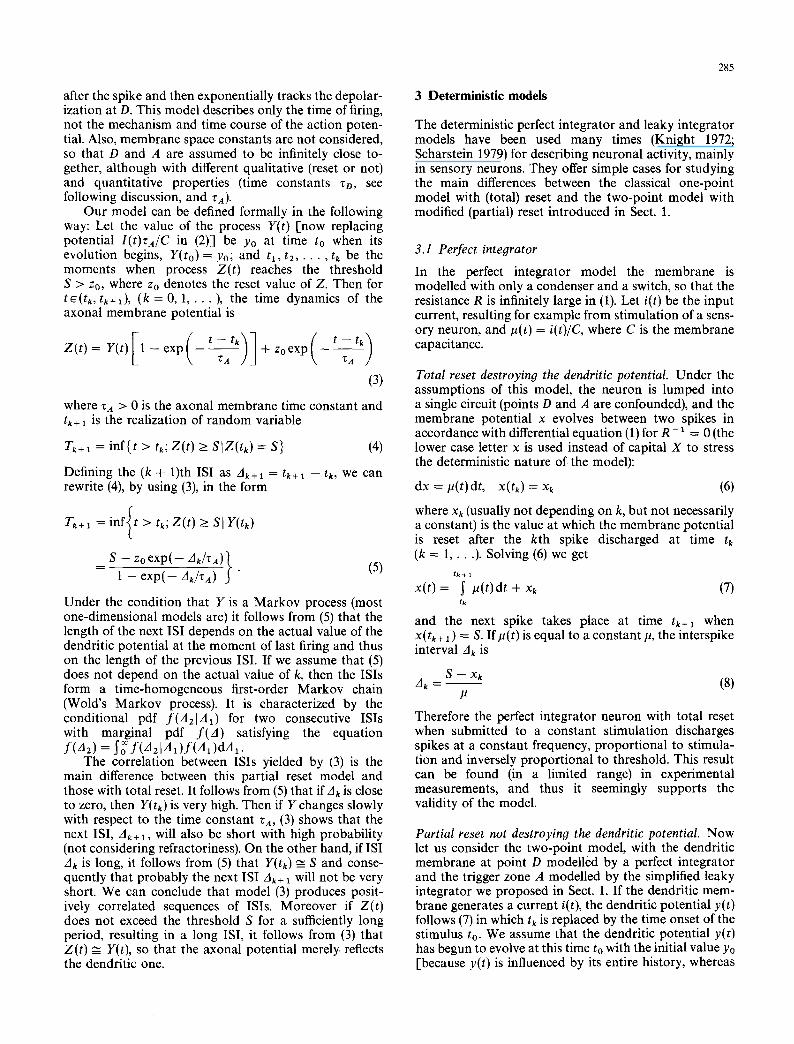
Fig. IA-C. Comparison of total and partial reset models when axonal potential is described by leaky integrator. A Level of stimulation is kept constant, then set to zero. B Total reset (one-point) model pro- duces constant ISis, and membrane potential X remains zero after resetting if no stimulation is present; #z is asymptotic level of membrane potential. C Partial reset (two-point) model produces constant ISis under constant stimulation; dendritic potential Y decays exponentially from steady-state level/~zo after end of stimulation while axonal poten- tial Z tracks trajectory of Y

3.2 Leaky integrator Now we suppose that membrane patches are described by leaky integrators either in the one-point (total reset) and two-point (partial reset) model neurons. In the two- point model we term zD and z~ the time constants of the dendritic and axonal membranes respectively. In the one- point model only one constant is considered and denoted r. The different behaviours of models are shown in Fig. 1.

Total reset destroying the dendritic potential. Under the assumptions of this model, which is the deterministic counterpart of (1), the membrane potential x evolves in accordance with the equation

where ~(t) is again the input of the neuron and x~ the reset value after the spike at time tk. If #(t) is equal to a constant p, then the solution of (11) is

x ( t ) = ~ t z I l - e x p ( t--ztk)]+XkeXp ( t--ztk )

(12)

which is a monotone function of time, with asymptotic level x( oo ) --/~z. If condition S < pz is imposed, then the model neuron fires regularly at intervals

A k = _ Z l n ( S Z l ~ - ~ . \ X k - - #T, ]

(13)

If the stimulation is stopped (/~ = 0) at the moment of spike tk, then the membrane potential decays exponenti- ally from the reset level x~ to zero. If the reset level is zero (as is usually assumed), then x(t)= 0 for t > tk (see Fig. 1B), because the basic assumption of the classical model is that the spike erases the dendritic potential.

Partial reset not destroying the dendritic potential. In the two-point model the equation for the axonal potential z(t) can be derived from (3) and (12). Assuming that y(to) = Yo and that the last spike took place at time tk > to, then for t > tk we have, combining properly modified versions of (12) and (3),

z(t) = #ZD + (Yo -- I~zv) exp t

+ zo exp . (14)

If to ~ tk, then we can assume y(t) = t~zD for t > tk and (14) takes the form

t - tk t z ( t ) = # z u [ 1 - e x p ( ~-A ) ] + z o e x p ( ~ t k ) .

(15)

This equation describes the same behaviour as (12). Con- sequently the model neuron with a dendrite described by

a leaky integrator without reset also fires regularly with period

A k = - -ZAln (S~- I tZ~ ~ (16) \Zo - p z o /

if the condition S < #ZD is met. Thus, unlike the perfect integrator, a constant input yields a constant output and, unlike the one-point model (13), the ISI given by (16) depends on both constants z~ and ~D. For p ~ + ~ , the limit of dk is 0 (except for the absolute refractory period taR). Result (16) could be expected, as/~ZD is the asymp- totic depolarization on the dendrite and if condition t ~ to is fulfilled then, following partial reset (3), the axon depolarization exponentially (with time constant zA) approaches to level /~za. The difference between the one- and two-point models becomes apparent when the input is not constant. For example, if at time of spike tk >> to the input is set to zero [#(t) = 0 for t > tk, which is the same example we studied in the one-point model], then from (12) we have for t > tk,

t t - - t k

+ zo exp . (17)

Instead of the constant (zero) value for x(t) yielded by the classical model, function (17) is not monotone. If we take zo = 0 then z(t) increases on the interval { tk, tk + ~A [ln(ZD + ZA) -- ln(zA)] } and then decreases to zero. In this way a spike can be produced even after canceling the external input if the residual dendritic potential y(t) is strong enough (Fig. 1C).

If instead of (3) Kohn's model is considered, i.e. two leaky integrators in series, the first one without reset and the second one with reset, then the firing period in the steady state is given by the formula in (16) in which the limiting level ~ D is replaced by #ZD~A. The difference between #zD and ~zDr~ depends on the scale for #, i.e. on the relationship between the external stimulation and i(t), which has to be specifically investigated. Neverthe- less our model qualitatively coincides with Kohn's when the input is constant and with the classical leaky integ- rator when zA = zD = z.

4 Stochastic models

The models presented in the previous section would be appropriate if we sought only the deterministic behavi- our of neurons. A stochastic description can be achieved merely by introducing some variability directly into these models, e.g. by postulating that # is replaced by a random variable U which is maintained constant between two consecutive spikes and sampled at each firing time tk. Levine and Shefner (1977; see also Levine 1991) used U in (7); then the distribution of ISis can be computed using (8) by assuming for example that U is gamma distributed (Smith 1979). Sclabassi (1976) used U in Eq. (12). It is clear that to ensure continuous firing, U has to be defined

287 '

on the interval (S/z, + oo). Then A k is the realization of a random variable whose distribution is a transformation of U given by (13). The outputs of both examples are, of course, renewal processes. However, we prefer to consider more realistic models where the input is continuously varying.

4.1 One-point model with total reset

Perfect integrator. The Wiener diffusion process with drift kt > 0 is defined by the SDE

dX = ladt + adW, X ( t k ) = Xk (18)

where # and a > 0 are constants characterizing respec- tively the intensity and variability of the neuronal input and W = { W(t); t _> 0} is a standard Wiener process with zero mean and variance t. Model (18) can be considered as the natural random counterpart of the deterministic perfect integrator (6) because the mean value of X in (18) coincides with the trajectory of model (6), and the mean ISI for this model is given by the right-hand side of (8).

Leaky integrator. One broad class of neuronal models can be based on Stein's concept (Stein 1965) in which the behaviour of the membrane potential is described by the SDE

dX = _ _1 Xd t + adN+(t) + idS - ( t ) , X ( t k ) = Xk (19) T

where z > 0 , i < 0 < a are constants, N + = { N +(t), t > 0}, N - = { N - (t), t _> 0} are two independent homo- geneous Poisson processes with N + (0) = N - (0) = 0 and intensities coa, 09~ respectively (for interpretation of (19) see e.g. Tuckwell 1988). Because the F P T problem is not easy to solve for (19) and because most central neurons bear a high number of synaptic endings, a diffusion approximation of Stein's model has been considered (e.g. Ricciardi and Sacerdote 1979; L~msk~ 1984). The limiting process is the Ornstein-Uhlenbeck process defined by the SDE

d X = ( - X + k t ) d t + a d W , X ( t k ) = x k (20)

where W,/t and a have the same interpretation as in (18). The mean value of process (20) coincides with the traject- ory of the deterministic leaky integrator in (11); conse- quently, model (20) can be considered as the diffusion counterpart of this deterministic model. If r ~ + ~ , the stochastic leaky integrator (20) tends to the perfect integ- rator (18), and Stein's model tends to the so-called ran- domized random walk (Feller 1971), which consequently possesses the feature of perfect integration.

4.2 Two-point model with partial reset

Application of (3) to Stein's model (19) or any other model presented before is formally simple as is shown in Fig. 2, which illustrates the difference between the orig- inal and modified Stein models. However, the solution of

288

o Y Lt tk

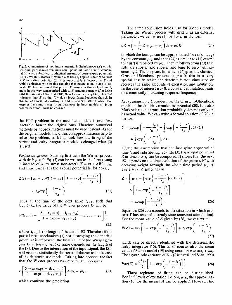
Fig. 2. Comparison of membrane potential in Stein's model (X) with its two-point partial-reset version (axonal potential Z and dendritic poten- tial Y) when submitted to identical streams of postsynaptic potentials (PSPs). When Z crosses threshold S at time tk a spike is fired with reset of Z to resting potential (0). Z is immediately influenced by Y and rapidly coincides with it; this explains that before spike, Y and Z co- incide. We have supposed that process X crosses the threshold at time tk

and is in this way synchronised with Z. X remains constant after firing until the arrival of the first PSP, then follows a completely different trajectory than Z, so that X yields a lower firing frequency than Z. In absence of threshold crossing X and Z coincide after a while. For keeping the same mean firing frequency in both models all input parameter values must be changed

the FPT problem in the modified models is even less tractable than in the original ones. Therefore numerical methods or approximations must be used instead. As for the original models, the diffusion approximations help to solve the problem, so let us look how the firing of the perfect and leaky integrator models is changed when (3) is used.

Perfect integrator. Starting first with the Wiener process with drift/t > 0, Eq. (3) can be written in the form (using Y instead of X to stress non-reset), Y = I~t + a W + Yo, and thus, using (18) the axonal potential is, for t > tk,

- - t k Z ( t ) = [ # t + a W ( t ) + yo] 1 - e x p

( t - - t k ) (21) + zoexp za

Thus at the time of the next spike tk+l, such that tk + 1 >> to, the value of the Wiener process W will be

F S_--__Zo exp_(--_ Ak+l/za) ] 1 W(tk+,) = [_ 1 - exp(-- Ak+t/za) -- ptk+l -- Yo

(22)

where Ak + ~ is the length of the actual ISI. Therefore if the partial reset mechanism (3) not destroying the dendritic potential is employed, the final value of the Wiener pro- cess W at the moment of spike depends on the length of the ISI. Due to the integration of the input signal, the ISis will become statistically shorter and shorter as in the case of the deterministic model. Taking into account the fact that the Wiener process has zero mean, (22) gives

E [ -S---s~ exp ( _--_ Ak+ 1/7~A)~ (23) [_ l - - exp( - -Ak+l /zA) ] + y~

which confirms the prediction.

The same conclusion holds also for Kohn's model. Taking the Wiener process with drift Y as an external parameter, we can write (1) for t > tk in the form

d Z = - - - Z + / ~ t + y o d t + a d W (24) zA

in which the term #t can be approximated for t ~ (tk, tk + 1 ) by the constant #tk, and then (24) is similar to (11) except that #(t) is replaced by Ptk. Then it follows from (13) that ISis are shorter and shorter and tend to zero with in- creasing k. The only case for which (24) gives the classical Ornstein-Uhlenbeck process is /~--0; this is a very special case in which the dendrite is not stimulated or receives the same amounts of excitation and inhibition. In the case of interest p > 0, a constant stimulation leads to a constantly increasing response frequency.

Leaky integrator. Consider now the Ornstein-Uhlenbeck model of the dendritic membrane potential (20). It is also Markovian as its transition probability depends only on its actual value. We can write a formal solution of (20) in the form

t -- to Y = y o e x p ( -~o ) + i e x p ( - t ~ o S ] a d W ( s )

to

Under the assumption that the last spike appeared at time tk and substituting (25) into (3), the axonal potential Z at time t > tk can be computed. It shows that the next ISI depends on the time evolution of the process W with decaying weight through the whole time period (to, t). For t ~> to, Z simplifies as

Z = [ l ~ Z D + ! e x p ( - t - ~ o s ) c r d W ( s ) ]

x [ 1 - exp( t ~ a t k ) l

+ zo exp ~ . (26)

Equation (26) corresponds to the situation in which pro- cess Y has reached a steady state (constant stimulation). For the mean value of Z given by (26), we can write

t - - t k t

(27)

which can be directly identified with the deterministic leaky integrator (15). This is, of course, also the mean value of Stein's model (19) using notation p = aO~a + i~ol. The asymptotic variance of Z is (Ricciardi and Sato 1990)

V a r ( Z ) - ~ I 1 - exp ( ~ t k ) ] 2 _ - t . ( 2 8 )

Three regimens of firing can be distinguished. For high levels of excitation, i.e. S ,~/~zo, the approxima- tion (16) for the mean ISI can be applied. However, the

condition relating threshold S to input # must be con- sidered with respect to the variance (28) of the process, which is controlled by a 2.

Low levels of excitation, on the other hand, are de- fined by S ~> ltzv, again relative to the variance (28), Var(Z) ~ Var [ Y( ~ )-I = a2~9/2. In this case the present model is equivalent to that analysed in detail by L~insk~ and Smith (1989, Sect. 4) under the condition that the axonal potential will not reach the dendritic potential during the refractory period (ZA ~ tAR) or a condition on the correlation time of process Y. Their model assumes that the axonal potential is reset to a random value which is here close to #vo. It results in an activity characterized by a coefficient of variation ( C V ) > 1 which tends to be Poissonian as S becomes higher (the CV, standard deviation/mean, is used as an approximate measure of the Poissonian character of firing, in which case CV = 1). Then the approximation of Keilson and Ross (1975) for the intensity of Poisson processes can be used. Even if the equivalence conditions are not met, the behaviours of both models are quite similar.

In the medium range, when the threshold is close to the asymptotic value of the process, S ~ #to, some ap- proximations can be made. Let us look for the condi- tional pdff(A21A1) for two consecutive ISis. Under the condition that the last ISI took the value A~, then the process Y took the value given by (5), y = [S - zoexp(--A1/ZA) ] [1 -- exp(-- A1/rA)] -1. Thus we are interested in the F P T of the Ornstein-Uhlenbeck process Y across the threshold S~ given by

$1 = S - z0exp( - t/ra) (29) 1 -- exp( -- t/Za)

under the condition Y(0) = y. Advanced methods exist for solutions of this problem, and an analytical solution for the threshold in the form S(t) = pro + A exp( - t/zo) is known (Ricciardi and Sato 1990, p 271). This is a differ- ent threshold from (29), but assuming that ZA = ZO = Z, S = #Zo (which corresponds to our original requirement), and t is not close to zero, then (29) can approximate this threshold and the conditional (pro + A > y) F P T den- sity is given by the formula

f(A2ly) =

2(#rD + A -- y)

a[1 - exp( -- 2A2/zD)]~/nv3[exp(2Az/ZD) -- 1]

{ ( p r o + A - y ) 2 } x exp . (30)

a2zD[exp(2A2/zo)- 1]

The results achieved by this approximation can serve as a lower bound for the ISI because the threshold used instead of (29) is lower. The conditional mode of (30) may be computed as

A,~= ? l n { ( p z o + A-- y)2 1 0"2TD 2

, , ' o,,~ (31)

289

6 0 ' ' ) ' 1 ' ' ' ' 1 ' ' ' ' 1 ' ' ' ' 1 ' ' ' '

A

50

'=~ 40

3o .z,

20

10

J

100 200 300

Serial number

400 500

100

lO

..=

= 1

. . 0 " . ~ * *

* ~ ~ .

~ . ~ **

o-~*,,~t~ s,..$~ ~ 1 7 6 1 7 6 ~ ~*** * ~* ~.. . *

~ ~ * ~ ~

, , , , , , , ,

o .

~

0 , 1 , , i i i , ) ) l , J i i h , , , I h i i i i J b

0.1 1 10 100

Interspike interval i + 1

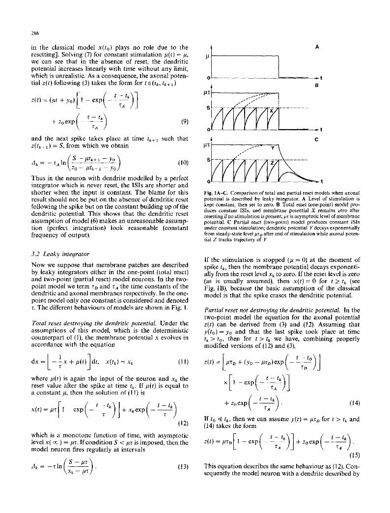
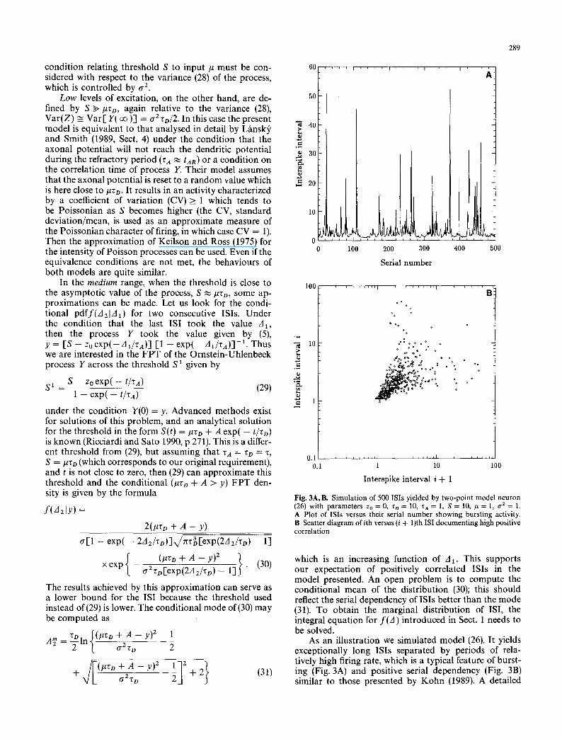
Fig. 3A, B. Simulation of 500 ISis yielded by two-point model neuron (26) with parameters Zo = 0, zo = 10, za = 1, S = 10, # = 1, 1 7 2 = 1. A Plot of ISis versus their serial n u mb e r showing burst ing activity. B Scatter d iagram of ith versus (i + 1)th ISI document ing high positive correlation

which is an increasing function of A1. This supports our expectation of positively correlated ISis in the model presented. An open problem is to compute the conditional mean of the distribution (30); this should reflect the serial dependency of ISis better than the mode (31). To obtain the marginal distribution of ISI, the integral equation for f (A) introduced in Sect. 1 needs to be solved.

As an illustration we simulated model (26). It yields exceptionally long ISis separated by periods of rela- tively high firing rate, which is a typical feature of burst- ing (Fig. 3A) and positive serial dependency (Fig. 3B) similar to those presented by Kohn (1989). A detailed

290

quantitative description of the model will require a deeper statistical study (in preparation).

5 Application to the first-order and second-order olfactory neurons

The first two layers of the olfactory system are made of a series of columnar elements interacting through inhibitory local neurons, each column being composed of typically 1000 first-order neurons terminating on a second-order neuron. Both types of neurons can be described by any of the models presented in Sect. 3 with obvious modifications. However, these models can be found too simplifying and more detailed descriptions can be looked for. For example, we recently proposed a one-point stochastic model of the first-order sensory neurons, also called neuroreceptors, in the olfactory system (Lfinsk~, and Rospars 1993) that can benefit from the two-point improvement, as presented now.

5.1 Dendritic potential

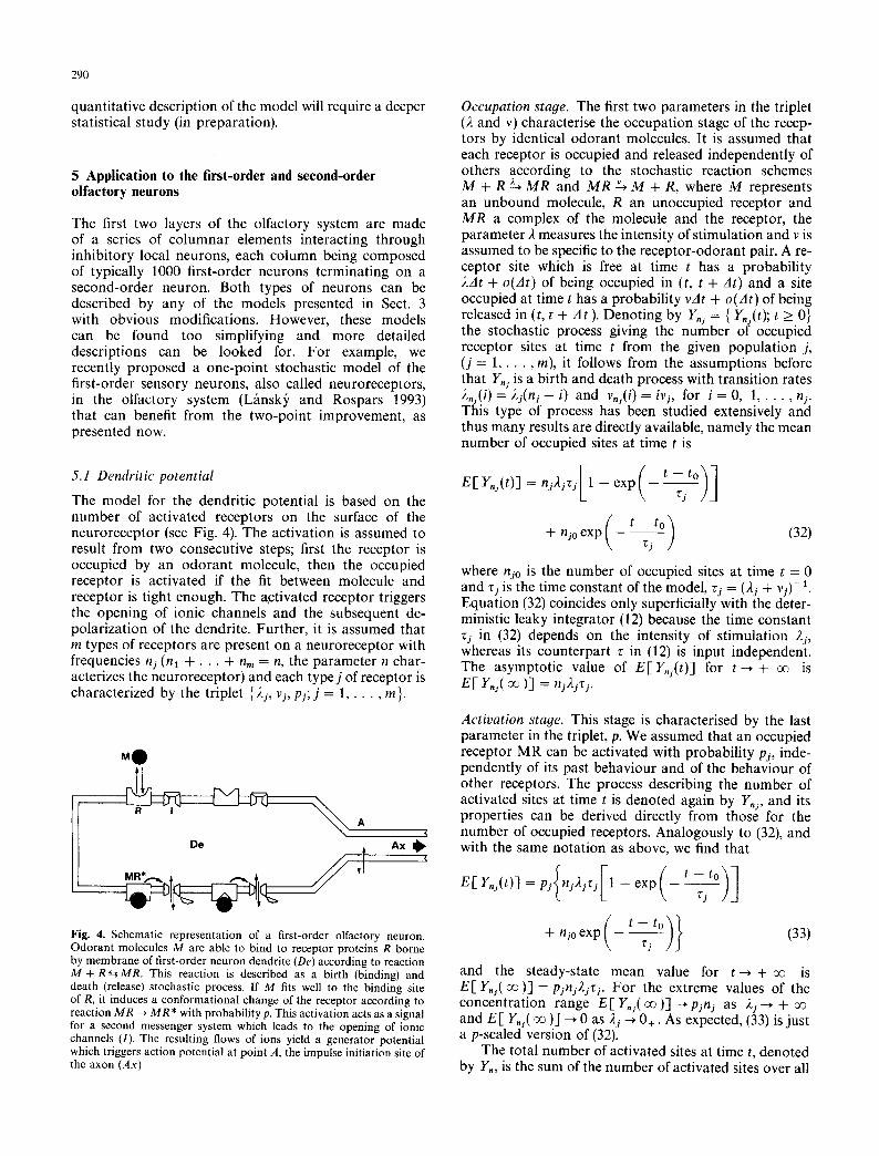
The model for the dendritic potential is based on the number of activated receptors on the surface of the neuroreceptor (see Fig. 4). The activation is assumed to result from two consecutive steps; first the receptor is occupied by an odorant molecule, then the occupied receptor is activated if the fit between molecule and receptor is tight enough. The activated receptor triggers the opening of ionic channels and the subsequent de- polarization of the dendrite. Further, it is assumed that m types of receptors are present on a neuroreceptor with frequencies nj (nl + �9 �9 �9 + n,, = n, the parameter n char- acterizes the neuroreceptor) and each type j of receptor is characterized by the triplet {2j, v~, pj; j = 1 . . . . . m}.

MO

De Ax {

Fig. 4. Schematic representation of a first-order olfactory neuron. Odorant molecules M are able to bind to receptor proteins R borne by membrane of first-order neuron dendrite (De) according to reaction M + R ~ , M R . This reaction is described as a birth (binding) and death (release) stochastic process. If M fits well to the binding site of R, it induces a conformational change of the receptor according to reaction M R ~ M R * with probability p. This activation acts as a signal for a second messenger system which leads to the opening of ionic channels (I). The resulting flows of ions yield a generator potential which triggers action potential at point A, the impulse initiation site of the axon ( A x )

Occupation stage. The first two parameters in the triplet (2 and v) characterise the occupation stage of the recep- tors by identical odorant molecules. It is assumed that each receptor is occupied and released independently of others according to the stochastic reaction schemes M + R ~ M R and M R ~ M + R, where M represents an unbound molecule, R an unoccupied receptor and M R a complex of the molecule and the receptor, the parameter 2 measures the intensity of stimulation and v is assumed to be specific to the receptor-odorant pair. A re- ceptor site which is free at time t has a probability 2At + o(At) of being occupied in (t, t + At) and a site occupied at time t has a probability vAt + o(At) of being released in (t, t + At ). Denoting by Y,j = { Y,j(t); t > 0} the stochastic process giving the number of occupied receptor sites at time t from the given population j, (j = 1 . . . . , m), it follows from the assumptions before that Y,j is a birth and death process with transition rates 2,j(i) = 2~(n~ - i) and v,j(i) = ivi, for i = 0, 1 . . . . . nj. This type of process has been studied extensively and thus many results are directly available, namely the mean number of occupied sites at time t is

t - - to

+ njo exp - (32) z j

where nio is the number of occupied sites at time t = 0 and rj is the time constant of the model, r i = (2 i + v j ) - 1 Equation (32) coincides only superficially with the deter- ministic leaky integrator (12) because the time constant r i in (32) depends on the intensity of stimulation 2i, whereas its counterpart z in (12) is input independent. The asymptotic value of E[Y , j ( t ) ] for t--* + ~ is E [ Y,j( ~ )] = nj2/cj.

Activation stage. This stage is characterised by the last parameter in the triplet, p. We assumed that an occupied receptor MR can be activated with probability pj, inde- pendently of its past behaviour and of the behaviour of other receptors. The process describing the number of activated sites at time t is denoted again by Y,j, and its properties can be derived directly from those for the number of occupied receptors. Analogously to (32), and with the same notation as above, we find that

t - - t o

- - t O + njo exp (33)

and the steady-state mean value for t--* + oo is E [ u = pjni2jz j. For the extreme values of the concentration range E [ Y , j ( ~ ) ] ~ pini as 2j ~ + and E[ Y,~( ~ )] ~ 0 as 2 i ~ 0+. As expected, (33) is just a p-scaled version of (32).

The total number of activated sites at time t, denoted by Y,, is the sum of the number of activated sites over all

291

subsets, 11, = S " . Y,. Thus the mean value of Y, can �9 �9 g . . . a j~ J. 2

be written directly from (33) as

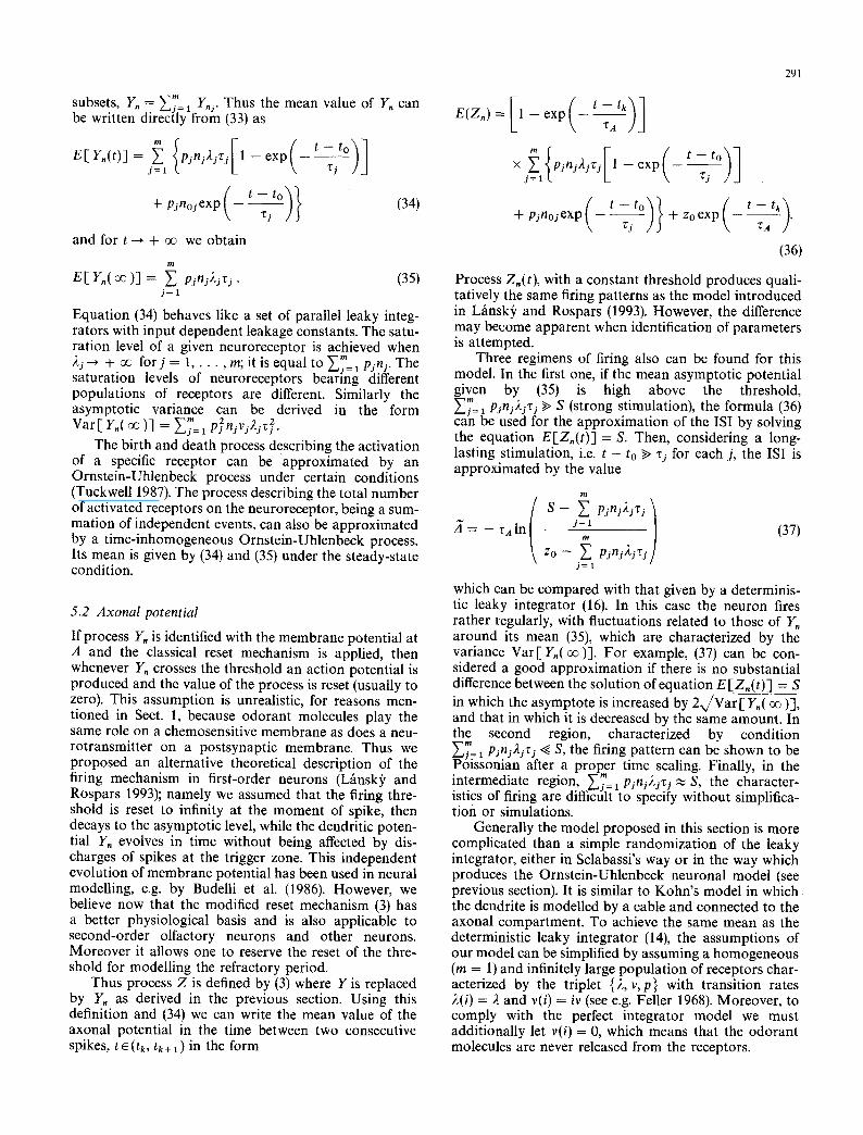
E[Y, ( t ) ] = pjnj2jzj 1 - exp j = l

- - t o + pjnojexp ~. (34)

and for t -* + oe we obtain

E [ IT,( oe )] = ~ pjni2jr j . (35) j = l

Equation (34) behaves like a set of parallel leaky integ- rators with input dependent leakage constants. The satu- ration level of a given neuroreceptor is achieved when 2~.--* + oo fo r j = 1 . . . . , m; it is equal to ~.~ . pjnj. The

J = l saturation levels of neuroreceptors bearing different populations of receptors are different. Similarly the asymptotic variance can be derived in the form V a r [ Y , ( m ) ] = ~ j= 1 2 2 m p j n j V j 2 j T j .

The birth and death process describing the activation of a specific receptor can be approximated by an Ornstein-Uhlenbeck process under certain conditions (Tuckwell 1987). The process describing the total number of activated receptors on the neuroreceptor, being a sum- mation of independent events, can also be approximated by a time-inhomogeneous Ornstein-Uhlenbeck process. Its mean is given by (34) and (35) under the steady-state condition.

5.2 Axonal potential

If process Y, is identified with the membrane potential at A and the classical reset mechanism is applied, then whenever Y, crosses the threshold an action potential is produced and the value of the process is reset (usually to zero). This assumption is unrealistic, for reasons men- tioned in Sect. 1, because odorant molecules play the same role on a chemosensitive membrane as does a neu- rotransmitter on a postsynaptic membrane. Thus we proposed an alternative theoretical description of the firing mechanism in first-order neurons (Lfinsk) and Rospars 1993); namely we assumed that the firing thre- shold is reset to infinity at the moment of spike, then decays to the asymptotic level, while the dendritic poten- tial Y, evolves in time without being affected by dis- charges of spikes at the trigger zone. This independent evolution of membrane potential has been used in neural modelling, e.g. by Budelli et al. (1986). However, we believe now that the modified reset mechanism (3) has a better physiological basis and is also applicable to second-order olfactory neurons and other neurons. Moreover it allows one to reserve the reset of the thre- shold for modelling the refractory period.

Thus process Z is defined by (3) where Y is replaced by Y~ as derived in the previous section. Using this definition and (34) we can write the mean value of the axonal potential in the time between two consecutive spikes, t~(tk, tk+l) in the form

E(Z,) = I1 -- exp ( t~-Atk)]

m t - - to xJ~=l{pjnj2jzJ[1--exp( ~ )1

+ pjnoj exp rj + Zo exp ~ .

(36)

Process Z,(t), with a constant threshold produces quali- tatively the same firing patterns as the model introduced in Lfinsk~ and Rospars (1993). However, the difference may become apparent when identification of parameters is attempted.

Three regimens of firing also can be found for this model. In the first one, if the mean asymptotic potential given by (35) is high above the threshold,

m ~j= ~ pjnj2jzj >> S (strong stimulation), the formula (36) can be used for the approximation of the ISI by solving the equation E[Z,(t)] = S. Then, considering a long- lasting stimulation, i.e. t - to >> zj for each j, the ISI is approximated by the value

S - ~ Pini2~zj zi = - rAIn j = 1 (37)

m

Zo- ~ pjnJ~jzj j = l

which can be compared with that given by a determinis- tic leaky integrator (16). In this case the neuron fires rather regularly, with fluctuations related to those of I1. around its mean (35), which are characterized by the variance Var[Y, (oo) ] . For example, (37) can be con- sidered a good approximation if there is no substantial difference between the solution of equation E [Z , ( t ) ] = S in which the asymptote is increased by 2x/Var [ Y~( oQ )], and that in which it is decreased by the same amoum. In the second region, characterized by condition ~i~=1 pjnj2jzj ~ S, the firing pattern can be shown to be Poissonian after a proper time scaling. Finally, in the intermediate region, ~j~-i p~nj2jzj ~ S, the character- istics of firing are difficult to specify without simplifica- tion or simulations.

Generally the model proposed in this section is more complicated than a simple randomization of the leaky integrator, either in Sclabassi's way or in the way which produces the Ornstein-Uhlenbeck neuronal model (see previous section). It is similar to Kohn's model in which the dendrite is modelled by a cable and connected to the axonal compartment. To achieve the same mean as the deterministic leaky integrator (14), the assumptions of our model can be simplified by assuming a homogeneous (m = 1) and infinitely large population of receptors char- acterized by the triplet {4, v,p} with transition rates 2(i) = ), and v(i) = iv (see e.g. Feller 1968). Moreover, to comply with the perfect integrator model we must additionally let v(i) = 0, which means that the odorant molecules are never released from the receptors�9

292

6 Discussion

6.1 Assumptions of the two-point model with partial reset

Information processing in the nervous system depends to a large extent on the transformation of the graded dendritic potential into a train of action potentials. The main characteristics of this transformation were estab- lished by extensive experimental investigations in sensory and central neurons (e.g. reviewed by Davis 1961, Galifret 1978, Kuffler et al. 1984), and neuron models should describe them adequately. Now, in most neuronal models in use the dendritic membrane potential is as- sumed to return to the resting level following the action potential. This simplification (here termed total reset) is unrealistic because there is no active resetting mechanism in dendrites.

A solution based on three assumptions is proposed in this article in an effort to avoid this discrepancy. The first assumption is the subdivision of the neuron in two compartments, dendrite and axon, instead of its usual lumping into only one representative compartment. The second one is that the dendritic compartment generates a graded (generator or postsynaptic) potential that de- pends only on the sensory or presynaptic stimulation of the neuron. The third assumption is that the representat- ive potential of the axonal compartment, which houses the spike-encoding mechanism, depends on the dendritic potential (a spike is fired when it crosses the threshold) and on the active repolarisation that follows the action potential. These properties are modelled by a simplified version of the RC circuit (leaky integrator) embodied in (3), which describes how the axonal potential returns to the level imposed by the dendritic potential. Equation (3) and the leaky integrator model are equivalent when the dendritic potential is constant, and approximately equiv- alent when it varies slowly, e.g. in a stimulated neuron close to steady state.

The partial reset model provides a more realistic description of the functioning of a neuron, while keeping several features of the previous models. In the application to the olfactory neuroreceptors, all conclusions derived previously are maintained, especially the existence of three regimens of firing according to the intensity of the odour stimulation (namely Poissonian, gamma-like and regular) and the sigmoid variation of the response fre- quency as a function of the logarithm of the odour concentration in the "regular" range. The main improve- ment brought about by our new model is to give a unified description of the first- and second-order neurons in the olfactory system. In our former attempt (Lfinsk~ and Rospars 1993), acceptable coding properties could be found only by suppressing the reset in neuroreceptors. In the second-order neurons resetting was maintained be- cause the classical models based on this concept were used. This discrepancy, which gave the main impetus to develop our present approach, has been corrected so that in both types of neurons the spike-encoding mechanism is the same.

In the model proposed, the axonal potential Z at point A depends on the dendritic potential Y at point

D but not vice versa, although D and A are infinitely close together. This asymmetry in the formulation of the model is the price to pay for having a simple (two-point) model which still retains the essential property that D is not reset. To formulate the model in more physiologically meaningful terms we may consider an elongated dendrite D'D, in contact with an axon by one of its ends D (as in insect neurons for example) and bearing odorant or neu- rotransmitter receptors on its other end D'. Then, de- polarization at D (and consequently A) is only a fraction of initial depolarization at D', but the repolarizing cur- rent at A during the falling phase of the action potential may not be strong enough to yield repolarization at D', which causes the aforementioned asymmetry. Of course, this is a simplification; actually an action potential can electrotonically invade dendrites and consequently mod- ify the dendritic currents. This complication has been neglected for keeping the model as simple as possible.

The absence of dendritic resetting in our model helps to show why the perfect integrator model of the mem- brane is too simplified and merely phenomenological. If the dendrite is modelled by such a circuit, which assumes the membrane is a perfect insulator, it is found that a constant stimulation is encoded by a spike train with frequency increasing to infinity. This unacceptable conse- quence is artificially avoided by resetting the dendritic potential each time a spike is generated. Therefore the perfect integrator with total reset is intrinsically unsatis- factory. Its close agreement with some properties of the data seems to result merely from the compensatory effects of two physiologically unrealistic mechanisms, perfect integration and total reset. However, a linear return to the firing level ("ramp-like" membrane poten- tial trajectory between two spikes), as expected from perfect integration with reset, has been experimentally observed and theoretically advocated by some authors (e.g. Stevens 1964; O'Neill et al. 1986). On the other hand, the close fit to experimental data suggests a misleading interpretation of the parameters specifying the model as pointed out by Levine (1991).

6.2 Properties of the model

Serial dependency. The main property of the model is its ability to predict positive serial dependency of ISis, i.e. a short (or long) ISI is expected to be followed with high probability by a short (respectively long) ISI. Serial de- pendency, both positive and negative, was often observed in real neurons (e.g. Correia and Landolt 1977; L~nsk~ and Radil 1987). This feature is not found in classical models with total reset which predict independent ISis. In this case other phenomena must be considered, such as inhibitory feedback (e.g. Perkel and Mulloney 1974; Floyd et al. 1982). However, these improvements yield only negative correlation, i.e. a short ISI is expected to follow a long one and vice versa, so that they leave unexplained the positive correlation observed. Now a more complete picture emerges because the inclusion of these sources of negative correlation in our partial reset model, which acts by itself as a source of positive correla- tion, would bring about the whole range of correlations

observed according to the balance of these opposite effects. The common descriptions of experiments in which spikes are recorded are based on histograms for estimating the marginal pdf of ISis and on computations of their sample moments, namely mean (or its reciprocal value which is confusingly called mean firing frequency) and variance. However, the pdf and moments give a com- plete description only when ISis form a renewal process, which is not the case at present. Here, as the spike moments are not regenerative points of the underlying point process, descriptions of higher dimension (e.g. autocorrelation coefficients, intensity function, spectral properties) are needed. These characteristics have been difficult to derive analytically, and thus simulation ex- periments will have to be performed.

The activity of the model introduced does not depend on its entire history but it produces ISis forming a Markov chain (Wold's Markov process). It means that the stochastic properties of the current ISI are deter- mined exclusively by the length of the previous one. Yamamoto and Nakahama (1983) computed from their experiments first-order joint interval histograms (similar to those of Kohn 1989) illustrating positive serial depend- ency, together with arguments for a higher-order Markov property. As pointed out before, the introduced model produces only the first-order Markov property, so that an unsolved question arises: if the leaky integrator (1) is used instead of the simplified version (3), is the current ISI determined only by the previous one or by the whole firing history?

Bursts and lon9 silences. Bursting is a very frequent type of neuronal behaviour found in different experimental preparations (e.g. Deving and Hyvfirinen 1969; Barbi and Ferdeghini 1980; Nagai and Ueda 1981; Yamamoto et al. 1986). Theoretical models of bursting are often based on the assumption of two alternating states during which the spikes are either blocked or produced (e.g. De Kwaadsteniet 1982; Griineis et al. 1989). A disadvantage of these models is that despite their close resemblance to the observed data, they are not based on biological reasoning. The other models for bursting utilize the con- cept of strong lateral inhibition (Barbi and Ferdeghini 1980) which is not acceptable for example in the case of olfactory neuroreceptors. Kohn (1989) also studied a two-compartment model which is close to that pres- ented here, with the axonal compartment (trigger zone) modelled by a leaky integrator. He investigated it by computer simulation, as the properties of his model (and to a lesser extent ours) are not derivable analytically. One of his main conclusions was that "dendritic inputs result- ed in a tendency for random bursting, ISI histograms with long tails and CV larger than one". These three features, which apply also to our model, have not the same status however. Bursts and long tails are related phenomena that become visible when serial correlation is high enough. If the correlation time of dendritic process Y, i.e. the time after which the potential is no longer influenced by its previous values, is short, then Y can be regarded as a white noise and the membrane potential behaves like the Wiener process. On the other hand, if the

293

correlation time (relatively to %) is long, the trajectory of Y may be expected not to change abruptly. When Y is high above the threshold it stays there for a certain time and the model produces a sequence of short ISis which can be interpreted as a burst. Similarly, when Y falls below the threshold it yields exceptionally long ISis, i.e. periods of silence between bursts, that cause the long tails of ISI histograms. Bursting and long ISis cannot be explained by total reset models without applying ad hoc (e.g. periodic) external stimulation and thus appear as specific features of partial reset models.

Coefficient of variation. CVs larger than one have been found in most experimental studies mentioned up to now, and they are not specific to partial reset models. They have been found in several neuronal models when- ever the reset value is chosen above the resting potential, as shown by Hanson and Tuckwell (1983) for the model with reversal potentials, L~insk) and Smith (1989) for (18) and (20) and Lfinsk) and Musila (1991) for (19). This is not surprising because such a reset partly mimics the persistent effect of the dendritic compartment over the trigger zone which characterises the partial reset models. However, this feature results from a more physiological assumption in the latter.

Latency and after-effect. The partial (Kohn's and ours) and total reset models behave differently in the transient states. Stein et al. (1974) noted that, in models with total reset, a step change of the input induces an immediate change of the output frequency to a new constant firing level, e.g. when the stimulation is turned on and off. This property being, in general, not shared by real neurons, these authors tried to describe it by direct modelling of the firing frequency using the first-order differential equa- tion. In this way a step change in stimulation results in an exponential change of the response frequency. A similar behaviour is also displayed by the partial reset models as a natural consequence of their more realistic basic as- sumptions that try to simulate physiological phenomena. Under constant stimulation the deterministic partial reset models coincide with the total reset ones because, in this case, the dendritic leaky integrator merely transforms a constant input into a constant dendritic potential.

Acknowledgements. This work has been partly supported by Academy of Sciences of the Czech Republic grant 511101, a fellowship from the Institut National de la Recherche Agronomique (to P.L.) and grant 90 C 702 "Sciences de la Cognition" from the Ministrre de la Recherche et de la Technologie (to J.P.R.).

References

Barbi M, Ferdeghini EM (1980) Relevance of the single ommatidium performance in determining the oscillatory response of the Limulus retina. Biol Cybern 39:45-51

Budelli RW, Soto E, Gonz~lez-Estrada MT, Macadar O (1986) A spike generator mechanism model simulates utricular afferents response to sinusoidal vibrations. Biol Cybern 54:237-244

Correia M J, Landolt JP (1977) A point process analysis of the spontan- eous activity of anterior semicircular canal units in the anesthetized pigeon. Biol Cybern 27:199-213

294

Davis H (1961) Some principles of sensory receptor action. Physiol Rev 41:391 416

De Kwaadsteniet JW (1982) Statistical analysis and stochastic modeling of neuronal spike train activity. Math Biosci 60:17-71

Doving K, Hyv/irinen J (1969) Afferent and efferent influences on the activity pattern of single olfactory neurons. Acta Physiol Scand 75:111-123

Eccles JC (1957) The physiology of nerve cells. Johns Hopkins Univer- sity Press, Baltimore

Feller W (1968) An introduction to probability theory and its applica- tion, vol 1. Wiley, New York

Feller W (I 971) An introduction to probability theory and its applica- tion, vol 2. Wiley, New York

Floyd K, Hick VE, Holden AV, Koley J, Morrison JFB (1982) Non-Markov negative correlation between interspike intervals in mammalian afferent discharge. Biol Cybern 45:89-93

Galifret Y (1978) Les m6canismes de transduction sensorielle. J Physiol (Paris) 74:121-129

Gerstein GL, Mandelbrot B (1964) Random walk models for the spike activity of a single neuron. Biophys J 4:41-68

Grfineis F, Nakao M, Yamamoto M, Musha T, Nakahama H (1989) An interpretation of I / f fluctuation in neuronal spike trains during dream sleep. Biol Cybern 60:161 169

Hanson FB, Tuckwell HC (1983) Diffusion approximation for neuronal activity including synaptic reversal potentials. J Theor Neurobiol 2:127-153

Kallianpur G, Wolpert RL (1987) Weak convergence of stochastic neuronal models. In: Kimura M, Kallianpur G, Hida T (eds) Stochastic methods in biology. Springer, Berlin Heidelberg New York, pp 116-145

Keilson J, Ross HF (1975) Passage time distributions for Gaussian Markov (Ornstein-Uhlenbeck) statistical processes. Selected Tables Math Stat 3:233-327

Knight BW (1972) Dynamics of encoding in a population of neurons. J Gen Physiol 59:734-766

Kohn A F (1989) Dendritic transformations on random synaptic inputs as measured from a neuron's spike train. Modeling and simulation. IEEE Trans Biomed Eng 36:44-54

Kuffler SW, Nicholls KR, Martin AR (1984) From neuron to brain. Sinauer, Sunderland, USA

Lfinsk~ P (1984) On approximations of Stein's neuronal model. J Theor Biol 107:631-647

Lfinsk~, P, Musila M (1991) Variable initial depolarization in Stein's neuronal model with synaptic reversal potentials. Biol Cybern 64:285-291

Lfinsk~, P, Radii T (1987) Statistical inference on spontaneous neuronal discharge patterns. Biol Cybern 55:299-311

Lfinsk~ P, Rospars JP (1993) Coding of odor intensity. BioSystems (in press)

Lfinsk~, P, Smith CE (1989) The effect of a random initial condition in neural first-passage-time models. Math Biosci 93:191-215

Lapicque L (1907) Recherches quantitatives sur I'excitation 6lectrique des nerfs traitbe comme une polarisation. J Physiol Pathol Gen 9:620-635

Levine MW (1991) The distribution of the intervals between neural impulses in the maintained discharges of retinal ganglion cells. Biol Cybern 65:459-467

Levine MW, Shefner JM (1977) A model for the variability ofinterspike intervals during sustained firing of retinal neurons. Biophys J 19:241-252

Nagai T, Ueda K (1981) Stochastic properties of gustatory impulse discharges in rat chorda tympani fibers. J Neurophysiol 45:574-592

O'Neill WD, Lin JC, Ma Y-C (1986) Estimation and verification of a stochastic neuron model. IEEE Trans Biomed Eng 33:654-666

Perkel DH, Mulloney B (1974) Motor pattern production in recipro- cally inhibitory neurons exhibiting postinhibitory rebound. Science 185:181-183

Ricciardi LM, Sacerdote L (1979) The Ornstein-Uhlenbeck process as a model of neuronal activity. Biol Cybern 35:1-9

Ricciardi LM, Sato S (1990) Diffusion processes and first-passage-time problems. In: Ricciardi LM (ed) Lectures in applied mathematics and informatics. Manchester University Press, Manchester, pp 206~85

Scharstein H (1979) Input-output relationship of the leaky-integrator neuron model. J Math Biol 8:403-420

Sclabassi RJ (t976) Neuronal models, spike trains and the inverse problem. Math Biosci 32:203-219

Shepherd GM (1988) Neurobiology. Oxford University Press, New York

Smith CE (1979) A comment on a retinal neuron model. Biophys J 25:385-386

Stein RB (1965) A theoretical analysis of neuronal variability. Biophys J 5:173-195

Stein RB, Leung KV, Mangeron D, O~uzt6reli (1974) Improved neur- onal models for studying neural networks. Kybernetik 15:1-9

Stevens CF (1964) Letter to the editor. Biophys J 4:417-419 Tuckwell HC (1987) Diffusion approximations to channel noise.

J Theor Biol 127:427-438 Tuckwell HC (1988) Introduction to theoretical neurobiology. Cam-

bridge University Press, Cambridge, UK Tuckwell HC, Wan FYM, Wong YS (1984) The interspike interval of

a cable model neuron with white noise input. Biol Cybern 49:155-167

Yamamoto M, Nakahama H (1983) Stochastic properties of spontan- eous unit discharges in somatosensory cortex and mesencephalic reticular formation during sleep-waking states. J Neurophysiol 49:1182-1198

Yamamoto M, Nakahama H, Shima K, Kodama T, Mushiake H (1986) Markov-dependency and spectral analysis on spike-counts in mes- encephalic reticular neurons during sleep and attentive states. Brain Res 366:279-298