Realistic computer modeling of the

mammalian olfactory cortex

Thesis by

Michael Christopher Valiier

In Partial Fulfillment of the Requirements

for the Degree of

Doctor of Philosophy

California Institute of Technology

Pasadena, Califorliia

2001

(Defended May 21. 2001)

0 2 0 0 1

Michael Christopher Vanier

,411 Rights Reserved

Acknowledgements

I have been at Caltech as a graduate student for a long time. so I have a corresporidinglp

long list of people to thank:

Jim Bower, my supervisor. for givilig me guidance about all aspects of science (the

official arid especially the unofficial), for being a friend, for singing in my rock band (which

he mistakenly thought was his rock band). for his patience. support and encouragement

even when I was veering wildly away from the official subject of my thesis work. and for

d e r n o n s t r a t that, a scientist doesn't have to be a boring person.

My Ph.D. committee rnernbers for their support, their interest. arid their encouragement.

I've always felt I had the best Ph.D. committee a student could ask for.

Everyone in the Bower lab for their support, friendship arid ericouragement.

Dave Beeman and everyone else in the GENESIS project for being a stilnulating and

fun group of people to he associated with.

Dave Bilitch. for teaching me an enornious aniount about computer programrrling through

a nlixture of good advice and bad example,

Upi Bhalla. for iriteresting discussions. for supplyirig rile with his olfactory bulb data

arid being willing to answer r n y rliarly questions about it. for his work on GENESIS. for his

serisc of humor. arid fbr being arl all-arolind fiiie person. Science could use more people like

T;Ofl.

Lrw Hahrrlg. who I've r~ever rilet . for his fine experimental work on the piriforni cortex

. *.

111

on which mrlch of the work described in this thesis is built. As a piriforril cortex modeler.

I aril very nluch indebted to him.

Matt Wilson, for building the first version of GENESIS and for building the first versiorl

of the piriform cortex model. I can't believe how much Matt accon1plislied given tlle limited

amount of data that was then available. Matt's nlodeling approacli. especially his approach

to handling scaling issues in network models, was a major influence on niy model.

Alex Protopapas, for providing me with most of the intracellular data that formed

the basis of this model and was an integral component of my two methodological papers.

Working with Alex was a pleasure.

Karim Elaagouby. for helping me get my brain-slice electrophysiology setup working

against all odds. Without Karim's help, I might never have finished my experi~nental work.

Dave Kewley, for sysadmin services above and beyond the call of duty. In particular.

t hanks to Dave for last-minute color printer fixes under desperate circumstances.

Also. on a more personal level, fed like to thank:

Rfy mother. Anna Dodge Vanier, for putting up with me and my sornemrhat rocky path

towards personal gro~;vtli. Morn has beer1 and contiln~es to be an unflinching source of love,

snpport and inspiration even in the most difficult times of this projcct.

Jar1 Tivol. whose love and friendsliip did more than a~iyorze else to keep me sane during

the last ftlw years. You're the best!

Claire Sergeant. for long-distaricr encouragement and for being a souridirig board for

my comedy routines in progress. We discussed nly work. we laughed about it. arid then

Hemingway punched us both in tlie nose.

Kayla Smith, for friendship and for being my new comedy buddy.

My friends Ernesto -'Boom Boorn" Soares. Alfredo "Toa1 ,Sonesl' Font anini, and Robert

.'Mr. Sensitive" Sneddorl, for being fun to hang out with. Thanks to Ernesto for getting me

irivolved in the Babe and Ricky's blues scene (see below), to Robert for lots of politically

incorrect conversations, and to Alfredo for teaching me to swear in Italian and for sharing

my affinity for clieesy lounge music (don't laugh: ita7s not unusual...). I especially want to

thank Alfredo for many useful conversatiorrs and for proofreadirlg large parts of t his thesis.

Sllana Coates for making my secorld summer in Woods Hole very memorable indeed :-)

Because of Shana I will probably have a fetish for women with English accents for the rest

of my life.

Melanie Walker. fbr her sense of humor. for being diEerent. a ~ i d for not taking herself

too seriously.

The folks at Air Adventures West in Taft, California, for teaclling me to skydivc. I can't

possibly hope to repay that: it changed my life.

The blks at TACIT (Theater Arts at t lie California Institute of Teclinology ) , for teachirlg

me to act. a very useful skill for a Caltcch grad student.

Sfanla and the hlks at Babe arid Rjeky's, for letting me play the blues in a real blurs

bar.

Don and Welidy Caldwell arid the Galtech Chamber Singers, for teaching me to sing.

for allowing me to play Dr. Harold Hill (a drearrl come true!) arid for some great times.

Jim Boyk, for teaching me to play piano and for being an all-around amazing guy. I

have met many cool people at Caltech but Jim is the coolest. If I ever make a lot of money,

Jirri will be set for life: that's a promise!

Linda Chappell, for helping me with housing problems while I was at Caltech. Thanks.

Linda!

Richard Stallman and the GNU project, for all the great software and inspiration. and

for lettirig me be a (very minor) part of it all.

Linus Torvalds and the Linux project, for a great operating system and for helping to

rid the world of Microsofi.

Mike Hucka. hacker and sysadmin extraordinaire, for being a great friend and for being

my iiberhacker. I'ni so glad I recruited yon :-)

Dedieat ion

I dedicate this thesis to the memory of my father. Andre Guy h n i e r . His love and his

sense of humor will be with me always.

Abstract

A co1.l-ibination of experiinental and computer modeling techriiques were used to investti-

gate t lle dynamics and cornputat ional fililctio~is of the rat olfactory j~>iriform) cortex. Ex-

perinlental characterization of synaptic responses to afferent and associatio~ial fiber voltage

sliocks were performed, in the preseilce and absence of the neuromodulator norepinephrine.

This data was used to generate computer models of synaptic transmission in piriform cor-

tex. Models of pyramidal neurons and feedback inhibitory interneurons were constructed

which accurately match intracellular experimental data in the presence arid absence of

norepinephrine. In order to achieve this, parameter search tools for autornatically match-

iiig computer models of neurons to data were developed. Models of feedforward iilhibitory

interrleurons were also constructed. An abstract spike generating model of the olfactory

bulb was built. These componeiits were combined to create a realistic computer rriodel of

the piriform cortex. This inode1 can accurately replicate the response of the real systerrz

to a strong shock stimulus, as reflected in current source density plots. Two versions of

the lnodel were created to model the oscillatory response of the system to weak shocks.

The first model replicates the surface field potential wit11 considc~rable accuracyI but fails to

replicat c. t lie crirrent source dexisity data. The second iilodel replicates the current source

density data and silggests a new organizirig principle for the olfactory systoni based on

noii-oxrerlapping ileuro~ial groups. This liypotllesis is experimentally testable.

Contents

I Introduction 1

. . . . . . . . . . . . . . . . . . . . . . . . . . . . . . 1.1 Overview of the thesis 3

. . . . . . . . . . . . . . . . . . . . . . . . 1.2 The rnarrlrnalian olfactory system 5

. . . . . . . . . . . . . . 1.2.1 The olfactory epithelium alid olfactory bulb 5

1.2.2 Primary olfactory (piriform) cortex . . . . . . . . . . . . . . . . . . . 7

. . . . . . . . . . . . . . . . . . . 1.2.3 Oscillations in the olfactory system 11

. . . . . . . . . . . . . . . . . . . . . . . . . . 1.3 Modeling tlle piriform cortex 16

. . . . . . . . . . . . 1.3.1 Why build realistic models of piriforril cortex? 16

. . . . . . . . . . . . . . . . . . . . . . . . . . . . 1.3.2 Realistic modeling 19

. . . . . . . . . . . . . . . . . . 1.3.3 The previous piriforln cortex model 20

. . . . . . . . . . . . . . . . . . . . . . . . . . . 1.3.3 New rrlodel features 20

. . . . . . . . . . . . . . . . . . . . . . . . . . . . 3 . 5 Tuning the nmdrl 22

. . . . . . . . . . . . . . . . . . . . . . 1.4 Questioxls the model can help arlswer 23

. . . . . . . . . . . . . . . . . . . . . 1 Codinginthrolfa~torysyst~rrrl 23

. . . . . . . . . . . . . . . . . . . 1.3.2 Origin and h c t i o n s of oscillations 25

. . . . . . . . . . . . . . . . 1 .4.3 Nenrornodnlat iorl in the pirifornl cortxx 26

. . . . . . . . . . . . . . . . . . . . . . . . . . . . . . . . 1.4.4 Other issues 26

. . . . . . . . . . . . . . . . . . . . . . . . . . . . . 1.5 &lodeling methodologies 27

. . . . . . . . . . . . . . . . . . . . . . . . . 1.5.1 Sirnulatiori erivironment 27

. . . . . . . . . . . . . . . . . . . . . . . . . . . 1.5.2 Parameter searching 27

. . . . . . . . . . . . . . . . . . . . . . . . . . . . 1.5.3 Bayesian methods 28

. . . . . . . . . . . . . . . . . . . . . . . 1.6 New work suggested by the model 29

. . . . . . . . . . . . . . . . . . . . . . . . . . . . 1.6.1 Experimerktal work 29

. . . . . . . . . . . . . . . . . . . . . . . . . . . . . . 1.6.2 Modelirlg work 30

. . . . . . . . . . . . . . . . . . . . . . . . 1.7 Summary of thesis contributions 31

. . . . . . . . . . . . . . . . . . . . . 1.7.1 The new piriform cortex model 31

. . . . . . . . . . . . . . . . . . . . . . . . . 1.7.2 Lessons from tlie model 32

. . . . . . . . . . . . . . . . . . . . . . . . . . . . 1.7.3 Experimerrtal work 33

. . . . . . . . . . . . . . . . . . . . 1.7.4 Developnient of simulation tools 33

I1 Experimental studies 47

2 Synaptic ERects of Norepinephrine in Piriform Cortex 53

. . . . . . . . . . . . . . . . . . . . . . . . . . . . . . . . . . . . . . 2.1 Abstiract 53

2.2 Iritrodrtetion . . . . . . . . . . . . . . . . . . . . . . . . . . . . . . . . . . . . 54

. . . . . . . . . . . . . . . . . . . . . . . . . . . . . . 2.3 Materials arid hiiletliods 57

2.3.1 Preparation of brain slices . . . . . . . . . . . . . . . . . . . . . . . . 57

2.3.2 Preparatio~l and applicatiori of pharmaceuticals . . . . . . . . . . . . 59

2.3.3 E1ectroph;vsiology . . . . . . . . . . . . . . . . . . . . . . . . . . . . . 59

. . . . . . . . . . . . . . . . . . . . . . . . . . . . . . . 2.3.4 Data analysis 61

. . . . . . . . . . . . . . . . . . . . . . . . . . . . . . . . . . . . . . . 2.4 Results 63

2.4.1 Synaptic effects of norepirlephrine . . . . . . . . . . . . . . . . . . . 63

2.4.2 Concentration-dependence of effects . . . . . . . . . . . . . . . . . . 63

2.4.3 Pharmacology of effects . . . . . . . . . . . . . . . . . . . . . . . . . 66

2.4.4 Effects of norepinephrine on paired-pulse facilitation . . . . . . . . . 68

. . . . . . . . . . . . . . . . . . . . . . . . . . . . . . . . . . . . . 2.5 Discussion 70

2.5.1 Differential effects of NE on layer l a and lb field potentials . . . . . 70

2.5.2 Pharmac.ologica1 basis for the NE effects in layer l a and I b . . . . . 72

2.5.3 Diff'erences from previously reported results . . . . . . . . . . . . . . 74

2.5.4 Funet iorlal significance . . . . . . . . . . . . . . . . . . . . . . . . . . 75

111 Matching neural models to experimental data

3 A Comparative Survey of Automated Parameter Search hqethods

for CompartmenLaf Neural Models 95

. . . . . . . . . . . . . . . . . . . . . . . . . . . . . . . . . . . . . . 3.1 Abstract 95

. . . . . . . . . . . . . . . . . . . . . . . . . . . . . . . . . . . . 3.2 1ntroduc.tiori 96

. . . . . . . . . . . . . . . . . . . . . . . . . . . . . . . . . . . . . . 3.3 Methods 99

. . . . . . . . . . . . 3.3.1 Sirnulation erivironrr~er~t and data analysis tools 99

. . . . . . . . . . . . . . . . . . . . . . . . . . . . . . . . . . 3.3.2 Models 100

. . . . . . . . . . . . . . . . . . . . . . . . . . . . . 3.3.3 Target data sets 106

. . . . . . . . . . . 3.3.4 Computing the niatch between data and models 107

. . . . . . . . . . . . . . . . . . . . . . . . 3.3.5 Parameter search methods 109

. . . . . . . . . . . . . . . . . . . . . . . . . . . . 3.3.6 Statisticalanalyses 116

. . . . . . . . . . . . . . . . . . . . . . . . . . 3.3.7 Resource requirements 117

. . . . . . . . . . . . . . . . . . . . . . . . . . . . . . . . . . . . . . . 3.4 Results 118

. . . . . . . . . . . . . . . . . . . . . . . . . . 3.4.1 Sirnple spiking models 118

. . . . . . . . . . . . . . . . . . . . . . . . . . . 3.4.2 Passive cable models 121

. . . . . . . . . . . . . . . . . . . . . . . . . . . 3.4.3 Pyramidal cell model 127

. . . . . . . . . . . . . . . . . . . . . . . . . . . . . . . . . . . . . 3.5 Discussiorl 134

. . . . . . . . . . . . . . . . . . . . . . . . . . . 3.5.1 Method comparisons 131

. . . . . . . . . . . . . . . 3.5.2 Differences betweer1 t llr search algorit hrns 13'7

. . . . . . . . . . . . . . . . . . . . . . . . . . . . 3.5.3 Mstdling functions 140

. . . . . . . . . . . . . . . . . . . . . 3.5.4 Variation in the pararrirter sets 111

. . . . . . . . . . . . . . . . . . . . 3.5.5 Robustrlrss of the paramrt+rr sets 143

. . . . . . . . . . 3.5.6 Recommendatior~s for effective paranietcr searchirig 114

. . . . . . . . . . . . . 3.5.7 Limitsations of paranletrr searching tecluliques 145

. . . . . . . . . . . . . . . . . . . . . . . . . . . . . . . . 3.6 Acknowledgeri~ents 149

. . . . . . . . . . . . . . . . . . . . . . . . . . 3.7 Ap~~endix: Model descri~jtions 157

4 On the Use of Bayesian Methods for Evaluating Compartmental

Neural Models 159

. . . . . . . . . . . . . . . . . . . . . . . . . . . . . . . . . . . . . . 4.1 Abstract 159

. . . . . . . . . . . . . . . . . . . . . . . . . . . . . . . . . . . . 4.2 Introduction 160

. . . . . . . . . . . . . . . . . . . . . . . . . . . . . . . . 4.3 Bayesian inference 166

. . . . . . . . . . . . . . . . . . . . . . . 1.4 Bayesiaxl compartment a1 rxlodeli~ig 171

. . . . . . . . . . . . . 4.4.1 Prior probabilities for compartmental niodrls 171

. . . . . . . . . . . . . . . . . 4.4.2 Likelihoods for compartrnerital models 174

. . . . . . . . . . . . . . . . . . . . . . . . . . . . . . . . . . . . . 4.5 Examples 187

. . . . . . . . . . . . . . . . . . . . . . . . . 1.5.1 Objectives and methods 187

. . . . . . . . . . . . . . . . . . . . . . . . . . . . . . . . . 4.5.2 The data 189

. . . . . . . . . . . . . . . . . . . . . . . . . . . . . . . . 4.5.3 The inodels 192

. . . . 4.5.4 I'arairleter estimation: dcternlini~lg optimal parameter values 200

. . . . . . . . . . 4 . 5 Corilpsriilg individual models from the same class 202

. . . . . . . . . . 1.5.6 Comparing illdivid~ial models from diEerent classes 205

. . . . . . . . . . . . . . . . . . . . . 4.5.7 Cornparirlg eiltirr rriodel classes 209

3.5.8 Estiniating the optirnal arxiount of noise for a noisy wramidal cell

model . . . . . . . . . . . . . . . . . . . . . . . . . . . . . . . . . . . 213

4.6 Discussion . . . . . . . . . . . . . . . . . . . . . . . . . . . . . . . . . . . . . 223

IV Modeling the piriform cortex

5 Building Models of Single Neurons in Piriforrn Cortex 253

5.1 Piriform cortex neurons . . . . . . . . . . . . . . . . . . . . . . . . . . . . . 253

. . . . . . . . . . . . . . . . . . . . . . . 5.2 Computer simulation environment 257

5.3 Modeling layer 2 pyramidal neurons . . . . . . . . . . . . . . . . . . . . . . 257

. . . . . . . . . . . . . . . . . . . . . . . . . . . . . . . . . . 5.3.1 Data set 257

5.3.2 Simplifying the neuron morphology . . . . . . . . . . . . . . . . . . . 258

. . . . . . . . . . . . . . . . . . . . . . . . . . . . 5.3.3 Building the model 267

. . . . . . . . . . . . . . . . . . . . . . . . . . . . 5.3.4 Tuning the rnodel 267

. . . . . . . . . . . . . . . . . . . . . . . . . . . . . 5.3.5 Neuroxxlsdulation 269

. . . . . . . . . . . . . . . . . . . . . . . . . . . 5.4 Modeling irihibitory neuroxls 271

. . . . . . . . . . . . . . . . . . . . . . . . . . . . . . . . . . 5.4.1 Dataset 271

5.4.2 Buildirlg and tunirig the models . . . . . . . . . . . . . . . . . . . . . 273

. . . . . . . . . . . . . . . . . . . . . . . . . . . . . 5.4.3 Kertroniodulation 273

. . . . . . . . . . . . . . . . . . . . . . . . . . . . 5.5 hlfotleli~lg synaptic irlputs 276

. . . . . . . . . . . . . . . . . . . . . . . . . . . . . . . . . 5.5.1 Data sets 276

. . . . . . . . . . . . . . . . . . . . . . . . 5.5.2 The basic. synapse model 278

. . . . . . . . . . . . . . . . . . . . . . . . . . . . . 5.5.3 NhIDA synapses 280

. . . . . . . . . . . . . . . . . . 5.5.4 Synaptic fasilitatiorl and depressioll 281

. . . . . . . . . . . . . . . . . . . . . . . . 5.5.5 Synaptic rieuronlod ulatiori 287

. . . . . . . . . . . . . . . . . . . . . . . . . . . 5.6 Lirrlitations of our approach 291

. . . . . . . . . . . 5.7 Appendix A: tlie neuron model sinlplificatiuri algoritlirll 293

. . . . . . . . . . . . . . . . . . . . . . . . . 5.8 Appendix B: model parameters 295

. . . . . . . . . . . . . 5.8.1 Pyramidal neuron channel model parameters 295

. . . . . . . . . . . . . . . . . . 5.8.2 Pyramidal neuron model parameters 305

. . . . . . . . . . 5.8.3 Feedback inhibitory interneuron model parameters 306

. . . . . . . . . . . . . . 5.8.3 Feedforward int. erneuron model paral~ieters 306

6 Building the Piriform Cortex Network Model 319

. . . . . . . . . . . . . . . . . . . . 6.1 Modelillg inputs from the olfactory bulb 319

. . . . . . . . . . . . . . . . . . . . . . . . . . . . . . . . . . 6.1.1 Data set 320

. . . . . . . . . . . . . . . . . . . . . . . . . . . . . . . 6.1.2 Data analysis 322

. . . . . . . . . . . . . . . . . . 6.1.3 Buildi~ig tlle spike gerlerat. irlg model 323

. . . . . . . . . . . . . . . . . 1 Validating the spike gerlerating rllodel 327

. . . . . . . . . . . . . . . . . . . . . . . . . . . . . . . . 6.1.5 Cloriclusions 331

. . . . . . . . . . . . . . . . . . . . . 6.2 Modelirlg tlir piriforrn cortex network 332

. . . . . . . . . . . . . . 6.2.1 Previous nlodtlilig work on pirifornl cortex 332

6.2.2 Corlstructiorl of tlle rrlodel . . . . . . . . . . . . . . . . . . . . . . . . 335

6.2.3 Outljuts from the cortical niodel . . . . . . . . . . . . . . . . . . . . 348

6.2.4 Parameterizing the nrodel . . . . . . . . . . . . . . . . . . . . . . . . 350

6.2.5 Response to background inputs . . . . . . . . . . . . . . . . . . . . . 354

6.2.6 Comparison with the Wilson /Bower model . . . . . . . . . . . . . . 356

6.2.7 Limitations of the model . . . . . . . . . . . . . . . . . . . . . . . . . 363

Exploring the Network Model of Piriforrn Cortex 387

7.1 Response to olfactory bulb background inputs . . . . . . . . . . . . . . . . . 389

7.1.1 Spontaneous activity . . . . . . . . . . . . . . . . . . . . . . . . . . . 389

7.1.2 Spontaneous activity with NE . . . . . . . . . . . . . . . . . . . . . . 391

7.2 The strong shock response . . . . . . . . . . . . . . . . . . . . . . . . . . . . 392

7.2.1 Basic features of the response . . . . . . . . . . . . . . . . . . . . . . 392

7.2.2 Role of background excitation in the strong shock response . . . . . 394

7.2.3 Role of feedforward irzhibition . . . . . . . . . . . . . . . . . . . . . . 401

7.3 The weak shock response: rrrodel with rarldolli connectivities . . . . . . . . 404

7.3.1 Basic features of the resporlse . . . . . . . . . . . . . . . . . . . . 406

7.3.2 IrlNuence of kedforward/feedback interrleurons . . . . . . . . . . . . 408

7.3.3 Infirtencc of feedback inhibitory interrleuroxls . . . . . . . . . . . . . 412

7.3.4 CSD resporxse . . . . . . . . . . . . . . . . . . . . . . . . . . . . . . . 420

7.4 The weak shock resl->onse: model with structured connertivities . . . . . . . 433

xvi

. . . . . . . . . . . . . . . . . . . . . . . . . . 7.4.1 S t r~c t~u le of the model 333

. . . . . . . . . . . . . . . . . . . 7.1.2 Response to xnllltiplr ilipllt sllocks 435

. . . . . . . . . . . . . . . . . . . . . . . . . . . . . . . . . 7.4.3 Discussion 446

8 Conclusions 457

. . . . . . . . . . . . . . . . . . . . . . . . . 8.1 Surn~rlary of ~irnulat~ion results 457

8.1.1 Strong sliock response: influence of background synaptic inputs . . . 458

. . . . . 8.1.2 The strong shock response: effects of feedforward inhibition 460

. . . . . . . . . . . . . . . . 8.1.3 Significance of the strong shock response 460

8.1.4 The weak sliock response, oscillations . and network coli~iectivity . . 461

. . . . . . . . . . . . . . . . . . . . . . . . . . . 8.2 Computational implications 463

. . . . . . . . . . . . . . . . . . . . . . . . . . . . . . . . . 8.3 Future directions 466

. . . . . . . . . . . . . . . . . . . . . . . . . . . . 8.3.1 Experimental work 466

. . . . . . . . . . . . . . . . . . . . . . . . . . . . . . 8.3.2 Modeling work 467

. . . . . . . . . . . . . . . . . . . . . . . . 8.4 The value of computer modeling 469

xvii

List of Figures

. . . . . . . . . . . . . . . . . . . . . . . . The mamrrlaliari olfactory systern 6

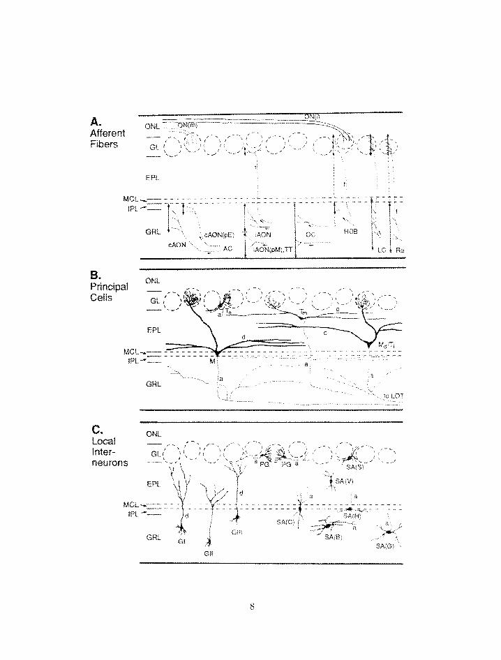
. . . . . . . . . . . . . . . . . . . . . . . . . . Anatomy of the olfactory bulb 9

. . . . . . . . . . . . . . . . . . . . . . . . Subdivisiorls of the piriforrrl cortex 10

. . . . . . . . . . . . . . . . . . Excitatory connections irl t lle piriform cortex 12

. . . . . . . . . . . . . . . . . . . . . . . . . . Pirifornl cortex neuron classes 13

. . . . . . . . . . . . . . . . . . Morpllology of a superficial pyramidal neuron 14

. . . . . . . . . . . . . . . . . . Inhibitory conrlections in the pirifornl cortex 15

. . . . . . . . . . . . . . . . . . . . . . . Oscillatiorls in the olfactory systerrl 17

. . . . . . . . . . . . . . . . . . . . . . . 2.1 Pirifornl cortex slice recording setup 56

2.2 Basic effect of ilorepiriephrine on syrlaptic transrriissiorl in piriforirl cort.ex . . 61

. . . . . . . . . . . . . . 2.3 Time-c;oursr of KE effects orl synaptic trarlsmission 65

. . . . . . . . . . . . . . . . . . . . . . . . . 2.4 Dose-response curve of NE effect 67

. . . . . . . . . . . . . . . . . . . . . . . . . . . . 2.5 Pharnlacology of NE effects 69

. . . . . . . . . . . . . . . . . . . . 2.6 Effects of NE on pairrd-pulse facilitation 71

Comparison of parameter search niethods on all models . . . . . . . . . . . . 119

Parameter search results for rnodel 2 . . . . . . . . . . . . . . . . . . . . . . . 122

Search results as a function of sinzulatiori number for rrzodels 1 and 2 . . . . 123

Parameter search results for model 4 . . . . . . . . . . . . . . . . . . . . . . . 125

Search results as a function of sirnulatior1 nurnber for models 3 and 4 . . . . 128

Paranieter search reslllts for model 5 . . . . . . . . . . . . . . . . . . . . . . . 130

Search results as a function of simulation nunher for model 5 . . . . . . . . . 131

Search results as a functiori of simulation number for modifed model 5 . . . . 135

Parameter search results for modified model 5 . . . . . . . . . . . . . . . . . 136

Outputs of the target model with and without noise . . . . . . . . . . . . . . 191

IS1 llistograms from a four-conductance model with rioise . . . . . . . . . . . 197

Covariance matrix of a sample four-conductance model . . . . . . . . . . . . 198

Histogram of IS1 standard deviation values for a four-conductance rnodel with

. . . . . . . . . . . . . . . . . . . . . . . . . . . . . . . . . . . . . . . . noise 199

Spike raster plots of target model versus best-nlatching models . . . . . . . . 204

A plot of the sum of the negative log likelilioods versus the percent noise

. . . . . . . . . . . . . . . . . . . . . . . . . . . . . . . . added t. o tlze nlodel 218

Raster plots of spiking times for a layer 2 pyramidal cell and spike probability

. . . . . . . . . . . . . . . . . . . . . . . . . . . . . . . . . . . . . . . profiles 219

5.16 Multipulsr facilitatio~i axid de~~ressiori irl layer 1b syriapses with 25 pAl NE:

. . . . . . . . . . . . . . . . . . . . . . . . . . . . . . . . . . . inodel vs . data 290

5.17 Activatioil (mz vs . 17) curves h r all voltage-dependmt ionic channels in the

. . . . . . . . . . . . . . . . . . . . . . . . . . . . . pyramidal neuron niodel 298

5.18 Time constant curves for all voltage-dependent ionic channels in tlie pyrarni-

. . . . . . . . . . . . . . . . . . . . . . . . . . . . . . . . . dal neuron niodel 299

5.19 Activation (utm vs . Ca co~centratiori) and time constant (T vs . Ca conceri-

tration) curves for calcium-depmdent potassium channel in tlle pyramidal

. . . . . . . . . . . . . . . . . . . . . . . . . . . . . . . . . . . . neuron model 300

5.20 Activation (rnm vs . V) curves for voltage-dependent ionic channels in the

. . . . . . . . . . . . . . . . . . . . . . feedback iriliibitory internei~ron rnodel 307

5.21 Time constant (7 - vs . 1') curves for voltage-dependent ioriic cliaiirlels in the

. . . . . . . . . . . . . . . . . . . . . . feedback iiihibitory illternn~roii model 308

. . . . . . . . . . . . . . 6.1 Variability in mitral cell responses to the sanie odor 321

6.2 Irlterspike interval (ISI) distribution in lriitral cells (real and simulated) . . . 325

. . . . . . . . . . 6.3 Backgrourid spiking responses of 100 sinitilateti rnitral cells 326

. . . . . . . . . . . 6.4 Rate coding in the olfactory bull) spike gerlrratirlg model 328

. . . . . . . . 6.5 Synchrorly coding in the olfactory bulb spike gerlerati~ig model 321)

. . . . . . . . . . . . . . . . . 6.6 Ailtocorrellogra~n of spike tirrles in mitral rells 330

. . . . . . . . . . . . . . . . . . . . 6.7 Major subdivisions of tlle piriforril cortex 336

6.8 Arrangenie~lt of neuron types in the pirifornl cortex model . . . . . . . . . .

6."3ositions of neurons in the piriform cortex model in 2-3 coordinates . . . . .

6.10 Scfiematic diagram of cori~iectio~is in the pirifornl cort. ex model . . . . . . . .

6.11 Strengths of afferent projections in the yirifomi cortex model . . . . . . . . .

. . . . . . . . . . . . . . . . . . 6.12 Excitatory connections in the piriforrn cortex

6.13 Transmenibrane current. loops in response to synaptic activation . . . . . . .

. . . . . . . . . . . . . . . 6.14 Voltage gradient in rcspoilse to synaptic activation

6.15 Background responses of pyramidal neurons in the piriform cortex model . .

6.16 Surface CSD plots of strong shock response in piriforrn cortex: experiment

. . . . . . . . . . . . . . . . . . . . . . . . . . . . . . . . . . . . . and model

6.17 Contour CSD plots of strong shock response of pirifornl cortex: experiment

and model . . . . . . . . . . . . . . . . . . . . . . . . . . . . . . . . . . . . .

6.18 Pgrarnidal neuron soma responses to a strong sllock input . . . . . . . . . . .

6.19 Surface field potential response of pirifor~n cortex t. o a weak shock: exyeri-

irient and nlodel . . . . . . . . . . . . . . . . . . . . . . . . . . . . . . . . . .

. . . . . . . . . . . 6.20 Pyraniidal newon sorna respollsrs to a weak sliock input

6.21 Interspike interval (ISI) distributions of the resporlses of a single mitral cell

to different odors . . . . . . . . . . . . . . . . . . . . . . . . . . . . . . . . . .

6.22 Iliterspikp iriterval distrihntio~ls of the responses of 18 niitral cells . . . . . .

6.23 Pooled interspike intrrv;tl distributbn of all ~ ~ i t r a l cells across all odors . . .

xxiii

6.24 Autocorrelograrns of two mitral cells during presentatioml of several odors . . 371

6.25 Autocorrelogralns of different mrlitral cells . . . . . . . . . . . . . . . . . . . . 372

6.26 PSTIIs of mitral cells syncllronized to odor onset but liot to respiration

ollset . . . . . . . . . . . . . . . . . . . . . . . . . . . . . . . . . . . . . . . . 374

6.27 PSTIIs of mitral cells synchronized to respiration onset following odor onset . 375

6.28 PSTIIs of a mitral cell showing firing rate changes after odor onset . . . . . . 376

Piriforrn cortex model: background responses of pyramidal neurons . . . . .

Piriforrrl cortex model: 2-D histograms of background firing rates in pyranli-

dal ileuroils with NE applicatioli . . . . . . . . . . . . . . . . . . . . . . . . .

CSD surface profile of strong shock response in piriforrn cortex: experimental

. . . . . . . . . . . . . . . . . . . . . . . . . . . . . . . . . and model results

CSD corltour profile of stroiig shock response in pirifornl cortex: experimental

and model results . . . . . . . . . . . . . . . . . . . . . . . . . . . . . . . . .

Piriforrn cortex model: netmrk response to a strong sliock stimulus . . . . .

Pirifornl cortex niodel: respor-rse of pyramidal rlellrorls to a strorlg shock

stirrlulus in superficial layer 1 b de1ldrit.e~ . . . . . . . . . . . . . . . . . . . .

Pirifornl cortex model: surhce CSD profiles in response tro a strong shock

with and withorlt backgrour-rd spikillg inputs . . . . . . . . . . . . . . . . . .

Pirifornl cortex rnodel: 2-I> llistograrr~s of pyramidal rletlroxl spikes ill re-

sponse to a strong shock with a i d withotit backgrollfld spiking inputs . . . .

7.9 Pirifornz cortex model without feedforward inhibition: resporlse of 13yrarriidal

ricuron somatic nrernbrane potentials to a strong shock stimulus. . . . . . .

7.10 Srlrface field potential response of piriforril cortex to a weak shock stimulus:

experiment and rnodel . . . . . . . . . . . . . . . . . . . . . . . . . . . . . . .

7.11 Piriform cortex model: power spectrum of weak shock response . . . . . . . .

7.12 Pirifornr cortex model: network response to a weak slrock stimulus . . . . . .

7.13 Excitatory connections in the piriform cortex . . . . . . . . . . . . . . . . . .

7.14 Inhibitory connect ions in the piriforrrl cortex . . . . . . . . . . . . . . . . . .

7.15 Piriforrn cortex nzodel: histogram of feedforwardlfeedback inhibitory neuron

and pyramidal neuron spiking after a weak shock stimulus . . . . . . . . . .

7.16 Piriforrn cortex model: parameter dependerice of weak shock-evoked oscilla-

tions . . . . . . . . . . . . . . . . . . . . . . . . . . . . . . . . . . . . . . . . .

7.17 Piriforrn cortex model: influence of connections between feedback inhibitory

interneurons; int racellular traces . . . . . . . . . . . . . . . . . . . . . . . . .

7.18 Pirifornl cortex model: influence of connectiorzs betweell feedback irlhibit*ory

interneurons: surface field potentials and power spectra . . . . . . . . . . . .

7.19 Experitnerztal GSD eolitour plots of piriforrli cortex responses to strorig and

weak shocks . . . . . . . . . . . . . . . . . . . . . . . . . . . . . . . . . . . .

7-20 Experirrrental CSL) surface plots of piriform cortex respolises to strong and

weak shocks . . . . . . . . . . . . . . . . . . . . . . . . . . . . . . . . . . . .

7.21 Piriforrn cortex nlodel: CSD corltour plot) of the response of the randorn

connectivity n~odel to a weak sliock stimulus. . . . . . . . . . . . . . . . . . 425

7.22 Schematic diagram of how rrlllltiple inputs to layer l a in the pirihrul cortex

might be gerlerated from a single weak shock. . . . . . . . . . . . . . . . . . 427

7.23 Piriforrn cortex nlodel: CSD contour plot of the response of the ralldorn

connectivity model to a weak shock stimulus with multiple input shocks. . . 428

7.24 Piriforrn cortex rnodel: intracellular response in layer la of a pyramidal neu-

. . . . . . . . . . . . . . . . . . . . . . . . . . ron to a weak shock stirnulus. 429

7.25 Piriforrn cortex rnodel: CSD surface plot,s of the response of the randorn

. . . . . . . . . . . . . connectivity model to weak and strong shock stimuli. 331

7.26 Piriforrn cort,ex model: structured connectiorrs from the olfactory bulb to the

. . . . . . . . . . . . . . . . . . . . . . . . . . . . . . . . . . piriform cortex. 436

7.27 Piriform cortex nlodel: structured intracortical connections. . . . . . . . . . 437

7.28 Piriform cortex rnodel: effect of structured connections on spike latencies. . 438

7.29 Piriforni cortex model: network response to a weak sliock stirnulus in the

. . . . . . . . . . . . . . . . . . . . . . . . . structured connectivity model. 331

7-30 Piriforxrl cortex model: CSD corlto~ir plot of the response of the structured

connectivity inode1 to a weak shock stimulus with multiple input shocks with

digerent pop~ilations of pyramidal lleurolls activated on successive wa~,~cs of

. . . . . . . . . . . . . . . . . . . . . . . . . . . . . . . . . . . . . . inputs. . 443

xxvi

7.31 Piriform cortex rnodel: CSL) surface plot of the response of the strllctured

conrlectivity rriodel to a weak sliock stii~iulus with riiultiple iriput sliocks with

different pop~lat~ions of pyramidal rieuroris activated on successive waves of

inputs. . . . . . . . . . . . . . . . . . . . . . . . . . . . . . . . . . . . . . . . 4.24

7.32 Piriform cortex model: network resporise to a weak shock stimulus in the

structured conriectivity rriodel wit11 raridom p~~ramidal-to-pyramidal connec-

tions.. . . . . . . . . . . . . . . . . . . . . . . . . . . . . . . . . . . . . . . . 445

7.33 Piriforrn cortex model: network response to a weak shock stimulus in the

struetured connectivity model with the same subset of neurons activated

each cycle. . . . . . . . . . . . . . . . . . . . . . . . . . . . . . . . . . . . . . 337

7.33 Pirifornl cortex model: CSD contour plot of the response of the structured

connectivity model to a weak shock stirnulus with rriultiple input shocks witli

the sarne population of pyramidal neurons activated on successive waves of

inputs. . . . . . . . . . . . . . . . . . . . . . . . . . . . . . . . . . . . . . . . 448

7.35 Piriforrn cortex model: irltracellular response of a pyramidal netiron in the

structured coriiiectivity model to a weak shock stirriullls with niultiple input

sf-locks with the same population of pyrarriidal rieurons activated or1 successive

waves of inputs. . . . . . . . . . . . . . . . . . . . . . . . . . . . . . . . . . . 449

xxvii

List of Tables

3.1 Parameter search results for model 2 . . . . . . . . . . . . . . . . . . . . . . . 120

3.2 Parameter search results for model 4 . . . . . . . . . . . . . . . . . . . . . . . 126

3.3 Parameter search results for nlodel 5 . . . . . . . . . . . . . . . . . . . . . . . 133

3.1 Parameter values for two different four-conductance models . . . . . . . . . . 203

4.2 Bayesian analysis for the within-class comparison. . . . . . . . . . . . . . . 205

4.3 Parameter values for four- and three-coriductance models . . . . . . . . . . . 207

4.4 Bayesian analysis for the between-class corllparison . . . . . . . . . . . . . . . 209

4.5 Bayesian analysis for the whole-class comparison . . . . . . . . . . . . . . . . 212

4.6 Surnrnary of paranieter esti~rlatiorl nietlilods . . . . . . . . . . . . . . . . . . . 223

5.1 Passive pararrleter values for tlie full arid simplified pyranlidal nertrorz rtzodel . 263

5.2 Paranleter values for tlze synaptic channel 111odels . . . . . . . . . . . . . . . 280

5.3 Reversal potentials for ionic channels . . . . . . . . . . . . . . . . . . . . . . 296

5.4 Conductances and gating variable exponents for pyramidal lieurorl ionic: chan-

. . . . . . . . . . . . . . . . . . . . . . . . . . . . . . . . . . . . . . . . . nels

5.5 Paraxrleters of the calciuni buffer . . . . . . . . . . . . . . . . . . . . . . . . .

5.6 Neuroxnodulation of cellular parameters . . . . . . . . . . . . . . . . . . . . .

5.7 NMDA synapse paranleters . . . . . . . . . . . . . . . . . . . . . . . . . . . .

5.8 Parameters for synaptic facilitation and depression . . . . . . . . . . . . . . .

5.9 Morphology of the reduced pyramidal neuron model and synaptic chalirkels

ill each compartment . . . . . . . . . . . . . . . . . . . . . . . . . . . . . . .

5.10 Conductarlces and gating variable exponents for feedback inhibitory neuron

ionic channels . . . . . . . . . . . . . . . . . . . . . . . . . . . . . . . . . . .

5.11 Parameter values for feedback inhibitory interneurons . . . . . . . . . . . . .

. . . . . . . . . . . . . . . . . . . . . . . . . . . . . . . . . . . 6.1 Network scales 337

6.2 Network connectivities . NA = not applicable . . . . . . . . . . . . . . . . . . 343

6 -3 Computational requirements for sixxulating the piriforrn cortex for one second

of sir nu la ti ox^ time at different scales . . . . . . . . . . . . . . . . . . . . . . . 349

Part I

Introduction

Introduction

Listen to the technology and find out what it is telling us.

Carver &lead

1.1 Overview of the thesis

The past few years have seer1 a great increase in interest iri olfactory neuroscience. Much

of this interest is attributable to the identification of putative olfactory receptors by rncrtlec-

ular biologists [11, 12, 52, 561, thus providing the vital link t~etwrerl odorants and the

responses of olfactory sensory neuroxis which was hitherto lacking. However, the nature of

the cornl>utatioris performed by the olfilctory regions of the brain remain obscure. For the

past several years. we have been usirlg a combillation of electroph3~siologicai experimexktal

techniques and coniputer lnodeli~lg to kelp elucidate the function of the olfactory system

2 4, 5, 25. 2 69, 1 Tliis work has focused largely on the piriibrrri cortex (primary

olfactory cortex) [2. 25. 26, 69. 711 but also on the olfactory bulb [4. 51. The constructiori

of realistic ~omputer sinlulations of tlle olfactory systexrl at both t lie neuro~lal and network

3

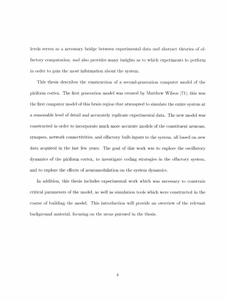
levels serves as a necessary bridge betwen experiinental data arid abstract theories of ol-

facttory computation. axid also provides many insights as t,o wllicll experiillelits to perfom1

in order to gain the nlost iriforirlatioil about the systern.

This thesis describes the constructiorl of a seeorsd-geueration cornputer model of the

piriform cortex. The first generation model was created by Matthew [71]; this was

the first computer model of this brain region that attempted to simulate the entire systern at

a reasonable level of detail and accurat'ely replicate experimental data. The new model was

constructed in order to incorporate much more accurate models of the ~onstit~x~ellt neurons,

synapses, network connectivities, and olfactory bulb inputs to the system. all based on new

data acquired in tlie last few years. The goal of this work was to explore the oscillatory

dynamics of the piriform cortex. to investigate coding strategies in the olfactory system,

and to explore the effects of neuromodulation on the systeni dynamics.

In addition, this thesis includes experimental work which was necessary to constrain

critical parameters of the model, as well as simulation tools which were constructed in the

course of bxiildirlg the model. This i~ltroduction will provide an overview of the relevant

background matserial, foocusing on the areas pursued in the thesis.

1.2 The mammaliali olfactory system

1.2.1 The olfactory epithelium and olfactory bulb

Odorants first contact the aervous system in the olfactory ~1j)it~helium. wl-tere they dissolve

in a thin sheet of mucus and evmtually hind to olfactory receptor molecules located on cilia

of olfactory sensory neurons. There appear to be about 1 0 distirlct olfactory receptor

molecules. each of which is distributed quasi-randomly over a large group of sensory neurons

in the epithelium [lli 121. A single sensory neuron appears to express only one of the

1000 receptor molecules [52]. but can ~levertllrless respond to a range of odorants

[49]. Additionally. multiple olfactory receptors can respond to a given odor [49]. Olfactory

sensory neurons send their axons along tlie olfactory nerve into the olfactory bulb.

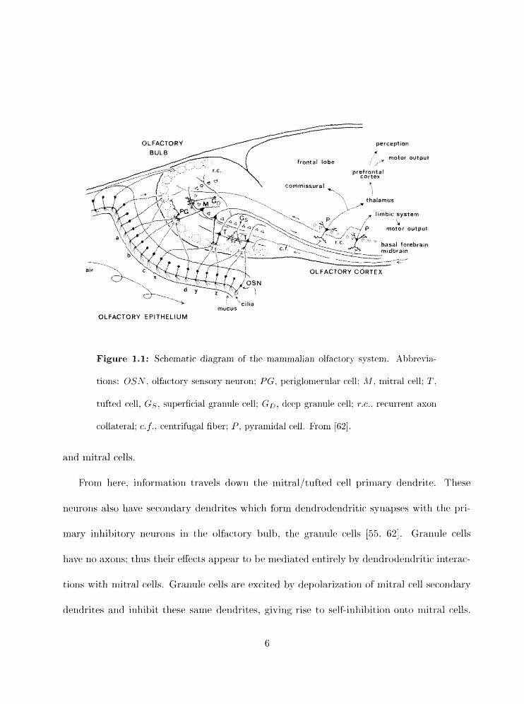
The anatomy of the olfactory bnlb is shown in figures 1.1 and 1.2 [62]. Inforrnation from

the olfactory sensory neurons travels from the olfactory epithelium to the bulb along the

olfactory nerve, ellding in dense dcildrit ic bundles known as glomeruli. Wit bin the glomeruli,

olfactory nerve axorls make synapses with the primary output neurons of the olfactory bulb.

tllc nlitral arld t,uficd cells. In addition. svrlall I-teuroris kriovrm as periglorllerular cells provide

intra- and interglornerular connect ions. Recent evidence suggests that olfactory sensory

neurons projc.cti1ig to a, single glomerulus all express a siliglc receptsor subtype

a glomerulus there arc standard axo--dcudritic eorlnectiorzs involving sensory neurons, mitral

cells and pcriglomerular cells as well as dendrodendritic syr-tapses betwee11 periglomerufar

4 motor output

frontal fabe ; /- prafrontal

cortex

\ . . eitra mucus

OLFACTORY EPITHELIUM

Figure 1.1: Schematic diagram of the rnarnrnalian olfactory system. Abbrevia-

tions: OS,Z-. olfactory sensory neuron; PG. periglomerular cell; A l , rnitral cell; T .

tufted cell, Gs, superficial granule cell; Go, deep granule cell; r.c.. recurrent axon

collateral; c. f . , centrifugal fiber: P, pyrarrlidal cell. Froni 1621.

and rnitral cells.

From here. informat ion travels down the rnitral/ t ufted cell prirlinry t f endrite. These

neurons also havie secondary dendrites which form dendroder-rdrit ic. s y r-rapses with t lie pri-

lrlary inhibitory neurorls in the olfactory bulb, the granule cells [55. 621. Granule cells

have no axons: thus their effects appear to be niediated entirely by derldrodendritic interace-

tiovrs with mitral cells. Grarlule cells are excited by depolarization of nlitral cell serondary

dendrites and inl-ribit these same dendrites. giving rise bo self-inhikition onto rrlitral cells.

Furtlierrnorc, nearby or distant dendrodcndritic synapses of the same granule cell may also

be activated, giving rise t'o lateral inhibitory interactions. Granul~ cells are also promixlent

targets for c.e&rifugal input to tllc olfactory hulb. both from the pirifornl cortex and from

neurons providing neuromod~ilat~ory input to the bulb 1621. Mitral cells integrate the affer-

ent and centrifugal inputs witti the inhibitory granule cell inputs and send their outputs to

the piriform cortex (and other brain regio~ls) through the lateral olfactory tract (LOT).

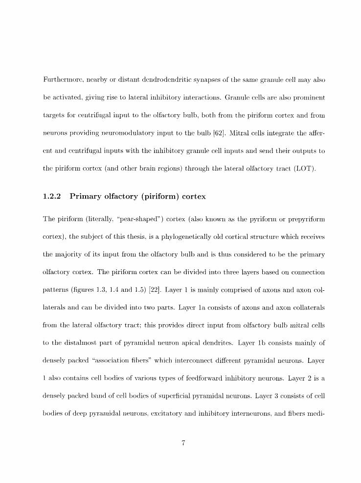
1.2.2 Primary olfactory (piriform) cortex

The piriforrn (literally, "pear-shaped") cortex (also know11 as the pyriforlrl or prepyrifornl

cortex), the subject of this thesis, is a phylogerretically old cortical structure which receives

the majority of its input from the olfactory bulb and is thus considered to be the primary

olfactory cortex. The piriforrn cortex can be divided into three layers based on corlnectioa

patterns (figures 1.3. 1.4 and 1.5) [22]. Layer 1 is mainly comprised of axons and axon col-

laterals and can be divided into two parts. Layer la consists of artoris and axon collaterals

from the lateral olhctory tract; this provides direct input from olfactory hulb mitral cells

to tlie distal~lost part of pyrarrlidal ncurorr apical dendrites. Layer Ib consists r~lairily of

densely packed '.association fibers" which interconnect differexit pyramidal neurons. Layer

1 also contains cell bodies of various types of feedforward inhibitory neurons. Layer 2 is a

densely packed band of cell bodies of superficial pyranlidal neurons. Layer 3 consists of cell

budics of deep p~ranlidal neurons, excitatory a11d inhibitory inter~lcurons, and fibers medi-

a. Afferent Fibers

MCL IQL

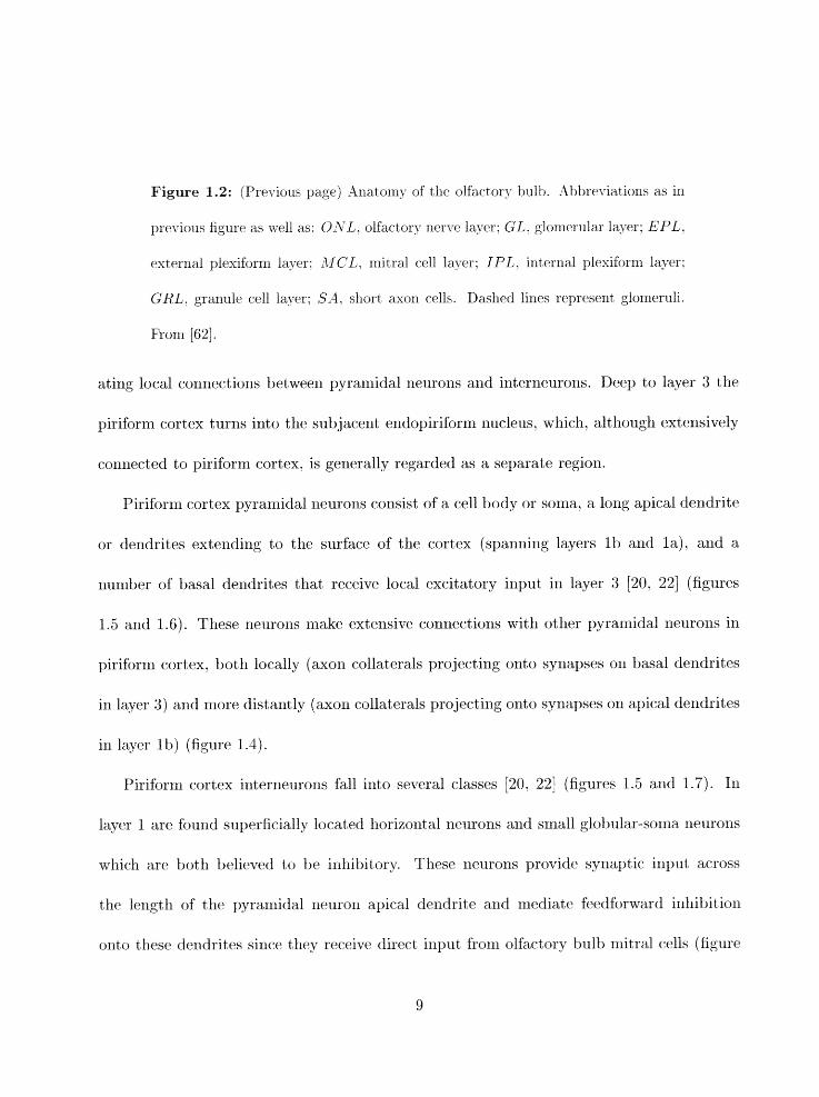
Figure 1.2: (Previous page) ,4natorny of the olfactory bulb. Abbreviations as in

previous figure as well as: O A ! L . olfactory nerve layer; GL. glornerular layer: EPL.

external plexiform layer: llICL;, rnitral cell layer; IPL . internal plexiform layer:

GRL. granule cell layer; SA. short axon cells. Dashed lines represent glomernli.

From j62j.

sting local connections bet,wee~i pyramidal neurons and interneurons. Deep to layer 3 the

piriform cortex turns into the subjacent endopiriform nucleus, which, although extensively

connected to piriform cortex, is generally regarded as a separate region.

Piriforrri cortex pyramidal neurons consist of a cell body or soma, a long apical dendrite

or dendrites extending to the surface of the cortex (spanning layers 1b and la). arid a

number of basal dendrites that, receive local excitatory input in layer 3 20. 221 (figures

1.5 and 1.6). These neurons make extensive connect ions with other pyramidal neurolis in

piriforrrl cortex, both locally (axon collaterals projecting onto syriapses on basal dendrites

in layer 3) and more distantly (axon collaterals projecti~lg onto synapses on apical dendrites

in layer lb ) (figure 1.4).

Piriform cortex interrleurons fall into several classes [20. 22 (figures 1.5 and 1.7). In

layer 1 are fourld superficially located horizontal neurons and small glohxilar-sorria neurons

which arc both believed to be inhit-~itory, These neurons provide syzlaptie input across

the lnlgth of the pyramidal neuroll apical dendrite and ~rlediatr feedforward inhibition

onto these derldrites since they receive direct iriput from olfactory bulb rrlitral cells (figure

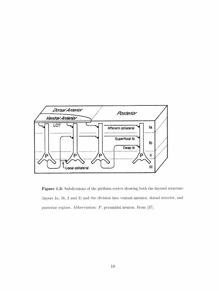
Figure 1.3: Subdivisions of the piriform cortex showing both the layered structure

(layers la. l b , 2 and 3) and the division into ventral anterior. dorsal anbrior. and

posterior regions. Xbttreviat ion: P. pyraxliidal neuron. From j3iij.

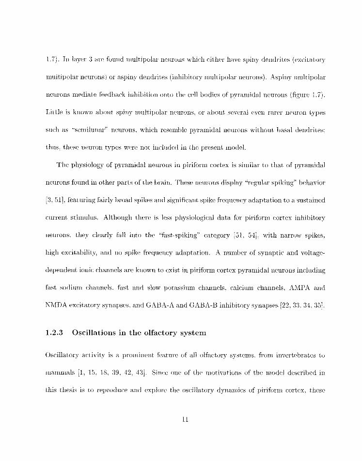
1.7). 1x1 layer 3 are fouiid multipolar neuroIls which either have spi~iy de~ldrites (excitatory

multipolar neurons) or aspiny dendrites (inhibitory nl~iltipolar ileurons) . Aspiny multipolar

neurolis mediate feedback irihibitioli onto the cell bodies of pyrarrlidal neurons (figure 1.7).

Little is know11 about spiny rnultipolar neurons. or about several even rarer neuron types

such as "semilunar" neurons. which resemble pyramidal neurons without basal dendrites:

thus, these xieurori types were not ilicluded in t lie present model.

The pllysiology of pyramidal neurons in piriforrn cortex is similar to that of pyramidal

neurons found in other parts of the brain. These neurons display "regular spiking" behavior

[3. 511, featuring fairly broad spikes and significant spike frequency adaptation to a sustaixled

current stimulus. Although there is less pllysiological data for piriforrli cortex inhibitory

neurons. they clearly fall into the '*fast-spiking" category [5 1. 541. with narrow spikes.

high excitability, and no spike frequency adaptation. A n u d e r of synaptic and voltage-

dependent ionic chaririels are known to exist in pirifor~n cortex pyramidal neurons ix~cludirig

fast sodium channels, fast and slow potassitlnl channels, calcium channels. AMPA and

NhlDA excitatory syriapses. and GABA-A and GABA-B inhibitory synapses [22.33,34. 351.

1.2.3 Oscillations in the olfactory system

Oscillatory a~t~ivity is a prominent feature of all olfactory syster~is. from invertebrates to

nlalrlnlals [l. 15. 18. 39. 32. 431. Since one of the motivations of the rnodel described in

this thesis is to reprod~lce and cxplorc the oscillatory dynamics of piriform cortex. these

dorsal ant piriform cbi ( APCd

t a ,,..-.-*... sup Ib

i t f

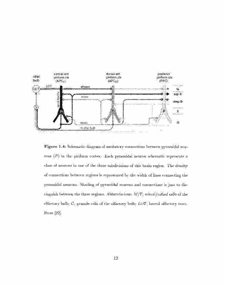
Figure 1.4: Schematic diagram of excitatory connections between pyramidal neu-

rons (P) in the piriform cortex. Each pyramidal neuron schematic represents a

class of neurons in one of the three subdivisions of this brain region. The density

of connections between regions is represented by the width of lines connecting the

pyra~nidal neurons. Shading of pyramidal neurons and connections is just to dis-

tinguish between the three regions. Abbreviations: M/T, mitral/tufted cells of the

olfactory bulb; G, granule cells of the olfactory bulb; LOT, lateral olfactory tract.

From [22] .

GAS%\-containing cells surface

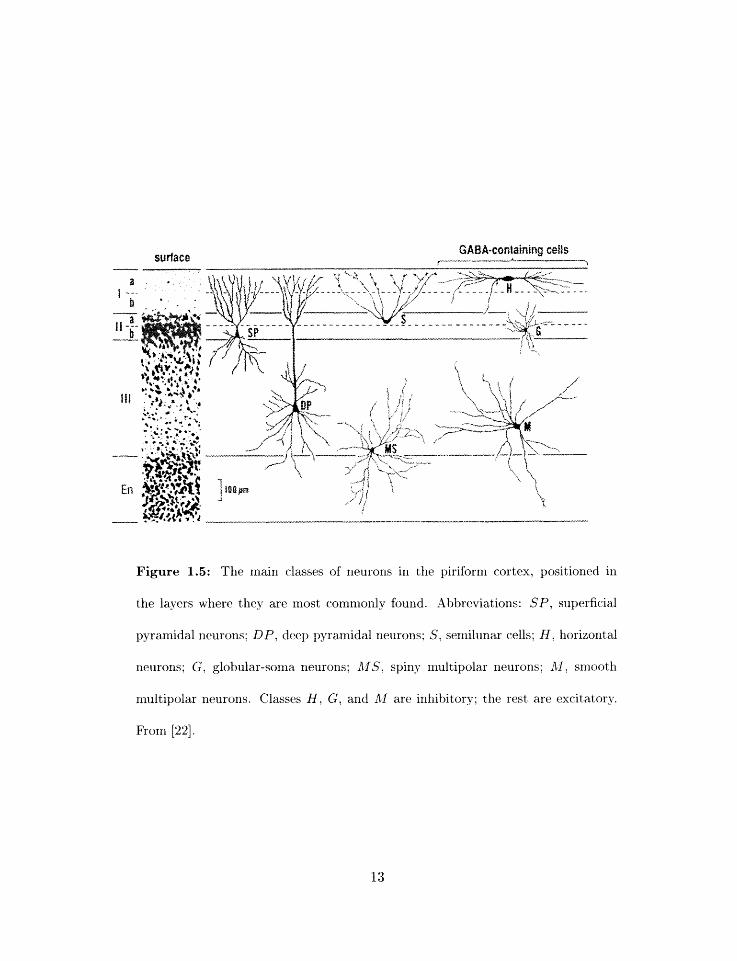
Figure 1.5: The main classes of neurons in the piriform cortex, positioned in

the layers where they are most commonly found. Abbreviations: SP, superficial

pyramidal neurons; DP, deep pyramidal neurons; S, semilunar cells; H, horizontal

neurons; G, globular-soma neurons; AgS, spiny multipolar neurons; AT, smooth

multipolar neurons. Classes H , G, and A1 are inhibitory; the rest are excitatory.

From [22].

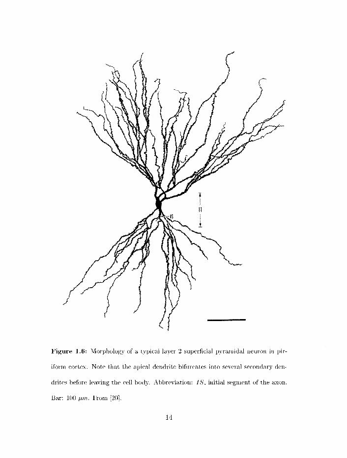
Figure 1.6: Morphology of a typical layer 2 superficial pyramidal neuron in pir-

iform cortex. Note that the apical dendrite bifurcates into several secondary den-

drites before leaving the cell body. Abbreviation: IS, initial segment of the axon.

Bar: 100 pnb. From [20].

Figure 1.7: Inliihitory connections iri the piriforni cortex. .ibbreviatioris: P.

~jyraniidal neurori: F F . fredforl~ard inliibitory interriruro~i: F B . feedback inliihitory

interneuron. From 1221.

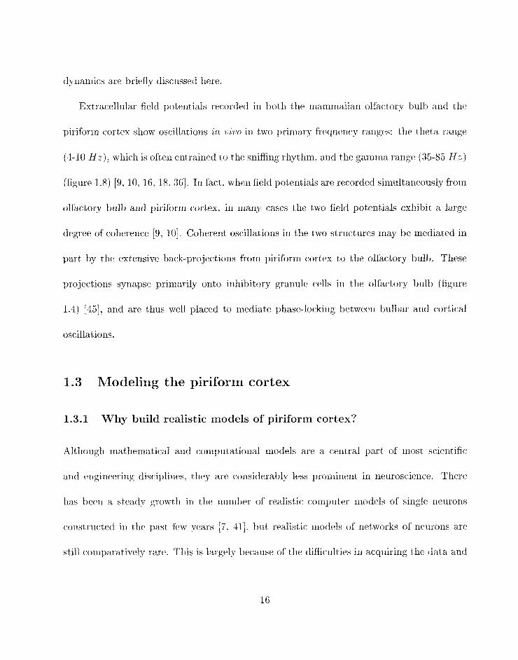
dyrlaniics are briefly discussed here.

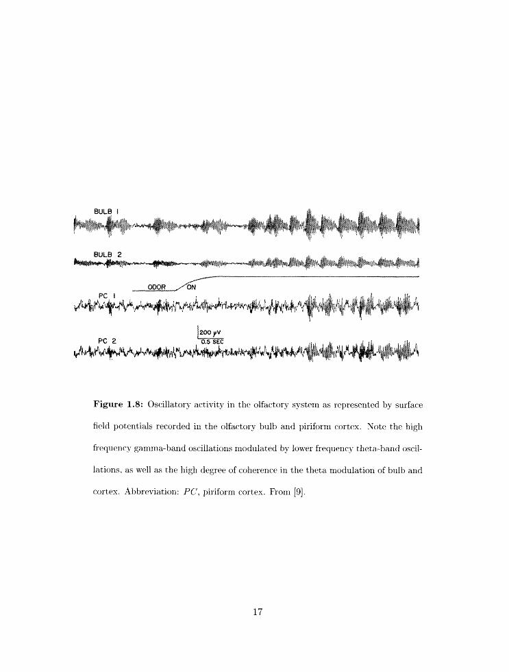
Extracellular field pot exit ials recorded in both the rnarnnlalian o l h r : t , ~ bull3 and t lie

piriforni cortex sllow oscillations in ' ~ ' 2 ~ 0 in two primary frequency ranges: the theta range

(4- 10 H z ) . which is often entrained to tlie sniffing rhythni. and the ganlnla range (35-85 Hz)

(figure 1.8) ['J. 10. 16. 18. 361. Iii fact. when field potentials are recorded simltaneously fro111

olfactory bulb and piriform cortex, in marly cases the two field potentials exhibit a large

degree of coherence [9, 101. Collerent oscillations in the two structures may be mediated in

part by the extensive back-projections from piriform cortex to the olfactory bulb. These

projections synapse priniarily onto inhibitory granule cells in the olfactory bulb (figure

1.4) [45], and are thus well placed to mediate phase-locking between bulbar and cortical

oscillations.

1.3 Modeling the piriform cortex

1.3.1 Why build realistic models of piriforrn cortex?

Alt liough mat hematical and cornput at iorial models are a celitral part of most scirlitific

arid erigineerillg disciplines. they are r:onsiderably less pronlinent in neuroscience. Tlsere

lias been a steady growttli in the nuirllrter of reafistic computer models uf sirigle neurons

constructed ill the past few years i7. 411. but realistic niodels of rsetworks of lieuroils are

still comparatively rare. Tliis is largely because of the difficulties in acquiring tlie data and

BULB I

Figure 1.8: Oscillatory activity in the olfactory system as represented by surface

field potentials recorded in the olfactory bulb and piriform cortex. Note the high

frequency gamma-band oscilla,tio~rs nlodulated by lower frequency theta-band oscil-

lations, as well a.s the high degree of coherence in the theta modulation of bulb and

cortex. Abbreviation: PC, piriform cortex. From [9].

building tlie sirnulatiorl tools necessary to construct these models. but also l~ecause r3f a lack

of under~t~ariding of tlie purpose of model building.

n7henever a system to be modeled (such as a neuron or a rietwork of neurons) consists

of a large number of interacting, nonlinear components. tlie behaviors of such a system can

be highly ilnpredictable and int,uition is not a reliable guide [67]. Realistic computer models

can thus be very useful to an experimentalist in sflowing the range of possible behaviors that

call be obtained when known components at one level (e.g., syrlaptic and ionic channels,

dendritic segments) are assembled into larger entities (e.9.. single neuron models, network

models). In addition, such rnodels act as a consistency check between data at different

levels, thus highlighting which data is likely to be false or incornplet#e. When data is known

to be incomplete, models allow investigators to perform "what-if" numerical experiments

to test the plausibility of differelit theories, whicli can serve as a useful guide to further

experiment at ion.

Realistic rnodels of neuronal networks can also aid illvestigators in understanding the

origins of network-level dynamical behaviors such as oscillations. Once a dynamical behavior

of interest can he replicated, rnodel coxrlponents can be rrloditied or relnoved to deterrzlirle

whicli aspects of tlie system are fx~ndarnental for achieving the correct behavior and wllich

are not. In this way, realistic network models can be ab~tract~ed in rnany diEerent ways

corresporldivzg to eacli type of behwior exhibited by tlie model. An example of this, based

or1 the work described llere. is [l-l]. Network rnodels are also uspful for critically evaluating

theories of neural corii~)utation and codirig [24. 26. 27. 711.

1.3.2 Realistic modeling

Since this thesis describes the coristrnctioli of a realistic computer ~riodel of piriform cortex.

it is important to state precisely wllat is meant by "realistic". Tlie key criteria are:

1. The level of detail in the model must be a reasonable reflectiori of tlie current body

of experimental knowledge given the limits of modern computers.

2. Tlle rilodel must reproduce relevant experirnental data to a liigli degree of acctiracy.

3. Tlie niodel should provide useful suggestions for further exprrirliental work arid useful

ideas about the dyriarnics and functions of the system being modeled.

These criteria have been met both for the previous model (at the time it was bnilt) and

tlie model described here; this is discussed in greater detail iri tlie following chapters. The

current model inevitably has lirx~itat~ions which will also be discussed in detail.

Clearly. buildi~ig realistic models is critically dependent 011 tlic. current state of tlie

exprriniental database: in fact. it rnay be argued that tlle rriost irnportarlt contri1)ution of

tliesr rriodels is to let experimentalists kriow wliich data needs to hr rollectrd to iniprove

the model. This feedback loop between rliodels arid experiments is tlie prilriary strength of

t lie realistic rriudelirig approaclr.

1.3.3 The previous piriform cortex model

The first realistic computer model of piriform cortex was tliat of h1:latthcw Wilson [71]

which is the direct ancestor of the nlodel described irk tliis thesis. Wilson's model was able

to replicate the surface field potelitial response of piriforrri cortex in response to weak and

strong shocks of the LOT, and also highlighted the importance of synaptic time constants

axid axonal conduction velocities in generatting field potentials which matdl experirnerltal

data. However. Wilson's rriodel had rriariy lilnitations: the simulated neurons were not

parameterized to fit experimental data. the inputs were not strongly based on experimen-

t a1 data, the connect ion patterns are no longer consistent with the most rccentjly acquired

data [22, 37; 381, and many aspects of synaptic transmissioll were ignored (e.9.. fast and

slow GABA-A subtypes, NMDA channels, neuromodulation, synaptic facilitation and de-

pression). I will briefly discuss new featrlres of tlie present rnodel below and give a more

detailed comparison between the two inodels in chapter 6.

1.3.4 New model features

A rn;z_jor goal of the work described irr this thesis has been to incorporate accurate models of

single ileurons in pirif'orm cortex into a large-scale cortical model. Tllc two prinlary classes

of neuron types in pirihrm cortex arp 13yramidal neuroris and a llunlber of inl~ibit~ory in-

tern~llron types. In contraat: to the previous model, the pirihrrn cortex model described licre

was corlstructed so as to accurately reproduce tlie inplxt-output relatiorls of both pyraniidal

and inhibitory i~lt~erneurons as well as tile synaptic dynamics of the systern. The pyramidal

neuron nod el corit.ains a variety of voltage- and calciurn-depexi(1e1it ionic channels. AMPA

arid NMDA excitatory synaptic receptors. arid fast and slow GABA-A and slow GABA-I3

irihibitory synaptic receptors.

The synaptic connect ivit ies of the piriform cortex rnodel have been significantly changed

to reflect new experimelital data. The previous niodel divided piriforrri cortex into anterior

(rostral) and posterior (caudal) subdivisions only. The modern view. reflected in the new

rnodel, is that piriform cortex is divided into three broad regions 0x1 the arit,erior-posterior

arid dorsoventral axes (figure 1.3) on tlie basis of external and internal synaptic connec-

tion patterns (figure 1.4) [22]. Thr majority of input from the olfactory bulb arrives on

pyramidal rieurorr dendrites in tlre veritral a~iterior piriform cortex (vAPC): these neurons

in turn project large numbers of long-range collaterals to the superficial layer l b dendritJes

of pyramidal neurons in the other two regions. Few local projections arise from vAPC

pyramidal neurons. Pyramidal neurons in tlie dorsal aritrrior piriform cortex (dAPC) and

tlre posterior piriforrn cortex (PPC) project to deep layer 1 b pyramidal rleuron dendrites

in thc. other regions and also give rise to significant nu~nbers of local projections onto basal

dendrites of riearby pyrar~idal neurons.

The realism of rnodeled inpats to piriforrrl cortex fror~i the olfactory bulb haw hceri

significa~itly improved with respect to the previous model. Out puts fro111 ulfact ory bulb

mitral cells arc. representled by R spik-geerat i~ig object that can generate a rlu~rlber of

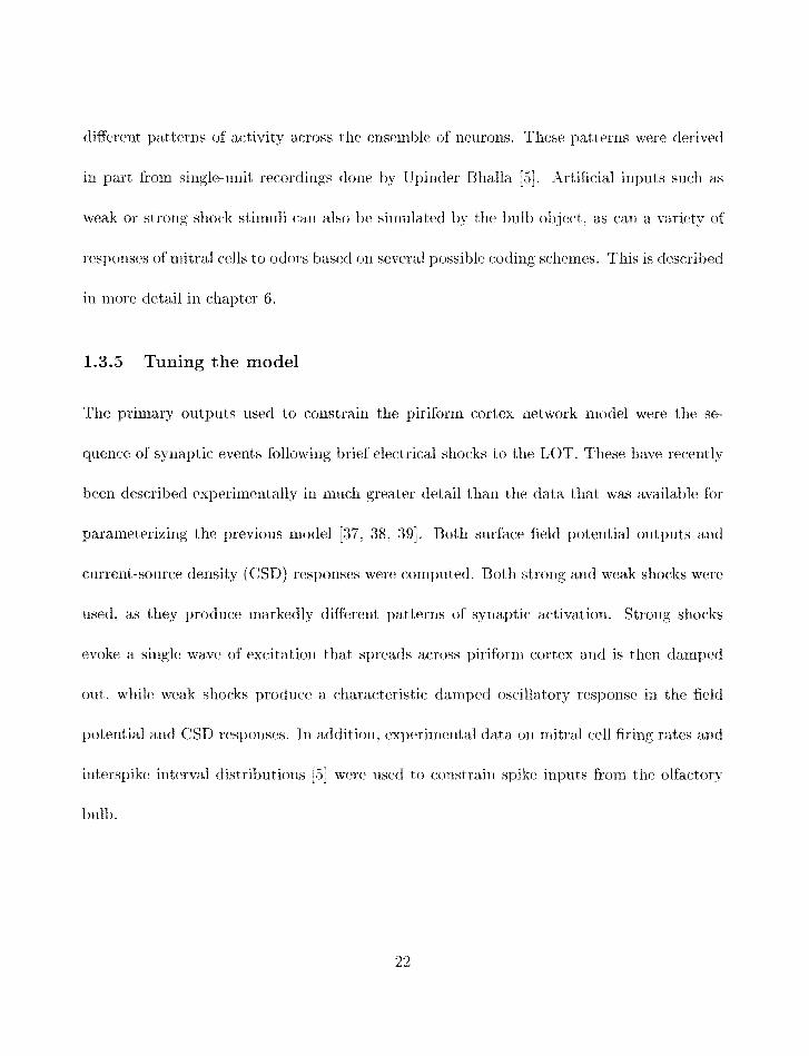
different patterns of activity across the ensernble of neurons. These patterns were derived

ill part fi.o~n s ing l~-~~r l i t recordings dorle by Upir1dr.r Bhalla 151. Artificial inputs such as

weak or strong shock stimuli can also be sirnlxlated by the bulb object. as call a variety of

resporlses of rnitral cells to odors based on several possible coding schemes. This is described

in more detail in chapter 6.

1.3.5 Tuning the model

The primary outputs used to constrain the piriform cortex network model were tlie se-

quence of syilapt ic events following brief electrical shocks to t he LOT. These have recently

been described experimentally in rnucfi greater detail than the data that was available for

parameterizing the previous model [37. 38. 391. Both surface field potential outputs and

current-source density (CSD) responses were computed. Both strong and weak shocks were

used. as they produce markedly different patterns of synaptic activation. Strong shocks

evoke a single wave of excitation that spreads across piriforrrl cortex and is then damped

out, while weak shocks produce a characteristic da~nped oscillatory response in the field

potential and CSD responses. In addition. experimental data on mitral cell firirlg rates and

interspike iilterval distributions 51 were used to corlstrain spike inputs from the olfactory

t>ufb.

1.4 Questions the model can help answer

1.4.1 Coding in the olfactory system

Despite decades of interisive research, there is rzo consensus as to llow odors are erzcoded in

the oritsputs of olfactory bulb mitral cells. Some authors believe that odorarits are encoded

by cha~iges in mitral cell firing rate, either in a small localized group of neurons [61, 621 or

in a larger distributed group of neurons [46. 571. Others believe that odorants are encoded

by synchronized firing of rnitral cells (or their analogs in insects. the projection neurons of

the antenna1 lobe [42. 431). while still others argue for more co~nplex spatiotemporal codes

involving chaotic d y naxnics [19, 6-11.

The lack of consensus in t liis area causes difficulties in tlie cons tructiori of realistic

rnodels of piriforni cortex, since the model cannot be expected to reproduce tlle behavior

of the real system without being supplied with realistic inputs. As will be seen. this was

resolved by creating sirnulati011 objects that can mimic rnany of the proposed olfactory

coding strategies. as well as accurately replicating the first-order statistics of rnit?ral cell

responses to background odors.

The yuestion of how odors are encoded in piriform cortex. or even wliat roles the. pir-

ifornl cortex may ).lave in odor processing. has also not been resolved. pri~narily i~etansr

tlle relevant data is so lir~iit~ed. Much of the fiinctional data relating to olfactory cort>ex

has beexi ob ta in4 frorri hurnan studies. Lesioris in pirifbvm cortex in hillmans disrupt, olf'ac-

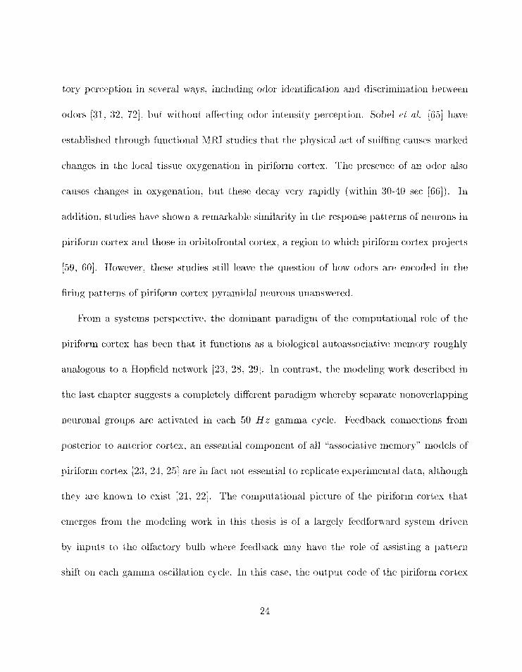
tory perceptioli in several ways, incltlding odor identification and discrimination between

odors 131. 32. 721. but witliout aRecting odor int,e~lsity perception. Sobel et al. [G5] have

establislied through functional MRI studirs that the physical act of sniffing causes rliarked

dianges in the local tissue oxygenatiorl in piriforrn cortex. The presencct of an odor also

causes changes in oxygenation. hut t#liese decay very rapidly (within 30-40 see [66]). In

addition, studies have shown a remarkable similarity in the response patterns of neurons in

piriforrn cortex and those in orbitofrorital cortex, a region to which piriforrn cortex projects

159, 601. However. these studies still leave the questioll of how odors are encoded in the

firing pat terns of piriforrrl cortex pyrarnidal neurons unanswered.

From a systems perspective, tlie clorninant paradigm of the colnputational role of the

piriforrn cortex has been that it functions as a biological autoassociative rnemory roughly

arialogous to a Hopfield network [23, 28. 291. 1x1 contrast, the modeling work described in

the last chapter suggests a completely different paradigrn whereby separate nonoverlapping

ncuronal groups are activated in each 50 Hx ganirna cycle. Feedback connet:tions from

posterior to anterior cortex. an esseritial eornpolierrt of all -'associative memory" models of

piriforrn cortex [23. 24. 25 are in fact not esseritial to replicate experinlental data. although

they are krlown to exist [21. 221. The computatio~lal picture of the pirihrrli cortex that

errierges from the rllodelirig w r k in this thesis is of a largely feedforward sy"t"m driven

by inputs to tlle olhctouy bulb where feedback may have the role of assisting a pattern

shift or1 each gaEirrra oscillatiort cyr-le, In this case. the outpttt code of the piriform cortex

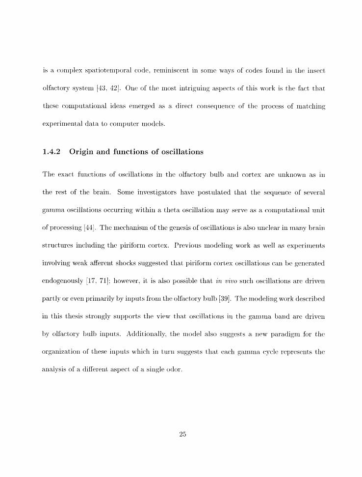
is a complex spatiotemporal code, reminiscent in some ways of c o d ~ s found in the insect

olfactory system 133. 421. Orle of the ~riost intrigui~lg aspects of this work is the fact that

tliesr computational ideas emerged as a direct consequence of tlie process of mattelling

experin~ental data to cornputer models.

1.4.2 Origin and functions of oscillations

The exact fulictions of oscillations in the olfactory bulb arltl cortex are unknown as in

the rest of the brain. Some investigators have postulated that the sequence of several

garlinia oscillatiorls occurring within a t lieta oscillation may serve as a eomput at ional unit

of processing [44 . The mechanism of the genesis of oscillations is also unclear in many brain

structures including the piriforrn cortex. Previous modeling work as well as experiments

involving weak afferent sllocks suggested that piriforrn cortex oscillatio~is can be generated

endogenously [17. 711; however, it is also possible that irz viz~o such oscillations are driven

partly or even primarily by inputs from the olfactory bulb [39]. The modeling work described

in this thesis strongly supports the view that oscillatiorls in the gamma band are driven

by olhctory bulb inputs. Additionally. t l ~ rriodel also suggests a riew paradigm for the

orga~iization of these inputs which in turn suggests that each gamrlza cycle represents the

analysis of a diRerent aspect of a, single odor.

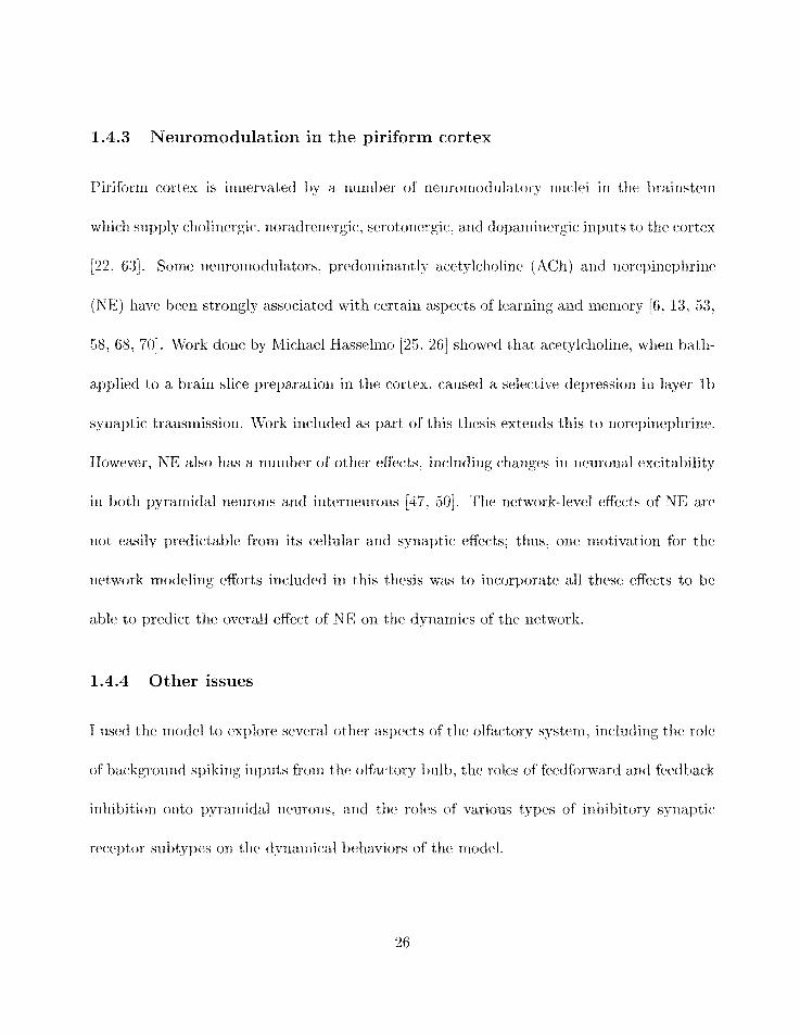
1.4.3 Neuromodulation in the piriform cortex

Pirifornl cortex is iriner~at~ed by a ilurribcr of neuro~nodulat~ory riuclei in tlre t~rairisteril

whiclr supply cholinergic, noradr~nergic. serotonergic, and dopalirinergic irrputs to the cortex

[22. 631. Some neuromodulators, predoiriiria~itly acetylclioline (ACh) allti norepinephriri~

(NE) have been strongly associated with certain aspects of learni~ig and memory [6. 13, 53.

58, 68. 701. Work done by Micllael Hasselrno [25, 261 showed that acetylcholirie. wheri bath-

applied to a brain slice preparation in the cortex. caused a selective depression in layer l b

synaptic transmission. Work included as part of this tliesis extends this to norepinephrine.

However, NE also has a number of other effects, including cbariges iri neuronal excitability

in both pyramidal neurons and irlterneurons [47. 501. The ~irtwork-level effects of NE are

not easily predictable from its cellular and synaptic effects: thus. one motivation for the

network modelillg efforts included in this thesis was to incorporate a11 these effects to be

able to predict the overall effect of NE on tllc dynarriics of the network.

1.4.4 Other issues

I used tlic rrlodel t80 explore several other aspects of tlie olfactory system, i~lcluding tl1e role

of background spiking illputs from the o1f;trtory F~ulb, the roles of fc3edforward and feedback

irihibitiori oilto pyraniidal rieurons, and the roles of various types of irillibit,ory synaptic.

recaeptor suhtypes ori the dyriairiieal behaviors of the model.

1.5 Modeling methodologies

In tfie course of I-~uilding iiiodels of single neurons in piriforln cortex. a number of tools

were developed to facilitate certain aspects of the inodeling process. A description of these

tools forms a major component of this thesis. These tools are briefly sunimarized here and

discussed in rrlore detail in the relevant cliapters.

1.5.1 Simulation environment

The computer models of piriform cortex described in this thesis were all simulated using

the sirnulatior1 program GENESIS (GEneral NEural SImulatioii Systern) 171. Single neu-

rons were simulated by dividing them into isopotelitial coxllpartrrients and using standard

compartnlental modeling techniques [41]: details of the models are to be fouiid in the fol-

lowing chapters. Many extension libraries totallirig approxiriiately 60.000 liries of C code

were added to GENESIS specificdly in order to build the pirifornl cortex model. These

libraries consisted of the olhctory bulb spike-generating objects. a variety of synaptic ob-

jects, objects controlling rleuromodulation. and cornmands to establish groups of syliaptic

connec t ions, weiglits a i d dela-~~s.

1.5.2 Parameter searching

1 have de~eloped a group of parailleter smrching methods usable witliiri GENESIS that

greatly simplify the process of assigning values to urrknowrl pararri~ters in siugle-neuron

models. Several rrletlrods have beer1 used. ilicluding conjugate-gradient. sirrrulated anneal-

irlg. genetic algorit lrins. arrd stochastic search. The 1iiglrl-y accurate mat dl ht.t,wee~~ the

pyramidal neuron rrrodel and the experinrlental data on wlliclr it was based is a direct corr-

sequenc:e of these methods. I believe that these riletliods will soon becorne an esseritial

component of the sirnrilation toolkit of scientists building realistic single-neuron models.

since assigning paranleters iteratively by hand is both much more tedious and gives much

poorer results than those obtained using these methods. At the same time. a certain arziorint

of expertise in using tliese methods is necessary in order to obtain the best results: this is

discussed at length in cllapter 3.

1.5.3 Bayesian methods

Eventually, a large enough number of realistic single-neuron models will exist that it will be

possible to ask which one is the best model given some set of data to be matched. Although

most modelers would currently answer this question based on a visual inspectior1 of the

results or orr the basis of what aspects of the data they are niost interested irr. it is possible

to ask this question much more rigorously if the nlodels generate output probabilistically.

I have sllown that in this case one can use the Bayesian franzework to cornpare irrdividual

rrzodels arld classes of niodels arid assign relative probabilities to the rnot_iels based on how

well they rlratch the data. A s models proliferate the Bqesiarr rnetllodcllogy will be essential

tjo allow the oh jec t i v ~ evaluation of diEerent models.

1.6 New work suggested by the model

1.6.1 Experimental work

The piriform cortex model has highligllted the importance of a more accurate urlderstandirlg

of the corirlection patterns between the olfactory bulb and the piriforrn cortex. As will he

shown in the last chapter. simple random connectivity between the t,wo structures results in

a r~iodel wlliclr can replicate the cortical surface EEG with reasonable accuracy but wliicll

cannot replicate the CSD response to a weak shock stimulus. However, a rnodel which

has highly structured corinections between bulb and cortex can replicate the CSD response.

Detailed anatomical and physiological studies will be necessary to detcr~iiirie the true nature

of the conrlectiori patterns between bulb and cortex. Tllese studies are crucially important

in that they will have a significarlt impact on our understandirig of how cornputatioris are

performed in this system.

From the perspective of inlproving the model. a nunll>er of experimerits need to be

performed. More data on pyralnidal neuron responses to a variety of input stimuli will be

necessary for ir~lprovirrg that model. In addition. little experinierltal data exists to constrain

the rnodels of feedforward inhibitory neurons. Tliesc neurons appear to Izavc. a profound

effect on respollscs of the ncttvork to both weak and strong shock stimuli. Therefore.

experirrlents to better cliaracterize these rieurons are essential.

From the perspective of coding. a very important experimental study is for Iargc-scale

in~iltiurlit recordings to bc obtained from arrays of olfactory bulb iriitral cells in awake

behaving animals involved in odor detection tasks. This will allow us to improve the quality

of tlie inputs tielivered to the modcl and also to refine our undcrstaiiding of c~odirig at the

level of the bulb and cortex.

1.6.2 Modeling work

Tlie modeling work presented here has suggested a number of future paths for continued

work. Tfie pyraniidal neurorz model caan be extended in a number of ways. One approach

would be to increase the realism of the neuron ~xiorphology, wlrich was heavily simplified in

the present model for cornputational reasons. One quest ion of interest concerns the possible

roles of dendritic spines, wliich can isolate the conductairce changes at synapses from tlie

main dendritic truck. thus effectively increasing tlie space constant of the neuron [do]. Tliis

may have a sigiiificant effect on syiiaptic integration in pyramidal neurons. In addition,

the possible roles of active dendritic currents [30] and a somatic spike-initiating zone [48]

re~iiairi to be established for these neurons.

Tllerc. are an eriormous number of corilponents of the present model which. have rlot

been explored fully owing to t i ~ n e constraints. The roles of syxlapt ic Ifacilit at ion. s ynap-

tie depression, and NMDA receptors in generating network-level pllel~onierla are rrot clear.

Sonie rzetwork-level pheriorrlena. such as tlie role of norepinel>llrine in tlie weak-shock re-

sponse. have not been fillly characterized. Sonle work has also been dorie 0x1 rrtodelirlg tiit.

surface EEG response to odors. but taliis work is far frorrr coiiipl~te arid has tllereforc not

beerr included in this thesis.

1.7 Summary of thesis contributions

1.7.1 The new piriform cortex model

A realistic computer rnodel of pirifor~ri cortex was constructed. This nrodel is the most

accurate model of this brain structure that has been built to date. The goals motivating

the construction of the niodel were as fbllows:

1. The network rnodel incorporates models of sirigle nelrrorls whicli were required to

match the input-output behavior of real neurons very accurately. In tlre case of pyra-

rxiidal neurons. the morphology was systematically simplified from tlie morpliology of

a real piriforni cortex pyramidal neuron.

2. The neurori models contain synaptic receptor types knowii to exist in the piriforni

cortex but ~ i o t previously irlcorporated iiito network rrrodels of this systern. iiiclnd-

irlg NMDA receptors. fast aiid slow GABA-A receptors [33. 34, 351. aiid synaptic

fa~ilit~ation arid depressiori [8].

3. The niodel features niore accurate iirp-cxts to the cortical rnodel from olfactory bulb

rrlitral cells,

4. The model ineltides neurorriodulat ion wit 11 rlorepinephrine (NE) at both the cellular

and syiiaptic levels.

1.7.2 Lessons from the rnodel

The piriforrn cortex model has erlipliasized the importance of the role of background spiking

input from tlie olfactory bull3 in keeping pyramidal neurons in the ventral anterior piriforrn

cortex close tao spiking threshold. Without these background inputs, the systerrl becomes

largely unresponsive and caniiot accurately replicate the strong shock response. The model

predicts that norepinephrine, which illcreases the excitability of pyrarrlidal neurons, rnlist

decrease t,he backgrou~id firing rate of olfactory bulb rnitral cells in order to prevent cortical

pyramidal neurons from spontaneously spiking at high rates. There is some experimental

support for this conclusion.

The model has also highlight ed t lie importance of feedforward inhibit ion in t he gener-

at ion of the strorlg shock response, and suggested that feedback onto these neurons niay

he involved in tlie dalnping of the surface EEG observed in the weak sl~ock response. The

model shows that feedback irrllibition alone is riot sufficient to replicate the strong shock

response.

Most significantly. tlle attempt to accurately replicate tlie CSD resporise to weak shock

stimuli has suggested that rriitral cells in the olfactory bulb and pyraniidal neurons in

piriform cortex may be divided irlto nonovcrlapping neuroual groups. such that rnitral cells

of a given group in the bulb prqject primarily or exclusively to pyrairlidal neurons of a

given group in the cortex. and similarly pyramidal neurolls in the cortex project primarily

or exclusively to other rleurons of the same group (with the possible exception of feedback

project ions from posterior to ant terior pirifornl cortex). This arrangement. if true. suggests

tliat the output code of piriforrrl cortex will not resemble a static attractor but will be a

coiriplex spatiotemporal pattern, arld that each garnrrla oscillatioli cycle nlay be involved in

arlalyzing separate aspects of the same inpr~t stimulus.

1.7.3 Experimental work

In order to obt air1 parameters relating to the effects of norepinephrine on synaptic trans-

mission in piriforrn cortex, a number of brain-slice experiments were performed which are

described in chapter 2. NE was found to have profound effects on aEerent synaptic trans-

mission in layers l a and l b of pirifornl cortex. as well as effects on synaptic facilitation and

depression and cellular excitability. These effects of NE were incorporated into the piriforrn

cortex network nzodel.

1.7.4 Development of simulation tools

Silnulatioil tools xiere developed as extellsiori libraries for the neural sirnulatiall progranl

GEnTESIS to siniulale synaptic, cellular. and izetwork-level elltities of the piriforrn cortex

model. An exterlsion library co~lsist~ing of the paraitleter seascllirzg code was devt:lopcd

and has been incorporated into recelit releases of GENESIS. Sirnulation tools for Bayesian

arlalysis of corrlpartmental niodels were also developed.

Bibliography

[I] E. D. ad ria^^. The Electrical Activity of the Ma~rilnalian Olfactory Bulb. Journal of

Physiology (London), 100:459-473, 1942.

[2] P. F. Baldi. M. C. Vanier, and J. M. Bower. 011 the Use of Bayesian Methods for

Evaluating Compartmental Neural Models. Journal of Computational Neumscience,

5:285-314. 1998.

[3] E. Barkai and M. E. Hasselmo. Modulatioli of the Input/Output Function of Rat

Piriform Cortex Pyramidal Cells. Journal of _nieurophysiology. 72(2):644-658, 1994.

[1] U. S. Bhalla and J. M. Bower. Exploririg Paramet,er Space in Detailed Siriglr Neuron

ftilodels - Sinlulations of the Mitral a i d Granrile Cells of the Olfactory-Bulb. Jou~nal

of Ne.urophysioloyy. 69(6): 19481965, 1993.

51 U. S. Bhalla arid J . &I. Bower. Multiday Recordings from Olfactory Bult, Neurons in

Awake Freely Moving Rats: Spatially and Teulporally Organized Variability in Odorant

Response Properties. Journal of Computatiorhnl i2'c.umscience, 4(3j :221-256. 19'37.

35

[6] A. Blokland. Acetplcl~oline: a Neurotransmitter for Lrarllirlg arld &Ienlory? Brain

Besearch Revie~lts. 21 (3):285--300. 1995.

[7] J. M. Bower and D. Beenlan. The Book of Genesis. 2nd. Ed. Springer Verlag. New

York, 1998.

[8] J. M. Bower and L. B. Haberly. Facilitating and Nonfacilitating Synapses 0x1 Pyranlidal

Cells - a Correlation Between Physiology and Morphology. Proceedings of T h e Nationul

Acadenag of Sciences of The United States of America, 83(4):1115-1119, 1986.

[9] S. L. Bressler. Spatial Orga~lizatiorl of EEGs fro111 Olfactory Bulb and Cortex. Elec-

tl?oe~cephuEog?*~~ph~y and Clinical Neurophysiology. 57:270-276. 1984.

[lo] S. L. Bressler and W. J. Freeman. Frequency Analysis of Olfactory System EEG in

Catl. Rabbit and Rat. Elect~oencephalography and Cliriical Neurophysiology, 50: 19-24,

1980.

[ll] L. Buck. The Molecular Architecture of Odor and Phero~lione Sensirlg in Mammals.

Cell. 100(6):611-618. 2000.

L. Buck arid R,. Axel. A Novel Multigene Farnily May Ellcode Odorant Receptors -- a;

aiilolecrrfar Basis for Odor Recognition. Cell, 65(l): 175-187. 1991.

1131 D. M. Collrpton. K. L. Dietrich. J. S. Snxitlr. and B. K. Davis. Spatial and Noxispatial

Learning in the Rat Followirlg Lesions to the Nrlcleus Locus-coernleus. ~Veuroreport,

7/1):177-182. 1995.

[11] S. M. Crook. G. B. Ermentrout. M. C. Vanirr. and J. M. Bower. Tllr Role of Axo~ial

Delay in the Syrrclxronization of Networks of Coupled Cortical Oscillators. Journal of

Comlputat$ortd Neumscience, 4(2):161-172. 1997.

[15] K. R. Delaney, A. Gelperin, M. S. Fee. J . A. Flores. R.. Gervais. D. W. Tank. and

D. Kleinfeld. Waves and S tirnulus-Modu1at;ed Dynamics in an Oscillating Olfactory

Nt.t,work. Proceedings of the NatBonal Acadesrr,y of Sczences. 91 (2) :669-673, 1994.

1161 W. J. Freeman. Distributio~l in Time and Space of Prepyriform Electrical Activity.

Journal of Neurophysiolqgy, 22:6il--1;-665, 1959.

[17] W. J. Freeman. Effects of Surgical Isolatiorl arid Tetarlizatiorl of Prepyriforrrl Cortex

in Cats. clournal of Neuruphysioloyy. 31:349-357, 1968.

[18] W. J. Freeman. Alass Action in the Ne~.vovs Sgstem. Acaderrlic Press, Kew York. 1975.

[l9] W. ,J. Freeman. Sirriulatioli of' Cliaotic: EEG Pattierrls with a Dynamic Model of tlie

Olfactory System. Bioloyieal Cybernetics. 56: 13C3150, 1987.

[20] L. B. Haberly. Structure of the Pirifornl Cortex of tllr Opossunl. 1. Descriptiorl of

Neuron Types with Golgi Metliods. ,Jourmr~nl of Compar~~tive Meuroloyg. 213(2) : 163-

18'7, 1983.

[21] L. B. Haberly. Neuronal Circuitry irl Olfactory Cortex - Anatoiny and Ftlnctional

Implications. C!hemzcaE Senses, 10(2) :219-238, 1985.

[22] L. B. Haberly. Olfactory Cortex. In G. M. Shepherd, editor. The Sg92uptic Organization

of the Brain. Oxford University Press, Oxford, England, 1998.

[23] L. B. Haberly and J . M.. Bower. Olfactory Cortex - Model Circuit for Study of

Associative Memory? TrendR In Neurosciences, 12(7) :258-264. 1989.

[24] M. E. Hasselmo. Acetylcholine and Learning irl a Cortical Associative Memory. Neural

Compututzora, 5 j l ) :32-14, 1993.

[25] M. E. Hasselnlo. B. P. Anderson. arld J. M. Rower. Clloli~lergic Modulation of Cortical

Associative Menlory Fuiiction. Journal of Neurophysiology, 67(5) : 1230-1246. 1992.

[26] M. E. Hasselrrlo and J. M. Bower. Cllolirlergic Suppression Specific to Intrinsic not Af-

ferent Fiber Synapses in K,at Piriforrn (Olfactory) Cortex. Journal n$ NeurophgsQology.

67(5): 1222 -1229, 1992.

1271 M. E. Hasselnio and J. 34. Bower. Acetylcholirle and hfemory. Trends In Nrurosciences.

16(6):218-222, 1993.

[28] J. J . Hopfield. Neural Networks 2nd Physical Systerlls wit11 Emergent Collective

Coniputatio~lal Abilities. Proceedings of the National Acndemg of Scirlices - Biologg.

79(8):2554-2558. 1982.

1291 3. 3. Hopfield. Neurons witli Graded R.esponse have Collective Conlputational Prop-

erties Like Those of 2-state Neurons. Proceedi.rr,gs of the Na t ioml Academy of Sciences

- Biology. 81 (10):3088-3092. 1984.

[30] D. Jolinston. J . C. Mager, C. M. Colbert, and B. R. Christie. Active Properties of

Neuronal Dendrites. AnrhuaE Review of Neuroscience, 19: 165-86, 1996.

[31] M. Jones-Gotrnan and R. J. Zatorre. Olfactory Idelltification Deficits in Patients with

Focal Cerebral Excision. Neuropsychologia, 26:387-400. 1988.

M. Jones-Gotmall and R. J . Zatorre. Odor Recognitio~l &lernory in Humans: Role of

Right Temporal and Orbitofrontal Regions. Bruin and Cognitzorl,. 22: 182-1 98. 1993.

E. D. Kant,er arid L. B. Haberly. NMDA-Dependent Illduction of Long-Term Poten-

tiation in AEerent, and Association Fiber Systen~s of Piriforl-n Cortex In Vitro. B m z ~ t

Research, 525(1):115-179. lc39O.

[31] E. D. Kanter and L. B. Haberly. Associative Long-Terrn Potentiation in Piriforrrl Cortex

Slices Requires GABA (A) Blockade. Ju1~rnaI of I Y e a r o ~ c I e ~ ce. 13(6) :2417-2182. 1993.

[35] A. Kapur. W. RT. Lytton, K. L. Kctclium. and L. B. Habrrly. R~gulat io~i of tlir NMDA

Component of EPSPs by Differerit Corllporie~lts of Postsynaptic GABAergic Iriliibi-

tion: Coniputer Sir~iulatio~i Arialysis in Piriforin Cortex. Jour~?~al of ~Ye~rophysiolog~.

78(5):2546-2559. 1997.

[36] L. M. Kay and W. J. Freeman. Bidirectiorlal Processing in the Olfactory-Limbic Axis

During Olfactory Behavior. Behnoioral Nerrroscience, 112(3):541-553. 1998.

371 K. L. Ketchunl and L. B. Haberly. Membrane Currents Evoked by Afferent Fiber

Stimulation in Rat Piriforrn Cortex. 1. Current Source-Density A~ialysis. Journal of

iliearophysdogy. 69 (1) :248-260, 1993.

1381 K. L. Ketchuni arid L. B. Haberly. Merntjrane Currents Evoked by Afferent Fiber

Stimulation in Rat Piriforrrs Cortex. 2. Analysis with a System Model. Journal of

Nestrophplsiol~yy~ 69 (l):26l-281: 1993.

391 K. L. Ketchum and L. B. Haberly. Synaptic Events that Gei~erate Fast Oscillations in

Piriforni Cortex. Jof~rnul OJ Neuroscience. 13(9):3980-3985. 19 93.

[10] C. Kocli. Biophgsics of Cornsputation: I7lforrnation P~*ocrssing irr Single Ne~~rons . Ox-

ford Urliversity Press, Oxford, U.K., 1999.

ill] C. Koch arid I. Segev. Methods in Neuronal Modeling. 2nd. Ed. MIT Press. Cambridge.

&Iassachusetts. 1997.

1121 G. Laurerlt and H. Davidowitz. E~lcodirig of Olfactory Irlformation wit11 Oscillatirlg

Neural Assemblies. Science, 265: 1872-1875, 1993.

[43] G. Laurerlt and hl. Naraghi. Odorarlt,-Induced Oscillations in tllr Mushrooin Bodies of

the Locust. J o u m l of Neuroscience, 14(5):2993-3003, 1994.

[44] J. E. Lisrnarl and M. A. P. Idiart. Storage of 7+/-2 Short-Term Menlorirs in Oscillatory

Subcycles. Science, 267: 1512-1515, 1995.

[45] M. B. Luskin and J. L. Price. The Topographic Organization of Associational Fibers

of the Olfactory Systern in the Rat, Including Ceiltifugal Fibers to the Olfactory Bulb.

Journal of Comparatit)e Neurology. 216:264-291, 1983.

[46] Kay L. M. and Laurent G. Odor- and Context-Dependent Modulatioil of Mitral Cell

Activity in Behaving Rats. iVature Neuroscience. 2 (1 1) : 1003-1009, 1999.

[47] D. V. Madis011 axid R. A. Nicoll. Noradrenaline Blocks Accomnlodation of Pyramidal

Cell Discharge in the Hippocampus. Nutu?e. 2139(5883) :636-638. 1982.

Z. F. Mainer~ J. Joerges. J . R . Huguerlard. a i d T . J. Sejjnowski. A Model of Spike

IIlitiatio~l in Neocortical Pyramidal Nwrons. Neuron. 15(6) : 14271439. 199 5.

B. Malnic. J. Hirorlo, T. Sato, and L. B. Buck. CornI>inatori;tl Rece~~tor Codes for

Odors. Cell. 96:713-723. 1999.

[50] G. J. Marek and C. K. Aghajania~l. Alpha(1B)-adrmocqtor-rneciiated Excitatio~l of

Piriforlrl Cortical Ixlterneurons. Europeo~~ Joarnul of Phormacolo,qy. 305(1-3):95-100.

1996.

[51] D. A. McCormick. B. W. Conmors. J . KT. Lightllall. and D. A. Prince. Comparative

Electrophysiology of Pyramidal and Sparsely Spiny Stellate Neurons of' the Neocortex.

Jnwmal of NeurophysioEoyy. 54(4):782-806, 1985.

[52] P. Modae r t s , F. Wang. C. Dulac, S. K. Chao, A. Nernes. M. Mendelsohn. J. Ed-

mondson7 arld R.. Axel. Vis~ializimg an Olfactory Sensory Map. Cell. 87(4):675-686;

1996.

[53] M. Ohno, M. Kobayashi; A. Kislli, and S. Watanabe. Working-Memory Failure by

Combined Blockade of Muscarinic and Beta-Adrenergic nansmission in the Rat Hip-

pocampus. Newreport . 8(7):1571-1575, 1997.

[54] A. D. Protopapas and J . M. Bower. Physiological Charact~rization of Layer I11 Non-

Pyramidal Keuro~is in Pirifornl (Olfactory) Cortex of' Rat. Brclin Research,. 865(l) : 1-1 1.

2000.

[55] W. Rall and G. R. Shepherd. Throretical Recollstructiorl of Field Pot,entials Complltrd

for Different S o r r l a - D e r t i Dist;rit)utions of Synaptic Input. In The Theo~t ieu t I;i,an-

dation of Dendritic R~ne t inn . MIT Press, Cambridge. Mass., 1995.

[56] K. J. Ressler. S. L. Sullivan. and L. B. Buck. Information Coding ill the Olfactory Sys-

ten1 - Evidence for a Stereotyped arid Highly Organized Epitope Map in the Olfactory

Bulb. Cell. 79(7): 1245- 1255. 1994.

[57] Katz L. C. Rubin B. D. Optical Imitgilig of Odorant Represelltations in the Mammalian

Olfactory Bulb. Neuron, 23:499-511. 1999.

[58] S. J. Sara, C. Dyonlaurent, and A. Herve. Novelty Seeking Behavior in the Rat is

Dependent Upon tlie Integrity of the Noradrenergic System. Cognitive Omin Research,

2(3):181-187. 1995.

[59] G. Schoenbaum arid H. Eichenbaum. I~lforrrlation Coding in the Rodent Prefiontal Cor-

tex. 1. Single-Neuron Activity in Orbitofrontal Cortex Compared with that in Pyriform

Cortex. Jownal of Neumphysioloy, 74(2) :733-750, 1995.

[GO] G . Sclloenbaum and H. Eicheribaurn. Informat ion Coding in the Rodent Prefrontal

Cortex. 2. Enselnble Activity in Orbitofrontal Cortex, clournaE of Neur*ophysiolqy,

74(2):751-762, 1995.

1 G. M. Shepllerd and S. Firesteiri. Toward a Pharrriacology of Odor Receptors a d the

Processiiig of Odor Images. Joa~nal of Steroid Biochrmistrg and Afolecular Biologg.

3Y(-tB ):583--592, 1991.

[62] G. R. Shepherd and C. A. Greer. Olfactory Billh. In G. M. Sllepherd. editor. Tire

Synaptic Organization of the Brain. Oxford University Press. Oxford. England. 1998.

[63] M. T. Shipley and M. Eiinis. Functional Orgarlizatiorl of Olfactory System. Joarrkal of

Neurohioloyy, 30jl) :123-176. 1996.

[64] C. Skarda and W. .J. Freeman. How Brains Make Chaos in Order to Make Sense of the

World. Behavioral and Brairk Sciences, 10: 161-195. 1987.

[65] N. Sobel, V. Prabhakaran, J. E. Desmond, G. H. Glover. R. L. Goode, E. V. Sulliva~l,

and J. D. E. Gabrieli. Sniffing and Smelling: Separate Subsysterns in the Human

Olfactory Cortex. Nature, 392:282--286, 1998.

[66] N. Sobel, V. Prabhakaran, 2. Zhao, .J. E. Drsmond. G. H. Glover. E. V. Sullivan, and

J . D. E. Gabricli. Tinie Course of Odorant-I~iduced Activation in the Human Prinrary

Olfactory Cortex. Journal of Neur~phpszology. 83(1):537-551. 2000.

671 S. H. Strogatz. Nonliri ear Dynamics and Chaos: vlztlr A p~jlications zn Physics. Bzologp.

Ch ernisfry, and Enyin eering. Addison-Wesley. Reading, Mass.. 1994.

681 S. 4. Thomas and R. D. Palmiter. Disruption of the Dopa~ni~le-Beta-Hydroxylasr Gene

in ?dice Suggests Roles for R'orepinephrine ill Motor Function. Learning. and Memory.

Bchavioml izie*uroscience, 11 1 (3):579 -589, 1997.

[6D] & t i . C. \'auier arid .J. &I. Bower. A Comparative Survey of Automated Paralneter-Sear&

Met hods for Compartmental Neural Models. ,fournal of Computational Ne rrmscien ce.

7(2): 149-171. 1999.

[70] D. A. Wilson. T. C. Pliarn, and R. M. Sullivan. Norepinephrine and Posttraining

Memory Consolidation in Neonatal Rats. Dehuvi~rul Nel~roscience, 108(6):1053-1058.

1994.

M. A. Wilson and J. M. Bower. Cortical Oscillations and Temporal Interactions in a

Computer Simulation of Piriforni Cortex. Journal qf Neurophysiolqy, 67(4):981-995,

1992.

[72] R. J . Zatorre and M. Jones-Gotnlan. Human Olfactmry Discriniinatio~i after Unilateral

Frontal or Temporal Lobectorny. Brain, 114:71-84, 1991.

Part I1

Experimental studies

Introduction

The work described in this section is part of an ongoing series of investigations into synaptic

transrnissioll ill piriform cortex originally begun by Michael Hasselmo [I]. Hasselrno's work

involved tlie effects of tlie nruroniodulator acetyld~oline ( ACh ) on synaptic tra~lsniissioli in

piriform cortex. ACh was cliosen because of its known relationship to learning and memory.

and because piriform cortex has been postulated to be tl-le site of olfactory rnemory storage

by several groups. The neuromodulator norepinephrine (NE) also has a strong relationship

with learning and memory, so the work in this section was done to extend these studies to

NE. Tlie results sl~ow that NE acts in a very similar way to ACh but has even stronger

effects on afferent synapses. leading to a network which is much more heavily driven by

afferent inputs than by associat io1la1 j inter-network) connect ions.

In anfdition to its effects on synaptic transmission, NE has a variety of other effects in

pirifurnr cortex. ilrcludi~ig modulation of menlbrane potential in pyralnidal and inhibitory

cells. rttotlltlation of s ~ p t i c facilitation and depression, a i d niodulation of tlie excitability

of pyrarnidd cells. All of these effects are i~icluded in tllti rletwork niodcl described later.

but there are lindoubtedly many more effects of NE whidl reniain to be discovered.

Bibliography

[I] M. E. Hasselrno- B. P. Anderson. and J. M. Bower. Cholinergic Modulation of Cortical

Associative Menlory Function. Jonrnul of illezlrophysiolog?/; 67(5) : 1230-1246, 1992.

Chapter 2

Synaptic Effects of Norepinephrine in

Piriform Cortex

2.1 Abstract

W recorded from a brain slice preparation of rat piriforrn (olfactory) cortex using extra-

cellular techniques in order to characterize the effects of norepinephrine (NE) on synaptic

trarlsmissioii in this brain region. 25 pi l l NE was sbo?vn to cause a large decrease in synaptic

field potenlials in the association filler layer of g)irifi)rm cortex (layer 1 h), wliereas the same

dose of NE caused a significant increzrse in field potential Ileights in the affererit fiber layer

(layer la). Tlie concei~tratiori depe~idences of the NE effects were determined in eacli case.

Pharmacological studies indicat#ed that tlie NE effects in layer 111 are alcdiated primarily

tliro~igh a prespnaptic effect deprlldeilt on ru-2 adrenergic receptors. while layer la effects are

dependent primarily on postsynaptic 0- 1 adrelicrgic receptors. NE was also showri to c;z~xst.

an increase iri paired-pulse facilitation in layer l b hut not in layer l a , live corlsider possiblc

reasons for differences bet,ween these results and other investigations in the 1it)crature. arid

discuss the y ossible funct iorial sigllificallce of these modulatory e f ects.

2.2 Introduction

Norepiriephrine (NE) is a monoanlixiergic neuromodulator/nrmotransmitter with a wide

distrib~ltion throughout the CNS [15, 171. NE can have a wide range of effects on cortical

nenrons. including rha~lging neurorial excitability [4 11. increasing the strengt 11 and dmat ion

of LTP ixi the hippocar~lpus [32. 331 and modulating ionic cliarlnels [IS]. However, its

computational roles in the brain remain unclear. There is evidence for ilivolverrlent of NE

in a variety of brain functions including memory [2. 14. 16. 51. 50. 60. 651, arousal [3, -191.

arid possibly nmdulatiorl of' neuronal signal-to-noise ratios [31. 53

For the last several years our laboratory has been studyirlg the possible functional effects

of neurornodulators within the circuitry of the piriforrrl (prinlary olfactory) cortex using

a conlbination of physiological [26] and modeling 1291 techniques. Piriform cortex has a

charackristic t tlree-layered structure that can be investigated directly using brain slice

techniques [20. 21. 22. 561 (figure 2.1). Layer 1 consists prirrlarily of aff'errnt fibers to

pyramidal neurons coming from olfactory bulb nlitral cells via t be lateral olPdctory tract

(layer la) arid associatioll fibers conrlecting pyramidal neurorls with each other (layer 1 b) .

Superficial pyramidal cells are located in layer 2. while deep pgrarxlidal and excitat,ory

arid inhibitory multipolar cells are located in layer 3. This laminar arrangement makes it

relatively easy to independently investigate t he synaptic properties of the diff'erent fiber

s y s terns. since st irnulat ing electrodes placed in layer l a or 1 b selectively activate afferent

and association fiber synapses. respectively 1261 (figure 2.1).

Both the circuitry of the olfactory cortex and the probable computational requiremeds

of olfactory processing suggest that this structure may implemellt some forril of associative

memory [Y. 20, 22, 29, 661. We have previously reported [26] that the neuromodulator

acetylcholine ( ACh) can t rarisiently decrease the strength of associatioil fiber syiiapses while

having no effect on afferent fiber synapses. In abstract models of piriform cortrex [29

found that, this effect could reduce interference between newly stored and old memories

during an associative learning process. tlius preserving the fidelity of previously stored

nlernories. Since NE is also strongly implicated in at least some Elerrlory processes (e.g.,

[1 2. 46, 58. 601) axid since pirifor~ri cortex receives a significant iloradreriergic project ion

frorrl forebrain lieuroils in the locus coeruleus (LC) [56. 571. we decided to cliaracterizc tlir

effects of NE on synaptic transtllission in piriform cortex.

In tliese studies we derrlonstratc-l a differential effect of NE 0x1 aEerent and associatiorl

fiber synapses. In agreeinerit with a prrvious report [31]. NE transiently and substantially

decreased tlie size of field pote~itials in layer lb. presumably reflecting a decrease ill synap-

tic transrrtissiori. In contrast to previously published results, we found that KE caused a

1 a stimulation t fibers) (afferen 1 a recordina

Y

I b stimulation (association fibers) I b recordinn

Figure 2.1: A schematic diagram of the piriform cortex and the setup of the

recording and stimulating electrodes. Pyramidal cells are shaded gray. Note that

the stimulating electrode in layer l a is relatively far from the recording electrode

in layer la; while the stimulating electrode in layer l b is close to the recording

electrode in layer lb . Abbreviations: LOT, lateral olfactory tract. See text for

details.

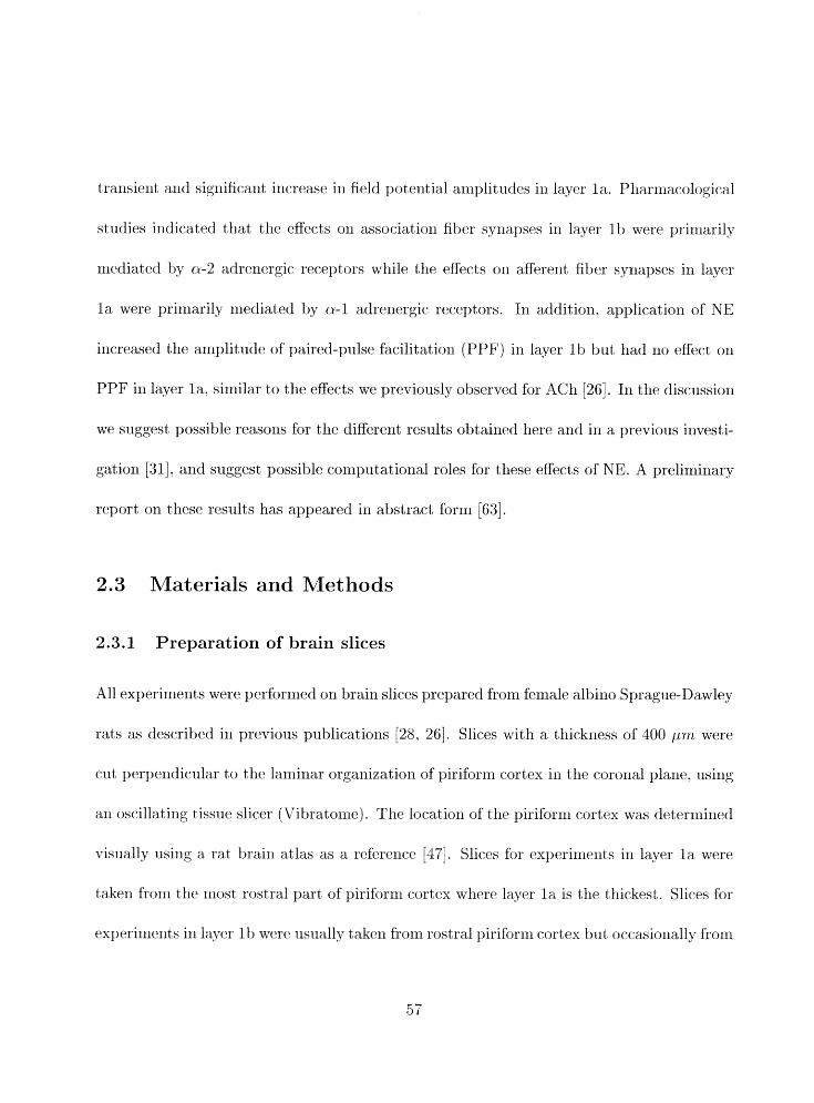
transient and significant increase in field potential a~rlplitudes in laver la. Pharmacological

studies indicated that tlie effects on ass~r ia t~ io l~ fiber syllapses in layer l b were primarily

mediated by a-2 adrenergic receptors while tlie effects 011 afferent fiber syrlapses in layer

l a were primarily mediated by a-1 adrenergic receptors. 111 addition, application of NE

increased the amplitude of paired-pulse facilitation JPPF) in layer l b but had no effect on

PPF in layer la, similar to the effects we previously observed for ACll [26]. In tlle discussion

we suggest possible reasorls for the different results obtained here and in a previous investi-

gation [31], and suggest possible coniputational roles for tliese effects of NE. A preliminary

report on tliese results has appeared in abstract form

2.3 Materials and Methods

2.3.1 Preparation of brain slices

All experiments were perfor~ned on brain slices prepared from female albino Sprague-Dawlcy

rats as described in previous publications 28. 261. Slices with a thickness of 100 p m were

cut pcrperldiculas to the laminar organization of pirifbrm cortex in the coronal plane. using

an oscillating tisstle slicer (Vibratomej. The locat io~~ of the piriform cortex was deterrrlirled

visnally using a rat t~rain atlas as a reference . Slices for experirnent,s in layer l a were

taken from the rrlost rostral part of piriforrri cortex where layer l a is the thickest. Slices for

experiments in layer 1 b were usually taken from rostral pirihrm cortex but occasionallly from

laore caudal regioris of ~jirifornl cortex. l b results frorii rostra1 and caudal piriform cortex

m r e essent idly identical. Slices were rxlaintained in an artificial cerebrospinal fluid ( ACSF)

solutiorl (P.jaH603 26 m,ltf; NaC1 124 rr~ilil: KC1 5 m M : KH2P04 1.2 mhf: CaC12 2.3 m&I;

MgS04 1.3 mA4; glucose 10 m A J ) at room te~nperature for approximately two liotlrs before

beginning the experiments. Albumin (0.125 g /L) arld kynurenic acid (0.66 mP1) were added

to the solution during this tirne but were not used in the solutiori bathing the slices during

experiments. Albumin was added to minimize protease darnage to the slices while kynurenic

acid, a nonselective glut amate antagonist, was added to prevent excitotoxicity. We have

found that adding albumin and kynurenic acid to the ACSF solution results in healthier

and longer-lived brain slices.

Slices were placed in a submersion-type slice chamber on top of a srnall nylon rnesh

which kept both sides of the slice exposed to ACSF. ACSF was kept oxygenated with a

95% 02/5% CC2 mixture bubbled through the solution. Tlie flow rate was 4 mllmin. The

slice chamber included a heating elerlierlt which kept ACSF maintained at a temperature of

33-35" C , Slices were transillurniriated. allwing visually guided placement of stimulating

and recording electrodes. Slices were left in the charlit~er for at least 15 miuutcs before com-

rrrencing recordirlg in order do wash off all traces of kpnurenic acid. whicll would otherwise

have interfered with the recordings due to its effects as a glutanlate antagonist.

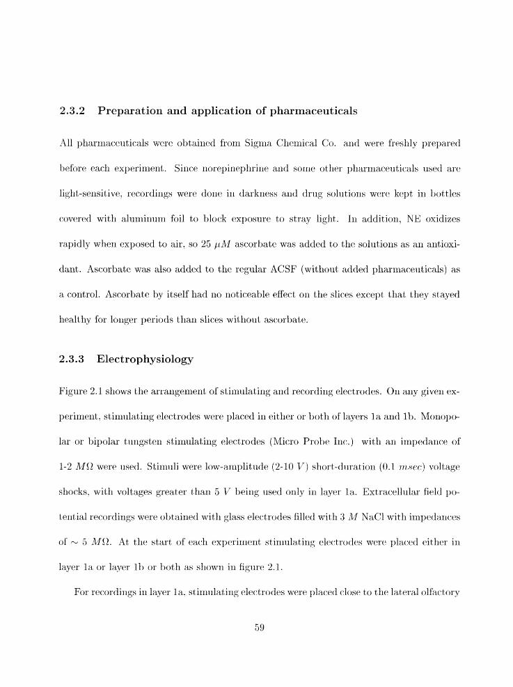
2.3.2 Preparation and application of pharmaceuticals

All pharmaceuticals were obtained from Sig~rla Chemical Co. and were freshly prepared

before each experiment. Sirice riorepincphririe and some other pllarmaceuticals used are

light-sensitive. recordings were done in darkness and drug solutions were kept irl bottles

covered with alurninuni foil to block exposure to stray light. In addition. NE oxidizes

rapidly when exposed to air, so 25 pJi9 ascorhate was added to the solutions as an antioxi-

dant. hscorbate was also added to the regular ACSF (without added pharrnaceuticalsj as

a control. Ascorbatc by itself had no rloticeable effect on the slices except that they stayed

hea l tb for longer periods than slices without ascorbate,

2.3.3 Electrophysiology

Figure 2.1 shows the arrangement of stimulating and recording electrodes. On any given ex-

periment, stimulatirrg electrodes were placed in either or both of layers l a and lb. Mouopo-

lar or bipolar tungsten stimulati~ig electrodes (Micro Probe Irlc.) with an inlpedarlce of

1-2 MO were used. Stimuli were low-amplitude (2- 10 V ) short-duratiorl (0.1 V L S ~ C ) voltage

shocks. with voltages greater tllan 5 V beirig used only in layer la . Extracellular field po-

tential recordixlgs were obtained with glass electrodes filled wit11 3 h4 NaCI wit11 impedances

of - 5 hff2. At the start of each experiment stimulating electrodes were placed either in

layer la or layer l b or both as slsovt-11 in figure 2.1.

For rerordi~lgs in layer la. stinlulati~lg electrodes were placed close to the lateral olfactory

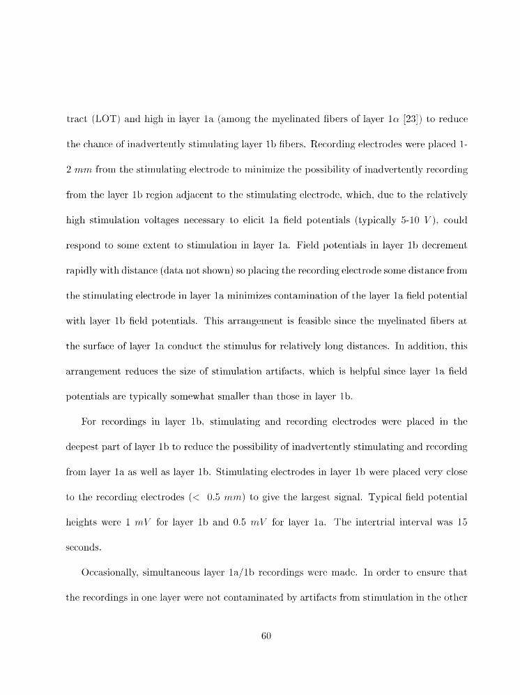
tract (LOT) arid liigll in layer l a (anlollg the myeliriated fibers of layer la [23] / to red~lcc~

the chance of illadwrterit ly stimulating layer I h fibers. kcording electrodes were placed 1-

2 mrn from tlie stimulating electrode to rninimize the possibility of irladverte~ltly recordirig

frorn the layer 1 b regiori adjacent to the stimulating electrode, which, due to the relatively

high stimulation voltages necessary to elicit l a field potentials (typically 5- 10 V ) . could

respond to some extent to stirnulatiori in layer la. Field potentials in layer l b decrement

rapidly with distarice (data riot shown) so placing the recordirig electrode sorne distarice fioni

the stimulat ing electrode in layer l a minimizes contaminat ion of the layer l a field potential

wit11 layer I11 field potentials. This arrangernent is feasible sirice the rn~elinat~ed fibers at,

tlie surface of layer l a conduct the stimulus for relatively long distances. In addition, this

arrangenlent reduces the size of stimulation artifacts, whicf.1 is helpful since layer l a field

potentials are typically somewhat smaller than those in layer 1 b.

For recordings in layer lb , stimulating and recordirig electrodes were placed in the

deepest part of layer l b to reduce the possibility of irradvertently stimulating and recording

frorn layer l a as well as layer lb . Stinlulating electrodes in layer l b were placed very close

to the recording electrodes (< 0.5 rarra) to give the largest signal. Typical field potential

heights were 1 n ~ l i for layer l b and 0.5 rrtl' for layer la. The i~lt~ertrial interval was 15

seconds.

Occasionally. simult aneous layer la / 1 b recordings were made. In order to ellsure that

the recordings in one layer were not contaminated by x t i f x t s from stimzllatioll in the other

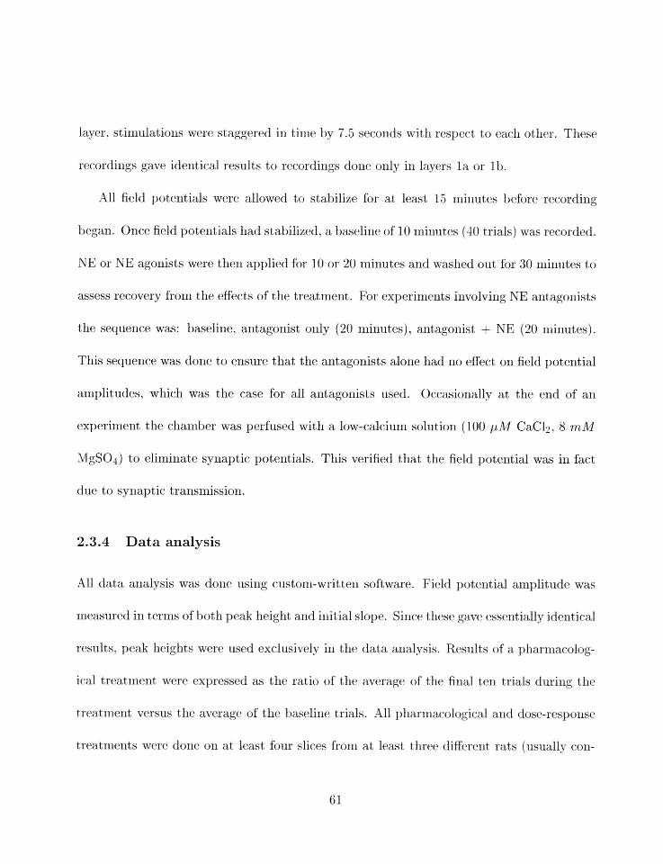
layer, stim~llations Miere staggered in time by 7.5 seconds with respect to eacll otlier. These

recordings gave identical results to recordings done only in layers la, or I b.

All field potentials were allowed to stabilize for at least 15 minutes before recording

began. Once field potmtials had stabilized, a baseline of 10 minutes (10 trials) was recorded.

NE or NE agonists were then applied for 10 or 20 minutes and washed out for 30 rniriutes to

assess recovery from the effects of the treatment. For experiments involving NE aiitagoiiists

the sequence was: baseline. antagonist only (20 minutes). antagonist + NE (20 minutes).

This sequence was done to ensure that the antagonists alone had no effect on field potential

amplitudes, which was tlie case for all antagonists used. Occasionally at the end of an

experiment the chamber was perfused with a low-calcium solution (100 jrM CaC12. 8 m M

MgS04) to eliminate synaptic potentials. This verified that the field potential was in fact

due to syilaptic transmission.

2.3.4 Dataanalysis

All data arialysis was done using c.ustotli-writterl software. Field pote~itial amplitude was

measured in ternis of both peak height and initial slope. Since these gave essentially identical

results. peak heights were used exclusively in tllr data analysis. Results of a pllarrnscolog-

ical treatment were expressed as the ratio of the average of thr: final t,en trials duririg tlie

treatment versus the average of' the baselirle trials. Ali pl~arinacological and dose-response

treatments were done on at least four slices froni at least three diEerent rats (usually con-

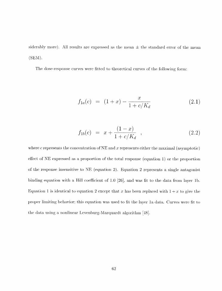
siderably rnor-e). 811 results are expressed as tlie rnean If the starldard error of the nieari

jsEnz).

The dose-resporlse curves were fitted to theoretical curves of the followi~ig form:

where c represents the concentrat ion of NE arid z represents either the maximal (asymptotic)

effect of NE expressed as a proportion of the total response (equation 1) or the proportion

of the response insensitive to NE (equation 2). Equation 2 represents a single antagonist

binding equation with a Hill coeEcient of 1.0 [26], and was fit to the data from layer 11,.

Equation 1 is identical to equation 2 except that x has beer1 replaced with 1 + z to give the

proper lirnitirig behavior: this equatiori was used to fit the layer la. data. Curves were fit tjo

the dxt a using a rlorllinear Levenburg-Marquardt algorit llm [18].

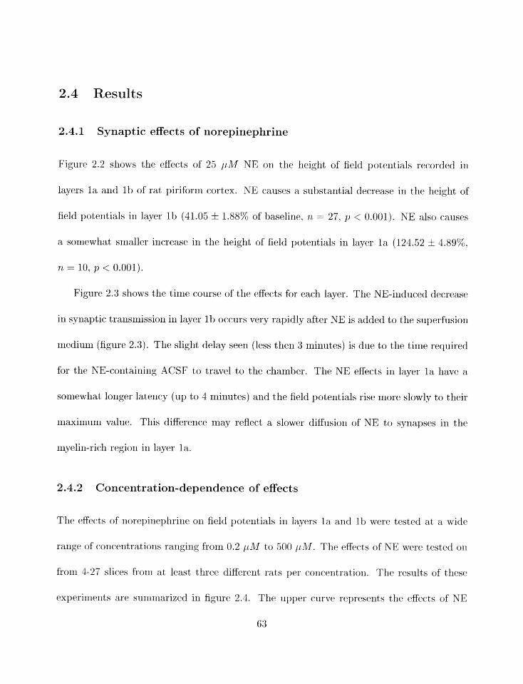
2.4 Results

2.4.1 Synaptic effects of norepinephrine

Figure 2.2 shows the effects of 25 irM NE or1 the height of field potentials recorded in

layers l a and l b of rat piriforrn cortex. NE causes a s~bstant~ial decrease in the height of

field potentials in layer l b (41.05 f 1.88% of baseline, n = 27. p < 0.001). NE also causes

a somewhat smaller increase in the height of field potentials in layer l a (123.52 f 4.89%.

rr. = 19: p < 0.001).

Figure 2.3 shows the tinir course of tlle effects for each layer. The NE-induced decrease

in synaptic traiisinissioi~ in layer l b occurs very rapidly after NE is added to the superfusion

medium (figure 2.3). The slight delay sem (less tlleri 3 minutes) is due to the time required

for the NE-containing ACSF to travel to the chamber. The NE effects in layer l a have a

so~newliat longer latency (up to 4 minutes) and the field potmtials rise more slowly to their

maxiinunl value. This differellee may reflect a slower diffusion of NE to synapses in tlle

myelin-rich region in layer la.

2.4.2 Concentration-dependence of effects

The effects of ~iorepi~lephrine on field potentials in lavers l a and Ib wore tested at a wide

range of co~icentrstions rizrlgixlg from 0.2 jri7CI to 500 ~ L V . The effects of NE were tested on

from 1-27 slices from at least three differerlt rats per coricrntratio~l. The results of tllese

ex~>erimerds are summarized in figure 2.4. Tlle upper curve represeIlis the effects of NE

63

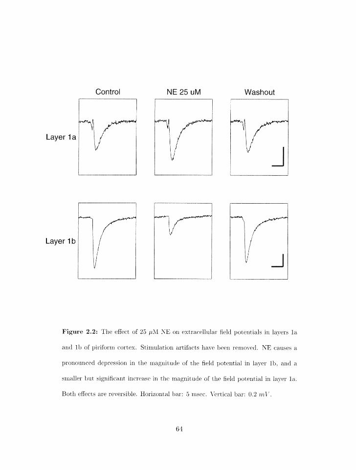
Layer 1 a

Layer 1 b

Control Washout

Figure 2.2: Tlie effect of 25 k i l l S E on extrac~ellular field poteritials in layers l a

arid l b of piriform cortex. Stimulation artifacts haye beer1 removed. YE causes a

pro~lourlecd depressiorl in the magnitude of the field potential in layer lb . arid a

srnaller hut signi5eant increase in the rrragrlitudcl of the .field potential in layer la.

Botl-t effects are reversitsle. Horizontal bar: 5 msec. lyertical bar: 0.2 rnl - .

" 0 5 10 15 20 25 30 35 40 45 50

time (min)

Figure 2.3: The time-course of the NE effect in layers l a and l b , relative to

baseline. Layer la data are displayed with open circles while layer l b data are

displayed with filled circles. The dark bar shows the duration of NE application (10

minutes at 25 pM).

in layer l a and tlie lower curve the effects of NE in layer lb. Tlie curves represexit tlie

optimal fits to tlie birldinlg equation described in the Metllods section, as determined by

a rionliriear regressiorl procedure. The asymptotically maxi~lurn increase in field potential

height in layer l a due to NE was 23.47%) with a dissociation constant Kd of 8.82 phf. Tlie

concentration giving 50% of tlie lnaxirntlm response according to this curve was 8.8 pM.

The asymptotically maxir~lum decrease in field potential height, in layer l b due to NE was

34.02% (this is the coniponent of tlie response resistant to NE) with a dissociation constant

Kd of 4.66 pM. The corlcerntratiori giving 50% of tlie maximum response was 4.37 p M .

2.4.3 Pharmacology of effects

We examined the effects of a number of noradrenergic agonists and antagonists in order to

deternline the likely receptor type(s j responsible for t lie NE effects. Tlie results. toget lier

wit11 the effects of NE alone, are shown in figure 2.5.

In layer la , the P-agonist isoproterenol at 25 pM caused a significant but very srriall

rise in field potential heights ( 105.22 f 1.42% of baseline, rr, = 6. p < 0.05). The (2-1 agonist

pl~enylel,hrirle (50 p M ) reproduced tlie NE effect on field potelitials (122.83 i 5.31% of

baseline, n = 7. p < 0.01). The a-2 ago~iist clonidi~le (25 phf) also caused a smaller but

significant increase in layer la field potential heiglit*~ (1 13.04 k 1.28% of baselinle. ri = 5.

p < 0.001). However, the n-1 antagonist yrazosini (2 pi2.f) completely bluckcd the effecst of

25 pllf NE in layer la , while the a-2 blocker yoliinlbine (5 p M f liad virtually rio effect.

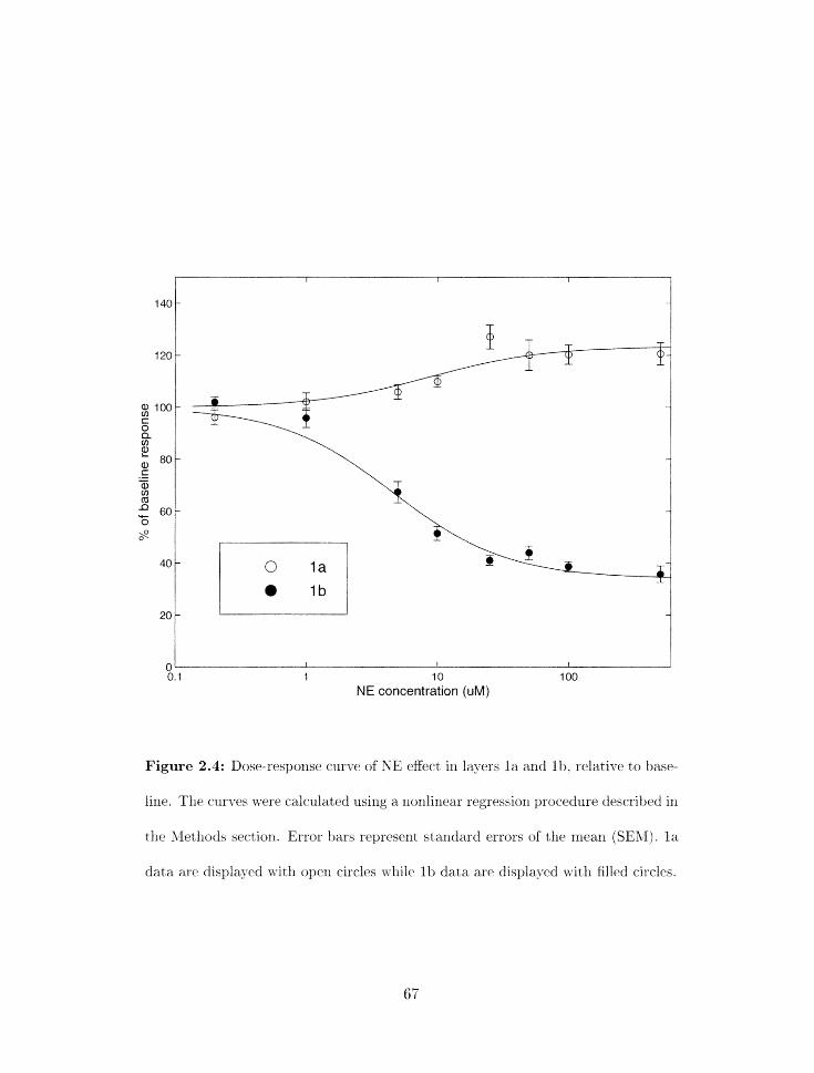
Figure 2.4: Dose-response curve of NE effect in layers l a and lb. relative to basti-

line. The curves w r e calculated using a ~lonlinear regression procedure described in

tlle Aletllods srrtiorl. Error bars represent staldard errors of tlre nrean (SEN). la

data are tlispla5-~d with open circles wllile 1b data art. displayed witli filled circles.

suggestirlg that the NE effect in layer l a is ~~rirnarily mediated by a-1 arlcl not a-2 receptors.

In layer lb. isoproterenol at 25 pM caused s significsrlt irtcrta.se in field potential heights

(113.14 f 3.65%) of baseline. rt = 10. p < 0.01). in sharp contrast to the effects of NE. The

a-2 agonist clonidine (25 p&lj caused a decrease in layer l b field potelitin1 lleigllts to

77.85 i 2.38% of baseline (n = 6. p < 0.001). 111 addition, tlle a-2 antagonist yohimbine

(5 p M ) almost completely blocked the eEects of 25 pM NE (95.15 f 1.38% of baseline.

n = 5). Interestingly. the a-1 agonist phellylephri~ie (50 p M ) also caused a slight decrease

in layer l b field potentials to 84.49 i 2.49% of baseline (n = 5, p < 0.001). However, the

a - I receptor antagonist prazosi~i (2 / A M ) was not able to block the NE effect in layer l b at

all. This suggests that the NE effect on layer l b field potentials is primarily mediated by

a-2 receptors.

2.4.4 Effects of norepinephrine on paired-pulse facilitation

Figure 2.6 presents tlle effects of NE on paired-pnlse facilitation (PPF) in piriform cortex.

Layer l a field potentials typically exhibit a large degree of paired-pulse fa~ilit~ation. whereas

layer 1b field poterltials show much less PPF ill]. The effcct,s of 25 p11\f NE on PPF arc

shown i11 figure 2.6 for an irlterpulsc irnterval of 50 psec. NE llad virtually no effect on

PPF ill layer l a (PPF without NE: 1.487 i 0.109: PPF with NE: 1.487 f 0.055: 72 = 4).

but caused a signi6cant irlerease in PPF in layer l b (PPF without NE: 1.197 ir 0.055: PPE

witti NE: 1.441 f 0.042: n = 10. p < 0.05). As a result. the depressioll of field potential

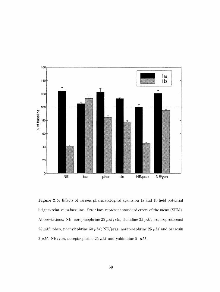
NE is0 phen clo N E/praz N Elyo h

Figure 2.5: Effects of various pharmacological agents on l a and l b field potential

heights relative to baseline. Error bars represent standard errors of the mean (SEhI).

Abbreviations: NE, norepinephrine 25 phf; clo, clonidine 25 / l A l ; iso, isoproterenol

25 pLU; phen, phenylephrine 50 pAl; SE/praz, norepinephrine 25 pAl and prazosin

2 pAf; NE/yoh, norepinephrine 25 pA1 and yohimbine 5 pA1 .

height with NE application is considerably reduced for tlie second pulse. Since PPF is a

pres~~naptic effect [24. 381 this strorigly suggests that tlle eEect of NE 011 associatiori fiber

synapses in layer 11, is primarily presynaptic, since if NE was acting postsynaptically both

pulses sliotlld have beer1 affected equally [24]. The lack of effect of NE on PPF ill layer l a

is completely consistent with the a- 1 receptor-dependence of the eEect . since a- 1 receptors

are generally located postsynaptically 18, 171.

2.5 Discussion

2.5.1 Differential effects of NE on layer l a and l b field potentials

Our results show that rlorepinephrine causes a pro~iounced decrease in the height of synaptic

field potentials in layer l b of piriforrn cortex (figures 2.2 and 2.3). NE decreases the height. of

field potentials to about one-third of their original height at high doses with a half-maximal

effect at 4.4 /AM (figure 2.1). This effect is consistent with previous results we [63. 64

others [31] have obtained. 111 co~itrast. liorepineplirirlc causes a significant increase of about

25% in field potential heights ill layer l a of' piriforrli cortex (figures 2.2 and 2.3). This effect

is co1lcentratiox1-depe11de1it with a half-maximal effect s t 8.8 pM (figure 2.41, a i d lias not

been. previously reported in t lle literature.

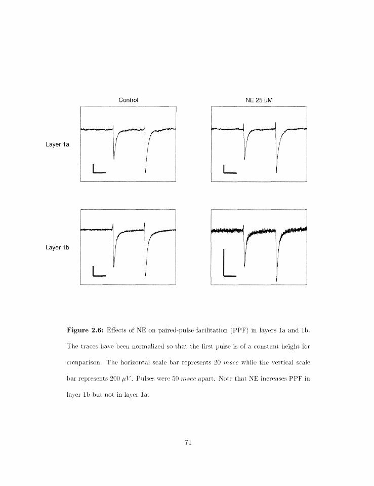
Control

Figure 2.6: Effects of XE: on paired-pulse facilitation (PPF) in layers l a and lh .

The traces hme Ixen aorrnalized so that tlrc first pulse is of a co~lstant heigltt for

tornparison. The horizorltal scale bar represerits 20 ~rzstvc 1%-hile the vertical scale

1-jar represents 200 ply. Pulses were1 50 I I ~ S F C ' apart. Note that YE increases PPF in

layer l b but not in layer 1 a.

2.5.2 Pharmacological basis for the NE effects in layer l a and i b

The results in figure 2.5 indicate that the effect of NE on layer 1h field poterltials is priiiiarily

due tjo NE acting on an n-2 adrenergic receptor subtype. The a-2 agonist clonidine (25 ~ L M )

caused a decrease in field potedial lleigl~t to 77% of baseline. This is considerably less than

the full NE effect: however. clorlidine is very weakly water-soluhle and thus it was difficult

to precisely control the concentration of drug delivered to the slice chamber. Therefore, we

may be overestimating the amount of clonidine that actually was in contact with the slices.

In additiorl. clorlidine is known to be a partial agonist for a-2 receptors [16. 491. Cloriidine

at tlie conceiitratiorl used (25 p M ) also has some affinity for a-1 receptors [6, 331, which

leaves open the possibility of some corltribution to the observed effect from a-1 receptors.

However, the a-1 agoriist phenylephrine even at the relatively high concentration of 50 phf

only caused a sn~all decrease in 1b field potentials, to 84% of baseline. More significantly,

the a-2 antagonist yohirnbine (5 p M ) alnlost completely blocked the effects of 25 ph.1 NE

(to '35%) of baseline). whereas the a-1 receptor arltago~iist prazosi~i (2 / A M ) was not able to

block the NE effect at all. Thus tlle contribution to this effect from a-1 receptors, if any,

appears to be small.

In coiitrast "c layer 111. tlie effect of NE on layer l a field pokedials is pri~xlarily due

to KE acting on an a-1 receptor subtype. The a-l agollist phenylephrine (50 ~ r A f ) fully

rel~rodncrd the NE effect (122%) of baselirlr). Clonidime (25 ~ L A I ) also caused a smaller hut

sigrlificant increase in layer la field potential lleiglits ( 1 13%) of baselil-te) . which. hoxrever,

may be due to cross-reaction with cv-l receptors. The 0-1 antagonist prazosiri (2 pA4)

completely blocked tlic effect of 25 jrAf NE in layer la. while the a-2 blocker yoliinibirle

( 5 p&I) had virtually rio eEect, suggesting tliat the NE effect is primarily rilediated 1)y 0-1

a ~ i d not a-2 receptors.

There is no compellixig evidence tliat the NE effects we observed in either layer l a or

layer l b are mediated to any significant degree by /3 adrenergic receptors. The ,6 agonist,

isoproterenol caused a significant incrt.ase in field potential heights in layer lb , which is the

exact opposite of the effects of NE. However, the size of the increase was fairly small (only

about 13% of baseline). It is thus quite possible that tlie a-2 recept,or-mediated suppressiorl

of field potentials we postulate are actually stronger than we observed, being masked to

some extent by the [j receptor-mediated increase in field potential heights.

From the pliarmacological data and the paired-pulse facilitation data we also conclude

tliat tlie NE effects on layer l a neurons are most likely to be niediated postsynaptically,

while the effects in layer l b are most likely to be presy~laptic. The evidence we present

liere for this conclusion is circumstai~tial, but plausible. First. a-1 receptors, of tlie sort,

implicated in t lle layer l a respollses. are generally found posts y napt ically

receptors. which appear to rrlediate tlie layer l b effects, are often fourld iri the presynaptir

trrlnilial [8. 17. 35. 61. 621 (although a-2 receptors have also been found postsynaptically

iri sorile studies. e.g. [I. 39, 451). Secondly. our experimental results from paired-pulse

Fhcilitation (PPF) are consistent; with this l~ypothesis. PPF is generally t~elieved to rely

on a presyrlaptic mecharlisr~~ [21. 381. arid NE 1las no e&rt 011 PPF iri layer l a (proposed

postsynaptic receptors) but does affect P P F in layer l b (proposed presynaptic; recel~tors).

Tllus tho pharmacology arrd tlle P P F data both s~iggest a second fundameda.1 diffrrericc.

between the effects of NE in these two populatiorls of synapses.

2.5.3 Differences from previously reported results

1x1 contrast to tlle results reported here, Hasselrno et al. [31] reported that application of NE

in layer l a caused no effect on layer 1 s field potentials for low concentratiorls and a slight

decrease for liigher concentrations. Collins et al. [13] using trarlsverse slices also suggested a

concentration-deper~dent effect of NE. but in their case low corlcentrat ions were reported to

result in an increase in evoked potentials, while higher concentrations produced a decrease.

It is difficult to directly relate the results from diEerent slice preparations: we suspect that

the recordings of Collins et al. combined hot11 l a and l h field potelltials to varying extents.

making a direct conlparison vc-it11 our results impossil>le. The concentrat ions used in the

experiments described here bracketed those used in both of tlle previous studies.

In our data it is quite clear that the effects of NE on field potelitials in layer l a are

more varial2le than in layer lh. ranging from a very sligl~t irlcrease to increases of over 200%)

in sorne slices. Ncl.ertheless. our data show that: the only effect of NE on layer la field

potentials is arl increase in field potexitial amplitude regardless of the conrentratiorl. We

found, howcver. that extreme care must be taker1 to assure that layer l a recording conditions

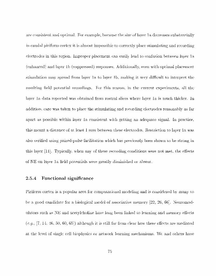
arc consistent and opti~nal. f i r example. t-jecause the size of layer l a decreases substantially

irr caudal piriforrn cortex it is almost impossible to correctly place stimulating arid recordirig

electrodes in this region. Improper placemerit can easily lead to eonfilsiorl betsveen layer l a

(enhanc:ed) and layer l b (suppressed) responses. Additiorlally. even wit h optimal placement

stimulation may spread frorrl layer l a to layer lb , making it very difficult trio interpret the

resulting field potential recordings. For this reason. in the current experiments. all "che

layer l a data reported was obtained from rostra1 slices where layer l a is much thicker. In

addition. care was taken to place the stimulating and recording electrodes reasonably as far

apart as possible within layer l a consistent witli getting an adequate signal. In practice,

this rrzeant a distance of at least 1 rnm between tllese electrodes. Restriction to layer l a was

also verified using paired-pulse facilitation which has previously been shown to be strong in

1 I]. Typically, wlien any of these recording corlditions were not met. the effects

of NE 011 layer l a field potentials were greatly dimirlislied or absent.

2.5.4 Functional significance

Piriforrn cortex is a ~jopular area for computational modeling arid is cor~sidcred by maIiy to

be a good calldidate for a biological model of associative n1rrllor.y [22. 26. 66

rrlators s~lcll as NE and acetylcholine have long been lirlked to learning and rrzertlory effects

(e.9.. [7. 13. -16. 50. 60. 651) althougll it is still far from c l ~ a r bow these effects are rriediated

at the level of single cell biophysics or network learrling meclianisms. We arid others have

demonstrated. however. that these modulators can have strong effects on the belravior of

synapses and cells in piriform cortex j l . 5, 18. 26. 30. 25. 27. 31. 10. 42. 13. 54. 551.

Taken in the coritext of our efforts to build realistic nrodels of tlie olfactory cortex

[lo, 36, 37. 661, the differential biophysical effects of both AClr and now ME on the two

principle sources of excitatory inputs on the apical dendrites of pyramidal cells can be

proposed to have a direct effect on the way in whicll this network processes inconling sensory

data [9]. Specifically, we have proposed that ACli. which suppresses layer l b association

fiber synapses. may serve to make the piriform cortical network more responsive to olfactory

afferent sensory inputs than to internal dynamics. We show here that ME both suppresses

association fiber synaptic transmission and enhances afferent fiber synaptic trarisnrissiorl.

Thus it would appear that NE provides a more extreme form of regulation than AClr

although with eEects in the same direction. Realistic xnodcling efforts currently underway

in our laboratory will use tlle data presented ixi this paper as well as previously published

results on ACh and NE to more directly contrast the consequences of these two important

neuromodulators on cortical function.

Acknowledgements

We would like to tllank Karin1 Elaagouby for expert advice on experinlrntal technique and

slice cllaxrlber construe t ion.

Bibliography

11 C. Aoki, C. Venkatrsan. C. G. Go, R. Forman, and H. Kurose. Cellular and Sub-

cellular Sites for Noradrenergic Action in the Monkey norsolateral Prefrontal Cortex

as Revealed by the Immunocgtochemical Localization of Noradrenergic Receptors and

Axons. Cerebral Cortex. 8(3):269-277, 1998.

[2] A. F. T. Arnsten and J. D. Jentsch. The Alpha-1-adrenergic Agonist. Cirazoline.

Impairs Spatial Working-Memory Performance in Aged Monkeys. Pharmacology Bio-

cfiernistry n~2d Behavior, 58(1):55-59, 1997.

31 G. Aston-Jones. C. Chiang. and T. Alexinsky. Dischxgc of Noradrenergic Locus-

Ccruleus Neurolis in Behaving rats and Morlkeys Suggests a Role in Vigilance. Prr,,gress

in Brain Research, 88:501- 520. 1991.

[1] E. Barkai, R. E. Bergmall. G. Horwitz, and M. E. Hasselmo. Modulatiori of Associative

hlvferrlory Fu~lctio~l ill a Biophysical Sirnulat ion of Rat Pirifbrrxl Cortex. Journ aI of

i4Teur~phgsiotogy. 7212) 3659-677. 1994.

[5] E. Barkai and M. E. Hasselrno. hlodulatioxl of the Input/Output Rllictiorr of Rat

Pirifornl Cortex Pyrarriidal Cells. Jot~rrraZ of Nearophpsiology. 72(2) :644-658. 19 94.

[6] B. Blochldauln, A. Korn, M. Wolzt. £3. Sch~ilidt. and H. G. Eichler. 1x1 vivo Studies on

Alpha-adrenergic Receptor Subtypes in Human Veins. Naulzyn-S~hna~iedehergs Arehives

of Phurmaeologg. 343(3):302-307, 1991.

[7] A. Blokland. Acetylcholine: a Nrurotrar~smitter for Learning and Memory? Brazn

Research Reviews. 21 (3):285-300. 1995.

[8] A. Borsodi and M. Wollenlann. a-adrenergic Receptors. In Abel Lajtha. editor. Harhd-

book of Neur.ochemistr:(l, 2nd. Ed.. volume 6. pages 27-38. Plenum Press. New York.

1982.

[9] J. Ad. Bower. Reverse Engineering the Nervous System: an 1a Vivo. 171 Vit1.0, and In,

Corrlpato Approach t$o Understanding the Mammalian Olfactory Systern. In S. F. Zor-

rretzer. T. ill. iZiilcKenna, arid C. Lau. editors, An In,t?*oduction ta Neural and Electronic

Netu~orks, 2nd. Ed., pages 27-38. Acadernic Press. San Diego, 1994.

[10] .J. &I. Bower and D. Beeman. The Book qf Genesis. Sprillger Verlag. New I'ork. 1995.

[I 11 J. M. Bower and L. B. Habcrly. Facilitating and Nonfarilitnting Synapses on Pyrsrrlidal

Cells - a Carrelati011 Bet~veen Physiology and hforphology. Proceedings 4 The Natimal

Aeadcmg o$ Scbe?zees of The I:n bted States of Arne?-btn, 83(4): 1 115-1 119, 1986.

I-'

v I-' g $

i" w . ' I-'

[l9] R. Gray arid D. Jolinst on. Noradrerialine and Beta-L4drenocrpt or Agollists Irlcrease

Activity of li'oltage-DepentlW Calcium Channels in Hippocanpal-Xeuroris. fVatu7.r..

327(6123):620-622, 1987.

[20] L. B. Haberly. Neurorial Circuitry in Olfactory Cortex - Anatomy arid Functiolial

Implications. Chemical Senses, 10(2) :219-238: 1985.

211 L. B. Haberly arld J. M. Bower. Arialysis of Association Fiber Systern irl Piriforrn Cor-

tex with Intracellular-R~ording and Staining Techniques. Journal of Neuroph ysiologg.

51(1):90-112. 1984.

[22] L. B. Haberly and J. M.. Bower. Olfactory Cortex - Model Circuit for Study of

Associative Mernnry? ?'rends In Neurosciences, 12(7):258-264. 1989.

[23] L. B. Haberly arid S. L. Feig. Structure of the Piriforrn Cortex of the Opossuni. 2. Fine

Str~icture of Cell Bodies and Neuropil. Jol~rnal i?f Co~npclrafilre Neurology. 216(l) :69--

88, 1983.

[24] E. W. Harris arid C. m7. Cotman. Effects of Synaptic Antagorlists on Perforant Path

Paired-pulsc PlasticiQ - DiEere~ltiation of Presynsptie and Postsynaptic Antagonism.

Bmin Research, 333(2) :M8-353. 1985.

%I. E. IIasselrno. Acetylcholine axid Learning in a Cortical Associative Memory. Neumi:

Compz~tatiorz. 5(1):32-44, 1993.

[26] M. E. Hasselrilo. B. P. Andersorl. and J. M. Bower. Clioliriergic Modulatiori of Cortical

Associative hlemorg Fxinction. .lounhol of Neuroph,ysiolog?qll. 67(5) : 1230-1216. 1992.

[27] bf . E. Hasselmo and E. Barkai. Clioliriergic Modxilation of Activity-Del~eridrnt Synap-

tic Plasticity in the Piriform Cortex and Associative hlernory Function in a Network

Biophysical Simulation. Jnurnal of Neuroscience. 15(10):6592-6604, 1995.

[28] M. E. Hasselmo and J. M. Bower. Affrrent and Association Fiber Digerences in Short-

term Potentiatiorl in Piriforrn (Olfactory) Cortex of the Rat. Jovrnul of Neurophysiol-

ogy, 64(1):179-190, 1990.

[29] M. E. Hasselmo and J . M. Bower. Cholinergic Suppression Specific to Irltrinsic not Af-

ferent Fiber Synapses in Rat Piriforni (Olfactory) Cortex. Journal of Neurophysiology.

67(5): 1222-1229. 1992.

[30] M. E. Hasselrrlo arid J. M. Bower. Acetylcliolirie and Memory. Trends 171 Nevrosczences.

16(6):218-222, 1993.

[31] M. E. Hasselmo. C. Linster., M. Patil. D. Ma. and M. Cekic. Noradreliergic Suppressiori

of Syrlaptic 'l'r.ansmissio11 &lay Influence Cortical S i g n i l l - t o - i s Ratio. Jourrbni' of

Neuroyhysioloyg. 17(6):3326- 3339. 1997.

FjT. F. Hopkins and D. .Johrrston. E'requenc~y-Depender~t Xoradrenergic Modulation of

Lorig-Terrn Potentiation in the Hippocampus. S c i e ~ c e , 226(4672) :350- 352. 1984.

[33] W. F. Hol3kins arid D. .Johnstori. Noradrenergic Enliancmient of Long-Tern1 PotBen-

tiatiorl at Mossy Fiber Synapses in the Hippocampus. *loumnl nf' A%Teurophysiolqg.

59(2):667-687. 1988.

[34] P. Jakala, M. Riekkinen. J. Sirvio, E. Koivisto. and P. Rickkinen. Clonidine. but not

Guaiifaciiie, Impairs Choice Reaction Time Performance in Young Healthy Volunteers.

Neurq;nsychopharv~,ucoZogy. 21 (4):495-502, 1999.

[35] Y. Kamisaki. T. Hamahashi. C. M. Okada, and T. Itoh. Clo~iidine Inhibition of

Potassium-Evoked Release of Glut amate and Aspart ate from Rat Cortical Synapt o-

somes. Brain Research; 568(1-2): 193-198. 1991.

361 C. Koch arid I. Segev. bfethods in Neuronal Modeling. M I T Press, Cambridge, Mas-

sachusetts, 1989.

[37] C. Koch a ~ i d I. Segev. hfethods in Neuronul hfodeling. 2nd. Ed. MIT Press. Cambridge,

Massacliusetts, 1997.

[38] S. W. KnWer, J . G. Nicllolls. and A. R. Martin. fro?^, Neuron to Bmir~: A Cell~u~lar

Approach to the hnctiors of the firprous Systm,. Sinarter Associates. Sunderland.

h4assaellusetts, 1984.

[39] -4. Lee. D. L. Rosin. and E. J . varl Bockstaele. Ultrastructural Evidr~irr for Pronli-

nent; Postsynaptic Loealizatio~i of Alyhaj26)-adreriergie R.ecey>tors in Catecholaniiner-

gic Derldrites in the Rat Nuclr~is Locus Coeruleus. .lour=nai of Comparative Ilier~rologg.

394(2):218-229. 1998.

[40] H. Liljeristrom arid M. E. Hasselrno. Clloliriergic Modulatior~ of Cortical Oscillatory

Dynamics. Journal of Neurop~siologyl. 74(1) 3288-297. 1995.

[41] D. V. Madisori arid R. A. Nicoll. Noradrenalirle Blocks Accommodatio~~ of Pyramidal

Cell Discharge in the Hippocampus. Nature, 299(5884) :636-638, 1982.

[42] G. J. Marek and G. K. Aghajanian. Excitation of I~lterneurons in Piriforrn Cortex by 5-

Hydroxytryptanline - Blockade by MDL- 100,907. a Highly Selective 5-HT2a Receptor

Antagonist. European Journal of Pharmacologyl. 259(2): 137-141. 1994.

1431 G. J. Marek and G. K. Aghajanian. Alpha(1B)-adrenoceptor-nlediated Excitation of

Piriforrn Cortical Irlternellrom. Et~ropean Journal of PPhanna~ology~ 305(1-3) :95-100,

1996.

[14] D. A. b4cCormick. H. C. Pape. and A. Williamson. Actions of Norepinephrine in the

Ccrebral-Cortex and Tlialarnus - I~nplicat ions for Function of' the Central Noradren-

ergic Systeni. Yroyress in Brain R e s e n ~ h . 83:293-305. 1991.

[15] T. A. h4ilner. A. Lee. S. A. Aicher. and D. L. Rosin. Hippocampal *4lplia(2.2)-

Adre~lergic Receptors are Located Predominantly Presynapt ically but are also Found

Postsynaptically and in Selective Astrocytes. hurnal of Com~~amtive -rv'e~rologg.

395(3):310-327. 1998.

1461 M. Ohlzo, M. Kohayashi. A. Kishi. arid S. mratanabe. Working-Mrrnory Failure by

Cornhined Blockade of Muscarinic arzd Beta-Adrenergic Transmission in the R,at Hip-

pocampus. Neurorepo~t. 8(7):1571-1575, 1997.

1171 G. Paxinos and C. Watson. The Rat Brain in Stereotazic Coordinates. Academic Press.

San Diego, 1997.

[48] W. H. Press. S. A. Teukolsky, W. T. Vetterling, and B. P. Flannrry. Numerical Recipes

in C. 2nd. Ed. Carnbridge University Press, New York. 1992.

[49] K. Rasrnussen, M. Brodsky. arzd C. E. Inturrisi. NMDA Antagonists and Clonidiue

Block C-FOS Expressio~z During Morphine Withdrawal. Synapse. 20(1):68-74. 1995.

S. J. Sara. G. Dyorzlaurent, and A, Herve. Novelty Seeking Behavior in the Rat is

Dependent Upon the Integrity of the Noradrenergic System. Coynative Bruin Research.

2(3):181-187, 1995.

[51] S. J. Sara. A. Vankov. and A. Wervr. Locus Coeruleus-Evoked Res~~onses in Bellavi~ig

Rats - a, Clue to the Role of Noradrenalirlcl in hIen~ory. Bruin Research Bulletirt.

35(5-6):457- 465, 1994.

[52] M. Segal. H. Markraal. and G. Ricliterlevirl. Actions of Norepinephrirle in tllr Rat

Hippocarnpus. Prqqress 171 Brain Research. 88:323-330. 1991.

[53] D. Servan-Schreiber. H. Printz. and J. D. Col le~~. A Network Model of Catccllolainirle

EEects - Gain. Signal-to-Noise Ratio, and Behavior. Science. 249 (4971) :892-895. 1990.

[54] P. W. Slieldoil and G. I(. Aghajanian. Serotonin (5-HT) Iilducrs IPSPs in Pyranlidal

Layer Cells of Rat Piriforrn Cortex - Evidelice for the Iiivolvemerlt of a 5-HT2-activated

Interneuron. Bruin Resea~h . 506/ 1) :62-69, 1990.

P. W. Sheldon and G. K. Aghajaniaii. Excitatory Responses to Serotonin (5-HT) in

Neurons of tlle Rat Piriforln Cortex - Evidence for Mediation by 5-HTlc Receptors in

Pyramidal Cells and 5-HT2 Receptors in Interneurons. 9ynapse. 9(3):208-218, 1991.

[56] G. Re. Slieplirrd, editor. The Sgauptic O9yunization of the Bmin, 4th. Ed. Oxford

University Press, New York, 1997.

[57] M. T. Shiplty and M. Ennis. Functiorial Organization of Olfactory System. Journal of

Neurohiolyg, 30(1): 123 -176, 1996.

[58] L. R. Squire. Menlor9 und Bmin. Oxford Urliversity Press. New York. 1987.

[59] I. Takayanagi and K. Koike. Effects of Agillg or1 Postsynaptic Alpha- 1-arirenoceptor

Mecllaaisms in Rat h r t a . Gelaelal Phar~nnc~loyg. 22(2) 321 1218, 1YN.

[GO] S. A. Thomas and R. D. Palmiter. Disruptiorl of tlle Doparnixie-Beta-Hydroxylasc~ Gerir

in Mice Suggests Roles for Norepirieplirint. in Motor Fxinction. Learning, arrd R.lermry.

Behaviornl Neuroscience. 11 1 (3):579-389, 1997.

[61] A. U. Trmdrlenburg. K. Starke. and N. Limhrrger. Presynaptic Alpha(2a)-

Adrenoceptors Irihibit the Release of Eridogerious Dopamirie iri Rabbit Caudate Nu-

cleus Slices. ll'nunyn S~hnaiedeherg~s ilrchzictes of Pharnracoloyg, 350(5):473-481. 1994.

[62] P. $. Trornbley. Noradrerlergic Modulation of Synaptic Transmission Between

Olfact,ory-Bulb Neurons in Culture - Implications to Olfactory Learning. Bmin Re-

search Bulletin, 35(3-6) :473-484, 1994.

[63] M. C. Vanier and J. M. Bower. Differential Effects of Norepinephrine on Field Poteritials

in Layers l a and Ih of Rat Olfactory Cortex. Society for ATeumczence Abstructs,

18:1353, 1992.

641 M. C. Vanier arid J. M. Bower. Differential Effects of Norepinepllrine on Synaptic

Tralis~riission in Layers l a and l b of Rat Qlhckory Cortex. In Computation and Neural

Sgstert-rs. pages 267-2'71. Kluvvclr Academic Publishers, Boston. 1993.

651 D. A. Wilson. T. C. Pharn. arid R. M. Sullixrali. Norepiricplirine and Posttraining

Memory Cortsolidation in Xeonatal Rats. Behnt!ioral Ne~rl-oscenee: 108(6) : 1053-1C)X

1994.

[66] M. A. IYilsoi~ and J. M. Bower. Cortical Oscillations axid Temporal Interactio~ls in a

Computer Siniulation of Pirifvrm Cortex. Jov~rnal of Neur.ophys%ulu,q~. Cj7(4):981--995.

1992.

Part 111

Matching neural models to experimental

data

Introduction

One probleni faced by all those who build realistic models of single neurons is that of match-

ing the outputs of the model to experimental data for the same cell type. The reason for

this difficulty lies in the highly nonlinear nature of neural models and the relatively large

number of poorly constrained parameter values that these models generally possess. The

usual way modelers have dealt with this problenl is by iteratively adjustirlg one paranieter

at a time until the model reproduces the data set. However, because of the lionlinearities

inherent in the models. when one pararnet#er is significantly changed many other parameters

will usually have to be changed as well. Sillce this process is tedious and time-corisuming,

there is a need for autoliiated methods that car1 do parameter-fitting with a mininiunl of

user intervention. The first of the papers in this section describes a group of such metll-

ods irnple~lented by the autllor within the framework of the GENESIS neural sirnulator.

cornpares their advantages and disadvantages, and gives suggestions for the most eEective

use of the methods. Tlie niethods developed for this -rvork are now available in a GENESIS

library wllicll will be included in the next. version of tlie software. These nietliods rrzake the

process of fitting single-cell niodels to data dramatically easier,

One questiorl regardirig single-cell rnodels is how to compare diEererit rnodels wliir.1~

have been paranleterized on the same data set. Such i~iodels might represent niodels froni

different investigators or rnodels at difFerent levels of complexity froin the same investigator.

What is needed is a rigorous quantitative framework for comparing models. The second

paper in this sect ion (done in collaboratioii wit 11 Pierre Baldi) uses t lle Bayesian probabilistic

framework to compare ixiodels. Using this framework, oiie can compare individual niodels

to determine which is more probable given the known data. One can also compare entire

classes of models, so that one can ask more generic questions. e.g., '.If I remove this ion

cllannel from this model. will the resulting class of models be more or less likely to match

this data set?" Bayesian methods can also provide a rigorous uilderpiiining for designing

matching functions, which are traditionally doiie in s r i ad- hoe fashion. Therefore, the work

ill this paper is complerneritary to the work in the previous one; the first paper addresses the

question: "How do I match a model to the data?", while the second addresses the questiorl

"How good are the inodels obtained by this process?" Together. the two papers are a first

step towards a xrlore yuarititat ive rrretllodology of neurorial rilodel building.

Chapter 3

A Comparative Survey of Automated

Parameter Search Methods

for Compart ment a1 Neural Models

3.1 Abstract

One of the most diactrllt artd tinlr-consursli aspects of building compartmental models of

single nellrorls is assigning values to free parameters in order to make nlodels match experi-

xzientad data. &Alltomated parameter search neth hods potentially represent a. more rapid and

less labor-intensive alternative to cboosilig paralzletcrs manually. Hero we compare t lze pcr-

forrlianee of four d i e re& pararrleter search methods on several single nrrtron models. Tlle

nledhnt-ts coltipared are eorljugate-gradient descent. genetic algorit)lrns. sirvlulated anneal-

ing, and stochastic search. Each method lias been tested on five different neuronal rrlodels

rangillg from simple ~rlodels with between 3 and 15 paratneters to a realistic pyramidal a l l

model with 23 parameters. Thr results denioristrat cl that genetic algorit llrns and sirmlated

a~rnealing are generally the most effective met hods. Simulated annealing was overwhelrrl-

irlgly tlie nlost effective method for simple models wit 11 small numljers of paralneters. l:,ut

the gerietic algorithm method was equally effective for rrlore complex models with larger

xiurnbers of pararneters. The discussion considers possible explanations for these results

and rnakes several specific recommendations for the use of parameter searches on neuronal

models.

3.2 Introduction

Conlpartniental neural models are I>eitrg used increasingly in neuroscience to model struc-

tures ranging from single synapses and neurons to large networks of neurons [3. 21, 251.

Sirigle neuron rnodels are often required to reproduce very specific features of existing ex-

perinlental dat,a. such as transrxiernbrane voltage trqectories and detailed ileuronal spiking

patterns generated experimentally in resporrse to complex stimuli. Typically, slrcli 1xiodc.1~

inchrde every voltage- and calciurn-dependent ioriic co~ldrlcta~lce known tto exist in a par-

ticrilar rlertrorr type. and tlreir morpliologies are based upon aliatornical data collected from

real neurons.

Ideally, all tlie corrstittierits of the lodele led neurorxal struetrrres slloutd he derived di-

rrctly fi-on1 experinlental data. In practice. this is usually not possible for several reasons.

It is often the case that the kinetics of many of the candidate ionic co~iductances have

rlot been adequately characterized experimentally. The spatial distribution arid chanriel

derisities of the irrcluded ionic corlductances are ofterl unknown, because these values are

relatively difficnlt to rneasure experimentally. Models may also incorporate intracellular

calcium and second-messenger dynamics [25]. which may not be sufficiently well character-

ized to completely constrairi the model. For these reasons, realistic neuronal modelers are

usually faced with the problem of constructing simulations co&aining a large number of

loosely constrained parameters under expectatiorls that the r~iodels will replicate complex

experiment a1 data wit li high accuracy.

Given the complexity of the models and the lack of sufficient exyerirrlental data, the

traditior~al way in which pararrleters are assigned to neural models involves varying param-

eters iteratively by hand based on a series of educated guesses. However, tlie large nunhers

of parameters involved (which is steadily increasing as lnodrls becorne more sophisticated)

makes ma~iually parmeterizing a model a very time-consuming and tediolis exercise. In

addition, ionic collductances in neural rnodels often interact with one another in lnighly uon-

linear ways [24. 36 . rnaking it impossible to accurately adjust parauneters independently of

each other. klannal parauieterizatiorl also does not provide any quantification of how closely

the nlodel replicates pliysiological data. Instead. typically several figtlrcs sliming sinlilar

waveforms and spikitlg patterns has sufficed as proof' of biological re1cvanc.c. In p rx t i t "~ .

this niearis that ~riodelers are always tempted to stop when the rl~odel produces a barely

adequate fit to the data. instead of trying to determine the hest possil~le rnatch between

the ir~odel and the data.

For these reasons, we [I, 3 . 401 and otllers [lo, 11. 381 have experimented with tlie use

of autoniated parameter search nietllods for assignirlg parameters to neural models. This

approacli requires the niodeler to have a target data set that the model rnust match. A

simulation is run, a numerical mat ell value is calculated, and the parameter search routine

automatically chooses the next set of pararneters to evaluate based on the previous results

and the match value. While, in theory. such a procedure could be iterated over the entire

set of possible parameters (a so-called brute force seardl), in fact. ever1 for simple models.

limitations in computer resources make it necessary for the pararneter searching software

to make what are in effect its own educated guesses as to what pararneters to use next.

Thus the design of the searching algorithnl is critical to the success of the process. Several

dierent search algoritlims exist which can in principle be applied to this problem. However.

an assessment of the value of one or ailother automated searching technique can only come

from a rigorous side-t3y-side comparison. In this paper. we speci6cally evaluate four commorl

seardzirlg algorithais which have been applied to neural models: corsjugatc gradient-descent

, stochastic searcll [ll]. genetic algorithms [I. 10. 401. and simulated amlealing [I. 101.

14T~ coxnpare tile effectiveness of these rrletliods in obtaining good pararneter sets given

tlie sante aniount of computer resources. Since it is often the case that the eEectiveness

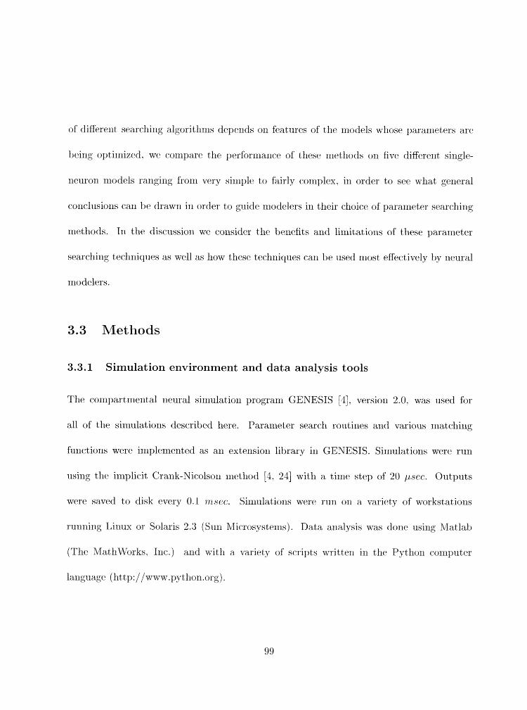
of differerlt searching algoritlirns deperids on features of tlic niodels wliosr paranieters are

t,eing optimized. wr compare the performarlce of these rnetliods on five different single-

neuron models raliging fro111 very sirliple to fairly cornplex. in order to see what general

conelasions car1 be drawn in order to guide nlodelers in tlieir choice of parameter searelling

methotls. 111 the discussion we consider the benefits and limitations of these parameter

searching techniques as well as how tliese techniques earl br used most effectively by rleural

modelers.

3.3 Methods

3.3.1 Simulation environment and data analysis tools

The compartmental neural sirnulatioli program GENESIS [4 , version 2.0, was used for

all of the simulations described here. Parameter search routines and various matching

functions were irnpleniented as an extension library in GENESIS. Si~xiulations were run

using the implicit Crank-Nieolson nletllod [4, 241 with a t h e step of 20 pstc. Outputs

were saved to disk every 0.1 rrt.see. Silzlulatioris were run on a variety of workstations

ronni~lg Linux or Solaris 2.3 (Sun Mirrosyster~is). Data alialysis was done usirig Matlab

(The Matli'VVorks. Iric.) and with a variety of scripts writterl in thc Python mmputcr

language (ht tp://www.pytlion.org).

3.3.2 Models

Five models were used to evaluate different parameter search metliods. For any given model.

tlie parameter search routines were run for a fixed number of sivrlulations and tlie progress

of tlle searcli was recorded as the simulation progressed. The purpose of this was to see

which searcli methods gave the best results for a fixed n u d e r of si~nulations. Models 1-4

were used only to test the paranleter search rriethods and are not realistic models of actual

neurons. whereas rnodel 5 is based on real data.

Models 1 and 2: simple spiking cell with adaptation

The first two models (known as sinlplel and s imp le2 respectively) were derived from a

simple orrc-compartment neuron rnodel with four voltage-dependent ionic conductances:

fast Na, delayed-rectifier K , illactivating K (A-current), and a slow no~i-inactivating K

conductance (M-current). The parameters for the first three channels were derived from a

model of the hippocampus by R.oger Traub [39] wliile tlre last was derived from a model

of a hullfiog synlpatlietic gangliorl cell [24 . Tlie kinetics of the channels were modified

solnewhat in order to produce a firing pattern similar to that of regular-spiking pyramidal

cells in cerebral cortex [30]. In the first niodel jsinzplrl) the &ee parameters represented

the mairnal conductances of the four ionic channels. The second versio~r ( sim~1le2) also

colltained four parameters that scaled the 7 ( L r ) curves (time constant as a f~i~ictiori of

membrane potential) of the activation gating variable of each of the channels. The first

rnodcl thus had four adjustat~le parartietcrs wliile tlie seco~id hat1 eight.

Before thc searches were started. the initial values of tlie parameters to be varied were

set to random values drawn fro111 a log-uriifor~a distributiori centered arou~ld the correct

values of the para~neters. A raridonl value from this distributiori is equal to the exporielitial

of a value drawn froni a distribution uniformly distributed between the natmal logarithms

of the endpoints. This distribution allows us to choose random values for parameters wit11

equal probabilities of choosing values of start/:c and start * :c. This is a natural choice for

nonriegativc scale-dependent parameters such as maximal conductances and scaling values

for r (V ) curves. The range of tlie distributio~i was from $ to 4 times the correct value.

We generally chose tlie rariges for a giver1 parameter by trial and error unless there was

experirncntal data to corlstraili tlie range. For models 1 and 2. a range of 4 was suEcient

because the initial parameter values were constrained to be no more than a factor of 4 from

tlte correct values. For these models, tlie goal of tlle parameter searches was to match the

spike tinlings of the target model's outputs; the shape of the interspike intxrval waveform

was not considered. The inputs were somatic UC current; injectiotis (current-clanip) at six

diEerent current levels. The reason for using multiple current levels is that in our experience

matct-ling a model to data using only a single value of irljectled curretit is relatively easy.

w'tiile matchiug a nlodel usirig a wide range of input currents is extremely difficult because

of the higlily rlo~rlinear behak~ior of neuror-zs, Thus it is esseritial to use as rtiucli dat;a to

constrain the model's bellmior as is feasible, and forcing the niodel to rnatcll the data over

a wide rarlgp of input currents has proven to be all easy way to strongly collstrain the

parameter values (see tlie Discussion j.

Models 3 and 4: passive dendrite models

Models 3 and 4 (known as ynsszrrel and passive2 respectively) were passive dendritx models.

i e . . they had no voltage- or calcium-dependent ionic conductances. Our approach was to

choose a fixed morpllology for the model and consider the passive electrical properties of the

model (melnbrane axial resistivity (RA), specific membrane capacitance ( C M ) and specific

menlbraiie resistivity ( R M ) ) to be unknown parameters. Since these models were passive

and lience linear. we used a single value of current injection (0.1 nA) at one location on the

cell as the input stimulus: using diEerent values would have simply multiplied tlie response

by a constant and so would have been redundant. We started the searclles at a random

point in paralneter space and required the search to fi~rd the optimal matcli as with nrodrls

1 and 2.

Model 3 was a 100-compartniet linear unbranched passive dendrit,e model. Tlrc. three

parameters were RA., RLVI. m d CA4. whiclr were assumed to be constant for all cornpart-

rtlents irr the cable. Current was iqjeeted at one end of tlre demrdrite. We measured tf-le

rrlernbralie poteritial at: three points along the dendrite and used this as our output data set

to be rliatelled to the target rrlodel.

Lilodel 4 was a brarlclred dendrite ntodel: in addition to the soma there were four derz-

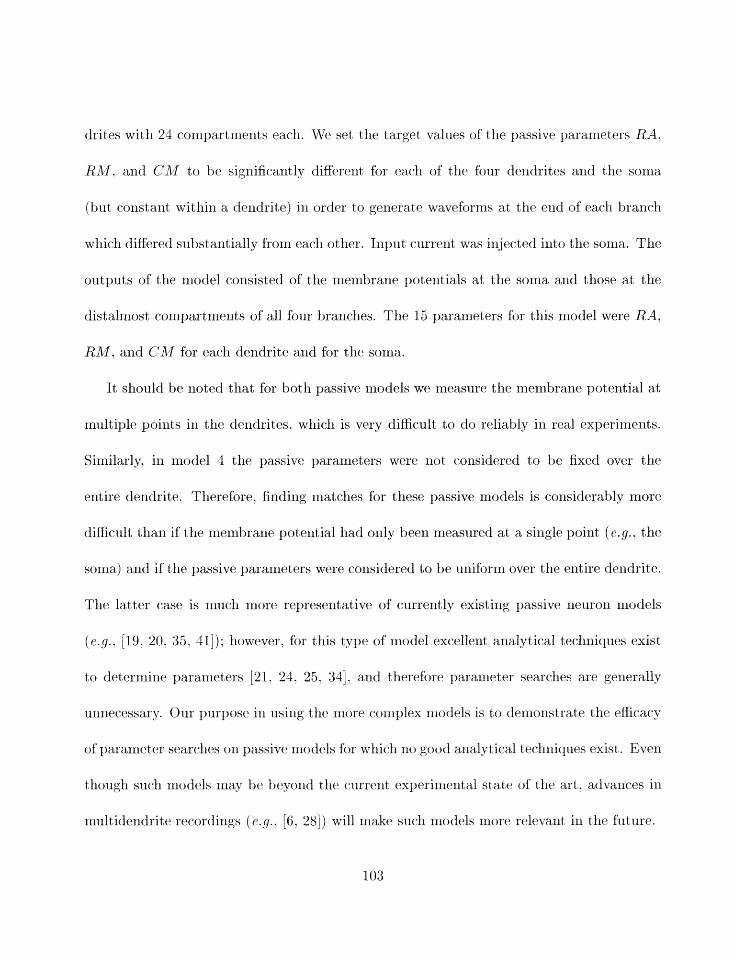
drites with 24 compartments each. WP set tlie target values of the passive parameters RA,

RM. and C M to be significantly different for each of tlre four deridrites arid the sorna

(but constant within a dendrite) in order to gexlerate waveforms at the end of each branch

which differed substantially fronr each other. Input current was injected into the sonra. The

outputs of the model consisted of tlie membrane potentials at the sorna and those at tlre

distalmost conipartnie~rts of all four branches. The 15 parameters for tliis model were RA.

Rhf , and C M for each dendrite and for the sorna.

It sllould be noted that for both passive models we rneasure the membrarie potential at

multiple points in tlie dendrites, which is very difficult to do reliably in real experiments.

Similarly, in nrodel 4 tlre passive parameters were not considered to be fixed over the

entire dendrite. Therefore, finding matches for these passive niodels is considerably more

difficult than if the membrane potential had only been measured at a single point (e.g., tlic

soma) and if the passive parameters were corrsidered to be uniform over the entire dendrite.

The latter case is much more represedative of currently existing passive neuroll nrodels

( r .9 . . [19. 20, 35, 411): however. for this type of rnodel excellent analytical techniques exist

t80 determine paranletters [2 1. 21. 25, 3.11, arid therefore paranl~ter searches are generally

unnecessary. Our purpose in using the more cornplex n~odels is to demorrstratc the efficacy

of parameter searches ori passive rnodels for which no good analytical Gechlliques exist. Even

though such models may be 'i3eyorrd tlic current experimental statx of the art, adwriccs in

multidendrite recordings (e.g., [6, 281) will make srlcll models more relevant in t8he future.

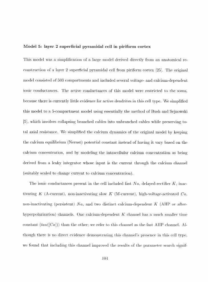
Model 5: layer 2 superficial pyramidal cell in piriforrn cortex

This model was a sirnplificatiorl of a large model derived directly from an anat>omical re-

coilstruction of a layer 2 superficial pyrarllidal cell from piriform cortex 1251. The original

rnodel consist ed of 503 compart rnent s aiid included several volt age- and calciuin-dependent

ionic corlductances. The active conductarlces of this model were restricted to the soma.

because there is currently little evidence for active dendrites in this cell type. We sirnplifietl

this model to a &compartment rnodel using essentially the method of Bush and Sejnowski

[ 5 ] , which involves collapsing branched cables into uiibranclied cables while preservirig to-

tal axial resistance. We simplified the calcium dynamics of the original rnodel by keeping

the calcium equilibrium (Nernst) potential constant irlstead of having it vary based on the

calcium concentration. and by modeling the intracellular calciurrl corlcerltration as being

derived from a leaky integrator whose input is the current through the calcium channel

(suitably scaled to change current to calcium concentration).

The ionic corlductances present in the cell included fast Na,, delayed-rectifier K . iliac-

tivating K (A-current), 11011-inactivating slow K (M-current 1. high-volttage-activated Ca.

norl-inactivating (persistent) Nn. and two distinct calcium-dependrrlt K (AHP or after-

lqperpolarizatioil) d ~ a ~ ~ ~ i e l s . One calcium-de:penderit K channel Ilas a rnucll smller tirile

coristarlt ( tau([Cu])) than the other: we rcfer to this charlnrl as the fast AHP cllannel. Al-

tllough there is no direct ~ridericc. denlonstrating this cllarlnel's presenee in this cell type.

we found that irlcludirlg this channel irnproved the results of the parameter search sipif-

icantly (see Ijelow). Most of the kinetic pararneters were taken either frorn existirlg data

for piriform cortex superficial pyramidal cells [2, 7. 13. 161, or. in cases where no such data

existed. from otlier cell types such as hippocampal pyramidal cells [12. 31. 391. Further dr-

tails on the lnodel can he found in the appendix. The model thus contained eight voltage-

or calcium-dependent ionic coriductarlces arrd a simple calciurrl buffer. wit11 23 parameters

chosen for fitting. In addition to the pararneter types used for ~rlodels 1-4, model 5 also

includes parameters of the following types:

1. voltage offsets for tlie activation (m,(V) or m,([Ca])) curve of an ionic channel

gating variable

2. parar~reters controllirlg the calcium buffer rnodel

3. voltage offsets for resting membrane potential

4. somat ic and dendritic membrane resistivities

Parameters that are offsets from a starting value (i.e.. not scale parameters) are cflosen

frorrl a, uniform distrihntion. as opposed to the log-uniform distribution cllosen for the scale

parameters.

We added a separate parameter for the resting ~nembrane potential t-~eeause the values

obtained horn our experiruients included an unspecified junction potential which could be as

high as several millivolts [42 . lVe also callsidered the specific rxlenlbrarze resistivity of the

soma and delldritic regiolis as separat,e parameters. Since the reconstructed nlorplrology

105

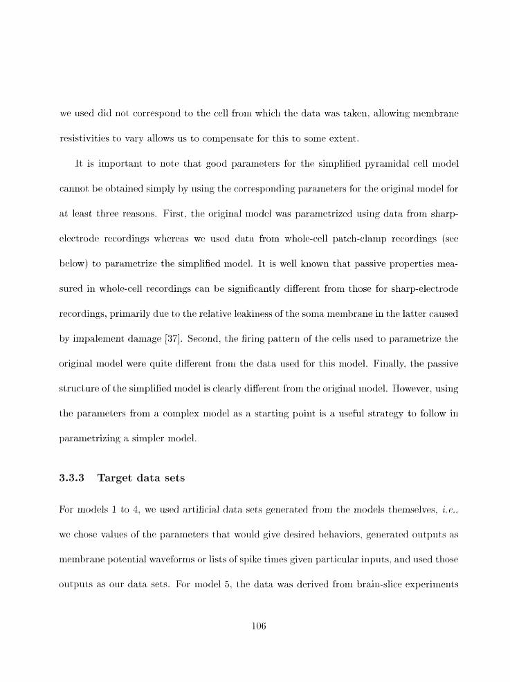
we used did not correspond to the cell from which the data was taken, allowing nleaibrarie

resistivities to vary allows us to conipensate for this to some extent.

It is irriportaitt to note that good paranieters for tlie sirnplified p~~rarnidal cell rnodel

cannot be obtained simply by nsing the corresponding parameters for the original rnodel for

at least three reasoris. First. tlie original model was parametrized using data, from sharp-

electrode recordings whereas we used data from whole-cell patch-clamp recordings (see

below) to parametrize the simplified model. It is well known that passive properties rnea-

sured in whole-cell recordings can be significantly different from those for sharp-electrode

recordings, primarily due to tlie relative leakiness of the soma membrane in tlie latter caused

1,y impalement damage 1371. Second, the firing pattern of tlie cells used to parametrize the

original rnodel were quite differelit from the data used for this rnodel. Finally, the passive

structure of the simplified model is clearly diEerent froni the origi~ial model. However, using

the parameters from a complex rnodel as a startirig point is a useful strategy to follow in

parametrizilig a simpler model.

3.3.3 Target data sets

For models 1 ta 4. we used artificial data sets generated from the inodels themselves. i. e..

we chose values of the 13arar~ieters that would give desired t>elia;\iiors. gezlerated outputs as

~ncnibrane potent ia1 wavefvrnis or lists of spike times given particlular inputs, and used those

olit-p~rts as our data sets. For rriodel 5. tlie data was derived froin brain-slice experinierzts

on rat ~liriform cortex. A layer 2 superficial pyramidal cell's responses tlo mrying levels of

current irljection were recorded with standard wlrsole-cell iritracellular recording teclzniques.

MTP took data frorll six diEerent values of current injection (spanning tlie range froni a level

at which tlie cell did not spike at all to a level at which the cell spiked fairly rapidly).

Tlle data was processed to extract the spike times; this was the data set that our model

had to match. Tlie original irlputs consisted of one-second current pulses: to speed up our

simulations the simulated current injections were limited to 300 rrisec.

3.3.4 Computing the match between data and models

We used two different rnatch functions to assess how well our rriodels matelied our data.

For models 1. 2, and 5 (spiking cell models) we processed the menibrane potential traces to

generate lists of spike times, and then used a match function to cornpare tlie spike times of

the model with tliose of the data set. For rnodels 3 and 4 (nonspiking dendritic models) tlie

match function computed the mean squared diEerence at each time point of the rllerrlbrane

potentials of the model output vs. the target data. The match functions are error fuiictioxis,

with 0 representirig a perfect match.

Spike timing match function

This matching futlction conlputes a weighted average absolute ditfererice in corresl~onding

spike tiriles hetween the two models, with sonle extra penalty terms. The spike tirning

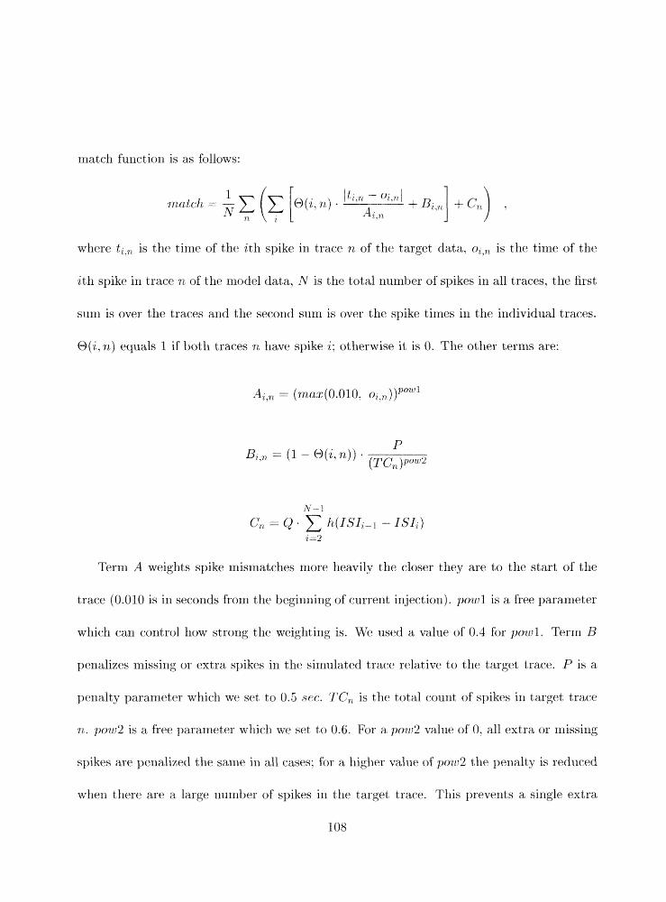
nlatcll functiori is as follows:

1 match = -

1G.n - 0i.n l A%.,

where is the time of the ith spike in trace n of the target data, o,,, is the time of the

ith spike in trace n of the nlodel data, N is the total riunrlber of spikes in all traces, the first

sum is over tlie traces and the second sum is over the spike tirnes in the individual traces.

O ( i , n) equals I if both traces n have spike i: otherwise it is 0. The other terms are:

Term A weights spike mismatches more heavily tlie closer tliey are to the start of tlie

trace (0.010 is in seconds from the beginrling of current injection). pow1 is a free paraaieter

which can control how strong the weighting is. VCTe used a value of 0.4 for pow 1. Terrii B

penalizes rnissing or extra spikes in the simulated trace relative to the target trace. P is a

penalty parameter wliiclh we set to 0.5 see. TC, is the total count of spikes in target trace

r ~ . pow2 is a free pararneter wliiclr. we set to 0.6. For a pow:! valtle of 0. all extra or rnissilcrg

spikes are penalized the sarxne in all cses: for a higher value of ~0211'2 the penalty is reduced

when there are a large nurrlber of spikes in the target trace. This prevents a single extra

108

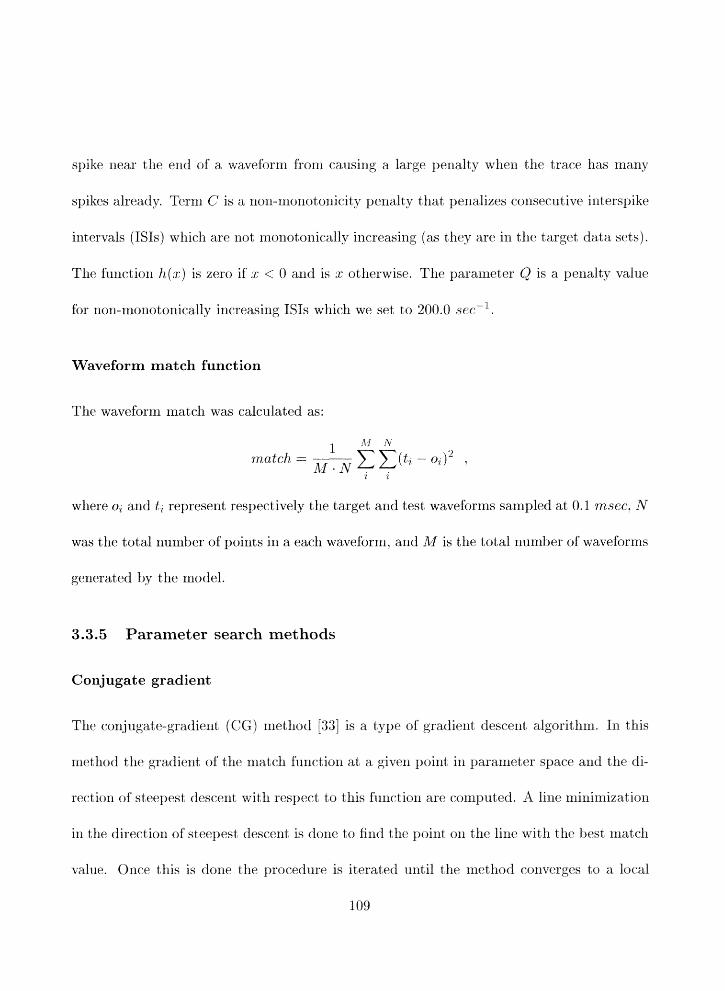
spike near tlie end of a wavefurm fro111 causing a large pelialty when the trace has many

spikes already. Tern1 C is a non-niortotonicit penalty that penalizes cox1secutive irlterspike

intervals (ISIs) which are not monoto~iically increasing (as they are in the target data sets).

The firnetion h ( r ) is zero if ~c < 0 and is x otherwise. Tbe paralrieter Q is a penalty value

for no11-1nonotonicaIly increasing ISIs which we set to 200.0 see-'.

Waveform match function

The waveform. match was calculated as:

where o, and t , represent respectively the target and test waveforms sampled at 0.1 msec, N

was the total number of points in a each waveform, and AI is the total number of waveforms

generated by the model.

3.3.5 Parameter search methods

Conjugate gradient

The conjugate-gradiellt (CG) method [33] is a type of' gradirrit descent algorithm. I11 this

method the gradient of the niatcli function at a given point in I>ara~~iet~er space and tlle di-

rect3ion of steepest descent with respect to this ftinction are computed. X line aiinimization

in the direction of steepest descent is done to find the point oli the line with the best rtlatcll

value. Orrce this is done the procedure is iterated until the method coriverges to a local

109

mini~num of the matelling function. Successive line nlillirnizatiolis are dorre in directions

which are col?jugate to one another so that successive nrillinrizatiorls are as nearly indepen-

dent of each otlier as possible. In theory this will guararitee that the paranlcter search will

find a local minirnunr of tire objective function. However. we found that when using the

spike tirning-based match function there were large regions of parameter space which were

conlpletely flat, i. e., where the gradient was zero. This generally occurred where no spikes

were produced by rnodels whose parameters were in that region. Since no useful gradierrts

could be calculated in these regions. the CG method could not be used directly. In these

cases we began by runni~lg 100 random sirnulations befort. beginning the CG search and

using tlie best match as a starting point. This usually resulted in a point where a gradient

could be calculated.

Genetic algorit hrn

The gerletic algoritlilri ( G Aj met hod 15. 18. 26. 321, treats each paranleter set as an individ-

ual in a large breedirrg population. A new gerleration of the populatiorl is derived from the

preceding generation by reproduction. crossing-over alld mutation. This was accomplished

by discretizirlg tlie pararlieter values into bit, strings and crossing-over and nnltating the

diEere11t hit strings. Paranleterg were represented as eitller 8-bib or 32-bit strings (8 bits for

models 1. to 4: 32 hits for nlodel 5): we found that the bit resolution had a nlinimal effect

on the results. We took a population of parameter sets and evaluated the fitness of each

one by computilig the match as described above. Since the fitness function must increase

for better matches, we calculated it by taking either the inverse of the nlatcll f-tlnction (for

model 5) or the square root of the inverse of the rxratch frlrictiorl (for models 1-41. Tht.

square root was used to reduce the difference in fitness between models and tllus has the

effect of lowering the selection pressure. This was found to be useful in niodels 1-4 since

there was often a very wide range of match values. and if selection is too strong premature

convergence of the algorithm may occur. This was not found to be the case fbr model 5 .

Once fitnesses were calculated, the next generat ion was determined by reproducing the

current generat ion, with each parameter set being chosen for reproduetiorl in proportion

to its fitness (fitness-proportio~ial reproduct ion). The11 a fixed percentage of the resulting

parameter sets were crossed over by choosing pairs of parameter sets at random. choosing a

breakpoint within the hit string and exchanging the bit strings above the breakpoirlt (single-

point recombinatioi~) . We crossed over $ of t he parameter st rings per gerierat ion. Finally,

each paraaieter set was subjected to nlutatio~i with a low probability per bit. We used a

nlutation probability of 0.02 per bit for xrlodels 1-4 and 0.01 for model 5. 111 this way. higllly

fit parameter sets are selected for and less fit sets art. eliniinated from tJre population over

a series of generations. Furtlierrnore, tlw processes of crossing-over arid recontbirration call

generate new parameter com^t.)inations whose fitness i s greater tltarl that of its predeccssurs.

For rnodels 1-4. we used a population size of 100 and ran the yararlieter searcll for

100 generations. giving a total of 10.000 sirnulatiorls per round. For r-ziodr.1 5, we used

a populatio~l size of 300 and ran tile search for 334 generations givixlg a total of about

100.000 simulations. Thesr ~~opulatiorl sizes are quite small for GAS [15. 321. but siricr tile

total nuxrlber of simulations was limited (intentionalld if a larger poprllatiorr size had been

used the simulation would have liad to have been run for fewer generations. PVe fou~ld that

these population sizes gave reasonable results but we did not irlvestigate the poplation-size

dependence of the GA systematically.

Our GA rmethod had t!wo nonstandard features: first: tlie best parameter set was always

preserved unaltered, This was to prevent genetic drift from eliminating good parameter. sets

and was necessary since the small population sizes used meant that random fluctuations

could have an excessively large effect on which parameter sets were propagated into the next

generation. Second. if the method went a large number of generations without improving

on the best parameter set. the entire parameter table (aside from the best parameter set)

was reseeded by choosing random values for all parameter sets. This provided an additional

way to keep the method from getting stuck in a subopti~nal region of pxameter space.

Simulated annealing

KTe used a continuous version of siniulated an~iealirig (SA) [23] adapted from Press et al.

331. This algorithm corlstructs an N-dinierlsional figure krlov~~l as a simplex out of N + 1

poirtts in the yaraxrreter space. In the deterministic form of tlie algoritiln.1. the siniplex is

moved through the ~larameter space based on tlie calculated match valries at the vertices of

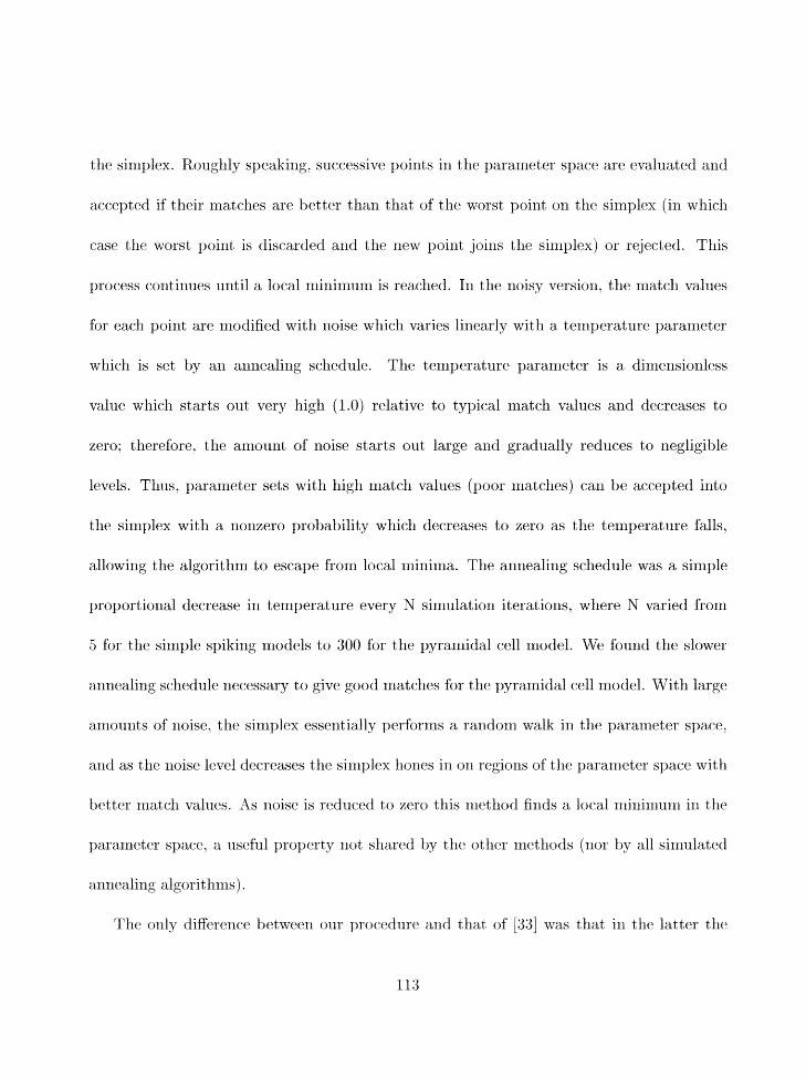
tlie simples. Roughly speaking. successive points in the parameter space arc evdluated and

accepted if their rilatclies are better than tliat of the worst point on the simplex (in which

case tlie worst point is dismrded arid the new point jitiris tlie simplex) or rejected. This

process continues until a local nlinimurri is reached. In tlie noisy version, the nlatcli values

for each point are modified with noise which varies linearly with a temperature parameter

which is set by an annealing scliedule, The temperature paraniet,er is a dimensionless

value which starts out very high (1.0) relative to typical match values and decreases to

zero; therefore. the arriount of noise starts out large and gradually reduces to negligible

levels. Thus. parameter sets with high match values (poor matches) can be accepted into

tlie siriiplex with a nonzero probability which decreases do zero as the temperature falls,

allowing the algorithm to escape from local minima. The anrlealing schedule was a simple

proportional decrease in temperature every N simulation iterations, where N varied frorn

5 for tlie simple spikirig models to 300 for the pyramidal cell model. We found the slower

arlnealirig schedule necessary to give good matches for the pyramidal cell model. With large

arlloririts of noise. the simplex essentially performs a random walk in the parameter space.

arid as the noise level decreases the sirnplex hones in on regions of the pararr-reter space witli

better match valtres. As noise is reduced to zero this nletllocf finds a local rxlirlinzum in the

~~arameter space, a useful property riot shared by the other rnetliods (nor by all simulated

arinealirkg alg~rit~hms j .

The only difference between our procedr~re and that of [33] was tliat ixi the latter the

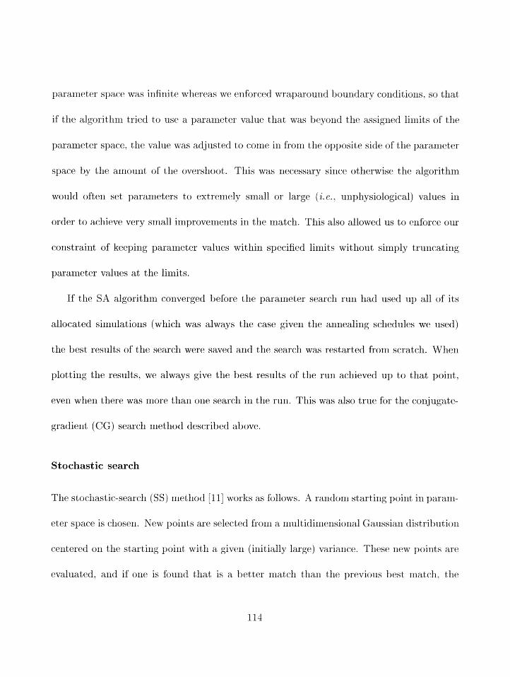
parameter spaccl was irifinite whereas vuTc enforced wraparouild boundary conditioiis, so that

if the algoritllnl tried. to use a parameter value that was beyond the assigried liniits of the

parameter space. the value was adjusted to come in frorri tlie opposite side of the pararrleter

space by the amount of the overshoot. This was necessary since otherwise the algorithm

would often set parameters to extremely srnall or large ( i. e., unphysiological) values in

order to achieve very srnall improvellleiits in the match. This also allowed us to enforce our

constraint of keeping parameter values within specified limits without simply truncatirig

parameter values at the limits.

If the SA algorithm converged before the pararneter search run had used up all of its

allocated simulations (which was always the case given the arr~lealing schedules we used)

the best results of the search were saved and the search. was restarted from scratch. When

plotting the results, we always give the best results of the run achieved up to that point,

even when there was more than one search in the run. Tliis was also true for the conjugate-

gradient (CG) search nietliod described above.

Stochastic search

The stocbast ic-searcli (SS ) met hod [I 11 works as follows. A raridom st artirig point in parani-

eter space is chosen. n'ew poililtas are selected from a riiultidi~ierisiond Gaussiari distribution

centered on the starting point with a give11 (initially large) variance. Tliese new points are

evaluated, and if one is found that is a better match than the previous best r-natch, the

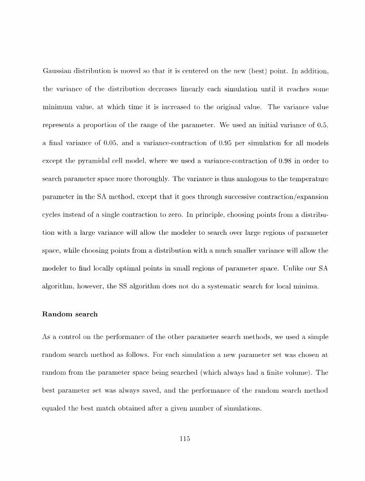
Gaussiali distributiori is moved so that it is centered on the new (best) point. 111 additiori.

tlic. variarice of the distrihrit iori decreases linearly each sirnulat ion until it reaclres somne

mininiurn value. at wlricli tinie it is increased to the original value. The variance value

represerits a proportiori of the range of the paranreter. Mie used an initial variance of 0.5,

a final variance of 0.05. and a variance-contraction of 0.95 per simulation for all models

except tlle pyrarnidal cell model, where we used a variance-contraction of 0.98 in order to

search paranieter space more thoroughly. The variance is thus analogous to the teinperature

pararneter in the SA method, except that it goes through successive contraction/expansion

cycles instead of a single contraction to zero. 1x1 principle. clioosing points from a distribu-

tion with a large variance will allow the modeler to search over large regions of parameter

space. while clioosing points from a distributiorl with a much smaller variance will allow the

modeler to fiud lncally optirrial points in small regions of paranieter space. Unlike our SA

algorithm. however, the SS algorithm does not do a systematic search for local minima.

Random search

As a control on the performance of the otlier ~laranreter search methods, we used a simple

random search niethod as follou~s. For each sirnulatioil a new parameter set was chosen at

raridor-ri from tlie parameter spaecl beirig searched (which always liacl a finite voliime). Tlie

best pararneter set was always saved. arid the perforrrrance of tlie raridonl searcli nlethod

equaled tlie best niatcli obtained after a given riumber of simulations.

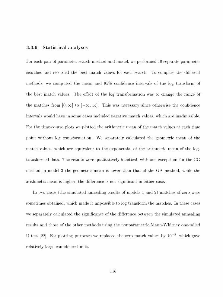
3.3.6 Statistical analyses

For each pair of para~neter search method and rnodel. tve perfurnled 10 sellarate parameter

searclles and recorded the best match values for each search. To compare the dierent

methods, we coniputed the meax1 and 95% confidence i~itervals of the log transform of

the best niatch values, The effect of the log transformation was to change the range of

the niatches from [O, ;] to [-x. m]. This was necessary since otherwise the confidence

intervals would have in some cases included negative match values, which are inadmissible.

For the tilme-course plots we plotted tlie arithmetic mean of the match values at each time

point without log traxlsforrnat ion. We separately calculated the geometric mean of the

match values, which are equivalent to the exponential of the arithmetic mean of tlie log-

transformed data. The results were qualitatively identical, with one exception: fbr the CG

method in model 3 the geometric mean is lower than that of the GA metbod. while the

arithmetic mean is higher: the difference is not significa~lt in either case.

In two cases (the simulated annealing results of models I and 2) nlatches of zero were

sor~ietirnes obtained. which made it impossible to log trans-fbrm the nlatches. In these cases

we separately calculated the significance of the difference betweerz the sirrlulated axinealing

results and tllose of tlie other nletllods using the nonparametrie klann-WThitliey one-tailed

U test 1221. For plotting purposes we replaced the zero lrlatch values by lo-" which gave

relatively large confident:e limits.

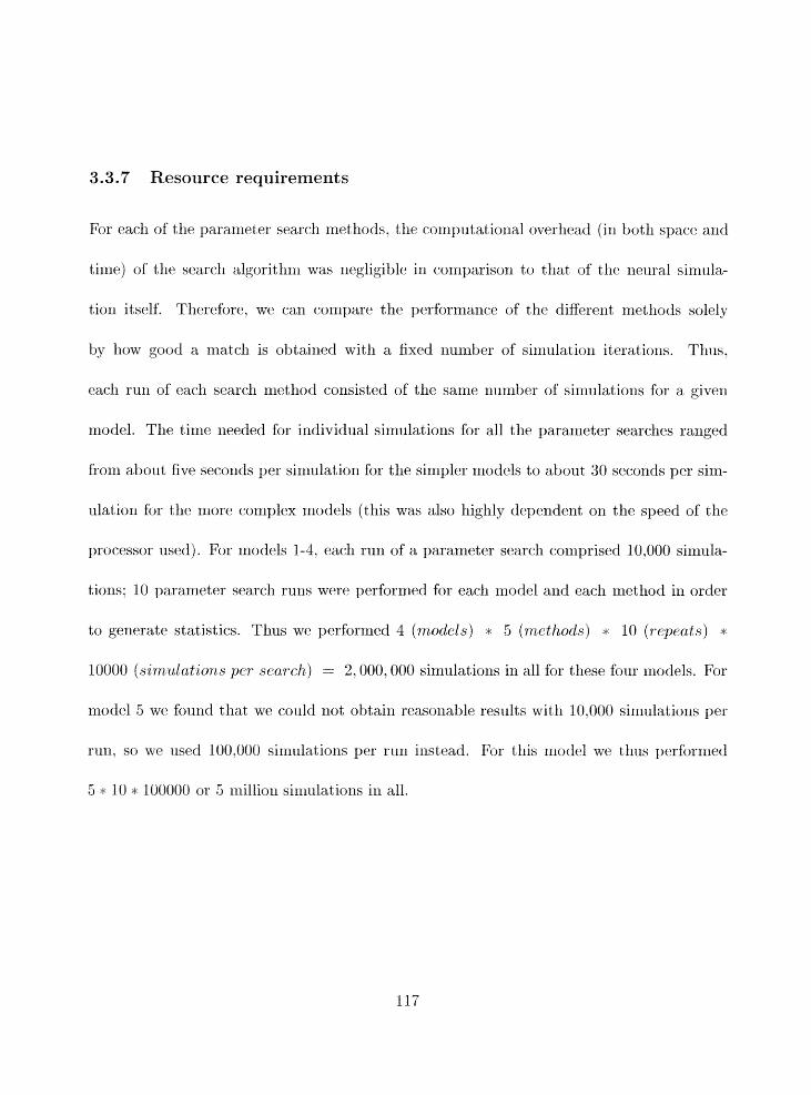
3.3.7 Resource requirements

For each of tlle parameter search methods. tlie coxnput,atiolial overllead (in both space and

time) of the search algorithm was negligible iri conlparison to tliat of' the neural simula-

tion itself. Therefore. we can compare the performance of the different methoc-ls solely

by liow good a match is obtained witli a fixed number of simulation iteratio~rs. Thus,

each run of eacli search method consisted of tlie same number of simulations for a given

model. The time needed for individual sinlulations for all the parameter searches ranged

from about five seconds per sinlulation for tlie simpler models to about 30 seconds per sim-

ulation for tlle more corriplex xriodels (this was also highly dependent on the speed of tlie

processor used). For models 1-4, each run of a parameter search comprised 10,000 simula-

tions; 10 parameter search runs were performed for each mriodel and each method in order

to generate statistics. Thus we performed 4 (v~odels) + 5 (methods) * 10 (repeats) *

10000 (simulations per search) = 2.000.000 simulatio~ls in all for these four models. For

model 5 we found that we could not obtain reaso~iable results witli 10.000 sinlulatio~is per

run. so we used 100.000 simulatiorls per run instead. Ebr this rrludel we thus perforn~ed

5 * 10 a 100000 or 5 xnilliorz siaiulations in all.

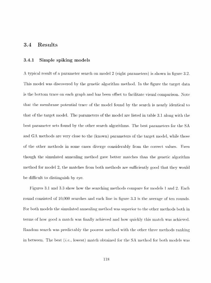
3.4 Results

3.4.1 Simple spiking models

.4 typical result of a parameter search on 1~1odel 2 (eight parameters) is sllowrl in figure 3.2.

This model was discovered by the genetic algorithm method. In the figure the target data

is the bottom trace 011 each graph and has been offset; to facilitate visual comparison. Note

that the membrane potential trace of the model found by the search is nearly identical to

that of the target model. The parameters of the model are listed in table 3.1 along with the

best parameter sets found by the other search algorithms. The best parameters for the SA

and GA methods are very close to the (known) parameters of the target model. while those

of the other rnetllods in some eases diverge cor~siderably from the correct values. Even

though the simulated ailllealing met hod gave better matches t hail the genetic algorithm

nletllod for model 2, the matches from both methods are sufficiently good that they would

be difficult to distinguish by eye.

Figures 3.1 and 3.3 show how the searelling rriethods cornpare for inodels 1 and 2. Each

round cousistcd of 10,000 searches and each line in figure 3.3 is tlre average of tell romids.

For both models t llo sirrlulat cd annealing met liod was s~lperior to the other met hods bot 11 in

terms of jliow good a match was finally acfrieved and how quickly this inatch was achieved.

Random searcli was predictal2ly the poorest method with the other three metllods ranking

in between. The best ( i . e., lowest) match obtained for tile SA niet;hotl for both r:rloclels was

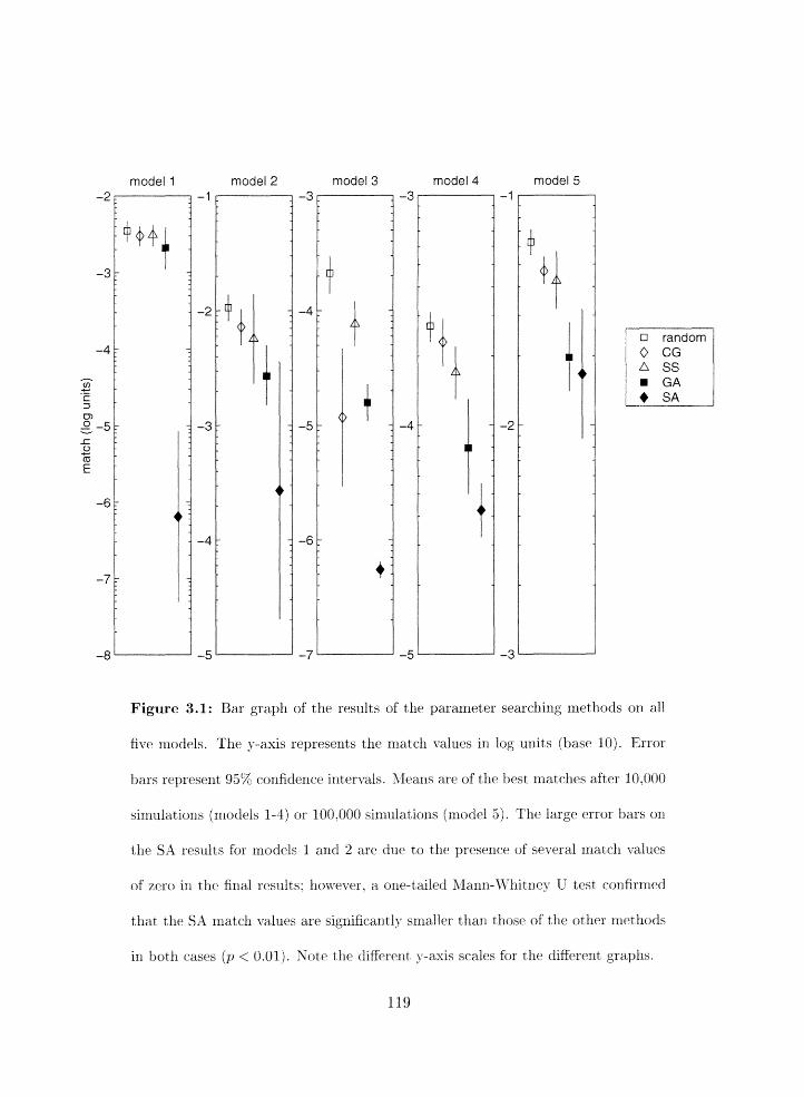
model 1 model 2 model 3 model 4 model 5

Figure 3.1: Bar graph of the results of the parameter searching methods 011 all

f i s c l models. The y-axis represents tlle nlatcli values in log units (base 10). Error

bars represent 95% confidenec. intervals. Means are of the best matches after 10.000

siniulatioris (models 1-4) or 100.000 siniulatioris (model 5). The large error bars ori

the SA resiilcs for rrlodels 1 and 2 arc due to the presclriee of several matdl d u e s

of zero in the final results: hourever, a oncl-tailed Llarin-JThitrzey C test confirriled

that the SX inatell values are signif'icarltly snlaller than those of the other metfiods

in botli cases ('I < 0.01). Xote tlie different y-axis scales for the diEebrent graphs.

Table 3.1: The target parameters for nlodel 2 (simple spiking model) compared

with the best parameters found by all search methods used. hlaxirnal corlductances

are in S/nt%ad scaling factors for time constants ( r values) are dime:isio:lless. -411

time constants refer to rroltage-dependent activation gates. ;Ya is a fast inactit.atirig

sodiunl channel; I<(DR) is a delayed-rectifier potassium current; f<(,-l) is an inacti-

I-ating potassium current; Ii-(;2l) is a slam- non-inaetimting potassium cnrrent. Note

that the matches found by the SX and G-4 metfrods are x-ery close to tlic correct

~jarameter -dues.

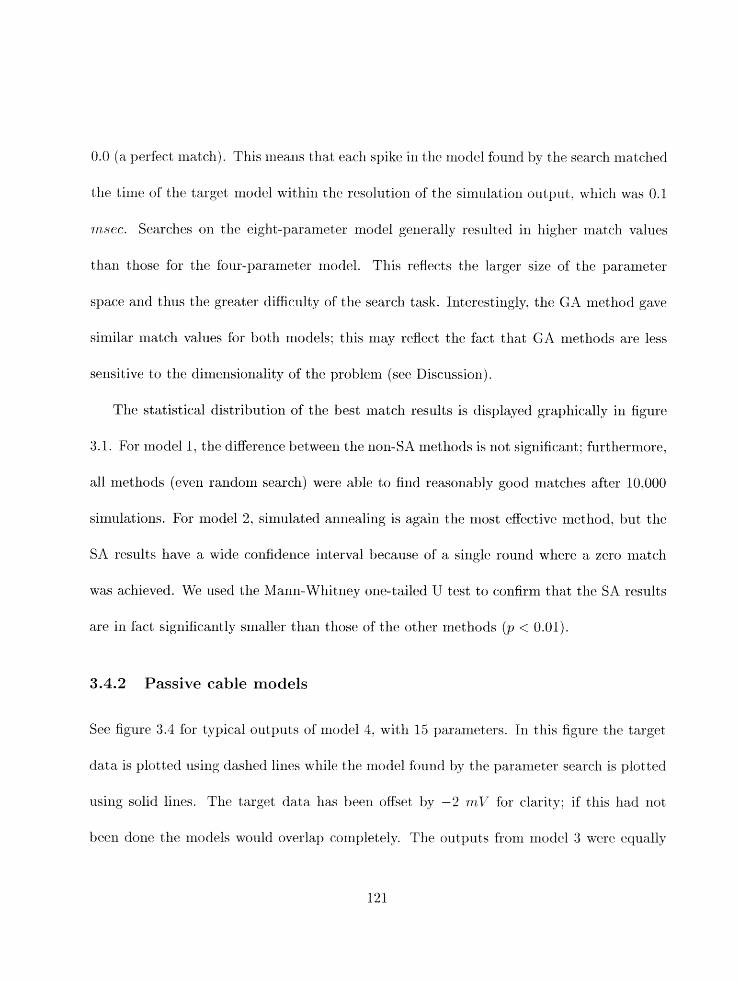
0.0 (a perfect rnatcli) . This Inearis that each spike in the lliodel found by the search lrlat8clled

the time of tliti target model within the resolation of the simulation output. wllicli m s 0.1

msec. Searches on tlir eight-l~arameter model generally resulted in higller matcli val~les

than those for the four-parameter model. This reflects the larger size of the parameter

space and thus the greater dificulty of the search task. Interestirlgly. the GA method gave

silriilar match values for both models; this may reflect the fact that GA urctthods are less

sensitive to the dimensionality of tlle problem (see Discussion).

Tlle statistical distribution of the best match results is displayed graphically in figure

3.1. For model 1, the difference between the non-SA methods is not significant; furthermore.

all methods (even random search) were able to find reasoriably good nlatclies after 10.000

siniulations. For rnodel 2, simulated arlnealing is again the most effective method. but the

SA results have a wide confidence interval because of a single round where a zero match

was achieved. We used the Mann-Whitney one-tailed U test to confirm that the SA results

are in fact significantly smaller than those of the other methods ( p < 0.01).

3.4.2 Passive cable models

See figure 3.4 for typical outputs of model 1. with 15 parameters. In this figure the target

data is plotted usirig dashed lines while the model fou~id by the pxameter search is plotted

rrsirig solid lines, The target data llas been offset by -2 wzr' for clarity: if this had not

been done the models would overlap completely. The outputs from model 3 were equally

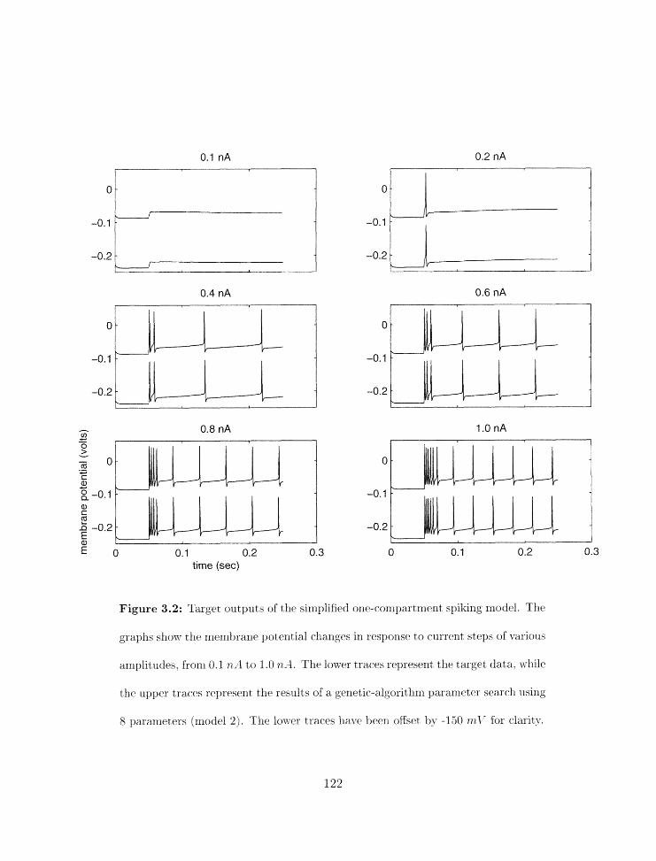
0.1 0.2 0.3 time (sec)

Figure 3.2: Target outputs of the simplified oiie-conly~artnlent spiking rrzodel. Tlle

graphs show the rnembrane potential dlanges in response to currpnt strps of various

amplitudes, from 0.1 nA4 tto 1.0 tz-4. The lower traces represent the target data. u-hile

the upper traces represent the results of a genetic-a1gori"chm paranleter. search using

8 pararrletess jrnodel 2). The 1otve.r traces haye beerr offset 'by -150 n21' for clarity.

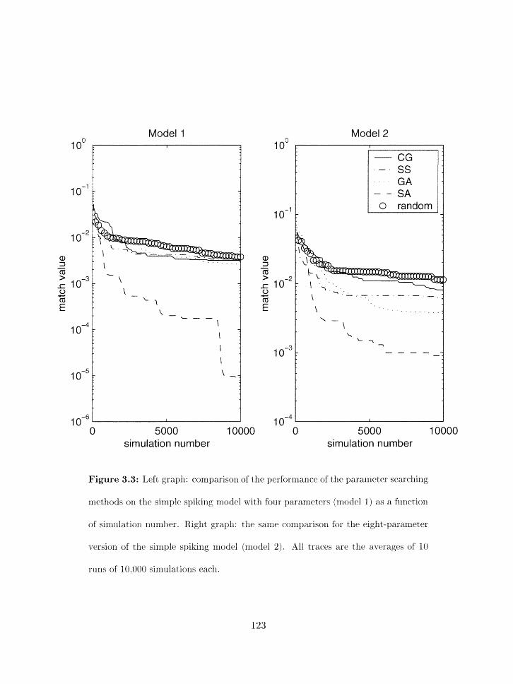
Model 1

simulation number

Model 2

0 random

o - ~ 0 5000 10000

simulation number

Figure 3.3: Left graph: comparison of the ~~erformance of the pararneter searclrlirlg

rnethods on the sirnpfe spiking model witl-r four parameters jtnodel 1) as a function

of sirnulatiorl nurnber. Right graph: the same eonlparison for the eight-parameter

version of the simple spiking rnodel (model 2). All traces are the averages of 10

runs of 10,000 sirnulat ions each.

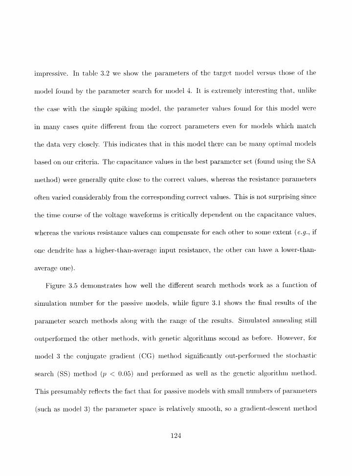
impressive. 111 table 3.2 we show the parameters of the target motiel versus tllosp of the

model foulid by the parameter search for irlodel 4. It is extremely iilteresting tliat. nnlikr

tlie case with the sil~lple spiking ri~odel. the parameter values found for tliis model were

in many cases quite different horn the a~r rec t paranleters even for models which match

the data very closely. This indicates that in this model tliere can be rnany optimal models

based on our criteria. The ~apacit~ance values irl the best paraxneter set (found using tlie SA

method) were generally quite close to the correct values. whereas tlie resistance parameters

often varied considerably from the corresponding correct values. This is not surprising since

tlie time course of the voltage waveforms is critically dependent on the capacitance values.

whereas tlle various resistance values can compensate for each other to some extent (e.g., if

one dendrite lias a higher-tharl-average input resistance. tllp other can have a lower-than-

average one).

Figure 3.5 demonstrates how well the different search methods work as a function of

simlllation number for the passive models. while figure 3.1 sllows tlie firm1 results of the

parameter search niethods along with the range of the results. Simulated annealing still

out performed tlic other niet hods. with genetic algorit linls second as before. However. for

rllodel 3 tlic co14j ugate gradient (CG ) niet hod significantly out-perfijrrned the stochastic

search (SS) method jp < 0.05) a i d perfor~rled as well as the gerietic algoritlirn ixletllod.

This presumably reflects tlie fact tliat for passive nlodels with small rinmbrrs of paraxneters

(sncli as irlodrl 3) the pararneter space is relatively snloutll, so a gradient-descent method

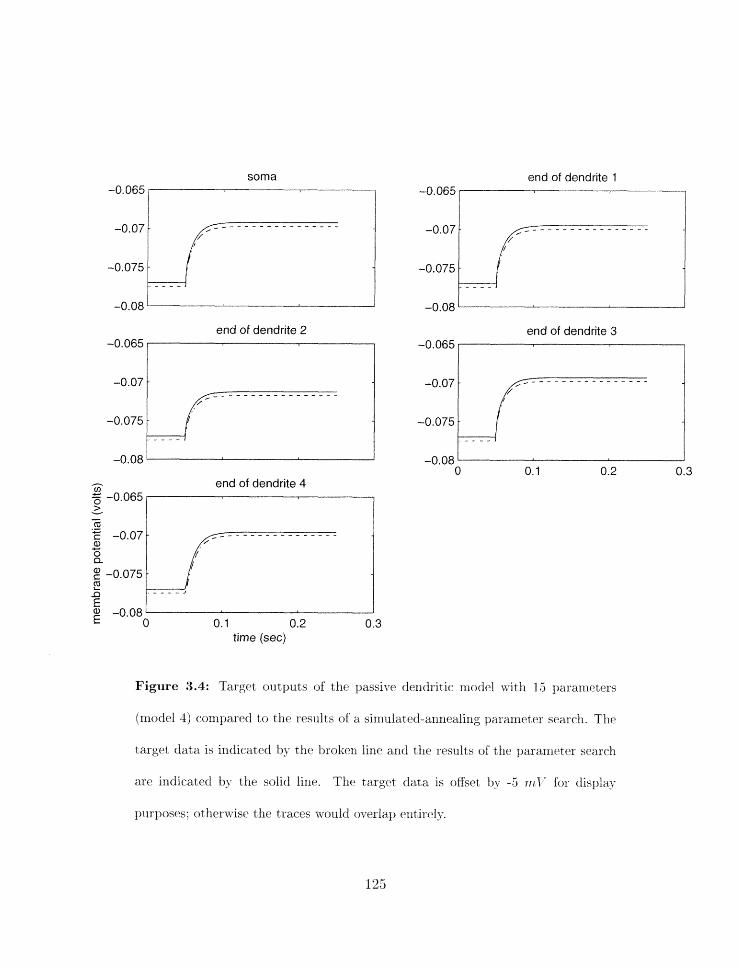
end of dendrite 2 -0.065

h

V) end of dendrite 4

> \-C

end of dendrite 1 -0.065

end of dendrite 3 -0.065

time (see)

Figure 3.4: Target outputs of the passive dendritit model with 15 gjararrlctters

jrxlodcl 4 j compared to tho results of a sirrlulated-annealiq parameter srarcl1. The

target- data is indicated by the broketi line and the results of the parameter search.

are indicated by the solid line. 'I'l1c-l target clata is oEset 11y -5 nrlv for display

purposes: uther\vise tile traces would o~er lap c.ntire1-y.

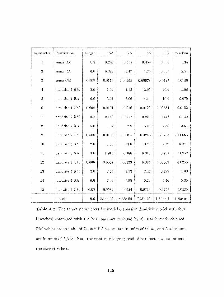
parameter

soma RA1

soma RtZ

soma Chi

dendrite 1 RRI

dendrite 1 RIA

dendrite 1 CS'I

dendrite 2 RII

dendrite 2 R-4

dendrite 2 CAI

dendrite 3 RRlI

dendrite 3 RA

dendrite 3 ChI

dendrite 4 RM

dendrite 4 RA

de~idrite 4 CLI

target

Table 3.2: The target parameters for model 4 (passive deridritic rrloclel n-itll four

branches) compared ~s-ith the best parameters found by all seareli rnett-lods used.

RhI values are in lirlits of S-2 - rn? R-4 d u e s are in units of Q . m, and Ghf ~a lues

are in units of F/~11'. Note the relatively large spread of parameter ~a iues arouncl

the correct values.

like the CG method can be reasoriably effective. Interestirrgly. wllerr we look at nlodel 4.

which is rnorr cornplex. tlrc CG method gives slightly worse results tliail the SS rriethod

(altllo~lglr this is not statistically significant). Tliis rnay reflect the larger mlinber of nrodels

with equivalent nratclr values for this rnodel. i. e., the larger mlml~rr of local nrinima for the

CG method (but not the SS method) to get trapped in.

3.4.3 Pyramidal cell model

Figure 3.6 shows the outputs of a parameter searching method for the pyramidal cell rnodel.

This niodel was discovered by the SA method after about 48.000 simulations. After this

the parameter search converged and subsequent searches in this run were conlpletely new

pararrreter searches wlliclr converged to higher match values: irl fact. this represents tlie

best SA result we achieved. The parameter values for this rnodel are listed in table 3.3. In

this case we do not h o w what the correct parameter values are so we csxinot assess the

perforlxlance of the methods on this criteria. However. figure 3.6 sllows that the methods

can achieve extrerrrely good rnatches to the data over a wide range of input currents, at least

wit.11 respect to tllr spike timings. The nrajor di-fference between tlle rnodel and the data is in

tlie spike prr- arid afterl~oterltial. suggesti~ig that other conducta~lces or features need to be

added to the model if greater accuracy is r~eeded or if tile spike afterpotential is of intercst

to tftt. rrtodeler. One interesting possibility would bc to add a separate s p i k e - i n i i i xortr

to the rnodel [29]. An int,rrestixrg feature of this model is that we added a fast calcium-

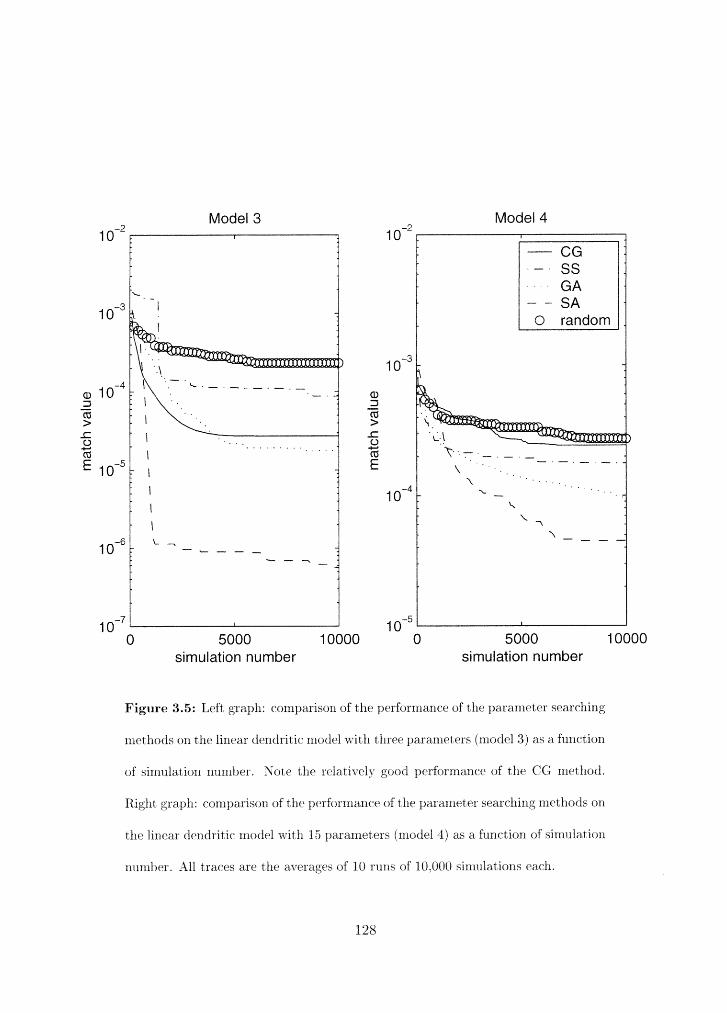
Model 3 Model 4

simulation number 5000

simulation number

Figure 3.5: Left graph: comparison of the performance of tlle paranleter searching

nlettlods on the linear dc~rrdritic rrlodel with three parameters (niodel3) as a function

of simulation trurnher. Sote the relatively good performance of the CG method.

Right graph: conlparison of the performance of the paranleter searching mettlods on

the linear dendritic rrlaclel ~vitl.1 1.3 parameters (niodel 4) as a furlction of sin~ulatiori

nu~nber. l"l_ll traces are the averages of 10 runs of 10,000 sinlulations each.

dependelit potassium channel to the model. eve11 though there is no exprrinlental evide~ict.

fbr snch a cllannel. because urc fou11d that adding this channel substantially improved the

matches we obtained (see below and Discussio~i). Figure 3.7 shows a graph of tlle results

of the diEerent metllods as a furrctiorr of simulatiori number. while figure 3.1 shows tlle

statistical distribution of the best match results. Note that for this model the gerietic

algorithm method was almost exactly as effective as the simulated annealing method. The

CG and SS metliod are roughly equivalent, while (as expected) the random search method

is the least effective.

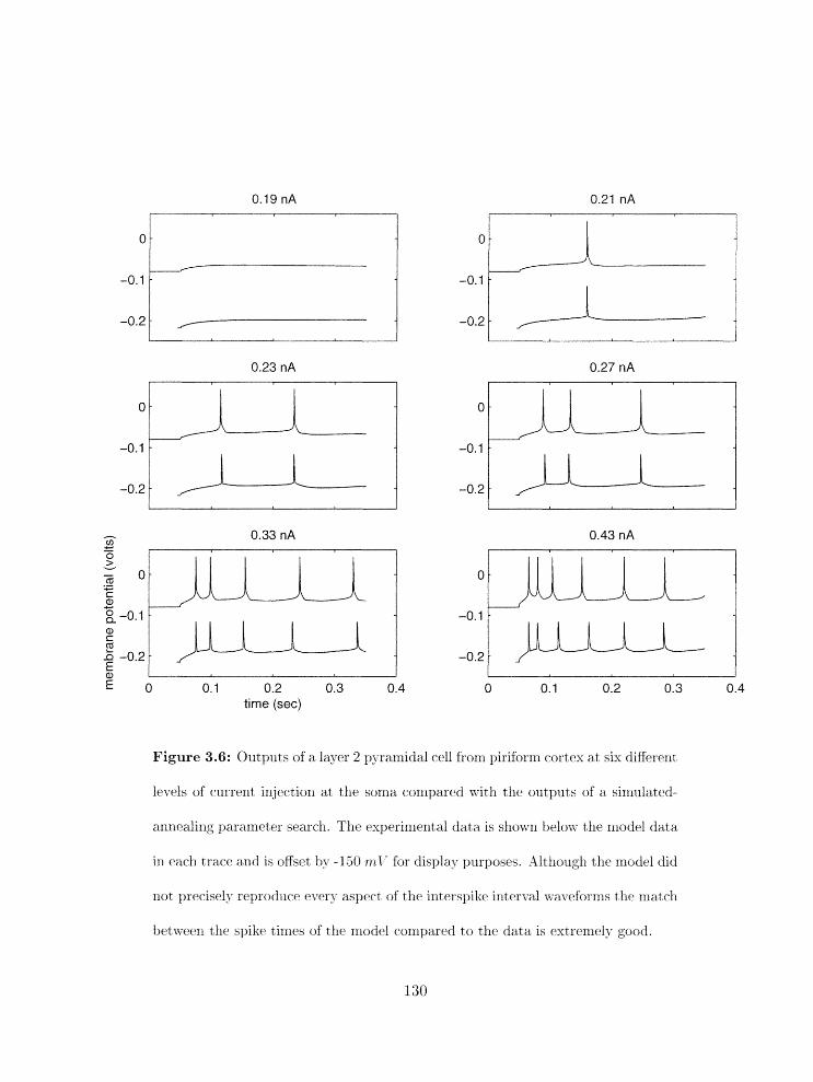
tij I € 0 0.1 0.2 0.3 0.4

time (see)

Figure 3.6: Outputs of a layer 2 pyramidal cell from yiriform cortex at six diEerent

Ic-lrrels of currerit irljectiorl at the soma compared ~v i th the outputs of a simulated-

annealing parameter search. The experirnerltal data is shorn-n belory the b nod el data

in each trace and is offset by - 150 nlT " for display purposes. Although the model did

riot ~jrecisely reproduce every aspect of the interspike interval wat-eforrns the match

bet-tveen the spike tirltes of the model cornpared to the data is rxtrernel?; good.

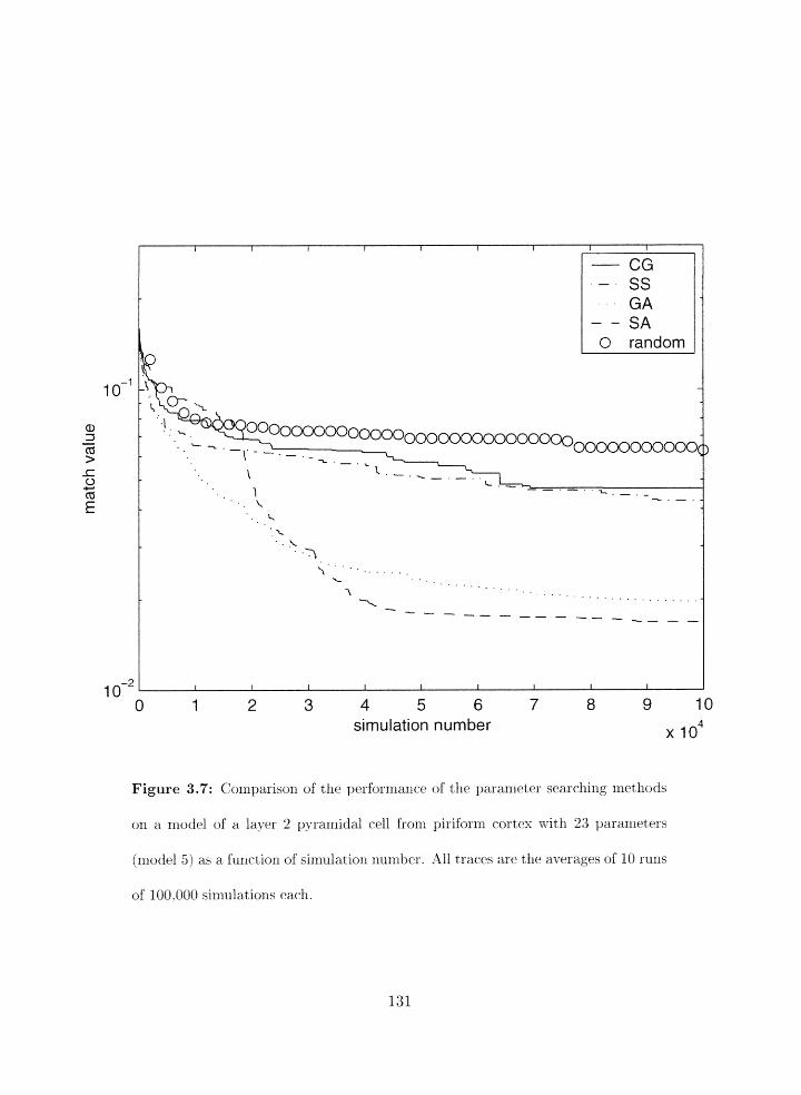
simulation number x lo4

Figure 3.7: Cornparison of the ~)erformaxlce of tlre pararrlclter searching methods

on a model of a layer 2 pyramidal cell from yiriform cortex with 23 pararlfeters

(model 5) as a furittiori of sirnulat-iori nurnber. -All traces are the averages of 10 runs

of' 100.000 sirnulat ions each.

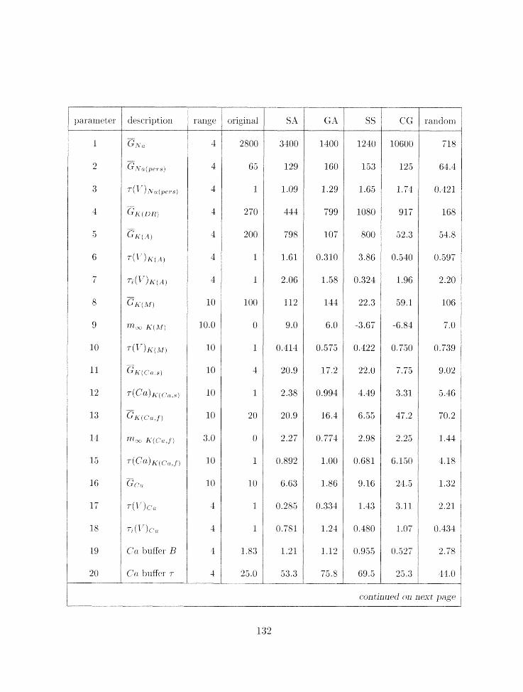
continued orr r ~ x t $rageJ

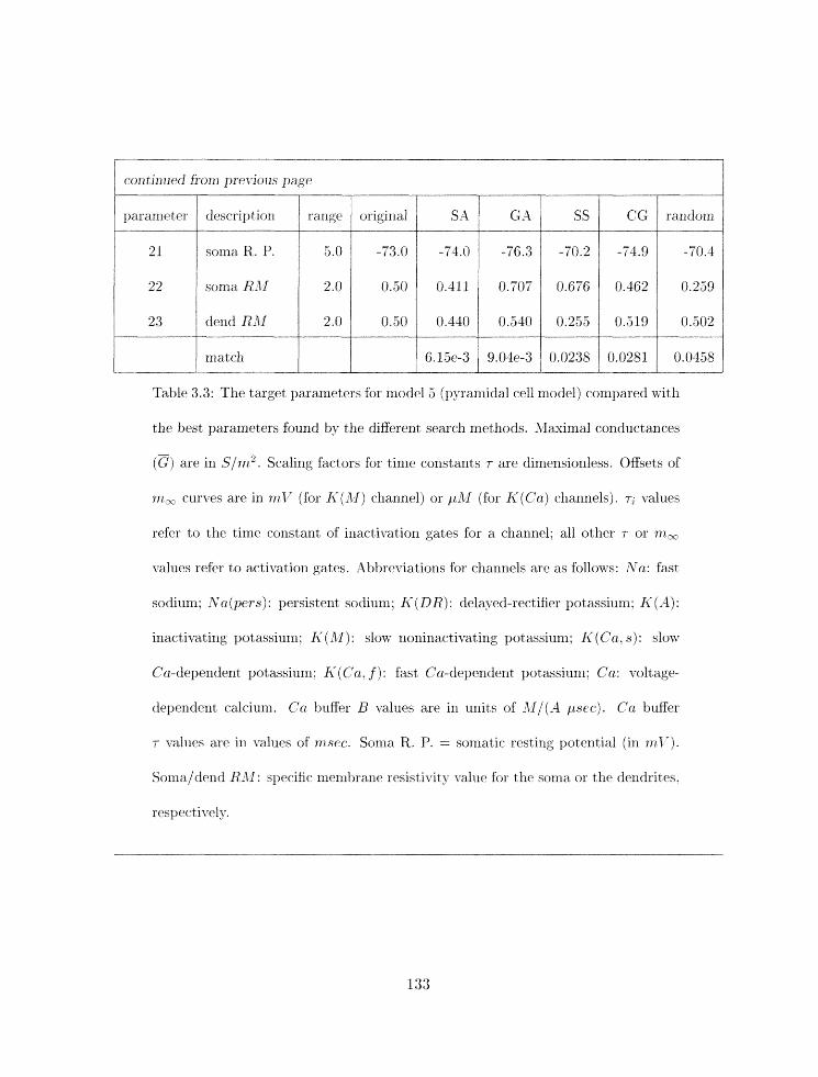
I continued from prex-ions page

Table 3.3: The target parameters for nlodel 5 (pyramidal cell model) compared with

the best parameters found by the different search methods. Maximal conductances

(c) are in S/m? Scaling factors for tirlir constants T are dimensionless. Offsets of

rn, curves are in rr? 1 ' (for I < ( A l ) channel) or jriZ1 (for K(Cn) channels). T, values

refer to the time constant of inactivation gates for a channel; all other r or nz,

values refer to activation gates. Abbreviations for channels are as follows: :Va: fast

sodium: n'a(yers) : persistent sodiunl: A-(DR) : delayed-rectifier pot assium; (A) :

inactivating potassium; ( Ill) : slow noninactivating pot assiunl; fi'(Ca, s) : slow

Ca-dependent potassium; K(Cn, f ) : fast Cu-dependent potassium; Ca: voltage-

dependent calcium. Ca buffer B values are in units of 131/(,-1 psec). Ca buffer

r values are in values of rrzsec. Soma R. P. =. somatic. restirrg potential (in nil7).

Sorna/dend R1ll: specific rrtenibrane resistivity t-alue for t l x soma or tlle dendrites.

respectively.

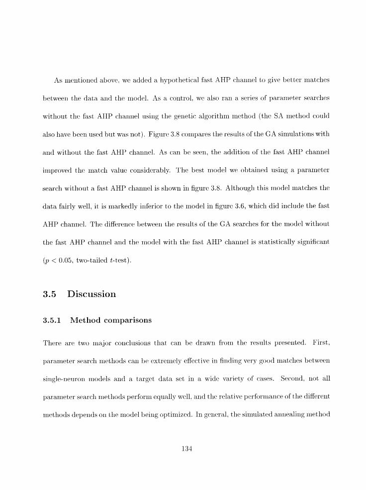
As rrienlioi1ed above. we added a hypothetical fast AHP chnnel to give better matches

betweell tlle data and the rrlodel. As a control. we also ran a series of 13arameter searclles

witllout the fast AHP channel using the genetic algorithm method (the SA method could

also have been used but was not). Figure 3.8 compares the results of the GA simulations with

and without the fast AHP channel. As can be seen. the additiori of the fast AHP channel

improved the match value considerably. The best model we obtained using a parameter

search without a fast AHP channel is shown in figure 3.8. Altllougli this model matches the

data fairly well. it is markedly inferior to the model in figure 3.6. which did include the fast

AHP channel. The difference between the results of the GA searclles for the niodel without

the fast AHP channel and the model wit11 the fast AHP channel is statistically sigrlificant

( p < 0.05, two-tailed t-test).

3.5 Discussion

3.5.1 Method comparisons

There are two major conclusions that can 1x3 drawn froin the results presented. First.

parameter search metliods can be extrenlely effective in finding very good matclies between

single-iieuroxi l~lotlrls and a target data set in a wide variety of cases. Second. not all

parameter searcli nletliods perform equally well. and the relative performance of the diffcrellt

~llethods deperlds or1 the model being optinlized. In general. the sii~lulatrd arlnealing xilethod

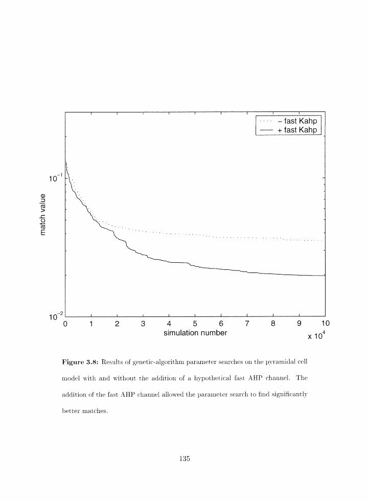
simulation number lo4

Figure 3.8: Results of genetic-algorithm parameter searclies on the ~~yralnidal cell

rriodel with arid without the additiorl of a hypothetical fast A H f channel. Tlie

addition of the fast XHP cltannel allowed the paranrleter search to 51td sigriificantly

better xnatehes.

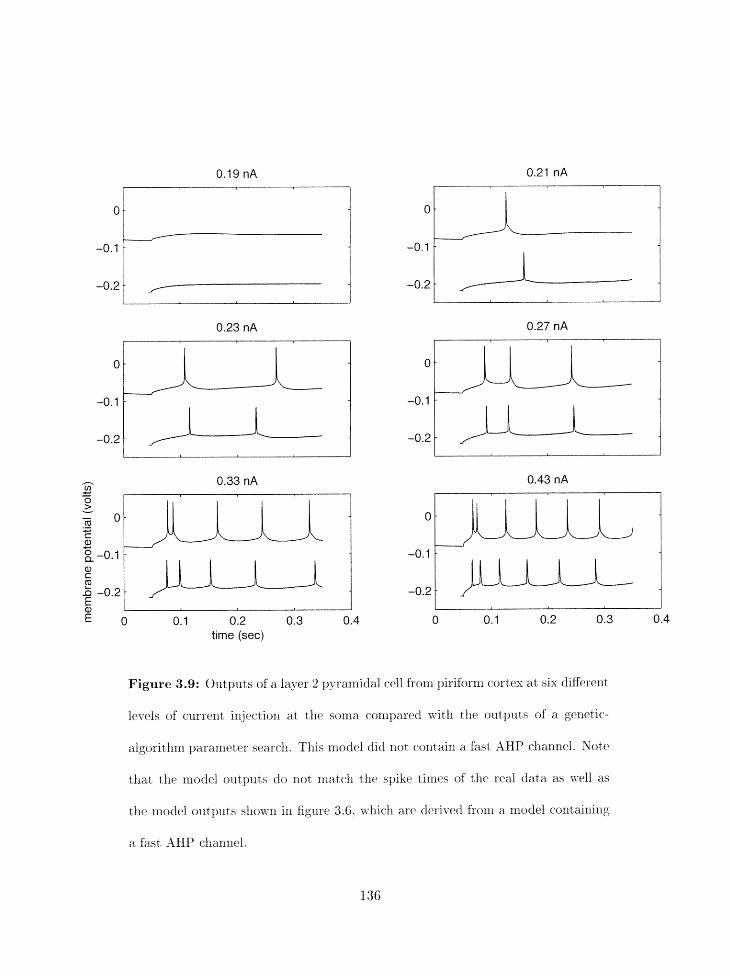
t:

0.1 0.2 0.3 0.4 time (sec)

Figure 3.9: Outputs of a layer 2 pyramidal cell from piriform cortex at six diEerent

levels of current irljectio~l at the Sonia conipared with tlie outputs of a gemtic-

algorithm pararrleier srarcll. This model did riot contain a Fat AHP channel. Sote

that the rnoclcll outputs do not rrlatch tllc spike times of tlze real data as rwll as

the rnodel otitptits sho-~.;ri in figurtl 3.6. whicll are derived frorrl a r~iodel cont-aixling

a fast -4HP channel.

and tlie genetic algorithm mt.t31iod were superior to tlie other rrletliods we investigated

(stocliastic search and cor1,jugate gradient) on all of our rnodels (except for mc~del 3. the

linear passive derldrite model. for wlsicli the conjugate gradie~st rrlethod was as good as

the gersetic algorithm method). The reader should be aware. however. that all of our

parameter searching methods liave parameters of their own whicli we liave deternlined by

experimentation (see below). Therefore. it is possible that diEerent choices of these meta-

parameters could lzave resulted in somewhat different results. In addition, variations of each

of these methods exist. especially for genetic algorithms [32]. More sophisticated algorithms

in each class may very well improve on tlie perforrr~ance of our searches. For this reasor1 the

reader should consider the data presented as a general guide providirlg an upper bound on

the perfornzance of these met hods on the models examined.

3.5.2 Differences between the search algorithms

While it is usehl to know which parameter searching algorithms are most appropriate for

single-neuron corxzpartmental rnodels of different complexity. it would also be usefir1 to kriow

why one algorithm was more effective than anottier for a given model. Unforttmatcly. under-

standing tliese relationships rigorously is very difficult as it irivolves an interaction 13etween

tlze searchirzg algorit 1111s and t lit. structure of the model's paranseter space. However, based

on previous arlalyses of this type [3. 111. it is possible to speculate on several possibilities

for the results we obtained.

In gerreral, it is likely that stochastic inetllocls rather tllarr those based on gradient-

descent will he more slxccessful for pararrreterizirlg single-ireuroxr conrpartmental rrlodels.

The reason fbr this is that siinple gradient-descent nletlrods sxxclr as corljugate gradients

are greedy. i.e.. they nrove to the nearest local rrlinirnuin in paranleter space and stay

there. This can be adequate if the space is relatively smootelr and has few local minima,

but it is ineffective for more ragged paranreter spaces with many local minima. In fact.

pararneter spaces of neural models can be very ragged wit lr sharp discontinuities separating

otherwise smooth sections [3. 11 . Consistent with this analysis. the one model for which the

co~rjugate-gradient met hod proved highly effective was the t hree-parameter passive model

(model 3) which. due to its linearity and the small nunlher of parameters. is inore likely to

have a smoothly varying parameter space.

Wit hill the class of stoclfiast ic models. our results clearly deinonstrate differeirces be-

tween genetic algorit hmis (G A). stoclrastic search (SS) and sinlulated annealirlg (S A). The

SS metlrod was markedly inferior overall to both the SA and the GA method. whidr is al-

rrlost certairrly due to the extrexrrely unsoplristieated search strategy this rnetbod employs.

In general. we obt8ained better results with the SA method tlralr the GA ~nethocl. The SA

rrret hod we used also possesses most of the ;Idvantages of gradient-descent met hods without

their disadvairt~ages. At high tenrperatures the method earl explore large expanses of pararn-

eter space, and as the temperature is lou~ered. the search narrows in or1 specific: regioxrs witlr

better niatcll values. The tenrperature-depende~it noise in the rrictlrod prevcnts tlrc search

frorn gettirig stuck in local minima. I;l;Tlien tlle temperature approaclies zero the SA method

converges tjo t>lre closest local rriiniinurri as does a gradient-descent search. 111 contrast. the

CA metf.iod never converges to a local 1ilinimun.l of the rriatclr function. Howc:x~er. our SA

rnethod can be expected to give poorer results with larger models. as this method car1 only

keep a record of a small rllrmber of points at a time (the points on the simplex. which mrnber

orre rnore than tlre nurnber of parameters j . For a search with a large eriough number of pa-

rameters the GA method, which can simultaneously search marly points in pararneter space.

may well overtake the SA method in performance. For our models the GA method was as

effective as the SA method for the largest model (model 5). It is likely that for an ever1

larger rnodel GAS would have been superior. Work on GAS [15. 18. 26, 321 lias suggested

that this method is often optimal for problems when a large nurnber of largely irrdepe~ldeilt

factors rriust be conlbined to create the best results. In contrast. in compartmental neural

rnodels optimal parameter values are typically higlily dependent on each other. especially

within a corn~~artment. so that changing the value of one para~ieter will require dianges

in tlie vaa1ues of all other pararrreters as well to optinlize tlie rnatch. This would suggest

that GAS are poorly suited for ~olrrpart~rxlental rilodels. However, wlrile GAS are less ef-

fective for problems corltainirig large rlu~nbers of strorigly interac:ting parameters, tllcy are

capable of irideperide~itly exploring large scgrne~lts of pararneter space simultaneously and

in parallel, wliicli nlay accorlnt for their greater relative usef~rlness with larger nrtrdels. The

illtrillsic parallelis~~i of GAS also makes tllern very t?;c:ll s~iited for inlplementation on parallel

3.5.3 Matching functions

The choice of matching function used can have a large inflrierice on the search process,

Pararrleter searches earl orlly niatcli accordirig to the specific criteria they are given, 111

our case, for our spiking niodels we origirially tried using sirnyle spike-matching functioiis

wllich coniputed the RN1S error between two lists of spike tirires. However, we found tlrat

this approach did not sufficiently penalize models whose behaviors were clearly qualitatively

incorrect. For example. sonit models with particular pararrieter settings generated small

bursts of spikes (e.g.. pairs of spikes separat,ed by a sliiall ISI) separated by a much larger

interburst interval. in contrast to the more uniform spiking pattern we were trying to

replicate. While this behavior would eventually liave been selected against even using an

RMS error function, we found it more efficieiit to put a factor into our lnatching fuiictioxr

to directly penalize bursting. This allowed us txo narrow down the eff'ective search space

enornrously and thus sped up the searches. To be rrlost effctctive, considerable thought rnust

be applied to the selectiori of rnatching funetiorls to achicve optirlial performance. Ofken.

initial experience with a rrlatcbillg frrrict ioll reveals t llat scfnie important aspect of the data

was overlooked. Therefore1 it is often useful to exarrlirle flow well the rzratchiiig functiorl

distinguislies good from bad models befbre romlnitting large anrounts of corni>uter time to

an extensive paran-reter search.

The choice of matching function can also coritribute significarit ly to the cornputat ional

cost of the parameter search. because a match must be corriputed for eacli sirnulatiori run.

For this reason we chose to use spike times exclusively as the criteria for matclning models

1. 2. arid 5 . If computational costs were not an issue, it would have been preferable to

use a codinat ion of spike timings and iriterspike interval (ISI) waveforms to match these

models. However. since most models generate relatively few spikes. a spike timing based

match function is much more etiicient to calculate than a match function which also incllldes

IS1 waveforms. because for the latter the membrane potential value at each time point must

be used in the computatioii. For some models. however, the duration of the individual

simulatiorls will still be much larger t l ia~i tlle tirrle needed to compute a match even if IS1

waveforms are used in the match function. In such cases, one should use IS1 waveforms as

well as spike tinlings in the match function. For the passive rnodels we had no choice but

to use mcnibrane potential waveforms, since the models do not generate spikes.

3.5.4 Variation in the parameter sets

Depending on tlie goals of the rnodeler, he or shc may or may not bc. interested in the

yuestiorr of whether diarent ruris of a parairleter searclr result in the same set of paranleter

values. On one extreme, the rrlodel may be used as a phelzornenolagical irlodel which is a

considerable abstractioii of the real systern, and tlle nrodeler may orlly wish to have a set of

paranreters that produces bellmior similar to that seen in the real systern. In this case tlie

l~niquerzess of tlie parameter set is of little interest. At the otlzer t-lxtreme, a modeler may

aspire to build a very detailed model whose parameters (some memured. sorrie estimated)

accurately represent tlsc corresponding real parameters of the system. In this case tlicl

modeler is very interc~t~ed in whether different parameter sets c s r l give rise to sirrsilarly

good rnatch values. as tlxis may irzdicate that the model is insuEciently constrained to

accurately c2iaractcrize the real system. In addition, the degree of variation of the best

pararneter sets gives clues to the nature of the parameter spaces beirig searched tlxrougli.

Tilie examined the question of non-uniqueness of the parameter sets found by our search

methods by calculating statistics on a parameter-by-parameter basis for the best matches

found by all the methods (data not shown). The best parameter sets found by the different

neth hods in rrsodels 1, 2 and 3 matclzed the correct parameter sets very closely, with little

variation in tlse pararrzeter values. This suggests that the parameter spaces for these models

are donzinated by a single deep minimum wlzich was reliably -found by many of the searches

(in particular the SA axid GA searches). Models 4 and 5, however. showed a considerable

degree of variation in the parameter values obtained between different successful nratches.

even for diEererit parameter sets wit11 colnparable match values discotrered by t*he s a l e

search algorithm. This suggests that parameter spaces of models with larger nurnbers of

parameters show asore degeneracy izi their match values. i. e.. tlsere is more thari one equally

good location in paamcter space which can be discovered by tllr search algoritlxms. The

best way to deal with this phenomenon. short of tliorougfily searcfxing pararrleter spaces

~ssiiig brute-force met llods. is to run several ~~tlrailieter sear~l~es wit ll t lie sanle met hod on

the same model and compute the variance of the para~riet~ers obtained. Typically. some

parameters are highly constrained while others show a range of possible values: this in turn

sxiggests which parameters are more or less iniport ant in detcrmirlirlg the ot~served behavior.

3.5.5 Robustness of the parameter sets

Another question of interest t,o modelers using parameter searching techniques is the degree

to which parameter sets are robust to small perturbations in the parameter values. For

instance, if parameter values need to be specified with great precision in order for a good

match to be achieved, the parameter set is not robust and therefore is unlikely to be physi-

ologically relevant. In practice, estirnat in$ robustness of parameter sets is discult because

one would ideally like to vary all possible colnbinations of parameters. However, some in-

sight into robustness can be achieved by varying each parameter individually (or pairs of

paranleters [3. 111) around its initial value while keepirlg the otller paranieters fixed and

irleasuring the change in the rnatch value, Robustness estimated in this way can suggest

which parameters need to be precisely set. arid which can vary over a wide range. This in

turn can suggest possibilities for the cellular regulation of paranieter values in the real sys-

tem [27]. It is also possible to build in such *'robustness cllrcks" into the nlatching furiction

directly by testixlg robustness for each pararrleter set and re~ectiiig sets that are below sonle

t f-lreshold of robustness; however. this will dramatically increase the coalputat ioilal cost of

tlie parameter search. A better alternative is to test the robustness of the best parameter

sets from a search and to reject tlrose which are not suEciently robust.

Another kind of robust~iess is robustness to srnall clianges of the inputs. lthr example.

one can make r~iultiple rxieasurernents of the outputs of neurons to quantify the variability of

tlie data source. iritroduce variability into the model in any of a number of diRerent ways,

arid use Bayesian rriethods to determine the probability of the model given the data [I].

This allows modelers to test the robustness of their models to small perturbations of the

inputs in a rigorous way.

3.5.6 Recommendations for effective parameter searching

While we have compared the general uscfirlncss of different parameter searching algorithms

and discussed matching functions, tlie process of parameter searching and the interpretation

of the results car1 be severely hindered or improved by other factors which we discuss here.

An importaxit issue in setting up a pararneter search colrcerxis the process of setting tlie

parameters of the search algorithm itself. The allowable ranges of the parameter values are

important paranleters for searcli methods: ideally they should be set to physiological rariges

hut in niany cases not enough is known to constrain these ra~lges. If the true parameters

lie outside the initially established range. then tlie searching algorithm will riot br-l able to

find tliem. Additionally. all searclr algoritllms have paranieters of tlieir own. suclr as tlre

annealing rate for the SA method and the population size, rnutation rate and reeonlbiriatiolz

rate for the GA nlethod. Unfortunately, currently there is little arialytical work which can

guide the choice of these paranleters. so they tend to be selected by experience and ad hrtc

rules of t h ~ ~ m b [Is. 321.

It is also necessary that the components of the model be carefully selected. A great deal

of wasted time can be avoided, for example. if the initial model (before parameter searclling

is done) at least qualitatively matches the gross features of the target data set). Parameter

searches do not remove the need for good judgment on the part of the modeler, and cannot

make a bad model good. As a corollary, however, we have often found that parameter

searches are often more useful wlien they fail than when they are successful. A failure in

a well-executed parameter search suggests that a model may be incapable of reproducing

the specified behavior (at least within the allowed parameter ranges). This failure naturally

leads to further experinlentation with either the model or the real system. For example.

one can explore whether adding a new ionic channel to the model would make the model

match the experirliental data much more closely (c . y., figures 3.6 and 3.8). If so. this car1

suggest new ideas for experirnerits.

3.5.7 Limitations of parameter searching techniques

FYhile parameter searclling techniques properly aj3plied will add significantly to the yual-

ity arid rigor of modeli~ig ef ir ts , several factors call limit the applicability of parameter

searching met hods.

Since parameter searches require it large nurnbrr of evaluatiolls of the model (tens to

1lrrndr.eds of thousands for the models we investigated 1. the time required to simulate a sizrgle

iteration of a, model must br relatively srnall. For instance. a model wliicll requires one hour

or niore to go through one iteration (e.8.. [8, 91) will take over a year of workstation tirrie

to run through 10.000 simulat ions. Obviously, unless the siniulat ion time can be reduced

significantly by ru~lnilig 0x1 faster cornputers ( e , ~ . , parallel supercomputers [Iri]). sucli a

model is currently not a good candidate for automated parameter searches. Under these

conditions parameter searches can sometimes still be run on simplified versions of a large

niodel with the hope that the results can then be applied to the larger model.

Xt; the present time it does not appear that the parameter search methods we describe

will be useful on rrlotlels with huge nurnljers (e.g.. hundreds) of parameters. We note that

~noving from a model with eight parameters to one with 23 para~lieters required a scale-

up of 10 in the nnrnber of iteratioris per paranleter search needed to get good results. Itj

is likely that rrlodrls with very large numbers of 1,arameters (> 100) can easily outrun the

capat>ilit ies of t llr current generxt ion of works tat ions. This is a key argtlment for deeloping

para~neter search methods to work on parallcl superconrputers, as we have begun doing:

4 . In additio~l. it is desiral~lr for iilodelrrs to illvestigate ways of redrlciiig the sizc of

the pararneter sgmc-es of their models. for illstance l ~ y forcing some ~~s ra l~ l e t e r s in diffctrctrrt

compartme~lts to have the same values (p.9. . [8] ) .

.Inother pcttiential difficulty with parametzer searches concerns overfitting of the data.

When a model is carefully tusred to matdl a specific data set. it may not gerieralize well to

similar data sets not used in the tuning. For instance, if a niodel is tuned to match spike

times very precisely at a given value of current injection it may fail to match spike times

at other current levels. For this reason. our owri studies enrploy a wide rarige of inputs

to provide an appropriate breadth of constraints on model behaviors. Sue11 snodefs are far

more likely to be underfit than overfit. If overfitting is suspected, it is a simple matter to

paranieterize one's model on a subset of the data, set (the training set) asrd once tlie model

is parameterized check how well it matches the rest of the data (the test set).

It is also critical not to place too much weight on the results of a parameter search

irr a weakly constrained or highly simplified model. In our pyramidal cell model, many of

the kinet ic parameters were only approxirnately known, those relating to calcium buEering

were only guesses, and we added a hypothetical fast AHP current. However, it is entirely

possible that a cornbixratiorl of different calcium buffering schemes, dendritic active currents,

or other channels we did not include could have given eqnally good or better results. For

this reason, our. modeling results allow us to speculate about the possible significarlce of

tlre h;vpothetical fast AHP channel, but it would be inappropriate to make ally strong

s-tatemerlts in the absence of more definitive exy3eriulental data. Of course, one of tlre more

useful consequertres of realistic rrlodeling is to rllotivate and provide context for further

experirrlerital studies.

Finally, as nlodels proliferaw it will become more important to have rigorous criteria

for comparing the quality of different models which arc intended to matdl the same data

set. We have recently begull explorirlg this issue, using Bayesian rriet llods to compare

neural lnodels qua~ltitatively [I]. As neural nlodels t~erome more complex. the subject of

parameter searching in these rrlodels will continue to develop and will he critical to progress

in cornput at ional neuroscience.

3.6 Acknowledgements

We wo~zld like to thank Alex Protopapas for helpfi~l comnlerrts. for tlie experimental data

on which rriodel 5 was based, as well as for a detailed model of a layer 2 pyramidal cell imi

piriform cortex which formed the basis for our sinlplified model.

Bibliography

[I] P. F. Baldi, M. C. Vanier. and J. M. Bower. 0 x 1 tlle Use of Bayesian Methods for

Evaluating Compartmental Neural Models. .Journal of Computntzo7aaE Ner~rosczence,

5285-314, 1998.

[2] M. I. Banks. L. B. Habcrly, and M. B. Jackson. Layer-specific Properties of the Tran-

sient K-current (I-A) in Piriforrn Cortex. Journal of Neurosczerrce, 16(12):3862-3876,

1996.

[3] U. S. Bhalla and J . M. Bower. Exploring Parameter Space in Detailed Single Neuroll

114odels - Sinlulations of the Mitral and Granule Cells of the Olfa~t~ory-Bulb. ,Tourmi

o$ Neurophysiolnyg, 69(6) : 198-1965. 1993.

[4] J. M. Bower and D. Beemarl. The Book of Gerzesis. Sprillger Verlag. New York. 1995.

P. C. Bush a~id T. J . Scjnowski. Reduced Compartnnerltal h4odels of Neocortjica,l Pyra-

rnidal Cells. Jou~nal of izjeuroscience Rlethnds, 46:159-166. 1993.

151

I-' LC C3 P-

if I-' . . g

I-' L" cp c.

m

1121 C. R. French. P. Sall. K. J. Buckett. and P. \TT. Gage. A Voltage-Dcpexldent Persistexlt,

Sodium Current in Marnlrlalia~i Hippocampal-Neurons. h u r n n l of Genc~ul Physiology,

95(6):1139-1137. 1990.

[13] M. Galvan. A. Constant i. and P. Frariz. Calcium-Depend& Action-Potentials in

Guinea-pig Olfactory Cortex Neurons. efiugers Arch,il; European Journal of: Physi-

ology, 404(3):252258. 19%.

N. H. Goddard and G. Hood. Parallel Genesis for large-scale modeling. In J. M. Bower,

editor, Com~putnt~ort~al Neuroscience: Rends in Research 199% pages 911-917. Plenum

Publisliing, New York, 1997.

1151 D. E. Goldberg. Genetic Algorithms irr Search. Optzrnization, and hlachine Learrli7,g.

Addison-Wesley, Reading. Mass., 1989.

[16] J. V. Halliwell and C. N. Scholfield. Somatically Recorded Ca-Curre~it~s in Guinea-

pig Hippocampal and Olfactory Cortex Neurons are Resistant to Adenosine Action.

Neumscience Letters. iiO(1-3): 13-18, 1984.

[17] . H i . Ionic Ch,n,mels of Excitable Men, broncs. 27id. Ed. Sinauer Associates Ilic..

Sunderla~ld. h1assachusett2s. 1992.

1181 J. H. Hollalid. Adaptatiorj in i\'(~fural an0l Artificial Sg-stems. 2nd. ed. The MIT Press.

Calnbridge, 1992.

[19] W. R. Holnies arld IT. Rall. Elrctrotonic Length Estiixiittes iri Nexiroiis with De~idritic

Tttpering or Somatic Shunt. Jourrtnl q;F iTl'europhysiologg. 68(4): 1-1-21-1437. 1992.

1201 W. R. Holrrics and W. Rall. Estimatiilg the Electrotonic: Structxlrr of Neurons with

Compartmental Rdodels. Journal of Neurophysiology, 68(4):1438-1452, 1992.

[21] J. J . B. Jack. D. Noble. and R.. W. Tsien. Electric Current Flow in Excitable Cells.

Clarendoil Press, Oxford. 1983.

E. S. Keeping. Irhtroduetion to StatisticaE Inference. Dover Publicatiozls, Inc., New

York, 1995.

S. Kirkpatrick, C. D. Gelatt, and M. P. Vecchi. Optirriization by Sinlulated Annealing.

Seierzce, 220(4598):671-680i 1983.

[24] C. Koch and I. Segev. Methods in Neuronal &lodeling. MIT Press, Cambridge. Mas-

sachusetts. 1989.

[25] C. Koch and 1. Segev. Methods in NeulanaE Modeling. 2nd. Ed. M I T Press. Cambridge.

Massachusetts. 1997.

[26] 3. R. Koza. Genetic Progra~nrnf~kg: OR the Programming of C~rnp~i ters by hfea?is of

AbT~'tur~l Seledion. The ,2lIT Press. Cambridge. 199 2.

[27] G. Lenlassoli. E. hlarder. and L. F. Abbott. Activity-Depende~It Regulation of Con-

ductances in Model Neurons. Science, 259651031: 1915 1917. 1993.

15-4

[28] J . C. Magee and D. .Jolirlston. Synal~tic; Activation of Voltage-Gated Cllarmels in tlie

Derldrit,ps of Elipg>ocampal Pyramidal Neurons. Science. 268(3208):301-304. 1995.

Z. F. Mainelr. J. Joerges, J. R . Huguenard. and '1'. J. Sqjrlowski. A Model of Spike

lrlitiatiorl in Neocortical Pyramidal Neurons. Nearosr,, 15 (6) : 1427-1439, 199 5.

1301 D. A. McCormick. B. W. Connors. J. W. Lighthall, and D. A. Prince. Comparative

Electrophysiology of Pyramidal and Sparsely Spiny Stellate Neurons of the Neocortex.

Journal of Neuroph:ysioZqg, 53(4) 3782-806, 1985.

[31] D. A. McCorrnick arid J. R.. Huguenard. A Model of the Elrctrophysiological Properties

of Thalarnoeortical Relay Neurons. Journal yf Neurnphgsiologg, 68(4):1384-1400, 1992.

[32] M. Mitchell. An In tmd~c t ion to Genetic Algorith~ns. The MIT Press. Cambridge.

1996,

[33] W. H. Press, S. A. Trukolsky, 14'. T. Vetterling. arld B. P. Flannery. Numerical Recipes

in C. 2nd. Ed. Canibridgc Ulliversity Press, New York. 1992.

1341 W. Rall. The Throwtical Fof~ndation of Drndritzc F t ~ ~ ~ c t i ~ n . M I T Press. Carlibridge.

Mass., 1995.

[35] W. Rall. R. E. Burke. W. R . Holrnrs. J. J. B. .Jack. S. J. Rcdnlan. and I. Segev. Match-

ing Dendrit ic Neurorl Models to Experix~lendal Data. Pfi ysiolog-ieul Re.t?it..rr~s. 72(4j :S 159-

S186. 1992.

[36] J. Rinzrl. Excitatio~i Dynamics - Irlsiglits from Si~nplified Mrlnbranr Models. Federa-

lion Pweeedings, 43 (1 5) : 294-1-29-16. 1985.

[37] K. 3. Staley. T. S. Otis. and I. Mody. Membrarle-Prol~erties of Derltatr Gyrus Granule

Cells - A Comparison of Sliarp Microelectrodr and Whole-Cell Recordings. Journal of

Meurophyszology, 67(5) : 1346-1358. 1992.

[38] B. Tawfik and D. M. Dura~id. Nonlinear Parameter-Estimation by Linear Associatioli -

Application to a 5-Parameter Passive Neuron Model. IEEE Transactions on Biomedical

Engzneering. 11 (5):461-169: 1994.

[39] R. D. Traub, R. K. S. Wo~ong. R. Miles, and H. Michelso~i. A Model of a CA3 Hippocarn-

pal P yrarnidal Neuron Incorporating Voltage-Clamp Data on Intrirlsic Conductances.

Jounsnl of Neurophgsiology. 66(2):635-650. 1991.

401 M. C. Vanier and J. M. Bower. A Comparison of Aut,omated Parameter-Searchirlg

Methods for Neural Models. 111 J. M. Bower. editor, Proceedings qf the 1995 Gompu-

tatzonal Neuroscience Cn12ference (CNS*95). Monterry (CA). Acadernic Press. 1'39 6.

[41] J. A. White. P. H. Manis. arld E. D. Young. The Parrtlrieter-Identification Problem for

the Soulatic Sltu~it Model. finlogical Cybernetics, 66 (4):307-318. 1992.

L. Zllarlg and K. Kraevii.. Whole-Cell Recording of Anoxic. Effects on Hippocarnpal

Keurons irr Slices. Journal of A'eztrop!? ysiology. 69: 118-127. 1993.

3.7 Appendix: Model descriptions

GENESIS scripts cort.t airli1t.g detailed descriptions of ionic channels and cell morphologies

for all rrlodels cart. be dowrlloaded from

bt tp:/~www.hbb.caltech.edu/USERS/m~anier/parampaper/para~n.b.trnl. Io~lic. chanrlels were

modeled as gerleralizstions of the Hodgkin-Huxley rnodel [17]. in some cases adapted to use

calcium concentrat ion rat ller than rrt.ernbrarie p otential as the independerlt variable for the

activation and inactivation curves. The equation we used for calcium buEering in the pysa-

rnidal cell model is the following:

where [Ca] is the calcium ion concentration. r is the buffer time constant. and B is a. sca1irt.g

hetor wliiclrl converts calcium current influx into changes in calcium concert.tratiol1. 3 and

T were both pararrieters of the model; their initial values and ranges are in table 3.3.

Chapter 4

On the Use of Bayesian Methods for

Evaluating Compartment a1

Neural Models

'"A ul'odel should be as simple as possible, but no simpler."

(attributed to Einstein)

4.1 Abstract

Corriputatiorlal rrlodeling is being iricreasirlgly used in neuroscience. 111 derivirrg S I I C ~ mod-

els. inference issl~es suelr as model selection. r-model complexity. and rrlodel corrlparisorl rriust

co~rstantly be addressed. In this paper we briefly present thc. Bayttsian approach to inference.

Under a sirnplt. set of conlniorr serrse axionls. there exists essentially a unique wag of reason-

ing 111lder uncertainty by assigning a degree of confidezrcc to any llypotlresis or nrodel. given

the available data and prior information. Suclr degrees of confidence must obey all the rules

governing probabilities. and can be updated accordillglg as more data becomes available.

While the Bayesian methodology can be applied to any type of model. as an exarnple wc-.

outline its use for an important. and increasilzgly stalrdard. class of niodels in computational

neuroscience: compartnzcntal models of single neurons. Inference issues are particularly rel-

evant for these models: their parameter spaces are typically very large. ncnlrophysiological

and lreuroanatomical data is still sparse. and probabilistic aspects are ofterr ignored. As a

tutorial, we demonstrate the Bayesian approaclr on a class of one-compartment models with

varying numbers of conductances. We then apply Bayesian met hods on a compartmental

rrlodel of a real neuron to determine the optirnal aalount of noise to add to the model to

give it a level of spike-time variability comparable to that found in the real cell.

4.2 Introduction

C~znput~atiorial rrlodelir~g is being increasingly used in neuroscit.rtccl. over vastly differcllri;

spatio-temporal scales. honr malec-:ules to erltire brain areas, and at diEerent lrvefs of corn-

plexity [9]. While available neurophysiological and iieuroa~lat~ornicd data is also rapidly

increasing. wha t i s known today constitutes only a tiny &actioli of what remains to t3p

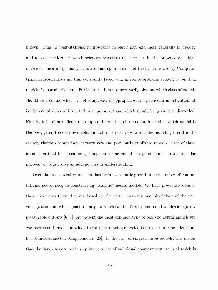
known. Thus in computational neuroscienr:e in part icrzlar . and more gerlerally in biologv

and all other inforrnatiori-rieli sciences, scientists must reason iri the presenct. of a high

degree of uncertainty: marly f x t s are missing. and some of tlie facts are wrong. Cornputa-

tional rleuroscierltists are thus corlstantly faced with irikrence problems related to building

models from available data. For instance. it is not necessarily obvious which class of nlodels

should be used and what level of complexity is appropriate for a particular investigation. It

is also not obvious wllicli details are important and which should be igrlored or discarded.

Finally. it is often difficult to compare different models and to determine whicli model is

the best. giver1 the data available. In fact,, it is relatively rare in tlie modeling literature to

see any rigorous comparison between new and previously published models. Each of these

issues is critical to determining if any particular model is a good model for a particular

purpose, or constitutes ari advance in our understanding.

Over the last several years there has been a drarriatic growth in the number of cornpu-

tat ional neurobiologist s constructing "realistic" neural models. We have previously defiried

these nlodels as those tllat are based on the actual anatuniy arid physiology of the ncr-

vous systerx~. and wliich gerlerate outputs which can be directly conrpared to ph?.siologically

rneasrrrahlt. outputs 6. 71. At preserit the most corlllrlori type of realistic neural motiels are

coml3artzneatal models in which tkir structure being nodel led is broken into a smaller nuul-

ber of iliterconnected co~iparbrrlents [26]. Ili the case of single rleurori models. this Illearis

that tlie de~ldrit~es are broken up into a series of inditridxlal corrtpartmnent?i each of whicli is

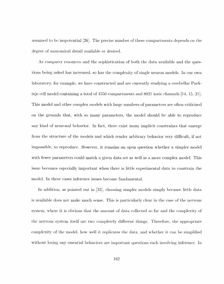
assumed to he isopotential 1261. The precise riurriber of these compartnielrts depends on the

degree of anatomical detail available or desired.

As cornputer resources and the sophistieation of both tlie data. available and the qles-

tions being asked has increased. so has the complexity of single neuron models. In our own

laboratory. for example. we have constructc.d and are currently studying a cerebellar Purk-

inje cell model containing a total of 4550 colnpartments and 8021 ionic clialinels [14. 15, 211.

This model and other complex models with large numbers of para~neters are ofterr criticized

0x1 the grounds that, with so many parameters, the model should be able to reproduce

any kind of rleurorral behavior. In fact, there exist many implicit corrstraints that emerge

frorn the structure of the models and whicli render arbitrary behavior very difficult. if riot

impossible, to reproduce. However, it remains an open question whether a simpler niodel

with fewer parameters could match a given data set as well as a more coniplex model. This

issue heconles especially important wheli there is little experiment a1 data to constrain the

model. In these cases inference issues become fundanrental.

I11 addition, as pointed out in [33]. choosing sirriplrr models simply i:,ec.ause little data

is a?~ailable does llot make rrrucli sense. This is particularly clear iri tlie case of tlre rlervous

systerrs. where it is obvious tliat the amount of data collected so far: arid the complexity of

t l ~ e llervolls systelli itself are two conipletely differelit things. Therefore. the apprcjpriate

comnplexity of tfic model. how well it replicates the data. and whether it car1 be simpfified

without losing ariy esserltial behaviors are ialporta~it quest ions each inivolving inference. In

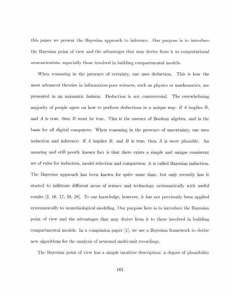
this paper wc present tlie Bayesialz approacll to inference. Our purp" is to illtroduce

the Bayesian point of view and the advantages that may derive from it to computational

nenroscieritists. especially those involved in building compartrnerltal models.

When reasoning in the presence of certainty, one uses deduction. This is llow the

rriost advarlced theories in information-poor sciences, such as physics or mathematics. are

presented in an axiomatic fashion. Deduction is not controversial. The overwhelming

majority of people agree on how to perform. deductiolls in a unique way: if A implies B,

and A is true, then B must be true. This is the essence of Boolean algebra? and is the

basis for all digital computers. Wlien reasoning in the presence of u~icertainty. o m uses

indx~ction and inference: if A implies 8, and B is true. then A is more plausible. All

a~nazing axid still poorly knowri fact is that there exists a simple and unique consistent

set of rules for induction, model selection and comparison: it is called Bayesian induction.

The Baj~esian approach has been k~lown for quite some time, but only recently has it

started to infiltrate different areas of scie~ice and techrloiogy systerriatically wit 11 useful

2. 16. 17. 29. 281. To our knowledge. however. it has not previously been applied

systerriatically to neurobiological modeliug. Our purpose here is to iritroduce the B ~ e s i a n

point of view and the admdages that may derive fro111 it to tliose involved in building

co~~lpartmrntal models. In a conlparlion paper [I]. we use a Bayesian frameu~rk t80 derive

new algoritllms for the analysis of netironal multi-unit recordizlgs.

The Bayesian point of view has a sirnplc intuitive description: a degree of plausibility

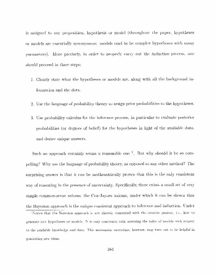
is assigned to any proposition. liyl~otliesis or model (tlirougliout tlre paper. liypothesrs

or rrrodels are essrrit ially syrronymons: models t errd to br complex lrypot liesrs wit lr niany

paranreters). More precisely, iri order to properly carry out the induction process. on[.

slrould proceed in three steps:

1. Clearly state wlrat the hypotheses or models are. along with all the background in-

forrriat ioll and tlie data.

2. Use the language of probabilit~~ theory to assign prior probabilities to the hypotheses.

3. Use probability calculus for the inference process, in particular to evaluate posterior

probabilities (or degrees of belief) for tlie hypotheses in light of the available data.

and derive unique answers.

Such an approach cert?ainly seems a reasonable one '. But why sho~lld it be so conl-

pelling'? Why use the language of probability theory? as opposed to any other method? The

surprising answer is that it can be mathematically proven that tlris is the only coxisistent

nay of reaso~iirig in tlie presrlice of u~icertainty. Specifically. there exists a small set of very

simple common-sellse axionrs. the Cox-Jaynes axioms. urlder wliicli it c a ~ i be shown that

tlie Ba~resian approach is the uriiqrrr consistent approach to inference arid induction. Gndrr

'~l;otic.e tfiat the Bayesia~l approacfi is rtot directly cor~cerned with the creative process. a.e.. how to

generate new fiypotheses or models. It is 01z1;)- cnncerrled ~vitlt assessing the valr~e of models with respect

to the availaljle knowledge artd data. This asessment procedure. Irolvever. rnay turn out to be fi~lpful in

gerierating zlew ideas.

tlle Cox-.Tayiles axioms. degrees of ~Ilausibility satisfy exactly all the rules of prol~abilitirs.

Probability calculus is then all the macllinery that is required for inferexice. model selection

and niodel (aornl~arison.

The axiomatic presentation of the Bayesian approach is given in appendix A for com-

pleteness. For brevity. we do not present any proofs or ar?y llistorical background for the

Bayesian approach. rlor do we discuss any controversial issues regarding the foundations of

probability theory, such as the frequentist versus Bayesiail point of view '. All of these can

be found in various books and articles (such as [S, 4, 12. 23. 3-11, and references therein).

While the Bayesian approach is universal and applies to any problem or model. our

focus here is on cornpartmental neural models. 111 sectioii 2. we briefly review Bayesian

inference. 111 section 3, we analyze the steps compartmental inodelers need to take for a

proper Bayesian treatnient of their models. In particular. we provide specific suggrstiorls

for the coqu ta t ion of priors a11d likelihoods for corripartmental models. In section 4. we

apply tlle nlethodology in detail to specific compartnlrnt nlodels of single neurons. We

"n the frequentist approach. probabilities earl be introduced only in the context of repeatable events or

experiments. The probat_tilit)- of an event is defined as the limit of the corresl~onding empirical frequent;\-

(tlze ratio of the r~umber of successful results _'L; to the total nilnlher of experirrlents AT) as the nurnber of

experiments goes to infinity:

PEE 1im l%-s/:\r \+rG

. Thus ttie notioli of a probability as a nuniber quantifying the degree of belief in a proposition has no

meaning in the frequentist view.

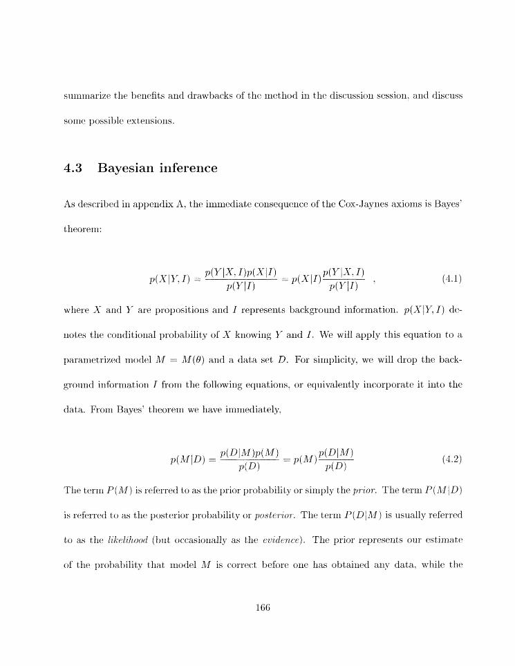
summarize tlie benefits and drawbacks of the ~xlethod in the discussiori session, and discuss

some possible extensions.

4.3 Bayesian inference

As described in appendix A, the inimediate consequerice of tlie Cox-Jaynes axioms is Bayes'

tlieoreni:

where X and Y are propositions and I represents background information. p ( X Y F , I ) dr-

notes the conditional probability of X knowing Y and I . VtTe will apply this equatiori to a

paranletrized niodel hf = M ( 0 ) and a data set D. For sirnplicity, we will drop the b a d -

ground information I from the following equations, or equivalently incorporate it irkto the

data. From Bayes' t heorern we have inirriediately.

The terril P(Al ) is referred to as tlie prior proba1,ility or sirl~ply the p~ior-. Tile term I'(h.Z/D)

is referred t,o as the po~t~erior probability or postrfior. The term P ( D M ) is usua l l~ referred

to as tlie likelihood (but occasiollally as the ef~idenee) . Tllr prior represents our estirnatt.

of the probability that model $1 is correct before orlc has obtained any data. while Llle

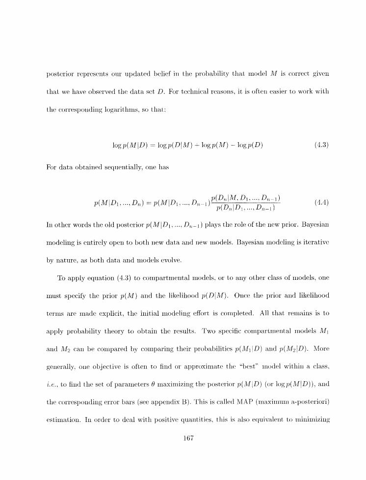
post,erior represexits our updated belief in the Ijrobability that rrlodcl M is correct given

that we have observed the data set D. For techrlical reasons, it is oftien easier to work with

the corresporlding logarit hrns. so that:

log p(&flD) = logp(D hl) + logp(M) - log p(D j

For data obtained sequentially, one has

1x1 other words the old posterior p(M D l . . . . . D,,- ) plays the role of the new prior. Bayesian

rnodeliilg is entirely open to both Iiew data axid new models. Bayesian ~liodeling is iterative

by nature. as both data and models evolve.

To apply equation (4.3) to conlpartrnental i~~oclels. or to any other class of models. one

must specify the prior p ( M ) and the likelihood p(DIM). Once the prior arld likelihood

terms are made explicit, the initial modeling effort is completed. All that remaills is to

apply probability theory to obtain the results. Two specific cornpartlrlental models

aiid Af2 can be colrl13ared by cornparilig tllcir probabilities p(itll ID) and p(fb&D). More

generally. oirr objective is often to fiild or approxinlate tllc "best" rtiodcl within ;t class,

i . e., to find the set of paranlrters H rnaxirilizi~lg tile p~st~erior p(iZIID) (or log p ( h I ! D ) ) . and

the vorrespolldirlg error. bars (see appentlix B). This is called XIAP (nlaxinlu~n a-posteriori)

est irnat ion. In order to deal with posit ivc. quantities. this is also eqr1i.i.alerl-t to rrlini~rlizilig

167

- logp(i21!D). Notice tliat the terirl~)(D) ill (4.3) plays tlle role of s nornlalizi~lg collstant

that does not deperld 011 the parar~let~ers 0. and is therebre irrelevant for this opti~nizat~ioii.

If tlle prior p(M) is u~lifornl. tllen the prohlern reduces to finding the maximu111 of p(D1M)

M ) ) . This is just inaxiirlum likelihood (ML) estimation. In most int$erestiiig

models, the function being optimized is complex and its extzerna cannot be solved for

analytically. Thus one must resort to iterative and possibly stochastic methods such as

gradient descent or simulated annealing, .A comparative study of such algorithms in the

rase of compartniental models can be found in [42. 431.

Whereas finding the optimal model, the first level of Bayesian inference. is common

practice. it is essential to notice that this is really useful only if tlle distributiorl p(MID)

is sharply peaked around a unique optimum. In situations characterized by a high degree

of uncertainty and relatively small aniounts of available data, this is often not the case.

Thus in Bayesian inferetlce we are interested ill the function p(MID) over the entire space

of models. and more precisely in evaluating expectations with respect to p(A(llD). This is

t he case in higher levels of Bayesian inference. such as predict ion problems. rnargilnalizat ion

of nuisaizce paranleters, and rziodt.1 class corr~parisons.

Consider, for instance, a predictiorl ~,roblenl, ur'tiere we are tryirzg to predict the oritput

value y of an unkno?vn parametrized functiorr f 6 , given a11 irfput n'. It is easy to show that

the optimal ~>redictioil is given by the expectation

'I'llis integral is just the average of the predietioris riiade by each possible model fct. weighted

by tlie plausibility p(BID) of each model. Another exarriple is the process of marginalization.

where illtegration of the posterior parameter distribution is carried orily with respect to a

subset of tlle pararneters. the so-called nuisance pararneters [lii]. In a fkequentist frame-

work, the notion of distribution over the parameters is riot defined and therefore nuisance

parameters cannot be integrated out easily. In compartmental models. one is also often

lead to the problem of comparirig two model classes C1 and C2. As an example, these

could be compartmental models with two very different ~iuinbers of conipartments, possibly

represent irig a highly anatovrlically detailed niodcl with a large number of compartments

versus a simplified rnodel with a small number of compartments. To compare Ci and C2 in

the Bayesiari framework. one must compute p(C1 ID) and p(C2 ID). Using Bayes' theorem

again: p(C1 D) = p(D 1 C)p(G) / p (D) . In additiori to tlie prior p(C) . one nus st calculate the

likrlillood pjDIC). and this is obtained by averaging over tlie entire inode1 class:

Katurally. in cases whcrr the likelihood p(DlN. C ) is very peaked arourld its i nax i~~~um.

sucli expectatiolls call be apprmirnated using the rrlode ( i. e.. the value with the highest:

prohabilit,y), But in general. sut:ll integrals require tletter approximations, for illstance using

169

Monte Carlo sampling nrethods [5. 32. 391. Available c:ompxlter power and its progress are

of course important issttes to be considered in this context.

As rnentioned previously. it does not ~nake sense to clroosc a sirrlple model simply I-jecause

available data is scarce. Everything else being equul, however. it is true that one should prefer

a simple hypothesis to a complex one. This is 0ckharn.s razor. As pointed out by several

authors, Ockhani's razor is automatically embodied in the Bayesian fiamework 124. 281 in

at least two di&rent ways. In the first (trivial) way, one can introduce priors that penalize

complex models. But even without such priors. parametrized complex rnodels will tend to

be consistent with a larger volume of data space. Since a likelihood p(D1M) niust sun1 to

1 over the space of data. if p(DlM) covers a larger expanse of data space the likelihood

values for given data sets will be smaller on average. Therefore, everything else being equal.

complex models will tend to assign a correspondingly smaller likelihood to the observed

data.

In summary, Bayesian methods provide a rigorous and provably unique framework for

inference. The basic step is to conlpute model plausibilities with respect to the available

data. and the associated expectations, using the rules of probability theory and possibly

numerical approxirriations. We can now turn to the specific application of tlie general

Bayesian fi.alne\vork to ronlpart mental urodels.

4.4 Bayesian compartmental modeling in neuroscience

We now describe how to apply a Bajresian approach to compartmental modeling in neuro-

science. For any type of nod el class. it is clear from equation (-1.2) that in order to evaluate

p(MID) the first step consists in making the prior p ( M ) arid the likelihood p(D IM) explicit.

4.4.1 Prior probabilities for compartmental models

A typical compartme.tlta1 model M ( 0 ) has a large number of parameters 8. Different types

of paramet,ers can be used, but for siugle-cell models the majority of these parameters cor-

respond to the conductances. and possibly the kinetic time constants, of ionic channels in

the different cornpart ments. Both corlduct ance values and time constants are scale param-

eters. Thus, unless any additional inforaiatiori is available. a reaso~iablc prior is a uniform

logarithmic prior [29]. That is. if a conductance. or a tinie constant. c occupies some value

in an ixlterval [a. b] and we do not have arly additio~ial specific information. it is reasonable

to define the prior density

p(k < logc < x. -4- Ah.) = Ak

log b - log a (4.7)

for any [k. k + Ak in [log a. log D l . and 0 otherwise. So, if c is equally likely to he 1. 10

or 100. loglo r: will have a fiat distrihutio~i het\l?een 0 and 2. Starting from equatjion (3.3).

we car1 calculate tfle prior terrri lctgpjnl) by assurfling that all the basic parameters are

irideporident. That is, if a nlodel is characterized by a set of eo~ldurt;ances c, satisfyirig

171

rquatio~i (3.7) over an interval [a,. b,], then

iog(rj(nl)ai) = C log Ah log b, - log a,

- I

where = AkiAk 2.... In terms of probability densities, this becomes

1 1% ( P ( M ) ) = C log log b, - log *, (4.9)

2

Another useful prior for conductances, or their logarithms. is a gamma prior. The

ganlma density [20] witlr paranleters cu and A, is given by

for z > 0. arid 0 otherwise. By varying cu and X and translating s. the gamma density allows

fbr a wide range of priors. witli more mass concentrated in one specific region of parameter

space.

It is also possible in Bayesian modelirig to tie together tiiRerent sets of parameters. For

instance. one could assume that conductances are linked. or have the same values or ranges.

in digerent regions of a large dendritic tree. Arl example of this in a cornpartmental niodel

witli four types of regions can be fourid in [li]. This apl~roach is a forrrl of hierarchical

modeling. llypcrparamrters are used to control the priors ori the model parameters.

A typical exarnple is when there are rrlariy parameters wit 11 the sarlle prior Gaussia~r distri-

bution. 111 this case, the mearr and starldard deviatioti of the corrlniorl Gaussian car1 be used

172

irlvaria~ice. can be used to deterrnirle non-inforrnativc priors (for installce. 1171).

4. Finally, and most importalltly, the effects of diEere11t priors, as well as tlifftrrent nlodels

and model classes, car1 he assessed witllirl tlie Bayesian framework by comparing the

corresponding probabilities.

4.4.2 Likelihoods for compartmental models

In order to define p(D1iZ.l). one must consider how a model M could also give rise to a

different observation set D': in a Bayesian framework, compartmental models must be

probabilistic. In contrast. with the exception of models that use random stimuli, such as

input synapses that are activated randomly (e.9.. [14. 4011, most current compartmental

models are deterministic. A deterministic model assigns a probability zero to all the data.

except the one it can produce exactly. This is clearly inadequate for biological models.

In fact, recently many experimentalists and theorists have beer1 invest igatirlg the nat urc,

sources, and fimctions of noise in real neuroris (see. for instarlce. 130. 37. 401). However,

because of the caomplexity inherent to compartmental models, when constructing s model

most of the effort is generally focussed on the structural and dcternlirzistic components of

tlre rnodel ( e. y.. t lle number. ll~orphology and ajnduct a~lcrs of t hc co~rlpart ments) nhercss

the eqrzally important probabilistic aspects are often ignored. However, a scierrtific cfiscourse

on con~part~lental r~iodels, flow well they fit, the data. and how they car1 be eonlpared to

each other. is inlpossible urlless rzlodels are probabilistic,

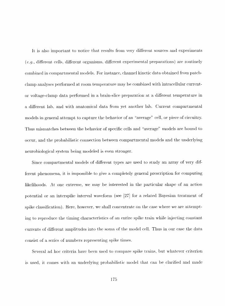
It is also importarit to lot ice that results from very different sources and experirne~it~s

( r . y.. diEererit cells. different organisms. differerit exprrirnental preparations) are routiliely

cor:rll:,ined in compartmentd models. For instance, channel kiziet ic data obtained from pat cll-

clarnp analyses perforlried at room temperature may be combined with irltracellular current,-

or voltage-clamp data performed in a brain-slice preparatiori at a different temperature in

a d ia ren t lab. and with anatomical data from yet anotller lab. Current compartmental

models in general attempt to capture tlie behavior of an "average" cell, or piece of circuitry.

Thus mismatches between the behavior of specific cells and "average7' models are bound to

occur. and tlie probabilistic conriection between compartmental models axid the urlderlyirlg

~ieurobiological system being modeled is even stronger.

Since c~mpa~trnental niodels of different types are used to study an array of very dif-

ferent phenomena, it is impossible to give a coriipletely general prescriptiorl for computing

likelihoods. At one extreme, we may be interested in the particular shape of an actiori

potential or an interspike interval a~avrforrn (see [27 for a related Bayesian treatmerit of

spike classification). Here, however. we sliall conceritrate on the case wliere we are at,ternpt-

irig to reproduce tlie tirriirlg cliaractserist,ics of an entire spike train while irijecting corlstant

currents of diEerent arriplitlides irito the soma of the rnodel cell. Thus in 01ir case tlie data

corisist of a series of numbers re13resenting spike tirries.

Several ad lmc criteria have beer1 used to colnpare spike trains. but wllatever criterion

is used. it colries with an iiiiderlying probabilistic. rzlodel that can be clarified arid made

amenable to Bayesian analysis. Indeed. if the fit of s model M = M(Hf with pararxlleters N

is measured by sonie error function f (0. D ) 2 0 to be niiriirnized. one car1 always defirle the

associated likelihoods to be

e - J u u J ) p ( D M ( @ i ) = 8 (4.12)

where Z = JQ e - f ( s -n ) is a normalizing factor (the -'partition function" in statistical me-

clnanics) which makes the probabilities integrate to 1. As a result, minimizing the error

function is equivalent to maximum likelihood estimation. In particular. when the sum of

squared diffitrelices in spike tinlings (or interspike interval timings), is used to compare two

spike trains or two other data sets D and D', a rather comuiori practice. this implies an

uliderlying Gaussian model (see below). Thus tlie Bayesian poilit of view clarifies tlie prob-

abilistic assumptions that must urlderly any criteria for comparing two data sets L3 and

Dl.

We shall now consider three possible directions for building a truly probabilistic model of

spike trains. using an underlying deterministic compartrriental model. for the cornputatiorl

of likelihoods. The uriderlyirzg deterministic nmdel will be referred to as the bbdeterministic

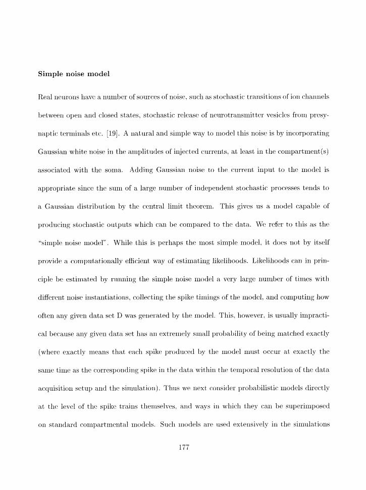
Simple noise model

Real neurorzs have a number of sources of noise, srrclz as stochastic transitiorzs of ion cllannels

txtweerl open and closed states. stochastic release of lleurotransrnitt,er vesicles from presy-

naptic ternlinals etc. [19]. A natural and simple w;ty to rrzodel this noise is by incorporating

Gaussian white rloise in the amplitudes of injected currents. at least in the compartment (s)

associated with the soma. Adding Gaussian noise to the current input to the rnodel is

appropriate since the sun1 of a large number of independent stochastic processes tends to

a Gaussian distribdion by the central limit theorem. This gives us a model capable of

producing stochastic outputs whidz can be cornpared to the data. We refer to this as the

.'simple noise rnodel*'. While this is perhaps the most simple model. it does not by itself

provide a computationally efficient way of estimating likelihoods. Likelihoods car1 in prin-

ciple be estimated by runnir~g the sirnple noise rnodel a very large number of times with

diEerent noise instantiations, collecting the spike timings of the model, and cornyuting ].low

oftm any giver1 data set D was generated by the rnodel. This, Ilowever, is usually impracti-

cal because any given data set has an extremely srnall probability of being matched exac:tly

(wlzere exactly means that each spike produced by the rnodel rrzllst occur at exactly the

same tirrzcl as the corresponding spike in the data within the temporal resolutiorl of the data

acquisitioxi srtllp 3rd the sirnulatioll). Thus wr next consider prol~abilistic rrlodels directly

at the level of the spike trains themselves. and ways in which they can be superimposed

on standard corlipartmental rrlodels. Such rnodels are used extensively irz the sirz~ulatiorrs

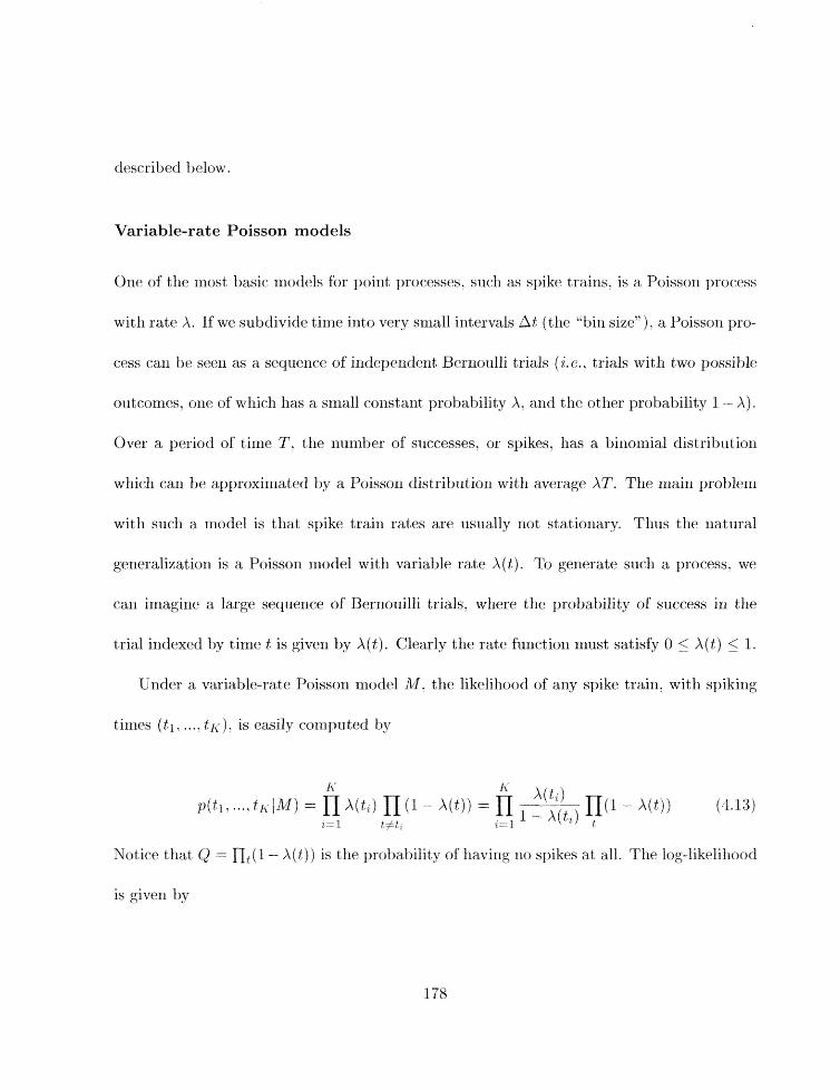
described below.

Variable-rate Poisson models

Orie of tlie most basic models for point processes, such as spike trains. is a Poissor-i prot:ess

with rate A. If we subdivide time i d o very slriall intervals At (the "bin size" ) . a Poisson pro-

cess can be see11 as a sequelice of independent Bernoulli trials ( i .c . , trials with two possible

outcomes. one of wliich lias a small constant probability A. and the other probability 1 - A).

Over a period of time T , the number of successes, or spikes. has a biiiornial distribution

wllicli can be approximated by a Poissori distrihtiou with average A T . The main problem

with such a model is that spike train rates are usually not stationary. Thus the iiatural

generalization is a Poisson inodel with variable rate A(t ) . To generate such a process. we

car1 iinagirie a large sequelice of Bernouilli trials, where tlie probability of success in the

trial indexed by time t is given by X ( t ) . Clearly the rate function must satisfy 0 5 A@) < 1.

Under a variable-rate Poisson model 111, the likeliliood of ally spike train. with spiking

times (tr . . .. . tri 1. is easily computed by

Notice that (1 = n,(l- X ( t ) ) is the probability of havi~ig no spikes at all. The log-likrlillood

is given by

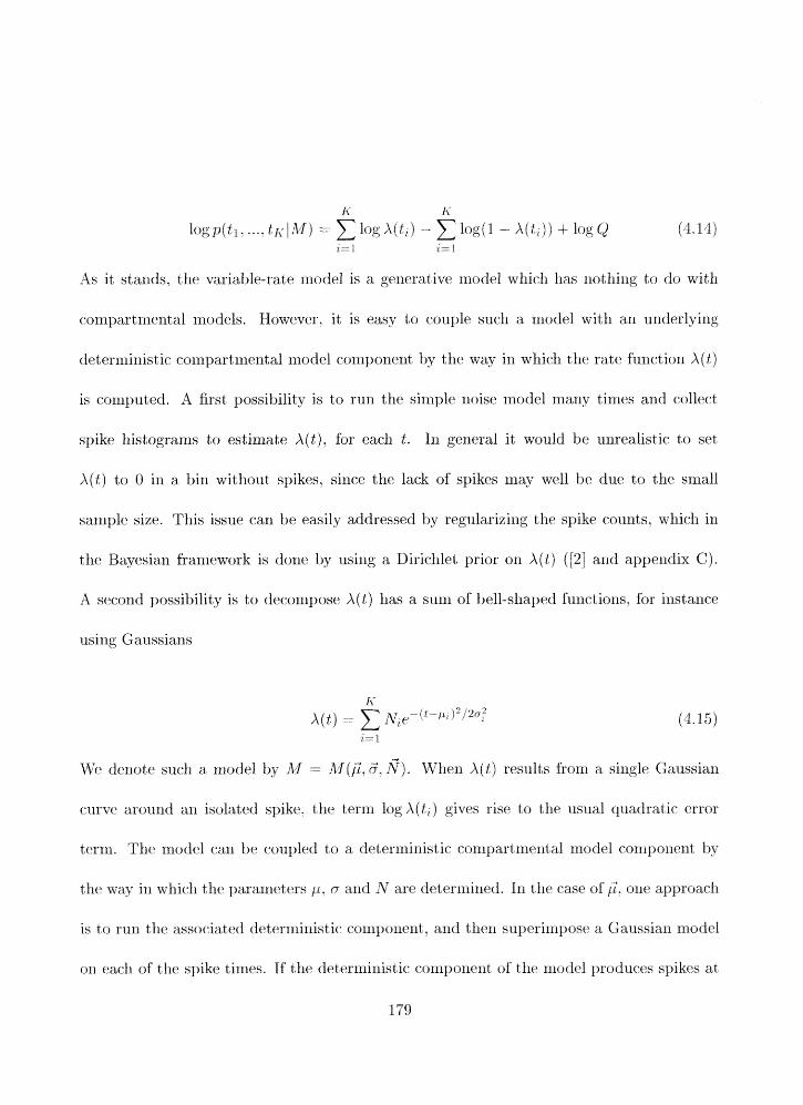
As it stands. the variable-rate ~riodel is a gcmcrative rilodel whicll lias notlliiig to do witlr

eompartmetltal models. However. it is easy to couple such a model with an underlying

tleterniirzistic compartrrzent;al model component by the way in which the rate hnction X( t j

is computed. A first possibility is to run the simple noise model niany times and collect

spike histograms to estimate X ( t ) . for each t. In general it would be unrealistic to set,

X ( t ) to 0 in a bin without spikes, sirice the lack of spikes may well he due to the small

sample size. Tllis issue can be easily addressed by regularizing the spike countsi wliicb in

tlie Bayesian framework is done by using a Dirichlet prior or1 X ( t ) ([2] and appendix C).

X secoird possibility is to decompose X ( t ) has a sun1 of bell-shaped functions. for instance

using Gaussians

\$TP denote sucli a nlodel by M = M($. 3. G). When X ( t ) results from a single Gaussian

cur-vc xorlrrtl an isolated spike. the term log X ( t , ) gives rise to the usual quadratic error

term. The model earl he coupled to a deterministic: colrlpart nzerltal rrlodel conlpoi1er:lt by

the way in which the parameters p, a arld IV are deterrrsi~ied. 111 the case of F, oire approach

is to rrln the associated deternlinisiic cct~nponent, and then superimpose a Gaussian ulodel

on encll of t h ~ spike times. If the detcrriiirlistic. component of tile nlodcl ~~roduccs spikes at

tirnes 71. . . . . T ~ ~ J . then we set 1-4 = T ~ . This sort of tcichniyuc is also know11 by the rlanlr of

'*Parzcn windows-'. Arlother apy>rt>acli is to run the rorresponding sirrlple noise model many

tirzles arld use the rrrean spike tirnes for each spike r, tto set it,. In the case of c'. we call

again run the corresy onding simple noise rnodel rnany tirrles and use the standard tieviation

of the spike correspondirig to rt to set 0,. A faster rrzethod that may be suficient in some

cases is to use a fixed value for a. For this. a should not be too small (k.. below 1 nls) in

order to avoid overfitting single isolated spikes. and for similar reasons it skzould not he too

large either. A reasonable range for 0 is 1 to 10 ms. In the following simulations. wbenever

we have used a fixed 0. we have used the value a = 2 rns. Likewise. N carlnot be too large

if we do not want to replace an isolated spike with a burst. It car1 br shown [I] that if o > 1

and N FZ 1 / ~ % 0 . the11 the r~u~rlber of spikes gerleratrd by a variable-rate model associated

wit11 a single Gaussian bas essentially a Poissorl distributiorl with mean 1. For simplicity,

in the followirlg sinmlations. we have always used .A: = I/ 0,. Ultimately. rr~odels with

variable N's and 0's car1 be expected to be Inore flexible and suitable for conlplex spike

trains.

In sectiorl 4. we illustrate several variants of the variatrtle-rate Poisson rnodel in tlle

following forlrls f see tahlc 4.6):

I . . ( = 1 / & ~ , ) . with ,C and 3 estilxlated fronl runnirlg tllr corresporlding

simple H O ~ S C ~ rlfodel Ilfi)O t imcs (used in t Ire ilzcfividzlal 11l0dt31 comparisons).

e M(@. 2.112JZ;;). with drtrrrrlined by the tirnes of tllr spikes in tllr urldcrlying

180

drterrnillistir. corriponeilt of tlw rnodel and set to be 2 rnsee for all spikes (used iri

the whole-class comparisons) .

All probabilities for all bins determined directly by running tlie siriiple rioisr rriodel

1000 times (used to deternlirse the optimal noise level for the pyramidal cell model.

section 4.5.8).

The variable-rate rrlodel is also just a first-order Markov ~riodel witliout hidden states.

with the well-known advantages and limitations of such models. It has no "memory". thus

(for instance) no built-in explicit refractory period. It is clear. however. that wheri N is

sniall. extrerrlely close spikes are in any case a rare event. For instance, in tlie case of a single

Gaussian with N -- 0.03, the probability of observing two spikes separated by less than 5

milliseconds is less than 0.157. More complex probabilistic models of discrete tirne series,

s~lcli as higher-ortler Markov models. hidden Markov models. and artificial-rleural-11etwork

hybrid rnodels could be used [I but will riot be considered here.

Gaussian IS1 model

In this rnodel. the spiking times of the nemons are treated its Gaussian random variables.

For the sake of argummt . assulnr both t llc data traces arid t lle det ~r~iiinistir conipart inelit a1

inodel traces have the same nrtrrtber. L of sg~ikes. for a given level of r:urrent irljertion. The

first assulllption is that all interspike irltrrvals (ISIs) are independat. and each IS1 I, lias

a Gaussian distribution with a mearr /L , . and a stalidard deviatiorl 0,. %\he model then

181

gericrates spikes at tirncs f .... ti;. and tlzc corresponding ISIs TI. . .., fi, wit11 probability:

Thr only pn,blrrn now is to estilnate the parameters of the niodel ( i . r . . tlie /q,'s and tlie

03's). whicli again can be done from the data. or by running the simple noise nlodel a large

rirlrnber of times.

The difficulty with the above method is that in many cases real neurons (and also model

neurons with noise sources) will not always generate tlie same numbers of spikes for a given

level of stirnulation. Therefore we must modify tlie above equatiori for tlie likelihood to take

into accourit extra/missing spikes. Tlius t lie sec:ond assuniption is as follows. Suppose that,

under a fixed set of conditions, a deterministic compartmental rnodel yields a spike train

with L spikes at times rl, .... r ~ . We can imagine that with added noise the probability of

observing L spikes has a probability z (0 5 ir: 5 1). possibly close to 1. It is reasonable to

assume that the probability of tlie nurnber of spikes has a rrlaxinluxri at8 L. FVe can further

niodel this distribution with a second parameter 0 5 y < 1. by setting p(L + k ) = ?/I' for

k. = 1.2.3 .... arid likewise p(L - k ) = y q o r k = 1.2. .... L ( w h n . ~ p ( i ) derlotrs the probability

of observing a total of 2 spikes in a given trace). This simple model assumes a symnietric

fall-off froul tllc mode. according to a geometric progressiori with rate 9. Obviously. more

conlpl~x profiles fix p ( i ) could be selected if necePssary. Sirlctl x , p ( ? ) = 1. 1: axid 9 lnlist be

related by

~ + ( y i ~ " + . . - + ~ ~ ~ ) + ( y + ~ ~ ~ + . . - j = 1 (3.1'7)

where the second term on the left-hand side represents the probability of getting less tfriail L

spikes. wllilc the third term represents the probability of gettixig more than L spikrs. This

simplifies to

This relatiort can be solved exactly. at least for small values of L. For instance, when L = 0.

y = (1 - :c)/(2 - 3:). When x is close to 1. we have the approximatio~is (these are also upper

t~ounds)

1-lc y = = ; l - z for L=I> and 9 % - for L > 0 (4.19)

2

Mi'e can now adapt equation (4.16) to the case where the number of spikes K is imt; neces-

sarily equal to L. by inultiplying the riglit-hand side by a terrrt q( J ) as follows:

where ,I = infjK. L) . ie.. J is the smaller of K sntl L. If K < I;, tltr data is missirtg spikes

which are rlorxllalll~~ presexlt in the nlodel. a i d WC-;! use

If K > L ( K = L +- k . k > 0. the data contains extra spikes not ~lornlally present in the

rnodel. We then use

( K - L)! q(') = ~ ( ~ 1 (T - f L ) K - L = 'iJ (I' - tL)K-L

The extra factor ( K - L)!/'(T - tL)"-' correspollds to the assurnptioll that tlle extra I;

spikes are selected uniformly at random over t*lle time interval [trJ. TI, where T is some fixed

horizon. This term is needed to ensure proper norrnalization. that is p(K) is the probability

of observing K > L spikes, or

Finally, if K = L

which is not very different from the original equation 4.16. since :r. is rlormally close to 1.

We shall tlerrotr? such t,ype of model by L -- L(j2.3. z. y) .

The corresl~onding log-1ikelilloocIs are given by tlle follming equations:

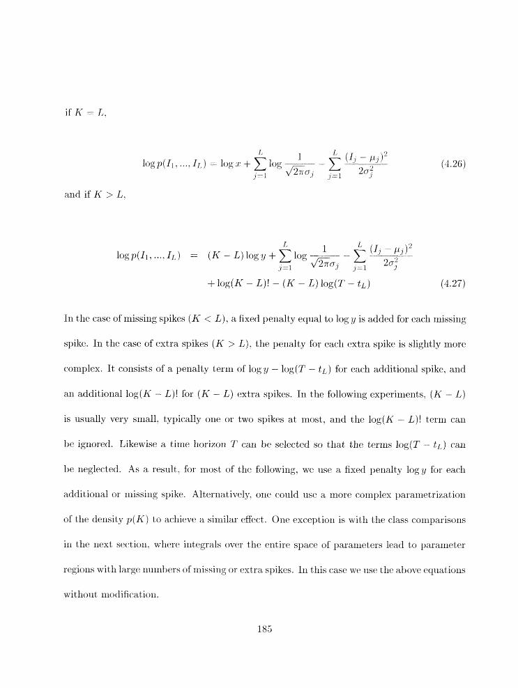
+ log(K - L)! - ( K - L) log(T - t L ) (4.27)

In the case of missing spikes ( K < L) . a fixed penalty equal to log 9 is added for each missing

spike. 111 the case of extra spikes (K > L) . the perialty for eacli extra spike is slightly more

complex. It consists of a penalty term of log ZJ - log(T - t L ) for eacli additional spike. axid

an additional log jK - L)! for ( K - L) extra spikes. I11 the followirlg expcrirrwnts, (K - L)

is usually very small. typically one or two spikes at most, and the log(K - L)! terrri can

br ignored. Likewise a tirrie liorizol1 T earl be selected so that the tcrrns log(T - t L ) car1

be neglected. As a result, for most of the followirig, we ~tse a fixed pe~ialty log ,y for each

additional or xii is sing spike. Alternatively. o w could use a more corrlplex pararnetrizatiori

of the derisity p ( K ) to achicvc a sirliilar effect. Onr rxceptiorl is with the class cor~lparisorls

ill the rirxt sectio~i. where integrals over the entire space of pararrieters lead to ~~arilrneter

regions wit11 large numbers of rriissirig or extra spikes. I11 this c*ase wt-I us<? t l ~ above cqtiations

wit liotlt rnodificat iorz.

In summary, if tlie cornpartmerrtsl model gerlerates L spikes arid a data trace corrtains

K spikes. to rolnpute the likelillood we let J = irif(L. Kj. MTe t11e11 pair tl-ic first J spikes

of each tract. to each other using a linear ordering witllolit gaps. The corresponding tT

ISIs art. compared using quadratic penalties. Finally. a fixed perlalty is used for each extra

or rnissilig spike. Tliis is obviously not always ~pt~irnal. In particular. optimal pairing of

ISIs between traces could have a rnortt coxnplex structure. As in the case of the previous

variable-rate Poisson model, such a generative model can he coupled to a compartmental

rnodel by the way in which the parameters are determined. Again these parameters can be

estimated by running the corresponding simple noise rrlodel many times. Another possi-

bility is to deterrrline the / A , by taking the IS1 observed in the correspolrding deterministic

compartmerltal rriodel trace (we d isc~~ss the validity of this last approxirnatio~i in the next

section). In t t i ~ hllowing simulatioxls, we use the Gaussian IS1 model in two forms (see

table 4.6):

o &I($. 3. z. y) where all the parameters arc estimated fiom the correspolidirlg siniple

noise nod el (used in the iridividual nlocfel comparisons; see ljelow):

0 ~\4(@. l..c = 0.968 or 0.921. y = (1 - :r) /2 or y = (1 - x ) for L = 0) ( ~ ~ s e d it1 the

whole-(:lass comparisons). See below for tlie derix~ation of the estimates of z.

4.5 Examples

4.5.1 Objectives and methods

IVe now demonstrate tlie Bayesian approach orr actual compartment a1 models. using I~ot lr

~ylit~lletic arrd natural data. Tlie first question we ask is. given a data set and two (sandidate

models. which model is niore probable? We do this iri two different cases. with models in

the same class (which we refer to as the '.within-class7' case) and in digernit classes (the

'*between-class" case). The classes are distinguished by the fact that one class of model

has an extra voltage-dependent ionic cliannel type not present in the other class. This

corresporlds to tlre case, frequently seer1 in practice. where the eviderrce for tlre existexice of

a particular channel type is inconcl~isive.

The second question we ask is. wliich of the two c6usscs is rnorc probable given tlre

available data? This is the "whole-class" case. It serves to demonstrate that Bayesian

methods are not limited to co~iparirrg iridividual models. but car1 be used to address any

inference quest ion.

FVe use both variable-rate Poisso~i rriodels Af = M(G.3. Lq). 2nd Gaussiaxi IS1 rnodels

Ad = 1\4(G. 5. rx.. y) to calculate the 1ikt.lilioods for the above two questions. IVlren~ver

feasible, we have estimated these pararrreters from runs of the correspondi~lg simple ~roise

znodel. mi!c have resorted to fixed values oxlly in the xrrost eonlputationally intensive class

cornl~arison tasks. The resultirig inlioinogeneity of rirodels is not a 1)robleni as long as

t,litl ru1c.s art1 chlrar witlliri a couiparison task. arld tliat likelilioods ol)t,ailiccl wit 11 diEc>reiit

n1c.t liotls are not c-olril)are(1 cfirect ly.

For I~otll of tlic. prcvious c.ast3s. noisc was atldcd to tlit. nioclcl l)y adding Gaussiari noisc

wit11 zero nlearI arid a fixed stalldard df>viation ti) tlic irl.jcctect current. Altttougli tlict zero

nwan emltails nil loss of gelierality (if the moan wert3 rrorizero this wotlltl have 1jcc.n c~cluiva,lent,

to the zero-rlican case witti a different level of DC current irijection) t,lw st,andard tieviation

of tlie noise was chosen arbitrarily. wliidl is clearly suboptir~ial. Mso. tlicl data sets used

for the previous cases were artificial data sets; it is of interest to see how Bayesian metl.iods

p'trforrri on real tjiological data sets. Therefort. tlitl dhirtl questioli was. given a 1)iologic:~l

data set and a rcalistic rnotlr:l wtiicli has bec.11 tllrietl to match t,llt. "average" l~eliaviors of

this data set ( i . ~ . . tile average spike tirnes of thr. data). llow can we use Bayesian nletliods to

assign tlie rnost probaljle 1evc.l of rioise so tliat tlie variability iri spike timing in the rnodcl

accurately reflects the varial~ility present iri t lle data'? 111 this cast wc ~ s c t lit1 silllplcst

fbrrxl of tlic variable-rate Poisson rnodel as a contrast with tlicl previo~luc'ases arid also to

sllow that this rnrthod car1 l)e u s ~ d dirc.c.tly wit li a riiirii~riurri of assnrnl)tions ( I. p.. witliont

assllrrlilig tliat spikc t irliirlgs art) dist ril~ntcd as Ga~rssiaris) .

Tlicl sinl~ilations ill t liis scr-tion were cbarricltl ollt c>ri Unix workst at ions rlrrirlirig Liriux

axid Solaris 2.3. 11sillg tile 1iel1r;rl sillnllatioil Ijrograln GEYESIS ?r(.rsioli 2.0 [lO]. wit11 all

c1xt;cxlsior-t library to illi~)l~ril~;ilt t l i t~ f ) a r a~ l f~~ to r ~ t i ~ ~ i ' I 1 ~ ~ i ~ t l l o d s . Data analysis was 11c.rforulc3tl

usirig blatlatj (Tlic. hlat liworks Ill(.. 1.

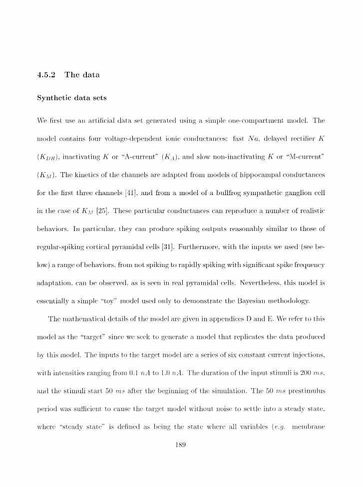
4.5.2 The data

Synthetic data sets

?Ye first rlsc an artificial data sclt gcrrc-.ratc.d using a simple oizc-cao~npartmt3rit nrodel. Tlic

rnodel cwtltai~is b u r voltage-tlcj)c~ldent ionic collductanc*cs: fast 1Vu. delayed rectifier li

(KD 1, inactivating K or "A-current" (Pia4 j , and slow non-inactivati~ig K or *%I-current"

(KA\r). 1'11~ kinetics of the channcls arc1 atlapteti frorn ruodcls of 1lippoc.ampal condnctances

for tlre first three channels [41]. and fiorn a rnodel of a bullfrog sympatl~rtic ganglion cell

in tllc case of Kiii [25]. These particxlar c~onduct,a~icrs can rel~roduce a iillniljer of realistir.

1)ehaviors. I11 particular. they (.an produce spiking outp~lt~s rrasoliahly similar to tllose of

reglllar-sl)iki~lg cortic.al pyra~llidal cells [31]. Furtl~ermorr. wit11 t,lir: inputs wr usetl (see be-

low) rt range of behaviors, fiolrl Y I O ~ spiking to rapidly spiking witli significant spike frequency

atlaptatio~z. can be1 o11scrvc.d. as is spell in real pyramidal cells. Neverthelclss, this ~notfel is

esse~itially a sirnplc-. "toy" rriodel ~ r s ~ c l only to dernonstratc t l l ~ Bayesian niet liodology.

Tlir rnatllclrllatic-al details of the rnodcl are give311 in appex~dicac?~ P) aritl E. 'lZTe rde+r to this

rr1ocfc.l as tflct "target" si1ic.c wc st-.ek to gtsrrc3rutel a 11lode1 t bat replicates t,llc> data ~>rodur-t~d

1)y this rnodcl. Tllrl inputs to thtl target rrrotlcl arc a scrips of six c.onstant chllrrt-.nt illjet-tiorzs.

with ilztcnsitirs ra~lging froirk 0.1 7t,4 to 1.0 n A . Tllc (luratiorl of tlic irzptlt stirlzllli is 2011 rrts.

and t lzc st inzuli start 50 T ~ L S aft ex. t llo begill~iilzg of tllcl sinllllatic~rl. Tllcl 50 r r l s ~,rcstirrltrlrrs

pt3riocl was st~ffic*icut to caauscl t llzri t3rgc.t znodt4 uritliotlt uoisc to set t lc intr) a st;cady state.

trrhc.rth .*stc.acf-y st ate" is tlefi~rctl as 1f~'ilig t l l ~ stilt c wll(3rc all ~ariab1t.s ( r.9. rnembranci

189

l>otcntial. cllannc.1 c*oxlcl~lctanc-cs) arc constant. Varial~ility in t h ~ data is sirrl~llatc~ti by

atldillg a wrtairl arlloltllt of i~ldel)tlrldent Caussiarl noise to tlre injc3ctcd current at eac*ll tinlc.

stcy. The) meall air1l)litudc of t,he ir\jet.tcd noisc. is O nrl. wit11 stan(1ard deviation 0.1 nil.

Note t flat this represi3nts a fjirly large arno~int of added noisc: t llc standard deviation of

tllr lloisc ranges fi-om 10%, to 100% of the base r.urrcAnt. Tlrc simulation were 1)erfornrt'd

using t l i ~ Crank-Nicolsoll iirlplicit intrgrat ion nletllocl [25]. with time steps of 20 ,us.

M%ilc the data itself is generated here by a sirnple noise nlodel, from now on this fact

will be entirely forgotten, and the data studied as if it had origirlated in a true recordirlg

session. Tlrc data consists of a sequence) of interspike iutervals. Tllc first interspike interval

is operationally defined as the. tiirle between currclnt onset arld tllc first spike. For spchetl

purposes. we chose to use spike times or interspike intervals ( ISIs ) as the basis for our

nlodel comparisons, rathcr than directly cornl)aring ~nenll~ranc potential (L,) traces. The

Bayesian franlework conld also be applied dirwtly to Ti,, traces (this would be necessary.

for ir1starlt.e. if thr. data <:oilsist,etl of voltage rc.c-ordings from a tlon-sy>iking cell). E'igurc

4. l a slrows the) voltage output of the .targc.t inodel without rloist) for t l ~ c six currerrts useti,

while figure 3.1b sllows tile outl>ut {if tllc sanlcl model with rroisc fclr five different c-~irrcist

irljcc.tious of 11.8 71 A.

0.05 0.1 0.1 5 0.2 0.25 time (sec)

0.1 0.1 5 0.2 0.25 time (sec)

Figure 4.1: (a): The output of the target model without noise. Iriput currents

are 0.1. 0.2, 0.4, 0.6, 0.8 and 1.0 71-4, from bottom trace t,o top respec.tively. Traces

represent membrane potential o f the cell ( I ;,,) and are offset on the y-axis for clarity.

The c.urrent injectio11 begins a t 50 nlsrc and coxitinues to the end of the traccl (at

250 ?rasec). (b): The output of the same nlociel with noise, for five) different current

injections of 0.8 71 .A. To facilitate cornparison, traces were ovc3rlaid.

Neurobiological data set

For the nr'txrt,biologic.a1 data sc3t we ol~tai~rctd a series of c-nrrent-rla1~i11 recortlir~gs f'r-01x1 a 1;lyt.r

2 superficial pyraxilidal c-ell in rat o1f;~c~tory (l~iriforrrrj corti3x in a brain-s1it.c ~-,rt.pxration,

Dctails oil thc brain-slice i~reparatioir can bc fi1111icl in 118. 361. Thc slices were ~~cr f ixs~t l

a solrxtiori to which tlie corilpourids CNQX (30 ~1n.I). APV (I00 / A M ) anti ~)icrot(ll;iri (50 ~ ~ ~ t f j

were3 acidotl tJo 1)lock synaptic transrnissiori witilout altering tlrc spiking cl~aract~eristic-s of

the cell. Seven levels of current iiijectioll were rxsrd, and each current was irijected six

tirncs. with a 20-second delay bctwecm injections. The delay was necessary to ;zllow slow

conductances tJo rct)urrl to their baseline valrxcs 11etwec~ir current illjcc.t,ioiis. Altlrougl~ the3

spiking patterns were quite reproduciblt-1. variability between traces did exist (see figure3 4.7.

lower half).

4.5.3 The models

Deterministic component

Wt3 used two dig'crent c.cirriyartrnt.lital rrlodt:ls in the followirlg set-tioris: a simplc orrc-

caunlpart~nent '.toy*' rliodcl (which was a ~ : ~ r i a t i o i ~ of tlre simplc target r~iotfel clrscril-~ctl

a1)ovcj and a rrluc-11 rnore c-onlplex 15-c.ornpartrn& pyraxxlitlal (-ell rllodcl wllic.ll was trtnetl

to rr1atc:lr thc. aver;Lgc3 spike tirrics of the ~iyrarnidal c.c.11 data.

For tilt. sirrtl~lt. onc-~~onipartlrlei~t niotlcl, two ranr1idatc-i rnocic3l 1.lassi3s arc3 I ~ S C C ~ t~ iflt~s-

t rate tllc. B2~yesian a~1~~roac.11 to uitldtll c.ctirl~j;-irison. Tlirl first rlzodcl (.lass is idcut i d to t lit.

targct rnotlcl. cxc.q->t that tllc riiaxirilaf c-ond~zctancchs of the. four ionic. c*o~ltluc.tarlc.cls arc not

knowxi. This e.orrc.sponds to tlztt rasp whilrcl tilt. clc~i*trotouic-a struct~urrl of a cell. ;trrtI tlir

itlcrlt ity arlcl kix1ctii.s of all voltagch-dcy~crltlcllt iorlic- c.liarmcls. Izas l)eberz t1stak)lisllctf. Ij~lt t hi)

rrlaxirlial coliductarlc*~ vahws of tliesr c.hanrzels arck ~lriknoivn. Tlllls the de~terrninistic. r-urn-

ponent of each xnodel in the first class (Cd is characterizetl by four para~rieters. riZio will use

subscripts to refer to the riurilbcr of parameters of tllc deterlilirlistic c+orny>onent of a model

or a class. Tlnls. for insta~iccl. C4(6. 2 , 1 / ( 2 6 ) ) denotes tllcl sub-class of variable-rate

Poisson models. with four variable conductance parameters in the l~rlderl~~irlg det,t.rninistic

cornpollent. /3 deterlrlirl~d by tlic d~ter~riir~isti( . (*o~rq)orle~lt. (7 = 2 YrLseC:. a ~ i d N = 1/(2&).

In what follows. we do not distinguisll l>etweell classes arid subclasses. as t,hillgs should

clear from t llo context.

The second rrlodel class (C:3) is identical to tlle first one. except tliat we. rc3~ilovc thci KA4

rorlduct ancc frorrl the rnodel. This represcl~its t lze case where t lze evidence for t llc $>resexlee of

this contlricta~lcc: in the real caell is irrc*onc+lusiw. W e remove tllc K. conclucta~ic*e sy ecbifically

1)ecausr. of our irltuitioli that this c.orrduc.taii(.c lias a very srnall cEc~ct 011 thc ability of tl~tl

1i1ocft.l to gerlcratc3 ontplrts t)hat rilatcll the targct datJa s ~ t . The Baycsiari nletliods al loi~ 11s

to test this intuition in a cluantitat ivc t-tilct prcc*isc rii:tnllctr. Tlrrzs r1ac.h nlodcl in tlit-1 scc.oncl

class is c.llarar-tt>rixrd 1 ) ~ - tlirccl y>t.zrarntbtclrs.

Ei~r tlic* aizalysis of t lzc. pyr;~rnidal r.f.11 cfxt a a sc11>aratc nlt~itc~l wit 11 15 c - o I ~ ~ ~ ) ~ ~ ~ I T z c I ~ ~ s .

scvcn voltagtl- or c.alt.illrrl-dc~l)c1lcicf11t iorzir c.orid-nctatlc.t.s alitl sirnpfc rnodc.1 for r*wllt.iuril

I)uEerirrg was coilstrllc-tt.d. Details orr this rrlotlc.1 arc1 irlr-lll<l(~ri in ap~)r.xrdix F. All ~~yrarrridal

r*t:ll rnotltlls nstlti lrad exar*tly tlrc sarrrtl tfctcrmiriistic- cornf>orlilrit.

Probabilistic component

As discnssed in tlie previous sectioii. wr use but 11 t hr3 variable-rate Poisson rrrodel arrd the

Gaussian IS1 model to estiirratc likeliliootls. 111 rrrost cases, we deterrxrirrcld t lrcl i)arainetcrs

of t hesr nlodrls fronl t,lle corres~,oridirrg si~nplc iioisc irlodrl (2. r.. t 21e det eririirrist ir corn-

partrlreiital rnodel with a lroisc sonrce] . Noise was added to the corrlpartmerrtal ~rrodcls as

zero-rnealr Caxlssian noise with a fixtd arriplitude. The am1)litudt. of t,lzis rioist. was 0.1 ?LA

for all rriodels except for tlie pyranridal CCII rrrodel. wlrerc a range of noise ani~>litudcs from

0.025 ?LA to 1.6 n i l were used.

lFor the variabltl-rate Poissorr niodel. wcl used a bill sin. of 1 .rnsec. t,Irro~iglrout. or1 tlie

ass~lr~ii~tion that there is a vanislririgly low prok~al~ility of having rrlorr tllarr orir2 spike iri the

bin. Irr csascs wErclrr1 Gallssiaxr distribritioris werc3 suyeriiti~)osect oxi spike1 tiirses to generate

pok)a'r:tility ~)rofilcs. tllr freight of tllc Gaussiail ccritercd on rlaclr spike was set to 1)r> clqlxal

t 1 / ( . as s i e I . T l r ~ orrly rjt her ~,ararrrr.tc.rs irclrhtlrtl arc tlrrl rlrrxrls axlrl

stalldart1 cicviatiolrs of thc Garissiarr distrit)utit.jrrs c-c.~ztt>rccf at ( ~ ~ c l l spik(-1. For tlrc c*vrrrl)ar-

isom of irldivitl~ial rrlodels. we rail t I ~ l i o d ~ ~ l s wit 11 ~roiso 1000 t irrr~~s ailcl c-alczilat c~tl t lzcl

trliiarrs xrltl starrdartl tltlvi;~tiorrs of all spikes. ti2:t> ~ i s ~ t l the rrroans arxl sblrdastl ittbviation

of' pa(-11 ~,artic.nlar spike ( c.9.. r llc secorid spikil at curri3rrt irvtil 3) to sc~t tirrsr i);nsarllfxtr.rs.

For thc class c.oin~>arisorr (seret iorr 4.3.7) this was not c.orrri~ut~at ionally feasil>le. so wr rail

tire corri~spondiiig det ernrinist ir. corn1)onrnt arid ust3tl t fit. spike times to det,ernlirrc t lrti p 's.

tvitli a starldard cleviatiorl of 2 rrlscc.. used a slightly larger starrclarcl clcviation than

for the, Gt.tussiari IS1 ~rlodcl below) becaust. we observed that tfic stalrrlard cleviations

of tlre spike tiriles were typically soincwllat larger than tlrosc fbr the ISIs (data not shown)

(see table 4.6). For the pjrranlidal cell model we did not use superimposed Gatwsian dis-

t ribut ions ccrrtercd on t lie spike t ii~les: instead we rrierely rari ~irrrulat~ions wit 11 noise 1000

tirnes. collected the spike coltnts in each bin and used this count to directly estimate the

jjrobability of having a spike in each bin. This has the ad~ant~agc of being extremc~ly simple

in practice and free frolzr airy assurnptioris about the distrit>utioris of spike tirrriiigs; however.

tlrere reniailis the problem of what probability to choose wlrerr no spikes fall iii a bin (see

l~elow and appendix C) .

For the Gaussian IS1 rnoclfel, we picked several xriodels fiorn both tlie tkrcv- aiid four-

parameter classes wit 11 condut t ar1c.e) pararrretcrs randoully chosen within t llc prior railgc

and ran r.a<.lr of tlrern 1000 t in1i.s wit 11 rroise. For earl1 inodel. wcl c-ornl~utcld the <*ovarianc*c

r f i a t r i~~s of t l l ~ ISIs across rllrls and. ucsrr>ss diEc1rerrt c-urrerzt iri*jec-tions. Scvc3ral sainple IS1

flistogranw arc. sllown ill iignrcx 4.2. Tllr. lirrc throng11 the distribl~tions rr.~>rrsent tlirl 1%

of tlrc clrte3rririilistic' coniy>orierlt of t 11t3 ~iloclclt. Not icc t flat this l i r i~~ is very ~.LOSC t C) t lw

riieari, saznple~ (norrrraliz~dj c.ctvarianc*i~ rrl2~trix is sfsown using a grayscale colnuirrap ill

figrirc 4.3. wit 11 whit(. rt~g>rc.serrtiug f iigli t'o-riariii~~~t\ i)la('k r~~)res(.r~t ing ant i~ 'ovar ia~r<~. i~ll(1

gray reprcise~iting rzo covariaric-cl. Tlir c.1-~varialrc.cl is very c l o s ~ to zcm away frortr t l l ~ rriain

diagonal. Sonic. axztic.orrt.laticj11 exists l)c~tt.t;t.e~i adja-tcberrt spikes iri lriany cases. Additionally

tlie last currrrit i~ijection (spikes 65-106) stlows a pt>sitivcl correlatiou tictwee~i IS1 times

for the earlier spikes: ixr this casc the axnplitude of tlze inpixt current was sufficiently large.

relativc to tlzcl aurount of current noise that the cell's firing patt,c3r~i before spike frequency

adapt,ation set in is quite regular. leading tto high covarialiccs. Similar results were obtairled

for ot lier four-coridur t aiictk rxzodels wit b diffi.rent paraliieters aird wit lr t 1iret.-conduct ance

models with random parameter values from within the allowed range (not shown). In figure

4.4. wc sliow a hist80grarn of starldartl deviat,ioris for tlze ISIs of a typical rnoc-lt.1. Most of t l ~

standard deviations (over 60%) cluster in a sirigltl bin. corresponding to starrdard deviations

raligiirg from 0 to 0.55 ~ n s . Thus. to a first approxirnation. we see that

1. The variolxs ISIs have a Gaussian distriblxtioii and are irrdeperident (thc covariance

~xrat~rix terms are typically rloscl t,o 0 away from the rnain diagolial).

2. Tile rnc3ari of c1schll Gaussian ran bc ag>l>roximatc.d by lisilig t,ht c*orrc.sj>onding value. in

tlic sarrlc rriodcb'i ruri dc.terlriirzisticillly. 2. e., witliout ariy mist..

Tlic procctfurc to otttain tllc pararnctc3rs J and jj vvric-ltl tfclliclnding ori tfio cornj>arisoll

196

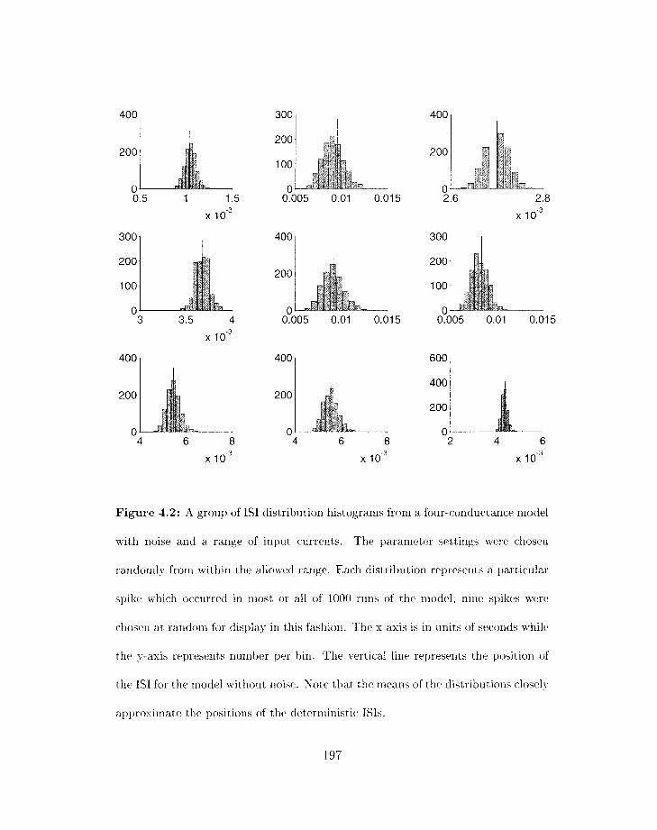
Figure 4.2: A group of IS1 distribution histograms frorn a four-co~iductance model

with noise arid a range of input currents. Tlie para~iieter settings were clioserl

randomly from within the allowed range. Each distril>ution represents a particular

spike which occurred in riiost or all of 1000 runs of the model; nine spikes were

chose11 at raridom for display ~ I I this fashion. The x-axis is iri units of seconds while

the y-axis represents nurriber per bin. The vertical line represents the position of

the IS1 for the niodel without noise. Note that the nieans of the distributions closely

approxirnatc t,he positions of the deter~rliriistic ISIs.

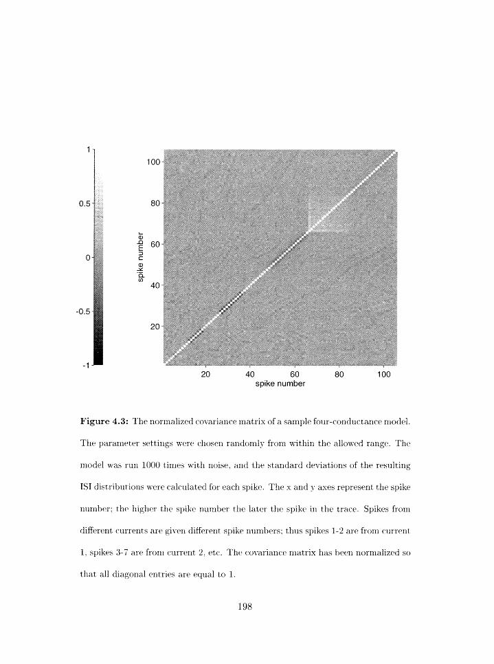
20 40 60 80 100 spike number

Figure 4.3: The norrrialized covariance ~na t r ix of a sample four-co~lductance model.

The parameter settings were chosen randomly from within the allowed rangti. The

modt.1 was run 1001) times with noise, arid the sta~idard deviations of the resulting

IS1 distributions were calculated for each spikc. The s and y axes represent the spike

number: the higher the spikc number the later the spike irl tlie trace. Spikes from

different currents are given different spike nurnbers; thus spikes 1-2 are from current

1, spikes 3-7 arc frorn current 2. ctc. Tht. covariance matrix has heen nornlalized so

that all ciiagorial entries are equal to 1.

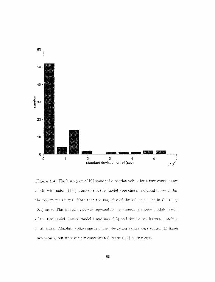
0 1 2 3 4 5 6 standard deviation of IS1 (sec) 1 o - ~

Figure 4.4: Thc. histograrri of IS1 starld;zrd dr1.l-iation -r-allie~s for a fortr-coridnc.ti-tr1c'ci

rtlodcl wit11 noi.;r. The ~~arar-rlctc>rs of this model were chosen raricloxri~ frorn tvirfrlirl

tllty~ararrlc,tcr rar1gc.s. Nett. that tlw ~rrajority of the. ~;tlncls clustcr in thci rang<.

(0.1) rrlsc3c*. This was analysis was repcatcld fix five raxldorlilt- c.lic~scn rrroc-ltlls ixi clac.11

of tiic tsvo niodtl c.lasst.5 (rrzock1 1 arid rxlotlrll 2 ) anti sirrlilar rtlsults wercl obtainc~ci

in all cases. -4'izsoiutt3 syikcl tirricl stzinclard dcs-lation valucis n.clrc horrlcl~\-.T;Ilat largtr

(not tillolv~l) hilt S V ~ ~ ~ C ~nili~ll?; co1i(*c1ltrilto~1 XII tllil (0.2) 111s~~' r;.irlge.

f)cGing 1,erforuzcd. 111 sect ions 4.5.5 arid 4.5.6, we ran t lie c.orrt.sljondi1zi-r; sirzrplc rzoisc mnodt~ls

1000 tirrlos and used tlzc iziciticlric*r of rziissirig/clxtra spik<bs to rlctcrrrzi~ztl :ra arzd y separately

fbr eaclz level of cur r~nt ir!jilc.t,ion. In tJ1c' cSasc of thr. class chompr-triso~l (sr'r't,ior~ 4.5.7). this was

rzot f(lasi111r. so wc cliosrl several rziodels in eaclz class uritli parameters rarzdorrzly distrif>utetl

iri the allowabltl rarigcl. Wc) used t*lzesc to gerieratc fixed estiliiates for .x. ancl jy. wlliclz wr

the11 used for all niodels arid all currerits. The estirnatrs vvcre n. = 0.968 (resp. -1; = 0.921)

for tlie four-coriductarlce (resp. tlzree-corzductarice) class. with 9 = (1 - x ) / 2 jy = (1 - r)

when L = 0) (table 4.6). as described above. We also used a fixed value of T = 400 msec,

twicc tlzc lerzgtlz of tlie currerlt stinzulus.

Wlzilc tlie general questiori of tthc ag)proxirriation of tlic simple noise models by tllc

corres3)onding variable-ratc Poisson rnodels or Gaussiari IS1 nzodels could receive a detailed

Bayesian treatment, it is riot the focus of tlie present sttidy. Frorn now ori, the focus is

or1 lzour well these rrzo tlels fit t lzr~ giver1 tlat a sets. Finally. riot ice t tiat another underlying

assumptiorr wc use in tlic corriparisoris is that tht. level of the current ir;jectiori in e;tr.li tracc;

is kriown. This is 21, starldarci assurnytion in real life sitnations. related to liaw tlie data is

ac*yuirc)d tlntlc3r c~x~)erirrzcrital c.ontrol conclit iolzs.

4.5.4 Parameter estimation: determining optimal parameter values

h r t,lzc\ "within-cblass" auct b?~ctwecrl-class" c*orny>arisoris. we would like to choosc~ reasonai~ly

o1)tirrzaf pararnetcr srts for nzodels irz one or both classc~s. In tliis rasp. w~ lasc ari autoxlzatcbtl

para~iieter sear(-11 ~>rocedurc to find ;L good irratcll i)ctwc~eii the raildidatc niociels and t l l ~

target rirotf~l. Tlic tfct ails of t lrcl sc~areh l)rtjrcdure it self arc irrclevaxlt to the Ba;\i~siarr coin-

pariso~i. but arc bric8y tlescribcd here for c*or~)lctc~ircss. To spettl 111) ~>araiirotc~r scxchrls.

a modifid target data set is t,aken by rrlilriirig tlii: target mortel witlio-tit noise. WP uscx

silmllated annealing. with a. ~~iodifird sinrplex gradirnt-descei1d proctlcfure [35 ] . for tlrc opti-

rnizatiori itself. kVe have previously coinpared a rrurnb'r of parainet,er searching algoritliiris

for neural models [12. 331. arid fourid this one to be highly efficient. Tlre opti~nization al-

gorithm systematically varies the values of the adjustable parameters (four parameters for

class 1, three para~net~ers for class 2) lxiltil a best rriatcli is found. 'I'lic matc.liing fun{-tion

used is related to tlie likelihood of tlie corresporldilig Gaussia~r IS1 11rodrl. M;'"'. L ~ ~ y p t 2 . . .

denote di&rezrt four-corii~,art:rrrent niodels derived bv tliis procedtire on i-liffereiit runs (table

4.6).

For the ~?\.ramidal cell nod el. a similar procedure was followed. det~riiiinistic ttargct

data set was c:lrosrn by calculating the riir:aii spikc tirile for earl1 spikc in tlrc real data. A

paralmrter srarc:li imt hod 1)asrtl on t,lic. griict ic algorit hill iriet llod 112 + 13 was used to assigri

vallies to frec ~~araineters. Although wc could llavtl x1sc.d siintrlatctf ail~realiirg as was tiorre>

with the siriipler models. wc. lravc found that gilneti<- algorithms arc. oftcn nrorc suitat~lc for

~ilodels with 1argt.r iinnik)ers of ~~ttrarilctcrs (ill tliis cascl tlir. ~~yrarnidnl cc.H n1odt.l hatl 24

~>arariic~tcrs).

4.5.5 Comparing individual models from the same class

As t l i ~ rnost basic* test of t lle Bayesian rxretllotl. wc3 chostl twtj indely)cndent rnodcls frorrl

the class of foilr-rosiciuc t aricil rnotlels by rurlrlirig two separat P parasiieter se~arc1lc.s. Si1rc.t.

tlrt-3 parameter seardi algorithm is stochastic. this prodaced two differerlt (*andidate models

~ l : ~ " a d hcrfPt'. both of wlridl snatched the spike tirriillgs of tho data set witliiri a fairly

sniall error. The spike outputs of the det,errninistic. cosrtporient of tlie calldidate muodcls are

shown as raster plots in figure 4.3(a). Each raster represents one spike. The response for

different levels of current irrjcctiori are offset oli the y-axis. uritlr the lowest level displayed as

current 1 arid the highest as current 6. Thr blue (lriiddlcj rastms represcrit tlie target sncjdel.

tlie grreri (~rpper) rasters represent tlir first foor-parameter rilodel and the red (lower) rast,ers

represer.it tlie secorld four-parameter model. The time axis begins a t tlie beginriirig of the

current injection. i. e., at 50 rrlsec after the beginning of tlie sirn~rlatiori. In this case. tlie

two c-orresyondirig sisriple rioisr rnoclels alrnost always ~>roduc.ed the sarnc. nurnt-,rr of spikes

per trace3. so rro ~ j e l i a l t~ for missirig/rxtra spikes llad to be imposel. Specifically, in tllc

Galzssiari IS1 rrzodt~l. t1zt-t ~)aranlett>r .r is always very close to 1 and is c.stinlatt3d by r.rrrirlirig

t hc c*orresl>oridiug sirry>lcl rtoise 1rlodr.l 1000 times. Tlit. j>araruetcr y (+an f )c. est irrlatcltl lrsir~g

(4.19). brrt is riot nctdrd fjecause L = K arlcl orzly (3.26 j is rrsed for thr3 likelihoods.

Tlitl g~ara~ii~tt ' rs of thtl rt'sulti~ig I I Z ~ ) ~ C I S arc. sl~owrl irr tabltt -2.1. along with tlicl origiztal

~~aramef crs of t hc t argct mocit.1. It is irn~>ort a r~ t to riot ice> that l)cc.ausc' of t lrc al~prt~xiri~atiolls

wt. make arid the sc~arch ~jroccd~rre. tllr two rnodcls tlcriveci llavc good likclilloods. but rlo

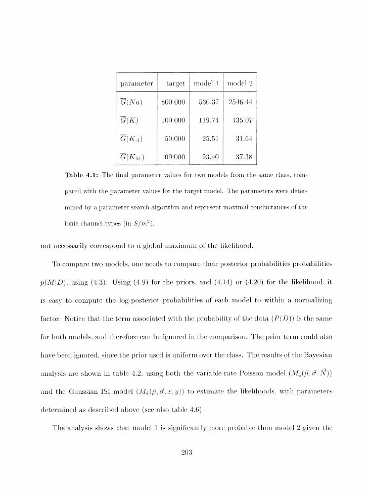
Table 4.1: The filial pararrlrtcir values for two n i ~ d ~ l : , fro111 tllt same class, corn-

pared with the parameter values for tlicl target model. The pararrleters were deter-

rnirrcd by a parameter search algoritli~n ant1 represent maximal conrluetances of the

ionic ellannel types (in S/rn2).

rrot necessarily correspond t,o a global rssaxinlurn of tlsc likelillood.

To coml>art3 two rlrrodels. one ~leecls to cosnparc their posterior prol~abilities ~>ro'r>abilit,ics

p(MID). using (4.3). Using (4.9) for the priors. and (4.14) or (4.20) for t l ~ likc~lilsood. it

is clasy to conlpute ttsc log-~~ost~erior robab abilities of each rrrodel tJo within a normalizix~g

factor. Notice that title terrrr associated with thr3 probability of tlre data ( P ( D ) ) is the samc

for botlr rilodclls. ant1 thercfortl car1 'rjc. igsloretl irr tlic corrrlparison, T h e prior terrrr conld also

have I>c.en ignored. since tire prior rrsetl is uuiforln over ttlc class. Tire rcsults of tllc II3;tvesian

4

analysis are s l l t~~v~ l in tablcl 4.2. r~sing both tlw varialjlc-ratc Poisson xnotlcl jAf4 (@. (5. N ) 1

anti t llr Gatrssian JSI nrodrl (3ldG. Z, 2 . ! I ) ) to <.st ilnato tlic3 iikt.litlc~otis. with pararnc3tflrs

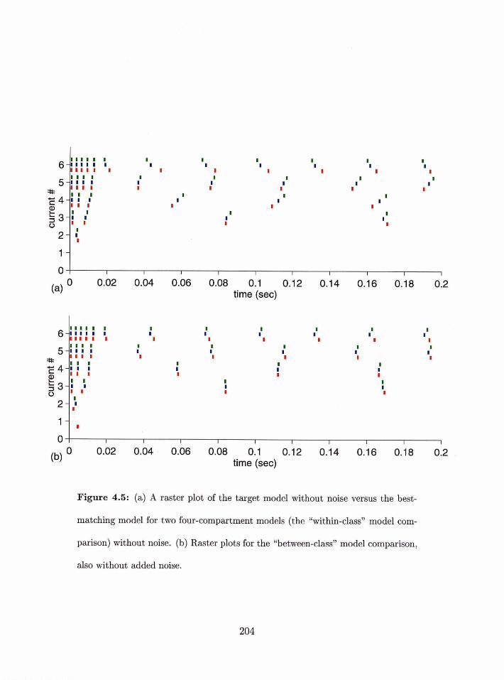
0.04 0.06 0.08 0.1 0.12 0.14 0.16 0.18 0.2 time (sec)

0 I I I I I I I I I I I

(b) O 0.02 0.04 0.06 0.08 0.1 0.12 0.14 0.16 0.18

time (sec)

Figure 4.5: (a) A raster plot of the target model without noise versus the best-

matching model for two four-compartment models (the "within-class" model com-

parison) without noise. (b) Raster plots for the "between-class" model comparison,

also without added noise.

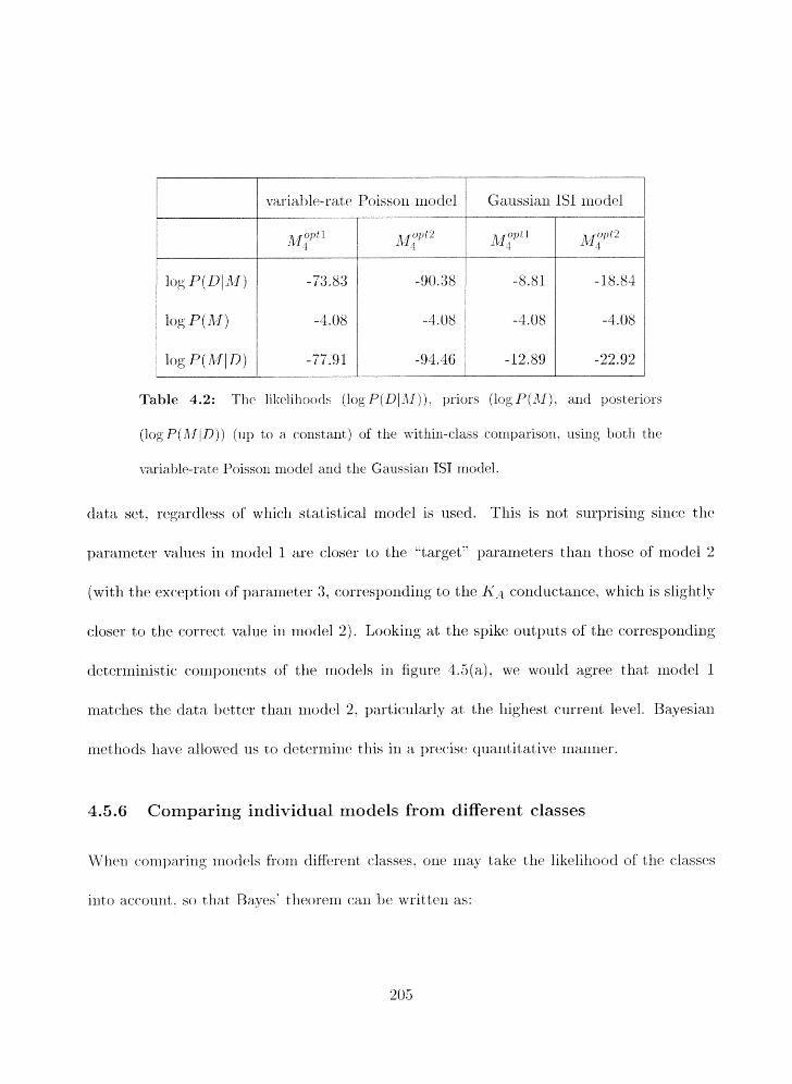
Table 4.2: The likrlil~oocls (log P(D 1 ,I1 j ) . priors (log P(-?I), arltf post priors

(log P( Al j D)) (up to a constant) of the within-class ronl~jarison. using both the

variable-rate Poisson model and the Gaussian IS1 model.

data set, regardless of wliicli stat.istical model is used. Tliis is not surprising since the

parameter valires in model 1 are closer to the k*tJarg~t" parameters than those of model 2

(with the exc.eption of parameter 3. corresponding to the K, conductance. whic:li is slightly

closer to the correct value in nlodel 2). Looking at the spike outputs of the corrcsporlding

tfc.terministic conzpo~ler~ts of the rrlodels in figure 4.5(a). we would agree that model 1

rnatc*lles t 1163 c-iat a better t llan rrlodel 2. particularly at t llcl highest c-nrrent 1t~vc.l. Bayesian

rrlrltlioc-1s l l a ~ ~ allowecl 11s to deterrriirlc this in a precise quantitativt~ rnalincr.

4.5.6 Comparing individual models from different classes

When c-onll)ariug motfels from diEert.rlt classes, one may t akc t lze likelihood of t lie (*lasses

illto accaotult . so t hilt Bayes' t heorern (:an bt> writ)ten as:

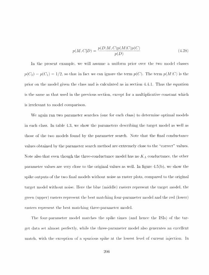
111 tlic prcserit cxariiple. we will ilssu~i~t> a u~iiforlii prior ovcr tlicl tkvo rnotlel c'lasscs

JI(C;~) = p(CI) = 1/2. so tliat iri fact wc car1 igliorc tlie tcrni p(C). Thr tcrr~i f~(Af I C ) is t h .

prior 011 tlic triode1 given ttllc class and is calculated as in section 4.4.1. Tlrus the equation

is tlic, salrle as tliat used in t11c previo~s section, except for at rnultiplicativc coristarit which

is irrelevarit to niodel comparison.

IYCJ again ran two pararnrter searclirs (one for each class) to determine optimal niottels

in each class. 111 t#ablr> 4.3. wr show tlic pararileters t;2cscribing the target rriodcl as well as

tliose of tlis two riiodels found by tlic para~1et~t.r searcli. Note tliat tlie final conductance

values obtained by t11c parameter search met lro tl are ext vculely close to tlic "c;orrc.c.t" vtt111es.

Note also that even though tlic tliretl-collducta~ice ~ilodcl has no KA4 conductance. the ot,ller

parameter valxles arc. very closc to tfie original values as well. In figure 3.5jl1). we show tlic

spike outp~its of the two final models without noise as raster plots. comparetl to tlic original

target ~iiodel without rioise. Hrrcl tlic 11lnc (nliddle) rastcrs represelit tlie targc3t model. tlrc

grreli (ullper) rasters rel~rtbsclnt tiir best iriatJc.hirig fbur-para1i1rtt.r ~liotirl arid t l i ~ retl (1owt:r)

rasters rcl>res~tit the best rilat<*liizig t1ir.c~-paralnf-.tcr niodel.

Thr3 i'ijxlr-l,aramclt~r rllotlcl niat c*lres the spikc t iri1t.s jariit 1icric.ci t li~' ISIs) of t lie tar-

get dat it set allnost l>c;lrfc,c.tly. wlzilc t hc. t lire-patrarrict CT nlodcl also gcxierat cis ;ui c.xc.ellcrit

niatcli. with t f i ~ extbr~~tion of a sl>1lriolls spikc at tile low~st level of currc:nt irijc-\cI;ion. 111

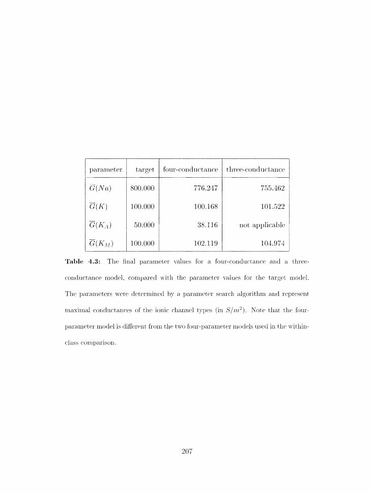
Table 4.3: The final parameter \-ahlcls for a bur-conductanct, and a three-

coridnctaxlce modcll, c~ornpared with the pararilrter \-dues for the target rnodc~l.

Tlle pararrlcters triere dletc~rirlincld by a parameter seardi algorithm arid represent

masirilal cctild1rctar1c.e~ of the ionic. cllanrlcll types (in S/ inq) . Zott. that the four-

~>ararriett~r model is diEerclirit fro111 t h ~ tvio four-paraxnt3tfr"r ~nodels used in tlzc xvitllin-

class c.oln~~arison.

ortlcr to calr.nlati~ likelihctods, we rari tllc sirrlplc noise versi(>n of bcrttli trloclols 10110 tirrzes

aritl est iiilatc-ld tllr rzlearls and starictard dtlviatioris of earl1 spikr t iincl and IS1 . Tlltl tlrlrcrl-

~ ~ a r a ~ i i r t e r ~llodcl wit11 lioisr gcrlcratcd a spurious s p i k ~ in i?;lch of tlle 1000 nins. so wc. can

orily estirrlatr all upper bound 0.001 for tlle parameter ? I in tlle Gaussiini IS1 illode1 (7.e..

no spike will occur ill less t l ~ a n one in a thousand trials). A further step could consist ill

putting a prior on 1) also. and estiliiatirlg its posterior. The results of tlre Bayesia~~ alialysis

are sllown in t*able -2.4.

Note that the log probability for the tllree-roridnct,ant:e inotiel is rmch srrlaller than

that for t,llc four-r.onductance rriodel. both for the variable-rat,c arid Gallssiari IS1 models.

Tlw ~llagliitudr of the: difference is llillcli larger for tllr. Gaussian IS1 lilodel tllari fbr thc.

variable-rate Poisson nlocfel. since, as discllssed below. tile Poissorl rrlodel does not perzalize

rnissing/extra spikes as harsllly as does the Gaussiarl IS1 niodel (Iwrr we have a spikr in the

rxlodcl wllicll is rllissillg fiorn the data). These results are intercstirlg in that our irltuitictn

was sliowrl to be wrong: tllc Ki currrrlt appears to lzlakr a signific;ar~t colltributioli to tlle

spiking pro~~erties of this inotlcl. Note also that even tlioligll tllr prior for t,llc f i rliodrl

gives a slrlallel: ~~callalty tllarl for tllr .2L1 rrlodcl (pelializing a irlorr (.OIIIII~PX rrlo(i(:l). this

has littlc c.&:c.t on tlxl firtal restrlts, since tllr likelillootl terms art. nlucll larger. The r~srrlts

of t l r ~ Bayt:siail a~lalysis arc3 SIIORII ill till)le 4.4. both for tlw variat~le- rat^ PO~SSOII irlod~i

(, 11 ( . 3 . ) a l s s i 1 1 f ( . J. 1 ) ( i = 3 or 1). wit ll j~arilll~~t(lrs

detc3rrnilletl as clfesc*ri!,c~d at~otrt. (see also table 4.6).

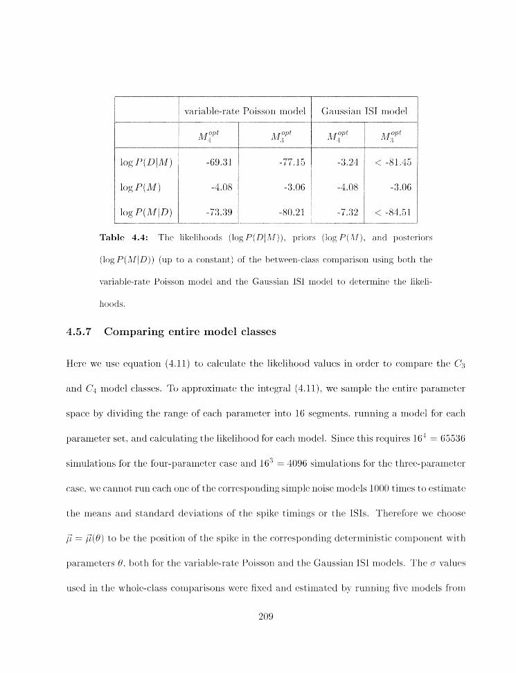
Table 4.4: Tlrlc liktlil-loads (log P ( D 41)). priors (log P(Al), arid posteriors

(log P(,%IID)) (up to a co~lstant) of the betwt3en-class coxnparison using both the

J-ariable-rate Poisson rnoct~l and the Gaussian IS1 rrlodtl to dcterrilirlc the likeli-

hoods.

4.5.7 Comparing entire model classes

Werc wc ase equation (3.11) to calculate the likelilloocl val-ues in order to rornpare the CZ3

arxd C4 nxodel classes. To approxilnate the integral (4.11). we sarllple thrl entirc. pararrletcr

space by dividing tlxe raxrge of each paraureter irlto 16 segments. rzlrrrlirlg a rnodei for eacalx

pararlxetpr set. arrd c:alculating tlltl likelihootl for cac.11 modt.1. Since this rcqliires 16' = 65536

sir~nllatiorls fix the four-11ararll~tt.r case arrd 16'' = 1096 sirrlulatiolxs for tlw tllrrt3-para~rrrter

~ S C . we cariil~t run (la(4l orre of the c.orrclsg)r)rxdiq sirrrplc rxoisc. rnodcls 1000 tilncs to ~~stiirratt-.

tllc rnrans and stalldart1 ric3viations of thc spikc tirrrirlgs or t11e ISTs. Thc.rclfc~rc wc c-ftclosci

j2 --- to 11c the position of t l r ~ spike ixr the c.orrt>sl>onding dtlterrrsirlistic* c.ornponcarrt with

13aranictcrs 8. "rlotlr fix t l r ~ variable-ratc Poissorr airci thc Gaussialr XSI rxlcldcls. Tflc n valllcs

rrscd irs tlrc w ~ ~ ~ I ~ c - c ' ~ ~ L s s t'c)~rr~)itris~r~s wekrtl f ixed arrd cstinsatccl. by rrrrlning fivr. xnoriels frorrl

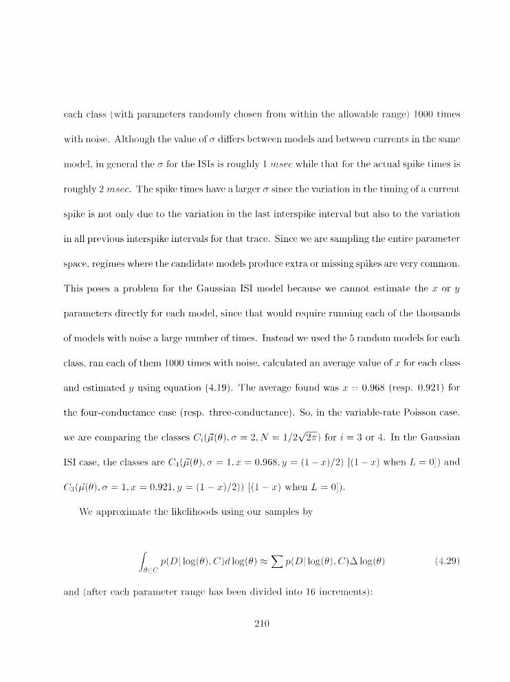
cai-h ralass (wit 11 p;;trarnet ers ra~ldonily c~1~osc.n fro~ii witthiil t lie allowal~lr rarzge) 1001) t irilcs

with noise. Altllougli t 1 i~ value of cr dif i rs 11c3twc:lr.n models and l~cltwccn (atirrt'~lts ill tht' sarrlo

rnoclcl. irr geiloral the n. h r the 1 3 s is rougllly 1 r r ~ . i i r ~ + while that kjr t lrci ac.tual spikr t i1rlc.s is

rougllly 2 msee. Tlit spike tiiires have a larger n since tlrr variation in the tiriiing of a cr~rreilt

spike is not orzly due to tlre variation irk tlie last interspike interval but also to tlie variatiorz

irl all prctvious iriterspik~ intervals for t311at trace. Since we are sarnpling tlie entire parariieter

space. regiriies wliere the calldidate rilodels produce extra or missing spikes are very cornmoli.

This poses a problem for the Gaussian IS1 rilodel because we canrlot estimate tlre x: or y

parameters directly for each model, since that woxrld require rurirliirg each of tlit thousands

of ~ilodels with noise a large number of times. Irlsteacl we used tlre 5 raridonr rnodels for each

class. la11 each of tf~ern 1000 times wit11 noise, calculated an average valuc of x for each class

and estirllatcd y usirig equation (4.19). The) average found was 2. = 0.968 (resp. 0.921) for

the bur-courluctarice case (resp. three-co~lductaiice). So. in the v:;trial,lt.-rate Poisson case,

WP arc. coml)aring the classes C, ( @ ( N ) . n = 2. N = 1 / 2 6 ] fhr i = 3 or 4. Irr the Gatlssiarl

IS1 casr. tile c-1assf.s arc C4(F(H). n = 1.3: = 0.968.3 = (1 - : c ) /Z ) [ ( I - .r) w1it.n L = 01) ailti

C:,(,7(@). rr = 1. .r = 0.921. $1 = (1 - . r ) /2 ) ) [(I - :I-) wherl L = O]).

IVc. approxirizatc the likelilloods trsirzg our sarnples tjy

p(D/ log(N). C)dlog(H) - X, (D~ log(@). C')A log(@)

and (aftcr each ~ ~ a r a n t ~ t e r rarzgc. has bcerl divided irit o 16 incrernerrts j :

210

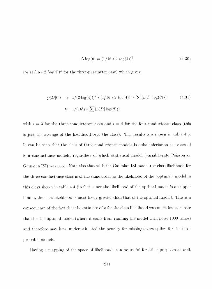
A log(@) = (1116 * 2 Log(4) 1 '

(or ( 1 / 16 ;x 2 ioy (4) 1:' for the tlirec-parametw case) wllic.11 givils:

with i = 3 for the tl~ree-corlciucta11ce class arrd 9 = 4 for the four-conductance class (this

is just the averagc of the likrlillootl over the class). 'I'll(> results are sllowri irl table 1.5.

It call 1:,e seer1 that ttlit. class of thrt.e-c:onduct,aii(;c~ rr~odels is quite inferior to the class of

lo~~r-conc-l~~ct,anc.c. models. regardless of wllich statistical rnodel (variable-rate Poissori or

Gaussian ISI) was used. Note also that with the Gaussian ISI model tllc class likelihood for

tile t hrecx-condtlcta~lce class is of the sarrle order as tllct likelillood of the b*optirrlal" rrlodel in

this class s11o-u.n in tablr 4.4 (in fact. since tlze likelihood of tho optirrlal model is an upper

t>oulld. t l ~ c class likeliltood is rrlost likely greater tlrali that of tlrcl optiural rrrotfel). This is a

ro1rseclucllc.e of the facet that tllct estirrlt-btc of y for the class likelihood was rn~tclr less a(-clir.a,tc

t l i a ~ for the c)~jtiixlal 1node1 ( w l ~ r e it c a i ~ ~ frour rx~nrlillg t l ~ 111o(ieI with 11(1isc> ltl{lO ti~rres)

artct t1le:r.c.for.c. may llaw nlitlerrstinlatett ttlc 1)clnalty for nlissi~gicxtra spikes for the rlrost

llrobablc rxlodtls.

Wavirlg a nrap~)ing of thc spac.~ of likclilloocis can I)? usclful for otllcr linrIjosos as well.

Table 4.5: Tlic likt~lilloods (log P(13)/~21)), priors (log P(,11). arid posteriors

(log P(A1j D ) ) (up to constants) of the I\-hole-class comparison using both the

variable-rate Poissoil rnodel arid the Gaussian IS1 model to d~terniine thc likeli-

lloods.

For instance. oric could determine whether there is orie urliyue rrlaxirriuni in the likelillood

fi~nrtion or sex~rral. and how peaked tlie likelihoods are arouncl eadi local maximum. On(.

car1 also ilsc this data for prediction problcrns. sucli as the probleni of predicting when tlie

first spikc is most likely to occur giver1 the class. Not,e also tliat if ow. has tllcl resources

to do a brute-forct-b rnal)pit.ig of tlie parameter-sy~ace. using an opt,i~nizatioi~ method for a

yararnder st.arc:il is unnecessary. Iri general, this will not t>e possible. 1,tlt hferkov cliairi

Montc Carlo llictliods are being dc.~ielop~d for more cfficierlt sanipling of l-tigli-di~licnsiorlal

distrib~ltiuris [5. 38. 391.

4.5.8 Estimating the optimal amount of noise for a noisy pyramidal cell

model

As a final illtist rat ion of Bayesiari rrictt lzods iri cornpart rnrnt a1 rieliral rriodelirig. wr. presc>rit

1ic.r~ an al~plic;.i.tion of these nietlrods to s ~~rodelilrg ~)rol) l~ln ilivolvirrg real biological data.

As we have noted. at present most co~npartrnental ~rroc-iels are deterministic. i.i... for a give11

input, they will produce spikes at exactly the salnc times. There are several reasons for this

situation:

1. Most experimentalists do not spsternatically try to cluar~tif~ the variability in tlreir

data. I-teing mow cor~c.erned wit11 tlie rrleari responses (although this is cliangirrg; for

ir~st nncr see [30] 1.

2. It is not txivial to incorporate noise sources irito a eon~partrrientd model in a way wl~irli

refierts tlie biological processes of noise-gcneration. Furth~rmore, many possible noise

sources ( e. 9.. chanric.1 rroise) would be cornputatiorially expeimivc> to rnodel exy~licitly.

3. T11t.rt. has 1)tlt.n no systematic* prt>redlirtl for colnyaring tlic uutpllts of a noisy c-orrl-

p2~rtrrrrrltal rriodt.1 to tile corres~)o~idirrg rcal data trac.cxs in ortlcr to firid out lrow rrrnc.1~

iroisc nclclds to ltc added to t11e rnotit.1 iu ortkr to opt irnall?; rnatel~ t11c variattility in

t,hc c-litda.

In this set-tion wc t f r ~ ~ r ~ o ~ i s t r a t ~ how t l ~ e Bayesialz alj~jrot-~c-h car1 solve ~>roblcril 3 . 111

c,rctc!r to clo this wr oijtairltlci rec-ordings $onl a layer 2 superficial pyra~rridaf cell in olfactory

7 i2 C C

ct k"

5 4 i-2 m =1. B ti' 09

E rt

P

$ 0

09 'p 3 0 w %

P 'a 3 0 i",

9 m

E p ti' 09

c'. M s %

a

k" C

U:

'2. z' ":

5 rt u C

2 C

Iri t l i ~ c.veiit tliat iio spikes rv6.r occnrrr(l it1 tllc t)iii. a i)rol,aljility of 0.5/r1rniir/ i was

11sec1. Tliis was tloncl to prr3vent data traces which llacl spikcs in tllcstl bills frorri 1)c.ing

assigriclcl a probal~ility of zero. Siniilarly. bins in wliicli spikcs always orr:urrr.cl wclrtl

assigncti prolja1,ilit ies of 1 - 0 . 5 / r t T-UTLS. to pr~veilt data trares whirl1 did not 1i;rvcl

spikes ill these bins fro111 l~eiiig, assiglied a prohal)ility of zero. Iii practic*~. tlit3 first

case was fairly coinmon but tliti second case iiever occurred witli tlie iioise aiiiplitudes

we used. Zero probabilities are avoided ill this way because they would pritnarily

ail artifact of the srnall sample size (see appendix C for a t811eoretical justification of

this step).

3. Eacli data trace was comparecl to each yrot~ability profile. and tlic) spike times in

thr: data traces were assiglied probability values. Thc. ~iegativc log pro1,ahilitit.s wc3rr

calculated ancl summed for all data tract. (six repeats for sever1 different currents).

-I. This pro(-edure was repeated for all noise levels tested.

As desctilttld abovc. this method gives an estinlatc of tlic negativc log likt.lilloot1 valric~

for eat-11 lcvc~l of noist.. \Yo igiiorc P ( D ) as usual sirxcc it is irrclt.x~a~lt to inodcl c-onlparisori.

In this cast3, we also assuiiic~ that all noistx valtlcs have pq~lal prior ~)rot>al)ilitics. Tllrls our

proc*c~i~~r t is silnpfy a riiaxini~xm-likr.lilioc~d estiinaticizl of the. ol)tinlal rloistl v;~lttcl.

The rt~s~ilt:: of this analysis arci sflourn in figurc14.6. Thc x-axis is the ~('rc-i'lit ri~)isc>. wliicli

is tlir prrc-mtagcl of tllc erlergy in t l ~ r noise relative to that in tlw DC t'urr~rlt irijec-lion.

This was liseil l~ccausc rrlost of the eEe1i.t of a wllite-noisr stisillllzls is filterrii out tlstl

low-pass cliarac-terist irs of t lie cell ~lseriibrane. arid t hcreforc it is nleaslingless to rozilpare

whit<>-rloisc. arrii)littstles directly with DC rrirrent alry>litudes. We yerforrsic~d an AC arlalysis

of otir sirnlllated <;ell (not sllowil) and calculated that the signal attenuation with increasing

freqllency was sucll that ~ h i t ~ - ~ l o i s r stiliilll~rs would he only about 1.4% its effective as ail

c.quivalcnt DC st iniulns of t lse same rnagrli t nde. The percent noise was caalculat ed as follows:

(rzol:se a~n,~jlzt?rdel ~t: (noisc nftenlsation factor) 76 noise = (4.32)

DC ir~jjut cflrrertt arrtplitude

where1 tllc iloisc a.rn~>lit~-rtdc is the standard deviation of tlic amplit~lile distribution of t h ~

~loistl (the lrrean is zero) and the rloisr att8r1rlratioir factor is about 1.4%) as dr:scril,ed al~ovr.

Figure 4.6 clearly slioxvs that tllt3re is arl optirrlal level of noise at aljolit 10% noise. Tliis

is slrown graphically in figure 1.7, nllere wr contrast the prol~ability profiles of our lliorlel

at three different sroise levels with the sarrze DC current level with raster plots of the spike

tiirles fror-rl tlrp real data fix axle DC current l~lvel (wllich tvas thr. sairie as that usec-1 in t l l ~

nod el). The rastcr plots are in the lower porticIzl of tlrcl figur.~ while tllp prol)al~ility ~~rofilcs

arc irr tlrcl tq~pc'r part) of tlli. figtire. Tlrr lowcst ~>ro\)ahilit-\. j,rofilr rel~rclsentu a vcry low 1~vt31

of rroisc. thr irlitltlle profile rtprrserlts a rstedilslil levrl. ariii tllc upper pri>fil~ reprcscats a

v ~ r y high 1evr.l of' ~luisc. All 1,rofilcs xvert. c-c,~rl~>rst r c l ilsirlg t llr variablr-rat t. Poissoll met hod.

Tlrc c.ctr.nt of fhcl prcifilrls in the y dircctir~lr lras lwcn sc-alfbti tlifflrrcritl~ (1:2:4 ratio fur low,

of tllr spike tlata give11 the ~rriddlc profile is sigzlificaritly grt.at,er tllan tlic 1ikt.lilrootl given

[>it.lwr of tlltl c,t;lrel. profiles (it is more tlrari 100 Ictg llnits Inore j,r.ot>at)lc. tharl tlrt. upper

p~~fi lc l arrcl rrlorr t llan 1000 log lmi ts more probal~lo t hall t , b lower ~~rofilc) . Tlrrl reasolis

for tlris are clear. The low-rloise profile re1)resents a rrlodel whiclr puts spikes very pre<:isely

at certain t,inres: the real data has a finite arrrount of scatter arourrcl t llcl rriearl spike times.

arrd t,lrus niany of tlrc spikes in the data. will fall outside tlre distribution of tllc spikes in

tlre m d e l and will thus 1x3 assigned a very low probability value. Tlrc lrigll-noise. profile is

alruost, a flat equiproba1,ilit distriblitio~i across the duration of the current i~rject~ion. This

rrieans that while no data spike will be assigned a very low prot,ability. neither will any of

tlienl be assigned very lliglr Ijrobabilities. Tlle nledium-noise case is the best cornpromise

between these extremes: the widths of the peaks for individual spikes can be seen to increase

in accord with tlre sg>reatl of tlre data. Note also that models with rroise are capable of

~:,rod~~cirlg spikes before or after the DC currerrt was applied. sir1c.c the noise current was

applicd fbr the entire duvatiorl of the simulation.

Tlrr sigrrific*a~lcr of tlris procrdurc is that Bqesiarr rlrc>tlrods llave given us tllcl ability

to cl~oose ari irrlljortarit paranleter. for a rrrotfei wlrich is otherwise very tfiNic.ult to c~l~oosc3

irl a rigorons r~llt~lrrcr. T l r ~ s ~ ~~rc'tllods ca~r illso q~la~ltify ~ I O W gooci the clroiccb is rcklativrl

to ottlcr ~jossihle &oic*es. Tlris is rrot to say that the sirny)le rrlethi~tl wc. l~avc. nsclct lr~rcb is

witllo-rit its li~nitatiorrs. hiiost ot)viousty. tllc variat~le-rat<> Poissoll rrzotlt3l treats all spik~js as

illfft31>c~lltler1t c>rrtities ancl thus rnisscls tlro corrt3latictns i>c t~ -~c .n stlrc.c.ssi\ri3 spikes i r ~ a tIl;rtse.

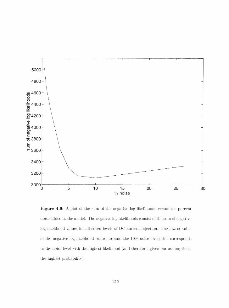
0 5 10 15 20 25 30 % noise

Figure 4.6: -4 plot of the sun1 of tilt> 11egatir.e log likcliiloods vcrslxs tllr pcrc*exlt

xioist. adcltlcf to tllc rnodc-.l. Thc rtclgativc log iikelihooc_ts c'oxliiist of the sum of xlc-llgativc

log likelillootf \-alum for all ser.tJn levels of DC current iruclctiort. Thc3 lo \~-~s t ~ a l u c

of t h r s xir3gatit.c log IikcliIllootl orrurs aronncl tltc 10% iloiscl l~t-el: this r.orrc~sponds

to t ~ L C xloist3 i ( ~ t ) l wit 11 t lit lligllclst lilic~iihood jarltt tlierc>forc?., giwn our assmlnpt ions.

the Ilighest probability)

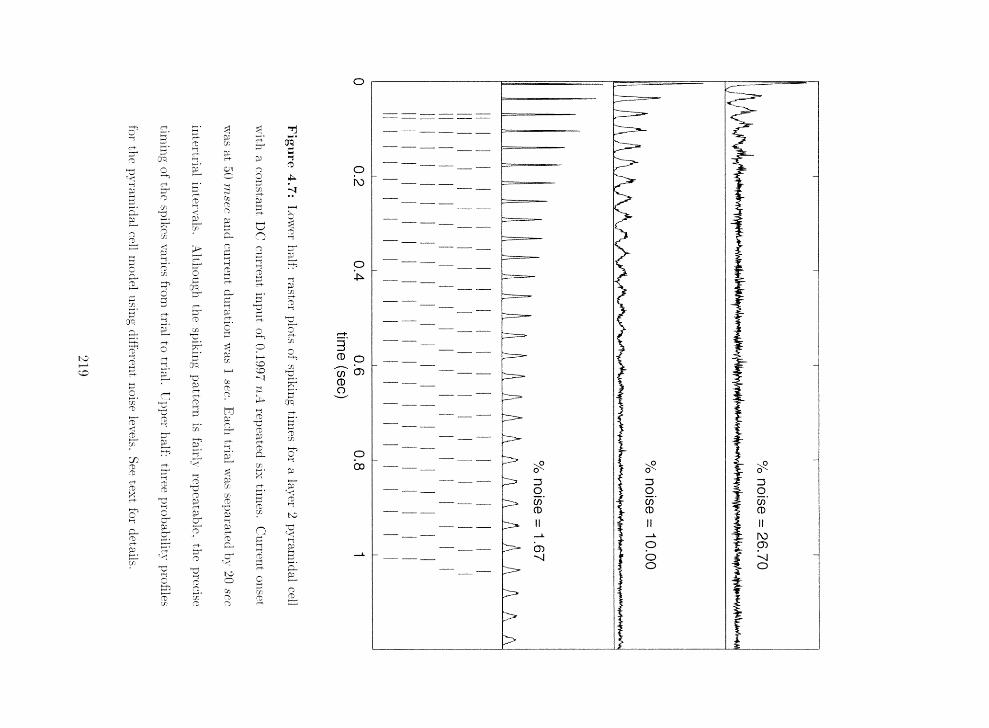
Fnrt Ilrr dt.?~c~lo~)rrlti111 of t hc Baq'esi;tll ~rlctt hodology- in tilt. contcst of c*ornpartnlent a1 xicrlral

rrloclt~ls will 1la.vcl to address this qucstioil. On(*c1 I~ctter l3ayt-lsiail ~riethocls arc availahlt., we

will bca able t o 111itke c3vcrl stror1gc.r st,atttmc~rlts abont whicfl inotlcls are morc ~>rolr)atilc than

otlzers.

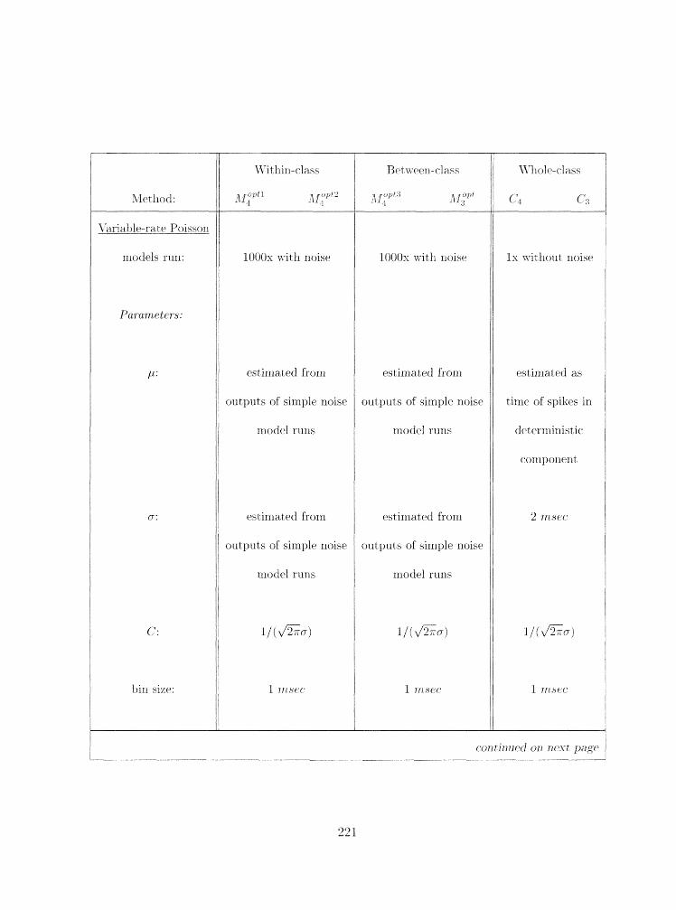
bin size:

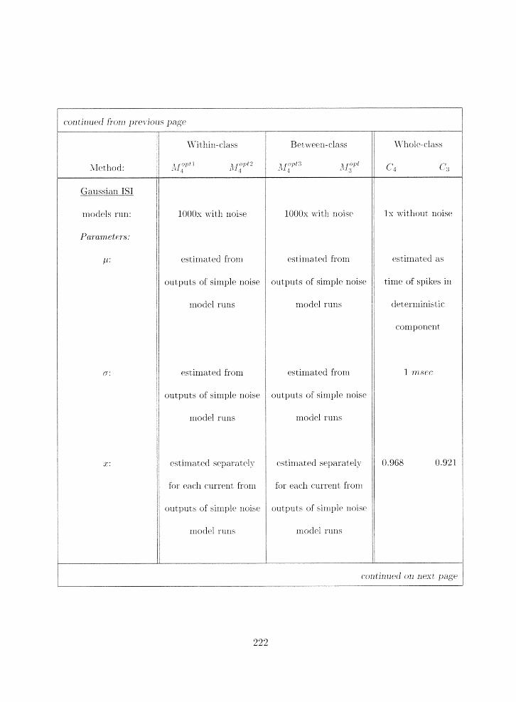
ron t i~l t~r lc l from ~) r~ r - ious page1 1

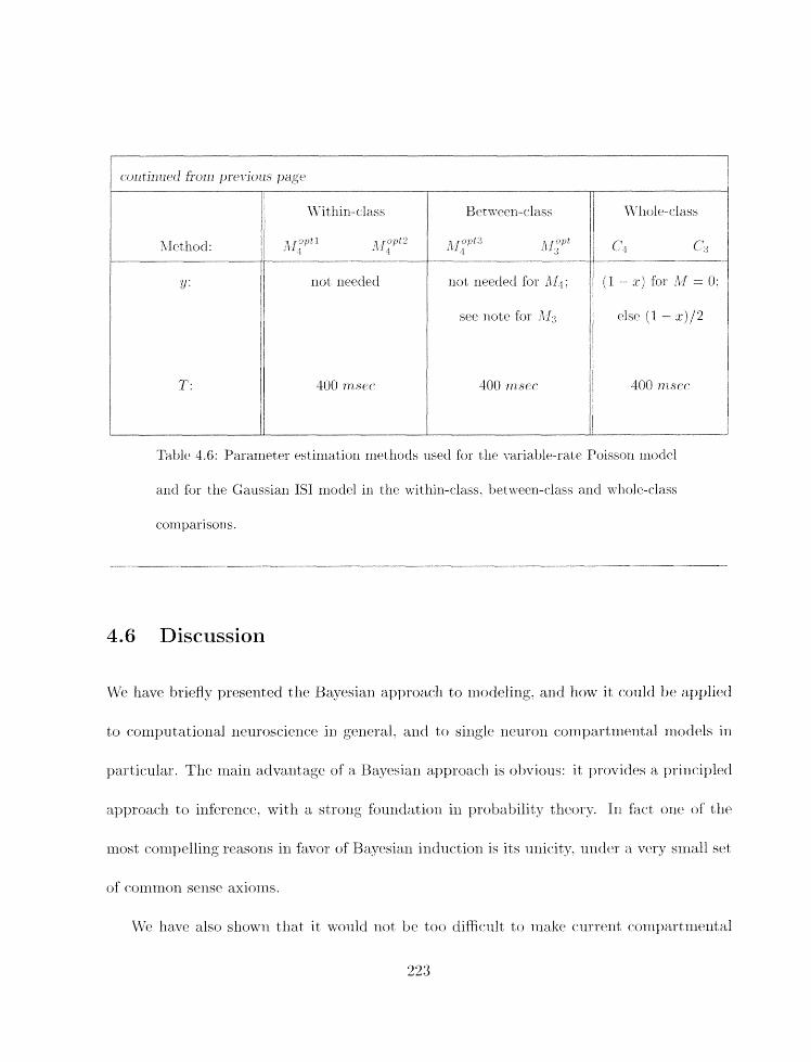
Tablc 4.6: Pararncltcr est inlatio~i rncthods used for t lie variable-rat c Poisson rnodel

and for tllc Gaussian IS1 model in tlic sl-ithin-rlass, t~etween-class and \vhole-rlass

4.6 Discussion

'IVc. have briefly pr~sent~ed the Bayesiarl apl>rcjacll to illodeling. and llow it could br. applied

to c*e)nll>utation;tl ~leuroscicrlc-c- iil general. arld to silrglti rleurorr c.orrsy>autm~ntal rrlocicls in

~>:krtic.ular. The rmin advaxltagt. of a Baycsian al~proach is ol>vious: it prc>victc.s a ~)rillcil>lta(l

a~)proac.lr to infe>renc.c. with a strorlg fourlciatiorr in prohbility t l1eor.y. In facat orlc . of thc

rllost tsonl~>ellirig reasons in ftLvcjr of Bayesiars inrludiorr is i t s iuiic-ity. unde'r ;t wry sn~;tli stxt

of c'C)IXlTl1C)II SPlSt' axlo~ifs.

JVtl llavr also sllowu that it would 11ot bc too cliflrit-ult to nrakcl c-rirrcnt r.o~nl>art~zletlti'~l

223

nrodPls rliore Bilyclsian. at least at tlrc rrzost t>asic. lcvcl. Tllc riraimi adtralrtagcl of Bayclsian

" lsS1lE'S, rrlct llods for c.ornpart rnent aI rnotf elirig is t lie clarificatiorr of a n~rrrif-tcr of rriodcliri, '

at tlir'c. different ltvcls at least. First, a Bayesiari al~~~roac-fi fort.cls orir to c1;xriEy tlitl prior

k~lowletlgc. going int,o the niodel, the data. and the li~potlleses. Second. the Bavesiari a$)-

proach clarifies how to proceed wit 11 irzfercnce. i . e., how to cornparc rnodels wit11 each other

arid with the data objcct8ively. providing unambiguous unique arlswers to well-posed yucs-

tions. In this way it establislles a forrrial basis for rriodel corrlparisons. Finally. Bayesiari

rnetlrods require us to corlsider quantitatively issues of noise arid variability in the data,

used to constr~ict and test, a rnodel. Tliis is a crit,ical (and underrorrsideredj issue in com-

putat ional neuroscience. IVithout this step, it is inlpossible to lrave a rigorous scierit ifir

disc.oursc on models. to deterrniuc lrow well they fit the data, arid ultimately to corripare

rnodels and llypot heses. In this paper, we havc. denionstrated several ways t,o cor1struc.t a

prok~abilistic corn~~artmerrtal rrzodcl out of its deterrrlirristic cornponerits.

The Bayesian framework is eritirelg open to. and actually encaourages. questioriirig of

arzy piece of inforrnatiori. It deals with tJze sul>jectivity iriliererit in tlic. rno(t(3ling Itrocaess

riot 1>y ig110""iig it f~llt ratller fly irlcorporating it up front ixr tlrc nioclelirlg I>roc*iAss. it

is fnndarrrc~utally arl iterative l>rocc3ss in whicli rrlodels arc, ~~rogucssiv~lj- refined. arrd thus

rc1A~c-t s and suppc~rts t lie rlat 11re of re.alistic- ~irluronal rnodelirlg [8] . As Baypsiari met hods

are applied to c.ornptitationa1 rir-lnrosc.icnt*r. it is also likely that ricw cornl>tltatiorial ideas

will c.rrlc.rge as has l~t~crl t l z ~ cast. irr ot1rc.r fi~lc1s ([%!). 28. 331. and rcfi.rc111c.t.s tlicrrilr). For

i1tstarzc.e. thtc variattle-rat$ Poisson niotfrl was in part suggested by thrl Bayrsiail al>I,xoacl1.

and thc. c-lificultic~s ellcountered witli the Galissiarl IS1 rrlodel. Tllrl Bayesiarz approat"l1

call lcact to ;I. b e t t t ~ urldeustantlirig of thc wcakness~s of a ruotlcl. and tlzereby llc~lj) to

gcncratc hc%t er rzlotlcls. ID atldit ion. having an ol>jt.ct ivc way of cornparing rnodels. and

rrlaking predictions based 0x1 rrzodels. will t)econirt ~rrort. i~izytort~arit as the n-urzilter. scope

arltf cor~lplexit~y of t*omyartnierltal rrlodels representirig t llc sarnrJ braill st ruct ures increases.

It is our belief that corrlpartnlerltal nlodels are still at a very early stage of tlt~velopnlexit:

for instance. there are rrot rriany Purkinje cell conipartrnental rnodels in tllr world. Thus

issues of nlotlcl comparison and predictiorl are still sorrieurlzat hidderl in the background,

but u7ill progressively becorrle rnore central as x~t.uuobiologica1 databases grow ill size arid

ro~nplexi ty.

Irz the present case. the two main statistical niociels for the spike tiriiirlgs wc used have

c.ornplernent,ary advantages and disadvalltages. Tlle variable-rate Poisson rnodel handles

extra or missing spikes rriorc grac.efilllv than tlze Galissian IS1 rrrodel, sinctl it indepeudmt ly

c-ornputes tlrcl probal~ility of getting a spikc ill every time iut8crval. TLlc Gaussian IS1 lras a

vr3r.y atl-llc)c. arztl irzelegarlt ~~roc*edrir~ for dealing with iriissi~lg or extra spikes wllich recjuires

tlte est imat iori of (at least ) two new ~~ararlleters. If olvevcr. tflc Poisson ~norfel uuc2crpt.1lalizf.s

rriissirsg spikes (it iean t ~ t a sliowrl that tht. ~)enalt\- for a ~zlissirlg spikc' is ro~igllly I log unit. ill

c-orltrast t c i m~lc*li highclr values for tlzc Gussian 1SI mot-icl on average). Thus nc.itl1t.r anot3r.l

is an ideal xnodcl of thc syikc-grncratirig process in this 1)artitular data set. and tlltlrehrc

rriorc srrcll rnodels need to t>c. dcr;elol>crl in tlie f ~ ~ t l i r ~ , .IF(' v i~r iat~l~-rat~[" Poissoli l x i ~ d ~ l .

liowc3vcr. is cxtrerriely sirnplc ancl ilexil~le and can provide at lcast a first approximation in

a wide range rjf situatiolrs. Tliis was ill~istrated in thc last scctiou, wliercl tlic variable-ratr

I'oissou rrrodc.1 was used to derivc an estirnatc. of the rioise inprrt needed for a corxipartlriental

xllodcl to optimally rrratcli a biological clata set.

The rrrain drawback of t lle Bayesian approach is that it can bc corriput at iorually iriteusive.

especially wlleli averages rieed to be cornputec-l over liigh-dirrlerisional distributions. For tlic

largest compartmental models, it is unlikely that one will t ~ c . able to carry out a complete

Bayesian analysis on currently available computers. But co~it~inuing progrcss iu Molite Carlo

15. 391 arld otlier approxirriat ion tedi~liques, as we11 as steady in(:reases in raw computing

power in workstat ions and parallel cornputers. is likely to rrrake t hesc met liods feasible for

cornpartrrrental neural rnocrlels at a reasoriable level of rornylexity irz tlie near future. 11s ad-

dition. it shorxld be clear that a sirnple rrietliod sucli as the varial->le-rate Poisson rnetliod earl

already l)c usecll irxxrnediatcly, in ~orljunct~ion with tlic nrost corripltx existing corripartniclntal

riiodels, to est irnate likelifioods of large data sets and cornparc rnodels pairwise.

Givt)-ri tlie corripl~tatiorlitl dernauds of tlic Bityesiau approac.li. howt~ver. sonic rnodelcrs

rrtiglit worider what t liesc~ met lrocls providcl t liat carrnot be obt ainc~tl nrerely t )p coni1,aring

dcternlinistic models according t o sorlxe error criterioli. First of all. uric of our goals llerc

has I>cezi to gclnt>rate gerseric prot.~abilistk r~lorlels of spiking i>rocsesses tvliic.11 call be ovcrlaid

on conul,artnitf.rit,al nsc~cl~ls. in contrast to error ft~nnictions in pararrteter srwx*lies. tvliicll art3

typically (*olist ruct rltl to st roiigly srllect for part iclilar ftlaturrs of t llc. data. S13c.olitll-y. rrror

'lveli f1.tllc.t ions are not prol)abilit ies. Slri~wing that a particular nrodel mat cl1c.s a dat a set g'

a particlllar error criterioil better than a ~ l o t l i ~ r model says iiothirlg aljont liow 11111~11 1iiorc3

proljahle one niodrl is relative. to tllr other. For this a prohal~ilistic iliodel is clearly rsseiitial.

It is not diffcult to ir-riagiiicl an error function which overwlielnringly favors oitt3 nlotfcl over

another (for iilstaricrt, if tlie error filllc.t,ioii gives an enormous weight to the first spike in the

data arid virtually ig1iorr:s the rest) evni tllough tllc two inodels are ahrlost equally probable

given a reasoilable probabilistic spike-geiierat ion niodel. Tlills. est ablislling a probabilistic

iriodcl and. especially. sliowi~ig i)llat it is reasonable given the degree of variability in the

data (sect ion -1.5.8) are essent is1 for proper niodel comparison.

As tlie scopc3 and complexity of corllpartnierltal irlodeliiig in neuroscience continues to

increase . it will 1)c~corrie iricreasiilgly im~,ortant to have an oljjective way of corrlparirig nlod-

els. arld rrlakixig i~r~dic*t,ioils based or1 those rriodels. Because corn~)utatiorial nruroscicrice

a i d compartmerltd ixlodcling arc still at an early stage of develop~nent. issties of rigorous

1nodt.l corii~jarison airrd pedictioii have not yet h e n considereti seriously by rnost investi-

gat ors. However . as rlclrrcjl,iological databases grow ill size and (*olril,lcxity. our st alltiarcis

for rliodrl coliiparisorl will also llavc to 1x1 r a i sd iri ordrr for. Ilrograss to 1,o ~liacfc [8]. WP

brllicve tliat B~tts iar l raethods will provide1 a solid fouu[iatioti for tlic.sc rffr~rts.

Appendix A: The Cox-Jaynes axioms

Tlle ol~jects wr deal with irr ilifc>rerlct. are propositions about t)llc wt)rltl. For iristancr. 2%

typiral propositio~l X is .*nc>urorl A is firilig all ac.tiolr potcatial at tirrir. t" . A ijr<jpositio~l is

ritlirr true or false. arrd we tlenots by X tllr romplernent of a propositiorr X. A llypotlresis H

about tlrr world is a proposition. albeit a possibly coniplex orie c-olnposed of the cor?juriction

of' niariy rllorc. elementary propositions. A model &I call also be virwrd as an llypotlrrsis.

The difference is that models tend to be very complex hypotheses irlvolvilig a large nurnber

of pararrietrrs. In discussions wllerr paranleters arc3 important. wc will consider that &I =

M(H) wlrrrr H is tlie vector of all pararn~tprs. A conlplex nod el 111 car1 easily be reduced to

a binary propositiorl in the form: .'~riodel M accounts for data D with all error level fa' (this

is a vague staterrlerlt that will be nlade inore precise ill the followirig discussiori). But for

ariy pur130s~':, in what follows there is no real disti~ictio~l betweell rilodels and hyl~otheses.

Whereas propositions are ritlier true or false. we wish to reason irr tlie presence of u~r-

(a~rt~airrty. Therefore t,lre next s t ~ p is to consider that. given a certailr arrio~lnt of' inf'ormatio~l

I. ~~r rar, associate with ea(=li 1iy1,otlrrsis a tlegrec of plausibility or ~*cirlfidrricr~ (also called

irr tllr litpratnre degrcvl or strerlgtll of' Ijclicf). Lt.t xis rrprcserlt it 1 1 ~ - the syxrlbol n(X 11).

Wlrilr ~ ( ~ Y l l ) is just a syriil)ol for now. it is rlrar- that in ordcr to have a sc:it.~lbific cliscoursc

o ~ r ~ slrolild br able to con1par.c. ciegrres of <*olifid~rrcc>. That is. for any two propositic~ns S

and I tT, either wc Ijelieve in ,Y marc thau in 1'. or we I ~ C ~ ~ C V P in lr ~~i(_irtl t l lm in X. or wc

ljtilicvcl in ijotll equally. L t t us nsr tllr synrbol **>" to tlrnot>r tlris rclatioiislli~j. sc3 that we

228

write .rr(X 11) > n(17 I ) if aiid 0111; if S is rriorr plarlsiblc tllnrl IF . It would tje v c ~ y hard rlot

to agree that in order for things to 1)c serisif)lr;. tllr-1 relatioiisfli~> '">" striould t>tl traiisitivc.

Tliat is if ,ru' is rriorr plausi1)lc tliaiz 1'. ant$ Y is rziore ~tl;t~~sit>lc tllaii Z . tlie~i X rlrust also

he rrlore plar~sihlo tlian Z. More forrrlally this is tlie first axionl:

This axionr is trivial; it has. however. ail inlportant coliseqnenet.: ">" is au ordering rela-

tionship. arld tllereforc degrees of belief call be expressed by real nuiribers. That is, from

now oil x(X1I) represents a nuniber. This does not, lneaii that such a ntlnlljer is easv

to calculate, but rlrerely tliat s~lcli a riuiiiber exists, a i d t lie orderirig anlorig hypot lleses

is reflected in tire orderirig of real nurnbers. To proceed any further arid stand a cliairce

of c~al~ulat~iiig degrees of beliefs we rit3ed additional axioms or rules for relating numl>ers

represeiltiilg strengths of belief. 'Vhc alllazing fact is that only two aclditioiral axioms are

ileecfed to c.onstrairl the theory ent,irely. This axiorrlatic. resentat at ion is usually attributed

to Cox and .Tityii~s /13. 221. To better iindc>rstarld tliese r\ro rcrrlaiiliilg axiorris. tlie readcr.

rrlay iinaginc a world of very siinplc rzc3uroils. where at cacli ilrstallt ixi tiriic a givcii rlcBuron

cean either t)c or1 or off. Thrrs. all t l ~ elcrrrcrrtary llypotlles~>s or prol>ositioris ill this world,

at a giver1 tirrlc.. 1~a .v~ tilt' silrl~~lc ftlrrn: *"lienroil -4 is on" or **ilt>urorl A is off". Clclarly.

tfitl 111011e ('oilfideiit \r;c3 are that Ileriroii A is 011, tlit less confidezlt wt. arc that nruron ,rl is

off. So. &)r airy given propositioli S, tIlc.re slii~ulcf br a rciIationsllil> t~ctween .ir(S 11) aucf

~ ( 2 1 ) . Witliollt iissu~iii~lg arij-thing about tliis relationshil~. it is serlsiljit~ to c-onsider illst.

everything r l s ~ k i n g 'qrisl. thc relationsllip sliould be3 tllc sarnc for ail ~lcuroris and for all

types of I-jackgrourld infbrrnation. i. e.. for all ~)rupositions X anti I. Tlms. in rn2trhernaticaal

terrns, the second axionl stat8es that tllert. exists a. functiorl F st~cll that

The third axiom is only slightly more complex. Consider this time two Ilelxrons R a i d

B and the correspo~lding 4 possible joint states. Then our degrec of belief that A is or!

and B is off. for instance, naturally depends on our degrec of belief that rlellrorl A is 0x1.

and our degree of belief that neurori B is off. krlowirlg that A is on. Again. it is sensible

t,h;tt this relatio~lship lw independent of the ~rcurovls considered and the type of background

inforrriatio~l I . Thus, in rnathelllat,ical tlerrns. tile third axioxrl states that there exists a

frrrlctiorz G sut:h that

~ ( x . Y I ) = C[7i(XlI) . ?r(lF/X. I ) ]

So far, WP li;tv(\ 11ot said 1~111~21 about t l i ~ ~ infcjrrnation I. I is a f>roy,ositiorl r-t>rrclsl>ontii~ig

to tllc c.oqjurri.tion of all t l ~ available piclers of irsforrrlatiorl. I can rc\~>rc.scnt I~ackgrotxrrtf

kncrwledgc. sue-ll as gtwcral ax~atomical or physiologic*al inhrrnatiori irr r1r.11roscicnc.c.. I van

also inclrxrlc sl~cc-ific. t-lx~~crimental or other data. When it is nee-cssary rci Et>c.us or1 a 1)artic.ula.r

corlms of data D. wc can writc I = ( I . D ) . 111 any c.a.sc. I is not necessarily fixt~l ancl can

230

1 1 ~ aug~rlcnt~tl witli. or rcplac.c.d by, any nuiirl~cr of syrrrl>ols re~)resc.rtti~lg propositiorts. as

alrradj- spell in the, riglrt lrarld side of eyuat ion (4.35). Wlirn data is acqi1irc.d seq~ieizt i d ly

for irlstaiicc.. we uiay writ,() I = ( I . Dl . . .. . D,, ,I. Insidc a disc-iissioi~ xvllere I is well tlefi1rc.d

arid fixed. it (earl be dropped alt,ngetller fro111 tlie equations.

The tlircc axioirls above deternli~r' entirely. up to scaling. llow to calt.ulatr degrees of

belief. In ~)art~iciilar. orre call prove that there is always a rescaling ilrl of degrees of beliefs

sllcll that p ( X I) = ~w(n(X1) ) is ill [O. 11. Furthermore. p is uriique arrd satisfies all tlre

rules of probability. Specifically, if degrees of belief are restricted to the [O. 11 interval, then

the fi~rictiori F arid G must 1)e giver1 by: F ( J ) = 1 - ~r: and G(z. = n:y The corres~>oridirrg

proof will not br given lrere and car1 be found. for illstance, ill [13. 231. As a result. tlrtl

second axiom can be rewrittcln as tlie Surri Rule of probability:

p(X1I) - k J 1 ( x - p ) = 1

,Anrl the third axiom as tlie Product Rule:

Frorrl hcre on, wc. can replacc degrees of ~.orifidic.nec hy ~~robaijilitie?i. Noticc that if uncer-

tainties arc. removeci, that is if J I ( ~ jlj is 0 or 1. then ~ q i ~ a t i o n (-1.36) arrtl cquatioil (-1.37)

yield. as a special r-asp. tltr two Imsic. rultrs of c-tedtrction or Boolea~l algch-a. for tllc. ~legatiorz

anti c.oi!j~i~tc.tio~l of propositiorls [(I) .+S or .'i "is illways true: (2) *.S a11d I-" is trtw i f and

231

orlly if bot li X arld Y arc t nrr.].

Till- irrlrrrrdiate coiisr3q~lc1ricc of crluatiorr (3.36) arid rclllatiorl (1.37) is t l i ~ so-callrci 13ayc.s'

t lir~or~rn:

Baycs' theorc'ni is fu~idamental t>ecause it allows inversiori: interchanging collditioiliiig and

lion-conditioni propositions. In a sense, it embodies learning sirrce it describes exactly

liow to updatr our degree of belief p ( X I I ) in X , in light of thr new piece of irlforrnation

1>rovided by Y to obttaiii the) new p ( X / Y . I ) . p ( X 11) is also called the prior prol~ability (or

vbprior" for sliort ) alid p ( X 11'. I) the posterior probability with respect to I- (or "posterior"

fix sliort). This rule can also be iterated as rriorc iilforlliation becornes available.

Appendix B: Error bars

For illustration purposes. corisidcr a rriodeling sitllatiorr wit ll orie parnmr3ter 0. anti a uni-

fbrirl prior. Lct f ( 0 ) = - logp(DIH) I>r thr negntivrl lclg-likrlillooti of th. data. Cudor

~iiild diN'c~rr.ritial~ili ty cctncf itiorls. a rll;%xirnlulr likcjlilrootl estimator Nil satisfies f ' @d = I).

Thcrcforci iri tlrr ueiglll~orliood of B. WP c*ari cxy~and $jQ) ill a Taylor's series:

where C = (,i("). So tllc likelihood. as well as tllr post,erior p(HD). locally ixllavr like a

Gaussian. with a sta~idard deviation 1/ d m . associat,ed wit,ll the curvature of f .

Appendix C: Dirichlet distributions

Let X = X ( t ) be the probability of firing in a givt:n tinle bin t in a variablr-ratr inodel.

uatnral prior on X is the Diriclllet distriblitio~i with paranieters

also called a Beta distribution in the two-dimensional case. Tlze pararrleters n"tu and y ==

( q l . qr) of tlre distribution ~rlust sat is@ 6%. qz > 0 and q, = 1. Tlre pararrleter a detprnlixlrs

llow peaked tllr d i s t r ib~~t io~i is an,urld its rnrarl associated with E( A ) = ql . Assuule now that

tlle data D for the same time bin corlsists of a total of TC obsc~rvatioris, f of wllirh ('orres1101rd

to a firing t:vt1rlt. Tllc. likelillootl assoc-iat t:d nit11 this o l~s~ rva t io~ i is p(D A) = ~ j ( 1 - A ) ( 3. - f 1.

-2 nlaxirlnl~rl likeliiinod rsbinlatioli of X yic~lds (~iot smprisitigly) X = f / ~ r . with tlie pruljitnrl

Illat- this rslirtlrtte is O if j' = 0. A simr>lc cafculation shows that the 3lAP rstirriatc for X

wit11 thc Biricfilet prior is givt.11 instead by

Tllc rff~ct of tllc prior anlolints to atldixlg pseudo-t~otint s to tire oi~servecl data. ?Vith a

symrrietric Dirichlct prior (for instanrt.. gl = a = 0.5). as long as we clioos~ n > 2. tbt.

MAP estixnate ran never 11' zero. Tlit: ~~ost~erior distril)utiorr p(XID) is also a. Diriclllet

tlistrit)ution. For this reason. the Diriclilet distrii->ution is said to t>e corijugatt3 for t,lrc

corresponding binomial/xmlltiriorr~ial rrrodel. Tllrl Bayesiaxr analysis of tlle pyrarrlidal cell

model llsirrg t lrc. variable-rate Poisson niodel in sect ion 4.5.8 is cssemt ially equivalent to risirrg

a Dirichl~t prior with = yl = 0.5 and n: ==: 3.001 for n --- 1000.

Appendix D: Model equations for the one-compartment model

Tlle I~asic eyuat ion for t lie compartrritlntal models is the currerlt-balance erluat ion:

wltcrc C is the xnt~rril~rartc c~a~~aritanrc. V;,, is tlic rrre~robraric~ potential. R,,, is thc nlclinbranrl

rcsistanc.c. E,, is tile .'leak cwrrcut" rc.versal ~mt-ciltial (a poorly dc.finetI ant1 yet nearly

~lnivflrsal coiirr3lrtit11l alilorlg c.olnpartlxlelxta1 rilotlelc.rs [lo. 251). I,,,,,,, is the mrrl of (*tirrr~lts

tllrotlgll voltagc-dcl,clrtdcr1.t iorlic c.ollduc.tances. and litLm is the input c.urrt3~rt. I,,,,,, (-an 1x1

furt l i ~ r snl.>dividct_f as follows:

whcrc Gs is the conduc;tanecl value for channel X. EXu is tllr rcv~rsal pcttcntial for Nu.

and Er< is tlle reversal potential for K . These conductanct: values art. titne- and voltage-

dependent according to the following equations:

~ h c ~jaranlrtrrs Gr*. ~ 1 l ~ 1 . e C rt.r~rt:so~lts an iolli(- cllatl~lrrl species. arc. tllr variablr ~,avanlott~rs

of tilt. nodc cis. The gat>illg variables n r . f.1. 7). .r. y. and 2 all can ltc. tfescritjctf by the‘ Wotfgkin-

I I n x l r ~ fi)r~n;rlis~ri j10. 191 as:

for a given gatirlg variable X. wllere T\-, X,. ox, and Ds arc all functions of membrane

potential 'C j,, . ax is tllc forward rate (*onstant arid /jy is tllr reverse rate <:onstant for the

clla~llicl opeliiilg reac-tion [19]. These fnnct ions are listed below. 111 some cases tr and /i

(.onstants were used to cornpllte X, and I- values. whilcl in other cases the) latter values

wen. calculated directly. Nottr that C;,, is iil volts. Tlle cliannel inodcls are adapted froin

tllosc in [41] except for the KAi cllanrlel wllicll is adapted from [25]. To get tlic cells to

spike ill a rllitlzrzer similar to that of regular-spiking cortical pyramidal cells t hc kiriet ir:s of

t hr. pot assiurrz chanrrels wf5re altered relat ive to t llosc in t flc refererlc.es.

delaved-rectifier K cliaririel:

ITzj channel:

Appendix E: Fixed parameters of the one-compartment model

c ~ l l area = i n * (10 prn)' = 1.2566 * rn 2 (4.64)

Appendix F: The pyramidal cell model

Tllr ~>prainitfal cell ir~odcl was hased oil arr airatoiriical r~const~rnctiorl ctE a layer 2 sul~crficial

pj~rarnjtfxl cell iu olfactcjry (piriforrn) cortrx: this reroristrut-t ioii llad 2670 col~ipartmerits.

We siinplified tlrr iiior~>hology of this model dourn to a 15-conipartiricnt irlodcl ~lsirlg es-

sentially tlir nrethod of Bush a d Stljrrowski [Il l . Our iriodel also included several activr

ionic* cond11ctanc.e~ located in the soina. No active conductaiiccs were placed in tlle den-

drites. because there is little evideiice for suclr cllarlnels in this cell type at this time. Tlre

cond~ictances iricluded fast inactivatiilg Na. fast persisttlr.it Na. delayed-rectifier K. slow

iloir-inact ivat ing K ( .*M-ctrrrent" ) fast aiid slow calciuln-act ivated K . and higli voltage-

activated Ca. Thr inodel also contairied a simple model of calcium i>u&ring. Space does

not permit a full descriptioil of the nlodcl here. hut details on the irlodel aiid fill1 paraiii~ter

sets can bt-, ol>tained by rontacting the authors.

Acknowledgements

WTch gratefully acknowlcdgc~ tlic assistaiicc~ of Alexander Protol~apas. wllo c.olitribut~<l the‘

exl~erirnental data on which section 4.5.8 is based. Alex also generated the parametas for

tlltl anatomical reconstructioir of thr layer 2 l~~~rarriidal cell which was a startillg poilit fur

t lle pyranlidal cell ~riodel described in t liat sect ion.

The work of Pierre Baldi was supported in part by a grant from the Office of Naval Researt:h.

Bibliography

[I] P. F. Baldi. Probabilistic Models of Neuronal Spike Trains. 111 Marco Gori. editor.

Lectlrrc Notes i n Artificial Intelligence: Adupt i~tc Processing of T e v ~ p n m l In;formation.

Springer V~rlag. New Uork, 1997. Iri press.

[2] I'. F. Baldi and S. Brlirlak. Bioiqformatics: the ni9uchine Learrcing A p p a c h . M I T

Press, Carrzbridg-e. MA, 1998.

[3] V. Barnett. Conrparatir~e Statistical Ir~fel-encc. Jol111 Wiley. New York. 1982.

[1] J . 0. Bergrr. Statistical Decisorr Tl~ror-p and Bnyrsi an Ar,ulljsis. S~jringcr Vi:rlag. New

l'i>rk. 1985.

[5j .J. B~sag . P. Grcc3n. D. Higdoll. and K. %Icrrgcrse~i. Bqesiall Conl~jutatioll and Stocllas-

tic Systems. Statistical Seiencr. 10(1):3 66. 1995.

[7] .I. h1. Bower. Rrvwse E~lginecrilig tlrc Nervous Systclrr: ari l i i I 1 l i tro. arrrl Iri

Conbyt~to Al>pro;tcli to Understarrtlixig t lie Manirnalian Olfac*tory System. 1x1 S. Zc~rrict-

zer. .J. Davis, and C. Lau. editors. An Introcluctio?~ to iVet~snL I L ? ~ C I EI~ctr~rt ' l :~ ' ~Vef?~ork'.~i.

2nd. Ed. A-lcadernic* Press, Sari Diego. 1995.

[8] J. &I. Bower. What Will Savc Neuroscierlce'? Neu?~oi~rrugr. 4(3):S29 -533. 19 96.

[9] J. M. Bower. editor. C ~ n l p a t ~ l i o n a l Ne?iroscier~~e: Trends in Resmrch 199% Plenunl

Press, New York, 1997.

[10] J. M. Bower and D. Beemarl. Tihe Book of Gerresis. Springer Verlag. New b r k . 1995.

[l 11 P. C. Buslr arrd T. .J. Sejriowski. Reduced Corrlpartrrlerital Motlels of' Neocortical Pyra-

izridal Cells. Journal of Neumscience hfetfisods, 46: 159-166, 1993.

[12] P. Clreesenlan. An Irrcluirv into Conrpllter Understallding. Co~rrpututional Intelligence.

4:57- 142, 1988. with diserissiorr.

j13j R . T. Cox. Pn)bat)ility. Fretluency arid Ec~aso~lat~le Expert a t ion. Ani ericur, .lourrial N/

Physics. 14: 1-13. 1964.

[11] E. DcS(-hllttor and J. M. Bower. An Actimi ilembrrrllt. hloric>l of tlic Ccrr.l)c.llar Purkirgo

Cell I. Sirrrtilatiori of Crtrreirt Clarn~~s ill Slice. ,Journal of ;Veur.ophysioloyyy 171:315 300.

1994.

[15] E. DeSc l~ r t t~ r and .J. M. Bower. An Activc M~l~ll~rarrck hlodrl of the C~rcLellar Purkilgc

Cell II. Sinrulatiori of Synaptic- Kes~>onses. Jn~~r-nal of Ncumptlrgsioln~~y. 71:401 411).

1994.

[16] P. C. Gregory arid T. J. Loredo. A Yew Method for the Drt~ct ion of' a Periodic Sigrlal

of Tirlkrlown Shape aiid Period. The AsCrophysicak Jourr&al, 398: 1 4 6 168. 1992.

[17] S. F. Gull. Drv~lopme~lts in hlv~auirxrlinl Entropy Data Ailalvsis. In .J. Skilling. editor.

iZda:r:inaum E n t v y and Bayesian A4ethods. pages 53-71. Kluwer, Dordrecl~t. 1989.

[18] M. E. Hassrlnlo. B. P. Aridersolr. and J. M. Bower. Clrolirlergic Modnlat,iorl of Cortical

Associativcl Memory F~inctiori. Jo,ur?~ai (?f' N e ~ ~ r o p h y ~ i ~ l ~ g y . 67(3) : 1230- 1246. 1992.

1 B. Hille. Ionic Cfhannrls of E~:citahl~ hfembranes, 2nd. Ed. Sinaner Associates Irrc..

Snriderlarrd. Massachusetts. 1992.

[20] P. G. Horl. S. C. Port, aud C. .J. Storlci. Ir~trodt~ction to Probabilitg Tfhr.org. Houghtoir

k1iBin. Boston. 1971.

[21] D. .J;legrr. E. DrSch~~ttclr. arrd .J. M.. Bowc~. T11e Role of Synal~tic- and Voltagcl-Gated

Currents in tilt> C ' d r o l of PtlrkirxjP-Ce1I Spiking a Modcling Study. Jovrrtc~l ojf

LntT~ur.<jst.ie?r~tt~ l 7 f l):91 106. 1997.

1221 E. T. .Jayries. B,?vesiaii M~tlrods: Geri~ral R;tckgrormtl. 1x1 .J. H. .Jllsti{.c. rtlitor. A1a.i.-

imum E?~trwp$ a n d B u y esiart hfithods irt Sta,.tdsfic.s. pages 1 25. Cariitjridgc Uxiivcrsity

Press, Carrrbridge. 1986.

[23] E. T. .Jaynes. Pruhuhility Tlreor!]: The Logic N/ Science. Uirput~lislicd. 1995. 111 prepa-

ration.

[24] W. H. JeEreys arid J . 0. Berg~r . Ockliarri's Razor a d Bayesiair Analysis. Arr~elrcrrn

Scientist, 80:64-72. 1992.

[25] C. Koch arrd I. Segrv. A4rthods irk Neur*oricil &lodeling. MIT Press. Cailrl~ridge. Mas-

sacliusetts. 1989.

[26] C. Kocll and I. Segev. Aletlrods inl Nrr~lnncii &lodeling. 2nd. Ed. MIT Pn:ss. Calribridgr.

hlassaclrusetts. 1997.

[27] M. S. Lrwicki. Bayesiarl hfodeli~ig and Classiticatioti of Nc:ural Sigxials. Nfzuml Corrr-

p?~tation. 6(5):1005- 1030. 1993.

[E8] D. .J. C. hfac.K;r)-. A Pracstical Bayesian Fraxiieaork for Back-Prnpagatioll Nrtworks.

N e u r ~ ~ E Cnrn~j?iCnto.r~. l ( 3 ) :44S -472. 1992.

[30j Z. F. 4lai1le1i atid T. J . Sqj~lowski. Reliability Of Spike Tirrlixig 111 Neocortical Neurolrs.

Sriericc, 268: 1503 1506. 1995.

[31] D. .A. SlrCor~liick. U . FI'. Co~lnors. .J. W. Liglltliall. slid D. A. Priric:r.. Co~~iparativ<h

Electrophysiology of Pyra~riidal arid Sparsply Spiny Stc3llttt-r X~cnrolrs of tlrc. Neorortcx.

.Jo.nr.nnl r!f Nr ~r.oph~sioIogy. 54{4:782 806. 1985.

[32] R. hl. Neal. Prol)al)ilistic. Inference Using hTarko\- Cliairl Morlte Carlo hIetliods. Tech-

nical Report. Departrlle~lt of Co~nl~uter Science. Urliversity of Toronto. Canada. 1993.

[33] R. M. Neal. Bayesian Learning for Neural Networks. PhD Thesis. Del,artrrrnlt of

Computer Science, University of Toronto, Canada. 1995.

[31] S. J. Press. Baljesian Statzstics: Principles, hIodlodrls. a ~ , d Applicatio~is. tJoli~i Wiley,

New York. 1989.

[35] W. H. Press. S. A. Teukolsky. W. T. Vetterling. arid B. P. Flalltlery. N ~ ~ n ~ e r i ( : a l Recipes

i n C. 2nd. Ed. Carnbric3g.e University Press. New York. 1992.

[36] A. D . Protopapas and ,J. M. Bower. Noradrenaline 1rrc:rcrases Iriforrliatio~r Witlrout

Changing Encodirig in Cortical Neurons. lir~j~ui"llZsi~c:d. 19%'.

[37] hI. Shatlleli and LV. Nr\vsonre. Noise. Xewal Cocicls And Col-tied Orgallizatiou. Correiif

Opirtiorr i?t 19-eurobirilogg. 4:569 579, 1993.

3 8 .A. F. Srnitli and G. 0. Rolwrts. Bqrsi i~l i Co~~ll~litatiorl Via tlw Gibbl; Sa~rll)lrr and

Rc3latetl Markov Clrain iL.10nf;e Carln 1lctlir)ds. Jottrnal of the Roycrl Sfnfisficut" Sor i~ ty .

53(1):3 23, 1993.

[39] -4. F. hi. Snlitll. Bayclsiarl Conll>ntatiorld LTetllods. Pirilocsnphicnl Trs~lisar.f ions qf t h p

Royal S'ocieCy r?f London A. 33?:369 3136, 19991.

[40] W. R . Sofiky arid C. Koch. The Highly Irregular Firing Of Cortical-Cells Is Ir1<.o1lsistt.1lt

With Te~uporal Integratioil Of Randorn EPSPs. .Iolrrrial Of Ncarnscierr ce. 13(1) 233.1

350, 1993.

1411 R. D. Tranb. R. K. S. FVonong. R. Miles. and H. h4iclielsorl. A Mo(lr1 of a CA3 Hi~~pocanl-

pal Pyramidal Neuron Iricorporating Voltage-Clamp Data on Intrinsic Conductances.

,Jn.r~rnai' of Nesrmpl",lisiolo.gy. 66(2):635-650. 1991.

[42] M. C. Vanier and J . M. Bower. A Comparison of Antorrlat~d Parar1iet~er-S1.arclii11g

Methods for Neural Models. In J . h1. Bower. editor, Proceedings of the 1995 Com,pt~-

tntforanl Neirroscie~~ce Confi.rerare (CNS"95). Monterey (CAI. Acaderllic. Press. 1996.

[13] ha. C. Vanier and J . RI. Bower. A Co~iiparative Survey of Alltomated Pararileter-Searcll

Metllcjtls Eor Cctrrrpartmr?ntal Nclliral -2;'lotlels. ,lour-nul of Cornputrrt~nal Neumsc.ierbc.c.

7(2):149 171. 1999.

Part IV

Modeling the piriform cortex

Introduction

The rerriaining chapters describe work dolie building a realistic nsodcl of mamrnaliarl ol-

fact,ory fpiriform) cortex and some of tllc s<:ientific cxploratiolls I liave perfbrsned on this

risodel. This work is a corltirsuatiori of klattliew Wilson's rnodelirlg work irz this slysterrs

[I]. However. tlse lrlodrl dcscril~ed in thr:st: chapters i~rars allrlost no resenlblanre to tlse

earlier model. The rlcur model was corrstructed frorrr the ground up based on new data. and

irrcorporates major ilnprnvemeuts in the accuracy of the cornyonont cell rrsodc.ls, tllc inputs

to the model frorzr olfactory bulb rrsitral cells. and tlse network connectivities. The moclcl

also irlcorporates a rr~rrirber of entirely new ncuronal features irsclrrding nc~rorrsodulat~im at

several levels. syrlal~t ic facilitation arsd dcl>ression. Pc'MD-"tj~ua~~'ie a d nrnlt iple types of

i~rhitrit~ory syrlapscs onto apical dendrites. Tllc resultirsg rnodel is the rnust coxnplcx realistic'

nctwork r-rlodcls of this brain region ever c~ci-nstructed and will serve as a ~ i ~ l u s t > l t ~ ~latfornl

for exploring this systeul fbr years to cume. In these calsai>tcrs 1 will clt.sr.rit)c irs soruil detail

tl:ici prnc~ss I,;\; which tile nroctc.1 was constructed ant-l valic-latetl. "in,rllat has b ~ c n learned froxsi

Lfle rrrctcltll. as ~ w l l as a ntirxlltt~r of areas wlrerc. tllr rllatfel can br improved azrd/or cxterrdecl

in t hr filt tlrfl.

Tllc rriatcrial OII sirr11,lifyirlg cell iriorg)liologics ili thc: wx t ~ l i a p t ~ r is itditl)t<'(i fro111 ctiitp-

ter 12 of [2].

Bibliography

[I] M. A. Wilsorl and J. M. Bower. Cortical Osr+illations and Temporal Illteractions in a

Computer Sinlulatio~l of Piriforrri Cortex. Jourrral qJ Neurophysiology. 67(4):981-995.

1992.

[Z] C. Kocll and I. Segev. hfetlrods in, Ne f~ lvr~n l &lodelzray, 2rd. Ed. hlIT Press. Caxnbridg<\.

Massachusetts. 1997.

Chapter 5

Building Models of Single Neurons in

Piriform Cortex

Onel feature of tlle piriforrn cortex rnodel described in this thesis whirl1 i-ieparts sigrlificantly

kern the previous versiori of the rnodel [38] is that tllc irldividrial r ~ u r o ~ t illodr'ls were built ti)

replicate experinlerltal data very accurately. In this ellapttr, I will describe the constr~~ct ioll

of these 1noclit.1~ in sorr1e detail.

5.1 Piriforrn cortex neurons

Irr the rllarnrnaliall braiu. yiriforrrt cortex ~tyrarnidal neuro-tls consist of a c-ell li>ody (sorna), a

long apical dil~tdrittl ~xttlrlding ta tlte surfatac~ of tho cortt3x (s~~an-tlirlg layers 11) arid la) . arid

a nnllll)rr of basal ctr~ldritrs that reci~ivr local excitatory illput ill layer 3 [l6. 31);. The. nlt~st

ililrzierolls typcvof 13)-rarnidal rlerrrorls arc suy>erfic-ial ~~yrainidal urtt;lrons. whose cell b0dic.s

arc. denstlly packed into layer 2 (figure. 5.1. left). I11 acinitioll. sonrrx ~,yrar-nidal neurous arcl

located d[~eper in layer 3: tlicsc deep pyramidal ~lc~uroiis 1 1 2 1 ~ ~ lor1gc.r apical dendrites t1ian

su~>~rficial pyrarnidal lleurons. Tltere arc also a small 1)oprllatiori of --serzliluiiar" neurons in

layer 2 which arc3 similar to ~~yranlidal neurons. but without basal de~idrit~es.

In addition to thcl pyrarnidal neurons. wliicll bear a close resernblarlce to pyramidal

neurorls found in other areas of tlie neocortex and the hippocarrlpus, there are a variety of

internruroll types found in piriform cortex [16, 391 (figure 5.1, right). In layer 1 are found

superficially locatecll inl~ibitory horizontal arid globular-solria neurons. These riclurorls receivt.

direct ir~yrrt from olfactory bulb rnitral cells arzd mediate feedforward inliibitiorl across the

lerlgtli of the pyrarnidal rzeurori apical dendrite. There is also speclllation that tllcy rx1il.y

receive fbedback excit at iorr fro111 pyraniidal rwnroiis [I 81. 111 layer 3 are foulid mnlt ipolar

rlelrrorls wllicli can be spiriy or aspiny. Spiny rrlultipolar rierirorzs are c.xc:it,atjory. but little

data, exists on tlieir physiology. Aspiny multipolar rieuroiis rrlediate -feedback inliil>itioll onto

t l ~ cell bodies of' pyrarrlidal iieurorls [17. 361.

The. physiology of yyrarriictal ur3uroris in piriform cortex is sirr~ilar to that of pyralilidal

tirurolls fi~und ill other. parts of the brain [3'3!. Tllescx rlellrolis display "regular s1)ikilig"

i~c:liavior L3-11. feat uri~lg fairly 1)road spikes and sig~lificarlt spil;~. fictl~lexl(.y adapt at ion to ;i

sustained c~irrexlt st iinulus. Altllouglr lit,t le ~~hysictlogy llas bcrn y~uformctf (in i ~ i l ~ i l ~ i t ory

intt.rlli:tirons. t liry clearly fall into t l l ~ **fast -s~>ikillg" caatrgory [15. 34. 381. wit li ilarrow

surface

Figure 5.1: The main classes of neurons in the piriform cortex, positioned in

the layers wlrere they are rnost cornmorrly found. Abbreviations: S P , superficial

pyramidal neurons; DP, deep pyramidal neurons; S, semilllnar cells; H, horizon-

tal neurons; G, globular-sorna neurons; AlS, spiny multipolar neurons; A l , srrlooth

rrrultipolar neurons. I , 11, I I I : layers of piriforrr~ cort,ex. EN: erldopiriform nu-

cleus. Neuron classes W , G, and A1 are inhibitory: the rest arr excitatory. Frorri

spikcs. liigli excait abilit y, and little or no spikc frt.clucr1c.y adapt at ion, A rilirriber of synaptic.

and vnltage-depclnde11t ionic* c-hailnels arc1 known to exist in piriforlrz cortex IIJ-rarnidal rleu-

rolls includillg fast sodillrrl celiannels. fast and slow ~>cttassinrn channels. calciurrl clla1lric.1~.

AhIPA and NMDA excitatory synallses. fast arid slow GABA-A inliibitory synallses. and

slow GABA-B inliil3itory synapses 12. 9. 10. 11. 12. 17. 25. 451.

For tlle purposes of the network rrlodelirlg described iri the followirlg cllapters. I have

corist ructed rnodels of superficial pyramidal ueurons. layer 1 feedhrmrd irrllibitory interneu-

rolls (horizontal arid globular-soma neurons), and layer 3 fcedback inhibitory i~ltcrrreurons

(aspiny mllltipolar neurons). The pleserit network niodel does riot contain deep pyrarrlidal

neuroris. senliluriar neurons, or spiriy rririlt ipolar neurons. because t liese nelrrorls art. rnudl

less nurrlerous tlian the neurons included in the rnodcl. and t>ecause very litkle plrysiologicsal

tf ata is available on theni. Nevertheless. iucorporat ing models of tliese rieurori types irit,o

tlle frarxrework of tlie rietwork riiodel will be an irnyclrtant area for future developnierit of

tlie rriodel.

Anotl1r.r fkatrire of piriforrn cortex neurons is that a rrnrnl>er of c~llnlar and s~rial>tit.

lx<ll'erties (*all IIP i i l ~ d l ~ l i i t ~ d Ijy r1orrl3iri(:~1liri1~~ (NE) ( s e ~ (hapter 2 allti /8. 14. 21. 331 1.

KF, transic3ntly ~llotiulates the strcngtll of syna~~t ic aitd volt3agc~-dt.l>c1ic1t~r~t iimic* channels

axid alters the restilig rilc~~librari~ pot.~ixitial in botlr pyramidal cells aritl irtttrncun~ns. Tlic~i;,,

effects of NE have bec.11 incorl~oratcd iiitct the rzcltrori rliodels.

5.2 Computer simulation environment

Sirnulatioils arid data airalysis presrnted in this cha11tc.r and c1laptc.r~ 6 aild 7 were ~)rrfi,rrrlcd

on a variety of Unix workstations rllrlrlirlg Linux or Solaris. All n'l~rorzal simulations were

pc~rfornied using tllr neural sinlulatiorl prograin GENESIS [5]. Many rxtcnsioil libraries

were constructed as C extensions to GENESIS in order to iltodel the variety of synaptic.

neurorl and rletwork features that are spec:ificb to the model. 111 addition. a parairieter

scarcfling library was built anti used to riiatcll tile parameters of the single neuron niodels

to experimental data (chapter 3: set: also [47] aiid below). Data analysis was performed

using RlATLAB (the Mathworks Irlc.) and by a variety of c:llstonl-writteii programs in C

a ~ ~ ( l python (httj1://~~1~.pgtf~or1. 0731) .

5.3 Modeling layer 2 pyramidal neurons

5.3.1 Data set

Layer 2 (superficial) yyramidt?l neurolls in pirifornl cortex arc tlrc. priiilary excitatory neuron

type in tlie ~~irifornr cortex 116. 391. Tllry have cllaracteristic spikiilg pat terns. corrrspcjndillg

closely to t lie -*rc.glilar-spikiiIg" pat tmrl descril~rd for rleocort ical ilrhnrolls [;l4]. Tllr.? arc.

c:harac.tt:riz~d by rslodrratc s~~ ik ing rates with spike fiequcncy aclaptatioii aftcr a t*urrent

s k p . Ft~r tflc I>urI>osc' of tlr~iir~g this Y~~oCICI I useil a data set (.oiisistii~g of ~lltlrllbra~lti

potential trares fioln experirllerlt s in a braill-slit*r prcparat ion [35] . A scrics of (.orlstallt-

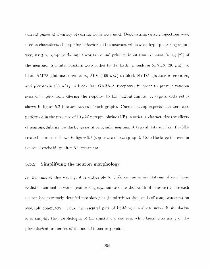
c*rlrrent pulses at a. variety of ctlrrerlt lcvels were used. Drj~olarizirig currerzt irijertions werc3

used to cl~aractcrizc. the spiking belrwiors of tfirb ncurons. while wc3ak liyp"-'ry)olarizing inputs

wcrc. r~sckd to conlpntr t llr iriprlt rrsist,ance and prillrary iriy~rlt t irilcl cox~sta~it (iriuo) [27] o f

thc neurons. Syna~jtic I>loc.kcrs were added to the bathing mediual (CNQX (30 plJ1) to

block AMPA gluttanlate recxptors. APV (1 00 /~1!1) to block NMDA gllltarrlat,~ receptors.

and picrotoxin (50 p M ) t80 block fitst GABA-A re~ept~ors) iri order to prevent ralldorn

synaptic iriputs fro111 altering the response to the currellt inputs. A typical data set is

shown in figrire 5.2 (l~ottorn traces of each graph). Current-clamp, experirrlents were also

perf'ornred in tlrr. presence of 10 i~i2:f norepinephrine (NE) in order to c.liarat.terizc t l~p effects

of ~leurorrlodulatiori oli the behavior of pyrarriidal neurons. A t,ypir.al data set from tlie NE-

treated neurons is sliown in figure 5.2 (top traces of eadi graph). Note thcl large increase iu

rleurolial e~cit~ahility after NE treatr~ie~it.

5.3.2 Simplifying the neuron morphology

At tile time of this writing, it is unft.asi11lc to build c o m f ~ u t ~ r sirrlmlaticiris of very largti

rcalist ic. rre~~ronal nehorks / rori~g>rising r.9.. l~unc!retls to t housantls of ncurt~ns j whc.rc c1ac.h

ururon has extr.rrriely tletailrd moryl~ologic~s jlruiidrrds to tllor~sarldx of c*ozrlpart~nent$ ctn

at~:iilahlt. c-orn1)rltcrs. Tlms. 2 ~ 1 1 ~sscllitial pcxt of I>rrildirzg a rcz~listic. r~c>t'~t"orli ~ i r ~ ~ u l a t i ~ ~ ~

is to siniplify tlic ~iior~~lrologies of thc c-olistit~zent xtenroris. u-hilc keeping as many of tlti.

pl~ysiological properties of tlit. n~odel i11tac.t as possit~le.

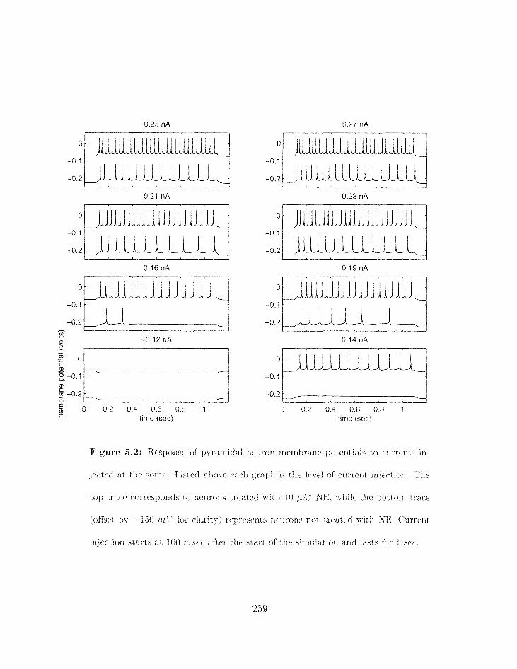
a,

3 -0.2 x.2

0 0.2 0.4 0.6 0.8 1 time (sec)

-0.2

0 0.2 0.4 0.6 0.8 1 time (see)

Figure 5.2: Responstl of pyratnidal ntluron rnernt~rarlc potentials to rurrents iu-

top t race currr3s~>o1rtls to neurons trcat r t l wLr11 I0 p.-;ll SE. \vjIlil(~ t the bot t 0x11 trace

ioEsct Ify -130 1 8 ~ 1 - for clarity) r.cl,resrsr~ts rltluro~ls not trclated with YE. C~rrrrrlt

irljt.ction starts at 100 rn.5er afttlr tllc start of tilt> sisniliatiorl and lasts for 1 ,s.cr..

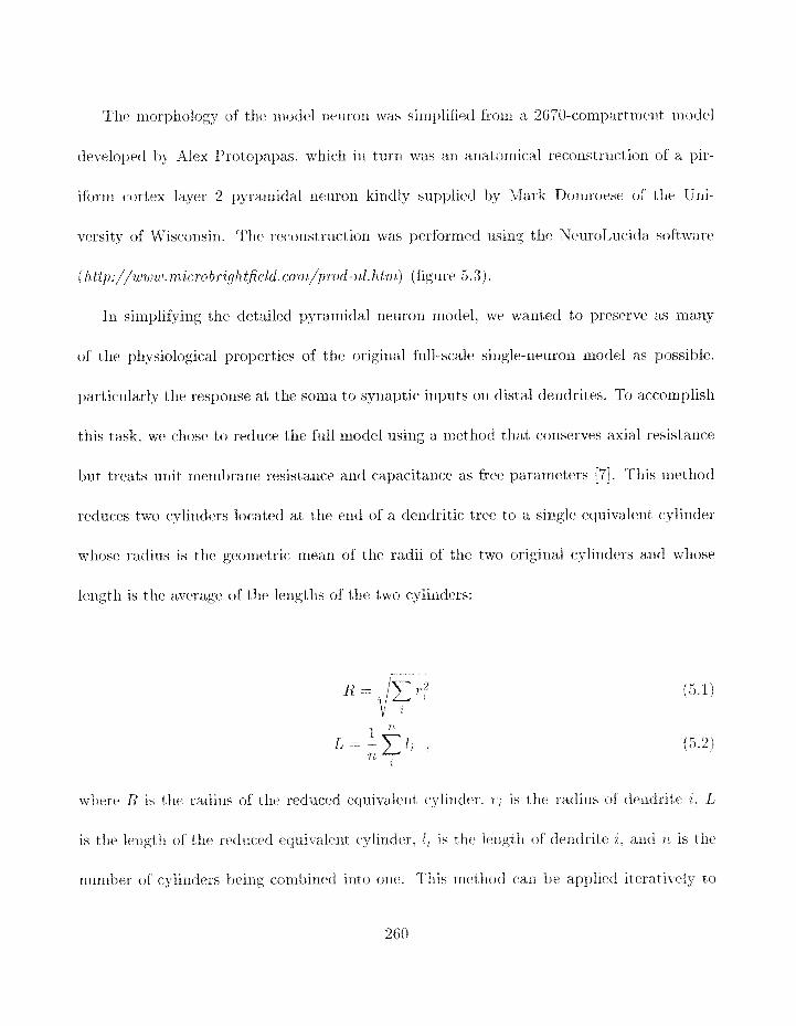
T l i ~ rilor~jlrology of tlir nitxi~l iieurolr was simplified froin a 2670-col,rpartlrl~~11t r~lodcil

drvelol~ed by Alex Prc)to~japas. nlricli in torn was ail arlatorirical rrco11sbrll(*tiol1 of a pir-

ifi~rllr cortex layer 2 pyrallridal neuron kindly supplied by Mark Dolrlrorsc of the Uni-

vr.rsity of Wis(*orlsirl. Tlie recoilstr~~ct~ioti was perforined using the NeuroLucida. software

( htfj)://ut,oro. rnf cro hligh tfirld. conr/~~rod-nl. htnr) (figure 5.3).

In sirnplifj~irig the detailed pyrarriidal neuron niodel, we wanted to preserve as irraily

of the physiological properties of the original full-scale single-lieuroll model as possil>le.

particularly the respollse at tllr soma t,o synaptic inputs or1 distal dendrites. To accomplisli

this task. we chose to red1x;c the full niodel using a rrrethod that conserves axial resistalrcc..

Ijut treats llxiit ~iierrlfiralle resistance and capacitallce as f r c ~ paranleters [7]. Tlris rrlethod

reduces two cyli~lders located at the errd of a dendritic tree to a single equivalent cylinder

wllose radius is the georrietric mean of tlre radii of the two origirlal cylirrders and whose

lerrgtfr is tlie average of the lerigtlrs of tlrc two cylinders:

whc:rc. E is thc radius of tlie reduced equivalc~nt c.(vlindcr. r*, is tlrc radius of tltl~rtlritcl i , %

is tilt. li.ilgtlr of tlrc rrd11cr3d tlc~uivalr~lt cylilldrr. 1 , is t l r ~ leiigtli of drlidritc. i . a l ~ l 71 is tile

~nii~iber of' rylilldrrs 1)riiig c*oriibiricd into on^. Tliis iiwtliorl can bc app1ir.d itoratively to

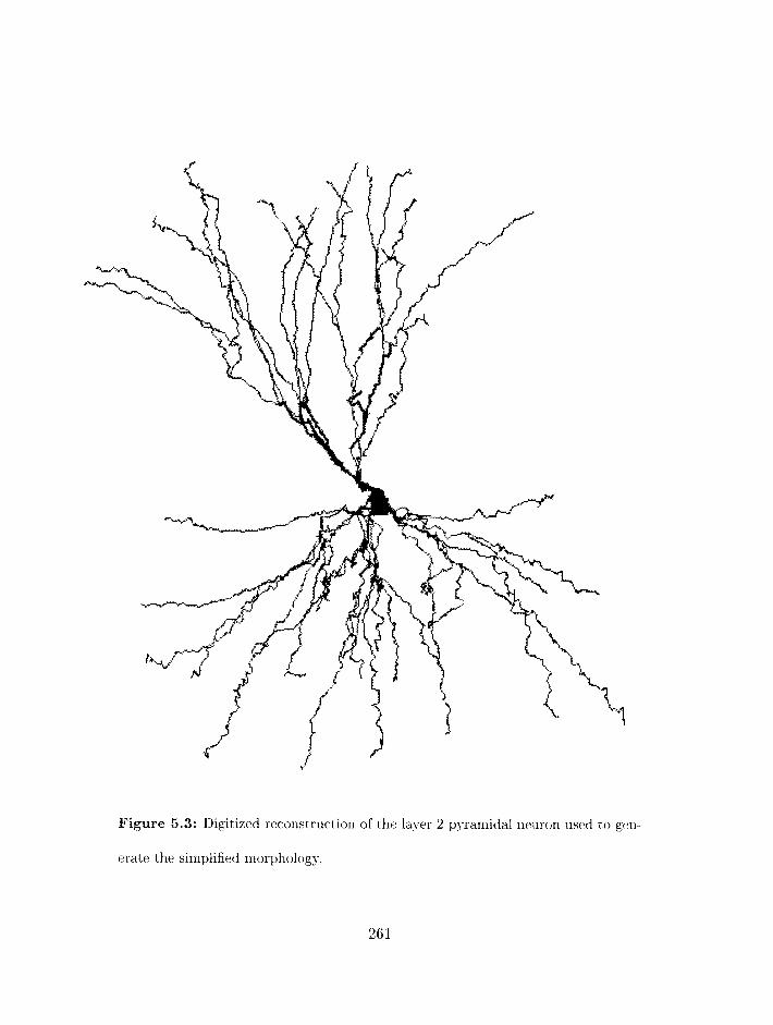
Figure 5.3: Digitized recor~structio~i of the layer 2 pyramidal neuron used to gen-

erat e t lie simplified morphology.

rc.dlicf. tlli. original rnodtll as rnncll as dcsirclrl. Wlie11 any TWO c-ylilidcrs had wiclely difftlrirlg

lengtlis. WP rt31rioved tllo slllilllc~ ~lf ' l ldr i t~ to avoid distortillg tllc gecj~ricltPy of the ~ i e ~ ~ r o u .

Becarrsc this rnrt llotf tloes ~ io t c'onservtl total ca(311 area. t l ~ c spec-ific menit~rane r~sistarlcc.

arid rapacitancfl of tlie model w e r ~ re3scaled until tlir input resistax~ce R,,, and input t init.

constant TO are roughly tlif same in hot11 models. To ensure-. accurate sirrlulatiorl rc-lslrlts.

it is also necessary t,liat each compartment have ail electrotonic: lerlgtli of less than 0.1 X

(see chapter I arid j27j). Note that the sta~ldard rnetliod for redlrcing corrlplcx dendritic

trees (tlre "312 power-law" or eqllivalrnt cylinder method of Rall [27. 371) was not used

since t he deiidritic. diarr~eters at brancl~ points on tlie (:ell recorlstrllctiori did riot ronforrrl

to tlic. 3/2 power law. Tlie niethods used also assume a passive dendritic tree. This is valid

in the context of our model sirlcc all tlie active ~oriduct~ances are located in the soma. In

addit ion, thew is at present no strong evidcncc for active cortductanc*es 0x1 t l1r-l tlerldrit cs of

piriforrli c-ortex pyramidal ileurorls (Lewis Haberly, persolla1 c*omrnunicatiol~). in colltrast to

ncoc:ortical a11d hippoc:ampal pyramidal cells j2-1. 42, 431.

Thr. neuron rrlodel sirri~~lification algoritlim is descrit)ed ill dctail irr Appcritlix A. The

ri)sulting xllodcl is shown irl figurc 5.4. Table 5.1 cornpares the p s s i v ~ pilra~iet~ers. input

rc~sistilnces. arid iriput time c-onstants of the origilial ancl sirnplifirrl nr.jlron niocl~ls. Thc

sprrifics re:sistivity atid capacitancc~ ~~arali lctrrs wt>rcl ac!just.td by lialid to produrc a good

match hc~twr<~t.il the full arid recluc~d models. Figrirc 5.5 sllows tllc~ rc>sy>onsc3 of 110th n~oclcls

to ;1 weak synapt ii- input oil tlte distal apical tlerlcfrite. The rrsporistl of thcl siml~lifieci ruodcll

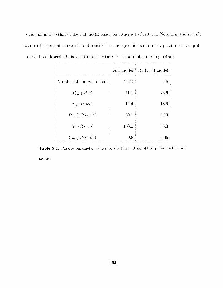
is very siniilar tto that; of the fill1 rliodel based on either set of criteria. not^ that the spec=ific

valxles of the rrtcrnbrano and axial resistivities and specific* rnt.mt)rarlt. c.al>at:itanccs arc3 c-yuitc

tliEt3rcnt: as desc-ril~ecl at~ovt., this is a feature of tile silnplification algoritltnl.

Table 5.1: Passive parameter values for tlw full arid sirriplified yyrarnidal npurorr

rriodel.

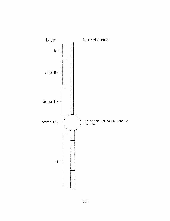
Ionic channels

Na, Na pers, Kdr, Ka, Ca buffer

KM, Kahp, Ca

Figure 5.4: (Previous page) Schenlatic structure of the sirriplificld 15-coni~~artrric~r~t

l~yraniidal rieuroli model. Layers of the pirifornl cortex in which the neuron tompart-

rrlents art. located are listed on the left side of the neuron. Each segrrient represents

a single coxripartrnerit. JVoltage- arid calriu~n-dcl2eriderft ionic. chanrit~ls are listecf or1

the right. Xott. that ioriic cllarmels are found only in tlit. sorria. _4l)t>r(lt-iations:

sup l b . supt.rfic.ia1 layer Ib: d e ~ p Ib, deep layer lb . sorrla(I1). somatic. rcgiori irk

layer 2; 111, basal dcridritic. regiori iri layer 3; SCL. fast inatti~~atilig sodiurrl rlia1i11~L:

IYn per.s, persistent sodiurn channel: Kdr.. delayed-rectilicr potassiuni c.liarine1. l<u.

fast iriact irating pot assiurn channel; I<,lf, sloiv-, lion-inact ivatirig volt age-deye~id~rit

~~otassiurrr channel (31-cnrrt.nt); Ii-afrp, slow ralciuni-dependent ~>otassiurrl c'liarinrl:

Ca . liigli ~oftagt> act i ~ a t e d calciurn cirannel. Tlzcl sorrla of t llc ntlurolr. rrzotlel also

corzt airls if. r~alciurrl bmE(~.

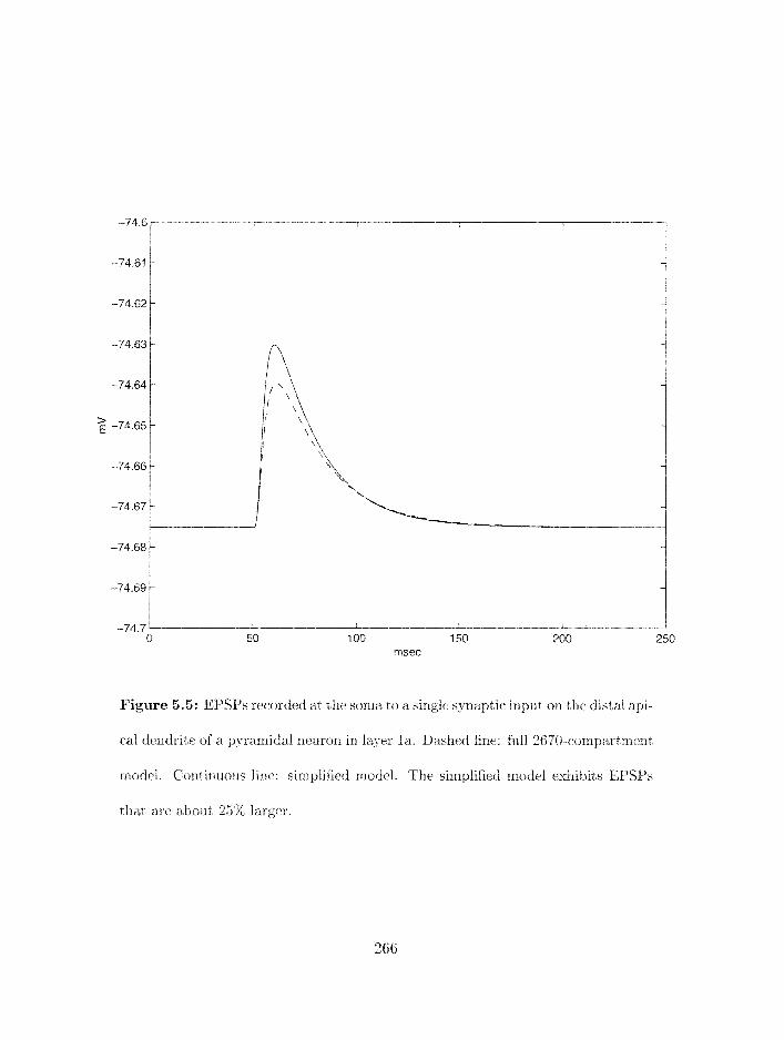
Figure 5.5: EPSPs recorded at the sorria to a single s5-riaptic input on the distal api-

cal dendrite of a pyramidal rieurorl in layer la. Dashed line: full 2670-compartment

xnodcl. Corttinuorrs line: sinlplified model. Tire sirrtpfi-fied model exiiibits EPSPs

that are about 23% larger.

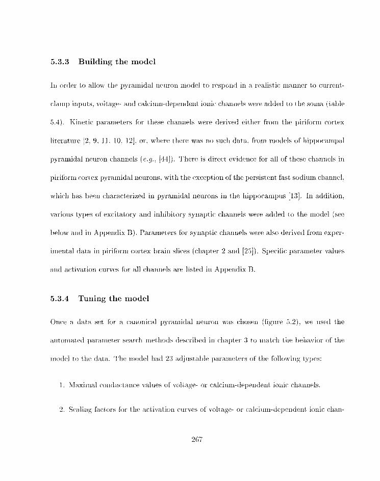
5.3.3 Building the model

In order to allow tlle pyraniidal rieuron model to resporid in a realistic rriarirrer to current-

clamp input s, volt age- and ~:alciunl-dependellt ioriic cllaririels were added to the soma jt able

5.4). Kinetic parmieters for these chaiinels were derived either from the piriform cortex

lit,erature [2. 9. 11. 10, 12 , or. where there was no sucli data. from models of hippocarnpal

pyramidal neuron channels (e.g., L4-21). There is direct evidence for all of these channels in

piriform cortex pyrarrlidal neurons, with the exceptio~i of the persistent fast sodiurn chmnel,

which has been clraracterized in pyramidal neuroris in the hippocampus [13]. Iri addition.

various types of excitatory and inhibitory syrrapt ic cliannels were added to the xrlodel (see

below and in Appendix Bj. Parameters for synaptic channels were also derived from exper-

irriental data in piriform cortex brain slices (chapter 2 and [25]). Specific paranieter values

arid activation curves for all channels are listed in Appendix B.

5.3.4 Tuning the model

Once a dat,a set for a canonical pyramidal nellrori was chosen (figlire 5.21, we used the

autorrlated paraxrieter search ililethods described in chapter 3 to rnateh the bella~~ior of thc

tllodel to tlie data. T l i ~ rriodel liad 23 adjustsable paralrleters of the following types:

1. Maxirnal conductarlce values of voltage- or ealciu~n-dependent ionic ehanlzelt;.

2. Scalirig factors for the ac-tint ion caurves of volt age- or calcium-clepende11.t ionic chsn-

3. Soma rostirig potential.

4. Sornat ic: and deridrit ic menlbrane resistivities.

Since tlie experimerltal data was obtained in tlle presence of synaptic blockers, the pa-

rarneters of the synaptic channels were not varied when turiirlg tlie neuron models. Maxinlal

conductances of the cliannels were varied because these values are riot available in the litera-

ture. Kinetic parameters were varied for some channels because the data sources were either

not derived frorn experinients on. pirifbrrli cortex pyramidal neurons or because the available

data was not of high quality. The shape of the kinetic activatiorl curves and time ~onst~ant

curves was never altered; instead. the midpoints of sonie of the activation curves andlor

the overall time scale of the time constant curves could vary over a narrow range. Tlie

resting potential was also allowed to vary over a narrow range to cornperisate for unkliowrl

jurict ion potentials, wliich can alter the apparent xnellibrane potential by several rrlillivolts

[39]. Simr tlle neilrori morphology was obtained fionl a difirent cell t2iati the pllysiological

data, we also iricluded the sornatic and dendritic rrr~rribrar~e resistivities as paranietcrs. in

case the morphology represented a sunlewhat larger or smaller cell than the physiological

data. Full cfetaiis on the resrllting cfianllel pxameters can be found irl Apperdix B. This

approact1 is reasonable giver1 t l ~ a t the objective of tlic parameter search was to gelkcrate

a phenornerzctlogically correct nludel for the purposes of network nlodeling, ratlitr than to

find a unique r:orrect set of parameters.

The result of the parameter search is sli0%%711 in figure 5.6. As can be seen. the resulting

nlodel replicates the intracellular current claxnp data to liigh accuracy. The input resistance

of the pyraniidal nttlron niodcl was 98 &Ifl and tlze input tirne co~lstant ( taua

20.2 msec. which is well within the typical range for these xleurons [35] .

One of the objectives of the work described in this thesis was to exauline the effect of neu-

rornodulators on the dynarrlical behavior of the pirifornl cortex. The implementation of

synaptic rleurornodulation is described below. Here. we describe the niodifications of the

pyramidal ncurori model needed to incorporate neurornodulation by norepinephrine (NE) .

Our experiments have shown that NE increases the resting potential and tlle excitability

of pyramidal neurons. as well as reducing spike frequency adaptation (figure 5.2). Ex-

perinzenh in other systems suggest that these eEects are rnediated in part by suppression

of slow potassium coslductarlces [29. 301. In order to incorporate. these effects into our

pyramidal neuron model. we took the nlodel discovered by the parameter search methods

and allowed several parameters to vary (see t allle 5.6 1. These paranteters represented t lze

resting nlemhrant. potential of the neuron and the lnaxlmal corlductances of four voltage-

and calciurn-depcuder~t potassium chttrlllels (fast delved-rectifier chanxlcl. inactivating A-

current, slow non-inact-imting %I-c-urrmlt. anti calcinnl-dependent potassiusn current), -411

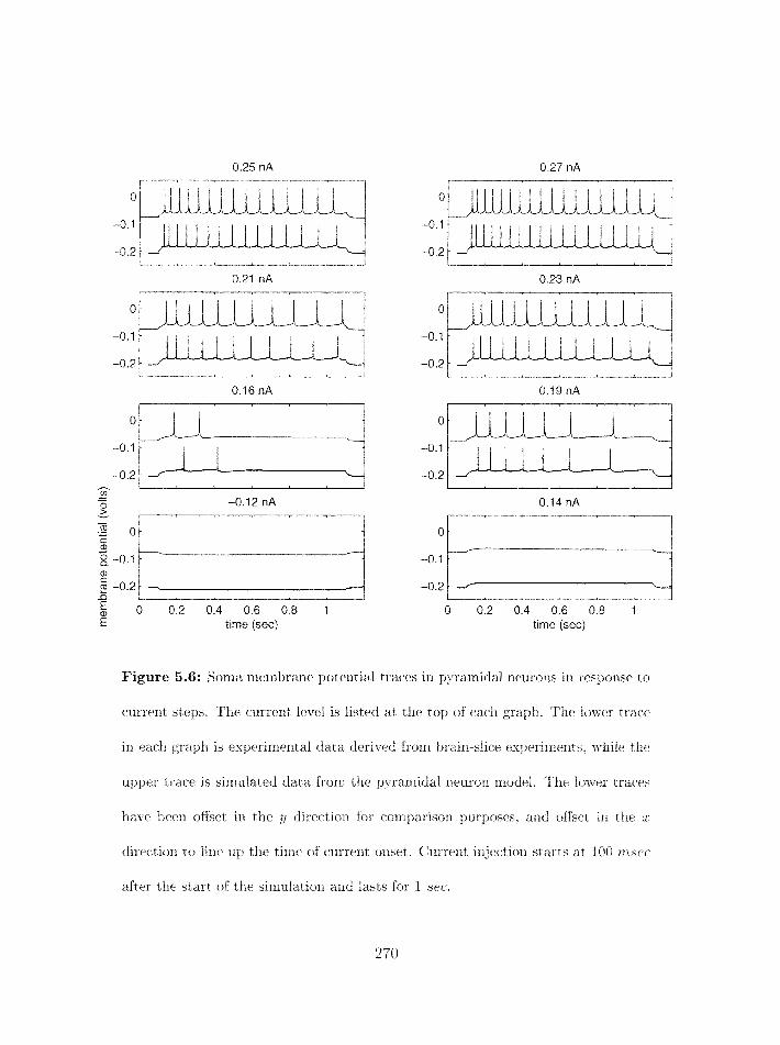
tij .c.. g -0.1 m 5 -0.2 13

0 0.2 0.4 0.6 0.8 1 time (sec)

I I

0 0.2 0.4 0.6 0.8 1 time (see)

Figure 5.6: Soma membrane potential traces in pyramidal neurons in resporlse to

currerlz steps. Tile rrtrrent level is listed at the top of each graph. The lower I-race

in each graph is experinlental data derir-ed fronl brain-slice esperi~nerlts. while the

upper trace is simulated data from the pyrarnidal neuroxr model. Ti le lower traces

har-e beerr aEset in the y direction for colrzparison purposes, and offset in the s

direction to line up the tirrlcll ctf current anset. Current injectiorl starm at 100 I I I N C ~ C ~

after the start of the sirrrrltatiorl axid lasts for 1 set.

other ~ ~ a r a i n ~ t e r s were kept at tllc same values as tliose in tlie urirrlodrllated rleuroil.

Thr resporlsc of the i~euromochlated ~leuroli to current-clain~~ iriputs is s l~ow~l in figllrc.

5.7. Tlic parameter changt~s required to tnr11 the unrnodulated nellrotl into a nerrrorrzodn-

lated neuron are listed in Appendix B. As can 1)c. seen, the neuromodulat.ed rlerlrorl nlatches

tlie spiking behavior of t h ~ real neuron quite closely. althougll not as rlosely as for the un-

modulated neuron. This is to be expected. since fewer paraineters were allowed to vary in

the neurornodulated case.

5.4 Modeling inhibitory neurons

5.4.1 Data set

Various types of in1lil)itory neurons are found ill piriforrn cortex (chapters I a11d [16, 391).

Unfortunately. very little ir~tracellular data is available for these cell types. with the ex-

ceptiorl of layer 3 inliibitory interrlrurons (putative aspiny multipolar ileurorls [IS. 36, 381).

Tlle spikiiig behavior of these inliibitorj~ intJerneurons is very silnpli:. correspoiidiilg to tllr

*.fast-spiking" class of rlrurorls described for 11eocortic:al lleuroiis [3-1]. These wllrons are

iligllly excitable. have ;t low spikillg threshold. and show little t80 no spike frequency adap-

tation. In addition. sorrit3 ~xperixnents on the e&cts of norepinc~~tlriirc llavt. been (~erfc~r.r:r:it?rf~~e<i

on tllis rlenron type [13. 33 . Tyi~itral sljiking I>ellaviors <if this xlruron type are showrl in

tigurc 5.8. and t2iP sljiking freq~lcrlcirs as a functio~l of currerlt jf/I c-urvtli is sla)wrl in figurc~

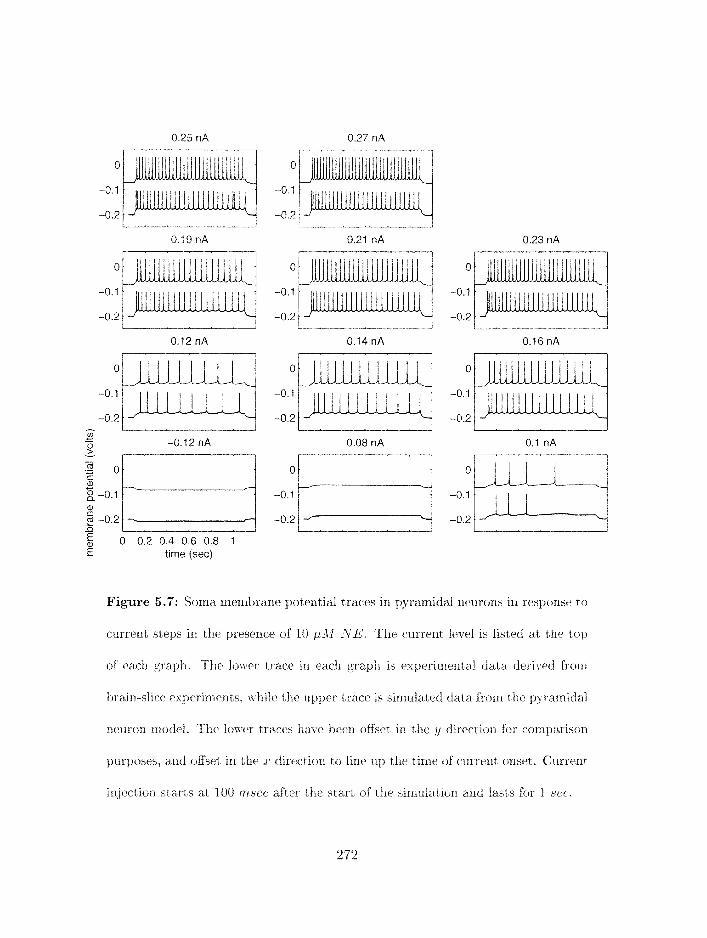
I . . . . . )

0.16 nA

0 0.2 0.4 0.6 0.8 1 E! time (sec)

Figure 5.7: Sorna mernhrane poterttiai traces in pyramidal neurons in response to

current steps in the preserlce of' 10 pAl JVE. The current lelic4 is listed at the top

of each grapll. The lower trace in each graph is esperini~ntal data der i~ed frorrl

brain-slire experiments, white the upper trace is sir~iulat ecl data from the pyrraniidal

neuroil rnodel. Tltc lots-er traces haye lteexl offset in the y dirc>ction for tomparison

pur1Jost.s. a1rr"iEset in the x dirr.ctian to lirir up the time of currezlt onset. Currer-ti-

irijectiorl starts at I00 mser after the start of the simulation arlcf lasts for 1 sec.

5.9 for several neurons. Wot,e that tlie cxcital3ilities of tliese neurons car1 vary corlsiderably

from lieurorz to neuron.

5.4.2 Building and tuning the models

Since detailed reconstructions of the morphologies of inhibitory interneurons were not avail-

able, and since the spikirlg characteristics of tliesc neurons are simple and easily nlodeled, we

chose to use one-compartment models for these neurons. Voltage-dependent ionic channels

included fast Na, delayed-rect ifier K , and fast inactivating K ( A-current ) . Parameters for

tliese ellanrlels and for the neuron as a whole are listed in Appeildix E3. The A-current was

added to decrease the cxcithility of tlre feedback inhibit org neurons to more physiological

levels. Synaptic channels are described below. Because of the simplicity of these models,

automated parameter search methods were not needed to assign parameters to the rnodels

in the cases where data was available.

No intracellular data is available for plitative feedforward inhibitory irlterzleurorls in

piriforrn cortex. Therefore. these neurorrs were rrlodeled using only fast f i t , a r d delayed-

rectifier K clilaniiels. Paraineter sets for tliese rzeuroris are listed in Appendix B.

NE is krlown to irlcrease the excitability of layer 3 irlhibitory rrelirorls irz pirilirtrnl cortex, in

part by illcreasirlg the restirlg rne~nbra~le poterltial jli]. Altllougll precise f/I curves fbr this

25 -0.1' I 0 0.2 0.4 0.6 0.8 1

time (sec)

Figure 5.8: Tntracellular recordings of sorrla membrane potexitial traces ixl layer 3

inlzitsitorj- irllerrzeurons in responsc to current steps. The current Ier-el is listed at

the top of each graph. Curreztt irlcjectioxi starts at 50 rrbser after the start of the

sinrulation artd lasts fix I ser.

iir.uron type uridcr the influcnrc of NE lrave rtot beer1 reported in the literature. a siniilar

strategy was used to irlc;reasr tile excitability of these lieurolls ill the model. f,/I curves fiorrl

tllcl l~iodel with and witllout NE ar t sllow~i iri figrzrc 5.10. Thcl excitablity of the rnodel

iiiterrreurori is within the typical rarrge of the data. NE causes a significarit increase of tllc

exeitat~ility of the model int erneuron.

There is no data, available on rreurornodulatiorr of synaptic irrputs to inlribitory internell-

rons. Therefore, iir our rnodel these synaptic inputs are unaEecteci by NE.

5.5 Modeling synaptic inputs

An essential r:ornl,onentz of a realistic: rleuronal network rriodel are accurate rriodels of the

various types of synaptic-: corrductarlces present in neurons of tlie rnodel. Tliese arc: described

irl this section.

5.5.1 Data sets

Data on fast excitatory synaptic transmission in aeerent and associatio~lal fiber pathways

was derived fro111 tjraiu-slice experirrreuts on ~ ~ i r i f o r ~ n cortex descril~ed in detail in chapter

2. This data set also irsclutled exteilsive data on the effect of neuromudulators on syllaptir-

trarlsiriissio~r in pirifc~orrn cor tes. as well informatior1 on synapt it. farilitat ion. ilddit ional

data or1 synaptic Fdcilitatiorz arltl depression was derived from uxlpublished data fi-ctrrl brain-

slice cxperirrlerlti described 11r:low. Other syilapt ic parameters were taken froirs ['Lsj.

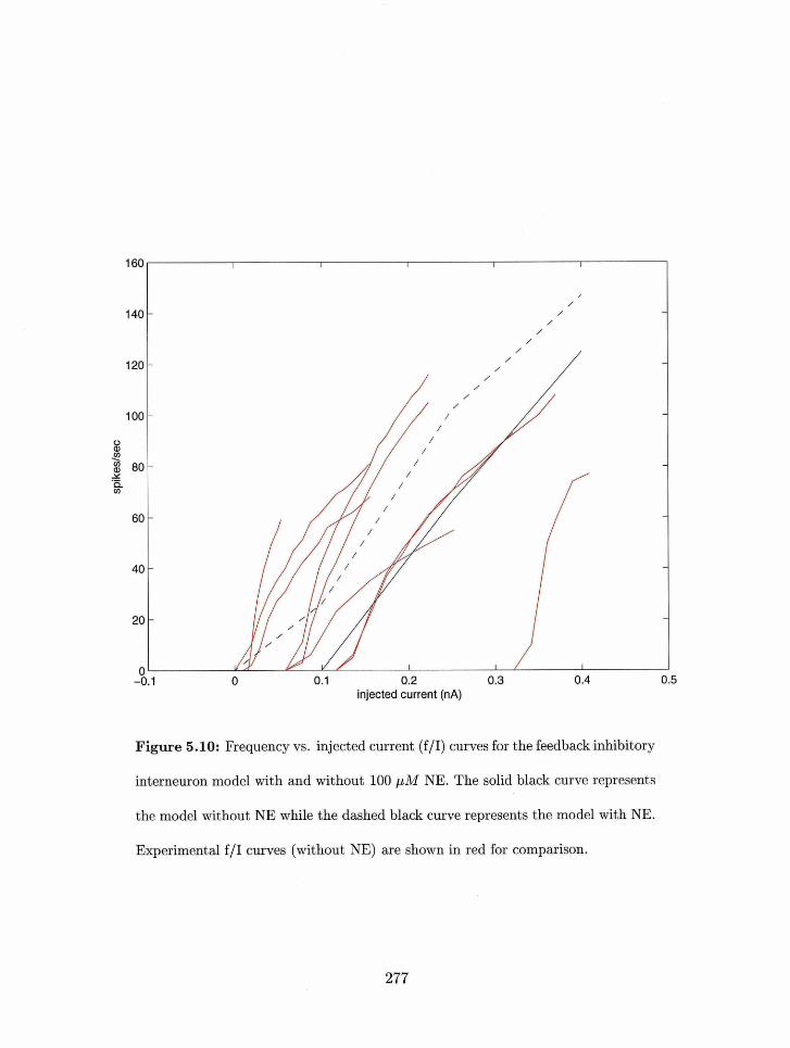
0 -0.1 0 0.1 0.2 0.3 0.4 0.5

injected current (nA)

Figure 5.10: Frequency vs. injected current (f/I) curves for the feedback inhibitory

interneuron model with and without 100 pM NE. The solid black curve represents

the model without NE while the dashed black curve represents the model with NE.

Experimental f/I curves (without NE) are shown in red for comparison.

5.5.2 The basic synapse model

The basic synaptic model used in tlle sirxiulatiolls is a gerieralized alpha fu~iction:

A G,,, ( t ) = C . - ( e - t ~ ~ l - ,-a!7-2 ). T~ > 72 .

7-1 - 7 2

w11ere G is the nlaximuln conductarice of the synaptic charinel. 7-1 is the decay time constant.

is the rise time constant. and A is a norrr~alization factor which ensures that the rnaxirnunl

coriductarice is c. Total synaptic current for a given channel is computed using tlie equation:

where 1;' is the rnenlbrane potential of the neuronal corzlpartment the synaptic cllannel is as-

sociated witli arrd ET,, is the reversal potential of tlie channel. Table 5.2 shows the different

synaptic types used in the model along with the different parameter values used. AMPA

refers to fast excitatory gl~ltamate channels [39] which are selectively excited by AMPA

(-amino-3-llydrox y1-5-~netliy I-4-isoxazoIrpropionic acid). NMDA (N-rlletlry I-D-aspart ate)

el-rannels are slow excit atory glut arnat e dlaxinels which arc. volt age-dependent as well as

synaptically a~ t imt~ed . Both types of channels axe permeable to sodiurxl and ~~otassium ions

(and calcinrll. ill the case of NMDA channels), and have high reversal ~~otentials. GAB4-.4

cllannels arc inhibitory ckiannels permeable to rdlloride and have reversal potentials in the

range of neuronal reversal pote~~tials: tllus. their effect on neurm behavior is ~redorni~iantly

througll a curr.~nt~-sllunti~ig iil~challisrn [22. 251. GABA-U cllarlllels are infiibitory channels

~~errneable to potassium a d Llave a fyg~rpolarizcd reversal potential.

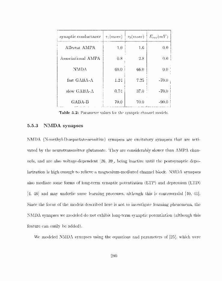
Afferent A&IPA

Associational AMPA

NMDA

fast GABA-A

slow GABA-A

GABA-B

Table 5.2: Pararnet er ~~alues for tlie synaptic channel models.

5.5.3 NMDA synapses

NMDA (N-methyl-D-aspartate-sensitid synapses are excitatory syrlapses that are acti-

vated by the neurotransrrsit tcr glut amatc. They are considerably slower than AMPA chaxl-

nrls, and are also voltage-dependerrt [26. 391. bring inactive until the postsynaptic depo-

larizatiori is high enough to relieve a magmiesiiml-rtlediated charrriel block. NMDA synapses

also mediate some forms of lorsg-ternn syrsaptic y otentiat ion (LTP) and depression (LTW

and r ~ i q underlie some lrarrlirlg pmcess~s. altho~lgh this is co~rtrovrrsial [40, -111.

Since the focus of the models described here is not to investigate learrsiug plrcnorrrena. tlle

NMDA synq>ses we triodeled do not exhibit long-terrrs synaptic potentiation (although this

feature cart. easily be added).

\!TP nlodeled YhIDA syllapsrs using the rqnatiosls and parameters of j2-51. m--lsich werr.

derived frorn exj>erirnerits in piriforrrl cortex. Tllcl equatiorls were as follows:

wllere N(V, tj represents the voltage dependence of the synaptic channel and the other terms

are as described above. [Mg+] represents the fixed extracellular rrlag~lesium co~icentration

(1 vtll.1) while rj and 7 det#ermine the strength of the voltage dependence. Specific pasarneter

vahies are listed in Appendix B.

5.5.4 Synaptic facilitation and depression

Both afferent (layer la) and associational (layer 1 b) excitatory synapses in piriforrn cortex

are known to exhibit sliort-t,erln synaptic facilitation (dlwter 2 and ) and depression

(urlpublishcd data). wherel)y the strength of an ex~itat~ory syrlaptic ~~oterltial (EPSP) is

transiently nriodiiied based on the history of previous ixlptrts to tlzat synapse. Tile dynamics

of these processes differ stibstarltially betw~en associatinrral and atf'ereut synapses. In order

to characterize this pllt110mer10n. we perhrrlled brain-slice experirnents rlsillg a variety of

interprrlse intervals 011 both types of syrlapses irz tlie presence and absence of 25 plLf XE. De-

tails of the exg>erimental procedures arc described in cllapter 2. Figure 5.1 1 shows the effects

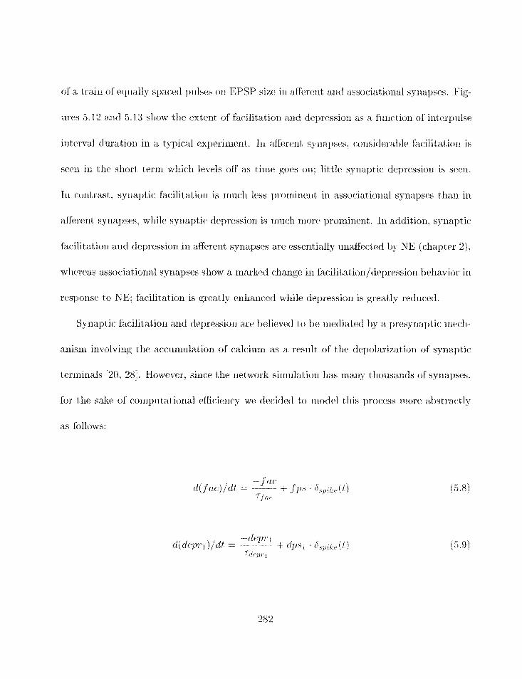
of a train of ecj~ially spaced pulses or1 EPSP size in aRererit alld associational svnapses. Fig-

ures 5.12 and 5.13 sliow tlie extent of facilitation azltl depressiori as a function of interpulse

interval duration in a typical experinlent. 111 &r<>nt synay>ses. co~isiderable facilitation is

seen in the short term which levels off as time goes on: little synaptic depressiori is seen.

In contrast. synaptic facilitation is much less prorliinent in assoriat ional synapses t ha11 in

afferent synapses, while synaptic depression is nluch Elore prominent. In addition, synaptic

facilitation and depression in afferent synapses are esseritially unaft'ected by NE (chapter 2).

whereas associational synapses show a marked change in facilitationldepression behavior in

response to NE; facilitatio~l is greatly erilianced while depression is greatly reduced.

Synaptic facilitation and depression are believed to be mediatetl by a presynaptic mech-

arlisrn irlvolving the accumulatior1 of calcium as a result of the depolarization of synaptic

terminals [20. 281. However, since the network siniulation has many tllousarids of synapses,

for the sake of cornprttational efficiency we decided to model this process more abstractly

as follows:

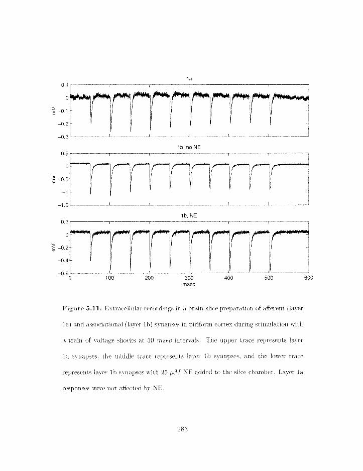
Figure 5.11: Extrac~llular recordirigs in a brairi-slice preparation of afferent (layer

la) and associat ional (layer I b) synapses in piriforrn cortex during st inzulation wit 11

a train of voltage slilocks at 30 r r ~ s ~ c irltervals. The upper. trace rel~rese~its layer

l a sFnapses. tbc rniddle trace represents l a ~ c r l b synapses. and the lower tract.

rc.yrt.sents La;t-6.r l b synapses with 25 p:lf XE added to the slice chambrr. Layer l a

resI3onst.s \%-ere rtot aEec*ted by SE.

200 msec

2o

0 I I

125 msec 2

- )I E 0 i? 20 msec

normalized time

150 msec

22

0 1

100 msec 2

o 0 50 msec

0 1

0 2 4 6 8 19 normalized time

Figure 5.12: Synaptic peak heights for successive pulses in a multiple-shock

paradigm. The black traces represent layer l a synapses, while the red traces repre-

sent layer l b synapses. The y axis represents normalized peak heights, with the first

peak being 1.0 by definition. The z axis represents pulse number. The interpulse

interval is shown above each graph. The time axis is normalized to multiples of the

interpulse interval.

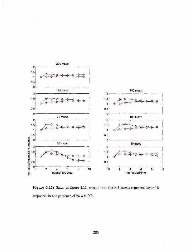
Figure bJ.3: Same as figure 5.12, except that the red traca mprment layer l b

rmpoase8 in the prmence of 25 yM NE.

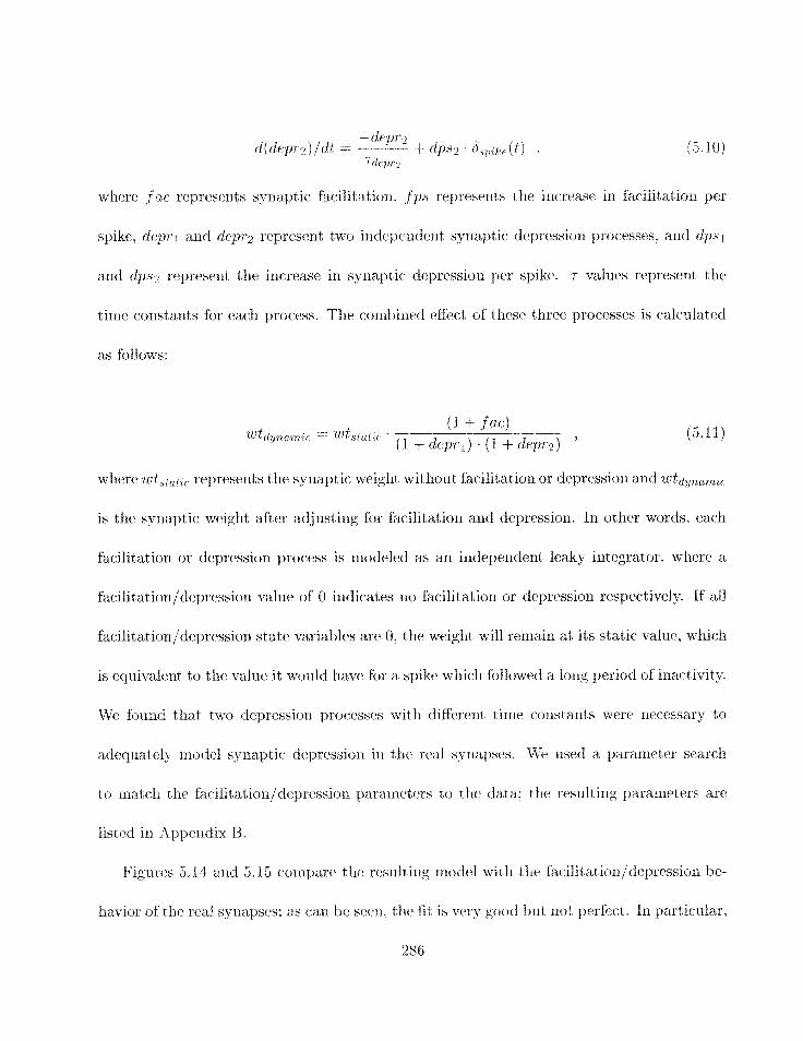
- def>rz d (derjr 1 / dl! = -------- + d p ~ r . n^hp)i;,(t) .

7 c l e p r

wlrclrt: ,f nc represents synaptic fa~ilit~atiort. f ps re~resent~s the increase in filcilitatiort per

spike. r l e~ j r~ arid depr2 represent two irrdependent syriaptic depressiori pro<:esses. and dp.sl

and dps2 represent the increase in synaptic depression per spike. r values represent the

time constants for eacli process. The corribirled effect of these three processes is calculated

as follows:

w11ere / ~ t ~ ~ ~ ~ ~ ~ represents the synaptic weight without facilitation or depression and lotd,,,,,,,,

is the synaptic weight after adjustirig for facilitation and depression. In other words, each

facilitation or depression process is niodeled as an independent leaky integrator, where a

facilitatiorl/depressiorl value of 0 indicates rto facilitation or depression respectively. If all

facilitationldeprrssion state variables are: 0. tlte weight will remain at its static value. wliiclt

is equiv'alerrt t,o thc. value it wotild haw for a spike wliicli followed a long period of inactivity.

found that two depressiorl processes with d ia~rent time constants were necessary to

adeqtxatelp model sy~iaptic depressiori in the rcal synapses. We used a paranreter search

to rxlatch tile f;rrilitation/d~~1ressi011 pararrleters to t lie data: t l ~ resulting 13aramrtrrs arc

listed in Appertdix 13,

Figures 5.14 and 5.15 coinpxrr. t hc resulting model with the faci1it8at;iorr/depressior~ be-

1ia:vior of'the real synapses: as can he seeri. tlte fit is very good brrt not perfect. in particular.

286

short-term facilitation in associational (layer I h) synapses is not captured by the model. TcVe

decided not, to use a more co~tiplcx model to acllievr a better fit, because this would have

slowed down the sirnulatio~l and becarrsr synaptic facilitation is weak in layer 1 b sy riapses

(chapter 2 and [(i]). and is often absent altogetiler (unpublished data).

Tilie reran tlie parameter search for the case of associational synapses treated with nore-

pinephrine; the results are shown in figure 5.16. The nlodel accurat~ely replicates tlie effect

of NE on these synapses: synaptic depressioll is reduced while facilitation is augmented.

5.5.5 Synaptic neuromodulation

We have shown that norepinephrine tra~lsient ly depresses syriapt ic transnlission in associ-

atiurlal synapses in piriform cortex. while transiently enlianci~tg synaptic transmission in

afferent synapses (chapter 2). Neurornodr~lat ion was irlcorporated into the synaptic act iva-

t ion equations described above as a multiplicative scale factor on t lie synaptic conductances:

where G,5,,,,,,,,,,d(t) and GYn ,7iLOd ( t ) are respectively tlie unnlodulated and modulated

syrlaptic conductances, a1id AT ( f ) is the t i m e - n e t neuro~nodx~lat ion of that synaptic.

channel. N ( I ) was channel-specific and was a f~~nct~ion of the rtcurontodulstor concentral-ion.

Our experinrerits also sho~ved that synaptic facilitation arid depression depends on tile

neurolrzodulator level. To rnodel this ill GENESIS, wt. developed synaptic. ellanlliel objects

200 msec 2

125 msec

75 msec

20 msec

normalized time

150 msec 2 1

0 0 100 msec

50 msec

0 0 2 4 6 8 10

normalized time

Figure 5.14: A comparison of multipulse facilitation and depression in layer l a

synapses in the data and the model, The black traces represent the experimental

data while the red traces represent the model outputs. Interpulse intervals are listed

above each graph.

200 msec 2

0 125 msec 150 msec

2

V

75 msec

s Z l E 0 2 20 msec

normalized time

100 msec

50 msec

4 6 normalized time

Figure 5.15: A comparison of multipulse facilitation and depression in layer l b

synapses in the data and the model. The black traces represent the experimental

data while the red traces represent the model outputs. Interpulse intervals are listed

above each graph.

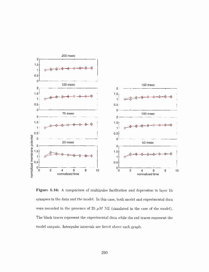
200 msec

2o

0-5 0 1 125 msec

2 I

75 msec

20 msec

normalized time

150 msec

100 msec

u -

50 msec 2 I

"0 2 4 6 8 10 normalized time

Figure 5.16: A comparison of multipulse facilitation and depression in layer l b

synapses in the data and the model. In this case, both model and experimental data

were recorded in the presence of 25 pM NE (simulated in the case of the model).

The black traces represent the experimental data while the red traces represent the

model outputs. Interpulse intervals are listed above each graph.

wllicll corltairlcd two sets of facilitat ion/depressim g~ara~rleters (one for unrrlodulated and

one for ncuromodulated synapses). When the iieurornodulator level was al jov~ a t hresll-

old. the model would use the rieurornctdulateci parameter set: otherwise it would use the

unrrlodulated pararrrrter set. This approacll was necessary because rieuroniodulat ion of

facilitatioll/depression was only systematically invest igated for orie concentrat ion of NE

(25 phf) .

Parameters for synaptic neuromodulation are listed iu hpperidix 13.

5.6 Limitations of our approach

Our approach to modeling siugle nexlrons is a pherloniriiologiml one. guided by the needs

of the network inodeling to be described in the subsequcrlt chapters of this thesis. Marly

cornprornisas had to be rriade in order to produce neurori rnodels which could he simulated

in large nunlbrrs on currently available workstations, and this may result irl urlrealistic

niodel behavior for a nrrmber of reasons.

MTc used the same neurorr model h r everv 1leuro11 of a given t-yp~' in the network model.

This rxieairs that wei itre assulriillg that differellt nellrons of tllrh same type do not differ

sigrlificaridlg in their properties. Wlliltl the evidence presently availa1)lc is cor1sistc:nt with

this view. sorne variatiorr is i ~ l e r i t ~ a b l ~ ant1 iiray have significaut effects om1 rlctwork t~ehaviars.

In particular. real ilrurons displq sigrlificarlt anatonlical variations wllicll are not present

in our models [l(i]. and some pllysiological variation is seen its well [ 3 ] .

The process of simplifj~i~lg the neuron morplrologics 111c24' o f ~ s r ~ r e or distort I I ~ ~ Z I ~ irrz-

portant pherlom~ila [26]. The specific organization of synaptic inputs 0x1 delrdrites inav

urzderlicb import ant co~nputat ional pherlornexia that would rlot he observed in our model.

Syriapses on fine der~dritic branches will also see a larger input resistance than syliapses

in our model. This effect is even more pronounced for excitatory synapses, most of which

are located on dendritic spines 191. The absence of spines. which serve to partially isolate

synapses frorn the main dcndri t ic trunk. results in larger dendritic conductance clzailges

in response to excitatory input than would he seer1 in real neurons. The localizatiorl of

voltage-dependent ionic cllannels to tlie soma is also riot entirely realistic: real rleurons

llave a spike-initiation zone which has a rrruclr lrigher coacentrations of soditr~n cllannels.

with srrlaller cotlcentrations of sodiur~r cliarirlels in the soma [31]. Having a large density of

sodium channels iu the soma results in large transrilenlbrane currents which car1 distort the

field potentials lneasured from the m d e l (see cha~>ters 6 and 7). In addition, pyramidal

cells in most brain regiorls are known to have voltage-dcperldcnt channels on their dendrites

21. 12. 431. FVe did not irlcludr sncll clrarinels in our ~~yramidal cell model becausr. tllerc

is uo evidence for their existence ill piriforlrl cortex: nevertl1eless. this will be an irrlportarlt

subject for future experimelztal and rr1odc.ling work.

The nerzrotr rrlodels cleseril-led in this c l ~ a p t ~ r alrd -t~setl. in the network rrzocfel are ~lltirelgi

deterrrninistic: any variability in their respoxzses derivc.s frorn v;iriatiou ill their inputs. In

priricig~le. this c-ould restllt in artifaetttal befrlaviors if tllr inp~lts were cxtrerrlely regular.

However. as will be sceii in tlrc c:llapters ori network modeling, iiryuts to the network rirodel

always includecl a large rarrdonr cornpoirent, Tirerefore. we fec.1 that this siinplificatiorr is

justified, es~~ecially since irrcorprjrating iriodels of cliarlnel noise or otlier noise-generating

plienoinena (chapter 4 and [I. 321) would have slowed dowrr the simulations colisiderahly.

All of these linlitations point to areas where the present neurov nlodels can be ilxiproved.

Some cllarrges such as adding spike-init iat ion zones. are straightforward arid can be done

with a moderate amount of effort. Otlrers, sucli as using neurarrs with detailed morphologies,

would increase the computational complexity of the network nlodel greatly. If the true

dynaniical bchaviors of the network are critically deperident on these phenoniena, Ilrogrt-tss

in modeling braiir regions at the network level will he very slow indeed. I-Iowever, the hope is

that at least sorile of the significarit dynarnical phenomena of the real system can be captured

usiiig reduced neuron models eml~edded in rretwork models. As the followirig dlapters

demonstrate. many network-level phenomena in the piriform cortex can be rrproduwd

faithfully using a rletwork model built froril tlze neuron models described in this chapter.

5.7 Appendix A: the neuron model simplification algorithm

Tlrc rlerrroli rlrodel sinlplification algorittirn proceeded as follows:

1. i-ribranched cllaills of conrpartmeiit s were reduced to a single cornpart irlcnt iraving

the sarrrc oli:ctrotonic. arld yfiysical length. Tliis was doile by calculati~rg the total

electrotonic lerlgt h of the branch and then adjusting t 'lie diarneter of the riew culn-

293

partment to give the same total electrotomlic length. Tf-ie c:lectrotonic length el for a

single tronlpartmerlt is defined as follows:

el = lIX , (5.13)

wliere l is the compartment leligtli and X is the compartment space constant:

where R,, is tlie specific rnembrane resistivity. R,, is the specific axial resistivity, and

d is tlie diameter of the compartment [ 2 3 ] .

2. Branches were collapsed into single compart ments, starting from the distal end and

proceeding inward towards the soma, according to the algorithm of Bush and Se-

jriowski [7] described above. This was repeated until only five compartments remained:

a basal der-rdrit ic compsrt ment . the sorrla cornpar t ment . and three compartnierrts rep-

resentirig the apical dendrite: tlle proximal (layer 1b) apical dendrite. tlrc middle

(distal layer lb) apical dendrite. alld the distal (layer la) apical dendrite. Tlre apical

dendritic compartments. which can be joirted together. art. kept separate because the

coxlnec:t ion topology of the network ii~odel (c-llapter 6) requires sel~arate corrlpart merits.

3. Because tlle basal and apical dexldritic compart ments were eortsiderably longer than

the 0.1 X limit normally considered to be tllc rnaxirrsurrz lellgth compatible with riu-

29-1,

nlerical accuracy 1271. we subdivided each of t llc tlendrit ic cornpart ments into several

conlpartments each. which resulted in fif een corrlpartrrrerlts all less tllarl 0.1 X in

lengt ll.

5.8 Appendix B: model parameters

In this section are listed the specific para~rreters for the various nleurorl n~odels. GENESIS

simulation scripts for all neurons described here are also milable online at

htt~~://wa,u). hhb. c ~ l t e c f t ~ . edrr/IiSERS/mvu71ier/theesis/thesi.~. html.

5.8.1 Pyramidal neuron channel model parameters

Currents through ionic and synaptic channels are described by this eyuat ion:

where ch represents a channel species. tirn is tlle membrane potential, GCh is the channel

conductance and E,h is the reversal potential for the channel. Reversal potentials for

voltage-dependent ionic cilannels are listed irz t abltn 5.3. All voltilge-dey enderrt ionic cl~an~lcls

were specific* to a given ionic species arld used the reversal potential for that species. In

order to simplify the model, xrtt elected not to change the C a eq~ilihriu~xl poterltial based

011 the cballging in.trac:ellular c.alc.iurr1 corlcentratiolz.

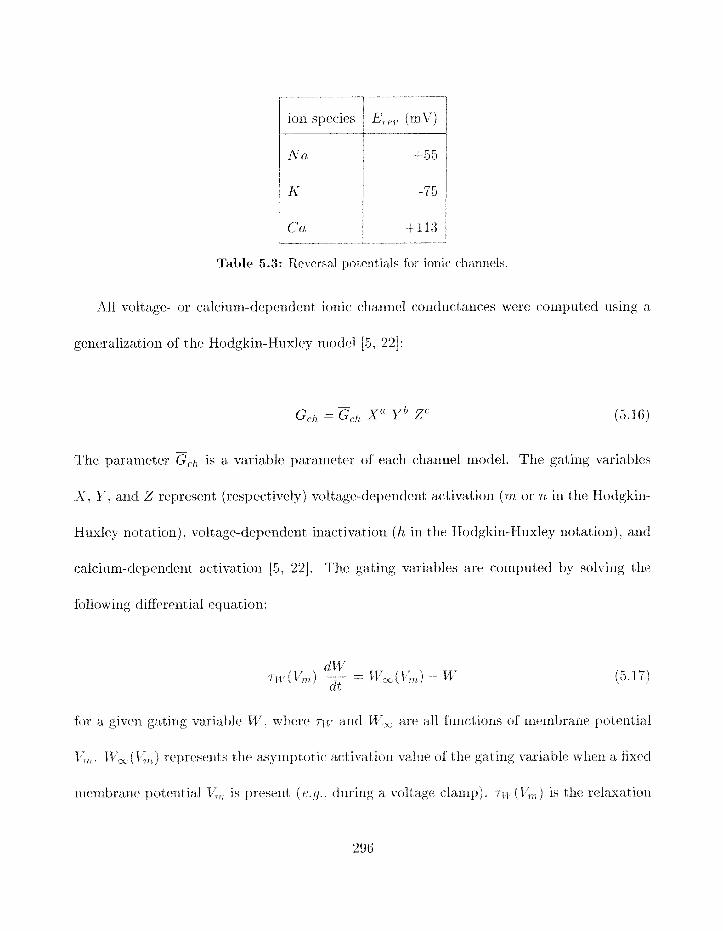
Table 5.3: Re~ersal ~~otentials for ionic channels,

All voltage- or calcium-dependent ionic cllannel corlductances were computed usirig a

gexieralizatio~i of the Hodgkin-Huxley model [5. 22

The parameter Cci, is a variable ~ ~ a r a ~ n e t e r of each charlrlel rnodel. The gating variables

X. Y . arld Z represent (respectively) vo1txp;r-deperiderlt activatiorl (rrt or 71 in the Hodgkin-

Huxley notat ion) , voltage-dependent inactivatioll ( h in the Hodgkin-Huxley notation). and

citlcinni-(leprlldrlt act ivat ioa [5. 221, The gating variables are computed by solvirlg the

following diRerent ial eyuat ion:

for a giver1 gatiug vt3-rial1le H'. where qi- arid Tlt7, ar t all functions of rr~erxlbrarlc potential

k,,, . J$rx(Krt) represelit3s the a~yrilpt~otic. activatiuzl mluc of the gatillg variable when a fixed

~llcrrlhrallr potential 1 ;,, is presrllt ( r '9.. durilig a. x~oltage clanlp) . .rii - (I;,, ) is tllv relaxat ion

t ilrlc constarlt of t llr gating variable under tllesr cordit iolls 1221.

Voltarre-de~endent channels

The a~t~ivatioil and tinle corlstant kil~et~ics curves for the voltage- and calci~ltrl-depe11den.t~

chan~lels are sl~oum in figures 5.1 7. 5.18. and 5.19. hlaxirmulxl conductances and gating

variable exporlents are listed in table 5.4. The data on wliidl the charlnel niodels were

based are described below. Note that kinetics for rrlost of tlxe channels were altered from

tlie original source to fit tlle data by means of a parameter search (chapter 3).

Table 5.4: llaxi~nilnl eonctuctartces and gating variable exl~onents for the ionic

cl1annc.l xxlodels used in pyramidal neurons. Co~lductance units art. S/rrr3. Garirlg

variable clxporlerzts arcs di~l-tcnsionless.

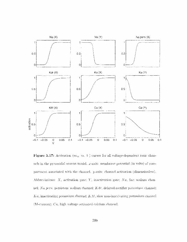
Na pers (X)

Kdr ( X )

Figure 5.17: -4ctivation ( m , YS. 1 rurt7c.s for all voltage-dcpende1It ionic. chari-

riels in t lit pyramidal riclurori rnodel. x-axis: membrane potential (in 1-olt s ) of corn-

~lartrrlerlt associated %-it11 thc clianncl. 9-axis: chan~tel atrtivatioxi jdirnertsionlcsi;).

-At,hrcllviations: X. activatio~l gate: 1'. irlactivation gate: _Ya, fast sodinrn clrari-

riel; ..\-a prrs. persistettt sodiunr ~trar-int~i: I<cfr. delayed-rectifier potassiunrl channel:

Ica, irlarti~ating potassitlrri ~*lla~-tncl: I<_"l. slort- riuxi-inactivating potassium c'liannc->I

(hl-current 1 : Ctr , high \.oft age a c t i ~ a t t ~ l calcirrnt ehar1rtt.l.

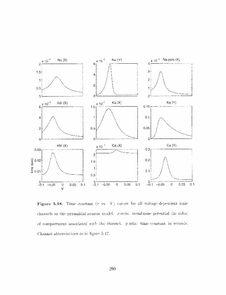
I O-U~ (Y) , 0-4 Na pers (Xf

Figure 5.18: Timi. const ant (r vs. I *) r*rrr\-rs for all vt,ltagr-tley~encfc~r~t ior l i~ '

channcis in the p>-rar~iitlal neurorl model. x-axis: rrienrbrant. potential (in volts)

of corny>art rnent associated witll the cllamnel. 9-axis: time constant in seconds.

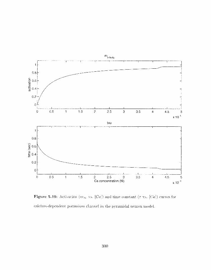
0

0 0.5 1 1.5 2 2.5 3 3.5 4 4.5 5 Ca concentration (Mj x 1

Figure 5.19: ;\cti\-atioil ( r r t , YS. [Cti]) and tirni. corlstsrlt (r TS. [Co]) cur\-cs for

calciurrl-cleperlck~lt potassiu~n c't.lanrrc1 in the pyranliclal neuroxl rrzoclcl.

NU channels

No data is available for tire fast (i~iactivatingj -Vcr chaririel in yirifbrrrl cortex. so kirietics for

this chanrlel were taken from Roger Traub's model of 2iippoc;ampal pyramidal netirons [41].

Similarly. tho data for the persistent Na clrannel nxodel was taker1 from the hippocanzpus

[13].

K channels

No data is available for the delayed-rectifier K charinel in piriforni cortex, so we again

used tlre rliodel of Traub [13] based on data horn the hippocampus. The nrodel of the fast

inact,ivatirig K channel (.'A-current") was based on recordings in the piriforrn cortex by

Barlks and Haberly [Z]. Tlle model of the slow. non-inactivating K chanilc.1 (-(M-current" )

was based on recordings in the piriform cortex [9].

Ca channel

The Cn clrari~rel used in our niodel is a high-voltage-activated cliarlnrl [22] based on voltagr-

(*lamp data recorded in pirifornl cortex pyramidal neuroIls [lo].

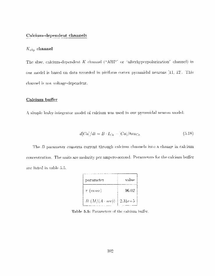
Calcium-dependent channels

K,), channel

Tlie slow. calciuns-depentie~lt K cllallrlel ("AHP" or '*afterllyperpolarization" clla~lrlel) in

our model is based or1 data recorded in piriform cortex pyramidal xiellrorls [ll. 121. This

charlnel is not voltage-dependent.

Calcium buRer

.4 sirnple leaky-integrator model of calcium was used irs our pyramidal neuron nsodel:

The B parameter converts current througls calcium channels into a change in calciurrl

concerltratio~s. Tlie units are rnolarity per ampere-second. Parameters for tlle calcium b1lffi.r

are listed in table 5.5.

Table 5.5: Parameters of thc-l eafc-iuxn bu&r

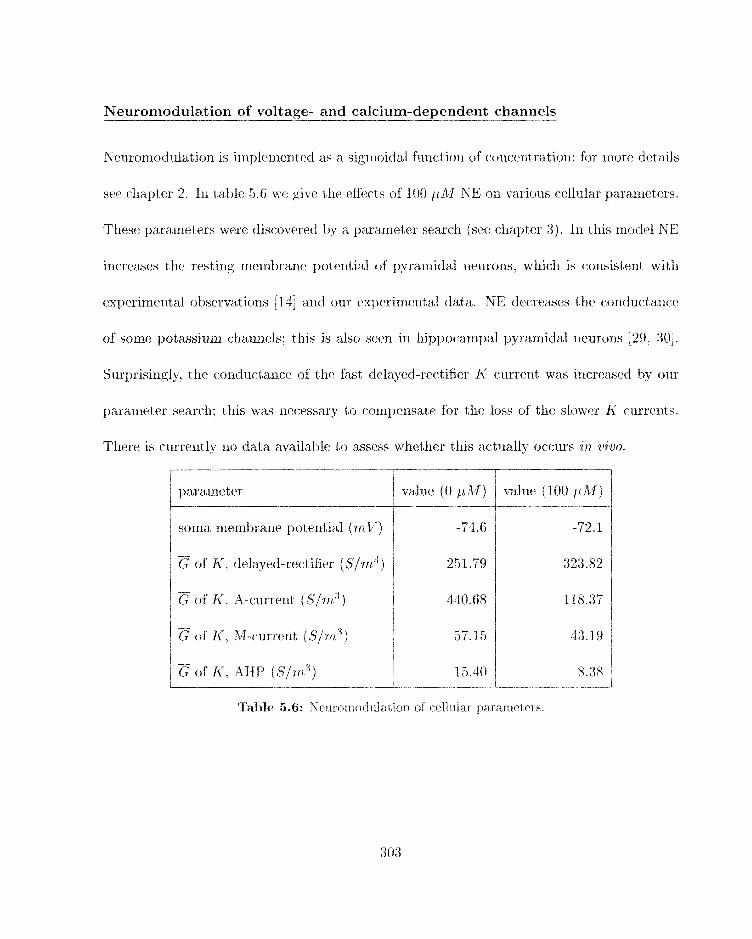
Neuromodulation of voltage- and calciurn-dependent channels

Neurorrrodulation is irrrplen~errted as a sigrnoidal functioir of c*oirc.ei~tratiorr: for more. dctails

see chapter 2. 111 tat~lc. 5.6 we give the effects of 100 plll NE on vtnrious c-c.1lula.r pararrreters.

These parameters werrk discovered by a paramter search (see chapter 3) . In this inodel NE

increases the restirlg iiremhrarre potential of pyrarliidal ireurons. wlricfr is consisteirt wit11

experin~ental observatioi~s [14] a i d our experimental data. NE dtlcreases the c~ntluct~aircc

of sonic 13otassium channels: this is also seen in hippocarnpal pyramidal Irrurons [29. 301.

Surprisingly, t lre conductance of t l e fast delayed-rect ifier K current was increased by our

parameter search: tAis was rlecessary to c.umpensate for the loss of the slower K curreills.

There is currently no data available t,o assess whether this actually occurs in viuo.

pararrreter value ( 100 irhf) I

sonla membrarie potential @ z V )

- G of K . delilyed-rect ifier ( S/m3 )

I

j C of K . AHP ( S / T ~ L ~ )

Table 5 -6: Xeurorrlod~~latio~l of cellular pararnet rrs.

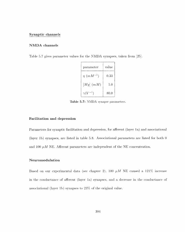
Synaptic channels

NMDA channels

Table 3.3 gives parameter values for the XMD-4 synapses, taker1 horn

Table 5.7: N-111DA4 synapse para~neters.

Facilitation and depression

Para~neters for synapt ir facilitation and depressioll. for affercrlt (layer la) 2nd associat ioml

(layer lb) synapses. are listed in table 3.8. Associl~tional parameters are listed fur both 0

and 100 pM NE. Affererlt paraaleters are indepenctenitt of the YE concentratiorl.

Rased err our expc~rirrten.ta,I data (see c'irapter 21. 100 pi2.f XE caused a 121% increase

in the tmnductancr of agerent; (layer la) synapses, and a decrease in the cor1ductanr.t. of

associatiollitl (layer lb) sgriapses to 23% of the origilial value.

afferent value assoc value (0 L L - ~ J NE)

Table 5.8: Parameters for synaptic facilitatiorl arld clepression. f p s rrleans "facil-

itation per spike". and c J : p . ~ [ ~ ~ ] mean *~clepressior~ per spike7' for the first or second

synaptic depression process. respectively. fps and d p ~ ~ ~ ~ ~ are dime~isio~~lrss.

5.8.2 Pyramidal neuron model parameters

Tlic pyranii(1al neuron rriodel is a lirlear 15-compartment rnodel (figure 5.4); the dilrlerlsions

of the coru~partments are listed in t,al>Ie 5.9. Synaptic channels are distributed across the

nexlrorl as irldicated, rlL;CPA4 and il;'AZUA diannels are excitatory glrztamatergic syri;zl>tic

channels while GABA4 and GABAB represent fast and slow inhibitory GABAergic chaw

rlcls. Ma;uimal c.onductanc*c values for the syrlaptir. r-llaririels vary ac*cording to each netxron's

pitsition in the network and arc. described in clzq~ter 6. Voltage-dependexit ionic. channels

are for~rld only in the soma. The somat;ic restirlg potential was -74.7 ml'. blorc. details or1

the synaptic. and voltage-dependexit ionic channels are givell above.

5.8.3 Feedback inhibitory interneuron model parameters

Feedback inliibitory neurons were modeled as single-comparti~~crlt neurons. Syiraptic. eklari-

rlels iricluded fast Nu. hs t delayed-rect ifier K. arid illact ivat irig K ( **A-c:urrerzt" (rigxxres

5.20 and 5.21). The fast Nn and delayed-rectifier K chanrlels were similar to the corrc3-

spolidirrg cllanliels for pyramidal rleuroxis except that the midpoint of the activatiori curves

was shifted slightly. The A-crrrrent) was not based on expcrirnerltal data but was created

to reduce the excitability of these neurons to a more pliysiological level. Neurori param-

eters arc listed iri tables 5.10 and 5.11. Application of 100 p&rC NE increases the resting

xneriibrane potential of the feedback inhibitory rieuron model by 10 rrt V.

5.8.4 Feedforward interneuron model parameters

Feedforwarcl. inhibit;ory netirons. like ferdtjack irlliibitory neurons, are riiodeled as one-

co~rpartnlent neurolls with fast Na a i d delayed-rectifier K channels. These rtetzrons are

divided irito two classes: tlfiose without excitatory feedback fro111 pyrar-t-zidal cells arzd those

with feedback. Feedforwarti irlhibit ory rlerrrorls without feedt3at:k are ident imI to feedi~ack

intcrrieurons except that their rest irzg riienlhrane pot~rltials arc. sliglitly lower (-73 rr, l " ) .

they do riot lime the inactivating K currclnt (:I-rurrerit). aizd XE does irot alter the,. ~r rx-

eitability. Tllere is crirrently iio cxl>erirnental data oil the effect of XE on these nerzrons.

Feedforward inlzibitory llertrorrs wit11 fecdbacak froin. yyranlidal cells are very ssirrsilar to tliosc

wittiout feedback. except for a lziglier resting mexnbraiie poterltial (-65 rrzt ' j .

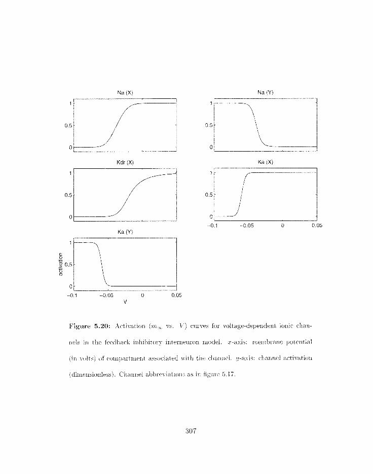
Kdr (X)

Figure 5.20: Xttitatiorz ( i n , .i-s. 1 -) trlr.iTes for voltage-depttrlcleat ionic cli.lan-

rlels in the f~edhaek irihibitory irlterrleurorl nlodel. x-axis: rrlernbranr poterltial

(iri volts) of c-onlpartrrrexlt associated with the chanxic.l. ;z-axis: charttlcl a<.tit.ation

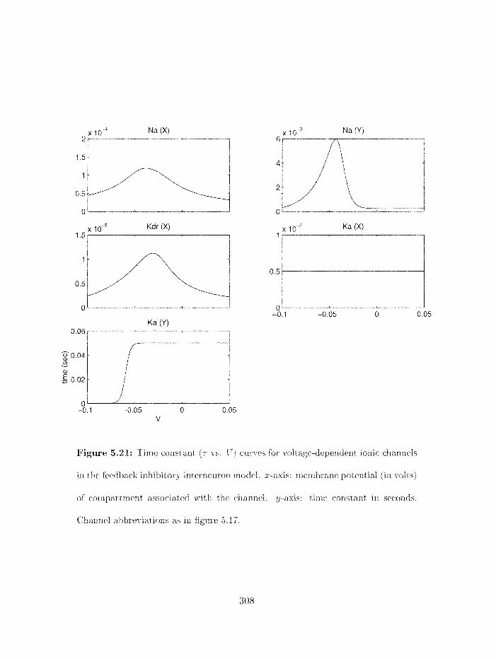
x I o - ~ ~ c i r (x) 1.5

Figure 5.21: Tirrlc ~o~ls ta r i t (7- 1.5. 1') c11rves for voltage-de~jelidrllt ionic cllari~lrls

in the feedback inbibitary interneluorr rnodcl. x-axis: ~nernbrarp potential (in wits)

of ci,inpartrnrnt associated ~l-itll the clianncl. - i s : time co~lstarlt iri seconds.

Cflarlriel ztbhreviat ions as in figtlre 5.1'1".

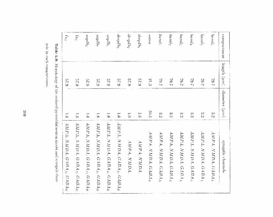
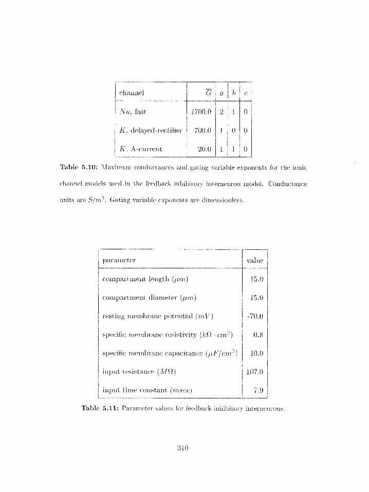
Table 5.10: 3laxirnurn corlductances and gating variable exponents for the ionic

cbarirlel models used in the feedback inhibitory interrleuron model. Conductance

units are S/rrz3. Gating variable tixponmts arc dimnsionless.

cumpartlxletit diameter ( p n ~ )

restir~g membralre potent,ial (rr,l.f)

specific nienlbranr. resistivity (k!1 . c ~ n ' ) )

specific mcrrlbranc ~apitcit~arlcr ( j r ~ / c n ~ 2 )

input resist anre (*44!!)

irtplit t irrre const ant ( rrtsec.)

Table 5.11 : Paranlet el- valtlcs for feecf back ixihibitory interncurorts.

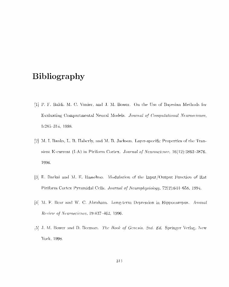
Bibliography

[I] P. F. Baldi. M. C. Vanier, and J . M. Bower. On the Use of Bayesian Metllods for

Evaluating Compartmental Neural Models. Journ,al t?f Co~~~p.utational Near.osc'ience.

5:285-314, 1998.

[Z] M. I. Banks. L. B. Hal)crly. arid M. B. Jackson. Layer-specific Properties of the Tran-

sient K-csurrent (I-A) in Piriform Cortex. Jownal Neuroscl:e~t,ee, 16(12):3862-3876.

1996.

[3] E. Barkai and hl. E. Hasselrno. Modillatiorl of the Input/Outpnt Function of Rat

Piriforrn Cortex Pyramidal Cells. Jofsmnl of Neuroyhgsiolngy. 72 (2) :644-658. 1994.

[4] M. F. Brar and m7. C. Abraharn. Long-term Depression it1 Hip~,ocarnl>ns. ilri~irrnl

Review of i4Tru?-oesci~n cp. 19:33'7-462. 1996.

[5! .I. M. BOWPI. illlci D. BCPIIIBII. The Book of G ~ n r s i s . 2nd. Ed. Springer firlag. NPW

I"ork. 1998.

[6] J . 51. Bower arld L. B. Haherly. Facilitat8ilig and Nonfa~ilitat~ing Syxlal~ses 0x1 Pyra~liidal

Cells - a Correlation Betx~eerl Physiology and Morplzology. Pmceedirrgs c?p The liationnl

Actidrmy of Scieraces of The United States of Americci. 83(4):1115 -1119. 1986.

[7] I'. C. Bush and T. J. Sejnowski. Reduced Compart~nental Models of' Neocortical Pyra-

~nidal Cells. ,lourrial qtl Neuroscience hfethods, 46: 159-166, 1993.

[8] G. G. S. Collins. G. A. Probctt. J. Anson. and N. J. Mclaoghlirl. Excitatory anti

Inhibitory Effects of Noradrenaline on Synaptic Transmission in the Rat Olfactory

Cortcx Slice. Bruin Research, 294(2):2 11-223, 1984.

[9] A. Collstanti a ~ l d M. Galvwn. M-current in Voltsage-clamped Olfactory Cortex Neurons.

Neuroscience Letters. 39(1):65-70, 1983.

A. Constanti. M. Galvan, P. Ranz, and J. A. Sirn. Calcium-dependent Inward Currents

in Voltage-clanlped Guinea-pig Olfactory Cortex Neurons. efiugers Arclri?) Eurupeun

Journal c!p Pl? ysiolqg. 404/3):259 265. 1985.

[l I] A. Collstwnti axld 5. A. Sim. A Slow. hI1lscarirlc.-sensit ive Cn-dc~~c~lderlt-I< Clirrent

in Guinea-pig 0lfi~ctor-y Cortex Nrurons 1x1 Vitro. Journal of Pl,gsiolog?i (Lor~don).

365:P47 -PA?, 1985.

[12] tl. Constant i and J . A. Sirn. Calcium-dellendent Pot assinn1 C~11ld11cta1lc.c~ in Gui~lea-

pig Olfactc~ry Cortex Nenrons In Vit ro. .Iozl~.na,l of Physiolorj;y (Lon dor1/. 387: 173 - 19.3.

C. R . Frerich. P. Sah. K. J . Buckett, and P. JV. Gage. A \;oltagc.-Uepcndei~t Persistent

Sodiurri Currexlt in Mamznaliali I-Ii~>pocarnpal-Ne~1ro11s~ Joumul of Cenrrul Ph y.sinl(~g:y.

95(6):1139-1157, 1990.

[14] R. L. Gellman a ~ i d G. K. Aghajaniall. Pyramidal Cells in Piriforni Cortex Receive

a Convergence of Inputs from Monoanline Activated GABAergic Interxieurons. Bmi'11

R r s e a ~ h , 600(1):63-73. 1993.

[15] R. L. Gellnran and G. K. Aghwjanian. Serotonin(2) Reccpt#<)r-Mediatd Excitatioil

of Iriterrieurorls in Piriform Cortex - Ant agorlisni by Atypical Ant ipsychot ic. Drugs.

Neuroscience, 58(3):515-525. 1994.

L. I3. Waberly. Structure of the Pirifor~i Cortex of the Opossum. 1. Description of

Neurorr Types with Golgi Methods. ,lournub of Con2paratit;e Nef~mlogy. 213(2):163-

187. 1983.

[17] L. B. Wal~rrly. Olfactory Cortxx. Irl G. hI. Sllepllrrll. editor. Tlie S?jnqtir Olgnnizufio7i

c?p t l ~ e Bruin. Oxford Vnivcrsity Press. Oxford. Englt-tild, 1998.

[I81 L. B. Haheriy and .J. M. Bower. X~lalysis of Associatioll Filler Sjfstenl ill Piriform Car-

tcx wit ll 1ntrac:ellular-Nec'c~rdiiig alrd Stainillg "li.clzniy\~c.s. J o ~ r n a l of iICT~ur.nplz ye5ioIo5~y.

5l/ij:YO-112. 198-1.

[19] L. B. Hal~erly and S. L. Fcig. Structure of the Piriforril Cortex of tlrc Opossn~n. 2. F i r i ~

S t r~~c tu re of Cell Bodies arid Ntluropil. Jous-laai of C Q ~ ~ J I U ~ ' I I ~ ~ ~ : P N P ? L T O ~ Q ~ ~ ~ . 216(l) :69

88. 1983.

[20] E. W. Harris and C. W. Cotmam. Effects of Synaptic Aritago~list~s 0x1 Perforant Path

Paired-p~rlse Plasticity - Dift'erentiation of Presyrlaptic and Postsyllxptic Antagonism.

B~-ai.tk Reseurch, 334(2 j :348-353. 1985.

[21] M. E. Hasselmo. C. Linster. M. Patil. D. Ma, and M. Cekic. Noradrenergic Snppression

of Syriapt#ic Transxnissio~l May Irifluerlcc Cortical Signal-to-Noise Ratio. Jour?,al of

Neurophysinlogy. 77jG) :3326-3339. 1997.

[22] B. Hille. Ionic Cl~onnels qf Excitable Mrmbmnr.. 2nd. Ed. Siriauer Associates Iric..

Sunderland, Massachusetts. 1992.

[23] J. J. IJ. Jack, D. Noble, and R. W. Tsieri. Electric Current Flow 211 Excitable Cells.

Ciareridon Press, Oxford, 1983.

[24] D. .Johnstoil. .J. C. Magee. C. M. Colbert. and B. R. Christie. Active Properties of

Keuronaf De~ldrit~es. ArlrtuaE Re.uie.ul of 1Ve~sr.oscierr ce. 19: 165- 86. 1996.

[25] A. Kaj>l~r. W. \Y. Lyttoil. K. L. Ketchunl. and L. 13. EIitl,rrly. Regulation of the Nl IUA

Conlpurrent of EPSPs by Different Coinporlcmlts of Postsyrraptic* GABAergic. Illllibi-

tion: Cortrputer Sirnulatior1 Arlalysis in Piriforrrr Cort3ex. Journal of Nefrrophysklogy.

75(5):2546-2559. 1997.

1261 C. Kocil. BEo~~hyslcs Nf Computation: In~fomzntio~i Procrsszng in Single Neu~vns . Ox-

ford Universitiy Press, Oxford. G.K.. 1999.

[27] C. Kocll and I. Segev. hlefhvds in Neoronal Alodelirzg. 2nd. Ed. M I T Press. Cambridge.

hfassacltlusetts, 1997.

[28] S. W. Kuffler. J . G. Nicholls, and A. R. Martin. Frortz Ne1~rofi to Brain: A Cellular

A p p u c h to the Ff~r~ct ion of the Neruous Sgstcm. Sinauer Associates, Sundcrlallc'l.

NIassachusetts. 1984.

[29] D. V. Madison and R. A. Nicoll. Noradrerlalirle Blocks Accommodation of Pyranlidal

Cell Disdlarge in the Hippocampus. Nat~ure, 299(5884):636-638. 1982.

1301 D. V. hladisoli and R. A. Nicoll. Cyclic Aderiosine 3'-5' hlonopllosphitte Mediat#es Betn-

Receptor Actions of Noradrnlaline in Rat Hippocarnpal Pyramidal Cells. Jour~znl N/

Phgsiobogy (London). 3?2:245-259, 1986.

[31] Z. F. Mairien. J. Joergrs, 3. I?. Hugutrlsrd. and T. J. Sqirlowski. A Model of Spike

Irlitia.t,io-tl in Neocorticai Pyramidal Neurons. ~ ~ e u r o n . 15jCij : 1427 - 143% ,995.

[32] Z. F. hlainen and T. .T. Sejnowski. Reliability Of Spikc Tinii~lg 111 N e ~ c ~ r t i c a l N~ULTOIIS.

Sciert ce. 268: 1503-1506, 1995.

331 G. .J. Marek and G. K. Agllajalliarr. A41plla[ 1B)-;vtrt:iloc.rptor-mediated Exritatioil of

Pirififrm Corti(:al Interll~urorls, E%I-.I .uJ)~~~~! ,1~711'17a/ of Pflarmacology. 3695(1-3) 395- 100.

1996.

13-11 D. A. McCorrllick. B. W. Connors. J. i%'. Liglltha.11. and D. A. Prince. Comparative

Electropllysiology of Pyramidal alld Sparsely Spiny Stellate Neurons of the Neocortex.

Journal of' Neumph ysiolo~y. 53j3) : 782--806, 1985.

[35] A. D. Protopapas. Pyrarnidal cell Responses to Telrlporally Structured Stimuli: Ex-

periments and Computer Simulatio~ls. PhD Thesis. Departmelit of Biology. Califorrlia

Institute of Technology, 1998.

[36] A. D. Protopapas and J. M. Bower. Pllysiological Characterizatioll of Layer III Non-

Pyramidal Neurons in Piriforrrl (Olfactory) Cortex of Rat. Brain Research. 865(1) : 1-1 1.

2000.

[37] W. Rall. The Tlhrorelicol Four~dofiorl of Dendriflc F?knct?(jn. M I T Press. Cambridge.

bI-ass.. 1995.

[38j P. W. Siirrldoll and G. K. Aghajanian. Excitatory Resl~onsrs to Serotoriirl (5-HT) in

Nertrorls of tllr Rat Piriforln Cortex - Evidence for Silediatioll by 5-EITfc- Receptors in

Pyrarrlidal Cells and 5-HT2 Recel~tors in Int errlenrons. Sylicipse 9 (33) :208 2 18. 19'3 1.

[39] G. R. Slieplierd. editor. The S g ~ ~ p t r c 07ynnizntion 4 the Brain. 4th. Ed. Oxford

Cliiv~rsity Press. New York. 1997.

[40] T. .J. Sllors and L. D. Matzel. LTI': Mcnlory. .-\rox~sal. Neitlin.. Botli. Rrhaoionil and

Dmzn Scie~kces. 20(4):634. 1997.

[41] C. F. Stevens. A Million Dollar Question: Does LTP = blernory? Ne~run . 20(1): 1-2.

1998.

[42] G. J. Stuart. Voltage- Activated Sodium Channels Aaiplify Inhibition in Neocortical

Pyraniidal Neurons. Nature Neurusczerz,ce. 2j2) : 144150. 1999.

[13] G . J . Stuart and B. Sakmartri. Active Propagat ion of Sornat,ic Action Poteritials into

Neo~ort~ical Pyramidal Cell Dendrites. Nature, 367:69-"7. 1994.

[34] R . D. Tranh, R. K. S. \Vonong, R.. Miles. and H. Michelsorl. X Model of a CA3 Hippocarn-

pal Pyrarriidal Neuroli Irlcorporat ing 'tic~ltagp-Clanip Data on Iritrirlsic Conductances.

rlourrsnl ($ iVe~sroph.gsiol(~gy, 66(2):635-650. 1991.

[45] G. Tseng and L. I3. Ilabcrly. Charactrrizatio~l of Svliaptirally hlediateti F8st and Slow

Inftibit#sry Processes in Pirifornl Cortex irl an In Vitro Slice Preparation. Journ,al of

Ne4iri,llfigs2~l(1t9y, 39(5) : 1352-1376. 1988.

[46] Madis011 D. V.. Malrxlka R.. C.. and Yicoll R.. A. Mec1lallisnl.i Underlyillg Lotlg-Ter111

Potentiation of Synaptic. Ransnlission. Arlrl~~ol Revfeu' f\'t:r~i.oscie~,ce. 14:37Y-397.

1991.

M. C. Vailier arld J. M. Bower. A Comparative Survry of Autoxllated Para~net>er-Search

Methods for Compartme~ltal Neural hlodrls. . Ioz~Y~u~ of Compu tu t z~ r~a l N e u r o ~ c i e n ~ e ,

7(2):149171. 1999.

[48] M. A. Wilson and J. M. Bower. Cortical Oscillations and Temporal Interactions in a

Cornputer Sirxlulation of Pirifornl Cortex. Jol~rlhal of Nec~rophyszology. 67(4):981-995.

1992.

[49] L. Zhang and K. Kriljevit. Wllole-Cell R,ecordirlg of Anoxic ERects on Hil3pocampal

Neurons in Slices. ,Tournu1 of Neur.ophysiology, 69:118-127. 1993.

Chapter 6

Building the Piriform Cortex Network

Model

111 this chapt,er. we discuss tlie process of constructing and parameterizing the pirifor~ri

cortex network ~ncjdel in sorrie detail.

6.1 Modeling inputs from the olfactory bulb

A realistic network rrtodel of a brain structure is of linlitt3cl usefulness withont sollie rea-

sunatjle representation of tiit: inputs to the network. In order to providc this input. a spike

generating model was built withi11 GESESIS which call ge~leratc a variety of firillg patterlls

either knowrt or believed to bc present in the niitral cell o~itprrts frijrn tlic olfactory tnufb.

This zllodel is purely phextorxlcnotogical: it produces a series of spike ozltprits which arc sta-

t istically sirililar to those seer1 in exy~erirrrerit a1 data. T)ut it does rlot replicate t l l ~ irlternal

dylzarnics of the olfactory bulb rior does it receive feedback from the piriform cortex model.

The ~tat~istical apg~roacll was ttakexl because of tlicl erlorr-rlous mriatiorl in spike resporlses of

irrdivid~ral rnitral cells in response to repeated preseatations of the sarrlc odor (figure 6.1).

The corlstruction of this model and the data set or1 wliich it was based art, described in this

section.

6.1.1 Data set

The data set which was used as the basis for the olfactory btilb spike gerstrating object was

collected by Uyirlder S. LZhalla as part of his thesis work in the Biology Departmctnt at the

California Iristitute of Tecllr~ology [4]. Tlir data set ronsisted of extracellular recordirrgs

from rrlitral cells in make 1,ehavirrg rats exposed to t h r e ~ diEerent odors (citral. isoarnyl

acetate, and metliyl salicylate) at rlanomolar corrcentrations. Thc low concentrat iorrs were

chosen to avoid proble~ns relating to odor adaptation; llowever . the cortccntrations were st ill

readily detectable by the rats. A tot#al of 44 rselrrorls from stwen differt-lnt rats werct recorded

over rnultiple days. Spike tixlzcs werc extractttcl fror-n tlie raw tlat,a by rxlanlzal clristering

rrrethods usirlg the Urairiwme software paclrage. In addition. a ttzernrisbr xTas asetl to

rrr~riit~or the respiration rate of the rat. Furtlter details of tlic experinlental procedtrrcs are

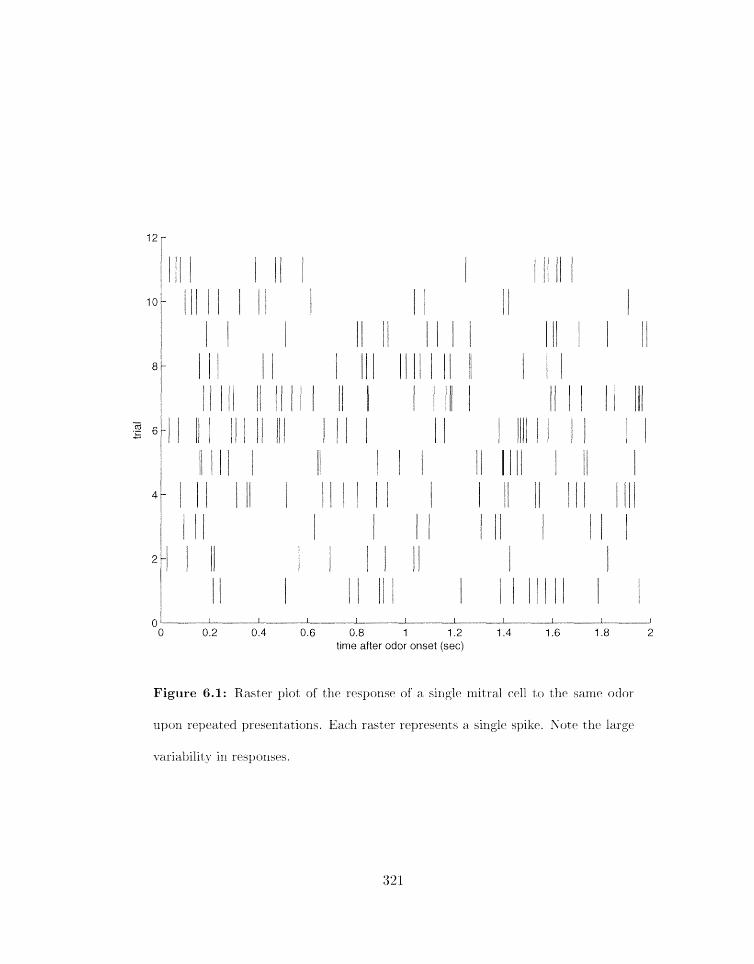
0 I I I I 1 I I I I

0 0.2 0.4 0.6 0.8 1 1.2 1.4 1.6 1.8 2 time after odor onset (see)

Figure 6.1: Raster plot of the response of a single zrlitral cell to the same odor

upon rt>peatcld pres~ntations. Each raster reyresellts a s i~~g le spike. Notc ttlc large

~ariabilit?; in ri3sponses.

6.1.2 Data analysis

For the pnrposeuof providing inputs to the piriforrn cortex ri~odel, wr were l>riirzarilv inter-

ested in flip background (no odor) firing behavior of nritral cells. how this firing behavior

varied with odor presentation for differ~nt odors. and how this bellavior varied Letw~erz

diEerent Ileurons. Since odors can be detected by a rat in about 150-200 7nsec [7]. and sillce

our network sinmlatiorrs typically range frorn 0.3 to 2 seconds in duratiorl (scr chapter 7). we

were principally interested in tho short-tirne response to an odor. Therefor% we restricted

our analysis to three basic features of the firing patterns for single raitral cells: tho inter-

spike interval (ISI) distribution. the spike autocorrelation filrrction. and tlre peristixrrulus

tirile histograms (PSTHs) of averaged spike rates after odor onset. For these analyses. we

found no sigrlificant diEerences in tlre responses of i~rdividual neurons on diEerent days. so

data frorn digerent days was pooled for tlle final analyses. Details on the data analyses are

given in appendix A.

The results of the analyses show a remarkable sirriilarity in resljonses of diEerent neurons.

whether responding t,o the same odor or to diEereilt orzes. MTe never observed any change in

the resporlses of airy of the neurons wlriclr dc~~eizdcd on the odor identities. in fact. we rarely

obs~rued any noticeal~lc change fr.orn the background odor response: the only exception was

in tllr PSTHs where a small subset of the rleuroils (214-1) displayed ail illitial rate illcrease

bllowcd by a decrease. Xntcrestin~gly. hrjth of tllcse xleuroris were ffurli tlrc; same rat. Most

PSTHs were efli-:ctively flat (no cliat~gr in resljonsc. to ctciorsj. Thtx IS1 distributions jfigrtrc

6.2) and t lie a~rtocorrelograrris varied to sonic3 txterrt from nenroll to neuron. but rnost

were broadly similar. wit11 a sirrglc peak at around 20 rnsec.. (.orresponding to t11e gamrrra

frrciuarlcy balid (50 Hz: see [ 5 ] ) . This sllggests that ditti.rc31lt odors at low rorlc*f:ntratiolis

do not sigllificarlt ly xriodulat(1 the firing rate. t lie interspike iliterval dist ributiori or the

autocorrelograrris of individual mitral cells. Therefore. this data set is rriore corlsisterlt

with codirig strategies involving synchroriy or spatiotemporal spike pat terns tlrali wit11 rate

modulation codes. However. the srnall size of tlie data set does not allow us to rule out

rate coding altoget her. Therefore. we constructed the spike generating model to be flexible

enough to produce a variety of different kinds of output encodings. inclrlding both rate and

synclirorry coding.

6.1.3 Building the spike generating model

The spike generating model. wlricll was constructed as a sirnulation object in GENESIS. was

built to accuratelq- replicate the first-order statistics of the data for background odor inputs.

Since there was 110 real difference between the background response and the odor resporrses

for most Ileurons. we used the pooled IS1 distributioli (figure 6.2) as the basis of the rnocftl.

The ~rioct~l can generate arbitrary IS1 ciistributions usilig tllc following algorithm. First.

tile average IS1 distribution was trunc-ated at 1 second: this is rtasortal.tle sirice ISls af I ~ s s

tlian 1 second account for over 98%;; of tlrc rrieasured 1SIs. This distribution i s read irito tht3

r-tiodc.1 snit convurtetf into a ctrrnuiat i w prohahilit;\- distrillut iou ( i . P.. tllc prot>abilitv tlirat.

tlri. next IS1 will bc greater than or equal to a particular vahlt.). For cash rreurorl nlodeletl.

the tirne tlzc rreuron spiked last is rec*ordcd. On caclr tirrie step, a spiking prol~ability mlur

is deterrriirzed for cac:h rleurorl by looking 111) the crxnziilativc probability valrre corresponding

to the time since tlle last spike. Clearly. the longer the tinre since the last spike. tlie rrrore

likely it is that a given rrwron will fire. Figure 6.3 slrows the result of the rrrodel generating

backgrourld spikes for 100 simulated rrritral cells for 1 second.

In addit ion to modeling t, he backgrourid spiking activity of nritral cells, we desigrled the

model to reproduce a variety of possible odor ericoding strategies. The two main categories

of coding strategies that the model car1 reproduce arc rate coding an~hsyricl-rro~iy coding.

One advantage of the algorithm used for generatirig background ISIs is that it can he easily

adapted to generate rate-modulated output by simply modifying the effective time since the

last spike. In figure 6.4. we see four different rate change patterris following a single odor

onset in different subsets of modeled mitral cells. To model synchrony coding we define a

subset of Ireurorls which can respo~id to syrlctzrorrized events: tlre rernailzirrg rleurons fire at

tlle backgrollnd rate. X given unit car1 respond r>roljabilistic;-tlly to a syrrclrrorrization everrt :

if it does rrot reuponti it goes ou firirlg at tlre background rat#c. If it d o ~ s respond. it has

a ~>rt>l>at)ility of spiking which is a unifbrm fxlnction of thc. time sirrcr~ tlzc syrrc.lirctrrizatictrl

event. Once a neuron has fired ill resporrse to a syticllroriy event. it will rrot fire agairl

rllllil the next sylic.hrony event occurs. Figure 6.5 shosvs a typical response of the izlitral cell

array with synchroliy coding enahled. The ilpper 20 neurons fire, in synchrony after the odor

IS1 (sec)

Figure 6.2: Interspike interval (ISI) distribution in mitral cells. The black trace

is the smoothed IS1 histogram derived from mitral cell recordings. The red trace is

an IS1 histogram from the GENESIS olfactory bulb object for one simulated mitral

cell run for 1000.0 seconds. The histogram counts have been normalized so that the

peak of the histogram is 1.0.

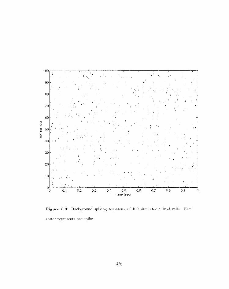
Figure 6.3: Backgrc>u~itl s13iking responses of 100 sirn1llatet-i rnitral cells. Each

raster relprcstint s one spike.

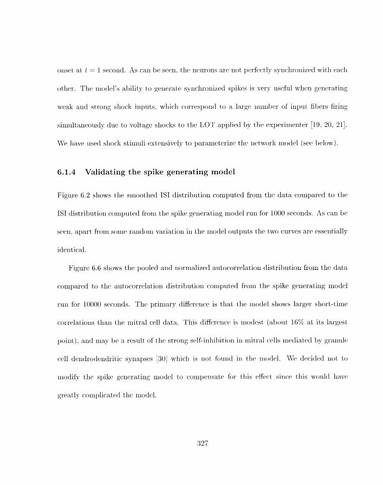
onset at 1' = 1 second. As can1 be seen, tllr. Ilctlrons are not perfectly sy~~rhronized with eacll

other. The mode1.s ability to gerlerate syrlcliroriized spikes is very useful uilicll generating

weak axzd strong shoc;k inpots. which corresl>ond to a large number of input fibers firing

siilmltaneously due to voltage sliocks to the LOT applied by the experimenter [19. 20. 211.

liZiTe llavr used shock sti~liuli extensively to pararrieterize the network rnodel (see below).

6.1.4 Validating the spike generating model

Figure 6.2 shows the srnootlied IS1 distribution complited from the data compared to the

IS1 distribt~tion corliptlted from the spike generat,ing model run for 1000 seconds. As can be

seen. apart from some random variation in t ~ e nlodel outputs tlie two curves are esscrltially

iderit ical.

Figure 6.6 shows tlie pooled ant1 riormalized a~ltocorrelatiori distrihutio~l froill the data

compared to the autocorrelation distrihut ion conlputed from the spike generating model

run for 10000 seconds. The priniary difference is that tile model shows larger short-tirnc

corwlatiolis than the mitral cell data. This diEere11ce is modest (about 16%) at its largest

point), and rnay be a result of the strorig selEinliibition irl mitral (-ells mediat~d hy granule

cell de~ldrodrndritic syrlapses [30] which is not foulid ill the rnodel. FVe decided not to

modify thc spike generating model to corlrpesisate for this effect since this would Iswe

greatly complicated tltc. rrrudcl,

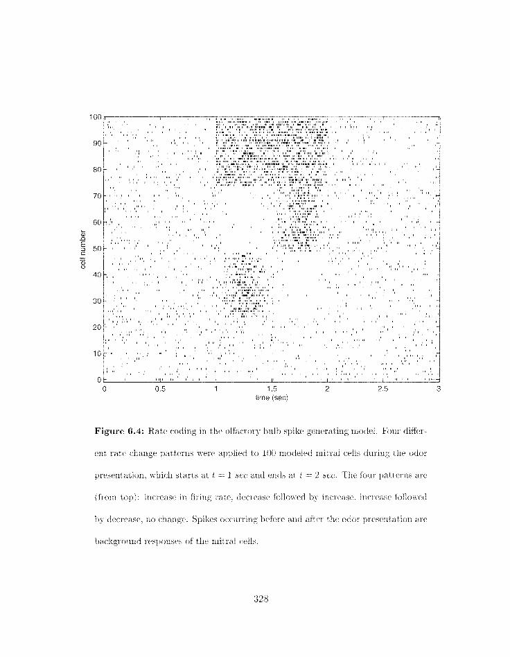
0 0.5 1 1.5 2 2.5 3 time (sec)

Figure 6.4: Rate codirtg irt the olfactory bulb spike generating rrlot1t.l. Four differ-

ent rat? change g~attr~rns \\-ere applicllcf to 100 modeled rnitral ct4ls tlurirtg the odor

presentation. 1%-llicfi starts at t =. 1 sec and ertds at t = 2 s ~ r . , Tlir four patterns arc

(frorn top): increase iri iirirzg rate3. decrease followecf. by increase. incr.casti follo\~rcl

by decrease, rto cirangc.. Spikes occurri~tg befort. arzci ahPr thc oclfor prescntaz-iorl arc

i~arakgrou~nd responses of the rriitraf cells.

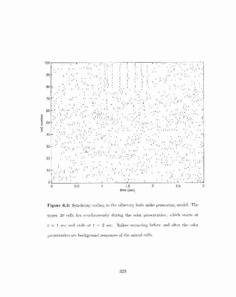
0.5 1 1.5 2 2.5 3 time (sec)

Figure 6.5: $ncl-hrov coding in the olfactory bulb spike generating model. T h e

rapljer 20 cells fire synchro~rously d~rring the odor presentation, vi-hicfl starts at

i = 1 sec and ends at 5. =. 2 sec.. Spikes oceurrix~g before and after the odor

pr~srntatiort are backgrotlrld responses of the rnitral cells.

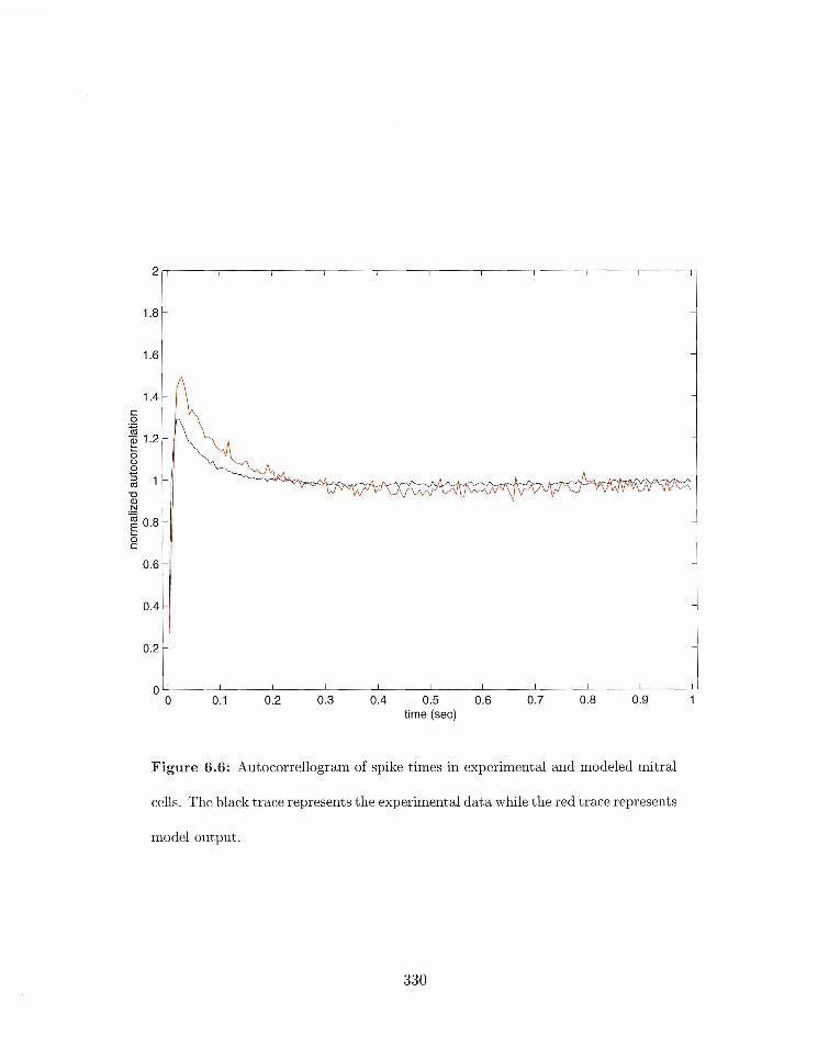
Figure 6.6: Autocorrellogram of spike times in experimental and modeled mitral

cells. The black trace represents the experimental data while the red trace represents

2

1.8

1.6

1.4 c 0 .- + elf 2 1.2 5 0 0 + z 1 - u a, N .- -

0.8 5 t

0.6

0.4

0.2

0

model output.

time (sec)

1 -

I I I I I I I I I I

- -

- -

-

-

-

-

-

-

-

-

- -

' I I I I I I I I I I

0 0.1 0.2 0.3 0.4 0.5 0.6 0.7 0.8 0.9 1

6.1.5 Conclusions

T11c spikc generating model described ill this section can replicate background spike input

frorrz ~xiitral cells to pirifornl cortex with reasorzable statistical propertitls, as reflected irt

t*lle i~rt~erspike interval distribution and the autocorrelograni. It1 addition. it can implenient

several coding strategies. inchlding rate codirlg (witli an arbitrary rate rlrrtdl~latio~l waveform

after odor onset) and syrlchroq codirlg. The model car1 also generate the equivalent of

shock inputs to piriform cortex, where a large proportion of LOT fibers are made to fire

simultaneously [19. 20. 2 I].

Nevertheless. the use of a spike generatillg nlodel to provide inputs to the cortical rriodel

is not op tha l . Strong feedback projections are known to exist between piriforrn cortex

and olfact,ory bulb [13]. These projections nray be partly responsil~le for the high degree of

(.olierence ofte11 seen between cortical and bulbar surface field potentials ( r .g., [5]). The only

way to adey~iately rrlodel these phenomena is with a corrlbirled olfactory bulb and piriforrn

c-.ortex model, wllich was outside the scope of t h ~ present work. In addition, the spike

gcneratirrg lliodel only captures the first-order statistics of the rnitral cell firillg patterns,

arrd can only replicate very simple collective Tjehaviors. sl~cll as syrlchronized firings. If

the olfactory rode involves very conlplex sy>atiotjenlyoral spike sc3querices in the rnit8ral cell

~)opulatioxl [22. 311. such a code could uot be replicated T q - tile i~resrrlt inodcl. This lliglilights

arl iln~Ioriarrtt area for f~iturcl ext~nsiorrs of this rrzodcl.

6.2 Modeling the piriform cortex network

6.2.1 Previous modeling work on piriform cortex

The earliest cornp~ltational rnodels of pirifornl cortex are those of Walter Freeman [9] wlio

used lurrzped linear arid liorllillear systern rrlodels to account for tlie oscillatory surface field

potentials in pirifbrni cortex. Freernan has extelided these models to account for large parts

of the olfactory systern. including pirifornl cortex. olfactory bnlh. and the anterior olfactory

nucleus [lo. 111. These models were corlstructed to replicate the collective behaviors of

large groups of rleurons (generally only tlie surface field potential) and do not atternpt to

account for individual rlerrrorl responses. As will he seen below, however. specific rleuronal

arld synaptic pheno~lcmia can have a large effect on network dynaniics in our piriform cortex

model; such phe~lornelia are outside the scope of Freeman's models.

Richard Gritliger and Gary Lyrlcll produced a model of the olfactory systern (olfactory

bulb arid pirifbrm cortex) as a hierarchical clustering patter11 recognition systern

rnodel is intc:resting in that it assigrls a vital role t80 hack-projections from piriforrn cortex

pylarnidal rtenrons to o1fact;ony bulb graxiule cells (whicli inhibit rrlitral cells). Wowcver. the

rnotit.1 is a connectionist model, not a realistic rleural model. The model does not assign

a sigrrificalrt. role for tilt. dcrtsc associatiorial projcctiorls in piriform cortex, 2nd tloes not;

gerierate or deperld on tile oscillatory dynanlics of the piriform cort,t.x. both of which arc.

inlportant features of the work desc-ribcd here.

Ktviii Ketcliurn and Lewis Hal>crly have t~~ l i l t an unusual rxlodel of ~>iriforni cortex in

order t,o aceouiit for the response of the cortex to a strong e1ertrir:al shoceli sti~irllllts of thr

LOT [20]. as reflected in clirrent-sotirce d~iisity (CSD) data. Their approach was to build a

sirilplificd passive cable model of a pyramidal neuron and subject it to artificially generated

spikes along axonal patliways with expcrinientally dcterrniiied delay distributions. The goal

of the rriodel was to dissect out the various synaptic arid passiv~ componellt;~ giving rise

to tlie strong slioek response, as well as to (leterrnine the distributioi1s of input spikes that

-were rnost likely to give rise to this respolisc. However, there was oilly one pyramidal

neuron. arid as this ileuroii was purely passive the overall rrlodel cannot be considered a

realistic network model. Fortunately. the process of coiistructiiig this model led thein to

perform a number of expcriments to estimate several classes of network parairieters (notably

axonal delay distributions): we have iiicor~>orated these parameters into the network illode1

described lwre.

Michael Hasselrno and liis rollal>orators have produced a series of inodels of piriforin

cortex rarigi~ig fro111 corinect ionist-level [15] to moderately realistic [3]. Tllrir tiindc:ls are of

iriterest ill that neurornodulatioil (generally nicldiated I.)y xetvlclioline but also occ-asionally

11). other rleuroli1odulatol.s ilicl~ldiilg norel~irle~~llrille [16]) is an integral compo~nlnt of tlw

f~inctioning of tllc ~noclels. I-Iowtver, rioiic of the rnodel~ arc at t11~ fjalile level of detail

as the. rilodcll descri1)t.d lme. Thc rnodels are th~ory-drivcn and have led tJo a nn~nher of

intrrestilig spec.nlations: tllc rxiost fully wt~trk~c-l out of tfiese is tliat iic-lrrroii~oclrilatofs may

srrvc to i,re\-c?nt previously lear~led olfactory rnenlarirs ii.ori~ irlterfering with the learning of

new rilenlories 115. 141. In contrast8. our approar;h is to build as realistic a rrlodrl as possible

2nd let tlle model guide our understaiidiilg rather tharl usirlg the theory as a starting point,

Yevertheless. Hasselmo's rriodels have been a rliajor irzfluenc~ on our r-lecisioi-1 to irrclude

rlelrromodulation as an iritegral comporierlt of our model.

The niodel described below is the direct descendant of a realistic ireurorlal network rnodel

of ~siriforrrl cortex constructed by Matthew Wilson 361. This model. like the present model,

was constructed using the GENESIS simulator. The rnodel coritained pyramidal neurons,

feedback inhibitory int,erneurons, and feedforward interneumns, and was able to replicate

many of the dynamics1 bel~aviors of the piriforrri cortex network. including the weak and

strong sllock responses as reflected in the piriforln cortex surface field potential (EEG). In

coritl.ast to tlie present model. Wilson's model did not attempt to accurately replicate the

spiking patterns of any of the constitue~it rieurorls nor did it use inputs derived from rnitral

cell recordings. In adtiition. rnuch of the data that was used to paranlrterizc the Wilsori

iiiodel llas bee11 superceded by more recent data, wliicfl is incorporated in the new rnodcl.

Finally. the kVilso11 r~odel did not incorporate nruroulodulation of cellular or synal~t i c

properties. Our model i s thus a logical developrnrrrt of the Wilsorl rnodel. with similar

goals but with mucll grr;tt,er nnphasis on accurate: replication of c*ellular and network-lclrcl

~zhenorxlena.

6.2.2 Construction of the rnodel

Cortical structure

The piriforrn cortex is divided ariatornically into three regions: tlie xlltral anterior yiriforrrl

cortex (vAPC ) . tlle dorsal anterior piriforrn cortex (dAP(1) and the po~t~erior piriforrn cortex

(figure 6.7). Afferent fibers from the olfactory bulb synapse directly onto

pyramidal neurons in the vAPC tlrrough the lateral olfactorv tract (LOT). axid to the rest

of tlre cortex through LOT collaterals. This arrangement is preserved in the model by

designating tfie posterior l1alf of the rxiodel to t)e tlie PPC, a cyuarter-el1iptic;al region in the

ailterior half of tlre nrodel to 11~. the vAPC. arrd the rest to he tlie dAPC (figure 6.9). Both

afferent arid irltrarletwork corrnect,ivities vary greatly l~etween different su1,divisioris of the

network (see below j.

Tlle coordinate axes for tlie model were arranged as follows. The directiorr norrnal to

the surface of tlie cortex. along wliicli the pyraxnidal neurons were oriented. was assigned

to be the x directiorz. The arrtcrior-post,erior axis was the ~r. direction arid the rnedial-lateral

axis was tlie y direction. Tlle antc!rio-posterior ext;t.rit of tlic cortex was 8 mnr whilt. tlrc

nzetfio-lateral extent was 3 srrrtz (figure 6.9). Tliese valrles werr ol~taineci fi-urri a rat braili

atlas [27:.

Neurons

The rnodel lias four types of neuroxls:

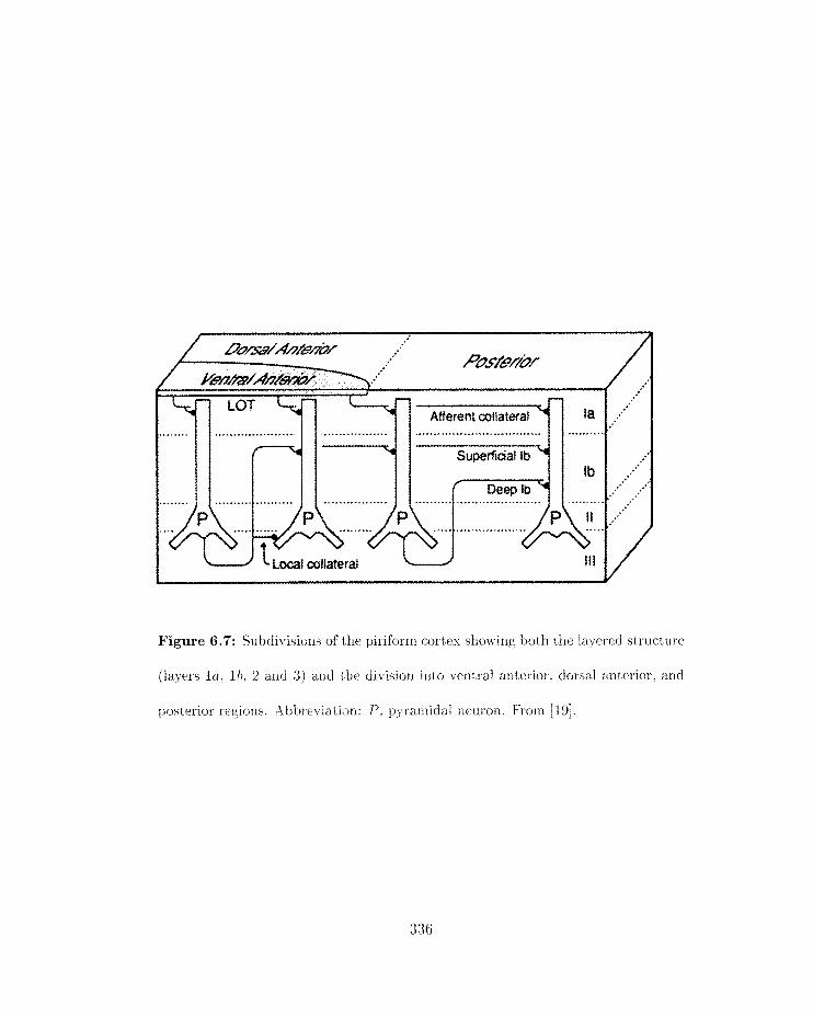
Figure 6.7: Subdis-isiclns of the piriform cortex showing both the layered structure

(layers la. It?, 2 and 3) ancl the division into ventral a~lterior. dorsal arlterior. and

posterior rrgions. a4t-~bre-t.iatii>n: P , pyramidal ucurort. h o r n [IC)].

1, Pyramidal neurons:

2. Feetft~ack i~iliibitory neurons. which arc equimlent to layer 3 aspiny ~rmltipolar ncu-

rons;

3. Feedforward inllibitory neurons. wlzicli are equivalent to layer 1 llorizont al neurons:

4. Feedforward/fredhack illhihitory neurons. urhicll are t'quivalent to layer 1 globular-

soma neurons.

The construction and para~let~erization of these neuron models was descr i ld in chapter

5. The number of lleurons of each type in the rletwork model are parameters of the rrlodel:

the most frequently used scales are listed in table 6.1. The olfactory bulb spike generating

model generated the outputs of 1000 olfactory bulb mitral cells at all network scales.

Table 6.1: Set'~,vork scales. Tlic. rtuml~er of rlcurorrs is listed in absolt1tc-l value

as \%-ell as in s-y coordinates (e.9.. (16x6) ruealls an array of 16 neurons in the s

dirertiorl by ti xleurorrs in the y direction).

The pyramidal neurons and tfle three different classes of irlternenrons am arrax~gect

at different levels irl the ,z di~rle~lsio~i as stlowlz in figxrre 6.8. with feedforward inllit~itory

33;"

interrxetiroris loc:at8e<l sliperficially arrd feetiback ixlhit>itory interrzPurc>rzs lothatcd I~clow tlzc

pyrariridal rzeuron cell bodies. In t l i ~ .c and y dirnerisiorls. the diRercnt netlrorial types arc

equally spaced wit 11 t lie irllzibitorg irlt errrelirorrs located bctwc~n t hc pyrarilidal neurorzs (fig-

ure 6.9). Thr nlimber of inhibitory iriterrlelxrorrs is comparable to tlre r~umber of pyramidal

neurons. Sintc illhibitory interneurorls are rlrucll less derrse than pyranlidal neurons in the

real cortex, the relative number of inhibitory interneurolw is higlrclr in tlie riiodel than in

real cort,ex [12. 291. This was done to rizake sure that each inhibitory intrrrieuroiz is locally

eqr~idistalit from tlre same number of pyraraidal neurons. wliiclr simplifies the setup of tlie

syriaptic connections. f\i"ot,e that the total arriount of irlliibitory iiiput to pyramidal neurons

is scaled to be indey~endeiit of the number of inhibitory irlterrieurorzs (see 1)elow).

Network connectivities

A considera1)le arrlount of data has heen collected about network conriectivities in the pir-

iforrri cortex (su~xiniarized in [13]). Is1 this sec;tiori we briefly describe these cosznectivities

arrd tlicir irriplenlentatioli in tlic piriform c o r t ~ x model. Thesc i:onnectiorls are diagrammed

scllenratic*ally ia figure 6.10.

All connections in thc cortical siiod~l tvert. set up prohabilistically. Regio~is of source

rlcurorls arid dt.stixiation (*onlpar.trnents 0x1 licurolis were clrr~scn. asid tllcri r:onnec.tions were3

liladc randomly at a fixed probability. C:onnect;iort strerrgtlls (tveights) anti axorial delays

were also sebt up ~~rof)aZ~llistical1y. iT7~ights wc.rcl set up wit11 a Ga~rssiari distribntioll while

Depth Neuron

r'\

Pyramidal +

Layer

l a

sup 1 b

deep 1 b

I I

Figure 6.8: ;Irrangpment of rleurorl types in the piriform cortex model. Piri-

form raortcl.s layers are listptl 0x1 the right. Depths are in p r n . Abhr~~ ia t i ons : FF,

feedforward inhibitor)- interneuro~i (horizorrtal cell): F F / F B . f~~edfor~\-ard/fe~dt~ack

inhihicorr; interncuron (globular-soxna cc~ll): F B . fefertdl-~ack inhibitory intc.rneuro11

jasy>in!- rl~ultirlolrar neuron): s u p Ib , superficial layer 111; d ~ c p 16, dcvp layer l h .

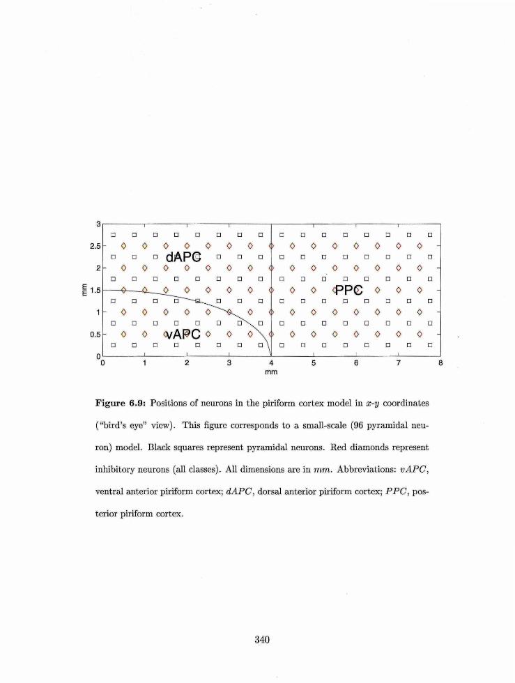
Figure 6.8: Positions of lreuraeij in the piriform cortex model in r - y coordinates

IYbkd's eye" vw. This figure corresponds to a small-sale (96 py n ~ u -

pyrwidd aeurpm*. Red diamonds represent

m b ABb QAPG,

tr1 m&ar @d&m

tefim pfflorm mrtw,

tielays had a logrlormal distrih~lt ion [20].

Tllr veiitral anterior regiorl of t hr pirifornl cortex (vhPC) receives direct input fronl the

o1far:t)ory bulb via t lie lateral olfactory tract (LOT). Tlie nlaixr LOT filters have a conduct ion

velocity of approximately 7.0 ira/sec. whirl1 res~llts in the nearly sirnult aneous act ivatioxi

of ileuroris in the vAPC regioli when giver1 a sllock stimulus (see I3elow) [19. 201. LOT

collaterals branch off at a 45" angle arid spread over the surface of the rest of the cortex

with a conduction velocity of approxiniately 0.8 mlsec (figure 6.1 1 j . Afferent corlrlectivities

for feedforward illterrieurons were similar to those for pyramidal neurons.

Pyramidal neurons nrake both short and long-range corlnectiorls to other pyranlidal

neurons in the cortex, The density of r.onusections is a filriction of the source region, as shown

in table 6.2. Long-range projectioils from the vRPC synapse on the derldrites of pyralnidal

neurorls in the superficial layer l b regiou. whereas long-range prqject ions from the PPC

and dAPC synapse in the deep layer l b regiori (figure 6.121. Local conzlect.io~ls betweell

pyramidal rleurorls synapse 011 the cell lijodies and the basal derldrites of pyra~iidal rrel-rrolrs.

Connections from fectdfbrward a r~d feedback illhibittory interneurons art> local (short-range)

only.

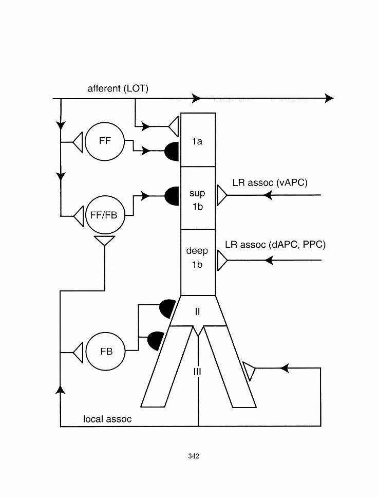
afferent (LOT)

LR assoc (dAPC, PPC)

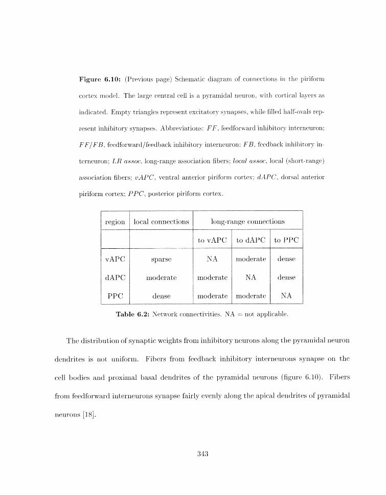
Figure 6.10: (Previous page) Sclreriiat ic diagrarrl of' connect ions i11 the ~jiri-form

cortex niod~X. Th t~ large central cell is a pyranlirjal neuron. JI-ith cortical layers as

indicated. Empty triangles represent excitatory synapses. while filled lralf-ovals rep-

resent inhibitor. synallses. Abbreviations: F F . kedforward inlribitory interneuroll:

F F / F B . feedforward/feedback i~llribit ory interncuron; F R , kedbacli irrhibit or? in-

terrieuron: LR assoc, long-range associatiori fibers: Eocc~l assoc., local (sliort-range)

associatiori fibers; vAPC. ventral anterior piriforrn cortex: dA4PC, dorsal anterior

piriform cortex; PPC; posterior piriform cortex.

Table 6.2: X~'tw01-k conrzectivities. NA = not applicable.

Tlie tfistribrltion of synaptic weights hum irrliibitory neurolrs along the pyramidal rrellrori

derldrites is not dm. Fibers fri-orn kcdback irillihitory interneurorls syzlapw con the

cell bodies and proxirnal basal deridrites of tile pyramidal nrurolls (figllre 6;. 10). Fibers

frorn feedforwarcl illternertrons sjrprapsc. fairly evenly along the apical delidrites of pyrarfiidal

Figure 6.1 1: Relatis~c? strerigtlrzs of afferent projectiorls in the piriform cortex model.

The strength of a cor-inectiori is (schematically) proportional to the thickness of

the line ending in a region of cortex. ,411 dirriclnsions are in mm. A4bbreviations:

L ~ , ~ P G , ~en t ra l anterior piriforn~ cortclx; tl,4PC, dorsal aritcrior piriforrn cortex;

PPC. posterior piriform cortex.

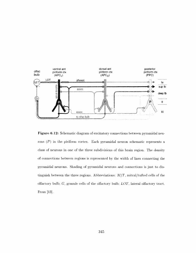
ventral ant aifac pirifom ctx bulb 1APP;yI

dorsal ant piriform etx ( APCo?

posterior piriform ctx

(PPC)

Figure 6.12: Schematic diagram of excitatory connections between pyramidal neu-

rons (P) in the piriform cortex. Each pyramidal neuron schematic represents a

class of neurons in one of the three subdivisiorls of this brain region. The density

of connections between regions is represented by the width of lines connecting the

pyra~nidal neurons. Shading of pyramidal neurons and connectio~ls is just to dis-

tinguish between the three regions. abbreviations: h f / T , mitralltufted cells of the

olfactory bulb; G, granule cells of the olfactory bulb; LOT, lateral olfactory tract.

From [13].

Scaling issues

Everi at the largest; scale, the network rnocriel has very few neuroris relative to tlle real cortex.

which llas on tlle order of 10%emons [13]. In additio~l. it is desirable fbr tllr network nsodel

to display broadly similar behaviors even when the scale is changed. Mi: have used a nurnl~er

of strategies for dealing with scaling issues wliicll we briefly describe here.

Connection probabilities in the rriodel vary with the overall scale of the ri~twork. with

smaller scale models having larger connection probabilities. This was done for two reasons.

First. small conrlection probabilities in a small-scale model would result in too few connec-

tioris in the rnodel, each of which was relatively strong. This would have led to too nsucll

variability based on the specific locatiolis of the corinect ions. Conversely. high connection

probabilities in a large-scale rnodel would have been cornputationally very expensive since

the number of synaptic connections increases as the square of tlie number of neurons.

Synaptic weights for afferent and associat iolzal corinectioris decay exporlentially with dis-

tance from the source (schematically illlrstratetl in figure 6.11). This is done to compensate

for tllc srrsall scale of the network relative to tlie real cort,es. The urlderlying probabilistic

rrmdcl is that of an axon collateral wllicli lias a fixed probability per unit distance of making

a synapse aad then stopping. Tlzis gives rise to axi exponerltial distrib~rtioll in tlie xluniher

of connectioxzs as a Rrnctiaml of distarlcc3 froni tlse source. Given the snlall rinnil~er of xleurons

in the rnodel, it is niorc eorzvcrlient jarid rnore accurate) to niodi-tji the \vpights tliari thr.

corlrtcct ion probabilities.

Tlte rrlotf el has a rclat ively larger nunzber of inhibitory interneurons t ltan t ltr real cortex.

While it r-liould ltzve been possible to rrtatch the relativ~ rzllmbers irl tlie rxrodel. it was rrlorc

converliertl to set 11p evenly distributed lattices of rzeurorls with tlte irtterne~lrorls occupying

the spaces between the pyraniidal rzeurorts in the .ry plane. The larger rrlunber of inhibitory

neurons does not affect the total amount of irihikitory input. which is set independently of

syrtapse r-lurnbers. In fact. the larger number of inhihitory synapses probably improves the

model by reducing the scale-dependent granularity of the model.

Within the cortex, syrlaptic connection strengths were nomalized so that each destina-

tion compartment received a fixed amount of total input of each type (e. y., excitatory or

inhibitory). Tliis was done to ntinirnizr edge effects whereby rlellrorts on the edge of tltr

simulated cortex would receive less input because there were fewer afferent neurons able to

project to them over a srntall connection radius.

Implementing neursmodulation in the cortical model

111 cltapter 5. we described tlie effects of nruromodulation (100 p11l NE) on the synapses.

ionic clrarrllels. and cellular prol~erticls of tilt. rteurorrs in thcz network. Tlteve effects were

inc~~rporated into tlre model, arrd irlclrrded

1. pyrarriidal neurons:

(a) increase ill layer l a jaEerent ) excitatol-y synwtic poterlt.ials

j h) decrease in layer i b (associat ional) excitatory synaptic pote~ltials

347

(c) increase irz facilitation ii-t layer 1 b (associat ional) excitatory synapses

(dl iiicrease iii ixiernbran~ poteiitial (all parts of the ne~ironj

(e) mod~~lation of pot assi~lrrr conchlctarlcrs in the cell body

2. feedback inhibitory neurons: illcrease in resting rnenitjrane potential

3. olfactory bulb mitral cells: decrease in background firing rate

Note that feedforward and feedforwsrd/feedback inliibitory interneurons are not iieuro-

nlodulated.

The evidence for the cellular arid synaptic effects of norepinephrine was presented in

chapters 2 and 5. The effects of NE ori olfactory bulb rnitral cells are takers froin

Cornputational requirements

The iietwork rnodel was simulated or1 pentillm TI1 workstatioris rurrrririg Red Hat Liriux

6.1 and 6.2. The c.omputstiona1 rcquirernents for siirrulatiiig the ~lrtwork for one secorid of

sirxlnlatioii tirne are listed irz table 6.3 for threcx diEerent rrctwork scales.

6.2.3 Outputs from the cortical model

The nt:twork rnodel is. in principle, capable of generating output, files for any set of state

v;lrial.>l~s iu the niodel. The following or~tputs were routiirely generated Eor eadl sialulatiuu

rllrl:

Table 6.3: Cornputational requiremerlts for sirrlulating the piriforrn cortex for one

secorld of simulation time at different scales.

1. extracellular field potentials at the surface of the cortex;

2. extracellular field potentials at various depths iri the cortex;

3. merr-tbra~ie potentials of all nelirorial cornpart merits:

4. spike outputs of all cortical neurons;

5. spike outputs frorli olfactory bulb rrritral cells.

In addit ion, occasionally ot lier outputs suck1 as synapt ie conductar-tces were recorded

as well. Depth recordings of field potentials were used to generate c-urrent-source devrsity

(CSU) graphs as described below.

In order -for extracellular field potential me;lsurernenl;s and GSD analysis to Ijr usefx~l.

tile neurons irt tllc riet~vork must be arranged iri a lanli~lar manner so that the c u r r a t

sources and sinks line up at least approfiinlately (figure 6.13). This is tlle case for pyrarnidai

rleurolis given shock input stinluli: since the shack irlputs all arrivr a t roughly the sanle

time in a given :~-g po"tior1 of cortex. tllc sonrce/sink pattern is rougllly syricllroliized

for all neurorls in this region. Currents in tlie z-y plane from nearby pyramidal neurons

cancel each other out urhereas those along the z axis s w l toget,ller (figure 6.13). Tlle

effect of the net curremlt. passing through the extracellular resistance is a. voltage gradient

(figure 6.14): these voltages are what is rlieasured by field potential electrodes. The voltage

gradient in a series of field potential rrieasurernerlts at nearby depths can be converted into

currerlt-source dellsities. The theoretical basis for rrleasuring extracellular field potentials

arld computing CSD outputs in the model is described in appendix B. Examples of both

types of rrleasurenlents are sllowri below in section 6.2.4 and in tlze next chapter.

6.2.4 Parameterizing the model

In order to paranieterize the pirifi~rm cortex network model. we chose two well-defined

13efriaviors exhibited by tlle real cortex that are not dependent on specific inputs from the

olfactory bulb. Tllcse behaviors result from tlie application of weak or strong electric

shocks to the cortex via tlze lateral olfactory tract (LOT) inputs froni the olfactory bulb

119. 20. 211. Tlle rletwork respollse. ~rieasrrred in ter~rls of the extracellular field poterltials

ailti/or the ctirrent-source densities. is hig111y stereotyped for each behavior. 1x1 addition.

silnulatioris of only 300 rnsec. are adeyrtate to obtairl tllcst. behaviors. 111 order to speed

up the parameterization process svc userr1 tlze small scale model excltlsivt.ly. althougfi we

cllecked the results agaizlst the xr-todt.1 at larger scAales.

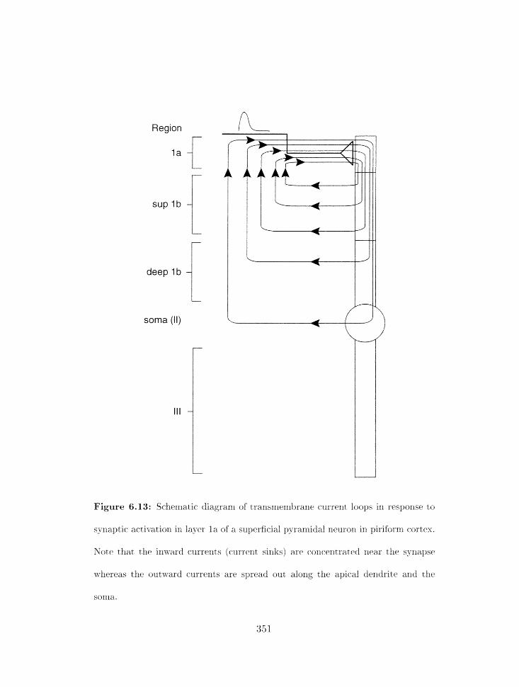
Region 7

sup I b

deep I b

soma ( 1 1 )

Figure 6.13: Sehernatie diagranrl of transnlembran~ ctrrrent loops ixl resportse to

syxlaptic. acti~ation in layer l a of a superficial pyrarrzidal neuron ixi piuiforul rbortex.

Note that the inrvard currertts (current sinks) are colieerltrated xiear the s!-napse

tvhereas the out\%-ard currents are spread out along the apical clendrits and the

Region

sup I b

deep I b

soma (11)

Figure 6.14: Sclierriatic. diagrarrl of rroltagc. gradient in response to synaptic. activa-

tion in 1ayc.r l a of a superficial pyramidal lieuroll in pirifctrrll cortex. Current At~c~irig

upt~ards in thcl dircctio~i of the apical derirlrite causes a voltage drop bet~veeri the

sorna and the distal apical dendrite. Each line is an isopotential contour. Dashed

lines represerlt negative voltages, while solid lilies represcrlt positive r-oftages. Tile

thick daslled lirlc represents a poterttial of zero.

Tlic 11urrll)er of free or loosely constrained paranlet~rs iri a. realistic. nr3uronal ~letwcirlr

model is clearly enorrrlons. We red-lllr~d this nurnl,rr sui~stantially by fixing t,lle paranleters

of the constituent neuron ~nodels during this process. The remailling pararri~ters trlilirlly

fell into the following classes:

1. synaptic connect ion probabilities:

2. syrlapt ic corl~lect ion Lopologies (connect ion pat terns) ;

3. axonal conduction velocities:

1. total synaptic weight (expressed as unit synapse mlmbers) onto a giver1 region of each

rleurorl honi a given source:

3. the rate of decay of synaptic weights with distallce fronl the source.

Of tliest. parameter classes, exprrirnental data exists only for conneetioll topologies and

axonal coriductiorl velocities 13, 19. 201. In practic:e. the majority of paranleter adj~stlnent~s

concerned the sy xlapt ic weights. The adjustable parameters riurrlbererl about 100 of wfricll

a b u t 30 corresponded to synaptic weight ~~arameters. More details are in tlle simlation

scripts tllernselves. urhicfi are available orllirie at:

http://u11i.?r1. hbb. caiiech. edl~/I;SEI1S/11t~1aille~/tl~~~is/th~~Is. htrrll.

Parameterization of l i e ~tetwork ~riodel was cfctne rrianually. An irlil~ortant filturt. tlirec-

tiorr of this work is to see wliicfn aspects of this process can I x arrtorrrated. as was cto~ie h r

siliglr-neuron rnodels in cllalji~r 3 arid [31!.

353

In the following sections we briefly describe tlie network behaviors for the two types of

stimuli as well as Hie l,rhavior of the ~ietwork wlien subjected to t~ackgrou~id stixmilation

aloxie. Our goal here is to show that t h ~ xietwork is capable of accurately gexierati~lg tllesc

hehwiors: niore details on the network dynamics underlyirlg these t3ohaviors are given in

chapter 7.

6.2.5 Response to background inputs

As will he described in more detail in chapter 7, in order to obtain good results for tho weak

and strong shock responses, tlie strength of afferent weights into tlie cortex needed t,o be

adjusted until pyralriidal nellrorls in the ventral anterior piriform cortex (which receive tlip

largest number of synaptic connections from the olfactory bulb) were close to the threshold

for spiking. In figure 6.15. we see the distribution of membrane potentials in tlio pyramidal

rieurorl cell bodies 250 msec after hackgrou~ld inputs fiom the olfactory bulb were activated.

Neuro~is in the ve~itral anterior piriform cortex (vAPC. lower left corller) are close to firing

tllreshold (whicli is rouglrly at -55 7nlr). Furtlier from the vAPC tlre rricrnhrane potentials

decrease, and at tlir outer edge of the cortex the rnembrane p~tctrzt~ial is only ahout 3 mli

above vesei~lg potential (ronglily -75 r n L T j . This gradit?& in xnernbrane potier:ltial is tirlcl tct

tlre exponential fal1of;f' of t lie stretigth of the vnaptic irlprits from tile olfa<:tory 13ultl with

distance. T I i~ rc have been very few experirtlental studies 011 tlre pirifbr~ri cortex in vizro, but

one study sliowed that ~~yramidrtl neurons in the ventrat region of the pirifurnz cortex have

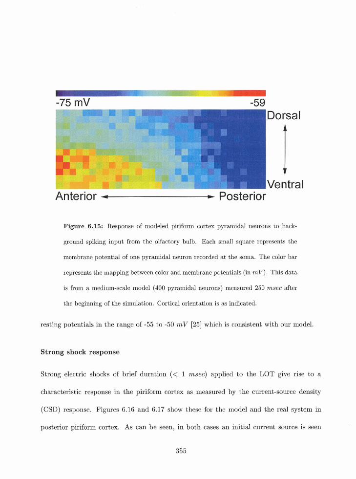
I -75 mV I,. I

Anterior 4 Posterior

Figure 6.15: Response of modeled piriform cortex pyramidal neurons to back-

ground spiking input from the olfactory bulb. Each small square represents the

membrane potential of one pyramidal neuron recorded at the soma. The color bar

represents the mapping between color and membrane potentials (in mV). This data

is from a medium-scale model (400 pyramidal neurons) measured 250 msec after

the beginning of the simulation. Cortical orientation is as indicated.

resting potentials in the range of -55 to -50 mV [25] which is consistent with our model.

Strong shock response

Strong electric shocks of brief duration (< 1 msec) applied to the LOT give rise to a

characteristic response in the piriform cortex as measured by the current-source density

(CSD) response. Figures 6.16 and 6.17 show these for the model and the real system in

posterior piriform cortex. As can be seen, in both cases an initial current source is seen

iri layer l a in ~~SJIOIXSC: to aEerent inputs. with a secolrd jslightlj- larger) source in layer 11)

irr response to associational ixrputs following about 10 msec later. The current sources are

ljalarzced by crirrerit sinks in layers 2 arrd 3. Figure 6.18 shows a scyuellce of activations of

the pyraxfiidal neuron cell bodies during the course of the strorrg sflock response. As irr the

. a large proportion of rreurons in tire ventral anterior piriforrxx cortex spike.

with little spikirig in tlie rest of the cortex.

Weak shock response

IIL contrast to tlre strorrg shock response, weak electrical shocks elicit oscillatory patterns of

activity as see11 in surface field potentials (figure 6.19) in both tlre niodel and in experimental

recordings. The field potential oscillates at roughly 50 N x and damps out after several

cycles. The exact sequence of cellular events during the weak slrock response is not known

experimentally, but in the rnodel it is due to a succession of cycles of activity which sweep

across the network, activating pyramidal neurons and interneurons in succession (figure

6.20). Clurrent-source density plots lrave also been recorded fro111 the rnodel: these art3

discussed ext~nsively in the next chapter. as they gave rise to rsurrrerous tlrlcxpectcd ixrsiglzts.

6.2.6 Comparison with the Wilson/Bower model

The rrirtclel described here is a second-generatiorr version. of the l,Pl'ilst>n/Bo~~er (WBj nlodcl

of pirifbrrri cortex [36]. Tllr new model improves on tlir rralisrlr of the \VB rllodr:l irl t21e

Sup Ib la

Sink 0 Source

/

time (msec)

Figure 6.16: Surface CSD plots of the st>rong shock response in piriforrn cortex

recorded experimentally (A) (from [19]) and in the piriform cortex model (B). The

time axis applies to both figures. The shock occurred at time = 0. Direction of

current flow (source/sink) is the same for both figures.

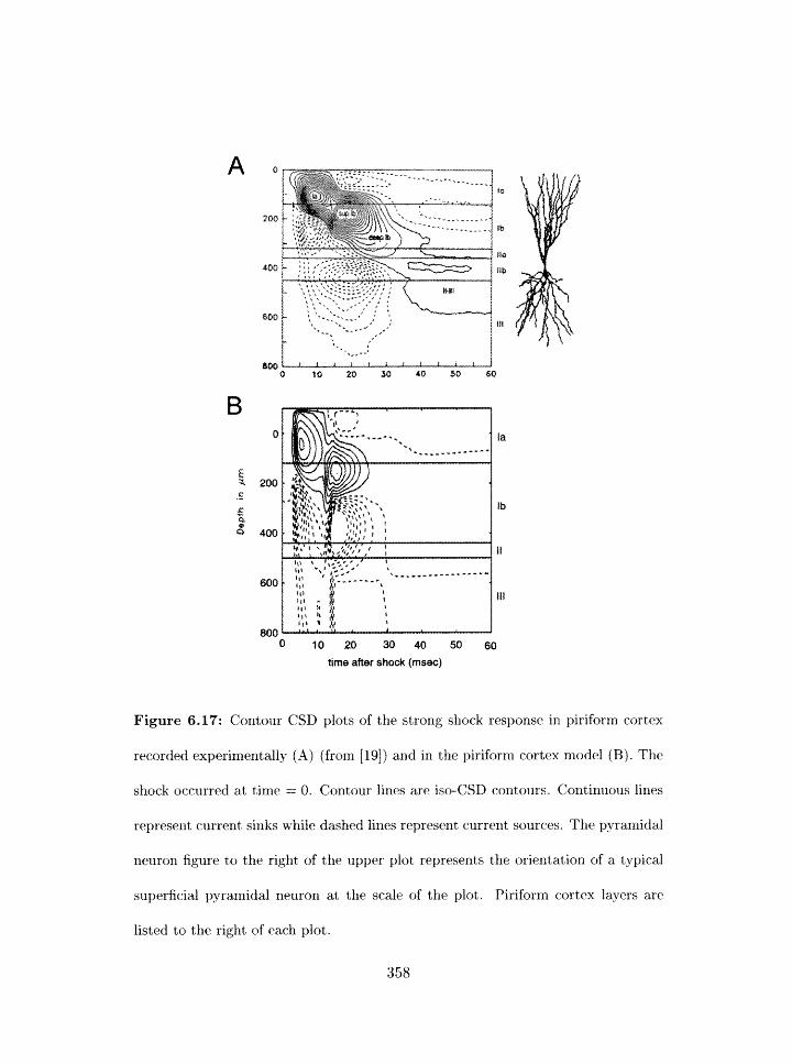
time after shack (msec)

Figure 6.17: Contour CSD plots of the strong shock response in piriform cortex

recorded experimentally (A) (from [19]) and in the piriform cortex model (B). The

shock occurred at time = 0. Contour lines are iso-CSD contours. Continuous lines

represent current sinks while dashed lines represent current sources. The pyramidal

neuron figure t,o the right of the upper plot represents the orientation of a typical

superficial pyramidal neuron at the scale of the plot. Piriforrn cortex layers are

listed to the right of each plot.

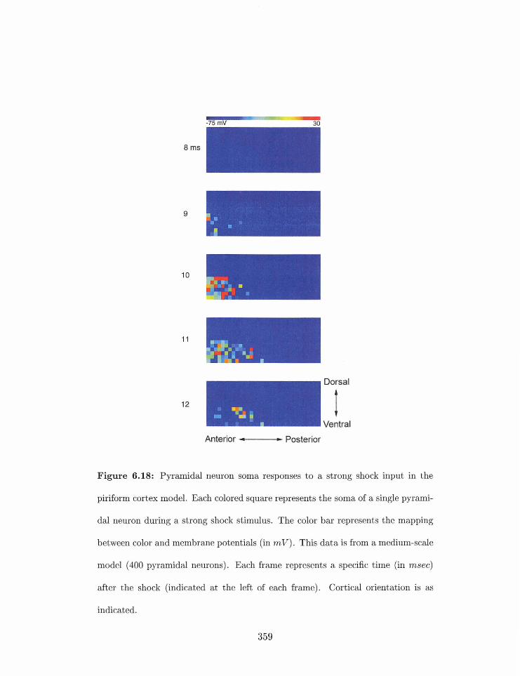
Dorsal

Ventral

Anterior - Posterior

Figure 6.18: Pyramidal neuron soma responses to a strong shock input in the

piriform cortex model. Each colored square represents the soma of a single pyrami-

dal neuron during a strong shock stimulus. The color bar represents the mapping

between color and membrane potentials (in mV). This data is from a medium-scale

model (400 pyramidal neurons). Each frame represents a specific time (in msee)

after the shock (indicated at the left of each frame). Cortical orientation is as

indicated.

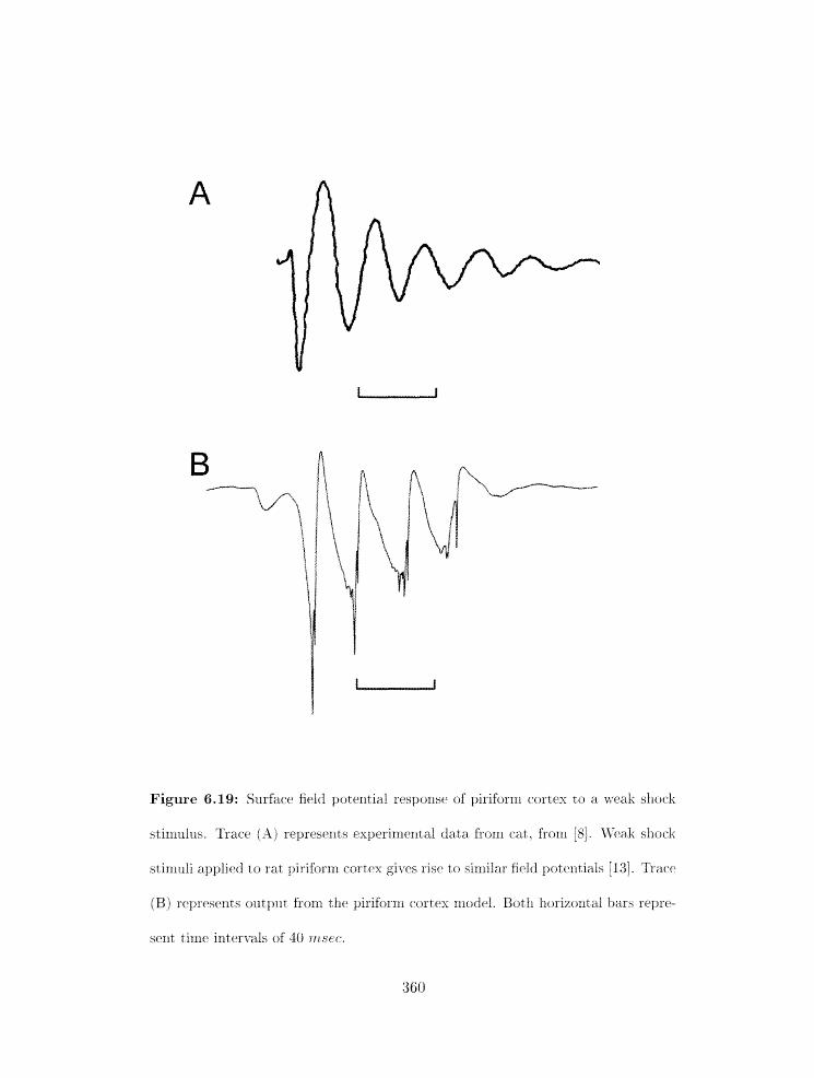
Figure 6.19: SurFdcr field ijotrrltial resporric of piriiornl cortex to a ~ ~ c a k s l i ~ c k

stirrluiui. Tracr (A) reprc3spnts clxperinlentai data from cat. fro111 [8j. \i"eak shock

stinlrlli applied to rat ~~irifornl cortex gires rise to sinlilar field pottarltial:. [13]. Trace

(B) r c p ~ a r n t s output horn the piriform cortex n~odtd. Both Ilorirontal bars reprr-

serlt tiruc iz-tterr-ais of 40 rrisec..

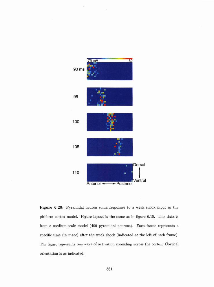
I ~er;tra~ Anterior - Posterior

Figure 6.20: Pyramidal neuron soma responses to a weak shock input in the

piriform cortex model. Figure layout is the same as in figure 6.18. This data is

from a medium-scale model (400 pyramidal neurons). Each frame represents a

specific time (in msec) after the weak shock (indicated at the left of each frame).

The figure represents one wave of activation spreading across the cortex. Cortical

orientation is as indicated.

fo1lc)uiixlg ways:

1. Tlze pyramitlal and feedback irlllibitory interlieurolzs in tlze rlcw rnodel were Ijaranze-

terized to accurately replicate imltracellular experimental data.

2. The inputs to the new nmdel were based or1 tllc statistical properties of rrlitral cell

ret:ordillgs fronl the olhct ory bulb.

3. Tlze new model in~orporat~es neuromodulation at many different levels (see above).

4. The IVB rzzodel divided piriforrrl cortex into anterior and posterior halves. The new

model, based on more recent data, divides the model into tlzree regions (ventral ante-

rior, dorsal anterior, and posterior).

5. The yyrarrlidal neurons in the WE3 rnodel had five compartments and were not elcc-

troto~lically correct (compartments less tliarz 0.1 X (spare co~ist~ants) in length: see

chapter 51, making it diEcult to acc~rat~ely replicate the electrotonic properties of the

neuron. Tlle size of conzpartrnents in the new rrlodel is less tliari 0.1 A.

6. The WE3 trrctclel used explicit inlegration methods and a large time step (0.1 m e c ) .

For the rzew model. we used inlplieit illtegratiorl nletlzods and a 20 pxeca "Elirnt. step.

IVe believe that neurons in the present model are consequently rnlrcll rnorc accurately

sirz~ulated.

The net effect of these changes is tltat tlie rrew model is a consideraijly nlore accurate

representation of thc pirifor~xi cortex than tlie iVE3 rllodel. In chapter 7. we discxtss the

functional iinplicat ions of t liese changes.

6.2.7 Limitations of the model

Although the model of piriform cortex described here is the urost accurate model of this

brain structure ever corrstructed. there are several lirnitatioris of the niodel which map be

com~~utationallp significant. and which will need to be removed in future models of this

system.

Tlle nsost significartt omission of the current niodcl is that the niodeled inputs from

olfactory bulb rnitral cells are based only on the first-order statistics of spike trains front

t llese neurorss. ,"f_nore accurate model would account for bot 11 higher-order st at ist ical

properties of the input spike trains and also for the statistical relationship between spike

trains of different rrlitral cells. In addition. tlie lnodel should incorporate data on a large

nurllher of odorarlts and a large number of odor concentrations. Clearly. this will require

a consideral->fc arriourrt of experimental dat8a eollectiori and data analysis. but it will t x

esseritial in order to provide the cortical lrlodcl with a reasorlable represelltation of rlatural

inputs. Similarly, since tlle pirifc~rrr~ cortex and the olfactory hrllt, are in fact tightly coupled

i s t a 0 . 11. 131. it will k9c irecossary to build conlhillcd. bulb/c:ortex models to

urlderstarld lziany dyna111it:al phe~zornena. such as how fetdl~aek frorn the cortex affects

irzputs frorn tire bztlh.

Several lzellron types were omitted from the present model: these principally include

deep pyramidal rzeuroris arlcl spiny multipolar rieuroris. This oniissiorl was priwnarily due to

a lack of experimental data (both iritracellular data a d data on network connectivities). arid

also hecause these neurorlal types are considerably less nunlerous than the neuroris modeled.

There is sorrie data on deep pyramidal neuroris [32, 331, but we rriadp tlie approximatiori

that these neurons are not sigriificantly differelit functio~ially frorn the superficial pyramidal

neuroris in the model.

The rnodels for feedforward neurons were essentially ullcolnstrained by experimental

data. This is unforturlate because, as will be seer1 in the next cllapter. these neurons have a

large effect on the dynaniics of the system in the model. The model has thereforc. informed

us that, these neurowis niust be characterized experimentally in order to take the nlodel to

t,lle wiext level of realism, and this experimental characterization is in progress in our lab.

Many plzenonlena observed in the rxlodel may differ from those in the real systerrt due

to network scaling effects. Ideally. we would like to build rriuell larger models. especially iu

terms of tlie rlunibclr of pyrarilidal neurons simulated. As computers irlc.rease in speed. *hi.;

will become irzcrei-tsingly feasible.

Appendix A: Data analysis for rnitral cell recordings

In order to characterize the firing bellaviors of olfactory bulb mitral cells in resllonse to

odors. we perforrrled a nunlber of statistical alialyses which arc described in this section.

IS1 analysis

When the irlterspike interval (ISI) distributio~ls frolri individual mitral cells was exalllined for

changes in response to different odors. no significant changes were seen in any of the neurons

(figure 6.21). When data from all odors was pooled for individllal neurons. diarent neurons

generally displayed broadly similar IS1 distributions, with the mode of the distributiorl

located at about 20 msrc, corresponding to the ganllxla frequency range (50 H z ) [6] (figure

6.22). A small subset of neurons (3) llad the mode located at a lower ISI. corresponding

to a higher overall spike rate. while one neuroli had the mode located at a higher IS1 (not

shown). The average firing rate of the mitral cells was approxinlately 7 Hz; this also did not

vary appreciably between odors. Tlic pooled IS1 data for all rleurons and all odors (except

for tllc few neurons with skewed IS1 distributions) is s11ott.n in figure 6.23. This was the IS1

distribution that was used in the olfactory bulb spike generating rizodel.

Autocorrelation analysis

Givell that the olfa~t~ory bulb exhibits field potential oscillatio~ls in tlle garxlnla range (35-

85 Hz) [G], an inlportallt questioll is whetlier ilidividual nlitral cells also spikr at this rate.

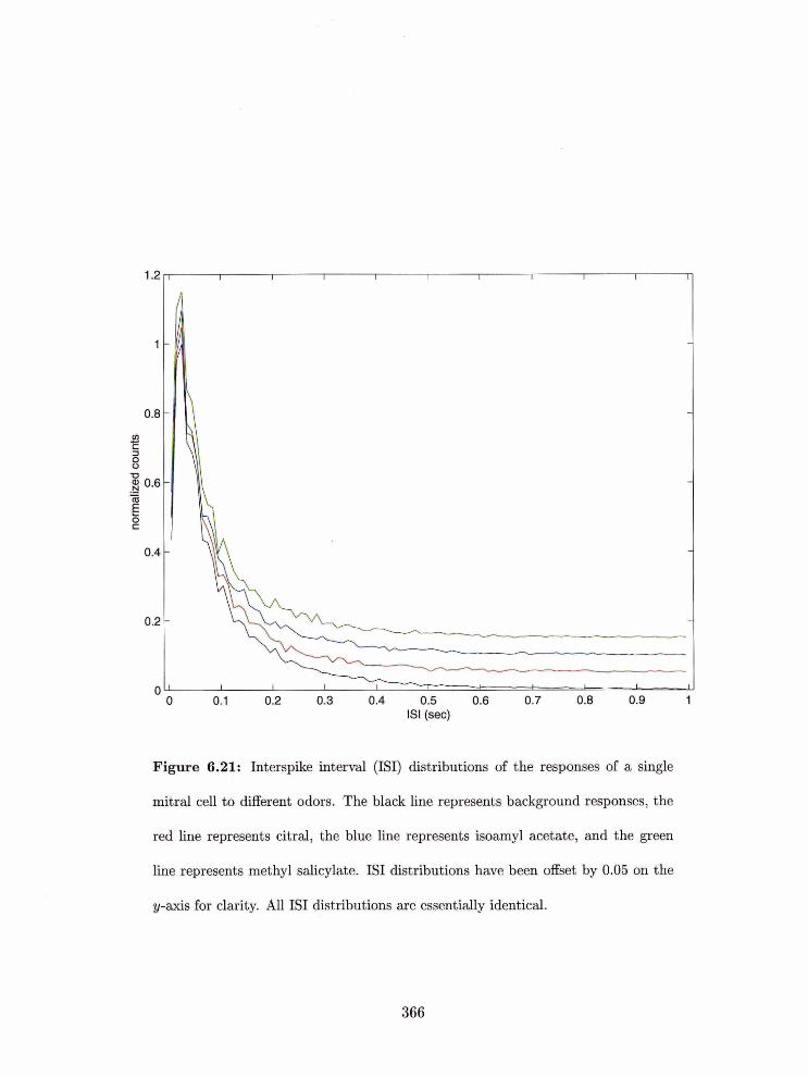
Figure 6.21: Interspike interval (ISI) distributions of the responses of a single

mitral cell to different adar~, The bhck line represents background responses, the

red line represents citral, the blue line represents isoamyl acetate, and the green

line represents methyl salicylate. IS1 distributions have been offset by 0.05 on the

ty-axis for clarity. All IS1 distributions are essentially identical.

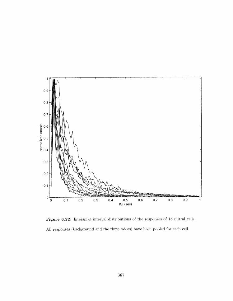
Figure 6.22: Interspike interval distributions of the responses of 18 mitral cells.

All responses (background and the three odors) have been pooled for each cell.

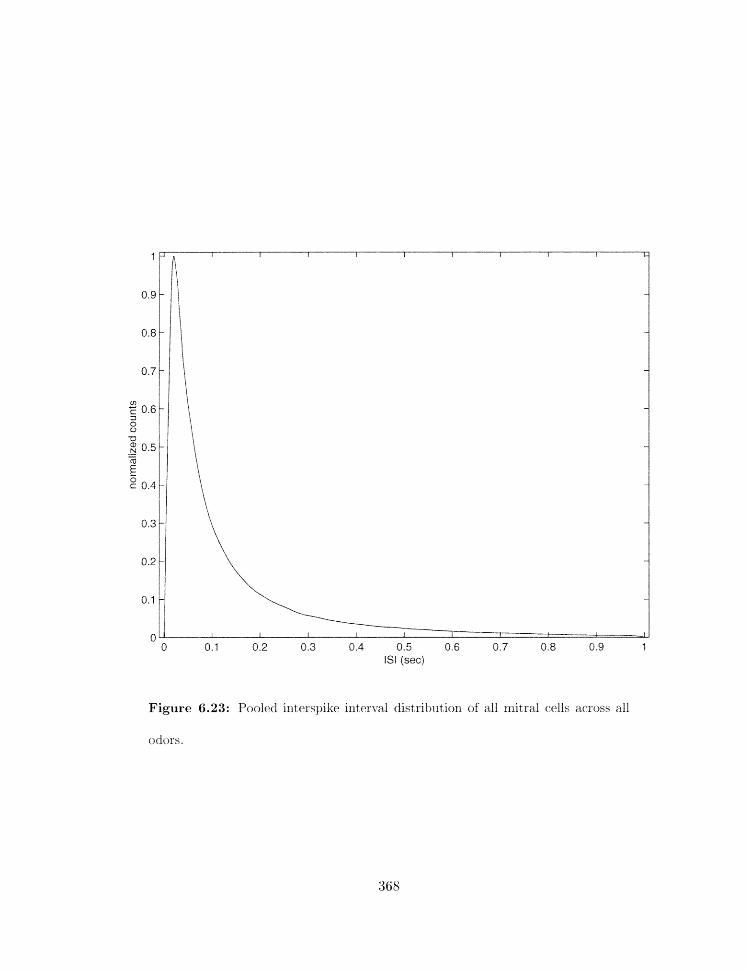
Figure 6-23: Pooled irltersyike interval distribution of all mitral caelils across all

odors.

Givm tfle low average spiking rate. it is clear that rnost lrelrroils do not: Ilowever, sinel the

IS1 distritjutiori slrows a peak at about 50 H z it rernains possible that a subset of rierlrolls

fired at this rate for some period of tinic-.. To ascertain this we eolriputed the alltororrelation

fu~lction for the data sets [I]. If a rnitral re11 fireti repeatedly every 20 msec (50 H z ) . tlierl

peaks should bc found in the autocorrelogram at 20 nbsec. 40 rrhsec. etc. This would rlot

show rrp in tlie IS1 distribution because each interspike interval rvould be the same.

The autocorrelatioiz algoritllixi we used was optimized for spike data as follows. For each

neuron, each spike from a given trial was taken and compared to all subsequent spikes on

that trial. For each sucll pair, tlie tirne diRerertee was calculated arid recorded. and the

data was binned to produce a (one-sided) autjocorrelogram, Our data sets wrrc generally

5 seeoxlds ill duration 41 but we were only interested in the antocorrelogram for the first

secoiid after odor onset (or after odor purge for background odors [dl) because this is the

time in which odor identification is believed to occur [i. 231.

The results slzow that different odors did not sEect the autucorrelogram of a givexi

Yleuron to any sigllificarlt degree at tire concentrat ions used (figure 6.24). 1x1 addit ion,

altllough rrcarly all arrtor:orrelogranzs stlowed a peak at arollzlcl 20 mst-ic, tllerc was no

evidence q?hatsoc.ver for peaks at larger multiples of 20 msec. Tlris resalt: is irlteresting in

that it suggests that diff~rerzt ncuroris arc im1volvt.d in diEerent 50 H z cycles, and that a

giver? rleuron rarely fires on mnr>rc. than two r:onsecutivc c;yclei;. DiN"c3rcnt: rlclirorls genctrally

exllibited broadly sirnilar autocorrelograxl~s, with a slzarp peak at 211 Trksec. and a slow

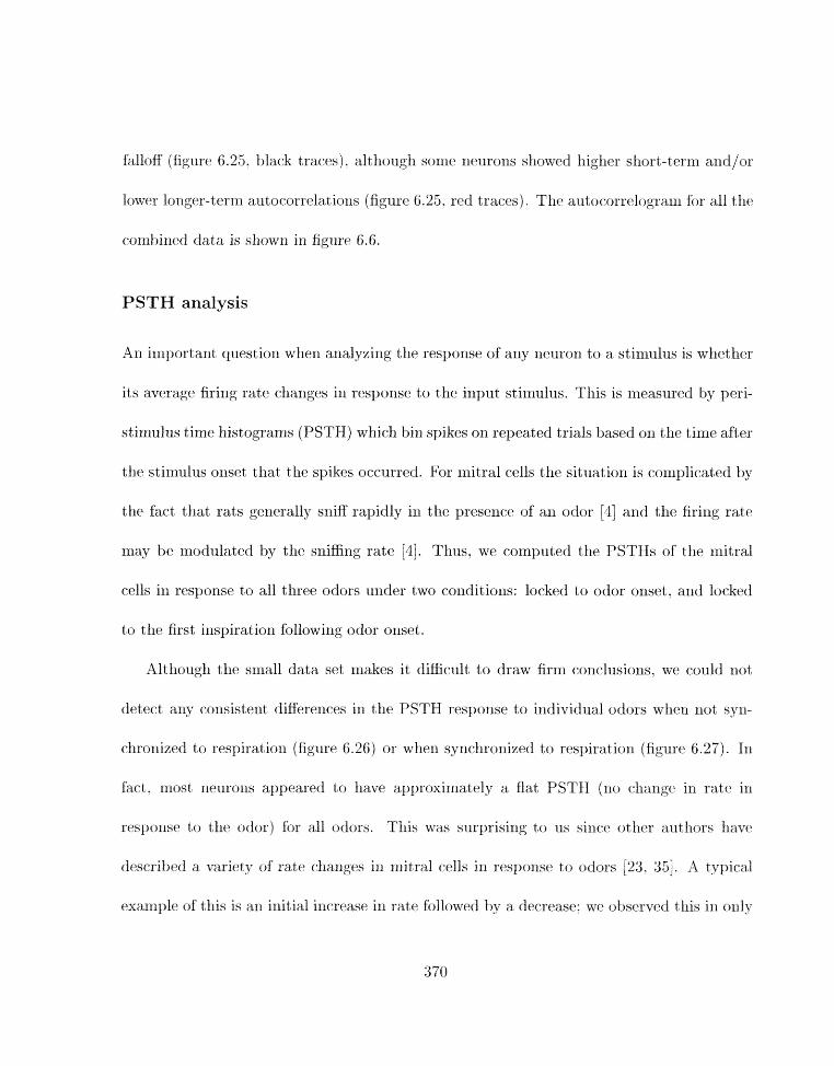
falloff (figure 6.25. black traces). although some Iieuroris sllowrd liigller short-tern1 and/or

lower longer-terln autororrelatior~s (figure 6.25. red traces). Tlie al~tucorrelogram for all t hr

cornbi~sed data is sflowrs in figure 6.6.

PSTH analysis

An irlzportant question when analyzing the resporrse of any neurori to a stimulus is whether

its average firing rate changes in resporise t80 the input stimulus, This is nieasured by peri-

stimulus time histograms (PSTH) which bin spikes on repeated trials based or1 the time afier

tlie stirnlulus onset that the spikes occurred. For rnitral cells the situation is coniplicated by

tlie fkct that rats generally sniff rapidly in the presence of an odor [4] and the firing rate

may be modulated by the sniffing rate 41. Thus, we computed tlie PSTHs of the mitral

cells in response to all three odors under two conditions: locked to odor onset. and locked

to the first inspiration following odor onset.

Although the small data set rnakes it difficult to draw firm conclusions, we could not

detect any corrsisterzt diEerenc;es in the PSTH response to ilidividlial odors when not xyri-

chronized to respiration (figure 6.26) or when syncahronized to respiration (figure 6.27). In

fx t . most rseurorss appeared tu have ap~~roxirnately a Aat PSTH (110 change in rate in

response to the odor) for all odors. This was surprising to us siac.c> rtthrr- a\lthors llavcl

described a variety of rate changes in mitral cells in response to odors [E3. 351. A rp ica l

example of this is ail initial increase in rate followed by a decrease: we observed this iss only

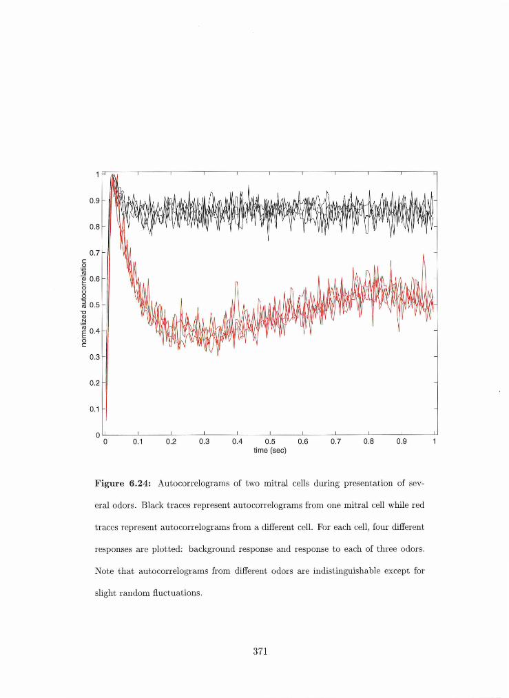
I I I I I I I I I I I 0 0.1 0.2 0.3 0.4 0.5 0.6 0.7 0.8 0.9 1

time (sec)

Figure 6.24: Autocorrelograms of two mitral cells during presentation of sev-

eral odors. Black traces represent autocorrelograms from one mitral cell while red

traces represent autocorrelograms from a different cell. For each cell, four different

responses are plotted: background response and response to each of three odors.

Note that autocorrelograrns from different odors are indistinguishable except for

slight random fluctuations.

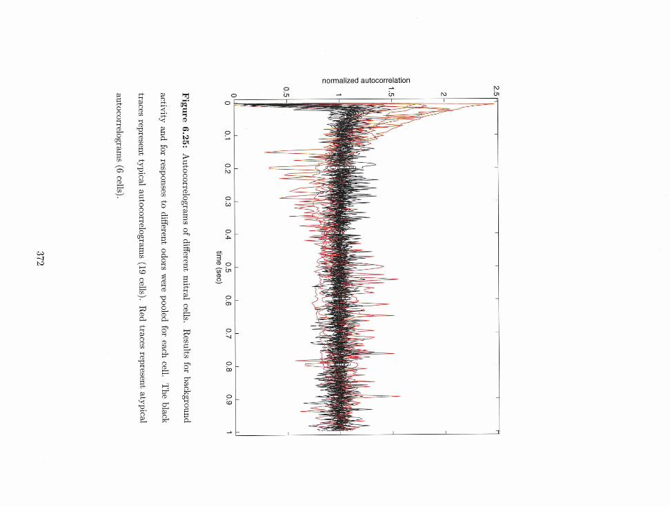
normalized autocorrelation -L

2 in IU

two Ileuroxrs out of 14 ( e.g.. figure 6.28). Interestiligly. this change was only ot,scrved in tlle

PSTHs synchronized to respiration. and was observed for all t11r.c~ odors. Tllr ratr change

was slightly more than twice tlre backgrou~ld firing ratr. JVP bbclirw that tlre difference

Isetwee~:t these results and those of other groups that lravc found rate increases ixr response

to odors is largely due to the low concentrations used: whrrr high concentrations are used

[35] . significallt rate changes are routinely seerr.

Appendix B: Extracellular field potential measurement and

current-source density (CSD) calculation

Tlie network niodel was designed to output extracellular field potentials from any set of

arbitrary locat ions in the cortex. Tllese field potential measurements can he processed

offlille to generate currexlt,-source derisity (CSD) plots. which give a grapliical representation

of the derisity of current sources and sinks at different depths of the cortex (in a particular

x-jj locatioilj as a fuxlctioll of time. These ~ u t p ~ l t s were used extensively in paranletprizing

tlre behaviors of tlrc cortical rnodel. Irt this section we briefly tlesrribc the theory behind

tlresc measurerric~lts and their implementation irr the cortical rnodcl.

Extracellular field potentials

When ail electrode is placed illto the extrscrllular rrlediunl in a cortical struct~tre. thc voltage

~nbcasnred at the electrode tip (wlric.11 is refrrrrcl to as the extracellular field potential) is

373

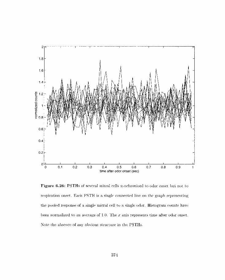
time after odor onset (sec)

Figure 6.26: PSTHs of several niitral cells synchronized to odor onset but not to

respiration onset. Eadl PSTH is a single connected line on the graph representing

the pooled response of a single mitral cell to a single odor. Histogram counts have

been normalized to an average of 1.0. The J: axis represents time after odor onset.

Note the absence of any obvious structure in the PSTHs.

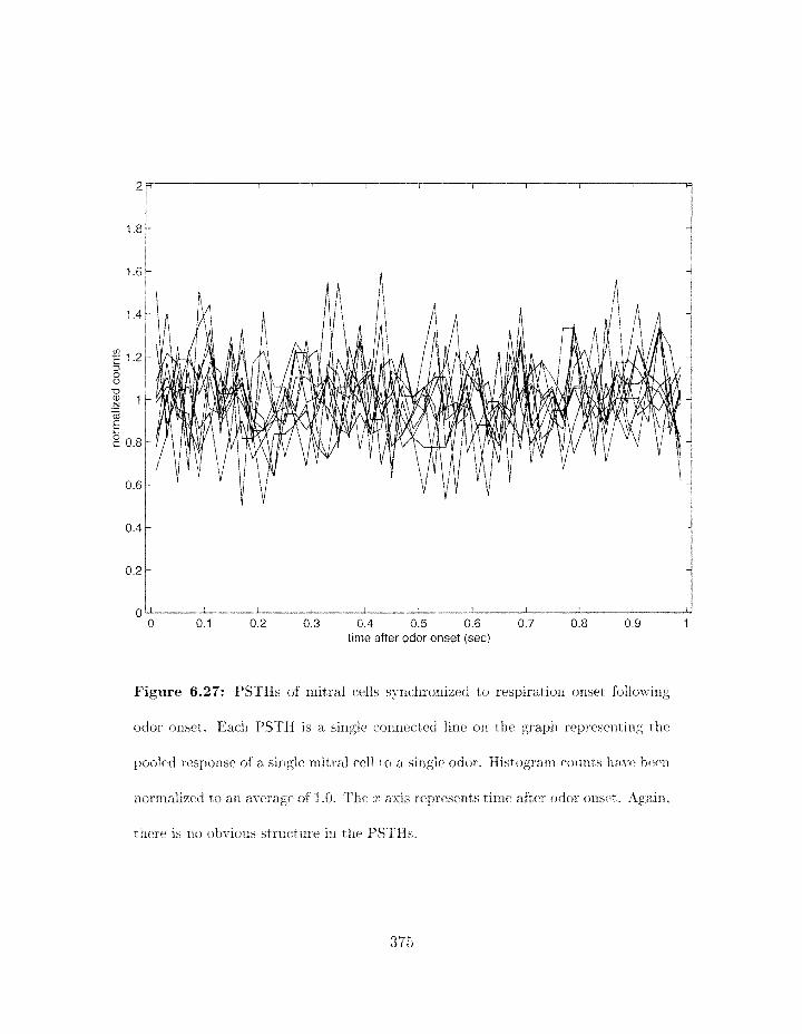
time after odor onset (sec)

Figure 6.27: PSTHs of rnitral cells synchronized to respiratiorl oriset follo13-ing

odor onset. Earl1 PSTH is a single rorrrlected line ort the graph representing the

pooled response of a sirlgle rnitral cell to a single odor. Histogram tourits have heen

xzornlalized to an average of 1.0. The x. axis rc3presertts tirne after odor onset. Again,

there i s no abt-ious structure in the PSTHs.

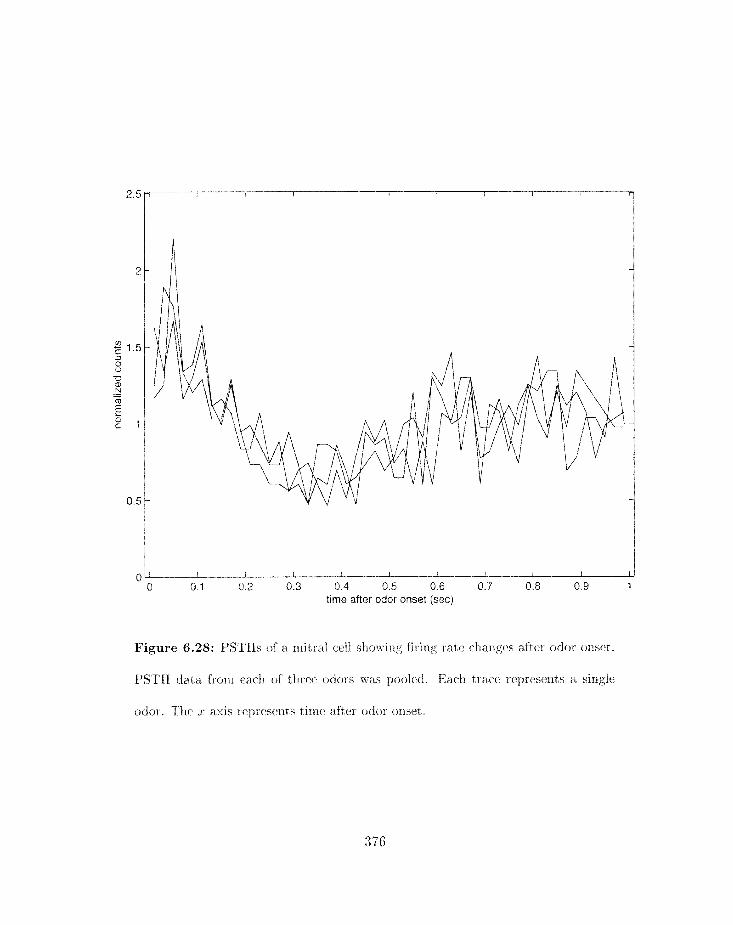
0 0 0.1 0.2 0.3 0.4 0.5 0.6 0.7 0.8 0.9 1

time afler odor onset fsec)

Figure 6.28: PSTIls of a mitval cell showing firirlg rate cfianges after odor oxlset.

PSTH data from earl1 of three odors was pooled. Each trace represents a single

odor. Tllr .r axis represents time after odor onset.

rlle result of tllr superx~ositiori of tllc effects of a l a r g ~ rlurnbrr of t:urrellt solirccs and

sinks propagating t hrouglr a resistiw medium (figures 6.13 a d 6.14). Current sourcmcs

rrpreserit current flowing from the inbracellular to the extracellular xlittdiom, while current

sinks represent current Aowirig in tlle reverse direction. These cxirrr:tit sources/sillks are

due to sy napt ic charlnels. volt age-depeiident and calciurn-depelldr~lt ionic c;hatiricls. and

capacitive and resistive inenlhrarle current*^ [19. 20. 24. 281. Tlle value of the field p~t~ent ial

depends on the number. strength. location arid polarity of current sources near tllr recording

electrode, as well as the extracellular resistivity.

By Kirchoff's law, the total amount of current flowing into n rieurorl (current sinks)

equals the total current flowing out (current sources) (figure 6.13). If sources arid sinks

arc. distributed evcrlly over the neuron. tlie measured field potential will he very small.

Therefore. field potential measmernents are only useful when there is a spatial separation

brtweelr sources and sirlks for a. large number of neurons arid a given input stimulus. This

is tlre case for pirihrm cortex pyramidal neurons when voltage sllock stirnuli are applied to

tile LOT, because tlle terrrporal pattern of activation of syr1apsc.s on t lx neuronal dendrites

are very differexkt in differerrt layers of cortex 19, 381. Syriapses irl particular layers are

stimulated nearly syrrcllro~iolwly. givilrg rise silllultanronsly to large numbers of current

sources in some layers arld large mlmbers of current sinks in other layers. Typicsally. tlie

sinks are localized iu a. narrow region of dendrite where syllaptic. input arrivt:~. while the

soltrces arc. distrihllled over a broader expanse of dendrite (representing pibssivcl resisaivr

a i d capacit ive equalizi~lg currerlts) (figure 6.13).

Tllr: field potential ill a non-capacitive extrwellular mediuin of llrliforlll resistivit)~ driver1

by point curre~it sources is givt.11 by 1261:

where Fi, is the field potential. Re is the extracellular resistivity (in units of f2 -m). nsourcrs

is the total nuniber of current sources. I, are tlle current sources, and

represents the Euclidean distance between the source (at (x,. y,. z,) ) and the electrode tip (at

( 2 . y. 2 ) . Compartment objects in GENESIS compute the value of I,,, due to all currellt

sources associated with the compartment. Virtual electrodes car1 be placed at arbitrary

points in the silriulated cortex. and the field potentials are calculated at each time step

acc:ording to r(3natiorl 6.1. In ~~rsct ice, two types of field potentials were i:omputed: surface

field poteritials at the tap of the siniulated cortex. and field potentials at varying dtptlls in

cortex. Tlre latter were used to compute clirrerlt-source deilsities as we describe i l~x t .

Current-source densities

hlthougll solrle insights call br gained directly from exarllirling extracellular field potentials.

in certaiil circ.ulristarrct.s. r ; l ~ data can be processed to givc what arc. krlotvil as cnr-rc3rlt-

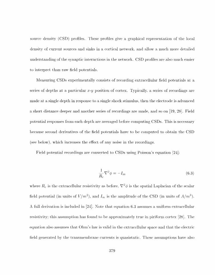
sourer dcrlsity j C'SD) profiles. These profiles give a grapfzical rrprese~lt at ion of the local

dcrzsity of current) sources and sirzks in a cortical network, and allow a rnuclz rrzore detailed

uslderstarzding of the synaptic iritcractiarls in t lle network. CSD profiles art. also much easier

to interpret tllarl raw field poteiltials.

Measuring CSDs experilllent ally consists of recordillg extracellular field potentials at a

series of depths at a particular 2-y position of cortex. Typically. a series of recordings are

made at a single depth in response to a single shock stirnulus. then t h electrode is advanced

a short distance deeper and another series of recordings are made, and so on [19, 281. Field

potential responses frorrl each depth are averaged before conlputing CSDs. This is necessary

because second derivatives of the field potentials have to be cornpxrted to obtain the CSD

{see below), whicll increases the effect of any noise in the recordings.

Field potential recordings are converted to CSDs using Poisson's equation [24]:

where Re is the extracellular resistivity as before. V" is the spatial Laplacian of tlle scalar

field pote~ltial (in units of V / V ~ ' ) . arid Irri is tlie anl~jlitude of the CSD (in units of A/vlr3).

A full derivation is included irz [24]. Note that equatio~l 6.3 assurrzes a imifornl extracellular

resistivity: this asstrmpt ion has found to be approxinlatrly true iri ~~iriforrrl cortex [28]. Tlle

equation also assumes that Ollrn's law is valid is1 the extrarrellular space and elat the electric.

field generated by tlze transu-tenlbranc. currents is quasistatic.. Thesc assumptions have also

been verified in piriform cortex [28].

Because of the larriinated s t ruc t~~re of piriforrri cortex and the fact that tlle cortex is

activated llomogenrously with respect to tlic laniiliar planes (layers la. 113. 2 etc.). tlw field

potential is locally translat ionaliy irlvariant: in the two direct ions parallel to the lamimr

planes (the s and y dimensions in our simulations) [24]. Intuitively. tliis is becalise the

superposition of currents in these directioris from rriariy nearby pyranridal neurons (receivitlg

similar input stimuli) cancel each other out to a large extent. leavimig little net current in

tllese directions and thus little or no potential gradient, Under t hese circumst s~lces. equation

6.3 car1 be reduced to the one-diniensional Poisson equation:

We used this equation to calculate CSD prof les frorn field potential nieasurernents taken

at depth irlcrernents of 20 p n ~ at a riurriber of different s-y locations evenly spaced in the

pirifc~rnn cortex model. Resistivities are not a,vailable for piriforln cortex. so the scale of the

CSDs is arbitrar3-. We? found that the response of the network model was sufficiently regular

that: repeated trials and snioothing of the response were not nccessay in order to generate

CSD profiles.

Bibliography

[I] M. Abeles. Corticonics. Cambridge University Press. Cambridge. 1991.

[2] J. Aml3ros-I~lgerson. R. Granger. and G. Lynch. Sirnulati011 of Palrocort,ex Performs

Hierarchical Clustering. Science. 247(4948): 1344-1338. 1990.

[3] E. Barkai: R.. E. B~rgman, G. Horwitz, and M. E. Hasselmo. Modulatiorl of Associative

Memory Furzction in a Biophysical Simulation of Rat Piriform Cortex. Journal o j

Nevrophgsinloyy, 72 (2):659-677, 1994.

[4] U. S. Bhalla and J. M. Bower. Multiday Rrcordiags from Olfkctory Bulb Neurons in

Awake Freely Movilig Rats: Spatially and Temporally Orgarlized Variability in Odorartt

Response Properties. Journal of Comput;atior~uZ ATe.ur.oseie??,ce. 3(3):221 256. 1997.

!5j S. L. Bresslcr. Spatial Orgarlizatiorl of EEGs horn Olfact80ry Bull, and Cortex. Elrc-

troaneephalqr~tph~ y o92d Catnicai i%Teu-rophgsiol~gyI 57:270-276, 19 84.

[l5] M. E. Hasselmo. B. P. A~idersoll. and 3. M. Rowel:. Cholinergic Modulation of Cortical

Associative. k1emory Functioii. Jos~rr~~nl nf Nesrwphgs boloyp. 67(i;) : 123012363. 1992.

!l6] M. E. Hasselrrlo. C. Linster. M. Patil. D. &/fa. and M. Crkic. Noradrrnergic Suppressiuri

of Synaptic Transmissioil May Illfluencp Cortical Signal-t80-Noise Ratio. Journal o f

Neurophgsiodogy. 77(6):3326-3339. 1997.

[li] M. Jiang. E. R. Griff, M. Ennis. L. A. Zirnrner. and M. T. Shipley. A~tivat~ion of Locus

Coeruleus Enhances the Responses of Olfactory Bulb Mitral Cells to Weak Ofhetory

Nerve Input. Journal of Nearosczence. 16(19):6319-6329. 1996.

181 A. Kapur. W. W. Lytton. K. L. Ketchurn. and L. B. Haberly. Regulation of the NMDA

Cornporlerlt of EPSPs by Different Components of Postsynaptic GABAergic Inhibi-

tion: Computer Simulation Analysis in Piriform Cortex. .lou?-?~al of Ne~rophljsiologg

78(5):2546-2559, 1997.

[19] K. L. Krtdlum arid L. B. Haberly. Membrane Currents Evoked by AEcreilt Fiber

Stinrulatiorl ill Rat Pirifornl Cortex. 1. Current Source-hnsity Analysis. Journal elf

~Ve~6mphp".iotogy, 69 j 1 j :248-260, 1993.

j20j K. L. Ketchum and L. B. Waberly. hlernbrane Currents Em,ked by Affcrrrlt Fiber

Stinlulatiorl in Rat PiriEornt Cortex. 2. rZzzalysis with a Systeln Model, Journal qf

~Vez~l..ophgsioEo,qy. 69j 1 ):261-281 1993.

0; C33 Cs ri

0; a 2

1 m C? C=; ri . i--.

r-i ri V

08

6 U .e

.% U 03

8

2? ?! 3 Y s m i;,

2 .a F: . n 3 cd

C, GI G . n

h w .n 3 . F-4

i;

2

r-i Xi 63 v-4

[28] R. Rodriguez and L. B. Waherly. Allslgsis of Synaptic Events ill the Opossum Piriform

Cortrx with Inlproved Current Source Density Tecllniques. Jolrl-n,al of LVe r~r.ophysiolom.

61(4):702718. 1989.

[29] G. R. Shepherd. editor. The Sgnaptic Organizaton of the Brain. 4th. Ed. Oxford

University Press, New York. 1997.

[30] G. R.. Shepherd and C. 4. Greer. Olfactory Bulb. Irl G. M. Shepllerd. editor, The

Sgnaptic O~qa,nizat io~~ of the Brain. Oxford University Press. Oxford. England. 1998.

[31] C. Skarda and W. J. Freenlan. How Brains Make Chaos in Order to Make Sense of tllr

World. Behaviorai! and Brain Sciences. 10: 161- 195, 1987.

1321 G. Tseng and L. £3. Haberly. Deep Neurons in Piriforrn Cortex. 1. Morphology arld

Synaptically Evoked-Respo~lses Including a Unique High-Amplitude Paired Shock Fa-

cilitation. Jourrsd of Nesr~ophysioZoyy. 62(2):369-385. 1989.

[33] G. Tse~ig s ~ l d L. I3. Haberly. Deep Neurons in Piriform Cortex. 2. Menibrane Properties

t llat Urlderlic Unusual Syllaptic Responses. .lor~rn ol o j ATpclrophysiolr,q;y. 62 (2) :38F 400.

1989.

&I. C. J'anier and J. M. Bower. .4 Cornparativr Survey of Aut0matc.d Paraln~ter-Search

hIetllo~is for Colnl1art~rnerita1 Xeural &lodels. Jo~krrial of ,f~omputatiorra,l Nr.ur.osciencr:.

7 ( 2 ) : 139171. 1999.

351 D. A. UTilsorl. Habituatiorl of Odor Responses ill the Rat i lnt~rior Piriforlxl Cortex.

Jour~inl c?f -Ve~?-ophg.~ioIogy. 79(3):142?5- 14-20 1998,

[36] M. A. Wilson and .T. M. Bower. Cortical Oscillations and Texrl~,oral Ixlteractions in a

Computer Sirnulation of Pirihrrn Cortex. .Journal of Meurophy&oloyy, 67(4) :9S 1-995.

1992.

Chapter 7

Exploring the Network Model of Piriform

Cortex

The network model of piriform cortex described in the previo~~s chapter has beell used to

explore the dynamics of this system in a variety of ways. Some of tllese explor~ions will be

described in this chapter. Tllrsr explorations fornl orlly a tiny fiactiorl of all tllc possible

irlvestigations t,hat the ~llodel makes 1)ossible; ncvert heless. they have already suhsta~lb~ially

increased our ulderstandirlg of several aspects of the sys ten1 dynamics. sugges ted numerous

new experiments. and give11 rise to riew ideas regarding how the piriforrn cortex may process

i~lfor~l lat io~~.

First, the resItorrst. of the pirifurrn cortex rrlodel to background irlput;s &om the olfildory

hllll, and to stro~ig electrical slioc:k stimuli of' tllr lateral olfactory tract (LOT) will be

descril~ed, TIiis has suggested that background inputs are essential for depolarizirrg ricuro~is

in the veritral anterior regiori of cortex ta the point where they fire readily in response to

input stimuli. 1 will also sliow- that background iriputs need to be substantially reduced imi

the presence of norepinep hrine, or else the cortical rriodel will spoxit aneously generate large

numl>ers of spikes. The strong shock resporlse in tlie model was fourid to depend critically

on 110th background iriputs from tlle olfactory bulb and the presence of strong feedforward

inhibition to prevent rieural activity from propagating out of tlre ventral anterior piriform

cortex.

I will the11 contrast two significantly different versions of the piriform cortex nlodel from

the standpoint of their ability to replicate tlre experimental response to weak electrical

sliocks to tlie LOT (the weak shock response). Tlie first version of tlie rnodel features

random connectivity betweeri the olfactory bulb and cortex, as well as strong feedback

connect ions between posterior and anterior cortex. The connectivity pattern of this model

is siniilar to that of the Wilsor~/Bower piriforni cortxx model 211. This vcrsiori of the new

rnodel replicates the oscillatory surhce field potential, but fails to replicate crucial features

of the current-source density (CSD) respoxise. The second version of the rnodel. in contrast.

features liigllly str~rctzrred corlnections l~etween the olfactory bulb and pirifomi cortex and

witlliri the cortex: this rriodel replicates the C'SD response rri~lcth xnorc. accurately. Whiltl

highly speculative in soule ways, the latter rnctdrl casts a completely new light on how

piriforxrr cortex may encode odors and may function computationally, and is experimentally

testable.

7.1 Response to olfactory bulb background inputs

7.1.1 Spontaneous activity

1Vhc.n the pirifurm cortex model is subjected to background spiking activity with a st atistical

distribution similar to that of olfactory bulb rnitral cells (see chapter 6 for details). the

menlhrane potentials of pyra~nidal neurons in the ventral anterior piriforni cortex (vAPC)

rise close to spikirig threshold, wliereas the rnerrlbrarie yoteiitials of pyramidal rieurorls in tlie

posterior pirif'orrn cortex (PPC:) remain close to resting potential (figure 7.1). Tlle reason

fbr the difference is the much deriser proje~t~ion. horn rni-tral cells tjo pyramidal rlexirons

in vAPC as conlparecl to the rest of piriform cortex [5]. Experirrierrtally. piriform cortex

pyrarrlidal rleurorls in vitro have bee11 recorded with rnembrane potentials in the rarige of

the vAPC rleurorrs in tlre nrodel (-55mV tto -50mbT) [14]: as itr tlie model. tllesr lieuroris

were located in tlie ventral half of tlie pirifornx cortex. Pyrarilidal rreurons in vivo also often

spike sporltarleously at ronglily 1-5 H z [14. 16. 1'7 ; however, in. tlre model backgrourrd iriyut

is rrot srracient do cause syikirzg iu pyranridal neurons. This is bec.atise in the model tlie

pj~raunidal zreurolis are suniciently close to firi~lg tlrresliold that if one Yreurorr fires, typically

all of the rlettrolis fire in a wwe-like patberil which spreads across the cortex bee belo-u;).

Tlre discrepancy between the ~rrodcl and tltr experi~nental data is due to sealing effects; each

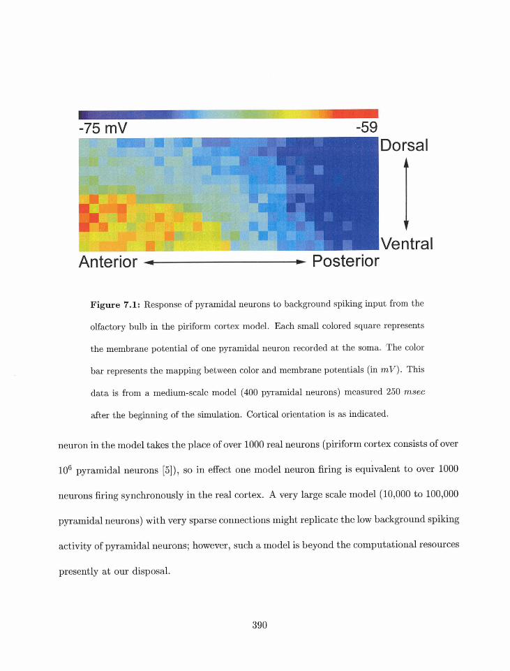
Anterior 4 .- Posterior

Figure 7.1: Response of pyramidal neurons to background spiking input from the

olfactory bulb in the piriform cortex model. Each small colored square represents

the membrane potential of one pyramidal neuron recorded at the soma. The color

bar represents the mapping between color and membrane potentials (in rnV). This

data is from a medium-scale model (400 pyramidal neurons) measured 250 rnsec

after the beginning of the simulation. Cortical orientation is as indicated.

neuron in the model takes the place of over 1000 real neurons (piriform cortex consists of over

lo6 pyramidal neurons [ 5 ] ) , so in effect one model neuron firing is equivalent to over 1000

neurons firing synchronously in the real cortex. A very large scale model (10,000 to 100,000

pyramidal neurons) with very sparse connections might replicate the low background spiking

activity of pyramidal neurons; however, such a model is beyond the computational resources

presently at our disposal.

7.1.2 Spontaneous activity with NE

Experirnelitally. additioll of 100 LAM NE to a brain-slice prepasat,iorr of pirifornl cortex

causes a nurnber of cllaagcs in synapt ir transmission and neuronal excitability (described

in detail in chapters 2. 3. and 6) . Wriefiy. the lriost important of these effects include

1. increasing the strength of synaptic tra~zs~~iissiori onto piriforrn cortex pyrarnidal mu-

rons along the aEerent (layer la) pathway:

2. decreasing the strength of synaptic transmission between pyramidal neurons along tlre

associat ional (layer 1b) pathway) :

3. increasing tlie excitability of pyramidal neurons and feedback inllibitory inrterrieurons.

Tllese effects were incorporated into tlre pirihrrri cortex network model. When a con-

ceritratiorr of 100 p&I NE was inlposed on the model in the presence of random background

inputs, the pyrarnidal lleurolls Ilegarl to spike spontaneously at roughly 10 Hz (figure 7.2,

top). Although the spontarleous spiking rate of pyramidal neurons in piriform cortex under

the ilifluerlc~ of NE is 1101; k~iow~i, it is extrenlely urllikely that these rleurorls fire at sucll a

high spontaneous rate in ~ i u o sirice xrlost; of the existing exyerirnental data iridicates that

piriform cortical rreuromls generally have low spikirlg rates j < 20Hzj even during odor pre-

senta tion [13. 13j. 111 order to prevellt NE ap1,lication fro111 causillg 13j~ralnidal Ireuroms to

fire s1~olztaneousf y in resporlse to backgrorrnd inputs, it was rier:essary to reduce t lie batk-

gm0\11d iilput tiriflg rate j i , e.. t h ~ background firing rate of ~liitral cells) do 40% of the rate

391

iri tlie absence of KE (figlire 7.2. bottom). It has been determinetl experimentally that iz;E

reduces i~ackground firirlg of mitral cells i)v rouglily 50%) in oiq~o [8 . wcvlzich agrees we11 with

Gls~ rriodel.

7.2 The strong shock response

7.2.1 Basic features of the response

Experimentally, stinlulatiorl of the lateral olfactory tract (LOT) with very brief (0.1 msec)

electrical slsocks causes cliaracteristic responses in piriforrri cortex as seer1 in current-source

density (CSD) profiles. Tlsese shocks have been used extcrlsively by Lewis Haherly and his

collaborators [9, 10. 111 and Walter Freeman [4] to characterize the dynarnical behaviors

of tlic piriform cort8ex network. These behaviors are qualitatively difl'erent for strong (high

voltage) and wcak (low voltage) electrical shocks. A typical experimental strong shock

resporlsc is show11 in tlze top half of figures 7.3 arsd 7.4 [9. 101. The response cotnilsists of two

separate peaks occurring after the shock stinsulus. Tlsc first peak is due to direct affcrent

stisnulation in layer la of the piriforlni cortex, while tlie second is "uelieved to be due to

associational fiber activity in layer lb. w1tit:li ill turrz is a conseyuerice of' pyranlidal lieurorl

firilzg in ventral aliterior pirifornl cortex [5. 10 . Few- tnincuroris fire in resporlse to the strong

shock irz dorsal anterior or posterior piriforaz cortex

In tlse yiriform cortex rrsodel. the strollg; shock is siz~~ttnilated I-ty riraking the elltire pop-

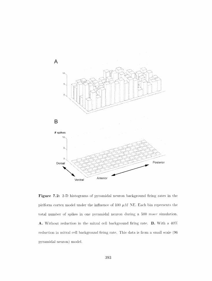
# spikes

f O ;

Figure 7.2: 2-D histograiris of pyraiilidal rleLlron i,ar.kgroiinrl firiilg rates in the

piriform cortex ~riorirl under the irlfliirncc. of 100 p i 1 NC. Each bill rrpres~rlti the

total nrrnlbel: of spikes in one ~~yrarnidal neurorl durirlg a 300 nr.iir.c* iirrnllatiori.

A. iT-ithout reductioir in the rrlitral cd i backgrotr~ld firing rate. B, Witlr a 40%:

reduction in rnitraf cell background firing rat:t3. This data is from a small scak (96

pyrarniclal neurort) model.

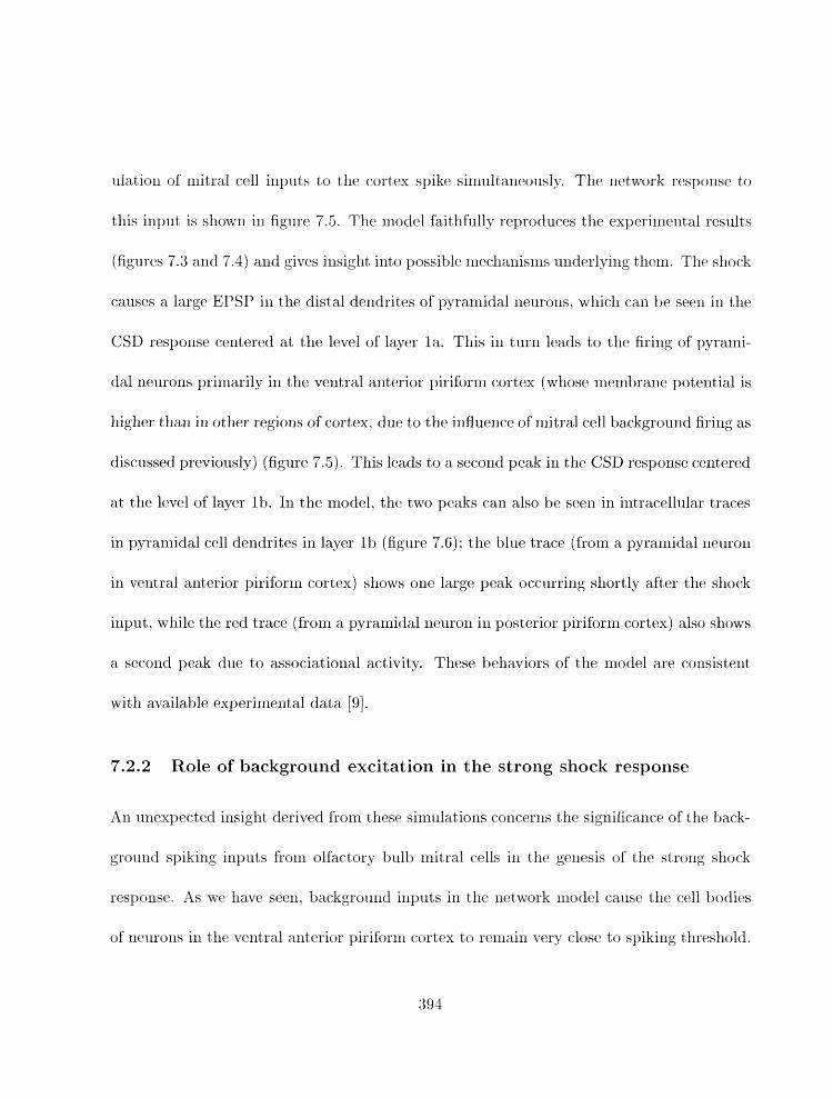
ulation of mitral cell inputs to the cortex spike simultaneously. Tlzt ~letuiork response to

this input is shown in figure 7.5. The model faithfully reproduces tlie exy~erirnerrtal resrilts

(figures 7.3 and 7.4) and gives iiisigllt into possible liiecllarlisnls underlying thenl. Thp shock

causes a large EPSP in the distal dendrites of pyramidal neurons. which can be seen ixl the

CSD response centered at the level of layer la. This in turn leads to the firing of pyraini-

dal neurons primarily in tlie veiitral anterior piriform cortex (whose mei~lbrane potexitial is

higlier than ill otlier regions of cortex; due to the irifiuence of mitral cell background firing as

discussed previously) (figure 7.5). This leads to a secoild peak in the CSD response centered

at the level of layer Ib. In the model, tlic two peaks can also be seexi in intracellular traces

in pyramidal cell dendrites in layer l b (figure 7.6) : the blur trace (from a pyrairiidal ileuron

in ventral anterior piriforrn cortex) shows one large peak occurrillg shortly after the shock

input, while the red trace (from a pyramidal nelirori in posterior piriform cortex) also shows

a second peak due to associational activity. These behaviors of the model are consisterit

with available experimental data 191.

7.2.2 Role of background excitation in the strong shock response

An ~xnexpected iusigl~t derived from these sirnlllatiorzs conecrils the significance of the buck-

grortiid spiking inp~lt#s horn olfactory bulb mitral cells in dlre gerlcsis of tht: strorlg shock

response. As we have seen, baekgrcsur-td illputs in the network ruodcl cause the cell t~cldies

of neurons in the ventral andcrior pirihrrsl cortex to rclrlain very close to spikirlg tirrcshold.

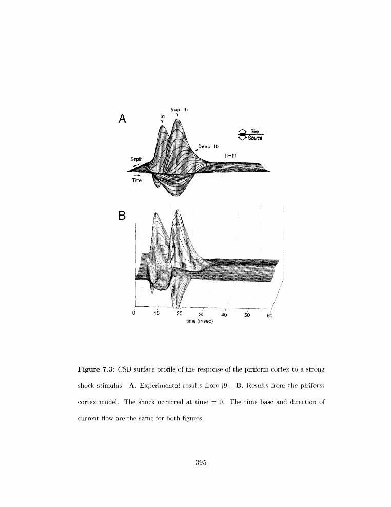
Sup Ib la

B

/ /

0 10 20 30 40 50 60

ttme (msec)

Figure 7.3: CSD surface profile of the response of the pirifonn cortex to a strong

shock stimulus. A. Experimental results from [S]. B. Results from the piriform

cortex model. The shock occurred at tirne = 0. The time base and direction of

current flow are the same for both figures.

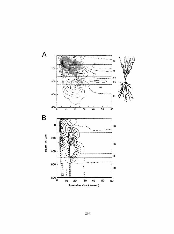
aoo

400

8011

time after shock (msec)

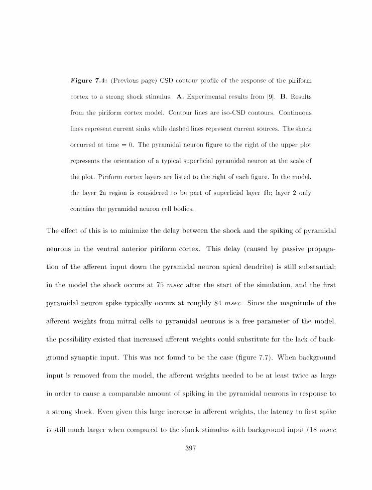
Figure 7.4: (Pre~ious page) CSD contour profilt of the resportst. of the pirifoml

c.ortt.s to a strong shock stirntllus. A. Experimental results frolrl [9]. E3, Results

frortl the piribrrn cortex rrlodel. Contour lir1c.s are iso-CSD rontours. Continucnus

lilies represent current sinks xhile dashed lines rpllresent current sources. The sllock

occurred at time = 0, The pyrarnidal neuron figure to the right of' the upper plot

represents the oriclxltation of a typical superficial pyramidal neuron at the scale of

the plot. Piriforni cortex layers are listed to the right of each figure. 111 the model.

the layer 2a region is considered to be part of superficial layer Ib; layer 2 o~lly

cont airs t be pyramidal rleurori cell bodies.

Tlie e&ct of tliis is to minimize the delay between the shock and tlie spiking of pyramidal

neurons in tlre ventral anterior piriforrn cortex. This delay (caused by passive propaga-

tion of the aEerent input down the pyramidal neuron apical dendrite) is still substantial:

in tlie model the shock occurs at 75 msec after tlie start of the sirnulation, and the first

pyramidal neuron spike typically occurs at roughly 84 ynsec. Since the magnitude of the

aEere~it weights from nritral cells to pyramidal neurons is a free parameter of the rrlodel.

the possibility existed that irlcreascd itEc:rent weights could subst it ~xte for the lack of batrk-

gmund syxraptic input. This was riot found to be thc case !figure 1.7). When hackgrctllnd

input is remof~ed frorrz the rriodel. the aEerent weigl~ts needed to he at least twice as large

in order to cause a comparable anuourit of spikillg in the pyrarnidal neurons in respouse to

a strong shock. Even given this large increae in af'fercnt weights, the latency to first. spike

is stilt nlucll larger when conipared to the shock stinlulus with background input j 18 mscc

397

FF inhibitory Pvramidal m

-75 --'J

5 m s -L i

Figure 7.5: (Previous page) Response of pyramidal neurons (measured at tile

sorna) arrd feeclforward (FF) ixlhibitory interneurons in tlse pirifortn cortex nlodel

to a strong shock stimulus. This data is froxxi a snrall-scafe rnotiel (96 p3-ramidal

neurons). The color bar represents the membrane potential irr rn 1 -. Each horizoxital

pair of frames represerlts a specific time (in rnsec) after the shock stimulus (indi-

cated at the left of each pair of frames). 3ote the spreading of actix~ation among

the fecdforward inhibitory interneurons: spikes in these neurons pre~ent spiking i11

pyramidal neurons outside of the ventral anterior pirifornl cortex. The schematic

diagram at the top of the page represents afferel1.t connections to feedforward in-

terneurons (left) ancl pyranlidal neurons (right). as well as the inhibitory connections

between feedforward interneurons and pyraniidal neurons.

vs. 9 m,.sec). In figure 7.7'. we see the CSD profile for the strong shock with aiicl withoxit

background input; without backgrourld inputs the two peaks are much farther apart than

in the experinlental data (or in the model data with backgrorind inputs). If the afferent

weights in the niodel are increased still ft~rther in order to decrease tlze latency. pyranzidal

neurons outside the veritral anterior region begin to spike. particularly iii the posterior piri-

forl-ti cortex where feedforward inhibition is relat i-vely weak (fliglxre 7.8) : this cor3tradicts &Ire

Thus, the xwiodel suggests that backgrou~ci sl~iking iriputs from the olfactory bull> arc

riecessary ili order to give rise to a strong S I ~ C I C ~ response that accurately refiects the ex-

y erirrlerital data. Experirnerrdall~., it was sflown Inally years ago by IValter Rflenian that

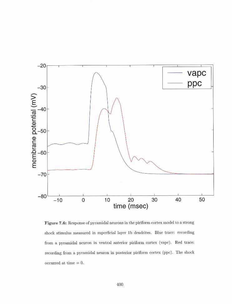
time (msec)

-20 I I I I I I I

Figure 7.6: Response of pyramidal neurons in the piriform cortex model to a strong

shock stimulus measured in superficial layer l b dendrites. Blue trace: recording

from a pyramidal neuron in ventral anterior piriform cortex (vapc). Red trace:

recording from a pyramidal neuron in posterior piriform cortex (ppc). The shock

occurred at time = 0.

vapc -30 - PPC -

n

-

.- CI

s a,

-

a,

-

-70 - -

-80 I I I I I I I

-1 0 0 10 20 30 40 50

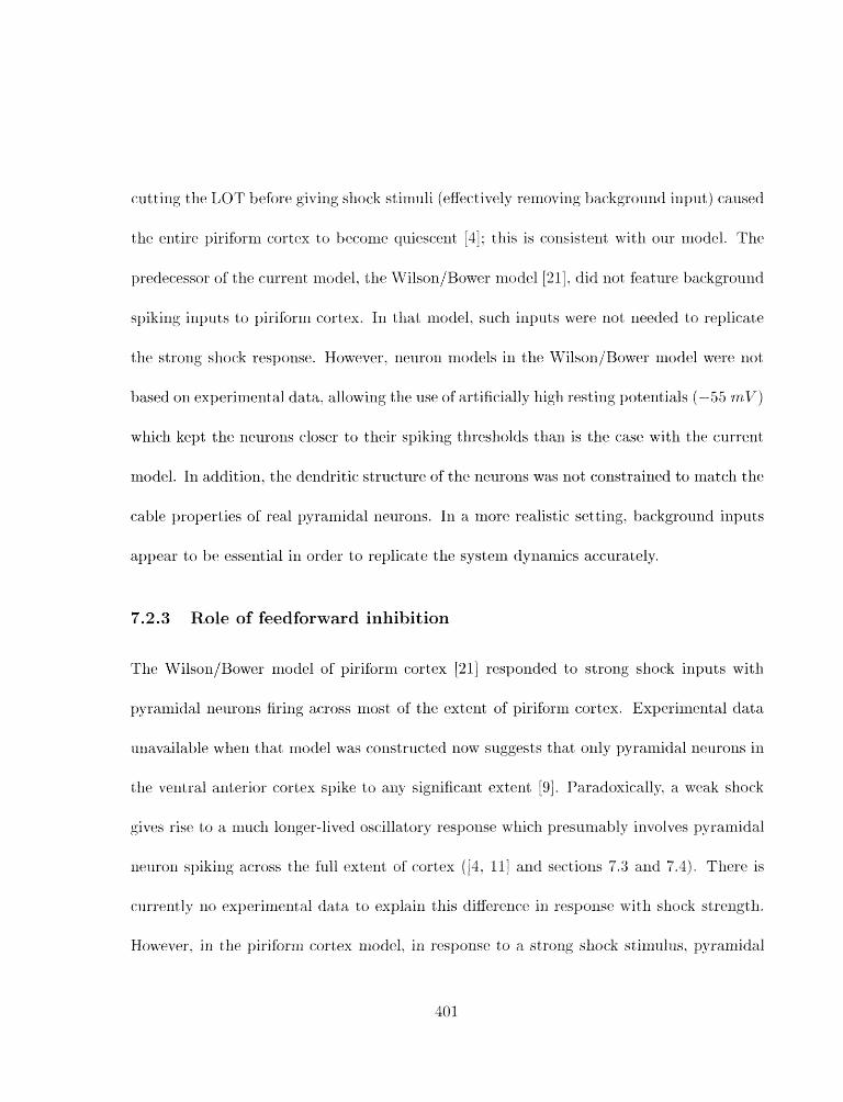
cuttirig the LOT befbrc givirig sllock stiniuli hEectively removillg background input,) caused

the erltirc i~iriforrn cortex to hrc:ome qlliescellt [A]: this is collsiste~it with our rnodel. The

predecessor of the current model. t l l ~ Wilsori/Bower rnodel 1211. did not feature background

spikirlg inputs to yirifornr cortex. In that niodel, such inputs werc not needed to replicate

the strong skrock response. However. rreurolz models in the lVilsori/Bower rnodel were not

based on experimental data. allowing the use of artificially high resting potentials (-55 mV)

which kept the neurons closer to their spiking thresholds thtlri is the case with the currexit

model. In addition. the dendritic structure of the neurorzs was not constrained to match the

cable properties of real pyramidal neurons. In a more realistic; setting. hackgrourid inputs

appear to be essential in order to replicate tile syst?errl dyrzamics accurately.

7 2 . 3 Role of feedforward inhibition

The Wilson/Bower rrlotlel of piriforrn cortex [21 responded t;o strorig shock inputs with

pyramidal rrcurons firing across most of the extent of piriforrn cortex. Experimental data,

uxlavailat->le when that rrzodel was corzstru~t~ed now suggests that only pyraniidal neurons in

tlre ve~rt~ral anterior cortex spike to any significant cxtcrzt 91. Paradoxically. a weak shock

gives risc to a niucll longer-lixd oscillatory response which pr~surnably ixivolucts pyramidal

nruroli spikirig aczross the full extent of cortex (13. 111 and sections 7.3 arid 7.4). There is

currently no exz>erirziental data to explairr this diEerenc.c in response with shock strength.

However, in the piriforrrl cortex model, it-z response to a strong slloctli stirtlul~xs, g~yrantid;zl

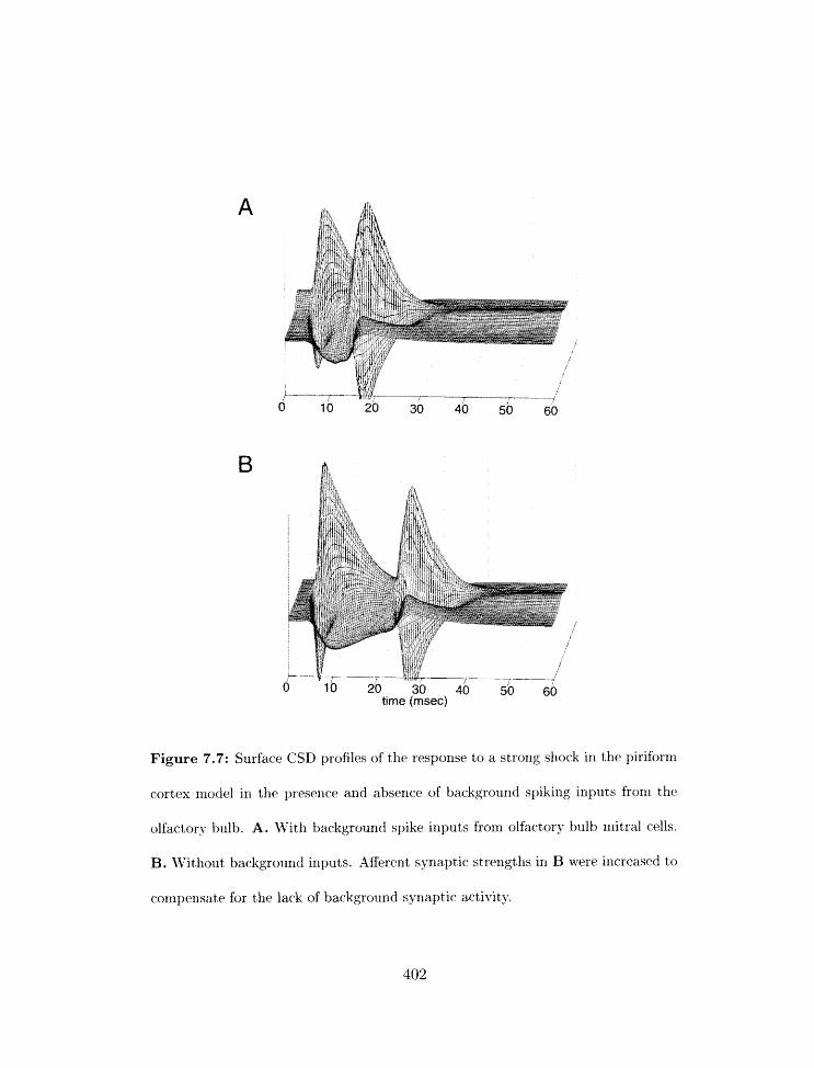
d rb 20 30 40 50 60 time (rnsec)

Figure 7.7: Surface CSD profiles of the response to a strong shock in t,he piriform

cortex rnodel in the presence and absence of background spiking inputs from the

olfttctory bulb. A. With background spike inputs from olfactory bulb mitral cells.

B. WTitRout background inputs. Afferent synaptic strengths in B were increased to

cornpe~lsate for the lack of background synaptic activity.

Figure 7.8: 2-D histogranis of piribrm cortex rrlodel pyrarrzidal Ilcuron spikes in

respollse to a strong shock wit11 and without background spiking inputs. Each Itin

rerzresents tire total number of spikcs in one pyramidal neurorl durillg a 230 nrsrc

sinlufation. A. IYit h background spike inputs frorn olfactory bulb rzlitral cells. B.

11,-itllout background inputs. Strength of afIlerer~t irzputs Ilat-c. beer1 increased to

reduce latclrtcy to Ib peak, causing neurons o~ltsidc the ventral arlrerior piriforrn

cortrx to spike. This data i s f'ror-rl a s~rtall scale (96 ~jyranlidal neuron) rrzodet.

403

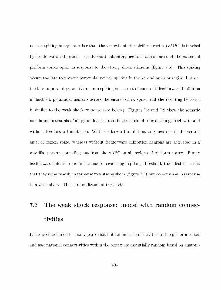
rielirori spikirlg in regiorls other tllail the ventral ant#erior ~~irifornl cortex (vAPC) is blocked

by kedforward inliibition. Fieedfor?vard inhibitory rlnt.urons across zrlost of tlic extent of

piriform cortex spike in response to the strolig shock stimlilus (figure 7.5). Tliis spiking

occurs too late to preverrt pyramidal iietlron spiking in the ventral anterior region. but riot

too latie to prevent pyramidal rleuromi spiking in the rest of cortex. If feedforward iriliibition

is disabled. pyramidal neuroris across the entire cortex spike, and the resuftirig beliavior

is similar to the weak shock response (see below). Figures 7.5 arid 7.9 show the sorliatic

membrane poteritials of all pyra~nidal neurons in the model during a strong shock with and

without feedforward inhibition. '1Vitll feedforward inliibit8iorl, orilly neurons in tlie veiitral

anterior region spike, whereas without kedfvrward inllibitiori neurons are activated in a

wavelike pattern spreading out from the vAPC to all regions of piriforrri cortex, Purely

feedforward interneurons in the model have a high spiking threshold: tlie effect of this is

that ttlely spike readily in response to a strong shock (figure 7.5) but: do not spike in response

to a weak sliock. This is a prediction of tlre rliodcl.

7.3 The weak shock response: model with random connec-

It has been assuiiled for nlany years that both aBerent c.onnet:divities to thc piriforrri cortex

and associat iorlal eo-tirlectivit ies wit hill t lie cortex are essentially raridonl tjased 0x1 anat 01x1-

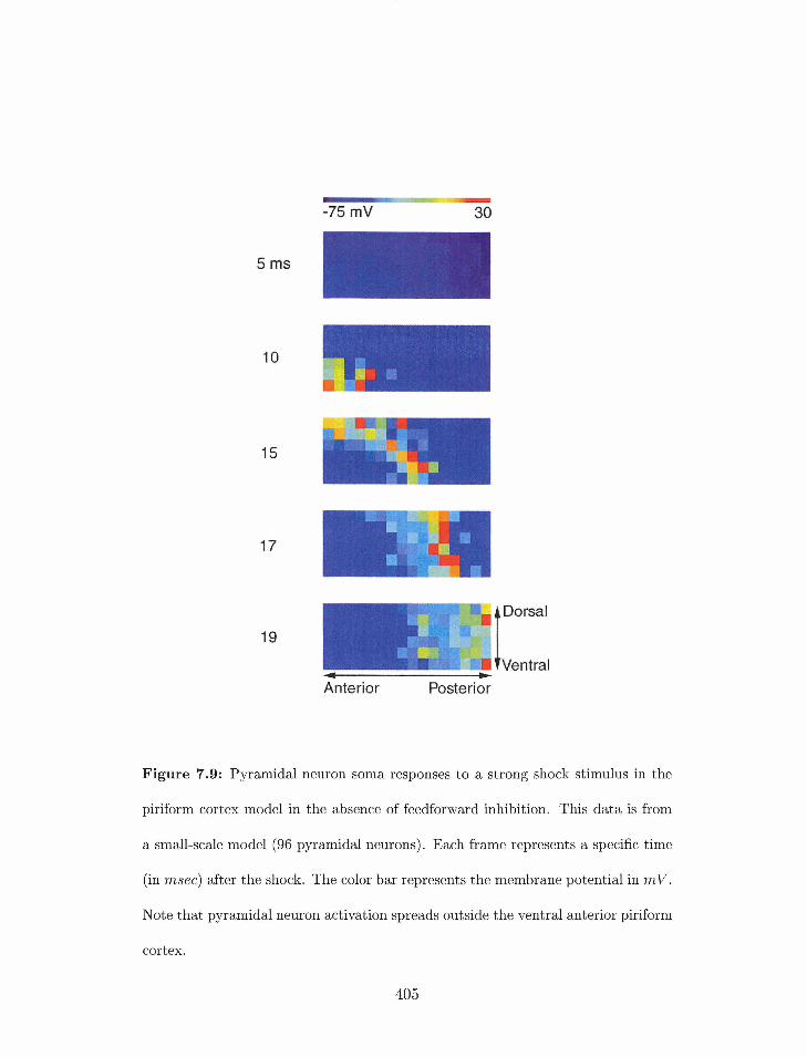
Posterior

Figure 7.9: Pyramidal neuron soma responses to a strong shock stimulus in the

piriform cortex model in the absence of feedforward inhibition. This data is from

a small-scale model (96 pyramidal neurons). Each frame represents a specific time

(in rnsec) after the shock. The color bar represents the membrane potential in rnV.

Note that pyramidal neuron activation spreads outside the ventral anterior piriform

cortex.

ical data showing arl absence of tjopographical orga~iizatio~i in tlir two patliways j7. 12. 181.

A random c;orlrtrctivity pattern was also used in the Wilsor~/Bo\ver pirihrrrl cortex model:

however. CSD respollses to weak shocks were not ineasurcd ill that model [21]. brca~lst~ tllc

relevant data [Ill was not available at the time t>hat rrlodel was built.

This section describes the weak shock response in a version of the piriform cortex model

which features random corinectivity hetween the olhctory bulb and cortex and strong feed-

back connections fioxn posterior to anterior piriform cortex. In addition to replicatirig the

strong shock response, this model also reproduces the piriform cortex oscillatory field poten-

tial in resporise to weak shock stimuli. The dependerlce of this response on several parameter.

settings will be explored. The CSD resporise to weak shocks will then be examined. This

version of the rr-todel does riot accurately reproduce tliis response; the reasoxis for this will

be discussed in some detail. arid an alternative model which does match tlie CSD response

will be presented in the next section.

7.3.1 Basic features of the response

Experirnentallj~. stimulation of the lateral olfactory tract (LOT) with a weak elrctriral shock

causes a dalllped oscillatory rrsllonsr i ~ i pirifornl cortjex as seexi in thr surface field potential

(figure 7.10. top) [Ii, 11;. The oscillatory frequency is in the garrirna range (40 to 70 H z ) : the

precise freque1lc.y varies betweeri species [I]. hut in rats is rlsually ro~~gllly 50 H z . Several

ctsr:illatory c:ycles oecrn before the response damps out completely.

In tlie v~rsiorl of tlle irctwork motlel with randout connectivity. the weak sliock was

sim~llated by xnaki~rg 20% of the agerent films froin the olfactory 1mlb spike simuitarirously.

As in tXie data. tlte rnodel prodrxces a damptd oscillatory ~jattern (figure 1.10. Ir~ottoxn) with

oscillatio~is in the gamrna range (figure 7.11). The network response is shown in figure 7.12

for onc cycle of this oscillation. The mechanisxn of the weak sliock response in this model

will now be described in some detail.

The syrlcliroiiized spike inputs frorxr tlle weak sllock stirriulus cause a rise in membrane

potentials in distal derldrites of pyramidal neurons (layer la) . These inputs propagate

down the dendrite and bring a substantial fraction of the ileurorrs in the ventral anterior

piriforrn cortex above spiking threslrold. These neurons have exte~lsive long-range excitatory

c:onnections with tlie rest of piriforrn cortex wllicll are prirlcipally l(>cated on superficial layer

11, dendrites j5. 61 (fig~lre 7.13). 111 addition. shortl-range excitatory connections onto basal

deiidrites of pyrarrridal neurons are also activated. The combined effect of these connections

in tlle model is to c:ausc? a wave of spiking which spreads across pyranridal llclirons in

the cort*ex (iigrxre 7.12). Pyramidal rleurorls also activate internelrroiis znediating feedback

inhibition onto other pyrarriidal rleurolis (f gmre 7.14): spiking in irrhibitory irlterrieurons in

the Elrodel lags spikirig in pyramidal Elcuroils by no more than a few milliseclon(1s (figure

7.12). Wllen the wave of wrarlridal rielrroir spiking waelres the posterior end of ~~iriforni

cortex, neurons in the ant prior end arc-. re-excitjed by long-range connect ions frvrii pyrfmlidal

nptrrons iri the ~~osterior pirifornt cortex whicli synaylse on the apical dendrites of pyranlidal

neurolis in tlie anterior pirifor~il cwrtex in the deep layer It:, regio~i (figure 7.13). This

g ixs rise to the next wave of spiking. Thus. in this rnodel the response of pirifctrril cortex

to a weak sliock consists of a series of traveling-wave oscillations. These travelixlg-u~ax~c

dyn;~mics liave beell predicted by other xnodels (notably tile WilsoniBower piriform eorttex

model [21]) arid have also been suggested by some experimental studies [Ill. In colltrast

to tlie strong sliock respoxlse in this nlodel. tllcl weak shock docs riot cause actixratiorl of

purely feedforward inllibitory interneurons. This is due to the more tiyperpolarized resti~ig

menibrane potentials in these neurons in the model (section 7.2.3).

7.3.2 Influence of feedforward/feedback interneurons

Tho danlping out of the surface field pote~itial in this model, as in the Wilsorl!Bower model

[21] is primarily due to feedback pmjections from pyramidal neurons onto one of the two

groups of feedforward interneurons (the feedforwardifeedback i~lterneurons described in

chapter 6). The presence of this feedback pathway has not been definitively established,

but there is indirect evidence for it [5. 6 . In the pirifbr~i cortex niodel. a eonlhinatioli

of aRerent (feedforward) actiwt ion and feedback act ivat ioii from pyramidal rieurorrs causes

these rleuroris to spike startixlg at ahout 50 nLsee after the weak stlock stimulus. This spiking

coliti~lues until the pyramidal rreuruns cease spiking and the shock rcsponsc terrninakes

(figure 7.15).

If tlie synaptic. weights of the ppralilidal neuroli to .fcledf;>rward/feedback iritt:r~ie~tror~

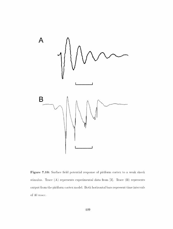
Figure 7.10: Surface field poterttial response of ~jirihrm. cortex to a weak s'irock

stirnutus, 'Trace ( A ) represents experimental data from 231. Trace (B) rrpresexlts

output from tire piriforrn tortc3x model. Both ltorizontaf bars represezlt time irltervals

of 40 rrrser.

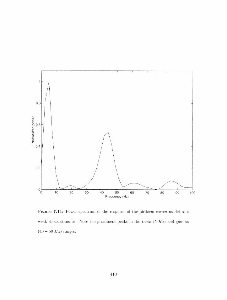
Frequency (Hz)

Figure 7.11: Power syectvurrl of the resllansp of the ~~irifornl cortex xnodel to a

weak S ~ I O C ~ sti11111111s. Note the prorrtill~~lt peaks in the theta (5 Hz) and garnrrla

(30 - 50 H z ) ranges.

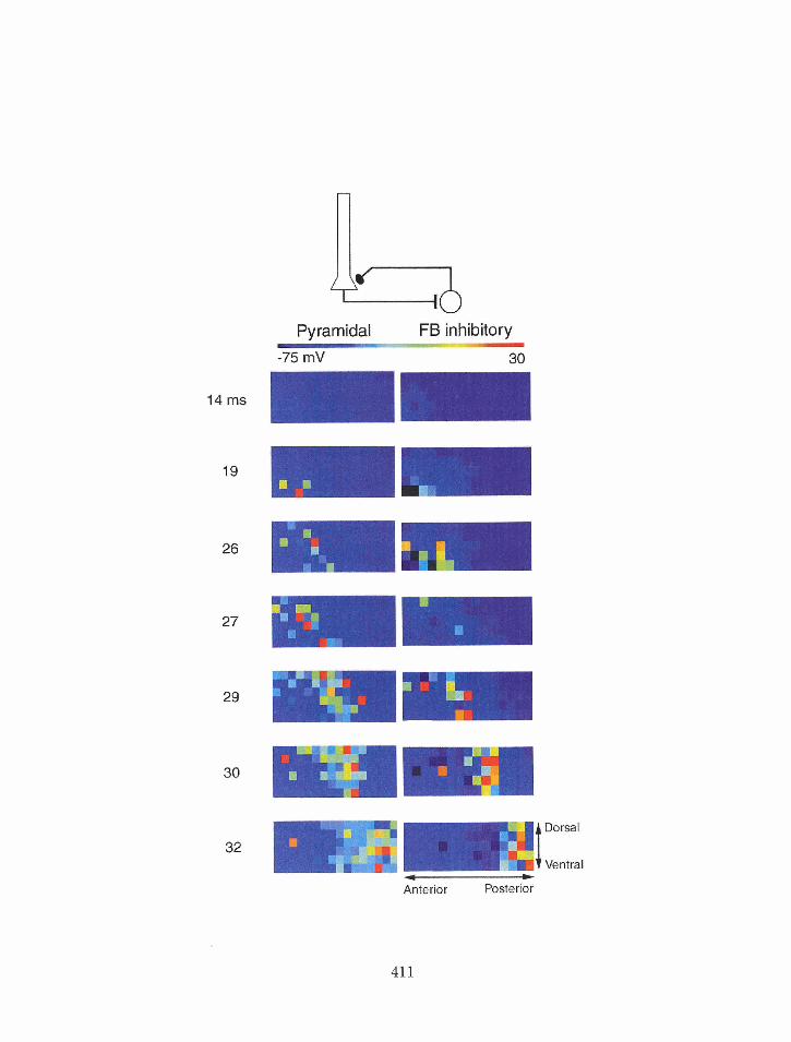
14 rns

Pyramidal FB inhibitnrv

& Dorsal

Anterior Posterior

Figure 7.12: (Previous page) Response of pyra~rxidal ~ i ~ r ~ r c t n s (measureri at tliti

sorna) and feedback (FB) irlhihitory interneurons in the piriforrn cbortex moclcl tr) a

weak shock stiniulus. This data is fro111 a small-scale xnoc-lctl (96 pyramidal ~irurorisj.

The color bar represents the membrane pote~ltial in rn17. Earl1 horizontal pair of

frames represents a specific time (in nzsccj after the shock stirnulus (indicated at

the left of each pair of frames). The schematic diagram at the top of tlic, page

represents conrlectiorls het?veen pyranlidal rleurons (left) and feedback i~lhihitory

neurons (right).

pathway arc. doubled, damping of the oscillatory field potential occurs nlucli more rapidly

(figure 7.16, B): orlly tllree oscillatory cycles are seen instead of five. Conversely, if this

pathway is abolished, damping of the resy onse does not occur: instead. persistent oscillatiorls

arc. sceri. Depending on the specific parariieter values, periodically modulated oscillations

or ~onst~ant amplitude oscillatory pattterns can be observed in the field p~t~olltials (figure

7.16. C aiid D).

7.3.3 Influence of feedback inhibitory interneurons

Tlir galrlrrla oscillation fi.(?quprl~y of this r~lodrl is critically depr~ldent on paranletel-.; relating

tto filedback iilllibitory internr:urons. Tlierr is sorne experiinrrltal rvid~rlce for inhil~itory

inbrractiorls betwren tllrsrt intrnlcuroils [3j. In tllc. nlodel. these corlilrc-tio~ls p r ~ v e ~ i t thr.

2iigllly excitable krdback int erlleilrorls from firing inorr. t ha11 once per gallllrla cycle. If'

these nmtually i~lhibit~ory intrractions are reinovrd. r.acl1 fccdl~ack illtorlleuron spikes tawice

412

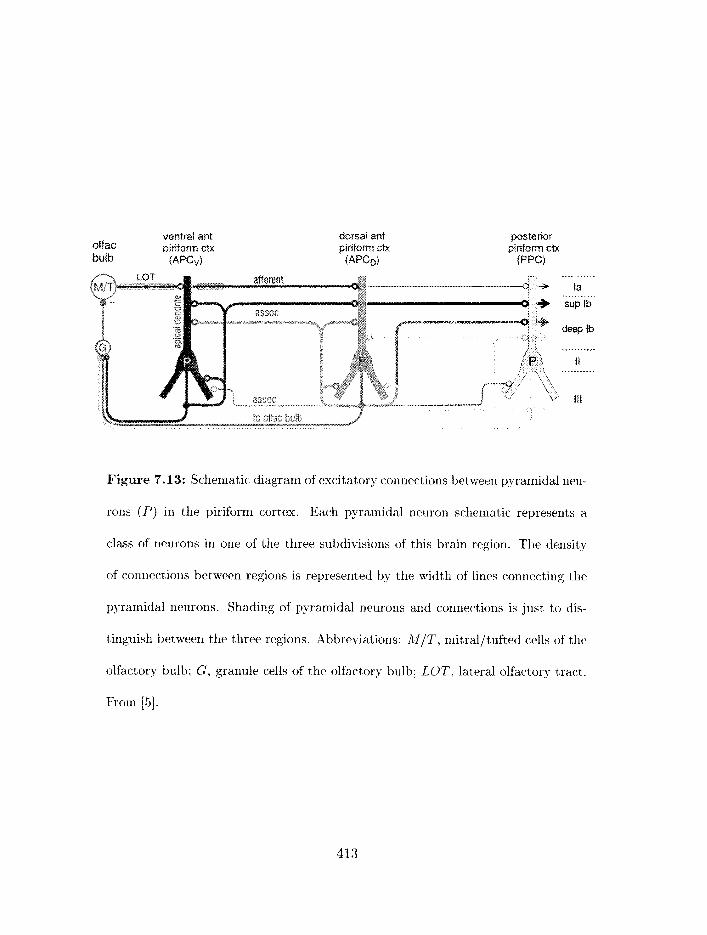
ventral ant otfac: pjrifarrn ctx bulb ( Af'CvI

dorsal ant piritorm ctx (APCo)

A...,,,..."

la ,,..--.,... sup Ib

Figure 7.13: Schematic diagram of excitatory co~lnections between pyramidal neu-

rons (P) in the piriform cortex. Each pyramidal neuron schematic represents a

class of neurons in one of the three subdivisio~ls of this brain region. The density

of c.onnections between regions is represented by the width of lines corlnecting the

pyramidal neurons. Shading of pyramidal neurons and connections is just to dis-

tinguish between the three regions. Abbreviations: AllT mitralltufted cells of the

olfactory bulb; G, granule cells of the olfactory bulb; LOT, lateral olfactory tract.

From [5].

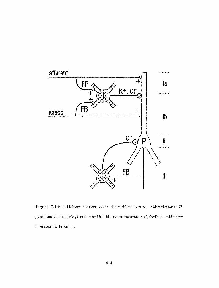
Figure 7.14: Inhibitory conrtectiorls in the pirifbrrrl cortex. Xbbri~viatiatls: P.

pyramidal neuron: F F . fet.edforxvarcf. inllil-titory interneuron; FB, feedbark irthihitor;).

interneuron. From [5?.

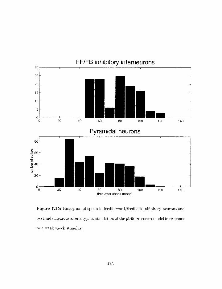
FFIFB inhibitory interneurons

Pyramidal neurons I I I I I I I I I

0 20 40 60 80 100 120 140 time after shock (msec)

Figure 7.15: Histogram of spikes in feedforward/feedback inhibitory neurons and

pyramidal neurons after a typical simulation of the piriform cortex niodel in response

to a weak shock stimulus.

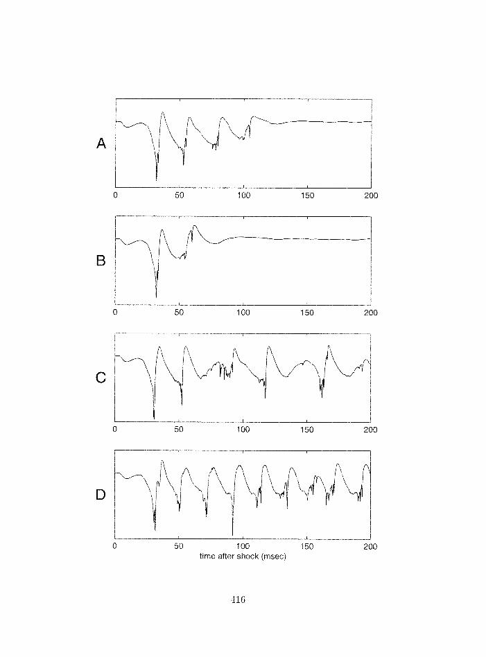
50 1 00 150 200 time after shock (msec)

Figure 7.16: (Previous page) Deperlde~lc+c of weak shock-evoked oscillatiarls on

parameter settings in the pirifornl cortex rrrodel. Each figure represr3rrts tllcb surface3

field potential recorded in posterior piriform cortex. A. Starldard paranrcltc.r set. B.

Synaptic weights from feedforward / feedbark interrreurons are doubled. C . Synal~tic

wights from feedforward/fcledhack interneurorls are set to zero. D. Same as C ,

but connectiorzs bttt~-een feedback interneurorls %-ere also set to zero. Traces are

unfiltered.

per oscillatory cycle (figure 7.171, which greatly increases the effective time corlstarlt of

inhibitiorl. This in turn reduces the oscillatory response to a weak shock stirxlulus f orn

four to five successive traveling waves of spiking activity to three waves, and also cllarrges

the shape and tlle power spectrum of the surface field potential substarltially (figure 7.18).

Specifically. whereas the power spectrurtl in the original model has most of the power in the

theta (4- 10 H z ) and garrirlla (40-70 H z ) band, as in pirifornl cortex 11. the model witllout

irr:terconnectiorls between feedback illllibitory interneurons has a much broader distribution

wit11 significant power ill the i)rtJa (20-35 Hz) band. reflecting thc slower oscillatic~n rate.

Some versions of tlle JVilson/Bowtr piriform cortex model 20. 211 also co~itairled synaptic

c.olrrlections t~&ween feedha& inltibitory intern~urons, but the possible functions of these

t-orznections were nc~t, explored.

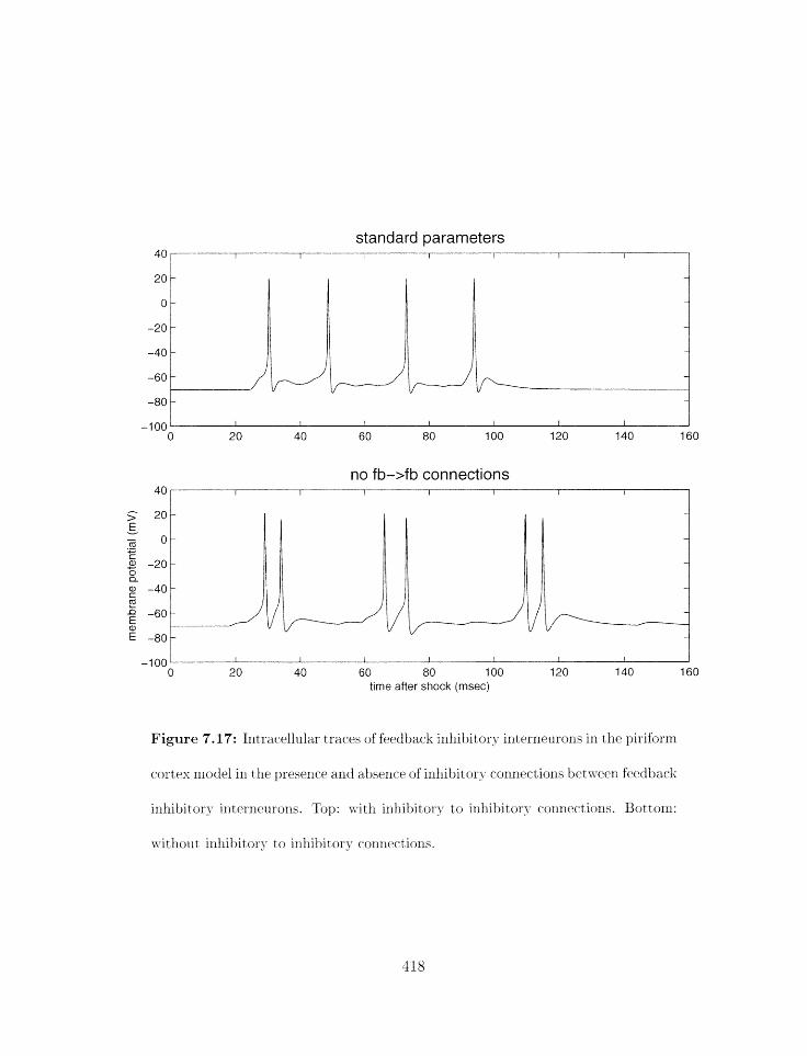
standard parameters 40

no fb->fb connections 40

5 20 E - - nf 0 .- ..-. c 2 -20 0 a. 2 -40 e! a -60 5 E -80

-1001 1 I I I I I I 1

0 20 40 60 80 100 120 140 160 time after shock (msec)

Figure 7.1'7: Xnt raceflufar traces of feedback inhibitory i1lterrlczurol-t~ iri the pirifornr

ctlrtes ~rlodel in the preser1c-t. and al~sence of ir-tfiik)itc)rr; co~lrlectiorls betwec~z feecil~ach-

inl-tibitor!- interneurorls. Top: tvith inhillit or?; to inhit>i.tor;)- co~trrect ioxis. Bot torn:

'~%-itl~ont inllibitory to inhibitory connections.

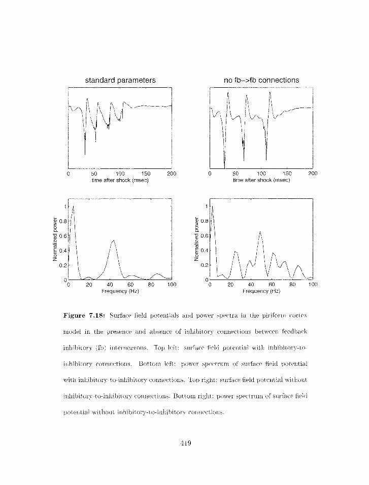
standard parameters no fb->fb connections

0 50 100 150 200 time after shock (msec)

- 0 20 40 60 80 100

Frequency (Hz)

0 50 1 00 150 200 time after shock (msec)

0 20 40 60 80 100 Frequency (Hz)

Figure 7.18: Surface field potentials and power spectra in the piriforrtl cortex

nlodel i ~ i the presence and absenve of inhibitor.; corinections between Eecclback

inhibitory (fi)) inttrneurons. Top left: surface* field potential ivitli inliibitory-to-

inhittit ory c*onnectiozzs. Bot t on1 left : power spcet rum of surface field putetit ial

with irrhihitory-to-inhil~itory conllcctiorls. Top right: surface ficld 13otrntial 5vitlrout

inhibitory-t o-ir~l~itjitc~r.; connect ions. Bot t on1 right : power spprwtrunl of surEa.(~ fic1c-t

potential 15-ithout inhibitory-t o-i111iibitor~- ~or-tn~ctions.

7.3.4 CSD response

Thrl Wilson/Bower model of pirifonrl c:crrtrx !20. 211 did riot irlcludr CSD results for weak

slloek sti~ntili. because at the tinic that rv~odel was constructed there was no relevant ex-

pef.inlerri;al data available. Recently. experimental CSD allalysis has been performed in the

piriforrn cortex of rats receiving weak shock stimuli 111 and tlie results are very revealing.

I I ~ figure 7.19 [9] we see contour plots of the CSD responses to strong and weak shock stirn-

uli. In figure 7.20 we see the same data presented as CSD surface plots. There are a nuniher

of i~lteresting features of these results which point out serious flaws in tlie piriform cortex

lrlodel with rarldorrl corlrrectivities described above. Here, I will describe both tlie essential

features of the experimental weak shock response and why the random connectivity model

carlriot replicate them.

A technical detail needs to be nientiolletl at this point. C'SD responses as measured in

our piriform cortex models feature very large ionic currents in the vicinity of the soma axid

exte~ldirig well into the apical de~ldrite. These currents are a curlsequence of tho pyramidal

ner~rozl rrlodel used and are not observed in ex~~erimentally rrleasured CSDs. The reason

for this discrepant:y is unclear, hut may refiect diEerences in cable propcrtic3s I~etween tho

irior~>ll~logies of the real neuron arld tllr siz~lplified model neurons used in the rietwork model.

These large ionic currents ~~lakcl interl3retatioli of the nlodel CSDs extrerriely difficult*. as

tltey overlap with synaptically ge~rerated curreirt sinks in layer Ib. In order to circumvent

this prcgblerii. syllaptic C:SDs were lzreasurrd &or11 the rrlotlel by ignorirlg all but tlie syna~?tic.

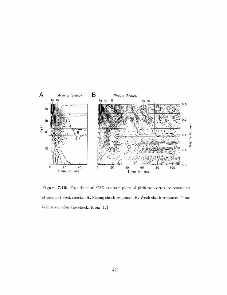
A Strong shock B Weak Shock la Ib la lb I I la Ib I I

0 20 40 Time in ms

20 V.U

40 60 80 100 Time in ms

Figure 7.19: Experimental CSD contour plots of piriform cortex responses to

strong and weak shocks. A. Strong shock response. B. Weak shock response. Time

is in m.sec after the shock. From [Ill

0 Sink i / t Source

Figure 7.20: Experi~nerltal CSD surface plots of pirifornl cortex responses to strong

and weak shocks. A. Strong shock response. B. Weak shock response. Time is in

rrzsec after the shock. From [ll]

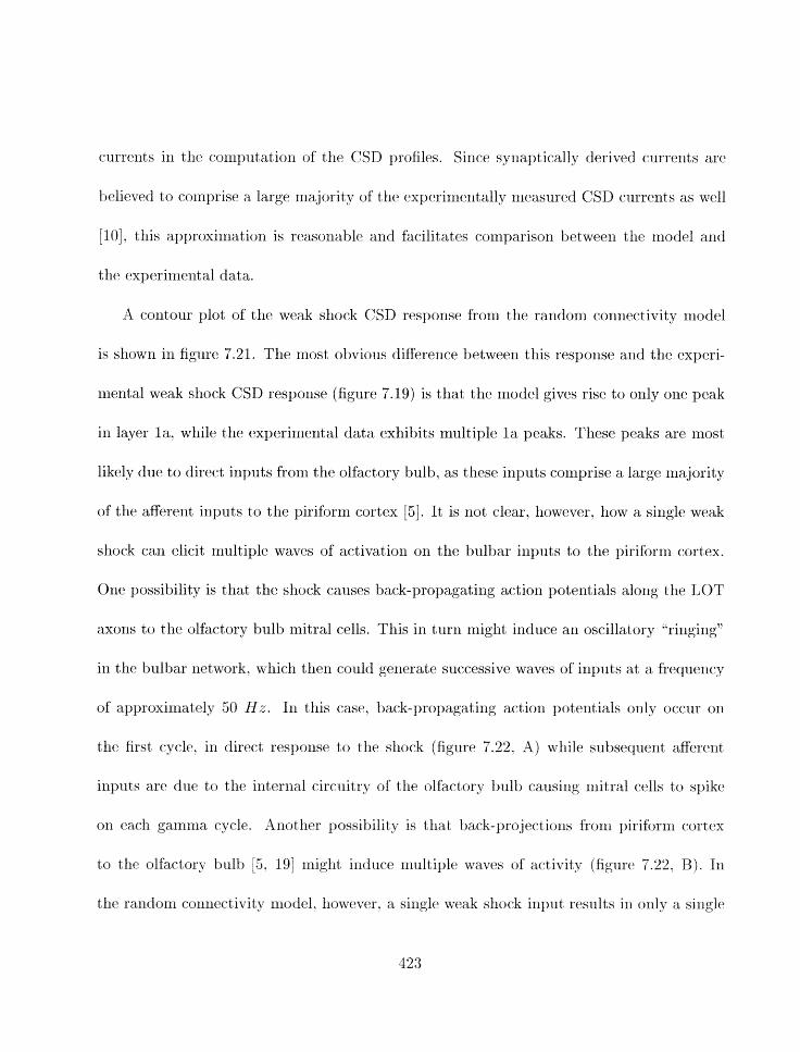
currents in the computation of the GSD profiles. Siilce syilaptically derived curreiits are

believed to coinprise a large majority of tlie experinrentally ineasured CSD crlrrerits as well

[10]. this approxiinatiori is reasonable aird hci1itatc.s cornparison betweer1 tire inode1 axid

t lre experiirierltal data.

A contour plot of tlre weak sliock GSD response from the random comrectivity model

is show11 in figure 7.21. The rnost obvious difference between this response aiid the experi-

mental weak shock CSD response (figure 7.19) is that the model gives rise to only o m peak

in layer la , while the experimental data exhibits multiple l a peaks. These peaks are nrost

likely due to direct inputs from the olfactory bulb. as these inputs comprise a large majority

of tlre afferent inputs to the piriforrn cortex [5]. It is not clear. however, how a single weak

slrock can elicit rnultiple waves of activatiorl on the bulbar inputs to the piriform cortex.

One possibility is that the shock causes back-propagating actiorr potentials alozrg the LOT

axons to tlrc olfactory bulb mitral cells. This in turn might induce an oscillatory ..ringingn

in ttir bulbar network. which then could gerlerate successive waves of inputs at a frequerlty

of approximately 50 H z . Irr this case. l,ack-propsating action poterrtials only occur on

tht. first cycle, in direct response to the shock (figure 7.22. A) while srrhsequellt a@c?uent

inputs are due to the internal cifcliitry of the olfactory bulb causing mitral cells to spike

on each gamma cycle. Ariot her possibility i s that Ijack-project ions from pirifovnr cortex

to tl1c.i olfactory ?;bull, 5. 1'31 nligflt ilidnce multiple w a ~ ~ c s of activity (figure 7.22. B). 1x1

the random connectivity nrodel. b0wre.ii.r. a single weak shock input results in only a sirlgle

peak in layer l a (figure 7.21). In order to niodel the phenomenon of multiple l;t peaks.

simulations were run wliereby the weak sllock was repeated nriultiple times at 50 N: (figure

7.23). Interestingly. not all of the rnultiple input shocks (at 20. 40. 60. 80. arid 100 srrsec

after tlie first shock) car1 he seer1 in the CSD profile. This is because activation of layer l b

afferents raise thr mernbrane potential in distal apical deridrites close to the syriaptic rever-

sal poteritial. which drarnatically reduces the input currents from subsequent shocks (figure

7.23) because the synaptic driving force is rriuch smaller. Other than tliis. the resulting CSD

profiles were not substantially different from those elicited by a sirzgle weak shock. In both

cases, large current sinks were generated ill lajrer l b as a result of fecdforward projections t80

superficial layer 1 b dendrites orz pyrarnidal neurons and feedback projections to deep layer

11, dr-lndr i t es .

Ariother sigxiificant discrepancy between the exyerilriental CSD results and those of the

random eonriectivity model involves the latency between the CSD peaks in layer l a (caused

by afferent input) and layer 1b (caused by associational input). The experimental data

sllows that tlze 1atent-y between tlrcsp peaks is rougllly tlie sanie for bo-tli the weak and t*lsc>

strong s h o ~ k response (about 6 to 8 ~ n s e c ) (figures 7.11 a11d 7.19). 111 the razldorii co~lrieetivity

rnodel. tlic 1atcnc.y f>et\veen these pt&s is rilucll lziglzer b r the weak slloek than tlie strong

shot-k: for the strong sliock tlie latency is 8-9 msec (figure 7.4) while for the weak shock it

is over 20 msec (figures 7.21 a d 7.25). eEectively skipping an entirc ganinia cycle (at 50

H z . i .e., 20 ~rrsr-ie).

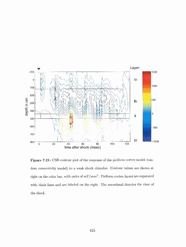
Layer:

Figure 7.21: CSD contour plot of the response of the piriform cortex model (ran-

dom connectivity model) to a weak shock stimulus. Contour values are shown at

right on the color bar, with units of mv/mm2. Piriform cortex layers are separated

with black lines and are labeled on the right. The arrowhead denotes the time of

the shock.

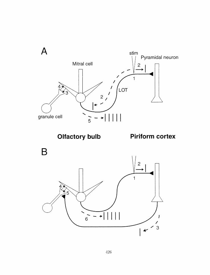
stirn \ Pyramidal neuron

Olfactory bulb Piriform cortex

Mitral cell \

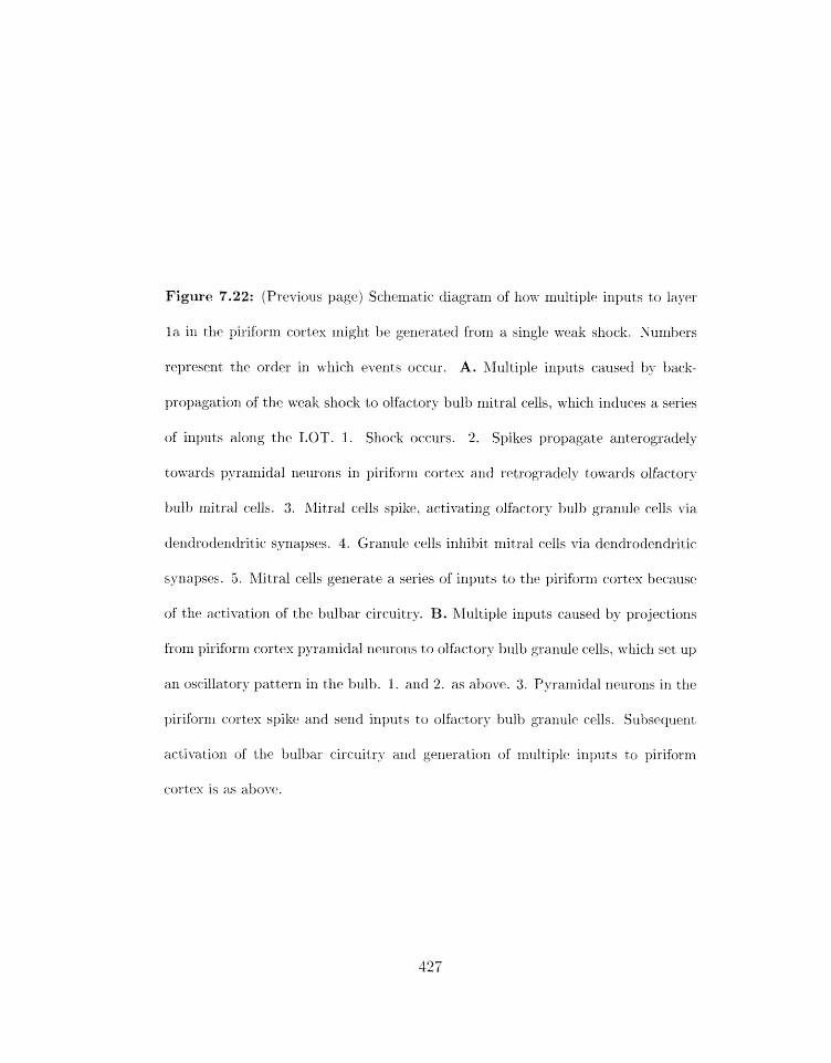
Figure 7.22: (Previous page) Scliernatic diagram of how mdtiyle inputs to layer

l a in tlie piriform cortex might he generated from a single weak shock. Xumbers

represent the order in which events occur. A, lllultiple inputs caused by hack-

propagation of the weak shock to olfactory bulb mitral cells. which induces a series

of inputs along tlie LOT. 1. Shock occurs. 2. Spikes propagate anterogradel3-

towards pyraxiidal neurons irl piriforr~i cortex arid retrogradely towards olfactory

bulb niitral cells. 3. Alitral cells spike. activating olfactory kulb grarlule cells via

dendrodendritic synapses. 4. Granule cells inhibit rnitral cells via deridrodendritic

synapses. 5. hlitral cells generate a series of inputs to the piriform cortex because

of the activatian af the bulbar circuitry. I3. itlultiple inputs caused by projeetioris

from piriform cortex pyramidal lieurorzs to olfactory bulb granule cells, t~bicli set up

an oscillatory patter11 in the bulb. 1. and 2. as above. 3. Pyranlidal neurorls in the

pirifor~ii cortex spik arid send iriputs to olfactorv bull:, granule cclls. Subsequent

activation of the bulbar circuitry and generation of rnultiplc inputs to piriform

cortex is as above.

Layer:

Figure 7.23: CSD contour plot of the response of the piriform cortex model (ran-

dom connectivity model) to a weak shock stimulus with multiple input shocks oc-

curring at a rate of 50 H z . Contour values are shown at right on the color bar,

with units of mv/mrn2. Piriform cortex layers are separated with black lines and

are labeled on the right. Arrowheads denote the times of the shocks.

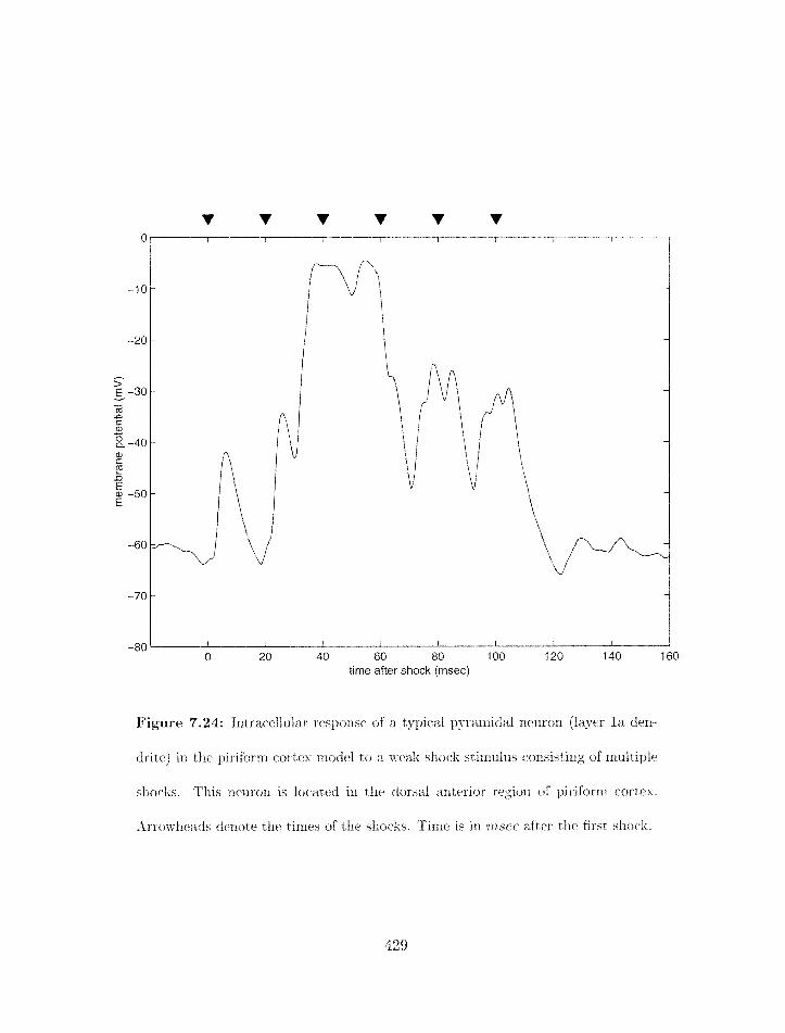
-70

-80 0 20 40 60 80 1 00 120 140 160

time after shock (msec)

Figure 7.24: Intracellular response of a typical pyranlidal ncuurorl (layer l a den-

clritr") in the piriform cortex rrlodel to a weak slkock stirriulus cortsisting of multiple

shocks. This neurorr is located in the ctorsal anterior regiorl of ~lirifornr cortex.

;'irmsi=llcads dcnotc) the tirnes of the shocks. Tirrlc is in rnser after the first shock.

Thc CSD peak any~litudes of the weak shock response. in thc. (>xperirrlental data arc:

also much snla1lt.r than those of the strorlg sl-lock response: ixr figure 1.20. the amplitude

of the strong shock respollsr is roughly twenty tiilies greater than that of thc weak shock

response. In the rarrdom corir~ec t ivity model, however. the CSD resporlses are of cornparable

arrlplitndes for both weak and strong shocks (figure 7.25). In addition. the ratio of layer l b

to layer l a peak heights, whidl is close to unity for weak and strong shocks cxperirnerltally

(figure 7.20) and for strong shocks irt the model (figure 7.3). is much higlirr for weak shocks

in the niodel.

Tlzese results suggest several points about piriforrn cortex dynamics. First, tllr am-

plitude of tlle layer l b peak in the CSD plots is roughly proportional to the number of

pyrairlidal rieurorls firing in response to the input stimulus, since this is what determines

the amount of synaptic activity which is directly measured in the CSDs. Thus, the fact

that tliis peak is twenty times srrialler in the weak shock response than in the strorrg slrock

resljonse i~iplies that roughly 1/20 as atany neurons fire in respollse to the weak shock as

co~rtpared tto the strong shock. We have assurrted tlmt a strortg shuck c:ttlises all pyraniidal

neurons in tlie ventral arrterior regiorl of piriforln cortex to fire. Tlrus, we ~lvould naively

expect; a rrtuclr srnaller nunlher of neurons to fire in resporise to a weak sluock per garrlrlza

cycle. 111 contrast. ixt the cortical mrltrdel t lie raridonl connectivity betweexi olhctory bulb

xrlitiral cells and pirifom cortex pyl-amidal rieurons has the effect tliat ac*tivating (in this

rase) l / 5 of the bulbar inputs causes ail of tlrc pyramidal ItrLIroiis ttc, rocriv~ on average

A: strong shock

B: weak shock

time after shock (rnsec)

Figure 7.25: CSD surfxe plot of the response of the piriform cortex ~riodel (ran-

dom connectivity model) to weak and strong shock stimuli. Current sinks point

upwards. Peaks are labeled with the layer of piriform cortex in whidl they occur.

A. Strorig stlock response. B. Weak shock response.

abolit 1 15 as 1r1u(-11 excitatory input. whirl1 causes all the ricurolls to spike with a very long

latency as opposed to causirlg 1j5 of the nelirorrs firing wit11 a short latency (figllres 7.12.

7.21. and 7.25). This acconr1ts for the much larger CSD amplitudes in responst. to tlle weak

shock seen in the rnodcl as corr1parc.d to the data. and also accounts for the mudl larger

size of the l b peaks conipared to the l a peak(s) .

These results suggest that there is something fundamentally wrong with the rand0111

corlnect ivity model despite the fact that it replicates the oscillatory surface field pot,ential

fairly accurately. Interestingly. this model nevertheless reflects the view of many neurosci-

ent ists 011 the genesis of the oscillatory dynamics in piriforrr~ cortex -1. 211. I11 particular. the

WilsonjBower piriforrn cortex model. which was the ilnrllediate predecessor of the randon1

connectivity lrlodel described above, exhibited the same kinds of dynamical bellaviors in

response to weak shock stiniuli (although CSDs for weak shock stimuli were not measured

in that model). Below I describe a different model which replicates the CSD response to

weak shocks much rrlore accurately. As will 'lx seen, the difference between the two rnodels

has rrlajor corlsequerlces for theories of neural coding and inform&ion processing in the

piriforrn cortex (discussed in chapter 8').

7.4 The weak shock response: rnodel with structured con-

nectivities

This sectiorl describes tlre weak shock response in tlie seeorid version of tlre piriforni cortex

model. This rnodel features liighly structured conriectivity l ~ t w e e n the olfactory bulb and

piriforni cort,ex and wit fiir~ cortex. Like the raridom corirlectivity rnodel. this rnodel can

accurately reproduce the strong shock response. Unlike the previous rnodel. however, this

model also replicates the weak shock CSD response of the system with co~isiderable accnracy.

7.4.1 Structure of the rnodel

The struct,urecl connectivity rnodel has several significant dierences from the rarrdorn con-

nectivity rlrodel, shown schematically in figures 7.26 and 7.27. They are:

1. Mitral cells in tlre olfactory bulb and pyralnidal neurons in pirifornr cortex are divided

into rron-overlapping ncxronal groups on the basis of their cor1nec:tion patterxls. For

convt:rrierrce in recording sinnllated CSDs. I used four groups in Ijoth olhctory bulb

and cortex (figure 7.26). Ho-~vever. it is possible that s mudl larger nunil>cr of groups

r n q exist (see cliapter 8).

2. hfitral cells in I-he olhctory i~ull, irl a particular group project exclusively to ~~j~rani idal

rleulroxrs iri piriforrrr cortex of a particular grou13. T1rus. rrlitral cells iml bulbar group 1

(red color in tile figure) project to pyraniidal rleurorls in cortical group I. etc. (figurc

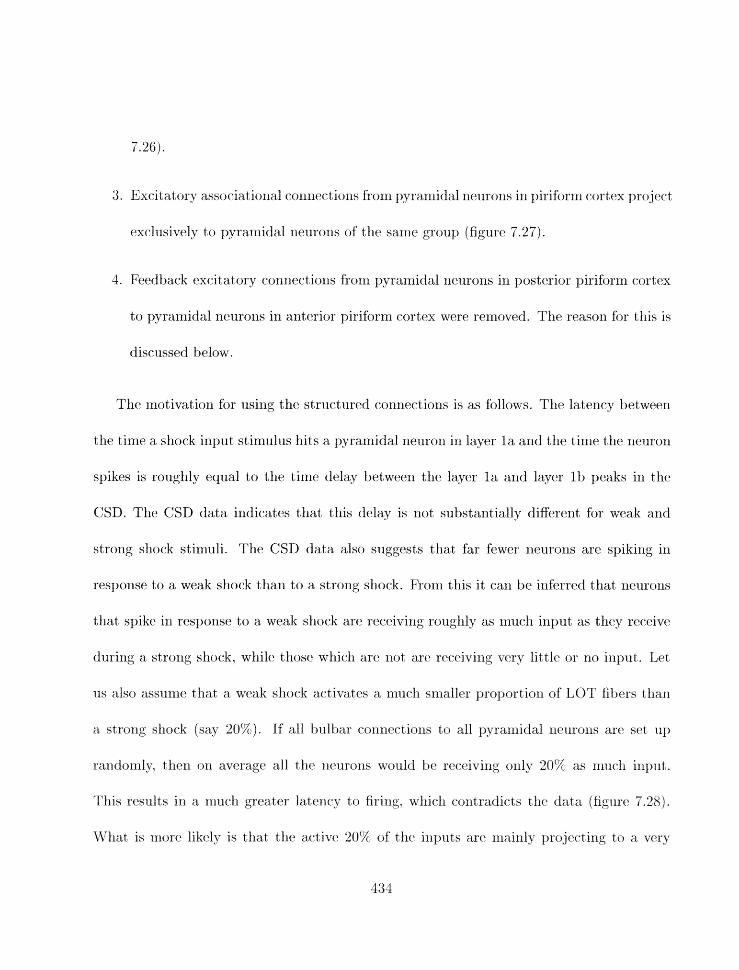
3. Excit atury associat ional coriric.etions frorsl pyramidal rieurons in piriforln eort ex project

exclusively to pyramidal neurons of the sarr1~ group (figure 7.27).

3. Redback excitatory conrlectiorls froni pyraniidal rleurons in posterior piriforrri cortex

to pyranlidal neurons in anterior piriform cortex were removed. Tlie reason for this is

discussed below.

The motivation for using the structured connections is as follows. Tile latency between

tlie tinicl a shock input stimlrl~is hits a pyramidal nenroil iri layer l a and the tinie the neuron

spikes is roughly equal to the tinic delay between the layer l a and layer l b peaks ill the

CSD. The CSD data indicates that this delay is not substantially different for weak arid

strong shock stimuli. The CSD data also suggests that far fewer neurons are spiking in

response to a weak shock tlian to a strong shock. From this it can be inferred that nerlrorls

that spike in resI>onse to a weak shock are receiving roughly as much input as they receive

during a strorlg shock. whilc those which arc not art" receiving very littltl or no input, Let

11s also assunle that a weak sllock activates a lnu~li srrialler yroportioxi of LOT fibers tllarl

a stro~ig shock (say 20%). If all hulbar raonnections to all pyramidal nerlrous ale set 1113

randomly. tlzen a11 werage all the zit2urans would be rrt*eiving only 20% as mut:h injtlit.

This results in a wriucfl greater latency to firixig. which colitradicts the data (figure 7.28).

Wliat is more likely is that the acbivcl 20% of' tlic inputs arc. ~llairilj- l~rojectilig to a vt3r-y

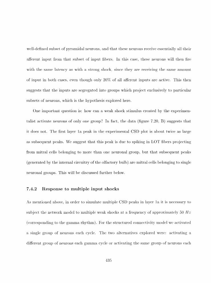
well-defiried subset of pyraniidal rieurons. arzd that these lleurorrs rer:eive essentially all their

agerent input from that subset of input fibers. In this cease. these rzeurotzs will then fire

with tho sarncA latency as with a strong shock, since dhcy are rcc.eiving the same amount

of input in both cases. even though only 20% of all afforelit inputs are active. This then

suggests that t lie inputs are segregated into groups which project exclusively to particular

subsets of neurons. which is the hypothesis explored here.

One inlportant question is: how can a weak shock stimulus ~rea ted by the experinien-

talist activate neuroris of only one group? In fact. the data (figure 7.20. B) suggests that

it does not. The first layer l a peak in the experimental CSD plot is about twice as large

as subsequelit peaks. We suggest that this peak is due to spiking in LOT fibers projecting

from lnitral cells belonging to more than one rlcuronal group. but that subseqllent peaks

(generated by t l e internal circuitry of tlre olfact,ory bulb) are mitral cells belonging to single

neurorral groups. This will be discussed further below.

7.4.2 Response to multiple input shocks

As rxicrltiolzed above, irl order to sirilulate rrzultiple CSD peaks ill layer l a it is rlecessary to

subject the network rriodel to niultiple weak shocks at t?, freyuerzry of approxirnatcaly 50 Hx

(corresl>onding to tlie galnma rhyt tznl), For the structured connectivity nlorlel we actimted

a single group of neurons each cycle. The two alternatives explored were: activatirlg a

dieilrent group of rleurorzs eaeli gamnla cyclt or activating the sarw group of rletlrons eat:ti

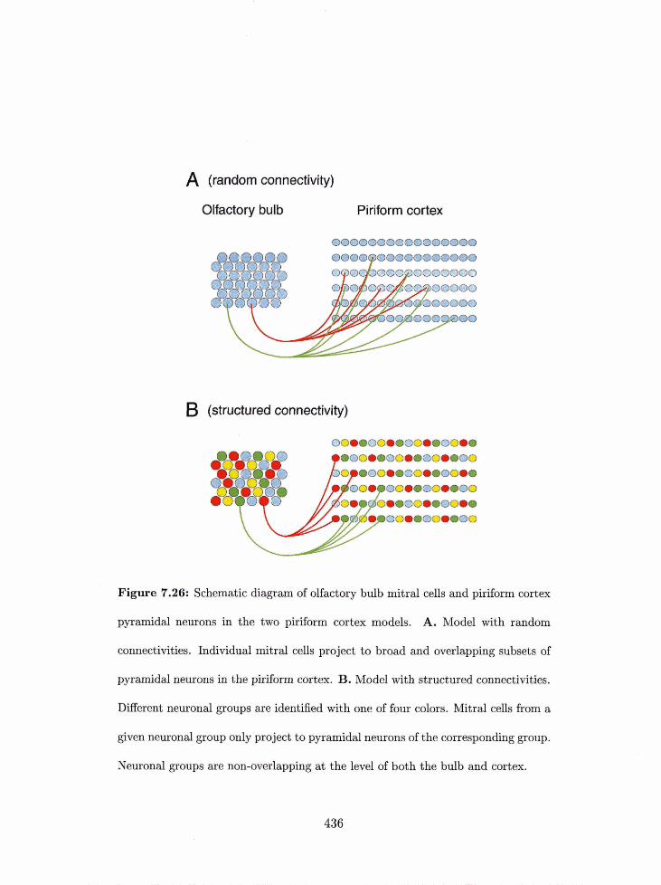
A (random connectivity)

Olfactory bulb Piriform cortex

B (structured connectivity)

Figure 7.26: Schematic diagram of olfactory bulb mitral cells and piriform cortex

pyramidal neurons in the two piriform cortex models. A. Model with random

connectivities. Individual mitral cells project to broad and overlapping subsets of

pyramidal neurons in the piriform cortex. I3 . Model with structured connectivities.

Different aeuronal groups are identified with one of four colors. Mitral cells from a

given neuronal group only project to pyramidal neurons of the corresponding grcrup.

Neuronal groups are non-overlapping at the level of both the bulb and cortex.

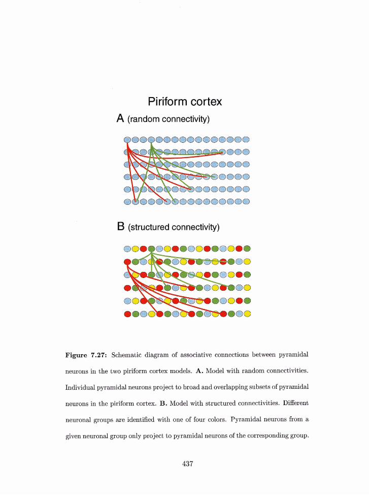
Piriform cortex A (random connectivity)

B (structured connectivity)

Figure 7.27: Schematic diagram of associative connections between pyramidal

neurons in the two piriform cortex models. A. Model with random connectivities.

Individual pyramidal neurons project to broad and overlapping subsets of pyramidal

neurons in the piriform cortex. B. Model with structured connectivities. Different

neuronal groups are identified with one of four colors, Pyramidal neurons from a

given neuronal group only project to pyramidal neurons of the corresponding group.

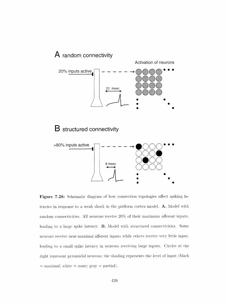
A random connectivity Activation of neurons

20% inputs activ -be@@@* *

@@@@

@@a@ * * * * 0 *

B structured connectivity

>80% inputs active - - - - -

000. 8 msec f--J,

0.00 0000 * * * * 0

Figure 7.28: Scliemat ic diagranl of I-~ow connection topologies aEect spiking la-

tencies in response to a weak shoclc in the piriforrrl cortex rnodel. A. hlodel xith

rarzdom connet-tivities. ,411 neurons recci~e 20% of their rilasirrzum afferent inpctts.

leading to a large spike latency. B. Llodcl with structured c.itn~ircti.;ities. Soxiir.

neurozrs re{-eive near-maxirrzal aRere11t. inputs while otiters reccivr-. very little inprxt,

Lradiilg to a small spike latency in rlctrrorls tccci.i~ing large i ~ i ~ ~ t l t s . Circles at the

right repn~s~ri t pparrridai neurons: tire shading represents thr level of input (black

=. masi~nal: white == 11011~: gray = partial).

Different neuronal groups activated each cycle

Activating a different nrrrrorral group eaclr cycle gives rise to an ordered series of waves of

excitation in tlie cortical model alternating between different neurorial groups (figure 7.29).

The rleliro~ial groups in tlie cortex were set tip with a regular spatial spacirig of period 4

(figure 7.27). Tliis arrangement was used in order to produce more consisterlt CSD plots.

since each simulated CSD recordi~lg electrode is equidistant from Iieurons of each group.

This is riecessary in a small scale model; in the real system tlre riulllber of rieurolls is so

rliucli larger that activation of any one group would have a roughly equivalent eEect on the

CSD profile as lorig as neurons from all groups arc. randomly distributed throughout tlie

cortex. As car1 be seen in figure 7.29, the first wave activates a ~tarticular group of ncxrons

(group 1). the: next wave activates a different (rioii-overlapping) group (group 2). etc.

The CSD profile for the structured co~inect~ivity niodel is shown in figure 7.30. If we

coalpare this t30 the experinlental data (figure 7.19. B), we see that, the model replicates t11e

main feat ures of the data. In ~art~icular. t lie rriodel displays en ordered sequence corisist irig

of a layer l a peak followed by a layer 111 peak. then another layer l a peak. rtc. The 1a/lb

patter11 is rc~~cated every 20 ntsec.. A closeup of the first two peaks sfiow~i as a surface

plot (figure 7.3l) shows that tllc two peaks arc of nearly ttre snnlc liieight. with the layer

l a peak somewlr~at larger. The latency between the l a and 1b peaks is rotlgllly 9 U~SCC.

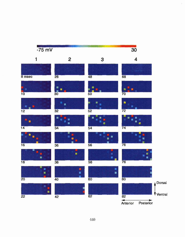
t Dorsal

42 82 VWIE~I

Anterior Posterior

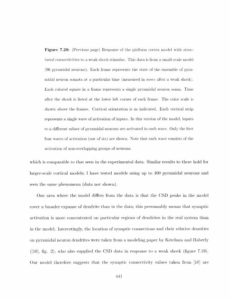
Figure 7.29: (Previous page) Response of tllc piriform cortex nrodcl \vi.ith struc-

tured c<)~lrzectivities to a weak slioclc stimulus. This data is frorri a sniall-scale. model

(96 ~>yrarnidal neurons). Eacll frame represents the state of the ~nsenible of pyra-

midal Ileurorr so~rrata at a particular time (xleasured in r n s w after a weak slzock).

Each colored square in a frame represents a single pyrarnidal neuron soma. Tirrle

after the shock is listed a t the lower left corner of each frame. The color scale is

sliowri above the frames. Cortical orieritation is as indicated. Each vertical strip

reprcserlts a single wave of activation of inputs. In this version of the model. inputs

to a different subset of pyramidal neurons are activated in each wave. Only the first

four waves of activation (out of six) are shoi~n . Note that each wal-e t:onsists of the

activatiorl of 11on-overlapping groups of neurons.

which is cornparable to that seen in the experirrlental data. Similar results to these hold for

larger-scale cortical models: I have tested models using up to 400 pyrarzlidal neurons and

seen the same pllenomena (data not shown).

One area where the rnodel differs from tllch data is that the CSD peaks in the rnodel

cover a broader expanse of dendrite than in tllc data; this I>resurnat>ly nleans that synaptic

activation is more conce~ltrated on particiilar regiorzs of derldritcs in the real system tllrtli

in t ht. rtzodel. I~lterestingly, the locat iorl of syrlqtic conrtcct ions and tlieir relativ~ densities

on pyrarnidal 11etlrorl dendrites were taken from a modeling paper by Ketchurn and IisberIy

([10j, fig. 2). who also supplied the CSD data ill respollse to a weak shock (figure 7.19).

0111. rllodel therefor(: suggests that the S ~ I I X ~ T ~ C c~iir~ectivity VB~UC'S take11 fioin [10j arc3

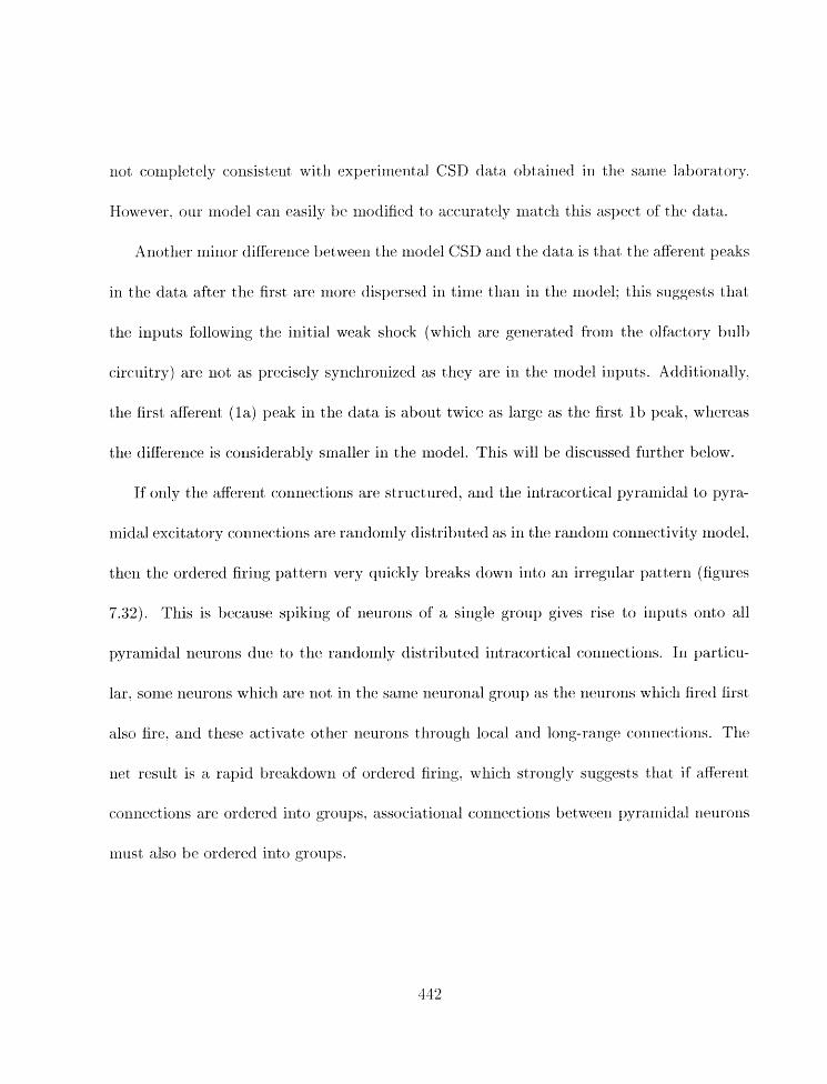
not cornpletely consisterlt with ~xperint~rrt al CSD data obtained in the sanrr lal>oratory.

However. our rrlodel can easily be niodified to accurately rriatcli this aspect of the data.

Anotlrer minor difference between the rrrodel CSD arid the data is that tlie afirerlt peaks

in the data after the first are rriore c-lispersed in time tlia~i in tlre nlodel: tltis suggests that

the i q ~ t d o l l o w i n g the initial weak shock (which are generated from the olfactory bulb

circuitry) are not as precisely synchronized as they are in the rnodel inputs. Additionally,

the first afferent ( l a ) peak in the data is about twice as large as the first l b peak, whereas

the difference is considerably smaller in the model. This will be disclissed further below.

If only the aff'erent connect ions are struc tured, and the int racortical pyramidal to pyra-

rriidal excitatory corrriect ions are randomly distributed as in the randonl connectivity rnodel,

then the ordered firing pattern very quickly breaks dowri into an irregular pattern (figures

7.32). This is because spiking of neurons of a single group gives rise to inputs onto all

pyrar~lidal neuroris due to the rarrdomly dist ributed intracortical connect ions. In particu-

lar. some rieuroris which are notiin tlie sarrie xieuronal group as tlie rieurons which fired first

also fire. arid these activate other neurons tlirough local and long-range contiec:tioris, T tie

net result is a rapid breakdown of ordered firing. which strorlgly suggests tliat if aEerent

connections are ordered i~ito groups. associatio~lal corlnectio~is betwecri pyrarriidal neurons

rrlrlst also be ordered into g rou~~s .

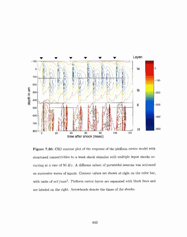
v v TF Layer:

I I

I I I

time after shock (msec)

Figure 7.30: CSD contour plot of the response of the piriform cortex model with

structured connectivities to a weak shock stimulus with multiple input shocks oc-

curring at a rate of 50 H z . A different subset of pyramidal neurons was activated

on successive waves of inputs. Contour values are shown at right on the color bar,

with units of mv/rnm2. Piriform cortex layers are separated with black lines and

are labeled on the right. Arrowheads denote the times of the shocks.

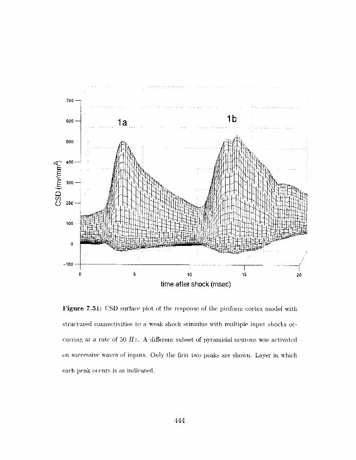
-100

0 5 10 15 20

time after shock (msec)

Figure 7.31: CSD surface plot of the response of the piriforni cortex model with

structured connectivities to a weak shock stiniulus with multiple input shocks oc-

curring a t a rate of 50 H z . A different subset of pyramidal neurons was activated

on successive waves of inputs. Only the first two peaks are shown. Layer in which

ea.ch peak occurs is as indicated.

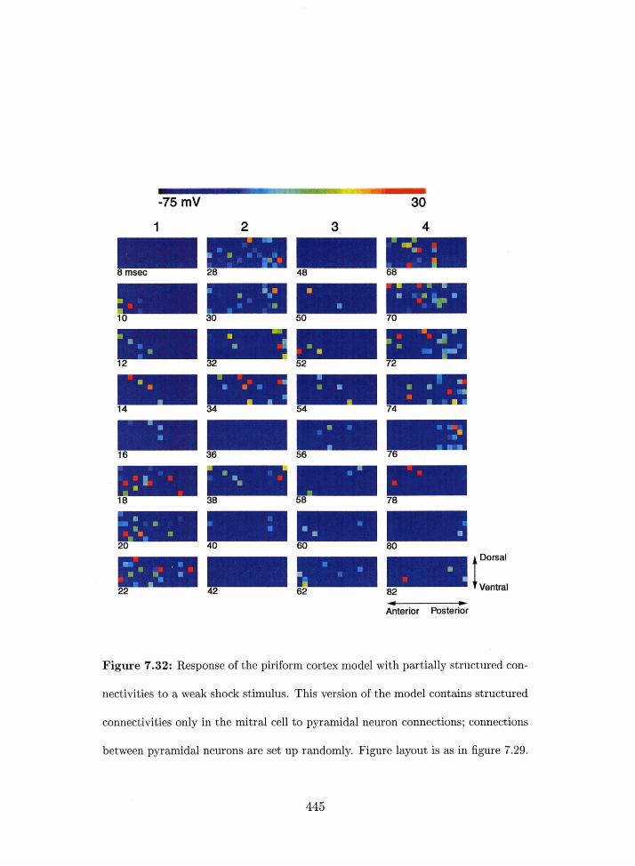
20 40 A Donal

4 C Anterior Posterior

Figure 7.32: Response of the piriforrn cortex model with partially structured con-

nectivities to w weak shack stimulus. This version of the model contains structured

connectivities only in the mitral cell to pyramidal neuron connections; connections

between pyramidal neurons are set up randomly. Figure layout is as in figure 7.29.

Same neuronal group activated each cycle

If the sartle nelrronal group is artimted on eacli gamnia cycle. the ordered series of r-r~urorsal

activations seen previously again breaks down to give rise to a more disordc?red firing patterri

(figure 7.33). In particular. note that the second wave of activatiorl does riot cause pyramidal

rieurons in the ventral allterirtr pirifurm cortex to spike at all. The CSD contour plot (figure

7.34) also shows that most of tlie layer l b peaks after tlre first are substantially attenuated.

wliicll is not surprising given that the pyramidal neurorls are firing quasi-randomly after the

first wave of ext:itation. These results depend 011 the presence of slow potassiurrs cllanrlels

(predominantly Knt ) which are activated when pyraniidal neurons spike (figure 7.35). These

channels have slow enough time constants that t h c ~ have riot returned to their baseline state

when the next wave of inputs arrives. wliicli prevents the pyranlidal neurorrs from firing in

response to the these inputs.

7.4.3 Discussion

I liave slsowrs that a piriforni cortex sliodcl can reproduce exgerinlental CSD data for a weak

sliock stimrllus as long as the ~nitral (-ells in tllc olfactory t~ulil and tlitl pyrarrsidal rierzrorrs

in thc olfactory cortex arc divided into non-o~~rlappirlg grolrys s-llicli arc pr~domirurntly

connected to otlier rlertrolxs of the sasrie group. Tlris is a radichal Zrypothesis tlrat ftas rrialiy

coxiseqt~ences from the stalldpoi~tt of colxspat at ~OIZS that the olfixct ory SYS~C'III may 1x1 per-

forrliing. I will stinlnlarizc tlhc, cviclcslcc, here and in the next- clraptcr I will present lily view

4 - - Anterior Posterior

Figure 7.33: Response of the piriform cortex model with structured connectivities

to a weak shock stimulus. In this version of the model, the same subset of pyramidal

neurons are activated on each wave of inputs. Figure layout is as in figure 7.29.

time after shock (ms~c)

Figure 7.34: CSD contour plot of the response of the piriform cortex model with

structured connectivities to a weak shock stimulus with multiple input shocks oc-

curring at a rate of 50 H z . The same subset of pyramidal neurons was activated

on successive waves of inputs. Contour values are shown at right on the color bar,

with units of mv/mrn2. Piriform cortex layers are separated with black lines and

are labeled on the right. Arrowheads denote the times of the shocks. Note the

attenuation of the layer l b peaks after the second shock.

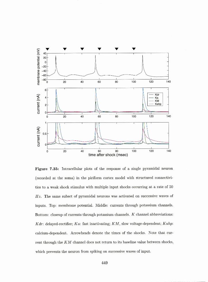
60 80

time after shock (msec)

Figure 7.35: Intracellular plots of the response of a single pyramidal neuron

(recorded at the soma) in the piriform cortex model with structured connectivi-

ties to a weak shock stimulus with multiple input shocks occurring at a rate of 50

H z . The same subset of pyramidal neurons was activated on successive waves of

inputs. Top: membrane potential. Middle: currents through potassium channels.

Bottom: closeup of currents through potassium channels. K channel abbreviations:

Kdr : delayed-rectifier; Ka: fast inactivating; K M , slow voltage-dependent ; Kahp:

calcium-dependent. Arrowheads denote the times of the shocks. Note that cur-

rent through the K M channel does not return to its baseline value between shocks,

which prevents the neuron from spiking on successive waves of input.

of thc. ~oniputat~ional irr~plications of tliesc~ results.

As sllown above. a cortical motlel witli randorri conr~ectivitics between tllcl olfactory

bulb arid the olFa,ctory cortex caririot replicate tlie CSD response to a weak sliciek stimulus.

If a weak shock activates orily a srnall slibset of iriptlt: fibers. as scerris likely, then eacli

pyramidal neurori in ventral anterior piriforni cortex of a rancloraly conrlected rnodel will

receive a correspondingly sniallcr input, wliidi will result in a long latency t,o firing (figure

'7.28). In contrast, in the data we see a sliort latency to firing in response to both strong

arid weak shocks (figure '7.19). This s~iggests that only a subset of neurons in the vAPC are

firing in response to a weak sliock. but that these neurons are receiving a siniilar anlonnt

of iriput when either weak or strong sliock stimuli are imposed on the systerli. If we divide

neurons into neuronal groups in both the bulb axid t lie cortex (the s truct u r d cor~iiect ivity

rriodel: figure 7.26). the latencies are siniilar for both weak arid strong shock stirmlli. Note

that the division into groups is irrelevant for the strong sflock response, since all i11i)lrt fibers

are activated. Tlie structured corlrlectivity model also replicates otlier features of the CSD

response, such as the relative peak heights in layer l a and 113.

In addit ion. I have shown that act imt ing tlie sarnf. neuronal group eacli c y c l ~ results

in disorganized &ring. due to the activity of slow potassiulrl r.tirrerrts in pyraxnibl rle~lro~is

which cannot rctlrrn to their baseIi~lc levels t>y the tinic tlie ncxt wave of inputs arrives.

Tliis suggests that successive cycles of activity iri yiriforrn cortex sllould consist of di-ffererzd

netrrolittl grou~>s. Tliis was wliy the fcledback colillect ions froai 1)ost;erior to ant prior pirihrs1.l

cortex were disabled in rrrodel 2: it was rlot clear u-llich groups in posterior piriforlri cortex

sllould project to .tvllich groups in anterior piriforrzl cortex. f i r instance. if the grclups are

activated in the seqllerlcr 1/2/0/4 etc.. tllcrl nrllrons in group 1 iri tlic. posterior pirifornl

cortex sllould presulxlably have feedback projectioris to rlcurons in group 2 in anterior pir-

ifornt cortex in order to reinforce the pattern. Alterr-rativeiy, if tlle groups are activated in

the sequence 1 / 1 / 1 / 1 etc. then rreurons in posterior piriforni cortex should have feedback

projectioris to neurons of the same group. In either case. these feedback conneetiolrs in the

rnodel are clearly not needed in order to replicate the experirrzental weak shock CSD data.

As mention~d above, the first afferent peak in the CSD data is disproportionately large

in corriparison with subsequent peaks. a feature which is not replicated by our model. This

is probably due to tire fact that the first peak is tlze result of tlie ex1,erimental stirnulus,

whereas the subseqrient peaks are most likely to be generated by the bulbar circuitry on its

own (figure 1.22). If we s s u m e that neurons in tlie olfactory bulb and piriforni cortex are in

fact organized into nori-overlapping groups as proposed above, tlieri it is very unlikely that

arr c3xperinierttally allplied weak shock stimulus would activate most or all neurorrs from a

single group and ~ r o others; rather, tlze sltock would activate a subset of rlcurorts frorri rrtany

rieurorlal groups. Howevt.r. sui>se<luent waves of excitation. gc.uer;l;ted by the olfjct ary bulb.

might well corzsist only of specific ncuronal groups. and corrsist of rrlost of the Ilenrous of

eac:fr acti~rated group. The rrlairl role of the weak s1loc.k rnay tllrls 11r to activate q l a t t c rn

correspor~cling to a partic-ular odor in tllc olhctory bulb. which tlie~i plays back t h ~ rest

of the odor pattern to tlle cortex, In otller words. the weak shor:k may eEectively excitt.

nellroils from several patterns. of which the rnost strongly excited patt)ern will be played

back in subsequent cycles. Tllese suhsequeilt cycles would consist of inputs from a si~ialler

nu~nher of neurons comprising rilost neurolis of a few neuronal groups.

In this context it is iniportant to note that several experimentalists have recently fourld

that individual mitral cells do not project randomly onto pyramidal rleurons in piriform

cortex. hut rather appear to have a small number of dense patclles of con~lections at widely

separated locations throughout the piriforirl cortex [2. 151. In addition. when mitral cells

that are sufficiently close to each other (so that they inigllt be assumed to receive input

fiom the same glomerulus) were stairled, their projectio~l patterns were found to be very

similar [2]. This is consistent with the llypothesis that neurons in the olfactory bulb rnay be

organized into groups as long as the groups are organized along glomerular lines. Similar

investigations have not been reported for projections wit hirl piriforrn cortex. However,

such experimnts will be necessary to test the llypothesis described above. Computational

implications of this liypot hesis arc. discussed in t he next chapter .

Bibli

[I] S. L. Bressler. Spatial Organization of EEGs frorn Olfactory Bulb and Cortex. Elec-

troencephnlog~aph, y and Clznieal Nciurophysiolqy. 57:270-276, 1984.

[2] N. Buori\~iso. M. F. Revial. and F. .Jourdan. The Projertioils of Mitral Cells from Small

Local Regions of the Olfactorp-hulk) - Arl Anterograde Tracing Study Using PHA-L

(Phaseolus-Vulgaris Lcnkoagglutinirl) . European Journal r,f Ne~ur~~c ience . 3(6):493-

500. 1991.

31 W. J. Freeman. The Electrical Activity of a Primary Sensory Cortex: Arialysis of EEG

Waves. Iv,terna-f-ionaE Bevieto of iVeurohiologg, 5:53-119, 1963.

[1] FY. J . Frat~lna~i. EEec:ts of Surgical Isolatiori a d Tetanizat ion of Prel~yriform Cortex

in Cats. S o u ~ ~ r a l n j ,Ve.~~rophys.t;oZo~qy~ 31:349-357. 1968.

I,. R. Habefly. Olfactory Cort*ex. In G. M. Shcl~herd. editor. T h e Syr&a,j?tic Oryun-izntiti-rr

clJ the Brai~i. Oxford University Prcss, Oxford. England, 1998.

[O;] L. B. Nabrrly and .J. M. Bower. Arialysis of Assoc:iation Fiber Systrrii in Piriforni Cor-

tex wit li Intracellular-Recordi~lg and St airiing 'I'echniqnes. tlo?tr.naf oj( ,Ri'e~mphg.i.-ioluyy~

51(1):90-112. 1984.

L. B. Haberly and J. L. Price. The Axonal Projection Patterns of the Mitral and

Tufted Cells of the Olfactory Bulb in the Rat. Brairk Research. 129:152- 157, 1977.

[8] M. Jiang. E. R. GriE. M. Ennis. L. A. Zirnmer. and M. T. Sliipley. Activation of Locus

Coeruleus Enhances the Responses of Olfactory Bulb Mitral Cells to Weak Olfactory

Nerve Input. Journal cljr Neuroscknce, 161 19):6319- 6329. 1996.

[9] K. L. Ketchurri and L. B. Haberly. Me~xlbrane Currents Evoked by Afferent Fiber

Stimulation in Rat Piriforrri Cortex. 1. Current Source-Density Analysis. Journal qf

Neu~oplrysiology. 69(1):248-260. 1993.

K. L. Ket,ehulrr and L. B. Haberly. Membrane Currents Evoked by AEerent Fiber

Stirnulatic~n in Rat Piriform Cortex. 2. Analysis with a Systern Model. Journal of

Neu~h.yszolugy, 6"3 1 ):261-281, 1995.

[11] K. L. Ketdmm arid L. B. Hnbrrly. Synaptic Events that Generate Fast Oscillatio~ls iri

Pirifitrm C:ortex. -hurnnl 4 Neuroscience, 1319) :3980-3985. 1993.

IZ4. B. Luskirl and J. L. Price. The 70pographic Organizatioli of Associational Fibers

of the Olfactory System in the Rat. Zricludixlg Ccrltifugal Fibers to the Olfactory Bnlb.

[13] J. bfcCollun~. J. Larso~i. T. Ott,o. F. Scliottler. R . Granger. arid G Lynch. Short-

Latency Single Unit Processing in Olfactory Cortex. .Journal Nf Cogrritioe Nrulvsciencr.

3(3):293-290. 1991.

1131 J. W. Nemitz axid S. J. Goldberg. Neuronal Responses of Rat Pyrifornl Cortex to Odor

Stirnula,tiorr - An Extracellular and I~itracellular S tudy. Journal of Neurophysiolqy.

49(1):188-203, 1983.

[15] H. Ojima. K. Mori. a d K. Kislii. The 'Tkajectory of Mitral Cell Axons in tlie Rabbit

Olfactory Cortex Revealed by Intracellular HELP Irljection. Journal of Conlpnrntive

Neumlogy, 230(1) :77-87, 1984.

1161 G. Srlloenbaurn and H. Eicllenbanm. Inforrrlatiorl Coding in the Rodent Prefrontal Cor-

tex. 1. Single-Neuron Activity in Orbitofrontal Cortex Compared with that iri Pyriforrn

Cortex. Journal ojN-iurophysinlogyi 73(2):733-750, 1995.

[1 71 G . Schornbaulri arid H. Eichenl~aum. lxifornlat iori Codillg in t i le Rodelit Prefi-oat a1

Cortex, 2. Erlsrrnble Activity in C)rl-,itofi-ont al Cortex. Journal 4 Neurophysiologg*

74(2) :751-762. 1995.

[ I X ] .1. W. Scott. R. L. McBride. and S. P. Schnridrr. The Organization of Projections frorll

the Olfactory Bulb to the Piriforxli Cortex and Olfactory Ttlbercle in tilt. Rat. .lournrrl

[19] G. R. Shcplierd. editor. Tire S?/~aaptic Organizatio?~ of the Brain. 4th. Ed. Oxford

University Press, New York. 1997.

[20] M. A. Wilso~i. An Analysis of Olfactory Cortical Behavior and Function Using Com-

puter Simulation Tecllniques. P hD Tllesis. Depart ment of Coniput attion and Neural

Systerns. Califor~iia Institute of Technology, 1990.

[21] M. A. Wilson and J. M. Bower. Cortical Oscillations arld Temporal Interactions in a

Computer Simulatiori of Piriform Cortex. Journal r?f Nearophysiology, 67(4):981-995.

1992.

Chapter 8

Conclusions

In this chapter I will sumniarize tlie maill results that have been obtained from the pirif'orrn

cortex model, discuss the dynamical and cornput at ional implications of these results. and

point out tlie marly areas of continuing exploration, both experimental and computatiolial.

8.1 Summary of simulation results

A realistic computer sirriulatioii model of rnarnrrlalia~l olfactory (piriform) cortex was con-

structed. This niodel exterids the previous sirnulation work of Matthew FT7ilson. and Jarnes

Bower [31. 321. Tile rlew model incorporates nluch more ailatomical and physiological detail

t ha~ l the %Tilson/Bower piriform cortex model. and is tllr most accurate niodel of this brain

structtire that has thus far beer1 ca~lstructed. The new nlodel features sinsttlated pyraniidal

rleuroris and iiihibitory interneurons which accurately replicate c.xperirnentat intracellular

relil)oiisPs to curreilt irljection. Tlie niodcl also illcorporates patterns of syilaptie conncc-

tio~is based on the most clirrent anat,o~llical and ~,liysiological data. Tlie model replicates

large scale ftratwes of the system dynamics. iiirludirlg the response of the systeiil to brief'

weak and strong electrical shocks of' the lateral olfactory tract (LOT). The next sectioiis

suml-~iarizcl the modeling results.

8.1.1 Strong shock response: influence of background synaptic inputs

The notion that backgrourid synaptic activity can have a significant effect on the integra-

tive properties of neurons has been explored by many researchers i11 both experirnents and

siillnlatioiis, inclllding Bernaiidcr and Kocll [3]. DeSchutter and Bower [6 , Pare and Des-

texhr [i, 271 and Walter Freemarl [lo]. Background spiking activity can cause significant

nienibraric depolarizations. reduce input resistances, and increase f uctuations irl somatic

membrane poteiitials. Walter Freeman looked at background inputs in tlie context of ex-

peri~ncrrts on piriform cortex and demonstrated the need for thesr inputs in tlie productiori

of weak stlock evoked cortical oscillatio~ls [lo].

The piriform cortex model is able to accurately replicate the rrspollse of tlie pirifur.111

cortex to a str.oug electrical shock stinlulus to the LOT. both fro111 tht. standpoint of the

surface) field ~,otelltial and current-soul-c.(. density (CSD) respollses. Tlle rllodel described

in tllcl pr~vious cllapters has 13rovided insights into the possible role of bw(:kgrou~id spiking

activity in olhclory bulb rrlitral eclls (whicll project directly to piriform cortex pyrartiihl

nelrrorzs) irz terms of its effects o1z piriforrrl cortex. and sy>e<:ifieally on tlle strong sliock

response. Backgrourld spikixig iri these irlputs to tlze rnodel irlduces a gradiertt of excitahil-

ity in pirifbrni cortex. with pyramidal Izeurolrs in ventral anterior piriforni cortex (VAPC)

being most strongly excited. Without background excitation. rieurons in vAPC are too

unrespo~lsive to fire even in resporise to a strong shock stimulus. Increasing thc strength of

shock-driven afferent inputs canrlot cornperzsate for the loss of background inputs because

tlie abserlce of background inputs results in a prolonged delay before pyramidal neurons can

fire in response to shock inputs. Background spiking was not needed to replicate the strong

sllock response in the Wilsori/Bower model. because the neurons used in that rnodel were

not constrained to have realistic behaviors in txrnis of spiking and dendritic int'egration.

Thus. adding a new level of detail to the simulated neurons puts a significant constraint on

t l ~ e network rrlodel which was riot previously apparent. Applicatiorr of the neurornodulator

norepinepbrixle leads to runaway spikirig in the cortical rnodel urzless the mitral cell hack-

ground spiking rate is decreased by approxirriately 50%. Experimental data supports tlzis

nzechanism.

The most detailed experimental study to date on the strong shuck respolrsc, that of

Ketef-lurn and Haberly , did not inwstigate the role of background input8s in this resytonse.

Krtclium and Haberly's xnodeling study of tlle strong shortk response [21] also did not address

this quest ion. If ~\%~cver, in their model intracort iral spiks were iml~osed I I ~ C I I L a passive

cat3le rrmdel rrlearit to rctpresent a typical pyranrlidal r-reuron. \Vllezz tlic zrlodel xleuroris ~r-rust

tIicmselves gerieratc spikes. as is tlrc case in the network rriodel described here, hackground

iny>uts ar t necessary to bias neurons in the ventral anterior pirifornr cortex irlto a regirrre

where they car1 spike readily in resyctnse to iriputs.

8.1.2 The strong shock response: effects of feedforward inhibition

Feedforward inhibitiori was fourid to be necessary in reproducing tlie strong shock response.

Without feedforward inhibition. excitation spreads across the fill1 extent of tlic network,

whereas experimental data suggests that only neurons iri the vAPC fire in response to

strorig shjcks [20]. In corltrast to the present work. feedforward iriliibitiorl was not needed

to damp out tlie strong sliock stimullls in tlie Wilson/Bower model: instead, a strong shock

led to activation of neurons across the entire cortex. This was reasonable given the data

available at that tirne hut is no longer consistent with rrrore recent data.

8.1.3 Significance of the strong shock response

The yuestiori of the significance of the strong sliock response is interesting. Giver1 that amst

or all of tlie LOT input fibers in the model (and presumably irt viva) gerrerate spikes in

resporlse to a strong shock, it is highly urlfikely that tlie response of the systc-tnl tto titiese

sliocks has any computational signific:an<:e. Itlsteac-i. the strorrg shclck respor-rse is more likely

tct bc a consequence of rrreclzanisnlci for protertirlg the pirifornl cortex froriz ir?jury. Pirifornr

cortex. arid especially tllc deep layer of pirihrrn c~r t ex , is k~fo%vn to be highly susccptii~le

to epileptic activity [5. 8. 91. 111 the nod el. feedforwart1 iniiibitory neurons fire in respolist.

to a strong shock stinlulus but not in response to a weak shock. Tlie ~nodrl suggests that

thtl activatiorr of high-thresllold feedforward inhibitory ilrurons prev~nts tile majority of tllr

cortical pyramidal rleurons froin spiking i~ response to a strong shock. whicll in turn would

prevent the initiation of epileptic activity in response to prolongetl and excessive afferent

activity.

8.1.4 The weak shock response, oscillations, and network connectivity

A 1l111liher of lnechanisms have been proposed for the genesis of oscillatory activity in var-

ious brain regions by Walter Freeman [Ill. Wilson and Bower [32] . Roger n a u b and his

, Mircea Steriade and his collaborators [25], and others. Most of tliese

mc!cllanisms involve oscillatio~ls produced by the intrinsic circuitry of the region. Several

such mechanisnis have been descri1,ed. including recurrent connections betwem excitatory

321, recurrent connections between excitatory and inllihitory r~eurons [I1

tual inhibition brtwerli populations of i~lhibitory neurons [30 . and/or irltrinsic neuro~ial

oscillators driving the rlly t hrn [25].

In piriforrir cortex. oscillatory activity. as reflected in surfact. field potentials arrd tlle

CSD rcspoxise [IO. 221. is elicited hp weak electrical shock stimulatio~l of the LOT. Until

recently. the ge~lcrally held view of oscillations ill the piriforni cortex has been that; they

are due either to r~current connectiolrs betwren excitatory arid inhibitory neurons [I11 or

to a combinatioll of recurrent excitatory connectiorls and recmre~it rxcitatory/iiihil?itory

ronnections [32]. However. more recent exl~erirnental dat*a from Kctchuxn and Hxlxrly [20]

suggest that oscillatiorls in pirifor~li cortex are driven largely by o~cillat~ions in the olfactory

bulb.

Two versions of the piriforrn cortex model were built to explore this phenomenon. One

version of t lie model (the random connectivity model) features random corlxlect ivity br-

tween the olfactory bulb and cortex and within pirifornl cortex, and also features strong

feedback connections betweerr posterior and anterior piriform cortex. This model, like the

Wilsorl/Bower model. is able to reproduce the weak sllock evoked oscillatory surface po-

tential, and exhibits a natural frequency of oscillation at 50 Hz. However. this model

was unable to replicate the CSD response to weak shocks. Tlle second version of the model

(the structured connect ivity model) features highly struct wed afferent connectio~ls between

olfactory bulb mitral cells and piriform cortex pyramidal rlrurorls. as well as highly struc-

tured associatio~lal co~rrlections between pyramidal rleurorls withill piriform cortex (figures

1.26 axid 7.277). Specifically, neurons in both the bulb and cortex were divided up into

110x1-ovcrlal~pin:, neurollal groups. and conxlrctions were allowed only betweell rleuroxls of

corresponding grollps. This model replicated tlle rrlairl features of the weak shock CSD

response. Tllc ruodel also predicted that successive ganlrlla (50 H z ) cycles of activit)~ in

piritbrm cortex are rnediatrd by distirlct sets of nellroris. Tile rrlodeling work does llot

rule out tlip possibility that some cornpo~lrnt of the oscillatory activity of pirif'or~n cortex

is interrlally generated: in fact. the work of' Freemarl [lo] supports this view. The possi-

ble cornl>utatic-,rial consequences of highly strilct ured conrlrct ivit ies in piriforrn cortex are

discussed in the next section.

8.2 Computational implications

The two models of piriforrrl cortex used to explore the weak sliock response suggest differelit

corrlputational strategies. The connectioll pattern in the random connectivity nlodel is rem-

iniscent of ari al~t~oassociative memory or attractor neural rletwork (ANN) 12. 17. 181. ANN

niodels typically feature broad, diffuse, arid uristructured connectivity between large popri-

lations of neurons in the rietwork as well as broadly distributed inputs to the network. Tlic

computational power of such networks reside not in the presence or absence of connections

between neurons but in tlie specific weights assigned to each connection (although tliese

concepts are identical in the limit of zero weights), Tliis idea has been postulated several

times as a possible computational paradigm for piriform cortex j13, 14. 151. However. our

silrilllatiorl results show that a rriodel with bigllly structured corlricctivities provides a much

better match to the weak shock CSD data. Tliis in turn suggests that thc 12aradigrzi of tlic

piriformti cortex as a biological analog of an AXf i needs to t ~ c revised.

Tlle corriptitational paradigrrls st1ggestc.d by the strrrt.tured con~leetivity nlodel fall into

two categories deperidirlg on t h ~ ext,elit of feedback frorn ~~osterior to anterior pirifornii

cortex. Witllolit this feedback. the systelri would frirlct ion as a prixrlarily &edPors.;ard sys-

tern. wlzereas wit 11 feedback tlir systeni niiglit resenible awl AXN in which tlic at tractor

is a sequelice of patterns ratlier tharz a single pattern [16]. 1x1 either. case. tlie systerrl is

better described as a collectiori of parallel semi-irideperidewlt subnet~rorks (one subnetwork

per group) which interact wit 11 each other prizriarily through inhibitory connections rat lier

tlian as a single homogeneous iietwork. Ketcliurri and Haherly. who performed the CSD ex-

perimc~lts on piriforni cortex involviwig weak shock stimuli [22]. recognized that their data

suggested that oscillations in piriforin cortex me primarily driven by oscillatioris in the ol-

factory bulb as opposed to endogenously generated oscillations. However. they appasent ly

did rrot realize the irriplicatioris of their data on the coiinectiori structure of piriforrri cortex.

Other work, bot li experimental and modeling, has stiggested tliat olfactory codes may

have rrrultiple temporal as well as spatial components. Evidence frorii the locust [23] suggests

tliat an cricoding strategy similar to tliat suggested by tlie cortical model described here may

exist in itrsect olfactory systems. In tliat systeni, odor informatiori appears to be erzcoded

as an evolvirzg sequence of syrlchronized oscillatory asselnblies. The rieurowial activation

sequerlce sfiown in the current piriforni cortex rnocfel is also sonlewhat rerriirliscerit of the

Gra~iger/Lgnch model of tlre olfirctc~ry systerll [I]. wliirll drsc:ril)ed the ~lfact~ory systerri as a

hierarchical clustering network. In. their nlodel. the activation of diEerent rieurorlal grortljs

cach garrrxna cycle is a frrnction of Eeedt>acli from yirifornl cortex to olfxtory bulb. Tlw

rziodels clescriberl in this thesis cannot assess the 13lansibility of this idea. sin(-e they do not

include cbortieo-hrilbar fe3t.dt)ack. This remaimri; an interestimig avenuc for fixture work.

Tlze notion that neurons in the olfactory bulb arid cortex arc divided into non-overlaplling

gronps raises a large nuall>c:r of questions. If such groups exist. s f~irldarrlental y~lestion is

how nlarly neuronal groups are present. In the modeling work descril~ed above only four

groups were used: howtlvt.r, this was rnainly a reAectiori of tlie sxnall scale of the rnodel. and

a much larger number of ileuronal groups nlight exist in the real system. If so. a particu-

lar odor rrlight be encoded riot by which neuronal group is activated. but by whicli set of

ricurorial groups are co-actimted. One intriguing possibility is that tl-lere irlay be one group

for each glorneruhls in the olfactory bulb, giving a total of roughly 1000 groups. This could

provide an enormuxis conlputational sribstrate for odor encoding: for exanlple. if fbr a giver1

odor ten distinct glomeruli arc activated on each garrlrna cycle. the total number of possible

odors encodable by this strategy would be jassurnillg five galnnia cycles of activity and rro

overlap in group identities between cycles)

or 3.6 x 10"" different odors. In actual fact. the real nuxilber is allrlost certairily substali-

t ially lower, since ot l-ter variables 11esidt.s odor identity ( e. g.. odor c*oucentration) need to

he erleocled as well. In this regard, it is of interest that different odors are known to ac-

t ivate diEerent subsets of' glonleruli [28. 291. arid t hat increasing t he cotlcelitrat ion of an

odor recrliits additiorlal sets of glolxleruli [28]. It is also of interest that removillg the ol-

factory bulb f ion~ rieolrat a1 mice causes t hr olfar tory receptor neurolis to project directly

iiito piriforrii cortex. wliert. they illd~lrcl the forlriatio~i of' glorn~rular-like strllctures [I2

This irnp1it.s that t 11r sul~strate for gloriierular orgarrization may exist ~ I I tlie piriforn~ cortex

as well as in thc. olfactory bulb. wliich is corisisteirt wit11 tlie arguments presented above.

However. our current inodels do not address tlie issue of whether ireuronal groups are set up

developmentally, are adaptively set up in response to iriput?s. or both. kket anotlrer irnpor-

ttant question is the degree of overlap between the responses of neurons of different groups.

In the extreme, there would be no conriections whatsoever between neurons of different

groups. Alternatively. sorrle intrrconiiectivity may exist. especially between groups that are

frequently co-activated.

8.3 Future directions

8.3.1 Experimental work

A crucial aspect of the future d~velopmer~t of the piriforri~ rort,ex modeling eEort is tlie

c.ontimietl acqlrisitioii of new experiniental data. Were we will emphasize the data which is

rrzvst nt.caessary fitr irn~~roving the niodel in the short terrti.

If the i~irifi,rm cortex is orgar1izt.d aloilg glornt.rnlar lilies. which is suggested b y the

modeling work described above. it would desirable to do cxperinlrnts u~herriil a single

glomerular regioii of tlie olfactory bulb is stimulated while recording iritracclltilariy from

1,yramidal neurons in piriforril cortex. Tlle tlleory would predict that a given pyrarxiidal

neuron would resporicl very strongly to the st irnulat ion of a srrlall nunnljer of glornerrili, and

would resgolld very little to stirlll~latioll of otller glorn~rlili. Iu additioxl. tbe tlncory suggests

that a given ~>yrarnidal nerirorl will be unlikely to spike on coxisecutive gamrria cycles during

a, weak shock stilnulus. wliicli can also be tested experinlentally. Tliese expeririients are

currently under way in our laboratory.

Although there is evidence for nonrandom connectivity between olfactory hull> and

cortex [1. 261. no such evidence exists for connectioiis witliiri the piriforrn cortex. One

prediction of the rnodel is that indivudual pyramidal neurons project to a comparatively

snlall xiurrrber of other pyra~nidal rreurorrs wliicli also receive input prirrlarily frorrl the same

subset of rnitral cells. This could be txst ed using standard anatomical met hods.

In order to improve the rnodels of single neurons, more experimental data will need to be

obtained. Tllis is particularly important for feedforward inhibitory interneurons. for which

no intracellular data currently exists. In addit ion. detailed information about dendrit ic

structxire arzd active dendritic c~irrents in pyramidal rreurolls in piriforrri cortex is rieedecl in

order to irnprove tlle glyrarrridal neurorr riiodel.

8.3.2 Modeling work

Tftiert. arc3 inarzy ways in w1zief.l the piriforul cortex rrrodel can be extended. Thesc divide

ilaturally into i~n~>roverner-ztties in nnodelrd lzerlrorls and network-level imyrovenzents.

The feedforward i~itcrneuron models in the network need to be re-parameterized once

intrat:ellular data becoriles available. Tlie pyramidal neurorl model rieeds to be re-exanlirled

iri order to miderstand why the model generates large extracellular ionic eurrerlts which

are not seen in experimental CSD results. FVe are also interested in several rieurori fea-

tures wllicli were left out: of tlie current pyrarnidal neuron model, including active deiidritic

currents, dendrit ic spines, arid spike-initiat ing zones. Tllese may a f ect not only the ([:SD

results but also the neurons' sensitivity to afferent inputs. At the network level, the possible

roles of feedback from posterior to anterior piriforrn cortex needs to be investigated irl the

context of the neuronal group hypothesis presented earlier.

Some work on modeling the background surface EEG response of tlie syste~ri lias already

been done. In experiments, this respoxise shows a sequence of oscillations at tlie gamma

fi-equency niodulated by a rnucli slower theta rhythm (3-7 H z ) . A key questioli is whether

this modulation is generated inside the piriform cortex. as suggested by previous niodeling

work [32] or imposed externally. Preliminary results suggest that this modulation is likely

to be external, in contrast to previously accepted views: lzowever. rriucli work remailis to br

done to est9stl>lish this corzclusively.

Tliere are nurrlerorrs synaptic pliclnoa~erza which have not yet heen explored systcrxlat-

ically in tlle current model. Tliese include syriaptie facilitation. synaptic del~ression. and

synaptic long-term potelltiatiolt (LTP). The first two pllellomena haw beef1 i~iclnded in the

n~odel. but rio atternpt was rrlade to investigate their c.ompntatiorla1 or dynarrzieal eEects

on the s;vstern. LTP llas rrot yet heerr incorporated into tlie 1r1odel: liowe\~er. it will almost

certainly need to be included in f i l tu r~ versiorls of Clie nlodel irr order to create a conlp1~l.t.

t#heory of how t h system processes inf~rrnat~ion and in order to xlndcrstarld how rlcuro~lal

groups fbml and /or cliarrge with experience. Neurornodulation by norepinephrine arid its

effect on weak and strong shock responses has heel1 explored to some extent. but more work

remains tto be done on this subject as well.

Firrally. the neuronal group hypotB1iesis could be investigated in the context of more ab-

stract models of cortical function. in. order to better understand the possible computational

advantages that may result f om sucli an arrangement.

8.4 The value of computer modeling

New experirnerltal tech~liyues in rleurobiology have been likened to new kinds of microscopes:

t,lley allow scientists t,o probe more deeply into the structure of the brain arld collect infor-

rnation or1 nr:uT details of the system [21]. In contrast. realistic compnter nlodelirrg of neural

systerns is a kind of' -bmacrost.ope" whicll allows scientists to test the corrsistency of facts

ol~tairird at difl'ererlt levels. This process often gives rise to rlcw and unexpected insigllts

and suggests new experirrrrrits which wolrld m t have beell c-o~lsi(lered worth doirlg in the

adjse1rc.e of ilne rnoclel. Althougll realistic. lllodelirrg of large zleurolral rlctworks is extrerrlcly

difficult and time-consuming. I t~elicve that rio otllcr teclirlic~~le 113s as marll pote~itial for

integrat;itlg the diverse aspects of netlrobiology ilrt o a r'oliereut framework. The cont inlic.c-1

<lrvelo~>sner~t of realistic rnotlels of mleurorlal rletwarks and tools for network modeling, such

as the work descril)c>d in this thesis. will be essential in order to understand lrow brains

process inforrrzation.

Bibliography

[I] J . Ambros-Ingerson. R. Granger, and G. Lyiic:h. Simulation of Paleocortex Performs

Hierarchical Clustering. Science. 247(4948) : 13441348, 1990.

[2] D. J. Ainit. hfodeling Bruin Fancfion: The W'odd of Attmctor Nearul Nrtvlorks. Carn-

bridge University Press, Cam11ridg.e. 1'389.

[3] 0. Brrnanrler. R. 3. Douglas, K.A.C. Martin. and C. Koch. Synaptic Background

Activity Infiuences Spatiotrmporal Integration in Single Pyramidal Cells. Proceedings

of The Natiorhul Acudemg of Sciences of The United Slates of A m r ~ c a , 88(2;1): 1156'3-

11573. 1991.

K. Bumviso, &I. F. Revial. and F. ,Jonrdan. The Projec,tio~ls of Mitral Cells from Small

Local Regicl~ls of the Olfactory-bulb An Aiiterogradr Tracirlg Study Usirlg PHA-L

(Phascolns-Vulgaris Leukoagglutinin) . Eur~penn Jo urlral of fiumsciencr:. 3(6) :493-

500, 1991.

[5] R . Dernir. L.B. Habrrlv. and M.B. .Ja(:kson. Characteristics of Plateau Activity D~ir i~lg

the Latent Period Prior to Eyileptiforni Discharges ill Slices frorri Kad Piriforlli Cortex.

Journnl of Neuro~~fi;us%oln!,y. 83j2): 1088-1098. 2WO.

E. DeSchuttcr and 3. M. Bower. An Actiw Mernbrane Model of the Cerebellar Ptirkirije

Cell IT. Sillt~lat~ion of Synaptic Responses. Jo.urna,E of Neurophysiology. 71:W-919.

1993.

[7] A. Destexhc and D. Pare. Impact of Network Activity on the Integrative Properties of

Ncocortical Pyranlidal Neurons in Vivo. Journal of NmrophyszoEo,qy. 81 (3) : 1531-1547.

1999.

[8] J. Dolierty and K. Gale. Evoked Epileptifbrrn Discharges in the Rat Arlterior Pirifornl

Cortex: Gerleratiorl and Local Propagation. B r ~ ~ i n Research. 861 (1) :77-87. 2000.

[9] U. Ebert. P. W l a ~ . and W.G. Loscher. High Susceptibility of the Anterior and Posterior

Pirifornz Cortex to Iriduct ion of Convulsions by Bicuculline. Eumpean Jo~rnaZ of

:l'eur.osrienee. 12(12) :4195 -4205, 2000.

W. J. F'rr3cnlttn. Effects of Surgical lsolatioli and Tetarlizatio~l of Prepyrifornl Cortex

in Cats. Jo.ur..rra% of I'\:e.crro~?hysir)Iogy. 31:349 -357, 1968.

[I I] W. .J. Freernail. ~Wnss Action in the ATerl;o,~s Systoil . Acarlrrnic: Press. New York. 1975.

[12] P.P.C. Graziadei arld G. A. M. Gsaziad~i. Neurorlal c1i;trlgt.s in the foreljrain of mice fol-

lowirlg penetration by rege~leratirlg olfactory axons. Journal of Compcl~a~titre Neurology.

247(3)3344-356. 1986.

[13] L. B. Haberly. Neuronal Circuitry ill Olfactory Cortex - Anatorrly and Functional

Implications. Cf~,emicaZ Senses, 1(3(2) :219238. 1985.

[14] L. B. Haherly arld .J. M.. Bower. <)lfact,ory Cortex - Model Circuit for Study of

Associative Mernory? Dends In, Neurosciences. 12(7):258-264: 1989.

[15] M. E. Hasselrno. Acetylcholine and Learning in a Cortical Associative Mernory . Nel~raZ

Corn1jutntion, 5/1):32-44. 1993.

[16j J. Hertz. A. Krogh. and R. G. Palmer. Introduction to the Theory of Neural Compu-

tution. Addison-iwesley. Redwood City. CA, 199 1.

J. J. H opfield. Neural Networks and Pllysical Systems with Emergent Collective

Computational Abilities. Pr-oeeedings of the National Acadeqhy of Sciences - Uiologg.

79(8)32554-2558. 1982.

1181 J. J. Hopfield. Krnroris with Graded Response have Collective Coxnputatiorlal Prop-

erties Like Thost. of 2-state Xeurotls. Pr~eeeding-s of the iVaCional _Academy r ~ f Sciel-lees

- Eliology, 81 (10):3088- 3092, 1984.