Stochastic Model for Sunk Cost Bias ∗

Jon Kleinberg1, Sigal Oren2, Manish Raghavan1, and Nadav Sklar2

1Computer Science Dept., Cornell University, Ithaca, New York, USA2Computer Science Dept., Ben-Gurion University of the Negev, Be’er Sheva, Israel

June 22, 2021

Abstract

We present a novel model for capturing the behavior of an agent exhibiting sunk-costbias in a stochastic environment. Agents exhibiting sunk-cost bias take into account theeffort they have already spent on an endeavor when they evaluate whether to continueor abandon it. We model planning tasks in which an agent with this type of bias triesto reach a designated goal. Our model structures this problem as a type of Markovdecision process: loosely speaking, the agent traverses a directed acyclic graph withprobabilistic transitions, paying costs for its actions as it tries to reach a target nodecontaining a specified reward. The agent’s sunk cost bias is modeled by a cost that itincurs for abandoning the traversal: if the agent decides to stop traversing the graph,it incurs a cost of λ ·Csunk, where λ ≥ 0 is a parameter that captures the extent of thebias and Csunk is the sum of costs already invested.

We analyze the behavior of two types of agents: naive agents that are unawareof their bias, and sophisticated agents that are aware of it. Since optimal (bias-free)behavior in this problem can involve abandoning the traversal before reaching thegoal, the bias exhibited by these types of agents can result in sub-optimal behaviorby shifting their decisions about abandonment. We show that in contrast to optimalagents, it is computationally hard to compute the optimal policy for a sophisticatedagent. Our main results quantify the loss exhibited by these two types of agents withrespect to an optimal agent. We present both general and topology-specific bounds.

∗Work supported in part by BSF grant 2018206, Vannevar Bush Faculty Fellowship, MURI grantW911NF-19-0217, AFOSR grant FA9550-19-1-0183 and ISF grant 2167/19.

1

arX

iv:2

106.

1100

3v1

[cs

.GT

] 2

1 Ju

n 20

21

1 Introduction

Imagine that you paid $50 to go to a rock concert and five minutes into the show you realizethat the acoustics are horrible, the venue is smelly and the band is not playing well. Will youstay or go? Would you have made a different decision if the concert were free? Many willchoose to stay in the concert in the first case but leave in the second one. This phenomenon,in which effort or cost invested in the past affects current decisions, has fascinated many re-searchers from different disciplines. This is evident from the variety of names the phenomenonhas been studied under: the sunk cost effect [Arkes and Blumer, 1985, Thaler, 1980], esca-lation of commitment [Staw, 1976] and the Concorde fallacy [Dawkin, 1976, Weatherhead,1979]. The latter is named after the famous supersonic airplane whose development wascontinued long after it was clear that it did not have any economic justification. Some of themany situations in which sunk cost has been observed include auctions [Augenblick, 2016],medical treatment [Coleman, 2010, Eisenberg et al., 2012], project development [Garland,1990] and poker [Smith et al., 2009].

Factoring sunk cost into future decisions is at odds with standard economic theory advo-cating that decisions should only depend on marginal costs and gains. Several explanationshave been offered for the sunk cost effect. [Arkes and Blumer, 1985] suggest it is a man-ifestation of the “do not waste” rule that we are often taught as children. Early work inpsychology [Aronson, 1968, Staw, 1980] attributes this to self justification: decision-makerscontinue in the same course of action to justify their initial decision and avoid cognitivedissonance. [Thaler, 1980] applies prospect theory [Kahneman and Tversky, 1979] to explainthis bias.

In this paper, we analyze the performance of agents who engage in activities that requiremulti-step planning in the presence of sunk cost bias. Through this, our work is situatedin a recently growing literature in algorithmic game theory aiming to model and theoreti-cally analyze planning related biases (e.g., [Kleinberg and Oren, 2014, Gravin et al., 2016,Kleinberg et al., 2016, Albers and Kraft, 2016, Tang et al., 2017, Kleinberg et al., 2017]).Despite the crucial role played by sunk cost bias in empirical studies of behavior, it hasreceived very little theoretical study in this style; the main prior contribution is a model of[Kleinberg et al., 2017] that considered the interplay of sunk cost bias with present bias in adeterministic setting. However, looking at the scenarios discussed so far, we see that manyof them crucially involve agents who are planning with respect to uncertainty about futureoutcomes: the sunk cost bias often becomes particularly dangerous when an agent takes anaction while the future remains uncertain, and then is subject to the sunk cost from this ac-tion after the uncertainty is resolved. Indeed, many of the most natural questions that arisewhen studying sunk cost bias in isolation (separately from other effects such as present bias)do not have natural formulations in deterministic models. It is therefore an important andunexplored question to analyze the effects of sunk cost bias in a model featuring uncertainty.

A Stochastic Model of Sunk Cost. We present a stochastic model aiming to studyscenarios involving sunk cost bias and uncertainty. We focus on situations in which takingsunk cost into account is irrational,1 for example, a gambler who has already “invested”

1We note that as [McAfee et al., 2010] advocates taking sunk cost into account can sometimes be rational.For example, in a project with an unknown completion time, the time already invested can hint at the actual

2

$100 in a slot machine and keeps playing because they are sure that after “investing” somuch money they will hit the jackpot soon. These situations involve the following basicingredients: an agent needs to formulate a plan in which it traverses a set of states, tryingto reach a designated goal state. The transitions between states are stochastic based on theagents’ actions, and the agent must deal with its own sunk cost bias as it formulates andupdates its plan for traversing the states.

Motivated by these considerations, we model the agent’s problem using a directed acyclicgraph in which the agent must traverse a path from a start node s to a target node t, witha reward of R for reaching t. Each node is assigned a cost of going forward and there isa probability distribution on its outgoing edges, determining the next node that the agentwould reach. This is a type of a Markov decision process. After each step, the agent has tochoose whether to stop or keep traversing the graph. If the agent at some node v decides tocontinue traversing the graph then it pays the cost assigned to v and moves to a neighboringnode of v determined stochastically according to a distribution on v’s neighbors.

We model the decision making process of agents with sunk cost bias similarly to [Kleinberget al., 2017]. We assume that an agent exhibiting sunk cost bias has some parameter λ ≥ 0that represents the extent to which the agent cares about sunk cost2. While the regime of0 ≤ λ ≤ 1 is perhaps more natural, for sake of generalization, we present and analyze ourmodel using the more general assumption of λ ≥ 0. Let Csunk be the cost that the agentalready invested. An agent with sunk cost bias views the option of quitting as having a costof λCsunk, hence it will continue traversing the graph if and only if the expected payoff fromcontinuing is greater than −λCsunk. We stress that, while our paper uses the basic meansof accounting for sunk cost employed by [Kleinberg et al., 2017], the models studied in thetwo papers are inherently different. The current paper studies a stochastic model focusingon the effects of sunk cost bias by itself; in contrast, the model of [Kleinberg et al., 2017]is a deterministic formalism that studies the simultaneous effect of present bias and sunkcost bias, and through its deterministic structure cannot encapsulate the key issues that weaddress here.

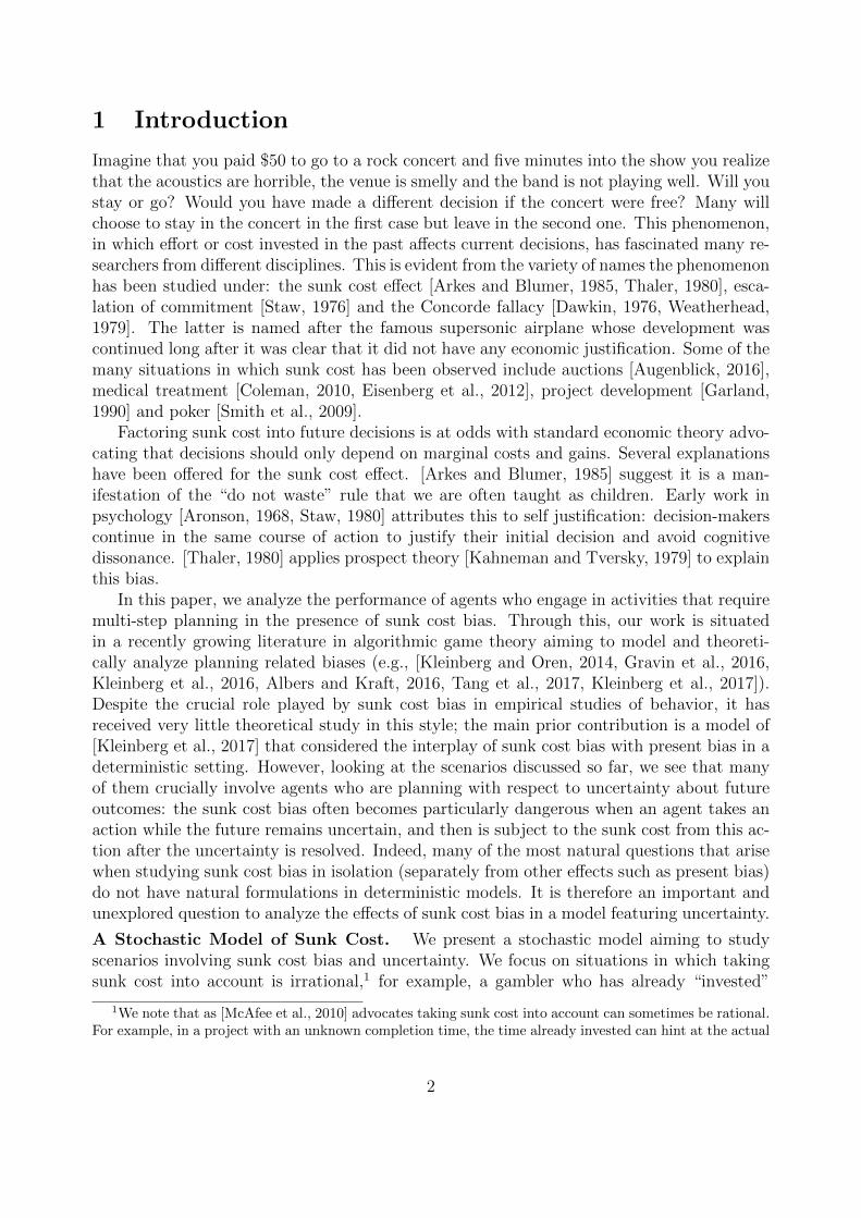
Following O’Donoghue and Rabin [O’Donoghue and Rabin, 1999, 2001], we analyze thebehavior of two types of agents: naive agents that are unaware of their bias, and sophisticatedagents that are aware of it. Even though a sophisticated agent is aware of its bias it cannotsimply ignore it. However, loosely speaking, it can take future actions to minimize thenegative implications of its bias. To understand the behavior of the different agents, itis best to walk through a simple example. Consider a slot machine with a probability of1/3 of winning a reward of $10. As part of a promotion the casino prices the first roundat $3 instead of the usual price of $4. This scenario is depicted in the graph in Figure 1.An unbiased (e.g., optimal) agent would only play as long as the expected payoff is greaterthan 0. Hence, in this game, it will only play the first round. Now, consider a naive agentexhibiting sunk cost bias with a parameter λ = 1/3. If it loses the first round it would havea sunk cost of 1/3 · 3 = 1. Thus, its payoff for quitting would be −1 while its expectedpayoff for continuing would be 1/3 · 10− 4 = −2/3. The naive agent will therefore play the

completion time.2It is natural to limit λ to non-negative values as negative values imply that the agent believes that if it

would stop it would get some of its investment back. This is the opposite of sunk cost bias.

3

s; 3

v1; 4 v2

t

2/3

2/3

1/3

1/3

Figure 1: For R = 10, naive sunk cost bias agents will continue at v1 and end up with anegative expected payoff.

next round as well and attain a negative expected payoff. In fact, we show that the negativepayoff of a naive agent can be exponentially large in the size of the graph.

A sophisticated agent with sunk cost bias is aware of its bias. This means that it knowswhich action it will take in any subsequent node for any possible sunk-cost and can usethis information to compute its expected payoff. This is different than a naive agent who isunaware of its bias and hence, wrongfully, believes that in the future, it will behave the sameas an unbiased agent and therefore, in all subsequent nodes, will have the same expectedpayoff as an unbiased agent.

We observe that the expected payoff of a sophisticated agent is always non-negative sinceit would stop traversing the graph if it knows that its expected payoff for doing so will benegative. This is the case in the example in Figure 1 in which the sophisticated agent knowsthat if it will play the first round and lose than it will also play the second round. This impliesthat its expected payoff for playing the slot machine is 1/3 ·10−3+2/3(1/3 ·10−4) = −1/9.The fact that sophisticated agents sometimes stop traversing the graph prematurely makestheir payoff potentially smaller than that of an optimal agent, although they avoid some ofthe more dramatic payoff shortfalls of naive agents.

Results. We begin by considering naive agents. Since they believe that in the futurethey will behave as optimal agents, their policy can be efficiently computed similarly to thepolicy of optimal agents. This is done by going over the graph in reverse topological orderand computing the expected payoff of continuing at each node. Naive agents can then decidewhether to continue or not by comparing these values against their sunk cost. We show thatsince they are oblivious to their sunk cost bias, we can construct instances in which theyaccumulate some sunk cost in the beginning. Then, due to this sunk cost, they continuetraversing the graph and accumulate more and more sunk cost even when their expectedpayoff is negative. As a result, they may end up with a negative payoff that is exponential inthe graph’s size. This result illustrates the danger of marketing strategies that reduce initialentrance costs to lure individuals to begin some risky endeavor (e.g., as the investing appRobinhood gives a free stock to anyone opening a new account) or take on some bad habit(e.g., tobacco companies giving free cigarettes to employees).

Our main focus in this paper is on sophisticated agents. The behavior of agents thatare aware of their bias is much more complex. In contrast to optimal and naive agents,they cannot compute their optimal policy by going over the nodes in reverse topologicalorder. This is because the decision of whether to stop or continue at each node dependson the amount of sunk cost they accumulated along the way. When there are differentpaths reaching the same node, the amount of sunk cost may vary depending on the realized

4

path. In fact, we show that the problem of computing the optimal policy for a sophisticatedagent is #P-Hard. This is done by reducing from the 0 − 1 knapsack solution countingproblem. Roughly speaking, we construct instances in which computing the expected payoffof a sophisticated agent if it starts traversing the graph requires counting the number ofvalid solutions to a corresponding knapsack problem. It is worth noting that a differenttype of hardness (i.e., NP-hardness) was proven by [Kleinberg et al., 2017] for sophisticatedagents exhibiting both sunk cost bias and present bias. The results strengthen one anotherand show that under different models being sophisticated about one’s sunk cost bias may bequite challenging. As part of future research, it would be fascinating to model and analyzeheuristics that individuals may use to bypass this hardness.

We continue with comparing the payoff of a sophisticated agent against the payoff ofan optimal agent. Roughly speaking, sophisticated agents exhibit the opposite problemthan naive agents: they take a too conservative approach and stop traversing the graphprematurely. As a result, they can have a payoff of 0 even when the optimal agent has apositive payoff. When λ is approaching infinity this gap can attain its maximal value whichis R. However, the payoff difference of R is far from tight for smaller values of λ. Hence,we look for tighter bounds that are more suitable for such values. We provide a numberof bounds on the difference between the payoff of optimal and sophisticated agents. Forexample, we show that πs ≥ πo − λ

1+λ· R, where πs and πo are the expected payoffs of the

sophisticated and optimal agents respectively. We present some evidence that this boundis not tight, particularly, for 0 ≤ λ ≤ 1. We suspect that graphs achieving the worst casedifference, for 0 ≤ λ ≤ 1, are fan graphs (graphs that include a path plus an edge from eachnode in the path to the target). We show that for such graphs πs ≥ πo − 1

e· λ ·R and prove

that this bound is essentially asymptotically tight (in the graph’s size).

2 Model and Naive Agents

In our model an agent is traversing a directed acyclic graph (i.e., DAG). The graph is aMarkov decision process (i.e., MDP) where each state u has a cost c(u) 3 which is the costof an agent at u to continue traversing the graph and for each neighboring states u and v,p(u, v) denotes the probability of a u→ v transition. The graph also has a designated targetnode t. If the agent reaches t it receives a reward of R. An agent traversing the graph formsa policy that decides for each node in the graph whether to continue traversing the graphor not. The goal of an agent is to choose a policy that maximizes its expected payoff – theprobability of reaching the target multiplied by R minus the expected cost. We can definethe expected payoff of an agent inductively as follows: if the agent decides to continue fromu, the expected payoff at a vertex u is the weighted average of the expected payoff of eachneighbor vertex minus the cost for continuing. If it decides to stop, its expected payoff is 0.We denote the expected payoff of an optimal agent (i.e., bias-free agent) currently at node

3This is a restricted type of MDP in which for every node u the transition cost to each neighbor is thesame.

5

sR/2

v1R/2

v2λR

v3λR(1 + λ)

v4λR(1 + λ)2

vn−1λR(1 + λ)n−3

vnt

1/2

1/2 1 1 11

1/2

1/2

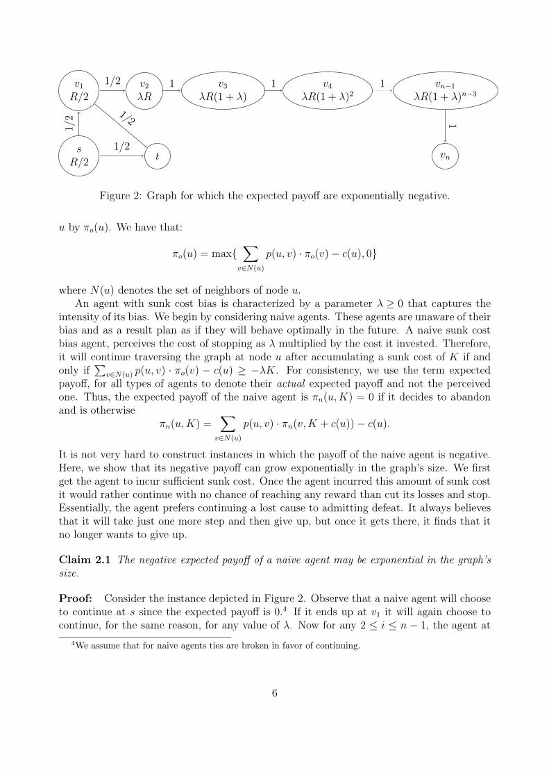
Figure 2: Graph for which the expected payoff are exponentially negative.

u by πo(u). We have that:

πo(u) = max{∑

v∈N(u)

p(u, v) · πo(v)− c(u), 0}

where N(u) denotes the set of neighbors of node u.An agent with sunk cost bias is characterized by a parameter λ ≥ 0 that captures the

intensity of its bias. We begin by considering naive agents. These agents are unaware of theirbias and as a result plan as if they will behave optimally in the future. A naive sunk costbias agent, perceives the cost of stopping as λ multiplied by the cost it invested. Therefore,it will continue traversing the graph at node u after accumulating a sunk cost of K if andonly if

∑v∈N(u) p(u, v) · πo(v) − c(u) ≥ −λK. For consistency, we use the term expected

payoff, for all types of agents to denote their actual expected payoff and not the perceivedone. Thus, the expected payoff of the naive agent is πn(u,K) = 0 if it decides to abandonand is otherwise

πn(u,K) =∑

v∈N(u)

p(u, v) · πn(v,K + c(u))− c(u).

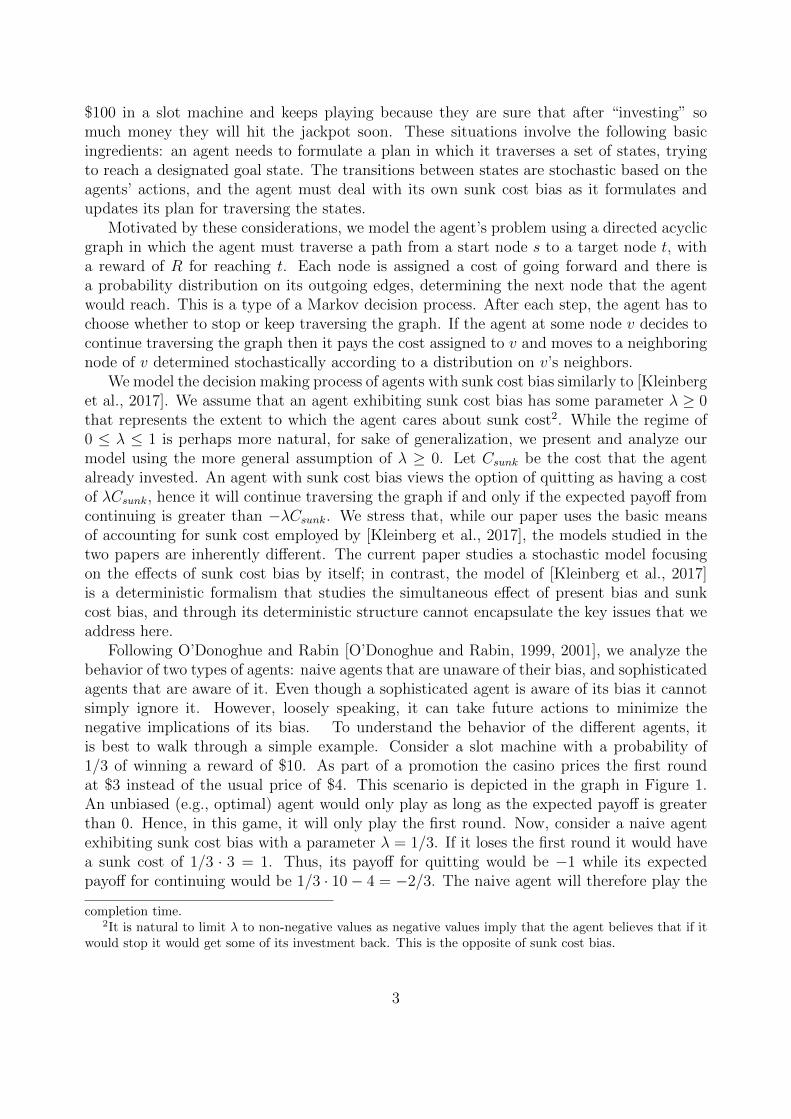
It is not very hard to construct instances in which the payoff of the naive agent is negative.Here, we show that its negative payoff can grow exponentially in the graph’s size. We firstget the agent to incur sufficient sunk cost. Once the agent incurred this amount of sunk costit would rather continue with no chance of reaching any reward than cut its losses and stop.Essentially, the agent prefers continuing a lost cause to admitting defeat. It always believesthat it will take just one more step and then give up, but once it gets there, it finds that itno longer wants to give up.

Claim 2.1 The negative expected payoff of a naive agent may be exponential in the graph’ssize.

Proof: Consider the instance depicted in Figure 2. Observe that a naive agent will chooseto continue at s since the expected payoff is 0.4 If it ends up at v1 it will again choose tocontinue, for the same reason, for any value of λ. Now for any 2 ≤ i ≤ n − 1, the agent at

4We assume that for naive agents ties are broken in favor of continuing.

6

s; 4W

u; 7W

v

t

1/2

1/2

1/2

1/2

Figure 3: Sophisticated agent gets 0, optimal agent gets W .

vi will continue to vi+1 since it will accumulate a cost of

R +i−3∑j=0

λR(1 + λ)j = R · (1 + λ)i−2

Thus, it will have a perceived cost of stopping of λR · (1+λ)i−2 which is the same as the costit thinks it will have for continuing one step and then stopping. Since the expected payoff ofthe two first steps is 0, we get that the expected payoff of the naive agent is −1

4R(1 + λ)n−2.

3 Sophisticated Sunk Cost Bias Agent

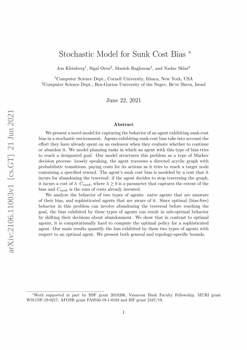
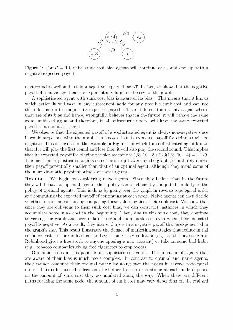
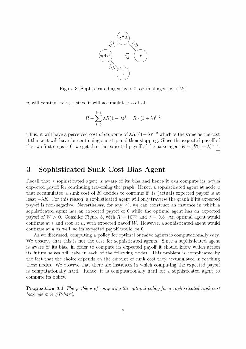
Recall that a sophisticated agent is aware of its bias and hence it can compute its actualexpected payoff for continuing traversing the graph. Hence, a sophisticated agent at node uthat accumulated a sunk cost of K decides to continue if its (actual) expected payoff is atleast −λK. For this reason, a sophisticated agent will only traverse the graph if its expectedpayoff is non-negative. Nevertheless, for any W , we can construct an instance in which asophisticated agent has an expected payoff of 0 while the optimal agent has an expectedpayoff of W > 0. Consider Figure 3, with R = 10W and λ = 0.5. An optimal agent wouldcontinue at s and stop at u, with expected payoff W . However, a sophisticated agent wouldcontinue at u as well, so its expected payoff would be 0.

As we discussed, computing a policy for optimal or naive agents is computationally easy.We observe that this is not the case for sophisticated agents. Since a sophisticated agentis aware of its bias, in order to compute its expected payoff it should know which actionits future selves will take in each of the following nodes. This problem is complicated bythe fact that the choice depends on the amount of sunk cost they accumulated in reachingthese nodes. We observe that there are instances in which computing the expected payoffis computationally hard. Hence, it is computationally hard for a sophisticated agent tocompute its policy.

Proposition 3.1 The problem of computing the optimal policy for a sophisticated sunk costbias agent is #P-hard.

7

sC

u1w1

v10

u2w2

v20

unwn

vn0

q0

q′

R + λ(B + C)

t

1/2

1/2

1/2

1/21/2

1/2

. . .

. . .

1

1

1/2

1/21

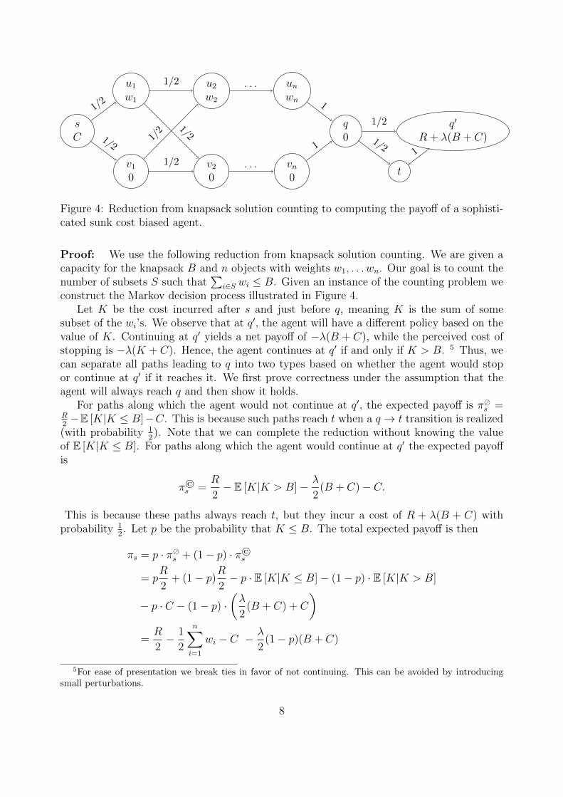
Figure 4: Reduction from knapsack solution counting to computing the payoff of a sophisti-cated sunk cost biased agent.

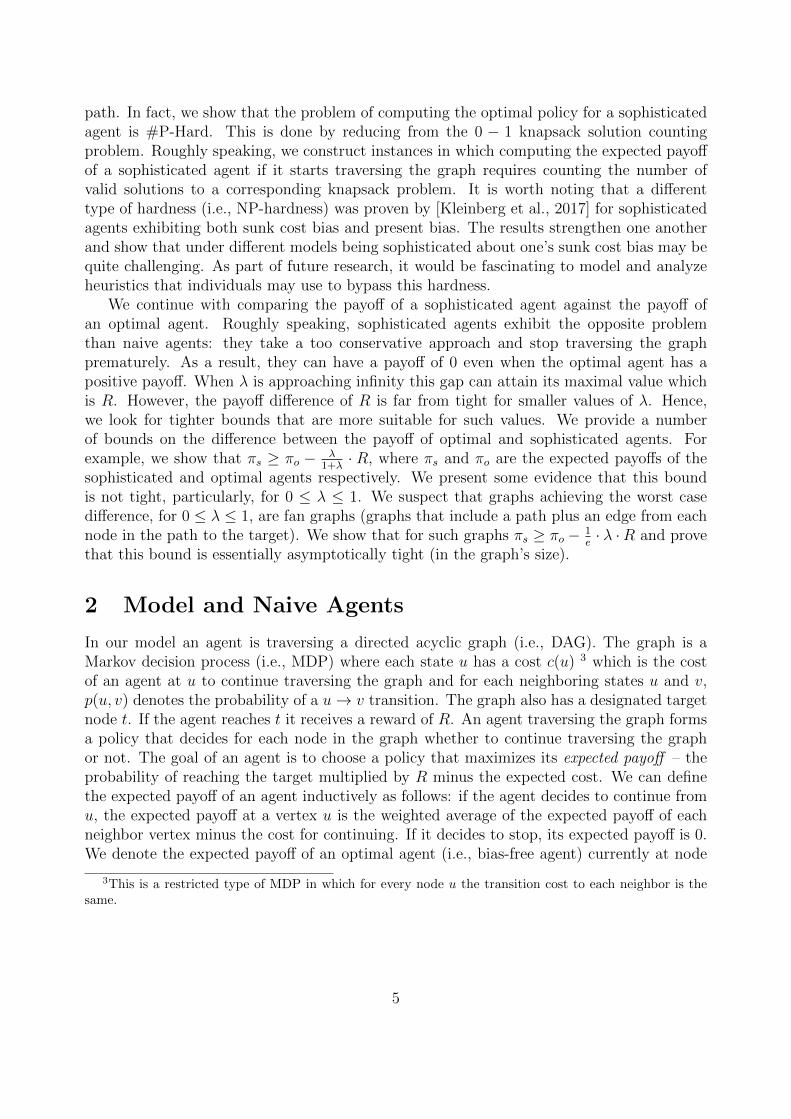
Proof: We use the following reduction from knapsack solution counting. We are given acapacity for the knapsack B and n objects with weights w1, . . . wn. Our goal is to count thenumber of subsets S such that

∑i∈S wi ≤ B. Given an instance of the counting problem we

construct the Markov decision process illustrated in Figure 4.Let K be the cost incurred after s and just before q, meaning K is the sum of some

subset of the wi’s. We observe that at q′, the agent will have a different policy based on thevalue of K. Continuing at q′ yields a net payoff of −λ(B + C), while the perceived cost ofstopping is −λ(K + C). Hence, the agent continues at q′ if and only if K > B. 5 Thus, wecan separate all paths leading to q into two types based on whether the agent would stopor continue at q′ if it reaches it. We first prove correctness under the assumption that theagent will always reach q and then show it holds.

For paths along which the agent would not continue at q′, the expected payoff is π�s =R2−E [K|K ≤ B]−C. This is because such paths reach t when a q → t transition is realized

(with probability 12). Note that we can complete the reduction without knowing the value

of E [K|K ≤ B]. For paths along which the agent would continue at q′ the expected payoffis

π©s =

R

2− E [K|K > B]− λ

2(B + C)− C.

This is because these paths always reach t, but they incur a cost of R + λ(B + C) withprobability 1

2. Let p be the probability that K ≤ B. The total expected payoff is then

πs = p · π�s + (1− p) · π©s

= pR

2+ (1− p)R

2− p · E [K|K ≤ B]− (1− p) · E [K|K > B]

− p · C − (1− p) ·(λ

2(B + C) + C

)=R

2− 1

2

n∑i=1

wi − C −λ

2(1− p)(B + C)

5For ease of presentation we break ties in favor of not continuing. This can be avoided by introducingsmall perturbations.

8

where in the last step we use:

p · E [K|K ≤ B] + (1− p) · E [K|K > B] = E [K] =1

2

n∑i=1

wi.

By rearranging we get that:

p =2πs +

∑ni=1wi −R + 2C

λ(B + C)+ 1

Since the number of paths such that K ≤ B is p · 2n, and the number of such paths is thesame as the number of solutions to the knapsack problem, we have

# Solutions = 2n(

2πs +∑n

i=1wi −R + 2C

λ(B + C)+ 1

).

Hence, if the sophisticated agent can compute its expected payoff in polynomial time, it canalso solve the #P-hard problem of knapsack solution counting. To complete the reduction,we first show that the agent will always reach q if it starts to traverse the graph. To dothis, we observe that from any node before q (not including s) the expected payoff is at leastR2− λ(B + C)−

∑ni=1wi. Therefore, the agent will continue as long as

R

2− λ(B + C)−

n∑i=1

wi≥− λC.

By rearranging we get the reduction holds for any R≥2∑n

i=1wi + 2λB.Finally, recall that we need to show that the problem of computing the optimal policy

for a sophisticated agents is #P-hard. This requires us to construct an instance in which theagent has to know the exact expected payoff to compute its policy. We prove the followingclaim:

Claim 3.2 For any 0 < α < 1 there exists C and R such that a sophisticated agent willtraverse the graph if and only if #Solutions ≥ α · 2n.

Proof: Let R = 2∑n

i=1wi + 2λB. We show that for any 0 < α < 1 there exists C suchthat the expected payoff of the sophisticated agent is 0 if p = α. This implies that the agentwill traverse the graph if and only if p ≥ α as required. Observe that

πs =R

2− 1

2

n∑i=1

wi − C −λ

2(1− α)(B + C) = 0

=⇒ C =R−

∑ni=1wi − λ(1− α)B

2 + λ(1− α)

Finally, notice that both R and C have a polynomial representation as they are defined byarithmetic operations over numbers that their representation is polynomial in the problem’ssize.

9

The claim implies the proof of Proposition 3.1 since if the sophisticated agent can computeits optimal policy for any instance constructed for 0 < α < 1, we can use its poly-timealgorithm to run a binary search over the fractions of valid solutions. Since the size of thesearch space is 2n, our binary search will compute the exact number of solutions to theknapsack problem in polynomial time.

Note that even though a naive agent can efficiently decide on its actions (as it plansto behave optimally), the same reduction as in the proof of Proposition 3.1 shows thatcomputing the expected payoff of a naive agent is also #P-Hard.

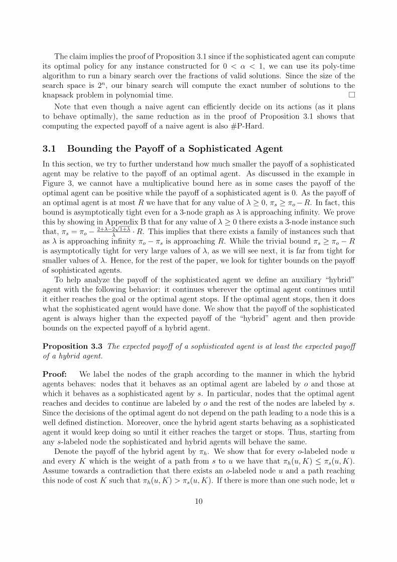
3.1 Bounding the Payoff of a Sophisticated Agent

In this section, we try to further understand how much smaller the payoff of a sophisticatedagent may be relative to the payoff of an optimal agent. As discussed in the example inFigure 3, we cannot have a multiplicative bound here as in some cases the payoff of theoptimal agent can be positive while the payoff of a sophisticated agent is 0. As the payoff ofan optimal agent is at most R we have that for any value of λ ≥ 0, πs ≥ πo−R. In fact, thisbound is asymptotically tight even for a 3-node graph as λ is approaching infinity. We provethis by showing in Appendix B that for any value of λ ≥ 0 there exists a 3-node instance suchthat, πs = πo − 2+λ−2

√1+λ

λ·R. This implies that there exists a family of instances such that

as λ is approaching infinity πo − πs is approaching R. While the trivial bound πs ≥ πo − Ris asymptotically tight for very large values of λ, as we will see next, it is far from tight forsmaller values of λ. Hence, for the rest of the paper, we look for tighter bounds on the payoffof sophisticated agents.

To help analyze the payoff of the sophisticated agent we define an auxiliary “hybrid”agent with the following behavior: it continues wherever the optimal agent continues untilit either reaches the goal or the optimal agent stops. If the optimal agent stops, then it doeswhat the sophisticated agent would have done. We show that the payoff of the sophisticatedagent is always higher than the expected payoff of the “hybrid” agent and then providebounds on the expected payoff of a hybrid agent.

Proposition 3.3 The expected payoff of a sophisticated agent is at least the expected payoffof a hybrid agent.

Proof: We label the nodes of the graph according to the manner in which the hybridagents behaves: nodes that it behaves as an optimal agent are labeled by o and those atwhich it behaves as a sophisticated agent by s. In particular, nodes that the optimal agentreaches and decides to continue are labeled by o and the rest of the nodes are labeled by s.Since the decisions of the optimal agent do not depend on the path leading to a node this is awell defined distinction. Moreover, once the hybrid agent starts behaving as a sophisticatedagent it would keep doing so until it either reaches the target or stops. Thus, starting fromany s-labeled node the sophisticated and hybrid agents will behave the same.

Denote the payoff of the hybrid agent by πh. We show that for every o-labeled node uand every K which is the weight of a path from s to u we have that πh(u,K) ≤ πs(u,K).Assume towards a contradiction that there exists an o-labeled node u and a path reachingthis node of cost K such that πh(u,K) > πs(u,K). If there is more than one such node, let u

10

be the last such node in the topological order. This implies that for every node v subsequentto it and any K ′ > 0 a cost of a path reaching v we have that πh(v,K

′) ≤ πs(v,K′).

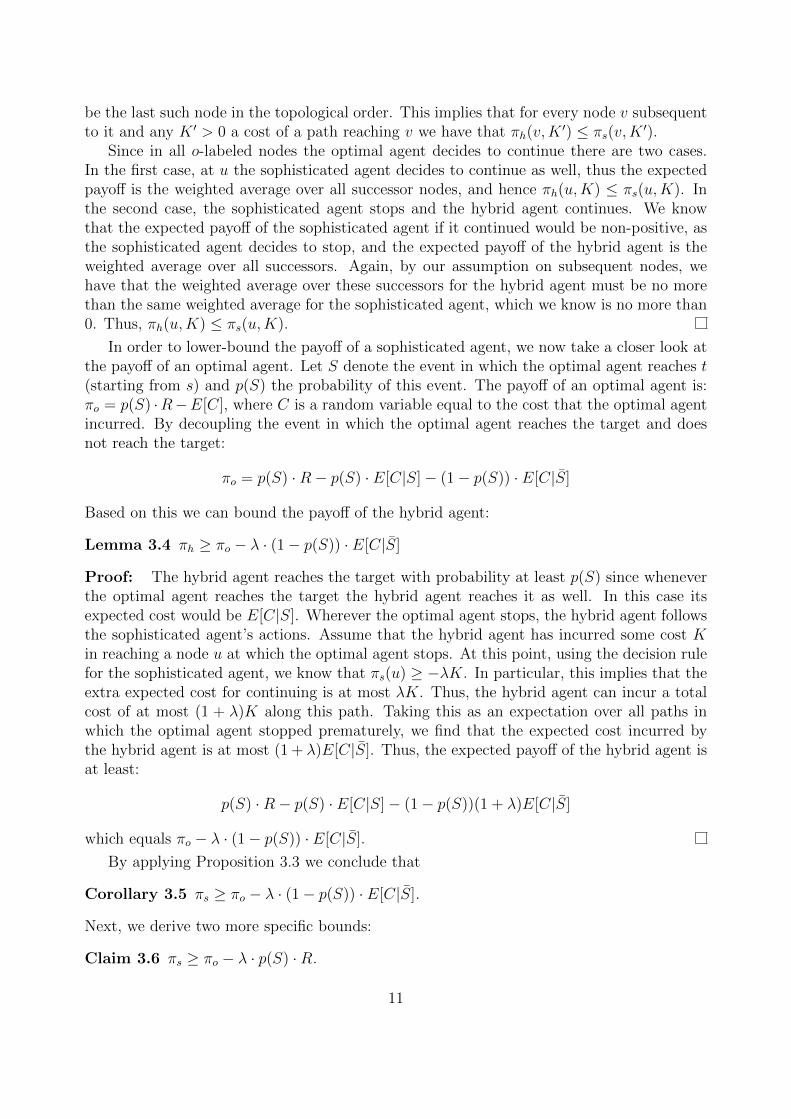
Since in all o-labeled nodes the optimal agent decides to continue there are two cases.In the first case, at u the sophisticated agent decides to continue as well, thus the expectedpayoff is the weighted average over all successor nodes, and hence πh(u,K) ≤ πs(u,K). Inthe second case, the sophisticated agent stops and the hybrid agent continues. We knowthat the expected payoff of the sophisticated agent if it continued would be non-positive, asthe sophisticated agent decides to stop, and the expected payoff of the hybrid agent is theweighted average over all successors. Again, by our assumption on subsequent nodes, wehave that the weighted average over these successors for the hybrid agent must be no morethan the same weighted average for the sophisticated agent, which we know is no more than0. Thus, πh(u,K) ≤ πs(u,K).

In order to lower-bound the payoff of a sophisticated agent, we now take a closer look atthe payoff of an optimal agent. Let S denote the event in which the optimal agent reaches t(starting from s) and p(S) the probability of this event. The payoff of an optimal agent is:πo = p(S) ·R−E[C], where C is a random variable equal to the cost that the optimal agentincurred. By decoupling the event in which the optimal agent reaches the target and doesnot reach the target:

πo = p(S) ·R− p(S) · E[C|S]− (1− p(S)) · E[C|S̄]

Based on this we can bound the payoff of the hybrid agent:

Lemma 3.4 πh ≥ πo − λ · (1− p(S)) · E[C|S̄]

Proof: The hybrid agent reaches the target with probability at least p(S) since wheneverthe optimal agent reaches the target the hybrid agent reaches it as well. In this case itsexpected cost would be E[C|S]. Wherever the optimal agent stops, the hybrid agent followsthe sophisticated agent’s actions. Assume that the hybrid agent has incurred some cost Kin reaching a node u at which the optimal agent stops. At this point, using the decision rulefor the sophisticated agent, we know that πs(u) ≥ −λK. In particular, this implies that theextra expected cost for continuing is at most λK. Thus, the hybrid agent can incur a totalcost of at most (1 + λ)K along this path. Taking this as an expectation over all paths inwhich the optimal agent stopped prematurely, we find that the expected cost incurred bythe hybrid agent is at most (1 + λ)E[C|S̄]. Thus, the expected payoff of the hybrid agent isat least:

p(S) ·R− p(S) · E[C|S]− (1− p(S))(1 + λ)E[C|S̄]

which equals πo − λ · (1− p(S)) · E[C|S̄].

By applying Proposition 3.3 we conclude that

Corollary 3.5 πs ≥ πo − λ · (1− p(S)) · E[C|S̄].

Next, we derive two more specific bounds:

Claim 3.6 πs ≥ πo − λ · p(S) ·R.

11

Proof: As we know that optimal agent always has a non-negative payoff we have that:

p(S) ·R− p(S) · E[C|S]− (1− p(S)) · E[C|S̄] ≥ 0

=⇒ (1− p(S)) · E[C|S̄] ≤ p(S) ·R− p(S) · E[C|S]

=⇒ (1− p(S)) · E[C|S̄] ≤ p(S) ·R

By applying Corollary 3.5 we have that πs ≥ πo − λ · (1− p(S)) · E[C|S̄] ≥ πo − λ · p(S) ·R

We can get a closed form bound by using the fact that πs ≥ 0:

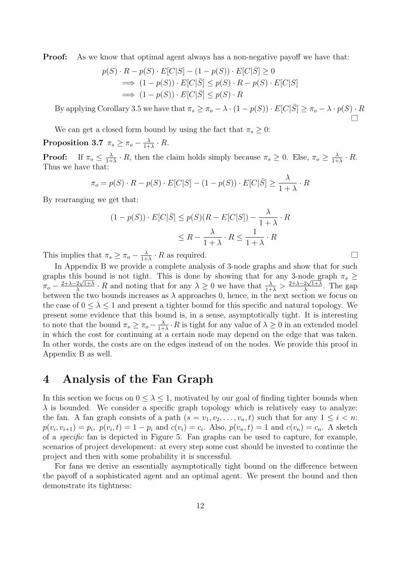
Proposition 3.7 πs ≥ πo − λ1+λ·R.

Proof: If πo ≤ λ1+λ· R, then the claim holds simply because πs ≥ 0. Else, πo ≥ λ

1+λ· R.

Thus we have that:

πo = p(S) ·R− p(S) · E[C|S]− (1− p(S)) · E[C|S̄] ≥ λ

1 + λ·R

By rearranging we get that:

(1− p(S)) · E[C|S̄] ≤ p(S)(R− E[C|S])− λ

1 + λ·R

≤ R− λ

1 + λ·R ≤ 1

1 + λ·R

This implies that πs ≥ πo − λ1+λ·R as required.

In Appendix B we provide a complete analysis of 3-node graphs and show that for suchgraphs this bound is not tight. This is done by showing that for any 3-node graph πs ≥πo − 2+λ−2

√1+λ

λ· R and noting that for any λ ≥ 0 we have that λ

1+λ> 2+λ−2

√1+λ

λ. The gap

between the two bounds increases as λ approaches 0, hence, in the next section we focus onthe case of 0 ≤ λ ≤ 1 and present a tighter bound for this specific and natural topology. Wepresent some evidence that this bound is, in a sense, asymptotically tight. It is interestingto note that the bound πs ≥ πo− λ

1+λ·R is tight for any value of λ ≥ 0 in an extended model

in which the cost for continuing at a certain node may depend on the edge that was taken.In other words, the costs are on the edges instead of on the nodes. We provide this proof inAppendix B as well.

4 Analysis of the Fan Graph

In this section we focus on 0 ≤ λ ≤ 1, motivated by our goal of finding tighter bounds whenλ is bounded. We consider a specific graph topology which is relatively easy to analyze:the fan. A fan graph consists of a path (s = v1, v2, . . . , vn, t) such that for any 1 ≤ i < n:p(vi, vi+1) = pi, p(vi, t) = 1− pi and c(vi) = ci. Also, p(vn, t) = 1 and c(vn) = cn. A sketchof a specific fan is depicted in Figure 5. Fan graphs can be used to capture, for example,scenarios of project development: at every step some cost should be invested to continue theproject and then with some probability it is successful.

For fans we derive an essentially asymptotically tight bound on the difference betweenthe payoff of a sophisticated agent and an optimal agent. We present the bound and thendemonstrate its tightness:

12

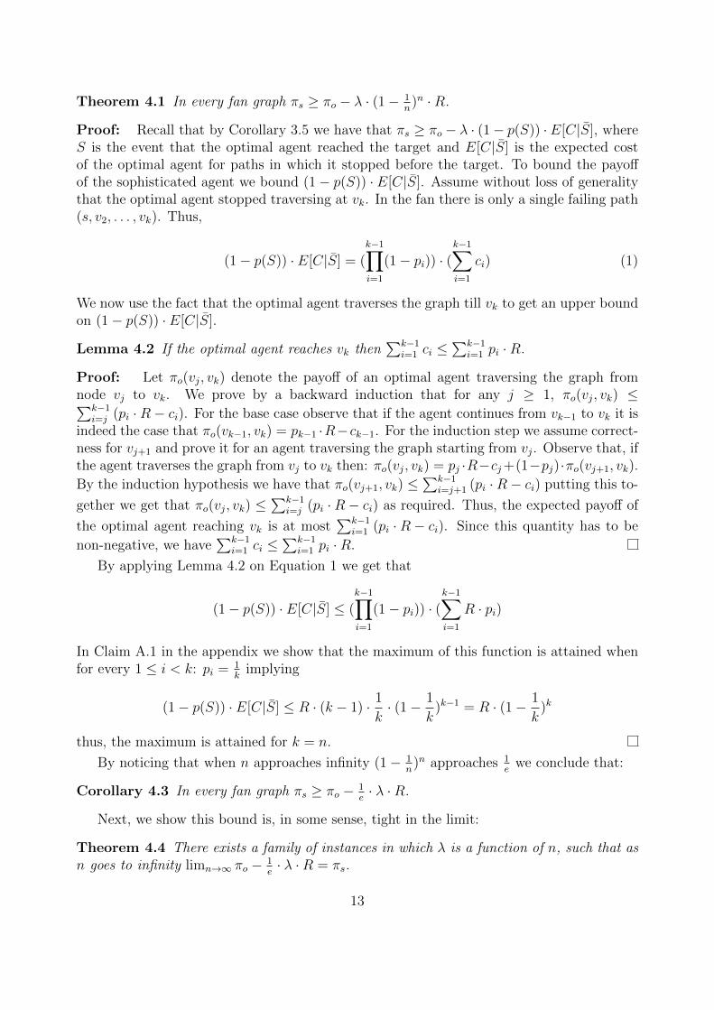
Theorem 4.1 In every fan graph πs ≥ πo − λ · (1− 1n)n ·R.

Proof: Recall that by Corollary 3.5 we have that πs ≥ πo − λ · (1− p(S)) ·E[C|S̄], whereS is the event that the optimal agent reached the target and E[C|S̄] is the expected costof the optimal agent for paths in which it stopped before the target. To bound the payoffof the sophisticated agent we bound (1− p(S)) · E[C|S̄]. Assume without loss of generalitythat the optimal agent stopped traversing at vk. In the fan there is only a single failing path(s, v2, . . . , vk). Thus,

(1− p(S)) · E[C|S̄] = (k−1∏i=1

(1− pi)) · (k−1∑i=1

ci) (1)

We now use the fact that the optimal agent traverses the graph till vk to get an upper boundon (1− p(S)) · E[C|S̄].

Lemma 4.2 If the optimal agent reaches vk then∑k−1

i=1 ci ≤∑k−1

i=1 pi ·R.

Proof: Let πo(vj, vk) denote the payoff of an optimal agent traversing the graph fromnode vj to vk. We prove by a backward induction that for any j ≥ 1, πo(vj, vk) ≤∑k−1

i=j (pi ·R− ci). For the base case observe that if the agent continues from vk−1 to vk it isindeed the case that πo(vk−1, vk) = pk−1 ·R−ck−1. For the induction step we assume correct-ness for vj+1 and prove it for an agent traversing the graph starting from vj. Observe that, ifthe agent traverses the graph from vj to vk then: πo(vj, vk) = pj ·R−cj+(1−pj)·πo(vj+1, vk).

By the induction hypothesis we have that πo(vj+1, vk) ≤∑k−1

i=j+1 (pi ·R− ci) putting this to-

gether we get that πo(vj, vk) ≤∑k−1

i=j (pi ·R− ci) as required. Thus, the expected payoff of

the optimal agent reaching vk is at most∑k−1

i=1 (pi ·R− ci). Since this quantity has to be

non-negative, we have∑k−1

i=1 ci ≤∑k−1

i=1 pi ·R.

By applying Lemma 4.2 on Equation 1 we get that

(1− p(S)) · E[C|S̄] ≤ (k−1∏i=1

(1− pi)) · (k−1∑i=1

R · pi)

In Claim A.1 in the appendix we show that the maximum of this function is attained whenfor every 1 ≤ i < k: pi = 1

kimplying

(1− p(S)) · E[C|S̄] ≤ R · (k − 1) · 1

k· (1− 1

k)k−1 = R · (1− 1

k)k

thus, the maximum is attained for k = n.

By noticing that when n approaches infinity (1− 1n)n approaches 1

ewe conclude that:

Corollary 4.3 In every fan graph πs ≥ πo − 1e· λ ·R.

Next, we show this bound is, in some sense, tight in the limit:

Theorem 4.4 There exists a family of instances in which λ is a function of n, such that asn goes to infinity limn→∞ πo − 1

e· λ ·R = πs.

13

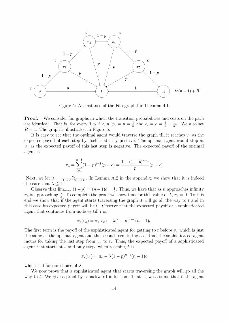
Figure 5: An instance of the Fan graph for Theorem 4.1.

Proof: We consider fan graphs in which the transition probabilities and costs on the pathare identical. That is, for every 1 ≤ i < n, pi = p = 1

nand ci = c = 1

n− 1

n2 . We also setR = 1. The graph is illustrated in Figure 5.

It is easy to see that the optimal agent would traverse the graph till it reaches vn as theexpected payoff of each step by itself is strictly positive. The optimal agent would stop atvn as the expected payoff of this last step is negative. The expected payoff of the optimalagent is

πo =n−1∑i=1

(1− p)i−1(p− c) =1− (1− p)n−1

p(p− c)

Next, we let λ = πo(1−p)n−1(n−1)c . In Lemma A.2 in the appendix, we show that it is indeed

the case that λ ≤ 1.Observe that limn→∞(1− p)n−1(n− 1)c = 1

e. Thus, we have that as n approaches infinity

πo is approaching λe. To complete the proof we show that for this value of λ, πs = 0. To this

end we show that if the agent starts traversing the graph it will go all the way to t and inthis case its expected payoff will be 0. Observe that the expected payoff of a sophisticatedagent that continues from node vk till t is:

πs(vk) = πo(vk)− λ(1− p)n−k(n− 1)c

The first term is the payoff of the sophisticated agent for getting to t before vn which is justthe same as the optimal agent and the second term is the cost that the sophisticated agentincurs for taking the last step from vn to t. Thus, the expected payoff of a sophisticatedagent that starts at s and only stops when reaching t is

πs(v1) = πo − λ(1− p)n−1(n− 1)c

which is 0 for our choice of λ.We now prove that a sophisticated agent that starts traversing the graph will go all the

way to t. We give a proof by a backward induction. That is, we assume that if the agent

14

arrives at vk+1 from vk then it will go all the way to t. For the base case observe that ifthe agent arrives at vn, then the payoff for abandoning is −λc(n − 1). On the other hand,moving to t incurs the same payoff: R− (λc(n− 1) +R) = −λc(n− 1) which is the same asquitting. For ease of presentation we assume that the agent breaks ties in favor of continuingand hence the agent will choose to continue.6 For the induction step we assume correctnessfor vk+1 and prove for an agent traversing the graph from vk. By the induction hypothesis,since the sophisticated agent continues to traverse the graph from vk+1 till t then its expectedpayoff for continuing is πs(vk). To complete the proof we show that the expected payoff isgreater than or equal to the agent’s sunk cost (i.e., πs(vk) ≥ −λc(k − 1)):

Lemma 4.5 πs(vk) ≥ −λc(k − 1).

Proof: We need to show that:

πo(vk)− λ(1− p)n−k(n− 1)c ≥ −λc(k − 1)

By rearranging we get that:

πo(vk) ≥ λc((1− p)n−k(n− 1)− (k − 1)

)Since λc > 0, if ((1 − p)n−k(n − 1) − (k − 1)) ≤ 0 the lemma trivially holds. Else, assumethat ((1− p)n−k(n− 1)− (k − 1)) > 0, hence we can divide by this and get that

λ ≤ πo(vk)

c((1− p)n−k(n− 1)− (k − 1))

By substituting for our choice of λ we get that:

πo(1− p)n−1(n− 1)c

≤ πo(vk)

c((1− p)n−k(n− 1)− (k − 1))

By rearranging we get that:

1− (1− p)n−1

(1− p)n−1(n− 1)≤ 1− (1− p)n−k

(1− p)n−k(n− 1)− (k − 1)

which implies that

(1− p)n−k(n− 1)− (k − 1) + (1− p)n−1(k − 1)︸ ︷︷ ︸f(k)

≤

(1− p)n−1(n− 1)

Finally, we apply Lemma 4.6 to show that the above inequality holds. This is done byproving that f(k) is bounded from above by (1− p)n−1(n− 1) for any integer 1 ≤ k ≤ n.

6To avoid applying a tie-breaking rule we can add small perturbations to the costs to make sure that theagent will strictly prefer to continue.

15

Lemma 4.6 The function f(x) = (1 − p)n−x(n − 1) − (x − 1) + (1 − p)n−1(x − 1) where0 < p < 1 is bounded above by (1− p)n−1(n− 1) for each 1 ≤ x ≤ n.

Proof: In order to prove this claim we show that f is convex in [1, n] and that f(1) =f(n) = (1− p)n−1(n− 1). Therefore, for each x ∈ [1, n], f(x) ≤ (1− p)n−1(n− 1).

Observe that indeed f(1) = f(n) = (1− p)n−1(n− 1). In addition:

f′(x) = − ln(1− p)(n− 1)(1− p)n−x + (1− p)n−1 − 1

f′′(x) = ln2(1− p)(n− 1)(1− p)n−x

Thus, for 1 < x < n and 0 < p < 1 we have that f′′(x) ≥ 0. Therefore, f(x) ≤ (1−p)n−1(n−

1) for each x ∈ [1, n] as required.

5 Conclusion and Further Directions

Sunk cost bias is a key behavioral bias that people exhibit, and it interacts in complex wayswith uncertainty about the future. We have proposed a model that allows us to study thisinteraction, by analyzing the loss in performance of agents that experience sunk cost bias asthey perform a planning problem with stochastic transitions between states.

There are a number of further questions suggested by this work. A central open questionis whether fan graphs represent the worst case for sophisticated agents with sunk cost bias.It would also be interesting to explore how the stochastic environment for sunk cost bias canbe adapted to incorporate agents with other kinds of biases as well.

16

References

Susanne Albers and Dennis Kraft. Motivating time-inconsistent agents: A computationalapproach. In Proc. 12th Workshop on Internet and Network Economics, 2016.

Hal R Arkes and Catherine Blumer. The psychology of sunk cost. Organizational behaviorand human decision processes, 35(1):124–140, 1985.

Elliot Aronson. Dissonance theory: Progress and problems. 1968.

Ned Augenblick. The sunk-cost fallacy in penny auctions. The Review of Economic Studies,83(1):58–86, 2016.

Martin D Coleman. Sunk cost and commitment to medical treatment. Current Psychology,29(2):121–134, 2010.

Richard Dawkin. The selfish gene. Oxford university Press, 1:976, 1976.

Jonathan D Eisenberg, H Benjamin Harvey, Donald A Moore, G Scott Gazelle, and Pari VPandharipande. Falling prey to the sunk cost bias: a potential harm of patient radiationdose histories. Radiology, 263(3):626–628, 2012.

Howard Garland. Throwing good money after bad: The effect of sunk costs on the decisionto escalate commitment to an ongoing project. Journal of Applied Psychology, 75(6):728,1990.

Nick Gravin, Nicole Immorlica, Brendan Lucier, and Emmanouil Pountourakis. Procrastina-tion with variable present bias. In Proceedings of the 2016 ACM Conference on Economicsand Computation, EC ’16, pages 361–361, New York, NY, USA, 2016. ACM. ISBN 978-1-4503-3936-0.

Daniel Kahneman and Amos Tversky. Prospect theory: An analysis of decision under risk.Econometrica 47,2, pages 263–291, 1979.

Jon Kleinberg and Sigal Oren. Time-inconsistent planning: A computational problem inbehavioral economics. In Proceedings of the Fifteenth ACM Conference on Economics andComputation, EC ’14, pages 547–564, New York, NY, USA, 2014. ACM. ISBN 978-1-4503-2565-3.

Jon Kleinberg, Sigal Oren, and Manish Raghavan. Planning problems for sophisticatedagents with present bias. In Proceedings of the 2016 ACM Conference on Economics andComputation, EC ’16, pages 343–360, New York, NY, USA, 2016. ACM. ISBN 978-1-4503-3936-0.

Jon Kleinberg, Sigal Oren, and Manish Raghavan. Planning with multiple biases. In Pro-ceedings of the 2017 ACM Conference on Economics and Computation, EC ’17, pages567–584, New York, NY, USA, 2017. ACM. ISBN 978-1-4503-4527-9.

R Preston McAfee, Hugo M Mialon, and Sue H Mialon. Do sunk costs matter? EconomicInquiry, 48(2):323–336, 2010.

17

Ted O’Donoghue and Matthew Rabin. Doing it now or later. American Economic Review,89(1):103–124, March 1999.

Ted O’Donoghue and Matthew Rabin. Choice and procrastination. Quarterly Journal ofEconomics, 116(1):121–160, February 2001.

Gary Smith, Michael Levere, and Robert Kurtzman. Poker player behavior after big winsand big losses. Management Science, 55(9):1547–1555, 2009.

Barry M Staw. Knee-deep in the big muddy: A study of escalating commitment to a chosencourse of action. Organizational behavior and human performance, 16(1):27–44, 1976.

Barry M Staw. Rationality and justification in organizational life. Research in organizationalbehavior, 2:45–80, 1980.

Pingzhong Tang, Yifeng Teng, Zihe Wang, Shenke Xiao, and Yichong Xu. Computationalissues in time-inconsistent planning. In Proceedings of the Thirty-First AAAI Conferenceon Artificial Intelligence, pages 3665–3671, 2017.

Richard Thaler. Toward a positive theory of consumer choice. Journal of Economic Behavior& Organization, 1(1):39–60, 1980.

Patrick J Weatherhead. Do savannah sparrows commit the concorde fallacy? BehavioralEcology and Sociobiology, 5(4):373–381, 1979.

18

A Missing Proofs from Section 4

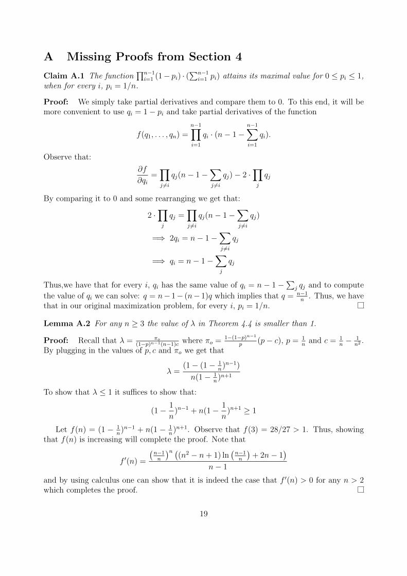
Claim A.1 The function∏n−1

i=1 (1− pi) · (∑n−1

i=1 pi) attains its maximal value for 0 ≤ pi ≤ 1,when for every i, pi = 1/n.

Proof: We simply take partial derivatives and compare them to 0. To this end, it will bemore convenient to use qi = 1− pi and take partial derivatives of the function

f(q1, . . . , qn) =n−1∏i=1

qi · (n− 1−n−1∑i=1

qi).

Observe that:

∂f

∂qi=∏j 6=i

qj(n− 1−∑j 6=i

qj)− 2 ·∏j

qj

By comparing it to 0 and some rearranging we get that:

2 ·∏j

qj =∏j 6=i

qj(n− 1−∑j 6=i

qj)

=⇒ 2qi = n− 1−∑j 6=i

qj

=⇒ qi = n− 1−∑j

qj

Thus,we have that for every i, qi has the same value of qi = n− 1−∑

j qj and to compute

the value of qi we can solve: q = n− 1− (n− 1)q which implies that q = n−1n

. Thus, we havethat in our original maximization problem, for every i, pi = 1/n.

Lemma A.2 For any n ≥ 3 the value of λ in Theorem 4.4 is smaller than 1.

Proof: Recall that λ = πo(1−p)n−1(n−1)c where πo = 1−(1−p)n−1

p(p− c), p = 1

nand c = 1

n− 1

n2 .By plugging in the values of p, c and πo we get that

λ =(1− (1− 1

n)n−1)

n(1− 1n)n+1

To show that λ ≤ 1 it suffices to show that:

(1− 1

n)n−1 + n(1− 1

n)n+1 ≥ 1

Let f(n) = (1 − 1n)n−1 + n(1 − 1

n)n+1. Observe that f(3) = 28/27 > 1. Thus, showing

that f(n) is increasing will complete the proof. Note that

f ′(n) =

(n−1n

)n ((n2 − n+ 1) ln

(n−1n

)+ 2n− 1

)n− 1

and by using calculus one can show that it is indeed the case that f ′(n) > 0 for any n > 2which completes the proof.

19

s

v

t

ε;1

(1+λ)ε

1− ε; 0

1; 1+

λ(1+λ)ε

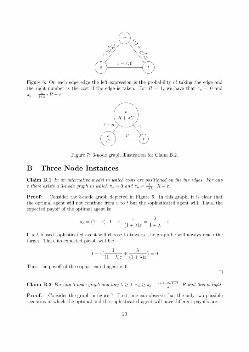
Figure 6: On each edge edge the left expression is the probability of taking the edge andthe right number is the cost if the edge is taken. For R = 1, we have that πs = 0 andπo = λ

1+λ·R− ε.

sC

vR + λC

t

1− p

p

1

Figure 7: 3-node graph illustration for Claim B.2.

B Three Node Instances

Claim B.1 In an alternative model in which costs are positioned on the the edges. For anyε there exists a 3-node graph in which πs = 0 and πo = λ

1+λ·R− ε.

Proof: Consider the 3-node graph depicted in Figure 6. In this graph, it is clear thatthe optimal agent will not continue from v to t but the sophisticated agent will. Thus, theexpected payoff of the optimal agent is:

πo = (1− ε) · 1− ε · 1

(1 + λ)ε=

λ

1 + λ− ε

If a λ biased sophisticated agent will choose to traverse the graph he will always reach thetarget. Thus, its expected payoff will be:

1− ε( 1

(1 + λ)ε+

λ

(1 + λ)ε) = 0

Thus, the payoff of the sophisticated agent is 0.

Claim B.2 For any 3-node graph and any λ ≥ 0, πs ≥ πo − 2+λ−2√1+λ

λ·R and this is tight.

Proof: Consider the graph in figure 7. First, one can observe that the only two possiblescenarios in which the optimal and the sophisticated agent will have different payoffs are:

20

• The optimal agent traverses the graph for a single step and the sophisticated agentcontinues.

• The optimal agent traverses the graph for a single step and the sophisticated agent isunwilling to start.

These are the only scenarios we should consider as if the optimal agent does not traverse thegraph or continues at v then the sophisticated agent will do the same.

We begin by considering the scenario in which the optimal agent traverses the graph fora single step and the sophisticated agent continues. Observe that πo = pR−C. Notice thatif the sophisticated agent would start traversing the graph it would continue at v. Thus,its expected payoff for traversing the graph is pR − C − (1− p)λC ≤ 0. By rearranging we

get that p ≤ C(1+λ)R+λC

. Thus, to maximize the expected payoff of the optimal agent, we set

p = C(1+λ)R+λC

and get that:

πo =C(1 + λ)

R + λC·R− C

To maximize πo we take a derivative with respect to C and compare it to 0:

∂πo∂C

=R(1 + λ)(R + λC)− λCR(1 + λ)

(R + λC)2− 1 =

R2(1 + λ)

(R + λC)2− 1

R2(1 + λ)

(R + λC)2− 1 = 0 =⇒ R2(1 + λ) = (R + λC)2

C =R

λ

(√1 + λ− 1

)which gives

p =R(√

1 + λ− 1)

(1 + λ)

λ(R +R(√

1 + λ− 1))=

(√1 + λ− 1

)√1 + λ

λ

=1 + λ−

√1 + λ

λ

Therefore:

πo =1 + λ−

√1 + λ

λ·R− R

λ(√

1 + λ− 1)

=(2 + λ− 2

√1 + λ)

λ·R

For 0 < λ ≤ 1 we get that 0 < πo − πs ≤ 0.172R.Finally, we consider the scenario in which the sophisticated agent traverse the graph and

continues at v while the optimal agent stops traversing the graph at v. We show thatoptimizing the payoff difference for this scenario get us to the same optimization problem

21

as we just solved. Denote by c(v) the cost at v. Since the sophisticated agent continues wehave that R − c(v) ≥ −λC =⇒ c(v) ≤ R + λC. Also, since the expected payoff of thesophisticated agent is positive we have that:

πs = pR− C + (1− p)(R− c(v)) > 0 =⇒R + pc(v)− c(v)− C > 0 =⇒

c(v) <R− C1− p

Consider the difference between the payoffs of the agents:

πo − πs = −(1− p)(R− c(v)) = (1− p)(c(v)−R)

Clearly, the difference is maximized for the maximal value of c(v). Since c(v) ≤ min{R−C1−p , R+

λC} we get that this value is maximized when R−C1−p = R+λC by rearranging we get that in

this case p = C(1+λ)R+λC

. Since in this case we have that:

πo − πs ≤ (1− p)(min{R− C1− p

,R + λC} −R) = p ·R− C

This implies the exact optimization problem as in the first case, which completes the proof.

22