Stel component analysis: Modeling spatial correlations in image class structure

Nebojsa Jojic1, Alessandro Perina2, Marco Cristani2, Vittorio Murino2,3 and Brendan Frey4

Abstract

As a useful concept in the study of the low level image

class structure, we introduce the notion of a structure ele-

ment – ‘stel.’ The notion is related to the notions of a pixel,

superpixel, segment or a part, but instead of referring to an

element or a region of a single image, stel is a probabilis-

tic element of an entire image class. Stels often define clear

object or scene parts as a consequence of the modeling con-

straint which forces the regions belonging to a single stel

to have a tight distribution over local measurements, such

as color or texture. This self-similarity within a region in

a single image is typical of most meaningful image parts,

even when in different images of similar objects the corre-

sponding parts may not have similar local measurements.

The stel itself is expected to be consistent within a class,

yet flexible, which we accomplish using a novel approach

we dubbed stel component analysis. Experimental results

show how stel component analysis can assist in image/video

segmentation and object recognition where, in particular, it

can be used as an alternative of, or in conjunction with,

bag-of-features and related classifiers, where stel inference

provides a meaningful spatial partition of features.

1. Introduction

Due to the high sensitivity of pixel intensities to vari-

ous imaging conditions, images are often represented by

indices referring to a set of possible local features. The

image features are chosen so that they are more robust to

imaging conditions than the straight-forward color intensity

measurements, and often, their spatial configuration is dis-

carded, e.g., in bag of- words models [5, 6]. In such mod-

els, each image class has a distinctive palette of features

typically found in most instances of the class, although the

image locations in which these features are found vary sub-

stantially. Therefore, the distribution over indices into a sin-

gle palette describes an entire image class.

1 jojic@microsoft.com; Microsoft Research, Redmond, WA, USA2 {alessandro.perina, marco.cristani, vittorio.murino}@univr.it

Dipartimento di Informatica, Universita di Verona, Italy3 Istituto Italiano di Tecnologia, Genova, Italy4 frey@psi.toronto.edu; University of Toronto, Canada

In contrast, in the probabilistic index map model [1] the

feature palette is pertinent only to a single instance of a

class, while the indexing configuration is assumed to be rel-

evant to the entire class of images. As illustrated in the

cartoon example of the face category in Fig. 1A, this repre-

sentation allows for “palette invariance” in image modeling

and dramatically reduces sensitivity of models to various

unimportant, but usually troublesome causes of variability

in images, such as illumination, surface color, or texture

variability.

This paper provides modeling ideas that go beyond these

basic concepts of feature palette and index map modeling,

illustrated briefly in Fig. 1. We define index maps as or-

dered sets of indices si ∈ 1, . . . , S, linked to spatially dis-

tinct areas i ∈ 1, . . . , N of images or videos, where N is

the number of such image areas (e.g. pixels). These indices

point to a table of S possible local measurements, referred

to as a palette. Probabilistic index maps (PIMs) consider

the uncertainty in the indexing operation as well as in the

nature of the palette. Each image location i is associated

with a prior distribution over indices p(si = s). Indices

point to palette entries which each describe a distribution

over local measurements.

We refer to an area of an image with the same assigned

index s as a structure element, or stel. A stel will be con-

sidered probabilistically as a map q(sti= s) over image lo-

cations i defining the certainty of pixels of the t−th image

belonging to the s−th stel. Several of these maps, extracted

from a face dataset, are shown in Fig. 1A. The preserva-

tion of a stel over a coherent image class, such as an ob-

ject class or a category, a video segment, etc., is defined in

flexible terms through the learned prior distribution over

stels p({si}N = s). The extent of tolerable variation of the

shape of the stel area, which will often be discontiguous,

strongly depends on the power of the statistical model over

the indices si. While the PIM model has the advantage over

bag-of-features models in terms of capturing spatial struc-

ture in images, it does not deal with (1) the possibility of

consistent palettes across images of the class (e.g. in a video

sequence, subsequent images do have similar palettes), and

(2) with possible dependencies among the spatially sepa-

rated indices si. As a result of the second drawback, PIM

does no capture correlations that exist in structural elements

of an image class due to global effects, such as a slight

2044978-1-4244-3991-1/09/$25.00 ©2009 IEEE

s = 5s = 4s = 3s = 2s = 1

k= 1

k =

2

S = 5, K = 3

k= 3

q( s ) q( a ) yk

s = 5s = 4s = 3s = 2s = 1 a = 3a = 2a = 1

1 2 3

1 2 3

1

0

1

0

s = 5s = 4s = 3s = 2s = 1

P(s

|a) =

rk(s

)

B)

D)

Λs

Λs

C)

k= 2

k= 1

Λsp(Λs)

)(srk

y1

...

...

...

...

q(s=

2)

Chimneys Roof

s=3k=

1k=

2

Sky

STEL COMPONENT ANALYSIS

SCA and image parsing SCA and part-specific palettes

Training set

Seg

men

tati

on

sS

-Ba

gs

of

fea

ture

s

Sheep

Bird

PRIOR

MIXING

INDEX MAP PROBABILISTIC INDEX MAP

1

2

3

4

Palettes

sij P(sij)

A) E) F)

Img

1

Img

2

Img

3yK

a1 a2 aN

sNs2s1

z1 z2 zN

s=2s=1

k=1

k=2

s=2s=1

s=2s=1

k=1

k=2

yk

yk

PRIOR

MIXING

q(s=

2)

Figure 1. SCA Illustration

change in face proportions (Fig. 1A) which may induce

many correlated changes in indices across the image.

We address both of these problems in this paper and pro-

pose a new model (Fig. 1B), which we call stel compo-

nent analysis. The model of index variation, in the spirit

of principle component analysis and other subspace mod-

els used for modeling real-valued pixel intensities, captures

correlated variations in discrete indices by blending several

component PIMs based on real-valued weights y. This is

illustrated in Fig. 1C, where three PIM components are

shown, and Fig. 1D, where the blending of these compo-

nents allows for a better agreement of the observed facial

image with the model. The model, described in the next

section and in Fig. 1B, was estimated from a set of fa-

cial images in an unsupervised manner. As most of the

stel structure in this example reflects the grouping of sur-

face normals, the component mixing strengths y capture the

varying pose angle for this set of images, as discussed in

Experiments. However, for other image categories, differ-

ent structure may be learned, as illustrated in the rest of the

figure. For example, SCA with two stels can be used to seg-

ment foreground objects from the background (Fig. 1E). As

in case of a PIM relative, LOCUS [2], the segmentations

are performed jointly over a set of images from the same

category without any supervision, exploiting the self sim-

ilarity patterns in images to define stels as segments of an

image class, rather than individual images. The figure also

emphasizes the difference between the prior over stels p(s)and the inferred indices for individual images q(st

i), which

depend on both the prior and the self similarity properties

of an individual image.

In more complex categories, the model benefits from

learning a prior over individual image palettes, which is

similar to what is achieved in the bag-of-feature models, ex-

cept that these appearance models can now be part-specific.

In Fig. 1F, SCA is applied to roof images, where the prior

over individual image palette is represented by different

histograms over image features in the three different stels.

Here, we illustrate stel segmentation by grouping parts of

different images obtained as pointwise products between

stel maps q(sti) and the pixel intensities. Each of the stels

has a learned prior over image features, allowing a sepa-

ration of the sky color from other features. This example

illustrates the advantages of the model presented here over

both bag-of-words models and the PIM model. Where the

image class does indeed have consistent features across its

instances, our model, unlike PIM, captures this through a

prior over palettes. But, unlike the bag-of-words models,

our model keeps the features typical of different image parts

separated, and the segmentation most appropriate for mod-

eling the image class is inferred jointly with these feature

distributions through unsupervised learning.

2. Stel component analysis

To make image models invariant to changes in local mea-

surements, while sensitive to changes in image structure, a

measurement zti

(e.g. the pixel intensity or a feature) at the

2045

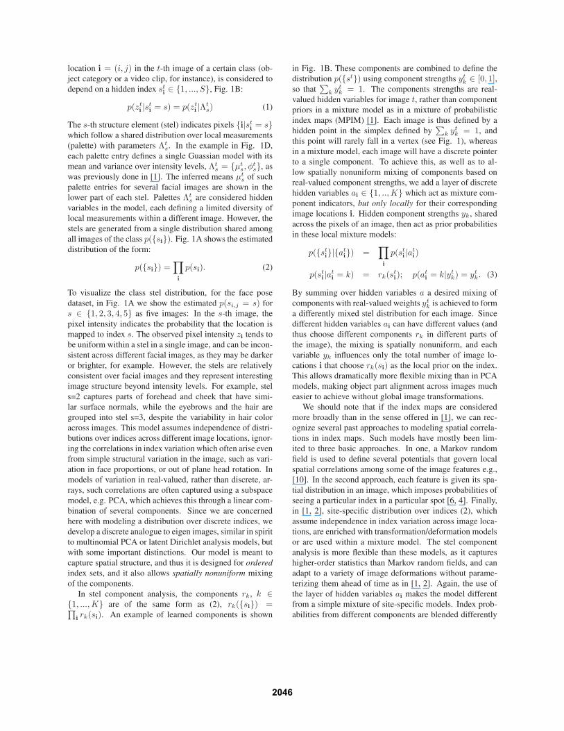
location i = (i, j) in the t-th image of a certain class (ob-

ject category or a video clip, for instance), is considered to

depend on a hidden index sti∈ {1, ..., S}, Fig. 1B:

p(zti|st

i= s) = p(zt

i|Λt

s) (1)

The s-th structure element (stel) indicates pixels {i|sti= s}

which follow a shared distribution over local measurements

(palette) with parameters Λts. In the example in Fig. 1D,

each palette entry defines a single Guassian model with its

mean and variance over intensity levels, Λts = {µt

s, φts}, as

was previously done in [1]. The inferred means µts of such

palette entries for several facial images are shown in the

lower part of each stel. Palettes Λts are considered hidden

variables in the model, each defining a limited diversity of

local measurements within a different image. However, the

stels are generated from a single distribution shared among

all images of the class p({si}). Fig. 1A shows the estimated

distribution of the form:

p({si}) =∏

i

p(si). (2)

To visualize the class stel distribution, for the face pose

dataset, in Fig. 1A we show the estimated p(si,j = s) for

s ∈ {1, 2, 3, 4, 5} as five images: In the s-th image, the

pixel intensity indicates the probability that the location is

mapped to index s. The observed pixel intensity zi tends to

be uniform within a stel in a single image, and can be incon-

sistent across different facial images, as they may be darker

or brighter, for example. However, the stels are relatively

consistent over facial images and they represent interesting

image structure beyond intensity levels. For example, stel

s=2 captures parts of forehead and cheek that have simi-

lar surface normals, while the eyebrows and the hair are

grouped into stel s=3, despite the variability in hair color

across images. This model assumes independence of distri-

butions over indices across different image locations, ignor-

ing the correlations in index variation which often arise even

from simple structural variation in the image, such as vari-

ation in face proportions, or out of plane head rotation. In

models of variation in real-valued, rather than discrete, ar-

rays, such correlations are often captured using a subspace

model, e.g. PCA, which achieves this through a linear com-

bination of several components. Since we are concerned

here with modeling a distribution over discrete indices, we

develop a discrete analogue to eigen images, similar in spirit

to multinomial PCA or latent Dirichlet analysis models, but

with some important distinctions. Our model is meant to

capture spatial structure, and thus it is designed for ordered

index sets, and it also allows spatially nonuniform mixing

of the components.

In stel component analysis, the components rk, k ∈{1, ...,K} are of the same form as (2), rk({si}) =∏

irk(si). An example of learned components is shown

in Fig. 1B. These components are combined to define the

distribution p({st}) using component strengths ytk ∈ [0, 1],

so that∑

k ytk = 1. The components strengths are real-

valued hidden variables for image t, rather than component

priors in a mixture model as in a mixture of probabilistic

index maps (MPIM) [1]. Each image is thus defined by a

hidden point in the simplex defined by∑

k ytk = 1, and

this point will rarely fall in a vertex (see Fig. 1), whereas

in a mixture model, each image will have a discrete pointer

to a single component. To achieve this, as well as to al-

low spatially nonuniform mixing of components based on

real-valued component strengths, we add a layer of discrete

hidden variables ai ∈ {1, ..,K} which act as mixture com-

ponent indicators, but only locally for their corresponding

image locations i. Hidden component strengths yk, shared

across the pixels of an image, then act as prior probabilities

in these local mixture models:

p({sti}|{at

i}) =

∏

i

p(sti|at

i)

p(sti|at

i= k) = rk(st

i); p(at

i= k|yt

k) = ytk. (3)

By summing over hidden variables a a desired mixing of

components with real-valued weights ytk is achieved to form

a differently mixed stel distribution for each image. Since

different hidden variables ai can have different values (and

thus choose different components rk in different parts of

the image), the mixing is spatially nonuniform, and each

variable yk influences only the total number of image lo-

cations i that choose rk(si) as the local prior on the index.

This allows dramatically more flexible mixing than in PCA

models, making object part alignment across images much

easier to achieve without global image transformations.

We should note that if the index maps are considered

more broadly than in the sense offered in [1], we can rec-

ognize several past approaches to modeling spatial correla-

tions in index maps. Such models have mostly been lim-

ited to three basic approaches. In one, a Markov random

field is used to define several potentials that govern local

spatial correlations among some of the image features e.g.,

[10]. In the second approach, each feature is given its spa-

tial distribution in an image, which imposes probabilities of

seeing a particular index in a particular spot [6, 4]. Finally,

in [1, 2], site-specific distribution over indices (2), which

assume independence in index variation across image loca-

tions, are enriched with transformation/deformation models

or are used within a mixture model. The stel component

analysis is more flexible than these models, as it captures

higher-order statistics than Markov random fields, and can

adapt to a variety of image deformations without parame-

terizing them ahead of time as in [1, 2]. Again, the use of

the layer of hidden variables ai makes the model different

from a simple mixture of site-specific models. Index prob-

abilities from different components are blended differently

2046

in different parts of the image, which simple mixture mod-

els do not allow. This gives the model more flexibility in

parsing images, and, as desired, allows for variable mixing

of the components for different images to model smooth ge-

ometric changes (Fig. 1).

The joint distribution over all observed variables z ={zt

i}, and hidden variables/parameters h ={{yt

k}, {ati, st

i},

{Λts}, {rk}} is

p(z,h) =∏

t

(

p({ytk}

Kk=1)p({Λt

s})∏

i

p(zti|st

i, {Λt

s})

∏

k

(ytkrk(st

i))[a

ti=k])

)

(4)

where [·] is the indicator function. The priors on yk can be

kept flat (as in our experiments), or learned in a Dirichlet

form. The prior on PIMs rk was kept flat, i.e. omitted in

equations.

Following the variational inference recipe, we in-

troduce a tunable distribution q(h) over the hidden

variables/parameters, define as a bound on the log

likelihood log p(z), the negative free energy −F =∑

hq(h) log q(h)

p(z,h) , and pursue the strategy of minimiz-

ing this free energy iteratively. We used the sim-

plest of the algorithms from this family, where the ap-

proximate posterior distribution q(h) is fully factorized,

q(h) =∏

k q(rk)∏

i,t q(ati)q(st

i)∏

t q(ytk)q({Λt

s}), with

q(rk), q(ytk) and q(Λt

s) being Dirac functions centered at

the optimal values (or vectors) rk, ykt , {Λt

s}. As a result,

the (approximate) inference reduces to minimizing the fol-

lowing free energy,

F =∑

t

p({Λts}) +

∑

t,i,s

q(sti= s) log p(zt

i|st

i, {Λt

s}) +

+∑

t,i,a

q(ati= a) log yt

a +

+∑

t,i,a,s

q(ati= a)q(st

i= s) log ra(st

i= s), (5)

which is reduced by each of the following steps:

• The palettes for different stels in a single image t are

assigned so as to balance the need to agree with the

prior p(Λ) with the statistics of the local measurements

within a (probabilistic) stel in the image:

Λts = arg max log p({Λt

s}) + (6)

+∑

i

q(sti= s) log p(zt

i|st

i= s, {Λt

s}).

(More details below).

• The stel segmentation of image t is based on the sim-

ilarity of observed local measurements to what is ex-

pected in a particular class stel s according to the esti-

mated palette Λts in this particular image, as well as the

expected stel assignment based on mixed components

rk(s).

q(sti= s) ∝ p(zt

i|st

i, {Λt

s})eP

aq(at

i=a)ra(st

i=s). (7)

• The spatially nonuniform component mixing, defined

by q(a), is updated so as to balance the agreement with

the overall strength yta of the component a in the partic-

ular image t, with the agreement of the stel assignment

with the stel component ra:

q(ati= a) ∝ yt

aeP

sq(st

i=s) log ra(st

i=s). (8)

• The stel component strengths ya are assigned propor-

tional to their use in the image:

yta ∝

∑

i

q(ati= a). (9)

• The stel components ra are updated to reflect the as-

signment statistics over all images:

ra(s) ∝∑

t

q(ati= a)q(st

i= s). (10)

Local measurements zt, palette models p(zt|Λts) and

palette priors p(Λs)The local measurements zi may vary depending on the

application, and can be scalar or multidimensional, discrete

or real-valued. To obtain the face model in Fig. 1, as in

[1], we assumed that the local measurements are simply the

real-valued image intensities, that the palette model Λs =(µs, φs) is Gaussian, p(zt

i|st

i= s, {Λt

s}) = N (zti;µt

s, φts),

and that the prior on the palette Λs is flat. The palette up-

date is therefore based on sufficient statistics over intensities

within stels in individual images (See [1] for details). Al-

ternative local measurements include color, disparity, flow,

SIFT [7] or some other local features. As more expressive

palette models, we use the histogram representation for dis-

crete local measurements, and the mixture of Gaussians for

the real-valued measurements (Fig. 4).

For the case of discrete measurements, we define the

palette as a histogram over C possible observations {ζj},

j ∈ {1, ..., C}. The observation distribution is multino-

mial with parameters uj = p(z = ζj), and the palettes

Λs = {us,j} are defined by these probabilities. With a flat

prior on Λ, the equation (6) reduces to

uts,j ∝

∑

i

q(sti= s)[zt

i= ζj ] (11)

When measurements consist of different modalities, which

are generally uncorrelated at the local level (except

2047

through higher level variables in the model), they are

combined by setting p(zi|s) =∏

m p(zm,i|Λm,s) =∏

m

∏

j u[zm,i=ζm,j]m,s,j , where m denotes different modality

(e.g., available pixel label and discrete texture features as-

sociated with each pixel).

To avoid complete palette invariance, we also add a Dirich-

let prior on the histogram palette models:

p(Λ) = p({uj}) =1

Z({αj})

∏

j

uαj−1j , (12)

which is estimated from the data iteratively together with

other updates. The effect of this prior on the palette updates

in (6) for different modalities m is utm,s,j ∝ αm,s,j − 1 +

∑

iq(st

i= s)[zt

m,i = ζm,j ], and the appropriate update on

palette priors αj can be shown to be:

{αs,m,j} = arg max∑

t

(αs,m,j − 1) log utm,s,j , (13)

subject to the appropriate normalization constraint. The ad-

dition of the (learnable) prior over palette entry allows the

model to discover and exploit consistency of local measure-

ments across instances of a class, if there is any. In case of

real-valued measurements of arbitrary dimensionality, the

palette entry is defined by a mixture of C Gaussians, and the

appropriate palette priors are added similarly as in the case

of discrete measurements. The treatment of Gaussian com-

ponent probabilities in each entry is identical to the treat-

ment of discrete measurement frequencies above, while the

mean and covariance matrix have the appropriate conjugate

priors (Gaussian and scaled inverse Gamma, respectively).

Being a mixture, each palette entry has a hidden variable

pointing to one of the C Gaussians.

When the raw local measurement is real-valued, e.g. a

filter response, we can still choose to discretize it rather than

use a real-valued model. Finally, we often combine discrete

and real-valued modalities, in the same way the multiple

discrete modalities are combined (Fig. 4).

Relationship to other models. We can express many other

models frequently used in vision and elsewhere as special

cases by assuming an appropriate number of stels S, the

components K, and the palette entry size C. The color his-

togram model and the bag of words/features model [5, 6]

are achieved with S = 1. On the other hand, when S > 1,

but only a single component rk(s) is used, K = 1, and

each palette entry represents a single Gaussian, C = 1, and

the prior over palettes is fixed to flat, our model reduces

to a probabilistic index map (PIM) [1]. Finally, the basic

ingredient of LOCUS [2] is a model we get when we set

S = 2 (foreground/background), and use a large C to rep-

resent color histograms in each palette entry1. If we fix the

stel partition q(sti) to a division of image into regions by

1Both LOCUS and PIM contained transformation variables, which cap-

1 20

1

1 20

1

1 20

1

1 20

1

1 20

1

1 20

1

1 20

1

SCA

yk

PCA[1,2]

PCA[2,3,4]

PCA[4,5,6]

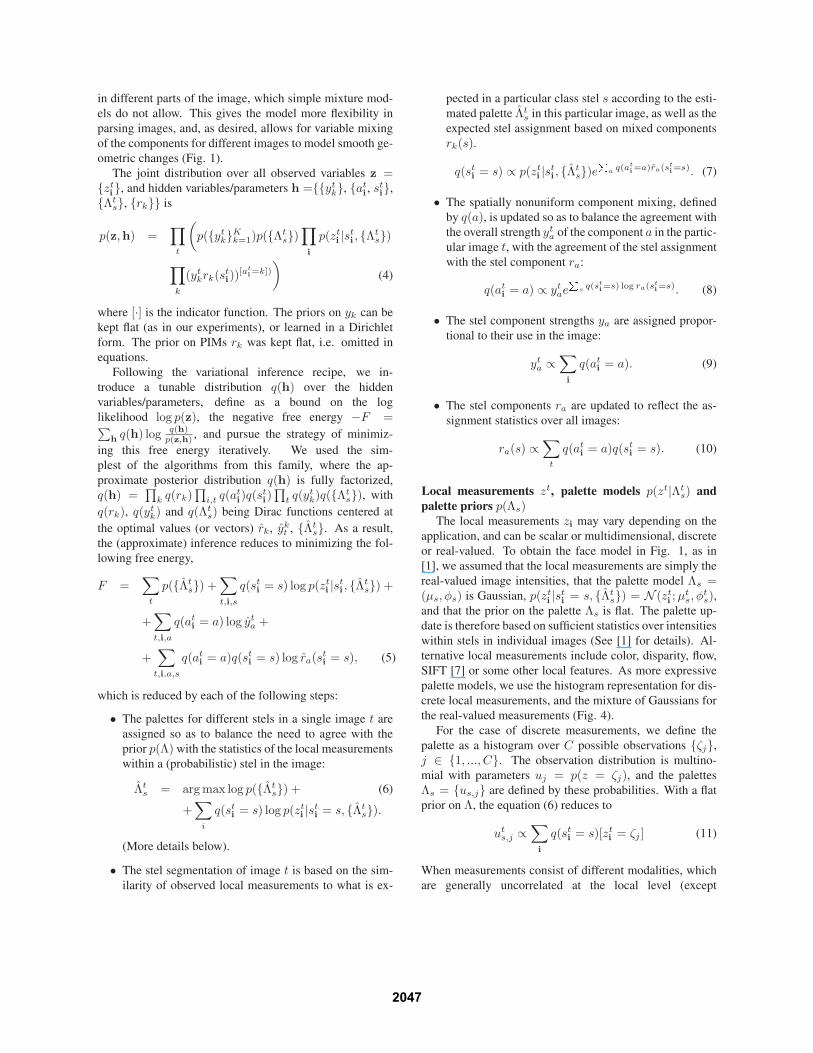
Figure 2. SCA component strengths yk, K=2, for a set of im-

ages of faces with varying pose, have a single degree of freedom

(y1 + y2 = 1) and this degree of freedom captures the pose angle

well. Below the yk strengths, we show images generated from the

model using the yk inferred from the input. The rest of the fig-

ure illustrates the PCA reconstruction, which does not manage to

separate pose from other causes of variability.

hand, rather than let them be estimated from images them-

selves, the model becomes similar to [4].

3. ExperimentsThe main contribution of this paper is a novel represen-

tation of images, which allows for unsupervised extraction

of image parts, with this process synchronized over many

examples of images from a certain class, e.g., a single video

clip, or an object category. The representation can be used

in a variety of ways in computer vision, often in conjunc-

tion with other models, and the purpose of this section is to

provide some illustrations.

Head pose angle estimation: Comparison with PCA. In

this experiment, we used a database [3] of 250 images of

18 subjects, each captured at 25 head poses (some exam-

ples in Fig. 1). The poses in images were manually la-

beled with the estimated out-of-plane rotation angle (from

0 to 45 deg). In five-fold crossvalidation, we trained both

a PCA model and a stel component analyzer (SCA) (K=2,

S=7, Gaussian palettes), and chose the optimal predictor of

the pose angle based on the component strengths y of PCA

and the stel component analyzer. In case of PCA, the pre-

dictors we considered used up to the 6 components with

highest egienvalues, and, furthermore, to allow for some il-

lumination invariance, we considered sparse variants that

also discarded the first, the first two, or the first three com-

ponents. For both PCA and the stel-based angle prediction,

the cross validation included linear regression, robust lin-

ear regression, and the nonlinear regression. The SCA out-

performed PCA projection as the input to regression in this

test, as the average test error for the optimal PCA-based

regressor was 9 deg and the optimal SCA-based regressor

had a test error was 8 deg. The standard deviation over the

ture correlations due to a given set of simple 2D geometric transformations,

while stel component analysis learns (approximately) arbitrary correlations

in possible index assignments across an image. The palette choices we dis-

cuss here apply to all three models.

2048

s = 3s = 2s = 1

k = 1

µ0, (σ0)

Frame 30 Frame 70 Frame 100 Frame 110

1 2 3 1 2 3 1 2 3 1 2 3

Frame 150 Frame 170 Frame 190Frame 120

1 2 3 1 2 3 1 2 3 1 2 3

yk

MSRiu anaivana

VIDEO SEGMENTATION - ParametersS=3,K=3,C=3 ( larry )

VIDEO SEGMENTATION - Results

larry

Video Method

A)

B)

C)

D)

A)

B)

D)

BG FG Overall

[8]

1 2 3 1 2 3 1 2 3

k = 2

k = 3

α

c=1 c=2 c=3 c=1 c=2 c=3 c=1 c=2 c=3

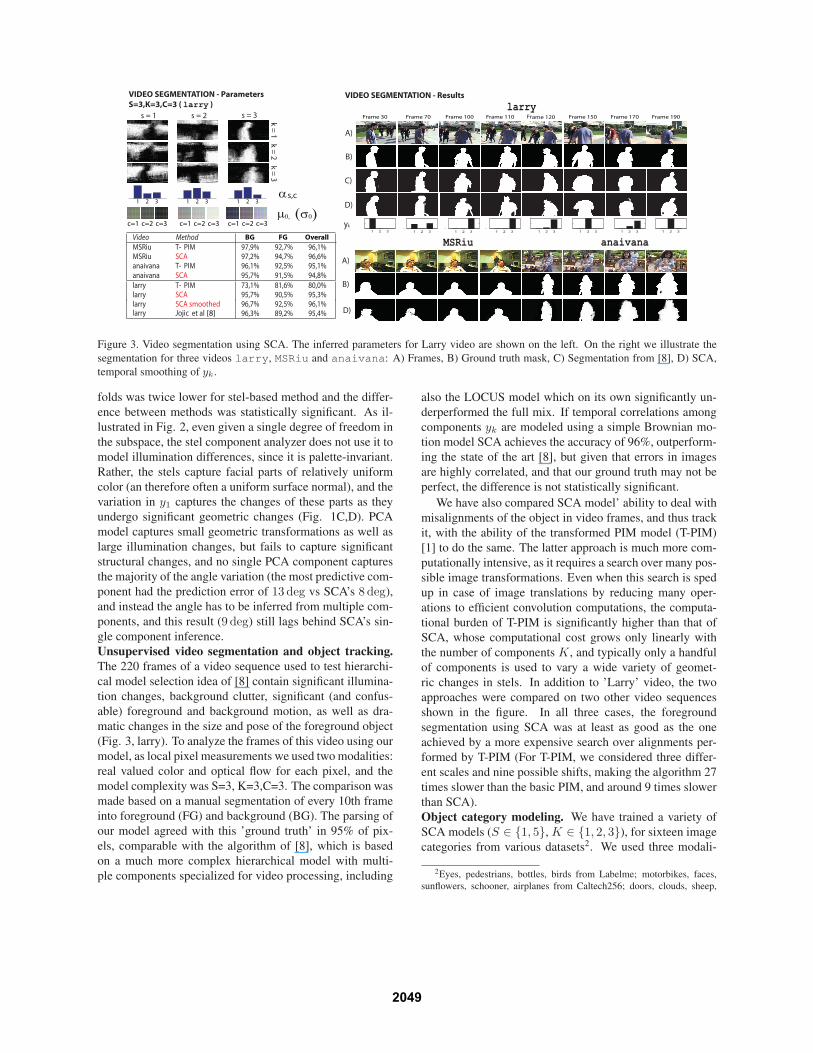
Figure 3. Video segmentation using SCA. The inferred parameters for Larry video are shown on the left. On the right we illustrate the

segmentation for three videos larry, MSRiu and anaivana: A) Frames, B) Ground truth mask, C) Segmentation from [8], D) SCA,

temporal smoothing of yk.

folds was twice lower for stel-based method and the differ-

ence between methods was statistically significant. As il-

lustrated in Fig. 2, even given a single degree of freedom in

the subspace, the stel component analyzer does not use it to

model illumination differences, since it is palette-invariant.

Rather, the stels capture facial parts of relatively uniform

color (an therefore often a uniform surface normal), and the

variation in y1 captures the changes of these parts as they

undergo significant geometric changes (Fig. 1C,D). PCA

model captures small geometric transformations as well as

large illumination changes, but fails to capture significant

structural changes, and no single PCA component captures

the majority of the angle variation (the most predictive com-

ponent had the prediction error of 13 deg vs SCA’s 8 deg),

and instead the angle has to be inferred from multiple com-

ponents, and this result (9 deg) still lags behind SCA’s sin-

gle component inference.

Unsupervised video segmentation and object tracking.

The 220 frames of a video sequence used to test hierarchi-

cal model selection idea of [8] contain significant illumina-

tion changes, background clutter, significant (and confus-

able) foreground and background motion, as well as dra-

matic changes in the size and pose of the foreground object

(Fig. 3, larry). To analyze the frames of this video using our

model, as local pixel measurements we used two modalities:

real valued color and optical flow for each pixel, and the

model complexity was S=3, K=3,C=3. The comparison was

made based on a manual segmentation of every 10th frame

into foreground (FG) and background (BG). The parsing of

our model agreed with this ’ground truth’ in 95% of pix-

els, comparable with the algorithm of [8], which is based

on a much more complex hierarchical model with multi-

ple components specialized for video processing, including

also the LOCUS model which on its own significantly un-

derperformed the full mix. If temporal correlations among

components yk are modeled using a simple Brownian mo-

tion model SCA achieves the accuracy of 96%, outperform-

ing the state of the art [8], but given that errors in images

are highly correlated, and that our ground truth may not be

perfect, the difference is not statistically significant.

We have also compared SCA model’ ability to deal with

misalignments of the object in video frames, and thus track

it, with the ability of the transformed PIM model (T-PIM)

[1] to do the same. The latter approach is much more com-

putationally intensive, as it requires a search over many pos-

sible image transformations. Even when this search is sped

up in case of image translations by reducing many oper-

ations to efficient convolution computations, the computa-

tional burden of T-PIM is significantly higher than that of

SCA, whose computational cost grows only linearly with

the number of components K, and typically only a handful

of components is used to vary a wide variety of geomet-

ric changes in stels. In addition to ’Larry’ video, the two

approaches were compared on two other video sequences

shown in the figure. In all three cases, the foreground

segmentation using SCA was at least as good as the one

achieved by a more expensive search over alignments per-

formed by T-PIM (For T-PIM, we considered three differ-

ent scales and nine possible shifts, making the algorithm 27

times slower than the basic PIM, and around 9 times slower

than SCA).

Object category modeling. We have trained a variety of

SCA models (S ∈ {1, 5}, K ∈ {1, 2, 3}), for sixteen image

categories from various datasets2. We used three modali-

2Eyes, pedestrians, bottles, birds from Labelme; motorbikes, faces,

sunflowers, schooner, airplanes from Caltech256; doors, clouds, sheep,

2049

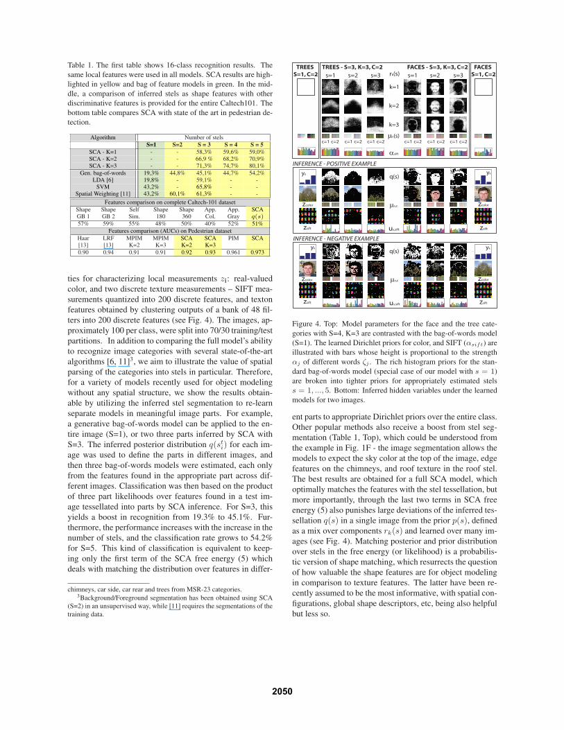
Table 1. The first table shows 16-class recognition results. The

same local features were used in all models. SCA results are high-

lighted in yellow and bag of feature models in green. In the mid-

dle, a comparison of inferred stels as shape features with other

discriminative features is provided for the entire Caltech101. The

bottom table compares SCA with state of the art in pedestrian de-

tection.

Algorithm Number of stels

S=1 S=2 S = 3 S = 4 S = 5

SCA - K=1 - - 58,3% 59,6% 59,0%

SCA - K=2 - - 66,9 % 68,2% 70,9%

SCA - K=3 - - 71,3% 74,7% 80,1%

Gen. bag-of-words 19,3% 44,8% 45,1% 44,7% 54,2%

LDA [6] 19,8% - 59,1% - -

SVM 43,2% - 65,8% - -

Spatial Weighting [11] 43,2% 60,1% 61,3% - -

Features comparison on complete Caltech-101 dataset

Shape Shape Self Shape Shape App. App. SCA

GB 1 GB 2 Sim. 180 360 Col. Gray q(s)57% 59% 55% 48% 50% 40% 52% 51%

Features comparison (AUCs) on Pedestrian dataset

Haar LRF MPIM MPIM SCA SCA PIM SCA

[13] [13] K=2 K=3 K=2 K=3

0.90 0.94 0.91 0.91 0.92 0.93 0.961 0.973

ties for characterizing local measurements zi: real-valued

color, and two discrete texture measurements – SIFT mea-

surements quantized into 200 discrete features, and texton

features obtained by clustering outputs of a bank of 48 fil-

ters into 200 discrete features (see Fig. 4). The images, ap-

proximately 100 per class, were split into 70/30 training/test

partitions. In addition to comparing the full model’s ability

to recognize image categories with several state-of-the-art

algorithms [6, 11]3, we aim to illustrate the value of spatial

parsing of the categories into stels in particular. Therefore,

for a variety of models recently used for object modeling

without any spatial structure, we show the results obtain-

able by utilizing the inferred stel segmentation to re-learn

separate models in meaningful image parts. For example,

a generative bag-of-words model can be applied to the en-

tire image (S=1), or two three parts inferred by SCA with

S=3. The inferred posterior distribution q(sti) for each im-

age was used to define the parts in different images, and

then three bag-of-words models were estimated, each only

from the features found in the appropriate part across dif-

ferent images. Classification was then based on the product

of three part likelihoods over features found in a test im-

age tessellated into parts by SCA inference. For S=3, this

yields a boost in recognition from 19.3% to 45.1%. Fur-

thermore, the performance increases with the increase in the

number of stels, and the classification rate grows to 54.2%

for S=5. This kind of classification is equivalent to keep-

ing only the first term of the SCA free energy (5) which

deals with matching the distribution over features in differ-

chimneys, car side, car rear and trees from MSR-23 categories.3Background/Foreground segmentation has been obtained using SCA

(S=2) in an unsupervised way, while [11] requires the segmentations of the

training data.

rk(s)s=1 s=2

TREES - S=3, K=3, C=2 FACES - S=3, K=3, C=2TREES S=1, C=2 s=3 s=1 s=2 s=3

k=1

k=2

k=3

FACES S=1, C=2

µ0(s)

q(s)

µs,c

us,sift

yk

ykyk

yk

c=1 c=2 c=1 c=2 c=1 c=2 c=1 c=2 c=1 c=2 c=1 c=2

zcolor

zsift

q(s)

µs,c

us,sift

zcolor

zcolorzcolor

zsiftzsift

zsift

INFERENCE - POSITIVE EXAMPLE

INFERENCE - NEGATIVE EXAMPLE

αsift

Figure 4. Top: Model parameters for the face and the tree cate-

gories with S=4, K=3 are contrasted with the bag-of-words model

(S=1). The learned Dirichlet priors for color, and SIFT (αsift) are

illustrated with bars whose height is proportional to the strength

αj of different words ζj . The rich histogram priors for the stan-

dard bag-of-words model (special case of our model with s = 1)

are broken into tighter priors for appropriately estimated stels

s = 1, ..., 5. Bottom: Inferred hidden variables under the learned

models for two images.

ent parts to appropriate Dirichlet priors over the entire class.

Other popular methods also receive a boost from stel seg-

mentation (Table 1, Top), which could be understood from

the example in Fig. 1F - the image segmentation allows the

models to expect the sky color at the top of the image, edge

features on the chimneys, and roof texture in the roof stel.

The best results are obtained for a full SCA model, which

optimally matches the features with the stel tessellation, but

more importantly, through the last two terms in SCA free

energy (5) also punishes large deviations of the inferred tes-

sellation q(s) in a single image from the prior p(s), defined

as a mix over components rk(s) and learned over many im-

ages (see Fig. 4). Matching posterior and prior distribution

over stels in the free energy (or likelihood) is a probabilis-

tic version of shape matching, which resurrects the question

of how valuable the shape features are for object modeling

in comparison to texture features. The latter have been re-

cently assumed to be the most informative, with spatial con-

figurations, global shape descriptors, etc, being also helpful

but less so.

2050

Classifying Caltech101 categories without local features.

To investigate this further, we followed the same training

and test recipe, but on all 101 categories from Caltech101,

for which the best features, used discriminatively provide

classification rates of 40-59% as shown in the Tab.1 (The

numbers are due to [9]: GB features correspond to geomet-

ric blur [12] which captures some of the spatial configura-

tion in feature distributions, and App. Color and Gray are

SIFT features [7] calculated from color and gray images, the

rest of the features capture gradient orientations, and thus

mostly local shape features). In analyzing Caltech101 im-

ages, we only used color as a local measurement, to perform

inference within a single image, but we performed classifi-

cation using only the inferred stel segmentation, q(s), with-

out parts of the likelihood that have to do with matching

of image measurements to those expected for the category.

This corresponds to dropping out the first two terms from

the free energy (5) which deal with evaluating the unifor-

mity of observed features zi and their agreement with the

prior over the entire class defined by Λ. Therefore, the only

terms kept are the last two terms concerned with the KL

distance between the prior p(s) and the inferred stel tessel-

lation for the image q(s). Such classification yields accu-

racy of 25%. However, the discriminative use of inferred

stels, through SVM classification using only inferred stels

as features resulted in classification accuracy of 51%, mak-

ing the global shape features defined by stel segmentation of

comparable quality to the top features used in object clas-

sification. This is encouraging, as these features capture

rather different aspects of images and could thus be used in

multi-feature approaches which previously yielded best re-

sults on this dataset [9]. It is important to note here that for

an already trained SCA model, inference of stels q(s) for

any new given image consists of only a 4-5 iterations of Eq.

(7)-(9), as the SCA components rk, and palette priors are

linked to the entire category, not a single image. Thus, in-

ference for a single image is linear in the number of pixels,

and is in fact more computationally efficient than the com-

putation involved in methods that require a large number of

filter banks or SIFT extraction, which SCA does not require

when the considered image measurement is just color.

The SCA model also outperforms state of the art in

pedestrian detection (Table 1, bottom).

4. Conclusions

We have introduced a novel model that captures the cor-

relations in spatial structure of an image class. Instead

of relying on consistency of image features across images

from the same class, the model mines self similarity patterns

within individual images. Inference in this model leads to

consistent segmentation of images into structural elements

(stels), shared across the entire class, even when the images

differ dramatically in their local colors and features. Signif-

icant variation in stels can be tolerated by a subspace model,

stel component analyzer, which captures correlated changes

in image structure and thus avoids over-generalization that

the PIM model was prone to when faced with significant

structural variation. The model can be inferred from the

data in an unsupervised manner and this affords this rep-

resentation of images significant advantages in a variety of

computer vision applications, some of which have been il-

lustrated above. In addition, the analysis described here can

help scale up the approaches to computer vision which de-

pend on manual segmentation of image parts. Recent soci-

ological innovations have made it possible to recruit a large

number of volunteers to manually segment images through

collaborative games, or by motivating them by other types

of incentives. However, even in these cases, the SCA model

may prove to be an invaluable tool for refinement of user-

provided segmentations, such as the ones obtainable from

LabelMe database.

References

[1] N. Jojic and C. Caspi, “Capturing image structure with prob-

abilistic index maps,” CVPR 2004, pp. 212-219.

[2] J. Winn and N. Jojic, “LOCUS: Learning Object Classes

with Unsupervised Segmentation,” ICCV 2005, pp. 756-763.

[3] D. Graham, N. Allinson. “Characterizing Virtual

Eigensignatures for General Purpose Face Recognition,” (in)

Face Recognition: From Theory to Applications

[4] S. Lazebnik, C. Schmid, J. Ponce, “Beyond Bags of Fea-

tures: Spatial Pyramid Matching for Recognizing Natural

Scene Categories,” IEEE CVPR, 2006

[5] D.M. Blei, A.Y. Ng, M.I. Jordan, “Latent dirichlet alloca-

tion,” J. Mach. Learn. Res., 2003

[6] L. Fei-Fei, P. Perona, “A Bayesian Hierarchical Model for

Learning Natural Scene Categories,” IEEE CVPR 2005.

[7] D. Lowe, “Distinctive Image Features from Scale-Invariant

Keypoints,” IJCV, 2004

[8] N. Jojic, J. Winn, L. Zitnick, “Escaping local minima

through hierarchical model selection: Automatic object dis-

covery, segmentation, and tracking in video,” IEEE CVPR

2006

[9] M. Varma, D. Ray “Learning The Discriminative Power-

Invariance Trade-Off” ICCV 2007

[10] J. Shotton, J. Winn, C. Rother, A. Criminisi “Textonboost:

Joint appearance, shape and context modeling for multi-class

object recognition and segmentation” ECCV 2006

[11] M. Marszaek, C. Schmid “Spatial Weighting for Bag-of-

Features” IEEE CVPR 2006

[12] A.C. Berg, J. Malik “Geometric Blur for Template Match-

ing” IEEE CVPR 2001

[13] S. Munder and D. M. Gavrila “An experimental study on

pedestrian classification” IEEE TPAMI, 2006

2051