Statistics and Practice on the Trend's Reversal and ... - MDPI

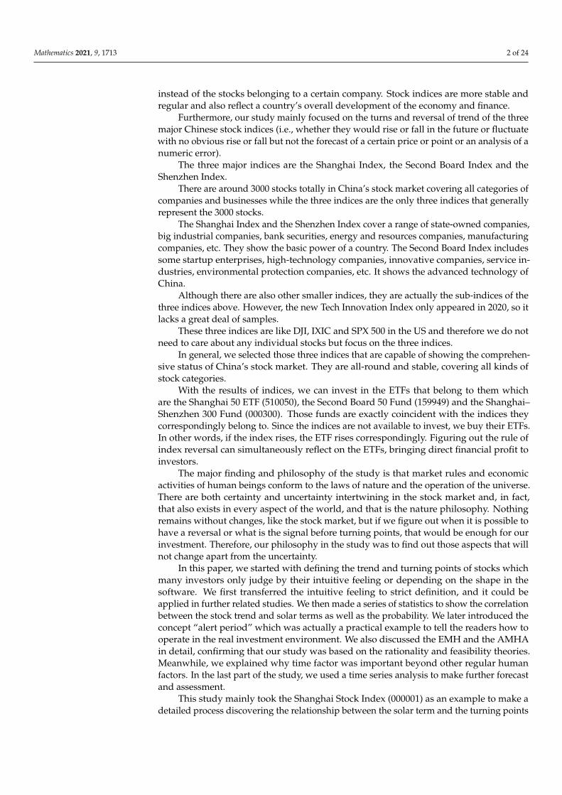
mathematics

Article

Statistics and Practice on the Trend’s Reversal and TurningPoints of Chinese Stock Indices Based on Gann’s Time Theoryand Solar Terms Effect

Tianbao Zhou 1 , Xinghao Li 2 and Peng Wang 1,*

��

Citation: Zhou, T.; Li, X.; Wang, P.

Statistics and Practice on the Trend’s

Reversal and Turning Points of

Chinese Stock Indices Based on

Gann’s Time Theory and Solar Terms

Effect. Mathematics 2021, 9, 1713.

https://doi.org/10.3390/math9151713

Academic Editors: Davide Valenti

and Bahram Adrangi

Received: 2 June 2021

Accepted: 18 July 2021

Published: 21 July 2021

Publisher’s Note: MDPI stays neutral

with regard to jurisdictional claims in

published maps and institutional affil-

iations.

Copyright: © 2021 by the authors.

Licensee MDPI, Basel, Switzerland.

This article is an open access article

distributed under the terms and

conditions of the Creative Commons

Attribution (CC BY) license (https://

creativecommons.org/licenses/by/

4.0/).

1 College of Science, Beijing Forestry University, Beijing 100083, China; [email protected] School of Information Science & Technology, Beijing Forestry University, Beijing 100083, China;

[email protected]* Correspondence: [email protected]

Abstract: Despite the future price of individual stocks has long been proved to be unpredictableand irregular according to the EMH, the turning points (or the reversal) of the stock indices trendstill remain the rules to follow. Therefore, this study mainly aimed to provide investors with newstrategies in buying ETFs of the indices, which not only avoided the instability of individual stocks,but were also able to get a high profit within weeks. Famous theories like Gann theory and the Elliottwave theory suggest that as part of the nature, market regulations and economic activities of humanbeings shall conform to the laws of nature and the operation of the universe. They further refined onlythe rules related to specific timepoints and the time cycle rather than the traditional analysis of thecomplex economic and social factors, which is, to some extent, similar to what the Chinese traditionalculture proposes: that every impact on and change in the human society is always attributable tochanges in the nature. The study found that the turns of the stock indices trend were inevitable atspecific timepoints while the strength and intensity of the turns were uncertain, affected by variousfactors by then, which meant the market was intertwined with both certainty and uncertainty atthe same time. The analysis was based on the data of the Shanghai Index, the Second Board Indexand the Shenzhen Index, the three major indices that represent almost all aspects of the Chinesestock market, for the past decades. It could effectively reduce the heteroscedasticity, instability andirregularity of time series models by replacing 250 daily high-frequency data with the extreme pointsnear every twenty-four solar terms per year. The forecasts focusing on the future stock trend ofthe all-solar-terms group and the eight-solar-terms group were proved accurate. What is more, theindices trend was at a high probability to turn in a range of four days at each solar term. The alertperiod also provided the readers with a practical example of how it works in the real investmentenvironment.

Keywords: n-day extreme point; valid time radius; ARIMA–ARCH model; efficient-market hypothe-sis; adaptive market hypothesis

1. Introduction1.1. General Survey of the Study

According to the efficient-market hypothesis (EMH) and the adaptive market hypoth-esis (AMH), the future price of an individual stock is impossible to predict and, as theefficiency of the market goes high, the market tends to be more stochastic and disordered,and there are no methods to make any valid prediction ahead from the present. Eventhough the market is not that efficient in the real world, the prediction is still very hardand unrealistic to make [1].

On the contrary, many researchers have been studying and proved that stock indicesare rather predictable to some extent in terms of volatility, revenue, returns, etc. [2,3]. Stockindices are comprehensive special-type stocks that represent a category of individual stocks

Mathematics 2021, 9, 1713. https://doi.org/10.3390/math9151713 https://www.mdpi.com/journal/mathematics

https://www.mdpi.com/journal/mathematics

https://www.mdpi.com

https://orcid.org/0000-0001-6782-626X



https://creativecommons.org/

https://creativecommons.org/licenses/by/4.0/

https://creativecommons.org/licenses/by/4.0/


https://www.mdpi.com/journal/mathematics

https://www.mdpi.com/article/10.3390/math9151713?type=check_update&version=2

Mathematics 2021, 9, 1713 2 of 24

instead of the stocks belonging to a certain company. Stock indices are more stable andregular and also reflect a country’s overall development of the economy and finance.

Furthermore, our study mainly focused on the turns and reversal of trend of the threemajor Chinese stock indices (i.e., whether they would rise or fall in the future or fluctuatewith no obvious rise or fall but not the forecast of a certain price or point or an analysis of anumeric error).

The three major indices are the Shanghai Index, the Second Board Index and theShenzhen Index.

There are around 3000 stocks totally in China’s stock market covering all categories ofcompanies and businesses while the three indices are the only three indices that generallyrepresent the 3000 stocks.

The Shanghai Index and the Shenzhen Index cover a range of state-owned companies,big industrial companies, bank securities, energy and resources companies, manufacturingcompanies, etc. They show the basic power of a country. The Second Board Index includessome startup enterprises, high-technology companies, innovative companies, service in-dustries, environmental protection companies, etc. It shows the advanced technology ofChina.

Although there are also other smaller indices, they are actually the sub-indices of thethree indices above. However, the new Tech Innovation Index only appeared in 2020, so itlacks a great deal of samples.

These three indices are like DJI, IXIC and SPX 500 in the US and therefore we do notneed to care about any individual stocks but focus on the three indices.

In general, we selected those three indices that are capable of showing the comprehen-sive status of China’s stock market. They are all-round and stable, covering all kinds ofstock categories.

With the results of indices, we can invest in the ETFs that belong to them whichare the Shanghai 50 ETF (510050), the Second Board 50 Fund (159949) and the Shanghai–Shenzhen 300 Fund (000300). Those funds are exactly coincident with the indices theycorrespondingly belong to. Since the indices are not available to invest, we buy their ETFs.In other words, if the index rises, the ETF rises correspondingly. Figuring out the rule ofindex reversal can simultaneously reflect on the ETFs, bringing direct financial profit toinvestors.

The major finding and philosophy of the study is that market rules and economicactivities of human beings conform to the laws of nature and the operation of the universe.There are both certainty and uncertainty intertwining in the stock market and, in fact,that also exists in every aspect of the world, and that is the nature philosophy. Nothingremains without changes, like the stock market, but if we figure out when it is possible tohave a reversal or what is the signal before turning points, that would be enough for ourinvestment. Therefore, our philosophy in the study was to find out those aspects that willnot change apart from the uncertainty.

In this paper, we started with defining the trend and turning points of stocks whichmany investors only judge by their intuitive feeling or depending on the shape in thesoftware. We first transferred the intuitive feeling to strict definition, and it could beapplied in further related studies. We then made a series of statistics to show the correlationbetween the stock trend and solar terms as well as the probability. We later introduced theconcept “alert period” which was actually a practical example to tell the readers how tooperate in the real investment environment. We also discussed the EMH and the AMHAin detail, confirming that our study was based on the rationality and feasibility theories.Meanwhile, we explained why time factor was important beyond other regular humanfactors. In the last part of the study, we used a time series analysis to make further forecastand assessment.

This study mainly took the Shanghai Stock Index (000001) as an example to make adetailed process discovering the relationship between the solar term and the turning points

Mathematics 2021, 9, 1713 3 of 24

of the index trend, and used the solar term for the time series analysis to predict the futuretrend.

Meanwhile, we also tested the Second Board Index and the Shenzhen Index as evi-dence of applicability of our study. However, for convenience, we only show the results ofthese two indices directly with the same approach as dealing with the Shanghai Index.

1.2. Introduction of Chinese Twenty-Four Solar Terms

The Chinese traditional twenty-four solar terms are the theory and wisdom of naturalclimate and the turning points of seasons summarized by the ancient Chinese people.

With the arrival of one solar term after another, farming, planting and other agricul-tural activities also usher in one key timepoint after another. The twenty-four solar termsprovide people with crucial time information such as when to sow, when to enhance farm-ing, when to rest and stop farming and when to harvest. Moreover, the temperature andclimate of each year also change significantly in these 24 solar terms, forming fluctuations.The seasonal cycle of rising and falling, annual cooling, heating, rainfall and snowfall oftenoccur at a time very close to or exactly at the solar term.

Twenty-four solar terms have been widely used in the field of traditional Chinesemedicine [4], which makes us more firmly believe that the natural law represented by theChinese twenty-four solar terms, as the traditional culture, has already had a potentialimpact on various aspects of human society [5]. Our study uses the twenty-four solar termsto discover the possible impact on the stock market [6,7].

Today’s twenty-four solar terms are based on the position of the sun on the ecliptic.That’s the annual motion track of the sun which is divided into 24 equal parts, each 15◦

is one part (Figure 1), each one is a solar term; the first one is Chunfen and the last oneis Dahan. On 30 November 2016, the twenty-four solar terms were officially listed in theUNESCO representative works on intangible human cultural heritage.

In the time cycle theory of Gann theory [8], the division of Gann’s wheel and the dateor time cycle corresponding to the angle often lead to the turning of stock trend. Gann’swheel can represent the cycle of one year, ten years or even thirty years, and the division ofGann’s wheel in one year as a cycle is exactly the same as with the 24 solar terms in China,and the most important eight angles also perfectly match the most important eight solarterms in the 24 solar terms.

We were inspired by Gann theory, but we were more willing to propose a Chinese-stylemethod and theory. Therefore, in the following parts of the study, we mainly discussed therelationship between the solar terms and the stock reversal.

Making significant analysis and achievement on solar terms may also inspire otherresearchers to apply them in other fields, and the philosophy of the time factor is reallyimportant in guidance. We reviewed it in the Discussion part of the paper.

1.3. Data

The data we used in Chapter 2 are as follows:Shanghai Index (code 000001): daily closing price (point) of marketing days from

3 January 1995 to 14 August 2020, 6463 datapoints in total.Second Board Index (code 399006): daily closing price (point) of marketing days from

1 June 2010 to 9 February 2021, 2693 datapoints in total.Shenzhen Index (code 399001): daily closing price (point) of marketing days from

3 January 1995 to 3 February 2021, 6439 datapoints in total.The data we used in Chapter 5 are as follows:Based on the data above but differently, we only used the price near each solar term

which is the biggest n-day extreme point in a 4-day time radius of each solar term.The last several solar terms were used as the test group.The data are open and easily found on many websites such as https://money.163.com,

accessed on 28 February 2021; readers that are not in China may also download them forfree; to find them, enter the stock code.

https://money.163.com

Mathematics 2021, 9, 1713 4 of 24Mathematics 2021, 9, x FOR PEER REVIEW 4 of 27

Figure 1. Time that each solar term takes place annually.

1.3. Data The data we used in Chapter 2 are as follows: Shanghai Index (code 000001): daily closing price (point) of marketing days from 3

January 1995 to 14 August 2020, 6463 datapoints in total. Second Board Index (code 399006): daily closing price (point) of marketing days from

1 June 2010 to 9 February 2021, 2693 datapoints in total. Shenzhen Index (code 399001): daily closing price (point) of marketing days from 3

January 1995 to 3 February 2021, 6439 datapoints in total. The data we used in Chapter 5 are as follows: Based on the data above but differently, we only used the price near each solar term

which is the biggest n-day extreme point in a 4-day time radius of each solar term. The last several solar terms were used as the test group. The data are open and easily found on many websites such as https://money.163.com,

accessed on 28 February 2021; readers that are not in China may also download them for free; to find them, enter the stock code.

1.4. Time Cycle Theory and Division of Time In this section, we introduce an innovated philosophy in stock analysis, which actu-

ally was not that new in ancient China, the main refrain throughout our study. The phi-losophy is that time matters at all times. According to our previous experience and the Chinese traditional culture, human society is affected by natural factors at every moment, and one of the factors is time (including the time cycle, timepoints and time periods).

Despite the fact that the absolute price of a stock is generally supposed to be unpre-dictable, the turning points and reversal of trend of stock indices have rules to follow.

Figure 1. Time that each solar term takes place annually.

1.4. Time Cycle Theory and Division of Time

In this section, we introduce an innovated philosophy in stock analysis, which actuallywas not that new in ancient China, the main refrain throughout our study. The philosophyis that time matters at all times. According to our previous experience and the Chinesetraditional culture, human society is affected by natural factors at every moment, and oneof the factors is time (including the time cycle, timepoints and time periods).

Despite the fact that the absolute price of a stock is generally supposed to be unpre-dictable, the turning points and reversal of trend of stock indices have rules to follow. Ganntheory [9–14] suggests that the cycle of time is almost everywhere in the stock market, likeour pulse cycle and four seasons of the year. Nobody denies the existence of the time cycleas it retains its rationality and regularity in the nature. Whether or not we know, the regularshocks and vibrations in the stock market caused by time do happen.

In our paper, we only analyzed the trend and turning points of the Shanghai Indexrather than a certain stock or an absolute stock price. We supposed that the index is a wideand general performance of the stock market which eliminates many extreme and irregularcases.

Many theories have focused on calendar effects [15–17], and all of them show theeffort in searching for the independent time factors over regular human factors that mayaffect the stock market. However, such a division of time is so modern that the turns do notalways falls on them. Besides the solar terms, in China, we have 12 zodiacs (correspondingto a 12-year cycle), lunar months (corresponding to the monthly change of the moon),10 heavenly stems and 12 earthly branches as well as the constellation of both the Chineseversion and the Western version (Figure 2). Thus, we can see that throughout the history,ancient people were always doing tremendous work in summarizing many kinds of timecycles in order to survive, forecast and develop their civilization.

Mathematics 2021, 9, 1713 5 of 24

For this reason, we had no need to summarize anything anew. We simply adapted thesolar terms of the ancient people and firmly believe that the 24 solar terms are already aneffective division of time periods which have potential influences on other aspects of lifenot only in the agriculture, but also in the stock market, human body, mood, stability ofthe society, etc. Therefore, in this paper, we made an effort to figure out whether there is alink and correlation between the turning points of the Shanghai Index trend and the solarterms.

Finally, we made an example to explain the concept of time in four-dimensional spaceas follows:

We say that altitude is not equal to temperature (i.e., it gets colder with height), butimagine a two-dimensional worm being moved up and down by someone else in the air;it may get confused about what makes it feel cold for a while as it is not able to detectthat it is actually the change in altitude that causes the change of temperature. Therefore,we, the human beings, also lack the ability to discover the cause in time (i.e., time is afour-dimensional factor that may cause volatility in our three-dimensional world), and webelieve that while we are moving ahead along the time axis (t axis), we may come acrossmany specific timepoints that influence certain aspects of our world (e.g., the stock market,investors’ mood, efficiency of the market, world events, etc.); that is the reason why Gannand Elliott both stressed the time cycle, the wave cycle, etc.

Mathematics 2021, 9, x FOR PEER REVIEW 6 of 27

Figure 2. Twenty-four solar terms, 12 earthly branches in China corresponding to the Western cal-endar and constellation (From Sina Weibo, author: KENUT).

2. Turning Point and Extreme Point 2.1. Time Cycle Theory and Division of Time

Definition 1. Price (point) of a stock (index). Let the price of a stock per day 𝑥 = 𝑥(𝑡) be a function of date.

P.S. Based on the fact that we only focused on indices in this paper, we did not dis-tinguish between the price and the point, the stock and the stock index.

Definition 2. Extreme point of range. Extreme point of range 𝑃 = 𝑃(𝑛, 𝑡) is an extreme point over n days before and after, t is a date. We call it an n-day extreme point, where n is an integer, i.e., ∃ 𝑡∗ 𝑠. 𝑡. ∀𝑡 ∈ [𝑡∗ − 𝑛, 𝑡∗ + 𝑛] If: 𝑥(𝑡) < 𝑥(𝑡∗), 𝑃 (𝑛, 𝑡∗) is a high n-day extreme point; 𝑥(𝑡) 𝑥(𝑡∗), 𝑃 (𝑛, 𝑡∗) is a low n-day extreme point.

Usually, we call them both n-day extreme points in brief.

The names of these 24 solar terms are only shown in pinyin and the readers can easily find the explanations online (Table 1). Every solar term has its significant and irreplacea-ble meaning in the Chinese culture.

Figure 2. Twenty-four solar terms, 12 earthly branches in China corresponding to the Westerncalendar and constellation (From Sina Weibo, author: KENUT).

2. Turning Point and Extreme Point2.1. Time Cycle Theory and Division of Time

Definition 1. Price (point) of a stock (index). Let the price of a stock per day x = x(t) be a functionof date.

Mathematics 2021, 9, 1713 6 of 24

P.S. Based on the fact that we only focused on indices in this paper, we did notdistinguish between the price and the point, the stock and the stock index.

Definition 2. Extreme point of range. Extreme point of range P = P(n, t) is an extreme pointover n days before and after, t is a date. We call it an n-day extreme point, where n is an integer, i.e.,∃ t∗ s.t. ∀t ∈ [t∗ − n, t∗ + n]If:

x(t) < x(t∗), P+(n, t∗) is a high n-day extreme point;x(t) > x(t∗), P−(n, t∗) is a low n-day extreme point.

Usually, we call them both n-day extreme points in brief.

The names of these 24 solar terms are only shown in pinyin and the readers can easilyfind the explanations online (Table 1). Every solar term has its significant and irreplaceablemeaning in the Chinese culture.

Table 1. Names and order of the 24 solar terms.

Lichun Yushui Jingzhe Chunfen Qingming Gu’yu3 4 5 6 7 8

Lixia Xiaoman Mangzhong Xiazhi Xiaoshu Dashu9 10 11 12 13 14

Liqiu Chushu Bailu Qiufen Hanlu Shuangjiang15 16 17 18 19 20

Lidong Xiaoxue Daxue Dongzhi Xiaohan Dahan21 22 23 24 1 2

What is more, the names of solar terms in the table are ordered according to theChinese lunar calendar, where Lichun is the first term in a lunar year, Yushui is the secondterm and Dahan is the last term. However, for convenience, the numbering of solar termsis according to the international solar calendar, in which Xiaohan is the first, happeningaround 5 January each year while Dongzhi is the last, taking place near 22 December eachyear. The order above is just for convenience in later mathematical equations.

Definition 3. Strong turning point. When n = 20, we call an n-day extreme point a strong turningpoint P = P(20, t).

We finally screened out 174 strong turning points. The sequence of strong turningpoints is

{p20

k}

, k = 1, 2, 3 . . . , 174; 6436 daily closing prices of the Shanghai Index weretaken from 3 January 1995 to 14 August 2020 (the day this study began); the sequence isxn = xn(tn), n = 1, 2, 3 . . . , 6436, representing the order of market trading days.

We then fitted the daily price based on the interpolation of these 174 strong turningpoints:

For the adjacent solar points p20k−1, p20

k , we set up a linear polynomial:

Lk(x) = ax + b (1)

Lk(xk−1) = p20k−1 (2)

Lk(xk) = p20k (3)

Altogether, from all Lk(xk), we eventually obtained 6436 interpolated price data(including 174 strong turning points themselves).

We obtained the correlation coefficient ρ = 0.9878

ρ =∑6436

i=1 (hi − hmean)(xi − xmean)√∑6436

i=1 (hi − hmean)2√

∑6436i=1 (xi − xmean)

2(4)

Mathematics 2021, 9, 1713 7 of 24

We refined 174 strong turning points to replace 6436 daily price data, which seems tolose a great portion of information; however, it appeared that the 174 strong turning pointscould still fit the trend of the index in the previous 25 years well. That was because mostof the daily price data simply belonged to the link between two adjacent extreme points(may have been strong turning points) and did not have extra information (i.e., every trendhad already been presented by two extreme points). Instead, more meaningless price dataonly bring in more instability, volatility and error that may interfere with the investors’observations (Figure 3).


Figure 3. (a) Original index data by turning points of the Shanghai Index. (b) Fitted data by turning points of the Shanghai Index.

That provides a reference for long-term investors: when the price does not reach the extent of a strong turning point (in fact, we often choose n = 10 or 15 for different terms of investment), the index would not have a strong reversal, and the investor can keep hold-ing their stock. When the index goes over or falls below this extent, one would better not expect it to restore soon and it is a time to buy or to sell.

Definition 4. Valid time radius: m-day valid time radius: when an n-day extreme point is close to the nearest solar term point within m days (before or after), we believe that this n-day extreme point is related to that solar term point and the solar term is valid (Figure 4).

Figure 4. Valid time radius.

2.2. Valid Extreme Point TQ refers to the total quantity of n-day extreme points of a stock index while VQ

stands for the valid extreme points among those total n-day extreme points. We then used the proportion to estimate the probability of validity (p = proportion = VQ/TQ) which means the probability of p that a solar term causes the reversal of the trend of the stock index.

Here, we showed the proportion of valid turning points and valid 10-day extreme points (Tables 2–6).

Figure 3. (a) Original index data by turning points of the Shanghai Index. (b) Fitted data by turning points of the ShanghaiIndex.

That provides a reference for long-term investors: when the price does not reach theextent of a strong turning point (in fact, we often choose n = 10 or 15 for different terms ofinvestment), the index would not have a strong reversal, and the investor can keep holdingtheir stock. When the index goes over or falls below this extent, one would better notexpect it to restore soon and it is a time to buy or to sell.

Definition 4. Valid time radius: m-day valid time radius: when an n-day extreme point is close tothe nearest solar term point within m days (before or after), we believe that this n-day extreme pointis related to that solar term point and the solar term is valid (Figure 4).


Figure 3. (a) Original index data by turning points of the Shanghai Index. (b) Fitted data by turning points of the Shanghai Index.

That provides a reference for long-term investors: when the price does not reach the extent of a strong turning point (in fact, we often choose n = 10 or 15 for different terms of investment), the index would not have a strong reversal, and the investor can keep hold-ing their stock. When the index goes over or falls below this extent, one would better not expect it to restore soon and it is a time to buy or to sell.

Definition 4. Valid time radius: m-day valid time radius: when an n-day extreme point is close to the nearest solar term point within m days (before or after), we believe that this n-day extreme point is related to that solar term point and the solar term is valid (Figure 4).


2.2. Valid Extreme Point TQ refers to the total quantity of n-day extreme points of a stock index while VQ

stands for the valid extreme points among those total n-day extreme points. We then used the proportion to estimate the probability of validity (p = proportion = VQ/TQ) which means the probability of p that a solar term causes the reversal of the trend of the stock index.

Here, we showed the proportion of valid turning points and valid 10-day extreme points (Tables 2–6).


Mathematics 2021, 9, 1713 8 of 24

2.2. Valid Extreme Point

TQ refers to the total quantity of n-day extreme points of a stock index while VQstands for the valid extreme points among those total n-day extreme points. We then usedthe proportion to estimate the probability of validity (p = proportion = VQ/TQ) whichmeans the probability of p that a solar term causes the reversal of the trend of the stockindex.

Here, we showed the proportion of valid turning points and valid 10-day extremepoints (Tables 2–6).

Table 2. Proportion of valid strong turning points of the Shanghai Index.

m-Day Valid Time Radius Quantity of Valid Extreme Points (VQ) Quantity of Total Extreme Points (TQ) Proportion (p)

3 days 115 173 66.1%4 days 145 173 83.3%

Table 3. Proportion of valid 10-day extreme points of the Shanghai Index.


3 days 216 342 63.1%4 days 277 342 80.1%

Table 4. Proportion of valid 5-day extreme points of the Shanghai Index.


3 days 472 724 65.2%4 days 599 724 82.7%

The result of the China Second Board Index was similar to the Shanghai index, andthat showed the applicability to Chinese stock indices.

Table 5. Proportion of valid 5-day extreme points of the Second Board Index.

Probability 5-Day Extreme Points 10-Day Extreme Points Strong Turning Points

3-day valid time radius 63.9% 71.9% 69.8%4-day valid time radius 80.1% 83.1% 80.2%

Table 6. Proportion of valid 5-day extreme points of the Shenzhen Index.

Probability 5-Day Extreme Points 10-Day Extreme Points Strong Turning Points

3-day valid time radius 64.8% 65.4% 66.1%4-day valid time radius 82.7% 81.6% 82.2%

In the medium-term and long-term stock investment, the radius conditions of threedays and four days were enough to provide a strong reference for investment strategy. Then-day extreme points of different n values often occurred near the solar term point, andinvestors should pay more attention to the three or four days before and after the solarterm. If the price is too high (too low), then we need to be alert. After several verificationswith different n, the proportions were similar where the probability was over 80% with the4-day valid time radius while it only occupies a half of the days between two solar terms(i.e., 4 days before and after occupy 8 days in 15 workdays between adjacent solar terms).

In this way, we supposed that solar terms have an impact on the stock trend and itis like damping, forcing the stock trend to turn or at least hinder its present trend status.

Mathematics 2021, 9, 1713 9 of 24

With a solar term every 15 days, the stock trend was suggested to have a major change,forming what we saw, ups and downs in serrated fluctuations.

In this section, we verified that a turn or a reversal (i.e., an n-day extreme point, n ≥ 5)always occurred near solar terms.

2.3. Alert Period

In this chapter, we show a practical example of how to react and make actual stockindex investment decisions. As we confirmed before, predicting a certain price is almostimpossible; thus, we estimated a relative index. Furthermore, we needed to be dynamic,which meant that every movement and change was possible, and we did not set up a goalthat it will rise or fall by a specific time; the philosophy is that we judge by the presentstatus, as well as welcome the use of news and other message for assistance.

Based on the efficient markets theory (Eugene Fama, 1970), we were not able to predictthe absolute price, but with the statistics above, we were able to provide a relative trend-turning strategy, in which we assess the n value in every daily closing price in the recentdays to make dynamic qualitative analysis of the probability of reversal of the coming solarterm.

As time goes forward, when it comes to 4 days before a coming solar term, we are inthe alert period and when we are 4 days after this solar term, we are out of the alert period.

The period at most lasts for 8 to 9 days but may end earlier if there’s already asignificant reversal (or turning point) taking place during the period. As time movesahead, combine the biggest n value so far in the present alert period and the quantity ofthe remaining days in the present period; the probability of forecasting whether there is areversal of the present trend in the period (or turning point) converges to 100%.

Event At stands for the predictability of the existence of n-day extreme points in onealert period of a solar term. Right now is No.t day of the present alert period.

Event Bk stands for no significant reversal of the trend in the first k days in the alertperiod.

Event Cm stands for the biggest n value of the n-day extreme point in the present alertperiod which we call m for clarity (if the stock index enters an alert period after rising, thenwe only focus on the low n-day extreme point to be m, and vice versa.)

P.S. At only means the possibility to make a right judgement or forecast of the trendreversal (i.e., there are n-day extreme points or not) rather than to predict the existence ofn-day extreme points. The word “predictability” makes a big difference in the definition.The n value is chosen by investors according to their investment term.

For long-term investment, we suggest it to be over 15, for medium-term investment, itshould be around 10, and for short-term investors, n can be around 5.

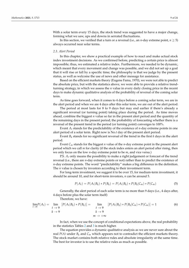
P(At) = P(At|Bk) ∗ P(Bk) = P(At|Bk) ∗ P(Bk|Cm) ∗ P(Cm) (5)

Generally, the alert period of each solar term is no more than 9 days (i.e., 4 days after,4 days before plus the solar term itself)

Therefore, we have:

limt→9

P(At) = limt→ 9k→ 9

[P(At|Bk) ∗ P(Bk)] = limt→ 9k→ 9

m→ +∞

[P(At|Bk) ∗ P(Bk|Cm) ∗ P(Cm)] = 1 (6)

In fact, when we use the concept of conditional expectations above, the real probabilityin the statistics Tables 2 and 3 is much higher.

The equation provides a dynamic qualitative analysis as we are never sure about thereal P(A) under Bk and Cm which appears not to contradict the efficient markets theory.The stock market contains both relative rules and absolute irregularity at the same time.The best for investor is to use the relative rules as much as possible.

Mathematics 2021, 9, 1713 10 of 24

The orange arrows mean the probability to rise or fall and the longer an arrow is, thehigher the probability it stands for.

This is a virtual case; we made it to better explain our strategy and vividly show howour method works in real trade (Figures 5 and 6).


Figure 5. Practical example of the alert period (stock falling case).

In that case, we found that the actual reversal point (actually, it was a 13-day extreme point) reached the m value of 13 where the price was much lower than that outside the alert period; it also had a very long time to another similar low price.

As the m value becomes bigger and the time is closing to the solar term, we suppose that the possibility of reversal is higher. There may be several signals to show the potential turns and reversal such as t = 5 (goes high after a very low price with a large m value) and t = 9 (the actual turning point). Therefore, the decision should be made dynamically, ac-cording to the m and k values in the past. Significant reversals in the alert period are al-ways the real reversal points in stock indices.

Figure 6 shows a very frequent case where the index does not have a reversal near the solar term; although there are high price and low price when t = 3 or t = 7, it is not low enough compared with a recent extreme point (e.g., the day before t = 1 and 5 days before t = 1). Despite the fact that t = 3 or t = 7 correspond to the two lowest prices in the alert period, there are other lower prices outside the period very close to them, so they do not work.

Figure 5. Practical example of the alert period (stock falling case).

In that case, we found that the actual reversal point (actually, it was a 13-day extremepoint) reached the m value of 13 where the price was much lower than that outside thealert period; it also had a very long time to another similar low price.

As the m value becomes bigger and the time is closing to the solar term, we supposethat the possibility of reversal is higher. There may be several signals to show the potentialturns and reversal such as t = 5 (goes high after a very low price with a large m value)and t = 9 (the actual turning point). Therefore, the decision should be made dynamically,according to the m and k values in the past. Significant reversals in the alert period arealways the real reversal points in stock indices.

Figure 6 shows a very frequent case where the index does not have a reversal nearthe solar term; although there are high price and low price when t = 3 or t = 7, it is not lowenough compared with a recent extreme point (e.g., the day before t = 1 and 5 days beforet = 1). Despite the fact that t = 3 or t = 7 correspond to the two lowest prices in the alertperiod, there are other lower prices outside the period very close to them, so they do notwork.

Mathematics 2021, 9, 1713 11 of 24Mathematics 2021, 9, x FOR PEER REVIEW 12 of 27

Figure 6. Practical example of an alert period (turbulence case between two ascending trends).

The case contradicts the common sense, that is, buying on the low and selling on the high; the case proved it only in the alert period, and it is necessary to assess it not accord-ing to how many days the stock has been falling in total, but combine the m value it creates with the distance to the solar term.

In other words, while getting closer to the solar term, there is a higher possibility to have a reversal of the trend, but if the biggest n is not so big so far, the probability is always low no matter how close to or far from the solar term it is. The conclusion turns out to be a turbulence but not a reversal or turning point and, in this way, investors can hold their stock at least until the next alert period and the stock index will keep its trend like before the alert period.

2.4. Non-Marketing Day According to the turnover of the Shanghai Index (actually, it works for all stocks), it

is very easy to find out that the turnover in the next day after a weekend or a holiday, in the preparation phase and the first few minutes are very much higher than that in normal marketing days. Thus, we believe that there is still capital flow and transactions allocating for the next marketing day even though they fall on weekends or holidays.

Therefore, we regard each continuous holiday and weekend as one day regardless of whether it contains a solar term. All the statistics described (e.g., the valid time radius) above are applied in this way.

3. Arguments on the Efficient Markets Theory (Hypothesis) 3.1. General Survey of the Efficient Markets Theory (Hypothesis)

The efficient markets theory was first systematically proposed by Eugene Fama (1970) and summarized three forms of the market which are weak form efficiency, semi-strong form efficiency and strong form efficiency. With higher efficiency, the stock price is supposed to be unpredictable and investors do not stably make money through a rule. The efficient markets theory provides us with a fair competing model where everybody

Figure 6. Practical example of an alert period (turbulence case between two ascending trends).

The case contradicts the common sense, that is, buying on the low and selling on thehigh; the case proved it only in the alert period, and it is necessary to assess it not accordingto how many days the stock has been falling in total, but combine the m value it createswith the distance to the solar term.

In other words, while getting closer to the solar term, there is a higher possibility tohave a reversal of the trend, but if the biggest n is not so big so far, the probability is alwayslow no matter how close to or far from the solar term it is. The conclusion turns out to bea turbulence but not a reversal or turning point and, in this way, investors can hold theirstock at least until the next alert period and the stock index will keep its trend like beforethe alert period.

2.4. Non-Marketing Day

According to the turnover of the Shanghai Index (actually, it works for all stocks), itis very easy to find out that the turnover in the next day after a weekend or a holiday, inthe preparation phase and the first few minutes are very much higher than that in normalmarketing days. Thus, we believe that there is still capital flow and transactions allocatingfor the next marketing day even though they fall on weekends or holidays.

Therefore, we regard each continuous holiday and weekend as one day regardless ofwhether it contains a solar term. All the statistics described (e.g., the valid time radius)above are applied in this way.

3. Arguments on the Efficient Markets Theory (Hypothesis)3.1. General Survey of the Efficient Markets Theory (Hypothesis)

The efficient markets theory was first systematically proposed by Eugene Fama (1970)and summarized three forms of the market which are weak form efficiency, semi-strongform efficiency and strong form efficiency. With higher efficiency, the stock price is sup-posed to be unpredictable and investors do not stably make money through a rule. Theefficient markets theory provides us with a fair competing model where everybody is smart

Mathematics 2021, 9, 1713 12 of 24

and eager to earn money, so there is no exception for one to find out a better way thanothers.

In a weak form efficient market, stock price cannot be predicted by technological stockanalysis (i.e., by applying a mathematical model or numeric analysis to its historical price).In a semi-strong form efficient market, investors only win through inside information andother unfair or illegal methods, and in a strong form efficient market, the stock price isdefinitely unpredictable at any time.

3.2. Adaptive Market Hypothesis and Imperfection of Efficient-Market Hypothesis

The adaptive market hypothesis (AMH) was proposed to show the predictabilityand operability of the stock market and its profit [18–20]. The AMH also gives us a morerealistic perspective compared with the EMH. In fact, the efficient markets theory or theEMH is based on an idealistic model which markets in almost all countries are not yetable to realize; both in developing markets like China and in the developed market of theUS, the stock market is only likely to reach the weak level or the semi-strong level whichmeans that there is still a tremendous possibility for regular investors to win [21–23], andwe accept this possibility, acknowledging that the we still have hope, but we are not goingto apply this viewpoint in this paper. In fact, the efficient markets theory has little impacton the time cycle theory and our 24-solar-term method. There is also a study that showsthe nonuniversality of the efficient markets theory and found cases to contradict it [24].

First of all, speaking of the efficient markets theory, it always links to historicalprice and future price (i.e., an absolute numerical value), whereas we focus on the turnsand reversal of the trend and the regular changes between the stock and some specifictimepoints; we are more likely to conduct a statistics research on the relationship betweenthe stock trend and time which is a relative concept (i.e., when to turn and which timepointmatters more), not an ordinary numeric prediction. Therefore, we talk about neither thehistorical stock price nor the open financial report, insider information or turnover, we areinterested in revealing independent time factors based on the stock market; the time goesforward, and if we handle a rule, we know that something big may happen at a specifictimepoint in advance. For example, we know the stock trend probably changes aroundChunfen (6), but we have few ideas about the exact time it will take place and what level ofprice the stock will eventually reach after the effect of Chunfen (6) term, which not onlyproves that time factors matter but is also consistent with the efficient markets theory.

This was exactly what we wrote in the abstract, “the turns of the stock indices trendwere inevitable at specific timepoints while the strength and intensity of the turns wereuncertain, affected by various factors by then”, in which we emphasized the certainty oftime factors and the remaining uncertainty about the stock.

Secondly, we focused on stock market indices, which were general collections of thestock market, as we knew that a specific stock is surely impossible to predict, but theuncertainty and irregularity are greatly neutralized when it comes to a stock index. Theonly difference is that if the market efficiency is really weak, our regular analysis would beour second tool, an assistance tool, after the time factor theory (i.e., the time cycle and solarterms theory).

3.3. Why Time Factors Are Superior to the Efficient Markets Theory (Hypothesis)

As we mentioned repeatedly before, the time factor is a four-dimensional factor havingan overwhelming impact on our three-dimensional world. Although we can act againstthe impact it brings, time will forever take the dominant place in the result.

There are several conditions or assumptions in the efficient markets theory about theinvestors’ mentality, the flow of information and the transactions of money. When all ofthese conditions are ready, the theory works and the stock becomes unpredictable, but thereality is that the cycle of time and some specific timepoints (i.e., 24 solar terms) alwaysinterfere with these conditions, making the efficient markets theory hard to realize in realmarkets. The tides of moon cause reactions in the human body, and specific timepoints may

Mathematics 2021, 9, 1713 13 of 24

also lead to emotional instability and irrationality [25,26]. Gann knew the logic and made286 stock transactions within 25 marketing days from October 1909 and won 264 timesunder the supervision of The Ticket and Investment Digest [27].

With all the discussion above, we regard the time factor as a natural factor to thehuman world and prove in this paper that the analysis and forecast on stock trends arepracticable.

4. Time Series Analysis of Solar Terms4.1. Grouping of Solar Terms

Eight of the Chinese 24 solar terms are very prominent, namely, Chunfen (6), Xiazhi(12), Qiufen (18) and Dongzhi (24), which represent the most vigorous timepoints in eachseason and are the most important four solar terms; the other four are Lichun (3), Lixia (9),Liqiu (15) and Lidong (21). These four represent the beginning of each season and are thesecond important four solar terms.

To our surprise, the importance of these eight solar terms exactly coincides with thewheel of the cycle theory in Gann theory. In Gann’s wheel, the most important four anglesare 90◦, 180◦, 270◦ and 360◦ (0◦), and the corresponding timepoints of each year are exactlythe four solar terms of Chunfen (6), Xiazhi (12), Qiufen (18) and Dongzhi (24). The secondimportant four angles, 45◦, 135◦, 225◦ and 315◦ exactly correspond to the four solar termsof Lichun (3), Lixia (9), Liqiu (15) and Lidong (21). Regardless of the angle in Gann theoryor solar terms, they all point to a common rule, that is, the stock trend is most likely to turnat these eight points. We can summarize the above results as follows: variable or moresignificant extreme points often occur at the solar term point, and the solar term pointusually makes the stock trend turn according to its strength, and the turning strength islarge or small.

For convenience, we took the Shanghai Index as an example to present the detailedprocess of analysis step by step while results of the Second board Index and the ShenzhenIndex were directly showed in the following table together with the Shanghai Index usingthe same approach.

The data we used, as mentioned before, were 6436 daily closing prices from 3 January1995 to 14 August 2020 of the Shanghai Index (Figure 7); however, we only selected thebiggest extreme n-day points near every solar term. In other words, we wanted to selectthe data of each solar term at the beginning, but since there were bigger n-day points in the4-day radius, we chose the extreme points to replace every solar term. The total numberwas not changed.


Figure 7. Time series plot of the Shanghai stock index in 1995–2020.

4.2. Strategy in Analysis In this chapter, based on the method of random chain [28], analyzing autocorrelation

of the price series [29–31], we suggested to apply the ARIMA–ARCH time series model to fit and forecast the index as time series analysis is a modern tool for predicting. Time series models, meanwhile, can introduce long-term correlation cases and their volatility dealing with price, production, population growth, etc.

In general, the autocorrelation (hereinafter referred to simply as the “correlation”) of a stock index is long-term; thus, it may involve a great deal of data for a regular time series analysis, making the model extremely complicated and inaccurate.

Besides, the traditional time series fitting is based on high-frequency data (i.e., daily closing prices) on continuous marketing days. However, most of the high-frequency data are meaningless as they are only the trend connection between two turning points and have no special significance. Those high-frequency data contribute nothing but add more error, volatility and turbulence that mislead investors into believing them to be a turn.

Considering the intervals are almost equal between two solar terms, it is suitable to use the extreme points around each solar term as items in the time series. By doing this, we actually extract representatives of every trend and magnify the period in the analysis (i.e., two solar terms cover around 15 days; that is 15 times more than when simply ap-plying two daily prices).

Throughout this paper, we only focused on the forecast of the index trend, not the price.

For the stationary time series after the difference, we used the ARIMA model to fit [32]. ARIMA is the autoregressive integrated moving average model denoted ARIMA(p,d,q). 𝛷(𝐵) = 𝛻 𝑥 = 𝛩(𝐵)𝜀𝐸(𝜀 ) = 0, 𝑉𝑎𝑟(𝜀 ) = 𝜎 , 𝐸(𝜀 𝜀 ) = 0, 𝑠 ≠ 𝑡𝐸(𝑥 𝜀 ) = 0, ∀𝑠 < 𝑡 (7)

where 𝛻 = (1 − 𝐵) ; 𝛷(𝐵) = 1 − 𝜑 𝐵 − ⋯ − 𝜑 𝐵 is the autoregressive coefficient pol-ynomial of the ARIMA model; 𝛩(𝐵) = 1 − 𝜃 𝐵 − ⋯ − 𝜃 𝐵 is the moving average coeffi-cient polynomial of the ARIMA model.

The sequence after the d-order difference is

Figure 7. Time series plot of the Shanghai stock index in 1995–2020.

Mathematics 2021, 9, 1713 14 of 24

4.2. Strategy in Analysis

In this chapter, based on the method of random chain [28], analyzing autocorrelationof the price series [29–31], we suggested to apply the ARIMA–ARCH time series model tofit and forecast the index as time series analysis is a modern tool for predicting. Time seriesmodels, meanwhile, can introduce long-term correlation cases and their volatility dealingwith price, production, population growth, etc.

In general, the autocorrelation (hereinafter referred to simply as the “correlation”) of astock index is long-term; thus, it may involve a great deal of data for a regular time seriesanalysis, making the model extremely complicated and inaccurate.

Besides, the traditional time series fitting is based on high-frequency data (i.e., dailyclosing prices) on continuous marketing days. However, most of the high-frequency dataare meaningless as they are only the trend connection between two turning points andhave no special significance. Those high-frequency data contribute nothing but add moreerror, volatility and turbulence that mislead investors into believing them to be a turn.

Considering the intervals are almost equal between two solar terms, it is suitable touse the extreme points around each solar term as items in the time series. By doing this, weactually extract representatives of every trend and magnify the period in the analysis (i.e.,two solar terms cover around 15 days; that is 15 times more than when simply applyingtwo daily prices).

Throughout this paper, we only focused on the forecast of the index trend, not theprice.

For the stationary time series after the difference, we used the ARIMA model to fit [32].ARIMA is the autoregressive integrated moving average model denoted ARIMA(p,d,q).

Φ(B) = ∇dxt = Θ(B)εtE(εt) = 0, Var(εt) = σ2

ε , E(εtεs) = 0, s 6= tE(xsεt) = 0, ∀s < t

(7)

where ∇d = (1− B)d; Φ(B) = 1 − ϕ1B − . . . − ϕpBp is the autoregressive coefficientpolynomial of the ARIMA model; Θ(B) = 1− θ1B − . . . − θqBq is the moving averagecoefficient polynomial of the ARIMA model.

The sequence after the d-order difference is

∇dxt =d

∑i=0

(−1)iCidxt−i =

Θ(B)Φ(B)

εt (8)

where {εt} is the white noise sequence with the zero mean.For the residual sequence with heteroscedasticity, we have the autoregressive condi-

tional heteroskedastic model ARCH(q) [33]. By using an ARCH(q) model, we can charac-terize the conditional variance changing with time.

The structure of the ARCH(q) model is as follows: assuming that the historical dataare known, the sequence of the zero mean residuals has heteroscedasticity.

E(εt) = 0, Var(εt|εt−1, εt−2 . . .) = ht (9)

ht = λ0 +q

∑i=1

λiε2t−i (10)

The ARCH(q) model requires existence of non-negative variance and unconditionalvariance.

Var(εt|εt−1, εt−2 . . .) = λ0 +q

∑i=1

λiε2t−i ≥ 0 (11)

where λ1, λ2, . . . λq ≥ 0,Var(εt) = σ2 (12)

Mathematics 2021, 9, 1713 15 of 24

where 0 ≤ λi < 1, λ1 + λ2 + · · ·+ λq < 1.The 24 solar terms were divided into four groups: the all-terms group (all 24 solar

terms), four-terms group A (Lichun (3), Lixia (9), Liqiu (15) and Lidong (21)), four-termsgroup B (Chunfen (6), Xiazhi (12), Qiufen (18) and Dongzhi (24)) and the eight solar termsgroup (altogether, there were eight solar terms). The historical data were divided into theexperimental group and the test group (the last five solar terms).

4.3. Time Series Analysis of the All-Terms Group

According to Cramer’s decomposition theorem (Cramer, 1961), nonstationary se-quence can be decomposed as follows:

xt =d

∑j=0

β jtj + ψ(B)αt (13)

where {αt } is the white noise sequence with the zero mean.We found that the stock data had an upward trend, so it was necessary to make a

first-order difference to meet the stationarity of the series [34].

∇xt = xt − xt−1 (14)

In this database, we had 615 solar terms through about 25 years, thus, xt stood for theprice of each solar term (Figure 8).

In fact, we used the biggest n-day extreme price with a 4-day radius to represent theprice of one solar term, and we did not distinguish them in the following part, calling all ofthem the price of a solar term.


Figure 8. Result after the first-order difference of the Shanghai Index (daily revenue).

The daily return of the Shanghai stock index fluctuated around the average value of 0, and the fluctuation was different in different periods. It fluctuated sharply in 2007–2008 and in 2015 while it was relatively stable in other periods (Table 7).

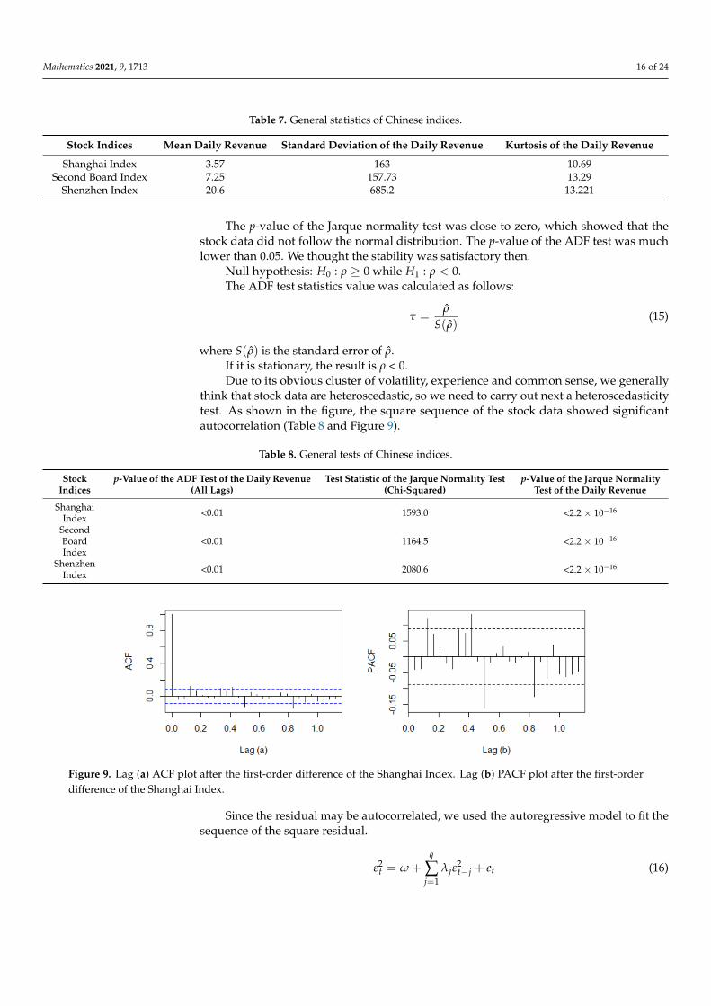
Table 7. General statistics of Chinese indices.

Stock Indices Mean Daily Revenue Standard Deviation of the Daily Revenue Kurtosis of the Daily Revenue Shanghai Index 3.57 163 10.69

Second Board Index 7.25 157.73 13.29 Shenzhen Index 20.6 685.2 13.221

The p-value of the Jarque normality test was close to zero, which showed that the stock data did not follow the normal distribution. The p-value of the ADF test was much lower than 0.05. We thought the stability was satisfactory then.

Null hypothesis: 𝐻 : 𝜌 ≥ 0 while 𝐻 : 𝜌 < 0. The ADF test statistics value was calculated as follows: 𝜏 = 𝜌𝑆(𝜌) (15)

where 𝑆(𝜌) is the standard error of 𝜌. If it is stationary, the result is 𝜌 < 0. Due to its obvious cluster of volatility, experience and common sense, we generally

think that stock data are heteroscedastic, so we need to carry out next a heteroscedasticity test. As shown in the figure, the square sequence of the stock data showed significant autocorrelation (Table 8 and Figure 9).

Figure 8. Result after the first-order difference of the Shanghai Index (daily revenue).

The daily return of the Shanghai stock index fluctuated around the average value of 0,and the fluctuation was different in different periods. It fluctuated sharply in 2007–2008and in 2015 while it was relatively stable in other periods (Table 7).

Mathematics 2021, 9, 1713 16 of 24

Table 7. General statistics of Chinese indices.

Stock Indices Mean Daily Revenue Standard Deviation of the Daily Revenue Kurtosis of the Daily Revenue

Shanghai Index 3.57 163 10.69Second Board Index 7.25 157.73 13.29

Shenzhen Index 20.6 685.2 13.221

The p-value of the Jarque normality test was close to zero, which showed that thestock data did not follow the normal distribution. The p-value of the ADF test was muchlower than 0.05. We thought the stability was satisfactory then.

Null hypothesis: H0 : ρ ≥ 0 while H1 : ρ < 0.The ADF test statistics value was calculated as follows:

τ =ρ̂

S(ρ̂)(15)

where S(ρ̂) is the standard error of ρ̂.If it is stationary, the result is ρ < 0.Due to its obvious cluster of volatility, experience and common sense, we generally

think that stock data are heteroscedastic, so we need to carry out next a heteroscedasticitytest. As shown in the figure, the square sequence of the stock data showed significantautocorrelation (Table 8 and Figure 9).

Table 8. General tests of Chinese indices.

StockIndices

p-Value of the ADF Test of the Daily Revenue(All Lags)

Test Statistic of the Jarque Normality Test(Chi-Squared)

p-Value of the Jarque NormalityTest of the Daily Revenue

ShanghaiIndex <0.01 1593.0 <2.2 × 10−16

SecondBoardIndex

<0.01 1164.5 <2.2 × 10−16

ShenzhenIndex <0.01 2080.6 <2.2 × 10−16


Table 8. General tests of Chinese indices.

Stock Indices p-Value of the ADF Test of the Daily Revenue

(All Lags)

Test Statistic of the Jarque Normality Test (Chi-Squared)

p-Value of the Jarque Normality Test of the Daily Revenue

Shanghai Index <0.01 1593.0 <2.2 × 10−16 Second Board Index <0.01 1164.5 <2.2 × 10−16

Shenzhen Index <0.01 2080.6 <2.2 × 10−16

Figure 9. (a) ACF plot after the first-order difference of the Shanghai Index. (b) PACF plot after the first-order difference of the Shanghai Index.

Since the residual may be autocorrelated, we used the autoregressive model to fit the sequence of the square residual.

𝜀 = 𝜔 + 𝜆 𝜀 + 𝑒 (16)

Null hypothesis: 𝐻 : all 𝜆 = 0 while 𝐻 : at least one 𝜆 = 0 LM(𝑞)~𝜒 (𝑞 − 1) (17)

We then looked at the sequence after the one-order difference. We conducted the LM test: the p-value of the ARCH–LM test was 2.2 × 10−16, so we rejected the original hypoth-esis and accepted there was the ARCH effect. In conclusion, the return sequence of the Shanghai stock index (i.e., the price sequence after the first-order difference) had the ARCH effect (Table 9, Figures 10 and 11).

Table 9. The result of the ADF test of daily revenue, square sequence and of the LM test.

Stock Indices Test Statistics of the ADF Test of

Square Revenue p-Value of the ADF Test of

Square Revenue Test Statistics of the LM Test

(Chi-Squared) p-Value of the LM

Test Shanghai Index −3.20 (>40 lags) 0.06+ (>40 lags) 212.72 <<0.01

Second Board Index −2.09 (>40 lags) 0.05+ (>40 lags) 94.68 6.077 × 10−15 Shenzhen Index −3.40 (>37 lags) 0.0539 (>37 lags) 138.81 <<0.01

Figure 9. Lag (a) ACF plot after the first-order difference of the Shanghai Index. Lag (b) PACF plot after the first-orderdifference of the Shanghai Index.

Since the residual may be autocorrelated, we used the autoregressive model to fit thesequence of the square residual.

ε2t = ω +

q

∑j=1

λjε2t−j + et (16)

Mathematics 2021, 9, 1713 17 of 24

Null hypothesis: H0 : all λi = 0 while H1 : at least one λ = 0

LM(q) ∼ χ2(q− 1) (17)

We then looked at the sequence after the one-order difference. We conducted theLM test: the p-value of the ARCH–LM test was 2.2 × 10−16, so we rejected the originalhypothesis and accepted there was the ARCH effect. In conclusion, the return sequence ofthe Shanghai stock index (i.e., the price sequence after the first-order difference) had theARCH effect (Table 9, Figures 10 and 11).

Table 9. The result of the ADF test of daily revenue, square sequence and of the LM test.

Stock Indices Test Statistics of the ADFTest of Square Revenue

p-Value of the ADF Testof Square Revenue

Test Statistics of the LM Test(Chi-Squared) p-Value of the LM Test

Shanghai Index −3.20 (>40 lags) 0.06+ (>40 lags) 212.72 <<0.01Second Board Index −2.09 (>40 lags) 0.05+ (>40 lags) 94.68 6.077 × 10−15

Shenzhen Index −3.40 (>37 lags) 0.0539 (>37 lags) 138.81 <<0.01


Figure 10. (c) Squared ACF plot after the first-order difference of the Shanghai Index. (d) Squared PACF plot after the first-order difference of the Shanghai Index.

Firstly, we established an ARIMA model [35] for the mean value of the series of the all solar terms group of the Shanghai stock index and selected the last five solar terms to examine the forecast. After a repeated comparison, we chose ARIMA(36, 1, 12) and in fact, in some mathematical forecasts, the parameters were often large [36] as our data were very complicated and was never auto-correlated only in the short term [37–41].

Figure 11. ARCH(2) model’s residual of the Shanghai Index’s daily revenue.

We found that the ARCH(2) model made a good fit for the residual of several periods with obvious fluctuation (Figure 12). The Ljung–Box test showed that the p-value was much bigger than 0.05, that is, the residual and the square of the residual after the process of the ARCH model were white noise sequences, which indicated that the original se-quence information was fully extracted by the ARCH(2) model.

Figure 10. Lag (c) Squared ACF plot after the first-order difference of the Shanghai Index. Lag (d) Squared PACF plot afterthe first-order difference of the Shanghai Index.

Firstly, we established an ARIMA model [35] for the mean value of the series of theall solar terms group of the Shanghai stock index and selected the last five solar terms toexamine the forecast. After a repeated comparison, we chose ARIMA(36, 1, 12) and in fact,in some mathematical forecasts, the parameters were often large [36] as our data were verycomplicated and was never auto-correlated only in the short term [37–41].


Figure 10. (c) Squared ACF plot after the first-order difference of the Shanghai Index. (d) Squared PACF plot after the first-order difference of the Shanghai Index.

Firstly, we established an ARIMA model [35] for the mean value of the series of the all solar terms group of the Shanghai stock index and selected the last five solar terms to examine the forecast. After a repeated comparison, we chose ARIMA(36, 1, 12) and in fact, in some mathematical forecasts, the parameters were often large [36] as our data were very complicated and was never auto-correlated only in the short term [37–41].


We found that the ARCH(2) model made a good fit for the residual of several periods with obvious fluctuation (Figure 12). The Ljung–Box test showed that the p-value was much bigger than 0.05, that is, the residual and the square of the residual after the process of the ARCH model were white noise sequences, which indicated that the original se-quence information was fully extracted by the ARCH(2) model.


Mathematics 2021, 9, 1713 18 of 24

We found that the ARCH(2) model made a good fit for the residual of several periodswith obvious fluctuation (Figure 12). The Ljung–Box test showed that the p-value wasmuch bigger than 0.05, that is, the residual and the square of the residual after the processof the ARCH model were white noise sequences, which indicated that the original sequenceinformation was fully extracted by the ARCH(2) model.

Although GARCH(1,1) is also used in many economic analyses, ARCH(2) still did agood job in reflecting volatility in the index as the volatility we forecast was just a qualityanalysis and we only needed to know the comparative value (i.e., when it is bigger, whenit is lower) rather than a certain degree of volatility. GARCH(1,1) is for long-term volatilityfitting, but the way we established our model (i.e., using extreme points near solar terms)already made the term long enough, so the coefficient of GARCH(1,1) resulted in aninsignificant level.


Figure 12. Fitted volatility of the ARCH(2) model’s residual of the Shanghai Index’s daily revenue.

Although GARCH(1,1) is also used in many economic analyses, ARCH(2) still did a good job in reflecting volatility in the index as the volatility we forecast was just a quality analysis and we only needed to know the comparative value (i.e., when it is bigger, when it is lower) rather than a certain degree of volatility. GARCH(1,1) is for long-term volatility fitting, but the way we established our model (i.e., using extreme points near solar terms) already made the term long enough, so the coefficient of GARCH(1,1) resulted in an in-significant level.

Finally, we obtained the following ARIMA(36, 1, 12)–ARCH(2) model for the all-terms group (Table 10):

Mean model: ∇𝑥 = ∑ 𝑎 ∙ ∇𝑥 + ∑ 𝑏 ∙ 𝜀 +𝜀 (18)

Variance model: 𝜀 = ℎ 𝑒 , 𝑒 is an i. i. d. random variable with 𝑋~𝑁(0,1) (19)ℎ = 7071 + 0.5220𝜀 + 0.2657𝜀 (20)

Table 10. Parameters of the ARIMA model of the all-terms group. 𝒂𝟏 𝒂𝟐 𝒂𝟑 𝒂𝟒 𝒂𝟓 𝒂𝟔 𝒂𝟕 𝒂𝟖 𝒂𝟗 𝒂𝟏𝟎 𝒂𝟏𝟏 𝒂𝟏𝟐 0.3453 0.0826 –0.1808 –0.4352 –0.362 0.5318 –0.029 –0.2256 –0.4321 –0.0133 0.4535 –0.7389 𝒂𝟏𝟑 𝒂𝟏𝟒 𝒂𝟏𝟓 𝒂𝟏𝟔 𝒂𝟏𝟕 𝒂𝟏𝟖 𝒂𝟏𝟗 𝒂𝟐𝟎 𝒂𝟐𝟏 𝒂𝟐𝟐 𝒂𝟐𝟑 𝒂𝟐𝟒 0.1671 –0.0873 –0.0442 –0.0140 0.1065 0.1481 –0.1670 –0.1647 0.7616 0.0644 0.1055 –0.2275 𝒂𝟐𝟓 𝒂𝟐𝟔 𝒂𝟐𝟕 𝒂𝟐𝟖 𝒂𝟐𝟗 𝒂𝟑𝟎 𝒂𝟑𝟏 𝒂𝟑𝟐 𝒂𝟑𝟑 𝒂𝟑𝟒 𝒂𝟑𝟓 𝒂𝟑𝟔 –0.0661 0.0259 –0.0690 –0.0528 –0.0865 –0.0446 0.0157 –0.1216 –0.0275 –0.0707 0.0430 –0.0356 𝒃𝟏 𝒃𝟐 𝒃𝟑 𝒃𝟒 𝒃𝟓 𝒃𝟔 𝒃𝟕 𝒃𝟖 𝒃𝟗 𝒃𝟏𝟎 𝒃𝟏𝟏 𝒃𝟏𝟐 –0.425 –0.1062 0.3482 0.4383 0.2371 –0.6237 0.1711 0.4217 0.4134 –0.033 –0.4812 0.9222

According to the model, the forecast of five periods in the future is as follows (Table 11 and Figure 13).

Figure 12. Fitted volatility of the ARCH(2) model’s residual of the Shanghai Index’s daily revenue.

Finally, we obtained the following ARIMA(36, 1, 12)–ARCH(2) model for the all-termsgroup (Table 10):

Mean model:

∇xn =36

∑i=1

ai·∇xn−i +12

∑j=1

bj·εn−j+εn (18)

Variance model:

εn =√

hnen , en is an i.i.d. random variable with X ∼ N(0, 1) (19)

hn = 7071 + 0.5220ε2n−1 + 0.2657ε2

n−2 (20)

Table 10. Parameters of the ARIMA model of the all-terms group.

a1 a2 a3 a4 a5 a6 a7 a8 a9 a10 a11 a120.3453 0.0826 −0.1808 −0.4352 −0.362 0.5318 −0.029 −0.2256 −0.4321 −0.0133 0.4535 −0.7389

a13 a14 a15 a16 a17 a18 a19 a20 a21 a22 a23 a240.1671 −0.0873 −0.0442 −0.0140 0.1065 0.1481 −0.1670 −0.1647 0.7616 0.0644 0.1055 −0.2275

a25 a26 a27 a28 a29 a30 a31 a32 a33 a34 a35 a36−0.0661 0.0259 −0.0690 −0.0528 −0.0865 −0.0446 0.0157 −0.1216 −0.0275 −0.0707 0.0430 −0.0356

b1 b2 b3 b4 b5 b6 b7 b8 b9 b10 b11 b12−0.425 −0.1062 0.3482 0.4383 0.2371 −0.6237 0.1711 0.4217 0.4134 −0.033 −0.4812 0.9222

According to the model, the forecast of five periods in the future is as follows(Table 11 and Figure 13).

Mathematics 2021, 9, 1713 19 of 24

Table 11. Forecasts of the all-terms group of the Shanghai Index.

Period in the Future Solar Terms Date Real Price Forecast Volatility Trend Forecasting

1 Mangzhong (11) 5 June 2020 2933.20 2885.48 113.05 Good2 Xiazhi (12) 21 June 2020 2959.71 2902.43 227.54 Good3 Xiaoshu (13) 6 July 2020 3450.59 2919.50 174.06 Good4 Dashu (14) 22 July 2020 3196.77 2908.75 90.40 Good5 Liqiu (15) 7 August 2020 3361.22 2942.28 95.24 Good


Table 11. Forecasts of the all-terms group of the Shanghai Index.

Period in the Future Solar Terms Date Real Price Forecast Volatility Trend Forecasting 1 Mangzhong (11) 5 June 2020 2933.20 2885.48 113.05 Good 2 Xiazhi (12) 21 June 2020 2959.71 2902.43 227.54 Good 3 Xiaoshu (13) 6 July 2020 3450.59 2919.50 174.06 Good 4 Dashu (14) 22 July 2020 3196.77 2908.75 90.40 Good 5 Liqiu (15) 7 August 2020 3361.22 2942.28 95.24 Good

Figure 13. Comparisons between the forecast and real price in five periods in the future of the Shanghai Index (all-terms group).

Now we make analysis of other groups (Tables 12 and 13)

Table 12. Forecasts of the all-terms group of the Second Board Index.

Period in the Future Real Price Forecast Volatility Trend Evaluation 1 2716.15 2720.12 112.44 Good 2 2882.44 2777.35 105.15 Good 3 3067.30 2789.20 99.56 Good

Table 13. Forecasts of the all-terms group of the Shenzhen Index.

Period in the Future Real Price Forecast Volatility Trend Evaluation 1 14,930.08 14,148.27 578.71 Good 2 15,710.19 14,002.82 588.81 Not good 3 15,233.15 14,010.34 669.58 Good

Figure 13. Comparisons between the forecast and real price in five periods in the future of the Shanghai Index (all-terms group).

Now we make analysis of other groups (Tables 12 and 13)

Table 12. Forecasts of the all-terms group of the Second Board Index.

Period in the Future Real Price Forecast Volatility Trend Evaluation

1 2716.15 2720.12 112.44 Good2 2882.44 2777.35 105.15 Good3 3067.30 2789.20 99.56 Good

Table 13. Forecasts of the all-terms group of the Shenzhen Index.


1 14,930.08 14,148.27 578.71 Good2 15,710.19 14,002.82 588.81 Not good3 15,233.15 14,010.34 669.58 Good

We would like to make an explanation here since the figure may be a bit small. Theorange line is the real trend that links orange points which are the daily closing prices ofthe index while the blue line links several blue points which are the forecast prices on solar

Mathematics 2021, 9, 1713 20 of 24

terms. Every forecast price on each solar term was matched to the real price, showing thegap in the price and the shape of the trend.

We found that there was a certain difference in forecasting the future stock price at thefuture solar terms by using the historical solar terms; however, the forecast of the trendwas very accurate, and the trend in the future period was consistent with the real trend.

In that case, we were informed what the next trend would be like so that, combinedwith the methods in the chapters before, we would have a better handling of our investment.This was a quality analysis as we were never able to calculate the profit, costs, risks, etc. inthe future; otherwise it would contradict the efficient markets theory.

The time series analysis in this paper was for trend reversal, so we paid more attentionto the turning of the trend at solar terms rather than to the absolute price.

4.4. Time Series Analysis of the Eight-Terms Group

As mentioned before, the time series plot of the eight important solar terms each yearalso described the historical trend of the stock well.

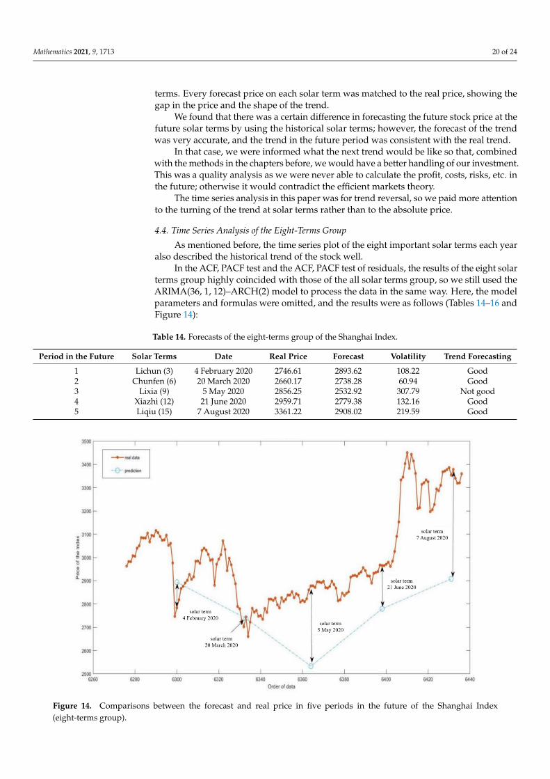
In the ACF, PACF test and the ACF, PACF test of residuals, the results of the eight solarterms group highly coincided with those of the all solar terms group, so we still used theARIMA(36, 1, 12)–ARCH(2) model to process the data in the same way. Here, the modelparameters and formulas were omitted, and the results were as follows (Tables 14–16 andFigure 14):

Table 14. Forecasts of the eight-terms group of the Shanghai Index.

Period in the Future Solar Terms Date Real Price Forecast Volatility Trend Forecasting

1 Lichun (3) 4 February 2020 2746.61 2893.62 108.22 Good2 Chunfen (6) 20 March 2020 2660.17 2738.28 60.94 Good3 Lixia (9) 5 May 2020 2856.25 2532.92 307.79 Not good4 Xiazhi (12) 21 June 2020 2959.71 2779.38 132.16 Good5 Liqiu (15) 7 August 2020 3361.22 2908.02 219.59 Good


Figure 14. Comparisons between the forecast and real price in five periods in the future of the Shanghai Index (eight-terms group).

Table 15. Forecasts of the eight-terms group of the Second Board Index.

Period in the Future Real Price Forecast Volatility Trend Evaluation 1 2813.99 2539.15 146.55 Good 2 2882.44 2884.49 149.74 Good 3 3128.86 3007.35 214.16 Good

Table 16. Forecasts of the eight-terms group of the Shenzhen Index.

Period in the Future Real Price Forecast Volatility Trend Evaluation 1 14,141.1529 14,317.92 1064.31 Good 2 14,134.8495 14,208.60 919.57 Good 3 15,233.1493 14,518.74 828.33 Good

We could see that, like in the all-terms group, the time series analysis had some errors in forecasting, but it could better forecast the trend of stocks in the future. In fact, there were two trends from the first period to the second period in the future, falling one by one. However, the stock finally bottomed out on 22 March. The forecast trend of the sec-ond period to the third period in the future was wrong, showing a certain delay. However, by the fourth period in the future, the forecast value increased sharply, showing the cor-rection of the previous error. When the fifth period in the future was reached, the trend forecast coincided with the actual trend.

4.5. Time Series Analysis of the Four-Terms Group After many attempts, the forecast was still not good, indicating an obvious deviation

with the real data of the test group. Therefore, we believe that it would be better to forecast using all solar terms or eight solar terms. The data is lost to a great extent if we use very few solar terms to forecast. Thus, we do not recommend conducting a time series analysis with few solar terms.

Figure 14. Comparisons between the forecast and real price in five periods in the future of the Shanghai Index(eight-terms group).

Mathematics 2021, 9, 1713 21 of 24

Table 15. Forecasts of the eight-terms group of the Second Board Index.


1 2813.99 2539.15 146.55 Good2 2882.44 2884.49 149.74 Good3 3128.86 3007.35 214.16 Good

Table 16. Forecasts of the eight-terms group of the Shenzhen Index.


1 14,141.1529 14,317.92 1064.31 Good2 14,134.8495 14,208.60 919.57 Good3 15,233.1493 14,518.74 828.33 Good

We could see that, like in the all-terms group, the time series analysis had some errorsin forecasting, but it could better forecast the trend of stocks in the future. In fact, therewere two trends from the first period to the second period in the future, falling one by one.However, the stock finally bottomed out on 22 March. The forecast trend of the secondperiod to the third period in the future was wrong, showing a certain delay. However, bythe fourth period in the future, the forecast value increased sharply, showing the correctionof the previous error. When the fifth period in the future was reached, the trend forecastcoincided with the actual trend.

4.5. Time Series Analysis of the Four-Terms Group

After many attempts, the forecast was still not good, indicating an obvious deviationwith the real data of the test group. Therefore, we believe that it would be better to forecastusing all solar terms or eight solar terms. The data is lost to a great extent if we use veryfew solar terms to forecast. Thus, we do not recommend conducting a time series analysiswith few solar terms.

5. Conclusions

Individual stocks were confirmed to be unpredictable and stochastic according to theEMH and AMH. Even though the efficiency of the stock market around the world didnot reach an idealistic level, generally speaking, it was still very hard and ineffective forinvestors to forecast a certain stock. Analyzing the three major indices of the China’s stockmarket was a good tool to cover all stock categories in the market while making the studymore practicable and reasonable.

However, stock indices proved to be rather predictable to some extent. Therefore,according to the study, investors can invest in ETFs that belong to the indices as an ETF iscompletely coincidental with the index it belongs to. Furthermore, ETFs provide investorswith a variety of options of risk and profit. The Shanghai ETF is smooth whereas the SecondBoard 50 Fund fluctuates a lot. Investors are able to get a high profit from individual stocksas well through implementing the results of this study.

The correlation between the turning points of indices and the Chinese 24 solar termswas positive (ρ = 0.9878).

Turning points always occur near solar terms. Through testing n-day extreme pointswith a different n value, the sharp turns of the trend often happened near the solar terms,and if we choose 4 days as the valid time radius, the probability is about 80%. Investorsshould be alert for four days before and four days after a solar term. If the price is too high(low), it is more likely to be affected by the coming solar term, and the higher (lower) theprice is, the more instability the trend then would have.

However, solar terms are not always strong turning points, but they might causeweaker turning points. In other words, solar terms might not cause a sharp reversal of thestock trend; strong turning points were just some exceptions. Usually, the turning pointswere not that strong but sufficient for medium-term and short-term investors.

Mathematics 2021, 9, 1713 22 of 24

The alert period provided investors with a good strategy for short-term and medium-term trading. When judging the upcoming reversal, it should be dynamic. According tothe practical examples in the alert period, investors should also notice significant signalssuch as the present n-day extreme points combined with the distance to the solar term. Byunderstanding the alert period carefully, investors would have a positive profit in theirfuture investment.

The 24 solar terms in each year and their links accurately fitted the trend of the stockin that year. Using 24 price datapoints instead of nearly 250 daily datapoints of the wholeyear could make the daily data of high frequency more concise and easier to process.With 250 high-frequency daily datapoints, there is strong volatility, which leads to theobvious heteroscedasticity of the data and increases the complexity of data analysis. Theuse of 24 solar terms instead of annual data also greatly reduces this unstable and irregularfluctuation. This also coincides with Gann theory.

The forecast of future trends in the all-terms group and the eight-terms group wasprecise, but there remained a gap with the absolute price. We were only able to forecastthe timepoints and the turning points; as for the absolute price, we hardly made it. This isbecause the stock market involves a great deal of instability and is extremely complicated.Besides, through the failure of the four-terms group, we found that we should not choosetoo few solar terms and that every solar term is equal, having its own meaning and function,and all of them represent trends of certain periods.

6. Philosophy and Deeper Discussion

This chapter is an extension of Section 1.4; we make a brief review and discusssomething valuable that we may be able to apply in other studies.

The fact is that the turning of the stock trend has rules to follow, which is the inevitableresult at specific timepoints, while the strength and intensity of the turning is uncertain,affected by various factors at that time. The stock market contains both certainty anduncertainty at the same time, where natural instincts play a role as the inner factor whilethe environment—as an outer factor. Like the EMH and the AMH, they mainly focus onthe outer factor, in other words, they prefer to look at those changeable things. However, aswe were inspired by Gann, Elliott and the Chinese 24 solar terms, we would rather look forthose that do not change, and that is the key to have a better understanding and cognitionof our real world, of course, including the stock market.

For this reason, it is the higher dimensional time factor and time cycle that producean overwhelming impact on the stock market, so it reminds us of taking into accountthe importance of time when conducting such a study. That is why Gann summarized atremendous amount of time periods to inform the possible reversal in the capital marketwhile the ancient Chinese figured out 24 divisions of a year as 24 solar terms which allsolely point to time.

In addition, the ancient Chinese elaborated a complex system, and there are actuallymany other divisions of time, years, months, etc. in the Chinese culture. For example, theten heavenly stems and the twelve earthly branches decide what a year would be like, andthat is a 60-year cycle as there are 60 different combinations of one out of the ten heavenlystems with one out of the twelve earthly branches. By the way, one combination is calledGengzi, which is supposed to be the year of disasters and conflicts; the latest Gengzi yearwas 2020.

We encourage other researchers to explore and apply our approach to other fields tosee whether there is a rule to follow based on time factors. We will also demonstrate ourmethod to other foreign stock markets. We also suggest that researchers read more ancientworks, books and references related to time divisions and time factors, hoping our studywill open a brand-new door in financial analysis.

Author Contributions: Conceptualization, T.Z.; methodology, T.Z. and X.L.; software, X.L.; investi-gation, T.Z. and X.L.; data curation, X.L.; writing, T.Z. and X.L.; supervision, P.W. All authors haveread and agreed to the published version of the manuscript.

Mathematics 2021, 9, 1713 23 of 24

Funding: This research received no external funding.

Institutional Review Board Statement: Not applicable.

Informed Consent Statement: Not applicable.

Data Availability Statement: All the data are free and available to download from https://money.163.com (accessed on 28 February 2021).

Conflicts of Interest: The authors declare no conflict of interest.

References1. Colin-Jaeger, N.; Delcey, T. When efficient market hypothesis meets Hayek on information: Beyond a methodological reading. J.

Econ. Methodol. 2020, 27, 97–116. [CrossRef]2. Mehdi, Z.; Samad, G. A hybrid approach of adaptive wavelet transform, long short-term memory and ARIMA-GARCH family

models for the stock index prediction. Expert Syst. Appl. 2021, 182. [CrossRef]3. Kuhe, D.A. The Dynamic Relationship between Crude Oil Prices and Stock Market Price Volatility in Nigeria: A Cointegrated

VAR-GARCH Model. Curr. J. Appl. Sci. Technol. 2019, 1–12. [CrossRef]4. Gan, X. Study on the Correlation between the Changes of Four Seasons and Solar Terms and the Dynamics of Some Physiological

Indexes of Human Body. Master’s Thesis, Beijing University of Chinese Medicine, Beijing, China, 2013. Available online:https://kns.cnki.net/kcms/detail/detail.aspx?FileName=1013205433.nh&DbName=CMFD2013 (accessed on 28 February 2021).

5. Gong, G. Stock Market and 24 Solar Terms. Bus. China 2008, 5, 124. Available online: https://kns.cnki.net/kcms/detail/detail.aspx?FileName=JSGZ200805059&DbName=CJFQ2008 (accessed on 28 February 2021).

6. Hede, C. 24 Solar Terms and the Turning Point of Stock Market. Stock. Mark. Trend Anal. Wkly. 2008, 52, 24. Available online:https://kns.cnki.net/kcms/detail/detail.aspx?FileName=FSDT200852011&DbName=CJFQ2008 (accessed on 28 February 2021).

7. Wang, W. A Study on the Solar Term Effects of Stock Market. Master’s Thesis, Southeast University, Nanjing, China, 2017.Available online: https://kns.cnki.net/kcms/detail/detail.aspx?FileName=1018003229.nh&DbName=CMFD2018 (accessed on28 February 2021).

8. Liu, D. Research on the Core Thoughts of Gann’s Investment Theory and Applications. Master’s Thesis, Dongbei University ofFinance and Economics, Dalian, China, 2010. Available online: https://kns.cnki.net/kcms/detail/detail.aspx?FileName=1011065695.nh&DbName=CMFD2012 (accessed on 28 February 2021).

9. Gann, W.D. The W. D. Gann Master Commodity Course; Snowball Publishing: Dallas, TX, USA, 2009.10. Gann, W.D. 45 Years in Wall Street; Wilder Publications: Saint Paul, MN, USA, 2014.11. Morena, C. Unlocking W. D. Gann’s Methods; Amazon Independently Published: Bellevue, WA, USA, 2020.12. Hyerczyk, J.A. Pattern, Price and Time; Wiley: Hoboken, NJ, USA, 2009.13. McMillan, D.G. Non-linear predictability of UK stock market returns. Oxf. Bull. Econ. Stat. 2003, 65, 557–573. [CrossRef]14. Ali, S.R.M.; Ahmed, S.; Hasan, M.N.; Östermark, R. Predictability of Extreme Returns in the Turkish Stock Market. Emerg. Mark.

Financ. Trade 2021, 57, 482–494. [CrossRef]15. Paul, B. McGuinness, Turn-of the-month’ return effects for small cap Hong Kong stocks. Appl. Econ. Lett. 2006, 13, 891–898.

[CrossRef]16. Yadav, S.P. Calendar Anomaly in Indian Stock Market with Respect to Empirical Study of Quarter of the Year Effect, Month

of the Year Effect, Day of the Week Effect on NIFTY for the Years Jan. Vishwakarma Bus. Rev. 2013, 3, 76–85. Available online:https://schlr.cnki.net/zn/Detail/index/SFJG_01/SFJGC115080C8D7892EDA0B7A4ED71F129CD (accessed on 31 March 2021).

17. Urquhart, A.; McGroarty, F. Calendar effects, market conditions and the Adaptive Market Hypothesis: Evidence from long-runU.S. data. Int. Rev. Financ. Anal. 2014, 35, 154–166. [CrossRef]

18. Tripathi, A.; Vipul, V.; Dixit, A. Adaptive market hypothesis and investor sentiments: Global evidence. Manag. Financ. 2020, 46,1407–1436. [CrossRef]

19. Xiong, X.; Meng, Y.; Li, X.; Shen, D. An empirical analysis of the Adaptive Market Hypothesis with calendar effects: Evidencefrom China. Financ. Res. Lett. 2019, 31. [CrossRef]

20. Dhankar, R.S.; Shankar, D. Relevance and evolution of adaptive markets hypothesis: A review. J. Indian Bus. Res. 2016, 8, 166–179.[CrossRef]

21. Abubakar, M. A Survey of Literature on Theory and Empirics of Efficient Market Hypothesis. Asian J. Econ. Bus. Account. 2017,1–8. [CrossRef]

22. Bhattarai, K.; Margariti, V. An Empirical Test of the Theory of Efficient Markets of Stock Prices. Financ. Mark. 2018, 3. [CrossRef]23. Zhang, H.; Wei, J.; Huang, J. Scaling and predictability in stock markets: A comparative study. PLoS ONE 2017, 9. [CrossRef]

[PubMed]24. Ansari, M.; Jafari, H. The Effect of Market Anomalies on the Inefficiency of Stock Returns. Am. J. Theor. Appl. Bus. 2020, 6, 23–27.

[CrossRef]25. Cohen-Charash, Y.; Scherbaum, C.A.; Kammeyer-Mueller, J.D.; Staw, B.M. Mood and the market: Can press reports of investors’

mood predict stock prices? PLoS ONE 2017, 8. [CrossRef] [PubMed]



http://doi.org/10.1080/1350178X.2019.1675896

http://doi.org/10.1016/J.ESWA.2021.115149

http://doi.org/10.9734/cjast/2019/v38i330363

https://kns.cnki.net/kcms/detail/detail.aspx?FileName=1013205433.nh&DbName=CMFD2013

https://kns.cnki.net/kcms/detail/detail.aspx?FileName=JSGZ200805059&DbName=CJFQ2008

https://kns.cnki.net/kcms/detail/detail.aspx?FileName=JSGZ200805059&DbName=CJFQ2008

https://kns.cnki.net/kcms/detail/detail.aspx?FileName=FSDT200852011&DbName=CJFQ2008




http://doi.org/10.1111/j.1468-0084.2003.00061.x

http://doi.org/10.1080/1540496X.2019.1591949

http://doi.org/10.1080/13504850500426046

https://schlr.cnki.net/zn/Detail/index/SFJG_01/SFJGC115080C8D7892EDA0B7A4ED71F129CD

http://doi.org/10.1016/j.irfa.2014.08.003

http://doi.org/10.1108/MF-08-2019-0396

http://doi.org/10.1016/j.frl.2018.11.020

http://doi.org/10.1108/JIBR-12-2015-0125

http://doi.org/10.9734/AJEBA/2017/34688

http://doi.org/10.18686/fm.v3i2.1077

http://doi.org/10.1371/journal.pone.0091707

http://www.ncbi.nlm.nih.gov/pubmed/24632944

http://doi.org/10.11648/j.ajtab.20200603.12

http://doi.org/10.1371/journal.pone.0072031

http://www.ncbi.nlm.nih.gov/pubmed/24015202

Mathematics 2021, 9, 1713 24 of 24

26. Wang, Y.; Lin, C.; Lin, J. Does weather impact the stock market? Empirical evidence in Taiwan. Qual. Quant. 2012, 46, 695–703.[CrossRef]

27. Billy, J. The W.D. Gann Technical Review; Wu, J., Ed.; Shanxi People’s Publishing House: Taiyuan, China, 2015.28. Working, H. Note on the Correlation of First Differences of Averages in a Random Chain. Econometrica 1960, 28, 916–918.

[CrossRef]29. Krämer, W.; Runde, R. Testing for autocorrelation among common stock returns. Stat. Pap. 1991, 32, 311–320. [CrossRef]30. Lim, K.; Luo, W.; Kim, J.H. Are US stock index returns predictable? Appl. Econ. 2013, 45, 953–962. [CrossRef]31. Booth, G.G.; Koutmos, G. Interaction of volatility and autocorrelation in foreign stock returns. Appl. Econ. Lett. 1998, 5, 715–717.

[CrossRef]32. Wang, Y. Applied Time Series Analysis, 5th ed.; China Renmin University Press: Beijing, China, 2016.33. Tsay, R.S. Analysis of Financial Time Series, Wiley-Interscience, 2nd ed.; Wiley: Hoboken, NJ, USA, 2012.34. Chang, Y.; Feng, Y.; Cao, X. Analysis and Prediction of Stock Price Based on Non Linear Time Series Model. Math. Pract. Theory

2018, 48, 21–26. Available online: https://kns.cnki.net/kcms/detail/detail.aspx?FileName=SSJS201822003&DbName=DKFX2018(accessed on 31 March 2021).

35. Feng, P.; Cao, X. An Empirical Study on the Stock Price Analysis and Prediction Based on ARMA Model. Math. Pract. Theory2011, 22, 84–90. Available online: https://kns.cnki.net/kcms/detail/detail.aspx?FileName=SSJS201122012&DbName=CJFQ2011(accessed on 30 May 2021).

36. Liu, S.; Zhu, Y.; Zhang, K.; Gao, J. Short-term wind power forecasting based on error correction arma-garch model. Acta Energy Sol.Sin. 2020, 41, 268–275. Available online: https://kns.cnki.net/kcms/detail/detail.aspx?FileName=TYLX202010036&DbName=DKFX2020 (accessed on 31 March 2021).

37. Gulen, S.; Popescu, C.; Sari, M. A New Approach for the Black–Scholes Model with Linear and Nonlinear Volatilities. Mathematics2019, 7, 760. [CrossRef]

38. Albulescu, C.T.; Tiwari, A.K.; Kyophilavong, P. Nonlinearities and Chaos: A New Analysis of CEE Stock Markets. Mathematics2021, 9, 707. [CrossRef]

39. Caraiani, P. Testing for nonlinearity and chaos in economic time series with noise titration. Econ. Lett. 2013, 120, 192–194.[CrossRef]

40. Fama, E.F. Efficient capital markets: A review of the theory and empirical work. J. Financ. 1970, 25, 383–417. [CrossRef]41. Wang, P.; Moore, T. Stock market integration for the transition economies: Time-varying conditional correlation approach. Manch.

Sch. 2008, 76, 116–133. [CrossRef]

http://doi.org/10.1007/s11135-010-9422-9

http://doi.org/10.2307/1907574

http://doi.org/10.1007/BF02925507

http://doi.org/10.1080/00036846.2011.613782

http://doi.org/10.1080/135048598354195

https://kns.cnki.net/kcms/detail/detail.aspx?FileName=SSJS201822003&DbName=DKFX2018

https://kns.cnki.net/kcms/detail/detail.aspx?FileName=SSJS201122012&DbName=CJFQ2011

https://kns.cnki.net/kcms/detail/detail.aspx?FileName=TYLX202010036&DbName=DKFX2020

https://kns.cnki.net/kcms/detail/detail.aspx?FileName=TYLX202010036&DbName=DKFX2020

http://doi.org/10.3390/math7080760

http://doi.org/10.3390/math9070707

http://doi.org/10.1016/j.econlet.2013.04.020

http://doi.org/10.2307/2325486

http://doi.org/10.1111/j.1467-9957.2008.01083.x

Statistics and Practice on the Trend's Reversal and ... - MDPI

Documents

Transcript of Statistics and Practice on the Trend's Reversal and ... - MDPI