Statistical Methods in Integrative Genomics

Statistical Methods in Integrative Genomics

Sylvia Richardson1, George C. Tseng2, and Wei Sun3,4

Sylvia Richardson: [email protected]; George C. Tseng: [email protected]; Wei Sun: [email protected] Biostatistics Unit, Cambridge Institute of Public Health, University of Cambridge, CB2 0SR, United Kingdom

2Department of Biostatistics, University of Pittsburgh, Pittsburgh, PA 15261

3Department of Biostatistics, Department of Genetics, University of North Carolina, Chapel Hill, NC 27599

4Public Health Sciences Division, Fred Hutchinson Cancer Research Center, Seattle, Washington 27516

Abstract

Statistical methods in integrative genomics aim to answer important biology questions by jointly

analyzing multiple types of genomic data (vertical integration) or aggregating the same type of

data across multiple studies (horizontal integration). In this article, we introduce different types of

genomic data and data resources, and then review statistical methods of integrative genomics, with

emphasis on the motivation and rationale of these methods. We conclude with some summary

points and future research directions.

Keywords

genomics; integrative genomics; horizontal data integration; vertical data integration

1. INTRODUCTION

It is an exciting time to work on statistical methods for genomic problems. The rapid

development of high-throughput techniques allows researchers to collect large amounts of

genomic data, which can answer more biological questions and enable the development of

more effective therapeutic strategies for human diseases. Since multiple types of genomic

data are often available within and across studies, the integrated analysis of genomic data

has becomes popular. One may integrate the same type of genomic data across multiple

studies (horizontal integration), or integrate different types of genomic data in the same set

of samples (vertical integration). We will review both horizontal and vertical integration

studies, while putting more emphasis on the latter. Before discussing statistical methods, we

will give a brief review of different types of genomic data as well as resources on where to

DISCLOSURE STATEMENTThe authors are not aware of any affliations, memberships, funding, or financial holdings that might be perceived as affecting the objectivity of this review.

HHS Public AccessAuthor manuscriptAnnu Rev Stat Appl. Author manuscript; available in PMC 2017 June 01.

Published in final edited form as:Annu Rev Stat Appl. 2016 June ; 3: 181–209. doi:10.1146/annurev-statistics-041715-033506.

Author M

anuscriptA

uthor Manuscript

Author M

anuscriptA

uthor Manuscript

obtain genomic data and its related annotations. Many of our discussions and analytical

rationales are cancer-focused although most of the discipline applies to general diseases.

1.1. Different Types of Genomic Data

1.1.1. DNA—A common genomic analysis is to study DNA features from germline

(normal) tissue and tumor tissue separately, as they often have very different characteristics.

DNA variants from germline tissue include single nucleotide polymorphisms (SNPs), indels

(short insertion or deletion), copy number variation (CNV), and other structural changes

such as translocations. SNP arrays can provide high confidence genotype estimates because

the underlying genotypes belong to one of three classes: AA, AB, and BB, where A and B

indicate the two alleles of a SNP. Most SNP arrays are designed to target common variants

(e.g. those DNA variants that occur in more than 1% of individuals in a population). Both

Array CGH and SNP array can measure CNVs. While array CGH can only measure total

copy number, SNP arrays can measure the copy number in each of two homologous

chromosomes, i.e., allele-specific copy number (Wang et al. 2007; Sun et al. 2009).

Recently, high-throughput sequencing, including whole genome sequencing or exome

sequencing (exome-seq) has been used to study DNA variants. With sufficient read-depth,

sequencing data can provide more accurate estimates of SNP genotypes and copy number

calls. In addition, sequencing data can detect rare mutations (i.e., the mutations with low

population frequencies) that are usually not captured by arrays (Nielsen et al. 2011; Mills et

al. 2011).

In cancer studies, we are often interested in somatic DNA mutations that occur in tumor

tissues but not found in the germline. Somatic point mutations, including single nucleotide

changes and indels, are often rare. It is likely that two cancer patients share few or no

somatic point mutations across the whole exonic regions. In this sense, cancer may be better

considered as a collection of rare diseases rather than one disease. Due to such rareness,

somatic point mutations are usually detected by sequencing. A somatic copy number

aberration (SCNA) often occupies a relatively long genomic region (e.g., one-third of a

chromosome may be deleted or amplified), and can be relatively common. SCNAs can be

studied by either array CGH, SNP array, or by high throughput sequencing. Studying

somatic DNA mutations (either point mutations or SCNAs) is challenging because tumor

samples are often composed of a mixture of tumor and normal cells (e.g., the normal cells

from connective tissues or blood vessels) and tumor cells may have more than or less than 2

copies of DNA on average. These two issues are known as purity and ploidy issues.

Unknown purity and ploidy affect each other and should be estimated together (Van Loo et

al. 2010; Carter et al. 2012). In addition, recent sequencing studies have revealed that tumor

cell populations may be composed of several subclones. Some somatic mutations may

only occur in one or some of the subclones, and thus have low allele frequencies. It is

challenging to distinguish such mutations from sequencing errors (Ding et al. 2014).

1.1.2. Epigenetic Marks—Normal cells within the human body share almost identical

DNA, with sporadic somatic mutations contributing a small amount of variation between

cells. Despite this similarity, different types of cells are observed to have dramatically

different sizes, shapes, and/or functions. Such cell-type-specific traits are often maintained

Richardson et al.

Annu Rev Stat Appl. Author manuscript; available in PMC 2017 June 01.

Author M

anuscriptA

uthor Manuscript

Author M

anuscriptA

uthor Manuscript

by epigenetic marks, which are modifications on DNA molecules or proteins that can be

passed to daughter cells during mitosis. The term “epi” means “over, outside of, around” in

Greek. Although epigenetic marks do not change the DNA sequence itself, they may also be

inheritable, and their role in the etiology of human diseases are increasingly recognized

(Jiang, Bressler & Beaudet 2004). We will introduce three types of epigenetic marks: open

chromatin regions, histone modifications, and DNA methylation.

Within a cell nucleus, DNA is packed around multiple proteins called histones. This

complex of DNA and proteins is referred to as chromatin. Chromatin usually takes a

condensed form so that the packed DNA sequence is not accessible by other proteins, such

as regulatory transcription factors. Open chromatin regions, where previously packed DNA

sequence is loosened and exposed, often harbor active regulatory elements bound to DNA.

Open chromatin regions can be detected by DNase I hypersensitive sites (DHSs)

sequencing (DNase-seq), where DNA sequences on DHSs are captured and then located by

high-throughput sequencing techniques (Figure 1) (Song & Crawford 2010).

Histone modifications include different types of chemical modifications (e.g., methylation,

acetylation, or phosphorylation) on different amino acids of histone proteins. Chromatin

immunopreciptation (ChIP) followed by microarray (ChIP-chip) or sequencing (ChIP-

seq) are popular choices to capture DNA sequence associated with modified histones

(Figure 1). The ChIP step enriches for such DNA sequences, and the following microarray

or sequencing step determines their likely genomic location. Each type of histone

modification may occur on short/long genomic regions, and is associated certain biological

features e.g., active promoters or genes with suppressed expression (ENCODE Consortium

2012; Rashid, Sun & Ibrahim 2014).

DNA methylation usually refers to the addition of a methyl group to cytosine residues within

CpG dinucleotides. In the human genome, there are approximately 28 million CpG sites,

which are not uniformly distributed. Clusters of CpG sites (a.k.a. CpG islands) tend to occur

on gene promotors (Stirzaker et al. 2014). DNA methylation on promoter regions usually

represses gene expression; in contrast, DNA methylation in genic or exonic regions is often

positively associated with gene expression. Popular techniques to measure DNA methylation

including array-based methods (e.g., Infinium HumanMethylation450 Bead-Chip (HM450)),

whole genome bisulfite sequencing (WGBS), and reduced representation bisulfite

sequencing (RRBS) (Figure 1). From the HM450 array, two measurements are obtained for

a CpG locus, reflecting methylation (M) and unmethylation (U) signals, respectively. A

commonly used measurement of methylation is referred to as beta-value, which equals to

M/(M + U) (See Figure 1 for examples). Using WGBS, one can count the number of

sequence reads with methylated or unmethylated CpG’s, where methylated CpG’s are

marked by bisulfite transformation. Although RRBS covers less than 5% of CpG’s genome-

wide (~ 1 million of the 28 million CpG sites), its coverage is enriched for CpG’s at

promotor regions (~ 0.5 million of 2 million CpG sites on promoters) (Stirzaker et al. 2014).

1.1.3. RNA—Three types of RNA molecules are commonly encountered in genomic

data: messenger RNA (mRNA) which encode proteins, and two non-coding RNAs with

regulatory roles: microRNA (miRNA) and long non-coding RNA (lncRNA). In fact, the field

Richardson et al.


Author M

anuscriptA

uthor Manuscript

Author M

anuscriptA

uthor Manuscript

has also gradually recognized miRNA as one epigenetic machinery (Malumbres 2013).

Expression (of any type of RNA) has traditionally been studied by different types of

microarrays, where the expression of one gene/RNA may be measured by one or more

microarray probes. In recent years, RNA-seq has been replacing microarrays to become

the major platform of transcriptomic studies. Compared with microarrays, RNA-seq

provides more accurate estimates of gene expression, allows de novo discovery of

transcripts, and delivers new information such as allele-specific expression and RNA

isoform-specific expression. Recent studies have systematically evaluated different RNA-seq

protocols and paved the way for future large scale RNA-seq studies (Kratz & Carninci

2014). Using RNA-seq data, the expression of one gene could be quantified by the number

of RNA-seq fragments mapped to this gene, after correcting for read-depth and gene length.

1.1.4. Protein—Proteins perform many fundamental functions within living organisms

and understanding their abundance or activity is biologically important. The protein

expression is, however, often less studied, mostly because amino acids do not form double

helix structure as in nucleotides and the amplification and hybridization techniques used in

microarray and sequencing for DNA and RNA are not conveniently applicable to proteins..

The activity of a protein may depend on a specific set of post-translational modifications

(PTM). There are over 200 types of PTMs that may occur in multiple positions of a protein,

and thus the combinations of such PTMs lead to an enormous number of protein states that

cannot be handled by any current technology. A particular form of PTM,

phosphorylation, has been better studied because phosphorylated proteins

(phosphoproteins) play important roles in signaling pathways and assays are available to

measure phosphoprotein abundance in large scale (Terfve et al. 2012). Existing techniques

for proteomics study can be classified into two classes. One is antibody-based array and the

other is mass spectrometry (MS). The Cancer Genome Atlas (TCGA) project has

measured expression more than 100 proteins or phosphoproteins across thousands of cancer

patients using an antibody-based array named reverse phase protein array (RPPA).

Traditional gene expression array measures genome-wide expression of one sample on an

array. In contrast, each spot in a RPPA corresponds to a sample, and a RPPA measures the

expression of one protein or phosphoprotein across all the samples spotted on this array.

Therefore the output of RPPA is comparable for one protein across all the samples, but in

general not comparable for multiple proteins of one sample. Proteomics is a fast-growing

field. Several large scale proteomics projects are ongoing, e.g., The Clinical Proteomic

Tumor Analysis Consortium (Ellis et al. 2013).

1.2. Genomic Data Resources

There are huge amount of publicly available genomic data deposited in different databases

(Table 1). The results of Genome-Wide Association Studies (GWAS), including DNA

genotype and phenotype data, are often deposited at dbGAP, which is hosted by National

Center for Biotechnology Information (NCBI). Since genotyping information can

theoretically trace to patient identity, one needs to complete a secure access application

through dbGAP to protect privacy of patients. Gene expression and epigenetic data are often

deposited at NCBI GEO (Gene Expression Omnibus) or ArrayExpress. The NCBI SRA

Richardson et al.


Author M

anuscriptA

uthor Manuscript

Author M

anuscriptA

uthor Manuscript

(Sequence Read Archive) is a central location for storing sequencing data. The SRA Toolkit

provides convenient solutions for downloading large files of sequencing data.

There are also grsowing data resources from large consortium projects. A widely cited

example is The Cancer Genome Atlas (TCGA). The TCGA data portal allows users to

directly download open access data, which includes de-identified data of clinical and

demographic features, mRNA or microRNA expression, copy number alterations, DNA

methylation, and protein or phosphoprotein abundance (Figure 2). The primary sequence

data and genotype data belong to controlled access data, which can be downloaded from

CGHub (Cancer Genomics Hub). The International Cancer Genome Consortium (ICGC) is

another large consortium that also collects genomic data from different types of cancers. A

few other notable genomic data resources include the Roadmap Epigenomics Project, which

focuses on genome-wide epigenetic marks; Genotype-Tissue Expression project (GTEx),

which produces RNA-seq data from different human tissues, and ENCODE (Encyclopedia

Of DNA Elements) project, which aims to study all functional elements in the human

genome sequence.

Although lots of datasets are freely available for academic use, effort is needed to become

familiar with different data resources and make correct use of them. Many datasets are

publicly available but are not well-annotated, making them difficult to use. Databases with

standardized uploading protocols are typically easier to use. For example, GEO adopts the

MIAME standard and has volunteer personnel to constantly check data quality when new

datasets are uploaded. Furthermore, sequencing or genotyping data of human samples often

involve issues regarding privacy and legal consent, and thus their datasets need protection

through protocols such as dbGAP. The administrative burden to access such data is usually

not negligible and should be considered when using these datasets.

1.3. Genomic Annotation Databases

Genomic annotations, such as locations and functions of genomic features, are valuable

knowledge to assist analysis of any genomic study. Due to limitations of space, we only

provide a brief review of selected annotation databases (Table 2). Arguably, the most

important annotation for most genomic studies is the reference genome. The most recent

release of human reference genome is GRCh38.p2 (released on December 8, 2014 by

Genome Reference Consortium), which is the second patch release for the GRCh38

reference assembly. Reference genomes can be accessed online at Ensembl or the UCSC

Genome Browser, among other online locations. At the DNA level, NCBI dbSNP provides a

comprehensive annotation of known SNPs, taken from various sequencing/genotyping

projects such as the 1000 Genomes Project. Current version of dbSNP (Human build

142) has a total of 112 million reference SNPs (refSNPs). Gene structure annotation

includes the location of a gene and its exons, as well as its transcripts (i.e., RNA isoforms).

Ensembl’s Genebuild pipeline automatically annotates genes based on existing evidence of

mRNA and proteins in public scientific databases (Curwen et al. 2004). The GENCODE

annotation combines the automatic annotation from Ensembl and manual annotation from

the HAVANA (Human and Vertebrate Analysis and Annotation) team (Harrow et al. 2012).

The functional annotation of each gene is incorporated by many gene-centered databases

Richardson et al.


Author M

anuscriptA

uthor Manuscript

Author M

anuscriptA

uthor Manuscript

such as NCBI Entrez Gene database. Gene Ontology (GO) database provide standardized

ontology terms for gene functions in three categories: biological process, molecular

function, and cellular component (Ashburner et al. 2000). There are also many databases for

pathway annotations such as KEGG and NCI Pathway Interaction Database. Pathway

Commons provide a centralized location to store pathway information from multiple

databases. Many annotation databases can be conveniently found in the “Annotation”

category of Bioconductor, a comprehensive collection of bioinformatics tools on the R

language platform. There are also numerous useful databases to systematically catalog

existing biological findings such as GWAS Catalog (disease association findings), COSMIC

(mutations and gene translocation), miRanda (miRNA target genes), Genomics of Drug

Sensitivity in Cancer (GDSC, for drug response in cancer), MIPS (protein-protein

interactions), and Transfac (transcription factor binding motifs), just to name a few.

2. Horizontal Data Integration

With rapidly accumulated GWAS, gene expression and methylation studies, and often

limited sample size in each study, applications and development of meta-analysis methods to

increase statistical power and achieve a consensus conclusion have significantly grown and

evolved in the past decade. The ultimate goal is usually to improve detection of differentially

expressed genes, disease associated SNPs or differentially methylated sites. Due to the large-

p-small-n nature of omics datasets (also partly because Microsoft Excel could only

accommodate at most 256 columns in the 90’s), samples are usually arranged on the

columns and gene features (SNPs, gene symbols or methylation sites) are on the rows, a

reversed convention than general statistical practices. As a result, when multiple GWAS or

transcriptomic studies are combined for meta-analysis, the datasets are laid out horizontally

with gene features matched on the rows. As a result, such multi-study data integration is

often called “horizontal genomic meta-analysis” and is the focus of this section. In contrast,

when multiple omics datasets of the same cohort of samples are combined, the datasets are

aligned vertically with samples matched on the columns. The data integration is called

“vertical genomic integrative analysis” (Section 3). For horizontal meta-analysis, interested

readers may refer to the following publications for details: GWAS meta-analysis review

papers (Thompson, Attia & Minelli 2011; Begum et al. 2012; Evangelou & Ioannidis 2013),

microarray meta-analysis review papers (Ramasamy et al. 2008; Tseng, Ghosh & Feingold

2012) and relevant comparative studies (Wang et al. 2013; Chang et al. 2013). Below we

mainly focus on GWAS and transcriptomic meta-analysis to illustrate the basic principles

and common issues, as well as discussing related challenges and opportunities.

2.1. Data collection and preprocessing

Researchers first determine a systematic search and inclusion/exclusion criteria to identify,

extract, annotate and prepare datasets for meta-analysis. This process may involve special

data management consideration and tedious preprocessing protocol. In GWAS meta-

analysis, for example, raw genotyping data are usually not allowed to share without patient

consent. The GWAS meta-analysis consortium usually needs to develop a rigorous data

exchange protocol to determine sharing of clinical information and summary statistics (e.g.

effect size and its standard deviation) for millions of SNPs for meta-analysis. For

Richardson et al.


Author M

anuscriptA

uthor Manuscript

Author M

anuscriptA

uthor Manuscript

transcriptomic meta-analysis, determining whether studies have similar underlying

biological comparison suitable for meta-analysis is critical. After data preparation, methods

may be applied to ensure quality control for meta-analysis (Kang et al. 2012).

2.2. Statistical methods for meta-analysis

Many traditional meta-analysis methods have been applied to genomic applications. These

include two major categories: combine p-values and combine effect sizes. In the first

category, Fisher’s method and Stouffer’s method are probably the most popular. Methods

taking the minimum and maximum p-values have been used. In the second category, fixed,

random or mixed effects models are popular. In transcriptomic meta-analysis, non-

parametric methods based on ranks have also been developed (Hong et al. 2006).

2.3. Targeted biological objectives and underlying hypothesis setting

An important prerequisite decision behind genomic meta-analysis is to determine the

targeted biological objective and the corresponding hypothesis setting. Tseng, Ghosh &

Feingold (2012) demonstrated two hypothesis settings (HSA and HSB) to detect biomarkers

differentially expressed (or SNPs associated to disease) in “all studies” or “one or more

studies”, respectively. Although HSA is more often the desired biological objective, HSB can

be considered when study heterogeneity is expected and of research interest (e.g. when

studies utilize different tissues; see next paragraph). These two hypothesis settings are

closely related to traditional union-intersection test (UIT) and intersection-union test (IUT),

and choosing a hypothesis setting affects the selection of a suitable meta-analysis method.

For example, Fisher’s method combines p-values by summation of log-transformed p-

values. One sufficiently small p-value is enough to generate statistical significance and thus,

the method is for HSB (IUT). Chang et al. (2013) conducted a comprehensive comparative

study to compare different methods for transcriptomic meta-analysis according to different

hypothesis settings. Song & Tseng (2014) discussed a robust hypothesis setting to relax HSA

from the stringent requirement of differential expression in “all studies” to “most studies”

and proposed a solution by order statistics.

2.4. Cross-study heterogeneity

Genomic studies often contain heterogeneity across studies due to different cohorts,

experimental protocols, platforms or tissues used to generate the data. Although the main

purpose of meta-analysis is to combine consensus information to improve statistical power,

the heterogeneities across studies are also often of importance. For example, if different

tissues are applied in different studies, tissue-specific biomarkers are expected and of

concern. In the HSB (IUT) hypothesis setting described above, adaptively weighted concept

(a.k.a. subset-based approach) and meta-lasso approach have recently been developed to

identify gene-specific subset of studies that contain differential expression (Li 2011; Li et al.

2014) or disease association information (Bhattacharjee et al. 2012; Han & Eskin 2012). The

result characterizes both homogeneous and heterogeneous signals across studies.

Richardson et al.


Author M

anuscriptA

uthor Manuscript

Author M

anuscriptA

uthor Manuscript

2.5. Horizontal meta-analysis for purposes other than biomarker detection

The discussion so far focuses on meta-analysis of multiple genomic datasets to improve

biomarker detection. Beyond biomarker detection, the concept of horizontal meta-analysis

can be extended to virtually any statistical learning area that has been developed and applied

to a single high-throughput experimental dataset. In transcriptomic analysis, for example,

gene set analysis (a.k.a. pathway analysis) is a popular and powerful tool to characterize

biological pathways associated with the disease or condition contrast (Khatri, Sirota & Butte

2012; Newton & Wang 2015). The methods can be extended towards a meta-analytic setting

to improve statistical power and to reach a more consensus conclusion (Shen & Tseng

2010). Other statistical learning areas such as dimension reduction, clustering, classification

and network analysis may also take advantage of combining information from multiple

studies to improve performance and leave many open and challenging opportunities in the

field.

3. Vertical Data Integration

With vertical integration, we are concerned with multiple data types on the same set of samples. Following the fundamental principle of systems biology that biological

mechanisms are built upon multiple molecular phenomena acting at different levels, we aim

to gain understanding of complex phenotypic traits by jointly analyzing different layers of

genomic information. Vertical integration tasks are directly linked to the type of biological

questions that are posed, and the methods used are correspondingly and extremely varied.

Main distinguishing characteristics are whether the biological question is focused on

predictive, regressive (supervised) or exploratory (unsupervised) aims, and how prior

biological information is utilized within the statistical analysis. Most approaches to vertical

integration are model-based and we shall focus our review on these. None model-based

approaches will be briefly discussed when we describe examples of analysis strategies aimed

at answering specific biological questions (see Section 3.4).

3.1. Integrative clustering

Many diseases exhibit substantial heterogeneity with respect to biological characteristics and

clinical outcomes. Motivated by the known influence of genetic aberrations (germline and

somatic) and the accessibility of tumor samples, early work focused almost exclusively on

cancer and on using simple hierarchical clustering of gene expression profiles to uncover

cancer subtypes. The landmark papers by Golub et al. (1999) on leukemia and by Perou et

al. (2000) on breast cancer were followed by numerous studies endeavoring to describe

molecular subtypes for a large variety of cancers, with only a few studies related to non-

cancer pathologies, such as myopathies (Greenberg et al. 2002) or auto-immune diseases

(Lee et al. 2011). Cancer genomes exhibit considerable heterogeneity with abnormalities

occurring in different genes among different individuals, posing a great challenge to identify

those genes with functional importance and therapeutic implications. Hence, to go beyond a

straightforward catalog and to provide deeper biological insight and clinical significance, it

became apparent that additional biological information should be incorporated into the

clustering process; and new robust clustering strategies that would integrate simultaneously diverse genomic characteristics were warranted.

Richardson et al.


Author M

anuscriptA

uthor Manuscript

Author M

anuscriptA

uthor Manuscript

3.1.1. iCluster—An important step in this direction was made by Shen, Olshen &

Ladanyi (2009) who proposed iCluster, an integrative clustering approach to infer latent

subtypes based on multiple genomic data types measured on the same samples. They

achieve this by specifying a latent model for each data type Xj (where each dataset is row

centered):

(1)

where Z = (z1, …, zN−1) are the latent subtypes common to the m data types and Wj are the

coefficient the latent subspaces. The independent error terms (ε1, …, εm), with diagonal

covariance matrix, represent the residual variance in each dataset after accounting for the

correlation between data types. In order to derive a computationally efficient procedure for

evaluating the likelihood in (1), a Gaussian latent variable model representation, based on a

continuous parametrization Z* of Z, is used. An EM iterative algorithm is employed to

derive the reduced representation Ê (Z*|X). Additional lasso-type penalties are imposed on

the factor scores W to obtain a sparse solution and pinpoint important features contributing

to the clustering. Finally, the class indicators Z are recovered using a K-means procedure on

Ê(Z*|X) to derive N clusters. Model choice for the lasso penalty and the number of clusters

is based on an empirical separability criterion.

This approach, preceded by a number of filtering steps, was used in the high profile

METABRIC paper (Curtis et al. 2012) to derive a novel classification of breast cancer

patients into clinically meaningful subgroups. Information from inherited variants (CNVs

and SNPs) and acquired somatic copy number aberration (SCNAs) was integrated to define

these subgroups. While iCluster was originally formulated for clustering continuous data

types, iCluster+ (Mo et al. 2013) extends the framework to cope with both discrete and

continuous data, replacing the linear formulation in (1) by a generalized linear one.

3.1.2. Bayesian integrative clustering approaches—The METABRIC paper and

its potential importance for clinical management of breast cancer opened the door to

numerous studies of tumor heterogeneity. It also stimulated the development of alternative

clustering approaches, aiming to exploit the power of Bayesian mixture models to increase

the flexibility of integrative clustering. Besides being able to use different types of data

(discrete and continuous) and to include a natural assessment of uncertainty provided by the

use of Bayesian Dirichlet multinomial models as underlying structure, it was also considered

important to allow for the possibility of not assuming the same clustering on all data types.

Instead, the Bayesian formulations aim to find related clustering structures across the data

types. Two main approaches have been taken to model cluster dependence, consisting in

either relating clusters or in uncovering common and specific cluster patterns between the

data types.

Building on the work of Savage et al. (2010) and Yuan, Savage & Markowetz (2011) for

integrative clustering of two data types, Kirk et al. (2012) proposed MDI (Multi Dataset

Integration). Denoting the observed data for gene i in data type k by Xik, where i = 1, …, n

Richardson et al.


Author M

anuscriptA

uthor Manuscript

Author M

anuscriptA

uthor Manuscript

and k = 1, …, K. A Dirichlet-Multinomial allocation model (DMA) for each data type is

specified:

• each gene i is classified into one of N components (N fixed, same for each

dataset, components may be empty) with allocation probabilities given by

P(zik = j) = πjk for j = 1, …, N;

• in each dataset k, a mixture model is specified using appropriate

parametric densities, fk, involving parameters Θk;

• association parameters ϕkm ≥ 0 are introduced to control the strength of

association between pairs (k, m) of datasets:

where πzikk is the allocation probability of gene i to the component zik in data type k.

Estimation proceeds by stochastic simulation using Gibbs sampling, exploiting natural

conjugacy in the model formulation. As clusters are allowed to be empty, N should be

sufficiently large, with N = n/2 a practical recommended choice. If ϕkm is large, then groups

of co-clustering genes in dataset k will be encouraged to have the same ‘label’ in dataset m.

Interpretation of these parameters and the associated posterior probabilities for a sample i to

be ‘fused’ across the datasets, i.e., to have the same label in a subset of data types, allow a

rich interpretation of the posterior output.

Lock & Dunson (2013) propose BCC (Bayesian Consensus Clustering) which aims to

simultaneously uncover source-specific clusters for each data type and a common clustering

pattern for all data types. Such a decomposition, in line with a tradition of hierarchical

modeling of several data sources in epidemiology into common and specific patterns (see for

example Knorr-Held & Best (2001) or Ancelet et al. (2012)), makes stronger structural

assumptions than MDI. As in MDI, BCC uses a fixed number N of clusters for each data

type. BCC considers an overall ‘consensus clustering’ C, with corresponding latent

allocation zi and links the cluster labels zik in the different data types to the consensus

clustering C through a dependence function ν:

where αk ∈ [1/N, 1] controls the level of ‘adherence’ of data type k to overall clustering and

the function ν aligns the cluster labels in the different data types. Similar to MDI, estimation

of BCC is implemented through Gibbs sampling. By using a formulation and

parametrisation that increases linearly with the number of clusters rather than in a quadratic

fashion as for MDI, the BCC algorithm is more scalable to a large number of data sources

and samples. On the other hand, the appropriateness of the basic assumption of the existence

of a consensus clustering has to be evaluated for each case study. Both MDI and BCC use

Richardson et al.


Author M

anuscriptA

uthor Manuscript

Author M

anuscriptA

uthor Manuscript

datasets from The Cancer Genome Atlas (TCGA) to illustrate performance and

interpretability of the clustering patterns uncovered, integrating up to four TGCA data

sources.

It is clear that flexible clustering approaches, which exploit jointly several genomics levels,

plays an important role in integrative genomics. A natural extension of such approaches

would be to incorporate additional outcome data, i.e., to use a joint model of features and

response in a semi-supervised manner, rather than proceed sequentially with clustering first,

then by linking clusters with survival outcome as presented in the METABRIC paper. In the

genetic epidemiology context, Papathomas et al. (2012) used a joint clustering of genes and

lung cancer outcomes to explore potential for gene-gene interactions. They adopt a non-

parametric Bayesian approach referred to as profile regression (Molitor et al. 2010), which

also allows the selection of the important features that drive the clustering. Integration of

additional structure in the data, i.e., spatial organization, into the formulation of integrative

clustering models, would also be of great interest, as it may provide additional

interpretability of the clusters (see Pettit et al. (2014)). Such extension would be particularly

relevant in view of the recent developments of single-cell technologies.

3.2. Integrative regression

Integrative clustering addresses vertical integration for unsupervised tasks. For supervised

problems, regression approaches are ubiquitously employed. When regression tasks involve

many more features than samples, the so-called large p small n paradigm, additional

structure or constraints are needed in order to derive useful solutions. A large body of work

has been developed along the lines of penalized regressions, which produce shrinkage

estimates of the regression coefficients, the most common being ℓ2 or ℓ1 penalties

corresponding to ridge or lasso regressions, respectively. Penalized regression approaches

for high dimensional data and their numerous extensions have been thoroughly reviewed in

the article by Bühlmann, Kalisch & Meier (2014) in ARSIA Volume 1. In this section, we

will cover in more details Bayesian approaches, which combine variable selection for high

dimensional problems with integrative genomics tasks, than their penalised regression

counterparts.

3.2.1. Including prior information into variable selection—Given a set of p covariates, {Xj, j = 1, …, p}, let us consider the regression model of outcome y on the set of

covariates:

(2)

where y = (y1, …, yn)T, Xn × p is the covariate matrix, n the number of samples with p ≫ n,

and β = (β1, …, βp)T is the vector of regression coefficients (response and covariates are

assumed centered).

Bayesian variable selection methods typically include binary variable selection indicators γj

indicating if variable Xj is included or not (γj = 1 if βj ≠ 0 and γj = 0 if βj = 0) and aim to

explore the vast set of 2p possible models corresponding to γ = (γ1, …, γp). Alternatively,

Richardson et al.


Author M

anuscriptA

uthor Manuscript

Author M

anuscriptA

uthor Manuscript

spike and slab priors for the regression coefficients have also been considered (Ishwaran &

Rao 2005). Focussing for now on conditional formulations,(2) reduces to:

(3)

where βγ is the vector of non-zero coefficients, Xγ is the n × pγ reduced design matrix with

columns corresponding to γj = 1 and pγ is the overall number of non zero coefficients.

Full Bayesian inference require prior specification for the regression coefficients. In order to

explore the vast model space efficiently, conjugate priors for the regression coefficients βγ

are commonly adopted, so that the regression coefficients can be integrated out. Both

independent priors (Hans, Dobra & West 2007) and Zellner g-prior structure with a hyper-

prior on g have been used (Bottolo & Richardson 2010). A range of efficient stochastic

algorithms to explore the vast model space have been proposed, e.g. the Stochastic Shotgun

(SSS) sampler (Hans, Dobra & West 2007), some inspired from population Monte Carlo,

e.g. the Evolutionary Stochastic Search (ESS) sampler (Bottolo & Richardson 2010; Bottolo

et al. 2011a).

The prior model of the binary indicators has direct influence on the sparsity of the model

space. Under an exchangeability assumption, it can be tuned to encompass prior

assumptions on the mean and variability of the overall expected number of selected

covariates (Bottolo & Richardson 2010). On the other hand, specific external information Wj

might be available on each of the covariates Xj, information that could make the selection of

Xj more or less likely. Such a situation arises, for example, in genetic association studies

where additional functional characterizations of the SNPs in terms of genomic regions or

functional annotation might be relevant. To integrate such information in a flexible manner,

a natural extension of (3) is to specify a hierarchical model for {γj} and use a probit link for

linking the underlying probabilities to the external information:

(4)

If α1 ≃ 0 then the model (4) is equivalent to a standard exchangeable prior on the selection

indicators. Estimating (α0, α1) together with (3) allows quantifying the influence of the

external information. Quintana & Conti (2013) propose such an extension and illustrate its

benefits in a genetic association study of smoking cessation involving 121 SNPs. For each

SNP, they integrate external information on gene regions and on a quantitative association

with a nicotine metabolite ratio. Integrative regression can also be used when building

directed networks, as discussed in Section 3.3.

Besides quantitative information, structural and distributional information can also be

integrated in a variable selection framework to improve inference. For example, Stingo et al.

(2011) include prior information on gene networks to better select discriminatory variables.

They model the joint distribution of the binary selection indicators {γj} as a Markov

Random Field (MRF):

Richardson et al.


Author M

anuscriptA

uthor Manuscript

Author M

anuscriptA

uthor Manuscript

where Nj is the set of direct neighbors of variable j is a preset graph, e.g., extracted from

KEGG database; d controls the sparsity of the model and f controls the strength of ‘spatial’

structure, with both d and f fixed.

The Bayesian approaches discussed above for integrating information into the variable

selection have analog in the penalized regression context. Group lasso (Yuan & Lin 2006)

allows groups or network of genes to be viewed as additional information to tailor the

penalization. These ideas were refined in the genomic context by Pan, Xie & Shen (2010)

who used a group penalty based on KEGG pathway information to predict survival of

glioblastoma patients. To incorporate external information provided by additional sources of

data, Bergersen, Glad & Lyng (2011) propose a weighted lasso approach, where the weights

are inversely proportional to a quantitative function linking external information, response

and covariates. An additional tuning parameter controlling the relative strength of all the

weights is calibrated through cross validation. This exible approach allow a variety of

external information to be straightforwardly incorporated into the analysis, e.g. copy number

alterations when looking for prognostic gene expression signatures, and was shown to

improve predictive ability.

3.2.2. Multiple response model—Faced with a set of correlated responses or related

phenotypes, performing joint regression analysis of these responses is another way of

borrowing information to increase sensitivity. Multiple response models extend the single

outcome regression (3) to multidimensional responses Y (n × ℓ) where ℓ is the number of

responses, by considering the residual variance-covariance between the responses Σ (ℓ × ℓ).

The likelihood (2) becomes:

(5)

where as before Xγ(n × pγ) and Bγ(pγ × ℓ) now represents the matrix of regression

coefficients for the selected variables. In (5), it is assumed that the predictors have an effect

(possibly different) on multiple outcomes at once and the borrowing of information is

effected through the correlation between the responses. The 2p model search task remains as

previously and Bayesian algorithms can be extended straightforwardly to multiple response

models.

This approach was used by Bottolo et al. (2013) to analyze groups of correlated lipid

phenotypes. Inspired by the known structure of HDL and LDL cholesterol pathways,

different combinations of lipid biomarkers (Trigyceride, HDL and LDL cholesterol, APOA1

and APOB) were analyzed following (5) and regressed on a genome wide set of 273,675

SNPs derived from Affymetrix Genome-Wide Human SNP arrays 6.0 (tagged r2 > 0.8) To

cope with the challenging computational task of performing model exploration on this large

Richardson et al.


Author M

anuscriptA

uthor Manuscript

Author M

anuscriptA

uthor Manuscript

set of SNPs, observed on 3175 individuals, a GPU (Graphics Processing Units) version of

the ESS algorithm (GUESS) was developed. Synthetic measures of evidence such as a list of

“top models”, together with estimate of their posterior probability and Bayes factors (BF)

against the null model, as well as marginal posterior probability of inclusion for each SNP

(using model averaging) rescaled to be comparable across different combination, were

derived. The results provided new insight into the genetic control of lipid pathways, refining

some of the previous GWAS results (Bottolo et al. 2013).

3.2.3. Joint regression of two -omics datasets and eQTL models—Many

biological questions can be expressed under the generic framework of performing the joint

regression analysis of two or more different types of genomics datasets. In this section, we

focus on analyses where a large number of responses is regressed on a very large number of

predictors. Multiple response models described in Section 3.2.2, which assume that a set of

predictors affect all the responses at once, are not adapted to analyses involving a large

number of responses. A canonical example of genomic studies involving a large number of

responses are the so-called eQTL studies, which investigate the genetic control of expression

by regressing expression profiles on DNA variants (Figure 3). Other examples are mQTL

studies, which link DNA variations to metabolite synthesis (Marttinen et al. 2014) or studies

investigating the influence of SCNAs on tumor gene expression. Flexible ways of borrowing

information between the high dimensional phenotypes are required to increase power. In

other words, rather than testing the association between each pair (marker × expression)

separately and subsequently face a huge multiplicity adjustment, the high dimensional set of

responses, e.g. gene expression, is treated as related outcomes. The statistical aims are thus

expanded to not only uncover the multivariate association of each (expression) response with

a large number of features, e.g., genetic markers, but to also highlight the features that are

associated with many responses. Finding key control points associated with the the

expression of many genes, sometimes called ‘hot spots’, is an important step towards a

better understanding of biological pathways.

Different approaches have been proposed for discovering regression links between a large

number q of responses (yk, 1 ≤ k ≤ q) and a large set of predictors X in a way that exploits

the relatedness of the responses. Penalized approaches use structured regularization to

account for the correlation of the responses. For example, Peng et al. (2008) propose a

combination of ℓ1 and ℓ2 penalties to encourage the detection of master regulators, while

Kim (2012) use a tree-guided lasso to account for the relationship between the genes. An

early Bayesian approach is the Mixture Over Markers (MOM) method (Kendziorski et al.

2006), which associates each response with any of the p predictors (or none of them) via a

mixture model, so each response is associated with at most one marker, a workable but

restrictive assumption. Stochastic partition approaches where the responses are partitioned

into disjoint subsets that have a similar dependence on a subset of covariates, have also been

implemented in eQTL analyses, making strong assumptions on the commonality of effects

within the blocks (Monni 2009); see also Zhang et al. (2010) for an application of Bayesian

partitioning to find pleiotropic and epistatic eQTL modules.

Richardson et al.


Author M

anuscriptA

uthor Manuscript

Author M

anuscriptA

uthor Manuscript

Bayesian approaches combining high dimensional variable selection for each response with

a hierarchical structure on the selection indicators have the benefit of being fully multivariate

while retaining scalability. The key quantities that are involved in such models are:

• the latent binary vectors γk = (γk1, …, γkj, …, γkp)T for each regression of

yk on X, where each indicator has a Bernoulli prior

• Γ = (γkj,1 ≤ k ≤ q, 1 ≤ j ≤ p), the (q × p) matrix of selection indicators

• a hierarchical structure for the matrix of prior probabilities for Γ

that facilitates sparsity control in each regression as well as the borrowing of information

across responses to highlight important predictors common to several responses.

Different prior structures for ωkj have been proposed. Bottolo et al. (2011b) introduce a

multiplicative parametrization: ωkj = ωk × ρj with ωk ~ Beta (aωk, bωk), ρj ~ Gam (cρj, dρj),

subject to the constraint: 0 ≤ ωkj ≤ 1. In this choice of parametrization, ρj captures the

‘propensity’ for predictor j to influence several outcomes at the same time, while ωk controls

the sparsity of each regression. Scott-Boyer et al. (2011) propose a mixture model for ωkj

with an atom at zero to reduce the false discovery rate, a Beta distribution for the second

mixture component, and a SNP specific mixture weight: ωkj = pj δ0 (ωkj) + (1 − pj) Beta(aj,

bj)(ωkj). Both approaches are implemented by MCMC. The choice of a g prior structure for

the regression coefficients in Bottolo et al. (2011b) allows the latter to be fully integrated out

and to use a hierarchical extension of their ESS sampler to traverse the model space, while

the prior structure defined by Scott-Boyer and implemented in their algorithm iBMQ

(Imholte et al. 2013) requires joint updating of the variable selection and regression

coefficients. Despite efficient MCMC implementation, fully Bayesian joint eQTL analysis

strategy are nevertheless quite demanding in terms of computational time and would

typically need to be run in parallel on each chromosome on a few thousands genes only.

Ultra fast implementation of a linear model, which tests the association of each SNP with

each transcript, as implemented in Shabalin (2012) could be used as a pre-selection step.

Both Bottolo et al. (2011b) and Scott-Boyer et al. (2011) make the simplifying assumption

of no residual dependence between the responses conditional on the selected model. Adding

a model of the residual structure to the previous set-up, in a framework akin to Seemingly

Unrelated Regressions, has been proposed by Bhadra & Mallick (2013). The additional

computational complexity is severe and such approaches will not easily scale up for large q.

To encompass additional nuisance correlation in a computationally feasible manner, Stegle

et al. (2010) and Fusi, Stegle & Lawrence (2012) propose a variational Bayesian approach

Richardson et al.


Author M

anuscriptA

uthor Manuscript

Author M

anuscriptA

uthor Manuscript

which accounts for additional known and hidden sources of variation using an

computationally tractable latent factor approach. The factors can be used as covariates in

standard eQTL mapping, or can be interpreted as corresponding to transcription factor

activations if additional biological information is provided to the model. The efficient

software PEER (Stegle et al. 2012), which is designed to uncover such hidden factors, has

been used to re-analyze several eQTL studies where an increase of power for eQTL

detection is shown. In the same spirit, Bayesian reduced rank regression has been used by

Marttinen et al. (2014) to analyze gene-metabolome associations, account for known factors

and combine information over multiple SNPs and phenotypes.

3.3. Graphical model

Graphical models or biological networks are powerful tools to describe the relationships of

different biological entities. Commonly used biological networks include protein-

protein interaction networks, co-expression networks, transcription

regulation networks, signaling pathway, and etc. (Figure 4). Many statistical

methods have been developed to construct or to exploit the knowledge from such networks

to analyze genomic data. We will focus on three approaches in the subsection. First, we use

gene expression quantitative trait loci (eQTLs) to construct a Directed Acyclic Graph (DAG)

for gene expression. Second, we integrate miRNA expression, gene expression data,

annotation data to infer the miRNA-gene regulations. Third, we will review graphical model

approaches for pathway activity estimation.

3.3.1. eQTL-guided DAG construction—A co-expression network is usually an

undirected graph. However, there are many situations where a directed graph is desirable, for

example, to infer the consequence of a perturbation by a drug. DAG models have been used

to construct directed graphs using gene expression data (Neto et al. 2008, 2010; Hageman et

al. 2011; Bühlmann, Kalisch & Meier 2014). In such a DAG, each vertex represents a gene

and each edge represents a direct causal relation between two genes. For example, an edge

g1 → g2 implies that perturbation of g1 alters g2 while changes on g2 leaves g1 unaffected. It

is well known that interventions or perturbations are needed to infer causal relations.

However, a huge number of interventions on gene expression (e.g., gene knock out) are

needed to infer causal relations of thousands of genes, which are not feasible yet. The

eQTLs of gene expression provide natural perturbations to the expression of a large number

of genes. It can be considered as a randomized experiments on DNA genotype (i.e.,

Mendelian Randomization (Smith 2007; Sheehan et al. 2008)), and the design of experiment

(i.e., interventions on DNA genotype rather than gene expression) is also consistent with our

intuition that DNA genotype affects gene expression rather than vice versa (Chen et al.

2007). The genetic variants of eQTL studies may be genotype, copy number variations, or

other DNA variants. Without loss of generality, we assume such genetic variants is DNA

genotype in the following.

The example in Figure 5(A) illustrates a situation where eQTLs can help to estimate edge

directions in a DAG. Consider genes g2 and g3, which are co-expressed, and thus there is an

undirected edge g2 − g3 in the graph. Without external data, we cannot distinguish g2 → g3

and g2 ← g3 because two DAGs encode the same dependence assumption and have the same

Richardson et al.


Author M

anuscriptA

uthor Manuscript

Author M

anuscriptA

uthor Manuscript

likelihood: L(g2 → g3) = f(g3|g2)f(g2) = f(g2, g3) = f(g2 |g3)f(g3) = L(g3 → g2). If we know

that g2 has an eQTL, denoted by c2. Then the partially directed graph is c2 → g2 − g3, and

the possible DAG is c2 → g2 → g3 or c2 → g2 ← g3. These two graphs can be distinguished

because they encode different conditional independence assumptions. c2 → g2 → g3 implies

c2 ⊥ g3|g2 and c2 → g2 ← g3 implies c2 ~ g3|g2, and thus have different likelihoods. To

understand the reason that c2 ~ g3|g2, one may consider an example “rain → wet grass ←

sprinkler”, where given the event that grass being wet, the two parent vertices rain and

sprinkler are dependent.

To use eQTLs to derive causal gene expression network, we also need to separate direct and

indirect eQTL effects. Using the example in the previous paragraph and assuming the causal

relation is c2 → g2 → g3, then c2 may appear to be an eQTL for both g2 and g3. We need to

know that c2 directly affects g2, but indirectly affects g3 for the purpose of DAG estimation.

Such information can be obtained by separating cis-eQTL and trans-eQTL using RNA-seq

data (Sun 2012; Sun & Hu 2013). All of the cis-eQTLs directly influence their target genes

and a trans-eQTL may be inuencing its target’s expression directly or indirectly. Therefore,

it is desirable to use only cis-eQTLs for DAG construction.

Neto et al. (2008) developed the QTL Directed Dependency Graph (QDG) method and

implemented in the R package qtlnet. The QDG method was originally designed to study the

relations of multiple phenotypes given their QTLs, though it can be applied for eQTL

studies as well. The QDG method assumes “multiple QTLs associated with these traits had

previously been determined”. It has the following steps. (1) Construct a DAG skeleton

from the PC algorithm, which is a popular algorithm for DAG skeleton construction (Spirtes,

Glymour & Scheines 2000). (2) Distinguish QTLs with direct and indirect effect. (3) Orient

each edge by LOD score, which is the log10 likelihood ratio for the edge Yi → Yj versus Yj

→ Yi given all the vertices (either phenotype or DNA genotype) connected to Yi or Yj. (4)

Randomly choosing an order of all the edges, and then following this order, sequentially

update the directions of the edges using the LOD score conditioning on the vertices that are

parents of Yi or Yj. (5) Repeat step (4) for 1000 times and choose the graph with the highest

score, which could be a likelihood-based measure of goodness of fit.

In a later paper, Neto et al. (2010) developed a new method named QTLnet, which jointly

estimates the graphical structure of the phenotypes and the underlying genetic architecture.

This method would be computationally too demanding to study genome-wide eQTL data

with tens of thousands genes and millions of SNPs. In addition, the genetic architecture of

human gene expression is relatively simple, with the vast majority of the eQTLs being local

eQTLs. Therefore it may be a reasonable approximation to assume the genetic architecture

only involves local eQTLs and then estimate eQTLs before DAG estimation. In contrast to

QDG, which reports the most likely graph, the QTLnet approach reports graph structure

based on Bayesian model averaging. In other words, the posterior probability of edge Yi →

Yj is the summation of the posterior probabilities of the graphs that have the edge Yi → Yj.

Another type of approach for graphical model estimation is structural equation models

(SEM) that permit both cyclic and acyclic graphs. Li et al. (2006) employed a score-based

model selection method. Logsdon & Mezey (2010) estimated network skeleton by applying

Richardson et al.


Author M

anuscriptA

uthor Manuscript

Author M

anuscriptA

uthor Manuscript

an adaptive lasso regression for each gene expression trait, and then transformed the skeleton

into a DAG or a Directed Cyclic Graph (DCG) based on eQTL perturbations. Cai, Bazerque

& Giannakis (2013) extended the work of Logsdon & Mezey (2010) by providing the

adaptive lasso a set of initial parameter estimates from penalized regressions using the

LASSO penalty.

3.3.2. Construction of miRNA regulation network—Recent studies have shown

that microRNA (miRNA), a class of short non-coding RNA molecule (21–24 nucleotides),

may play an important role in transcriptional and post-transcriptional regulation of gene

expression (Pasquinelli 2012). The human genome may encode over 1,000 miRNAs, which

may target more than half of human transcripts. One miRNA’s sequence may match the

complementary sequences of one or more mRNAs, and thus this miRNA can bind these

base-paired mRNAs, which leads to mRNA degradation or represses the translational

process. Therefore, over-expression of a miRNAs usually reduces the expression of its

targets. In plants, a miRNA is often perfectly or almost perfectly matched with its targets.

However, animal miRNAs typically exhibit only partial complementarity to their mRNA

targets. A “seed region” of about 6–8 nucleotides in length at the 5’ end of an animal

miRNA is thought to be an important determinant of target specificity (Pasquinelli 2012).

Many computational approaches have been developed to predict miRNA targets based on

sequencing similarity. However, these methods have limited accuracy due to the relatively

low target specificity based on sequence data alone. Motivated by this problem, several

methods have been developed to integrate gene expression, miRNA expression as well as

miRNA target annotation based on sequence similarity to infer the miRNA regulatory

network (Muniategui et al. 2013). Here we briefly review a Bayesian graphical model

approach (Stingo et al. 2010).

Denote the expression of G genes by Y = (Y1, …, YG), and the expression of M miRNAs by

X = (X1, …, XM). Stingo et al. (2010) construct a DAG for these G + M variables where the

only allowable edges are those of the form of Xi → Yk where i = 1, …, M and j = 1, …, G.

In other words, they assume that Xi ⊥ Xj for any i, j = 1, …, M and i ≠ j, and Yk ⊥ Yl|X for

any k, l = 1, …, G and k ≠ l (Figure 5(B)). Since the marginal distribution of X does not

affect the estimation of regulatory relations, the assumption Xi ⊥ Xj is a reasonable choice

to simplify the computation. When sample size is large enough, one may further relax the

assumption Yk ⊥ Yl|X, though imposing this assumption may be the best one can do given a

limited sample size and/or computational power. An additional assumption is that all the

edges must point from Xi to Yj, which is justifiable by the regulatory role of miRNA. Give

such an underlying DAG, the problem reduces to G regression problems where the g-th

problem aims to select those miRNAs that regulate the g-th gene.

Stingo et al. (2010) assumes a linear model with Gaussian errors such as

(6)

Richardson et al.


Author M

anuscriptA

uthor Manuscript

Author M

anuscriptA

uthor Manuscript

where εg ’s are i.i.d. (0, σg), and the negative sign in front of the term

indicates that miRNAs repress gene expression. The prior distribution for the regression

coefficients βgm ’s are

(7)

where Gam() indicates a gamma distribution, I(βgm =0) is an indicator function, rgm = 1 if the

m-th miRNA regulates the g-th gene and rgm = 0 otherwise. Then the key part of the method,

which is to incorporate the annotation based on sequencing similarity, is implemented as the

prior distribution for rgm:

(8)

where is a score describing the degree of confidence of that the m-th miRNA regulates

the g-th gene. The regression coefficients τu ’s are additional set of parameters with at hyper

prior set as a gamma distribution Gam(aτ, bτ). Then Stingo et al. (2010) designed an MCMC

approach to sample all the parameters, among them rgm ’s are of primary interest because

they indicate whether the m-th miRNA regulate the g-th gene.

3.3.3. Inference of each gene’s contribution to the activity of a pathway—Most human diseases are complex diseases (e.g., diabetes or cancer) that are associated with

mutations or perturbations of multiple genes. Such complex diseases may be better

described at the pathway level. For example, two patients may have different sets of

mutations but each may modify the activity of the same pathway. Therefore, to study the

importance of a gene that belongs to a known pathway, one may quantify the change of

pathway activity by turning on or off this gene. As shown in Figure 4 (C) and (D), the

contribution of a gene to a pathway (e.g., a transcriptional regulation pathway or a signaling

pathway) should be measured by its protein activity, which could be the abundance of an

active form, e.g., a specific phosphoprotein, conditioning on the states of other proteins

within the pathway. These quantities are often latent variables that cannot be directly

measured in genome-scale using current techniques. PARADIGM (PAthway Recognition

Algorithm using Data Integration on Genomic Models) is popular computational method

that addresses this challenge by integrating different types of genomic data and pathway

annotation.

In the PARADIGM model, Vaske et al. (2010) assume the pathway information is known.

Considering a pathway as a graph, a vertex of this graph can be a protein-coding gene, a

protein complex, a gene family, an abstract processes (e.g., apoptosis), or other

biological entities. Each vertex has three states: activated, nominal, or deactivated relative to

a control level and is encoded as 1, 0 or −1, respectively. Therefore the graph is a factor

graph, and such a simplified assumption of three states greatly reduces the difficulty of

model estimation. Each edge of this graph has a sign, indicating whether the parent vertex

Richardson et al.


Author M

anuscriptA

uthor Manuscript

Author M

anuscriptA

uthor Manuscript

has a positive or negative influence on the child vertex. PARADIGM includes four entities

for the j-th protein-coding gene: DNA copy number (cj), mRNA expression (gj), protein

abundance (pj), and protein activity (aj), see Figure 6A for an example of three protein

coding genes. Directed edges with positive signs are introduced as cj → gj → pj → aj. The

relation between protein coding genes are introduced based on pathway annotation. For

example, if activated protein 1 induces the activity of protein 2, a directed edge a1 → a2 with

positive sign is added. If activated protein 2 represses the expression of gene 3, a directed

edge a2 → g3 with negative sign is added (Figure 6A).

The graph allows one to compute the expected state of the i-th vertex, denoted by μi, given

its parents. Assuming the parents contribute additively, μi = sign(Σj∈Pai μj βji), where Pai

denotes the parent set of the i-th vertex, and βji = 1 or −1 is the sign of the edge j ℩ i. PARADIGM also allows the contribution from all the parents to be summarized by an

“AND” or “OR” operation (Figure 6B). We use Xi to denote the underlying state of the i-th

vertex. If Xi is unobserved, it follows a categorical distribution across the three classes such

that P(Xi = a) = 1 − ε if a = μi and P(Xi = a) = ε/2 otherwise, where ε is a small value, e.g., ε

= 0.001. For some of the vertices, the values of Xi ’s are observed (assuming no

measurement error) and the purpose of PARADIGM method is to infer the state of

unobserved Xi ’s. They employ an EM algorithm to infer such hidden states. Finally, an IPA

(Integrated Pathway Activity) is estimated for each biological entity. Note that the name IPA

may be misleading. It does not estimate pathway activity per se. Instead, it calculates how

much each entity contributes to the pathway activity. Specifically, let ℓ(i, a) = log[P(D|Xi =

a)/P(D|Xi ≠ a)], which is the log likelihood ratio comparing the situation Xi = a versus. Xi ≠

a. Then

In other words, IPA(i) is the signed log-likelihood ratio if the most likely state is 1 or −1, and

IPA(i) is 0 otherwise. Vaske et al. (2010) further demonstrated that clustering IPAs may

reveal meaningful clusters that cannot be identified by clustering each type of genomic data

directly.

3.4. Other methods for integrative genomics

In the previous sections, we have highlighted some recent work for integrative genomics.

Since integrative genomics is a very active research area with huge amount of literature, we

cannot give an exhaustive review of all work in this area. In the following, we summarize

some methods that aim to answer some specific biological questions.

3.4.1. Phenotype association/prediction—Xiong et al. (2012) proposed a method

named Gene Set Association Analysis (GSAA) to identify disease-associated gene sets.

They first assessed the association between a phenotype and the expression and genotype of

a gene separately. Then they combined the z-statistics of differential expression and

genotype association using Fisher’s method for each gene, and used the combined gene-

Richardson et al.


Author M

anuscriptA

uthor Manuscript

Author M

anuscriptA

uthor Manuscript

specific test statistic for gene set enrichment analysis (Newton & Wang 2015). Instead of

analyzing each type of data separately, Tyekucheva et al. (2011) first summarized each type

of genomic data at the gene level, and then studied the association between a gene and a

phenotype using one regression model. In this approach, the phenotype was used as the

response variable and different types of genomic data were used as covariates. They scored

this gene using a test statistic for the null hypothesis that the regression coefficients for all

the genomic data are 0’s. Then this test statistic was used for gene set enrichment analysis.

Another question that is often of interest is whether one type of genomic data mediates the

effect of the other type of genomic data on phenotype. For example, whether gene

expression mediate the effect of DNA genotype on disease outcomes. Huang, VanderWeele

& Lin (2014) used mediation analysis to address this question, and provided quantification

of SNP genotype’s direct effect and indirect effect (mediated by gene expression) on disease

outcomes.

In addition to association testing, genomic data can be used for the prediction of phenotypes.

It is not an unusual situation that many genomic features may have relatively small effects

on the phenotype, so that there is not enough power to identify such genomic features by

association testing. However, one may still be able to perform predictions without selecting

phenotype-associated genomic features. An example is OmicKriging (Wheeler et al. 2014).

Kriging is a well-known geo-statistical method for prediction of spatially measured

outcomes, by making prediction using observations from nearby locations (Cressie 1993). In

OmicKriging, Wheeler et al. (2014) assumes the similarity matrix of phenotype data across

all samples is . where Sj is the similarity matrix for the j-th

type of genomic data and I is an identify matrix to capture variance due to environmental

factors. Given such phenotype similarity derived from genomic data, one can easily make

predictions on phenotypes. For example, the phenotype of a testing sample could be a

weighted average of the phenotypes of training samples, where the weights are the

similarities between this testing sample and all the training samples. Wheeler et al. (2014)

showed that their method could provide good prediction of several phenotypes after

combining multiple types of genomic data.

3.4.2. Gene expression regulation modules—Several integrative genomic methods

have been developed to identify gene expression regulation modules. Sun, Yu & Li (2007)

developed a method to detect modules where a local eQTL modifiles the expression of a

gene, which modifiles the activity of a transcription factor (TF), and the TF in turn regulates

the expression of a group of genes. They integrated TF binding site data and gene expression

data to infer latent TF activities and then used genotype data, gene expression and estimated

TF activity to build regulation modules. Akavia et al. (2010) proposed a method named

CONEXIC (copy number and expression in cancer) to detect modules where copy number

affects the expression of a driver gene, which in turn regulates the expression of a group of

genes.

3.4.3. Study functional consequence of somatic mutations by integrating somatic mutation data and gene-gene interaction annotations—Because somatic

Richardson et al.


Author M

anuscriptA

uthor Manuscript

Author M

anuscriptA

uthor Manuscript

point mutations tend to be rare, it is difficult to assess their effects directly. Several methods

have been developed to borrow information of known gene-gene interactions (e.g., protein-

protein interactions or regulation relations) to study the functional consequence of somatic

point mutations. The method of DriverNet (Bashashati et al. 2012) seeks to study the

consequence of somatic mutations on gene expression by connecting genes A and B such

that A has a somatic mutation, B has extreme gene expression, and A and B are connected

by known gene-gene interaction(s).

Driver mutations that increase the survival advantages of tumor cells often occur together

with a number of passenger mutations in cancer patients. Many methods have been

developed to find such drivers by identifying recurrently mutated genes. Several recent

works have shown that exploiting a “mutual exclusive pattern of somatic mutations” may

help to identify a set of driver mutations. MEMo (Ciriello et al. 2012) selects a group of

recurrently mutated genes that are close in the gene-gene interaction graph and having

mutually exclusive mutations. The focus on genes that are close in the gene-gene interaction

graph is partly due to the high computational cost of exhaustive search. However, recently

Leiserson et al. (2013) developed a computationally efficient approach to select multiple

groups of genes such that the genes within groups have mutually exclusive mutations and

good coverage (i.e., most patients have mutations in at least one gene), while without relying

on gene-gene interaction information.

HotNet (Vandin, Upfal & Raphael 2011) identifiles significantly altered subnetworks in an

interaction network by a network diffusion approach, which can be understood as a random

walk on a gene-gene interaction graph. In other words, a somatic mutation in gene A may

also affect gene A’s neighbors in the interaction graph. After network diffusion, HotNet

evaluates the frequency that a subnetwork being altered across a number of patients and find

those subnetworks that are recurrently altered. Network diffusion provides a network-

smoothed version of the consequence of somatic mutations. Hofree et al. (2013) propose to

cluster the network-smoothed mutation profiles by non-negative matrix factorization.

TieDIE (Paull et al. 2013) use network diffusion to identify pathways linking somatic

mutations and transcriptional regulation pathways.

Acknowledgments

W.S. is supported in part by US NIH grant R01GM105785. G.C.T. is supported in part by US NIH grant R01CA190766.

Glossary

Array CGHcomparative genomic hybridization (CGH) on DNA microarray to compare the copy number

of two DNA samples.

Read depththe (average) number of times a nucleotide is covered by sequencing process.

Somatic mutation

Richardson et al.


Author M

anuscriptA

uthor Manuscript

Author M

anuscriptA

uthor Manuscript

a DNA mutation that is not inherited from a parent and not passed to offspring. In contrast, a

germline mutation is an inheritable DNA mutation occurred in the germ cells (i.e., sperm

and eggs).

Tumor puritythe percentage of tumor cells within a tumor sample.

Ploidythe number of sets of chromosomes within a cell. A normal human cell is diploid, i.e., with 2

sets of chromosomes.

Tumor subcloneAll the tumor cells within one subclone are descended from the same cell and have the same

set of somatic mutations.

Histone modificationmethylation, acetylation, and phosphorylation of certain amino acids of histone proteins.

DNA methylationan epigenetic mark of DNA sequence by adding a methyl group (CH3) to DNA nucleotides.

DNase I hypersensitive sitesgenomic loci that are sensitive to cleavage by the DNase I enzyme. Such sensitivity implies

the DNA sequence is loosened and exposed instead of taking a condensed form.

ChIP-chip/ChIP-seqChromatin immunoprecipitation (ChIP) followed by microarray (chip) or sequencing.

Bisulfite sequencingsequencing DNA after bisulfite treatment that converts un-methylated cytosine to uracil

while leaving methylated cytosine unaffected.

Microarray probea fragment of DNA sequence located in spot of a microarray.

Phosphorylationthe addition of a phosphate (PO4

3−) group to a protein other organic molecule.

Mass spectrometrya technique that measures the amount of analytes (e.g., protein peptides) by their mass-to-

charge ratios.

Reverse phase protein arraya protein array designed to measure the expression of one protein across multiple samples.

1000 Genome ProjectAn international collaboration to produce an extensive public catalog of human genetic

variation.

Richardson et al.


Author M

anuscriptA

uthor Manuscript

Author M

anuscriptA

uthor Manuscript

Protein-protein nteractionphysical interaction of two or more proteins for various biological function, e.g. signal

transduction.

Co-expression networka network where two genes are connected if their expression are dependent, either with or

without conditioning on the expression of other genes.

Transcription regulation networka network where an edge indicates a transcriptional regulation. The regulators can be

transcription factors, or other molecules, such as microRNAs.

Signaling pathwaya pathway for signal transduction. It starts with activation of a specific receptor by

extracellular molecules. Then the receptor triggers a series of events, such phosphorylation

of proteins, and these events lead to certain cell response.

cis-eQTLA cis-eQTL is located on the same chromosome as its target gene and inuences the gene

expression in an allele-specific manner.

trans-eQTLA trans-eQTL of a gene can be located anywhere in the genome and it inuences the gene

expression of both alleles to the same extent.

DAG skeletonan undirected graph that is constructed by removing the directions of all the edges within a

DAG.

Protein complexa group of two or more proteins that are physically associated and its function may require

each individual protein to be active.

Gene familya collection of genes in which any single gene is sufficient to perform a specific function.

Apoptosisprogrammed cell death.

LITERATURE CITED

Akavia UD, Litvin O, Kim J, Sanchez-Garcia F, Kotliar D, et al. An integrated approach to uncover drivers of cancer. Cell. 2010; 143:1005–1017. [PubMed: 21129771]

Ancelet S, Abellan JJ, Del Rio Vilas VJ, Birch C, Richardson S. Bayesian shared spatial-component models to combine and borrow strength across sparse disease surveillance sources. Biometrical Journal. 2012; 54:385–404. [PubMed: 22685004]

Ashburner M, Ball CA, Blake JA, Botstein D, Butler H, et al. Gene ontology: tool for the unification of biology. Nature genetics. 2000; 25:25–29. [PubMed: 10802651]

Richardson et al.


Author M

anuscriptA

uthor Manuscript

Author M

anuscriptA

uthor Manuscript

Bashashati A, Haffari G, Ding J, Ha G, Lui K, et al. Drivernet: uncovering the impact of somatic driver muta-tions on transcriptional networks in cancer. Genome Biology. 2012; 13:R124. [PubMed: 23383675]

Beerenwinkel N, Schwarz RF, Gerstung M, Markowetz F. Cancer evolution: mathematical models and computational inference. Systematic biology. 2015; 64:e1–e25. [PubMed: 25293804]

Begum F, Ghosh D, Tseng GC, Feingold E. Comprehensive literature review and statistical considerations for GWAS meta-analysis. Nucleic acids research. 2012:gkr1255.

Bergersen LC, Glad IK, Lyng H. Weighted lasso with data integration. Statistical applications in genetics and molecular biology. 2011; 10:1–29.

Bhadra A, Mallick BK. Joint high-dimensional bayesian variable and covariance selection with an application to eqtl analysis. Biometrics. 2013; 69:447–457. [PubMed: 23607608]

Bhattacharjee S, Rajaraman P, Jacobs KB, Wheeler WA, Melin BS, et al. A subset-based approach improves power and interpretation for the combined analysis of genetic association studies of heterogeneous traits. The American Journal of Human Genetics. 2012; 90:821–835. [PubMed: 22560090]

Bottolo L, Chadeau-Hyam M, Hastie DI, Langley SR, Petretto E, et al. Ess++: a c++ objected-oriented algorithm for bayesian stochastic search model exploration. Bioinformatics. 2011a; 27:587–588. [PubMed: 21233165]

Bottolo L, Chadeau-Hyam M, Hastie DI, Zeller T, Liquet B, et al. Guess-ing polygenic associations with multiple phenotypes using a gpu-based evolutionary stochastic search algorithm. PLoS genetics. 2013; 9:e1003657. [PubMed: 23950726]

Bottolo L, Petretto E, Blankenberg S, Cambien F, Cook SA, et al. Bayesian detection of expression quantitative trait loci hot spots. Genetics. 2011b; 189:1449–1459. [PubMed: 21926303]

Bottolo L, Richardson S. Evolutionary stochastic search for bayesian model exploration. Bayesian Analysis. 2010; 5:583–618.

Brem RB, Yvert G, Clinton R, Kruglyak L. Genetic dissection of transcriptional regulation in budding yeast. Science. 2002; 296:752–755. [PubMed: 11923494]

Bühlmann P, Kalisch M, Meier L. High-dimensional statistics with a view toward applications in biology. Annual Review of Statistics and Its Application. 2014; 1:255–278.

Cai X, Bazerque JA, Giannakis GB. Inference of gene regulatory networks with sparse structural equation models exploiting genetic perturbations. PLoS computational biology. 2013; 9:e1003068. [PubMed: 23717196]

Carter SL, Cibulskis K, Helman E, McKenna A, Shen H, et al. Absolute quantification of somatic DNA alterations in human cancer. Nature biotechnology. 2012; 30:413–421.

Chang L, Lin H, Sibille E, Tseng G. Meta-analysis methods for combining multiple expression profiles: comparisons, statistical characterization and an application guideline. BMC bioinformatics. 2013; 14:368. [PubMed: 24359104]

Chen LS, Emmert-Streib F, Storey JD, et al. Harnessing naturally randomized transcription to infer regulatory relationships among genes. Genome Biol. 2007; 8:R219. [PubMed: 17931418]

Ciriello G, Cerami E, Sander C, Schultz N. Mutual exclusivity analysis identifies oncogenic network modules. Genome research. 2012; 22:398–406. [PubMed: 21908773]

Cressie NA. Statistics for spatial data. Wiley series in probability and mathematical statistics. 1993

Curtis C, Shah SP, Chin SF, Turashvili G, Rueda OM, et al. The genomic and transcriptomic architecture of 2,000 breast tumours reveals novel subgroups. Nature. 2012; 486:346–352. [PubMed: 22522925]

Curwen V, Eyras E, Andrews TD, Clarke L, Mongin E, et al. The Ensembl automatic gene annotation system. Genome research. 2004; 14:942–950. [PubMed: 15123590]

Ding L, Wendl MC, McMichael JF, Raphael BJ. Expanding the computational toolbox for mining cancer genomes. Nature Reviews Genetics. 2014; 15:556–570.

Ellis MJ, Gillette M, Carr SA, Paulovich AG, Smith RD, et al. Connecting genomic alterations to cancer biology with proteomics: the NCI clinical proteomic tumor analysis consortium. Cancer discovery. 2013; 3:1108–1112. [PubMed: 24124232]

Richardson et al.


Author M

anuscriptA

uthor Manuscript

Author M

anuscriptA

uthor Manuscript

ENCODE Consortium. An integrated encyclopedia of DNA elements in the human genome. Nature. 2012; 489:57–74. [PubMed: 22955616]

Evangelou E, Ioannidis JP. Meta-analysis methods for genome-wide association studies and beyond. Nature Reviews Genetics. 2013; 14:379–389.

Fusi N, Stegle O, Lawrence ND. Joint modelling of confounding factors and prominent genetic regulators provides increased accuracy in genetical genomics studies. PLoS computational biology. 2012; 8:e1002330. [PubMed: 22241974]

Golub TR, Slonim DK, Tamayo P, Huard C, Gaasenbeek M, et al. Molecular classification of cancer: class discovery and class prediction by gene expression monitoring. science. 1999; 286:531–537. [PubMed: 10521349]

Greenberg S, Sanoudou D, Haslett J, Kohane I, Kunkel L, et al. Molecular profiles of inammatory myopathies. Neurology. 2002; 59:1170–1182. [PubMed: 12391344]

Hageman RS, Leduc MS, Korstanje R, Paigen B, Churchill GA. A Bayesian framework for inference of the genotype–phenotype map for segregating populations. Genetics. 2011; 187:1163–1170. [PubMed: 21242536]

Han B, Eskin E. Interpreting meta-analyses of genome-wide association studies. PLoS genetics. 2012; 8:e1002555. [PubMed: 22396665]

Hans C, Dobra A, West M. Shotgun stochastic search for large p regression. Journal of the American Statistical Association. 2007; 102:507–516.

Harrow J, Frankish A, Gonzalez JM, Tapanari E, Diekhans M, et al. Gencode: the reference human genome annotation for the ENCODE project. Genome research. 2012; 22:1760–1774. [PubMed: 22955987]

Hofree M, Shen JP, Carter H, Gross A, Ideker T. Network-based stratification of tumor mutations. Nature methods. 2013; 10:1108–1115. [PubMed: 24037242]

Hong F, Breitling R, McEntee CW, Wittner BS, Nemhauser JL, Chory J. Rankprod: a bioconductor package for detecting differentially expressed genes in meta-analysis. Bioinformatics. 2006; 22:2825–2827. [PubMed: 16982708]

Huang YT, VanderWeele TJ, Lin X. Joint analysis of snp and gene expression data in genetic association studies of complex diseases. The annals of applied statistics. 2014; 8:352. [PubMed: 24729824]

Imholte GC, Scott-Boyer MP, Labbe A, Deschepper CF, Gottardo R. ibmq: a r/bioconductor package for integrated bayesian modeling of eqtl data. Bioinformatics. 2013; 29:2797–2798. [PubMed: 23958729]

Ishwaran H, Rao JS. Spike and slab variable selection: frequentist and bayesian strategies. Annals of Statistics. 2005:730–773.

Jiang, Yh; Bressler, J.; Beaudet, AL. Epigenetics and human disease. Annu. Rev. Genomics Hum. Genet. 2004; 5:479–510. [PubMed: 15485357]

Kang DD, Sibille E, Kaminski N, Tseng GC. Metaqc: objective quality control and inclusion/exclusion criteria for genomic meta-analysis. Nucleic acids research. 2012; 40:e15. [PubMed: 22116060]

Kendziorski C, Chen M, Yuan M, Lan H, Attie A. Statistical methods for expression quantitative trait loci (eqtl) mapping. Biometrics. 2006; 62:19–27. [PubMed: 16542225]

Khatri P, Sirota M, Butte AJ. Ten years of pathway analysis: current approaches and outstanding challenges. PLoS computational biology. 2012; 8:e1002375. [PubMed: 22383865]

Kim S, Xing EP, et al. Tree-guided group lasso for multi-response regression with structured sparsity, with an application to eqtl mapping. The Annals of Applied Statistics. 2012; 6:1095–1117.

Kirk P, Griffin JE, Savage RS, Ghahramani Z, Wild DL. Bayesian correlated clustering to integrate multiple datasets. Bioinformatics. 2012; 28:3290–3297. [PubMed: 23047558]

Knorr-Held L, Best NG. A shared component model for detecting joint and selective clustering of two diseases. Journal of the Royal Statistical Society: Series A (Statistics in Society). 2001; 164:73–85.

Kratz A, Carninci P. The devil in the details of RNA-seq. Nature biotechnology. 2014; 32:882–884.

Lee JC, Lyons PA, McKinney EF, Sowerby JM, Carr EJ, et al. Gene expression profiling of cd8+ t cells predicts prognosis in patients with crohn disease and ulcerative colitis. The Journal of clinical investigation. 2011; 121:4170. [PubMed: 21946256]

Richardson et al.


Author M

anuscriptA

uthor Manuscript

Author M

anuscriptA

uthor Manuscript

Leiserson MD, Blokh D, Sharan R, Raphael BJ. Simultaneous identification of multiple driver pathways in cancer. PLoS computational biology. 2013; 9:e1003054. [PubMed: 23717195]

Li J, Tseng GC, et al. An adaptively weighted statistic for detecting diffrential gene expression when combining multiple transcriptomic studies. The Annals of Applied Statistics. 2011; 5:994–1019.

Li Q, Wang S, Huang CC, Yu M, Shao J. Meta-analysis based variable selection for gene expression data. Biometrics. 2014; 70:872–880. [PubMed: 25196635]

Li R, Tsaih SW, Shockley K, Stylianou IM, Wergedal J, et al. Structural model analysis of multiple quantitative traits. PLoS genetics. 2006; 2:e114. [PubMed: 16848643]

Lock E, Dunson D. Bayesian consensus clustering. Bioinformatics. 2013; 29:2610–2616. [PubMed: 23990412]

Logsdon BA, Mezey J. Gene expression network reconstruction by convex feature selection when incorporating genetic perturbations. PLoS computational biology. 2010; 6:e1001014. [PubMed: 21152011]

Malumbres M. mirnas and cancer: an epigenetics view. Molecular aspects of medicine. 2013; 34:863–874. [PubMed: 22771542]

Marttinen P, Pirinen M, Sarin AP, Gillberg J, Kettunen J, et al. Assessing multivariate gene-metabolome associations with rare variants using bayesian reduced rank regression. Bioinformatics. 2014; 30:2026–2034. [PubMed: 24665129]

Mills RE, Walter K, Stewart C, Handsaker RE, Chen K, et al. Mapping copy number variation by population-scale genome sequencing. Nature. 2011; 470:59–65. [PubMed: 21293372]

Mo Q, Wang S, Seshan VE, Olshen AB, Schultz N, et al. Pattern discovery and cancer gene identification in integrated cancer genomic data. Proceedings of the National Academy of Sciences. 2013; 110:4245–4250.

Molitor J, Papathomas M, Jerrett M, Richardson S. Bayesian profile regression with an application to the national survey of children’s health. Biostatistics (Oxford, England). 2010; 11:484.

Monni S, Tadesse MG, et al. A stochastic partitioning method to associate high-dimensional responses and covariates. Bayesian Analysis. 2009; 4:413–436.

Muniategui A, Pey J, Planes FJ, Rubio A. Joint analysis of miRNA and mRNA expression data. Briefings in bioinformatics. 2013; 14:263–278. [PubMed: 22692086]

Neto EC, Ferrara CT, Attie AD, Yandell BS. Inferring causal phenotype networks from segregating populations. Genetics. 2008; 179:1089–1100. [PubMed: 18505877]

Neto EC, Keller MP, Attie AD, Yandell BS. Causal graphical models in systems genetics: a unified framework for joint inference of causal network and genetic architecture for correlated phenotypes. The Annals of Applied Statistics. 2010; 4:320. [PubMed: 21218138]

Newton MA, Wang Z. Multiset statistics for gene set analysis. Annual Review of Statistics and Its Application. 2015; 2

Nielsen R, Paul JS, Albrechtsen A, Song YS. Genotype and snp calling from next-generation sequencing data. Nature Reviews Genetics. 2011; 12:443–451.

Pan W, Xie B, Shen X. Incorporating predictor network in penalized regression with application to microarray data. Biometrics. 2010; 66:474–484. [PubMed: 19645699]

Papathomas M, Molitor J, Hoggart C, Hastie D, Richardson S. Exploring data from genetic association studies using bayesian variable selection and the dirichlet process: application to searching for gene× gene patterns. Genetic epidemiology. 2012; 36:663–674. [PubMed: 22851500]

Pasquinelli AE. MicroRNAs and their targets: recognition, regulation and an emerging reciprocal relationship. Nature Reviews Genetics. 2012; 13:271–282.

Paull EO, Carlin DE, Niepel M, Sorger PK, Haussler D, Stuart JM. Discovering causal pathways linking genomic events to transcriptional states using tied diffusion through interacting events (TieDIE). Bioinformatics. 2013; 29:2757–2764. [PubMed: 23986566]

Peng J, Zhu J, Bergamaschi A, Han W, Noh D, et al. Regularized multivariate regression for identifying master predictors with application to integrative genomics study of breast cancer. The annals of applied statistics. 2008; 4:53–77. [PubMed: 24489618]

Perou CM, Sørlie T, Eisen MB, van de Rijn M, Jeffrey SS, et al. Molecular portraits of human breast tumours. Nature. 2000; 406:747–752. [PubMed: 10963602]

Richardson et al.


Author M

anuscriptA

uthor Manuscript

Author M

anuscriptA

uthor Manuscript

Pettit JB, Tomer R, Achim K, Richardson S, Azizi L, Marioni J. Identifying cell types from spatially referenced single-cell expression datasets. PLoS computational biology. 2014; 10:e1003824. [PubMed: 25254363]

Quintana M, Conti D. Integrative variable selection via bayesian model uncertainty. Statistics in medicine. 2013; 32:4938–4953. [PubMed: 23824835]

Ramasamy A, Mondry A, Holmes CC, Altman DG. Key issues in conducting a meta-analysis of gene expression microarray datasets. PLoS medicine. 2008; 5:e184. [PubMed: 18767902]

Rashid N, Sun W, Ibrahim JG. Some statistical strategies for dae-seq data analysis: Variable selection and modeling dependencies among observations. Journal of the American Statistical Association. 2014; 109:78–94. [PubMed: 24678134]

Savage RS, Ghahramani Z, Griffin JE, Bernard J, Wild DL. Discovering transcriptional modules by bayesian data integration. Bioinformatics. 2010; 26:i158–i167. [PubMed: 20529901]

Scott-Boyer M, Imholte G, Tayeb A, Labbe A, Deschepper C, Gottardo R. An integrated hierarchical bayesian model for multivariate eqtl mapping. Statistical applications in genetics and molecular biology. 2011; 11:2821–2821.

Shabalin AA. Matrix eqtl: ultra fast eqtl analysis via large matrix operations. Bioinformatics. 2012; 28:1353–1358. [PubMed: 22492648]

Sheehan N, Didelez V, Burton P, Tobin M. Mendelian randomisation and causal inference in observational epidemiology. PLoS medicine. 2008; 5:e177. [PubMed: 18752343]

Shen K, Tseng GC. Meta-analysis for pathway enrichment analysis when combining multiple genomic studies. Bioinformatics. 2010; 26:1316–1323. [PubMed: 20410053]

Shen R, Olshen AB, Ladanyi M. Integrative clustering of multiple genomic data types using a joint latent variable model with application to breast and lung cancer subtype analysis. Bioinformatics. 2009; 25:2906–2912. [PubMed: 19759197]

Smith GD. Capitalizing on Mendelian randomization to assess the effects of treatments. Journal of the Royal Society of Medicine. 2007; 100:432–435. [PubMed: 17766918]

Song C, Tseng GC. Hypothesis setting and order statistic for robust genomic meta-analysis. The Annals of Applied Statistics. 2014; 8:777–800. [PubMed: 25383132]

Song L, Crawford GE. DNase-seq: a high-resolution technique for mapping active gene regulatory elements across the genome from mammalian cells. Cold Spring Harbor Protocols. 2010; 2010 pdb– prot5384.

Spirtes, P.; Glymour, C.; Scheines, R. Causation, prediction and search. Vol. 81. The MIT Press; 2000.

Stegle O, Parts L, Durbin R, Winn J. A bayesian framework to account for complex non-genetic factors in gene expression levels greatly increases power in eqtl studies. PLoS computational biology. 2010; 6:e1000770. [PubMed: 20463871]

Stegle O, Parts L, Piipari M, Winn J, Durbin R. Using probabilistic estimation of expression residuals (peer) to obtain increased power and interpretability of gene expression analyses. Nature protocols. 2012; 7:500–507. [PubMed: 22343431]

Stingo FC, Chen YA, Tadesse MG, Vannucci M, et al. Incorporating biological information into linear models: A bayesian approach to the selection of pathways and genes. The Annals of Applied Statistics. 2011; 5:1978–2002. [PubMed: 23667412]

Stingo FC, Chen YA, Vannucci M, Barrier M, Mirkes PE. A Bayesian graphical modeling approach to microrna regulatory network inference. The annals of applied statistics. 2010; 4:2024. [PubMed: 23946863]

Stirzaker C, Taberlay PC, Statham AL, Clark SJ. Mining cancer methylomes: prospects and challenges. Trends in Genetics. 2014; 30:75–84. [PubMed: 24368016]

Sun W. A statistical framework for eQTL mapping using RNA-seq data. Biometrics. 2012; 68:1–11. [PubMed: 21838806]

Sun W, Hu Y. eQTL mapping using RNA-seq data. Statistics in biosciences. 2013:1–22.

Sun W, Wright FA, Tang Z, Nordgard SH, Van Loo P, et al. Integrated study of copy number states and genotype calls using high-density SNP arrays. Nucleic acids research. 2009; 37:5365–5377. [PubMed: 19581427]

Richardson et al.


Author M

anuscriptA

uthor Manuscript

Author M

anuscriptA

uthor Manuscript

Sun W, Yu T, Li KC. Detection of eQTL modules mediated by activity levels of transcription factors. Bioinformatics. 2007; 23:2290–2297. [PubMed: 17599927]

Terfve C, Cokelaer T, Henriques D, MacNamara A, Goncalves E, et al. Cellnoptr: a exible toolkit to train protein signaling networks to data using multiple logic formalisms. BMC systems biology. 2012; 6:133. [PubMed: 23079107]

Thompson JR, Attia J, Minelli C. The meta-analysis of genome-wide association studies. Briefings in bioinformatics. 2011; 12:259–269. [PubMed: 21546449]

Tseng GC, Ghosh D, Feingold E. Comprehensive literature review and statistical considerations for microarray meta-analysis. Nucleic Acids Research. 2012; 40:3785–3799. [PubMed: 22262733]

Tyekucheva S, Marchionni L, Karchin R, Parmigiani G. Integrating diverse genomic data using gene sets. Genome Biology. 2011; 12:1–14.

Van Loo P, Nordgard SH, Lingjærde OC, Russnes HG, Rye IH, et al. Allele-specific copy number analysis of tumors. Proceedings of the National Academy of Sciences. 2010; 107:16910–16915.

Vandin F, Upfal E, Raphael BJ. Algorithms for detecting significantly mutated pathways in cancer. Journal of Computational Biology. 2011; 18:507–522. [PubMed: 21385051]

Vaske CJ, Benz SC, Sanborn JZ, Earl D, Szeto C, et al. Inference of patient-specific pathway activities from multi-dimensional cancer genomics data using paradigm. Bioinformatics. 2010; 26:i237–i245. [PubMed: 20529912]

Wang K, Li M, Hadley D, Liu R, Glessner J, et al. PennCNV: an integrated hidden markov model designed for high-resolution copy number variation detection in whole-genome SNP genotyping data. Genome research. 2007; 17:1665–1674. [PubMed: 17921354]

Wang X, Chua HX, Chen P, Ong RTH, Sim X, et al. Comparing methods for performing transethnic meta-analysis of genome-wide association studies. Human Molecular Genetics. 2013; 22:2303–2311. [PubMed: 23406875]

Wheeler HE, Aquino-Michaels K, Gamazon ER, Trubetskoy VV, Dolan ME, et al. Poly-omic prediction of complex traits: OmicKriging. Genetic epidemiology. 2014; 38:402–415. [PubMed: 24799323]

Xiong Q, Ancona N, Hauser ER, Mukherjee S, Furey TS. Integrating genetic and gene expression evidence into genome-wide association analysis of gene sets. Genome research. 2012; 22:386–397. [PubMed: 21940837]

Yoshihara K, Shahmoradgoli M, Martínez E, Vegesna R, Kim H, et al. Inferring tumour purity and stromal and immune cell admixture from expression data. Nature communications. 2013; 4:2612.

Yuan M, Lin Y. Model selection and estimation in regression with grouped variables. Journal of the Royal Statistical Society: Series B (Statistical Methodology). 2006; 68:49–67.

Yuan Y, Savage RS, Markowetz F. Patient-specific data fusion defines prognostic cancer subtypes. PLoS computational biology. 2011; 7:e1002227. [PubMed: 22028636]

Zhang W, Zhu J, Schadt EE, Liu JS. A bayesian partition method for detecting pleiotropic and epistatic eqtl modules. PLoS computational biology. 2010; 6:e1000642. [PubMed: 20090830]

Zheng X, Zhao Q, Wu HJ, Li W, Wang H, et al. MethylPurify: tumor purity deconvolution and differential methylation detection from single tumor DNA methylomes. Genome Biology. 2014; 15:1–13.

Richardson et al.


Author M

anuscriptA

uthor Manuscript

Author M

anuscriptA

uthor Manuscript

SUMMARY POINTS

1. All models have their explicit and implicit assumptions. Model fitting

to the underlying data structure largely determines success of omics

data analysis.

2. In data integration, certain biological mechanisms and prior knowledge

are often known across different omics data. Proper modeling of such

prior knowledge is crucial to enhance statistical power and identify

biologically interpretable results.

3. Incorporating prior biological information using Bayesian hierarchical

modelling is a very powerful way for data integration.

4. Integration of multiple omics data involves ultra-high dimensional

problems. Feature selection and its related model selection problem is a

major topic when developing a novel method.

5. Network-based methods are effective approaches to integrate multiple

types of data and biological knowledge.

Richardson et al.


Author M

anuscriptA

uthor Manuscript

Author M

anuscriptA

uthor Manuscript

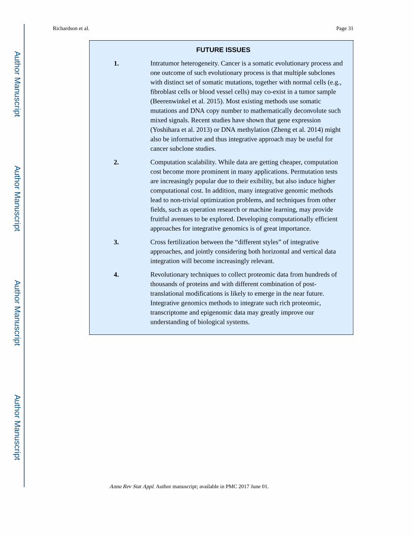
FUTURE ISSUES

1. Intratumor heterogeneity. Cancer is a somatic evolutionary process and

one outcome of such evolutionary process is that multiple subclones

with distinct set of somatic mutations, together with normal cells (e.g.,

fibroblast cells or blood vessel cells) may co-exist in a tumor sample

(Beerenwinkel et al. 2015). Most existing methods use somatic

mutations and DNA copy number to mathematically deconvolute such

mixed signals. Recent studies have shown that gene expression

(Yoshihara et al. 2013) or DNA methylation (Zheng et al. 2014) might

also be informative and thus integrative approach may be useful for

cancer subclone studies.

2. Computation scalability. While data are getting cheaper, computation

cost become more prominent in many applications. Permutation tests

are increasingly popular due to their exibility, but also induce higher

computational cost. In addition, many integrative genomic methods

lead to non-trivial optimization problems, and techniques from other

fields, such as operation research or machine learning, may provide

fruitful avenues to be explored. Developing computationally efficient

approaches for integrative genomics is of great importance.

3. Cross fertilization between the “different styles” of integrative

approaches, and jointly considering both horizontal and vertical data

integration will become increasingly relevant.

4. Revolutionary techniques to collect proteomic data from hundreds of

thousands of proteins and with different combination of post-

translational modifications is likely to emerge in the near future.

Integrative genomics methods to integrate such rich proteomic,

transcriptome and epigenomic data may greatly improve our

understanding of biological systems.

Richardson et al.


Author M

anuscriptA

uthor Manuscript

Author M

anuscriptA

uthor Manuscript

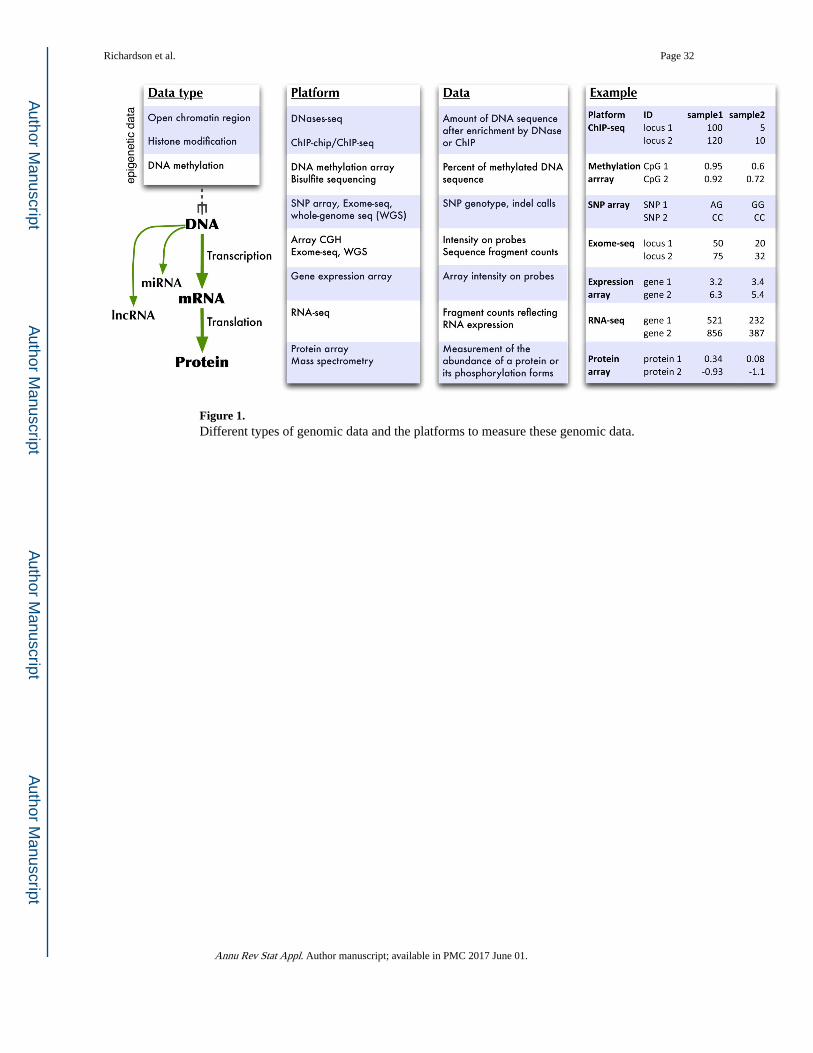
Figure 1. Different types of genomic data and the platforms to measure these genomic data.

Richardson et al.


Author M

anuscriptA

uthor Manuscript

Author M

anuscriptA

uthor Manuscript

Figure 2. A screenshot of a spreadsheet shown in the TCGA data portal web page when querying

available data from breast cancer patients. The column of this spreadsheet corresponds to a

combination of data types and platforms. For each platform, there could be data from tiers 1

to 3. Usually raw data belong to tier 1, and processed data belong to tier 2 or 3. One type of

genomic data may be collected on multiple platforms. For example, gene expression are

measured by both microarray and RNA-seq and two types of DNA methylation arrays (JHU-

USC HumanMethylation27 and JHU-USC HumanMethylation450) have been used. A

platform name often starts with the institute that processes those tumor samples using that

particular platform. For example, BI Genome_Wide_SNP_6 means Affymetrix 6.0 array

from Broad Institute. Each row of this spreadsheet corresponds to a patient. The meaning of

the patient ID can be found at https://wiki.nci.nih.gov/display/TCGA/TCGA+Barcode

Richardson et al.


Author M

anuscriptA

uthor Manuscript

Author M

anuscriptA

uthor Manuscript

https://wiki.nci.nih.gov/display/TCGA/TCGA+Barcode

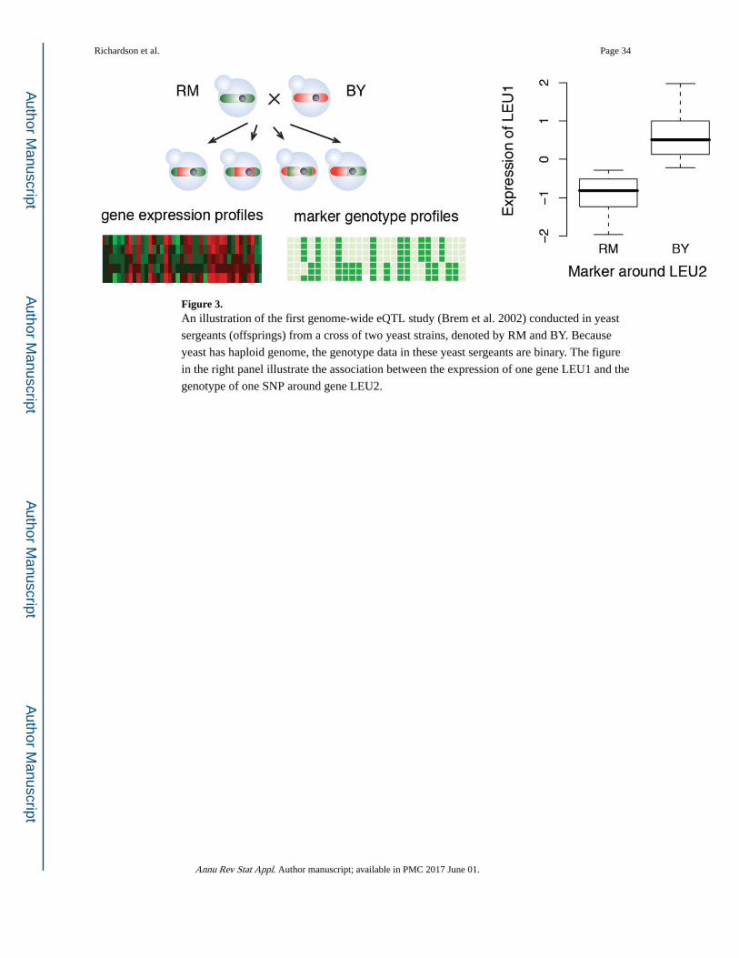
Figure 3. An illustration of the first genome-wide eQTL study (Brem et al. 2002) conducted in yeast

sergeants (offsprings) from a cross of two yeast strains, denoted by RM and BY. Because

yeast has haploid genome, the genotype data in these yeast sergeants are binary. The figure

in the right panel illustrate the association between the expression of one gene LEU1 and the

genotype of one SNP around gene LEU2.

Richardson et al.


Author M

anuscriptA

uthor Manuscript

Author M

anuscriptA

uthor Manuscript

Figure 4. Examples of biological networks (A) Protein-protein interaction. The edges are detected

from experiment for physical interaction. (B) Co-expression network. The edges are inferred

from the expression data of a group of samples, as dichotomized correlation or partial

correlation matrix. (C) Gene regulatory network. The Octagons indicate protein activity and

the ovals indicates gene expression. The dash line between g3 and a3 indicates a3 is the

activity of the protein that is encoded by g3. (D) Signaling pathway. EGFR (epidermal

growth factor receptor) is a receptor located at cell surface that can be activated by epidermal

growth factor. The symbol−P arounds a protein indicates a phosphorylation of the

corresponding protein.

Richardson et al.


Author M

anuscriptA

uthor Manuscript

Author M

anuscriptA

uthor Manuscript

Figure 5. Statistical approaches to use graphical model for integrative genomics. (A) To infer directed

co-expression network with the aid of DNA variation information. (B) To infer the

regulatory relation between miRNA and gene expression.

Richardson et al.


Author M

anuscriptA

uthor Manuscript

Author M

anuscriptA

uthor Manuscript

Figure 6. The PARADIGM method of integrative genomics (Vaske et al. 2010). (A) The graphical

model of underlying states. a1 → a2 indicates activated protein 1 regulates the activity of

protein 2. a2 → g3 indicates activated protein 2 regulates the expression of g3. (B) Examples

of “AND” and “OR” relations. (C) Adding observed data into the graph. Here observed data,

like the underlying state, has three values, −1, 0, or 1. Having observed data in certain

vertices mean that the underlying states of those vertices are known.

Richardson et al.


Author M

anuscriptA

uthor Manuscript

Author M

anuscriptA

uthor Manuscript

Author M

anuscriptA

uthor Manuscript

Author M

anuscriptA

uthor Manuscript

Richardson et al.

Table 1

Genomic data resources

Resource URL Description

dbGAP www.ncbi.nlm.nih.gov/gap DNA genotype and phenotype data

ArrayExpress www.ebi.ac.uk/arrayexpress Gene expression and epigenetic marks

GEO www.ncbi.nlm.nih.gov/geo Gene expression and epigenetic marks

SRA www.ncbi.nlm.nih.gov/sra Sequencing data

TCGA tcga-data.nci.nih.gov/tcga Multiple types of open access genomic data

CGHub cghub.ucsc.edu Multiple types of controlled-access genomic data

ICGC dcc.icgc.org Multiple types of genomic data

Roadmap www.roadmapepigenomics.org Epigenomics data

GTEx www.gtexportal.org/home RNA-seq from different tissues

ENCODE www.encodeproject.org Epigenetic and gene expression data


http://www.ncbi.nlm.nih.gov/gap

http://www.ebi.ac.uk/arrayexpress

http://www.ncbi.nlm.nih.gov/geo

http://www.ncbi.nlm.nih.gov/sra

http://tcga-data.nci.nih.gov/tcga

http://cghub.ucsc.edu

http://dcc.icgc.org

htpp://www.roadmapepigenomics.org

http://www.gtexportal.org/home

http://www.encodeproject.org

Author M

anuscriptA

uthor Manuscript

Author M

anuscriptA

uthor Manuscript

Richardson et al.

Table 2

Annotation databases

Category Database URL

Genome browser Ensembl www.ensembl.org/index.html

UCSC genome browser genome.ucsc.edu

SNP/indels dbSNP www.ncbi.nlm.nih.gov/SNP

Gene structure GENCODE www.gencodegenes.org

Ensembl’s Genebuild www.ensembl.org/index.html

Functional annotation Pathway Commons www.pathwaycommons.org

Pathway Interaction Database pid.nci.nih.gov

KEGG www.genome.jp/kegg

Gene Ontology (GO) geneontology.org


http://www.ensembl.org/index.html

http://genome.ucsc.edu

http://www.ncbi.nlm.nih.gov/SNP

http://www.gencodegenes.org

http://www.ensembl.org/index.html

http://www.pathwaycommons.org

http://pid.nci.nih.gov

http://www.genome.jp/kegg

http://geneontology.org

Statistical Methods in Integrative Genomics

Documents

Transcript of Statistical Methods in Integrative Genomics