Integrative statistical methods for the genomic analysis of ...
266
Integrative statistical methods for the genomic analysis of immune-mediated disease Oliver S Burren Department of Medicine University of Cambridge This dissertation is submitted for the degree of Doctor of Philosophy Darwin College June 2019
-
Upload
khangminh22 -
Category
Documents
-
view
3 -
download
0
Transcript of Integrative statistical methods for the genomic analysis of ...

Integrative statistical methods forthe genomic analysis of
immune-mediated disease
Oliver S Burren
Department of Medicine
University of Cambridge
This dissertation is submitted for the degree of
Doctor of Philosophy
Darwin College June 2019


Declaration
I hereby declare that except where specific reference is made to the work of others,the contents of this dissertation are original and have not been submitted in wholeor in part for consideration for any other degree or qualification in this, or anyother university. This dissertation is my own work and contains nothing which isthe outcome of work done in collaboration with others, except as specified in thetext and Acknowledgements. This dissertation contains fewer than 60,000 wordsexcluding appendices, bibliography, footnotes, tables and equations and has fewerthan 150 figures.
Oliver S BurrenJune 2019

Abstract
Genome wide association studies (GWAS) have proved to be a successful methodin cataloguing loci influencing thousands of complex human disease phenotypes.However, elucidating the causal mechanisms underlying such associations hasproved challenging due to the regulatory nature of the majority of signals.
In Chapters 2 and 3, I hypothesised that promoter-capture Hi-C (PCHi-C)data might have utility in physically linking disease-associated regulatory variantsto their target genes, in a tissue-specific manner. To examine the genome-wideenrichment of GWAS summary statistics within PCHi-C chromatin contact mapsI developed a novel statistical method, ‘blockshifter’. I applied blockshifter to acompendium of GWAS summary statistics for 31 traits and PCHi-C data across17 primary blood tissues, and found convincing evidence for the enrichment ofimmune-mediated disease (IMD) GWAS signals in lymphocyte specific chromatininteractions, providing support for the hypothesis. Taking a more gene-centricapproach I developed ‘COGS’, a novel method for integrating GWAS and PCHi-Cto prioritise specific causal variants, genes and cellular contexts for functionalfollow up. With a focus on IMD, I prioritised tissue-context specific interactions inCD4+ T cells linking putative causal variants for type 1 diabetes, to the promoterof IL2RA. The effect of these variants on IL2RA expression was subsequentlyvalidated by allele specific expression, by a collaborator, supporting the approach.
In Chapter 4, I hypothesised that summary statistics from multiple, wellpowered GWAS of related diseases might be exploited to provide insight into rarerrelated diseases or disease subtypes. To investigate this I developed a PCA basedframework to generate a lower dimensional basis, summarising input GWAS traits.I constructed such a basis from ten IMD GWAS studies, excluding variants inthe HLA region, and projected on summary GWAS data from multiple sourcesin order to characterise individual principal components (PCs). By projecting onboth summary and individual level genotype data for juvenile idiopathic diseasesubtypes, I was able to show that a single PC was able to discriminate enthesitis-related and systemic forms of the disease from other subtypes.


I would like to dedicate this thesis to my wife Amanda.

Acknowledgements
Firstly I extend my thanks to my supervisor, Dr. Chris Wallace, without whomthis thesis would not have been possible for many reasons. Thanks also to myco-supervisor, Dr. Mikhail Spivakov, for helping me navigate the history ofchromatin dynamics and gene regulatory processes. I owe a debt of gratitude tothe denizens of The Fishbowl, past and present, Dr. Mary Fortune, Dr. JonnyGriffiths, Mr. Martin Kelemen, Ms Kath Nicholls and Mr. Stephen Coleman. ToDr. Stasia Grinberg and Dr. James Liley, my longer term colleagues, thanks foryour companionship, help with mathematics and its notation, and general supportover the past three years.
From my previous laboratory, I would like to take the opportunity to saythanks to Prof. John Todd and Prof. Linda Wicker, who afforded me multipleopportunities for both personal and professional development during my tenure atthe Diabetes and Inflammation Laboratory (DIL). Thanks are also due to Dr. TonyCutler and (soon to be Dr.) Dan Rainbow, whose immunological and empiricalexpertise, generously given, stimulated my interest in this area. Thanks also toProf. Ken Smith for taking a chance on me and introducing me to rarer forms ofimmune-mediated disease.
I have been lucky to have had input from a number of clinicians, over thecourse of this work but would like to especially thank, Prof. Lucy Wedderburnfor her clinical insights into JIA and Dr. Jagtar Singh for the discussions, ontreatments, and the clinical course of more adult forms of arthritides.
My deepest gratitude is to my family; to my wife, Mands for both the emotionaland practical side of supporting a post-graduate husband, and my children, Aliceand Eve, for keeping me tethered (my ‘book’ is now finished!).
Finally I would like to acknowledge all the patients, healthy controls andresearchers on whose samples and analyses this thesis would not have beenpossible.


Table of contents
List of figures xvii
List of tables xxi
List of Abbreviations xxiii
1 Introduction 11.1 Foreword . . . . . . . . . . . . . . . . . . . . . . . . . . . . . . 11.2 The role of genome organisation in health and disease . . . . . . 2
1.2.1 The canonical eukaryotic protein coding gene . . . . . . 21.2.2 Chromatin structure . . . . . . . . . . . . . . . . . . . 31.2.3 Regulation of chromatin state . . . . . . . . . . . . . . 41.2.4 Chromatin organisation in three dimensions . . . . . . . 61.2.5 Chromatin organisation and disease . . . . . . . . . . . 10
1.3 Statistical methods for genomic analysis . . . . . . . . . . . . . 121.3.1 Relevant population genetics concepts . . . . . . . . . . 121.3.2 Genome Wide Association Studies . . . . . . . . . . . . 141.3.3 Hypothesis testing . . . . . . . . . . . . . . . . . . . . 151.3.4 Frequentist approaches to genetic association testing . . 171.3.5 Bayesian approaches to genetic association testing . . . 201.3.6 Approaches to high dimensional data . . . . . . . . . . 221.3.7 Principal component analysis (PCA) . . . . . . . . . . . 23
1.4 Towards causal mechanisms in immune-mediated disease . . . . 261.4.1 Epidemiology of immune-mediated disease . . . . . . . 261.4.2 Genetics of of immune-mediated disease . . . . . . . . 271.4.3 Immune-mediated diseases have both shared and distinct
genetic architectures . . . . . . . . . . . . . . . . . . . 271.4.4 Integrating functional genomics with GWAS . . . . . . 29

xii | Table of contents
1.4.5 Towards a mechanistic taxonomy of immune-mediateddisease . . . . . . . . . . . . . . . . . . . . . . . . . . 30
1.5 Organisation of the thesis . . . . . . . . . . . . . . . . . . . . . . 311.6 Publications . . . . . . . . . . . . . . . . . . . . . . . . . . . . 32
2 Detecting tissue specific enrichment of GWAS signals in PCHi-C data 352.1 Foreword . . . . . . . . . . . . . . . . . . . . . . . . . . . . . 35
2.1.1 Chapter Summary . . . . . . . . . . . . . . . . . . . . 352.1.2 Attributions . . . . . . . . . . . . . . . . . . . . . . . . 352.1.3 Motivation . . . . . . . . . . . . . . . . . . . . . . . . 362.1.4 Software availability . . . . . . . . . . . . . . . . . . . 36
2.2 Background . . . . . . . . . . . . . . . . . . . . . . . . . . . . 362.2.1 Gene set enrichment analysis inspired methods . . . . . 372.2.2 Matched SNP sets methods . . . . . . . . . . . . . . . . 382.2.3 Circularised permutation methods . . . . . . . . . . . . 392.2.4 Statistical modelling methods . . . . . . . . . . . . . . 40
2.3 PCHi-C maps: description and exploratory data analyses . . . . 422.3.1 Tissue coverage . . . . . . . . . . . . . . . . . . . . . . 422.3.2 Data format description . . . . . . . . . . . . . . . . . . 422.3.3 CHiCAGO score distributions across cell types . . . . . 432.3.4 CHiCAGO scores reflect lineage specificity . . . . . . . 442.3.5 Characterisation of the localised structure within a PCHi-
C map . . . . . . . . . . . . . . . . . . . . . . . . . . . 452.4 GWAS compendium: description and data processing . . . . . . 47
2.4.1 Defining approximately LD independent blocks . . . . . 502.4.2 Poor man’s imputation pipeline . . . . . . . . . . . . . 502.4.3 Evaluation of PMI performance . . . . . . . . . . . . . . 512.4.4 Generation of single causal variant posterior probabilities 522.4.5 Prior selection . . . . . . . . . . . . . . . . . . . . . . 532.4.6 HLA region . . . . . . . . . . . . . . . . . . . . . . . . 53
2.5 blockshifter development . . . . . . . . . . . . . . . . . . . . . 542.5.1 The blockshifter method . . . . . . . . . . . . . . . . . 54
2.6 Power and type 1 error rates for blockshifter . . . . . . . . . . . 562.6.1 Simulation of GWAS . . . . . . . . . . . . . . . . . . . 572.6.2 Enrichment scenarios . . . . . . . . . . . . . . . . . . . 572.6.3 Simulation results . . . . . . . . . . . . . . . . . . . . 59
Table of contents | xiii
2.7 Tissue specific enrichment of associated variants with PIRs across31 traits . . . . . . . . . . . . . . . . . . . . . . . . . . . . . . 60
2.8 Discussion . . . . . . . . . . . . . . . . . . . . . . . . . . . . . . 61
3 Integrating GWAS and PCHi-C data to prioritise causal genes andtissues 653.1 Foreword . . . . . . . . . . . . . . . . . . . . . . . . . . . . . 65
3.1.1 Chapter Summary . . . . . . . . . . . . . . . . . . . . 653.1.2 Attributions . . . . . . . . . . . . . . . . . . . . . . . . 663.1.3 Motivation . . . . . . . . . . . . . . . . . . . . . . . . 663.1.4 Software availability . . . . . . . . . . . . . . . . . . . 67
3.2 Background . . . . . . . . . . . . . . . . . . . . . . . . . . . . 673.2.1 LD and Proximity approaches . . . . . . . . . . . . . . 673.2.2 Population genetics approaches . . . . . . . . . . . . . 693.2.3 High throughput molecular genomic approaches . . . . 70
3.3 Promoter-capture platform coverage . . . . . . . . . . . . . . . 703.3.1 Capture platform reannotation . . . . . . . . . . . . . . . 713.3.2 Distribution of captured transcriptional start sites . . . . . 71
3.4 A method to integrate GWAS summary statistics with PCHi-C maps 733.4.1 Method overview . . . . . . . . . . . . . . . . . . . . . 733.4.2 Annotation of coding variants . . . . . . . . . . . . . . 743.4.3 Annotation of PCHi-C ‘blindspot’ (‘Virtual Promoter’) . 743.4.4 Annotation of PIRs . . . . . . . . . . . . . . . . . . . . 753.4.5 COGS method description . . . . . . . . . . . . . . . . 75
3.5 Application of COGS to a GWAS compendium . . . . . . . . . 773.5.1 Overall COGS scores for 31 traits . . . . . . . . . . . . 773.5.2 Are prioritised genes biologically relevant? . . . . . . . 77
3.6 Impact of different gene-variant linking methods on COGS per-formance . . . . . . . . . . . . . . . . . . . . . . . . . . . . . 803.6.1 A framework for comparing gene-variant linking methods
using GWAS summary statistics . . . . . . . . . . . . . . 813.6.2 Comparison of PCHi-C-, proximity- and TAD-based COGS
scores . . . . . . . . . . . . . . . . . . . . . . . . . . . 823.6.3 PCHi-C prioritised genes are more likely to be differen-
tially expressed in disease patients . . . . . . . . . . . . 843.6.4 Overlap of COGS prioritised genes with eQTLs . . . . . 86
3.7 Comparison of PCHi-C COGS scores between tissues . . . . . . 87
xiv | Table of contents
3.7.1 A heuristic approach to prioritising sets of tissues . . . . 893.7.2 Tissue specific COGS gene prioritisation across 8 immune-
mediated diseases . . . . . . . . . . . . . . . . . . . . . . 913.8 Cell context specific COGS analysis of immune-mediated disease 94
3.8.1 ImmunoChip study collection description . . . . . . . . 953.8.2 Allowing for multiple causal variants within a locus . . 953.8.3 Comparison of COGS scores between single and multiple
causal variant approaches . . . . . . . . . . . . . . . . . 963.8.4 Cataloguing PCHi-C prioritised genes across immune-
mediated disease . . . . . . . . . . . . . . . . . . . . . 993.8.5 Integration of functional data with COGS scores . . . . 993.8.6 Functional validation in IL2RA . . . . . . . . . . . . . . 102
3.9 Discussion . . . . . . . . . . . . . . . . . . . . . . . . . . . . . 104
4 Shared and distinct genetic architectures in immune-mediated dis-ease 1114.1 Foreword . . . . . . . . . . . . . . . . . . . . . . . . . . . . . . 111
4.1.1 Chapter Summary . . . . . . . . . . . . . . . . . . . . . 1114.1.2 Attributions . . . . . . . . . . . . . . . . . . . . . . . . . 1114.1.3 Motivation . . . . . . . . . . . . . . . . . . . . . . . . 1124.1.4 Software Availability . . . . . . . . . . . . . . . . . . . 112
4.2 Background . . . . . . . . . . . . . . . . . . . . . . . . . . . . 1134.3 Basis disease data preparation . . . . . . . . . . . . . . . . . . 117
4.3.1 UK10K as a reference genotype dataset . . . . . . . . . 1194.3.2 SNP selection . . . . . . . . . . . . . . . . . . . . . . . 119
4.4 Creating a PCA ‘basis’ . . . . . . . . . . . . . . . . . . . . . . . 1214.4.1 PCA basis creation using β . . . . . . . . . . . . . . . . 1214.4.2 PCA basis creating using γ . . . . . . . . . . . . . . . . 123
4.5 Evaluating basis performance . . . . . . . . . . . . . . . . . . . 1254.5.1 Linear regression coefficient conversion to the odds ratio
scale for a binary trait . . . . . . . . . . . . . . . . . . 1264.5.2 Comparison of γ basis PC scores with matched UKBB
self-reported projections . . . . . . . . . . . . . . . . . 1274.6 Development of a Bayesian shrinkage method . . . . . . . . . . 128
4.6.1 Method description . . . . . . . . . . . . . . . . . . . . 1294.6.2 Shrinkage evaluation . . . . . . . . . . . . . . . . . . . 132
4.7 Estimating the variance of projected PC scores . . . . . . . . . . 133
Table of contents | xv
4.7.1 Analytical variance estimation . . . . . . . . . . . . . . 1334.7.2 Empirical variance estimation . . . . . . . . . . . . . . 1354.7.3 Variance estimate evaluation . . . . . . . . . . . . . . . 1374.7.4 Assessing the significance of trait projections . . . . . . 138
4.8 Annotation of basis principal components . . . . . . . . . . . . 1384.8.1 Projection of UKBB self-reported trait GWAS . . . . . 1394.8.2 Projection of UKBB blood count GWAS . . . . . . . . 1434.8.3 Projection of whole blood eQTL data . . . . . . . . . . 145
4.9 Using the basis to characterise JIA . . . . . . . . . . . . . . . . 1494.9.1 JIA disease subtypes . . . . . . . . . . . . . . . . . . . 1494.9.2 JIA subtype GWAS analysis . . . . . . . . . . . . . . . 1504.9.3 Projection of JIA subtype GWAS . . . . . . . . . . . . 1504.9.4 Annotating PCs related to JIA . . . . . . . . . . . . . . 1544.9.5 Comparing JIA subtypes PC scores in the presence of
shared controls . . . . . . . . . . . . . . . . . . . . . . 1564.10 Projecting individual genotypes onto the basis . . . . . . . . . . 157
4.10.1 Computation of posterior odds ratios . . . . . . . . . . . 1584.10.2 Effect of parmameters on posterior log(OR) estimates . 1594.10.3 Projection of JIA disease subtype genotype data into basis
space . . . . . . . . . . . . . . . . . . . . . . . . . . . 1604.10.4 Evaluating individual level eQTL data using the basis . . 162
4.11 Discussion . . . . . . . . . . . . . . . . . . . . . . . . . . . . . 164
5 Discussion 1695.1 Linking themes . . . . . . . . . . . . . . . . . . . . . . . . . . 169
5.1.1 Effect of single causal variant assumptions . . . . . . . 1695.1.2 Data availability . . . . . . . . . . . . . . . . . . . . . . 1715.1.3 The importance of orthogonal functional evidence . . . 1735.1.4 A new taxonomy . . . . . . . . . . . . . . . . . . . . . 174
5.2 Further Work . . . . . . . . . . . . . . . . . . . . . . . . . . . 1755.2.1 PCHi-C facillitated gene prioritisation in alternative contexts1755.2.2 Further exploration of basis polygenic risk scores . . . . 176
5.3 Concluding Remarks . . . . . . . . . . . . . . . . . . . . . . . 178
References 179

xvi | Table of contents
Appendix A 203A.1 Summary of PCHi-C datasets . . . . . . . . . . . . . . . . . . . 203A.2 GWAS study references . . . . . . . . . . . . . . . . . . . . . . 205
Appendix B 207B.1 COGS prioritised genes Peters et al. (2016) . . . . . . . . . . . 207B.2 Prioritised COGS genes from Burren et al. (2017) . . . . . . . . 210
Appendix C 227C.1 Relationship between PCA and SVD . . . . . . . . . . . . . . . 227C.2 IMD basis projection forest plots . . . . . . . . . . . . . . . . . 229
List of figures
1.1 Chromsomal organisation . . . . . . . . . . . . . . . . . . . . . 41.2 Histone covalent modifications . . . . . . . . . . . . . . . . . . 51.3 Chromatin conformation capture methods . . . . . . . . . . . . 71.4 GWAS Growth . . . . . . . . . . . . . . . . . . . . . . . . . . 151.5 PCA Projection . . . . . . . . . . . . . . . . . . . . . . . . . . 24
2.1 GoShifter method overview . . . . . . . . . . . . . . . . . . . . 402.2 Overview of PCHi-C Peak Matrix Format . . . . . . . . . . . . 432.3 CHiCAGO score distribution . . . . . . . . . . . . . . . . . . . 442.4 Dendrogram of PCHi-C CHiCAGO scores . . . . . . . . . . . . 452.5 Method for detecting local correlation structure in PCHi-C data . 462.6 PCHi-C Local correlation . . . . . . . . . . . . . . . . . . . . . 472.7 PMI coverage performance . . . . . . . . . . . . . . . . . . . . 482.8 PMI vs Imputed summary statistics . . . . . . . . . . . . . . . . 522.9 blockshifter permutation strategy . . . . . . . . . . . . . . . . . 562.10 blockshifter Type I error calibration . . . . . . . . . . . . . . . 592.11 blockshifter tissue enrichment across 31 traits . . . . . . . . . . . 61
3.1 Comparison of FTO and IRX3 publication counts over time . . . 683.2 Protein coding gene coverage of PCHi-C platform . . . . . . . . 723.3 Bait HindIII fragment sizes and promoter overlap distributions . 733.4 Overview of COGS causal gene prioritisation method . . . . . . 763.5 Distribution of COGS scores . . . . . . . . . . . . . . . . . . . 783.6 Summary of COGS gene prioritisation across 31 traits . . . . . . 793.7 Reactome gene set enrichment using COGS . . . . . . . . . . . 803.8 Comparison of PCHi-C, TAD and Proximity based COGS scores 823.9 PCHi-C bait distance distribution from TAD boundaries for COGS
prioritised genes . . . . . . . . . . . . . . . . . . . . . . . . . . 83
xviii | List of figures
3.10 Enrichment of COGS priortised genes for differential expressionin Peters et al. (2016) . . . . . . . . . . . . . . . . . . . . . . . 85
3.11 COGS prioritisation of BCL-6 in Crohn’s disease . . . . . . . . 863.12 Computation of feature specific COGS scores . . . . . . . . . . 883.13 Dendrogram of PCHi-C CHiCAGO scores . . . . . . . . . . . . 893.14 Tissue specific COGS prioritsiation of AHR in rheumatoid arthritis 923.15 Heatmap of hierarchical COGS analysis using COGS threshold
> 0.5 . . . . . . . . . . . . . . . . . . . . . . . . . . . . . . . 933.16 COGS Score comparison sCVPP and mCVPP inputs . . . . . . 983.17 aBF and GUESSFM COGS comparison in 19p13.2 for type 1
diabetes . . . . . . . . . . . . . . . . . . . . . . . . . . . . . . 1003.18 sCOGS and mCOGS comparison in for type 1 diabetes . . . . . . 1013.19 Tissue specific COGS results across five immune-mediated diseases1023.20 Genomic and genetic architecture of 10p15.1 type 1 diabetes
susceptibility locus . . . . . . . . . . . . . . . . . . . . . . . . 103
4.1 Genetic correlation across 6 immune-mediated diseases . . . . . 1154.2 SNP intersection across basis diseases . . . . . . . . . . . . . . 1204.3 Basis SNP genome coverage . . . . . . . . . . . . . . . . . . . . 1214.4 PCA basis using β . . . . . . . . . . . . . . . . . . . . . . . . 1224.5 Hierarchical clustering of β PC scores . . . . . . . . . . . . . . 1234.6 PCA basis using γ . . . . . . . . . . . . . . . . . . . . . . . . . 1244.7 Hierarchical clustering of UKBB projected γ PC scores . . . . . 1274.8 Proposed Bayesian shrinkage for 2q33.2 locus . . . . . . . . . . . 1314.9 Basis PCA using shrunk γ . . . . . . . . . . . . . . . . . . . . 1324.10 Hierarchical clustering of PC scores using shrunk γ . . . . . . . 1334.11 Variance estimation of PC score method comparison . . . . . . 1384.12 Summary of significant UKBB self-reported traits. . . . . . . . 1404.13 Heatmap of significant UKBB SRD . . . . . . . . . . . . . . . . 1414.14 Heatmap of significant UKBB self-reported medication projections1424.15 Results of projection of 13 main blood count traits . . . . . . . . 1454.16 Heatmap of significant gene projections from Võsa et al. (2018) 1474.17 Heatmap of variance enriched pathways from projection of Võsa
et al. (2018) . . . . . . . . . . . . . . . . . . . . . . . . . . . . 1484.18 Projected PC scores across 7 JIA subtypes . . . . . . . . . . . . . 1514.19 Hierarchical clustering of HLA correlations for JIA subtypes . . 1524.20 Heatmap of JIA disease subtype projections . . . . . . . . . . . 153

List of figures | xix
4.21 Context of JIA subtype projections for PC1 . . . . . . . . . . . 1554.22 Context of JIA subtype projections for PC3 . . . . . . . . . . . 1564.23 Posterior odds ratio parameter effects . . . . . . . . . . . . . . 1604.24 Comparison of JIA subtype PC δ values from genotype and sum-
mary data approaches . . . . . . . . . . . . . . . . . . . . . . . . 1614.25 QQ plots for gene expression regressions on basis PC scores
for Raj et al. (2014) . . . . . . . . . . . . . . . . . . . . . . . . 163


List of tables
1.1 Example Contingency table . . . . . . . . . . . . . . . . . . . . 171.2 Possible biallelic configurations . . . . . . . . . . . . . . . . . 18
2.1 GWAS Compendium . . . . . . . . . . . . . . . . . . . . . . . 49
3.1 PCHi-C sequence capture by Biotype using Ensembl v75 geneannotation. . . . . . . . . . . . . . . . . . . . . . . . . . . . . 72
3.2 Topologically associated domain coverage across eight cell typeselucidated from classical Hi-C analysis . . . . . . . . . . . . . . 82
3.3 ImmunoChip study collection . . . . . . . . . . . . . . . . . . . 953.4 Comparison between COGS prioritised gene counts derived under
single and multiple causal variant methods . . . . . . . . . . . . 97
4.1 Immune mediated disease studies used to construct basis. . . . . 1184.2 Basis matched UKBB self-reported disease phenotypes . . . . . 1254.3 Table of 13 main blood measurements analysed by Astle et al. (2016)1444.4 JIA disease subtype cohort description . . . . . . . . . . . . . . 1504.5 JIA disease subtype projection scores on PC3 . . . . . . . . . . 1524.6 Gene expression from Võsa et al. (2018) significantly associated
with a basis principal component . . . . . . . . . . . . . . . . . 164
A.1 PCHi-C dataset summary . . . . . . . . . . . . . . . . . . . . . 204A.2 Table of GWAS studies with appropriate references used in Chap-
ters 2 and 3 . . . . . . . . . . . . . . . . . . . . . . . . . . . . 206
B.1 Prioritised COGS genes from Peters et al. (2016) . . . . . . . . 208B.2 Act/Non-Act CD4+ T cell PCHi-C COGS prioritised genes . . . . 211


List of Abbreviations
Acronyms / Abbreviations
3C Chromosome conformation capture
4C Chromosome conformation capture-on-chip
5C Carbon-copy chromosome conformation capture
aBF Wakefield’s asymptotic Bayes Factor
ATAC-Seq Assay for transposable accessible chromatin using sequencing
CHi-C Capture Hi-C
ChIA-PET Chromatin interaction analysis by paired-end tag sequencing
ChIP-Seq Chromatin immunoprecipitiation and sequencing
COGS Capture Hi-C omnibus gene score
cSNP Protein-coding single nucleotide polymorphism
CV Coefficient of variation
DHS DNase I hypersensitivity site
eQTL Expression quantitative trait locus/loci
eRNA Enhancer RNA
EUR The 1000 genomes European population cohort
GO Gene ontology
GSEA Gene-set enrichment analysis
GWAS Genome-wide association study

xxiv | List of Abbreviations
HCC Hepatocellular carcinoma
HLA Human leukocyte antigen
HPO Human phenotype ontology
HWE Hardy-Weinberg equilibrium
IBD Inflammatory bowel disease
ILAR International League of Associations for Rheumatology
IMD Immune-mediated disease
LCR Locus control region
LD Linkage disequilibrium
MAF Minor allele frequency
mCOGS Multiple casual variant COGS
miRNA Micro-RNA
MPRA Massively parallel reporter assays
mRNA messenger RNA
MVN Multivariant normal distribution
NCP Non-centrality parameter
OLS Ordinary least squares
OR Odds ratio
pBF Pseudo-Bayes factor
PCA Principal component analysis
PCHi-C Promoter capture Hi-C
PIR Promoter interacting region
PMI Poor man’s imputation
PPD Preaxial polydactyly

List of Abbreviations | xxv
PRS Polygenic risk score
sCOGS Single casual variant COGS
sCVPP Single causal variant posterior probability
snoRNA Small nucleolar RNA
SNP Single nucleotide polymorphism
snRNA Small nuclear RNA
SRD Self-reported disease
SVD Singular value decomposition
TAD Topologically assocaited domains
TSS Transcriptional start site
UKBB United Kingdom biobank
VPF Virtual promoter fragment
WTCCC Wellcome Trust Control Consortium

Chapter 1
Introduction
1.1 Foreword
The main aims of this thesis are threefold:
Aim One: Investigate whether the promoter interacting regions (PIRs) identifiedby promoter-capture Hi-C (PCHi-C) are enriched for GWAS signals in acell-context specific manner.
Aim Two: Develop methods to integrate GWAS signals with PCHi-C data inorder to prioritise putatively causal SNPs, genes and tissue contexts forfunctional followup.
Aim Three: Develop a framework for constructing a summary of the genetic rela-tionships between multiple immune-mediated diseases (IMD) and evaluatinghow they might be useful in characterising rarer or clinically heterogeneousIMDs.
The work presented in this thesis is, like a majority of contemporary research,of a cross-disciplinary nature encompassing the fields of genetics, genomics andstatistics. Given this scope, I have organised the material such that each subsequentchapter contains a more specific introduction to the relevant concepts, studiesand literature that it is concerned with. In contrast, this introductory materialis of a more general nature covering key concepts and technologies that forma foundation for subsequent chapters. In Section 1.2, to provide background toaims one and two, I describe how eukaryotic genomes are organised, the mainempirical methods for measuring facets of this organisation (including PCHi-C),and how such genomic organisation is of relevance to human disease. Section 1.3

2 | Introduction
introduces key population genetic concepts and statistical frameworks that I relyon throughout this thesis to achieve my aims. In the final section (Section 1.4), Iprovide a general introduction to IMDs with an emphasis, relating to aim three,on their shared and distinct genetic architectures. I finish by briefly touching onhow the integration of genetic and functional data might afford a more, robust,molecular taxonomy of IMDs.
1.2 The role of genome organisation in health anddisease
In 1958 ’On protein synthesis’ was published setting out Sir Francis Crick’s’Central Dogma’ on how information stored in DNA could give rise to the complexbiochemistry essential for life (Crick, 1958). In it, he stated a flow of informationfrom DNA, which through transcription to intermediate RNA species, is ultimately,translated to proteins, in order to elicit cellular function.
Five years later Monod and Jaques were the first to characterise this processin prokaryotes using the polycistronic lac operon in Escherichia coli (Jacob andMonod, 1961). Empirically, they demonstrated the presence of ‘regulatory’ genesand sequence elements, whose function was to control the activity of a set of targetgenes. These regulatory genes, which we now call ‘transcription factors’, wereshown to function by interacting with the cognate DNA sequence elements toregulate the expression of a short lived intermediate that they called ‘messenger’RNA (mRNA).
1.2.1 The canonical eukaryotic protein coding gene
At the sequence level, the canonical eukaryotic protein-coding gene, which I referto subsequently as a ‘gene’, consists of multiple elements that are required forfunctional transcription.
The Promoter Found directly upstream of the transcriptional start site (TSS),the promoter initiates binding of RNA Polymerase II (Pol II), the enzymeresponsible for transcribing DNA to mRNA. Generally such promoter se-quences consist of two elements; a region immediately upstream of the TSSknown as the ‘core promoter’ and a region upstream to this, known as the‘proximal element’ or ‘regulatory promoter’ (Kanhere and Bansal, 2005).The former provides sequence cues for the binding of the Poll II complex,
1.2 The role of genome organisation in health and disease | 3
with the latter thought to provide a more subtle, context-specific modulationof expression rate through the binding of cofactors such as transcriptionfactors. As a result promoters are highly heterogeneous between genesreflecting different abilities to drive transcription in different tissue contexts.
The Enhancer In Eukaryotes the activity of the promoter in controlling tran-scription is augmented by actions of short (between 100-500 bp) sequences,known as enhancers. Enhancers function by the binding of specific tran-scription factors that once recruited interact with co-factors and Pol II topotentiate transcription of a target or set of target genes. In higher organisms,enhancers, unlike promoters are often found at some distance (up to 1Mb)either upstream or downstream from their target gene. This effect overdistance means that they are often found in the intronic regions of non-targetgenes or even ‘skip’ multiple intervening genes to exert their function.
To understand such action at a distance it is useful to summarise currentknowledge about the organisation of DNA within a eukaryotic cell.
1.2.2 Chromatin structure
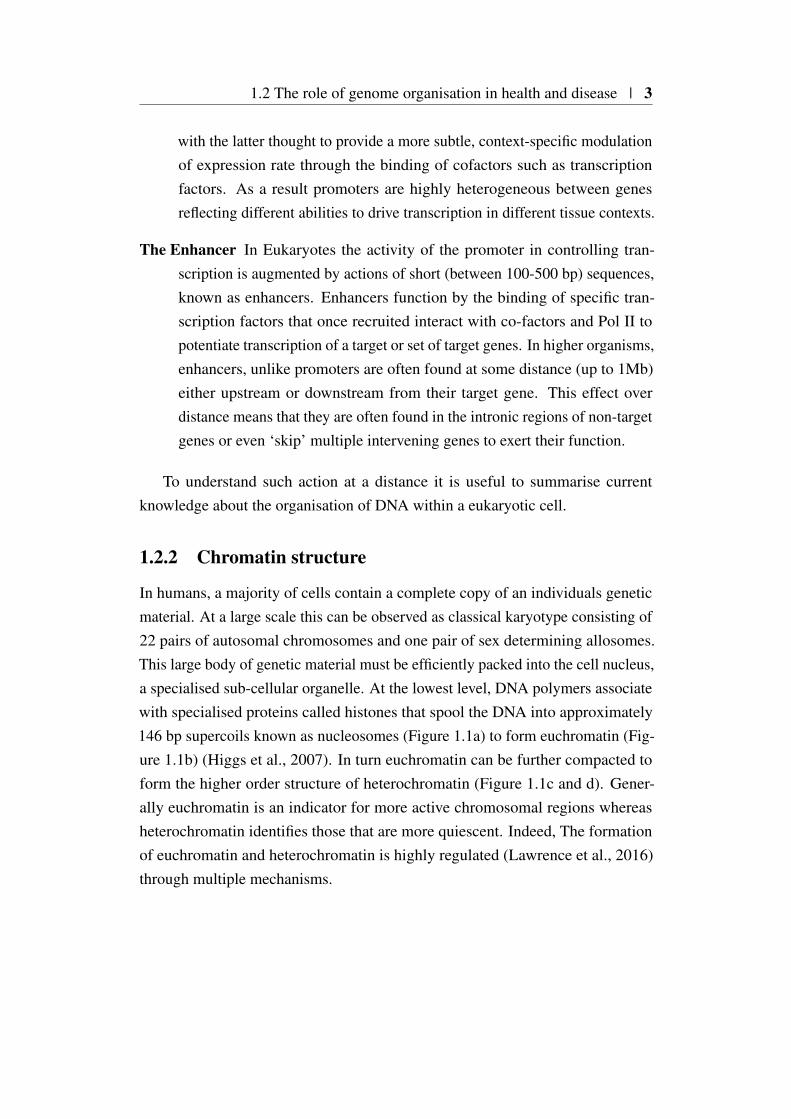
In humans, a majority of cells contain a complete copy of an individuals geneticmaterial. At a large scale this can be observed as classical karyotype consisting of22 pairs of autosomal chromosomes and one pair of sex determining allosomes.This large body of genetic material must be efficiently packed into the cell nucleus,a specialised sub-cellular organelle. At the lowest level, DNA polymers associatewith specialised proteins called histones that spool the DNA into approximately146 bp supercoils known as nucleosomes (Figure 1.1a) to form euchromatin (Fig-ure 1.1b) (Higgs et al., 2007). In turn euchromatin can be further compacted toform the higher order structure of heterochromatin (Figure 1.1c and d). Gener-ally euchromatin is an indicator for more active chromosomal regions whereasheterochromatin identifies those that are more quiescent. Indeed, The formationof euchromatin and heterochromatin is highly regulated (Lawrence et al., 2016)through multiple mechanisms.

4 | Introduction
d)d)c)b)a)
Fig. 1.1 A model for the formation of chromatin in Eukayotes. a) Specialisedproteins called core histones (blue) form ≈ 146 bp DNA coils called nucleosomes.b) Nucleosomes form at regular intervals along the DNA double helix in theso called ‘beads on a string’ configuration. This configuration is permissive togene transcription and is modulated by chemical modification of histone tails. c)Mediated by the non core histone, H1, this ‘bead on a string’ configuration, knownas euchromatin, is further packed into fibres known as chromatin. d) These denselypacked 30nm chromatin fibres, known as heterochromatin are generally lesspermissive to gene transcription. Image adapted from an original image by RichardWheeler under CC BY-SA 3.0 license [https://commons.wikimedia.org/wiki/File:Chromatin_Structures.png].
1.2.3 Regulation of chromatin state
DNA-Methylation
At the DNA level, the addition of methyl groups to individual cytosine (C) basesis widespread. In mammals this methylation occurs at specific di-nucleotidesknown as CpG’s (5’-C-phosphate-G-3’). This methylation is context specifc, forexample, the methylation of gene promoter regions is associated with attenuationof gene transcription, where as methylation of gene bodies has a reciprocal re-lationship (Jones, 2012). It is thought that DNA-methylation indirectly affectschromatin structure by recruiting, methyl-CpG-binding domain proteins (MBDs)which with co-factors promote chromatin remodelling (Du et al., 2015) .
Covalent histone modification
At the unit of the nucleosome, constituent histone proteins have polypeptide‘tails’ (Figure 1.1b) that through the action of specific enzymes may be covalentlymodified. For example, Histone 3 (H3) has a specific lyseine at position 27(K27) that when acetylated (ac) correlates with more active chromatin (H3K27ac).Many such histone modifications have been described, correlating with differentchromatin activation levels which are reviewed in (Lawrence et al., 2016).
1.2 The role of genome organisation in health and disease | 5
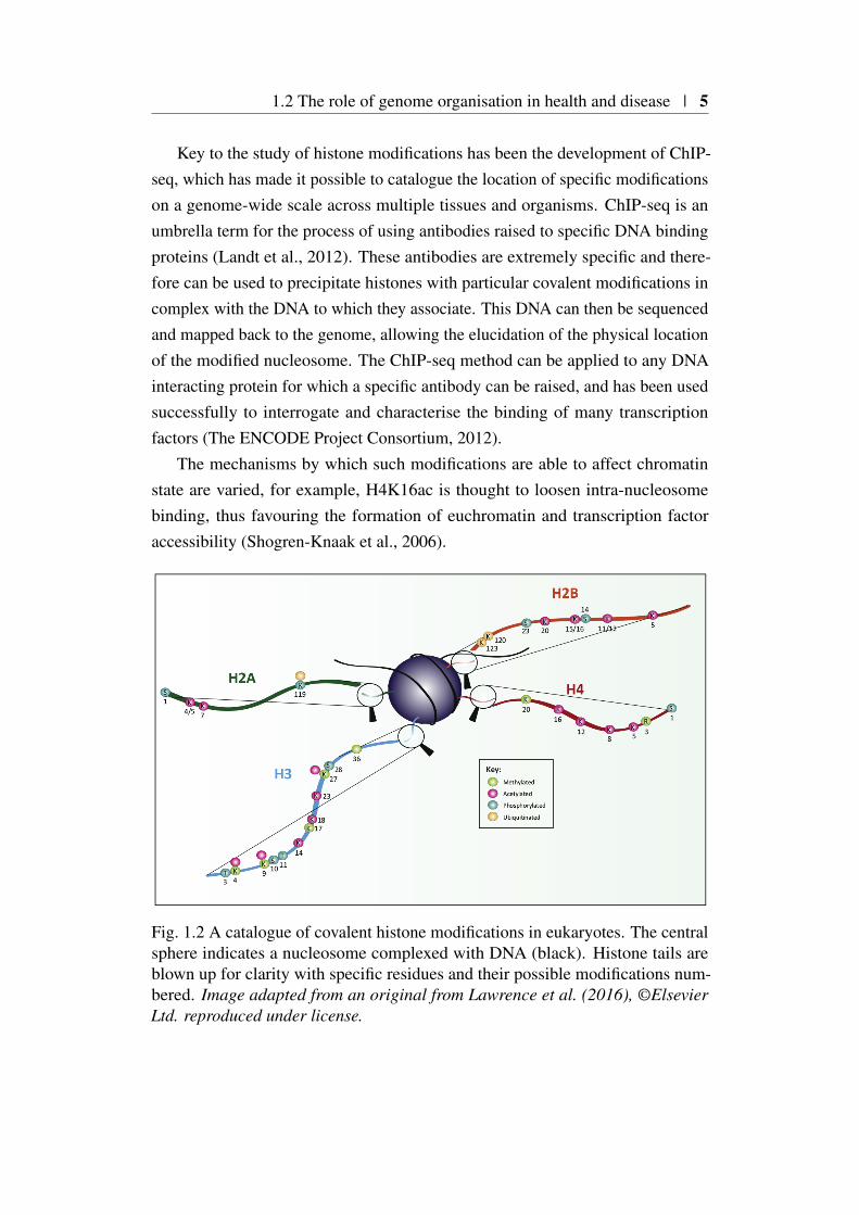
Key to the study of histone modifications has been the development of ChIP-seq, which has made it possible to catalogue the location of specific modificationson a genome-wide scale across multiple tissues and organisms. ChIP-seq is anumbrella term for the process of using antibodies raised to specific DNA bindingproteins (Landt et al., 2012). These antibodies are extremely specific and there-fore can be used to precipitate histones with particular covalent modifications incomplex with the DNA to which they associate. This DNA can then be sequencedand mapped back to the genome, allowing the elucidation of the physical locationof the modified nucleosome. The ChIP-seq method can be applied to any DNAinteracting protein for which a specific antibody can be raised, and has been usedsuccessfully to interrogate and characterise the binding of many transcriptionfactors (The ENCODE Project Consortium, 2012).
The mechanisms by which such modifications are able to affect chromatinstate are varied, for example, H4K16ac is thought to loosen intra-nucleosomebinding, thus favouring the formation of euchromatin and transcription factoraccessibility (Shogren-Knaak et al., 2006).
Fig. 1.2 A catalogue of covalent histone modifications in eukaryotes. The centralsphere indicates a nucleosome complexed with DNA (black). Histone tails areblown up for clarity with specific residues and their possible modifications num-bered. Image adapted from an original from Lawrence et al. (2016), ©ElsevierLtd. reproduced under license.

6 | Introduction
DNA accessibility
The accessibility of chromatin and its constituent DNA is also a useful marker ofactivity. One such assay, DNase hypersensitivity (DHS) assay with sequencing(DNase-Seq), involves digesting chromatin with the DNA cleaving enzyme DNaseI (Song and Crawford, 2010). Regions of open chromatin are more accessibleto the enzyme, and are therefore more likely to be a cleaved. These cleavageproducts, can be isolated and sequenced and their physical locations, knownas DHS regions, found by mapping to a reference genome. The DHS assay istechnically challenging and more recently has been replaced with the assay fortransposase-accessible chromatin using sequencing (ATAC-Seq) which requiresless biological input material (Buenrostro et al., 2015).
Chromatin segmentation
Due to the number of modifications that individual nucleosomes can undergo thenumber of possible combinations is large (Figure1.2), requiring the combinedanalysis of heterogeneous sources of data derived from CHiP-Seq, ATAC-Seq andRNA-Seq experiments. This precipitated the development of software to integratedatasets performed on the same cell type to identify patterns of modifications,transcription factor binding, accessibility and transcription that correlate withchromatin activity (Ernst and Kellis, 2012; Hoffman et al., 2012). This has allowedthe annotation of tissue specific ‘chromatin segments’, regions of chromatin withsimilar properties (e.g. combinations of histone modifications) (Ernst and Kellis,2015) and their subsequent characterisation into more conceptual constituentelements such as enhancers.
1.2.4 Chromatin organisation in three dimensions
However, this linear cataloguing of the non-coding portion of the genome describedin the previous section, misses additional complexity, in that chromatin fibresassociate to form higher order three dimensional structures. Whilst some ofthese associations are structural, allowing the very long fibres of chromatin tobe efficiently packed within a cell, many have specific functions associated withreplication and the regulation of gene expression. The recent development ofhigh-throughput methods, known as chromatin conformation assays, for assessingthis three dimensional structure has begun to reveal the underlying complexity ofthis structure and how it effects cellular function.
1.2 The role of genome organisation in health and disease | 7
Chromatin conformation assays
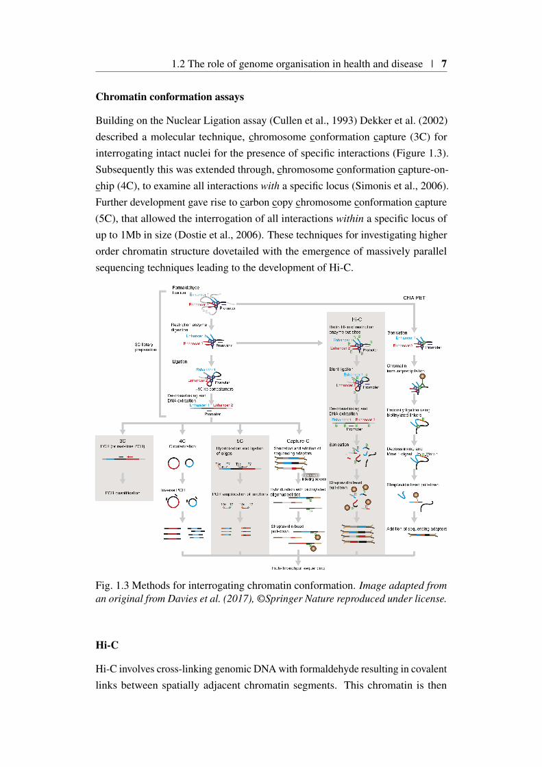
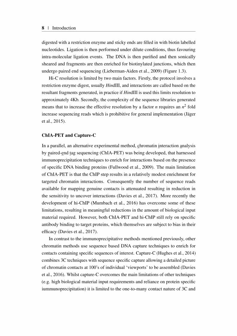
Building on the Nuclear Ligation assay (Cullen et al., 1993) Dekker et al. (2002)described a molecular technique, chromosome conformation capture (3C) forinterrogating intact nuclei for the presence of specific interactions (Figure 1.3).Subsequently this was extended through, chromosome conformation capture-on-chip (4C), to examine all interactions with a specific locus (Simonis et al., 2006).Further development gave rise to carbon copy chromosome conformation capture(5C), that allowed the interrogation of all interactions within a specific locus ofup to 1Mb in size (Dostie et al., 2006). These techniques for investigating higherorder chromatin structure dovetailed with the emergence of massively parallelsequencing techniques leading to the development of Hi-C.
Fig. 1.3 Methods for interrogating chromatin conformation. Image adapted froman original from Davies et al. (2017), ©Springer Nature reproduced under license.
Hi-C
Hi-C involves cross-linking genomic DNA with formaldehyde resulting in covalentlinks between spatially adjacent chromatin segments. This chromatin is then
8 | Introduction
digested with a restriction enzyme and sticky ends are filled in with biotin labellednucleotides. Ligation is then performed under dilute conditions, thus favouringintra-molecular ligation events. The DNA is then purified and then sonicallysheared and fragments are then enriched for biotinylated junctions, which thenundergo paired end sequencing (Lieberman-Aiden et al., 2009) (Figure 1.3).
Hi-C resolution is limited by two main factors. Firstly, the protocol involves arestriction enzyme digest, usually HindIII, and interactions are called based on theresultant fragments generated, in practice if HindIII is used this limits resolution toapproximately 4Kb. Secondly, the complexity of the sequence libraries generatedmeans that to increase the effective resolution by a factor n requires an n2 foldincrease sequencing reads which is prohibitive for general implementation (Jägeret al., 2015).
ChIA-PET and Capture-C
In a parallel, an alternative experimental method, chromatin interaction analysisby paired-end tag sequencing (ChIA-PET) was being developed, that harnessedimmunoprecipitation techniques to enrich for interactions based on the presenceof specific DNA binding proteins (Fullwood et al., 2009). The main limitationof ChIA-PET is that the ChIP step results in a relatively modest enrichment fortargeted chromatin interactions. Consequently the number of sequence readsavailable for mapping genuine contacts is attenuated resulting in reduction inthe sensitivity to uncover interactions (Davies et al., 2017). More recently thedevelopment of hi-ChIP (Mumbach et al., 2016) has overcome some of theselimitations, resulting in meaningful reductions in the amount of biological inputmaterial required. However, both ChIA-PET and hi-ChIP still rely on specificantibody binding to target proteins, which themselves are subject to bias in theirefficacy (Davies et al., 2017).
In contrast to the immunoprecipitative methods mentioned previously, otherchromatin methods use sequence based DNA capture techniques to enrich forcontacts containing specific sequences of interest. Capture-C (Hughes et al., 2014)combines 3C techniques with sequence specific capture allowing a detailed pictureof chromatin contacts at 100’s of individual ‘viewports’ to be assembled (Davieset al., 2016). Whilst capture-C overcomes the main limitations of other techniques(e.g. high biological material input requirements and reliance on protein specificiummunoprecipitation) it is limited to the one-to-many contact nature of 3C and
1.2 The role of genome organisation in health and disease | 9
subsequent multiplexing considerations limit the number of viewports that can beassayed to the hundreds.
Capture Hi-C
These limitations have lead to the parallel development of Capture Hi-C (CHi-C) (Dryden et al., 2014). This method combines in situ ligation adaptations toconventional Hi-C methodology using a sequence capture library design to targetspecific regions of the genome. The promoter capture Hi-C (PCHi-C) methodologyused extensively in this thesis, for example, targets the 5’ and 3’ of restrictionfragments that overlap gene promoters genome-wide (Mifsud et al., 2015). Thisresults in the subsequent enrichment of distal sequences that come into contactwith the promoter regions targeted by the capture design.
It should be stressed that whilst some of the techniques described above havebeen subsumed by subsequent developments, there is no ‘best’ technique. At thegenome-wide scale Hi-C can give a relatively non-biased overview of 3D genometopology useful for the understanding of how higher level chromatin organisationoperates genome-wide. In contrast capture-C can be used to characterise specificinteractions identified through orthologous empirical methods (e.g. ChIP-Seq orATAC-Seq) in detail. As such PCHi-C occupies the middle ground operating asa bridge between genome-wide Hi-C and locus specific capture-C, important fortransducing information between the two scales of chromatin organisation.
Chromatin looping
An important locus for deriving tissue specific mechanisms of enhancer actionover a distance has been the murine locus control region (LCR) responsible forthe expression of the β −globin gene cluster. The LCR itself contains multipletissue context specific enhancers, the most distal of which is located 70kb fromthe β −globin gene locus. Tolhuis et al. (2002) were able to show, using 3C, thatthe tissue specific expression of the α and β −globin genes were modulated bythe physical interaction of specific LCR enhancers to the promoters of these genes,looping out the intervening εγ and βh1 genes.
Topologically associated domains (TADs)
At a more global level Dixon et al. (2012) used Hi-C to describe the phenomenonof topologically associated domains(TADs). These domains are areas of chromatin

10 | Introduction
that interact with increased frequency when compared with those outside of theTAD, and their boundaries are enriched for the DNA binding proteins CTCF andcohesin. Chromatin looping events identified through Hi-C were found to alsopreferentially occur within rather than between TADs (Dixon et al., 2012; Raoet al., 2014; Sexton et al., 2012), an observation that was subsequently validatedusing capture-C (Hughes et al., 2014). Whilst such TAD architecture seems to beindependent of tissue context (Dixon et al., 2012) its ablation, through the removalCTCF binding domains can have significant localised effects on the regulationof gene expression (Zuin et al., 2014). Recent work in mice has demonstratedthat novel tissue-specific TAD borders can occur at promoters of developmentallyregulated genes. These borders can be separated by the differential enrichmentof DNA-specific binding proteins such as cohesin and histone modifications suchas H3K4me3 and H3K27ac (Bonev et al., 2017). The question remains as towhether the correlation between such epigenetic marks and the regulation ofchromatin organisation is causative. Whilst this is an active area of research,recent work has shown provisional support for H3K4me1 having a causal rolein the stabilisation of long range chromatin looping events through the activerecruitment of cohesin (Yan et al., 2018).
1.2.5 Chromatin organisation and disease
In the previous section I discussed the role and main mechanisms underlyingthe choreography between the 3D genome and gene expression. An outstandingquestion is to what extent alterations at the sequence level can attenuate or ablatechromatin contacts and thereby alter tissue specific transcriptional programmes tocause disease?
In rare monogenic disease
An early example of how ectopic long range chromatin looping could be modulatedthrough the actions of a single nucleotide polymorphism (SNP) was observedthrough the genetic mapping of preaxial polydactyly (PPD). Using the sasquatch
(Ssq) mouse model for PPD, Lettice et al. (2003) characterised a prominent limbenhancer (ZRS) modulating Shh gene expression over 1Mb away responsiblefor the PPD phenotype. Using segregation analysis in multiple human familiesexhibiting the PPD phenotype they were able to show that all affected individualswere homozygous for SNPs overlapping the human-syntenic region of ZRS. Inthis highly penetrant monogenic setting, where homozygosity for a specific and
1.2 The role of genome organisation in health and disease | 11
rare non-coding allele segregates with disease status, there are few additionalexamples. Indeed, whilst sequencing studies have identified a large volume ofprotein coding SNPs responsible for mongenic disease (Lek et al., 2016), a recentstudy investigating the effect of rare variation on neurodevelopmental disordersestimated that between 1-3% of cases might be caused by de novo non-codingvariation (Short et al., 2018).
In common polygenic disease
This situation is somewhat reversed in the context of common polygenic disease,where a majority of associated variants, identified through genome-wide asso-ciation studies (GWAS) have been found to occur outside of the regions of thegenome coding for proteins (1000 Genomes Project Consortium et al., 2015). Thishas been problematic because GWAS have not typically led to the identification ofdisease causing genes. This observation (which I expand upon in Section 1.4.4),alongside results emerging from model organisms such as yeast (Bloom et al.,2013), opened up the possibility that knowledge about 3D genome organisationand its interplay with gene regulation might have utility in the interpretation ofcausal mechanisms underlying complex traits. One such early study used 3Cevidence to show that a Type 1 diabetes (T1D) association signal on chromosome16, located within the intron of the gene CLEC16A, might instead regulate a moredistal gene DEXI for which little biology was known (Davison et al., 2012). Thisstudy highlighted that the physical location of an association might be an imperfectmethod of prioritising genes for functional characterisation and that chromatinconformation capture might provide a valuable orthogonal method.
This was brought in to sharp contrast by Smemo et al. (2014), who inves-tigated an obesity associated locus within the intron of the FTO gene on chro-mosome 16 (Frayling et al., 2007). Previous efforts to characterise the region,including mouse knockout studies, had provided support for causality of the FTO
gene (Church et al., 2009). Using 4C Smemo et al. (2014) showed evidence forthe interaction in mouse brain tissue of a region, syntenic for the human associ-ated region, with the promoter of Irx3 rather than Fto precipitating considerablecontroversy. This controversy was resolved by Claussnitzer et al. (2015) whoused multiple sources of genomic evidence (including Hi-C) to elucidate a rolefor the human causal variant in abrogating ARID5B transcription binding. This inturn affected regulation of IRX3 and IRX5 expression through chromatin loopingcausing a downregulation of thermogenesis.
12 | Introduction
1.3 Statistical methods for genomic analysis
In the previous section I introduced the concept that common variants, throughchromatin looping events, can modulate complex disease risk via the dysregulationof distal gene expression. Next I expand on the statistical techniques and chal-lenges relevant to robustly identifying common causal variants in complex disease.My focus on methods for testing association rather than linkage is mostly technicalas the high genetic heterogenity combined with low effect sizes underlying a ma-jority complex disease genetic architectures considerably disadvantages the powerof linkage compared to association based approaches (Risch and Merikangas,1996).
1.3.1 Relevant population genetics concepts
Prior to discussing such statistical methods, it is worth touching on populationgenetics concepts that have particular relevance to the methods of statisticalassociation I subsequently describe. In this section I introduce allele frequencies,how over many generations these vary and give rise to structure in genetic data.Finally I touch upon ‘heritability’ a concept that can be used to measure the relativecontributions of environment and genetics to the variability of a phenotype withina population.
Allele frequency and Hardy-Weinberg equilibrium
In 1908, separate publications from Wilheim Weinberg and G. H. Hardy set outa mathematical framework for modelling allele frequencies within a populationthat would arise over many generations of random mating. Consider a SNP for adiploid organism consisting of a alleles A0 and A1. In a large population of size N
the frequencies of A0 and A1 can be estimated as p = C(A0)2N and q = C(A1)
2N , C(A0)
and C(A1) are the observed allele counts of A0 and A1 accordingly. In a largepopulation p and q can be viewed as the probability of obtaining A0 or A1 fromrandom sampling, and given that there are only two possible alleles p+ q = 1.An assumption of this model is that whilst each individual contains two alleles(as they are diploid), these are independently sampled from the population andso may be considered separately. A natural extension of this model is to considerthe probability of obtaining a specific set of alleles or genotype when sampling anindividual from the population. Given the previous observation of the probabilityof sampling a single allele (i.e. p+q = 1) it follows that (p+q)2 = 12. Here p2

1.3 Statistical methods for genomic analysis | 13
and q2 correspond to the frequencies of the homozygous genotypes, A0A0 andA1A1 respectively and frequency of the heterozygous genotype, that exists in twoconfigurations A0A1 and A1A0 is 2
√p2q2. This Hardy-Weinberg principle of
equilibrium (HWE) relies on the assumption of stable allele frequencies within apopulation, and thus makes a number of implicit assumptions that relate to this,that include random mating, no population migration and that the target alleles arenot under selection.
Linkage Disequilibrium
Due to the mechanism of meiosis, the process of recombination randomly shufflinggenetic material between parental gametes, alleles at neighbouring SNPs becomeless correlated. On an individual level this results in a set of SNPs (normallyspatially proximal) at different loci being non-randomly associated, these allelesare said to be in linkage disequilibrium (LD). To characterise LD pairwise betweentwo SNPs various metrics have been defined (Devlin and Risch, 1995). By farthe most commonly applied is the correlation coefficient r. Let PA and PB bethe estimated minor allele frequency at SNPs A and B respectively where PAB isfrequency of the minor alleles at A and B co-occurring on the same chromosomethen
r =PAB −PAPB√
PA(1−PA)PB(1−PB). (1.1)
Here PAB is equivalent to the haplotype1 frequency of minor alleles at A and B. Ingeneral the square of the correlation coefficient is used in order to remove the signintroduced, as this arbitrarily dependent on the way in which alleles are labelled.
Heritability
Total heritability, H2, is the proportion of the phenotypic variance, σ2P that can be
attributed to genetic differences, σ2G, among individuals (Equation 1.2).
H2 =σ2
G
σ2P. (1.2)
This definition is flexible, for example, we might imagine σ2G combining with
an environmental factor, E, with a phenotypic variance σ2E such that σ2
P = σ2G +
σ2E . However, this flexibility makes H2 hard to estimate without making strong
1A group of alleles from the same chromosome
14 | Introduction
assumptions. Instead we might think of σ2G as the sum of variances across a
range of additive (A), dominant (D) and interaction (I) effects, such that σ2G =
σ2A +σ2
D +σ2I . This leads to the definition of narrow-sense heritability, which is
the proportion of phenotypic variance explained by additive genetic effects
h2 =σ2
A
σ2P. (1.3)
We can define a further quantity, h2g, called SNP heritability, as the proportion
of variation in the trait that can be explained by additive effects of commonly-occurring SNPs whose genotype we can measure2. In practice h2
g ≤ h2 ≤ H2
reflecting the increasing flexibility of their underlying definitions.
1.3.2 Genome Wide Association Studies
GWAS, employ, in a hypothesis-free manner, the methods described in the sub-sequent sections, to a phenotyped population for which the majority of commonvariation (MAF>5%) has been measured with the aim of uncovering whethersuch variation is associated with the target phenotype. These associations, oncediscovered, can implicate novel biological mechanisms underpinning the measuredphenotype, for example autophagy in Crohn’s disease (Zhang et al., 2008), andmore recently are being used to stratify individual disease risk (Wray et al., 2019),a pre-requisite of ‘personalised’ medicine (Jameson and Longo, 2015). Whilstearly studies examined the theoretical underpinnings of such approaches under avariety of scenarios (Wang et al., 2005), robust technologies to measure such alarge amount of genotypes across a suitably powered cohort were in their infancy.The first reported GWAS, concerning age-related macular degeneration (Kleinet al., 2005), assayed 160,000 SNPs across 96 cases and 50 controls, finding anassociation with the CFH gene, implicating a role for the complement system ofinnate immunity in disease pathogenesis. A watershed moment occurred in 2007on the publication of the Wellcome Trust Case Control Consortium paper (Well-come Trust Case Control Consortium, 2007). This married the technologicalbreakthrough in the large scale measurement of SNP genotypes, begun with the in-ternational HapMap project (International HapMap Consortium et al., 2007), witha collaborative approach to data sharing and analysis enabling the first large scaleGWAS, that included 2,000 cases for each of seven diseases and 3,000 controls,
2indeed this is also known by the pseudonym ‘chip’ heritability in reference to the underlyinggenotyping platforms employed
1.3 Statistical methods for genomic analysis | 15
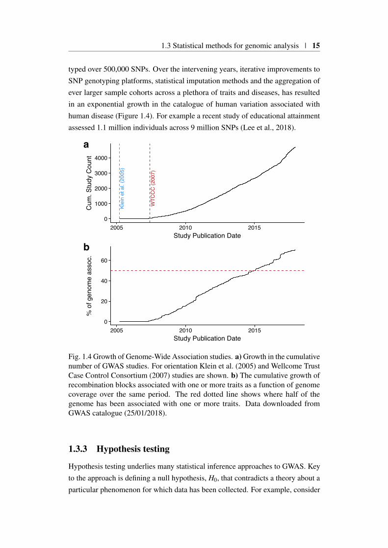
typed over 500,000 SNPs. Over the intervening years, iterative improvements toSNP genotyping platforms, statistical imputation methods and the aggregation ofever larger sample cohorts across a plethora of traits and diseases, has resultedin an exponential growth in the catalogue of human variation associated withhuman disease (Figure 1.4). For example a recent study of educational attainmentassessed 1.1 million individuals across 9 million SNPs (Lee et al., 2018).
WTC
CC
(200
7)
Klei
n et
al.
(200
5)
0
1000
2000
3000
4000
2005 2010 2015Study Publication Date
Cum
. Stu
dy C
ount
a
0
20
40
60
2005 2010 2015Study Publication Date
% o
f gen
ome
asso
c.
b
Fig. 1.4 Growth of Genome-Wide Association studies. a) Growth in the cumulativenumber of GWAS studies. For orientation Klein et al. (2005) and Wellcome TrustCase Control Consortium (2007) studies are shown. b) The cumulative growth ofrecombination blocks associated with one or more traits as a function of genomecoverage over the same period. The red dotted line shows where half of thegenome has been associated with one or more traits. Data downloaded fromGWAS catalogue (25/01/2018).
1.3.3 Hypothesis testing
Hypothesis testing underlies many statistical inference approaches to GWAS. Keyto the approach is defining a null hypothesis, H0, that contradicts a theory about aparticular phenomenon for which data has been collected. For example, consider

16 | Introduction
a random variable X with an observed value x, if the distribution of X under H0 isknown, H0 : X ∼ fX , then it is possible to associate a probability of observing avalue sampled from fX by
Pr(X = x | H0). (1.4)
More generally we might take repeated samples from fX , selecting a statistic,known as a ‘test’ statistic, in order to provide a summary of those repeatedsamples. In most contexts this test statistic is devised such that it has a knowndistribution under H0. Under the Neyman-Pearson approach, we partition thisknown H0 distribution, into values of the test statistic which are unlikely to beobserved if repeated samples of x are truly drawn from this distribution. Thispartition is called the critical region, and its probability is defined as α . If thesample test statistic, falls within this critical region, then H0 is rejected and thealternative, H1 is accepted. The value of α , is also known as the Type 1 errorrate as it equates to the probability of erroneously rejecting H0 when it shouldhave been accepted. The Neyman-Pearson approach also defines β , the Type IIerror rate, which, in contrast, reflects the probability of erroneously accepting H0,with it’s value relating to both sample size and the nature of H1. This approachto hypothesis testing is applied in a frequentist setting, where we assume that aparameter or test statistic of X has a true value, and that this is can be estimated byappropriate sampling from fx. This is in contrast to a Bayesian philosophy, thatassumes that the parameters are themselves random variables and as such havetheir own distributions. Thus, in the Bayesian setting, we instead estimate theposterior probability of H0,
Pr(H0 | X = x) =Pr(X = x | H0) Pr(H0)
Pr(X = x), (1.5)
which summarises how strongly H0 is supported by the observed value, x. Akey concept here is the requirement for selecting a prior probability for the nullhypothesis, Pr(H0) before observing x. This reflects our belief that H0 is not fixedbut is itself a random variable and as such has an associated probability of beingtrue. In the field of genetics, frequentist approaches are used more widely, incontrast to Bayesian approaches, which are used for pragmatic reasons, such asfor settings when sample size is small, there is a need to include prior informationor where we wish to compare non-nested hypothesis (Section 1.3.5).
1.3 Statistical methods for genomic analysis | 17
1.3.4 Frequentist approaches to genetic association testing
Generally, associations arise where we observe that one set of observations orevents is statistically dependent on another. Most statistical tests for associationutilise this dependence and examine the likelihood under the null hypothesis,H0 that the two events are truly independent. It is important to note that suchassociation tests in isolation cannot imply causality, a subject of debate outside thescope of this thesis. Tests of genetic association apply this principal of dependenceto the field of genetics, by examining whether a quantitative or binary outcome isdependent on exposure to one or more underlying genetic variants.
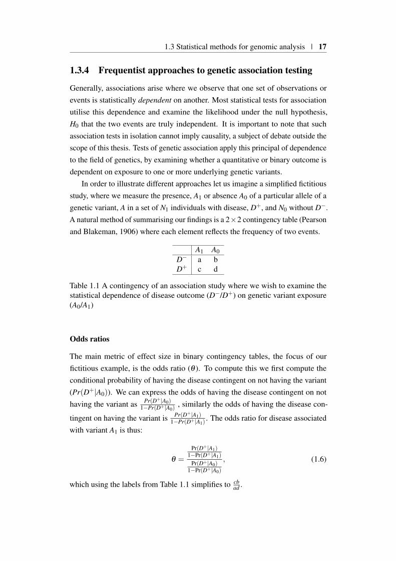
In order to illustrate different approaches let us imagine a simplified fictitiousstudy, where we measure the presence, A1 or absence A0 of a particular allele of agenetic variant, A in a set of N1 individuals with disease, D+, and N0 without D−.A natural method of summarising our findings is a 2×2 contingency table (Pearsonand Blakeman, 1906) where each element reflects the frequency of two events.
A1 A0D− a bD+ c d
Table 1.1 A contingency of an association study where we wish to examine thestatistical dependence of disease outcome (D−/D+) on genetic variant exposure(A0/A1)
Odds ratios
The main metric of effect size in binary contingency tables, the focus of ourfictitious example, is the odds ratio (θ ). To compute this we first compute theconditional probability of having the disease contingent on not having the variant(Pr(D+|A0)). We can express the odds of having the disease contingent on nothaving the variant as Pr(D+|A0)
1−Pr(D+|A0), similarly the odds of having the disease con-
tingent on having the variant is Pr(D+|A1)1−Pr(D+|A1)
. The odds ratio for disease associatedwith variant A1 is thus:
θ =
Pr(D+|A1)1−Pr(D+|A1)
Pr(D+|A0)1−Pr(D+|A0)
, (1.6)
which using the labels from Table 1.1 simplifies to cbad .
18 | Introduction
This estimate of effect size does not tell us whether this effect is significant,such that it is meaningfully different from the value we would expect if D andA were independent (i.e. θ = 1). In order for this we need to elucidate, givenour study size, the uncertainty attached to our estimate of the odds ratio (θ ). Thedistribution of θ is skewed towards values greater than one because low values areconstrained by zero whereas large values are not. This can be overcome by usingthe natural logarithm of θ such that β = log(θ). We can compute an approximation
of the standard error of β as σβ=√
1a +
1b +
1c +
1d , where a,b,c and d are the
counts from the joint distributions of our contingency table (Table 1.1). Under theassumption that sample size is large, the estimate of our odds ratio, θ , follows anormal distribution, allowing us to obtain a standardised Z score (Z = β
σβ
). Thistest statistic can then be used as the basis of a hypothesis test where under the nullβ = 0, which is rejected if the Z-score intersects with the critical region definedby α .
Testing for association in biallelic single nucleotide polymorphisms
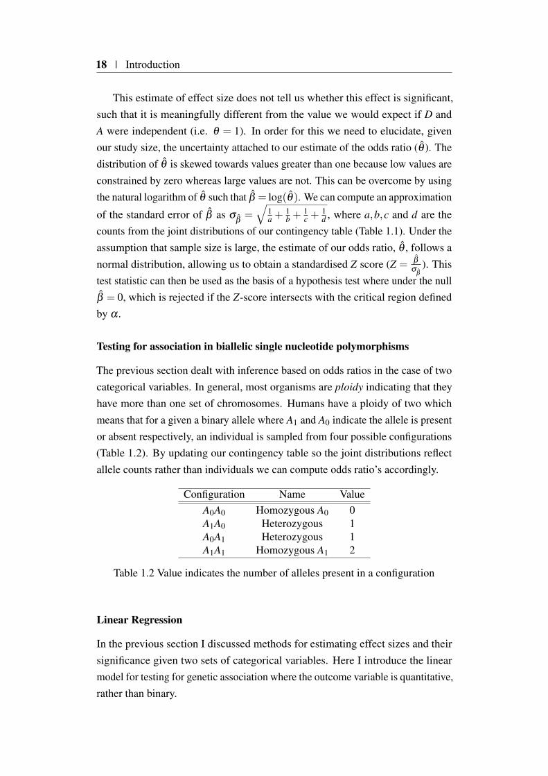
The previous section dealt with inference based on odds ratios in the case of twocategorical variables. In general, most organisms are ploidy indicating that theyhave more than one set of chromosomes. Humans have a ploidy of two whichmeans that for a given a binary allele where A1 and A0 indicate the allele is presentor absent respectively, an individual is sampled from four possible configurations(Table 1.2). By updating our contingency table so the joint distributions reflectallele counts rather than individuals we can compute odds ratio’s accordingly.
Configuration Name ValueA0A0 Homozygous A0 0A1A0 Heterozygous 1A0A1 Heterozygous 1A1A1 Homozygous A1 2
Table 1.2 Value indicates the number of alleles present in a configuration
Linear Regression
In the previous section I discussed methods for estimating effect sizes and theirsignificance given two sets of categorical variables. Here I introduce the linearmodel for testing for genetic association where the outcome variable is quantitative,rather than binary.
1.3 Statistical methods for genomic analysis | 19
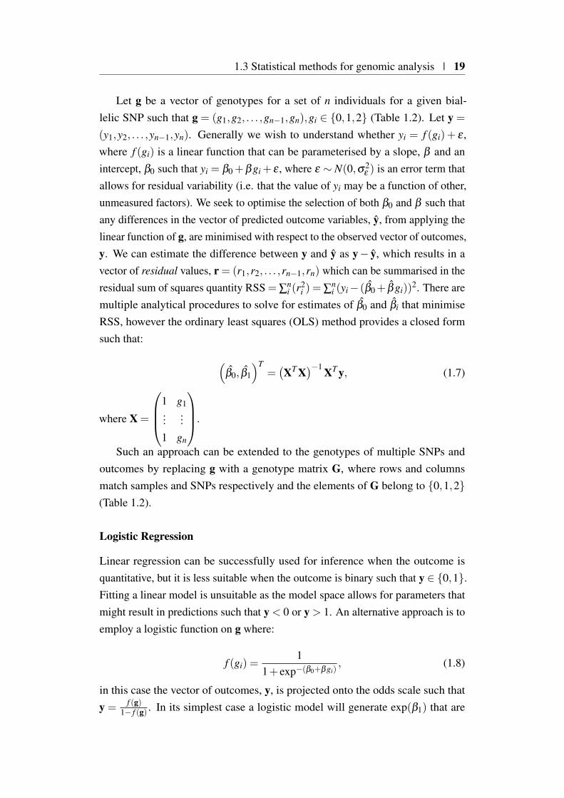
Let g be a vector of genotypes for a set of n individuals for a given bial-lelic SNP such that g = (g1,g2, . . . ,gn−1,gn),gi ∈ 0,1,2 (Table 1.2). Let y =
(y1,y2, . . . ,yn−1,yn). Generally we wish to understand whether yi = f (gi)+ ε ,where f (gi) is a linear function that can be parameterised by a slope, β and anintercept, β0 such that yi = β0 +βgi + ε , where ε ∼ N(0,σ2
ε ) is an error term thatallows for residual variability (i.e. that the value of yi may be a function of other,unmeasured factors). We seek to optimise the selection of both β0 and β such thatany differences in the vector of predicted outcome variables, y, from applying thelinear function of g, are minimised with respect to the observed vector of outcomes,y. We can estimate the difference between y and y as y− y, which results in avector of residual values, r = (r1,r2, . . . ,rn−1,rn) which can be summarised in theresidual sum of squares quantity RSS = ∑
ni (r
2i ) = ∑
ni (yi− (β0+ βgi))
2. There aremultiple analytical procedures to solve for estimates of β0 and βi that minimiseRSS, however the ordinary least squares (OLS) method provides a closed formsuch that:
(β0, β1
)T=(XT X
)−1 XT y, (1.7)
where X =
1 g1...
...1 gn
.
Such an approach can be extended to the genotypes of multiple SNPs andoutcomes by replacing g with a genotype matrix G, where rows and columnsmatch samples and SNPs respectively and the elements of G belong to 0,1,2(Table 1.2).
Logistic Regression
Linear regression can be successfully used for inference when the outcome isquantitative, but it is less suitable when the outcome is binary such that y ∈ 0,1.Fitting a linear model is unsuitable as the model space allows for parameters thatmight result in predictions such that y < 0 or y > 1. An alternative approach is toemploy a logistic function on g where:
f (gi) =1
1+ exp−(β0+βgi), (1.8)
in this case the vector of outcomes, y, is projected onto the odds scale such thaty = f (g)
1− f (g) . In its simplest case a logistic model will generate exp(β1) that are
20 | Introduction
equal to the odds ratio computed using simpler methods previously described. Itsmain utility is in its ability to incorporate other covariates and nuisance parametersby the addition of terms to the linear predictor.
1.3.5 Bayesian approaches to genetic association testing
Canonical frequentist approaches described in Section 1.3.4 have an importantlimitation in that their currency, the p-value is unable to capture how confidentwe are that a SNP is truly associated with a trait (Stephens and Balding, 2009).Conversely a Bayesian posterior provides a strength of evidence for a givenhypothesis albeit with additional assumptions and computational burdens. Suchposterior probabilities naturally allow the comparison of different hypothesis andlead to a Bayesian interpretation of hypothesis testing, central to this are theconcept of Bayes factors.
Bayes Factors
In 1935 Harold Jeffreys described how Bayes theorem could be used to comparecompeting hypotheses (Jeffreys, 1973). As an illustrative example, consider twohypothesis H0 and H1, representing the null and alternative respectively. Giventhe observation of some data, D, we compute posterior probabilities Pr(H0|D) andPr(H1|D). We are interested in the relative support for H1 compared to H0 whichcan be expressed as a quantity known as the Bayes Factor.
BF =Pr(H1|D)
Pr(H0|D). (1.9)
If we define the prior odds as Pr(H1)Pr(H0)
, then Pr(H1|D)Pr(H0|D) , the posterior odds (PO) can
be expressed byPO = BF×prior odds,
as set out by Kass and Raftery (1995).In the context of a case/control setting, let θ be the odds ratio for a given
SNP under additive assumptions, and let β = log(θ), we may assume that β = 0and β ∼ N(0,W ) for some specified W under H0 and H1 respectively. Thus weconstruct the Bayes factor as:
BF =Pr(D|β ∼ N(0,W ))
Pr(D|β = 0). (1.10)

1.3 Statistical methods for genomic analysis | 21
Here, W can be estimated from one of the frequentist approaches previouslymentioned.
Wakefields asymptotic Bayes Factors
In three papers (Wakefield, 2007, 2008, 2009) Wakefield introduced an asymptoticBayes Factor (aBF), for use in association studies, with a simple closed form,requiring as input only the maximum likelihood estimate of β and its varianceV . Such an approach was not only computationally tractable but circumventedthe considerable difficulties in obtaining genotype level information, as it couldbe computed from summary level statistics (e.g. p-values or odds ratios andtheir standard errors). The aBF relies on a normal prior N(0,W ) on β . For adichotomous trait a value of W = 0.2 has been suggested (Giambartolomei et al.,2014) as this approximates to a Pr(θ > 1.4|θ < 1.4−1) of 5 %. This prior whencombined with the assumption that maximum likelihood estimate of β is sampledfrom a normal distribution N(β ,V ) yields:
aBF =
√V +W
V× exp
(− z2W
2(V +W )
)(1.11)
where z2 is the Wald statistic β 2
V .
Fine mapping using asymptotic Bayes Factors
The Wellcome Trust Case Control Consortium et al. (2012) show that under thescenario of a single causal variant within a given genomic region containg k SNPs,then the Bayes factor for that region to be causal is the mean of the individualBayes Factors for all the SNPs in the region,
BFreg =1k
k
∑i=1
BFi, (1.12)
where BFi is the Bayes factor associated with the ith SNP being causal, which canbe approximated by aBFi introduced in the previous section. Furthermore theydefine the single causal variant posterior probability for ith SNP, which substitutingfor aBF becomes
22 | Introduction
sCVPPi ≈aBFi
kaBFreg
≈ aBFi
∑kj=1 aBF j
. (1.13)
However such a relationship does not consider the case where there are no causalvariants within the region. To do this we must alter the definition of BFreg, toinclude a term for the Bayes factor associated with a model containing no causalvariants or Pr(D|H1)
Pr(D|H0)= 1 such that
sCVPPi ≈aBFiπ(
π ∑kj=1 aBF j
)+π0
, (1.14)
where π and π0 are the prior probabilities for a SNP to be causal or not causalrespectively. Under the assumption that π is small with respect to k then weapproximate π0 = 1− kπ ≈ 1 leading to
sCVPPi ≈aBFiπ(
π ∑kj=1 aBF j
)+1
. (1.15)
Therefore under the strong assumptions, that a given physical region containsa single causal variant, we can define single causal variant posterior probabilities(sCVPP) for each a SNP. By ordering and taking the cumulative sum of these pos-terior probabilities we can compute credible sets of SNPs that incorporate a givenamount of posterior probability (e.g. 95%). In some cases given well poweredstudies and dense genotyping or imputation this can lead to the identification ofsingle variants upon which the overwhelming majority of the posterior probabilityis focused, which are then amenable to empirical follow up (Huang et al., 2017).
1.3.6 Approaches to high dimensional data
In previous sections I have focused on inference, however statistical approaches arealso concerned with describing and summarising the structure of high dimensionaldata such as arises from GWAS. Such high dimensional data occurs where thenumber of observations or predictors, p is much larger than the sample size n,resulting in the so called curse of dimensionality; as p increases so does the volumeof the space from which our n are sampled, resulting in increased sparsity. If p farexceeds n, as is usual in genomics, then this sparsity is such that robust inference is
1.3 Statistical methods for genomic analysis | 23
challenging. Statistical approaches in this area concern themselves with three mainapproaches, feature selection, shrinkage (transformation) and extraction (Hastieet al., 2009).
Feature Selection: These are approaches that seek to uncover a subset of thepredictors or features that are of relevance to the outcome variable(s). Ex-amples include forward stepwise selection, where predictors are recursivelyadded to a model, and retained only if they improve model performance.
Feature Shrinkage: Shrinkage approaches are concerned with fitting a modelwith all predictors whilst constraining coefficient estimates. An example ofsuch an approach is ridge regression, which modifies conventional regressionapproaches (Section 1.3.4), that minimise residual sum of squares, to includea shrinkage parameter, that penalises larger coefficients. Although suchan approach improves model performance, its interpretation compared tofeature selection methods is challenging as the coefficients of predictors arestill non-zero. This has lead to the development of alternative approachessuch as the lasso that perform shrinkage, allowing for zero coefficientestimates.
Feature Extraction: This final class of approaches seeks to transform the predic-tors available in high dimensional datasets in order to derive a much smallernumber of features that provide useful summaries of any structure that maybe apparent within the data. In most cases, derived features consist of linearcombinations of the the original features, therefore reducing the numberof dimensions that need to be considered. One of the main approaches isprincipal component analysis (PCA), which I discuss further in the nextsection.
1.3.7 Principal component analysis (PCA)
Consider A a matrix of n observations across p variables where p >> n. In sucha situation, it is desirable to obtain a representation that summarises A using areduced number of variables. PCA is one method that achieves this by concen-trating the variance across all p into independent principal components usingeigen-decomposition of the covariance matrix, C = AT A. Eigen-decomposition isthe process of factorising a square diagonisable matrix, such as C into an orthogo-nal set of p eigenvectors, v, and p eigenvalues, λ , such that Cv = λv. Thus, C or
24 | Introduction
indeed A when applied to an eigenvector only shrinks or elongates the eigenvectorby the magnitude of the corresponding eigenvalue. These eigenvectors are linearcombinations of the original variables that are ordered by the amount of variancethey capture, the magnitude of which is captured by the corresponding eigenvalue.This allows dimension reduction as we can select a subset of the p eigenvectors,that capture a majority of the variance in A to take forward for analysis.
18
99
0
100
0 100X
Y
a18
99
0
100
0 100X
Y
b
18
99
0
100
0 100X
Y
c
18
99
−100
−50
0
50
−100 −50 0 50 100PC1
PC2
d
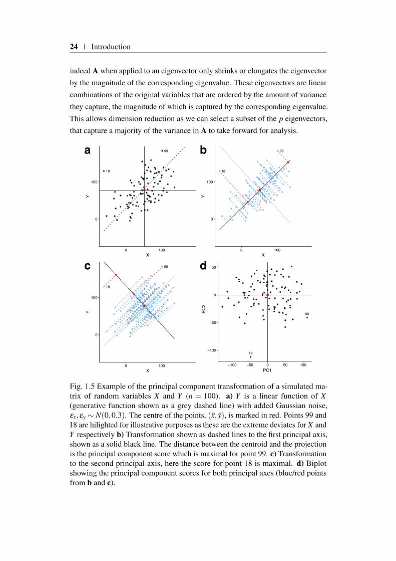
Fig. 1.5 Example of the principal component transformation of a simulated ma-trix of random variables X and Y (n = 100). a) Y is a linear function of X(generative function shown as a grey dashed line) with added Gaussian noise,εx,εy ∼ N(0,0.3). The centre of the points, (x, y), is marked in red. Points 99 and18 are hilighted for illustrative purposes as these are the extreme deviates for X andY respectively b) Transformation shown as dashed lines to the first principal axis,shown as a solid black line. The distance between the centroid and the projectionis the principal component score which is maximal for point 99. c) Transformationto the second principal axis, here the score for point 18 is maximal. d) Biplotshowing the principal component scores for both principal axes (blue/red pointsfrom b and c).

1.3 Statistical methods for genomic analysis | 25
Figure 1.5a illustrates this point, showing the simple case of a two-dimensionalprojection of a set of points onto two possible principal component axes. Here,matrix v, becomes the axes, for a new coordinate system or basis. To transform Aonto this new basis we compute Av, illustrated as dashed lines connecting originalpoints to the principal axes (bold lines) in Figure 1.5b (1st principal axis) andFigure 1.5c (2nd principal axis).
For this simple case, we observe that there are two such principal axes orcomponents (as there are two variables), that have two notable relations to eachother. Firstly both axis share the same origin (x,y), which leads to an alternativeviewpoint of PCA as an optimisation problem that seeks to find the set of k
dimensions (where k ≤ p) that minimise the euclidean distance between a setof points. The centroid can be thought of as the zeroth principal axis serving asthe origin linking all k dimensions. This constraint enforces the second notablerelation, that any k is orthogonal to any other k, such there is no shared variancebetween any k. As the total variance, the trace of C, is constrained this meansthat each subsequent k captures less variance than the previous. Indeed ∑λ =
tr(C), where λ are elements of the vector of eigenvalues obtained from eigen-decomposition of C and it is this relation that allows us to compute the ratioof variance explained by each principal axis. The distance of the projection(blue/red points) on the principal axis (bold) from the centroid are the principalcomponent ‘scores’ for each sample. We can plot these scores in a ‘biplot’ (Figure1.5d) to obtain a graphical summary of the sample, here PC1 and PC2 captureapproximately 60% and 40% of the total variance respectively.
In this case the PCA is for illustrative purposes only as n > p it has no benefitover a simple scatter plot. Careful thought needs to be given to how input variablesare scaled, for example if one variable is measured in metres and another inkilometres then it will appear that the former has a higher variance. As PCAoptimises variance between variables this will unintentionally cause the variablemeasured in metres to have a much greater effect on the basis generated. Onemethod to overcome this is to standardise the variables by mean-centring anddividing through by the variance, thus performing PCA on the correlation ratherthan variance-covariance matrix (i.e. C).
Whilst eigen-decomposition of the variance-covariance matrix, C is onemethod of performing PCA, in practice it is computed through the singular valuedecomposition of A as detailed in Appendix C.1. This approach has multiplebenefits in that it does not require the computationally intensive calculation of thevariance-covariance matrix, and the loss in precision this can involve.
26 | Introduction
1.4 Towards causal mechanisms in immune-mediateddisease
In the first section I described various high-throughput genomic methods that havebeen developed to interrogate the context-specific mechanisms by which genescan be regulated with a focus on chromatin organisation. I introduced GWAS andrelated statistical approaches that have been used to identify regions of the genomeharbouring risk SNPs for common complex disease. Here, I expand (Section 1.2.5)on the evidence that integrating GWAS data, both across related traits, and withother sources of high-throughput data is essential to understanding the molecularmechanisms that ultimately modulate complex disease risk. I propose that suchknowledge is useful as it could be used to augment or replace disease classificationstraditionally based on clinical phenotypes, with more mechanistic ones recognisingthe blurred lines that often separate related diseases. For the purposes of thisthesis I concentrate on a smaller subset of related phenotypes, incorporatingautoinflammatory and autoimmune diseases that I unify under the umbrella termimmune-mediated disease (IMD).
1.4.1 Epidemiology of immune-mediated disease
A key property of the adaptive immune system is the ability to recognise pathogensfrom self-antigens. Dysregulation of this process results in damage to healthytissues, autoimmunity and auto-inflammation. Currently, over 80 diseases havebeen found to have an underlying immune-mediated pathogenesis, with approxi-mately half presenting as rare diseases, defined as affecting 5 people or fewer in10,000 (Hayter and Cook, 2012). The collective health burden of more commonIMDs such as type 1 diabetes (T1D), rheumatoid arthritis (RA), inflammatorybowel disease (IBD) and multiple sclerosis (MS) is high with approximately 7 - 9%of the European population affected (Cooper et al., 2009). Although environmentis a contributing factor in disease susceptibility, the genetic heritability, definedas the proportion of phenotypic variance (Section 1.3.1) attributable to geneticvariability, is also important, ranging from 0.39 in primary biliary cirrhosis (PBC)to 0.9 in ankylosing spondylitis (AS) (Gutierrez-Arcelus et al., 2016).

1.4 Towards causal mechanisms in immune-mediated disease | 27
1.4.2 Genetics of of immune-mediated disease
It was in the early 1970’s that a role for the human leukocyte antigen (HLA)region was first suggested in ankylosing spondilitis (AS) (Brewerton et al., 1973),and to this day the HLA-B27, class I association with this disease remains thestrongest HLA effect of all IMDs. Subsequent work identified a role for the class IIHLA-DQβ in modulating risk for T1D (Todd et al., 1987), and in the interveningyears associations across a majority of IMDs have been mapped to this region.Such relationships provide significant insight into putative disease processes giventhat IMDs can be roughly dichotomised as having a predominantly class I or classII disease association (Parkes et al., 2013). Class I HLA associated diseases, whichinclude psoriasis and AS, seldom share associated alleles and are predominantlyseronegative, that is they are not associated with specific auto-antibodies. Incontrast those characterised by associations in the class II HLA region, whichinclude T1D and systemic lupus erythematosus (SLE), often share risk allelesbut associate with specific auto-antibodies (e.g. anti-neutrophilic cytoplasmicautoantibody for SLE) and are thus predominantly seropositive. Furthermore, suchseropositive disease are often found to have associations proximal to genes thatare the targets of their autoantibodies, for example INS in T1D (Bell et al., 1984)and insulin auto-antibodies. In the intervening years with the advent of GWAS,hundreds of regions of the genome have now been associated with one or moreIMDs, and detailed analysis supports a central role for both the adaptive and innateimmune system in IMD susceptibility, supported by a more limited number ofdisease-specific loci. Such a wealth of new data has lead to a more systematicanalyses of whether associations are shared or distinct between distinct IMDs.
1.4.3 Immune-mediated diseases have both shared and distinctgenetic architectures
Evidence for co-morbidity between autoimmune and auto-inflammatory diseaseshas long been observed. For example, between 4 and 9% of individuals withT1D are also affected by coeliac disease (CEL) (Somers et al., 2006) comparedto a general population incidence of 0.8% (Choung et al., 2017). In the era ofGWAS it has been possible to examine both genome-wide and locus specificevidence for genetic overlap between immune-mediated diseases. An early studyexamining whether a genetic overlap could be responsible for the co-morbiditybetween T1D and CEL found evidence for overlap at 7 out of 28 regions showing
28 | Introduction
association in either disease (Smyth et al., 2008). Interestingly, two of theseoverlapping loci, located at 2q12 and 6q25, demonstrated opposing effects betweenthe two diseases. Following up on this, Cotsapas et al. (2011) found evidence forpervasive sharing across seven immune-mediated diseases. These early studieswere limited by sample size and the genotyping platforms on which they wereconstructed, which were conceived to cover, by exploiting linkage disequilibriumin European populations, as much common variation as possible. Without densergenotyping maps it was therefore difficult to elucidate trait-specific fine scalegenetic architecture, and thus whether the overlap observed was due to the sharingof causal variants or different variants in genomic proximity.
With this in mind a consortium of 11 immune disease mediated traits, pooledboth established and emerging associated regions, mining the developing 1000Genomes resource (1000 Genomes Project Consortium et al., 2015), to obtain allavailable variants observed with a minor allele frequency above 1% in Europeanpopulations local to known IMD associations. This compendium of approximately186 densely genotyped regions, assaying approximately 200,000 SNPs, formedthe backbone for a new bespoke genotyping platform, the ImmunoChip, whichcould be used to fine map existing associations (Cortes and Brown, 2011) at anunprecedented resolution.
This dense mapping, showed that although there was extensive sharing betweenIMD risk loci as had been suggested by GWAS, the picture was more complex thaninitially suggested (Parkes et al., 2013). Whilst associated ImmunoChip regionswere shared between diseases, a number exhibited opposing effects, conferringrisk in one disease but protection in another. Focusing on T1D, Onengut-Gumuscuet al. (2015) collected summary statistics for an additional 15 IMDs that hadbeen analysed using the ImmunoChip platform into the ImmunoBase resource3.Using an enrichment method that controlled for LD, they were able to robustlydemonstrate, within T1D-associated ImmunoChip regions, an enrichment patternthat discriminated between antibody positive and negative diseases as previouslysuggested (Parkes et al., 2013). Fortune et al. (2015) adapted a pre-existingstatistical colocalisation method, coloc (Giambartolomei et al., 2014), to showrobust evidence for the sharing of causal variants at over a third of the associatedregions analysed. However the picture of phenotypic and genetic sharing betweendiseases is complex, for example Fortune et al. (2015), highlighted three regions,associated with T1D but not with other autoimmune diseases, that instead showed
3https://www.immunobase.org

1.4 Towards causal mechanisms in immune-mediated disease | 29
overlap with type 2 diabetes. This observation has subsequently been extended tofive T1D/T2D regions where evidence suggests a shared causal variant (althoughin one region opposing effects) by a more recent study (Aylward et al., 2018).Even within IMD, shared genetic architecture is complex, for example psoriaticarthritis and RA show relatively little genetic overlap even though treatment withanti-TNF therapy is effective in both indications (Eyre et al., 2017). Understandingsuch results biologically is hampered as whilst GWAS are effective at identifyingassociated variants, elucidating the mechanism by which they act has proved farmore challenging.
1.4.4 Integrating functional genomics with GWAS
Having found convincing associations and assessed their overlap between diseasesfor IMD densely mapped regions, it was clear that a majority of associated variantsexisted outside of the regions of the genome coding for proteins, a theme commonto complex disease (1000 Genomes Project Consortium et al., 2015; Mauranoet al., 2012).
In a landmark paper Farh et al. (2015), developed PICS, an attempt to uselead variants retrieved from the GWAS catalogue (MacArthur et al., 2017), incombination with the 1000 genomes reference panel, to fine map associationsignals in the absence of dense genotyping information. They integrated theseresults with empirically derived markers for active regulatory chromosome regionsacross 33 cell types from the Epigenome Roadmap project (Roadmap EpigenomicsConsortium et al., 2015). This showed that candidate causal variants were en-riched in a trait and cell type specific manner within such regulatory regions. Forexample, putative causal variants for IMDs were enriched in lymphoid specificregulatory regions, a result that was subsequently confirmed in a study of T1Dusing credible sets of SNPs (Section 1.3.5) derived from ImmunoChip densegenotype data (Onengut-Gumuscu et al., 2015).
Although this integrative approach could be used to prioritise target cell typesand regulatory regions, this was offset against a growing understanding of thecomplexity underlying cell type specific gene regulation. Importantly this reg-ulatory complexity challenged the established doctrine of the prioritisation ofcausal candidate genes through the ad hoc combination of being physically locatedwith an associated region and having relevant biology (for specific examples seeSection 1.2.5).

30 | Introduction
One systematic approach to link causal variants to their target genes is toelucidate the genetic architecture underlying gene expression, through expressionquantitative trait locus (eQTL) studies. Guo et al. (2015) used a statistical method,coloc (Giambartolomei et al., 2014), to look for colocalisation between eQTLsidentified from a study of three primary immune cell types with GWAS summaryresults for 10 immune-mediated traits tissues. Interestingly, they found onlylimited overlap, describing convincing statistical colocalisation in only six genes.A more recent study employing a Mendelian randomisation approach to connecteQTL and GWAS studies also found limited evidence for colocalisation betweeneQTLs (Zhu et al., 2016) within immune-mediated traits (Huang et al., 2017).Such a lack of colocalisation within IMD, is most likely explained by the fact thateQTL studies are expensive and technically demanding to carry out, limiting notonly sample size and thus power, but also the breadth of tissue contexts that canbe assayed. More recent studies are beginning to highlight the role of underlyingtissue contexts underlying IMD causal variant mechanisms (Alasoo et al., 2018;Soskic et al., 2019).
The overarching conclusion of the integrative studies highlighted is that with-out an understanding of the tissue context within which causal variants, identifiedthrough association studies, act, elucidation of underlying causal mechanisms ischallenging.
1.4.5 Towards a mechanistic taxonomy of immune-mediateddisease
Whilst, the systematic translation of GWAS results to causal mechanisms hasproved challenging, the distinct and shared genetic architectures between differentIMDs present an opportunity to organise diseases based on shared molecularphenotypes. Indeed, medicine is to some extent, through the application ofdiagnostic labels, a systematic categorisation of disease-causing phenotypes. Inthe past this clustering of individuals sharing clinical features, and pathologieshas provided both insight into disease aetiology as well as the development ofevidence based treatment options (McCarthy, 2017). As a consequence manydiseases are currently classified by their presentation, which in the case of IMDs,is often a proxy for target destruction (e.g. T1D and insulin producing pancreaticβ -cells). However in previous sections I have described how, at least at a the levelof genetic risk, a more complex picture has emerged, such as in T1D where acentral role for adaptive immune system dysregulation interfaces with biological
1.5 Organisation of the thesis | 31
pathways influencing β -cell function that are themselves shared with Type 2diabetes. Such pervasive sharing between IMDs (Cotsapas et al., 2011; Fortuneet al., 2015; Gutierrez-Arcelus et al., 2016; Li et al., 2015; Parkes et al., 2013)provides scientific support for a new taxonomy of IMDs such as that suggested overa decade ago by McGonagle and McDermott (2006), that recognises that IMDs fallon a spectrum that at its extremities separates auto-inflammatory and autoimmunediseases. However the further development of such a taxonomy depends onfirst gaining a greater understanding of the underlying causal mechanisms andpathways at work. Such an effort is already well underway, with much progressbeing in made in the fine-mapping of causal variants (Asimit et al., 2019; Huanget al., 2017; Wallace et al., 2015; Wang et al., 2018), however as set out in theprevious section such information needs to be integrated with other sources ofgenomic information, in order to suggest causal genes and tissues, critical foruncovering disease mechanisms. Uncovering mechanism for individual causalvariants is only part of the story, as these then need to be integrated with existingknowledge to identify biological pathways that might be shared across multipleassociated regions (Evangelou et al., 2014; Raychaudhuri et al., 2009; Rossin et al.,2011; Võsa et al., 2018). This suggests that approaches at the causal variant scale,as well as more holistic approaches that consider the full spectrum of IMD geneticarchitectures, are likely to be syntergistic in attempts to develop a therapeuticallyuseful molecular taxonomy of disease aetiology.
1.5 Organisation of the thesis
In this thesis I develop novel methods and apply them to IMD genomic andgenetic datasets in order to better understand causal mechanisms and how atthe genome level these are shared and distinct between different diseases. Inchapters 2 and 3 I develop methods to integrate novel data on three dimensionalgenome organisation with data from GWAS. These methods allow a data drivenprioritisation of putative causal genes and tissue contexts in which they operate. Inchapter 4 I develop a PCA dimension reduction technique to in order to summarisethe genetic relationships between ten IMDs using GWAS summary statisticsas input. Amongst other applications, I investigate whether such summarieshave utility in teasing apart the genetic architecture of a clinically heterogeneousjuvenile idiopathic arthritis (JIA) cohort, of modest sample size.
32 | Introduction
1.6 Publications
During this thesis I have contributed to a number of publications which havearisen either directly or indirectly from the work contained in this thesis. Whereapplicable these are referenced in each relevant chapter, but I list them here forcompleteness.
• Schofield, E. C., T. Carver, P. Achuthan, P. Freire-Pritchett, M. Spivakov,J. A. Todd, and O. S. Burren (2016). CHiCP: a web-based tool for theintegrative and interactive visualization of promoter capture Hi-C datasets.Bioinformatics 32(16), 2511–2513.Initial concept, co-developed the software and wrote the paper.
• Javierre, B. M.*, O. S. Burren*, S. P. Wilder*, R. Kreuzhuber*, S. M. Hill*,S. Sewitz,J. Cairns, S. W. Wingett, C. Várnai, M. J. Thiecke, F. Burden, S.Farrow, A. J.Cutler, K. Rehnström, K. Downes, L. Grassi, M. Kostadima,P. Freire-Pritchett,F. Wang, BLUEPRINT Consortium, H. G. Stunnenberg,J. A. Todd, D. R. Zerbino, O. Stegle, W. H. Ouwehand, M. Frontini, C.Wallace, M. Spivakov, and P. Fraser (2016). Lineage-Specific GenomeArchitecture Links Enhancers and Non-coding Disease Variants to TargetGene Promoters. Cell 167(5),1369–1384.e19.Method development and analysis described in Chapters 2 and 3, contributedto writing the paper.
• Burren, O. S.*, A. Rubio García*, B.-M. Javierre*, D. B. Rainbow*, J.Cairns, N. J.Cooper, J. J. Lambourne, E. Schofield, X. Castro Dopico, R.C. Ferreira, R. Coulson, F. Burden, S. P. Rowlston, K. Downes, S. W.Wingett, M. Frontini, W. H.Ouwehand, P. Fraser, M. Spivakov, J. A. Todd,L. S. Wicker, A. J. Cutler,and C. Wallace (2017). Chromosome contactsin activated T cells identify autoimmune disease candidate genes. GenomeBiology 18(1), 165.Method development and analysis described in Chapters 2 and 3, co-wrotethe paper.
• Inshaw, J. R. J., A. J. Cutler, O. S. Burren, M. I. Stefana, and J. A. Todd(2018). Approaches and advances in the genetic causes of autoimmunedisease and their implications. Nature Immunology 19(7), 674–684.Performed analysis using methods detailed in Chapter 2 to prioritise type 1diabetes candidate genes.
• Eijsbouts, C. Q., O. S. Burren, P. J. Newcombe, and C. Wallace (2019,January). Fine mapping chromatin contacts in capture Hi-C data. BMCGenomics 20(1), 77.This paper describes an alternative statistical method to CHiCAGO forcalling promoter interacting regions resulting in a posterior probability foreach interaction. I Investigated whether incorporation of these posterior

1.6 Publications | 33
probabilities with the method described in chapter 2 could improve candidategene prioritisation.
• Thaventhiran, J. E. D.*, H. L. Allen*, O. S. Burren*, J. H. R. Farmery, E.Staples, Z. Zhang, W. Rae, D. Greene, I. Simeoni, J. Maimaris, C. Penkett,J.Stephens, S. V. V. Deevi, A. Sanchis-Juan, N. S. Gleadall, M. J. Thomas,R. B. Sargur, P. Gordins, H. E. Baxendale, M. Brown, P. Tuijnenburg, A.Worth,S. Hanson, R. Linger, M. S. Buckland, P. J. Rayner-Matthews, K. C.Gilmour, C. Samarghitean, S. L. Seneviratne, P. A. Lyons, D. M. Sansom,A. G. Lynch, K. Megy, E. Ellinghaus, D. Ellinghaus, S. F. Jorgensen, T.H. Karlsen, K. E.Stirrups, A. J. Cutler, D. S. Kumararatne, S. Savic, S. O.Burns, T. W. Kuijpers, E. Turro, W. H. Ouwehand, A. J. Thrasher, and K. G.C. Smith (2018). Whole Genome Sequencing of Primary Immunodeficiencyreveals a role for common and rare variants in coding and non-codingsequences. bioRxiv (Under revision).Performed analyses to elucidate novel causes of Primary Immunodeficiencyand co-wrote the paper.
* indicates equal contribution.


Chapter 2
Detecting tissue specific enrichmentof GWAS signals in PCHi-C data
2.1 Foreword
2.1.1 Chapter Summary
In this chapter I introduce a promoter capture Hi-C dataset (PCHi-C) covering 17primary haematopoietic cell types (Javierre et al., 2016). I compile a compendiumof univariate GWAS summary statistics across 31 traits, proposing a simple LDbased method, Poor Man’s Imputation (PMI), in order to impute missing data.To assess whether the tissue and trait specific enrichment of GWAS associationsreported in the literature (Farh et al., 2015; Onengut-Gumuscu et al., 2015) can bereplicated using context specific PCHi-C annotations I develop a novel statisticalmethod, blockshifter, that takes into account the correlation inherent in both GWASand PCHi-C datasets. Through simulation I assess blockshifter performance underdifferent assumptions and conditions. I conclude by presenting the results of theapplication of blockshifter to the GWAS compendium.
2.1.2 Attributions
Parts of the work presented in this chapter are included in Javierre et al. (2016)and Burren et al. (2017) and were carried out collaboratively with Fraser, Spi-vakov, Ouwehand and Diabetes and Inflammation Laboratories as part of theBLUEPRINT/IHEC project (Stunnenberg and Hirst, 2016). Specifically:-
• Dr. Mattia Frontini and Dr. Tony Cutler supplied sorted primary cells.

36 | Detecting tissue specific enrichment of GWAS signals in PCHi-C data
• Dr. Biola Marie-Javierre, under the supervison of Prof. Peter Fraser carriedout all promoter-capture Hi-C experiments.
• Dr. Steven Wingett carried out initial sequence data processing using theHiCUP pipeline (Wingett et al., 2015).
• Dr. Jonathan Cairns and Dr. Mikhail Spivakov supplied PCHi-C chromatincontact maps called using the CHiCAGO pipeline (Cairns et al., 2016).
• Dr. Chris Wallace helped with the conceptualisation of PMI, blockshifter
and simulation design.
2.1.3 Motivation
In chapter 1 I described how variants associated with common disease, are enrichedin non-coding regions of the genome with putative tissue specific gene regulatoryfunction, in a disease relevant manner. One mechanism for the action of suchregulatory regions is through the formation of physical chromatin interactions withtheir target gene promoters. However, the overall relevance of such a mechanism tounderlying disease processes is currently unknown. One line of evidence for sucha contribution is through the demonstration of the enrichment of disease associatedvariants in a tissue specific manner, using PCHi-C data. Most published GWASfunctional enrichment methods focus on allowing for local correlation structurecaused by LD. However, PCHi-C datasets contain significant local structure thatmust be taken into account. This motivated me to develop a novel statisticalmethod for examining GWAS enrichment in promoter interacting regions (PIRs)that explicitly takes into account this structure, whilst also taking into account LD.
2.1.4 Software availability
PMI and blockshifter methods described in this chapter are available from https://github.com/ollyburren/CHIGP and blockshifter simulations are available fromhttps://github.com/ollyburren/blockshifter_simulations. Both are available underGNU General Public License v3.0.
2.2 Background
Understanding the tissue context in which disease associated variants function canprovide important information for the design of follow up functional experiments.

2.2 Background | 37
In Chaper 1, I touched on various analyses that integrate GWAS with tissue specificgenome annotations in order to prioritise relevant tissue contexts (Farh et al., 2015;Maurano et al., 2012; Onengut-Gumuscu et al., 2015) which I expand upon here.
2.2.1 Gene set enrichment analysis inspired methods
Early software tools for analysing the enrichment of GWAS association signals inspecific functional annotations, built on methodologies such as gene set enrichmentanalysis (GSEA) (Subramanian et al., 2005), developed to analyse high throughputgene expression datasets. In the context of GWAS, a set of genes with some sharedfunctional annotation is selected, for example, those sharing a common GeneOntology (GO) term (Ashburner et al., 2000). Variants are then assigned to geneson the basis of proximity, with the most significant association within a fixedgenomic window surrounding a gene being taken forward for analysis (Wang et al.,2007). This yields two sets of association p-values; those mapping to genes in thefunctional annotation to be assayed and the other mapping to a set of backgroundgenes, that do not. In the example of Wang et al. (2007) the non-parametricKolmogorov-Smirnov test is then used to examine whether both sets of associationp-values are drawn from the same distribution, to infer enrichment. Recognisingthe need to adjust for confounders such as gene size and LD, the procedure aboveis repeated a number of times using a set of association statistics generated fromshuffling case/control assignment. This permutation step has drawbacks in that itrequires access to the underlying genotype data and is computationally intensive,however it does allow the generation of a well specified null distribution of teststatistics which is critical in order to suitably adjust the observed test statistic.
In order to remove the requirement of individual genotyping data, Liu et al.(2010), used the publicly available HapMap reference genotype data set (Inter-national HapMap Consortium et al., 2007) to define local LD structure betweenvariants for approximately independent LD blocks. This LD across each block isthen used as the covariance matrix, Σ, for a multivariate normal (MVN) distribu-tion, such that Z ∼ MVN(0,Σ), which can be used to rapidly generate summaryassociation statistics under the null hypothesis of no association. Such an approachallows the generation, genome-wide, of a background distribution of summaryassociation statistics, that take into account local correlation structure due to LD.This obviates the need for study-specific individual genotyping data, requiringonly summary association statistics for the trait of interest, for which enrichmentis to be assessed.
38 | Detecting tissue specific enrichment of GWAS signals in PCHi-C data
Early efforts to characterise enrichment in specific classes of genome annota-tions, whilst finding plausible enrichment (Maurano et al., 2012), were challengingto confidently interpret. This was mainly due to the reliance on parametric en-richment methodologies that were less robust to local interdependencies withinclasses of genomic annotations. For example, the base composition of a genomicregion may correlate with empirical techniques, underlying an annotation, such asChIP-seq (Benjamini and Speed, 2012). Such phenomena introduce complicatedlocalised correlation structures within an annotation, that lead to an inflation inenrichment statistics generated if they are not explicitly accounted for.
Another limiting factor was that in order to increase trait coverage by us-ing curated databases of robustly associated trait variants, such as the GWAScatalogue (MacArthur et al., 2017), implicit thresholds were applied, as suchcatalogues build on findings curated from the literature, rather than the full set ofGWAS summary statistics for a given trait. This thresholding not only precludedthe incorporation of potentially informative sub-genomewide results (Schork et al.,2013), but also reduced resolution, and depending on the size distribution of anno-tation classes being examined lead to challenges in non-biased variant assignment.
Another consideration of thresholding is ascertainment bias, or so calledwinner’s curse (Xiao and Boehnke, 2009). Let β be the natural logarithm ofthe population odds ratio at a given SNP, and β its sample estimate, it followsthat E(β ) = β , however when a threshold, α ′, is applied to β we observe that
E(β | |β |> α ′) = β , here α ′ is chosen such that α = 1−2Φ
(|β |σ
β
)is the required
significance threshold ( where Φ is the integral of the pdf of the normal distributionand σ
βis the standard error of β ). This occurs in the context of an under powered
analysis where the effect size at the declared associated SNP will tend to be moreextreme by chance than its true value, conversely, truly associated SNPs, witheffect sizes less extreme by chance, will tend not to be declared associated.
Various methods for integrating GWAS with functional annotations that over-come some of these inherent challenges have been suggested. These can roughlybe divided into three approaches, which I describe in detail in the followingsections.
2.2.2 Matched SNP sets methods
In a matching approach, SNPs in the functional annotation of interest are matched,by various confounding characteristics (e.g. LD and allele frequency) to a controlset of SNPs, as exemplified by the GARFIELD software package (Iotchkova

2.2 Background | 39
et al., 2019). GARFIELD takes as inputs all univariate p-values from a givenGWAS, these are then pruned, using LD information from a relevant referenceset of genotypes such that r2 is less than 0.1 between variants within 1Mb of atrait-associated variant. Functional genomic annotations are assigned to SNPsbased on either direct overlap of SNPs in the pruned list or overlap with those instrong LD (r2 > 0.8).
As previously discussed, due to factors including gene length, minor allelefrequency and residual LD after pruning, the significance of any enrichments calcu-lated will be inflated. To overcome this an empirical distribution of the enrichmentunder the null hypothesis, that there is no enrichment, must be computed. To dothis GARFIELD repeats the steps described in the previous paragraph on randomsets of variants that have been matched to the true set by key metrics includingnumber of LD partners, distance to the closest transcriptional start site (TSS) andminor allele frequency (MAF). Thus, by computing many of these matched nullenrichment statistics an empirical p-value can be computed that is adjusted forpotential confounders.
2.2.3 Circularised permutation methods
Drawing on insight gained from the ENCODE project (ENCODE Project Consor-tium et al., 2007), Bickel et al. (2010) rigorously described a ‘block subsamplingmethod’ which can robustly assess the dependence of one genomic annotationwith another. The utility of such an approach, albeit in a simpler form was demon-strated in the analysis of tissue specific gene expression within human regions ofdiffering levels of Neanderthal ancestry (Sankararaman et al., 2014). Trynka et al.(2015) were the first to show that such an approach, exemplified in the GoShiftersoftware, could be used to overcome not only the non-random distribution ofgenomic annotations with respect to each other, but also the correlation betweenGWAS signals caused by LD.
In brief the method employed by GoShifter (Trynka et al., 2015), is composedof three steps; Firstly, (Figure 2.1(a)) for a given SNP indexing an association,all variants above a certain LD threshold (r2 > 0.8) are retrieved using a relevantreference genotype set (e.g. 1000 Genomes (1000 Genomes Project Consortiumet al., 2015)). Secondly the proportion of annotations which overlap one or more ofthese variants is computed. Finally the region encompassing all variants identifiedin initial step is circularised (Figure 2.1(b)). Random rotations of the circularisedregion are then performed whilst keeping SNP position constant, preserving the
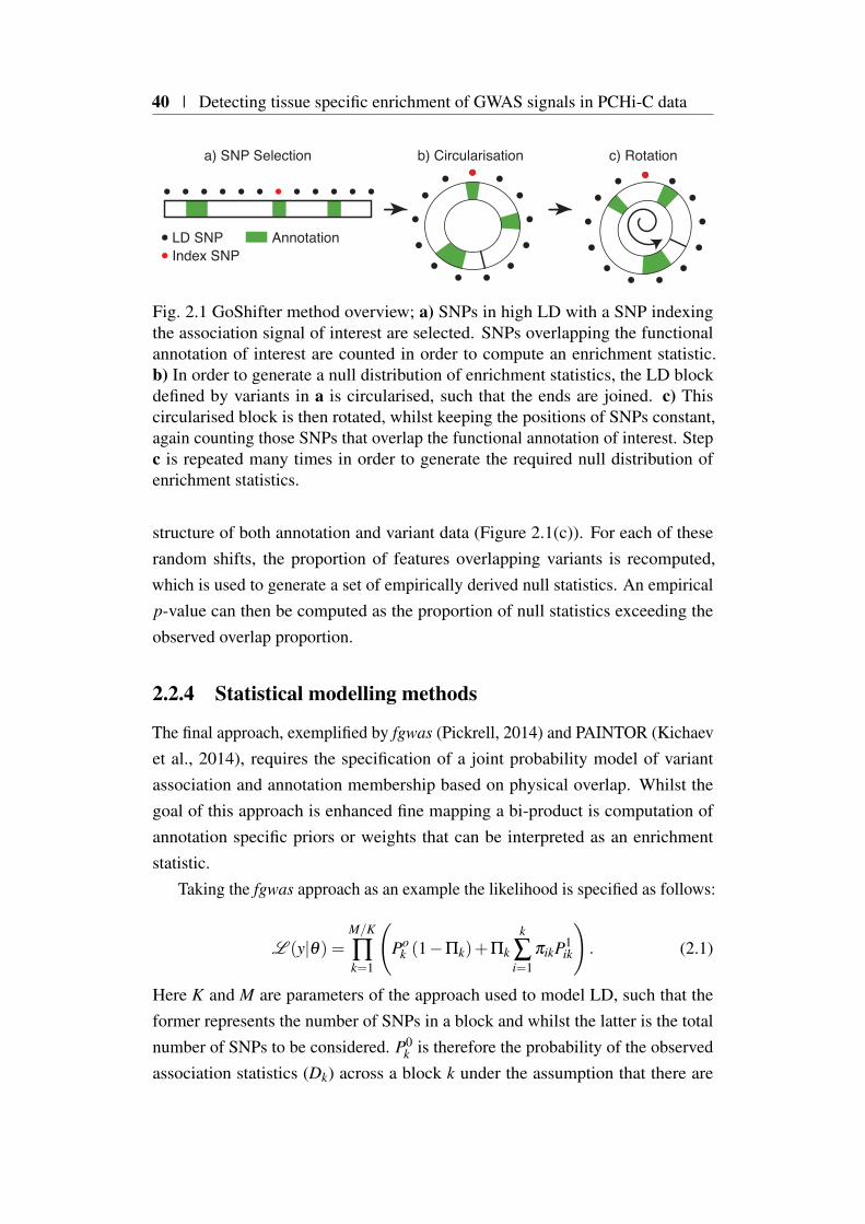
40 | Detecting tissue specific enrichment of GWAS signals in PCHi-C data
Index SNPAnnotationLD SNP
c) Rotationb) Circularisationa) SNP Selection
Fig. 2.1 GoShifter method overview; a) SNPs in high LD with a SNP indexingthe association signal of interest are selected. SNPs overlapping the functionalannotation of interest are counted in order to compute an enrichment statistic.b) In order to generate a null distribution of enrichment statistics, the LD blockdefined by variants in a is circularised, such that the ends are joined. c) Thiscircularised block is then rotated, whilst keeping the positions of SNPs constant,again counting those SNPs that overlap the functional annotation of interest. Stepc is repeated many times in order to generate the required null distribution ofenrichment statistics.
structure of both annotation and variant data (Figure 2.1(c)). For each of theserandom shifts, the proportion of features overlapping variants is recomputed,which is used to generate a set of empirically derived null statistics. An empiricalp-value can then be computed as the proportion of null statistics exceeding theobserved overlap proportion.
2.2.4 Statistical modelling methods
The final approach, exemplified by fgwas (Pickrell, 2014) and PAINTOR (Kichaevet al., 2014), requires the specification of a joint probability model of variantassociation and annotation membership based on physical overlap. Whilst thegoal of this approach is enhanced fine mapping a bi-product is computation ofannotation specific priors or weights that can be interpreted as an enrichmentstatistic.
Taking the fgwas approach as an example the likelihood is specified as follows:
L (y|θ) =M/K
∏k=1
(Po
k (1−Πk)+Πk
k
∑i=1
πikP1ik
). (2.1)
Here K and M are parameters of the approach used to model LD, such that theformer represents the number of SNPs in a block and whilst the latter is the totalnumber of SNPs to be considered. P0
k is therefore the probability of the observedassociation statistics (Dk) across a block k under the assumption that there are

2.2 Background | 41
no causal variants or P(Dk|H0). Conversely, P1ik is the probability of Dk under
the assumption of one causal variant, or P(Dk|H1). Finally, for the kth block, Πk
and πik are prior probabilities for the block or the ith SNP to be the causal SNPrespectively. Importantly, πik is modelled as:
πik =exi
∑ j∈Skex j
, (2.2)
where Sk is the set of SNPs in block k and
xi =L
∑l=1
λlIil, (2.3)
where l indexes annotations while L is the number of annotations and Iil is setto 1 if the ith SNP overlaps annotation l and zero if not. The relevant parameterfor assessment of enrichment of GWAS association signals in an annotation l isλl . fgwas optimises the likelihood (Equation 2.1), for a given dataset, and in sodoing ’learns’ values of λ across all input functional annotations, L. Care hasto be taken not to overfit the model to the data and fgwas employs a penalisedregression strategy in order to mitigate this. The likelihood function employedby fgwas is hierarchical, and this additional flexibility allows the modelling of anarbitrary number of annotations in an additive manner.
Limitations of existing approaches
Trynka et al. (2015) used simulation to compare GoShifter to the matched SNPset approach and noted that the latter was not well calibrated to control for Type 1error. They also detected a dependence between choice of matching parametersand observed enrichment. Conversely the circularised permutation approach theyemploy is based on few assumptions, it does however suffer from the fact thatit takes an implicit thresholding approach requiring an input of index variants.As previously discussed (Section 2.2) this will result in missing associations thatmight be driven by sub genome-wide signals and loss of resolution when appliedat the genome-wide scale.
Both statistical modelling and circularised permutation approaches can be usedto examine conditional enrichment between annotations, allowing insights to begained as to how correlation between two sets of distinct annotations (e.g gene TSSand DNaseI hypersensitivity) might be driving enrichment. In theory, matchedSNP set approaches could be accommodated to allow for this functionality, in
42 | Detecting tissue specific enrichment of GWAS signals in PCHi-C data
practice the increase in constraint in selecting matching background sets wouldmake accurate estimation of empirical p-values increasingly challenging.
Both statistical modelling and SNP matching approaches do not make specificprovision for localised structure within an annotation. As mentioned it is importantto control for intra-annotation dependencies within features of the same annotationtype in order to prevent inflation of enrichment test statistics. Indeed, this is a keystrength of circularised permutation techniques.
Another consideration is the complexity of the approach. The statistical mod-elling approaches are the most computationally and operationally complex, espe-cially when multiple annotations are considered. Both GoShifter and GARFIELDare considerably less complex and as a result easier to employ, however this comesat the cost of flexibility in the number of annotations that can be jointly considered.It should be noted that the statistical modelling approaches generate enrichmentstatistics that are calibrated to be employed as prior probabilities in downstreamfine mapping experiments, as such, enrichment is an intermediate rather than anultimate goal of such approaches.
2.3 PCHi-C maps: description and exploratory dataanalyses
2.3.1 Tissue coverage
In this thesis I analyse PCHi-C contact maps for a total of 17 primary cell types ofthe haematopoietic lineage and their empirical derivation as detailed in Javierreet al. (2016). Briefly, each cell type was assessed over at least 3 biologicalreplicates (Table A.1). Promoter interacting HindIII fragments were called usingthe CHiCAGO pipeline (Cairns et al., 2016).
2.3.2 Data format description
Contact maps in PeakMatrix format, consist of a baited or sequence capturedHindIII fragment, known as a ‘bait’ and a list of interacting HindIII fragments orpromoter interacting regions (PIR) within a particular cellular contexts (Figure 2.2).Thus one row represents one interaction, between a bait and PIR. Additionalcolumns map CHiCAGO scores from each of the cell types examined. As thenumber of bait pair interactions analysed by CHiCAGO is large, only those that

2.3 PCHi-C maps: description and exploratory data analyses | 43
Chromosome 8
29.2 mb
29.3 mb
29.4 mb
29.5 mb
29.6 mb
29.7 mb
29.8 mb
Gen
es
PromoterInteracting
RegionBait
DUSP4
Tiss
ue 1
Signicant Interaction
Tiss
ue 2
Non Signicant Interaction
8 29786004 29791167 8 29201519 29223254 7.95 3.23PIR CoordsBait Coords
Peak Matrix Format
CHiCAGO Scores
Fig. 2.2 Illustration showing PCHi-C contact map of interactions for DUSP4. Thepromoter capture HindIII fragment is labelled as ‘Bait’ and is highlighted in grey.For ‘Tissue 1’ (black), a significant (CHiCAGO score > 5) interaction with adownstream HindIII fragment or ‘Promoter Interacting Region’ (PIR) is shownin blue. In contrast for ‘Tissue 2’ (red) CHiCAGO does not identify a significantinteraction. This information is encoded in one line of Peak Matrix format asillustrated.
show evidence for at least one significant interaction (CHiCAGO score > 5) acrossthe 17 cell types are included.
2.3.3 CHiCAGO score distributions across cell types
I first wanted to understand at a global level, how CHiCAGO scores varied acrossthe different cell types. However, although CHiCAGO scores are quantitativethey are challenging to interpret due to their complicated bimodal distribution(Figure 2.3a), with a majority of scores having a score of zero, a second peakaround 2 and an extremely large range (0-52). One method, employed in Javierre

44 | Detecting tissue specific enrichment of GWAS signals in PCHi-C data
et al. (2016) to rescale data with large ranges, is the sinh−1 transform, whichreduces the variance and thus range in a non linear fashion. This is desirableso that large CHiCAGO scores do not have undue influence on any inferencesmade. In general, with this transformation applied the distribution across tissuesis very similar (Figure 2.3b), however neutrophils exhibit a different distribution,with many more very low scoring fragments observed, potentially reflecting theirunusual segmented nuclear morphology (Javierre et al., 2016).
0
500000
1000000
1500000
0 10 20 30 40 50CHiCAGO score
PIR
cou
nt
a)
Endothelial precursorsErythroblasts
Foetal thymusMacrophages M0Macrophages M1Macrophages M2Megakaryocytes
MonocytesNaive B
Naive CD4Naive CD8Neutrophils
Total BTotal CD4 Activated
Total CD4 MFTotal CD4 NonActivated
Total CD8
0 2 4 6 8sinh-1(CHiCAGO Score)
Tiss
ue T
ype
b)
Fig. 2.3 Distribution of CHiCAGO scores. a) Distribution of raw CHiCAGOscores, across all cell types. There is an extreme right hand tail distribu-tion, and for clarity scores above 50 are not shown. b) A ridge plot showingarcsin(CHiCAGO score) distributions across Cell types. In both panels the reddashed line represents CHiCAGO significance level.
2.3.4 CHiCAGO scores reflect lineage specificity
I used principal component analysis (PCA) on sinh−1 transformed CHiCAGOscores to examine structure within the data. Overall approximately 50% of the
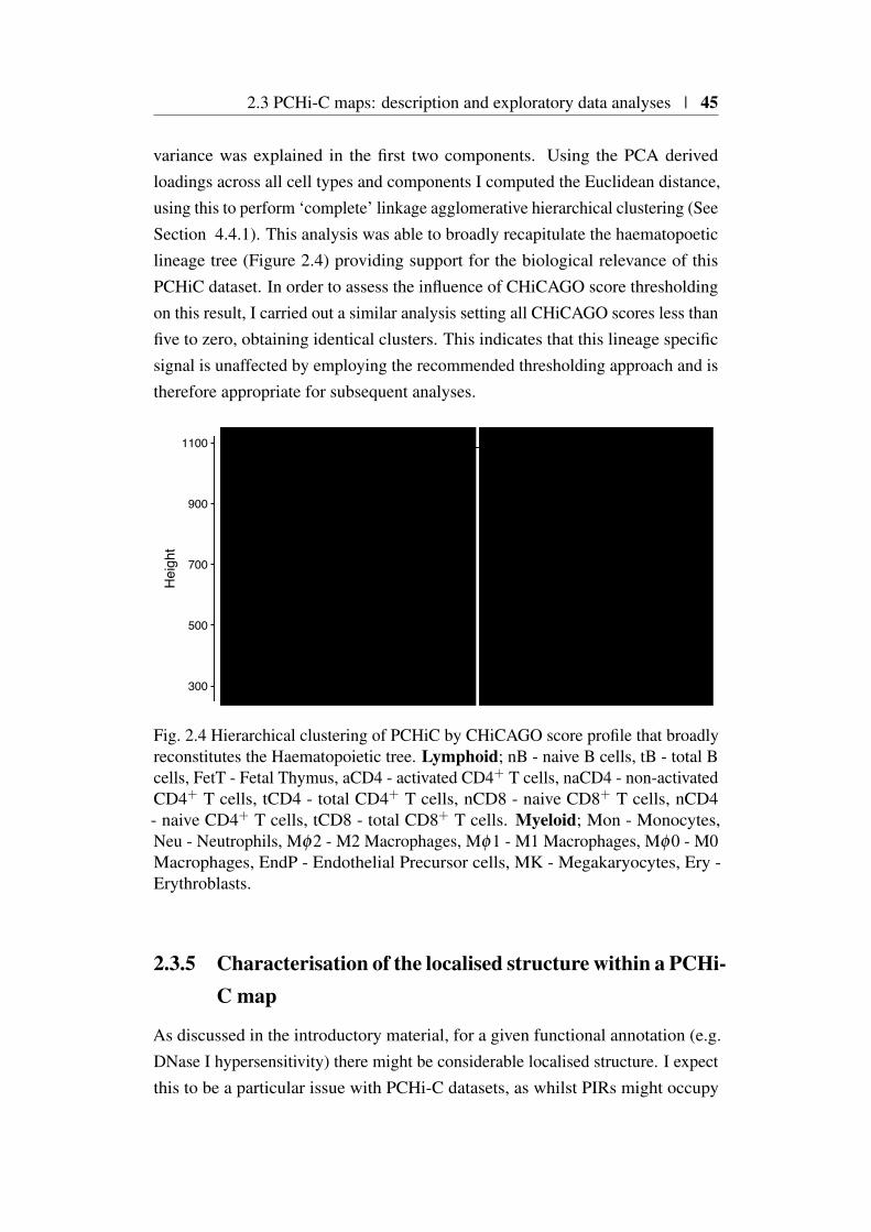
2.3 PCHi-C maps: description and exploratory data analyses | 45
variance was explained in the first two components. Using the PCA derivedloadings across all cell types and components I computed the Euclidean distance,using this to perform ‘complete’ linkage agglomerative hierarchical clustering (SeeSection 4.4.1). This analysis was able to broadly recapitulate the haematopoeticlineage tree (Figure 2.4) providing support for the biological relevance of thisPCHiC dataset. In order to assess the influence of CHiCAGO score thresholdingon this result, I carried out a similar analysis setting all CHiCAGO scores less thanfive to zero, obtaining identical clusters. This indicates that this lineage specificsignal is unaffected by employing the recommended thresholding approach and istherefore appropriate for subsequent analyses.
nB tB
FetT
tCD
8
tCD
4
nCD
4
nCD
8
aCD
4
naC
D4
Mϕ
2
Mϕ
0
Mϕ
1
EndP MK
Ery
Mon
Neu
300
500
700
900
1100
Hei
ght
MyeloidLymphoid
Fig. 2.4 Hierarchical clustering of PCHiC by CHiCAGO score profile that broadlyreconstitutes the Haematopoietic tree. Lymphoid; nB - naive B cells, tB - total Bcells, FetT - Fetal Thymus, aCD4 - activated CD4+ T cells, naCD4 - non-activatedCD4+ T cells, tCD4 - total CD4+ T cells, nCD8 - naive CD8+ T cells, nCD4- naive CD4+ T cells, tCD8 - total CD8+ T cells. Myeloid; Mon - Monocytes,Neu - Neutrophils, Mφ2 - M2 Macrophages, Mφ1 - M1 Macrophages, Mφ0 - M0Macrophages, EndP - Endothelial Precursor cells, MK - Megakaryocytes, Ery -Erythroblasts.
2.3.5 Characterisation of the localised structure within a PCHi-C map
As discussed in the introductory material, for a given functional annotation (e.g.DNase I hypersensitivity) there might be considerable localised structure. I expectthis to be a particular issue with PCHi-C datasets, as whilst PIRs might occupy
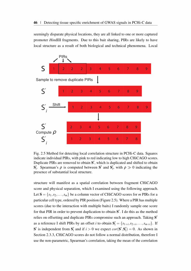
46 | Detecting tissue specific enrichment of GWAS signals in PCHi-C data
seemingly disparate physical locations, they are all linked to one or more capturedpromoter HindIII fragments. Due to this bait sharing, PIRs are likely to havelocal structure as a result of both biological and technical phenomena. Local
S
987654321
987654321
98765432221
Shift
Sample to remove duplicate PIRs
Compute ρ87654321
98765432
PIRs
S’i
S’i
S’
S’
S
Fig. 2.5 Method for detecting local correlation structure in PCHi-C data. Squaresindicate individual PIRs, with pink to red indicating low to high CHiCAGO scores.Duplicate PIRs are removed to obtain S′, which is duplicated and shifted to obtainS′
i. Spearman’s ρ is computed between S′ and S′i, with ρ ≫ 0 indicating the
presence of substantial local structure.
structure will manifest as a spatial correlation between fragment CHiCAGOscore and physical separation, which I examined using the following approach.Let S = s1,s2, . . . ,sm be a column vector of CHiCAGO scores for m PIRs for aparticular cell type, ordered by PIR position (Figure 2.5). Where a PIR has multiplescores (due to the interaction with multiple baits) I randomly sample one scorefor that PIR in order to prevent duplication to obtain S′. I do this as the methodrelies on offsetting and duplicate PIRs compromise such an approach. Taking S′
as a reference I shift PIRs by an offset i to obtain S′i = s1+i,s2+i, . . . ,sm+i. If
S′ is independent from S′i and if i > 0 we expect cor(S′,S′
i) = 0. As shown inSection 2.3.3, CHiCAGO scores do not follow a normal distribution, therefore Iuse the non-parametric, Spearman’s correlation, taking the mean of the correlation

2.4 GWAS compendium: description and data processing | 47
coefficient ρ as a summary of the correlation structure across cell types. Focussingon chromosome 1 I selected values of i, the fragment offset, that allowed theinterrogation of both local and distal correlation structures.
0.0
0.1
0.2
0.3
0.4
0.5
1 2 5 10 50 100 100020003000
Fragment offset (chr1)
ρ
Fig. 2.6 Extent of correlation between CHiCAGO scores and physical location forPCHi-C maps
Across all cell types I observed large amounts correlation at smaller offsets,demonstrating that local correlation structure presents specific challenges whenworking with PCHi-C datasets (Figure 2.6). This effect decays and is nominal atlarger distances reflecting the nature of the underlying biological process beingassayed. At extreme offsets above 1000 I see a small negative correlation, thatcan be explained as stochastic sampling variation in ρ as it approaches zero. Thisfinding of significant local dependence between PIRs underscores the importanceof employing an enrichment method specifically designed to mitigate against thisin order to generate well calibrated and believable enrichment statistics.
2.4 GWAS compendium: description and data pro-cessing
In order to investigate a broad range of phenotypes I downloaded GWAS summarystatistics, covering 8 immune-mediated and 23 other traits, from online resources(Table2.1). Genotyping error can create false associations, therefore I filtered all
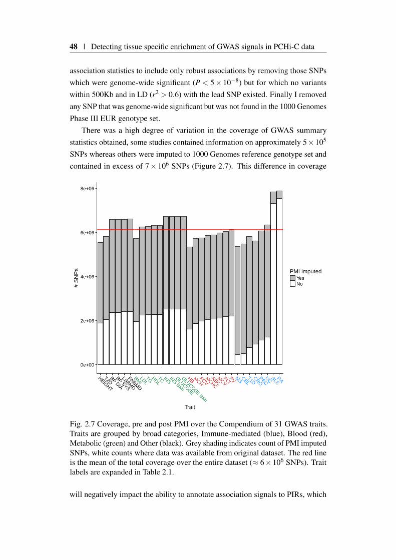
48 | Detecting tissue specific enrichment of GWAS signals in PCHi-C data
association statistics to include only robust associations by removing those SNPswhich were genome-wide significant (P < 5× 10⁻⁸) but for which no variantswithin 500Kb and in LD (r2 > 0.6) with the lead SNP existed. Finally I removedany SNP that was genome-wide significant but was not found in the 1000 GenomesPhase III EUR genotype set.
There was a high degree of variation in the coverage of GWAS summarystatistics obtained, some studies contained information on approximately 5×10⁵
SNPs whereas others were imputed to 1000 Genomes reference genotype set andcontained in excess of 7× 10⁶ SNPs (Figure 2.7). This difference in coverage
0e+00
2e+06
4e+06
6e+06
8e+06
HEIGHT
T2DBP DIA
BP SYS
LSBMD
FNBMD
BMILDL
TG HDLTC INS
INS BMI
GLUCOSE
GLUCOSE BMI
HB MCH
PCVM
CHC
RBCM
CVPLT
PV MS
CELT1D
CROPBC
UC SLERA
Trait
# S
NP
s PMI imputedYesNo
Fig. 2.7 Coverage, pre and post PMI over the Compendium of 31 GWAS traits.Traits are grouped by broad categories, Immune-mediated (blue), Blood (red),Metabolic (green) and Other (black). Grey shading indicates count of PMI imputedSNPs, white counts where data was available from original dataset. The red lineis the mean of the total coverage over the entire dataset (≈ 6×10⁶ SNPs). Traitlabels are expanded in Table 2.1.
will negatively impact the ability to annotate association signals to PIRs, which

2.4 GWAS compendium: description and data processing | 49
Trait Label Cases ControlsMultiple sclerosis MS 9,772 17,376Celiac disease CEL 4,533 10,750Type 1 diabetes T1D 8,000 8,000Crohn’s disease CRO 6,333 15,056Primary billiary birrhosis PBC 2,764 10,475Ulcerative colitis UC 6,687 19,718Systemic lupus erythrematosus SLE 4,036 6,959Rheumatoid arthritis RA 14,361 43,923Type 2 diabetes T2D 12,171 56,860Haemoglobin HB 4,627Mean corp. haemoglobin MCH 4,627Packed cell volume PCV 4,627Mean corp. haemoglobin conc. MCHC 4,627Red blood cell count RBC 4,627Mean corpuscular volume MCV 4,627Platelet count PLT 48,666Platelet volume PV 18,600Body mass index BMI 322,200Low density lipoprotein LDL 95,454Tryglycerides TG 96,598High density lipoprotein HDL 99,900Total cholesterol TC 100,184Insulin sensitivity INS 51,750Insulin sensitivity BMI adj. INS BMI 51,750Glucose sensitivity GLUCOSE 58,074Glucose sensitivity BMI adj. GLUCOSE BMI 58,074Height HEIGHT 253,288Diastolic blood pressure BP DIA 69,395Systolic blood pressure BP SYS 69,395Lumbar spine bone mineral density LSBMD 32,961Femoral neck bone mineral density FNBMD 32,961
Table 2.1 Compendium of 31 GWAS studies analysed. References for each studyincluded are available in Table A.2.
50 | Detecting tissue specific enrichment of GWAS signals in PCHi-C data
in turn will complicate between study comparisons. Imputation can be usedto compute approximate association statistics for missing variants, however, itgenerally requires access to underlying genotype data, which in this case wasunavailable for most traits. Methods exist for imputing summary statistics in theabsence of genotyping data such as GCTA (Yang et al., 2011) and IMPG (Pasaniucet al., 2014). These rely on access to either signed Z scores, odds ratios or β
coefficients and their standard errors, in order to estimate direction of effect, whichwere not available for all studies in the compendium. This motivated me to developan alternative method to allow the processing of a wide range of traits for whichSNP coverage is heterogeneous and only univariate p-values are available.
2.4.1 Defining approximately LD independent blocks
As previously discussed (Section 1.3.1), LD is pervasive in the genome, and thusa single causal variant at a given genetic locus will result in the statistical, butnon-causal, association of multiple variants. In order to assess the evidence forvariant causality that is comparable across multiple traits it is useful to derivean a priori heuristic approach to grouping putative causal variants sharing anassociation signal. In order to generate approximately independent LD blocks, Iused recombination frequency data derived from the CEU sample set of the Inter-national HapMap Consortium (International HapMap Consortium et al., 2007) asall GWAS in the compendium were derived from samples of European ancestry.To generate blocks, for each chromosome, I ordered variants for which recombi-nation frequency data was available according to GRCh37 human genome build.I next computed the cumulative sum of recombination frequencies across theordered variants, for each chromosome, using 1cM boundaries to define groups ofvariants in linkage disequilibrium. Using these ordered blocks of variants I derivedadjacent physical intervals. To do this I selected the variant from the previousblock with the largest physical location to define a start, defining the end as theposition of the variant in the current block with the maximal physical coordinate.Such a scheme creates adjacent but potentially overlapping physical regions, andto avoid this I added 1 base-pair the start coordinate of each block.
2.4.2 Poor man’s imputation pipeline
The poor man’s imputation pipeline (PMI) I developed, approximates the p-valuesfor missing SNP summary statistics for a given study using a suitable reference
2.4 GWAS compendium: description and data processing | 51
genotype set. Firstly the genome is split into approximately LD independent LDregions (Section 2.4.1) enabling downstream LD computations to be tractable. Foreach region I retrieve from a relevant reference genotype set (e.g. 1000 genomes)all SNPs that have MAF > 1% and use these to compute pairwise LD in the1000 Genomes European population cohort (EUR). The pipeline pairs each SNPwith missing p-values to the study SNP with maximum pairwise r2, r2
max, if thatr2
max > 0.6, and imputes the missing p-value as that at the paired SNP. SNPs withmissing data or without a pair above threshold are discarded, as are SNPs that areincluded in the study but do not map to the reference genotype set.
2.4.3 Evaluation of PMI performance
Before using PMI in further analyses I wanted to assess the its performancecompared to classical imputation, where full genotypes are available. Firstly, Iselected all chromosome 1 SNPs from Okada et al. (2014), as a representativesample. This study constitutes a well powered and fully EUR imputed data set.To create a simulated non-imputed data set I pruned these results to contain onlySNPs for which p-values were reported in Stahl et al. (2010). I ran PMI on thispruned data set and using bedtools (Quinlan, 2014), aligned the PMI generatedp-values with those from Okada et al. (2014). This resulted in a comparisonbetween 235,412 PMI imputed SNPs (Figure2.8).
Generally, there was good agreement between PMI imputed p-values andthose derived from classical imputation as reported in Okada et al. (2014) (ρ =0.94). However, I note that there is considerably more noise in the more modestlyassociated SNPs for which PMI tends to inflate evidence for association. Anexplanation for this is that the assignment of p-values based on the PMI methoddoes not take into account the degree of LD. For example a pair of SNPs wherer2 > 0.99 will be highly correlated and therefore it is reasonable to expect similarp-values. Conversely, if two SNPs are in more modest LD (e.g. r2 = 0.6) wemight expect a decay in association between the two. Such an effect is modelledby classical imputation approaches (used in (Okada et al., 2014)) but not PMIand thus might explain some of the modest inflation in PMI summary statisticsdetected.

52 | Detecting tissue specific enrichment of GWAS signals in PCHi-C data
0
20
40
60
0 20 40 60Okada et al. − log10(P)
PMI −
log 1
0(P)
40,00080,000120,000160,000
Count
Fig. 2.8 Comparison of p-values imputed by PMI versus those reported in Okadaet al. (2014) for Chromosome 1, each hexagonal point represents a bin of SNPswith dark blue and light blue representing low and high counts respectively.
2.4.4 Generation of single causal variant posterior probabili-ties
As discussed in Chapter 1, univariate GWAS p-values are unable to capture howconfident we are that a SNP is truly associated with a trait. The asymptotic Bayesfactor described in Wakefield (2009) is an attractive alternative as it integratesinformation about study design and MAF into one metric albeit with the additionof some strong assumptions (Section 1.3.5). The main assumption is that, for agiven locus, there exists up to one causal variant. This leads to the question of thebest way, genome-wide, to segment the genome, so as to minimise violation of thisassumption. One option is to select the set of segments for which LD for a givenpopulation is minimised between adjacent segments. Liu et al. (2010) utilisedHapMap recombination data in the setting of GWAS pathway analysis to achievethis and in follow up work I had found this to be a suitable segmentation (Burrenet al., 2014). Therefore for these reasons and for consistency I used the same LDsegmentation employed in the PMI pipeline (≈ 1cM). Another reason for using

2.4 GWAS compendium: description and data processing | 53
this framework is that because the single causal variant posterior probabilities(sCVPP) are derived from a joint model of signals across a given region, LD isnaturally taken into account. This mitigates some of the negative effects of PMI,naturally attenuating imputed signals with many LD partners. This occurs becausethe sum of sCVPP across an LD block is equal to the posterior probability forthe region to contain a causal variant (Wellcome Trust Case Control Consortiumet al., 2012), which cannot exceed 1. Due to this joint modelling, large signals forvariants with many LD partners, exacerbated by PMI, will be equitably sharedthus reducing their overall individual impact, naturally reflecting the difficulty ofassigning causality to variants within blocks of extended LD.
2.4.5 Prior selection
The computation of aBF requires the selection of two priors. The first is πi whichis expectation of the ith SNP to be causal. I used πi = 10−4 ∀ i, that is we expect1 in 10,000 SNPs across the genome to be causal (Giambartolomei et al., 2014).The second prior relates to the value of
√W , the standard deviation of a normal
prior for effect size θ such that θ ∼ N(0,W ), which depends on study designconsiderations. For case/control studies I employ a value of 0.2, this is equivalentto a 95% belief that the true relative risk is in the range of 0.66− 1.5 at anycausal variant (Huang et al., 2017). For quantitative trait settings I use 0.15, this isbecause under the assumption that the outcome variable is normalised such thatit’s variance is 1, this is equivalent to a variance in trait explained of approximately0.01 for a SNP with a MAF of 30%. The justification for these priors in discussedfurther in the supplementary text of Giambartolomei et al. (2014) and Huang et al.(2017).
2.4.6 HLA region
I excluded the HLA region (GRCh37:chr6:25-35Mb) from all downstream analysisdue to its extended LD and known strong and complex association with autoim-mune disease. Both of these properties would overwhelm subsequent analysismaking it difficult to assess whether enrichment was solely driven by the HLA.

54 | Detecting tissue specific enrichment of GWAS signals in PCHi-C data
2.5 blockshifter development
I sought to develop a method for efficient integration of GWAS data with PCHi-Cmaps in order to assess enrichment of GWAS associations for each trait acrossdifferent tissues. Due to the reliance of PCHi-C on HindIII restriction fragmentsand the high degree of localised structure in the data, publicly available enrichmenttools (as discussed Section 2.2) were unsuitable. Furthermore I wanted to developa non-thresholded approach based on the causal variant posterior probabilitiescomputed for the reasons outlined in Section 2.4.4.
Considerations
Any tool developed would first and foremost need to be able to account forsubstantial local correlation structure (Section 2.3.5) that is present in both GWASand PCHi-C datasets (Figure 2.6). In order to be easily interpretable, any methodshould compare the enrichment of a set of PCHi-C contacts between two sets oftissues (a test and control set) in a competitive manner. Finally the implementationshould allow for the fast computation of enrichment statistics without the need forhigh performance computing infrastructure.
For global tissue enrichment purposes we are concerned with PIRs and ignoretheir promoter specific bait linkages i.e. a PIR which interacts with any bait isconsidered to potentially relate to enhancer presence. This results in considerableduplication as the same PIR can interact with multiple baits. I removed theseusing the R duplicate command prior to subsequent analysis in order to speedup performance.
2.5.1 The blockshifter method
I developed a hybrid circularised permutation method (Section 2.2.3) called block-
shifter, implemented in R, that satisfied the requirements above. This methodis competitive in nature and therefore requires user defined sets of test and con-trol tissues for comparison, in addition to pre-computed GWAS study sCVPPi
(Section 2.4.4).blockshifter uses a statistic, δ , the difference in the mean sCVPP between
variants overlapping a set of test and controls PIRs,
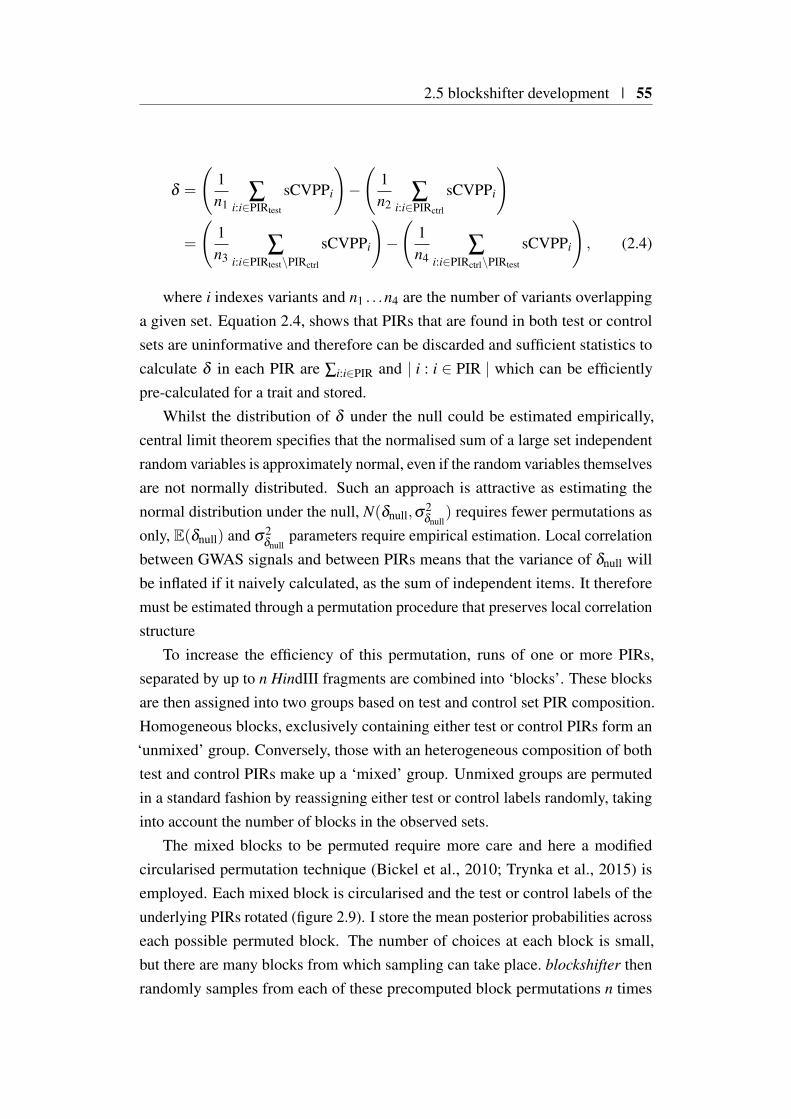
2.5 blockshifter development | 55
δ =
(1n1
∑i:i∈PIRtest
sCVPPi
)−
(1n2
∑i:i∈PIRctrl
sCVPPi
)
=
(1n3
∑i:i∈PIRtest\PIRctrl
sCVPPi
)−
(1n4
∑i:i∈PIRctrl\PIRtest
sCVPPi
), (2.4)
where i indexes variants and n1 . . .n4 are the number of variants overlappinga given set. Equation 2.4, shows that PIRs that are found in both test or controlsets are uninformative and therefore can be discarded and sufficient statistics tocalculate δ in each PIR are ∑i:i∈PIR and | i : i ∈ PIR | which can be efficientlypre-calculated for a trait and stored.
Whilst the distribution of δ under the null could be estimated empirically,central limit theorem specifies that the normalised sum of a large set independentrandom variables is approximately normal, even if the random variables themselvesare not normally distributed. Such an approach is attractive as estimating thenormal distribution under the null, N(δnull,σ
2δnull
) requires fewer permutations asonly, E(δnull) and σ2
δnullparameters require empirical estimation. Local correlation
between GWAS signals and between PIRs means that the variance of δnull willbe inflated if it naively calculated, as the sum of independent items. It thereforemust be estimated through a permutation procedure that preserves local correlationstructure
To increase the efficiency of this permutation, runs of one or more PIRs,separated by up to n HindIII fragments are combined into ‘blocks’. These blocksare then assigned into two groups based on test and control set PIR composition.Homogeneous blocks, exclusively containing either test or control PIRs form an‘unmixed’ group. Conversely, those with an heterogeneous composition of bothtest and control PIRs make up a ‘mixed’ group. Unmixed groups are permutedin a standard fashion by reassigning either test or control labels randomly, takinginto account the number of blocks in the observed sets.
The mixed blocks to be permuted require more care and here a modifiedcircularised permutation technique (Bickel et al., 2010; Trynka et al., 2015) isemployed. Each mixed block is circularised and the test or control labels of theunderlying PIRs rotated (figure 2.9). I store the mean posterior probabilities acrosseach possible permuted block. The number of choices at each block is small,but there are many blocks from which sampling can take place. blockshifter thenrandomly samples from each of these precomputed block permutations n times
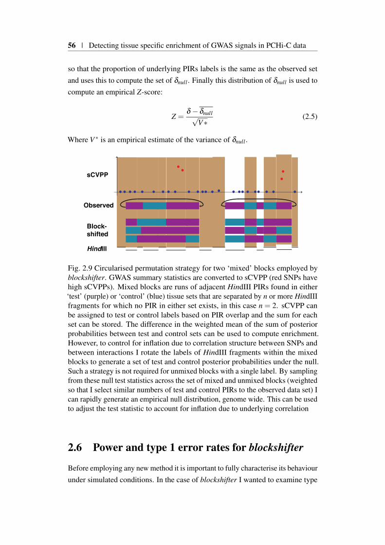
56 | Detecting tissue specific enrichment of GWAS signals in PCHi-C data
so that the proportion of underlying PIRs labels is the same as the observed setand uses this to compute the set of δnull . Finally this distribution of δnull is used tocompute an empirical Z-score:
Z =δ −δnull√
V∗(2.5)
Where V ∗ is an empirical estimate of the variance of δnull .
HindIII
sCVPP
Observed
Block-shifted
Fig. 2.9 Circularised permutation strategy for two ‘mixed’ blocks employed byblockshifter. GWAS summary statistics are converted to sCVPP (red SNPs havehigh sCVPPs). Mixed blocks are runs of adjacent HindIII PIRs found in either‘test’ (purple) or ‘control’ (blue) tissue sets that are separated by n or more HindIIIfragments for which no PIR in either set exists, in this case n = 2. sCVPP canbe assigned to test or control labels based on PIR overlap and the sum for eachset can be stored. The difference in the weighted mean of the sum of posteriorprobabilities between test and control sets can be used to compute enrichment.However, to control for inflation due to correlation structure between SNPs andbetween interactions I rotate the labels of HindIII fragments within the mixedblocks to generate a set of test and control posterior probabilities under the null.Such a strategy is not required for unmixed blocks with a single label. By samplingfrom these null test statistics across the set of mixed and unmixed blocks (weightedso that I select similar numbers of test and control PIRs to the observed data set) Ican rapidly generate an empirical null distribution, genome wide. This can be usedto adjust the test statistic to account for inflation due to underlying correlation
2.6 Power and type 1 error rates for blockshifter
Before employing any new method it is important to fully characterise its behaviourunder simulated conditions. In the case of blockshifter I wanted to examine type
2.6 Power and type 1 error rates for blockshifter | 57
1 error rate and it’s relationship to a gap parameter indicating the number ofmissing PIRs allowed within a ‘block’, which in turn defines the total number ofblocks. Intuitively selecting too small a gap size will result in a large number ofsmaller blocks with a tendency to be of the unmixed block type and the resultantpermutation may be insufficient to estimate the variance of δnull. Conversely toolarge a gap size will result in fewer larger blocks with a tendency to be mixed,where larger scale PIR structure might begin to obscure more local correlation.
As described blockshifter, permutes PIR labels whilst maintaining the locationof GWAS summary statistics. Any simulation would require a reference test andcontrol PIR dataset that remains constant between simulations. I therefore selecteda test (Activated or Non-activated CD4+ T cells) and control (megakaryocyteor erythroblast) set of PIRs with CHiCAGO score > 5, as a reference set forblockshifter input.
In contrast I wanted to simulate GWAS summary statistics such that I couldcontrol the level of enrichment and use these to understand the performance ofblockshifter under different scenarios.
2.6.1 Simulation of GWAS
In order to simplify computation I limited the simulation to utilise data for chro-mosome 1, under the reasonable assumption that this would be representativeof genome-wide results. Firstly, I split chromosome 1 into approximately inde-pendent LD blocks as described in Section 2.4.2. I used the EUR genotypes tocompute a correlation matrix, ΣΣΣ for variants with a minor allele frequency > 1%,using the snpStats R package(Clayton and Leung, 2007). GWAS Z scores canbe simulated from a multivariate normal distribution with mean µµµ and correlationmatrix ΣΣΣ (Burren et al., 2014; Liu et al., 2010). Each LD block may contain nocausal variants (GWASnull ∼MVN(000,ΣΣΣ)) or one (GWASalt ∼MVN(µµµ,ΣΣΣ), whereµµµ = 0).
2.6.2 Enrichment scenarios
For GWASalt , I picked a single causal variant, i, and calculated the expectednon-centrality parameter (NCP) for a 1 degree of freedom χ2 test of association atthis variant and it’s neighbours. This framework is natural because, under a singlecausal variant assumption, the χ2 at any variant, j, can be expressed as the χ2 atthe causal variant multiplied by the squared correlation, Σi j, between variants i
58 | Detecting tissue specific enrichment of GWAS signals in PCHi-C data
and j (Chapman et al., 2003). In each case, I set the NCP at the causal variant to80 to ensure that each causal variant was genome-wide significant (P < 5×10⁻⁸).µ , the expected Z score is defined as the square root of this constructed χ2 vector.
To assess type 1 error rate and power I constructed three artificial scenarios asfollows:-
Null enrichment scenario: This scenario, is used to confirm control of type1 error rate, and causal variants are assigned to PIRs without regard forwhether they were identified in test or control tissues.
Moderate enrichment scenario: In order to examine power, the ability of block-
shifter to reject the null hypothesis in the presence of simulated enrichment,causal variants were preferentially located in test PIRs with a 50% probabil-ity.
Strong enrichment scenario: This scenario mimics the preceding scenario withcausal variants being located in test PIRs with a 100% probability.
For all scenarios, I randomly chose 50 GWASalt blocks leaving the remaining219 GWASnull . Enrichment is determined by the preferential location of simulatedcausal variants within test PIRs. In all scenarios, each causal variant has a 50%chance of lying within a PIR, to mirror a real GWAS in which we expect only aproportion of causal variants to be regulatory in any given cell type. Note that aPIR from the test set may also be in the control set, thus, as with a real GWAS,not all causal variants will be informative for this test of enrichment.
In order to understand the effect of PMI, for each scenario, I further consideredvariable levels of genotyping density, corresponding to ‘full’ genotyping (every-thing in 1,000 Genomes), HapMap imputation (the subset of SNPs also in Stahlet al. (2010) dataset) or genotyping array (the subset of SNPs on the Illumina550 k array). Where genotyping density is less than full, I used PMI to fill in Z
scores for missing SNPs. I ran blockshifter, with 1,000 null permutations, for eachscenario and PMI-genotype density condition for 4,000 simulated GWAS, with ablockshifter block gap size parameter (the number of contiguous non-PIR HindIIIfragments allowed within one superblock) of between 1 and 20. For all simulationsI mirrored the number of cases and controls from the RA dataset (Okada et al.,2014).
For comparison, I also investigated the behaviour of a naive test for enrichmentfor the null scenario that does not attempt to account for strong local correlation
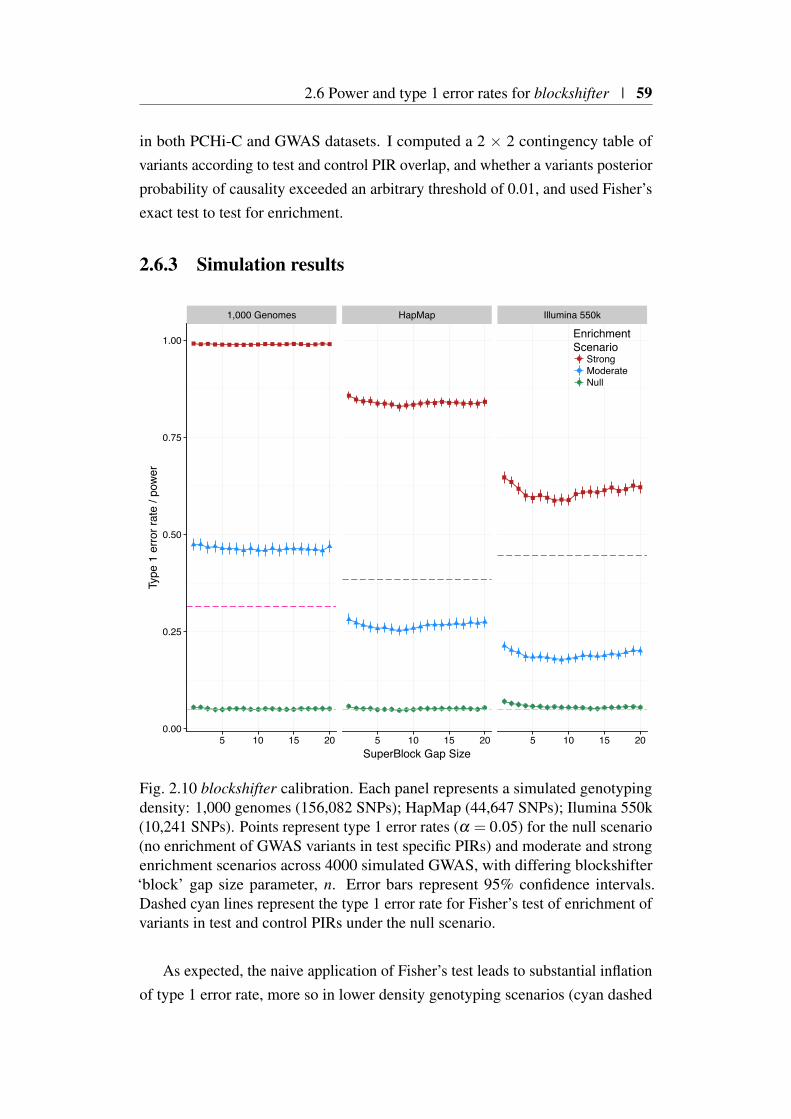
2.6 Power and type 1 error rates for blockshifter | 59
in both PCHi-C and GWAS datasets. I computed a 2 × 2 contingency table ofvariants according to test and control PIR overlap, and whether a variants posteriorprobability of causality exceeded an arbitrary threshold of 0.01, and used Fisher’sexact test to test for enrichment.
2.6.3 Simulation results
1,000 Genomes HapMap Illumina 550k
5 10 15 20 5 10 15 20 5 10 15 200.00
0.25
0.50
0.75
1.00
SuperBlock Gap Size
Type
1 e
rror r
ate
/ pow
er
EnrichmentScenario
StrongModerateNull
Fig. 2.10 blockshifter calibration. Each panel represents a simulated genotypingdensity: 1,000 genomes (156,082 SNPs); HapMap (44,647 SNPs); Ilumina 550k(10,241 SNPs). Points represent type 1 error rates (α = 0.05) for the null scenario(no enrichment of GWAS variants in test specific PIRs) and moderate and strongenrichment scenarios across 4000 simulated GWAS, with differing blockshifter‘block’ gap size parameter, n. Error bars represent 95% confidence intervals.Dashed cyan lines represent the type 1 error rate for Fisher’s test of enrichment ofvariants in test and control PIRs under the null scenario.
As expected, the naive application of Fisher’s test leads to substantial inflationof type 1 error rate, more so in lower density genotyping scenarios (cyan dashed

60 | Detecting tissue specific enrichment of GWAS signals in PCHi-C data
lines in Figure 2.10). blockshifter maintains type 1 error rate control, although agap size of 5 or more is required to deal with the extended correlation inducedby PMI in lower density genotyping scenarios. As expected blockshifter poweris attenuated, by the reduction in genotyping density. Furthermore, the effect ofapplying PMI to impute missing data on blockshifter seems to result in a lesspowerful test with sparser, more PMI imputed values resulting in an attenuatedblockshifter enrichment statistic (Figure 2.10). Importantly, PMI data do notdisplay evidence for an elevated type 1 error rate.
2.7 Tissue specific enrichment of associated variantswith PIRs across 31 traits
I applied blockshifter to analyse the compendium of 31 GWAS summary statisticsfor PCHiC tissue specific enrichment. By design blockshifter is a competitive testfor enrichment and requires the selection of tissues or tissue groups to compare. Anatural dichotomy, in terms of haematopoeitic lineage, exists between lymphoidand myeloid tissues which cluster in two distinct groups as shown in Figure2.4. Analysis with blockshifter showed that variants associated with autoimmunedisease traits are enriched at PIRs in lymphoid compared to myeloid cells (Figure2.11a). A non parametric Wilcoxon rank sum test comparing blockshifter Z-scoresfor autoimmune traits compared to the rest of the compendium showed that thistrend was significant (Wilcoxon two-sided Padj. = 1.42×10⁻⁵). A further analysisof innate immune cells (monocytes, macrophages and neutophils) compared tomegakaryocytes and erythroblasts showed that autoimmune traits were enriched inthe former (Wilcoxon two-sided padj. = 7.03×10⁻⁴). There was some evidencethat blood traits were enriched in myeloid compared to lymphoid PIRs (Wilcoxontwo-sided Padj. = 0.005), however there was no support for this being specificto megakaryocytes or erythroblasts when the two were compared directly whichmight have been expected. There was no enrichment observed for the metabolicor ‘other’ categories.
Given the observed enrichment of autoimmune GWAS signals in lymphoidtissues, I performed additional comparisons to see if this could be further localised(Figure 2.11b). The most significant of these was the enrichment of autoimmuneGWAS signals in PIRs for CD4+ T cells that had been activated, compared tothose that had not (Wilcoxon two-sided Padj. = 2.03×10⁻⁶).
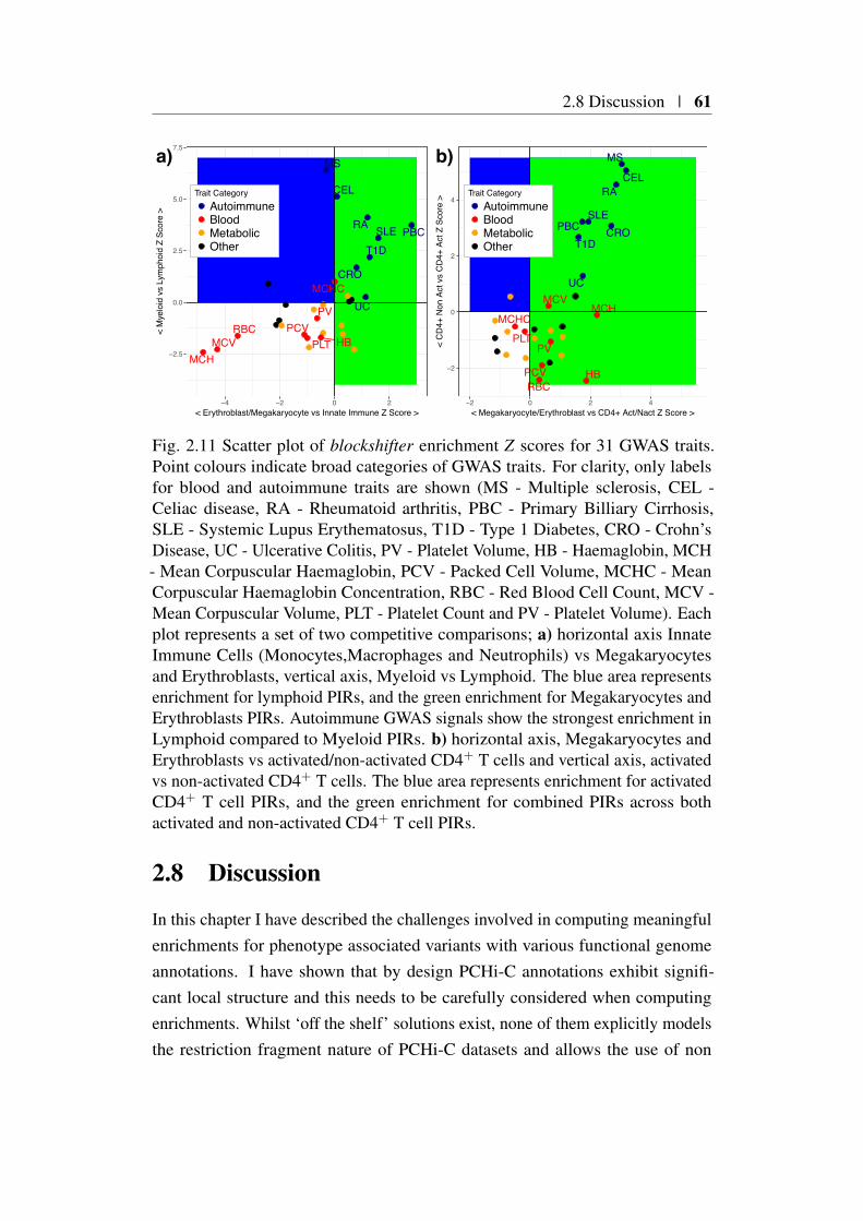
2.8 Discussion | 61
CRO
CEL
HBMCH
MCHC
MCV
MS
PBC
PCVPLT
PV
RA
RBC
SLET1D
UC
−2.5
0.0
2.5
5.0
7.5
−4 −2 0 2< Erythroblast/Megakaryocyte vs Innate Immune Z Score >
< M
yelo
id v
s Ly
mph
oid
Z Sc
ore
>
Trait CategoryAutoimmuneBloodMetabolicOther
a)
CRO
CEL
HB
MCHMCHC
MCV
MS
PBC
PCV
PLTPV
RA
RBC
SLE
T1D
UC
−2
0
2
4
−2 0 2 4< Megakaryocyte/Erythroblast vs CD4+ Act/Nact Z Score >
< C
D4+
Non
Act
vs
CD
4+ A
ct Z
Sco
re >
Trait CategoryAutoimmuneBloodMetabolicOther
b)
Fig. 2.11 Scatter plot of blockshifter enrichment Z scores for 31 GWAS traits.Point colours indicate broad categories of GWAS traits. For clarity, only labelsfor blood and autoimmune traits are shown (MS - Multiple sclerosis, CEL -Celiac disease, RA - Rheumatoid arthritis, PBC - Primary Billiary Cirrhosis,SLE - Systemic Lupus Erythematosus, T1D - Type 1 Diabetes, CRO - Crohn’sDisease, UC - Ulcerative Colitis, PV - Platelet Volume, HB - Haemaglobin, MCH- Mean Corpuscular Haemaglobin, PCV - Packed Cell Volume, MCHC - MeanCorpuscular Haemaglobin Concentration, RBC - Red Blood Cell Count, MCV -Mean Corpuscular Volume, PLT - Platelet Count and PV - Platelet Volume). Eachplot represents a set of two competitive comparisons; a) horizontal axis InnateImmune Cells (Monocytes,Macrophages and Neutrophils) vs Megakaryocytesand Erythroblasts, vertical axis, Myeloid vs Lymphoid. The blue area representsenrichment for lymphoid PIRs, and the green enrichment for Megakaryocytes andErythroblasts PIRs. Autoimmune GWAS signals show the strongest enrichment inLymphoid compared to Myeloid PIRs. b) horizontal axis, Megakaryocytes andErythroblasts vs activated/non-activated CD4+ T cells and vertical axis, activatedvs non-activated CD4+ T cells. The blue area represents enrichment for activatedCD4+ T cell PIRs, and the green enrichment for combined PIRs across bothactivated and non-activated CD4+ T cell PIRs.
2.8 Discussion
In this chapter I have described the challenges involved in computing meaningfulenrichments for phenotype associated variants with various functional genomeannotations. I have shown that by design PCHi-C annotations exhibit signifi-cant local structure and this needs to be carefully considered when computingenrichments. Whilst ‘off the shelf’ solutions exist, none of them explicitly modelsthe restriction fragment nature of PCHi-C datasets and allows the use of non
62 | Detecting tissue specific enrichment of GWAS signals in PCHi-C data
thresholded GWAS summary statistics, stimulating the development of a novelmethod.
Whilst extensive catalogues of index variants curated from GWAS exist(MacArthur et al., 2017; Zheng et al., 2017), due to historical privacy con-cerns (Homer et al., 2008), the full summary statistics encompassing all analysedvariants for are a given study are harder to obtain. As for most large scale dataanalysis projects, a considerable amount of effort was involved in collecting andsubsequently conducting quality control on GWAS summary statistics. In thecase of immune-mediated disease ,this was ameliorated by the existence of Im-munoBase (https://www.immunobase.org), a publicly available database of curatedsummary statistics, with a streamlined data access agreement (Onengut-Gumuscuet al., 2015).
In the time since this work was completed other publicly available compendiaof summary statistics, with a broader phenotype remit, are gaining momentum.Whilst the Genome-Wide Repository of Associations between SNPs and pheno-types (GRASP) database contains summary data for over 2,000 studies, theseare censored such that only variants satisfying P<0.05 are included (Eicher et al.,2015). This can be problematic in that coverage will therefore be a function ofstudy size. This when combined with the variable nature of genotyping platformswill result in highly heterogeneous coverage. Of more utility are efforts, exem-plified by the GWAS catalogue (MacArthur et al., 2017), to compile completesummary statistics over a broad range of traits under light touch ‘click-through‘data access agreements. These efforts, if supported, have the ability to significantlyfacilitate integrative types of analysis such as that described here.
Once summary statistics are available, due to nature of the underlying genotyp-ing platforms utilised, coverage is heterogeneous (Figure 2.7). To a certain extentsome of this is historical, as extensive infrastructure (Das et al., 2016; McCarthyet al., 2016) has been developed in order to simplify the task of imputing genotypedata to high density reference haplotype datasets. Nevertheless, datasets currentlyavailable do suffer from this heterogeneity. It was therefore necessary to developPMI in order to overcome this.
Through simulation I was able to show that blockshifter was increasinglyconservative and that power was attenuated as genotyping density decreased,increasing the number of PMI imputed SNPs incorporated. One concern is thattwo diseases (multiple sclerosis and coeliac disease) with the lowest genotypingdensity (Figure 2.11) exhibit the most enrichment. One explanation for this is thatthe simulation of GWAS summary statistics is non-trivial under the alternative and
2.8 Discussion | 63
simulated causal variants were assumed to have GWAS p-values that were abovegenome-wide significance. Further work could be undertaken to use more up todate GWAS simulation frameworks, such as simGWAS (Fortune and Wallace,2018) to further investigate the performance of blockshifter under sub-genomewidesignificant causal variant conditions in order to understand whether this mightcause significant inflation. It should be noted, however, that rheumatoid arthritisand SLE, two large studies imputed to 1000 Genome reference still exhibitedenrichment supporting the overall finding for enrichment across the ensemble ofimmune-mediated/autoimmune diseases studied.
The primary motivation behind the development of blockshifter was to as-certain whether I could integrate a large PCHi-C dataset with GWAS summarystatistics to obtain biologically relevant enrichments. Given that the chromatininteractions assayed by PCHi-C are enriched for enhancer elements (Javierreet al., 2016), failure to replicate, robustly, a global enrichment for GWAS sig-nals in a relevant tissue specific manner would discourage the further develop-ment of methods to integrate GWAS and PCHi-C datasets. Generally given thehaematopoieitic focus of the PCHi-C dataset, I detected broadly expected en-richment patterns with autoimmue disease enrichment in lymphoid rather thanmyeloid tissue (Onengut-Gumuscu et al., 2015). In contrast, blood traits such asmean corpuscular haemoglobin showed enrichment in erythroblast/megakaryocytecompared to innate immune cells such as macrophages and monocytes. It wasinteresting that enrichment was not detected for platelet volume or platelet count,given the precursor role of megakaryocytes in the genesis of platelets. One ex-planation is the growing evidence suggesting a role for platelets in both adaptiveand innate immune function (Morrell et al., 2014), as such there might be unap-preciated overlap in cellular programs underlying megakaryocyte and adaptiveand innate immune tissues, resulting in no overall enrichment in this competitivesetting.

Chapter 3
Integrating GWAS and PCHi-Cdata to prioritise causal genes andtissues
3.1 Foreword
3.1.1 Chapter Summary
In this chapter I develop a method, capture Hi-C omnibus gene score (COGS), tointegrate genetic and chromatin conformational data in order to prioritise causalgenes and tissues for GWAS traits. I employ COGS to prioritise candidate causalgenes across the 17 PCHi-C and 31 GWAS datasets described in Chapter 2.To characterise its utility I compare COGS prioritisation results using PCHi-C,conventional Hi-C and proximity-based input methods. To identify putative tissuespecific mechanisms I develop a heuristic framework, hierarchical COGS which Ithen apply to the compendium. Focusing on activated and non-activated CD4+ Tcells, I analyse ImmunoChip data across four autoimmune diseases and comparethe effect on COGS performance of fine mapping approaches assuming eithersingle or multiple causal variants in approximately LD-independent genomicregions. Finally, I integrate orthogonal functional annotations to refine prioritisedgenes and describe a biological validation in IL2RA, by a collaborator, in supportof the approach.
66 | Integrating GWAS and PCHi-C data to prioritise causal genes and tissues
3.1.2 Attributions
Parts of the work presented in this chapter are included in Javierre et al. (2016), Bur-ren et al. (2017) and Inshaw et al. (2018) and were carried out collaboratively withFraser, Spivakov, Ouwehand and Diabetes and Inflammation Laboratories as partof the BLUEPRINT/IHEC project (Stunnenberg and Hirst, 2016). Specifically:-
• Ms Ellen Schofield helped me to co-develop https://www.chicp.org (Schofieldet al., 2016), a resource to visualise PCHi-C interaction maps in the contextof GWAS association statistics. Whilst this work is outside of the scopeof this thesis, it was a useful tool in checking the validity of many of theanalyses described in this chapter.
• Dr. Csilla Varnai, Mr. Michiel Thiecke and Dr. Mikhail Spivakov providedTAD annotations used in COGS input method comparison (Section 3.6.1).
• Dr. Roman Kreuzhuber, under the supervision of Dr. Oliver Stegle carriedout eQTL analysis (Section 3.6.4).
• Dr. Chris Wallace helped with the conceptualisation of COGS (Sections 3.4and 3.7.1) and supplied GUESSFM results (Section 3.8.4).
• Dr. Antony Cutler, Mr. Arcadio Rubio-Garcia and Dr. Chris Wallaceprovided analysed ChIP-Seq, RNA-Seq data and eRNA annotations foractivated and non-activated CD4+ T cells (Section 3.8.5).
• Mr. Daniel Rainbow and Dr. Chris Wallace provided allele specific expres-sion data and analysis for IL2RA (Section 3.8.6).
3.1.3 Motivation
In the previous chapter I demonstrated that disease associated variants, identifiedthrough GWAS, were enriched in PCHi-C identified PIRs in a tissue specificmanner, thus providing further support for their role in mediating disease risk.However such a global analysis has limited value in suggesting specific causalmechanisms for functional follow up.
By definition, each tissue specific PIR, identified by PCHi-C, is paired with agene promoter. This motivates further investigation as to whether they can be usedto link variants which causally affect disease risk to their target genes in specifictissues. Such a data-driven approach to causal gene prioritisation might improve
3.2 Background | 67
the efficacy of downstream functional characterisation, by providing a ranking ofnot only causal genes but also relevant tissue contexts.
3.1.4 Software availability
An implementation of the COGS method as described in this chapter is availablefrom https://github.com/ollyburren/CHIGP under GNU General Public Licensev3.0. A more portable and recent R package version, including a vignette, isavailable from https://github.com/ollyburren/rCOGS under an MIT licence. Col-laboratively, I co-developed a browser based tool with Ellen Schofield to visualisePCHi-C results in the context of GWAS summary statistics (Schofield et al., 2016)which is publicly accessible at https://www.chicp.org (full source code is madeavailable from https://github.com/ollyburren/django-chicp).
3.2 Background
In the introductory material I described how GWAS has been successful in iden-tifying complex disease associated variants (MacArthur et al., 2017). However,integration with functional annotations has demonstrated that many of these sig-nals map to tissue specific regulatory sequence elements (Dendrou et al., 2016;Farh et al., 2015; Maurano et al., 2012; Onengut-Gumuscu et al., 2015) affectingthe regulation of gene expression rather than protein coding sequence. Frequently,through ‘chromatin looping’, these regulatory elements interact with target genepromoters over large physical distances, often ‘skipping’ upstream or downstreamintervening gene promoters, presenting a significant challenge for variant inter-pretation. Whilst targeted functional characterisation of individual GWAS lociis essential (Claussnitzer et al., 2015; Davison et al., 2012; Smemo et al., 2014),systematic, data-driven approaches have utility in narrowing the hypothesis spaceby prioritising putative causal variants, genes and importantly the tissue contextsthrough which they act.
3.2.1 LD and Proximity approaches
In the early days of GWAS, where emphasis was placed on locus discovery andreplication, resources were directed to enlarging sample collections and developingcomplimentary methods for efficient and robust data analysis (Clayton and Leung,2007; Purcell et al., 2007). This, combined with a paucity of information about the
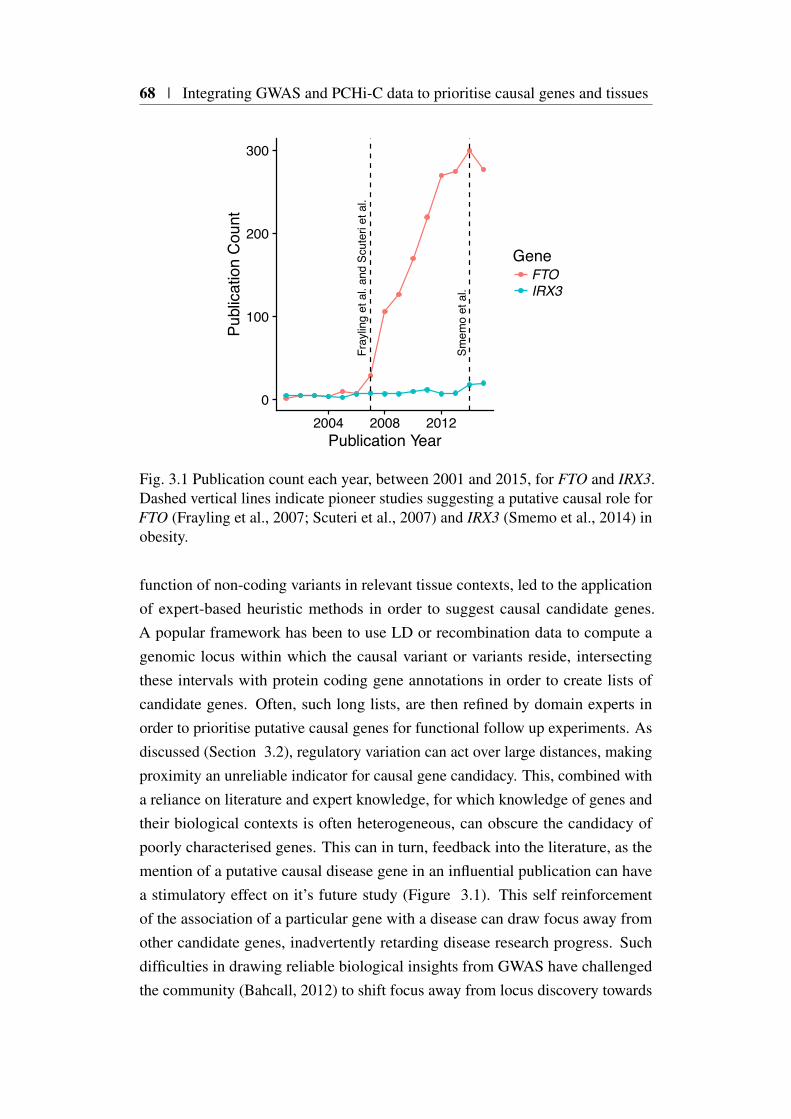
68 | Integrating GWAS and PCHi-C data to prioritise causal genes and tissues
0
100
200
300
2004 2008 2012
Smem
o et
al.
Fray
ling
et a
l. an
d Sc
uter
i et a
l.
Publication Year
Publ
icat
ion
Cou
ntGene
FTOIRX3
Fig. 3.1 Publication count each year, between 2001 and 2015, for FTO and IRX3.Dashed vertical lines indicate pioneer studies suggesting a putative causal role forFTO (Frayling et al., 2007; Scuteri et al., 2007) and IRX3 (Smemo et al., 2014) inobesity.
function of non-coding variants in relevant tissue contexts, led to the applicationof expert-based heuristic methods in order to suggest causal candidate genes.A popular framework has been to use LD or recombination data to compute agenomic locus within which the causal variant or variants reside, intersectingthese intervals with protein coding gene annotations in order to create lists ofcandidate genes. Often, such long lists, are then refined by domain experts inorder to prioritise putative causal genes for functional follow up experiments. Asdiscussed (Section 3.2), regulatory variation can act over large distances, makingproximity an unreliable indicator for causal gene candidacy. This, combined witha reliance on literature and expert knowledge, for which knowledge of genes andtheir biological contexts is often heterogeneous, can obscure the candidacy ofpoorly characterised genes. This can in turn, feedback into the literature, as themention of a putative causal disease gene in an influential publication can havea stimulatory effect on it’s future study (Figure 3.1). This self reinforcementof the association of a particular gene with a disease can draw focus away fromother candidate genes, inadvertently retarding disease research progress. Suchdifficulties in drawing reliable biological insights from GWAS have challengedthe community (Bahcall, 2012) to shift focus away from locus discovery towards

3.2 Background | 69
developing methods that integrate both genetic and genomic information in orderto suggest causal mechanisms in a more data-driven, hypothesis-free fashion.
3.2.2 Population genetics approaches
One of the main data-driven approaches for linking causal variants to targetgenes and relevant tissue contexts is to harness population genetic approaches, thatexamine how molecular genomic quantitative traits correlate with genetic variation.Such studies were pioneered in humans, by the analysis of the modulation of geneexpression by genetic variation (Stranger et al., 2007). Typically such expressionquantitative trait loci (eQTL) analyses, begin by the collection of gene expressionmeasurements for hundreds of genotyped individuals for the cell type of interest,either using microarray, or more recently, RNA-Seq analysis techniques. Thiscatalogue of n genotypes and p expression levels can be combined in a seriesof univariate linear regressions to identify those variants that are significantlyassociated with target gene expression. In the naive setting one could considera genome-wide analysis where each available variant is regressed against eachgene (n× p tests). In practice such a strategy is not employed, because of thesignificant multiple testing burden incurred. Since target gene proximity is relatedto eQTL frequency (Brem et al., 2002) analysis is instead restricted to detectinglocal eQTLs (Albert and Kruglyak, 2015), such that analysed variants are limitedto those overlapping a fixed physical window centred on the gene of interest,resulting in many fewer tests.
In humans the detection of such local eQTL’s in a multitude of tissue con-texts has been successful, with a recent study, GTEx, robustly detecting one ormore local eQTLs for 86% of protein-coding genes across 44 post-mortem tis-sue types (GTEx Consortium, 2017). Identifying overlapping eQTL and GWASsignals provides a powerful and intuitive mechanism for prioritising genes andtissue contexts for follow up of GWAS results. In the face of ever broadeningtissue catalogues of eQTLs, interpreting such overlaps has proved challenging. Forexample, GTEx found that 93% of all common variants are nominally (P < 0.05)associated with expression of at least one gene in one or more of the tissues thatthey studied (GTEx Consortium, 2017). Indeed the application of more robuststatistical methods (Giambartolomei et al., 2014; Zhu et al., 2016) designed toovercome the effect LD plays in such overlaps, have found relatively limited robustevidence for overlap (GTEx Consortium, 2017; Guo et al., 2015; Zhu et al., 2016).

70 | Integrating GWAS and PCHi-C data to prioritise causal genes and tissues
The powerful eQTL paradigm described is extensible to any high throughput‘omic’ technology that can be used to robustly generate quantitative molecular phe-notypes. Indeed it is now routinely used to assess a multitude of other functionalannotations such as chromatin accessibility (Alasoo et al., 2018; Tehranchi et al.,2016). Whilst genotyping need only be carried out once per individual, molecularphenotyping needs to be repeated for each trait and tissue permutation of interest.In practice, due to understandable economic considerations this limits not only co-hort size and thus power to detect variants with more subtle effects, but also thosefunctioning in specific tissue contexts relevant to disease aetiology (Rockman,2012).
3.2.3 High throughput molecular genomic approaches
Initial human genome-wide catalogues of chromatin modification elucidated thatregions associated with complex disease were enriched for modifications markingregions of regulatory activity using correlation between disparate elements in orderto infer target effector genes (Farh et al., 2015; Maurano et al., 2012; Thurman et al.,2012). As discussed in detail in Chapter 1, advances in high throughput chromatinconformational capture (Dekker et al., 2002) along with subsequent sequencecapture extensions, have allowed the consideration of specific disease loci in three-dimensions and the physical linkage of putative causal variants with their targetgene promoters (Dryden et al., 2014; Martin et al., 2015). Further developmentof high resolution PCHi-C has facilitated the genome-wide analysis of physicallinkages between GWAS association signals and their target genes (Mifsud et al.,2015). However, none of these previous studies have combined the statistical finemapping methods described in Chapter 1 with PCHi-C data across disease relevantcell types to infer causal linkages systematically.
3.3 Promoter-capture platform coverage
Throughout this chapter as the source of PCHi-C promoter interacting regions(PIRs), I use data from Javierre et al. (2016) as described in Chapter 2. ThePCHi-C platform employed uses the same capture library as described in Mifsudet al. (2015), originally designed to capture the promoters of 89% of Ensemblprotein-coding genes, noncoding RNAs, antisense RNAs, small nuclear RNAs(snRNAs), microRNAs (miRNAs) and small nucleolar RNAs (snoRNAs) availableat that time. Complete coverage is not possible due to the technical challenges in

3.3 Promoter-capture platform coverage | 71
designing probes to capture all promoter containing HindIII fragments, such asthose in regions of the genome where there is a high degree of repetitive sequence.
3.3.1 Capture platform reannotation
Any approach linking putative causal variants to genes via PCHi-C and GWAS in-tegration will benefit from a thorough and up-to-date integration of gene promoterlocations with HindIII fragment capture design.
I therefore re-annotated the underlying promoter sequence capture platform(Mifsud et al., 2015) using Ensembl version 75 (Yates et al., 2016) gene anno-tations. I defined a promoter as the physical location immediately 5’ to a genetranscriptional start site (TSS). As genes may consist of multiple transcripts thisresults in a many-to-many mapping of promoters to fragments. Assignment ofgenes to fragments was conducted at the gene level and multiple TSS for the samegene in the same capture fragment were collapsed.
3.3.2 Distribution of captured transcriptional start sites
In summary 22,076 captured HindIII fragments (baits), containing 31,253 nonredundant promoters were annotated, covering 18,202 protein-coding and 10,928non-protein coding genes (Table 3.1). This resulted in a 90% coverage of proteincoding space of at least one promoter per gene. There was no evidence to supporta systematic failure to capture genes in specific genomic loci such as telomericregions (Figure 3.2).
The underlying resolution of PCHi-C is dependent on the distribution ofHindIII cut sites within the human genome, resulting in a mean and median lengthof approximately 9Kb and 7Kb for captured fragments respectively (Figure 3.3a).As expected I found a relationship between fragment size and the number ofpromoters captured, with larger fragments capturing more promoters (Figure 3.3b).
As previously mentioned, a single bait might also contain multiple promoters;these can include promoters for alternative transcripts for the same gene or moreproblematically, promoters for multiple genes. Setting aside non-protein codinggenes, I found that approximately 18% of captured fragments fell into the lattercategory of what I term, promiscuous baits. This rises to 33% on the incorporationof non-coding classes of genes.
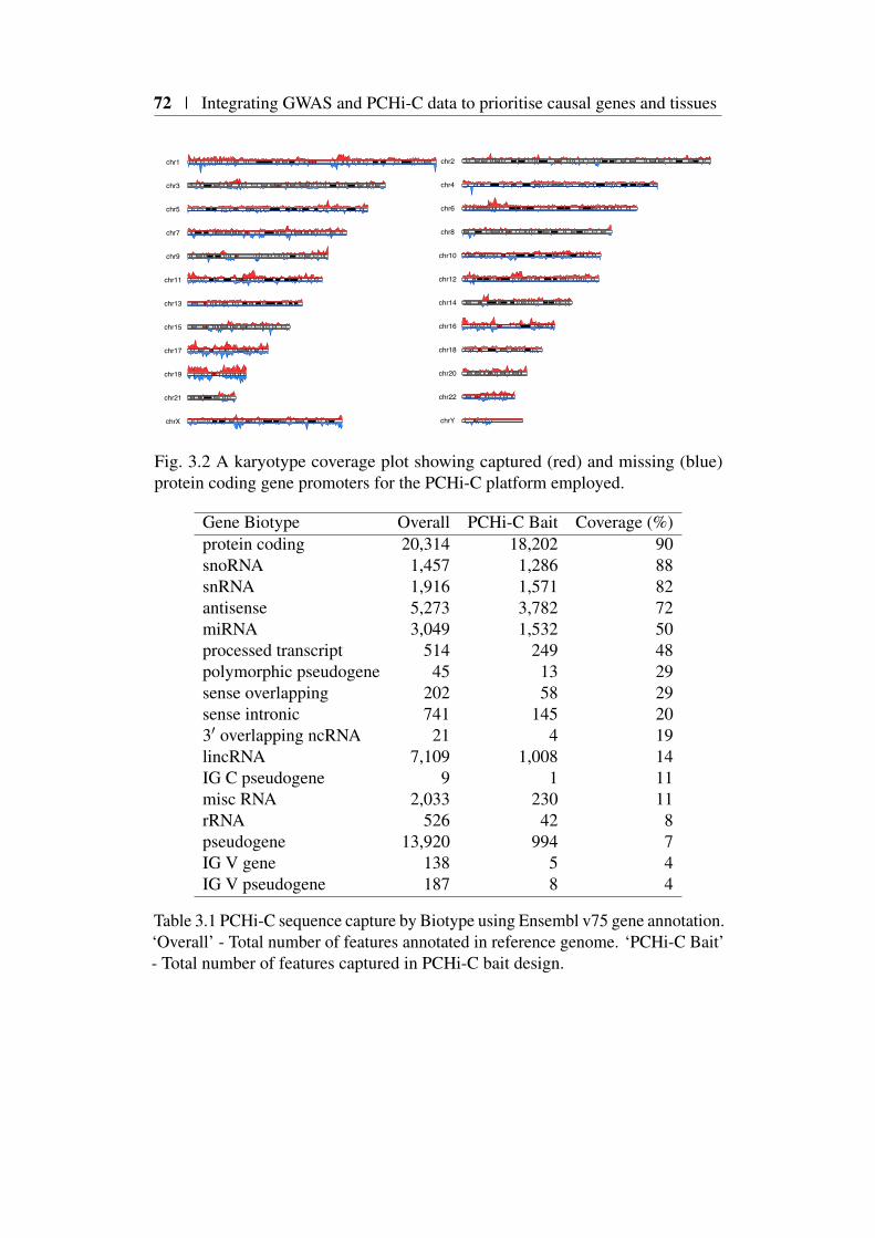
72 | Integrating GWAS and PCHi-C data to prioritise causal genes and tissues
chr1
chr3
chr5
chr7
chr9
chr11
chr13
chr15
chr17
chr19
chr21
chrX
chr2
chr4
chr6
chr8
chr10
chr12
chr14
chr16
chr18
chr20
chr22
chrY
Fig. 3.2 A karyotype coverage plot showing captured (red) and missing (blue)protein coding gene promoters for the PCHi-C platform employed.
Gene Biotype Overall PCHi-C Bait Coverage (%)protein coding 20,314 18,202 90snoRNA 1,457 1,286 88snRNA 1,916 1,571 82antisense 5,273 3,782 72miRNA 3,049 1,532 50processed transcript 514 249 48polymorphic pseudogene 45 13 29sense overlapping 202 58 29sense intronic 741 145 203′ overlapping ncRNA 21 4 19lincRNA 7,109 1,008 14IG C pseudogene 9 1 11misc RNA 2,033 230 11rRNA 526 42 8pseudogene 13,920 994 7IG V gene 138 5 4IG V pseudogene 187 8 4
Table 3.1 PCHi-C sequence capture by Biotype using Ensembl v75 gene annotation.‘Overall’ - Total number of features annotated in reference genome. ‘PCHi-C Bait’- Total number of features captured in PCHi-C bait design.
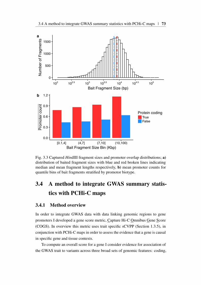
3.4 A method to integrate GWAS summary statistics with PCHi-C maps | 73
0
500
1000
1500
102 102.5 103 103.5 104 104.5 105
Bait Fragment Size (bp)
Num
ber o
f Fra
gmen
tsa
0.0
0.3
0.6
0.9
1.2
[0.1,4] (4,7] (7,10] (10,100)Bait Fragment Size Bin (Kbp)
Prom
oter
cou
nt
Protein codingTrueFalse
b
Fig. 3.3 Captured HindIII fragment sizes and promoter overlap distributions; a)distribution of baited fragment sizes with blue and red broken lines indicatingmedian and mean fragment lengths respectively, b) mean promoter counts forquantile bins of bait fragments stratified by promotor biotype.
3.4 A method to integrate GWAS summary statis-tics with PCHi-C maps
3.4.1 Method overview
In order to integrate GWAS data with data linking genomic regions to genepromoters I developed a gene score metric, Capture Hi-C Omnibus Gene Score(COGS). In overview this metric uses trait specific sCVPP (Section 1.3.5), inconjunction with PCHi-C maps in order to assess the evidence that a gene is causalin specific gene and tissue contexts.
To compute an overall score for a gene I consider evidence for association ofthe GWAS trait to variants across three broad sets of genomic features: coding,

74 | Integrating GWAS and PCHi-C data to prioritise causal genes and tissues
‘virtual’ promoter, and PIRs (derived from, for example, PCHi-C), within a givenapproximately LD independent region (Section 2.4.1).
I quantify ‘evidence for association’ using the sCVPP. In a gene/tissue priori-tisation setting and in the absence of individual level genotyping data the use ofsCVPP is natural albeit at the cost of the significant assumption that there is atmost 1 causal variant (per trait) in any genetic locus under consideration. Onebenefit is that sCVPP can, through simple summation, be combined within a givengenetic locus, to estimate posterior probabilities that a given feature overlaps acausal variant. This property facilitates the integration of GWAS data at a singlebasepair resolution, within the larger HindIII regions underlying PCHi-C contactmaps. Another attractive feature of sCVPP is that they are computed from a jointmodel of SNPs across an LD block (Wellcome Trust Case Control Consortiumet al., 2012) and thus naturally adjust for LD between variants within that block.
3.4.2 Annotation of coding variants
Whilst PCHi-C data has the prospect of linking non-coding variation to targetgenes, any systematic method should take also into account other functionalannotation classes that occur in the coding space. To do this I annotated allSNPs within dbSNP 138 (Sherry et al., 2001) using VEP (McLaren et al., 2016)employing gene annotations from Ensembl v75 (Yates et al., 2016). I then filteredthese annotations so that I obtained the set of SNPs that overlapped protein codinggenes. Whilst there is some literature that implies that coding variation may haveregulatory potential (Stergachis et al., 2013), this has proved controversial (Xingand He, 2015) and I chose to assign function to such variants exclusively withinthe gene within which they occurred. I made no distinction between classes ofcoding variation as although non-synonymous coding variants by definition alterprotein sequence, there is evidence that synonymous variants can effect profoundchanges through, for example the introduction of cryptic splice sites (Rice et al.,2013). Thus, the final set of coding SNPs (cSNPs) included all exonic variants inprotein coding genes annotated by VEP/Ensembl v75.
3.4.3 Annotation of PCHi-C ‘blindspot’ (‘Virtual Promoter’)
A limitation of the PCHi-C method is that interactions between a captured fragmentand its adjacent HindIII fragments are not able to be reliably called, as signalis overwhelmed by random Brownian effects (Cairns et al., 2016). In order to

3.4 A method to integrate GWAS summary statistics with PCHi-C maps | 75
capture these I created a virtual ‘promoter’ fragment (VPF) by merging eachcapture fragment (bait) with those immediately 5’ and 3’ (Figure 3.4b).
3.4.4 Annotation of PIRs
I defined PIRs for a gene as those contributing an interaction exceeding a CHiCAGOthreshold of 5 as recommended by Cairns et al. (2016). In the case where a genehas multiple baits, due to the presence of multiple TSS, it is possible for the samePIR to be linked to a gene more than once. In such an instance, I only consid-ered the highest scoring PIR within a given tissue when applying CHiCAGOthresholding.
3.4.5 COGS method description
Consider a region of the genome, r that contains nr variants vi,i∈r where i indexesSNPs across the genome and the notation i∈ r means SNPi is located within regionr. A region can contain intervals, that represent one of three categories of genomicfeatures previously described: coding SNPs (Section 3.4.2), VPF (Section 3.4.3)and PCHi-C PIRs (Section 3.4.4). The posterior probability for any feature or setof features, fr, overlapping r to contain the causal variant under a single causalvariant assumption is
∑i:vi∈ fr
sCVPPi, (3.1)
where sCVPPi is the single causal variant posterior probability for the ith variant.Across m regions r1,r2, . . . ,rm there may be at most m causal variants, and Icalculate the posterior probability that sets of features spread across these regionscontain at least one causal variant as one minus the posterior probability thereis no causal variant in any of them, on the assumption that there is completeindependence between the regions,
COGSg = 1−m
∏j=1
1− ∑i:vi∈ fr j
sCVPPi
. (3.2)
I select the regions such that they are approximately LD independent, and so theassumption of independence may not strictly hold, for this reason the computedvalue is not a true posterior probability and I use the term COGS score instead.When the set of features are defined as all those linked to a specific gene g, Idenote this COGSg.
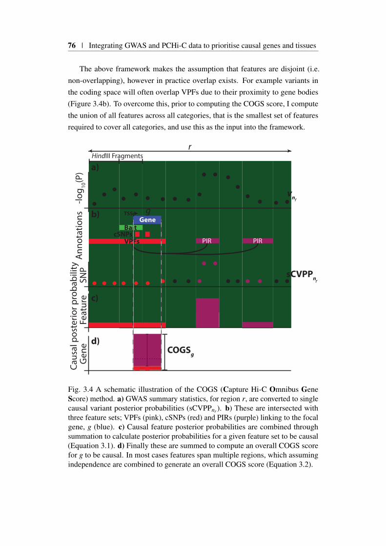
76 | Integrating GWAS and PCHi-C data to prioritise causal genes and tissues
The above framework makes the assumption that features are disjoint (i.e.non-overlapping), however in practice overlap exists. For example variants inthe coding space will often overlap VPFs due to their proximity to gene bodies(Figure 3.4b). To overcome this, prior to computing the COGS score, I computethe union of all features across all categories, that is the smallest set of featuresrequired to cover all categories, and use this as the input into the framework.
Gene
cSNPsVPFs PIRPIR
Bait
r
r
r
vn
COGSg
sCVPPn
-log 10
(P)
Caus
al p
oste
rior p
roba
bilit
ySN
PG
ene
Feat
ure
g
HindIII Fragments
Ann
otat
ions TSS
d)
c)
b)
a)
Fig. 3.4 A schematic illustration of the COGS (Capture Hi-C Omnibus GeneScore) method. a) GWAS summary statistics, for region r, are converted to singlecausal variant posterior probabilities (sCVPPnr). b) These are intersected withthree feature sets; VPFs (pink), cSNPs (red) and PIRs (purple) linking to the focalgene, g (blue). c) Causal feature posterior probabilities are combined throughsummation to calculate posterior probabilities for a given feature set to be causal(Equation 3.1). d) Finally these are summed to compute an overall COGS scorefor g to be causal. In most cases features span multiple regions, which assumingindependence are combined to generate an overall COGS score (Equation 3.2).

3.5 Application of COGS to a GWAS compendium | 77
3.5 Application of COGS to a GWAS compendium
Initially, in order to simplify the assessment of COGS performance, I consideredthe non-redundant set of PIRs linking to a gene, g, across all 17 primary tissues,along with VPF and cSNPs. It is worth restating that variants overlapping the HLAregion were removed prior to running COGS, due to both its extended LD structureand known strong and complex association with immune-mediate disease, suchthat a single causal variant assumption would not be defensible.
3.5.1 Overall COGS scores for 31 traits
I used COGS to integrate this aggregated contact map with the compendium ofPMI imputed GWAS summary statistics for each of the traits detailed in chapter 2(Table 2.1). Across all traits, the mean count of protein coding genes for whichCOGS scores were generated was 16,910; differences in counts between traits areexpected due to variability in input GWAS summary statistic coverage. Overall,the majority of gene scores were close to zero, with 99% of genes having a scoreless than 0.05 (Figure 3.5).
I created a set of ‘high scoring’ genes for each trait by selecting those with anoverall COGS gene scores greater than 0.5. In total, across all traits, 2,604 uniqueprotein coding genes were prioritised, with a median of 112 genes prioritised pertrait (Figure 3.6a).
Height had the most genes prioritised, and INS the least. It is established thatthe number of GWAS associations discovered relates to sample size, thereforeI looked to see whether there was evidence for a relationship between samplesize and the number of genes prioritised (Figure 3.6B). I observed no correlationbetween sample size and prioritised gene count (Spearman’s ρ ≈−0.09,P ≈ 0.6).This is not unexpected as the number of genes prioritised will also be affected bymany other factors, including trait heritability and the relevance of primary bloodcell specific PCHi-C data used.
3.5.2 Are prioritised genes biologically relevant?
Due to the large set of genes prioritised I was motivated to perform a systematicanalysis across all traits in order to provide support for their biological relevance.One approach, GSEA, can be a useful indicator as to whether a set of empiricallydescribed genes, such as those prioritised by COGS, are enriched for a particularbiological function. I performed a GSEA of prioritised COGS genes over all traits

78 | Integrating GWAS and PCHi-C data to prioritise causal genes and tissues
CDCELMS
PBCRA
SLET1DUCHB
MCHMCHC
MCVPCVPLTPV
RBCBMI
GLUCOSEGLUCOSE BMI
HDLINS
INS BMILDLTCTG
BP DIABP SYSFNBMDHEIGHTLSBMD
T2D
0.00 0.01 0.02 0.03 0.04 0.05Overall COGS Score
Trai
t/CO
GS
sco
re d
ensi
ty
Trait CategoryOtherMetabolicBloodAutoimmune
Fig. 3.5 A density plot of COGS scores across all traits. For clarity the horizontalaxis is truncated at 0.05, although the observations extend to 1.
using the Reactome (Fabregat et al., 2016) resource as a source of curated genesets.
I downloaded the Reactome genesets in gmt format from MolSigDB (v6.2) (Liber-zon et al., 2015; Subramanian et al., 2005), filtering each gene set so as to onlyinclude those genes for which a COGS score could be computed. I used Fisher’stest in order to assess whether there was evidence for enrichment of COGS pri-oritised genes (Overall COGS score > 0.5) compared to background (OverallCOGS score ≤ 0.5) for each of 674 genesets. I selected as significant thosewith a Benjamini-Hochberg FDR < 5%, calculated across all gene sets and baits(Figure 3.7).
As expected, genes prioritised for autoimmune diseases (blue, Figure 3.7)were enriched in inflammation and immune-response-related gene sets, such asT cell receptor signaling, whereas genes prioritised for metabolic traits (green,Figure 3.7) were preferentially enriched for lipid transport and metabolism.
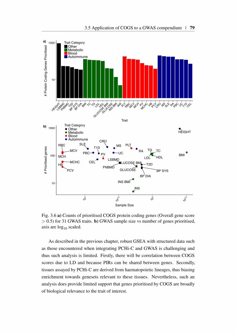
3.5 Application of COGS to a GWAS compendium | 79
10
1000
HEIGHT
LSBMD
FNBMDT2D
BP SYS
BP DIA BMITC TG
LDLHDL
GLUCOSE BMI
GLUCOSE
INS BMIINS
PLTRBC
MCVMCH PV
MCHC HBPCV
CRO MSSLE RA
PBC UCT1D CEL
Trait
# Pr
otei
n C
odin
g G
enes
Prio
ritis
edTrait Category
OtherMetabolicBloodAutoimmune
a)
HEIGHT
LSBMD
FNBMDT2D
BP SYSBP DIA
BMITCTG
LDL HDLGLUCOSE BMI
GLUCOSE
INS BMI
INS
PLTRBCMCV
MCH PV
MCHCHB
PCV
CROMSSLE
RAPBC UCT1D
CEL
10
100
1000
104
104.5
105
105.5
Sample Size
# Pr
iorit
ised
gen
es
Trait CategoryOtherMetabolicBloodAutoimmune
b)
Fig. 3.6 a) Counts of prioritised COGS protein coding genes (Overall gene score> 0.5) for 31 GWAS traits. b) GWAS sample size vs number of genes prioritised,axis are log10 scaled.
As described in the previous chapter, robust GSEA with structured data suchas those encountered when integrating PCHi-C and GWAS is challenging andthus such analysis is limited. Firstly, there will be correlation between COGSscores due to LD and because PIRs can be shared between genes. Secondly,tissues assayed by PCHi-C are derived from haematopoietic lineages, thus biasingenrichment towards genesets relevant to these tissues. Nevertheless, such ananalysis does provide limited support that genes prioritised by COGS are broadlyof biological relevance to the trait of interest.
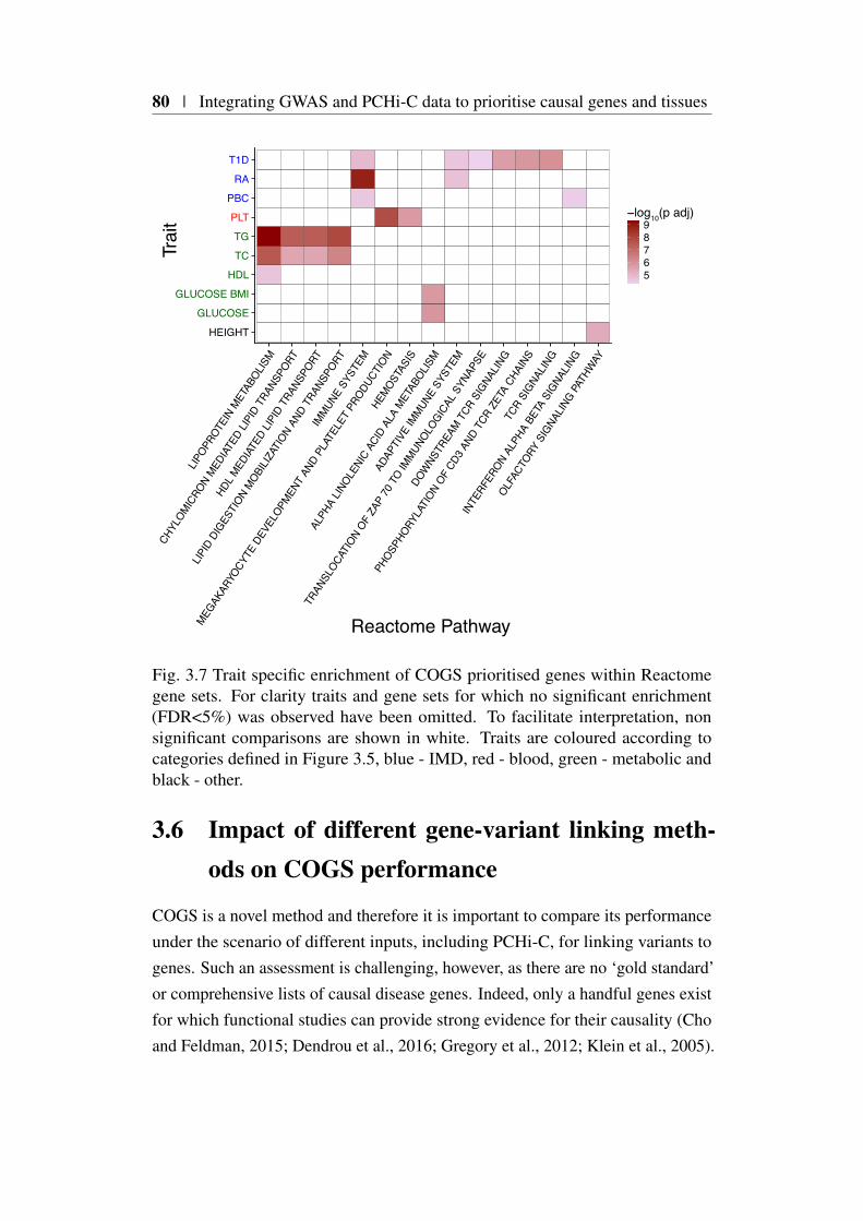
80 | Integrating GWAS and PCHi-C data to prioritise causal genes and tissues
HEIGHT
GLUCOSE
GLUCOSE BMI
HDL
TC
TG
PLT
PBC
RA
T1D
LIPOPR
OTEIN
MET
ABOLIS
M
CHYL
OMICRO
N MED
IATED
LIPI
D TR
ANSP
ORT
HDL M
EDIAT
ED LI
PID
TRAN
SPORT
LIPID
DIG
ESTI
ON MOBI
LIZAT
ION
AND
TRAN
SPORT
IMMUN
E SY
STEM
MEGAK
ARYO
CYTE
DEV
ELOPM
ENT
AND
PLAT
ELET
PRO
DUCT
ION
HEMOST
ASIS
ALPH
A LIN
OLENI
C AC
ID A
LA M
ETAB
OLISM
ADAP
TIVE
IMMUN
E SY
STEM
TRAN
SLOCA
TION
OF ZA
P 70
TO IM
MUNOLO
GICAL
SYN
APSE
DOW
NSTR
EAM T
CR S
IGNA
LING
PHOSP
HORY
LATI
ON OF
CD3 A
ND T
CR Z
ETA
CHAI
NS
TCR
SIGNA
LING
INTE
RFER
ON AL
PHA
BETA
SIG
NALIN
G
OLFAC
TORY
SIG
NALIN
G PATH
WAY
Reactome Pathway
Trai
t
56789
−log10(p adj)
Fig. 3.7 Trait specific enrichment of COGS prioritised genes within Reactomegene sets. For clarity traits and gene sets for which no significant enrichment(FDR<5%) was observed have been omitted. To facilitate interpretation, nonsignificant comparisons are shown in white. Traits are coloured according tocategories defined in Figure 3.5, blue - IMD, red - blood, green - metabolic andblack - other.
3.6 Impact of different gene-variant linking meth-ods on COGS performance
COGS is a novel method and therefore it is important to compare its performanceunder the scenario of different inputs, including PCHi-C, for linking variants togenes. Such an assessment is challenging, however, as there are no ‘gold standard’or comprehensive lists of causal disease genes. Indeed, only a handful genes existfor which functional studies can provide strong evidence for their causality (Choand Feldman, 2015; Dendrou et al., 2016; Gregory et al., 2012; Klein et al., 2005).
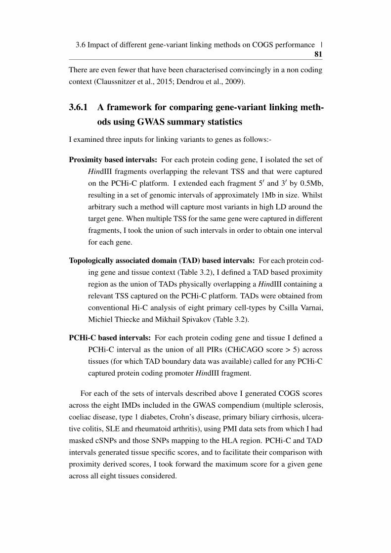
3.6 Impact of different gene-variant linking methods on COGS performance |81
There are even fewer that have been characterised convincingly in a non codingcontext (Claussnitzer et al., 2015; Dendrou et al., 2009).
3.6.1 A framework for comparing gene-variant linking meth-ods using GWAS summary statistics
I examined three inputs for linking variants to genes as follows:-
Proximity based intervals: For each protein coding gene, I isolated the set ofHindIII fragments overlapping the relevant TSS and that were capturedon the PCHi-C platform. I extended each fragment 5′ and 3′ by 0.5Mb,resulting in a set of genomic intervals of approximately 1Mb in size. Whilstarbitrary such a method will capture most variants in high LD around thetarget gene. When multiple TSS for the same gene were captured in differentfragments, I took the union of such intervals in order to obtain one intervalfor each gene.
Topologically associated domain (TAD) based intervals: For each protein cod-ing gene and tissue context (Table 3.2), I defined a TAD based proximityregion as the union of TADs physically overlapping a HindIII containing arelevant TSS captured on the PCHi-C platform. TADs were obtained fromconventional Hi-C analysis of eight primary cell-types by Csilla Varnai,Michiel Thiecke and Mikhail Spivakov (Table 3.2).
PCHi-C based intervals: For each protein coding gene and tissue I defined aPCHi-C interval as the union of all PIRs (CHiCAGO score > 5) acrosstissues (for which TAD boundary data was available) called for any PCHi-Ccaptured protein coding promoter HindIII fragment.
For each of the sets of intervals described above I generated COGS scoresacross the eight IMDs included in the GWAS compendium (multiple sclerosis,coeliac disease, type 1 diabetes, Crohn’s disease, primary biliary cirrhosis, ulcera-tive colitis, SLE and rheumatoid arthritis), using PMI data sets from which I hadmasked cSNPs and those SNPs mapping to the HLA region. PCHi-C and TADintervals generated tissue specific scores, and to facilitate their comparison withproximity derived scores, I took forward the maximum score for a given geneacross all eight tissues considered.
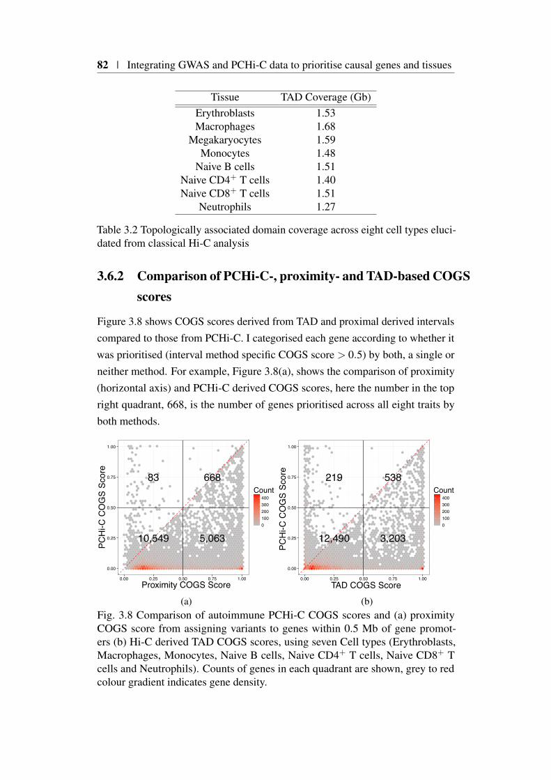
82 | Integrating GWAS and PCHi-C data to prioritise causal genes and tissues
Tissue TAD Coverage (Gb)Erythroblasts 1.53Macrophages 1.68
Megakaryocytes 1.59Monocytes 1.48
Naive B cells 1.51Naive CD4+ T cells 1.40Naive CD8+ T cells 1.51
Neutrophils 1.27
Table 3.2 Topologically associated domain coverage across eight cell types eluci-dated from classical Hi-C analysis
3.6.2 Comparison of PCHi-C-, proximity- and TAD-based COGSscores
Figure 3.8 shows COGS scores derived from TAD and proximal derived intervalscompared to those from PCHi-C. I categorised each gene according to whether itwas prioritised (interval method specific COGS score > 0.5) by both, a single orneither method. For example, Figure 3.8(a), shows the comparison of proximity(horizontal axis) and PCHi-C derived COGS scores, here the number in the topright quadrant, 668, is the number of genes prioritised across all eight traits byboth methods.
10,549
83
5,063
668
0.00
0.25
0.50
0.75
1.00
0.00 0.25 0.50 0.75 1.00Proximity COGS Score
PCH
i-C C
OG
S Sc
ore
0100200300400
Count
(a)
12,490
219
3,203
538
0.00
0.25
0.50
0.75
1.00
0.00 0.25 0.50 0.75 1.00
TAD COGS Score
PCH
i-C C
OG
S Sc
ore
0100200300400
Count
(b)Fig. 3.8 Comparison of autoimmune PCHi-C COGS scores and (a) proximityCOGS score from assigning variants to genes within 0.5 Mb of gene promot-ers (b) Hi-C derived TAD COGS scores, using seven Cell types (Erythroblasts,Macrophages, Monocytes, Naive B cells, Naive CD4+ T cells, Naive CD8+ Tcells and Neutrophils). Counts of genes in each quadrant are shown, grey to redcolour gradient indicates gene density.
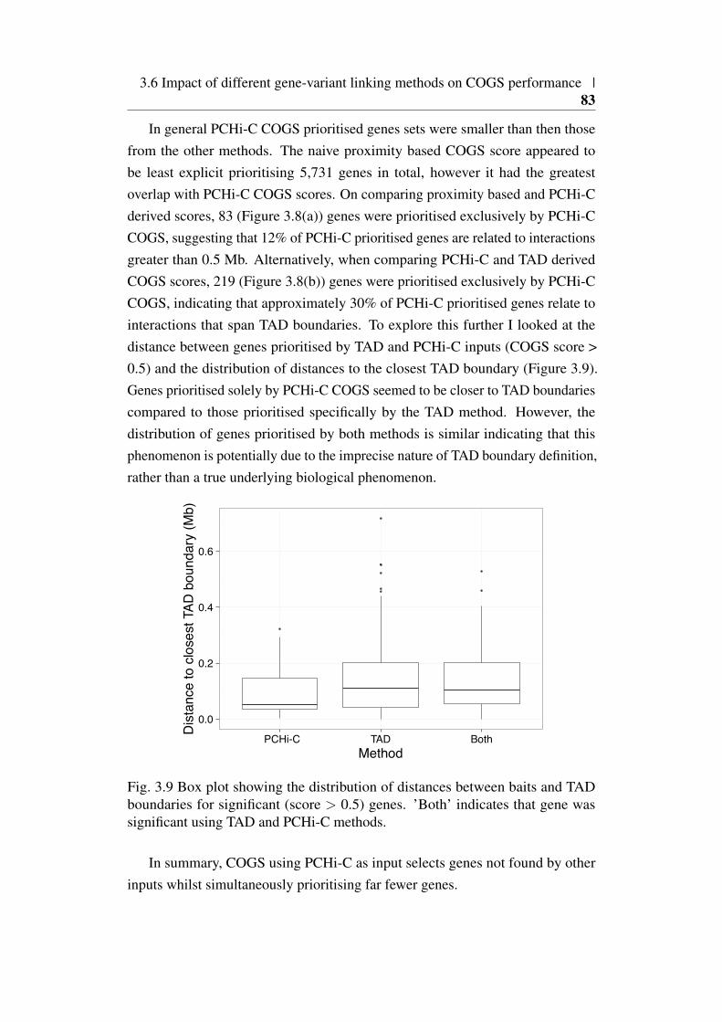
3.6 Impact of different gene-variant linking methods on COGS performance |83
In general PCHi-C COGS prioritised genes sets were smaller than then thosefrom the other methods. The naive proximity based COGS score appeared tobe least explicit prioritising 5,731 genes in total, however it had the greatestoverlap with PCHi-C COGS scores. On comparing proximity based and PCHi-Cderived scores, 83 (Figure 3.8(a)) genes were prioritised exclusively by PCHi-CCOGS, suggesting that 12% of PCHi-C prioritised genes are related to interactionsgreater than 0.5 Mb. Alternatively, when comparing PCHi-C and TAD derivedCOGS scores, 219 (Figure 3.8(b)) genes were prioritised exclusively by PCHi-CCOGS, indicating that approximately 30% of PCHi-C prioritised genes relate tointeractions that span TAD boundaries. To explore this further I looked at thedistance between genes prioritised by TAD and PCHi-C inputs (COGS score >0.5) and the distribution of distances to the closest TAD boundary (Figure 3.9).Genes prioritised solely by PCHi-C COGS seemed to be closer to TAD boundariescompared to those prioritised specifically by the TAD method. However, thedistribution of genes prioritised by both methods is similar indicating that thisphenomenon is potentially due to the imprecise nature of TAD boundary definition,rather than a true underlying biological phenomenon.
0.0
0.2
0.4
0.6
PCHi-C TAD BothMethod
Dis
tanc
e to
clo
sest
TAD
bou
ndar
y (M
b)
Fig. 3.9 Box plot showing the distribution of distances between baits and TADboundaries for significant (score > 0.5) genes. ’Both’ indicates that gene wassignificant using TAD and PCHi-C methods.
In summary, COGS using PCHi-C as input selects genes not found by otherinputs whilst simultaneously prioritising far fewer genes.

84 | Integrating GWAS and PCHi-C data to prioritise causal genes and tissues
3.6.3 PCHi-C prioritised genes are more likely to be differen-tially expressed in disease patients
In addition to quantifying the relative size of prioritised gene sets, I wanted toassess evidence for biologically plausibility. I used data from a study (Peters et al.,2016) of gene expression data across a range of relevant tissues for individualswith active inflammatory bowel disease (IBD) and healthy controls, hypothesisingthat biological plausibility would be reflected in enrichment of genes differentiallyexpressed between patients and controls within a prioritised gene set.
To generate a set of differentially expressed genes, I downloaded the data fromArrayExpress (Kolesnikov et al., 2015) (E-MTAB-3554). The data set consistsof PEER (Stegle et al., 2012) normalised microarray expression values across 49patients with Crohn’s disease, 42 with ulcerative colitis and 43 healthy controls,across sorted CD4+ T cells, CD8+ T cells, B cells, Monocytes, and Neutrophils. Imodified an R script from Chris Wallace to compute differential expression usinglimma (Ritchie et al., 2015) with a null hypothesis that expression for a given genewas the same across all three groups within a tissue. As PCHi-C and TAD COGSscores calculated for the previous comparison are derived by combining over celltypes I selected the union of genes differentially expressed in at least one cell type.
To generate a set of prioritised genes for the IBD component diseases, ulcer-ative colitis and Crohn’s disease, I used input GWAS statistics from Andersonet al. (2011) and Franke et al. (2010) with coding and HLA variants removed. Icomputed PCHi-C, TAD and proximal gene scores using only cell-types matchingthose in Peters et al. (2016).
I used Fisher’s test to examine enrichment for prioritised genes, for each ofthe three methods, for genes showing evidence of differential expression betweenhealthy, and Crohn’s disease (CD) or ulcerative colitis (UC) at a 5% false discoveryrate. I found PCHi-C genes were enriched for differentially expressed genes forUC (P = 0.002) and CD (P = 0.04). I found no evidence of enrichment in anydata sets using proximal and TAD methods (Figure 3.10).
Whilst such an analysis is not conclusive, it provides further evidence thatintegrating PCHi-C data with GWAS through COGS can prioritise biologicallyrelevant genes, and that this is in some sense more informative, evidenced bysmaller prioritised gene lists and higher enrichment in a biologically relevantexpression dataset than than proximity or TAD based COGS scores.
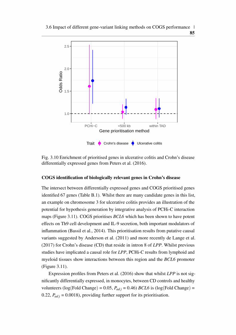
3.6 Impact of different gene-variant linking methods on COGS performance |85
1.0
1.5
2.0
2.5
PCHi−C <500 kb within TAD
Gene prioritisation method
Odd
s R
atio
Trait Crohn's disease Ulcerative colitis
Fig. 3.10 Enrichment of prioritised genes in ulcerative colitis and Crohn’s diseasedifferentially expressed genes from Peters et al. (2016).
COGS identification of biologically relevant genes in Crohn’s disease
The intersect between differentially expressed genes and COGS prioritised genesidentified 67 genes (Table B.1). Whilst there are many candidate genes in this list,an example on chromosome 3 for ulcerative colitis provides an illustration of thepotential for hypothesis generation by integrative analysis of PCHi-C interactionmaps (Figure 3.11). COGS prioritises BCL6 which has been shown to have potenteffects on Th9 cell development and IL-9 secretion, both important modulators ofinflammation (Bassil et al., 2014). This prioritisation results from putative causalvariants suggested by Anderson et al. (2011) and more recently de Lange et al.(2017) for Crohn’s disease (CD) that reside in intron 8 of LPP. Whilst previousstudies have implicated a causal role for LPP, PCHi-C results from lymphoid andmyeloid tissues show interactions between this region and the BCL6 promoter(Figure 3.11).
Expression profiles from Peters et al. (2016) show that whilst LPP is not sig-nificantly differentially expressed, in monocytes, between CD controls and healthyvolunteers (log(Fold Change) = 0.05, Pad j = 0.46) BCL6 is (log(Fold Change) =0.22, Pad j = 0.0018), providing further support for its prioritisation.
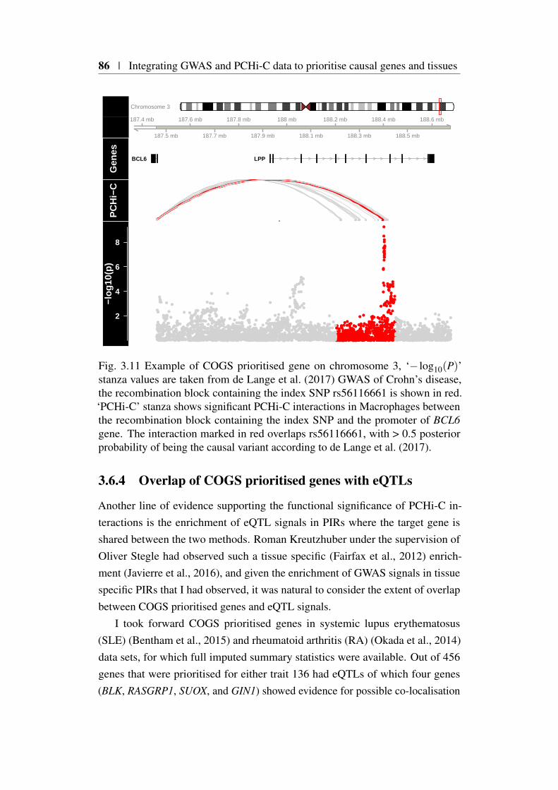
86 | Integrating GWAS and PCHi-C data to prioritise causal genes and tissues
Chromosome 3
187.4 mb
187.5 mb
187.6 mb
187.7 mb
187.8 mb
187.9 mb
188 mb
188.1 mb
188.2 mb
188.3 mb
188.4 mb
188.5 mb
188.6 mbG
enes
BCL6 LPP
PC
Hi−
C
2
4
6
8
−log
10(p
)
Fig. 3.11 Example of COGS prioritised gene on chromosome 3, ‘− log10(P)’stanza values are taken from de Lange et al. (2017) GWAS of Crohn’s disease,the recombination block containing the index SNP rs56116661 is shown in red.‘PCHi-C’ stanza shows significant PCHi-C interactions in Macrophages betweenthe recombination block containing the index SNP and the promoter of BCL6gene. The interaction marked in red overlaps rs56116661, with > 0.5 posteriorprobability of being the causal variant according to de Lange et al. (2017).
3.6.4 Overlap of COGS prioritised genes with eQTLs
Another line of evidence supporting the functional significance of PCHi-C in-teractions is the enrichment of eQTL signals in PIRs where the target gene isshared between the two methods. Roman Kreutzhuber under the supervision ofOliver Stegle had observed such a tissue specific (Fairfax et al., 2012) enrich-ment (Javierre et al., 2016), and given the enrichment of GWAS signals in tissuespecific PIRs that I had observed, it was natural to consider the extent of overlapbetween COGS prioritised genes and eQTL signals.
I took forward COGS prioritised genes in systemic lupus erythematosus(SLE) (Bentham et al., 2015) and rheumatoid arthritis (RA) (Okada et al., 2014)data sets, for which full imputed summary statistics were available. Out of 456genes that were prioritised for either trait 136 had eQTLs of which four genes(BLK, RASGRP1, SUOX, and GIN1) showed evidence for possible co-localisation
3.7 Comparison of PCHi-C COGS scores between tissues | 87
in RA and two genes (BLK and SLC15A4) in SLE. Additionally the genes pri-oritised for RA included 5/9 candidates (C8Orf13, BLK, TRAF1, FADS2 andSYNGR1) that were identified in a study that combined whole blood eQTLs withthe same RA GWAS data by Mendelian randomisation (Zhu et al., 2016). The rela-tively large number of GWAS prioritised genes without eQTL support agrees withprevious reports of limited overlap of disease variants with eQTL datasets (Guoet al., 2015; Huang et al., 2017).
3.7 Comparison of PCHi-C COGS scores betweentissues
Analyses in Chapter 2 have shown that tissue specific PCHi-C interactions showpreferential enrichment for GWAS signals. This motivated me to extend the COGSframework, such that it would be suitable for jointly prioritising causal genes and
tissue contexts. In Section 3.4.5, I ignored tissue specificity to simplify initialmethod development and assessment. However, by restricting the sets of featuresavailable to COGS it is possible for it to operate in a tissue specific manner.
In section 3.4.5 I showed how, under the assumption of at most a singlecausal variant within a genomic region r, the posterior probability for a fragmentto contain a causal variant is the sum of sCVPP over SNPs overlapping thatfragment. The fact that the coordinates of each HindIII fragment are known a
priori allows fragment posterior probabilities to be computed and stored for agiven trait prior to computing a specific gene’s COGS score. However, giventhat the set of rm regions are selected, not on the basis of alignment with HindIIIfragments, but for approximate LD independence, adjustment is necessary. Thisentails the identification and splitting of all fragments overlapping approximateLD independent region boundaries, which I term ‘LD aware’ HindIII fragments(Figure 3.12a). Coding variation presents an additional complication, as it needsto be assessed on a gene-by-gene basis (Section 3.4.2), however again all cSNPsare known a priori, as such it is simple to compute ‘LD aware’ HindIII fragmentswith all cSNPs removed (Figure 3.12b).
With ‘LD aware’ HindIII fragment posterior probabilities for a given traitprecomputed the generation of tissue specific COGS scores is greatly facilitated, asit is a simple operation of selecting fragment posterior probabilities correspondingto a gene and tissue of interest for a given region, adding in cSNPs as for the focalgene, and then combining across regions using Equation 3.2 (Figure 3.12c).

88 | Integrating GWAS and PCHi-C data to prioritise causal genes and tissues
Frag
men
t /Fe
atur
e
PP C
ausa
lr3r2r1
Frag
men
t /Fe
atur
eSN
P
c)
b)
a)HindIII Fragments
`LD Aware’ HindIII Fragments
GeneFocal GeneVirtual Promoter PIRPIR
PP C
ausa
l
Fig. 3.12 Computation of feature specific COGS scores. a) The locus shownconsists of three approximately LD independent regions, r1 to r3, which areintersected with HindIII fragments to create ‘LD aware’ fragments (alternatinggrey) with all coding variants (red) removed. b) sCVPP computed using the sameLD independent regions are intersected with these ‘LD aware’ HindIII fragmentsto obtain causal fragment posterior probabilities, which only needs to occur onceper trait. c) These fragment posterior probabilities can then be annotated withany combination of VPF (pink), tissue specific PIRs (purple) and coding variants(red) from which a feature specific COGS score can be calculated for the focalgene (blue). In this example, coding variation in an alternative gene (green) is notconsidered even though there is overlap with a focal gene PIR.
Such a scheme is fast and flexible, for example, say we wished to compute aCOGS gene score for lymphoid cells without taking into account VPF and cSNPevidence. In this case I would select the union of PIRs across nine cell types(nB, tB, FetT, aCD4, naCD4, tCD4, nCD8, nCD4, tCD8 - Figure 3.13) takingforward the fragment posterior probabilities of the non redundant set of PIRswith CHiCAGO scores greater than five. As for each trait fragment posteriorprobabilities (excluding cSNPs) are stored, the computation of the COGS scorerequires a simple lookup of the relevant fragments, which can then be combinedusing Equation 3.2.
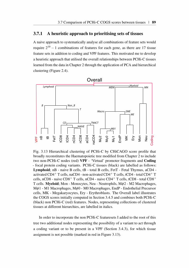
3.7 Comparison of PCHi-C COGS scores between tissues | 89
3.7.1 A heuristic approach to prioritising sets of tissues
A naive approach to systematically analyse all combinations of feature sets wouldrequire 219 − 1 combinations of features for each gene, as there are 17 tissuefeature sets in addition to coding and VPF features. This motivated me to developa heuristic approach that utilised the overall relationships between PCHi-C tissueslearned from the data in Chapter 2 through the application of PCA and hierarchicalclustering (Figure 2.4).
nB tB
FetT
tCD
8
tCD
4
nCD
4
nCD
8
aCD
4
naC
D4
Mϕ
2
Mϕ
0
Mϕ
1
EndP MK
Ery
Mon
Neu
Cod
ing
Overall
VPF
MyeloidLymphoid
B Non_BT
TNACTCDNAIVE
M01
Macro
MEM
MEEME
MN
Fig. 3.13 Hierarchical clustering of PCHi-C by CHiCAGO score profile thatbroadly reconstitutes the Haematopoietic tree modified from Chapter 2 to includetwo non-PCHi-C nodes (red) VPF - ‘Virtual’ promoter fragments and Coding- focal protein coding variants. PCHi-C tissues (black) are labelled as follows:Lymphoid; nB - naive B cells, tB - total B cells, FetT - Fetal Thymus, aCD4 -activated CD4+ T cells, naCD4 - non-activated CD4+ T cells, tCD4 - total CD4+ Tcells, nCD8 - naive CD8+ T cells, nCD4 - naive CD4+ T cells, tCD8 - total CD8+
T cells. Myeloid; Mon - Monocytes, Neu - Neutrophils, Mφ2 - M2 Macrophages,Mφ1 - M1 Macrophages, Mφ0 - M0 Macrophages, EndP - Endothelial Precursorcells, MK - Megakaryocytes, Ery - Erythroblasts. The Overall label illustratesthe COGS scores initially computed in Section 3.4.5 and combines both PCHi-C(black) non PCHi-C (red) features. Nodes, representing collections of clusteredtissues at different hierarchies, are labelled in italics.
In order to incorporate the non PCHi-C featuresets I added to the root of thistree two additional nodes representing the possibility of a variant to act througha coding variant or to be present in a VPF (Section 3.4.3), for which tissueassignment is not possible (marked in red in Figure 3.13).

90 | Integrating GWAS and PCHi-C data to prioritise causal genes and tissues
For a given GWAS I use COGS to compute a score for each binary decisionpoint or node. For simplicity consider a single region containing a focal gene forwhich COGS scores derived from two feature sets F and F ′ are to be compared.The ratio of these scores is a ratio of likelihoods under different hypotheses ora Bayes factor (Kass and Raftery, 1995). COGS scores, however incorporateinformation across multiple regions that are assumed to be independent of oneanother. A COGS score ratio therefore incorporates products of (possibly) depen-dent probabilities. In order to disambiguate and highlight this I therefore use theterm them psuedo-Bayes Factor (pBF) interpreting these pBF in a similar mannerto Kass and Raftery (1995), such that they represent ‘a summary of the evidenceprovided by the data in favour of one scientific theory, represented by a statisticalmodel, as opposed to another’.
For example (Figure 3.14) at the root or ‘Overall’ node I compute two COGSgene scores; one considering only coding variants and the other considering onlynon-coding variants, that is those located in target gene VPFs or overlapping anytarget gene PIR across all 17 primary blood cell types. The ratio of COGS scoresincorporating these different feature sets therefore reflects the strength of evidencefor a single putative causal variant exerting its effect through an alteration ofprotein coding sequence, as opposed to a broader non-coding space alternative.If the evidence for these models is balanced, such that there is equal supportfor either, then the pBF ≈ 1, and the method returns an ‘Overall’ hypothesislabel indicating that a coding and non-coding mechanism are statistically notdiscriminable (Figure 3.14). Alternatively, if the data supports one of the binaryhypotheses over the other then that hypothesis is returned. I again refer to Kass andRaftery (1995) for guidance on what magnitude of pBF provides a suitable supportthreshold, employing pBF < 1
3 or pBF > 3, to support a given binary choiceand pBF ≥ 1
3 or pBF ≤ 3 as ‘balanced’ (inconclusive) evidence to discriminatebetween hypotheses.
I apply these tests in a hierarchical manner ‘stepping’ down the tree whenevidence is strong enough to support a decision, or sticking otherwise. Forexample if a ’Non-coding’ hypothesis is favoured over ‘coding’ we move to the‘Non-coding’ node (Figure 3.14) and compute a pBF for the next binary choice,whether the data favours a causal variant operating through a virtual ‘Promoter’region or through a PCHi-C identified chromatin looping or ‘Interaction’ event.This biologically structured and hierarchical examination of the hypothesis spacecontinues until either 1
3 ≤ pBF ≤ 3, such that no decision is favoured or we reach aterminal ‘leaf’ node for which further categorisation is not possible (Figure 3.14).

3.7 Comparison of PCHi-C COGS scores between tissues | 91
This hierarchical COGS analysis results in COGS scores at each node, andI introduce the term lCOGS scores to disambiguate between COGS scores atterminal ‘Leaf’ nodes from their more general counterparts.
3.7.2 Tissue specific COGS gene prioritisation across 8 immune-mediated diseases
I applied the hierarchical COGS method described to the compendium of GWAStraits for protein coding genes where the overall COGS score (including all tissuePIRs, coding variants and VPF) exceeded 0.5 in order for them to be comparablewith results described in Section 3.5.1. Due to haematopoietic focus of the PCHi-Cinteraction data I restricted my analysis to only blood and immune based traits,as for metabolic and anthropomorphic traits haematopoietic contexts are unlikelyto be truly relevant for discrimination between cell types. I arranged the countsof genes at each node for each trait into a matrix, and performed hierarchicalclustering using the ‘average’ linkage method on a log10(count+1) transformedmatrix in order to accommodate the large range (0−694) of values encountered(Figure 3.15).
Generally the number of genes able to be assigned to specific cell types orleaf nodes was low (IQR 0−2, mean 1.75 ), with mean gene counts ranging from0.3 in total CD8+ T cells to 9.7 in neutrophils. In comparison non-leaf nodescounts were higher (IQR 0−4, mean 8.1) with a large proportion driven by nontissue-specific interactions. This extensive sharing of PIRs across cell-types, couldbe due to shared underlying transcriptional programs between related tissue typesor due to the limitations in PCHi-C resolution, with disparate but tissue specificenhancers sharing a common PIR HindIII fragment. Secondly, in regions of highLD sCVPP will be shared across many variants, reducing resolution, and thusmaking it more likely that collateral PIRs in disparate tissues will contribute to thefinal COGS score. Such effects will be compounded by the genetic heterogeneityand study design of the traits included in the GWAS compendium. With the currentapproach it is impossible to disentangle the effect of power, PMI and heritabilityfrom these counts in order to make robust biological inference.
With these caveats in mind, there are notable features that arise from thehierarchical clustering. The foremost is that generally immune-mediated traits(blue in Figure 3.15), with the exception of coeliac disease (CEL) appear tocluster. On explanation might be that CEL may be affected by limited genotypecoverage, and thus a greater reliance on PMI, which is compounded by sample
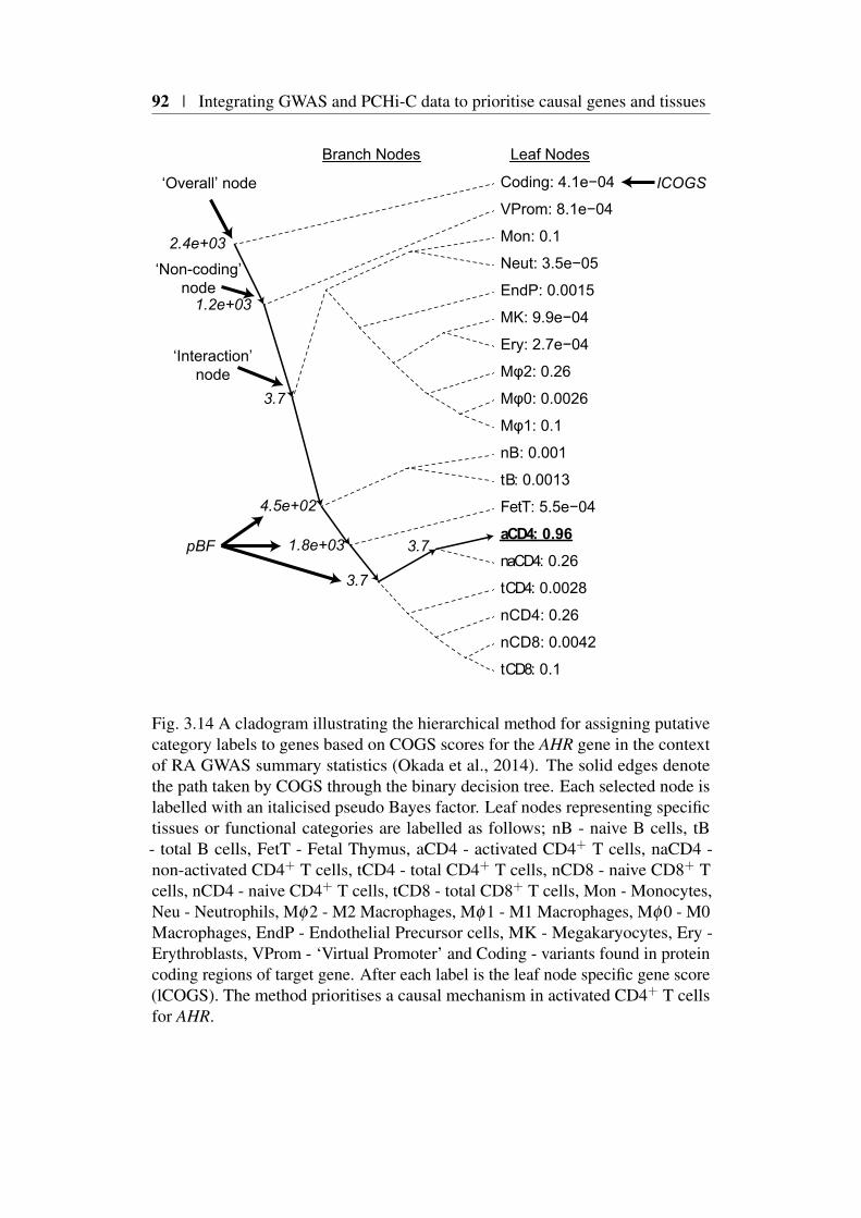
92 | Integrating GWAS and PCHi-C data to prioritise causal genes and tissues
2.4e+03
1.2e+03
3.7
4.5e+02
1.8e+03
3.7
t CD8: 0.1
nCD8: 0.0042
nCD4: 0.26
t CD4: 0.0028
3.7naCD4: 0.26
aCD4: 0.96
FetT: 5.5e−04
t B: 0.0013
nB: 0.001
Mφ1: 0.1
Mφ0: 0.0026
Mφ2: 0.26
Ery: 2.7e−04
MK: 9.9e−04
EndP: 0.0015
Neut: 3.5e−05
Mon: 0.1
VProm: 8.1e−04
Branch Nodes Leaf Nodes
Coding: 4.1e−04
‘Interaction’node
‘Non-coding’node
‘Overall’ node
pBF
lCOGS
Fig. 3.14 A cladogram illustrating the hierarchical method for assigning putativecategory labels to genes based on COGS scores for the AHR gene in the contextof RA GWAS summary statistics (Okada et al., 2014). The solid edges denotethe path taken by COGS through the binary decision tree. Each selected node islabelled with an italicised pseudo Bayes factor. Leaf nodes representing specifictissues or functional categories are labelled as follows; nB - naive B cells, tB- total B cells, FetT - Fetal Thymus, aCD4 - activated CD4+ T cells, naCD4 -non-activated CD4+ T cells, tCD4 - total CD4+ T cells, nCD8 - naive CD8+ Tcells, nCD4 - naive CD4+ T cells, tCD8 - total CD8+ T cells, Mon - Monocytes,Neu - Neutrophils, Mφ2 - M2 Macrophages, Mφ1 - M1 Macrophages, Mφ0 - M0Macrophages, EndP - Endothelial Precursor cells, MK - Megakaryocytes, Ery -Erythroblasts, VProm - ‘Virtual Promoter’ and Coding - variants found in proteincoding regions of target gene. After each label is the leaf node specific gene score(lCOGS). The method prioritises a causal mechanism in activated CD4+ T cellsfor AHR.
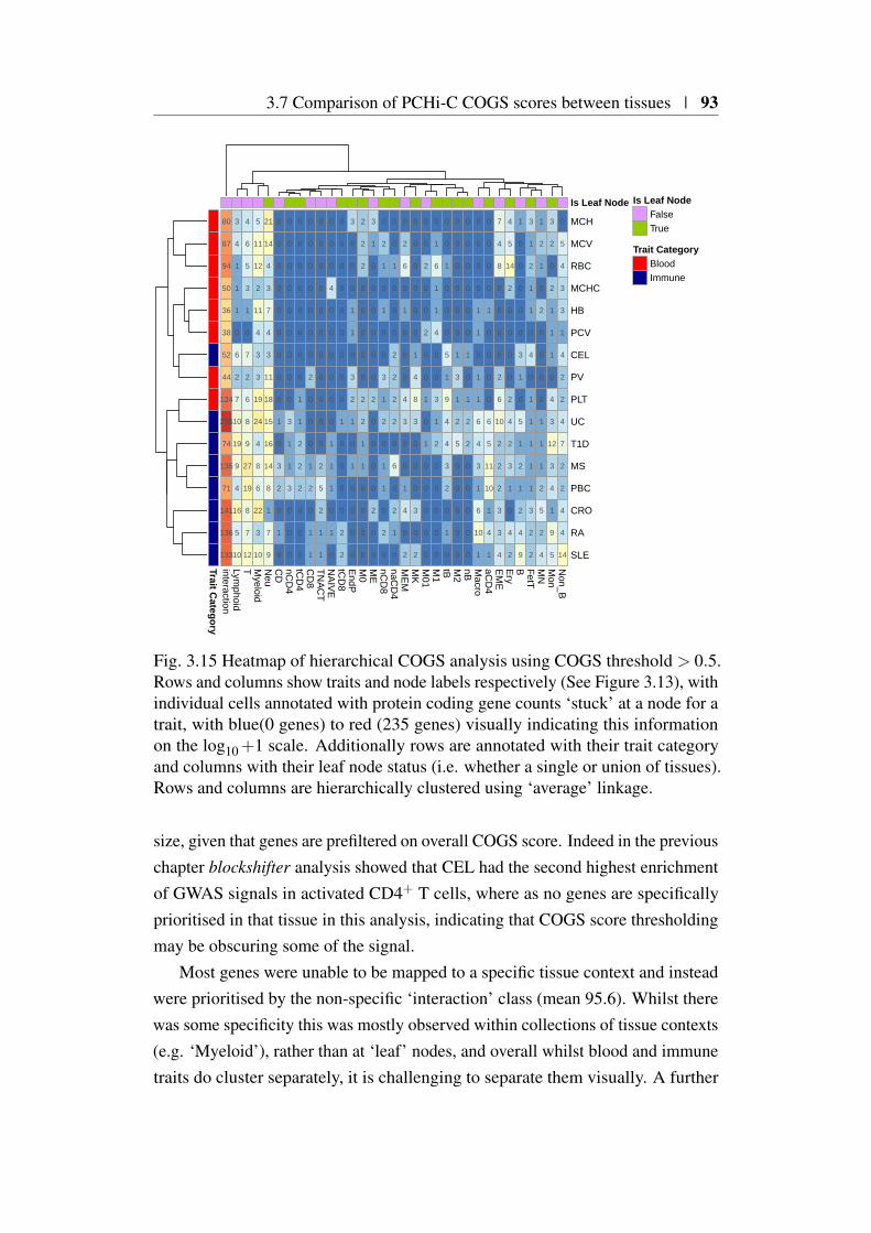
3.7 Comparison of PCHi-C COGS scores between tissues | 93
80
87
94
50
36
38
52
44
124
235
74
135
71
141
136
133
3
4
1
1
1
0
6
2
7
10
19
9
4
16
5
10
4
6
5
3
1
0
7
2
6
8
9
27
19
8
7
12
5
11
12
2
11
4
3
3
19
24
4
8
6
22
3
10
21
14
4
3
7
4
3
11
18
15
16
14
8
1
7
9
0
0
0
0
0
0
0
0
0
1
0
3
2
0
1
0
0
0
0
0
0
0
0
0
0
3
1
1
3
0
0
0
0
0
0
0
0
0
0
0
1
1
2
2
2
0
0
0
0
0
0
0
0
0
0
2
0
0
0
1
2
0
1
1
0
0
0
0
0
0
0
0
0
0
0
2
5
2
1
1
0
0
0
4
0
0
0
0
0
0
1
1
1
0
1
0
0
0
0
0
0
0
0
0
0
1
0
0
0
0
2
2
3
0
0
0
1
1
0
3
2
1
0
1
0
0
0
0
2
2
2
0
0
0
0
0
2
2
1
1
0
0
0
0
3
1
0
0
0
0
0
0
2
0
0
0
0
2
0
0
0
2
1
0
1
0
0
3
1
2
0
1
1
0
2
0
0
0
1
0
0
0
2
2
2
2
0
6
0
2
1
0
0
2
6
0
1
0
0
0
4
3
0
0
1
4
0
2
0
0
0
0
0
0
1
4
8
3
0
0
0
3
0
2
0
0
2
0
0
2
0
0
1
0
1
0
0
0
0
0
0
1
6
1
1
4
0
0
3
1
2
0
0
0
0
0
0
0
1
0
0
0
5
1
9
4
4
3
2
0
1
0
0
0
0
0
0
0
1
3
1
2
5
0
0
0
0
0
0
0
0
0
0
0
1
0
1
2
2
0
0
0
0
0
0
0
0
0
1
1
0
1
1
6
4
3
1
6
10
1
0
0
0
0
1
0
0
0
0
6
5
11
10
1
4
1
7
4
8
0
0
0
0
2
6
10
2
2
2
3
3
4
4
5
14
2
0
0
0
0
2
4
2
3
1
0
4
2
1
0
0
0
0
0
3
1
0
5
1
2
1
2
4
9
3
1
2
1
1
0
4
0
1
1
1
1
1
3
2
2
1
2
1
0
2
0
0
0
0
1
1
1
2
5
2
4
3
2
0
2
1
1
1
0
4
3
12
3
4
1
9
5
0
5
4
3
3
1
4
2
2
4
7
2
2
4
4
14
interactionLym
phoidT M
yeloidN
euC
DnC
D4
tCD
4C
D8
TN
AC
TN
AIV
EtC
D8
EndP
M0
ME
nCD
8naC
D4
ME
MM
KM
01M
1tB M
2nB M
acroaC
D4
EM
EE
ryB F
etTM
NM
onN
on_B
MCH
MCV
RBC
MCHC
HB
PCV
CEL
PV
PLT
UC
T1D
MS
PBC
CRO
RA
SLE
Is Leaf Node
Trait Category
Is Leaf NodeFalseTrue
Trait CategoryBloodImmune
Fig. 3.15 Heatmap of hierarchical COGS analysis using COGS threshold > 0.5.Rows and columns show traits and node labels respectively (See Figure 3.13), withindividual cells annotated with protein coding gene counts ‘stuck’ at a node for atrait, with blue(0 genes) to red (235 genes) visually indicating this informationon the log10+1 scale. Additionally rows are annotated with their trait categoryand columns with their leaf node status (i.e. whether a single or union of tissues).Rows and columns are hierarchically clustered using ‘average’ linkage.
size, given that genes are prefiltered on overall COGS score. Indeed in the previouschapter blockshifter analysis showed that CEL had the second highest enrichmentof GWAS signals in activated CD4+ T cells, where as no genes are specificallyprioritised in that tissue in this analysis, indicating that COGS score thresholdingmay be obscuring some of the signal.
Most genes were unable to be mapped to a specific tissue context and insteadwere prioritised by the non-specific ‘interaction’ class (mean 95.6). Whilst therewas some specificity this was mostly observed within collections of tissue contexts(e.g. ‘Myeloid’), rather than at ‘leaf’ nodes, and overall whilst blood and immunetraits do cluster separately, it is challenging to separate them visually. A further
94 | Integrating GWAS and PCHi-C data to prioritise causal genes and tissues
challenge is that a PIR can interact with more than one gene promoter, and aspreviously discussed a proportion of captured promoter fragments contain morethan one gene promoter. This leads to the tissue specific prioritisation of multiplegenes, and whether this is due to underlying biology or a limitation of PCHi-Cresolution remains to be elucidated. Overall this suggests pinpointing specificcellular contexts using PCHi-C input alone is difficult, supporting the inclusionof additional genomic information prior to functional followup, which I discussfurther in Section 3.8.5.
3.8 Cell context specific COGS analysis of immune-mediated disease
Notwithstanding the evidence presented for a role for CD4+ T cell chromatinorganisation in immune-mediated disease, differences in DNA methylation ofimmune-related genes have been observed in CD4+ T cells from autoimmunedisease patients compared to healthy controls (Coit et al., 2013; Paul et al., 2016).CD4+ T cells are at the centre of the adaptive immune system and exquisitecontrol of activation is required to guide a CD4+ T cells fate through selection,expansion and differentiation into one of a number of specialised subsets (Murphyand Weaver, 2017). The analysis of gene expression in CD4+ T cells from 20healthy individuals across a 21 hour activation time course supported early (< 4hours) modulation of transcriptional programs to be of particular importance, asthis is when a majority of differential gene expression is observed (Burren et al.,2017).
These multiple strands of evidence for the importance of early CD4+ T cellactivation, coupled with a desire to further understand how disease variants mightoperate in a particular cell context specific environment, motivated me to take amore focused approach to the integration of autoimmmune and autoinflammatoryrisk loci with PCHi-C maps. To this end I decided to focus on comparing chromatinstructure between resting and activated CD4+ T cell within the context of IMD.
The focus on IMD also provided the opportunity to use an alternative collectionof association summary statistics and genotype data afforded by the ImmunoChipplatform. This genotyping platform is specifically designed to provide densegenotype coverage of approximately 180 regions with robust demonstration ofassociation with one or more IMDs (Cortes and Brown, 2011). The main benefitof using such a platform is that dense genotyping obviates the need to rely on PMI
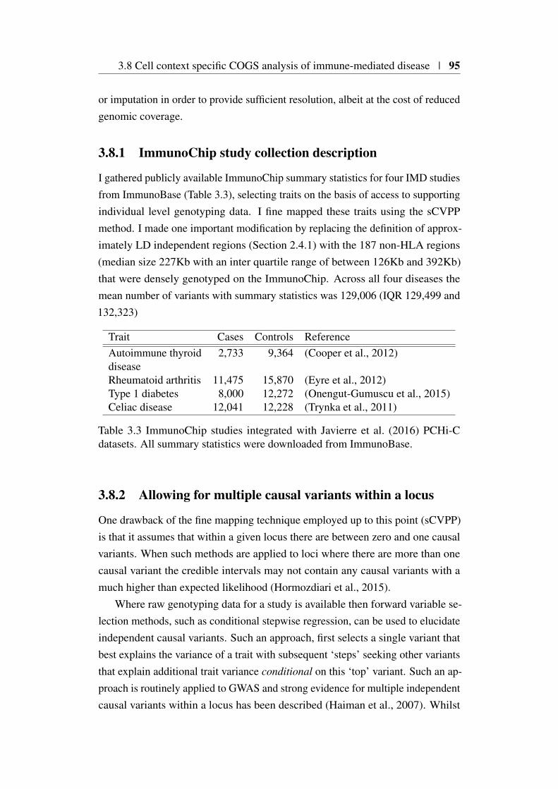
3.8 Cell context specific COGS analysis of immune-mediated disease | 95
or imputation in order to provide sufficient resolution, albeit at the cost of reducedgenomic coverage.
3.8.1 ImmunoChip study collection description
I gathered publicly available ImmunoChip summary statistics for four IMD studiesfrom ImmunoBase (Table 3.3), selecting traits on the basis of access to supportingindividual level genotyping data. I fine mapped these traits using the sCVPPmethod. I made one important modification by replacing the definition of approx-imately LD independent regions (Section 2.4.1) with the 187 non-HLA regions(median size 227Kb with an inter quartile range of between 126Kb and 392Kb)that were densely genotyped on the ImmunoChip. Across all four diseases themean number of variants with summary statistics was 129,006 (IQR 129,499 and132,323)
Trait Cases Controls ReferenceAutoimmune thyroiddisease
2,733 9,364 (Cooper et al., 2012)
Rheumatoid arthritis 11,475 15,870 (Eyre et al., 2012)Type 1 diabetes 8,000 12,272 (Onengut-Gumuscu et al., 2015)Celiac disease 12,041 12,228 (Trynka et al., 2011)
Table 3.3 ImmunoChip studies integrated with Javierre et al. (2016) PCHi-Cdatasets. All summary statistics were downloaded from ImmunoBase.
3.8.2 Allowing for multiple causal variants within a locus
One drawback of the fine mapping technique employed up to this point (sCVPP)is that it assumes that within a given locus there are between zero and one causalvariants. When such methods are applied to loci where there are more than onecausal variant the credible intervals may not contain any causal variants with amuch higher than expected likelihood (Hormozdiari et al., 2015).
Where raw genotyping data for a study is available then forward variable se-lection methods, such as conditional stepwise regression, can be used to elucidateindependent causal variants. Such an approach, first selects a single variant thatbest explains the variance of a trait with subsequent ‘steps’ seeking other variantsthat explain additional trait variance conditional on this ‘top’ variant. Such an ap-proach is routinely applied to GWAS and strong evidence for multiple independentcausal variants within a locus has been described (Haiman et al., 2007). Whilst
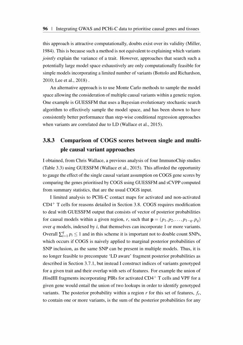
96 | Integrating GWAS and PCHi-C data to prioritise causal genes and tissues
this approach is attractive computationally, doubts exist over its validity (Miller,1984). This is because such a method is not equivalent to explaining which variantsjointly explain the variance of a trait. However, approaches that search such apotentially large model space exhaustively are only computationally feasible forsimple models incorporating a limited number of variants (Bottolo and Richardson,2010; Lee et al., 2018) .
An alternative approach is to use Monte Carlo methods to sample the modelspace allowing the consideration of multiple causal variants within a genetic region.One example is GUESSFM that uses a Bayesian evolutionary stochastic searchalgorithm to effectively sample the model space, and has been shown to haveconsistently better performance than step-wise conditional regression approacheswhen variants are correlated due to LD (Wallace et al., 2015).
3.8.3 Comparison of COGS scores between single and multi-ple causal variant approaches
I obtained, from Chris Wallace, a previous analysis of four ImmunoChip studies(Table 3.3) using GUESSFM (Wallace et al., 2015). This afforded the opportunityto gauge the effect of the single causal variant assumption on COGS gene scores bycomparing the genes prioritised by COGS using GUESSFM and sCVPP computedfrom summary statistics, that are the usual COGS input.
I limited analysis to PCHi-C contact maps for activated and non-activatedCD4+ T cells for reasons detailed in Section 3.8. COGS requires modificationto deal with GUESSFM output that consists of vector of posterior probabilitiesfor causal models within a given region, r, such that p = (p1, p2, . . . , p1−q, pq)
over q models, indexed by i, that themselves can incorporate 1 or more variants.Overall ∑
qi=1 pi ≤ 1 and in this scheme it is important not to double count SNPs,
which occurs if COGS is naively applied to marginal posterior probabilities ofSNP inclusion, as the same SNP can be present in multiple models. Thus, it isno longer feasible to precompute ‘LD aware’ fragment posterior probabilities asdescribed in Section 3.7.1, but instead I construct indices of variants genotypedfor a given trait and their overlap with sets of features. For example the union ofHindIII fragments incorporating PIRs for activated CD4+ T cells and VPF for agiven gene would entail the union of two lookups in order to identify genotypedvariants. The posterior probability within a region r for this set of features, fr,to contain one or more variants, is the sum of the posterior probabilities for any
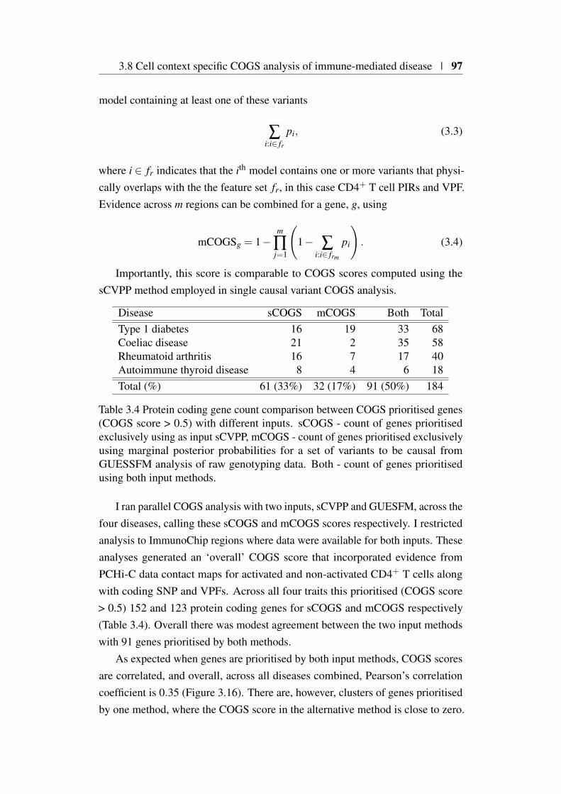
3.8 Cell context specific COGS analysis of immune-mediated disease | 97
model containing at least one of these variants
∑i:i∈ fr
pi, (3.3)
where i ∈ fr indicates that the ith model contains one or more variants that physi-cally overlaps with the the feature set fr, in this case CD4+ T cell PIRs and VPF.Evidence across m regions can be combined for a gene, g, using
mCOGSg = 1−m
∏j=1
(1− ∑
i:i∈ frm
pi
). (3.4)
Importantly, this score is comparable to COGS scores computed using thesCVPP method employed in single causal variant COGS analysis.
Disease sCOGS mCOGS Both TotalType 1 diabetes 16 19 33 68Coeliac disease 21 2 35 58Rheumatoid arthritis 16 7 17 40Autoimmune thyroid disease 8 4 6 18Total (%) 61 (33%) 32 (17%) 91 (50%) 184
Table 3.4 Protein coding gene count comparison between COGS prioritised genes(COGS score > 0.5) with different inputs. sCOGS - count of genes prioritisedexclusively using as input sCVPP, mCOGS - count of genes prioritised exclusivelyusing marginal posterior probabilities for a set of variants to be causal fromGUESSFM analysis of raw genotyping data. Both - count of genes prioritisedusing both input methods.
I ran parallel COGS analysis with two inputs, sCVPP and GUESFM, across thefour diseases, calling these sCOGS and mCOGS scores respectively. I restrictedanalysis to ImmunoChip regions where data were available for both inputs. Theseanalyses generated an ‘overall’ COGS score that incorporated evidence fromPCHi-C data contact maps for activated and non-activated CD4+ T cells alongwith coding SNP and VPFs. Across all four traits this prioritised (COGS score> 0.5) 152 and 123 protein coding genes for sCOGS and mCOGS respectively(Table 3.4). Overall there was modest agreement between the two input methodswith 91 genes prioritised by both methods.
As expected when genes are prioritised by both input methods, COGS scoresare correlated, and overall, across all diseases combined, Pearson’s correlationcoefficient is 0.35 (Figure 3.16). There are, however, clusters of genes prioritisedby one method, where the COGS score in the alternative method is close to zero.
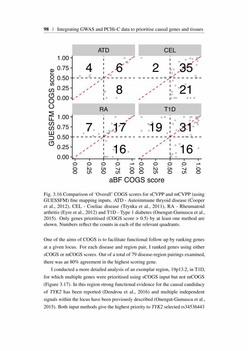
98 | Integrating GWAS and PCHi-C data to prioritise causal genes and tissues
RA T1D
ATD CEL
0.00
0.25
0.50
0.75
1.000.00
0.25
0.50
0.75
1.00
0.000.250.500.751.00
0.000.250.500.751.00
aBF COGS score
GU
ESSF
M C
OG
S sc
ore
16177
163119
21352
864
Fig. 3.16 Comparison of ‘Overall’ COGS scores for sCVPP and mCVPP (usingGUESSFM) fine mapping inputs. ATD - Autoimmune thryoid disease (Cooperet al., 2012), CEL - Coeliac disease (Trynka et al., 2011), RA - Rheumatoidarthritis (Eyre et al., 2012) and T1D - Type 1 diabetes (Onengut-Gumuscu et al.,2015). Only genes prioritised (COGS score > 0.5) by at least one method areshown. Numbers reflect the counts in each of the relevant quadrants.
One of the aims of COGS is to facilitate functional follow up by ranking genesat a given locus. For each disease and region pair, I ranked genes using eithersCOGS or mCOGS scores. Out of a total of 79 disease-region pairings examined,there was an 80% agreement in the highest scoring gene.
I conducted a more detailed analysis of an exemplar region, 19p13.2, in T1D,for which multiple genes were prioritised using sCOGS input but not mCOGS(Figure 3.17). In this region strong functional evidence for the causal candidacyof TYK2 has been reported (Dendrou et al., 2016) and multiple independentsignals within the locus have been previously described (Onengut-Gumuscu et al.,2015). Both input methods give the highest priority to TYK2 selected rs34536443
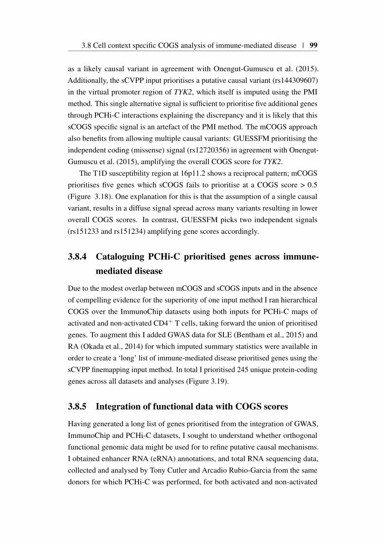
3.8 Cell context specific COGS analysis of immune-mediated disease | 99
as a likely causal variant in agreement with Onengut-Gumuscu et al. (2015).Additionally, the sCVPP input prioritises a putative causal variant (rs144309607)in the virtual promoter region of TYK2, which itself is imputed using the PMImethod. This single alternative signal is sufficient to prioritise five additional genesthrough PCHi-C interactions explaining the discrepancy and it is likely that thissCOGS specific signal is an artefact of the PMI method. The mCOGS approachalso benefits from allowing multiple causal variants: GUESSFM prioritising theindependent coding (missense) signal (rs12720356) in agreement with Onengut-Gumuscu et al. (2015), amplifying the overall COGS score for TYK2.
The T1D susceptibility region at 16p11.2 shows a reciprocal pattern; mCOGSprioritises five genes which sCOGS fails to prioritise at a COGS score > 0.5(Figure 3.18). One explanation for this is that the assumption of a single causalvariant, results in a diffuse signal spread across many variants resulting in loweroverall COGS scores. In contrast, GUESSFM picks two independent signals(rs151233 and rs151234) amplifying gene scores accordingly.
3.8.4 Cataloguing PCHi-C prioritised genes across immune-mediated disease
Due to the modest overlap between mCOGS and sCOGS inputs and in the absenceof compelling evidence for the superiority of one input method I ran hierarchicalCOGS over the ImmunoChip datasets using both inputs for PCHi-C maps ofactivated and non-activated CD4+ T cells, taking forward the union of prioritisedgenes. To augment this I added GWAS data for SLE (Bentham et al., 2015) andRA (Okada et al., 2014) for which imputed summary statistics were available inorder to create a ‘long’ list of immune-mediated disease prioritised genes using thesCVPP finemapping input method. In total I prioritised 245 unique protein-codinggenes across all datasets and analyses (Figure 3.19).
3.8.5 Integration of functional data with COGS scores
Having generated a long list of genes prioritised from the integration of GWAS,ImmunoChip and PCHi-C datasets, I sought to understand whether orthogonalfunctional genomic data might be used for to refine putative causal mechanisms.I obtained enhancer RNA (eRNA) annotations, and total RNA sequencing data,collected and analysed by Tony Cutler and Arcadio Rubio-Garcia from the samedonors for which PCHi-C was performed, for both activated and non-activated

100 | Integrating GWAS and PCHi-C data to prioritise causal genes and tissues
Chromosome 19
10.4 mb
10.5 mb
10.6 mb
Gen
es
ICAM1
MRPL4
ICAM4
ICAM5 TYK2
RAVER1
S1PR5
ZGLP1
CTD−2369P2.12
PCHi−C
00.20.40.60.8
GU
ESSF
M
00.20.40.60.8
mC
OG
S
00.20.40.60.8
sCVP
P
00.20.40.60.8
sCO
GS
Fig. 3.17 Comparison of T1D (Onengut-Gumuscu et al., 2015) COGS scoresderived from sCVPP and GUESSFM inputs at the 19p13.2 susceptibility locus.For clarity only protein coding genes with a COGS score > 0.01 from eitherinput are shown. The dark green stanza shows the union of interactions with theTYK2 promoter in activated and non-activated CD4+ T cells, for clarity otherinteractions in the region are not shown. The blue ‘GUESSFM’ stanza shows themarginal posterior probabilities for SNPs to be causal allowing for multiple causalSNPs. The blue ’mCOGS’ stanza presents the overall COGS scores computedfrom GUESSFM model posterior probabilities for a given gene (see ‘Genes’stanza). Similarly the red stanzas present sCVPP and resultant sCOGS scoresfrom allowing a maximum of one causal variant.
CD4+ T cells. Briefly, eRNAs are defined as bi-directionally transcribed RNAspecies that map to ChIP-Seq derived enhancer regions but do not map to knowngene annotations (Li et al., 2016). This bi-directionality is key to the robustidentification of intronic eRNAs as it allows their separation from pre-mRNA on
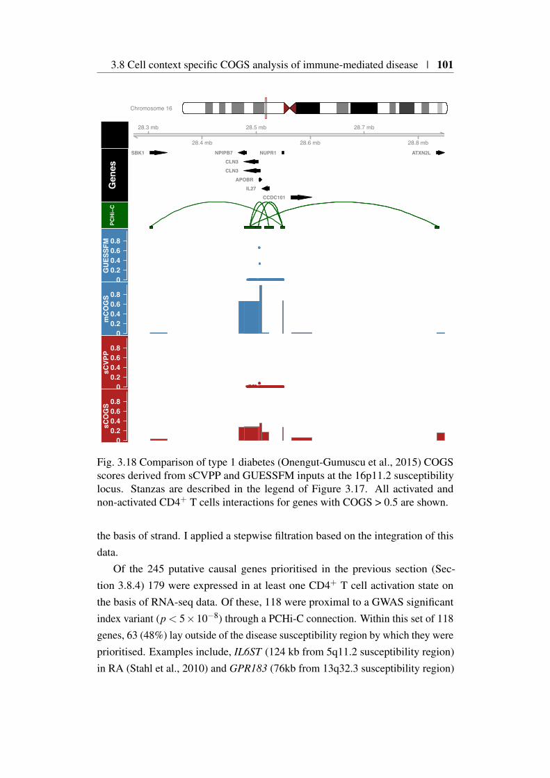
3.8 Cell context specific COGS analysis of immune-mediated disease | 101
Chromosome 16
28.3 mb
28.4 mb
28.5 mb
28.6 mb
28.7 mb
28.8 mb
Gen
es
ATXN2LNUPR1
CCDC101
APOBR
SBK1
CLN3
IL27
NPIPB7
CLN3
PCHi−C
00.20.40.60.8
GU
ESSF
M
00.20.40.60.8
mC
OG
S
00.20.40.60.8
sCVP
P
00.20.40.60.8
sCO
GS
Fig. 3.18 Comparison of type 1 diabetes (Onengut-Gumuscu et al., 2015) COGSscores derived from sCVPP and GUESSFM inputs at the 16p11.2 susceptibilitylocus. Stanzas are described in the legend of Figure 3.17. All activated andnon-activated CD4+ T cells interactions for genes with COGS > 0.5 are shown.
the basis of strand. I applied a stepwise filtration based on the integration of thisdata.
Of the 245 putative causal genes prioritised in the previous section (Sec-tion 3.8.4) 179 were expressed in at least one CD4+ T cell activation state onthe basis of RNA-seq data. Of these, 118 were proximal to a GWAS significantindex variant (p < 5×10⁻⁸) through a PCHi-C connection. Within this set of 118genes, 63 (48%) lay outside of the disease susceptibility region by which they wereprioritised. Examples include, IL6ST (124 kb from 5q11.2 susceptibility region)in RA (Stahl et al., 2010) and GPR183 (76kb from 13q32.3 susceptibility region)
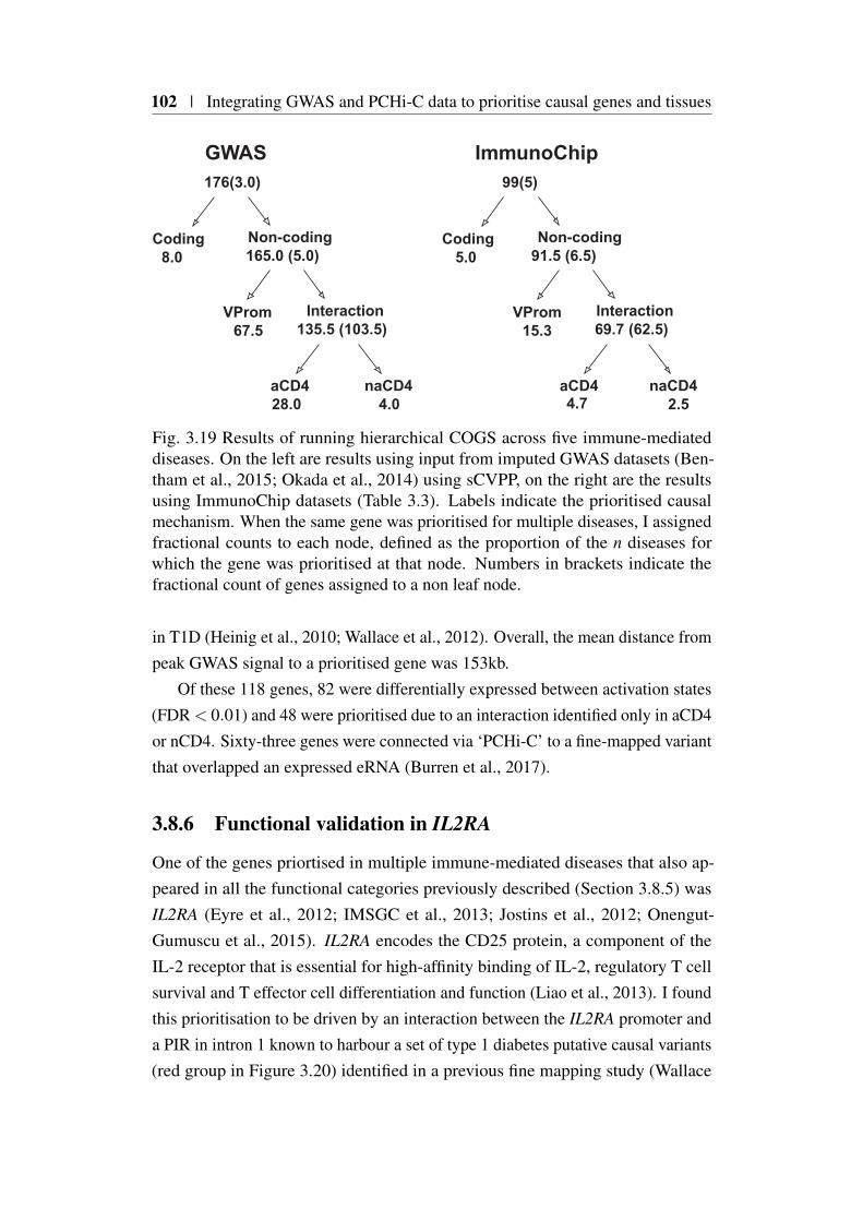
102 | Integrating GWAS and PCHi-C data to prioritise causal genes and tissues
aCD4 naCD4
GWAS176(3.0)
Coding8.0
Non-coding165.0 (5.0)
VProm67.5
Interaction135.5 (103.5)
aCD428.0
naCD44.0
ImmunoChip99(5)
Coding5.0
Non-coding91.5 (6.5)
VProm15.3
Interaction69.7 (62.5)
4.7 2.5
Fig. 3.19 Results of running hierarchical COGS across five immune-mediateddiseases. On the left are results using input from imputed GWAS datasets (Ben-tham et al., 2015; Okada et al., 2014) using sCVPP, on the right are the resultsusing ImmunoChip datasets (Table 3.3). Labels indicate the prioritised causalmechanism. When the same gene was prioritised for multiple diseases, I assignedfractional counts to each node, defined as the proportion of the n diseases forwhich the gene was prioritised at that node. Numbers in brackets indicate thefractional count of genes assigned to a non leaf node.
in T1D (Heinig et al., 2010; Wallace et al., 2012). Overall, the mean distance frompeak GWAS signal to a prioritised gene was 153kb.
Of these 118 genes, 82 were differentially expressed between activation states(FDR < 0.01) and 48 were prioritised due to an interaction identified only in aCD4or nCD4. Sixty-three genes were connected via ‘PCHi-C’ to a fine-mapped variantthat overlapped an expressed eRNA (Burren et al., 2017).
3.8.6 Functional validation in IL2RA
One of the genes priortised in multiple immune-mediated diseases that also ap-peared in all the functional categories previously described (Section 3.8.5) wasIL2RA (Eyre et al., 2012; IMSGC et al., 2013; Jostins et al., 2012; Onengut-Gumuscu et al., 2015). IL2RA encodes the CD25 protein, a component of theIL-2 receptor that is essential for high-affinity binding of IL-2, regulatory T cellsurvival and T effector cell differentiation and function (Liao et al., 2013). I foundthis prioritisation to be driven by an interaction between the IL2RA promoter anda PIR in intron 1 known to harbour a set of type 1 diabetes putative causal variants(red group in Figure 3.20) identified in a previous fine mapping study (Wallace
3.8 Cell context specific COGS analysis of immune-mediated disease | 103
10p15.1
GFM SNP Groups
Genes
PCHi-C Non-activated
PCHi-C Activated
regRNAIL2RA RBM17
6.10 Mb6.05 Mb 6.15 Mb
HindIIIFragment
Fig. 3.20 Genomic and genetic architecture of 10p15.1 type 1 diabetes susceptibil-ity locus. PCHi-C interactions link the IL2RA promoter to autoimmune diseaseassociated genetic variation which leads to expression differences in IL2RA mRNA.GUESSFM SNP groups (‘GFM SNP Groups’ stanza) from (Wallace et al., 2015)are partitioned by colour. PCHi-C data is for activated (green) and non-activated(purple) CD4+ T cells, in unambiguous cases PIRs are coloured by GUESSFMSNP group overlap. Figure adapted from an original prepared by Tony Cutler,Arcadio Rubio Garcia and Chris Wallace.
et al., 2015). This set of variants (Figure 3.20) is in high LD (r2 > 0.8) withrs12722495 which has been shown to associate with the surface expression CD25in memory T cells (Dendrou et al., 2009).
Using a targeted RNA-sequencing approach, and software I helped to de-velop previously (Rainbow et al., 2015), Daniel Rainbow measured the relativeexpression of IL2RA mRNA in five individuals heterozygous across the red groupof SNPs (Figure 3.20 who were also homozygous across most other associatedSNPs, in a 4 hour activation time course of CD4+ T cells. Allelic imbalance wasobserved consistently for two reporter SNPs in intron 1 and the 3′ UTR in non-activated CD4+ T cells in each individual (Figure 3.21a) validating a functionaleffect of the PCHi-C derived interaction between this PIR and the IL2RA promoterin non-activated CD4+ T cells. While the allelic imbalance was maintained innon-activated cells cultured for 2-4 hours, the imbalance was lost in cells activatedunder in vitro conditions. Since increased CD25 expression with rare alleles in thered group of SNPs has previously been observed on memory CD4+ T cells but notnaive or T regulatory subsets that are also present in total CD4+ T cell population,we purified memory cells from eight red group heterozygous individuals andconfirmed activation induced allelic imbalance of IL2RA mRNA expression in thismore homogeneous population (Figure 3.21b). One possible explanation for thisis that formation of additional chromatin loops with alternative GUESSFM SNPgroups (blue, magenta, grey, cyan and green Figure 3.20) on activation overcomesthe basal effect of the more constitutive enhancer effect modulated by contact
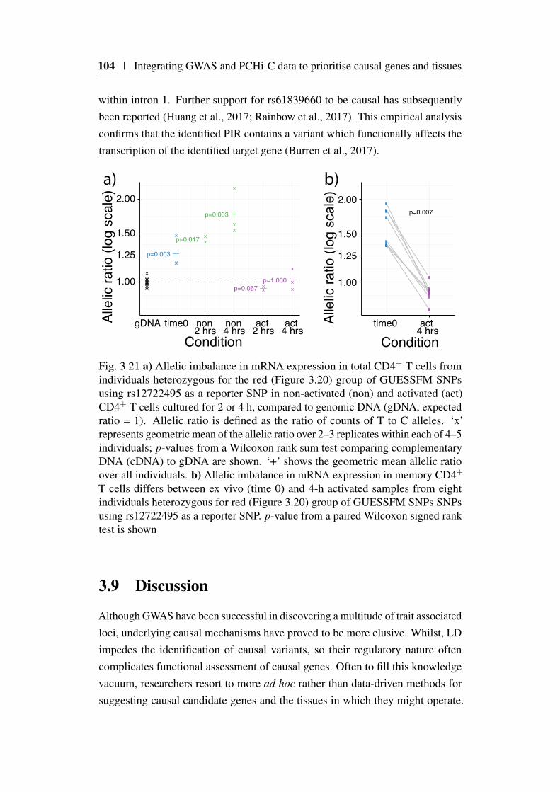
104 | Integrating GWAS and PCHi-C data to prioritise causal genes and tissues
within intron 1. Further support for rs61839660 to be causal has subsequentlybeen reported (Huang et al., 2017; Rainbow et al., 2017). This empirical analysisconfirms that the identified PIR contains a variant which functionally affects thetranscription of the identified target gene (Burren et al., 2017).
p=0.003
p=0.017
p=0.003
p=0.067p=1.0001.00
1.25
1.50
2.00
gDNA time0 non2 hrs
non4 hrs
act2 hrs
act4 hrs
Condition
Alle
lic ra
tio (l
og s
cale
)
p=0.007
1.00
1.25
1.50
2.00
time0 act4 hrs
ConditionAl
lelic
ratio
(log
sca
le)
b)a)
Fig. 3.21 a) Allelic imbalance in mRNA expression in total CD4+ T cells fromindividuals heterozygous for the red (Figure 3.20) group of GUESSFM SNPsusing rs12722495 as a reporter SNP in non-activated (non) and activated (act)CD4+ T cells cultured for 2 or 4 h, compared to genomic DNA (gDNA, expectedratio = 1). Allelic ratio is defined as the ratio of counts of T to C alleles. ‘x’represents geometric mean of the allelic ratio over 2–3 replicates within each of 4–5individuals; p-values from a Wilcoxon rank sum test comparing complementaryDNA (cDNA) to gDNA are shown. ‘+’ shows the geometric mean allelic ratioover all individuals. b) Allelic imbalance in mRNA expression in memory CD4+
T cells differs between ex vivo (time 0) and 4-h activated samples from eightindividuals heterozygous for red (Figure 3.20) group of GUESSFM SNPs SNPsusing rs12722495 as a reporter SNP. p-value from a paired Wilcoxon signed ranktest is shown
3.9 Discussion
Although GWAS have been successful in discovering a multitude of trait associatedloci, underlying causal mechanisms have proved to be more elusive. Whilst, LDimpedes the identification of causal variants, so their regulatory nature oftencomplicates functional assessment of causal genes. Often to fill this knowledgevacuum, researchers resort to more ad hoc rather than data-driven methods forsuggesting causal candidate genes and the tissues in which they might operate.
3.9 Discussion | 105
The results presented in this chapter suggest that PCHi-C gene prioritisation usingthe COGS method developed perform better than the proximity based methods thathave been widely adopted in the field (Section 3.6.1). This increased performanceof PCHi-C COGS was evident, in the smaller total number of genes prioritised,and the suggestion of causal genes that were not found using either proximity orTAD based inputs (Section 3.6.2).
I found that by adapting COGS to generate prioritisation scores in a tissuedependent manner I was able to identify, albeit for only a modest number ofcases, evidence for the importance of specific tissue context and trait combinations(Section 3.7). Overall hierarchical clustering of these results was inconclusiveusing the canonical COGS threshold (COGS>0.5) although I obtained morerobust results that discriminated blood and immune traits when this was lowered(COGS>0.01). Leaving aside technical considerations, this apparent lack of tissuespecificity might be explained by the fact that the transcriptional programs bywhich causal variants modulate disease risk might be active across a wide range ofcontexts and therefore difficult to resolve at the individual tissue level.
Of course there are a wide range of technical reasons for these results whichwarrant discussion. In order to explore as many traits as possible, I employed anLD based method, PMI, in order to increase SNP coverage across GWAS datasets.Using sCVPP derived from PMI as COGS input is likely to lead to a less robustgene prioritisation for a number of reasons. Consider the instance where a causalSNP is not directly typed and thus no association summary statistics are directlyavailable, in such a case the association can only be measured by ‘proxy’ variantsin LD. Generally, as LD between this ‘proxy’ SNP and the causal SNP decaysso too will the association. In this example, PMI will assign the association p-value of the ‘proxy’ to the untyped causal variant, attenuating the signal, reducingdownstream fine-mapping resolution, ultimately leading to a degradation in COGSprioritisation. The opposite is also true, if the causal variant is typed, as untypedvariants in LD, by PMI, will be assigned the same p-value. In regions of high LDthis will exacerbate the phenomenon of LD shelving, that occurs when many SNPsare in high LD with the causal variant, such that they all have similar associationsummary statistics (illustrated in Figure 3.17). Whilst such LD shelving is a truebiological phenomenon that is recognised to limit all fine-mapping methods, PMIamplifies this, resulting in an increased uncertainty in gene prioritisation, thatmanifests as a larger number of genes which themselves have lower prioritisationscores.

106 | Integrating GWAS and PCHi-C data to prioritise causal genes and tissues
I found the assessment of which input method, sCOGS or mCOGS performedbest challenging due to the lack of a gold standard of confirmed causal genesunderlying disease susceptibility. One might expect that differences in perfor-mance between the two input methods to be somewhat dependent on how oftenthe single causal variant assumption is violated. Recently, Asimit et al. (2019)used a Bayesian multinomial stochastic search method (MFM), to simultaneouslyfine-map autoimmune disease susceptibility loci across six autoimmune diseases.They found that their fine-mapping results within regions with the strongest bi-ological prior (i.e. containing known genes that regulate T-cell function) andeffect were more likely to be discordant with the more widely applied stepwiseconditional regression approach widely employed. One interpretation of this isthat the phenomena of multiple independent variants within a disease associatedregions is likely to exist genome-wide, but is currently hidden due to insufficientstudy power or sample size. With this in mind I would expect sCVPP input toperform less well than the GUESSFM input for those regions and overall and thismight explain the more modest overlap between the sCVPP and GUESSFM inputmethods that I observed.
Underscoring the trade off, when integrating genomic and GWAS data, arethe logistics of data access; sCVPP requires only summary statistics and thuscan integrate a large selection of traits, whilst GUESSFM requires individuallevel data limiting its application. It seems likely that using the fine-mappingresults of Asimit et al. (2019) as COGS input might provide a more robust set ofprioritised causal genes than the input methods I have presented although furtherwork is required to investigate this.
As well as the limitations due to fine-mapping input, a discussion of PCHi-Climitations and how these might effect causal gene prioritisation is required. Themost serious, involves the blind spot for observing shorter range interactions thatinvolve HindIII fragments and adjoining baited interactions and I attempted tocapture these as virtual promoter fragments (VPF). This approach whilst reason-able might result in the inappropriate assignment of variants to a gene given theexpected size of a VPF is approximately 27kb. From imputed GWAS and iChipCOGS prioritisation I found that 38% and 15% of genes were prioritised by VPFrespectively (Figure 3.19), a sizeable fraction of the total number of unique genesselected. Whilst incorrect assignment of variants to a gene on the basis of VPFswill result in more genes prioritised adding noise to the gene list, it would notby itself disadvantage true causal genes from being prioritised. In such cases theintegration of additional sources of genomic information, for example chromatin

3.9 Discussion | 107
accessibility and gene expression data prior to selecting genes and tissue contextsfor functional followup is essential (Kumasaka et al., 2019; Pickrell, 2014).
A second more pernicious issue is that many baited fragments are promiscuousin that they contain promoter regions for more than one gene. For these promis-cuous baits it is impossible to resolve which promoter or promoters are involvedin the chromatin looping, using the current PCHi-C data alone. One approach isto use gene expression patterns to provide a filter for target genes identified byspecific chromatin interactions, which I discuss in section 3.8.5. Furthermore, myanalysis to date has concentrated on protein coding genes as these have the mostmature and complete annotation, however, research has suggested a role for noncoding genes in the modulation of autoimmune disease susceptibility (Castellanos-Rubio et al., 2016). The PCHi-C platform used does provide some coverage ofthe non protein coding genome, however this is not exhaustive by design anddue to the overlapping nature of the coding and non-coding genome, the issue ofpromiscuous baits is worsened.
The introduction of an alternative restriction enzyme that cuts at greater fre-quency thus resulting in, on average, shorter fragments, might overcome some ofthese issues (Chesi et al., 2018). It will however introduce additional challenges;the shorter fragments will make it more difficult to identify unique sequence forcapture design, exacerbated by the increased number of fragments to be captured,which in turn will require more sequencing in order to provide adequate sequencecoverage.
Another limitation is the threshold approach to CHiCAGO scores that are usedto call interactions. All of the methods developed so far use a threshold score of5, so that an interaction with a score of 4.99 will be omitted. I am aware of analternative method, based on a Bayesian sparse variable selection approach (Ei-jsbouts et al., 2019), that will allow the assignment of posterior probabilities tointeractions that might obviate the need for this threshold approach. An extensionof COGS would be required in order to integrate the two posterior distributions(location of causal variants and PCHi-C contacts) and this is a promising avenuefor future research.
Excluding single cell implementations, all genomic technologies give an av-erage of the molecular events across the (sometimes mixed) population of cellsbeing assayed. In the case of immune subsets this is particularly relevant as broadcategories, such as CD4+ T cells will be heterogeneous containing further subdi-visions that may or may not be relevant for disease biology. It is important to bearthis in mind when considering PCHi-C maps, as without single cell profiling (Tan

108 | Integrating GWAS and PCHi-C data to prioritise causal genes and tissues
et al., 2018), it is impossible to resolve whether interactions are common across theassayed tissue type or are specific to, an underlying, and as yet unsorted, subset.
Given the limitations of PCHi-C and the differences between input methodsand thus the veracity of the genes prioritisised, I think it important that furthergenomic information is taken into context before embarking on further functionalstudies. Ideally such genomic data should be for the same cellular contexts andif possible the same individual donors for which PCHi-C was performed. In myanalysis the integration of chromatin state and RNA expression data enabled furtherfiltering allowing, a reduction from 245 putative candidate genes, identified fromcombining results using both sCVPP and GUESFM COGS results across immune-mediated diseases, to 118, found to be expressed in either activated or non-activatedCD4+ T cells (Section 3.8.5). I was able to reduce this further by consideringspecific annotations such eRNA overlap and context specific interactions. Notonly did such integration reduce the number of genes but it also has the benefit ofsuggesting causal mechanisms amenable to followup functional experiments, andI described one such example involving the gene IL2RA. These results suggestan overarching framework to GWAS causal candidate gene prioritisation, thatincorporates an initial scan with blockshifter to identify target tissues of particularinterest followed by detailed finemapping and subsequent integration, using COGSwith relevant tissue types.
The example of IL2RA demonstrates how complicated and subtle the mecha-nisms by which common variants modulate disease risk. In this associated region,multiple independent variants that in some cases can be shared and at other timesdistinct, between different immune-mediated diseases act to affect the expressionof IL2RA and potentially other causal genes in this region (e.g. RBM17). Resultsin this region show the importance of tissue context in disease mechanisms, asCD4+ T-cell activation was sufficient to overcome the allelic affect observedfor rs61839660 in non-activated cells. This demonstrates the challenges that areinvolved in elucidating causal mechanisms in common disease, in that even fora data set of 17 cell types with known relevance to IMD, only a small minorityof cellular contexts have been assessed. It is therefore almost certain that we aremissing key contexts in which many common variants act in order to modulatedisease risk. Whilst the framework set out here will be useful, I emphasise that theintegration of multiple strands of evidence and empirical techniques are necessaryfor the robust identification of causal genes and tissue contexts and ultimatelyunderlying disease mechanisms.

3.9 Discussion | 109
My analysis adds to a growing body of evidence that regulatory variationassociated with complex disease is often subtle and context specific. To date, therehas been a focus on methods that integrate GWAS and eQTL data as discussed insection 3.2.2. Due to logistical, technical and economic barriers, the generation ofwell powered catalogues of eQTLs across a range of tissue contexts has provedchallenging. Non-population based techniques, such as PCHi-C, that do notrequire a large amount of resource, have utility as they can be used to probea larger set of disease-relevant tissues and contexts. Indeed, subsequent to thework described here many studies have been completed in other disease relevanttissues including; pancreatic islets cells for type 2 diabetes (Miguel-Escalada et al.,2018), cardiomyocytes for heart disease (Choy et al., 2018), iPSC osteoblasts forbone mineral density disorders (Chesi et al., 2018) and iPSC-induced neuronsfor neurological disorders (Song et al., 2018). Another promising applicationof COGS, that I am developing, is to use pleiotropy between common and raremono/oligo-genic disease to suggest novel causal genes in the latter, for examplebetween IMDs and primary immune deficiency (Thaventhiran et al., 2018).
In summary methods, such as COGS, that link putative causal variation withtarget genes, show great promise in prioritising disease mechanisms and tissuecontexts. Along with orthogonal population based methods they provide a pow-erful and data driven approach to informing the design of, but not replacing,detailed empirical approaches for the characterisation of the causal molecularevents underlying human disease.


Chapter 4
Shared and distinct geneticarchitectures in immune-mediateddisease
4.1 Foreword
4.1.1 Chapter Summary
In this chapter I develop a principal component analysis based framework thatuses GWAS summary statistics to summarise the similarities and differencesin genetic architecture between a set of clinically related diseases. I apply thisframework to a set of immune-mediated diseases (IMDs) in order to generate alower-dimensional ‘basis’ that summarises their combined genetic architecturesinto a set of ordered principal components (PC). I attempt to characterise PCsby projecting on summary statistics for a wide range of binary and quantitativetraits. Next, I apply the method to a GWAS of juvenile idiopathic arthritis (JIA)disease sub-types where cohorts sizes are small, in order to characterise theirshared and distinct genetic architectures. Finally I turn my attention to updatingthe proposed framework to allow the projection of individual level genotype dataonto the basis. With this I attempt further characterisation of basis componentsusing eQTL datasets targeting relevant primary immune cell types.
4.1.2 Attributions
The work presented in this chapter relies on an unpublished case/control cohortexamining the genetics of JIA disease subtypes. Genotype and phenotype data
112 | Shared and distinct genetic architectures in immune-mediated disease
was supplied by John Bowes, Sam Smith, Annie Yarwood, Damian Tarasek andWendy Thomson and I had no part in study design, recruitment or genotype qualitycontrol.
All UK BioBank GWAS summary statistics were generated by the NealeLaboratory and were downloaded from http://www.nealelab.is/uk-biobank/.
4.1.3 Motivation
After initial concerns about privacy (Homer et al., 2008), summary statisticsfor well powered GWAS are becoming increasingly available in the public do-main (MacArthur et al., 2017). For immune-mediated diseases that cluster inindividuals or families, there is strong evidence for a shared genetic architec-ture (Cho and Feldman, 2015; Cotsapas et al., 2011; Onengut-Gumuscu et al.,2015; Smyth et al., 2008; Zhernakova et al., 2009). Whilst studies and methodshave been developed to exploit this in order identify pleiotropic loci across mul-tiple diseases (Solovieff et al., 2013), there have been few attempts to integratesummary GWAS data across multiple phenotypes in more holistic fashion at thegenome-wide scale.
The lack of methods in this areas coupled with the increasing availability ofGWAS summary statistics motivates the development of novel approaches thatare able to generate useful summaries of input traits, that in turn can be usedfor disease classification and characterisation (Cortes et al., 2017). Furthermore,such summaries learned from large well powered GWAS, might facilitate thecharacterisation of the genetic architecture of non input traits. This is particularlyattractive in rare or clinically heterogeneous immune-mediated disease wherecohort sizes are typically modest and conventional GWAS approaches are underpowered, as such an approach has the potential to provide insights into the sharedand distinct genetic architectures which might impact therapeutic intervention.
4.1.4 Software Availability
In the course of this work I developed ‘cupcake’, an R library of functions thatencapsulates the methods described in the chapter. This package, is freely availablefrom https://github.com/ollyburren/cupcake under an MIT license agreement.

4.2 Background | 113
4.2 Background
Immune mediated diseases, whilst diverse, have been found to co-occur bothwithin individuals and families supporting the presence of a shared genetic archi-tecture (Somers et al., 2006). For example, between 4-9% of individuals withtype 1 diabetes (T1D) are also affected by coeliac disease (CEL) (Cronin et al.,1997). Whilst the studies supporting these claims are affected by ascertainmentbias, more recent evidence from GWAS has provided a stronger foundation forsuch assertions (Li et al., 2015; Parkes et al., 2013; Zhernakova et al., 2009). Thishas lead to concerted efforts to understand both the similarities and differencesbetween the genetic architectures of IMDs, which can be divided into three mainapproaches which I discuss in more detail below.
Cross-phenotype analysis and colocalisation
Soon after the publication of the first large scale multi-trait GWAS (WellcomeTrust Case Control Consortium, 2007) Smyth et al. (2008) presented a systematicpairwise analysis between T1D and CEL susceptibility loci, finding convincingevidence that seven non-HLA loci were common between traits. Two of theseseven loci showed evidence of heterogeneity in effect direction between the twodiseases indicating that the same locus could be both protective and modulate riskin different disease contexts. However, at this early stage of GWAS developmentgenotype platform density was low, which precluded inference as to whethershared loci were a result of shared or distinct causal variants.
Cotsapas et al. (2011) performed a detailed study of seven separate IMDs (CEL,Crohn’s disease (CRO), multiple sclerosis (MS), psoriasis (PSO), rheumatoidarthritis (RA), systemic lupus erythematosus (SLE) and T1D) selecting SNPs ortheir proxies that were genome-wide significant in one or more disease studies.They developed the Cross-Phenotype Meta Analysis (CPMA) statistic; usingsummary GWAS p-values in order to detect evidence for association of a SNP tomultiple disease phenotypes. On applying CPMA to 107 SNPs, selected due togenome-wide significance in one or more of the underlying studies, they foundevidence for sharing, between two or more diseases at 42 SNPs. Furthermorethey described 9 SNPs for which they found strong evidence for opposing effectsbetween diseases at the same locus, indicating that such a phenomenon might bewidespread across IMDs.

114 | Shared and distinct genetic architectures in immune-mediated disease
Whilst both Smyth et al. (2008) and Cotsapas et al. (2011), present compellingevidence for pervasive shared susceptibility loci across IMD, they are limited totesting each SNP independently and are unable to make inferences about whethersharing is due to the same or different causal variants.
An alternative approach presented in (Fortune et al., 2015), that overcomes thisis to take a more targeted approach and examine evidence for colocalisation (Gi-ambartolomei et al., 2014) at associated loci between pairs of traits. In this studyraw genotype data for four autoimmune traits (RA,T1D,CEL and MS), that hadbeen typed on the ImmunoChip platform was assembled and assessed pairwisefor colocalisation. Out of 90 regions assessed, significant evidence supportingcolocalisation was found at 33. In a related approach Pickrell et al. (2016) usedsummary statistics to investigate, genome-wide, the evidence for shared causalvariants across 42 GWAS for a broad range of phenotypes and diseases. Theyidentified over 300 loci where there was evidence for a shared locus.
Genetic correlation
An alternative approach to quantify the genetic overlap is to enumerate the geneticcorrelation between two traits genome-wide. This requires the estimation, for eachtrait, of the SNP level heritability, that is the proportion of the variance of the traitexplained by a given SNP (Section 1.3.1).
If raw genotyping data is available and sample sizes are not prohibitivelylarge the most accurate method of estimating SNP heritability is to apply a linearmixed model, as implemented in the GCTA software package (Yang et al., 2011).More recently LD score regression (Bulik-Sullivan et al., 2015), a method whichrequires only summary GWAS statistics and can be applied efficiently to verylarge GWAS has been developed. At the foundation of LD score regression is theassumption that causal variant effect sizes are inflated due to LD with each other.The LD score for a variant j, is defined as
ℓ j = ∑k
r2jk, (4.1)
where r2 is the correlation between variant j and the kth variant. Under a polygenicmodel the expected value of z1 jz2 j for the z scores for two traits denoted bysubscript 1 and 2 at variant j is
E[z1 jz2 jℓ j
]=
√N1N2ρg
Mℓ j +
ρNs√N1N2
, (4.2)

4.2 Background | 115
where N1 and N2 are the sample sizes of the traits, Ns is the number of samplesshared between both studies, ρg and ρ are, respectively, the genetic and phenotypiccorrelation between the traits and M are the total number of SNPs being considered.This means that ρg can be estimated by the slope of the regression of z1 jz2 j on LDscore ℓ j. This approach has been used to analyse the genetic correlation betweenhundreds of traits (Zheng et al., 2017), including GWAS summary statistics for siximmune-mediated diseases (Figure 4.1), finding significant correlations betweena number of diseases. Whilst such an approach is useful to understand how theoverall genetic architecture of two traits might be related, it can be misleadingand Bulik-Sullivan et al. (2015) illustrate this using the example of the near zerocorrelation between both CD with RA even though these diseases are knownto share multiple risk loci. This seemingly paradoxical finding occurs becausealthough risk variants are shared between CD and RA (Parkes et al., 2013), theseare balanced by variants with opposing effects elsewhere resulting in a negligiblenet correlation.
1
0.7
0.2
0.07
0.2
0.07
1
0.07
0.1
0.3
0.1
1
−0.1
0.05
0.2
1
0.6
0.5
1
0.2 1
CD
UC
AST
SLE
PBC
RA
CD UC AST SLE PBC RATrait
Trai
t
0
5
10
Z
Fig. 4.1 Genetic correlation computed using LD score regression (Bulik-Sullivanet al., 2015). Results were downloaded from LDHub (Zheng et al., 2017) on06/04/2019 and do not include the HLA region. Pairwise comparisons are labelledwith genetic correlation values, and are coloured by Z score if the Bonferroniadjusted p-value < 0.05
116 | Shared and distinct genetic architectures in immune-mediated disease
A drawback from using genetic correlation to infer shared genetic architecturesis that it operates over the whole genome, thus precludes the cataloguing of whichrisk variants are shared, opposing and distinct across a number of traits presentingsubstantial challenges for biological interpretation.
Genome-wide multi trait approaches
A more holistic approach, disPCA developed by Chang and Keinan (2014), usesprincipal component analysis (PCA) in order to summarise a matrix of associationscores across 31 GWAS datasets. Firstly, for each gene, a summary associationstatistic, based on genomic distance is computed. The resultant matrix, whererows and columns reflect GWAS studies and genes respectively, is then columnmean-centred. This transformed matrix is then suitable for PCA, resulting inloadings for each disease across 31 principal components ordered by the amountof overall variance each explains. Chang and Keinan (2014), chose to concentrateon the first two components, explaining a total of 8.69% of the variance. Thisanalysis demonstrated not only clustering of UC and CD but also SLE with CEL,which was followed up with pathway analysis using the underlying gene loadings,although the results as presented are not convincing.
Overall, this approach has limitations, firstly as I have demonstrated in previouschapters, the assignment of variants to genes on the basis of physical/geneticlocation is non-trivial and as such it is challenging to know whether the gene-levelassociations they use as input accurately reflect underlying gene biology. Secondlysuch gene-level summaries will mask pleiotropy, instead relying on a more diffusedefinition of cross-phenotype association that conflicts with convincing resultsthat many loci with shared associations are actually due to distinct causal variantsbetween traits (Fortune et al., 2015). Finally, Chang and Keinan (2014) mentionthat their approach fails to take into account the direction of effect of underlyingcausal variants, as such antagonistic and shared effects are treated equally. Asdiscussed in the previous section heterogeneity in effect size and direction betweendiseases is likely to be pervasive and thus not accounting for this is likely toundermine any results from using disPCA.
The approach exemplified by disPCA whilst limited, is of interest as it bridgesan important methodological gap, using PCA as a dimension reduction technique,to generate interpretable summaries over a genome-wide scale dataset. This invitesthe exploration of whether such summaries are of utility as lower dimensionalcomposite predictors themselves or whether their underlying loadings, that capture

4.3 Basis disease data preparation | 117
relationships between SNPs, have further application. The former application,using summaries as covariates in regression based methods, is well describedin the literature; for example most standard GWAS analysis pipelines make useof PC scores from ancestral PCA to control for confounding due to populationstratification (Price et al., 2006). However, PCA based dimension reductionapproaches have also been used to create composite phenotypes, that is lowerdimensional summaries, that maximise either the variance or heritability acrossmultiple phenotypes, which are known, a priori, to be correlated (Avery et al.,2011; Klei Lambertus et al., 2007). These approaches can provide multiplebenefits, not only in terms of maximising the power for association analysis,as the top components by definition maximise the variance between traits, butalso in relieving the multiple testing burden when examining multiple relatedtraits (Aschard et al., 2014).
4.3 Basis disease data preparation
In order to create a detailed map of the genetic architecture of immune-mediateddisease I created a collection of GWAS summary statistics (Table 4.1) across 10diseases, from publicly available resources including the GWAS catalogue andImmunoBase. For inclusion a study needed to fulfil a number of criteria:
Cohort size greater than 10,000 samples: The uncertainty attached to an oddsratio estimate depends on the total number of cases and controls analysed.Whilst arbitrary, I felt that a minimum cohort size of this magnitude allowedthe inclusion of cohorts across a wide spectrum of IMD whilst filtering outstudies that might lack power and be unlikely to contribute to the proposedapproach.
Summary GWAS data availability: The approach requires that estimates of theodds ratios and their significance be available genome-wide. This precludesthe inclusion of studies that, for example, present only summary statisticsfor the genome-wide significant loci.
Study performed on cohorts with European ancestry only: Although a popu-lation agnostic view of the genetic architecture of complex disease isfavoured (DIAGRAM Consortium et al., 2014; Liu et al., 2015; Okadaet al., 2014) there are technical reasons for limiting studies to those of Euro-pean ancestry in downstream analysis. The main reason is that such a filter
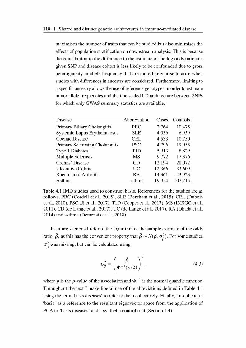
118 | Shared and distinct genetic architectures in immune-mediated disease
maximises the number of traits that can be studied but also minimises theeffects of population stratification on downstream analysis. This is becausethe contribution to the difference in the estimate of the log odds ratio at agiven SNP and disease cohort is less likely to be confounded due to grossheterogeneity in allele frequency that are more likely arise to arise whenstudies with differences in ancestry are considered. Furthermore, limiting toa specific ancestry allows the use of reference genotypes in order to estimateminor allele frequencies and the fine scaled LD architecture between SNPsfor which only GWAS summary statistics are available.
Disease Abbreviation Cases ControlsPrimary Biliary Cholangitis PBC 2,764 10,475Systemic Lupus Erythematosus SLE 4,036 6,959Coeliac Disease CEL 4,533 10,750Primary Sclerosing Cholangitis PSC 4,796 19,955Type 1 Diabetes T1D 5,913 8,829Multiple Sclerosis MS 9,772 17,376Crohns’ Disease CD 12,194 28,072Ulcerative Colitis UC 12,366 33,609Rheumatoid Arthritis RA 14,361 43,923Asthma asthma 19,954 107,715
Table 4.1 IMD studies used to construct basis. References for the studies are asfollows; PBC (Cordell et al., 2015), SLE (Bentham et al., 2015), CEL (Duboiset al., 2010), PSC (Ji et al., 2017), T1D (Cooper et al., 2017), MS (IMSGC et al.,2011), CD (de Lange et al., 2017), UC (de Lange et al., 2017), RA (Okada et al.,2014) and asthma (Demenais et al., 2018).
In future sections I refer to the logarithm of the sample estimate of the oddsratio, β , as this has the convenient property that β ∼ N(β ,σ2
β). For some studies
σ2β
was missing, but can be calculated using
σ2β=
(β
Φ−1(p/2)
)2
, (4.3)
where p is the p-value of the association and Φ−1 is the normal quantile function.Throughout the text I make liberal use of the abreviations defined in Table 4.1using the term ‘basis diseases’ to refer to them collectively. Finally, I use the term‘basis’ as a reference to the resultant eigenvector space from the application ofPCA to ‘basis diseases’ and a synthetic control trait (Section 4.4).

4.3 Basis disease data preparation | 119
4.3.1 UK10K as a reference genotype dataset
The employment of a reference genotype dataset as a foundation for downstreamanalyses has multiple benefits and I selected the set of genotypes made publiclyavailable as part of the UK10K project (project consortium, 2015). This study hasmade available genotypes, identified through whole genome sequencing, for 3,781healthy individuals from two British cohorts of European ancestry, namely theAvon Longitudinal Study of Parents and Children (ALSPAC) and TwinsUK.
The reasons for this choice were because of its size, coverage, availabilityand ancestral relevance to the immune disease studies to be analysed. One keybenefit is that the challenge in harmonising effect alleles across input studies isameliorated if this is carried out using a set of reference genotypes for which anaccurate estimate of control allele frequencies is available.
4.3.2 SNP selection
The main criteria for selecting SNPs was data availability, the proposed frameworkrequires that GWAS summary data are available for each SNP across all basisdiseases. The studies selected encompass a relatively large time interval, inthe context of GWAS, and this is reflected in the SNP coverage across studies(Figure 4.2a). This resulted in a set of 294,573 SNPs for which the relevant datawas available across all 10 traits. I found the category of SNPs found in only onestudy was most frequent, driven predominantly by rare SNPs from the Benthamet al. (2015) study of SLE (Figure 4.2b). A second peak of sharing at six studies,reflected the fact that SLE, UC, CD, T1D, RA and PSC studies were all imputedusing 1000 genomes data. This exposes the trade off in covering more diseasesat the expense of reduced SNP coverage. I decided that maximising the numberof basis diseases was of greater value than a denser SNP map based on the factthat the underlying genotyping platforms use a tag SNP approach (Johnson et al.,2001) in order to capture the most genetic diversity by using as few assays/SNPsas possible. A sparser SNP map that still allows signal detection, albeit at a lowerresolution is an acceptable trade off if this increases disease coverage, leading to aricher basis.
I excluded SNPs within the HLA region(chr6:20-40Mb) due to its long andcomplex LD structure. Furthermore it is known to harbour SNPs that have aprofound involvement in IMD susceptibility; such large effects have the capacity
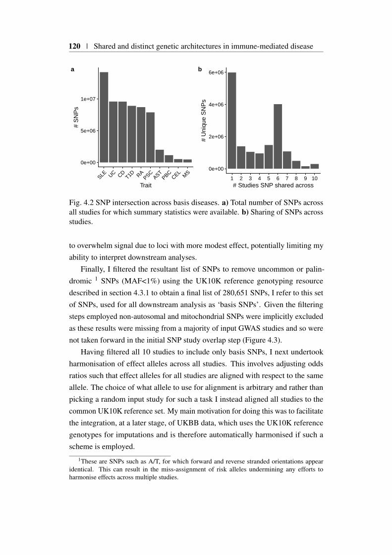
120 | Shared and distinct genetic architectures in immune-mediated disease
0e+00
5e+06
1e+07
SLE UC CDT1D RA
PSCAST
PBCCEL
MS
Trait
# S
NP
sa
0e+00
2e+06
4e+06
6e+06
1 2 3 4 5 6 7 8 9 10# Studies SNP shared across
# U
niqu
e S
NP
s
b
Fig. 4.2 SNP intersection across basis diseases. a) Total number of SNPs acrossall studies for which summary statistics were available. b) Sharing of SNPs acrossstudies.
to overwhelm signal due to loci with more modest effect, potentially limiting myability to interpret downstream analyses.
Finally, I filtered the resultant list of SNPs to remove uncommon or palin-dromic 1 SNPs (MAF<1%) using the UK10K reference genotyping resourcedescribed in section 4.3.1 to obtain a final list of 280,651 SNPs, I refer to this setof SNPs, used for all downstream analysis as ‘basis SNPs’. Given the filteringsteps employed non-autosomal and mitochondrial SNPs were implicitly excludedas these results were missing from a majority of input GWAS studies and so werenot taken forward in the initial SNP study overlap step (Figure 4.3).
Having filtered all 10 studies to include only basis SNPs, I next undertookharmonisation of effect alleles across all studies. This involves adjusting oddsratios such that effect alleles for all studies are aligned with respect to the sameallele. The choice of what allele to use for alignment is arbitrary and rather thanpicking a random input study for such a task I instead aligned all studies to thecommon UK10K reference set. My main motivation for doing this was to facilitatethe integration, at a later stage, of UKBB data, which uses the UK10K referencegenotypes for imputations and is therefore automatically harmonised if such ascheme is employed.
1These are SNPs such as A/T, for which forward and reverse stranded orientations appearidentical. This can result in the miss-assignment of risk alleles undermining any efforts toharmonise effects across multiple studies.

4.4 Creating a PCA ‘basis’ | 121
chr1chr3chr5chr7chr9chr11chr13chr15chr17chr19chr21chrX
chr2chr4chr6chr8chr10chr12chr14chr16chr18chr20chr22chrY
Fig. 4.3 Basis SNP genome coverage.
4.4 Creating a PCA ‘basis’
In the previous section I described the preparation of a set of harmonised GWASsummary statistics across ten immune-mediated diseases. I next focused on devel-oping a framework to provide a lower dimensional summary of the similaritiesand differences in the genetic architectures across traits using principal componentanalysis (PCA). The output of PCA is a ‘basis’, a transformation of the inputdata into a new coordinate system, where each principal axis or component isorthogonal.
To do this I used the aligned datasets to construct a 10×280,651 matrix of β ,where rows and columns reflect diseases and SNPs respectively. I added to thismatrix an additional row of zeroes, that constituted a synthetic ‘control’ disease,modelling a situation where there is no association across any SNPs. I included this‘control’ disease in order to provide a reference point or ‘baseline’ for downstreamcomparative analysis. I use the term M to refer to this 11× 280,651 matrix insubsequent sections.
4.4.1 PCA basis creation using β
As described in Chapter 1, PCA, is a relatively simple method, that can be usedto construct importance ranked summaries or components of high-dimensionalmatrices. For moderately sized matrices, such as M, I was able to use the inbuiltR function prcomp, in order to conduct PCA. One important consideration priorto PCA, is whether to adjust variables to have unit variance before analysis, toprevent variables of different scales dominating the resultant PCA basis. For a
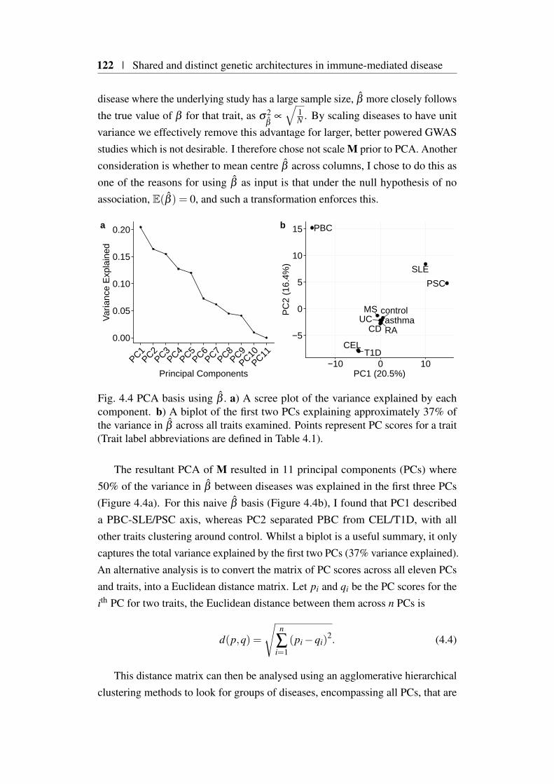
122 | Shared and distinct genetic architectures in immune-mediated disease
disease where the underlying study has a large sample size, β more closely followsthe true value of β for that trait, as σ2
β∝
√1N . By scaling diseases to have unit
variance we effectively remove this advantage for larger, better powered GWASstudies which is not desirable. I therefore chose not scale M prior to PCA. Anotherconsideration is whether to mean centre β across columns, I chose to do this asone of the reasons for using β as input is that under the null hypothesis of noassociation, E(β ) = 0, and such a transformation enforces this.
0.00
0.05
0.10
0.15
0.20
PC1PC2
PC3PC4
PC5PC6
PC7PC8
PC9PC10
PC11
Principal Components
Var
ianc
e E
xpla
ined
a
CD
CEL
MS
PBC
PSC
RA
SLE
T1D
UC asthmacontrol
−5
0
5
10
15
−10 0 10PC1 (20.5%)
PC
2 (1
6.4%
)
b
Fig. 4.4 PCA basis using β . a) A scree plot of the variance explained by eachcomponent. b) A biplot of the first two PCs explaining approximately 37% ofthe variance in β across all traits examined. Points represent PC scores for a trait(Trait label abbreviations are defined in Table 4.1).
The resultant PCA of M resulted in 11 principal components (PCs) where50% of the variance in β between diseases was explained in the first three PCs(Figure 4.4a). For this naive β basis (Figure 4.4b), I found that PC1 describeda PBC-SLE/PSC axis, whereas PC2 separated PBC from CEL/T1D, with allother traits clustering around control. Whilst a biplot is a useful summary, it onlycaptures the total variance explained by the first two PCs (37% variance explained).An alternative analysis is to convert the matrix of PC scores across all eleven PCsand traits, into a Euclidean distance matrix. Let pi and qi be the PC scores for theith PC for two traits, the Euclidean distance between them across n PCs is
d(p,q) =
√n
∑i=1
(pi −qi)2. (4.4)
This distance matrix can then be analysed using an agglomerative hierarchicalclustering methods to look for groups of diseases, encompassing all PCs, that are
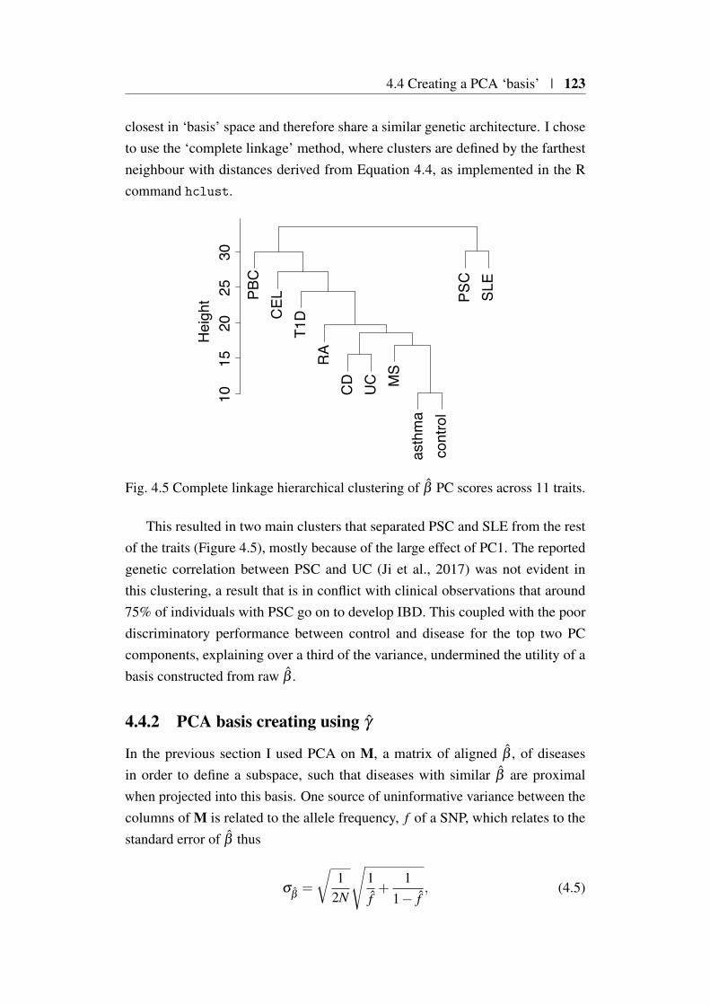
4.4 Creating a PCA ‘basis’ | 123
closest in ‘basis’ space and therefore share a similar genetic architecture. I choseto use the ‘complete linkage’ method, where clusters are defined by the farthestneighbour with distances derived from Equation 4.4, as implemented in the Rcommand hclust.
PBC
CEL
T1D
RA
CD
UC M
Sas
thm
aco
ntro
lPS
CSL
E
1015
2025
30H
eigh
t
Fig. 4.5 Complete linkage hierarchical clustering of β PC scores across 11 traits.
This resulted in two main clusters that separated PSC and SLE from the restof the traits (Figure 4.5), mostly because of the large effect of PC1. The reportedgenetic correlation between PSC and UC (Ji et al., 2017) was not evident inthis clustering, a result that is in conflict with clinical observations that around75% of individuals with PSC go on to develop IBD. This coupled with the poordiscriminatory performance between control and disease for the top two PCcomponents, explaining over a third of the variance, undermined the utility of abasis constructed from raw β .
4.4.2 PCA basis creating using γ
In the previous section I used PCA on M, a matrix of aligned β , of diseasesin order to define a subspace, such that diseases with similar β are proximalwhen projected into this basis. One source of uninformative variance between thecolumns of M is related to the allele frequency, f of a SNP, which relates to thestandard error of β thus
σβ=
√1
2N
√1f+
11− f
, (4.5)
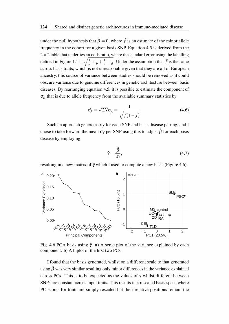
124 | Shared and distinct genetic architectures in immune-mediated disease
under the null hypothesis that β = 0, where f is an estimate of the minor allelefrequency in the cohort for a given basis SNP. Equation 4.5 is derived from the2×2 table that underlies an odds ratio, where the standard error using the labellingdefined in Figure 1.1 is
√1a +
1b +
1c +
1d . Under the assumption that f is the same
across basis traits, which is not unreasonable given that they are all of Europeanancestry, this source of variance between studies should be removed as it couldobscure variance due to genuine differences in genetic architecture between basisdiseases. By rearranging equation 4.5, it is possible to estimate the component ofσβ that is due to allele frequency from the available summary statistics by
σ f =√
2Nσβ=
1√f (1− f )
. (4.6)
Such an approach generates σ f for each SNP and basis disease pairing, and Ichose to take forward the mean σ f per SNP using this to adjust β for each basisdisease by employing
γ =β
σ f, (4.7)
resulting in a new matrix of γ which I used to compute a new basis (Figure 4.6).
0.00
0.05
0.10
0.15
0.20
PC1PC2
PC3PC4
PC5PC6
PC7PC8
PC9PC10
PC11
Principal Components
Var
ianc
e E
xpla
ined
a
CD
CEL
MS
PBC
PSC
RA
SLE
T1D
UC asthmacontrol
−1
0
1
2
−2 −1 0 1 2PC1 (20.5%)
PC
2 (1
6.6%
)
b
Fig. 4.6 PCA basis using γ . a) A scree plot of the variance explained by eachcomponent. b) A biplot of the first two PCs.
I found that the basis generated, whilst on a different scale to that generatedusing β was very similar resulting only minor differences in the variance explainedacross PCs. This is to be expected as the values of γ whilst different betweenSNPs are constant across input traits. This results in a rescaled basis space wherePC scores for traits are simply rescaled but their relative positions remain the

4.5 Evaluating basis performance | 125
Self Reported Disease Label No. Cases No. ControlsAsthma bb_asthma 39,049 298,110Rheumatoid arthritis bb_RA 3,730 333,429Ulcerative colitis bb_UC 1,795 335,364Malabsorption Coeliac disease bb_CEL 1,452 335,707Multiple sclerosis bb_MS 1,228 335,931Crohns Disease bb_CD 1,032 336,127Systemic lupus erythematosis bb_SLE 366 336,793Type 1 diabetes bb_T1D 286 336,873
Table 4.2 UK BioBank self-reported phenotypes[https://biobank.ctsu.ox.ac.uk/crystal/field.cgi?id=20002] matching diseases from which the basis was con-structed.
same. For GWAS where MAF are greater than 0.1, the standard error due tosample size is orders of magnitude smaller than γ . This means that, in practice,the influence of MAF on σ
βis small for the cohort sizes and allele frequencies
usually encountered in GWAS. However in this context which is motivated by awish to consider GWAS performed on small cohorts its derivation and inclusion inthe scaling is justified.
4.5 Evaluating basis performance
One approach to examining the relevance of the basis space developed in theprevious section is to interrogate its ability to predict the PC scores for basis traitsfrom an alternative source of GWAS summary statistics.
One source of summary statistics over thousands of traits is the UK Biobank(UKBB) (Sudlow et al., 2015). This large cohort has collected both genetic andphenotypic data over a large range of traits for approximately 500,000 individuals.Performing high quality GWAS across such a large cohort for so many traits istechnically challenging. To overcome this the Neale laboratory have created soft-ware tools such as HAIL ( https://github.com/hail-is/hail) and PHESANT (Millardet al., 2017), which they have used to generate and release publicly the summarystatistics for over 11,000 UKBB traits (http://www.nealelab.is/uk-biobank/). Fromthis resource I selected eight self-reported diseases (SRD) for which there was amatching basis trait (Table 4.2).
In general these SRD GWAS contained an order of magnitude fewer cases,resulting in much less powered GWAS, for example, self-reported T1D covers only286 cases, compared to the 5,913 included in the basis. The exception is asthma

126 | Shared and distinct genetic architectures in immune-mediated disease
which contained nearly double the number of cases included from Demenais et al.(2018). It is important to note that these diseases, are by definition, self-reportedphenotypes, and as such are likely to be significantly ‘softer’ than those fromwhich the basis is constructed. By this I mean case/control status is not necessarilydriven by a clinical diagnosis which can result in a misclassification of both caseand control status which further undermines power. I hypothesised that if thebasis reflected true differences in the genetic architecture between input traits, thatthese matched SRD, when projected into basis space, should be closer to theircounterparts than other diseases.
4.5.1 Linear regression coefficient conversion to the odds ratioscale for a binary trait
For computational efficiency, the Neale laboratory have employed a linear regres-sion approach to all data considered, even if the trait under consideration is binary.Thus, in order for me to project these data onto the basis, summary statisticsneeded to be transformed to the matching log odds ratio scale.
The UKBB summary statistics downloaded from the Neale Laboratory com-pendium include the total number of samples considered N, as well as N1 the totalnumber of affected samples (i.e. exhibit the particular self-reported binary pheno-type). Also reported are ∑
Ni XiYi (i.e. XTY ) and ∑
Ni Xi where i indexes individuals
included in the study of each trait. These quantities for each SNP, are sufficientto compute an odds ratio, under the assumption of Hardy-Weinberg equilibriumunder an additive model. In the case of a binary trait where Y ∈ 0,1, with 0 and1 representing whether a given sample is a control or case respectively, the allelefrequency in cases is
fcase =∑
Ni XiYi
2N1. (4.8)
Conversely, the allele frequency in controls is
fctrl =∑
Ni Xi −∑
Ni XiYi
2(N −N1), (4.9)
and the estimated odds ratio is therefore
fcase(1− fctrl)
fctrl(1− fcase). (4.10)
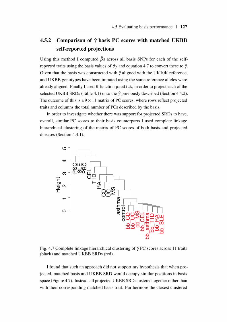
4.5 Evaluating basis performance | 127
4.5.2 Comparison of γ basis PC scores with matched UKBBself-reported projections
Using this method I computed β s across all basis SNPs for each of the self-reported traits using the basis values of σ f and equation 4.7 to convert these to γ .Given that the basis was constructed with γ aligned with the UK10K reference,and UKBB genotypes have been imputed using the same reference alleles werealready aligned. Finally I used R function predict, in order to project each of theselected UKBB SRDs (Table 4.1) onto the γ previously described (Section 4.4.2).The outcome of this is a 9×11 matrix of PC scores, where rows reflect projectedtraits and columns the total number of PCs described by the basis.
In order to investigate whether there was support for projected SRDs to have,overall, similar PC scores to their basis counterparts I used complete linkagehierarchical clustering of the matrix of PC scores of both basis and projecteddiseases (Section 4.4.1).
PSC
SLE
PBC
CEL
T1D
RA
CD
UC MS
asth
ma
cont
rol
bb_C
Dbb
_UC
bb_M
Sbb
_CEL
bb_a
sthm
abb
_T1D
bb_R
Abb
_SLE
01
23
45
Hei
ght
Fig. 4.7 Complete linkage hierarchical clustering of γ PC scores across 11 traits(black) and matched UKBB SRDs (red).
I found that such an approach did not support my hypothesis that when pro-jected, matched basis and UKBB SRD would occupy similar positions in basisspace (Figure 4.7). Instead, all projected UKBB SRD clustered together rather thanwith their corresponding matched basis trait. Furthermore the closest clustered

128 | Shared and distinct genetic architectures in immune-mediated disease
basis trait was the synthetic ‘control’ trait. These observations, taken togetherwith the fact that basis trait clustering does not reflect previous studies on sharedgenetic architectures of IMD (Cho and Feldman, 2015; Ji et al., 2017; Márquezet al., 2018), suggests that the basis as constructed is still overwhelmed by sourcesof variance between traits not related to their genetic architecture.
4.6 Development of a Bayesian shrinkage method
In the previous sections I described the creation of a basis in order to provide alow dimensional representation of the shared and distinct genetic architectures often immune-mediated diseases. However, evaluation of the resultant basis showedthat it was not reflective of known disease overlap. The main reason for thisis that the current proposal uses as input, log transformed odds ratio estimates,with no regard to their significance. Whilst there are arguments, in the form ofthe omnigenic model (Boyle et al., 2017), that a large number of variants arelikely to both directly and indirectly influence a trait, most will have such smalleffect sizes, such that that large sample sizes would be required for their accurateestimation. This means that a vast majority of odds ratios estimates for SNPsincluded in the basis are ’noisy’ and have large standard errors associated withthem. It seems reasonable that such a large source of variance arising from bothtechnical and stochastic processes would be expected to overwhelm the basis,thus obscuring true associations driving similarities and differences between thegenetic architecture of diseases.
One way of taking account of this stochastic variance is to apply a thresholdand only select SNPs exhibiting significant association in one or more traits. Suchan approach whilst attractive due to its apparent simplicity has several drawbacks.Leaving aside the Winner’s Curse effect (Section 2.2.1), the foremost challenge isto develop a suitable strategy by which to select such a threshold. If for examplewe select only genome-wide significant variants (p < 5×10⁻⁸), those variants thatare below but close to this threshold threshold will be unable to contribute to basisgeneration even though they may contain useful information. Another difficulty ishow to adequately deal with LD differences across the genome. If a locus is instrong LD, then by thresholding it is likely that more SNPs are included in thebasis compared to a locus in weaker LD. This means that loci with high LD willhave greater influence on the basis generated, thus creating a bias. To summarise,
4.6 Development of a Bayesian shrinkage method | 129
any proposed method should not rely on thresholding and also intrinsically takeinto account the differential amounts of LD across the genome.
4.6.1 Method description
One approach that fulfils these criteria is the Bayesian single causal variant fine-mapping approach introduced in previous chapters that summarises, in the contextof an arbitrary genomic region, the posterior probability for a variant to be causal.A key facet of this approach is that posterior probabilities are jointly modelledacross all variants within a the genomic region considered. This property isuseful as if regions are selected in such a way that they are approximately LDindependent from each other, the effect of LD can be largely mitigated. Such amethod, when combined over multiple diseases, can be used to assign individualSNP weights, that can then be used to rescale input odds ratios. These rescaledodds ratios, weighted or shrunk in proportion to their disease relevance, can beused to generate a basis that holds promise in overcoming some of the challengesdiscussed in the previous section.
To describe the implementation of such a weighting scheme in detail, considera genomic region, r that is approximately LD independent from neighbouringregions. As discussed in the previous chapter if for a particular trait, we haveassociation p-values, f and β for a set of SNP with r, then we can compute asingle causal variant posterior probability (sCVPP) for each SNP (Section 1.3.5).The next challenge is integrating sets of sCVPP across multiple diseases. Let i
and j index a matrix of sCVPP across s SNPs and d, diseases, respectively, withinregion r. I first compute a disease specific weighting such that
α j =s
∑i=1
sCVPPi j. (4.11)
To combine across diseases I compute a disease weighted average for the ith SNPsCVPP within r as
hi =∑
dj=1 α jsCVPPi j
∑dj=1 α j
, (4.12)
which once multiplied by γ leads to γ′, a vector of shrunk γ of length s for a target
disease.For ease, given the invariant nature of both σ f and h across diseases, in future
sections I refer to h′i, as the combined weighting of the ith SNP such that
130 | Shared and distinct genetic architectures in immune-mediated disease
h′i =hi
σ f. (4.13)
I illustrate this process by using the example of seven IMDs (ommiting threediseases with no association across the region for clarity) across the 2q33.2 region(Figure 4.8). In this region there is evidence for a strong association proximalto the gene CTLA4 in both RA and T1D, however LD within the region makesidentifying further associated SNPs in other diseases challenging. By computingsCVPP, I found some evidence for putative causal variants in other diseases that aredistinct from RA and T1D. In order to combine these sCVPP into a single weightI consider two things. Firstly, for a given disease the posterior probability that the2q33.2 region being considered contains a causal variant2, which is reflected in α j.Secondly, the disease weighted (using α) contribution of a particular SNP to thetotal posterior probability for the region, across all diseases. In the example thisresults in most of weight being applied to the SNP proximal to CTLA4 previouslyidentified in T1D and RA, with most other variants receiving almost no weight.Importantly, putative causal variants in the other diseases such as PSC and CELare non-zero weighted, but because there is less evidence for these both at thesCVPP level and across diseases their weight is attenuated. The application ofthese weights results in both a relative down weighting of SNPs unlikely to beinvolved in disease susceptibility and a concomitant up weighting on SNPs whereevidence exists for their involvement in disease.
The scheme as described applies only to an approximately LD independentregion r, to apply it genome-wide I use a similar approach to that described in theprevious chapters. Briefly, I split the genome into approximately independent LDblocks using recombination data from the international HapMap project (Interna-tional HapMap Consortium et al., 2007). I then compute weightings separately foreach block, concatenating these in order to obtain the complete set of weightingsacross all SNPs to be included in the basis.
Whilst the underlying approach was developed for genetic fine-mapping it isimportant to note that this is a separate goal from the weighting metric that weseek. The density of SNPs considered precludes accurate fine-mapping and asillustrated in the previous chapter we rely on their being up to one causal variant ina given LD block. In contrast, here we seek a weight that best captures how likelya given SNP within the region is relevant across all basis diseases being considered.By performing PCA we summarise information across all basis variants, and thus
2Under the assumption that the causal variant is included in the set of SNPs being considered

4.6 Development of a Bayesian shrinkage method | 131
CTLA4 ICOSCD28
5
10
15−log
10(p)
CEL MS PBC PSC RA SLET1D
0.2
0.4
0.6
0.8
sCVP
P
0.1
0.2
0.3
0.4
0.5
h
−0.1
0
0.1
0
0.005
0.01
0.015
^ ^
ββ
h x
Fig. 4.8 An example of the β weighting scheme across seven selected IMDs inthe 2q33.2 region. The top stanza shows gene positions for GRCh37 as obtainedfrom Ensembl BioMart. − log10(p) - are the transformed p-values for each studycoloured by disease as follows: blue - Coeliac disease (CEL), pink - Multiplesclerosis (MS), darkgreen - Primary biliary cholangitis (PBC), red - Primarysclerosing cholangitis (PSC), orange - Rheumatoid arthritis (RA), lightgreen -Systemic lupus erythematosis (SLE) and brown - Type 1 diabetes (T1D). Thiscolouring scheme is repeated for all subsequent relevant stanzas. sCVPP - singlecasual variant posterior probabilites for each disease. h - final cross diseaseweights. β - The raw estimates of the log(Odds Ratio) across disease. h× β -weight transformed log(Odds Ratio).
as long as violations of underlying fine mapping assumptions are not systematicthe weighting is justified as these will be distributed over the thousands of regionsand the relatively large number of SNPs being considered.

132 | Shared and distinct genetic architectures in immune-mediated disease
4.6.2 Shrinkage evaluation
Using the basis diseases I generated weightings across all 280,651 input SNPs.The range of h was between 1.2× 10⁻⁸ and 0.21 with 99% of weights beingbelow 0.05. I applied these weightings to M, the matrix of β , by multiplying eachelement by its corresponding h′ and used the resultant matrix to compute a basisas previously described in section 4.4.1.
0.0
0.1
0.2
0.3
PC1PC2
PC3PC4
PC5PC6
PC7PC8
PC9PC10
PC11
Principal Components
Var
ianc
e E
xpla
ined
a
CD
CELMS
PBC
PSC
RA
SLE
T1D
UCasthma
control
−0.05
0.00
0.05
0.10
−0.10 −0.05 0.00 0.05 0.10PC1 (31.0%)
PC
2 (1
7.1%
)
b
Fig. 4.9 Basis PCA using shrunk γ . a) A scree plot of the variance explained byeach component. b) A biplot of the first two PCs.
For the resultant basis I found that a much larger proportion (≈ 60%) of thevariance explained was found in the first three principal components comparedwith previous basis that used γ as an input (Figure 4.9a). Furthermore these PCscores for the first two input diseases seem to reflect known disease biology. Forexample PC1 seems to discriminate auto-inflammatory diseases such as CD, UCand PSC from those categorised as more classical autoimmune diseases such asSLE, PBC and T1D (McGonagle and McDermott, 2006).
I evaluated the resultant basis, as before (Section 4.5), using matched UKBBSRD with the proposed Bayesian shrinkage scheme applied prior to projectiononto the basis (Figure 4.10).
I found that this basis produced PC scores for projected SRD UKBB traits thatwere more similar to their basis counterparts than between other diseases. Theonly exception to this was for RA which appeared to match more closely withthe synthetic control trait. One possible explanation for this is that the projectedstudies are all self-reported and symptoms of RA are more often confused withother conditions such as osteoarthritis than other projected traits.
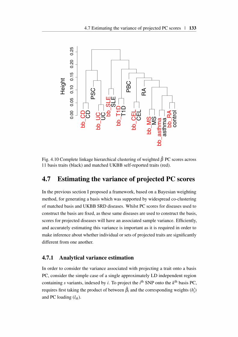
4.7 Estimating the variance of projected PC scores | 133
bb_C
DC
DPS
Cbb
_UC
UC bb
_SLE SL
Ebb
_T1D T1
DPB
Cbb
_CEL
CEL
RA
bb_M
SM
Sbb
_ast
hma
asth
ma
bb_R
Aco
ntro
l
0.00
0.05
0.10
0.15
0.20
0.25
Hei
ght
Fig. 4.10 Complete linkage hierarchical clustering of weighted β PC scores across11 basis traits (black) and matched UKBB self-reported traits (red).
4.7 Estimating the variance of projected PC scores
In the previous section I proposed a framework, based on a Bayesian weightingmethod, for generating a basis which was supported by widespread co-clusteringof matched basis and UKBB SRD diseases. Whilst PC scores for diseases used toconstruct the basis are fixed, as these same diseases are used to construct the basis,scores for projected diseases will have an associated sample variance. Efficiently,and accurately estimating this variance is important as it is required in order tomake inference about whether individual or sets of projected traits are significantlydifferent from one another.
4.7.1 Analytical variance estimation
In order to consider the variance associated with projecting a trait onto a basisPC, consider the simple case of a single approximately LD independent regioncontaining s variants, indexed by i. To project the ith SNP onto the kth basis PC,requires first taking the product of between βi and the corresponding weights (h′i)and PC loading (lik).
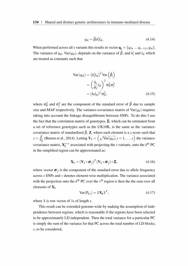
134 | Shared and distinct genetic architectures in immune-mediated disease
qik = βih′ilik. (4.14)
When performed across all s variants this results in vector qk = q1k . . .qs−1,k,qsk.The variance of qik, Var(qik), depends on the variance of β , and h′i and lik whichare treated as constants such that
Var(qik) =(h′ilik
)2 Var(
βi
)=
(hi
σ flik
)2
σ2Nσ
2f
= (hilik)2
σ2N , (4.15)
where σ2N and σ2
f are the component of the standard error of β due to samplesize and MAF respectively. The variance-covariance matrix of Var(qk) requirestaking into account the linkage disequilibrium between SNPs. To do this I usethe fact that the correlation matrix of genotypes, ΣΣΣ, which can be estimated froma set of reference genotypes such as the UK10K, is the same as the variance-covariance matrix of standardised β , Z, where each element is a z-score such thatz = β
σβ
(Burren et al., 2014). Letting Vk =(√
Var(qik), i = 1, . . . ,s)
the variance-
covariance matrix, Xs×sk associated with projecting the s variants, onto the kth PC
in the simplified region can be approximated as:
Xk = (Vk σσσ f )T (Vk σσσ f )ΣΣΣ, (4.16)
where vector σσσ f is the component of the standard error due to allele frequencyacross s SNPs and denotes element-wise multiplication. The variance associatedwith the projection onto the kth PC over the vth region is then the the sum over allelements of Xk
Var(Pkv) = 1Xk1T , (4.17)
where 1 is row vector of 1s of length s.This result can be extended genome-wide by making the assumption of inde-
pendence between regions, which is reasonable if the regions have been selectedto be approximately LD independent. Then the total variance for a particular PCis simply the sum of the variance for that PC across the total number of LD blocks,r, to be considered,

4.7 Estimating the variance of projected PC scores | 135
Var(Pk) =r
∑v=1
Pkv. (4.18)
Whilst such a scheme takes into account the component of variance due tominor allele frequency, σ2
fit does not take into account the component due to
sample size, σ2N . This is beneficial as under the reasonable assumption that study
design is fixed across all projected SNPs, this quantity is constant allowing thecomputation of the variance associated with the projection of any case/controlstudy design. I approximate σ2
N as
σ2N =
N1 +N0
N0N1, (4.19)
where N1 and N0 are the case and control size of the projected study respectively.This means that the variance of projecting an arbitrary trait, t onto the the kth PC is
N1 +N0
N0N1×Var(Pk), (4.20)
where N1 and N0 are the case and control size of t GWAS respectively. This setupprovides the benefit that the value Var(Pk) needs only be estimated once for a givenbasis, mitigating the computational overhead associated with having to empiricallyestimate the variance associated with projecting many traits onto the basis.
4.7.2 Empirical variance estimation
In the previous section I presented an analytical result that makes both implicit andexplicit assumptions about LD independence, due to its reliance on the approx-imation of ΣΣΣ from a reference genotype set and approximately LD independentgenomic regions. In order to validate the result I next developed simulations forevaluating the variance of a projected trait under different conditions.
Simulation under H0
The first condition I examined was the projection of a synthetic GWAS trait underthe null hypothesis of no association. Under this condition, E(β ) = 0, and anestimate of β for a single SNP can be obtained from β = N(0,σ2
β), where
σ2β≈ 1
2N
(1f+
1(1− f
)) , (4.21)

136 | Shared and distinct genetic architectures in immune-mediated disease
where N is the simulated sample size under consideration, and f is the estimatedminor allele frequency obtained from UK10K reference genotype resource. Inorder to simulate sets of β under H0 under differing sample sizes robustly we mustincorporate LD. Thus the simulation of β s for a given LD block involves samplingfrom a multivariate normal,
β ∼ MVN(
0,(
σβ
σTβ
)ΣΣΣ
). (4.22)
For a given sample size this is done for each LD block, and the results con-catenated to create a vector of β under H0, which can be re-scaled and projectedonto the basis.
Under the assumption that PC scores from this simulation will be distributednormally it is possible to estimate approximately, the number of simulationsrequired for a reasonable empirical estimate of the PC score variance. Thisinvolves setting a target variance, σ2, and then simulating PC scores such thatPCscore ∼ N(0,σ2), 1,000 times for each value of n, where n = 200,500,103,2×103,104,105 reflecting the number of simulations performed, and setting σ2 =
0.1, a reasonable estimate given the observed basis PC scores (Figure 4.9). Ateach n I computed the coefficient of variation (CV) σ
µwhere σ and µ are estimates
for the standard error and mean computed over the 1,000 simulations for a given n.CVs had a range from 5% where n = 200 to 0.2% where n = 105. I took forwardan n = 500 as this gave a CV of 3% that balanced the stability of the varianceestimate with the increasing computational burden associated with larger valuesof n. Using the proposed framework I simulated and projected GWAS summarystatistics under H0 across sample sizes ranging from 1,000 to 15,000 individuals.
Simulation under H1
The previous simulations are generated under the null hypothesis of no associationacross any SNPs. In application such a strong assumption will be violated andtherefore I also wanted to assess how appropriate both analytical and simulatedPC score variance were compared to those obtained from actual GWAS data.
To do this I used imputed genotypes for T1D from WTCCC (Wellcome TrustCase Control Consortium, 2007) supplied by Chris Wallace. I carried out QC,filtering out SNPs with poor imputation scores, violating HWE (ZHWE > 5), andnot overlapping the set of basis SNPs. This left approximately 286,000 variantsacross 5,271 individuals (1,929 cases and 3,342 controls). I used this set of variants

4.7 Estimating the variance of projected PC scores | 137
to create a basis as described previously (Section 4.6.2) with the T1D trait excluded.This is because additional correlation between β s between a basis and projectedtraits would be introduced which is not due to a shared disease architecture butinstead because of sample sharing. This correlation is non negligible when thereis a large degree of sample overlap between traits such as occurs for Cooper et al.(2017) and Wellcome Trust Case Control Consortium (2007) GWASs (Discussedfurther in Section 4.9.5).
In order to estimate the variance associated with the projection PC scores Iemployed a bootstrap methodology (Efron, 1979). Let N1 and N0 be the numberof cases and controls for which the variance of PC scores are to be estimated. Inthe first step I sample N1 case and N0 control genotypes to form a ‘source’ set ofgenotypes. To perform a bootstrap estimate of the PC variance for a particularcase/control configuration I sample with replacement N1 case and N0 controlgenotypes from this ‘source’ set, which I use to conduct a case/control GWAS(using 1958 birth cohort codings for regional locations as a covariate). Finallythe resultant β are projected onto the basis in the usual fashion to derive PCscores which are stored. I repeated both steps 500 times for a given value of N0
and N1 allowing a robust estimation of the variance PC scores under differentGWAS case and control size scenarios. Unlike the H0 framework I was limitedby the underlying WTCCC study size in the configurations that can be assessed,I therefore assessed matched numbers of cases and controls for sample sizes of500,1000 and 1900.
A further source of variance not related to disease genetic architecture might beintroduced by population substructure. Whilst the bootstrap above does incorporategeographical birth location as a covariate in order to mitigate this, the samplingregime as described has the potential to preferentially select cases or controlsfrom a particular region. To obviate this I performed the bootstrap a second timemaking sure that geographic location proportions amongst cases and controls werepreserved after sampling.
4.7.3 Variance estimate evaluation
The results of simulations and bootstraps indicate that the analytical estimates ofthe variance of PC scores were well calibrated (Figure 4.11). Empirical estimatesof the variances under H0, both H1 with and without population stratificationwere aligned with analytical estimates and well within 95% confidence intervalssupporting their utility in downstream analysis.
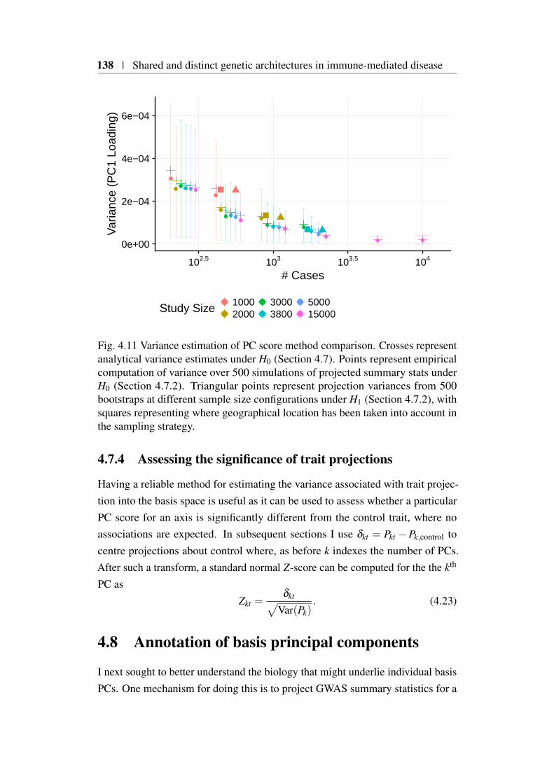
138 | Shared and distinct genetic architectures in immune-mediated disease
0e+00
2e−04
4e−04
6e−04
102.5 103 103.5 104
# Cases
Var
ianc
e (P
C1
Load
ing)
Study Size 10002000
30003800
500015000
Fig. 4.11 Variance estimation of PC score method comparison. Crosses representanalytical variance estimates under H0 (Section 4.7). Points represent empiricalcomputation of variance over 500 simulations of projected summary stats underH0 (Section 4.7.2). Triangular points represent projection variances from 500bootstraps at different sample size configurations under H1 (Section 4.7.2), withsquares representing where geographical location has been taken into account inthe sampling strategy.
4.7.4 Assessing the significance of trait projections
Having a reliable method for estimating the variance associated with trait projec-tion into the basis space is useful as it can be used to assess whether a particularPC score for an axis is significantly different from the control trait, where noassociations are expected. In subsequent sections I use δkt = Pkt −Pk,control tocentre projections about control where, as before k indexes the number of PCs.After such a transform, a standard normal Z-score can be computed for the the kth
PC asZkt =
δkt√Var(Pk)
. (4.23)
4.8 Annotation of basis principal components
I next sought to better understand the biology that might underlie individual basisPCs. One mechanism for doing this is to project GWAS summary statistics for a

4.8 Annotation of basis principal components | 139
diverse range of traits onto the basis and catalogue PC and trait combinations thatare significantly different from the ‘control’ basis trait PC score.
4.8.1 Projection of UKBB self-reported trait GWAS
One source of traits is the previously mentioned the UKBB (Sudlow et al., 2015).In addition to the seven self-reported traits already projected (Section 4.5) there arefurther traits with binary outcomes for which summary statistics are available fromthe Neal laboratory compendium. I chose to take forward three main categoriescovering self-reported medical conditions (UKBB code 20002, n = 282) cancer(UKBB code 20001, n = 28) and treatment/medications3 (UKBB code 20003,n = 542), which are all self-reported.
I downloaded summary statistics for all of the categories mentioned from theNeale Laboratory compendium, filtering to obtain summary statistics for SNPsincluded in the basis. After converting to the odds ratio scale (Section 4.5.1) andapplying weights (Section 4.6) I projected all 854 traits onto the basis. I used theanalytical variance estimations (Section 4.7) of PC score projections to assignsignificance to combinations of traits and principal components. To select combi-nations for further study I used the Benjamini–Hochberg procedure (Benjaminiand Hochberg, 1995) to adjust p-values for multiple testing over all trait and PCcombinations, selecting those with a false discovery rate (FDR) less than 5%for downstream analysis. In total across all traits I took forward 210 significanttrait-PC combinations, compassing 108 unique traits in order to annotate basiscomponents (Figure 4.12). I decided to exclude PC11 from downstream analysis,due to the small amount of overall variance it explains, and the fact that this likelycomposed of a large proportion of stochastic variance.
PC1 This component is effective at discriminating between autoinflammatorydiseases, including CD and UC with negative δ values, and those of a moreclassical autoimmune phenotype such as RA and SLE whereδ is positive(Figure 4.13). Gastroenteritis/Dysentry has the most positive δ values, how-ever it is likely that this is a false positive result, given that the number ofcases is small (n=104), and such a result contradicts clinical observationsthat link gastroenteritis to an increased risk of developing IBD (García Ro-dríguez et al., 2006). Self reported medication δ values tend to correlate
3This category contains data on any regular treatments taken weekly, monthly, etc. It does notinclude short-term medications (such as a 1 week course of antibiotics) or prescribed medicationthat is not taken, or over-the-counter medications, vitamins and supplements.
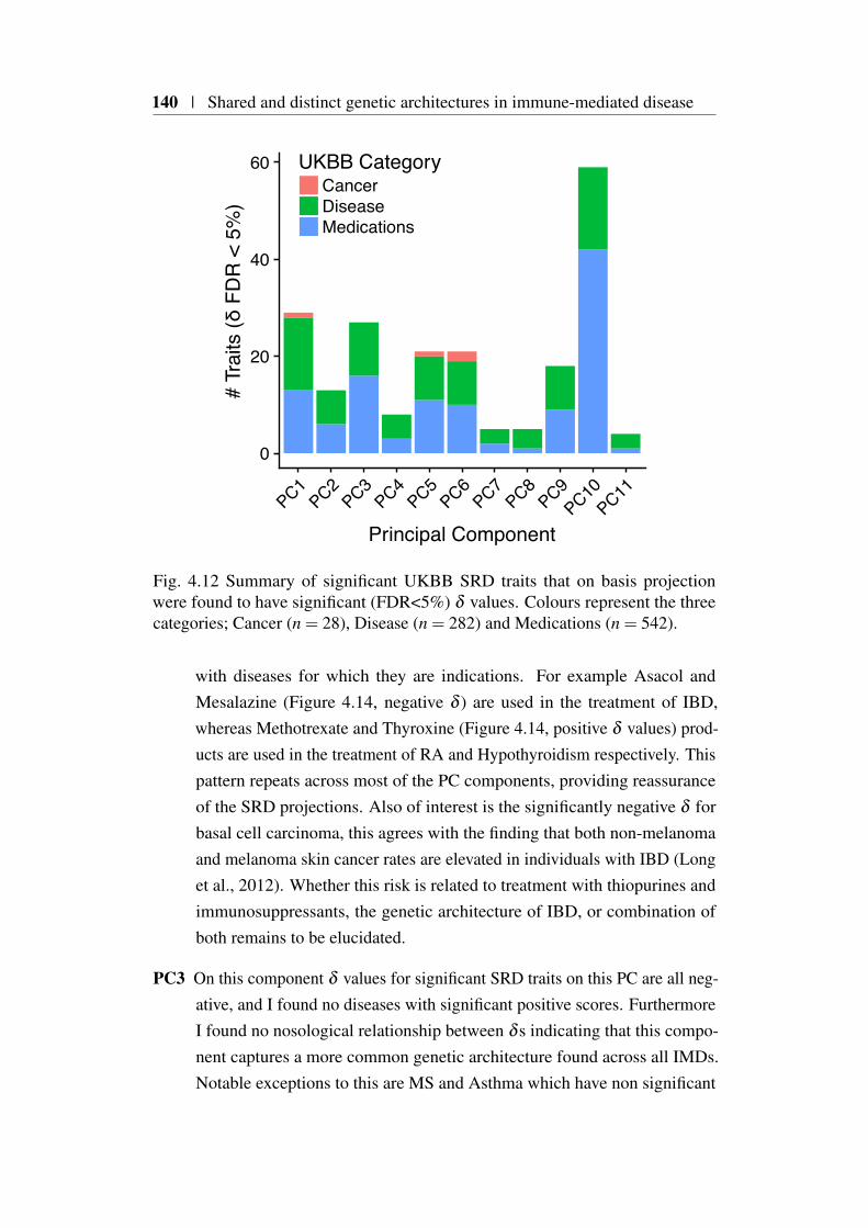
140 | Shared and distinct genetic architectures in immune-mediated disease
0
20
40
60
PC1PC2
PC3PC4
PC5PC6
PC7PC8
PC9PC10
PC11
Principal Component
# Tr
aits
(δ F
DR
< 5
%)
UKBB CategoryCancerDiseaseMedications
Fig. 4.12 Summary of significant UKBB SRD traits that on basis projectionwere found to have significant (FDR<5%) δ values. Colours represent the threecategories; Cancer (n = 28), Disease (n = 282) and Medications (n = 542).
with diseases for which they are indications. For example Asacol andMesalazine (Figure 4.14, negative δ ) are used in the treatment of IBD,whereas Methotrexate and Thyroxine (Figure 4.14, positive δ values) prod-ucts are used in the treatment of RA and Hypothyroidism respectively. Thispattern repeats across most of the PC components, providing reassuranceof the SRD projections. Also of interest is the significantly negative δ forbasal cell carcinoma, this agrees with the finding that both non-melanomaand melanoma skin cancer rates are elevated in individuals with IBD (Longet al., 2012). Whether this risk is related to treatment with thiopurines andimmunosuppressants, the genetic architecture of IBD, or combination ofboth remains to be elucidated.
PC3 On this component δ values for significant SRD traits on this PC are all neg-ative, and I found no diseases with significant positive scores. FurthermoreI found no nosological relationship between δ s indicating that this compo-nent captures a more common genetic architecture found across all IMDs.Notable exceptions to this are MS and Asthma which have non significant

4.8 Annotation of basis principal components | 141
*
*
*
*
**
*
*
*
**
*
**
*
*
**
*
**
*
*
*
*
*
**
*
*
*
*
*
*
*
*
*
*
*
***
*
**
*
*
**
*
*
*
*
*
*
*
*
*
*
*
*
*
*
*
*
*
*
*
*
*
*
*
*
*
**
*
*
*
*
*
*
*
*
*
*
*
*
**
*
**
Crohns DiseaseColitis Not Crohns Or Ulcerative Colitis
Ulcerative ColitisFracture Metatarsal
Gastroenteritis DysentryLiver Hepatocellular Cancer
Multiple SclerosisSystemic Lupus Erythematosis Sle
Scleroderma Systemic SclerosisSjogren S Syndrome Sicca Syndrome
Type 1 DiabetesInsomnia
Nasal PolypsAsthma
Hayfever Allergic RhinitisAnaemia
Eczema DermatitisAllergy Hypersensitivity Anaphylaxis
Allergy Or Anaphylactic Reaction To FoodBasal Cell CarcinomaMalignant Melanoma
PsoriasisAppendicitis
Hiatus HerniaDeep Venous Thrombosis Dvt
High CholesterolHypertension
DiabetesEmphysema Chronic Bronchitis
Ankylosing SpondylitisBronchiectasis
Chronic Obstructive Airways Disease CopdMalabsorption Coeliac Disease
Diabetic Eye DiseaseSarcoidosis
Rheumatoid ArthritisHyperthyroidism Thyrotoxicosis
Hypothyroidism MyxoedemaPernicious Anaemia
PC1PC2
PC3PC4
PC5PC6
PC7PC8
PC9PC10
Principal Component
UKB
B Se
lf re
porte
d di
seas
e/ca
ncer
−0.08−0.040.000.04
Difference from control (δ)
Fig. 4.13 Heatmap of significant UKBB SRD projections. PC score distance fromcontrol (δ ) is indicated by colour. An asterix indicates δ is significant at FDR<5%.For clarity, PC11 is omitted as it explains a negligible amount of variance betweenbasis traits making its interpretation challenging.
positive δ values. Interestingly, treatment response to anti-TNF therapy, amainstay biological treatment for many immune-mediated diseases, mirrorsthis pattern. For example it is routinely used in the treatment of RA, whichhas a significantly negative δ values, whilst it is not efficatious in the treat-ment of asthma (Holgate et al., 2011). Indeed in multiple sclerosis whichhas the most positive δ values, anti-TNF therapy is a contraindication andcan exacerbate disease symptoms (Cho and Feldman, 2015; Gregory et al.,2012).

142 | Shared and distinct genetic architectures in immune-mediated disease
*
*
*
*
*
*
*
*
*
*
*
*
*
*
*
*
*
*
*
*
*
*
*
*
*
*
*
*
*
*
*
*
*
*
*
*
*
*
*
*
*
*
*
*
*
*
*
*
*
*
*
*
**
*
*
*
*
*
*
*
*
*
*
*
*
*
*
*
*
Asacol Mr 400mg E C TabletMesalazine
Asacol 400mg E C TabletPentasa Sr 250mg M R Tablet
Simvador 10mg TabletVitamin B12 Preparation
Insulin ProductThyroxine Sodium
Levothyroxine SodiumThyroxine Product
NabumetoneHydroxychloroquine
MethotrexateUrsodeoxycholic Acid
BudesonideBetnovate Cream
LoperamideAzathioprine
SulfasalazineFolic Acid Product
PrednisoloneClonazepamCo Proxamol
Salmeterol Fluticasone PropionateGabapentin
MetforminAlendronate Sodium
AtorvastatinSimvastatin
Fybogel Orange S F GranulesBecotide 50 Inhaler
Seretide 50 EvohalerVentolin 100micrograms Inhaler
Beclomist 50micrograms Nasal SprayIsmo Isosorbide Mononitrate
AcyclovirBimatoprost
PC1PC2
PC3PC4
PC5PC6
PC7PC8
PC9
Principal Component
UKB
B Se
lf re
porte
d m
edic
atio
n
−0.06−0.030.000.030.06
Difference from control (δ)
Fig. 4.14 Heatmap of significant UKBB self-reported medication. PC score dis-tance from control (δ ) is indicated by colour. An asterix indicates δ is significantat FDR<5%. A large number of asthma medications are significantly associatedwith PC10, and so it it is omitted to facilitate interpretation. For clarity, PC11 isomitted as it explains a negligible amount of variance between basis traits makingits interpretation challenging.
PC5 This PC is defined by two basis traits, PSC and PBC that are not part of theself-reported UKBB set, having positive δ values. I found that, ursodeoxy-cholic acid, that is used to treat both PSC and PBC had the most positive δ
values out of all projected traits. This observation supports the notion thatthis PC represents a Coelic disease and PBC/PSC axis. The observationthat hepatocellular carcinoma (HCC), also correlates with the δ values of
4.8 Annotation of basis principal components | 143
PSC and PBC provides further support, as the cirrhosis endemic in bothdiseases is associated with increased in risk of HCC development (Lindoret al., 2009).
PC9 and PC10 Both of these PCs seem to separate asthma and allergic diseasesfrom the other IMDs. I found that δ values between diseases and relatedtreatments were strongly correlated. This was especially evident for PC10where a more negative PC score captures the genetic architecture of allergicdisease (e.g. asthma, Hayfever and Anaphylaxis), as well as a more generalcomponent of IMDs. I found that 34 out of 40 (85%) medications with asignificantly negative δ values, were for treatments for allergy or asthma.
4.8.2 Projection of UKBB blood count GWAS
The study by Astle et al. (2016), presents a comprehensive genetic associationanalysis of 36 blood cell count phenotypes across 173,430 individuals of Europeanancestry which suggests a causal relationship between certain blood cell pheno-types and immune-mediated disease. Thus projecting summary GWAS statisticsfrom this study onto the basis presents an opportunity to investigate whetherthe proposed framework is able to uncover similar relationships. Furthermoresuch cell type specific relationships might shed light on the causal tissue contextsunderlying basis PCs.
Basis projection
I downloaded4 GWAS summary statistics for all 36 traits, filtering each for SNPsintersecting the basis and aligned the alleles such that they were concordant withthe basis. This resulted in a 36×280,651 matrix on which I applied the proposedshrinkage (Section 4.6) prior to projection onto the basis space.
In order to select significant blood trait δ values I concatenated those aris-ing from this analysis with those derived from the UKBB self-reported binarytraits (Section 4.8.1) taking forward those with a FDR < 5%, for further anal-ysis. I focused on the 13 main blood cell indices on which Astle et al. (2016)conducted Mendelian randomisation analysis (Table 4.3), which found significantrelationships between IMD risk and counts for eosinophils (Asthma and CEL),lymphocytes (Asthma, CEL and MS) and neutrophils. For eosinophil counts(EO#) they found a positive relationship between Asthma, RA, T1D and CEL
4http://www.bloodcellgenetics.org/
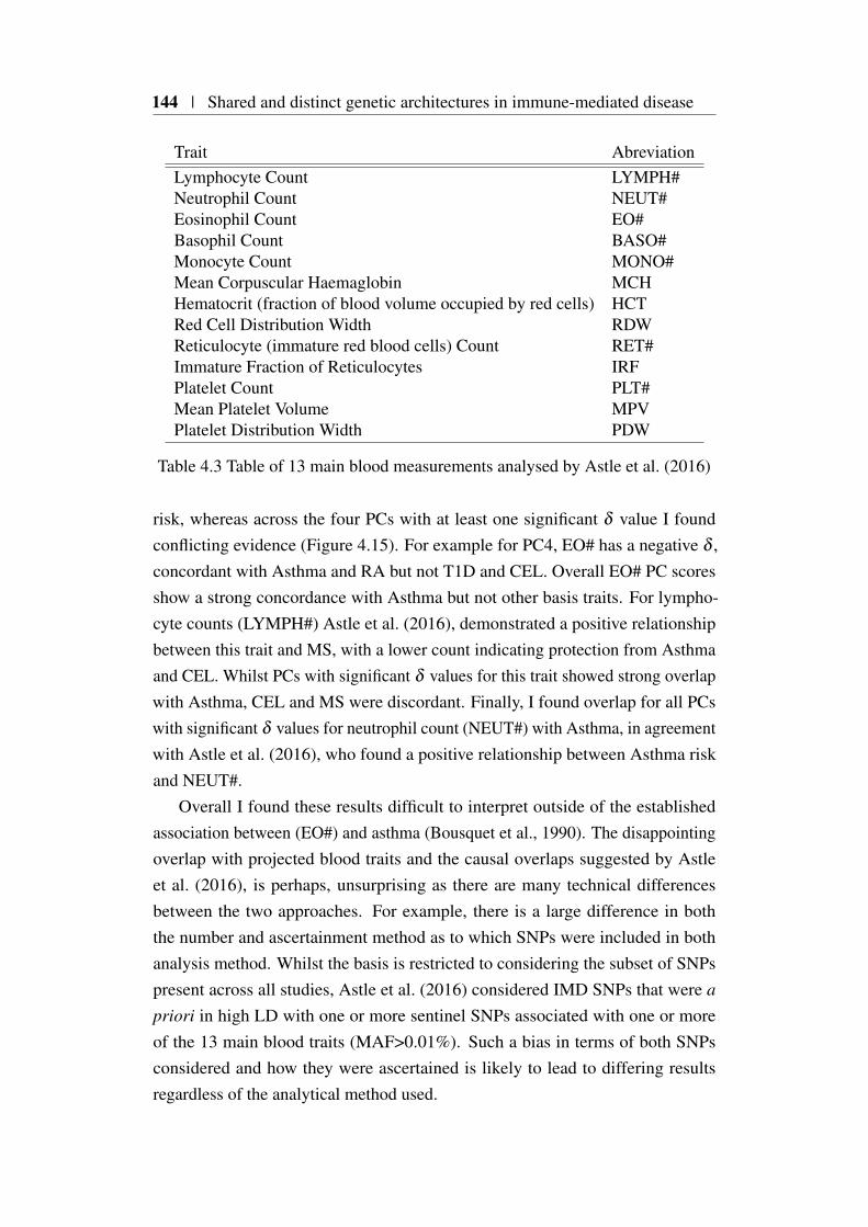
144 | Shared and distinct genetic architectures in immune-mediated disease
Trait AbreviationLymphocyte Count LYMPH#Neutrophil Count NEUT#Eosinophil Count EO#Basophil Count BASO#Monocyte Count MONO#Mean Corpuscular Haemaglobin MCHHematocrit (fraction of blood volume occupied by red cells) HCTRed Cell Distribution Width RDWReticulocyte (immature red blood cells) Count RET#Immature Fraction of Reticulocytes IRFPlatelet Count PLT#Mean Platelet Volume MPVPlatelet Distribution Width PDW
Table 4.3 Table of 13 main blood measurements analysed by Astle et al. (2016)
risk, whereas across the four PCs with at least one significant δ value I foundconflicting evidence (Figure 4.15). For example for PC4, EO# has a negative δ ,concordant with Asthma and RA but not T1D and CEL. Overall EO# PC scoresshow a strong concordance with Asthma but not other basis traits. For lympho-cyte counts (LYMPH#) Astle et al. (2016), demonstrated a positive relationshipbetween this trait and MS, with a lower count indicating protection from Asthmaand CEL. Whilst PCs with significant δ values for this trait showed strong overlapwith Asthma, CEL and MS were discordant. Finally, I found overlap for all PCswith significant δ values for neutrophil count (NEUT#) with Asthma, in agreementwith Astle et al. (2016), who found a positive relationship between Asthma riskand NEUT#.
Overall I found these results difficult to interpret outside of the establishedassociation between (EO#) and asthma (Bousquet et al., 1990). The disappointingoverlap with projected blood traits and the causal overlaps suggested by Astleet al. (2016), is perhaps, unsurprising as there are many technical differencesbetween the two approaches. For example, there is a large difference in boththe number and ascertainment method as to which SNPs were included in bothanalysis method. Whilst the basis is restricted to considering the subset of SNPspresent across all studies, Astle et al. (2016) considered IMD SNPs that were a
priori in high LD with one or more sentinel SNPs associated with one or moreof the 13 main blood traits (MAF>0.01%). Such a bias in terms of both SNPsconsidered and how they were ascertained is likely to lead to differing resultsregardless of the analytical method used.

4.8 Annotation of basis principal components | 145
*
*
*
*
*
*
*
*
*
*
*
*
*
*
*
*
*
*
*
*
*
* *
*
PDW
MPV
PLT#
IRF
RET#
RDW
HCT
MCH
MONO#
BASO#
EO#
NEUT#
LYMPH#
PC1PC2
PC3PC4
PC5PC6
PC7PC8
PC9PC10
Principal Component
Trai
t
−0.020−0.015−0.010−0.0050.0000.005
Difference from control (δ)
Fig. 4.15 Results of projection of 13 main blood count traits from Astle et al.(2016), see Table 4.3 for trait abbreviations. PC score distance from control (δ ) isindicated by colour. An asterix indicates δ is significant at FDR<5%.
4.8.3 Projection of whole blood eQTL data
One approach to characterising the biology underlying basis components is theintegration of genetic data influencing gene expression in a relevant tissue type asthis has the potential to link the genetic regulation of the expression of specificgenes to a component. Recently, Võsa et al. (2018) performed a meta-analysisof whole blood eQTL data on a total of 31,684 healthy individuals of Europeanancestry. I sought to project this dataset onto the basis in order provide a richercharacterisation of basis components.
146 | Shared and distinct genetic architectures in immune-mediated disease
I downloaded summary statistics from http://www.eqtlgen.org/cis-eqtls.htmlfor cis eQTLs, from testing for association between a given gene’s expression(across 19,960 genes expressed in blood) and each SNP within a 1Mb regionfrom the gene centre. To this I added summary statics downloaded from http://www.eqtlgen.org/trans-eqtls.html for what Võsa et al. (2018) term trans-eQTLs,that result from association testing between a given gene’s expression and eachSNP from a curated list of 10,317 trait-associated SNPs outside of a 5Mb regionfrom the gene centre.
For each gene, I filtered summary statistics to obtain only those for SNPsincluded in the basis. Given that the summary statistics available are predominantlycentred on a given gene this leads to large amounts of missing data, where aneQTL summary statistic is not present for most basis SNPs. Over 19,942 genes forchromosomes included in the basis, the mean number of variants with summarystatistics was 1,804 (IQR 1,742-1,861). I set effect sizes for variants wheresummary statistics were not available to zero under the reasonable assumptionthat untested or unreported variants were likely to have negligible effects sizeson target gene expression. After aligning effect alleles and performing Bayesianshrinkage I projected all genes onto the basis, resulting in a total of 11 componentscores for each of 19,942 genes for which at least one basis SNP was available.
I generated Z scores using empirical mean and variance estimates across allgene projections for a given PC such that
Zkg =Pkg − Pk√
Var(Pk), (4.24)
where Pkg, is the PC score for the kth component associated with projecting a gene,g onto the basis (Figure 4.16).
I devised a gene set enrichment strategy in order to assess whether com-ponents were associated with specific biological gene-sets through eQTLgengene projections. To do this I downloaded Reactome (Fabregat et al., 2016),KEGG (Kanehisa and Goto, 2000) and HALLMARK gene-sets in gmt formatfrom http://software.broadinstitute.org/gsea/msigdb (Liberzon et al., 2015). I cre-ated a gene ‘universe’ by selecting the unique set of identifiers for protein codinggenes for which PC scores were available across all components. I used this tofilter pathways such that genes without a PC score were removed, this resultedin pathways containing very few genes, to counter this I only took forward thosewith more than 10 genes for downstream analysis. Given that for a component,genes can have both positive and negative PC scores, using the raw PC scores for

4.8 Annotation of basis principal components | 147
** * * * * *
** * * * *
*
*
* * *
*
*
** * *
*
*
*
* * *
*
** * ** ** * *
*
* * * *
* *
* *
* * *
*
*
* ** * * * *
*
**
* *
*
*
*
** * * *
*
*
*
*
*
**
** * *
*
*
*
*
* *
NTN5CARD9
KIAA1841KSR1ETS2
FAM213BMMEL1KRT222PTPN22
FKRPPRKD2ERAP2
POM121CBACH2FRG1B
GTF2IRD2BFDFT1NEIL2GPX4
CCL3L3ANKRD55
RWDD4C5
CD247C8orf88
KIAA1683C14orf164TNFSF14
INPP5EALG1LPDCD1AAGABNDFIP1AHSA2SUOXAHI1BLK
IL18RAPFAM167A
ITGAXSMARCE1SLC22A5
GSDMBORMDL3
PC1PC2
PC3PC4
PC5PC6
PC7PC8
PC9PC10
Principal Component
Gen
e
−0.01
0.00
0.01
0.02
Differencefrom control
Fig. 4.16 Heatmap of significant gene projections from Võsa et al. (2018). Colourindicates difference from control PC score, ’*’ denotes significant at FDR < 5%.
enrichment might be misleading as these effects might be antagonistic, resultingin no net enrichment. A more robust approach is to compare the variance of PCscores between genes within a set and their complement. To do this I used thevar.test function in R which implements an F-test on the ratio of variancesof PC scores of genes in the two groups. I used this approach to assess each ofthe filtered gene-sets in order to identify those with evidence of large PC scorevariance.
As might be expected I found that gene-sets with relevance to both adaptiveand innate immunity showed evidence of enrichment (Figure 4.17) across all basis
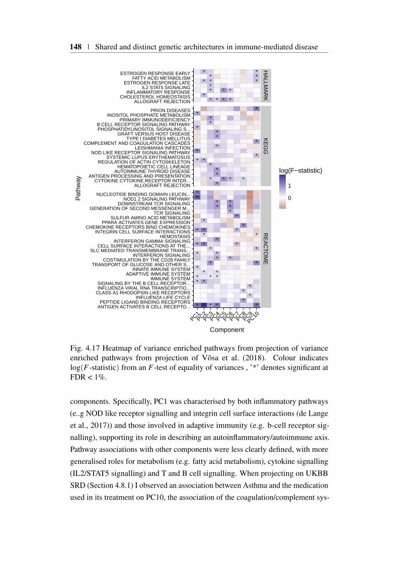
148 | Shared and distinct genetic architectures in immune-mediated disease
*
*
* *
*
*
*
* *
*
*
*
*
*
**
*
*
*
* *
*
*
**
*
*
*
*
*
*
* * *
*
*
*
*
*
*
*
*
*
*
**
*
*
*
*
**
*
*
*
*
*
*
**
*
*
*
**
*
**
*
*
*
*
*
*
*
*
*
*
*
*
*
HA
LLMA
RK
KE
GG
RE
AC
TOM
E
PC1PC2
PC3PC4
PC5PC6
PC7PC8
PC9PC10
ALLOGRAFT REJECTIONCHOLESTEROL HOMEOSTASIS
INFLAMMATORY RESPONSEIL2 STAT5 SIGNALING
ESTROGEN RESPONSE LATEFATTY ACID METABOLISM
ESTROGEN RESPONSE EARLY
ALLOGRAFT REJECTIONCYTOKINE CYTOKINE RECEPTOR INTER...
ANTIGEN PROCESSING AND PRESENTATIONAUTOIMMUNE THYROID DISEASE
HEMATOPOIETIC CELL LINEAGEREGULATION OF ACTIN CYTOSKELETON
SYSTEMIC LUPUS ERYTHEMATOSUSNOD LIKE RECEPTOR SIGNALING PATHWAY
LEISHMANIA INFECTIONCOMPLEMENT AND COAGULATION CASCADES
TYPE I DIABETES MELLITUSGRAFT VERSUS HOST DISEASE
PHOSPHATIDYLINOSITOL SIGNALING S...B CELL RECEPTOR SIGNALING PATHWAY
PRIMARY IMMUNODEFICIENCYINOSITOL PHOSPHATE METABOLISM
PRION DISEASES
ANTIGEN ACTIVATES B CELL RECEPTO...PEPTIDE LIGAND BINDING RECEPTORS
INFLUENZA LIFE CYCLECLASS A1 RHODOPSIN LIKE RECEPTORSINFLUENZA VIRAL RNA TRANSCRIPTIO...SIGNALING BY THE B CELL RECEPTOR...
IMMUNE SYSTEMADAPTIVE IMMUNE SYSTEM
INNATE IMMUNE SYSTEMTRANSPORT OF GLUCOSE AND OTHER S...
COSTIMULATION BY THE CD28 FAMILYINTERFERON SIGNALING
SLC MEDIATED TRANSMEMBRANE TRANS...CELL SURFACE INTERACTIONS AT THE...
INTERFERON GAMMA SIGNALINGHEMOSTASIS
INTEGRIN CELL SURFACE INTERACTIONSCHEMOKINE RECEPTORS BIND CHEMOKINES
PPARA ACTIVATES GENE EXPRESSIONSULFUR AMINO ACID METABOLISM
TCR SIGNALINGGENERATION OF SECOND MESSENGER M...
DOWNSTREAM TCR SIGNALINGNOD1 2 SIGNALING PATHWAY
NUCLEOTIDE BINDING DOMAIN LEUCIN...
Component
Pat
hway
0
1
log(F−statistic)
Fig. 4.17 Heatmap of variance enriched pathways from projection of varianceenriched pathways from projection of Võsa et al. (2018). Colour indicateslog(F-statistic) from an F-test of equality of variances , ’*’ denotes significant atFDR < 1%.
components. Specifically, PC1 was characterised by both inflammatory pathways(e..g NOD like receptor signalling and integrin cell surface interactions (de Langeet al., 2017)) and those involved in adaptive immunity (e.g. b-cell receptor sig-nalling), supporting its role in describing an autoinflammatory/autoimmune axis.Pathway associations with other components were less clearly defined, with moregeneralised roles for metabolism (e.g. fatty acid metabolism), cytokine signalling(IL2/STAT5 signalling) and T and B cell signalling. When projecting on UKBBSRD (Section 4.8.1) I observed an association between Asthma and the medicationused in its treatment on PC10, the association of the coagulation/complement sys-
4.9 Using the basis to characterise JIA | 149
tem provides further support for this as the importance of this biological pathwaywith respect to Asthma has previously been reported (de Boer et al., 2012).
4.9 Using the basis to characterise JIA
In the previous sections I proposed a framework for creating a basis that facilitatesthe comparison of the genetic architecture of clinically and/or phenotypicallyrelated disease by creating a low dimensional summary using publicly availableGWAS summary statistics. Such a representation appears to mirror disease nosol-ogy, with for example PC1 discriminating between auto-inflammatory and moreautoimmune diseases (Section 4.6.2). In an extension, by projecting new datasetsinto basis space, demonstrated using UKBB SRDs, I was able to show that basiswas able to cluster these on the basis of shared genetic architectures (Figure 4.10).
In this section, I expand on this application, describing how it can be used tobetter understand the genetic difference underpinning a clinically heterogenousdisease, using juvenile idiopathic arthritis (JIA) as a motivating example.
4.9.1 JIA disease subtypes
JIA is the most common cause of chronic childhood rheumatic disease, withheterogeneous arthritides occuring prior to the age of 16 years and persisting forat least 6 weeks (Ravelli and Martini, 2007). This heterogenity has led to theInternational League of Associations for Rheumatology (ILAR) criteria, whichdivides JIA into subtypes on the basis of clinical features (Petty et al., 2004) andcomprises seven main disease subtypes (Table 4.4).
In previous work Hinks et al. (2017), investigated the HLA region in order tosuggest genetic associations that were common or distinct between subtypes. Thisanalysis was by design restricted to examining disease overlap using SNPs withinthe HLA region, but nevertheless suggested an overlap between polyoligoarthritis(PO), extended oligoarthritis (EO) and rheumatoid factor negative (RF-), themost common disease subtypes. In addition to this Ombrello et al. (2017), usinga cohort of 770 children, found no evidence for a shared genetic architecturebetween systemic JIA (Sys) and the other JIA disease subtypes, supporting theobservation that Sys is a distinct disease. However, the method employed toexamine overlap was limited to examining either targeted regions (Prahalad et al.,2013) or those covered by ImmunoChip genotyping platform (Hinks et al., 2013)and so was not a full genome-wide analysis.

150 | Shared and distinct genetic architectures in immune-mediated disease
Subtype Abbreviation Case# Phenotype
Psoriatic PsA 150Psoriasis/ dactylitis/onycholysis
Enthesitis-related ERA 185
Ankylosing spondilytis/Sacroiliac joint tenderness/inflammatory lumbosacral pain/HLA-B27
Polyoligo RF+ RF+ 199Five or more joints andRheumatoid factor positive
Systemic Sys 283 Daily fever
Extended oligo EO 394Five or more joints after6 months
Polyoligo RF- RF- 573Five or more joints andRheumatoid factor negative
Persistant oligo PO 650 Four or fewer joints
Table 4.4 JIA disease subtype cohort description. Disease subtypes and theirclinical phenotypes and are derived from (Hinks et al., 2017). Case# indicates thenumber of individuals with a particular ILAR classification of JIA disease subtypefor which genotype data was available for analysis in this thesis.
4.9.2 JIA subtype GWAS analysis
I obtained quality controlled genotype, data from collaborators at The Universityof Manchester, for samples for all seven ILAR coded subtypes of JIA (Table 4.4)and 5,181 shared controls. I had no input into the collection, recruitment orprocessing of genotyping calls. I was supplied with a matrix of PC scores derivedfrom PCA of the genotype matrix, performed by the Manchester group in order toestimate and thus control for subtle ancestry specific effects that might confoundsubsequent analysis.
I used this data to perform a case/control GWAS of JIA subtypes limited to thevariants contained in the basis using the same 5,181 controls for analysis acrossall subtypes. Briefly, I used the R package snpStats (Clayton and Leung, 2007) tofit a logistic model, for each of the subtypes using sex and as recommended by theManchester group the first three PCs obtained from PCA of the genotype matrixas covariates.
4.9.3 Projection of JIA subtype GWAS
The GWAS performed in the previous section resulted in a set of summary statisticsfor each of the 7 subtypes. After aligning effect alleles with the basis, I applied the
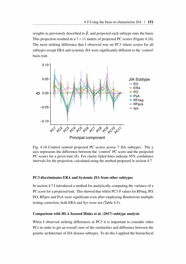
4.9 Using the basis to characterise JIA | 151
weights as previously described to β , and projected each subtype onto the basis.This projection resulted in a 7×11 matrix of projected PC scores (Figure 4.18).The most striking difference that I observed was on PC3 where scores for allsubtypes except ERA and systemic JIA were significantly different to the ‘control’basis trait.
−0.10
−0.05
0.00
0.05
0.10
PC1
PC2PC3
PC4PC5
PC6PC7
PC8PC9
PC10PC11
Principal component
JIA SubtypeEOERAPOPsARFnegRFpossys
δ
Fig. 4.18 Control centred projected PC scores across 7 JIA subtypes. The yaxis represents the difference between the ‘control’ PC score and the projectedPC scores for a given trait (δ ). For clarity faded lines indicate 95% confidenceintervals for the projection, calculated using the method proposed in section 4.7
PC3 discriminates ERA and Systemic JIA from other subtypes
In section 4.7 I introduced a method for analytically computing the variance of aPC score for a projected trait. This showed that whilst PC3 δ values for RFneg, PO,EO, RFpos and PsA were significant even after employing Bonferroni multipletesting correction, both ERA and Sys were not (Table 4.5).
Comparison with HLA focused Hinks et al. (2017) subtype analysis
Whist I observed striking differences at PC3 it is important to consider otherPCs in order to get an overall view of the similarities and difference between thegenetic architecture of JIA disease subtypes. To do this I applied the hierarchical
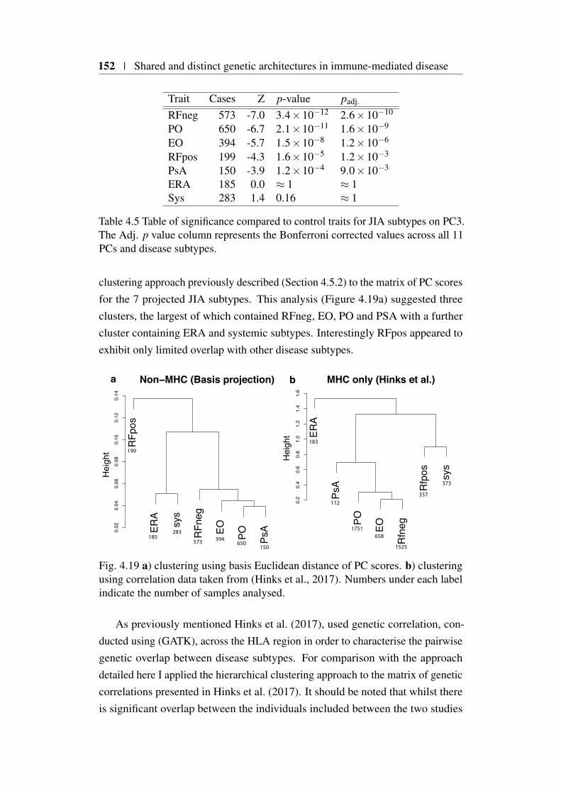
152 | Shared and distinct genetic architectures in immune-mediated disease
Trait Cases Z p-value padj.
RFneg 573 -7.0 3.4×10⁻¹² 2.6×10⁻¹⁰
PO 650 -6.7 2.1×10⁻¹¹ 1.6×10⁻⁹
EO 394 -5.7 1.5×10⁻⁸ 1.2×10⁻⁶
RFpos 199 -4.3 1.6×10⁻⁵ 1.2×10⁻³
PsA 150 -3.9 1.2×10⁻⁴ 9.0×10⁻³
ERA 185 0.0 ≈ 1 ≈ 1Sys 283 1.4 0.16 ≈ 1
Table 4.5 Table of significance compared to control traits for JIA subtypes on PC3.The Adj. p value column represents the Bonferroni corrected values across all 11PCs and disease subtypes.
clustering approach previously described (Section 4.5.2) to the matrix of PC scoresfor the 7 projected JIA subtypes. This analysis (Figure 4.19a) suggested threeclusters, the largest of which contained RFneg, EO, PO and PSA with a furthercluster containing ERA and systemic subtypes. Interestingly RFpos appeared toexhibit only limited overlap with other disease subtypes.
183
150650
ERA
PsA
PO EO
Rfn
eg
Rfp
os sys
0.2
0.4
0.6
0.8
1.0
1.2
1.4
1.6
b MHC only (Hinks et al.)
Hei
ght
RFp
os
ERA
sys
RFn
eg
EO PO PsA0.
020.
040.
060.
080.
100.
120.
14
a Non−MHC (Basis projection)
Hei
ght
394573
283185
112
199
1751
373
337
1525
658
Fig. 4.19 a) clustering using basis Euclidean distance of PC scores. b) clusteringusing correlation data taken from (Hinks et al., 2017). Numbers under each labelindicate the number of samples analysed.
As previously mentioned Hinks et al. (2017), used genetic correlation, con-ducted using (GATK), across the HLA region in order to characterise the pairwisegenetic overlap between disease subtypes. For comparison with the approachdetailed here I applied the hierarchical clustering approach to the matrix of geneticcorrelations presented in Hinks et al. (2017). It should be noted that whilst thereis significant overlap between the individuals included between the two studies
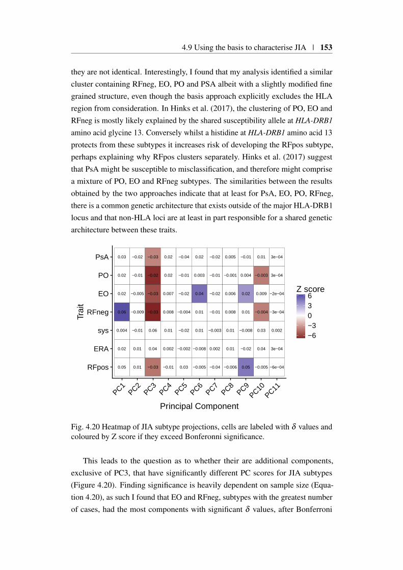
4.9 Using the basis to characterise JIA | 153
they are not identical. Interestingly, I found that my analysis identified a similarcluster containing RFneg, EO, PO and PSA albeit with a slightly modified finegrained structure, even though the basis approach explicitly excludes the HLAregion from consideration. In Hinks et al. (2017), the clustering of PO, EO andRFneg is mostly likely explained by the shared susceptibility allele at HLA-DRB1
amino acid glycine 13. Conversely whilst a histidine at HLA-DRB1 amino acid 13protects from these subtypes it increases risk of developing the RFpos subtype,perhaps explaining why RFpos clusters separately. Hinks et al. (2017) suggestthat PsA might be susceptible to misclassification, and therefore might comprisea mixture of PO, EO and RFneg subtypes. The similarities between the resultsobtained by the two approaches indicate that at least for PsA, EO, PO, RFneg,there is a common genetic architecture that exists outside of the major HLA-DRB1locus and that non-HLA loci are at least in part responsible for a shared geneticarchitecture between these traits.
0.02
0.02
0.02
0.03
0.06
0.05
0.004
0.009
0.04
−0.003
0.01
−0.004
−0.005
0.03
−2e−04
3e−04
3e−04
3e−04
−3e−04
−6e−04
0.002
−0.005
0.01
−0.01
−0.02
−0.009
0.01
−0.01
−0.03
0.04
−0.02
−0.03
−0.03
−0.03
0.06
0.007
0.002
0.02
0.02
0.008
−0.01
0.01
−0.02
−0.002
−0.01
−0.04
−0.004
0.03
−0.02
0.04
−0.008
0.003
0.02
0.01
−0.005
0.01
−0.02
0.002
−0.01
−0.02
−0.01
−0.04
−0.003
0.006
0.01
−0.001
0.005
0.008
−0.006
0.01
0.02
−0.02
0.004
−0.01
0.01
0.05
−0.008
RFpos
ERA
sys
RFneg
EO
PO
PsA
PC1PC2
PC3PC4
PC5PC6
PC7PC8
PC9PC10
PC11
Principal Component
Trai
t
−6−3036
Z score
Fig. 4.20 Heatmap of JIA subtype projections, cells are labeled with δ values andcoloured by Z score if they exceed Bonferonni significance.
This leads to the question as to whether their are additional components,exclusive of PC3, that have significantly different PC scores for JIA subtypes(Figure 4.20). Finding significance is heavily dependent on sample size (Equa-tion 4.20), as such I found that EO and RFneg, subtypes with the greatest numberof cases, had the most components with significant δ values, after Bonferroni
154 | Shared and distinct genetic architectures in immune-mediated disease
correction. Interestingly, both Sys and ERA had no significant δ values for anycomponent, whilst some of this is no doubt due to sample size, I note that thesmallest disease subset, PsA is significantly associated with PC3. Such an obser-vation is also supported by the analysis of Ombrello et al. (2017), who found thatusing polygenic risk scores built from combinations of the most common subtypes(PO,RFneg and RFpos), had no predictive power when applied to a cohort ofsystemic JIA patients.
In summary, the projections of JIA subtypes into basis space that I observedappear to have some support from alternative studies (Hinks et al., 2017; Ombrelloet al., 2017). However, the results do raise the important question as to what,biologically or clinically, the principal components represent. Furthermore, whencomparing between subtypes (rather than with control) care needs to be takendue to the fact that input summary statistics are computed using a shared pool ofcontrol subjects, which I discuss further in Section 4.9.5.
4.9.4 Annotating PCs related to JIA
The characterisation of components as described previously (Section 4.8) is valu-able as it can be used to gain knowledge about how individual components relate toJIA disease subtypes. For PC1 all JIA subtypes have positive δ values indicatinga tendency towards autoimmunity however, only PO, RFneg and RFpos showsignificance (FDR<0.05). The ERA subtype has clinical and genetic (throughthe presence of HLA-B27) similarities with adult-onset ankylosing spondyli-tis (Colbert, 2010). However, I observed significantly different PC1 scores (t-testp = 0.01) between UKBB SRD ankylosing spondylitis (N = 1,058) and ERAwith a tendency of ERA towards an autoimmune phenotype. One explanationfor this might be a tendency for the misclassification of other forms of JIA tothe ERA subtype based on a reliance on the the presence of HLA-B27 (MAFapprox 7%). Unfortunately summary statistics for a large AS GWAS outside ofUKBB, such as that presented in International Genetics of Ankylosing SpondylitisConsortium (IGAS) et al. (2013) are not publicly available, precluding validationof this finding.
Returning to PC3 which separates Sys and ERA from other disease subtypes,I previously described (Section 4.8.1) how this component also separated self-reported MS and asthma from other IMDs and a possible link with anti-TNFtherapy. However a more complicated picture emerges when JIA is taken intoaccount, as whilst there is limited evidence for the efficacy of anti-TNF treatments

4.9 Using the basis to characterise JIA | 155
Basal Cell CarcinomaNabumetone
Thyroxine SodiumHydroxychloroquine
Thyroxine ProductLevothyroxine Sodium
MethotrexateInsulin Product
Ventolin 100micrograms InhalerBetnovate Cream
Pentasa Sr 250mg M R TabletAsacol 400mg E C Tablet
Asacol Mr 400mg E C TabletMesalazine
Gastroenteritis DysentrySystemic Lupus Erythematosis Sle
Scleroderma Systemic SclerosisSjogren S Syndrome Sicca Syndrome
PBCHypothyroidism Myxoedema
Hyperthyroidism ThyrotoxicosisType 1 Diabetes
Rheumatoid ArthritisMultiple Sclerosis
AppendicitisDiabetes
AsthmaHayfever Allergic Rhinitis
Malabsorption Coeliac DiseaseAnkylosing Spondylitis
PSCUlcerative Colitis
Colitis Not Crohns Or Ulcerative ColitisCrohns Disease
RFnegRFpos
PsAPO
ERAEOsys
−0.10 −0.05 0.00 0.05 0.10
Change in basis score from control
Trai
t
Category JIA UKBB SRMedications
UKBB SRDisease
UKBB SRCancer Basis
Fig. 4.21 Forest plot showing the context of JIA subtype projections for PC1.Coloured points indicate the difference in trait scores with synthetic control,marked with a red dotted line. Error bars indicate 95% confidence intervals. Forclarity basis trait PC scores (purple) have been merged with overlapping UKBBtraits. Whilst non-basis UKBB traits have been filtered to show only those thatare significantly different from control at FDR < 5%, other traits are includedregardless, these are shown with dashed error bars.
in treating systemic JIA (Russo and Katsicas, 2009), beneficial outcomes havebeen observed in children with ERA (Gmuca et al., 2017; Weiss et al., 2018).
I did not observe a specific overlap between PsA and self-reported Psoriasisfor components with significant δ s, perhaps due to the misclassification within thePsA subtypes suggested by Hinks et al. (2017). Forest plots for all PCs such asthe example in Figure 4.22 are available in Appendix C.2.

156 | Shared and distinct genetic architectures in immune-mediated disease
BimatoprostFybogel Orange S F Granules
Vitamin C ProductPrednisolone
LoperamideFolic Acid Product
Vitamin B12 PreparationSimvador 10mg Tablet
AzathioprineAsacol 400mg E C Tablet
Thyroxine ProductMesalazine
MethotrexateInsulin Product
Levothyroxine SodiumThyroxine SodiumMultiple Sclerosis
AsthmaPSC
Rheumatoid ArthritisDiabetic Eye Disease
Systemic Lupus Erythematosis SleSarcoidosis
Ulcerative ColitisHyperthyroidism Thyrotoxicosis
Colitis Not Crohns Or Ulcerative ColitisPBC
Malabsorption Coeliac DiseasePernicious Anaemia
Hypothyroidism MyxoedemaCrohns DiseaseType 1 Diabetes
sysERA
POEO
RFnegRFpos
PsA
−0.10 −0.05 0.00 0.05Change in basis score from control
Trai
t
Category JIA UKBB SRMedications
UKBB SRDisease Basis
Fig. 4.22 Forest plot showing the context of JIA subtype projections for PC3. Forfurther details see Figure 4.21 legend.
4.9.5 Comparing JIA subtypes PC scores in the presence ofshared controls
Up to this point I have focused on a statistical method for comparing a projecteddisease PC score with a synthetic basis control trait, where no effect is assumedat each basis SNP. A natural approach to testing the significance of principalcomponent scores between sets of traits is the t-statistic which involves computingthe the pooled mean and variance of the sets of PC scores to be compared. Thisis complicated when comparisons involve study designs that utilise a commonpool of samples, where pooled variance will be underestimated if independence isassumed. Lin and Sullivan (2009) show that the correlation between study effectestimates with shared samples can be estimated as follows:
4.10 Projecting individual genotypes onto the basis | 157
Corr(βk, βl) =
(nkl0
√nk1nl1
nk0nk0+nkl1
√nk0nl0
nk1nk1
)/√
nknl = ρkl, (4.25)
where nk1, nk0, and nk (or nl1, nl0, and nl) are, respectively, the number of cases,the number of controls, and the total number of subjects in the kth (or lth) studyand nkl0 and nkl1are the total number of controls and cases that overlap. LetX = x1, . . . ,xnx−1,xnx and Y = y1, . . . ,yny−1,yny, be vectors of the PC scoresfor two groups of traits for a given PC. The variance of the difference between themeans of the two groups is
Var(X − Y ) =∑
nxi Var(xi)
n2x
+∑
nyj Var(y j)
n2y
− 2nxny
∑i, j
Cov(xi,y j), (4.26)
where, by (Equation 4.25), Cov(xi,yi) = ρkl√
Var(xi)Var(yi). This allows thecomputation of a t-statistic t = X−Y√
Var(X−Y )that is appropriately adjusted for shared
cases or controls.I applied this method to examine, for PC3 the difference in projected PC scores
between two sets of JIA subtypes, with one set containing ERA and sys, and theother containing all other subtypes. As expected I found this to be particularlysignificant (p = 1.66 × 10⁻⁹), even taking into account shared controls. Forcomparison, the application of a pooled variance approach without taking intoaccount shared controls was inflated (p = 4.58×10⁻¹⁰), and whilst this makesno difference to the conclusion for this comparison, for more subtle comparisonssample sharing will affect type 1 error.
4.10 Projecting individual genotypes onto the basis
Up to this point I have considered the projection of effect size estimates only,however extending the method to allow as input individual genotypic data allowsother applications and datasets to be applied to the method. This is because thePC scores for each PC component derived from such an application apply to anindividual rather than a specific trait. For example if we project on the genotypedata for a set of individuals for whom we also have gene expression data we mightlook for evidence for the correlation between individual level PC scores and geneexpression.
158 | Shared and distinct genetic architectures in immune-mediated disease
4.10.1 Computation of posterior odds ratios
The projection of individual level genotype data into the basis space requires theconversion of specific genotypes onto the odds ratio scale. To do this I used aBayesian framework developed by Chris Wallace inspired by the work of Aitkinand Chadwick (2003). This framework assumes that, at any SNP, we wish toestimate the individual odds ratio as determined by the allele frequency in controls,and a single case. In subsequent sections I use Bin(n, p) to represent a binomialdistribution of n trials with a probability of success p and Beta(α,β ) to representa Beta distribution with shape parameters α and β .
I assume that genotypes in controls follow a Bin(2, f0) distribution, where f0 ∼Beta(α0,β0). I also assume a large number of controls, such that the parameters(α0,β0) may be estimated by maximum likelihood (equal to maximum a posteriori
estimates assuming a flat prior on f0). Assuming f0 has been estimated as f0 theobserved frequency of a specific allele in n0 control subjects, and Hardy-WeinbergEquilibrium, I equate the estimated and theoretical expectation and variance of f0
E( f0) = f0 =α0
α0 +β0
V ( f0) =f0(1− f0)
2n0=
α0β0
(α0 +β0)2(α0 +β0 +1)
and solve for
α0 = (2n0 −1) f0
β0 = (2n0 −1)(1− f0)
If f1 is the allele frequency in cases, with prior distribution Beta(α1,β1),and we observe a single case G ∼ Bin(2, f1), then the posterior distribution off1|G ∼ Beta(α1 +G,β1 +2−G).
To estimate (α1,β1), I set prior limits on the log odds ratio, Ω. First I assumethat
E(logΩ) = E (log( f0)+ log(1− f1)− log(1− f0)− log( f1))
= ψ(α0)−ψ(β0)−ψ(α1)+ψ(β1)
= 0 (4.27)

4.10 Projecting individual genotypes onto the basis | 159
where we make use of the relations that if f0 ∼ Beta(α0,β0), then
1− f0 ∼ Beta(β0,α0), (4.28)
andE(log( f0)) = ψ(α0)−ψ(α0 +β0) (4.29)
where ψ() denotes the digamma function. Second, we assume that
Pr(|logΩ|> log2) =∫ 1
0Pr(l( f0)< f1 < u( f0)) f ( f0)d f0
= 1− ε (4.30)
where l( f0) and u( f0) are the lower and upper limits on f1 corresponding toΩ = 1
2 and 2, respectively, and ε is the small probability that f1 lies outside theselimits, i.e. we assume large odds ratios are a priori unlikely. I used the R functionuniroot to optimise conditions (4.27)– (4.30) to estimate (α1,β1) and thereforegenerate a function to convert individual genotypes to the odds ratio scale, givenonly allele frequencies in control subjects.
4.10.2 Effect of parmameters on posterior log(OR) estimates
The Bayesian framework depends upon two parameters, control sample size andthe prior probability that an odds ratio exceeds a target log odds ratio, Ω, of 2(See previous section). To analyse the effect of altering these parameters I firstexamined the behaviour of the framework over a range of control sample sizes(Figure 4.23a). Reflecting the larger variance of odds ratios at small control samplesizes and minor allele frequencies, I observed a small attenuation in posterior oddsratios with decreasing control sample size, although across the broad range ofsample sizes this made relatively little difference. More generally the selectionof a lower control sample size leads to more conservative estimates of posteriorodds ratio estimates. I next examined how the prior probability for odds ratiosto exceed 2 might affect posterior odds ratio estimations (Figure 4.23b). AsP(| log(OR)|> log(2)) decreases I observed that the relationship between allelefrequency and posterior odds ratios depends much more strongly on the prior thanon sample size.
Reflecting on these observations I decided to take forward the empiricallyobtained curves from using a sample size of 2,500 and P(| log(OR)|> log(2) =
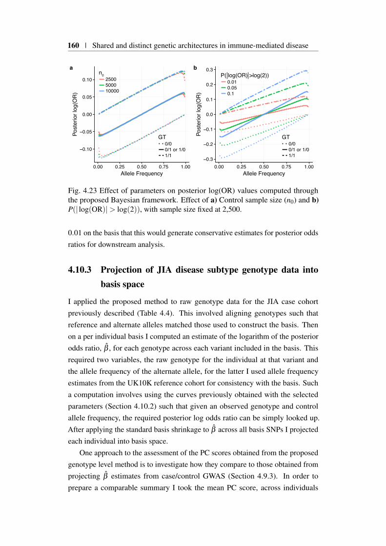
160 | Shared and distinct genetic architectures in immune-mediated disease
−0.10
−0.05
0.00
0.05
0.10
0.00 0.25 0.50 0.75 1.00Allele Frequency
Post
erio
r log
(OR
)
GTGT0/00/1 or 1/01/1
n02500500010000
a
−0.3
−0.2
−0.1
0.0
0.1
0.2
0.3
0.00 0.25 0.50 0.75 1.00Allele Frequency
Post
erio
r log
(OR
)
P( log(OR) >log(2))0.010.050.1
b
0/00/1 or 1/01/1
Fig. 4.23 Effect of parameters on posterior log(OR) values computed throughthe proposed Bayesian framework. Effect of a) Control sample size (n0) and b)P(| log(OR)|> log(2)), with sample size fixed at 2,500.
0.01 on the basis that this would generate conservative estimates for posterior oddsratios for downstream analysis.
4.10.3 Projection of JIA disease subtype genotype data intobasis space
I applied the proposed method to raw genotype data for the JIA case cohortpreviously described (Table 4.4). This involved aligning genotypes such thatreference and alternate alleles matched those used to construct the basis. Thenon a per individual basis I computed an estimate of the logarithm of the posteriorodds ratio, β , for each genotype across each variant included in the basis. Thisrequired two variables, the raw genotype for the individual at that variant andthe allele frequency of the alternate allele, for the latter I used allele frequencyestimates from the UK10K reference cohort for consistency with the basis. Sucha computation involves using the curves previously obtained with the selectedparameters (Section 4.10.2) such that given an observed genotype and controlallele frequency, the required posterior log odds ratio can be simply looked up.After applying the standard basis shrinkage to β across all basis SNPs I projectedeach individual into basis space.
One approach to the assessment of the PC scores obtained from the proposedgenotype level method is to investigate how they compare to those obtained fromprojecting β estimates from case/control GWAS (Section 4.9.3). In order toprepare a comparable summary I took the mean PC score, across individuals

4.10 Projecting individual genotypes onto the basis | 161
−0.001
0.000
0.001
0.002
PC1 PC2 PC3 PC4 PC5 PC6 PC7 PC8 PC9 PC10 PC11Principal Component
EOERAPOPsARFnegRFposSys
Subtype
Genotypes
−0.04
0.00
0.04
PC1 PC2 PC3 PC4 PC5 PC6 PC7 PC8 PC9 PC10 PC11Principal Component
Summary statistics
δ_δ
Fig. 4.24 Comparison of JIA subtype PC δ values derived from genotype (toppanel) and summary data approaches (bottom panel).
for each JIA subtype and plotted them along side the summary method results((Figure 4.24) Whilst the scaling of PC scores for the genotype method wasmuch reduced compared to the summary statistic method, the overall patternsacross disease subtypes was conserved (Figure 4.24) offering support for theproposed framework. I found that a t-test of individual PC3 scores for ERA andSystemic were significantly different from other subtypes, P = 4.61×10⁻³ andP = 1.96×10⁻⁸ respectively, matching the significant difference observed whenperforming a similar analysis using summary PC scores (Section 4.9.5).
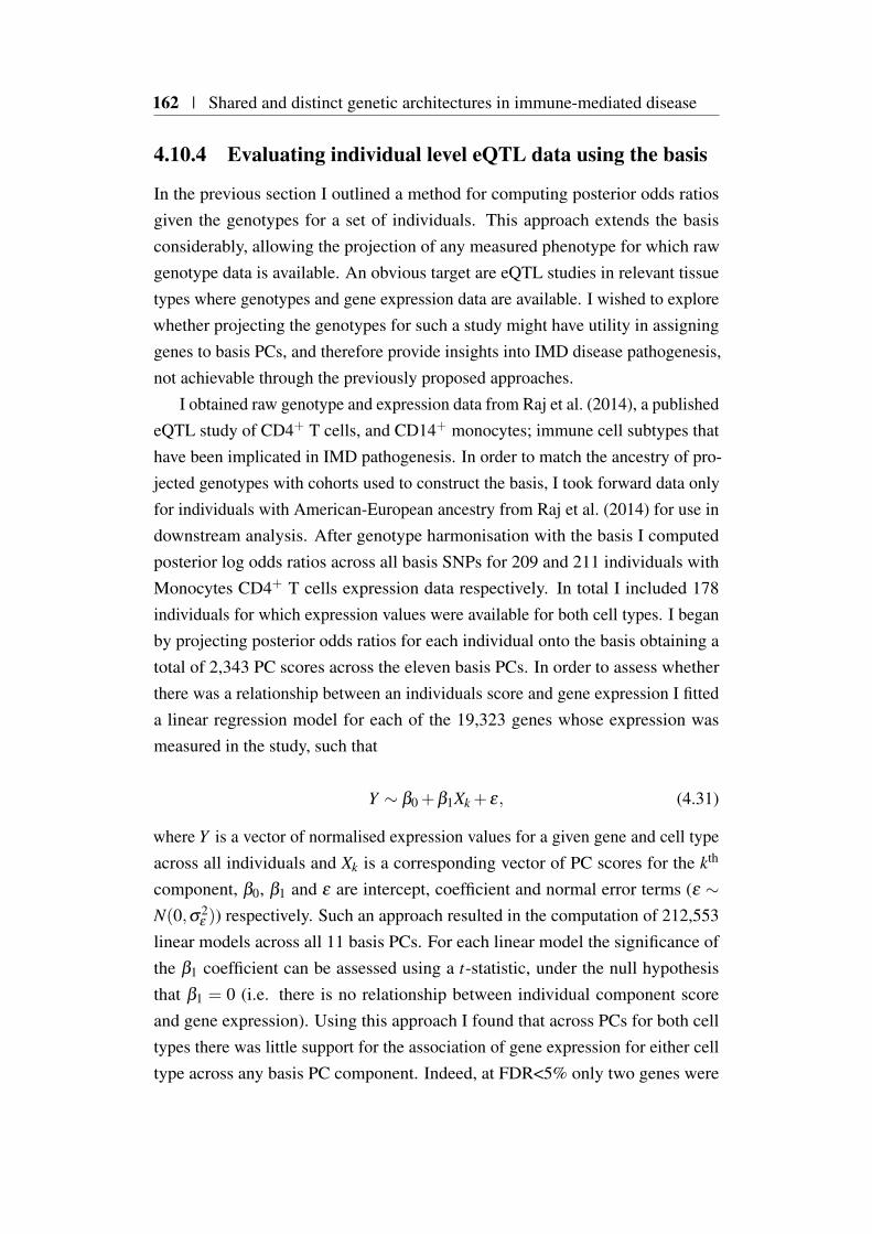
162 | Shared and distinct genetic architectures in immune-mediated disease
4.10.4 Evaluating individual level eQTL data using the basis
In the previous section I outlined a method for computing posterior odds ratiosgiven the genotypes for a set of individuals. This approach extends the basisconsiderably, allowing the projection of any measured phenotype for which rawgenotype data is available. An obvious target are eQTL studies in relevant tissuetypes where genotypes and gene expression data are available. I wished to explorewhether projecting the genotypes for such a study might have utility in assigninggenes to basis PCs, and therefore provide insights into IMD disease pathogenesis,not achievable through the previously proposed approaches.
I obtained raw genotype and expression data from Raj et al. (2014), a publishedeQTL study of CD4+ T cells, and CD14+ monocytes; immune cell subtypes thathave been implicated in IMD pathogenesis. In order to match the ancestry of pro-jected genotypes with cohorts used to construct the basis, I took forward data onlyfor individuals with American-European ancestry from Raj et al. (2014) for use indownstream analysis. After genotype harmonisation with the basis I computedposterior log odds ratios across all basis SNPs for 209 and 211 individuals withMonocytes CD4+ T cells expression data respectively. In total I included 178individuals for which expression values were available for both cell types. I beganby projecting posterior odds ratios for each individual onto the basis obtaining atotal of 2,343 PC scores across the eleven basis PCs. In order to assess whetherthere was a relationship between an individuals score and gene expression I fitteda linear regression model for each of the 19,323 genes whose expression wasmeasured in the study, such that
Y ∼ β0 +β1Xk + ε, (4.31)
where Y is a vector of normalised expression values for a given gene and cell typeacross all individuals and Xk is a corresponding vector of PC scores for the kth
component, β0, β1 and ε are intercept, coefficient and normal error terms (ε ∼N(0,σ2
ε )) respectively. Such an approach resulted in the computation of 212,553linear models across all 11 basis PCs. For each linear model the significance ofthe β1 coefficient can be assessed using a t-statistic, under the null hypothesisthat β1 = 0 (i.e. there is no relationship between individual component scoreand gene expression). Using this approach I found that across PCs for both celltypes there was little support for the association of gene expression for either celltype across any basis PC component. Indeed, at FDR<5% only two genes were

4.10 Projecting individual genotypes onto the basis | 163
significant across all cell types and PCs examined (Table 4.6), neither of whichshows evidence for involvement in IMD aetiology.
Fig. 4.25 Quantile-quantile normal plots for p-values obtained from regressingan individual’s PC score with expression data from Raj et al. (2014). Coloursrepresent cell-types; CD14+ (Monocytes) - coral and CD4+ - turquoise.
Whilst such an observation is disappointing, there could be a number ofexplanations for this. Firstly, variants that effect gene expression are nominallyfound in proximity (cis) to their target gene (Brem et al., 2002; GTEx Consortium,2017) and whilst evidence for trans-eQTLs are emerging, their robust detectionrequires sample sizes 200 times larger than that analysed here (Võsa et al., 2018).This means that for a given gene a majority of input SNPs will be non-informative,instead adding stochastic noise, and it is likely that this noise will be sufficientto overcome any true signal arising from variants with genuine associations withexpression.
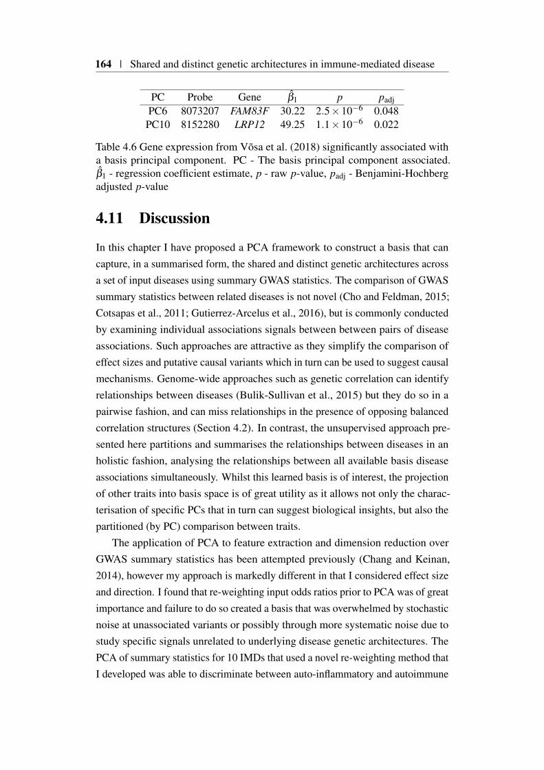
164 | Shared and distinct genetic architectures in immune-mediated disease
PC Probe Gene β1 p padjPC6 8073207 FAM83F 30.22 2.5×10⁻⁶ 0.048PC10 8152280 LRP12 49.25 1.1×10⁻⁶ 0.022
Table 4.6 Gene expression from Võsa et al. (2018) significantly associated witha basis principal component. PC - The basis principal component associated.β1 - regression coefficient estimate, p - raw p-value, padj - Benjamini-Hochbergadjusted p-value
4.11 Discussion
In this chapter I have proposed a PCA framework to construct a basis that cancapture, in a summarised form, the shared and distinct genetic architectures acrossa set of input diseases using summary GWAS statistics. The comparison of GWASsummary statistics between related diseases is not novel (Cho and Feldman, 2015;Cotsapas et al., 2011; Gutierrez-Arcelus et al., 2016), but is commonly conductedby examining individual associations signals between between pairs of diseaseassociations. Such approaches are attractive as they simplify the comparison ofeffect sizes and putative causal variants which in turn can be used to suggest causalmechanisms. Genome-wide approaches such as genetic correlation can identifyrelationships between diseases (Bulik-Sullivan et al., 2015) but they do so in apairwise fashion, and can miss relationships in the presence of opposing balancedcorrelation structures (Section 4.2). In contrast, the unsupervised approach pre-sented here partitions and summarises the relationships between diseases in anholistic fashion, analysing the relationships between all available basis diseaseassociations simultaneously. Whilst this learned basis is of interest, the projectionof other traits into basis space is of great utility as it allows not only the charac-terisation of specific PCs that in turn can suggest biological insights, but also thepartitioned (by PC) comparison between traits.
The application of PCA to feature extraction and dimension reduction overGWAS summary statistics has been attempted previously (Chang and Keinan,2014), however my approach is markedly different in that I considered effect sizeand direction. I found that re-weighting input odds ratios prior to PCA was of greatimportance and failure to do so created a basis that was overwhelmed by stochasticnoise at unassociated variants or possibly through more systematic noise due tostudy specific signals unrelated to underlying disease genetic architectures. ThePCA of summary statistics for 10 IMDs that used a novel re-weighting method thatI developed was able to discriminate between auto-inflammatory and autoimmune
4.11 Discussion | 165
diseases, in agreement with a clinical taxonomy suggested by (McGonagle andMcDermott, 2006), providing support for the efficacy of the approach.
The basis obtained forms a compact summary of the relationships betweeninput diseases The projection of external data onto the basis is especially usefulas it allows the transfer of knowledge derived from diseases, with large samplesize and resultant power, onto other phenotypes, which themselves can be, of verylimited sample size. I found this particularly useful for biologically annotatingindividual PCs using UKBB data over a wide range of traits. Reassuringly,PC scores between UKBB SRD and matched basis diseases were most similar.Furthermore UKBB SR medication data showed a strong relationship with thediseases and corresponding treatments. I note that these results are concordant withthe observations of Wu et al. (2019), who for example, found a strong relationshipbetween RA and immuno-suppressant drugs using a polygenic risk score (PRS)approach.
On extending the approach to consider the more quantitative, intermediatephenotypes of blood count and eQTL data from Astle et al. (2016) and Võsa et al.(2018) respectively, my results were less clear. In comparison to the Mendelianrandomisation analysis results described by Astle et al. (2016), I found only modestoverlap.
For my analysis involving blood eQTLs (Võsa et al., 2018) I was limitedsomewhat by data availability, as summary statistics were only available acrossall genes for a limited subset of SNPs. To overcome this I made the assumptionthat effect sizes at missing SNPs were zero, and whilst this is a strong assumption,its effect can be somewhat ameliorated by considering a within study empiricalsignificance measure. Whilst I was able to find significant PC scores for genesand pathways that corresponded to basis and other projected traits (e.g. integrincell surface interactions and IBD (de Lange et al., 2017) and PC1) many wereassociated with more than one PC, mirroring the situation previously describedwhere biological concepts are shared across multiple PCs. One possibility isthat PCs are capturing different facets of the same biological concept (e.g. B-cell receptor activation pathway) with opposing effects across PCs and thereforediseases, however further work is required to describe this fully. Further workmight consider alternative methods to achieve sparser PCs, such that biologicalconcepts are concentrated across fewer components.
I examined in detail the application of the basis to provide insight into thegenetic architecture of basis-related diseases, that due to their rarity or clinicalheterogeneity, might lack sufficient power. Using JIA as example to investigate
166 | Shared and distinct genetic architectures in immune-mediated disease
this, I projected disease subtypes onto the basis, hypothesising that despite thesmall input sample size a PC score comparison might shed light as to whethergenetic architecture might be responsible for the observed clinical heterogeneity.PC3 δ values were able to effectively discriminate Sys and ERA, which werestatistically indistinguishable from the basis ‘control’ from other JIA subtypes,which all had significant negative δ values. This was unlikely to be completelydriven by sample size due to the significance of PsA, the smallest subtype cohort.Whilst the studies of Hinks et al. (2017) and Ombrello et al. (2017) provide somesupport for the observed genetic heterogenity between subtypes.
In light of the projection of UKBB traits, which suggest that PC3 is a moregeneral component for which a majority of diseases except Asthma and MShave significant δ s. This is of some interest as PC3 scores for traits suggesteda link between the efficacy of anti-TNF therapy. Whilst the effect of rs1800693is well documented as a major factor in the exacerbating disease symptoms inMS (Gregory et al., 2012), via splicing of TNFRSF1A, this was not responsible forthis observation as basis loadings for SNPs were minimal for the region 12p13.31(median PC3 loading rank across all SNPs in the region was 210,673). Such anexample provides an illustration as to how the approach could provide insight intodisease pathology, although further work would be required to understand howrobust such assertions might be.
I extended the framework to allow the projection of individual level genotypedata into the basis space, using a Bayesian framework. This projection of posteriorβ onto the basis has overlap with the calculation of single trait polygenic riskscores (PRS) (Chatterjee et al., 2016), where rather than weighting allele countsby raw (or regularised) effect sizes ascertained from a single trait ‘discovery’GWAS, posterior log odds ratios are weighted by the loadings obtained from thebasis. In this way we obtain multi-trait PRS stratified by PC for each individualprojected. The results from the application of this method to individual genotypedata from the JIA disease subtype cohort, matched those generated using summaryGWAS data, providing support for the framework. However on application to aneQTL dataset of relevant tissues, I was unable to find any convincing relationshipsbetween individual-level PC score and gene expression, even in light of themultiple examples of colocalisation between eQTL datasets and IMD GWASsignals that have previously been described in overlapping tissue contexts (Guoet al., 2015; Zhang et al., 2015). Although this appears contradictory to recentstudies that highlight a significant role for trans-eQTLs (Boyle et al., 2017; Liuet al., 2018; Võsa et al., 2018), it seems most likely that the main reason I was
4.11 Discussion | 167
unable to confirm this was because of lack of power in the Raj et al. (2014) dataset used. Further work will be required to examine whether larger studies eQTLstudies in relevant tissues are able to provide more insight into PC characterisation.
One important consideration was the best approach to missing data, that arisesfrom the heterogeneity of genotyping platforms and downstream imputation acrossSNPs with the GWAS I wished to consider. Whilst there are methods to dealwith missing data using PCA, these are often computationally taxing and assumethat data is missing at random (Ilin and Raiko, 2010). I chose to include a widerrange of basis traits at the cost of decreased SNP coverage. I made this choicebecause I felt this would lead to a richer basis under the expectation that phenotypicheterogeneity is driven by differences in underlying genetic architecture. Thereis evidence to support this, for example T1D, where SNPs proximal to genesinvolved in pancreatic β -cell function (e.g. GLIS3, BCAR1 and INS) are sharedwith type 2 diabetes but not other IMDs (Aylward et al., 2018; Fortune et al.,2015).
Whilst there are a myriad of further extensions that might be applied to theapproach described, one of the most obvious is extending the number of traits usedeither to create or be projected on to the basis. For the former, given that summarystatistics for well powered GWAS for a range of phenotypes are now routinelyavailable (MacArthur et al., 2017), the possibility of creating a richer basis en-compassing a much wider range of diseases and phenotypes that are not limitedto IMD is possible. Such a resource might have utility in not only partitioningdiseases, through PCs related to specific genetic architectures but also framingdiseases in their overall context. This latter application might have utility in thedevelopment of new disease taxonomies that are based on molecular rather thanclinical phenotypes. In addition to creating a richer basis, the identification andprojection of additional rare forms of IMD holds promise. This could be extendedover rare disease subtypes for which data is available, for example teasing apartantibody specific forms of eosinophilic granulomatosis with polyangiitis (Lyonset al., 2018) and perhaps using the basis to better understand the genetic architec-ture of even rarer diseases of the immune system where roles for both commonand rare variants are suggested, such as Primary Immunodeficiency (Thaventhiranet al., 2018).

Chapter 5
Discussion
In this thesis I have developed methods for integrating genomic datasets at differentresolutions in order to develop a better understanding of immune-mediated diseasesusceptibility. The COGS method (Chapter 3), concerned with suggesting causalvariants, genes and tissue contexts using PCHi-C data and GWAS summarystatistics, operates at the highest resolution, making use of the single base-pairresolution of SNPs. In contrast blockshifter (Chapter 2) acts at a lower resolution,employing a genome-wide approach, in order to suggest relationships between thedisease specific genetic architectures and overall tissue specific, three dimensionalchromatin organisation. Chapter 4 takes this further, describing a frameworkacting at a genome-wide and multi-trait scale, initially to summarise the geneticrelationships between a set of clinically related diseases, but which has relevanceto understanding the genetic basis of a wide range of both binary and quantitativehuman phenotypes.
5.1 Linking themes
5.1.1 Effect of single causal variant assumptions
Common to all three chapters is the use of Bayesian fine-mapping methods to as-sign posterior probabilities for a variant to be causal, predicated on the assumptionof a single causal variant within an associated locus. In practice it is likely thatthis key assumption is often violated, and results from Asimit et al. (2019) suggesta sobering picture where the presence of multiple disease causing variants withina single locus might be currently underestimated.
170 | Discussion
The effect of violating this assumption is dependent on the locus and diseasespecific genetic architectures, but I envisage two main scenarios. In the mostbenign scenario, consider a locus in which there are multiple causal variants inlow LD, but with heterogeneous effect sizes such that one ‘lead’ variant possessesa much larger association signal than the others. Setting aside technical reasons,such a situation could arise if the variant has a higher effect size or is more commonin the population than the other causal variants. In such a case it is likely thatthe majority of the causal variant posterior probability is assigned to this ‘lead’variant, thus masking the other causal variants in the locus.
As described in Asimit et al. (2019), a more worrying but rarer scenarioconsists of two causal variants, that whilst not being highly correlated with eachother, are in LD with a third variant that itself is not causal. As, via LD, thisthird variant captures both causal variant associations, under single causal variantassumptions, it will misleadingly be assigned a high posterior probability forcausality.
Such scenarios are of most relevance to the methods developed in Chapter 3that operate at the highest resolution. The effect of the first scenario on COGSprioritisation will likely be more benign, as the prioritisation will be performed onthe ‘lead’ signal at the expense of other causal variants within the locus. As a resultgenes and tissues, whilst of relevance to disease biology, are possibly incomplete,obscuring more subtle causal mechanisms. In contrast, scenario two is likely toresult in a misleading prioritisation, as posterior probability is assigned to variantswhich are unrelated to disease pathogenesis, and as such could lead to genes andtissues unsuitable for informing downstream functional studies. Although thiseffect is likely to be mitigated by the size of the underlying HindIII fragmentsand the correlation between the states of neighbouring fragments. Whilst theability to resolve these scenarios, once the single causal variant assumption isrelaxed, is linked to underlying sample size, it might provide an explanation forthe modest overlap of prioritised genes obtained for single and multiple causalvariant fine-mapping inputs to COGS that I observed.
I expect the single causal variant assumption to have a more limited effecton the other, lower resolution approaches presented. Considering blockshifter, Iwould argue that this limitation although important at individual loci is somewhataveraged out at the genome-wide scale, and this is further ameliorated by thecompetitive nature of the test, where enrichment is computed not with respect to anull distribution, but as the comparison of two sets of tissues, similarly affected byunderlying assumptions.
5.1 Linking themes | 171
Whilst the shrinkage method underpinning the analyses in Chapter 4 is synthe-sised from the single causal variant fine-mapping approach, its goals are somewhatdifferent in that it seeks to amplify effect sizes for SNPs which are likely to as-sociated with disease whilst attenuating those that are more likely due to morestochastic processes. In such a situation picking a non-causal variant that encapsu-lates information about a multiple number of causal variants does not significantlydisadvantage the method, under the assumption that input studies of shared ge-netic ancestry are selected. Indeed, for this application, where SNP coverage islimited it is more likely that a second key assumption, that the causal variant(s)are genotyped, is most likely violated, which I discuss in the next section.
5.1.2 Data availability
Another theme that runs through this thesis is that of data availability, mainlypertaining to GWAS datasets. This can be subdivided into two separate consid-erations: the public availability of full GWAS summary statistics for publishedstudies, and due to the rapid technological advances in this area, the heterogeneousnature of SNP coverage between different traits.
With regards to the public availability of GWAS summary statistics, greatstrides have been made over the time since the commencement of this work. Forexample the work detailed in Chapters 2 and 3, required a considerable effortin order to compile a set of summary statistics over 31 traits. This fracturedavailability of GWAS summary statistics is in part historical and founded onsomewhat overblown concerns about patient anonymity (Homer et al., 2008).Thankfully we are reaching a stage where online resources that aggregate andcurate and make publicly available, full GWAS summary statistics across the wholerange of human quantitative traits and disease phenotypes are being realised. Forexample The GWAS Catalog1 (MacArthur et al., 2017), has taken this communityrequirement seriously and now provides access to the full summary statisticsof over 750 studies/traits. However, given that in total they have curated datainformation about ‘lead’ SNPs for nearly 4,000 publications, clearly further workis required.
Critical to such efforts are not only suitable funding mechanisms that recognisethe community benefit of such resources, but also the support of funders and peer-reviewed publications to encourage researchers to submit full summary statisticsrepository as part of the manuscript submission process. Such an approach,
1https://www.ebi.ac.uk/gwas/home
172 | Discussion
exemplified by ArrayExpress (Kolesnikov et al., 2015) and GEO (Clough andBarrett, 2016) for gene expression data, would not only provide better coverageof a diverse range of phenotypes but would present additional opportunities, forexample they might provide a starting point for the development of light-touchmeta-data standards for efficiently describing GWAS studies. Such standards neednot be onerous but, for example, could incorporate guidelines on reporting effectsizes and the allele to which they pertain, enabling researchers to rapidly examineheterogeneity of effect direction at a given SNP or locus.
The differential SNP coverage between studies, presents a more technical chal-lenge, and for the chapters concerned with PCHi-C integration a quote attributedto Charles Babbage springs to mind:
Errors using inadequate data are much less than using no data at all.
Here ‘inadequate data’ is relevant to the use of the PMI methodology I developedin order to fill in instances where variants were not genotyped in the original study,and as the sobriquet suggests, this imputation method should not be conflatedwith the more rigorous procedures used to infer missing genotypes (Howie et al.,2009) or association statistics (Pasaniuc et al., 2014). Such an approach wasnecessary, as not only was the fine-mapping procedure I employed predicatedon coverage of the causal variant, but also such resolution is required whenintegrating genomic annotations for reasons of sufficient coverage of individualfeatures. For blockshifter I was able to simulate the effect of PMI on outcome,demonstrating that it decreased power to detect true enrichment, such that itseffect on downstream results would be relatively benign. The affect on COGSprioritisation was more complicated and I showed that PMI, for certain loci couldhave marked effects on gene prioritisation, and in my final analysis I opted to useonly dense ImmunoChip summary statistics, or those studies of IMD for whichconventional imputation was performed (Bentham et al., 2015; Okada et al., 2014).
For the PCA framework, I argued that, given the design of genotyping plat-forms, the effect of a sparse SNP map on my results would be minimal as mostcommon variation would be effectively tagged. This tension between data avail-ability and the desire to cover as rich a set of diseases/phenotypes as possible isrelevant throughout this thesis. Whilst a researcher, invested in a particular diseaseor phenotype might find this unacceptable, I took the view that covering as manytraits as possible would lead to greater insight. On reflection this is somewhatapplication specific. It is reasonable to cast the net widely when attempting to elu-cidate relevant tissue contexts, or genetic relationships between diseases, whereas
5.1 Linking themes | 173
a greater focus on specific diseases and fine-mapping strategies is reasonable whenattempting a more detailed prioritisation of potential causal mechanisms usingPCHi-C facilitated COGS at a specific locus.
5.1.3 The importance of orthogonal functional evidence
Undoubtedly, whilst the use of PCHi-C data in this thesis is novel there aremultiple technical and biological reasons why it is no panacea for the elucidationof causal mechanisms in complex disease. A chief limitation is that resolution isrestricted to the restriction fragment level and thus far removed from the theoreticalsingle base-pair scale of genetic association studies. This limitation not onlyprecludes the identification of causal variants but also introduces the possibilitythat multiple gene regulatory elements, acting on different target genes and inheterogeneous tissue contexts are contained within a single fragment. Leavingaside the technical challenges of employing alternative, ‘frequent-cutter’ restrictionenzymes strategies, an alternative method to overcome such challenges is tointegrate orthogonal high resolution genomic data in an attempt to triangulatepromising regulatory sequences containing putative causal variants. In this thesisI used an informal hierarchical method, first using COGS to prioritise genes,before descending to the individual promoter interacting fragment level to look foroverlap with tissue matched annotations such as eRNAs, using this as a prospectivefilter to suggest promising candidates for functional followup (Table B.2). Clearlygiven the investment required in such downstream studies the examination ofall sources of available evidence is prudent. Indeed in a number of regions LDprevents the statistical identification of causal variants, whilst large sample sizesand/or GWAS studies across different ethnicities has the potential to overcomethis situation, such approaches are resource intensive. Thankfully, new high-throughput functional screens requiring only few donors are being developed toovercome some of these situations. For example massively parallel reporter assays(MPRA) (Melnikov et al., 2012) have been used successfully to interrogate theenhancer potential of regulatory sequences containing putative causal SNPs for redblood cell traits (Ulirsch et al., 2016). However such approaches are technicallychallenging and their reliance on plasmid transfection currently precludes theassessment of certain IMD tissue contexts such as monocyte lineages. Anothertechnique which shows great promise is the use of CRISPR activation assays;where a strong transcriptional activator such as VP64 is tethered to a catalyticallydead Cas9 which in conjunction with specific guide-RNAs can be targeted to
174 | Discussion
specific regulatory sequences. The motivation for such manipulations is theyallow the assessment of the activity of a regulatory sequence in a tissue-contextagnostic manner, as the proximal localisation of the transcriptional activator tothe regulatory element will drive expression of the element and its target gene,irrespective of cellular context. Such an approach has been used to interrogate theIL2RA region, discussed in detail within this thesis, corroborating the contributionof rs61839660 to IMD disease risk discussed in Chapter 3 (Simeonov et al., 2017).
5.1.4 A new taxonomy
The importance of taxonomies for organising data in the biological sciences havebeen recognised since, 1758, when Carl Linnaeus proposed a systematic classifi-cation of plants and animals based on the detailed observations of many differentorganisms. Indeed, disease taxonomies such as The International Classification ofDiseases (ICD) are the very heart of modern medicine, however these are beginningto lag behind a growing body of molecular phenotypes, obscured by similaritiesin clinical disease presentation, that can be important for efficiently treating dis-ease (Mirnezami et al., 2012). To address this, new initiatives are being developedthat can capture such rich, molecular phenotypes, in an extensible and flexiblemanner. One example is the Human Phenotype Ontology (HPO) (Köhler et al.,2017), which, whilst initially targeting rare disease, is being extended to covermore common diseases, providing not only detailed clinician-lead taxonomies butalso facilitating relationships across disease domains. The development of suchnew taxonomies is intimately linked to the elucidation of the molecular phenotypesthat underlie disease susceptibility as these will ultimately determine the spectrumof disease covered by a particular classification. The methods and analysis pre-sented in Chapters 2 and 3 can be viewed as very early stage prioritisation methodsfor uncovering such molecular phenotypes by suggesting promising genes, tissuecontexts and biological pathways that through careful functional validation, mightlead to novel disease classifications.
Chapter 4 presents a promising approach for disease classification based onshared and distinct genetic architectures. In application to IMD, what emergesis a spectrum of risk encompassing auto-inflammatory diseases such as IBD atone extreme and classic autoimmune diseases such as SLE at the other. Thepresence of blurred lines between different but clinically related diseases is notunexpected (Cleynen et al., 2016; McGonagle and McDermott, 2006), howeverthe ability to ‘learn’ orthogonal partitions of risk across common clinically related
5.2 Further Work | 175
diseases affords the opportunity to project rarer phenotypes in order to uncoverunappreciated genetic similarities and differences. Whilst this is of some interest,characterising the biology that each component relates to will greatly increaseutility of the method, whether for suggesting novel therapeutic avenues (or thoseto avoid) or to realise a deeper molecular classification of particular disease.However the approach, as presented here, suffers somewhat from the overlap ofconcepts between components which makes relating them to biological processeschallenging. Some of this overlap could be biological, for example the samevariants in a particular biological pathway exerting antagonistic effects in differentdiseases and further work looking at PC loadings and variants will be required toinvestigate this.
A natural extension is to consider methods, such as VARIMAX (Jackson,2014), for transforming the principal components in order to promote sparsityin underlying loadings, which might result in greater discrimination of conceptsacross components. In practice given that the total number of components is small(n = 11) it is unlikely that this will have a profound effect, given that orthogonality,and thus variance explained, between components is to be preserved. It might bepromising to investigate alternative matrix factorisation methods, where underlyingassumptions of orthogonality are relaxed. Given the computational burdens ofsuch techniques I would expect a filtering of SNPs, based on weightings would bepropitious prior to their employment.
5.2 Further Work
5.2.1 PCHi-C facillitated gene prioritisation in alternative con-texts
In chapter 3 I prioritised putative causal genes and tissue contexts based onPCHi-C maps of 17 haematopoietic cell types. As detailed above, there were anumber of limitations both at the level of causal variant identification and PCHi-Cresolution, and I outlined the importance of using multiple, orthogonal lines ofevidence to assess prioritised causal mechanisms, prior to functional validation.One extension that might improve the robustness of such a prioritisation wouldbe the incorporation of such alternate sources of evidence directly into the COGSmethodology. Given its Bayesian foundations a promising avenue for futureextensions could be the consideration of more informative priors, based on the
176 | Discussion
intersection of orthologous genomic datasets with GWAS association signals. Aspreviously introduced in Chapter 2, fgwas (Pickrell, 2014) uses such an approachin order to suggest novel associations as well as identify genomic annotations ofinterest, and involves the computation of such informative priors simultaneouslyacross multiple annotations for a given trait or disease. This invites a combinedapproach where fgwas is used to compute fine-mapping posterior probabilitiesin the context of relevant genomic annotations (e.g. ChIP-Seq), which are thenused as an input to COGS to suggest causal genes. Such an analysis could providepilot data indicating whether additional effort to mediate, with functional data, thebeta binomial priors adopted in the multi-causal variant GUESSFM (Bottolo andRichardson, 2010; Wallace et al., 2015) approach would be worthwhile.
Another promising application of PCHi-C is in the identification of causalmechanisms underlying monogenic causes of disease. As detailed in the Chapter 1rare variation in non-coding regions can result in profound phenotypic effects (Let-tice et al., 2003). Given the availability of whole genome sequences (WGS) andextensive phenotypic information for a wide range of rare diseases (Ouwehand,2019), PCHi-C could be applied in a number of ways in order to further understandthe causal mechanisms underlying rare diseases. For example WGS data couldbe mined for the presence of compound heterozygotes, where PCHi-C data isused to ‘connect’ a heterozygous regulatory sequence deletion with a deleteriousprotein truncating single nucleotide variant in the same gene. Alternatively, if arare disease is characterised by specific tissue defects (especially those with rele-vance to Haematopoietic cell lineages), tissue-specific COGS scores from relatedcomplex diseases (e.g. IMD and primary immune deficiency) could be used tosuggest causal genes underlying the rare disease. Here the notion is that both rareand common diseases share causal genes, but differ in the level of penetranceand expressivity. Such applications, whilst in their infancy are beginning to bearfruit (Thaventhiran et al., 2018).
5.2.2 Further exploration of basis polygenic risk scores
With the advent of genomic technologies, we are now able to measure, withunprecedented resolution and accuracy, molecular phenotypes in a scalable fashion,ushering in an era of ‘genomic medicine’. Genetics is forming the vanguard ofsuch an approach, through the development of polygenic risk-scores (PRS), which,in their simplest manifestation, are formed from a weighted sum of a set of riskvariants present within an individual (Chatterjee et al., 2016; Wray et al., 2007).
5.2 Further Work | 177
Such approaches are not new and have been applied in the field of livestockbreeding for many years, but, with the advent GWASs of large sample size, arenow being applied to human disease (Wray et al., 2019). In certain settings,for example breast cancer, PRS, are beginning to be assessed for their utilityin augmenting more traditional risk profiling measures such as family historyand highly penetrant mutations in BRCA1/2 so as to provide a clinical screeningmechanism for identifying individuals at high risk of developing disease andwhether this might manifest as a particularly aggressive disease subtype (e.g.oestrogen receptor negative breast cancers) (Mavaddat et al., 2019). Settingaside technical issues, for example, the applicability of such GRS across differentpopulations, their translation into a clinical setting is challenging. Firstly, thepredictive power of a PRS is tied to the narrow-sense heritability of the trait,which for example in breast cancer is approximately 40%, but can extend to90% for example, in ankylosing spondylitis. Even in such diseases which arehighly heritable, their application could lead to a prevention paradox (Rose, 1981),where only a small number of cases come from high risk individuals wheresuch a PRS might be discriminatory, thus undermining their use in a clinicalsetting. Ultimately, the clinical utility of a disease-specific PRS, will be shapedby the existence and availability of interventions that modulate risk in individualsidentified as being at high risk. For example knowing that a young child is at highgenetic predisposition of being obese is likely to have more clinical utility thansuch an observation in an adult patient (Hunter and Drazen, 2019).
In my opinion for the reasons set out above, the applicability of PRS to in-dividual disease prediction/screening in a clinical setting for IMD is somewhatlimited, and their maximum utility most probably lies elsewhere, for example indisease stratification. In such a setting individuals are stratified as to their riskof developing a particular IMD, and high risk individuals are then targeted fordetailed longitudinal study. In chapter 4, I made a brief reference to the parallelsbetween such PRS and the PCA basis developed. In the context of individualgenotype projections, basis PC scores are derived from linear combinations ofindividual allele counts giving an individual PC score for each component andcan thus be interpreted as partitioned multi-trait PRS. Further exploration of thepresented method is, I think justified, given the results observed for JIA subtypes.One potential application might be to use the basis to interrogate disease prognosisin Crohn’s disease, as a previous within-cases GWAS presented evidence sucha process might be orthogonal to disease susceptibility (Lee et al., 2017), andfurther analysis might yield additional, clinically relevant insights. The benefit of
178 | Discussion
this cohort is that participants were recruited at phenotypic extremes under theexpectation this would maximise genetic discrimination, and as such might existat the extremes of the distributions for polygenic risk. The projection of both sum-mary and individual data from this study on to the basis thus framing them in thecontext of multiple IMDs, could help to shore up such evidence of orthogonality,and also lead to additional insights into previously unexamined overlaps in IMDgenetic architectures with disease prognosis. One further application might beto use the basis to further explore the genetic architecture of rare diseases, thatmanifest an immune-mediated component, for example common variable immunedeficiency (Li et al., 2015). Such an analysis could suggest, not only commonmolecular aetiologies with prexisting IMDs, but might give some insight into theinterplay between common and rare variants underlying disease pathogenesis.
5.3 Concluding Remarks
For a majority of common human disease we are now firmly in the ‘post-GWAS’era. Whilst ever larger sample sizes, coupled with new sequencing technologieswill extend the collection of associated loci and causal variants, focus is nowturning towards elucidating underlying causal mechanisms (Visscher et al., 2017).As set out in this thesis and elsewhere identifying causal variants, their targeteffectors and relevant tissue contexts is challenging. Such an effort is justified,however as the rewards, are likely to be substantial, encompassing the identificationof novel therapeutic targets, and the development of disease classifications builton firm genetic and molecular foundations. Only once these are realised will thelarge amounts of time and resources invested in GWAS over the last decade befully justified.
References
1000 Genomes Project Consortium, Auton, A., Brooks, L.D., Durbin, R.M., Garri-son, E.P., Kang, H.M., Korbel, J.O., Marchini, J.L., McCarthy, S., McVean, G.A.et al. (2015). A global reference for human genetic variation. Nature 526(7571),68–74.
Aitkin, M. and Chadwick, T. (2003). Bayesian analysis of 2 x 2 contingency tablesfrom comparative trials.
Alasoo, K., Rodrigues, J., Mukhopadhyay, S., Knights, A.J., Mann, A.L., Kundu,K., Hale, C., Dougan, G. and Gaffney, D.J. (2018, March). Shared geneticeffects on chromatin and gene expression indicate a role for enhancer primingin immune response. Nature Genetics 50(3), 424–431.
Albert, F.W. and Kruglyak, L. (2015, April). The role of regulatory variation incomplex traits and disease. Nature Reviews Genetics 16(4), 197–212.
Anderson, C.A., Boucher, G., Lees, C.W., Franke, A., D’Amato, M., Taylor,K.D., Lee, J.C., Goyette, P., Imielinski, M., Latiano, A. et al. (2011, March).Meta-analysis identifies 29 additional ulcerative colitis risk loci, increasing thenumber of confirmed associations to 47. Nat. Genet. 43(3), 246–252.
Aschard, H., Vilhjálmsson, B.J., Greliche, N., Morange, P.E., Trégouët, D.A. andKraft, P. (2014, May). Maximizing the power of principal-component analysisof correlated phenotypes in genome-wide association studies. American Journalof Human Genetics 94(5), 662–676.
Ashburner, M., Ball, C.A., Blake, J.A., Botstein, D., Butler, H., Cherry, J.M.,Davis, A.P., Dolinski, K., Dwight, S.S., Eppig, J.T. et al. (2000, May). Geneontology: tool for the unification of biology. The Gene Ontology Consortium.Nat Genet 25(1), 25–29.
Asimit, J.L., Rainbow, D.B., Fortune, M., Grinberg, N.F., Wicker, L.S. andWallace, C. (2019, January). Sharing information between related diseasesusing Bayesian joint fine mapping increases accuracy and identifies novelassociations in six immune mediated diseases. bioRxiv, 553560.
Astle, W.J., Elding, H., Jiang, T., Allen, D., Ruklisa, D., Mann, A.L., Mead, D.,Bouman, H., Riveros-Mckay, F., Kostadima, M.A. et al. (2016). The AllelicLandscape of Human Blood Cell Trait Variation and Links to Common ComplexDisease. Cell 167(5), 1415–1429.e19.

180 | References
Avery, C.L., He, Q., North, K.E., Ambite, J.L., Boerwinkle, E., Fornage, M.,Hindorff, L.A., Kooperberg, C., Meigs, J.B., Pankow, J.S. et al. (2011, October).A phenomics-based strategy identifies loci on APOC1, BRAP, and PLCG1associated with metabolic syndrome phenotype domains. PLoS genetics 7(10),e1002322.
Aylward, A., Chiou, J., Okino, M.L., Kadakia, N. and Gaulton, K.J. (2018, Novem-ber). Shared genetic risk contributes to type 1 and type 2 diabetes etiology.Human Molecular Genetics.
Bahcall, O. (2012, July). Asking for more. Nature Genetics 44(7), 733.
Barrett, J.C., Clayton, D.G., Concannon, P., Akolkar, B., Cooper, J.D., Erlich,H.A., Julier, C., Morahan, G., Nerup, J., Nierras, C. et al. (2009, June). Genome-wide association study and meta-analysis find that over 40 loci affect risk oftype 1 diabetes. Nat. Genet. 41(6), 703–707.
Bassil, R., Orent, W., Olah, M., Kurdi, A.T., Frangieh, M., Buttrick, T., Khoury,S.J. and Elyaman, W. (2014, July). BCL6 controls Th9 cell development byrepressing Il9 transcription. J Immunol 193(1), 198–207.
Bell, G.I., Horita, S. and Karam, J.H. (1984, February). A Polymorphic LocusNear the Human Insulin Gene Is Associated with Insulin-dependent DiabetesMelliitus. Diabetes 33(2), 176–183.
Benjamini, Y. and Hochberg, Y. (1995). Controlling the False Discovery Rate:A Practical and Powerful Approach to Multiple Testing. Journal of the RoyalStatistical Society. Series B (Methodological) 57(1), 289–300.
Benjamini, Y. and Speed, T.P. (2012, May). Summarizing and correcting the GCcontent bias in high-throughput sequencing. Nucleic Acids Research 40(10),e72–e72.
Bentham, J., Morris, D.L., Graham, D.S.C., Pinder, C.L., Tombleson, P., Behrens,T.W., Martín, J., Fairfax, B.P., Knight, J.C., Chen, L. et al. (2015, December).Genetic association analyses implicate aberrant regulation of innate and adaptiveimmunity genes in the pathogenesis of systemic lupus erythematosus. NatureGenetics 47(12), 1457–1464.
Bickel, P.J., Boley, N., Brown, J.B., Huang, H. and Zhang, N.R. (2010, Decem-ber). Subsampling methods for genomic inference. The Annals of AppliedStatistics 4(4), 1660–1697.
Bloom, J.S., Ehrenreich, I.M., Loo, W.T., Lite, T.L.V. and Kruglyak, L. (2013,February). Finding the sources of missing heritability in a yeast cross. Na-ture 494(7436), 234–237.
Bonev, B., Cohen, N.M., Szabo, Q., Fritsch, L., Papadopoulos, G.L., Lubling,Y., Xu, X., Lv, X., Hugnot, J.P., Tanay, A. et al. (2017, October). Multiscale3d Genome Rewiring during Mouse Neural Development. Cell 171(3), 557–572.e24.
Bottolo, L. and Richardson, S. (2010, September). Evolutionary stochastic searchfor Bayesian model exploration. Bayesian Analysis 5(3), 583–618.

References | 181
Bousquet, J., Chanez, P., Lacoste, J.Y., Barnéon, G., Ghavanian, N., Enander,I., Venge, P., Ahlstedt, S., Simony-Lafontaine, J. and Godard, P. (1990, Oc-tober). Eosinophilic inflammation in asthma. The New England Journal ofMedicine 323(15), 1033–1039.
Boyle, E.A., Li, Y.I. and Pritchard, J.K. (2017, June). An Expanded View ofComplex Traits: From Polygenic to Omnigenic. Cell 169(7), 1177–1186.
Brem, R.B., Yvert, G., Clinton, R. and Kruglyak, L. (2002, April). Geneticdissection of transcriptional regulation in budding yeast. Science (New York,N.Y.) 296(5568), 752–755.
Brewerton, D.A., Hart, F.D., Nicholls, A., Caffrey, M., James, D.C. and Sturrock,R.D. (1973, April). Ankylosing spondylitis and HL-A 27. Lancet (London,England) 1(7809), 904–907.
Buenrostro, J., Wu, B., Chang, H. and Greenleaf, W. (2015, January). ATAC-seq: A Method for Assaying Chromatin Accessibility Genome-Wide. Currentprotocols in molecular biology / edited by Frederick M. Ausubel ... [et al.] 109,21.29.1–21.29.9.
Bulik-Sullivan, B., Finucane, H.K., Anttila, V., Gusev, A., Day, F.R., Loh, P.R.,ReproGen Consortium, Psychiatric Genomics Consortium, Genetic Consortiumfor Anorexia Nervosa of the Wellcome Trust Case Control Consortium 3, Dun-can, L. et al. (2015, November). An atlas of genetic correlations across humandiseases and traits. Nature Genetics 47(11), 1236–1241.
Bulik-Sullivan, B.K., Loh, P.R., Finucane, H.K., Ripke, S., Yang, J., SchizophreniaWorking Group of the Psychiatric Genomics Consortium, Patterson, N., Daly,M.J., Price, A.L. and Neale, B.M. (2015, March). LD Score regression dis-tinguishes confounding from polygenicity in genome-wide association studies.Nature Genetics 47(3), 291–295.
Burren, O.S., Guo, H. and Wallace, C. (2014). VSEAMS: a pipeline for variant setenrichment analysis using summary GWAS data identifies IKZF3, BATF andESRRA as key transcription factors in type 1 diabetes. Bioinformatics 30(23),3342–3348.
Burren, O.S., Rubio García, A., Javierre, B.M., Rainbow, D.B., Cairns, J., Cooper,N.J., Lambourne, J.J., Schofield, E., Castro Dopico, X., Ferreira, R.C. et al.(2017, September). Chromosome contacts in activated T cells identify autoim-mune disease candidate genes. Genome Biology 18(1), 165.
Cairns, J., Freire-Pritchett, P., Wingett, S.W., Várnai, C., Dimond, A., Plagnol,V., Zerbino, D., Schoenfelder, S., Javierre, B.M., Osborne, C. et al. (2016).CHiCAGO: robust detection of DNA looping interactions in Capture Hi-C data.Genome Biol 17(1), 127.
Castellanos-Rubio, A., Fernandez-Jimenez, N., Kratchmarov, R., Luo, X., Bhagat,G., Green, P.H.R., Schneider, R., Kiledjian, M., Bilbao, J.R. and Ghosh, S.(2016, April). A long noncoding RNA associated with susceptibility to celiacdisease. Science 352(6281), 91–95.

182 | References
Chang, D. and Keinan, A. (2014, September). Principal component analysischaracterizes shared pathogenetics from genome-wide association studies. PLoScomputational biology 10(9), e1003820.
Chapman, J.M., Cooper, J.D., Todd, J.A. and Clayton, D.G. (2003). Detectingdisease associations due to linkage disequilibrium using haplotype tags: a classof tests and the determinants of statistical power. Human Heredity 56(1-3),18–31.
Chatterjee, N., Shi, J. and García-Closas, M. (2016, July). Developing andevaluating polygenic risk prediction models for stratified disease prevention.Nature reviews. Genetics 17(7), 392–406.
Chesi, A., Wagley, Y., Johnson, M.E., Manduchi, E., Su, C., Lu, S., Leonard, M.E.,Hodge, K.M., Pippin, J.A., Hankenson, K.D. et al. (2018, August). Genome-scale Capture C promoter interaction analysis implicates novel effector genes atGWAS loci for bone mineral density. bioRxiv, 405142.
Cho, J.H. and Feldman, M. (2015, July). Heterogeneity of autoimmune diseases:pathophysiologic insights from genetics and implications for new therapies. Nat.Med. 21(7), 730–738.
Choung, R.S., Unalp-Arida, A., Ruhl, C.E., Brantner, T.L., Everhart, J.E. andMurray, J.A. (2017, January). Less Hidden Celiac Disease But Increased GlutenAvoidance Without a Diagnosis in the United States: Findings From the NationalHealth and Nutrition Examination Surveys From 2009 to 2014. Mayo ClinicProceedings 92(1), 30–38.
Choy, M.K., Javierre, B.M., Williams, S.G., Baross, S.L., Liu, Y., Wingett, S.W.,Akbarov, A., Wallace, C., Freire-Pritchett, P., Rugg-Gunn, P.J. et al. (2018, June).Promoter interactome of human embryonic stem cell-derived cardiomyocytesconnects GWAS regions to cardiac gene networks. Nature Communications 9(1),2526.
Church, C., Lee, S., Bagg, E.A.L., McTaggart, J.S., Deacon, R., Gerken, T., Lee,A., Moir, L., Mecinovic, J., Quwailid, M.M. et al. (2009, August). A MouseModel for the Metabolic Effects of the Human Fat Mass and Obesity AssociatedFTO Gene. PLOS Genetics 5(8), e1000599.
Claussnitzer, M., Dankel, S.N., Kim, K.H., Quon, G., Meuleman, W., Haugen, C.,Glunk, V., Sousa, I.S., Beaudry, J.L., Puviindran, V. et al. (2015, September).FTO Obesity Variant Circuitry and Adipocyte Browning in Humans. N Engl JMed 373(10), 895–907.
Clayton, D. and Leung, H.T. (2007). An R package for analysis of whole-genomeassociation studies. Human Heredity 64(1), 45–51.
Cleynen, I., Boucher, G., Jostins, L., Schumm, L.P., Zeissig, S., Ahmad, T.,Andersen, V., Andrews, J.M., Annese, V., Brand, S. et al. (2016, January).Inherited determinants of Crohn’s disease and ulcerative colitis phenotypes: agenetic association study. Lancet (London, England) 387(10014), 156–167.
Clough, E. and Barrett, T. (2016). The Gene Expression Omnibus Database.Methods in Molecular Biology (Clifton, N.J.) 1418, 93–110.
References | 183
Coit, P., Jeffries, M., Altorok, N., Dozmorov, M.G., Koelsch, K.A., Wren, J.D.,Merrill, J.T., McCune, W.J. and Sawalha, A.H. (2013, June). Genome-wideDNA methylation study suggests epigenetic accessibility and transcriptionalpoising of interferon-regulated genes in naïve CD4+ T cells from lupus patients.Journal of Autoimmunity 43, 78–84.
Colbert, R.A. (2010, August). Classification of juvenile spondyloarthritis:enthesitis-related arthritis and beyond. Nature reviews. Rheumatology 6(8),477–485.
Cooper, G.S., Bynum, M.L.K. and Somers, E.C. (2009, December). Recentinsights in the epidemiology of autoimmune diseases: improved prevalenceestimates and understanding of clustering of diseases. Journal of Autoimmu-nity 33(3-4), 197–207.
Cooper, J.D., Simmonds, M.J., Walker, N.M., Burren, O., Brand, O.J., Guo, H.,Wallace, C., Stevens, H., Coleman, G., Wellcome Trust Case Control Consor-tium et al. (2012, December). Seven newly identified loci for autoimmunethyroid disease. Human Molecular Genetics 21(23), 5202–5208.
Cooper, N.J., Wallace, C., Burren, O.S., Cutler, A., Walker, N. and Todd, J.A.(2017, April). Type 1 diabetes genome-wide association analysis with imputa-tion identifies five new risk regions. bioRxiv, 120022.
Cordell, H.J., Han, Y., Mells, G.F., Li, Y., Hirschfield, G.M., Greene, C.S., Xie,G., Juran, B.D., Zhu, D., Qian, D.C. et al. (2015). International genome-widemeta-analysis identifies new primary biliary cirrhosis risk loci and targetablepathogenic pathways. Nat. Commun. 6, 8019.
Cortes, A. and Brown, M.A. (2011). Promise and pitfalls of the Immunochip.Arthritis Res Ther 13(1), 101.
Cortes, A., Dendrou, C.A., Motyer, A., Jostins, L., Vukcevic, D., Dilthey, A.,Donnelly, P., Leslie, S., Fugger, L. and McVean, G. (2017, September). Bayesiananalysis of genetic association across tree-structured routine healthcare data inthe UK Biobank. Nature Genetics 49(9), 1311–1318.
Cotsapas, C., Voight, B.F., Rossin, E., Lage, K., Neale, B.M., Wallace, C., Abeca-sis, G.R., Barrett, J.C., Behrens, T., Cho, J. et al. (2011, August). PervasiveSharing of Genetic Effects in Autoimmune Disease. PLoS Genetics 7(8).
Crick, F.H. (1958). On protein synthesis. Symposia of the Society for ExperimentalBiology 12, 138–163.
Cronin, C.C., Feighery, A., Ferriss, J.B., Liddy, C., Shanahan, F. and Feigh-ery, C. (1997, December). High prevalence of celiac disease among patientswith insulin-dependent (type I) diabetes mellitus. The American Journal ofGastroenterology 92(12), 2210–2212.
Cullen, K.E., Kladde, M.P. and Seyfred, M.A. (1993, July). Interaction betweentranscription regulatory regions of prolactin chromatin. Science 261(5118),203–206.
184 | References
Das, S., Forer, L., Schönherr, S., Sidore, C., Locke, A.E., Kwong, A., Vrieze,S.I., Chew, E.Y., Levy, S., McGue, M. et al. (2016). Next-generation genotypeimputation service and methods. Nature Genetics 48(10), 1284–1287.
Davies, J.O.J., Oudelaar, A.M., Higgs, D.R. and Hughes, J.R. (2017, February).How best to identify chromosomal interactions: a comparison of approaches.Nature Methods 14(2), 125–134.
Davies, J.O.J., Telenius, J.M., McGowan, S.J., Roberts, N.A., Taylor, S., Higgs,D.R. and Hughes, J.R. (2016, January). Multiplexed analysis of chromosomeconformation at vastly improved sensitivity. Nature Methods 13(1), 74–80.
Davison, L.J., Wallace, C., Cooper, J.D., Cope, N.F., Wilson, N.K., Smyth, D.J.,Howson, J.M.M., Saleh, N., Al-Jeffery, A., Angus, K.L. et al. (2012). Long-range DNA looping and gene expression analyses identify DEXI as an autoim-mune disease candidate gene. Hum. Mol. Genet. 21(2), 322–333.
de Boer, J.D., Majoor, C.J., van ’t Veer, C., Bel, E.H.D. and van der Poll, T. (2012,April). Asthma and coagulation. Blood 119(14), 3236–3244.
de Lange, K.M., Moutsianas, L., Lee, J.C., Lamb, C.A., Luo, Y., Kennedy, N.A.,Jostins, L., Rice, D.L., Gutierrez-Achury, J., Ji, S.G. et al. (2017, February).Genome-wide association study implicates immune activation of multiple inte-grin genes in inflammatory bowel disease. Nature genetics 49(2), 256–261.
Dekker, J., Rippe, K., Dekker, M. and Kleckner, N. (2002, February). CapturingChromosome Conformation. Science 295(5558), 1306–1311.
Demenais, F., Margaritte-Jeannin, P., Barnes, K.C., Cookson, W.O.C., Altmüller,J., Ang, W., Barr, R.G., Beaty, T.H., Becker, A.B., Beilby, J. et al. (2018,January). Multiancestry association study identifies new asthma risk loci thatcolocalize with immune-cell enhancer marks. Nature Genetics 50(1), 42–53.
Dendrou, C.A., Cortes, A., Shipman, L., Evans, H.G., Attfield, K.E., Jostins, L.,Barber, T., Kaur, G., Kuttikkatte, S.B., Leach, O.A. et al. (2016, November).Resolving TYK2 locus genotype-to-phenotype differences in autoimmunity.Science Translational Medicine 8(363), 363ra149.
Dendrou, C.A., Plagnol, V., Fung, E., Yang, J.H.M., Downes, K., Cooper, J.D.,Nutland, S., Coleman, G., Himsworth, M., Hardy, M. et al. (2009, Septem-ber). Cell-specific protein phenotypes for the autoimmune locus IL2ra using agenotype-selectable human bioresource. Nat Genet 41(9), 1011–1015.
Devlin, B. and Risch, N. (1995, September). A comparison of linkage disequilib-rium measures for fine-scale mapping. Genomics 29(2), 311–322.
DIAGRAM Consortium, Asian Genetic Epidemiology Network Type 2 Diabetes(AGEN-T2D) Consortium, South Asian Type 2 Diabetes (SAT2D) Consortium,Mexican American Type 2 Diabetes (MAT2D) Consortium, Type 2 DiabetesGenetic Exploration by Next-generation sequencing in multi-Ethnic Samples(T2D-GENES) Consortium, Mahajan, A., Go, M.J., Zhang, W., Below, J.E.,Gaulton, K.J. et al. (2014, March). Genome-wide trans-ancestry meta-analysisprovides insight into the genetic architecture of type 2 diabetes susceptibility.Nature Genetics 46(3), 234–244.

References | 185
Dixon, J.R., Selvaraj, S., Yue, F., Kim, A., Li, Y., Shen, Y., Hu, M., Liu, J.S. andRen, B. (2012, April). Topological Domains in Mammalian Genomes Identifiedby Analysis of Chromatin Interactions. Nature 485(7398), 376–380.
Dostie, J., Richmond, T.A., Arnaout, R.A., Selzer, R.R., Lee, W.L., Honan, T.A.,Rubio, E.D., Krumm, A., Lamb, J., Nusbaum, C. et al. (2006, October). Chromo-some Conformation Capture Carbon Copy (5c): A massively parallel solutionfor mapping interactions between genomic elements. Genome Research 16(10),1299–1309.
Dryden, N.H., Broome, L.R., Dudbridge, F., Johnson, N., Orr, N., Schoenfelder,S., Nagano, T., Andrews, S., Wingett, S., Kozarewa, I. et al. (2014, November).Unbiased analysis of potential targets of breast cancer susceptibility loci byCapture Hi-C. Genome Research 24(11), 1854–1868.
Du, Q., Luu, P.L., Stirzaker, C. and Clark, S.J. (2015, April). Methyl-CpG-bindingdomain proteins: readers of the epigenome. Epigenomics 7(6), 1051–1073.
Dubois, P.C.A., Trynka, G., Franke, L., Hunt, K.A., Romanos, J., Curtotti, A.,Zhernakova, A., Heap, G.A.R., Adány, R., Aromaa, A. et al. (2010, April). Mul-tiple common variants for celiac disease influencing immune gene expression.Nat. Genet. 42(4), 295–302.
Efron, B. (1979, January). Bootstrap Methods: Another Look at the Jackknife.The Annals of Statistics 7(1), 1–26.
Eicher, J.D., Landowski, C., Stackhouse, B., Sloan, A., Chen, W., Jensen, N., Lien,J.P., Leslie, R. and Johnson, A.D. (2015, January). GRASP v2.0: an update onthe Genome-Wide Repository of Associations between SNPs and phenotypes.Nucleic Acids Research 43(Database issue), D799–804.
Eijsbouts, C.Q., Burren, O.S., Newcombe, P.J. and Wallace, C. (2019, January).Fine mapping chromatin contacts in capture Hi-C data. BMC genomics 20(1),77.
ENCODE Project Consortium, Birney, E., Stamatoyannopoulos, J.A., Dutta, A.,Guigó, R., Gingeras, T.R., Margulies, E.H., Weng, Z., Snyder, M., Dermitzakis,E.T. et al. (2007, June). Identification and analysis of functional elements in1% of the human genome by the ENCODE pilot project. Nature 447(7146),799–816.
Ernst, J. and Kellis, M. (2012, March). ChromHMM: automating chromatin-statediscovery and characterization. Nature Methods 9(3), 215–216.
Ernst, J. and Kellis, M. (2015, April). Large-scale imputation of epigenomicdatasets for systematic annotation of diverse human tissues. Nat. Biotech-nol. 33(4), 364–376.
Estrada, K., Styrkarsdottir, U., Evangelou, E., Hsu, Y.H., Duncan, E.L., Ntzani,E.E., Oei, L., Albagha, O.M.E., Amin, N., Kemp, J.P. et al. (2012, May).Genome-wide meta-analysis identifies 56 bone mineral density loci and reveals14 loci associated with risk of fracture. Nat. Genet. 44(5), 491–501.
186 | References
Evangelou, M., Smyth, D.J., Fortune, M.D., Burren, O.S., Walker, N.M., Guo,H., Onengut-Gumuscu, S., Chen, W.M., Concannon, P., Rich, S.S. et al. (2014,December). A method for gene-based pathway analysis using genomewide as-sociation study summary statistics reveals nine new type 1 diabetes associations.Genet. Epidemiol. 38(8), 661–670.
Eyre, S., Bowes, J., Diogo, D., Lee, A., Barton, A., Martin, P., Zhernakova, A.,Stahl, E., Viatte, S., McAllister, K. et al. (2012, December). High-density ge-netic mapping identifies new susceptibility loci for rheumatoid arthritis. NatureGenetics 44(12), 1336–1340.
Eyre, S., Orozco, G. and Worthington, J. (2017, July). The genetics revolutionin rheumatology: large scale genomic arrays and genetic mapping. NatureReviews. Rheumatology 13(7), 421–432.
Fabregat, A., Sidiropoulos, K., Garapati, P., Gillespie, M., Hausmann, K., Haw,R., Jassal, B., Jupe, S., Korninger, F., McKay, S. et al. (2016, January). TheReactome pathway Knowledgebase. Nucleic Acids Res 44(D1), D481–D487.
Fairfax, B.P., Makino, S., Radhakrishnan, J., Plant, K., Leslie, S., Dilthey, A.,Ellis, P., Langford, C., Vannberg, F.O. and Knight, J.C. (2012, May). Geneticsof gene expression in primary immune cells identifies cell type-specific masterregulators and roles of HLA alleles. Nat Genet 44(5), 502–510.
Farh, K.K.H., Marson, A., Zhu, J., Kleinewietfeld, M., Housley, W.J., Beik, S.,Shoresh, N., Whitton, H., Ryan, R.J.H., Shishkin, A.A. et al. (2015). Ge-netic and epigenetic fine mapping of causal autoimmune disease variants. Na-ture 518(7539), 337–343.
Fortune, M.D., Guo, H., Burren, O., Schofield, E., Walker, N.M., Ban, M., Sawcer,S.J., Bowes, J., Worthington, J., Barton, A. et al. (2015, July). Statisticalcolocalization of genetic risk variants for related autoimmune diseases in thecontext of common controls. Nature Genetics 47(7), 839–846.
Fortune, M.D. and Wallace, C. (2018, May). simGWAS: a fast method forsimulation of large scale case-control GWAS summary statistics. bioRxiv,313023.
Franke, A., McGovern, D.P.B., Barrett, J.C., Wang, K., Radford-Smith, G.L., Ah-mad, T., Lees, C.W., Balschun, T., Lee, J., Roberts, R. et al. (2010, December).Genome-wide meta-analysis increases to 71 the number of confirmed Crohn’sdisease susceptibility loci. Nat. Genet. 42(12), 1118–1125.
Frayling, T.M., Timpson, N.J., Weedon, M.N., Zeggini, E., Freathy, R.M., Lind-gren, C.M., Perry, J.R.B., Elliott, K.S., Lango, H., Rayner, N.W. et al. (2007,May). A Common Variant in the FTO Gene Is Associated with Body MassIndex and Predisposes to Childhood and Adult Obesity. Science 316(5826),889–894.
Fullwood, M.J., Liu, M.H., Pan, Y.F., Liu, J., Xu, H., Mohamed, Y.B., Orlov, Y.L.,Velkov, S., Ho, A., Mei, P.H. et al. (2009, November). An oestrogen-receptor-alpha-bound human chromatin interactome. Nature 462(7269), 58–64.
References | 187
García Rodríguez, L.A., Ruigómez, A. and Panés, J. (2006, May). Acute gas-troenteritis is followed by an increased risk of inflammatory bowel disease.Gastroenterology 130(6), 1588–1594.
Giambartolomei, C., Vukcevic, D., Schadt, E.E., Franke, L., Hingorani, A.D.,Wallace, C. and Plagnol, V. (2014, May). Bayesian test for colocalisationbetween pairs of genetic association studies using summary statistics. PLoSGenet 10(5), e1004383.
Gieger, C., Radhakrishnan, A., Cvejic, A., Tang, W., Porcu, E., Pistis, G.,Serbanovic-Canic, J., Elling, U., Goodall, A.H., Labrune, Y. et al. (2011). Newgene functions in megakaryopoiesis and platelet formation. Nature 480(7376),201–208.
Gmuca, S., Xiao, R., Brandon, T.G., Pagnini, I., Wright, T.B., Beukelman, T.,Morgan, E.M. and Weiss, P.F. (2017). Multicenter inception cohort of enthesitis-related arthritis: variation in disease characteristics and treatment approaches.Arthritis Research & Therapy 19(1), 84.
Gregory, A.P., Dendrou, C.A., Attfield, K.E., Haghikia, A., Xifara, D.K., Butter,F., Poschmann, G., Kaur, G., Lambert, L., Leach, O.A. et al. (2012, August).TNF receptor 1 genetic risk mirrors outcome of anti-TNF therapy in multiplesclerosis. Nature 488(7412), 508–511.
GTEx Consortium, G. (2017, October). Genetic effects on gene expression acrosshuman tissues. Nature 550(7675), 204–213.
Guo, H., Fortune, M.D., Burren, O.S., Schofield, E., Todd, J.A. and Wallace, C.(2015). Integration of disease association and eQTL data using a Bayesian colo-calisation approach highlights six candidate causal genes in immune-mediateddiseases. Hum. Mol. Genet..
Gutierrez-Arcelus, M., Rich, S.S. and Raychaudhuri, S. (2016, March). Autoim-mune diseases - connecting risk alleles with molecular traits of the immunesystem. Nature Reviews. Genetics 17(3), 160–174.
Haiman, C.A., Patterson, N., Freedman, M.L., Myers, S.R., Pike, M.C., Wal-iszewska, A., Neubauer, J., Tandon, A., Schirmer, C., McDonald, G.J. et al.(2007, May). Multiple regions within 8q24 independently affect risk for prostatecancer. Nature Genetics 39(5), 638–644.
Hastie, T., Tibshirani, R. and Friedman, J. (2009). The Elements of StatisticalLearning: Data Mining, Inference, and Prediction, Second Edition. SpringerSeries in Statistics. Springer New York.
Hayter, S.M. and Cook, M.C. (2012, August). Updated assessment of the preva-lence, spectrum and case definition of autoimmune disease. AutoimmunityReviews 11(10), 754–765.
Heinig, M., Petretto, E., Wallace, C., Bottolo, L., Rotival, M., Lu, H., Li, Y.,Sarwar, R., Langley, S.R., Bauerfeind, A. et al. (2010, September). A trans-acting locus regulates an anti-viral expression network and type 1 diabetes risk.Nature 467(7314), 460–464.
188 | References
Higgs, D.R., Vernimmen, D., Hughes, J. and Gibbons, R. (2007). Using Genomicsto Study How Chromatin Influences Gene Expression. Annual Review ofGenomics and Human Genetics 8(1), 299–325.
Hinks, A., Bowes, J., Cobb, J., Ainsworth, H.C., Marion, M.C., Comeau, M.E.,Sudman, M., Han, B., Immunochip, J.A.C.f., Becker, M.L. et al. (2017, April).Fine-mapping the MHC locus in juvenile idiopathic arthritis (JIA) revealsgenetic heterogeneity corresponding to distinct adult inflammatory arthriticdiseases. Annals of the Rheumatic Diseases 76(4), 765–772.
Hinks, A., Cobb, J., Marion, M.C., Prahalad, S., Sudman, M., Bowes, J., Martin, P.,Comeau, M.E., Sajuthi, S., Andrews, R. et al. (2013, June). Dense genotyping ofimmune-related disease regions identifies 14 new susceptibility loci for juvenileidiopathic arthritis. Nature Genetics 45(6), 664–669.
Hoffman, M.M., Buske, O.J., Wang, J., Weng, Z., Bilmes, J.A. and Noble, W.S.(2012, March). Unsupervised pattern discovery in human chromatin structurethrough genomic segmentation. Nature methods 9(5), 473–476.
Holgate, S.T., Noonan, M., Chanez, P., Busse, W., Dupont, L., Pavord, I., Haku-linen, A., Paolozzi, L., Wajdula, J., Zang, C. et al. (2011, June). Efficacy andsafety of etanercept in moderate-to-severe asthma: a randomised, controlledtrial. The European Respiratory Journal 37(6), 1352–1359.
Homer, N., Szelinger, S., Redman, M., Duggan, D., Tembe, W., Muehling, J.,Pearson, J.V., Stephan, D.A., Nelson, S.F. and Craig, D.W. (2008, August).Resolving individuals contributing trace amounts of DNA to highly complexmixtures using high-density SNP genotyping microarrays. PLoS genetics 4(8),e1000167.
Hormozdiari, F., Kichaev, G., Yang, W.Y., Pasaniuc, B. and Eskin, E. (2015).Identification of causal genes for complex traits. Bioinformatics 31(12), i206–i213.
Howie, B.N., Donnelly, P. and Marchini, J. (2009, June). A flexible and accurategenotype imputation method for the next generation of genome-wide associationstudies. PLoS genetics 5(6), e1000529.
Huang, H., Fang, M., Jostins, L., Umicevic Mirkov, M., Boucher, G., Anderson,C.A., Andersen, V., Cleynen, I., Cortes, A., Crins, F. et al. (2017). Fine-mappinginflammatory bowel disease loci to single-variant resolution. Nature 547(7662),173–178.
Hughes, J.R., Roberts, N., McGowan, S., Hay, D., Giannoulatou, E., Lynch,M., De Gobbi, M., Taylor, S., Gibbons, R. and Higgs, D.R. (2014, February).Analysis of hundreds of cis-regulatory landscapes at high resolution in a single,high-throughput experiment. Nature Genetics 46(2), 205–212.
Hunter, D.J. and Drazen, J.M. (2019, May). Has the Genome Granted Our WishYet? The New England Journal of Medicine.
References | 189
ICBP, Ehret, G.B., Munroe, P.B., Rice, K.M., Bochud, M., Johnson, A.D., Chas-man, D.I., Smith, A.V., Tobin, M.D., Verwoert, G.C. et al. (2011). Geneticvariants in novel pathways influence blood pressure and cardiovascular diseaserisk. Nature 478(7367), 103–109.
Ilin, A. and Raiko, T. (2010). Practical Approaches to Principal ComponentAnalysis in the Presence of Missing Values. Journal of Machine LearningResearch 11(Jul), 1957–2000.
IMSGC, Beecham, A.H., Patsopoulos, N.A., Xifara, D.K., Davis, M.F., Kemp-pinen, A., Cotsapas, C., Shah, T.S., Spencer, C., Booth, D. et al. (2013, Novem-ber). Analysis of immune-related loci identifies 48 new susceptibility variantsfor multiple sclerosis. Nature Genetics 45(11), 1353–1360.
IMSGC, Wellcome Trust Case Control Consortium 2, Sawcer, S., Hellenthal, G.,Pirinen, M., Spencer, C.C.A., Patsopoulos, N.A., Moutsianas, L., Dilthey, A.,Su, Z. et al. (2011). Genetic risk and a primary role for cell-mediated immunemechanisms in multiple sclerosis. Nature 476(7359), 214–219.
Inshaw, J.R.J., Cutler, A.J., Burren, O.S., Stefana, M.I. and Todd, J.A. (2018, July).Approaches and advances in the genetic causes of autoimmune disease and theirimplications. Nature Immunology 19(7), 674–684.
International Genetics of Ankylosing Spondylitis Consortium (IGAS), Cortes,A., Hadler, J., Pointon, J.P., Robinson, P.C., Karaderi, T., Leo, P., Cremin, K.,Pryce, K., Harris, J. et al. (2013, July). Identification of multiple risk variantsfor ankylosing spondylitis through high-density genotyping of immune-relatedloci. Nature Genetics 45(7), 730–738.
International HapMap Consortium, Frazer, K.A., Ballinger, D.G., Cox, D.R.,Hinds, D.A., Stuve, L.L., Gibbs, R.A., Belmont, J.W., Boudreau, A., Hardenbol,P. et al. (2007). A second generation human haplotype map of over 3.1 millionSNPs. Nature 449(7164), 851–861.
Iotchkova, V., Ritchie, G.R.S., Geihs, M., Morganella, S., Min, J.L., Walter,K., Timpson, N.J., UK10K Consortium, Dunham, I., Birney, E. et al. (2019).GARFIELD classifies disease-relevant genomic features through integrationof functional annotations with association signals. Nature Genetics 51(2),343–353.
Jackson, J.E. (2014). Varimax Rotation. In Wiley StatsRef: Statistics ReferenceOnline. American Cancer Society.
Jacob, F. and Monod, J. (1961, June). Genetic regulatory mechanisms in thesynthesis of proteins. Journal of Molecular Biology 3(3), 318–356.
Jameson, J.L. and Longo, D.L. (2015, June). Precision medicine–personalized,problematic, and promising. The New England Journal of Medicine 372(23),2229–2234.
Javierre, B.M., Burren, O.S., Wilder, S.P., Kreuzhuber, R., Hill, S.M., Sewitz,S., Cairns, J., Wingett, S.W., Várnai, C., Thiecke, M.J. et al. (2016). Lineage-Specific Genome Architecture Links Enhancers and Non-coding Disease Vari-ants to Target Gene Promoters. Cell 167(5), 1369–1384.e19.
190 | References
Jeffreys, H. (1973). Scientific Inference. Cambridge University Press.
Ji, S.G., Juran, B.D., Mucha, S., Folseraas, T., Jostins, L., Melum, E., Kumasaka,N., Atkinson, E.J., Schlicht, E.M., Liu, J.Z. et al. (2017, February). Genome-wide association study of primary sclerosing cholangitis identifies new risk lociand quantifies the genetic relationship with inflammatory bowel disease. NatureGenetics 49(2), 269–273.
Johnson, G.C., Esposito, L., Barratt, B.J., Smith, A.N., Heward, J., Di Genova,G., Ueda, H., Cordell, H.J., Eaves, I.A., Dudbridge, F. et al. (2001, October).Haplotype tagging for the identification of common disease genes. NatureGenetics 29(2), 233–237.
Jones, P.A. (2012, July). Functions of DNA methylation: islands, start sites, genebodies and beyond. Nature Reviews Genetics 13(7), 484–492.
Jostins, L., Ripke, S., Weersma, R.K., Duerr, R.H., McGovern, D.P., Hui, K.Y.,Lee, J.C., Schumm, L.P., Sharma, Y., Anderson, C.A. et al. (2012). Host-microbe interactions have shaped the genetic architecture of inflammatorybowel disease. Nature 491(7422), 119–124.
Jäger, R., Migliorini, G., Henrion, M., Kandaswamy, R., Speedy, H.E., Heindl,A., Whiffin, N., Carnicer, M.J., Broome, L., Dryden, N. et al. (2015, February).Capture Hi-C identifies the chromatin interactome of colorectal cancer risk loci.Nature Communications 6, 6178.
Kanehisa, M. and Goto, S. (2000, January). KEGG: kyoto encyclopedia of genesand genomes. Nucleic Acids Res 28(1), 27–30.
Kanhere, A. and Bansal, M. (2005). Structural properties of promoters: simi-larities and differences between prokaryotes and eukaryotes. Nucleic AcidsResearch 33(10), 3165–3175.
Kass, R.E. and Raftery, A.E. (1995, June). Bayes Factors. Journal of the AmericanStatistical Association 90(430), 773–795.
Kichaev, G., Yang, W.Y., Lindstrom, S., Hormozdiari, F., Eskin, E., Price, A.L.,Kraft, P. and Pasaniuc, B. (2014, October). Integrating functional data toprioritize causal variants in statistical fine-mapping studies. PLoS Genet 10(10),e1004722.
Klei Lambertus, Luca Diana, Devlin B. and Roeder Kathryn (2007, October).Pleiotropy and principal components of heritability combine to increase powerfor association analysis. Genetic Epidemiology 32(1), 9–19.
Klein, R.J., Zeiss, C., Chew, E.Y., Tsai, J.Y., Sackler, R.S., Haynes, C., Henning,A.K., SanGiovanni, J.P., Mane, S.M., Mayne, S.T. et al. (2005, April). Com-plement factor H polymorphism in age-related macular degeneration. Science(New York, N.Y.) 308(5720), 385–389.
Kolesnikov, N., Hastings, E., Keays, M., Melnichuk, O., Tang, Y.A., Williams, E.,Dylag, M., Kurbatova, N., Brandizi, M., Burdett, T. et al. (2015, January). Array-Express update—simplifying data submissions. Nucleic Acids Research 43(D1),D1113–D1116.
References | 191
Kumasaka, N., Knights, A.J. and Gaffney, D.J. (2019, January). High-resolutiongenetic mapping of putative causal interactions between regions of open chro-matin. Nature Genetics 51(1), 128–137.
Köhler, S., Vasilevsky, N.A., Engelstad, M., Foster, E., McMurry, J., Aymé, S.,Baynam, G., Bello, S.M., Boerkoel, C.F., Boycott, K.M. et al. (2017). TheHuman Phenotype Ontology in 2017. Nucleic Acids Research 45(D1), D865–D876.
Landt, S.G., Marinov, G.K., Kundaje, A., Kheradpour, P., Pauli, F., Batzoglou, S.,Bernstein, B.E., Bickel, P., Brown, J.B., Cayting, P. et al. (2012, September).ChIP-seq guidelines and practices of the ENCODE and modENCODE consortia.Genome Research 22(9), 1813–1831.
Lawrence, M., Daujat, S. and Schneider, R. (2016, January). Lateral Think-ing: How Histone Modifications Regulate Gene Expression. Trends in Genet-ics 32(1), 42–56.
Lee, J.C., Biasci, D., Roberts, R., Gearry, R.B., Mansfield, J.C., Ahmad, T.,Prescott, N.J., Satsangi, J., Wilson, D.C., Jostins, L. et al. (2017, February).Genome-wide association study identifies distinct genetic contributions to prog-nosis and susceptibility in Crohn’s disease. Nature Genetics 49(2), 262–268.
Lee, J.J., Wedow, R., Okbay, A., Kong, E., Maghzian, O., Zacher, M., Nguyen-Viet, T.A., Bowers, P., Sidorenko, J., Karlsson Linnér, R. et al. (2018). Genediscovery and polygenic prediction from a genome-wide association studyof educational attainment in 1.1 million individuals. Nature Genetics 50(8),1112–1121.
Lee, Y., Francesca, L., Pique-Regi, R. and Wen, X. (2018, May). BayesianMulti-SNP Genetic Association Analysis: Control of FDR and Use of SummaryStatistics. bioRxiv, 316471.
Lek, M., Karczewski, K.J., Minikel, E.V., Samocha, K.E., Banks, E., Fen-nell, T., O’Donnell-Luria, A.H., Ware, J.S., Hill, A.J., Cummings, B.B. et al.(2016). Analysis of protein-coding genetic variation in 60,706 humans. Na-ture 536(7616), 285–291.
Lettice, L.A., Heaney, S.J.H., Purdie, L.A., Li, L., de Beer, P., Oostra, B.A., Goode,D., Elgar, G., Hill, R.E. and de Graaff, E. (2003, July). A long-range Shhenhancer regulates expression in the developing limb and fin and is associatedwith preaxial polydactyly. Human Molecular Genetics 12(14), 1725–1735.
Li, J., Jørgensen, S.F., Maggadottir, S.M., Bakay, M., Warnatz, K., Glessner, J.,Pandey, R., Salzer, U., Schmidt, R.E., Perez, E. et al. (2015). Association ofCLEC16a with human common variable immunodeficiency disorder and role inmurine B cells. Nat. Commun. 6, 6804.
Li, W., Notani, D. and Rosenfeld, M.G. (2016, April). Enhancers as non-codingRNA transcription units: recent insights and future perspectives. Nature Reviews.Genetics 17(4), 207–223.

192 | References
Li, Y.R., Zhao, S.D., Li, J., Bradfield, J.P., Mohebnasab, M., Steel, L., Kobie, J.,Abrams, D.J., Mentch, F.D., Glessner, J.T. et al. (2015). Genetic sharing andheritability of paediatric age of onset autoimmune diseases. Nat. Commun. 6,8442.
Liao, W., Lin, J.X. and Leonard, W.J. (2013, January). Interleukin-2 at thecrossroads of effector responses, tolerance, and immunotherapy. Immunity 38(1),13–25.
Liberzon, A., Birger, C., Thorvaldsdóttir, H., Ghandi, M., Mesirov, J.P. andTamayo, P. (2015, December). The Molecular Signatures Database (MSigDB)hallmark gene set collection. Cell Syst 1(6), 417–425.
Lieberman-Aiden, E., van Berkum, N.L., Williams, L., Imakaev, M., Ragoczy,T., Telling, A., Amit, I., Lajoie, B.R., Sabo, P.J., Dorschner, M.O. et al. (2009,October). Comprehensive mapping of long range interactions reveals foldingprinciples of the human genome. Science (New York, N.Y.) 326(5950), 289–293.
Lin, D.Y. and Sullivan, P.F. (2009, December). Meta-analysis of genome-wideassociation studies with overlapping subjects. American Journal of HumanGenetics 85(6), 862–872.
Lindor, K.D., Gershwin, M.E., Poupon, R., Kaplan, M., Bergasa, N.V., Heathcote,E.J. and American Association for Study of Liver Diseases (2009, July). Primarybiliary cirrhosis. Hepatology (Baltimore, Md.) 50(1), 291–308.
Liu, J.Z., Mcrae, A.F., Nyholt, D.R., Medland, S.E., Wray, N.R., Brown, K.M.,Hayward, N.K., Montgomery, G.W., Visscher, P.M., Martin, N.G. et al. (2010,July). A Versatile Gene-Based Test for Genome-wide Association Studies.American Journal of Human Genetics 87(1), 139–145.
Liu, J.Z., van Sommeren, S., Huang, H., Ng, S.C., Alberts, R., Takahashi, A.,Ripke, S., Lee, J.C., Jostins, L., Shah, T. et al. (2015, September). Associationanalyses identify 38 susceptibility loci for inflammatory bowel disease andhighlight shared genetic risk across populations. Nature Genetics 47(9), 979–986.
Liu, X., Li, Y.I. and Pritchard, J.K. (2018, September). Trans effects on geneexpression can drive omnigenic inheritance. bioRxiv, 425108.
Locke, A.E., Kahali, B., Berndt, S.I., Justice, A.E., Pers, T.H., Day, F.R., Powell,C., Vedantam, S., Buchkovich, M.L., Yang, J. et al. (2015). Genetic studiesof body mass index yield new insights for obesity biology. Nature 518(7538),197–206.
Long, M.D., Martin, C.F., Pipkin, C.A., Herfarth, H.H., Sandler, R.S. and Kappel-man, M.D. (2012, August). Risk of Melanoma and Nonmelanoma Skin CancerAmong Patients With Inflammatory Bowel Disease. Gastroenterology 143(2),390–399.e1.
Lyons, P., Peters, J., Alberici, F., Liley, J., Coulson, R., Astle, W., Baldini, C.,Bonatti, F., Cid, M., Elding, H. et al. (2018, December). Genetically distinctclinical subsets, and associations with asthma and eosinophil abundance, withinEosinophilic Granulomatosis with Polyangiitis. bioRxiv, 491837.
References | 193
MacArthur, J., Bowler, E., Cerezo, M., Gil, L., Hall, P., Hastings, E., Junkins,H., McMahon, A., Milano, A., Morales, J. et al. (2017, January). The newNHGRI-EBI Catalog of published genome-wide association studies (GWASCatalog). Nucleic Acids Research 45(Database issue), D896–D901.
Manning, A.K., Hivert, M.F., Scott, R.A., Grimsby, J.L., Bouatia-Naji, N., Chen,H., Rybin, D., Liu, C.T., Bielak, L.F., Prokopenko, I. et al. (2012, June). Agenome-wide approach accounting for body mass index identifies genetic vari-ants influencing fasting glycemic traits and insulin resistance. Nat. Genet. 44(6),659–669.
Martin, P., McGovern, A., Orozco, G., Duffus, K., Yarwood, A., Schoenfelder,S., Cooper, N.J., Barton, A., Wallace, C., Fraser, P. et al. (2015, November).Capture Hi-C reveals novel candidate genes and complex long-range interactionswith related autoimmune risk loci. Nature Communications 6.
Maurano, M.T., Humbert, R., Rynes, E., Thurman, R.E., Haugen, E., Wang, H.,Reynolds, A.P., Sandstrom, R., Qu, H., Brody, J. et al. (2012, September).Systematic localization of common disease-associated variation in regulatoryDNA. Science (New York, N.Y.) 337(6099), 1190–1195.
Mavaddat, N., Michailidou, K., Dennis, J., Lush, M., Fachal, L., Lee, A., Tyrer,J.P., Chen, T.H., Wang, Q., Bolla, M.K. et al. (2019, January). Polygenic RiskScores for Prediction of Breast Cancer and Breast Cancer Subtypes. AmericanJournal of Human Genetics 104(1), 21–34.
McCarthy, M.I. (2017). Painting a new picture of personalised medicine fordiabetes. Diabetologia 60(5), 793–799.
McCarthy, S., Das, S., Kretzschmar, W., Delaneau, O., Wood, A.R., Teumer, A.,Kang, H.M., Fuchsberger, C., Danecek, P., Sharp, K. et al. (2016). A referencepanel of 64,976 haplotypes for genotype imputation. Nature Genetics 48(10),1279–1283.
McGonagle, D. and McDermott, M.F. (2006, August). A proposed classificationof the immunological diseases. PLoS medicine 3(8), e297.
McLaren, W., Gil, L., Hunt, S.E., Riat, H.S., Ritchie, G.R.S., Thormann, A., Flicek,P. and Cunningham, F. (2016, June). The Ensembl Variant Effect Predictor.Genome Biology 17, 122.
Melnikov, A., Murugan, A., Zhang, X., Tesileanu, T., Wang, L., Rogov, P., Feizi,S., Gnirke, A., Callan, C.G., Kinney, J.B. et al. (2012, February). Systematicdissection and optimization of inducible enhancers in human cells using amassively parallel reporter assay. Nature Biotechnology 30(3), 271–277.
Mifsud, B., Tavares-Cadete, F., Young, A.N., Sugar, R., Schoenfelder, S., Ferreira,L., Wingett, S.W., Andrews, S., Grey, W., Ewels, P.A. et al. (2015, June).Mapping long-range promoter contacts in human cells with high-resolutioncapture Hi-C. Nature Genetics 47(6), 598–606.
194 | References
Miguel-Escalada, I., Bonàs-Guarch, S., Cebola, I., Ponsa-Cobas, J., Mendieta-Esteban, J., Rolando, D.M.Y., Javierre, B.M., Atla, G., Farabella, I., Morgan,C.C. et al. (2018, August). Human pancreatic islet 3d chromatin architectureprovides insights into the genetics of type 2 diabetes. bioRxiv, 400291.
Millard, L.A.C., Davies, N.M., Gaunt, T.R., Davey Smith, G. and Tilling, K.(2017, October). Software Application Profile: PHESANT: a tool for per-forming automated phenome scans in UK Biobank. International Journal ofEpidemiology.
Miller, A.J. (1984). Selection of subsets of regression variables. Journal of theRoyal Statistical Society. Series A (General), 389–425.
Mirnezami, R., Nicholson, J. and Darzi, A. (2012, February). Preparing forPrecision Medicine. New England Journal of Medicine 366(6), 489–491.
Morrell, C.N., Aggrey, A.A., Chapman, L.M. and Modjeski, K.L. (2014, May).Emerging roles for platelets as immune and inflammatory cells. Blood 123(18),2759–2767.
Morris, A.P., Voight, B.F., Teslovich, T.M., Ferreira, T., Segrè, A.V., Steinthors-dottir, V., Strawbridge, R.J., Khan, H., Grallert, H., Mahajan, A. et al. (2012,September). Large-scale association analysis provides insights into the ge-netic architecture and pathophysiology of type 2 diabetes. Nat. Genet. 44(9),981–990.
Mumbach, M.R., Rubin, A.J., Flynn, R.A., Dai, C., Khavari, P.A., Greenleaf, W.J.and Chang, H.Y. (2016, November). HiChIP: efficient and sensitive analysis ofprotein-directed genome architecture. Nature Methods 13(11), 919–922.
Murphy, K. and Weaver, C. (2017). Janeway’s Immunobiology (9th ed.). GarlandScience. Taylor & Francis Group, LLC.
Márquez, A., Kerick, M., Zhernakova, A., Gutierrez-Achury, J., Chen, W.M.,Onengut-Gumuscu, S., González-Álvaro, I., Rodriguez-Rodriguez, L., Rios-Fernández, R., González-Gay, M.A. et al. (2018). Meta-analysis of Immunochipdata of four autoimmune diseases reveals novel single-disease and cross-phenotype associations. Genome Medicine 10(1), 97.
Okada, Y., Wu, D., Trynka, G., Raj, T., Terao, C., Ikari, K., Kochi, Y., Ohmura,K., Suzuki, A., Yoshida, S. et al. (2014). Genetics of rheumatoid arthritiscontributes to biology and drug discovery. Nature 506(7488), 376–381.
Ombrello, M.J., Arthur, V.L., Remmers, E.F., Hinks, A., Tachmazidou, I., Grom,A.A., Foell, D., Martini, A., Gattorno, M., Özen, S. et al. (2017, May). Geneticarchitecture distinguishes systemic juvenile idiopathic arthritis from other formsof juvenile idiopathic arthritis: clinical and therapeutic implications. Annals ofthe Rheumatic Diseases 76(5), 906–913.
Onengut-Gumuscu, S., Chen, W.M., Burren, O., Cooper, N.J., Quinlan, A.R.,Mychaleckyj, J.C., Farber, E., Bonnie, J.K., Szpak, M., Schofield, E. et al.(2015, April). Fine mapping of type 1 diabetes susceptibility loci and evidencefor colocalization of causal variants with lymphoid gene enhancers. NatureGenetics 47(4), 381–386.
References | 195
Ouwehand, W.H. (2019, January). Whole-genome sequencing of rare diseasepatients in a national healthcare system | bioRxiv.
Parkes, M., Cortes, A., van Heel, D.A. and Brown, M.A. (2013, September).Genetic insights into common pathways and complex relationships amongimmune-mediated diseases. Nature Reviews. Genetics 14(9), 661–673.
Pasaniuc, B., Zaitlen, N., Shi, H., Bhatia, G., Gusev, A., Pickrell, J., Hirschhorn,J., Strachan, D.P., Patterson, N. and Price, A.L. (2014). Fast and accurateimputation of summary statistics enhances evidence of functional enrichment.Bioinformatics 30(20), 2906–2914.
Paul, D.S., Teschendorff, A.E., Dang, M.A.N., Lowe, R., Hawa, M.I., Ecker, S.,Beyan, H., Cunningham, S., Fouts, A.R., Ramelius, A. et al. (2016, November).Increased DNA methylation variability in type 1 diabetes across three immuneeffector cell types. Nature Communications 7, 13555.
Pearson, K. and Blakeman, J. (1906). On the Theory of Contingency and Its Rela-tion to Association and Normal Correlation. Number v. 1-4 in A MathematicalTheory of Random Migration. Dulau and Company.
Peters, J.E., Lyons, P.A., Lee, J.C., Richard, A.C., Fortune, M.D., Newcombe,P.J., Richardson, S. and Smith, K.G.C. (2016, March). Insight into Genotype-Phenotype Associations through eQTL Mapping in Multiple Cell Types inHealth and Immune-Mediated Disease. PLoS Genet 12(3), e1005908.
Petty, R.E., Southwood, T.R., Manners, P., Baum, J., Glass, D.N., Goldenberg,J., He, X., Maldonado-Cocco, J., Orozco-Alcala, J., Prieur, A.M. et al. (2004,February). International League of Associations for Rheumatology classificationof juvenile idiopathic arthritis: second revision, Edmonton, 2001. The Journalof Rheumatology 31(2), 390–392.
Pickrell, J.K. (2014). Joint analysis of functional genomic data and genome-wideassociation studies of 18 human traits. Am. J. Hum. Genet. 94(4), 559–573.
Pickrell, J.K., Berisa, T., Liu, J.Z., Ségurel, L., Tung, J.Y. and Hinds, D.A. (2016).Detection and interpretation of shared genetic influences on 42 human traits.Nature Genetics 48(7), 709–717.
Prahalad, S., Conneely, K.N., Jiang, Y., Sudman, M., Wallace, C.A., Brown, M.R.,Ponder, L.A., Rohani-Pichavant, M., Zwick, M.E., Cutler, D.J. et al. (2013,June). Susceptibility to childhood-onset rheumatoid arthritis: investigation of aweighted genetic risk score that integrates cumulative effects of variants at fivegenetic loci. Arthritis and Rheumatism 65(6), 1663–1667.
Price, A.L., Patterson, N.J., Plenge, R.M., Weinblatt, M.E., Shadick, N.A. and Re-ich, D. (2006, August). Principal components analysis corrects for stratificationin genome-wide association studies. Nature Genetics 38(8), 904–909.
project consortium, U. (2015, October). The UK10k project identifies rare variantsin health and disease. Nature 526(7571), 82–90.

196 | References
Purcell, S., Neale, B., Todd-Brown, K., Thomas, L., Ferreira, M.A.R., Bender,D., Maller, J., Sklar, P., de Bakker, P.I.W., Daly, M.J. et al. (2007, September).PLINK: a tool set for whole-genome association and population-based linkageanalyses. American Journal of Human Genetics 81(3), 559–575.
Quinlan, A.R. (2014). BEDTools: The Swiss-Army Tool for Genome FeatureAnalysis. Curr Protoc Bioinformatics 47, 11.12.1–11.1234.
Rainbow, D.B., Pekalski, M.L., Cutler, A., Burren, O.S., Walker, N., Todd, J.,Wallace, C. and Wicker, L. (2017, January). A rare IL2ra haplotype identifiesSNP rs61839660 as causal for autoimmunity. bioRxiv.
Rainbow, D.B., Yang, X., Burren, O., Pekalski, M.L., Smyth, D.J., Klarqvist,M.D.R., Penkett, C.J., Brugger, K., Martin, H., Todd, J.A. et al. (2015, Novem-ber). Epigenetic analysis of regulatory T cells using multiplex bisulfite sequenc-ing. Eur J Immunol 45(11), 3200–3203.
Raj, T., Rothamel, K., Mostafavi, S., Ye, C., Lee, M.N., Replogle, J.M., Feng,T., Lee, M., Asinovski, N., Frohlich, I. et al. (2014, May). Polarization of theeffects of autoimmune and neurodegenerative risk alleles in leukocytes. Science(New York, N.Y.) 344(6183), 519–523.
Rao, S.S.P., Huntley, M.H., Durand, N.C., Stamenova, E.K., Bochkov, I.D.,Robinson, J.T., Sanborn, A.L., Machol, I., Omer, A.D., Lander, E.S. et al.(2014, December). A 3d map of the human genome at kilobase resolutionreveals principles of chromatin looping. Cell 159(7), 1665–1680.
Ravelli, A. and Martini, A. (2007, March). Juvenile idiopathic arthritis. Lancet(London, England) 369(9563), 767–778.
Raychaudhuri, S., Plenge, R.M., Rossin, E.J., Ng, A.C.Y., Consortium, I.S.,Purcell, S.M., Sklar, P., Scolnick, E.M., Xavier, R.J., Altshuler, D. et al. (2009,June). Identifying Relationships among Genomic Disease Regions: PredictingGenes at Pathogenic SNP Associations and Rare Deletions. PLOS Genetics 5(6),e1000534.
Rice, G.I., Reijns, M.A., Coffin, S.R., Forte, G.M., Anderson, B.H., Szynkiewicz,M., Gornall, H., Gent, D., Leitch, A., Botella, M.P. et al. (2013, August). Syn-onymous mutations in RNASEH2a create cryptic splice sites impairing RNaseH2 enzyme function in Aicardi-Goutières syndrome. Human mutation 34(8),1066–1070.
Risch, N. and Merikangas, K. (1996, September). The future of genetic studies ofcomplex human diseases. Science (New York, N.Y.) 273(5281), 1516–1517.
Ritchie, M.E., Phipson, B., Wu, D., Hu, Y., Law, C.W., Shi, W. and Smyth,G.K. (2015, April). limma powers differential expression analyses for RNA-sequencing and microarray studies. Nucleic Acids Research 43(7), e47.
Roadmap Epigenomics Consortium, Kundaje, A., Meuleman, W., Ernst, J.,Bilenky, M., Yen, A., Heravi-Moussavi, A., Kheradpour, P., Zhang, Z., Wang, J.et al. (2015, February). Integrative analysis of 111 reference human epigenomes.Nature 518(7539), 317–330.
References | 197
Rockman, M.V. (2012, January). The QTN program and the alleles that matter forevolution: all that’s gold does not glitter. Evolution; International Journal ofOrganic Evolution 66(1), 1–17.
Rose, G. (1981, June). Strategy of prevention: lessons from cardiovascular disease.British Medical Journal (Clinical Research Ed.) 282(6279), 1847–1851.
Rossin, E.J., Lage, K., Raychaudhuri, S., Xavier, R.J., Tatar, D., Benita, Y.,Constortium, I.I.B.D.G., Cotsapas, C. and Daly, M.J. (2011, January). ProteinsEncoded in Genomic Regions Associated with Immune-Mediated DiseasePhysically Interact and Suggest Underlying Biology. PLOS Genetics 7(1),e1001273.
Russo, R.A.G. and Katsicas, M.M. (2009, May). Clinical remission in patientswith systemic juvenile idiopathic arthritis treated with anti-tumor necrosis factoragents. The Journal of Rheumatology 36(5), 1078–1082.
Sankararaman, S., Mallick, S., Dannemann, M., Prüfer, K., Kelso, J., Pääbo,S., Patterson, N. and Reich, D. (2014, March). The genomic landscape ofNeanderthal ancestry in present-day humans., The landscape of Neandertalancestry in present-day humans. Nature 507(7492), 354–357.
Schofield, E.C., Carver, T., Achuthan, P., Freire-Pritchett, P., Spivakov, M., Todd,J.A. and Burren, O.S. (2016). CHiCP: a web-based tool for the integrativeand interactive visualization of promoter capture Hi-C datasets. Bioinformatics(Oxford, England) 32(16), 2511–2513.
Schork, A.J., Thompson, W.K., Pham, P., Torkamani, A., Roddey, J.C., Sulli-van, P.F., Kelsoe, J.R., O’Donovan, M.C., Furberg, H., Consortium, T.T.a.G.et al. (2013, April). All SNPs Are Not Created Equal: Genome-Wide Associ-ation Studies Reveal a Consistent Pattern of Enrichment among FunctionallyAnnotated SNPs. PLOS Genetics 9(4), e1003449.
Scuteri, A., Sanna, S., Chen, W.M., Uda, M., Albai, G., Strait, J., Najjar, S.,Nagaraja, R., Orrú, M., Usala, G. et al. (2007, July). Genome-wide associationscan shows genetic variants in the FTO gene are associated with obesity-relatedtraits. PLoS genetics 3(7), e115.
Sexton, T., Yaffe, E., Kenigsberg, E., Bantignies, F., Leblanc, B., Hoichman, M.,Parrinello, H., Tanay, A. and Cavalli, G. (2012, February). Three-DimensionalFolding and Functional Organization Principles of the Drosophila Genome.Cell 148(3), 458–472.
Sherry, S.T., Ward, M.H., Kholodov, M., Baker, J., Phan, L., Smigielski, E.M. andSirotkin, K. (2001, January). dbSNP: the NCBI database of genetic variation.Nucleic Acids Research 29(1), 308–311.
Shogren-Knaak, M., Ishii, H., Sun, J.M., Pazin, M.J., Davie, J.R. and Peterson,C.L. (2006, February). Histone H4-K16 acetylation controls chromatin structureand protein interactions. Science (New York, N.Y.) 311(5762), 844–847.
198 | References
Short, P.J., McRae, J.F., Gallone, G., Sifrim, A., Won, H., Geschwind, D.H.,Wright, C.F., Firth, H.V., FitzPatrick, D.R., Barrett, J.C. et al. (2018, March).De novo mutations in regulatory elements in neurodevelopmental disorders.Nature 555(7698), 611–616.
Simeonov, D.R., Gowen, B.G., Boontanrart, M., Roth, T.L., Gagnon, J.D., Mum-bach, M.R., Satpathy, A.T., Lee, Y., Bray, N.L., Chan, A.Y. et al. (2017, Septem-ber). Discovery of stimulation-responsive immune enhancers with CRISPRactivation. Nature 549(7670), 111–115.
Simonis, M., Klous, P., Splinter, E., Moshkin, Y., Willemsen, R., de Wit, E.,van Steensel, B. and de Laat, W. (2006, November). Nuclear organization ofactive and inactive chromatin domains uncovered by chromosome conformationcapture–on-chip (4c). Nature Genetics 38(11), 1348–1354.
Smemo, S., Tena, J.J., Kim, K.H., Gamazon, E.R., Sakabe, N.J., Gómez-Marín, C.,Aneas, I., Credidio, F.L., Sobreira, D.R., Wasserman, N.F. et al. (2014, March).Obesity-associated variants within FTO form long-range functional connectionswith IRX3. Nature 507(7492), 371–375.
Smyth, D.J., Plagnol, V., Walker, N.M., Cooper, J.D., Downes, K., Yang, J.H.M.,Howson, J.M.M., Stevens, H., McManus, R., Wijmenga, C. et al. (2008, Decem-ber). Shared and distinct genetic variants in type 1 diabetes and celiac disease.The New England Journal of Medicine 359(26), 2767–2777.
Solovieff, N., Cotsapas, C., Lee, P.H., Purcell, S.M. and Smoller, J.W. (2013,July). Pleiotropy in complex traits: challenges and strategies. Nature reviews.Genetics 14(7), 483–495.
Somers, E.C., Thomas, S.L., Smeeth, L. and Hall, A.J. (2006, March). Au-toimmune Diseases Co-occurring Within Individuals and Within Families: ASystematic Review. Epidemiology 17(2), 202.
Song, L. and Crawford, G.E. (2010, February). DNase-seq: a high-resolutiontechnique for mapping active gene regulatory elements across the genome frommammalian cells. Cold Spring Harbor Protocols 2010(2), pdb.prot5384.
Song, M., Yang, X., Ren, X., Wang, C., Jacob, F., Wu, K., Traglia, M., Li, B.,Maliskova, L., Jones, I. et al. (2018, December). cis-Regulatory ChromatinContacts in Neural Cells Reveal Contributions of Genetic Variants to ComplexNeurological Disorders. bioRxiv, 494450.
Soranzo, N., Spector, T.D., Mangino, M., Kühnel, B., Rendon, A., Teumer,A., Willenborg, C., Wright, B., Chen, L., Li, M. et al. (2009, November).A genome-wide meta-analysis identifies 22 loci associated with eight hema-tological parameters in the HaemGen consortium. Nature Genetics 41(11),1182–1190.
Soskic, B., Cano-Gamez, E., Smyth, D.J., Rowan, W.C., Nakic, N., Esparza-Gordillo, J., Bossini-Castillo, L., Tough, D.F., Larminie, C.G.C., Bronson, P.G.et al. (2019, March). Chromatin activity at GWAS loci identifies T cell statesdriving complex immune diseases. bioRxiv, 566810.

References | 199
Stahl, E.A., Raychaudhuri, S., Remmers, E.F., Xie, G., Eyre, S., Thomson, B.P., Li,Y., Kurreeman, F.A.S., Zhernakova, A., Hinks, A. et al. (2010, June). Genome-wide association study meta-analysis identifies seven new rheumatoid arthritisrisk loci. Nat. Genet. 42(6), 508–514.
Stegle, O., Parts, L., Piipari, M., Winn, J. and Durbin, R. (2012, February). Usingprobabilistic estimation of expression residuals (PEER) to obtain increasedpower and interpretability of gene expression analyses. Nature Protocols 7(3),500–507.
Stephens, M. and Balding, D.J. (2009, October). Bayesian statistical methods forgenetic association studies. Nature Reviews. Genetics 10(10), 681–690.
Stergachis, A.B., Haugen, E., Shafer, A., Fu, W., Vernot, B., Reynolds, A.,Raubitschek, A., Ziegler, S., LeProust, E.M., Akey, J.M. et al. (2013, December).Exonic transcription factor binding directs codon choice and affects proteinevolution. Science (New York, N.Y.) 342(6164), 1367–1372.
Stranger, B.E., Nica, A.C., Forrest, M.S., Dimas, A., Bird, C.P., Beazley, C., Ingle,C.E., Dunning, M., Flicek, P., Koller, D. et al. (2007, October). Populationgenomics of human gene expression. Nature genetics 39(10), 1217–1224.
Stunnenberg, H.G. and Hirst, M. (2016, November). The International HumanEpigenome Consortium: A Blueprint for Scientific Collaboration and Discovery.Cell 167(5), 1145–1149.
Subramanian, A., Tamayo, P., Mootha, V.K., Mukherjee, S., Ebert, B.L., Gillette,M.A., Paulovich, A., Pomeroy, S.L., Golub, T.R., Lander, E.S. et al. (2005).Gene set enrichment analysis: a knowledge-based approach for interpretinggenome-wide expression profiles. Proc. Natl. Acad. Sci. U. S. A. 102(43),15545–15550.
Sudlow, C., Gallacher, J., Allen, N., Beral, V., Burton, P., Danesh, J., Downey,P., Elliott, P., Green, J., Landray, M. et al. (2015, March). UK Biobank: AnOpen Access Resource for Identifying the Causes of a Wide Range of ComplexDiseases of Middle and Old Age. PLOS Medicine 12(3), e1001779.
Tan, L., Xing, D., Chang, C.H., Li, H. and Xie, X.S. (2018, August).Three-dimensional genome structures of single diploid human cells. Sci-ence 361(6405), 924–928.
Tehranchi, A.K., Myrthil, M., Martin, T., Hie, B.L., Golan, D. and Fraser, H.B.(2016, April). Pooled ChIP-Seq Links Variation in Transcription Factor Bindingto Complex Disease Risk. Cell 165(3), 730–741.
Teslovich, T.M., Musunuru, K., Smith, A.V., Edmondson, A.C., Stylianou, I.M.,Koseki, M., Pirruccello, J.P., Ripatti, S., Chasman, D.I., Willer, C.J. et al.(2010). Biological, clinical and population relevance of 95 loci for blood lipids.Nature 466(7307), 707–713.
Thaventhiran, J.E.D., Allen, H.L., Burren, O.S., Farmery, J.H.R., Staples, E.,Zhang, Z., Rae, W., Greene, D., Simeoni, I., Maimaris, J. et al. (2018, Decem-ber). Whole Genome Sequencing of Primary Immunodeficiency reveals a role
200 | References
for common and rare variants in coding and non-coding sequences. bioRxiv,499988.
The ENCODE Project Consortium (2012, September). An integrated encyclopediaof DNA elements in the human genome. Nature 489(7414), 57–74.
Thurman, R.E., Rynes, E., Humbert, R., Vierstra, J., Maurano, M.T., Haugen, E.,Sheffield, N.C., Stergachis, A.B., Wang, H., Vernot, B. et al. (2012, September).The accessible chromatin landscape of the human genome. Nature 489(7414),75–82.
Todd, J.A., Bell, J.I. and McDevitt, H.O. (1987, October). HLA-DQ Beta gene con-tributes to susceptibility and resistance to insulin-dependent diabetes mellitus.Nature 329(6140), 599.
Tolhuis, B., Palstra, R.J., Splinter, E., Grosveld, F. and de Laat, W. (2002, De-cember). Looping and interaction between hypersensitive sites in the activebeta-globin locus. Molecular Cell 10(6), 1453–1465.
Trynka, G., Hunt, K.A., Bockett, N.A., Romanos, J., Mistry, V., Szperl, A., Bakker,S.F., Bardella, M.T., Bhaw-Rosun, L., Castillejo, G. et al. (2011, November).Dense genotyping identifies and localizes multiple common and rare variantassociation signals in celiac disease. Nature Genetics 43(12), 1193–1201.
Trynka, G., Westra, H.J., Slowikowski, K., Hu, X., Xu, H., Stranger, B.E., Klein,R.J., Han, B. and Raychaudhuri, S. (2015). Disentangling the Effects of Colo-calizing Genomic Annotations to Functionally Prioritize Non-coding Variantswithin Complex-Trait Loci. Am. J. Hum. Genet. 97(1), 139–152.
Ulirsch, J.C., Nandakumar, S.K., Wang, L., Giani, F.C., Zhang, X., Rogov, P., Mel-nikov, A., McDonel, P., Do, R., Mikkelsen, T.S. et al. (2016, June). SystematicFunctional Dissection of Common Genetic Variation Affecting Red Blood CellTraits. Cell 165(6), 1530–1545.
Visscher, P.M., Wray, N.R., Zhang, Q., Sklar, P., McCarthy, M.I., Brown, M.A.and Yang, J. (2017, July). 10 Years of GWAS Discovery: Biology, Function,and Translation. American Journal of Human Genetics 101(1), 5–22.
Võsa, U., Claringbould, A., Westra, H.J., Bonder, M.J., Deelen, P., Zeng, B.,Kirsten, H., Saha, A., Kreuzhuber, R., Kasela, S. et al. (2018, October). Unravel-ing the polygenic architecture of complex traits using blood eQTL meta-analysis.bioRxiv, 447367.
Wakefield, J. (2007, August). A Bayesian measure of the probability of falsediscovery in genetic epidemiology studies. American Journal of Human Genet-ics 81(2), 208–227.
Wakefield, J. (2008, June). Reporting and interpretation in genome-wide associa-tion studies. International Journal of Epidemiology 37(3), 641–653.
Wakefield, J. (2009, January). Bayes factors for genome-wide association studies:comparison with P-values. Genet Epidemiol 33(1), 79–86.
References | 201
Wallace, C., Cutler, A.J., Pontikos, N., Pekalski, M.L., Burren, O.S., Cooper,J.D., García, A.R., Ferreira, R.C., Guo, H., Walker, N.M. et al. (2015, June).Dissection of a Complex Disease Susceptibility Region Using a BayesianStochastic Search Approach to Fine Mapping. PLoS Genet 11(6), e1005272.
Wallace, C., Rotival, M., Cooper, J.D., Rice, C.M., Yang, J.H.M., McNeill, M.,Smyth, D.J., Niblett, D., Cambien, F., Cardiogenics Consortium et al. (2012,June). Statistical colocalization of monocyte gene expression and genetic riskvariants for type 1 diabetes. Human Molecular Genetics 21(12), 2815–2824.
Wang, G., Sarkar, A., Carbonetto, P. and Stephens, M. (2018, December). Asimple new approach to variable selection in regression, with application togenetic fine-mapping. bioRxiv, 501114.
Wang, K., Li, M. and Bucan, M. (2007, December). Pathway-Based Approachesfor Analysis of Genomewide Association Studies. American Journal of HumanGenetics 81(6), 1278–1283.
Wang, W.Y.S., Barratt, B.J., Clayton, D.G. and Todd, J.A. (2005, February).Genome-wide association studies: theoretical and practical concerns. NatureReviews. Genetics 6(2), 109–118.
Weiss, P.F., Xiao, R., Brandon, T.G., Pagnini, I., Wright, T.B., Beukelman, T.,Morgan-DeWitt, E. and Feudtner, C. (2018, January). Comparative effectivenessof tumor necrosis factor agents and disease-modifying antirheumatic therapyin children with enthesitis-related arthritis: the first year after diagnosis. TheJournal of rheumatology 45(1), 107–114.
Wellcome Trust Case Control Consortium (2007, June). Genome-wide associationstudy of 14,000 cases of seven common diseases and 3,000 shared controls.Nature 447(7145), 661–678.
Wellcome Trust Case Control Consortium, Maller, J.B., McVean, G., Byrnes, J.,Vukcevic, D., Palin, K., Su, Z., Howson, J.M.M., Auton, A., Myers, S. et al.(2012, December). Bayesian refinement of association signals for 14 loci in 3common diseases. Nature Genetics 44(12), 1294–1301.
Wingett, S., Ewels, P., Furlan-Magaril, M., Nagano, T., Schoenfelder, S., Fraser,P. and Andrews, S. (2015, November). HiCUP: pipeline for mapping andprocessing Hi-C data. F1000Research 4.
Wood, A.R., Esko, T., Yang, J., Vedantam, S., Pers, T.H., Gustafsson, S., Chu,A.Y., Estrada, K., Luan, J., Kutalik, Z. et al. (2014, November). Defining therole of common variation in the genomic and biological architecture of adulthuman height. Nat. Genet. 46(11), 1173–1186.
Wray, N.R., Goddard, M.E. and Visscher, P.M. (2007, October). Predictionof individual genetic risk to disease from genome-wide association studies.Genome Research 17(10), 1520–1528.
Wray, N.R., Kemper, K.E., Hayes, B.J., Goddard, M.E. and Visscher, P.M. (2019).Complex Trait Prediction from Genome Data: Contrasting EBV in Livestock toPRS in Humans: Genomic Prediction. Genetics 211(4), 1131–1141.
202 | References
Wu, Y., Byrne, E.M., Zheng, Z., Kemper, K.E., Yengo, L., Mallett, A.J., Yang,J., Visscher, P.M. and Wray, N.R. (2019). Genome-wide association study ofmedication-use and associated disease in the UK Biobank. Nature Communica-tions 10(1), 1891.
Xiao, R. and Boehnke, M. (2009, July). Quantifying and correcting for thewinner’s curse in genetic association studies. Genetic epidemiology 33(5),453–462.
Xing, K. and He, X. (2015, April). Reassessing the "duon" hypothesis of proteinevolution. Molecular Biology and Evolution 32(4), 1056–1062.
Yan, J., Chen, S.A.A., Local, A., Liu, T., Qiu, Y., Dorighi, K.M., Preissl, S.,Rivera, C.M., Wang, C., Ye, Z. et al. (2018, February). Histone H3 lysine 4monomethylation modulates long-range chromatin interactions at enhancers.Cell Research 28(2), 204–220.
Yang, J., Lee, S.H., Goddard, M.E. and Visscher, P.M. (2011, January). GCTA: atool for genome-wide complex trait analysis. Am J Hum Genet 88(1), 76–82.
Yates, A., Akanni, W., Amode, M.R., Barrell, D., Billis, K., Carvalho-Silva,D., Cummins, C., Clapham, P., Fitzgerald, S., Gil, L. et al. (2016, January).Ensembl 2016. Nucleic Acids Research 44(D1), D710–D716.
Zhang, H., Massey, D., Tremelling, M. and Parkes, M. (2008). Genetics ofinflammatory bowel disease: clues to pathogenesis. British Medical Bulletin 87,17–30.
Zhang, X., Joehanes, R., Chen, B.H., Huan, T., Ying, S., Munson, P.J., Johnson,A.D., Levy, D. and O’Donnell, C.J. (2015). Identification of common geneticvariants controlling transcript isoform variation in human whole blood. Nat.Genet..
Zheng, J., Erzurumluoglu, A.M., Elsworth, B.L., Kemp, J.P., Howe, L., Haycock,P.C., Hemani, G., Tansey, K., Laurin, C., Pourcain, B.S. et al. (2017, January).LD Hub: a centralized database and web interface to perform LD score re-gression that maximizes the potential of summary level GWAS data for SNPheritability and genetic correlation analysis. Bioinformatics 33(2), 272–279.
Zhernakova, A., van Diemen, C.C. and Wijmenga, C. (2009, January). Detect-ing shared pathogenesis from the shared genetics of immune-related diseases.Nature Reviews. Genetics 10(1), 43–55.
Zhu, Z., Zhang, F., Hu, H., Bakshi, A., Robinson, M.R., Powell, J.E., Montgomery,G.W., Goddard, M.E., Wray, N.R., Visscher, P.M. et al. (2016, May). Integrationof summary data from GWAS and eQTL studies predicts complex trait genetargets. Nature Genetics 48(5), 481–487.
Zuin, J., Dixon, J.R., Reijden, M.I.J.A.v.d., Ye, Z., Kolovos, P., Brouwer, R.W.W.,Corput, M.P.C.v.d., Werken, H.J.G.v.d., Knoch, T.A., IJcken, W.F.J.v. et al.(2014, January). Cohesin and CTCF differentially affect chromatin architectureand gene expression in human cells. Proceedings of the National Academy ofSciences 111(3), 996–1001.
Appendix A
A.1 Summary of PCHi-C datasets
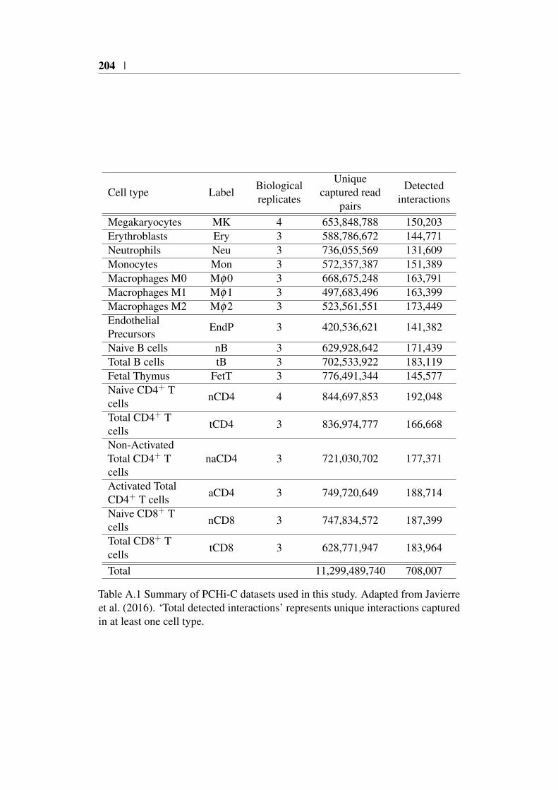
204 |
Cell type LabelBiologicalreplicates
Uniquecaptured read
pairs
Detectedinteractions
Megakaryocytes MK 4 653,848,788 150,203Erythroblasts Ery 3 588,786,672 144,771Neutrophils Neu 3 736,055,569 131,609Monocytes Mon 3 572,357,387 151,389Macrophages M0 Mφ0 3 668,675,248 163,791Macrophages M1 Mφ1 3 497,683,496 163,399Macrophages M2 Mφ2 3 523,561,551 173,449EndothelialPrecursors
EndP 3 420,536,621 141,382
Naive B cells nB 3 629,928,642 171,439Total B cells tB 3 702,533,922 183,119Fetal Thymus FetT 3 776,491,344 145,577Naive CD4+ Tcells
nCD4 4 844,697,853 192,048
Total CD4+ Tcells
tCD4 3 836,974,777 166,668
Non-ActivatedTotal CD4+ Tcells
naCD4 3 721,030,702 177,371
Activated TotalCD4+ T cells
aCD4 3 749,720,649 188,714
Naive CD8+ Tcells
nCD8 3 747,834,572 187,399
Total CD8+ Tcells
tCD8 3 628,771,947 183,964
Total 11,299,489,740 708,007
Table A.1 Summary of PCHi-C datasets used in this study. Adapted from Javierreet al. (2016). ‘Total detected interactions’ represents unique interactions capturedin at least one cell type.

A.2 GWAS study references | 205
A.2 GWAS study references
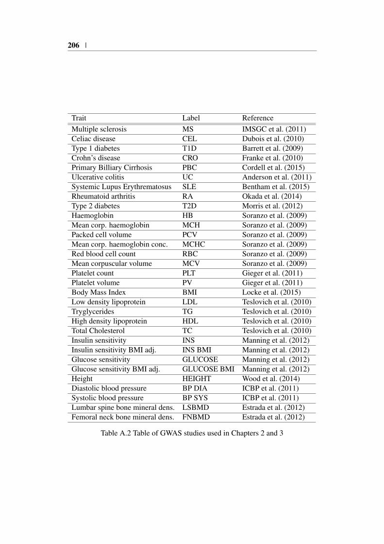
206 |
Trait Label ReferenceMultiple sclerosis MS IMSGC et al. (2011)Celiac disease CEL Dubois et al. (2010)Type 1 diabetes T1D Barrett et al. (2009)Crohn’s disease CRO Franke et al. (2010)Primary Billiary Cirrhosis PBC Cordell et al. (2015)Ulcerative colitis UC Anderson et al. (2011)Systemic Lupus Erythrematosus SLE Bentham et al. (2015)Rheumatoid arthritis RA Okada et al. (2014)Type 2 diabetes T2D Morris et al. (2012)Haemoglobin HB Soranzo et al. (2009)Mean corp. haemoglobin MCH Soranzo et al. (2009)Packed cell volume PCV Soranzo et al. (2009)Mean corp. haemoglobin conc. MCHC Soranzo et al. (2009)Red blood cell count RBC Soranzo et al. (2009)Mean corpuscular volume MCV Soranzo et al. (2009)Platelet count PLT Gieger et al. (2011)Platelet volume PV Gieger et al. (2011)Body Mass Index BMI Locke et al. (2015)Low density lipoprotein LDL Teslovich et al. (2010)Tryglycerides TG Teslovich et al. (2010)High density lipoprotein HDL Teslovich et al. (2010)Total Cholesterol TC Teslovich et al. (2010)Insulin sensitivity INS Manning et al. (2012)Insulin sensitivity BMI adj. INS BMI Manning et al. (2012)Glucose sensitivity GLUCOSE Manning et al. (2012)Glucose sensitivity BMI adj. GLUCOSE BMI Manning et al. (2012)Height HEIGHT Wood et al. (2014)Diastolic blood pressure BP DIA ICBP et al. (2011)Systolic blood pressure BP SYS ICBP et al. (2011)Lumbar spine bone mineral dens. LSBMD Estrada et al. (2012)Femoral neck bone mineral dens. FNBMD Estrada et al. (2012)
Table A.2 Table of GWAS studies used in Chapters 2 and 3

Appendix B
B.1 COGS prioritised genes Peters et al. (2016)

208 |
Table B.1 Genes significantly (FDR<5%) differentially expressed between UC/CDand healthy controls with PCHi-C COGS scores > 0.5. Genes are ordered byCOGS score.
Gene Name COGS score DE pad j Disease
FAIM3 1.000 0.000 UC
COX4I1 1.000 0.036 UC
RPS24 1.000 0.011 CD
IKZF1 0.999 0.001 CD
ACSS1 0.999 0.017 UC
CHD1 0.988 0.032 CD
CD274 0.987 0.002 CD
ROPN1L 0.944 0.042 UC
ADO 0.941 0.006 CD
TFAM 0.939 0.001 CD
ETS1 0.934 0.001 UC
MIDN 0.927 0.011 CD
SBNO2 0.926 0.000 CD
IPMK 0.922 0.028 CD
RQCD1 0.914 0.038 UC
STK32B 0.894 0.022 UC
CTDSP1 0.877 0.008 UC
ADAM10 0.854 0.006 UC
MYC 0.836 0.034 CD
FCGR2A 0.836 0.021 UC
FCRLA 0.835 0.018 UC
SGMS1 0.835 0.000 UC
CD244 0.823 0.003 CD
PIM3 0.822 0.001 UC
BCL6 0.811 0.001 UC
RTP2 0.800 0.043 UC
RASGRP1 0.795 0.005 CD
IKZF3 0.793 0.000 UC
LYRM7 0.771 0.001 UC
DGKD 0.758 0.004 CD
CHRNE 0.737 0.041 UC
ARRB2 0.717 0.001 UC
PIP4K2C 0.686 0.009 UC
Continued on next page
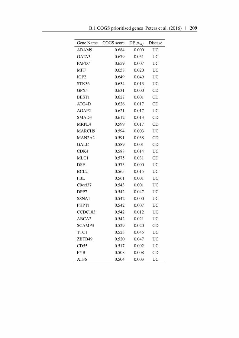
B.1 COGS prioritised genes Peters et al. (2016) | 209
Gene Name COGS score DE pad j Disease
ADAM9 0.684 0.000 UC
GATA3 0.679 0.031 UC
PAPD7 0.659 0.007 UC
MFF 0.658 0.020 UC
IGF2 0.649 0.049 UC
STK36 0.634 0.013 UC
GPX4 0.631 0.000 CD
BEST1 0.627 0.001 CD
ATG4D 0.626 0.017 CD
AGAP2 0.621 0.017 UC
SMAD3 0.612 0.013 CD
MRPL4 0.599 0.017 CD
MARCH9 0.594 0.003 UC
MAN2A2 0.591 0.038 CD
GALC 0.589 0.001 CD
CDK4 0.588 0.014 UC
MLC1 0.575 0.031 CD
DSE 0.573 0.000 UC
BCL2 0.565 0.015 UC
FBL 0.561 0.001 UC
C9orf37 0.543 0.001 UC
DPP7 0.542 0.047 UC
SSNA1 0.542 0.000 UC
PHPT1 0.542 0.007 UC
CCDC183 0.542 0.012 UC
ABCA2 0.542 0.021 UC
SCAMP3 0.529 0.020 CD
TTC1 0.523 0.045 UC
ZBTB49 0.520 0.047 UC
CD55 0.517 0.002 UC
FYB 0.508 0.008 CD
ATF6 0.504 0.003 UC

210 |
B.2 Prioritised COGS genes from Burren et al. (2017)
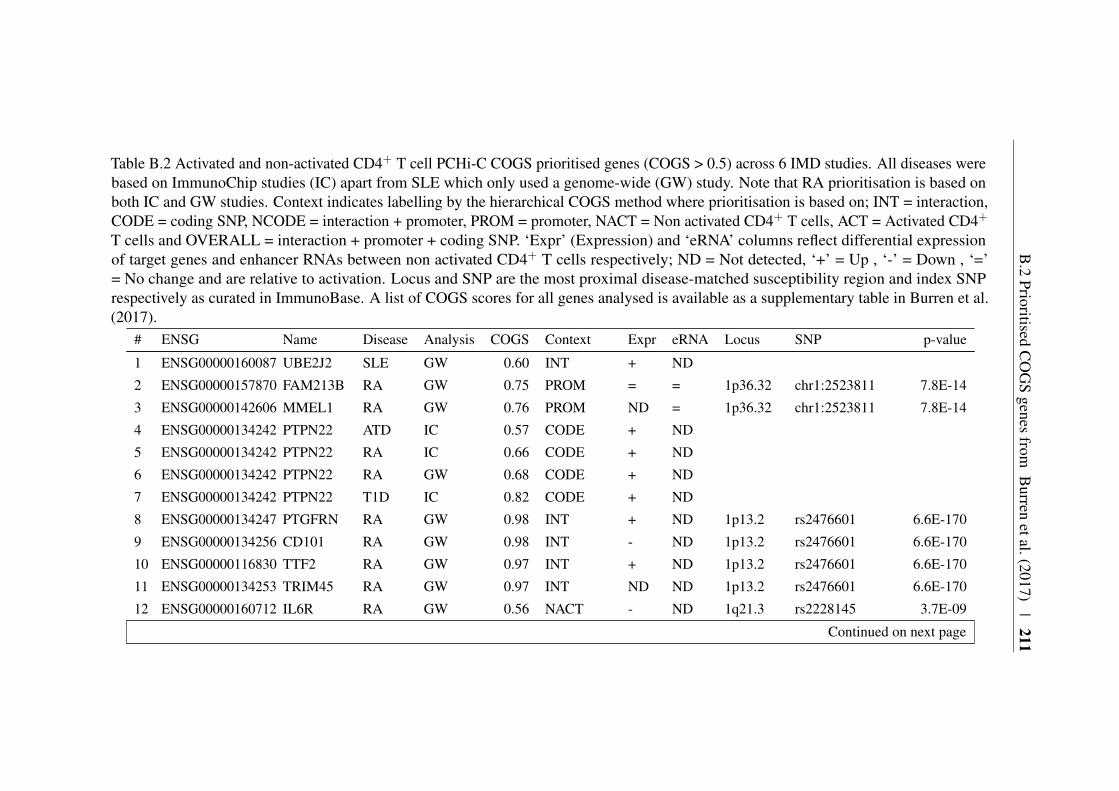
B.2
PrioritisedC
OG
Sgenes
fromB
urrenetal.(2017)
|211
Table B.2 Activated and non-activated CD4+ T cell PCHi-C COGS prioritised genes (COGS > 0.5) across 6 IMD studies. All diseases werebased on ImmunoChip studies (IC) apart from SLE which only used a genome-wide (GW) study. Note that RA prioritisation is based onboth IC and GW studies. Context indicates labelling by the hierarchical COGS method where prioritisation is based on; INT = interaction,CODE = coding SNP, NCODE = interaction + promoter, PROM = promoter, NACT = Non activated CD4+ T cells, ACT = Activated CD4+
T cells and OVERALL = interaction + promoter + coding SNP. ‘Expr’ (Expression) and ‘eRNA’ columns reflect differential expressionof target genes and enhancer RNAs between non activated CD4+ T cells respectively; ND = Not detected, ‘+’ = Up , ‘-’ = Down , ‘=’= No change and are relative to activation. Locus and SNP are the most proximal disease-matched susceptibility region and index SNPrespectively as curated in ImmunoBase. A list of COGS scores for all genes analysed is available as a supplementary table in Burren et al.(2017).
# ENSG Name Disease Analysis COGS Context Expr eRNA Locus SNP p-value
1 ENSG00000160087 UBE2J2 SLE GW 0.60 INT + ND
2 ENSG00000157870 FAM213B RA GW 0.75 PROM = = 1p36.32 chr1:2523811 7.8E-14
3 ENSG00000142606 MMEL1 RA GW 0.76 PROM ND = 1p36.32 chr1:2523811 7.8E-14
4 ENSG00000134242 PTPN22 ATD IC 0.57 CODE + ND
5 ENSG00000134242 PTPN22 RA IC 0.66 CODE + ND
6 ENSG00000134242 PTPN22 RA GW 0.68 CODE + ND
7 ENSG00000134242 PTPN22 T1D IC 0.82 CODE + ND
8 ENSG00000134247 PTGFRN RA GW 0.98 INT + ND 1p13.2 rs2476601 6.6E-170
9 ENSG00000134256 CD101 RA GW 0.98 INT - ND 1p13.2 rs2476601 6.6E-170
10 ENSG00000116830 TTF2 RA GW 0.97 INT + ND 1p13.2 rs2476601 6.6E-170
11 ENSG00000134253 TRIM45 RA GW 0.97 INT ND ND 1p13.2 rs2476601 6.6E-170
12 ENSG00000160712 IL6R RA GW 0.56 NACT - ND 1q21.3 rs2228145 3.7E-09
Continued on next page
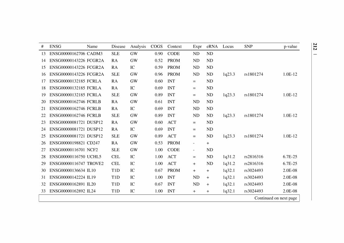
212|
# ENSG Name Disease Analysis COGS Context Expr eRNA Locus SNP p-value
13 ENSG00000162706 CADM3 SLE GW 0.90 CODE ND ND
14 ENSG00000143226 FCGR2A RA GW 0.52 PROM ND ND
15 ENSG00000143226 FCGR2A RA IC 0.59 PROM ND ND
16 ENSG00000143226 FCGR2A SLE GW 0.96 PROM ND ND 1q23.3 rs1801274 1.0E-12
17 ENSG00000132185 FCRLA RA GW 0.60 INT = ND
18 ENSG00000132185 FCRLA RA IC 0.69 INT = ND
19 ENSG00000132185 FCRLA SLE GW 0.89 INT = ND 1q23.3 rs1801274 1.0E-12
20 ENSG00000162746 FCRLB RA GW 0.61 INT ND ND
21 ENSG00000162746 FCRLB RA IC 0.69 INT ND ND
22 ENSG00000162746 FCRLB SLE GW 0.89 INT ND ND 1q23.3 rs1801274 1.0E-12
23 ENSG00000081721 DUSP12 RA GW 0.60 ACT = ND
24 ENSG00000081721 DUSP12 RA IC 0.69 INT = ND
25 ENSG00000081721 DUSP12 SLE GW 0.89 ACT = ND 1q23.3 rs1801274 1.0E-12
26 ENSG00000198821 CD247 RA GW 0.53 PROM - +
27 ENSG00000116701 NCF2 SLE GW 1.00 CODE - ND
28 ENSG00000116750 UCHL5 CEL IC 1.00 ACT = ND 1q31.2 rs2816316 6.7E-25
29 ENSG00000116747 TROVE2 CEL IC 1.00 ACT + ND 1q31.2 rs2816316 6.7E-25
30 ENSG00000136634 IL10 T1D IC 0.67 PROM + + 1q32.1 rs3024493 2.0E-08
31 ENSG00000142224 IL19 T1D IC 1.00 INT ND + 1q32.1 rs3024493 2.0E-08
32 ENSG00000162891 IL20 T1D IC 0.67 INT ND + 1q32.1 rs3024493 2.0E-08
33 ENSG00000162892 IL24 T1D IC 1.00 INT + + 1q32.1 rs3024493 2.0E-08
Continued on next page

B.2
PrioritisedC
OG
Sgenes
fromB
urrenetal.(2017)
|213
# ENSG Name Disease Analysis COGS Context Expr eRNA Locus SNP p-value
34 ENSG00000162894 FAIM3 T1D IC 1.00 INT - + 1q32.1 rs3024493 2.0E-08
35 ENSG00000162896 PIGR T1D IC 1.00 INT ND + 1q32.1 rs3024493 2.0E-08
36 ENSG00000162897 FCAMR T1D IC 0.67 INT ND + 1q32.1 rs3024493 2.0E-08
37 ENSG00000152518 ZFP36L2 CEL IC 0.82 INT - -
38 ENSG00000115421 PAPOLG CEL IC 1.00 INT = ND 2p16.1 rs13003464 4.3E-16
39 ENSG00000162924 REL RA IC 0.59 NCODE + ND 2p16.1 rs34695944 1.7E-15
40 ENSG00000162924 REL RA GW 0.93 NCODE + ND 2p16.1 rs34695944 1.7E-15
41 ENSG00000162924 REL CEL IC 1.00 INT + ND 2p16.1 rs13003464 4.3E-16
42 ENSG00000233404 FLJ20373 CEL IC 0.77 INT ND ND 2q12.1 rs990171 1.2E-16
43 ENSG00000115590 IL1R2 CEL IC 0.77 INT + ND 2q12.1 rs990171 1.2E-16
44 ENSG00000115598 IL1RL2 CEL IC 0.62 INT + ND 2q12.1 rs990171 1.2E-16
45 ENSG00000152127 MGAT5 SLE GW 0.99 INT + ND
46 ENSG00000115232 ITGA4 CEL IC 0.99 INT - ND 2q31.3 rs1018326 3.1E-16
47 ENSG00000151690 MFSD6 RA GW 0.86 INT = ND 2q32.3 rs13426947 7.2E-10
48 ENSG00000189362 TMEM194B RA GW 0.95 ACT + ND 2q32.3 rs13426947 7.2E-10
49 ENSG00000138386 NAB1 SLE GW 0.72 CODE + ND
50 ENSG00000138378 STAT4 RA GW 0.52 INT + ND 2q32.3 rs13426947 7.2E-10
51 ENSG00000138378 STAT4 RA IC 0.53 INT + ND 2q32.3 rs13426947 7.2E-10
52 ENSG00000138378 STAT4 CEL IC 0.99 INT + ND 2q32.3 rs6715106 8.4E-09
53 ENSG00000173559 NABP1 RA IC 0.58 INT + ND 2q32.3 rs13426947 7.2E-10
54 ENSG00000173559 NABP1 RA GW 0.60 INT + ND 2q32.3 rs13426947 7.2E-10
Continued on next page

214|
# ENSG Name Disease Analysis COGS Context Expr eRNA Locus SNP p-value
55 ENSG00000173559 NABP1 CEL IC 0.99 INT + ND 2q32.3 rs6715106 8.4E-09
56 ENSG00000119004 CYP20A1 T1D IC 0.66 INT + + 2q33.2 rs3087243 7.4E-21
57 ENSG00000173166 RAPH1 T1D IC 0.83 INT + + 2q33.2 rs3087243 7.4E-21
58 ENSG00000178562 CD28 T1D IC 0.81 INT = + 2q33.2 rs3087243 7.4E-21
59 ENSG00000187118 CMC1 RA GW 0.94 INT = ND 3p24.1 rs3806624 8.6E-09
60 ENSG00000163512 AZI2 RA GW 0.56 INT - ND 3p24.1 rs3806624 8.6E-09
61 ENSG00000206559 ZCWPW2 RA GW 0.56 INT ND ND 3p24.1 rs3806624 8.6E-09
62 ENSG00000136068 FLNB RA GW 0.50 NACT = ND 3p14.3 rs35677470 1.7E-07
63 ENSG00000163687 DNASE1L3 RA GW 0.65 CODE ND ND
64 ENSG00000163687 DNASE1L3 RA IC 0.82 CODE ND ND
65 ENSG00000114850 SSR3 RA GW 0.80 INT = ND
66 ENSG00000163659 TIPARP RA GW 0.78 INT - ND
67 ENSG00000197980 LEKR1 RA GW 0.75 INT = ND
68 ENSG00000213186 TRIM59 CEL IC 1.00 NACT = ND 3q25.33 rs1353248 9.8E-09
69 ENSG00000114209 PDCD10 SLE GW 0.54 INT = ND
70 ENSG00000163536 SERPINI1 SLE GW 0.54 INT - ND
71 ENSG00000145495 MARCH6 RA GW 0.61 INT = ND
72 ENSG00000145491 ROPN1L RA GW 0.83 INT ND ND
73 ENSG00000154122 ANKH RA GW 0.67 INT - ND
74 ENSG00000134352 IL6ST RA GW 1.00 INT + ND 5q11.2 rs7731626 7.3E-24
75 ENSG00000134352 IL6ST RA IC 1.00 INT + ND 5q11.2 rs6859219 4.0E-16
Continued on next page
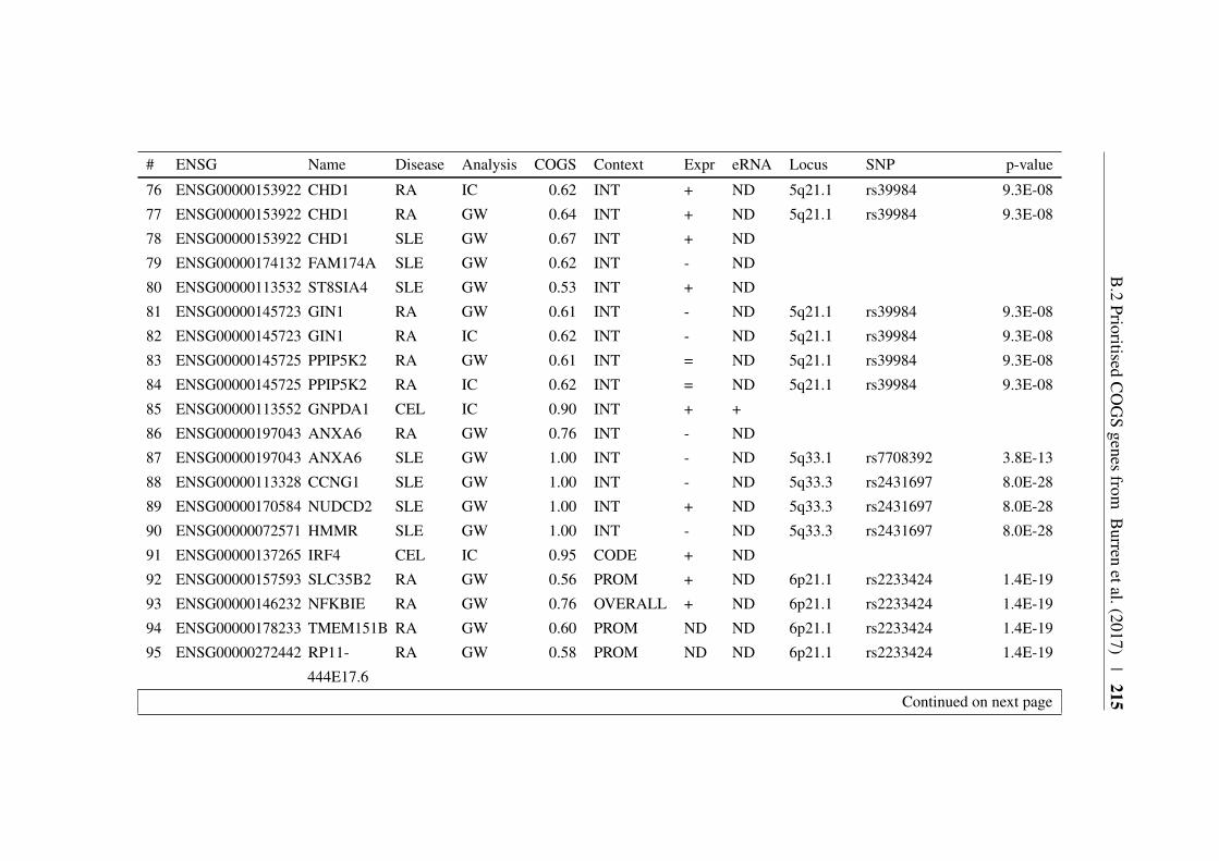
B.2
PrioritisedC
OG
Sgenes
fromB
urrenetal.(2017)
|215
# ENSG Name Disease Analysis COGS Context Expr eRNA Locus SNP p-value
76 ENSG00000153922 CHD1 RA IC 0.62 INT + ND 5q21.1 rs39984 9.3E-08
77 ENSG00000153922 CHD1 RA GW 0.64 INT + ND 5q21.1 rs39984 9.3E-08
78 ENSG00000153922 CHD1 SLE GW 0.67 INT + ND
79 ENSG00000174132 FAM174A SLE GW 0.62 INT - ND
80 ENSG00000113532 ST8SIA4 SLE GW 0.53 INT + ND
81 ENSG00000145723 GIN1 RA GW 0.61 INT - ND 5q21.1 rs39984 9.3E-08
82 ENSG00000145723 GIN1 RA IC 0.62 INT - ND 5q21.1 rs39984 9.3E-08
83 ENSG00000145725 PPIP5K2 RA GW 0.61 INT = ND 5q21.1 rs39984 9.3E-08
84 ENSG00000145725 PPIP5K2 RA IC 0.62 INT = ND 5q21.1 rs39984 9.3E-08
85 ENSG00000113552 GNPDA1 CEL IC 0.90 INT + +
86 ENSG00000197043 ANXA6 RA GW 0.76 INT - ND
87 ENSG00000197043 ANXA6 SLE GW 1.00 INT - ND 5q33.1 rs7708392 3.8E-13
88 ENSG00000113328 CCNG1 SLE GW 1.00 INT - ND 5q33.3 rs2431697 8.0E-28
89 ENSG00000170584 NUDCD2 SLE GW 1.00 INT + ND 5q33.3 rs2431697 8.0E-28
90 ENSG00000072571 HMMR SLE GW 1.00 INT - ND 5q33.3 rs2431697 8.0E-28
91 ENSG00000137265 IRF4 CEL IC 0.95 CODE + ND
92 ENSG00000157593 SLC35B2 RA GW 0.56 PROM + ND 6p21.1 rs2233424 1.4E-19
93 ENSG00000146232 NFKBIE RA GW 0.76 OVERALL + ND 6p21.1 rs2233424 1.4E-19
94 ENSG00000178233 TMEM151B RA GW 0.60 PROM ND ND 6p21.1 rs2233424 1.4E-19
95 ENSG00000272442 RP11-
444E17.6
RA GW 0.58 PROM ND ND 6p21.1 rs2233424 1.4E-19
Continued on next page
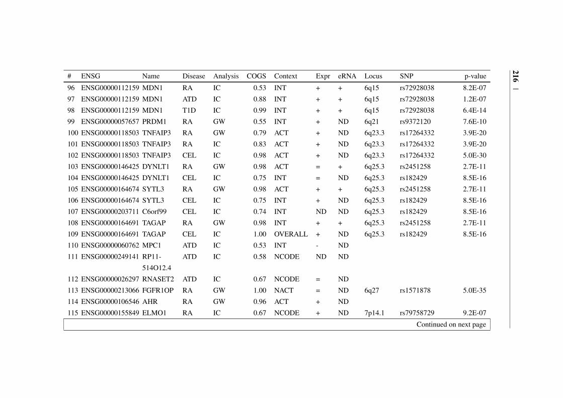
216|
# ENSG Name Disease Analysis COGS Context Expr eRNA Locus SNP p-value
96 ENSG00000112159 MDN1 RA IC 0.53 INT + + 6q15 rs72928038 8.2E-07
97 ENSG00000112159 MDN1 ATD IC 0.88 INT + + 6q15 rs72928038 1.2E-07
98 ENSG00000112159 MDN1 T1D IC 0.99 INT + + 6q15 rs72928038 6.4E-14
99 ENSG00000057657 PRDM1 RA GW 0.55 INT + ND 6q21 rs9372120 7.6E-10
100 ENSG00000118503 TNFAIP3 RA GW 0.79 ACT + ND 6q23.3 rs17264332 3.9E-20
101 ENSG00000118503 TNFAIP3 RA IC 0.83 ACT + ND 6q23.3 rs17264332 3.9E-20
102 ENSG00000118503 TNFAIP3 CEL IC 0.98 ACT + ND 6q23.3 rs17264332 5.0E-30
103 ENSG00000146425 DYNLT1 RA GW 0.98 ACT = + 6q25.3 rs2451258 2.7E-11
104 ENSG00000146425 DYNLT1 CEL IC 0.75 INT = ND 6q25.3 rs182429 8.5E-16
105 ENSG00000164674 SYTL3 RA GW 0.98 ACT + + 6q25.3 rs2451258 2.7E-11
106 ENSG00000164674 SYTL3 CEL IC 0.75 INT + ND 6q25.3 rs182429 8.5E-16
107 ENSG00000203711 C6orf99 CEL IC 0.74 INT ND ND 6q25.3 rs182429 8.5E-16
108 ENSG00000164691 TAGAP RA GW 0.98 INT + + 6q25.3 rs2451258 2.7E-11
109 ENSG00000164691 TAGAP CEL IC 1.00 OVERALL + ND 6q25.3 rs182429 8.5E-16
110 ENSG00000060762 MPC1 ATD IC 0.53 INT - ND
111 ENSG00000249141 RP11-
514O12.4
ATD IC 0.58 NCODE ND ND
112 ENSG00000026297 RNASET2 ATD IC 0.67 NCODE = ND
113 ENSG00000213066 FGFR1OP RA GW 1.00 NACT = ND 6q27 rs1571878 5.0E-35
114 ENSG00000106546 AHR RA GW 0.96 ACT + ND
115 ENSG00000155849 ELMO1 RA IC 0.67 NCODE + ND 7p14.1 rs79758729 9.2E-07
Continued on next page
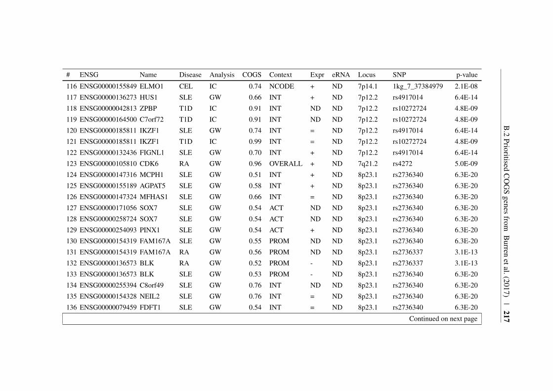
B.2
PrioritisedC
OG
Sgenes
fromB
urrenetal.(2017)
|217
# ENSG Name Disease Analysis COGS Context Expr eRNA Locus SNP p-value
116 ENSG00000155849 ELMO1 CEL IC 0.74 NCODE + ND 7p14.1 1kg_7_37384979 2.1E-08
117 ENSG00000136273 HUS1 SLE GW 0.66 INT + ND 7p12.2 rs4917014 6.4E-14
118 ENSG00000042813 ZPBP T1D IC 0.91 INT ND ND 7p12.2 rs10272724 4.8E-09
119 ENSG00000164500 C7orf72 T1D IC 0.91 INT ND ND 7p12.2 rs10272724 4.8E-09
120 ENSG00000185811 IKZF1 SLE GW 0.74 INT = ND 7p12.2 rs4917014 6.4E-14
121 ENSG00000185811 IKZF1 T1D IC 0.99 INT = ND 7p12.2 rs10272724 4.8E-09
122 ENSG00000132436 FIGNL1 SLE GW 0.70 INT + ND 7p12.2 rs4917014 6.4E-14
123 ENSG00000105810 CDK6 RA GW 0.96 OVERALL + ND 7q21.2 rs4272 5.0E-09
124 ENSG00000147316 MCPH1 SLE GW 0.51 INT + ND 8p23.1 rs2736340 6.3E-20
125 ENSG00000155189 AGPAT5 SLE GW 0.58 INT + ND 8p23.1 rs2736340 6.3E-20
126 ENSG00000147324 MFHAS1 SLE GW 0.66 INT = ND 8p23.1 rs2736340 6.3E-20
127 ENSG00000171056 SOX7 SLE GW 0.54 ACT ND ND 8p23.1 rs2736340 6.3E-20
128 ENSG00000258724 SOX7 SLE GW 0.54 ACT ND ND 8p23.1 rs2736340 6.3E-20
129 ENSG00000254093 PINX1 SLE GW 0.54 ACT + ND 8p23.1 rs2736340 6.3E-20
130 ENSG00000154319 FAM167A SLE GW 0.55 PROM ND ND 8p23.1 rs2736340 6.3E-20
131 ENSG00000154319 FAM167A RA GW 0.56 PROM ND ND 8p23.1 rs2736337 3.1E-13
132 ENSG00000136573 BLK RA GW 0.52 PROM - ND 8p23.1 rs2736337 3.1E-13
133 ENSG00000136573 BLK SLE GW 0.53 PROM - ND 8p23.1 rs2736340 6.3E-20
134 ENSG00000255394 C8orf49 SLE GW 0.76 INT ND ND 8p23.1 rs2736340 6.3E-20
135 ENSG00000154328 NEIL2 SLE GW 0.76 INT = ND 8p23.1 rs2736340 6.3E-20
136 ENSG00000079459 FDFT1 SLE GW 0.54 INT = ND 8p23.1 rs2736340 6.3E-20
Continued on next page

218|
# ENSG Name Disease Analysis COGS Context Expr eRNA Locus SNP p-value
137 ENSG00000255046 RP11-
297N6.4
SLE GW 0.54 INT = ND 8p23.1 rs2736340 6.3E-20
138 ENSG00000164733 CTSB SLE GW 0.54 INT - ND 8p23.1 rs2736340 6.3E-20
139 ENSG00000205883 DEFB135 SLE GW 0.57 NACT ND ND 8p23.1 rs2736340 6.3E-20
140 ENSG00000136997 MYC RA GW 0.70 INT + + 8q24.21 rs1516971 1.3E-10
141 ENSG00000095261 PSMD5 RA GW 0.73 INT = + 9q33.2 rs10985070 5.0E-11
142 ENSG00000056558 TRAF1 RA GW 0.89 NCODE + + 9q33.2 rs10985070 5.0E-11
143 ENSG00000119397 CNTRL RA GW 0.85 INT - + 9q33.2 rs10985070 5.0E-11
144 ENSG00000134460 IL2RA RA GW 1.00 PROM + + 10p15.1 rs706778 4.6E-14
145 ENSG00000134460 IL2RA RA IC 1.00 PROM + + 10p15.1 rs706778 4.6E-14
146 ENSG00000134460 IL2RA ATD IC 1.00 NCODE + + 10p15.1 rs706779 2.7E-07
147 ENSG00000134460 IL2RA T1D IC 1.00 NCODE + ND 10p15.1 rs41295121 4.9E-08
148 ENSG00000134453 RBM17 RA IC 0.67 ACT + + 10p15.1 rs706778 4.6E-14
149 ENSG00000134453 RBM17 RA GW 0.77 ACT + + 10p15.1 rs706778 4.6E-14
150 ENSG00000134453 RBM17 ATD IC 0.99 INT + + 10p15.1 rs706779 2.7E-07
151 ENSG00000134453 RBM17 T1D IC 1.00 NCODE + ND 10p15.1 rs41295121 4.9E-08
152 ENSG00000170525 PFKFB3 RA GW 0.65 NCODE + ND 10p15.1 rs10795791 3.0E-06
153 ENSG00000212743 DKFZP667-
F0711
RA GW 0.75 PROM = + 10p15.1 rs947474 4.1E-10
154 ENSG00000212743 DKFZP667-
F0711
CEL IC 0.76 OVERALL = + 10p15.1 rs2387397 1.9E-08
Continued on next page

B.2
PrioritisedC
OG
Sgenes
fromB
urrenetal.(2017)
|219
# ENSG Name Disease Analysis COGS Context Expr eRNA Locus SNP p-value
155 ENSG00000212743 DKFZP667-
F0711
T1D IC 0.86 NACT = ND 10p15.1 rs41295121 4.9E-08
156 ENSG00000065675 PRKCQ ATD IC 0.54 INT - + 10p15.1 rs706779 2.7E-07
157 ENSG00000107485 GATA3 RA GW 1.00 PROM = = 10p14 rs3824660 2.0E-08
158 ENSG00000107485 GATA3 SLE GW 0.68 INT = ND
159 ENSG00000128815 WDFY4 SLE GW 0.88 CODE = ND
160 ENSG00000150347 ARID5B RA GW 0.69 INT + + 10q21.2 rs12764378 4.5E-10
161 ENSG00000150347 ARID5B SLE GW 0.99 INT + + 10q21.2 rs4948496 1.0E-10
162 ENSG00000185507 IRF7 SLE GW 0.69 NCODE = ND 11p15.5 rs4963128 4.9E-09
163 ENSG00000099834 CDHR5 SLE GW 0.84 OVERALL ND ND 11p15.5 rs4963128 4.9E-09
164 ENSG00000185940 KRTAP5-
5
T1D IC 1.00 INT ND ND 11p15.5 rs72853903 6.2E-10
165 ENSG00000205864 KRTAP5-
6
T1D IC 1.00 INT ND ND 11p15.5 rs72853903 6.2E-10
166 ENSG00000129965 INS-IGF2 T1D IC 1.00 PROM ND ND 11p15.5 rs72853903 6.2E-10
167 ENSG00000254647 INS T1D IC 1.00 PROM ND ND 11p15.5 rs72853903 6.2E-10
168 ENSG00000180176 TH T1D IC 1.00 PROM ND ND 11p15.5 rs72853903 6.2E-10
169 ENSG00000184281 TSSC4 T1D IC 1.00 INT + ND 11p15.5 rs72853903 6.2E-10
170 ENSG00000026508 CD44 SLE GW 0.83 INT + + 11p13 rs2732549 1.2E-23
171 ENSG00000135362 PRR5L RA GW 0.68 INT = ND
172 ENSG00000178105 DDX10 RA GW 0.71 ACT + ND 11q22.3 chr11:107967350 1.4E-08
Continued on next page
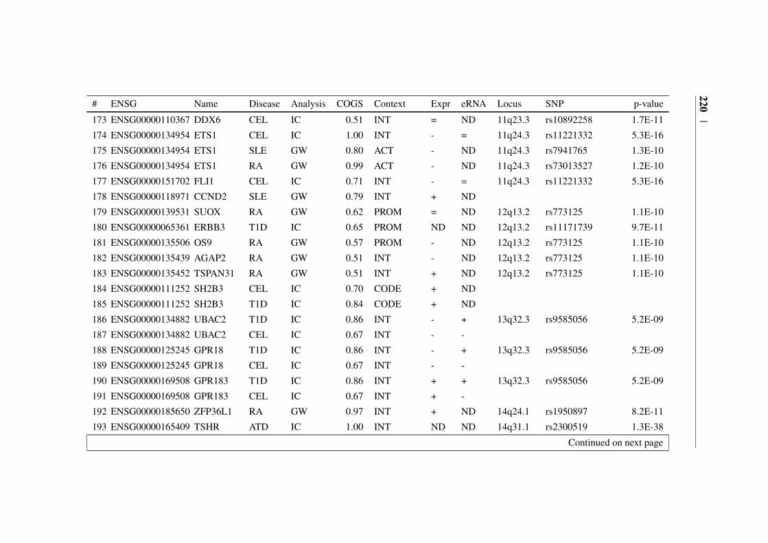
220|
# ENSG Name Disease Analysis COGS Context Expr eRNA Locus SNP p-value
173 ENSG00000110367 DDX6 CEL IC 0.51 INT = ND 11q23.3 rs10892258 1.7E-11
174 ENSG00000134954 ETS1 CEL IC 1.00 INT - = 11q24.3 rs11221332 5.3E-16
175 ENSG00000134954 ETS1 SLE GW 0.80 ACT - ND 11q24.3 rs7941765 1.3E-10
176 ENSG00000134954 ETS1 RA GW 0.99 ACT - ND 11q24.3 rs73013527 1.2E-10
177 ENSG00000151702 FLI1 CEL IC 0.71 INT - = 11q24.3 rs11221332 5.3E-16
178 ENSG00000118971 CCND2 SLE GW 0.79 INT + ND
179 ENSG00000139531 SUOX RA GW 0.62 PROM = ND 12q13.2 rs773125 1.1E-10
180 ENSG00000065361 ERBB3 T1D IC 0.65 PROM ND ND 12q13.2 rs11171739 9.7E-11
181 ENSG00000135506 OS9 RA GW 0.57 PROM - ND 12q13.2 rs773125 1.1E-10
182 ENSG00000135439 AGAP2 RA GW 0.51 INT - ND 12q13.2 rs773125 1.1E-10
183 ENSG00000135452 TSPAN31 RA GW 0.51 INT + ND 12q13.2 rs773125 1.1E-10
184 ENSG00000111252 SH2B3 CEL IC 0.70 CODE + ND
185 ENSG00000111252 SH2B3 T1D IC 0.84 CODE + ND
186 ENSG00000134882 UBAC2 T1D IC 0.86 INT - + 13q32.3 rs9585056 5.2E-09
187 ENSG00000134882 UBAC2 CEL IC 0.67 INT - -
188 ENSG00000125245 GPR18 T1D IC 0.86 INT - + 13q32.3 rs9585056 5.2E-09
189 ENSG00000125245 GPR18 CEL IC 0.67 INT - -
190 ENSG00000169508 GPR183 T1D IC 0.86 INT + + 13q32.3 rs9585056 5.2E-09
191 ENSG00000169508 GPR183 CEL IC 0.67 INT + -
192 ENSG00000185650 ZFP36L1 RA GW 0.97 INT + ND 14q24.1 rs1950897 8.2E-11
193 ENSG00000165409 TSHR ATD IC 1.00 INT ND ND 14q31.1 rs2300519 1.3E-38
Continued on next page
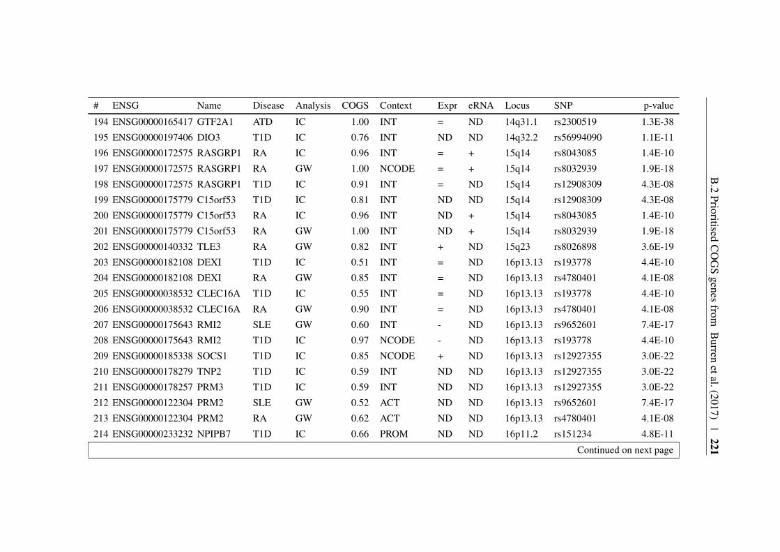
B.2
PrioritisedC
OG
Sgenes
fromB
urrenetal.(2017)
|221
# ENSG Name Disease Analysis COGS Context Expr eRNA Locus SNP p-value
194 ENSG00000165417 GTF2A1 ATD IC 1.00 INT = ND 14q31.1 rs2300519 1.3E-38
195 ENSG00000197406 DIO3 T1D IC 0.76 INT ND ND 14q32.2 rs56994090 1.1E-11
196 ENSG00000172575 RASGRP1 RA IC 0.96 INT = + 15q14 rs8043085 1.4E-10
197 ENSG00000172575 RASGRP1 RA GW 1.00 NCODE = + 15q14 rs8032939 1.9E-18
198 ENSG00000172575 RASGRP1 T1D IC 0.91 INT = ND 15q14 rs12908309 4.3E-08
199 ENSG00000175779 C15orf53 T1D IC 0.81 INT ND ND 15q14 rs12908309 4.3E-08
200 ENSG00000175779 C15orf53 RA IC 0.96 INT ND + 15q14 rs8043085 1.4E-10
201 ENSG00000175779 C15orf53 RA GW 1.00 INT ND + 15q14 rs8032939 1.9E-18
202 ENSG00000140332 TLE3 RA GW 0.82 INT + ND 15q23 rs8026898 3.6E-19
203 ENSG00000182108 DEXI T1D IC 0.51 INT = ND 16p13.13 rs193778 4.4E-10
204 ENSG00000182108 DEXI RA GW 0.85 INT = ND 16p13.13 rs4780401 4.1E-08
205 ENSG00000038532 CLEC16A T1D IC 0.55 INT = ND 16p13.13 rs193778 4.4E-10
206 ENSG00000038532 CLEC16A RA GW 0.90 INT = ND 16p13.13 rs4780401 4.1E-08
207 ENSG00000175643 RMI2 SLE GW 0.60 INT - ND 16p13.13 rs9652601 7.4E-17
208 ENSG00000175643 RMI2 T1D IC 0.97 NCODE - ND 16p13.13 rs193778 4.4E-10
209 ENSG00000185338 SOCS1 T1D IC 0.85 NCODE + ND 16p13.13 rs12927355 3.0E-22
210 ENSG00000178279 TNP2 T1D IC 0.59 INT ND ND 16p13.13 rs12927355 3.0E-22
211 ENSG00000178257 PRM3 T1D IC 0.59 INT ND ND 16p13.13 rs12927355 3.0E-22
212 ENSG00000122304 PRM2 SLE GW 0.52 ACT ND ND 16p13.13 rs9652601 7.4E-17
213 ENSG00000122304 PRM2 RA GW 0.62 ACT ND ND 16p13.13 rs4780401 4.1E-08
214 ENSG00000233232 NPIPB7 T1D IC 0.66 PROM ND ND 16p11.2 rs151234 4.8E-11
Continued on next page

222|
# ENSG Name Disease Analysis COGS Context Expr eRNA Locus SNP p-value
215 ENSG00000261832 CLN3 T1D IC 0.66 PROM ND ND 16p11.2 rs151234 4.8E-11
216 ENSG00000188603 CLN3 T1D IC 0.66 PROM - ND 16p11.2 rs151234 4.8E-11
217 ENSG00000184730 APOBR T1D IC 0.99 OVERALL - ND 16p11.2 rs151234 4.8E-11
218 ENSG00000176046 NUPR1 T1D IC 0.66 NACT ND ND 16p11.2 rs151234 4.8E-11
219 ENSG00000157423 HYDIN SLE GW 0.64 INT ND ND
220 ENSG00000103091 WDR59 T1D IC 0.95 INT = ND 16q23.1 rs8056814 3.0E-19
221 ENSG00000186187 ZNRF1 T1D IC 0.95 INT + ND 16q23.1 rs8056814 3.0E-19
222 ENSG00000168928 CTRB2 T1D IC 1.00 PROM ND ND 16q23.1 rs8056814 3.0E-19
223 ENSG00000168925 CTRB1 T1D IC 1.00 PROM ND ND 16q23.1 rs8056814 3.0E-19
224 ENSG00000131148 EMC8 SLE GW 0.97 ACT + ND 16q24.1 rs11644034 9.6E-18
225 ENSG00000131148 EMC8 RA GW 1.00 ACT + ND 16q24.1 rs13330176 1.4E-12
226 ENSG00000131143 COX4I1 SLE GW 0.97 ACT = ND 16q24.1 rs11644034 9.6E-18
227 ENSG00000131143 COX4I1 RA GW 1.00 ACT = ND 16q24.1 rs13330176 1.4E-12
228 ENSG00000140968 IRF8 SLE GW 0.99 ACT + ND 16q24.1 rs11644034 9.6E-18
229 ENSG00000140968 IRF8 RA GW 1.00 ACT + ND 16q24.1 rs13330176 1.4E-12
230 ENSG00000174327 SLC16A13 SLE GW 0.98 ACT ND ND 17p13.2 rs2286672 2.9E-09
231 ENSG00000132522 GPS2 SLE GW 0.98 ACT = ND 17p13.2 rs2286672 2.9E-09
232 ENSG00000261915 RP11-
542C16.2
SLE GW 0.98 ACT ND ND 17p13.2 rs2286672 2.9E-09
233 ENSG00000215041 NEURL4 SLE GW 0.99 PROM = ND 17p13.2 rs2286672 2.9E-09
234 ENSG00000072818 ACAP1 SLE GW 0.99 PROM - ND 17p13.2 rs2286672 2.9E-09
Continued on next page

B.2
PrioritisedC
OG
Sgenes
fromB
urrenetal.(2017)
|223
# ENSG Name Disease Analysis COGS Context Expr eRNA Locus SNP p-value
235 ENSG00000170175 CHRNB1 SLE GW 0.97 ACT - ND 17p13.2 rs2286672 2.9E-09
236 ENSG00000174282 ZBTB4 SLE GW 0.98 INT - ND 17p13.2 rs2286672 2.9E-09
237 ENSG00000259224 SLC35G6 SLE GW 0.98 INT ND ND 17p13.2 rs2286672 2.9E-09
238 ENSG00000181222 POLR2A SLE GW 0.98 INT = ND 17p13.2 rs2286672 2.9E-09
239 ENSG00000239697 TNFSF12 SLE GW 0.98 INT = ND 17p13.2 rs2286672 2.9E-09
240 ENSG00000248871 TNFSF12-
TNFSF13
SLE GW 0.98 INT ND ND 17p13.2 rs2286672 2.9E-09
241 ENSG00000161955 TNFSF13 SLE GW 0.98 INT ND ND 17p13.2 rs2286672 2.9E-09
242 ENSG00000161956 SENP3 SLE GW 0.98 INT + ND 17p13.2 rs2286672 2.9E-09
243 ENSG00000161960 EIF4A1 SLE GW 0.99 INT + ND 17p13.2 rs2286672 2.9E-09
244 ENSG00000129226 CD68 SLE GW 0.99 INT ND ND 17p13.2 rs2286672 2.9E-09
245 ENSG00000129255 MPDU1 SLE GW 0.99 INT + ND 17p13.2 rs2286672 2.9E-09
246 ENSG00000129194 SOX15 SLE GW 0.99 INT ND ND 17p13.2 rs2286672 2.9E-09
247 ENSG00000129245 FXR2 SLE GW 0.98 ACT = ND 17p13.2 rs2286672 2.9E-09
248 ENSG00000268503 AC007421.1 SLE GW 0.98 ACT ND ND 17p13.2 rs2286672 2.9E-09
249 ENSG00000129214 SHBG SLE GW 0.98 ACT ND ND 17p13.2 rs2286672 2.9E-09
250 ENSG00000141510 TP53 SLE GW 0.98 ACT = ND 17p13.2 rs2286672 2.9E-09
251 ENSG00000141499 WRAP53 SLE GW 0.98 INT - ND 17p13.2 rs2286672 2.9E-09
252 ENSG00000179148 ALOXE3 SLE GW 0.98 INT ND ND 17p13.2 rs2286672 2.9E-09
253 ENSG00000179094 PER1 SLE GW 0.97 ACT = ND 17p13.2 rs2286672 2.9E-09
254 ENSG00000161405 IKZF3 RA IC 0.55 PROM + ND 17q12 chr17:38031857 2.3E-12
Continued on next page

224|
# ENSG Name Disease Analysis COGS Context Expr eRNA Locus SNP p-value
255 ENSG00000161405 IKZF3 RA GW 0.66 PROM + ND 17q12 chr17:38031857 2.3E-12
256 ENSG00000186075 ZPBP2 T1D IC 0.51 PROM ND ND 17q12 rs12453507 1.0E-08
257 ENSG00000186075 ZPBP2 RA IC 0.60 PROM ND ND 17q12 chr17:38031857 2.3E-12
258 ENSG00000186075 ZPBP2 RA GW 0.71 PROM ND ND 17q12 chr17:38031857 2.3E-12
259 ENSG00000120068 HOXB8 SLE GW 0.54 INT ND ND
260 ENSG00000170689 HOXB9 SLE GW 0.52 INT ND ND
261 ENSG00000184557 SOCS3 RA GW 0.58 PROM + ND
262 ENSG00000087157 PGS1 RA GW 0.55 PROM = ND
263 ENSG00000175354 PTPN2 RA GW 0.73 ACT + ND 18p11.21 rs8083786 6.3E-18
264 ENSG00000175354 PTPN2 T1D IC 0.91 ACT + ND 18p11.21 rs1893217 1.2E-15
265 ENSG00000099625 C19orf26 SLE GW 0.59 INT ND ND
266 ENSG00000099624 ATP5D SLE GW 0.59 INT = ND
267 ENSG00000167470 MIDN SLE GW 0.59 INT + ND
268 ENSG00000099622 CIRBP SLE GW 0.59 INT = ND
269 ENSG00000267303 CTD-
2369P2.12
RA GW 0.58 CODE ND ND
270 ENSG00000161847 RAVER1 RA GW 0.58 CODE = ND
271 ENSG00000105397 TYK2 RA IC 1.00 CODE = ND
272 ENSG00000105397 TYK2 T1D IC 1.00 CODE = ND
273 ENSG00000105401 CDC37 RA GW 0.96 INT + ND 19p13.2 chr19:10771941 8.6E-10
274 ENSG00000180739 S1PR5 RA GW 0.96 INT - ND 19p13.2 chr19:10771941 8.6E-10
Continued on next page
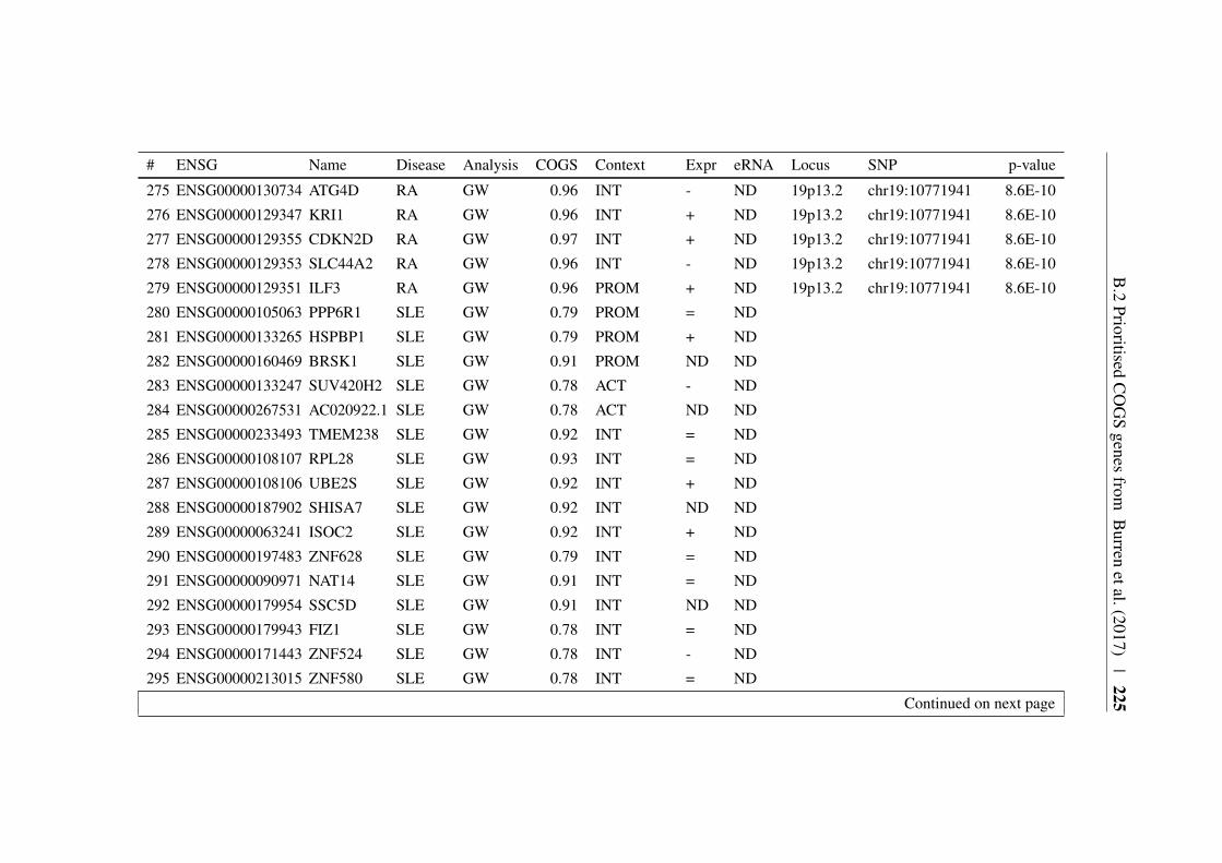
B.2
PrioritisedC
OG
Sgenes
fromB
urrenetal.(2017)
|225
# ENSG Name Disease Analysis COGS Context Expr eRNA Locus SNP p-value
275 ENSG00000130734 ATG4D RA GW 0.96 INT - ND 19p13.2 chr19:10771941 8.6E-10
276 ENSG00000129347 KRI1 RA GW 0.96 INT + ND 19p13.2 chr19:10771941 8.6E-10
277 ENSG00000129355 CDKN2D RA GW 0.97 INT + ND 19p13.2 chr19:10771941 8.6E-10
278 ENSG00000129353 SLC44A2 RA GW 0.96 INT - ND 19p13.2 chr19:10771941 8.6E-10
279 ENSG00000129351 ILF3 RA GW 0.96 PROM + ND 19p13.2 chr19:10771941 8.6E-10
280 ENSG00000105063 PPP6R1 SLE GW 0.79 PROM = ND
281 ENSG00000133265 HSPBP1 SLE GW 0.79 PROM + ND
282 ENSG00000160469 BRSK1 SLE GW 0.91 PROM ND ND
283 ENSG00000133247 SUV420H2 SLE GW 0.78 ACT - ND
284 ENSG00000267531 AC020922.1 SLE GW 0.78 ACT ND ND
285 ENSG00000233493 TMEM238 SLE GW 0.92 INT = ND
286 ENSG00000108107 RPL28 SLE GW 0.93 INT = ND
287 ENSG00000108106 UBE2S SLE GW 0.92 INT + ND
288 ENSG00000187902 SHISA7 SLE GW 0.92 INT ND ND
289 ENSG00000063241 ISOC2 SLE GW 0.92 INT + ND
290 ENSG00000197483 ZNF628 SLE GW 0.79 INT = ND
291 ENSG00000090971 NAT14 SLE GW 0.91 INT = ND
292 ENSG00000179954 SSC5D SLE GW 0.91 INT ND ND
293 ENSG00000179943 FIZ1 SLE GW 0.78 INT = ND
294 ENSG00000171443 ZNF524 SLE GW 0.78 INT - ND
295 ENSG00000213015 ZNF580 SLE GW 0.78 INT = ND
Continued on next page

226|
# ENSG Name Disease Analysis COGS Context Expr eRNA Locus SNP p-value
296 ENSG00000171425 ZNF581 SLE GW 0.78 INT = ND
297 ENSG00000173581 CCDC106 SLE GW 0.81 INT ND ND
298 ENSG00000175063 UBE2C CEL IC 0.54 INT - ND
299 ENSG00000101470 TNNC2 CEL IC 0.54 INT ND ND
300 ENSG00000124104 SNX21 CEL IC 0.54 INT = ND
301 ENSG00000198026 ZNF335 CEL IC 0.92 PROM = ND
302 ENSG00000062598 ELMO2 CEL IC 0.54 INT = ND
303 ENSG00000159110 IFNAR2 RA GW 0.84 INT - ND 21q22.12 rs2834512 2.1E-08
304 ENSG00000100099 HPS4 SLE GW 0.66 INT - ND
305 ENSG00000100104 SRRD SLE GW 0.66 INT + ND
306 ENSG00000100109 TFIP11 SLE GW 0.65 INT + ND
307 ENSG00000187045 TMPRSS6 CEL IC 0.55 INT ND =
308 ENSG00000187045 TMPRSS6 RA IC 0.64 ACT ND ND 22q13.1 rs909685 1.4E-16
309 ENSG00000187045 TMPRSS6 T1D IC 0.86 INT ND ND 22q12.3 rs229533 1.8E-08
310 ENSG00000100385 IL2RB CEL IC 0.55 INT + =
311 ENSG00000133466 C1QTNF6 T1D IC 0.69 PROM = ND 22q12.3 rs229533 1.8E-08
312 ENSG00000166897 ELFN2 CEL IC 0.55 INT - =
313 ENSG00000100060 MFNG CEL IC 0.55 INT - =
314 ENSG00000100321 SYNGR1 RA GW 0.69 PROM ND ND 22q13.1 rs909685 1.4E-16
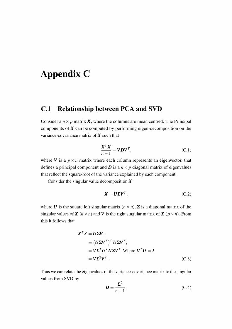
Appendix C
C.1 Relationship between PCA and SVD
Consider a n× p matrix XXX , where the columns are mean centred. The Principalcomponents of XXX can be computed by performing eigen-decomposition on thevariance-covariance matrix of XXX such that
XXXT XXXn−1
=VVV DDDVVV T , (C.1)
where VVV is a p× n matrix where each column represents an eigenvector, thatdefines a principal component and DDD is a n× p diagonal matrix of eigenvaluesthat reflect the square-root of the variance explained by each component.
Consider the singular value decomposition XXX
XXX =UUUΣΣΣVVV T , (C.2)
where UUU is the square left singular matrix (n×n), ΣΣΣ is a diagonal matrix of thesingular values of XXX (n×n) and VVV is the right singular matrix of XXX (p×n). Fromthis it follows that
XXXT X =UUUΣΣΣVVV ,
=(UUUΣΣΣVVV T)T
UUUΣΣΣVVV T ,
=VVV ΣΣΣTUUUTUUUΣΣΣVVV T ,Where UUUTUUU = III
=VVV ΣΣΣ2VVV T . (C.3)
Thus we can relate the eigenvalues of the variance-covariance matrix to the singularvalues from SVD by
DDD =ΣΣΣ
2
n−1, (C.4)

228 |
where principal components are given by XXXVVV =UUUΣΣΣVVV TVVV =UUUΣΣΣ as VVV TVVV = III.

C.2 IMD basis projection forest plots | 229
C.2 IMD basis projection forest plots
Forest plots showing the context of JIA subtype projections for all PCs. Colouredpoints indicate the difference in trait scores with synthetic control, marked witha red dotted line. Error bars indicate 95% confidence intervals. For clarity basistrait PC scores (purple) have been merged with overlapping UKBB traits. Whilstnon-basis UKBB traits have been filtered to show only those that are significantlydifferent from control at FDR < 5%, other traits are included regardless, these areshown with dashed error bars. UKBB SRD, UKBB SRM and UKB SRC labelsin the legend correspond to UK Biobank self-reported disease, medication andcancer categories respectively.
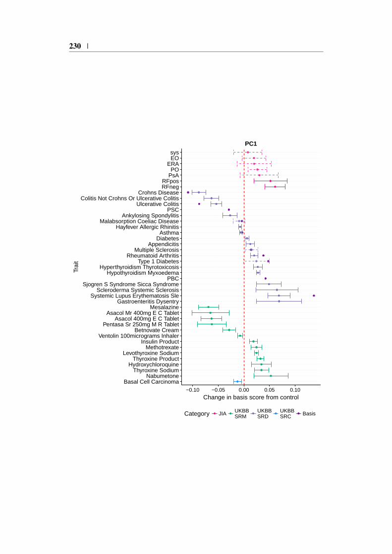
230 |
Basal Cell CarcinomaNabumetone
Thyroxine SodiumHydroxychloroquine
Thyroxine ProductLevothyroxine Sodium
MethotrexateInsulin Product
Ventolin 100micrograms InhalerBetnovate Cream
Pentasa Sr 250mg M R TabletAsacol 400mg E C Tablet
Asacol Mr 400mg E C TabletMesalazine
Gastroenteritis DysentrySystemic Lupus Erythematosis Sle
Scleroderma Systemic SclerosisSjogren S Syndrome Sicca Syndrome
PBCHypothyroidism Myxoedema
Hyperthyroidism ThyrotoxicosisType 1 Diabetes
Rheumatoid ArthritisMultiple Sclerosis
AppendicitisDiabetes
AsthmaHayfever Allergic Rhinitis
Malabsorption Coeliac DiseaseAnkylosing Spondylitis
PSCUlcerative Colitis
Colitis Not Crohns Or Ulcerative ColitisCrohns Disease
RFnegRFpos
PsAPO
ERAEOsys
−0.10 −0.05 0.00 0.05 0.10
Change in basis score from control
Trai
t
Category JIA UKBBSRM
UKBBSRD
UKBBSRC Basis
PC1
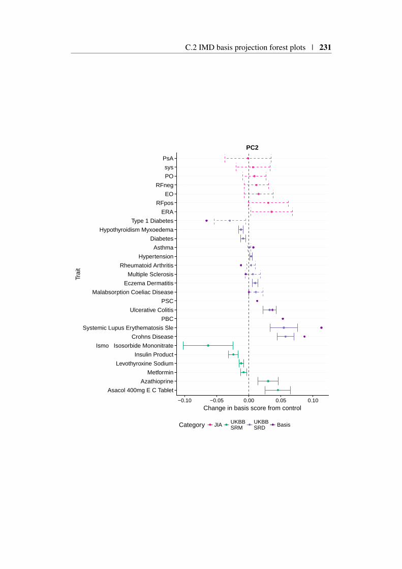
C.2 IMD basis projection forest plots | 231
Asacol 400mg E C Tablet
Azathioprine
Metformin
Levothyroxine Sodium
Insulin Product
Ismo Isosorbide Mononitrate
Crohns Disease
Systemic Lupus Erythematosis Sle
PBC
Ulcerative Colitis
PSC
Malabsorption Coeliac Disease
Eczema Dermatitis
Multiple Sclerosis
Rheumatoid Arthritis
Hypertension
Asthma
Diabetes
Hypothyroidism Myxoedema
Type 1 Diabetes
ERA
RFpos
EO
RFneg
PO
sys
PsA
−0.10 −0.05 0.00 0.05 0.10
Change in basis score from control
Trai
t
Category JIA UKBBSRM
UKBBSRD Basis
PC2
232 |
BimatoprostFybogel Orange S F Granules
Vitamin C ProductPrednisolone
LoperamideFolic Acid Product
Vitamin B12 PreparationSimvador 10mg Tablet
AzathioprineAsacol 400mg E C Tablet
Thyroxine ProductMesalazine
MethotrexateInsulin Product
Levothyroxine SodiumThyroxine SodiumMultiple Sclerosis
AsthmaPSC
Rheumatoid ArthritisDiabetic Eye Disease
Systemic Lupus Erythematosis SleSarcoidosis
Ulcerative ColitisHyperthyroidism Thyrotoxicosis
Colitis Not Crohns Or Ulcerative ColitisPBC
Malabsorption Coeliac DiseasePernicious Anaemia
Hypothyroidism MyxoedemaCrohns DiseaseType 1 Diabetes
sysERA
POEO
RFnegRFpos
PsA
−0.10 −0.05 0.00 0.05
Change in basis score from control
Trai
t
Category JIA UKBBSRM
UKBBSRD Basis
PC3
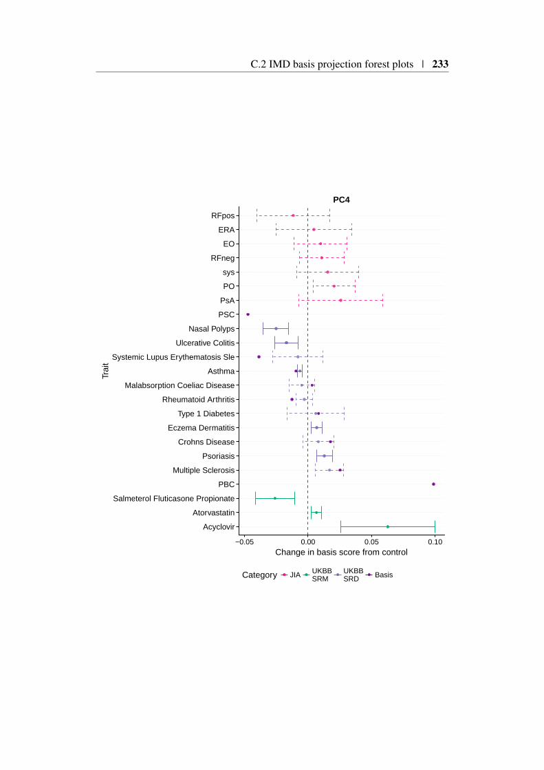
C.2 IMD basis projection forest plots | 233
Acyclovir
Atorvastatin
Salmeterol Fluticasone Propionate
PBC
Multiple Sclerosis
Psoriasis
Crohns Disease
Eczema Dermatitis
Type 1 Diabetes
Rheumatoid Arthritis
Malabsorption Coeliac Disease
Asthma
Systemic Lupus Erythematosis Sle
Ulcerative Colitis
Nasal Polyps
PSC
PsA
PO
sys
RFneg
EO
ERA
RFpos
−0.05 0.00 0.05 0.10
Change in basis score from control
Trai
t
Category JIA UKBBSRM
UKBBSRD Basis
PC4
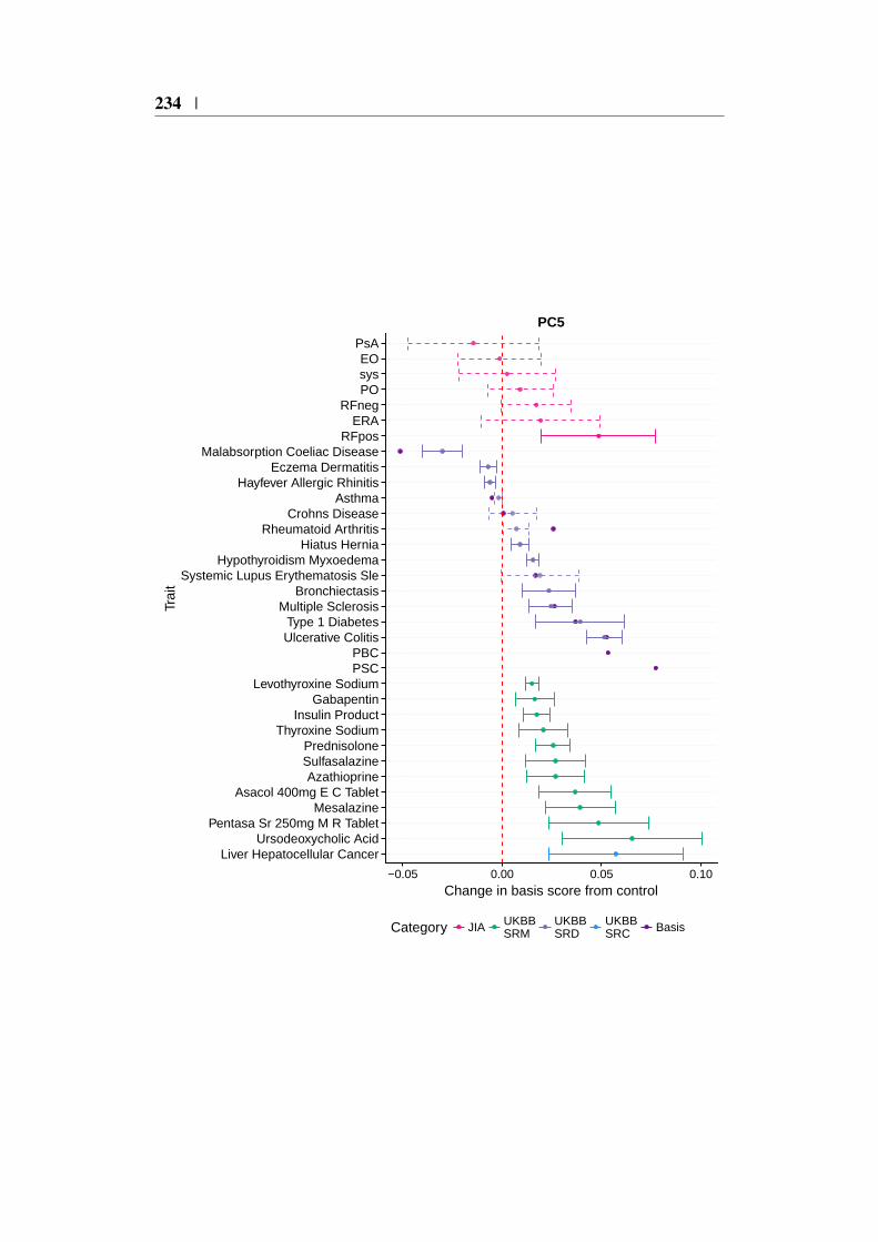
234 |
Liver Hepatocellular CancerUrsodeoxycholic Acid
Pentasa Sr 250mg M R TabletMesalazine
Asacol 400mg E C TabletAzathioprine
SulfasalazinePrednisolone
Thyroxine SodiumInsulin Product
GabapentinLevothyroxine Sodium
PSCPBC
Ulcerative ColitisType 1 Diabetes
Multiple SclerosisBronchiectasis
Systemic Lupus Erythematosis SleHypothyroidism Myxoedema
Hiatus HerniaRheumatoid Arthritis
Crohns DiseaseAsthma
Hayfever Allergic RhinitisEczema Dermatitis
Malabsorption Coeliac DiseaseRFpos
ERARFneg
POsysEO
PsA
−0.05 0.00 0.05 0.10
Change in basis score from control
Trai
t
Category JIA UKBBSRM
UKBBSRD
UKBBSRC Basis
PC5

C.2 IMD basis projection forest plots | 235
Malignant MelanomaBasal Cell CarcinomaLevothyroxine Sodium
Thyroxine ProductAlendronate Sodium
SimvastatinVentolin 100micrograms Inhaler
Becotide 50 InhalerBudesonide
Co ProxamolClonazepam
Beclomist 50micrograms Nasal SprayPSC
Malabsorption Coeliac DiseasePBC
SarcoidosisHypothyroidism Myxoedema
PsoriasisUlcerative Colitis
Deep Venous Thrombosis DvtSystemic Lupus Erythematosis Sle
High CholesterolMultiple Sclerosis
Rheumatoid ArthritisType 1 Diabetes
Hayfever Allergic RhinitisAsthma
Crohns DiseaseInsomnia
EOPsA
RFnegsysPO
RFposERA
−0.10 −0.05 0.00 0.05
Change in basis score from control
Trai
t
Category JIA UKBBSRM
UKBBSRD
UKBBSRC Basis
PC6

236 |
Folic Acid Product
Methotrexate
Multiple Sclerosis
PSC
Systemic Lupus Erythematosis Sle
Crohns Disease
Ulcerative Colitis
Type 1 Diabetes
Malabsorption Coeliac Disease
Asthma
PBC
Rheumatoid Arthritis
ERA
sys
PO
RFneg
PsA
EO
RFpos
−0.050 −0.025 0.000 0.025 0.050
Change in basis score from control
Trai
t
Category JIA UKBBSRM
UKBBSRD Basis
PC7
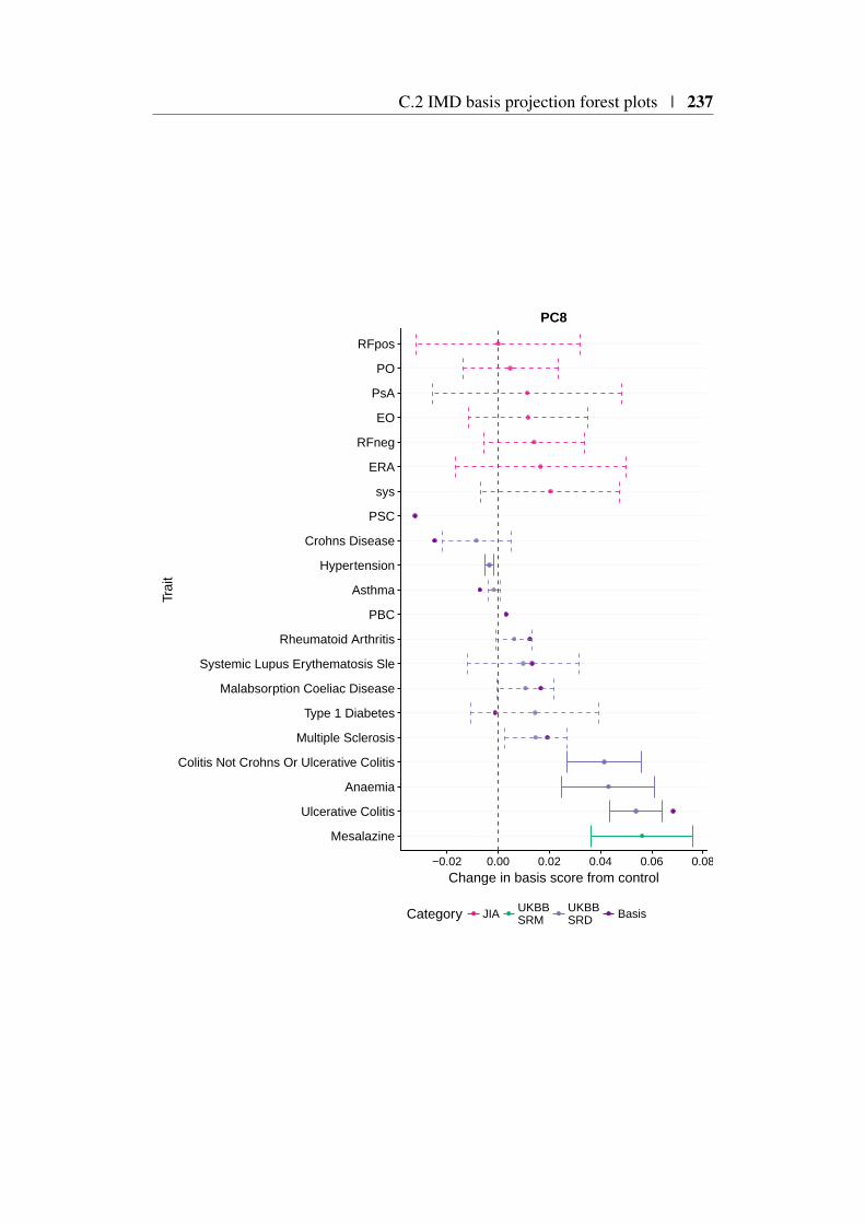
C.2 IMD basis projection forest plots | 237
Mesalazine
Ulcerative Colitis
Anaemia
Colitis Not Crohns Or Ulcerative Colitis
Multiple Sclerosis
Type 1 Diabetes
Malabsorption Coeliac Disease
Systemic Lupus Erythematosis Sle
Rheumatoid Arthritis
PBC
Asthma
Hypertension
Crohns Disease
PSC
sys
ERA
RFneg
EO
PsA
PO
RFpos
−0.02 0.00 0.02 0.04 0.06 0.08
Change in basis score from control
Trai
t
Category JIA UKBBSRM
UKBBSRD Basis
PC8
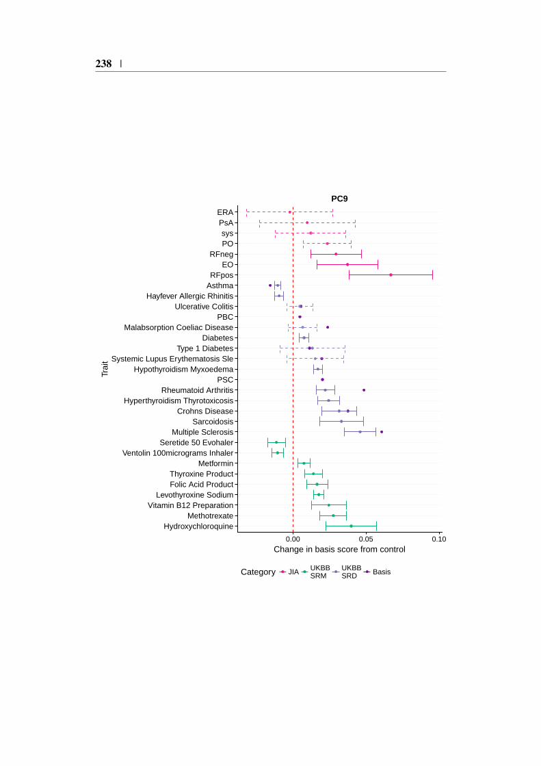
238 |
HydroxychloroquineMethotrexate
Vitamin B12 PreparationLevothyroxine Sodium
Folic Acid ProductThyroxine Product
MetforminVentolin 100micrograms Inhaler
Seretide 50 EvohalerMultiple Sclerosis
SarcoidosisCrohns Disease
Hyperthyroidism ThyrotoxicosisRheumatoid Arthritis
PSCHypothyroidism Myxoedema
Systemic Lupus Erythematosis SleType 1 Diabetes
DiabetesMalabsorption Coeliac Disease
PBCUlcerative Colitis
Hayfever Allergic RhinitisAsthmaRFpos
EORFneg
POsys
PsAERA
0.00 0.05 0.10
Change in basis score from control
Trai
t
Category JIA UKBBSRM
UKBBSRD Basis
PC9
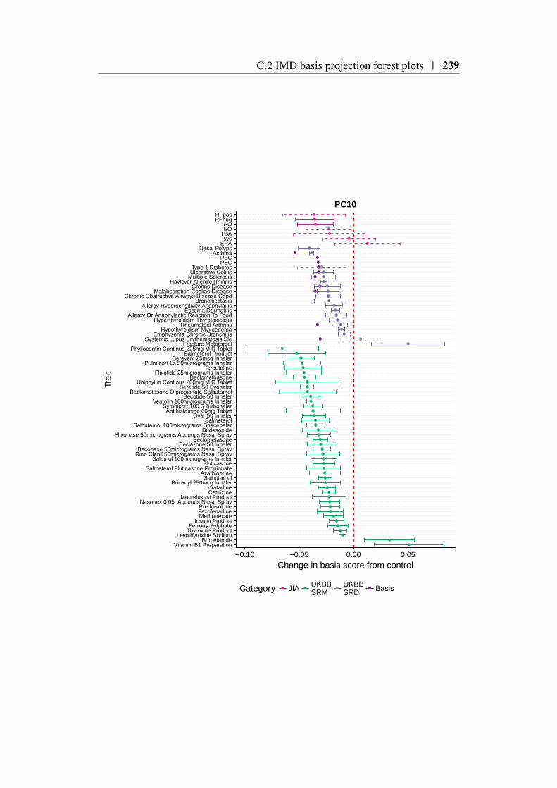
C.2 IMD basis projection forest plots | 239
Vitamin B1 PreparationBumetanide
Levothyroxine SodiumThyroxine ProductFerrous Sulphate
Insulin ProductMethotrexateFexofenadinePrednisolone
Nasonex 0 05 Aqueous Nasal SprayMontelukast Product
CetirizineLoratadine
Bricanyl 250mcg InhalerSalbutamol
AzathioprineSalmeterol Fluticasone Propionate
FluticasoneSalamol 100micrograms Inhaler
Rino Clenil 50micrograms Nasal SprayBeconase 50micrograms Nasal Spray
Beclazone 50 InhalerBeclometasone
Flixonase 50micrograms Aqueous Nasal SprayBudesonide
Salbutamol 100micrograms SpacehalerSalmeterol
Qvar 50 InhalerAntihistamine 60mg Tablet
Symbicort 100 6 TurbohalerVentolin 100micrograms Inhaler
Becotide 50 InhalerBeclometasone Dipropionate Salbutamol
Seretide 50 EvohalerUniphyllin Continus 200mg M R Tablet
BeclomethasoneFlixotide 25micrograms Inhaler
TerbutalinePulmicort Ls 50micrograms Inhaler
Serevent 25mcg InhalerSalmeterol Product
Phyllocontin Continus 225mg M R TabletFracture Metatarsal
Systemic Lupus Erythematosis SleEmphysema Chronic Bronchitis
Hypothyroidism MyxoedemaRheumatoid Arthritis
Hyperthyroidism ThyrotoxicosisAllergy Or Anaphylactic Reaction To Food
Eczema DermatitisAllergy Hypersensitivity Anaphylaxis
BronchiectasisChronic Obstructive Airways Disease Copd
Malabsorption Coeliac DiseaseCrohns Disease
Hayfever Allergic RhinitisMultiple SclerosisUlcerative ColitisType 1 Diabetes
PSCPBC
AsthmaNasal Polyps
ERAsys
PsAEOPO
RFnegRFpos
−0.10 −0.05 0.00 0.05
Change in basis score from control
Trai
t
Category JIA UKBBSRM
UKBBSRD Basis
PC10