STATISTICAL ANALYSIS FOR TRAFFIC DATA

by

XULI LI, B.E.

A THESIS

IN

STATISTICS

Submitted to the Graduate Faculty of Texas Tech University in

Partial Fulfillment of the Requirements for

the Degree of

MASTER OF SCIENCE

Approved

May, 2003

ACKNOWLEDGEMENTS

I would like to express my sincere gratitude to the members of my thesis commit­

tee: Dr. Shan Sun, co-chair. Dr. Robert L. Paige, co-chair. Dr. Yong Bai, member

and Dr. Hossein Mansouri, member. Completion of this thesis would have been

impossible without their guidance, support, and encouragement. I thank Dr. Shan

Sun for her inspiration on me in this field and her tremendous support throughout

the whole process of my thesis and my study. I thank Dr. Paige for his invaluable

work in directing my thesis, especially for the work of computation by using computer

programs. I thank Dr. Bai for providing this set of data and his work in summarizing

the data. The design of variables and speciation largely came from his insight in the

research on traffic engineering. I thank Dr. Mansouri for the knowledge of regression

analysis and statistical analysis provided in his classes, which was very helpful for

conducting this work.

My study in Texas Tech University has been generously supported by the De­

partment of Mathematics and Statistics. I would like express my gratitude to Dr.

Harold R. Bennett, for offering me this valuable opportunity of studing at Texas Tech

University.

The work presented here could not have been completed without the love, support,

and encouragement from my family, to whom I dedicate this work. My parents, Chai

fengyun amd Li Xue, my two sisters, Xuyang and Changshun, my husband Lishuang

and my son Jitong.

u

CONTENTS

ACKNOWLEDGEMENTS ii

ABSTRACT iv

LIST OF TABLES v

LIST OF FIGURES vi

I INTRODUCTION 1

1.1 The Need for Accident Analysis 1

1.2 Literature Review 2

1.3 Objectives of Our Study 3

II STATISTICAL THEORY UNDERLYING OUR ANALYSIS 4

2.1 Factor Analysis 4

2.2 Binary Logistic Regression Model and Model Diagnostics 6

III DATA SET DESCRIPTION 10

3.1 Data Source 10

3.2 Data and Variable Description 10

IV RESULTS OF STATISTICAL ANALYSIS 21

4.1 Results from Percentage Analysis 21

4.2 Results from Correlation Analysis 32

4.3 Results from Factor Analysis 32

4.4 Results from Logistic Regression Model Fitting 34

V CONCLUDING REMARKS 39

BIBLIOGRAPHY 40

APPENDIX A SAMPLE OF OFFICER'S ACCIDENT REPORT 41

ui

ABSTRACT

The purpose of this research is to recode and describe data in terms of the na­

ture and extent of fatality-involved crashes in Texas by using comprehensive police-

reported data set. Various factors including responsible drivers' information, time,

climatic information, crash information, geometric conditions of road, and contribu­

tion factors from drivers were analyzed. After summarizing these effects, a logistic

regression model is built to explain the likelihood of an intersection-involved crash

as a function of some of variables. These findings could be used to enhance the

enforcement of engineering.

IV

LIST OF TABLES

3.1 Variables Recorded in Report 11

3.2 Percentage Analysis of Variables-Age, Gender 12

3.3 Percentage Analysis of Variable-Accident Type 13

3.4 Percentage Analysis of Variables -Time, Day 14

3.5 Percentage Analysis of Light, Property Damage and Pavement . . . . 16

3.6 Percentage Analysis of Variables-Road Surface, Weather Condition 17

3.7 Percentage Analysis of Variables-Traffic Control, Road Class 18

3.8 Percentage Analysis of Variables-Vehicle Type 19

3.9 Percentage Analysis of Variable-Driver Error 20

4.1 Variables Underlying Our Analysis 22

4.2 Percentage Analysis of Variables at Different Location-Age Gender . . 23

4.3 Percentage Analysis of Variables at Different Location-Time, Day . . 24

4.4 Percentage Analysis of Variables at Different Location-Accident Type 25

4.5 Percentage Analysis of Variables-Climatic and Road Conditions . . . 27

4.6 Percentage Analysis of Variables at Different Locations-Traffic Control 28

4.7 Percentage Analysis of Variable at different Locations-Vehicle Type . 29

4.8 Percentage Analysis of Variable at Different Location- Driver Error . 31

4.9 Correlation Analysis 33

4.10 Variables Underlying Factor Analysis 33

4.11 Factor Analysis-Factor Pattern 34

4.12 Factor Analysis-Final Communality Estimates 34

4.13 Summary of Forward Selection 35

4.14 Logistic Regression Analysis Results-Parameter Estimation 36

4.15 Logistic Regression Analysis Results-Odd Ratio 37

4.16 Analysis of Effects Not in the Model 38

LIST OF FIGURES

2.1 A Graph of Logit Function 9

3.1 Comparison of Accident Rate Based on Driver Information 12

4.1 Comparison of Accident Rates Based on Variable Age 23

4.2 Time Series Analysis with Variable Time of Day 24

4.3 Comparison of Accident Rates Based on Accident Type 25

4.4 Comparison of Accident Rates Based on Light Condition and Road Class 26

4.5 Comparison of Accident Rates Based onTraffic Control and Road Class 28

4.6 Comparison of Accident Rates Based on Traffic Control 29

4.7 Comparison of Accident Rates Based on Vehicle Type and Road Class 30

4.8 Comparison of Accident Rates Based on Vehicle Type 30

4.9 Comparison of Accident Rates Based on Road class and Driver Error 32

VI

CHAPTER I

INTRODUCTION

1.1 The Need for Accident Analysis

Traffic accidents and fatalities have adversely affected the lives of most Americans.

Many people have lost parents, siblings, children, friends and relatives to the tragic

crashes that take place on our nation's highways every day. Several studies have

been conducted to determine the factors which contributed to the accidents for the

purpose of reducing the amount of accidents. In the annual report. Traffic Facts 2000:

A Compilation of Motor Vehicle Crash Data from the Fatality Analysis Reporting

System and the General Estimates System, NHTSA (National Highway Traffic Safety

Administration) pointed out that the fatality rate per 100 million vehicle miles of

travel fell to a new historic low of 1.5 in 2000. However, nearly 6.4 million police-

reported motor vehicle crashes still occurred on the national highway system in 2000-

one every 5 seconds. On the average, one person was injured in these crashes every 10

seconds, and someone was killed every 13 minutes (Traffic safety facts, 2000). Traffic

crashes are the leading cause of death in the U.S. for people aged 6 to 33, and the

economic cost is estimated to be 230.6 billion dollars per year, or 2.3 percent of the

U.S. gross domestic product (GDP)(www.brakesonfatalities.org).

Work zone safety is currently a major concern to transportation and highway

engineers because of the relatively high rate of accidents in these areas. NHTSA

presented descriptive statistics about the traffic crashes in construction/maintenance

zones, which indicated about 3 percent of fatality-involved accidents occurred in such

areas (Traffic safety facts, 2000). There is a strong indication that during the next

decade, emphasis will be placed on maintenance and rehabilitation of the nations'

highways rather than on construction of new highways. This will result many more

work zones. Unless effective measures are taken to increase safety in these work zones,

a significant increase in accident rate could occur.

1.2 Literature Review

The data analysis of accidents is a complex project for statisticians and engineers

since it needs a series of well-done steps to reach the final goal-the reduction of deaths,

injures, and economic losses from motor vehicle crashes.

NHTSA presents descriptive statistics about the traffic crashes of all severities,

from those that result in property damage to those that result in the loss of human life.

The advantage of this report is that it provides nation-wide comparison of accident

rates based on different geographic locations, different climate conditions, different

types of vehicles, different types of roads, etc. The disadvantage of this report is that

there is no other statistical analysis rather than frequencies, percentages.

A summary of the statistical study methods used in highway safety analysis is pro­

vided by National Cooperative Highway Research Program (NCHRP). Those methods

include factor analysis, principal components analysis, regression model, risk estimar

tion, ordered probit models meta analysis and logit logistical regression model, and

etc.

Kim (1994) and his group conducted a study on alcohol-impaired motorcycle

crashes in Hawaii from 1986 to 1995. They found out that young male drivers were

involved in the overwhelming majority of both types of crashes, based on the compar­

ison of the characteristics of alcohol-impaired motorcyclists involved in crashes with

those of the non-impaired data in the same location. The logistic regression model

is used to explain the odds of alcohol impairment as a function of various covariates,

such as age, the square of age, temporal aspect (day, time) and the status of driver

(resident or nonresident). Those variates have significant contributions to the odd

ratios of alcohol impairment crashe.

Lin (1993) formulated a time-dependent logistic regression model to assess the

safety of motor carrier operations. Nine logistic regression models are estimated,

which consist of time-independent effects (i.e., age, experience, driving pattern, and

off-duty time before the trip of interest) and time main effects (the driving time and a

series of time related interactions). He found that driving time has the strongest direct

effect on accident risk. Accident risk increases by 50 percent or more, after the fourth

hours of driving. Driving age and off-duty time had generally little effect on accident

risk if the driver had enough rest before starting a new trip. Other researchers used

those methods to study the relationship between safety-belt use and crashes (Li, Kim,

and Nitz, 1999). Donelson (1999) and his colleague studied rates of occupant death in

vehicle Rollover. Statistical models of fatality risk were developed with multivariate

logistic regression applied to data on single-vehicle rollover of any severity. Under

the sponsorship of AAA Foundation for Traffic Safety (Falls Church, VA), engineers

indicated speed variance and its influence on accidents, accident characteristics at

construction and maintenance zone in urban areas. (Garber et al.,1988, 1995). Most

of these studies were based on police-reported data even though the accuracy of

the crash data is dependent on the training and expertise of those police officers

collecting the information and on the difficulty in collecting the information. Using

police-reported data is still a popular way in traffic data anlysis.

1.3 Objectives of Our Study

Quantitative methods of analyzing the effects on accidents need to be developed.

Percentage analysis, frequency tables, and histograms are provided as the basic tools

for data analysis. Graphs are also provided to visualize data. Statistical correlations

was used to find the correlations between variables. Factor analysis is conducted to

reduce the number of variables if possible. One of the main objectives of this study

is to use intersection-dependent logistic regression to formulate a quantitative model

and to formulate a process for data analysis.

CHAPTER II

STATISTICAL THEORY UNDERLYING OUR ANALYSIS

2.1 Factor Analysis

Factor analysis is one of the most widely used multivariate technique, introduced

by Spearman and developed by Thurstone, Thomson, Lawlwy, and others. In factor

anlysis, the main concern is to identify the internal relationships between a set of

random variables, let x be a p byl random vector with mean vector /x and variance-

covariance matrix E. Suppose the interrelationships between the elements of x can

be explained by the factor model

X =/x-I-Lf-I-€ (2.1)

where /x is a vector of constants; f is a random vector of order A; by 1 (A; < p), with

elements / i , • • • ,/*, which are called the common factor; L is a p by A; matrix of

unknown constants, called factor loadings; and the element ei, • • • ,€p of the p by 1

random vectors e are called specific factors. It is assumed that the vectors f and

e are uncorrelated. Thus the above modle implies that a given element of x say Xi

perhaps representing the measurement on certain characteristics, can be viewed as a

linear combination of all common factors and one of the specific factor Cj, specially,

xi = fii + / i i/i -I- 1- hkfk + ei

X2 = fji2 + hifi + y- hkfk + C2

Xp = Hp + Ipifi -\ 1- Ipkfk + Cp

where kj, the (i, j)*'' wlement of L is the factor loading of Xj on the j * ' ' common

factor fj. If A; = 1 then the factor model reduces to a one factor model which was

developed by Spearman (1940). In any factor anlysis problem, an attempt is made

to determine the common factors such that the correlations among the components

of X are completely account for by these factors. This amounts to saying, since

cov{e,f) = 0, that D{x) — D{Lf) = D{e) is a diagonal matrix; that is, the specific

factors are uncorrelated. Under the assumptions

E{x) = 0, E{€) = 0

cov{e, f) = 0, D(f) = A, A positive define,

D{e) = * = diagi^i, • • • , *p), ^^ > 0

made on the random quantities in the model given in Equation 2.1, we have

D{x) = E = L A L ' + * .

Since L and f are both unknown, another model equivalent to the model in Equation

2.1 is:

X = /x -I- LA^ A"5f + e = n + L*f* -I- e

where L* = LA 5 and f* = A~2f. In this form of the model, the variance-covariance

matrix of x is

D{x) = E = L*L*' + * .

Hence, without loss of generality, in the model given in the Equation 2.1, we can

assume that D{x.) = 1 * , an identity matrix of order A;, which leads to

E = L L ' 4- ̂ . (2.2)

The standard factor model is based on the model in Equation 2.1 together with the

assumption in equation 2.2. The objective is to determine an L and * such that that

the assumption in equation 2.2 is satisfied

Note co?;(x,f) = L, that is cov{xi,fj) = kj. This implies that the covariance

between the random vector x and the vector of common factors f is completely

determined by the factor loading matrix L. Also note that corr{xi, fj) = -U= = /y

when var{xi) = an = 1, that is when E is in the correlation form. In this case.

the factor loadings are nothing but the correlation coefficients between the original

variables and the common factors. Suppose A; by 1 vectors /j and /_,, respectively, are

the i*'' and j " * rows of L. then for i^ j ,

Oij = C0v{Xi,Xj) = li Ij = liilji H 1- kkljk

and

an = var{xi) = l-U + ^i = Ui^ + ••• + kk^ -I- *i = hi^ + ^ i

where h^ = /j / j . Thus the variance of Xj is partitioned into two variance compo­

nents, namely /i^ and ^ j , corresponding to the common factors and specific factor

respeciively. The quantity ^ j , the contribution of the specific factor e,, is called the

uniqueness or specific variance, and the quantity h^ , the contribution of common

factors, is called communality of common variance. Further, li^ is the contribution

of the 1** common factor to the common variance, li^ is the contribution of the 2"''

common factor to the common variance, and so on.

2.2 Binary Logistic Regression Model and Model Diagnostics

Suppose Yi iox i = I,--- ,t are independent binomial {ni,p{i) random variables

with probabilities Pi = pxi) which are functions of a vector of numerical valued

covariates Xi. The logistic regression model is that

l o g r ^ ^ = ^ ' x (2.3) 1 - p(x)

where f3 is & vector of regression coefficients to be estimated from the observed data

{yi,ni,Xi); i = 1,- • • ,t. In equation 2.3 ^ and x are column vectors of length c and

/3'x = Aa;i + • • • + jScXc- (2.4)

As we will see, P usually contains an intercept. The intercept. Pi, is included by

setting the first component Xi of x equal to 1. The vector x can be used to model

continuous and discrete covariates as well as linear contrasts, and models for interac­

tions between various covariates.

The left-hand side of equation 2.3 is called the logit or log-odds of p{x). The

right-hand side of equation 2.3 is a linear function of the covariates or risk factors

that are believed to influence Y. Solving for p in equation2.3 gives

In published literature, we see equation 2.3 written about as often as equation 2.4

even thought they are equivalent expressions. Notice that the covariates x enter the

model in a linear fashion, although the functional form p(x) at equation 2.5 is not

itself linear. We can easily verify that equation 2.5 is a valid probability and is always

between 0 and 1. The function

is monotone increasing in x for (6 > 0) and is the cumulative distribution function

of the logistic distribution. When 6 < 0, this function is monotone decreasing. The

next is the estimation of P regression parameters. The regression coefficients /3 are

obtained as maximum likelihood estimates. The likelihood function for 0 is:

m = iogll[p{0'xi)y^\i-p{0'xi)r-yA t

= '^{yilogp{l3'Xi) + {ui - yi)log{l - p(/3'xi)]}

(2.8)

where p{/3 Xi) is the logistic function of given equation in 2.5. The term involving

binomial coefficients Yli^^si^) ^^^ ^^ ingored in the likelihood function at 2.8 because

they are not functions of the parameters /3.

The simplest diagnostics for detecting outliers are the Pearson and the deviance

residuals. The Pearson residual is the binomial count yi normalized by its estimated

mean and standard deviation:

Vi - riiPi Xi =

{{nM^-Pi)W'

7

This chi-squared residual is the most intuitive definition for a residual in logistic

regression. When all of the n̂ are large and the correct model is fitted, we would

expect all of the Xi values to behave as normal observations with zero means amd unit

variances. The deviance residual is the contribution that j/j makes to the likelihood.

The log-likelihood ratio deviance statistic

When all of the n̂ are large and the logistic model is correct, then G^ should be

nearly equal to the Pearson chi-squared statistic.The deviance residual di is defined

as

When all of the rij are large and the fitted p, are not extreme, then the rfj should be

close in the value to the Xi- For binary response data, it is important to remember

that the logistic regression function is modeled as

logit{p)= log Y^ (2.9)

where p is the probability of the response level identified in the response profiles

section by using SAS having order 0, and 1 for binary outcome response variable.

Figure 2.1 is a curve of logistic regression function.

a o

Figure 2.1: A Graph of Logit Function

CHAPTER III

DATA SET DESCRIPTION

3.1 Data Source

Data set for this analysis was taken from the Texas statewide motor vehicle

crash database (Department of Public Safety of Texas, Austin). All of these data

are fatality-involved accidents occurred around construction/maintenance zones from

year 1997 to year 1999 in the state of Texas. The total number of cases is 376. Our

analysis is also based on police-reported data. A copy of original record of an accident

and a data table are attached as Appendix A and Appendix B.

3.2 Data and Variable Description

Table 3.1 is a summary of variables from police-reported data. Statistics provided

by NHTSA indicate that, in 1996, citizens aged 70+ made up 9% of the U.S. popu­

lation, 8.2% of drivers in fatal crashes, and 12.7% of driver fatalities. Older drivers

tend to drive less and at safer times, and have lower DWI (driving while intoxicated)

and fewer speeding involvements than younger drivers. However, drivers aged 75+

have the second highest fatal crash rate (fatal crashes per estimated miles driven)

for any age group (seconded only to drivers under 24 years old.) Considering crash

rate, drivers aged 65+ are two and one-half times more likely to be involved in a

fatal crash than drivers aged 25-64, and the risk rises sharply at age 70. NHTSA

statistics also indicate that in two-vehicle fatal crashes involving an older driver and

a younger driver, the vehicle driven by the older driver was more than 3 times as

likely to be the one that was struck (www.ci.austin.tx.us). A histogram and frequen­

cies of accidents with respecte to age of drivers and gender of drivers are listed in

the Table 3.2. The rates we researched from the study are consistent with the rates

summarized by NHTSA. Over 45% of accidents related to elder drivers and younger

drivers (< 24). Male drivers are more likely to be involved in accidents than female

drivers. Our results of accident rates based on drivers gender is also in agreement

10

with FARS (Fatality Analysis Reporting System) analysis-about three quarters acci­

dents related to male drivers from this set of data. Figure 3.1 provides a comparison

of accident rates based on driver information, which is a visiualization of Table 3.2.

Table 3.1: Variables Recorded in Report

Name of Category

Responsible Driver

Time Information

Climatic Environment

Crash Information

Geometric of Road

Contribution Factor

Name of Variable

Age

Gender

Time

Day

Month

Year

Light Condition

Weather condition

Road Surface Condition

Accident Type

Vehicle Type

Accident Severity

Property Damage

Number of Vehicles Involved

Road Class

Intersection

Pavement Type

Traffic Control

Driver Error

Mechanical Failmre

Abbreviate Name

Age

Gender

Time

Day

Month

Year

Light

Weather

Road

Accident type

Vehicle Type

AS

Property

VehicleNo.

Road class

Intersection

Pavement

Traffic control

DR

MF

11

Table 3.2: Percentage Analysis of Variables-Age, Gender

Variable

Age

Gender

Index

1

2

3

4

5

6

7

8

0

1

Observations

15-19

20-24

25-34

35-44

45-54

55-64

65-74

75+

Male

Female

Pecentage

9.84

12.77

23.94

18.09

12.77

9.31

6.65

6.65

76.06

23.94

FREQUENCT

1-Hale 2-Feinale 1 - 15-20 2 - 20-24 3 - 25-34 4 - 25-44 5 - 45-54 6 - 55-64 7 - 65-74 B - 75+

Figure 3.1: Comparison of Accident Rate Based on Driver Information

Table 3.3 is the percentage analysis of accident type. Variable accident type is

coded as rear-end right-angle, left-turn, crashed with fixed object, slidewipe, pedestrian

related accidents, runing off road, head on of two vehicles, coUison with parked vehi-

12

cles, bicycle-related accidents and motorcycle-related accidents. From 1997 to 1999,

20% of fatal crashes involved a single vehicle running off the road. About 34% of fatal

crashes involved running off roads and fixed objects. Head-on crashes can occur when

a vehicle is traveling the wrong way on a one-way route, when a vehicle attempts to

pass without sufficient clearance on an undivided route, or when a driver loses con­

trol of his vehicle and crosses over into an opposing lane of oncoming traffic. There

is 14.36% of accidents related to head-on based on this set of data. Head-on coUison

and rear-end and right-angle collisons are three type of coUisons which contributed

37% of total crashes.

Table 3.3: Percentage Analysis of Variable-Accident Type

Variable

Accident Type

Observations

Rear-end

Right-angle

Left-turn

Fixed object

Sidewipe

Pedestrian-related

Run off road

Head-on

Parked vehicle

Bicycle-related

Motorcycle-related

Percentage

11.17

11.17

5.32

14.36

4.26

14.36

20.21

14.36

0.27

1.06

3.46

13

In the research provided by FARS, Midnight to 3:00 am. on Saturdays and Sun­

days was proved to be the deadliest 3-hour period through 2000. In the FARS re­

search, variable time of a day is divided by 8 periods with each period with 3 hours.

In our analysis, a day is divided by four periods based on the volumns of vehicles,

which are morning rush hours (6:00am-10:00am), daytime (10:00am-4:00pm), evening

rush hours (4:00pm-8:00pm), and night time ( 8:00pm-6:00am). About 43.35% of the

accidents occurred at night. Fridays and Saturdays are the two days with a higher

amount of accidents compared with others days of the week. These results are gen­

erally consistent with the results of the FARS study. In their research, Sunday is the

second leading and Friday is the third leading place based on accident rates. Consider

the traffic volumes in the daytime, it is not strange to find that accident rates in the

daytme is higher than that of night time. Table 3.4 provides percentages of accident

rates.

Table 3.4: Percentage Analysis of Variables -Time, Day

Variable Observations Percentage

Time

Day

6:00am-10:00am

10:00am-4:00pm

4:00pm-8:00pm

8:00pm-6:00am

Monday

Tuesday

Wednesday

Thursday

Friday

Saturday

Sunday

12.77

23.94

19.95

43.35

10.37

11.44

12.23

11.97

19.68

19.15

15.16

14

Variable light is coded as daylight, dawn, dark but not lighted, dark lighted and

dusk. From percentage analyses of variable light, property damage and pavement

type in Table 3.5, we found that the accident rates decreased with light condition

improved. Variable property damage is coded based on the level of damage in terms

of U.S. dollars. Variable pavement is coded as asphalt, concrete, gravel, and other

type of pavement type. We found that these two types of roads are more likelyt to be

involved in accidents compared with other type of roads since most of the pavements

of roads are asphalt and concrete.

Road surface condition is coded as dry road, wet road, muddy or ice road and

other road suface condition. 90.43% of accidents occurred when the road surface is

dry. Accient rate based on road surface condition is simillar to the accident rate based

on weather condition. The Pearson Correlation Coefficients between road surface

condition and weather condition is positive (0.4287), which is significant by using

test level of 0.05. A summary of percentages analysis of these two variables are listed

in Table 3.6.

Table 3.7 provides percentage analysis with variable traffic control and road class.

A well controlled road will be helpful in reducing accidents. The center stripes or

dividers are the most frequently used traffic control devices in road design. But the

center strip or divider is also the leading traffic control condition with highest accident

rates. Flashing red lights always cause the drivers more attention. In this condition,

the rate of accident is the lowest. Driving on state a highway, including interstate

highway and statewide highway, is not an easy work because of less traffic controls

and the high speed of a vehicle (an analysis about speed of vehicle and accidents will

discussed in the later part). About eighty percent of accidents are related to these two

types of highway. Research of FARS indicated that more than half of fatal crashes

occurred on roads with posted speed limits of 55 mph or more.

Vehicle type is coded as commercial truck related accidents and passenger car

related accidents. From analyses in Table 3.8, we found that vehicles are more likely

to be involved in accdents. About 90% accidents related to vehicle or passenger car,

15

Table 3.5: Percentage Analysis of Light, Property Damage and Pavement

Variable

light

Property

Pavement Type

Observations

Daylight

Dawn

Dark-not lighted

Dark-lighted

Dusk

Under 500

Between 500 and 1000

Between 1000 and 2000

Between 2000 and 3000

Between 3000 and 4000

Between 4000 and 5000

Above 5000

Asphalt

Concrete

Gravel

Shell

Dirt

Other

Percentage

48.40

1.60

31.38

16.49

2.31

57.45

40.16

1.86

0.27

0

0

0.27

75.53

21.28

2.93

0

0

0.27

including commercial truck with vehicle, vehicle with vehicle, vehicle with pedestrian

and vehicle with fixed object. From a nation-wide of analysis provided by FARS,

47.9% of accidents related to passenger car (or vehicle).

Table 3.9 provides a detail pecentage analysis about driver error. In the Texas

Department of Public Safety crash database, driver error is coded with 70 categories.

We summarized the information and got 30 categories with each category has an

16

Table 3.6: Percentage Analysis of Variables-Road Surface, Weather Condition

Variable

Road

Weather

Observations

Dry

Wet

Muddy

Snow or Icy

Other

Clear

Rainning

Snowing

Fog

Blowing dust

Smoke

Sleeting

Hign winds

Other

Percentage

90.43

9.31

0

0.27

0

92.82

5.59

0

1.33

0.27

0

0

0

0

independent effect on the accidents. Speeding is a concern for both drivers and traffic

engineers since a 50 mph crash is 15 times more likely to kill than a crash at 25

mph. Chances of severe injury or death double for every 10 mph over 50 mph that

a vehicle is traveling. Forty percent of the persons who were killed in traffic crashes

in 2000 died in alcohol-related crashes. Ten percent of the injured persons received

their injuries in alcohol-related crashes. In summary, speeding, fail to control speed,

driving inder the influerence of alcohol are three leading driver errors in our analysis,

which is consistent with most of other research by FARS and other researchers. Driver

inattention, failure to drive in a single lane is also dangerous, especially in the night

time. The analysis can be obtained from the following chapter. A frequency chart

17

Table 3.7: Percentage Analysis of Variables-Traffic Control, Road Class

Variable Observations

Traffic control No control or inoperative

Officer or flagman

Stop and go signal

Stop sign

Flashing red light

Turn marks

Warning signs

RR gates or signals

Yield sign

Center strip or divider

No passing zone

Other control

Road class Interstate highway

US or state highway

Farm-to-market road

Country road

City street

ToUway

Other roads (alley)

Beltway 8

Percentage

13.83

2.66

4.79

6.38

0.27

0.27

7.98

0.53

0.53

47.61

6.12

9.04

43.09

36.97

11.70

0

7.98

0.27

0

0

of time versus driver error indicated that drivering at night is likely to involved in

speeding, failure to control speed and failure to drive in a single lane.

18

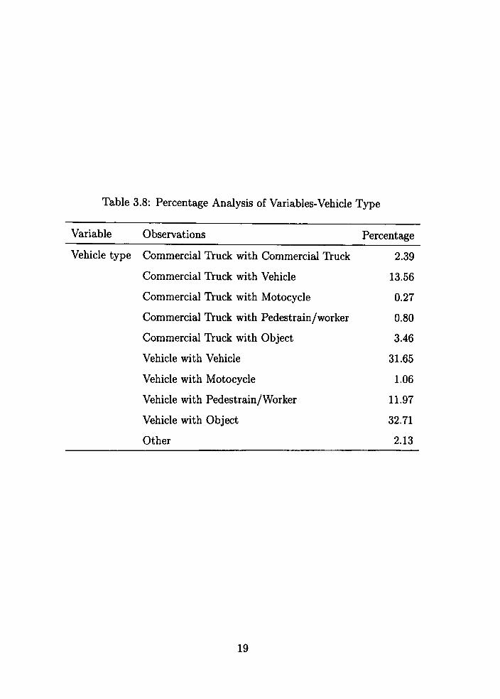
Table 3.8: Percentage Analysis of Variables-Vehicle Type

Variable Observations Percentage

Vehicle type Commercial Truck with Commercial Truck 2.39

Commercial Truck with Vehicle 13.56

Commercial Truck with Motocycle 0.27

Commercial Truck with Pedestrain/worker 0.80

Commercial Truck with Object 3.46

Vehicle with Vehicle 31.65

Vehicle with Motocycle 1.06

Vehicle with Pedestrain/Worker 11.97

Vehicle with Object 32.71

Other 2.13

19

Table 3.9: Percentage Analysis of Variable-Driver Error

Variable

Driver Error Observations

Backed with safty

Changed Ian when unsafe

Disregard stop and go signals

Disregard stop sign or light

Disregard warning sign

Driver inattention

Drove without headlights

Failed to control speed

Failed to diver in a singal lane

Failed to give half of roadway

Failed to pass satety

Failed to stop

Failed to yield

Fatigued or asleep

Faulty evasive action

Fleeding or evading police

Following too closely

Ill(explained I narrative)

Impaired visibility(explain in narrative)

Oversize vehicle or load

Overtake and pass insufficient clearance

Parked in traffic lane

Passed into no passing zone

Speeding

Turning improperly

Under influence -alcohol

Under influence-drug

Wrong side

Wrong way-one way road

Other factor

Percentage

0

1.60

1.33

1.86

1.06

9.04

0.27

16.76

9.04

0.27

0.53

0.53

6.38

2.13

2.13

1.06

0.53

1.06

0.80

0.27

0.53

0

0.27

18.62

1.33

7.84

0

3.46

1.06

8.24

20

CHAPTER IV

RESULTS OF STATISTICAL ANALYSIS

4.1 Results from Percentage Analysis

Table 4.1 is a summary of variables used in our analyses. We also merge some

categories by considering their frequencies. The following table lists variables for our

analysis including percentage analysis, factor analysis and binary logistic regression

model fitting. Observations and percentage analysis for variables based on different

locations of accidents are listed in Table 4.2 through Table 4.8. Some variables were

dropped because they were irrelevant to our study and other variables were dropped

due to the insignificant contribution to accidents. The dropped variables are month

of the year, year, accident severity, number of vehicles involved, property damage,

and mechanical failure.

From Table 4.2, we found that drivers aged 25-34 years are more likely to be

involved in accidents either at intersection or non-intersection locations. A significant

trend based on the comparison is that elderly drivers made more mistakes when they

are driving at an intersection location. Based on the results, elderly drivers have a risk

higher to be involved in accidents with fatality. We found that drivers aged 75 or older

should pay more attention when they are driving on roads with more intersections.

Young people should pay more attention when driving on the non-intersection roads.

Frequency analysis results, in terms of intersection and non-intersection, based on the

gender of drivers at two locations are similar. Figure 4.1, a graph which visualized

Table 4.2, provides an insight of data analysis based on variable age.

21

Table 4.1: Variables Underlying Our Analysis

Name of Category

Responsible Driver

Time Information

Climatic Environment

Crash Information

Geometric of Road

Contribution Factor

Name of Variable

Age

Gender

Time

Day

Light Condition

Weather condition

Road Surface Condition

Accident Type

Vehicle Type

Property damage

Road Class

Intersection

Pavement Type

Traffic Control

Driver Error

Abbreviate Name

Age

Gender

Time

Day

Light

Weather

Road

Accident type

Vehicle Type

Property

Road class

Intersection

Pavement

Traffic control

DR

For the variables of time of day and day of the week, we found that there is little

difference between the frequencies of two locations. Figure 4.2 depicts two curves of

time series analysis. The changes of two curves indicate that accident rates of two

types of location have no difference.

22

Table 4.2: Percentage Analysis of Variables at Different Location-Age Gender

Index

1

2

3

4

5

6

7

8

0

1

Observations

15-19

20-24

25-34

35-44

45-54

55-64

65-74

75+

Male

Female

Intersection

(percentage)

6.32

13.68

24.21

17.89

10.53

7.37

6.32

13.68

76.84

23.16

Non-intersection

(percentage)

11.03

12.46

23.84

18.15

13.52

9.96

6.76

4.27

75.80

24.20

PREOUENCT

intersection

O-Intereection l-Nonintersection 1- 15-20 2 - 20-24 3 - 25-34 4 - 25-44 5 - 45-54 6- 55-64 7 - 65-74 8 - 75+

Figure 4.1: Comparison of Accident Rates Based on Variable Age

Table 4.4 compares different accident types. The frequencies of the type of rear-

end accidents at two locations are nearly the same. The difference of two frequencies

23

Table 4.3: Percentage Analysis of Variables at Different Location-Time, Day

Index Observations Intersection Non-intersection

(percentage) (percentage)

1

2

3

4

Morninig Rush Hourss

Daytime

Evening Rush Hours

Night time

12.63

25.26

21.05

41.02

12.81

23.29

19.57

44.13

0

1

Weekday

Weekend

64.21

35.79

66.19

33.81

6:0Clani-10:00Bm iaCI0am-4;(X)pnn

IrtersQction h A iS |

4;00prT)-8:O0pm

O O O nl

aXpm—6:00Bm

Figure 4.2: Time Series Analysis with Variable Time of Day

is less than 1% percent. A significant difference exists for the frequencies of the

right-angle type accident at two locations. About one-quarter of accidents happened

at intersection locations are rear-end type, but just about 6.4% of this type of acci­

dents occurred on the roads without intersection. It is not surprising that the rate

of pedestrian-related accidents is higher on the roads with intersection because the

function of those roads. Running off the road is the leading accident type for a

24

non-intersection road. Head-on is in second place with a frequency of 17%.

Table 4.4: Percentage Analysis of Variables at Different Location-Accident Type

Index Observations

FREQUENCY

Intersection Non-intersection

(percentage) (percentage)

1

2

3

4

5

6

7

Rear-end

Right-angle

Fixed object

Pedestrian-related

Run off road

Head-on

Others

10.53

25.26

12.63

17.89

9.47

6.32

17.89

11.39

6.41

14.95

13.17

23.84

17.08

13.17

O-Interaection l-Noninteraection 1-Rear-end 2-Right-angle 3-Fi3ced object

4-PedeBtrain-related 5-Run off road 6-Head-on 7-Othere

Figure 4.3: Comparison of Accident Rates Based on Accident Type

25

Table 4.5 summarizes the percentage analysis of variables at different locations

based on light, road, weather, road class, and pavement type. The classification of

light conditions are modified after considering the frequency of analysis, which is

coded as daylight, dark not light, and dark light. About half of accidents occurred

at daylight condition. Driving on a road with fewer intersections and without light

is more dangeous than driving on the same type of roads with good light conditions.

Observations of road surface condition were classified as dry road conditions and wet

road condition considering the weather condition of state of Texas. Variable weather

condition is merged as clear weather, rainy weather, and other weather condition.

From the frequency table, we found that most accidents involved in dry road condition

and clear weather conditions. Interstate highways are roads where most accidents

involved. A comparison of intersection versus road class and accident type indicate

that a driver should pay more attention when they are driving on highways, even in

a very good light condition. Figure 4.4 is a comparison of accident rates based on

variable light condition and road class.

FREQUENCY 160

light

Intersection

0= Intersection 1= Nonintersection

Figure 4.4: Comparison of Accident Rates Based on Light Condition and Road Class

26

Table 4.5: Percentage Analysis of Variables-Climatic and Road Conditions

Variable

Light

Road Surface

Weather

Road Class

Pavement Type

Index

1

2

3

0

1

1

2

3

1

2

3

4

1

2

3

Observations

Daylight

Dark-not lighted

Dark-lighted

Dry

Wet

Clear

Rainning

Other

Interstate HWy.

US or State Hwy.

Farm-to-market road

City Street

Asphalt

Concrete

Ohter

Intersection

(percentage)

50.53

26.32

23.16

91.58

8.42

95.79

4.21

0

32.63

38.95

11.58

16.84

73.68

24.21

2.10

Non-intersection

(perc( ;ntage)

50.53

33.10

16.27

90.04

9.96

91.81

6.05

2.14

46.98

36.30

11.74

4.98

76.16

20.28

3.56

A comparison of accident rates at different locations based on variable traffic con­

trol and road class in Table 4.6 pointed out that interstate highways where the center

stripe or divider are used as the traffic control sign are more likely to involve accidents.

Local roads with multiple type of traffic controls have less accidents occurred.

27

Table 4.6: Percentage Analysis of Variables at Different Locations-Traffic Control

Index

1

2

3

4

5

6

7

8

Observations

No control or inoperative

Officer or flagman

Stop and go signal

Stop sign

Warning signs

Center strip or divider

No passing zone

Other control

Intersection

(percentage)

14.74

1.05

13.68

21.05

5.26

35.79

1.05

7.37

Non-intersection

(percentage)

13.52

3.20

1.78

1.42

8.90

51.60

7.83

11.74

FREQUENCY 70

60-50 40 30 20 10 0

roaddass ^ ^ 1 2 ^ ^ 3 G5SS 4

1 2 3 4 5 6 7 1 2 3 4 5 6 7 acckJenttype

I 0 1 I 1 1 htersecUon

0= Intersection 1= Nonintersection

Figure 4.5: Comparison of Accident Rates Based onTraffic Control and Road Class

28

FRBgUENCT

Traffic Control

Intersection

0-Intereection l-Noninteraection 1-No control or inoperative 2-Officer or flagman 3-8top and go eignal 4-8top sign

5-Warnina siana 6-CenterBtriD or divider 7- Nopaaoina tone 8-other control

Figure 4.6: Comparison of Accident Rates Based on Traffic Control

A comparison of accident rates at different locations based on variable vehicle

type and road class in Table 4.7 indicated that commerical truck-related accidents

are more likely to occur on highways. Passenger car-related accidents are more likely

to occur on local roads.

Table 4.7: Percentage Analysis of Variable at different Locations-Vehicle Type

Index Observations Intersection Non-intersection

(percentage) (percentage)

1

2

3

4

5

Commercial Truck Related

Vehicle with Vehicle

Vehicle with Pedestrain/Worker

Vehicle with Object

Other

13.68

44.21

14.74

23.16

4.21

22.78

27.40

11.30

35.94

2.85

29

FREQUENCY 120

3

0

3 4 5 vetucietype

1 1 Intersection

0= Intersection 1= Nonintersection

Figure 4.7: Comparison of Accident Rates Based on Vehicle Type and Road Class

FREQUENCY

Vehicle Type

intersection

O-Intersection l-Nonintersection l-Conmerical Truck Related 2-Vehicle vsVehicle

3-Vehicle with Pedestrain 4- Vehicle withObiect 5-Other

Figure 4.8: Comparison of Accident Rates Based on Vehicle Type

30

Speeding or speed-related factors are leading factors either at intersection or non-

intersection location. Table 4.8 is the percentage analysis of accident rates at two

locations based on variable driver error. Figures 4.9 and 4.10 visiualized the frequen­

cies based on variable driver error which indicates that highway driving accidents are

more likely to involve in speeding or speed-related accidents.

Table 4.8: Percentage Analysis of Variable at Different Location- Driver Error

Index

1

2

3

4

5

6

7

8

Observations

Speeding

Fail to control speed

Failed to driver in a single lane

Driver inattention

Under influence of alcohol

Fail to yield

Wrong side

Others

Intersection

(percentage)

19.15

16.49

9.04

9.04

9.84

6.38

3.46

26.06

Non-intersection

(percentage)

22.42

16.01

9.61

8.54

8.54

2.85

4.63

27.40

31

FREQUENCY 80i 70 60 50 40 30 20 t)] 0

roaddass 1 ^ ^ 2 E ^ S 3 K ^ 4

1 2 3 4 5 6 7 8

I 0 1

1 2 3 4 5 6 7 8 DR1

I 1 1 Intersection

0= Intersection l-Nonintersection

Figure 4.9: Comparison of Accident Rates Based on Road class and Driver Error

4.2 Results from Correlation Analysis

A correlation analysis is conducted. Table 4.9 is a summary of correlation coef­

ficients between two variables. Numbers with boldfaces are correlation coefficients

that are significant at p < .01 level after testing. The highest correlation is 0.58993,

between road surface condition and weather condition. Medium correlations exist

between time of day and light condition. There is a low correlation between time and

vehicle type and between time and light condition.

4.3 Results from Factor Analysis

Table 4.10 lists all variables participated the factor analysis. The factor pattern

for factor analysis is in Table 4.11. Table 4.12 lists variables underlying factor analysis

with final communality estimated.

32

Table 4.9: Correlation Analysis

Variables

Light

Time

Vehicle Type

Weather

Road

Driver Error

Light

1.00000

0.49326

0.30170

0.03866

0.07923

0.17667

Time

1.00000

0.27852

0.08767

0.01496

0.19919

Vehicle Type

1.00000

0.05845

0.01439

0.28166

Weather

1.00000

0.58993

0.06174

Road

1.00000

0.11692

Driver Ern

1.000(

Table 4.10: Variables Underlying Factor Analysis

Name of Category

Responsible Driver

Time Information

Crash Information

Geometric of Road

Name of Variable

Age

Time

Accident Type

Vehicle Type

Property damage

Road Class

Traffic Control

Abbreviate Name

Age

Time

Accident type(AT)

Vehicle Type(VT)

Property

Road class(RC)

IVaffic control(TC)

There is only one factor extracted. This factor explained about 10% of total

variance of variables undering factor analysis. So the factor analysis in reducing the

dimension of variable by factor anlysis is not applicable for this dataset.

33

Table 4.11: Factor Analysis-Factor Pattern

Variable

Age

Time

Accidenttype

Property

Vehicletype

Roaddass

trafficcontrol

Factorl

-0.24834

0.36614

0.11294

-0.63385

0.68571

0.00168

0.07247

Table 4.12: Factor Analysis-Final Communality Estimates

Variable

Age

Time

Accidenttype

Property

Vehicletype

Roaddass

Trafficcontrol

Factorl

Communality

0.04267782

0.09176948

0.04288922

0.31495154

0.35103717

0.03012925

0.03907704

0.91253153

4.4 Results from Logistic Regression Model Fitting

To better understand the relationships between the responsible driver factors

(driver's age and gender); climatic condition factors (light condition and weather

condition), geometric of road (road class, traffic control pavement), and other factors

such as vehicle type, driver error, associated with intersection dependent accidents,

a binary logistic regression model was constructed. The following variables are con-

34

sidered for logistic regression analysis: age, gender, time, day, light, road surface

condition, weather condition, road class, pavement, traffic control, vehicle type ,and

driver error. Among all the variables listed above, gender, day, and road surface con­

ditions are dichotomous valued covariates, and we can regress on this value directly.

Road class is an ordered categorical variable so regressing directly on its values is an

acceptable approach. For the other variables which are not ordered, it does not make

sense to regress analysis on this variable. We have to create indicator (also called

dummy) variables. For example, there is no natural way to order variable light, this

does not make any sense that daylight<dark not lighted< lighted. In modeling the

above data set, we in fact use several new predicators, for example,

X2 = I if daylight condition

X2 = 0 not.

For variable light, we need two dummy variables, these are enough to cover every

observation for light condition. In general, for t treatments, one would required t — 1

dummy variables. Drivers in their 20s and 30s!l; constitute the largest segment of

accidents and decreasing steadily after the drivers reach 40 years. The squared-age

terms is also considered for model fitting. A summary of model selection procedure

is listed in Table 4.13, by using forward selection is list.

Table 4.13: Summary of Forward Selection

Step

1

2

3

4

Variable

Trafficcontrol

DRl

Roaddass

Light

DF

7

7

1

2

Chi-Square

76.6965

23.2885

6.3440

4.6513

Pr >ChiSq

< .0001

0.0015

0.0118

0.0977

Traffic control is the only variable which is significant after testing based on a test

of 0.10 level. A detail description about the contribution of the observations under

35

variable traffic control is listed in Table 4.14. For ease of interpretation, the parame­

ters, standard errors, probability values, odds ratios, and 95% confidence interval are

provided.

Table 4.14: Logistic Regression Analysis Results-Parameter Estimation

Variables

Intercept

Light 1

Light 2

Roaddass

TC 1

TC 2

TC 3

TC 4

TC 5

TC 6

TC 7

DR 1

DR 2

D R 3

DR 4

D R S

D R 6

D R 7

Parameter

-2.9689

-0.4000

0.4294

0.3660

-0.0324

-1.3294

2.0607

2.68S4

-0.3598

-0.3185

-2.1603

0.2596

1.6452

1.4305

1.6315

1.9230

2.8147

-10.6776

Standard

Error

28.9224

0.2116

0.2307

0.1619

0.3829

0.9901

0.5613

0.6678

0.5092

0.3029

0.9393

28.9221

28.9211

28.9225

28.9227

28.9218

28.9239

202.4

Odd Estimation

0.0105

3.5729

3.4643

6.8079

0.0072

1.8030

13.4793

22.3683

0.4992

1.1054

5.2897

0.0001

0.0032

0.0024

0.0032

0.0044

0.0095

0.0028

Prob.

0.9182

0.0687

0.0627

0.0160

0.9326

0.1794

0.0002

< .0001

0.4798

0.2931

0.0216

0.9928

0.9646

0.9606

0.9550

0.9470

0.9226

0.9679

Observations

Lighted

Dark not lighted

No control

Officer or flagman

Stop and go signal

Stop sign

Warning sign

Center strip or divider

No passing zone

Speeding

Fail to control speed

Failed to driver in a single lane

Driver inattention

Under influence of alcohol

Fail to yield

Wrong side

36

Table 4.15: Logistic Regression Analysis Results-Odd Ratio

Variable

Light 1

Light 2

Roaddass

TC 1

T C 2

T C 3

T C 4

T C 5

T C 6

T C 7

D R l

DR2

D R 3

DR4

D R 5

DR6

D R 7

Odd ratio

estimate

0.690

1.582

1.442

1.671

0.457

13.548

25.305

1.204

1.255

0.199

0.490

1.958

1.580

1.932

2.585

6.307

<0.001

95% Wald

0.343

0.736

1.071

0.557

0.043

3.158

5.814

0.312

0.474

0.021

0.184

0.851

0.555

0.661

1.005

1.860

<0.001

Confident

interval

1.388

3.400

1.942

5.009

4.815

58.118

110.132

4.649

3.321

1.870

1.305

4.509

4.501

5.644

6.654

21.386

>999.999

The table reveals that traffic control 3-stop and go signal (TC3) and traffic control

4-stop sign (TC4) are strongly associated with increased odds of intersection-involved

crashes. When driving under the influence of alcohol, the driver is 3 times more likely

to be involved an intersection-related accidents than if not intoxicated. Table 4.16 lists

all variables which are not in the model. The p-values indicate that those variables

are not significant as a contribution factor to an intersection-related accident.

37

Table 4.16: Analysis of Effects Not in the Modd

Effect

Age

Gender

Time

Day

Weather

Road

Accident type

Vehicle type

Pavement

DF

7

1

3

1

2

1

6

4

2

Chi-Square

6.7613

0.5513

2.0552

0.3540

1.6424

0.1244

8.7068

4.5758

0.5286

Pr >ChiSq

0.4541

0.4578

0.5610

0.5519

0.4399

0.7243

0.1907

0.3337

0.7677

38

CHAPTER V

CONCLUDING REMARKS

Traffic control-stop sign plays a significant role in preventing intersection-related

accidents compared with other factors. The model is:

log -^^-^ = -2.9689 -I- 2.6854x; (5.1) 1 - p{y)

where x is traffic control 4-stop sign. p{y) is the probability that an accident occurred

at an intersection location. We can calculate probability that an accident occurred

at an intersection location by the following equation

exp{0'x) , . ^^y^ = l-fexp(^-x)- (^-'̂

So, when a; = 0, an intersection is equipped with a stop sign, the probability that

an accident occurred is 4.89%. When a; = 1, an intersection has no stop sign, the

probability that an accident occurred is 42.95%.

39

BIBLIOGRAPHY

Traffic Safety 2000. p.iii

Kim, Karl. Lawrence Nitz and Lei Li. (1994). Analyzing the relationship be­

tween crash types and injuries in motor vehicle collision in Hawaii. Transporta­

tion Research Record. Washington, D.C.: Transportation Research Board. No.

1467. pp. 9-13.

Li, L., K. Kim, and L. Nitz, (1999). Predictors of safety belt use among crash

involved drivers and front seat passengers: Adjusting for over-reporting. Acci­

dent Analysis and Prtevention. 31(6): 631-638.

Garber, N.J. and Woo, T.H. (1990). Accident Characteristics at Construction

and Maintenance Zones in Urban Areas. Report No. VTRC90-R12. Virginia

Transportation Research Council, Charlottesville, VA.

Garber, Nicholas J. and Ravi, Gadiraju. Speed Variance and its Influence on

Accidents, AAA Foundation for Traffic Safety, 1988.

Lin, T -D., P.P. Jovanis, and C -Z. Yang, (1993). Modeling the Safety of Truck

Driver Sevice Hours Using Time-Dependent Logistic Regresion. Transportation

Research Board. National Research Council, Washington, D.C. 1993, pp.1-10.

Donelson, A.C., K.Ramachandran, K. Zhao, and A. Kalinowski, (1999). Rates

of Occupant Deaths in Vehicle Rollover: The Importance of Fatality Risk Fac­

tors. Transportation Research Record 1665, Transportation Research Board,

National research Council, Washington, D.C, 1999 pp. 109-117.

40

APPENDIX

A SAMPLE OF OFFICER'S ACCIDENT REPORT

41

'CXAS ffiACC O F F C O r S ACCID6NT REPORT S T O (E< »U>1) M X . T O » C C O £ M T RECORDS TEXAS OEPARTUEHT OF WJOUC SAFETY. PO SOX « « 7 . AUSTW TX WTTVOMO

PV/CEVSMERE A C C O e ^ T O C C U R R B )

COUNTY Houston County

f ACCOENT V»S OUTSIOE OTYIWITS. «OCATE OtSTANCE FROM NEAREST TOWW

CITYORTOIM4 H o u s t o n

nnnn UdES NORTH S E W OF

T>«S»i3lV»«aiBfBTVnBTT"

CITYORTOWN

R O O O N V W C M

A C C O O i T O C C U R R E D .

M T E R S E C T M O STREET O R R R K-MG NUMBER

NOT AT MTERSECTION

•LOCKNLMaER

Westheimer RD nwfTflftfcvt^ie i>6>/rttiU«ein««Titt{Te<«

Briarhurst Dr. tTRCCTCMnOAONAaC NOOTE NUtMCHOR t TRCfT COOC

_ D " D K I D D Of I M I N S E W • " • • " ' < • « ' o. • * * « . M i w a

' — F ^ « a a . L . « • • . HIMT H I W H C M . .

CONSTR 2 0 N E

N O I W T

YES CONSTR D Y E S SPEED iONE r - i . _ uMf

~ « ° ; „ 10/23/2002 S^°^ Friday _ 8 3 0 H * " F EXACTLY NOON OB "OUH L J P " MIDNCHT. SO STATE

LOC

DOMOTWtUV

H M S S.ACC

LOC

CODE

SEVERITY

FAT REC

DR REC

DPS NO

UNTT NO I • MOTOR VEKCU V^HClfOEHT NO 356848-38122954-846385 iF BODY STYIE • VAN OR BUS.

. M04CATE SEATING CAPACTTY

2|« 2002 iaSS Red Dodge 5SSf Viper

owERs Thomlin. Lee 1388 North Post Oak

irSl Sport UCENSE rv} . PLATE TX DBV 583

'TX FWST

55896187 A ,05/08/77 AOORESSffTREET.CfTV. STATES^

W

YEAR ITATE NUI«ER

^ ^ 429 555 4231

, Teacher •TATE NIA«ER CLAIS/TVPE l O OAV VEAR

SPECWEN TAKEN ( A U X ) H O l X n u G ANAIYSS) H 1 1 « I E A T H 2 « 0 0 O JOTMER 4.NONE S-REFUSEO ( 4 | AUCOMOLCRUG ANALYSIS RESULT

lESSEE OWNER Thomlin. Lee

PEACE OFFICER EMS ORIVB) | | I | F«E FCHTEH ON EMBIGENCYTLj YES

1388 North Post Oak

UAaOTY NSURANCE

NAtC|ALWAVSSHOWL£tSEErL£ASEO.CrTl«nwrtSCSMOWOM*e^

> ^ Y E S

AOORESS^TREET.aTT t T A l ^ V ^

Spencer & Associates 4658465434 MSURANCE COW ANY NAtC POUCYNUkeER

VEHICLE DAMAGE RATING FC6 + BD4 + FD4

UNIT U O T O R V e i C t f M T R A J N H PEDALCYCUST • C O / I C f U e i A O / I ^ O T C I O

N0.2. To-EonpsjS'RiANr-UHERn '-',««a£ioEm NO. 58456-51484-487512 T O » £ D [ ^ PQJESTRIAN | _ J OTHER Q

1966

r BODY STYIE - VAN OR BU& _» I01CATE SEATING CAPAOTY

COLOR Green Ford HOOEL

NAME _ _ S T Y I E " " ' * ' ' • UCENSE 0 2

.PLATE TX BC5487

gai^^ Bone, Chris LAST

0Riversj)( FIRST

54655415 B SIBBLT"

Doe

19483 Main Street. AOORESS|SfUeT.6l fV. i rATE.>>l f^^il^ 531 555 6482

NUMBER

. Construction Worker

SPECWEN TAKEN (ALCOHOLORUG ANALYSS) t.eR£ATH ^BL0OO MOTHER AMME SAEFUSED

CLASS/TXC l O DAT YEAR

ALCOHOIXIRUG ANALYS6 RESULT E lESSS OWNER Bone, Chris 19483 Main Street.

PEACE OFFICER EMS DRIVSl FIRE FIGHTER ON EMERGENCY? • YES Q N O

NlUC VU.WAVt SHOW LESSEEFL£ASE0.OT»CinMISC S H O W O W e t AOCM£S$(STREeT.CITV.KTATC.S^

U A B l i T Y

N S U R A N C E B YES N O

-fBoassesFBtniinr- MueVkMEA VEHICLE DAMAGE RATING

OAMMJE T O PROPERTY OTHSt THAN V&UCl£S

NAiCAi^AA6R£ss^Tft£f r 6iTY i T A f C v i t f A i M A ~ net tooicuiU DAMAGE ESTItMIE

UGHT U CONDTTION U 1

1-0AY\X!KT 20AVIN M)ARK.NOT LIGHTS} AOARIdXXTEO MXJSK

VICATHEH | l |9 I

1 .C IEARXX0UDY S-SMOKE

2.RAiNlNG 7..SL£ETMG

>.SN0IAING «-HIGH W N O S

4 .F0G MOTHER

5.BLX)vuNG0uST O v e i c a d

SURFACE CONDITION

1-DRY

2-VI€T

VMUDOY

4.SNOWrACY

SOTHER

1 « A C K T 0 P

2.C0NCRETE

I G R A V E L

* « < E U .

^ O B T

»OTMER

DESCRIBE R 0 « 0 CONOaiONS ( I N V E S T O T O R S OPWON)

Roads were damp with the morning moisture.

n YOUR OPINION. DO THIS ACCIDENT RESULT M AT LEAST IVOOOX DAMAGE TO ANY ONE PERSON̂ S PROPERTY? K I Y E S D N O

CHARGES FLED ^ E Lee Thomlin ^^^u««c-.«««.«ioo..p«d«,o..p».,«.iim.

NAME CHARGE

T̂ ENOTjiKJ 10/23/02 8:41 A HOW Radio Dispatch CMTE HOUn

rvFS)OBPRiK'TEDNAMEOFBWESTiGAToa J o h f i F r e o n c K s o n

SIGNATURE OF WVESrtGATOR O N C 5 6 5 8 5

TIME ARRI\«D AT 4 0 / 9 1 / 0 9 SCENE OF *CCOENT ' " ' * ^ « ^ " * -

DATE REPORT UAOE ' 0 / 2 3 / 0 2

0£F>ARTMB>IT *oP

CTTATCN 3520423 NUMBER ''^^•^^'^

CrTATlON NUMBER

8:55 A

SREPORT COaf\£TE f ^ l ^ S ^ N O

OIST/^REA

i r.«.pnn.,d 11/3/2002 3:4

42

SOUCITAIDN

(SOU

w o c r u rvmom amm TO mant ODMTMT .mM

. T T a « « V C M A O M M C I O I L . . f r f t O M I K M O a O H . M M k T f l • N t / C t T M U l O A . 0 « < M V O ( M « « « t i O M « ( M a T K I « S 0 A u a . « c o . . . .«AltH OMt « O U A r o « r .ocpor V . o It TO Mxjot N . M> toua iAnoN

U N I T N O 1

D A M A G E F C 8 • B 0 4 • F 0 4

R A T M G

O C C U P A N T S

1 P O S I T I O N

D R I V E R

E J E C T E D

* - net w m c o M J

TOACDDUE TO DAMAGE

I^YESQNO

venClE REMOSfi

BY Bob

C O D E F O R T Y P E

R E S T R A I N T U S E D

C - C M U I M C t T M I M T

N - M M *

AjRaAOCOoe

M • lO ttfXOnttMT

H E U M E T U S E CODE FOR

N J U R Y S E V B U T Y

ALCOHOUDRUO ANALYSS (COMPLETE r CASUALTIES

NOT M MOTOR venCLE)

t - lNOW< O M M O C O K . a i | * n < - • « i A T M

1 • W M M N M > t CMMAOCD A . M C A ^ A O r A T W O M U T 1 . M J O O O ^

1 M D W ( ( M ( « C W M M M 1 « M O M I » C A ^ « a T * r M ] l - O T t C M 1

4 . « > I M O M C raUitil W A M V * « » €

• - ( M O O W M I f M > « 1 N - aClT t M A J C O S . flEFUHD

^ jf^ Bobs Tow ing

Jones

COMI^fTE AU. DATA ON ALL OCCUPANTS NAMES POGaCNS RESTRAINTS USED. ETC. HOVtEVER IT IS NOT NECESSARY TO SHOW ADDRESSES UNLESS M U £ 0 OR HAJRED

NAICAASTNAkCnRlT) A0OR£S« f iTAECT.Cn V . I T A T C . V )

SCEFRONT TiKxrin. Lea 1388 North R3S( Oak

• O i ,

Y

CJCCTEC

A

rrpf i^XTMMMT

\MtO

A

M W M

Y

•cuir Mie

2 5

K X

M

wuurr cooc

c

1 UNIT NO 2 STiU.'SVi'SnA D A M A G E

R A T I N G

occuPAwrs posrriON

• DRIVER

• . •

f

T O V I E D D U E

T O D A M A G E

VEHCLf REMOWEJ

ev

riTn j

1

C O M P L E T E A L L D A T A O N ALL. O C C U P A N T S ' N A M E S P O S I T I O N S R E S T R A I N T S U S H ) . E T C , H O V ^ E V E R .

I T S N O T N E C E S S A R Y T O S H O W A D D R E S S E S U N L E S S H L I E D O R M A J R E O

H A I C i A S T N A t C R R S T ) AOORESipTR£eT.CITV.ITA1E.a.)

SEE FRONT B o n a . C t l l i t 19403 M a m Street

•Ol

Y

C J C C T C I ]

Y

r r F t MEtTMAfMT MMKAO

N Y

• C U i C I M C

4 2

aa

M

uuurr CDoe

K

COMPVfTE F CASUALTIES NOT M MOTOR N^HCLE

PEDESTRIAN. PaVMCtCUST. ETC

CASUALTY NAME (LAST NAME FIRSTl CASUALTY ADDRESS (STRKT. CfTY, STATt ZIP)

otSPOsrrcN OF raufD A N O O R MJUREO

ITEM NUMBERS

1

TAi<ENTO

Houston Hospital

ev

OfTicer Jane McOemitano

• O L aFiotten mmu >cu«ei uit TAKEN

1 uJ

K X coce

IF AMBULANCE USS), SHOW

NornEO

B41 * "

A T S C C W

9 : 0 1 * * *

nCUAWKI DRIVER

4

1 COHPUETE THIS SECTION f PERSON WLLED

ITEMNVJMBER DATE OF DEATH

10/23/02 TWEOF DEATH

8:45 ITEM NUMBER DATE OF DEATH TIME OF DEATH ITEM NUMBER DATE OF DEATH TME OF DEATH

INVESTGATOR-S NARRATIVE OPINION OF WIAT HAPPENED (ATTACH ADOaiONAL SHEETS f NECESSARY)

Lee Thomlin was speeding excessi>«ly. He swerved and collided with Chris Bones' Ford pickup on Westheimer Rd. Lee Thomlin's vehicle was thrown from the road, striking property, while causing Bones' vehicle to flip over and skid across the road tor 140 feet.

When arriving at scene, there was an overturned red vehicle tacing east in the #1 W/Bound lane of Westheimer Rd. TTie \chicle had major front and driver side damage. I also saw a green pickup facing SE on the NE section of the a\«nue.

DIAGRAM Q l X WAr ^ T W O W A Y Q O I V O E O

^

1 1 1

I ' < + T T

v\ V

J It

FACTORS AND CONDITONS USTED ARE THE KVESTOATOR-S OPINION

OTHER FACTORSCONOinONS MAY OR

f ACTORSCONDfTONS CONTRBUTWO MAY NOT HAVE CONTRIBUTED

U N I T 1

UNTT 3

'41 '73

'61 a

s

1

U N I T 1

U M T 2

1

• 2

3

0-NOCONTRGLORMCRERATrV£ S OmCCR OR f\AOMM •

2.STOP AFOOOSKMAL 1 3-STOP B«CN •

f lASMI ta RED LKXT I

T R A F F C CONTROL • TURN WVRKS 10 - MOPASSMC ^CMEJA • WARNINCSICM n . O T * * R « W T R C L I** • I M O k i e s OR SCNtkL* - V C L O S K M -CCNTERSTmPEOROCVCER

tj 1 AMMkLCNRCMO-OOCSTC 2 A N d M L W R O W - V W U } I eACKEOWfTMO/T SAIEIY 4 CHA.NCEDLANEMCNUMA/E 9 DEFECTIVE aRNO*CAOLAI«>8 • DCFeCTMEORNOSTOPLAUPS 7 0 E r e C T f V E 0 n N O T * ( . l A I * * » > OCFECTfVEonNOTuRMSIGNALLAfcfS • DEFECTIVE OR HOTRAILER BRAKES

to DEFECTIVEORNOVCMCLEBRAKES I I DEFECTfVCST£ER»4G*CCHAMai 13 DEFECTfVCORSUCKTMeS

13 OEi^CTivETRALERHrTai 14 DtSABLEDMTRAAXLANE 15 DtSAECAROBTOFANDaOSiCMAL Ift OlSREO>tOSrCPBiaNCRLK>fT

1 0<SRE'>ROTURNM«iftKSATMTERSECTiO<

(ff D tSTtWCTKMMVEMOf 30 DRfVERMATTCraiCM 31 DROVE WITMCXff»CA0LO«l 22 fACEDTOCONTRCL SPEED n FA«.CDTOORIVEM$*<GLELAf« 24 FAC£DTOGn/EHALFOFROA(NVAT 23 FAKXDTOXEOWARMNGSIGN 2e f A t i O T O P A S S TOLEFT SAFELV 21 FALEDTOPASSrORiOfT SAFELV

JT FAtfDTOVeLOROW-TURHWOLCFT H FALEDTOVCLDROW-TURNONRED ) • FALEDTOrCLDRCNV-VCLDSKW

40 FA TCUEDORASLEEP 41 FAULTYEVASIVEACTKN «3 FIREMVEMOJE «> HXEMSOREVADWGPOLCE 44 FOLLOWED TCOCLOSCLV 45 HAD BEEN ORMtMO

• 0«S«£CARDWAftWlM0««>**TCCN6TRUCT<WJ« FAt iOTOrCLDROWTOPCOCSIRlAN

» F A a £ 0 T O v c a > R a « . e * C R C E w : v v E M C i E » L O * o r g n « < ^ o 11 FAl£OTOV«LOROW-OP£N»*TERSecT<W »' ' ^ f i ' ^ ^ F ^ ^ ^ . yt FACCOTOVCLDROW-PRfVATEDRfVE U F A R ^ D T O r C L O R O W - S T O P S K X

MTOTRAFnCLANE • " S3 CVERSUE VEMCLE OR LOAD " 53 OVERTAKEA*CFASS»«SJFFiaEMTCI.£A»WCr J* 54 P A R K E D A M O F A I L E O T O S E T B R M C ' ^ 53 PARKCOWTRAF«CLA»«E *

P A A K E O IMTMCX/T U C X T S

PASSED « NOP ASSWCOVC PASSEDONRKXT SMOULDER PeD€STRIAHFA«.EOTOYCU)ROWTOVEMKl£ SPEEOmO-UNSAFE (LINOERLMT) SPEEDING • O'ER LMT T AfCMGICDCATKM ^ P L A M «4 H A R H A T r^ TURNED •PROPERLY-CUT COR»€B(W LEFT TIWNE D APRCPeRL Y - WIDE RHXT ruRNEDifcPROPERLY.iW«<XCLAI« T URNE C WME N UNSAfE U^OCR VfP.UENCE - ALC04CL • X X R MFLuENCE -DRUG wrfKXJSiOe -APPROCMORiNtMTERSeCTO* WRO*C SiOe • NOT PASSING WROriC WA f • ONE W* ' ROAD DRIVER »WM TENT tON- ICEtmCBt i P ^ " * * USEl ROKOR-AOE or »«RFAC'2R (WRITE C W L W C S E L C W / ,

11/8/2002

43

PERMISS[ONTOCOPY

In presenting this thesis in partial fulfillment of the requirements for a masters

degree at Texas Tech University or Texas Tech University Health Sciences Center, I

agree that the Library and my major department shall make it freely available for

research purposes. Permission to copy this thesis for scholarly purposes may be

granted by the Director of the Library or my major professor. It is understood that

any copying or publication of this thesis for financial gain shall not be allowed

without my further written permission and that any user may be liable for copyright

infringement.

Agree (Permission is granted.)

Student Signature Date

Disagree (Permission is not granted.)

Student Signature Date