state of the climate in 2011 - World Glacier Monitoring Service
282
-
Upload
khangminh22 -
Category
Documents
-
view
2 -
download
0
Transcript of state of the climate in 2011 - World Glacier Monitoring Service

Bulletin of the A
merican M
eteorological Society
July 2012 Vol. 93
No. 7
Supplem
ent
, Vol. 93, Issue 7

STATE OF THE CLIMATE IN 2011
Editors
Jessica Blunden Derek S. Arndt
Ted A. Scambos
Wassila M. Thiaw
Peter W. Thorne
Scott J. Weaver
Kate M. Willett
Howard J. Diamond
A. Johannes Dolman
Ryan L. Fogt
Margarita C. Gregg
Bradley D. Hall
Martin O. Jeffries
Michele L. Newlin
James A. Renwick
Jacqueline A. Richter-Menge
Ahira Sánchez-Lugo
Associate Editors
AMERICAN METEOROLOGICAL SOCIETY

Copies of this report can be downloaded from doi: 10.1175/2012BAMSStateoftheClimate.1 and http://www.ncdc.noaa.gov/bams-state-of-the-climate/
This report was printed on 85%–100% post-consumer recycled paper.
Cover credits:
Front: ©Jakob Dall Photography — Wajir, Kenya, July 2011
Back: ©Jonathan Wood/Getty Images — Rockhampton, Queensland, Australia, January 2011
HOW TO CITE THIS DOCUMENT
Citing the complete report:
Blunden, J., and D. S. Arndt, Eds., 2012: State of the Climate in 2011. Bull. Amer. Meteor. Soc., 93 (7), S1–S264.
Citing a chapter (example):
Gregg, M. C., and M. L. Newlin, Eds., 2012: Global oceans [in “State of the Climate in 2011”]. Bull. Amer. Meteor. Soc., 93 (7), S57–S92.
Citing a section (example):
Johnson, G. C., and J. M. Lyman, 2012: [Global oceans] Sea surface salinity [in “State of the Climate in 2011”]. Bull. Amer. Meteor. Soc., 93 (7), S68–S69.

SiJULY 2012STATE OF THE CLIMATE IN 2011 |
EDITOR & AUTHOR AFFILIATIONS (ALPHABETICAL BY NAME)
Achberger, C., Earth Sciences Centre, University of Gothen-
burg, Gothenburg, Sweden
Ackerman, Steven A., CIMSS University of Wisconsin Madi-
son, Madison, Wisconsin
Ahmed, Farid H., Direction de la Météo Nationale Comori-
enne, Comores
Albanil-Encarnación, Adelina, National Meteorological Ser-
vice of Mexico, Mexico
Alfaro, Eric J., Center for Geophysical Research and School of
Physics, University of Costa Rica, San Jose, Costa Rica
Allan, Rob, Met Office Hadley Centre, Exeter, United Kingdom
Alves, Lincoln M., Centro de Ciencias do Sistema Terrestre
(CCST), Instituto Nacional de Pesquisas Espaciais (INPE),
Cachoeira Paulista, Sao Paulo, Brazil
Amador, Jorge A., Center for Geophysical Research and
School of Physics, University of Costa Rica, San Jose, Costa
Rica
Ambenje, Peter, Kenya Meteorological Department (KMD),
Nairobi, Kenya
Antoine, M. David, Laboratoire d’Océanographie de Ville-
franche, Villefranche-sur-Mer, France
Antonov, John, NOAA/NESDIS National Oceanographic Data
Center, Silver Spring, Maryland
Arévalo, Juan, Instituto Nacional de Meteorología e Hidrología
de Venezuela (INAMEH), Caracas, Venezuela
Arndt, Derek S., NOAA/NESDIS National Climatic Data Cen-
ter, Asheville, North Carolina
Ashik, I., Arctic and Antarctic Research Institute, St. Petersburg,
Russia
Atheru, Zachary, IGAD Climate Prediction and Applications
Centre (ICPAC), Nairobi, Kenya
Baccini, Alessandro, The Woods Hole Research Center, Fal-
mouth, Massachusetts
Baez, Julian, DMH-DINAC/CTA-UCA, Asunción, Paraguay
Banzon, Viva, NOAA/NESDIS National Climatic Data Center,
Asheville, North Carolina
Baringer, Molly O., NOAA/OAR Atlantic Oceanographic and
Meteorological Laboratory, Miami, Florida
Barreira, Sandra, Argentine Naval Hydrographic Service, Bue-
nos Aires, Argentina
Barriopedro, D. E., Centro de Geofísica da Universidade de
Lisboa, Lisbon, Portugal
Bates, John J., NOAA/NESDIS National Climatic Data Center,
Asheville, North Carolina
Becker, Andreas, Global Precipitation Climatology Centre,
Duetscher Wetterdienst, Offenbach am Main, Germany
Behrenfeld, Michael J., Oregon State University, Oregon
Bell, Gerald D., NOAA/NWS Climate Prediction Center, Camp
Springs, Maryland
Benedetti, Angela, European Centre for Medium-Range
Weather Forecasts, Reading, United Kingdom
Bernhard, Germar, Biospherical Instruments, San Diego,
California
Berrisford, Paul, NCAS Climate, European Centre for Medium
Range Weather Forecasts, Reading, United Kingdom
Berry, David I., National Oceanography Centre, Southampton,
United Kingdom
Beszczynska-Moeller, A., Alfred Wegener Institute, Bremer-
haven, Germany
Bhatt, U. S., Geophysical Institute, University of Alaska Fair-
banks, Fairbanks, Alaska
Bidegain, Mario, Unidad de Ciencias de la Atmósfera, Universi-
dad de la República, Uruguay
Bieniek, P., Geophysical Institute, University of Alaska Fair-
banks, Fairbanks, Alaska
Birkett, Charon, Earth System Science Interdisciplinary
Research Center, University of Maryland at College Park,
College Park, Maryland
Bissolli, Peter, Deutscher Wetterdienst (German Meteorologi-
cal Service, DWD), Offenbach, Germany; and WMO RA VI
Regional Climate Centre on Climate Monitoring, Offenbach,
Germany
Blake, Eric S., NOAA/NWS National Hurricane Center, Miami,
Florida
Blunden, Jessica, ERT Inc., NOAA/NESDIS National Climatic
Data Center, Asheville, North Carolina
Boudet-Rouco, Dagne, Institute of Meteorology of Cuba,
Havana, Cuba
Box, Jason E., Byrd Polar Research Center, The Ohio State
University, Columbus, Ohio
Boyer, Tim, NOAA/NESDIS National Oceanographic Data
Center, Silver Spring, Maryland
Braathen, Geir O., WMO Atmospheric Environment Research
Division, Geneva, Switzerland
Brackenridge, G. Robert, CSDMS, INSTAAR, University of
Colorado, Boulder, Colorado
Brohan, Philip, Met Office Hadley Centre, Exeter, United
Kingdom
Bromwich, David H., Byrd Polar Research Center, The Ohio
State University, Columbus, Ohio
Brown, Laura, Interdisciplinary Centre on Climate Change and
Department of Geography & Environmental Management,
University of Waterloo, Waterloo, Ontario, Canada
Brown, R., Climate Research Division, Environment Canada,
Montreal, Quebec, Canada
Bruhwiler, Lori, NOAA/Earth System Research Laboratory,
Boulder, Colorado

Sii JULY 2012|
Bulygina, O. N., Russian Institute for Hydrometeorological
Information, Obninsk, Russia
Burrows, John, University of Bremen, Bremen, Germany
Calderón, Blanca, Center for Geophysical Research, University
of Costa Rica, San Jose, Costa Rica
Camargo, Suzana J., Lamont-Doherty Earth Observatory,
Columbia University, Palisades, New York
Cappellen, John, Danish Meteorological Institute, Copenhagen,
Denmark
Carmack, E., Institute of Ocean Sciences, Sidney, British Co-
lumbia, Canada
Carrasco, Gualberto, Servicio Nacional de Meteorología e
Hidrología de Bolivia (SENAMHI), La Paz, Bolivia
Chambers, Don P., College of Marine Science, University of
South Florida, St. Petersburg, Florida
Christiansen, Hanne H., Geology Department, University
Centre in Svalbard, UNIS, Norway; and Department of Geo-
sciences, University of Oslo, Oslo, Norway
Christy, John, University of Alabama in Huntsville, Huntsville,
Alabama
Chung, D., Institute for Photogrammetry and Remote Sensing,
Vienna University of Technology, Vienna, Austria
Ciais, P., Laboratoire des Sciences du Climat et de
l’Environnement (LSCE), CEA-CNR-UVSQ, Gif-sur-Yvette,
France
Coehlo, Caio A. S., CPTEC/INPE, Center for Weather Fore-
casts and Climate Studies, Cachoeira Paulista, Brasil
Colwell, Steve, British Antarctic Survey, Cambridge, United
Kingdom
Comiso, J., Cryospheric Sciences Branch, NASA Goddard Space
Flight Center, Greenbelt, Maryland
Cretaux, Jean-Francois, Laboratoire d’Études en Géophysique
et Océanographie Spatiales, Toulouse, France
Crouch, Jake, NOAA/NESDIS National Climatic Data Center,
Asheville, North Carolina
Cunningham, Stuart A., National Oceanography Centre,
Southampton, United Kingdom De Jeu, Richard A. M., Earth and Climate Cluster, Depart-
ment of Earth Sciences, Faculty of Earth and Life Sciences, VU
University Amsterdam, Amsterdam, Netherlands
Demircan, M., Turkish State Meteorological Service, Ankara,
Turkey
Derksen, C., Climate Research Division, Environment Canada,
Toronto, Ontario, Canada
Diamond, Howard J., NOAA/NESDIS National Climatic Data
Center, Silver Spring, Maryland
Dlugokencky, Ed J., NOAA/Earth System Research Laboratory,
Boulder, Colorado
Dohan, Kathleen, Earth and Space Research, Seattle, Washington
Dolman, A. Johannes, Department of Earth Sciences, Faculty
of Earth and Life Science, VU University Amsterdam, Amster-
dam, Netherlands
Dorigo, Wouter A., Institute for Photogrammetry and Remote
Sensing, Vienna University of Technology, Vienna, Austria
Drozdov, D. S., Earth Cryosphere Institute, Tumen, Russia
Duguay, Claude, Interdisciplinary Centre on Climate Change
and Department of Geography & Environmental Management,
University of Waterloo, Waterloo, Ontario, Canada
Dutton, Ellsworth, NOAA/Earth System Research Laboratory,
Boulder, Colorado
Dutton, Geoff S., Cooperative Institute for Research in
Environmental Sciences, University of Colorado, Boulder,
Colorado
Elkins, James W., NOAA/Earth System Research Laboratory,
Boulder, Colorado
Epstein, H. E., Department of Environmental Sciences, Univer-
sity of Virginia, Charlottesville, Virginia
Famiglietti, James S., UC Center for Hydrologic Modeling,
Earth System Science, Civil and Environmental Engineering,
University of California, Irvine, California
Fanton d’Andon, Odile Hembise, ACRI-ST, France
Feely, Richard A., NOAA/OAR Pacific Marine Environmental
Laboratory, Seattle, Washington
Fekete, Balázs M., CUNY Environmental CrossRoads Initiative,
The City College of New York at CUNY, New York
Fenimore, Chris, NOAA/NESDIS National Climatic Data Cen-
ter, Asheville, North Carolina
Fernández-Prieto, D., European Space Agency, ESRIN, Fra-
scati, Italy
Fields, Erik, University of California, Santa Barbara, Santa Bar-
bara, California
Fioletov, Vitali, Environment Canada, Toronto, Ontario, Canada
Fogt, Ryan L., Department of Geography, Ohio University,
Athens, Ohio
Folland, Chris, Met Office Hadley Centre, Exeter, United
Kingdom
Foster, Michael J., CIMSS University of Wisconsin Madison,
Madison, Wisconsin
Frajka-Williams, Eleanor, National Oceanography Centre,
Southampton, United Kingdom
Franz, Bryan A., NASA Goddard Space Flight Center, Green-
belt, Maryland
Frey, Karen, Graduate School of Geography, Clark University,
Worcester, Massachusetts
Frith, Stacey H., NASA Goddard Space Flight Center, Green-
belt, Maryland
Frolov, I., Arctic and Antarctic Research Institute, St. Peters-
burg, Russia

SiiiJULY 2012STATE OF THE CLIMATE IN 2011 |
Frost, G. V., Department of Environmental Sciences, University
of Virginia, Charlottesville, Virginia
Ganter, Catherine, Bureau of Meteorology, Melbourne, Australia
Garzoli, Silvia, NOAA/OAR Atlantic Oceanographic and Me-
teorological Laboratory, Miami, Florida
Gitau, Wilson, Department of Meteorology, University of
Nairobi, Kenya
Gleason, Karin L., NOAA/NESDIS/National Climatic Data
Center, Asheville, North Carolina
Gobron, Nadine, Climate Risk Management Unit, Institute for
Environment and Sustainability (IES), European Commission
Joint Research Centre, Ispra, Italy
Goldenberg, Stanley B., NOAA/OAR Atlantic Oceanographic
and Meteorological Laboratory, Miami, Florida
Goni, Gustavo, NOAA/OAR Atlantic Oceanographic and Me-
teorological Laboratory, Miami, Florida
González-García, Idelmis, Institute of Meteorology of Cuba,
Havana, Cuba
González-Rodríguez, Nivaldo, Institute of Meteorology of
Cuba, Havana, Cuba
Good, Simon A., Met Office Hadley Centre, Exeter, United
Kingdom
Goryl, Philippe, European Space Agency, Italy
Gottschalck, Jonathan, NOAA/NWS Climate Prediction Cen-
ter, Camp Springs, Maryland
Gouveia, C. M., Centro de Geofísica da Universidade de Lisboa,
Lisbon, Portugal
Gregg, Margarita C., NOAA/NESDIS National Oceanographic
Data Center, Silver Spring, Maryland
Griffiths, Georgina M., NIWA, Auckland, New Zealand
Grigoryan, Valentina, Climate Research Division, Armstatehy-
dromet, ArmeniaGrooß, Jens-Uwe, Forschungszentrum Jülich, Jülich, Germany
Guard, Chip, Weather Forecast Office, Guam
Guglielmin, Mauro, Insubria University, Varese, Italy
Hall, Bradley D., NOAA/OAR Earth System Research Labora-
tory, Boulder, Colorado
Halpert, Michael S., NOAA/NWS Climate Prediction Center,
Camp Springs, Maryland
Heidinger, Andrew K., NOAA/NESDIS University of Wiscon-
sin Madison, Madison, Wisconsin
Heikkilä, Anu, Finnish Meteorological Institute, Helsinki, Finland
Heim, Richard R., Jr., NOAA/NESDIS National Climatic Data
Center, Asheville, North Carolina
Hennon, Paula A., Cooperative Institute for Climate and Satel-
lites, North Carolina State University; and NOAA/NESDIS
National Climatic Data Center, Asheville, North Carolina
Hidalgo, Hugo G., Center for Geophysical Research and School
of Physics, University of Costa Rica, San Jose, Costa Rica
Hilburn, Kyle, Remote Sensing Systems, Santa Rosa, California
Ho, Shu-peng (Ben), UCAR COSMIC, Boulder, Colorado
Hobbs, Will R., Scripps Institution of Oceanography, University
of California, San Diego, La Jolla, California
Holgate, Simon, The Permanent Service for Mean Sea Level,
National Oceanography Centre, Liverpool, United Kingdom
Hook, Simon J., Jet Propulsion Laboratory, California Institute
of Technology, Pasadena, California
Hovsepyan, Anahit, Climate Research Division, Armstatehy-
dromet, Armenia
Hu, Zeng-Zhen, NOAA/NWS Climate Prediction Center,
Camp Springs, Maryland
Hugony, Sebastien, MeteoFrance, French Polynesia
Hurst, Dale F., Cooperative Institute for Research in Environ-
mental Sciences, University of Colorado Boulder/NOAA,
Boulder, Colorado
Ingvaldsen, R., Institute of Marine Research, Bergen, Norway
Itoh, M., Japan Agency for Marine-Earth Science and Technology,
Tokyo, Japan
Jaimes, Ena, Servicio Nacional de Meteorología e Hidrología de
Perú (SENAMHI), Lima, Perú
Jeffries, Martin, Geophysical Institute, University of Alaska
Fairbanks, Fairbanks, Alaska
Johns, William E., Rosenstiel School of Marine and Atmospher-
ic Science, Miami, Florida
Johnsen, Bjørn, Norwegian Radiation Protection Authority,
Østerås, Norway
Johnson, Bryan, NOAA Earth System Research Laboratory,
Global Monitoring Division, and University of Colorado, Boul-
der, Colorado
Johnson, Gregory C., NOAA/OAR Pacific Marine Environmen-
tal Laboratory, Seattle, Washington
Jones, L. T., European Centre for Medium-Range Weather Fore-
casts, Reading, United Kingdom
Jumaux, Guillaume, Météo France, Réunion
Kabidi, Khadija, Direction de la Météorologie Nationale du
Maroc, Rabat, Morocco
Kaiser, Johannes W., European Centre for Medium-Range
Weather Forecasts, Reading, United Kingdom
Kang, Kyun-Kuk, Interdisciplinary Centre on Climate Change
and Department of Geography & Environmental Management,
University of Waterloo, Waterloo, Ontario, Canada
Kanzow, Torsten O., Helmholtz-Centre for Ocean Research
Kiel (GEOMAR), Kiel, Germany
Kao, Hsun-Ying, Earth & Space Research, Seattle, Washington
Keller, Linda M., Department of Atmospheric and Oceanic
Sciences, University of Wisconsin-Madison, Madison,
Wisconsin
Kendon, Mike, Met Office, Exeter, Devon, United Kingdom

Siv JULY 2012|
Kennedy, John J., Met Office Hadley Centre, Exeter, United
Kingdom
, Turkish State Meteorological Service,
Ankara, Turkey
Key, J., NOAA/NESDIS Center for Satellite Applications and
Research, Madison, Wisconsin
Khatiwala, Samar, Lamont-Doherty Earth Observatory, Co-
lumbia University, Palisades, New York
Kholodov, A. L., Geophysical Institute, University of Alaska
Fairbanks, Fairbanks, Alaska
Khoshkam, M., Islamic Republic of Iranian Meteorological Orga-
nization (IRIMO), Tehran, Iran
Kikuchi, T., Japan Agency for Marine-Earth Science and Technol-
ogy, Tokyo, Japan
Kimberlain, Todd B., NOAA/NWS Climate Prediction Center,
Camp Springs, Maryland
King, Darren, National Institute of Water and Atmospheric
Research Ltd., Auckland, New Zealand
Knaff, John A., NOAA/NESDIS Center for Satellite Applications
and Research, Fort Collins, Colorado
Korshunova, Natalia N., All-Russian Research Institute of
Hydrometeorological Information – World Data Center,
Obninsk, Russia
Koskela, Tapani, Finnish Meteorological Institute, Helsinki,
Finland
Kratz, David P., NASA Langley Research Center, Hampton,
Virginia
Krishfield, R., Woods Hole Oceanographic Institution, Woods
Hole, Massachusetts
Kruger, Andries, South African Weather Service, Pretoria,
South Africa
Kruk, Michael C., ERT Corp., NOAA/NESDIS National Cli-
matic Data Center, Asheville, North Carolina
Kumar, Arun, NOAA/NWS Climate Prediction Center, Camp
Springs, Maryland
Lagerloef, Gary, Earth & Space Research, Seattle, Washington
Lakkala, Kaisa, Finnish Meteorological Institute, Arctic Re-
search Centre, Sodankylä, Finland
Lammers, Richard B., Institute for the Study of Earth, Oceans,
and Space, University of New Hampshire, Durham, New
Hampshire
Lander, Mark A., University of Guam, Mangilao, Guam
Landsea, Chris W., NOAA/NWS National Hurricane Center,
Miami, Florida
Lankhorst, Matthias, Jet Propulsion Laboratory, California
Institute of Technology, Pasadena, California
Lapinel-Pedroso, Braulio, Institute of Meteorology of Cuba,
Havana, Cuba
Lazzara, Matthew A., Space Science and Engineering Center,
University of Wisconsin-Madison, Madison, Wisconsin
LeDuc, Sharon, IEDRO, Deale, Maryland
Lefale, Penehuro, Meteorological Service of New Zealand Ltd
(MetService), Wellington, New Zealand
León, Gloria, Instituto de Hidrología de Meteorología y Estudios
Ambientales de Colombia (IDEAM), Bogotá, Colombia
León-Lee, Antonia, Institute of Meteorology of Cuba, Havana,
Cuba
Leuliette, Eric, NOAA/NESDIS Laboratory for Satellite Altim-
etry, Silver Spring, Maryland
Levitus, Sydney, NOAA/NESDIS National Oceanographic Data
Center, Silver Spring, Maryland
L’Heureux, Michelle, NOAA/NWS Climate Prediction Center,
Camp Springs, Maryland
Lin, I-I, National Taiwan University, Taipei, Taiwan
Liu, Hongxing, Department of Geography, University of Cincin-
nati, Cincinnati, Ohio
Liu, Y., Cooperative Institute of Meteorological Satellite Studies,
University of Wisconsin, Madison, Wisconsin
Liu, Yanju, Climate Center, China Meteorological Administra-
tion, Beijing, China
Liu, Yi, School of Civil and Environmental Engineering, University
of New South Wales, Sydney, Australia
Lobato-Sánchez, Rene, National Meteorological Service of
Mexico, Mexico
Locarnini, Ricardo, NOAA/NESDIS National Oceanographic
Data Center, Silver Spring, Maryland
Loeb, Norman G., NASA Langley Research Center, Hampton,
Virginia
Loeng, H., Institute of Marine Research, Bergen, Norway
Long, Craig S., NOAA National Center for Environmental
Prediction, Camp Springs, Maryland
Lorrey, Andrew M., National Institute of Water and Atmo-
spheric Research, Ltd., Auckland, New Zealand
Lumpkin, Rick, NOAA/OAR Atlantic Oceanographic and Me-
teorological Laboratory, Miami, Florida
Lund Myhre, Cathrine, Norwegian Institute for Air Research,
Kjeller, Norway
Luo, Jing-Jia, Centre for Australian Weather and Climate Re-
search, Melbourne, Australia
Lyman, John M., NOAA/OAR Pacific Marine Environmental
Laboratory, Seattle, Washington; and Joint Institute Marine
and Atmospheric Research, University of Hawaii, Honolulu,
Hawaii
MacCallum, Stuart, University of Edinburgh, Edinburgh, United
Kingdom
Macdonald, Alison M., Woods Hole Oceanographic Institution,
Woods Hole, Massachusetts

SvJULY 2012STATE OF THE CLIMATE IN 2011 |
Maddux, Brent C., AOS/CIMSS University of Wisconsin
Madison, Madison, Wisconsin; and KNMI (Royal Netherlands
Meteorological Institute) De Bilt, Netherlands
Manney, Gloria, Jet Propulsion Laboratory, California Institute
of Technology, Pasadena, California; and New Mexico Insti-
tute of Mining and Technology, Socorro, New Mexico
Marchenko, S. S., Geophysical Institute, University of Alaska
Fairbanks, Fairbanks, Alaska
Marengo, José A., Centro de Ciencias do Sistema Terrestre
(CCST), Instituto Nacional de Pesquisas Espaciais (INPE),
Cachoeira Paulista, Sao Paulo, Brazil
Maritorena, Stephane, University of California, Santa Barbara,
Santa Barbara, California
Marotzke, Jochem, Max-Planck-Institut für Meteorologie, Ham-
burg, Germany
Marra, John J., NOAA/NESDIS National Climatic Data Center,
Honolulu, Hawaii
Martínez-Güingla, Rodney, Centro Internacional para la Inves-
tigación del Fenómeno El Niño (CIIFEN), Guayaquil, Ecuador
Martínez-Sánchez, Odalys, NOAA National Weather Service,
San Juan, Puerto Rico
Maslanik, J., Aerospace and Engineering Sciences, University of
Colorado, Boulder, Colorado
Massom, Robert A., Australian Antarctic Division, Kingston,
Tasmania, Australia; Antarctic Climate and Ecosystems Coop-
erative Research Center (ACE CRC), University of Tasmania,
Tasmania, Australia
Mathis, Jeremy T., School of Fisheries and Ocean Sciences,
University of Alaska Fairbanks, Fairbanks, Alaska
McBride, Charlotte, South African Weather Service, Pretoria,
South Africa
McClain, Charles R., NASA Goddard Space Flight Center,
Greenbelt, Maryland
McGrath, Daniel, Cooperative Institute for Research in Envi-
ronmental Studies, University of Colorado-Boulder, Boulder,
Colorado
McGree, Simon, Australian Bureau of Meteorology, Melbourne,
Australia
McLaughlin, F., Institute of Ocean Sciences, Sidney, British
Columbia, Canada
McVicar, Tim R., CSIRO Land and Water, Canberra, Australia
Mears, Carl, Remote Sensing Systems, Santa Rosa, California
Meier, W., National Snow and Ice Data Center, Cooperative
Institute for Research in Environmental Sciences, University
of Colorado, Boulder, Colorado
Meinen, Christopher S., NOAA/OAR Atlantic Oceanographic
and Meteorological Laboratory, Miami, Florida
Menéndez, Melisa, Environmental Hydraulic Institute, Universi-
dad de Cantabria, Santander, Spain
Merchant, Chris, University of Edinburgh, Edinburgh, United Kingdom
Merrifield, Mark A., Joint Institute Marine and Atmospheric
Research, University of Hawaii, Honolulu, Hawaii
Miller, Laury, NOAA/NESDIS Laboratory for Satellite Altimetry,
Silver Spring, Maryland
Mitchum, Gary T., College of Marine Science, University of
South Florida, St. Petersburg, Florida
Montzka, Stephen A., NOAA/Earth System Research Labora-
tory, Boulder, Colorado
Moore, Sue, NOAA/National Marine Fisheries Service, Office of
Science and Technology, Seattle, Washington
Mora, Natalie P., Center for Geophysical Research, University of
Costa Rica, San Jose, Costa Rica
Morcrette, Jean-Jacques, European Centre for Medium-Range
Weather Forecasts, Reading, United Kingdom
Mote, Thomas, Department of Geography, University of Geor-
gia, Athens, Georgia
Mühle, Jens, Scripps Institution of Oceanography, University of
California San Diego, La Jolla, California
Mullan, A. Brett, National Institute of Water and Atmospheric
Research, Ltd., Wellington, New Zealand
Müller, Rolf, Forschungszentrum Jülich, Jülich, Germany
Myhre, Cathrine, Norwegian Institute for Air Research, Kjeller,
Norway
Nash, Eric R., Science Systems and Applications Inc., NASA God-
dard Space Flight Center, Greenbelt, Maryland
Nerem, R. Steven, Department of Aerospace Engineering Sci-
ences, University of Colorado, Boulder, Colorado
Newlin, Michele L., NOAA/NESDIS National Oceanographic
Data Center, Silver Spring, Maryland
Newman, Paul A., NASA Goddard Space Flight Center, Labora-
tory for Atmospheres, Greenbelt, Maryland
Ngari, Arona, Cook Islands Meteorological Service, Rarotonga,
Cook Islands
Nishino, S., Japan Agency for Marine-Earth Science and Technol-
ogy, Tokyo, Japan
Njau, Leonard N., African Centre of Meteorological Applications
for Development (ACMAD), Niamey, Niger
Noetzli, Jeannette, University of Zürich, Zürich, Switzerland
Oberman, N. G., MIREKO, Syktivkar, Russia
Obregón, Andre, Deutscher Wetterdienst (German Meteorological
Service, DWD), Offenbach, Germany; and WMO RA VI Regional
Climate Centre on Climate Monitoring, Offenbach, Germany
Ogallo, Laban, IGAD Climate Prediction and Applications Centre
(ICPAC), Nairobi, Kenya
Oludhe, Christopher, Department of Meteorology, University of
Nairobi, Nairobi, Kenya
Overland, J., NOAA/OAR Pacific Marine Environmental Labora-
tory, Seattle, Washington

Svi JULY 2012|
Oyunjargal, Lamjav, Institute of Meteorology and Hydrology,
National Agency for Meteorology, Hydrology and Environ-
mental Monitoring, Ulaanbaatar, Mongolia
Parinussa, R. M., Earth and Climate Cluster, Department of
Earth Sciences, Faculty of Earth and Life Sciences, VU Univer-
sity Amsterdam, Amsterdam, Netherlands
Park, Geun-Ha, NOAA/OAR Atlantic Oceanographic and
Meteorological Laboratory, Miami, Florida
Parker, David E., Met Office Hadley Centre, Exeter, United
Kingdom
Pasch, Richard J., NOAA/NWS National Hurricane Center,
Miami, Florida
Pascual-Ramírez, Reynaldo, National Meteorological Service
of Mexico, Mexico
Pelto, Mauri S., Nichols College, Dudley, Massachusetts
Penalba, Olga, Departamento Ciencias de la Atmósfera y los
Océanos, Facultad de Ciencias Exactas y Naturales, Universi-
dad de Buenos Aires, Buenos Aires, Argentina
Pérez-Suárez, Ramón, Institute of Meteorology of Cuba,
Havana, Cuba
Perovich, D., ERDC – Cold Regions Research and Engineering
Laboratory, Hanover, New Hampshire
Pezza, Alexandre B., Melbourne University, Melbourne,
Australia
Phillips, Dave, Environment Canada, Toronto, Canada
Pickart, R., Woods Hole Oceanographic Institution, Woods
Hole, Massachusetts
Pinty, Bernard, Climate Risk Management Unit, IES, EC Joint
Research Centre, Ispra, Italy
Pinzon, J., Biospheric Science Branch, NASA Goddard Space
Flight Center, Greenbelt, Maryland
Pitts, Michael C., NASA Langley Research Center, Hampton,
Virginia
Pour, Homa Kheyrollah, Interdisciplinary Centre on Climate
Change and Department of Geography & Environmental Man-
agement, University of Waterloo, Waterloo, Ontario, Canada
Prior, John , Met Office, Exeter, Devon, United Kingdom
Privette, Jeff L., NOAA/NESDIS National Climatic Data Cen-
ter, Asheville, North Carolina
Proshutinsky, A., Woods Hole Oceanographic Institution,
Woods Hole, Massachusetts
Quegan, Shaun, Centre for Terrestrial Climate Dynamics,
University of Sheffield, Sheffield, United Kingdom
Quintana, Juan, Dirección Meteorológica de Chile, Chile
Rabe, B., Alfred Wegener Institute, Bremerhaven, Germany
Rahimzadeh, Fatemeh, Atmospheric Science and Meteorologi-
cal Research Center (ASMERC), Tehran, Iran
Rajeevan, M, National Atmospheric Research Laboratory,
Gadanki, India
Rayner, Darren, National Oceanography Centre, Southampton,
United Kingdom
Rayner, Nick A., Met Office Hadley Centre, Exeter, United
Kingdom
Raynolds, M. K., Institute of Arctic Biology, University of Alaska
Fairbanks, Fairbanks, Alaska
Razuvaev, Vyacheslav N., All-Russian Research Institute of
Hydrometeorological Information, Obninsk, Russia
Reagan, James, NOAA/NESDIS National Oceanographic Data
Center, Silver Spring, Maryland
Reid, Phillip, Australian Bureau of Meteorology Centre for Aus-
tralian Weather and Climate Research, Tasmania, Australia
Renwick, James A., National Institute of Water and Atmo-
spheric Research, Ltd., Wellington, New Zealand
Revadekar, J., Indian Institute of Tropical Meteorology, Pune,
India
Rex, Markus, Alfred Wegener Institute for Polar and Marine
Research, Potsdam, Germany
Richter-Menge, J., ERDC – Cold Regions Research and Engi-
neering Laboratory, Hanover, New Hampshire
Rivera, Ingrid L., Center for Geophysical Research, University
of Costa Rica, San Jose, Costa Rica
Robinson, David A., Rutgers University, Piscataway, New Jersey
Rodell, Matthew, Hydrospheric and Biospheric Sciences
Laboratory, NASA Goddard Space Flight Center, Greenbelt,
Maryland
Roderick, Michael L., Research School of Earth Sciences and
Research School of Biology, The Australian National Univer-
sity, Canberra, Australia
Romanovsky, Vladimir E., Geophysical Institute, University of
Alaska Fairbanks, Fairbanks, Alaska
Ronchail, Josyane, University of Paris, Paris, France
Rosenlof, Karen H., NOAA/Earth System Research Laboratory,
Boulder, Colorado
Rudels, B., Finnish Institute of Marine Research, Helsinki, Finland
Sabine, Christopher L., NOAA/OAR Pacific Marine Environ-
mental Laboratory, Seattle, Washington
Sánchez-Lugo, Ahira, NOAA/NESDIS National Climatic Data
Center, Asheville, North Carolina
Santee, Michelle L., NASA Jet Propulsion Laboratory, Pasa-
dena, California
Sawaengphokhai, P., Science Systems Applications, Inc., Hamp-
ton, Virginia
Sayouri, Amal, Direction de la Météorologie Nationale du
Maroc, Rabat, Morocco
Scambos, Ted A., National Snow and Ice Data Center, Univer-
sity of Colorado-Boulder, Boulder, Colorado
Schauer, U., Alfred Wegener Institute, Bremerhaven, Germany

SviiJULY 2012STATE OF THE CLIMATE IN 2011 |
Schemm, Jae, NOAA/NWS Climate Prediction Center, Camp
Springs, Maryland
Schmid, Claudia, NOAA/OAR Atlantic Oceanographic and
Meteorological Laboratory, Miami, Florida
Schreck, Carl, Cooperative Institute for Climate and Satellites,
North Carolina State University, Asheville, North Carolina
Semiletov, Igor, International Arctic Research Center, Univer-
sity of Alaska Fairbanks, Fairbanks, Alaska
Send, Uwe, Scripps Institution of Oceanography, University of
California, San Diego, La Jolla, California
Sensoy, Serhat, Turkish State Meteorological Service, Kalaba,
Ankara, Turkey
Shakhova, Natalia, International Arctic Research Center, Uni-
versity of Alaska Fairbanks, Fairbanks, Alaska
Sharp, M., Department of Earth and Atmospheric Sciences,
University of Alberta, Edmonton, Alberta, Canada
Shiklomanov, Nicolai I., Department of Geography, George
Washington University, Washington, DC
Shimada, K., Tokyo University of Marine Science and Technol-
ogy, Tokyo, Japan
Shin, J., Korea Meteorological Administration, Seoul, Republic
of Korea
Siegel, David A., University of California, Santa Barbara, Santa
Barbara, California
Simmons, Adrian, European Centre for Medium Range
Weather Forecasts, Reading, United Kingdom
Skansi, Maria, Servicio Meteorológico Nacional, Buenos Aires,
Argentina
Smith, Sharon L., Geological Survey of Canada, Natural Re-
sources Canada, Ottawa, Ontario, Canada
Smith, Thomas M., NOAA/NESDIS Center for Satellite
Applications and Research, Silver Spring, Maryland; and
Cooperative Institute for Climate and Satellites, University of
Maryland, College Park, Maryland
Sokolov, V., Arctic and Antarctic Research Institute, St. Peters-
burg, Russia
Spence, Jacqueline, Meteorological Service, Jamaica
Srivastava, A. K., India Meteorological Department, Pune, India
Stackhouse, Paul W., Jr., NASA Langley Research Center,
Hampton, Virginia
Stammerjohn, Sharon, Institute of Arctic and Alpine Research,
University of Colorado-Boulder, Boulder, Colorado
Steele, M., Applied Physics Laboratory, University of Washing-
ton, Seattle, Washington
Steffen, Konrad, Cooperative Institute for Research in Envi-
ronmental Studies, University of Colorado-Boulder, Boulder,
Colorado
Steinbrecht, Wolfgang, DWD (German Weather Service), Ho-
henpeissenberg, Germany
Stephenson, Tannecia, Department of Physics, University
of the West Indies, Jamaica
Stolarski, Richard S., Johns Hopkins University, Balti-
more, Maryland
Sweet, William, NOAA/NOS Center for Operational
Oceanographic Products and Services, Honolulu, Hawaii
Takahashi, Taro, Lamont-Doherty Earth Observatory,
Columbia University, Palisades, New York
Taylor, Michael A., Department of Physics, University of
the West Indies, Jamaica
Tedesco, Marco, City College of New York, New York,
New York
Thépaut, Jean-Noël, European Centre for Medium Range
Weather Forecasts, Reading, United Kingdom
Thiaw, Wassila M., NOAA/NWS Climate Prediction
Center, National Centers for Environmental Prediction,
Camp Springs, Maryland
Thompson, Philip, Joint Institute Marine and Atmospheric
Research, University of Hawaii, Honolulu, Hawaii
Thorne, Peter W., Cooperative Institute for Climate
and Satellites, NCSU/NOAA NCDC, Asheville, North
Carolina
Timmermans, M.-L., Yale University, New Haven, Con-
necticut
Tobin, Skie, Bureau of Meteorology, Melbourne, Australia
Toole, J., Woods Hole Oceanographic Institution, Woods
Hole, Massachusetts
Trachte, Katja, LCRS, Philipps-Universität Marburg,
Germany
Trewin, Blair C., Australian Bureau of Meteorology, Mel-
bourne, Australia
Trigo, Ricardo M., Centro de Geofísica da Universidade
de Lisboa, Lisbon, Portugal
Trotman, Adrian, Caribbean Institute of Meteorology and
Hydrology, Barbados
Tucker, C. J., Biospheric Science Branch, NASA Goddard
Space Flight Center, Greenbelt, Maryland
, Turkish State Meteorological Service,
Ankara, Turkey
Van de Wal, Roderik S. W., Institute for Marine and
Atmospheric Research Utrecht, Utrecht University,
Utrecht, Netherlands
van der Werf, G. R., Department of Earth Sciences, Fac-
ulty of Earth and Life Sciences, VU University Amster-
dam, Netherlands
Vautard, Robert, Laboratoire des Sciences du Climat et
de l’Environnement (LSCE), CEA-CNR-UVSQ, Gif-sur-
Yvette, France

Sviii JULY 2012|
Votaw, Gary, NOAA National Weather Service, San Juan,
Puerto Rico
Wagner, Wolfgang W., Institute for Photogrammetry and
Remote Sensing, Vienna University of Technology, Vienna,
Austria
Wahr, John, Department of Physics and Cooperative Institute
for Research in Environmental Sciences, University of Colo-
rado, Boulder, Colorado
Walker, D. A., Institute of Arctic Biology, University of Alaska
Fairbanks, Fairbanks, Alaska
Walsh, J., International Arctic Research Center, University of
Alaska Fairbanks, Fairbanks, Alaska
Wang, Chunzai, NOAA/OAR Atlantic Oceanographic and
Meteorological Laboratory, Miami, Florida
Wang, Junhong, Earth Observing Laboratory, NCAR, Boulder,
Colorado
Wang, Lei, Department of Geography and Anthropology, Louisi-
ana State University, Baton Rouge, Louisiana
Wang, Menghua, NOAA/NESDIS Center for Satellite Applica-
tions and Research, Camp Springs, Maryland
Wang, Sheng-Hung, Byrd Polar Research Center, The Ohio
State University, Columbus, Ohio
Wanninkhof, Rik, NOAA/OAR Atlantic Oceanographic and
Meteorological Laboratory, Miami, Florida
Weaver, Scott, NOAA/NWS Climate Prediction Center, Camp
Springs, Maryland
Weber, Mark, University of Bremen, Bremen, Germany
Weingartner, T., School of Fisheries and Ocean Sciences, Uni-
versity of Alaska Fairbanks, Fairbanks Alaska
Weller, Robert A., Woods Hole Oceanographic Institution,
Woods Hole, Massachusetts
Wentz, Frank, Remote Sensing Systems, Santa Rosa, California
Whitewood, Robert, Environment Canada, Toronto, Canada
Wilber, Anne C., Science Systems Applications, Inc., Hampton,
Virginia
Willett, Kate M., Met Office Hadley Centre, Exeter, United
Kingdom
Williams, W., Institute of Ocean Sciences, Sidney, British Co-
lumbia, Canada
Willis, Joshua K., Jet Propulsion Laboratory, California Institute
of Technology, Pasadena, California
Wilson, R. Chris, Jet Propulsion Laboratory, California Institute
of Technology, Pasadena, California
Wolken, G., Alaska Division of Geological & Geophysical Sur-
veys, Fairbanks, Alaska
Wong, Takmeng, NASA Langley Research Center, Hampton,
Virginia
Woodgate, R., Applied Physics Laboratory, University of Wash-
ington, Seattle Washington
Wovrosh, Alex J., Department of Geography, Ohio Uni-
versity, Athens, Ohio
Xue, Yan, NOAA/NWS Climate Prediction Center, Camp
Springs, Maryland
Yamada, Ryuji, Climate Prediction Division, Japan Meteo-
rological Agency, Japan
Yamamoto-Kawai, M., Tokyo University of Marine Sci-
ence and Technology, Tokyo, Japan
Yoder, James A., Woods Hole Oceanographic Institution,
Woods Hole, Massachusetts
Yu, Lisan, Woods Hole Oceanographic Institution, Woods
Hole, Massachusetts
Yueh, Simon, Jet Propulsion Laboratory, Pasadena, Califor-
nia
Zhang, Liangying, Earth Observing Laboratory, NCAR,
Boulder, Colorado
Zhang, Peiqun, National Climate Centre, CMA, Beijing,
China
Zhao, Lin, Cold and Arid Regions Environmental and Engi-
neering Research Institute, Lanzhou, China
Zhou, Xinjia, UCAR COSMIC, Boulder, Colorado
Zimmermann, S., Institute of Ocean Sciences, Sidney,
British Columbia, Canada
Zubair, Lafeer, International Research Institute for Cli-
mate and Society, Palisades, New York
EDITORIAL AND PRODUCTION TEAM
Hyatt, Glenn M., Lead Graphics Production, NOAA/NESDIS
National Climatic Data Center, Asheville, North Carolina
Misch, Deborah J. , Graphics Support, The Baldwin Group, Inc.,
NOAA/NESDIS National Climatic Data Center, Asheville,
North Carolina
Riddle, Deborah, Graphics Support, NOAA/NESDIS National
Climatic Data Center, Asheville, North Carolina
Sprain, Mara, Editorial Assistant, The Baldwin Group, Inc.,
NOAA/NESDIS National Climatic Data Center, Asheville,
North Carolina
Veasey, Sara W., Graphic Production, NOAA/NESDIS National
Climatic Data Center, Asheville, North Carolina

SixJULY 2012STATE OF THE CLIMATE IN 2011 |
TABLE OF CONTENTS
List of authors and affiliations ..................................................................................................................................... iAbstract ........................................................................................................................................................................xiii1. INTRODUCTION ............................................................................................................................................1
2. GLOBAL CLIMATE .........................................................................................................................................7 a. Overview .............................................................................................................................................................7 b. Temperature .....................................................................................................................................................14 1. Surface temperature ...................................................................................................................................14 2. Lower tropospheric temperature...........................................................................................................15 3. Lower stratospheric temperature ..........................................................................................................16 4. Lake surface temperature .........................................................................................................................18 c. Cryosphere .......................................................................................................................................................19 I. Pemafrost thermal state .............................................................................................................................19 2. Northern Hemisphere continental snow cover extent ....................................................................21
3. Alpine glaciers ............................................................................................................................................. 22 d. Hydrological cycle .......................................................................................................................................... 23 1. Surface humidity ......................................................................................................................................... 23 2. Total column water vapor ....................................................................................................................... 25 3. Precipitation ................................................................................................................................................. 26 4. Cloudiness .................................................................................................................................................... 27 5. River discharge ............................................................................................................................................ 28 6. Groundwater and terrestrial water storage ....................................................................................... 29 7. Soil moisture ................................................................................................................................................ 30 8. Lake levels .................................................................................................................................................... 34 e. Atmospheric circulation ............................................................................................................................... 35 1. Mean sea level pressure ............................................................................................................................ 35 2. Surface winds .............................................................................................................................................. 36 f. Earth radiation budget at the top-of-atmosphere ................................................................................. 38 g. Atmospheric composition ............................................................................................................................ 40 1. Atmospheric chemical composition ...................................................................................................... 40 2. Aerosols ........................................................................................................................................................ 44 3. Stratospheric ozone .................................................................................................................................. 46 4. Stratospheric water vapor ....................................................................................................................... 48 h. Land surface properties ............................................................................................................................... 49 1. Forest biomass and biomass change ...................................................................................................... 49 2. Land surface albedo ....................................................................................................................................52 3. Terrestrial vegetation dynamics - fraction of absorbed photosynthetically active radiation. 53 4. Biomass burning .......................................................................................................................................... 54
3. GLOBAL OCEANS .......................................................................................................................................57 a. Overview ...........................................................................................................................................................57 b. Sea surface temperatures ............................................................................................................................ 58 c. Ocean heat content ....................................................................................................................................... 62 d. Global ocean heat fluxes .............................................................................................................................. 65 e. Sea surface salinity ......................................................................................................................................... 68 f. Subsurface salinity .......................................................................................................................................... 72 g. Surface currents ............................................................................................................................................. 75 1. Pacific Ocean ................................................................................................................................................76 2. Indian Ocean ............................................................................................................................................... 77 3. Atlantic Ocean ............................................................................................................................................ 77

Sx JULY 2012|
h. Meridional overturning circulation observations in the subtropical North Atlantic ................... 78 i. Sea level variability and change .....................................................................................................................81 j. Global ocean carbon cycle ............................................................................................................................ 84 1. Air-sea carbon dioxide fluxes.................................................................................................................. 84 2. Subsurface carbon inventory .................................................................................................................. 86 3. Ocean acidification ..................................................................................................................................... 88 4. Global ocean phytoplankton ................................................................................................................... 89
4. TROPICS ............................................................................................................................................................ 93 a. Overview .......................................................................................................................................................... 93 b. ENSO and the tropical Pacific .................................................................................................................... 93 1. Oceanic conditions .................................................................................................................................... 93 2. Atmospheric circulation: Tropics ........................................................................................................... 95 3. Atmospheric circulation: Extratropics ................................................................................................. 96 4. ENSO temperature and precipitation impacts ................................................................................... 97 c. Tropical intraseasonal activity ..................................................................................................................... 97 d. Tropical cyclones ............................................................................................................................................ 98 1. Overview ...................................................................................................................................................... 98 2. Atlantic basin ............................................................................................................................................... 99 3. Eastern North Pacific basin ................................................................................................................... 105 4. Western North Pacific basin ................................................................................................................. 107 5. Indian Ocean basins ................................................................................................................................. 109 6. Southwest Pacific basin ............................................................................................................................112 7. Australian region basin .............................................................................................................................113 e. Tropical cyclone heat potential .................................................................................................................114 f. Intertropical convergence zones ...............................................................................................................116 1. Pacific ............................................................................................................................................................116 2. Atlantic .........................................................................................................................................................118 g. Atlantic multidecadal oscillation ................................................................................................................119 h. Indian Ocean dipole ..................................................................................................................................... 122
5. THE ARCTIC ................................................................................................................................................. 127 a. Overview ........................................................................................................................................................ 127 b. Air temperature, atmospheric circulation, and clouds ...................................................................... 127 c. Ozone and UV radiation ............................................................................................................................ 129 d. Terrestrial snow ........................................................................................................................................... 132 e. Glaciers and ice caps (outside Greenland) ............................................................................................ 133 f. Greenland ice sheet ...................................................................................................................................... 134 g. Permafrost ...................................................................................................................................................... 137 h. Lake ice ........................................................................................................................................................... 138 i. Sea ice cover ................................................................................................................................................... 140 j. Ocean ............................................................................................................................................................... 142 1. Wind-driven circulation .......................................................................................................................... 142
2. Ocean temperature and salinity ........................................................................................................... 143 3. Sea level ...................................................................................................................................................... 145 k. Ocean acidification ...................................................................................................................................... 145
6. ANTARCTICA .............................................................................................................................................. 149 a. Overview ........................................................................................................................................................ 149 b. Circulation ..................................................................................................................................................... 150

SxiJULY 2012STATE OF THE CLIMATE IN 2011 |
c. Surface manned and automatic weather station observations .........................................................151 d. Net precipitation (P–E) .............................................................................................................................. 154 e. 2010/11 Seasonal melt extent and duration .......................................................................................... 156 f. Sea ice extent and concentration ............................................................................................................. 157 g. Ozone depletion ........................................................................................................................................... 159
7. REGIONAL CLIMATES ........................................................................................................................... 163 a. Overview ........................................................................................................................................................ 163 b. North America ............................................................................................................................................. 163 1. Canada ......................................................................................................................................................... 163 2. United States ............................................................................................................................................. 165 3. Mexico ......................................................................................................................................................... 167 c. Central America and the Caribbean ....................................................................................................... 169 1. Central America ....................................................................................................................................... 169 2. The Caribbean .......................................................................................................................................... 170 d. South America ...............................................................................................................................................174 1. Northern South America and the tropical Andes ............................................................................174 2. Tropical South America east of the Andes ....................................................................................... 175 3. Southern South America ........................................................................................................................ 177 e. Africa ............................................................................................................................................................... 178 1. Northern Africa ........................................................................................................................................ 178 2. Western Africa ......................................................................................................................................... 179 3. Eastern Africa ............................................................................................................................................ 180 4. Southern Africa ......................................................................................................................................... 182 5. Western Indian Ocean countries ......................................................................................................... 184 f. Europe .............................................................................................................................................................. 186 1. Overview .................................................................................................................................................... 186 2. Central and western Europe ................................................................................................................. 189 3. The Nordic and Baltic countries ...........................................................................................................191 4. Iberia ............................................................................................................................................................ 192 5. Mediterranean, Italian, and Balkan Peninsulas .................................................................................. 193 6. Eastern Europe ......................................................................................................................................... 195 7. Middle East ................................................................................................................................................. 196 g. Asia ................................................................................................................................................................... 199 1. Russia ........................................................................................................................................................... 199 2. East Asia ..................................................................................................................................................... 203 3. South Asia .................................................................................................................................................. 208 4. Southwest Asia...........................................................................................................................................211 h. Oceania ............................................................................................................................................................215 1. North Pacific, Micronesia ........................................................................................................................215 2. Australia .......................................................................................................................................................218 3. New Zealand ............................................................................................................................................. 221
APPENDIX 1: Seasonal Summaries .......................................................................................................... 225APPENDIX 2: Relavent Datasets and Sources .................................................................................... 229ACKNOWLEDGMENTS ................................................................................................................................ 237ACRONYMS AND ABBREVIATIONS .................................................................................................... 238REFERENCES ....................................................................................................................................................... 240

Sxii JULY 2012|

SxiiiJULY 2012STATE OF THE CLIMATE IN 2011 |
ABSTRACT—J. BLUNDEN AND D. S. ARNDT
Large-scale climate patterns influenced temperature and weather patterns around the globe in 2011. In particu-lar, a moderate-to-strong La Niña at the beginning of the year dissipated during boreal spring but reemerged during fall. The phenomenon contributed to historical droughts in East Africa, the southern United States, and northern Mexico, as well the wettest two-year period (2010–11) on record for Australia, particularly remarkable as this follows a decade-long dry period. Precipitation patterns in South America were also influenced by La Niña. Heavy rain in Rio de Janeiro in January triggered the country’s worst floods and landslides in Brazil’s history.
The 2011 combined average temperature across global land and ocean surfaces was the coolest since 2008, but was also among the 15 warmest years on record and above the 1981–2010 average. The global sea surface temperature cooled by 0.1°C from 2010 to 2011, associ-ated with cooling influences of La Niña. Global integrals of upper ocean heat content for 2011 were higher than for all prior years, demonstrating the Earth’s dominant role of the oceans in the Earth’s energy budget. In the upper atmosphere, tropical stratospheric temperatures were anomalously warm, while polar temperatures were anomalously cold. This led to large springtime stratospheric ozone reductions in polar latitudes in both hemispheres. Ozone concentrations in the Arctic strato-sphere during March were the lowest for that period since satellite records began in 1979. An extensive, deep, and persistent ozone hole over the Antarctic in September indicates that the recovery to pre-1980 conditions is proceeding very slowly.
Atmospheric carbon dioxide concentrations increased by 2.10 ppm in 2011, and exceeded 390 ppm for the first time since instrumental records began. Other greenhouse gases also continued to rise in concentration and the combined effect now represents a 30% increase in radia-tive forcing over a 1990 baseline. Most ozone depleting substances continued to fall. The global net ocean carbon dioxide uptake for the 2010 transition period from El Niño to La Niña, the most recent period for which analyzed data are available, was estimated to be 1.30 Pg C yr-1, almost 12% below the 29-year long-term average.
Relative to the long-term trend, global sea level dropped noticeably in mid-2010 and reached a local minimum in 2011. The drop has been linked to the La Nina conditions that prevailed throughout much of 2010–11. Global sea level increased sharply during the second half of 2011.
Global tropical cyclone activity during 2011 was well-below average, with a total of 74 storms compared with the 1981–2010 average of 89. Similar to 2010, the North Atlantic was the only basin that experienced above-normal activity. For the first year since the widespread introduction of the Dvorak intensity-estimation method in the 1980s, only three tropical cyclones reached Category 5 intensity level—all in the Northwest Pacific basin.
The Arctic continued to warm at about twice the rate compared with lower latitudes. Below-normal summer snowfall, a decreasing trend in surface albedo, and above-average surface and upper air temperatures resulted in a continued pattern of extreme surface melting, and net snow and ice loss on the Greenland ice sheet. Warmer-than-normal temperatures over the Eurasian Arctic in spring resulted in a new record-low June snow cover extent and spring snow cover duration in this region. In the Canadian Arctic, the mass loss from glaciers and ice caps was the greatest since GRACE measurements began in 2002, continuing a negative trend that began in 1987. New record high temperatures occurred at 20 m below the land surface at all permafrost observatories on the North Slope of Alaska, where measurements began in the late 1970s. Arctic sea ice extent in September 2011 was the second-lowest on record, while the extent of old ice (four and five years) reached a new record minimum that was just 19% of normal.
On the opposite pole, austral winter and spring tem-peratures were more than 3°C above normal over much of the Antarctic continent. However, winter temperatures were below normal in the northern Antarctic Peninsula, which continued the downward trend there during the last 15 years. In summer, an all-time record high tempera-ture of -12.3°C was set at the South Pole station on 25 December, exceeding the previous record by more than a full degree. Antarctic sea ice extent anomalies increased steadily through much of the year, from briefly setting a record low in April, to well above average in December. The latter trend reflects the dispersive effects of low pres-sure on sea ice and the generally cool conditions around the Antarctic perimeter.

Sxiv JULY 2012|

S1JULY 2012STATE OF THE CLIMATE IN 2011 |
chapter, another Sidebar (2.2) focuses on how satel-lite information is used to examine a single ECV, soil moisture. Ocean acidity, a recently-recognized GCOS ECV, is an important climate indicator and is now the focus of both a new section in the Arctic chapter and a new subsection in the Global Oceans chapter.
The following ECVs, included in this edition, are considered “fully monitored”, such that they are ob-served and analyzed across much of the world, with a sufficiently long-term dataset that has peer-reviewed documentation:
Atmospheric Surface: air temperature, pre-cipitation, air pressure, water vapor.Atmospheric Upper Air: earth radiation budget, temperature, water vapor, cloud properties.Atmospheric Composition: carbon dioxide, methane, ozone, nitrous oxide, chloro-f luorocarbons, hydrochlorof luorocarbons, hydrof luorocarbons, sulfur hexaf luorides, perflurocarbons, aerosols.Ocean Surface: temperature, salinity, sea level, sea ice, current, ocean color. Ocean Subsurface: temperature, salinity.Terrestrial: snow and ice cover, albedo.
ECVs in this edition that are considered “partially monitored”, meeting some but not all of the above requirements, include:
Atmospheric Surface: wind speed and direc-tion.Atmospheric Composition: long-lived green-house gases not listed as fully monitored above.Ocean Surface: carbon dioxide.Ocean Subsurface: current, carbon.Terrestrial: soil moisture, permafrost, glaciers and ice sheets, river discharge, groundwater, lake levels, fraction of absorbed photosyn-thetically-active radiation, biomass, fire disturbance.
ECVs that are expected to be added in the future include:
Atmospheric Surface: surface radiation budget.Atmospheric Upper Air: wind speed and direction.Ocean Surface: sea state.Ocean Subsurface: nutrients, ocean tracers, phytoplankton.Terrestrial: surface ground temperature, sub-surface temperature and moisture, water use, land cover, leaf area index.
1. INTRODUCTION—D. S. Arndt and J. BlundenThis is the 22nd annual edition of the State of the
Climate series, from its origin as NOAA’s Climate Assessment, and the 17th consecutive year of its as-sociation with the Bulletin of the American Meteo-rological Society. As always, its primary goals are to document the weather and climate events of the year and place them into accurate historical perspective, and to provide information on the state, trends, and variability of the climate system’s many variables and phenomena.
The vast inf luence of La Niña across much of the climate system was pervasive during 2011, and is understandably pervasive in this document. La Niña’s influence is shared among climate’s many disciplines and across its many regions, but in dif-ferent ways, and with different sensitivities. As such, multiple definitions have evolved to characterize it. In this report, La Niña is described in some sections as a protracted episode beginning in late 2010 and lasting through 2011, and in some as a “double dip” episode, separated by a brief ENSO-neutral period during mid-2011. We have chosen not to enforce a standard description across the document, opting to preserve the authors’ perspective on a section-by-section basis.
This series has been consciously conservative with statements of attribution regarding drivers of events on the scale of climate variability and change. Only widely-understood and established attribution relationships, such as those for ENSO’s influence, are employed here. However, recognizing emerging demand and utility for event-focused attribution, the Bulletin has decided to publish an annual collection of such analyses, coincident with this series, the first of which was produced this year (Peterson et al. 2012). This allows this series to continue its focus as a chief scorekeeper of the climate’s evolving state.
In recent years, this series has pursued a broader representation of the climate system by adding es-sential climate variables (ECVs, as defined in GCOS 2003). This year’s edition adds albedo to the ECVs addressed in this series. It is fitting that this new section draws upon satellite-borne observations for its analysis. As satellite-based data records continue to evolve and mature, they have become more in-tegrated into the climate monitoring community’s various portfolios, and indeed through the sections of this document. This chapter’s Sidebar (1.1) takes a broad view of the advantages, challenges, and opportunities of constructing climate data records from multiple satellite sensors. In the Global Climate

S2 JULY 2012|
An overview of this report’s findings is presented in the Abstract and Fig. 1.1. Chapter 2 features global-scale climate variables; Chapter 3 highlights the global oceans; and Chapter 4 includes tropical climate phenomena including tropical cyclones. The Arctic and Antarctic respond differently through time and are reported in separate chapters (5 and 6, respectively). Notably, the Arctic chapter has been freshened and broadly reorganized by its editors. Chapter 7 provides a regional perspective authored largely by local government climate specialists. Sidebars included in each chapter are intended to provide background information on a significant climate event from 2011, a developing technology, or an emerging dataset germane to the chapter’s content.
Chapter 8 has been renamed Appendix 1. Addition-ally, a list of relevant datasets and their sources for all chapters is now provided in Appendix 2.
Finally, we have often commented that the State of the Climate series not only offers annual snapshots of the climate’s state, but also of our capacity to moni-tor it. However, this year’s edition served as a sober reminder that the series also reflects our ability to compile and collaborate. Human events and econo-mies contributed to the loss of data or authorship from several nations, including Egypt, Iraq, and parts of the South Pacific. We wish our colleagues in these places our best and look forward to working with them in a future with fewer obstacles to their participation.

S3JULY 2012STATE OF THE CLIMATE IN 2011 |
FIG
. 1.1
. Geo
grap
hica
l dis
trib
utio
n of
not
able
clim
ate
anom
alie
s an
d ev
ents
occ
urri
ng a
roun
d th
e w
orld
in 2
011.

S4 JULY 2012|
Climate assessments in prior BAMS State of the Climate supplements have primarily drawn on the many in situ mea-surements available for the land, oceans, atmosphere, and ice sheets. These records tend to be long term—some spanning more than a century—and mature, in that their characteristics are well understood. Nevertheless, they are often limited in their spatial extent for multiple reasons. Thus, while some parts of Earth are densely measured by in situ techniques, other parts remain unmeasured.
In the late 1970s, NOAA and the Department of Defense (DoD) initiated routine observations of Earth’s environment through operational satellite pro-grams. The early satellite sensors and algorithms were designed pri-marily for weather applications and were basic by today’s standards. However, a continuing stream of technological and scientific advance-ments has so increased the diversity and quality of satellite products (in many cases retroactively) that these records are now the desired input to many large-scale analyses. Perhaps more importantly, the periods of record for many satel-lite observations have achieved climate-relevant lengths in recent years (e.g., see Sidebar 2.2). It is fair to say that satellite climatology has come of age.
The National Research Coun-cil (NRC 2004) defines a climate data record (CDR) as a time se-ries of measurements of sufficient length, consistency, and continuity to determine climate variability and change. Satellite CDRs offer unique information that can complement or supplement traditional in situ re-cords. Indeed, the two observation types are necessary companions in that satellite products are usually calibrated, validated, or corroborat-ed with in situ measurements, and in situ data are often put in spatial context using satellite observations.
The development of climate-quality satellite records has been neither fast nor easy. The inhospitable environment of space, the complexity of satellite sensors, and the inability to repair hardware in orbit means that sensor performance tends to deteriorate continuously with time. Thus, new satellites—sometimes with improved designs—are regularly launched to carry on the work of ailing instruments. The cumulative result is long-term records composed of multiple sensor-specific segments of data, each with unique idiosyncrasies. To create a valid CDR, experts must scientifically correct, normalize, and stitch together these segments (Fig. SB1.1).
FIG. SB1.1. Raw data from the High Resolution Infrared Radiation Sounder (HIRS) instruments, carried onboard successive NOAA’s Polar-Orbiting Environmental Satellites, is initially inconsistent due to the unique and chang-ing character of the different flight instruments. The top pane (a) shows the monthly-averaged temperature over the tropics for HIRS channel 12, a chan-nel sensitive to upper tropospheric water vapor. After cocalibration and nor-malization, the data can be merged into a coherent climate data record from which climate signals can be detected (b). Figures courtesy of Lei Shi, NOAA’s National Climatic Data Center.
SIDEBAR 1.1: SATELLITE CLIMATE DATA RECORDS COME OF AGE—J. L. PRIVETTE AND J. J. BATES

S5JULY 2012STATE OF THE CLIMATE IN 2011 |
More than two decades of community research has produced a wide set of proven techniques for these tasks. Starting in the early 1990s, NOAA and NASA cosponsored the Pathfinder Program to develop precursor CDRs and to advance satellite data management methods (NOAA 2004). This marked the first time that the incongruent data segments from multiple NOAA and DoD operational satellites had been fully recovered, cataloged, cocalibrated, and processed into coherent long-term records. Subsequent funding solicitations further developed the methods.
In recent years, several US and foreign agencies have lever-aged the Pathfinder lessons to produce modern CDRs. For example, NOAA initiated a Climate Data Record Program (CDRP) in 2009 to develop and sustain CDRs in an operational context (Privette et al. 2009). Here, “operational” is loosely defined as the generation of products on time, all the time, including decision-support systems, modeling, and climatology. Following guidance from the NRC (2004), the CDRP developed its CDR requirements, specifically that they be:
scientifically defensibleextensiblecontinuously assessed and improvedtransparentreproduciblesustainablepreservedaccessible
The CDRP is currently developing and implementing systems and processes based on these requirements.
NOAA is initially focused on CDRs that address Earth’s water and energy cycles to facilitate integrative assessments. Nearly a dozen competitively-selected CDRs—including data sets, algorithms, and documentation—have been developed, are publicly available, and are being sustained operationally.
Three of these are in the present State of the Climate supple-ment, namely sea ice extent, mean layer temperatures, and sea surface temperature. Additional CDRs are in various stages of development. The program is also developing cli-mate information records (CIRs), i.e., CDR-derived products of particular phenomena or regions of interest to society or industry. Detailed information about NOAA’s CDR program and related CDR products are available at: http://www.ncdc.noaa.gov/cdr.
As CDR development has matured and interest prolifer-ated, several international organizations have become active in fostering CDR quality, interoperability, and agency coordi-nation. For example, the Global Climate Observing System (GCOS 2011) recently issued guidelines for CDR producers. The Sustained, Coordinated Processing of Environmental Satel-lite Data for Climate Monitoring (SCOPE-CM; WMO 2009) activity seeks to, among other things, ensure continuity and overlap in the reprocessing of climate-relevant data to support integrated climate analysis and reanalysis. The recently-formed Committee for Earth Observing System (CEOS 2012) Working Group on Climate seeks to facilitate the implementation and exploitation of essential climate variable time series through coordination of CEOS member agencies.
After decades of progress in satellite technology and remote sensing science, NOAA and others have instituted programs that reprocess the more than three decades of global satellite data into consistent and accurate time series records that provide new insights into climate change and variability. These records, in concert with traditional in situ measurements, are leading to more precise and comprehensive climate assessments, including those in the State of the Climate supplements. By sustaining these records operationally, pro-ducers will also be able to support increasingly sophisticated decision-support systems throughout society.

S6 JULY 2012|

S7STATE OF THE CLIMATE IN 2011 |JULY 2012
2. GLOBAL CLIMATE—K . M. Wil let t , A . J. Dolman, B. D. Hall, and P. W. Thorne, Eds.
a. Overview—P. W. Thorne, K. M. Willett , A. J. Dolman, and B. D. HallThe year 2011 was dominated by La Niña and by diver-
gent Arctic Oscillation conditions at year start (negative) and year end (positive). The La Niña that developed in mid-2010 and lasted through boreal spring 2011 was one of the strongest La Niña events in the historical instru-mental record and is looking very much like a protracted La Niña episode (with typical boreal spring to fall neutral conditions) that has continued into early 2012. Typical signatures of La Niña, such as enhanced rainfall over Australia and reduced temperatures over much of the eastern Pacific, are the dominant geographical features in Plate 2.1 for the majority of climate variables consid-ered. The divergent behavior of the Arctic Oscillation had significant impacts on boreal winter season climate at the beginning and end of the year over Northern Hemisphere mid-to-high latitude regions.
La Niña events typically lead to a reduction in near-surface and tropospheric temperatures globally, and 2011 was no exception. It was, however, still above the 1981–2010 average being between 9th and 12th warmest at the surface (since the late 19th century) and between 8th and 12th warmest in the troposphere (since 1958 for radiosonde and 1979 for satellite datasets). This followed near-record warmth in 2010 associated with the moderate El Niño present at the start of 2010, which rapidly decayed to La Niña conditions.
During 2011, the hydrological cycle exhibited substan-tial global variability. The Southern Hemisphere positive anomalies in precipitation led to significant anomalies in soil moisture and terrestrial water storage, particularly in Australia. Conversely, many Northern Hemisphere sub-tropical locations, most notably northern Mexico, much of the southern United States, and East Africa experienced major droughts. These hydrological cycle anomaly im-prints dominate many of the atmospheric and terrestrial variables considered herein.
The year 2011 was especially interesting in the strato-sphere. The combination of La Niña’s influence on the tropical circulation and phase of the quasi-biennial oscillation were associated with a marked slowdown in the Brewer Dobson circulation. Tropical stratospheric temperatures were anomalously warm while, conversely, polar temperatures were anomalously cold. This led to large spring-time ozone reductions in polar latitudes in both hemispheres. It also had implications for transport of stratospheric water vapor.
Trace gas concentrations continued to change largely as expected, given knowledge of anthropogen-ic source inventories and natural sink mechanisms. Carbon dioxide concentrations exceeded 390 ppm for the first time since instrumental records began. Other greenhouse gases also continued to rise in concentration and the combined effect represented a 30% increase in radiative forcing over a 1990 base-line. Most ozone depleting substances continued to fall. Relative to peak concentrations, a fall of 33% has accrued back towards 1980 levels, when it is believed ozone depletion was not significant.
The inclusion of terrestrial indicators continues to expand and their inclusion helps to inform on the interconnectedness of the climate system. For example, despite substantially above-average rainfall over Australia, biomass burning was anomalously high over much of the country, an apparently coun-terintuitive finding. In fact, the rainfall anomalies promoted above-average vegetation growth, which subsequently produced above-average biomass burning during the dry season. It is only through a complete characterization of all relevant elements of the climate system that such insights can accrue. In the same vein, certain indicators cannot be updated for logistical or technological reasons in real-time, but their inclusion in delayed mode provides a valu-able context.
Sidebars this year highlight: issues of data stew-ardship, rescue, and provenance; soil moisture; and solar transmission. Publicly available datasets used in this chapter are detailed in Appendix 2. Anomaly maps for 2011 for the majority of variables are given in Plate 2.1 and all available time series are compiled into Plate 2.2, allowing ease of comparison. In addi-tion, an online resource contains additional figures using alternative choices of dataset at http://dx.doi .org//10.1175/2012BAMSStateoftheClimate.3.

S8 | JULY 2012

S9STATE OF THE CLIMATE IN 2011 |JULY 2012

S10 | JULY 2012
PLATE 2.1. (a) ERA-Interim 2011 anomalies of MSU Channel 4 equivalent for the lower stratospheric tempera-ture; (b) ERA-Interim 2011 anomalies of MSU Channel 2LT equivalent for the lower tropospheric temperature; (c) NOAA-NCDC 2011 anomalies of surface temperature; (d) ARCLAKE 2011 summer season anomalies of lake surface temperature; (e) PATMOS-x 2011 anomalies of cloudiness; (f) SSMIS (Ocean) and radiosonde and ground-based GPS (circles) (Land) 2011 anomalies map of TCWV anomalies of total column water vapour; (g) ERA-Interim 2011 anomalies of surface specific humidity; (h) ERA-Interim 2011 anomalies of surface relative humidity; (i) RSS and GHCN precipitation; (j) Water Balance Model (WBM) analysis by authors showing 2011 anomalies of river discharge over continents and into oceans; (k) GRACE satellite observations of 2011 minus 2010 annual mean terrestrial water storage (the sum of groundwater, soil water, surface water, snow, and ice, as an equivalent height of water in cm); (l) WACMOS satellite observations of 2011 anomalies of soil moisture; (m) HadSLP2r 2011 anomalies of sea level pressure; (n) Satellite radiometer (ocean) and in situ (land; 1152 sites from ISD-Lite and Tim McVicar) 2011 anomalies of surface wind speed; (o) MACC reanalysis for 2011 anoma-lies of total aerosol optical depth; (p) GOME/SCIAMACHY/GOME2 2011 anomalies of stratospheric ozone; (q) MODIS White Sky broadband 2011 anomalies of land surface albedo from the visible spectrum; (r) MODIS White Sky broadband 2011 anomalies of land surface albedo from the near-infrared spectrum; (s) Combined SeaWiFS (NASA) and MERIS (ESA) 2011 anomalies of fraction of absorbed photosynthetically active radiation (FAPAR); (t) MACC GFAS processed MODIS observations for 2011 anomalies of biomass burning in terms of annual carbon emission per unit area.

S11STATE OF THE CLIMATE IN 2011 |JULY 2012
PLATE 2.2 Global (or representative) average time series for essential climate variables. Anomalies are shown relative to the base period in parentheses although original base periods may differ. Data products are colored black for in situ (IS), red for satellite (S) and blue for reanalyses (R); (a) Northern Hemisphere lower strato-spheric ozone in March (1IS, 2S); (b) Southern Hemisphere lower stratospheric ozone in October (1IS, 2S); (c) Lower stratospheric temperature (4IS, 2S, 2R); (d) Lower tropospheric temperature (4IS, 2S, 4R); (e) Surface temperature (4IS, 3R); (f) Lake surface temperature (2S); (g) Precipitation over land (3IS); (h) Northern Hemi-sphere continental snow cover extent (1S); (i) Lower stratospheric water vapor over Boulder, Colorado (1IS, 2S); (j) Surface wind speed over land (1IS); (k) Surface wind speed over ocean (1S, 4R); (l) FAPAR (1S); (m) Land surface albedo in the visible spectrum (1S); (n) River discharge flood frequency (2IS showing two magnitudes of flood); (o) Precipitation over ocean (3S); (p) Terrestrial groundwater storage (1S); (q) Cloudiness (1IS, 5S); (r) Total column water vapor over land (2IS, 1S); (s) Total column water vapor over ocean (2S); (t) Surface specific humidity over land (3IS, 5R); (u) Surface specific humidity over ocean (3IS, 5R); (v) Surface relative humidity over land (3IS, 3R); (w) Surface relative humidity over ocean (2IS, 3R); (x) Glacier cumulative mean specific balance (1IS). See relevant sections and figures for more details.

S12 | JULY 2012
SIDEBAR 2.1: CLIMATE DATA RESCUE AND STEWARDSHIP: FILLING THE GAPS IN 21ST CENTURY NEEDS—R. ALLEN, P. BROHAN, S. LEDUC, AND K. M. WILLETT
FIG. SB2.1. Digitized (solid red line) versus likely undigitized (dashed red line) data including potential available data for historical reanalyses. The blocks shaded blue through time show the range of ACRE-facil-itated historical weather reanalyses in the context of contemporary international NCEP-NCAR and ECMWF reanalyses. (Source: Allan et al. 2011, Fig. 3)
Decisions of substantial socioeconomic importance are being made based on climate data. Ideally, this requires high spatial and temporal resolution, globally complete coverage, well-documented metadata, long temporal length, and quanti-fied uncertainties, in addition to free access and full traceability. However, climate data are recorded by a variety of sources, sometimes without a direct interest in weather and/or climate, and do not yet meet these requirements.
The longest instrumental records are those of tempera-ture, precipitation, and pressure. For many times and places, digitized material is available only on monthly timescales but, with concerns about the modulation of climate extremes under global warming, there is a growing need for the recovery and digitization of daily and subdaily data.
Many records remain only in paper form, scattered in repositories around the world. It is estimated that there are at least as many undigitized as there are currently digitized data (Fig. SB2.1), and that many hard copy records are rapidly deteriorating beyond recognition. A compounding issue is that in some countries historical data are seen as a potential source of revenue, and are therefore not shared openly. Thus, there are gaps in our global holdings that could, albeit with consider-able effort, be filled.
The major impediments to data rescue are finance, per-sonnel, infrastructure, and the administration to coordinate a coherent global program. Key activities center on short-term
funded regional data rescue projects. International global efforts, such as the International Environmental Data Res-cue Organization (IEDRO; http://iedro.org/), International Atmospheric Circulation Reconstructions over the Earth Initiative (ACRE; http://www.met-acre.org/), and the Inter-national Surface Temperature Initiative (ISTI; http://www.surfacetemperatures.org/), have evolved from “grassroots” actions by the climate community. Such initiatives are, however, insufficiently resourced to make the needed, additional data available for research and societal applications. Recent global economic downturns have exacerbated this situation. All of this is happening among continued calls for more data in order to improve the evidence basis for climatic variability and change. Nevertheless, considerable efforts worldwide are being made to rescue, digitize, image, combine, log, and store historical weather observations for posterity, and also facilitate greater data sharing and openness. These are summarized in Fig. SB2.2 and described in more detail below.
Data rescue and digitizationData rescue is time consuming and costly. There are ar-
chives all over the world, for example, National Meteorological Service (NMS) repositories, archives of marine and terrestrial records from colonial eras, and records held by individuals. These data need to be located, scanned, transcribed into a machine readable format, and then assimilated into appropri-
ate, well-resourced international databases, ideally where provenance is well maintained.
ACRE is the largest current global histori-cal terrestrial and marine weather data rescue project (Allan et al. 2011). As Fig. SB2.2 shows, the initiative has many links and collaborators around the globe. Whereas ACRE focuses on mainly pre-World War II weather data from local, regional, and international repositories from all sources, IEDRO complements ACRE by working closely with NMSs to develop their capacity to recover, image, and digitize any important surface and upper air records, especially in developing countries.
Often these records contain material of historical interest (Fig. SB2.3). ACRE has established inter/cross-disciplinary engage-ments between climate, social, economic, environmental, and political sciences and the humanities worldwide, i.e., Historic Weather

S13STATE OF THE CLIMATE IN 2011 |JULY 2012
FIG. SB2.2. The full global range of collaborations, linkages, and projects involved in ACRE to date. Acronyms not defined in the text in Figs. SB2.1 and SB2.2 are defined and detailed at http://sites.google.com/a/met-acre.org/acre/links.
FIG. SB2.3. Human interest in a historical weather record: “On Sunday 29th Aug: aneroid was compared with standard mercurial in HMS Carlisle and found to be reading 0.26 ins. too low. An examination of the aneroid showed it to contain an ants nest and to be otherwise defective. This aneroid is being surveyed and until a new [one] is received the Captain’s private barograph will be used. This barograph was corrected on 29th August” – from the logbook of HMS Tarantula (in 1920), via http://oldweather.org.
(http://historicweather.cerch.kcl.ac.uk/node/12) and Shipping Archives and Integrated Logbooks of Ships (SAILS) (http://sailsproject.cerch.kcl.ac.uk/). The combination of human inter-est and scientific value in the historical records has led to the successful oldWeather project (http://oldweather .org/), where thousands of volunteers transcribe weather and historical information in records from the UK and US national archives.
Data repositoriesThere are many online databanks. Often, they are regional
in scope [e.g., European Climate Assessment and Dataset (ECAandD) or the Southeast Asian Climate Assessment and
Dataset (SACAandD)] or for specific variables [e.g., the International Sur-face Pressure Databank (ISPD)]. Most were developed and are maintained by a small number of people with limited resources. It is vital to transition such arrangements to guaranteed long-term funding through international partnerships with stable f inances. Few databanks contain full traceability to data origin or measurement stan-dards, and metadata are very sparse. To attempt true comprehensiveness and data provenance, these reposito-ries need a framework of international effort and cooperation, combining expertise beyond climate science such as metrologists, statisticians, and software engineers. ISTI is attempting just that. It aims to be a resource for the creation of multiple climate data products by providing an open com-prehensive databank with traceability and a data portal with visualization
tools for derived products (Thorne et al. 2011).
Data sharingHaving open access to all climate data is a major objective.
Until worldwide data sharing becomes a reality, various interna-tional efforts from the scientific data community will continue to champion this cause. Such efforts include databanks as men-tioned above, specified networks such as the Global Climate Ob-serving System (GCOS) Surface Network (http://gosic.org/gcos /GSN-program-overview.htm) or international collaboration projects such as CLIMDEX (http://www.climdex.org). The value of truly open global climate data cannot be overstated.

S14 | JULY 2012
b. Temperature1) SURFACE TEMPERATURE—A. Sánchez-Lugo, J. J. Kennedy,
and P. BerrisfordLa Niña conditions in the tropical Pacific Ocean
during much of 2011 contributed to an overall cooler year than 2010 (Fig. 2.1, see online supplemental Figs. S2.1 and S2.2 for comparison), which ranked as either warmest or second warmest year on record, according to four independent analyses with periods of records extending back to the mid-to-late 1800s [NASA-GISS, Hansen et al. 2010; HadCRUT3, Brohan et al. 2006; NOAA-NCDC, Smith et al. 2008; and, for the first time in this section, Japan Meteorologi-cal Agency (JMA), Ishihara 2006]. Nevertheless, the global surface temperature in 2011 was above the 1981–2010 base period average (Fig. 2.2a). Compared with other years in which La Niña was present (sec-tion 2e1, Fig. 2.31), 2011 was unusually warm, only matched by 2001 which featured a relatively weak La Niña episode.
2011—the coolest year since 2008—was among the top 15 years on record, ranking from 9th to 12th warmest since records began. The year was 0.09°C above the 1981–2010 average annual value in Had-CRUT3, 0.11°C in the NOAA-NCDC analysis, 0.16°C in the NASA-GISS analysis, and 0.07°C in the JMA analysis. Each agency analyzes air temperatures over land and sea surface temperatures (SSTs) observed from ships and buoys separately and then merges the land and SST datasets to form a global analysis. While their methods differ, leading to minor differences in anomalies, all four analyses are in close agreement (Fig. 2.2a). The datasets show global temperatures rising gradually at a rate of between 0.71°C and 0.77°C
century-1 since 1901 and between 0.14°C and 0.17°C decade-1
since 1971. According to the global 2-me-ter temperature in the ERA-Interim re-analysis, 2011 was the ninth warmest year since records began in 1979, 0.13°C above the 1981–2010 aver-age and the upward trend for 1979–2011 (Fig. 2.2b) was 0.12°C decade-1.
Similar to the com-bined global land and
FIG. 2.1. HadCRUT3 monthly mean anomalies (°C, 1971–2000 base period) for surface temperature by latitude. Gray areas indicate regions where data are unavailable.
FIG. 2.2. Global average surface temperature annual anomalies (°C, 1981–2010 base period). In situ datasets for the globe: as listed in the text. In situ datasets for land only: NOAA/NCDC (see text), CRUTEM3 (see text), CRUTEM4 (Jones et al. 2012), NASA/GISS (see text), BERKELEY (Rohde et al. 2012, submitted to J. Geophys. Res.), and JMA (see text). In situ dataset for ocean only: NOAA/NCDC, HadSST2 (see text), NASA/GISS, and JMA. Reanalyses datasets: ERA-Interim (Dee et al. 2011a), MERRA (Rienecker et al. 2011), NCEP CFSR (Saha et al. 2010), and JRA-25/JCDAS (Onogi et al. 2007).

S15STATE OF THE CLIMATE IN 2011 |JULY 2012
ocean surface temperatures, the global land-only surface temperatures and global SSTs, analyzed separately, also show increasing trends (Fig. 2.2c–f). The global average land surface temperature increased at a rate of between 0.09°C and 0.10°C decade-1 since 1901 and between 0.23°C and 0.28°C decade-1 since 1971, while the global average SST increased at a rate of between 0.06°C and 0.07°C decade-1 since 1901 and between 0.10°C and 0.13°C decade-1 since 1971.
Despite two La Niña episodes (the first strong and the second weaker), global-average SSTs remained above-av-erage throughout the year (Figs. 2.2e–f), ranking as either 11th or 12th warmest on record. The global SST in 2011 was 0.02°C above the 1981–2010 average in the NASA-GISS analysis, 0.06°C in the NOAA-NCDC analysis, 0.09°C in the HadSST2 (Rayner et al. 2006), and 0.04°C in the JMA analysis. Annual-mean SSTs were above average across the Atlantic, Indian, and western Pacific Oceans, and below average across the eastern and equatorial Pacific Ocean, southern Atlantic Ocean, and some regions of the Southern Oceans (Plate 2.1c, see online supplemental Figs. S2.3, S2.4, and S2.5 for comparison; see also section 3b).
Unusually high temperatures affected most land areas during 2011, with the most prominent warmth across Russia (Plate 2.1c; see also section 7g1). Unusu-ally low temperatures were observed across parts of Australia, the northwestern United States, and central and southeastern Asia (see also sections 7h2, 7b2, and 7g2, respectively). Averaged globally, the 2011 land surface temperature was 0.29°C above the 1981–2010 average in the NASA-GISS analysis, 0.25°C in the NOAA-NCDC analysis, and 0.20°C in the CRUTEM3 (Brohan et al. 2006) and JMA analysis, ranking from 5th to 10th warmest on record, depending on choice of dataset. In ERA-Interim the 2-m temperature over land was 0.30°C above the 1981–2010 average, making 2011 the eighth warmest year on record.
2) LOWER TROPOSPHERIC TEMPERATURE—J. R. ChristyBased on several sources of observational evidence,
the temperature of the global lower tropospheric layer (MSU channel 2LT equivalent, surface to ~8 km) was approximately +0.15°C (0.05°C–0.20°C) above the 1981–2010 period average (Fig. 2.3). Global monthly
tropospheric temperature anomalies reflect La Niña progression by being cooler in January–March and October–December than in the mid-year period, relative to the long-term average. Since the major global atmospheric temperature responses to these tropical ocean temperature changes are in the boreal winter, calendar-year anomalies do not capture their main impact very well. Considering the previous 33 (satellite) and 54 (radiosonde) years of records, 2011 ranked from 8th to 12th warmest, depending on the dataset examined.
New versions of some of the datasets are used. RAOBCORE and RICH radiosonde datasets have been updated. Satellite dataset RSSv3.3 has had very minor new adjustments applied to v3.2, while UAHv5.4 merely recalculated anomalies relative to 1981–2010 rather than 1979–1998 as in v5.3. HadAT and RATPAC are much the same.
Reanalysis products are also included. These assimilate all available observational data into a global forecast model that provides dynamical and thermodynamical coherency in space and time (Dee et al. 2011b). The period of record for ERA-Interim now dates back to 1979. MERRA, JRA-25/JCDAS, and 20CR are also included. Issues with incorporating new observing systems and controlling for errors are two of the factors that lead to differences among the
FIG. 2.3. Global average lower tropospheric temperature annual anomalies (°C; 1981–2010 base period) for the MSU channel 2LT equivalent layer. Radiosondes: HadAT2 (Thorne et al. 2005 – 465 day, 384 night stations), RATPAC (Free et al. 2005 – 85 stations), RAOBCORE (Haimberger et al. 2011, manuscript submitted to J. Climate – 1184 stations) and RICH (Haimberger et al. 2011 , manu-script submitted to J. Climate – 1184 stations). Satellites: UAHv5.4 (Christy et al. 2011) and RSSv3.3 (Mears and Wentz 2009). Reanalyses: as described in Fig. 2.2 in addition to 20CR (Compo et al. 2011). Major volcanic eruptions which cause 2–3 year cooling episodes are indicated by triangles in 1963, 1982, and 1991.

S16 | JULY 2012
reanalysis datasets and relative to the observation-only datasets.
The latitude cross section with time (Fig. 2.4) dis-plays the major impacts, mainly tropical, of El Niño warming (e.g., 1998, 2010), La Niña cooling (e.g., 1989, 2011), and volcanic cooling (e.g., El Chichón in 1982, Pinatubo in 1991). Areas poleward of 30°N have experienced noticeable warming over the period.
The estimated linear trend for the entire time series (Fig. 2.3) beginning in 1958 (radiosonde era) and also beginning in 1979 (satellite era) is +0.150 ± 0.025 °C decade-1 where “±0.025” represents the spread of the various datasets—an indication of er-ror arising from different methodological choices. In terms of statistical confidence, the spread is ±0.06 °C decade-1. However, an examination of the time series indicates a somewhat stair-step evolution (not strictly linear) with what may be viewed as quasi-shifts to warmer temperatures in the late 1970s and during the large 1997/98 ENSO event. Note that the differ-
ence between the linear and stair-step approx-imations is not great. The spatial distribution of trends from 1979 to 2011 (Fig. 2.5) shows latitudinal symmetry between 40°N and 40°S. This broadly reflects the presence of early, strong El Niño warm events (e.g., 1983) and later La Niña cool events (e.g., 2010/11) in the cooling tropical central Pacific, with warming elsewhere.
This warming is due in part to two substantial volcanic eruptions in the first half of the 33-year record, the cooling effect of which depressed tropical tropospheric temperatures for two to three years at those times. The pattern of trends in the extratropics, however, reveal an opposing anomaly structure, with the northern regions indicating significant warming since 1979 while the southern polar areas largely ex-perienced little warming or actual cooling.
The pattern of anomalies associated with the La Niña mode is seen in their 2011 spatial distribution (Plate 2.1b). The areas of cooler atmospheric tempera-tures over the Pacific Ocean, symmetric about the equator, are balanced by warmer anomalies farther poleward and eastward, then by negative anomalies poleward and eastward again. Elsewhere, in 2011, northwest North America and southern Greenland were cool while the south and east of North America was warm. In particular, the exceedingly hot and dry summer in the southern US and northern Mexico appear in the annual average. Noteworthy positive anomalies occurred from Europe to northern Asia and the North Pole, with negative anomalies in southern Asia. Somewhat similarly, in the Southern Hemisphere, positive anomalies were experienced generally around 30°S –60°S and negative anomalies toward the equator.
3) LOWER STRATOSPHERIC TEMPERATURE—C. Long and J. R. Christy
The lower stratosphere during the early months of 2011 was strongly influenced by the La Niña condi-tions and the phase of the quasi-biennial oscillation (QBO). The cooler tropical troposphere associated with a La Niña (section 2b2) is generally accompanied by a warmer tropical lower stratosphere. Descending
FIG. 2.4. ERA-Interim monthly mean anomalies (°C, 1981–2010 base period) of lower tropospheric temperature MSU channel 2LT equivalent by latitude.
FIG. 2.5. ERA-Interim decadal trends in lower tropo-spheric temperature (°C 10yr-1) for the MSU channel 2LT equivalent layer 1979–2011.

S17STATE OF THE CLIMATE IN 2011 |JULY 2012
westerly winds in the tropical lower stratosphere, as in 2011, are associated with a decrease in the residual Brewer Dobson circulation, reducing transport from the tropics to the extratropics and polar latitudes (Baldwin et al. 2001). Associated with this phase of the QBO is a warmer tropical lower stratosphere and higher ozone amounts (section 2g3). In the polar regions, cooler temperatures are found with lower amounts of ozone. This pattern dominated the 2011 anomalies over the globe (Plate 2.1a), quite in con-trast to 2010 (Free 2011, Plate 2.1a). Figure 2.6 shows that in the Northern Hemisphere winter months of 2010/11, cold anomalies were present in the mid-to-high latitudes, while the tropics were anomalously warm. Similarly, the Southern Hemisphere lower stratosphere polar temperatures were below normal
for most of 2011. The Northern Hemisphere winter 2010/11 was also atypical for recent years in that no midwinter warming occurred. Min-imal poleward heat flux was observed during the January–February time frame, associated with colder February–March polar temperatures (see online supplemental Fig. S2.6).
The lower st rato-spheric g loba l mean temperatures, as mea-
sured by the MSU channel 4 and its equivalent channel 9 of AMSU, are shown in Fig. 2.7. They show a general downward trend from 1979 to 1996 (-0.505°C decade-1 and -0.402°C decade-1 for UAH and RSS, respectively) interrupted by the El Chichón and Mount Pinatubo volcanic eruptions. From 1996 to present, there has been very little trend (-0.022°C decade-1 and -0.034°C decade-1 for UAH and RSS, respectively). The warm tropical temperatures during December 2010–February 2011 show up in the global mean. Three of the four radiosonde datasets have a stronger cooling trend than the satellites during the period 1979–1996 (-0.628°C decade-1, -0.566°C decade-1, and -0.714°C decade-1 for HADAT2, RICH, and RATPAC, respectively). The exception was the RAOBCORE dataset, with a cooling trend of -0.395°C decade-1. In the later 2000s, the radiosonde datasets are less consistent. Their trends during 1996–2011 are 0.046°C decade-1, 0.170°C decade-1, 0.139°C decade-1, and -0.111°C decade-1 for HADAT2, RAOBCORE, RICH, and RATPAC, respectively. The reanalyses should reproduce the lower stratospheric temperatures that the satellites observe quite well as these satellite channels are the primary source of temperature information. However, the ERA-Interim and MERRA show smaller cooling trends from 1979 to 1996 (-0.316°C decade-1 and -0.397°C decade-1) than the satellites and radiosonde datasets (see online supplemental Fig. S2.7 for trends over the globe). The two reanalyses have increasing differences in the later 2000s with the ERA-Interim showing a warm-ing trend from 1996–present (0.195°C decade-1) and MERRA showing a slight cooling trend (-0.037°C decade-1) during this period.
FIG. 2.6. ERA-Interim monthly mean anomalies (°C; 1981–2010 base period) of lower stratospheric temperature MSU channel 4 equivalent by latitude.
FIG. 2.7. Global average lower stratospheric tempera-ture annual anomalies (°C; 1981–2010 base period) for the MSU channel 4 equivalent layer. Radiosondes, satellites, and reanalyses are as shown in Fig. 2.3. Major volcanic eruptions which cause 2–3 year warming epi-sodes are indicated by triangles in 1963, 1982, and 1991.

S18 | JULY 2012
Despite efforts to utilize the Stratospheric Sound-ing Unit (SSU) observations pre-1998 and then transi-tion to AMSU-A post-1998, trend determination of the upper and mid-stratosphere is still suspect (Seidel et al. 2011). The NESDIS/STAR (L. Wang et al. 2012) evaluation of the SSU channels does offer hope that the SSU data can soon be utilized for middle and upper stratospheric monitoring. Several institutes (NESDIS, CPC, RSS) are looking into extending the SSU long-term dataset with the AMSU-A on the cur-rent POES satellites and AMSR data from NPP and JPSS satellites.
4) LAKE SURFACE TEMPERATURE—S. Hook, R. C. Wilson, S. MacCallum, and C. Merchant
In addition to the Inland Water Body Project (IWBP) satellite thermal infrared (TIR) lake prod-uct (Schneider and Hook 2010) introduced last year, the Along-track scanning radiometer Reprocessing for Climate / Lake (ARCLAKE) (MacCallum and Merchant 2012), also TIR, is included here. For the average of the 84 lakes (quasi-global) common to both datasets 2011 is cooler than 2010. There are notable differences between the two, highlighting the uncertainty due to different methodological choices.
The IWBP contains 184 lakes, with 111 lakes yield-ing at least 15 valid seasonal means covering 1985 to 2011. Seasonal means are constructed from summer nighttime data averaged over the warm season (see Fig. 2.8) from the Advanced Very High Resolution Radiometers (AVHRR; 1985–2009), the Along-Track Scanning Radiometers (ATSR; 1992–2011), and the Moderate Resolution Imaging Spectroradiometer (MODIS; 2010–2011) aboard the Terra satellite. For
MODIS and ATSR, skin temperatures were retrieved whereas AVHRR measurements were retrieved as bulk temperatures. To merge the datasets, the skin measurements of MODIS and ATSR were adjusted to equivalent AVHRR measurements. This maximizes data coverage and extends the satellite records, which improves trend calculation (Schneider and Hook 2010).
The ARCLAKE project covers 258 large lakes, with 164 yielding warm season average time series covering both hemispheres from 1992 to 2011 (Mac-Callum and Merchant 2012). It is based only on the series of three ATSRs, reprocessed with improved ARCLAKE cloud detection and physics-based surface temperature estimation. Overlaps between sensors in the series have been used to stabilize the calibration of the full time series, minimizing the potential for instrument-related artifacts in trend calculations.
Using ARCLAKE, 2011 warm season average lake temperatures were generally above average in the Northern Hemisphere, especially over Europe and northeastern North America (Plate 2.1d), agreeing with land-air and sea surface temperatures (Plate 2.1c). Cool anomalies over eastern and southeastern Asia and Alaska are also reasonably consistent. Else-where, the signal is more mixed and less consistent with land-air and sea temperatures, with cooling over parts of Africa and Central and South America. Global and regional average anomaly time series are presented for 84 lakes common to both datasets (Fig. 2.8). Year-to-year variability is large both within and among regions, and also between IWBP and AR-CLAKE, which use different methodologies. From 2010 to 2011 IWBP shows a small warming in the
Northern Hemisphere, cooling in the tropics, and no change in the South-ern Hemisphere. ARCLAKE shows 2011 as cooler than 2010 generally, except for the Southern Hemisphere. The IWBP global mean trend is +0.04 ± 0.02°C yr-1 (p < 0.001), likely domi-nated by the large number of North-ern Hemispheric lakes. Weighting the three regions (northern, southern, and tropical) equally yields a global trend of +0.02°C yr-1. ARCLAKE trends are less certain because of the shorter time period and apparently greater interannual variability. The year-to-year variations show similar features, and all the trends are consis-tent within uncertainties with those
FIG. 2.8. Global and regional annual average anomalies (°C) for 84 com-mon sites for (top) ARCLAKE (1992–2011 base period) computed from ATSR data and (bottom) IWBP (1985–2011 base period) computed from merged satellite data (AVHRR, ATSR, and MODIS). Tropical (30°S–30°N) anomalies for ARCLAKE are computed as all-year aver-ages while IWBP tropical anomalies are computed for the dry season. The extratropical Northern and Southern Hemisphere anomalies are warm-season averages (Jul–Sep and Jan–Mar respectively).

S19STATE OF THE CLIMATE IN 2011 |JULY 2012
of IWBP. Cooling from the 1991 Mount Pinatubo eruption and warming from the strong 1998 El Niño event are apparent.
The 164 lakes in the ARCLAKE dataset (Fig. 2.9a) show several spatially coherent patterns in trends (1992–2011). Trends for the African rift valley, Ca-ribbean, and central Asian lakes are negative (0 to -0.05°C yr-1). In contrast, there are generally larger warming trends for lakes in North America and Eu-rope (up to +0.16°C!yr-1 in the case of Lake Nipigon, Canada). The 111 IWBP lakes (Fig. 2.9b) show more widespread warming, strongest in Northern Europe, where Lake Vanern, Lake Vattern, Lake Ladoga, and Lake Onega have warmed between 0.05°C yr-1 and 0.10°C yr-1. Trends are slightly smaller in southeast-ern Europe and the Middle East. Despite differing periods and methods, both ARCLAKE and IWBP are consistent in identifying relatively rapid warming in the lakes of both North America and Europe.
c. Cryosphere1) PERMAFROST THERMAL STATE—H. H. Christiansen,
M. Guglielmin, J. Noetzli, V. Romanovsky, N. Shiklomanov, S. Smith, and L. Zhao
Permafrost temperatures are collected in the Global Terrestrial Network on Permafrost (GTN-P), and available through national databases such as the Alaskan repository at http://www.permafrostwatch.
FIG. 2.9. Lake temperature trends (°C) for (a) 164 lakes in ARCLAKE for 1992–2011, and (b) 111 IWBP lakes with 15 valid seasons for 1985–2011. In each plot, circles indicate lakes present in both datasets, and black borders indicate trends that are larger than the trend uncertainty.
FIG. 2.10. Mean annual ground temperature (MAGT; °C) for (a) the Arctic averaged over 2007–09 and (b) the Antarctic for 2010 (except King George Island, 2009). The MAGT, at the depth of zero annual am-plitude, or at the nearest measurement point to it, is presented for all boreholes from which data are available. Permafrost zones after Brown et al. (1997). (Source: Romanovsky et al. 2010b)

S20 | JULY 2012
org and the Norwegian re-pository at http://www.ngu.no/kart/permafrost. A Northern Hemisphere Arctic permafrost thermal snapshot (2007–09) shows significant regional dif-ferences (Fig. 2.10a). Warm ocean currents inf luence the climate of northern Scandina-via, Svalbard, and northwest Russia, resulting in up to 0°C permafrost temperatures in the discontinuous permafrost. In high Arctic Svalbard, the -3°C permafrost temperature is the highest in the continu-ous permafrost zone (Chris-tiansen et al. 2010). In the rest of Russia and North America, permafrost temperatures vary from 0°C to -2.5°C within the discontinuous zone with colder conditions in the continuous zone; permafrost temperatures reach as low as -15°C in the high Arctic (Romanovsky et al. 2010a; Smith et al. 2010).
In Antarct ica, the f irst ground t herma l snapshot (Vieira et al. 2010) has been updated (Fig. 2.10b). In Northern Victoria Land, the active layer thickened by 1 cm year-1 from 1996 to 2009 (Guglielmin and Can-none 2011), while in McMurdo Sound no clear trend was recognized from 1999 to 2007 (Adlam et al. 2010). In Northern Victoria Land, mean annual perma-frost temperature increased by 0.1°C year-1 between 0.3 m and 3.6 m depth despite stable air temperatures
(Guglielmin and Cannone 2011). Conversely, a recon-structed ground surface temperature history from McMurdo Sound boreholes, suggests a slight cooling from 1998 to 2003, followed by a slight warming to 2008 (Guglielmin et al. 2011).
Permafrost generally warmed across the North-ern Hemisphere during the past 20 to 25 years (Romanovsky et al. 2011; Isaksen et al. 2007). Smaller
warming rates are generally observed in permafrost at temperatures close to 0°C, especially if it is ice-rich, because latent heat effects dominate the ground thermal regime (see section 5g).
The permafrost in the European Alps and Scandinavian mountains is discontinuous, with mean annual ground temperature generally between 0°C and -3°C (Haeberli et al. 2010). The steep topography, heterogeneous surface characteristics, and snow cover result in high spatial variability of the ground thermal conditions. Decadal records (Fig. 2.11) for European moun-
FIG. 2.11. Observed permafrost temperatures (°C) from (a) 10 m and (b) 20 m depth for selected boreholes in European mountains. Data from Swiss sites are provided by PERMOS, and for Norwegian sites by the Norwegian Meteorological Institute. (Modified from Haeberli et al. 2010, Fig. 4)
FIG. 2.12. Relative changes (anomalies from respective long-term mean val-ues) in active layer thickness for selected Arctic Circumpolar Active Layer Monitoring (CALM) sites. Red lines represent average relative change from multiple CALM sites within the region. Dashed gray lines indicate minimum and maximum relative change. Sites with long, continuous active-layer re-cords are used for analysis. The number of CALM sites within each region varies as indicated in parentheses.

S21STATE OF THE CLIMATE IN 2011 |JULY 2012
tain permafrost show a general warming trend with smaller increases in temperature where permafrost temperatures are close to 0°C (Isaksen et al. 2007; Haeberli et al. 2010; PERMOS 2010). Permafrost temperature anomalies associated with extreme warm years (2003, 2009) are superimposed on the warming trend (PERMOS 2010; Phillips et al. 2009; Zenklusen-Mutter et al. 2010). Scandinavian trends are more pronounced (Isaksen et al. 2011). The ob-served trends in permafrost temperatures are consis-tent with changes in air temperatures, but snow cover, soil properties (including ice and moisture content), and vegetation also determine the magnitude of the changes in ground temperature (e.g., Haeberli et al. 2010; Romanovsky et al. 2010b).
In the warm permafrost of the higher altitudes of Central Asia, ground temperatures have increased by up to 0.5°C decade-1 since the early 1990s, with a general increase in active layer thickness (e.g., Zhao et al. 2010).
Decadal trends in active layer thickness (ALT) vary by region (Fig. 2.12). Permafrost has disappeared in several of the Circumpolar Active Layer Monitoring
(CALM) sites. A progressive increase in ALT has been observed since the 1990s in all regions, with the exception of northern Alaska, western Canadian Arctic, and West Siberia. Smaller increases have been observed in Scandinavian sites such as Arctic Sweden and Svalbard compared to East Siberia, the Russian Far East, and Greenland. In North America, a pro-gressive increase of ALT is observed only at sites in the Alaskan Interior, whereas ALT on the Alaskan North Slope was relatively stable over the 1995–2011 period.
2) NORTHERN HEMISPHERE CONTINENTAL SNOW COVER EXTENT—D. A. Robinson
Annual mean snow cover extent (SCE) over North-ern Hemisphere (NH) lands averaged 24.7 million km2 in 2011 (Fig. 2.13). This was 0.3 million km2 less than the 42-year average, ranking 2011 as having the 17th least extensive cover on record (Table 2.1). This evaluation considers snow over the continents, includ-ing the Greenland ice sheet. The SCE in 2011 ranged from 48.5 million km2 in January to 2.3 million km2 in August. Monthly SCE is calculated at the Rutgers Global Snow Lab from daily SCE maps produced by
TABLE 2.1. Monthly and annual climatological information on Northern Hemisphere and continental snow extent between November 1966 and December 2011. Years 1968, 1969, and 1971 have 1, 5, and 3 missing months respectively, thus are not in-cluded in the annual. Ranks are from most extensive (1) to least (ranges from 42 to 46 depending on the month).
Number of Years
AnnualMean Std. Dev. 2011
NorthernHemisphere
Eurasia RankNorth
America (inc. Greenland).
Jan 45 46.7 1.5 48.5 6 11 4
Feb 45 45.6 1.8 47.4 10 13 8
Mar 45 40.4 1.8 42.1 9 11 6
Apr 45 30.5 1.7 29.6 31 41 10
May 45 19.5 1.9 16.6 43 44 26
Jun 44 10.1 2.2 6.1 43 44 43
Jul 42 4.2 1.2 2.5 41 41 41
Aug 43 3.1 0.7 2.3 42 42 37
Sep 43 5.3 0.9 5.2 22 23 21
Oct 44 17.9 2.5 17.2 30 27 27
Nov 46 33.6 2.0 36.4 4 5 13
Dec 46 43.2 1.8 42.7 34 26 36
Ann 42 25.0 0.9 24.7 26 27 22

S22 | JULY 2012
meteorologists at the National Ice Center (a US joint NOAA, Navy, and Coast Guard facility), who rely primarily on visible satellite imagery to construct the maps. Comprehensive summaries may be viewed at the Rutgers Global Snow Lab website (http://climate .rutgers.edu/snowcover).
The first three months of 2011 had snow cover ex-tents near or in the upper quartile over Eurasia (EU) and North America (NA), resulting in the sixth most extensive January SCE. Eurasian cover began a rapid retreat in April, leading to the fifth least extensive cover over this continent. Meanwhile, above-average April SCE was noted over NA, to end a very snowy season. By May, NA had caught up with EU losses, thus there was an early end to the melt season over both continents.
The 2011/12 snow season commenced in a rather average manner in September and October. Storms quickly spread snow across the NH from late October to mid-November, ranking as the fourth most extensive SCE achieved in November. The seasonal advance of snow cover slowed considerably in Decem-ber, resulting in a ranking of 13th least exten-sive NH cover over the past 46 years.
The Arctic Oscillation (AO) was strongly negative in winter 2010/11 but strongly posi-tive for much of late November and December 2011. This was associated with November to
April 2010/11 SCEs for the contiguous United States ranking in the top 20%, and December 2011 ranking in the lower quartile (see section 7b2 for more detail on US snow cover).
3) ALPINE GLACIERS—M. S. PeltoThe World Glacier Monitoring Service (WGMS)
record of mass balance and terminus behavior (WGMS 2011) provides a global index for alpine glacier behavior. Mass balance was -766 mm in 2010, negative for the 20th consecutive year. Preliminary data for 2011 from Austria, Norway, New Zealand, and United States indicate it is highly likely that 2011 will be the 21st consecutive year of negative annual balances.
Alpine glaciers have been studied as sensitive indicators of climate for more than a century, most commonly focusing on changes in terminus position and mass balance (Oerlemans 1994). The worldwide retreat of mountain glaciers is one of the clearest sig-nals of ongoing climate change (Haeberli at al. 2000). The retreat is a reflection of strongly negative mass balances over the last 30 years (WGMS 2011). Glacier mass balance is the difference between accumulation and ablation. The recent rapid retreat and prolonged negative balances has led to some glaciers disappear-ing and others fragmenting (Pelto 2010; Bhambri et al 2011; Shahgedanova et al. 2010).
The cumulative mass balance loss of the last 30 years is 13.6 m w.e. (Fig. 2.14), equivalent to cutting a 15 m thick slice off the top of the average glacier. The trend is remarkably consistent from region to region (WGMS 2011). WGMS mass balance results based on a global dataset of 30 reference glaciers with 30 years of record is not appreciably different, -13.1 m w.e. The decadal mean annual mass balance was -198 mm in the 1980s, -382 mm in the 1990s, and -740 mm for 2000–10. The declining mass balance trend during a
FIG. 2.14. The mean annual balance (bars, left axis) reported for all glaciers reported to the WGMS and their cumulative annual balance since 1980 (line, right axis). Units are in mm water equivalent (w.e.).
FIG. 2.13. Twelve-month running anomalies of monthly snow cover extent (million km2) over Northern Hemisphere lands (including Greenland) as a whole and Eurasia and North America separately between November 1966 and December 2011. Anomalies are calculated from NOAA snow maps. Mean hemispheric snow extent is 25.1 million km2 for the full period of record. Monthly means for the period of record are used for nine missing months between 1968 and 1971 in order to create a continuous series of running means. Missing months fall between June and October, no winter months are missing.

S23STATE OF THE CLIMATE IN 2011 |JULY 2012
period of retreat indicates that alpine glaciers are not approaching equilibrium and retreat will continue to be the dominant terminus response.
In 2011 there was below-average winter accumu-lation in the Alps and significantly above-average spring and summer temperatures. This resulted in consistently strong negative balances on Austrian glaciers in 2011: Sonnblickkees, -2460 mm; Jamtal-ferner, -1434 mm; Kesselwandferner, -640 mm; and Hintereisferner, and -1420 mm (Fischer 2012). The Austrian Glacier Inventory examined 90 glaciers. Of these, 87 were in retreat, 3 were stationary, and average terminus change was -17 m, reflecting the continued negative mass balances of the region.
In Norway, terminus f luctuation data from 31 glaciers for 2011 indicated 27 retreating, 2 stable, and 2 advancing. The average terminus change was -17.2 m (Elverhoi 2012). The retreat rate closely matched the 2010 rates. Mass balance surveys found deficits on all Norwegian glaciers. In the North Cas-cades, Washington (Pelto 2011), La Niña conditions and record wet and cool conditions from March to June led to positive mass balances on all 10 glaciers examined. In southeast Alaska, 2011 snowlines were 50 m above average on Lemon Creek and Taku Glacier of the Juneau Icefield, indicative of moderate negative balances.
In New Zealand, observations on 50 glaciers found snowlines that were much higher than normal, indi-cating strong mass balance losses (NIWA 2011). Sum-mer melt conditions were considerably above average.
In the high mountains of central Asia, detailed glacier mapping inventories, such as from GLIMS (Global Land Ice Measurements from Space) using ASTER, Corona, Landsat, and SPOT imagery, of thousands of glaciers indicated increased strong thin-ning and area loss since 2000 throughout the region except the Karakorum. In the Russian Altai, mapping of 126 glaciers indicated a 19.7% reduction in glacier area from 1952 to 2004, with a sharp increase in losses after 1997 (Shahgedanova et al. 2010). In Garhwal Himalaya, India, for 58 glaciers examined from 1990 to 2006, area loss was 6% (Bhambri et al 2011). In the Nepal Himalaya area, loss from 1963 to 2009 was nearly 20%, (Bajracharya et al. 2011), and thickness losses increased from an average of 320 mm yr-1 dur-ing 1962–2002 to 790 mm yr-1 during 2002–07 in the Khumbu region, including area losses at the highest elevation on the glaciers (Bolch et al. 2011). In the Tien Shan Range, over 1700 glaciers were examined: from 1970 to 2000, glacier area decreased by 13%, and from 2000 to 2007 glacier area shrank by 4% (Narama et al.
2010). An inventory of 308 glaciers in the Nam Co Basin, Tibet, noted an increased rate of area loss for the 2001–09 period; 6% area loss (Bolch et al. 2010).
A new means of assessing global glacier volume is via GRACE (Rodell et al. 2011), which, due to its spa-tial resolution, is unable to resolve specific changes of individual glaciers or watersheds. In the high moun-tains of central Asia, GRACE imagery found mass losses of -264 mm yr-1 for the 2003–09 period (Matsuo and Heki 2010). This result is in relative agreement with the other satellite image assessments, but is at odds with another more recent global assessment from GRACE that estimated Himalayan glacier losses at 10% of that found in the aforementioned examples for volume loss for the 2003–10 period (Jacob et al. 2012). At present, the detailed inventories are better validated.
d. Hydrological cycle1) SURFACE HUMIDITY—K. M. Willet t , D. Berry, and
A. SimmonsThere was little progress during 2011 in the devel-
opment of global surface humidity products. There-fore, 2011 updates are limited to the NOCS 2.0 marine specific humidity analysis (Berry and Kent 2011) and the reanalyses. Given that ERA-Interim’s (Dee et al. 2011a) earlier validation of its land surface humidity (Simmons et al. 2010) showed good behavior, this product was used to map surface humidity anomalies during 2011 (Plates 2.1g,h). ERA-Interim background 2-m humidity fields (specific and relative) were used over ocean rather than the assimilated fields due to issues of quality in the ingested humidity and tem-perature data from ships. Reanalysis estimates are also provided by NCEP CFSR, MERRA, and 20CR. JRA-25/JCDAS humidity fields suffered a large discontinu-ity due to the end of precipitable water retrieval data from microwave imagers during 2011. This is clear in the monthly means but not so apparent in the annual mean. The in situ data were quality controlled and, in the case of NOCS 2.0, bias and height corrected. Issues still remain to be resolved over the pre-1982 marine humidity data in HadCRUH (Willett et al. 2008) and Dai (Dai 2006). NOCS 2.0 provides estimates over all ice-free regions of the oceans but only those regions with high confidence were used in this assessment, predominantly the shipping lanes in the Northern Hemisphere. Confidence in the in situ data decreases post-2006 due to reducing numbers of observations and loss of call sign information in the source data (ICOADS; Woodruff et al. 2011), which removes the ability to reliably link observations to their metadata

S24 | JULY 2012
(e.g., Kent et al. 2007). HadCRUH and Dai updates are underway—the original data are included here for completeness.
In terms of absolute moisture content at the sur-face, following a fairly moist and very warm 2010, 2011 was drier on average although moist relative to the last 39 years. This can be seen in both the land and marine averages (Fig. 2.15) and is consistent with 2011 being cooler than 2010 (section 2b1). While limited in coverage, the in situ data tell a concurrent story of surface moistening over the oceans. Globally, MERRA and 20CR show a similar moistening over the oceans but the other reanalyses do not reproduce the observed trends. The uncertainties in the marine datasets, both in situ and reanalyses, are likely to be as large as the trends themselves.
Over land, the relative drying of the atmosphere since 2000 (Simmons et al. 2010), in terms of rela-tive humidity, continued to abate slightly, as in 2010. Over oceans, no such drying was observed in either
the reanalyses or in situ data and 2011 showed little change. The is-sues noted above fo r r e a n a l y s e s specific humidity are likely also to affect the relative humidity and so further investiga-tion is necessary.
T h e g l o b a l pattern of specific humidity (Plate 2.1g) shows clear La Niña charac-teristics over the P a c i f i c O c e a n consistent with the continuing La Niña conditions throughout 2011. There are notable dry regions, such as the southern US and Mexico, east-ern China, and east central Af-rica. Australia is particularly moist. The global pattern
of relative humidity (Plate 2.1h) shows similar or re-duced spatial coherence. There is agreement among different data sources on the large features mentioned
FIG. 2.16. COSMIC and ground based GPS radio oc-cultation measurements (circles) 2011 anomalies (mm; 2007–2010 base period for COSMIC; 1997–2010 base period for GPS) of total column water vapor.
FIG. 2.15. Global average surface humidity annual anomalies (1979–2003 base period). For the in situ datasets 2 m surface humidity is used over land and ~10 m over the oceans. For the reanalyses 2 m humidity is used over the whole globe. For ERA-Interim only points over open sea are evaluated. HadCRUH and HadCRUHext use the 1974–2003 base period. Dai uses the 1976–2003 base period. All reanalyses products use the 1981–2010 base period. NOCS 2.0 used a 1979–2003 base period. All data have been adjusted to have a mean of zero over the common period 1979–2003 to allow direct comparison.

S25STATE OF THE CLIMATE IN 2011 |JULY 2012
above, but care should be taken in interpretation over typically data sparse regions, such as central Africa.
2) TOTAL COLUMN WATER VAPOR—C. Mears, J. Wang, S. Ho, L. Zhang, and X. Zhou
The map of total column water vapor (TCWV) anomalies for 2011 (Plate 2.1f) includes data from satellite-borne microwave radiometers, homogenized radiosonde, and ground-based GPS measurements (Wentz 1997; Wentz et al. 2007; J. Wang et al. 2007; Dai et al. 2011). In the tropical Pacific Ocean there is a C-shaped dry anomaly that is most pronounced south of the equator. This is similar to 2010 although smaller in spatial extent. In the western tropical Pacific, there is a strong wet anomaly that extends with diminished intensity to the northeast and south. Many of these features are associated with the La Niña event. Over land, radiosondes indicate dry anomalies over eastern China and southern North America.
Many of the same features are present in the 2011 surface specific humid-ity and precipitation anomalies (Plates 2.1g and 2.1i, respectively). The pattern in TCWV anomalies is confirmed by COSMIC measurements (Fig. 2.16; Ho et al. 2010), which have the advantage of extending over land regions. GPS sites generally concur with COSMIC and the radiosondes, except over central Europe. Potential biases in European GPS sites due to a change in processing in April 2011 are being investigated.
Over the ocean, the TCWV global anomaly time series (Fig. 2.17a) from the microwave radiometers shows maxima in 1987/88, 1997/98, and 2009/10, as-
sociated with El Niño events, as well as a more subtle increasing trend corresponding with increasing global temperatures. Relative minima are apparent in North-ern Hemisphere winters during the La Niña events of 1988/89, 1992/93, 1999/00, 2007/08, and from late 2010 onwards. The ocean-only COSMIC data also show the strong maximum in 2009/10. This feature is apparent in the land-only COSMIC data (Fig. 2.17b) in 2010/11 but is larger in the GPS and radiosonde data. A time vs. latitude Hovmuller plot derived from the satellite radiometers (Fig. 2.18) shows that, over the
FIG. 2.17. Global average total column water vapor anomalies (mm; 1997–2010 base period, COSMIC uses 2007–10) from satellite-borne microwave radiometers (SSM/I, SSMIS, AMSR-E and WindSat) over ocean, COSMIC over land and ocean, radiosondes, and radio occultation measurements from ground based GPS over land. The time series were smoothed to remove variability on time scales shorter than six months.
FIG. 2.18. Satellite radiometer (SSM/I, SSMIS, AMSR-E and WindSat measurements) monthly mean anoma-lies (mm; 1997–2010 base period) for total column wa-ter vapor (ocean only) by latitude. Data were smoothed in the time direction to remove variability on time scales shorter than four months.
FIG. 2.19. Globally averaged precipitation anomalies (mm yr-1; 1961–90 base period over land, 1992–2011 base period over oceans) for (a) three in situ datasets over land, and (b) and (c) three satellite-based datas-ets over ocean. Global ocean averages cover 60°S to 60°N using a common definition of “ocean”. Panel (c) shows low-pass filtered time series by convolution with a Gaussian distribution with four-month width at half-peak power whereas panel (b) shows annual averages of this for comparison with land data.

S26 | JULY 2012
ocean domain, the changes associated with El Niño/La Niña are largest in the tropics.
3) PRECIPITATION—D. E. Parker, K. Hilburn, P. Hennon, and A. Becker
Globally, precipitation over land remained above the 1961–90 average in 2011 in records from both the Global Historical Climatology Network Monthly Version 2 (GHCN; Peterson and Vose 1997) and the Global Precipitation Climatology Centre (GPCC) Monitoring Product (Schneider et al. 2011; Fig. 2.19a). 2011 was the 2nd wettest year in the GHCN record, behind 2010, but only the 12th wettest year in the GPCC record where 2010 was the 6th. The Global Precipitation Climatology Project Version 2.1 (GPCP; Adler et al. 2003) is not yet updated to include 2011 but is shown in Fig. 2.19a for completeness. The posi-tive anomalies of 2011 rainfall over land from GHCN and GPCC were about 20 mm – 40 mm, slightly lower than in 2010. The GPCC record, which indicates the smaller anomaly, is based on more observing stations.
Figure 2.20, from the GHCN data, suggests that zonal average precipitation was above the 1961–90 normal around 15°S–25°S, 0°–25°N, and 35°N–50°N. The world map of land and ocean precipitation in Plate 2.1i uses GHCN precipitation over land; cover-age is sparse, especially over Africa and Amazonia. Seasonal and annual precipitation anomalies from GPCC are shown in online supplemental Figs. S2.8, S2.9, and S2.10. There are some differences between the GPCC and GHCN annual anomalies, especially over Australia, likely due to both sampling and meth-odological differences. Note that GPCC data contain statistically infilled estimates over regions with few or no stations. Droughts are apparent in Europe and the southern US / northern Mexico region. The latter, a La Niña-related drought, likely contributed to the slightly-below-average precipitation at 25°N–35°N in Fig. 2.20. The year 2011 was the second successive wet year in Australia, contributing to the above-average
zonal mean at 15°S–25°S in Fig. 2.20. This reflects the influence of La Niña and the warm eastern Indian Ocean, which also contributed to the strongest ever monsoon season across Thailand (see section 7g). Plentiful rains over parts of the Horn of Africa during September–November 2011 (see online supplemental Figs. S2.9 and S2.10) somewhat relieved the drought arising from the failure of the previous two rainy seasons (see Sidebar 7.2).
The global ocean precipitation climatology uses Remote Sensing Systems (RSS) Version-7 intercali-brated passive microwave rain retrievals (Hilburn and Wentz 2008). Version-7 data available at the time of writing include: F11, F13, F14, and F15 SSM/I, F17 SSMIS, AMSR-E, and WindSat. For Version-7, a change made to the beamfilling correction in the RSS rain algorithm has increased light rain rates in the extratropics, which led to an overall increase in the global mean rain rate. The 1992–2011 global aver-age rain rates over the ocean from 60°S to 60°N are: 1113 mm yr-1, 1109 mm yr-1, and 1147 mm yr-1 from RSS, GPCP (through 2010), and CMAP, respectively. Figure 2.19b,c shows global ocean time series for RSS, Version 2.2 GPCP through 2010 (Adler et al. 2003), and V1201 CMAP (Xie and Arkin 1997). All three datasets trended downward over 2010, but this has reversed in RSS and CMAP and they trended upward slightly in 2011. On a longer time scale, GPCP and CMAP have trended downward since 2006, while RSS has not.
A time-latitude section of precipitation over the oceans (Fig. 2.21) shows that the equatorial wet anomaly in early 2010 was replaced by a very strong dry anomaly in mid-2010, which persisted throughout 2011. The anomaly map for 2011 (Plate 2.1i) shows a La Niña pattern with an expansive and intense dry anomaly over the central Pacific. The dry anomaly extends deep into the Southern Hemisphere along the South Pacific convergence zone. In the Northern
FIG. 2.21. RSS ocean precipitation anomalies (mm; 1992–2011 base period) by latitude. Gray areas indicate regions where data are unavailable.
FIG. 2.20. GHCN land precipitation anomalies (%, 1961–90 base period) by latitude. Gray areas indicate regions where data are unavailable.

S27STATE OF THE CLIMATE IN 2011 |JULY 2012
Hemisphere, the anomaly extends north across the Pacific towards Mexico. A moist anomaly is present in the far western Pacific, just east of the Philippines. Relative to 2010, the precipitation anomaly pattern for 2011 shifted to the east about 30° and greatly intensi-fied, especially the dry anomaly in the central Pacific.
4) CLOUDINESS—M. J. Foster, S. A. Ackerman, A. K. Heidinger, and B. C. Maddux
Observed global cloudiness in 2011 reflected La Niña. Several continental anomalies corresponded to severe drought or flooding, again consistent with La Niña, coupled with positive phases of the Arctic Oscillation in the boreal spring and fall, and a pro-nounced Siberian High (section 2e1). The primary dataset used for this anlaysis, Pathfinder Atmospheres Extended (PATMOS-x), is a 30-year record of cloud retrievals taken from the Advanced Very High Resolution Radi-ometers (AVHRR). Global cloudiness in 2011 was 1.5% lower than the climatological an-nual mean relative to 1981–2010; this marks the seventh least-cloudy year on record.
The La Niña resulted in enhancement of convective cloudiness in the western equato-rial Pacific and over Indonesia, with a corre-sponding reduction in the central equatorial and southeastern Pacific (Plate 2.1e). This was driven by SST anomaly patterns (Plate 2.1c) and positive low-level easterly wind anomalies. Large portions of the negative an-nual anomalies in the central equatorial and southeastern Pacific are significant at the 5% (greater than two standard deviations) level. Some of the year-to-year variability in the global cloudiness record, especially over oceans, corresponds with phases of ENSO (Fig. 2.22).
Noteworthy continental cloudiness events included positive anomalies over Australia and negative anomalies over the southern United States, eastern Africa, south-central Siberia, and much of Europe. Of these, the southern United States (extending into the Gulf of Mexico) and the south-central Sibe-rian events experienced annual anomalies with the highest confidence of statistical significance, while areas over Europe, eastern Africa, and Australia were still significant at the 5% level. The negative annual anomalies over Europe are consistent with the positive
phases of the Arctic Oscillation in the boreal spring and fall. The negative anomalies in Siberia are con-sistent with a strong Siberian High.
Figure 2.23 shows global mean annual cloudiness anomalies from six data records. The surface weather observations are shown separately from the five sat-ellite records, highlighting the difference between observing clouds from below (including observations from weather stations and ship observations by both human and automated methods) versus top-down from satellites. Surface-based observations differ in the spatial extent of the field-of-view as well as the configuration of the cloud field itself. In addition, there are fundamental differences in resolution ( both spatial and temporal), units of measurement, viewing
FIG. 2.23. Annual global cloudiness anomalies (%; 1971–1996 base period for in situ and 2000–08 base period for satellites). (a) Surface weather observations (SOBS; Hahn and Warren 2007), (b) Satellite observations: Moderate Resolution Imaging Spec-troradiometer (MODIS; Ackerman et al. 2008) and Multiangle Imaging Spectroradiometer (MISR; Di Girolamo et al. 2010) in-struments, which are located on NASA’s Terra satellite and are ongoing (a MODIS instrument is also located on NASA’s Aqua satellite and is included in the MODIS cloud product from 2003); International Satellite Cloud Climatology Project (ISCCP D2) data derived from the imaging radiometers on the operational weather satellites of several nations; High Resolution Infrared Sounder (HIRS; Wylie et al. 2005); and PATMOS-x AVHRR (Heidinger and Pavolonis 2009), which are instruments located on the NOAA polar-orbiting satellite series.
FIG. 2.22. Annual global cloudiness anomalies (%; 1981–2010 base period) from the PATMOS-x record calculated zonally for each degree latitude.

S28 | JULY 2012
angle, and spectral range, among satellite and surface methods. So, while it is useful and often enlighten-ing to track clouds both from above and below, when these measurements are condensed to single points in a time series, the conclusions that can be drawn from their direct comparison are ambiguous at best (Hughes 1984; Mokhov and Schlesinger 1994). Since 2000, the various satellite cloud records are much more stable than previously, though not in complete harmony. This difference is likely due in part to ref-erencing to a 2000–08 average base period; also, the advent of additional satellites, with more advanced sensors and more stable orbits, allowed for develop-ment of intercalibration techniques that consequently reduced the range among cloud detection algorithms. Extreme events, such as the eruption of Mount Pina-tubo and strong phases of ENSO, may also contribute to the large differences between the earlier records.
5) RIVER DISCHARGE—B. M. Fekete, R. B. Lammers, and G. R. Brakenridge
The Dartmouth Flood Observatory, operated from University of Colorado, maintains an operational system to monitor f loods worldwide from satellite systems. The observatory also compiles a compre-hensive database of floods reported by news media outlets since 1985. The limited consistency of this database (particularly prior to the Internet era) does not allow for straightforward assessment of trends in the frequency of flood events, but it is still informa-tive (Fig. 2.24).
The apparent increase in both modest and major flood events from 1985 to 2007 may reflect, in part, better reporting. The year-to-year variation describes the global interannual patterns of flood events. Ac-cording to this database, 2011 was not extraordinary in terms of number of flood events.
The water balance model (WBM) analysis (Fekete and MacDonald 2011; Fekete et al. 2010), with the
same configuration (Vörösmarty et al. 1998; Wisser et al. 2010a,b) as used in the 2009 and 2010 State of the Climate discharge assessments, shows more detail. It was driven by daily air temperature from the NCEP/NCAR reanalysis (Kalnay et al. 1996; Kistler et al. 2001) and monthly precipitation forcing from the lat-est version (V4.0) of the Global Precipitation Climate Center’s (GPCC) monitoring product, which was downscaled to daily time steps by daily partitioning of the monthly precipitation based on the NCEP re-analysis. The runoff variations of the last three years (2009–11) are compared to the 1901–2000 average from Wisser et al. (2010a) for continents and receiv-ing ocean basins in Fig. 2.25, and 2011 anomalies are highlighted in Plate 2.1j.
2011 was wetter than the 1901–2000 long-term mean on three continents (Asia, Australia, and South America) and remaining islands. Australia stands out with 42% more runoff than the long-term mean, which is consistent with the numerous major flood events reported during the year (see Sidebar 7.4). The high runoff in Australia can be seen in the el-evated runoff discharging into the Indian and Pacific Oceans. Africa experienced continued hydrological drought although less severe than the previous two
FIG. 2.25. Water balance model runoff estimates (a) and (b) over continents, and (c) and (d) by receiving oceans. (a) and (c) Long-term mean runoff (mm yr-1; for the 1901–2000 period) and annual runoff for each of the last three years (2009, 2010, 2011). (b) and (d) Annual anomalies (%; 1901–2011 base period) for 2009, 2010, and 2011.
FIG. 2.24. Major floods worldwide from 1985 to 2011 ac-cording to the Dartmouth Flood Observatory database. Magnitude is defined as a product of the severity of the flood event (expressed as an index ranging between 1 and 2), the duration of the flood, and the affected area.

S29STATE OF THE CLIMATE IN 2011 |JULY 2012
years (see Sidebar 7.2). Runoff into Arctic and Atlantic Oceans stayed near normal, while the Mediterranean and Black Seas experienced severe drought.
To assess these results, mean annual discharge anomalies with respect to their long-term means from six large river basins (three in Siberia from Arctic-RIMS1 archive and three in North America from USGS2) are compared with the WBM simula-tions in Fig. 2.26. With the exception of the Colo-rado River at Yuma (which is heavily regulated and significantly altered by extensive consumptive water use and interbasin transfers that are not currently adequately accounted for), the simulated river dis-charge anomalies follow the same patterns as the
observations, but often with different magnitude. These results suggest that the overall global runoff assessments are realistic for macroscale as-sessments of the hydrological cycle.
6) G R O U N D W AT E R A N D T E R R E S T R I A L W A T E R STORAGE—M. Rodell, D. P. Chambers, and J. S. Famiglietti
Groundwater is a vital re-source and a dynamic com-ponent of the water cycle. Unconfined aquifer storage is less responsive to short-term weather conditions than the near-surface terrestrial water storage (TWS) components (soil moisture, surface water, and snow). However, with the exception of permanently fro-zen regions, it typically exhib-its a larger range of variability over multiannual periods than the other components (Rodell and Famiglietti 2001; Alley et al. 2002). Groundwater is poorly monitored at the global scale, but TWS change data from the Gravity Re-covery and Climate Experi-ment (GRACE; Tapley et al. 2004) satellite mission are a reasonable proxy for uncon-fined groundwater at climatic scales.
Plate 2.1k maps changes in mean annual TWS from 2010 to 2011, based on GRACE, ref lecting hydroclimatic conditions in 2011 (see Plates 2.1e–i). Widespread drying occurred between 20°N and 60°N, contrasting with wetting between 10°S and 30°S. Severe drought impacted the southern United States and northern Mexico. Southern Europe, the north At-lantic coast of Africa, and parts of western and eastern China, experienced net losses of water in 2011 after having surpluses in 2010. Northern Sudan, which was already in drought, did not get any relief. South of the equator, the lower Amazon basin and some other parts of northern South America recovered from drought, while southern Africa had a relatively wet
FIG. 2.26. Mean annual river discharge anomalies (%) for observed and simu-lated time series for the three largest Siberian rivers (observed near the river mouth) and three major river basins in the conterminous United States from the Arctic-RIMS archive. Data for the Siberian rivers are only available up to 2008. Simulations are based on the WBM analysis.

S30 | JULY 2012
year. Other than continued replenishment of aquifers in the southeast, Australia reversed course from 2010, becoming wetter in the west and dryer in the north-east. Drought in equatorial Africa and recovery from drought in the Indochinese peninsula also stand out. Aquifers in central California (Famiglietti et al. 2011) and northern India (Rodell et al. 2009; Tiwari et al. 2009), which are stressed by groundwater pumping at
unsustainable rates, both raised their water levels in 2011. Significant reductions in TWS along the coast of Alaska, in the Patagonian Andes (also seen in Fig. 2.27), and in Greenland (see section 5f) and Antarc-tica (see section 6e) represent ongoing glacier and ice sheet ablation, not groundwater depletion.
Figures 2.27 and 2.28 show time series of zonal mean and global GRACE-derived non-seasonal, monthly mean TWS anomalies, excluding Greenland and Antarctica. Drying in the northern latitude band and wetting in the southern band in 2011 are clear
(Fig. 2.27). On average, Earth’s land was relatively wet in 2011 (Fig. 2.28). From June 2010 to May 2011, global TWS increased by about 2.2 cm, which is equivalent to an 8 mm decline in mean sea level dur-ing that period (see Fig. 3.27), and TWS peaked again in December.
7) SOIL MOISTURE—R. A. M. De Jeu, W. A . Dor igo, R . M. Par inussa , W. W. Wagner, and D. Chung
Soil moisture retrievals from satellite observations are excellent indicators for climate variability because they integrate precipita-tion and evaporation. However, at
large spatial scales the variation of soil moisture, in turn, affects evaporation and precipitation, via the water availability for evaporation and the subsequent partitioning of the Earth surface energy fluxes (Sen-eviratne et al. 2010).
Soil moisture has been globally observed from space since 1978 using microwave satellites (both passive and active), with a typical spatial resolution of
about 0.25°. Satellite soil moisture represents the water content of the top few centimeters. Recently, a consistent multidecadal record of global soil mois-ture was developed by harmonizing and merg-ing different satellite soil moisture datasets (Y. Y. Liu et al. 2012; see Side-bar 2.2). This homog-enized dataset was used to calculate surface soil moisture anomalies for 2011 by subtracting the
1979–2010 climatology. Annual 2011 anomalies (Plate 2.1l) are predominantly positive in the South-ern Hemisphere and negative in the Northern Hemisphere. Figure 2.29 reflects the major monthly hydroclimatic variations for 2011.
In early 2011, Australia suffered from several flooding events, especially in Queensland and Victo-ria, associated with La Niña conditions. From January to May the Okavango delta in southern Africa was completely f looded, resulting in a strong positive anomaly in the soil moisture data. This exceeded a
FIG. 2.27. GRACE satellite observations of annual mean terrestrial water storage (the sum of groundwater, soil water, surface water, snow, and ice, as an equivalent height of water in cm) anomalies (2003–07 base period) by latitude.
FIG. 2.28. As for Fig. 2.27 but for near-global average terrestrial water storage monthly mean anomalies (2003–07 base period) in cm equivalent height of water.

S31STATE OF THE CLIMATE IN 2011 |JULY 2012
similar flooding event in 2010 (De Jeu et al. 2011; Ives 2011). The delta is a large, flood-pulsed wetland and the flood was primarily caused by the seasonal flood wave of the Okavango River. Local rainfall variations played a smaller role. The flooding was asynchronous with the local rainy season and a result of interannual differences in local and upstream rainfall, as well as longer-term effects of surface-groundwater interac-tions within the delta (Wolski and Hudson 2008). The area of inundation displays a strong interannual variability, varying between 3500 km2 and 14 000 km2 (McCarthy et al. 2004; Gumbricht et al. 2004)
Following major f lood events in 2010, Pakistan again experienced a series of f lood events between July and September due to strong monsoonal rains. These are clearly visible in the September anomaly image of Fig. 2.29. However, the flood events of 2011 covered a smaller area than the events in 2010 (De Jeu et al. 2011).
In 2011, three regions experienced severe droughts: the Horn of Africa, the southern US, and eastern Europe (see sections 7e, 7b, and 7f, respectively). The Horn of Africa drought became visible in soil moisture in March 2011 and persisted for the rest of the year. The southern US drought region showed a
FIG. 2.29. Monthly soil moisture anomaly images for 2011 as derived from the multidecadal satellite soil mois-ture dataset. The anomalies are relative to a base period of 1979–2010. Note: The November anomaly image should carefully be interpreted; this image is solely based on ASCAT observations, because AMSR-E was switched off in October 2011.

S32 | JULY 2012
FIG. SB2.4. Timeline of past, current, and future space-borne coarse resolu-tion radiometers (orange) and scatterometers (green) suited for soil moisture retrieval on a global scale. (Source: updated version of Dorigo et al. 2010)
Since the launch of the Nimbus-7 satellite in October 1978, there is a long legacy of satellite observations suitable for global soil moisture moni-toring (Fig. SB2.4), but it took more than 20 years to develop the first satellite global soil moisture dataset. In 2002, a dataset was developed from scatterometer observations on-board the European Remote Sensing Satellites ERS-1 and ERS-2 (Wagner et al. 2003). Other research groups soon followed. De Jeu and Owe (2003) made a global soil moisture product from the historical Nimbus-7 SMMR data and Njoku et al. (2003) presented the first dataset based on AMSR-E observations.
Today, numerous global soil mois-ture products from various satellites and research groups are freely available. These datasets vary in quality but all provide global soil moisture estimates of the top few centimeters at a rather coarse spatial resolution of 25 km–50 km (GCOS 2011). Global datasets are increasingly important in environmental research. For example, Liu et al. (2007) demonstrated the impact of El Niño on water resources in eastern Australia using TRMM soil moisture. Brocca et al. (2010) showed that runoff prediction for the Tiber River in Italy can be improved by incorporating ASCAT soil moisture, and Jung et al. (2010) used TRMM soil moisture to investigate a recent decline in global evaporation.
These different datasets are even more valuable if combined into one consistent multidecadal climate data record. This was addressed as part of the Water Cycle Multimission Observation Strategy (WACMOS) project from the Support To Science Element (STSE) program of the European Space Agency (ESA). Within this project, two extensively validated soil moisture products were selected to create a harmonized dataset; one from the Vienna University of Technology (TU Wien) based on active microwave observations (Wagner et al. 2003; Bartalis et al. 2007) and one from the VU University Amsterdam in col-laboration with NASA, based on passive microwave observa-tions (Owe et al. 2008). The harmonization of these datasets incorporates the strengths of both microwave techniques and spans continuously from 1978 onwards (Fig. SB2.4). However,
there were several challenges to developing such a dataset, e.g., differences in instrument specifications result in different absolute soil moisture values, the global passive and active microwave retrieval methods produce conceptually different quantities, and products vary in their relative performances depending on vegetation cover (Y. Y. Liu et al. 2012, manuscript submitted to Remote Sens. Environ.). This is clearly visible in Fig. SB2.5, where the original soil moisture retrievals from various satellites are plotted for a region in the Sahel. Here, both the active and passive soil moisture retrievals show similar season-ality but they have different magnitudes. TU Wien soil moisture retrievals are expressed as a degree of saturation (with a value between 0 and 1) while VUA retrievals are given in volumetric values (m3 m-3). Besides this, the SSM/I-based estimates are less accurate than for the other sensors, owing to its limited soil moisture retrieval capabilities. It carries a Ku band (19 GHz) ra-diometer, which is less suitable for soil moisture retrieval than L (1.4 GHz), C (6.9 GHz), and X (10.7 GHz) band radiometers (Owe et al. 2008). A statistical methodology based on scaling, error characterization, ranking, and blending was developed to address these issues to create one consistent dataset (Liu et al. 2011, 2012). A third soil moisture dataset, provided by a land surface model (GLDAS-1-Noah), was used to scale the differ-ent satellite-based products to the same range. The blending of the active and passive datasets was based on their respective sensitivity to vegetation cover. While this approach imposes
SIDEBAR 2.2: BUILDING A CLIMATE RECORD OF SOIL MOISTURE FROM HISTORICAL SATELLITE OBSERVATIONS—R. A. M. DE JEU, W. A. DORIGO, R. M. PARINUSSA, W. W. WAGNER, Y. Y. LIU, D. CHUNG, AND D. FERNÁNDEZ-PRIETO

S33STATE OF THE CLIMATE IN 2011 |JULY 2012
FIG. SB2.5. Soil moisture over an area in the Sahel region (7°N, 12°E) according to different satellite observations. Note that soil moisture derivations from scatterometer sensors (indicated in black) are ex-pressed as an index (right axis) and the VU soil moisture retrievals are expressed in m3 m-3 (left axis). (Source: De Jeu et al. 2009)
FIG. SB2.6. Trends in annual average satellite soil moisture (in m3 m-3 yr-1), 1979–2010 base period. These values were derived from the harmonized soil moisture dataset, a 30+ year harmonized satellite soil moisture data record based on (historical) passive and active micro-wave observations.
the absolute values of the land surface model dataset to the final product, it preserves the relative dynamics (e.g., seasonality, interannual variations) and trends of the original satellite-derived retrievals (Y. Y. Liu et al. 2012). The ranking and blending strategy used does not increase the accuracy of the final product with respect to the merged ones, but allows a selective use of the most accurate measure-ments and increases the temporal density of the observations available. Finally, this method allows the long-term product to be extended with data from other current (e.g., SMOS) and future operational satellites and will be further improved as part of ESA Climate Change Initia-tive program (http://www.esa-cci.org/).
A simple trend analysis of this harmonized dataset is presented in Fig. SB2.6. Subtle soil moisture trends can be seen over the entire globe varying from -0.06 m3 m-3 to 0.06 m3 m-3
over the last 31 years. The strongest negative trends can be found in Russia, Kazakhstan, and the Sahel region. Strong positive trends are observed in northeastern Brazil and southern Africa. Most of these trends can directly be linked to the behavior of ocean oscillation systems. For example, the trends over Australia could be related to the polar movement of the Subtropical Ridge (STR), the Indian dipole, and the severe El Niño conditions within this period (Liu et al. 2007; Murphy and Timbal 2008; Y. Y. Liu et al. 2009).

S34 | JULY 2012
negative anomaly throughout the year, and the Cen-tral and Eastern European drought was observable in the soil moisture data in November 2011.
8) LAKE LEVELS—C. Birkett and J.-F. CretauxLake volumes are indirect indicators of climatic
change because they respond to changes in precipita-tion integrated over their catchment basins. The re-sponse can be seen in open lakes and reservoirs but is particularly marked for closed lakes, i.e., those having no significant surface or subsurface outflow. Closed lakes can act as low-pass filters to variations in aridity, with a characteristic time constant of between 1 and 1000 years, depending largely on lake geomorphol-ogy. Deep lakes with steep shore topography are good proxies for high amplitude-low frequency changes, while shallow water basins are better indicators for rapid low-amplitude changes (Hostetler 1995). Lake variations can correlate with several modes of vari-ability, e.g., ENSO, Indian Ocean, Pacific decadal, or North Atlantic Oscillations.
Research studies in 2011 continued to be re-gional or local in scope (Lee et al. 2011; Sarmiento and Palanisami 2011; Zhang et al. 2011), but global analyses require the systematic monitoring of all global lake volumes. Satellite imagery could provide changing lake surface area but currently no opera-tional products exist. Satellite-based radar altimetry continues to provide surface water elevation products with datasets spanning 20 years (1992–2012). These lake level datasets can stand alone or be combined with ground-based measurements. They have varying temporal/spatial resolutions and varying accuracies, ranging from a few centimeters to tens of centimeters. Several web sites offer altimetric lake level products (e.g., NASA/USDA, ESA, LEGOS). The NASA/USDA website currently provides a first-order water-level status guide to drought or high water conditions in both lakes and reservoirs (Fig. 2.30). This is based on a mean nine-year lake level datum derived from a subset of the Topex/Poseidon dataset (1993–2002). Of the ~75 lakes, in February 2012, a third had below-average levels, another third above-average water levels. True climatic interpretation of the reservoir results are hampered by the magnitude of unknown anthropogenic effects. This status map at the NASA/USDA web site will be discontinued during 2012 as the operational program changes its policy to employ a datum based on a single date to enable an improve-ment in product accuracy. An ideal global lakes database would continue with such a level or volume
status indicator, as well as provide other parameters such as lake areal extent, surface water temperature and salinity, ice cover duration and thickness and basin-scale water storage anomalies. The type of lake included should also expand to include ephemeral lakes in both water-challenged and high latitude regions.
FIG. 2.30. (Top) Map showing the near-real-time (as of end of 2011) lake-level status of ~70 lakes with respect to a short-term mean (1993–2002). Red depicts low water drought and navy depicts high water. (Bottom) Examples of lake level time series (m) for five coun-tries. (Source: USDA/FAS CropExplorer)

S35STATE OF THE CLIMATE IN 2011 |JULY 2012
e. Atmospheric circulation1) MEAN SEA LEVEL PRESSURE—R. Allan and C. K. FollandThe La Niña that developed in mid-2010 (apparent
in Plate 2.1m) became one of the strongest, in terms of the Southern Oscillation index (SOI) in the historical instrumental record (Fig. 2.31, top). By mid-2011 it had declined but then later resurged to a more moderate La Niña (Fig. 2.31, bot-tom). It resulted in major precipitation and temperature impacts across the entire Indo-Pacific region, and at higher latitudes in both hemispheres (Plate 2.1).
El Niño and La Niña can be measured by the SOI, the normalized mean sea level pres-sure (MSLP) difference between Tahiti and Darwin (Allan et al. 1996). Other indices using SST are also commonly utilized (see Kaplan 2011), and these can differ in year-to-year magnitude relative to the atmospheric indicators shown here. El Niño (negative SOI) and La Niña (positive SOI) events vary in magnitude, duration, and evolution, with no two events or episodes exactly the same. There is also the propensity in the climate system for the occasional development of protracted El Niño and La Niña episodes (Allan et al. 2003), when a La Niña (El Niño) event appears to be ending and/or moving into an El Niño (La Niña) only to be revitalized and continue as an La Niña (El Niño). Figure 2.31 (top) shows the presence of these protracted El Niño and La Niña episodes in the SOI record since 1876, and that they can last for up to six years (e.g., 1990–95 protracted El Niño). El Niño and La Niña events can be near-global in their influence on world weather patterns, owing to ocean-atmosphere interactions across the
Indo-Pacific region with teleconnections to higher latitudes in both hemispheres.
The Antarctic Oscillation (AAO), otherwise known as the southern annular mode (SAM; Kaplan 2011), was notably positive from December 2011 through January 2012. This is clearly identified by the low pressure anomalies over southern high latitudes in Fig. 2.32b (see also section 6b).
The Northern Hemisphere winters of 2010/11 and 2011/12 experienced contrasting North Atlantic Oscillation (NAO)/Arctic Oscillation (AO) conditions (Figs. 2.32a,c compared with 2.32b,d). In 2010/11, the NAO/AO indices were dominated, especially initially, by long periods of extremely negative values, with positive pressure anomalies over higher latitudes and negative anomalies over the midlatitudes, and an as-sociated reduction in the westerlies over the North Atlantic–European sector. This contrasted with the early 2011/12 boreal winter, when a major phase of the opposite conditions prevailed.
FIG. 2.31. The Southern Oscillation index (SOI) time series (top) from 1876–2012 and (bottom) for the 1998–2011 period. Data are from HadSLP2r (Allan and Ansell 2006).
FIG. 2.32. Winter NAO patterns for December 2010–February 2011 and December 2011–February 2012. (a) and (b) HadSLP2r sea level pressure anomalies (hPa; 1961–1990 base period). (c) and (d) Daily NAO Index (hPa) where red bars show the positive phase and blue bars show the negative phase.

S36 | JULY 2012
In boreal summer, especially July and August, there is a comparable atmospheric circulation pat-tern to the winter NAO known as the summer NAO (SNAO; Folland et al. 2009). This is more restricted in latitude (Fig. 2.33a) and explains a somewhat smaller fraction of sea level pressure variance. Its southern node stretches from the northeast Atlantic to Scan-dinavia, such that when the SNAO is positive, this area has an anticyclonic anomaly, bringing generally warm and dry conditions to northwest Europe. There is a corresponding northward shift of the jet stream. Figure 2.33d shows the standardized daily time series of the SNAO index for summer 2011, indicating a neu-tral mean state. However, this reflected a southward
shifted negative southern node (Fig. 2.33c) that gave a rather cool, wet, summer over many parts of the UK, though Scandinavia, while rather wet overall was generally warm (see section 7f for more details). The SNAO shows pronounced multiannual to mul-tidecadal variations like the winter NAO, but uncor-related with winter NAO variability over the last 150 years. Figure 2.33b shows sea level pressure anomalies in July and August averaged over 2007–11 near Eu-rope. A strong impact of the negative SNAO pattern (-0.66 standard deviations) was wetter than normal conditions over the southern node (not shown). The previous five-year mean (2002–06), including the two very warm UK summers of 2003 and 2006, was by contrast +0.64 standard deviations.
2) SURFACE WINDS
(i) Land surface winds and atmospheric evaporative demand—R. Vautard, T. R. McVicar, J.-N. Thépaut, and
M. L. RoderickLand surface winds have a major inf luence on
society and the economy, impacting infrastructure, forests, wind energy production, hydrology, and ecosystems through land-surface exchanges. Long-term wind changes are difficult to characterize because measurements have undergone changes in location, observation protocols, and techniques in many places. Nevertheless, many regional studies concur in declining surface wind speeds in the mid-
FIG. 2.33. Summer NAO patterns for July to August. (a) Standard pattern in hPa anomalies, (b) and (c) HadSLP2r sea level pressure anomalies (hPa; 1961–90 base period), and (d) daily summer NAO index (Folland et al. 2009) where red bars show the positive phase and blue bars show the negative phase.
FIG. 2.34. Global and regional average annual mean land wind speed (a) anomalies (1981–2011 base period), (b) frequency of wind speeds > 3 m s-1 and (c) frequency of wind speeds > 10 m s-1. Region definitions, means, and trends are shown in Table 2.2. In all panels global data do not include Australian data since the two data-sets have undergone different processing procedures, and while the mean Australian anomaly is shown in (a), occurrence frequencies were not calculated for Australia in (b) and (c).

S37STATE OF THE CLIMATE IN 2011 |JULY 2012
latitudes and the tropics and increasing winds in the high latitudes (see McVicar et al. 2012 for a global review). A major part of this trend in the Northern Hemisphere ap-pears attributable to land cover changes, including forest growth, reforestation programs, cropland abandonment, and urbanization (Vautard et al. 2010), and also increased aerosol levels (Jacobson and Kaufman 2006).
In 2010, mean land surface wind speeds, as averaged over a site ensemble selected by Vautard et al. (2010), were shown to reach record-low values (Peterson et al. 2011a). Here, the NOAA ISD-LITE database was utilized, quality controlled similarly to Vautard et al. (2010), and augmented with Australian data (McVicar et al. 2008). The quality control leads to an objective selection retaining more than 1000 stations with observations over 1981 to 2011. With this dataset, 2011 constitutes the third weakest land surface winds year (Fig. 2.34a). In each large region of the Northern Hemisphere, mean surface wind speed was also very low, especially over Asia (record low over central Asia, second lowest value over East Asia). Over North America, the mean wind was third lowest and over Europe, sixth lowest. In the Southern Hemisphere, 2011 mean wind over Australia was also record low.
Changes in the mean frequency of surface wind speeds larger than 3 m s-1 are shown in Fig. 2.34b. Globally, this frequency for 2011 (51.8%) was a new record low, just below the 2010 value (51.9%). For stronger wind speeds (> 10 m s-1), the 2011 frequency was 25% below the frequencies found ~30 years ago; note the record low in central Asia (Fig. 2.34c). Exactly how these changes relate to wind speeds aloft remains an interesting research question, with potential implications for renewable wind energy (McVicar et al. 2012; Mostafaeipour 2010; Cheng et al. 2012).
The wind anomaly pattern resembled that of 2010 (see Peterson et al. 2011a and Plate 2.1n), with strong negative anoma-lies over China, eastern North America, Asia, Australia, and western Europe con-trasting with positive anomalies found at several high-latitude regions (McVicar et al. 2012, table 2). Over northwest North America and Scandinavia, ERA-Interim (Dee et al. 2011a), reproduced the ob-served positive anomalies reasonably well, although with smaller magnitude (compare Fig. 2.35 with Plate 2.1n). Negative anomalies are found over cen-tral Europe, Asia, and, to a lesser extent, eastern North America. The dissimilarity between reanalysis and observed land wind speed trends has been previously
documented in both the Northern (Pryor et al. 2009) and Southern Hemispheres (McVicar et al. 2008). Many global climate models also do not concur with observed land winds (Johnson and Sharma 2010, table 5). On the other hand, reanalyses over oceans are in broad agreement with observations (section 2e2ii).
These anomalies and trends in wind speed bear sig-nificance for water resources. The kinetic energy in the wind is small by comparison with the turbulent (latent and sensible) heat fluxes at the surface (Peterson et al. 2011b). Despite this, the worldwide declines in pan evaporation, known as the “pan evaporation paradox” (i.e., declining pan evaporation rates in a warming globe), have been partly attributed to declining wind speeds (Roderick et al. 2007; McVicar et al. 2012, table 7). Reported declines in pan evaporation vary substantially between sites, but in the most intensively studied regions to date (US, China, and Australia), large-scale spatial averages decline at a rate of ~2 mm yr-1 yr-1 over the last 30–50 years (Fig. 2.36;
Region Area definition Mean Wind Speed (m s-1)
Trend (m s-1 yr-1)
Number of Stations
Globe NA 3.5 -0.0078 1100
Europe20°W, 40°E; 30°N, 75°N
3.9 -0.0086 410
Central Asia40°W, 100°E;30°N, 75°N
2.5 -0.0085 50
East Asia100°W, 160°E;
30°N, 75°N2.7 -0.0077 230
North America17°W, 50°W;30°N, 75°N
4.1 -0.0105 250
Australia NA 2.1 -0.0069 44
TABLE 2.2. Global and regional average wind speeds and trends over the 1981–2011 period. Number of stations varies year to year. Global data do not include Australian data since the two datasets have undergone different processing procedures.
FIG. 2.35. ERA-Interim 2011 anomalies (m s-1; 1988–2010 base period for comparison with Plate 2.1n) for surface wind speed.

S38 | JULY 2012
McVicar et al. 2012). The hydrological implications of changing atmospheric evaporative demand are geographically variant (see Donohue et al. 2007). In extremely water-limited locations this change will have negligible implications for water resources as evaporation is already limited by water. However, in energy-limited locations and those straddling the energy-limit / water-limit divide (Viviroli et al. 2007), observed trends in atmospheric evaporative demand will have important impacts for water resource avail-ability (Roderick et al. 2009; McVicar et al. 2012).
(ii) Ocean surface winds—C. MearsSurface wind speed over the oceans has been
monitored continuously by satellite-borne microwave radiometers since the launch of the first Special Sen-sor Microwave/Imager (SSM/I) satellite in late 1987. These instruments make measurements of upwelling microwave radiation to infer the surface roughness of the world’s oceans, and thus the surface wind speed (Wentz 1997). Since the first SSM/I instrument, a
number of additional microwave im-aging sensors have been launched and intercalibrated to the accuracy neces-sary for climate studies (Wentz et al. 2007). Globally-averaged ocean surface winds (Fig. 2.37) exhibited a maximum in 1988–89, followed by a minimum in 1991, and an increasing trend from 1990 to 2007. In 2008–09, global ocean wind speed fell slightly, followed by recovery in 2010–11. Reanalyses show a steady increase over time, with some variability between the products. The earlier record (up to early 1990s) is less certain than later times due to fewer simultaneous
satellite observations and calibration uncertainty for the first two SSM/I instruments.
Global anomalies for 2011, relative to the 1988–2010 base period, showed large positive anomalies in the central tropical Pacific, the South Pacific east of 180°W, and in the North Atlantic near 55°N. The
latter coincided with the positive phase of the NAO (Hurrell et al. 2003; section 2e1) during the cool season months in 2011. Strong negative anomalies occurred east of Madagascar, in the Caribbean Sea, and in the mid-latitude North Pacific (Fig. 2.38; Plate 2.1n).
f. Earth radiation budget at the top-of-atmosphere—T. Wong, P. W. Stackhouse Jr., D. P. Kratz, P. Sawaengphokhai, A. C. Wilber, and N. G. LoebAnalyses of the Clouds and the Earth’s
Radiant Energy System (CERES; Wielicki et al. 1998) instrument data taken from the combined NASA Terra and Aqua
FIG. 2.36.Recent observed rates of pan evaporation trends (mm yr-1) from 55 regional studies. There is incomplete geographic cover-age (as shown) and the studies have different start and end dates. (Source: McVicar et al. 2012, Table 5)
FIG. 2.37. Surface wind speed anomalies (m s-1; 1988–2010 base pe-riod) over the global ice-free oceans as measured by Remote Sens-ing Systems from satellite-borne microwave radiometers (avail-able online at http://www.remss.com) and reanalyses products as described in Fig. 2.1. The satellite time series has been smoothed to remove variability on time scales shorter than four months.
FIG. 2.38. Satellite radiometer monthly mean anomaly (m s-1; 1988–2010 base period) surface wind speed over the ice-free oceans averaged by latitude. Data have been smoothed in time to remove variability on time scales shorter than four months. Gray areas indicate regions where data are unavailable.
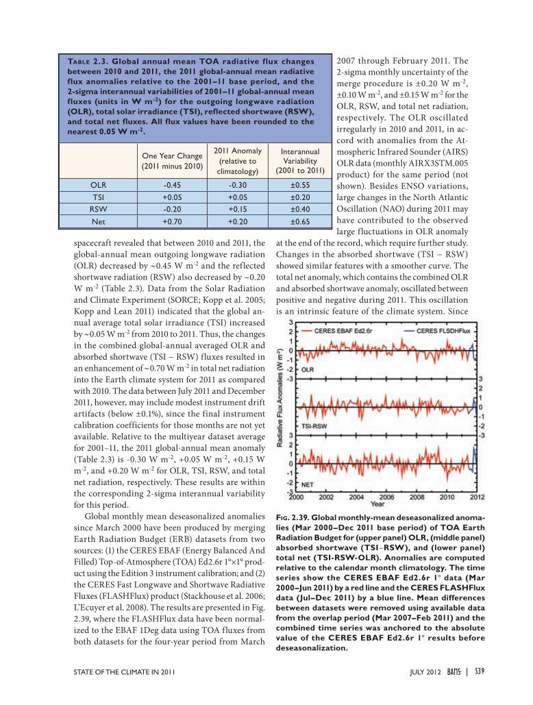
S39STATE OF THE CLIMATE IN 2011 |JULY 2012
spacecraft revealed that between 2010 and 2011, the global-annual mean outgoing longwave radiation (OLR) decreased by 0.45 W m-2 and the reflected shortwave radiation (RSW) also decreased by ~0.20 W m-2 (Table 2.3). Data from the Solar Radiation and Climate Experiment (SORCE; Kopp et al. 2005; Kopp and Lean 2011) indicated that the global an-nual average total solar irradiance (TSI) increased by 0.05 W m-2 from 2010 to 2011. Thus, the changes in the combined global-annual averaged OLR and absorbed shortwave (TSI " RSW) fluxes resulted in an enhancement of 0.70 W m-2 in total net radiation into the Earth climate system for 2011 as compared with 2010. The data between July 2011 and December 2011, however, may include modest instrument drift artifacts (below ±0.1%), since the final instrument calibration coefficients for those months are not yet available. Relative to the multiyear dataset average for 2001–11, the 2011 global-annual mean anomaly (Table 2.3) is -0.30 W m-2, +0.05 W m-2, +0.15 W m-2, and +0.20 W m-2 for OLR, TSI, RSW, and total net radiation, respectively. These results are within the corresponding 2-sigma interannual variability for this period.
Global monthly mean deseasonalized anomalies since March 2000 have been produced by merging Earth Radiation Budget (ERB) datasets from two sources: (1) the CERES EBAF (Energy Balanced And Filled) Top-of-Atmosphere (TOA) Ed2.6r 1°#1° prod-uct using the Edition 3 instrument calibration; and (2) the CERES Fast Longwave and Shortwave Radiative Fluxes (FLASHFlux) product (Stackhouse et al. 2006; L’Ecuyer et al. 2008). The results are presented in Fig. 2.39, where the FLASHFlux data have been normal-ized to the EBAF 1Deg data using TOA fluxes from both datasets for the four-year period from March
2007 through February 2011. The 2-sigma monthly uncertainty of the merge procedure is ±0.20 W m-2, ±0.10 W m-2, and ±0.15 W m-2 for the OLR, RSW, and total net radiation, respectively. The OLR oscillated irregularly in 2010 and 2011, in ac-cord with anomalies from the At-mospheric Infrared Sounder (AIRS) OLR data (monthly AIRX3STM.005 product) for the same period (not shown). Besides ENSO variations, large changes in the North Atlantic Oscillation (NAO) during 2011 may have contributed to the observed large fluctuations in OLR anomaly
at the end of the record, which require further study. Changes in the absorbed shortwave (TSI " RSW) showed similar features with a smoother curve. The total net anomaly, which contains the combined OLR and absorbed shortwave anomaly, oscillated between positive and negative during 2011. This oscillation is an intrinsic feature of the climate system. Since
One Year Change(2011 minus 2010)
2011 Anomaly (relative to climatology)
InterannualVariability
(2001 to 2011)
OLR -0.45 -0.30 ±0.55TSI +0.05 +0.05 ±0.20
RSW -0.20 +0.15 ±0.40
Net +0.70 +0.20 ±0.65
TABLE 2.3. Global annual mean TOA radiative flux changes between 2010 and 2011, the 2011 global-annual mean radiative flux anomalies relative to the 2001–11 base period, and the 2-sigma interannual variabilities of 2001–11 global-annual mean fluxes (units in W m-2) for the outgoing longwave radiation (OLR), total solar irradiance (TSI), reflected shortwave (RSW), and total net fluxes. All flux values have been rounded to the nearest 0.05 W m-2.
FIG. 2.39. Global monthly-mean deseasonalized anoma-lies (Mar 2000–Dec 2011 base period) of TOA Earth Radiation Budget for (upper panel) OLR, (middle panel) absorbed shortwave (TSI"RSW), and (lower panel) total net (TSI-RSW-OLR). Anomalies are computed relative to the calendar month climatology. The time series show the CERES EBAF Ed2.6r 1° data (Mar 2000–Jun 2011) by a red line and the CERES FLASHFlux data (Jul–Dec 2011) by a blue line. Mean differences between datasets were removed using available data from the overlap period (Mar 2007–Feb 2011) and the combined time series was anchored to the absolute value of the CERES EBAF Ed2.6r 1° results before deseasonalization.
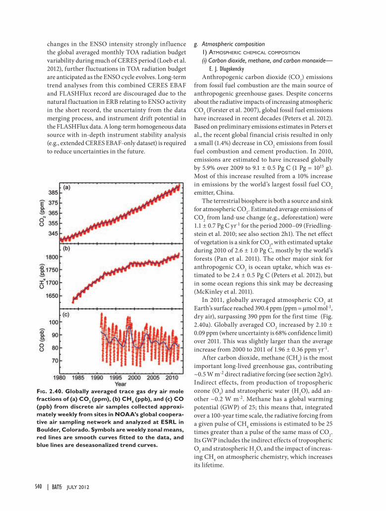
S40 | JULY 2012
changes in the ENSO intensity strongly inf luence the global averaged monthly TOA radiation budget variability during much of CERES period (Loeb et al. 2012), further fluctuations in TOA radiation budget are anticipated as the ENSO cycle evolves. Long-term trend analyses from this combined CERES EBAF and FLASHFlux record are discouraged due to the natural fluctuation in ERB relating to ENSO activity in the short record, the uncertainty from the data merging process, and instrument drift potential in the FLASHFlux data. A long-term homogeneous data source with in-depth instrument stability analysis (e.g., extended CERES EBAF-only dataset) is required to reduce uncertainties in the future.
g. Atmospheric composition1) ATMOSPHERIC CHEMICAL COMPOSITION
(i) Carbon dioxide, methane, and carbon monoxide— E. J. Dlugokencky Anthropogenic carbon dioxide (CO2) emissions
from fossil fuel combustion are the main source of anthropogenic greenhouse gases. Despite concerns about the radiative impacts of increasing atmospheric CO2 (Forster et al. 2007), global fossil fuel emissions have increased in recent decades (Peters et al. 2012). Based on preliminary emissions estimates in Peters et al., the recent global financial crisis resulted in only a small (1.4%) decrease in CO2 emissions from fossil fuel combustion and cement production. In 2010, emissions are estimated to have increased globally by 5.9% over 2009 to 9.1 ± 0.5 Pg C (1 Pg = 1015 g). Most of this increase resulted from a 10% increase in emissions by the world’s largest fossil fuel CO2 emitter, China.
The terrestrial biosphere is both a source and sink for atmospheric CO2. Estimated average emissions of CO2 from land-use change (e.g., deforestation) were 1.1 ± 0.7 Pg C yr-1 for the period 2000–09 (Friedling-stein et al. 2010; see also section 2h1). The net effect of vegetation is a sink for CO2, with estimated uptake during 2010 of 2.6 ± 1.0 Pg C, mostly by the world’s forests (Pan et al. 2011). The other major sink for anthropogenic CO2 is ocean uptake, which was es-timated to be 2.4 ± 0.5 Pg C (Peters et al. 2012), but in some ocean regions this sink may be decreasing (McKinley et al. 2011).
In 2011, globally averaged atmospheric CO2 at Earth’s surface reached 390.4 ppm (ppm = $mol mol-1, dry air), surpassing 390 ppm for the first time (Fig. 2.40a). Globally averaged CO2 increased by 2.10 ± 0.09 ppm (where uncertainty is 68% confidence limit) over 2011. This was slightly larger than the average increase from 2000 to 2011 of 1.96 ± 0.36 ppm yr-1.
After carbon dioxide, methane (CH4) is the most important long-lived greenhouse gas, contributing ~0.5 W m-2 direct radiative forcing (see section 2g1v). Indirect effects, from production of tropospheric ozone (O3) and stratospheric water (H2O), add an-other ~0.2 W m-2. Methane has a global warming potential (GWP) of 25; this means that, integrated over a 100-year time scale, the radiative forcing from a given pulse of CH4 emissions is estimated to be 25 times greater than a pulse of the same mass of CO2. Its GWP includes the indirect effects of tropospheric O3 and stratospheric H2O, and the impact of increas-ing CH4 on atmospheric chemistry, which increases its lifetime.
FIG. 2.40. Globally averaged trace gas dry air mole fractions of (a) CO2
(ppm), (b) CH4 (ppb), and (c) CO (ppb) from discrete air samples collected approxi-mately weekly from sites in NOAA’s global coopera-tive air sampling network and analyzed at ESRL in Boulder, Colorado. Symbols are weekly zonal means, red lines are smooth curves fitted to the data, and blue lines are deseasonalized trend curves.

S41STATE OF THE CLIMATE IN 2011 |JULY 2012
After about a decade of steady mixing ratios (mole fraction), atmospheric CH4 began increasing again in 2007 (Fig. 2.40b). That increase continued in 2011, although the causes remain uncertain (Dlugokencky et al. 2009;; Rigby et al. 2008). Bousquet et al. (2011) used observations from multiple independent mea-surement programs within a model framework to assess the changes in emissions and sinks responsible for renewed growth in atmospheric CH4. They found that changes in tropical wetland emissions were the dominant driver in 2007, with a minor contribution from Arctic wetlands. For 2008, two independent model approaches were not consistent. Neither a strong increase in emissions from wetlands in the tropics nor the Arctic was implied. They found that changes in the concentration of hydroxyl radical (OH), which would affect the CH4 sink, were less than 1%, and they had only a small impact on observed CH4 changes. During 2011 globally averaged atmospheric CH4 at Earth’s surface increased by ~5 ± 2 ppb (ppb = nmol mol-1, dry air) to an annual mean of 1803 ppb (preliminary values; Fig. 2.40b). The causes are likely related, in part, to increasing emissions from rapidly developing economies in Asia and to larger-than-av-erage emissions from tropical wetlands (Dlugokencky et al. 2009;; Bousquet et al. 2011;; EDGAR 2009).
Carbon monoxide (CO) does not absorb strongly in the thermal infrared region, so it does not contrib-ute directly to radiative forcing. However, it is a key species in atmospheric chemistry, particularly in cy-cling of reactive species like the OH and hydroperoxyl radical (HO2). Changes in the atmospheric CO burden affect the lifetimes of other long-lived greenhouse gases, such as methane, hydrochlorofluorocarbons (HCFCs), and hydrofluorocarbons (HFCs), so it has an indirect effect on climate. No significant long-term trend has been detected in globally averaged CO de-termined from NOAA/ESRL measurements, which began in 1990 (Novelli et al. 2003), but CO anoma-lies occurred during 1997–98, and again in 2002–03 (Fig. 2.40c). These anomalies are likely the result of interannual variability in emissions from tropical and boreal biomass burning. Since the lifetime of CO is relatively short (few months), the CO enhancements quickly disappeared. The preliminary globally aver-aged CO mole fraction in 2011 is ~80.5 ppb, slightly less than in 2010.
(ii) Nitrous oxide and sulfur hexaf luoride—B. Hall, J. W. Elkins, and G. Dutton
Atmospheric nitrous oxide (N2O) and sulfur hexafluoride (SF6) have significant manmade sources
and are two of six gases selected for emission reduc-tion under the Kyoto Protocol of the United Na-tions Framework Convention for Climate Change (UNFCCC). Atmospheric N2O currently has the third strongest climate forcing of the long-lived greenhouse gases after carbon dioxide and methane. Current emissions of N2O are expected to contribute more to future ozone depletion than current emissions of halogenated ozone-depleting substances (ODS) (Ravishankara et al. 2009). Nitrous oxide is produced naturally by both the oxidation of ammonium and the denitrification of nitrate. Significant emissions of N2O can occur following the application of nitro-gen fertilizers (including manure) on agricultural crops (Davidson 2009). Recent work suggests strong sources from tropical land areas with high temporal variability (Kort et al. 2011), although the cause of the variability has not been determined. The mean global atmospheric N2O mixing ratio for 2011 was 324.3 ppb, an increase of 1.1 ppb over 2010 (Fig. 2.41). This year-on-year increase is higher than the average growth rate of 0.75 ± 0.01 ppb yr-1 observed from 1977 to 2010 (Elkins and Dutton 2011).
Sulfur hexafluoride (SF6) is an important green-house gas because it has a large global warming potential (GWP; 23!900 times greater than CO2 for a 100-year time horizon). This large 100-year GWP is primarily the result of its very long atmospheric lifetime of 3200 years (Solomon et al. 2007). Sulfur hexafluoride is primarily used as a dielectric insula-tor for transmission of electricity and emissions are entirely anthropogenic. Its global average mixing ratio in 2011 was 7.31 ppt (ppt = pmol mol-1, dry air), an increase of 0.28 ppt over 2010 (Fig. 2.41). The average
FIG. 2.41. Global average nitrous oxide (N2O, ppb) and sulfur hexafluoride (SF6, ppt) mole fractions deter-mined from NOAA discrete and in situ samples. Error bars for N2O are based on monthly averages (1 std. dev.). Error bars for SF6 are omitted for clarity, and are approx. 0.04 ppt in the 1990s and 0.02 ppt thereafter.

S42 | JULY 2012
linear growth rate was 0.22 ± 0.01 ppt yr -1 from 1995 to 2007. Since 2007, the growth rate has averaged 0.28 ppt yr-1.
(iii) Ozone-depleting gases and their replacements —S. A. Montzka and G. DuttonLong-lived halocarbons are important greenhouse
gases and contribute significantly to present-day radiative forcing. Those halocarbons that contain bromine (Br) and chlorine (Cl) also influence radia-tive forcing indirectly through destruction of strato-spheric ozone. Because of concern over stratospheric ozone depletion, production of many halocarbons has been restricted in recent years through amendments and adjustments to the 1987 Montreal Protocol on Substances that Deplete the Ozone Layer. As a result, mixing ratios of most of the potent ozone-depleting gases have been declining at Earth’s surface; this decline continued in 2011 (Fig. 2.42).
While mixing ratios of many ODSs are declining, those of some halogenated gases continue to increase globally (Fig. 2.42c,d). The most rapid increases are observed for HCFCs and HFCs, which are common replacements for CFCs, halons, and other ODSs. HCFCs contain chlorine and deplete ozone with a reduced efficiency compared to CFCs. HFCs do not participate in ozone-destroying reactions.
Future levels of ozone-depleting halogen in the stratosphere (and, therefore, the threat to strato-
spheric ozone) can be estimated from weighted sums of tropospheric halocarbon abundances. Since the efficiency for Br to destroy ozone is higher than that of Cl, Br atoms are assigned a higher weighting fac-tor (a factor of 60 is used here, after Montzka et al. 2011). These sums are derived from surface-based measurements and are expressed as Equivalent Ef-fective Chlorine (EECl; Fig. 2.42e).
The EECl content of the lower atmosphere de-clined fairly steadily through 2011 at a mean rate
of 27 ppt yr-1 since the peak in 1994 (Fig. 2.42e). Despite these substantial changes, full recovery of stratospheric ozone is not ex-pected until the middle to latter part of the 21st century, owing to the long lifetimes of many of these chemicals (Table 2.4; Montzka et al. 2011). A similar conclusion can also be drawn from measure-ments of trace gases obtained by the AGAGE group (Prinn et al. 2000). Both NOAA and AGAGE measurements show similar trends in EECl in recent years (Montzka et al. 2011). Progress towards EECl declining back to the 1980 level can be readily assessed with the NOAA Ozone-Depleting Gas In-dex (ODGI) in Table 2.4 (Hofmann and Montzka 2009). This index (Fig. 2.43) is derived from EECl (Fig. 2.42e), scaled so that a value
FIG. 2.42. (a)–(d) Atmospheric abundances (global mean tropospheric mixing ratios, dry air mole fraction) of the most abundant CFCs, HCFCs, HFCs, chlorinated solvents, and brominated gases, and (e) changes in atmospheric Equivalent Effective Chlorine (EECl) where EECl is derived
-pearing in the other four panels.
FIG. 2.43. Equivalent Effective Stratospheric Chlorine (EESC, left axis) and the Ozone Depleting Gas Index (ODGI) for midlatitudes (right axis) derived from NOAA/GMD data (red) and for various scenarios (blue) (Daniel et al. 2011). EESC is derived from EECl by adding three years to the time axis to represent the lag associated with mixing air from the troposphere to the middle stratosphere where the ozone layer resides.

S43STATE OF THE CLIMATE IN 2011 |JULY 2012
of 100 represents the EECl [or Effective Equivalent Stratospheric Chlorine (EESC)] abundance at its peak, and 0 represents the 1980 level (a reference point during which ozone depletion was thought to have been small). In 2011, the ODGI-Mid-Latitudes
was 66.6. Less progress is evident for the index when the tropospheric data are weighted to be relevant for considering Antarctic changes; the ODGI-Antarctica was 82.4 in 2011.
TABLE 2.4. Mixing ratios, radiative efficiencies, and lifetimes of chemicals considered in the AGGI and ODGI (CO2 mixing ratios in ppm, N2O and CH4 in ppb, all others in ppt).
Industrial Designation or Common Name
Chemical Formula AGGI ODGI
Radiative Efficiency
(W m-2 ppb-1)a
Mean Sur-face Mixing Ratio 2011
[change from prior
year]b
Lifetime(year)a
Carbon Dioxide CO2 Y N 1.41 x 10⁻⁵ 390.4[1.9] c
Methane CH4 Y N 3.7 x 10⁻⁴ 1803.0[3.8]c ~9
Nitrous oxide N2O Y N 3.03 x 10⁻³ 324.2[1.1] 114
ChlorofluorocarbonsCFC-11 CCl3F Y Y 0.25 238.5[-2.1] 45
CFC-12 CCl2F2 Y Y 0.32 527.4[-2.6] 100
CFC-113 CCl2FCClF2 Y Y 0.30 74.7[-0.7] 85
HydrochlorofluorocarbonsHCFC-22 CHClF2 Y Y 0.20 212.6[6.8] 11.9
HCFC-141b CH3CCl2F Y Y 0.14 21.3[0.9] 9.2
HCFC-142b CH3CClF2 Y Y 0.20 21.0[0.8] 17.2
Hydrofluorocarbons
HFC-134a CH2FCF3 Y N 0.16 62.6[5.4] 13.4
HFC-152a CH3CHF2 Y N 0.09 6.5[0.4] 1.5
HFC-143a CH3CF3 Y N 0.13 11.1[1.0] 47.1
HFC-125 CHF2CF3 Y N 0.23 9.7[1.4] 28.2
HFC-23 CHF3 Y N 0.19 24.0[0.8] 222
Chlorocarbons
Methyl Chloroform CH3CCl3 Y Y 0.06 6.3[-1.3] 5.0
Carbon Tetrachloride CCl4 Y Y 0.13 87.1[-1.3] 26
Methyl Chloride CH3Cl N Y 0.01 538[-1.9] 1.0
Bromocarbons
Methyl Bromide CH3Br N Y 0.01 7.05[-0.03] 0.8
Halon 1211 CBrClF2 Y Y 0.30 4.0[-0.1] 16.0
Halon 1301 CBrF3 Y Y 0.32 3.2[0.02] 65
Halon 2402 CBrF2CBrF2 Y Y 0.33 0.45[-0.01] 20
Fully fluorinated species
Sulfur Hexafluoride SF6 Y N 0.52 7.31[0.28] 3,200
PFC-14 CF4 N N 0.10 79.0[0.7] c > 50 000
PFC-116 C2F6 N N 0.26 4.2[0.11] c > 10 000
a Radiative efficiencies and lifetimes are taken from Daniel et al. (2011), Montzka et al. (2011), and Prinn et al. (2005). For CO2, numerous removal processes complicate the derivation of a lifetime.
b Mixing ratios are global surface means determined from the NOAA global cooperative sampling network (Hofmann et al. 2006), except for PFC-14 and PFC-116, and HFC-23 which were measured by the AGAGE group (Mühle et al. 2010; Miller et al. 2010).
c Preliminary estimate for 2011.

S44 | JULY 2012
(iv) Perfluorocarbons—J. MühlePerfluorocarbons (PFCs) are extremely long-lived,
potent greenhouse gases. PFC-14 (CF4) and PFC-116 (C2F6) have lower limits for atmospheric lifetimes of 50!000 and 10!000 years, respectively, and global warming potentials (100-year time horizon) of 7390 and 12!200, respectively (Montzka et al. 2011). An-thropogenic PFC-14 and PFC-116 were historically emitted as by-products of aluminum production (IAI 2011) and are also emitted from the electronics indus-try. However, the onset and extent of PFC emissions from the electronics industry is poorly known due to limited reporting (Worton et al. 2007;; Mühle et al. 2010). A small natural source of CF4 from degassing of Earth’s crust has been identified (Harnisch and Eisenhauer 1998;; Harnisch et al. 2000), which, be-cause of its extraordinarily long atmospheric lifetime, accounts for its significant preindustrial abundance (Harnisch et al. 1996a,b) of 34.7 ± 0.2 ppt (Mühle et al. 2010), or ~44% of its 2011 abundance.
Based on preliminary data, global average surface mixing ratios of PFC-14 and PFC-116 were ~79 ppt and ~4.2 ppt in 2011, respectively (Fig. 2.44). Mixing ratios of PFC-14 rose at ~1.1 ppt yr-1 from the late 1970s to the early 1990s and by ~0.7 ppt yr-1 after-wards. Mixing ratios of PFC-116 rose at ~0.09 ppt yr-1 from the late 1970s to the mid-1990s, at ~0.12 ppt yr-1 until the mid-2000s, and at ~0.08 ppt yr-1 in recent years (Mühle et al. 2010 and preliminary data).
(v) The combined influence of long-lived trace gases on the radiative balance of the atmosphere— B. Hall and S. A. MontzkaGreenhouse gases affect the radiative balance
of the atmosphere because they efficiently absorb
terrestrial infrared (IR) radiation. Recent trends in the radiative forcing (RF) of radiatively important gases are shown in Fig. 2.45. The NOAA Annual Greenhouse Gas Index (AGGI) was developed based upon the direct radiative influence from long-lived greenhouse gases, also known as radiative forcing, relative to the preindustrial era (1750; Hofmann et al. 2006). It represents the additional influence (over preindustrial values) due to long-lived trace gases in a given year relative to 1990, the Kyoto Protocol baseline year. Indirect effects (e.g., arising from ozone depletion or water-vapor feedbacks) are not consid-ered in this index. The index is derived from global surface measurements of CO2, CH4, N2O, CFC-12, and CFC-11 (the major long-lived greenhouse gases) and 15 minor greenhouse gases (e.g., HCFCs, HFCs; see Table 2.4).
Based on preliminary global mean data through 2011, the increases in the abundances of these gases over their preindustrial values amounted to an addi-tional direct RF to the atmosphere totaling approxi-mately 2.84 W m-2. This compares with 2.18 W m-2 in 1990. Thus, the accumulation of long-lived trace gases in the atmosphere since 1990 has resulted in a 30% increase in RF due to long-lived gases.
2) AEROSOLS—A. Benedetti, J.-J. Morcrette, J. W. Kaiser, and L. T. Jones
Atmospheric aerosols have been recognized as a major source of uncertainty in future climate predic-tion (Forster et al. 2007;; Denman et al. 2007). Most have a general cooling effect, ref lecting incoming solar radiation back to space. However, black car-bon has the potential to enhance warming through absorption of solar radiation (Ramanathan and
FIG. 2.44. Global average surface concentrations of PFC-14 (blue) and PFC-116 (magenta) (ppt) from the AGAGE network (Mühle et al. 2010).
FIG. 2.45. Direct radiative forcing (W m-2) due to long-lived trace gases (left axis), and the radiative forcing from long-lived trace gases, relative to 1990, defined as the Annual Greenhouse Gas Index (right axis). The value of the AGGI was 1.30 in 2011, an increase of 30% since 1990.

S45STATE OF THE CLIMATE IN 2011 |JULY 2012
Carmichael 2008). Quantifying the relative impact of the different aerosol types, including volcanic aerosols and those associated with biomass burning, along with aerosol-induced feedbacks in clouds and
precipitation, is crucial for understanding current climate (Lohmann and Feitcher 2005).
Reanalyses have been heavily used by the scientific community since their introduction in the 1980s (Dee et al. 2011a). Atmospheric composition from reanalyses poses greater problems due to unknown biases in emissions, limited availability of constrain-ing observations, shorter periods covered, and the complexity associated with accounting for all atmo-spheric constituents and modeling their interactions.
ECMWF has recently completed an eight-year reanalysis of atmospheric composition from 2003 to 2010, including aerosols, reactive gases, and green-house gases, under the EU-funded project Monitor-ing Atmospheric Composition and Climate (MACC; Simmons 2010). The aerosol analysis is based on assimilation of aerosol optical depth (AOD) obser-vations (MODIS sensor) and the latest inventories and parameterizations for sea salt, desert dust, black carbon, organic matter, and sulfate aerosol. Pre-liminary assessments show that the MACC aerosol
FIG. 2.46. MACC aerosol reanalysis aerosol optical depth anomaly in carbonaceous aerosols (dominated by biomass burning) for the 2011 Sep–Nov season.
FIG. 2.47. Aerosol optical depth anomalies for the East Africa/Middle East/Indian Ocean area over Jun–Aug in 2011: (a) sulfate, (b) biomass burning, (c) desert dust, and (d) sea salt. The location of the Nabro volcano (13.36°N, 41.69°E) is marked with a star in (a).

S46 | JULY 2012
reanalysis tends to underestimate Saharan dust and overestimate sea salt. These are constant biases and do not necessarily affect estimates of anomalies. An-thropogenic aerosols, particularly biomass burning, appear to have realistic amplitude and distribution, and benefit from estimates of fire emissions from fire radiative power [Global Fire Assimilation System (GFAS);; Kaiser et al. 2012; Plate 2.1t]. Recently, the MACC reanalysis was extended through 2011 to pro-vide consistent data for this State of Climate report.
A map of time-averaged total AOD anomaly for 2011 is shown in Plate 2.1o, relative to a 2003–10 base period. This shows enhanced total AOD in parts of East Africa and the Middle East, mainly due to an anomalous amount of sulfate and dust, related to the eruption of the volcano Nabro (13.4°N, 41.7°E). A pos-itive anomaly in AOD is also visible over Australia as a result of the intense fire activity during the months of September and October. The biomass burning activity over South America in 2011 appeared to be less intense than climatological expectations. This is shown clearly by September–November anomalies of carbonaceous aerosols, which are dominated by biomass burning (Fig. 2.46; section 2h4).
The boreal summer (JJA) of 2011 (Fig. 2.47) ex-hibited a large anomaly in AOD across the whole of north-equatorial Africa, especially west of the Horn of Africa. This was due to the volcano Nabro, situated in Eritrea, near the Ethiopian border, which erupted from 12 June through 7 July. The combination of volcanic emissions and seasonally dry conditions, i.e., lack of wet removal of soluble aerosol particles (Plate 2.1; Sidebar 7.2), helps to explain the lasting presence of aerosol particles. Large positive anomalies in AOD are evident over the entire Middle East and the Indian Ocean, the latter consistent with an increase in sea salt (Fig. 2.47d).
The MACC reanalysis is constrained by observa-tions of total AOD, hence the redistribution into dif-ferent species is entirely dependent on the model. At
present, the MACC model does not rep-resent volcanic aerosol sources explicitly. Instead, the observed AOD signal from volcanic ash is attributed to other spe-cies. In the region shown in Fig. 2.47, the volcanic ash signal has been attributed mainly to dust and sulfate. Independent data from the AERONET station close to Lake Victoria (Fig. 2.48) show high values of fine-mode AOD starting in the second half of June and persisting through July, which is indicative of the
presence of fine aerosols being advected southward from the volcanic source.
3) STRATOSPHERIC OZONE—M. Weber, W. Steinbrecht, C. Long, V. E. Fioletov, S. H. Frith, R. Stolarski, and P. A. Newman
The 2011 annual mean total ozone was above the 1980–2008 mean in the tropics and below at higher latitudes and, in particular, both polar regions (Plate 2.1p). This pattern is related to the westerly phase of the quasi-biennial oscillation (QBO), as discussed in section 2b3.
Figure 2.49 shows time series of total ozone in polar regions (60 –90 ) from different ground and
FIG. 2.48. Time series of aerosol optical depth (AOD) at the station of ICIPE_Mbita (0.42°S, 34.2°E) during June (left) and July (right) 2011. Red dots are the AERONET total AOD, yellow dots are the AERONET fine-mode AOD. The dark blue line represents the MACC reanalysis total AOD, while the light blue line represents the MACC reanalysis fine-mode AOD.
FIG. 2.49. March and October polar total ozone (in Dobson Units, DU) in the Northern and Southern Hemisphere, respectively. WOUDC ground-based measurements combining Brewer, Dobson, and filter spectrometer data (red: Fioletov et al. 2002, 2008), the merged BUV/SBUV/TOMS/OMI MOD V8 (blue: Stolarski and Frith 2006), and GOME/SCIAMACHY/GOME-2 “GSG” (green: Weber et al. 2007).
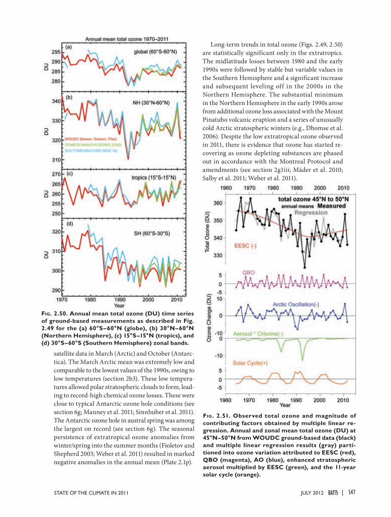
S47STATE OF THE CLIMATE IN 2011 |JULY 2012
satellite data in March (Arctic) and October (Antarc-tica). The March Arctic mean was extremely low and comparable to the lowest values of the 1990s, owing to low temperatures (section 2b3). These low tempera-tures allowed polar stratospheric clouds to form, lead-ing to record-high chemical ozone losses. These were close to typical Antarctic ozone hole conditions (see section 6g; Manney et al. 2011; Sinnhuber et al. 2011). The Antarctic ozone hole in austral spring was among the largest on record (see section 6g). The seasonal persistence of extratropical ozone anomalies from winter/spring into the summer months (Fioletov and Shepherd 2003; Weber et al. 2011) resulted in marked negative anomalies in the annual mean (Plate 2.1p).
Long-term trends in total ozone (Figs. 2.49, 2.50) are statistically significant only in the extratropics. The midlatitude losses between 1980 and the early 1990s were followed by stable but variable values in the Southern Hemisphere and a significant increase and subsequent leveling off in the 2000s in the Northern Hemisphere. The substantial minimum in the Northern Hemisphere in the early 1990s arose from additional ozone loss associated with the Mount Pinatubo volcanic eruption and a series of unusually cold Arctic stratospheric winters (e.g., Dhomse et al. 2006). Despite the low extratropical ozone observed in 2011, there is evidence that ozone has started re-covering as ozone depleting substances are phased out in accordance with the Montreal Protocol and amendments (see section 2g1iii; Mäder et al. 2010; Salby et al. 2011; Weber et al. 2011).
FIG. 2.50. Annual mean total ozone (DU) time series of ground-based measurements as described in Fig. 2.49 for the (a) 60°S–60°N (globe), (b) 30°N–60°N (Northern Hemisphere), (c) 15°S–15°N (tropics), and (d) 30°S–60°S (Southern Hemisphere) zonal bands.
FIG. 2.51. Observed total ozone and magnitude of contributing factors obtained by multiple linear re-gression. Annual and zonal mean total ozone (DU) at 45°N–50°N from WOUDC ground-based data (black) and multiple linear regression results (gray) parti-tioned into ozone variation attributed to EESC (red), QBO (magenta), AO (blue), enhanced stratospheric aerosol multiplied by EESC (green), and the 11-year solar cycle (orange).

S48 | JULY 2012
Figure 2.51 shows a multivariate linear regression with different explanatory variables considered to be major factors in ozone changes (Steinbrecht et al. 2011) applied to the 45°N–50°N zonal annual mean total ozone from the World Ozone and Ultraviolet Radiation Data Centre (WOUDC) ground data (Fiole-tov et al. 2002, 2008). Major factors include the QBO, AO (Arctic Oscillation), solar activity, major volcanic eruptions, and changes in stratospheric halogen or EESC (Equivalent Effective Stratospheric Chlorine; Newman et al. 2007). The large downward swing in ozone from 2010 to 2011 follows the large changes in AO (-12 DU) and QBO (-5 DU). The anthropogenic ozone recovery as expressed by the EESC curve is a modest increase of 3 DU since 1997.
Following an upper stratospheric decline of 10% to 15% from the early 1980s to the mid-1990s, mainly attributed to the anthropogenic release of ozone de-pleting substances (ODS), upper stratospheric ozone has leveled off. In the last 10 years, the various records even show signs of an increase (Steinbrecht et al. 2009; Jones et al. 2009; WMO 2011).
Ozone trends in the tropical lowermost strato-sphere are mainly driven by tropical upwelling (SPARC 2010; Lamarque and Solomon 2010). Randel and Thompson (2011) observed a negative trend of
-2% to -4% decade-1 in the 17-km – 21-km altitude range from a combination of satellite (SAGE I+II) and ozonesondes. This indicates a long-term increase in the tropical upwelling and associated strengthening of the meridional circulation.
4) STRATOSPHERIC WATER VAPOR—D. Hurst and K. RosenlofStratospheric water vapor continued to increase
during 2011 over most of the globe, but the anomalies varied significantly with latitude and altitude. Based on data from the Aura Microwave Limb Sounder (MLS), lower stratospheric tropical anomalies at 82 hPa were strongly positive during January, and high southern latitude anomalies were strongly negative during July (Fig. 2.52). Negative anomalies that en-circled Antarctica during July were likely associated with polar vortex dehydration. In the tropics, the coldest temperatures that determine stratospheric entry values of water vapor occur near 82 hPa. Entry values are normally lowest in January and highest in July, so the positive tropical anomalies in January imply that 2011 annual minimum cold point tem-peratures were warmer than the 2005–10 January average. Lower stratospheric water vapor anomalies
FIG. 2.52. Global stratospheric water vapor anomalies (ppmv) at 82 hPa for January (upper) and July (lower) 2011 from the Aura Microwave Limb Sounder (MLS).
FIG. 2.53. Time series of MLS vertical profiles of monthly water vapor mixing ratios (upper) and anomalies (lower; 2005–10 base period) in the tropics (15°N–15°S). The prominent and reoccurring lower stratospheric QBO signals observed from 2004–08 are not apparent during 2009–11 (lower figure).

S49STATE OF THE CLIMATE IN 2011 |JULY 2012
during January were strongest over the central Pacific region. The underlying dynamical mechanisms (see below) are unclear.
Time series of water vapor vertical profiles and their anomalies from August 2004 through 2011 also show the strong positive anomaly in the tropical lower stratosphere during January–February 2011 (Fig. 2.53). Unlike the previous dry anomalies that originated in the lower tropical stratosphere and propagated to the upper stratosphere, the strong Janu-ary 2011 wet anomaly was almost completely eroded before reaching the middle stratosphere. The weak vertical propagation of this strong anomaly suggests a slowing of the tropical upwelling.
Time series of lower stratospheric water vapor anomalies at three locations where routine frost point hygrometer soundings are made (Fig. 2.54) depict increasing trends since late 2004. These are from MLS
and balloon-borne frost point hygrometer measure-ments. The current water vapor increase started after a rapid drop of ~0.5 ppmv (10%) in 2000–01 and sev-eral subsequent years of low mixing ratios. Over the longer term, the frost point hygrometer record over Boulder, Colorado (40°N), depicts a net increase of 1.0 ± 0.2 ppmv (27 ± 6%) from 1980 to 2010 (Hurst et al. 2011). Only about 30% of this long-term growth is attributable to increased stratospheric water vapor production associated with increasing atmospheric methane (section 2g1i). Complete global satellite-based water vapor records are too short to corrobo-rate or refute the magnitude of the 30-year Boulder trend. High spatial and temporal coverage began with operational MLS in August 2004. Before then, satellite-borne solar occultation instruments did not offer complete global measurement coverage, while balloon-borne frost point hygrometers provided data with sparse spatial and temporal density.
The MLS record reveals strong tropical water vapor signals related to the QBO from 2004 through 2008 (Figs. 2.53, 2.54; Zhou et al. 2001). The QBO influence results in a quasi-two-year cycle of low and high water vapor values originating at ~100 hPa and propagating upward with time. Damped QBO signals are also apparent at higher latitudes prior to 2009 (e.g., Lauder and Boulder). Since 2009, these QBO signals are no longer evident in the tropical and midlatitude water vapor records.
In summary, the increasing trend in stratospheric water vapor since ~2006 continued through 2011. Large positive anomalies in tropical entry values (82 hPa) during January–February 2011 point to abnormally warm tropical cold point temperatures. Anomalies in tropical entry values related to the QBO during 2004–08 have not been observed since 2009. The exact mechanisms behind the 2011 stratospheric water vapor anomalies are currently unknown and require additional study.
h. Land surface properties 1) FOREST BIOMASS AND BIOMASS CHANGE—S. Quegan, P. Ciais, and A. BacciniThe focus of recent forest biomass estimates has
been on: (1) reducing the large uncertainties in the tropical land use change flux and the associated tropi-cal sink due to regrowth of secondary forest; (2) quan-tification of the tropical sink in intact forest; and (3) identification of the location, cause, and strength of the land carbon sink at temperate and boreal latitudes consistently seen in atmospheric inversion studies (e.g., http://transcom.lsce.ipsl.fr). A major motiva-
FIG. 2.54. Lower stratospheric water vapor anomalies (ppmv; differences from 2005–10 monthly averages) from three frost point sonde locations: Boulder, Colo-rado, USA; San Jose, Costa Rica; and Lauder, New Zealand. Blue symbols depict mean anomalies be-tween 16 km and 18 km for individual soundings with balloon-borne frost point hygrometers; black lines are monthly mean anomalies at 82 hPa from MLS retrievals within ±2° latitude and ±15° longitude of the sonde sites; purple lines are MLS zonal monthly mean anomalies at 82 hPa within the ±2° latitude band surrounding each sonde site.

S50 | JULY 2012
SIDEBAR 2.3: LONG-TERM CHANGES OF ATMOSPHERIC SOLAR TRANSMISSION—E. DUTTON
Both the solar and thermal infrared transmission of the atmosphere play important roles in Earth’s energy balance. For example, the anticipated long-term worldwide decrease in infrared atmospheric transmission, due to increasing green-house gas abundance, gives rise to the issues and concerns of global warming. Similarly, long-term increases in the solar transmission would contribute to warming, while a decrease would have the opposite effect. While considerable attention and effort has gone into observations necessary to track and understand the long-term global background of the atmo-spheric infrared transmission, relatively few similar records of the solar transmission exist.
One of the longest, continuous observational records of solar transmission through the free troposphere and above is maintained by NOAA at the Mauna Loa observatory in Hawaii (Dutton and Bodhaine 2001). This consists of qualified daily and monthly averages of clear-sky morning “apparent” solar transmission obtained from pyrheliometer observations by the methodology first described by Ellis and Pueschel (1971). The “apparent” is an optical term applied to the solar transmission values used here because they are determined from ratios of direct beam solar irradiances observed at different solar zenith angles (atmospheric paths) such that the computed transmis-sion is relative to the irradiance already transmitted along the shorter path. The irradiance is measured with a calibrated pyrheliometer. The linear calibration factor cancels out in the apparent transmission ratio, yielding a more accurate and stable result.
This measure of solar transmission is particularly sensitive to aerosols. The computational procedure diminishes the ef-fect of water vapor, which is the other major contributor to variable clear-sky solar transmission, due to saturation effects. There is also a minor ozone contribution, although this is not significant on the scale of the variations seen. Spectral aerosol optical depth is also observed (sun photometer) at the site and confirms the primary aerosol role in current observed solar transmission variability. Although only a single site, Mauna Loa can be considered representative of a much larger portion of the Earth because of its remote central Pacific location and high elevation, above most local effects, especially in the early morning during downslope-wind conditions when daily trans-mission measurements are made.
The complete apparent transmission (AT) record (Fig. SB2.7a) shows the extended impact of three major explosive volcanic eruptions (Agung, 1964; El Chichón, 1982; and Pina-tubo, 1991). These injected large quantities of sulfur dioxide (SO2) into the stratosphere, where it was converted to sulfate aerosol and remained for many months while spreading around the world. A certain amount of month-to-month variability and a small amplitude (~0.007 AT) annual cycle (spring minimum, winter maximum) persisting throughout much of the record are also seen. This annual cycle has been attributed to the season-ally enhanced transport of Asian tropospheric aerosol over the
site (Bodhaine et al. 1981). Not so apparent in the record are potential variations in the overall background transmission, which have the most enduring effects. Examination of the last decade (Fig. SB2.7b) and other information by Solomon et al. (2011) has shown a small net downward tendency, possibly due to multiple periods of injection of stratospheric aerosols. Figure S2.7b suggests a general decrease of about 0.003 AT occurring between 1998 and 2010. This trend is also seen in collocated spectral aerosol optical depth measurements. How-ever, the downturn appears to have ended in the last 2–3 years. Currently, it is not possible to discern a continuing coherent long-term behavior in the record, but the 55-year AT record permits putting the current variability into historical context.
Using these and other data, Solomon et al. (2011) computed that the decline in transmission (or equivalently, an increase in AOD) from the late 1990s to 2010 was sufficient to reduce tropospheric warming by about 0.07°C compared to a scenario with a relatively “clean” stratosphere, as was previously widely used in global climate models for that decade. The source of the general decrease in solar transmission is suspected to be several small, largely unnoticed, volcanic eruptions that together have increased the stratospheric component of the total column aerosol over a large portion of the globe (Vernier et al. 2011).
FIG. SB2.7. Mauna Loa, Hawaii, apparent transmission in (a) monthly means (points), with 5-month running smoother (line) and (b) 100-point running means (con-verging to 49 points at the end of 2011) of available clear-sky morning daily averages from the NOAA MLO observatory at 3.4 km ASL using a tracking solar pyrhe-liometer converted following Ellis and Pueschel (1971). Major explosive volcanoes are indicated. Smoothing in (b) gives anomalous periods with fewer observed days less weight than in the presentation of monthly averages (a).

S51STATE OF THE CLIMATE IN 2011 |JULY 2012
tion for improved information on biomass has also been the UNFCCC Decision 1.1 (2010 Conference of the Parties, Cancun; http://www.unfcc.int/resource/docs/2010/cop16/eng/07a01.pdf) which encourages developing country Parties to contribute to mitigation actions in the forest sector.
Although the periodic reports of the Food and Agricultural Organization (FAO 2006, 2010) remain a key source for information on biomass, they are based on national forest inventories/statistics and suffer from lack of systematic inventory data in many forest biomes, particularly in developing countries, leading to data gaps, sampling biases, inconsistency of meth-ods, lack of spatial information, and unrepresentative samples (Grainger 2008). The search for more con-sistent global approaches, particularly for the tropics, has prompted use of satellite data calibrated against
in situ biomass, with special emphasis on using the archive of forest height estimates derived from the Geoscience Laser Altimeter System onboard the Ice, Cloud and land Elevation Satellite (ICESat) before its failure in 2009 (Lefsky 2010). This approach has given rise to two recent pan-tropical biomass maps (Saatchi et al. 2011; Baccini et al. 2012) at grid scales of 1 km and 0.5 km, respectively. The continental scale aggregates of above-ground biomass from the two maps are 94.6 Pg C, 50.2 Pg C, and 48.3 Pg C (Saatchi et al. 2011) and 117.7 Pg C, 46.5 Pg C, and 64.5 Pg C (Baccini et al. 2012) for South America, Asia, and Africa, respectively. Baccini et al. (2012) exploit these new biomass estimates to recalculate the tropical land use change flux as 0.96 Pg C yr-1 for the period 2000–10, which is 11–12% lower than the recent global assessment of Friedlingstein et al. (2010; Fig. 2.55); both studies use the same rates of deforestation, taken from FAO (2010).
In contrast, Pan et al. (2011) took a bottom-up ap-proach to estimating forest sinks and sources, based on estimates from inventory data and field observa-tions coupled to statistical models.!This builds on national inventory datasets, enhanced by data from research networks [e.g., the tropical RAINFOR pro-ject (Malhi et al. 2002)] and new tropical deforestation and tropical forest regrowth estimates, and includes all carbon pools, not just biomass. The world’s for-ests were estimated to yield a net global sink of 1.2 ± 0.9 Pg C yr-1 over the period 2000–07, made up of a net sink of 2.3 ± 0.5 Pg C yr-1 in established forests, regrowth in tropical forests of 1.7 ± 0.5 Pg C yr-1, and tropical deforestation “gross” emissions of 2.8 ± 0.5 Pg C yr-1. Around 73% of the global sink comes from increased biomass, and of this, 80% occurs in the tropics, both from biomass increment in intact forest and regrowth (Table 2.5). Deforestation and Amazon drought caused the biomass increment in tropical intact forest to decrease by 25% in the last decade compared to the 1990s.
As well as these global estimates, there have been important developments at the regional scale. Ma et al. (2012) and Peng et al. (2011) used long-term permanent forest sampling plots to show that recent climate change, especially reduced precipitation, has caused a decline of around 7.3 million tons of carbon per year in the biomass carbon sink in western Canada; this is equal to approximately 4% of Canada’s total annual carbon emissions. Bellassen et al. (2011) demonstrated that good estimates of the forest carbon sink in the intensively managed
FIG. 2.55. Annual net emissions (Pg C yr-1) from land-use change in the tropics calculated by Friedlingstein et al. (2010) and Baccini et al. (2012).
Biomass increment (Tg C yr-1) 1990–99 2000–07
Boreal 117 120Temperate 345 454Tropical intact 1167 870
Tropical regrowth 1361 1497
All tropics 2529 2367
Global 2991 2941
TABLE 2.5. Biomass increments for 1990–99 and 2000–07 by latitude zone; the global values are also shown (values taken from Pan et al. 2011).

S52 | JULY 2012
European forests can be derived by using a process model (ORCHIDEE) to combine the reconstructed forest age structure (a proxy for biomass stocks) with the effects of carbon dioxide (CO2) increase and climate. They found that the aging of forest stands accounts for most of the inventory-observed forest sink across European countries. However, the sink trend is explained predominantly by CO2 fertiliza-tion and by the effects of climate trends (87%), with a smaller contribution (13%) from trends in forest age structure. In the United States, Williams et al. (2012) also used a process model (CASA) driven by satellite observation of disturbance history at very high spatial resolution (Landsat time series data) to separate the effect of forest age structure (disturbance recovery) from those of climate and CO2. They found carbon sinks to be mainly explained by age structure in the South Central, Pacific Northwest, and Pacific Southwest regions. In other regions, the effect of age was smaller. At country scale, the age structure contribution to forest NEP (the sink before harvest and disturbance) was modeled to be 0.16 Pg C yr-1, which is smaller than former estimates based on inventory data (0.27 Pg C yr-1 to 0.41 Pg C yr-1). The difference was attributed either to the effects of CO2 and climate, or to undersampling of disturbed areas by the forest inventory sampling scheme, due to the smaller scale of disturbance compared to the mesh of the US inventory.
2) LAND SURFACE ALBEDO—B. PintyThe land surface albedo, i.e., the fraction of solar
radiation scattered backward by land surfaces, results from complex nonlinear radiation transfer processes determining the amount of radiation that is scattered by the vegetation and its background, transmitted through the vegetation layer, or absorbed by the veg-etation layer and its background.
Figure 2.56 illustrates the range of variations of surface albedo quantities observed for a full year over the globe in the two-dimensional visible (VIS) and near-infrared (NIR) broadband spectral domains. These data result from a resampling of the MODIS white-sky albedo (equivalent to a bihemispherical reflectance under perfect isotropic illumination, i.e., independent from ambient atmospheric conditions) product collection 5 at 0.01° spatial resolution (Schaaf et al. 2002). Partial or full snow cover conditions are associated with a large dynamical range of albedo val-ues particularly in the visible domain. By contrast, the spectral signature of snow-free conditions is restricted to a much smaller domain (Fig. 2.56 bottom left). In the latter instances, the variability in albedo is largely controlled by the amount of vegetation covering the background featured by the Fraction of Absorbed Photosynthetically Active Radiation derived from the JRC-Two-stream Inversion Package (TIP; Pinty et al. 2011a,b). Note that very small changes in vis-ible surface albedo can be associated with significant variations in vegetation dynamics.
FIG. 2.56. MODIS broadband visible and near-infrared white-sky surface albedo (NASA) collection 5 (after re-sampling). Snow-covered pixels (according to the MODIS snow flag) are identified in black. Snow-free pixels are associated with an estimate of the Frac-tion of Absorbed Photosynthetically Active Radiation (derived from the JRC-TIP) represented by the green color scale.
FIG. 2.57. Zonal means of the MODIS white-sky broad-band surface albedo (NASA) normalized anomalies in the (a) visible and (b) near-infrared domain relative to a 2003–11 base period.

S53STATE OF THE CLIMATE IN 2011 |JULY 2012
The geographical distribution of normalized anomalies in visible and near-infrared surface albedo for 2011 relative to a 2003–11 base period (for which two MODIS sensors are available) are shown in Plates 2.1q and r, respectively. Mid- and high-latitude re-gions of the Northern Hemisphere are characterized mainly as a consequence of interannual variations in snow cover amount and duration in winter and spring seasons (section 2c2). The amplitude of these changes can reach ±30% in relative units, and are slightly larger in the visible than in the near-infrared domain. Snow-free regions experienced dramatic variations with noticeable positive anomalies over the southwestern United States as a consequence of the exceptionally persistent summer heat and drought (see section 7b2 for more details). The situation in Australia and southern Africa contrasts notably with strong negative anomalies in both spectral domains. These changes are associated with more favorable veg-etation growing conditions by comparison to previous years (see sections 2d3, 2h3). More subtle variations in albedo occur in a number of other regions, in particular over Central and South America, as well as the intertropical zone of Africa (especially the eastern part), India, and China. These variations are attributed to vegetation dynamics over these regions sensitive to stress from ambient conditions, such as water availability and temperature.
Analysis of the zonally-averaged albedo anomalies in the visible (Fig. 2.57a) and near-infrared (Fig. 2.57b) spectral domain indicates considerable interannual variations related to the occurrence of snow events in winter and spring at mid- and high-latitudes but also in vegetation conditions during the summer periods. Persistent negative
anomalies are noticeable for 2010 and 2011 between 20°S and 40°S.
The amplitude of the globally averaged normal-ized anomalies (Fig. 2.58) are within ±7% (3%) in the visible (near-infrared) domain. Limited positive anomalies dominate the start and end of 2011 while the remaining seasons exhibit well-marked negative anomalies. Figure 2.58 also suggests the presence of spectrally correlated multi-annual variations during 2003–11, with positively biased values at the begin-ning of the record.
3) TE R R E S T R I A L V E G E T A T I O N D Y N A M I C S - FRACTION OF ABSORBED PHOTOSYNTHETICALLY ACTIVE RADIATION—N. Gobron
Significant spatiotemporal variations in vegetation dynamics occurred on regional and continental scales during 2011. The state of vegetation is examined using estimates of the Fraction of Absorbed Photosyntheti-
FIG. 2.58. Globally averaged MODIS White Sky broad-band surface albedo (NASA) normalized anomalies in the (a) visible and (b) near-infrared domain relative to a 2003–11 base period.
FIG. 2.59. SeaWiFS and MERIS 2011 seasonal anomalies (1998–2011 base period) for FAPAR. Positive anomalies indicate favorable vegetation growing conditions (blue) while negative values are markers of vegetation under stress (orange).
FIG. 2.60. SeaWiFS and MERIS 10-day anomalies (1998–2011 base period) of FAPAR by latitude. Gray areas indicate regions where data are unavailable.

S54 | JULY 2012
cally Active Radiation (FAPAR) from 1998 to 2011 (Gobron et. al. 2010). Global anomalies highlight geographical regions subject to changes in 2011 with respect to previous years (Plate 2.1s).
The largest positive (favorable for vegetation) annual anomalies are observed over Australia and southern Africa, northeastern Brazil, central United States, Asia, and central Europe. The strongest nega-tive anomalies occurred over the southern United States and northern Russia, eastern Africa, and Amazonia to a lesser extent. Over central Russia, the extreme negative FAPAR anomalies that occurred in 2010 have recovered towards a more normal state. Australia and southern Africa had plentiful precipita-tion and soil moisture in 2011 (sections 2d3, 2d7, 7e4).
The southern United States, in particular Texas, suffered precipita-tion deficit in spring and a summer heat record, which translated into strong negative seasonal (Fig. 2.59c) and annual anomalies. Amazonia did not fully recover from the droughts of 2010, as the signature of this event is still noticeable. The drought that occurred over the eastern regions of Africa is well depicted, especially at the seasonal level during the first half of the year.
Zonally averaged anomalies (Fig. 2.60) illustrate hemispheric dif-ferences, with persistent negative anomalies occurring over the South-ern Hemisphere during all seasons from approximately 2002 to 2009. In contrast, since 2010, rather strong positive anomalies are observed over regions located between 20°S–40°S. This figure highlights strong sum-mer negative anomalies above 20°S and below 40°S for 2011.
When globally averaged, FAPAR anomalies (Fig. 2.61) indicate that 2011 marked the return of vegeta-tion to a positive state following a more than three-year period of negative departures.
4) BIOMASS BURNING—J. W. KAISER AND G. R. VAN DER WERF
The burning of vegetation releases large amounts of trace gases and aerosols to the atmosphere. While fires occur naturally, humans have modified back-ground fire regimes both by lighting more fires and by modification of land and land cover types. In ad-dition, fire fighting and prescribed burning present a departure from background fire conditions.
Fire emissions for contemporary times are calcu-lated either by multiplying burned area, biomass, and the fraction of biomass that is actually consumed in a fire (Seiler and Crutzen 1980), or by using measure-ments of emitted energy from fires (Wooster et al. 2005). Both approaches rely heavily on satellite data, and the calculated dry matter consumed is subse-quently multiplied by emission factors derived from field measurements to estimate trace gas and aerosol emissions (Andreae and Merlet 2001). The MACC Global Fire Assimilation System (GFAS; Kaiser et al. 2012) developed in the Monitoring Atmospheric Composition and Climate (MACC) project for the European Union’s (EU) GMES (Global Monitoring
Time Period 2003–10 2011 2011 w.r.t. 2003–10
Quantity Mean Range ValueAbsoluteAnomaly
RelativeAnomaly
Global 2043 1774–2312 1987 -57 -3%
N America 99 71–138 111 +11 +12%
C America 65 53–91 72 +7 +11%
SH America 357 177–456 199 -159 -44%
Europe and Mediterranean
37 30–62 26 -11 -30%
NH Africa 413 331–458 409 -5 -1%
SH Africa 521 488–591 564 +42 +8%
N Asia 202 105–470 159 -43 -21%
SE Asia 135 111–162 95 -40 -29%
Tropical Asia 93 22–218 80 -12 -13%
Australia 120 52–176 273 +153 +127%
TABLE 2.6. Annual continental-scale biomass burning budgets in terms of carbon emission (Tg C yr-1) reported in GFASv1.0. Definition of regions as in Kaiser et al. 2011, 2012.
FIG. 2.61. Global average ten-day anomalies with a 6-month running mean (1998–2011 base period) for FAPAR.

S55STATE OF THE CLIMATE IN 2011 |JULY 2012
for Environment and Security) atmospheric services merges both approaches and is capable of estimating emissions in near-real time.
Over 2003–10, GFASv1.0 estimates carbon emis-sions of approximately 2.0 Pg C yr-1. This is in close agreement with estimates from the Global Fire Emis-sions Database (GFED3; Giglio et al. 2010; van der Werf et al. 2010), which has a longer record starting in 1997, but cannot be updated as frequently as GFAS. The 1997–2002 years not included in GFASv1.0 did not deviate much from the 2003–10 period, with the notable exception of 1997–98. At that time, record-high emissions from Indonesia, in combination with higher-than-average emissions from the boreal region and Central America, yielded emissions that were, on a global scale, over 30% above average.
The global fire emissions of 2.0 Pg C in 2011 were close to the 2003–10 climatological mean (Table 2.6). On a regional scale, Australia experienced an exceptionally active fire season; its emission was 127% higher than the 2003–10 average and 47% higher than the largest value reported (for 2001) in the longer time series of GFED3. Plate 2.1t shows that the fires
FIG. 2.62. Biomass burning in terms of annual carbon emission per unit area at 0.5° resolution: (a) climatol-ogy, and (b) values for 2011. Derived from MODIS observations processed in the MACC GFAS (Kaiser et al. 2012).
in 2011 burned mostly in the interior of Australia, while in other years most fires were detected farther north (Fig. 2.62).
In most regions, fire activity increases during fire seasons with drought conditions. This happened in 2011 in Texas and northern Mexico, where hot and dry anomalies are exhibited (Plate 2.1). The larger land surface albedo and lower FAPAR (Plates 2.1q–s) are manifestations of associated vegetation mortality.
In arid regions such as the interior of Australia, however, fire activity is, in large part, a function of available biomass, which depends on rainfall during the wet season preceding the fire season. In Australia, there was enough rainfall (Plate 2.1i) for the grasses in this arid region to form a continuous fuel bed (Plates 2.1q–s), which subsequently burned in austral spring of 2011. The smoke from these fires were recorded as a strong positive smoke aerosol anomaly (Fig. 2.46). A similar mechanism appears to lie behind the in-creased fire activity in southern Africa.
Fire activity in South America was the second low-est since 2003, in line with decreasing deforestation rates reported by the Brazilian Space Agency (INPE 2012). Fires are used in the deforestation process to remove biomass and usually the amount of deforesta-tion and fire activity are related, although 2007 and 2010 saw elevated emissions, possibly related to fires in cerrados (savanna) and degraded forests (Kaiser et al. 2011). The low fire activity is also reflected in a negative aerosol anomaly over South America (Plate 2.1o; Fig. 2.46). In most other regions including the boreal and deforestation regions, fire activity in 2011 was within the 2003–10 range.

S56 | JULY 2012

S57STATE OF THE CLIMATE IN 2011 |JULY 2012
3. GLOBAL OCEANS—M. C. Gregg and M. L. Newlin, Eds.a. Overview—M. C. Gregg and M. L. Newlin
The state of the oceans during 2011 was domi-nated by a moderate-to-strong La Niña during winter 2010/11 in the Pacific Ocean, followed by a return to near-normal conditions until the reemergence of another La Niña in August 2011. A strengthen-ing of a negative Pacific decadal oscillation (PDO) also followed in the second half of 2011, with the development of a positive Indian Ocean dipole in the fall, and above-normal sea surface temperatures (SST) in the tropical North Atlantic and midlatitude southern oceans (section 3b). The global SST cooled by 0.1°C from 2010 to 2011 and changed from the 5th to 12th highest year since 1982, being associated with cooling influences of the 2010–12 La Niña (sec-tion 3b). However, the 2011 global integrals of upper ocean heat content are higher than for all prior years analyzed (section 3c). Overall in 2011, saltier (higher evaporation) regions of the ocean surface continued to be anomalously salty, and fresher (higher precipita-tion) regions anomalously fresh. This pattern, which has held since at least 2004, suggests an increase in the hydrological cycle, consistent with climate model predictions for a warming atmosphere (section 3e). These surface-forced changes extend to subsurface levels (section 3f) where long-term freshening in the water column of high latitudes in the Pacific Ocean is observed. A general year-to-year freshening was also seen in 2011 across much of the Atlantic, as well as in the Indian Ocean.
Relative to the long-term trend, global sea level dropped noticeably in mid-2010 and reached a local minimum in 2011. The drop was linked to the strong La Niña conditions throughout the latter part of 2010 and most of 2011. This sea level drop was followed by a sharp increase in global sea level during the second half of 2011 (section 3i). High values of chlorophyll were observed throughout much of the tropical Pacif-ic Ocean, subtropical North Atlantic Ocean, tropical Indian Ocean, and in portions of the Southern Ocean. Conspicuously low values of chlorophyll were found in the western Indian Ocean, the tropical Atlantic, and globally throughout the subtropics (section 3j). The global net ocean CO2 uptake for the 2010 transi-tion period from El Niño to La Niña is estimated to be 1.30 Pg!C yr-1 (PG = 10 15 g), lower than the 29-year long-term mean of 1.47 Pg!C yr-1 (section 3j). The 2010 global ocean inventory of anthropogenic CO2 is 160 ± 26 Pg!C (estimated using a Green's function method). The ocean inventory represents ~43% and ~29% of fossil fuel and total (fossil fuel and land use changes)
anthropogenic CO2 emissions, respectively, over the industrial period.
On a basin scale, the Pacif ic Ocean was dominated by both a negative Pacific decadal oscillation and two La Niña events (winter and fall). This resulted in below-normal 2011 sea surface temperatures in the tropical Pacific (cool-est since 1985; section 3b). Zonal surface current anomalies in the tropical Pacific basin switched from negative values in late 2010 to El Niño-like (positive) values in early 2011, as SST anomalies reached their peak negative value. For the next months, as the surface current anomaly remained positive, the SST anomaly decreased in magnitude (section 3g). In the latter half of 2011, the surface current anomaly returned to neutral-to-La Niña-like (negative) values, leading the return of cold SST anomalies by several months. The warming trend in the western tropical Pacific and the cool-ing trend in the eastern tropical Pacific from 1993 to 2011 are consistent with a general trade wind intensification during that time period.
The Indian Ocean was influenced by a positive Indian Ocean dipole. The sea surface became fresher in 2011 relative to 2010 in the eastern equatorial Indian Ocean and the western equato-rial Pacific, likely owing to La Niña, but saltier in the western tropical Pacific near 5°S, likely owing to a southward shift in the South Pacific con-vergence zone (section 3e). Overall, the tropical Indian Ocean cooled by 0.24°C from a historical high in 2010.
The Atlantic Ocean is characterized by the remote influence from the previous year El Niño, a persistent negative North Atlantic Oscillation (NAO), and a long-term cooling trend. The ocean net heat flux (i.e., the sum of shortwave radiation, longwave radiation, turbulent latent and sensible heat flux) anomalies showed a tripole structure in the North Atlantic associated with the change of NAO from a negative phase in 2010 to a more positive phase in 2011, and the fluxes were a forc-ing for SST variability (section 3d). The tropical Atlantic SST reached a historical high in 2010, and cooled by 0.33°C from 2010 to 2011 (section 3b). This continued a downward trend in North Atlantic SST since 2006.
After six years of data, a clear seasonal signal is beginning to emerge with a low Meridional Over-turning Circulation (MOC) in April and a high MOC in October. The seasonal cycle of the MOC appears to be largely attributed to seasonal vari-

S58 | JULY 2012
ability in the interior rather than Ekman or Florida current fluctuations. This is being shown as likely due to seasonal upwelling through a direct wind-driven response off Africa (section 3h).
Results for 2010 show the equatorial Pacific (14°N–14°S) was the major source for atmospheric carbon dioxide, emitting about 0.48 Pg!C yr-1, and the temperate oceans between 14° and 50° in both hemispheres are the major sink zones, with an uptake flux of 0.70 Pg!C yr-1 for the northern and 1.05 Pg!C yr-1 for the southern zone. Both CO2 effluxes for the El Niño and La Niña periods in the eastern equatorial Pacific are higher than the 29-year mean fluxes. The highest CO2 effluxes over the past 29 years are due to intensified upwelling of deep water rich in CO2 caused by an increase of wind speed for 2010.
Details on changes in the patterns of variabil-ity from 2010 to 2011 are presented in this chapter. Some sections in this chapter describe the state of the oceans during 2011 whereas others describe 2010 due to lags in availability of quality-controlled data streams. This chapter consists of nine sections describing the ocean climate for 2010 and 2011: (b) Sea surface temperatures, (c) Ocean heat content, (d) Global ocean heat fluxes, (e) Surface salinity, (f) Sub surface salinity, (g) Surface currents, (h) Meridional overturning circulation in the North Atlantic for 2010, (i) Sea level variations, and (j) the global ocean carbon cycle, which is subdivided into sections on air-sea carbon (results mostly for 2010), subsurface carbon inventory (results for 2010), a new section on ocean acidification, and global ocean phytoplankton. Sidebar 3.1 highlights the NASA Aquarius satellite launched June 2011 to study the links between ocean circulation and the global water cycle.
b. Sea surface temperatures—Y. Xue, Z. Hu, A. Kumar, V. Banzon, T. M. Smith, and N. A. RaynerSea surface temperatures (SST) play a key role in
regulating climate and its variability by modulating air-sea fluxes. In particular, slow variations in SST such as those associated with El Niño-Southern Oscil-lation (ENSO), the Atlantic multidecadal oscillation (AMO), the Pacific decadal oscillation (PDO), the Indian Ocean dipole (IOD), and the Atlantic Niño, are a source of potential predictability for climate fluctua-tions on timescales of a season and longer (Deser et al. 2010). A summary of global SST variations in 2011 is provided, with emphasis on the recent evolutions of ENSO, PDO, and IOD, and the 2011 SST is put in the context of the historical record since 1950. To quantify uncertainties in SST variations, three SST
products are analyzed: (1) the Optimal Interpolation SST version 2 (OISST; Reynolds et al. 2002), (2) the Extended Reconstructed SST version 3b (ERSST; Smith et al. 2008), and (3) the Met Office Hadley Centre’s sea ice and SST dataset (HadISST; Rayner et al. 2003). The weekly OISST is a satellite-based analysis that uses in situ data for bias adjustments of the Advanced Very High Resolution Radiometer (AVHRR) data, which has been available since No-vember 1981. The ERSST and HadISST analyses are historical analyses beginning in the 19th century, and both analyses use statistics developed over the more recent period to extend the SST analysis back in time when in situ observations were sparse. The ERSST includes in situ data only, while the HadISST includes both in situ measurements and AVHRR retrievals from 1982 onwards. Thus, all three SST products represent a "bulk" SST at the depth of the ship and buoy instruments, which can range from less than a meter to several meters from the surface. In this section, SST variations are quantified as SST anomalies (SSTAs) defined as departures from the 1981–2010 climatology (http://www.cpc.ncep.noaa.gov/products/people/yxue/sstclim).
The yearly mean SSTA in 2011 was characterized by below-normal SST in the central and eastern tropi-cal Pacific (Fig. 3.1a), reflecting the La Niña condi-tions in early 2011 and then again in fall/winter 2011 (see section 4b for detailed descriptions of the La Niña
FIG. 3.1. (a) Yearly mean OISST anomaly (°C, relative to 1981–2010 base period) in 2011, (b) 2011 minus 2010 OISST anomaly.

S59STATE OF THE CLIMATE IN 2011 |JULY 2012
conditions in 2011). The negative SSTAs in the tropical Pacific extended into the subtropics in both hemispheres and along the west coast of North America, and were surrounded by a horseshoe-like pattern of positive SSTAs in the far western tropical Pacific and the central North and South Pacific. The SSTA pattern in the Pacific Ocean resembled the negative phase of the Pacific decacal oscillation (PDO) pattern of Power et al. (1999), while the SSTA in the North Pacific resembled the negative phase of the PDO pattern of Mantua et al. (1997). Negative SSTA was present in the north-west subtropical Pacific and near the Maritime Continent. Outside of the Pa-cific Ocean, positive SSTA occurred in the western and southern Indian Ocean while alternating positive and negative SSTA prevailed in the North Atlantic.
The 2011 minus 2010 SSTA differ-ences show that relative to the previous year, SST cooled substantially across the tropical oceans and warmed in midlatitude oceans (Fig. 3.1b). The cooling in the tropical Pacific was related to the contrast between La Niña conditions in 2011 and a combination of El Niño followed by La Niña conditions in 2010. The warming in the central North Pacific was associated with strengthening of the nega-tive PDO in the second half of 2011 (see Fig. 3.2c). The cooling near the Kuroshio Extension and in the Indo-Pacific region and the tropical Atlantic was likely associated with the remote influences of the 2009/10 El Niño and the 2010/11 La Niña, and will be discussed in detail later in this section. The substantial cool-ing in the subpolar North At-lantic was probably associated with the evolution of North Atlantic Oscillation (NAO).
The temporal evolution of normalized seasonal mean SSTA in 2011 is shown in Fig. 3.3. The winter 2010/11 (De-cember–February) SSTA was less than -1.5 standard devia-tion (hereafter referred to as STD) in the central tropical
Pacific, indicating a moderate-strength La Niña (Fig. 3.3a). The La Niña conditions weakened dur-ing March–May 2011 (Fig. 3.3b) and SSTA returned to near-normal conditions by June–August 2011 (Fig. 3.3c). However, the decline of La Niña did not continue, and a second La Niña (SSTA is < -0.5 STD) reemerged during September–November 2011 (Fig. 3.3d).
FIG. 3.2. (a) Monthly standardized NAO index from http://www.cpc.ncep.noaa.gov. (b) Time–latitude section of SSTA averaged between 80°W and 10°W. (c) Monthly standardized PDO index. (d) Time–latitude section of SSTA averaged between 160°E and 90°W. SSTA is relative to 1981–2010 base period (°C).
FIG. 3.3. Seasonal mean SSTAs (°C, relative to 1981–2010 base period) for (a) Dec 2010–Feb 2011, (b) Mar–May 2011, (c) Jun–Aug 2011, and (d) Sep–Nov 2011.

S60 | JULY 2012
Following the peak phase of the La Niña conditions in spring 2011, negative SSTA (< -1.5 STD) emerged in the northwest subtropical Pacific and near the Maritime Continent and the positive SSTA in the tropical North Atlantic weakened substantially (from +1.5 STD to +0.5 STD; Fig. 3.3b). The cooling in the Indo-Pacific region and the tropical Atlantic in spring 2011 may be associated with the remote influences of La Niña. The tropical Indian Ocean and tropical Atlantic are usually cooled after the peak phase of La Niña and warmed after the peak phase of El Niño with a 3–6 month lag (Enfield and Mayer 1997; Klein et al. 1999; Hu et al. 2011). By summer 2011, positive SSTA larger than +1.5 STD emerged in the far western tropical Indian Ocean (Fig. 3.3c). In fall 2011, positive SSTA expanded to the whole tropical Indian Ocean except the area south of Java where negative SSTA persisted in summer and fall. The east-west SSTA gradient resembled the positive phase of the IOD pattern (Saji et al. 1999).
The evolution of SSTAs across the tropical oceans is further analyzed using the time-longitude plot of SSTA averaged in 20°S–20°N from October 2009 to December 2011 (Fig. 3.4). In early 2010, the SST
was more than 0.6°C above normal in the eastern tropical Pacific, the western tropical Indian Ocean, and the tropical Atlantic related to the influences of the 2009/10 El Niño. The SST in the tropical North Atlantic actually reached a historical high in April 2010, and this warming has been attributed to the combined effects of the remote inf luences of the 2009/10 El Niño, persistent negative NAO, and long-term trend (Hu et al. 2011). The yearly mean SSTA in the tropical Indian Ocean also reached a historical high in 2010 (see Fig. 3.5b), probably also due to the combined influences of El Niño and long-term trend.
In the tropical Pacific, there was a fast transition from El Niño to La Niña during spring 2010. At about the same time, SST near the Maritime Continent warmed up and the western Indian Ocean cooled down. This was probably related to the return of the La Niña conditions in the tropical Pacific. The SST near the Maritime Continent was more than 0.6°C above normal according to OISST and ERSST but was 0.3°C above normal based on HadISST. The offset between OISST and HadISST is consistent with what was found in 2010 (Xue et al. 2011, figure 3.5), which might be related to differences in satellite bias correc-tion in the two SST products. It is also noted that the peak value of the negative SSTA in the eastern tropi-cal Pacific was about -1.2°C in OISST and HadISST while it was only -0.9°C in ERSST. Based on a simple comparison of the Niño 3.4 SST, the average SSTA in 5°S–5°N, 170°W–120°W, over the period 1982–2011, ERSST generally underestimates the amplitude of strong SST anomalies associated with ENSO, prob-ably due to the lack of satellite observations and the procedure used for SST reconstruction.
In early 2011 when the 2010/11 La Niña reached its peak phase, negative SSTA emerged in the tropical Indian Ocean. There was an eastward propagation of negative SSTA to the Maritime Continent (Fig. 3.3b). During summer 2011, positive SSTA emerged in the far western tropical Indian Ocean and expanded to the central tropical Indian Ocean in fall 2011. The east-west gradient of SSTA led to establishment of positive IOD conditions in July–October 2011 (see CPC’s Monthly Ocean Briefing at http://www.cpc.ncep.noaa.gov/products/GODAS). On the other hand, the tropical North Atlantic SST cooled down substan-tially in spring 2011 under the remote influences of La Niña conditions, but remained about 0.6°C above normal during the North Atlantic hurricane season that favoreds above-normal hurricane activities.
A tripole SSTA in the North Atlantic, character-ized by positive SSTA in the subtropics and high
FIG. 3.4. Time–longitude section of SSTA (°C, relative to 1981–2010 base period) averaged between 20°S and 20°N from Oct 2009 to Dec 2011 for the datasets (a) OISST, (b) HadISST, and (c) ERSST.

S61STATE OF THE CLIMATE IN 2011 |JULY 2012
latitudes and negative SSTA in midlatitudes, per-sisted from spring 2010 to the winter 2010/11 (Figs. 3.2b, 3.3a). Xue et al. (2011) pointed out that the long persistence of the tripole SSTA was largely forced by persistent negative NAO, which often warms the SST in the subtropics and high latitudes, and cools the SST in midlatitudes by modifying evaporative heat loss from the ocean (Deser and Blackmon 1993). When NAO switched to positive in early spring 2011 (Fig. 3.2a), the tripole SSTA weakened substantially (Fig. 3.3b). In the remaining months of 2011, NAO fluctu-ated between positive and negative phases and did not provide consistent forcing to the ocean.
The connection between the two-year La Niña cycle and the persistent negative PDO is explored further. The PDO index is calculated as the standardized time series of the projection onto the first empirical orthogonal function (EOF) of monthly ERSST in the North Pacific north of 20°N in the period 1900–93, following the approach of Mantua et al. (1997) in which the global mean SSTA in each month was first removed be-fore the calculation. Zonal average SSTA between 160°E–90°W was used to highlight the evolution of SSTA associ-ated with the PDO. Figure 3.2d shows that positive SSTA emerged in the central North Pacif ic around June 2010, coincident with the onset of negative phase of the PDO (Figs. 3.2c,d). This also corre-sponded well with the onset of La Niña around June 2010 in the tropical Pacific. The nega-tive PDO intensified to -1.5 during summer 2010 when the mixed layer depth was the shallowest in the central North Pacific. The PDO weak-ened slightly and remained at about -1 from October 2010 to June 2011, and then suddenly intensified to be less than -2 in
July–August 2011. The strengthening of negative PDO was about one month earlier than the strengthening of negative SSTA in the tropical Pacific in August 2011. It appears that the development of negative PDO around June 2010 and strengthening of negative PDO in July 2011 may not be directly forced by La Niña, although the persistence of negative PDO was prob-ably related to forcings from La Niña. A future study is needed to understand the connections between La Niña and negative PDO.
The historical perspective of the yearly mean SSTA in 2011 is shown in Fig. 3.5 as a basin average
FIG. 3.5. Yearly mean SSTA (°C, relative to 1981–2010 base period) from ERSST (bar) and HadISST (blue line) for 1950–2011 (bar) and OISST for 1982–2011 (black line) averaged over the (a) tropical Pacific, (b) tropical Indian Ocean, (c) tropical Atlantic, (d) North Pacific, (e) North Atlantic, and (f) global ocean.

S62 | JULY 2012
for the (a) tropical Pacific, (b) tropical Indian Ocean, (c) tropical Atlantic, (d) North Pacific, (e) North At-lantic, and (f) global ocean. The SSTA time series of OISST are largely consistent with those of ERSST in the common period 1982–2011. However, ERSST is generally warmer than OISST, and the difference can reach 0.1°C in some cases. HadISST also agrees well with OISST and ERSST, except it is generally cooler in the tropical Indian Ocean and the differences can reach 0.2°C.
The mean SSTA in the global ocean has a domi-nant warming trend over which are superimposed interannual variations largely associated with El Niño and La Niña events (Fig. 3.5f). For example, the peaks and valleys in the global ocean SSTA often correspond with those in the tropical Pacific SSTA (Fig. 3.5a). However, the correspondence was not good in 2010, during which the tropical Pacific SST was weakly below normal while the global ocean SST was close to the historical high, which can be attributed to the historical high value in the tropical Indian and tropical Atlantic Ocean. From 2010 to 2011, under the influence of the two-year La Niña cycle, the tropical Pacific SSTA cooled by about 0.14°C (Fig. 3.5a) and became the second coolest year since 1982 ranked us-ing OISST. At the same time, the global ocean SSTA cooled by about 0.1°C (Fig. 3.5f) and became the 12th highest year since 1982.
The tropical Indian Ocean SSTA was dominated by an upward trend with an increase of 0.9°C over the period 1950–2010 when the historical high value was reached (Fig. 3.5b). The interannual variations in the tropical Indian Ocean SSTA corresponded well with those in the tropical Pacific SSTA due to the remote influences of ENSO. From 2010 to 2011, the tropical Indian Ocean SSTA decreased by 0.24°C. In the tropi-cal Atlantic, SSTA increased by 0.33°C from 2009 to 2010 when the historical high value was reached (Fig. 3.5c). From 2010 to 2011, the tropical Atlantic Ocean SSTA decreased by 0.4°C and the cooling tendency was the strongest since 1982. The North Pacific SSTA trended downward from 1950 to 1987, and then re-bounded from -0.5°C in 1987 to 0.31°C in 1990, and has been persistently positive since then (Fig. 3.5d). The North Atlantic SSTA trended downward from 1951 to early 1970s, and then trended upward and reached a historical high in 2006. It has been decreas-ing since 2006 (Fig. 3.5e).
In summary, the 2011 SSTA was characterized by reemergence of the second La Niña in August 2011, strengthening of negative PDO in the second half of 2011, development of positive Indian Ocean dipole
in fall 2011, and positive SSTA in tropical North At-lantic. The 2011 minus 2010 SSTA differences show that SST cooled down substantially cross the tropical oceans but warmed up in midlatitudes.
c. Ocean heat content—G. C. Johnson, J. M. Lyman, J. K. Willis, S. Levitus, T. Boyer, J. Antonov, and S. A. GoodStorage and transport of heat in the ocean are
central to aspects of climate such as El Niño (Zebiak 1989), the North Atlantic Oscillation (Curry and McCartney 2001), hurricanes (Mainelli et al. 2008), sea-level rise (Johnson and Wijffels 2011), the global energy budget (Church et al. 2011), and constraining global warming scenarios (Knutti and Tomassini 2008).
First, an estimate of upper (0 m – 700 m) ocean heat content anomaly (OHCA) for the period 1 January–31 December 2011 (Fig. 3.6a) is discussed, computed from a combination of in situ ocean temperature data (World Ocean Database 2009 – Johnson et al. 2009; and Argo – Roemmich et al.
FIG. 3.6. (a) Combined satellite altimeter and in situ ocean temperature data estimate of upper (0 m – 700 m) ocean heat content anomaly OHCA (109 J m-2) for 2011 analyzed following Willis et al. (2004), but relative to a 1993–2011 base period. (b) The difference of 2011 and 2010 combined estimates of OHCA expressed as a local surface heat flux equivalent (W m-2). For panel comparisons, note that 95 W m-2 applied over one year results in a 3 × 10⁹ J m-2 change of OHCA.

S63STATE OF THE CLIMATE IN 2011 |JULY 2012
2009) and satellite altimetry data following Willis et al. (2004), but displayed relative to a 1993–2011 baseline, hereafter the combined estimate. Changes in the combined estimate between 2011 and 2010 (Fig. 3.6b), as well as a map of the linear trend of the com-bined estimate from 1993 to 2011 and its statistical significance (see Fig. 3.7), are then described. Three different time series of global integrals of in situ only estimates of upper OHCA are presented (see Fig. 3.8). Since OHCA changes are related to depth-integrated ocean temperature changes, increases in OHCA are sometimes referred to below as warming and OHCA decreases as cooling.
In recent years, many of the globally distributed in situ subsurface ocean temperature data are from Argo. Annual estimates of expendable-bathythermo-graph (XBT) fall rate corrections have been applied for deep and shallow probe data using table 2 of Wi-jffels et al. (2008), but with no XBT data used after 2005. Details of fields analyzed here may change after more Argo real-time data are subject to delayed-mode scientific quality control, as more data are reported, and as XBT corrections improve.
The combined estimate of OHCA in 2011 (Fig. 3.6a) shows eddy and meander variability down to the 100-km mapping scales, as does, to a greater extent, the difference of the 2011 and 2010 combined esti-mates (Fig. 3.6b). Strong small-scale spatial variability in OHCA fields is associated with the western bound-ary currents in every gyre, as well as the Antarctic Circumpolar Current (Fig. 3.6b). The difference in the combined estimates between 2011 and 2010 (Fig. 3.6b) illustrates the large year-to-year variability in regional OHCA, with changes reaching or exceeding the equivalent of a 95 W m-2 magnitude surface flux applied over one year (~3 x 10⁹ J m-2). For compari-son, the global average of incident solar radiation on Earth is ~340 W m-2. Ocean advection likely plays a dominant role in many of these changes.
Local sea level anomalies are the result of OHCA and salinity variability throughout the water column, even to the bottom (e.g., Purkey and Johnson 2010), as well as mass signals (Llovel et al. 2009). Despite this, there are many large-scale visual similarities between the combined estimate of upper OHCA (Fig. 3.6a) and sea level (see Fig. 3.26a) fields in 2011. This similarity reflects both the large contribution of upper OHCA variations to sea-level variations and the influence of the altimeter data in the combined estimate.
Large-scale patterns are evident in the combined estimate of OHCA for 2011 (Fig. 3.6a) and its dif-ference from 2010 (Fig. 3.6b). The pattern of annual
mean OHCA (Fig.3.6a) on the equator in the Pacific mostly reflects La Niña conditions, with anomalously low values around the equator in the east and anoma-lously high values in the west. This pattern is to be expected, since the La Niña that began in early 2010 persisted into 2011 (section 3b).
In 2011, the North Pacific shows an OHCA dipole in the midlatitudes west of 160°E (Fig. 3.6a), per-haps associated with a Kuroshio Extension position southward of the long-term mean. The pattern of anomalous warmth in the central Pacific and cold in the subpolar, eastern subtropical, and eastern tropical Pacific is typical of the negative phase of the Pacific decadal oscillation (PDO; Mantua et al. 1997) and La Niña. The band of high OHCA in the South Pacific that extends from the Solomon Islands in the west to about 40°S west of Chile (Fig. 3.6a) has been present at various latitudes since 2006 (see previous State of the Climate reports). This year, it migrated several degrees south of its 2010 position, as seen in the north-south dipole in year-to-year OHCA (Fig. 3.6b), and is associated with anomalous zonal currents in 2011, as well as the change since 2010 (see Fig. 3.17). Wind stress curl changes between 2010 and 2011 (see Fig. 3.10b) are well correlated with this shifting band, as are positive salinity anomalies both surface (see Fig. 3.12) and subsurface (see Fig. 3.14).
Except for a cold anomaly patch centered around 15°S, 75°E, in 2011 the Indian Ocean was mostly higher in OHCA than the base period (Fig. 3.6a). This cold anomaly is associated with a positive anomaly in sea surface salinity (see Fig. 3.12).
In the subpolar North Atlantic, the Labrador Sea remained high in OHCA in 2011 (Fig. 3.6a), although it cooled quite a bit since 2010 (Fig. 3.6b). This ocean cooling is consonant with an increasing NAO index since the very low values in the winter of 2009/10. The continued high OHCA values in the eastern subpolar North Atlantic (Fig. 3.6a) suggest that subtropical influences are strong there (e.g., Johnson and Gruber, 2007), consistent with anomalously salty surface con-ditions in that region in 2010 (see Fig. 3.12). In 2011, a band of low OHCA was still present in the region of the Gulf Stream Extension (Fig. 3.6a), as it was in 2010. This band is consistent with a southward shift of that current (see Fig. 3.17), expected given the low NAO index in the winter of 2009/10 (e.g., Taylor and Stephens 1998). While the tropical Atlantic mostly cooled from 2010 to 2011 (Fig. 3.6b) it remained warmer than the 1993–2011 average (Fig. 3.6a).
A few distinct (Fig. 3.7a) and statistically sig-nificant (Fig. 3.7b) regional patterns stand out in the

S64 | JULY 2012
1993–2011 OHCA local linear trends. In the Indian Ocean, the warming trend was widespread and sta-tistically significant in many locations.
In the Atlantic Ocean, the Labrador, Irminger, and Greenland-Iceland-Norwegian Seas have all trended warmer over 1993–2011 (Fig. 3.7a), reflecting a robust regional warming trend over the interval despite the cooling from 2010 to 2011 (Fig. 3.6b). These changes may be owing to an overall decrease in the NAO index from 1993 to 2011. Eastern portions of the Atlantic also trended warmer across both hemispheres. Areas with warming trends in the Atlantic are widespread, including highly statistically significant trends in eastern portions of both hemispheres. Cooling trends are limited in the Atlantic to the Gulf Stream Extension, probably related to a southward shift in that current, also expected with an overall declining NAO index.
Statistically significant (Fig. 3.7b) 1993–2011 regional trends in the Pacific Ocean (Fig. 3.7a) in-clude warming in the western tropical Pacific and extratropical cooling in the east, consistent (via the geostrophic relation) with general strengthening of
the interior subtropical-tropical circulation attributed to trade wind intensification (Merrifield and Maltrud 2011). The statistically significant warming in the central North Pacific and cooling south of Alaska and off the west coast of North America are also con-sistent with an overall downward trend in the PDO index from 1993 to 2011. There is a similar-looking trend pattern in the South Pacific.
The overall 1993–2010 trends in Southern Ocean OHCA were towards warming, consistent with previ-ous analyses (e.g., Böning et al. 2008), but with some local cooling trends on both sides of the Antarctic Peninsula and near Antarctica in the Indian Ocean (Fig. 3.7a).
FIG. 3.7. (a) Linear trend from 1993 to 2011 of the com-bined satellite altimeter and in situ ocean temperature data estimate of upper (0 m–700 m) OHCA (W m-2) analyzed following Willis et al. (2004). Areas with sta-tistically significant trends are outlined in black. (b) Signed ratio of the linear trend to its 95% uncertainty estimate, with increasing color intensity showing re-gions with increasingly statistically significant trends.
FIG. 3.8. Time series of annual average global integrals of in situ estimates of upper (0 m–700 m) OHCA (1021 J, or ZJ) for 1993–2011 with standard errors of the mean. The NODC estimate (http://www.nodc.noaa.gov/OC5/indprod.html) follows Levitus et al. (2009). Uncertainties are estimated solely from the variance of quarterly estimates of OHCA. The PMEL/JPL/JIMAR estimate is a weighted integral (Lyman and Johnson 2008) using Argo and WOD 2009 (Johnson et al. 2009) data with the Wijffels et al. (2008) Table 2 XBT bias adjustments applied and no XBT data after 2005. Uncertainty estimate methodology follows Lyman et al. (2010). The Hadley estimate applies XBT bias adjustments from Table 1 of Wijffels et al. (2008) to the EN3 dataset (Ingleby and Huddleston 2007; http://www.metoffice.gov.uk/hadobs) and is computed from estimates of monthly OHCA following Palmer et al. (2007). Uncertainty estimate methodology follows Palmer and Brohan (2011) but adds uncertainty in the XBT bias correction. For comparison, all estimates have been individually offset (vertically on the plot), f irst to their individual 2004–11 means (the best sampled time period), and then to their collective 1993–2011 mean (the record length).

S65STATE OF THE CLIMATE IN 2011 |JULY 2012
Three different upper ocean estimates (0 m – 700 m) of globally-integrated in situ OHCA (Fig. 3.8) reveal a large increase in global integrals of that quantity since 1993. While levels appear to be increasing more slowly since around 2003 or 2004 than over the previous decade, the sum of the mass and thermal expansion components of the global sea level budget agree with observed sea-level rise rates since at least 2005 (see Fig. 3.28). The highest values for each global OHCA estimate are for 2011, although uncertainties only permit statistically significant trends to be estimated over about ten years or longer (Lyman 2011). Interannual details of the time series differ for a variety of reasons, including differences in climatology, treatment of the seasonal cycle, map-ping methods, instrument bias corrections, quality control, and other factors (Lyman et al. 2010). Some of these factors are not taken into account in some of the displayed uncertainties, so while the error bars shown do not always overlap among the three esti-mates, they are not necessarily statistically different from each other. However, all three curves agree on a significant warming of the upper ocean since 1993, accounting for a large portion of the global energy imbalance over this time period (Church et al. 2011).
d. Global ocean heat fluxes—L. Yu, P. W. Stackhouse Jr., and R. A. WellerThe net heat f lux (Qnet) at the ocean surface is
the sum of the four air-sea heat transfer processes: shortwave radiation (SW), longwave radiation (LW), latent heat (LH), and sensible heat (SH) fluxes. Solar radiation is the ultimate heat source for the Earth. About 47% of the total solar radiation reaching the Earth is absorbed by the surface ocean and land (Trenberth et al. 2009). Of the energy absorbed by the ocean, some is radiated back to the atmosphere by LW, some is transformed into SH and LH and released to the atmosphere through conduction and evapora-tion, and the remaining energy is either transported by currents or stored and sequestered in the ocean. Knowing how these heat exchange processes balance at the ocean surface and how much the net residual heat flux has changed are fundamental to the under-standing of the role of the ocean in mitigating radia-tive perturbations and modulating the global climate.
Daily estimates of LH and SH on 1° grids over the global oceans are routinely produced by the Objectively Analyzed air-sea Fluxes (OAFlux) project (http://oaflux.whoi.edu) at the Woods Hole Oceanographic Institution (Yu and Weller 2007). The computation of the OAFlux products uses the state-
of-the-art bulk flux algorithm version 3.0 developed from the Coupled Ocean-Atmosphere Response Experiment (COARE;; Fairall et al. 2003), with the surface meteorological variables determined from an optimal blending of satellite retrievals of surface wind and temperatures and surface meteorology from reanalysis/forecast models. The accuracy of the OAFlux LH and SH estimates was evaluated using 120-plus buoys available over the global oceans (Yu et al. 2008). The averaged root-mean-square (rms) differences between OAFlux and buoy over the buoy locations are 9.6 W m-2 (8%) for LH and 2.6 W m-2 (15%) for SH. The OAFlux project also develops global daily vector wind analysis from synergizing passive radiometer wind speed retrievals and radar scatterometer vector wind retrievals (Yu and Jin 2012, manuscript submitted to J. Geophys. Res.). The wind analysis for the post-QuikSCAT (after November 2009) period uses satellite measurements from the Special Sensor Microwave Imager/Sounder (SSMIS), the Advanced Scatterometer (ASCAT) aboard the EUMETSAT METOP satellite, and the WindSat (a passive polarimetric microwave sensor) aboard the Department of Defense Coriolis satellite. Global daily surface SW and LW flux products on
1° grids are now delivered in near real-time (within one week) by the CERES (Clouds and Earth’s Radiant Energy Systems) Fast Longwave And SHortwave Ra-diative Fluxes (FLASHFlux) project (http://flashflux.larc.nasa.gov) at the NASA Langley Research Center (Stackhouse et al. 2006). This output data product is made possible by processing Terra and Aqua observa-tions from CERES and cloud property retrievals from the Moderate-resolution Imaging Spectroradiometer (MODIS) using simplified calibration assumptions with fast radiation algorithms (Kratz et al. 2010). Evaluation of the FLASHFlux surface radiation with ground measurements from the Surface Radiation Budget Network (SURFRAD) stations shows an rms error of 29.3 W m-2 (15.7%) for downward SW and 18.6 W m-2 (6.0%) for downward LW.The annual mean Qnet in 2011 produced by com-
bining FLASHFlux and OAFlux datasets is displayed in Fig. 3.9 (next page). An area-weighted spatial mean of 25 W m-2 was removed to adjust global mean bal-ance. The regions of net heat gain (positive Qnet) and net heat loss (negative Qnet) are in broad agreement with the climatological mean pattern (Josey et al. 1999). The tropical oceans receive an excess of heat energy owing to the high rate of insolation through-out the year, and the strongest heating (> 140 W m-2) is located on the equator in the eastern Pacific. The

S66 | JULY 2012
subtropics and high latitudes experience net heat loss to the atmosphere, with the maximum heat loss (< -140 W m-2) occurring over the western boundary currents (WBCs) in the northern midlatitudes. The primary mechanism of the large net heat loss in the vicinity of the WBCs is latent and sensible heat fluxes in the fall and winter seasons, during which the cold and dry air masses advected from the lands by strong westerly winds induce sharp air-sea temperature and humidity contrasts, intensifying latent and sensible heat release to the atmosphere. The 2011 minus 2010 difference plot of Qnet
(Fig. 3.9b) shows organized large-scale changes in net heat f lux into the global oceans. One marked change was ob-served in the North Atlantic, characterized by a tripole structure with an area of sig-nificant negative anomalies (more ocean heat loss) in the Labrador and Irminger Seas between 45°N and 65°N, a band of positive anomalies (more ocean heat gain) in the midlatitudes centered over the Gulf Stream pathway and stretching northeastward to
the Norwegian Sea, and a band of negative anomalies (more ocean heat loss) in the subtropics between the equator and 30°N. The tripole pattern reflected the atmospheric conditions of a generally more positive NAO phase in 2011 compared to the persis-tently negative phase in 2010 (see Fig. 3.2). The anomaly pattern of surface net radiation SW+LW (Fig. 3.9c) was very similar to that of LH+SH (Fig. 3.9d), but LH+SH accounts more for the magnitude of Qnet anomalies. This is in good agreement with the study of Cayan (1992) that, in the extratropical oceans, the variance in SW and LW is small and Qnet is dominated by the variance of LH and SH. The North Atlantic tripole pattern
is also seen in the 2011 minus 2010 wind speed difference field (Fig. 3.10a), but with opposite signs. The 2011 mean wind vectors is superim-
posed to help characterize the change in prevailing winds. Compared to 2010, there was a strengthen-ing of westerlies across the midlatitudes on a more northerly track and a strengthening of trade winds in the tropical Atlantic. The pattern is consistent with past positive NAO phase (Hurrell 1995;; Visbeck et al. 2001). It can be observed that enhanced LH+SH (negative anomalies in Fig. 3.9d) occurred in regions of strengthened wind speeds (positive anomalies). Similarly, the regions of weakened LH+SH (positive anomalies) coincided with the regions of weakened wind speeds (negative anomalies). Wind direction
FIG. 3.9. (a) Annual mean net heat flux (W m-2) into the ocean (Qnet) in 2011. Positive (negative) values denote ocean heat gain (loss). (b) An-nual mean difference in Qnet between 2011 and 2010. The 2011 minus 2010 mean difference in surface radiation (SW+LW) and turbulent heat fluxes (LH+SH) are shown in (c) and (d), respectively. In (b)–(d), positive (negative) values denote where the ocean gained more (lost less) heat in 2011 compared to 2010.
FIG. 3.10. (a) Differences between the 2011 and 2010 wind speed at 10-m height (colored background), with the 2011 mean wind vector superimposed (black arrows). Positive (negative) values denote a strengthening (weaken-ing) of prevailing winds compared to 2010. (b) Differences between the 2011 and 2010 wind stress curl (colored background), with the wind stress vector differences between 2011 and 2010 superimposed (black arrows). Positive (negative) values denote anticyclonic (cyclonic) curl anomalies.

S67STATE OF THE CLIMATE IN 2011 |JULY 2012
is also important. For instance, the excessive tur-bulent heat loss in the Labrador and Irminger Seas resulted from both the intensified subpolar cyclonic wind circulation and the cold and dry air advected to the region by the westerlies. It is known that the basin-scale NAO SST variability is driven primarily by the atmospheric forcing via the effects of LH+SH, mixing, and the wind-driven Ekman currents (Cayan 1992; Deser and Blackmon 1993). The 2011 surface warming tendency of the North Atlantic Ocean from 2010 corresponded well with positive (more ocean heat gain) Qnet anomaly and concurring negative (weakened) wind anomaly. Meanwhile, the regional surface cooling tendency also correlated well with negative (more ocean heat loss) Qnet anomaly and positive (strengthened) wind anomaly. The North Atlantic is clearly an example that surface net heat flux is a forcing for SST anomalies.
Surface heat flux plays a dual role in dynamics of large-scale SST anomalies. While it contributes to the generation of SST anomalies in the North Atlantic, surface heat flux also responds to the SST anomalies that have been generated from other processes and can act to oppose those anomalies. The latter role of Qnet is displayed in the Pacific and Indian Oceans. The sea surface in the eastern part of the Pacific in 2011 was dictated by a developing La Niña in the tropics and negative PDO phase in the North Pacific. Compared to 2010, colder SST anomalies appeared over the central tropical Pacific between 160°E and 120°W with a center on the equator near the date line (see Fig. 3.1). In general, the upper OHCA year-to-year tendency also appears to be damped by year-to-year changes in Qnet. Unlike the North Atlantic where negative SST anomalies were well correlated with negative Qnet anomalies, the negative SST anomalies here were associated with positive Qnet anomalies that can be attributed primarily to the LH+SH com-ponent. In the tropics, ENSO SSTs are governed by ocean dynamics through wind-driven upwelling of cold water from the thermocline (Wyrtki 1981). The cooler ocean surface led to a weaker evaporative heat loss, which together with enhanced downward radia-tion, resulted in more downward Qnet. In the tropical Indian Ocean, SST anomalies follow the ENSO index. As the regional sea surface cooled from 2010 to 2011, an increase in Qnet, owing to reduced evaporative heat loss and enhanced radiation, was also observed. These positive Qnet anomalies acted as a damping to the existing negative SST anomalies, suppressing the growth of ENSO-induced SSTs.
Consistent with past La Niña events (Ropelewski and Halpert 1989), the western Pacific warm pool and deep tropical convection in 2011 were retracted to the far west of the date line. As a result, the convection across the Maritime Continent was enhanced. The increased cloudiness led to a reduction of downward SW+LW by more than 10 W m-2 and dominated the change of Qnet in the region. Away from the con-vergence center in both zonal directions, convection was suppressed in both directions, resulting in large increase in SW+LW (> 15 W m-2) across the central equatorial Pacific and eastern Indian Oceans. Cor-responding change in wind was evident, with weaker wind speed in the center of convergence and enhanced equatorial westerlies in the Indian Ocean and enhanced easterlies near the date line. The change in wind speed governed the change in LH+SH in the warm pool (Zhang and McPhaden 1995). It can be seen that the tropical western Pacific and eastern Indian Oceans were regions where the SW+LW anomalies compen-sated the LH+SH anomalies in producing the Qnet anomalies. In other regions such as the eastern Pacific and North Atlantic, the SW+LW anomalies worked in concert with the LH+SH anomalies to increase the Qnet anomalies.
In the North Pacific, Qnet served primarily as a forcing for the PDO SSTs, and the anomalies of the two variables have the similar sign. In the southern oceans between 30°S and 50°S, the Qnet anomalies were overwhelmingly negative due to the increased heat loss by LH+SH in response to positive SST anomalies. The changing relationships between Qnet and SST with the ocean basins demonstrate that the global climate system is ruled by intricate feedbacks between the ocean and the atmosphere. Overall, yearly variability of Qnet over the global
oceans is attributable more to variability of LH+SH.
FIG. 3.11. Year-to-year variations of global aver-aged annual mean latent flux plus sensible heat flux (LHF+SHF; black curve), LHF (red curve), and SHF (blue curve). The shaded areas indicate the error bars of the flux estimates at the 95% confidence level.

S68 | JULY 2012
The long-term perspective of the change in 2011 LH+SH is shown in the annual mean time series averaged over the global oceans from 1958 to 2011 (Fig. 3.11). The 2011 LH+SH was slightly down from the 2010 mean, continuing the downward trend that started around 2000. A tendency toward reversing the upward trend that characterized the decades of 1980s and 1990s is thus indicated. The 54-year time series displays decadal oscillations dominated by LH, with a low at 99 W m-2 in 1977 and a high at 109 W m-2 in 1999. It is worth noting that LH is not only an important component in the global heat and energy balance but also a key component of the freshwater flux over the oceans that contributes to the change of ocean surface salinity (see Fig. 3.13).
e. Sea surface salinity—G. C. Johnson and J. M. LymanOcean storage and transport of freshwater are
intrinsic to aspects of global climate, including the water cycle (e.g., Schanze et al. 2010), El Niño (e.g., Maes et al. 2006), and anthropogenic climate change (e.g., Held and Soden 2006). Only since 2004 has the advent of Argo (an array of profiling floats that measures temperature and salinity year-round in the upper 2 km of the ice-free global ocean, nominally at 10 day intervals and 3 3 spacing; Roemmich et al. 2009) allowed an annual assessment of global upper ocean salinity and its complement, freshwater.
The near-global Argo data are used to determine near-global annual average bulk (viz. near-surface, as opposed to skin) sea surface salinity (SSS) anomalies for 2011 relative to a long-term climatology, describe how annual SSS anomalies have changed in 2011 relative to 2010, and assess 2004–11 SSS trends and their statistical significance. The data, downloaded from an Argo global data assembly center in January 2012, are a mix of real time (preliminary) and delayed mode (scientific quality-controlled). The estimates presented here could change after all the data have been subjected to careful scientific quality control, and as other data sources (e.g., Aquarius satellite, Sidebar 3.1) are integrated into the estimates.
The shallowest salinity value flagged as good from each Argo profile is used in this analysis, generally at 9-m depth, with some as shallow as 4 m, and those with depth > 25 m are excluded. These data are subjected to a statistical check to discard extreme outliers, defined as points within a 3°-radius of a grid point with temperature or salinity values three times the interquartile range above the third or below the first quartiles. After this check, the remaining data are cast as differences from climatological monthly
mean surface salinity fields from the World Ocean Atlas 2009 (WOA 2009; Antonov et al. 2010). The re-sulting anomalies are objectively mapped (Bretherton et al. 1976) for each year using a covariance function combining a 6 (latitude and longitude) length-scale Gaussian with a 9 length-scale exponential and a noise-to-signal variance ratio of 2.2.
Climatological SSS patterns are correlated with surface freshwater flux [the sum of evaporation, pre-cipitation, and river runoff (e.g., Beránger et al. 1999)] but horizontal and vertical advection and mixing are also important in many locations, at least on seasonal time scales (Yu 2011). In each ocean basin, subtropical salinity maxima centered between roughly 20° and 25 in latitude (Fig. 3.12, grey contours) are signatures of the predominance of evaporation over precipita-tion. Conversely, in most regions where climatologi-cal surface salinities are relatively fresh, such as the
FIG. 3.12. (a) Map of the 2011 annual surface salinity anomaly estimated from Argo data [colors in 1978 Practical Salinity Scale (PSS-78)] with respect to monthly climatological salinity fields from WOA 2009 (yearly average, gray contours at 0.5 PSS-78 intervals). (b) The difference of 2011 and 2010 surface salinity maps estimated from Argo data [colors in PSS-78 yr-1 to allow direct comparison with (a)]. White ocean areas are too data-poor to map. While salinity is often reported in practical salinity units, or PSU, it is actually a dimensionless quantity reported on the PSS-78.

S69STATE OF THE CLIMATE IN 2011 |JULY 2012
high latitudes and the intertropical convergence zones (ITCZs), precipitation generally dominates over evaporation.
The 2011 SSS anomalies (Fig. 3.12a, colors) reveal some large-scale patterns that also hold in 2004 through 2011. The regions around the subtropical salinity maxima are on balance salty with respect to WOA 2009. Most of the high-latitude climatologi-cally fresh regions appear fresher than WOA 2009, including in the vicinity of the Antarctic Circumpolar Current near 50 S and in the western subpolar gyre of the North Pacific. These patterns are consistent with an intensified hydrological cycle (that is, more evaporation in drier locations, and more precipita-tion in rainy areas), as seen in simulations of global warming. These simulations suggest this signal might be discernible over the last two decades of the 20th century (Held and Soden 2006), consistent with the multiyear nature of these anomalies. While anoma-lous ocean advection could influence the SSS pattern over decadal time scales, changes observed at the local extrema are presumably relatively insensitive to such effects because horizontal gradients there are minimal. This SSS anomaly pattern and its inter-pretation are consistent with other analyses (Hosoda et al. 2009; Durack and Wijffels 2010). Changes in ocean interior salinity values also appear consistent with an increase in the hydrological cycle (Helm et al. 2010; section 3f).
In contrast to some other high-latitude areas, the subpolar North Atlantic and Nordic Seas in 2011 were mostly anomalously salty with respect to the historical WOA 2009 climatology (Fig. 3.12a, colors), as they have been since at least 2004 (see previous State of the Climate reports). The salty anomaly in this region is consistent with a stronger influence of subtropical gyre waters in the northeastern North Atlantic in recent years coupled with a reduced ex-tent of the subpolar gyre (Häkkinen et al. 2011). On the basin scale, the North Atlantic loses freshwater to the atmosphere whereas the North Pacific gains it (Schanze et al. 2010), so the changes here may again be consistent with an increased hydrological cycle (Durack and Wijffels 2010).
Sea surface salinity changes from 2010 to 2011 (Fig. 3.12b, colors) strongly reflect 2011 anomalies in pre-cipitation (see Fig. 2.21 and Plate 2.1i), and to a lesser extent year-to-year changes in evaporation, with the latter being closely related to latent plus sensible heat flux changes (see Fig. 3.9d). Advection by anomalous
ocean currents (see Fig. 3.17) also plays a role in sea surface salinity changes. For instance, prolonged La Niña conditions over the last few years, associated with an anomalously strong Indonesian Throughflow (England and Huang 2005), may be partly responsible for the freshening observed northwest of Australia, as the throughflow does bring relatively fresh water into the Indian Ocean. Precipitation anomalies in this region, while consistent with freshening, are not large (see Fig. 2.21 and Plate 2.1i). The South Pacific convergence zone also appears to have shifted south from 2010 to 2011, consistent with the dipole in sa-linity changes centered around 10 S in the southwest tropical Pacific. Farther to the southeast, the apparent southward shift in the subtropical surface salinity maximum is associated with year-to-year changes in the ocean heat content (see Fig. 3.6b), so the salty shift is associated with a warm shift.
There are also correspondences between the surface salinity changes from 2010 to 2011 and sub-surface changes over the same period (see Figs. 3.14, 3.15, 3.16). Some of the surface changes are confined mostly to the upper one or two hundred meters, including many of those in the tropics. However, others apparently extend deep into the water column, suggesting influences of shifting ocean currents and fronts. Deeper-penetrating changes are found in the high southern latitudes, near the Antarctic Cir-cumpolar Current, and in the North Atlantic, near the Gulf Stream Extension and the North Atlantic Current.
Trends from 2004 through 2011 are estimated by local linear fits to annual average SSS maps (Fig. 3.13a), as are the ratio of these trends to their 95% significance (Fig. 3.13b). The starting year is 2004, when Argo coverage became near-global. The most striking trend patterns are in the Pacific and Indian Oceans. Saltier surface values in the western and central tropical Pacific extend into the eastern Pacific subtropics in both hemispheres. Some freshening also occurs in the western subtropics of each hemisphere in the Pacific and around the Philippine Sea, extend-ing into the Indian Ocean northwest of Australia (the latter again perhaps owing to the La Niña of the past few years). Large-scale freshening is also evident in the eastern tropical South Pacific. These recent trends differ from the previously reported 50-year trends discussed above. The differences are not surprising given the very different time periods over which the trends are computed.

S70 | JULY 2012
SIDEBAR 3.1: AQUARIUS SATELLITE MISSION PROVIDES NEW, DETAILED VIEW OF SEA SURFACE SALINITY—G. LAGERLOEF, F. WENTZ, S. YUEH, H.-Y. KAO, G. C. JOHNSON, AND J. M. LYMAN
The Aquarius satellite mission (http://aquarius.nasa.gov), launched on 10 June 2011, has been mea-suring sea surface salinity (SSS) from space since 25 August 2011. Aquarius’s primary scientific goal is to study links among the ocean circulation, the global water cycle, and climate by measuring ocean surface salinity (Lagerloef et al. 2008). Recent multidecadal SSS trends provide a strong indication of changes in the global water cycle, with wetter areas gaining in rainfall and low rainfall regions becoming more arid (see section 3e; also Gordon and Giulivi 2008). Aquarius data will allow analyses of these changes at higher spatial and temporal resolution than pres-ently possible with the in situ SSS observing system (Figs. SB3.1-3). Aquarius will complete a year of measurements in autumn 2012, allowing the start of detailed exploration of the annual coupling of SSS, rainfall, surface currents, and sinks such as subduc-tion and vertical mixing. Aquarius data in subsequent years will improve annual cycle statistics, yield new information on ENSO and other interannual climate variations, and advance our understanding of the marine freshwater budget (Lagerloef et al. 2010).
Sea surface salinity data from Aquarius and the previously launched European Soil Moisture Ocean Salinity (SMOS) mission (http://www.esa.int/smos; Font et al. 2004; Lagerloef and Font 2010) provide a fundamentally new ocean remote sensing capability. The Aquarius microwave sensor, built by NASA, is the prime instrument on the joint United States and Argentina Aquarius/SAC-D observatory. The Argentine Comisión Nacional de Actividades Espaciales (CONAE) developed the Satélite de Aplicaciones Científicas (SAC-D) spacecraft, which carries Aquarius and other scientific sensors.
Salinity remote sensing involves measuring the ocean’s surface microwave emission at 1.413 GHz (in the L-band portion of the spectrum protected for radio as-tronomy). This emission is modulated by the electrical conduc-tivity of seawater, hence salinity, of the top few cm. Aquarius also measures radar backscatter at 1.26 GHz, to mitigate the emission variations due to surface roughness (Yueh et al. 2010; Le Vine et al. 2007), the largest error source in the salinity retrieval. Aquarius provides seven-day global coverage and is designed to achieve a monthly average global root-mean-square (rms) measurement error less than 0.2 (PSS-78) at 150-km resolution (Lagerloef et al. 2008).
FIG. SB3.1. (a) Mean global map of the first four months (Sep–Dec 2011) of Aquarius satellite sea surface salinity (PSS-78) measure-ments omitting a land correction (see text) near coastlines and using an optimized combined active-passive algorithm of Yueh and Chaubell (2012). (b) Same as (a) but with the land correc-tion applied, and using the present roughness correction that combines NCEP operational analysis winds and Aquarius scat-terometer data. Data are interpolated to 0.5° grid resolution, and Aquarius data have a 150-km smoothing scale applied.
Aquarius composite four-month mean (September–December 2011) global SSS maps, using two experimental processing algorithms (Figs. S3.1a.b), differ mainly in the inclu-sion of the land correction and also in their methods of surface roughness correction. The size of the Aquarius footprint limits the accuracy for measurements close to coastal boundaries where the land emission adds a negative bias for which a land correction has been developed. The data without the correc-tion (Fig. SB3.2a) exhibit a spurious low-salinity shadow along

S71STATE OF THE CLIMATE IN 2011 |JULY 2012
the continental boundaries that is absent in the image with the correction applied (Fig. SB3.2b). This land correction appears to be effective and will continue to be studied and improved. Both the land and roughness corrections in Fig. SB3.2b are part of the present baseline data processing. Subtle differences between these images in the ocean interior, far from the coast, are associated with a slight difference in roughness correction. Data where wind speed is greater than 15 m s-1 and SST is less than 5°C have been ignored in these figures because the SSS retrievals are not yet reliable under those conditions.
An SSS map derived from Argo data for the same four-month period (Fig. SB3.2a), objectively analyzed as described in section 3e shows the same predominant large-scale and well-known climatological ocean salinity features that can be seen in both Aquarius maps. These features include higher salinity in the subtropics versus lower salinity in high-precipitation belts near the equator and at high latitudes, an Atlantic Ocean that is generally saltier than the Pacific, as well as the striking salty-fresh contrast between the Arabian Sea and the Bay of Bengal.
Dif ferences between the Aquarius and Argo maps (Fig. SB3.2b) highlight some important features. The Aquarius Southern Ocean SSS values are biased high relative to the Argo fields. This bias is actively under study, and is partly associated with high winds and low surface temperatures that complicate the retrieval processing. In the tropics, however, the Aquarius data reveal important details at spatial and temporal scales that Argo does not resolve, such as prominent low-salinity water associated with outflow from the Amazon and Orinoco Rivers, and the sharper and better-defined SSS gradients around the intertropical convergence zones (ITCZ) of both the Atlantic and Pacific. In addition, the shallowest salinity measurements for most Argo floats, often between 4 m and 10 m, may miss surface-intensified, highly-stratified fresh pools from precipita-tion and river outflows found in low wind conditions. The two data sources are highly complementary, with Argo data vital for analyzing and correcting biases in Aquarius SSS data and
FIG. SB3.2. (a) Objectively analyzed Argo SSS for the same four-month period as Fig. SB3.1. (b) The differ-ence between the Aquarius data in Fig. SB3.1b minus the Argo map in (a). Crosshatch patterns are parallel to the orbit path and are attributed to small residual calibration differences that are currently under in-vestigation.
FIG. SB3.3. A 7-day (29 Aug–04 Sep) snapshot of a portion of the Pacific low salinity region within the ITCZ showing small-scale salinity struc-ture related to surface current meanders and eddies. Aquarius data are interpolated to 0.33°-grid resolution, surface currents are 1° resolution.
Aquarius data resolving temporal and spatial SSS variability missed by Argo.
A seven-day composite of Aquarius SSS with current vec-tors overlaid across most of the North Pacific ITCZ (Fig. SB3.3) illustrates the close relation between surface currents (Dohan and Maximenko 2010) and SSS patterns associated with the narrow, meandering, eastward-flowing North Equatorial
Counter Current (NECC). Such newly resolved detail of SSS, not as evident from spatially smoother SSS maps constructed from in situ data alone, will allow new insights about the interactions among net air-sea freshwater flux, ocean currents, and SSS. Unvalidated Aquarius data are presently available for evaluation, and the first validated data will be released in December 2012.

S72 | JULY 2012
f. Subsurface salinity—T. Boyer, S. Levitus, J. Antonov, J. Reagan, C. Schmid, and R. LocarniniMixed layer salinity and evaporation minus pre-
cipitation (E"P) are well correlated in many parts of the world’s oceans (Yu 2011). Since E"P is difficult to accurately measure over the ocean, it has been proposed that near-surface salinity could be used to constrain E"P estimates, acting as a sort of rain gauge (Schmitt 2008; Yu 2011). Durack and Wijffels (2010) have shown that E"P surface forcing has led to an intensification of the global hydrological cycle over the last 50 years, exemplified by increasing salinity at the sea surface in areas dominated by evaporation and decreasing surface salinity in areas dominated by precipitation. These surface-forced changes extend to subsurface levels. Globally-averaged near-surface waters have increased in salt content in recent times compared to long-term means, while intermediate waters have decreased in salt content (Roemmich and Gilson 2009; Helm et al. 2010). These changes can have major implications for water mass composition and circulation patterns. Investigating interannual
and long-term variability of subsurface salinity, in conjunction with sea surface salinity (SSS) and sur-face fluxes, can improve understanding not only of changes in the ocean, but also changes in the atmo-sphere affecting the global climate system.
The method used to investigate changes to sub-surface salinity was to use all available subsurface ocean salinity profile data for year 2011 and construct 1°!gridded fields of salinity anomalies at different depths from these data for comparison with simi-larly calculated fields from 2010 and the long-term mean salinity field. The majority of data used in this analysis are from the Argo profiling float program (Roemmich et al. 2009). For 2011, 121!414 Argo sa-linity profiles were recorded, the majority of which extend from the near surface to 2000-m depth. The geographic distribution of these data includes most of the ice-free ocean with bottom depth deeper than 2000 m. Only 14!682 of these profiles have yet under-gone rigorous Argo scientific quality control because at least six months of data from the same Argo float subsequent to a profile’s date are needed for proper drift analysis. However, more than half of the non-delayed mode (real-time) data were adjusted, if nec-essary, based on knowledge of the salinity drift for a float that was obtained during the scientific quality control done on earlier float cycles. In addition to the Argo data, 32!662 profiles of daily averaged salinity at different depths down to 750 m from the TAO/TRITON (Pacific), PIRATA (Atlantic), and RAMA (Indian) Equatorial Ocean moored buoy arrays were included. A total of 10!274 real-time ship-based on conductivity temperature depth (CTD) salinity pro-files, obtained through the Global Temperature and Salinity Profile Project (GTSPP), were also used in this analysis. Data from a few additional cruises were provided by the International Council for the Explo-ration of the Seas (ICES), the CLIVAR program, and the New Zealand Ministry of Fisheries. A final contri-bution to the analysis is 30!825 salinity profiles from gliders, also obtained through GTSPP. These glider data are regional, with many profiles in a limited area over a short time period. However, the geographic regions are diverse: the western North Pacific Ocean, around Australia, the Mediterranean Sea, tropical Atlantic Ocean, Gulf of Mexico, and coastal North Pacific Ocean. Additional scientific quality control was performed on all salinity and salinity anomaly data as per Boyer et al. (2009). Data from 2010 were reanalyzed to account for the increased number of de-layed mode Argo data (52!124 of 112!642 profiles) and additional CTD data (4439 profiles). The 2010 fields
FIG. 3.13. (a) Map of local linear trends estimated from annual surface salinity anomalies for 2004–11 from Argo data (colors in PSS-78 yr-1). (b) Signed ratio of the linear trend to its 95% uncertainty estimate, with increasing color intensity showing regions with increas-ingly statistically significant trends. White ocean areas are too data-poor to map.

S73STATE OF THE CLIMATE IN 2011 |JULY 2012
FIG. 3.14. Zonally averaged (a) 2011 salinity anomaly and (b) 2011 mi-nus 2010 salinity field for the Pacific Ocean. Blue shading represents negative (fresh) anomalies < -0.1, red shading represents positive (salty) anomalies > 0.1. The contour interval for the anomalies is 0.2. In the background of each figure (thick blue contours) is the zonally averaged climatological mean salinity (Antonov et al. 2010). Contour intervals for the background are 0.4. All values are on the PSS.
did not change significantly with regards to large-scale patterns from the fields used in the 2010 State of the Climate analysis (Levitus et al. 2011). All data and quality control flags used in the present analysis are available through the World Ocean Database (Boyer et al. 2009). All calculated fields are available at http://www.nodc.noaa.gov/OC5/3M_HEAT_CONTENT/.
The above described salinity data were analyzed as follows: Individual profiles of observed salinity were interpolated to 26 standard levels from the sur-face to 2000-m depth. Each standard level value was subtracted from the appropriate World Ocean Atlas (WOA; Antonov et al. 2010) long-term mean monthly salinity value for the 1° geographic grid box in which the salinity profile was taken. This removes the an-nual salinity cycle, leaving salinity anomaly profiles relative to the long-term mean. Salinity anomalies were bin averaged over the 1° grid boxes for each standard depth. The binned mean salinity anomalies are then objectively analyzed (Antonov et al. 2010) to generate a salinity anomaly value for each 1° ocean grid box at each standard depth from the surface to 2000 m, or the ocean bottom, whichever is encoun-tered first. The 12 analyzed monthly salinity anomaly fields are averaged at each standard depth to produce an annual mean salinity anomaly field on a 1° global field for each depth level. This process is followed for years 2010 and 2011. The gridded 1° mean anomalies were averaged along each 1° latitude belt separately for the Atlantic, Pacific, and Indian Oceans. Zonal mean salinity anomalies for 2011 compared with the long-term mean are shown along with the zonal mean difference between salinity for 2011 and 2010. The latter give an indication of interannual change between the two years, while the former provides the context via a comparison with long-term salinity change patterns. A Student’s t test was performed on all zonal mean anomalies at each stan-dard depth. The mean anomalies are significant for all values > 0.1 (red and blue shading in Fig. 3.14) at the 99% level. For comparison with SSS and to understand upper ocean salinity in more detail, analyzed salinity anomaly values at each depth level in the upper 100 m for each 1° grid box were aver-aged using volume weighting to give a mean salinity anomaly for the upper 100 m. This mean salinity anomaly of the upper 100 meters exhibits the same
large-scale patterns of positive and negative salinity anomaly as Fig. 3.12a, with reduced amplitude.
The Pacific Ocean zonal mean salinity difference between 2011 and the long-term mean (Fig. 3.14a) reveals long-term freshening of the water column of the southern high latitudes (e.g., Böning et al. 2008) to depths > 1000 m and as far north as 35°S. Meijers et al. (2011) attribute the freshening in this area to southward movement of the Antarctic Circumpolar Current and water mass changes possibly due to increased precipitation and ice melt. There was little change in the salinity anomaly in this region from 2009 to 2010 (Levitus et al. 2011) and an increase in salinity near 60°S from 2010 to 2011 (Fig. 3.14b) illus-trates the year-to-year variability about the long-term trend. The increased salinity in the upper 200 m be-tween 40°S and the equator, interrupted by a band of freshening between 20°S and 10°S, evident in the 2011 salinity anomaly compared with the long-term mean was reinforced from 2010 to 2011, with the exception of the near surface (upper 50 m) salinity north of 10°S. Figure 3.12a (in section 3e) shows that the reason for this banding is, generally, salinification in the top 100 m in the western South Pacific and freshening in the eastern South Pacific from 40°S to the equator, with the freshening in the east weaker except in the area 20°S to 10°S. Figure 3.12a also shows very strong salinification under the SPCZ which intensified from 2010 to 2011, with salinification > 0.1 to depths of 400 m. This interannual change effectively counters the pattern of subsurface freshening propagating from the south seen between 2009 and 2010. In both

S74 | JULY 2012
2010 and 2011, the North Pacific was saltier in the upper 200 m than the long-term average between 20°N and 30°N (Fig. 3.14a; Levitus et al. 2011), counter to the trend shown in Boyer et al. (2005) for 1955 to 1998, and it was fresher in the main thermocline for the subtropics down to 600 m. The latter is a continuation of the trend described in Ren and Riser (2010). Except for changes in the high southern latitudes, differences between 2010 and 2011 in the Pacific were > 0.2, mainly in the upper 300 m of the water column. The salinity changes from 2009 to 2010 in the Pacific were also confined to the upper 300 m (Levitus et al. 2011).
An increase of salinity in the sub-tropical and tropical North Atlantic and a decrease in salinity in the subpo-lar North Atlantic has been described from the mid-1950s through the mid-1990s (Curry et al. 2003; Boyer et al. 2007; Wang et al. 2010). More recently, both the subpolar North Atlantic and the subtropic North Atlantic have become saltier (Boyer et al. 2007; Wang et al. 2010). The 2011 analysis (Fig. 3.15a) is consistent with these patterns. The 2011 Atlantic zonal mean salinity anomalies exhibit deep (> 500 m) large-scale increases (> 0.2) in salinity over most of the North Atlantic compared with the long-term mean. In the South Atlantic, salinification is confined mainly north of 40°S, deeper than 400 m to 30°S, reaching only to 200 m from that latitude to the equator. Freshening to depths > 500 m is found in the Atlantic, similar to the Pacific, south of 40°S. The near-surface signa-ture of this freshening is stronger in the Atlantic than the Pacific in the high southern latitudes. The zonal mean salinity for 2011 minus 2010 shows a general year-to-year freshening across much of the Atlantic in the upper 100 m (Fig. 3.15b). Figure 3.12, section 3e, reveals a more patchy distribution of small positive and negative anomalies between the two years, with general freshening along the equator and in the western North Atlantic. The freshen-ing along the equator extends to 300 m. Deeper down, the larger freshening that occurred between 2009 and 2010
to 1000 m, 30°N to 40°N (Levitus et al. 2011), reversed in 2010 to 2011, with salinification > 0.2 from 500 m to > 1000 m in this area.
In the Indian Ocean, mean zonal salinity anoma-lies for 2011 (Fig. 3.16a) for the high southern latitudes (> 45°S) were fresher from the surface to > 1000 m than the long-term mean, except for latitudes farther south of 60°S, which were fresher only in the upper 100 m of the water column, and more saline at deeper levels. This is the same pattern seen in the Pacific
FIG. 3.15. Zonally averaged (a) 2011 salinity anomaly and (b) 2011 mi-nus 2010 salinity field for the Atlantic Ocean. Blue shading represents negative (fresh) anomalies < -0.1, red shading represents positive (salty) anomalies > 0.1. The contour interval for the anomalies is 0.2. In the background of each figure (thick blue contours) is the zonally averaged climatogical mean salinity (Antonov et al. 2010). Contour intervals for the background are 0.4. All values are on the PSS.
FIG. 3.16. Zonally averaged (a) 2011 salinity anomaly and (b) 2011 mi-nus 2010 salinity field for the Indian Ocean. Blue shading represents negative (fresh) anomalies < -0.1, red shading represents positive (salty) anomalies > 0.1. The contour interval for the anomalies is 0.2. In the background of each figure (thick blue contours) is the zonally averaged climatogical mean salinity (Antonov et al. 2010). Contour intervals for the background are 0.4. All values are on the PSS.

S75STATE OF THE CLIMATE IN 2011 |JULY 2012
and Atlantic basins as well. The Indian Ocean was also fresher in the upper 200 m from 30°S to 10°S, and from 300 m to 1000 m in roughly the same latitude span. The latitude band from 45°S to 30°S was more saline down to 700 m, with a subsurface extension northward to almost 10°S that reaches as deep as 300 m. North of 10°S, most of the water col-umn is more saline than the long-term mean. Much of the freshening in the Indian Ocean, outside high southern latitudes, is in the eastern Indian extend-ing westward from the west coast of Australia (see Fig. 3.12). Comparing 2011 to 2010 (Fig. 3.16b), the freshening in the band 15°S–35°S was more intense between the two years than between 2009 and 2010 (Levitus et al. 2011), to depths of 500 m. In the western Indian Ocean, there was a large (> 0.2) increase in salinity from 20°S to the equator which is confined to the upper 200 m. In the North Indian Ocean, the eastern Arabian Sea and eastern Bay of Bengal were fresher compared to the year before (Fig. 3.12), with this freshening dominating the zonal mean salinity anomalies down to 400 m.
g. Surface currents—R. Lumpkin, G. Goni, and K. DohanThis section describes ocean surface current
changes, transports derived from ocean surface cur-rents, and features such as rings inferred from surface currents. Surface currents are obtained from in situ and satellite (al-timetry and wind) observations.
Near-surface currents are measured in situ by drogued satellite-tracked drifting buoys and by current meters on moored buoys (see Appendix 2 for specific dataset informa-tion). During 2011, the drifter array ranged in size from a minimum of 352 drogued buoys to a maximum of 576, with a median size of 416 drogued drifters (undrogued drifters continue to measure SST, but are subject to significant wind slippage; Niiler et al. 1987). The moored array included 36 buoys with current meters, all between 16 S and 21 N. These tropical moorings compose the TAO/TRITON (Pacific; 16 buoys with
current meters reporting in 2012), PIRATA (Atlantic; 6 buoys) and RAMA (Indian; 14 buoys) arrays.
Global fields of ocean currents are estimated using two methodologies, both using the AVISO Ssalto/Duacs multimission altimeter near-real time gridded product. The first is a synthesis of AVISO with in situ drifter measurements and reanalysis winds (Niiler et al. 2003), which adjusts the altimeter-derived geo-strophic velocity anomalies to match the observed in situ eddy kinetic energy. The second is the purely satellite-based OSCAR (Ocean Surface Current Anal-yses-Real time) product, which uses AVISO altimetry, winds, SST, and the Rio05 mean dynamic topography (Rio and Hernandez 2004) to create 1/3°-resolution surface current maps averaged over the 0 m – 30 m layer of the ocean (Bonjean and Lagerloef 2002). In both cases, anomalies are calculated with respect to the time period 1992–2007. Ocean transports are derived from a combination of sea height anomaly (from altimetry) and climatological hydrography.
Global zonal current anomalies and changes in anomalies from 2010 are shown in Fig. 3.17 and dis-cussed below for individual ocean basins.
FIG. 3.17. Global zonal geostrophic anomalies (cm s-1) for (a) 2011 and (b) 2011 minus 2010 derived from a synthesis of drifters, altimetry, and winds.

S76 | JULY 2012
1) PACIFIC OCEAN
In the tropical Pacific, 2011 began with surface currents near their climatological January values. This changed dramatically by February, however, with eastward anomalies developing from the South American coast to ~170 W, with maxima of 30 cm s-1 – 40 cm s-1 in the band 100 W–150 W. By March, the eastward equatorial anomalies spanned the basin. They persisted in strength in April, and then weakened quickly in May. By June, large-scale surface currents had returned to their climatological values. During the peak of this event in March–April, eastward anomalies peaked at 30 cm s-1 – 40 cm s-1 at 110 W to 170 E. These surface current anomalies, with their associated advection of warm SST, acted to quickly erase the La Niña (cold) SST anomalies in the eastern tropical Pacific that had persisted since 2010 (Fig. 3.18; see also section 3b), yielding near-neutral values for the Niño 3, 3.4, and 4 indices by midyear.
In July 2011, westward equatorial anomalies of 10 cm s-1 – 20 cm s-1 began developing at 110°W–160 W. This anomalous pattern expanded westward through August and September, at which point westward anomalies of 15 cm s-1 – 20 cm s-1 were seen from ~100 W to the western edge of the basin. By October, the pattern began weakening in the band 160 W–170 E, and by November the pattern was much patchier, with westward anomalies dominant only in the band 90 W–160 W. In December, westward
anomalies of 15 cm s-1 – 25 cm s-1 again developed in the western Pacific, in the band 130 W–160 E.
Because of the alternating signs of zonal current anomalies in early vs. late 2011, annual mean zonal anomalies (Fig. 3.17) are not as dramatic as they were in 2010 (a predominantly La Niña year for zonal cur-rent anomalies). The 2010 anomalies dominate 2011 minus 2010 (Fig. 3.17b).
Surface current anomalies in the equatorial Pa-cific typically lead SST anomalies by several months, with a magnitude that scales with the SST anomaly magnitude. Recovery to normal current conditions is also typically seen before SST returns to normal. Thus, current anomalies in this region are a valuable predictor of the evolution of SST anomalies and their related climate impacts. This leading nature can be seen clearly in the first principal empirical orthogonal function (EOF) of surface current (SC) anomaly and separately of SST anomaly in the tropical Pacific basin (Fig. 3.18). In the altimetry time period 1993–2011, the maximum correlation between SC and SST is R=0.68 with SC leading SST by 81.1 days. In 2011, the most dramatic feature of this mode was the extremely rapid change in the SC anomaly from negative values in late 2010 to El Niño-like (positive) values in early 2011. This switch in the sign of the SC anomaly happened as the SST anomaly reached its strongest negative value (Fig. 3.18); for the next few months, while the SC anomaly remained positive, the negative SST
anomaly decreased in magnitude. In the latter half of 2011, the SC anomaly returned to neutral-to-La Niña-like (negative) values, leading the return of cold SST anomalies by several months (Fig. 3.18). It is interesting to note that, unlike earlier years, a positive SST anomaly did not follow the positive SC anomaly in early 2011; this is likely due to the extreme magnitude of the 2010 La Niña SST anomaly (the most nega-tive value in this time series) and the relatively brief duration of the positive SC anomaly in 2011.
In the State of the Climate in 2010, it was noted that the Kuroshio exhibited a narrower and stronger annual mean signature, and shifted approximately 1 in latitude to the north compared to 2006–09. This pattern continued through 2011, with no large-scale pattern in the 2011 minus 2010 differ-ence (Fig. 3.17b) indicating a shift in
FIG. 3.18. Principal empirical orthogonal functions (EOF) of surface current (SC) and SST anomaly variations in the tropical Pacific from the OSCAR model. (Top) Amplitude time series of the EOFs normalized by their respective standard deviations. (Bottom) Spatial structures of the EOFs.

S77STATE OF THE CLIMATE IN 2011 |JULY 2012
the Kuroshio Extension latitude with respect to 2010.
2) INDIAN OCEAN
In January 2011, westward equato-rial anomalies of ~20 cm s-1 were seen in the central Indian Ocean (75! E–90 E), north of a band of eastward anomalies at 50 E–100 E, 10 S. The westward equatorial anomalies per-sisted through June, with the pattern shifting westward through this period. In July, eastward equatorial anomalies of 10 cm s-1 – 20 cm s-1 developed at 60 E–85 E; this pattern weakened and shifted to the west in August, and was extremely weak in September when westward equatorial anomalies again developed in the center of the basin. These anomalies developed in intensity through November, reaching peak values of 30 cm s-1 – 40 cm s-1 in November at 65 E–75 E. They then rapidly weakened, and December saw a return to near-normal climatological surface current values across the basin at large scales. In the annual mean (Fig. 3.17), westward anomalies dominated the basin in 2011, in contrast to the weak eastward anomalies of 2010.
The shedding of eddies from the Agulhas Cur-rent into the Atlantic basin as seen in altimetry remained at its climatological value. The transport of the Agulhas can be estimated by combining sea height anomaly and climatological hydrography; in 2011, the transport of the Agulhas decreased by ~5 Sv (Sverdrup, equal to 106 m3 s-1, a unit commonly used for ocean volume transports) with respect to the 2010 mean, with much weaker values seen for the second half of 2011 (Fig. 3.19). A dramatic, brief maximum of 84 Sv was observed at the beginning of 2011, exceeding all previous maxima observed since 1993.
3) ATLANTIC OCEAN
In the first few months of 2011, the tropical Atlantic basin did not exhibit any basin-wide zonal surface current anomalies, although westward anoma-lies tended to dominate near the equa-torial band east of ~30 W. Through bo-real spring to summer, these relatively weak westward equatorial anomalies expanded across the basin. These anomalies persisted through Septem-ber and October, and intensified in
November to 10 cm s-1 – 20 cm s-1 at 20 W–30 W. The overall annual mean anomaly (Fig. 3.17) was westward in 2011, similar to the 2010 pattern.
In the Gulf of Mexico, surface current speed anomalies of 30 cm s-1 – 35 cm s-1 were present along and north of the climatological Loop Current path in 2011. An overall increase in the Loop Current strength is not likely, as the measured transport of the Florida Current between Florida and the Bahamas increased by less than 1 Sv between 2010 and 2011 (see section 3h). Thus, this pattern suggests that the Loop Current penetrated farther north on average during 2011.
The North Brazil Current, which sheds rings that carry waters from the South Atlantic Ocean into the North Atlantic, continued to exhibit anomalous be-havior as reported in the State of the Climate in 2010 report (Fig. 3.20). Sea heights associated with the current and rings continued having the large values observed in 2010; and seven rings were identified to shed. Transport values of this current and its retro-flection remained average during 2011.
FIG. 3.19. Transport of the Agulhas Current from a combination of sea height anomaly and climatological hydrography (http://www.aoml.noaa.gov/phod/altimetry/cvar/agu/index.php).
FIG. 3.20. Position of the Brazil-Malvinas front at its separation from the South American continental shelf break, resolved by the change in sea height across the front (http://www.aoml.noaa.gov/phod/altim-etry/cvar/mal/BM_ts.php). The solid line is a 28-day running average; dots indicate annual averages.

S78 | JULY 2012
Against the east coast of South America, the south-ward-flowing warm, salty Brazil Current meets the northward flowing cold, fresh Malvinas Current to create the Confluence Front. During 2011, the separa-tion of the front from the continental shelf break con-tinued to exhibit annual periodicity driven by wind stress curl variations (cf., Goni and Wainer 2001). The annual mean position of the front in 2011 was 38.5 S, a shift to the south from the 37.5 S position in 2010. This location is as far south as the annually-averaged front has been seen since the launch of the TOPEX/Poseidon altimeter in 1992, and was matched by only one other year (2004). Since 1992, the front has shifted significantly southward in response to wind stress curl changes driven by SST anomalies advected from the Indian Ocean (Lumpkin and Garzoli 2010; Goni et al. 2011).
h. Meridional overturning circulation observations
in the subtropical North Atlantic—M. O. Baringer, S. A. Cunningham, C. S. Meinen, S. Garzoli, J. Willis, M. Lankhorst, A. Macdonald, U. Send, W. R. Hobbs, E. Frajka-Williams, T. O. Kanzow, D. Rayner, W. E. Johns, and J. MarotzkeFor several years, this section has re-
ported on the meridional redistribution of mass associated with the large-scale vertical circulation within ocean known as the meridional overturning circula-tion (MOC). Here, the MOC is defined as the maximum of the vertically inte-grated basin-wide stream function, which changes as a function of latitude and time and is influenced by many physical sys-tems embedded within it. It is related to the meridional transport of heat (MHT) in the oceans, although the relationship may not be direct and can vary with lati-tude; for example, where horizontal gyre circulation is strong, the heat transport can largely be ascribed to the wind-driven circulation. Variability in oceanic MHT can in turn contribute to heat storage, sea-level rise, and air-sea fluxes and hence influence local climate on land. Therefore, closing the ocean heat budget is a central area of study for understanding and pre-dicting societally-relevant impacts from the oceans. Changes in MOC and MHT can be inferred from “fingerprint” chang-es in ocean temperature, sea-level rise, and changes in individual current systems (see Baringer et al. 2011 and previous State of
the Climate reports for more discussion). This annual report focuses on the longest time series observations of ocean heat and mass transport currently available and what can be inferred from them about the current state of the MOC and MHT.
Recommendations for a coordinated observing system to begin to measure MOC were presented at the international conference OceanObs’09 in September 2009 (e.g., Cunningham et al. 2010; Rintoul et al. 2010) and subsequent planning workshops focused on expanding existing observations to include the subpolar North and South Atlantic (e.g., Garzoli et al. 2010). The most complete MOC observing system has been in place since April 2004, and spans the sub-tropical gyre in the North Atlantic near 26.5 N. The system is composed of UK-NERC RAPID-WATCH moorings, US-NSF Meridional Overturning Cir-culation Heat-Transport Array (MOCHA), and the US-NOAA Western Boundary Time Series program (see also Rayner et al. 2010; Chidichimo et al. 2010).
The estimates of MOC from the 26.5°N array include data from April 2004 to December 2010 (see also Rayner et al. 2010), shown in Fig. 3.21. Over this
FIG. 3.21. Daily estimates of the strength of the meridional over-turning circulation (MOC; blue line) and its components, the Florida Current (FC; green), wind-driven Ekman transport (Ek; red), and the geostrophic interior (Int; black), as measured by the UK National Environmental Research Council Rapid Climate Change Program, the National Science Foundation’s Meridional Overturning and Heat transport Array, and the NOAA Western Boundary Time Series Program. The interior volume transport estimate (accurate to 1 Sv, Cunningham et al. 2007) is based on the upper ocean transport from April 2004 to December 2010 (see also Rayner et al. 2010; Kanzow et al. 2010), with a 10-day low pass filter applied to the daily transport values.

S79STATE OF THE CLIMATE IN 2011 |JULY 2012
time period, the MOC had a mean transport of 18.1 Sv with a high of 31.6 Sv, a low of -2.6 Sv in December 2009 and a standard deviation of 4.7 Sv (using the twice daily values filtered with a 10-day cutoff as described in Cunningham et al. 2007). From early December 2009 through the end of April 2010, the MOC sustained low values with a mean of 9.8 Sv. At the end of the time series in December 2010, the MOC was again relatively low, with a transport of about 13 Sv. These two low MOC “events” were produced by a combination of changes occurring on different time scales (e.g., short-term Ekman and Florida Current transport changes) and long-term changes in the southward geostrophic f low. Overall, the Florida Current and Ekman (EK) transport were about 2 Sv less northward than usual and the southward thermohaline circulation was about 2 Sv stronger, leading to a year-long anomaly of about 5 Sv – 6 Sv in the MOC. With these two events present at the end of the multiyear time series, a linear regression of MOC versus time yields a decrease of -6 ± 0.3 Sv decade-1 (95% confidence). A linear trend estimated with the time series ending in December 2009 has a trend of only -4.8 Sv decade-1. Baringer et al. (2011) reported an insignificant trend through April 2009 of -0.8 ± 1.6 Sv decade-1. It is clear that 2010 was an unusual year for MOC transport across 26 N, but given the large variability of MOC estimates, it would be imprudent to ascribe too much to the last year of values in determining a decadal trend. After six years of data, however, a clear seasonal signal is beginning
to emerge (Kanzow et al. 2010), with a low MOC in April and a high MOC in October with peak to peak range of 6.9 Sv. The seasonal cycle of the MOC ap-pears to be largely attributable to seasonal variability in the interior rather than Ekman or Florida Current fluctuations; Kanzow et al. (2010) show that the inte-rior seasonal cycle is likely due to seasonal upwelling through a direct wind-driven response off Africa.
Two other approaches for estimating Atlantic MOC were developed by Willis and Fu (2008) and Send et al. (2011). Near 41 N, Willis and Fu (2008) used a combination of Argo data and satellite al-timetry (measuring sea-surface height fluctuations on 10-day global grid) to determine the absolute geostrophic transports in the upper 2000 m of ocean referenced to subsurface Argo drift velocities. The use of altimetry data, which is well resolved in time, helps to reduce aliasing from the Argo profile data. The MOC time series from 41°N following Willis (2010) is shown in Fig. 3.22 with a three-month run-ning mean applied. The mean value is 13.8 Sv, with similar, slightly smaller variability than found in the 26 N MOC time series (3.0 Sv vs. 3.3 Sv). The decrease in mean MOC strength with increasing latitude is a common feature of observations and models (e.g., Ganachaud and Wunsh 2000; Wuncsh and Heimbach 2009). Willis (2010) reported an insignificant trend in the MOC from 2002 to 2009, consistent with the insignificant trend in the 26 N data to April 2009, before the relatively low transport “event” in late 2009–early 2010. Of note is that the low MOC “event” described earlier in the 26 N data, appears in the 41 N data slightly earlier in time. Both time series have relatively strong annual cycles, slightly shifted in phase. Further examination of the causes of this likely basin-scale “event” and the causes of the shift of seasonal variability is needed.
Since 2000, an array of dynamic height moorings and one current meter mooring have been in place near 16 N to measure the transport fluctuations of the North Atlantic Deep Water (NADW; Kanzow et al. 2008). This NADW time series provides transport estimates of the deepest part of the MOC and has been shown by Kanzow et al. (2008) to be a reason-able index for the strength of the MOC at 16 N for multiannual timescales (e.g., a stronger southward negative flow of NADW corresponds to an increased MOC). The NADW transport time series shows substantial variability (on the order of 3.5 Sv), with a weaker annual cycle than at 26 N or 41 N (Fig. 3.22). There is some suggestion of a decrease in the south-ward NADW of 20% over the observation period that
FIG. 3.22. Estimates of the MOC in the Atlantic Ocean from the Argo/Altimetry estimate at 41°N (black; Willis 2010), the Rapid/MOC/MOCHA/WBTS 26°N array (red; Cunningham et al. 2007), and the German/NOAA MOVE array at 16°N (blue; Send et al. 2011) are shown for 2000–12. All time series have a three-month running mean applied.

S80 | JULY 2012
would imply a decrease in the MOC (Send et al. 2011). This is consistent with the trend computed from the complete 26 N time series; however, multidecadal fluctuations of the MOC are expected from natural variability and cannot as yet be ascribed to climate change (Send et al. 2011).
Another time series of a major ocean current that contributes to the MOC variability is also the longest open ocean transport time series. Figure 3.23 shows the time series of the Florida Current, which has been measured since 1982 using a submarine cable across the Straits of Florida in combination with regular hydrographic sections Bahamas (e.g., Meinen et al. 2010; Baringer and Larsen 2001). In 2011, the median transport through the Florida Straits was 31.4 1.1 Sv. For the previous four years, the annual average Florida Current transport decreased from 32.1 1.0 Sv in 2007 to 30.7 1.5 Sv in 2010 (error bars represent
the standard deviation of daily values divided by the square root of the degrees of freedom calculated for each year where typical decorrelation time scales are about 20 days). The annual mean of 2011, no longer falls within the lowest quartile of mean annual values (long-term median annual average and interquartile range of 31.8 ± 0.5 Sv). Note that while recently the annual means appear to have decreased (April 2004 to December 2010 trend of -1.9 ± 0.2 Sv decade-1, 95% significance), there is only a small significant long-term trend to the Florida Current transport (Fig. 3.23, bottom; trend for complete daily time series is -0.2 ± 0.06 Sv decade-1). The daily f luctuations of Florida Current transport generally fall within 95% confidence levels (32.0 ± 1.0 Sv); the 95% confidence range of daily transport values is shown in Fig. 3.23. There were, however, five extreme low transport events during the year (Fig. 3.23); the most significant events lasting over three days or more occurred dur-ing 17–19 July and 30 July–2 August, with values as low as 25.1 Sv. In comparison, there were only three events with transport higher than the 95% confidence range, and no such event lasted for more than a day. Due to the fact that these events were relatively short lived, it is likely they were local responses to atmo-spheric forcing and coastally-trapped wave processes and are not particularly indicative of a climatically important shift (e.g., Mooers et al. 2005). Neverthe-less, these transient f luctuations can have impor-tant environmental consequences due to dynamic sea-level changes. For example, it was previously reported that in the summer of 2009, the east coast of the United States experienced a high sea-level event that was unusual due to its unexpected timing, large geographic scope, and coastal flooding that was not associated with any storms (Sweet et al. 2009). Sweet et al. showed that this anomalous event was related to the anomalously low Florida Current transport; a reduced Florida Current transport corresponds to a lower sea-surface height gradient across the front and hence higher sea-level onshore. In 2011, the low transport events could reasonably be inferred to have influenced sea-level along the eastern US; however, as of this report, no relationship has been documented.
In the South Atlantic, a time series of MOC and MHT has been maintained since 2002 (Fig. 3.24), using a high-density expendable-bathythermograph (XBT) line (Garzoli and Baringer 2007; Dong et al. 2009). The mean heat transport across 35 S is 0.55 ± 0.14 PW (petawatt, 1 PW = 1015 watts). Following an increase in heat transport since 2008, the year 2011 had a substantial increase in the mean annual
FIG. 3.23. (Top) Daily estimates of the transport of the Florida Current during 2011 (red solid line) compared to 2010 (dashed blue line). The daily values of the Florida Current transport for other years since 1982 are shown in gray and the 95% confidence interval of daily transport values computed from all years is shown in black (solid line); the long-term annual mean is dashed gray. The mean transport in 2011 was 31.4 ± 1.1 Sv, which is less than the long-term mean for the daily values of the Florida Current transport (32.2 Sv). (Bottom) Daily estimates of the Florida Current trans-port for the full time series record (gray), a smoothed version of transport (heavy black line; using a 30-day running mean six times) and the mean transport for the full record (dashed gray).

S81STATE OF THE CLIMATE IN 2011 |JULY 2012
transport value (0.68 PW), the highest recorded an-nual mean (however, still within one standard error of the mean). According to Dong et al. (2009) the changes in MHT are well correlated with changes in the MOC. This correlation implies an increase in the MOC in the South Atlantic since 2008. The meridional coherence of changes in MOC and heat transport and the relative lead/lag is an active area of research. Heimbach et al. (2011) found that changes in the upper ocean near 35 S could be precursors to changes in the MOC across 26°N as early as four years into the future.
i. Sea level variability and change—
M. A. Merrifield, P. Thompson, D. P. Chambers, G. T. Mitchum, M. Menéndez, R. S. Nerem, E. Leuliette, L. Miller, S. Holgate, J. J. Marra, and W. Sweet Sea level is a primary indicator of
climate variability and change over a wide range of time and space scales. Global mean sea level provides a mea-sure of volume changes associated with ocean heat content changes and water mass exchange with the land. Regional sea level variations ref lect changes in the wind-forced circulation and transports of heat and salt. Extreme sea levels reflect storm patterns and their variation from year to year, as well as
sea level extremes associated with ENSO and other climate modes of variability. Not only is sea level change a key climate indicator, it is also potentially one of the more important impacts of climate change.
Sea level variability during 2011 is characterized by first examining seasonal anomalies (Fig. 3.25), which highlight changes associated with variable winds and climate modes of variability. Annual mean sea level deviations and changes from the previous year are considered (Fig. 3.26), and global mean sea level is shown to have been significantly below the long-term trend during 2011 (Fig. 3.27), but is trend-ing sharply back upwards late in the year. Ongoing assessments of the sea level budget are reviewed (Fig. 3.28) to provide context for the 2011 sea level drop in terms of the La Niña conditions that dominated the year. Lastly, extreme sea level conditions during 2011 are characterized based on 30-plus-year tide gauge records (Fig. 3.29). Data for this assessment were obtained from the multimission gridded sea surface height (SSH) altimeter product produced by Ssalto/Duacs and distributed by AVISO, with sup-port from CNES (http://www.aviso.oceanobs.com), and from the University of Hawaii Sea Level Center (http://uhslc.soest.hawaii.edu/), with support from the NOAA Climate Observations Division.
The regional sea level patterns (Fig. 3.25) show that La Niña conditions prevailed during 2011. The La Niña event peaked during the winter of 2010/11
FIG. 3.24. Heat transport in the South Atlantic near 35°S derived from quarterly transects along the high-density line AX18 (gray dashed line) and smoothed values of heat transport (using a five-point running mean; blue solid line). Heat transport values are computed following the methodology of Baringer and Garzoli (2007).
FIG. 3.25. Seasonal SSH anomalies (cm) for 2011 relative to the 1993–2011 base period are obtained using the multimission gridded sea surface height altimeter product produced by Ssalto/Duacs and distributed by AVISO, with support from CNES (http://www.aviso.oceanobs.com).

S82 | JULY 2012
with high sea levels in the western tropical Pacific and low values in the eastern tropical Pacific (Fig. 3.25a). The stronger trade winds associated with La Niña weakened during the middle of 2011 (see Fig. 3.10), causing a reduction of the zonal sea level gradient and the buildup of positive anomalies in the equatorial Pacific off South America (Fig. 3.25b). As the trades picked up again during the second half of 2011, Pacific sea level anomalies ended the year with an enhanced La Niña state (Fig. 3.25d), although not as strong as the first quarter of the year (Fig.3.25a). Sea levels in the eastern Indian Ocean were positive throughout the year, with a peak in the first quarter. A westward propagating negative anomaly in the central Indian Ocean was evident south of the equator, which was followed by a positive anomaly in the last quarter of the year.
In the Atlantic, the continuation of the negative North Atlantic Oscillation (NAO) index into Janu-ary was reflected in a negative anomaly in the Baltic (Fig. 3.25a). The index then turned strongly positive for most of the year, excluding the months of June,
July, and August. The strongly positive index at the end of 2011 is reflected in the negative Mediterranean anomalies and a reversal to positive anomalies in the Baltic (Fig. 3.25d).
Annually-averaged sea level during 2011 was dominated by a La Niña pattern across the Pacific and Indian Oceans (Fig. 3.26a). In the North Pacific, anomalous winds in the Aleutian Low region exhib-ited a negative wind stress curl (see Fig. 3.10), which contributed to high sea levels in the central Pacific and low sea levels along the western coast of North America. This wind and sea level pattern is typical of the negative phase of the Pacific decadal oscillation (PDO; Mantua et al. 1997; Cummins et al. 2005), which is consistent with the negative values of the PDO index since mid-2010. Over the Southern Ocean, wind stress curl changes in the region of strong west-erlies accompanied a broad negative sea level anomaly west of the southern tip of South America (Fig. 3.26a). Annual sea levels were generally high in the tropical Indian Ocean, with the exception of the strong nega-tive anomaly in the eastern Indian Ocean mentioned previously. Sea level deviations in the Atlantic Ocean showed bands of relatively high sea level in the South Atlantic just north of the equator, and in the subpolar North Atlantic.
The sea level tendency for 2011, measured as the difference between the 2011 and 2010 annual means, shows weak to negative changes over broad regions of the ocean (Fig. 3.26b). Positive changes were most evident in the South Pacific convergence zone (SPCZ), off the west coast of Australia, and in the central North Pacific (Fig. 3.26b). The changes in the tropi-cal Pacific suggest a tendency for stronger trades in 2011 relative to 2010, and a net strengthening of La Niña conditions. In general, enhanced rates of sea-level rise have been observed in the western tropical Pacific for at least the past two decades (Merrifield 2011; Becker et al. 2012). These changes appear to be associated with a multidecadal enhancement of the trade winds in the Pacific (Merrifield and Maltrud 2011). Negative sea level changes were most evident in the Southern Ocean, the Indian Ocean south of the equator, and the off-equatorial regions in the eastern Pacific. Annual sea level changes in the Atlantic were relatively weak compared to the other ocean basins, but Baltic sea levels showed a large increase relative to 2010 while the Mediterranean showed a decrease (Fig. 3.26b). These changes are associated with a NAO index that showed the most positive value since 1994 in 2011, as compared to the most negative value on record in 2010.
FIG. 3.26. (a) The 2011 SSH anomaly (Ssalto/Duacs product with anomaly, cm) from the 1993–2011 base period is compared to the 2011 anomaly computed for tide gauge data (dots) obtained from the University of Hawaii Sea Level Center (http://uhslc.soest.hawaii.edu/). (b) The difference between 2011 and 2010 an-nual means (cm).

S83STATE OF THE CLIMATE IN 2011 |JULY 2012
The average global rate of sea level change com-puted over the years 1993–2011 is 3.2 ± 0.4 mm yr-1 (Fig. 3.27; Beckley et al. 2010; Leuliette and Scharroo 2010; Nerem et al. 2010). Relative to the long-term trend, global sea level dropped noticeably in mid-2010 and reached a local minimum in 2011. The drop has been linked to the strong La Niña conditions that have prevailed throughout 2010–11 (section 3b). Global sea level increased sharply during the second half of 2011.
The relative contributions to the total sea level changes from addition of mass and density changes has been measured since 2005 when global upper ocean temperature and salinity observations from the Argo float array and ocean mass variations from the Gravity Recovery and Climate Experiment (GRACE) became available (Leuliette and Willis 2010; Llovel et al. 2009). The observations show (Fig. 3.28a) that the sea level budget since 2005 can be closed to within the range of uncertainties over a variety of time scales. Although the contribution of deep ocean heat content to the long-term trend in sea level deserves attention, for now this contribution appears to be smaller than the uncertainty. Over this brief time period and for latitudes between ± 66° where altimetry observa-tions are available, the mean rate of total sea level rise is 1.4 ± 0.4 mm yr-1 (1 standard error; Leuliette and Willis 2010). This rate computed with the data since 2005 is not comparable to the longer-term rate from 1993 since at least 10 years of data are required to determine a reliable long-term rate (Nerem et al. 1999). This rate is, however, in agreement (Fig. 3.28a) with the sum (1.3 ± 0.4 mm yr-1) of the rates of the
upper ocean steric (0.2 ± 0.2 mm yr-1) and ocean mass components (1.2 ± 0.3 mm yr-1) (Fig. 3.28b).
This sea level budget material is based on a short record, but shows proximity to the ability to under-stand total sea level changes measured by altimetry and tide gauges in terms of ocean density and mass changes. In addition, these contributions can be un-derstood both in terms of buoyancy and mass inputs as well as redistributions of each quantity. In future years, such analyses will be of central importance in this annual review.
Extreme sea level events are measured in daily tide gauge records. The highest sea level events are primarily caused by a combination of storm surges associated with midlatitude and tropical storms and tidal fluctuations, but other factors such as mean sea level variation can contribute to extreme sea level values. The daily averages considered here exclude the semidiurnal and diurnal tidal contributions to
FIG. 3.27. Time series of global mean sea level (mm) since 1993 from the TOPEX and Jason series of satellite radar altimeters. Seasonal signals have been removed from the data and inverse barometer and global iso-static adjustment corrections have been applied (see Nerem et al. 2010).
FIG. 3.28. Monthly estimates (in mm) from (a) Jason-1 and Jason-2 of global mean sea level (black), which are in general agreement with the sum of the steric com-ponent from Argo and ocean mass component from GRACE (red), and (b) the individual components (in mm) as measured by GRACE (red) and Argo (blue). Seasonal signals were removed and the time series were smoothed with a three-month running mean. Error bars represent one standard error.

S84 | JULY 2012
extreme levels. An estimation of the return period associated with the measured annual maxima of daily averaged sea level for 2011 provides a means of com-paring last year’s extremes with previous years (Fig. 3.29a). The return periods are estimated from the empirical distribution function of the annual maxima for each tide gauge record. The more unusual sea level extremes during 2011 were in the SPCZ region, along the coast of Florida, and in parts of the coast of the Scandinavian countries in northern Europe. Extreme events along the west coast of North America and Europe were unremarkable. The extremes in the west-ern Pacific were consistent with the strengthening of La Niña conditions during 2011, whereas the higher extreme values in northeast Europe were coincident with the positive phase of the Arctic Oscillation (a close relative of the NAO) during the 2011 winter, which drives ocean storms farther north. The larger values obtained along the Florida coast are associated with the passage of a strong nontropical storm.
Interannual fluctuations in extreme sea levels can depend on regional climate patterns. To investigate the climate variability in extreme sea levels, a non-stationary extreme value analysis has been applied to the monthly maxima of daily-averaged tide gauge records, following Menéndez and Woodworth (2010). The statistical relationship of ENSO in extreme sea
levels is studied by adding the linear covariate (Niño 3.4 climate index) in the location parameter of the general-ized extreme value (GEV) distribution. Although a higher influence of ENSO is expected across the tropical Pacific, the sensitivity of extreme sea levels to ENSO has a worldwide effect (Fig. 3.29b). A negative value of the Niño 3.4 index char-acterizes a La Niña event, hence the nega-tive values in Fig. 3.29b correspond to a positive extreme sea level change during La Niña, and positive values correspond to negative extreme sea level change. The higher return periods in the western tropical Pacific and low values along the eastern Pacific (Fig. 3.29a) are generally consistent with La Niña conditions.
j. Global ocean carbon cycle—C. L. Sabine, R. A. Feely, R. Wanninkhof, T. Takahashi, S. Khatiwala, and G.-H. Park1) AIR-SEA CARBON DIOXIDE FLUXES
Although independent estimates of decadal-scale ocean carbon uptake agree
within their uncertainty (Gruber et al. 2009), data-based studies suggest regional, year-to-year variations in oceanic carbon dioxide (CO2) uptake (Doney et al. 2009). These studies underscore the need for global, long-term observations of the surface ocean carbon cycle and for systematic handling of such data to secure their long-term accessibility. The number of annual surface CO2 observations has been growing exponentially since the 1960s such that today well over one million observations are reported to data centers each year. In 2011, a new product called the Surface Ocean CO2 Atlas (SOCAT) was released. SOCAT contains 6.3 million surface water CO2 measurements from more than 1850 voyages in the global oceans and coastal seas between 1968 and 2007. Two SOCAT products are publicly available: (1) a global dataset of recalculated surface ocean fCO2 (fugacity of CO2, similar to partial pressure) in a uniform format which have been subject to data quality control; and (2) a global, gridded monthly mean surface water fCO2 data product with minimal temporal and spatial interpola-tion (http://www.socat.info). The SOCAT products are intended to complement the LDEO database, which contains much of the same data but was processed with different quality control procedures. The latest release of the LDEO database includes 3.7 million data points from 1957 to 2010 (Takahashi et al. 2011).
FIG. 3.29. (a) Return period/averaged recurrence interval (years) associated with the highest sea level event during 2011 at each station. (b) Influence of Niño 3.4 index on extreme sea levels (m unit index-1).

S85STATE OF THE CLIMATE IN 2011 |JULY 2012
The LDEO database is used to generate the LDEO CO2 climatology, which provides the monthly pat-terns of air-sea CO2 fluxes during a “normal” non-El Niño year taken to be 2000 (Takahashi et al. 2009). The annual mean for the 2000 net CO2 uptake flux over the global oceans is estimated to be 1.4 ± 0.7 Pg (1015g) C yr-1. The equatorial Pacific (14°N–14°S) is the major source for atmospheric CO2, emitting about 0.48 Pg!C yr-1, and the temperate oceans between 14° and 50° in the both hemispheres are the major sink zones with an uptake flux of 0.70 Pg!C yr-1 for the northern zone and 1.05 Pg!C yr-1 for the southern zone. The uncertainty in the gas exchange rate is estimated at ± 30%, and hence the estimated sea-air CO2 flux climatology is uncertain to at least this mag-nitude. Improvements in wind speed products and parameterization of gas exchange rate are needed for a reduction of the uncertainty in CO2 flux estimates.
The seasonal and interannual variability in CO2 fluxes for the last three decades is estimated using the algorithms of Park et al. (2010). Due to lags in avail-ability of quality-controlled data streams, the surface air-sea CO2 fluxes reported in the State of the Climate reports are a year behind. The global net uptake CO2 flux for the 2010 transition period from El Niño to La Niña was estimated to be 1.30 Pg!C yr-1, lower than the 1982–2010 long-term mean of 1.47 Pg!C yr-1. The smaller CO2 effluxes in the equatorial Pacific during the first four months of the El Niño period partially compensate CO2 effluxes in the remaining months during the La Niña (Fig. 3.30). During the El Niño period, the central equatorial Pacific shows less CO2 outgassing compared to the 29-year mean values (Fig. 3.30b). This flux anomaly pattern is a result of the El Niño Modoki, showing greater SST anomalies in the central equatorial Pacific than in the eastern
equatorial Pacific (Ashok et al. 2007). However, despite the El Nino conditions at the start of 2010, the equatorial Pacific still showed high CO2 effluxes. Effluxes of CO2 for both the El Niño and La Niña periods in the eastern equatorial Pacific are higher than the 29-year average (Fig. 3.30b,c). These high CO2 effluxes are at-tributed to intensified upwelling of deep water rich in CO2 caused by an increase of wind speed observed for 2010.
Compared to long-term averages, higher CO2 uptake is found in the high latitudes of the northern and southern Atlantic Ocean, and higher CO2 effluxes and less CO2 uptakes are observed in the high southern Pacific Ocean. Negative CO2 f lux anomalies (blue colors in Fig. 3.30a) found in the high-latitude Atlantic Ocean are predominantly caused by SST anomalies in the regions. For the high southern Pacific Ocean, the positive CO2 flux anomalies (red colors in Fig. 3.30a) are caused primarily by SST anomalies and partially reinforced by wind speed anomalies. The monthly flux maps and anomalies from 1982 to 2010 can be ob-tained from http://cwcgom.aoml.noaa.gov/erddap/griddap/aomlcarbonfluxes.graph.
During 2011 a comprehensive com-parison of model-based and data-based estimates of sea-air CO2 fluxes and trends over the past two decades was performed.
FIG. 3.30. Global distributions of air-sea CO2 flux anomalies (mol C m-2 yr-1) for (a) 2010, (b) Jan–Apr, and (c) May–Dec, compared to the 1982–2010 mean values for the corresponding months as calculated from the Park et al. (2010) approach. Positive values indicate less uptake or more release of CO2 by the ocean.

S86 | JULY 2012
There is good agreement of increasing uptake trends of about 0.12 Pg!C decade-1 with significant interannual variability driven by large-scale climate reorganizations such as ENSO. However, there are appreciable offsets in the absolute magnitudes. The empirical approach, numerical ocean biogeochem-istry models such as those from the National Center for Atmospheric Research (NCAR), and atmospheric inverse models all show anthropogenic CO2 uptake of 1.4 Pg!C yr-1 – 2.0 Pg!C yr-1. In contrast, global constraints and models adjusted to global constraints, such as the University of East Anglia (UEA) model runs, show uptakes ranging from 1.9 Pg!C yr-1 to 2.5 Pg!C yr-1 (Fig. 3.31). The differences may be related to the carbon cycle representation in the model, but they may also be related to differences in the physical forcing in the models. The various wind products are improving. Since 98% of the ocean area has fairly low wind speeds in the 4 m s-1 – 11 m s-1 range where the different wind products generally agree, this is not a huge problem for most areas. However, there are still issues in certain key regions (e.g., Southern Ocean and coastal regions) with the available wind products. The use of different wind products and different exchange coefficients in publications makes it challenging to objectively compare results. Moreover, reanalyses products are continually updated and version and source of the wind product used should be specified. For example, the global CO2 fluxes calculated using
the pCO2 climatology normalized to year 2000 and two different wind products, NCEP Reanalysis II and CCMP, are 1.4 Pg!C yr-1 and 1.2 Pg!C yr-1, respectively, despite normalization of parameterization of gas transfer and wind speed for the different global mean winds of the products. This is caused by systematic large-scale differences in the two products with the NCEP II product showing lower winds in the equato-rial band and higher winds at higher latitudes. The CO2 fluxes estimated from NCEP winds show less CO2 eff luxes in the equatorial Pacific and greater CO2 uptake in the subtropic and northern areas than from CCMP winds, and therefore show a greater net uptake.
2) SUBSURFACE CARBON INVENTORY
The U.S. CLIVAR/CO2 Repeat Hydrography Program has spent the last decade reoccupying 19 hydrographic sections initially sampled in the 1990s as part of the World Ocean Circulation Experiment (WOCE) hydrographic survey. These reoccupations provide information on how ocean carbon and other physical and biogeochemical tracers are changing over time (http://ushydro.ucsd.edu /). Between Febru-
FIG. 3.31. Comparison of anthropogenic air-sea CO2 fluxes (Pg C yr-1) based on a composite of ocean models (blue line with squares) and an empirical data–based approach (red line with circles). For the comparison, CO2 fluxes caused by atmospheric CO2
increase, the riverine CO2 flux (0.45 Pg C yr-1), and undersampling error of observations (0.2 Pg C yr-1) are added to the net air-sea CO2 fluxes derived in the Park et al. (2010) approach. The CO2 fluxes from the empirical approach, here, were calculated using the cross-calibrated multiplatform (CCMP) wind speeds (Atlas et al. 2011).
FIG. 3.32. Sections of dissolved inorganic carbon across the Pacific sector of the Southern Ocean (S4P) in (a) Feb–Apr 2011, (b) Feb–Mar 1992, and (c) the 2011 minus 1992 difference (µmol kg-1). The 1992 data are from Chipman et al. (1997).

S87STATE OF THE CLIMATE IN 2011 |JULY 2012
ary and April 2011, an east-west cruise line (S4P) in the South Pacific, nominally along 67°S, was occupied as a repeat of a similar cruise run between February and March 1992. Figure 3.32 shows the observed dissolved inorganic carbon (DIC) distributions from each of these cruises. The bottom panel on Fig. 3.32 shows the estimated DIC increases over the 19-year interval, which varies from no change below 800 m to values greater than 40 µmol kg-1 at approximately 200 m depth near 138°W. The main concentration increases are between the surface and 300 m, as ex-pected from an uptake of atmospheric CO2. The lack of observable changes in the initial analysis of the deep ocean is consistent with previous observations that any changes in deep ocean carbon in the Pacific sector of the Southern Ocean are below reliable detec-tion limits (Sabine et al. 2008). Additional analyses are being conducted to improve the techniques for isolating the anthropogenic component of the DIC concentrations.
While repeat hydrographic measurements are crit-ical for documenting regional changes in the uptake and storage of anthropogenic CO2, on a global scale, inverse methods have been instrumental in mapping out spatial variations. Figure 3.33a shows one such global estimate of the storage rate of anthropogenic CO2 for 2010 based on a Green's function method utilizing transient tracers (Khatiwala et al. 2009, 2012, manuscript submitted to Biogeosciences). The map shows the largest storage rate is in the North Atlantic associated with the transport of anthropogenic CO2 into the ocean interior associated with the forma-tion of North Atlantic Deep Water and Labrador Sea Water. High storage rates are also seen at 40°S–50°S associated with the subtropical convergence, another area where intermediate and mode waters are formed and move CO2 into the ocean interior.
On a global scale, the 2010 open ocean inventory of anthropogenic CO2 is estimated using Green's function method to be 151 ± 26 Pg!C (Khatiwala et al. 2009, 2012, manuscript submitted to Biogeosciences). This estimate is based on the GLODAP database of hydrographic and biogeochemical observations (Key et al. 2004) and does not cover the coastal and marginal seas. Estimates for the latter have been recently compiled and updated to 2010 by Khatiwala et al. (2012, manuscript submitted to Biogeosciences) and are as follows: Arctic Ocean, 2.7 Pg!C – 3.5 Pg!C (Tanhua et al. 2009); Nordic Seas, 1.0 Pg!C – 1.6 Pg!C (Olsen et al. 2010); Mediterranean Sea, 1.6 Pg!C – 2.5 Pg!C (Schneider et al. 2010); and the East Sea/Sea of Japan, 0.40 ± 0.06 Pg!C (Park et al. 2006). This gives
a total ocean inventory of approximately 160 Pg!C for 2010.
In the Pacific, both inverse methods and repeat hydrography estimates are in reasonable agreement. Both methods show higher storage in the South Pacific compared with the North Pacific (Murata et al. 2007; Sabine et al. 2008), and higher rates in the western North Pacific compared with the eastern ba-sin (Sabine et al. 2008). In other regions, however, the methods do not agree. For example, inverse estimates show higher storage in the North Atlantic relative to the South Atlantic, opposite of the pattern found by studies based on repeat hydrography (Wanninkhof et al. 2010), possibly due to temporal variability not accounted for by the former (Khatiwala et al. 2012, manuscript submitted to Biogeosciences).
With the exponential growth of atmospheric CO2 in the atmosphere, the global rate of annual an-thropogenic CO2 storage is increasing dramatically with time (Fig. 3.33b). Based on a Green's function estimates, the annual storage rate has doubled since the 1970s. As discussed in the previous section, dif-ferent methods vary in the estimated current uptake
FIG. 3.33. (a) Map of the 2010 annual change in anthropogenic CO2 column inventory (mol m-2 yr-1). (b) Time history of the global ocean anthropogenic CO2 uptake rate (Pg C yr-1) based on the Green's Function approach of Khatiwala et al. (2009, 2012, manuscript submitted to Biogeosciences).

S88 | JULY 2012
and storage rate, but these differences are within the stated uncertainties. As long as atmospheric CO2 continues to increase, the oceans will continue to store anthropogenic carbon.
Based on a recent compilation of emissions by Andres et al. (2012, manuscript submitted to Bio-geosciences), the ocean inventory represents ~43% of fossil fuel and ~29% of total (fossil fuel and land use changes) anthropogenic CO2 emissions over the industrial period. This is consistent with the earlier work of Sabine et al. (2004) who found that the ocean inventory accounted for nearly half of the fossil fuel CO2 emitted since the preindustrial era. It should be noted that these values are based on the total accu-mulation of CO2 in the ocean since the preindustrial era. If, as in some recent publications (e.g., Le Quéré et al. 2009), the computation is carried out on the basis of the annual rate of CO2 uptake, which varies significantly with time (Fig. 3.33b), rather different values would be obtained. Thus, at a current ocean uptake rate of 2.5 Pg!C yr-1 (Khatiwala et al. 2009) and fossil fuel and total emission rates of ~8.5 Pg!C yr-1 and ~10 Pg!C yr-1, respectively, (Solomon et al. 2007; Andres et al. 2012, manuscript submitted to Biogeosciences; Carbon Dioxide Information Analysis Center), values of 1/3 and 1/4 of emissions are arrived at for the ocean sink. This highlights the importance of clearly stating the assumptions and qualifications when making statements concerning the efficiency of the ocean sink.
3) OCEAN ACIDIFICATION
The ocean absorption of CO2 from the atmosphere has reduced the accumulation of greenhouse gases in the atmosphere, thus slowing the rate of climate change (Solo-mon et al. 2007). However, when CO2 enters the ocean it reacts with water to form carbonic acid and its dissociation products. This CO2 increases ocean acidity and decreases ocean pH in a process commonly referred to as “ocean acidification” (Caldeira and Wickett 2003). The addition of CO2 to the ocean causes a decrease in carbonate ions, thus lowering calcium carbonate saturation states, mak-ing it more difficult for organisms to produce calcium carbonate shells or skeletons (Fabry et al. 2008; Guinotte and Fabry 2008). Since the beginning of the industrial era, the pH of open-ocean surface waters has decreased by about 0.1 pH units, equivalent to an overall increase of ~30% in the hydrogen ion concentration. For example, over the past twenty years atmospheric and oceanic CO2 near Hawaii have increased by approximately 40 ppm and 40 µatm, respectively, while the pH of those same surface waters have decreased by about 0.04 units (Fig. 3.34).
Recent models have suggested that undersaturated wa-ters, that is, waters with carbonate ion concentrations low enough to dissolve calcium carbonate shells, would shoal to depths affecting western US shelf ecosystems, home to
FIG. 3.34. Time series of atmospheric CO2 (ppm) at Mauna Loa (MLO) and the South Pole (SPO) and surface ocean pH and pCO2 (µatm) at Ocean Station Aloha (HOT) in the subtropical North Pacific Ocean. [Source: Mauna Loa data: Dr. Pieter Tans, NOAA/ESRL (http://www.esrl.noaa.gov/gmd/ccgg/trends); HOTS/Aloha data: Dr. Matthew Church, University of Hawaii (http://hahana.soest.hawaii.edu)].
FIG. 3.35. Depth distribution of corrosive undersatu-
North American continental margin in Aug–Sep 2011. The undersaturated waters are the direct result of the combined impacts of acidification, upwelling, and hypoxic conditions on the continental shelf.

S89STATE OF THE CLIMATE IN 2011 |JULY 2012
rich fisheries and diverse communities, over the next several decades to a century (Orr et al. 2005; Hauri et al. 2009). How-ever, in 2007, the first detailed observa-tions of carbon chemistry in this region revealed that anthropogenically-acidified waters, undersaturated in aragonite, were already upwelling onto the continental shelf to depths of 40!m – 120 m in most areas and all the way to the surface along a transect in northern California (Feely et al. 2008). Figure 3.35 shows the depth distribution of the undersaturated waters along the continental shelf from a recent cruise in August–September 2011. The undersaturated waters reach depths as shallow as 20 m–30 m off the Washington, Oregon, and northern California coasts.
One area of new research in ocean acidification is linking ocean acidification with low oxygen (hypoxic) events along the continental shelves. Oxygen-poor environments present physiological challenges for marine organisms and these are also expected to increase in prevalence under anthropogenic climate change as a result of surface ocean warming and increased stratification (Bopp et al. 2002; Matear and Hirst 2003; Stramma et al. 2008; Rykaczewski and Dunne 2010). The term “hypoxia” implies levels of oxygenation under which macrofauna are nega-tively impacted. Conditions ranging from hypoxic (< 65 #M) to anoxic (0 #M) have been observed in near-bottom waters on the inner continental shelf within the California Current System with an ap-parent increase in the frequency and intensity of the oxygen deficit since 2000 (Chan et al. 2008; Grantham et al. 2004; Hales et al. 2006). The conditions of cor-rosivity and hypoxia are linked on a process level be-cause when remineralization of organic matter occurs under oxic conditions, oxygen is consumed approxi-mately in stoichiometric equivalence (170:117) with the production of CO2. Processes that create aquatic oxygen deficits can also exacerbate the formation of corrosive conditions for calcareous organisms. Thus, globally there may be connections between regional hypoxia and ocean acidification on a global scale.
4) GLOBAL OCEAN PHYTOPLANKTON—D. A. Siegel, D. Antoine, M. J. Behrenfeld, O. H. Fanton d’Andon, E. Fields, B. A. Franz, P. Goryl, S. Maritorena, C. R. McClain, M. Wang, and J. A. Yoder
Phytoplankton photosynthesis in the sunlit up-per layer of the global ocean is the overwhelmingly
dominant source of organic matter that fuels marine ecosystems. Phytoplankton contribute roughly half of the global (land and ocean) net primary production (NPP; gross photosynthesis minus plant respiration) and phytoplankton carbon fixation is the primary conduit through which atmospheric CO2 concentra-tions interact with the ocean’s carbon cycle. Phyto-plankton productivity depends on the availability of sunlight, macronutrients (e.g., nitrogen, phospho-rous), and micronutrients (e.g., iron), and thus is sensitive to climate-driven changes in the delivery of these resources to the euphotic zone.
From September 1997 until December 2010, a near-continuous record of global satellite ocean color observations was available from the Sea view-ing Wide-Field of view Sensor (SeaWiFS) mission (e.g., McClain et al. 2004; McClain 2009). Great ef-forts were made to insure the stability and accuracy of the SeaWiFS radiometric calibration, enabling investigators to address relationships among ocean environmental conditions and phytoplankton pro-ductivity (e.g., Behrenfeld et al. 2006; McClain 2009; Siegel et al. 2012, manuscript submitted to Remote Sens. Environ.). The ecosystem property most often derived from ocean color data is surface chlorophyll concentration (Chl). Chl provides a measure of phy-toplankton pigments and its variability reflects the combined influences of changes in phytoplankton biomass and its physiological responses to light and nutrient levels (e.g., Falkowski 1984; Behrenfeld et al. 2005, 2008; Siegel et al. 2005; Siegel et al. 2012, manuscript submitted to Remote Sens. Environ.). Figure 3.36 shows the SeaWiFS mission (November 1997–November 2010) mean fields of Chl. Values of Chl span three orders of magnitude globally (0.03 mg m"3 to > 30 mg m"3) and their spatial patterns mimic large scale climatological patterns in Ekman pump-
FIG. 3.36. Mean Chl distribution calculated over the entire Sea-WiFS record from monthly level 3 imagery (1 Nov 1997–30 Nov 2010) in units of log(mg Chl m-3). Also shown is the location of the mean 15°C SST isotherm (black line).

S90 | JULY 2012
ing and seasonal convective mixing (Sverdrup 1955; Yoder et al. 1993). Higher values of Chl are found in regions of seasonal deep mixing (e.g., North Atlantic and Southern Oceans) and sustained vertical upwell-ing (e.g., equatorial Atlantic and Pacific Oceans, off California and Peru coasts), while low values are found in the low-nutrient, permanently stratified central ocean gyres (Fig. 3.36).
Unfortunately, the SeaWiFS ceased operating in December 2010 and assessments of global ocean phy-toplankton for 2011 require other satellite data assets. Here, observations from NASA’s Moderate Resolution Imaging Spectroradiometer (MODIS) on the Aqua platform and the European Space Agency’s (ESA) Medium-Resolution Imaging Spectrometer (MERIS) instruments1 are used. Observations of chlorophyll concentration, using bio-optical algorithms similar to the SeaWiFS operational algorithms, were available from both sensor datasets and monthly binned imag-ery starting in July 2002 for both MODIS and MERIS. Raw data from the two satellite sensors are collected and processed by different groups, although many of the same field data and algorithms are employed for both (processing details are in the references listed in the caption for Fig. 3.37). Consequentially, the meth-ods and source data used to track temporal changes in the satellite calibrations are different for MODIS and MERIS (e.g., NRC 2011).
Anomalies of loge(Chl) for the year 2011 for both MODIS and MERIS are shown in Figs. 3.37a and b, respectively. Annual anomalies were calculated from monthly anomalies for each dataset summed over the year 2011. Natural log transformations are commonly used to interpret data that vary over many orders of magnitude and loge(Chl) anomalies can be inter-preted as the difference in Chl normalized by its mean value, or simply a percentage change (Campbell 1995).
Both MODIS and MERIS chlorophyll values in 2011 show differences from the long-term mean that are greater than 40% in many areas (Figs. 3.37a,b). A good correspondence is found in the spatial locations of anomalous Chl values between the two datasets, although the MODIS Chl anomalies appear to be more negative overall. Both datasets find high values of Chl for 2011 throughout much of the tropical Pa-cific Ocean, subtropical North Atlantic Ocean, tropi-
1 Note communication with the Envisat satellite (which hosts MERIS) ceased on April 8, 2012. This will likely end the MERIS satellite ocean color record presented here (see http://www.esa.int/esaCP/SEMQ2EHWP0H_index_0.html for further details).
cal Indian Ocean, and in portions of the Southern Ocean. Conspicuously low values of Chl during 2011 were found in the western Indian Ocean, the tropical Atlantic, and globally throughout the subtropics.
The climate state of 2011 can be characterized by the development of a strong La Niña event during the second half of the year and a strong negative Pacific decadal oscillation (PDO; see section 3b). In fact, the “wishbone” shaped feature indicative of a La Niña transition can be seen in the log-transformed Chl distribution across the tropical Pacific (Figs. 3.37a,b). The 2011 SST anomaly (SSTA; Fig. 3.37c) is indicative of a reemergence of La Niña conditions, strengthen-ing of negative PDO, development of a positive Indian Ocean dipole, and above-normal SST values in the tropical North Atlantic and midlatitude Southern
FIG. 3.37. Spatial distribution of summed monthly anomalies for 2011 for (a) MODIS loge(Chl) (% differ-ence from climatology), (b) MERIS loge(Chl) (% differ-ence from climatology), and (c) SST (°C). Anomalies are calculated on a 1° basis as differences in the year 2011 from monthly mean distribution over available data from each mission. MODIS observations are from Reprocessing 2010.0 (http://oceancolor.gsfc.nasa.gov/WIKI/OCReproc20100MA.html). MERIS observations are from its third data processing (http://earth.eo.esa.int/pcs/envisat/meris/documentation/meris_3rd_re-proc/MERIS_3rd_Reprocessing_Changes.pdf). SST anomalies are based upon the Reynolds weekly SST version 2.

S91STATE OF THE CLIMATE IN 2011 |JULY 2012
Oceans (see section 3b). These patterns in SSTA im-print generally inverse signals in the Chl anomalies (compare Figs. 3.37a,b with Fig. 3.37c). However, the expected inverse relationship is not perfect and high/low Chl anomalies are found where the SSTA signals are mixed, such as in the tropical Indian Ocean.
To place the year 2011 in a broader climatological context monthly anomalies of loge(Chl) averaged over the cool region of the Northern Hemisphere (NH) oceans (Fig. 3.38a, mean SST < 15°C), the warm ocean (Fig. 3.38b, mean SST > 15°C), and the cool region of the Southern Hemisphere (SH) oceans (Fig. 3.38c) for the SeaWiFS (red), MODIS (blue) and MERIS (green) data records are compared. (The black line in Fig. 3.36 shows the location of the mean 15°C isotherm.) Anomalies are calculated as the difference in monthly log-transformed chlorophyll determinations for each 1° bin from the respective mission’s climatology and then summed over the three regions of interest. As before, the natural log-transformed anomalies can be interpreted as percent differences from normal conditions. This evaluation of long-term temporal anomalies follows procedures from previous State of the Climate reports and other publications (e.g., Behrenfeld et al. 2006, 2009; O’Malley et al. 2010; Siegel et al. 2012, manuscript submitted to Remote Sens. Environ.).
For the most part, aggregate Chl anomalies are bounded approximately by ±10% differences from normal conditions for the cool oceans (Figs. 3.38a,c) and roughly ±4% for the warm oceans (Fig. 3.38b). Conspicuous outliers are found for the MERIS mis-sion early in the record (particularly for the cool ocean aggregates) and for the MODIS record in late 2011. Sampling is likely to have an important role in the dispersion of results for the high latitude ag-gregates during the winter because high solar zenith angles greatly reduce the extent of the regions where good ocean color assessments can be made. The MO-DIS record for the last part of 2011 is 15% to about 30% lower than normal conditions, depending on the ocean region. This extreme result is neither expected nor supported by the MERIS data record, which instead shows positive Chl anomalies in late 2011 for the warm ocean (Fig. 3.38b).
The disparity among satellite data records illus-trated in Fig. 3.36, especially for 2011, clearly chal-lenges the ability to distinguish global ocean ecosys-tem changes over interannual time scales. While the global aggregate time series (Fig. 3.38) shows only a fair correspondence between missions, the spatial patterns for 2011 anomalies look broadly similar for
FIG. 3.38. Monthly anomalies for loge(Chl) averaged over (a) the cool region of the Northern Hemisphere oceans (mean SST < 15°C), (b) the warm ocean (mean SST > 15°C), and (c) the cool region of the Southern Hemisphere oceans for the SeaWiFS (red), MODIS (blue), and MERIS (green) data records. Figure 3.36 shows the location of the mean 15°C isotherm. Values are calculated from 1° gridded monthly log-trans-formed anomalies using each mission’s climatology fol-lowing procedures from previous State of the Climate reports and other publications (e.g., Behrenfeld et al. 2006; 2009; O’Malley et al. 2010; Siegel et al. 2011).

S92 | JULY 2012
MODIS and MERIS (Figs. 3.37a,b). The calculation of the global aggregates averages over many regional-scale anomaly features, creating a time series where smaller, persistent biases become apparent. This means that details in satellite sensor performance, data processing, and tracing of radiometric standards are very important when global aggregates are created and long-term trends are interpreted (e.g., Antoine et al. 2005; Siegel and Franz 2010; NRC 2011; Siegel et al. 2012, manuscript submitted to Remote Sens. Environ.).
The SeaWiFS data record made extensive use of external standards (lunar views and intense ground efforts) to monitor changes in sensor gains and offsets over time and to set the sensor’s absolute calibration (e.g., Franz et al. 2007; McClain 2009). The relative uncertainty levels in lunar calibrations for SeaWiFS’s top of the atmosphere ref lectance determinations were ~0.1% (compared with the low-frequency fit re-lationship), making SeaWiFS the long-term standard against which other satellite ocean color records are compared (e.g., Franz et al. 2007; Eplee et al. 2011; NRC 2011; Siegel et al. 2012, manuscript submitted to Remote Sens. Environ.). The recent Sustained Ocean Color Observations report (NRC 2011) made impor-tant recommendations based on lessons learned from previous ocean color missions such as SeaWiFS. Sev-eral recommendations from the report highlighted the importance of assessing changes in radiometric calibration over time and the repeated reprocessing of these data streams (NRC 2011).
Neither MODIS nor MERIS were designed to make monthly lunar views through the Earth view-ing telescope that illuminates the complete optical path and all radiometric detectors (as SeaWiFS does). Consequently, other means have been employed to trace changes in sensor calibration over time (sum-marized in NRC 2011). Brief ly, MERIS relies on a dual solar diffuser approach where changes in the primary diffuser are monitored by a second diffuser that is infrequently exposed to sunlight (Rast and Bezy 1999; Delwart and Bourg 2011). The tracking of radiometric changes in MERIS is further complicated
by the sensor design, which employs multiple cameras with multiple detectors per camera to span the cross-track view. Similarly, MODIS temporal calibration is complicated by the scanner design, which relies on a rotating scan mirror (rather than a rotating telescope) for cross-track observation and leads to dif-ferent temporal changes at each scan angle. MODIS requires both a solar diffuser calibration and lunar observations to track changes in radiometric calibra-tion (Xiong et al. 2010). However, these on-board measurements are insufficient to fully characterize the changes at all scan angles or to assess changes in polarization sensitivity (Franz et al. 2008) and addi-tional calibration sources have been used to augment the on-board calibration system (Kwiatkowska et al. 2008; Meister et al. 2012). The MODIS Aqua dataset presented here (version 2010.0) used SeaWiFS as a calibration source when it was available (Meister et al. 2012). The severe underestimates of Chl levels for 2011 shown in Fig. 3.38 are caused to large degree by the lack of SeaWiFS observations to cross-calibrate the MODIS sensor signals. Work is currently under-way to use natural ground (land) targets to correct the MODIS Aqua signals in the absence of SeaWiFS observations (B. Franz 2012, personal communica-tion). These are details, but the details are critical for assessing long-term changes in satellite ocean color observations—particularly at global scales.
The ecology and biogeochemistry of the oceans are constantly changing in response to climate variability and change. These changes of the ocean biosphere ex-hibit tremendous spatial heterogeneity that cannot be sampled adequately from point-source or ship-based measurements. Viewing integrated global ocean re-sponses is the province of satellite observations and, for the moment, the ability to visualize these changes is impaired. Regaining full vision will require creative approaches for characterizing current space assets, continually reevaluating and reprocessing existing datasets, and focusing priorities of future sensors on the end-to-end mission requirements that ensure the retrieval of global, climate-quality data products over the lifetime of ocean sensor missions.

S93STATE OF THE CLIMATE IN 2011 |JULY 2012
based on the area-averaged sea surface temperature (SST) anomalies in the east-central equatorial Pacific (5°N–5°S, 170°W–120°W). The Oceanic Niño Index (ONI) is a three-month running average of the Niño-3.4 index and is used by NOAA to classify ENSO events historically1.
A time series of the ONI shows two distinct La Niña episodes during 2011 (Fig. 4.1). The first lasted from June–August (JJA) 2010 through March–May (MAM) 2011, reaching moderate strength (ONI between -1.0°C and -1.4°C) between July–September (JAS) 2010 and January–March (JFM) 2011. ENSO-neutral conditions then prevailed from April–June (AMJ) to August–October (ASO) 2011, followed by a return to weak La Niña conditions through the end of the year (ONI between -0.5°C and -0.9°C).
The spatial structure and evolution of the tropical Pacific SSTs and anomalies during 2011 are shown in Fig. 4.2. During December 2010–February 2011 (DJF), La Niña conditions were associated with an enhanced equatorial cold tongue that extended from the west coast of South America to the International Date line (hereafter date line)2, and with a westward retraction in the area of warmest SSTs (> 30°C) to the area north of New Guinea (Fig. 4.2a). Negative SST anomalies cooler than -1.0°C extended across the cen-
1 For historical purposes, the CPC classifies an El Niño (La Niña) episode when the ONI is greater (less) than or equal to +0.5°C (-0.5°C) for five consecutive overlapping seasons (as measured by the ERSST-v3b dataset using 1971–2000 monthly mean normals, Smith et al. 2008).
2 The date line has no physical significance as it merely tra-verses around the Antimeridian at 180° longitude, but is still a useful and popularly used reference point for describing activity in the tropics.
4. THE TROPICS—H. J. Diamond, Ed.
a. Overview—H. J. Diamond
The year was characterized by two distinct La Niña episodes sandwiched around a period of ENSO-neutral conditions from April to August. The La Niña at the beginning of the year was of moderate strength with NOAA’s Oceanic Niño Index (ONI) between -1.0°C and -1.4°C, while the La Niña the latter part of the year was weaker, with the ONI between -0.5°C and -0.9°C.
Overall, global tropical cyclone (TC) activity during 2011 was well-below normal, with a total of 74 storms the 1981–2010 global average is 89). This activity was only slightly higher than the record-low number of global TCs (since the start of the satel-lite era) set in 2010. Only the North Atlantic basin experienced above-normal activity in 2011. It was also the first year since the widespread introduction of the Dvorak intensity-estimation method in the 1980s when only three TCs globally briefly reached the Saffir-Simpson Category 5 intensity level, all in the Northwest Pacific basin.
This chapter consists of seven sections: (1) ENSO and the tropical Pacific; (2) Tropical intraseasonal activity; (3) seasonal TC activity in the seven TC ba-sins: the North Atlantic, Eastern North Pacific, West-ern North Pacific, North Indian and South Indian Oceans, Southwest Pacific, and Australia; (4) TC heat potential, which aids in summarizing the section for TCs from an ocean heat perspective; (5) Intertropi-cal convergence zone (ITCZ) behavior in the Pacific and Atlantic basins; and (6) the Indian Ocean dipole (IOD). A section detailing the Atlantic Multidecadal Oscillation (AMO) complements some of the other work related to Atlantic hurricane activity, ENSO, the IOD, and the Madden-Julian oscillation (MJO). In picking up on some information published in last year’s report on the use of indigenous knowledge re-lated to tropical activity in the South Pacific, a sidebar on the use of indigenous knowledge as an indicator for tropical cyclone activity in Polynesia is included in this year’s chapter.
b. ENSO and the tropical Pacific—M. L’Heureux, M. Halpert,
and G. D. Bell
1) OCEANIC CONDITIONS
The El Niño-Southern Oscillation (ENSO) is a coupled ocean-atmosphere phenomenon over the tropical Pacific Ocean. Opposite warm and cool phases of ENSO, called El Niño and La Niña, respec-tively, are classified by NOAA’s Climate Prediction Center (CPC) using the Niño-3.4 index, which is
FIG. 4.1. Time series of the Oceanic Niño Index (ONI, °C) during DJF 2010/11 through OND 2011. The data are derived from the ERSST-v3b dataset (Smith et al. 2008).

S94 | JULY 2012
Pacific. By September–November (SON), a weak La Niña had returned (ONI of -0.7°C) as the equato-rial cold tongue again became stronger than average (Fig. 4.2g) and SST anomalies colder than -1.0°C covered the eastern equatorial Pacific (Fig. 4.2h).
Consistent with the above evolution, the sub-surface temperature structure varied considerably during the year (Fig. 4.3). In DJF, temperatures were below average from the surface to 150 m depth east of 160°W, and above average (anomalies exceeding +4°C) in the western Pacific between 100 m and 200 m depth (Fig. 4.3a). This overall anomaly pat-tern is typical of La Niña, and reflected a shallower- (deeper-) than-average thermocline in the eastern (western) Pacific.
During MAM, subsurface temperatures returned to near average across the eastern half of the equato-rial Pacific and the area of above-average tempera-tures expanded eastward (Fig. 4.3b). This evolution reflected the transition to ENSO-neutral conditions that began in AMJ, partly in association with the
tral and eastern equatorial Pacific, and throughout the subtropical eastern Pacific in both hemispheres (Fig. 4.2b). Conversely, SSTs were above average in the western equatorial Pacific and portions of the western subtropical Pacific of both hemispheres. The resulting horseshoe-shaped anomaly pattern is typical of La Niña.
During MAM, La Niña became weak (ONI of -0.6°C) as SST anomalies weakened throughout the tropical Pacific and conditions returned to near-aver-age in the eastern Pacific (Figs. 4.2c,d). This evolution is consistent with the 1950–2010 trend during boreal springtime La Niña events, which favors relatively warmer conditions in the eastern equatorial Pacific and relatively cooler conditions in the central Pacific (L’Heureux et al. 2012).
During JJA, ENSO-neutral conditions were pres-ent, with near-average SSTs observed across much of the central and east-central equatorial Pacific (Figs. 4.2e,f). However, large regions of below-average SSTs persisted in the off-equatorial central and eastern
FIG. 4.2. Seasonal SSTs (left) and anomalies (right) for (a) and (b) DJF 2010/11, (c) and (d) MAM 2011, (e) and (f) JJA 2011 and (g) and (h) SON 2011. Contour interval for total (anomalous) SST is 1°C (0.5°C). Anomalies are departures from the 1981–2010 seasonal-adjusted Optimum Interpolation (OI) SST climatology (Smith and Reynolds 1998).

S95STATE OF THE CLIMATE IN 2011 |JULY 2012
Additionally, westerly wind anomalies prevailed at 200 hPa throughout the year across the central equa-torial Pacific, as did a cyclonic circulation couplet straddling the equator (near 150°W) in the subtrop-ics of both hemispheres (Fig. 4.5). These conditions were associated with below-average precipitation near the date line in all seasons (brown shading in Figs. 4.4, 4.5). Collectively, they reflected well-known La Niña-related features such as an enhanced equatorial Walker circulation and a suppressed Hadley circula-tion over the central Pacific.
While the large-scale tropical atmospheric cir-culation retained general La Niña characteristics throughout the year, there were some notable circu-lation differences among the seasons. The pattern of enhanced convection over Indonesia (green shading) and suppressed convection over the west-central equatorial Pacific was strongest during DJF as mature La Niña conditions developed (shading in Figs. 4.4a, 4.5a). The region of suppressed convection near the
downwelling phase of a strong equatorial oceanic Kelvin wave (see section 4c). By SON, the subsurface temperature pattern again ref lected an increased east-west thermocline gradient more reminiscent of conditions during DJF, heralding the return of La Niña (Fig. 4.3d).
2) ATMOSPHERIC CIRCULATION: TROPICS
Although SSTs and subsurface temperatures in the equatorial Pacific were near average during the boreal summer, many aspects of the tropical atmospheric circulation retained their La Niña characteristics. As a result, the low-level 850-hPa trade winds in the western and central equatorial Pacific (west of 150°W) were enhanced throughout the year, as was the cross-equatorial flow over the eastern Pacific (Fig. 4.4).
FIG. 4.3. Equatorial depth–longitude section of ocean temperature anomalies (°C) averaged between 5°N and 5°S during (a) DJF 2010/11, (b) MAM 2011, (c) JJA 2011, and (d) SON 2011. The 20°C isotherm (thick solid line) approximates the center of the oceanic thermocline. The data are derived from an analysis system that assimilates oceanic observations into an oceanic global circulation model (Smith et al. 2008). Anomalies are departures from the 1981–2010 period monthly means.
FIG. 4.4. Anomalous 850-hPa wind vector and speed (contours, m s-1) and anomalous OLR (shaded, W m-2) during (a) DJF 2010/11, (b) MAM 2011, (c) JJA 2011, and (d) SON 2011. Anomalies are departures from the 1981–2010 period monthly means.

S96 | JULY 2012
3) ATMOSPHERIC CIRCULATION: EXTRATROPICS
While the strongest extratropical anomalies as-sociated with La Niña occurred during DJF and MAM, an anomalous anticyclone was evident over the extratropical central-to-eastern North Pacific Ocean throughout the year (see Figs. A1.2–A1.5). This feature likely reflected the persistence of below-average convection over the central equatorial Pacific.
The position of the East Asian jet stream (located 30°N–40°N) is sensitive to the location of anomalous convective heating during ENSO and to the associ-ated subtropical circulation anomalies. During La Niña, the lack of convection over the central equato-rial Pacific and increased convection over Indonesia causes a westward retraction of the East Asian jet stream to west of the date line, along with a westward shift and amplification of the jet exit region.
This jet structure favors an anomalous westward shift in the downstream ridge axis normally located over western North America. Such a shift during 2011 was indicated by the lack of a mean ridge over western North America throughout the year, along with the anomalous anticyclone over the central and eastern North Pacific.
Another indication of this westward shift during DJF (see Fig. A1.2) was the presence of a mean upper-level ridge in the vicinity of the climatological mean Aleutian Low. Over the United States, this anomalous circulation translated into a storm track that was shifted north of normal, and contributed to above-average precipitation across the northern US and below-average precipitation across the southern US.
ENSO often occurs in combination with other climate factors or teleconnection patterns, such as the Arctic Oscillation (AO) or North Atlantic Oscil-lation (NAO), and the tropical multidecadal signal or AMO (see section 4d2). For example, while the 500-hPa circulation over the North Pacific during DJF reflected characteristics of La Niña, the larger-scale hemispheric circulation showed strong links to the negative phase of the AO/NAO.
As this AO pattern dissipated, the 500-hPa heights near Hudson Bay flipped from above average during DJF to below average during MAM (Fig. A1.3). Also during this period, the axis of the anomalous North Pacific ridge shifted eastward from the Aleutian Islands, near the date line, to 150°W. Downstream, the anomalous trough over the northwestern US and western Canada strengthened considerably during MAM. Over North America, this evolution contrib-uted to temperature and precipitation patterns dur-
date line was weakest during the second half of the year, even as La Niña reemerged (Figs. 4.4c,d; 4.5c,d). The enhanced convection near Indonesia gradually weakened into JJA (Figs. 4.4c, 4.5c), and by SON had become near to below average across the region (Figs. 4.4d, 4.5d).
Consistent with the declining strength of the convective anomalies through the year, the anoma-lous 200-hPa equatorial westerlies over the tropical Pacific were also strongest during DJF (Fig. 4.5a) and weakest during SON (Fig. 4.5b). The anomalous cy-clonic circulation anomalies in the subtropics of both hemispheres, located just to the east of suppressed convection, also weakened as the year progressed.
At 850 hPa, the anomalous low-level easterlies were strongest during MAM (Fig. 4.4b) and remained close to their peak intensity though the rest of the year, although the core of the largest anomalies shifted into the western equatorial Pacific during JJA and SON (Figs. 4.4c,d).
FIG. 4.5. Anomalous 200-hPa wind vector and speed (contours, m s-1) and anomalous OLR (shaded, W m-2) during (a) DJF 2010/11, (b) MAM 2011, (c) JJA 2011, and (d) SON 2011. Anomalies are departures from the 1981–2010 period monthly means.

S97STATE OF THE CLIMATE IN 2011 |JULY 2012
little or no activity. Overall, the MJO tends to be most active during neutral and weak ENSO periods, and is often absent during strong El Niño events (Hendon et al. 1999; Zhang and Gottschalck 2002; Zhang 2005).
The MJO is seen by continuous eastward propaga-tion of 200-hPa velocity potential anomalies around the globe. A time-longitude section of this parameter shows three periods during 2011 with MJO activity (Fig. 4.6). These include: (1) a short-lived episode dur-ing January (MJO #1); (2) moderate-strength activity during March to mid-May (MJO #2); and (3) strong activity from late September to early December (MJO #3). There was little MJO activity during the summer, when the intraseasonal variability was often domi-nated by higher frequency and faster propagating
ing MAM that more closely resembled the canonical wintertime La Niña signal.
La Niña also affected the circulation over the South Pacific Ocean. For example, the anticyclonic anomalies over the central subtropical South Pacific reflected a strengthening of the normal mid-Pacific trough and a westward retraction of the ridge axis to the extreme western Pacific. These conditions were associated with easterly 200-hPa wind anomalies across the central Pacific near 30°S, which coincided with the exit region of the South Pacific jet core (Fig. 4.5) and therefore mirrored the weakening and westward retraction of the East Asian jet to west of the dateline.
4) ENSO TEMPERATURE AND PRECIPITATION IMPACTS
During DJF and MAM, the precipitation patterns typically associated with La Niña (Ropelewski and Halpert 1989; see also http://www.cpc.ncep.noaa.gov/products/precip/CWlink/ENSO/regressions/) were observed over many parts of the world. These included below-average precipitation over the equato-rial western and central Pacific Ocean, much of the southern tier of the contiguous United States, the Horn of Africa, and southeastern South America. Impacts also included above-average precipitation over northern Australia, Indonesia, the Philippines, Southeast Asia, and northeastern South America.
La Niña-related temperature impacts during DJF and MAM included cooler-than-average conditions over northern Australia, the west coast of South America, and the northwestern and north-central United States extending into Canada and Alaska. During DJF, cooler-than-average conditions across parts of the northern US were influenced by the nega-tive phase of the AO/NAO.
c. Tropical intraseasonal activity—J. Gottschalck and G. D. Bell
The Madden-Julian oscillation (MJO; Madden and Julian 1971, 1972, 1994; Zhang 2005) is a leading climate mode of tropical convective variability that occurs on intraseasonal timescales. The convective anomalies associated with the MJO often have the same spatial scale as ENSO, but differ in that they exhibit a distinct eastward propagation and gener-ally traverse the globe in 30–60 days. The MJO can strongly affect the tropical and extratropical atmo-spheric circulation patterns, and may produce ENSO-like anomalies (Mo and Kousky 1993; Kousky and Kayano 1994; Kayano and Kousky 1999). The MJO is often quite variable in a given year, with periods of moderate-to-strong activity sometimes followed by
FIG. 4.6. Time–longitude section for 2011 of anoma-lous 200-hPa velocity potential (! 106 m2 s-1) averaged between 5°N and 5°S. For each day, the period mean is removed prior to plotting. Green (brown) shading highlights likely areas of anomalous divergence and rising motion (convergence and sinking motion). Red lines and labels highlight the main MJO episodes. The June–August atmospheric Kelvin wave activity is also indicated. Anomalies are departures from the 1981–2010 base period daily means.

S98 | JULY 2012
during this three-month period, as seen by multiple traverses around the globe of the areas of enhanced and suppressed convection. Although these propa-gating anomaly patterns continued into June, their forward speed and spatial scale at that time became more characteristic of higher-frequency atmospheric Kelvin wave activity.
The third period of MJO activity occurred from late September to early December (MJO #3), and ref lected the strongest and longest MJO episode since October 2007–February 2008 (Gottschalck and Bell 2009). The MJO again displayed two successive complete cycles, with the enhanced convective phase over the Maritime Continent in late September shift-ing eastward and returning to this region in early November and again in early December. The periods of the two cycles to traverse the global tropics were approximately 45 and 30 days, respectively. The en-hanced convective phase of the first cycle, during its time in the Western Hemisphere, contributed to the development of favorable conditions over the Atlantic basin for the formation of Major Hurricane Rina in mid-October.
Convection was particularly intense over the Indian Ocean during late October/early November and again in late November/early December. The initiation and continuation of this strong MJO activ-ity coincided with the Intensive Observing Period (IOP) of the Dynamics of the MJO (DYNAMO) field campaign, whose objective was to better understand the mechanisms of MJO onset and maintenance. Consequently, this MJO activity was well sampled by various in situ measurements, the NOAA P3 aircraft, and two ship research vessels.
d. Tropical cyclones1) OVERVIEW—H. J. Diamond and B. C. Trewin
The International Best Track Archive for Climate Stewardship (IBTrACS) comprises historical tropi-cal cyclone best-track data from numerous sources around the globe, including all of the Regional Spe-cialized Meteorological Centers (RSMC; Knapp et al. 2010). To date, IBTrACS represents the most complete compilation of tropical cyclone data and offers a unique opportunity to revisit the global climatology of tropical cyclones. Using IBTrACS data (Schreck et al. 2012), a 30-year average value for storms (based upon WMO-based RSMC numbers) will be noted for each basin.
The global tallying of total tropical cyclone (TC) numbers is challenging and involves more than sim-ply adding up basin totals because some storms cross
atmospheric Kelvin waves (Wheeler and Kiladis 1999; Wheeler and Weickmann 2001).
The first period of MJO activity (MJO #1) fea-tured the eastward propagation of enhanced equato-rial convection (green shading) across the Western Hemisphere and suppressed convection (brown shading) across the Eastern Hemisphere. Although this activity was generally short-lived, it caused a significant weakening of the low-level trade winds across the western Pacific, which helped to trigger a downwelling oceanic Kelvin wave (Roundy and Kiladis 2006) in late January (Fig. 4.7, dashed line). This oceanic Kelvin wave acted to increase the subsurface temperatures in the central and eastern Pacific during March and April as it approached the South American coast, thereby contributing to the weakening of the 2010/11 La Niña episode. This was the only appreciable downwelling oceanic Kelvin wave of the year.
A longer period of MJO activity began in early March and lasted well into May (MJO #2), with the most robust convective signatures seen during March and early May. Two complete cycles were evident
FIG. 4.7. Time–longitude section for 2011 of the anoma-lous upper ocean (0 m – 300 m) heat content (°C) aver-aged between 5°N and 5°S. Blue (yellow/red) shading indicates below- (above-) average heat content. The downwelling phases (dashed lines) of equatorial oceanic Kelvin waves are indicated. Anomalies are departures from the 1981–2010 base period means.

S99STATE OF THE CLIMATE IN 2011 |JULY 2012
Northeast Pacific basins experienced well-below-normal TC numbers (although the Northeast Pacific had an above-normal average number of hurricanes and major hurricanes). Part of the explanation for the low global number of tropical cyclones was that the characteristic La Niña boost to numbers in the Australian region, which would normally offset La Niña-induced deficits in many other hurricane re-gions, was absent in 2011, with both the Australian region and the Southwest Pacific basins experiencing near-normal activity.
2) ATLANTIC BASIN—G. D. Bell, E. S. Blake, C. W. Landsea,
T. B. Kimberlain, S. B. Goldenberg, J. Schemm, and R. J. Pasch
(i) 2011 Seasonal activity The 2011 Atlantic hurricane season produced
19 tropical storms (TS), of which 7 became hurri-canes and 4 became major hurricanes. The 30-year IBTrACS seasonal averages are 11.9 named storms, 6.4 hurricanes, and 2.7 major hurricanes (MH). The August–October (ASO) period is typically the peak of the season, and all but five named storms during 2011 formed in ASO.
The 2011 seasonal Accumulated Cyclone Energy (ACE) value (Bell et al. 2000) was 126.3 ! 104 kt2, which corresponds to 137% of the 1981–2010 median (Fig. 4.8). NOAA classifies the 2011 season as above normal (http://www.cpc.ncep.noaa.gov/products/outlooks/background_information.shtml). This is the 12th above-normal season since the current high activity era for Atlantic hurricanes began in 1995
basin boundaries, some basins overlap, and multiple agencies are involved in tracking and forecasting TCs. Compiling the activity over all seven TC basins, the 2011 season (2010/11 in the Southern Hemisphere) saw a well-below-average (1981–2010 base period) number of named storms (NS; wind speeds " 34 kts or 17.5 m s-1) and hurricanes/typhoons/cyclones (HTC; wind speeds " 64 kts or 32.9 m s-1) and an above-average number of major HTCs (wind speeds " 96 kts or 49.4 m s-1). Globally, 74 named storms3 developed during the 2011 season (global average is 89), with 38 becom-ing HTCs (global average is 44). Of these, 22 (compared to 26 in 2006, 18 in 2007, 20 in 2008, 16 in 2009, and 22 in 2010) attained major/intense status (global average is 19). Therefore, while the overall NS count was well-below average, the number of major/intense storms was above the IBTrACS global average.
On the whole, while global tropical cyclone activity was again below normal in 2011, it was higher than in 2010, which set the record for the lowest number of global TCs since the start of the satellite era. There were no clear-cut Category 5 systems during the year, an unusual occurrence, with the year’s most intense systems: (1) Adrian, Dora, Eugene, Hilary, and Ken-neth in the Northeast Pacific; (2) Ophelia in the North Atlantic; (3) Nanmadol, Songda, and Muifa in the Northwest Pacific; and (4) Yasi in the Australian region, all peaking at Category 44.
The only basin which had substantially above-normal activity in 2011 was the North Atlantic, where elevated TC activity is a typical response to La Niña has been seen in 12 of the last 17 seasons since 1995. Conversely, the South Indian, North Indian, and
3 It should be noted that in the Western North Pacific there were an additional seven unnamed tropical depressions recorded by the Japan Meteorological Agency (JMA) that were not included in this total.
4 Typhoons Songda and Muifa were classified as Category 5 operationally by the Joint Typhoon Warning Center but Category 4 in the best-track dataset produced by Japan Me-teorological Agency, the responsible World Meteorological Organization center for the Northwest Pacific.
FIG. 4.8. NOAA’s ACE index expressed as percent of the 1981–2010 median value. ACE is calculated by summing the squares of the six-hourly maximum sustained wind speed (knots) for all periods while the storm has at least tropical storm strength. Red bars show NOAA’s predicted ACE ranges in their May and August seasonal hurricane outlooks. Pink, yellow, and blue shadings correspond to NOAA’s classifications for above-, near-, and below-normal seasons, respectively. The 165% threshold for a hyperactive season is indicated. Vertical brown lines separate high- and low-activity eras.

S100 | JULY 2012
coming Major Hurricane Rina) that formed over the western Caribbean Sea and Bay of Campeche, regions that often see increased activity during La Niña (e.g., 1989, 1996, and 2010). Five of these six systems made landfall as tropical storms, with only Don weakening to a tropical depression before mov-ing over southeastern Texas. Arlene and Nate struck Mexico; Harvey made landfall in Belize and Mexico; Lee came ashore in south-central Louisiana, and Rina struck the Yucatan Peninsula.
The third cluster of tracks consisted of seven tropical storms that formed north of the MDR over the subtropical North Atlantic, and remained at sea throughout their life cycle (though Jose and Sean did pass close to Bermuda). This is one of the larg-est number of baroclinically-initiated (i.e., not from tropical waves) tropical storms since the satellite era began. On average, three to four named storms form over the subtropical North Atlantic per season and roughly two become hurricanes (McTaggart-Cowan et al. 2008; Kossin et al. 2010).
(iii) Hurricane landfallsIrene was the first US hurricane landfall since
2008. This storm initially made US landfall in North Carolina (after making landfall in the Bahamas as a major hurricane), and then made another landfall as a tropical storm in New Jersey, subsequently causing major flooding in the Northeast. Irene was the most significant hurricane to strike the northeastern US since Hurricane Bob in 1991.
An analysis of the low US hurricane landfall frequency during 2009–11 (e.g., only one landfall in three seasons) was performed. The lack of landfalls during the below-normal 2009 season (Bell et al. 2010), and the occurrence of one landfall during the above-normal 2011 season, are consistent with past seasons of similar strength, although at the lower end of the distribution (Blake et al. 2011). However, the lack of hurricane landfalls during the hyperactive 2010 season (ACE > 165% of the median) is quite anomalous (Bell et al. 2011), as all previous hyperac-tive seasons had featured at least one US landfall, 92% had at least two landfalls, and 67% had at least three landfalls.
Two main atmospheric factors known to limit US hurricane landfalls were present during both 2010 and 2011: (1) a persistent mid-level trough and strong southwesterly flow over the western North Atlantic (Fig. 4.9) which steered all but one approaching hurricane (Irene) away from the US Atlantic coast; and (2) the absence of hurricanes either forming or
(Goldenberg et al. 2001), and the 14th busiest season since 1966. NOAA’s seasonal hurricane outlooks, is-sued in late May and early August (http://www.cpc .ncep.noaa.gov/products/outlooks/hurricane-archive .shtml) by the CPC, indicated a high likelihood of an above-normal 2011 season (red bars).
Four global climate factors influenced the 2011 Atlantic hurricane season. Three of these contrib-uted to more conducive conditions within the Main Development Region (MDR), including the active-Atlantic phase of the tropical multidecadal signal (sections 4d2vi and 4g of this report, and Bell and Chelliah 2006); La Niña (discussed in section 4b); and anomalously warm SSTs in the MDR (section 4d2iv). A fourth climate factor, the Indian Ocean dipole, may have acted to limit the overall activity for the 2011 season and is discussed in sections 4d2viii and 4h of this report.
(ii) Storm tracksThe Atlantic storm tracks during 2011 (Fig. 4.9,
brown lines) were generally divided into three clus-ters. One cluster comprised six storms that formed over the central and eastern tropical Atlantic, which is the eastern half of the MDR (Fig. 4.9, green boxed region encompassing the tropical Atlantic Ocean and Caribbean Sea between 9.5°N and 21.5°N; Goldenberg et al. 2001). Five of these storms eventually became hurricanes (three became major) and three made landfall. Maria and Ophelia made landfall in New-foundland, Canada, with tropical storm strength, and Irene made landfall as a hurricane along the US Atlantic coast.
The second cluster consisted of six systems (four named storms and two hurricanes, with one be-
FIG. 4.9. ASO 2011: 500-hPa heights (contours, m), anomalies (shading), and layer mean wind vectors (m s-1) between 600 hPa and 300 hPa. Atlantic named storm tracks are shown in brown. Green box denotes the MDR. Vector scale is below right of color bar. Anomalies are with respect to the 1981–2010 period monthly means.

S101STATE OF THE CLIMATE IN 2011 |JULY 2012
propagating over the central and northern Gulf of Mexico. Historically, 50% of above-normal seasons have previously featured at least one hurricane forma-tion in these regions. Also, such seasons often feature hurricanes that move into the central Gulf from the Caribbean Sea, yet none took such a track during either 2010 or 2011.
(iv) Atlantic sea surface temperaturesSea surface temperatures (SST) in the MDR were
above average during August–October 2011, with the largest departures (between +0.5°C and +1.0°C) observed in the Caribbean Sea and western tropical North Atlantic (Fig 4.10a). The mean SST departure within the MDR was +0.33°C (Fig 4.10b), which is +0.44°C warmer than the average departure for the entire global tropics (Fig 4.10c). These conditions were partly responsible for the above-normal Atlantic hurricane season.
This anomalous warmth is related to weaker-than-average easterly trade winds (e.g., westerly anomalies) across the tropical Atlantic (Fig 4.11a). This combina-tion of weaker trade winds and anomalously warm SSTs in the MDR (both of which typically become es-tablished prior to the start of the season) has generally prevailed since 1995 (Fig 4.11b) in association with the warm phase of the Atlantic Multidecadal Oscillation (AMO; Enfield and Mestas-Nuñez 1999) and the ac-tive Atlantic phase of the tropical multidecadal signal.
(v) Atmospheric circulationThe atmospheric circulation during ASO 2011
featured an interrelated set of conditions known to be exceptionally conducive for TC formation and inten-
FIG. 4.10. (a) ASO 2011 SST anomalies (°C). (b) Time series of consecutive ASO area-averaged SST anoma-lies in the MDR [green box in (a)]. (c) Time series show-ing the difference between ASO area-averaged SST anomalies in the MDR and those for the entire global tropics (30°N–30°S). Anomalies are departures from the ERSST-v3b (Smith et al. 2008) 1981–2010 period monthly means.
FIG. 4.11. (a) and (c) ASO 2011 anomalies and (b) and (d) dif-ference between the 1995–2010 and 1971–1994 ASO means. Panels (a) and (b) show 1000-hPa heights (shading, m) and wind vectors (m s-1). Panels (c) and (d) show 700-hPa relative vorticity (shading, ! 10-6 s-1) and wind vectors. In (c) thick arrow shows the axis of the African easterly jet (AEJ). In (d) thick solid (dashed) arrow indicates the mean position of the AEJ during 1995–2010 (1971–1994). Vector scales are below right of color bars. Green boxes denote the MDR. Anomalies are with respect to the 1981–2010 period monthly means.

S102 | JULY 2012
Also during ASO 2011, anomalous easterly flow at 200 hPa extended from the Gulf of Guinea to the eastern North Pacific (Fig 4.12a), although this flow was less extensive than seen in 2010. This pattern reflected a stronger and more westward extension of the tropical easterly jet, and occurred in association with enhanced upper-level ridges that spanned the entire subtropical Atlantic in both hemispheres. This interhemispheric symmetry is another prominent feature of the current high activity era (Fig. 4.12b).
The above circulation anomalies resulted in weaker vertical wind shear (less than 8 m s-1) across the southern and western MDR (Fig 4.13), with the most anomalously weak shear located over the cen-tral tropical Atlantic and Caribbean Sea (Fig 4.13b). However, the area of anomalously weak shear was far less extensive than in 2010.
These conditions were part of the larger-scale pattern that included increased shear over both the eastern equatorial Atlantic and the eastern tropical North Pacific (Fig. 4.13b, blue shading), and are typi-cal of other above-normal seasons since 1995 (Bell and Chelliah 2006; Bell et al. 2011). There was also an area of weaker-than-average shear over the north-western Atlantic near Bermuda during ASO 2011, which could have helped promote the high number of named storms that formed in the subtropics.
sification within the MDR (Landsea et al. 1998; Bell et al. 2011; Goldenberg et al. 2001; Bell and Chelliah 2006; Kossin and Vimont 2007). Ten tropical storms formed in the MDR this year, eventually producing six of the seven total hurricanes, all major hurricanes, and 88% of the seasonal ACE value.
In the lower atmosphere, ASO conditions within the MDR included weaker trade winds, a deep layer of anomalous cross-equatorial flow, and below-average 1000-hPa heights (Fig. 4.11a, blue shading). Across the Atlantic basin and sub-Saharan Africa, the low-level westerly anomalies extended above 700 hPa, the ap-proximate level of the African Easterly jet (AEJ; Fig. 4.11c), and were associated with an anomalous 2.5°–5° latitude northward shift of the AEJ core (black arrow, Fig. 4.11c).
As a result, the bulk of the African easterly wave energy (Reed et al. 1977) was often centered well within the MDR. The AEJ also featured increased cyclonic shear along its equatorward flank (Fig. 4.11c, red shading), which dynamically favors stronger east-erly waves. These conditions have generally prevailed since 1995, and are opposite to those seen during the low activity era of 1971–94 (Fig 4.11d).
FIG. 4.12. 200-hPa streamfunction (shading, ! 106
m2 s-1) and wind vectors (m s-1). (a) Anomalies during ASO 2011 and (b) difference between 1995–2010 and 1971–1994 ASO means. In (a) brown solid (dashed) line over the eastern MDR shows location of mean ridge axis during ASO 2011 (ASO 1995–2010). Anomalous ridges are indicated by positive values (red) in the NH and negative values (blue) in the SH. Anomalous troughs are indicated by negative values in the NH and positive values in the SH. Green boxes denote the MDR. Vector scale is below right of color bar. Anoma-lies are with respect to the 1981–2010 base period monthly means.
FIG. 4.13. ASO 2011 vertical wind shear magnitudes and vectors (m s-1): (a) total and (b) anomalies. Green boxes denote the MDR. Vector scales are below right of color bars. Anomalies are with respect to the 1981–2010 period monthly means.

S103STATE OF THE CLIMATE IN 2011 |JULY 2012
Gray 1992; Landsea et al. 1998; Bell et al. 2009; Goldenberg and Shapiro 1996; Goldenberg et al. 2001; Bell and Chelliah 2006; Kossin and Vimont 2007).
Between 1994 and 1995, the ocean-atmosphere system switched to the active Atlantic phase of the tropical multidecadal signal, which features an enhanced West African monsoon system (Fig. 4.15b) and above-average SSTs in the MDR (i.e., the warm phase of the AMO; Fig. 4.10). As a result, the at-mospheric circulation within the MDR
became much more conducive to Atlantic hurricane activity in 1995, as also indicated by the transition to weaker vertical wind shear (Fig. 4.16a), weaker 700-hPa zonal winds (Fig. 4.16b), and cyclonic (rather than anticyclonic) relative vorticity at 700 hPa across the southern MDR (Fig. 4.16c).
(vii) Indian Ocean dipole The Indian Ocean dipole (IOD) reflects opposite
patterns of anomalous tropical convection between the western and eastern Indian Ocean (Saji et al. 1999; Saji and Yamagata 2003a,b). A strong positive phase of the IOD was present during ASO 2011 (Fig. 4.17a), as indicated by enhanced convection over the western equatorial Indian Ocean and suppressed convection
These circulation anomalies were accompanied by a stronger Atlantic ITCZ and enhanced convection across the MDR (Fig 4.14). They were also associated with an enhanced West African monsoon system, as indicated by enhanced convection across the Af-rican Sahel and Sudan regions and by a large area of negative velocity potential anomalies over northern Africa (Fig 4.15a). Similar anomaly patterns have been present throughout the current high activity era (Fig 4.15b).
For the Atlantic basin, the above conditions meant that many tropical storms formed within the MDR, primarily from easterly waves moving westward from Africa. These systems entered an extensive area of below-average pressure, deep tropical moisture, in-creased low-level convergence, and increased cyclonic shear south of the AEJ core-conditions known to be conducive for tropical cyclone formation. Many of these systems then generally strengthened while propagating westward within the extended region of weak vertical wind shear and anomalously warm SSTs.
(vi) The tropical multidecadal signalSince 1995, more than 70% (12 of 17) of Atlantic
hurricane seasons have been above normal, and only 2 have been below normal (Fig. 4.8). This elevated level of activity contrasts sharply with the 1971–94 low-activity era, when one-half of seasons were below normal and only three were above normal.
The sharp transition to the current high activity era reflected a phase change in the tropical multi-decadal signal. This signal includes the leading modes of tropical convective rainfall variability and Atlantic SSTs occurring on multidecadal time scales (Bell and Chelliah 2006; Bell et al. 2007). It directly links atmospheric variability across the central and eastern MDR to multidecadal f luctuations in the strength of the West African monsoon system (Landsea and
FIG. 4.14. ASO 2011 anomalous outgoing longwave radiation (OLR, W m-2). Red (black) box denotes the western (eastern) portion of the Indian Ocean dipole (IOD). Green box denotes the MDR. Anomalies are with respect to the 1981–2010 period monthly means.
FIG. 4 .15. 200 -hPa velocity potential (shading, ! 106 m2 s-1) and divergent wind vectors (m s-1): (a) ASO 2011 anomalies and (b) difference between the 1995–2010 and 1971–94 ASO means. Green boxes de-note the MDR. Vector scale is below right of color bar. Departures are with respect to the 1981–2010 period monthly means.

S104 | JULY 2012
over the eastern tropical Indian Ocean (Fig. 4.14, red and black boxes, respectively).
There have been eight significant positive IOD events since reliable global outgoing longwave ra-diation (OLR) data became available in 1979. Figure 4.17b shows the Atlantic hurricane activity for these eight seasons. While these events have occurred dur-ing all phases of ENSO, they are typically associated with reduced Atlantic hurricane activity. The positive IOD event in 2011 may have been one reason why the overall Atlantic activity was lower (i.e., at the low end of the NOAA seasonal outlook issued in August, see Fig. 4.8) than what might have been expected given the combination of conducive climate factors present.
Specifically, the observations suggest that the IOD may have acted to limit the 2011 Atlantic hurricane activity by weakening both the West African mon-soon circulation and the La Niña-related convection patterns. There are three indications of a weaker West African monsoon system compared to the 1995–2010 mean. First, the anomalous upper-level divergent cir-
culation over northern Africa was weaker and less fo-cused, and the anomalies were actually less than those over the western equatorial Indian Ocean (Fig. 4.15a). Second, the position of the 200-hPa subtropical ridge axis over the eastern MDR was located approximately 10° latitude farther south than the 1995–2010 mean (red lines, Fig. 4.12a). A similar southward shift of the ridge axis was seen during the 2007 Atlantic hur-ricane season, which also featured a strong positive IOD (Bell et al. 2008). Third, the anomalous southerly f low in the lower atmosphere was confined to the southern MDR and Gulf of Guinea region, rather than extending well into the central MDR and the African Sahel region (Fig. 4.11a).
The positive IOD also appears to have affected the La Niña-related convection patterns. One component of La Niña is an extensive area of enhanced convec-tion across Indonesia and the eastern Indian Ocean. However, convection was suppressed over the eastern
FIG. 4.16. Time series showing consecutive ASO values of area-averaged (a) 200-hPa–850-hPa vertical shear of the zonal wind (m s-1), (b) 700-hPa zonal wind (m s-1) and (c) 700-hPa relative vorticity (! 10-6 s-1). Blue line shows unsmoothed values and red line shows a five-point running mean of the time series. Averaging regions are shown in the insets.
FIG. 4.17. (a) ASO time series of the IOD, calculated as the difference in area-averaged OLR anomalies (W m-2) between the western and eastern Indian Ocean (western minus eastern; boxes shown in Fig. 4.14). Anomalies are with respect to the 1981–2010 base period. (b) Anomalous Atlantic major hurricane (blue) and ACE/10 (i.e., ! 103 kt2) activity associated with storms first named in the MDR when there was a strong positive IOD during ASO. Anomalies for years during 1979–1994 (low-activity era) and 1995–2011 (high-activity era) are based on the respective period means. Corresponding El Niño (red E), La Niña (blue L), and ENSO-neutral (green N) periods are indicated.

S105STATE OF THE CLIMATE IN 2011 |JULY 2012
(ii) Environmental influences on the 2011 seasonFigure 4.19 illustrates the background conditions
for TC activity in the ENP during 2011. The overall patterns were dominated by La Niña. Sea surface temperatures (SSTs) were below normal over most of the ENP (Fig. 4.19a) and positive outgoing longwave radiation (OLR) anomalies (Fig. 4.19b, warm colors) suggest that convection was suppressed in the ITCZ. Enhanced vertical wind shear existed over most of the basin (Fig. 4.19c). Each of these factors acted to suppress TC activity, particularly in the ITCZ. Conditions were somewhat more favorable along the Central American coastline. Enhanced convection was observed along the coast (Fig. 4.19b, cool colors) and the SST anomalies were less negative in that area. Consistent with these patterns, most of the TCs did form near the coast.
Although conditions over the ENP were generally unfavorable for TCs during 2011, Fig. 4.19d shows 850-hPa westerly wind anomalies over the basin.
Indian Ocean during ASO 2011 in association with the positive IOD (Fig. 4.15), meaning that the La Niña forcing onto the atmospheric circulation was weaker than if no IOD signal had been present. A similar observation was made by Bell et al. (2008) for the 2007 Atlantic hurricane season.
3) EASTERN NORTH PACIFIC BASIN—M. C . K ruk ,
C. J. Schreck, and P. A. Hennon
(i) Seasonal activityThe Eastern North Pacific (ENP) basin is offi-
cially split into two separate regions for the issuance of warnings and advisories by NOAA’s National Weather Service. NOAA’s National Hurricane Cen-ter (NHC) is responsible for issuing warnings in the eastern part of the basin that extends from the Pacific Coast of North America to 140°W, while NOAA’s Central Pacific Hurricane Center (CPHC) in Hono-lulu, Hawaii, is responsible for issuing warnings in the Central North Pacific region between 140°W and the date line. In this section, analysis summarizing the tropical cyclone (TC) activity in both these warning areas will be presented using combined statistics, along with information specifically addressing the observed activity and impacts in the Central North Pacific (CNP) region.
The ENP hurricane season officially spans from 15 May to 30 November, although storms can develop outside of the official season, especially during El Niño events. Hurricane and TC activity in the eastern area of the basin typically peaks in September, while in the central Pacific TC activity normally reaches its seasonal peak in August (Blake et al. 2009).
Only 11 named storms (NSs) formed in the ENP during 2011 and none formed in the CNP (Fig. 4.17). The 1981–2010 IBTrACS seasonal averages for the basin are 16.7 NSs, 8.9 hurricanes, and 4.3 major hur-ricanes. While the 2011 numbers are below average, all but one of the NSs (TS Fernanda) strengthened to at least hurricane status. The number of result-ing hurricanes (10) and major hurricanes (6) were actually both above average. Five of the six major hurricanes even reached Category 4 status. This was the first time since records began in 1949 that more than 90% of the NSs became hurricanes and more than 50% also became major hurricanes. Despite the large fraction of strong storms, the ACE index for 2011 was 121.8 ! 104 kt2 (Fig. 4.18), which is below the 1981–2010 mean of 144.0 ! 104 kt2 (Bell et al. 2000; Bell and Chelliah 2006).
FIG. 4.18. Seasonal TC statistics for the ENP basin over the period 1970–2011: (a) number of named storms, hurricanes, and major hurricanes, and (b) the ACE index with the seasonal total of 2011 highlighted in red. The time series shown includes the correspond-ing 1981–2010 base period means for each parameter.

S106 | JULY 2012
over the ENP (Fig. 4.19b), Fig. 4.20 shows periods of enhanced convection (negative OLR anomalies) associated with the MJO. The TCs generally formed during these convective periods. Irwin, Jova, and Tropical Depression Twelve (not shown) developed in association with a particularly strong MJO during October 2011 (Fig. 4.20). The Wheeler and Hendon (2004) Real-time Multivariate MJO (RMM) Index shows a record value of 3.63 standard deviation amplitude during this event (M. C. Wheeler, 2011, personal communication).
(iii) TC impacts Just one TC made landfall along the Pacific coast
of Mexico during the season (Major Hurricane Jova). Two other TCs made a close brush against the shoreline, but never came ashore. In comparison with climatology, the 2011 season is near the 1951–2000 average of 1.34 landfalling TCs (Jáuregui 2003).
Along the Pacific coast of Mexico, Hurricane Beatriz (19–22 June) made a close approach to land from Acapulco northward to Manzanillo, causing some f looding and the closure of many popular tourist hotels. The rainfall was welcome, however, as it helped alleviate an ongoing severe drought across
These anomalies favored TC genesis by enhancing the low-level cyclonic vorticity. The westerlies would also enhance easterly wave activity through barotropic energy conversion and wave accumulation (Maloney and Hartmann 2001; Aiyyer and Molinari 2008).
Eastern North Pacific TC activity is strongly influenced by the Madden-Julian oscillation (MJO; Maloney and Hartmann 2001; Aiyyer and Molinari 2008). Figure 4.20 shows the evolution of unfiltered (shading) and MJO-filtered (contours) OLR during the 2011 ENP hurricane season. The MJO filter con-tains eastward propagation with wave numbers 0–9 and periods of 30–96 days following Kiladis et al. (2005). While convection was generally suppressed
FIG. 4.20. Longitude–time Hovmöller of unfiltered (shading) and MJO-filtered (contours) anomalies of OLR averaged 10°N–20°N. Negative contours are drawn in blue, positive in red, and the zero contour is omitted. Letters indicate the genesis of ENP TCs.
FIG. 4.19. Maps of Jun–Nov 2011 anomalies of (a) SST, (b) OLR, (c) 850-hPa–200-hPa vertical wind shear vector (arrows) and scalar (shading) anomalies, and (d) 850-hPa winds (arrows) and zonal wind (shading) anomalies. Anomalies are relative to the annual cycle from 1981–2010, except for SST, which is relative to 1982–2010 due to data availability. Hurricane symbols denote where each ENP TC attained TS strength. Wind data are obtained from the NCEP–DOE Reanalysis 2.

S107STATE OF THE CLIMATE IN 2011 |JULY 2012
super typhoons per year is shown for the period 1945–2011 (based on JTWC data).
The 2011 WNP TC season started in April with two TDs (1W and 2W), followed by Tropical Storm Aere in early May. At the end of May, Super Typhoon Songda occurred. In June, three TSs formed in the WNP (Sarika, Haima, and Meari), but none intensi-fied into a typhoon. From the four TCs that formed in July, one was a TD (Tokage) and three became ty-phoons (Ma- On, Nock-ten, Muifa), with Muifa reach-ing super typhoon status. Another super typhoon occurred at the end of August (Nanmadol), which was preceded by Typhoon Merbok and TD 13W, with Tropical Storm Talas forming a few days after Super Typhoon Nanmadol. Seven TSs occurred during Sep-tember, the highest monthly number of the season, tying the maximum number of September NSs in the historical record (Fig. 4.21c). Of these seven TCs, four became typhoons (Roke, Sonca, Nesat, and Nalgae), with Nalgae becoming the fourth super typhoon of the 2011 season. In contrast, October was quiet, with only one TS forming in the WNP (Fig. 4.21c), an un-usual event, which has only happened during three previous years of the historical record (1945, 1946, and 1976). Low TC activity continued in November, when only two TDs developed (24W and 25W; Figs. 4.21c,e). Only three other years in the historical record had no named storms during November (1963, 1994, and 2010). The season finished with TD 26W and TS Washi forming during December.
The total accumulated cyclone energy (ACE) in the 2011 season was below normal, in the bottom quartile of the climatological distribution (Fig. 4.22a). Due to the occurrence of Super Typhoon Songda, the value of ACE for the month of May was in the top quartile of the climatological distribution (Fig. 4.22b). Songda was responsible for 88% of the May ACE. July and August ACE values were also above the climatologi-cal median for those months, due mainly to Super Typhoons Muifa and Nanmadol. September ACE was slightly below the climatological median, even with the presence of Super Typhoon Nalgae. The ACE in October was in the bottom 10th percentile of the climatological distribution, while the ACE value in November was zero, which occurred previously only in 1963 and 2010. The highest value of ACE for a single TC in 2011 was Super Typhoon Muifa (top fifth percentile of the climatological and historical distributions), followed by Super Typhoon Songda, Typhoon Ma-on, and Super Typhoon Nanmadol, all in the top quartile of the climatological and historical distributions of ACE for individual storms.
the region. Beatriz eventually turned west and then southwest on 22 June and dissipated over the cooler waters of the open ocean.
The strongest storm of the season in the ENP was Major Hurricane Dora, which attained 135 kt (69 m s-1) winds and a minimum central pressure of 929 hPa on 21 July. Just two days later the storm had weakened to tropical storm strength over the open waters of the eastern Pacific. The hurricane was impressively large and had a well-defined eye during its most intense phase. The only impacts to Mexico were high seas, dangerous rip currents, and a few rain showers along the south shores near Acapulco.
Major Hurricane Hilary (21–30 September) was a powerful Category 4 hurricane with peak wind speeds of 125 kt (64 m s-1). This storm peaked in intensity very close to the Mexican coastline, but never made landfall. The impacts from Hilary were focused near Tabasco, Mexico, where more than 210 mm of rain was attributed to spiral bands around the storm. Low-lying agricultural fields were plagued by the rains, forcing some farmers to evacuate their livestock.
Jova (6–13 October) was the most damaging storm of the season and was blamed for eight deaths and six injuries as it made landfall near Jalisco, Mexico, as a Category 2 hurricane. Rainfall from Jova was estimated at over 250 mm, which left the key city streets and port of Manzanillo under 1–2 meters of standing water.
Kenneth was the strongest recorded late-season major hurricane (19–25 November) in the ENP basin, with peak winds at 125 kt (64 m s-1). The storm’s track was nearly due west along the 10° N line of latitude. Despite its strength, no major impacts were reported because it stayed far from land.
4) WESTERN NORTH PACIFIC BASIN—S. J. Camargo
The tropical cyclone (TC) data used here is from the Joint Typhoon Warning Center (JTWC) West-ern North Pacific (WNP) best-track dataset for the 1945–2010 period and from the JTWC preliminary operational data for 2011. The 1981–2010 IBTrACS seasonal averages for the basin are 25.4 (total sys-tems), 15.5 (typhoons), and 6.0 (super typhoons). The total number of TCs in the season was 27, with 20 named storms (TSs), 10 typhoons (TYs), and 4 super typhoons (STYs). Furthermore, a tropical depression (TD) was named as Tokage by the Regional Special-ized Meteorological Center (RSMC)-Tokyo, but was not assessed as a named storm by the JTWC. In Fig. 4.21a, the number of named storms, typhoons, and

S108 | JULY 2012
the climatological median of 20 days. In 2011 the number of TC days with TYs and intense TYs were 63% and 12%, respectively (climatological average is 74% and 12%). The median lifetime for TSs and TYs in 2011 was 6.87 days, below the median climatology of 8 days. From the 20 TSs and TYs, 2 (5) had a lifetime in the top (bottom) quartile of the distribution (25th percentile: 5.75 days; 75th percentile: 10.75 days). The storms with the longest lifetimes in 2011 were Super Typhoon Muifa (14.25 days) and Typhoon Ma-on (13.25 days).
The mean genesis location in 2011 was 14.9°N, 137.6°E, which was shifted northwest-ward of the climatological mean genesis position (13.1°N, 142.8°E). The mean track po-sition (21.4°N, 129.8°E), was also shifted northwestward of the mean climatological track position (19.4°N, 133.7°E). This northwestward shift is typical of La Niña years (Camargo et al. 2007; Chan 2000; Lander 1994). The 2010/11 moderate La Niña event weakened consider-ably during the 2011 Northern Hemisphere spring and sum-mer months, returning in the Northern Hemisphere fall as a weak-to-moderate La Niña, inf luencing the genesis and track positions of the typhoons in the 2011 season. There were 13 storms that made landfall in 2011, slightly below the JTWC
1951–2010 climatological median of 15. Two systems made landfall as TDs (median is three), eight made landfall as TSs (median is six), and two struck as TYs (median is four).
One of the remarkable features of the 2011 season was the dramatic change in western North Pacific TC activity from September (tying the historical maxi-mum for that month) to October (tying the historical
There were 124 days with TCs and 109.5 days with TSs in 2011 in the WNP, both in the bottom quartile of the climatological distribution (climatological medians: 157.25 and 134.5 days, respectively). From these active days, only 78.5 had TYs, also in the bottom quartile of the climatological distribution (climatological median 117.75 days). There were 14.5 days with intense typhoons (Categories 3–5), below
FIG. 4.21. (a) Number of TSs, TYs, and STYs per year in the WNP for the period 1945–2011. Panels (b), (d), and (f) show the cumulative number of tropical cyclones with TS intensity or higher (named storms), TYs, and STYs, respectively, per month: 2011 (black line), and climatology (1971–2010) as box plots (interquartile range: box; median: red line; mean: blue asterisk; values in the top or bottom quartile: blue crosses; high (low) records in the 1945–2010 base period: red diamonds/circles). Panels (c), (e), and (g) show the number of NSs, TYs, and STYs, respectively, per month in 2011 (black line) and the climatological mean (blue line); the blue “+” signs denote the maximum and minimum monthly historical records; and the red error bars show the climatological interquartile range for each month (in the case of no error bars, the upper and/or lower percentiles coincide with the median). (Source: 1945–2010 JTWC best-track dataset and 2011 JTWC preliminary operational track data)

S109STATE OF THE CLIMATE IN 2011 |JULY 2012
pines and very near the equator, in agreement with the low occurrence of TCs in OND. While neither the JAS nor the OND GPI has the typical La Niña pattern, with positive anomalies in the northeast and negative anomalies in the southwestern part of the basin, the OND GPI is more similar to other La Niña events, confirming that the cold event only affected the TC activity in the later part of the season. The relative humidity anomalies are dominantly below normal in OND in the region, which appears to be the main reason for the negative anomalies in GPI in OND, similar to other La Niña events (Camargo et al. 2007).
The largest impacts of the 2011 season occurred due to a late-season storm in December. Tropical Storm Washi (named Sendong in the Philippines) first made landfall in the island of Mindanao in the Philip-pines on 16 December, then made a second landfall over the island of Palawan (Philippines) the next day. Though the Philippines are often struck by tropical cyclones, the storms usually take a more northern path, affecting the island of Luzon and rarely make landfall in Mindanao. Lyon and Camargo (2009) have shown that during La Niña events, there is a tendency to have below-normal rainfall in Philippines during JAS (mainly in northern Philippines), while during OND there is above-normal rainfall in the whole Philippines, including Mindanao, and that these rainfall anomalies can be related to TCs affecting the Philippines. The flash flooding caused by Washi in Mindanao was catastrophic, with more than 1250 deaths. The storm was unusually wet. Torrential rain fell over a period of 10 hours, bringing more than 200 mm in some places, destroying some villages with flood waters and landslides (see http://www.mb.com.ph/articles/345284/pagasa-typhoons-142mm-rain-12-hours-super-heavy). On 17 December, more than 100 000 people were evacuated. The economic dam-age in infrastructure and agriculture in the region was also very high.
5) INDIAN OCEAN BASINS
(i) North Indian Ocean—M. C. Kruk and K. L. Gleason
The North Indian Ocean (NIO) tropical cyclone (TC) season typically extends from April to Decem-ber, with two peaks in activity during May–June and November, when the monsoon trough is positioned over tropical waters in the basin. TCs in the NIO basin normally develop over the Arabian Sea and Bay of Bengal between latitudes 8°N and 15°N. These systems are usually short lived and relatively weak and often quickly move into the Indian subconti-nent. However, strong and “severe cyclonic storms”
minimum for that month). The reason for this abrupt change appears to be a combination of two factors: the strengthening of the La Niña event and an MJO event in the suppressed phase in October over the western North Pacific. Figure 4.23 shows the environmental conditions in the July–September (JAS) season (left panels) and the October–December (OND) season (right panels) over the western North Pacific. In Fig. 4.23, the anomalies of the potential intensity (Emanuel 1988, 1995; Figs. 4.23a,b), genesis potential index (GPI; Camargo et al. 2007; Figs. 4.23c,d) and 600-hPa relative humidity (Figs. 4.23e,f) are shown in the top, middle, and bottom panels, respectively. The potential intensity positive anomalies are dominant in OND. In contrast, the positive anomalies of GPI in OND occur only in a small region near the Philip-
FIG. 4.22. (a) ACE index per year in the WNP for 1945–2011. The solid green line indicates the median for the climatology years 1971–2010, and the dashed lines show the climatological 25th and 75th percentiles. (b) ACE index per month in 2011 (red line) and the median during 1971–2010 (blue line), where the green error bars indicate the 25th and 75th percentiles. In case of no error bars, the upper and/or lower percentiles coincide with the median. The blue “+” signs denote the maximum and minimum values during the period 1945–2011. (Source: 1945–2010 JTWC best-track da-taset, 2011 JTWC preliminary operational track data)

S110 | JULY 2012
The major impact from these systems was heavy rainfall. All storms weakened below tropical storm strength within about 12 hours of being named as they interacted with land and gradually dissipated.
Tropical Storm Two (19–20 October) was the most damag-ing storm of the year, despite having peak winds of only 35 kt (18 m s-1). The storm formed off the coast near the border of Bangladesh and Myanmar and slowly moved ashore. Early estimates indi-cate that over 200 people died from the storm and economic damages exceeded $1.5 mil-lion (US dollars). The storm caused massive flash flooding, washed away over 2000 homes and left many stranded in high water for days after the storm (http://thewatchers.adorraeli.com/2011/10/21/myanmar-battered-with-f lash-f loods-and-tropical-cyclone).
In the Arabian Sea, Tropical Storm Keila (1–3 November) caused havoc and damages in Muscat, Oman, as it made
landfall on 2 November. Widespread heavy rains flooded city streets, forced the evacuation and closure of hospitals, and resulted in 14 deaths and 200 injuries (http://earthobservatory.nasa.gov/NaturalHazards/view.php?id=76346). The last storm to hit the Muscat region was in May 2002.
The strongest storm of the year, Cyclone Thane (Fig 4.25), occurred very late in the season (25–30 December). The storm developed as a tropical dis-turbance within the monsoon trough in the Bay of Bengal and intensified into a cyclone west of Indo-nesia with maximum sustained winds of 80 kt (40 m s-1). The storm made landfall on 30 December near Tamil Nadu and Andhra Pradesh in India as a weakening very severe cyclonic storm. Dam-ages and injuries from the storm in Andhra Pradesh were minimized by good planning and preparation, as well as adequate logistics and supplies in place. However, in Tamil Nadu, closer to where the storm made landfall, some cities were completely cut off as
can develop with winds exceeding 130 kt (67 m s-1; Neumann et al. 1993).
The 2011 TC season produced six named storms (NSs), one cyclone (CYC), and no major cyclones (MCYC; Fig. 4.24a). While the number of NSs is slightly above the 1981–2010 IBTrACS seasonal aver-age of 4.0 NSs, the numbers of CYCs and MCYCs are below the long-term averages of 1.4 and 0.6, respec-tively. The season produced an ACE index value of 12.4 ! 104 kt2, which is below the 1981–2010 average of 16.2 ! 104 kt2 (Fig. 4.24b). There is generally an enhancement in tropical cyclone activity, especially in the Bay of Bengal, during the cool phase of ENSO (Singh et al. 2000), which was the prevailing condi-tion for that season. The strongest storm of the year, Cyclone Thane, developed in the Bay of Bengal late in the season.
The first three storms of the season (Tropical Storms One, Two, and Keila) formed close to land and remained relatively weak as they came ashore.
FIG. 4.23. Potential intensity anomalies (m s-1) for (a) JAS and (b) OND 2011 from 1971–2010 climatology. Genesis potential index anomalies for (c) JAS and (d) OND 2011. 600-hPa relative humidity anomalies (in %) for (e) JAS and (f) OND 2011. In all panels, positive contours are shown in solid lines, negative contours in dash dotted lines and the zero contour in a dotted line. [Source: atmospheric variables: NCEP/NCAR Reanalysis data (Kalnay et al. 1996); SST (Smith and Reynolds 2005).]

S111STATE OF THE CLIMATE IN 2011 |JULY 2012
Madagascar, Mozambique, and the Mascarene Is-lands, including Mauritius and Réunion.
The historical SIO TC data is probably the least re-liable of all the TC basins (Atkinson 1971; Neumann et al. 1993), primarily due to a lack of historical record keeping by individual countries and no centralized monitoring agency; however, the historical dataset for the region has been updated (Knapp et al. 2010). The historical data are noticeably deficient before reliable satellite data were operationally implemented in the region beginning about 1983.
The 2010/11 SIO season storm numbers were below average, with six named storms (NSs), two CYCs, and one major cyclone (MCYC; Fig. 4.26a). The 1981–2010 IBTrACS seasonal averages are 12.5 NSs, 6.1 CYCs, and 2.1 MCYCs. The quiet season is also reflected in the 2010/11 ACE index of 27.5 ! 104 kt2, which was below the 1981–2010 average of 91.5 ! 104 kt2 (Fig. 4.26b). This is the third consecutive year with below-normal ACE values, and the lowest since 1983.
The strongest cyclone and the only one to make landfall during the 2010/11 season was Major Cy-clone Bingiza. On 8 February, an area of convection developed approximately 880 km north-northeast of
interior road networks were damaged and washed away. Nearly three dozen fatalities are blamed on the storm in Cuddalore, India (http://www.disasterwatch.net/resources/NeedAssessment-Thanecylone.pdf).
(ii) South Indian Ocean—K. L. Gleason and M. C. Kruk
The South Indian Ocean (SIO) basin extends south of the equator from the African coastline to 105°E, with most cyclones (CYCs) developing south of 10°S. The SIO tropical cyclone (TC) season extends from July to June encompassing equal portions of two cal-endar years (e.g., the 2010/11 season is comprised of storms from July 2010 to June 2011). The peak activity typically occurs from December to April when the ITCZ is located in the Southern Hemisphere and is migrating toward the equator. Historically, the vast majority of the landfalling CYCs in the SIO impact
FIG. 4.24. Annual TC statistics for the NIO over the period 1970–2011: (a) number of tropical storms, cyclones, and major cyclones, and (b) the estimated annual ACE Index (kt2 × 104) for all tropical cyclones during which they were at least tropical storm or greater intensities (Bell et al. 2000). The 1981–2010 base period means are included in both (a) and (b). Note that the ACE Index is estimated due to a lack of consistent six-hour-sustained winds for every storm.
FIG. 4.25. Satellite image of Cyclone Thane over the NIO at the apex of its strength prior to landfall. (Source: NASA Earth Observatory, AQUA MODIS satellite imagery)

S112 | JULY 2012
ters and made a second landfall along Madagascar’s southwestern coast, producing five days of rainfall in a region already saturated by previous f looding events. The storm was responsible for 22 deaths and the destruction of 25 000 homes; a large portion of the food crops in several districts was destroyed as a result of the heavy wind and rains (http://reliefweb.int/node/392511).
6) SOUTHWEST PACIFIC BASIN—A. M. Lorrey, S. McGree,
J. A. Renwick, and S. Hugony The 2010/11 TC season for the southwest Pacific
(between 135°E and 120°W) started up in late Decem-ber with the formation of Tropical Cyclone Tasha and concluded in late March with Tropical Cyclone Bune. A total of nine TCs occurred in the region, which was consistent with the number of predicted storms based on the Island Climate Update analog forecast (see http://www.niwa.co.nz/climate/icu). Five TCs reached at least Category 3 on the Saffir-Simpson scale, and three systems reached at least Category 4. This activity was also in line with the prediction of at least three storms reaching Category 3 status and at least one storm reaching Category 4 strength. There were more numerous TCs during the early part of the season—the peak activity occurred in January, which had five named storms. Several tropical depres-sions also formed late in the season; however, none developed into a named storm. Damages associated with TC activity for the 2010/11 season are estimated to have exceeded at least $3.5B (US dollars), with a total of four reported fatalities. Forecasts indicated an increased risk of TCs impacting island nations sur-rounding the Coral Sea and to the southwest of Fiji. New Zealand was also at higher risk of experiencing an extratropical cyclone interaction this season.
The distribution of TC activity was in line with expectations, with six extratropical cyclones (Sinclair 2002) entering the New Zealand sector (some having greater impacts than others). Australia (as noted in section 4d7) was significantly affected by the stron-gest event of the season when TC Yasi made landfall in Queensland on 3 February. Yasi is estimated to be the second costliest TC in Australian history. The 1981–2010 IBTrACS seasonal averages for the basin are 7.9 named storms, 7.7 TCs, and 4.3 major TCs.
La Réunion Island. As this convection moved west-southwestward, the system gradually became more organized and was named Bingiza late on 9 Febru-ary. A slow moving cyclone, Bingiza continued to migrate to the southwest and was upgraded to a severe tropical storm about 335 km east of the northeast coast of Madagascar on 12 February. Bingiza began to develop rapidly as it continued to move toward the Madagascar coast, reaching peak intensity on 13 February with maximum sustained winds of 89 knots (46 m s-1) and a minimum pressure of 953 hPa, making it an intense tropical cyclone. On 14 February, Major Cyclone Bingiza made landfall near Saranam-bana, along Madagascar’s northeastern coast, and quickly weakened over land. After Bingiza emerged over the Mozambique Channel between Africa and Madagascar on 15 February as a tropical depression, it reintensified into a tropical storm over the warm wa-
FIG. 4.26. Annual TC statistics for the SIO over the period of 1970–2011: (a) number of tropical storms, cyclones, and major cyclones and (b) the estimated annual ACE Index (kt2 × 104) for all tropical cyclones during which they were at least tropical storm or greater intensities (Bell et al. 2000). The 1981–2005 base period means are included in both (a) and (b). Note that the ACE Index is estimated due to a lack of consistent six-hour-sustained winds for every storm.

S113STATE OF THE CLIMATE IN 2011 |JULY 2012
eye’s south. There were heavy rains along Yasi’s track, with a maximum 24-hour total of 471 mm at South Mission Beach. Yasi weakened steadily after landfall but remained a TC until it reached the Mount Isa area, while moisture from the TC contributed to flash flooding in South Australia and Victoria on 4–5 February. There was widespread and severe damage to property and vegetation from wind and storm surge, with Tully, Mission Beach, and Cardwell the worst-affected centers.
Two other TCs reached Category 4 intensity, but neither made landfall. Zelia tracked parallel to the east coast of Australia between 14 and 18 January, passing southwest of New Caledonia and just north-east of Norfolk Island towards the end of its life. Its peak intensity of 100 kt (51 m s-1) was reached on 16 January near 19°S, 158°E, to the west of New Caledonia. Bianca formed on 26 January west of Broome, and then tracked parallel to the northwest coast, before moving farther offshore after passing north of Exmouth and reaching its peak intensity of 95 kt (49 m s-1) near 25°S, 106°E. It then recurved southeast, resulting in a TC warning being issued for metropolitan Perth for the first time since 1989, but ultimately weakened below TC intensity before reaching the coast.
Carlos, which was an identifiable system from 13 to 26 February, only briefly reached Category 1 intensity near Darwin on 16 February. After track-ing west-southwest across the Kimberley region, it reintensified after crossing out to sea near Broome, before returning to track along the coast between Karratha and Exmouth as a Category 2 system on 22–23 February. Carlos continued to move westward away from the coast on 24 February, reaching its peak intensity of 65 kt (33 m s-1) as it did so, before dissipating off the coast on 26 February. The main impacts of Carlos arose from extremely heavy rain in the Darwin area as the system formed, with Darwin setting new records for one-day (367.6 mm), three-day (684.8 mm), seven-day (847.4 mm), and monthly (1110.2 mm) rainfall. Widespread flooding occurred through the region. A tornado associated with the TC also caused significant damage in Karratha.
The other two landfalls on the Australian main-land during the season were both in Queensland: Tasha made landfall just south of Cairns on 25 De-cember as a Category 1 system [40 kt (21 m s-1)] and Anthony near Bowen on 30 January as a Category 2 system [50 kt (26 m s-1) sustained winds]. Both made landfall near their peak intensity. Neither caused any major wind or storm surge damage but moisture
7) AUSTRALIAN REGION BASIN—B. C. Trewin
(i) Seasonal activityThe 2010/11 tropical cyclone (TC) season was near
normal in the broader Australian basin (areas south of the equator and between 90°E and 160°E5, which includes Australian, Papua New Guinea, and Indo-nesian areas of responsibility). The season produced 11 TCs, near the 1983/84 # 2010/11 average (the aver-age coincides with comprehensive satellite coverage of the region) of 10.8 and somewhat counter to the well-above-normal activity typical of strong La Niña seasons in the Australian region; the season was well-above average during the first half of the season, but only 1 TC formed after mid-February. There were no TCs in March for only the second time since the satel-lite era began around 1970. The 1981–2010 IBTrACS seasonal averages for the basin are 9.9 NSs, 7.5 TCs, and 4.0 major TCs.
There were four TCs in the eastern sector6 of the Australian region during 2010/11 (one of these, Yasi, entered from the Southwest Pacific region), and seven TCs in the western sector (two of which, Carlos and Errol, formed in the northern sector, that sector’s only TCs of the season). Four systems made landfall in Australia as TCs, while one was dissipating when it made landfall on the Indonesian portion of Timor.
(ii) Landfalling and other significant TCsThe most significant TC of the season was Yasi,
the most intense TC to make landfall in Queensland since at least 1918. Yasi formed north of Vanuatu on 30 January and entered the Australian region late on 31 January. It continued to track west-southwest towards the Australian coast, passing directly over Willis Island on the morning of 2 February and reach-ing Category 5 intensity that afternoon (see http://www.bom.gov.au/cyclone/about/intensity.shtml for Australian tropical cyclone classification system).
Yasi made landfall on 3 February near Mission Beach, about halfway between Cairns and Towns-ville. At landfall it was near its peak intensity of 110 kt (57 m s-1), and a pressure of 929 hPa was recorded by a barometer near Mission Beach. There was also a peak storm surge of 5.3 m near Cardwell, to the
5 The Australian Bureau of Meteorology’s warning area over-laps both the southern Indian Ocean and Southwest Pacific.
6 The eastern sector covers areas east of the eastern Austra-lian coast to 160°E, as well as the eastern half of the Gulf of Carpentaria. The western sector covers areas between 90°E and 125°E. The northern sector covers areas from 125°E to the western half of the Gulf of Carpentaria.

S114 | JULY 2012
Hemisphere and November through April in the Southern Hemisphere. Anomalies are defined as departures from the mean TCHP calculated during the same months for the period 1993–2011. These anomalies show large variability within and among the tropical cyclone basins. During the 2011 season, the basins exhibited the following TCHP anomalies:
The Western North Pacific (WNP) basin exhibited both positive and negative TCHP anomaly values, while the Eastern North Pacific (ENP) had slightly negative values (Fig. 4.27). The Southwest Pacific basin had both positive and negative anomalies, although the cyclone basin continued exhibiting mostly high posi-tive values.In the North Indian Ocean (NIO) basin, both the Bay of Bengal and Arabian Sea exhibited positive anomalies. In the Atlantic basin, the Gulf of Mexico (Fig. 4.27 insert, lower right) showed positive and negative anomalies associated with the vari-ability of the Loop Current. In contrast to 2009 and 2010, the tropical Atlantic exhibited mostly negative values, which were largely observed in the sea height and sea surface temperature fields7. In general, with respect to the 2010 anomalies, the WNP and NIO basins exhibited lower values of TCHP. On the other hand, the SIO and Southwest Pacific basins, as well as sec-tions of the Gulf of Mexico, showed elevated TCHP values (Fig. 4.28).
7 It should be noted that there were warm SST anomalies in the Atlantic in 2011, and SSTs do not necessarily equate to TCHP values.
from both, particularly Tasha, contributed to flood-ing farther inland. Errol, with a peak intensity of 65 kt (33 m s-1), formed west of Darwin and moved to the northwest dissipating as it made landfall on the Indonesian island of Timor (not to be confused with the independent nation of East Timor) on 18 April.
e. Tropical cyclone heat potential—G. J. Goni, J. A. Knaff,
and I-I Lin
This section summarizes the seven previously described TC basins from the standpoint of tropical cyclone heat potential (TCHP), by focusing on upper ocean temperature conditions during the season with respect to average values. TCHP, defined as the ocean heat content contained between the sea surface and the depth of the 26°C isotherm, has been shown to be more closely linked to intensity changes of tropical cy-clones than sea surface temperature (SST) alone (Shay et al. 2000; Goni and Trinanes 2003; Lin et al. 2008, 2009a), provided that atmospheric condi-tions are also favorable. In general, fields of TCHP show high spatial and temporal vari-ability associated with oceanic mesoscale features that can be globally detected with satellite altimetry (Lin et al. 2008; Goni et al. 2009). It has been shown that areas with high values of TCHP can be an im-portant factor for the rapid intensification of tropical cyclones (TCs; e.g., Shay et al. 2000; Mainelli et al. 2008; Lin et al. 2009a).
To examine TCHP interannual vari-ability, anomalies are computed during the months of TC activity in each hemisphere: June through November in the Northern
FIG. 4.27. Global anomalies of TCHP corresponding to 2011 computed as described in the text. The numbers above each box correspond to the number of Category 1 and above cyclones that traveled within each box. The Gulf of Mexico conditions during Jun–Nov 2011 are shown in the insert shown in the lower right corner.
FIG. 4.28. Differences between the TCHP fields in 2011 and 2010.

S115STATE OF THE CLIMATE IN 2011 |JULY 2012
came a Category 3 major hurricane (Fig. 4.29a), when traveling over waters with TCHP values above 60 kJ cm-2, and the cooling produced by this TC, even after weakening, reached values larger than 3°C in its track.
In the case of ENP Hurricane Hilary, while moving roughly parallel to the Mexican coast and within a very favorable atmospher-ic environment, Hilary quickly in-tensified up to 55 kts (28 m s-1) on 22 September. While still moving west-northwest within a similarly favorable atmospheric environ-ment, Hilary encountered higher values of TCHP and became a hurricane (Fig. 4.29b). The TCHP increased nearly three-fold from 15 kJ cm-2 to values exceeding 40 kJ cm-2 as the TC began its most rapid period of intensification. In this case, TCHP fields improved operational forecasts that were made by both the Statistical Hur-ricane Intensity Prediction Scheme (SHIPS; DeMaria et al. 2005) and Rapid Intensity Index (RII; Kaplan et al. 2010). During the next 24 hours, Hilary intensified very rapidly from 55 kts to 125 kts (28 m s-1 to 64 m s-1). It is noteworthy that the atmospheric conditions remained nearly constant dur-ing this period, illustrating the positive effect that TCHP has on
TC development and demonstrating how TCHP information can improve TC intensity forecast model output. With respect to Hurricane Hilary for example, TCHP values remained greater than 30 kJ cm-2 and this, coupled with favorable atmospheric conditions, persisted for the next 48 hours, allowing Hilary to sustain itself as a major hurricane for more than four days. Eventually, deteriorating ocean and atmospheric conditions caused Hilary to weaken as it continued to move west-northwestward towards the eastern portion of the basin.
The Southwest Pacific basin saw slightly reduced TC activity despite the anomalously elevated TCHP (Fig. 4.27). Nonetheless, three Category 4–5 TCs (Atu, Wilma, and Yasi) occurred in this region. Highlighted
Five TCs, where the location of their intensifica-tion coincided with relatively high values of TCHP along their tracks, are highlighted in Fig. 4.29. These were Irene (Atlantic), Hilary (ENP), Yasi (Southwest Pacific), and Songda and Muifa (WNP). The cooling associated with the wake of major TCs reached values of up to 50 kJ cm-2 in TCHP and above 3°C in SST. This is important since large cooling could affect the intensification for subsequent TCs in the same region and may also inf luence the upper ocean thermal structure on regional scales within weeks to months after the passage of the cyclones (Emanuel 2001; Hart et al. 2007; Dare and McBride 2011).
Hurricane Irene, the first hurricane of the Atlantic season, developed during late August, and rapidly be-
FIG. 4.29. (left) Oceanic TCHP and surface cooling given by the difference between post- and pre-storm values of (center) TCHP and (right) SST for Hurricanes (a) Irene and (b) Hilary, (c) Tropical Cyclone Yasi, and Typhoons (d) Songda and (e) Muifa. The TCHP values correspond to two days before each TC reaches its maximum intensity value.

S116 | JULY 2012
poleward tilt on its eastern end, and varies in position from around 5°N–7°N in February–May to 7°N–10°N in August–November. The other major convergence zone, the South Pacific convergence zone (SPCZ), extends diagonally from around the Solomon Islands (10°S, 160°E) to near 30°S, 140W°, and is most active in the November–April half-year.
The Pacific began 2011 in a moderate to strong La Niña, which weakened through the first two quarters of the year to neutral conditions. A weaker La Niña returned in August 2011. Thus, the year was dominated by stronger-than-normal surface easterlies near the date line, cooler sea surface temperatures from the date line eastwards, and the convergence zones being further poleward than usual in both hemispheres, with an enhanced dry zone along the equator. A double ITCZ was present in March and April, with a fairly prominent southern branch
in Fig. 4.29c, Severe Tropical Cyclone Yasi, which was observed to rapidly intensify over high values of TCHP (> 50 kJ cm-2) made landfall as a strong Cat-egory 4 TC in northern Queensland, Australia (see section 4d7ii above).
In the WNP, all of the Category 4 and 5 TCs were observed to intensify over high values of TCHP (typi-cally > 75 kJ cm-2 in the western North Pacific) except for Typhoon Roke. Roke was observed intensifying over lower TCHP values (~40 kJ cm-2 – 50 kJ cm-2). However, this was a relatively fast-moving typhoon, traveling at around 7.5 m s-1, as it intensified to its peak at Category 4. As fast-moving TCs induce less storm-induced cooling, they tend to intensify over relatively lower TCHP regions (Lin et al. 2009b). Dur-ing the WNP typhoon season, 10 typhoons reached Category 1 intensity and 60% of these reached either Category 4 or 5 status, which is the highest percent-age of Category 4–5 typhoon occurrence since 20078. Among these, Super Typhoon Songda was first identi-fied on 20 May, and from 24–26 May was over an area of high TCHP (> 100 kJ cm-2), and rapidly intensified to a Category 5 TC, at a rate of 37 kts day-1 (19 m s-1 day-1; Fig. 4.29d). Between 2005 and 2011, this was the only Category 5 typhoon that occurred during the month of May over the WNP.
The high TCHP of values > 100 kJ cm-2 observed in May 2011 suggests that the ocean provided sufficient energy for intensification (Lin et al. 2009a,b), along with other possibly favorable atmospheric conditions. Finally, in the WNP basin, Super Typhoon Muifa (Fig. 4.29e) was first observed on 25 July at latitude 5.6°N. After 4.5 days of genesis time, Muifa rapidly intensified, from Category 2 (85 kts or 44 m s-1) to Category 5 (140 kts or 72 m s-1) in only 12 hours on 30 July. This extremely rapid intensification rate, equivalent to 55 kts (28 m s-1) in 24 hours is almost double the 30 kts (15 m s-1) per day criteria for rapid intensification (Kaplan et al. 2010). It is noteworthy that this rapid intensification took place over an area with high TCHP values that exceeded 120 kJ cm-2.
f. Intertropical convergence zones 1) Pacific—A. B. Mullan
The intertropical convergence zone (ITCZ) lies approximately parallel to the equator, with a slight
8 It should be noted that while both Songda and Muifa were briefly classified as Category 5 typhoons in the JTWC opera-tional database, they were not officially classified as such by Japan Meteorological Agency, which is the official monitor-ing World Meteorological Organization center for the WNP.
FIG. 4.30. (a) TRMM 3B43 rainfall anomaly for JFM 2011 (mm day-1; relative to 1999–2008 mean); (b) Cross sections of JFM rainfall anomalies (% of 1999–2008 mean) for each year 1998 to 2011, averaged over sec-tor 150°E–180°. Lines are colored according to ENSO status, except for 2011 (black). Stars mark latitude of selected island rainfall sites: Nadi (Fiji; 18°S, 175°E), Honiara (Solomon Islands; 9°S, 160°E), Tarawa (Kiri-bati; 1°N, 173°E), Kosrae (Micronesia; 5°N, 163°E), Kwajalein (Marshall Islands; 9°N, 167°E). The anoma-lous El Niño year is 1998.

S117STATE OF THE CLIMATE IN 2011 |JULY 2012
agree well with island rainfall records. Penrhyn (at 10°S) in the Northern Cook Islands received about 40% of its long-term seasonal rainfall and Tarawa in the western Kiribati Islands (near the equator) was exceptionally dry, at about 5% of normal (ICU 2011). North of the equator, Kosrae (at 5°N) in the Federated States of Micronesia received less than 75% of normal rainfall for the quarter (http://www.prh.noaa.gov/peac/update.php). Conversely, Fiji at 18°S and Kwajalein at 9°N were considerably wetter than normal. The rainfall anomaly north of about 8°N (Fig. 4.30b) appears exceptionally large, because January–March is normally the dry season in this part of the Pacific.
Figure 4.31 shows Pacific rainfall transects for all four quarters, divided into four longitude sectors. The Pacific transects are derived from the 0.25°-resolution NASA TRMM rainfall data (3B43 product; Huffman et al. 2007), except for July–December 2011 where 0.5° 3A12 data were used due to the current unavailability of 3B43. The 2011 positions of the convergence zones can be compared with the 1999–2008 climatology (see Mullan 2011 for the corresponding figure for 2010). The weak double ITCZ is evident in Fig. 4.31b.
The ITCZ and SPCZ are markedly poleward of their normal positions in January–March (first
two panels of Fig. 4.31a). Thereafter, the peak ITCZ rainfal l tended to occur near its normal latitude, or even equatorward in the second and third quarters as ENSO-neutra l condit ions p r e v a i l e d . T h e SPCZ ra infa l l was displaced south of its normal latitude for much of t he yea r. T h e S P C Z c o u l d also be described as being far ther west than normal in the sense that a coherent convergence z one did not extend much f a r t her e a s t t h a n 150°W. This is evident in Fig. 4.30a and also in the third panels of Figs. 4.31a–d. Thus,
between 150°W and 90°W, as is typical of La Niña years.
The poleward shift in the convergence zones was most clearly defined in the first quarter of the year (Fig. 4.30). Figure 4.30a shows the January–March rainfall anomalies relative to the Tropical Rainfall Measuring Mission (TRMM) 3B43 1999–2008 climatology. Reduced convection near the equator west of the date line is quite marked and the latitudinal extent of this enhanced dry zone was unusual even for La Niña conditions. Figure 4.30b demonstrates this by presenting transects of TRMM rainfall anomalies from 20°N to 30°S, averaged over the 150°E–180° sector. Even though the TRMM data cover a fairly short period (starting in 1998), there is a clear separation in the rainfall transects according to the ENSO status, which is determined here from NOAA’s Oceanic Niño Index (ONI; http://www.cpc.ncep.noaa.gov/products/analysis_monitoring/ensostuff/ensoyears.shtml). (For the purpose of Fig. 4.30b, the quarter was classified as El Niño if two or more months exceeded the ONI +0.5°C threshold.)
In La Niña years, rainfall in the first quarter tends to be above normal poleward of about 8°S and 4°N, as an average over the 150°E–180° sector. The dry zone was more extensive in 2011, and the TRMM transects
FIG. 4.31. Rainfall rate (mm day-1) from TRMM analysis for the four quarters (a)–(d) of 2011. The separate panels for each quarter show the 2011 rainfall cross section between 20°N and 30°S (solid line) and the 1999–2008 climatology (dotted line), separately for four 30° sectors from 150°E–180° to 120°W–90°W. The climatology and 2011 rainfall in the first two quarters are from the TRMM 3B43 data, whereas the 2011 rainfall in the last two quarters are from TRMM 3A12 data.

S118 | JULY 2012
received less than 50% of its normal rainfall for eight months of the year.
2) ATLANTIC—A. B. Pezza and C. A. S. Coelho
The Atlantic ITCZ is a well-organized convective band that oscillates approxi-mately between 5°N–12°N during July–November and 5°N–5°S during January–May (Waliser and Gautier 1993; Nobre and Shukla 1996). Atmospheric equato-rial Kelvin waves can modulate the ITCZ interannual variability (Mekonnen et al. 2008; Mounier et al. 2007) and ENSO is also known to inf luence the ITCZ on the seasonal time scale (Münnich and Neelin 2005). In 2011, the prevailing global scenario was that of a moderate-to-strong La Niña from January to April followed by yet another La Niña (weak to moderate) developing from September, with global climate anomalies typical of positive Southern Oscillation index (SOI) persisting in many areas of the globe. The ITCZ responded to this pat-
tern and presented a noticeable enhancement, with negative average annual outgoing longwave radiation (OLR) anomalies in most of the equatorial Atlantic sector surrounding South America (Fig. 4.32a) driven primarily by the anomalous convection observed during the first half of the year (Fig. 4.32b). This pat-tern contributed to breaking the drought conditions
island groups south of the equator in particular tended to experience persistent rainfall anomalies for much of 2011, with an occasional respite during ENSO-neutral months. Tarawa (western Kiribati) and Penrhyn (Northern Cook Islands) had below-normal rainfall for 11 months of the year. Tahiti (French Polynesia), which lies farther to the east (150°W),
FIG. 4.32. (a) Atlantic NOAA-interpolated OLR (Liebmann and Smith 1996) anomalies (W m-2) for 2011 and (b) TRMM anomalous precipitation rate (mm hr-1) for Jan–Jun 2011. The anomalies were calculated based on the climatology for the period (a) 1975–2010 and (b) 1998–2010.
FIG. 4.33. (a) Atlantic ITCZ position inferred from OLR during March 2011. The colored thin lines indicate the approximate position for the six pentads of March 2011. The black thick line indicates the Atlantic ITCZ climatological position. The SST anomalies (°C, Reynolds et al. 2002) for March 2011 based on the 1982–2010 climatology are shaded. The two boxes indicate the areas used for the calculation of the new Atlantic Index in (b); (b) March SST anomaly time series (°C) averaged over the South American sector (5ºS–5ºN, 10ºW–50ºW) minus the SST anomaly time series averaged over the tropical coast of northern Africa (5ºN–25ºN, 20ºW–50ºW) for the period 1982–2011 forming the Atlantic Index. The positive phase of the index indicates favorable conditions for enhanced Atlantic ITCZ activity.
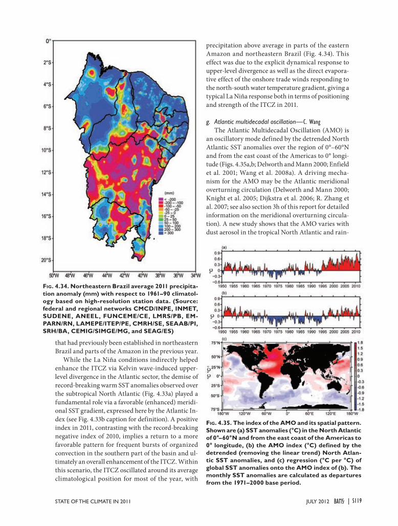
S119STATE OF THE CLIMATE IN 2011 |JULY 2012
precipitation above average in parts of the eastern Amazon and northeastern Brazil (Fig. 4.34). This effect was due to the explicit dynamical response to upper-level divergence as well as the direct evapora-tive effect of the onshore trade winds responding to the north-south water temperature gradient, giving a typical La Niña response both in terms of positioning and strength of the ITCZ in 2011.
g. Atlantic multidecadal oscillation—C. Wang
The Atlantic Multidecadal Oscillation (AMO) is an oscillatory mode defined by the detrended North Atlantic SST anomalies over the region of 0°–60°N and from the east coast of the Americas to 0° longi-tude (Figs. 4.35a,b; Delworth and Mann 2000; Enfield et al. 2001; Wang et al. 2008a). A driving mecha-nism for the AMO may be the Atlantic meridional overturning circulation (Delworth and Mann 2000; Knight et al. 2005; Dijkstra et al. 2006; R. Zhang et al. 2007; see also section 3h of this report for detailed information on the meridional overturning circula-tion). A new study shows that the AMO varies with dust aerosol in the tropical North Atlantic and rain-
that had previously been established in northeastern Brazil and parts of the Amazon in the previous year.
While the La Niña conditions indirectly helped enhance the ITCZ via Kelvin wave-induced upper-level divergence in the Atlantic sector, the demise of record-breaking warm SST anomalies observed over the subtropical North Atlantic (Fig. 4.33a) played a fundamental role via a favorable (enhanced) meridi-onal SST gradient, expressed here by the Atlantic In-dex (see Fig. 4.33b caption for definition). A positive index in 2011, contrasting with the record-breaking negative index of 2010, implies a return to a more favorable pattern for frequent bursts of organized convection in the southern part of the basin and ul-timately an overall enhancement of the ITCZ. Within this scenario, the ITCZ oscillated around its average climatological position for most of the year, with
FIG. 4.34. Northeastern Brazil average 2011 precipita-tion anomaly (mm) with respect to 1961–90 climatol-ogy based on high-resolution station data. (Source: federal and regional networks CMCD/INPE, INMET, SUDENE, ANEEL, FUNCEME/CE, LMRS/PB, EM-PARN/RN, LAMEPE/ITEP/PE, CMRH/SE, SEAAB/PI, SRH/BA, CEMIG/SIMGE/MG, and SEAG/ES)
FIG. 4.35. The index of the AMO and its spatial pattern. Shown are (a) SST anomalies (°C) in the North Atlantic of 0°–60°N and from the east coast of the Americas to 0° longitude, (b) the AMO index (°C) defined by the detrended (removing the linear trend) North Atlan-tic SST anomalies, and (c) regression (°C per °C) of global SST anomalies onto the AMO index of (b). The monthly SST anomalies are calculated as departures from the 1971–2000 base period.

S120 | JULY 2012
fall in the Sahel, suggesting that a positive feedback exists between North Atlantic SST, dust aerosol, and Sahel rainfall on multidecadal timescales (C. Wang et al. 2012). In addition to multidecadal variability, the AMO also demonstrates high-frequency variability such as an interannual variation via its connection to the tropical North Atlantic and the Atlantic Warm Pool (AWP; a large body of warm water comprising the Gulf of Mexico, Caribbean Sea, and the western tropical North Atlantic), and as such has exhibited a seasonal influence on the behavior of tropical cy-clones (TCs) in the Atlantic and Eastern North Pa-cific (ENP) basins. The extended reconstructed SST (ERSST) data from 1950 to 2011 (Fig. 4.35b) shows that the AMO was in the cold phase from the late 1960s to the early 1990s and in the warm phase before the late 1960s and again after the early 1990s (Enfield et al. 2001). The AMO is related to SST anomalies over the global oceans as shown in Fig. 4.35c.
The AMO variability is associated with changes of climate and extreme events, such as drought and flood in North America and Europe, and hurricane activity in the North Atlantic and ENP (Enfield et al. 2001; McCabe et al. 2004; Goldenberg et al. 2001; Bell and Chelliah 2006; Wang et al. 2008a; Wang and Lee 2009). Recent studies show that the relationship of the AMO to TCs is due to its tropical component since the climate response to the North Atlantic SST anomalies is primarily forced at the low latitudes (e.g., Lu and Delworth 2005; Sutton and Hodson 2007). The AMO variability coincides with the multidecadal signal of the AWP and the AWP is in the path of, or a birthplace for, Atlantic TCs (Wang et al. 2008a). Thus, the influence of the AMO on climate and Atlantic TC activity operates through the mechanism of the AWP-induced atmospheric changes by having an effect on vertical wind shear in the hurricane main development region (MDR). A large AWP reduces
such shear, while a small AWP enhances it. A large AWP also weakens the southerly Great Plains low-level jet, thus reducing the northward moisture transport from the Gulf of Mexico to the eastern United States and decreasing the boreal summer rainfall over the central US, while a small AWP has the opposite effect (Wang et al. 2006, 2008b). It has also been shown that the AWP variability can produce the ob-served out-of-phase relationship between TC activity in the tropical North Atlantic and ENP (Wang and Lee 2009).
As of 2011, the AMO has been in its warm phase since 1995. For all months in 2011, the North Atlantic SST anomalies were positive (Fig. 4.36a), with the maxi-mum of the North Atlantic SST anomalies in January (+0.61°C) and the minimum in November (+0.30°C). Spatially, the North Atlantic SST anomalies during the boreal winter showed a tripole pattern with the positive SST anomalies in the subpolar North Atlantic and the tropical North Atlantic and the negative SST anomalies in the subtropical North Atlantic (Fig. 4.36b). The SST anomaly pattern divided the AWP into two parts: a colder Gulf of Mexico and a warmer Caribbean Sea/western tropical North Atlantic. The op-posite SST anomaly pattern was consistent with a previous study (Muñoz et al. 2010), which showed that the air-sea fluxes as-
FIG. 4.36. The AMO in 2011. Shown are the (a) monthly North Atlantic SST anomalies (°C), (b) DJF 2010/11 SST anomalies (°C), (c) MAM SST anomalies, (d) JJA SST anomalies (°C), and (e) SON SST anomalies (°C). The monthly SST anomalies are calculated as departures from the 1971–2000 base period.

S121STATE OF THE CLIMATE IN 2011 |JULY 2012
Previous studies have shown that the inf luence of the AMO on TC activ-ity may operate through the atmospheric changes induced by the AWP or the Atlantic meridional mode (Wang et al. 2008a; Vimont and Kossin 2007). In particular, the AWP can play an important role in the hurricane track (Wang et al. 2011). During the 2011 Atlantic TC season of June to November, the AWP was consistently large (Fig. 4.37a) and the isotherm of 28.5°C extended eastward covering almost the en-tire tropical North Atlan-tic (Figs. 4.37b,c,d,e). An eastward expansion of the AWP shifted the hurricane genesis location eastward, decreasing the possibility for a hurricane to make landfall in the southeast United States. A large AWP
also tended to shrink the North Atlantic subtropical high eastward (C. Wang et al. 2007) and produced a TC steering flow pattern along the Eastern Seaboard of the United States, which steered hurricanes away from the southeastern coast of the US (Wang et al. 2011). The large AWP in 2011 was also associated
sociated with ENSO events in the tropical Pacific and local processes were responsible for the SST anomaly distribution. During the boreal spring, summer, and fall of 2011, the cold SST anomalies in the subtropical North Atlantic weakened and the North Atlantic was mostly warm (Figs. 4.36c,d,e).
FIG. 4.37. The AWP in 2011. Shown are the (a) monthly AWP area in 2011 (1012 m2; blue) and the climatological AWP area (red), spatial distributions of the 2011 AWP in (b) July, (c) August, (d) September, and (e) October. The AWP is defined by SST larger than 28.5°C. The black contours in (b)–(e) are the climatological AWP based on the data from 1971–2000.
FIG. 4.38. (a) Monthly anomalies of SST (°C, solid lines) and precipitation (mm day-1, dashed lines) in the eastern (IODE: 90E°–110°E, 10°S–0°; blue lines) and western pole (IODW: 50°E–70°E, 10°S–10°N; red lines) of IOD. (b) As in (a), but for the IOD index (measured by the SST differ-ence between IODW and IODE, green line) and surface zonal wind anomaly (m s-1) in the central equatorial IO (Ucio), from 70°E–90°E, 5°S–5°N, black line. The anomalies were calculated rela-tive to the climatology over the period 1982–2010. These are based on the NCEP optimum interpolation SST (Reynolds and Chelton 2010), monthly GPCP precipitation analysis (http://precip.gsfc.nasa.gov/), and JRA-25 atmospheric reanalysis (Onogi et al. 2007).

S122 | JULY 2012
event occurred in the tropi-cal Indian Ocean (Figs. 4.38 and 4.39d) in spite of the La Niña conditions in the Pa-cific. In particular, the cold SST anomalies in the eastern Indian Ocean were weak,9 and the 2011 IOD was not well developed during its peak phase in SON compared to the past three strong positive IODs in 1994, 1997, and 2006. This is similar to what hap-pened in 2007 and 2008 (Luo et al. 2008) and reconfirms the idea that the IOD can sometimes originate from the internal air-sea interactions in the IO (Behera et al. 2006; Luo et al. 2010). The strong La Niña event in 2010 helped to induce excessive surface westerl ies in the centra l equatorial IO by enhancing the Walker cell in the IO. The westerly anomalies tend to cool the SST in the western IO by increasing surface latent heat loss from the ocean but warm the SST in the east by deepening the oceanic thermocline there; this favors the occurrence of a negative IOD in the second half of 2010 (Fig. 4.38). After the collapse of the negative IOD near the end of 2010, the excessive westerlies caused a cool/dry condition in most places of the tropical IO and a warm/
wet condition in the Bay of Bengal and northwest of Australia during early 2011 (Figs. 4.38a, 4.39a). The related anomalous cyclonic winds in the southeastern IO raised the thermocline underneath and induced strong subsurface cooling and cold SST anomalies along ~10°S. The cold signals propagated westward but disappeared before they reached the western boundary of the IO (Figs. 4.39, 4.40). The drought
9 Like an El Niño or La Niña event, a weak or strong IOD is defined by a threshold value of one standard deviation of the IOD index.
with the out-of-phase relationship between TCs in the North Atlantic and the ENP as described previously in this chapter.
h. Indian Ocean dipole—J. J. Luo
The Indian Ocean dipole (IOD)—a climate mode in the tropical Indian Ocean (IO)—usually starts in boreal summer, peaks in fall, and decays rapidly in early winter. It has been believed that El Niño (La Niña) favors the development of positive (negative) IOD. During 2011, however, a weak positive IOD
FIG. 4.39. SST (°C, colored scale), precipitation (green contours: ±1, ±2, …, ±5 mm day-1). Solid (dashed) lines denote positive (negative) values, and surface wind anomalies during (a) DJF 2010/11, (b) MAM 2011, (c) JJA 2011, and (d) SON 2011.

S123STATE OF THE CLIMATE IN 2011 |JULY 2012
center in the IO gradually moved eastward and reached the eastern IO and Maritime Continent during June–August 2011 (Fig. 4.39c) which is typical of the weakening of the Pacific La Niña condition.
Cold SST anomalies started to develop near the coast of Java, Indonesia, in July 2011; this is closely linked with the southeasterly anomalies along the west coast of Sumatra, which could be partly driven by the north-south air pressure gradient associated with the dry center west of Sumatra and the wet center in the Bay of Bengal. The southeasterly anomalies raised the coastal thermocline and hence, induced the SST cooling. The colder-than-normal SST may, in turn, enhance the north-south pressure gradient and the southeasterly winds. As a result, both the SST cooling and southeasterly winds were enhanced quickly through this air-sea positive feedback. These signals expanded equatorward and westward and peaked in September 2011. There did not appear to be any subsurface cooling propagated from the
western IO (Fig. 4.40a), suggesting that the local air-sea coupling in the eastern IO must have played a key role in generating the positive IOD event in 2011.
In the western IO, warm SST anomalies started to occur in May 2011 and grew rapidly in June–July 2011 in association with more surface solar radiation heating under less cloud conditions (Figs. 4.38a, 4.39c). The warm SST anomalies caused anomalous easterlies in the western IO during May–July 2011. In August 2011, the anomalous winds in the western IO and the east merged and led to basin-wide easterlies. This caused a pronounced dipole structure of precipitation anomalies, with flooding in the western IO and drought in the east during August–November 2011 (Fig. 4.39d). This dipole structure suddenly collapsed in December 2011 due to the strong westerly anomalies across the equatorial IO basin in association with the influences of both intraseasonal oscillation in the IO and the reenhancement of La Niña conditions in the Pacific.
FIG. 4.40. 20°C isotherm depth (D20, m) anomalies in (a) the equatorial Indian Ocean (2°S–2°N) and (b) off-equatorial South Indian Ocean (12°S–8°S) in 2011. The data are derived from the NCEP ocean re-analysis available at http://www.cpc.ncep.noaa.gov/products/GODAS/.

S124 | JULY 2012
Long before the advent of numerical weather and climate models, Polynesian communities recognized that changes in biophysical phenomena could be used to forecast changes in local weather and climate con-ditions (Lefale 2010). Social, cultural, and traditional economic activities were planned and acted upon in response to these changes and revolved around the different seasons. Foremost among these was the ca-pacity to forecast appropriate and inappropriate times for food gathering such as the planting and harvesting of crops and the catching of fish.
While weather and climate patterns have been monitored in the Southwest Pacific using Western scientific techniques since the late 1800s (1890 in Apia, Samoa, for example), little attention has been paid to the atmospheric observations and related expertise developed in-place by Polynesian people. However, recent work aimed at reaffirming Polynesian knowl-edge of weather and climate phenomena has shown that Maori, Cook Islanders, and Samoans possess their
own unique local knowledge systems to forecast the onset of extreme events such as tropical cyclones and storms (Lefale 2003; King et al. 2007).
In Aotearoa/New Zealand, Maori have developed a detailed knowledge of biophysical processes and phenomena, including, among other skills, forecasting adverse weather and climate conditions (King et al. 2005). Ngati Koata, a tribal group from the north of the South Island, knew bad weather was imminent when stones were found in the belly of caught “rawaru” (blue cod). The stones are understood to give the rawaru ballast in the water as bigger waves and swell coincide with stormy conditions. Such indicators were not used in isolation, but rather as parts of a range of indicators that were (and continue to be) observed to confirm, via consensus, the forecast being made.
It is widely recognized in the Cook Islands, es-pecially the southern islands, that a plentiful crop of mangoes typically indicates an active season of cyclones ahead (Fig. SB4.1). Knowledge of this phenomenon
is common throughout the South Pacific region, from Vanuatu and Fiji in the west to Samoa and French Polynesia to the east. Migratory birds are also well recognized as indicators of severe weather, espe-cially during summer. The “torea” (Pacific Golden Plover) is known to migrate between the Cook Is-lands and Alaska in the months of February–March and September–October, respectively (see http://cookislands.bishopmuseum.org/showarticle.asp?id=4). However, according to Mr. George “Birdman” Mateariki, a bird catcher on the island of Atiu, “The birds on Atiu just disappeared in December [2004], and when those 5 cyclones came in from February 2005 for the Cook Islands, it dawned on me that the torea knew what would happen” (Cook Islands government 2011).
FIG. SB4.1. A bumper mango season in Rarotonga, Cook Islands. Local indigenous knowledge indicates that the risk of tropical cyclones is still high for the nation. (Photo Credit: Mr. Arona Ngari, Director, Cook Islands Meteorological Service)
SIDEBAR 4.1: MANAGING CLIMATE RISKS USING POLYNESIAN KNOWLEDGE—P. LEFALE, D. KING, AND A. NGARI

S125STATE OF THE CLIMATE IN 2011 |JULY 2012
Similar biophysical indicators of change are used in Samoa. For example, the sudden appearance of cockroaches in large numbers in the evening during the cyclone season is understood to portend an approaching cyclone that can bring death and destruction (Fig SB4.2). Further, the appearance of frigate birds during a tropical cyclone signals the eye of the storm has arrived and that the worst of the storm is over. It is important to emphasize that the development and application of such knowledge was (and continues to be) fundamen-tally about managing climate-related risks linked with daily and seasonal changes in local weather and climate conditions (Cook Islands govern-ment 2006).
Reaffirming such knowledge pro-vides an opportunity to understand what has assisted Polynesian people
to cope and adapt to weather and climate variability in the past. It also provides lessons on how to deal with the risks associated with future weather and climate extremes (and related natural hazards), through greater awareness of the natural world and the inherent linkages between atmospheric and biophysical phenomena.
FIG. SB4.2. Widespread damage occurred in the village of Nikaupara on the island of Aitutaki in the Southern Cook Islands caused by Tropical Cyclone Pat in February 2010. (Photo Credit: Mr. Johnny Hosking in liaison with Air Rarotonga)

S126 | JULY 2012

S127STATE OF THE CLIMATE IN 2011 |JULY 2012
5. THE ARCTIC—M. O. Jeffries and J. Richter-Menge, Eds.a. Overview—M. O. Jeffries and J. Richter-Menge
Calendar year 2011 was characterized by continu-ing change throughout the Arctic environmental system. A key driver of systemwide change is a ~2°C increase in annual mean surface air temperature since the mid-1960s, which is 1.5°C greater than (more than double) the temperature increases at lower lati-tudes. This chapter describes some of the systemwide changes in ten categories: Air temperature, atmo-spheric circulation and clouds; Ozone and UV radia-tion; Terrestrial snow; Glaciers and ice caps (outside Greenland); Greenland Ice Sheet; Permafrost; Lake ice; Sea ice; Ocean; and Ocean acidification. Some of the key events are summarized below.
Ozone concentrations in the Arctic stratosphere during March 2011 were the lowest ever recorded since 1979, and led to elevated surface UV levels throughout the Arctic and sub-Arctic.
Annually-averaged Arctic temperatures contin-ued to show area-wide positive (warm) anomalies, relative to the end of the 20th century. There were multi-month-long shifts in the dominant wind pat-tern, responding to changes in the polar vortex, which affected the distribution of surface temperatures and snow and ice conditions. For example, warm air temperature anomalies over the Eurasian Arctic in spring 2011 resulted in a new record low June snow cover extent and spring snow cover duration, and earlier (by 10–30 days) lake ice break-up and shorter (by 14–21 days) ice duration. Conversely, penetration of Arctic air masses into northern and eastern Europe in autumn 2010 and spring 2011 caused earlier freeze-up and later break-up, respectively, and thus longer (by 28–42 days) lake ice duration.
On the Greenland ice sheet, below-normal sum-mer snowfall, a decreasing trend in surface albedo, and elevated surface and upper air temperature anomalies resulted in a continued pattern of extreme surface melting and a negative mass balance. To the west, the mass loss from glaciers and ice caps in the Canadian Arctic was the greatest since GRACE (Gravity Recovery and Climate Experiment) satellite measurements began in 2002, continuing a negative trend that dates back to 1987.
Warm summer temperatures occurred in Alaska; Barrow, on the North Slope, experienced a record 86 consecutive days with minimum temperatures at or above freezing. New record high temperatures occurred at 20 m below the land surface at all per-mafrost observatories on the North Slope, where measurements began in the late 1970s.
Sea ice extent in September 2011 was the second lowest on record, while the extent of old ice (four and five years) reached a new record minimum that was only 19% of the mean for the period 1982–2005. For a second consecutive summer, the northern routes of the Northwest Passage and the Siberian Coast pas-sage of the Northern Sea Route were open, and for a fourth consecutive summer, the southern route of the Northwest Passage was ice-free. An increase and decrease, respectively, in winter and summer cloud cover contributed to surface warming in the Arctic Basin and perhaps the near-record low sea ice extent.
Also responding to the near-record low sea ice extent in nearly all sectors of the Arctic Basin, upper ocean temperatures in summer 2011 were generally warmer than in the previous few summers. The sea surface temperature anomaly averaged over the Beaufort, Chukchi, East Siberian, Laptev, and Kara Seas was +1.45 C, the highest since the historical maximum value (+2.8 C) observed in 2007.
b. Air temperature, atmospheric circulation, and clouds—
J. Overland, U. Bhatt, J. Key, Y. Liu, J. Walsh, and M. WangThe annual mean surface air temperature over
Arctic land areas has experienced an overall warming of about 2°C since the mid-1960s (Fig. 5.1). In 2011, the annual mean air temperature was slightly warmer than in 2009 and 2010. The cooler temperatures in 2009 and 2010 reflected cold continents in winter, while Eurasia had warmer temperatures in spring 2011. Area-wide positive temperature anomalies (Fig. 5.2), which show systematic changes since the end of
FIG. 5.1. Arctic-wide annual average surface air tem-perature anomalies relative to the 1961–90 mean, based on land stations north of 60°N. Data are from the CRUTEM 3v dataset at http://www.cru.uea.ac.uk/cru /data/temperature/. Note this curve does not include marine observations.

S128 | JULY 2012
the 20th century, continued in 2011. Note the almost complete absence of negative temperature anomalies in Fig. 5.2. This temperature pattern is a manifesta-tion of “Arctic amplification”, which is characterized by temperature increases 1.5°C greater than (more than double) the increases at lower latitudes (Over-land et al. 2011a).
Spatial distributions of seasonal near-surface temperature anomalies (Fig. 5.3) were inf luenced by changes in the polar vortex, which is ref lected in the sign and magnitude of the Arctic Oscillation index (AO; Table 5.1). A positive index corresponds to strong zonal wind flow, while a negative index cor-responds to more meridional and spatially-variable flow. Table 5.1 indicates a large range in the magni-tude of the AO in 2011; this has been characteristic of the AO since December 2009. It has been suggested that changes in the polar vortex are increasingly in-fluenced by changes in Arctic surface characteristics, e.g., reduced sea ice and changes in snow cover, but these ideas are still highly controversial (Overland et al. 2011b).
The distinct shifts between large negative and positive phases of the AO index had a striking effect on the location of major warm and cold regional temperature anomalies in the Arctic and sub-Arctic throughout the year. Early winter 2011 saw a continu-ation of the negative AO Warm Arctic-Cold Conti-nent pattern (Overland et al. 2011a) of the previous year, with warm temperatures lying north of far eastern Siberia and Alaska, in the vicinity of greater Baffin Bay and far northeastern Canada, and to some extent in the Kara Sea. Beginning in February, there was a major shift to a positive AO index, with cold temperatures in the Baffin Bay region and warmer anomalies developing in Eurasia due to westerly winds. A new record low June snow cover extent (since satellite observations began in 1966) occurred over Eurasia in 2011 (see section 5d) due to persistent warm spring air temperature anomalies over almost the entire Eurasian sector of the Arctic. In summer, when the AO shifted to a negative state, warm tem-perature anomalies returned to northern Canada with cool temperature anomalies in the Bering Sea. November and December had a strong positive AO pattern again, with warm anomalies in Eurasia and
FIG. 5.3. Seasonal, near-surface (1000 hPa) air tempera-ture anomalies (°C) in 2011 relative to the 1981–2010 baseline period. (a) Dec 2010–Feb 2011, (b) Mar–May 2011, (c) Jun–Aug 2011, and (d) Sep–Nov 2011. (Source: NCEP/NCAR)
FIG. 5.2. Annual average near-surface (1000 hPa) air temperature anomalies (°C) for 2001–11 relative to the period 1971–2000. Data are from NOAA/ESRL, http://www.esrl.noaa.gov/psd/. (Source: NCEP/NCAR)
TABLE 5.1. Monthly Arctic Oscillation Index for 2011 (from NOAA/CPC). Values are normalized by the stan-dard deviation of the monthly index.
JAN FEB MAR APR MAY JUNE JULY AUG SEP OCT NOV DEC
-1.68 1.57 1.42 2.27 -0.04 -0.86 -0.47 -1.06 0.66 0.80 1.46 2.22

S129STATE OF THE CLIMATE IN 2011 |JULY 2012
western Canada, and cold anomalies in Greenland and eastern Asia.
The large negative values of the AO during summer 2011, and the associated wind pattern, represent an unusual event. Unlike summer climatology, which has generally weak winds confined to the Arctic, in July 2011 multiple low 850-hPa geopoten-tial height centers formed in southerly locations along the continental rim of the Arctic Basin (Overland et al. 2011b). This provided the unusual warming in west Greenland during summer 2011 (similar to 2010), warm temperatures in Barrow, Alaska, cold temperatures in western Sibe-ria, and kept warm storms from entering the Bering Sea. Barrow had a record (based on over 80 years of observations) 86 consecutive days with minimum temperatures at or above freezing beginning June 30. The previous record was 68 days set in 2009. For the sixth consecutive year, the first freeze of autumn in Fairbanks, Alaska, occurred more than two weeks later than its long-term average. Unlike 2007, when the wind pattern in every summer month contributed toward record sea ice loss in the Pacific Arctic via northward transport of ice and heat toward the North Pole, the near-record sea ice loss in September 2011 occurred despite a more variable wind circulation.
In 2011, Arctic cloud cover was somewhat higher than the average of the last 10 years (2002–11) in win-ter (January–March) and lower than average in the summer (June–August), particularly over the west-ern Arctic Ocean. Figure 5.4 shows the cloud cover anomalies for representative winter and summer months. In spring and autumn, cloud cover was similar to the 10-year mean (not shown). The annual average cloud cover in 2011 over the Arctic Ocean was not significantly different from recent years. The 2011 wintertime increase and summertime decrease in cloud cover resulted in greater surface warming, as Arctic clouds generally have a warming effect in the winter and a cooling effect in the summer. This potentially con-tributed to the near-record low sea ice extent. This contrasts with the general trend over the period 1982–2004, when a decrease in wintertime and increase in springtime cloud cover over parts of the Arctic acted to dampen surface
warming (Wang and Key 2003, 2005). While clouds inf luence the surface energy budget (Y. Liu et al. 2009), they also respond to changes in the sea ice cover (Vavrus et al. 2011), as was evident in 2011. Figure 5.5 shows the cloud cover anomaly for the first half of September 2011, with higher-than-normal cloud cover in the poleward portions of the Beaufort, Chukchi, and Laptev Seas; sea ice concentration was lower than normal in these same areas (Fig. 5.5b). This is not coincidental, as a feedback analysis of data from 2000 to 2010 indicates that a 1% decrease in ice concentration leads to a 0.3–0.4% increase in cloud cover (Liu et al. 2012).
c. Ozone and UV radiation—G. Bernhard, G. Manney, V. Fioletov, J.-U. Grooß, A. Heikkilä, B. Johnsen, T. Koskela, K. Lakkala, R. Müller, C. L. Myhre, and M. Rex Ozone concentrations in the Arctic stratosphere
during March 2011 were the lowest since satellite records began in 1979 (Manney et al. 2011). The
FIG. 5.4. Cloud cover anomalies (%) in (a) February and (b) July 2011 relative to the corresponding monthly means for the period 2002–11, based on data from the Moderate Resolution Imaging Spectroradiometer (MODIS) on the Aqua satellite.
FIG. 5.5. (a) Cloud cover anomalies and (b) sea ice anomalies for September 2011 relative to the September mean for the period 2002–11. In both figures, the unit of anomaly is % above or below normal. Cloud cover is based on Aqua MODIS data. Sea ice con-centration is from the Special Sensor Microwave/Imager (SSM/I) using the NASA team algorithm.

S130 | JULY 2012
Together, carbon dioxide (CO2) and methane (CH4) are responsible for ~80% of direct radiative forcing caused by long-lived greenhouse gases: 2.29 W m-2 out of 2.81 W m-2 in 2010 (update of Hofmann et al. 2006). Observations of CO2 and CH4 are of particular interest in the Arctic, where there are two potentially large reservoirs of carbon that are vulner-able and where land surface temperatures have been increasing and are projected to increase in the future (McGuire et al. 2009; O’Connor et al. 2010).
The first reservoir, methane-rich clathrate hy-drates, occurs in sediments at the bottom of the Arctic Ocean. There is concern that rising ocean water temperatures, especially on the relatively shallow eastern Siberian Arctic continental shelf, will cause the clathrates to destabilize and release mas-sive pulses of methane to the atmosphere (Kennett et al. 2000). However, measurements of CH4 in ice cores (e.g., Severinghaus et al. 1998) do not support the idea that massive pulses of CH4 from clathrates caused rapid climate warming in the past. It remains to be seen whether the climate response to current and future clathrate release will differ from previous records.
The second reservoir, Arctic permafrost, contains ~1000 Pg C (Pg C = 1015 g carbon) in the top 3 m (Tarnocai et al. 2009), significantly more carbon than is currently in the atmosphere (~830 Pg C). As the Arctic warms and permafrost thaws, this ancient car-bon can be released as either CO2 or CH4. A recent review of the potential impacts of climate change in the 21st century on northern peatlands, much of it underlain by permafrost, suggests that both CO2 and CH4 emissions from this source will increase signifi-cantly in the future (Frolking et al. 2011).
Carbon dioxide and methane abundances from weekly samples collected at seven Arctic and sub-Arctic sites and Mauna Loa, Hawaii, are shown in Fig. SB5.1. High latitude CO2 values are the same as at Mauna Loa, and all sites show a strong seasonal cycle superimposed on the long-term trend to higher values (Fig. SB5.1a). The seasonal cycle of CO2 at high northern latitudes results from seasonal uptake (photosynthesis) and release (respiration) of carbon by the biosphere. The steep upward trend in CO2 is due to global fossil fuel use.
Like CO2, the CH4 records also have a seasonal cycle superimposed on a long-term trend to higher values (Fig. SB5.1b). Unlike CO2, the CH4 record shows higher values at the Arctic and sub-Arctic sites than at Mauna Loa. The seasonal cycle at all sites is due to greater photochemical destruction of CH4
in summer than in winter. However, photochemical destruction is slower at high latitudes. This, combined
SIDEBAR 5.1: SOURCES OF ATMOSPHERIC CARBON DIOXIDE AND METHANE IN THE ARCTIC—E. J. DLUGOKENCKY AND L. BRUHWILER
with CH4 transport from lower latitudes and a currently small contribution from high latitude sources, explains the greater CH4 abundance at high latitudes. As the Arctic warms, contri-butions from local methane sources will likely increase, possibly by a large amount. However, to date, there is no evidence that natural emissions of CH4 in the Arctic have increased signifi-cantly in the past decade (Bruhwiler and Dlugokencky 2011).
FIG. SB5.1. (a) CO2 and (b) CH4 dry air mole fractions from seven Arctic and sub-Arctic air sampling sites and from Mauna Loa Ob-servatory (MLO), all in the NOAA ESRL air sampling network. The northern sites are Alert, Canada (ALT), Barrow, Alaska (BRW), Cold Bay, Alaska (CBA), Pallas, Finland (PAL), Shemya Is-land, Alaska (SHM), Summit, Greenland (STM), and Ny Ålesund, Svalbard, Norway (ZEP). Further information about the sites is available at http://www.esrl.noaa.gov/gmd/dv/site/site_table .html#ccg_surface.

S131STATE OF THE CLIMATE IN 2011 |JULY 2012
minimum total ozone column for March 2011, averaged over the “equivalent latitude” (Butchart and Remsberg 1986) band 63°N–90°N, was 297 DU (Dobson Units). The previous record low, 315 DU, was observed in 2000 (Fig. 5.6). The fraction of the Polar vortex with total ozone below 275 DU is typi-cally near zero for March, but reached nearly 45% in March 2011. Minimum total ozone in spring 2011 was continuously below 250 DU for about 27 days, and occurred over a maximum area of about 2!000!000 km2. Record-low values (not illustrated) between 220 DU and 230 DU were reached in small regions of the vortex for about one week in late March 2011.
The ozone loss in spring 2011 was comparable to that observed during the annually-recurring “ozone hole” over the Antarctic. The record loss was mostly caused by chemical destruction of ozone, attributed to the existing stratospheric burden of ozone-depleting halogens and favored by an unusually prolonged cold period in the lower stratosphere in 2011. Low temperatures facilitate the formation of polar strato-spheric clouds (PSC), which provide surfaces for heterogeneous reactions that activate stratospheric chlorine. The activated chlorine, in turn, destroys ozone rapidly in catalytic cycles. A good indicator of the potential for chlorine activation and ozone loss is the volume of air within the Polar vortex with temperatures below the PSC occurrence threshold (Rex et al. 2004). Temperatures below the threshold temperature for PSC formation of about -77°C existed between December 2010 and early April 2011. Under these conditions, over 80% of the ozone present in January, from about 18 km to 20 km altitude, had been chemically destroyed by late March (Manney et al. 2011).
The extraordinary situation in 2011 is illustrated in Fig. 5.7, which compares satellite measurements of to-tal ozone column on 3 April 1981 (a year with a long-lasting and cold Polar vortex, and relatively low stratospheric chlorine concentrations), 3 April 2002 (long-lasting warm vortex, high total chlorine loading), and 3 April 2011 (long-lasting cold vortex, high chlorine). The figure emphasizes that chemical ozone loss resulting from chlo-rine activation is most effective in years when there is a long-lasting cold vortex, such as 2011.
T he low le ve l s of tot a l ozone led to elevated UV levels
throughout the Arctic and sub-Arctic. Figure 5.8 il-lustrates the UV radiation in terms of the UV index, which is a measure of the ability of UV radiation to cause sunburn in human skin (WHO 2002). Changes in the UV index anti-correlate with changes in total ozone (compare 2011 data in center and bottom pan-els of Fig. 5.8). Noontime UV indices of March 2011 exceeded historical measurements for this month at all Arctic sites where ground-based UV monitor-ing systems are located (Bernhard et al. 2011). The maximum enhancement of the UV index relative to the climatological average was 122% (Fig. 5.8c). While these large relative changes are unprecedented, the absolute increases in UV levels were modest at all Arctic sites (e.g., increase by less than one UV index unit) because the low-ozone event occurred early in spring when the solar elevation was still small. Larger absolute increases of UV indices occurred at lower
FIG. 5.6. Time series of area-averaged minimum total ozone for March in the Arctic, calculated as the mini-mum of the daily average column ozone poleward of 63°N equivalent latitude. Winters in which the polar vortex broke up before March (1987, 1999, 2001, 2006, and 2009) are shown as open symbols. Ozone in those years was relatively high because of mixing with air from lower latitudes. Figure adapted from Müller et al. (2008), updated using the combined total column ozone database of the New Zealand National Institute of Water and Atmospheric Research (NIWA), Version 2.7, provided by H. Chisholm of NIWA and G. Bodeker of Bodeker Scientific. The area-averaged minimum total ozone quantity is explained in Müller et al. (2008)
FIG. 5.7. Comparison of total ozone column (DU) measured by satellites on 3 April 1981, 2002, and 2011. Data are from the Total Ozone Mapping Spectrometer (TOMS) onboard the Nimbus-7 (1981) and Earth Probe (2002) satellites, and the Ozone Monitoring Instrument (OMI) onboard the AURA spacecraft (2011).

S132 | JULY 2012
latitudes during excursions of the Polar vortex in April. For example, on 22 April, the clear-sky UV in-dex over parts of Mongolia (48°N, 98°E) estimated by TEMIS (Tropospheric Emission Monitoring Internet Service at http://www.temis.nl/uvradiation/UVindex .html) was 8.6 when a lobe of the vortex extended to central Asia. The long-term average for this day at this location is 5.4 with a standard deviation of 0.5, i.e., the anomaly was more than six standard deviations larger than the climatological mean.
d. Terrestrial snow—C. Derksen and R. BrownTime series of satellite-derived Arctic (land area
north of 60°N, excluding Greenland) snow cover extent (SCE), snow cover duration (SCD), and snow water equivalent (SWE) anomalies (relative to a 1988–2007 base period) were calculated to place the 2010/11 snow season in the context of trends and variability during recent decades. Monthly SCE and seasonal SCD (computed separately for the first and second halves of the snow year) anomalies were com-puted from the weekly NOAA snow chart climate data record (CDR) maintained at Rutgers University and described in Brown and Robinson (2011). The SWE anomalies for 1980–2011 were calculated from an as-similation of surface observations of snow depth and satellite passive microwave measurements (Takala et al. 2011), the Canadian Meteorological Centre (CMC)
daily gridded global snow depth analysis (Brasnett 1999), and the ERA-interim atmospheric reanalysis (Dee et al. 2011a).
Air temperatures over the North American Arc-tic (NA) were below normal in April and early May, coincident with a strongly positive Arctic Oscillation (AO) (see Table 5.1), so SCE was above or near the long-term average during these months (Figs. 5.9a,b). When the AO shifted to a negative phase in May, the surface temperature anomalies became positive. By June, SCE anomalies over the NA sector of the Arctic were the second lowest on record (Fig. 5.9c). Unlike the slow start to the NA melt season, an extensive and persistent warm air temperature anomaly covered the Eurasian Arctic (EUR) through the entire spring sea-son (see Fig. 5.3b), driving below-normal SCE in April and May, with a new record low June SCE over EUR since satellite observations began in 1966 (Fig. 5.9c).
Spatial patterns of seasonal SCD anomalies derived from the NOAA CDR for 2010/11 show an early spring melt anomaly located over the Ob and Yenisey basins (Fig. 5.9d) contributed to the shortest spring SCD for EUR in the NOAA snow chart record (Fig. 5.9f). A striking feature in the SCD anomaly time series is the seasonal asymmetry of the trends through the data record. The fall start date of snow cover over the Arctic has remained stable during the satellite era (Fig. 5.9e), in contrast to the trend
FIG. 5.8. Seasonal variation of the noontime UV Index for four Arctic and sub-Arctic sites measured by ground-based radiometers. The upper panel for each site compares the climatological average (blue line) with the measurements in 2011 (red dots), and historical minima and maxima (shaded range). The latter were calcu-lated from measurements during the periods indicated in the top-right corner of the panel. The center panel shows the anomaly in the UV Index, calculated as the percentage departure from the climatological average. The numbers indicate the maximum anomalies for March and April 2011. The bottom panel shows a similar anomaly analysis for total ozone derived from measurements of the following satellites: TOMS/Nimbus-7 (1991–92), TOMS/Meteor-3 (1993–94), TOMS/EarthProbe (1996–2004), and OMI (2005–11). The shaded range for the ozone dataset is based on data for the years 1991–2009. Ozone data are available at http://toms.gsfc.nasa.gov and http://ozoneaq.gsfc.nasa.gov/.

S133STATE OF THE CLIMATE IN 2011 |JULY 2012
FIG. 5.9. (a)–(c) Monthly Arctic snow cover extent standardized (and thus unitless) anomaly time series (1988–2007 base period) from the NOAA snow chart CDR for (a) April, (b) May, and (c) June 1967–2011 (solid lines denote 5-yr moving average). (d) Snow cover duration (SCD) departures (1998–2010 base period) from the NOAA IMS data record for the 2011 spring season. (e)–(f) Arctic seasonal SCD standardized anomaly time series (1988–2007 base period) from the NOAA record for the first (fall) and second (spring) halves of the snow season (solid lines denote 5-yr moving average). (g) Time series of multidataset average monthly April snow water equivalent standardized anomalies (± the standard error) relative to 1988–2007 base period (solid lines denote 5-yr moving average). (h) April 2011 snow depth anomaly (% of 1999–2010 average) from the CMC snow depth analysis.
towards less snow in the spring period (Fig. 5.9f). The below-average Arctic SCE and SCD during 2011 is consistent with a decline in spring snow cover since the 1970s, identified from multiple datasets by Brown et al. (2010); the rate of this reduction has accelerated over the past five years.
The multi-dataset SWE anomaly series for the month of April is charac-terized by a high degree of interannual variability, with no significant trends (Fig. 5.9g). Across the NA Arctic, 2011 was characterized by the third highest April SWE anomaly in the record. This is also reflected in the mean April snow depth analysis from CMC (Fig. 5.9h), which shows predominantly positive snow depth anomalies over NA. Across EUR, the 2011 April SWE anomaly was near normal.
In summary, although peak SWE was close to average for EUR, and well above average for the NA Arctic, spring SCE and SCD during 2011 were below average across the Arctic because of warm air temperature anomalies during May and June. The observed reductions in spring SCE and SCD are consistent with the poleward amplification of snow cover sensitivity to warming air temperatures (Dery and Brown 2007). In spite of documented positive trends in observed precipitation over high lati-tudes (X. Zhang et al. 2007; Mekis and Vincent 2011), there is no evidence of pan-Arctic SWE trends when multiple datasets are considered.
e . G lac ie r s and i ce caps (ou t s ide
Greenland)—M. Sharp and G. WolkenWith an area of over 400!000 km2,
Arctic glaciers and ice caps are a sig-nificant contributor to global sea level change (Meier et al. 2007; Gardner et al. 2011; Jacob et al. 2012). Glaciers and ice caps gain mass by snow accumulation and lose mass by iceberg calving, surface melt, and runoff. The climatic mass balance (Bclim, the difference between annual snow accumulation and runoff) is an index of how they respond to cli-

S134 | JULY 2012
mate change and variability. Note that Bclim is a new term (Cogley et al. 2011) synonymous with net mass balance (Bn) used in previous State of the Climate re-ports (e.g., Sharp and Wolken 2011a). Consistent with warming surface temperatures, the negative trend in Bclim of most Arctic glaciers and ice caps continues, albeit with regional variability.
At the time of writing, the only mass balance information available for 2010/11 is an estimate of -96 ± 49 Gt (which, in this case, is an estimate of the complete mass balance, M, which includes mass losses by iceberg calving) for the Canadian Arctic Islands. Derived using GRACE satellite gravimetry, this is the most negative value for this region during the GRACE observation period, 2002–present (B. Wouters 2012, personal communication) and com-pares with the 2004–09 mean of -63 Gt yr-1 (Gardner et al. 2011). The large mass loss is consistent with very warm land surface and upper air (700 hPa) tempera-ture anomalies due to anomalous meridional winds transporting heat into the region from the vicinity of southern Greenland, where anomalously warm sea surface temperatures occurred (Sharp and Wolken 2011b; sections 5b and 5f). In the previous balance year, 2009/10, the GRACE-derived M estimate for this region was -73 ± 55 Gt (B. Wouters 2012, personal communication), confirming the growing
importance of glaciers and ice caps in the Canadian Arctic Islands as contributors to global sea level rise (Gardner et al. 2011).
At the time of writing, the most recent in situ measurements of Bclim for the twenty Arctic glaciers previously reported in the State of the Climate re-ports (e.g., Sharp and Wolken 2011a) are those for the 2009/10 balance year (World Glacier Monitoring Service 2011). The data (Table 5.2) show that all but one of the twenty glaciers had a negative climatic mass balance. Climatic mass balances of two of the four glaciers in Svalbard, including the one with a posi-tive balance, were all less negative than the previous year. In Iceland, mass balances were all very negative, consistent with high summer air and sea surface temperature anomalies over Iceland and southern Greenland (Sharp and Wolken 2011b). Climatic mass balances of Alaskan glaciers were all negative, with very high mass loss occurring in the eastern Alaska Range (Gulkana). The climatic mass balances of the four glaciers in Arctic Canada were all negative, extending a period of very negative balances in the region that began in 1987 (Sharp et al. 2011).
f. Greenland ice sheet—M. Tedesco, J. E. Box, J. Cappellen, T. Mote, R. S. W. van de Wal, and J. WahrThe duration of melting in 2011 was above average
over much of Greenland, lasting up to ~30 days longer than the 1979–2010 average. Areas along the west and northwest coasts experienced the largest positive anomalies in the number of days when melting occurred (Fig. 5.10). The number of melting days in 2011 estimated from spaceborne passive microwave observations (Tedesco 2007) did not, however, break the previous record set in 2010 (Tedesco et al. 2011); 2011 ranked sixth, after 2010, 2007, 1998, 2002, and 2005.
The area of melt for the period June–August 2011 (Mote 2007) was the third greatest since records began in 1979, behind only 2007 and 2010. Note that the annual ranking is sensitive to the length of the season selected; expand-ing the season from 15 May to 15 September drops 2011 to the sixth most extensive melt year, following
TABLE 5.2. Annual (2009–10) climatic balances (Bclim) of 20 glaciers in the Arctic. Source: World Glacier Monitoring Service (2011).
Country Glacier/Ice Cap Latitude (°) Longitude (°)2009/10 Bclim (Kg m-2)
Canada Devon 75.42 N 83.25 W - 417Meighen 79.95 N 99.13 W - 387Melville South 75.43 N 114.99 W - 939White 79.45 N 90.67 W - 188
Iceland Bruarjökull 64.67 N 16.17 W - 1570Dyngjujökull 64.67 N 17.00 W - 1540Eyjabakkajökull 64.65 N 15.58 W - 1750Hofsjökull E 64.80 N 18.58 W - 2830Hofsjökull N 64.95 N 18.92 W - 2400Hofsjökull SW 64.72 N 19.05 W - 3490Köldukvislarjökull 64.58 N 17.83 W - 2870Langjökull (South Dome)
64.62 N 20.30 W - 3800
Tungnáarjökull 64.32 N 18.07 W - 3551Norway (Svalbard)
Austre Broggerbreen
78.88 N 11.83 E - 440
Hansbreen 77.08 N 15.67 E - 14Kongsvegen 78.80 N 12.98 E + 130Midre Lovenbreen 78.88 N 12.07 E - 200
USA (Alaska) Gulkana 63.25 N 145.42 W - 1832Lemon Creek 58.38 N 134.36 W - 580Wolverine 60.40 N 148.92 W - 85

S135STATE OF THE CLIMATE IN 2011 |JULY 2012
FIG. 5.10. (a) Map of the 2011 anomaly (relative to a 1979–2010 base period) for the number of melting days and (b) fractional area (%) of the Greenland ice sheet identified as melting by SSM/I (passive microwave). The standard deviation of the 1981–2010 base period is shaded.
2010, 2007, 2002, 1998, and 2005, in that order. The area subject to melting in summer 2011 was above the average (Fig. 5.10b), with an average value of 31% of the ice sheet area, compared to 33% in 2007 and 32% in 2010 (the 1981–2010 average is 24.1%). No other years since 1979 have had an average >30%. The linear trend for the area of the ice sheet subject to melting, updated to include 2011, is 16!800 km2 yr-1 (R2=0.58). This indicates that, on average, in 2011 an area the size of Spain was subject to melting where no melting occurred in 1979.
In situ measurements of surface mass balance, and model estimates (Box et al. 2011), confirm the
extreme nature of melting in 2011 on the Greenland ice sheet. The weighted-average mass balance (-1.9 m w.e.) measured at the K-transect (in west Greenland near Kangerlussuaq; van de Wal et al. 2005) was the second lowest in 21 years of record and added to the cumulative mass loss that has been characteristic of this location since the late 20th century (Fig. 5.11). Ac-cording to K-transect measurements, the equilibrium line elevation at the end of summer 2011 is estimated to be 1710 m above sea level (a.s.l.) compared to a value of ~ 1500 m a.s.l. in the early 1990s.
Over the entire Greenland ice sheet, estimates obtained by Gravity Recovery and Climate Experi-ment (GRACE; Velicogna and Wahr 2006) satellites indicate a cumulative loss of 422 Gt in 2011. This is 80% larger than the 2003–09 average annual loss rate of 233 Gt yr-1 (Fig. 5.12), the second largest annual loss rate in the GRACE record since observations began in 2003, and close to the 2010 record of 442 Gt.
Negative albedo anomalies estimated from the Moderate-Resolution Imaging Spectroradiometer (MODIS, the MOD10A1 product; Klein and Stroeve 2002) are widespread over the ice sheet during the 2011 melt period. MODIS data indicate a statistically significant decrease in the overall albedo of 0.055 during the 12-year period of record (Fig. 5.13a). The albedo anomaly map for summer 2011 (JJA) indicates large negative values, i.e., lower albedo, over west Greenland (Fig. 5.13b), where darker bare ice is ex-posed following the ablation of the previous winter’s snow accumulation.
The extreme melting in 2011 is consistent with relatively warmer temperatures over Greenland (Cappelen et al. 2000, Cappelen 2011). During sum-mer 2011, several ground stations recorded the warm-est temperature since the beginning of records, e.g., Upernavik (records dating back to 1873) and Thule Air Force Base (records dating back to 1961; Box et al.
FIG. 5.11. The cumulative mass balance in the vicinity of the equilibrium line altitude (Hs = ~ 1500 m a.s.l., 67°N, 50°W) along the K-Transect of the Greenland ice sheet.

S136 | JULY 2012
2011). Anomalously low temperatures were recorded during spring and autumn 2011. At Kangerlussuaq, April 2011 had the lowest temperature since records began in 1949. Consistent with ground observa-tions, surface temperature estimated under clear sky conditions by MODIS (Wan et al. 2002; Wan 2008) since 2000 indicate an anomalously cold spring and an anomalously warm summer in 2011 (see section 5b for further description of these seasonal air tem-perature anomalies and the influence of atmospheric circulation).
MODIS data indicate statistically significant ice sheet surface warming in the past decade in both winter (+3.1 ± 1.9°C) and summer (+1.8 ± 0.7°C). Moreover, seasonally-averaged 2011 upper air tem-perature data available from twice-daily radiosonde observations (Durre et al. 2006) in the vicinity of Greenland support the ground- and MODIS-based surface temperature observations, indicating anoma-lous tropospheric warmth in summer and winter and mid-tropospheric cold anomalies in spring. Summer (JJA) 2011 had a persistent negative North Atlantic Oscillation (NAO) index, 2.4 standard deviations below the 1971–2000 summer average. This led to warm air advection from the south along the western coast, causing higher departures from normal sum-mer temperature and drier-than-normal conditions in south Greenland. The Arctic Oscillation (AO)
index was also persistently negative in summer 2011 (see Table 5.1).
A pattern of below-average precipitation for the period September 2010–August 2011 is evident at the west, southwest, and southeast stations of the Dan-ish Meteorological Institute (Cappelen et al. 2000, Cappelen 2011), with the largest anomalies in the south (above one standard deviation). Conversely, in east and northeast Greenland, precipitation was above average (Box et al. 2011). According to measure-ments at the DMI stations, no annual precipitation
FIG. 5.13. (a) Greenland ice sheet albedo for the period 2000–11 and (b) summer (JJA) albedo anomaly in 2011 relative to the 2000–08 base period. Both (a) and (b) are derived from MODIS.
FIG. 5.12. Monthly unsmoothed values (+ symbols) of the total mass (Gigatons) of the Greenland ice sheet from GRACE. On the horizontal axis, each year begins on 1 January.

S137STATE OF THE CLIMATE IN 2011 |JULY 2012
record was set in 2011. Although the melt season started late in 2011, dry and warm conditions, to-gether with reduced accumulation caused a record bare ice exposure, which, in turn, enhanced the melt. At the south of the ice sheet, lower-than-normal win-ter accumulation allowed bare ice to appear earlier in the ablation zone.
g. Permafrost—V. E. Romanovsky, S. L. Smith, H. H. Christiansen, N. I. Shiklomanov, D. S. Drozdov, N. G. Oberman, A. L. Kholodov, and S. S. Marchenko The most direct indicators of permafrost stability
and changes in permafrost state are temperature and active layer thickness (ALT). A general increase in permafrost temperatures has been observed during the last several decades in Alaska (Osterkamp 2008; Smith et al. 2010; Romanovsky et al. 2010b), northern Canada (Smith et al. 2010), and Siberia (Romanovsky et al. 2010a).
At most Alaskan permafrost observatories there was substantial warming during the 1980s and especially in the 1990s (Fig. 5.14). The magnitude and nature of the warming varied spatially, but was typically from 0.5°C to 2°C at the depth of zero
seasonal temperature variation (Osterkamp 2008). However, during 2000–05, permafrost temperature was relatively stable on the North Slope of Alaska (Romanovsky et al. 2011; Smith et al. 2010; Fig. 5.14b), and there was even a slight decrease (ranging from 0.1°C to 0.3°C) in Interior Alaska during the last four years (Fig. 5.14c).
The most recent data may indicate that the coastal warming trend has propagated southward towards the northern foothills of the Brooks Range, where a noticeable warming in the upper 20 m of permafrost has become evident since 2008. In 2011, new record-high temperatures at 20 m depth were measured at all observatories on the North Slope, where measure-ments began in the late 1970s (Fig. 5.14b). Although these patterns of permafrost warming on the North Slope and a slight cooling in Interior Alaska are in good agreement with air temperature differences between the Arctic and the sub-Arctic, snow distribu-tion variability may also have played a role.
In northwestern Canada, similar increases in cold permafrost temperature have been observed during the last 40 years (Burn and Kokelj 2009). Smaller increases in permafrost temperature have been ob-
FIG. 5.14. (a) Location of sites where permafrost temperature was measured at (b) 20 m below the surface at locations from north to south across the North Slope of Alaska in the continuous permafrost zone, and (c) at 15 m below the surface in the Brooks Range and in interior Alaska. Note the higher permafrost temperatures in (c) interior Alaska than on the (b) North Slope due to the warmer climate of the interior.

S138 | JULY 2012
served for warm permafrost in the discontinuous zone, with recent data indicating a negligible change (Romanovsky et al. 2011; Smith et al. 2010). In the high Canadian Arctic, greater warming has been observed, with recent data indicating a continuing steady increase in permafrost temperature since 2000 (Romanovsky et al. 2011; Smith et al. 2010). Permafrost temperature has increased by 1°C – 2°C in northern Russia during the last 30 to 35 years, but this trend was interrupted by colder conditions in summer 2009 and winter 2009/10 at many loca-tions, especially in the western sector of the Russian Arctic. Long-term permafrost temperature records are limited for the Nordic area, with a few beginning at the end of the 1990s. These, however, show recent decadal warming of 0.04°C yr-1 to 0.07°C yr-1 in the highlands of southern Norway, northern Sweden, and Svalbard, with the largest warming in Svalbard and northern Scandinavia (Isaksen et al. 2011; Chris-tiansen et al. 2010).
Identification of trends in ALT is difficult, as thaw depth responds to interannual variations in summer air temperature (e.g., Smith et al. 2009; Popova and Shmakin 2009). Decadal trends in ALT vary region-ally, with a progressive increase in ALT observed
SIDEBAR 5.2: CHANGING ARCTIC TUNDRA VEGETATION BIOMASS AND GREENNESS—D. A. WALKER, U. S. BHATT, H. E. EPSTEIN, P. BIENIEK, J. COMISO, G. V. FROST, J. PINZON, M. K. RAYNOLDS, AND C. J. TUCKER
Eighty percent of the non-alpine tundra biome in the Arctic is within 100 km of the Arctic Ocean and adjacent seas, its distribution largely controlled by cold summer air masses as-sociated with the pack ice. It is expected that if sea ice contin-ues to decline the adjacent tundra areas will warm during the summer (Lawrence et al. 2008), and the higher temperatures will increase tundra primary productivity and biomass (Bhatt et al. 2010; Elmendorf et al. 2011; Callaghan et al. 2011; Epstein et al. 2012).
Recently, Raynolds et al. (2012) established a very strong correlation (r2 = 0.94, p < 0.001) between zonal (climax)above-ground plant biomass at the peak of the growing season at mesic (moist) sites and the annual maximum NDVI (Normalized Difference Vegetation Index). The latter is an index of vegeta-tion greenness derived from Advanced Very High Resolution Radiometer (AVHRR) data. Derived for zonal/climax vegeta-tion along two transects in North America and Eurasia, the Raynolds et al. (2012) relationship was used by Epstein et al. (2012) to determine that above-ground tundra biomass at representative sites increased by 19.8% during the period of the NDVI record (1982–2010). This has major implications for tundra ecosystems, including active layer depth, permafrost temperature and distribution, hydrology, wildlife, and human use of Arctic landscapes.
The biomass-greenness relationship described above offers the promise of easily determining total above-ground tundra biomass from NDVI. However, since the data were limited to vegetation on zonal sites, and it is not known how well the relationship holds for complex landscapes composed of many plant community types, NDVI continues to be used primarily as a measure of greenness and a proxy for total above-ground biomass.
During 30 years of AVHRR observations (1982–2011), area-averaged MaxNDVI (Fig. SB5.2b) has increased 15.5% in the North American Arctic, with a particularly sharp increase since 2005, and 8.2% in the Eurasian Arctic, although values have been nearly constant since 2001 (Bhatt et al. 2010, updated to 2011). Summer land temperatures in the tundra regions also show different geographic patterns between 1982 and 2011, with the area-averaged Summer Warmth Index (SWI, the sum of mean monthly temperatures > 0°C, or thawing degree months) increasing 10.1% for North America and decreasing 2.6% for Eurasia (Fig. SB5.2a). Large areas of the Eurasian Arc-tic are apparently cooling during the summer growing season and contributing to the smaller NDVI response. A decreasing NDVI trend is particularly pronounced in the region adjacent to the northern Barents and Kara Seas (Fig. SB5.2b), where an increase in extent and persistence of the open water sea-
in some Nordic countries, e.g., in the Abisko area of Sweden since the 1970s, with an accelerated rate after 1995, and disappearance of permafrost in several mire landscapes (e.g., Åkerman and Johansson 2008; Callaghan et al. 2010). This increase ceased during 2007–10, coincident with drier summer conditions (Christiansen et al. 2010). ALT has increased since the late 1990s on Svalbard and Greenland, but the rates vary spatially and temporally (Christiansen et al. 2010). In the eastern Canadian Arctic, ALT has in-creased since the mid-1990s, with the largest increase occurring in bedrock of the discontinuous permafrost zone (Smith et al. 2010). Active-layer thickness on the North Slope of Alaska has been relatively stable, without pronounced trends during the last 15 years (Streletskiy et al. 2008; Shiklomanov et al. 2010).
h. Lake ice—C. R. Duguay, L. Brown, K.-K. Kang, and H. K. PourLake ice phenology, which encompasses freeze-up
(ice-on) and break-up (ice-off) dates, and ice cover duration (ICD), is largely influenced by air temper-ature changes and is therefore a robust indicator of regional climate (e.g. Duguay et al. 2006; Kouraev et al. 2007; Latifovic and Pouliot 2007). Ground-based observational records have provided evidence of later

S139STATE OF THE CLIMATE IN 2011 |JULY 2012
FIG. SB5.2. (a) Magnitude of changes in sea ice break-up (as represented by 50% sea ice concentration) and Summer Warmth Index for land area. (b) Magnitude of changes in summer (May–Aug) open water and tundra MaxNDVI (annual maximum NDVI, usu-ally reached in early August). Magnitude of change is the slope of the simple linear regression trend line multiplied by the num-ber of years of record (30 years: 1982–2011). The sea ice concentration and open water data were derived from SMMR and SSM/I passive microwave records. Ice concen-tration time series were assembled using data averaged over a three-week period centered on the week when mean con-centrations were 50%; the more negative the value on the scale, the earlier 50% ice concentration, or break-up, occurs. Open water indicates the integrated summer open water amount. All the above informa-tion was derived from AVHRR data and the Global Inventory, Modeling and Mapping Studies (GIMMS) dataset.
son in the summer and into the fall could be providing a winter-long source of moisture to these areas, increasing winter snowpack and decreasing winter temperatures (Cohen et al. 2012).
freeze-up and earlier break-up dates in the Northern Hemisphere, particularly during the second half of the 20th century (e.g., Brown and Duguay 2010). In the last 20 years, however, ground-based lake ice networks have been diminished to the point where they can no longer provide the quality of observations necessary for climate monitoring. Satellite remote sensing is the most logical alternative for Arctic-wide lake ice observing.
Spatial and temporal variability in ice phenology and ICD derived at the pixel level from the NOAA Interactive Multisensor Snow and Ice Mapping Sys-tem (IMS) 4-km resolution grid daily product (Na-tional Ice Center 2008) was analyzed for the 2010/11 ice season and compared to average conditions for the full length of the available satellite historical record (since 2004). The IMS incorporates a wide variety of satellite imagery (AVHRR, GOES, SSMI, etc.) as well as derived mapped products (USAF Snow/Ice Analysis, AMSU, etc.) and surface observations (see Helfrich et al. 2007 for details).
Freeze-up in 2010 was close to the 2004–10 mean throughout much of the Arctic. The major exception was northern and eastern Europe, where freeze-up occurred 20–40 days earlier than mean freeze-up. The
most likely explanation for this very early freeze-up is penetration of cold air from the Arctic into Europe in autumn 2011 (see section 5b).
Break-up in 2011 was close to the 2004–10 mean in the North American Arctic. In contrast, a large number of lakes in northernmost Europe and eastern Siberia experienced earlier break-up (10–20 days), while lakes in much of eastern Europe and the south-ern portion of northern Europe experienced later break-up (10–30 days). The earlier break-up in eastern Siberia is consistent with the record-low June snow cover extent (see section 5d) over Eurasia. The later break-up in eastern Europe and the southern portion of northern Europe is consistent with colder early spring temperatures in this region (see section 5b).
Compared to the 2004–10 mean, ICD (Fig. 5.15) in 2010/11 was ~14 days shorter in central and eastern Arctic Canada and 14–21 days shorter in eastern Sibe-ria. In contrast, ICD was 14–21 days longer in Baffin Island and western Canada/Alaska and as much as 28–42 days longer in northern and eastern Europe. The combination of earlier freeze-up and later break-up due to colder winter/early spring weather explains the longer ICD over Europe.

S140 | JULY 2012
FIG. 5.16. Sea ice extent in March 2011 (left) and September 2011 (right), illustrating the respective monthly winter maximum and summer minimum extents. The magenta line indi-cates the median maximum and minimum ice extents in the given month for the period 1979–2000. Maps are from the National Snow and Ice Data Center Sea Ice Index, http://nsidc.org /data/seaice_index.
i. Sea ice cover—D. K. Perovich, W. Meier, J. Maslanik, and J. Richter-Menge
Sea ice extent is the primary variable for sum-marizing the state of the Arctic sea ice cover. Passive microwave instruments on satellites have routinely and accurately monitored the extent since 1979. There are two months that define the annual cycle and thus are of particular interest: March, at the end of winter, when the ice is at its maximum extent, and September, at the end of summer, when the ice reaches its minimum extent. Maps of ice extent in March 2011 and September 2011 are presented in Fig. 5.16.
As reported by the National Snow and Ice Data Center, on 9 September 2011, sea ice extent reached a minimum for the year of 4.3 million km2. The 2011 minimum is the second lowest, only 0.2 million km2 greater than the 2007 record minimum (http://nsidc .org/arcticseaicenews/) and 31% (2.1 million km2) smaller than the 1979–2000 average. The last five summers (2007–2011) have experienced the five lowest minima in the satellite record, and the past decade (2002–11) has experienced nine of the ten lowest minima.
Maximum sea ice extent in 2011 occurred on 7 March and was 14.6 million km2. While the date of maximum extent was about normal compared to the 1979–2000 average, the ice extent itself was 7.7% less than the 1979–2000 average of 15.9 million km2.
FIG. 5.15. Ice cover duration anomalies (days) in 2010–11 relative to the 2004–10 mean from the NOAA IMS 4-km product.

S141STATE OF THE CLIMATE IN 2011 |JULY 2012
The time series of the anomalies in monthly av-erage sea ice extent in March and September for the period 1979–2011 are shown in Fig. 5.17. The anoma-lies are computed with respect to the 1979–2000 base period. The large interannual variability in September ice extent is evident. Both winter and summer ice extent exhibit a negative trend, with values of -2.7% decade-1 for March and -12.0% decade-1 for September over the period of record.
Monthly ice extents averaged for the periods 1979–2000 and 2001–11 are shown in Fig. 5.18. Ice extents for the 2001–11 average are lower than the 1979–2000 average for all months, and for most months the curves are more than one standard deviation apart. The decline in ice extent is greatest in August, Sep-tember, and October, and those months also show an increase in interannual variability for the 2001–11 period. The difference in ice extent between these two periods suggests a shift to a new regime of reduced sea ice.
The recent pronounced decrease in the extent of the September sea ice cover has been accompanied by large changes in its spatial distribution compared to 1980 (Fig. 5.16; for more details see figure SIO4 in Perovich et al. 2011). In 2011, there was a pronounced retreat of ice around the periphery of the Arctic basin and ice loss in the Ca-
nadian Arctic Archipelago (CAA), similar to the pattern of ice distribution observed in the past three years. Ice remains in the central Arctic, along northeast Greenland, and adjacent to the northern edge of the CAA. North of Alaska and Siberia, the ice edge forms an arc with lobes of ice extending from both edges. These lobes consist of a mixture of dispersed floes of first-year and multiyear ice amid consider-able amounts of open water. This contrasts with many earlier years, including 2007, when the ice edge at the end of summer was compact and most of the remaining ice was a consolidated pack.
Further evidence of the dramatic re-duction in the extent of the summer sea ice cover is the conditions in the southern and northern routes of the Northwest Passage and the Siberian Coast passage of
the Northern Sea Route. All three routes have been open (i.e., appeared ice-free in the passive microwave imagery) the past two years and the Northwest Pas-sage southern route has been open every year since 2007. Additional information on the routes and on sea ice in the Greenland and Baltic Seas is available from the International Ice Charting Working Group news release (IICWG 2011).
The age of the ice is another key descriptor of the state of the sea ice cover. Older ice tends to be thicker
FIG. 5.17. Time series of the percentage difference in ice extent in March (the month of ice extent maximum) and September (the month of ice extent minimum) relative to the 1979–2000 base pe-riod. Based on a least squares linear regression (straight sloping red and black lines) for the period 1979–2011, the rate of decrease for the March and September ice extents is -2.7% decade-1 and -12.0% decade-1, respectively. Data are from the National Snow and Ice Data Center.
FIG. 5.18. Mean monthly sea ice extent for the periods 1979–2000 (black line) and 2001–11 (red line). The vertical bars represent one standard deviation about the mean.

S142 | JULY 2012
FIG. 5.19. Sea ice age in the first week of March derived from tracking the drift of ice floes in 1988, 2009, 2010, and 2011. Figure courtesy of J. Maslanik and C. Fowler.
and thus more resilient than younger ice. The age of the ice is determined using satellite observations to track ice parcels over several years. This method has been used to provide a record of ice age since the early 1980s. Figure 5.19 shows sea ice age derived from tracking ice par-cels from 1979 through 2011. The distribution of ice of different ages illustrates the extensive loss in recent years of the older ice types (Maslanik et al. 2011). Analysis of the time series of areal coverage by age category indicates that the loss of the older (4- and 5-year ice) which began in ear-nest in 2005 (Maslanik et al. 2011) has contin-ued, reaching a record minimum in summer 2011 of only 19% of the
1982–2005 mean. There is some recovery of third-year ice coverage from 2010 to 2011. The net increase in third-year ice from 2010 to 2011 (0.36 million km2) is greater than the decrease in 4+ year ice (-0.11 mil-lion km2), which suggests a potential gain in ice mass within the multiyear ice cover. However, given that the older ice types tend to be thicker (e.g., Maslanik et al. 2007), this increase might be relatively slight.
j. Ocean—A. Proshutinsky, M.-L . Timmermans, I. Ashik , A. Beszczynska-Moeller, E. Carmack, I. Frolov, R. Ingvaldsen, M. Itoh, T. Kikuchi, R. Krishfield, F. McLaughlin, H. Loeng, S. Nishino, R. Pickart, B. Rabe, B. Rudels, I. Semiletov, U. Schauer, N. Shakhova, K. Shimada, V. Sokolov, M. Steele, J. Toole, T. Weingartner, W. Williams, R. Woodgate, M. Yamamoto-Kawai, and S. Zimmermann
1) WIND-DRIVEN CIRCULATION
In 2011, the annual wind-driven circulation regime was anticyclonic (clockwise; Fig. 5.20, left panel), with an enlarged and well-organized Beaufort gyre (BG) and strong outflow of sea ice and surface fresh water via Fram Strait to the Greenland Sea. The Transpolar Drift, in its conventional definition, did not exist in 2011. Instead, it split into two branches and sea ice and fresh water in Fram Strait mainly originated from the Kara Sea and partly from the Lincoln Sea. Sea ice and surface waters from the Laptev Sea were largely swept into the BG. Near-surface waters and sea ice from the Chukchi and East Siberian Seas were driven westwards by winds, closing the large-scale circula-tion cell of the BG in the Canada Basin (Fig. 5.20).
FIG. 5.20. (left) Simulated wind-driven ice motion (arrows) and observed sea level atmospheric pressure (hPa, black lines) for 2011. Results are from a 2D coupled ice-ocean model (Proshutinsky and Johnson 1997, 2011) forced by wind stresses derived from 2011 NCEP/NCAR reanalysis 6-hourly sea level pressure fields. (middle) Ekman transport (vectors, m2 s-1) and sea level pressure (SLP) averaged over 1948–88 showing typical climatic conditions: relatively fresh waters from the entire Arctic Ocean are accumulated in the Beaufort Gyre (BG) region via Ekman transport. (right) 2011 Ekman transport and SLP anomalies relative to 1948–88 climatic conditions. In 2011, SLP over the BG region was somewhat lower than climatology while the accumulation of freshwater increased. The right panel also suggests that the increase of freshwater content in the BG region could originate from local sources.

S143STATE OF THE CLIMATE IN 2011 |JULY 2012
A large-scale anticyclonic circulation regime (similar to that shown in Fig. 5.20, left panel) persisted between 1997 and 2011, with only one short-lived re-versal to a cyclonic regime in 2009. The anticyclonic regime has dominated for at least 15 years, instead of the typical 5–8 year pattern reported by Proshutinsky and Johnson (1997, 2011). It may be that after the anomalous 2007 conditions (a historical minimum September sea ice extent and maximum upper-ocean warming and freshening), the Arctic climate system shifted towards a new pattern characterized by a more persistent anticyclonic regime and with rela-tively small changes from year to year. On the other hand, a comparison of sea level pressure and Ekman transport shows that the mean fields for 1948–88 (Fig. 5.20, center panel) and 1948–2011 (not shown) are es-sentially identical, implying that the climate (using a conventional definition of 30-year averaged fields) of ocean dynamics is stable, but that strong interannual and decadal variability exists.
2) OCEAN TEMPERATURE AND SALINITY
(i) Upper ocean temperature
Upper ocean temperatures in summer 2011 (Fig. 5.21) were generally warmer than in the previous few summers, in keeping with stronger sea ice melt, which occurred in nearly all sectors of the Arctic Ocean (see Figs. 5.16, 5.17). The sea surface tem-perature (SST) anomaly averaged over the Beaufort, Chukchi, East Siberian, Laptev, and Kara Seas was +1.45 C, the highest since the historical maximum value (+2.8 C) observed in 2007 (Steele et al. 2008).
Partitioning this warming into that found in the western Arctic (Beaufort and Chukchi Seas) versus the eastern Arctic (East Siberian, Laptev, and Kara Seas), the distribution of warming in 2011 was very similar to that in 2007, i.e., about 60% western and 40% eastern. During the intervening cooler years, the partition was more heavily biased toward the western Arctic. Interannual variations in SST anomalies re-flect differences in the pace of sea ice retreat, as well as changing advection of warm ocean currents from the south (Steele et al. 2010). In recent years, solar radiation has penetrated more easily into the upper ocean under thinning and retreating ice cover to cre-ate warm near-surface temperature maxima (Jackson et al. 2010, 2011).
(ii) Upper-ocean salinity
Relative to the 1970s Environmental Working Group climatology of the Arctic Ocean (Timokhov and Tanis 1997, 1998), the major upper-ocean salin-ity differences in 2011 (Fig. 5.22) are saltier central Nansen and Amundsen basins and a fresher Canada Basin, with the maximum freshwater anomaly cen-tered in the BG. Another key feature of the upper ocean salinity, relative to climatology, is that the upper ocean is generally saltier around the southern boundary of the Canada Basin due to intensified upwelling at the basin boundaries associated with the large-scale wind-driven circulation in 2011 (Fig. 5.20, left panel). This circulation pattern shifted the position of the upper-ocean front between saltier wa-ters of the Eurasian Basin and fresher Canada Basin
waters. The magnitude of salinity dif-ference from climatology is less than 1 in the Barents Sea, much smaller than in regions of the central Arctic Basin. Upper-ocean salinity in 2011 is fresher than 1970s climatology on the south side of the Barents Sea Open-ing (BSO) and to the east of Svalbard, while areas of the central Barents Sea and to the north of Svalbard exhibit higher salinity.
In 2011, the magnitude of the fresh-water content in the BG region was comparable to 2008–10 conditions, with the exception that freshwater tended to spread out from the 2007–09 BG center due to some reduction of Ekman pumping. In total, during 2003–11, the BG region accumulated more than 5000 km3 of freshwater; a
FIG. 5.21. (a) Summer (Jun–Sep) SST anomalies (°C) in 2011 rela-tive to (b) the summer 1982–2006 base period. The anomalies are derived from satellite data according to Reynolds et al. (2002). The September mean ice edge (thick blue line) is also shown.
(a) (b)

S144 | JULY 2012
FIG. 5.22. (a) Anomalies of upper-ocean salinity at 20-m depth in 2011 rela-tive to 1970s climatology (see Proshutinsky et al. 2011b, figure O.3). (b) Atlantic Water Layer (AWL) temperature maximum anomalies (°C) in 2011 relative to 1970s climatology (see Proshutinsky et al. 2011b; Fig. 5.6). Contour lines show the 500-m and 2500-m isobaths.
gain of approximately 25% (update to Proshutinsky et al. 2009) relative to climatology of the 1970s.
(iii) The Atlantic water layer
Warm water of North Atlantic origin, the Atlantic Water Layer (AWL), resides at depths between ap-proximately 200 m and 900 m [less in the vicinity of Fram Strait (FS)] and is characterized by temperatures greater than 0°C and salinities greater than 34.5. In 2011, AWL maximum temperature anomalies (rela-tive to 1970s climatology) were generally highest on the Eurasian side of the Lomonosov Ridge, with maximum anomalies greater than +2°C in FS (Fig. 5.22). Warming was less pronounced in the Canada Basin than in the Eurasian Basin. There was little to no temperature anomaly (< 0.1°C) at the south-east boundary of the Canada Basin or in the basin boundary regions adjacent to Greenland and the CAA. Negative (cooling) temperature anomalies were observed in the vicinity of Nares Strait.
The characteristics of the AWL are regulated by the Atlantic water inflow through Fram Strait and via the BSO. After reaching a maximum in 2006 (Fig. 5.23), AWL temperature and salinity in FS have been decreasing and increasing, respectively. In sum mer 2010, AWL temperature returned to the long-term mean (2.7°C). The autumn and winter AWL temperatures were slightly lower in 2010/11 than the previous year, while in summer 2011 the mean temperature remained close to that observed in 2010. In summer 2011, an anomalously warm and saline southward flow of AWL was observed in! the western FS (not shown). This may indicate that the warm AWL anomaly, which had entered the Arctic Ocean in 2006, has returned to FS after completing a loop in the Eurasian Basin.
The volume flux via the BSO (Fig. 5.23) was low in 1997–2002 and then relatively high in 2003–06. In 2006, the volume flux was at a maximum in win-ter and very low during fall. After 2006, the inflow has been relatively low, in particular during spring and summer months. A weak increasing trend in volume transport has been observed since 2009, and the volume flux in 2011 was close to the 1997–2011 mean. The AWL temperature in the BSO (Fig. 5.23) varies asynchronously with water transport, and has been declining since 2006. Thus, since 2009 the temperatures have decreased while the volume flux has increased slightly.
(iv) The Pacific water layer
The Pacific Water Layer (PWL) is located in the Canada Basin at depths between approximately 50 m and 150 m (Steele et al. 2004) and originates from the Bering Strait inflow. The PWL properties and circulation patterns depend significantly on the wind regime (Fig. 5.20) and sea ice conditions (Fig. 5.16). In 2011, winds tended to push Pacific waters north-ward and westward (Fig. 5.20, left panel) and there were indications of a PWL winter water signal near the Alpha Ridge in 2011, which was not observed in 2007. This is possibly due to the difference in PWL pathways into the Arctic basins in 2007–10, relative to previous years (Proshutinsky et al. 2011a).
The characteristics of the PWL also depend on wa-ter transport through the!Bering Strait. Subsequent to the high volume transport of 2007 [~1.0 Sverdrup (Sv), similar to 2004], the 2008 volume transport showed a return to approximately the long-term climatology (~0.8 Sv), and the data indicate a small increase from that value for 2009 and 2010, with 2010 transports still being below the 2007 maximum.!Annual mean tem-
peratures, which showed a step increase of ~1°C in 2002,!re-verted to colder temperatures in 2008 and 2009, with some indication of a warming recur-ring in 2010.!Annual mean sa-linities increased from 2003 to 2008 and since then have been in a slight decline, but remain higher than 2003 though still less than in 1991.!Combined, these changes suggest 2008 and 2009 had modest heat fluxes which were comparable to 2002–03 and 2005–06, while the 2010 heat flux is somewhat

S145STATE OF THE CLIMATE IN 2011 |JULY 2012
higher, similar to 2004 and less than the record high heat flux of 2007.!Freshwater flux variability closely resembles volume f lux variability, with 2008 and 2009 being less than 2007, and 2010 being closer to the maximum values so far observed in the strait.
3) SEA LEVEL
In 2011, sea level (SL) along the Siberian coast increased relative to previous years. This caused an increase, to 2.66 ± 0.41 mm yr-1, in the estimated rate of SL rise since 1954 for the nine stations (after correc-tion for glacial isostatic adjustment; Proshutinsky et al. 2004). Until the late 1990s, SL changes were mostly driven by changes of sea level atmospheric pressure (SLP; more than 30% of variability, Proshutinsky et al. 2004) due to the inverse barometer effect. In contrast, from 1997 to 2011, mean SL has generally increased while SLP has remained more or less stable. The tendency toward SL rise in this period may be due to steric effects associated with a reduction of sea ice and ocean surface warming (Henry et al. 2012). After 2008, SL decreased to a minimum in 2010 and then increased in 2011. This variable change likely results from a combination of many forcing factors. One important factor is associated with Ekman transport directed toward coastlines (Fig. 5.20, right panel); in 2011, Ekman transport was responsible for positive sea level anomalies along the Siberian coast.
k. Ocean acidif ication—J. T. MathisSince the Industrial Revolution, rising carbon
dioxide (CO2) levels in the atmosphere and increased absorption by the oceans have created an ocean acidification (OA) phenomenon (e.g., Caldiera and Wickett 2003) that now threatens a number of ma-rine ecosystems (e.g., Fabry et al. 2009). Nowhere is this problem more pronounced than in the highly productive waters of the Pacific Arctic Region (PAR), i.e., the northern Gulf of Alaska, and the Bering, Chukchi and Beaufort Seas. There, mixing processes and colder temperatures naturally precondition the water column to have lower pH and carbonate min-eral saturation states (") values compared to more temperate ocean environments.
Data recovered from ocean moorings in 2011 confirm that pCO2 in bottom waters of the PAR can exceed 1500 #atm for several months each year. This value is well above the threshold for aragonite (a relatively soluble form of calcium carbonate, CaCo3) undersaturation (" <1) and greater than model predictions of persistent aragonite undersaturation throughout the PAR this century (Steinacher et al. 2009). These recent data are consistent with previous studies that found seasonal aragonite undersaturation occurring in surface and shallow subsurface waters of the PAR at least a decade faster than models predicted (e.g., Caldiera and Wickett 2005).
The PAR is undergoing extraordinary changes in " brought on by both natural and anthropogenic
FIG. 5.23. (a) Mean temperature of Atlantic water with a temperature >1°C and the volume inflow in the West Spitsbergen Current, northern Fram Strait, measured by a mooring array at 78°50'N maintained since 1997 by the Norwegian Polar Institute and the Alfred Wegener Institute for Polar and Marine Research. (b, upper panel) Volume flux anomalies (Sv) in the Atlantic Water with a temperature >3°C in the Barents Sea Opening. The lines show three-month (blue) and one-year (red) moving averages. Anomalies are calculated based on the 1997–2011 mean. (b, lower panel) Temperature anomalies in the AWL. The lines show measured values (blue) and 1-year (red) moving average. Anomalies are calculated with respect to the 1997–2006 base period.
S146 | JULY 2012
perturbations in an environment that is both sensi-tive and susceptible to further reductions of " (e.g., Mathis et al. 2011). Remineralization of organic matter exported from surface waters due to primary production (see Sidebar 5.3) rapidly increases bottom water pCO2 over the continental shelves in summer and fall, suppressing pH and ". The removal of CO2 from surface waters by high rates of phytoplankton primary production increases carbonate mineral
concentrations between spring and summer, but these increases are partly counteracted by mixing with sea ice melt water and terrestrial runoff that have low carbonate mineral concentrations. While the processes described above play an important role in conditioning marine waters of the PAR to have naturally low ", ocean uptake of anthropogenic CO2 has shifted " values for aragonite below the satura-tion horizon in broad regions of the continental shelf
Sea ice breakup and melt during spring influence primary production in the Arctic Ocean and its adjacent shelf seas by enhancing light availability as well as increasing stratification and stabilization of the water column. Dramatic declines in sea ice extent, thickness, and annual duration have recently been associated with significant increases in primary production in several sectors of the Arctic Ocean, in addition to significant shifts in the species composition and timing of phytoplankton blooms.
Newly-compiled satellite observations of primary produc-tion in the Arctic Ocean over the period 1998–2009 reveal a ~20% overall increase, resulting primarily from increases in open water extent (+27%) and duration of the open water season (+45 days; Arrigo and van Dijken 2011). However, no statistically significant secular trend in net primary production per unit area was found, stressing the overall importance of sea ice decline in driving the observed trends. Of the eight geographic sectors of the Arctic Ocean investigated by Ar-rigo and van Dijken (2011), four exhibited statistically signifi-cant trends in primary production over this 12-year period: Greenland (-13%), Kara (+70%), Siberian (+135%), and Chukchi (+48%). Frey et al. (2011) additionally show spatially continu-ous trends in sea ice cover and primary production across the pan-Arctic (Fig. SB5.3). For the Arctic Ocean as a whole, annual phytoplankton primary production averaged 493 ± 41.7 Tg C yr-1 over the 1998–2009 period (based on direct satellite observations), as opposed to an estimate of 438 ± 21.5 Tg C yr-1 over the 1979–1998 period (based on linear relationships with open water extent; Arrigo and van Dijken 2011). However, these overall estimates are likely conservative, as they do not account for potential primary productivity that may occur within or beneath sea ice cover.
The community composition of phytoplankton blooms in the Arctic has also shown measurable trends, with recent observations revealing shifts towards a dominance of smaller sized phytoplankton. With a freshening of the Arctic Ocean and associated reduction in the supply of nutrients, trends towards a dominance of smaller picophytoplankton over larger nano-phytoplankton have been observed (Li et al. 2009). Even though the total amount of production may not change, a smaller com-munity size structure of primary producers generally may not allow for large transfers of carbon up the food chain.
SIDEBAR 5.3: ARCTIC OCEAN MARINE ECOSYSTEM RESPONSE TO CHANGING SEA ICE AND OCEAN CONDITIONS—K. E. FREY AND S. E. MOORE
New observations of the timing of phytoplankton blooms in the Arctic Ocean also show significant changes. Kahru et al. (2010) report significant trends towards earlier phytoplankton blooms for 11% of the area of the Arctic Ocean that could be observed with satellite imagery during the period 1997–2009. Areas experiencing earlier blooms in particular include Hudson Bay, Foxe Basin, Baffin Bay, Greenland coasts, Kara Sea, and near Novaya Zemlya; these are also areas roughly coincident with trends towards earlier sea ice breakup during early sum-mer. In some of these regions, peak blooms in phytoplankton production have advanced from September to early July (a shift of up to ~50 days). Wassmann (2011) also suggests that earlier sea ice retreats cause earlier onsets of the pelagic bloom, thus shortening the growth season of ice algae (which in turn is restricted to occur earlier because of critical limita-tions of available sunlight). These changes in production were accompanied by biogeochemical shifts in the system, including profound freshening of waters in the Canada Basin and an un-dersaturation of the surface waters with respect to aragonite, a relatively soluble form of calcium carbonate found in plankton and invertebrates (see section 5k for further information on ocean acidification).
The timing of phytoplankton and/or sea ice algal production is critical for the quantity and quality of primary production and associated grazers and therefore also the transfer of carbon and energy to higher trophic-level species. Specifically, shifts in primary and secondary production have direct impacts on benthic communities (Grebmeier et al. 2010). Organic carbon supply to the benthos in regions of the northern Ber-ing Sea has declined ~30–50%, as has the infaunal biomass of bivalves that are winter prey for the entire world population of the threatened Spectacled Eider. Recent changes in Arctic benthic biodiversity include shifts in community composition and biomass, which may be related to climate warming. In several cases, switches from longer-lived and slow-growing Arctic species and/or communities to faster-growing tem-perate species and/or communities reflect increasing water temperatures. Similarly, northern range extensions of several sea floor dwellers likely are tied to the warming habitat. In the Atlantic Arctic, this process is anticipated to result in the “Atlantification” of the benthos, i.e., the replacement of Arctic

S147STATE OF THE CLIMATE IN 2011 |JULY 2012
SIDEBAR 5.3: ARCTIC OCEAN MARINE ECOSYSTEM RESPONSE TO CHANGING SEA ICE AND OCEAN CONDITIONS—K. E. FREY AND S. E. MOORE
FIG. SB5.3. Trends in annual sea ice duration (days yr-1) and total annual net primary pro-duction (g C m-2 yr-1) across the Arctic Ocean and its adjacent shelf seas from 1998 to 2009 (Frey et al. 2011). Annual sea ice persistence data (based on a 15% sea ice concentration threshold) are derived from SSM/I passive microwave radiances (Cavalieri et al. 2008) and primary production data are from Arrigo and van Dijken (2011).
communities with those endemic to the North Atlantic. New research on sediment-associated microbes, including bacteria, archaea, viruses, and microscopic fungi, are currently expanding our knowledge of this topic.
These and other changes in the marine ecosystem are impacting higher-trophic species, including seabirds and ma-rine mammals. For example, 7 of 19 of the world’s Polar bear sub-populations are declining in number, with trends in two populations linked to reductions in sea ice (Vongraven and Richardson 2011). For the fourth time in the past five years, thousands of walruses hauled out on the northwest coast of Alaska by mid-August 2011, apparently triggered by a lack of sea ice in the Chukchi Sea (Garlich-Miller et al. 2011). The unprecedented haul-outs on land result in pup mortality by
seas around Alaska, with unknown consequences for marine ecosystems.
Because of the numerous natural and anthropogenic forcing mechanisms, the PAR will serve as a bellwether for the impacts of global ocean acidification in the coming decades as the Arctic and sub-Arctic continental shelves rapidly transition to a new state.
crushing and a switch in foraging by walrus from moving sea ice to static shore sites. Conversely, the decline in sea ice provides access to waters north of Bering Strait for feeding by seasonally migrant baleen whales. For example, in August 2010, two bowhead whales (one from Alaska and one from West Greenland, each tagged with satellite transmitters) entered the Northwest Passage from opposite directions and spent approximately 10 days in the same area. This is the first time distributional overlap between the two presumed-isolated populations has been documented. Reduced summertime ice in the Northwest Passage (see section 5i) may remove a physical barrier and therefore facilitate genetic exchange between the two populations (Heide-Jørgensen et al. 2012).

S148 | JULY 2012

S149STATE OF THE CLIMATE IN 2011 |JULY 2012
6. ANTARCTICA—R. L. Fogt and T. A. Scambos, Eds.a. Overview—R. L. Fogt and T. A. Scambos
Antarctica’s climate in 2011 appears to have been marked by a quiet start and a relatively intense end-ing. Annual mean surface pressure anomalies and 2 m temperature anomalies based on ERA-Interim are displayed in Figs. 6.1a and b, respectively, with the shading denoting how many standard deviations these anomalies were from the 1981–2010 mean. ERA-Interim was employed since it is a newer higher reso-lution (both horizontally and vertically) reanalysis that uses a four-dimensional variational assimilation scheme; further, ERA-Interim has proven to per-form better than other reanalyses across Antarctica (Bromwich et al. 2011). Despite Fig. 6.1 indicating above-average surface pressures and temperatures (with the exception of the Weddell Sea) throughout the year over Antarctica, monthly circulation pat-terns were generally unremarkable until December (actually beginning in the last weeks of November) when more intense low pressures, and in particular a strong low in the Amundsen Sea, led to widespread cooler conditions and resulted in the highest southern annular mode (SAM) index on record for December [+3.53 based on the Marshall (2003) SAM index and +2.573 based on the NOAA CPC SAM index]. The late period was also marked by a strong zonal wavenumber-3 (ZW3) component to the circulation. These patterns occurred during the height of the 2011/12 field season and caused several disruptions and inconveniences, particularly in West Antarctica.
Notable Antarctic climate events during 2011 include:
Winter and spring temperature anomalies exceeding +3°C over much of the Antarctic continent, more than 2 standard deviations above the long-term mean;Below-normal winter temperatures in the northern Antarctic Peninsula, which contin-ued the downward trend there during the last 15 years, effectively stabilizing the tempera-ture trend during the last 30 years;A sea ice extent anomaly which increased steadily through much of the year, from a brief record-setting low in April, to well above aver-age in December, the latter trend reflecting the dispersive effects of low pressure systems on sea ice, and generally cool conditions around the Antarctic perimeter; Surface melt that was still moderately below normal, but greater than the past two summer seasons (for melt, the 2010/11 austral summer, not the most recent summer, is reviewed since the year’s analysis begins at the calendar year end); Greater-than-average precipitation along the Dronning Maud Land coast, but generally lower than average along the Bellingshausen Sea coast;An extensive, deep, and persistent ozone hole in September, indicating that, while not worsening currently, the recovery to pre-1980 conditions is proceeding very slowly; andAn all-time record high temperature of -12.3°C observed for South Pole station (on 25 December), exceeding the previous record by more than a full degree.
In October, NASA scientists also noticed that a major fracture, or rift, appeared in the large Pine Island Glacier Ice Shelf, several kilometers further up-stream than previous rifts (as monitored over the past 30 years). The new rifting is likely a result of changing stress con-ditions due to basal melt of the ice and thinning, and the recent retreat of the grounding line. The glacier, already sig-nificantly out of balance (more outflow than incoming snowfall) and accelerat-ing, will probably see a further increase in flow speed as a result.
The climatological averages refer-enced in this chapter refer to the mean conditions during 1981–2010 period, unless otherwise specified.
FIG. 6.1. 2011 Annual mean (a) surface pressure (hPa) and (b) surface temperature (ºC) anomalies based on the ERA-Interim reanalysis. The shading represents how many standard deviations the anoma-lies are from the 1981–2010 mean (color bar at bottom for scale). Contour interval is 2 hPa for (a) and 1ºC for (b).

S150 | JULY 2012
b. Circulation—A. J. Wovrosh, S. Barreira, R. L. Fogt, and T. A. ScambosAntarctic and southern high-latitude circulation
features during 2011 were characterized by mild to moderate patterns until late in the year, when an intense Amundsen Sea Low (ASL) and strong zonal wavenumber-3 (ZW3) pattern emerged, although with the ridge and trough locations westward displaced compared to Raphael (2004). Figure 6.2 presents a vertical cross section extending from the troposphere to the strato-sphere of geopotential height and temperature anomalies averaged over the polar cap (60°S–90°S), as well as circumpolar (50°S–70°S) averaged zonal wind anomalies. The year was then divided into parts for which consistent circu-lation anomalies were observed, namely January–April, May–June, July–November, and December. For each of these periods, mean surface pressure and surface temperature anomalies are plotted in Fig. 6.3 to highlight the spatial circulation patterns. In all cases, the period 1981–2010 was used to calculate the climatological mean and stan-dard deviation. Similar results are obtained with the NCEP-NCAR reanalysis, although the higher spa-tial resolution (both horizontal and vertical) of ERA-Interim allows for more features to be distinguished, particularly in the temperature field and throughout the strato-sphere. The use of reanalyses or other gridded products is neces-sary to fill in the gaps between the sparse observational network; 2011 Antarctic climate anomalies from direct observations are discussed in section 6c.
The year began with compara-tively weak geopotential height anomalies throughout the tropo-sphere and stratosphere during January–April (Fig. 6.2). February stands out with stronger-than-average circumpolar zonal winds in the upper troposphere (~50 hPa – 200 hPa), primarily driven by
a strong high pressure in the Indian Ocean sector (apparent in the January–April mean in Fig. 6.3a). In the Antarctic interior, surface pressure anomalies were near normal in May–June (Fig. 6.3c), with a few colder-than-average regions in East Antarctica, and warmer-than-average temperatures in the South
FIG. 6.2. Zonally averaged climate parameter anomalies for the southern polar region in 2011 relative to the 1981–2010 period: (a) polar cap (60ºS–90ºS) averaged geopotential height anomalies (m); (b) polar cap aver-aged temperature anomalies (ºC); (c) circumpolar (50ºS–70ºS) averaged zonal wind anomalies (m s-1). The shading represents how many standard deviations the anomalies are from the 1981–2010 mean, as in Fig. 6.1. Red vertical bars indicate the four separate climate periods shown as spatial climate anomalies in Fig. 6.3; the dashed lines near December 2010 and December 2011 indicate circulation patterns wrapping around the calendar year. Primary contour interval is 50 m in (a), 1ºC in (b), and 2 m s-1 in (c), with additional contours at ±25 m, ±0.5ºC, and ±1 m s-1 in (a), (b), and (c), respectively. Values for the SAM index are shown along the bottom in black and red. (Source: ERA-Interim reanalysis.)

S151STATE OF THE CLIMATE IN 2011 |JULY 2012
Atlantic (Fig. 6.3d). More distinguishable during this period were the below-average temperatures in the polar stratosphere (Fig. 6.2b), which generally persisted until December.
The austral winter and spring seasons (July–No-vember) were marked by high surface pressure (Fig. 6.3e) and associated above-average geopotential heights throughout the troposphere (Fig. 6.2a). Surface temperatures were also well above normal for all but the Antarctic Peninsula (Fig. 6.3f). These temperature anomalies exceeded 3°C for much of
the Antarctic continent, and were more than two standard deviations above the 1981–2010 mean. The circumpolar zonal winds were weaker than average during much of this time, although the SAM index was never strongly negative (never < -2). Examining the monthly circulation anomalies, the pattern was similar to ZW3 throughout much of the winter, espe-cially in August (not shown separately). During this month, strong ridges were observed at 45°E, 150°E, and 60°W, and the meridional flow associated with this led to the intrusion of many warm air masses in that month, significantly warming the continental areas to the west of these longitudes.
In December, the circulation pattern switched dra-matically. As heights fell over Antarctica (Fig. 6.2a), surface pressures dropped (Fig. 6.3g), and the above-average temperatures diminished to near normal or below average over the continent (Fig. 6.3h). Overall, the circulation pattern was again dominated by ZW3 (Raphael 2004), but the location of the alternating trough and ridge waves were rotated westward. The Amundsen Sea Low (ASL) was very deep and exten-sive, with central pressures as much as 12 hPa (or > 2.5 standard deviations) below the mean. The ASL center was also shifted significantly northwestward (to ~150°W, see Fig. 6.3g), leading to a shift in the location of the air temperature anomalies associated with a strong ASL. The intense and shifted pattern of pressure in December (actually beginning in the second half of November) led to severe logistical problems with several major US field research cam-paigns. At the WAIS Divide camp (79.5°S, 112.1°W), nine intense storms were recorded between early December and mid-January 2012; at Pine Island camp (75.8°S, 100.3°W), persistent poor weather resulted in a five-week delay in science activity, and the season had to be abbreviated when weather did not improve in January. Although the SAM index reached a new high record in December, the deep ASL and the alter-nating wave-train of pressures extending from New Zealand towards southern South America are more reminiscent of the Pacific South American pattern and the resurgence of La Niña in the autumn of 2011.
c. Surface manned and automatic weather station
observations—S. Colwell, L. M. Keller, and M. A. LazzaraThe Antarctic climate extremes over 2011 are
ref lected in observations at staffed and automatic weather stations (AWS). A map of key locations de-scribed in this section and throughout the chapter is displayed in Fig. 6.4. Climate data from two repre-sentative staffed stations (Rothera and Vostok) and
FIG. 6.3 (left) Surface pressure anomaly and (right) 2 m temperature anomaly contours (every 4 hPa with an additional contour at ±2 hPa and every 1ºC, respec-tively, zero contours emitted) relative to 1981–2010 climatology for (a) and (b) January–April 2011; (c) and (d) May–June 2011; (e) and (f) July–November 2011; (g) and (h) December 2011. The shaded regions correspond to the number of standard deviations the anomalies are from the 1981–2010 mean, as in Fig. 6.1. (Source: ERA-Interim reanalysis.)

S152 | JULY 2012
two automatic stations (Byrd and Gill) are displayed in Figs. 6.5a–d. At the staffed stations, wind speeds were near normal throughout the year, reflected in Figs. 6.5a–b.
Monthly mean temperatures on the western side of the Antarctic Peninsula were near average for most of the year. However, temperatures at Marambio station on the eastern side were below average for most months, and many stations on the northern Antarctic Peninsula experienced a cool winter, with temperatures around 4°C – 5°C below the 1981–2010 climatology in much of July–September, reflected in Figs. 6.1a and 6.3f. The Antarctic Peninsula region as a whole experienced significantly high pressures during July and August (reflected in Fig. 6.3e), with Rothera station recording a record mean August pressure of 1001.7 hPa, 14.8 hPa above the long-term mean (Fig. 6.5a).
In the Weddell Sea and Dronning Maud Land region, monthly mean temperatures at Halley and Neumayer stations fluctuated around the long-term mean for most of the year, consistent with the weak annual mean temperature anomalies there (Fig. 6.1b). High monthly mean pressures were recorded
at both stations from July to September, with very low pressures (> 8 hPa below average) in December. Around the Indian Ocean coast of East Antarctica, the monthly mean temperatures at Mawson, Davis, and Casey similarly tended to oscillate around the mean, with temperatures more than 4°C above the long-term mean recorded at Davis and Mawson in July, consistent with the warm air advection of the ZW3 influence described in the previous section. In December, all three stations recorded pressures more than 5.5 hPa below the long-term mean, reflecting the dramatic change in circulation at this time.
Reviewing the East Antarctic interior, monthly mean temperatures at Vostok station (Fig. 6.5b) were generally above average, with a new record monthly mean of -60.6°C being set in August, 7.5°C above the long-term mean. Overall, 2011 was the second warm-est year on record at Vostok with an annual mean temperature of -53.5°C. Interestingly, the Dome C II station had a record low monthly mean temperature (-7.6°C below normal) for June, but more normal conditions for July and August. At Amundsen-Scott South Pole station, the temperatures varied over the year, sometimes significantly above average and
FIG. 6.4. Map identifying locations of automatic and staffed Antarctic weather stations described in chapter 6.

S153STATE OF THE CLIMATE IN 2011 |JULY 2012
sometimes below. In May, the mean temperature was 4.8°C below average, at -62.6°C, the coldest May average ever recorded. In December, the monthly mean temperature was about average but a new record maximum temperature (for any month) of -12.3°C was recorded on 25 December. Multiple AWS records near the South Pole confirmed the record warmth, for example, Nico AWS (100 km grid east of the pole) set a record of -8.2°C for the same day. A satellite ther-mal infrared image from that day (Fig. 6.5e) shows
warm conditions in both the Ross Embayment and the southernmost Ronne Ice Shelf areas, and a series of lows moving inland and southwards across the Ross Ice Shelf.
West Antarctica and the Ross Sea embayment also saw record warmth in July with AWS units Ferrell, Byrd (Fig. 6.5c), Marble Point, Possession Island, and Gill (Fig. 6.5d) all report-ing record high monthly tempera-tures (approximately -6°C along the Ross Sea coast; -11.8°C at Byrd). Pos-session Island also reported record high monthly mean temperatures for February, June, and August.
The AWS units on the Ross Sea and Ross Ice Shelf had above-normal monthly mean temperatures for most of 2011, reflected in the local maximum temperature anomaly there in Fig. 6.1b. As a result, Ferrell, Gill, Marble Point, and Possession Island all observed their warmest annual mean in 2011. Dome C II also had above-normal temperatures for most of the year, while Byrd was slightly below normal for most of the year. Even though temperatures were quite warm, the wind speeds were close to normal for the year for most of the AWS units. The exceptions occurred in February where Gill tied the record maximum wind speed (Fig. 6.5d) and Dome C II was 0.2 m s-1 below the record maximum wind speed. All the stations from Byrd across the Ross Ice Shelf to Dome C II had unusually low mean pressure (around 6 hPa – 7 hPa below normal) for May (Fig. 6.5c). Near-record or record low pressure occurred in
December at all of the AWS units discussed here, with pressures around 8 hPa – 9 hPa below normal. Gill reported a record low December mean pressure of 973.1 hPa, 9.6 hPa below normal (Fig. 6.5d). As noted above, coastal stations in East Antarctica also had very low pressures in December, reflecting the regional circulation anomalies that are part of the deep ASL, record positive SAM, and strong ZW3 pattern at this time (Fig. 6.2g).
FIG. 6.5. (a)–(d) 2011 Antarctic climate anomalies at four representative stations (two staffed, two automatic). Monthly mean anomalies for tem-perature (ºC), MSLP (hPa), and wind speed (m s-1) are shown, with plus signs (+) denoting record anomalies for a given month at each station in 2011. Climatological data start in 1976 for Rothera, 1958 for Vostok (with some gaps), 1980 for Byrd, and 1985 for Gill. The base period for calculating anomalies was 1981–2010 for the staffed stations, and the full period of observation for the automatic stations. (e) Satellite mosaic of thermal-band emission on 25 December 2011, date of an all-time record high temperature at South Pole (-12.3ºC). The red dot shows the location of Amundsen-Scott South Pole station.

S154 | JULY 2012
Atmospheric warming over the Antarctic Peninsula (AP) during the second half of the 20th century was remarkable, with local trends exceeding 0.5°C decade-1 (Vaughan et al. 2003; Turner et al. 2005). The complexity of the atmospheric and oceanic circulation around the AP precludes clear attribution of this warming, although modified circulation patterns, largely driven by changes in latitudinal pressure gradients measured by the southern annular mode (SAM) index (Vaughan et al. 2001; Marshall 2003), likely played an important role (Thompson and Solomon 2002; van den Broeke and van Lipzig 2004). There has been increased advection of warm, maritime air towards the AP, and subsequently, an increased upwelling of Circum-polar Deep Water (CDW) onto the continental shelf of the Amundsen-Bellingshausen Sea (ABS; Orr et al. 2008; Jacobs et al. 2011; Martinson 2011). Dramatic reductions in sea ice extent (-6.6% decade-1) in the ABS likely contributed to this warming as well, possibly as a driver and certainly as a positive feedback (Meredith and King 2005; Turner et al. 2009).
This warming has had important glaciological impacts, including widespread glacier front retreat and acceleration along the western margin of the AP and the collapse of the Larsen A and B ice shelves on the eastern edge, the latter being unprecedented during the Holocene (Pritchard and Vaughan 2007; Scambos et al. 2003; Cook and Vaughan 2010; Domack et al. 2005). A key mechanism in the final collapse of these ice shelves has been the propagation of surface meltwater-filled crevasses through the ice shelf, rendering it into a series of narrow, elongated icebergs (Scambos et al. 2003). This process is dependent on having sufficient surface meltwater, and thus is directly tied to the intensity and duration of surface melting on the ice shelf.
Increased surface melting on the Larsen B Ice Shelf, just prior to its collapse, resulted from strong northeasterly and westerly winds, the latter associated with strong föhn flow over the Peninsula, bringing dry, adiabatically warmed air over the ice shelf (van den Broeke 2005). An increase in this phenom-enon is attributed to the increased speed of the circumpolar
westerlies, associated with the positive polarity of the SAM index. This atmospheric pattern is characterized by more air passing over, rather than being blocked by, the orography of the Peninsula (Orr et al. 2004, 2008; Marshall 2003).
In contrast to the strong warming trends observed during the previous half-century, between 2000 and 2011, AP sta-tions have shown much greater variability, with many stations showing a slight cooling trend (Fig. SB6.1a; Table SB6.1). The mean annual temperature trend at Marambio station switched from a warming of +0.65 ± 0.47°C decade-1 between 1971 and 2000 to a cooling of -1.57 ± 2.4° C decade-1 between 2000 and 2011. The cooling has been strongest at other northern AP stations (Bellingshausen, O’Higgins, Esperanza), with a cooling trend of about -0.7°C decade-1 over the last 15 years, following a tendency that started with the end of the 1998 El Niño. However, marked cooling is also evident on the Larsen C Ice Shelf, the largest remaining ice shelf on the AP. This site
FIG. SB6.1. (a) Mean annual air temperature records (ºC) for selected stations on the Antarctic Peninsula. Dashed line for Larsen C indicates incomplete tem-perature record, precluding calculation of mean an-nual temperature. (b) Seasonal SAM index calculated from station data (updated from Marshall 2003).
d. Net precipitation (P!E)—D. H. Bromwich and S.-H. WangPrecipitation minus evaporation (P"E) closely ap-
proximates the surface mass balance over Antarctica, except for the steep coastal slopes (e.g., Bromwich et al. 2000; van den Broeke et al. 2006). Precipitation variability dominates P"E changes over the Antarctic continent. Precipitation and evaporation/sublimation fields from the Japanese reanalysis (JRA; Onogi et al. 2007) were examined to assess Antarctic net precipi-tation (P"E) behavior for 2011. The evaporation in JRA was calculated from the surface latent heat flux variable. In comparisons to other long-term global reanalyses (e.g., NCEP1 and NCEP2), JRA has higher
model resolution, both horizontally and vertically, greater observational usage, and a more advanced model configuration (Onogi et al. 2007; Bromwich et al. 2007). Nicolas and Bromwich (2011) show that the reliability of JRA P"E is highly ranked in relation to other global reanalyses.
Figures 6.6a–d show the 2011 JRA annual and austral fall (MAM) anomalies of P"E and mean sea level pressure (MSLP). In general, the annual anoma-lies over the high interior of the continent were small (within ±50 mm yr-1), consistent with the low values of snow accumulation in this region. Most coastal regions in 2011 displayed opposite P"E anomalies to
SIDEBAR 6.1: RECENT COOLER CONDITIONS ON THE NORTHERN ANTARCTIC PENINSULA—D. MCGRATH AND K. STEFFEN

S155STATE OF THE CLIMATE IN 2011 |JULY 2012
the previous year, especially over the Ross Ice Shelf (between 150°W and 170°E) and Queen Maud Land (between 0° to 50°E). The two strongest negative annual P"E anomalies for 2011 were observed in Wilkes Land (between 90°E and 130°E) and Victoria Land (between 150°E and 170°E), extending the P"E anomaly observed in those regions in 2010 (Brom-wich and Wang 2011). The majority of the Ronne Ice Shelf had lower net precipitation in 2011, in contrast to small negative or positive anomalies during 2010.
These annual P"E anomaly features (Fig. 6.6a) were generally consistent with the mean atmospheric circulation implied by the MSLP anomalies (Fig. 6.1a).
In 2010 (not shown), negative pressure anomaly cen-ters over the Amundsen-Bellingshausen Sea (~105°W) and the East Antarctic coast (~120°E) produced stronger offshore f low and less precipitation along these regions. During 2011, there was a similar pair of negative pressure anomalies (Fig. 6.1a), but they were weaker and located farther north away from the coast. The positive pressure anomaly over the South Atlantic Ocean during 2010 was extended into the southern Indian Ocean during 2011. The secondary negative anomalies over the Southern Ocean (~45°E) and the Weddell Sea (~30°W) in 2010 were replaced by positive anomalies in 2011. The seasonal P"E
Station Name
Location (°S, °W)
Station Record
Mean Annual Temperature
(°C)
Trends to 2000
(°C decade-1)
Trends 2000–2011
(°C decade-1)
Bellingshausen -65.4, -64.4 1968–2011 -2.3 ± 0.8 +0.35 ± 0.28 -0.45 ± 1.3
Esperanza -67.5, -68.1 1945–2011 -5.3 ± 1.3 -0.40 ± 0.19 -1.35 ± 2.2
Faraday/Vernadsky -62.2, -58.9 1950–2011 -3.7 ± 1.6 +0.59 ± 0.26 +0.37 ± 1.2
Larsen C -66.9, -60.9 1995–2011 -14.4 ± 1.3 - -1.11 ± 2.4
Marambio -63.4, -57.0 1971–2011 -8.5 ± 1.3 +0.65 ± 0.47 -1.57 ± 2.4
O’Higgins -63.3, -57.9 1963–2011 -3.7 ± 0.8 +0.23 ± 0.21 -0.71 ± 1.5
Rothera -64.2, -56.7 1978–2011 -4.33 ± 1.4 +1.15 ± 0.94 +0.86 ± 1.6
TABLE SB6.1. Mean annual air temperature and trends with 95% confidence intervals calculated by standard least-squares linear regression over specified time intervals.
has cooled by -1.11 ± 2.4°C decade-1 between 2000 and 2011, although interannual variability is large. It is important to note that none of the reported trends over the past decade are statistically significant, and cooling of a similar magnitude previ-ously occurred over short time periods earlier in the record (Fig. S6.1a). However, with the observed variability over the past decade, there is no longer a statistically significant (p < 0.05) warming trend for the northern AP over the last 30 years.
The observed warming from 1950 to 2000, and the more recent temperature variability, cannot be simply and solely attributed to processes associated with the positive trend in the SAM index over this period (Fig. SB6.1b). These processes certainly influence AP climate, and likely contributed to sum-mertime warming of the eastern AP through increased föhn winds on the lee side of the peninsula (Marshall 2007; Orr et al.
2008). However, a significant portion of the regional warming, especially in winter, can be attributed to warming of the cen-tral tropical Pacific Ocean and subsequent atmospheric wave trains directed towards West Antarctica (Ding et al. 2011). This likely contributes to increased upwelling of CDW in the Amundsen Sea sector, driving high basal melt rates for glaciers in this region (Steig et al. 2012). The strong negative anomaly in sea ice metrics for the ABS region also has a strong influence on the regional climate (Massom et al. 2008; Stammerjohn et al. 2012), although the exact cause of this negative anomaly is challenging to precisely attribute. The multiple forcing mecha-nisms therefore both highlight the complexity of the profound changes occurring on the AP and attest to the need for con-tinued research to make accurate predictions for the future.

S156 | JULY 2012
anomalies can have a large influence on regional an-nual P"E anomalies. In particular, austral fall values alone contributed more than 50% of the 2011 annual P"E anomalies between the Antarctic Peninsula and the Ross Ice Shelf (60°W to 170°E; Figs. 6.6a–b), and showed good correspondence with austral fall MSLP anomalies (Fig. 6.6d).
The inf luence of La Niña on P"E also can be observed in Fig. 6.6: from austral fall 2010 to aus-tral winter 2011, negative MSLP anomalies in the Amundsen-Bellingshausen Seas shifted away from the Antarctic coast, ultimately resulting in the large P"E anomaly changes west of the Antarctic Penin-sula (from positive to negative) and the Marie Byrd
Land-Ross Ice Shelf region (from negative to positive). Earlier studies suggest that those MSLP anomaly features are consistent with simultaneously strong La Niña (Bromwich et al. 2000, 2004) and positive SAM events (Fogt and Bromwich 2006; Fogt et al. 2011). Figure 6.6e shows the time series of average monthly total P"E over the West Antarctica sector (75°S–90°S, 120°W–180°) and monthly SOI and SAM indices (with 12-month run-ning means). It is clear that SOI and SAM are in phase with each other but have opposite behavior to P"E in most months from 2008 onward. The correlation coefficients between monthly P"E and index values are SOI: -0.17 (-0.37 for annual running mean), and SAM: -0.24 (-0.71 for annual running mean). There was also some evidence that the SOI and SAM index are becoming out of phase during later months of 2011.
e. 2010/11 Seasonal melt extent and dura-
tion—L. Wang and H. LiuSurface snow melt on the Antarctic Ice
Sheet during the 2010/11 austral summer was estimated from satellite data using the Special Sensor Microwave/Imager (SSM/I) instrument by applying a wavelet transfor-mation-based edge-detection method (Liu et al. 2005). This tracks melt onset and end dates from the time series of daily brightness temperatures recorded by the horizontally polarized 19 GHz frequency channel. By ac-cumulating the number of days enclosed by melt onset and end pairs during the austral year in the time series, the total number of melt days is calculated for each image pixel. The first and the last melt day in the year
were also recorded as the start day of the melt season and the end day of the melt season. Based on these techniques, maps were generated for melt start day (Fig. 6.7a), melt end day (Fig. 6.7b), and annual melt duration (Fig. 6.7c).
As in most years, seasonal melt during 2010/11 was confined almost entirely to the coastal areas. In extremely warm years (such as 2005) some melt signal was observed well inland, e.g., on the Ross Ice Shelf (Liu et al. 2006). However, the 2011 melt season saw almost no melt events in the interior. The total area that experienced surface melt, or melt extent (Torinesi et al. 2003; Liu et al. 2006), was 1 069 375 km2. This is greater than the previous season (945 000 km2)
FIG. 6.6. (a)–(d) 2011 annual/seasonal precipitation minus evapo-ration (P"E; mm) and MSLP (hPa) anomalies departure from the 1981–2010 means: (a) annual P"E anomalies; (b) austral fall (MAM) P"E anomalies; (c) annual MSLP anomalies; and (d) austral fall (MAM) MSLP anomalies. (e) Monthly total P"E (mm; red) for the West Antarctic sector bounded by 75°S–90°S, 120°W–180°, along with the SOI (green, from NOAA’s CPC) and SAM (blue, from Marshall 2003) indices since 2008. Centered annual running means are plotted as solid lines.

S157STATE OF THE CLIMATE IN 2011 |JULY 2012
and continues the increasing trend since the 2008/09 season (Wang and Liu 2011). However, the value is still well below the reported average melt extent of the past decades, such as the 26-year (1978–2004) median melt extent (1#277#500 km2) reported in Liu et al. (2006), and the 20-year mean (1980–99; 1#280#000 km2) reported in Torinesi et al. (2003). The Melt Index (Zwally and Fiegles 1994; Torinesi et al. 2003; Liu et al. 2006) for austral summer 2010/11, calculated as an annual index by accumulating the number of melting days over a certain area (e.g., the entire Antarctica), was 40#280#625 day·km2, slightly larger than last year’s melt index (39#349#375 day·km2; Wang and Liu 2011). The melt peak day (Fig. 6.7d) was 29 December#2010, with two smaller peaks in November 2010 and March 2011. The smaller peaks were caused by off-season melt events on the Wilkins Ice Shelf (Figs. 6.7a–b).
Melt area is strongly correlated with latitude; as expected, more melt occurred at lower latitudes than higher ones. Exceptions are the large area of short-period melt on the Ronne-Filchner Ice Shelf, and sporadic melt on Marie Byrd Land (Fig. 6.7c). Extensive melt was seen on the Peninsula, Wilkins, Queen Maud Land, Amery, Shackleton, and Abbot Ice Shelves. Little melt was detected on Ross Ice Shelf,
Victoria Land, and Wilkes Land (see Fig. 6.7a for locations). Overall, the melt season of 2010/11 was relatively melt-intensive compared to the past few years in the Antarctic melt record (Tedesco 2009; Tedesco and Monaghan 2009). The magnitude and spatial pattern were similar to those of the previous melt season.
f. Sea ice extent and concentration—R. A. Massom, P. Reid, S. Stammerjohn, S. Barreira, and T. Scambos
During 2011, zonally-averaged Antarctic sea ice extent was characterized by three broad phases that were closely associated with the changes in large-scale patterns of atmospheric circulation described in section 6b.
From near-average levels at the beginning of the year (compared to the 1981–2010 mean), the zonally-averaged sea ice extent tracked at 1–2 standard devia-tions below the long-term mean from mid-January through mid-May (Fig. 6.8a)—including some brief times when it dipped below the 30-year record. Over this period, negative ice extent anomalies in the (1) eastern Bellingshausen Sea, (2) Weddell Sea (apart from in the southwest), (3) western Amundsen to Ross Seas, and (4) the West Pacific Ocean sec-
tor between 75°E and#120°E outweighed strong positive anomalies over much of the eastern Amundsen Sea and the Indian Ocean sector (10°E–70°E; Fig. 6.8b). These positive/negative ice-edge anomalies are likely to be due to a com-bination of wind-driven ice advection/compaction and in situ thermodynamic growth, the latter associated with the development of cold pools of SST (in the eastern Ross Sea in particular, e.g., in Fig. 6.8d).
The pattern of the 2010/11 season sea ice retreat and ad-vance during the January–May period (not shown) to a large degree reflects the strong posi-tive SAM/La Niña conditions, with generally negative surface pressure anomalies at higher latitudes, particularly in the Amundsen and Bellingshaus-en Seas, and below-average sea surface temperatures in
FIG. 6.7. Maps for (a) melt start day, (b) melt end day, and (c) melt duration of Antarctic ice sheet during 2010/11 austral summer. Daily melt extent is shown in (d) with melt peak day indicated.

S158 | JULY 2012
the tropical Pacific. These conditions brought about earlier-than-normal sea ice retreat in the eastern Bellingshausen, western Weddell, and southern Ross Sea regions, contrasting with later-than-normal retreat in the outer eastern Ross Sea, Amundsen Sea, and Indian Ocean regions. For the most part, the sea ice advance anomaly pattern in 2011 mirrored the previous year’s retreat pattern (in 2010/11) in that where the 2010/11 sea ice retreat was early, the 2011 sea ice advance was late (in the southern Belling-shausen Sea, western Weddell Sea, eastern Antarctica between ~80°E–120°E, and southern Ross Sea). Con-versely, where the 2010/11 sea ice retreat was late, the advance was early (in the outer Amundsen Sea, outer Ross Sea, Indian Ocean between ~40°E–80°E, and the West Pacific sector between ~120°E and 160°E).
Of particular interest during April–May was a rapid change from a strongly negative to positive sea ice extent anomaly in the eastern Ross Sea sector. This was a result of a combination of high cyclonic activity, cold air advection, fresh water influx into the mixed layer (precipitation), and cool SSTs.
During the second phase, from mid-May to mid-November, the zonally-averaged extent largely fluctuated about the mean, with the exception of a dip towards two standard deviations below the long-term mean from mid-June to mid-July (Fig. 6.8a). The intervening wintertime dip occurred largely as a result of a southward incursion of the ice edge along a broad front from the tip of the Antarctic Peninsula eastwards across the Indian Ocean sector and in the western Ross Sea, coinciding with a band of anoma-lously warm SSTs in that region (not shown). This major incursion of the ice edge south of the long-term mean largely persisted through November, but was counterbalanced after mid-July by strong positive ice extent and concentration anomalies elsewhere (e.g., across the southwestern Pacific Ocean sector east of 120°E, the Ross Sea, and the northwestern Weddell and Bellingshausen Sea—the latter against the long-term negative trend; Comiso 2010; Stam-merjohn et al. 2012). During this phase, the general atmospheric circulation reflected a weakening from near-neutral (mid-year) to moderately strong negative
FIG. 6.8. (a) Plot of daily anomaly (black line) from the 1981–2010 climatology of daily Southern Hemisphere sea ice extent for 2011, based on satellite passive mi-crowave ice concentration data from the GSFC Boot-strap Version 2 dataset (Comiso 1999). Blue banding represents the range of daily values for 1981–2010, while the red line represents ±2 standard deviations. Figures at the top are monthly mean extent anomalies ($ 106 km2). (b) and (c) Sea ice concentration anomaly maps for February and December 2011 derived versus the monthly means for 1981–2010, with monthly mean contours of ACCESS MSLP. (Bell is Bellingshausen Sea.) (d) and (e) Maps of monthly mean sea ice concen-tration for February and December 2011, respectively, with mean ice edge/extent contours for 1981–2010 (black lines) and SST anomaly contours superimposed. The SST anomalies were calculated against the 1981–2010 mean and are based on data from the Optimal Interpolation SST version 2 dataset (Reynolds et al. 2002; Smith et al. 2008). (f) Sea ice duration anomaly for 2011/12, and (g) duration trend (see Stammerjohn et al. 2008). Both the climatology (for computing the anomaly) and trend are based on 1981/82 to 2010/11 data (Comiso 1999), while the 2011/12 duration-year data are from the NASA Team Near-Real-Time Sea Ice (NRTSI) dataset (Maslanik and Stroeve 1999).

S159STATE OF THE CLIMATE IN 2011 |JULY 2012
SAM conditions (during austral spring; Fig. 6.2) and generally positive surface pressure anomalies at higher latitudes (Fig. 6.3e). As a consequence, the sea ice retreat anomaly pattern in 2011/12 was marked by late retreat across the Weddell, West Pacific, and outer Ross Sea regions, more or less#opposite to that observed in the 2010/11 season.
The final phase, from mid-November onwards (Fig. 6.8a), entailed a rapid change to a strongly posi-tive zonally-averaged ice extent anomaly and coin-cided with strong positive SAM/La Niña conditions with a classic ZW3 pattern in atmospheric pressure; low pressure centers in the eastern Weddell Sea, off East Antarctica at ~110°E, and in the Amundsen Sea (Figs. 6.2e; 6.8c). This resulted in the persistence of above-average ice extents and concentrations in the northeastern Weddell Sea, Ross Sea, and central West Pacific Ocean, plus near-average conditions elsewhere, with the exception of negative regional anomalies in the outer eastern Amundsen Sea, central Ross Sea, and northwestern Weddell Sea (Figs. 6.8c,e). The anomalously extensive sea ice in the Ross Sea also coincided with a region of cooler-than-average SSTs at this time (Fig. 6.8e). Overall Antarctic sea ice extent in December 2011 was the fifth highest since satellite records began in 1979.
The persistence of heavy pack and fast ice condi-tions along the Indian Ocean coastal sector during December continued to severely affect shipping op-erations and the resupply of Mawson Station (~62.9°E, 67.6°S). Conversely, in February, a strong storm in the McMurdo Sound area removed multiyear fast ice completely, during the early period of lower-than-normal sea ice extent in the southern Ross Sea. This
resulted in damage to the ice pier at McMurdo Station, and probably contributed to the calving of two large icebergs from the McMurdo Ice Shelf at the southern end of the sound.
Given the midyear transition in the atmospheric circulation and sea ice anomaly patterns, the resulting sea ice season duration showed generally weak anomalies (Fig. 6.8f) overall (compared to 2010/11, for example). This was due to the fact that sea ice advance and retreat anomalies in most regions largely canceled each other out. In the western Weddell Sea, for example, the annual advance was late but the retreat was also late, so the ice season duration was near normal [relative to the long-term trends (Fig. 6.8g); see also Stammerjohn et al. 2012]. Greatest dif-ferences in 2011/12 compared to the long-term trends in annual sea ice season duration occur in the inner eastern Ross Sea (more strongly negative in 2011/12) and the relatively narrow zone in the Indian Ocean sector between ~110°E and 150°E (more strongly posi-tive). The notable regional “hot-spot” of a long-term trend towards shortening of the sea ice season in the Amundsen-Bellingshausen Sea was less extensive in 2011/12 (Figs. 6.8f,g). Although ice extent and concen-tration anomalies were negative in this region in the first half of the year (in line with the long-term trend; Comiso 2010), the switch to positive anomalies for the remainder of the year created a near-zero duration anomaly for 2011/12.
g. Ozone depletion—P. A. Newman, E. R. Nash, C. S. Long, M. C. Pitts, B. Johnson, M.L. Santee, J. Burrows, and G. O. BraathenThe Antarctic ozone hole was moderately more
severe in 2011 compared to the 1990–2011 period (average taken after the marked deple-tion in the 1980s). Figure 6.9 displays select October aver-ages of total ozone derived from NASA instruments between 1970 and 2011. Prior to 1980 (top row), se-vere ozone depletion over Antarctica was not apparent. After 1990, nearly every year has seen a se-vere loss. As is clear f rom t he b ot tom right panel (2011),
FIG. 6.9. October averages of total column ozone (Dobson Units, DU) derived from the Nimbus-4 BUV (1970–72), Nimbus-7 TOMS (1979), and OMI instruments (2006, 2009–11). The white line denotes the 220 DU (a nominal indicator of ozone depletion). Images courtesy of NASA (see http://ozonewatch.gsfc.nasa.gov).

S160 | JULY 2012
the Antarctic ozone loss in this past year was both deep and expansive.
The Antarctic ozone hole’s area and depth are typically used as severity metrics. The area usually peaks in mid-September to early October. In 2011, the daily maximum area measured by the Ozone Monitoring Instrument (OMI) peaked at 26.0 million
km2 on 12 September. The time-averaged area (7 September to 13 October) was 24.7 million km2. This made the 2011 ozone hole the seventh largest ozone hole over the 1990–2011 period (the 2006 ozone hole was the largest at 26.6 million km2). The average depth of the 2011 ozone hole was 106 Dobson Units (DU)—averaged over the period of lowest ozone from 21 September to 16 October (the lowest OMI value was 95 DU on 8 October). The 2011 polar vortex was long lived, keeping the ozone hole near or above daily maximum values from mid-September through mid-November of previous years. Using a 15 September–30 November area average, 2011 was the second largest area in the 1990–2011 period (2006 was the largest for this period). Analyses from the SBUV and GOME-2 satellite instruments pro-vide confirmation of these ozone hole es-timates, albeit with slight differences due to instrument and retrieval differences.
Atmospheric profiles of ozone over Antarctica during early October 2011 show 100% depletion. Ozonesonde measurements on 9 October 2011 from South Pole show 98% ozone depletion in the 14 km – 21 km altitude range. Profile observations from satellites also reveal this severe ozone loss. Aura satel-lite observations from the Microwave Limb Sounder (MLS) instrument reveal that ozone decreased from above 3 ppmv to approximately 1 ppmv on the 485 K isentropic surface (about 40 hPa or 21 km) between 1 August and 1 October.
The ozone hole is caused by the con-version of chlorine molecules from nonreactive forms into ozone-destroying forms on the surfaces of particles in polar stratospheric clouds, or PSCs (i.e., HC1+C1ONO2 C12 + HNO3 ). The molecular chlorine photolyzes as the sun rises in spring, and this chlorine (com-
bined with bromine) directly causes catalytic ozone loss. Figure 6.10a shows CALIPSO satellite observations of total PSC volume during the May–October period for six years. The May–October 2011 season showed the third largest average PSC volume (updated from Pitts et al. 2009).
The Aura MLS measures nonreactive HCl (Fig. 6.10b, top panels) and ozone-destroying ClO (Fig. 6.10b, bottom
FIG. 6.10. (a) Daily time series of CALIPSO PSC volume for the Antarctic winter season (updated from Pitts et al. 2009). (b) HCl (top panel) and ClO (bottom panel) vortex-averaged time series on the 485K (~21 km, or 40 hPa) potential temperature surface from the Aura MLS in ppbv. The dashed black contour shown on the maps denotes the vortex edge. Gray shading on left denotes range of Aura MLS measurements dur-ing 2005–10, while red lines denote the 2011 values. The white circle on the ClO map shows the edge of polar night at local noon (updated from Manney et al. 2011). (c) September monthly mean temperature at 50 hPa, 60°S–90°S from MERRA data (black points and line) and NCEP/DOE data (red points). The MERRA data are biased 1ºC colder than the NCEP/DOE data (Rienecker et al. 2011). In 2011, the average temperature was about 4ºC below both the MERRA average and the NCEP/DOE average.

S161STATE OF THE CLIMATE IN 2011 |JULY 2012
panels). It is thus able to track the activation and de-activation of chlorine. The June–July HCl decreases as temperatures cool and PSCs form. As noted in the above equation, PSCs convert HCl and ClONO2 into reactive chlorine (mainly ClO and Cl2O2). The resultant June–August ClO increase occurs because of this conversion. ClO peaks in September from the continued presence of PSCs and the rising sun over Antarctica. In late September, the complete destruc-tion of ozone and evaporation of PSCs causes ClO (rapid decrease) to be converted back to HCl (rapid increase). As the right panels of Fig. 6.10b show, lower HCl and higher ClO than usual were found inside the 2011 Antarctic polar vortex. The high values of ClO and low values of HCl were unusually persistent in 2011 compared to MLS climatology. Time series of SCIAMACHY satellite observations of OClO and NO2 show persistently high values of OClO and low NO2 into October 2011, consistent with the higher MLS ClO. The higher ClO and OClO, combined with persistently low NO2, enhanced conditions for ozone depletion in 2011, consistent with the relatively large extent of the Antarctic ozone hole during October. Ozone-depleting substances in the 2011 Antarctic ozone hole have only decreased by about 0.2 ppb from peak levels in the 2000–02 period of 4.0 ppb.
This amounts to a 12% drop towards the 1980 level of 2.1 ppb.
Temperature variability of the Antarctic strato-sphere modulates the year-to-year ozone hole severity. Below-average (above-average) Antarctic temperatures result in large and deep (small and shallow) ozone holes. Figure 6.10c shows Antarctic (60°S–90°S) September 50 hPa monthly mean tem-peratures. September 2011 was 4°C below average, and therefore consistent with higher levels of PSCs and greater chlorine activation (see also Fig. 6.2b).
The Antarctic stratosphere is warmed by the re-turn of sunlight at the end of the polar winter and by large-scale weather systems (planetary-scale waves) that form in the troposphere and move upward into the stratosphere. The deposition of easterly momen-tum from these waves decelerates the polar night jet and causes a poleward and downward circulation. This downward circulation adiabatically warms the Antarctic lower stratosphere. During the 2011 Ant-arctic winter and spring, there were relatively weak wave events. This resulted in a colder-than-normal Antarctic vortex (as shown in Figs. 6.10c and 6.2b) and an unusually persistent Antarctic ozone hole. Low ozone values (< 220 DU) were observed until 21 December 2011.

S162 | JULY 2012

S163STATE OF THE CLIMATE IN 2011 |JULY 2012
7. REGIONAL CLIMATES— A . Sánchez-Lugo, J. A. Renwick, W. M. Thiaw, and S. J. Weaver, Eds.
a. Overview—A. Sánchez-Lugo, J. A. Renwick, W. M. Thiaw, and S. J. WeaverThis chapter provides a summary of regional
climate conditions—primarily temperature and precipitation—across the globe during 2011, and highlights notable weather events. The chapter is divided into seven main sections: North America, Central America and the Caribbean, South America, Africa, Europe, Asia, and Oceania. Information for a specific region has been provided by local scien-tists, and the source of the data used is typically the agency affiliated with the authors, unless otherwise noted. Information from 2010 may be included in some instances to accurately cover relevant climate seasons, such as the austral summer and boreal winter seasons.
In summary, North America weather conditions were characterized by strong seasonal and regional variability in precipitation and temperature. Notable events include the United States tornado outbreaks, flooding in Canada, and wildfires in Mexico. Across Central America, two tropical systems caused signifi-cant economic losses. In the Caribbean, precipitation patterns were greatly influenced by the La Niña event, resulting in a “very wet” dry season for several islands. Across South America, above-average precipitation was observed across northern parts of the continent throughout the year, with below-average precipita-tion across the southern regions. Of note were the deadly floods in Brazil—the worst natural disaster in the country’s history. Africa was marked by ex-treme events that triggered humanitarian crises. The drought in East Africa in 2011 was one of the worst in several decades. Across Europe, the European drought was one of the worst events in the century. Russia experienced up to 10°C above-average tem-peratures on several occasions throughout the year, with the most notable warmth in March where some areas were as much as 20°C above average. Also of note was the extremely wet two-year period Australia experienced after a decade-long dry period.
For varying reasons, contributions from Egypt, Madagascar, Iraq, and the southwest Pacific were not received this year and thus are not included in this supplement.
b. North America
1) CANADA—R. Whitewood and D. PhillipsNationally, 2011 was the eighth warmest year on
record since records began in 1948. Winter (DJF
2010/11), summer, and autumn were warmer than normal, with spring close to normal. Canada experi-enced its 15th driest year in 2011. Winter, spring, and autumn were all drier than normal, whereas summer was wetter than normal.
(i) Temperature
The national average temperature for 2011 was 1.5°C above the 1961–90 base period, marking the eighth warmest year since national records began in 1948 (Fig. 7.1). Figure 7.1 also shows that the national annual average temperature has undergone a linear increase of 1.6°C over the 64-year period and that it has been at or above normal since 1993. Much of Can-ada’s warmth was in the north, where temperatures were more than 2°C above normal, while southern British Columbia, Alberta, and Saskatchewan had temperatures close to normal in 2011 (Fig 7.2).
The Canadian winter (December 2010–February 2011) was the sixth warmest on record since 1948 with a national average temperature of 2.5°C above normal. This was especially noteworthy over the
FIG. 7.1. Graph of annual mean temperature anomalies (°C) from 1961–90 normal for Canada 1948–2011.
FIG. 7.2. Map of 2011 annual mean temperature anoma-lies (°C) from 1961–90 normal period for Canada.

S164 | JULY 2012
northern portions of Canada as some areas of the Arctic and northern Quebec had temperature anomalies of more than 5°C above normal.
Spring 2011 was the only season this year with cooler-than-normal tem-peratures, although only 0.1°C below normal (within the bounds of statisti-cal uncertainty), ranking as the 29th coldest spring since 1948. Most of these negative anomalies occurred from Brit-ish Columbia, through the Prairies, and into the northern territory of Nunavut. The national average temperature for the summer of 2011 was 1.2°C above normal, which makes this the fourth warmest summer since 1948. Autumn 2011 was the third warmest autumn with a na-tional average temperature of 2.2°C above normal.
(ii) Precipitation
Overall, Canada experienced a drier-than-normal year in 2011 (5% below normal), ranking 15th driest in the 64-year period of record. This was also the first year since 1998 with a drier-than-normal national average and was the driest since the persistent wet anomalies which began in 1970 (Fig. 7.3). Most of the drier-than-normal conditions occurred in the northern Yukon, Northwest Territories, and north-ern Saskatchewan and Alberta, with many regions indicating precipitation that was 80% of normal (Fig. 7.4). Conversely, the Maritimes, southern Ontario, central Manitoba, and the coastal areas of British Columbia experienced precipitation that was at least 120% of normal.
Winter 2010/11 was slightly drier than average, at 97.5% of normal. Areas of below-normal precipitation include the southern Prairies, Ontario, northern Yu-kon and Northwest Territories, and southern Nuna-vut and Northwest Territories, while wetter-than-normal conditions prevailed in northern Nunavut, northern Alberta, and the Maritimes.
Spring 2011 was 87% of normal (eighth driest), however, with substantial regional variability. From the Prairies northward to the Arctic, conditions were drier than normal, while southern portions of Brit-ish Columbia, Manitoba, Ontario, Quebec, and New Brunswick were all at least 120% of normal.
Summer 2012 was the only season with above-normal precipitation for Canada, (109% of normal, seventh wettest). The Yukon, Northwest Territories, northern Prairie Provinces, northern Ontario, most of Quebec, and the Maritimes experienced precipita-
tion at least 140% of normal, while most of Nunavut and southern Manitoba experienced conditions that were less than 60% of normal.
Autumn saw the return to drier-than-normal conditions for Canada, 90% of normal, ranking as the 10th driest autumn since national records began in 1948, as the Prairies, northern Yukon, and the Northwest Territories experi-enced precipitation that was no more than 60% of normal. Only southern Ontario had above-normal precipitation at 140%.
FIG. 7.3. Graph of 1948–2011 annual total precipitation percent de-parture from 1961–90 normal for Canada.
FIG. 7.4. Map of 2011 annual total precipitation percent departure from the 1961–90 normal period.

S165STATE OF THE CLIMATE IN 2011 |JULY 2012
(iii) Notable events
Precipitation this year resulted in a record amount of flooded acreage across central Canada. Officials warned that conditions were ripe for one of the most disastrous spring floods in years, given that several Manitoba lakes and rivers were already near their highest levels ever. Cold temperatures throughout the winter resulted in deep soil-frost penetration, meaning that spring melt water would be prohibited from soaking into the ground. When spring arrived, temperatures remained cold, slowing the inevitable high snowpack melt. Heavy spring rains and snow fell, raising water levels on many of Manitoba’s major rivers and lakes. The Red River peaked in Winnipeg on 7 April as the result of an ice jam driving up the water levels. The high stage ranked as the third largest in the last 150 years.
On 9 May the Assiniboine River reached its highest level since 1923 in the city of Brandon, nearly seven meters above average and 20 to 30 times wider in some places. This flooding lasted 120 days and was the largest on record. An estimated 7100 Manitobans were displaced from their homes, with 2700 unable to return by year’s end. Flooding swamped three million hectares of farmland and local states of emergency were declared in 70 Manitoba communities. In ad-dition, flood waters forced the closure of 850 roads, including parts of the Trans-Canada Highway.
The spring also brought f looding to southern Quebec, likely the worst for the province since Con-federation in 1867. The spring thaw led to swelling rivers that empty into Lake Champlain. Adding to the high water were intense rains, pushing water levels to record highs for 37 days in a row. The overflow moved down the Richelieu River, breaching river banks and flooding hundreds of farms. Losses were estimated at more than $78 million (US dollars).
On 21 August, a waterspout came ashore in God-erich, Ontario. Once on land, this tornado caused damage comparable to an EF-3, as measured in the US, causing extensive damage while killing 1 person and injuring 40 others. The Insurance Bureau of Canada estimated that the insured damage exceeded $100 million (US dollars).
In western Canada, conditions around the north-ern Alberta community of Slave Lake were primed for a potentially dangerous fire season in the late spring. A fire broke out on 15 May and spread rapidly due to the 100 km hr-1 winds. Racing through Slave Lake at 4.2 km hr-1, the wildfire led to the evacuation of 7000 residents. One-third of the homes and businesses in Slave Lake (about 400 structures) were incinerated in
the ~1000°C heat. The Insurance Bureau of Canada reported the Slave Lake wildfire was the second costli-est natural disaster in Canadian history at more than $700 million (US dollars), $400 million of which were uninsurable losses.
2) UNITED STATES—J. Crouch, R. R. Heim Jr., and C. Fenimore Based on preliminary data, the annual average
temperature in 2011 for the contiguous United States was 12.2°C, which is 0.6°C above the long-term (1901–2000) average, tying for the 22nd warmest year since records began in 1895 (Fig. 7.5). The nationally-averaged precipitation during 2011 was slightly below average and ranked as the 51st driest year on record. However, the nationally-averaged value masked re-gional extremes.
(i) Temperature
Anomalous warmth dominated much of 2011. As shown in Fig. 7.6a, the 2011 temperature pattern on a statewide level consisted of positive anomalies throughout much of the country. The winter season (December 2010–February 2011) was marked by anomalously cold temperatures across the eastern half of the country. Conversely, the winter season across the western US was near average, with only the West climate region experiencing winter temperatures that were above average. Regional spring (March–May) temperatures were above normal from New Mexico to the Eastern Seaboard. The nationally-averaged summer temperature was the second warmest on record, nearly identical to the summer of 1936 and highlighted by Oklahoma having an average summer
FIG. 7.5. Annual mean temperature (°C) for the con-tiguous U.S. for the period 1895–2011. The filter is a weighted average that is used to smooth the year-to-year changes in the data values that may help identify the presence/absence of trends throughout the data record. (Source: NOAA/NCDC)
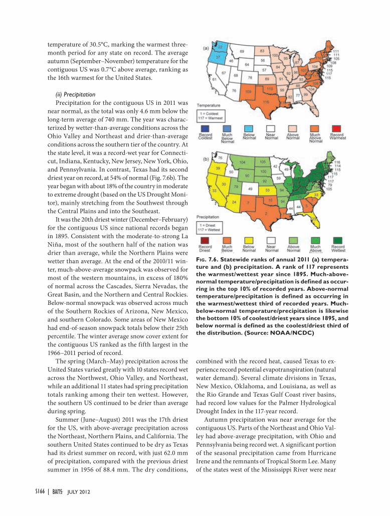
S166 | JULY 2012
temperature of 30.5°C, marking the warmest three-month period for any state on record. The average autumn (September–November) temperature for the contiguous US was 0.7°C above average, ranking as the 16th warmest for the United States.
(ii) Precipitation
Precipitation for the contiguous US in 2011 was near normal, as the total was only 4.6 mm below the long-term average of 740 mm. The year was charac-terized by wetter-than-average conditions across the Ohio Valley and Northeast and drier-than-average conditions across the southern tier of the country. At the state level, it was a record-wet year for Connecti-cut, Indiana, Kentucky, New Jersey, New York, Ohio, and Pennsylvania. In contrast, Texas had its second driest year on record, at 54% of normal (Fig. 7.6b). The year began with about 18% of the country in moderate to extreme drought (based on the US Drought Moni-tor), mainly stretching from the Southwest through the Central Plains and into the Southeast.
It was the 20th driest winter (December–February) for the contiguous US since national records began in 1895. Consistent with the moderate-to-strong La Niña, most of the southern half of the nation was drier than average, while the Northern Plains were wetter than average. At the end of the 2010/11 win-ter, much-above-average snowpack was observed for most of the western mountains, in excess of 180% of normal across the Cascades, Sierra Nevadas, the Great Basin, and the Northern and Central Rockies. Below-normal snowpack was observed across much of the Southern Rockies of Arizona, New Mexico, and southern Colorado. Some areas of New Mexico had end-of-season snowpack totals below their 25th percentile. The winter average snow cover extent for the contiguous US ranked as the fifth largest in the 1966–2011 period of record.
The spring (March–May) precipitation across the United States varied greatly with 10 states record wet across the Northwest, Ohio Valley, and Northeast, while an additional 11 states had spring precipitation totals ranking among their ten wettest. However, the southern US continued to be drier than average during spring.
Summer (June–August) 2011 was the 17th driest for the US, with above-average precipitation across the Northeast, Northern Plains, and California. The southern United States continued to be dry as Texas had its driest summer on record, with just 62.0 mm of precipitation, compared with the previous driest summer in 1956 of 88.4 mm. The dry conditions,
combined with the record heat, caused Texas to ex-perience record potential evapotranspiration (natural water demand). Several climate divisions in Texas, New Mexico, Oklahoma, and Louisiana, as well as the Rio Grande and Texas Gulf Coast river basins, had record low values for the Palmer Hydrological Drought Index in the 117-year record.
Autumn precipitation was near average for the contiguous US. Parts of the Northeast and Ohio Val-ley had above-average precipitation, with Ohio and Pennsylvania being record wet. A significant portion of the seasonal precipitation came from Hurricane Irene and the remnants of Tropical Storm Lee. Many of the states west of the Mississippi River were near
FIG. 7.6. Statewide ranks of annual 2011 (a) tempera-ture and (b) precipitation. A rank of 117 represents the warmest/wettest year since 1895. Much-above-normal temperature/precipitation is defined as occur-ring in the top 10% of recorded years. Above-normal temperature/precipitation is defined as occurring in the warmest/wettest third of recorded years. Much-below-normal temperature/precipitation is likewise the bottom 10% of coolest/driest years since 1895, and below normal is defined as the coolest/driest third of the distribution. (Source: NOAA/NCDC)

S167STATE OF THE CLIMATE IN 2011 |JULY 2012
average to drier than average. Minnesota had its third driest autumn on record.
(iii) Notable events
The US tornado season of 2011 was one of the most destructive and deadly on record. During the year, seven individual tornado and severe weather outbreaks caused damage exceeding $1 billion (US dollars), with total damage exceeding $28 billion (US dollars). This represents the most damage from severe weather in a single year since record keeping began in 1980. The 2011 confirmed tornado count stood at 1676, with 33 tornado reports still pending for December. This places 2011 as the second most active year on record for number of tornadoes since the modern record began in 1950.
The most active tornado period of the year was the spring (March–May), with 1150 confirmed tor-nadoes across the country, the most on record for any three-month period. The most active month was April, when 758 tornadoes were confirmed. This is the most on record for any month, surpassing the 550 reported in May 2003, and was driven by the two larg-est tornado outbreaks on record during 14–16 April and 25–28 April. These outbreaks both surpassed the April 1974 Super Outbreak for the most tornadoes during a single outbreak. The 199 tornadoes on 27 April was the most for any single day on record and the 316 fatalities on the same day was the most in the modern period of record for a 24-hour period. The 22 May Joplin, Missouri, tornado caused damages estimated at $3 billion (US dollars) and led to 158 fatalities, surpassing the previous records for both damages and fatalities from a single tornado in the modern tornado record.
During the late spring and early summer, historic flooding impacted much of the central United States. An above-average snowpack across the Northern Rockies, Northern Plains, and Ohio Valley combined with an anomalously wet spring caused significant runoff into the rivers. Some of the worst f looding occurred along the Mississippi, Ohio, Missouri, Souris, and James Rivers. The high water levels put signif icant stress on the levee systems along these rivers, and several levees were deliberately breached to flood farm lands and pro-tect cities. Record historical crests were set along the Missouri and Mississippi
Rivers, surpassing the floods of the 1920s and 1930s. Total damages approached $5 billion (US dollars).
During 2011, approximately 74!500 fires burned over 3.5 million hectares across the US. The southern US had the third most active wildfire year with re-spect to acres burned since records began 2000. Over 1.5 million hectares burned across Texas, the most of any state and 43% of the national total. The 2011 damages exceeded $1 billion (US dollars).
3) MEXICO—R. Lobato-Sánchez, R. Pascual-Ramírez, and A. Albanil-Encarnación
After a very wet rainy season in 2010, Mexico experienced its second warmest year since 1971 and thirteenth driest year since 1941. According to preliminary data from the National Meteorological Service of Mexico, the nationally-averaged annual mean temperature was 21.8°C, 1.1°C above the normal temperature. Total precipitation was below average, at 89% of normal.
(i) Temperature
The national average temperature for 2011 was 21.8°C, (1.1°C above the 1971–2000 normal) and ranked second only to 2006 as the warmest year since 1971 (Fig. 7.7). The annual average temperature has been above normal since 1993. In 2011, the an-nual mean temperature was between 1.0°C and 1.3°C above normal for much of the country. However, some states such as Baja California and the central states of Michoacan, Mexico State, Morelos, Tlaxcala, and Puebla were cooler than normal, while Sonora, Morelos, and Yucatan were near normal (Fig. 7.8a).
Daily mean temperatures for 2011 are shown in Fig. 7.9. Through the year, the average temperature was influenced by three events. The first was an early February winter storm in the northwest that impacted the average national temperature, which dropped nearly two standard deviations below the long-term average. Second, a persistent climatic pattern led to the mean temperature during spring and summer being warmer than average, marking values over the
FIG. 7.7. Annual mean temperature anomalies (°C) for Mexico for the period 1971–2011. The red line represents the trend. (Source: Meteorological Service of Mexico)

S168 | JULY 2012
threshold of two standard deviations. Finally, in late November, a cold front caused the average national temperature to drop below the threshold of two stan-dard deviations.
January was the coldest month of the year with 15.9°C (0.6°C below normal,) while the period Oc-tober–December registered a mean of 18.9°C that was ranked as normal. June was the warmest month of 2011 averaging 25.9°C (2.9°C above normal). Through the rainy season (July–September), the mean temperature was 25.5°C (2.4°C above normal). The
states of Coahuila, Nuevo León, and Zacatecas each had the warmest year over the last 41 years. Tem-peratures in Chihuahua, Durango, Aguascalientes, Distrito Federal, Tlaxcala, and Campeche ranked as second warmest. Guanajuato, Hidalgo, Quintana Roo, and Tamaulipas each ranked among their top five warmest.
(ii) Precipitation
Nationally, the year 2011 ranked as the thirteenth driest for Mexico since 1941, averaging 697.2 mm, ~90% of normal. Rainfall was much below normal during nine months. Only June, July, and November had precipitation near or above normal. The rain-fall spatial distribution showed marked differences between the southern and northern regions of the country (Fig. 7.8b). The wettest zones with annual rainfall over 1500 mm were located southward of 22°N covering the zones of Nayarit, Colima, Guer-rero, Veracruz, Tabasco, and Chiapas; Colima, Chi-apas, and Quintana Roo were the wettest states across the country. In contrast, total rainfall of less than 50% of normal was observed from central zones to north-ward regions. Below-normal rainfall was reported in Coahuila, Chihuahua, Durango, and Baja California, all averaging less than 25% of normal. Durango and Aguascalientes were classified as the driest, with Zacatecas and Guanajuato second driest, Baja Cali-fornia Sur and Coahuila the third driest, and Nuevo Leon and Chihuahua reached the fourth driest year.
(iii) Notable events
The year 2011 set a new record with the largest area (956!405 hectares) burned by forest fires, exceeding the previous record of 1998 with 843!633 hectares; Coahuila was the federal state with the largest area burned, 44% of the total.
The long-term drought during 2011 was due to a significant reduction in rainfall beginning in late autumn 2010. In June, the drought-affected region expanded to 85% of the country; this decreased pro-gressively with the onset of the rainy season, reaching 55% in September, but increased again in October to 61%. By late December, the drought impacts de-creased slightly in the north, mainly due to the winter storms described in the previous section; however, it had expanded towards the central region. The area that experienced moderate to exceptional drought covered 54.6% of the nation, according with the North American Drought Monitor definition, with 9.7 % in the highest category of exceptional drought.
FIG. 7.8. (a) 2011 annual mean temperature anomalies (°C) for Mexico (based on 1971–2010 mean) and (b) 2011 annual precipitation anomalies (% of 1941–2010 mean). (Source: National Meteorological Service of México)
FIG. 7.9. Daily mean temperature in 2011 (solid blue). Shaded area represents the normal threshold of ±2 standard deviations derived from 1971–2000. (Source: National Meteorological Service of Mexico)

S169STATE OF THE CLIMATE IN 2011 |JULY 2012
As of the date of this publication, the impacts of the drought on agriculture, livestock, and human populations have not been completely calculated. Most of the dams located in the northern region had their lowest levels following a poor recharge in the summer 2011. The bean crop dropped by almost half due to the late onset of the rainy season, delaying the sowing. Only 53.4% of croplands were planted in the main bean-producing states of Chihuahua, Durango, Zacatecas, and San Luis Potosí; in Sinaloa, less than 50% of agricultural lands were cultivated during the fall–winter 2011/12 season and pastures were not suf-ficient to feed the livestock. The federal government implemented national and local programs to support the population in order to mitigate the drought im-pacts, including water delivery for domestic use and temporary employment programs to reinvigorate local economies.
c. Central America and the Caribbean
1) CENTRAL AMERICA— J. A. Amador, H. G. Hidalgo, E. J. Alfaro, B. Calderón, N. P. Mora, and I. L. Rivera
For this region, 11 stations were analyzed from 6 countries. The stations located on the Caribbean side are: Phillip Goldson International Airport (MZBZ), Belize; Puerto Barrios, Guatemala; Puerto Lempira, Honduras; Puerto Cabezas, Bluefields, Nicaragua; and Puerto Limón, Costa Rica. The following stations are located on the Pacific side: Tocumen International Airport (MPTO) and David, Panamá; Liberia, Costa Rica; Choluteca, Honduras; and San José, Guatemala.
(i) Temperatures
On the Caribbean side, the mean temperature for the 2001–10 decade was warmer than the 1971–2000 average, with 0.5°C above average at MZBZ, Puerto Lempira, and Puerto Cabezas, and Bluefields. Meanwhile, near-average conditions were present at Puerto Barrios and Puerto Limón. The 2011 mean temperature was near average when compared to the 2001–10 decade, with the exception of Puerto Barrios and Puerto Lempira. During the last decade, the Pacific southernmost stations at MPTO and David, experienced above-average temperatures. In contrast, Liberia had cooler-than-average temperatures, while the northernmost stations of Choluteca and San José had near-average temperatures. A striking feature of 2011 was the higher frequency of near mean tempera-ture conditions and smaller frequency of high mean temperature values in all the Pacific side stations (shown as green line distributions in Fig. 7.10). Since many stations have a large amount of missing data in
their daily minimum and maximum temperatures, these two variables were analyzed regionally by taking an average of the five stations on the Pacific slope and the six stations on the Caribbean side. Both minimum and maximum temperatures for the last decade and 2011 were warmer than the 1971–2000 average in the Caribbean and Pacific basins.
(ii) Precipitation
Across Central America’s Pacific side, the stations experienced a near-average rainy season (May–No-vember), with the exception of Choluteca and David, which had a significant early start when compared to the 1971"2000 average. However, when compared to the 2001–10 decade, most stations had a normal start to the rainy season, with the exception of David, which had a late start. Consistent with the La Niña inf luence and the impact of warmer-than-normal Caribbean sea surface temperatures, the end of the rainy season was later than normal across all stations. With respect to the previous decade, 2011 had a late ending in all stations (but significant in only two sta-tions) with the exception of Choluteca, which showed normal conditions.
(iii) Notable events
The year 2011 was slightly below average in terms of tropical storm activity in the Caribbean basin (6°N"24°N, 92°W"68°W), which is unusual considering the development of La Niña and much weaker-than-average 900 hPa winds (inserted arrows in Fig. 7.10) during the period of the prevalence of the Caribbean low-level jet (a characteristic of La Niña events in the region and a condition favorable for tropical cyclone formation; Amador et al. 2006). In the Caribbean basin, Tropical Storm Harvey (19–22 Au-gust) and Hurricane Irene (21–28 August), and in the Pacific, Tropical Storm Dora (18–24 July), impacted Central America in different ways, but no human casualties were reported from any of those systems.
The significant 2011 storms that wreaked havoc across Central America were Tropical Depression 12-E (12–13 October) and Hurricane Rina (23–28 October). Rina triggered landslides and floods due to heavy rains in Belize, Guatemala, Honduras, and Nicaragua. A total of 46 fatalities, mostly from Hon-duras and Nicaragua, were attributed to Rina. De-spite the relatively high storm activity in the eastern Pacific, the major regional impact to economic and social welfare was not caused by a hurricane, but by Tropical Depression 12-E (approximate trajectory in red dots in Fig. 7.10). This storm caused significant
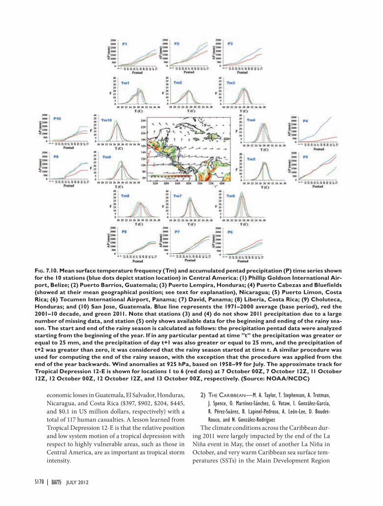
S170 | JULY 2012
economic losses in Guatemala, El Salvador, Honduras, Nicaragua, and Costa Rica ($397, $902, $204, $445, and $0.1 in US million dollars, respectively) with a total of 117 human casualties. A lesson learned from Tropical Depression 12-E is that the relative position and low system motion of a tropical depression with respect to highly vulnerable areas, such as those in Central America, are as important as tropical storm intensity.
2) THE CARIBBEAN—M. A. Taylor, T. Stephenson, A. Trotman, J. Spence, O. Martínez-Sánchez, G. Votaw, I. González-García, R. Pérez-Suárez, B. Lapinel-Pedroso, A. León-Lee, D. Boudet-Rouco, and N. González-Rodríguez
The climate conditions across the Caribbean dur-ing 2011 were largely impacted by the end of the La Niña event in May, the onset of another La Niña in October, and very warm Caribbean sea surface tem-peratures (SSTs) in the Main Development Region
FIG. 7.10. Mean surface temperature frequency (Tm) and accumulated pentad precipitation (P) time series shown for the 10 stations (blue dots depict station location) in Central America: (1) Phillip Goldson International Air-port, Belize; (2) Puerto Barrios, Guatemala; (3) Puerto Lempira, Honduras; (4) Puerto Cabezas and Bluefields (showed at their mean geographical position; see text for explanation), Nicaragua; (5) Puerto Limon, Costa Rica; (6) Tocumen International Airport, Panama; (7) David, Panama; (8) Liberia, Costa Rica; (9) Choluteca, Honduras; and (10) San Jose, Guatemala. Blue line represents the 1971–2000 average (base period), red the 2001–10 decade, and green 2011. Note that stations (3) and (4) do not show 2011 precipitation due to a large number of missing data, and station (5) only shows available data for the beginning and ending of the rainy sea-son. The start and end of the rainy season is calculated as follows: the precipitation pentad data were analyzed starting from the beginning of the year. If in any particular pentad at time ”t” the precipitation was greater or equal to 25 mm, and the precipitation of day t+1 was also greater or equal to 25 mm, and the precipitation of t+2 was greater than zero, it was considered that the rainy season started at time t. A similar procedure was used for computing the end of the rainy season, with the exception that the procedure was applied from the end of the year backwards. Wind anomalies at 925 hPa, based on 1958–99 for July. The approximate track for Tropical Depression 12-E is shown for locations 1 to 6 (red dots) at 7 October 00Z, 7 October 12Z, 11 October 12Z, 12 October 00Z, 12 October 12Z, and 13 October 00Z, respectively. (Source: NOAA/NCDC)

S171STATE OF THE CLIMATE IN 2011 |JULY 2012
(MDR) for hurricanes (10°N–25°N, 80°W–20°W) in June and July.
(i) Temperatures
Parts of the eastern Caribbean experienced below-average temperatures for the latter half of the year. Antigua recorded its third coolest July and second coolest August and experi-enced slightly below-average tempera-tures in September and December. In Dominica, the 2011 mean temperature at Melville Hall Airport (TDPD) was 26.7°C, which was the lowest value in the last 30 years.
In Puerto Rico, the 2011 average maximum temperature at the Luis Muñoz Marin International Airport (TJSJ) in San Juan was 0.6°C cooler than the 1981–2010 average of 30.4°C. The mean temperature at TJSJ was below average for 39% of the year and above average during 34% of the year. The
2011 average minimum temperature at TJSJ was 23.6°C, which is 0.5°C cooler than the 1981–2010 average. Across the US Virgin Islands, the mean annual temperature at Henry E. Rohlsen Airport (TISX) in Saint Croix and Cyril E. King Airport (TIST) in Saint Thomas was 0.7°C and 0.6°C below average, respectively.
In Cuba, monthly minimum and maxi-mum temperatures were near average during 2011 (Fig. 7.11a). However, April and May were significantly warmer than average, with maximum temperature anomalies above 1.0°C across all of Cuba. April 2011 was the third warmest April of the last 30 years in Cuba. There were sig-nificant positive anomalies of the effective temperature throughout the country, and positive anomalies (as high as 1.4°C) across the western and central regions. In addi-tion, the percentage of days with maximum temperatures above the 90th percentile was the highest since April 1961.
For Jamaica, extreme temperatures were recorded by several automatic weather sta-tions across the island. The highest maxi-mum air temperature recorded was 37.3°C, at Barton Isles, St. Elizabeth, in July, while an extreme minimum air temperature of 13.8°C was recorded at Bunkers Hills, Tre-
lawny, in February.
(ii) Precipitation
Precipitation patterns during the Caribbean’s dry season (December–April) were impacted by the 2010/11 La Niña event. The impact held true to noted
FIG. 7.11. (a) 2011 monthly mean maximum (Tx) and minimum (Tn) temperature anomalies (°C) for Cuba; (b) Annual precipita-tion anomalies represented as Standardized Precipitation Index (unitless; based on 1971–2000 base period). (Source: Institute of Meteorology of Cuba)
FIG. 7.12. 2011 mean monthly rainfall (mm) for Jamaica (blue bars) and long-term average 1971–2000.

S172 | JULY 2012
tendencies (Stephenson et al. 2007), with the Carib-bean being wetter than average in the south and east, but drier than average in the north and northwest.
In Jamaica, rainfall totals were 70–90% of normal during every month through April, with the largest deficit (67% of normal) occurring in April (Fig. 7.12). The Dominican Republic reported a similar deficit in rainfall for January–March (SERVIR 2011). In Cuba, 82% of the country experienced moderate to severe drought conditions during March–May, and in Puerto Rico, only 85% of the normal precipitation fell through April. St Croix’s TISX recorded its driest January on record.
In contrast, the southern and eastern Caribbean experienced much-above-average rainfall. The Bar-bados Meteorological Service references a “very wet” dry season with cumulative rainfall of 507.2 mm dur-ing January–May, almost twice the 1961–90 average. Rainfall in April was 143.3 mm, or twice the monthly mean, and through May there were approximately five more rain days (# 1 mm) per month than the long-term average. The wet “dry season” contributed to an annual rainfall of 1681 mm, the fifth highest since 1942. Similarly, dry season rainfall at both Canefield Airport (TDCF) and Melville Hall Airport (TDPD) in Dominica was 150% of the 1982–2010 average, with TDCF recording 2458.5 mm—the highest since 1982. Monthly rainfall at the E.T. Joshua Airport (TVSV) in St. Vincent and the Grenadines for January–April exceeded each month’s long-term average (1979–2011 base period), with April rainfall (236.7 mm) being more than twice the average of 92.8 mm. In St. Lucia, April was the wettest month for the year, with 407.9 mm, which represented the highest April amount recorded at Hewanorra Airport (TLPL) since 1973. An abnormally wet “dry season” was also noted for Grenada (above average for January–April) and for Trinidad (see special issue of CAMI Monthly Bulletin, 2012, Vol. 5, No. 1).
By June, with the de-cline of La Niña and the onset of very warm Carib-bean SSTs, most islands experienced average or above-average rainfall, with a few records set be-tween June and August due to the passage of a series of tropical systems,
including Tropical Storms Emily and Irene. From as early as April, SSTs in the MDR were 0.5°C above average, representing the 14th warmest April SSTs in the last 100 years. The warm surface temperatures persisted through July, with June recording the third largest anomaly since 1950. Rainfall totals in June and July were above average, particularly across the Greater Antilles, significantly offsetting the deficit previously recorded for these northern territories, and, notably occurring during the period referred to as the midsummer drought (July–August). For Jamaica, the July rainfall total (200 mm) was the seventh highest since records began in 1881 (Fig. 7.12). In Antigua, the July and August rainfall were the second and ninth highest, respectively for those months, since national records began in 1928. St. Croix’s TISX had its second wettest June and third wettest July. Martinique had its seventh wettest July and second wettest August on record. In Puerto Rico, a rainfall surplus of 914.4 mm from late May through September was reported for the San Juan Metro Area with 141% of the normal precipitation falling across all Puerto Rico. In fact, summer 2011 was the wettest summer on record at TJSJ with a rainfall total of 1098 mm between June and August. For May–November, most islands reported near-normal rainfall or slightly above-normal activity. The Caribbean Drought and Precipitation Monitoring Network (CIMH 2012) noted that August–October rainfall in the eastern Caribbean islands of Trinidad, Barbados, and St. Lucia was normal, while conditions for Grenada, St. Vincent, Dominica, Antigua, and St. Kitts ranged from moderately to abnormally wet. St. Thomas’s TIST had its wettest August and driest October on record. In the north, Jamaica’s rainfall was near aver-
FIG. 7.13. top: 2011 observed daily maximum temperature (°C, red), 1981–2010 daily maximum temperature normal (°C, brown), 2011 observed daily minimum temperature (°C, blue), 1981–2010 daily minimum temperature normal (°C, light blue). bottom: 2011 accumulated rainfall (mm) and 1981–2010 mean accumulated rainfall (mm) for (a) TJSJ, (b) TIST, and (c) TISX. (Source: NOAA/NWS)

S173STATE OF THE CLIMATE IN 2011 |JULY 2012
age. By December, with the onset of the Caribbean dry season, the La Niña pattern of a dry north-wet south appeared to reemerge. Whereas Barbados, Trinidad, and St. Kitts were wetter than average, Jamaica was drier than average.
Overall, in Puerto Rico, 2011 ranked as the second wettest year in nearly 113 years of record keep-ing in the San Juan Metro Area. An impressive rainfall total of 2239 mm was reported at TJSJ, which is 807.7 mm above average (Fig. 7.13a). This total was 34.3 mm less than 2010, the wettest year on record. According to the Cooperative Weather Observer Data, 2011 was a wet year across the entire forecast area, with 126% of the normal pre-cipitation falling across all of Puerto Rico and 121% of normal falling across the US Virgin Islands (USVI). 2011 ranked as the ninth wettest year on record at TIST, as well as TISX, with rainfall totals of 1172 mm and 1212 mm, respectively (Figs. 7.13b,c).
For Cuba, the annual average rainfall for 2011 was near average. Based on the Standardized Precipitation Index (SPI), 20% of the country had above-average rainfall accumulation during 2011, with 5% of the country falling in the moderate to extreme category, while 33% of the country reflected deficit, with 15% in the moderate to extreme category (Fig. 7.11b).
(iii) Notable events
Significant 2011 storms for Caribbean islands include Tropical Storm Emily and Hurricane Irene. Although Emily was a fairly disorganized storm as it tracked into the northeastern Caribbean, it generated strong thunderstorms and gusty winds along its path. Within a 72-hour period on 31 July–3 August, more than 225 mm of rainfall was recorded at St. Vin-cent and Grenadine’s TVSV. On 2–3 August, Emily tracked south of Puerto Rico and the USVI, leaving rainfall accumulations between 102 mm and 152 mm, with locally higher amounts of up to 254 mm. The higher rainfall accumulations were observed across the eastern half and portions of southwest Puerto Rico. After tracking over Hispaniola and exiting the northeastern Caribbean on 6 August, its remnants regenerated into a tropical storm, before dissipating the next day. In Puerto Rico, the storm caused at least $5 million (US dollars) in infrastructure damage.
Hispaniola was also impacted, where five fatalities were reported in addition to nearly 8000 homes be-ing damaged.
Also notable was Hurricane Irene, which was the first hurricane of the season. Irene originated from a well-defined Atlantic tropical wave east of the Lesser Antilles. On 21 August, Irene made landfall in Puerto Rico at Category 1 hurricane strength, resulting in severe f looding, significant property damage, and one fatality. The 72-hour maximum precipitation totals ranged from 381 mm to 559 mm. With rainfall from this storm, August 2011 ended as the wettest August on record as well as the wettest month ever across the San Juan Area, with a rainfall total of 471.4 mm. Irene tracked just north of Hispaniola as an intensifying cyclone, causing heavy rainfall and strong winds and killing seven people. After crossing the Turks and Caicos Islands, the hurricane quickly strengthened into a Category 3 major hurricane while passing through The Bahamas. It left behind a trail of extensive structural damage in its wake, primarily on Cat, Mayaguana, Acklins, and Crooked Islands. Government reports noted that upwards of 90% of all homes and structures on the islands were dam-aged. Thereafter, Irene curved north and impacted the United States. Total Caribbean economic losses were estimated at nearly $1.5 billion (US dollars), with combined insured losses listed around $1 billion (US dollars), primarily due to damage in the Bahamas.
FIG. 7.14. (a) 2011 annual mean temperature anomalies (°C) for South America (1971–2000 base period), and (b) 2011 annual precipitation anomalies (%) (1971–2000 base period). (Sources: National Meteorological Services of Argentina, Brazil, Bolivia, Chile, Colombia, Ecuador, Paraguay, Peru, Suriname, Uruguay, and Venezuela. The data was compiled and processed by CIIFEN, 2011)

S174 | JULY 2012
d. South America
The 2011 annual mean temperature was near normal to above normal in northern South America, the tropical Andes, and western Amazonia. Peru, Chile, and the Atlantic coast of South America were characterized by near-normal to below-normal tem-peratures (Fig. 7.14a). The annual total precipitation was above normal in northern South America and central Amazonia, but generally below normal in western South America, Argentina, Paraguay, and Uruguay (Fig. 7.14b).
Climate conditions across the region during 2011 were influenced by a La Niña event during the first few months of the year, and the reemergence of La Niña conditions during the latter part of the year. Typically, La Niña produces above-average precipita-tion across northern South America, and below-aver-age precipitation across southeastern South America.
1) NORTHERN SOUTH AMERICA AND THE TROPICAL ANDES—R. Martínez-Güingla, J. Arévalo, G. Carrasco, E. Jaimes, and G. León
(i) Temperatures
The La Niña influence over the northern parts of South America was evident in the region’s tem-perature. Temperatures during January–March were predominantly cooler than normal across Colombia, Ecuador, and Peru, with temperature anomalies rang-ing from 0.5°C to 2°C below the 1971–2000 average. Coinciding with the decline of La Niña in June, tem-peratures across the area were warmer than average. In Ecuador, temperature anomalies were between 0.5°C and 1.5°C above average during July–Septem-ber. Although minimum temperatures across Peru were near normal during April–June, maximum temperatures were 3°C above average. With the re-emergence of La Niña in October, temperatures across northern South America were cooler than normal during the final months of the year.
(ii) Precipitation
In Venezuela, above-normal precipitation was observed during most of 2011, mainly due to the inf luence of La Niña. The largest precipitation anomaly (166% of normal) was observed during Janu-ary–March. July–September was the only time during the year that recorded below-average precipitation, at 94% of normal. Overall, 2011 was among the top five wettest years for several stations across the country.
Colombia experienced above-average precipitation throughout the year, attributed to La Niña conditions during the first and last few months of the year. North
and central regions of Colombia were affected by heavy rainfall during January–March, with anomalies between 150% and 200% of normal. In December, precipitation anomalies ranging from 600% to 900% of normal were observed over northern Colombia. Overall, the heavy precipitation observed across Colombia throughout the year caused more than 250 deaths and affected two million people.
The coastal region in Ecuador reported anomalies that were 0–80% of normal during January–March. During April–June, specifically in April, 150–250% of normal rainfall was observed across the country. July–September was characterized by above-average precipitation over the highlands and the southern coast, with anomalies ranging between 150% and 800% of normal (El Oro Province). The highest monthly precipitation anomaly of 840% of normal was registered in Zaruma (located in southern Ecua-dor) in July. During October–December, precipitation deficits were observed across the coastal region, with positive anomalies in the Amazonia area.
In Bolivia, above-average precipitation was ob-served in the eastern Llanos, Altiplano, and valleys during January–March. In January, a maximum daily precipitation of 194 mm was registered in eastern Llanos, where the monthly normal is 162 mm.
In Peru, precipitation anomalies over the north-ern region during January–March were 0–40% of normal, while above-average precipitation was observed across the central and southern regions. During April–June, precipitation anomalies over the northern Amazon jungle and the northern and central highlands reached 400% of normal. During October–December, northern and central parts of the country experienced above-average precipitation, while the south had below-average precipitation.
(iii) Notable events
The Libertador Municipality in the Capital Dis-trict of Venezuela—one of the most densely popu-lated areas in the country—was affected by heavy precipitation that prompted flooding and triggered landslides, leaving over 8900 families homeless. The Orinoco River, the country’s largest river, had an above-normal flow level during most of the year. In August, the Apure River f looded, affecting many rural populations.
In Colombia, more than 350 windstorms occurred between June and September in different areas of the country, affecting thousands of families. Strong hailstorms were registered in Bogota, Santander,

S175STATE OF THE CLIMATE IN 2011 |JULY 2012
and Cundinamarca in April, July, and October, re-spectively.
Between January and February, in Cuzco, Peru, a precipitation anomaly over 400% of normal and stream f low of Paucartambo River of 400% were registered. This isolated main archeological sites, resulting in economic losses in the tourism sector.
2) TROPICAL SOUTH AMERICA EAST OF THE ANDES— J. A. Marengo, J. Ronchail, L. M. Alves, and J. Baéz
(i) Temperatures
In January, all of tropical South America expe-rienced warmer than average conditions, about 1°C above the 1961–90 average, while near-average tem-peratures were observed in February and March. In April, warm conditions continued over central and southern Brazil, western Bolivia, and Paraguay, and continued in May and June in northwestern Amazo-nia and Bolivia. During July–August, warmer-than-average conditions persisted across most of the region, with anomalies around +2°C in southeastern Brazil.
However, some regions experienced cooler-than-average conditions, nearly 1°C below average, during June–August, due to various cold waves that impacted the area. At the beginning of June, a freezing episode in the southern Andes of Peru impacted 13!400 people and 4500 head of cattle. At the end of June and begin-ning of July, cold waves brought cooler-than-average temperatures to the region. Minimum temperatures between 2.8°C and 5.3°C were observed in São Paulo, where the mean July minimum temperature is 11.7°C (1961"90 base period), and the minimum tempera-ture dropped from 20.3°C to 12.6°C, between 1 and 4 July, in Vilhena (Southern Amazon). By mid-July, more than 6000 people and 41!000 head of cattle had been affected by temperatures as low as -26°C and 1.6 meters of snow in the Bolivian department of Potosi (southern Altiplano).
In August, five cold surges affected southeastern South America; the two most intense affected Vilhena and southern Brazil. Cold air surges continued dur-ing September–November. In the city of São Paulo, the maximum temperature dropped from 33.1°C to 17.9°C in two days. In December 2011, the lack of rainfall in south central Brazil contributed to warm conditions in the states of Mato Grosso and São Paulo, with temperatures up to 3°C above average.
(ii) Precipitation
During 2011, rainfall was slightly below aver-age (50 mm below the 1961–90 average) across the 5°S–15°S latitude band in South America, as well as
in southern Bolivia, southern Brazil, and Uruguay. Southern Bolivia, southern Brazil, and Uruguay were impacted by drought, which had begun in August 2010, affecting crops that resulted in nearly $60 million (US dollars) in losses. Meanwhile, rainfall was nearly 150 mm above average from Colombia to northeastern Brazil, eastern Bolivia, and northern Paraguay.
In January 2011, heavy rains, f loods, and mud-slides in the Oxapampa region in the central Andes of Peru affected more than 1100 people. In the highlands of the state of Rio de Janeiro, heavy rainfall during January caused the worst flooding and landslides in Brazil in decades. Between 11 and 13 January, nearly 1000 people died and 35!000 were left homeless (see Sidebar 7.1). In the city of São Paulo, January 2011 was the wettest since 1943, reaching 491.5 mm, almost twice the month’s average.
In February, rainfall in southern Peru, Bolivia, Paraguay, and northern Argentina was about 200 mm above normal. Above-average rainfall (50 mm–200 mm) was observed across northeastern South America and Colombia.
In March, a reversal of rainfall patterns occurred, with below-average rainfall in Bolivia and Paraguay. Above-average rainfall persisted over northern South America and southeastern Brazil (about 150 mm above average). The January–March sequence re-sulted in deficit of rainfall (as much as 200 mm below average) in parts of western and southern Amazonia, just at the peak of the rainy season. In the Peruvian Amazon, however, the water level of the Amazonas River in Iquitos increased very rapidly after the 2010 drought episode, due to very wet local conditions.
In April, rainfall was 200–300 mm above average in Ecuador and most of western Colombia. In May, rainfall was up to 200 mm above average from north-ern South America to northeastern Brazil. In the state of Pernambuco, in northeastern Brazil, intense rainfall left 144!000 people homeless. In contrast, rainfall was below average from southern Colombia to southern Brazil.
During June–August, below-average rainfall was detected over northern Brazil, Venezuela, and eastern Colombia (200 mm below average). As a consequence, the level of the Rio Negro in Manaus registered a drop of about 1.24 m between 13 and 16 September, which is considered the largest reduction in a short time period since 1903 (according to the Serviço Geológico do Brasil). In contrast, intense rainfall continued in western Colombia and northeastern Brazil. Nine people were killed in Pernambuco and

S176 | JULY 2012
SIDEBAR 7.1: THE 2011 INTENSE RAINFALL AND FLOODS IN RIO DE JANEIRO—J. A. MARENGO AND L. M. ALVES
During January 2011, heavy rainfall sparked flash flooding and mudslides across the highlands of the state of Rio de Janeiro in southeastern Brazil, devastating moun-tain towns. According to Brazilian official sources, the floods and landslides claimed the lives of 916 people and left 35 000 people homeless. This was one of the worst natural disasters in Brazil’s history. During the first half of January, rainfall in Brazil was primarily concentrated in a swath from the states of São Paulo, Minas Gerais, Goiás, and southeastward to Rio de Janeiro. While the 1961–90 average rainfall for January in that region is about 230 mm, the rainfall accumulated during January 2011 was approximately 460 mm. According to the Brazilian Meteorological agencies CPTEC INPE (http://www.cptec.inpe.br) and INMET (http://www.inmet.gov.br), the anomalous rainfall was caused by the South Atlantic convergence zone (SACZ), a typical summer time rainfall-producing mechanism that was fed by moisture transport coming from the Amazon region during that period and by a favorable signal of convection and precipitation by the Madden–Julian oscillation (MJO), that persisted until mid-January. The large-scale pattern was characterized by a weakening of La Niña in the equatorial Pacific Ocean, while over the South Atlantic Ocean, off the coast of southeastern Brazil, sea surface temperatures were 2°C above normal. Three episodes of SACZ were detected: 1–7 January, 11–17 January, and 18–21 January. The two earlier episodes produced intense low-level convergence over southeastern Brazil,
intensified by plenty of moisture coming from the Ama-zon region. As a consequence, rainfall in the highlands of Rio de Janeiro during 1–7 January was about 86 mm–160 mm and about 300 mm in 11–17 January (Fig. SB7.1), well above the January average. These conditions favored weeks of saturated soil, and together with the intense rainfall from 11 to 13 January, floods and mudslides were triggered. Numerous houses located in risk areas on the deforested slopes of the mountains were buried, killing hundreds of people. In one of the most affected cities, Nova Friburgo, rainfall on 11–12 January was 182.8 mm, 79% of the monthly
average of 232 .5 mm (Fig. SB7.2). Ac-cording to the Civil Defense of the state of Rio de Janeiro, 428 people d ied in this city alone. Croplands were de-stroyed. Highways, roads , hospitals , and sewage systems all collapsed. The isolation of these cities and the risk of epidemics left the population and local governments in a permanent state of alert.
FIG. SB7.1. (a) Accumulated rainfall (mm) 11–17 January 2011 in the southeastern Brazil re-gion and (b) rainfall anomalies (mm) for the same period from the 1961–90 base period. The cities of Rio de Janeiro and Nova Friburgo are marked on the map. (Source: CPTEC-INPE)
FIG. SB7.2. Daily precipitation (mm) during 1–17 January 2011 in Petrópolis (blue bar), Nova Friburgo (red bar), and Rio de Janeiro (green bar). Monthy January average (1961–90 base period): Nova Friburgo: 232.5 mm; Petrópolis: 201.5 mm; and Rio de Janeiro: 136.4 mm. (Source: INMET)

S177STATE OF THE CLIMATE IN 2011 |JULY 2012
one in Paraiba, and more than 340 families lost their homes in mid-July. By the first week of August, the state of Parana in southern Brazil experienced heavy rainfall and storms, affecting more than 20 cities and 150!000 people. The Iguacu River reached a record flow of 12.5 million L s-1.
In September, drier-than-average conditions persisted in western Amazonia (100 mm–200 mm below average). During the second week of September, intense rainfall in the state of Santa Catarina in south-ern Brazil left almost 15!000 people homeless, affected more than 900!000 people, and destroyed highways.
From November to December, f loods and land-slides affected hundreds of people and damaged roads and crop fields in the northern and central Andes of Peru. At the beginning of December 2011, heavy rainfall across northern Venezuela caused rivers to overflow, affecting almost 2000 people. On the other hand, most of tropical South America had below-average precipitation (as much as 200 mm below normal in Amazonia).
3) SOUTHERN SOUTH AMERICA—M. Bidegain, M. Skansi, O. Penalba, and J. Quintana
(i) Temperatures
Near- or above-average temperatures were ob-served over most of southern South America dur-ing 2011, with average anomalies up to +1.0°C (Fig. 7.14a). The greatest positive anomaly was observed in Patagonia (south of 40°S in Chile and Argentina). During December 2010–February 2011 (austral
summer), warmer-than-average temperatures (+0.5°C to +1.0°C) were observed in Argentina, Uruguay, and central Chile. This behavior was accompanied by positive deviations of the mean maximum and minimum temperatures and below-normal rainfall in the region, during La Niña. From December 2010 through the first days of January 2011, extremely high temperatures (at or above the 90th percentile) affected different regions of Argentina and southern Chile. Over eastern Uruguay the mean monthly tempera-ture anomaly was as high as 3°C above the 1961–90 average in January. Between 6 and 11 February, Patagonia experienced above-average temperatures, setting records in several locations. The anomalously warm conditions continued during March–May 2011 (austral autumn) over Argentina and Uruguay. In contrast, the southern South America winter
(June–August) was cooler than average (-0.5°C to -1.0°C) in Chile, central Argentina, and Uruguay. A cold wave between 25 June and 10 July brought cooler-than-average temperatures, 5°C to 10°C below aver-
age, for several days. In Argentina, daily minimum temperatures were as low as -16.0°C in Malargüe (Mendoza Province) on 3 July and -7.7°C in Bolivar (Buenos Aires Province) on 6 July. In central Chile, the minimum temperature was -3.0°C in Santiago on 3 July and -4.8°C in Curico on 4 July. These extreme low temperatures during the Southern Hemisphere core winter claimed the lives of five people in Uru-guay. The invasion of cold air also brought heavy snowfall. Snow covered half of Argentina and Chile during 6–8 July, including northern Chile (Atacama Desert) and southern Buenos Aires Province where snowfall is rare. According to the Argentine Weather Service, temperature anomalies of -1°C to -2°C were widespread across Argentina during July 2011. Similar conditions were observed in Chile between Valparaiso and Temuco.
During austral spring (September–November) above-average mean temperature anomalies (+0.5°C to +1.5°C) were observed over the entire region (Uru-guay, Argentina, and Chile). In September, several maximum temperature records were set in northwest-ern Argentina. In Santiago (central Chile), the mean maximum temperature of 23.3°C was the highest ever recorded, 4.2°C above average. Meanwhile most of southern South America was cooler than average in October 2011. According to the Argentine Weather Service, several locations in Argentina experienced their coolest October in the last five decades. In Chile, this cooling was more moderate, with anomalies around -1°C.
(ii) Precipitation
During 2011, below-average precipitation across southeastern South America was attributed to the La Niña episode, which began during the latter part of 2010. In Argentina, the annual rainfall was below the
1961–90 average across much of the region, with eastern Buenos Aires and Cordoba Province being the most affected at 60–80% of normal. In central Chile, annual precipitation was below normal, re-sulting in the fourth driest year since 1950. In May 2011, several cities in Argentina and Chile recorded their lowest precipitation totals since 1961, including Iguazú (4.0 mm), Río Cuarto (2.0 mm), and Trelew (0.5 mm). The driest anomalies during June–August 2011 were observed across eastern Brazil, Argentina, northeastern Bolivia, and central and southern parts of Chile. Although isolated heavy rainfall impacted these areas, it wasn’t enough to alleviate the dry conditions.

S178 | JULY 2012
Heavy rain fell on 15 July across Uruguay and southern Brazil. The maximum 24-hour accumulated rainfall total was 140 mm observed in Lavalleja and Rocha, both located in Uruguay. In northern Chile's Atacama Desert, a cutoff low pressure system on 3–8 July brought heavy snowfall (up to 20 cm) and strong winds (above 20 m s-1), seri-ously affecting the mining industry in the high mountains of the Andes and land transportation between Chile, Bo-livia, and Argentina.
In Argentina and Uruguay, the drier-than-average conditions were more intense during the second half of the year. However, rainfall in October brought relief to the northern part of the region, and in November to the central and western part of the province of Buenos Aires. In particular, the northern province of Buenos Aires showed defi-cits in all months during the latter half of the year. Anomalies were the lowest in August, September, and December, reaching values that were 20% of normal. Nine meteorological stations located in northeastern Argentina recorded their lowest December precipi-tation totals since 1961. In Chile, the driest months were May–July, October, and December. The central region was the most affected, with deficits of 50–60%. The greatest impacts were in agriculture, freshwater resources, and hydroelectric power.
(iii) Notable events
Overall, below-average rainfall prevailed through-out much of Argentina in 2011. The excess precipita-tion occurred locally and some of the events were very intense. Extreme events occurred in February, April, and August. On 23 February, a severe storm brought heavy rain, hail, and strong winds to various neighborhoods around the capital of the province of Mendoza (western Argentina), resulting in floods and fallen trees. On 26 February, another severe storm af-fected the province of Catamarca, isolating locations due to overflowing rivers and landslides. Two days of heavy rain caused a state of emer-
gency in Comodoro Rivadavia city (central-east of Patagonia). A total of 120 mm of rain fell on 12–13 April, almost four times April’s monthly average. On 8 August, Iguazú Falls (northeastern Argentina) streamflow increased to eight times its normal flow in only a few hours due to the intense rainfall in southern Brazil.
In northern Chile, intense rainfall occurred dur-ing 3–8 July and again on 31 July that affected the Atacama Desert region. Daily totals between 20 mm and 25 mm were observed, where precipitation is typi-cally near zero or less than 5 mm during the month.
e. Africa
1) NORTHERN AFRICA—K. Kabidi and A. Sayouri This region includes Morocco, Algeria, and Tu-
nisia. The 1971–2000 base period has been used to assess anomalies in both temperature and precipita-tion in 2011.
(i) Temperature
Generally, both maximum and minimum tem-peratures were higher than average over the region. The year 2011 was the warmest in the last ten years. The annual maximum temperature averaged be-tween 0.5°C and 3.5°C above normal with the larg-est anomaly observed in Taza, in the north-central sector of Morocco, south of the Rif Mountain. The annual maximum temperature anomaly was strongly influenced by extreme warm temperatures during the summer season.
During winter, both positive and negative anoma-lies were observed. The mean temperature anomaly ranged between -2.4°C at Nador in eastern Morocco to +1.5°C in Sidi Slimane in central Morocco. An exceptional cold wave occurred in January and Feb-ruary. The region experienced significant snowfalls, with temperatures reaching -7°C in Algeria. Positive temperature anomalies returned during the spring season, with anomalies greater than +1.7°C. Summer was characterized by exceptional heat waves and ex-
FIG. 7.15. Temperature anomaly (°C) in northern Africa on 2 July 2011. (Source: NOAA/NCEP)

S179STATE OF THE CLIMATE IN 2011 |JULY 2012
treme temperatures were recorded. June and July tem-perature anomalies surpassed +4.4°C in Sidi Slimane (Fig. 7.15), as mean temperatures reached 45.3°C and 49°C in Sidi Slimane and Ain Saleh, respectively.
(ii) Precipitation
Overall, the annual precipitation was above aver-age, especially during autumn when rainfall amounts reached 171% of normal in Rabat in Morocco. Several locations recorded rainfall amounts approaching 100 mm in a 24-hour period during this time, resulting in flooding. The winter season was quite active with the development of storms that produced heavy rains approaching 80 mm in Chefchaouen, Morocco, in a 24-hour period, and over 50 mm also in 24-hour period in Tangier, Morocco. In Algeria, a winter storm produced over 60 mm of rainfall in Echelf and Constantine. More storms that produced over 60 mm rainfall in less than 24 hours occurred in the northern areas of Algeria and Morocco during the spring, especially in March and May. Rainfall surpluses exceeded 180% of normal. Summer was dominated by the presence of an anticyclonic system across northern Africa and dry conditions, except for intense heavy rains that fell in northwestern Mo-rocco in early June. During autumn, strong storms produced heavy rains and caused flooding in many locations in Algeria and in Morocco during autumn, especially during October. Records indicated 94.6 mm at Chefchaouen (northern Morocco), 104 mm at Bouchegouf (northeastern Algeria), and 78 mm at El kala (northern Algeria). Rainfall totals averaged 320% of normal in Nador (eastern Morocco).
(iii) Notable events
October and November were marked by a suc-cession of significant heavy rainfall events that led to several floods in Morocco, Algeria, and Tunisia. These events caused important infrastructure dam-age and loss of human life, especially in Algeria.
Also in Algeria, several forest fires associated with a heat wave and daily temperatures exceeding 49°C, burned at the end of July and the beginning of August. An estimated 15!000 ha of land was affected, accord-ing to the Forestry Department of Algeria.
2) WESTERN AFRICA—L. N. Njau and W. M. ThiawWestern Africa extends from the Guinea coast to
Chad and the Central African Republic. All analyses are based on the 1971–2000 base period.
(i) Temperature
The year 2011 was once again very warm in Western Africa. The monthly temperature remained above average every month and across the region. In January, the temperature was 1.5°C above normal and the greatest anomalies (3.5°C above the 1971–2000 base period) were observed in Mauritania, central Niger, and northern Sudan. The positive anomalies increased in February, with temperatures 3.5°C above average in Niger, western Chad, and northern Nigeria. In March, temperature decreased, but maintained positive anomalies (> 2.5°C) in Mali, northern Burki-na Faso, and western Niger with highest anomalies (> 3.5°C) over central Mali and western Niger. April had a major decline in temperature anomalies, with (< 1.5°C) over northern Mauritania and northwest Mali that persisted in May with the temperature anoma-lies (< 1.5°C) covering the central part of the Sahel. Unlike the previous year, the June 2011 temperature anomalies (> 1.5°C) intensified spatially over parts of Mauritania, Mali, Burkina Faso, Ghana, Benin, Togo, Niger, and Chad, with an epicenter (> 2.5°C) over northwest Mauritania. In July, temperature anomalies
FIG. 7.16. Jun–Sep 2011 (a) rainfall (mm) for Western Africa and (b) anomalies (departure from the 1971–2000 base period). The boxed region indicates the approximate boundaries of the Sahel region. (Source: NOAA/NCEP)

S180 | JULY 2012
(> 1.5°C) were observed over parts of western, central, and eastern Sahel. Temperature anomalies in August ranged between -1°C and 1°C over the continent, but peaked in September with anomalies of +1.5°C to +2°C covering parts of Mauritania, Mali, Burkina Faso, Ghana, Benin, Togo, Niger, and northwestern Nigeria, and intensified in October over these parts with an epicenter greater than 2.5°C, over northwest Mauritania. In November, positive temperature anomalies from 1.5°C to 2.0°C covered western part of West Africa, with a weak epicenter > 2°C over northwestern Guinea. In December, the temperature anomalies were generally normal over West Africa.
(ii) Precipitation
The year 2011 was characterized by overall near-average conditions (compared with the 1971–2000 base period) across most areas in West Africa (NOAA gridded gauge precipitation analysis, PREC/L). Rain-fall totals from June to September ranged between < 100 mm in the northern part of the Sahel to >1200 mm in the western Guinean coast, and along the coastal border of Nigeria and Cameroon (Fig. 7.16a). The rainy season was slightly above average across the Sahel and portions of the Gulf of Guinea. However, rainfall amounts were much less than in 2010, the wettest year in the Sahel in over 50 years. Rainfall was 50 mm – 100 mm above average across the Sahel (Fig.7.16b). Surpluses over 200 mm were observed along the coast of Guinea and along the south border between Cameroon and Nigeria. Rainfall was much below average over most areas in Cote d’Ivoire and portions of western Ghana, with deficits between 100 mm and 300 mm.
(iii) Notable events
Overall, the June–September rainy season had a slow start, an early withdrawal, and dry spells, espe-cially in central Sahel. This resulted in poor harvests, food shortages, and scarcity of water availability in affected areas that called for international humanitar-ian relief assistance. However, in the western end of the Sahel, the West African monsoon system inten-sified in August, with excessive rains and flooding, especially in Guinea and Mali. Torrential rains dur-ing 23–24 August led to floods in the northwestern, central, and northeastern sectors of Guinea, causing significant material damage, and leaving more than 4000 people homeless.
3) EASTERN AFRICA—W. Gitau, C. Oludhe, L. Ogallo, Z. Atheru, and P. Ambenje
The Greater Horn of Africa (GHA) can broadly be divided into three sectors. The northern sector encompasses northern and central Somalia, Djibouti, Eritrea, Ethiopia, Sudan, and South Sudan. The equa-torial sector covers southern Somalia, Kenya, Uganda, Burundi, Rwanda, and northern Tanzania. The southern sector covers central and southern Tanzania.
March–May marks the main rainfall season or “Long Rains” over the equatorial sector, while a second rainfall season, the “Short Rains” is observed from late September to early December. June to early September marks the rainfall season over the north-ern sector and the coldest season over the equatorial sector. The western highlands of Kenya also experi-ence significant rainfall during this season. The southern sector receives rainfall from December to February. The base period for this section is 1961–90 unless otherwise stated.
(i) Temperature
In eastern Africa, noteworthy minimum tem-peratures, as opposed to mean and maximum tem-peratures, have been observed recently; hence, these temperatures are discussed in this section. Warmer-than-average minimum temperature anomalies pre-vailed over much of the GHA, except for northern and central Sudan in the northern sector of the region, and
FIG. 7.17. Minimum temperature anomalies for 2011 (°C, 1961–90 base period). (Source: IGAD Climate Prediction and Applications Centre)

S181STATE OF THE CLIMATE IN 2011 |JULY 2012
portions of northwestern and northeastern Uganda in the equatorial sector of the region. Minimum temperature anomalies exceeded +2°C in central Tanzania, southwestern Kenya, and parts of Ethiopia (Fig. 7.17). Mombasa, Kenya, reported the highest average January minimum temperature in the last 11 years (departure computed based on 2000–10 mean).
The minimum temperature also ranked among the highest during most months in 2011 at this location (not shown).
(ii) Precipitation
From December 2010 to February 2011, parts of western Ethiopia, southern Uganda, western Kenya, and northwestern, western, eastern, and southern Tanzania received between 75% and 125% of their long-term average rainfall (1961–90). However, north-eastern Kenya, much of Somalia, much of central and eastern Ethiopia, Djibouti, Eritrea, northern and central Sudan, received less than 25% of the long-term average rainfall. Many stations in this sector recorded rainfall totals below the 40th percentile, based on the 1961–2010 period.
March–May is the main rainfall season over much of the equatorial sector. The eastern parts of this sec-tor received between 25% and 75% of their long-term average, while the western equatorial sector and much of the southern sector received between 75% and 125% of the long-term average (Fig. 7.18). The low rainfall, which followed the October–December 2010 below-average rainfall season in this sector, resulted in an inadequate supply of water for domestic and industrial use, depleted pasture stocks, increased food insecurity, and conflicts between communities over scarce resources.
June–August (JJA) marks the main rainfall season over the northern sector. The western equatorial sec-
tor also receives substantial rainfall during this period. The western, central, and southeastern parts of the northern sector received be-tween 75% and 125% of the JJA long-term average rainfall (not shown). Much of the central and western parts of the equatorial sector of the GHA received more than 125% of the long-term average rainfall.
September–November (SON) marks the second rainfall season known as “Short Rains” over the equatorial sector, while December marks the onset of the rainfall season over the southern sector. During SON 2011, most areas in the Greater Horn of Africa received above-average rainfall, except for Tanzania and the northern areas of Ethiopia and Somalia. However, much of Tanzania, especially the
FIG. 7.18. Rainfall anomalies (% of normal) for March–May 2011 (1961–90 base period). (Source: IGAD Cli-mate Prediction and Applications Centre)
FIG. 7.19. Daily rainfall evolution (mm) over north-central Tanzania derived from satellite and rain gauge measurement for the period Nov 2011–Jan 2012. (a) Solid line indicates cumulative rainfall climatology for the period; dotted line indicates cumulative rainfall from Nov 2011 to Jan 2012. (b) Bars show daily rainfall estimates. (Source NOAA/NCEP)

S182 | JULY 2012
north-central part, received above-average rainfall in December (Fig. 7.19). The enhanced rainfall over the equatorial and southern sectors during the SOND 2011 season resulted in improved availability of water for domestic and industrial use, and high prospects for livestock production due to improved pasture conditions. However, the recurrence of flash floods during the season caused challenges to manage out-break of water-borne diseases and post-harvest stor-ages. The enhanced rainfall activity was associated with warmer-than-average sea surface temperatures over the western Indian Ocean during the SOND 2011 season, which corresponds to the positive phase of Indian Ocean dipole (see section 4h).
4) SOUTHERN AFRICA—A. Kruger, C. McBride, and W. M. Thiaw
This region includes the countries south of 10°S with emphasis on the Re-public of South Africa.
(i) Temperature
For the Republic of South Africa, the annual mean temperature anomalies for 2011, based on the preliminary data of 27 climate stations, was about 0.1°C above the 1961–90 base period. Although 2011 was coolest year of the last 11 years, the warming trend indicated by the data of these particular climate stations is still statistically significant at the 5% level. Figure 7.20 shows that the mean tem-peratures of the past 15 years were all above normal.
(ii) Precipitation
The climate of South Africa is very diverse. The complex topography and the different types of rain-fall systems influence mean precipitation. Summer rainfall typically occurs from October to April, with a peak in December through March. January–March 2011 precipitation was characterized by above-average rainfall over most of the interior, but was drier than normal over the coastal regions and the northeastern interior. During April–June, almost the whole coun-try received above-average rainfall, except for some isolated regions in the far southwest and northeast.
July–September was dry over most of the interior, as well as the west coast. However, above-average rainfall was received over most of the coastal regions, as well as parts of the northeastern interior. Below-average rainfall was seen in October–December over most of the interior, but above-average rain-fall prevailed in the western, southeastern, and eastern coastal regions. Above-average rainfall was also received over significant parts of the eastern interior. The annual rainfall anomaly (Fig. 7.21) suggests near-average conditions over much of north-eastern South Africa, including parts of the Maize Triangle and the Western Cape Province. Rainfall was above average across the interior of South Africa, with rainfall ap-proaching 200% of the climatological mean in some areas, especially in the Northern Cape Province.
FIG. 7.20. Annual mean temperature anomalies (°C, 1961–90 base period) for 27 climate stations in South Africa, 1961–2011. The bold black line indicates the five-year running mean. (Source: South African Weather Service)
FIG. 7.21. Rainfall anomalies (% of normal, 1961–90 base period) for South Africa and Lesotho for 2011. (Source: South African Weather Service)

S183STATE OF THE CLIMATE IN 2011 |JULY 2012
For southern Africa, rainfall totals from Novem-ber 2010 to April 2011 ranged from less than 100 mm along the west coast of South Africa and coastal Namibia, to more than 1200 mm along the border between northern Zambia and the Democratic Re-public of Congo, and along the northern part and east coast of Madagascar (Fig. 7.22). Southern Africa austral summer features two basic climate zones. The southwestern sector is much drier on average than the remainder of the region. The area of maximum precipitation in the northern part of the region ob-served rainfall between 700 mm and 1200 mm. To the south, rainfall in the crop areas of eastern Botswana, Zimbabwe, central Mozambique, and northeastern South Africa received 300 mm – 800 mm.
(iii) Notable events
Persistent heavy downpours during January and February 2011 across portions of Zambia, Zimba-bwe, and Mozambique elevated water levels along the Zambezi, Pungoe, Buzi, Save, Limpopo, Inco-mati, and Maputi Rivers in central and southern Mozambique, and caused f looding that displaced local populations and damaged crops. In particu-lar, increased discharges from the Cahora Bassa, Kariba, and the Massingir Dams triggered flooding downstream on the Zambezi River and the Limpopo River, respectively. The flooding in January in South Africa caused extensive damage countrywide, with 33 municipalities in eight provinces declared disas-ter areas, according to the 2011 update of the South African Weather Service CAELUM database (which also includes other events in South Africa). The worst hit areas were in the Northern Cape, North-West, and KwaZulu-Natal Provinces, where 19 people lost their lives. The flooding affected more than 14!400 households and damaged more than 13!000 houses. In KwaZulu-Natal alone, damage was estimated at about $88 million (US dollars). Damage to roads and bridges was estimated at $38 million (US dollars) while damage to infrastructure was estimated at $18 million (US dollars). The Vaal, Bloemhof, Gariep, and Vanderkloof Dams, which include the largest dams in South Africa, reached their capacity. The Orange River burst its banks between Upington and Kakamas in the Northern Cape Province. During March, heavy rains caused havoc in Johannesburg and Pretoria. Three people drowned and temporary housing along the Jukskei River, between the two cities, was washed away. Heavy rains also fell in Reivilo, in North-West province, towards the end of April and beginning of May, resulting in damaged roads. Farmers could not transport their animals to auctions and persistent wetness led to various animal diseases. A hailstorm in May damaged or destroyed 53 houses in the Hoyi area of Mpumalanga province, with 341 people affected. In the Eastern Cape province snowfalls led to the closure of the Barkly Pass between Barkly East and Elliot. In addition, roads in the Sneeuberg Mountain area near Nieu-Bethesda were also damaged.
Unseasonably heavy rain fell in June over the Gauteng, KwaZulu-Natal, and Free State provinces, causing localized flooding. In KwaZulu-Natal, 200 people were evacuated from the Powerton informal settlement near Durban after water levels rose in the low-lying areas. Sixteen people were rescued from a farm near Bloemfontein in the Free State prov-ince after the Renosterspruit River burst its banks.
FIG. 7.22. Nov 2010–Apr 2011 (a) rainfall (mm) for Southern Africa and (b) rainfall anomalies (departure from the 1971–2000 base period). (Source: NOAA/NCEP)

S184 | JULY 2012
Heavy rain also affected the Western Cape province as well as towns along the Garden Route along the south coast. Roads were submerged, houses flooded, schools closed, and people were evacuated. According to reports, 1895 households and 7300 people were affected. In the Eastern Cape prov-ince at least 6 people drowned and 1400 people were displaced following f looding in Port Elizabeth, Uitenhage, Butterworth, and Lusikisiki. Eight people from Palmiet River Primary School, about 30 km outside Uitenhage, were rescued by helicopter after the bridge between the school and the main road collapsed.
The volcanic ash cloud that originated from the Puyehue-Cordon Caulle volca-nic complex in south-central Chile, South America, moved over the southern parts of the country on 18–19 June and affected f lights to and from Cape Town, Port Elizabeth, and East London.
In Namibia, snow fell on 7 June on the Spreet-shoogte Pass between Windhoek and Sossusvlei, which is a very unusual occurrence in this region.
During July a veld fire, driven by strong winds, caused extensive damage to about 8500 ha over at least 17 farms in the district of Ermelo, in Mpumalanga province. Damage was estimated at more than $1.3 million (US dollars). Two people died and extensive damage occurred in East London, Eastern Cape, fol-lowing heavy rain accompanied by hail and strong wind. People were rescued from their houses and vehicles after they were surrounded by flood waters. Gale-force winds also caused extensive damage to property in places in the Western Cape. Heavy snow-falls occurred over the Free State, KwaZulu-Natal, Western and Eastern Cape. Major roads in the four provinces were closed due to the heavy snowfall and ice on the roads. In addition, very cold conditions with rain and snow were reported in most parts of the country. Several towns were snowed in, with schools and businesses closed, power supplies disrupted, and people stranded on roadsides. Some farmers sustained severe stock losses due to the heavy snow and accompanying strong winds.
In August, 13 people were killed when two Albatross airplanes crashed into the Mamotswiri Peak mountains near Tzaneen, Limpopo province, during bad weather conditions. Snowfall caused the closure of Van Reenen’s Pass, between the Free State and KwaZulu-Natal provinces. Veld fires fanned by gale-force winds raged out of control in North-West
and the Free State provinces where two people lost their lives.
During October, 1 person died, 166 people were injured, and 2790 were left homeless after a tornado and heavy rain hit the Duduza settlement near Nigel in the Gauteng province. More than 550 homes were destroyed and a disaster area was declared. A tornado also hit the community of Meqheleng in Ficksburg, in eastern Free State, leaving 1 person dead and affecting about 405 people. Heavy rain, hail, and strong winds left several families homeless in the Tsetse village out-side Ventersdorp in North-West province. Thirteen people lost their lives in November when heavy rain fell over Paulpietersburg, Pietermaritzburg, and Dur-ban in KwaZulu-Natal. Seven hundred houses were destroyed and thousands of people were displaced.
5) WESTERN INDIAN OCEAN COUNTRIES—G. Jumaux and F. Hassane
This region is made of many islands grouped into five countries, including Comoros, Madagascar, Mau-ritius, Seychelles, and Réunion (France).
(i) Temperature
For Réunion, 2011 was the warmest year on re-cord since 1971, with an annual mean temperature anomaly of +1.14°C (+0.77°C and +1.51°C for annual minimum and maximum temperature, respectively). Réunion also had its warmest June, July, August, and November monthly temperatures since 1971 (Fig. 7.23). For the Union of Comoros, the mean tem-perature anomaly was once again above its 1971–2000 long-term average.
FIG. 7.23. Annual mean temperature anomalies (°C) in Réunion (average of 10 stations) for the period 1971–2011 (1971–2000 base period). (Source Météo France, La Réunion)

S185STATE OF THE CLIMATE IN 2011 |JULY 2012
SIDEBAR 7.2: AFRICA: THE DROUGHT OF EAST AFRICA IN 2011—W. M. THIAW
In 2011, East Africa witnessed one of its most severe droughts in several decades. The drought resulted from two consecutive failed rainy seasons in September–De-cember 2010, (Short Rains season), and in March–May 2011 (Long Rains season), and was considered the worst drought in 60 years according to the UN Food and Ag-riculture Organization (FAO). Rainfall was much below average across East Africa during the 2011 Long Rains (Fig. SB7.3). The season was off to a slow start in Febru-ary and March. It was also marked by frequent dry spells and an early withdrawal of the rains. Some localities in
eastern Africa did not receive rainfall during the entire season. The areas that were most affected by the drought included central and northeastern Kenya, southeastern Ethiopia, and southern Somalia. The lack of rainfall during this season adversely affected crop production and pas-tures in many sectors in this subregion. River basins such as Juba, Mara, and Shebelle saw their resources depleted, impacting water availability for wildlife and pastoral com-munities. These conditions led to the worst food crisis in this region, which started in May 2011. The UN officially declared famine in localities in Somalia. Millions of people
were in immediate need for humanitarian assistance and many people died of diseases related to hunger or malnutrition. The drought was partially associated with the La Niña episode of 2010/11. While the re-lationship between La Niña (El Niño) and the Short Rains has clearly been established, and is known to be conducive to below- (above-) average rainfall in eastern Africa (Ropelewski and Halpert 1987), the ENSO teleconnec-tion for the March–May season are not well defined in the scientific literature. This is due in part to the fact that SST anomalies in the tropics are weakest during the spring season. In addition, weather systems during the March–May season are closely tied to the oscillation of the ITCZ over Africa, and topography plays a particularly important role. However, Lyon and DeWitt (2012) found that the rainfall deficit in East Africa during March–May 2011 is part of a long-term precipitation downward trend that can be linked to SST changes in the tropical Pacific. Persistent low-level winds from northeastern Africa and the presence of a midlevel sub-tropical ridge maintained the ITCZ farther south and contributed to the suppressed rainfall activity.
FIG. SB7.3. Monthly rainfall anomalies (mm) for March, April, May, and June 2011 for eastern Africa (departure from the 1971–2000 base period). (Source: NOAA/NCEP)
(ii) Precipitation
For Réunion, the annual precipitation amount was about 85% of the long-term average and was the 15th driest year since 1971; however, the western part of the island received rainfall that was about 160% of normal. In contrast, 2011 was the driest year in the historical record in the southern areas of the region, where only 50% of the long-term average rainfall was recorded. For the Union of Comoros precipitation was
about 26% of long-term average, while the northern part of Grande Comoros was dry during 2011.
(iii) Notable events
Tropical Cyclone Bingiza made landfall in north-eastern Madagascar on 14 February 2011 as an intense storm with maximum sustained wind of 165 km hr-1. The storm weakened as it crossed northern Mada-gascar and emerged into the Mozambique Channel

S186 | JULY 2012
before turning southward to move across western Madagascar. The storm killed 22 people and injured 13 others.
f. Europe
1) OVERVIEW—K. Trachte, A. Obregón, P. Bissolli, J. J. Kennedy, D. E. Parker, R. M. Trigo, and D. BarriopedroThe standard base period used
in this section is 1961–90 for tem-perature and precipitation, unless otherwise specified. Changes in the baseline among European coun-tries conform to different standards applied by the national weather services. All seasons mentioned in this section refer to the Northern Hemisphere.
More detailed information about Europe can be found in the Monthly Bulletin on the Climate in RA VI – Eu-rope and Middle East, provided by the WMO RA VI Pilot Regional Climate Centre on Climate Monitoring (RCC-CM, http://www.dwd.de/rcc-cm).
The mean annual air temperature in 2011 for Europe tied with 2007 as the warmest year on record; however, given the observational uncertainties,
it is not definitively distinguishable from any of the six warmest years since 1850 (Fig. 7.24). According to the CRUTEM3 dataset (Brohan et al. 2006) the land surface air temperature for the European region (35°N–75°N, 10°W–30°E) was 1.23°C ± 0.14°C above the 1961–90 average. Most of Europe had anomalies of +1°C to +2°C (Fig. 7.25). Only parts of southern Greece, most of Turkey, the eastern Black Sea areas, and the western Caucasus region were below aver-age. All seasons except winter were characterized by above-average temperatures throughout most of Europe. This reflects the continuation of the long-term warming trend in Europe.
Winter season (DJF 2010/11) was anomalously cold in large parts of Europe (Figs. 7.26, 7.27, DJF), mainly due to the very cold December 2010, when
FIG. 7.24. Annual average land surface air temperature anomaly (°C) for Europe (35°N–75°N, 10°W–30°E) from 1850 to 2011, relative to the 1961–90 base period. The blue bars show the annual average anomaly values and the black error bars indicate the 95% confidence range of the uncertainties. The green bar is the annual value for 2011. The smooth orange line shows the an-nual values after smoothing with a 21-point binomial filter. The dashed portion of the line indicates where the smoothed curve is affected by the choice of end-point padding and is liable to change in future. The hatched orange area indicates the 95% confidence range on the smoothed values. Data are from the CRUTEM3 dataset (Brohan et al. 2006).
FIG. 7.25. Annual mean temperature anomalies for 2011 in Europe and over the North Atlantic (°C, 1961–90 base period) based on CLIMAT and ship ob-servations. (Source: Deutscher Wetterdienst)
FIG. 7.26. Seasonal anomalies (°C, 1961–90 base period) of gridded land surface temperature for Europe. Data from the CRUTEM3 dataset (Brohan et al. 2006).

S187STATE OF THE CLIMATE IN 2011 |JULY 2012
the standardized North Atlantic Oscillation (NAO) index reached strong negative values (-1.85) and the associated weakening of westerly winds reduced warm advection into the north of the continent. In-stead, cold air from Russia extended far to the west. In February 2011, a cold trough formed over Russia, leading cold Arctic air to Scandinavia and eastern Europe. Thus, northern and eastern Europe were particularly cooler than average in winter 2010/11, with seasonal anomalies below -1°C over large areas, reaching -4°C in small areas of northwestern Russia. In contrast, Greenland, Iceland, and the Middle East had much-warmer-than-normal air temperatures. Greenland and Iceland were influenced temporar-ily by a mild Atlantic airflow. Southern Europe had winter temperatures near or slightly-above normal; most of this area (except Iberia) was under prevailing high pressure, particularly the eastern Mediterranean region.
Spring (MAM) was dominated by well-above-normal air temperatures across most European areas with anomalies exceeding +3°C in the west (Figs. 7.26, 7.27, MAM) due to unusually frequent high pressure systems over continental Europe that also brought record-breaking sunshine. Ireland, the United King-
dom (UK), Netherlands, Luxembourg, France, Spain, Germany, Switzerland, and Austria experienced a record or near-record warm spring. Only southern Greenland, a larger area around the Black Sea, and the Middle East were outside this high-pressure zone and had below-average temperatures.
Mean air temperatures in summer (JJA) were also above normal in large areas of Europe, particularly over eastern Europe (Figs. 7.26, 7.27, JJA). Only central parts of Iceland, Ireland, the UK, and northwestern France experienced below-average temperatures. This east-west temperature dipole was associated with pre-dominance of lower (higher) than usual geopotential height anomalies over the western (eastern) half of the continent (Figs. 7.26, 7.27, JJA) and some resemblance to the summer NAO pattern, which displayed strong negative values (-1.4). While not as hot as 2010, it was a hot summer in eastern Europe, with seasonal mean anomalies above +2ºC over the Baltic countries and of +3°C to +4°C in western Russia; Moscow had its third warmest summer on record (Barriopedro et al. 2011).
Autumn (SON) was warmer than average in most European countries, especially in northern and west-ern Europe, Greenland, the Iberian Peninsula, and the western Mediterranean Sea, where temperature anomalies exceeded +1 to +2°C, reaching more than +3°C in northern Scandinavia. Several blocking pat-terns at high latitudes favored the extremely warm conditions over Scandinavia (Figs. 7.26, 7.27, SON). The blocking was particularly strong in November,
FIG. 7.27. Seasonal anomalies (1961–90 base period) of 500-hPa geopotential height (contour, gpm) and 850-hPa temperature (shading, °C) using data from the NCEP/NCAR reanalysis. Winter (DJF), spring (MAM), summer (JJA), and autumn (SON). Black (white) thick lines highlight those geopotential height (temperature) contours with all the encircled grid points having absolute anomalies above their 1-sigma level of the base period.
FIG. 7.28. European precipitation totals (% of normal, 1961–90 base period) for 2011. Only grid points with annual normals above 15 mm month-1 are represented. (Source: Global Precipitation Climatology Centre; Schneider et al. 2011)

S188 | JULY 2012
which was very warm, relative to normal in northern and western Europe, although it was cooler than av-erage in the Middle East, Turkey (-3.2°C anomaly), and the eastern Black Sea regions, and locally on the northern Balkan Peninsula, in relatively good agree-ment with the extreme positive phase (2.1) of the east Atlantic / western Russia pattern.
In December 2011, the large-scale circulation pat-tern over Europe changed considerably. The blocking high retreated to Russia, and a mild westerly airflow reached large parts of Europe. The region covered by above-normal temperatures therefore extended to include eastern and northern European regions, with anomalies of more than +4°C (eastern Scandinavia, northern and central European Russia, the Baltic countries, Belarus, and northern Ukraine). December was cooler than normal only in the eastern Mediter-ranean area, the Middle East, and the northern North Atlantic. It was characterized by strongly positive values of the NAO (2.2).
Precipitation totals in 2011 were above normal over Turkey, Scandina-via, and some other areas of northern Europe (Fig. 7.28). Most of the rest of Europe was frequently affected by anti-cyclonic systems and, consequently, had below-average annual precipitation to-tals, particularly the Balkan Peninsula, northern Italy, France, and some other regions of western Europe, where ac-cumulated totals were nearly one-third below their normal. Many areas of the Mediterranean experienced year-round dry conditions, particularly acute in au-tumn, except the southernmost regions of Europe, which were affected by rela-tively frequent heavy rainfall episodes.
Most of Europe received near- or below-average precipitation in winter 2010/11 (Fig. 7.29, DJF). Only Green-land, the Iberian Peninsula, and some areas in eastern Europe and Turkey experienced higher-than-normal pre-cipitation totals of 140–180% over large areas, consistent with the canonical precipitation pattern associated with negative NAO phases.
Spring 2011 was extremely dry in England and Wales, western, central, and eastern Europe, and northern Italy, as well as the Balkan Peninsula, except Greece (Fig. 7.29, MAM), with large
areas recording accumulated totals below 50% of their normal (see Sidebar 7.3). In contrast, northern Europe (especially Greenland, Iceland, Scotland, and the whole Norwegian west coast) and southern Europe (southern and eastern Iberia, southern Italy, Greece, Turkey, the Middle East, and the Caucasus region) received higher-than-normal precipitation totals. This anomalous precipitation configuration is representative of the northward (and southward) shift of Atlantic storm tracks, as a consequence of blocking highs over northern Europe (Trigo et al. 2004).
The pattern was somewhat reversed during sum-mer (Fig. 7.29, JJA). The blocking high over northern and eastern Europe caused Atlantic low pressure systems to cross western and central Europe, but they were then deflected to the north. Heavy rain-fall during summer resulted in precipitation totals of up to 180% of normal in northern and central Europe. Northwestern Russia, the Balkan Peninsula, southern Italy, and Iberia, as well as Greenland and
FIG. 7.29. Seasonal anomalies (%, 1961–90 base period) of sea level pressure (hPa) from NCEP/NCAR reanalysis (contours). Colored shading represents the percentage of seasonal mean precipitation compared with the 1961–90 climatology from the monthly Global Precipitation Climatology Centre (GPCC) precipitation dataset. Only grid points with climatological mean (1961–90 reference period) seasonal precipitation above 15 mm month-1 are represented. Thick black lines highlight those sea level pressure anomalies having abso-lute anomalies above their 1-sigma level of the base period.

S189STATE OF THE CLIMATE IN 2011 |JULY 2012
Iceland, were all under the inf luence of positive height anomalies and hence experienced a dry season with summer precipitation totals as low as 50% of normal in some regions of these areas.
Similar to spring, the weather con-ditions in most areas of continental Europe were dominated by persistent high pressure systems during autumn (see Sidebar 7.3). These systems were associated with very dry conditions in northern Iberia, central and western Europe, and the Baltic States, as well as Italy, the Balkan Peninsula, and the western part of eastern Europe (Fig. 7.29, SON). In November, when high pressure became strongest especially over southern central Europe, less than 10mm fell in many places during the month, which corresponds to nearly 10% of normal in some regions of central Europe. There was 50% below-normal precipitation in Turkey when NAO index was positive in November. There is a negative relationship between the NAO index and Turkey’s precipitation.
In December, a very strong frontal zone was es-tablished over the northern middle latitudes, which separated humid air in the north from drier air in the south. Dryness dominated most of the Mediter-ranean area, the Iberian Peninsula, and the Middle East, as well as the Caucasus and part of the Balkan Peninsula. Conversely, the western, central, northern, and eastern regions of Europe experienced very wet conditions in December.
Of note, the NAO index was markedly negative in most of the winter and summer seasons. In contrast, it was positive during the dry periods of 2011 (Febru-ary–April and September–November), indicating that
a stronger-than-normal zonal airf low component existed, but did not affect most of the European con-tinent due to highly persistent continental blocking conditions. (see section 2e1).
2) CENTRAL AND WESTERN EUROPE—K . Trachte , A. Obregón, P. Bissolli, J. J. Kennedy, D. E. Parker, M. Kendon, and J. Prior
This region includes Ireland, United Kingdom, the Netherlands, Belgium, Luxembourg, France, Ger-many, Switzerland, Austria, Poland, Czech Republic, Slovakia, and Hungary.
(i) Temperature
Most of central and western Europe was warmer than average in 2011 (Fig. 7.25), with anomalies around +1°C to +2°C. The United Kingdom (UK) had its second warmest year since at least 1910. France saw its warmest year since 1900, Luxembourg since 1947, Switzerland since 1864, and Austria’s summits since 1851 when records began.
Winter was near or cooler than nor-mal in all areas of central and western Europe (Figs. 7.26, 7.27, DJF), with December the coldest winter month. Re-markably negative pressure anomalies of -12 hPa over central North Atlantic during this month led to a highly nega-tive NAO index (-1.85) and more easter-lies. Many countries experienced one of their coldest Decembers on record, but the winter as a whole was less cold than winter 2009/10. In early January, when the NAO index switched to positive val-ues, mild air came in from the Atlantic, temperatures rose above normal and FIG. 7.30. April 2011 mean temperature anomalies in Europe (°C,
1961–90 base period). (Source: Deutscher Wetterdienst)
FIG. 7.31. November 2011 mean temperature anomalies in Europe (°C, 1961–90 base period). (Source: Deutscher Wetterdienst)

S190 | JULY 2012
rivers, swollen by rain and melting snow, flooded in Germany, Austria, and Czech Republic.
Spring 2011 was exceptionally warm (more than +3°C), especially during April (Fig. 7.30). Periods of high pressure dominated over central and western Europe to an unusual extent. Several western coun-tries reported their warmest spring in at least 100 years (UK, Netherlands, France, Germany, and Swit-zerland) or second warmest on record (Luxembourg).
In summer, conditions were more anomalously cy-clonic and most areas of central and western Europe experienced near-normal to slightly-above-normal temperatures (Figs. 7.26, 7.27, JJA). However, Ireland and the UK mean temperatures dropped below normal, with anomalies down to -2°C in southwest Ireland.
Autumn seasonal average temperatures were above the 1961–90 normal in all areas of western and central Europe which were all located in the western part of the prevailing high pressure zone (Figs. 7.26, 7.27, SON). November was particularly warm in west-ern Europe, with monthly average records broken in some places. In contrast, southeastern central Europe was colder than average (Fig. 7.31) due to enhanced nocturnal cooling. An autumn mean temperature of 12.2°C made 2011 the warmest autumn in over 150 years in Dublin, Ireland. The UK, France, and Swit-zerland reported their second warmest autumns for at least 100 years, behind only 2006, with anomalies around +2°C. December was generally mild, but tem-peratures in northwestern Europe were near normal.
(ii) Precipitation
Central and western Europe had near- to below-normal annual precipitation, except in northern parts of both Ireland and the UK and on the German Baltic coast, where the annual totals locally reached 125% of normal (Fig. 7.28). Scotland experienced its wettest year since at least 1910 and Ireland reported its wettest year since 1986, whereas parts of Slovakia had their driest year since records started in the mid-19th century.
Winter was near normal, except for parts of Ire-land, the UK, southern France, and the Alpine region, which were often under anomalous high pressure influence and had precipitation totals of 50–80% of normal (Fig. 7.29, DJF). However, February was wetter than normal in Ireland and most northern parts of the UK due to a more intense and extended area of low pressure (990 hPa) between Southern Greenland and Iceland resulting in increased westerlies.
Spring was dry almost everywhere in the region, except in Scotland (Fig. 7.29, MAM), which was north of the high pressure zone. Germany, the Netherlands, and much of eastern England had their driest spring in more than 100 years, and France experienced its driest in more than 50 years. The dry, warm condi-tions led to wildfires in early May in the Netherlands, Scotland, Northern Ireland, and parts of England and Wales, and caused significant concern for agriculture and water resources.
In contrast, summer was wetter than normal in most areas due to prevailing cyclonic conditions (Fig. 7.29, JJA). Only Ireland, parts of central England, and southern parts of central Europe had slightly-below-normal precipitation. Ireland reported the driest sum-mer since 2006, while the Netherlands had its wettest since 1906. On 19–22 July thunderstorms with heavy precipitation caused damage in southern and eastern Germany. In Austria, f looding and landslides due to intense thunderstorms on 3–8 August swept four bridges away in Metnitztal, destroyed building roofs in the Innsbruck area, and damaged agricultural crops in Zillertal.
Autumn saw well-below-average precipitation totals (as low as 30% of normal) in many places due to strong high pressure influence, with the exception of northern parts of Ireland and the UK, which were located at the west flank of that blocking high and where up to 170% of normal precipitation was ob-served. Germany, Austria, the Czech Republic, Slova-kia, and Hungary all reported their driest November in more than 100 years, and Luxembourg reported its driest since 1947. In December, some strong cyclonic disturbances reached parts of central Europe, bring-ing a wet end to the year. A storm passed over western and central Europe on 15–16 December, with gusts of more than 100 km hr-1 over France.
(iii) Notable events
Low nighttime temperatures caused damages to vineyards during the first week of May as reported by Austria and Germany, resulting in a 15% drop in income from viticulture.
In Scotland, heavy rain on 11–12 August resulted in floods which disrupted road and rail transport in Glasgow and Edinburgh; this area had experienced persistent wet weather through much of July and early August.
Hurricane Katia moved over the North Atlantic north of Ireland and the UK as a post-tropical storm on 12 September; gusts over 100 km hr-1 were re-

S191STATE OF THE CLIMATE IN 2011 |JULY 2012
corded widely across northern England and southern Scotland.
On 24 October, daily rainfall at the station Dublin Casement Aerodrome in Ireland was 82.2 mm, the greatest daily October rainfall on record at this sta-tion since 1954.
On 8 December, a major storm affected Scotland, with winds gusting widely over 130 km hr-1, and up to 250 km hr-1 across the mountain summits—the highest gust recorded in the UK since 1996. The storm brought widespread disruption to transport networks and the loss of power to 150!000 homes.
Storm Joachim affected southern France, southern Germany, Switzerland, and Austria on 15–16 Decem-ber with strong gusts at hurricane force, heavy rain and snow. Gusts reached 183 km hr-1 on Zugspitze Mountain in the Alps (Germany). There were many disruptions of road, rail, and air traffic. Most damage was reported from Austria.
3) THE NORDIC AND BALTIC COUNTRIES—C. Achberger, K. Trachte, A. Obregón, P. Bissolli, and J. J. Kennedy
This region includes Iceland, Norway, Denmark, Sweden, Finland, Estonia, Latvia, and Lithuania.
(i) Temperature
The year 2011 was above the 1961–90 long-term mean in the Nordic and Baltic regions, with anoma-lies ranging between +1°C and +2.5°C. The highest anomalies were observed in Finland, northern Swe-den, and northern Norway (Fig. 7.25). For places in Finland, Sweden, and Norway, 2011 was one of the warmest three years since national records began in 1900 or earlier, despite a cold winter.
Winter temperatures (DJF 2010/11) were 1°C to 2°C colder than normal across large parts of the Nor-dic and Baltic region (Figs. 7.26, 7.27, DJF); down to 4°C below normal in southern Norway and Sweden. At the end of a cold February after intense arctic air advection, sea ice extent in the Baltic Seas reached 300!000 km2, the largest since 1987.
Spring temperatures were 0.5°C to 3°C above nor-mal across the whole region (Figs. 7.26, 7.27, MAM), since northern Europe was much affected by the extended high pressure zone. April was an exception-ally warm month, with monthly mean temperature records set in all Nordic countries.
Temperatures were 1°C to 3°C above normal across the region in summer (Figs. 7.26, 7.27, JJA). The east European blocking high and warm air advection extended far north to Scandinavia. Finland experi-enced its fourth warmest summer while Iceland and
Denmark summer temperatures were close to normal. Latvia experienced its warmest June–July period in the past 88 years.
Autumn temperatures continued to be above normal (Figs. 7.26, 7.27, SON), with anomalies of around +1°C in southern Denmark and Lithuania, and exceeding 5°C farther north. Again, high pres-sure influence extended far to the north. Norway and northern parts of Sweden reported their warmest autumn since 1900. December 2011 was much warmer than normal in Finland (by more than +7°C), Sweden, and the Baltic States, since mild Atlantic air masses often crossed southern parts of northern Europe when moving to the east.
(ii) Precipitation
Mean annual precipitation conditions were close to normal in most of the Nordic and Baltic regions. However, Norway experienced its wettest year since 1900, with a national average of 130% of normal. Similar anomalies were observed locally in Sweden. The Baltic countries and western Iceland were drier, with 60–80% of normal precipitation totals in some areas (Fig. 7.28).
Winter precipitation was lower than normal in most of the Nordic countries, reflecting prevailing anticyclonic conditions in the north, although there were strong local deviations (Fig. 7.29, DJF). However, in spite of relatively low precipitation totals (Norway received 30–50% of normal), the snow season started early due to low temperatures and considerable snow depths developed during the winter and early spring. The Baltic States, which were located near the mean center of low geopotential height (Fig. 7.27) had pre-cipitation totals that were 110–130% of normal; the primary form of precipitation was snow.
Spring was wet, with 130–150% of normal pre-cipitation in Sweden and Norway (Fig. 7.29, MAM). Low pressure systems were def lected north of the large European high pressure system. The largest anomalies (up to 300%) were in central Norway and the west Norwegian coast. Denmark and the Baltic countries were located within the anticyclonic area and had a dry spring (20% of normal); March and April in particular were very dry (20–40% of normal).
Summer 2011 was also a wet season in many parts of the region (130–170% of the normal; Fig. 7.29, JJA). Norway and Denmark, which were especially influenced by cyclonic conditions, experienced their second wettest summer since at least 1900. A large fraction of the summer precipitation came as heavy rainfall events. In contrast, most of Iceland was fre-

S192 | JULY 2012
quently under high pressure conditions and had only 30–50% of normal precipitation.
Autumn precipitation amounts varied consider-ably, from 130–170% of normal in southern and northern Norway and northern Sweden, which were north of the high pressure zone, to 30–70% in Den-mark and the Baltic States (Fig. 7.29, SON), which were within. November was a dry month in southern parts, but was followed by a wet December with fre-quent low pressure systems in most of the region (the wettest on record in Latvia).
(iii) Notable events
On 24 March, Finland reported heavy snow show-ers and strong wind gusts that caused a sudden drop in visibility to near zero. Seventy cars were damaged and several dozen people injured.
An unusually wide ranging Saharan Dust trans-port from Africa to Scandinavia occurred in early April.
Northern and northeastern Iceland were hit by an unseasonal snow storm on 23–24 May.
From 8 to 13 June, flooding occurred in Norway due to torrential rainfall with melting snow. The re-sult was devastating floods that washed away several houses and roads and caused landslides.
On 24 July, thunderstorms brought heavy precipi-tation across Finland and a daily precipitation total of 121 mm in Tornio. Flooding in the capital Helsinki on 22 August was caused by a line of thunderstorms from the Gulf of Finland.
On 25 and 26 December, Norway, Sweden, and southern and western parts of Finland were hit by high wind speeds in the severe winter storm Dag-mar (up to 113 km hr-1 in Finland), which was the most damaging winter storm since 2001, causing widespread electricity disruptions. In middle and northern Sweden, trains were halted and roads were temporarily closed. Also in December, the national monthly precipitation record was broken in Kemiön-saari in southern Finland with 190 mm, three times the December monthly average.
4) IBERIA—K. Trachte, A. Obregón, P. Bissolli, R. Trigo, D. Barriopedro, C. Gouveia, and D. E. Parker
This region includes Portugal and Spain.
(i) Temperature
The Iberian Peninsula was warmer than normal, with annual positive anomalies of +1°C to +2°C in most regions (Fig. 7.25), except in the southwest, where anomalies were 0°C to +1°C. Spain observed
its warmest year since 1961, while Portugal had its annually-averaged maximum temperature among the three warmest since 1931.
The winter season 2010/11 was mostly slightly above normal with 0°C to +1°C anomalies (Figs. 7.26, 7.27, DJF). Spring was warmer than normal (+2°C to +3°C throughout the Iberian Peninsula), except the southern coastal region, which had anomalies of +1°C to +2°C (Figs. 7.26, 7.27, MAM). It was the warmest spring since at least 1951 in Spain and the second warmest in Portugal since 1931. April and May were particularly warm, consistent with the dominance of strong anticyclonic conditions over western Europe (Fig. 7.26); the mean April temperature anomaly in Iberia reached +3.9°C, the highest value observed since 1951.
Summer was warmer than normal in southeastern Iberia (related to higher-than-normal geopotential) and near normal in the northwest (Figs. 7.26, 7.27, JJA). June and August were very warm, especially in southern and eastern Spain, with the spatially-averaged anomalies reaching +1.5°C and +1.4°C, respectively.
Autumn was much warmer than normal due to prevailing anticyclonic conditions in most areas in all three months (Figs. 7.26, 7.27, SON), the third warmest autumn in Portugal and Spain since 1931 and 1960, respectively. Both countries reported a mean anomaly above +2°C in October. December was near normal in the west, but still well above normal in the east.
(ii) Precipitation
Annual precipitation was below normal through-out the Iberian Peninsula (Fig. 7.28). Average rainfall in Spain was 565 mm (87% of the 1971–2000 normal) and 750 mm in Portugal (85% of the 1971–2000 nor-mal), mainly due to rainfall deficits during summer and the first part of autumn.
Winter 2010/11 saw far more cyclonic situations than usual and was especially wet in southern parts of Spain, at more than 150% of normal, whereas eastern areas were very dry. Despite the dry January (50–70% of normal), Portugal was relatively wet on average (Fig. 7.29, DJF), in agreement with a dominant negative NAO seasonal index (-1.0).
In northern Iberia, spring was dry whereas the rest of the peninsula experienced above-normal pre-cipitation totals (Fig. 7.29, MAM), due to prevailing cyclonic conditions in southern Europe. In Spain, March was wetter than normal (around 150% of the spatially-averaged normal), while April and May

S193STATE OF THE CLIMATE IN 2011 |JULY 2012
were near normal. Southern Portugal experienced 150–200% of its 1971–2000 precipitation average in April and May.
Summer was drier than usual throughout the Ibe-rian Peninsula; there was not much cyclonic activity (Fig. 7.29, JJA). Spain had only around 70% of normal precipitation.
Autumn precipitation in Iberia was slightly below normal (Fig. 7.29, SON), while the first half of autumn was exceptionally dry in Spain with prevailing an-ticyclonic conditions. September was Spain’s driest month for 2011, and its driest September since 1988, with a monthly average of only 15 mm rainfall—a third of normal. September was also dry in Portugal with 50–75% of normal, although some areas of Portugal had precipitation totals that were 250% of normal. The zonal dipole of Fig. 7.27 with negative autumn height anomalies over the eastern Atlantic was more pronounced in November, and all areas in Portugal and most of Spain had above-normal precipitation, at 125–150% of normal.
In December, the situation reversed. The Azores high became very strong and both Spain and Portu-gal experienced very dry conditions. Spain recorded precipitation totals (25 mm) of only 30% of the spa-tially-averaged mean (82 mm). Portugal also received much-below-average rainfall, with as little as 25% of normal in the south.
(iii) Notable events
On 16 February, a storm with heavy rainfall, snowfall and wind gusts exceeding 100 km hr-1 hit the western coast of the Iberian Peninsula, destroying roofs and downing trees.
The warm months of April and May in Portugal were associated with three heat waves, including several tropical nights (i.e., minimum temperature above 20°C). Between the periods of heat waves, heavy rainfall occurred on 29 April and flash floods with heavy sleet and hail affected the region of Lisbon.
The first half of October in Spain was the hot-test since at least 1961, with temperature anomalies ranging between +3°C and +4°C and maximum daily temperatures climbing up to 6°C above their normal values. Numerous stations in northern, central, and southern Spain exceeded 30°C and set new historical daily records for October. This month was also very warm in Portugal, which was affected by two heat waves between the latter part of September and the end of October. The extreme hot weather triggered an unusually high number of fires in October in northwestern Iberia. However, during 23–27 Octo-
ber, extreme rainfalls (up to 117.5 mm in 24 hours) affected northwestern Spain.
5) MEDITERRANEAN, ITALIAN, AND BALKAN PENINSULAS —K. Trachte, A. Obregón, P. Bissolli, S. Sensoy, and D. Parker
This region includes Italy, Malta, Slovenia, Croa-tia, Serbia, Montenegro, Bosnia and Herzegovina, Albania, Macedonia, Greece, Bulgaria, and Turkey.
(i) Temperature
Mean annual temperatures over the western Mediterranean region and in southeastern Europe were generally above the 1961–90 average. Annual temperature anomalies were mostly +1°C to +2°C, al-though the eastern Balkan Peninsula and the eastern Mediterranean had temperatures near normal (Fig. 7.25), and the northern part of Turkey was slightly cooler than normal.
Temperatures during winter 2010/11 were near normal in most areas but more than +1°C above average over the eastern Mediterranean and Turkey (Figs. 7.26, 7.27, DJF), and more than +2°C in east-ern Turkey, due to warm air advection. Parts of the Balkan Peninsula had slightly negative anomalies, particularly eastern parts. February was especially cold over most of the Balkan Peninsula, when cold Arctic air advanced far to the south .
During spring, anomalous warmth affected the western Mediterranean due to extended anticyclonic conditions, with anomalies of up to +2°C to +3°C in northern Italy and Slovenia (Fig. 7.29, MAM); April was especially warm. Conversely, most of Bulgaria, Greece, and Turkey experienced below-average tem-peratures in spring with anomalies at 0°C to -1°C due to cold air advection east of the high pressure zone; localized areas in Turkey observed even cooler anomalies.
Summer temperatures were above normal in most of the area (Fig. 7.29, JJA) due to warm air advection from the southeast. The western Balkan Peninsula experienced particular warmth, with +1°C to +3°C anomalies.
Autumn temperatures were above normal over the western Mediterranean basin due to extended anticyclonic conditions, whereas the eastern region experienced mostly below-average temperatures due to cold air advection from the north (Fig. 7.29, SON). August and September were extremely warm in Italy and on the Balkan Peninsula; October and November were cold in the east. Bulgaria and Turkey reported November monthly anomalies of -2.7°C, and -3.2°C, respectively, making it the coldest month of 2011

S194 | JULY 2012
(Fig. 7.31). In December, most of Italy and the Balkan Peninsula experienced mild air advection with above-average temperatures, especially in northern parts, with anomalies above +2°C in northwestern Croatia and northern Serbia.
(ii) Precipitation
The year 2011 had less precipitation than normal in northern Italy and most areas of the Balkan Peninsula (Fig. 7.28). Precipitation totals were only 60–80% of normal and in some areas in Slovenia and eastern Croatia even lower. Much-above-average precipita-tion occurred only over Sicily, which had more than 125% of normal.
Winter precipitation totals were 70–90% of average in Italy and the coastal regions of the Balkan Penin-sula (Fig. 7.29, DJF). There was more cyclonic activity in the western Mediterranean basin compared to the east. In northwestern Italy and Sicily, above-normal precipitation amounts were observed. Croatia and Greece reported dry-to-normal conditions, despite the sporadic occurrence of high precipitation events in Greece in January.
With increasing anticyclonicity, the precipitation deficit extended into spring on the Balkan Peninsula and in the northern Mediterranean Sea areas (Fig. 7.29, MAM). However, cyclonic conditions developed over the southern and eastern Mediterranean. South-ern Italy and Greece, as well as Turkey (especially its coastal areas) received above-normal precipitation. Sicily reported up to 170% of normal.
In almost all parts of Italy and the Balkan Pen-insula, anticyclonic conditions were prevailing and below-average precipitation totals were reported in summer (Fig. 7.29, JJA) and autumn (Fig. 7.29, SON), despite some heavy thunderstorms, whereas most parts of Turkey had higher-than-normal summer precipitation due to a high convective activity. The Adriatic countries experienced as little as 30–50% of the normal autumn precipitation. September was the driest month for Bulgaria, especially in the north. Serbia experienced very dry conditions, especially in November with nationally-averaged precipitation totals of less than 25% of normal. There was 50% below-normal precipitation in Turkey when NAO index was positive in November. (There is a nega-tive relationship between NAO index and Turkey’s precipitation.)
In December, when westerlies reached central and parts of southeastern Europe, the rainfall was normal or higher on the Balkan Peninsula, while Italy and eastern Turkey continued to see deficits.
(iii) Notable events
On 23 February, a dust storm, which formed west of the Nile delta spread northwards to Crete island (Greece).
In March, a Mediterranean depression brought heavy rainfall, bora (i.e., strong north-to-northeast-erly downslope winds at the east coast of the Adriatic Sea), and snowfall to southeastern Europe and Italy. In Greece, a landslide occurred due to heavy rain; and snowfalls on the Peloponnese, in the south, were reported during 8–10 March. In contrast, due to the very dry April, forest fires occurred in Bulgaria on 9 and 30 April.
Dust was transported northward from the North African coast off Egypt and Libya over the Mediter-ranean Sea on 16 April.
During a hailstorm, which occurred in Ankara on 16 June, the accumulated hail depth reached 20 cm. Some underpass exits were flooded or blocked by hail and traffic was disrupted. Hundreds of cars were damaged by the hail.
On 24–25 August a storm with egg-sized hail caused damage in western and central Bulgaria, and a long dry period from 13 to 30 August caused dam-age to agriculture.
During 8–17 October, Greece, Bulgaria, and Tur-key had extremely heavy rainfall. Turkey reported its highest daily total in October of 300.4 mm in Antalya. (The record high daily total was 332 mm, set in Janu-ary 1969.) October rainfall (395.8 mm) was 483% of normal (82 mm). In Shabla, eastern Bulgaria, due to a vigorous storm during 16–18 October, 156.5 mm precipitation within 24 hours was measured, around four times the monthly normal.
Extremely heavy rain on 21 October brought Du-brovnik, Croatia, a daily total of 185.5 mm, nearly twice the monthly normal. During 23–27 October, the Ligurian coast of northern Italy had extreme precipitation totals due to an intense storm system that caused mud and debris slides. Cyclone Rolf hit northwestern Italy during 3–8 November, with high rainfall intensities, producing a 454-mm daily total on 4 November in Vicomorassa, north of Genoa.
In Slovenia on 4 October, record-breaking October maximum temperatures of 29.8°C in Bilje and 25.9°C in Postojna were observed.

S195STATE OF THE CLIMATE IN 2011 |JULY 2012
6) EASTERN EUROPE—K. Trachte, A. Obregón, P. Bissolli, and D. E. Parker
This region includes European Russia, Belarus, Ukraine, Moldova, and Romania.
(i) Temperature
Eastern Europe was mainly warmer than normal during 2011, especially in the north where the year was +1°C to +2°C above the 1961–90 average (Fig. 7.25). Ukraine and Romania reported positive anoma-lies of +1°C and +0.4°C, respectively.
The winter season was colder than average, with negative anomalies below -4°C in northwestern Russia (Figs. 7.26, 7.27, DJF). Only southern parts of European Russia were warmer than normal on the seasonal average. February was especially cold throughout eastern Europe, when cold arctic air was advected. In the Ukraine, positive anomalies of +2°C to +3°C in January were followed by anomalies of -1.5°C to -2.5°C in February. The absolute minimum air temperature of 2011 of -31°C in the Ukraine was measured in February in the Luhansk region (not a record). Romania also reported a below-normal anomaly of -1.2°C in February.
During spring (Figs. 7.26, 7.27, MAM), there were positive anomalies in the anticyclonically influenced western part of the Ukraine and Belarus with +1°C to +2 °C and in northern European Russia up to +4°C, but southeastern areas, which were still under pre-vailing cold air advection had slightly below-average temperatures.
The summer season brought particularly high positive anomalies over eastern Europe due to an extended blocking high. Western Russia experienced positive anomalies of +3°C to +4°C and Belarus ob-served +2°C to +3 °C (Figs. 7.26, 7.27, JJA). It was the third warmest summer on record in Moscow, but far less extreme than in 2010. July had particularly high anomalies, up to more than +4°C, over large parts of western Russia. In the Ukraine, too, July was the warmest summer month with the highest monthly anomalies of summer 2011, and a monthly mean temperature of 19°C – 25°C. Romania reported anomalies of +2°C to +3°C in August for its western and mountain areas.
In the northern part of eastern Europe, the warmth continued into autumn (Figs. 7.26, 7.27, SON). Romania reported an anomaly of +2.6°C in September and more than +4°C in southwestern areas. In southwestern Russia, cold air advection developed and below-average temperature anomalies of 0°C to -1°C were observed in the same month. In
December, westerlies crossed Europe to the east, and all areas in eastern Europe experienced well-above normal temperatures, with anomalies of more than +4°C in most of European Russia, the northern Ukraine, and Belarus.
(ii) Precipitation
Precipitation totals in 2011 were generally around normal in eastern Europe. Only western Ukraine, Moldova, and western Romania had below-normal precipitation totals of 60–80% (Fig. 7.28). Some areas in western and southern regions of European Russia had totals of more than 125% of normal.
Winter had near-normal precipitation amounts, except for some areas in western and central European Russia, which had 110–130% of the long-term mean; southern parts of European Russia were dry (Fig. 7.29, DJF). There was a notable precipitation deficit during February in most of eastern Europe because of prevailing cold and dry air.
During spring, the Ukraine, Belarus, and parts of Russia were very dry under high pressure influence (Fig. 7.29, MAM). In March, much of the western parts of eastern Europe received only around 40% of normal precipitation.
During summer, the western areas of eastern Europe were cyclonically inf luenced and received above-normal precipitation totals while the eastern areas had anticyclonic conditions and below-average values. The Ukraine had its maximum precipitation anomalies in June and July, at 100–150% of normal. Central and southern regions of the country received persistent heavy rainfalls with 145 mm – 195 mm in the last 10 days of June, which is 250–350% of normal. In Romania, June and July precipitation was 112% and 129% of normal, respectively. In contrast, August had long periods of rainless weather in large parts of eastern Europe.
Autumn was dominated by anticyclonic conditions and much-below-average precipitation in the western areas of eastern Europe (Fig. 7.29, SON). The Ukraine, Moldova, and Romania each reported a large precipi-tation deficit with totals of 30–50% of the seasonal normal with greatest deficits in September. These deficits partly continued in December; in contrast, European Russia was mostly wet due to frequent low pressure systems, except in the south.

S196 | JULY 2012
7) MIDDLE EAST—A. Hovsepyan, V. Grigoryan, K. Trachte, A. Obregón, P. Bissolli, and D. E. Parker
This region includes Israel, Cyprus, Jordan, Leba-non, Syria, western Kazakhstan, Armenia, Georgia, and Azerbaijan.
(i) Temperature
The Middle East as a whole in 2011 had a near-normal annually-averaged temperature, but it was mostly 0.5°C to 1°C below average in western parts of the South Caucasus (Armenia, Azerbaijan, Georgia; Fig. 7.25).
Winter 2010/11 had mostly anticyclonic conditions and higher-than-average temperatures throughout the region, mostly by more than 1°C (Figs. 7.26, 7.27, DJF). The South Caucasus reported seasonal anomalies up to +5°C. February temperatures were much below normal in west Kazakhstan (-3°C to -4°C anomaly), due to cold air advection from the north, and slightly below normal south of the Caucasus.
In spring, temperatures in west Kazakhstan, Georgia, and eastern Azerbaijan were slightly below average due to cold air advection, but near-to-slightly-above normal in Armenia, western Azerbaijan, and in southern parts of the Middle East (Figs. 7.26, 7.27, MAM). Warmer-than-average conditions (around +1°C anomaly) dominated throughout the Middle East during the summer season (Figs. 7.26, 7.27, JJA) due to warm air advection from the south. Several countries reported record high maximum daily air temperatures. Armenia experienced an all-time national record of 43.7°C on 31 July. Azerbaijan re-corded 44.7°C (a new local record) on 31 July, and in the last week of July, temperatures reached 44.3°C in Israel, 46.5°C in Jordan, and 45°C in Syria.
Autumn began with above- or near-normal temperatures in September, and ended with a cold November, with anomalies around -1°C in Cyprus and below -4°C in parts of west Kazakhstan and the South Caucasus (Figs. 7.26, 7.27, SON), when cold air was advected east of a strong high over eastern central Europe. Armenia had its coolest November since 1966, with anomalies reaching as low as -6°C; new monthly minimum temperature records were set for certain locations (e.g., -29°C in northern Armenia). December was still slightly cooler than normal or near normal in most areas of the Middle East.
(ii) Precipitation
Annual precipitation totals were mostly near aver-age in the Middle East (70–130% of the normal), with some local wet and dry anomalies (Fig. 7.28).
The winter season in the South Caucasus brought particularly high precipitation totals in February, with up to more than 400% of normal in western Georgia, about 350% in eastern Georgia, and up to 240–300% of normal in the Lake Sevan basin in Armenia (Fig. 7.29, DJF), when a broad upper-level trough extended far to the south. Cyprus remained under high pressure influence and reported mainly below-average precipitation totals in winter 2010/11.
The southeastern Middle East was mostly under high pressure influence and experienced a very dry spring in 2011, while other parts of the region were wetter than normal (Fig. 7.29, MAM) due to prevail-ing cyclonic conditions. Eastern Syria and Jordan had an extremely dry March and May.
Summer was dry over the entire South Caucasus region and West Kazakhstan due to the large blocking high over eastern Europe. Dry conditions, especially in June and July, led to drought in Ararat Valley and Syunik Valley in the south of Armenia (Fig. 7.29, JJA). Autumn had very localized anomalies inland but mostly above-normal precipitation in both the Mediterranean and Black Sea coastal areas and in west Kazakhstan (Fig. 7.29, SON) due to occasional cyclonic activity. In contrast, December was dry in the Middle East and in the South Caucasus region; these areas were influenced by an extended Russian high.
(iii) Notable events
The year 2011 was remarkable due to the frequent occurrence of weather hazards and climate extremes, particularly for the South Caucasus.
On 23 January, a flood damaged energy systems in western Georgia, and a tornado was recorded in the northeast of Geri area, Cyprus. Strong winds were recorded often during the winter months in the South Caucasus. In particular, in February in Absheron peninsula, Azerbaijan, the wind speed reached 72 km!hr-1 – 100 km hr-1, with gusts up to 104 km hr-1. Due to a significant pressure gradient at high altitudes, a strong wind was reported in February in Pushkin pass, with the maximum velocity reaching 115 km hr-1 and gusts of 165 km hr-1.
In Armenia, heavy snowfall was recorded in March, and f looding due to heavy precipitation amounts occurred in Kazakhstan during 1–19 April. On 12 April, more heavy snowfall was reported from northern Armenia; on 20 April, “yellow” snowfall (snow with sand/dust from the Arabian deserts) oc-curred in Gyumri city, Armenia.

S197STATE OF THE CLIMATE IN 2011 |JULY 2012
SIDEBAR 7.3: DROUGHT AND PRECIPITATION EXTREMES IN EUROPE—J. J. KENNEDY, M. KENDON, K. TRACHTE, A. OBREGÓN, P. BISSOLLI, R. TRIGO, D. BARRIOPEDRO, AND C. GOUVEIA Spring and autumn 2011 exhibited a sharped spatial gradient in precipitation across Europe. While large midlatitude areas of western, central, and even parts of eastern and southern Europe were dominated by a long-lasting dry period in the two transition seasons, the northernmost and southernmost regions of Europe received outstandingly abundant precipitation. Seasonal precipita-tion totals amounted to 40–80% of normal (1961–90 base period) in the dry areas and 130–170% in some of the wet regions (Fig. 7.29).The driest areas were in western Europe in spring, and further east in autumn (Fig. 7.29). In some places, the precipitation anoma-lies observed during autumn and spring extended into the winter and summer months, respectively, resulting in a similar precipitation pattern for the whole of 2011 (Fig. 7.28), though it was less pronounced in central Europe due to a wet summer. The situation was particularly evident in the UK, where most of southern, central, and eastern England experienced both an exceptionally dry spring and a very dry autumn. As a result, much of central and eastern England received around 75%, or less, of the annual aver-age rainfall for 2011 overall, and less than 65% in some places. Several counties had their driest year since at least 1910. The dryness may be traced back to December 2009—with 20 out of the 25 months since then seeing below-average rainfall. In contrast, Scotland had its wet-test year since national records began in 1910 (it should be noted that some individual station records date back further), with much of southern and central Scotland receiving well over 125% of average. Other areas in western and central Europe had a very dry spring and autumn, but with a rainy summer in between the two seasons. Western Germany, the Netherlands, Belgium, Luxembourg, and northern France experienced an extremely dry spring, similar to exceptional droughts in 1976 and the 1990s (Fig. SB7.4). Germany had its driest spring since 1893 and the Netherlands had its driest in at least a century, with an average precipitation total of 49 mm (28% of normal) and a potential precipitation deficit exceeding the previ-ous record of 1976 until end of May. France recorded its driest spring in 50 years, with precipitation totals that were 46% of normal. This anomalous situation in spring was accompanied by an unusual recurrence of blocking
patterns over the midlatitudes of central Europe, whose centers of action were shifted southward of their usually preferred high-latitude regions (Fig. SB7.5a).
The dryness in England and the wet conditions in Scotland made 2011 a difficult year for agriculture in both areas. There were also wide concerns on water resourc-es in general; drought conditions were declared across parts of eastern England in early summer. The spring drought in central and western Europe created ideal conditions for large wildfires (e.g., those seen in Ireland and coastal parts of the Netherlands). In Germany, Austria, and Hungary, shipping was affected, due to low water levels on the Rhine and Danube Rivers. In May, levels reached their lowest point in a century. In contrast, the Mediterranean
region received well-above-normal precipitation in spring, due to several extreme rainfall events. On 1–2 March, a Mediterranean depression with heavy precipi-tation affected Italy and Slovenia. In Matera, Basiskata (Italy), 129 mm of rain fell in 24 hours. In Sicily, totals of
FIG. SB7.4. Standardized Precipitation In-dex (modified from Pietzsch and Bissolli 2011; deviation from 1961–90 base period) for spring 2011. (Source: Deutscher Wet-terdienst)
FIG. SB7.5. Seasonal blocking frequency (% seasonal days, i.e., 1% corresponds to ~1 day per season) in (a) MAM and (b) SON. Shaded areas denote the 1948–2010 mean blocking frequency. Black thick lines indicate the seasonal blocking activity in 2011. Dots highlight those areas where the seasonal frequency of blocking pat-terns was above the 90th percentile of the 1948–2010 distribution, with the size of the dot being propor-tional to the exceedance over the climatological mean in standard units (i.e., the standardized anomaly). Blocking patterns are identified following the method described in Barriopedro et al. (2010). (Source: NCEP/NCAR reanalysis)

S198 | JULY 2012
cont. SIDEBAR 7.3: DROUGHT AND PRECIPITATION EXTREMES IN EUROPE—J. J. KENNEDY, M. KENDON, K. TRACHTE, A. OBREGÓN, P. BISSOLLI, R. TRIGO, D. BARRIOPEDRO, AND C. GOUVEIA
117 mm in Messina and 109 mm in Palermo were record-ed. On 8–10 March snowfalls in southern Greece and on 9 March heavy snowfalls in Armenia were reported. In southern France, 400 mm – 500 mm precipitation totals fell during 12–16 March. In Novi Pazar, in southwest Serbia, torrential rainfall on 23 May caused flooding that damaged about 500 houses. Autumn 2011 was dominated by unusual warmth and long-lasting dry periods in most countries of Europe, resulting from anomalously high blocking activity over central and northeastern Europe (Fig. SB7.5b). Extremely dry conditions occurred in central, eastern, and south-eastern European countries. November was especially dry (Fig. SB7.6), with record-breaking precipitation deficits in many coun-tries. In Germany and Austria, the lack of precipitation affected shipping on rivers. It was the driest November in Germany since records began in 1881, as well as for the Netherlands and Slovakia. Hungary and Moldova reported only 1 mm – 3 mm of precipitation for around 75% of the country, only 2–7% of normal. The Czech Republic reported less than 2% of the normal monthly precipitation across most areas, and Prague had its driest November in its 206-year period of record. The autumn drought enabled fires in Austria, Romania, and Bulgaria. Damage to forests in Bulgaria was estimated at around $2.4 million (US dollars). Similarly, the dry and hot autumn months over western Iberia also provided optimum conditions for an unusually high number of fires in October. In contrast, heavy precipitation occurred in other places of southern Europe (e.g., more than 400 mm
fell in six hours at the famous Cinque Terre area of the Ligurian coast in northwestern Italy on 25 October). A Mediterranean storm hit coastal areas of southern France on 1–9 November with gusts up to 150 km hr-1 and tor-rential rain, locally up to 800 mm, over this period (Fig. SB7.7). In Italy, the same storm caused flooding around Genoa when rainfall totals reached 400 mm in 12 hours on 4 November. The Po River rose by four meters in Tu-rin. This storm was classified as a Mediterranean “tropical storm” by NOAA because of its tropical characteristics, the first ever issued for the Mediterranean. Persistent high pressure over western and central Eu-rope was responsible for this pronounced climate pattern of dry conditions in these areas and high precipitation north and south of it in both spring and autumn (Figs. 7.29; SB7.7). Despite positive NAO values from February to April and September to December (http://www.cpc.ncep.noaa.gov/products/precip/CWlink/pna/nao.shtml), the blocking high prevented low pressure systems from reaching continental Europe. Instead they were deflected to northern and southern parts of Europe leading to above-normal precipitation totals, following the typical mechanism during these blocking high patterns (Trigo et al. 2004). The surface pressure distribution was similar in spring and autumn, but pressure was highest towards western Europe in spring, whereas in autumn the center was located over eastern central Europe, exceeding 1025 hPa over the Balkan Peninsula and the western Black Sea area in November. A strongly developed low over Scandinavia at the end of November finally broke the drought situation in central Europe.
FIG. SB7.6. Standardized Precipitation Index (modi-fied from Pietzsch and Bissolli 2011; departure from 1961–90 base period) for November 2011. (Source: Deutscher Wetterdienst)
FIG. SB7.7. Accumulated precipitation (mm) for the period 1–9 Nov 2011 in southeast France. (Source: Météo France)

S199STATE OF THE CLIMATE IN 2011 |JULY 2012
Thunderstorms with severe hail and rainfall were reported from May to August in the South Caucasus. Seventeen days with hail were reported in different locations of Armenia, with hailstones sometimes reaching 25 mm in diameter. Hail caused loss to agriculture, damaging crops. During 24–27 May, heavy rainfall in the eastern part of Georgia was fol-lowed by flash floods that inundated houses. In early June, f loods damaged houses and crops in eastern Georgia. From 18 to 19 June, seven people died due to a landslide on Rikoti Pass, which destroyed several buildings. Another heavy rainfall was reported on 7 July in the Vanadzor town in northern Armenia with an intensity of 37 mm in 40 minutes; on 18 August, in Aparan, Armenia, 51 mm of rain fell in 40 minutes. And on 3 October, a massive landslide occurred in northern Armenia near the Georgia border after a heavy rainfall: 35 vehicles were buried, seven people were injured, and five people were killed.
On 26 September, a severe hailstorm in the areas of Amiantos and Kiperounta in Cyprus damaged fruit trees, and a tornado on 12 November affected the Cyprian holiday villages of Mazotos and Anafotia.
g. Asia
1) RUSSIA—O. N. Bulygina, N. N. Korshunova, and V. N. Razuvaev(i) Temperature
By and large, 2011 was a warm year in Russia. The mean annual temperature anomaly averaged over the Russian territory was +1.55°$ (Fig. 7.32). Along with 2005, this anomaly ranks as fourth or fifth warmest
since 1939. Temperature anomalies averaged over the Russian territory were positive for all seasons, except for winter (DJF) which was close to normal (0.15°$ below average).
January 2011 was warmer than the long-term aver-age overall. Maximum positive temperature anoma-lies of 9°C – 10°$, were recorded in northwestern Yakutia. In the south of Western Siberia, however, a large cold island formed, at the center of which mean monthly temperature anomalies reached -9°$. In the first ten-day period, air temperatures dropped as low as -35°$ to -44°$ in the south of the region. The largest negative temperature anomalies were recorded in the Minusinsk basin (-9.4°$), where the air under winter anticyclone cools significantly at night. In the third ten-day period, minimum temperatures dropped to -48°$ in Transbaikalia.
February was the only month during 2011 when mean temperatures were below the long-term aver-age. Northern European Russia experienced the cold island, at the center of which the negative anomalies of monthly mean temperature were greater than -8°$. Night temperatures dropped to -42°$ to -46°$, as-sociated with an intense anticyclone that spread over northern European Russia from the Kara Sea. In the second ten-day period, St. Petersburg experienced record-breaking cold for the entire period. In the latter half of February, cold weather spread to Cen-tral Volga and Ural. On the last day of winter, new record-breaking temperature minima were registered in the Volga Region: -31.6°$ in Ulyanovsk, -29.0°$ in Izhevsk, and -30.5°$ in Samara.
Spring over the Russian territory as a whole was much warmer than the long-term average, with a mean seasonal temperature anomaly of +1.91°$ (Fig. 7.32). This anomaly is largely connected with very warm March and April temperatures in the north of the country.
Most of Russia was warm during spring. Maxi-mum positive anomalies of mean monthly air tem-peratures were recorded on the Arctic coast of the Yamalo-Nenets Autonomous District (9°C – 12°$) and Taimyr (8°C – 10°$). During the last days of March, the temperature was more than 20°$ above normal. Another large warm island formed over northeastern Yakutia and continental areas of the Magadan Region, where mean monthly temperatures were 9°C – 10°C above normal.
The distribution of mean monthly temperature anomalies in April was similar to March, with tem-peratures in northern regions considerably higher than those in southern regions. The warm island,
FIG. 7.32. Annual and seasonal mean temperature anomalies (°C) averaged over the Russian Federation.

S200 | JULY 2012
with temperature anomalies at its center greater than 7°C – 8°C, formed above the eastern Yamalo-Nenets Autonomous District. Warm weather settled unusually early in the south of Western Siberia; new temperature records were established in a number of cities. This was associated with southwesterlies that brought warm air from Central Asia. May was also warmer than the long-term average. The aver-age surface temperature anomaly for summer 2011 was +1.40°C (Fig. 7.32), which ranked third for the period of observation, following the record-breaking year 2010 (+1.78°$) and 1998 (+1.45°$). The two vast warm areas with anomalies to +3.9°$ in central European Russia and to +2.9°$ in Yakutia occupied a large part of the Russian area. The area with small negative temperature anomalies (to -0.5°$) was situ-ated in the Western Siberian Lowland, between the two warm areas.
In June, particularly warm weather was recorded in the Yamal-Nenets Autonomous District, where mean monthly air temperature anomalies reached 5°C – 6°$ in the southeast of the District. Abnormally warm weather persisted throughout the first ten-day period in the Yamal-Nenets Autonomous District and central Krasnoyarsk Territory, with mean daily air temperatures being 10°C – 24°$ above normal in this period. Hot weather in both early and late June was recorded in central European Russia and the Volga Region.
During the first ten-day period of July in mid-Volga and Lower Volga, daytime temperatures rose to 40°C – 43°$. Southeasterlies brought dry and hot air from the Kazakhstan steppes to mid-Volga. New temperature records were established.
In early August, Dagestan was the warmest area in Europe, as a result of hot air coming from Iran and Turkey. The second ten-day period was hottest in the Volga and Central Chernozem Regions, where tem-peratures reached 35°C – 39°$. The Upper Volga ex-perienced abnormally warm weather in mid-August, when daytime temperatures rose to 35°C – 37°$. In Western Siberia, with the exception of deep southern regions and the Arctic coast of Yamal, mean monthly temperatures were below normal for two months run-ning (July and August).
Fall temperatures were above normal across Rus-sia, except in Northern Caucasia. September was mostly warmer than the long-term average. The first ten-day period of September was as warm as summer in the Southern Urals. At the end of September, mean daily temperatures in northern Western Siberia were 8°C – 10°C above normal.
For October, the mean monthly temperature averaged over the whole of Russia ranked third warmest since 1939. In central European Russia, western Siberia, and eastern Siberia the first ten-day period was nearly as warm as summer. Temperature records were broken in many centrally-located cities and Upper Volga. In mid-October, daily temperature maxima were observed in southern European Russia and southern Western Siberia. New daily temperature records were established. On 11 October, a new daily temperature record was established in Krasnodar (30.2°$), and on 15 October Novosibirsk set a new daily record maximum temperature(20.2°$).
A positive temperature anomaly averaged over all of Russia was recorded in November. November mean monthly temperatures were above normal over most of the Yamalo-Nenets Autonomous District, Tomsk Region, and Altai Republic. At the Arctic coast of Yamal, the temperature anomaly was more than +6°$. Maximum temperature anomalies of +7°C to +9°$ were recorded on Taimyr and Arctic islands. In southern European Russia, however, November was much colder than average, with mean monthly air temperature anomalies between -4°$ and -6°$. Night temperatures dropped to as low as -15°$ to -20°$, breaking minimum temperature records in a number of cities (e.g., Volgograd, Vladikavkaz, and Makhachkala). Clear nights with anticyclonic con-ditions contributed to extreme land surface cooling and, as a result, record-breaking low temperatures in central European Russia, with previous records being exceeded by 4°C to 5°$ in many cities.
In December, an intense heat island formed over the Arctic coast and islands in Western Siberia and European Russia, with the highest mean monthly temperature anomalies (+12°C to +14°$) recorded. At some stations in this region, December 2011 was the warmest such period on record. In Arkhangelsk, the mean monthly air temperature was -1.1°$, 9.2°$ above normal (Fig. 7.33). Throughout the month, the daily average temperature was higher than the aver-age maximum temperature (1961–90 base period). On 16 December, a new daily temperature record was es-tablished. The last days of December were abnormally warm in northwestern and central European Russia, as well as the Volga Region. Owing to air masses from a warm sector of the deep Atlantic cyclone region, temperature records established in Moscow and St. Petersburg in the 19th century were broken on 27 December. In Moscow, the temperature rose to 5.8°$ in the evening of 27 December, which is 2.5°$ higher than the previous record established in 1898

S201STATE OF THE CLIMATE IN 2011 |JULY 2012
(3.3°C). In St. Petersburg, the maximum temperature was even higher, 7.2°$, breaking the previous record of 5.2°$, set in 1881. New temperature records were also established in Kaliningrad, Pskov, Vologda, Tver, Smolensk, Petrozavodsk, Kostroma, Vladimir, Tula, Oryol, Bryansk, Tambov, Kursk, and Lipetsk.
(ii) Precipitation
Precipitation over Russia was generally near normal (80–120%) for the year as a whole. Due to predominantly cyclonic weather over most of Euro-pean Russia, excessive precipitation was observed in January, from 1.5 to 2 times the monthly normals. The precipitation amount in St. Petersburg was 82.4 mm, or 217% of normal, which is the highest since records began in 1891. Most of Eastern Siberia re-ceived below-normal precipitation and the southern Krasnoyarsk Territory, Tyva, and individual areas in Transbaikalia experienced a precipitation deficit. Cold weather with little snow also prevailed in the Maritime Territory. Owing to cyclones over the Sea
of Okhotsk, warm weather with snowfalls settled on Sakhalin. In the north of the Sakhalin region, 17 days with snowfalls were recorded in January. In February, a vast low-precipitation zone in European Russia was associated with a region of cold air, lying from northern regions to the Upper Volga (24–80% of monthly normal). By contrast, very heavy precipi-tation fell in the Amur Region and on the western coast of Kamchatka (300–500% of monthly normal).
In March, northern Siberia and most of the Far East received above-normal precipitation, in places more than three times the monthly normals. Snow-falls during early March in St. Petersburg increased snow supply substantially: on 5 March, the snow depth was 73 cm, the highest amount since records began more than a century ago. The monthly precipi-tation was above normal in the Upper Volga, mid-Vol-ga, and Ural. In April, heavy precipitation (200–250% of monthly normal) was recorded over a vast region of northern European Russia and northern Western Siberia, with precipitation totals more than twice the
FIG. 7.33. Air temperature anomalies (°C) in December 2011 (1961–90 base period). Insets show the series of mean monthly air temperatures and mean daily air temperatures at meteorological stations Arkhangelsk, St. Petersburg, and Moscow.

S202 | JULY 2012
monthly normal in places. A precipitation deficit was recorded in Transbaikalia, at 14–41% of the monthly normal. Heavy rain fell in Northern Caucasia in May. The monthly precipitation normal was exceeded by a factor of two in Chukotka and the Amur Region. In southern Transbaikalia, a precipitation deficit gave rise to extreme fire hazards and forest fires.
In June, a substantial precipitation deficit was recorded in northern European Russia; Altai and Transbaikalia experienced drought conditions that began in the third ten-day period of May. Above-normal precipitation fell in the Urals, Upper Volga, Yakutia, Kamchatka, and Sakhalin. A precipitation deficit was recorded in July in the Southern Urals, northern Kamchatka, southern Khabarovsk Terri-tory, and Amur Region. Western Siberia received copious precipitation that was produced by frequent cyclones. Monthly precipitation was two to three times higher than normal in northern Eastern Siberia. In August, the precipitation-deficit zone covered cen-tral and eastern European Russia. Northern Caucasia, particularly Dagestan, received much above-normal precipitation (300–400% of monthly normal).
In the first half of September, northwestern Euro-pean Russia and the Volga Region experienced heavy rains that ended fire hazards in this region. Most of Western Siberia received below-normal precipitation, with the southern part receiving only 11–30% of normal. Eastern Siberia received below-normal pre-cipitation; only a few individual meteorological sta-tions registered precipitation 20–30% above monthly normal. The precipitation deficit in southern Eastern Siberia contributed to high to extreme fire hazards. On 5–7 September, Typhoon Talas brought very heavy and long-lasting rains to the Maritime Territory and the southern Khabarovsk Territory. The largest amount of precipitation was registered at meteorological sta-tions Sosunovo and Rudnaya Pristan in the Maritime Territory, 266 mm and 249 mm, respectively. In the first half of October, torrential rains occurred in southern European Rus-sia. Settlement Arkhipo-Osipovka, Krasnodar Territory, received 199.1 mm of precipitation in eight hours on 5 October. A significant precipitation deficit was recorded in southwestern Siberia, while most of Yakutia received above-normal precipitation, 160–280%. Prevailing anticyclonic conditions in
November contributed to significant precipitation deficits over most of European Russia (20–40% of monthly normal).
In December, a vast low-precipitation zone spread from Transbaikalia to Chukotka. The coast of the Sea of Okhotsk received only 3–10% of its monthly precipitation normal.
(iii) Notable events
On 9–13 February, 34 avalanches were re-corded in Dagestan (Northern Caucasia). On 27–28 February, glaze-ice and rime de-position with a maximum diameter of 100 mm was observed in Kabardino-Balkaria (Northern Caucasia).On 16 May, the Republic of Buryatia experi-enced a severe dust storm, with wind speeds of 25–33 m!s-1. The storm caused damage to roofs of houses and transmission lines, and toppled trees.On 23–27 May, heavy showers caused floods on the rivers in the Krasnodar Territory, with 1312 houses inundated in 16 settlements. Floods also occurred in Adygeya (Northern Caucasia). Water rose as much as 6.52 m, which is more than 1 m higher than the dan-gerous limit; 558 houses were inundated and 12 houses were completely destroyed. In June and July, fires were widespread in Transbaikalia (25 fires over an area of 1059 ha and 18 fires over 1142 ha) and the Irkutsk Re-gion (89 forest fires over the area of 20!000 ha).
FIG. 7.34. Annual mean temperature anomalies (°C; 1981–2010 base period) over East Asia and surrounding regions in 2011 (Source: Japan Meteorological Agency).

S203STATE OF THE CLIMATE IN 2011 |JULY 2012
On 5 July, heavy rain with hail occurred in Republic of Bashkortostan; 96 mm of precipi-tation fell in less than three hours.In July, drought in the Altai Territory dam-aged 1883 ha of winter wheat, 250 ha of sun-flowers, and 1500 ha of spring crops.On 20 July, heavy rain was recorded in the Nizhniy Novgorod Region (European Rus-sia); 91 mm of precipitation fell in less than three hours.On 31 July, a rare tornado was recorded in Blagoveshchensk; wind speed at the epicenter was about 40 m s-1. One person was killed and thirteen were injured. The tornado toppled over trees, tore off roofs, turned cars upside-down, and damaged transmission lines.
2) EAST ASIA—P. Zhang, Y. Liu, R. Yamada, J. Shin, and L. Oyunjargal
This region includes China, Japan, Korea, and Mongolia.
(i) Overview
Annual mean temperatures across East Asia showed a nonuniform pattern in 2011 (Fig. 7.34), with positive anomalies over western China and negative anomalies over parts of southern, eastern, and northeast China, the Korean Peninsula, and Mongolia. Annual total precipitation (Fig. 7.35) was near normal in most parts of East Asia. Above-normal precipitation was observed over the Korean Peninsula and parts of Mongolia, while southern and western China received below-normal rainfall.
During January, the East Asian winter monsoon was significantly enhanced due to the pronounced Siberian High and Aleutian Low, leading to extremely low tempera-tures over wide areas of East Asia. In March, strong cold surges, originat-ing from the Siberian High, occurred over Japan, southern China, and the Indochina Peninsula. In association with the enhanced Asian summer monsoon, the Indochina Peninsula experienced heavy rainfall throughout the monsoon season that caused major floods in Thailand between the 26th
and 31st. Forty fatalities were reported and over one million people were af-fected. In the Surat Thani province,
as much as 1270 mm of rain fell during this period (March average rainfall for the province is 51 mm).
(ii) Temperature
The annual mean temperature over China for 2011 was 9.3°C, 0.5°C higher than normal (1971–2000 base period) and 0.2°C lower than 2010, ranking as the 15th consecutive warmer-than-average year since 1997. Except in South China, the annual mean temperatures were above normal over most areas of China, as much as 1°C – 2°C above normal in parts of Xinjiang and Qinghai (in Northwestern China) and Northeast China.
With the exception of winter, average seasonal temperatures were higher than normal in China. The seasonal surface temperature anomalies were -0.3°C, +0.2°C, +0.9°C, and +0.8°C for winter, spring, sum-mer, and autumn, respectively. It was cooler than av-erage in January, with -2.4°C temperature anomalies over the country. However, summer tied with 2007 as the third warmest since 1961. The annual mean hot days (daily maximum temperature # 35°C) across China was 10.6, 3.6 days more than normal, which ranked as the second most since 1961.
The average surface temperature over Japan (averaged over 17 observatories confirmed as being relatively unaffected by urbanization) in 2011 was 0.15°C above the 1981–2010 average. Interseasonal fluctuations in temperature were large, with below-normal temperatures in spring, and above-normal temperatures in summer and autumn. In particular, seasonal mean temperatures for autumn were signifi-cantly above normal in eastern and western Japan, and Okinawa/Amami.
FIG. 7.35. Annual precipitation ratio as percentage of normal (1981–2010 base period) over East Asia and surrounding regions in 2011. (Source: Japan Meteorological Agency)

S204 | JULY 2012
The average temperature over South Korea for 2011 was 12.4°C (averaged over 45 weather stations), which was 0.1°C below the 1981–2010 average. The seasonal surface air temperature anomalies over South Korea were -1.2°C, -0.7°C, 0.4°C, and 1.2°C for winter, spring, summer, and autumn, respectively.
The annual mean temperature averaged across Mongolia was -1.0°C, which is 0.6°C lower than the 1979–2008 average. Although monthly average tem-perature for January was significantly below normal, near-normal temperatures were recorded for all other months.
(iii) Precipitation
In China, the mean annual total precipitation was 556.8 mm, 9% below normal and 18% less than 2010, and ranked the driest since 1951. The total pre-cipitation was below normal consecutively in winter, spring, and summer, but much higher than normal in autumn. The annual rainstorm days were 10.3% less than normal and ranked as the lowest in the past 30 years. Rainstorms occurred mainly in southern northeast China, eastern north China, the middle and lower reaches of Yellow River and Yangtze River Basin, and south China.
The rain belt of the f lood season moved north-ward earlier than normal in 2011, for the beginning of Mei-Yu (the major summer rainfall period along the middle and lower reaches of the Yangtze River basin that usually occurs from 19 June to 9 July; also known as Bai-Yu in Japan and Changma in Korea) and the rainy season of north China was earlier than normal. Although the beginning of Mei-Yu started early with heavier precipitation and stronger inten-sity than normal, the mean total precipitation of the Yangtze River basin for 2011 was less than 1000 mm for the first year since 1979 and the lowest in the past 33 years. The annual total precipitation of the Huaihe and Zhujiang River basins were below normal and the lowest since 2005. The annual precipitation for the Yellow River basin was higher than normal. North China precipitation was slightly above normal, while Beijing was 125% of normal, marking the first year with annual total precipitation above 700 mm over the past 13 years. In Huaxi (in Western China), autumn rainfall was the highest in the past 36 years.
In Japan, area-averaged annual precipitation amounts were above normal in northern and western regions. At the end of July, record-breaking rainfall was observed in Niigata and Fukushima Prefectures. During autumn, precipitation amounts were above normal nationwide. In particular, record-breaking
rainfall occurred in western Japan due to Typhoons Talas and Roke in September.
In South Korea, the mean annual precipitation was 1622.6 mm, 124% of normal, which ranked as fifth highest since 1973 (highest was 142% of normal in 2003). Seasonal precipitation was 108%, 106%, 144%, and 87% of normal for winter, spring, summer, and fall, respectively. South Korea experienced its wettest summer since 1973 because the continuously hot and humid southwesterly flow along the edge of the North Pacific High collided frequently with dry continental air over the Korean Peninsula, resulting in severe atmospheric instability, which caused heavy rainfall.
In Mongolia, above-average precipitation pre-vailed throughout much of the country. Average precipitation was 191.5 mm, 120% of the 1979–2008 long-term average, making 2011 the third wettest year in the past 40 years. Seasonally, winter was the wettest of all seasons; January and February precipitation was between 1.9 and 2.8 times greater than normal in western, central, and Gobi regions, resulting in an extended period of snow cover in those regions. In May, central and eastern regions experienced 110% of average rainfall and in June, most parts of the country had 230% of normal rainfall. In October and November, snowfall was 1.4 to 3.1 times higher than average in central and south eastern regions and as a result, snow covered 90% of the country.
(iv) Notable events
From late December 2010 to January 2011, the East Asian winter monsoon was significantly enhanced, leading to extremely low temperatures over wide areas of East Asia.
Japan experienced below-normal January tem-peratures nationwide for the first time since 1986, as well as heavy snowfall on the Sea of Japan side of the country.
In South Korea, a daily minimum temperature of -12.8°C (12.2°C below the 1981–2010 average) was observed on 15 January in Busan, where the weather is usually warmer than other regions of the country in winter. It was the coldest temperature recorded at the station since 1915.
In Mongolia, the monthly mean January tempera-ture was 5.9°C below normal, the second lowest in the last 40 years. In particular, days with minimum temperatures below -45°C continued for two to three weeks in the western region.
In Mongolia, dust and snow storms with wind speeds surpassing 100 km hr-1 occurred frequently during spring. On 28–29 April, a strong dust and

S205STATE OF THE CLIMATE IN 2011 |JULY 2012
snow storm with wind speeds of 58 km hr-1 – 144 km hr-1 affected much of the country, causing widespread damage.
In South Korea, heavy rainfall occurred in south-ern and central regions on 9–10 and 26–28 July. During those periods, record high daily and 1-hr maximum precipitations were measured over South Korea. In particular, the total amount of precipitation observed in Seoul during 26–28 July was 587.5 mm, which was the largest amount since record keeping began. On 27 July, the heaviest one-day rainfall since 1907 occurred in Seoul, bringing more than 300 mm of precipitation. The frequency of heavy rainfall events increased in summer. The number of days with heavy rainfall over 30 mm hr-1 or 80 mm day-1 was 2.8 and 2.9 days, which were 1.3 and 1.1 days above normal, respectively. In particular, the number of days with heavy rainfall above 50 mm day-1 was 0.6 in July, the most in South Korea’s record extending back to 1973.
In South Korea, the average maximum tem-perature was 25.9°C in September, 5°C above the 1981–2010 average. The daily maximum temperature reached extreme values in some parts of South Korea. A heat wave warning was issued on 15 September 2011, which was the latest date of the year since heat wave warnings began in South Korea.
In Mongolia, an intense cold front moved through northern region of the country, bringing rain, freez-ing rain, and snow on mountains on 28 September. During this event, wet snow continued for 11 hours in Darkhan Province and its surroundings, causing $4 million (US dollars) in damage to power transmis-sion lines.
In China, regional meteorological hazards were abrupt and frequent. In early 2011, North China, the Yellow River and Huaihe River basin experienced the most serious autumn–winter drought in the past 41 years. The middle and low reaches of Yangtze River basin experienced the most serious winter–spring drought in the last 60 years, followed by an abrupt transition from drought to flooding in June. Southwestern China experienced the most serious summer–autumn drought in the past 60 years. The Huaxi region (in midwestern China) and Huanghuai regions (in northern China) experienced regional flooding in September. The southern part of South China experienced a serious rainstorm disaster in October. The heavy rainfall caused water logging and inundation in big cities such as Beijing during the summer and autumn. Persistent heat waves hit Jianghuai and Jiangnan in early May, Northwest
China and the southern part of North China in June, and most parts of South China in August; maximum temperatures in many areas broke historical records.
In Japan, precipitation totalling 851.1 mm was measured on 19 July over the village of Umaji in Kochi Prefecture due to Typhoon Ma-on, a one-day record for Japan.
Seven tropical cyclones made landfall over China. Direct economic losses of $3.8 billion (US dollars) and associated deaths of 28 people were significantly less than the 1990–2010 average.
Japan was also affected by seven tropical cyclones during 2011, three of which made landfall in July and September. The storms brought heavy rain and strong winds to a wide area of the country, and more than 90 people were killed. See section 4d4 for more detailed information about the western North Pacific tropical cyclone season.
In spring 2011, China was affected by 8 dust and sand events, many fewer than the 1971–2000 normal (19.2) and the 2001–10 average (12.7). The average number of dust days in northern China was 1.7 (3.9 days less than normal), which ranked the third few-
FIG. 7.36. Monthly averaged sea level pressure anoma-lies (hPa) for January 2011 (1979–2004 base period). The contours show sea level pressure at intervals of 4 hPa. The shading indicates sea level pressure anomalies. JRA/JCDAS data were used in the analysis. (Source: Japan Meteorological Agency)

S206 | JULY 2012
est since 1961. And the date of the first event was 12 March, which was the latest since 2001. On 28–30 April, a dust storm affected 11 provinces of China, the most affected by a single storm in 2011.
In Japan, Kosa (yellow sand/aeolian dust) was observed over a large area at the beginning of May. A cumulative total of 194 observations of Kosa were made in May, which was about six times higher than average (32.9) and marked the highest figure for the
month since records began in 1967. While there were 14 days in which any meteorological station in Japan observed Kosa in 2011, which was below the normal number of 24.2 days, a cumulative total of 220 ob-servations of Kosa were made in the year, which was near normal (225.3).
(v) Monsoon
During late December 2010 and January 2011, the East Asian winter monsoon was significantly enhanced, leading to extremely low temperatures over wide areas of East Asia. In the upper troposphere, ridges were seen over the western part of Siberia, and blocking highs developed over the eastern part in January. These conditions were suitable for the enhancement of the Siberian High. The Aleutian Low was enhanced to the east of Japan in January (Fig. 7.36), although it was obscure in December and February. The pronounced Siberian High and Aleutian Low led to a strong winter monsoon over East Asia in January.
The Siberian High was significantly developed in March. High surface pressure southwest of Lake Baikal peaked around 20 March with an extremely cold air mass in the lower troposphere (Fig. 7.37). Thereafter, high-pressure anomalies related to this cold air mass propagated southward along the east-ern periphery of the Tibetan Plateau and reached the South China Sea and the Indochina Peninsula late in the month, bringing significant cold surges.
FIG. 7.37. Evolution of cold surges around the South China Sea. The upper panels show anomalies of 10-m wind vectors (m s-1), sea level pressure at intervals of 4 hPa (contours), and 850-hPa temperature at intervals of 2°C (shading); the lower panels indicate 850-hPa wave activity fluxes (m2 s-2), anomalies of 850-hPa stream function at intervals of 2.5 × 10⁶ m2 s-1, and OLR (W m-2) (1979–2004 base period). JRA/JCDAS data were used in the analysis. (Source: Japan Meteorological Agency)
FIG. 7.38. Four-month mean 850-hPa stream func-tion and its anomaly for Jun–Sep 2011. The contours indicate the 850-hPa stream function at intervals of 4 × 10⁶ m2 s-1, and the color shading indicates 850-hPa stream function anomalies from the normal. In the Northern (Southern) Hemisphere, warm (cold) shading denotes anticyclonic (cyclonic) circulation anomalies (1981–2010 base period). JRA/JCDAS data were used in the analysis. (Source: Japan Meteorological Agency)

S207STATE OF THE CLIMATE IN 2011 |JULY 2012
In conjunction with these surges, convective activ-ity was enhanced over the South China Sea and the Indochina Peninsula as well as over the Maritime Continent, where it was strengthened due to La Niña. The intensity of northerly surges around the South China Sea was the strongest for March since 1979.
Convective activity (inferred from outgoing longwave radiation, OLR) for June–September 2011 was enhanced over southern Pakistan, the eastern Arabian Sea, the Bay of Bengal, the Indochina Pen-insula, the Philippines and the western Pacific, while it was suppressed over the eastern Indian Ocean and Indonesia. In the upper troposphere, the Tibetan High was pronounced over a broad area. In the lower tro-posphere, a prominent monsoon trough was observed stretching from northern India to the Philippines, and westerly/southwesterly winds were stronger than normal over a large area from the Arabian Sea to the Philippines (Fig. 7.38). These characteristics of con-
vective activity and atmospheric circulation indicate that the Asian summer monsoon was active.
From May to August, equatorial intraseasonal oscillations were observed propagating eastward with a period of less than 30 days. The areas of active convection originally enhanced by these oscillations were seen to propagate northward around India and east of the Philippines. In October, the active phase of a large-amplitude Madden-Julian oscillation (MJO) propagated eastward from northern South America to the Indian Ocean, and convective activity over the western Pacific, which tends to be enhanced until September, was suppressed.
The South China Sea summer monsoon (SCSSM) in 2011 broke out in the second pentad of May, two pentads earlier than normal, and withdrew in the third pentad of October, three pentads later than normal (sixth pentad of September). The intensity of the SCSSM was -1.34, which was weaker than normal (Fig. 7.39). From the onset monsoon to the first pentad of June, the front of the East Asian sub-
tropical summer monsoon (EASSM) maintained over the region from South China to the south of the Yangtze River valley. In the second pentad of June, the front of the EASSM advanced to the Yangtze River valley, and the Mei-yu period started. With the northward moving of the West Pacific Subtropi-cal High (WPSH), the major rain belt correspondingly moved northward. In the sixth pentad of June, the rain belt in eastern China northward advanced to North China and then North China entered rainy season. In the fifth pen-tad of July, with the ridge of the WPSH retreating southward, the rain belt in
FIG. 7.39. Variation of pentad zonal wind index (m s-1) over the monitoring region (10°N–20°N, 110°E–120°E). Red open bars represent the climatology. (Source: China Meteorological Administration)
FIG. 7.40. Latitude–time section (110°E–120°E) of pseudo-equivalent potential temperature (°C). (Source: China Meteorological Admin-istration)
FIG. 7.41. Annual mean temperature anomalies (°C, 1961–90 base period) averaged over India for the period 1901–2011. The smoothed time series (9-point binomial filter) is shown as a continuous line.

S208 | JULY 2012
eastern China shifted from southward North China. From the second pentad of September, the autumn rain in West China started. Due to tropical cyclone activity during the fifth pentad of September, warm and wet air was maintained over the South China Sea and the tropical western Pacific, which resulted in persistent heavy precipitation over South China. In the third pentad of October, with cold air from the north intruding into the coastal areas and the South China Sea, the thermodynamic property of the air mass changed. The front of the summer monsoon then began to withdraw from the South China Sea and weaken (Fig. 7.40).
3) SOUTH ASIA—A. K. Srivastava, M. Rajeevan, L. Zubair, and J. Revadekar
This region includes India, Pakistan, and Sri Lanka.
(i) Temperatures
South Asia experienced warm temperatures in 2011. While India had relatively few heat wave events, Pakistan experienced several heat waves during the summer months. Severe heat wave events were re-
ported in different parts of Pakistan in the last week April, the second week of May, and the first week of June. During these events, maximum temperatures were above normal by 6°C to 7°C. Pasni (Balochistan) recorded 50°C on 20 May, while the port city of Kara-chi reported 46°C on 21 May, which was the hottest day at Karachi in the past 30 years.
The annual mean temperature anomaly for India in 2011 was +0.45°C above the 1961–90 average, making it the ninth warmest year on record since national records began in 1901 (Fig. 7.41; 2009 was the warmest at +0.93ºC). Abnormally warm temperatures (+0.85ºC above average) during the post-monsoon season (October–December) contributed heavily to the positive annual temperature anomaly.
(ii) Precipitation
The summer monsoon season (June–September) contributes 60–90% of the annual rainfall over major portions of South Asia. In 2011, the region experi-enced normal monsoon rainfall activity. However, while India received normal rainfall, Pakistan expe-rienced one of its worst f loods during the summer monsoon season.
For India, the long-term average of the summer monsoon ra infa l l (1941–90 base period) is 890 mm. For 2011, the summer monsoon sea-sonal rainfall averaged over the coun-try as a whole was 102% of normal. While the northern plains experi-enced above-normal rainfall activ-ity, deficient rainfall was reported from northeastern parts and south peninsula (Fig. 7.42). In 2011, the monsoon onset over southern parts of India occurred on 29 May, which
FIG. 7.42. Spatial distribution of monsoon seasonal (Jun–Sep) rainfall (mm) over India in 2011: (a) actual, (b) normal, and (c) anomalies.
FIG. 7.43. Daily standardized rainfall time series averaged over the monsoon core zone over India (1 Jun–30 Sep 2011).

S209STATE OF THE CLIMATE IN 2011 |JULY 2012
was three days earlier than normal. The monsoon steadily advanced until 26 June, covering most parts of the country, except the northwest. After a hiatus of about two weeks, the monsoon covered the whole country on 9 July, about six days earlier than normal. During the season, rainfall over the country was well distributed in time, except in July. Rainfall for the country as a whole in June was 112% of normal. Rainfall in July was 85% of normal. However, rainfall activity was above normal both in August (109% of normal) and September (108% of normal).
During the monsoon season, 7 of 36 meteo-rological subdivisions received excess rainfall, 26 received normal rainfall, and 3 received de-
ficient rainfall. Of 603 meteorological districts for which data are available, 76% received excess/normal rainfall and the remaining 24% received deficient/scanty rainfall during the season. On the daily time scale, the rainfall distribution over the country was generally above or near normal on most of the days of the season, except for some days in July and September (Fig.7.43). Over the North Indian Ocean, ten low pressure areas were formed during the season, of which four systems intensified into monsoon depressions (one over land). However, two of the monsoon depressions were short-lived. Table 7.1 lists record 24-hr rainfalls that occurred during the 2011 monsoon season.
Station 24-hr Rainfall (mm)
DatePrevious Record(mm)
Date ofRecord
Year ofRecord
Kotaap 122.1 29 Jun 108.9 29 Jun 1977
Guna 337.2 23 Jun 191.5 29 Jun 1945
Damoh 275.8 22 Jun 103.6 8 Jun 1971
Sagar 165.0 23 Jun 158 28 Jun 1945
Vijaywada AP 115.9 7 Jun 64 12 Jun 1983
Phoolbagh 149.8 1 Jul 123.6 11 Jul 2003
Buldhana 166.0 8 Jul 122.9 25 Jul 1953
Guwahati AP 169.4 5 Aug 135.7 19 Aug 2005
Mukteswar 234.3 16 Aug 203.7 24 Aug 1948
Tehri 132 16 Aug 110.1 13 Aug 1970
Phoolbagh 209.4 16 Aug 193.2 19 Aug 2003
Nimach 258.8 9 Aug 185.9 15 Aug 1957
Chennai City 156.2 25 Aug 100.3 20 Aug 2008
Gadag 93 20 Aug 89.6 2 Aug 2002
Kenjorgarh 193.2 23 Sep 178.4 12 Sep 1963
Jaisalmer 88.2 2 Sep 81.2 9 Sep 2005
Dwarka 303.6 6 Sep 135.9 4 Sep 1921
Bhuj AP 194.9 7 Sep 176.1 15 Sep 1984
Okha 147.4 6 Sep 88 18 Sep 2005
Rajnandgaon 107.6 7 Sep 103 5 Sep 1994
TABLE 7.1. Record 24-hr rainfall over India during the 2011 monsoon season.

S210 | JULY 2012
During the winter (January–February) season, rainfall over the country was 80% of normal, while during the premonsoon season (March–May), rainfall was 89% of normal.
Pakistan, at the western edge of the pluvial region of the South Asian monsoon, receives more than half of its annual rainfall during the summer monsoon season (July–September). The summer monsoon typically sets over northeastern parts of the country around 1 July, with a standard deviation of five days. The 2011 summer monsoon was set on 28 June. The most significant feature of this monsoon season was the record-breaking heavy rainfall over parts of Sindh province. The 2011 monsoon seasonal rainfall averaged over Pakistan was 172% of normal (1961–90 base period) and ranked as the fifth heaviest monsoon rainfall over the past 52 years. Even though rainfall activity in July was only 83% of normal, the remain-ing two months experienced above-normal rainfall activity. Sindh province experienced exceptionally heavy rainfall (347% of normal) during the season, which was the second heaviest seasonal rainfall since 1961. Most of the rain fell in a four-week period from mid-August to early September. Some stations, including Mithi (1348 mm), Mirpur Khas (866 mm), Nawabshah (650 mm), Chhor (552 mm), and Dadu (485 mm), recorded very heavy rainfall that exceeded historical seasonal records. Mithi (Sindh) received 300 mm of rainfall during 1–14 September in four consecutive spells of monsoon rains, which is an all-time record. The heavy rainfall over the Sindh province was attributed to mid-tropospheric cyclones (MTC) that formed over the northeastern Arabian Sea and adjoining northwestern parts of India dur-ing late August and early September. The devastating floods affected millions of people, damaged millions of houses, damaged agricultural crops, and claimed at least 250 lives. The 2011 flooding were the worst since the 2010 floods, which devastated the whole country.
Overall, Sri Lanka’s total annual rainfall for 2011 was near normal; however, there were large seasonal and regional variations, with sustained regional defi-cits during March, February, June, July, August, and September. Five episodes of intense rainfall peaking on 6 January, 29 January–4 February, 28 October, 24 November, and 25–30 December compensated for the periods of deficit. The heavy rainfall over the eastern coastal region peaking on 6 January and the impacts of a tropical depression that led to heavy rainfall around 24 November over the southern coast led to loss of life and damage to fisheries and other coastal infrastructure. During 2011, La Niña conditions pre-
vailed from January to April and from September to December. Usually during La Niña episodes, rainfall in Sri Lanka is augmented modestly from January to April, there is a slight increase during June to Septem-ber, and there is a decline from October to December. During 2011, there were significant departures from this pattern, in part due to an unusual pattern of La Niña influences over the Indian Ocean region and due to heavy rainfall events related to storms and other weather events during January, February, Oc-tober, November, and December.
The northeast monsoon (NEM) normally sets in over southern peninsular India during October and over Sri Lanka in late November. The NEM contrib-utes 30–50% of the annual rainfall over southern pen-insular India and Sri Lanka as a whole. The 2011 NEM seasonal rainfall over south peninsular India was 96% of normal. The rainfall over Sri Lanka and northern Maldives during this season was slightly enhanced.
(iii) Notable events
Severe cold wave conditions prevailed over north-ern parts of India during the first two weeks of Janu-ary and also during the second half of December 2011. Maximum temperatures at a number of stations over the northern plains were 5°C – 10°C below normal on many days during January. The cold wave claimed about 500 lives (approximately 250 alone in the state of Bihar) during January and about 150 lives dur-ing December. The cold air that impacted parts of India during the first week of January moved into Bangladesh during the second and third weeks of the month. Night temperatures in Bangladesh were 5°C – 10°C below normal during the month, which had an adverse impact on agriculture.
In January, heavy snowfall up to 3 m across the high mountain passes of Rohtang and Kunzam cut off access to portions of far northern India including the Kashmir province.
Dust storms/thunderstorms/lightning accompa-nied by heavy rains during the premonsoon season claimed over 100 lives in the northern parts of India.
Mumbai city was unusually warm during 12–17 March. Colaba Observatory in Mumbai reported 41.6°C on 16 March, which was 10.5°C above normal and was the all-time highest temperature recorded at that location. Similarly, two other observatories in coastal districts, Ratnagiri (south of Mumbai) and Dahanu (north of Mumbai), also reported record high maximum temperatures, 40.9°C (10.1°C above nor-mal) and 40.6°C (9.4°C above normal), respectively, on the same day.

S211STATE OF THE CLIMATE IN 2011 |JULY 2012
The death toll due to heavy rains and floods in different parts of India during the southwest mon-soon was more than 300, mostly in the northern and central parts of the country. Heavy rainfall over the south peninsula in November 2011, due to northeast monsoon activity, killed more than 90 people in the state of Tamil Nadu. Very Severe Cyclone Thane (as designated by the India Meteorological Depart-ment) formed over the southeast Bay of Bengal on 26 December and crossed the north Tamil Nadu coast (southeast India) on 30 December, claiming at least 50 lives and causing widespread damage.
4) SOUTHWEST ASIA This regional includes Iran and Turkey. Informa-
tion from Iraq is unavailable this year.
(i) Iran—M. Khoshkam and F. RahimzadehSurface air temperatures were mostly cool across
Iran during winter and autumn 2011, while the spring and summer experienced above-normal temperatures over most parts of the country. Mixed patterns in-cluding seasons with much-below- and above-normal temperatures have been common in recent decades, accompanied by a long-term increase in temperature. Annual minimum and maximum temperatures in Iran have increased by 0.4°C – 0.5°C and 0.2°C – 0.3°C decade-1, respectively, over the 1960–2010 period (ASMERC 2011).
In 2011, Iran experienced wetter-than-normal conditions for winter, summer, and autumn (Table 7.2). These seasons also received more precipitation than they received in 2010. However, the statistics show a decreasing trend of precipitation over the longer term (1960–2010) (ASMERC 2011). Table 7.3 shows the amount of precipitation during August and
November, and for summer and autumn, for several stations where precipitation amounts were higher than normal.
Generally, observed data for 2011 and recent re-sults on longer-term variability (ASMERC 2011) show
TABLE 7.2. Seasonal amount of precipitation and temperature over Iran 2011.
*red: above long term, blue: below long term, dashed: mixed below and above long term
Parameter Season Winter Spring Summer Autumn
Precipitation Average (mm) 118 42 14.5 71
Respect to (%)
Long term 8% 27% 44% 14%
37% 32% 200% 300%previousyear
Range from–to (mm) 4 to 697 0 to 353 0 to 772 0 to 1293
Temperature Respect to long term -2.1 to 2.2 -1.0 to 2.6 -1.5 to 2.5 -9.9 to 4.5
Range from-to (°C) -6.2 to 22.1 8 to 35 16 to 39 1.7 to 27.2
TABLE 7.2. Seasonal amount of precipitation and temperature over Iran in 2011.
FIG. 7.44. Seasonal mean surface temperature anoma-lies (°C) in Iran in (a) winter and (b) summer 2011. (Source: I.R. of Iran Meteorological Organization)

S212 | JULY 2012
an increase in interannual and longer term variability of temperature and precipitation over time.
(A) TEMPERATURE
During winter 2010/11 (Table 7.2), the country experienced temperatures mostly 0° to 2°C below average. However, some parts of the coastal area both in the north and south (including the area across the Caspian Sea, the Persian Gulf, and the Oman Sea), and individual small areas in the southwest and southeast recorded anomalies of +2°C (Fig. 7.44a). Warmer-than-average conditions occurred across
most of the country, except in a limited area in the west in spring. The highest values occurred in parts of the east, including Khorasan Rasavi and Semnan Prov-inces, part of Yazd Province, and Bandarabbas station,
with anomalies more than +2°C. During summer, aver-age temperatures were 0.5°C – 1.5°C below average in limited areas distributed over the country, while the rest of the country experienced temperatures 1°C – 2°C above the long-term average, with anomalies of up to +3.8°C observed at Zabol station in the southeast (Fig. 7.44b). During autumn, a severe cold spell persisted across the country, accompanied by heavy precipita-tion and high winds, while warmer-than-average conditions of +1°C were limited to a small part in the southeast. Average temperatures were about 2°C – 4°C below the long-term averge. Broujerd, Kashmar, and Khakhal stations in the northwest recorded -12°C, -8.9°C, and -8.3°C anomalies, while Saravan, Zahe-dan, and Iranshahr stations in the southeast recorded anomalies of +1.1°C, +1.1°C, and +0.6°C, respectively.
TABLE 7.3a: The amount of precipitation (mm) in August 2011 and average of precipita-tion in long term for August and summer for a number of stations in Iran.
Stations August2011
Long-termaverage (Aug)
Summer2011
Long-term average
(Summer)
Ratio of summer 2011precip against long
term average
Baft 43.7 3 47.1 13.3 >3
Zabol 22 0.01 22 0.08 >200
Kerman 13.8 0.3 13.8 0.8 >17
Ghazvin 42.7 1 55.6 5.3 >10
Karaj 46.9 0.6 48.9 5.7 >8
Chitgar 42.5 0.5 42.9 5.7 >7
Tehrann-Mehrabad 22.3 1.1 23.11 5.4 >4
Abali 74.1 6.8 103 29 3.5
TABLE 7.3b: As in (a) but for November and autumn 2011.
Stations November2011
Long-termaverage (Nov)
Autumn2011
Long-term average
(Autumn)
Ratio of summer 2011precip against long
term average
Esfehan 77.2 9.0 93.5 26.7 >3
Naien 31.8 7.0 59.0 19.0 >3
Tehran 179.0 22.5 186.0 70.0 >2.5
Golpaigan 196.9 25 202 75 >2.5
Geophysic 232.8 40.5 239.5 107 >2
Moaelmkleiyep 158 35.5 170.4 88.0 >1.5
Bijar 107 44.5 121 89.0 >1.5
Lordgan 168.5 43.5 201.8 155 >1.3

S213STATE OF THE CLIMATE IN 2011 |JULY 2012
(B) PRECIPITATION
During winter 2010/11 (Table 7.2), areas with aver-age or above-average rainfall (up to 170% of normal) were confined to the southeast, areas around the Caspian Sea, parts of the northwest, and small parts in the south of the Zagross mountains. A small part of Yazd province received less than 60% of normal rainfall, while the rest of the country received pre-cipitation amounts between 60% and 90% of normal. Similar to 2010, the largest 2011 total rainfall of 697 mm fell in Bandar Anzali, located in the southwest of the Caspian Sea area, followed by 682 mm in the
southern Zagross mountain area. Through the middle and east of the country, and in localized regions in Sistan and Balochestan Province (across the Oman Sea), winter rainfall was less than 25 mm.
In spring, the amount of precipitation was 30–90% of normal across most of the country, but up to 170% of normal in the west and northwest. In contrast to the previous year, the spring of 2011 was the only season of the year where total precipitation was below normal. During spring (Fig. 7.45a), one-third of the country (middle band of Iran) received no measured rainfall, and less than two-thirds received less than 50 mm precipitation. Only the north, including the area across the Caspian Sea, the Alborz mountain area, and some small limited areas scattered across the country experienced more than 50 mm precipitation. These areas, in addition to some eastern coastal areas, received above-normal precipitation, while the rest of the country received below-normal precipitation (similar to 2010). The highest recorded precipitation was in Bandar Anzali with 772 mm.
During autumn, the entire country, except the east and southeast, received precipitation between 25 mm and 250 mm and even up to 1200 mm in the Caspian area. Precipitation was less than normal over the southern half of the country, but over 170% of normal in the north and northeast of the country, as in spring (Fig. 7.45b).
FIG. 7.45. Seasonal precipitation anomalies (%) in Iran in (a) spring and (b) autumn 2011. (Source: I.R. of Iran Meteorological Organization)
FIG. 7.46. (top) Spatial mean temperature anomalies (°C) in Turkey in 2011 (colors indicate terciles); (bot-tom) time series of annual mean temperature anoma-lies in Turkey.

S214 | JULY 2012
(ii) Turkey— M. Demircan(A) TEMPERATURE
Although there were significant temperature anomalies in individual months, Turkey’s annual mean temperature in 2011 was near normal (1971–2000 base period) of 13.2°C, based on records from 130 stations (Fig. 7.46). Much of the country had near-normal temperatures overall, although a number of areas in the south had above-normal temperatures while a few regions (Manisa, Balıkesir, Emirda%, Çankırı Batman, and Bitlis) recorded below-normal annual mean temperatures (Fig. 7.46). Monthly mean
temperatures were above normal in January, Febru-ary, March, July, August, and September while April, May, October, and November were below normal. June and December temperatures were near normal.
(B) PRECIPITATION
The rainfall distribution in Turkey is strongly affected by topography. On average, coastal stations and inland stations exhibit large differences in rain-fall. Averaged over the country, Turkey received 687 mm total precipitation for 2011, 30 mm above nor-mal (1971–2000 base period). Precipitation was also above normal in 2009 and 2010. During 2011, large parts of the country received above- or near-normal precipitation while Marmara, the northwest Aegean and western Black Sea regions, and Antakya, Isparta, Eski&ehir, Yozgat, Ceylanpınar, 'slahiye, Mardin and Bitlis received below-normal rainfall (Fig. 7.47). Precipitation in Sarıkamı& and Ni%de’s were 167% and 149% of normal, respectively. Monthly precipita-tion was above normal during February, April, May, June, September, and October and below normal during January, March, July, August, November, and December.
(C) NOTABLE EVENTS
A total of 324 extreme events were reported in Turkey during 2011, fewer than in 2009 or 2010 (Fig. 7.48). Nearly 36% (112) of these events were hail, while f loods accounted for 28% of extremes and storms 20%.
Due to flooding in Gaziantep on 11 April, cars and ground floors in many buildings became unusable.
During a hail storm in Ankara on 16 June, up to 20 cm of hail stones accumulated on the ground. Some underpasses were closed because the hail blocked
the exits, and traffic was significantly dis-rupted.
FIG. 7.47. (a) Spatial mean precipitation anomalies in Turkey in 2011 (standard deviations); (b) time series of annual precipitation anomalies in Turkey (%).
FIG. 7.48. Annual count of extreme events in Turkey.

S215STATE OF THE CLIMATE IN 2011 |JULY 2012
(h) Oceania
[Southwest Pacific section not available in 2011]
1) NORTHWEST PACIFIC, MICRONESIA—C. Guard and M. A. Lander
(i) Overview
This assessment covers the area from the interna-tional date line west to 130°E, between the equator and 20°N. It includes the US-affiliated islands of Micronesia, but excludes specific discussions con-cerning the western islands of Kiribati and nearby northeastern islands of Indonesia. In this Pacific region, the climate is strongly influenced by the phase and phase changes of ENSO (section 4b).
The state of the climate of the Pacific basin in 2011 began as a moderate-to-strong La Niña (Fig. 7.49). ENSO-neutral conditions were present by May. ENSO-neutral conditions prevailed through the bo-real summer (JJA), and by October 2011, La Niña conditions returned (weak to moderate by the end of the year). Tem-perature, rainfall, sea level, and tropical cyclone (TC) distribution all roughly corresponded to the behavior that would be expected in a year that experienced the described ENSO conditions. Such years tend to be rather wet, with fairly normal temperatures, but minimal TC activity. Sea levels are generally elevated.
During the first half of 2011, Micro-nesia experienced relatively strong east-erly trade winds and a well-developed
near-equatorial convergence zone or intertropical convergence zone (ITCZ) that brought above-normal rainfall to most locations. The midyear transition to ENSO-neutral conditions allowed monsoon activity to render the western half of Micronesia very wet during the boreal summer, while the August–Oc-tober transition back into La Niña maintained the generally wet pattern, but shifted TC activity west of Micronesia. During the brief period of ENSO-neutral conditions, the western Pacific monsoon reached eastward as far as Guam and the Commonwealth of the Northern Mariana Islands (CNMI), with several episodes of weak to moderate southwesterly surface winds observed during July–September. However, with the return of La Niña later in the year, the mon-soon made an early retreat from Guam and the rest of Micronesia. From October through the end of the year, widespread anomalous easterly surface winds returned, TC activity in Micronesia was greatly re-duced, and abundant rainfall eased to monthly values at or below normal throughout the region.
(ii) Temperature
Average monthly maximum temperatures (maxT) and minimum temperatures (minT) across most of
FIG. 7.49. Time series of the Niño 3.4 SST anomaly (°C) for the period Jan 2006(Jan 2012. La Niña has dominated the climate of the Pacific basin for much of this time period, with 33 months (45%) having SST in the La Niña category (light blue shaded region). Over the past 30 years, the state of the climate has been in La Niña, El Niño, and ENSO-neutral 29%, 26%, and 44% of all months respectively. Moderate-to-strong La Niña occurred in late 2007 to early 2008, and again in the latter half of 2010 through early 2011. A brief period of ENSO-neutral in the boreal summer of 2011 was fol-lowed once again by a return to a weak-to-moderate La Niña by the fall of 2011.
FIG. 7.50. Time series of MaxT anomaly (°C) at AAFB, Koror, Yap, and the Northern Hemisphere. Values are a 12-month moving average of the monthly averages.
FIG. 7.51. Time series of anomalies (°C) of MaxT (red) and MinT (blue) at AAFB. Anomalies are with respect to the 1981–2010 mean values; thus, the annual cycle is present.

S216 | JULY 2012
Micronesia have been rising for several decades at a rate that roughly matches the reported rise of global average temperature of +0.74°C in the last century. The temperature time series of Guam’s Andersen Air Force Base (AAFB), Koror (Palau, western Mi-cronesia, 7.3°N, 134.5°E), and Yap (Federated States of Micronesia, FSM, 9.5°N, 138.1°E) are coherent (Fig. 7.50), and generally follow the Northern Hemisphere temperature trend noted by the Hadley Climate Re-search Unit, but with larger interannual variation. Looking more closely at the long-term behavior of the temperature at AAFB (Fig. 7.51), the temperature peaked in the late 1990s, and has fallen slightly since
then. The 2011 temperatures across Micronesia were mostly above the 1981–2010 averages, especially in the first half of the year (see Table 7.4), but were below the peak warmth seen in the late 1990s.
In the Pacific tropics, the attribution and causal-ity of month-to-month and seasonal temperature anomalies are more difficult to identify than those for rainfall anomalies. Thus, most of the relatively small six-month temperature anomalies of 2011 as shown in Table 7.4 are not attributable to any discernible cause. The large anomalies seen in 2010 data did not reappear in the 2011 data. Thus, only a few locations and six-month periods are discussed for 2011.
LocationMax TempMin Temp
Rainfall
Jan–Jun
Jul–Dec
Jan–Jun
Jan–Jun
Jan–Jun
Jul–Dec
Jul–Dec
Jul–Dec
Jul–Dec
Jan–Dec
°C mo-1 °C mo-1 N mm2011mm
% N mm2011mm
%2011mm
%
Saipan15°N,146°E
+0.34+0.30
-0.14+0.07
449.1 969.0 215.8 1322.8 1240.8 93.8 2209.8 124.7
Guam13°N,145°E
+0.66+0.72
+0.03-0.06
691.6 932.9 134.6 1788.4 2000.0 111.8 2933.0 118.3
Yap9°N,138°E
+0.37-0.06
+0.44-0.12
1169.7 1642.6 140.4 1902.0 2363.0 124.2 4005.6 130.4
Palau7°N,134°E
+0.29-0.04
+0.15-0.26
1717.6 2617.2 152.4 2032.5 2612.1 128.5 5229.4 139.4
Chuuk7°N,152°E
+0.80+0.24
+0.35+0.15
1584.2 1957.3 123.6 1833.1 2204.5 120.3 4161.8 121.8
Pohnpei7°N,158°E
+0.15-0.17
-0.43+0.30
2266.4 2590.3 114.3 2336.6 2433.6 104.2 5023.9 109.1
Kapinga1°N,155°E
NANA
NANA
1683.8 1251.5 74.3 1454.9 1752.9 120.5 3004.3 95.7
Kosrae5°N,163°E
+0.27+0.79
-0.64+0.93
2567.9 2376.9 92.6 2342.9 2619.8 111.8 4996.7 101.8
Majuro7°N,171°E
+0.23+0.33
-0.31+0.24
1368.3 1609.3 117.6 1868.2 2058.7 110.2 3668.0 113.3
Kwajalein9°N,168°E
+0.26+0.02
+0.09-0.21
801.4 1231.4 153.7 1579.1 1791.7 113.5 3023.1 127.0
TABLE 7.4. Maximum and minimum temperature anomalies and rainfall anomalies for selected Micronesian locations for Jan–Jun 2011 and for Jul–Dec 2011. Maximum and minimum temperature anomalies are in ºC month-1 and rainfall anomalies are in mm. “N” is the normal rainfall taken from the 1981–2010 base period. Locations (latitude and longitude) are approximate. NA indicates that the temperature normals are not available. Kapinga stands for Kapingamarangi Atoll in Pohnpei State, Federated States of Micronesia (FSM).

S217STATE OF THE CLIMATE IN 2011 |JULY 2012
While most of Micronesia was wetter than normal during the first six-month period (January–June), the warmer-than-normal maxT values at most locations suggest convective-type daytime rain where the temperatures rise rapidly during breaks between the showers. This was especially the case for Guam (+0.66°C) and for Chuuk (FSM, 7.4°N, 151.8°E; +0.80°C). The larger higher-than-normal minT anomaly seen at Kosrae (+0.79°C) suggests a rather long period of nighttime cloudi-ness and reduced radiational cooling. Guam’s minT of +0.72°C likely reflects the higher daytime maxT.
Temperatures from July to December were closer to normal than those during the first half of the year at most locations. MaxT anomalies for the six-month period (July-December) were generally cooler in the eastern part of the basin (see Table 7.4, Majuro, Kosrae, Pohnpei) and warmer in the western part. Kosrae had the largest reduction of range between the daytime and nighttime temperatures, with a July–Decemeber maxT of -0.64°C and a minT of +0.93°C. This suggests a rather long and persistent period of daytime and nighttime cloudiness, but limited cloud observations on Kosrae did not allow confirmation of this assumption. Temperature anomalies for the first six-month period and for the last six-month period for selected Micronesian locations are summarized in Table 7.4.
(iii) Precipitation
Micronesian precipitation during 2011 was fairly typical of a year that begins with a moderate-to-strong La Niña and ends with the reemergence of another La Niña event. The six-month and annual rainfall values for selected locations are summarized in Table 7.4. In the first half of the year, virtually all of Micronesia was considerably wetter than normal. Notable exceptions were the near-equatorial island of Kapinamarangi and its northern neighbor, Kosrae. In more western loca-tions, Palau rainfall for January–June was a record-setting 152.4% of normal, while Yap was 140.4%, and the rainfall amounts at Guam and Saipan in the Mariana Islands were 134.6% and 215.8% of normal, respectively. Farther east, conditions poleward of 6°N were wet and those more equatorward were relatively dry. Thus, Chuuk and Pohnpei had rainfall values of 123.6% and 114.3% of normal, respectively, while loca-tions nearer the equator, such as Kapingamarangi and
Kosrae, had values that were 74.3% and 92.6% of their respective normal amounts. Finally, at the east end of the region in the Marshall Islands, Majuro had 117.6% normal rainfall and Kwajalein had 153.7% of normal.
During the last half of the year, many locations poleward of 6°N saw a 10–40% reduction in rainfall, while others had percentages similar to those in the first half. Locations equatorward of 6°N saw a 20–45% increase in rainfall. From west to east across Micro-nesia, compared with January–June anomalies, Palau rainfall decreased to 128.5% of normal, Yap rainfall decreased to 124.2%, Chuuk rainfall decreased only a few percent to 120.3%, and Pohnpei rainfall decreased to 104.2%. Farther east, Majuro rainfall decreased to 110.2% (-7.4%) and that at Kwajalien fell to 113.5%, a very large 40.2% reduction. Farther north, Guam rainfall decreased to 111.8% and that at Saipan plunged to 93.8% of normal.
Farther toward the equator, the rainfall percentage at Kosrae rose to 111.8% of normal, and at Kapinga-marangi, it ascended to 120.5%. The latter location ex-perienced a severe drought in 2010 that continued into 2011. While the January–February 2011 rainfall there was only 11.5% of normal, rains finally returned in March and continued to be above average thereafter.
For the most part throughout Micronesia, 2011 annual rainfall was wetter than normal. Figure 7.52 shows the annual rainfall amount and percent of nor-mal for the major Micronesian islands. Of the major islands, annual rainfall amounts ranged from a high of 5229.4 mm at Koror, Palau, (139.4% of normal) to a low of 2209.8 mm at Saipan in the CNMI (124.7% of normal). In addition to Palau at the western edge of the area, Yap was also extremely wet with an annual rainfall of 4005.6 mm (130.4%). At the eastern edge of the area, Majuro was wet with 3668.0 mm (113.3% of normal) and Kwajalein had 3023.1 mm (127.0%).
FIG. 7.52. Annual rainfall totals (% of normal) for selected locations on various Micronesian islands for 2011 (1981–2010 base period). Kapinga stands for Kapingamarangi Atoll in Pohnpei State, Feder-ated States of Micronesia (FSM).

S218 | JULY 2012
In the central FSM, Chuuk ended the year with 4161.8 mm (121.8% of normal), Pohnpei had 5023.9 mm (109.1%) and Kosrae finished with 4996.7 mm (101.8% of normal). The north central island of Guam had 2933.0 mm (118.3% of normal) for the year. Only Kapingmarangi ended the year with a slight deficit, measuring 3004.3 mm or 95.7% of normal.
(iv) Notable events
A severe drought occurred at the start of the year at Kapingamarangi. Because La Niña produced cooler-than-normal sea surface temperatures along the equator for several months beginning in the latter part of 2010, the atolls of Pohnpei State located at low latitude (e.g., Kapingamarangi at 1°N and Nukuoro at 4°N) had reduced rainfall from July 2010 through early 2011. The low rainfall was most pronounced at Kapingamarangi where the rainfall during September 2010 through February 2011 was 180.9 mm. This level of dryness (only 15% of normal rainfall during the six-month period) prompted the Weather Forecast Office (WFO) in Guam to issue some eight months of weekly drought advisories for Kapingamarangi. Much needed rainfall finally occurred at the atoll in March 2011, and continued for the remainder of the year. Damage to trees and crops occurred during the long dry spell.
Another notable weather anomaly was high an-nual precipitation at many islands in Micronesia. Annual rainfall totals in excess of 120% of normal were experienced at locations in the Republic of Palau, Yap State, Guam, Saipan in the CNMI, and in Chuuk State. The 2011 annual rainfall at the Koror (Palau) Weather Service Office set a new record high. The 5228.8 mm of rainfall was the highest annual total in a period of record at Koror that extends back to 1948 and also contains a period of climatic record-keeping by the Japanese that covers the years 1932–37. The previous record-high annual total at Koror occurred during 1974 when 4698.7 mm was observed. The 2011 annual rainfall total was even higher at the Palau International Airport where the 5474.2 mm was the second-highest 2011 annual total seen in all of Mi-cronesia. It was exceeded only slightly by the 5493.0 mm recorded at Palikir on Pohnpei Island. The PIA has only a short record that begins in 2004, but it is usually wetter there than at the Koror weather office located only a few miles to the southwest. There were a few rainfall events that caused minor mudslides on the island nation’s largest island, Babeldaob.
High sea levels that prevailed in late 2010 contin-ued into 2011 as a result of strong trade winds that increased the easterly wind stress, causing water to mound up in the west of the basin. This caused warm water to mix downward, increasing the oceanic vol-ume and causing sea levels to remain high during the first third of the year. After La Niña peaked in late 2010, sea levels in Micronesia reached their highest values of 2011 in January and February. Average heights ranged from around +10 cm above normal at Kwajalein, Yap, Chuuk, and Guam to around +20 cm above normal at Majuro, Pohnpei, and Palau. Extreme values ranged from +50 cm at Guam to +115 cm at Majuro and Palau. Sea levels began to fall in the boreal summer across Micronesia as La Niña waned and gave way to ENSO-neutral conditions. Sea level values almost made it to normal, but the reemergence of La Niña strengthened the trade winds, and once again, water began to mound up in the western Pacific.
2) AUSTRALIA—C. Ganter and S. Tobin(i) Overview
For Australia, back-to-back La Niña events gave a two-year rainfall total for the 2010–11 period of 1408!mm, the wettest such period on record. This surpasses the previous Australian record of 1407!mm, set under sustained La Niña conditions during 1973 and 1974. The 2011 rainfall total was 51.6% above average—705!mm, Australia’s second-wettest year since records commenced in 1900 (only 1974 was wetter, with 760!mm). As in 2010, 2011 saw numerous significant flood events throughout the year, some resulting in the loss of life.
For the first time since 2001, Australia’s annual mean temperature was below the 1961–90 average. With an anomaly of -0.14°C, 2011 ranks near the median of observations since 1910. Cooler annual temperatures in Australia are commonly associated with years of widespread, high rainfall. Such a pat-tern of positive rainfall anomalies across vast areas of continental Australia is typical of La Niña years.
Heavy rainfall at the start and end of the year, and unusual southerly flow in the first half of the year, suppressed maximum temperatures over much of the mainland. Despite 2011’s cool anomaly, the 10-year average for 2002–11 was the equal-warmest 10-year period on record for Australia (both 2002–11 and 2001–10 recorded an anomaly of +0.52°C).

S219STATE OF THE CLIMATE IN 2011 |JULY 2012
(ii) Temperature
Even though 2011 was cooler than average nation-ally, only northern Australia experienced below-normal annual temperatures (both maxima and minima), while across the south, temperatures were above average. Overnight warmth was especially notable in parts of southern Western Australia and South Australia where annual average minimum tem-peratures were the highest on record. Annual average maxima and mean were also the highest on record along the lower west coast of Western Australia by a large margin. For Australia overall, the maximum temperature anomaly was -0.25°C, with minima at -0.03°C (Fig. 7.53).
January, July, and August temperatures were well above average for most of Australia, excluding the tropics. Despite being cool over much of Western Australia during February and March, both maxima and minima were highest on record for parts of the western coast in both months. Away from the eastern
and western coastal strips, March was cooler than average for most of the country, with record-low March maxima and mean temperatures recorded in some regions of northern and southern Australia. Temperatures were very much below average during April, May, and June over northern Australia. June minima were lowest on record (departures of -4°C to -6°C) for a large area over northern Western Australia and the Northern Territory. July was warm through the southwest, and the most widespread positive anomalies occurred in August, with the majority of Australia south of the Tropic of Capricorn very much above average. For the remainder of the year, conditions were generally cooler than average over the tropics, but warmer than average over the more southern regions.
(iii) Precipitation
For the year as a whole, the majority of Australia received very-much-above-average rainfall (Fig. 7.54a). Large areas of record-high totals fell in the Kimberley, southeastern Western Australia, and across the north of the Northern Territory. It was the
FIG. 7.53. (a) Australian mean annual maximum tem-perature anomalies (°C; 1961–90 base period) for 2011; (b) Australian mean annual minimum temperature anomalies (°C; 1961–90 base period) for 2011.
FIG. 7.54. (a) Australian annual rainfall deciles (since 1900) for 2011; (b) Australian annual rainfall deciles (since 1900) for the two-year period 2010–11.

S220 | JULY 2012
wettest year on record for Western Australia and the third wettest for the Northern Territory. Most of the record precipitation fell during the summer months (DJF), and was associated with the Australian mon-soon and associated systems across southern parts of the continent. This is consistent with the influence of the 2010/11 La Niña, one of the strongest on record.
Above-average rainfall fell across most of the continent during the first four months of 2011, before the La Niña decayed in autumn (MAM). January brought record-breaking rainfall to the west of both New South Wales and Victoria, and for Victoria, summer was the wettest on record. Rainfall was also above average for much of Western Australia, north-ern Australia, southeast Queensland, and Tasmania. Very heavy rainfall continued in February and March, though missing the northeast and far southwest in February, and much of Western Australia and parts of the southeastern states in March. As the La Niña decayed, April saw very-much-above-average rainfall in the Kimberley and Top End.
Continuing a trend observed over the past decade, rainfall across southern parts of the continent was below average from May through September in most regions.
La Niña conditions redeveloped during austral spring, with a second, weaker event accompanied by a return to above-average national rainfall. Very warm conditions across the Indian Ocean to the west of the continent were also favorable for increased rainfall over western and southern parts of Australia. October rainfall was very much above average in the north and west, with large areas of highest-on-record totals in southern inland Western Australia. Novem-ber rainfall was generally very much above average, except for east coast Queensland and December saw above-average rainfall for much of the east and south of Australia.
(iv) Notable events
In the 2010/11 season, four tropical cyclones made landfall in Australia; Tasha, Anthony, Yasi, and Car-los. All cyclones contributed to f looding, and Yasi and Carlos caused significant wind damage. Carlos contributed to several record-breaking rainfall totals and flooding around Darwin in the Northern Terri-tory, while Yasi was one of the strongest tropical cy-clones to hit Queensland in almost a century, causing $1.3 billion (US dollars) in damage, according to the Insurance Council of Australia, Catastrophe Disaster Statistics (see http://www.insurancecouncil.com.au/IndustryStatisticsData/CatastropheDisasterStatistics/
tabid/1572/Default.aspx ). One of the more notable aspects of the 2010/11 cyclone season was the number of tropical depressions. At least 29 systems developed into tropical depressions between November 2010 and April 2011 in the Australian region, the most in a season since at least the mid-1990s (see section 4d7 for more detail).
Exceptionally cool overnight minima were experi-enced during May and June over northern Australia. Darwin minimum temperatures dropped below 20°C every night during June for the first time on record. In total, Darwin had 47 consecutive nights below 20°C, the fourth longest run in its record.
Between 9 and 11 July, damaging winds and waves were experienced along the west coast of Tasmania, a result of two strong cold fronts passing over the region. The wave-rider buoy at Cape Sorrell measured its highest wave on record, 18.68 m on the 11th, also the second highest wave ever recorded in the area.
During late January to early February, southern mainland Australia experienced a significant heat-wave. Woomera, in South Australia, broke its highest daily temperature record, with 48.1°C on 25 January. Sydney experienced its longest hot spell in its 152-year record, with seven consecutive days above 30°C (31 January–6 February) and five nights above 24°C between 2 and 6 February. August brought unseason-able warmth, with Tasmania recording its warmest August on record. Western Australia’s Pilbara region experienced a warm finish to the year. Between 20 and 22 December, numerous sites exceeded 45°C, with Roebourne Airport recording 49.4°C on 21 De-cember, the highest Western Australian December value (and second highest Australia-wide), and the highest temperature anywhere in Australia since 1998.
(v) Significant statistics
Mean annual maximum temperature anom-aly: -0.25°CMean annual minimum temperature anom-aly: -0.03°CMean annual rainfall anomaly: +52% (second highest since records began in 1900)Highest annual mean temperature: 28.4°C, Coconut Island (Queensland)Lowest annual mean temperature: 4.2°C, Thredbo (New South Wales)Highest annual total rainfall: 10!078 mm, Bel-lenden Ker Top Station (Queensland)

S221STATE OF THE CLIMATE IN 2011 |JULY 2012
Highest temperature: 49.4°C, Roebourne (Western Australia), 21 December—a new December state recordLowest temperature: -16.0°C, Charlotte Pass (New South Wales), 27 July Highest one-day rainfall: 477 mm, Morning-ton Island (Queensland), 1 March Highest wind speed (measured): 206 km hr-1, Willis Island (Queensland), 2 February (Tropical Cyclone Yasi)
3) NEW ZEALAND—G. M. Griffiths(i) Overview
Annual mean sea-level pressures were much higher than usual well to the east of the North Island in 2011, producing more northeasterly winds than usual over northern and central New Zealand. This circulation anomaly over the New Zealand region is typical of La Niña. The large-scale climate setting was primarily driven by a moderate-to-strong La Niña event at the start of 2011, which eased to neutral in (austral) win-ter (JJA), but redeveloped to moderate levels during
spring (SON). The anomalous northeasterly winds resulted in above-average annual temperatures and well-above-normal annual rainfall, for the northeast North Island and the north of the South Island.
The year 2011 will be remembered as one of ex-tremes for New Zealand. Subtropical lows during January produced record-breaking rainfalls. New Zealand experienced exceptional heat during the first half of February. Winter arrived extremely late—May was the warmest on record, and June was third warmest. In contrast, two significant snowfall events in late July and mid-August affected large areas of New Zealand, with snow lying to unusually low elevations and extremely low air temperatures experienced. Lastly, torrential rainfall in the north of the South Island caused a State of Emergency to be declared on 14 December, following record-breaking rainfall, widespread flooding, and landslides. Takaka recorded 392 mm of rainfall in 24 hours during this event, the highest 1-day rainfall observed in New Zealand during 2011.
SIDEBAR 7.4: AUSTRALIA'S WETTEST TWO-YEAR PERIOD—C. GANTER AND S. TOBIN
Australia experienced flooding and heavy rainfall across many regions during 2010 and 2011, an effect of strong La Niña conditions. This exceptionally heavy rainfall resulted in the wettest two-year period on record, with 1408 mm. This was the wettest of any 24-month period, nudging out the calendar years of 1973 and 1974 which had 1407 mm. During 2010–11, most of Australia received rainfall in the highest decile (see Fig. 7.54b). The spring and summer months from September 2010 to March 2011 were exceptionally wet, associated with a very active monsoon season. Individual months of note include September and December 2010, and March 2011, all record-wettest for their respective months, as well as October 2010 and February 2011, which were second wettest. February and March 2011 recorded the fifth- and third-highest rainfall for any month, respectively. From September 2010, flooding events were com-monplace. Heavy rainfall at the start of 2011 resulted in some of the most significant flooding, in terms of extent, impact, and severity, in Australia’s recorded history. One of the most significant flood events occurred in southeast Queensland and adjacent northern New South Wales. During the second week of January, severe river and flash flooding affected the Brisbane River catchment and Toowoomba/Lockyer Valley, resulting in Brisbane’s second highest flood level in 100 years (after January 1974). Farther south, exceptional rain from complex
and persistent low pressure systems caused flash flood-ing across western and central Victoria, and northern Tasmania. Parts of northeast and western New South Wales were also affected. Rainfall of 100 mm–300 mm occurred across much of northern Tasmania and large parts of Victoria. Victorians were again subject to heavy rainfall and flooding in early February, from thunderstorms associ-ated with ex-Tropical Cyclone Anthony. March 2011, the wettest month for Australia since January 1984, brought extensive flooding to the eastern Kimberley region in Western Australia resulting from a monsoonal burst. In late March, storm cells brought fur-ther flooding to northeast Tasmania (some sites received five times their usual March rainfall), as well as the New South Wales southeast coast and the far east of Victoria. The high rainfall brought abundant growth to the usu-ally arid center of Australia during 2010–11. In places, this growth was waist high, and estimates placed the vegeta-tion at levels not seen since 1974. Fires are commonplace during the northern Australian dry season, as grasses dry and cure. The subsequent fire season (August–October) saw the most widespread grass and scrub fires since 1974—mostly the result of lightning strikes—occur over central and northern Australia. In September alone, an area larger than Tasmania (approximately 1 500 000 ha) was burnt around Alice Springs in central Australia.
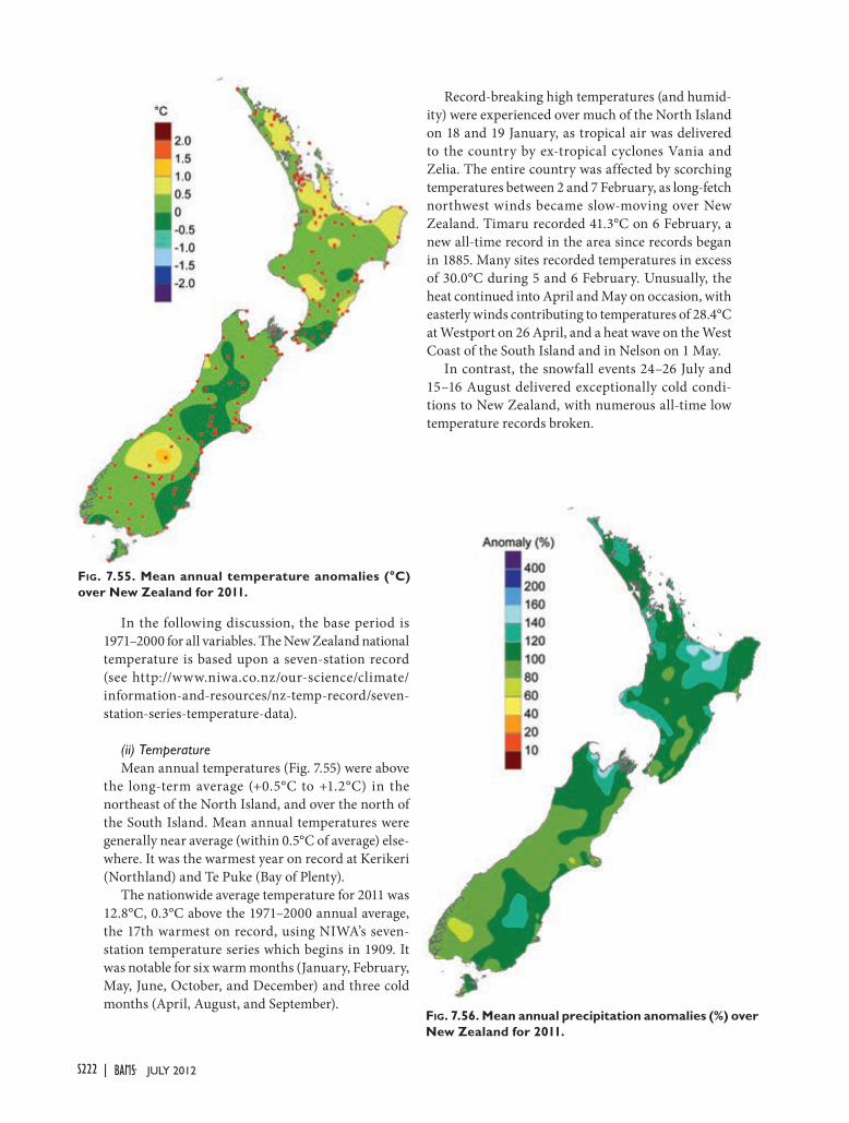
S222 | JULY 2012
In the following discussion, the base period is 1971–2000 for all variables. The New Zealand national temperature is based upon a seven-station record (see http://www.niwa.co.nz/our-science/climate/information-and-resources/nz-temp-record/seven-station-series-temperature-data).
(ii) Temperature
Mean annual temperatures (Fig. 7.55) were above the long-term average (+0.5°C to +1.2°C) in the northeast of the North Island, and over the north of the South Island. Mean annual temperatures were generally near average (within 0.5°C of average) else-where. It was the warmest year on record at Kerikeri (Northland) and Te Puke (Bay of Plenty).
The nationwide average temperature for 2011 was 12.8°C, 0.3°C above the 1971–2000 annual average, the 17th warmest on record, using NIWA’s seven-station temperature series which begins in 1909. It was notable for six warm months (January, February, May, June, October, and December) and three cold months (April, August, and September).
Record-breaking high temperatures (and humid-ity) were experienced over much of the North Island on 18 and 19 January, as tropical air was delivered to the country by ex-tropical cyclones Vania and Zelia. The entire country was affected by scorching temperatures between 2 and 7 February, as long-fetch northwest winds became slow-moving over New Zealand. Timaru recorded 41.3°C on 6 February, a new all-time record in the area since records began in 1885. Many sites recorded temperatures in excess of 30.0°C during 5 and 6 February. Unusually, the heat continued into April and May on occasion, with easterly winds contributing to temperatures of 28.4°C at Westport on 26 April, and a heat wave on the West Coast of the South Island and in Nelson on 1 May.
In contrast, the snowfall events 24–26 July and 15–16 August delivered exceptionally cold condi-tions to New Zealand, with numerous all-time low temperature records broken.
FIG. 7.56. Mean annual precipitation anomalies (%) over New Zealand for 2011.
FIG. 7.55. Mean annual temperature anomalies (°C) over New Zealand for 2011.

S223STATE OF THE CLIMATE IN 2011 |JULY 2012
(iii) Precipitation
In broad terms, six months of the year were wetter than normal and two were drier than normal (August and September). Four months were mixed, with large geographical differences between very wet regions and areas of extreme dryness. Annual rainfall totals for 2011 (Fig. 7.56) were above normal (more than 120% of normal) in parts of Northland, Auckland, Coromandel, Bay of Plenty, Nelson, and Central Otago, as well as around New Plymouth, Napier, Wanganui, and Palmerston North. In contrast, it was a relatively dry year (with annual rainfall totals 50–79% of normal) for the Kaikoura Coast and Can-terbury, as well as much of Fiordland and Westland. Elsewhere, annual rainfall was in the near-normal range (80–119% of normal).
The wettest place in 2011 was Cropp River, in the Hokitika River catchment (West Coast) which re-corded an annual rainfall total of 9493 mm. The driest of the available reporting locations was Clyde (Central Otago), which recorded 395 mm of rainfall in 2011.
Soil moisture deficits in 2011 were generally short-lived. At the beginning of 2011, significant soil mois-ture deficits of more than 110 mm affected parts of western Northland, Waikato, Bay of Plenty, Gisborne, Manawatu, and Wairarapa, as well as parts of Canter-bury and Central Otago. However, the extremely wet January in all North Island regions fully recharged soil moisture levels, and rainfall in March and April replenished all remaining dry soils in the South Is-land. August and September were relatively dry, and by the end of November, significant soil moisture deficits were observed in regions north of Taupo, as well as Hawkes Bay, Gisborne, Marlborough, and cen-tral Otago. Above-normal rainfall totals in December throughout the North Island improved soil moisture levels there, but deficits had become extreme (more than 130 mm of deficit) in Central Otago and parts of Southland by the end of 2011.
(iv) Notable events
Two significant snowfall events occurred in 2011. A polar blast during 24–26 July delivered a bitterly cold air mass over the country. Snowfall was heavy and reached low elevations over Canterbury, the Kaik-oura Ranges, the Richmond, Tararua, and Rimutaka Ranges, the Central Plateau, and around Mt. Egmont. Brief dustings of snow were also reported in the ranges of Motueka and Northland. During the event, snow closed major roads, businesses, public transportation services, airports, and schools, and the weight of the snow on power lines caused outages.
During 14–17 August, a second polar outbreak brought heavy snow to unusually low elevations across eastern and alpine areas of the South Island, as well as to suburban Wellington. On 14 August, snow fell to very low elevations across much of the South Island, as well as in central Wellington and the hill suburbs. On 15 August, the southerly winds continued to deliver extremely cold air and snowfalls to the country, and airports and schools remained closed in Christchurch, Queenstown, Invercargill, and Dunedin. On the West Coast, snow fell in Roto-manu, Inchbonnie, Reefton, Greymouth, Blackball, and Ikamatua. Snow fell again to sea level in Wel-lington, closing schools and Wellington Airport. Both Rotorua and New Plymouth reported snow falling in the central city. Snow fell briefly in Auckland city but did not settle, and was also reported from the Waitakere Ranges, Drury, Waiuku, Clevedon, and the Bombay Hills. The snow reached Northland, with hillside properties around Dargaville reporting snow falling. Taupo Airport was also closed as heavy snow fell around the lake. In the Waikato, snow was seen in central Hamilton (the first time since August 1980), Te Kuiti, and briefly in Raglan. Snow settled in Wanganui, reportedly for the first time since 1974. Between 15 and 17 August, many eastern and alpine South Island roads, as well as lower North Island roads, were affected by snow or ice, and airports, hos-pitals, mail deliveries, and power lines were impacted in these regions.
On 14 December, heavy rain caused severe land-slides and flooding in Nelson and Golden Bay. A State of Emergency was declared. Takaka recorded 392 mm of rainfall in 24 hours, a new record there, and the highest 1-day rainfall observed in New Zealand in 2011. In Nelson city, the Matai river walkway was closed by f looding, as were many urban and rural roads, isolating communities. More than 100 homes near rising rivers were evacuated. The Coastal High-way was closed at both Appleby Bridge and at Takaka Hill. The community of Collingwood was cut off after the road was washed away, and roads to Pakawau and Puponga were closed. A dam collapsed above Pohara Gully in Golden Bay, and on 15 December, schools in that region were closed after the extreme rainfall closed roads and damaged property. Many landslides threatened properties in the Nelson region, and more homes were evacuated. Many roads in Nelson, Waimea, and Golden Bay remained closed on 16 De-cember, including between Takaka and Collingwood.

S224 | JULY 2012
(v) Significant statistics
The highest recorded temperature was 41.3°C, observed at Timaru on 6 February (a new all-time high temperature record there).The lowest recorded air temperature was -10.2°C, recorded at Manapouri on 26 July (a new all-time low temperature record there).Of the regularly reporting gauges, Cropp River in the Hokitika River catchment (West Coast) recorded the highest annual rainfall total, with 9493 mm.The driest of the available reporting locations was Clyde (Central Otago), which recorded 395 mm of annual rainfall.Takaka experienced the highest 1-day rainfall (392 mm), recorded on 14 December (a new all-time daily rainfall record there).Nelson was the sunniest location in New Zealand, recording 2487 hours.The highest recorded wind gust was 189!km hr-1 at Cape Turnagain on 12 July.

S225STATE OF THE CLIMATE IN 2011 |JULY 2012
APPENDIX 1: SEASONAL SUMMARIES—M. Halpert
FIG.
A1.
1. D
ec 2
010–
Feb
2011
(to
p) s
urfa
ce t
empe
ratu
re a
nom
alie
s (°
C)
and
(bot
tom
) pr
ecip
itat
ion
perc
enti
les
base
d on
a g
amm
a di
stri
buti
on fi
t to
the
198
1–20
10 b
ase
peri
od.
Tem
pera
ture
ano
mal
ies
(198
1–20
10 b
ase
peri
od)
are
base
d on
sta
tion
dat
a ov
er la
nd a
nd s
ea s
urfa
ce t
empe
ratu
re
data
ove
r w
ater
. Pre
cipi
tati
on d
ata
wer
e ob
tain
ed fr
om t
he C
AM
S-O
PI d
a-ta
set t
hat i
s a
com
bina
tion
of r
ain
gaug
e ob
serv
atio
ns a
nd s
atel
lite-
deri
ved
esti
mat
es (
Jano
wia
k an
d X
ie 1
999)
. A
naly
sis
was
om
itte
d in
dat
a-sp
arse
re
gion
s (w
hite
are
as).
FIG. A
1.2.
Dec
201
0–Fe
b 20
11 (
top)
Nor
ther
n H
emis
pher
e an
d (b
otto
m)
Sout
hern
Hem
isph
ere
500-
hPa
geop
oten
tial
hei
ghts
(9-d
am c
onto
ur in
ter-
val)
and
ano
mal
ies
(sha
ding
) de
term
ined
from
the
198
1–20
10 b
ase
peri
od
mea
ns. D
ata
is fr
om t
he C
DA
S/R
eana
lysi
s P
roje
ct (
Kal
nay
et a
l. 19
96).
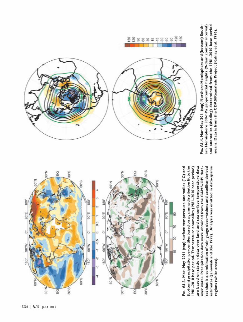
S226 | JULY 2012
FIG.
A1.
3. M
ar–M
ay 2
011
(top
) su
rfac
e te
mpe
ratu
re a
nom
alie
s (°
C)
and
(bot
tom
) pre
cipi
tati
on p
erce
ntile
s ba
sed
on a
gam
ma
dist
ribu
tion
fit t
o th
e 19
81–2
010
base
per
iod.
Tem
pera
ture
ano
mal
ies
(198
1–20
10 b
ase
peri
od)
are
base
d on
sta
tion
dat
a ov
er l
and
and
sea
surf
ace
tem
pera
ture
dat
a ov
er w
ater
. Pre
cipi
tati
on d
ata
wer
e ob
tain
ed f
rom
the
CA
MS
-OP
I da
ta-
set
that
is a
com
bina
tion
of r
ain
gaug
e ob
serv
atio
ns a
nd s
atel
lite-
deri
ved
esti
mat
es (
Jano
wia
k an
d X
ie 1
999)
. A
naly
sis
was
om
itte
d in
dat
a-sp
arse
re
gion
s (w
hite
are
as).
FIG. A
1.4.
Mar
–May
201
1 (t
op) N
orth
ern
Hem
isph
ere
and
(bot
tom
) Sou
th-
ern
Hem
isph
ere
500-
hPa
geop
oten
tial
hei
ghts
(9-
dam
con
tour
int
erva
l)
and
anom
alie
s (s
hadi
ng)
dete
rmin
ed f
rom
the
198
1–20
10 b
ase
peri
od
mea
ns. D
ata
is fr
om t
he C
DA
S/R
eana
lysi
s P
roje
ct (
Kal
nay
et a
l. 19
96).

S227STATE OF THE CLIMATE IN 2011 |JULY 2012
FIG. A
1.5.
Jun
–Aug
201
1 (t
op)
surf
ace
tem
pera
ture
ano
mal
ies
(°C
) an
d (b
otto
m)
prec
ipit
atio
n pe
rcen
tile
s ba
sed
on a
gam
ma
dist
ribu
tion
fit
to
the
198
1–20
10 b
ase
peri
od. T
empe
ratu
re a
nom
alie
s (1
981–
2010
bas
e pe
riod
) are
bas
ed o
n st
atio
n da
ta o
ver
land
and
sea
sur
face
tem
pera
ture
da
ta o
ver
wat
er. P
reci
pita
tion
dat
a w
ere
obta
ined
from
the
CA
MS
-OP
I da
tase
t th
at i
s a
com
bina
tion
of
rain
gau
ge o
bser
vati
ons
and
sate
llite
-de
rive
d es
tim
ates
(Ja
now
iak
and
Xie
199
9).
Ana
lysi
s w
as o
mit
ted
in
data
-spa
rse
regi
ons
(whi
te a
reas
).
FIG. A
1.6.
Jun–
Aug
201
1 (t
op) N
orth
ern
Hem
isph
ere
and
(bot
tom
) Sou
ther
n H
emis
pher
e 50
0-hP
a ge
opot
enti
al h
eigh
ts (
9-da
m c
onto
ur i
nter
val)
and
an
omal
ies
(sha
ding
) de
term
ined
fro
m t
he 1
981–
2010
bas
e pe
riod
mea
ns.
Dat
a is
from
the
CD
AS
/Rea
naly
sis
Pro
ject
(K
alna
y et
al.
1996
).

S228 | JULY 2012
FIG.
A1.
7. S
ep–N
ov 2
011
(top
) su
rfac
e te
mpe
ratu
re a
nom
alie
s (°
C)
and
(bot
tom
) pre
cipi
tati
on p
erce
ntile
s ba
sed
on a
gam
ma
dist
ribu
tion
fit t
o th
e 19
81–2
010
base
per
iod.
Tem
pera
ture
ano
mal
ies
(198
1–20
10 b
ase
peri
od)
are
base
d on
sta
tion
dat
a ov
er la
nd a
nd s
ea s
urfa
ce t
empe
ratu
re d
ata
over
w
ater
. Pre
cipi
tati
on d
ata
wer
e ob
tain
ed fr
om t
he C
AM
S-O
PI d
atas
et t
hat
is a
com
bina
tion
of r
ain
gaug
e ob
serv
atio
ns a
nd s
atel
lite-
deri
ved
esti
mat
es
(Jan
owia
k an
d X
ie 1
999)
. A
naly
sis
was
om
itte
d in
dat
a-sp
arse
reg
ions
(w
hite
are
as).
FIG. A
1.8.
Sep
–Nov
201
1 (t
op) N
orth
ern
Hem
isph
ere
and
(bot
tom
) Sou
th-
ern
Hem
isph
ere
500-
hPa
geop
oten
tial
hei
ghts
(9-d
am c
onto
ur in
terv
al) a
nd
anom
alie
s (s
hadi
ng)
dete
rmin
ed f
rom
the
198
1–20
10 b
ase
peri
od m
eans
. D
ata
is fr
om t
he C
DA
S/R
eana
lysi
s P
roje
ct (
Kal
nay
et a
l. 19
96).

S229JULY 2012STATE OF THE CLIMATE IN 2011 |
General Variable or Phenomenon
Specific Dataset or Variable Source Section
AerosolsAERONET data (NASA)
http://aeronet.gsfc.nasa.gov/ 2g2
Aerosol products http://www.gmes-atmosphere.eu/data/ 2g2
Air-sea fluxes
Woods Hole Oceano-graphic Institute (WHOI) OAFlux Project
http://oaflux.whoi.edu 3d
Albedo MODIS http://ladsweb.nascom.nasa.gov/ 2h2,5f
Biomass Burning Biomass Burning http://www.globalfiredata.org/ 2h4
Clouds, Cloudiness
HIRS No known public portal 2d4
ISCCP D2 http://isccp.giss.nasa.gov 2d4
MISR http://eosweb.larc.nasa.gov/PRODOCS/misr/level3 /overview.html
2d4
MODIS Cloud Mask http://ladsweb.nascom.nasa.gov/ 2d4,5b
PATMOS-x http://www.ncdc.noaa.gov/cdr/operationalcdrs.html 2d4
SOBS http://www.atmos.washington.edu/~ignatius/CloudMap 2d4
Evaporation JRA-25 http://jra.kishou.go.jp 6d
FAPAR FAPAR http://fapar.jrc.ec.europa.eu/ 2h3
Geopotential Height
ERA-Interim http://www.ecmwf.int/research/era 6b
Glacier Mass orVolume
Glacier Mass Balance http://www.geo.uzh.ch/microsite/wgms/mbb/sum10.html 5e
GRACE http://www.csr.utexas.edu/grace/ 2c3
Humidity, [Near] Surface
20th Century Reanalysis
http://www.esrl.noaa.gov/psd/data/20thC_Rean/ 2d1
Dai by email to [email protected] 2d1
ERA-Interim http://www.ecmwf.int/research/era 2d1
HadCRUH http://www.metoffice.gov.uk/hadobs/hadcruh 2d1
JRA-25 Atmospheric Reanalysis
http://jra.kishou.go.jp/JRA-25/index_en.html 2d1
MERRA http://gmao.gsfc.nasa.gov/merra/ 2d1
NCEP CFSR http://cfs.ncep.noaa.gov 2d1
NOCS 2.0 http://www.noc.soton.ac.uk/noc_flux/noc2.php 2d1
Isotherm depthNCEP Global Ocean Data Assimilation System
http://www.cpc.ncep.noaa.gov/products/GODAS 4h
Lake Ice NOAA IMS, 4m Daily http://nsidc.org/data/g02156.html 5h
Lake Levels
Altimetric Lake level Products, USDA
http://www.pecad.fas.usda.gov/cropexplorer /global_reservoir/index.cfm
2d8
ESA http://tethys.eaprs.cse.dmu.ac.uk/RiverLake/shared/main 2d8
LEGOS http://www.legos.obs-mip.fr/soa/hydrologie/hydroweb/ 2d8
Lake TemperatureARCLAKE http://hdl.handle.net/10283/88, http://www.geos.ed.ac.uk
/arclake/2b4
IWBP http://largelakes.jpl.nasa.gov 2b4
APPENDIX 2: RELEVANT DATASETS AND SOURCES

S230 JULY 2012|
Modes of Variability
Arctic Oscillation (AO)
http://www.cpc.ncep.noaa.gov/products/precip/CWlink /daily_ao_index/ao.shtml
2f3
Climate Prediction Center: AAO, AO, NAO, PNA
http://www.cpc.ncep.noaa.gov/products/precip/CWlink /daily_ao_index/teleconnections.shtml
3b, 6a
Oceanic Nino Index http://www.cpc.ncep.noaa.gov/products/analysis_monitoring /ensostuff/ensoyears.shtml
4a,4b
Southern Annular Mode Index
http://www.antarctica.ac.uk/met/gjma/sam.html 6a, 6b,6d,6f,SB6.1
Southern Oscillation Index
http://www.cpc.ncep.noaa.gov/data/indices/ 6b,6d,6f
Ocean Carbon
AOML Monthly Flux Anomalies
http://cwcgom.aoml.noaa.gov/erddap/griddap /aomlcarbonfluxes.graph
3j1
Hawaii Ocean Time-series (HOT)
http://hahana.soest.hawaii.edu/hot/hot_jgofs.html 3j3
Surface Ocean CO2 Atlas (SOCAT) Data Access System
http://www.socat.info 3j1
The U.S. CO2/Repeat Hydrography Program
http://ushydro.ucsd.edu 3j2
Trends in Atmospheric Carbon Dioxide: Mauna Loa, Hawaii
http://www.esrl.noaa.gov/gmd/ccgg/trends/ 3j3
Ocean CirculationAtlantic Meridional Overturning Circulation
http://www.noc.soton.ac.uk/rapidmoc/ 3h
Ocean Color
Level 3 MODIS Aqua Ocean Color Data
http://oceancolor.gsfc.nasa.gov/ SB5.3
Level 3 SeaWiFS Ocean Color Data
http://oceancolor.gsfc.nasa.gov/ SB5.3
Ocean Salinity
Global Ocean Heat and Salt Content
http://www.nodc.noaa.gov/OC5/3M_HEAT_CONTENT/ 3f
World Ocean Atlas 2009
http://www.nodc.noaa.gov/OC5/WOA09/pr_woa09.html 3f
World Ocean Database 2009
http://www.nodc.noaa.gov/OC5/WOD09/pr_wod09.html 3f
Ocean Temperature
World Ocean Database 2009
http://www.nodc.noaa.gov/OC5/WOD09/pr_wod09.html 3c
Outgoing Longwave Radiation
CERES FLASHFlux Project
http://flashflux.larc.nasa.gov 3d
NOAA-interpolated OLR
http://www.esrl.noaa.gov/psd/data/gridded /data.interp_OLR.html
4f2
Permafrost
Active Layer Thickness http://www.udel.edu/Geography/calm/data/north.html 5g
GTN-P, Alaskan Repository
http://www.permafrostwatch.org 2c1
GTN-P, Norwegian Repository
http://www.ngu.no/kart/permafrost 2c1
Permafrost Temperature
http://permafrost.gi.alaska.edu/sites_map 5g
Permafrost Data http://nsidc.org/data/g02190.html 2c1

S231JULY 2012STATE OF THE CLIMATE IN 2011 |
Phytoplankton, Ocean Color
MERIS 3rd Data Reprocessing
http://earth.eo.esa.int/pcs/envisat/meris/documentation /meris_3rd_reproc/MERIS_3rd_Reprocessing_Changes.pdf
3j4
Ocean Color Documents: MODIS-Aqua Reprocessing 2010.0
http://oceancolor.gsfc.nasa.gov/WIKI/OCReproc20100MA.html
3j4
Precipitation
CMAP http://www.esrl.noaa.gov/psd/data/gridded /data.ncep.reanalysis.html
2d3
GHCN http://www.ncdc.noaa.gov/temp-and-precip /ghcn-gridded-products.php
2d3
Global Precipitation Climatology Project (GPCP)
http://precip.gsfc.nasa.gov 2d3,4h
GPCC http://www.gpcc.dwd.de/ 2d3
SSM/I, TMI, and AMSR-E Data
http://www.remss.com 2d3
TRMM 3A12 http://disc.sci.gsfc.nasa.gov/precipitation/documentation /TRMM_README/TRMM_3A12_readme.shtml
4f2
TRMM 3B43 Rainfall http://disc.sci.gsfc.nasa.gov/precipitation/documentation /TRMM_README/TRMM_3B43_readme.shtml
4f1, 4f2
Precipitation (net) JRA-25 Atmospheric Reanalysis
http://jra.kishou.go.jp/JRA-25/index_en.html 6d
Pressure, Sea Level or Near-Surface
ACCESS http://www.bom.gov.au/nwp/access/NWPData.shtml 6f
AMRC (Antarctic Me-teorological Research Center) AWS
http://amrc.ssec.wisc.edu/data/ 6c,SB6.1
ERA-Interim http://www.ecmwf.int/research/era 6a,6b,6c
HadSLP2r http://www.metoffice.gov.uk/hadobs 2e1
JRA-25 Atmospheric Reanalysis
http://jra.kishou.go.jp/JRA-25/index_en.html 6d
READER http://www.antarctica.ac.uk/met/READER/ 6c
River Discharge
Arctic-RIMS1 River Discharge
http://rims.unh.edu 2d5
Dartmouth Flood Observatory
http://floodobservatory.colorado.edu 2d5
River Discharge http://waterdata.usgs.gov/nwis - USGS2 2d5
Sea Ice Concentration
Nimbus-7 SMMR and DMSP SSM/I
http://nsidc.org/data/nsidc-0051.html 5b, SB5.2
Nimbus-7 SMMR and DMSP SSM/I (Bootstrap)
http://nsidc.org/data/docs/daac/nsidc0079_bootstrap_seaice .gd.html
6f
Sea Ice DurationNear-Real-Time DMSP SSM/I-SSMIS Daily Polar Gridded
http://nsidc.org/data/nsidc-0081.html 6f
Sea Ice Extent
Nimbus-7 SMMR and DMSP SSM/I (Bootstrap)
http://nsidc.org/data/docs/daac /nsidc0079_bootstrap_seaice.gd.html
6f
NOAA IMS, 4km Daily http://nsidc.org/data/g02156.html 5i
Sea Ice Index
Sea Ice Concentration from DMSP SSM/I-SS-MIS Passive Microwave Data
http://nsidc.org/data/seaice_index/archives/index.html 5i

S232 JULY 2012|
Sea Level
Arctic Sea Level http://www.whoi.edu/science/PO/arcticsealevel/data.html 5j
Ssalto/Duacs Multimission Altimeter Products
http://www.aviso.oceanobs.com/en/data /product-information/duacs/index.html
3g
University of Hawaii Sea Level Center
http://uhslc.soest.hawaii.edu/ 3i
Sea Surface Salinity
Aquarius http://aquarius.nasa.gov SB3.1
World Ocean Atlas 2009
http://www.nodc.noaa.gov/OC5/WOA09/pr_woa09.html 3e
Sea Surface Temperature
Climate Prediction Center's Monthly Ocean Briefing
http://www.cpc.ncep.noaa.gov/products/GODAS 3b
ERSST-v3b http://www.esrl.noaa.gov/psd/data/gridded/data.noaa.ersst.html
4b1,4d,4g
HadSST2 http://www.metoffice.gov.uk/hadobs/hadsst2 2b1
NOAA Optimum Interpolation SST (OISST) v2
http://www.esrl.noaa.gov/psd/data/gridded /data.ncep.oisst.v2.html
4f2,4h,
5j2,6f
Snow CoverSnow Cover Extent and Duration
http://climate.rutgers.edu/snowcover/ 2c2,5d
SSM/I http://www.nsidc.org 6e
Snow Depth
Canadian Meteorological Centre Daily Gridded
http://nsidc.org/data/docs/daac/nsidc0447_CMC_snow_depth/index.html
5d
Snow Water Equivalent
ERA-interim Atmospheric Reanaly-sis
http://www.ecmwf.int/research/era 5d
GlobSnow N. Hemisphere Snow Water Equivalent
http://www.globsnow.info/ 5d
Soil Moisture GRACE http://www.esa-soimoisture-cci.org/ 2d6
Solar Transmission Mauna Loa Solar Transmission
http://www.esrl.noaa.gov/gmd/grad/mloapt.html SB2.3
Stratospheric Ozone
Calipso (Polar Stratospheric Clouds)
http://eosweb.larc.nasa.gov/PRODOCS/calipso /table_calipso.html
6g
GOME/SCIAMACHY/GOME2 Total Ozone Datasets, GSG Merged Data
http://www.iup.uni-bremen.de/gome/wfdoas 2g3, 6g
KNMI OMI http://ozoneaq.gsfc.nasa.gov 6g
Multi Sensor Reanalysis (MSR) of Total Ozone
http://www.temis.nl/protocols/O3global.html 2g3
NASA Aura Micro-wave Limb Sounder
http://aura.gsfc.nasa.gov/instruments/mls.html 6g
OMI Total Ozone (OMTO3)
http://mirador.gsfc.nasa.gov/cgi-bin/mirador /presentNavigation.pl?tree=project&project=OMI
2g3
Ozonesonde http://www.esrl.noaa.gov/gmd/dv/spo_oz/ 6g
WOUDC Ground-based Ozone
ftp://ftp.tor.ec.gc.ca/Projects-Campaigns/ ZonalMeans/ 2g3

S233JULY 2012STATE OF THE CLIMATE IN 2011 |
Stratospheric Water Vapor
Boulder Water Vapor Balloon Data
ftp://ftp.cmdl.noaa.gov/ozwv/water_vapor/Boulder_New/ 2f4
HALOE Data http://haloe.gats-inc.com/home/index.php 2f4
MLS Data http://disc.sci.gsfc.nasa.gov/Aura/data-holdings/MLS/index.shtml
2f4
Surface Current
Long Term Time Series of Surface Cur-rents
http://www.aoml.noaa.gov/phod/altimetry/cvar 3g
Long Term Time Series of Surface Currents: Agulhas Current
http://www.aoml.noaa.gov/phod/altimetry/cvar/agu/index.php
3g2
Long Term Time Series of Surface Cur-rents: Brazil-Malvina Region
http://www.aoml.noaa.gov/phod/altimetry/cvar/mal/BM_ts.php
3g3
Ocean Surface Current Analysis - Real time (OSCAR)
http://www.oscar.noaa.gov/ 3g
PO.DAAC Physical Oceanography Distrib-uted Active Archive Center
http://podaac.jpl.nasa.gov/ 3g
Ssalto/Duacs Multimission Altimeter Products
http://www.aviso.oceanobs.com/en/data/product-informa-tion/duacs/index.html
3i
The Global Drifter Program, Satellite-tracked Surface Drift-ing Buoys
http://www.aoml.noaa.gov/phod/dac/gdp.html 3g
Tropical Atmosphere Ocean Project
http://www.pmel.noaa.gov/tao/ 3g
Temperature,[Near]Surface
AMRC (Antarctic Me-teorological Research Center) AWS
http://amrc.ssec.wisc.edu/data/ 6c,SB6.1
Berkeley Land Temperature
http://berkeleyearth.org/analysis/ 2b1
CRUTEM3 http://www.metoffice.gov.uk/hadobs/crutem3 2b1, 5b
CRUTEM4 http://www.metoffice.gov.uk/hadobs/crutem4 2b1
ERA-Interim http://www.ecmwf.int/research/era 6a,6b,6c
HadCRUT3 Global Temperature
http://www.metoffice.gov.uk/hadobs/hadcrut3 2b1
JMA Global Temperature
http://ds.data.jma.go.jp/tcc/tcc/products/gwp/temp/map /download.html
2b1
JRA-25 Atmospheric Reanalysis
http://jra.kishou.go.jp/JRA-25/index_en.html 2b1
MERRA http://gmao.gsfc.nasa.gov/merra/ 2b1, 6g
NASA/GISS Global Temperature
http://data.giss.nasa.gov/gistemp/ 2b1
NCEP/NCAR Reanalysis
http://www.esrl.noaa.gov/psd/data/gridded/data.ncep .reanalysis.html
5b
NCEP-CFSR http://cfs.ncep.noaa.gov 2b1
NOAA/NCDC Global Temperature
http://www.ncdc.noaa.gov/cmb-faq/anomalies.html 2b1
READER http://www.antarctica.ac.uk/met/READER/ 6c, SB6.1

S234 JULY 2012|
Temperature,Upper
Atmosphere
20th Century Reanalysis
http://www.esrl.noaa.gov/psd/data/20thC_Rean/ 2b2
ERA-Interim http://www.ecmwf.int/research/era 2b2,2b3,
6b
HadAT2 http://www.metoffice.gov.uk/hadobs 2b2,2b3
JRA-25 Atmospheric Reanalysis
http://jra.kishou.go.jp/JRA-25/index_en.html 2b2
MERRA http://gmao.gsfc.nasa.gov/merra/ 2b2,2b3
NCEP/DOE Reanalysis 2
http://www.esrl.noaa.gov/psd/data/gridded/data.ncep .reanalysis2.html
6g
RAOBCORE, RICH http://imgw.univie.ac.at/en/products 2b2,2b3
RATPAC http://www.ncdc.noaa.gov/oa/climate/ratpac 2b2,2b3
RSS http://www.remss.com 2b2,2b3
UAH MSU http://vortex.nsstc.uah.edu/public/msu/ 2b2,2b3
TOA Earth Radiation Budget
CERES EBAF Ed2.6r 1Deg
http://ceres.larc.nasa.gov/sitemap_ceres.php 2f
Total Column Ozone
TOMS and OMI Sensors
http://ozoneaq.gsfc.nasa.gov/ 5c,6g
Total Column Water Vapor
andHumidity, Upper Air
COSMIC Land and Ocean Total Column Water Vapor
http://cosmic-io.cosmic.ucar.edu/cdaac/index.html 2d2
GPS Ground-Based Total Column Water Vapor
http://dss.ucar.edu/datasets/ds721.1/ 2d2
NCEP/NCAR Reanalysis
http://www.esrl.noaa.gov/psd/data/gridded /data.ncep.reanalysis.html
4d4
SSM/I -AMSR-E Ocean Total Column Water Vapor
http://www.remss.com 2d2
TCWV Radiosonde Junhong Wang, Earth Observing Laboratory, NCAR, Boulder, CO.
2d2
Trace Gases
Atmospheric Green-house Gas Index (AGGI)
http://www.esrl.noaa.gov/gmd/aggi/ 2g1
Carbon Dioxide http://www.esrl.noaa.gov/gmd/dv/iadv/ 2g1,SB5.1
Carbon Monoxide http://www.esrl.noaa.gov/gmd/dv/iadv/ 2g1
JPL MLS (HCl,ClO) http://mls.jpl.nasa.gov/index.php 6g
Methane http://www.esrl.noaa.gov/gmd/dv/iadv/ 2g1,SB5.1
Nitrous Oxide http://www.esrl.noaa.gov/gmd/hats/combined/N2O.html 2g1
ODGI http://www.esrl.noaa.gov/gmd/odgi/ 2g1
Perfluorocarbons http://agage.eas.gatech.edu/ 2g1
Sulphur Hexafluoride http://www.esrl.noaa.gov/gmd/hats/combined/SF6.html 2g1
SCIAMACHY (OClO, NO2)
http://www.sciamachy.org/ 6g
Tropical Cyclone Data
International Best Track Archive for Climate Stewardship (IBTrACS)
http://www.ncdc.noaa.gov/oa/ibtracs/ 4d
JTWC Best-track Dataset (2011 preliminary)
http://www.usno.navy.mil/NOOC/nmfc-ph/RSS/jtwc /best_tracks/
4d4
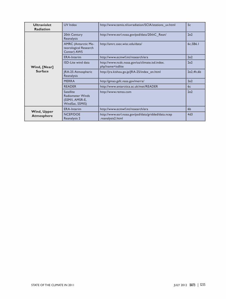
S235JULY 2012STATE OF THE CLIMATE IN 2011 |
Temperature,Upper
Atmosphere
20th Century Reanalysis
http://www.esrl.noaa.gov/psd/data/20thC_Rean/ 2b2
ERA-Interim http://www.ecmwf.int/research/era 2b2,2b3,
6b
HadAT2 http://www.metoffice.gov.uk/hadobs 2b2,2b3
JRA-25 Atmospheric Reanalysis
http://jra.kishou.go.jp/JRA-25/index_en.html 2b2
MERRA http://gmao.gsfc.nasa.gov/merra/ 2b2,2b3
NCEP/DOE Reanalysis 2
http://www.esrl.noaa.gov/psd/data/gridded/data.ncep .reanalysis2.html
6g
RAOBCORE, RICH http://imgw.univie.ac.at/en/products 2b2,2b3
RATPAC http://www.ncdc.noaa.gov/oa/climate/ratpac 2b2,2b3
RSS http://www.remss.com 2b2,2b3
UAH MSU http://vortex.nsstc.uah.edu/public/msu/ 2b2,2b3
TOA Earth Radiation Budget
CERES EBAF Ed2.6r 1Deg
http://ceres.larc.nasa.gov/sitemap_ceres.php 2f
Total Column Ozone
TOMS and OMI Sensors
http://ozoneaq.gsfc.nasa.gov/ 5c,6g
Total Column Water Vapor
andHumidity, Upper Air
COSMIC Land and Ocean Total Column Water Vapor
http://cosmic-io.cosmic.ucar.edu/cdaac/index.html 2d2
GPS Ground-Based Total Column Water Vapor
http://dss.ucar.edu/datasets/ds721.1/ 2d2
NCEP/NCAR Reanalysis
http://www.esrl.noaa.gov/psd/data/gridded /data.ncep.reanalysis.html
4d4
SSM/I -AMSR-E Ocean Total Column Water Vapor
http://www.remss.com 2d2
TCWV Radiosonde Junhong Wang, Earth Observing Laboratory, NCAR, Boulder, CO.
2d2
Trace Gases
Atmospheric Green-house Gas Index (AGGI)
http://www.esrl.noaa.gov/gmd/aggi/ 2g1
Carbon Dioxide http://www.esrl.noaa.gov/gmd/dv/iadv/ 2g1,SB5.1
Carbon Monoxide http://www.esrl.noaa.gov/gmd/dv/iadv/ 2g1
JPL MLS (HCl,ClO) http://mls.jpl.nasa.gov/index.php 6g
Methane http://www.esrl.noaa.gov/gmd/dv/iadv/ 2g1,SB5.1
Nitrous Oxide http://www.esrl.noaa.gov/gmd/hats/combined/N2O.html 2g1
ODGI http://www.esrl.noaa.gov/gmd/odgi/ 2g1
Perfluorocarbons http://agage.eas.gatech.edu/ 2g1
Sulphur Hexafluoride http://www.esrl.noaa.gov/gmd/hats/combined/SF6.html 2g1
SCIAMACHY (OClO, NO2)
http://www.sciamachy.org/ 6g
Tropical Cyclone Data
International Best Track Archive for Climate Stewardship (IBTrACS)
http://www.ncdc.noaa.gov/oa/ibtracs/ 4d
JTWC Best-track Dataset (2011 preliminary)
http://www.usno.navy.mil/NOOC/nmfc-ph/RSS/jtwc /best_tracks/
4d4
Ultraviolet Radiation
UV Index http://www.temis.nl/uvradiation/SCIA/stations_uv.html 5c
Wind, [Near] Surface
20th Century Reanalysis
http://www.esrl.noaa.gov/psd/data/20thC_Rean/ 2e2
AMRC (Antarctic Me-teorological Research Center) AWS
http://amrc.ssec.wisc.edu/data/ 6c,SB6.1
ERA-Interim http://www.ecmwf.int/research/era 2e2
ISD-Lite wind data http://www.ncdc.noaa.gov/oa/climate.isd.index.php?name=isdlite
2e2
JRA-25 Atmospheric Reanalysis
http://jra.kishou.go.jp/JRA-25/index_en.html 2e2,4h,6b
MERRA http://gmao.gsfc.nasa.gov/merra/ 2e2
READER http://www.antarctica.ac.uk/met/READER 6c
Satellite Radiometer Winds (SSM/I, AMSR-E, WindSat, SSMIS)
http://www.remss.com 2e2
Wind, Upper Atmosphere
ERA-Interim http://www.ecmwf.int/research/era 6b
NCEP/DOE Reanalysis 2
http://www.esrl.noaa.gov/psd/data/gridded/data.ncep .reanalysis2.html
4d3

S236 JULY 2012|

S237JULY 2012STATE OF THE CLIMATE IN 2011 |
ACKNOWLEDGMENTS
!e editors thank the sta" of the Bulletin of the American Me-teorological Society for their professionalism and assistance. Speci#cally, Lesley Williams and Melissa Fernau provided valuable editorial advice and logistical support. As always, the guidance and leadership of Bryan Hanssen and Jeff Rosenfeld was essential. !e chapter editors enthusiastically thank their respective internal reviewers, and anonymous external reviewers, for working on very tight timetables to improve the document.
Chapter 2:Various reanalysis datasets were provided by Paul Ber-risford and Hitoshi Sato (ERA-Interim), Mike Bosilov-ich (MERRA), Muthuvel Chelliah (NCEP CFSR), Yayoi Harada (JRA-25/JCDAS) and Cathy Smith (20CR).Surface humidity data were provided by several of the reanalysis authors above and by Aiguo Dai.Kate Willett was supported by the Joint DECC/De-fra Met Office Hadley Centre Climate Programme (GA01101).
Chapter 3:!e editors thank Joel Levy, Oceans chapter editor for the 2005–10 reports, for developing the chapter from its origins and assembling an impressive team of authors.
Chapter 4:Charles “Chip” Guard, NOAA/NWS/Guam Weather Forecast Office is thanked for his contributions to and assistance with the section dealing with tropical cyclones in the Western North Paci#c basin.Bill Ward, NOAA/NWS/Paci#c Region Headquarters, Honolulu, Hawaii is thanked for his detailed and very helpful internal review of the chapter.
Chapter 5:!e NOAA authors note that, with respect to their contributions, “The views, opinions, and findings contained in this report are those of the author(s) and should not be construed as an o$cial National Oceanic and Atmospheric Administration or U.S. Government position, policy, or decision.”Jim Overland acknowledges the support of the Arctic Research O$ce of the NOAA Climate Program O$ce.Chris Derksen and Ross Brown thank their data pro-viders: National Snow and Ice Data Centre; European Centre for Midrange Weather Forecasts; NOAA Earth System Research Laboratory; Rutgers University Snow Laboratory; and the Canadian Meteorological Centre.Marco Tedesco acknowledges NSF grant ARC 0909388
and the NASA Cryosphere Program, and Roderick van der Wal acknowledges Utrecht University, and several grants from the Dutch National Science Foun-dation (NWO), including the Spinoza Program and the Netherlands Polar Programme, for support for measurements along the K-transect in west Greenland.Vladimir Romanovsky acknowledges NSF grant ARC 0856864 and the Russian Academy of Science for partial support.Andrey Proshutinsky acknowledges NOAA support, and data and data analysis made possible by NSF grants ARC 856531, ARC 0856479 and ARC 0806306.!e ozone and UV essay was supported by NSF grant ARC 0856268 (Ultraviolet Radiation in the Arctic) and European Commission Seventh Framework Pro-gramme grant RECONCILE-226365-FP7-ENV-2008-1 (RECONCILE project). Work at the Jet Propulsion Laboratory, California Institute of Technology, was done under contract with the U.S. National Aeronautics and Space Administration.Skip Walker and Uma Bhatt acknowledge NSF grant ARC 0902175 and NASA grants NNG6GE00A and NNX09AK56G.Karen Frey acknowledges NSF grant ARC 1107645 and NASA grant NNX10AH71G.
Chapter 6:Drs. Jan Lieser and Alex Fraser (ACE CRC) are thanked for their comments on the sea ice section. Rob Massom acknowledges support from the Aus-tralian Government’s Cooperative Research Centre programme through the ACE CRC, and contribution to Project CPC18 and AAS Project 4116. Ted Scambos was supported under NASA grant NNX-09AM78G. Sharon Stammerjohn was supported under NSF/OPP 0217282.Matthew Lazzara and the AMRC AWS program acknowledge support from NSF grant number ANT-0944018.Dr. Michiel van den Broeke, Dr. Alberto Setzer, and Dr. Florence Fetterer are all thanked for their internal reviews of the chapter.
Chapter 7:!e editors acknowledge and thank the numerous Na-tional Hydrological and Hydrometeorological Services for collecting and providing data (and many authors) for this report.

S238 JULY 2012|
ACRONYMS AND ABBREVIATIONS
AAO Antarctic OscillationACE NOAA’s Accumulated Cyclone
Energy IndexAGGI NOAA’s Annual Greenhouse Gas
IndexALT Active layer thicknessAMO Atlantic Multidecadal OscillationAMSR-E Advanced Microwave Scanning
Radiometer for Earth Observing System
AMSU Advanced Microwave Sounding Unit
AO Arctic OscillationAOD Aerosol optical depthAOML Atlantic Oceanographic and
Meteorological Laboratory ATSR Along-Track Scanning RadiometersAVHRR Advanced Very High Resolution
RadiometerAVISO Archiving, Validating, and
Interpretation of Satellite Oceanographic data
CAMS Climate Anomaly Monitoring System
CDR Climate data recordCERES Clouds and the Earth’s Radiant
Energy SystemCLIVAR Climate Variability and
PredictabilityCPC Climate Prediction CenterCPHC NOAA’s Central Pacific Hurricane
CenterCRU Hadley Centre’s Climate Research
UnitECMWF European Centre for Medium-
Range Weather Forecasts ECV Essential climate variableEECl Effective equivalent chlorineEESC Effective equivalent stratospheric
chlorineEOS Earth Observatory SystemERB Earth radiation budgetERBE Earth Radiation Budget
ExperimentERSST Extended Reconstructed Sea
Surface TemperatureESA European Space AgencyESRL Earth System Research LaboratoryEU European Union
FAO Food and Agriculture OrganizationFAPAR Fraction of Absorbed
Photosynthetically Active Radiation
FLASHflux Fast Longwave and Shortwave Radiative Fluxes
GCOS Global Climate Observing SystemGHCN Global Historical Climatology
NetworkGISS NASA’s Goddard Institute of Space
StudiesGOME Global Ozone Monitoring
ExperimentGPCC Global Precipitation Climatology
CentreGPCP Global Precipitation Climatology
ProjectGPI Genesis potential index GRACE Gravity Recovery and Climate
ExperimentGTN-P Global Terrestrial Network on
PermafrostHadAT Hadley Centre’s radiosonde
temperature productHadCRUT3 Hadley Centre/CRU gridded
monthly temperatures datasetHadGEM1 Hadley Centre global modelHadISST Hadley Centre’s sea ice and SST
datasetHIRS-W High Resolution Infrared SounderIBTrACS International Best Track Archive
for Climate StewardshipICD Ice cover durationICPAC IGAD Climate Prediction and
Applications CentreIOD Indian Ocean dipoleISCCP International Satellite Cloud
Climatology ProjectJGOFS Joint Global Ocean Flux StudyJMA Japanese Meteorological AgencyJPL Jet Propulsion Laboratory JRA Japanese ReanalysisJTWC U.S. Navy’s Joint Typhoon Warning
CenterLHF Latent heat fluxMDR Main Development RegionMERIS Medium Resolution Imaging
SpectrometerMISR Multiangle Imaging
SpectroRadiometerMLS Microwave Limb Sounder

S239JULY 2012STATE OF THE CLIMATE IN 2011 |
MOC Meridional overturning currentMOCHA Meridional Overturning
Circulation Heat Transport Array MODIS Moderate Resolution Imaging
SpectroradiometerMSLP mean sea level pressureMSU Microwave Sounding UnitNAO North Atlantic OscillationNASA National Aeronautics and Space
AdministrationNCAR National Center for Atmospheric
ResearchNCDC National Climatic Data CenterNCEP National Centers for
Environmental PredictionNDVI Normalized Difference Vegetation
IndexNERC National Environmental Research
CouncilNHC National Hurricane CenterNOAA National Oceanic and Atmospheric
AdministrationNOMADS National Operational Model
Archive and Distribution SystemNSIDC National Snow and Ice Data CenterOAFlux Objectively Analyzed Air-Sea
FluxesODGI Ozone Depleting Gas IndexOHCA Ocean heat content anomalyOISST Optimal Interpolation SSTOLR Outgoing longwave radiationOMI Ozone Monitoring InstrumentONI Oceanic Niño Index OPI OLR precipitation indexOSCAR Ocean Surface Current Analysis-
Real TimePATMOS (-x) Pathfinder Atmospheres (Extended
Product)PDO Pacific decadal oscillationPIRATA Pilot Research Array in the
Tropical AtlanticPMEL Pacific Marine Environmental
LaboratoryPSC Polar stratospheric cloudsPSS Practical salinity scaleQBO Quasi-biennial oscillationQuikSCAT Quick ScatterometerRAMA Research Moored Array for
African-Asian-Australian Monsoon Analysis Prediction
RAOBCORE Radiosonde Observation Correction
RATPAC Radiosonde Atmospheric Temperature Products for Assessing Climate
RICH Radiosonde Innovation Composite Homogenization
RSS Remote Sensing SystemsSAM Southern annular modeSCD snow covered durationSCE snow cover extentSCIAMACHY Scanning Imaging Absorption
Spectrometer for Atmospheric Chartography
SeaWiFS Sea-viewing Wide Field of ViewSHF Sensible heat fluxSLP Sea level pressureSOI Southern Oscillation index SPCZ South Pacific convergence zoneSSM/I Special Sensor Microwave ImagerSSH Sea surface heightSSS Sea surface salinitySSTA Sea surface temperature anomalySWE Snow water equivalentTCHP Tropical cyclone heat potential TCWV Total column water vaporTOA Top of atmosphereTOMS Total Ozone Mapping SpectrometerTRITON Triangle Trans-Ocean Buoy
NetworkTRMM Tropical Rainfall Measuring
MissionTWC Terrestrial water storageWBC Western boundary currentWBM Water Balance Modelw.e. water equivalentWGMS World Glacier Monitoring ServiceWHOI Woods Hole Oceanographic
InstituteWMO World Meteorological OrganizationWOA World Ocean Atlas WOCE World Ocean Circulation
Experiment

S240 JULY 2012|
REFERENCES
Ackerman, S. A., R. E. Holz, R. Frey, E. W. Eloranta, B. C. Maddux, and M. McGill, 2008: Cloud detection with MODIS. Part II: Validation. J. Atmos. Oceanic Technol., 25, 1073–1086.
Adlam, L. S., M. R. Balks, C. A. Seybold, and D. I. Campbell, 2010: Temporal and spatial variation in active layer depth in the McMurdo Sound Region, Antarctica. Antarctic Sci., 22, 45–52.
Adler, R. F., and Coauthors, 2003: The version 2 Global Pre-cipitation Climatology Project (GPCP) monthly precipita-tion analysis (1979-present). J. Hydrometeor., 4, 1147–1167.
Aiyyer, A., and J. Molinari, 2008: MJO and tropical cyclo-genesis in the Gulf of Mexico and eastern Pacific: Case study and idealized numerical modeling. J. Atmos. Sci., 65, 2691–2704.
Åkerman, H. J., and M. Johansson, 2008: Thawing per-mafrost and thicker active layers in sub-arctic Sweden. Permafrost Periglacial Processes, 19, 279–292.
Allan, R. J., and T. J. Ansell, 2006: A new globally complete monthly historical gridded mean sea level pressure data set (HadSLP2): 1850-2004. J. Climate, 19, 5816–5842.
—, J. A. Lindesay, and D. E. Parker, 1996: El Niño Southern Oscillation and Climatic Variability. CSIRO Publications, 405 pp.
—, C. J. C. Reason, J. A. Lindesay, and T. J. Ansell, 2003: ‘Protracted’ ENSO episodes and their impacts in the Indian Ocean region. Deep-Sea Res. II., 50, 2331–2347.
—, P. Brohan, G. P. Compo, R. Stone, J. Luterbacher, and S. Brönnimann, 2011: The International Atmospheric Circu-lation Reconstructions over the Earth (ACRE) initiative. Bull. Amer. Meteor. Soc., 92, 1421–1425.
Alley, W. M., R. W. Healy, J. W. LaBaugh, and T. E. Reilly, 2002: Flow and storage in groundwater systems. Science, 296, 1985–1990.
Amador, J. A., E. J. Alfaro, O. G. Lizano, and V. O. Magaña, 2006: Atmospheric forcing of the eastern tropical Pacific: A review. Progr. Oceanogr., 69, 101–142.
Andreae, M. O., and P. Merlet, 2001: Emission of trace gases and aerosols from biomass burning. Global Biogeochem. Cycles, 15, 955–966.
Antoine, D., A. Morel, H. Gordon, V. Banzon, and R. Evans, 2005: Bridging ocean color observations of the 1980’s and 2000’s in search of long-term trends. J. Geophys. Res., 110, C06009, doi:10.1029/2004JC002620.
Antonov, J. I., and Coauthors, 2010: Salinity. Vol. 2, World Ocean Atlas 2009, NOAA Atlas NESDIS 69, 184 pp.
Arrigo, K. R., and G. L. van Dijken, 2011: Secular trends in Arctic Ocean net primary production. J. Geophys. Res., 116, C09011, doi:10.1029/2011JC007151.
Ashok, K., S. K. Behera, S. A. Rao, H. Weng, and T. Yamagata, 2007: El Niño Modoki and its possible teleconnection. J. Geophys. Res., 112, C11007, doi:10.1029/12006JC003798.
ASMERC, 2011: Assessment of homogeneity of temperature and precipitation time series during 1960-2010 over Iran. ASMERC research report.
Atkinson, G. D., 1971: Forecasters’ guide to tropical meteo-rology. U.S. Air Force Tech. Rep. 240, 360 pp.
Atlas, R., R. N. Hoffman, J. Ardizzone, S. M. Leidner, J. C. Jusem, D. K. Smith, and D. Gombos, 2011: A cross-cali-brated, multiplatfom ocean surface wind velocity product for meteorological and oceanographic applications. Bull. Amer. Meteor. Soc., 92, 157–174.
Baccini, A., and Coauthors, 2012: Estimated carbon diox-ide emissions from tropical deforestation improved by carbon-density maps. Nature Climate Change, 2, 182–185.
Bajracharya, S. R., S. B. Maharjan, and F. Shrestha, 2011: Glaciers shrinking in Nepal Himalaya. Climate Change: Geophysical Foundations and Ecological Effects, J. Blanco and H. Kheradmand, Eds., InTech, 445–458.
Baldwin, M. P., and Coauthors, 2001: The quasi-biennial oscillation. Rev. Geophys., 39, 179–229.
Baringer, M. O., and J. Larsen, 2001: Sixteen years of Florida current transport at 27°N. Geophys. Res. Lett., 28, 3179–3182.
—, and S. L. Garzoli, 2007: Meridional heat transport using expendable bathythermographs. Part I: Error estimates from model and hydrographic data. Deep-Sea Res. I, 54, 1390–1401.
—, and Coauthors, 2011: [Global oceans] Meridional overturning circulation observations in the subtropical North Atlantic [in “State of the Climate in 2010”]. Bull. Amer. Meteor. Soc., 92 (6), S95–S98.
Barriopedro, D., E. Fisher, J. Luterbacher, R. M. Trigo, and R. García-Herrera, 2011: The hot summer of 2010: Redrawing the temperature record map of Europe. Science, 322, 220.
Bartalis, Z., W. Wagner, V. Naeimi, S. Hasenauer, K. Scipal, H. Bonekamp, J. Figa, and C. Anderson, 2007: Initial soil moisture retrievals from the METOP-A Advanced Scatterometer (ASCAT). Geophys. Res. Lett., 34, L20401, doi:10.1029/2007GL031088.
Becker, M., B. Meyssignac, W. Llovel, A. Cazenave, and T. Delcroix, 2012: Sea level variations at tropical Pacific islands since 1950. Global Planet. Change, 80-81, 85–98.
Beckley, B. D., N. P. Zelensky, S. A. Holmes, F. G. Lemoine, R. D. Ray, G. T. Mitchum, S. D. Desai, and S. T. Brown, 2010: Assessment of the Jason-2 extension to the TOPEX/Poseidon, Jason-1 sea-surface height time series for global mean sea level monitoring. Marine Geodesy, 33, 447–471.
Behera, S. K., J.-J. Luo, S. Masson, S. A. Rao, H. Sakuma, and T. Yamagata, 2006: A CGCM study on the interaction between IOD and ENSO. J. Climate, 19, 1688–1705.

S241JULY 2012STATE OF THE CLIMATE IN 2011 |
Behrenfeld, M. J., E. Boss, D. A. Siegel, and D. M. Shea, 2005: Carbon-based ocean productivity and phytoplankton physiology from space. Global Biogeochem. Cycles, 19, GB1006, doi:10.1029/2004GB002299.
—, and Coauthors, 2006: Climate-driven trends in contem-porary ocean productivity. Nature, 444, 752–755.
—, K. Halsey, and A. Milligan, 2008: Evolved physiological responses of phytoplankton to their integrated growth environment. Phil. Trans. Royal Soc. B, 363, 2687–2703.
—, D. A. Siegel, R. T. O’Malley, and S. Maritorena, 2009: Global ocean phytoplankton [in “State of the Climate in 2008”]. Bull. Amer. Meteor. Soc., 90 (8), S68, S70–S73.
Bell, G. D., and M. Chelliah, 2006: Leading tropical modes associated with interannual and multidecadal f luctua-tions in north Atlantic hurricane activity. J. Climate, 19, 590–612.
—, and Coauthors, 2000: The 1999 North Atlantic and eastern North Pacific hurricane season [in “Climate Assessment for 1999”]. Bull. Amer. Meteor. Soc., 81 (5), S19–S22.
—, and Coauthors, 2007: Tropical cyclones: Atlantic basin [in “State of the Climate in 2006”]. Bull. Amer. Meteor. Soc., 88 (6), S48–S51.
—, and Coauthors, 2008: Tropical cyclones: Atlantic basin [in “State of the Climate in 2007”]. Bull. Amer. Meteor. Soc., 89 (7), S68–S71.
—, and Coauthors, 2009: Tropical cyclones: Atlantic basin [in “State of the Climate in 2008”]. Bull. Amer. Meteor. Soc., 90 (8), S79–S83.
—, and Coauthors, 2010: Tropical cyclones: Atlantic basin [in “State of the Climate in 2009”]. Bull. Amer. Meteor. Soc., 91 (7), S84–S88.
—, and Coauthors, 2011: [ Tropics] Tropical cyclones: Atlantic basin [in “State of the Climate in 2010”]. Bull. Amer. Meteor. Soc., 92 (6), S115–S121.
Bellassen, V., N. Viovy, S. Luyssaert, G. Le Maire, M.-J. Schel-haas, and P. Ciais, 2011: Reconstruction and attribution of the carbon sink of European forests between 1950 and 2000. Global Change Biol., 17, 3274–3292.
Beránger, K., L. Siefridt, B. Barnier, E. Garnier, and H. Roquet, 1999: Evaluation of operational ECMWF surface freshwater fluxes of oceans during 1991–1997. J. Marine Syst., 22, 13–36.
Bernhard, G., and Coauthors, 2011: Ozone and UV radiation. Arctic Report Card, J. Richter-Menge, M. O. Jeffries, and J. E. Overland, Eds., NOAA Rep., 24–33. [Available online at http://www.arctic.noaa.gov/reportcard.]
Berry, D. I., and E. C. Kent, 2011: Air-sea fluxes from ICO-ADS: The construction of a new gridded dataset with uncertainty estimates. Int. J. Climatol., 31, 987–1001.
Bhambri, R., T. Bolch, R. K. Chaujar, and S. C. Kulshreshtha, 2011: Glacier changes in the Garhwal Himalayas, India,
1968–2006 based on remote sensing. J. Glaciol., 97, 543–556.
Bhatt, U. S., and Coauthors, 2010: Circumpolar Arctic tun-dra vegetation change is linked to sea-ice decline. Earth Interact., 14 (8), 1–20.
Blake, E., E. J. Gibney, D. P. Brown, M. Mainelli, J. L. Frank-lin, T. B. Kimberlain, and G. R. Hammer, 2009: Tropical Cyclones of the Eastern North Pacific Basin, 1949-2006. Historical Climatology Series 6-5, NOAA National Cli-matic Data Center, 162 pp.
—, C. W. Landsea, and E. J. Gibney, 2011: The deadliest, costliest, and most intense United States tropical cyclones from 1851 to 2010. NOAA Tech. Memo. NWS NHC-6, NOAA National Hurricane Center, 47 pp. [Available online at http://www.nhc.noaa.gov/pdf/nws-nhc-6.pdf.]
Bodhaine, B. A., B. G. Mendonca, J. M. Harris, and J. M. Mill-er, 1981: Seasonal variation in aerosols and atmospheric transmission at Mauna Loa Observatory. J. Geophys. Res., 86 (C8), 7395–7398.
Bolch, T., T. Yao, S. Kang, M. F. Buchroithner, D. Scherer, F. Maussion, E. Huintjes, and C. Schneider, 2010: A glacier inventory for the western Nyainqentanglha Range and the Nam Co Basin, Tibet, and glacier changes 1976–2009. The Cryosphere, 4, 419–433.
—, T. Pieczonka, and D. Benn, 2011: Multi-decadal mass loss of glaciers in the Everest area (Nepal Himalaya) de-rived from stereo imagery. The Cryosphere, 5, 349–358.
Böning, C. W., A. Dispert, M. Visbeck, S. R. Rintoul, and F. U. Schwarzkopf, 2008: The response of the Antarctic Circumpolar Current to recent climate change. Nature Geosci., 1, 864–869.
Bonjean, F., and G. Lagerloef, 2002: Diagnostic model and analysis of the surface currents in the tropical Pacific Ocean. J. Phys. Oceanogr., 32, 2938–2954.
Bopp, L., C. Le Quéré, M. Heimann, A. C. Manning, and P. Monfray, 2002: Climate-induced oceanic oxygen fluxes: Implications for the contemporary carbon budget. Global Biogeochem. Cycles, 16, 2, doi:10.1029/2001GB001445.
Bousquet, P., and Coauthors, 2011: Source attribution of the changes in atmospheric methane for 2006–2008. Atmos. Chem. Phys., 11, 3689–3700.
Box, J. E., and Coauthors, 2011: Greenland ice sheet. Arctic Report Card, J. Richter-Menge, M. O. Jeffries, and J. E. Overland, Eds., NOAA Rep., 117–138. [Available online at http://www.arctic.noaa.gov/reportcard.]
Boyer, T. P., S. Levitus, J. I. Antonov, R. A. Locarnini, and H. E. Garcia, 2005: Linear trends in salinity for the World Ocean, 1955–1998. Geophys. Res. Lett., 32, L01604, doi:10.1029/2004GL021791
—, —, —, —, A. Mishonov, H. Garcia, and S. A. Josey, 2007: Changes in freshwater content in the North

S242 JULY 2012|
Atlantic Ocean 1955–2006. Geophys. Res. Lett., 34, L16603, doi:10.1029/2007GL030126.
—, and Coauthors, 2009: Introduction. World Ocean Da-tabase 2009, NOAA Atlas NESDIS 66, 216 pp.
Brasnett, B., 1999: A global analysis of snow depth for nu-merical weather prediction. J. App. Meteor., 38, 726–740.
Bretherton, F. P., R. E. Davis, and C. Fandry, 1976: A tech-nique for objective analysis and design of oceanographic instruments applied to MODE-73. Deep-Sea Res., 23, 559–582.
Brocca, L., F. Melone, T. Moramarco, W. Wagner, V. Naeimi, Z. Bartalis, and S. Hasenauer, 2010: Improving runoff pre-diction through the assimilation of the ASCAT soil mois-ture product. Hydrol. Earth System Sci., 14, 1881–1893.
Brohan, P., J. J. Kennedy, I. Harris, S. F. B. Tett and P. D. Jones, 2006: Uncertainty estimates in regional and global observed temperature changes: a new dataset from 1850. J. Geophys. Res., 111, D12106, doi:10.1029/2005JD006548.
Bromwich, D. H., and S-H. Wang, 2011: [Antarctica] Net precipitation [in “State of the Climate in 2010”]. Bull. Amer. Meteor. Soc., 92 (6), S164–167.
—, A. N. Rogers, P. Kallberg, R. I. Cullather, J. W. C. White, and K. J. Kreutz, 2000: ECMWF analyses and reanalyses depiction of ENSO signal in Antarctic precipitation. J. Climate, 13, 1406–1420.
—, A. J. Monaghan, and Z. Guo, 2004: Modeling the ENSO modulation of Antarctic climate in the late 1990s with Polar MM5. J. Climate, 17, 109–132.
—, R. L. Fogt, K. I. Hodges, J. E. Walsh, 2007: A tropo-spheric assessment of the ERA-40, NCEP, and JRA-25 global reanalyses in the polar regions. J. Geophys. Res., 112, D10111, doi:10.1029/2006JD007859.
—, J. P. Nicolas, and A. J. Monaghan, 2011: An assessment of precipitation changes over Antarctica and the Southern Ocean since 1989 in contemporary global reanalyses. J. Climate, 24, 4189–4209.
Brown, J., O. J. Ferrians, J. A. Heginbottom, and E. S. Melnikov, 1997: Circum-Arctic map of permafrost and ground-ice conditions. National Snow and Ice Data Cen-ter, Boulder, CO, digital media. [Available online at http://nsidc.org/data/ggd318.html.]
Brown, L. C., and C. R. Duguay, 2010: The response and role of ice cover in lake-climate interactions. Progr. Phys. Geog., 34, 671–704.
Brown, R., and D. Robinson, 2011: Northern Hemisphere spring snow cover variability and change over 1922–2010 including an assessment of uncertainty. The Cryosphere, 5, 219–229.
—, C. Derksen, and L. Wang, 2010: A multi-dataset analysis of variability and change in Arctic spring snow cover extent, 1967-2008. J. Geophys. Res., 115, D16111, doi:10.1029/2010JD013975.
Bruhwiler, L., and E. Dlugokencky, 2011: Carbon dioxide (CO2) and methane (CH4). Arctic Report Card, J. Richter-Menge, M. O. Jeffries, and J. E. Overland, Eds., NOAA Rep., 20–23. [Available online at http://www.arctic.noaa.gov/reportcard.]
Burn, C. R., and S. V. Kokelj, 2009: The environment and permafrost of the Mackenzie Delta area. Permafrost Periglacial Processes, 20, 83–105.
Butchart, N., and E. E. Remsberg, 1986: The area of the strato-spheric polar vortex as a diagnostic for tracer transport on an isentropic surface. J. Atmos. Sci., 43, 1319–1339.
Caldeira, K., and M. E. Wickett, 2003: Anthropogenic carbon and ocean pH. Nature, 425, 365.
—, and —, 2005: Ocean model predictions of chem-istry changes from carbon dioxide emissions to the atmosphere and ocean. J. Geophys. Res., 110, C09S04, doi:10.1029/2004JC002671 .
Callaghan, T. V., F. Bergholm, T. R. Christensen, C. Jonas-son, U. Kokfelt, and M. Johansson, 2010: A new climate era in the sub-Arctic: Accelerating climate changes and multiple impacts. Geophys. Res. Lett., 37, L14705, doi:10.1029/2009GL042064.
—, C. E. Tweedie, and P. J. Webber, 2011: Multi-decadal changes in tundra environments and ecosystems: Syn-thesis of the International Polar Year Back to the Future Project (IPY-BTF). Ambio, 40, 705–716.
Camargo, S. J., K. A. Emanuel, and A. H. Sobel, 2007: Use of a genesis potential index to diagnose ENSO effects on tropical cyclone genesis. J. Climate, 20, 4819–4834.
Campbell, J. W., 1995: The lognormal distribution as a model for bio-optical variability in the sea. J. Geophys. Res., 100 (C7), 13237–13254.
Cappelen, J., Ed., 2011: DMI monthly climate data collection 1768–2010, Denmark, The Faroe Islands and Greenland. DMI Tech. Rep. 11–05, 54 pp. [Available online at http://www.dmi.dk/dmi/tr11-05.pdf.]
—, B. V. Jørgensen, E. V. Laursen, L. S. Stannius, and R. S. Thomsen, Eds., 2000: The observed climate of Greenland, 1958–99 – with climatological standard normals, 1961–90. DMI Tech. Rep. 00–18, 152 pp. [Available online at http://www.dmi.dk/dmi/tr00-18.pdf.]
Cavalieri, D., C. Parkinson, P. Gloersen, and H. J. Zwally, 2008: Sea ice concentrations from Nimbus-7 SMMR and DMSP SSM/I passive microwave data. National Snow and Ice Data Center, Boulder, CO, digital media. [Available at http://nsidc.org/data/nsidc-0051.html.]
Cayan, D. R., 1992: Latent and sensible heat flux anomalies over the northern oceans, driving the sea surface tem-perature. J. Phys. Oceanogr., 22, 859–881.
CEOS, 2012: CEOS Working Group on Climate (WGC) Terms of Reference. Committee on Earth Observation

S243JULY 2012STATE OF THE CLIMATE IN 2011 |
Satellites, 2 pp. [Available online at http://www.ceos.org/images/TERMS_OF_REFERENCE_WGC.pdf.]
Chan, F., J. A. Barth, J. Lubchenco, A. Kirincich, H. Weeks, W. T. Peterson, and B. A. Menge, 2008: Emergence of anoxia in the California current large marine ecosystem. Science, 319, 920.
Chan, J. C. L., 2000: Tropical cyclone activity over the western North Pacific associated with El Niño and La Niña events. J. Climate, 13, 2960–2972.
Cheng, X., L. Wu, F. Hu, and Q.-C. Zeng, 2012: Parameter-izations of some important characteristics of turbulent fluctuations and gusty wind disturbances in the atmo-spheric boundary layer. J. Geophys. Res., 117, D08113, doi:10.1029/2011JD017191.
Chidichimo, M. P., T. Kanzow, S. A. Cunningham, W. E. Johns, and J. Marotzke, 2010: The contribution of eastern-boundary density variations to the Atlantic meridional overturning circulation at 26.5°N. Ocean Science, 6, 475–490.
Chipman, D. W., T. Takahashi, S. Rubin, S. C. Suther-land, and M. H. Koshlyakov, 1997: Carbon dioxide, hydrographic, and chemical data obtained during the R/V Akademik Ioffe cruise in the South Pacific Ocean (WOCE Section 4sP, February-April, 1992). TN ORNL/CDIAC-100, NDP-063, 38 pp. [Available online at http://cdiac.ornl.gov/oceans/ndp_063/.]
Christiansen, H. H., and Coauthors, 2010: The thermal state of permafrost in the Nordic area during IPY 2007-2009. Permafrost Periglacial Processes, 21, 156–181.
Christy, J. R., R. W. Spencer, and W. B Norris, 2011: The role of remote sensing in monitoring bulk tropospheric temperatures. Int. J. Remote Sens., 32, 1–15.
Church, J. A., and Coauthors, 2011: Revisiting the Earth’s sea-level and energy budgets from 1961 to 2008. Geophys. Res. Lett., 38, L18601, doi:10.1029/2011GL048794.
Cogley, J. G., and Coauthors, 2011: Glossary of glacier mass balance and related terms. IHP-VII Tech. Docu-ments in Hydrol. No. 86, IACS Contribution No. 2, 114 pp. [Available online at http://unesdoc.unesco.org/images/0019/001925/192525e.pdf.]
Cohen, J. L., J. C. Furtado, M. A. Barlow, V. A. Alexeev, and J. E. Cherry, 2012: Arctic warming, increasing snow cover and widespread boreal winter cooling. Environ. Res. Lett., 7, 014007, doi:10.1088/1748-9326/7/1/014007.
Comiso, J., 1999: Bootstrap sea ice concentrations from NIM-BUS-7 SMMR and DMSP SSM/I. National Snow and Ice Data Center, Boulder, CO, digital media. [Available online at http://nsidc.org/data/nsidc-0079.html.]
—, 2010: Variability and trends of the global sea ice cover. Sea Ice, 2nd ed., D. N. Thomas and G. S. Dieckmann, Eds., Wiley-Blackwell, 205–246.
Compo, G. P., and Coauthors, 2011: The twentieth century reanalysis project. Quart. J. Roy. Meteor. Soc., 137, 1–28.
Cook, A. J., and D. G. Vaughan, 2010: Overview of areal changes of the ice shelves on the Antarctic Peninsula over the past 50 years. The Cryosphere, 4, 77–98.
Cook Islands Government, 2006: Kia vai teateamamao (“Be Prepared”), produced by Cook Islands National Environ-ment Service, DVD.
—, 2011: An interview with Mr. George “Birdman” Mat-eariki. Signs of Nature for Atiu, produced by Emergency Management Cook Islands and Cook Islands Television, DVD.
Cummins, P. F., G. S. E. Lagerloef, and G. T. Mitchum, 2005: A regional index of northeast Pacific variability based on satellite altimeter data. J. Geophys. Res., 32, L17607, doi:10.1029/2005GL023642.
Cunningham, S. A., and Coauthors, 2007: Temporal variabil-ity of the Atlantic Meridional Overturning Circulation at 26.5°N. Science, 312, 935–938.
—, and Coauthors, 2010: The present and future system for measuring the Atlantic meridional overturning circulation and heat transport. OceanObs’09: Sustained Ocean Observations and Information for Society (Vol. 2), J. Hall et al., Eds., ESA Publication WPP-306, doi:10.5270/OceanObs09.cwp.21.
Curry, R. G., and M. S. McCartney, 2001: Ocean gyre circula-tion changes associated with the North Atlantic oscilla-tion. J. Phys. Oceanogr., 31, 3374–3400.
—, R. Dickson, and I. Yashayaev, 2003: A change in the freshwater balance of the Atlantic Ocean over the past four decades. Nature, 426, 826–829.
Dai, A., 2006: Recent climatology, variability, and trends in global surface humidity. J. Climate, 19, 3589–3606.
—, J. Wang, P. W. Thorne, D. E. Parker, L. Haimberger, and X. L. Wang, 2011: A new approach to homogenize daily radiosonde humidity data. J. Climate, 24, 965–991.
Daniel, J. S., and Coauthors, 2011: A focus on information and options for policymakers. Scientific Assessment of Ozone Depletion: 2010, Global Ozone Research and Monitoring Project Rep. 52, World Meteorological Or-ganization, 5.1–5.56.
Dare, R. A., and J. L. McBride, 2011: Sea surface tempera-ture response to tropical cyclones. Mon. Wea. Rev., 139, 3798–3808.
Davidson, E. A., 2009: The contribution of manure and fer-tilizer nitrogen to atmospheric nitrous oxide since 1860. Nature Geosci., 2, 659–662.
De Jeu, R. A. M., and M. Owe, 2003: Further validation of a new methodology for surface moisture and vegetation optical depth retrieval. Int. J. Remote Sens., 24, 4559–4578.
—, R. Parinussa, Y. Liu, W. Dorigo, W. Wagner, K. Scipal, H. Dolman, and Z. Su, 2009: Trends and dynamics in

S244 JULY 2012|
long term satellite soil moisture data sets. Proc. Earth Observation and Water Cycle Science Symposium, EGU Topical Conf. Series on the hydrological cycle, Frascati, Italy, ESA/ESRIN.
—, W. W. Wagner, W. A Dorigo, and Y. Y. Liu, 2011: [Global climate] Soil moisture [in “State of the Climate 2010”]. Bull. Amer. Meteor. Soc., 92 (6), S52–S53.
Dee, D. P., and Coauthors, 2011a: The ERA-Interim reanaly-sis: configuration and performance of the data assimila-tion system. Quart. J. Roy. Meteor. Soc., 137, 553–597.
—, and Coauthors, 2011b: [Global climate] The use of reanalysis data for monitoring the state of the climate [in “State of the Climate 2010”]. Bull. Amer. Meteor. Soc., 92 (6), S34–S35.
Delwart, S., and L. Bourg, 2011: Radiometric calibration of MERIS. Proc. SPIE, 8176, 817613, doi:10.1117/12.895090.
Delworth, T. L., and M. E. Mann, 2000: Observed and simulated multi-decadal variability in the Northern Hemisphere. Climate Dyn., 16, 661–676.
DeMaria, M., M. Mainelli, L. K. Shay, J. A. Knaff, and J. Kaplan, 2005: Further improvement to the Statistical Hurricane Intensity Prediction Scheme (SHIPS).Wea. Forecasting, 20, 531–543.
Denman, K. L., and Coauthors, 2007: Couplings between changes in the climate system and biogeochemistry. Cli-mate Change 2007: The Physical Science Basis, S. Solomon et al., Eds., Cambridge University Press, 499–587.
Dery, S., and R. Brown, 2007: Recent Northern Hemi-sphere snow cover extent trends and implications for the snow-albedo feedback. J. Geophys. Res., 34, L22504, doi:10.1029/2007GL031474.
Deser, C., and M. L. Blackmon, 1993: Surface climate variations over the North Atlantic Ocean during winter: 1900–1989. J. Climate, 6, 1743–1753.
Deser, M., A. Alexander, S. P. Xie, and A. S. Phillips, 2010: Sea surface temperature variability: Patterns and mecha-nisms. Ann. Rev. Marine Sci., 2, 115–143.
Dhomse, S., M. Weber, J. P. Burrows, I. Wohltmann, and M. Rex, 2006: On the possible cause of recent increases in NH total ozone from a statistical analysis of satellite data from 1979 to 2003. Atmos. Chem. Phys., 6, 1165–1180.
Di Girolamo, L., A. Menzies, G. Zhao, K. Mueller, C. Mo-roney, and D. J. Diner, 2010: Multi-angle imaging spec-troradiometer level 3 cloud fraction by altitude algorithm theoretical basis document. JPL Publ. D-62358, 23 pp.
Dijkstra, H. A., L. te Raa, M. Schmeits, and J. Gerrits, 2006: On the physics of the Atlantic multidecadal oscillation. Ocean Dyn., 56, 36–50.
Ding, Q., E. Steig, D. Battisti, and M. Kuttel, 2011: Winter warming in West Antarctica caused by central tropical Pacific warming. Nature Geosci., 4, 398–403, doi:10.1038/NGEO1129.
Dlugokencky, E. J., and Coauthors, 2009: Observa-tional constraints on recent increases in the atmo-spheric CH4 burden. Geophys. Res. Lett., 36, L18803, doi:10.1029/2009GL039780.
Dohan, K., and N. Maximenko, 2010: Monitoring ocean currents with satellite sensors. Oceanography, 23, 94–103.
Domack, E., and Coauthors, 2005: Stability of the Larsen B ice shelf on the Antarctic Peninsula during the Holocene epoch. Nature, 436, 681–685.
Doney, S., B. Tilbrook, S. Roy, N. Metzl, C. Le Quéré, M. Hood, R. A. Feely, and D. C. E. Bakker, 2009: Surface ocean CO2 variability and vulnerability. Deep-Sea Res. II, 56, 504–511.
Dong, S., S. L. Garzoli, M. O. Baringer, C. S. Meinen, and G. J. Goni, 2009: The Atlantic Meridional Overturn-ing Circulation and its northward heat transport in the South Atlantic. Geophys. Res. Lett., 36, L20606, doi:10.1029/2009GL039356.
Donohue, R. J., M. L. Roderick, and T. R. McVicar, 2007: On the importance of including vegetation dynamics in Budyko’s hydrological model. Hydrol. Earth Syst. Sci., 11, 983–995.
Dorigo, W. A., K. Scipal, R. M. Parinussa, Y. Y. Liu, W. Wagner, R. A. M. de Jeu, and V. Naeimi, 2010: Error char-acterisation of global active and passive microwave soil moisture datasets. Hydrol. Earth Syst. Sci., 14, 2605–2616.
Duguay, C. R., T. D. Prowse, B. R. Bonsal, R. D. Brown, M. P. Lacroix, and P. Ménard, 2006: Recent trends in Canadian lake ice cover. Hydrolog. Processes, 20, 781–801.
Durack, P. J., and S. E. Wijffels, 2010: Fifty-year trends in global ocean salinities and their relationship to broad-scale warming. J. Climate, 23, 4342–4362.
Durre, I., R. S. Vose, and D. B. Wuertz, 2006: Overview of the integrated global radiosonde archive. J. Climate, 19, 53–68.
Dutton, E. G., and B. A. Bodhaine, 2001: Solar irradiance anomalies caused by clear-sky transmission variations above Mauna Loa 1957-1999. J. Climate, 14, 3255–3262.
EDGAR, 2009: Emission Database for Global Atmospheric Research (EDGAR), release version 4.0. European Com-mission, Joint Research Centre (JRC)/Netherlands Envi-ronmental Assessment Agency (PBL). [Available online at http://edgar.jrc.ec.europa.eu.]
Elkins, J. W., and G. S. Dutton, 2011: [Global Climate] Atmo-spheric composition [in “State of the Climate in 2010”]. Bull. Amer. Meteor. Soc., 92 (6), S60 –S61.
Ellis, H. T., and R. E. Pueschel, 1971: Solar radiation: Absence of trends at Mauna Loa. Science, 172, 845–846.
Elmendorf, S. C., and Coauthors, 2011: Global assessment of experimental climate warming on tundra vegetation: heterogeneity over space and time. Ecol. Lett., 15, 164–175.

S245JULY 2012STATE OF THE CLIMATE IN 2011 |
Elverhoi, H., 2012: Glacier length change table 1997–2011. Norwegian Water Resources and Energy Directorate. [Available online at http://www.nve.no/Global/Vann%20og%20vassdrag/Hydrologi/Bre/Nedlastinger/Length_Change_Table_1997-2011.pdf.]
Emanuel, K. A., 1988: The maximum intensity of hurricanes. J. Atmos. Sci., 45, 1143–1155.
—, 1995: Sensitivity of tropical cyclones to surface ex-change coefficients and a revised steady-state model incorporating eye dynamics. J. Atmos. Sci., 52, 3969–3976.
—, 2001: The contribution of tropical cyclones to the oceans’ meridional heat transport. J. Geophys. Res., 106 (D14), 14771–14781.
Enfield, D. B., and D. A. Mayer, 1997: Tropical Atlantic sea surface temperature variability and its relation to El Niño-Southern Oscillation. J. Geophys. Res., 102 (C1), 929–945.
—, and A. M. Mestas-Nuñez, 1999: Multi-scale variabilities in global sea surface temperatures and their relation-ships with tropospheric climate patterns. J. Climate, 12, 2719–2733.
—, —, and P. J. Trimble, 2001: The Atlantic Multidecadal Oscillation and its relationship to rainfall and river flows in the continental US. Geophys. Res. Lett., 28, 2077–2080.
England, M. H., and F. Huang, 2005: On the interannual variability of the Indonesian throughflow and its linkage with ENSO. J. Climate, 18, 1435–1444.
Eplee, R. E., Jr., G. Meister, F. S. Patt, B. A. Franz, and C. R. McClain, 2011: Uncertainty assessment of the Sea-WiFS on-orbit calibration. Proc. SPIE, 8153, 815310, doi:10.1117/12.892340.
Epstein, H. E., D. A. Walker, M. K. Raynolds, U. S. Bhatt, C. J. Tucker, and J. E. Pinzon, 2012: Dynamics of aboveg-round phytomass of the circumpolar arctic tundra dur-ing the past three decades. Environ. Res. Lett., 7, 015506, doi:10.1088/1748-9326/7/1/015506.
Fabry, V. J., B. A. Seibel, R. A. Feely, and J. C. Orr, 2008: Impacts of ocean acidification on marine fauna and ecosystem processes. ICES J. Marine Sci., 65, 414–432.
—, J. B. McClintock, J. T. Mathis, and J. M. Grebmeier, 2009: Ocean acidification at high latitudes: The bell-wether. Oceanography, 22, 160–171.
Fairall, C. W., E. F. Bradley, J. E. Hare, A. A. Grachev, and J. B. Edson, 2003: Bulk parameterization on air–sea fluxes: Updates and verification for the COARE algorithm. J. Climate, 16, 571–591.
Falkowski, P. G., 1984: Physiological responses of phyto-plankton to natural light regimes. J. Plankton Res., 6, 295–307.
Famiglietti, J. S., and Coauthors, 2011: Satellites measure recent rates of groundwater depletion in Califor-nia’s Central Valley. Geophys. Res. Lett., 38, L03403, doi:10.1029/2010GL046442.
FAO, 2006: Global Forest Resources Assessment 2005. FAO Forestry Paper 147, Food and Agriculture Organization of the United Nations, Rome, 320 pp.
—, 2010: Global Forest Resources Assessment 2010. FAO Forestry Paper 163, Food and Agriculture Organization of the United Nations, Rome, 340 pp.
Feely, R. A., C. L. Sabine, J. M. Hernandez-Ayon, D. Ianson, and B. Hales, 2008: Evidence for upwelling of corrosive “acidified” water onto the continental shelf. Science, 320, 1490–1492.
Fekete, B. M., and A. M. MacDonald, 2011: [Global climate] River discharge [in “State of the Climate in 2010”]. Bull. Amer. Meteor. Soc., 92 (6), S46–S48.
—, R. B. Lammers, A. M. MacDonald, L. C. Bowling, and R. Lawford, 2010: [Global climate] River discharge [in “State of the Climate in 2009”]. Bull. Amer. Meteor. Soc., 91 (7), S35.
Fioletov, V. E., and T. G. Shepherd, 2003: Seasonal persistence of midlatitude total ozone anomalies. Geophys. Res. Lett., 30, 1417, doi:10.1029/2002GL016739.
—, G. E. Bodeker, A. J. Miller, R. D. McPeters, and R. Stolarski, 2002: Global and zonal total ozone varia-tions estimated from ground-based and satellite mea-surements: 1964–2000. J. Geophys. Res., 107, 4647, doi:10.1029/2001JD001350.
—, and Coauthors, 2008: The performance of the ground-based total ozone network assessed using satellite data. J. Geophys. Res., 113, D14313, doi:10.1029/2008JD009809.
Fischer, A., 2012, Gletscherbericht 2010/2011. Sammelberi-cht über die Gletschermessungen des Österreichischen Alpenvereins im Jahre 2011. Letzter Bericht: Bergauf 02/2011, Jg. 66 (136).
Fogt, R. L., and D. H. Bromwich, 2006: Decadal variability of the ENSO teleconnection to the high latitude South Pacific governed by coupling with the southern annular mode. J. Climate, 19, 979–997.
—, —, and K. M. Hines, 2011: Understanding the SAM inf luence on the South Pacific ENSO teleconnection. Climate Dyn., 36, 1555–1576.
Folland, C. K., J. Knight, H. W. Linderholm, D. Fereday, S. Ineson, and J. W. Hurrell, 2009: The summer North Atlantic oscillation: Past, present and future. J. Climate, 22, 1082–1103.
Font, J., G. Lagerloef, D. Le Vine, A. Camps, and O. Zanife, 2004: The determination of surface salinity with the Eu-ropean SMOS space mission. IEEE Trans. Geosci. Remote Sens., 42, 2196–2205.
Forster, P., and Coauthors, 2007: Changes in atmospheric constituents and in radiative forcing. Climate Change 2007: The Physical Science Basis, S. Solomon et al., Eds., Cambridge University Press, 129–234.

S246 JULY 2012|
Franz, B. A., S. W. Bailey, P. J. Werdell, and C. R. McClain, 2007: Sensor-independent approach to vicarious calibra-tion of satellite ocean color radiometry. Appl. Optics, 46, 5068–5082.
—, E. J. Kwiatkowska, G. Meister, and C. McClain, 2008: Moderate resolution imaging spectroradiometer on Terra: Limitations for ocean color applications. J. Appl. Remote Sens., 2, 023525, doi:10.1117/1.2957964.
Free, M., 2011: [Global climate] Lower stratospheric tempera-tures [in “State of the Climate 2010”]. Bull. Amer. Meteor. Soc., 92 (6), S38–S39.
—, D. J. Seidel, J. K. Angell, J. R. Lanzante, I. Durre, and T. C. Peterson, 2005: Radiosonde Atmospheric Temperature Products for Assessing Climate (RATPAC): A new dataset of large-area anomaly time series. J. Geophys. Res., 110, D22101, doi:10.1029/2005JD006169.
Frey, K. E., K. R. Arrigo, and R. R. Gradinger, 2011: Arc-tic Ocean primary productivity. Arctic Report Card, J. Richter-Menge, M. O. Jeffries, and J. E. Overland, Eds., NOAA Rep., 69–71. [Available online at http://www.arctic.noaa.gov/reportcard.]
Friedlingstein, P., and Coauthors, 2010: Update on CO2 emis-sions. Nature Geosci., 3, 811–812.
Frolking, S., J. Talbot, M. C. Jones, C. C. Treat, J. B. Kauff-man, E.-S. Tuittila, and N. Roulet, 2011: Peatlands in the Earth’s 21st century climate system. Environ. Rev., 19, 371–396.
Ganachaud, A., and C. Wunsch, 2000: The oceanic meridi-onal overturning circulation, mixing, bottom water for-mation, and heat transport. Nature, 408, 453–457.
Gardner, A. S., and Coauthors, 2011: Sharply increased mass loss from glaciers and ice caps in the Canadian Arctic Archipelago. Nature, 473, 357–360.
Garlich-Miller, J. L., J. G. MacCracken, J. Snyder, R. Meehan, M. Myers, J. M. Wilder, E. Lance, and A. Matz, Eds., 2011: Status review of the Pacific walrus (Odobenus rosmarus divergens). U.S. Fish and Wildlife Service, 155 pp. [Avail-able online at http://alaska.fws.gov/fisheries/mmm/walrus/pdf/review_2011.pdf.]
Garzoli, S. L., and M. O. Baringer, 2007: Meridional heat transport using expandable bathythermographs. Part II: South Atlantic transport. Deep-Sea Res. I, 54, 1402–1420.
— S. Speich, A. Piola, and E. Campos, 2010: South Atlantic Meridional Overturning Circulation (SAMOC) Third workshop. CLIVAR Exchanges, 54 (4), 28–29.
GCOS, 2003: The second report on the adequacy of the Global Observing Systems for Climate in support of the UNFCCC. GCOS-82, WMO/TD No. 1143, 74 pp. [Avail-able online at http://www.wmo.int/pages/prog/gcos/Publications/gcos-82_2AR.pdf.]
—, 2011: Systematic observation requirements for satellite-based data products for climate. GCOS No.154, 127 pp.
[Available online at http://www.wmo.int/pages/prog/gcos/Publications/gcos-154.pdf.]
Giglio, L., J. T. Randerson, G. R. van der Werf, P. S. Kasib-hatla, G. J. Collatz, D. C. Morton, and R. S. DeFries, 2010: Assessing variability and long-term trends in burned area by merging multiple satellite fire products. Biogeosciences, 7, 1171–1186.
Gobron, N., A. S. Belward, B. Pinty, and W. Knorr, 2010: Monitoring biosphere vegetation 1998-2009. Geophys. Res. Lett., 37, L15402, doi:10.1029/2010GL043870.
Goldenberg, S. B., and L. J. Shapiro, 1996: Physical mecha-nisms for the association of El Niño and West African rainfall with Atlantic major hurricane activity. J. Climate, 9, 1169–1187.
—, C. W. Landsea, A. M. Mestas-Nuñez, and W. M. Gray, 2001: The recent increase in Atlantic hurricane activity: Causes and implications. Science, 293, 474–479.
Goni, G. J., and I. Wainer, 2001: Investigation of the Brazil Current front dynamics from altimeter data. J. Geophys. Res., 36 (C12), 31117–31128.
—, and J. A. Trinanes, 2003: Ocean thermal structure monitoring could aid in the intensity forecast of tropical cyclones. Eos, Trans. Amer. Geophys. Union, 84, 573–578.
—, and Coauthors, 2009: Applications of satellite-derived ocean measurements to tropical cyclone intensity fore-casting. Oceanography, 22, 176–183.
—, F. Bringas, and P. N. Di Nezio, 2011: Observed low fre-quency variability of the Brazil current front. J. Geophys. Res., 116, C10037, doi:10.1029/2011JC007198.
Gordon, A., and C. F. Giulivi, 2008: Sea surface salinity trends over 50 years within the subtropical North Atlan-tic. Oceanography, 21, 20–29.
Gottschalck, J. G., and G. D. Bell, 2009: [Tropics] The Mad-den-Julian oscillation [in “State of the Climate in 2008”]. Bull. Amer. Meteor. Soc., 89 (7), S78–S79.
Grainger, A., 2008: Difficulties in tracking the long-term global trend in tropical forest area. Proc. Natl. Acad. Sci. USA, 105, 818–823.
Grantham, B. A., F. Chan, K. J. Nielsen, D. S. Fox, J. A. Barth, A. Huyer, J. Lubchenco, and B. A. Menge, 2004: Upwelling-driven nearshore hypoxia signals ecosystem and oceanographic changes in the northeast Pacific. Nature, 429, 749–754.
Grebmeier, J. M., S. E. Moore, J. E. Overland, K. E. Frey, and R. R. Gradinger, 2010: Biological response to recent Pacific Arctic sea ice retreats. Eos, Trans. Amer. Geophys. Union, 91, 161–162.
Gruber, N., and Coauthors, 2009: Ocean sources, sinks, and transport of atmospheric CO2. Global Biogeochem. Cycles, 23, GB1005, doi:10.1029/2008GB003349.

S247JULY 2012STATE OF THE CLIMATE IN 2011 |
Guglielmin, M., and N. Cannone, 2011: A permafrost warming in a cooling Antarctica? Climatic Change, 111, 177–195.
—, M. R. Balks, L. S. Adlam, and F. Baio, 2011: Permafrost thermal regime from two 30-m deep boreholes in South-ern Victoria Land, Antarctica. Permafrost Periglacial Processes, 22, 129–139.
Guinotte, J. M., and V. J. Fabry, 2008: Ocean acidification and its potential effects on marine ecosystems. Year in Ecology and Conservation Biology 2008, R. S. Ostfeld and W. H. Schlesinger, Eds., Ann. New York Acad. Sci., Vol. 1134, 320–342.
Gumbricht, T., P. Wolski, and T. C. McCarthy, 2004: Fore-casting the spatial extent of the annual flood in the Oka-vango Delta, Botswana. J. Hydrol., 190, 178–191.
Haeberli, W., J. Cihlar, and R. Barry, 2000: Glacier monitor-ing within the Global Climate Observing System. Ann. Glaciol., 31, 241–246.
—, and Coauthors, 2010: Mountain permafrost: Develop-ment and challenges of a young research field. J. Glaciol., 56, 1043–1058.
Hahn, C. J., and S. G. Warren, 2007: A gridded climatology of clouds over land (1971–1996) and ocean (1954–1997) from surface observations worldwide. ORNL/CDIAC-153, NDP-026E, 75 pp. [Available online at http://cdiac.ornl.gov/epubs/ndp/ndp026e/ndp026e.html.]
Häkkinen, S., P. B. Rhines, and D. L. Worthen, 2011: Warm and saline events embedded in the meridional circula-tion of the northern North Atlantic. J. Geophys. Res., 116, C03006, doi:10.1029/2010JC006275.
Hales, B., L. Karp-Boss, A. Perlin, and P. A. Wheeler, 2006: Oxygen production and carbon sequestration in an up-welling coastal margin. Global Biogeochem. Cycles, 20, GB3001, doi:10.1029/2005GB002517.
Hansen, J., R. Ruedy, M. Sato, and K. Lo, 2010: Global sur-face temperature change. Rev. Geophys., 48, RG4004, doi:10.1029/2010RG000345.
Harnisch, J., and A. Eisenhauer, 1998: Natural CF4 and SF6 on Earth. Geophys. Res. Lett., 25, 2401–2404.
—, R. Borchers, P. Fabian, H. W. Gaggeler, and U. Schot-terer, 1996a: Effect of natural tetrafluoromethane. Nature, 384, 32.
—, —, —, and M. Maiss, 1996b: Tropospheric trends for CF4 and C2F6 since 1982 derived from SF6 dated strato-spheric air. Geophys. Res. Lett., 23, 1099–1102.
—, M. Frische, R. Borchers, A. Eisenhauer, and A. Jordan, 2000: Natural fluorinated organics in fluorite and rocks. Geophys. Res. Lett., 27, 1883–1886.
Hart, R. E., R. N. Maue, and M. C. Watson, 2007: Estimating local memory of tropical cyclones through MPI anomaly evolution. Mon. Wea. Rev., 135, 3990–4005.
Hauri, C., N. Gruber, G.-K. Plattner, S. Alin, R. A. Feely, B. Hales, and P. A. Wheeler, 2009: Ocean acidification in the California current system. Oceanography, 22, 60–71.
Heide-Jørgensen, M. P., K.L. Laidre, L. T. Quakenbush, and J. Citta, 2012:, Northwest Passage opens for bowhead whales. Biol. Lett., 8, 270–273.
Heidinger, A. K., and M. J. Pavolonis, 2009: Gazing at cir-rus clouds for 25 years through a split window, part 1: Methodology. J. Appl. Meteor. Climatol., 48, 1100–1116.
Heimbach, P., C. Wunsch, R. M. Ponte, G. Forget, C. Hill, and J. Utke, 2011: Timescales and regions of the sensitivity of the Atlantic meridional volume mean heat transport: Toward observing system design. Deep-Sea Res. II, 58, 1858–1879.
Held, I. M., and B. J. Soden, 2006: Robust response of the hydrological cycle to global warming. J. Climate, 19, 5686–5699.
Helfrich, S. R., D. McNamara, B.H. Ramsay, T. Baldwin, and T. Kasheta, 2007: Enhancements to, and forthcoming de-velopments in the Interactive Multisensor Snow and Ice Mapping System (IMS). Hydrol. Process., 21, 1576–1586.
Helm, K. P., N. L. Bindoff, and J. A. Church, 2010: Changes in the global hydrological-cycle inferred from ocean salinity. Geophys. Res. Lett., 37, L18701, doi:10.1029/2010GL044222.
Hendon, H., C. Zhang, and J. Glick, 1999: Interannual variation of the Madden-Julian Oscillation during Austral Summer. J. Climate, 12, 2538–2550.
Henry, O., P. Prandi, W. Llovel, A. Cazenave, S. Jevrejeva, D. Stammer, B. Meyssignac, and N. Koldunov, 2012: Tidal gauge-based sea level variations since 1950 along the Nor-wegian and Russian coasts of the Arctic Ocean. J. Geophys. Res., in press, doi:10.1029/2011JC007706.
Hilburn, K. A., and F. J. Wentz, 2008: Intercalibrated passive microwave rain products from the unified microwave ocean retrieval algorithm (UMORA). J. Appl. Meteor. Climatol., 47, 778–794.
Ho, S.-P., Y.-H. Kuo,W. Schreiner, X. Zhou, 2010: [Global climate] Using SI-traceable global positioning system radio occultation measurements for climate monitoring [in “State of the Climate in 2009]. Bull. Amer. Meteor. Sci., 91 (7), S36–S37.
Hofmann, D. J., and S. A. Montzka, 2009: Recovery of the ozone layer. Eos, Trans. Amer. Geophys. Union, 90, 1–2.
—, J. H. Butler, E. J. Dlugokencky, J. W. Elkins, K. Masarie, S. A. Montzka, and P. Tans, 2006: The role of carbon diox-ide in climate forcing from 1979-2004: Introduction of the Annual Greenhouse Gas Index. Tellus, 58B, 614–619. [Up-dated annually at: http://www.esrl.noaa.gov/gmd/aggi.]
Hosoda, S., T. Suga, N. Shikama, and K. Mizuno, 2009: Global surface layer salinity change detected by Argo and its implication for hydrological cycle intensification. J. Oceanogr., 65, 579–586.

S248 JULY 2012|
Hostetler, S. W., 1995: Hydrological and thermal response of lakes to climate: description and modelling. Physics and Chemistry of Lakes, A. Lerman et al., Eds., Springer-Verlag, 63–82.
Hu, Z.-Z., A. Kumar, B. Huang, Y. Xue, W. Wang, and B. Jha, 2011: Persistent atmospheric and oceanic anomalies in the North Atlantic from summer 2009 to summer 2010. J. Climate, 24, 5812–5830.
Huffman, G. J., and Coauthors, 2007: The TRMM multi-satellite precipitation analysis: Quasi-global, multi-year, combined-sensor precipitation estimates at fine scale. J. Hydrometeor., 8, 38–55.
Hughes, N. A., 1984: Global cloud climatologies: A historical review. J. Clim. Appl. Meteor., 23, 724–751.
Hurrell, J. W., 1995: Decadal trends in the North Atlantic Oscillation: Regional temperatures and precipitation. Science, 269, 676–679.
—, Y. Kushnir, G. Ottersen, and M. Visbeck, 2003: An overview of the North Atlantic oscillation. The North Atlantic Oscillation: Climate Significance and Impact. Geophys. Monogr., Vol. 134, Amer. Geophys. Union, 1–37.
Hurst, D. F., S. J. Oltmans, H. Vömel, K. H. Rosenlof, S. M. Davis, E. A. Ray, E. G. Hall, and A. F. Jordan, 2011: Stratospheric water vapor trends over Boulder, Colorado: Analysis of the 30 year Boulder record. J. Geophys. Res., 116, D02306, doi:10.1029/2010JD015065.
IAI, 2011: Results of the 2010 anode effect survey. Interna-tional Aluminium Institute, 52 pp. [Available online at http://www.world-aluminium.org/cache/fl0000441.pdf.]
IICWG, 2011: News release: National ice services caution that “Open” does not mean ice-free. International Ice Charting Working Group, 21 October 2011. [Available online at http://nsidc.org/noaa/iicwg/docs/IICWG_2011/IICWG-XII_News_Release.pdf.]
Ingleby, B., and M. Huddleston, 2007: Quality control of ocean temperature and salinity profiles - historical and real-time data. J. Marine Sys., 65, 158–175.
INPE, cited 2012: Prodes project reporting. [Available online at http://www.obt.inpe.br/prodes/prodes_1988_2011.htm.]
Isaksen, K., J. L. Sollid, P. Holmlund, and C. Harris, 2007: Recent warming of mountain permafrost in Sval-bard and Scandinavia. J. Geophys. Res., 112, F02S04, doi:10.1029/2006JF000522.
—, and Coauthors, 2011: Degrading mountain permafrost in southern Norway - spatial and temporal variability of mean ground temperatures 1999–2009. Permafrost Periglacial Processes, 22, 361–377.
Ishihara, K., 2006: Calculation of global surface temperature anomalies with COBE-SST. Sokk!-jih! [Weather Service Bulletin], 73 Special Issue, S19–S25, (in Japanese).
Ives, M., cited 2011: Okavango Delta flood update. [Avail-able online at http://www.eyesonafrica.net/updates/flood-update.htm]
Jackson, J. M., E. C. Carmack, F. A. McLaughlin, S. E. Allen, and R. G. Ingram, 2010: Identification, characterization, and change of the near-surface temperature maximum in the Canada Basin, 1993-2008. J. Geophys. Res., 115, C05021, doi:10.1029/2009JC005265.
—, S. E. Allen, F. A. McLaughlin, R. A. Woodgate, and E. C. Carmack, 2011: Changes in near-surface waters in the Canada Basin, Arctic Ocean, from 1993 to 2009: a basin in transition. J. Geophys. Res., 116, C10008, doi:10.1029/2011JC007069.
Jacob, T., J. Wahr, W. T. Pfeffer, and S. Swenson, 2012: Recent contributions of glaciers and ice caps to sea level rise. Nature, 482, 514–518.
Jacobs, S. S., A. Jenkins, C. F. Giulivi and P. Dutrieux, 2011: Strong ocean circulation and increased melting beneath Pine Island Glacier ice shelf. Nature Geosci., 4, 519–523.
Jacobson, M. Z., and Y. J. Kaufman, 2006: Wind reduction by aerosol particles. Geophys. Res. Lett., 33, L24814, doi:10.1029/22006GL027838.
Janowiak, J. E., and P. Xie, 1999: CAMS–OPI: A global satellite-rain gauge merged product for real-time precipi-tation monitoring applications. J. Climate, 12, 3335–3342.
Jáuregui, E., 2003: Climatology of landfalling hurricanes and tropical storms in Mexico. Atmósfera, 16, 193–204.
Johnson, D. R., T. P. Boyer, H. E. Garcia, R. A. Locarnini, O. K. Baranova, and M. M. Zweng, 2009: World Ocean Data-base 2009 documentation. NODC Internal Rep. 20, 175 pp.
Johnson, F., and A. Sharma, 2010: A comparison of Aus-tralian open water body evaporation trends for current and future climates estimated from Class A evaporation pans and general circulation models. J. Hydrometeorol., 11, 105–121.
Johnson, G. C., and N. Gruber, 2007: Decadal water mass variations along 20°W in the northeastern Atlantic Ocean. Prog. Oceanogr., 73, 277–295.
—, and S. E. Wijffels, 2011: Ocean density change contribu-tions to sea level rise. Oceanography, 24, 112–121.
Jones, A., and Coauthors, 2009: Evolution of stratospheric ozone and water vapour time series studied with satellite measurements. Atmos. Chem. Phys., 9, 6055–6075.
Jones, P. D., D. H. Lister, T. J. Osborn, C. Harpham, M. Salmon, and C. P. Morice, 2012: Hemispheric and large-scale land surface air temperature variations: An exten-sive revision and an update to 2010. J. Geophys. Res., 117, D05127, doi:10.1029/2011JD017139.
Josey, S. A., E. C. Kent, and P. K. Taylor, 1999: New insights into the ocean heat budget closure problem from analy-sis of the SOC air–sea f lux climatology. J. Climate, 12, 2856–2880.

S249JULY 2012STATE OF THE CLIMATE IN 2011 |
Jung, M., and Coauthors, 2010: Recent decline in the global land evapotranspiration trend due to limited moisture supply. Nature, 467, 951–954.
Kahru, M., V. Brotas, M. Manzano-Sarabia, and B. G. Mitch-ell, 2010: Are phytoplankton blooms occurring earlier in the Arctic? Global Change Biol., 17, 1733–1739, doi: 10.1111/j.1365-2486.2010.02312.x.
Kaiser, J. W., A. Heil, and G. R. van der Werf, 2011: [Global climate] Biomass burning [in ”State of the Climate in 2010”]. Bull. Amer. Meteor. Soc., 92 (6), S72–S74.
—, and Coauthors, 2012: Biomass burning emissions es-timated with a global fire assimilation system based on observed fire radiative power. Biogeosciences, 9, 527–554.
Kalnay, E., and Coauthors, 1996: The NCEP/NCAR 40-year reanalysis project. Bull. Amer. Meteor. Soc., 77, 437–471.
Kanzow, T., U. Send, and M. McCartney, 2008: On the vari-ability of the deep meridional transports in the tropical North Atlantic. Deep-Sea Res. I, 55, 1601–1623.
—, and Coauthors, 2010: Seasonal variability of the At-lantic meridional overturning circulation at 26.5°N. J. Climate, 23, 5678–5698.
Kaplan, A., 2011: [Global climate] Patterns and indices of climate variability [in: “State of the Climate 2010”]. Bull. Amer. Meteor. Soc., 92 (6), S20–S25.
Kaplan, J., M. DeMaria, and J. A. Knaff, 2010: A revised tropi-cal cyclone rapid intensification index for the Atlantic and east Pacific basins. Wea. Forecasting, 25, 220–241.
Kayano, M., and V. Kousky, 1999: Intraseasonal (30-60 day) variability in the global tropics: Principal modes and their evolution. Tellus, 51A, 373–386.
Kennett, J. P., K. G. Cannariato, I. L. Hendy, and R. J. Behl, 2000: Carbon isotopic evidence for methane hydrate instability during quaternary interstadials. Science, 288, 128–133, doi:10.1126/science.288.5463.128.
Kent, E. C., S. D. Woodruff, and D. I. Berry, 2007: Metadata from WMO Publication No. 47 and an assessment of voluntary observing ship observation heights in ICOADS. J. Atmos. Oceanic Tech., 24, 214–234.
Key, R. M., and Coauthors, 2004: A global ocean carbon climatology: Results from GLODAP. Global Biogeochem. Cycles, 18, GB4031, doi:10.1029/2004GB002247.
Khatiwala, S., F. Primeau, and T. Hall, 2009: Reconstruction of the history of anthropogenic CO2 concentrations in the ocean. Nature, 462, 346–349.
Kiladis, G. N., K. H. Straub, and P. T. Haertel, 2005: Zonal and vertical structure of the Madden–Julian oscillation. J. Atmos. Sci., 62, 2790–2809.
King, D., W. Tawhai, A. Skipper, and W. Iti, 2005: Antici-pating local weather and climate outcomes using M%ori environmental indicators. NIWA AKL2005-129, 15 pp. [Available online at http://www.niwa.co.nz/sites/default/files/niwa_report_akl2005-129.pdf.]
—, J. Goff, and A. Skipper, 2007: Maori environmental knowledge and natural hazards in Aotearoa - New Zea-land. J. Roy. Soc. New Zealand, 37, 59–73.
Kistler, R., and Coauthors, 2001: The NCEP/NCAR 50-year reanalysis: Monthly means CD-ROM and documentation. Bull. Amer. Meteor. Soc., 82, 247–267.
Klein, A. G., and J. Stroeve, 2002: Development and valida-tion of a snow albedo algorithm for the MODIS instru-ment. Ann. Glaciol., 34, 45–52.
Klein, S. A., B. J. Soden, and N.-C. Lau, 1999: Remote sea surface temperature variations during ENSO: Evidence for a tropical atmospheric bridge. J. Climate, 12, 917–932.
Knapp, K. R., M. C. Kruk, D. H. Levinson, H. J. Diamond, and C. J. Neumann, 2010: The International Best Track Archive for Climate Stewardship (IBTrACS). Bull. Amer. Meteor. Soc., 91, 363–376.
Knight, J. R., R. J. Allan, C. K. Folland, M. Vellinga, and M. E. Mann, 2005: A signature of persistent natural thermoha-line circulation cycles in observed climate. Geophys. Res. Lett., 32, L20708, doi:10.1029/2005GL024233.
Knutti, R., and L. Tomassini, 2008: Constraints on the tran-sient climate response from observed global temperature and ocean heat uptake. Geophys. Res. Lett., 35, L09701, doi:10.1029/2007GL032904.
Kopp, G., and J. L. Lean, 2011: A new, lower value of total solar irradiance: Evidence and climate significance. Geophys. Res. Lett., 38, L01706, doi:10.1029/2010GL045777.
—, G. Lawrence, and G. Rottman, 2005: The Total Irradi-ance Monitor (TIM): Science results. Solar Physics, 230, 129–139.
Kort, E. A., and Coauthors, 2011: Tropospheric distri-bution and variability of N2O: Evidence for strong tropical emissions. Geophys. Res. Lett., 38, L15806, doi:10.1029/2011GL047612.
Kossin, J. P., and D. J. Vimont, 2007: A more general frame-work for understanding Atlantic hurricane variability and trends. Bull. Amer. Meteor. Soc., 88, 1767–1781.
—, S. J. Camargo, and M. Sitkowski, 2010: Climate modu-lation of North Atlantic hurricane tracks. J. Climate, 23, 3057–3076.
Kouraev, A. V., S. V. Semovski, M. N. Shimaraev, N. M. Mognard, B. Légresy, and F. Remy, 2007: Observations of Lake Baikal ice from satellite altimetry and radiometry. Remote Sens. Environ, 108, 240&253.
Kousky, V., and M. Kayano, 1994: Principal modes of outgo-ing longwave radiation and 250-mb circulation for the South American sector. J. Climate, 7, 1131–1143.
Kratz, D. P., S. K. Gupta, A. C. Wilber, and V. E. Sothcott, 2010: Validation of the CERES edition 2B surface-only flux algorithms. J. Appl. Meteor. Climatol., 49, 164–180.
Kwiatkowska, E. J., B. A. Franz, G. Meister, C. R. McClain, and X. Xiong, 2008: Cross-calibration of ocean color

S250 JULY 2012|
bands from Moderate Resolution Imaging Spectroradi-ometer on Terra platform. Appl. Optics, 47, 6796–6810.
Lagerloef, G., and J. Font, 2010: SMOS and Aquarius/SAC-D missions: The era of space borne salinity measurements is about to begin. Oceanography from Space, V. Barale et al., Eds., Springer.
—, and Coauthors, 2008: The Aquarius/SAC-D mission – Designed to meet the salinity remote sensing challenge. Oceanography, 21, 68–81.
—, R. Schmitt, J. Schanze, and H. Kao, 2010: The ocean and the global water cycle. Oceanography, 23, 82–93.
Lamarque, J. F., and S. Solomon, 2010: Impact of changes in climate and halocarbons on recent lower stratospheric ozone and temperature trends. J. Climate, 23, 2599–2611.
Lander, M. A., 1994: An exploratory analysis of the relation-ship between tropical storm formation in the western North Pacific and ENSO. Mon. Wea. Rev., 122, 636–651.
Landsea, C. W., and W. M. Gray, 1992: The strong associa-tion between Western Sahel monsoon rainfall and intense Atlantic hurricanes. J. Climate, 5, 435–453.
—, G. D. Bell, W. M. Gray, and S. B. Goldenberg, 1998: The extremely active 1995 Atlantic hurricane season: Environmental conditions and verification of seasonal forecasts. Mon. Wea. Rev., 126, 1174–1193.
Latifovic, R., and D. Pouliot, 2007: Analysis of climate change impacts on lake ice phenology in Canada using the historical satellite data record. Remote Sens. Environ., 106, 492–508.
Lawrence, D. M., A. G. Slater, R. A. Tomas, M. M. Holland, and C. Deser, 2008: Accelerated Arctic land warming and permafrost degradation during rapid sea ice loss. Geophys. Res. Lett., 35, L11506, doi:10.1029/2008GL033985.
Le Quéré, C., and Coauthors, 2009: Trends in the sources and sinks of carbon dioxide. Nature Geosci., 2, 831–836.
Le Vine, D. M., G. S. E. Lagerloef, R. Colomb, S. Yueh, and F. Pellerano, 2007: Aquarius: An instrument to monitor sea surface salinity from space. IEEE Trans. Geosci. Remote Sens., 45, 2040–2050.
L’Ecuyer, T. S., N. B. Wood, T. Haladay, G. L. Stephens, and P. W. Stackhouse, 2008: Impact of clouds on atmo-spheric heating based on the R04 CloudSat f luxes and heating rates data set. J. Geophys. Res., 113, D00A15, doi:10.1029/2008JD009951.
Lee, H., C. K. Shum, K. H. Tseng, J. Y. Guo, amd C. Y. Kuo, 2011: Present-day lake level variation from ENVISAT Altimetry over the northeastern Qinghai-Tibetan Plateau: Links with precipitation and temperature. J. Terrestrial Atmos. Ocean Sci., 22, 169–175.
Lefale, P. F., 2003: Seasons in Samoa. Water Atmos., 11, 10–11. [Available online at http://www.niwa.co.nz/publications/wa/vol11-no2-june-2003/seasons-in-samoa.]
—, 2010: Ua Afa le Aso Stormy weather today: Traditional ecological knowledge of weather and climate. The Samoa experience. Climatic Change, 100, 317–335.
Lefsky, M. A., 2010: A global forest canopy height map from the Moderate Resolution Imaging Spectroradiometer and the Geoscience Laser Altimeter System. Geophys. Res. Lett., 37, L15401, doi:10.1029/2010GL043622.
Leuliette, E. W., and R. Scharroo, 2010: Integrating Jason-2 into a multiple-altimeter climate data record. Marine Geodesy, 33, 504–517.
—, and J. K. Willis, 2011: Balancing the sea level budget. Oceanography, 24 (2), 122–129.
Levitus, S., J. I. Antonov, T. P. Boyer, R. A. Locarnini, H. E. Garcia, and A. V. Mishonov, 2009:Global ocean heat content 1955–2007 in light of recently revealed instru-mentation problems. Geophys. Res. Lett., 36, L07608, doi:10.1029/2008GL037155.
—, —, —, J. Reagan, and C. Schmid, 2011 : [Global oceans] Subsurface salinity [in “State of the Climate in 2010”]. Bull. Amer. Meteor. Soc., 92 (6), S88–S92.
L’Heureux, M. L., D. Collins, and Z. Hu, 2012: Linear trends in sea surface temperature of the tropical Pacific Ocean and implications for the El Niño-Southern Oscillation. Climate Dyn., in press, doi:10.1007/s00382-012-1331-2.
Li, W. K. W., F. A. McLaughlin, C. Lovejoy, and E. C. Carmack, 2009: Smallest algae thrive as the Arctic Ocean freshens. Science, 326, 539.
Liebmann, B., and C. A. Smith, 1996: Description of a com-plete (interpolated) outgoing longwave radiation dataset. Bull. Amer. Meteor. Soc., 77, 1275–1277.
Lin, I.-I., C. C. Wu, I.-F. Pun, and D.-S. Ko, 2008: Upper-ocean thermal structure and the western North Pacific category 5 typhoons. Part I: Ocean features and the category 5 ty-phoons’ intensification. Mon. Wea. Rev., 136, 3288–3306.
—, C.-H. Chen, I.-F. Pun, W. T. Liu, and C.-C. Wu, 2009a: Warm ocean anomaly, air sea fluxes, and the rapid inten-sification of Tropical Cyclone Nargis. Geophy. Res. Lett., 36, L03817, doi: 10.1029/2008GL035815.
—, I.-F. Pun, and C.-C. Wu, 2009b: Upper ocean thermal structure and the western North Pacific category-5 ty-phoons. Part II: Dependence on translation speed. Mon. Wea. Rev., 137, 3744–3757.
Liu, H., L. Wang, and K. Jezek, 2005: Wavelet-based edge detection approach to derivation of snow-melt onset, duration and extent from satellite passive microwave measurements. Int. J. Remote Sens., 26, 4639–4660.
—, —, and —, 2006: Spatiotemporal variations of snowmelt in Antarctica derived from satellite SMMR and SSM/I data (1978-2004). J. Geophys. Res., 111, F01003, doi:10.1029/2005JF000318.
Liu, Y., J. R. Key, and X. Wang, 2009: Influence of changes in sea ice concentration and cloud cover on recent Arc-

S251JULY 2012STATE OF THE CLIMATE IN 2011 |
tic surface temperature trends. Geophys. Res. Lett., 36, L20710, doi:10.1029/2009GL040708.
—, —, Z. Liu, X. Wang, and S. J. Vavrus, 2012: A cloudier Arctic expected with diminishing sea ice. Geophys. Res. Lett., 39, L05705, doi:10.1029/2012GL051251.
Liu, Y. Y., R. A. M. de Jeu, A. I. J. M. van Dijk, and M. Owe, 2007: TRMM-TMI satellite observed soil moisture and vegetation density (1998-2005) show strong connection with El Nino in eastern Australia. Geophys. Res. Lett., 34, L15401, doi:10.1029/2007GL030311.
—, A. I. J. M. van Dijk, R. A. M. de Jeu, and T. R. H. Holmes, 2009: An analysis of spatiotemporal variations of soil and vegetation moisture from a 29-year satellite-derived data set over mainland Australia. Water Resour. Res., 45, W07405, doi:10.1029/2008wr007187.
—, and Coauthors, 2011: Developing an improved soil moisture dataset by blending passive and active micro-wave satellite-based retrievals. Hydrol. Earth Syst. Sci., 15, 425–436.
Llovel, W., S. Guinehut, and A. Cazenave, 2009: Regional and interannual variability in sea level over 2002–2009 based on satellite altimetry, Argo float data and GRACE ocean mass. Ocean Dyn., 60, 1193–1204.
Loeb, N. G., S. Kato, W. Su, T. Wong, F. Rose, D. R. Doelling, and J. Norris, 2012: Advances in understanding top-of-at-mosphere radiation variability from satellite observations. Surv. Geophys., in press, doi:10.1007/s10712-012-9175-1.
Lohmann, U., and J. Feichter, 2005: Global indirect aerosol effects: A review. Atmos. Chem. Phys., 5, 715–737.
Lu, J., and T. L. Delworth, 2005: Oceanic forcing of the late 20th century Sahel drought. Geophys. Res. Lett., 32, L22706, doi:10.1029/2005GL023316.
Lumpkin, R., and S. Garzoli, 2010: Interannual to decadal changes in the southwestern Atlantic’s surface circulation. J. Geophys. Res., 116, C01014, doi:10.1029/2010JC006285.
Luo, J.-J., S. Behera, Y. Masumoto, H. Sakuma, and T. Ya-magata, 2008: Successful prediction of the consecutive IOD in 2006 and 2007. Geophys. Res. Lett., 35, L14S02, doi:10.1029/2007GL032793.
—, R. Zhang, S. K. Behera, Y. Masumoto, F.-F. Jin, R. Lukas, and T. Yamagata, 2010: Interaction between El Niño and extreme Indian Ocean dipole. J. Climate, 23, 726–742.
Lyman, J. M., 2011: Estimating global energy flow from the global upper ocean. Surv. Geophys., in press, doi:10.1007/s10712-011-9167-6.
—, and G. C. Johnson, 2008: Estimating global upper ocean heat content despite irregular sampling. J. Climate, 21, 5629–5641.
—, S. A. Good, V. V. Gouretski, M. Ishii, G. C. Johnson, M. D. Palmer, D. A. Smith, and J. K. Willis, 2010: Robust warming of the global upper ocean. Nature, 465, 334–337.
Lyon, B., and S. J. Camargo, 2009: The seasonally-varying influence of ENSO on rainfall and tropical cyclone activ-ity in the Philippines. Climate Dyn., 32, 125–141.
— ,and D. G. DeWitt, 2012: A recent abrupt decline in the East Africa Long Rains. Geophys. Res. Lett., 39, L02702, doi:10.1029/2011GL050337.
Ma, Z., and Coauthors, 2012: Regional drought-induced reduction in the biomass carbon sink of Canada’s boreal forests. Proc. Natl. Acad. Sci. USA, in press, doi:10.1073/pnas.1111576109.
MacCallum, S. N., and C. J. Merchant, 2012: Surface water temperature observations of large lakes by optimal es-timation. Can. J. Remote Sens., 38, 25–45, doi:10.5589/m12-010.
Madden, R., and P. Julian, 1971: Detection of a 40-50 day oscillation in the zonal wind in the tropical Pacific. J. Atmos. Sci., 28, 702–708.
—, and —, 1972: Description of global-scale circulation cells in the tropics with a 40-50 day period. J. Atmos. Sci., 29, 1109–1123.
—, and —, 1994: Observations of the 40-50 day tropical oscillation: A review. Mon. Wea. Rev., 122, 814–837.
Mäder, J. A., J. Staehelin, T. Peter, D. Brunner, H. E. Rieder, and W. A. Stahel, 2010: Evidence for the effectiveness of the Montreal Protocol to protect the ozone layer. Atmos. Chem. Phys., 10, 19005–19029.
Maes, C., K. Ando, T. Delcroix, W. S. Kessler, M. J. McPhaden, and D. Roemmich, 2006: Observed correlation of surface salinity, temperature and barrier layer at the eastern edge of the western Pacific warm pool. Geophys. Res. Lett., 33, L06601, doi:10.1029/2005GL024772.
Mainelli, M., M. DeMaria, L. Shay, and G. Goni, 2008: Ap-plication of oceanic heat content estimation to operational forecasting of recent Atlantic category 5 hurricanes. Wea. Forecasting, 23, 3–16.
Malhi, Y., and Coauthors, 2002: An international network to monitor the structure, composition and dynamics of Amazonian forests (RAINFOR). J. Vegetation Sci. 13, 439–450.
Maloney, E. D., and D. L. Hartmann, 2001: The Madden–Ju-lian oscillation, barotropic dynamics, and North Pacific tropical cyclone formation. Part I: Observations. J. Atmos. Sci., 58, 2545–2558.
Manney, G. L., and Coauthors, 2011: Unprecedented Arctic ozone loss in 2011. Nature, 478, 469–475.
Mantua, N. J., S. R. Hare, Y. Zhang, J. M. Wallace, and R. C. Francis, 1997: A Pacific interdecadal climate oscillation with impacts on salmon production. Bull. Amer. Meteor. Soc., 78, 1069 –1079.
Marshall, G. J., 2003: Trends in the southern annular mode from observations and reanalyses. J. Climate, 16, 4134–4143.

S252 JULY 2012|
—, 2007: Short communication: Half-century seasonal relationships etween the Southern Annular Mode and Antarctic temperatures. Int. J. Climatol., 27, 373–383, doi:10.1002/joc.1407.
Martinson, D. G., 2011: Antarctic circumpolar current’s role in the Antarctic ice system: An overview. Palaeogeogr., Paleoclimatol., Palaeoecol., 335–336, 71–74, doi:10.1016/j.palaeo.2011.04.007.
Maslanik, J., and J. Stroeve, 1999: Near-real time DMSP SSM/I daily polar gridded sea ice concentrations. National Snow and Ice Data Center, Boulder, CO, digital media. [Available online at http://nsidc.org/data/nsidc-0081.html.]
—, C. Fowler, J. Stroeve, S. Drobot, J. Zwally, D. Yi, and W. Emery, 2007: A younger, thinner Arctic ice cover: In-creased potential for rapid, extensive sea-ice loss. Geophys. Res. Lett., 34, L24501, doi:10.1029/2007GL032043.
—, J. Stroeve, C. Fowler, and W. Emery, 2011: Distribution and trends in Arctic sea ice age through spring 2011. Geo-phys. Res. Lett., 38, L13502, doi:10.1029/2011GL047735.
Massom, R. A., S. E. Stammerjohn, W. Lefebvre, S. A. Ha-rangozo, N. Adams, T. A. Scambos, M. J. Pook, and C. Fowler, 2008: West Antarctic Peninsula sea ice in 2005: Extreme ice compaction and ice edge retreat due to strong anomaly with respect to climate. J. Geophys. Res., 113, C02S20, doi:10.1029/2007JC004239.
Matear, R. J., and A. C. Hirst, 2003: Long-term changes in dissolved oxygen concentrations in the ocean caused by protracted global warming. Global Biogeochem. Cycles, 17, 1125, doi:10.1029/2002GB001997.
Mathis, J. T., J. N. Cross, and N. R. Bates, 2011: Coupling primary production and terrestrial runoff to ocean acidification and carbonate mineral suppression in the eastern Bering Sea. J. Geophys. Res., 116, C02030, doi:10.1029/2010JC006453.
Matsuo, K., and K. Heki, 2010: Time-variable ice loss in Asian high mountains from satellite gravimetry. Earth Planet. Sci. Lett., 290, 30–36.
McCabe, G., M. Palecki, and J. Betancourt, 2004: Pacific and Atlantic Ocean influences on multidecadal drought frequency in the United States. Proc. Natl. Acad. Sci. USA, 101, 4136–4141.
McCarthy, J., and Coauthors, 2004: Patterns in the Okavango Wetland in Botswana, between 1972 and 2000. Ambio, 7, 453–457.
McClain, C. R., 2009: A decade of satellite ocean color ob-servations. Ann. Rev. Marine Sci., 1, 19–42.
—, G. C. Feldman, and S. B. Hooker, 2004: An overview of the SeaWiFS project and strategies for producing a climate research quality global ocean bio-optical time series. Deep-Sea Res. II, 51, 5–42.
McGuire, D. A., and Coauthors, 2009: Sensitivity of the car-bon cycle in the Arctic to climate change. Ecol. Monogr., 79, 523–555.
McKinley, G. A., A. R. Fay, T. Takahashi, and N. Metzl, 2011: Convergence of atmospheric and North Atlantic carbon dioxide trends on multidecadal timescales. Nature Geosci., 4, 606–610.
McTaggart-Cowan, R., G. D. Deane, L. F. Bosart, C. A. Davis, and T. J. Galarneau, 2008: Climatology of tropical cyclo-genesis in the North Atlantic (1948–2004). Mon. Wea. Rev., 136, 1284–1304.
McVicar, T. R., T. G. Van Niel, L. T. Li, M. L. Roderick, D. P. Rayner, L. Ricciardulli, and R. J. Donohue, 2008: Wind speed climatology and trends for Australia, 1975-2006: Capturing the stilling phenomenon and comparison with near-surface reanalysis output. Geophys. Res. Lett., 35, L20403, doi:10.1029/2008GL035627.
—, and Coauthors, 2012: Global review and synthesis of trends in observed terrestrial near-surface wind speeds: Implications for evaporation. J. Hydrol., 416/417, 182–205.
Mears, C. A., and F. J. Wentz, 2009: Construction of the RSS V3.2 lower tropospheric temperature records from the MSU and AMSU microwave sounders. J. Atmos. Oceanic Tech., 26, 1492–1509.
Meier, M. F., M. B. Dyurgerov, U. K. Rick, S. O’Neel, W. T. Pfeffer, R. S. Anderson, S. P. Anderson, and A. F. Glazovsky, 2007: Glaciers dominate eustatic sea level rise in the 21st century. Science, 317, 1064–1067.
Meijers, A. J. S., N. L. Bindoff, and S. R. Rintoul, 2011: Frontal movements and property fluxes: Contributions to heat and freshwater trends in the Southern Ocean. J. Geophys. Res., 116, C08024, doi:10.1029/2010JC006832.
Meinen, C. S., M. O. Baringer, and R. F. Garcia, 2010: Florida current transport variability: An analysis of annual and longer-periods. Deep-Sea Res. I, 57, 835–846.
Meister, G., B. A. Franz, E. J. Kwiatkowska, and C. R. Mc-Clain, 2012: Corrections to the calibration of MODIS Aqua ocean color bands derived from SeaWiFS data. IEEE Trans. Geosci. Remote Sens., 50, 310–319.
Mekis, E., and L. Vincent, 2011: An overview of the second generation adjusted daily precipitation dataset for trend analysis in Canada. Atmos.-Ocean, 49, 163–177.
Mekonnen, A., C. D. Thorncroft, A. R. Aiyyer, and G. N. Kiladis, 2008: Convectively coupled Kelvin waves over tropical Africa during the boreal summer: Structure and variability. J. Climate, 21, 6649–6667.
Menéndez, M., and P. Woodworth, 2010: Changes in extreme high water levels based on a quasi-‐global tide-‐gauge data set. J. Geophys. Res., 115, C10011, doi:10.1029/2009JC005997.
Meredith, M. P., and J. C. King, 2005: Rapid climate change in the ocean west of the Antarctic Peninsula during the

S253JULY 2012STATE OF THE CLIMATE IN 2011 |
second half of the 20th century. Geophys. Res. Lett., 32, L19604, doi:10.1029/2005GL024042.
Merrifield, M. A., 2011: A shift in western tropical Pacific sea level trends during the 1990s. J. Climate, 24, 4126–4138.
—, and M. E. Maltrud, 2011: Regional sea level trends due to a Pacific trade wind intensification. Geophys. Res. Lett., 38, L21605, doi:10.1029/2011GL049576.
Miller, B. R., and Coauthors, 2010: HFC-23 (CHF3) emission trend response to HCFC-22 (CHClF2) production and recent HFC-23 emission abatement measures. Atmos. Chem. Phys., 10, 7875–7890.
Mo, K. C., and V. E. Kousky, 1993: Further analysis of the relationship between circulation anomaly anomaly pat-terns and tropical convection. J. Geophys. Res., 98 (D3), 5103–5113.
Mokhov, I. L., and M. E. Schlesinger, 1994: Analysis of global cloudiness 2. Comparison of ground-based and satellite-based cloud climatologies. J. Geophys. Res., 99 (D8), 17045–17065.
Montzka, S. A., and Coauthors, 2011: Ozone-depleting sub-stances (ODSs) and related chemicals. Scientific Assess-ment of Ozone Depletion: 2010, Global Ozone Research and Monitoring Project Rep. 52, World Meteorological Organization, 1.1–1.108.
Mooers, C. N. K., C. S. Meinen, M. O. Baringer, I. Bang, R. Rhodes, C. N. Barron, and F. Bub, 2005: Florida current response to cold front passages: Comparison of NOAA cable and Navy model volume transports. Eos, Trans. Amer. Geophys. Union, 86, 269, 272–273.
Mostafaeipour, A., 2010: Feasibility study of harnessing wind energy for turbine installation in province of Yazd in Iran. Renew. Sustain. Energy Rev., 14, 93–111.
Mote, T. L., 2007: Greenland surface melt tends 1973-2007: Evidence of a large increase in 2007. Geophys. Res. Lett., 34, L22507, doi:10.1029/2007GL031976.
Mounier, F., G. N. Kiladis, and S. Janicot, 2007: Analysis of the dominant mode of convectively coupled Kelvin waves in the West African monsoon. J. Climate, 20, 1487–1503.
Mühle, J., and Coauthors, 2010: Perf luorocarbons in the global atmosphere: Tetraf luoromethane, hexaf luoro-ethane, and octafluoropropane. Atmos. Chem. Phys., 10, 5145–5164.
Mullan, A. B., 2011: [Tropics] Intertropical convergence zones [in “State of the Climate in 2010”]. Bull. Amer. Meteor. Soc., 92 (6), S134–S136.
Müller, R., J.-U. Grooß, C. Lemmen, D. Heinze, M. Dameris, and G. Bodeker, 2008: Simple measures of ozone depletion in the polar stratosphere. Atmos. Chem. Phys., 8, 251–264.
Münnich, M., and J. D. Neelin, 2005: Seasonal inf lu-ence of ENSO on the Atlantic ITCZ and equato-rial South America. Geophys. Res. Lett., 32, L21709, doi:10.1029/2005GL023900.
Muñoz, E., C. Wang, and D. Enfield, 2010: The Intra-Amer-icas springtime sea surface temperature anomaly dipole as fingerprint of remote influences. J. Climate, 23, 43–56.
Murata, A., Y. Kumamoto, S. Watanabe, and M. Fukasawa, 2007: Decadal increases of anthropogenic CO2 in the South Pacific subtropical ocean along 32°S. J. Geophys. Res., 112, C05033, doi:10.1029/2005JC003405.
Murphy, B. F., and B. Timbal, 2008: A review of recent climate variability and climate change in southeastern Australia. Int. J. Climatol., 28, 859–879.
Narama, C., A. Kääb, M. Duishonakunov, and K. Abdra-khmatov, 2010: Spatial variability of recent glacier area changes in the Tien Shan Mountains, Central Asia, using Corona (~1970), Landsat (~2000) and ALOS (~2007) satel-lite data. Global Planet. Change, 71, 42–54.
National Ice Center, 2008: IMS daily Northern Hemisphere snow and ice analysis at 4 km and 24 km resolution. National Snow and Ice Data Center, Boulder, CO, digital media. [Available online at http://nsidc.org/data/g02156.html.]
Nerem, R., D. Chambers, E. Leuliette, G. Mitchum, and B. Giese, 1999: Variations in global mean sea level associ-ated with the 1997–1998 ENSO event: Implications for measuring long-term sea level change. Geophys. Res. Lett., 26, 3005–3008.
—, —, C. Choe, and G. Mitchum, 2010: Estimating mean sea level change from the TOPEX and Jason altimeter missions. Marine Geodesy, 33, 435–446.
Neumann, C. J., B. R. Jarvinen, C. J. McAdie, and J. D. Elms, 1993: Tropical Cyclones of the North Atlantic Ocean, 1871-1992. NOAA National Climatic Data Center, 193 pp.
Newman, P. A., J. S. Daniel, D. W. Waugh, and E. R. Nash, 2007: A new formulation of equivalent effective stratospheric chlorine (EESC). Atmos. Chem. Phys., 7, 4537–4552.
Nicolas, J. P., and D. H. Bromwich, 2011: Precipitation changes in high southern latitudes from global reanalyses: A cautionary tale. Surv. Geophys., 32, 475–494.
Niiler, P. P., R. E. Davis, and H. J. White, 1987: Water-fol-lowing characteristics of a mixed layer drifter. Deep-Sea Res. A, 34, 1867–1881.
—, N. A. Maximenko, G. G. Panteleev, T. Yamagata, and D. B. Olson, 2003: Near-surface dynamical structure of the Kuroshio Extension. J. Geophys. Res., 108, 3193, doi:10.1029/2002JC001461.
NIWA, 2011: NIWA Year in Review 2011. National Institute of Water and Atmosphere Research, 53 pp. [Available online at http://www.niwa.co.nz/about-niwa/annual-reports/2011-year-in-review.]
Njoku, E. G., T. J. Jackson, V. Lakshmi, T. K. Chan, and S. V. Nghiem, 2003: Soil moisture retrieval from AMSR-E. IEEE Trans. Geosci. Remote Sens., 41, 215–229.

S254 JULY 2012|
NOAA, 2004: The NOAA-NASA Pathfinder Program. Uni-versity Corporation for Atmospheric Research, 22 pp.
Nobre, P., and J. Shukla, 1996: Variations of sea surface temperature, wind stress and rainfall over the tropical Atlantic and South America. J. Climate, 9, 2464–2479.
Novelli, P. C., K. A. Masarie, P. M. Lang, B. D. Hall, R. C. Myers, and J. W. Elkins, 2003: Reanalysis of tropospheric CO trends: Effects of the 1997–1998 wildfires. J. Geophys. Res., 108, 4464, doi:10.1029/2002JD003031.
NRC, 2004: Climate Data Records from Environmental Satel-lites. National Academies Press, 150 pp.
—, 2011: Assessing Requirements for Sustained Ocean Color Research and Operations. National Academies Press, 100 pp.
O’Connor, F. M., and Coauthors, 2010: Possible role of wet-lands, permafrost, and methane hydrates in the methane cycle under future climate change: A review. Rev. Geo-phys., 48, RG4005, doi:10.1029/2010RG000326.
Oerlemans, J., 1994: Quantifying global warming from the retreat of glaciers. Science, 264, 243–245.
Olsen, A., A. M. Omar, E. Jeansson, L. G. Anderson, and R. G. J. Bellerby, 2010: Nordic seas transit time distributions and anthropogenic CO2. J. Geophys. Res., 115, C05005, doi:10.1029/2009JC005488.
O’Malley, R. T., M. J. Behrenfeld, D. A. Siegel, and S. Mari-torena, 2010: [Global oceans] Global ocean phytoplankton [in “State of the Climate in 2009”]. Bull. Amer. Meteor. Soc., 91 (7), S75–S78.
Onogi, K., and Coauthors, 2007: The JRA-25 reanalysis. J. Meteor. Soc. Japan, 85, 369–432.
Orr, A., D. Cresswell, G. J. Marshall, J. C. R. Hunt, J. Som-meria, C-G. Wang, and M. Light, 2004: A ‘low-level’ explanation for the recent large warming trend over the western Antarctic Peninsula involving blocked winds and changes in zonal circulation. Geophys. Res. Lett., 31, L06204, doi:10.1029/2003GL019160.
—, G. J. Marshall, J. C. R. Hunt, J. Sommeria, C-G. Wang, N. P. M. van Lipzig, D. Cresswell, and J. C. King, 2008: Characteristics of summer airf low over the Antarctic Peninsula in response to recent strengthening of westerly circumpolar winds. J. Atmos. Sci., 65, 1396–1412.
Orr, J. C., and Coauthors, 2005: Anthropogenic ocean acidi-fication over the twenty-first century and its impact on calcifying organisms. Nature, 437, 681–686.
Osterkamp, T. E., 2008: Thermal state of permafrost in Alaska during the fourth quarter of the twentieth century (plenary paper). Proc. Ninth Int. Conf. on Permafrost, Fairbanks, AK, Vol. 2, D. L. Kane and K. M Hinkel, Eds., Institute of Northern Engineering, University of Alaska, Fairbanks, 1333–1338.
Overland, J. E., U. Bhatt, J. Key, Y. Liu, J. Walsh, and M. Wang, 2011a: Temperature and clouds. Arctic Report Card,
J. Richter-Menge, M. O. Jeffries, and J. E. Overland, Eds., NOAA Rep., 11–19. [Available online at http://www.arctic.noaa.gov/reportcard.]
—, K. R. Wood, and M. Wang, 2011b: Warm Arctic-cold continents: Impacts of the newly open Arctic Sea. Polar Res. 30, 15787, doi:10.3402/polar.v30i0.15787.
Owe, M., R. A. M. De Jeu, and T. R. H. Holmes, 2008: Multisensor historical climatology of satellite-derived global land surface moisture. J. Geophys. Res., 113, F01002, doi:10.1029/2007JF000769.
Palmer, M. D., and P. Brohan, 2011: Estimating sampling uncertainty in fixed-depth and fixed-isotherm estimates of ocean warming. Int. J. Climatol., 31, 980–986.
—, K. Haines, S. F. B. Tett, and T. J. Ansell, 2007: Isolating the signal of ocean global warming. Geophys. Res. Lett., 34, L23610, doi:10.1029/2007GL031712.
Pan, Y., and Coauthors, 2011: A large and persistent carbon sink in the world’s forests. Science, 333, 988–993.
Park, G-H., K. Lee, P. Tishchenko, D. Min, M. J. Warner, L. D. Talley, D. Kang, and K. Kim, 2006: Large accumulation of anthropogenic CO2 in the East (Japan) Sea and its signifi-cant impact on carbonate chemistry. Global Biogeochem. Cycles, 20, GB4013, doi:10.1029/2005GB002676.
—, and Coauthors, 2010: Variability of global net sea-air CO2 f luxes over the last three decades using empirical relationships. Tellus, 62B, 352–368.
Pelto, M. S., 2010: Forecasting temperate alpine glacier survival from accumulation zone observations. The Cryosphere, 4, 67–75.
—, 2011: North Cascade Glacier Climate Project 2011 field season report. [Available online at http://glacierchange.wordpress.com/2011/08/28/north-cascade-glacier-climate-project-2011-field-season-report/.]
Peng, C., and Coauthors, 2011: A drought-induced pervasive increase in tree mortality across Canada’s boreal forests. Nature Climate Change, 1, 467–471.
PERMOS, 2010: Permafrost in Switzerland 2006/2007 and 2007/2008. Glaciological Report (Permafrost) 8/9, Cryo-spheric Commission of the Swiss Academy of Sciences, 68 pp. [Available online at http://www.permos.ch/down-loads/permos06-08.pdf.]
Perovich, D., W. Meier, J. Maslanik, and J. Richter-Menge, 2011: Sea ice. Arctic Report Card, J. Richter-Menge, M. O. Jeffries, and J. E. Overland, Eds., NOAA Rep., 42–54. [Available online at http://www.arctic.noaa.gov/report-card.]
Peters, G. P., G. Marland, C. Le Quere, T. Boden, J .G. Can-adell, and M. Raupauch, 2012: Rapid growth in CO2 emis-sions after the 2008-2009 global financial crisis. Nature Climate Change, 2, 2–4.

S255JULY 2012STATE OF THE CLIMATE IN 2011 |
Peterson, T. C., and R. S. Vose, 1997: An overview of the Global Historical Climatology Network temperature database. Bull. Amer. Meteor. Soc., 78, 2837–2849.
—, R. Vautard, T. R. McVicar, J.-N. Thépaut, and P. Berrisford, 2011a: [Global climate] Surface winds over land [in “State of Climate 2010”]. Bull. Amer. Meteor. Soc., 92 (6), S57.
—, K. M. Willett, and P. W. Thorne, 2011b: Observed changes in surface atmospheric energy over land. Geo-phys. Res. Lett., 38, L16707, doi:10.1029/2011GL048442.
—, P. A. Stott, and S. Herring, Eds., 2012: Explaining extreme events of 2011 from a climate perspective. Bull. Amer. Meteor. Soc., 93, 1041–1067, doi:10.1175/BAMS-D-12-00021.1
Phillips, M., E. Zenklusen, M. Kern-Lütschg, and M. Lehning, 2009: Rapid degradation of ground ice in a ventilated talus slope: Flüela Pass, Swiss Alps. Permafrost Periglacial Processes, 20, 1–14.
Pinty, B., I. Andredakis, M. Clerici, T. Kaminski, M. Taberner, M. M. Verstraete, N. Gobron, and J.-L. Wid-lowski, 2011a: Exploiting the MODIS albedos with the Twostream Inversion Package (JRC-TIP) Part I: Effective leaf area index, vegetation and soil properties. J. Geophys. Res., 116, D09105, doi:10.1029/2010JD015372.
—, —, —, —, —, —, —, and —, 2011b: Fractions of transmitted and absorbed f luxes in the vegetation and soil layers. J. Geophys. Res., 116, D09106, doi:10.1029/2010JD015373.
Pitts, M. C., L. R. Poole, and L. W. Thomason, 2009: CALIPSO polar stratospheric cloud observations: second-generation detection algorithm and composi-tion discrimination. Atmos. Chem. Phys., 9, 7577–7589, doi:10.5194/acp-9-7577-2009.
Popova, V. V., and A. B. Shmakin, 2009: The influence of seasonal climatic parameters on the permafrost thermal regime, West Siberia, Russia. Permafrost Periglacial Pro-cesses, 20, 41–56.
Power, S., T. Casey, C. Folland, A. Colman, and V. Mehta, 1999: Inter-decadal modulation of the impact of ENSO on Australia. Climate Dyn., 15, 319–324.
Prinn, R. G., and Coauthors, 2000: A history of chemically and radiatively important gases in air deduced from ALE/GAGE/AGAGE. J. Geophys. Res., 105 (D14), 17751–17792, doi:10.1029/2000JD900141.
—, and Coauthors, 2005: Evidence for variability of atmo-spheric hydroxyl radicals over the past quarter century. Geophys. Res. Lett., 32, L07809, doi:10.1029/2004GL022228.
Pritchard, H. D., and D. G. Vaughan, 2007: Widespread ac-celeration of tidewater glaciers on the Antarcitc Peninsula. J. Geophys. Res., 112, F03S29, doi:10.1029/2006JF000597.
Privette, J., J. Bates, T. Karl, B. Barkstrom, D. Markham, and E. Kearns, 2009: NOAA’s approach to providing CDRs
within a new interagency initiative. Proc. 5th Symp. Future National Operational Environmental Satellite Systems, Phoenix, AZ, Amer. Meteor. Soc., Paper J13.2. [Available online at http://ams.confex.com/ams/pdfpapers/149762.pdf.]
Proshutinsky, A. Y., and M. A. Johnson. 1997: Two circulation regimes of the wind-driven Arctic Ocean. J. Geophys. Res., 102 (C9), 12493–12514.
—, and M. Johnson, 2011: Arctic Ocean Oscillation Index (AOO): interannual and decadal changes of the Arctic climate. Geophysical Research Abstracts, Vol. 13, Abstract EGU2011-7850.
—, I. M. Ashik, E. N. Dvorkin, S. Hakkinen, R. A. Krish-field, and W. R. Peltier, 2004: Secular sea level change in the Russian sector of the Arctic Ocean. J. Geophys. Res., 109, C03042, doi:10.1029/2003JC002007.
—, and Coauthors, 2009: Beaufort Gyre freshwater reser-voir: State and variability from observations. J. Geophys. Res., 114, C00A10, doi:10.1029/2008JC005104.
—, and Coauthors, 2011a: Ocean. Arctic Report Card, J. Richter-Menge, M. O. Jeffries, and J. E. Overland, Eds., NOAA Rep., 42–54. [Available online at http://www.arctic.noaa.gov/reportcard.]
—, and Coauthors, 2011b: [The Arctic] Ocean [in “State of the Climate in 2010”]. Bull. Amer. Meteor. Soc., 92 (6), S145–S148.
Pryor, S. C., and Coauthors, 2009: Wind speed trends over the contiguous United States. J. Geophys. Res., 114, D14105, doi:10.1029/2008JD011416.
Purkey, S. G., and G. C. Johnson, 2010: Warming of global abyssal and deep Southern Ocean waters between the 1990s and 2000s: Contributions to global heat and sea level rise budgets. J. Climate, 23, 6336–6351.
Ramanathan, V., and G. Carmichael, 2008: Global and regional climate changes due to black carbon. Nature Geosci., 1, 221–227.
Randel, W. J., and A. M. Thompson, 2011: Interannual vari-ability and trends in tropical ozone derived from SAGE II satellite data and SHADOZ ozonesondes. J. Geophys. Res., 116, D07303, doi:10.1029/2010JD015195.
Raphael, M. N., 2004: A zonal wave 3 index for the Southern Hemisphere. Geophys. Res. Lett., 31, L23212, doi:10.1029/2004GL020365.
Rast, M., and J.-L. Bezy, 1999: The ESA Medium Resolution Imaging Spectrometer MERIS: A review of the instru-ment and its mission. Int. J. Remote Sens., 20, 1681–1702.
Ravishankara, A. R., J. S. Daniel, and R. W. Portmann, 2009: Nitrous oxide (N2O): The dominant ozone-depleting sub-stance emitted in the 21st century. Science, 316, 123–125.
Rayner, D., and Coauthors, 2010: Monitoring the Atlantic meridional overturning circulation. Deep-Sea Res. II, 58, 1744–1753.

S256 JULY 2012|
Rayner, N. A., D. E. Parker, E. B. Horton, C. K. Folland, L. V. Alexander, D. P. Rowell, E. C. Kent, and A. Ka-plan, 2003: Global analyses of sea surface temperature, sea ice, and night marine air temperature since the late nineteenth century. J. Geophys. Res., 108, 4407, doi:10.1029/2002JD002670.
—, P. Brohan, D. E. Parker, C. K. Folland, J. J. Kennedy, M. Vanicek, T. Ansell, and S. F. B. Tett, 2006: Improved analyses of changes and uncertainties in sea surface temperature measured in situ since the mid-nineteenth century: The HadSST2 data set. J. Climate, 19, 446–469.
Raynolds, M. K., D. A. Walker, H. E. Epstein, J. E. Pinzon, and C. J. Tucker, 2012: A new estimate of tundra-biome phytomass from trans-Arctic field data and AVHRR NDVI. Remote Sens. Lett., 3, 403–411.
Reed, R. J., D. C. Norquist, and E. E. Recker, 1977: The structure and properties of African wave disturbances as observed during Phase III of GATE. Mon. Wea. Rev., 105, 317–333.
Ren, L., and S. Riser, 2010: Observations of decadal-scale salinity changes in the thermocline of the North Pacific Ocean. Deep-Sea Res. II, 57, 1161–1170.
Rex, M., R. J. Salawitch, P. von der Gathen, N. R. P. Harris, M. P. Chipperfield, and B. Naujokat, 2004: Arctic ozone loss and climate change. Geophys. Res. Lett., 31, L04116, doi:10.1029/2003GL018844.
Reynolds, R. W., and D. B. Chelton, 2010: Comparisons of daily sea surface temperature analyses for 2007–08. J. Climate, 23, 3545–3562.
—, N. A. Rayner, T. M. Smith, D. C. Stokes, and W. Wang, 2002: An improved in situ and satellite SST analysis for climate. J. Climate, 15, 1609–1625.
Rienecker, M. M., and Coauthors, 2011: MERRA: NASA’s Modern-Era Retrospective Analysis for Research and Applications. J. Climate, 24, 3624–3648.
Rigby, M., and Coauthors, 2008: Renewed growth of at-mospheric methane. Geophys. Res. Lett., 35, L22805, doi:10.1029/2008GL036037.
Rintoul, S. R., and Coauthors, 2010: Deep circulation and meridional overturning: Recent progress and a strategy for sustained observations. Proc. OceanObs’09: Sustained Ocean Observations and Information for Society (Vol. 1), Venice, Italy, J. Hall et al. Eds., ESA Publication WPP-306, doi:10.5270/OceanObs09.pp.32.
Rio, M.-H., and F. Hernandez, 2004: A mean dynamic topog-raphy computed over the world ocean from altimetry, in situ measurements, and a geoid model. J. Geophys. Res., 109, C12032, doi:10/1029/2003JC002226.
Rodell, M., and J. S. Famiglietti, 2001: An analysis of ter-restrial water storage variations in Illinois with implica-tions for the Gravity Recovery and Climate Experiment (GRACE). Water Resour. Res., 37, 1327–1340.
—, I. Velicogna, and J. S. Famiglietti, 2009: Satellite-based estimates of groundwater depletion in India. Nature, 460, 999–1002.
—, J. S. Famiglietti, D. P. Chambers, and J. Wahr, 2011: [Global climate] Contributions of GRACE to climate monitoring [in “State of the Climate 2010”]. Bull. Amer. Meteor. Soc., 92 (6), S50–S51.
Roderick, M. L., L. D. Rotstayn, G. D. Farquhar, and M. T. Hobbins, 2007: On the attribution of chang-ing pan evaporation. Geophys. Res. Lett., 34, L17403, doi:10.1029/2007GL031166.
—, M. T. Hobbins, and G. D. Farquhar, 2009: Pan evapo-ration trends and the terrestrial water balance II. En-ergy balance and interpretation. Geography Compass, 3, 761–780.
Roemmich, D., and J. Gilson, 2009: The 2004–2008 mean and annual cycle of temperature, salinity, and steric height in the global ocean from the Argo Program. Progr. Oceanogr., 82, 81–100.
—, and Coauthors, 2009: The Argo Program: Observing the global oceans with profiling f loats. Oceanography, 22, 34–43.
Romanovsky, V. E., and Coauthors, 2010a: Thermal state of permafrost in Russia. Permafrost Periglacial Processs, 21, 136–155.
—, S. L. Smith, and H. H. Christiansen, 2010b: Permafrost thermal state in the polar Northern Hemisphere during the International Polar Year 2007-2009: A synthesis. Permafrost Periglacial Processes, 21, 106–116.
—, —, —, N. I. Shiklomanov, D. S. Drozdov, N. G. Oberman, A. L. Kholodov, and S. S. Marchenko, 2011: Permafrost. Arctic Report Card, J. Richter-Menge, M. O. Jeffries, and J. E. Overland, Eds., NOAA Rep., 139–147. [Available online at http://www.arctic.noaa.gov/report-card.]
Ropelewski, C. F., and M. S. Halpert, 1987: Global and region-al scale precipitation patterns associated with El Nino/Southern Oscillation. Mon. Wea. Rev., 115, 1606–1626.
—, and —, 1989: Precipitation patterns associated with the high index phase of the Southern Oscillation. J. Cli-mate, 2, 268–284.
Roundy, P. E., and G. N. Kiladis, 2006: Observed relation-ships between oceanic Kelvin waves and atmospheric forcing. J. Climate, 19, 5253–5272.
Rykaczewski, R. R., and J. P. Dunne, 2010: Enhanced nutrient supply to the California current ecosystem with global warming and increased stratification in an earth system model. Geophys. Res. Lett., 37, L21606, doi:10.1029/2010GL045019.
Saatchi, S. S., and Coauthors, 2011: Benchmark map of forest carbon stocks in tropical regions across three continents. Proc. Natl. Acad. Sci. USA, 108, 9899–9904.

S257JULY 2012STATE OF THE CLIMATE IN 2011 |
Sabine, C. L., and Coauthors, 2004: The ocean sink for an-thropogenic CO2. Science, 305, 367–371.
—, R. A. Feely, F. J. Millero, A. G. Dickson, C. Langdon, S. Mecking, and D. Greeley 2008: Decadal chang-es in Pacific carbon. J. Geophys. Res., 113, C07021, doi:10.1029/2007JC004577.
Saha, S., and Coauthors, 2010: The NCEP climate forecast system reanalysis. Bull. Amer. Meteor. Soc., 91, 1015–1057.
Saji, N. H., and T. Yamagata, 2003a: Structure of SST and sur-face wind variability during Indian Ocean dipole mode events: COADS observations. J. Climate, 16, 2735–2751.
—, and —, 2003b: Possible impacts of Indian Ocean dipole mode events on global climate. Climate Res., 25, 151–169.
—, B. N. Goswami, P. N. Vinayachandran, and T. Ya-magata, 1999: A dipole mode in the tropical Indian Ocean. Nature, 401, 360–363.
Salby, M., E. Titova, and L. Deschamps, 2011: Rebound of Antarctic ozone. Geophys. Res. Lett., 38, L09702, doi:10.1029/2011GL047266.
Sarmiento, S., and A. Palanisami, 2011: Coherence between atmospheric teleconnections and Mackenzie River Basin lake levels. J. Great Lakes Res., 37, 642–649.
Scambos, T. A., C. Hulbe, and M. Fahnestock, 2003: Climate-induced ice shelf disintegration in the Antarctic Penin-sula. Antarctic Peninsula Climate Variability: Historical and Paleoenvironmental Perspectives, E. Domack et al., Eds., Antarctic Research Series, Vol. 79, Amer. Geophys. Union, 79–92.
Schaaf, C. B., and Coauthors, 2002: First operational BRDF, albedo and nadir ref lectance products from MODIS. Remote Sens. Environ., 83, 135–148.
Schanze, J. J., R. W. Schmitt, and L. L. Yu, 2010: The global oceanic freshwater cycle: A state-of-the-art quantifica-tion. J. Marine Res., 68, 569–595.
Schmitt, R., 2008: Salinity and the global water cycle. Ocean-ography, 21, 12–19.
Schneider, A., T. Tanhua, A. Körtzinger, and D. W. R. Wal-lace, 2010: High anthropogenic carbon content in the eastern Mediterranean. J. Geophys. Res., 115, C12050, doi:10.1029/2010JC006171.
Schneider, P., and S. J. Hook, 2010: Space observations of in-land water bodies show rapid surface warming since 1985. Geophys. Res. Lett., 37, L22405, doi:10.1029/2010GL045059.
Schneider, U., A. Becker, A. Meyer-Christoffer, M. Ziese, and B. Rudolf, 2011: Global precipitation analysis products of the GPCC. Global Precipitation Climatology Centre (GPCC), Deutscher Wetterdienst. [Available online at http://www.gpcc.dwd.de/.]
Schreck, C. J., J. P. Kossin, and P. A. Hennon, 2012: Global tropical cyclone climatology using IBTrACS. 30th Conf. Hurricanes and Tropical Meteorology, Ponte Vedra Beach,
FL, Amer. Meteor. Soc., 1B.4. [Available on line at http://ams.confex.com/ams/30Hurricane/webprogram/Pa-per204685.html.]
Seidel, D. J., N. P. Gillett, J. R. Lanzante, K. P. Shile, and P. W. Thorne, 2011: Stratospheric temperature trends: Our evolving understanding. WIRES: Climate Change, 2, 592–616.
Seiler, W., and P. J. Crutzen, 1980: Estimates of gross and net f luxes of carbon between the biosphere and the at-mosphere from biomass burning. Climatic Change, 2, 207–247.
Send, U., M. Lankhorst, and T. Kanzow, 2011: Observation of decadal change in the Atlantic meridional overturning cir-culation using 10 years of continuous transport data. Geo-phys. Res. Lett., 38, L24606, doi:10.1029/2011GL049801.
Seneviratne, S. I., T. Corti, E. L. Davin, M. Hirschi, E. B. Jae-ger, I. Lehner, B. Orlowsky, and A. J. Teuling, 2010: Inves-tigating soil moisture-climate interactions in a changing climate: A review. Earth-Science Rev., 99, 125–161.
SERVIR, 2011: Severe precipitation deficit in Dominican Re-public, Jan – Mar 2011. Accessed 18 May 2012. [Available online at http://servirglobal.net/Global/Articles/tabid/86/Article/959/Default.aspx.]
Severinghaus, J. P., T. Sowers, E. J. Brook, R. B. Alley, and M. L. Bender, 1998: Timing of abrupt climate change at the end of the Younger Dryas interval from thermally fractionated gases in polar ice. Nature, 391, 141–146.
Shahgedanova, M., G. Nosenko, T. Khromova, and A. Mu-raveyev, 2010: Glacier shrinkage and climatic change inthe Russian Altai from the mid-‐20th century: An assessment using remote sensing and PRECIS regional climate model. J. Geophys. Res., 115, D16107, doi:10.1029/2009JD012976.
Sharp, M., and G. Wolken, 2011a: [The Arctic] Glaciers out-side Greenland [in “State of the Climate in 2010”]. Bull. Amer. Meteor. Soc., 92 (6), S155–S156.
—, and —, 2011b: Glaciers and ice caps (outside Green-land). Arctic Report Card, J. Richter-Menge, M. O. Jeffries, and J. E. Overland, Eds., NOAA Rep., 110–116. [Available online at http://www.arctic.noaa.gov/reportcard.]
—, D. O. Burgess, J. G. Cogley, M. Ecclestone, C. Labine, and G. J. Wolken, 2011: Extreme melt on Canada’s Arctic ice caps in the 21st century. Geophys. Res. Lett., 38, L11501, doi:10.1029/2011GL047381.
Shay, L. K., G. J. Goni, and P. G. Black, 2000: Effects of a warm oceanic feature on Hurricane Opal. Mon. Wea. Rev., 128, 1366–1383.
Shiklomanov, N. I., D. A. Streletskiy, F. E. Nelson, R. D. Hollister, V. E. Romanovsky, C. E. Tweedie, J. G. Bockheim, and J. Brown, 2010: Decadal variations of active-layer thickness in moisture-controlled land-scapes, Barrow, Alaska. J. Geophys. Res., 115, G00I04, doi:10.1029/2009JG001248.

S258 JULY 2012|
Siegel, D. A., and B. A. Franz, 2010: Oceanography: A century of phytoplankton change. Nature, 466, 569–570.
—, S. Maritorena, N. B. Nelson, and M. J. Behrenfeld, 2005: Independence and interdependencies of global ocean color properties: Reassessing the bio-optical assumption. J. Geophys. Res., 110, C07011, doi:10.1029/2004JC002527.
—, M. J. Behrenfeld, S. Maritorena, R. T. O’Malley, and E. Fields, 2011: [Global oceans] Global ocean phytoplankton [in “State of the Climate in 2010”]. Bull. Amer. Meteor. Soc., 92 (6), S105–S108.
Simmons, A., 2010: Monitoring atmospheric composition and climate. ECMWF Newsletter, 123, 10–13.
—, K. M. Willett, P. D. Jones, P. W. Thorne, and D. Dee, 2010: Low-frequency variations in surface atmospheric humidity, temperature and precipitation: inferences from reanalyses and monthly gridded observational datasets. J. Geophys. Res., 115, D01110, doi:10.1029/2009JD012442.
Sinclair, M. R., 2002: Extratropical transition of Southwest Pacific tropical cyclones. Part I: Climatology and mean structure changes. Mon. Wea. Rev., 130, 590–609.
Singh, O. P., T. M. Ali Khan, and S. Rahman, 2000: Changes in the frequency of tropical cyclones over the North In-dian Ocean. Meteor. Atmos. Phys., 75, 11–20.
Sinnhuber, B. M., G. Stiller, R. Ruhnke, T. von Clarmann, S. Kellmann, and J. Aschmann, 2011: Arctic winter 2010/2011 at the brink of an ozone hole. Geophys. Res. Lett., 38, L24814, doi:10.1029/2011GL049784.
Smith, S. L., S. A. Wolfe, D. W. Riseborough, and F. M. Nixon, 2009: Active-layer characteristics and summer climatic indices, Mackenzie Valley, Northwest Territories, Canada. Permafrost Periglacial Processes, 20, 201–220.
—, V. E. Romanovsky, A. G. Lewkowicz, C. R. Burn, M. Allard, G. D. Clow, K. Yoshikawa, and J. Throop, 2010: Thermal state of permafrost in North America: A con-tribution to the International Polar Year. Permafrost Periglacial Processes, 21, 117–135.
Smith, T. M., and R. W. Reynolds, 1998: A high-resolution global sea surface temperature climatology for the 1961–90 base period. J. Climate, 11, 3320–3323.
—, and —, 2005: A global merged land air and sea surface temperature reconstruction based on historical observa-tions (1880-1997). J. Climate, 18, 2021–2036.
—, —, T. C. Peterson, and J. Lawrimore, 2008: Im-provements to NOAA’s historical merged land-ocean surface temperature analysis (1880-2006). J. Climate, 21, 2283–2296.
Solomon, S., D. Qin, M. Manning, Z. Chen, M. Marquis, K. B. Averyt, M. Tignor, and H. L. Miller, Eds., 2007: Climate Change 2007: The Physical Science Basis. Cambridge Uni-versity Press, 996 pp.
—, J. S. Daniel, R. R. Neely III, J. P. Vernier, E. G. Dutton, and L. W. Thomason, 2011: The persistently variable
“background” stratospheric aerosol layer and global climate change. Science, 333, 866–870.
SPARC, 2010: SPARC Report on the evaluation of chemis-try climate models. SPARC Report No. 5, WCRP-132, WMO/TD-No. 1526, 426 pp. [Available online at http://www.sparc-climate.org/publications/sparc-reports/sparc-report-no5/.]
Stackhouse, P. W., Jr., D. P. Kratz, G. R. McGarragh, S. K. Gupta, and E. B. Geier, 2006: Fast Longwave and Shortwave Radiative Flux (FLASHFlux) products from CERES and MODIS measurements. Proc. 12th Conf. At-mospheric Radiation. Madison, WI, Amer. Meteor. Soc., P1.10. [Avilable online at http://ams.confex.com/ams/pdfpapers/113479.pdf.]
Stammerjohn, S. E., D. G. Martinson, R. C. Smith, X. Yuan, and D. Rind, 2008: Trends in Antarctic annual sea ice retreat and advance and their relation to El Niño–South-ern Oscillation and southern annular mode variability. J. Geophys. Res., 113, C03S90, doi:10.1029/2007JC004269.
—, R. Massom, D. Rind, and D. Martinson, 2012: Re-gions of rapid sea ice change: An inter-hemispheric seasonal comparison. Geophys. Res. Lett., 39, L06501, doi:10.1029/2012GL050874.
Steele, M., J. Morison, W. Ermold, I. Rigor, M. Ortmeyer, and K. Shimada, 2004: Circulation of summer Pacific halocline water in the Arctic Ocean. J. Geophys. Res., 109, C02027, doi:10.1029/2003JC002009.
—, W. Ermold, and J. Zhang, 2008: Arctic Ocean surface warming trends over the past 100 years. Geophys. Res. Lett., 35, L02614, doi:10.1029/2007GL031651.
—, J. Zhang, and W. Ermold, 2010: Mechanisms of summertime upper Arctic Ocean warming and the effect on sea ice melt. J. Geophys. Res., 115, C11004, doi:10.1029/2009JC005849.
Steig, E. J., Q. Ding, D. S. Battisti, and A. Jenkins, 2012: Tropical forcing of circumplolar deep water inf low and outlet glacier thinning in the Amundsen Sea Em-bayment, West Antarctica. Ann. Glaciol., 53, 19–28, doi:10.3189/2012AoGG0A110.
Steinacher, M., F. Joos, T. L. Frölicker, G.-K. Plattner, and S. C. Doney, 2009: Imminent ocean acidification in the Arctic projected with the NCAR global coupled carbon cycle-climate model. Biogeosciences, 6, 515–533.
Steinbrecht, W., and Coauthors, 2009: Ozone and tempera-ture trends in the upper stratosphere at five stations of the network for the detection of atmospheric composition change. Int. J. Remote Sens., 30, 3875–3886.
—, U. Köhler, H. Claude, M. Weber, J. P. Burrows, and R. J. van der A, 2011: Very high ozone columns at northern mid-latitudes in 2010. Geophys. Res. Lett., 38, L06803, doi:10.1029/2010GL046634.

S259JULY 2012STATE OF THE CLIMATE IN 2011 |
Stephenson, T. S., A. A. Chen, and M. A. Taylor, 2007: Toward the development of prediction models for the primary Ca-ribbean Dry Season. Theoret. Appl. Climatol., 92, 87–101.
Stolarski, R. S., and S. Frith, 2006: Search for evidence of trend slow-down in the long-term TOMS/SBUV total ozone data record: the importance of instrument drift uncertainty and fingerprint detection. Atmos. Chem. Phys., 6, 4057–4065.
Stramma, L., G. C. Johnson, J. Sprintall, and V. Mohrholz, 2008: Expanding oxygen-minimum zones in the tropical oceans. Science, 320, 655–658.
Streletskiy, D. A, N. I. Shiklomanov, F. E. Nelson, and A. E. Klene, 2008: 13 Years of observations at Alaskan CALM sites: Long-term active layer and ground surface tem-perature trends. Proc. Ninth Int. Conf. on Permafrost, Fairbanks, AK, Vol. 2, D. L. Kane and K. M. Hinkel, Eds., Institute of Northern Engineering, University of Alaska Fairbanks, 1727–1732.
Sutton, R. T., and D. L. R. Hodson, 2007: Climate response to basin-scale warming and cooling of the North Atlantic Ocean. J. Climate, 20, 891–907.
Sverdrup, H. U., 1955: The place of physical oceanography in oceanographic research. J. Marine Res., 14, 287–294.
Sweet, W., C. Zervas, and S. Gill, 2009: Elevated east coast sea level anomaly: June – July 2009. NOAA Tech. Rep. NOS CO-OPS 051, 30 pp.
Takahashi, T., and Coauthors, 2009: Climatological mean and decadal change in surface ocean pCO2, and net sea-air CO2 flux over the global oceans. Deep-Sea Res. II, 56, 554–577.
—, S. C. Sutherland, and A. Kozyr, 2011: Global ocean surface water partial pressure of CO2 database: Mea-surements performed during 1957-2010 (Version 2010). ORNL/CDIAC-159, NDP-088(V2010). Carbon Dioxide Information Analysis Center, Oak Ridge, TN, digital media. [Available online at doi:10.3334/CDIAC/otg.ndp088(V2010).]
Takala, M., K. Luojus, J. Pulliainen, C. Derksen, J. Lemm-etyinen, J.-P. Kärnä, and J. Koskinen, 2011: Estimating northern hemisphere snow water equivalent for climate research through assimilation of space-borne radiometer data and ground-based measurements. Remote Sens. Environ., 115, 3517–3529.
Tanhua, T., E. P. Jones, E. Jeansson, S. Jutterstrom, W. M. Smethie Jr., D. W. R. Wallace, and L. G. Anderson, 2009: Ventilation of the Arctic Ocean: Mean ages and invento-ries of anthropogenic CO2 and CFC-11. J. Geophys. Res., 114, C01002, doi:10.1029/2008JC004868.
Tapley, B. D., S. Bettadpur, J. C. Ries, P. F. Thompson, and M. M. Watkins, 2004: GRACE measurements of mass variability in the Earth system. Science, 305, 503–505.
Tarnocai, C., J. G. Canadell, E. A. G. Schuur, P. Kuhry, G. Mazhitova, and S. Zimov, 2009: Soil organic carbon pools in the northern circumpolar permafrost region. Global Bio-geochem. Cycles, 23, GB2023, doi:10.1029/2008GB003327.
Taylor, A. H., and J. A. Stephens, 1998: The North Atlantic Oscillation and latitude of the Gulf Stream. Tellus, 40A, 134–142.
Tedesco, M., 2007: Snowmelt detection over the Green-land ice sheet from SSM/I brightness temperature daily variations. Geophys. Res. Lett., 34 , L02504, doi:10.1029/2006GL028466.
—, 2009: Assessment and development of snowmelt retrieval algorithms over Antarctica from K-band space-borne brightness temperature (1979-2008). Remote Sens. Environ., 113, 979–997.
—, and A. J. Monaghan, 2009: An updated Antarctic melt record through 2009 and its linkages to high-latitude and tropical climate variability. Geophys. Res. Lett., 36, L18502, doi:10.1029/2009GL039186.
—, X. Fettweis, M. R. van den Broeke, R. S. W. van de Wal, C. J. P. P. Smeets, W. J. van de Berg, M. C. Serreze, and J. E. Box, 2011: The role of albedo and accumulation in the 2010 melting record in Greenland. Environ. Res. Lett., 6, 014005, doi:10.1088/1748-9326/6/1/014005.
Thompson, D. W. J., and S. Solomon, 2002: Interpretation of recent Southern Hemisphere climate change. Science, 296, 895–899, doi:10.1126/science.1069270.
Thorne, P. W., and Coauthors, 2005: Revisiting radiosonde upper-air temperatures from 1958 to 2002. J. Geophys. Res., 110, D18105, doi:10.1029/2004JD005753.
—, and Coauthors, 2011: Guiding the creation of a com-prehensive surface temperature resource for twenty-first-century climate science. Bull. Amer. Meteor. Soc., 92, ES40–ES47.
Timokhov, L., and F. Tanis, Eds., 1997: Environmental Working Group Joint U.S.-Russian Atlas of the Arctic Ocean–Winter Period. Environmental Research Institute of Michigan in association with the National Snow and Ice Data Center, Arctic Climatology Project, CD-ROM.
—, and —, Eds., 1998: Environmental Working Group Joint U.S.-Russian Atlas of the Arctic Ocean–Summer Period. Environmental Research Institute of Michigan in association with the National Snow and Ice Data Center, Arctic Climatology Project, CD-ROM.
Tiwari, V. M., J. Wahr, and S. Swenson, 2009: Dwindling groundwater resources in northern India, from satellite gravity observations. Geophys. Res. Lett., 36, L18401, doi:10.1029/2009GL039401.
Torinesi, O., M. Fily, and C. Genthon, 2003: Variability and trends of the summer melt period of Antarctic ice margins since 1980 from microwave sensors. J. Climate, 16, 1047–1060.

S260 JULY 2012|
Trenberth, K. E., J. T. Fasullo, and J. T. Kiehl, 2009: Earth’s global energy budget. Bull. Amer. Meteor. Soc., 90, 311–323.
Trigo, R. M., I. M. Trigo, C. C. DaCamara, and T. J. Osborn, 2004: Climate impact of the European winter blocking episodes from the NCEP/NCAR Reanalyses. Climate Dyn., 23, 17–28.
Turner, J., and Coauthors, 2005: Antarctic climate change during the last 50 years. Int. J. Climatol., 25, 279–294.
—, and Coauthors, 2009: Non-annular atmospheric circulation change induced by stratospheric ozone depletion and its role in the recent increase of Ant-arctic sea ice extent. Geophys. Res. Lett., 36, L08502, doi:10.1029/2009GL037524.
Van de Wal, R. S. W., W. Greuell, M. R. van den Broeke, C. H. Reijmer, and J. Oerlemans, 2005: Surface mass-balance observations and automatic weather station data along a transect near Kangerlussuaq, West Greenland. Ann. Glaciol., 42, 311–316.
Van den Broeke, M., 2005: Strong surface melting preceded collapse of Antarctic Peninsula ice shelf. Geophys. Res. Lett., 32, 12815, doi:10.1029/2005gl023247.
—, and N. P. M. van Lipzig, 2004: Changes in Antarctic temperature, wind and precipitation in response to the Antarctic Oscillation. Ann. Glaciol., 39, 119–126.
—, W. J. van de Berg, E. van Meijgaard, and C. H. Reijmer, 2006: Identification of Antarctic ablation areas using a regional atmospheric climate model. J. Geophys. Res., 111, D18110, doi:10.1029/2006JD007127.
Van der Werf, G. R., and Coauthors, 2010: Global fire emis-sions and the contribution of deforestation, savanna, forest, agricultural, and peat fires (1997–2009). Atmos. Chem. Phys., 10, 11707–11735.
Vaughan, D. G., G. J. Marshall, W. M. Connolley, J. C. King, and R. Mulvaney, 2001: Devil in the detail. Science, 293, 1777–1779.
—, and Coauthors, 2003: Recent rapid regional climate warming on the Antarctic Peninsula. Climatic Change, 60, 243–274.
Vautard, R., J. Cattiaux, P. Yiou, J.-N Thépaut, and P. Ciais, 2010: Northern Hemisphere atmospheric stilling partly attributed to an increase in surface roughness. Nature Geosci., 3, 756–761.
Vavrus, S. J., U. S. Bhatt, and V. A. Alexeev, 2011: Factors in-fluencing simulated changes in future Arctic cloudiness. J. Climate, 24, 4817–4830.
Velicogna, I., and J. Wahr, 2006: Measurements of time-variable gravity show mass loss in Antarctica. Science, 311, 1754–1756.
Vernier, J.-P., and Coauthors, 2011: Major influences of tropi-cal volcanic eruptions on the stratospheric aerosol layer
during the last decade. Geophys. Res. Lett. 38, LI12807, doi:10.1029/2011GL047563.
Vieira, G., and Coauthors, 2010: Thermal state of permafrost and active-layer monitoring in the Antarctic: advances during the International Polar Year 2007-09. Permafrost Periglacial Processes, 21, 182–197.
Vimont, D. J., and J. P. Kossin, 2007: The Atlantic Meridi-onal Mode and hurricane activity. Geophys. Res. Lett., 34, L07709, doi:10.1029/2007GL029683.
Visbeck, M. H., J. W. Hurrell, L. Polvani, and H M. Cullen, 2001: The North Atlantic oscillation: Past, present, and future. Proc. Natl. Acad. Sci. USA, 98, 12876–12877.
Viviroli, D., H. H. Durr, B. Messerli, M. Meybeck, and R. Weingartner, 2007: Mountains of the world, wa-ter towers for humanity: typology, mapping, and global significance. Water Resour. Res., 43, W07447, doi:10.1029/2006WR005653.
Vongraven, D., and E. Richardson, 2011: Biodiversity – Status and trends of polar bears. Arctic Report Card, J. Richter-Menge, M. O. Jeffries, and J. E. Overland, Eds., NOAA Rep., 75–78. [Available online at http://www.arctic.noaa.gov/reportcard.]
Vörösmarty, C. J., C. A. Federer, and A. L. Schloss, 1998: Potential evaporation functions compared on US wa-tersheds: Possible implications for global-scale water balance and terrestrial ecosystem modeling. J. Hydrol., 207, 147–169.
Wagner W., K. Scipal, C. Pathe, D. Gerten, W. Lucht, and B. Rudolf, 2003: Evaluation of the agreement between the first global remotely sensed soil moisture data with model and precipitation data. J. Geophys. Res., 108, 4611, doi:10/1029/2003JD003663.
Waliser, D. E., and C. Gautier, 1993: A satellite-derived cli-matology of the ITCZ. J. Climate, 6, 2162–2174.
Wan, Z. M., 2008: New refinements and validation of the MODIS land-surface temperature/emissivity products. Remote Sens. Environ., 112, 59–74.
—, Y. L. Zhang, Q. C. Zhang, and Z. L. Li, 2002: Validation of the land-surface temperature products retrieved from Terra Moderate Resolution Imaging Spectroradiometer data. Remote Sens. Environ., 83, 163–180.
Wang, C., and S.-K. Lee, 2009: Co-variability of tropical cy-clones in the North Atlantic and the eastern North Pacific. Geophy. Res. Lett., 36, L24702, doi:10.1029/2009GL041469.
—, D. B. Enfield, S.-K. Lee, and C. W. Landsea, 2006: Influ-ences of the Atlantic warm pool on Western Hemisphere summer rainfall and Atlantic hurricanes. J. Climate, 19, 3011–3028.
—, S.-K. Lee, and D. B. Enfield, 2007: Impact of the At-lantic warm pool on the summer climate of the Western Hemisphere. J. Climate, 20, 5021–5040.

S261JULY 2012STATE OF THE CLIMATE IN 2011 |
—, —, and —, 2008a: Atlantic warm pool acting as a link between Atlantic multidecadal oscillation and Atlan-tic tropical cyclone activity. Geochem. Geophys. Geosyst., 9, Q05V03, doi:10.1029/2007GC001809.
—, —, and —, 2008b: Climate response to anomalously large and small Atlantic warm pools during the summer. J. Climate, 21, 2437–2450.
—, S. Dong, and E. Munoz, 2010: Seawater density varia-tions in the North Atlantic and the Atlantic meridional overturning circulation. Climate Dyn., 34, 953–968.
—, H. Liu, S.-K. Lee, and R. Atlas, 2011: Impact of the At-lantic warm pool on United States landfalling hurricanes. Geophys. Res. Lett., 38, L19702, doi:10.1029/2011GL049265.
—, S. Dong, A. T. Evan, G. R. Foltz, and S.-K. Lee, 2012: Multidecadal co-variability of North Atlantic sea surface temperature, African dust, Sahel rainfall and Atlantic hurricanes. J. Climate, in press., doi:10.1175/JCLI-D-11-00413.1.
Wang, J., L. Zhang, A. Dai, T. Van Hove, and J. Van Baelen, 2007: A near-global, 8-year, 2-hourly atmo-spheric precipitable water dataset from ground-based GPS measurements. J. Geophys. Res., 112 , D11107, doi:10.1029/2006JD007529.
Wang, L., and H. Liu, 2011: [Antarctica] 2009/10 seasonal melt extent and duration [in “State of the Climate in 2010”]. Bull. Amer. Meteor. Soc., 92 (6), S167.
Wang, L., C.-Z. Zou, and H. Qian, 2012: Construction of stratospheric temperature data records from stratospheric sounding units. J. Climate, 25, 2931–2946.
Wang, X., and J. Key, 2003: Recent trends in Arctic surface, cloud, and radiation properties from space. Science, 299, 1725–1728.
—, and —, 2005: Arctic surface, cloud, and radiation properties based on the AVHRR Polar Pathfinder data set. Part II: Recent trends. J. Climate, 18, 2575–2593.
Wanninkhof, R., S. Doney, J. L. Bullister, N. M. Levine, M. J. Warner, and N. Gruber, 2010: Detecting anthro-pogenic CO2 changes in the interior Atlantic Ocean between 1989 and 2005. J Geophys. Res. 115, C11028, doi:11029/12010JC006251.
Wassmann, P., 2011: Arctic marine ecosystems in an era of rapid climate change. Progr. Oceanogr., 90, 1–17.
Weber, M., L. N. Lamsal, and J. P. Burrows, 2007: Improved SCIAMACHY WFDOAS total ozone retrieval: Steps towards homogenizing long-term total ozone datasets from GOME, SCIAMACHY, and GOME2. Proc. Envisat Symposium 2007, ESA SP-636, Montreux, Switzerland, European Space Agency, 5 pp. [Available online at http://envisat.esa.int/envisatsymposium/proceedings/posters/3P4/463281we.pdf]
—, S. Dikty, J. P. Burrows, H. Garny, M. Dameris, A. Kubin, J. Abalichin, and U. Langematz, 2011: The Brewer-Dobson
circulation and total ozone from seasonal to decadal time scales. Atmos. Chem. Phys., 11, 11221–11235.
Wentz, F. J., 1997:, A well calibrated ocean algorithm for special sensor microwave / imager. J. Geophys. Res., 102 (C4), 8703–8718.
—, L. Ricciardulli, K. A. Hilburn, and C. A. Mears, 2007: How much more rain will global warming bring? Science, 317, 233–235.
WGMS, 2011: Glacier Mass Balance Bulletin No. 11 (2008–2009). World Glacier Monitoring Service, Zurich, Swit-zerland, 102 pp.
Wheeler, M. C., and G. N. Kiladis, 1999: Convectively coupled equatorial waves: Analysis of clouds and tem-perature in the wavenumber-frequency domain. J. Atmos. Sci., 56, 374–399.
—, and K. M. Weickmann, 2001: Real-time monitoring and prediction of modes of coherent synoptic to intra-seasonal tropical variability. Mon. Wea. Rev., 129, 2677–2694.
—, and H. H. Hendon, 2004: An all-season real-time mul-tivariate MJO index: Development of an index for moni-toring and prediction. Mon. Wea. Rev., 132, 1917–1932.
WHO, 2002: Global Solar UV Index: A Practical Guide. World Health Organization, 28 pp. [Available online at: http://www.who.int/uv/publications/en/GlobalUVI.pdf.]
Wielicki, B. A., and Coauthors, 1998: Clouds and the Earth’s Radiant Energy System (CERES): Algorithm overview. IEEE Trans. Geosci. Remote Sens., 36, 1127–1141.
Wijffels, S. E, J. Willis, C. M. Domingues, P. Barker, N. J. White, A. Gronell, K. Ridgway, and J. A. Church, 2008: Changing expendable bathythermograph fall-rates and their impact on estimates of thermosteric sea level rise. J. Climate, 21, 5657–5672.
Willett, K. M., P. D. Jones, N. P. Gillett, and P. W. Thorne, 2008: Recent changes in surface humidity: Development of the HadCRUH dataset. J. Climate, 21, 5364–83.
Williams, C. A., G. J. Collatz, J. Masek, and S. N. Goward, 2012: Carbon consequences of forest disturbance and re-covery across the conterminous United States. Global Bio-geochem. Cycles, 26, GB1005, doi:10.1029/2010GB003947.
Willis, J. K., 2010: Can in situ floats and satellite altimeters detect long-‐term changes in Atlantic Ocean overturning? Geophys. Res. Lett., 37, L06602, doi:10.1029/2010GL042372.
—, and L.-‐L. Fu, 2008: Combining altimeter and subsur-face f loat data to estimate the time-‐averaged circula-tion in the upper ocean. J. Geophys. Res., 113, C12017, doi:10.1029/2007JC004690.
—, D. Roemmich, and B. Cornuelle, 2004: Interannual variability in upper ocean heat content, temperature, and thermosteric expansion on global scales. J. Geophys. Res., 109, C12036, doi:10.1029/2003JC002260.

S262 JULY 2012|
Wisser, D., B. M. Fekete, C. J. Vörösmarty, and A. H. Schumann, 2010a: Reconstructing 20th century global hydrography: A contribution to the Global Terrestrial Network- Hydrology (GTN-H). Hydrol. Earth Syst. Sci., 14, 1–24.
—, S. E. Frolking, E. M. Douglas, B. M. Fekete, A. H. Schumann, and C. J. Vörösmarty, 2010b: The significance of local water resources captured in small reservoirs for crop production: A global-scale analysis. J. Hydrol., 384, 264–275.
WMO, 2009: Implementation Plan for the Sustained and Coordinated Processing of Environmental Satellite Data for Climate Monitoring (SCOPE-CM), Version 1.3. World Meteorological Organization, 28 pp. [Available online at http://www.wmo.int/pages/prog/sat/documents/SCOPE-CM_Implementation-Plan.doc.]
—, 2011: Scientific Assessment of Ozone Depletion: 2010. Global Ozone Research and Monitoring Project-Report No. 52, World Meteorological Organization, 516 pp.
Wolski, P., and M. M. Hudson, 2008: Alternative futures of the Okavango Delta simulated by a suite of global climate and hydro-ecological models. Water SA, 34, 605–610.
Woodruff, S. D., and Coauthors, 2011: ICOADS release 2.5: Extensions and enhancements to the surface marine me-teorological archive. Int. J. Climatol., 31, 951–967.
Wooster, M. J., G. Roberts, G. L. W. Perry, and Y. J. Kaufman, 2005: Retrieval of biomass combustion rates and totals from fire radiative power observations: FRP derivation and calibration relationships between biomass consump-tion and fire radiative energy release. J. Geophys. Res., 110, D24311, doi:10/1029/2005JD006318.
World Glacier Monitoring Service, 2011: Glacier mass bal-ance data 2009/2010. [Available online at http://www.geo.uzh.ch/microsite/wgms/mbb/sum09.html.]
Worton, D. R., and Coauthors, 2007: Atmospheric trends and radiative forcings of CF4 and C2F6 inferred from firn air. Environ. Sci. Technol., 41, 2184–2189.
Wunsch, C., and P. Heimbach, 2009: The global zonally integrated ocean circulation, 1992–2006: Seasonal and decadal variability. J. Phys. Oceanogr., 39, 351–368.
Wylie, D. P., D. L. Jackson, W. P. Menzel, and J. J. Bates, 2005: Global cloud cover trends inferred from two decades of HIRS observations. J. Climate, 18, 3021–3031.
Wyrtki, K., 1981: An estimate of equatorial upwelling in the Pacific. J. Phys. Oceanogr., 11, 1205–1214.
Xie, P., and P. A. Arkin, 1997: Global precipitation: A 17-Year monthly analysis based on gauge observations, satellite estimates and numerical model outputs. Bull. Amer. Meteor. Soc., 78, 2539–2558.
Xiong, X., J. Sun, X. Xie, W. L. Barnes, and V. V. Salomonson, 2010: On- orbit calibration and performance of Aqua MODIS reflective solar bands. IEEE Trans. Geosci. Remote Sens., 48, 535–546.
Xue, Y., R. W. Reynolds, V. Banzon, T. Smith, and N. Rayner, 2011: [Global oceans] Sea surface temperature [in “State of the Climate in 2010”]. Bull. Amer. Meteor. Soc., 92 (6), S78–S81.
Yoder, J., C. R. McClain, G. C. Feldman, and W. E. Esaias, 1993: Annual cycles of phytoplankton chlorophyll con-centrations in the global ocean: A satellite view. Global Biogeochem. Cycles, 7, 181–193.
Yu, L., 2011: A global relationship between the ocean water cycle and near-surface salinity. J. Geophys. Res., 116, C10025, doi:10.1029/2010JC006937.
—, and R. A. Weller, 2007: Objectively Analyzed air-sea heat Fluxes (OAFlux) for the global ocean. Bull. Amer. Meteor. Soc., 88, 527–539.
—, J. Xin, and R. A. Weller, 2008: Multidecade global flux datasets from the Objectively Analyzed Air-sea Fluxes (OAFlux) Project: Latent and sensible heat fluxes, ocean evaporation, and related surface meteorological variables. OAFlux Project Tech. Rep. OA-2008-01, 64 pp.
Yueh, S. H., and J. Chaubell, 2012: Sea surface salinity and wind retrieval using combined passive and active L-band microwave observations. IEEE Trans. Geosci. Remote Sens., 50, 1022–1032.
—, S. Dinardo, A. G. Fore, and F. K. Lee, 2010: Passive and active L-band microwave observations and modeling of ocean surface winds. IEEE Trans. Geosci. Remote Sens., 48, 3087–3100.
Zebiak, S. E., 1989: Oceanic heat content variability and El Niño cycles. J. Phys. Oceanogr., 19, 475–486.
Zenklusen Mutter, E., J. Blanchet, and M. Phillips, 2010: Analysis of ground temperature trends in Alpine perma-frost using generalized least squares. J. Geophys. Res., 115, F04009, doi:10/1029/2009JF001648.
Zhang, C., 2005: Madden-Julian oscillation. Rev. Geophys., 43, 1–36.
—, and J. Gottschalck, 2002: SST Anomalies of ENSO and the Madden Julian oscillation in the equatorial Pacific. J. Climate, 15, 2429–2445.
Zhang, G. J., and M. J. McPhaden, 1995: The relationship between sea surface temperature and latent heat flux in the equatorial Pacific. J. Climate, 8, 589–605.
Zhang, G. Q., J. H. Xie, S. Q. Duan, M. Z. Tian, and D. H. Yi, 2011: Water level variation of Lake Qinghai from satellite and in situ measurements under climate change. J. Appl. Remote Sens., 5, 053532, doi:10.1117/1.3601363.

S263JULY 2012STATE OF THE CLIMATE IN 2011 |
Zhang, R., T. L. Delworth, and I. Held, 2007: Can the Atlan-tic Ocean drive the observed multidecadal variability in Northern Hemisphere mean temperature? Geophys. Res. Lett., 34, L02709, doi:10.1029/2006GL028683.
Zhang, X., F. W. Zwiers, G. C. Hagerl, F. H. Lambert, N. P. Gillet, S. Solomon, P. A. Stott, and T. Nozawa, 2007: Detection of human inf luences on twentieth-century precipitation trends. Nature, 448, 461–465.
Zhao, L., Q. Wu, S. S. Marchenko, and N. Sharkhuu, 2010: Thermal state of permafrost and active layer in Central Asia during the International Polar Year. Permafrost Periglacial Processes, 21, 198–207.
Zhou, X., M. Geller, and M. Zhang, 2001: Tropical cold point tropopause characteristics derived from ECMWF reanalyses and soundings. J. Climate, 14, 1823–1838.
Zwally, H. J., and S. Fiegles, 1994: Extent and duration of Antarctic surface melting. J. Glaciol., 40, 463–476.

S264 JULY 2012|

Bulletin of the A
merican M
eteorological Society
July 2012 Vol. 93
No. 7
Supplem
ent
, Vol. 93, Issue 7