1

mdmfia�

ilvsspt

m�dpbhdeRotstbl

tlr

JrtAUaJ

J

P. J. Sáncheze-mail: psanchez@intec.unl.edu.ar

V. Sonzogni

Centro Internacional de MétodosComputacionales en Ingeniería,

INTEC-UNL-CONICET, Güemes 3450, S3000GLN Santa Fe, Argentina

A. E. Huespe

J. Oliver

Technical University of Catalonia,Campus Nord, Modul C1, c/Jordi Girona 1-3,

08034 Barcelona, Spain

Stabilized Mixed Finite ElementsWith Embedded StrongDiscontinuities for Shear BandModelingA stabilized mixed finite element with elemental embedded strong discontinuities forshear band modeling is presented. The discrete constitutive model, representing the co-hesive forces acting across the shear band, is derived from a rate-independent J2 plasticcontinuum material model with strain softening, by using a projection-type proceduredetermined by the Continuum-Strong Discontinuity Approach. The numerical examplesemphasize the increase of the numerical solution accuracy obtained with the presentstrategy as compared with alternative procedures using linear triangles.�DOI: 10.1115/1.2190233�

IntroductionShear bands in plastic solids arise as a typical deformationode due to a strain localization phenomenon, during the inelastic

eformation processes, when the material becomes unstable. Nu-erical modeling of shear bands using discontinuous velocityelds was previously proposed by several authors �see, for ex-mple, Armero et al. �1�, Regueiro et al. �2�, and Samaniego et al.3��.

In a number of problems, a large stable process of irreversiblesochoric plastic deformation precedes the inception of a strainocalized mode. In these cases, and from a computational point ofiew, it should be considered the deficient response provided bytandard finite elements when kinematics incompressibility con-traints are present. This particular aspect of the numerical ap-roach is a classical, and extensively studied, issue in computa-ional mechanics �see Zienkiewicz et al. �4�, Hughes �5��.

In this paper we present a stabilized mixed finite element for-ulation, which has been recently developed for J2 plasticity

6,7�. The kinematics is enriched with the addition of an embed-ed strong discontinuity mode with elemental support, like thatroposed in Oliver �8,9�, for capturing the characteristic shearand type deformation mechanisms. The idea of using a well be-aved finite element for plasticity in conjunction with an embed-ed strong discontinuity kinematics is not new in shear band mod-lling. Armero et al. �1� have used a triangular MINI element andegueiro et al. �2� the classical quadrilateral BBAR element, bothf them enriched with an embedded strong discontinuity. Never-heless, the authors understand that the problem remains openince, in their opinion, the linear triangle has a number of advan-ages which make it particularly suitable to be enriched with em-edded discontinuities. The stabilized element here presented is ainear triangle.

The Continuum-Strong Discontinuity Approach �10� adopted inhis work, determines the shear strain rate-traction rate separationaw of the shear band. A characteristic of this procedure is that theesulting discrete law governing the shear band evolution, i.e., the

Contributed by the Applied Mechanics Division of ASME for publication in theOURNAL OF APPLIED MECHANICS. Manuscript received July 1, 2005; final manuscripteceived February 13, 2006. Review conducted by G. C. Buscagila. Discussion onhe paper should be addressed to the Editor, Prof. Robert M. McMeeking, Journal ofpplied Mechanics, Department of Mechanical and Environmental Engineering,niversity of California—Santa Barbara, Santa Barbara, CA 93106-5070, and will be

ccepted until four months after final publication of the paper itself in the ASME

OURNAL OF APPLIED MECHANICS.

ournal of Applied Mechanics Copyright © 20

cohesive force acting across the shear band surface, is a projectiononto the discontinuity surface of the bulk material constitutivemodel. In this work, the nonlocalized �bulk� material behaviorfollows a rate-independent J2 elastoplastic law with strain soften-ing response.

Alternative models for simulating shear bands have been nu-merous in the past. Recently, Cervera et al. �11� have presented amodel that uses the same stabilized mixed finite element shownhere, but without introducing the embedded strong discontinuitymode into the finite element. However, the authors think that theadditional features provided by the CSDA deserve to be studiedtoo.

The paper proceeds as follows: In Sec. 2, we present the en-riched kinematics with the strong discontinuity mode and the dis-crete constitutive model governing the shear band evolution. Sec-tion 3 presents the finite element formulation with the stabilizationprocedure and Sec. 4 its numerical implementation. In the presentwork, we are interested in the analysis of the numerical stabiliza-tion effect, its influence on the shear-band capturing and the sub-sequent post-critical response, particularly when embedded strongdiscontinuities are used. This analysis is presented in Sec. 5 bymeans of two numerical applications. In the first case, a slopeinstability problem, we compare the numerical response obtainedby different finite element implementations, including standardand stabilized mixed linear triangles with and without embeddedstrong discontinuities, quadrilaterals, etc. Also, we analyze theconvergence rate of the solution with the finite element mesh size.In the second example, the near incompressibility constraint isimposed already at the beginning of elastic regime. In this context,again we study the ability of the model to capture the shear bandand the obtained peak load is compared with an analytical solutiontaken from the literature. Finally, the conclusions are presented.

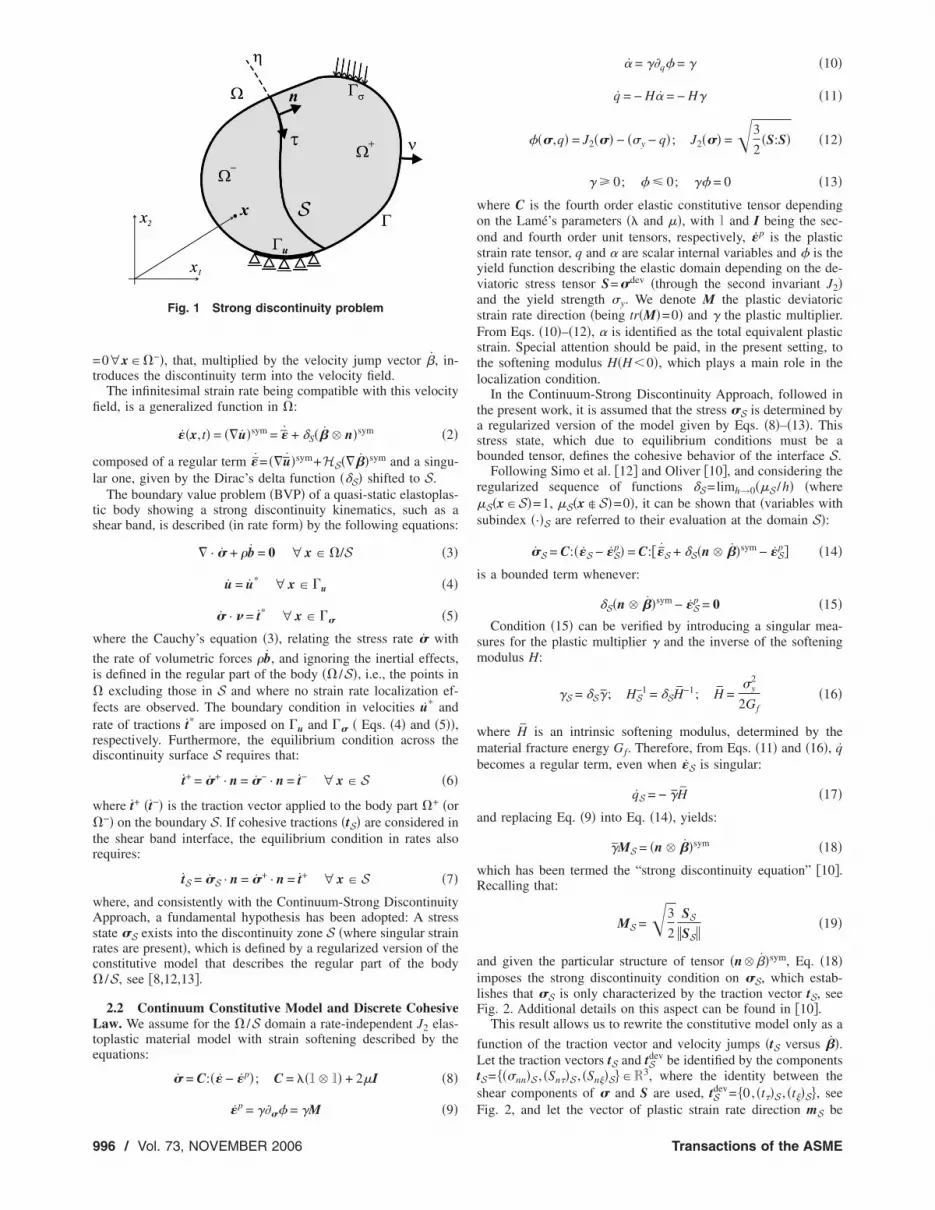
2 Problem Settings

2.1 Strong Discontinuity Kinematics. Let � be a bodywhich experiences a shear band failure mode. The material sur-face S, with normal n intersecting the body �, represents the zonewith localized strain rate, as it is shown in Fig. 1. The appropriatekinematics describing this phenomenon should account for a dis-continuous velocity field across S, such as the following one:

u�x,t� = u�x,t� + HS�x���x,t� �1�

where u�x , t� represents a continuum field, HS�x� is the Heavi-+

side’s step function shifted to S �HS�x�=1∀x�� and HS�x�

NOVEMBER 2006, Vol. 73 / 99506 by ASME

=t

fi

cl

ts

w

ti�frrd

w�tr

wAsrc�

Lte

9

0∀x��−�, that, multiplied by the velocity jump vector �, in-roduces the discontinuity term into the velocity field.

The infinitesimal strain rate being compatible with this velocityeld, is a generalized function in �:

��x,t� = ��u�sym = � + �S�� � n�sym �2�

omposed of a regular term �= ��u�sym+HS����sym and a singu-ar one, given by the Dirac’s delta function ��S� shifted to S.

The boundary value problem �BVP� of a quasi-static elastoplas-ic body showing a strong discontinuity kinematics, such as ahear band, is described �in rate form� by the following equations:

� · � + �b = 0 ∀ x � �/S �3�

u = u* ∀ x � �u �4�

� · � = t* ∀ x � �� �5�

here the Cauchy’s equation �3�, relating the stress rate � with

he rate of volumetric forces �b, and ignoring the inertial effects,s defined in the regular part of the body �� /S�, i.e., the points in

excluding those in S and where no strain rate localization ef-ects are observed. The boundary condition in velocities u* andate of tractions t* are imposed on �u and �� � Eqs. �4� and �5��,espectively. Furthermore, the equilibrium condition across theiscontinuity surface S requires that:

t+ = �+ · n = �− · n = t− ∀ x � S �6�

here t+ �t−� is the traction vector applied to the body part �+ �or−� on the boundary S. If cohesive tractions �tS� are considered in

he shear band interface, the equilibrium condition in rates alsoequires:

tS = �S · n = �+ · n = t+ ∀ x � S �7�

here, and consistently with the Continuum-Strong Discontinuitypproach, a fundamental hypothesis has been adopted: A stress

tate �S exists into the discontinuity zone S �where singular strainates are present�, which is defined by a regularized version of theonstitutive model that describes the regular part of the body/S, see �8,12,13�.

2.2 Continuum Constitutive Model and Discrete Cohesiveaw. We assume for the � /S domain a rate-independent J2 elas-

oplastic material model with strain softening described by thequations:

� = C:�� − �p�; C = ��1 � 1� + 2�I �8�

˙ p

Fig. 1 Strong discontinuity problem

� = ��� = �M �9�

96 / Vol. 73, NOVEMBER 2006

= ��q = � �10�

q = − H = − H� �11�

��,q� = J2��� − ��y − q�; J2��� =�3

2�S:S� �12�

� � 0; 0; � = 0 �13�

where C is the fourth order elastic constitutive tensor dependingon the Lamé’s parameters �� and ��, with 1 and I being the sec-ond and fourth order unit tensors, respectively, �p is the plasticstrain rate tensor, q and are scalar internal variables and is theyield function describing the elastic domain depending on the de-viatoric stress tensor S=�dev �through the second invariant J2�and the yield strength �y. We denote M the plastic deviatoricstrain rate direction �being tr�M�=0� and � the plastic multiplier.From Eqs. �10�–�12�, is identified as the total equivalent plasticstrain. Special attention should be paid, in the present setting, tothe softening modulus H�H�0�, which plays a main role in thelocalization condition.

In the Continuum-Strong Discontinuity Approach, followed inthe present work, it is assumed that the stress �S is determined bya regularized version of the model given by Eqs. �8�–�13�. Thisstress state, which due to equilibrium conditions must be abounded tensor, defines the cohesive behavior of the interface S.

Following Simo et al. �12� and Oliver �10�, and considering theregularized sequence of functions �S=limh→0��S /h� �where�S�x�S�=1, �S�x�S�=0�, it can be shown that �variables withsubindex �·�S are referred to their evaluation at the domain S�:

�S = C:��S − �Sp� = C:��S + �S�n � ��sym − �S

p� �14�

is a bounded term whenever:

�S�n � ��sym − �Sp = 0 �15�

Condition �15� can be verified by introducing a singular mea-sures for the plastic multiplier � and the inverse of the softeningmodulus H:

�S = �S�; HS−1 = �SH−1; H =

�y2

2Gf�16�

where H is an intrinsic softening modulus, determined by thematerial fracture energy Gf. Therefore, from Eqs. �11� and �16�, qbecomes a regular term, even when �S is singular:

qS = − �H �17�

and replacing Eq. �9� into Eq. �14�, yields:

�MS = �n � ��sym �18�

which has been termed the “strong discontinuity equation” �10�.Recalling that:

MS =�3

2

SS

�SS��19�

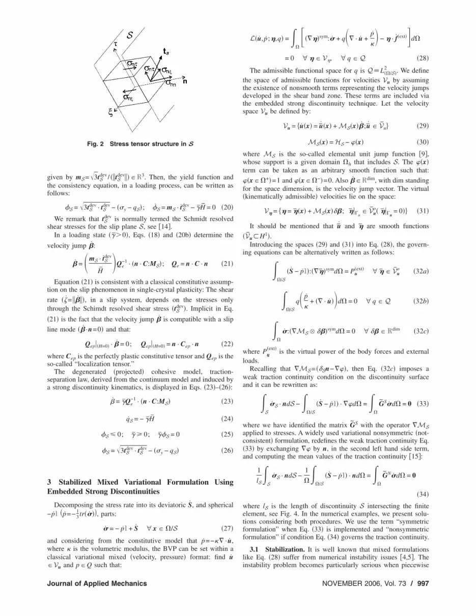
and given the particular structure of tensor �n � ��sym, Eq. �18�imposes the strong discontinuity condition on �S, which estab-lishes that �S is only characterized by the traction vector tS, seeFig. 2. Additional details on this aspect can be found in �10�.

This result allows us to rewrite the constitutive model only as a

function of the traction vector and velocity jumps �tS versus ��.Let the traction vectors tS and tS

dev be identified by the componentstS= ���nn�S , �Sn��S , �Sn��S��R3, where the identity between theshear components of � and S are used, tS

dev= �0, �t��S , �t��S�, see

Fig. 2, and let the vector of plastic strain rate direction mS be

Transactions of the ASME

gtf

s

v

t

rt

�l

ws

sa

3E

−

awc�

J

iven by mS=�3tSdev/ ��tS

dev���R3. Then, the yield function andhe consistency equation, in a loading process, can be written asollows:

S = �3tSdev · tS

dev − ��y − qS�; S = mS · tSdev − �H = 0 �20�

We remark that tSdev is normally termed the Schmidt resolved

hear stresses for the slip plane S, see �14�.In a loading state ���0�, Eqs. �18� and �20b� determine the

elocity jump �:

� = mS · tSdev

HQe

−1 · �n · C:MS�; Qe = n · C · n �21�

Equation �21� is consistent with a classical constitutive assump-ion on the slip phenomenon in single-crystal plasticity: The shear

ate ��= ����, in a slip system, depends on the stresses onlyhrough the Schimdt resolved shear stress �tS

dev�. Implicit in Eq.

21� is the fact that the velocity jump � is compatible with a slip

ine mode �� ·n=0� and that:

�Qep��H=0� · � = 0; �Qep��H=0� = n · Cep · n �22�

here Cep is the perfectly plastic constitutive tensor and Qep is theo-called “localization tensor.”

The degenerated �projected� cohesive model, traction-eparation law, derived from the continuum model and induced bystrong discontinuity kinematics, is displayed in Eqs. �23�–�26�:

� = �Qe−1 · �n · C:MS� �23�

qS = − �H �24�

S 0; � � 0; �S = 0 �25�

S = �3tSdev · tS

dev − ��y − qS� �26�

Stabilized Mixed Variational Formulation Usingmbedded Strong Discontinuities

Decomposing the stress rate into its deviatoric S, and sphericalp1 �p=− 1

3 tr����, parts:

� = − p1 + S ∀ x � �/S �27�

nd considering from the constitutive model that p=−�� · u,here � is the volumetric modulus, the BVP can be set within a

lassical variational mixed �velocity, pressure� format: find u

Fig. 2 Stress tensor structure in S

Vu and p�Q such that:

ournal of Applied Mechanics

L�u, p;�,q� =��

����sym:� + q� · u +p

� − � · f�ext��d�

= 0 ∀ � � V�, ∀ q � Q �28�

The admissible functional space for q is Q�L��/S�2 . We define

the space of admissible functions for velocities Vu by assumingthe existence of nonsmooth terms representing the velocity jumpsdeveloped in the shear band zone. These terms are included viathe embedded strong discontinuity technique. Let the velocityspace Vu be defined by:

Vu = �u�x� = u�x� + MS�x��; u � Vu� �29�

MS�x� = HS − ��x� �30�

where MS is the so-called elemental unit jump function �9�,whose support is a given domain �h that includes S. The ��x�term can be taken as an arbitrary smooth function such that:

��x��+�=1 and ��x��−�=0. Also ��Rdim, with dim standingfor the space dimension, is the velocity jump vector. The virtual�kinematically admissible� velocities lie on the space:

V� = �� = ��x� + MS�x���; ����u� Vu

o�����u= 0�� �31�

It should be mentioned that u and � are smooth functions

�Vu�H1�.Introducing the spaces �29� and �31� into Eq. �28�, the govern-

ing equations can be alternatively written as follows:

��/S

�S − p1�:����symd� = Pu�ext� ∀ � � Vu

o �32a�

��/S

q p

�+ �� · u�d� = 0 ∀ q � Q �32b�

��

�:��MS � ���symd� = 0 ∀ �� � Rdim �32c�

where Pu��ext� is the virtual power of the body forces and external

loads.Recalling that �MS= ��Sn−���, then Eq. �32c� imposes a

weak traction continuity condition on the discontinuity surfaceand it can be rewritten as:

�S

�S · ndS −��/S

�S − p1� · ��d� =��

GS�d� = 0 �33�

where we have identified the matrix GS with the operator �MSapplied to stresses. A widely used variational nonsymmetric �not-consistent� formulation, redefines the weak traction continuity Eq.�33� by exchanging �� by n, in the second left hand side term,and computing the mean values of the traction continuity �15�:

1

lS�

S�S · ndS −

1

��

�/S�S − p1� · nd� =�

�

GN�d� = 0

�34�

where lS is the length of discontinuity S intersecting the finiteelement, see Fig. 4. In the numerical examples, we present solu-tions considering both procedures. We use the term “symmetricformulation” when Eq. �33� is implemented and “nonsymmetricformulation” if condition Eq. �34� governs the traction continuity.

3.1 Stabilization. It is well known that mixed formulationslike Eq. �28� suffer from numerical instability issues �4,5�. The

instability problem becomes particularly serious when piecewise

NOVEMBER 2006, Vol. 73 / 997

l

pcitco

CCo

w

r

s

ztr

w

ta

c

9

inear polynomial functions of continuity C0 are chosen for inter-

olation of both spaces Vu and Q, because in that case the so-alled Ladyzhenskya-Babuska-Brezzi condition �or simply LBB�s not satisfied �16�. A remedy for this unwanted effect has beenhe introduction of stabilization terms Sst into the variational prin-iple Eq. �28�. Particularly, this term is added to the left hand sidef Eq. �32b�.

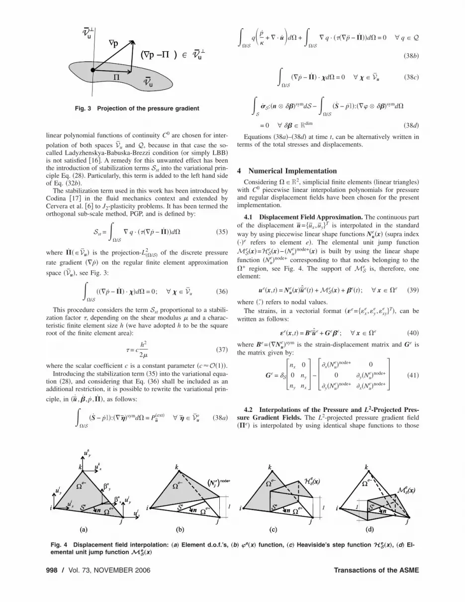
The stabilization term used in this work has been introduced byodina �17� in the fluid mechanics context and extended byervera et al. �6� to J2-plasticity problems. It has been termed therthogonal sub-scale method, PGP, and is defined by:

Sst =��/S

� q · ����p − ���d� �35�

here ���Vu� is the projection-L��/S�2 of the discrete pressure

ate gradient ��p� on the regular finite element approximation

pace �Vu�, see Fig. 3:

��/S

���p − �� · ��d� = 0; ∀ � � Vu �36�

This procedure considers the term Sst proportional to a stabili-ation factor �, depending on the shear modulus � and a charac-eristic finite element size h �we have adopted h to be the squareoot of the finite element area�:

� = ch2

2��37�

here the scalar coefficient c is a constant parameter �c�O�1��.Introducing the stabilization term �35� into the variational equa-

ion �28�, and considering that Eq. �36� shall be included as andditional restriction, it is possible to rewrite the variational prin-

iple, in �u , � , p ,��, as follows:

��/S

�S − p1�:����symd� = Pu�ext� ∀ � � Vu

o �38a�

Fig. 3 Projection of the pressure gradient

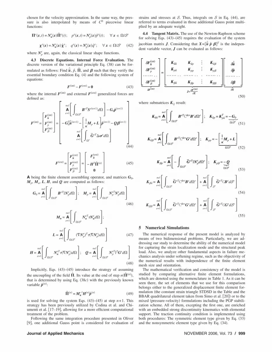
Fig. 4 Displacement field interpolation: „a… Element d.o.f.’s,e

emental unit jump function MS„x…

98 / Vol. 73, NOVEMBER 2006

��/S

q p

�+ � · ud� +�

�/S� q · ����p − ���d� = 0 ∀ q � Q

�38b�

��/S

��p − �� · �d� = 0 ∀ � � Vu �38c�

�S

�S:�n � ���symdS −��/S

�S − p1�:��� � ���symd�

= 0 ∀ �� � Rdim �38d�

Equations �38a�–�38d� at time t, can be alternatively written interms of the total stresses and displacements.

4 Numerical ImplementationConsidering ��R2, simplicial finite elements �linear triangles�

with C0 piecewise linear interpolation polynomials for pressureand regular displacement fields have been chosen for the presentimplementation.

4.1 Displacement Field Approximation. The continuous partof the displacement u= �ux , uy�T is interpolated in the standardway by using piecewise linear shape functions Nu

e�x� �supra index�·�e refers to element e�. The elemental unit jump functionMS

e �x�=HSe �x�− �Nu

e�node+�x� is built by using the linear shapefunction �Nu

e�node+ corresponding to that nodes belonging to the�+ region, see Fig. 4. The support of MS

e is, therefore, oneelement:

ue�x,t� = Nue�x�ue�t� + MS

e �x� + �e�t�; ∀ x � �e �39�

where �. � refers to nodal values.The strains, in a vectorial format ��e= ��x

e ,�ye ,�xy

e �T�, can bewritten as follows:

�e�x,t� = Beue + Ge�e; ∀ x � �e �40�

where Be= ��Nue�sym is the strain-displacement matrix and Ge is

the matrix given by:

Ge = �S�nx 0

0 ny

ny nx� − ��x�Nu

e�node+ 0

0 �y�Nue�node+

�y�Nue�node+ �x�Nu

e�node+ � �41�

4.2 Interpolations of the Pressure and L2-Projected Pres-sure Gradient Fields. The L2-projected pressure gradient field��e� is interpolated by using identical shape functions to those

e„x… function, „c… Heaviside’s step function HS

e„x…, „d… El-

„b…

Transactions of the ASME

csf

w

d

mee

wd

AM

ttv

isut

�

J

hosen for the velocity approximation. In the same way, the pres-ure is also interpolated by means of C0 piecewise linearunctions:

�e�x,t� = Nue�x��e�t�; pe�x,t� = Np

e�x�pe�t�; ∀ x � �/Se

�e�x� = Nue�x��e; qe�x� = Np

e�x�qe; ∀ x � �/Se �42�

here Npe are, again, the classical linear shape functions.

4.3 Discrete Equations. Internal Force Evaluation. Theiscrete version of the variational principle Eq. �38� can be for-

ulated as follows: Find u, p, �, and � such that they verify thessential boundary condition Eq. �4� and the following system ofquations:

F�int� − F�ext� = 0 �43�

here the internal F�int� and external F�ext� generalized forces areefined as:

F�int� = �Fu�int�

Fp�int�

F��int� � = �

Ae=1

nel ��/Se

BeTSe�n+1�d�� − G0p�n+1�

− G0Tu�n+1� − 1

�Mp + L�p�n+1� − Q��n+1�

Ae=1

nel ��e

GeT��ed�� ��44�

F�ext� = �Fu�ext�

Fp�ext�

F��ext� � = � Fu

�ext�

− HT��n�

0� �45�

being the finite element assembling operator, and matrices G0,p, Mu, L, H, and Q are computed as follows:

G0 = Ae=1

nel ��/Se

BeTINped�� ; Mp = A

e=1

nel ��/Se

NpeTNp

ed���46�

Mu = Ae=1

nel ��/Se

NueT�Nu

ed��;

L = Ae=1

nel ��/Se

��Npe�T���Np

e�d�� �47�

H = Ae=1

nel ��/Se

NueT���Np

e�d�� ; Q = Ae=1

nel ��/Se

NpeTITGed��

�48�Implicitly, Eqs. �43�–�45� introduce the strategy of assuming

he uncoupling of the field �. Its value at the end of step n���n��,hat is determined by using Eq. �38c� with the previously knownariable p�n�:

��n� = Mu−1H�n�p�n� �49�

s used for solving the system Eqs. �43�–�45� at step n+1. Thistrategy has been previously utilized by Codina et al. and Chi-menti et al. �17–19�, allowing for a more efficient computationalreatment of the problem.

Following the same integration procedure presented in Oliver

9�, one additional Gauss point is considered for evaluation of

ournal of Applied Mechanics

strains and stresses at S. Thus, integrals on S in Eq. �44�, arereferred to terms evaluated in those additional Gauss point multi-plied by an adequate weight.

4.4 Tangent Matrix. The use of the Newton-Raphson schemefor solving Eqs. �43�–�45� requires the evaluation of the system

jacobian matrix J. Considering that X= �u p ��T is the indepen-dent variable vector, J can be evaluated as follows:

�50�where submatrices Kij result:

�51�

�52�

�53�

K�u = Ae=1

nel ��/Se

GeTCdevBed�e� + Ae=1

nel �Se

GeTCBedSe��54�

K�� = Ae=1

nel ��/Se

GeTCdevGed�e� + Ae=1

nel �Se

GeTCGedSe��55�

5 Numerical SimulationsThe numerical response of the present model is analyzed by

means of two bidimensional problems. Particularly, we are ad-dressing our study to determine the ability of the numerical modelfor capturing the strain localization mode and the structural peakload. Also, we analyze other fundamental aspects in failure me-chanics analysis under softening regime, such as the objectivity ofthe numerical results with independence of the finite elementmesh size and orientation.

The mathematical verification and consistency of the model isstudied by comparing alternative finite element formulations,which are denoted using the nomenclature in Table 1. As it can beseen there, the set of elements that we use for this comparisonbelongs either to the generalized displacement finite element for-mulation �the constant strain triangle STDSD in the Table and theBBAR quadrilateral element taken from Simo et al. �20�� or to themixed �pressure-velocity� formulations including the PGP stabili-zation scheme. All of them, excepting the first one, are enrichedwith an embedded strong discontinuity kinematics with elementalsupport. The traction continuity condition is implemented usingboth procedures: The symmetric element type given by Eq. �33�

and the nonsymmetric element type given by Eq. �34�.

NOVEMBER 2006, Vol. 73 / 999

ttl

ws

Piep

w

chvsawaDasr

amw

aimlb

Fc

1

In the PGP formulation without embedded strong discontinui-ies �denoted “smooth velocity kinematics” in the Table 1�, solu-ions have been obtained by regularization of the softening modu-us H, redefining it in accordance with:

Hreg = hH �56�

here h is the characteristic size of the element and H the intrinsicoftening modulus computed as in Eq. �16�.

A comparison of the relative computational cost betweenGPSD and BBARSD elements is also reported. For this purpose,

t must be considered that the examples have been run in a PCquipped with a single Pentium 4 −3.0 GHz, 512 MB Ram—rocessor.

For all cases, a stability factor “c” near to unity �see Eq. �37��as adopted to perform the numerical tests.

5.1 2D Slope Stability Problem. When undrained loadingonditions are assumed, the constitutive behavior of saturated co-esive soils can be approximately modeled by an associative de-iatoric plastic flow law. In this context, we use a J2 model toimulate a typical plane strain geotechnical slope stability problemnd its corresponding shear band failure mode. A similar exampleas presented in Regueiro et al. �2� and in Oliver et al. �21� whereBBAR element with embedded strong discontinuities was used.ue to the lack, at least up to the author’s knowledge, of an

nalytical or exact solution for this problem, the above mentionedtrategies �denoted as BBARSD-N in Table 1�, will be used as aeference solution to compare quantitative results.

The effects of including, or not, the strong discontinuity modere particularly remarked in the present analysis. Also, the nu-erical stabilization influence on the solution, which is contrastedith similar formulations that do not use such strategy, is studied.The dimensions and boundary conditions of the physical model

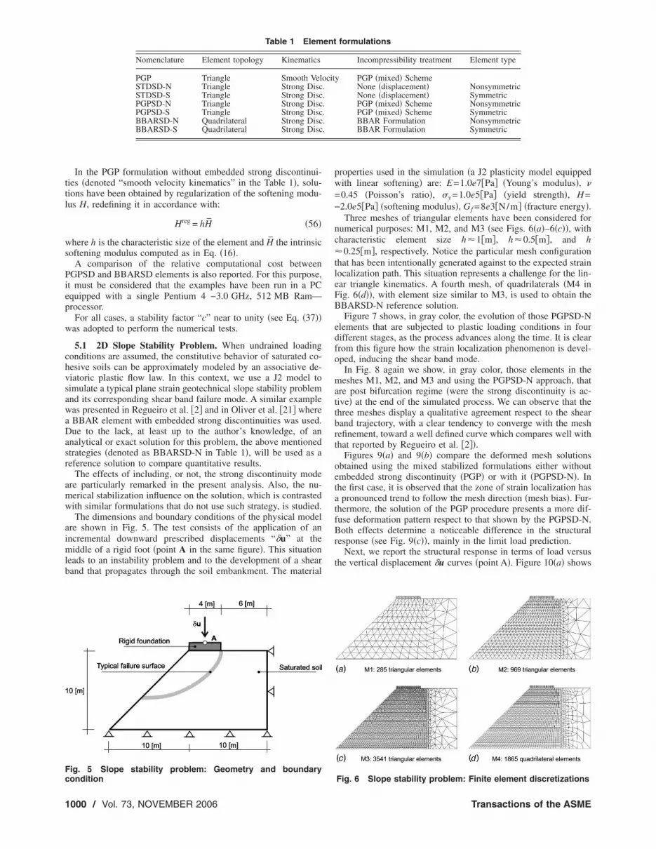
re shown in Fig. 5. The test consists of the application of anncremental downward prescribed displacements “�u” at theiddle of a rigid foot �point A in the same figure�. This situation

eads to an instability problem and to the development of a shearand that propagates through the soil embankment. The material

Table 1 Elem

Nomenclature Element topology Kinematics

PGP Triangle Smooth VelSTDSD-N Triangle Strong DiscSTDSD-S Triangle Strong DiscPGPSD-N Triangle Strong DiscPGPSD-S Triangle Strong DiscBBARSD-N Quadrilateral Strong DiscBBARSD-S Quadrilateral Strong Disc

ig. 5 Slope stability problem: Geometry and boundary

ondition

000 / Vol. 73, NOVEMBER 2006

properties used in the simulation �a J2 plasticity model equippedwith linear softening� are: E=1.0e7�Pa� �Young’s modulus�, �=0.45 �Poisson’s ratio�, �y =1.0e5�Pa� �yield strength�, H=−2.0e5�Pa� �softening modulus�, Gf =8e3�N/m� �fracture energy�.

Three meshes of triangular elements have been considered fornumerical purposes: M1, M2, and M3 �see Figs. 6�a�–6�c��, withcharacteristic element size h�1�m�, h�0.5�m�, and h�0.25�m�, respectively. Notice the particular mesh configurationthat has been intentionally generated against to the expected strainlocalization path. This situation represents a challenge for the lin-ear triangle kinematics. A fourth mesh, of quadrilaterals �M4 inFig. 6�d��, with element size similar to M3, is used to obtain theBBARSD-N reference solution.

Figure 7 shows, in gray color, the evolution of those PGPSD-Nelements that are subjected to plastic loading conditions in fourdifferent stages, as the process advances along the time. It is clearfrom this figure how the strain localization phenomenon is devel-oped, inducing the shear band mode.

In Fig. 8 again we show, in gray color, those elements in themeshes M1, M2, and M3 and using the PGPSD-N approach, thatare post bifurcation regime �were the strong discontinuity is ac-tive� at the end of the simulated process. We can observe that thethree meshes display a qualitative agreement respect to the shearband trajectory, with a clear tendency to converge with the meshrefinement, toward a well defined curve which compares well withthat reported by Regueiro et al. �2��.

Figures 9�a� and 9�b� compare the deformed mesh solutionsobtained using the mixed stabilized formulations either withoutembedded strong discontinuity �PGP� or with it �PGPSD-N�. Inthe first case, it is observed that the zone of strain localization hasa pronounced trend to follow the mesh direction �mesh bias�. Fur-thermore, the solution of the PGP procedure presents a more dif-fuse deformation pattern respect to that shown by the PGPSD-N.Both effects determine a noticeable difference in the structuralresponse �see Fig. 9�c��, mainly in the limit load prediction.

Next, we report the structural response in terms of load versusthe vertical displacement �u curves �point A�. Figure 10�a� shows

formulations

Incompressibility treatment Element type

y PGP �mixed� SchemeNone �displacement� NonsymmetricNone �displacement� SymmetricPGP �mixed� Scheme NonsymmetricPGP �mixed� Scheme SymmetricBBAR Formulation NonsymmetricBBAR Formulation Symmetric

ent

ocit......

Fig. 6 Slope stability problem: Finite element discretizations

Transactions of the ASME

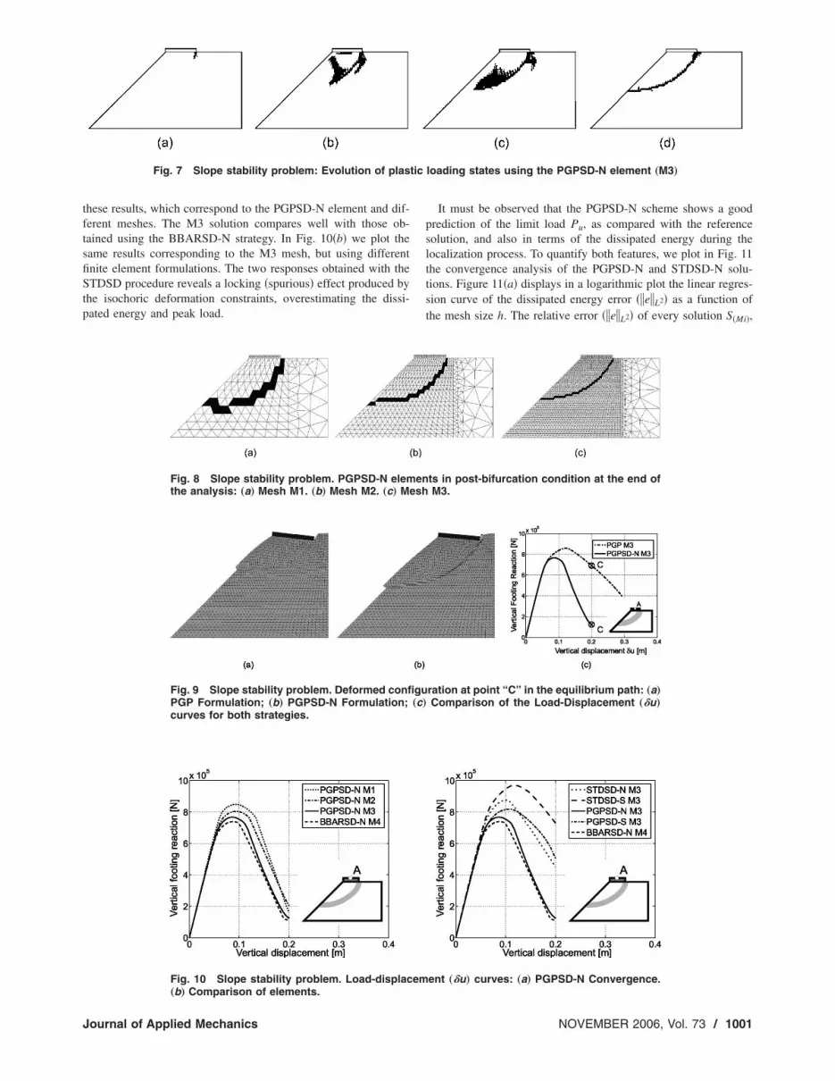
tftsfiStp

tic

J

hese results, which correspond to the PGPSD-N element and dif-erent meshes. The M3 solution compares well with those ob-ained using the BBARSD-N strategy. In Fig. 10�b� we plot theame results corresponding to the M3 mesh, but using differentnite element formulations. The two responses obtained with theTDSD procedure reveals a locking �spurious� effect produced by

he isochoric deformation constraints, overestimating the dissi-ated energy and peak load.

Fig. 7 Slope stability problem: Evolution of plas

Fig. 8 Slope stability problem. PGPSD-N elemthe analysis: „a… Mesh M1. „b… Mesh M2. „c… M

Fig. 9 Slope stability problem. Deformed confiPGP Formulation; „b… PGPSD-N Formulation;curves for both strategies.

Fig. 10 Slope stability problem. Load-displac

„b… Comparison of elements.

ournal of Applied Mechanics

It must be observed that the PGPSD-N scheme shows a goodprediction of the limit load Pu, as compared with the referencesolution, and also in terms of the dissipated energy during thelocalization process. To quantify both features, we plot in Fig. 11the convergence analysis of the PGPSD-N and STDSD-N solu-tions. Figure 11�a� displays in a logarithmic plot the linear regres-sion curve of the dissipated energy error ��e�L2� as a function ofthe mesh size h. The relative error ��e�L2� of every solution S�Mi�,

loading states using the PGPSD-N element „M3…

ts in post-bifurcation condition at the end ofM3.

ration at point “C” in the equilibrium path: „a…Comparison of the Load-Displacement „u…

ent „u… curves: „a… PGPSD-N Convergence.

enesh

gu„c…

em

NOVEMBER 2006, Vol. 73 / 1001

w�

wp

d P

1

here S�Mi� is the load vs. displacement ��u� curve of the mesh Mi

i=1,2 ,3�, is computed in terms of a L2 norm as follow:

�e�L2 =�S�Mi� − S�REF��L2

�S�REF��L2=

��0

�max

�S�Mi� − S�REF��2d�

��0

�max

�S�REF��2d�

;

i = 1,2,3 �57�

here the integration parameter � corresponds to the vertical dis-lacement ��u� and �max=max��u� is the same for all cases, while

Table 2 2D slope problem. Relative computational cost.

Mesh Residual forces Stiffness matrix Solver Total time

M1 1.44 1.16 2.10 1.37M2 1.44 1.12 1.25 1.30M3 1.48 1.06 1.33 1.31

Fig. 12 2D cracked panel: „a… Geometry and boundary conditi

Fig. 11 Slope stability problem. Relative errsponse „in terms of L2-norm…. „b… Ultimate loa

elements „hÉ2†mm‡….

002 / Vol. 73, NOVEMBER 2006

S�REF�=S�M3�BBARSD-N is the reference solution.

Similarly, Fig. 11�b� displays the linear regression curve of thelimit load prediction error as a function of the size mesh h. Therelative error of the peak load solution is determined by means of:

�e�Pu =�Pu�Mi� − Pu�REF��

�Pu�REF��; i = 1,2,3 �58�

where Pu�Mi� is the maximum value of the vertical footing reac-

tion displayed by mesh Mi and Pu�REF�= Pu�M3�BBARSD-N.

From Fig. 11 it is clearly observed a higher accuracy and con-vergene rate, either in limit load prediction as also in the dissi-pated energy, of the PGPSD-N model if compared with atheSTDSD-N element.

Finally, the comparative computational cost for PGPSD-N ele-ment, relative to BBARSD-N formulation, is outlined in Table 2.Every mesh M1, M2, and M3 of PGPSD-N elements is comparedwith an equivalent mesh of quadrilateral BBAR elements havingidentical number of nodes and element sizes.

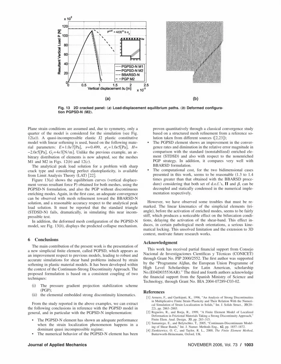
5.2 Center Cracked Panel. A square �10�10�cm2�� crackedpanel subjected to uniaxial vertical displacement is analyzed.

. „b… Mesh M1: 1301 elements „hÉ4†mm‡…. „c… Mesh M2: 5252

vs element size: „a… Load-displacement re-u.

ons

ors

Transactions of the ASME

Pq1mr−bM

cf

mPecsl�p

m

6

aaastpt

tg

J

lane strain conditions are assumed and, due to symmetry, only auarter of the model is considered for the simulation �see Fig.2�a��. A quasi-incompressible elastic J2 plastic constitutiveodel with linear softening is used, based on the following mate-

ial parameters: E=1.0e7�Pa�, �=0.499, �y =1.0e5�Pa�, H=2.0e5�Pa�, Gf =4e3�N/m�. Unlike the previous example, an ar-itrary distribution of elements is now adopted, see the meshes1 and M2 in Figs. 12�b� and 12�c�.The analytical peak load solution for a problem with sharp

rack type and considering perfect elastoplasticity, is availablerom Limit Analysis Theory �LAT� �22�.

Figure 13�a� shows the equilibrium curves �vertical displace-ent versus resultant force P� obtained for both meshes, using theGPSD-N formulation, and also the PGP without discontinuousnriching modes. Again, in the first case, an adequate convergencean be observed with mesh refinement toward the BBARSD-Nolution, and a reasonable accuracy respect to the analytical peakoad solution. It must be reported that the standard triangleSTDSD-N� fails, dramatically, in simulating this near incom-ressible test.

In addition, the deformed mesh configuration of the PGPSD-Nodel, see Fig. 13�b�, displays the predicted collapse mechanism.

ConclusionsThe main contribution of the present work is the presentation ofnew simplicial finite element, called PGPSD, which appears as

n improvement respect to previous models, leading to robust andccurate simulations for shear band problems induced by strainoftening in plastic material models. It has been developed withinhe context of the Continuum-Strong Discontinuity Approach. Theroposed formulation is based on a consistent coupling of twoechniques:

�i� The pressure gradient projection stabilization scheme�PGP�;

�ii� the elemental embedded strong discontinuity kinematics.

From the study reported in the above examples, we can extracthe following conclusions in reference with the PGPSD model ineneral, and in particular with the PGPSD-N implementation:

• The PGPSD-N element has shown an adequate performancewhen the strain localization phenomenon happens in adominant quasi incompressible regime;

Fig. 13 2D cracked panel: „a… Load-displacemtion PGPSD-N „M2….

• The numerical behavior of the PGPSD-N element has been

ournal of Applied Mechanics

proven quantitatively through a classical convergence studybased on a structured mesh refinement from a reference so-lution taken from different sources ��2,23��;

• The PGPSD element shows an improvement in the conver-gence rates and diminution in the relative error magnitude incomparison with the standard �nonstabilized� enriched ele-ment �STDSD� and also with respect to the nonenrichedPGP strategy. In addition, it compares very well withBBARSD formulation.

• The computational cost, for the two bidimensional casespresented in this work, seems to be reasonable �1.3 to 1.4times greater than that obtained with the BBARSD proce-dure� considering that both set of d.o.f.’s, � and �, can bedecoupled and statically condensed in the numerical imple-mentation respectively.

However, we have observed some troubles that must be re-marked. The linear kinematics of the simplicial elements �tri-angle�, before the activation of enriched modes, seems to be fairlystiff, which produces a noticeable effect on the bifurcation condi-tions, delaying the activation of the shear-band. This effect in-duces, in certain pathological mesh orientations, a serious kine-matical locking. This unsolved limitation and the extension to 3Dcontext, motivate future research works.

AcknowledgmentThis work has received partial financial support from Consejo

Nacional de Investigaciones Científicas y Técnicas �CONICET�through Grant No. PIP 2000/2552. The first author was supportedby the “Programme Al�an, the European Union Programme ofHigh Level Scholarships for Latin American, scholarshipNo.�E04D035536AR�.” The third and fourth authors acknowledgethe financial support from the Spanish Ministry of Science andTechnology, through Grant No. BIA 2004-07289-C03-02.

References�1� Armero, F., and Garikipati, K., 1996, “An Analysis of Strong Discontinuities

in Multiplicative Finite Strain Plasticity and Their Relation With the Numeri-cal Simulation of Strain Localization in Solids,” Int. J. Solids Struct., 33�20–22�, pp. 2863–2885.

�2� Regueiro, R., and Borja, R., 1999, “A Finite Element Model of LocalizedDeformation in Frictional Materials Taking a Strong Discontinuity Approach,”Finite Elem. Anal. Design, 33, pp. 283–315.

�3� Samaniego, E., and Belytschko, T., 2005, “Continuum-Discontinuum Model-ing of Shear Bands,” Int. J. Numer. Methods Eng., 62, pp. 1857–1872.

�4� Zienkiewicz, O. C., and Taylor, R. L., 2000, The Finite Element Method,

t equilibrium paths. „b… Deformed configura-

en

Butterworth-Heinemann, Oxford, UK.

NOVEMBER 2006, Vol. 73 / 1003

1

�5� Hughes, T. J. R., 1987, The Finite Element Method. Linear Static and DynamicFinite Element Analysis, Prentice-Hall,Englewood Cliffs, NJ.

�6� Cervera, M., Chiumenti, M., Valverde, Q., and Agelet de Saracibar, C., 2003,“Mixed Linear/Linear Simplicial Elements for Incompressible Elasticity andPlasticity,” Comput. Methods Appl. Mech. Eng., 192, pp. 5249–5263.

�7� Sanchez, P., Sonzogni, V., and Huespe, A., 2004, “Evaluation of a StabilizedMixed Finite Element for Solid Mechanics Problems and its Parallel Imple-mentation,” Comput. Struct. �to be published�.

�8� Oliver, J., 1996a, “Modeling Strong Discontinuities in Solids Mechanics viaStrain Softening Constitutive Equations. Part 1: Fundamentals,” Int. J. Numer.Methods Eng., 39�21�, pp. 3575–3600.

�9� Oliver, J., 1996b, “Modeling Strong Discontinuities in Solids Mechanics viaStrain Softening Constitutive Equations. Part Numerical Simulation,” Int. J.Numer. Methods Eng., 39�21�, pp. 3601–3623.

�10� Oliver, J., 2000, “On the Discrete Constitutive Models Induced by StrongDiscontinuity Kinematics and Continuum Constitutive Equations,” Int. J. Sol-ids Struct., 37, pp. 7207–7229.

�11� Cervera, M., Chiumenti, M., and Agelet de Saracibar, C., 2004, “Shear BandLocalization via Local j2 Continuum Damage Mechanics,” Comput. MethodsAppl. Mech. Eng., 193, pp. 849–880.

�12� Simo, J., Oliver, J., and Armero, F., 1993, “An Analysis of Strong Disconti-nuities Induced by Strain-Softening in Rate-Independent Inelastic Solids,”Comput. Mech., 12, pp. 277–296.

�13� Oliver, J., Cervera, M., and Manzoli, O., 1999, “Strong Discontinuities andContinuum Plasticity Models: The Strong Discontinuity Approach,” Int. J.Plast., 15�3�, pp. 319–351.

�14� Asaro, R. J., 1983, “Micromechanics of Crystals and Polycrystals,” Adv. Appl.

Mech., 23, pp. 1–115.

004 / Vol. 73, NOVEMBER 2006

�15� Oliver, J., Huespe, A., and Samaniego, E., 2003, “A Study On Finite Elementsfor Capturing Strong Discontinuities,” Int. J. Numer. Methods Eng., 56, pp.2135–2161.

�16� Brezzi, F., and Fortin, M.1991, Mixed and Hybrid Finite Element Methods,Springer, Berlin.

�17� Codina, R., 2000, “Stabilization of Incompressibility and Convection ThroughOrthogonal Sub-Scales in Finite Element Method,” Comput. Methods Appl.Mech. Eng., 190, pp. 1579–1599.

�18� Codina, R., Blasco, J., Buscaglia, G. C., and Huerta, A., 2001, “Implementa-tion of a Stabilized Finite Element Formulation for the Incompressible Navier-Stokes Equations Based on a Pressure Gradient Projection,” Int. J. Numer.Methods Eng., 37, pp. 419–444.

�19� Chiumenti, M., Valverde, Q., Agelet de Saracibar, C., and Cervera, M., 2002,“Una Formulación Estabilizada Para Plasticidad Incompresible Usando Trian-gulos y Tetraedros con Interpolaciones Lineales en Desplazamientos y Pre-siones,” Métodos Numéricos en Ingeniería V.

�20� Simo, J. C., and Hughes, T. J. R., 1998, Computational Inelasticity, Springer,New York.

�21� Oliver, J., Huespe, A. E., Blanco, S., and Linero, D. L., 2005, “Stability andRobustness Issues in Numerical Modeling of Material Failure in the StrongDiscontinuity Approach,” Comput. Methods Appl. Mech. Eng. �in press�.

�22� Kanninen, M. F., and Popelar, H., 1985, Advanced Fracture Mechanics, Ox-ford University Press, New York.

�23� Oliver, J., Huespe, A. E., Pulido, M. D. G., Blanco, S., and Linero, D. L.,2004, “Recent Advances in Computational Modeling Of Material Failure,” inProc. European Congress on Comput. Methods in Appl. Sciences and Eng., P.Neittaanmäki, T. Rossi, K. Majava, and O. Pironneau, eds, ECOMAS 2004,

Jyväskylä.

Transactions of the ASME