Stability-Constrained Optimization for Energy Efficiency inPolling-Based Wireless Networks

Yi XieDepartment of Computing

The Hong Kong Polytechnic UniversityHong Kong, SAR China

csyxie@comp.polyu.edu.hk

Rocky K. C. ChangDepartment of Computing

The Hong Kong Polytechnic UniversityHong Kong, SAR China

csrchang@comp.polyu.edu.hk

ABSTRACTA wireless device’s energy can be saved by putting it intothe sleeping mode (power saving mode, PSM) or decreasingits transmission power (transmission power control, TPC)which prolongs the packet transmission time. However, de-creasing one’s transmission power would prevent others fromtransmitting their packets. Clearly, there are complex inter-actions when each tries to optimize its own energy efficiency.Therefore, in this paper we are considering the problem ofoptimizing the energy efficiency for all wireless devices in thenetwork with the constraint that they are all stable. In par-ticular, we consider the polling-based MAC protocols withphase grouping and mobile grouping schedules, and we em-ploy both the PSM and TPC to save the energy. We haveformulated stability-constrained optimization problems forthem, and have proposed an iterative algorithm to computethe optimal power allocations for the wireless devices. Wehave conducted a lot of experiments to validate the accu-racy of the algorithm and to evaluate the gains in the en-ergy efficiency for the two schedules. The mobile groupingschedule is found to be much more energy efficient than thePG schedule, especially when the downlink traffic is higherthan the uplink traffic. We have also studied the impact ofthe optimized schedules on the delay performance.

1. INTRODUCTIONEnergy efficiency is one of the important design issues

to consider in wireless networks. Various mechanisms havebeen proposed to trade-off between energy consumption andthe communication quality [1]. In this paper we mainlyconcentrate on the media access control (MAC) sublayer ina wireless infrastructure network in which an access point(AP) serves as the relay for a number of wireless clients.The wireless MAC protocols can be based on random accessor coordinated access. For example, in the IEEE 802.11wireless LAN, the standard prescribes the distributed co-ordinated function (DCF) and point coordinated function

Permission to make digital or hard copies of all or part of this work forpersonal or classroom use is granted without fee provided that copies arenot made or distributed for profit or commercial advantage and that copiesbear this notice and the full citation on the first page. To copy otherwise, torepublish, to post on servers or to redistribute to lists, requires prior specificpermission and/or a fee.Valuetools’06, October 11-13, 2006, Pisa, ItalyCopyright 2006 ACM 1-59593-504-5 ...$5.00.

(PCF). The DCF is based on Carrier Sense Multiple Ac-cess with Collision Avoidance (CSMA/CA) and the PCF ismainly based on a polling scheme.

In this paper we consider the polling-based MAC proto-col for a wireless LAN. The polling-based MAC provides anumber of advantages over the random access MAC. For ex-ample, it can guarantee a certain level of quality-of-serviceto each client even when the channel is accessed simulta-neously by multiple clients. As we shall see in this paper,the polling-based MAC can also be used to optimize theenergy consumption of the entire wireless LAN. We will em-ploy 2 mechanisms to reduce the energy consumption—thepower saving mode (PSM) and the transmission power con-trol (TPC) [2]. The PSM reduces the energy consumptionby putting wireless devices into the sleeping mode (e.g. [3]),while the TPC reduces the transmission power to conserveenergy.

The TPC is based on the fact that the communicationenergy can be saved by transmitting packets over a longerduration, i.e., reducing the transmission rate [4]. We adoptthe TPC with the convex rate-power curve derived fromthe Shannon’s theorem. First, the ideal channel capacityis given by Cmax = W × log2(1 + S

N) bps, where W is the

bandwidth in Hz, N is the Gaussian noise power, and Sis the signal power. The transmission rate R is given byαCmax bps, where α ∈ (0, 1), depicts the ratio of the realchannel capacity to Cmax. By introducing an attenuationfactor A, which is the ratio of the transmission power P toS, the power-rate relationship (1) is shown in Figure 1(a).

R = αW log2(1 + P/(AN)). (1)

Moreover, the energy spent on transmitting 1 bit, e(t) =tP , is a convex function of its transmission time t = 1

R.

Therefore, e(t) can be reduced by lowering P , which resultsin a smaller R and a longer t. The relationship is illustratedin Figure 1(b).

Most of the power-saving mechanisms, including the PSMand TPC, will nevertheless degrade the communication andapplication performance. Therefore, many previous worksconsidered optimal trade-offs between energy consumptionand various performance metrics, such as throughput [5],delay [6, 7, 8], network utility [9], and error rate [2, 10].Moreover, the previous works considered the trade-offs forindividual wireless device and did not consider how the in-dividual energy-saving actions affect each other. This paperaddresses the energy consumption problem for the entirenetwork. In other words, an individual device cannot slow

(a) Power-rate curves (b) Energy-time curves

Figure 1: Trade-off of energy & transmission rate

its transmission rate to the extent that other devices wouldbe starved. As a result, we will optimize the total energyconsumption of all devices under the constraints that allthe devices are stable, i.e., stability-constrained optimiza-tion. By stability, we mean that the queue length wouldnot grow unbounded. Moreover, we will consider 2 pollingschedules—phase grouping and mobile grouping, and com-pare their performance in terms of the energy efficiency.

2. RELATED WORKThe phase grouping schedules have been widely deployed.

The typical example is the energy conserving MAC (EC-MAC) protocol [10] which uses an explicit transmission or-der with reservations. In the broadcast (downlink) phase,the wireless device listens to the downlink for the trans-mission order. The AP’s centralized scheduler tries to re-duce the energy consumption and support QoS in the up-link phase. Many mobile grouping polling-based protocolshave also been proposed to minimize the energy consump-tion by having less transitions, and control the packet trans-mission [11], such as the disposable token MAC Protocol(DTMP) [12], the E2MaC protocol [13], and the mobilegrouping schedule [14].

Moreover, a number of mechanisms have been proposed totrade-off between energy efficiency and other performancemetrics. Some packet transmission schedules in wirelesscommunications are designed to minimize the energy con-sumption subject to the deadline or the delay constraint,e.g., the optimal offline/online schedules [15] and the Move-right algorithm [16]. Cross-layer schemes are proposed tobalance the reduction of delay (transmission time) and theenergy conservation, e.g., the energy-efficient PCF [2] foruplink data transmission. It controls the transmission rateby the PHY rate adaptation, while uses the TPC to selectthe best transmit power level to combat the co-channel in-terference. According to the given power-rate function, theTPC may determine the most energy efficient transmissionstrategy for each data frame, e.g. an optimal rate-powercombination table in Miser [17]. Besides, Zhang and Chan-son have attempted to minimize the energy consumptionsubject to the given throughput constraints, or maximizethe throughput subject to a fixed energy storage [5]. Chiangand Bell defined network utility based on all user utilities,and studied the problem of maximizing the network utilitywith energy constraints [9]. Nuggenhalli et al designed adelay constrained transmission schedule that maximizes thelifetime of a transmitter [7], and further took the energyrecovery property of batteries into consideration [18].

Instead of considering specific performance metrics, we

Figure 2: Grouping schedules of polling-based MAC

consider the guarantee of stability as a foundation require-ment for wireless communication. The solution of our stability-constrained energy minimization problem is the optimal trans-mission power allocations, which is easy to deploy in wirelessnodes. That is, our optimal transmission power allocationshave provided a stable network consuming energy efficiently.When wireless applications require specific performances,e.g. a short delay or a large throughput, other energy ef-ficient schemes may be applied as the complementary partof our design.

The rest of the paper is organized as follows. In the nextsection, we describe the 2 polling schedules and model themusing cyclic-service queueing models. In section 4, we for-mulate stability-constrained optimization problems for the 2schedules. Then we compute optimal solutions and presentan iterative algorithm in section 5. In section 6, we firstevaluate the performance of the iterative algorithm and thencompare the energy efficiency of the 2 schedules. We havealso evaluated the impact of the PSM and TPC on the de-lay performance. We finally conclude this paper with futuredirections in section 7.

3. SYSTEM MODELSWe consider 2 types of polling schedules—phase group-

ing (PG) schedule and mobile grouping (MG) schedule. Inthe PG schedule, the uplink and downlink phases alternatebetween them, as illustrated in Figure 2. In the downlinkphase, the AP broadcasts packets to all wireless devices M1,M2, . . . . Thus, all devices have to stay active in order to re-ceive their packets. However, each device is polled individu-ally in the uplink phase. Therefore, using the PSM, a devicecan be put into the sleeping mode when it is not polled, andbe awaken into the active mode when it is polled during theuplink phase. On the other hand, the MG schedule groupsthe uplink and downlink phases for each wireless device, e.g.[12]. Each device stays in the sleeping state except when itis polled by the AP for message reception and transmission.Note that frequent transitioning between the sleeping modeand the active mode also consumes a significant amount ofenergy.

We model the MG and PG schedules using a cyclic-servicequeueing model [19]. We first describe the common modelelements here, and then continue the model description thatdiffers for these two schedules. Consider that there are cwireless devices in the network, which are serviced by anAP according to a fixed polling schedule. Each wireless de-

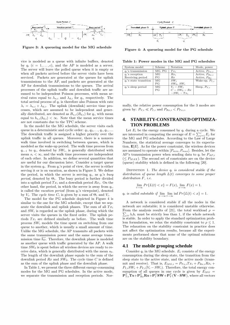
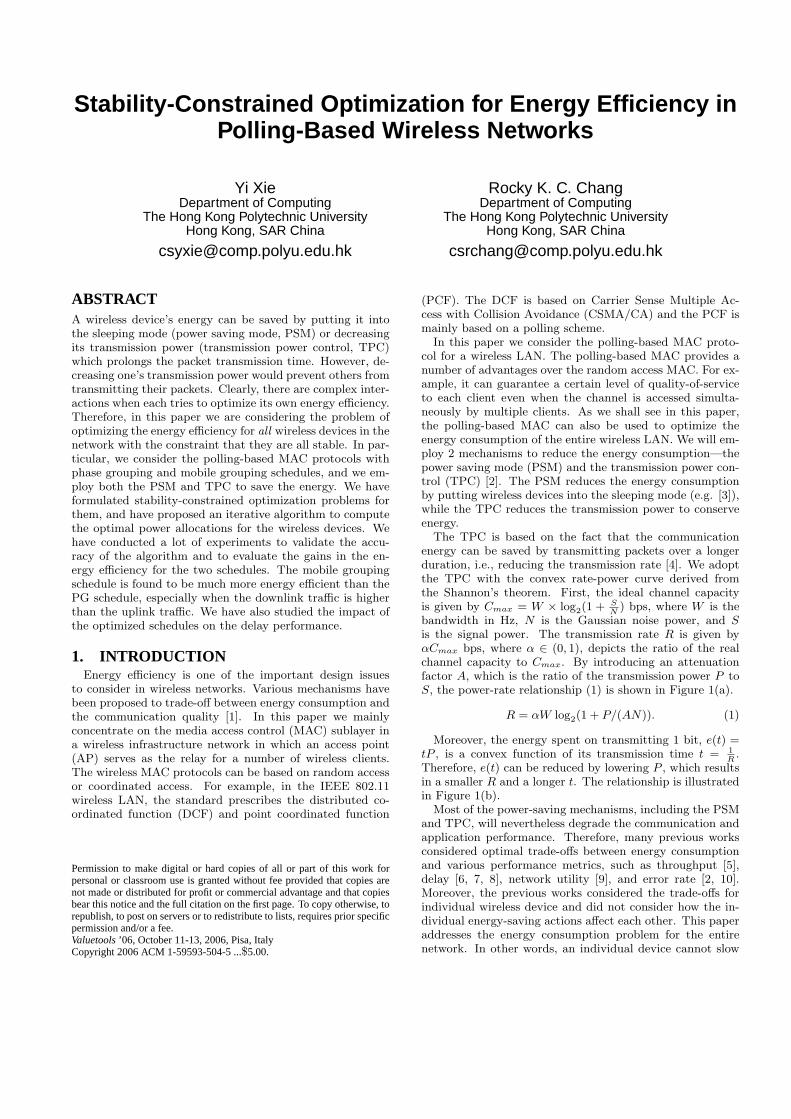
Figure 3: A queueing model for the MG schedule

vice is modeled as a queue with infinite buffers, denotedby qi (i = 1, . . . , c), and the AP is modeled as a server.The server will leave the polled queue when it is empty orwhen all packets arrived before the server visits have beenserviced. Packets are generated at the queues for uplinktransmissions to the AP, and packets are generated at theAP for downlink transmissions to the queues. The arrivalprocesses of the uplink traffic and downlink traffic are as-sumed to be independent Poisson processes, with mean ar-rival rates equal to λu,i and λd,i for qi, respectively. Thetotal arrival process of qi is therefore also Poisson with rateλi = λu,i + λd,i. The uplink (downlink) service time pro-cesses, which are assumed to be independent and gener-ally distributed, are denoted as Bu,i(Bd,i) for qi, with meanequal to bu,i(bd,i) < ∞. Note that the mean service timesare not constants due to the TPC scheme.

In the model for the MG schedule, the server visits eachqueue in a deterministic and cyclic order: q1, q2,. . ., qc, q1, ....The downlink traffic is assigned a higher priority over theuplink traffic in all queues. Moreover, there is a nonzerowalk time involved in switching between queues, which ismodeled as the wake-up period. The walk time process fromqi−1 to qi, denoted by SWi, is generally distributed withmean si < ∞, and the walk time processes are independentof each other. In addition, we define several quantities thatare useful for our discussion later. Consider a target queuein the system qi. From qi’s point of view, the server is eitherserving it or is on vacation, as shown in Figure 3. We definethe period, in which the server is serving qi, as qi’s busyperiod, denoted by Θi. The busy period is further dividedinto a uplink period Txi and a downlink period Rxi. On theother hand, the period, in which the server is away from qi,is called the vacation period (from qi’s viewpoint), denotedby Vi. The cycle time Ci is given by a sum of Θi and Vi.

The model for the PG schedule depicted in Figure 4 issimilar to the one for the MG schedule, except that we sep-arate the downlink and uplink phases. The sum of all Txi

and SWi is regarded as the uplink phase, during which theserver visits the queues in the fixed order. The uplink pe-riods Txi are defined similarly as before. The walk timeprocess SWi models the time spent on switching from onequeue to another, which is usually a small amount of time.Unlike the MG schedule, the AP transmits all packets withthe same transmission power and the same average trans-mission time bD. Therefore, the downlink phase is modeledas another queue with traffic generated by the AP. A walktime SW0 is spent before all wireless devices are ready to re-ceive data, which is generally distributed with the mean s0.The length of the downlink phase equals to the sum of thedownlink period Rx and SW0. The cycle time C is definedas the sum of the uplink phase and the downlink phase.

In Table 1, we present the three different energy-consumingmodes for the MG and PG schedules. In the active mode,we separate the transmission and reception periods. Nor-

Figure 4: A queueing model for the PG schedule

Table 1: Power modes in the MG and PG schedules

System model Scheme Notation Mode, power

qi’s transmission MG, PG Txi Active, PT x,i

qi’s reception MG Rxi Active, PRx,i

Receiving period PG Rx Active, PRx

qi’s state transition MG SWi Wake-up, PI,i

PG SW0, SWi

qi’s sleep period MG Vi − SWi Sleep, PV,i

PG C − SW0 − Rx−SWi − Txi

mally, the relative power consumption for the 3 modes aregiven by: PV,i � PI,i and PRx,i < PTx,i.

4. STABILITY-CONSTRAINED OPTIMIZA-TION PROBLEMS

Let Ei be the energy consumed by qi during a cycle. Weare interested in computing the average of E =

∑cj=1 Ej for

the MG and PG schedules. According to the Law of LargeNumbers, the statistical average converges to its expecta-tion, E[E]. As for the power constraint, the wireless devicesare assumed to operate within [Pmin, Pmax]. Besides, let theAP’s transmission power when sending data to qi be PAP,i

(≤ PMAX). The second set of constraints are on the device(queue) stability which is defined in the following [20].

Definition 1. The device qi is considered stable if thedistribution of queue length L(t) converges to some properdistribution F , i.e.

limt→∞

Pr{L(t) < x} = F (x), limx→∞

F (x) = 1.

qi is called substable if limx→∞

limt→∞

inf Pr{L(t) < x} = 1.

A network is considered stable if all the nodes in thenetwork are substable; it is considered unstable otherwise.From the analysis results of [21], the total workload ρ =∑

i∀ λibi must be strictly less than 1, if the whole networkis stable. In order to apply the standard optimization prob-lem formulation, we relax the stability constraint to ρ ≤ 1.The relaxation on the stability constraint in practice doesnot affect the optimization results, because all the experi-ments performed show that none of the optimal solutionsare on the stability boundary.

4.1 The mobile grouping scheduleConsider qi in the MG schedule. Ei consists of the energy

consumption during the sleep state, the transition from thesleep state to the active state, and the active mode (trans-mit and receive). That is, EMG,i = PTx,iTxi + PRx,iRxi +PI,iSWi + PV,i(Vi − SWi). Therefore, the total energy con-sumption of all queues in one cycle is given by EMG =PT

TxTx+PTRxRx+PT

I SW+PTV (V−SW), where all vectors

are of dimension c. The objective function then becomes

E(EMG) = E[PTTxTx] + E[PRx]T E[Rx] +

E[PI ]T E[SW] + E[PV]T (E[V]−E[SW]).

Moreover, E[C] is the same for all queues which is given by∑cj=1(E[Txj ]+E[Rxj ]+E[SWj ]). Combined with the power

constraints, the optimization problem for the MG scheduleis formulated as

minbd,bu

E(EMG) (2)

s.t.

c∑j=1

(λd,jbd,j + λu,jbu,j)− 1 ≤ 0.

PAP,i ≤ PMAX , ∀i.Pmin ≤ PTx,i ≤ Pmax, ∀i.

4.2 The phase grouping scheduleFor the PG schedule, qi consumes energy during the en-

tire downlink reception period, the mode transitions, thetransmission period, and the sleeping period. Therefore,EPG,i = PRx,iRx+PTx,iTxi +PI,i(SW0 +SWi)+PV,i(C−SW0 − Rx − SWi − Txi). Similar to the previous case, wecan obtain the objective function for the PG schedule as

E(EPG) = (E[PRx]T E[Rx] + E[PI ]T E[SW0])I(c, 1) +

+E[PI ]T E[SW] + E[PT

TxTx] + E[PV]T ×(E[C − SW0 −Rx]I(c, 1)−E[SW]−E[Tx]),

where E[C] = E[Rx] +c∑

j=1

(E[Txj ] + E[SWj ]) and I(c, 1)

is a c-dimensional identity vector, i.e. ec. Therefore, theoptimization problem for the PG schedule is formulated as

minbd,bu

E(EPG) (3)

s.t. bD

c∑j=1

λd,j +

c∑j=1

(λu,jbu,j)− 1 ≤ 0.

PAP,i ≤ PMAX , ∀i.Pmin ≤ PTx,i ≤ Pmax, ∀i.

5. COMPUTING OPTIMAL POWER ALLO-CATIONS

In this section we solve the stability-constrained optimiza-tion problems formulated in the last section. First, let Fi

be the r.v. for qi’s packet size in terms of the number of

bits. According to (1) and SNRi(PTx) =PT x,i/gii

Ni+∑c

j 6=iPT x,jgij

defined in [9], the uplink packet service time is given by

Bu,i =2Fi/αW

log2(1 + SNRi(PTx)), (4)

where PTx is the transmission power vector for all wirelessdevices. Besides, gij (i, j = 1, . . . , c) denotes the attenua-tions/gains between the wireless channels of qi and qj . Ni

is the noise power of the wireless channel for qi. Similarly,the downlink packet service time Bd,i is given by

Bd,i =2Fi/αW

log2(1 + SNRi(PAP )), (5)

where PAP is the AP’s transmission power vector.

Table 2: Results for cyclic-service queuing modelCycle period E[C] = s

1−ρ, where

s =c∑

j=1sj , ρi = λibi, and ρ =

c∑i=1

ρi

Busy period E[Θi] = ρiE[C].Vacation period E[Vi] = (1 − ρi)E[C].

5.1 The mobile grouping scheduleThe optimal solution to (2) consists of two optimal service

time vectors bu and bd. Our aim is to allocate P∗AP andP∗Tx in order to minimize the energy consumed by all de-vices with the assurance of stability. To make the followinganalysis tractable, we assume the followings.

1. Let Pmax = PMAX and the transmission powers inboth directions are the same, i.e. Pi ≡ PTx,i = PAP,i ∈[Pmin, Pmax],∀i.

2. No interference between wireless channels, i.e. gij = 0,∀i 6= j. By (4) and (5), we have Bi ≡ Bu,i = Bd,i

with mean bi = Hilog2(1+Pi/Ki)

, where Ki = giiNi and

Hi = 2E[Fi]/αW . Since SNR � 1, we have

Pi(bi) ≈ Ki × 2Hi/bi ,∀i. (6)

3. All queues have the same power consumptions whenreceiving, transitioning and sleeping, i.e., PR, PI andPV for all queues.

Denote the ratio of the downlink traffic by βi =λd,i

λd,i+λu,i;

therefore, we have E[Rxi] = βiE[Θi] and E[Txi] = (1 −βi)E[Θi]. We refer the 2 special cases of β = 1 and β = 0to as pure downlink and pure uplink, respectively. By ap-plying the well-known results for the cyclic-service queueingsystems [19] summarized in Table 2, the optimization prob-lem stated in (2) becomes

minb

sc∑

j=1

ρj [(1− βj)PTx,j + βjPR]

1− ρ+ s(PI + PV

c− 1

1− ρ),

s.t.

c∑j=1

λjbj − 1 ≤ 0.

Hi

log2(Pmax/Ki)− bi ≤ 0, ∀i.

bi −Hi

log2(Pmin/Ki)≤ 0, ∀i. (7)

Proposition 1. In the pure downlink case, the optimalpower allocation for the MG schedule is for the AP to trans-mit data to all wireless nodes with the maximal power.

Proof. In this case, β = 1, and bd,i = bi, ∀i. We adoptthe Karush-Kuhn-Tucker (KKT) optimality conditions [22]to find the optimal vector of the downlink mean service timesb∗d and the corresponding optimal power allocation P∗AP.For a Lagrangian multiplier set {u∗ ≤ 0,v∗ ≤ 0}, we have

λis[PR + PV (c− 1)]

(1−∑c

j=1 λjb∗d,j)2− u∗λi + v∗i = 0, ∀i. (8)

u∗(

c∑j=1

λjb∗d,j − 1) = 0. (9)

v∗i (Hi

log2(PMAX/Ki)− b∗d,i) = 0, ∀i. (10)

Note that the objective function is finite if∑c

j=1 λjb∗d,j 6=

1; therefore from (9), u∗ = 0. Moreover, according to (8),v∗i is strictly less than 0. In order to satisfy (10), it is thennecessary that b∗d,i = Hi

log2(PMAX/Ki), ∀i. That is, the AP

transmits with the maximal power.

When the uplink traffic exists, the interaction betweenPi and bi is more complicated. Prop. 2 gives a necessarycondition for an optimal solution. Moreover, the propositionserves as the basis for designing an iterative algorithm tosolve the optimization problem, which will be discussed laterin this section.

Proposition 2. If all wireless devices do not transmitdata using their extreme power, b∗ must satisfy L(b∗) =R(b∗) in an optimal MG schedule.

Proof. According to the KKT conditions, b∗ is a localminimum only when (11)-(14) are satisfied for a set of la-grangian multipliers {u∗ ≤ 0,v∗ ≤ 0, σ∗ ≤ 0}:

sλi[Li(b∗)−Ri(b

∗)]

(1−∑c

j=1 λjb∗j )2

− u∗λi + v∗i − σ∗i = 0, ∀i.(11)

u∗(

c∑j=1

λjb∗j − 1) = 0. (12)

v∗i (Hi

log2(Pmax/Ki)− b∗i ) = 0, ∀i.(13)

σ∗i (b∗i −Hi

log2(Pmin/Ki)) = 0, ∀i,(14)

where ρi = λibi, ρ =∑c

j=1 ρj , and

Li(b) = [(1− βi)Pi(bi) + βiPR](1− ρ) + PV (c− 1) +c∑

j=1

ρj [(1− βj)Pj(bj) + βjPR], (15)

Ri(b) = (1− βi)Pi(bi)(1− ρ) ln(Pi(bi)

Ki). (16)

Since∑c

j=1 λjb∗j 6= 1, it is easy to see from (12) that

u∗ = 0. If Pmin < P ∗i < Pmax, we have v∗i = σ∗i = 0 from(13) and (14). Lastly, based on (11), we obtain Li(b

∗) −Ri(b

∗) = 0 ∀i.

5.2 The phase grouping scheduleWe model the downlink phase in the PG schedule as an

M/G/1 queue q0 with rate λD =∑c

j=1 λd,j . Since the busyperiod distribution of this queue is the same as that for anM/G/1 queue with c priority classes, its mean transmissiontime is bD = (1/λD)

∑cj=1 λd,jbd,j [23]. In this case, the

total average walk time is s′ = s0 +∑c

j=1 sj , and the ex-

pected cycle period is E[C] = s′

1−ρ′ , where the total workload

ρ′ =∑c

j=1 ρu,j + ρD, ρu,i = λu,ibu,i, and ρD = λDbD. Fur-

thermore, the expected receiving period E[Rx] is the busyperiod of q0, i.e., ρDE[C]. The expected transmission pe-riod of qi is E[Txj ] = ρu,jE[C]. Using (4), (5), the results inTable 2, and assuming that PR, PI , and PV are constants,the optimization problem for the PG schedule becomes

minbd,bu

(PI − PV )(cs0 + s) +s0 + s

1− ρ′[

c∑j=1

PTx,jρu,j +

c(PR − PV )ρD + PV

c∑j=1

(1− ρu,j)].

s.t. λDbD +

c∑j=1

λu,jbu,j − 1 ≤ 0.

Hi

log2(Pmax/Ki)− bu,i ≤ 0, ∀i.

bu,i −Hi

log2(Pmin/Ki)≤ 0, ∀i.

Hi

log2 PMAX/Ki− bd,i ≤ 0, ∀i. (17)

By introducing the downlink ratio βi = λd,i/λi as before,we have λD =

∑cj=1 βjλj , and λu,i = (1 − βi)λi, where λi

is the total traffic sent from and received by qi. Similar tothe MG schedule, we have two special cases: β = 0 andβ = 1. There are therefore 2c decision variables (bd,i andbu,i, i = 1, . . . , c) involved in the optimization formulation.We can reduce the number of the decision variables to cby considering the result in Prop. 3. As a result, the lastconstraint in (17) can be removed.

Proposition 3. In an optimal PG schedule, the AP trans-mits data with its maximal power PMAX .

Proof. Note that E[EPG] increases monotonically withbD, because both ρD and ρ′ increase with bD. Therefore,the optimal downlink power allocation is obtained by b∗D =

(1/λD)∑c

j=1 λd,jb∗d,j , where b∗d,i = Hi

log2 PMAX/Ki,∀i. That

is, the AP uses the maximal power to transmit.

Similar to the MG schedule, we use the KKT conditions toobtain the necessary condition for an optimal PG schedule,which is stated in Proposition 4.

Proposition 4. If all wireless devices do not transmitdata using their extreme power, bu

∗ must satisfy L(b∗u) =R(b∗u) in an optimal PG schedule.

Proof. Let ρ∗D = b∗DλD. bu∗ is a local minimum only

when (18)-(21) are satisfied for a set of lagrangian multipli-ers {u∗ ≤ 0,v∗ ≤ 0, σ∗ ≤ 0}. Let Li(bu) = PTx,i(bu,i)(1−ρ) +

∑cj=1 ρu,jPTx,j(bu,j) + PV (c − 1 + ρD), and Ri(bu) =

PTx,i(bu,i)(1 − ρ) ln(PT x,i(bu,i)

Ki). The KKT conditions are

given by:

E[C]λu,i[Li(b∗u)−Ri(b

∗u)]

(1−∑c

j=1 λjb∗u,j − ρ∗D)2− u∗λu,i + v∗i − σ∗i = 0, ∀i. (18)

u∗(ρ∗D +

c∑j=1

λu,jb∗u,j − 1) = 0, (19)

v∗i (Hi

log2(Pmax/Ki)− b∗u,i) = 0, ∀i. (20)

σ∗i (b∗u,i −Hi

log2(Pmin/Ki)) = 0, ∀i. (21)

Obviously, u∗ = 0 according to (19). If Pmin < P ∗i <Pmax, we have v∗i = σ∗i = 0 from (20) and (21). As a result,we have Li(b

∗u)−Ri(b

∗u) = 0, ∀i from (18).

Proposition 5. In the pure downlink case, E(EPG) >E(EMG) with the same downlink transmission rates.

Proof. When β = 1, bu,i = 0,∀i, and ρ = ρD. Usingthe same bd,i, E(EPG)−E(EMG) is given by

cPIs0 +ρD

1− ρD[(cPR − PV )s0 + ((c− 1)PR − cPV )s] > 0,

because PR � PV in practice. In particular, E∗(EPG) >E∗(EMG) when the AP transmits data with PMAX and thesame b∗d,i according to Props. 1 and 3.

5.3 An iterative algorithmWe design iterative algorithms based on the results in

Prop. 2 and Prop. 4 for the MG and PG schedules, respec-tively. In the following we use the MG schedule as an ex-ample to illustrate how the iterative algorithms work.

Calculate bmin and bmax;Choose ε1, ε2, d, m = 0, and then determine P0

Tx;Initialize L(bm) 6= R(bm);

While | Norm(L)Norm(R)

− 1| < ε1 or | LT RNorm(L)Norm(R)

| > 1 − ε2

m = m + 1;for i = 1 : c

if i = 1li = Li(b

m−1,Pm−1); ri = Ri(bm−1,Pm−1);

elseli = Li([b

mt(t<i)

, bm−1t(t≥i)

], [P mt(t<i)

, P m−1t(t≥i)

]); (t = 1, . . . , c)

ri = Ri([bmt(t<i)

, bm−1t(t≥i)

], [P mt(t<i)

, P m−1t(t≥i)

]);

end ifif ri < li, bm

i = max{(1 − d)bm−1i , bmin,i}; end if

if ri > li, bmi = min{(1 + d)bm−1

i , bmax,i}; end if

P mi = Ki2

Hibmi ;

end forend while

We first determine the feasible region of the mean servicetimes, which is bounded by bmin and bmax. According tothe power constraints [Pmin, Pmax], the range of the decisionvariables must be within [bP

min,i, bPmax,i] ∀i, as derived from

(6). According to the stability constraint, we can obtainthe minimum (maximum) average service time for any qi,when other queues adopt bP

max,j (bPmin,j), j 6= i, as bρ

min,i =

(1 −∑

j 6=i λjbPmax,j)/λi (bρ

max,i = (1 −∑

j 6=i λjbPmin,j)/λi).

By combining the stability constraint with the power con-straints, the feasible region is therefore given by bmin,i =max{bρ

min,i, bPmin,i}, and bmax,i = min{bρ

max,i, bPmax,i}. Given

λ, note that an decrease in Pmin (Pmax) will increase bPmax,i

(bPmin,i), but decrease bρ

min,i (bρmax,i). That is, bmin,i is more

likely to be determined by Pmax, but bmax,i is more likelyto be determined by the stability constraint instead. More-over, given [Pmin, Pmax], bρ

max decreases with λ; therefore,bmax will be more likely determined by the stability con-straint. On the other hand, bmin is more likely determinedby Pmax when λ decreases.

Next we consider the main loop of the algorithm. Letbm be the vector of the mean service rates at the begin-ning of mth iteration. We set b0 = bmin, and P0

Tx canbe computed from (6). From Prop. 2, the ideal terminatingcondition is L(bm) = R(bm). To obtain a close-enough con-dition, we exploit the fact that two vectors in the Euclideanspace are the same if their norms are the same and the angle

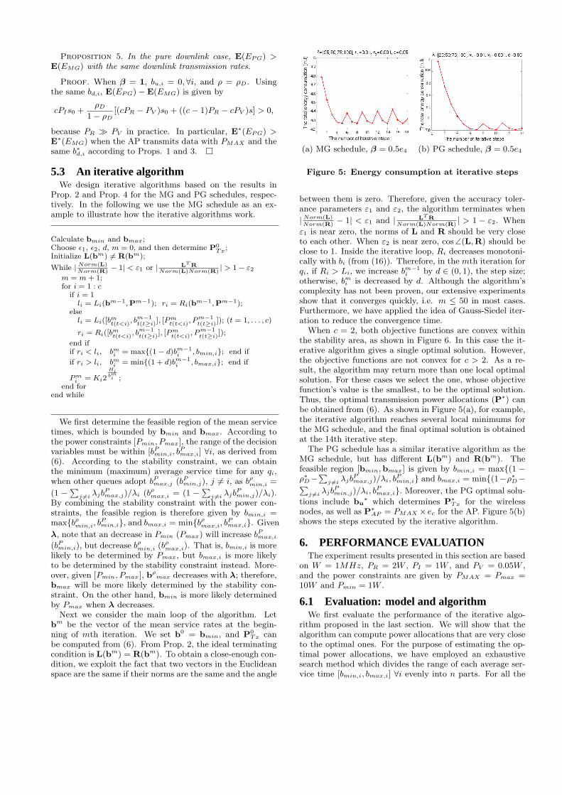
(a) MG schedule, β = 0.5e4 (b) PG schedule, β = 0.5e4

Figure 5: Energy consumption at iterative steps

between them is zero. Therefore, given the accuracy toler-ance parameters ε1 and ε2, the algorithm terminates when

| Norm(L)Norm(R)

− 1| < ε1 and | LT RNorm(L)Norm(R)

| > 1 − ε2. When

ε1 is near zero, the norms of L and R should be very closeto each other. When ε2 is near zero, cos ∠(L,R) should beclose to 1. Inside the iterative loop, Ri decreases monotoni-cally with bi (from (16)). Therefore, in the mth iteration forqi, if Ri > Li, we increase bm−1

i by d ∈ (0, 1), the step size;otherwise, bm

i is decreased by d. Although the algorithm’scomplexity has not been proven, our extensive experimentsshow that it converges quickly, i.e. m ≤ 50 in most cases.Furthermore, we have applied the idea of Gauss-Siedel iter-ation to reduce the convergence time.

When c = 2, both objective functions are convex withinthe stability area, as shown in Figure 6. In this case the it-erative algorithm gives a single optimal solution. However,the objective functions are not convex for c > 2. As a re-sult, the algorithm may return more than one local optimalsolution. For these cases we select the one, whose objectivefunction’s value is the smallest, to be the optimal solution.Thus, the optimal transmission power allocations (P∗) canbe obtained from (6). As shown in Figure 5(a), for example,the iterative algorithm reaches several local minimums forthe MG schedule, and the final optimal solution is obtainedat the 14th iterative step.

The PG schedule has a similar iterative algorithm as theMG schedule, but has different L(bm) and R(bm). Thefeasible region [bmin,bmax] is given by bmin,i = max{(1 −ρ∗D−

∑j 6=i λjb

Pmax,j)/λi, b

Pmin,i} and bmax,i = min{(1−ρ∗D−∑

j 6=i λjbPmin,j)/λi, b

Pmax,i}. Moreover, the PG optimal solu-

tions include bu∗ which determines P∗Tx for the wireless

nodes, as well as P∗AP = PMAX × ec for the AP. Figure 5(b)shows the steps executed by the iterative algorithm.

6. PERFORMANCE EVALUATIONThe experiment results presented in this section are based

on W = 1MHz, PR = 2W , PI = 1W , and PV = 0.05W ,and the power constraints are given by PMAX = Pmax =10W and Pmin = 1W .

6.1 Evaluation: model and algorithmWe first evaluate the performance of the iterative algo-

rithm proposed in the last section. We will show that thealgorithm can compute power allocations that are very closeto the optimal ones. For the purpose of estimating the op-timal power allocations, we have employed an exhaustivesearch method which divides the range of each average ser-vice time [bmin,i, bmax,i] ∀i evenly into n parts. For all the

possible nc vectors of average service times, we first selectthose that satisfy the stability requirement and then findthe one with the minimal energy consumption. Since themethod is very time consuming, we have carried it out onlyfor c = 1, . . . , 5.

We first consider a case of 2 queues in Table 3 for bothschedules. The results obtained from the iterative algorithmare marked by A (d = 0.05, ε1 = 0.01 and ε2 = 0.001).The results obtained from the exhaustive search method areindicated by N . We compare the optimal power P∗ obtainedfrom the two methods by computing an error rate eP =norm(P∗

A−P∗N)

norm(P∗N

)× 100%. The results show that the iterative

algorithm yields optimal solutions that are very close to, ifnot the same as, the exact ones obtained by the exhaustivesearch. Besides the optimal results, the table also shows thenumber of iterative steps required by the iterative algorithm,denoted as m and the locth iteration at which the optimalsolution is obtained. When loc = m, bu is determined byPmin or Pmax. When loc = m− 1, the iteration stops afterthe first local solution is found, i.e. the mth step leads toa higher energy consumption. Therefore, the single localsolution is the global optimal and both objective functionsare convex when c = 2.

The results for c = 3, 4, 5 are given in Table 4 and Table 5for the MG schedule and the PG schedule, respectively. Notethat β = k ∗ ec. For example, the case of k = 0.5 representsa 50-50 mix of the uplink and downlink traffic. Once againthe iterative algorithm yields quality solutions. Besides, ifλ is small, then the initial workload ρ(0) is very small. Thefinal optimal solution is determined by Pmin when the op-timal workload λT bmax is also small. For example, in the5-queue system with a light workload, the optimal trans-mission power allocation for the PG schedule is [1;1;1;1;1].

However, if the traffic rates are very high, ρ(0) is close to1. Then the wireless devices should send packets as fast aspossible, i.e. the packets are transmitted with the maximalpower allowed. For example, the optimal power allocationfor the MG schedule is Pmax when λ = [50; 100; 100; 150].

6.2 A comparison of the MG and PG schedulesFigure 6 presents the energy consumption obtained from

an exhaustive search method in 3 different workload sce-narios: light (Fig 6(a)), moderate (Fig 6(b)), and heavy(Fig 6(c)). For both schedules, E(E) is shown to be a con-vex function of the average service time when c = 2. Thevertical lines in these figures locate the optimal solutions.Moreover, when the traffic arrival rate is too low or too highin reference to the power limitations, the optimal servicerate could be determined by Pmin or Pmax, e.g. P∗ = [1; 1]in the PG schedule when λ = [30; 60] and β = 0.3× e2.

In most cases, E(EMG) < E(EPG) within the stabilityregion, except when λ is high enough. For example, in Fig-ure 6(c), E(EMG) > E(EPG) when the elements of bu areclose to the upper boundary. The reason is that the MGschedule approaches much closer to its stability boundarywhich leads to a very long cycle period. In this case, theMG schedule consumes much more energy due to the longcycle. Furthermore, we repeat the experiments with differ-

ent β by changing k from 0 to 0.9, and the values ofE∗

MGE∗

P G

are given in Figure 6(d). As shown, the optimal energy con-sumption for the MG schedule is always lower than the PG

schedule’s, i.e., E∗(EMG)E∗(EP G)

< 1. Therefore, the MG schedule is

(a)∑c

i=1 λi = 320, k = 0.5 (b) λi = 20 ∀i, k = 0.5

Figure 7: Minimal energy consumption v.s. c

(a) λ =[60;100], c = 2 (b) λ=[30;60;90 ], c = 3

Figure 8: Breakdown of energy consumption, k = 0.5

indeed more energy-efficient, especially when the proportionof the downlink traffic increases.

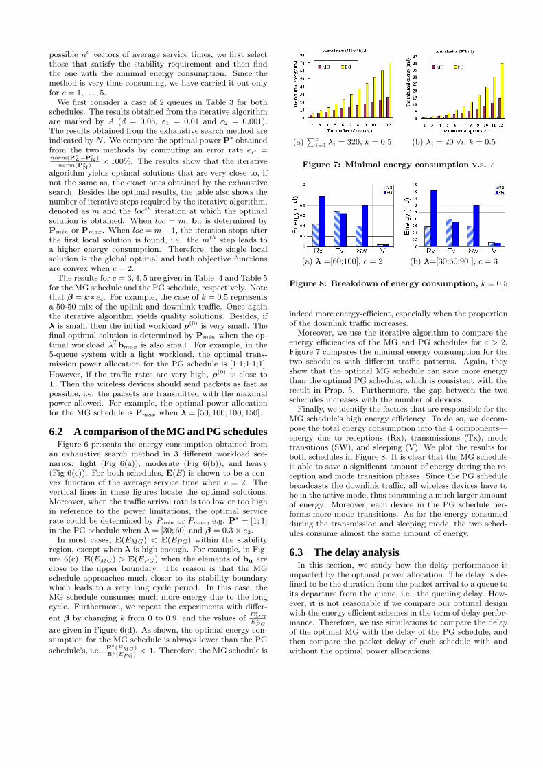
Moreover, we use the iterative algorithm to compare theenergy efficiencies of the MG and PG schedules for c > 2.Figure 7 compares the minimal energy consumption for thetwo schedules with different traffic patterns. Again, theyshow that the optimal MG schedule can save more energythan the optimal PG schedule, which is consistent with theresult in Prop. 5. Furthermore, the gap between the twoschedules increases with the number of devices.

Finally, we identify the factors that are responsible for theMG schedule’s high energy efficiency. To do so, we decom-pose the total energy consumption into the 4 components—energy due to receptions (Rx), transmissions (Tx), modetransitions (SW), and sleeping (V). We plot the results forboth schedules in Figure 8. It is clear that the MG scheduleis able to save a significant amount of energy during the re-ception and mode transition phases. Since the PG schedulebroadcasts the downlink traffic, all wireless devices have tobe in the active mode, thus consuming a much larger amountof energy. Moreover, each device in the PG schedule per-forms more mode transitions. As for the energy consumedduring the transmission and sleeping mode, the two sched-ules consume almost the same amount of energy.

6.3 The delay analysisIn this section, we study how the delay performance is

impacted by the optimal power allocation. The delay is de-fined to be the duration from the packet arrival to a queue toits departure from the queue, i.e., the queuing delay. How-ever, it is not reasonable if we compare our optimal designwith the energy efficient schemes in the term of delay perfor-mance. Therefore, we use simulations to compare the delayof the optimal MG with the delay of the PG schedule, andthen compare the packet delay of each schedule with andwithout the optimal power allocations.

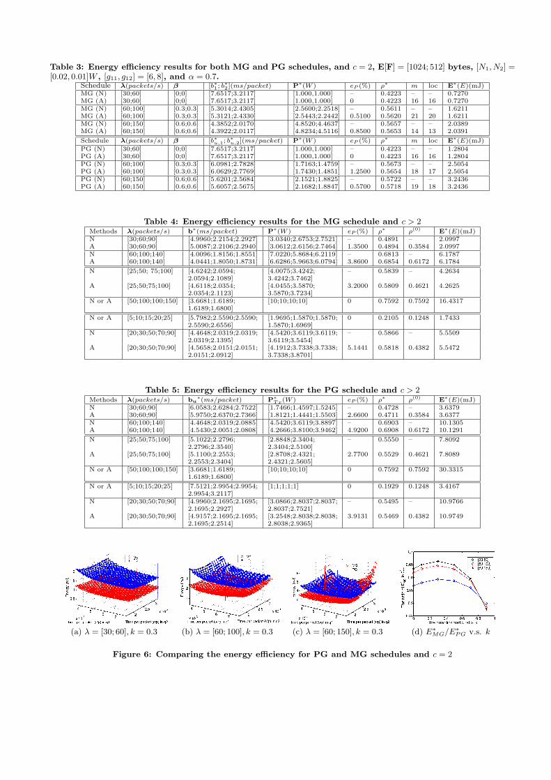
Table 3: Energy efficiency results for both MG and PG schedules, and c = 2, E[F] = [1024; 512] bytes, [N1, N2] =[0.02, 0.01]W , [g11, g12] = [6, 8], and α = 0.7.

Schedule λ(packets/s) β [b∗1 ; b∗2 ](ms/packet) P∗(W ) eP (%) ρ∗ m loc E∗(E)(mJ)MG (N) [30;60] [0;0] [7.6517;3.2117] [1.000,1.000] – 0.4223 – – 0.7270MG (A) [30;60] [0;0] [7.6517;3.2117] [1.000,1.000] 0 0.4223 16 16 0.7270MG (N) [60;100] [0.3;0.3] [5.3014;2.4305] [2.5600;2.2518] – 0.5611 – – 1.6211MG (A) [60;100] [0.3;0.3] [5.3121;2.4330] [2.5443;2.2442] 0.5100 0.5620 21 20 1.6211MG (N) [60;150] [0.6;0.6] [4.3852;2.0170] [4.8520;4.4637] – 0.5657 – – 2.0389MG (A) [60;150] [0.6;0.6] [4.3922;2.0117] [4.8234;4.5116] 0.8500 0.5653 14 13 2.0391

Schedule λ(packets/s) β [b∗u,1; b∗u,2](ms/packet) P∗(W ) eP (%) ρ∗ m loc E∗(E)(mJ)

PG (N) [30;60] [0;0] [7.6517;3.2117] [1.000,1.000] – 0.4223 – – 1.2804PG (A) [30;60] [0;0] [7.6517;3.2117] [1.000,1.000] 0 0.4223 16 16 1.2804PG (N) [60;100] [0.3;0.3] [6.0981;2.7828] [1.7163;1.4759] – 0.5673 – – 2.5054PG (A) [60;100] [0.3;0.3] [6.0629;2.7769] [1.7430;1.4851] 1.2500 0.5654 18 17 2.5054PG (N) [60;150] [0.6;0.6] [5.6201;2.5684] [2.1521;1.8825] – 0.5722 – – 3.2436PG (A) [60;150] [0.6;0.6] [5.6057;2.5675] [2.1682;1.8847] 0.5700 0.5718 19 18 3.2436

Table 4: Energy efficiency results for the MG schedule and c > 2Methods λ(packets/s) b∗(ms/packet) P∗(W ) eP (%) ρ∗ ρ(0) E∗(E)(mJ)N [30;60;90] [4.9960;2.2154;2.2927] [3.0340;2.6753;2.7521] – 0.4891 – 2.0997A [30;60;90] [5.0087;2.2106;2.2940] [3.0612;2.6156;2.7464] 1.3500 0.4894 0.3584 2.0997N [60;100;140] [4.0096;1.8156;1.8551] [7.0220;5.8684;6.2119] – 0.6813 – 6.1787A [60;100;140] [4.0441;1.8050;1.8731] [6.6286;5.9663;6.0794] 3.8600 0.6854 0.6172 6.1784

N [25;50; 75;100] [4.6242;2.0594; [4.0075;3.4242; – 0.5839 – 4.26342.0594;2.1089] 3.4242;3.7462]

A [25;50;75;100] [4.6118;2.0354; [4.0455;3.5870; 3.2000 0.5809 0.4621 4.26252.0354;2.1123] 3.5870;3.7234]

N or A [50;100;100;150] [3.6681;1.6189; [10;10;10;10] 0 0.7592 0.7592 16.43171.6189;1.6800]

N or A [5;10;15;20;25] [5.7982;2.5590;2.5590; [1.9695;1.5870;1.5870; 0 0.2105 0.1248 1.74332.5590;2.6556] 1.5870;1.6969]

N [20;30;50;70;90] [4.4648;2.0319;2.0319; [4.5420;3.6119;3.6119; – 0.5866 – 5.55092.0319;2.1395] 3.6119;3.5454]

A [20;30;50;70;90] [4.5658;2.0151;2.0151; [4.1912;3.7338;3.7338; 5.1441 0.5818 0.4382 5.54722.0151;2.0912] 3.7338;3.8701]

Table 5: Energy efficiency results for the PG schedule and c > 2Methods λ(packets/s) bu

∗(ms/packet) P∗T x(W ) eP (%) ρ∗ ρ(0) E∗(E)(mJ)

N [30;60;90] [6.0583;2.6284;2.7522] [1.7466;1.4597;1.5245] – 0.4728 – 3.6379A [30;60;90] [5.9750;2.6370;2.7366] [1.8121;1.4441;1.5503] 2.6600 0.4711 0.3584 3.6377N [60;100;140] [4.4648;2.0319;2.0885] [4.5420;3.6119;3.8897] – 0.6903 – 10.1305A [60;100;140] [4.5430;2.0051;2.0808] [4.2666;3.8100;3.9462] 4.9200 0.6908 0.6172 10.1291

N [25;50;75;100] [5.1022;2.2796; [2.8848;2.3404; – 0.5550 – 7.80922.2796;2.3540] 2.3404;2.5100]

A [25;50;75;100] [5.1100;2.2553; [2.8708;2.4321; 2.7700 0.5529 0.4621 7.80892.2553;2.3404] 2.4321;2.5605]

N or A [50;100;100;150] [3.6681;1.6189; [10;10;10;10] 0 0.7592 0.7592 30.33151.6189;1.6800]

N or A [5;10;15;20;25] [7.5121;2.9954;2.9954; [1;1;1;1;1] 0 0.1929 0.1248 3.41672.9954;3.2117]

N [20;30;50;70;90] [4.9960;2.1695;2.1695; [3.0866;2.8037;2.8037; – 0.5495 – 10.97662.1695;2.2927] 2.8037;2.7521]

A [20;30;50;70;90] [4.9157;2.1695;2.1695; [3.2548;2.8038;2.8038; 3.9131 0.5469 0.4382 10.97492.1695;2.2514] 2.8038;2.9365]

(a) λ = [30; 60], k = 0.3 (b) λ = [60; 100], k = 0.3 (c) λ = [60; 150], k = 0.3 (d) E∗MG/E∗

PG v.s. k

Figure 6: Comparing the energy efficiency for PG and MG schedules and c = 2

(a)c∑

i=1

λi = 320, k = 0.5 (b) λi = 20, k = 0.5

Figure 9: Delay comparison under optimal schedules

6.3.1 Average delay under optimal power allocationsThe simulation yields the average packet delay under dif-

ferent optimal power allocations. Denote the average delayof the downlink packets by TD and that for the uplink pack-ets by TU, and the total energy consumed per the pollingcycle by E. For c = 4, the average delay of the downlinkpackets and uplink packets under the optimal power alloca-tion are shown in Table 6, where σT =

∑ci=1(Ti − T )2/c is

the delay variance, and T =∑c

i=1 Ti. Three traffic work-loads of λ = [10; 15; 20; 25] × x, x = 1, 3, 5, and β = 0.5e4

are considered and the packet size is 512 bytes. Clearly, theoptimal MG schedule consumes less average energy per cy-cle than the corresponding optimal PG schedule. The smallσT values show that the four queues with different arrivalrates have similar delay. In other words, the optimal powerallocations do not adversely affect the delay fairness. For alloptimal PG schedules, the average delay of uplink packetsare longer than that for the downlink packets. Additionally,their downlink delay increases with x.

In order to simplify the delay analysis, we simulate the op-timal power allocation in a symmetric network with λ = kec

and β = 0.5ec, c = 2, . . . , 12, and the results are shownin Figure 9. The average delay for the downlink is TD =∑c

i TD,i/c and the average delay time for the uplink is TU =∑ci TU,i/c. TD is close to TU in all optimal MG schedules,

while TD is less than TU in all optimal PG schedules. Inmost cases, the optimal PG schedules have lower delay forthe downlink packets than the optimal MG schedules, whilethe optimal MG schedules have the lower delay for the up-link packets than the optimal PG schedules. Therefore, theoptimal PG schedule may provide the better delay perfor-mance when β increases, and the optimal MG schedule mayprovide the better delay performance when β decreases.

6.3.2 Energy efficiency v.s. delayWe investigate the relationship between the energy effi-

ciency and the delay performance. We still consider thesymmetric system with λ = 20ec and β = 0.5ec with theMG and PG schedules. Without the optimal power alloca-tion, we use a random power allocation which selects a powerallocation randomly from the feasible region [bmin,bmax].For these nonoptimal power allocations, we define 2 quan-tities in reference to the energy and delay obtained for theoptimal power allocation. Define the energy inflation ratio

(re) of a random allocation by E−E∗

E∗ , where E∗ and E arethe energy consumption obtained from the optimal powerallocation and the random power allocation, respectively.Similarly, we define the delay inflation ratio (rd) of a ran-

dom allocation byTD−T∗

D

T∗D

andTU−T∗

U

T∗U

for the downlink and

uplink traffic, respectively.Figure 10 depicts the results for 60 random allocations

with c = 4. Both the optimal MG and PG schedules defi-nitely achieve the minimal energy consumption, because allthe energy inflation ratios are positive, i.e. re ≥ 0. How-ever, neither the optimal MG schedule nor the optimal PGschedule can achieve the best delay performance, becausesome of the delay inflation ratios are negative.

We divide each figure in Figure 10 into 4 regions: Z1

(rd > re), Z2 (0 < rd < re), Z3 (−re < rd < 0), and Z4

(rd < −re). The random allocations in Z1 and Z2 havethe longer delay than the optimal allocation, i.e. rd > 0.Therefore, the optimal allocation outperforms the randomallocations in these 2 regions on both energy efficiency anddelay performance. On the other hand, the random alloca-tions in Z3 and Z4 have better delay performance than theoptimal allocation. However, trading the delay for energyefficiency may still be justified in Z3, because the energy in-flation ratio is always higher than the delay inflation ratioin this region, i.e. |rd| < re. Figure 10 shows that most ofthe random allocations fall into Z1 and Z2 (at least 94%).Only a small percentage (at most 6%) of the random alloca-tions belong to Z4. As a result, we can conclude that bothschedules can achieve optimal power allocation without theexpense of a higher average delay most of the time.

(a) PG’s downlink case (b) MG’s downlink case

(c) PG’s uplink case (d) MG’s uplink case

Figure 10: Energy inflation ratio and delay inflationratio for a random power allocation, c = 4.

7. CONCLUSIONS AND FUTURE WORKIn this paper we have considered the problem of optimiz-

ing energy efficiency for all wireless devices in a polling-based wireless network. We have employed both the powersaving mode (PSM) and the transmission power control (TPC)to conserve energy. Since the decrease in one’s transmissionpower could adversely affect other devices, we have formu-lated an optimization problem to minimize the energy con-

Table 6: The average delay obtained from simulation for λ = [10; 15; 20; 25]× x and β = 0.5e4

Scheduling x E(mJ) TU(ms) σT U TD(ms) σT D

MG 1 1.3564 [4.0246;3.8502;4.1127;4.1467] 0.0132 [3.6882;4.1600;4.0260;4.1960] 0.0402MG 3 3.5190 [4.7928;4.4650;4.9875;4.6139] 0.0383 [4.5765;5.0436;4.4353;4.7767] 0.0523MG 5 9.2480 [5.0329;4.3240;4.8556;5.2596] 0.1192 [4.3194;4.7842;4.7272;4.9750] 0.0571PG 1 2.6617 [5.3914;5.1583;4.9916;4.9916] 0.0265 [2.8538;2.8861;2.7985;3.3033] 0.0402PG 3 6.6091 [5.3249;5.0583;5.6859;5.0535] 0.0668 [3.8474;4.1120;3.9285;4.1517] 0.0163PG 5 15.4546 [5.0577;5.8118;6.4648;5.6484] 0.2511 [4.8643;5.2513;5.0549;4.7520] 0.0361

sumed during a polling cycle and, at the same time, ensurethat all devices are stable, i.e., their queue lengths wouldnot go unbounded. The resulted stability-constrained op-timization formulation enables us to compute the optimalpower allocations for 2 polling schedules—phase groupingand mobile grouping. The experiment results have shownthat the mobile grouping schedule is much more energy ef-ficient, because it decreases the number of mode transitionsand allows a device to sleep for a longer time. Using simu-lation, we have also investigated the impact of the optimalpower allocations on the queueing delay. The results showthat the optimal power allocation does not degrade the de-lay for over 90% of the time. Even when the average delaybecomes longer, the tradeoff is still considered beneficial asa whole.

AcknowledgmentThe work described in this paper was partially supported bya grant from the Research Grant Council of the Hong KongSpecial Administrative Region, China (Project No. PolyU5146/01E).

8. REFERENCES[1] J. Chen, K. Sivalingam, and P. Agrawal, “Performance

comparison of battery power consumption in wirelessmultiple access protocols,” ACM/Baltzer WirelessNetworks, vol. 5, no. 6, pp. 445–460, 1999.

[2] D. Ciao, S. Choi, A. Soomro, and K. Shin,“Energy-efficient PCF operation of IEEE 802.11awireless LAN,” in Proc. IEEE INFOCOM, 2002.

[3] S. Singh and C. Raghavendra, “PAMAS power awaremulti-access protocol with signalling for ad hocnetworks,” ACM Computer Communication Review,vol. 28, no. 3, pp. 5–26, 1998.

[4] A. Tarello, J. Sun, M. Zafer, and E. Modiano,“Minimum energy transmission scheduling subject todeadline constraints,” in Proc. IEEE WIOPT, 2005.

[5] F. Zhang and S. Chanson, “Throughput and valuemaximization in wireless packet scheduling underenergy and time constraints,” in Proc. IEEE RTSS,2003.

[6] T. Holliday, A. Goldsmith, and P. Glynn, “Optimalpower control and source-channel coding for delayconstrained traffic over wireless channels,” in Proc.IEEE ICC 2002.

[7] P. Nuggehalli, V. Srinivasan, and R. Rao, “Delayconstrained energy efficient transmission strategies forwireless devices,” in Proc. IEEE INFOCOM, 2002.

[8] C. Schurgers, V. Raghunathan, and M. Srivastava,“Modulation scaling for real-time energy aware packetscheduling,” in Proc. Global CommunicationsConference, 2001, pp. 3653–3657.

[9] M. Chiang and J. Bell, “Balancing supply anddemand of bandwidth in wireless cellular networks:Utility maximization over powers and rates,” in Proc.IEEE INFOCOM, 2004.

[10] J. Chen, K. Sivalingam, P. Agrawal, and R. Acharya,“Scheduling multimedia services in a low-power MACfor wireless and mobile ATM networks,” IEEE Trans.multimedia, vol. 1, no. 2, 1999.

[11] J. Havinga and J. Smit, “Energy-efficient wirelessnetworking for multimedia applications,” WirelessCommunications and Mobile Computing, vol. 1, 2001.

[12] R. Haines and A. Aghvami, “Indoor radioenvironment considerations in selecting a media accesscontrol protocol for wideband radio datacommunications,” in Proc. IEEE ICC, 1994.

[13] P. Havinga and G. Smit, “E2MaC: an energy efficientMAC protocol for multimedia traffic,” University ofTwente, Tech. Rep., 1998.

[14] P. Havinga, G. Smit, and M. Bos, “Energy efficientadaptive wireless network design,” in Proc. IEEEISCC, 2000.

[15] E. Biyikoglu, B. Prabhakar, and A. Gamal,“Energy-efficient packet transmission over a wirelesslink,” IEEE/ACM Trans. Networking, vol. 10, no. 4,2002.

[16] A. Gamal, C. Nair, B. Prabhakar, E. Biyikoglu, andS. Zahedi, “Energy-efficient scheduling of packettransmissions over wireless networks,” in Proc. IEEEINFOCOM, 2002.

[17] D. Qiao, S. Choi, A. Jain, and K. Shin, “MiSer: Anoptimal low-energy transmission strategy for IEEE802.11a/h,” in Proc. MobiCom 03, 2003.

[18] S. Jayashree, B. Manoj, , and C. Murthy, “Next stepin MAC evolution: Battery awareness?” in Proc.IEEE Globecom, 2004.

[19] M. Ferguson and Y. Aminetzah, “Exact results fornonsymmetric token ring systems,” IEEE Trans.Communications, vol. 33, no. 3, pp. 223–231, March1985.

[20] W. Szpankowski, “Stability conditions for somemultiqueue distributed systems: buffered randomaccess systems,” Adv. Appl. Probab., vol. 26, 1994.

[21] H. Takagi, “Queueing analysis of polling models: anupdate,” Stochastic Analysis of Computer andCommunication Systems, pp. 267–318, 1990.

[22] L. Foulds, Optimization Techniques. Springer-VerlagNew York Inc., 1981.

[23] G. Koole and P. Nain, “An explicit solution for thevalue function of a priority queue,” Queueing Systems,vol. 47, pp. 251–285, 2004.