Journal of Economic Behavior & OrganizationVol. 49 (2002) 173–197

Speculative behaviour and complex asset pricedynamics: a global analysis

Carl Chiarellaa,∗, Roberto Diecib, Laura Gardinica School of Finance and Economics, University of Technology, P.O. Box 123, Sydney, NSW 2007, Australia

b Facoltà di Economia, Università degli Studi di Parma, Parma, Italyc Facoltà di Economia, Università degli Studi di Urbino, Urbino, Italy

Received 9 April 2001; received in revised form 16 July 2001; accepted 19 July 2001

Abstract

This paper analyses the dynamics of a model of a share market consisting of two groups of traders:fundamentalists, who base their trading decisions on the expectation of a return to the fundamentalvalue of the asset, and chartists, who base their trading decisions on an analysis of past price trends.The model is reduced to a two-dimensional map whose global dynamic behaviour is analysed indetail. The dynamics are affected by parameters measuring the strength of fundamentalist demandand the speed with which chartists adjust their estimate of the trend to past price changes. Theparameter space is characterized according to the local stability/instability of the equilibrium pointas well as the non-invertibility of the map. The method of critical curves of non-invertible maps isused to understand and describe the range of global bifurcations that can occur. It is also shown howthe knowledge of deterministic dynamics uncovered here can aid in understanding the behaviourof stochastic versions of the model. © 2002 Elsevier Science B.V. All rights reserved.

JEL classification:C61; D84; G12

Keywords:Heterogeneous agents; Complex dynamics; Global dynamics; Non-invertible maps; Volatilityclustering; Speculation

1. Introduction

In recent years several models of financial markets based on interacting heterogeneousagents have been developed, see for example Day and Huang (1990), Brock and Hommes(1998), Lux (1998), Chen and Yeh (1997) and Chiarella and He (in press). Most of these

∗ Corresponding author. Tel.:+61-2-9514-7719; fax:+61-2-9514-7711.E-mail addresses:carl.chiarella@uts.edu.au (C. Chiarella), roberto.dieci@unipr.it (R. Dieci),gardini@econ.uniurb.it (L. Gardini).

0167-2681/02/$ – see front matter © 2002 Elsevier Science B.V. All rights reserved.PII: S0167-2681(02)00066-5

174 C. Chiarella et al. / J. of Economic Behavior & Org. 49 (2002) 173–197

models, some of which allow the size of the different groups of agents to vary according tothe evolution of the financial market, are of necessity not very mathematically tractable. Inthe present paper, in order to complement the aforementioned studies, we develop a discretetime model of asset price dynamics containing the essential elements of the heterogeneousinteracting agents paradigm whilst still remaining mathematically tractable. We assume thatthe share market consists of two types of traders:fundamentalists, who base their tradingdecisions on an estimate of the fundamental value of the asset, andchartists, a group whichbases its decisions on an analysis of past price trends. The chartists’ demand is an S-shapedfunction of the difference between the chartists’ estimate of the price trend (obtained throughan adaptive expectations scheme on past price changes) and the return on some alternativeasset. The model reduces to a two-dimensional non-linear map, whose dynamic behaviourwe analyse by first determining, in the space of the parameters, the local stability regionof the unique equilibrium point of the map, together with the regions of invertibility ornon-invertibility. It turns out that in the stability region, besides the local properties, globalones are also important in detecting other dynamic phenomena such as coexistence ofattractors, or chaotic transients before the convergence to the stable equilibrium. We indicatethe bifurcations that the fixed point undergoes when the key parameters, such as thestrengthof fundamentalists’ demand and thespeedwith which chartists adjust their estimate of thetrend to past price changes, are increased. We also analyze the regions in the parameterspace in which the equilibrium point is unstable and the map is non-invertible. We shallfocus on particular regimes characterized by chaotic behaviour, showing how the globalbifurcation known assnap-back repellor(leading to chaotic dynamics) can be detected byuse of thecritical curvesof the map (as proved in Gardini (1994)). Moreover, by makinguse of the properties of the critical curves of non-invertible maps (described in Chapter 4 ofMira et al. (1996), and used in several economic models by Puu (2000)), we show how upperand lower bounds for the asymptotic behaviour of the state variables (price and chartists’expectations) can be determined, although we are in the presence of chaotic dynamics.Simulations of a stochastic version of the model suggest that volatility behaviour of assetreturns is related to these bounds.

The paper is organized as follows. Section 2 derives the model of fundamentalists andchartists. Section 3 points out some general properties of the two-dimensional map drivingthe dynamics. Sections 4 discusses the bifurcations that can occur and Section 5 showshow the properties of the critical curves can help to understand the nature of the attrac-tors, their homoclinic bifurcations and other global bifurcations. Finally, an extension ofthe model beyond its deterministic structure is suggested in Section 6, showing how theknowledge of deterministic dynamics can help in understanding the volatility patterns ofsimple stochastic versions of the model. Section 7 concludes and makes some suggestionsfor future research.

2. The model

We adopt the basic fundamentalist/chartist model of Chiarella (1992), whose antecedentsare Day and Huang (1990), Beja and Goldman (1980), and Zeeman (1974). We denote byPt the logarithm of the asset price at timet and use the subscripti ∈ f, c to denote

C. Chiarella et al. / J. of Economic Behavior & Org. 49 (2002) 173–197 175

fundamentalists or chartists. In each time period each group of agents is assumed to investsome of its wealth in a risky asset and some in an alternative safe asset. LetΩi,t be thewealth of agenti andZi,t be the fraction of this wealth that agenti decides to invest in therisky asset, at timet . The agent’s wealth at time(t + 1) will then be given by

Ωi,t+1 = Ωi,t +Ωi,t (1 − Zi,t )gt +Ωi,tZi,t (Pt+1 − Pt),wheregt is the return on the alternative safe asset (e.g. bonds) and(Pt+1 −Pt) is the returnon the risky asset. Agenti computes the conditional mean and variance ofΩi,t+1 (denotedbyEi,t (Ωi,t+1) andVi,t (Ωi,t+1), respectively) assuming that(Pt+1 − Pt) is conditionallynormal, so that

Ei,t (Ωi,t+1) = Ωi,t +Ωi,t (1 − Zi,t )gt +Ωi,tZi,tEi,t (Pt+1 − Pt), (1)

Vi,t (Ωi,t+1) = Z2i,tΩ

2i,tVi,t (Pt+1 − Pt). (2)

Assuming that each group of agents has an exponential utility of wealth function, eachagent seeksZi,t so as to maximise

Ei,t [−exp(−αiΩi,t+1)], (3)

whereαi is agenti’s risk aversion coefficient. Under the assumption thatΩi,t+1 is condi-tionally normally distributed, this problem is equivalent to

maxZi,t

Ei,t (Ωi,t+1)− 1

2αiVi,t (Ωi,t+1)

.

The solution to this optimization problem is

ζi,t ≡ Zi,tΩi,t = Ei,t (Pt+1 − Pt)− gtαiVi,t (Pt+1 − Pt) ,

whereζi,t is the demand by agenti for the risky asset. The two groups of agents essentiallydiffer in the way they calculate the mean and variance of the price change over successivetime intervals.

The fundamentalists are assumed to have a reasonable estimate of the fundamental valueof the risky asset. This estimate has been obtained at some cost, such as large setup costs(e.g. a major financial institution), and the employment of highly paid professionals, suchas market analysts, economists, computer analysts, etc. Fundamentalists believe that theasset price follows a mean reversion process with the fundamental value being the long runmean. Hence they calculate that the expected excess return is proportional to the differencebetween the current log asset price and the log fundamental value, i.e.

Ef ,t (Pt+1 − Pt)− gt = η(Wt − Pt),whereη is the speed of mean reversion estimated by the fundamentalists andWt is the logof fundamental value at timet . They also assume that the conditional variance of pricechanges is constant, i.e.

Vf ,t (Pt+1 − Pt) = vf .

176 C. Chiarella et al. / J. of Economic Behavior & Org. 49 (2002) 173–197

Fundamentalist demand, in terms of returns, is thus given by

Dft = a(Wt − Pt), (4)

wherea (= η/αf vf > 0) is the strength of fundamentalist demand. If the log share pricePtis below (above) the log expected fundamental valueWt , then fundamentalists try to buy(sell) the share, because they think that the share is undervalued (overvalued) and thereforeits price will increase (decrease).

Chartists are assumed to be unable to bear the cost structure necessary to acquire the in-formation about the fundamental value available to fundamentalists. Rather they base theirestimate of the mean and variance of expected return on the risky asset on the costless infor-mation contained in recent return (log price) changes.1 Useψt,t+1 to denote the chartists’expectation at timet of the log price change (i.e. return) over the next trading period, i.e.

ψt,t+1 = Et(Pt+1 − Pt) = Et(Pt+1)− Pt .Then chartists are assumed to calculateEc,t (Pt+1 − Pt) by extrapolating past price

changes according to the simple adaptive scheme

ψt,t+1 = ψt−1,t + c(Pt − Pt−1 − ψt−1,t ), (5)

wherec (0 < c ≤ 1) is the speed with which they adjust their estimate of the trend to themost recent price changes. Alternatively the quantityτ = 1/c may be viewed as the timelag in chartists’ information.2

Thus, chartist asset demand is given by

ζc,t = ψt,t+1 − gtαcvc

.

Unlike the fundamentalists, the chartists change their estimatevc of the conditionalvariance according to the magnitude of|ψt,t+1 − gt |. As this quantity becomes larger theyexpect greater volatility and increase their estimatevc, hence lowering the slope of theirdemand function. This behaviour leads to the levelling off of the slope of chartist demandas |ψt,t+1 − gt | becomes larger. The chartist asset demand may thus be characterised ingeneral by

Dct = h(ψt,t+1 − gt ), (6)

where the functionh(·) has the properties: (i)h′(x) > 0 (∀x), (ii) h(0) = 0, (iii) there existsanx∗ such thath′′(x) < 0 (> 0) for all x > x∗ (< x∗) and, (iv) limx→∓∞h′(x) = 0. In ourexamples and simulations we takeh(x) = γ arctanx. However, it is important to remarkthat the qualitative analysis performed in the following sections (as also the qualitativedynamics) are not affected by a change of function, because these mainly depend on theproperties ofh(·) given above.

1 Alternatively we could conceive of chartists as a group having greater faith in the statistical analysis of recentprice trends than in attempts to estimate fundamental value.

2 The restrictionc ≤ 1, i.e. τ ≥ 1, has the simple economic interpretation that chartists cannot revise theirestimate ofψt,t+1 more frequently than they receive information about price changes. Here this frequency is onetime unit.

C. Chiarella et al. / J. of Economic Behavior & Org. 49 (2002) 173–197 177

Thus, total excess demand for the asset at timet (assuminggt = g andWt = W are bothconstant) is given by

Dt = a(W − Pt)+ h(ψt,t+1 − g). (7)

Let us now turn to the adjustment process of the share price in the market. FollowingDay and Huang, we assume the existence of amarket makerwhose function is to set excessdemand to zero at the end of each trading day. If the excess demand in periodt is positive(negative), the market maker sells (buys) the quantity of the asset needed to clear the market,and raises (reduces) the share price for the next periodt + 1. Precisely, what goes on ineach trading day can be described as follows: (i) at the beginning of dayt the market makerannounces the (log) pricePt for that day; (ii) the market participants then form excessdemandDt according to (7); (iii) the market maker, observing the excess demand, takesa long or short positionMt (by adjusting his or her inventory of assets) in order to clearthe market, i.e. such thatDt + Mt = 0; (iv) the market maker then announces, at thebeginning of the next trading period, the new (log) pricePt+1 calculated as the previous(log) price plus some fraction of the excess demand of the previous period, according toPt+1 = Pt + βpDt (βp > 0). The process then repeats itself.3

Thus, at the beginning of day(t + 1) the following dynamic adjustments occur, made bythe market maker and chartists, respectively:

Pt+1 = Pt + βp[a(W − Pt)+ h(ψt,t+1 − g)],ψt+1,t+2 = (1 − c)ψt,t+1 + cβp[a(W − Pt)+ h(ψt,t+1 − g)]. (8)

The focus of our analysis will be to undertake a global analysis of the map (8), showinghow, in the regions of the parameters space where the equilibrium point is unstable, adifferent attractor may exist having “good” properties from a practical point of view. That is,even if the fixed point of the economy is unstable, we can predict its “fate” in a macroscopicway giving, for example, the width of the oscillations that the state variables such asPt canundergo.

3. General properties of the map

In this section we investigate the nature of the map driving the dynamics of the model aswell as its regions of stability and invertibility/non-invertibility.

3.1. The map

From the previous section, the time evolution of price and chartists’ expectations isobtained by the iteration of the two-dimensional non-linear mapQ: (ψ, P )→ (ψ ′, P ′)

Q :

ψ ′ = (1 − c)ψ + cβp[a(W − P)+ h(ψ − g)]P ′ = P + βp[a(W − P)+ h(ψ − g)], (9)

3 In order to remain mathematically tractable our model does not take into account the possible large positive ornegative inventory positions of the market maker. Day and Huang suggest how these could be taken into accountin the way the market maker adjusts the new price. We leave the analysis of such effects to future research.

178 C. Chiarella et al. / J. of Economic Behavior & Org. 49 (2002) 173–197

where the symbol′ denotes the unit time advancement operator. The mapQ has the point(ψ, P ) = (0,W + 1/ah(−g)) as unique fixed point, so that in equilibrium fundamentalistdemand is−h(−g) (> 0) and chartist demand ish(−g)(< 0), i.e. in equilibrium fundamen-talists are net buyers (since the price is below their estimated long run mean) and chartistsare net sellers. Of course, this situation cannot be considered a true equilibrium situation,it is a result of the fact that our dynamic model is in fact a partial one in that it leaves in thebackground the market for the alternative asset. A general analysis would need to take intoaccount the dynamics of the alternative asset. Then(ψ − g) would be replaced by a singlequantity,ϕ say, which would be the chartists expectation of the difference in price changeof both asset prices. We would then be dealing with a three-dimensional dynamical system,at whose steady state it turns out thatϕ = 0 andP = W . Our analysis should thus be seenas that of a two-dimensional projection of this (more difficult to analyse) three-dimensionalsystem. For more details of the full three-dimensional system and some preliminary analysisof its dynamics we refer the reader to Chiarella et al. (2001a).

By introducing the log price deviationp = P −P we obtain the new mapT : (ψ, p)→(ψ ′, p′) given by:

T :

ψ ′ = (1 − c)ψ − cβp[ap− k(ψ)]p′ = p − βp[ap− k(ψ)], (10)

wherek(ψ) = h(ψ − g)− h(−g), and having the origin O= (0,0) as unique fixed point.

3.2. Local stability conditions

The local stability of the fixed point O depends on the Jacobian matrix of the map4 T ,

DT(ψ, p) =

1 − c + cβp

γ

1 + (ψ − g)2 −acβp

βpγ

1 + (ψ − g)2 1 − aβp

,

at (0,0). Denote by Tr and Det the trace and the determinant of DT(0,0), respectively,and byP(z) = z2 − Tr z + Det, the associated characteristic polynomial. A well knownnecessary and sufficient condition to have all the eigenvalues ofP(z) less than 1 in absolutevalue (and thus a locally attracting fixed point) consists of the inequalities:5

P(1) = 1−Tr + Det> 0, P(−1) = 1 + Tr + Det> 0, P(0) = Det< 1. (11)

For our map the conditions (11) can be rewritten as:aβp(2 − c) < 2(2 − c)+ 2cβpk

′(0),aβp(1 − c) > c[βpk

′(0)− 1].(12)

Fig. 1 represents the region of local stability of the origin in the parameter plane(c, a),0 < c ≤ 1, a > 0. From (12) it follows that, starting from parameters(c, a) inside the

4 Note that for the assumed functional form ofh, k′(ψ) = γ /[1 + (ψ − g)2].5 See, for instance, Gumowski and Mira (1980, p. 159).

C. Chiarella et al. / J. of Economic Behavior & Org. 49 (2002) 173–197 179

Fig. 1. The dark grey regions show the domain of stability of the equilibrium point O. The light grey regionsrepresent the domain of non-invertibility of the mapT . In (a),βpk

′(0) ≤ 1 and in (b),βpk′(0) > 1.

stability region, a loss of stability may occur either via a flip bifurcation, when crossing thecurve

a = 2

βp+ 2ck′(0)

2 − c (Flip-curve), (13)

or via a Neimark–Hopf bifurcation, when crossing the curve

a = c[βpk′(0)− 1]

βp(1 − c) (Hopf-curve). (14)

By assumingβp > 0 as fixed, we notice that the shape of the stability region in theparameter plane(c, a), indicated in dark grey in Fig. 1, is greatly affected by the strengthof chartists’ demand at the steady state (k′(0)).6 In particular, whenβpk

′(0) ≤ 1 (Fig. 1a)the region appears wider than in the opposite case (Fig. 1b). Fig. 1a shows that, whenstrength of chartist demand is relatively weak (k′(0) < 1/βp), at a given level of chartistsreaction speed (c) the equilibrium is stable for sufficiently low values of the fundamentalistsreaction parametera, but fundamentalists can cause instability by reacting too strongly to thedeviation from the fundamental value. Fig. 1, shows that when strength of chartist demandis relatively strong (k′(0) > 1/βp), the ability of fundamentalists’ demand to stabilise thesystem is restricted to a fairly narrow range of the parametera.

3.3. Invertibility of the map

For particular values of the parameters, the mapT is a non-invertible map of the plane.This means that, while starting from some initial values (say(ψ0,1, p0)) the forward iteration

6 We recall that for the particular chartist demand function that we have chosen, we havek′(0) = γ /(1 + g2).

180 C. Chiarella et al. / J. of Economic Behavior & Org. 49 (2002) 173–197

of (10) uniquely defines the trajectory(ψt,t+1, pt ) = T t (ψ0,1, p0) (t = 1,2, . . . ), thebackward iteration of (10) is not uniquely defined. In fact, a point(ψ, p) of the plane mayhave several rank-1 preimages.7

Let us assumeh(·) = γ arctan(·),γ > 0, so thatk(ψ) = γ arctan(ψ−g)−γ arctan(−g).It can be shown by elementary geometrical arguments that, by defining

m = (aβp − 1)(1 − c)c

, (15)

the map has a unique inverse form ≤ 0 orm ≥ γβp, while for 0< m < γβp the map isnon-invertible. In particular, by defining

ψ1 = g −√γβp

m− 1, q1 = βpk(ψ1)−mψ1, (16)

ψ2 = g +√γβp

m− 1, q2 = βpk(ψ2)−mψ2, (17)

the points(ψ, p) of the phase plane for which the function

q(ψ, p) = aβpp − aβp − 1

cψ, (18)

satisfiesq(ψ, p) < q1 or q(ψ, p) > q2 have a unique rank-1 preimage, while the pointsfor which: q1 < q(ψ, p) < q2 have three distinct rank-1 preimages. Thus, following thenotation used in Mira et al., for 0< m < γβp this map is of the typeZ1 − Z3 − Z1,which means that the phase plane is subdivided into different regionsZj (j = 1,3), eachpoint of which hasj distinct rank-1 preimages. Such regions are bounded by the so-calledcritical curvesof rank-1, defined as the locus of points having at least twomergingrank-1preimages (see Gumowski and Mira). For our map this set is defined as

LC = (ψ, p) ∈ R2 : q(ψ, p) = q1 ∪ q(ψ, p) = q2, (19)

whereq1 andq2 are given in (16) and (17), respectively, and it is therefore made up of twostraight lines, say LC= L ∪ L′, whereL andL′ have the equations

L : p = aβp − 1

aβpcψ + q1

aβp; L′ : p = aβp − 1

aβpcψ + q2

aβp. (20)

Each of thecritical points(ψ, p) ∈ LC has twomergingrank-1 preimages, and the locusof such preimages, denoted by LC−1 (this defines thecritical curveof rank-0), turns out tobe made up of two straight lines, say LC−1 = L−1 ∪ L′

−1, whose equations are

L−1 : ψ = g −√γβp

m− 1; L′

−1 : ψ = g +√γβp

m− 1. (21)

The critical curve LC−1corresponds here to the locus of points(ψ, p) of the phase planein which the determinant of the Jacobian matrixDT(ψ, p) vanishes.8 Also the images of the

7 Given an-dimensional mapF : Rn → Rn and a positive integerr we say that the pointy is a rank-r preimageof the pointx if F r(y) = x, i.e. if y is mapped intox in r iterations.

8 Generally speaking, for a differentiable map the critical curve LC−1 is a subset of the locus of points of thephase plane for which the determinant of the Jacobian matrix of the map vanishes.

C. Chiarella et al. / J. of Economic Behavior & Org. 49 (2002) 173–197 181

set LC are calledcritical curvesof higher rank, in particular LCk = T k(LC) = T k+1(LC−1)

(for k = 0,1,2, . . . ) are calledcritical curves of rank−(k+1) (LC0 = LC). In our examplethese always have two branches so that LCk = Lk ∪ L′

k = T k+1(L−1) ∪ T k+1(L′−1).

In order to compare the bifurcation curves in the parameter plane(c, a)with the ranges ofinvertibility or non-invertibility of the mapT , it is useful to draw on the same(c, a) plane theregion in which the non-invertibility condition 0< m < γβp is fulfilled. Taking into accountEq. (15), the conditionm > 0 can be rewritten as 0< c < 1, a > 1/βp,while the conditionm < γβp, becomes 0< c < 1, a < γ c/(1− c)+ 1/βp. The non-invertibility region of themapT is indicated in light grey in Fig. 1. It is worth noting that the higher is the value ofγ ,i.e. the strength of chartist demand at the steady statek′(0), the wider is the non-invertibilityregion. Moreover, we can see that in the region defined by 0< c < 1, a < 1/βp, the mapis invertible no matter what the value ofk′(0).

In the next section we shall investigate the dynamics of the map in different regions ofthe parameters space, mainly in order to highlight the impact of the parameterc, measuringthe speed of adjustment of chartists’ expectations. We will focus, in particular, on the caseβpk

′(0) > 1 (i.e. strength of chartist demand is relatively strong) in which, as we can seefrom Fig. 1b, the equilibrium “soon” becomes unstable as the parameterc is increased.

4. The Neimark–Hopf bifurcation and related global bifurcations in attracting sets

This section describes some of the possible types of dynamical behaviour of the model (8)when the parameters are allowed to vary both within the stability region for the equilibriumpoint O and beyond that region where the Neimark–Hopf curve is crossed. As alreadyremarked in Section 3, assuming the parameterc ∈ (0,1), we have to consider two cases,qualitatively represented in Fig. 1. That is, ifβpk

′(0) < 1 (i.e. chartist demand is relativelyweak), then we have a wide stability region (Fig. 1a) which includes any valuec ∈ (0,1)for sufficiently low values of the parametera, and stability is lost only via a Flip bifurcationas the strength of fundamentalist demanda is increased. Whenβpk

′(0) > 1 (i.e. chartistdemand is relatively strong) the stability region is reduced (Fig. 1b) and at low values ofa,the fixed point undergoes a Neimark–Hopf bifurcation, while the Flip-curve still exists forhigh values ofa. We have observed numerically that the crossing of the Flip curve very oftenresults in an increase in the basin of divergent paths, which is economically not an interestingcase. Hence, this section considers only examples of the Neimark–Hopf bifurcation.9

4.1. Stability region

Let us assumeβp = 2.6, g = 1 andγ = 2.5 so thatβpk′(0) = 3.25> 1, and consider a

point belonging to the stability region. Fig. 2a shows a trajectory in the phase-plane whichspirals around the attracting focus O. In this example the basin of attraction of O, sayB(O),which is the locus of points whose trajectories converge to the stable equilibrium, is a fairlywide region of the phase-plane. However, it is worth noting that for different values of theparametersc anda, always inside the stability region represented in Fig. 1b, we observe via

9 We refer the reader to Chiarella et al. (2001) for a more detailed analysis of the Flip bifurcations.

182 C. Chiarella et al. / J. of Economic Behavior & Org. 49 (2002) 173–197

Fig. 2. Different dynamic phenomena observed when the equilibrium point O is stable.

the examples in this section several other dynamic phenomena besides the attracting fixedpoint O. In particular, we may also have (i) a coexisting attractor (regular or chaotic), (ii)points having divergent trajectories, and (iii) a chaotic repellor.

In case (i), we denote byA the coexisting attractor, and byB(A) its basin of attractionwhich, as we shall see, may also be wider thanB(O). Case (ii) is quite common in non-linearmaps, but we are interested to see if such points are close to or far away from the attractors.Such points, which are not meaningful in a practical sense since they imply exploding pricesand returns, may be viewed as points converging to an attractor at infinity, on the “Poincaréequator”, i.e. an improper point of the phase-plane. We shall denote byB(∞) the set of pointshaving divergent trajectories (basin of attraction of a point at infinity). The complementaryset in the phase-plane is the set of points having bounded trajectories. As noticed in case(i) above, this set may be shared between two or more co-existing attracting sets.

An example is given in Fig. 2b where besides the stable focus O there exists a coexistingattracting four-cyclex1, x2, x3, x4 labelledA4. The white region denotes the closure of

C. Chiarella et al. / J. of Economic Behavior & Org. 49 (2002) 173–197 183

the basinB(O) while the closure of the basinB(A4) is in light grey. A third attractor is atinfinity, and the basinB(∞) is the dark grey region. It is thus clear from this figure that,although the unique fixed point of the system may be locally stable, we must be cautiousin asserting that the economy approaches the (locally) attracting equilibrium, because thetime evolution depends strongly on the initial state.

The diagrams in Fig. 2 indicate the importance of the “robustness” of the stabilityproperty with respect to external shocks, which may abruptly move the state of the sys-tem into a different basin of attraction. For example we can certainly say that the sta-bility of the fixed point O in Fig. 2a is robust with respect to external perturbations.From any initial condition in that region, trajectories converge towards the stable focus,a shock simply moves the point in the phase-plane to another initial condition in thesame basin. The effect of the shock is simply a slight quantitative change in the oscil-latory converging motion to the fixed point. This is no longer true in the case shown inFig. 2b. In fact, even if we start from an initial condition inB(O), a shock may push thephase-point into a different basin of attraction, thus, changing the qualitative behaviourof the trajectory. Trajectories may ultimately converge to the attracting cycleA4 or evendiverge.

It is important to note that in the case of a non-invertible map, as is the case in this regime,the basins of attraction of coexisting attracting sets are generally not connected (a propertywhich cannot occur in invertible maps). It is evident that the basin (in light grey) of thefour-cycleA4 in Fig. 2b is not connected. The basins have such a structure because thetotal basin is obtained by taking all the preimages of any rank of the “immediate basin”.Precisely, the immediate basin ofA4 is obtained by considering the four fixed points of themapT 4. For each point, we take the widest simply connected area included in the basinthat contains it. The immediate basinBI of the four-cycle ofT is the union of four disjoint,cyclical areas.10 Then the whole basin isB(A4) = ∪n≥0T

−n(BI ), and we obtain the lightgrey area shown in Fig. 2b.

The complementary set ofB(∞) may also display a different structure. Instead of co-existing attractors (which may also be the stable fixed point O and a chaotic attractor),we may have coexistence of the stable fixed point with a strange repellor, as already re-marked in (iii). The presence of such an “invisible chaos” shows up in the transient partof the trajectory.11 An example is shown in Fig. 2c. There the grey region denotesB(∞)while the white region gives the closure of the basinB(O). This means that any point inthe white region, except for a setΛ of zero Lebesgue measure, has a trajectory convergingto O. Fig. 2d shows the strange behaviour in the transient part of the trajectory that canoccur in this situation. It is clear that if we restrict our interest to a “short period”, as isoften the case in applications, then it is difficult to “classify” the robustness of the stabilityof O.12

10 That is the four light grey areas in Fig. 2b containing the pointsx1, x2, x3 andx4.11 The formation of such a chaotic repellor is often due to a sequence of flip bifurcations of saddles, changing

the saddles intorepelling nodesand giving rise tosaddle cycles of double period.12 In the case of Fig. 2c and d the dynamic behaviour over a short time is the same as the one observed when O

is unstable and a chaotic attractor exists around it (as we shall see again later). Thus, looking at the transient partwe cannot predict if the system is stable or unstable, i.e. whether the state will ultimately settle on the stable fixedpoint or if it will wander chaotically, and unpredictably, around it.

184 C. Chiarella et al. / J. of Economic Behavior & Org. 49 (2002) 173–197

4.2. Crossing the Neimark–Hopf bifurcation curve

Now we consider the types of dynamic behaviour that may occur when the fixed pointbecomes unstable via a crossing of the Neimark–Hopf bifurcation curve. Starting frominside the stability region of Fig. 1b with a value ofa sufficiently high, an increase of theparameterc leads to oscillatory behaviour which may become chaotic around O, and asc approaches the value 1 the dominating state is an attracting cycle (although coexistingwith a strange repellor) with a wide basin of attraction. While when the same Hopf-curve iscrossed at low values of the parametera, we have numerically observed a stronger “stabilityeffect”, with persistence of regular oscillations.

Let us fix a = 0.8 and increase the parameterc. When crossing the Neimark–Hopfbifurcation curve we observe a supercritical bifurcation, leaving a repelling focus O sur-rounded by the attracting closed invariant curveΓ in Fig. 3a, on which the trajectories areeither periodic (when therotation numberat the Neimark–Hopf bifurcation is rational) orquasi-periodic (when the rotation number is irrational), as described in Mira (1987).

In Section 5 we shall see the effects of the non-invertibility of the map, which shall leadus to the construction of anabsorbing areainside which the attractors are confined. Herewe simply observe that local and global bifurcations occurring to the attracting set existingaround O give rise to a chaotic attractorA of “annular shape”, as the one shown in Fig. 3b.Such a chaotic attractorA is generally the final effect of a period-doubling route, set offby the appearance of a stable cycle on the closed invariant curveΓ . The behaviour of thetrajectory in such a case is a kind of “permanent” erratic transient. The phase point wandersinside a chaotic area in an unpredictable way. However, as we shall show in Section 5, inthe non-invertible case the structure of the phase-plane in zones with a different number ofrank-1 preimages (also calledRiemann foliation13 in Mira et al.), enables us to predict thestrip inside which the state variables are confined. That is, even if, given a state, we cannotpredict what will be the state in the next period, we can determine its lower and upper bound,which means that we can relate the volatility of returns to the parameters of the model.

As c increases, several regimes with “periodic windows” and “chaotic areas” may beobserved. This regime is a two-dimensional analogue of what occurs in one-dimensionalchaotic maps. On further increasingc (at values of the parametera not too high), we observethe appearance of a periodic regime, which persists asc approaches the value 1. An exampleof an attracting cycle appearing after the chaotic regime is given in Fig. 3c . We note that inthis case a strange repellorΛ surrounding the stable cycle is likely to exist, and it is possiblethat looking at the trajectories over a “short period” there is not much difference betweenthe case of Fig. 3b and that of Fig. 3c. The difference is evident over a longer period or whenthe initial state is quite close to a periodic point of the cycle. In all the three situations shownin Fig. 3, we may consider the existing attractor (a closed curveΓ , a chaotic areaA or astable cycle) as “robust” with respect to external influences. In fact, the basinB(∞) is quite

13 As described in Mira et al., in the case of two-dimensional non-invertible maps the phase-plane can be identifiedwith several “sheets”, each being associated with one inverse of the map. The non-invertibility is thus characterizedby theoverlappingof different sheets constituting the regionsZj (with j different rank-1 preimages) and theboundaries of these regions are generally given by the critical curves of rank-1, crossing which the number ofdistinct rank-1 preimages changes. This characterization is known as thefoliation of the Riemann phase-plane.

C. Chiarella et al. / J. of Economic Behavior & Org. 49 (2002) 173–197 185

Fig. 3. Dynamic behaviour observed by increasingc starting from outside the stability region of O, on the right ofthe Neimark–Hopf bifurcation curve in Fig. 1b.

far from such attracting sets and almost all the points in the region of the phase-plane shownin the figures have a similar qualitative behaviour. This kind of “robustness” is increased atlower values ofa.

When crossing the Hopf-curve at low values ofa, an attracting closed curveΓ is observed,but no route to chaotic regimes: we have numerically observed that the oscillatory behaviour

186 C. Chiarella et al. / J. of Economic Behavior & Org. 49 (2002) 173–197

Fig. 4. Increasingc with respect to the situation represented in Fig. 2b.

persists and the oscillations become wider asa is decreased. Whereas, on increasinga thesystem goes towards a less stable regime, as already remarked in the previous section. Forexample, ata = 1 we have already seen the stable fixed point coexisting with an attractingfour-cycle in Fig. 2b. On increasingc from that situation we cross the Hopf-curve and anattracting closed invariant curveΓ appears. However we already know from Fig. 2b that Ois not far from the boundary of its basin, and the same is true forΓ , as shown in Fig. 4a. Thisleads us to foresee that the interval of values ofc for which an attracting closed invariantcurve exists will be very short. In fact, a global bifurcation occurs when the attracting sethas a contact with the frontier of its basin of attraction. In our example this contact occursin a point belonging to the frontier between the basin ofΓ and the basin of the four-cycleA4. Thus, after the contact, the only surviving attractor is the four-cycleA4, as shown inFig. 4b. We note that this contact bifurcation also corresponds to a global bifurcation of thebasinB(A4), which increases abruptly. The closure ofB(A4) is now the white region in

C. Chiarella et al. / J. of Economic Behavior & Org. 49 (2002) 173–197 187

Fig. 5. The same parameter values as in Fig. 2c, but with a value ofc slightly increased.

Fig. 4b and this new attracting set is also stable with respect to perturbations, being quitefar from the boundary of its basin. We also note that only a few unstable cycles exist inthat white region. From this cycle of period 4 the usual route to chaos via period doublingbifurcations is observed asc is further increased. A four-piece chaotic attractor is shownin Fig. 4c and a global bifurcation leads to the reunion of the chaotic pieces into a singleattractor of annular shape, shown in Fig. 4d.

Similarly, when we start from the situation shown in Fig. 2c and increasec we observe,on crossing the Hopf-curve, an attracting closed invariant curveΓ . Also now we shall havea global bifurcation causing the destruction ofΓ , but differently from the previous case:it cannot be predicted by the position ofΓ with respect to∂B(∞). In fact, as shown inFig. 5a,Γ is quite far from that boundary. But it is the existence of the strange repellorΛ

that will cause the global bifurcation. A contact betweenΓ and the strange repellor causes ahomoclinic explosion (orΓ -explosion) which transforms the strange repellor into a strangeattractor, as shown in Fig. 5b, after a very small increase ofc. Such a global bifurcationhas a very strong effect on the “observed attractor”, because after the disappearance of theattracting set around O the generic trajectory wanders, aperiodically, within the chaotic set(which was previously “invisible”, except for the transient part of a trajectory).

5. Role of the critical curves in the global bifurcations

This section discusses in more detail the mechanism underlying some of the globalbifurcations, by showing how the non-invertibility of the map for the examples of Section4 (which at first sight seems to lead to an increase of difficulty) allows us to easily explainimportant bifurcation phenomena. We again use the powerful technical tool of thecriticalcurves, first using them to construct an absorbing area, i.e. an area bounded by a few arcsof critical curves LC, LC1, . . . , which attracts nearby points and is trapping (once inside,a trajectory can never escape). Clearly, inside one absorbing area we have at least one

188 C. Chiarella et al. / J. of Economic Behavior & Org. 49 (2002) 173–197

attracting set; moreover, inside an absorbing area several attractors may follow one another,and the area itself may undergo global bifurcations.

The critical curves represent the two-dimensional analogue of the critical points (localextrema) in the dynamics of one-dimensional non-invertible maps (seekneading theoryinDevaney (1987) and Collet and Eckmann (1980)). Just as it occurs for the local extrema inone-dimensional maps, the critical curves bound the foliation of the Riemann phase-plane.Knowledge of the critical curves and of the absorbing areas gives us a quick and easy methodto determine whether a repelling node or focus is asnap-back-repellor, as described below.Moreover, as stated in Section 4.2, a knowledge of the absorbing areas is important as itallows us to understand the basic determinants of the volatility of returns in our model.

5.1. Absorbing areas

Consider again the case shown in Fig. 3a. As the parameterc is increased the closedinvariant curveΓ increases in size, and the non-invertibility ofT comes to play a role asΓ approaches and then crosses the critical curve LC−1. Note that from Fig. 3a it seemsthatΓ is closer to LC than to LC−1 and that a contact with LC might come first. But thisis impossible given the structure of the Riemann foliation of the zonesZ1–Z3 bounded byLC. To make a one-dimensional analogue, consider an intervalJ mapped by thelogisticmapf (x) = µx(1 − x). Clearlyf (J ) cannot cross the local maximum, denoted byC;f (J ) can only haveC on the boundary and this can occur only ifJ includes the criticalpointC−1. In the same way the critical curve LC cannot be crossed, the arcs crossing LC−1are mapped byT into arcs “folded” on LC and tangent to that curve.

Consider Fig. 6a. The crossing of LC−1 causes the appearance of “oscillations” in thesmooth shape ofΓ , due to the “folding” on LC and its further images. In fact, the portion ofΓ which crosses LC−1 (in the pointsa0 andb0) is folded back with two points of tangencyon LC (seea1 andb1 in Fig. 6a, where also the pointsa2 andb2 of tangency on LC1 areindicated as well as the points of tangency on critical curves of higher rank). More crossingsof LC−1 asc increases may occur, which are the cause of more oscillations in the shape ofΓ , as shown in Fig. 6b. We remark that such qualitative changes in the shape ofΓ modifythe quasi-periodic orbit of the asymptotic trajectories. Moreover, we can completely definethe area enclosingΓ by means of the critical curves. In fact, making use of the techniquesdescribed in Chapter 4 of Mira et al., we take a suitable piece of LC−1, and with a fewiterates of this segment we obtain a closed area, simply connected, which is mapped intoitself by T (see again Fig. 6a and b);Γ is tangent to the boundary of this area in severalpoints (those on LC and their images). Moreover, with a few more iterates of the same arcon LC−1, an “inner” boundary is also obtained. Thus an absorbing area of annular shape issoon defined (Fig. 6b), to both of whose external and internal boundariesΓ is tangent (seethe enlargement in Fig. 6c).

As c is further increased, several attracting sets alternate inside the absorbing area:quasi-periodic orbits, periodic orbits, flip sequences leading to chaotic dynamics, as wasshown in Fig. 3 in the previous section. The annular attracting set of Fig. 3b is inside anannular absorbing area. Another example is given in Fig. 7a. A small portion of LC−1 inthat figure was iterated 19 times and the resulting set is an invariant absorbing areaA1,inside which the trajectories are confined. An orbit is shown in Fig. 7b. The critical curves

C.C

hia

rella

eta

l./J.ofE

con

om

icB

eh

avio

r&

Org.4

9(2

00

2)

17

3–

19

7189

190 C. Chiarella et al. / J. of Economic Behavior & Org. 49 (2002) 173–197

Fig. 7. An invariant absorbing area of annular shape, obtained by means of the critical curves.

allow us to predict the lower and upper bounds of both state variables, such limiting valuesbeing obtained from the rectangle bounding the absorbing area.

Considering the iterated points of a trajectory we find that a global bifurcation occurs at aparticular value ofc, sayc∗ (in our example 0.525< c∗ < 0.526). Forc < c∗, the iteratedsequences are all inside the annular absorbing area as in Fig. 7a and b, whilst immediately,for c > c∗, some iterated points also go outside, although such “bursts” are quite rare, asshown in Fig. 7d. This is the effect of a global bifurcation due to the contact of the criticalcurves on the boundary of the absorbing areaA1 with a chaotic repellor existing outside.Such a contact destroys the invariance property of the areaA1 and after the bifurcation theiterated points can escape the old areaA1. These bursts could be a source of outliers ofreturns.

The bifurcation just refered to can be detected also by the use of critical curves. In fact,for c < c∗ the iterations of the small segmenta0b0 of LC−1 define an areaA1 which isinvariant, so that all the iteratesT n(a0b0), n > 0, belong to that area. Whilst forc > c∗ the

C. Chiarella et al. / J. of Economic Behavior & Org. 49 (2002) 173–197 191

area obtained by iterating the segmenta0b0 of LC−1 is no longer invariant, i.e. there existsa positive integerm such thatT m(a0b0) has points also outside. This corresponds to an“explosion” of the attracting set. After the contact the new iterates will cover a wider area,which we can predict by looking at the images of the critical segments. A wider portion ofLC−1, seea0c0 in Fig. 7c, is such that with a finite number of iterates we obtain a new widerabsorbing areaA2 (which includes the old areaA1, no longer invariant). The boundary ofthe new absorbing area is strictly included in∪12

n=1Tn(a0c0). From Fig. 7d, it is evident

thatA2 is the smallest invariant absorbing area existing after the contact bifurcation thatdestroysA1.

It is now clear that also the sequences of bifurcations shown in Figs. 4 and 5 of theprevious section all occur inside similar absorbing areas. Regular and chaotic dynamicsalternate inside an annular area around the repelling fixed point O.

5.2. The homoclinic bifurcation of a snap-back repellor

Consider again the annular absorbing areaA2 shown in Fig. 7. We see that a holeHexists including the fixed point O, a repelling focus. As locally the orbits spiral out from O,it turns out that all the points ofH\O have orbits entering the trapping annular absorbingarea. Thus, in such a situation, although the fixed point O is repelling, we cannot find anyhomoclinic orbit of the origin. The existence of a homoclinic orbit of a repelling focus Ooften causes the appearance of a set which “attracts” and then “repels” (as occurs in thecase of homoclinic orbits to saddles). A trajectory behaves chaotically far from O, then itapproaches and seems attracted to O, but soon after it is repelled away. This occurs withintermittency, and with unpredictable return time near O. The existence of such homoclinicorbits is a powerful tool used to prove the true chaotic nature of the observed orbits. Infact, Marotto (1978) first proved that such an orbit for a repelling node or focus implies theexistence of chaos in the sense of Li and Yorke (1975).

In our example, the fixed point O is a repelling focus for a wide interval of values ofc,i.e. for c > c 0.48. However when is it possible to find some homoclinic orbits of O?Certainly we cannot look for homoclinic orbits as long as the map has a unique inverse,because in invertible maps, homoclinic orbits of repelling nodes and foci cannot exist: butin our example, whena = 0.8, the mapT is non-invertible in the entire range ofc for whichO is unstable. In the regime of non-invertibility ofT we can make use of the properties ofthe critical curves of the map (see Gardini, 1994) to find the homoclinic orbits of cycles.For example, although chaotic dynamics certainly exist for the map in the cases shown inFig. 7, these do not involve the fixed point O. In fact, as long as the repelling fixed pointbelongs to an absorbing area, bounded by critical curves, but with a holeH surroundingO, then we can prove that all the preimages of any rank of O (which are infinitely many)are outside the absorbing area (and thus outside the chaotic area). This is true for all thepoints belonging to the holeH defined by the annular absorbing area, and it is an immediateconsequence of the fact that the absorbing area is trapping. We note that other qualitativechanges occur in the absorbing area, with tongues approaching O, but as long as the rank-1preimages of O are outside the invariant absorbing area, then the critical curves leave anempty hole around O (see Fig. 8a and the enlargement in Fig. 8b), and no homoclinic pointsof O can exist. This is because for anyn > 0, T −n(O) can never return near O.

192 C. Chiarella et al. / J. of Economic Behavior & Org. 49 (2002) 173–197

Fig. 8. The same parameter values as in Fig. 7 andc = 0.5298, a chaotic attractor, enclosed into an annularabsorbing area, bounded by critical curves.

Then we can easily conclude that asc increases, the first homoclinic bifurcation, orhomoclinic explosion, necessarily occurs when one of the rank-1 preimages of the fixedpoint O, from the outside of the absorbing areaA2, falls on the boundary and crossesit, through an LC arc. This occurs approximately atc 0.5335, at this value the holesurrounding O disappears (Fig. 8c). Even without computing the rank-1 preimages of O,we can be sure that we are at the homoclinic bifurcation of the fixed point, because at thisparticular value the images of the critical curves of LC must cross through O. As shown inthe enlargement of Fig. 8d, all the images LC12,LC13,LC14, . . . (LCk for k ≥ 12) of theLC curve cross the fixed point O, which means that one of its rank-1 preimages (say O−1)lies now on the boundary of the absorbing area, on the curve LC11. At this bifurcation valuehomoclinic orbits of O (and infinitely many) appear. In fact, the point O−1 on the curveLC11 of the boundary of the absorbing area must have a rank-1 preimage on the curve LC10,

C. Chiarella et al. / J. of Economic Behavior & Org. 49 (2002) 173–197 193

and so on iteratively, up to a preimage in the segment of LC−1 inside the areaA. In its turn,this point has an arborescent sequence of preimages of any rank inside the absorbing areaA, and infinitely many of these preimages can be obtained with the local inverse near thefixed point O, thus givingcritical homoclinic orbits. In fact, whenc is at the first homoclinicbifurcation value, the characteristic property (see also Gardini) is that all the homoclinicorbits of O are critical (i.e. include a critical point). While soon after the bifurcation valueinfinitely many non-critical homoclinic orbits of O exist.

We have demonstrated above the true chaotic nature of the orbits observed in this partic-ular regime of parameters. However, we have also found other regimes which seem chaotic(for instance with lower values ofc). In order to prove that these regime are truly chaotic,it is sufficient to notice that the same properties discussed above for the fixed point couldhold for a periodic orbit of any order: in other words, since the periodic points of ak-cycle,k = 1,2, . . . , are fixed points for the mapT k, all we have to do is to look for the existenceof homoclinic orbits of these periodic points, by considering their preimages.

6. Some stochastic simulations

In Sections 4 and 5, we have analysed the global dynamic behaviour of our simpledeterministic model of fundamentalists and chartists. The main dynamic behaviours thatwe have uncovered include various bifurcations, “invisible” chaos, disconnected basins ofattraction and intermittent “bursts” out of and then back into attracting regions.

Any model aiming to capture the basic aspects of financial market dynamics also needs totake into account, along with heterogeneity of agents beliefs, the effect of stochastic factors.The important issue is to determine how the deterministic non-linear dynamic phenomenaarising due to heterogeneous agents interact with the stochastic factors. Is it possible thatsome of the basic characteristics of time series of returns in financial markets such asvolatility clustering, fat tails, peaked distributions and skewness have as their origin theinteraction of the non-linear deterministic phenomena with the external noise impinging onthe financial market?

Standard finance theory, implicitly, leaves no role for deterministic dynamic factors inexplaining such behaviours. The standard dynamic models have stable deterministic parts(usually with monotonic trajectories) that are shocked by external noise factors, usuallymodelled as increments of Wiener processes, which are normally distributed. The task ofreconciling the non-normally distributed returns that are the output of a stable dynamic sys-tem shocked by normally distributed noise is thrown onto the standard deviation (volatility)which is assumed to be some (unmotivated) function of the state variables and/or of thenoise process itself (so-called heteroscedasticity, ARCH-effects etc.).

Models of the type developed in this paper leave a major role to the non-linear phenomenaarising from the dynamic interaction of heterogeneous agents in explaining the types ofreturn distributions displayed by financial market assets.

Stochastic factors could be considered either in the difference equation forp or in thedifference equation forψ or indeed in both. In the simulations reported here we haveconsidered a stochastic factor in the difference equation forψ . This captures, albeit ina crude fashion, the notion that the chartists adjust either aggressively or cautiously their

194 C. Chiarella et al. / J. of Economic Behavior & Org. 49 (2002) 173–197

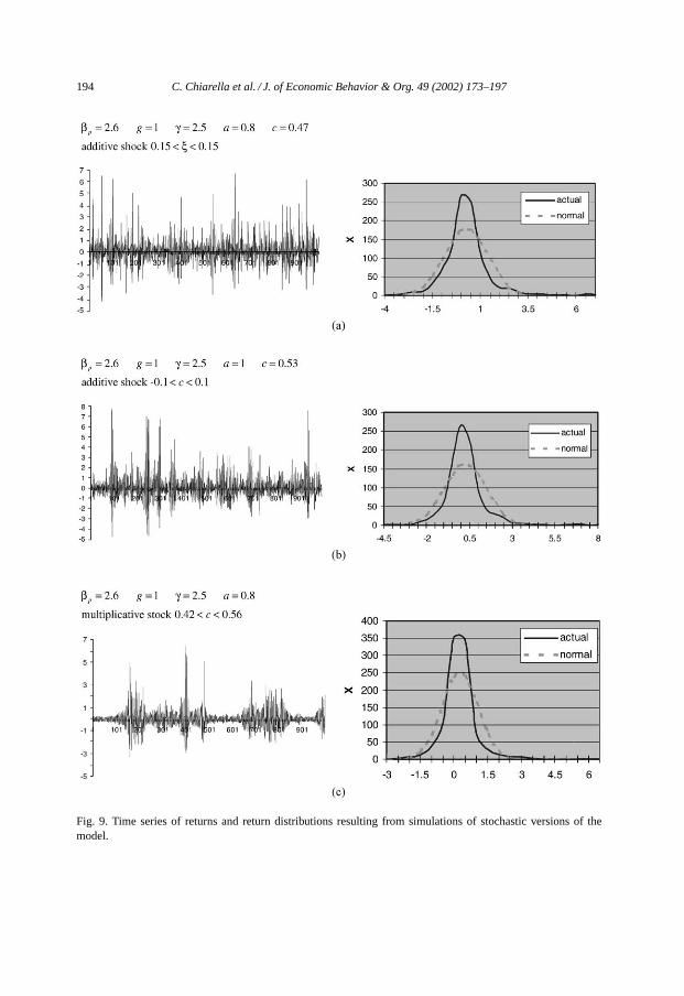
Fig. 9. Time series of returns and return distributions resulting from simulations of stochastic versions of themodel.

C. Chiarella et al. / J. of Economic Behavior & Org. 49 (2002) 173–197 195

estimate of expected return depending on whether there is a positive (good news) or negative(bad news) shock. We have considered two types of stochastic factors. The first additive, sothat the map (10) would be written

ψ ′ = (1 − c)ψ − cβp[ap− k(ψ)] + ξt , p′ = p − βp[ap− k(ψ)], (22)

whereξt is uniformly distributed on the interval [ξmin, ξmax]. The second multiplicative,in which the chartists’ speed of adjustment of expectations varies randomly around somemean value. In this case the map (10) would be written

Xt+1 = Tct (Xt ), (23)

wherect is a random parameter uniformly distributed on the interval [cmin, cmax] andTct isthe map given in (10) with the parameterct .

Fig. 9a displays the returns and the return distribution (compared with the correspondingnormal distribution) resulting from a simulation of (22) withξt distributed uniformly on[−0.15,0.15]. The parameters of the model are those relevant to Fig. 2a. In this case theequilibrium is stable but with orbits converging to it in a cyclical fashion. The stochasticversion of the model clearly shows both volatility clustering, fat tails, peaked distributionand skewness. Here, these are due solely to the oscillatory transients of the underlyingdeterministic model. In a sense this case is the closest to the vision of the stable deterministicpart of the models of the standard finance paradigm, with the only additional feature beingthe oscillatory approach to the equilibrium.

Fig. 9b displays the returns and the return distribution resulting from a simulation of(22) withξt distributed uniformly on [−0.1,0.1] and the parameters of the model are thoserelevant to Fig. 2b. Here also we see volatility clustering and the distributional characteristicsof real financial data. These are most likely due to the fact that the noise is pushing the statevariables between the (white) basin of attraction of the equilibrium and the (light grey)basin of attraction of the four-cycle.

Fig. 9c displays the returns and return distribution resulting from a simulation of (23) withc uniformly distributed on [0.42,0.56]. The parameters of the model are those (apart fromc) relevant to Fig. 3a and b. Thus, the variation ofc causes the map to vary across a widerange of outcomes including a closed curve similar to Fig. 3a and a chaotic attractor similarto Fig. 3b. It is this variation across maps which is the origin of the volatility clustering andfat tails that we see in Fig. 9c.

The simulations of this section are very preliminary and have been chosen to illustratequalitatively how the interaction of some of the non-linear deterministic phenomena of themodel with a simple external noise source can give rise to the qualitative types of returnbehaviour observed in financial markets. We leave to future research the task of calibratingsuch models to actual market data and doing more extensive simulation studies.

7. Conclusions

In this paper we have developed a discrete time model of asset price dynamics, basedon the interaction of two types of traders: fundamentalists, who hold an estimate of thefundamental value of the asset and whose demand is an increasing function of the difference

196 C. Chiarella et al. / J. of Economic Behavior & Org. 49 (2002) 173–197

between the fundamental value and the current price, and chartists, a group basing its tradingdecisions on an analysis of past price trends, whose demand is an S-shaped function of theexpected return differential with an alternative asset. We assume the existence of amarketmaker,whose role is to set excess demand to zero at the end of each trading period bytaking an off-setting long or short position, and who announces the next period price as afunction of the excess demand. We have demonstrated how the behaviour of the two typesof traders affects the dynamics by showing the effect, on the local and global dynamics, ofthe key parameters, namely the “strength” of fundamentalist and chartist demand (a andγ , respectively), and the speed of adjustment of chartists’ expectations (c). In particularwe have clarified how the strength of chartist demandγ affects the local stability of theequilibrium, by showing that for sufficiently low values ofγ the equilibrium is stablefor a wide range of values of the fundamentalist parametera and for any level of thechartists’ reaction speedc (0 < c ≤ 1); while whenγ is sufficiently high, i.e. chartistdemand is relatively strong, the ability of fundamentalists’ demand to stabilise the systemis restricted to a fairly narrow range of the parametera. Our analysis then focused on theglobal dynamical behaviour observed in this latter case. First we have shown that also whenthe equilibrium is locally stable other dynamic phenomena arise for sufficiently high valuesof c anda, such as chaotic transients before the convergence to the stable equilibrium or thecoexistence of attractors. We have then performed a detailed analysis of the global dynamicphenomena occurring when, by increasing the parameterc, the equilibrium O becomesunstable via a Neimark–Hopf bifurcation: we have numerically observed that when thisbifurcation occurs at sufficiently high values of the parametera, an increase ofc leads tooscillatory behaviour which may become chaotic around O, and asc approaches the value1 the dominating state is an attracting cycle (although coexisting with a strange repellor)with a wide basin of attraction. In this global analysis, the theory ofcritical curvesandvarious numerical tools have been extensively used, for example to explain in detail theappearance of chaotic dynamics associated withhomoclinic bifurcationsof fixed pointsand cycles. Finally, we have considered a stochastic version of the model to demonstrate, atleast qualitatively, how the interaction of the deterministic non-linear dynamic phenomenawith a simple external noise process, can generate the typical patterns of financial marketssuch as volatility clustering, fat tails, peaked return distributions and skewness.

Future developments of the model introduced here would be to analyse the dynamics ofthe three-dimensional map which arises when the dynamics of the market for the alternativeasset is also taken into account (as discussed briefly in Section 3). It is also important tofocus on attempts of each group to learn about their economic environment in the face ofstochastic factors. Finally, in order to focus on the dynamics induced by the interactionof fundamentalists and the speculative behaviour within a two-dimensional map, we haveleft in the background the dynamics of the wealth of the two groups. This is perhapsjustifiable in the present context since an exponential utility of wealth function underliesboth the fundamentalist and chartist demand functions, which in this case are independentof wealth. Clearly, in the long term, the evolution of the wealth of each group will alsodetermine their economic behaviour, and such evolution needs to be modelled. Chiarellaand He (2001b) have developed a model of heterogeneous agents with logarithmic utilityfunction which takes explicit account of the wealth dynamics of each group, but the analysisof this model is only possible via computer simulations. However the insights into the

C. Chiarella et al. / J. of Economic Behavior & Org. 49 (2002) 173–197 197

dynamics of speculative behaviour gained via the simpler model of this paper are useful inattempting to understand the dynamics of this more complete model as well as that of Chenand Yeh.

Acknowledgements

This work has been performed with the financial support of CNR, Italy, and withinthe scope of the national research project “Non-linear Dynamics and Stochastic Modelsin Economics and Finance”, MURST, Italy. Financial support of the Australian ResearchCouncil Grant number A79802872 is also acknowledged. We would like to thank the twoanonymous referees for helpful comments and Gian Italo Bischi for having read a previousversion of this paper, pointing out some misconceptions. We are particularly grateful toRichard Day, whose suggestions have led to major improvements. The usual caveat applies.

References

Beja, A., Goldman, M.B., 1980. On the dynamic behavior of prices in disequilibrium. Journal of Finance 35,235–248.

Brock, W., Hommes, C., 1998. Heterogeneous beliefs and routes to chaos in a simple asset pricing model. Journalof Economic Dynamics and Control 22, 1235–1274.

Chen, S.H., Yeh, C.H., 1997. Modelling speculators with genetic programming. In: Angeline, P., et al. (Eds.),Evolutionary Programming VI, Lecture Notes in Computer Science, Vol. 1213, Springer, Berlin, pp. 137–147.

Chiarella, C., 1992. The dynamics of speculative behaviour. Annals of Operations Research 37, 101–123.Chiarella, C., Dieci, R., Gardini, L., 2001a. A dynamic analysis of speculation across two markets. Working Paper,

School of Finance and Economics, University of Technology, Sydney, Australia.Chiarella, C., Dieci, R., Gardini, L., 2001b. Asset price dynamics in a financial market with fundamentalists and

chartists. Discrete Dynamics in Nature and Society 6, 69–99.Chiarella, C., He, X., in press. Heterogeneous beliefs, risk and learning in a simple asset pricing model.

Computational Economics.Chiarella, C., He, X., 2001. Asset Pricing and Wealth Dynamics under Heterogeneous Expectations. Quantitative

Finance 1, 509–526.Collet, P., Eckmann, J.P., 1980. Iterated Maps on the Interval as Dynamical Systems, Birkhauser, Basel, Boston.Day, R.H., Huang, W., 1990. Bulls, bears and market sheep. Journal of Economic Behavior and Organization 14,

299–329.Devaney, R.L., 1987. An Introduction to Chaotic Dynamical systems, The Benjamin/Cummings Publishing Co.,

Menlo Park, CA.Gardini, L., 1994. Homoclinic bifurcations inn-dimensional endomorphisms due to expanding periodic points.

Non-linear Analysis, T.M.&A. 23, 1039–1089.Gumowski, I., Mira, C., 1980. Dynamique Chaotique. Cepadues, Toulouse.Li, T.Y., Yorke, J.A., 1975. Period three implies chaos. American Mathematical Monthly 82, 985–992.Lux, T., 1998. The socio-economic dynamics of speculative markets: interacting agents, chaos and the fat tails of

return distributions. Journal of Economic Behaviour and Organization 33, 143–165.Marotto, F.R., 1978. Snap-back repellers imply chaos inRn. Journal of Mathematical Analysis and Applications

72, 199–223.Mira, C., 1987. Chaotic Dynamics, World Scientific, Singapore.Mira, C., Gardini, L., Barugola, A., Cathala, J.C., 1996. Chaotic Dynamics in Two-Dimensional Non-invertible

Maps, World Scientific, Singapore.Puu, T., 2000. Attractors, Bifurcations and Chaos. Springer, New York.Zeeman, E.C., 1974. On the unstable behaviour of stock exchanges. Journal of Mathematical Economics 1, 39–49.