arX

iv:0

707.

0006

v1 [

astr

o-ph

] 2

9 Ju

n 20

07A complete version can be obtained at http://www.astro.psu.edu/users/misawa/pub/Paper/40hires.ps.gz

Preprint typeset using LATEX style emulateapj v. 11/12/01

SPECTROSCOPIC ANALYSIS OF H I ABSORPTION LINE SYSTEMS IN 40 HIRES QUASARS1

Toru Misawa2, David Tytler3,4, Masanori Iye5,6, David Kirkman3,4, Nao Suzuki3,4, DanLubin3,4, and Nobunari Kashikawa5,6

A complete version can be obtained at http://www.astro.psu.edu/users/misawa/pub/Paper/40hires.ps.gz

ABSTRACT

We list and analyze H i absorption lines at redshifts 2 < z < 4 with column density (12 <log(NH I/[cm−2]) < 19) in 40 high-resolutional (FWHM = 8.0 km s−1) quasar spectra obtained withthe Keck+HIRES. We de-blend and fit all H i lines within 1,000 km s−1 of 86 strong H i lines whosecolumn densities are log NHI ≥ 15 cm−2. Unlike most prior studies, we use not only Lyα but also allvisible higher Lyman series lines to improve the fitting accuracy. This reveals components near to highercolumn density systems that can not be seen in Lyα. We list the Voigt profile fits to the 1339 H i com-ponents that we found. We examined physical properties of H i lines after separating them into severalsub-samples according to their velocity separation from the quasars, their redshift, column density andthe S/N ratio of the spectrum. We found two interesting trends for lines with 12 < log(NH I/[cm−2])< 15 which are within 200 – 1000 km s−1 of systems with log(NH I/[cm−2]) > 15. First, their columndensity distribution becomes steeper, meaning relatively fewer high column density lines, at z < 2.9.Second, their column density distribution also becomes steeper and their line width becomes broader byabout 2–3 km s−1 when they are within 5,000 km s−1 of their quasar.

Subject headings: quasars: absorption lines — quasars: general — intergalactic medium

1. introduction

Quasar absorption systems have historically been di-vided largely into three physically distinct categories: (i)absorption systems with strong metal lines arising in ornear intervening galaxies, (ii) weak H i systems in the Lyαforest that come from the intergalactic medium, and (iii)intrinsic systems that are physically related to the quasars,including associated and broad absorption line systems.

Metal absorption systems usually contain H i lineswith relatively large column densities, including two sub-categories: damped Lyman alpha (DLA) system and Ly-man limit system (LLS) with H i column densities oflog(NH I/[cm−2]) > 20.2 and 17.16, respectively. Deepimaging observations around quasars have provided ev-idences that the metal absorption systems are often pro-duced in intervening galaxies. Galaxies have been detectedthat can explain Mg II absorption lines (e.g., Bergeron& Boisse 1991), and C IV absorption lines (e.g., Chen,Lanzetta, & Webb 2001).

On the other hand, nearly all H i lines have smaller col-umn densities (log NHI ≤ 15) than those associated foundin gas that shows strong metal lines. The number of H ilines per unit z increases with redshift (Peterson 1978;Weymann et al. 1998a; Bechtold 1994), because the in-tergalactic medium is denser and less ionized at higherz. The Lyα absorption lines are produced in intergalac-tic clouds (e.g., Sargent et al. 1980; Melott 1980), whichare the higher density regions in the inter-galactic medium

(IGM). The Lyα lines are broadened by Hubble flow (e.g.,Rauch 1998; Kim et al. 2002a) as well as the Dopplerbroadening from the gas temperature.

Misawa et al. (2004) presented a study of H i absorp-tion lines seen towards 40 quasars in spectra from the KeckHIRES spectrograph. In a departure from prior work, theyconsidered the H i lines without considering the metallines. They classified the H i lines as either high den-sity lines [HDLs] which have or are near to strong H i linesthat are probably related to galaxies, and low density lines[LDLs] that are far from any strong H i lines and are morelikely to be far from galaxies and hence in the IGM.

Following Misawa et al. (2004), we define HDLs as allH i lines within ± 200 km s−1 of a lines with 15 < log NHI

< 19 cm−2. We define LDLs as lines with 12 < log NHI

< 15 which are within 200 – 1000 km s−1 of a line with15 < log NHI < 19 cm−2. This last velocity constraintis intended to make the LDL a “control” sample for theHDLs, where the two samples come from similar redshiftsand regions of the spectra with similar signal to noise.

Misawa et al. (2004) discovered that the HDLs havesmaller Doppler parameters (b-values), for a given columndensity than the LDLs, and they also found the same effectin a hydrodynamic simulation with 2.7 kpc cells. Misawaet al. (2004) suggested that the LDLs are cool or shock-heated diffuse intergalactic gas, and that the HDLs arecooler dense gas near to galaxies.

Misawa et al. (2004) fit all the accessible transitions in

1 The data presented here were obtained at the W.M. Keck Observatory, which is operated as a scientific partnership among the CaliforniaInstitute of Technology, the University of California and the National Aeronautics and Space Administration. The Observatory was madepossible by the generous financial support of the W. M. Keck Foundation.2 Department of Astronomy and Astrophysics, Pennsylvania State University, University Park, PA 168023 Center for Astrophysics and Space Sciences, University of California San Diego, MS 0424, La Jolla, CA 92093-04244 Visiting Astronomer, W. M. Keck Observatory, which is a joint facility of the University of California, the California Institute of Technology,and NASA5 National Astronomical Observatory, 2-21-1 Osawa, Mitaka, Tokyo 181-8588, Japan6 Department of Astronomical Science, The Graduate University for Advanced Studies, 2-21-1 Osawa, Mitaka, Tokyo 181-8588, Japan.

1

2 Misawa et al.

the H i Lyman series to help de-blend H i lines. Theirmain sample comprised 86 H i absorption systems eachwith log NHI > 15 cm−2. They also fit all H i lines within±1,000 km s−1 of these H i lines, to give a total sam-ple of 1339 H i lines, including the 86 lines. This is theonly large sample in which multiple Lyman series lines arefit together, although this method has been used on indi-vidual systems and small samples (Songaila et al. 1994;Tytler, Fan, & Burles 1996; Wampler et al. 1996; Car-swell et al. 1996; Songaila et al. 1997; Burles & Tytler1998a,1998b, Burles, Kirkman, & Tytler 1999; Kirkmanet al. 2000; O’Meara et al. 2001; Kirkman et al. 2003;Kim et al. 2002b; Janknecht et al. 2006).

In this paper, we present measurements of the absorp-tion lines that Misawa et al. (2004) have analyzed. Wegive a detailed description of each absorption system andwe summarize new results. The paper is organized as fol-lows: In §2, we give descriptions of the data and the linefitting. The results of our statistical analyses are presentedin §3. We discuss our results in §4, and summarize themin §5. In the Appendix, we describe the properties and wegive velocity plots for each H i system. We use a cosmol-ogy in which H0 = 72 km s−1Mpc−1, Ωm = 0.3, and ΩΛ

= 0.7.

2. spectra and line fitting

The 40 quasars in our sample have either DLA systemsor LLSs, and they were observed as a part of a survey formeasurements of the deuterium to hydrogen (D/H) abun-dance ratio. The detailed description of the absorptionand data reduction are presented in Misawa et al. (2004).We caution that our sample was biased in subtle ways bythe selection of LLS and DLAs that seemed more likely toshow D, i.e. those with simpler velocity structure.

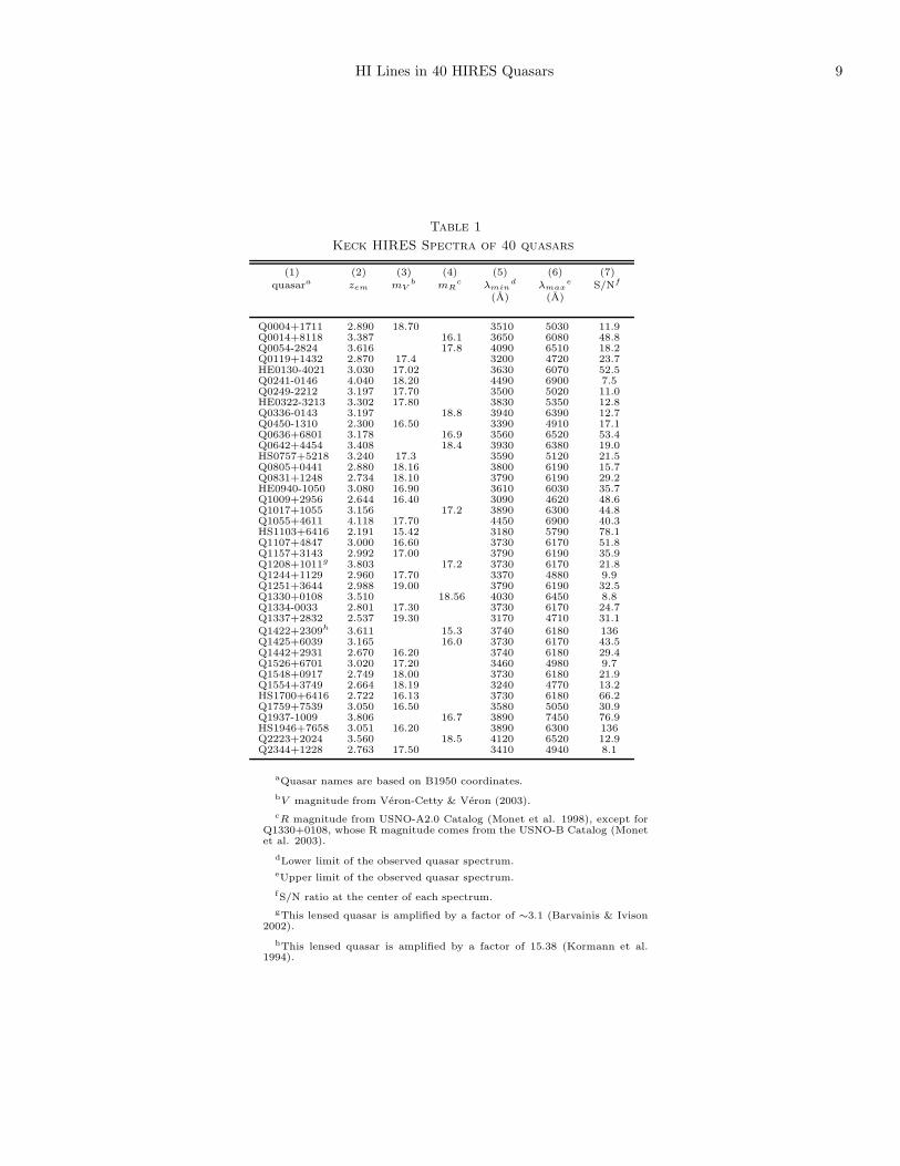
We list the 40 quasars in Table 1. Column (1) is thequasar name, (2) the emission redshift. Columns (3) and(4) are the optical magnitude in the V and R bands. Thelower and upper wavelength limits of the spectra are pre-sented in columns (5) and (6). Column (7) gives the S/Nratio at the center of the spectrum. Same data set wasalso used in Misawa et al. (2007) in a study of the quasarintrinsic absorption lines.

We will discuss only H i lines with log NHI > 15 cm−2

and other H i weaker lines within ±1,000 km s−1 of thesestrong H i lines. We selected this velocity range since itis enough to include the conspicuous clustering of strongmetal lines. Indeed such strong metal lines are normallyconfined to an interval of < 400 km s−1 even for DLAsystems (Lu et al. 1996b).

Here we briefly review the line detection and fitting pro-cedures that we discussed in more detail in Misawa etal. (2004). We began searching the literature for H ilines with log NHI > 15, including the DLA and LLS cat-alogues (Sargent, Steidel, & Boksenberg 1989, hereafterSSB; Lanzetta 1991; Tytler 1982), and metal absorptionsystems (Peroux et al. 2001; Storrie-Lombardi et al. 1996;Petitjean, Rauch, & Carswell 1994; Lu et al. 1993; Steidel& Sargent 1992; Lanzetta et al. 1991; Barthel, Tytler, &Thomson 1990; Steidel 1990a,b; Sargent, Boksenberg, &Steidel 1988, hereafter SBS; SSB). We also search for themourselves. If more than one strong H i line was detected ina single 2000 km s−1 velocity window, we take the position

of the H i line with the largest column density (hereafterthe “main component”) as system center. We found 86 H isystems with log NHI > 15, at 2.1 < zabs < 4.0, in 31 ofthe 40 quasars. Figure 1 of Misawa et al. (2004) gives thevelocity plot of one of these systems, and below we givethe rest.

We give parameters describing these 86 systems in Ta-ble 2. In successive columns list (1) the name of the quasar;(2) the redshift of the main component, that with thelargest column density ; (3) the H i column density ofthe main component N1; (4) N2, the second largest H icolumn density within ±1000 km s−1 of the main compo-nent; (5) the ratio of N2 to N1; (6) – (9) the S/N ratiosat Lyα, Lyβ, Lyǫ, and Ly10; (10) the number of lines inthe ± 1,000 km s−1 window; (11) the number of H i linesclassified as HDLs (described later); (12) comments on theH i system; (13) references. We will call this list sampleS0 (Table 3).

When we were fitting the lines, we rejected narrow lineswith Doppler parameter of b < 4.8 km s−1, which corre-sponds to the resolution of our spectra. We also identifyall lines with b < 15 km s−1 as possible metal lines (calledM I in Tables) because H i lines with this narrow width arerare (e.g., Hu et al. 1995, hereafter H95; Lu et al. 1996a,hereafter L96; Kirkman & Tytler 1997a, hereafter KT97).If there was more than one way to fit the lines, we chose thefit with the fewest lines. If the model did not give goodfits to all the Lyman series lines, we adopted the modelthat best fit the lower order lines where the SNR is best.For H i lines with column densities of log NHI ≥ 16.6 theLyman continuum optical depth is τ ≥ 0.25. For these sys-tems we checked if the residual flux at the Lyman limit wasconsistent. Our fitting method could readily overestimatethe Doppler parameter but not the column density. Oncethe fitting model is chosen, we used χ2 minimization in acode written by David Kirkman, to get the best fit param-eters of H i column density (log NHI), Doppler parameter(b), and absorption redshift (z). The internal errors aretypically σ(log NHI)=0.09 cm−2, σ(b)=2.1 km s−1, andσ(z)=2.5×10−5.

We prepared a sample S1 that is a sub-sample of S0 in-cluding only 973 H i lines and 61 H i systems with log NHI

> 15. S1 excludes 25 systems with difficulties such as (i)poor fitting due to gaps in the echelle formatted spectra,(ii) poor fitting due to strong DLA wings (i.e., log NHI

> 19), (iii) close proximity in redshift to the backgroundquasars (i.e., within 1,000 km s−1 of the emission redshift),and (iv) overlapping with other H i systems. The S/N ra-tios of the spectra are at least S/N ≃ 11 per 2.1 km s−1

pixel and the mean value is S/N ≃ 47 for Lyα lines. Amongthese 61 H i systems, three systems may be physically as-sociated with the quasars based on the partial coverageanalysis for the corresponding metal absorption lines (Mi-sawa et al. 2007). However, we keep these systems in S1sample, because we still cannot reject the idea that theyare intervening systems.

We give detailed descriptions of all the lines that we fitin the Appendix. We also give velocity plots of the firstfive Lyman transitions, Lyα, Lyβ, Lyγ, Lyδ, and Lyǫ.

3. results

HI Lines in 40 HIRES Quasars 3

We investigate the properties of line parameters such asthe column density, Doppler parameter, and the clusteringproperties of the H i lines. Since this sample contains notonly H i lines originating in the intergalactic diffuse gasclouds (i.e., LDLs), but also H i lines produced by inter-vening galaxies (i.e., HDLs), we also attempted to sepa-rate H i lines into HDLs and LDLs based on the clusteringtrend (Misawa et a. 2004).

Our analysis is similar to that of previous studies (e.g.,H95; L96; KT97), but with three key differences: (i) earlierstudies used all H i lines detected in the quasar spectra,whereas we use only H i lines within ± 1,000 km s−1 ofthe main components with log NHI ≥ 15, (ii) our samplecontains a number of strong lines (log NHI ≥ 15) in addi-tion to weak H i lines (log NHI < 15), and (iii) our samplecovers a wide redshift range: 2.0 ≤ zabs ≤ 4.0. The red-shift distributions of the 86 and 61 H i systems in samplesS0 and S1 are shown in Figure 1.

3.1. Sub-Samples for the Statistical Analysis

For further investigation, we prepared several sub-samples as follow. It is known that the comoving num-ber densities of low-ionization lines, such as H i lines, de-creases in the vicinity of quasars (Carswell et al. 1982;Murdoch et al. 1986; Tytler 1987). This trend is knownas the “proximity effect”, and is probably caused by theenhanced UV flux from the quasar towards which the ab-sorption is seen. We separate the 61 H i systems (sampleS1) into sub-samples S2a (the velocity difference from thequasar, ∆v > 5,000 km s−1) and S2b (∆v < 5,000 km s−1).We have already removed from S1 all H i systems within1,000 km s−1 of the quasars to avoid H i systems from thequasar host galaxies.

H95 emphasized that the line detection limit is almostwholly determined by the line blending (or blanketing),and not by the S/N ratio of the spectrum. In order to con-firm whether the distribution of line parameters is affectedby the quality of the spectrum, we made two overlappingsamples from S1 using the S/N ratio of each spectrum inthe Lyα region: S3a (S/N ≥ 40), and S3b (S/N ≥ 70).These sub-samples include 34 (∼ 60%) and 17 (∼ 30%) ofthe 61 H i systems of the sample S1.

Sample S1 covers a broader range of redshifts, 2.0 < z <4.0, when compared with previous studies: 2.55 < z <3.19 for H95, 3.43 < z < 4.13 for L96, and 2.43 < z < 3.05for KT97. When we investigate the redshift evolution ofH i absorbers, we also divided S1 into two sub-samples; S4a(z < 2.9) and S4b (z ≥ 2.9). Here the two sub-sampleshave nearly the same number of H i systems.

Finally, we made sub-samples according to the columndensities of H i lines, as the distributional trends of strongand weak H i lines are very different (see Figure 2 in Mi-sawa et al. 2004); the H i lines with relatively large col-umn densities tend to cluster around the main compo-nents, while the number of weak H i lines decreases nearthe center of H i systems because of line blanketing. Sinceone of our interests is to determine the boundary value ofcolumn density between HDLs and LDLs (although otherparameters may be necessary to separate them), we sepa-rate the 973 H i lines into eight sub-samples according totheir column densities. We use boundary values of log N= 13, 14, 15, and 16, where sub-sample S5ab contains H i

lines whose column densities are log(NH I/[cm−2]) valuesof a to b.

In Table 3 we summarize these 16 sub-samples. Herewe should emphasize that S51213, S51214, S51215, S51216,S51319, S51419, S51519, and S51619, are separated by theproperties of lines, while S2a, S2b, S3a, S3b, S4a, and S4bare separated by the unit of system.

3.2. Physical Properties of H i Absorbers

For each sub-sample prepared in the last section, we per-form statistical analysis, including analysis of the columndensity distribution, Doppler parameter distribution, andline clustering properties. The samples used here containboth HDLs and LDLs.

3.2.1. Column Density Distribution

The column density distribution of H i lines, dn(N)/dN ,are usually fit with a power law (Carswell et al. 1984,Tytler 1987, Petitjean et al. 1993; H95),

log

(

dn(N)

dN

)

= −β log N + A, (1)

where the index β was estimated to be 1.46 (H95), 1.55(L96), and 1.5 (KT97) with only weaker H i lines withlog NHI = 12 – 14.5. Janknecht et al. (2006) found β= 1.60±0.03 at lower redshift z < 1.9. The column den-sity distributions of our seven sub-samples (S1, S2a, S2b,S3a, S3b, S4a and S4b) per unit redshift and unit columndensity are analyzed. The plot in Figure 2 is the resultfor sub-sample S1. Since the turn-over of the distributionaround log NHI = 12.5 is probably due to line blendingand/or blanketing as described later in § 4, we fit the col-umn density distributions only for log NHI > 13. Thebest-fitting parameters, β and A, as well as the redshiftbandpass, ∆z, of each sub-sample are summarized in Ta-ble 4, along with the past results from KT97 and Petitjeanet al. (1993).

The indices that we find, β = 1.40±0.03, are slightlysmaller than the value in the past results, β = 1.46 –1.55,which means that our sample favors strong H i lines. Butwe expect this type of trend. Our samples contain not onlyLDLs but also HDLs, and since we cover only the velocityregions within ± 1,000 km s−1 of the main components,we have a strong excess of strong H i lines. We see the col-umn density distribution does not change with the velocitydistance from the quasars (S2a and S2b) or with the S/Nratio (S3a and S3b), but it is weakly affected by redshift(S4a and S4b). We also applied the Kolmogorov-Smirnov(K-S) test to the sub-samples. The results in Table 5 showthat we can not rule out the hypothesis that they are ran-dom samplings from the same population.

3.2.2. Doppler Parameter Distribution

The distribution of the Doppler parameter of H i lineshave been approximately given by the truncated Gaussiandistribution (H95; L96),

dn(b)

db=

A exp[

−(b−b0)2

2σ2b

]

b ≥ bmin

0 b < bmin

(2)

where b0 and σb are the mean and the dispersion of b dis-tribution and bmin is the minimum b value for an H i line.There are two origins of line broadening: thermal broad-ening (bT ), and micro-turbulence (btur). The total amount

of broadening is given by b =√

b2T + b2

tur.

4 Misawa et al.

In order to determine the correct Doppler parameter, wehave to individually resolve and fit H i lines using Voigtprofiles. However, most of weak H i lines disappear in theobserved spectrum due to line blending and blanketing,especially near strong lines. To derive the intrinsic (asopposed to observed) distribution of the Doppler param-eter, previous authors (i.e., H95; L96; KT97) have cho-sen artificial H i lines (as input data) with distributionscharacterized by a Gaussian, and used them for compari-son with the observed distributions. KT97 noted that theb-value distribution of lines seen in simulated spectra re-sembles the distribution of the input data, except for twodifferences: (i) an excess of lines with large b-values is seenin the recovered data, compared to the input data, whichis probably produced by line blending, and (ii) lines withvery small b-values (b < 15 km s−1) are found, which areprobably data defects or noise, as they are not present inthe input data. Nonetheless, the b-value distribution ofthe input and recovered data resemble each other betweenb = 20 km s−1 and b = 60 km s−1.

We would ideally like to determine the real distribu-tion of Doppler parameters; however, the only way to dothis is to perform simulations, and compare the recoveredDoppler parameter distribution with the observed distri-bution. Such simulations are expensive to perform, soin this work we simply compared the distribution in oursample with the past results of H95 and L96 at b = 20– 60 km s−1. We analyzed the observed distributions ofDoppler parameters for 15 sub-samples, and compare themwith the results in H95 (b0 = 28 km s−1, σb = 10 km s−1,and bmin = 20 km s−1) and L96 (b0 = 23 km s−1, σb =8 km s−1, and bmin = 15 km s−1), where the parametersare the inputs used for artificial spectra that reproduce theobserved distribution.

We see an excess of H i lines with large b-values of b> 50 km s−1 in all of the sub-samples, while we have nolines with b ≤ 15 km s−1 because we decided to classifythem into metal lines. All sub-samples except for S1213

have relatively large b-values, and their distributions arecloser to H95’s distribution than L96’s. In contrast, thedistribution of S1213, containing only H i lines with smallcolumn densities, log NHI < 13, resembles L96’s distribu-tion. We plot in Figure 3 the Doppler parameter distri-butions of sub-samples S1 and S1213. We also applied aK-S test to the sub-samples (S2a, S2b, S3a, S3b, S4a, andS4b). The results are listed in Table 6. The probability,that the distributions of sub-samples S2a (∆v(zem− zabs)> 5000 km s−1) and S2b (∆v(zem− zabs) ≤ 5000 km s−1)were drawn from the same parent population, is very small,∼2.4 %. This result could suggest that the Doppler pa-rameters of H i lines within 5000 km s−1 of quasars areaffected by UV flux from the quasars.

3.3. HDLs and LDLs

In the previous section, we carried out statistical anal-ysis using sub-samples containing both HDLs and LDLstogether. Here, we repeat these tests on the two samplesseparately.

Metal absorption lines seen in DLA systems or LLSs arestrongly clustered within several hundred km s−1, whichimplies their relationship to galaxies. In simulations Daveet al. (1999) also noted that galaxies tend to lie near

the dense regions that are responsible for strong H i lines.On the other hand, for weak H i lines, no strong cluster-ing is seen (e.g., Rauch et al. 1992; L96; KT97), althoughsome studies found only weak clustering trends (e.g., Webb1987; H95; Cristiani et al. 1997).

As Misawa et al. (2004) found, lines with log NHI ≥ 15show strong clustering trends at ∆v < 200 km s−1, whilelines with lower column densities cluster weakly at ∆v <100 km s−1 (Figure 4).

Misawa et al. (2004) defined HDLs as H i lines with15 < log NHI < 19 and other weaker H i lines within ±200 km s−1 of those stronger H i lines. They then definedthe LDLs as all other lines with 12 < log NHI < 15. Theychose log NHI = 15 cm−2 in the definition because thetwo point correlation was largest for a sub-sample of H ilines with 15 < log NHI < 19. We list the number of HDLsand LDLs in the sub-samples in Table 7.

3.3.1. Column Density Distribution

In Table 8 we give the parameters that describe thecolumn density distributions of HDLs and LDLs for fivesub-samples (S1, S2a, S2b, S4a, and S4b). The most obvi-ous result is that the HDLs have a smaller index than theLDLs. We see the same result in Figure 3 of Petitjean etal. (1993), and hence we now confirm this with the firstlarge sample to consider the sub-components of the HDLs.

The distributions of LDLs in sample S1, S2a, and S4bare almost consistent with the previous result in KT97. Onthe other hand, the power law indices for the LDLs of S2b(∆v ≤ 5000 km s−1) and S4a (z < 2.9), β = 1.90±0.16and 1.71±0.06, are larger than the values for the othersub-samples, β ∼ 1.52, which means that LDLs at lowerredshift or near the quasars tend to have lower column den-sities compared with those at higher redshift or far fromthe quasars. The change in the column density distribu-tion near to the quasars may be just a consequence of theenhanced UV radiation.

3.3.2. Doppler Parameter Distribution

The Doppler parameter distributions of HDLs and LDLsfor sub-samples (S1, S2a, S2b, S4a, and S4b) are also in-vestigated, and the results of K-S tests applied to themare summarized in Table 9. The only remarkable resultis that the probability, that the Doppler parameter distri-butions of LDLs at ∆v > 5,000 km s−1 (S2a) and ∆v ≤5,000 km s−1 (S2b) from the quasars were drawn from thesame parent population, is very small, ∼2.0%. We showsthese two distributions in Figure 5. In Figure 6 we seethat the cumulative distribution for the line b-values risesmore slowly for the LDLs near to the quasars (at ∆v ≤5000 km s−1), which means that these lines near to thequasars are broader by about 2–3 km s−1. For other pairsof the sub-samples, we could not rule out the hypothesisthat their parent populations are same.

4. discussion

In this section, we discuss our results, especially the factthat the column density distribution is changing with theredshift and the velocity distance from the quasars. Wealso compare our results to those at lower redshift (z <0.4) from the literature. After that, we also briefly discussthe completeness of H i lines in our 40 spectra.

HI Lines in 40 HIRES Quasars 5

4.1. Redshift Evolution of H i Absorbers

In § 3, we prepared two sub-samples, S4a and S4b, tocompare the physical properties of H i lines at lower red-shift (zabs < 2.9) and at higher redshift (zabs ≥ 2.9). Wedo not see a change in the column density distribution inthe sample as a whole, but once they are separated intoHDLs and LDLs, we notice that the index of the columndensity distribution of LDLs at zabs < 2.9 (β = 1.71±0.06)is clearly different from that of LDLs at zabs ≥ 2.9 (β =1.52±0.09). On the other hand, there was no redshift evo-lution for HDLs. This trend, shown in Figure 7, meansthat there is a deficit of relatively stronger LDLs (i.e.,log NHI ≥ 14.5) at lower redshift. One of the possibleexplanations is that at lower redshift, more H i lines withthe column densities just below log NHI = 15 (i.e., rela-tively strong LDLs) might be associated with HDLs. Inother words, stronger (i.e., log NHI = 14.5 – 15) LDLs getinto within 200 km s−1 of the nearest HDLs, and wouldbe classified into HDLs, which is consistent with the trendexpected in the hierarchical clustering model (Figure 8).

As for the Doppler parameter distribution, we did notfind any remarkable redshift evolutions in neither HDLsnor LDLs. L96 claimed that there is a redshift evolu-tion of the Doppler parameter between z = 2.8 and 3.7;the mean value of Doppler parameter at zabs = 3.7 (b0

= 23 km s−1; L96) is smaller than the value at zabs =2.8 (b0 = 28 km s−1; H95). The corresponding value inKT97 (b0 = 23 km s−1) is, however, different from theresult in H95. The difference may be due to the differ-ent line fitting procedure used in these studies; L96 andKT97 used the VPFIT software, while H95 used differentsoftware. Especially important is how the authors choseto treat blended lines. The difference could be related tothe difference of the spectrum resolutions; R=45000 (L96;KT97) and R=36000 (H95). Janknecht et al. (2006) didnot detect any evolution on the Doppler parameter at z= 0.5 – 1.9. Our results, which are based on the data settaken with one observational configuration and fit usingthe same procedure, suggests that the Doppler parameterdistribution of H i clouds does not evolve with redshift atz = 2 – 4.

4.2. Proximity Effect near Quasars

It has long been noted that the number of Lyα linesdecreases near to the redshift of the quasars (Carswell etal. 1982; Murdoch et al. 1986; Tytler 1987). This phe-nomenon is related to the local excess of UV flux fromthe quasars. The proximity effect has been used to evalu-ate the intensity of the background UV flux. Bajtlik et al.(1988) first measured the mean intensity of the backgroundUV intensity, Jν = 10−21.0±0.5 (erg s−1 cm−2 Hz−1 str−1)at the Lyman limit at 1.7 < z < 3.8, by estimating thedistance from the quasar at which the quasar flux is equalto the background UV flux. The typical radius is ∼ 5 Mpcin physical scale that corresponds to the velocity shift of∆v ∼ 4,000 km s−1 from the quasars. L96 also evaluatedthe background UV intensity to be Jν = 2×10−22 (erg s−1

cm−2 Hz−1 str−1) at z ∼ 4.1 in the spectrum of Q0000-26.We see two differences in LDLs within 5,000 km s−1

of the quasars, compared to those far from the quasars(∆v > 5,000 km s−1). We see fewer strong LDLs leadingto a large index for the column density power law, β =

1.90±0.16 (Figure 9). We also see that the distribution ofDoppler parameter is different from that of H i lines farfrom the quasars at 98.8 % confidence level. The lines nearto the quasar apparently tend to have broader lines (Fig-ures 5 and 6), although this is a tentative result becausewe consider few lines near to the quasars.

These results could be accounted for by assuming a two-phase structure: outer cold low-density regions and innerhot high-density regions in which temperature is deter-mined by the competition between photoionization heat-ing and adiabatic cooling. When gas is near to the quasars,the outer regions become too highly ionized to show muchH I, and only the inner hot regions would be observed inH I, which would increase the mean value of the Dopplerparameter. The increased ionization also decreases thetotal column densities of H I gas compared with gas farfrom the quasars (Figure 10). As reported in the past ob-servations (e.g., Kim et al. 2001; Misawa et al. 2004),log NHI and b(H i) have a positive correlation for log NHI

< 15. This correlations was also reproduced by hydro-dynamical simulations (e.g., Zhang et al. 1997; Misawaet al. 2004). These results suggest that high density re-gions tend to have larger Doppler parameters, if the ab-sorbers are not optically thick. Dave et al. (1999) alsopresented an interesting plot in their Figure 11 that sup-ported there existed three kinds of phases for H i absorbers(diffuse, shocked, and condensed phases). Among them,the diffuse phase whose volume densities are small (i.e.,it corresponds to LDLs in our paper) has a positive cor-relation between log NHI and b. On the other hand, ananti-correlation between log NHI and b is seen only for thecondensed phase with high volume density that is proba-bly associated with galaxies. The shocked phase, probablyconsisting of shock-heated gas in galaxies, does not showany remarkable correlations between them. Thus, if weassume all LDLs in our sample arise in the diffuse phaseabsorbers, our scenario above could reproduce the differ-ence between sub-samples S2a and S2b.

4.3. Comparison to H i Absorbers at Lower Redshift

The number density evolution of H i absorbers (i.e.,dN/dz ∝ (1 + z)−γ) has been known to slow dramati-cally at z ∼ 1.6, from a high-z rapid evolution with γ of1.85±0.27 (Bechtold 1994) to a low-z slow evolution withγ of 0.16±0.16 (Weymann et al. 1998b). This trend is sug-gested to be due to the decline in the extragalactic back-ground radiation using hydrodynamic cosmological simu-lations (e.g., Theuns, Leonard, & Efstathiou 1998). Thus,a comparison of H i absorbers at high-z and local universeis another interesting topic.

In § 3, we found that the column density distribution ofLDLs at z < 2.9 (β = 1.71±0.06) is steeper than that atz > 2.9 (β = 1.52±0.09). We proposed this trend couldbe due to the hierarchical clustering. If the assembly ofstructure in the IGM indeed dominates the column den-sity distribution, we would expect to find a steeper columndensity distributions at lower redshift as proposed in § 4.1.

Using the Hubble Space Telescope (HST) and the Far Ul-traviolet Spectroscopic Explorer (FUSE), Penton, Stocke,& Shull (2004) and Lehner et al. (2007) estimated power-law indices to be β of 1.65±0.07 at 12.3 ≤ log NHI ≤ 14.5and 1.76±0.06 at 13.2 ≤ log NHI ≤ 16.5 at z < 0.4, respec-

6 Misawa et al.

tively. On the other hand, Dave & Tripp (2001) found aflatter distribution (β = 2.04±0.23) at z < 0.3. The lattersteeper distribution was also reproduced by hydrodynami-cal simulations (e.g., Theuns et al. 1998). If we accept thesteeper result, the column density distribution would con-tinue to be steeper as going to the lower redshift, whichsupports our idea that the hierarchical clustering couldplay a main role of the evolution seen in the column den-sity distribution, although extragalactic radiation wouldcontribute to play a role.

Absorption line width is another parameter that is stillin argument whether it would evolve with redshift or not,as mentioned in § 4.1. While most of the space-based ul-traviolet observations could not measure line widths bymodel fittings because of the lacks of spectral resolutions,Lehner et al. (2007) for the first time measured Dopplerparameters of H i absorption lines accurately at lower red-shift (z < 0.4), and investigate their distributional trend.By comparing to the results at higher redshift, Lehneret al. (2007) discovered that Doppler parameters aremonotonously increasing from z = 3.1 to ∼0. Such atrend was not confirmed in past papers (e.g., Janknechtet al. 2006). The fraction of the broad Lyα absorbers(BLA; b ≥ 40 km s−1) is also confirmed to increase by afactor of ∼3 from z ∼ 3 to 0 (Lehner et al. 2007). Here,b = 40 km s−1 corresponds to gas temperature of Tgas ∼105 K, which is a border between the cool photoionized ab-sorbers and the highly ionized warm-hot absorbers. Theseresults suggests that a large fraction of H i absorbers atvery low redshift (i.e., z < 0.4) are hotter and/or morekinematically disturbed than at higher redshift (i.e., z >2.0).

In our sample,we do not see any clear difference ofmean/median Doppler parameter at z ≥ 2.9 (bmean =31.0±10.0, bmed = 28.1) and z < 2.9 (bmean = 32.0±10.9,bmed = 29.6). Neither HDLs nor LDLs shows any evo-lutional trends. These negative results could be becausewith our optical data we covered only higher redshift re-gions than z ∼ 1.6, at which dN/dz evolution dramaticallychanged. Similarly, the fraction of the BLA (fBLA = 0.182at z ≥ 2.9 and 0.196 at z < 2.9) shows an only marginalhint to the evolution. However, these fractions are con-sistent to the result from KT97 (fBLA = 0.179; Lehneret al. 2007) at 2.43 < z < 3.05 that is similar redshiftcoverage as our sample. Thus, Doppler parameter couldincrease as going to the lower redshift, but such a trendwould be remarkable only if we trace its distribution atvery low redshift (at z < 0.4) and compare it to that atmuch higher redshift (at z > 2).

As for the clustering trend of H i absorption lines, we seea very similar property at low and high redshift regions.As presented in Figure 4, we found a strong clusteringtrend within ∆v of 200 km s−1 for H i lines with log NHI

between 15 and 19, while only a weak correlation is seenfor weaker H i lines within ∆v of 100 km s−1. Penton etal. (2004) presented very similar results: 5σ (7.2σ) excesswithin ∆v of 190 km s−1 (260 km s−1) and only strongerH i lines contribute to this clustering. Penton, Stock, &Shull (2002) proposed such clustering trends within sev-eral hundreds of km s−1 are due to clusters of galaxies.There could exist similar kinematical structures both athigh-z and in local universe.

4.4. Completeness of H i Line Sample

For a statistical analysis, especially the number densityanalysis, the completeness of the H i line detection is in-fluenced by the detection limit of absorption lines (e.g.,equivalent width or column density). In this study, wehave used the H i lines detected in the 40 HIRES spectrathat have various S/N ratios. The strong line sample willhave subtle biases arising from the selection of the quasarsbecause they were once thought to be good targets for thedetection of deuterium. For example, we avoided quasarswith no LLSs, and we avoided LLSs with previously knowncomplex velocity structure. Nevertheless, we confirmedthat our sample is almost complete for weak lines in thefollowing way.

The minimum detectable equivalent width in theobserved-frame, Wmin, can be estimated using the follow-ing relation,

U =WminNC

σ(WminNC)=

Wmin(S/N)

(M2LM−1

C + ML − Wmin)1/2, (3)

where ML and MC are the numbers of pixels over whichthe equivalent width and the continuum level (NC) aredetermined (Young et al. 1979; Tytler et al. 1987). Thevalue of (S/N) is the S/N ratio per pixel. When we setU ≃ W/σ(W ) is 4 (i.e., 4σ detection), the eqn.(3) can besolved to give,

Wmin = (S/N)−2[64 + 16(S/N)2 ×

(ML + M2L/MC)]1/2 − 8 × ∆λ (A), (4)

where ∆λ is the wavelength width per pixel in angstroms(Misawa et al. 2002). Here, we set ML for 2.5 timesFWHM of each line, and MC for full width of each echelleorder. Once the minimum rest-frame equivalent width,Wrest[= Wmin/(1+ z)], has been evaluated, it can be con-verted to the minimum column density by choosing a spe-cific Doppler parameter; the result is insensitive to thechoice on the linear part of the curve of growth. Amongthe 86 H i systems in our data sample, the H i systemat zabs = 2.940 in the spectrum of Q0249-2212 is locatedin the region with the lowest S/N ratio (i.e., S/N ∼ 11).This corresponds to a 4σ detection limit of log NHI ∼ 12.3for an isolated Lyα line with any Doppler parameter seenin our sample (b = 15 – 80 km s−1). Thus, our sampleis complete for H i lines with log NHI > 12.3. Therefore,the bend in the column density distribution near log NHI

∼ 13 is probably due to the line blending and blanketing.

5. summary

We present 40 high-resolutional (FWHM = 8.0 km s−1)spectra obtained with Keck+HIRES. Over the wide col-umn density range (12 < log NHI < 19), we fit H i linesby Voigt profiles using not only Lyα line but also higherLyman series lines such as Lyβ and Lyγ up to Lyman limitwhen possible. To investigate the detailed line properties,we made several sub-samples that are separated accordingto the distance from the quasar, redshift, the column den-sity, and the S/N ratio of the spectrum. We also classifythem into HDLs (lines arising in or near to interveninggalaxies) and LDLs (lines not obviously near to galaxiesand hence more likely to be from the intergalactic diffusegas), based on the clustering properties. The main resultsare summarized below:

HI Lines in 40 HIRES Quasars 7

1. We present a database of H i absorption lines witha wide column density range (i.e., log NHI = 12–19)from a wide redshift range (i.e., z = 2–4).

2. Our data sample is complete at log NHI ≥ 12.3 with4σ line detection. The turnover at log NHI < 13seen in the log NHI distribution is not due to a qual-ity of our spectra but due to the line blending andblanketing.

3. The power-law indices of the column density distri-bution of LDLs shows evolution with redshift, fromβ = 1.52±0.09 at z ≥ 2.9 to β = 1.71±0.06 at z <2.9. This trend could be related to the hierarchicalclustering in cosmological timescale. No evolutionis seen for HDLs.

4. Within 5,000 km s−1 of the quasars, the power-lawindex of the column density distribution for LDLs(β = 1.90±0.16) is larger than those far from thequasars (β = 1.53±0.05). We also found a hint (Fig-ure 6) that the Doppler parameters are larger near

the quasars. These results could be due to the UVflux excess from the quasars. We do not see anysimilar trend for the HDLs.

5. We suggest that HDLs and LDLs are produced byphysically different phases or absorbers, becausethey have four key differences seen in (i) cluster-ing property, (ii) redshift evolution, (iii) Proximityeffect, and (iv) log NHI – bmin relation (see Misawaet al. 2004).

We acknowledge support from NASA under grantNAG5-6399, NAG5-10817, NNG04GE73G and by the Na-tional Science Foundation under grant AST 04-07138.This work was also in part supported by JSPS. The UCSDteam were supported in part by NSF grant AST 0507717and by NASA grant NAG5-13113. We also thank theanonymous referee for very useful comments and sugges-tions.

REFERENCES

Bahcall, J.N., Hartig, G.F., Jannuzi, B.T., Maoz, D., and Schneider,D.P., 1992, ApJ, 400, L51

Bajtlik, S., Duncan, R.C., and Ostriker, J.P., 1988, ApJ, 327, 570Barthel, P.D., Tytler, D.R., and Thomson, B., 1990, A&AS, 82, 339Barvainis, R.I. and Ivison, R., 2002, ApJ, 571, 712Bechtold, J., 1994, ApJS, 91, 1Becker, R.H., White, R.L., and Edwards, A.L., 1991, ApJS, 75,1Bechtold, J., 1994, ApJS, 91, 1Bergeron, J., and Boisse, P., 1991, A&A, 243, 344Burles, S., Kirkman, D., and Tytler, D., 1999, ApJ, 519, 18Burles, S., and Tytler, D., 1998a, ApJ, 499, 699Burles, S., and Tytler, D., 1998b, ApJ, 507, 732Burles, S., and Tytler, D., 1997, AJ, 114, 1330Carballo, R., Barcons, X., and Webb, J.K., 1995, AJ, 109, 1531Carswell, R.F., et al., 1996, MNRAS, 278, 506Carswell, R.F., Rauch, M., Weymann, R.J., Cooke, A.J., and Webb,

J.K., 1994, MNRAS, 268, L1Carswell, R. F., Morton, D. C., Smith, M. G., Stockton, A. N.,

Turnshek, D. A. and Weymann, R. J. 1984 ApJ, 278, 486Carswell, R.F., Whelan, J.A.J., Smith, M.G., Boksenberg, A., and

Tytler, D., 1982, MNRAS, 198, 91Carswell, R.F., Strittmatter, P.A., Williams, R.E., Beaver, E.A., and

Harms, R., 1975, ApJ, 195, 269Chen, H.-W., Lanzetta, K.M., and Webb, J.K., 2001, ApJ, 556, 158Chen, H.-W., Morton, D.C., Peterson, B.A., Wright, A.E., and

Jauncey, D.L., 1981, MNRAS, 196, 715Crampton, D., Cowley, A.P., and Hartwick, F.D.A., 1989, ApJ, 345,

59Crampton, D., Cowley, A.P., Schmidtke, P., Janson, T., and Durrell,

P., 1988, AJ, 96, 816Cristiani, S., D’Odorico, S., D’Odorico, V., Fontana, A., Giallongo,

E., and Savaglio, S., 1997, MNRAS, 285, 209Dave, R., & Tripp, T. M., 2001, ApJ, 553, 528Dave, R., Hernquist, L., Katz, N., and Weinberg, D.H., 1999, ApJ,

511, 521Dobrzycki, A., Engels, D., Hagen, H.-J., Elvis, M., Huchra, J., and

Reimers, D., 1996, BAAS, 188.0602Griffith, M., Langston, G., Heflin, M., Conner, S., Lehar, J., and

Burke, B., 1990, ApJS, 74, 128Hagen, H.-J., Groote, D., Engels, D., and Reimers, D., 1995, A&AS,

111, 195Hagen, H.-J., Cordis, L., Engels, D., Groote, D., Haug, U., Heber,

U., Kohler, T., Wisotzki, L., and Reimers, D., 1992, A&A, 253, L5Hewitt, A., and Burbidge, G., 1987, ApJS, 63,1Hu, E., Kim, T.-S., Cowie, L.L., Songaila, A., and Rauch, M., 1995,

AJ, 110, 1526 (H95)Janknecht, E., Reimers, D., Lopez, S., and Tytler, D., 2006, A&A,

458, 427Kim, T.-S., Cristiani, S., and D’Odorico, S., 2002a, A&A, 383, 747Kim, T.-S., Carswell, R.F., Cristiani, S., D’Odorico, S., and

Giallongo, E., 2002b, MNRAS, 335, 555Kim, T.-S., Cristiani, S., and D’Odorico, S., 2001, A&A, 373, 757

Kirkman, D., Tytler, D., Suzuki, N., Melis, C., Hollywood, S., James,K., So, G., Lubin, D., Jena, T., Norman, M.L., and Paschos, P.,2005, MNRAS, 360, 1373

Kirkman, D., Tytler, D., Suzuki, N., O’Meara, J.M., and Lubin, D.,2003, ApJS, 149, 1

Kirkman, D., Tytlrt, D., Burles, S., Lubin, D., and O’Meara, J.M.,2000, ApJ, 529, 655

Kirkman, D., and Tytler, D., 1999, ApJ, 512, L5Kirkman, D., and Tytler, D., 1997a, ApJ, 484, 672 (KT97)Kirkman, D., and Tytler, D., 1997b, ApJ, 489, L123Kohler, S., Reimers, D., Tytler, D., Hagen, H.-J., Barlow, T., and

Burles, S., 1999, A&A, 342, 395Kormann, R., Schneider, P., and Bartelmann, M., 1994, A&A, 286,

357Kuhr, H., Liebert, J.W., Strittmater, P.A., Schmidt, G.D., and

Mackay, C., 1983, ApJ, 275, L33Lanzetta, K.M., Wolfe, A.M., Turnshek, D.A., Lu, L., McMahon,

R.G., and Hazard, C., 1991, ApJS, 77, 1Lanzetta, K.M., 1991, ApJ, 375, 1Lehner, N., Savage, B. D., Richter, P., Sembach, K. R., Tripp, T. M.,

& Wakker, B. P., 2007, ApJ, 658, 680Lu, L., Sargent, W.L.W., and Barlow, T.A., 1998, AJ, 115, 55Lu, L., Sargent, W.L.W., Womble, D.S., and Takada-Hidai, M.,

1996a, ApJ, 472, 509 (L96)Lu, L., Wallace, L., Sargent, W., and Barlow, T.A., 1996b, ApJS,

107, 475Lu, L., Wolfe, A.M., Turnshek, D.A., and Lanzetta, K.M., 1993,

ApJS, 84, 1Melott, A.L., 1980, ApJ, 241, 889Misawa, T., Charlton, J.C., Eracleous, M., Ganguly, R., Tytler, D.,

Kirkman, D., Suzuki, N., and Lubin, D., 2007, ApJS, in press,astro-ph/0702101

Misawa, T., Kashikawa, N., Ohyama, Y., Hashimoto, T., and Iye,M., 2006, AJ, 131, 34

Misawa, T., Tytler, D., Iye, M., Paschos, P., Norman, M., Kirkman,D., O’Meara, J., Suzuki, N., Kashikawa, N., 2004, AJ, 128, 2954

Misawa, T., Tytler, D., Iye, M., Storrie-Lombardi, L.J., Suzuki, N.,and Wolfe, A.M., 2002, AJ, 123, 1847

Monet, D.G., et al. 2003, AJ, 125, 984Monet, D. et al., 1998, USNO-A2.0 (Flagstaff: US Nav. Obs.)Murdoch, H.S., Hunstead, R.W., Pettini, M., and Blades, J.C., 1986,

ApJ, 309, 19O’Meara, J.M., Tytler, D., Kirkman, D., Suzuki, N., Prochaska, J.X.,

Lubin, D., and Wolfe, A.M., 2001, ApJ, 552, 718Osmer, P.S., and Smith, M.G., 1976, ApJ, 210, 267Outram, P.J., Chaffee, F.H., and Carswell, R.F., 1999, MNRAS, 310,

289Penton, S. V., Stocke, J. T., & Shull, J. M., 2004, ApJS, 152, 29Penton, S. V., Stocke, J. T., & Shull, J. M., 2002, ApJ, 565, 720Peroux, C., Storrie-Lombardi, L.J., McMahon, R.G., Irwin, M., and

Hook, I.M., 2001, ApJ, 121, 1799Petitjean, P., Rauch, M., and Carswell, R.F., 1994, A&A, 291, 29

8 Misawa et al.

Petitjean, P., Webb, J.K., Rauch, M., Carswell, R.F., and Lanzetta,K., 1993, MNRAS, 262, 499

Prochaska, J.X., Wolfe, A.M., Tytler, D., Burles, S., Cooke, J.,Gawiser, E., Kirkman, D., O’Meara, J.M., and Storrie-Lombardi,L., 2001, ApJS, 137, 21

Rauch, M., 1998, ARA&A, 36, 267Rauch, M., Carswell, R.F., Chaffee, F.H., Foltz, C.B., Webb, J.K.,

Weymann, R.J., Bechtold, J., and Green, R.F., 1992, ApJ, 390,387

Reimers, D., Rodriguez-Pascual, P., Hagen, H.-J., and Wisotzki, L.,1995, A&A, 293, L21

Reimers, D., Vogel, S., Hagen, H.-J., Engels, D., Groote, D.,Wamsteker, W., Clavel, J., and Rosa, M.R., 1992, Nature, 360,561

Reimers, D., Clavel, J., Groote, D., Engels, D., Hagen, H.-J., Naylor,T., Wamsteker, W., and Hopp, U., 1989, A&A, 218, 71

Rodrıguez-Pascual, P.M., Fuente, A., Sanz, J.L., Recondo, M.C.,Clavel, J., Santos-Lleo, M., and Wamsteker, W., 1995, ApJ, 448,575

Rugers, M., and Hogan, C.J., 1996a, ApJ, 459, L1Rugers, M., and Hogan, C.J., 1996b, AJ, 111, 2135Sadakane, K., Takada-Hidat, M., Yoshida, M., Kosugi, G., and

Ohtani, H., 1993, PASJ, 45, 505Sanz, J.L., Clavel, J., Naylor, T., and Wamsteker, W., 1993, MNRAS,

260, 468Sargent, W.L.W., Steidel, C.C., and Boksenberg, A., 1989, ApJ, 69,

703 (SSB)Sargent, W.L.W., Boksenberg, A., and Steidel, C.C., 1988, ApJS, 68,

539 (SBS)Sargent, W.L.W., Young, P.J., Boksenberg, A., and Tytler, D., 1980,

ApJS, 42, 41Schneider, D.P., Schmidt, M., and Gunn, J.E., 1994, AJ, 107, 1245Songaila, A., Wampler, E.J., and Cowie, L.L., 1997, Nature, 385, 137Songaila, A., and Cowie, L.L., 1996, AJ, 112, 335Songaila, A., Cowie, L.L., Hogan, C.J., and Rugers, M., 1994, Nature,

368, 599

Steidel, C.C. and Sargetnt, W.L.W., 1992, ApJS, 80, 1Steidel, C.C., 1990a, ApJS, 74, 37Steidel, C.C., 1990b, ApJS, 72, 1Stengler-Larrea, E.A., Boksenberg, A., Steidel, C.C., Sargent,

W.L.W., Bahcall, J.N., Bergeron, J., Hartig, G.F., Jannuzi, B.T.,Kirhakos, S., Savage, B.D., Schneider, D.P., Turnshek, D.A., andWeymann, R.J., 1995, ApJ, 444, 64

Stepanian, J.A., Chavushian, V.H., Chaffee, F.H., Foltz, C.B., andGreen, R.F., 1996, A&A, 309, 702

Stepanian, J.A., Lipovetsky, V.A., and Erastova, 1990, Astrophyzica,32, 441

Storrie-Lombardi, L.J., and Wolfe, A.M., 2000, ApJ, 543, 552Storrie-Lombardi, L.J., McMahon, R.G., Irwin, M.J., and Hazard,

C., 1996, ApJ, 468, 121Theuns, T., Leonard, A., & Efstathiou, G., 1998, MNRAS, 297, L49Tytler, D., Fan, X.-M., and Burles, S., 1996, Nature, 381, 207Tytler, D., 1987, ApJ, 321, 49Tytler, D., 1982, Nature, 298, 427Veron-Cetty, M.-P. and Veron, P., 2003, A&A, 412, 399Wampler, E.J., Williger, G.M., Baldwin, J.A., Carswell, R.F.,

Hazard, C., and McMahon, R.G., 1996, A&A, 316, 33Webb, J.K., 1987, in IAU Symp. 124, Observational Cosmology, ed.

A.Hewitt, G.Burbidge, and L.Z.Fang (Dordrecht:Reidel), 803Weymann, R.J., Jannuzi, B.T., Lu, L., Bahcall, J.N., Bergeron,

J., Boksenberg, A., Hartig, G.F., Kirhakos, S., Sargent, W.L.W.,Savage, B.D., Schneider, D.P., Turnshek, D.A., and Wolfe, A.M.,1998a, ApJ, 506, 1

Weymann, R. J., et al., 1998b, ApJ, 506, 1Wolfe, A.M., Lanzetta, K.M., Foltz, C.B., and Chaffee, F.H., 1995,

ApJ, 454, 698Young, P.J., Sargent, W.L.W., Boksenberg, A., Carswell, R.F., and

Whelan, J.A.J., 1979, ApJ, 229, 891Zhang, Y., Anninos, P., Norman, M.L., and Meiksin, A., 1997, ApJ,

485, 496

HI Lines in 40 HIRES Quasars 9

Table 1

Keck HIRES Spectra of 40 quasars

(1) (2) (3) (4) (5) (6) (7)

quasara zem mVb mR

c λmind λmax

e S/Nf

(A) (A)

Q0004+1711 2.890 18.70 3510 5030 11.9Q0014+8118 3.387 16.1 3650 6080 48.8Q0054-2824 3.616 17.8 4090 6510 18.2Q0119+1432 2.870 17.4 3200 4720 23.7HE0130-4021 3.030 17.02 3630 6070 52.5Q0241-0146 4.040 18.20 4490 6900 7.5Q0249-2212 3.197 17.70 3500 5020 11.0HE0322-3213 3.302 17.80 3830 5350 12.8Q0336-0143 3.197 18.8 3940 6390 12.7Q0450-1310 2.300 16.50 3390 4910 17.1Q0636+6801 3.178 16.9 3560 6520 53.4Q0642+4454 3.408 18.4 3930 6380 19.0HS0757+5218 3.240 17.3 3590 5120 21.5Q0805+0441 2.880 18.16 3800 6190 15.7Q0831+1248 2.734 18.10 3790 6190 29.2HE0940-1050 3.080 16.90 3610 6030 35.7Q1009+2956 2.644 16.40 3090 4620 48.6Q1017+1055 3.156 17.2 3890 6300 44.8Q1055+4611 4.118 17.70 4450 6900 40.3HS1103+6416 2.191 15.42 3180 5790 78.1Q1107+4847 3.000 16.60 3730 6170 51.8Q1157+3143 2.992 17.00 3790 6190 35.9Q1208+1011g 3.803 17.2 3730 6170 21.8Q1244+1129 2.960 17.70 3370 4880 9.9Q1251+3644 2.988 19.00 3790 6190 32.5Q1330+0108 3.510 18.56 4030 6450 8.8Q1334-0033 2.801 17.30 3730 6170 24.7Q1337+2832 2.537 19.30 3170 4710 31.1Q1422+2309h 3.611 15.3 3740 6180 136Q1425+6039 3.165 16.0 3730 6170 43.5Q1442+2931 2.670 16.20 3740 6180 29.4Q1526+6701 3.020 17.20 3460 4980 9.7Q1548+0917 2.749 18.00 3730 6180 21.9Q1554+3749 2.664 18.19 3240 4770 13.2HS1700+6416 2.722 16.13 3730 6180 66.2Q1759+7539 3.050 16.50 3580 5050 30.9Q1937-1009 3.806 16.7 3890 7450 76.9HS1946+7658 3.051 16.20 3890 6300 136Q2223+2024 3.560 18.5 4120 6520 12.9Q2344+1228 2.763 17.50 3410 4940 8.1

aQuasar names are based on B1950 coordinates.

bV magnitude from Veron-Cetty & Veron (2003).

cR magnitude from USNO-A2.0 Catalog (Monet et al. 1998), except forQ1330+0108, whose R magnitude comes from the USNO-B Catalog (Monetet al. 2003).

dLower limit of the observed quasar spectrum.eUpper limit of the observed quasar spectrum.

fS/N ratio at the center of each spectrum.

gThis lensed quasar is amplified by a factor of ∼3.1 (Barvainis & Ivison2002).

hThis lensed quasar is amplified by a factor of 15.38 (Kormann et al.1994).

10

Misaw

aet

al.

Table 2

Properties of 86 H i systems

(1) (2) (3) (4) (5) (6) (7) (8) (9) (10) (11) (12) (13)quasar zabs log N1

a log N2b N1/N2 S/N(Ly-1) S/N(Ly-2) S/N(Ly-5) S/N(Ly-10) n1000

c nsysd status e referencef

(cm−2) (cm−2)

Q0004+1711 2.8284 15.51 14.46 0.0896 18 9.6 2.6 1.8 10 2 V5000

2.8540 15.75 14.94 0.1546 27 8.5 3.7 2.2 17 ... A, V5000

2.8707 19.93 16.03 0.0001 27 11 3.4 2.0 9 ... A, C, V5000 1Q0014+8118 2.7989 18.30 18.02 0.5282 63 5.2 ... ... 11 3 1

2.9090 16.09 15.60 0.3221 88 11 2.0 ... 18 4 13.2277 15.33 15.28 0.8855 93 41 9.3 4.2 18 7 13.3212 16.60 16.24 0.4438 154 48 14 9.0 16 8 V5000 1

Q0054-2824 3.2370 15.56 15.18 0.4108 17 8.0 ... ... 14 73.3123 16.64 14.91 0.0184 25 4.9 ... ... 16 43.4488 16.67 15.21 0.0346 32 12 3.1 2.2 17 93.5113 15.89 14.84 0.0899 50 14 4.9 3.2 17 5 13.5805 17.44 15.94 0.0318 96 16 6.3 5.9 21 6 V5000 1

Q0119+1432 2.4299 15.93 15.14 0.1646 39 11 ... ... 6 42.5688 16.39 14.62 0.0169 41 16 4.4 ... 11 52.6632 19.37 15.82 0.0003 49 25 7.6 5.7 11 ... C

HE0130-4021 2.8581 15.15 14.84 0.4902 59 7.2 ... ... 19 4Q0241-0146 ... ... ... ... ... ... ... ... ... ...Q0249-2212 2.6745 19.01 14.28 0.0000 15 4.8 ... ... 9 ... C 1

2.9401 17.23 14.65 0.0026 11 7.8 2.4 3.4 17 4 1HE0322-3213 3.0812 15.68 14.86 0.1515 26 15 6.2 ... 17 3

3.1739 19.43 14.18 0.0000 27 18 11 7.5 9 ... A, C3.1960 16.61 15.74 0.1345 36 22 8.7 6.5 15 ... A3.3169 16.16 15.33 0.1475 103 25 13 12 11 ... V1000

Q0336-0143 ... ... ... ... ... ... ... ... ... ...Q0450-1310 ... ... ... ... ... ... ... ... ... ...Q0636+6801 2.6825 15.57 15.02 0.2837 64 19 ... ... 15 3 1

2.8685 15.85 14.49 0.0431 87 41 7.3 ... 10 3 12.9039 18.22 15.45 0.0017 60 42 13 7.8 19 6 13.0135 15.79 14.95 0.1465 105 27 17 16 19 3 D 13.0675 15.28 14.30 0.1054 117 44 23 13 18 6 1

Q0642+4454 2.9726 17.36 14.68 0.0021 22 7.2 ... ... 18 3 D 13.1230 19.48 17.54 0.0116 23 8.9 ... ... 11 ... C 13.1922 15.27 14.48 0.1640 28 15 1.3 ... 18 3 13.2290 15.52 15.37 0.7158 27 15 3.4 ... 19 ... A3.2476 16.55 15.37 0.0669 29 16 4.0 ... 18 ... A, B 13.3427 15.40 14.84 0.2744 20 17 7.3 4.3 15 ... B, V5000 1

HS0757+5218 2.7261 15.46 14.98 0.3360 35 11 ... ... 10 22.8922 18.34 14.90 0.0004 25 18 1.4 ... 13 13.0398 19.82 16.74 0.0008 30 25 11 6.7 10 ... C

Q0805+0441 2.7719 15.30 15.14 0.6906 29 5.8 ... ... 25 7 12.8113 15.99 14.88 0.0765 37 8.3 ... ... 17 4 1

Q0831+1248 2.7300 15.74 14.07 0.0212 57 13 ... ... 11 ... V1000

HE0940-1050 2.8283 16.41 16.05 0.4305 52 12 ... ... 20 152.8610 17.06 14.53 0.0029 56 18 2.6 ... 18 42.9174 15.92 15.35 0.2669 63 21 6.2 ... 19 53.0387 15.55 13.84 0.0196 91 27 7.6 6.7 10 3 V5000

Q1009+2956 2.1432 17.82 15.33 0.0032 71 17 ... ... 9 62.4069 18.80 14.25 0.0000 126 36 9.6 ... 9 ... A 12.4292 17.34 14.53 0.0015 109 45 14 1.7 18 ... A2.5037 17.26 15.49 0.0167 131 53 21 15 14 4 1

Q1017+1055 2.9403 15.56 14.49 0.0844 12 8.2 ... ... 11 2 13.0096 15.98 14.80 0.0658 35 6.9 ... ... 21 5 13.0548 17.06 15.54 0.0302 25 8.9 ... ... 18 11 13.1120 15.26 15.01 0.5536 43 11 ... ... 26 7 V5000 1

Q1055+4611 3.8252 15.98 15.64 0.4603 53 37 15 ... 26 ... A3.8495 16.74 16.04 0.1997 31 35 14 4.4 23 ... A3.9343 17.30 16.32 0.1035 40 34 22 13 25 ... B

HS1103+6416 ... ... ... ... ... ... ... ... ... ...

HI

Lin

esin

40

HIR

ES

Quasa

rs11

Table 2—Continued

(1) (2) (3) (4) (5) (6) (7) (8) (9) (10) (11) (12) (13)quasar zabs log N1

a log N2b N1/N2 S/N(Ly-1) S/N(Ly-2) S/N(Ly-5) S/N(Ly-10) n1000

c nsysd status e referencef

(cm−2) (cm−2)

Q1107+4847 2.7243 16.58 13.92 0.0022 38 7.5 ... ... 12 3 D2.7629 19.13 17.51 0.0239 43 12 ... ... 12 ... C 12.8703 15.25 14.76 0.3226 83 18 ... ... 17 7

Q1157+3143 2.7710 17.63 14.56 0.0009 69 22 ... ... 13 32.8757 15.66 15.54 0.7713 85 28 ... ... 19 92.9437 17.44 17.16 0.5282 99 40 ... ... 18 5 V5000

Q1208+1011 3.3846 17.35 15.04 0.0049 24 18 6.1 3.0 19 63.4596 16.88 16.03 0.1430 22 18 8.4 5.5 19 103.5195 16.15 15.73 0.3802 26 19 11 7.7 24 63.7206 15.48 14.65 0.1485 27 19 14 12 21 6

Q1244+1129 2.9318 15.97 14.87 0.0784 31 14 5.0 3.5 17 3 V5000

Q1251+3644 2.8684 15.82 14.03 0.0161 63 20 ... ... 14 3Q1330+0108 ... ... ... ... ... ... ... ... ... ...Q1334-0033 2.7572 15.40 14.24 0.0693 60 9.0 ... ... 15 3 V5000

Q1337+2832 2.4336 18.92 16.32 0.0025 60 14 2.5 ... 14 82.5228 15.81 14.44 0.0423 161 22 6.9 2.1 18 5 V5000

Q1422+2309 3.3825 16.53 16.33 0.6427 389 278 83 54 19 43.5362 15.94 15.83 0.7691 462 370 170 70 22 ... B, V5000

Q1425+6039 2.7700 19.37 16.20 0.0007 38 6.3 ... ... 17 ... C, D2.8258 20.00 19.68 0.4716 33 9.0 ... ... 7 ... C 13.0671 16.20 14.90 0.0496 94 13 4.4 1.1 16 33.1356 16.66 16.15 0.3107 184 127 6.4 2.7 17 ... B, V5000

Q1442+2931 ... ... ... ... ... ... ... ... ... ...Q1526+6701 2.9751 15.12 15.11 0.9808 24 7.5 4.5 3.0 13 5 V5000

Q1548+0917 ... ... ... ... ... ... ... ... ... ...Q1554+3749 2.6127 17.97 14.45 0.0003 43 7.5 2.7 1.5 11 3 V5000

HS1700+6416 ... ... ... ... ... ... ... ... ... ...Q1759+7529 2.7953 15.26 14.92 0.4584 44 22 ... ... 16 5 1

2.8493 17.44 15.60 0.0145 49 27 7.9 ... 16 6 12.9105 19.90 17.62 0.0052 60 32 10 6.8 15 ... C 1

Q1937-1009 3.5725 17.94 15.89 0.0089 147 61 27 20 20 4 1HS1946+7658 3.0498 17.45 14.42 0.0009 266 44 ... ... 10 ... D, V1000 1Q2223+2024 ... ... ... ... ... ... ... ... ... ...Q2344+2024 2.4261 18.46 15.18 0.0005 16 6.8 ... ... 8 3 1

2.6356 15.45 14.03 0.0382 21 11 1.5 ... 7 2 12.7107 16.64 15.68 0.1092 31 13 4.8 1.7 12 6 V5000 12.7469 16.67 16.27 0.4039 34 14 6.7 3.1 19 10 V5000

aH i The largest column density.

bH i The second largest column density within ±1000 km s−1 of the largest column density.

cNumber of H i lines within ±1000 km s−1 of the main component.

dNumber of HDLs (see § 3.3).

eA : centers of H i systems are separated by less that 1000 km s−1, B : there are gaps in the spectrum within 1000 km s−1 of the maincomponent, C : normalization of spectrum is not good because of strong absorption with log NHI > 19, D : candidate for a quasar intrinsic

system (Misawa et al. 2007), V1000 : velocity difference from the quasar emission redshift is smaller than 1000 km s−1, V5000 : velocity

difference from the quasar emission redshift is smaller than 5000 km s−1.

f1 : Listed in NED or literature in 2002 (Peroux et al. 2001; Storrie-Lombardi et al. 1996; Petitjean, Rauch, & Carswell 1994; Lu et al.1993; Steidel & Sargent 1992; Lanzetta et al. 1991; Barthel, Tytler, & Thomson 1990; Steidel 1990a,b; SBS; SSB).

12 Misawa et al.

Table 3

Sub-samples of H I lines for statistical analysis

(1) (2) (3) (4)Sub-samplea Nsys

b Nlinec Criteria

S0 86 1339 All H i systems and lines

S1 61 973 H i systems meeting the conditions in § 2 d

S2a 48 767 ∆v(zem− zabs) > 5000 km s−1

S2b 13 206 ∆v(zem− zabs) ≤ 5000 km s−1

S3a 34 554 S/N ratio at Lyα is larger than 40S3b 17 280 S/N ratio at Lyα is larger than 70S4a 30 419 zabs < 2.9S4b 31 554 zabs ≥ 2.9

S51213 ... 244 12 < log NHI < 13S51214 ... 716 12 < log NHI < 14S51215 ... 866 12 < log NHI < 15S51216 ... 885 12 < log NHI < 16S51319 ... 728 13 < log NHI < 19S51419 ... 256 14 < log NHI < 19S51519 ... 106 15 < log NHI < 19S51619 ... 58 16 < log NHI < 19

aSub-samples S2a – S51619 are all derived from a sample S1.

bNumber of H i systems, i.e. lines with log NHI > 15 cm−2.

cNumber of H i lines, i.e. all H I lines within ±1000 km s−1 of the systems.

dShould satisfy four conditions; (i) separated from the quasar by more than

1000 km s−1, (ii) column density of the main component is log NHI < 19 cm−2, (iii)there are no gaps in the HIRES spectrum near Lyα, and (iv) there are no other H i

systems within ±2000 km s−1.

Table 4

Parameters of the column density distribution

(1) (2) (3) (4)sub-sample β a A b ∆z c

S1 (all lines) 1.398 ± 0.025 7.389 ± 0.407 1.606S2a (∆v > 5000 km/s) 1.390 ± 0.027 7.262 ± 0.431 1.266S2b (∆v ≤ 5000 km/s) 1.360 ± 0.048 6.801 ± 0.753 0.341

S3a (S/N > 40) 1.368 ± 0.034 6.937 ± 0.552 0.887S3b (S/N > 70) 1.350 ± 0.040 6.660 ± 0.615 0.453S4a (z < 2.9) 1.343 ± 0.031 6.537 ± 0.494 0.741S4b (z ≥ 2.9) 1.439 ± 0.031 8.015 ± 0.497 0.865

Kirkman & Tytler (1997) 1.5 8.79Petitjean et al. (1993) 1.46 8.08

aBest fit value and 1σ error of β in eqn.(1).

bBest fit value and 1σ error of A in eqn.(1).

cTotal redshift width of sub-sample.

Table 5

K-S test for column density

(1) (2) (3)sub-samples D Proba

(%)

S2a / S2b 0.063 52.6S3a / S3b 0.073 21.1S4a / S4b 0.055 44.5

aProbability that the two distri-butions were drawn from the sameparent population.

HI Lines in 40 HIRES Quasars 13

Table 6

K-S test for Doppler parameter

(1) (2) (3)sub-samples D Proba

(%)

S2a / S2b 0.116 2.4S3a / S3b 0.036 97.1S4a / S4b 0.063 28.9

aProbability that the two distri-butions were drawn from the sameparent population.

Table 7

Sub-samples separated into HDLs and LDLs

(1) (2) (3) (4)Sub-sample Nsys

a Nlineb Criteria

S1 HDLs 61 306 H i systems meeting the conditions in § 4.1LDLs 61 667 H i systems meeting the conditions in § 4.1

S2a HDLs 48 240 ∆v(zem− zabs) > 5000 km s−1

LDLs 48 527 ∆v(zem− zabs) > 5000 km s−1

S2b HDLs 13 66 ∆v(zem− zabs) ≤ 5000 km s−1

LDLs 13 140 ∆v(zem− zabs) ≤ 5000 km s−1

S4a HDLs 30 143 zabs < 2.9LDLs 30 276 zabs < 2.9

S4b HDLs 31 163 zabs ≥ 2.9LDLs 31 391 zabs ≥ 2.9

aNumber of H i systems

bNumber of H i lines

Table 8

Parameters of column density distribution

(1) (2) (3) (4)sub-sample β a A b ∆z c

S1 HDLs 1.269 ± 0.034 5.736 ± 0.545 0.415(all lines) LDLs 1.589 ± 0.075 10.04 ± 1.045 1.192

S2a HDLs 1.264 ± 0.032 5.663 ± 0.512 0.332(∆v > 5000 km/s) LDLs 1.526 ± 0.054 9.172 ± 0.757 0.933

S2b HDLs 1.167 ± 0.047 4.203 ± 0.739 0.082(∆v ≤ 5000 km/s) LDLs 1.897 ± 0.163 14.25 ± 2.278 0.259

S4a HDLs 1.223 ± 0.031 5.050 ± 0.496 0.190(z < 2.9) LDLs 1.712 ± 0.055 11.64 ± 0.766 0.551

S4b HDLs 1.283 ± 0.044 5.933 ± 0.693 0.227(z ≥ 2.9) LDLs 1.517 ± 0.091 9.102 ± 1.274 0.638

Petitjean et al. (1993) (HDLs + LDLs) 1.46 8.08Kirkman & Tytler (1997) (LDLs) 1.5 8.79

aBest fit value and 1σ error of β in eqn.(1).

bBest fit value and 1σ error of A in eqn.(1).

cTotal redshift width of sub-sample.

14 Misawa et al.

Table 9

K-S test for Doppler parameter

(1) (2) (3)sub-samples D Proba

(%)

HDLs (S1) / LDLs (S1) 0.049 67.9

HDLs (∆v > 5000 km s−1) / LDLs (∆v > 5000 km s−1) 0.084 18.8HDLs (∆v ≤ 5000 km s−1) / LDLs (∆v ≤ 5000 km s−1) 0.158 19.4

HDLs (∆v > 5000 km s−1) / HDLs (∆v ≤ 5000 km s−1) 0.091 76.6LDLs (∆v > 5000 km s−1) / LDLs (∆v ≤ 5000 km s−1) 0.143 2.0

HDLs (z < 2.9) / LDLs (z < 2.9) 0.095 34.3HDLs (z ≥ 2.9) / LDLs (z ≥ 2.9) 0.086 34.6HDLs (z < 2.9) / HDLs (z ≥ 2.9) 0.134 11.7LDLs (z < 2.9) / LDLs (z ≥ 2.9) 0.041 94.7

aProbability that the two distributions were drawn from the same parent pop-ulation.

HI Lines in 40 HIRES Quasars 15

Fig. 1.— The solid and dashed histograms represent the numbers of H i systems in samples S0 and S1 as a function of redshift. Thedot-dashed histogram is the number of quasars in which absorption lines could have been detected (namely the number of spectrum windows).

16 Misawa et al.

Fig. 2.— Observed column density distribution per unit redshift and unit column density for sample S1. The H i lines have been binnedinto intervals of 0.5 in log NHI . The open squares and vertical bars represent the observed data and 1σ errors. The solid line is the best fitpower law for our study. Dashed and dotted lines are the best fit power laws in the range of 12 < log NHI < 14 (KT97) and 12 < log NHI

< 22 (Petitjean et al. 1993).

Fig. 3.— Observed Doppler parameter distributions for sub-samples S1 and S1213. The H i lines have been binned into intervals of ∆b =5 km s−1. The open squares and vertical bars represent the observed data with their 1σ errors. Dashed and dotted lines are the input datawith truncated Gaussian distribution profiles for H95 (b0 = 28 km s−1, σb = 10 km s−1, and bcut = 20 km s−1) and L96 (b0 = 23 km s−1,σb = 8 km s−1, and bcut = 15 km s−1).

HI Lines in 40 HIRES Quasars 17

Fig. 4.— Two point correlation functions for sub-samples S51215 and S51519. The bin size is 50 km s−1. Solid histogram and vertical barsin each bin represent the value of correlation degree, ξ(v), and the Poisson error. Dotted vertical line denotes the velocity separation at whichthe lower 1σ deviation of ξ(v) first goes below ξ(v) = 0 over v > 50 km s−1.

Fig. 5.— Observed Doppler parameter distributions of LDLs for sub-samples S2a (∆v > 5000 km s−1) and S2b (∆v ≤ 5000 km s−1). TheH i lines have been binned into intervals of ∆b = 5 km s−1. Open square and vertical bars represent observed data and the 1σ errors. Dashedand dotted lines are the input data with truncated Gaussian distribution profiles for H95 (b0 = 28 km s−1, σb = 10 km s−1, and bmin =20 km s−1) and L96 (b0 = 23 km s−1, σb = 8 km s−1, and bmin = 15 km s−1).

18 Misawa et al.

Fig. 6.— The cumulative distribution functions for the b-values of LDLs. The 527 LDLs from ∆v > 5000 km s−1 (sample S2a) are shownwith the dashed line, the 140 LDLs at ∆v ≤ 5000 km s−1 (S2b) with the dotted line, and we show all 667 LDLs (S1) with the central thinsolid line. Lyα forest lines near to a quasar tend to have larger Doppler parameters compared with lines far from a quasar.

HI Lines in 40 HIRES Quasars 19

Fig. 7.— Column density distributions of LDLs at z < 2.9 (S4a) with open squares and solid lines, and at z ≥ 2.9 (S4b) with filled trianglesand dashed lines. The line frequency of stronger LDLs (i.e., log NHI > 14.5) at z < 2.9 preferentially decreases compared with those of LDLsat z ≥ 2.9, while the frequency of weaker LDLs does not change with redshift.

z~2.9

HDLs HDLs

QSOweak LDLs

strong LDLs

observer

Fig. 8.— Cartoon of the distribution of absorbers at z ≥ 2.9 and z < 2.9. Shaded circles are HDL absorbers. Dotted and small circles arestrong (e.g., log NHI > 14.5) and weak (e.g., log NHI < 14.5) LDL absorbers, respectively. If strong LDL absorbers would gather around HDLabsorbers within relative velocity of ∆v < 200 km s−1, the number of strong LDLs decrease as redshift decreases. Such trend is consistentwith the concept of the hierarchical clustering model.

20 Misawa et al.

Fig. 9.— Column density distributions of LDLs far from the quasars with relative radial velocity of ∆v > 5000 km s−1 (S2a) which areshown as open squares and solid lines, and near the quasars with ∆v ≤ 5000 km s−1 (S2b) denoted as filled triangles and dashed lines.The line frequency of stronger LDLs near the quasars preferentially decreases compared with those of LDLs far from the quasars, while thefrequency of weaker LDLs is not affected by the distance from the quasars.

5000 km/s QSOobserverUV flux

hot region

cold region

Fig. 10.— Cartoon of the distribution of absorbers far from the quasars (∆v > 5000 km s−1) and near the quasars (∆v ≤ 5000 km s−1).Shaded regions are dense regions that are adiabatically compressed and heated, while dotted regions are diffuse cold regions. If LDL absorbersnear the quasars are strongly affected by the UV flux from the quasars, H i gas at the diffuse cold regions would be preferentially ionized. Asa result, stronger LDLs would become to be weaker LDLs and only central hot regions are observed, which makes the relative frequency ofstronger LDLs smaller and the mean b value of LDLs larger.

HI Lines in 40 HIRES Quasars 21

APPENDIX

discussion of individual h i systems

In this section, we describe the results of fitting the 86 H i systems in sample S0. Velocity plots of them with ±1000 km s−1 widths for the lowest five orders of Lyman series (i.e., Lyα, Lyβ, Lyγ, Lyδ, and Lyǫ) are presented inFigure 11 as far as they are accessible. In Table 10 we give in column (1) ID number; columns (2) and (3) observedwavelength and velocity shift from the system center; column (4) absorption redshift; columns (5) and (6) column densitywith 1σ error; columns (7) and (8) Doppler parameter with 1σ error; column (9) line identification. If narrow lines withb < 15 km s−1 are not identified as specific metal lines, we use “M I” as unidentified lines in the column (10). Table 10lists only H I, M I, and metal lines that are detected within ±1000 km s−1 windows of the 81 H i systems. Metal lines inthe H i system windows are neither numerated in the table nor marked with ticks in Figure 11 because they happen tolocate within the H i system windows and they are not physically relate to the H i systems. Important metal absorptionlines in the 86 H i systems that are detected in our spectra are also summarized in a separate table (Table 11).

Q0004+1711 (zem = 2.890). — SSB observed this quasar, and detected strong C IV and Si IV absorption lines atzabs=2.5181 as well as a strong Mg II line at zabs = 0.8068. We confirm the prominent LLS at zabs = 2.881. Wesee Si II λ1260, Si II λ1527, C II λ1335, and O I λ1302 lines, but no C IV doublet. Our spectrum has a range of3510 A to 5030 A. Both Lyα and Lyβ are detected at zabs = 2.422 – 2.890.

zabs = 2.8284 — Although the spectrum has a range of Lyα up to Ly13, the S/N ratio is very low (S/N = 18 atLyα, and 1.8 at Ly10). This system is within 5000 km s−1 of the emission redshift of the quasar at zem = 2.89.

zabs = 2.8540 — This system is also within 5000 km s−1 of the quasar. Though the spectrum covers the Lymanlimit of the system (λlimit ∼ 3513 A), the low S/N ratio of the spectrum prevented us from measuring this. Thissystem is shifted only 1300 km s−1 blueward of the DLA system at zabs = 2.8707, and Lyα is strongly blendedwith the left wing of the DLA.

zabs = 2.8707 — This system was previously detected by SBS. Most components in the system are blanketed bythe wings of the main component, which has a large column density, log NHI = 19.93, and rather small Dopplerparameter, b = 12.57 km s−1. This system is also within 5000 km s−1 of the quasar.

Q0014+8118 (zem = 3.387). — This quasar has been well studied since its discovery in 1983 (Kuhr et al. 1983), asthere is a candidate D I line at zabs = 3.32. An upper limit on the D/H ratio was determined to be D/H < 25 –60 ×10−5 for this system (Songaila et al. 1994; Carswell et al. 1994). Rugen & Hogan (1996a,b) also detected aD I line in another LLS at zabs = 2.80 in this quasar. Burles, Kirkman, & Tytler (1999), however, claimed thatthese absorption lines were not primarily due to D I, based on their improved spectrum. Our spectrum ranges from3650 A to 6080 A. Both Lyα and Lyβ are detected at zabs = 2.558 – 3.387.

zabs = 2.7989 — The absorption profile around the main component (the “central trough” hereafter) is stronglydamped for Lyα, Lyβ, and Lyγ, which makes it difficult to fit the profile. If the trough was fit with a singlecomponent, the Doppler parameter was found to be rather large, b > 60 km s−1. Fortunately this system has manyC IV and Si IV lines. Therefore the C IV lines were used as a reference, and the trough was fit with two componentshaving b = 45 and 33 km s−1, respectively. Both components are found to have high column densities, log NHI >18. They may be resolved into narrower components.

zabs = 2.9090 — If the central trough was fit with only one line, the column density was found to be log NHI >16.8. However, there is no Lyman break feature around 3565 A. Lyβ has an asymmetrical profile. Therefore wefit the trough with two components having log NHI = 16.09 and 15.60. The best-fitting model for Lyα and Lyβ isslightly inconsistent with Lyγ and Lyδ.

zabs = 3.2277 — This is a very weak system with log NHI = 15.33, that may be a strong Lyα forest memberproduced by an intergalactic cloud. There are no metal lines in the system. The spectrum has a narrow data defectat ∆v = −500 to −400 km s−1 from the main component in Lyα window.

zabs = 3.3212 — Burles, Kirkman, & Tytler (1999) fit the central trough with four components positioned at∆v = −98.6, 0, +98, and +155 km s−1 from the main component. We also fit the trough with four componentspositioned at ∆v =−90, 0, +100, and +150 km s−1 from the main component, which is in good agreement withthe results of Burles, Kirkman, & Tytler (1999). The Lyman break around 3940 A suggests that this system has acolumn density larger than log NHI > 16.6. This system is within 5000 km s−1 of the quasar. A C IV complex atzabs = 2.40 around 5260 – 5275 A is blended with Lyα lines of this system.

Q0054-2824 (zem = 3.616). — In this quasar, SSB found strong Mg II lines at zabs = 1.3412 and 1.4398, and three Si IV

lines at zabs = 3.2791, 3.5068 and 3.5800, but associated C IV lines were not detected. The Si IV system at zabs =3.5800 is known to be associated with the conspicuous LLS at zabs = 3.585. Our spectrum ranges from 4090 A to6510 A. Both Lyα and Lyβ are detected at zabs = 2.987 – 3.616.

zabs = 3.2370 — This is a less reliable system, because the spectrum contains only three Lyman lines (Lyα, Lyβ,and Lyγ), and the S/N ratio is very low (S/N = 17 at Lyα). If the central trough is fit with only one component,

22 Misawa et al.

the column density of the main component is log NHI = 16.6. The ratio of N1 (the largest H i column densityin the fit) to N2 (the second largest H i column density in the fit) is then N1/N2 > 200, which is rather largecompared with the usual value of N1/N2 ∼ 0.3. Therefore we used two components to fit the trough. We detectedSi III and Si IV in this system.

zabs = 3.3123 — The model fit for Lyα, Lyβ, and Lyγ is inconsistent with Lyδ, which may be due to the lowS/N ratio of the spectrum around the Lyδ lines. There are no corresponding metal lines, despite the large columndensity of the main component, log NHI > 16.

zabs = 3.4488 — H i lines of orders higher than Lyδ are located in the Lyman continuum of the LLS at zabs =3.58. There are no corresponding metal lines at this redshift.

zabs = 3.5113 — SSB detected a tentative Si IV doublet at zabs = 3.507. Referring to that line, we found a H isystem with log NHI = 15.9 at zabs = 3.511. There are seven unidentified narrow lines with 7 < b < 14 km s−1 at5487 – 5499 A.

zabs = 3.5805 — This LLS was reported in SBS. Since many components are heavily blended with each otherin the central trough, the profile of higher order lines were used as a reference, and the profile was fit with fourcomponents. The Lyman break of this system is detected around 4180 A. This system has various metal lines,including C II, Si II, and Si IV. We did not find any velocity shift between low-ionization ions (C II and Si II)and high-ionization ions (Si IV), though such velocity shifts are often seen in DLA systems (e.g., Lu et al. 1996b;Prochaska et al. 2001). This system is within 5000 km s−1 of the quasar.

Q0119+1432 (zem = 2.870). — This quasar was discovered during the course of the Hamburg/CfA Bright QuasarSurvey (Hagen et al. 1995; Dobrzycki et al. 1996). No detailed analysis of this quasar has been published. Ourspectrum ranges from 4090 A to 6510 A. Both Lyα and Lyβ are detected at zabs = 2.120 – 2.870.

zabs = 2.4299 — Since this system is at low redshift compared to other H i systems in this study, the number densityof Lyα forest lines is relatively small around this system. The spectrum covers only Lyα and Lyβ. Nonethelessthe model is reliable thanks to the low number density of Lyα forest lines. Only six H i lines are detected within1000 km s−1 of the main component.

zabs = 2.5688 — The central trough of this system has a simple profile, but the profiles of higher-order lines suggestthat this system has a complex structure of narrow H i components. We used four components to fit the trough.We did not detect any metal lines in the system.

zabs = 2.6632 — The large column density of the main component, log NHI = 19.37, results in strong Dopplerwings at both sides of the line. A Lyman-break feature is also detected around 3350 A. We detected low-ionizationSi II and Si III lines, while high-ionization lines such as Si IV and C IV were not detected.

HE0130-4021 (zem = 3.030). — This quasar was discovered by Osmer & Smith (1976). Kirkman et al. (2000) obtainedthe spectrum of the quasar with a total integration time of 22 hr, and found an LLS at zabs = 2.8 with low D/Habundance ratio, D/H = 3.4× 10−5. The spectrum covers the range 3630 A to 6070 A. Both Lyα and Lyβ can bedetected at zabs = 2.539 – 3.030.

zabs = 2.8581 — Though the spectrum covers Lyα, Lyβ, Lyγ, and Lyδ, they are located in a region with lowS/N ratio, S/N < 10. The main component has a column density just over the limiting value of log NHI = 15.Nonetheless, this system is probably not a normal Lyα forest line, because it is accompanied by many metal linessuch as C IV, Si IV, Si III, and Si II.

Q0241-0146 (zem = 4.040). — The emission lines of the quasar, such as Lyα, O I, C II, Si IV, and C IV , are knownto be very broad and rounded. Storrie-Lombardi et al. (1996) found a DLA system at zabs = 2.86 with log NHI

= 19.8 and a metal line system with Mg II and Fe II lines at zabs = 1.435. Our spectrum ranges from 4490 A to6900 A. Both Lyα and Lyβ were detected at zabs = 3.377 – 4.040. However, no H i lines with log NHI > 15 weredetected in our spectrum.

Q0249-2212 (zem = 3.197). — SSB found a very strong C IV system at zabs =3.1036 and weak C IV systems at zabs

=2.6736 and 3.1294. The LLS detected at zabs = 2.937 has no associated metal lines. Our spectrum ranges from3500 A to 5020 A. Both Lyα and Lyβ are detected at zabs = 2.412 – 3.129.

zabs = 2.6745 — This system is a sub-DLA system with a column density log NHI = 19.0, resulting in strongDoppler wings; however, the S/N ratio is very low (S/N = 15 at Lyα). The Lyman break of this system at λ =3349 A is not covered by our spectrum.

zabs = 2.9401 — This system is also detected in a region of low S/N ratio (S/N = 11 at Lyα). The main componenthas log NHI = 17.2. There is a tentative Lyman break feature around 3595 A. This system, however, does not haveany metal lines, in spite of the large column density; this has already been noted by SSB.

HE0322-3213 (zem = 3.302). — Coordinate of this quasar is given in Kirkman et al. (2005). Our spectrum ranges from3830 A to 5350 A. Both Lyα and Lyβ are detected at zabs = 2.734 – 3.317.

HI Lines in 40 HIRES Quasars 23

zabs = 3.0812 — We fit the central trough with one component having log NHI = 15.68. The lines around themain component have column densities similar to that of the main component; log NHI = 14.81, 14.19, 14.48, and14.86 at ∆v = −600, +250, +550, and +900 km s−1 from the main component.

zabs = 3.1739 — Our spectrum covers from Lyα to Ly11 of this system. It was not possible to fit the centraltrough well, as it is asymmetrical. This effect is probably artificial, because it seems to be caused by the failure ofcontinuum fitting, as is often the case for the spectrum around strong absorption features. Nonetheless, our fittingmodel is reliable to some extent, since the profiles of higher orders are fit very well. This system is accompaniedby five Si II lines.

zabs = 3.1960 — This system is only 1600 km s−1 redward of the system at zabs = 3.1739. Various metal lines,such as C II, Si II, and Si III, were detected in the system. Though the spectrum has a wide data defect between5126 A and 5132 A, corresponding to ∆v = 600 – 900 km s−1 from the main component, we were able to fit theregions with reference to the profiles of higher orders.

zabs = 3.3169 — Our spectrum covers from Lyα to Lyman limit of this system, and the S/N ratio is very high(e.g., S/N = 103 at Lyα). There are many broad and smooth components blueward of the main component, whileonly narrow lines were detected in regions redder than the main component. The narrow line clustering around5262 A corresponds to unidentified metal lines. This system has corresponding C II and C III lines.

Q0336-0143 (zem = 3.197). — This quasar was discovered in the course of the Large Bright Quasar Survey (LBQS),and is known to have a DLA system at zabs = 3.061 with log NHI = 21.18 (Lu et al. 1993). Fe II, Si II, Si III, Si IV,C II, Al II, and O I are associated with this DLA system. Lu et al. (1993) also detected an Na I doublet at zabs =0.1666, though this identification is less reliable because of line blending with Al II λ1671 at zabs = 3.1146. TheMg II doublet at zabs = 1.456 is also uncertain, because the blue and red members of the doublet poorly agree inredshift. The system also provides accurate measurements of uncommon metal lines such as Ar I, P II and Ni II

(Prochaska et al. 2001). Our spectrum ranges from 3940 A to 6390 A. Both Lyα and Lyβ are detected at zabs

= 2.841 – 3.197. Unfortunately, the low S/N ratio of the spectrum prevents us from detecting not only this DLAsystem but also other H i systems with log NHI > 15.

Q0450-1310 (zem = 2.300). — This quasar was discovered by C. Hazard, and first studied by SBS and Steidel &Sargent (1992). They found one Fe II line at zabs = 1.1745, three Mg II lines at zabs = 0.4940, 1.2291 and 1.3108,and three C IV and Si IV lines at zabs = 2.0669, 2.1063 and 2.2315. Petitjean et al. (1994) found an additionalMg II line at zabs = 0.548, and four C IV lines at zabs = 1.4422, 1.5223, 1.6967 and 1.9985. The system at zabs

= 2.0669 is a DLA candidate, because it has a strong Lyα line with large rest-frame equivalent width (Wrest = 6A), and corresponding O I line which is often detected in DLA systems. The system at zabs = 2.2315 is probablyassociated with the quasar, as the velocity difference between the two is only 2080 km s−1, and because the systemhas a high-ionization N V doublet which is usually detected in the systems physically associated to quasars. Ourspectrum ranges from 3390 A to 4910 A, and most of the region is redder than the peak of the Lyα emission lines atthe redshift of the quasar, zabs = 2.300. Therefore we could not detect any H i lines in our spectrum with log NHI

> 15.

Q0636+6801 (zem=3.178). — This quasar at zem = 3.178 is one of the most luminous quasars known, and is listed asa radio quasar in Hewitt & Burbidge (1987). There are several C IV absorption systems at zabs = 2.4754, 2.8051,2.9040, 3.0174, and 3.0589. The system at zabs = 2.9040 is associated with the LLS at zabs = 2.909. At lowerredshift, the Mg II system is detected at zabs = 1.2941 (SSB). Our spectrum ranges from 3560 A to 6520 A. BothLyα and Lyβ were detected at zabs = 2.471 – 3.178.

zabs = 2.6825 — The absorption lines around this system were well fit due to the high S/N ratio (S/N = 64 atLyα) and the low number density of Lyα forest lines around the system. The Lyγ lines of the system are blanketedby the Lyman continuum of the LLS at zabs =2.904.

zabs = 2.8685 — The spectrum includes the Lyα to Ly8 lines of the system, though Ly7 and Ly8 are blanketedby the Lyman continuum of the LLS at zabs = 2.904. Four lines between ∆v = 400 km s−1 and 700 km s−1 fromthe main component in Lyα window are probably not H i lines, since corresponding lines of higher orders are notdetected.

zabs = 2.9039 — This system is an LLS with a large column density, and has a clear Lyman break around 3570 A.Songaila & Cowie (1996) have already evaluated the column density of the system, finding log NHI = 17.8. Ourbest fit to this line gave log NHI = 18.22. We detected 8 C IV and 6 Si IV doublets in the system, though Si IV λ1394components are affected by the spectrum gap. The system also has three O I lines, which strongly suggests that itis in a low ionized state, surrounded by gas clouds of large column density.

zabs = 3.0135 — This system, with log NHI = 15.79, has two C IV doublets. The spectrum ranges from Lyα tothe Lyman limit of the system. Misawa et al. (2007) identified this system as a quasar intrinsic system, based onthe partial coverage analysis of the C IV doublet.

24 Misawa et al.

zabs = 3.0675 — This is a weak system with log NHI = 15.28. The fitting model is very reliable because thespectrum ranges from Lyα to the Lyman limit of the system with a high S/N ratio (e.g., S/N = 117 at Lyα, 44 atLyβ, and 13 at Ly10).

Q0642+4454 (zem=3.408). — This quasar is one of the quasars for which LLS absorption was detected for the first time(Carswell et al. 1975). However, we did not detect the LLS which had been discovered at zabs = 3.295 by Carswellet al. (1975). SSB found three C IV systems at zabs = 2.9724, 3.1238, and 3.2483, and one Mg II system at zabs =1.2464. Our spectrum ranges from 3930 A to 6380 A. Both Lyα and Lyβ are detected at zabs = 2.831 – 3.408.

zabs = 2.9726 — The model is less reliable here, because only Lyα and Lyβ could be used as reference lines.Nonetheless, this system would be expected to have a large column density, as there are various metal lines suchas C IV, Si II, and Si IV. We fit the central trough with one component having log NHI = 17.36; however, the ratioof N1 to N2 is too large, N1/N2 > 103. This component may be resolved into multiple narrow components. Thissystem was classified into a quasar intrinsic system (Misawa et al. 2007).

zabs = 3.1230 — This system is a sub-DLA with log NHI = 19.48. The existence of O I line in the system stronglysuggests that the system has large column density, because O I lines are rarely seen except in DLAs. The Lymanbreak of the DLA system is seen around 3750 A in the low resolution spectrum in SSB. We did not detect C IV

lines in this system, though Si IV and C II lines were detected.

zabs = 3.1922 — This weak system does not have any corresponding metal lines. Around ∆v = 700 km s−1 fromthe main component, there are two unidentified metal lines. The sharp spike at ∆v = −150 km s−1 from the maincomponent is a data defect.

zabs = 3.2290 — There are two components with very similar column densities, log NHI = 15.52 and 15.37, at5145 A and 5150 A. The ratio of N1 to N2 is near unity. This system is only 1300 km s−1 blueward of the systemat zabs = 3.248.

zabs = 3.2476 — Based on the C IV doublet at zabs = 3.248 detected by SSB, we found a corresponding H i line withlog NHI > 15. Though the central trough is damaged by a wide data defect of 2 A width, it was possible to fit thetrough using the features of higher orders. The most interesting feature of this system is that the high-ionizationlines (e.g., Si IV) are surrounded by the low-ionization lines (e.g., C II and C III), which is the reverse of the trendusually seen in DLA systems.

zabs = 3.3427 — Since the Lyα lines of this system are also affected by the 2 A-wide data defect, we fit the systemby referring to the profiles of higher orders. The system is within 5000 km s−1 of the quasar.

HS0757+5218 (zem = 3.240). — This quasar was discovered during the course of the Hamburg/CfA Bright QuasarSurvey. No detailed analysis of the quasar spectrum has been published. Our spectrum ranges from 3590 A to5120 A. Both Lyα and Lyβ are detected at zabs = 2.500 – 3.212.

zabs = 2.7261 — Our spectrum covers the Lyα, Lyβ, and Lyγ lines of the system, though Lyγ is not useful becauseof low S/N ratio. Four narrow components were detected at 600 km s−1 – 800 km s−1 from Lyα of the maincomponent. They are unidentified metal lines.

zabs = 2.8922 — The central trough has a wide and smooth profile. We fit it with a single component havinglog NHI = 18.34. However, the Doppler parameter of the component is too large, b = 54 km s−1. This componentmay be resolved into multiple narrow components.

zabs = 3.0398 — Since this sub-DLA system has strong damping wings, the spectrum could not be normalizedcorrectly around the Lyα line, as is often the case for echelle-formatted spectra. Nonetheless, we fit the stronglydamped feature with five components by referring to higher orders. Metal lines corresponding to this system arenot detected, despite the large column density of the system.

Q0805+0441 (zem = 2.880). — This quasar is well known as the radio source 4C 05.34. Chen et al. (1981) first studiedthe absorption systems of the quasar in detail. SSB found three C IV systems at zabs = 2.4509, 2.4742, and 2.8758,and one Mg II system at zabs = 0.9598. There is also an LLS at zabs = 2.651, but this system does not haveassociated heavy element lines. Our spectrum ranges from 3800 A to 6190 A. Both Lyα and Lyβ are detected atzabs = 2.705 – 2.880.

zabs = 2.7719 — There is a weak upward spike at the center of the Lyβ line in the central trough. Based on thisfeature, we fit the trough with two components having log NHI = 16.30 and 15.14. We did not detect any metalabsorption lines.

zabs = 2.8113 — Because the central trough has an asymmetrical feature, we used two components to fit theprofile. The narrow line at 4625 A was identified as Si II λ1193 by Chen et al. (1981). However, we identify it asMg II λ2796 at zabs = 0.654, as the corresponding Mg II line of this doublet, Mg II λ2803, is detected at 4627 A inour spectrum.

HI Lines in 40 HIRES Quasars 25

Q0831+1248 (zem = 2.734). — SBS found an absorption system at zabs = 2.0844 with a C IV doublet and Al II λ1671line. Lanzetta et al. (1991) found another system at zabs = 2.796 with Si II and C II lines. Our spectrum coversfrom 3790 A to 6190 A. Both Lyα and Lyβ are detected at zabs = 2.695 – 2.734.

zabs = 2.7300 — Metal lines such as C IV and Si IV were detected in this system. As the system is just blueward ofthe emission redshift of the quasar at zem = 2.734, there are few absorption features redward of this system. Thissystem may be intrinsically associated with the quasar itself, as the velocity distance from the quasar is small.

HE0940-1050 (zem = 3.080). — This quasar was discovered during the course of the Hamburg/CfA Bright QuasarSurvey. Reimers et al. (1995) detected four heavy-element systems at zabs = 2.82 (C IV), 2.32 (C IV), 1.918 (Fe II,Al II, and Si II), and 1.06 (Mg II) with the 4 A resolution spectrum taken with the ESO 1.5m telescope. Reimers etal. (1995) did not detect any flux from the quasar below 3200A in a spectrum from IUE, probably due to a Lymanlimit systems at zabs ∼ 2.82 and/or 2.32. Our spectrum ranges from 3610 A to 6030 A. Both Lyα and Lyβ aredetected at zabs = 2.519 – 3.080.

zabs = 2.8283 — Our spectrum covers Lyα to Lyδ in this system. However, Lyγ and Lyδ are in low S/N regions.Three strong H i components with log NHI = 15.9, 16.4, and 16.0 are located at ∆v = −300, 0, and +490 km s−1

from the main component. Seven C IV doublets and five Si IV doublets, C II and Si III lines were detected in thesystem.

zabs = 2.8610 — We fit the central trough with one component having log NHI = 17.06. However, this componentmay be resolved into multiple narrower components, because the ratio of N1 to N2 is unusually large, N1/N2 ∼300. We also detected Si IV and C IV doublets in the system.

zabs = 2.9174 — We fit the main trough with five components, referring not only to the profiles of higher ordersbut also to the weak upward spikes in the damped region of the Lyα profile. We also detected Si III and Si IV linesat the redshift of the main component.

zabs = 3.0387 — This system is within 5000 km s−1 of the emission redshift of the quasar. At the bluer regionof the main component there are several unidentified metal lines. They could be identified as C IV lines at zabs ∼2.17, but one of them, at zabs = 2.158, has a Doppler parameter of b = 28 km s−1 which is unusually large for anordinary C IV line.

Q1009+2956 (zem=2.644). — Burles & Tytler (1998b) presented a measurement of the D/H ratio in the metal-poorabsorption system at zabs = 2.504. They estimated the D/H ratio in the system to be log(D/H) = −4.40+0.06

−0.08 at

the 67% confidence level. Our spectrum ranges from 3090 A to 4620 A. Both Lyα and Lyβ are detected at zabs =2.013 – 2.644.

zabs = 2.1432 — If the main trough is fit with a single component, it is found to be very broad, b ∼ 40 km s−1.We therefore used three components with narrower profiles, b = 26, 28, and 31 km s−1. The fitting model is stilluncertain, however, as we could refer to only Lyα and Lyβ, and both of them are entirely damped.

zabs = 2.4069 — We referred to Lyα, Lyβ, Lyγ, and Lyδ for the profile fitting. The lines of higher orders areblanketed by the Lyman continuum of the LLS at zabs = 2.50. We fit the central trough with one componenthaving log NHI = 18.8, and b = 48 km s−1. Although this component, with its rather large b value, may beresolved into several narrow components, there is too little information to be able to separate them out. Thissystem is accompanied by low-ionization metal lines such as O I, C II, Si II, and Si III.

zabs = 2.4292 — This system is only 1000 km s−1 to the red of the system at zabs = 2.407. The spectrum coversthe system from Lyα to Ly6, but they are all damped. We fit the central trough with one component havinglog NHI = 17.43. However, the ratio of N1 to N2 is unusually large, ∼ 350. The main component may be resolvedinto multiple narrower components. We also detected low-ionization metal lines such as C II, Si II, and Si III.

zabs = 2.5037 — This system is known to contain a candidate D I line. Detailed fitting was applied by Burles &Tytler (1998b), and they measured the D/H ratio to be log(D/H) = −4.40+0.06

−0.08. The H i column density of thesystem was estimated by Burles & Tytler (1998b) to be log NHI = 17.35, which is similar to our result, log NHI =17.26. The D I candidate is also detected in our spectrum. Additionally, we detect Si III lines.

Q1017+1055 (zem = 3.156). — SBS found the BAL type features for C IV and Si IV lines at zabs = 2.9720, thoughthere were no BAL type Lyα absorption lines. Three C IV systems at zabs = 2.5401, 2.9970, and 3.1101, two Mg II

systems at zabs = 0.974 and 1.2401, and an LLS at zabs = 3.048 were detected. Our spectrum ranges from 3890 Ato 6300 A. Both Lyα and Lyβ are detected at zabs = 2.792 – 3.156.

zabs = 2.9403 — This system is detected based on only Lyα and Lyβ lines in the regions with a low S/N ratio(S/N = 12 at Lyα and 8.2 at Lyβ). No metal lines were detected in the system.

zabs = 3.0096 — This system is probably identical to the C IV system detected at zabs = 2.997 in SBS. We detectedC IV and Si IV doublets in this system, as previously described in SBS.

26 Misawa et al.

zabs = 3.0548 — The central trough was fit with four components having column densities log NHI = 15.4, 17.1,14.9, and 14.0. This model, however, is somewhat uncertain, as the S/N ratio is very low (S/N = 25 at Lyα and8.9 at Lyβ). The system is accompanied by three weak Si IV doublets.

zabs = 3.1120 — This system is detected based on the C IV doublet at zabs = 3.11 described in SBS, thoughthe C IV doublet itself is not covered by our spectrum. We detect two Si IV doublets in the system. Due to theasymmetrical feature present in the Lyδ profile of the central trough, we fit it with two components having log NHI

= 15.3 and 15.0. This system is within 5000 km s−1 of the quasar.

Q1055+4611 (zabs = 4.118). — The system at zabs = 3.32 has been identified as a DLA with log NHI = 20.34 (Lu,Sargent & Barlow 1998). Storrie-Lombardi & Wolfe (2000) also found another DLA system at zabs = 3.05, andestimated the column density of the DLA to be log NHI = 20.3; this was confirmed by Peroux et al. (2001). Thereis also an LLS at zabs = 2.90 with large optical depth, τ = 4.4 (Peroux et al. 2001). Our spectrum covers a rangeof 4450 A to 6900 A. Both Lyα and Lyβ are detected at zabs = 3.338 – 4.118.

zabs = 3.8252 — The central trough was fit with three components with log NHI = 14.9, 16.0, and 15.6 at ∆v =−65, 0, and 100 km s−1 from the main component. There may exist additional components between ∆v = 0 and+100 km s−1, because there is an excessive residual flux at Lyγ and Lyδ. The system is accompanied by threeSi IV doublets. The H i lines of orders higher than Lyδ are all blanketed by the Lyman continuum of the LLS atzabs = 3.93.

zabs = 3.8495 — This system is shifted redward of the system at zabs = 3.82 by just 1000 km s−1. We fit thecentral trough with two components, using the profiles of Lyδ, Lyǫ, and Ly8 as a reference. The system containsSi III and Si IV lines. The Lyman break of the system is not seen, as it is blanketed by the Lyman continuum ofthe LLS at zabs = 3.93.

zabs = 3.9343 — The optical depth of the system at the Lyman break was estimated to be τ > 3, which correspondsto a column density of log NHI > 17.7. Using this result as a reference, we fit the main trough with two componentshaving a total column density of log NHI = 17.34. Although there is a data defect at ∆v = −750 – −650 km s−1

from the main component in Lyα window, the lines there can be fit using the profiles of higher orders as a reference.

HS1103+6416 (zem = 2.191). — This quasar was discovered during the Hamburg Quasar Survey (Hagen et al. 1995).Kohler et al. (1999) have studied the complex LLS at zabs = 1.892, using both ultraviolet spectra taken withthe HST and optical high resolution spectra taken with Keck. They found that the complex absorption lines aredistributed with a velocity width of ∼ 200 km s−1; they also found the system to contain at least 11 narrowcomponents with various ionization levels. Our spectrum ranges from 3180 A to 5790 A. Both Lyα and Lyβ aredetected at zabs = 2.100 – 2.191.

Q1107+4847 (zem = 3.000). — Carballo et al. (1995) first observed this quasar with a moderate resolution of 40 –120 km s−1, and detected three C IV systems at zabs = 2.697, 2.724, and 2.760. However, two of them, at zabs =2.697 and 2.724, are doubtful, because the C IV λ1551 components are absent. Our spectrum ranges from 3730 Ato 6170 A. Both Lyα and Lyβ are detected at zabs = 2.636 – 3.000.

zabs = 2.7243 — The main component has a rather large Doppler parameter, b = 48 km s−1. However, we cannotresolve the component into narrower components, as our spectrum covers only Lyα and Lyβ lines, which are bothstrongly damped. This system has four C IV and three Si IV doublets. There are many unidentified metal lines at∆v = 700 – 1000 km s−1 from the main component in Lyα window. Misawa et al. (2007) identified this system asa quasar intrinsic system.

zabs = 2.7629 — This partial DLA system, with column density log NHI = 19.13, is accompanied by various metallines such as C IV, Si II, Si III, Si IV, and O I. These metal lines result in complex structure, as described by Carballoet al. (1995). Our spectrum covers only Lyα and Lyβ lines, which are both strongly damped. Therefore we usedthe velocity distribution of metal lines as a reference for fitting the H i components in the central trough.

zabs = 2.8703 — Based on the profiles of Lyα, Lyβ, and Lyγ lines, it was possible to separate the components inthe central trough sufficiently. A weak Si IV doublet is also detected in the system. However, we did not detect thecorresponding C IV doublet, because it is located at the region of the spectral gap.

Q1157+3143 (zem = 2.992). — There are two LLS candidates at zabs ∼ 2.94 and 2.77 in the spectrum of this quasar(Kirkman & Tytler 1999). However, the H i column density of the LLS at zabs ∼ 2.77 has not been evaluatedexactly, because the LLS at zabs ∼ 2.94 blots out the spectrum below 3600 A, which prevents the detection of H ilines of orders higher than Lyγ for the LLS at zabs ∼ 2.77. Nonetheless, the system probably has a large columndensity because the system is accompanied not only by high ionization ions such as Si IV, C IV and O VI, but alsoby low ionization ions such as C II and Si II. These low ionization lines are expected to be present in systems withlarge column densities. Our spectrum covers from 3790 A to 6190 A. Both Lyα and Lyβ are detected at zabs =2.695 – 2.992.

zabs = 2.7710 — This is one of the two LLSs detected in the direction of this quasar by Kirkman & Tytler (1999).As our spectrum covers only Lyα and Lyβ and both are damped, we fit the central trough with one component

HI Lines in 40 HIRES Quasars 27

having log NHI = 17.63. The system has 7 C IV, 5 Si IV, 2 C II, and 6 Si III lines. The Lyman break is blanketedby the Lyman continuum region of another LLS at zabs ∼ 2.94.

zabs = 2.8757 — Around the center of this system there are two H i lines with very similar column densities, log NHI

= 15.54 and 15.66, and with a velocity separation of 210 km s−1. Interestingly, only one of them is accompaniedby various metal lines, such as Si III, Si IV, and C IV.

zabs = 2.9437 — This system is another LLS detected by Kirkman & Tytler (1999) with log NHI = 17.44. ThisLLS has a companion H i line with similar column density of log NHI = 17.16 having a separation of 250 km s−1.Si IV, and Si II lines were detected in the system. Two O I lines were also detected. However, the detection of O I

lines is tentative, because they have shifted as much as 400 km s−1 blueward of the main component.

Q1208+1011 (zem = 3.803). — This is a candidate gravitationally lensed quasar (Bahcall et al. 1992). Two pointsources with magnitudes of V = 18.3 and V = 19.8 are separated by 0′′.47. The spectra of both objects have strongLyα+N V and O VI+Lyβ emission lines at zem ∼ 3.8, and many common absorption features. The low resolution(25 A) spectrum of Bahcall et al. (1992), however, could not resolve whether these objects are (i) gravitationallensed images, or (ii) two quasars with a projected separation of a few kpc. Our spectrum ranges from 3730 A to6170 A. Both Lyα and Lyβ were detected at zabs = 2.636 – 3.803.

zabs = 3.3846 — The spectrum covers all Lyman series orders of this system, but they are positioned in regionswith low S/N ratio (e.g., S/N = 24 at Lyα). As the central trough is not separated into narrow components up toLy10, we fit the trough with a single component having log NHI = 17.35. We did not detect any metal lines in thesystem.

zabs = 3.4596 — The Lyα lines of this system are blended with C IV lines at zabs ∼ 2.50. Our fitting model, whenapplied to the Lyα, Lyγ, and Lyδ lines, does not agree with the wings of Lyβ, which suggests that the wings arenot Lyβ lines at zabs ∼ 3.46 but other, lower-redshift lines such as Lyα.

zabs = 3.5195 — We fit the central trough with two components based on the features of Ly8 and Ly10. Theprofiles of Lyα – Ly7 are all saturated.

zabs = 3.7206 — We fit the system with a component with a rather small column density, log NHI = 15.48. Nometal lines associated with the system were detected in our spectrum.

Q1244+1129 (zem = 2.960). — This quasar was discovered in the Hamburg/CfA Bright Quasar Survey. No results ofdetailed analysis for this quasar have been published. Our spectrum ranges from 3370 A to 4880 A. Both Lyα andLyβ were detected at zabs = 2.285 – 2.960.

zabs = 2.9318 — The central trough, which has an asymmetrical profile, was fit with four components using higherorder H i lines as a reference. No metal lines were detected in the system. The system is within 5000 km s−1 ofthe quasar.

Q1251+3644 (zem = 2.988). — There is a Lyman break at 3303 A in this system, produced by the LLS at zabs = 2.614(Stengler-Larrea et al. 1995). Our spectrum ranges from 3790 A to 6190 A. Both Lyα and Lyβ are detected atzabs = 2.695 – 2.988.

zabs = 2.8684 — Only Lyα and Lyβ lines are covered by the spectrum. Although both orders are affected byseveral data defects, the fit model is good. We did not detect any metal lines in this system.

Q1330+0108 (zem = 3.510). — A Lyman break at 4034 A, produced by the LLS absorber at zabs = 3.414, was detected(Stengler-Larrea et al. 1995). Our spectrum ranges from 4030 A to 6450 A. Both Lyα and Lyβ are detected atzabs = 2.929 – 3.510.

Q1334-0033 (zem = 2.801). — Although Wolfe et al. (1995) attempted to find DLA systems in the spectrum of thisquasar, they found no candidates for DLA systems in the observed redshift range, 1.634 < z < 2.745. No absorptionsystems in the spectrum of this LBQS quasar have been published. Our spectrum ranges from 3730 A to 6170 A.Both Lyα and Lyβ are detected at zabs = 2.636 – 2.801.

zabs = 2.7572 — Our spectrum covers only Lyα and Lyβ lines, and the S/N ratio around Lyβ is very low, S/N <10. Therefore the fitting model is not good. However, the existence of three C IV doublets in the system stronglysuggests that the system is real. This system is within 5000 km s−1 of the quasar.

Q1337+2832 (zem = 2.537). — This quasar was discovered by the CFHT/MMT survey (Crampton et al. 1988,1989).Our spectrum covers a range of 3170 A to 4710 A. Both Lyα and Lyβ are detected at zabs = 2.091 – 2.537.

zabs = 2.4336 — The optical depth of the system at the Lyman break was estimated to be τ > 3, correspondingto a column density of log NHI > 17.7. In our spectrum, we used only lines of orders up to Lyδ, because the S/Nratios of the higher orders are very low (S/N = 2.5 at Lyǫ). We fit the central trough with four components havinga total column density of log NHI = 18.9, based on the profile of Lyδ. While high ionization lines such as the C IV

28 Misawa et al.

and Si IV doublets of this system are not covered by the spectrum, low ionization lines (e.g., C II, Si II, Si III, andO I) were detected.

zabs = 2.5228 — This system is within 5000 km s−1 of the quasar. The central trough was fit with two componentshaving column densities of log NHI = 15.81 and 14.44, because the trough has an asymmetrical profile at Lyα andLyβ. We did not detect any metal lines in the system.

Q1422+2309 (zem = 3.611). — Kirkman & Tytler (1997b) have detected the LLS at zabs = 3.3816 with high ionizationmetal lines such as C IV and O VI. The H i column density of the LLS was estimated to be log NHI = 20.6 assumingthe LLS is collisionally ionized, and log NHI = 19.9 if it is photoionized. Our spectrum ranges from 3740 A to6180 A. Both Lyα and Lyβ are detected at zabs = 2.646 – 3.611.

zabs = 3.3825 — The spectrum covers the wavelength range from Lyα to the Lyman limit of this system. TheS/N ratio is high over all orders. We fit the central trough with two components having similar column densities,log NHI = 16.5 and 16.3, using the profile of orders higher than Lyǫ as a reference.

zabs = 3.5362 — The wavelength range of our spectrum also covers all Lyman orders. As the Lyα lines of thesystem are located in the gap of the spectrum, we fit them by reference to the higher orders. We resolved thecentral trough into 6 narrow components with column densities of log NHI = 14.5 – 15.9. Three C II and four Si III

lines were also detected. This system is within 5000 km s−1 of the quasar.

Q1425+6039 (zem = 3.165). — This quasar is one of four very luminous quasars at zem > 2 found by the Second QuasarSurvey (Stepanian et al. 1990 and references therein). Stepanian et al. (1996) carried out follow-up spectroscopyfor this quasar with the 6m telescope of the Special Astrophysical Observatory, and detected a strong DLA systemwith log NHI = 20.4 at zabs = 2.826. This system contains not only low-ionization ions (e.g., C II, Si II, Fe II, andAl II), but also high-ionization ions (e.g., O VI, N V, Si IV, and C IV). Our spectrum ranges from 3730 A to 6170 A.Both Lyα and Lyβ are detected at zabs = 2.636 – 3.165.

zabs = 2.7700 — This partial DLA system has a large column density of log NHI = 19.4, and results in strongdamping wings, preventing us from detecting the weak components around the DLA system. We fit the centraltrough with seven components. Three H i components near the center of the system are located at the same redshiftas three Si III components in the system. We fit the Doppler wings with four components using the profiles of Lyβlines as a reference. There are also Si II, Si IV, and C IV lines in the system. Although this system was classified asa possible candidate for a quasar intrinsic system, it was less reliable because of this DLA-like structure (Misawaet al. 2007).

zabs = 2.8258 — This DLA system has a large column density of log NHI = 20.0, which results in strong dampingwings. Almost all of the H i lines within 1000 km s−1 of the main component are blanketed by the wings. Thissystem is not suitable for our study of the structure of H i systems. In this DLA system, 7 C IV, 7 C II, 9 Si IV, 2Si III and 6 Si II lines were detected.

zabs = 3.0671 — We could not detect the Lyman break of the system around 3740 A due to a low S/N ratio.The Lyδ profile has two upward spikes on the bottom of the central trough. If the trough is fit with three narrowcomponents based on these spikes, the Doppler parameters of them are found to be b ∼ 7 km s−1, which is too lowfor H i lines. Therefore we fit the trough with two components, using the asymmetrical Lyα profile as a reference.

zabs = 3.1356 — The central trough was fit with two components having log NHI = 16.7 and 16.2, using theprofiles of orders higher than Lyǫ as a reference. The region between ∆v = −500 and −300 km s−1 from the maincomponent in Lyα window is affected by the gap of the spectrum. Therefore we fit the region based on lines oforder higher than Lyβ. The system is within 5000 km s−1 of the emission redshift of the quasar.

Q1442+2931 (zem = 2.670). — Carballo et al. (1995) found three C IV systems at zabs = 2.330, 2.439, and 2.474 inthe spectrum of this quasar. The strongest system at zabs = 2.439 was found to be accompanied by low-ionizationlines such as O VI and C II. Carballo et al. (1995) also detected two Lyα absorption lines with log NHI > 16 at zabs

= 2.555 and 2.617, though no metal lines were detected in their redshift range. Our spectrum ranges from 3740 Ato 6180 A. Both Lyα and Lyβ are detected at zabs = 2.646 – 2.670.

Q1526+6701 (zem = 3.020). — This quasar was discovered during observations taken with the NRAO Green Bank 300foot telescope (Becker et al. 1991). Storrie-Lombardi & Wolfe (2000) confirmed that there were no candidate DLAsystems in their observed redshift range, 1.955 < z < 2.980. Our spectrum ranges from 3460 A to 4980 A. BothLyα and Lyβ are detected at zabs = 2.373 – 3.020.

zabs = 2.9751 — We detected the system in a region of low S/N ratio (e.g., S/N = 24 at Lyα, and 7.5 at Lyβ). Wefit the central trough with three components using the profile of Lyβ as a reference. No metal lines were detectedin the system. The system is within 5000 km s−1 of the quasar.

Q1548+0917 (zem = 2.749). — SBS found a fairly weak, but unambiguous, Mg II doublet at zabs = 0.7708 in thespectrum of the quasar. They also detected three C IV doublets at zabs = 2.2484, 2.3195, and 2.4915. Ourspectrum ranges from 3730 A to 6180 A, which does not cover the heavy element systems detected in SBS.

HI Lines in 40 HIRES Quasars 29

Q1554+3749 (zem = 2.664). — This quasar was discovered by the Palomar Transit Grism Survey (PTGS; Schneider,Schmidt, & Gunn 1994). No absorption systems in the quasar have been published. Our spectrum ranges from3240 A to 4770 A. Both Lyα and Lyβ are detected at zabs = 2.159 – 2.664.

zabs = 2.6127 — The central trough was fit with two components having log NHI = 18.0 and 14.5. Although thetrough may be separated into more than two components, we cannot resolve it with our low S/N spectrum. Thestrong lines at ∆v = −450 km s−1 and −250 km s−1 from Lyα of the main component are not Lyα lines, becausethere are no corresponding Lyβ lines. They are also not Lyβ lines at higher redshift, since the correspondingredshift, zabs ∼ 3.27, is higher than the emission redshift of the quasar, zem = 2.664. Therefore they are likely tobe very strong metal absorption lines.

HS1700+6416 (zem = 2.722). — This quasar has been well studied by both ground and space telescopes (Reimers et al.1989; Sanz et al. 1993; Reimers et al. 1992; Rodrıguez-Pascual et al. 1995), as 6 (sub-)LLS candidates have beenidentified at zabs = 2.4336, 2.1681, 1.8465, 1.725, 1.1572 and 0.8642 with 16.0 < log NHI < 18.3. There are also4 C IV doublets at zabs = 2.7444, 2.7102, 2.5784 and 2.308. One of them is at zabs > zem. Our spectrum rangesfrom 3730 A to 6180 A. Both Lyα and Lyβ are detected at zabs = 2.636 – 2.722. We detected the C IV systems atzabs = 2.7444 and 2.7102 in our spectrum. However, the corresponding H i lines are very weak, log NHI ∼ 14.0.

Q1759+7529 (zem = 3.050). — Outram et al. (1999) studied this quasar in detail. They detected a DLA system atzabs = 2.625 with log NHI = 20.76. We also found a partial DLA system at zabs = 2.910 with log NHI = 19.80,which is accompanied by an LLS with log NHI = 17.02 having a separation of 420 km s−1. In the spectrum of thequasar, 9 C IV systems were detected at zabs = 1.8848, 1.935, 2.4390, 2.484, 2.7871, 2.795, 2.835, 2.84, and 2.896.Three systems at zabs = 1.935, 2.484 and 2.625 have complex structures with both low- and high-ionization lines.Galactic absorption lines of Na I λλ5892,5898 were also observed. Our spectrum ranges from 3580 A to 5050 A.Both Lyα and Lyβ are detected at zabs = 2.490 – 3.050.

zabs = 2.7953 — We fit the central trough with four components having column densities of log NHI = 13.4, 14.0,15.3, and 14.9, based on the profiles of Lyγ and Lyδ. There are no metal lines in the system.

zabs = 2.8493 — The central trough was fit with five components referring to the profile of Lyδ. Both sides ofthe Lyβ line could not be fit well by our model. If additional components were included in the fit, the model wasfound to absorb too much at Lyα as compared with the observed spectrum. No metal lines were detected in ourspectrum, though the corresponding C IV and Si IV lines are not in the observed range.

zabs = 2.9105 — The observed spectrum could not be correctly normalized, as this partial DLA system has strongdamping wings. We fit the strong trough with 8 components, using the profiles of lines of higher order than Lyβ.The column density of the main component is log NHI = 19.90, which is almost identical to the value determinedby Outram et al. (1999), log NHI = 19.80.

Q1937-1009 (zem = 3.806). — LLS with log NHI = 17.86 was detected at zabs = 3.572 by Burles & Tytler (1997). TheLLS is an ideal system for obtaining an estimate of the primordial value of D/H, because the system has very lowmetallicity – less than 10−2 solar abundance. The D/H ratio has been evaluated to be D/H = 3.3±0.3 × 10−5 atthe 67 % confidence level (Tytler, Fan, & Burles 1996; Burles & Tytler 1998a). The LLS is accompanied by variousmetal lines, such as C II, C III, C IV, N III, Si II, Si III, Si IV, Fe II, and Fe III. Our spectrum ranges from 3890 A to7450 A. Both Lyα and Lyβ are detected at zabs = 2.792 – 3.806.

zabs = 3.5725 — Burles & Tytler (1998a) found a candidate D I line in this system. They measured the columndensity of the H i line to be log NHI = 17.86. We fit the central trough with two components having columndensities of log NHI = 17.94 and 15.89. Various metal lines such as C II, C III, C IV, Si II, Si III, and Si IV were alsodetected in the system, though all of them have only a single component.

HS1946+7658 (zem = 3.051). — This quasar was discovered by Hagen et al. (1992) using objective prism observationsat the 80 cm Calar Alto Schmidt telescope. Three metal absorption systems have been found. Two of them arehighly ionized systems at zabs = 3.049 and 2.843 with C IV, Si IV, and N V lines. The other one is a low ionizationsystem at zabs = 1.738 with Mg II and Fe II lines (Hagen et al. 1992; Sadakane et al. 1993). Our spectrum rangesfrom 3890 A to 6300 A. Both Lyα and Lyβ are detected at zabs = 2.792 – 3.051. The system at zabs = 2.843 islocated in the spectral gap.

zabs = 3.0498 — As this system is within 1000 km s−1 of the emission redshift of the quasar, there are only a fewabsorption lines redward of the main component. The detection of N V lines in this system strongly suggests thatthe system is highly ionized by the UV flux of the quasar. This system is probably intrinsically associated with thequasar itself, because Misawa et al. (2007) found partial coverage in the N V doublet. Other metal lines, such asC IV, Si II, Si III, and Si IV, were also detected.

Q2223+2024 (zem = 3.560). — This quasar was first discovered by the MIT-Green Bank III 5 GHz survey (Griffith etal. 1990). Storrie-Lombardi & Wolfe (2000) confirmed that there was no DLA candidate in their spectrum with arange of 2.101 < z < 3.514. No detections of absorption systems have been published for this quasar. Our spectrumhas a range of 4120 A to 6520 A. Both Lyα and Lyβ are detected at zabs = 3.017 – 3.560.

30 Misawa et al.

Q2344+2024 (zem = 2.763). — This quasar is only ∼ 5′ separated on the sky from the quasar Q2343+125. Q2344+2024has C IV systems at zabs = 2.427 and 2.429, while Q2343+125 has corresponding C IV systems at zabs = 2.429and 2.431 (SBS). The velocity separation of these systems along the line of sight is less than 1000 km s−1. Thesecommon C IV systems could be produced by a Mpc-scale absorber, such as a cluster of galaxies at the given redshift,although Misawa et al. (2006) did not find any Hα emitting galaxies at z ∼ 2.43 in this pair quasar field, down tof(Hα) of 1.6×10−17 erg s−1 cm−2. Q2344+2024 has other C IV systems at zabs = 2.2754, 2.4265, 2.4371, 2.6964,2.7017, and 2.7817. Our spectrum has a range of 3410 A to 4940 A. Both Lyα and Lyβ were detected at zabs =2.324 – 2.763.

zabs = 2.4261 — The spectrum covers only Lyα and Lyβ in this system. The model fit is poor, because both Lyαand Lyβ are in regions with low S/N ratio (S/N = 16 at Lyα and 6.8 at Lyβ). Weak Si IV doublet lines are alsodetected in this system.

zabs = 2.6356 — We detected only a few H i components in the system; this is partially due to low S/N ratio.The Doppler parameter of the main component, b = 62 km s−1, is larger than would be expected for a H i line,suggesting that the main component may be separated into several narrow components. We did not detect anymetal lines in the system.

zabs = 2.7107 — The component that has the second largest column density, log NHI = 15.26, is separated by−750 km s−1 from the main component, which has log NHI = 16.64. It is unclear whether the two components arephysically related to each other. This system is within 5000 km s−1 of the emission redshift of the quasar.

zabs = 2.7469 — The H i component that has second largest column density, log NHI = 16.27, is redshifted+560 km s−1 from the main component, which has log NHI = 16.67. It is unclear whether the two componentsare physically related. There are no corresponding metal lines in the system. This system is within 1000 km s−1

of the emission redshift of the quasar.

HI Lines in 40 HIRES Quasars 31

Table A10

(Sample) Absorption lines in 86 H i systems

(1) (2) (3) (4) (5) (6) (7) (8) (9)No. λobs ∆v zabs log N σ(log N) b σ(b) ID

(A) (km s−1) (cm−2) (cm−2) (km s−1) (km s−1)

Q0004+1711 (zem=2.890)

zabs=2.8284

1 4639.9 -917.4 2.81671 13.505 0.018 29.48 1.43 H i λ12162 4641.1 -837.6 2.81772 13.246 0.027 27.24 1.99 H i λ12163 4643.0 -717.1 2.81926 12.739 0.069 11.86 1.81 M i4 4644.0 -650.4 2.82011 13.048 0.164 41.21 19.08 H i λ12165 4645.8 -531.6 2.82162 14.459 0.019 28.88 0.47 H i λ12166 4649.6 -289.2 2.82471 13.244 0.040 31.27 3.82 H i λ12167 4654.1 0.0 2.82840 15.506 0.040 43.76 0.61 H i λ12168 4656.1 132.7 2.83009 13.087 0.057 25.87 3.96 H i λ12169 4656.6 161.0 2.83045 12.996 0.042 5.13 0.52 M i

10 4656.8 177.5 2.83066 13.103 0.035 8.31 0.88 M i11 4657.2 203.4 2.83100 13.136 0.046 31.44 3.96 H i λ121612 4667.6 869.2 2.83951 13.722 0.014 73.98 3.36 H i λ121613 4669.6 999.2 2.84117 14.130 0.030 22.09 0.78 H i λ1216

Table A11

(Sample) Detected Metal Absorption lines in 86 H i systems

(1) (2) (3) (4) (5) (6) (7) (8) (9)quasar zsys ∆v zabs log N σ(log N) b σ(b) ID

(km s−1) (cm−2) (cm−2) (km s−1) (km s−1)

Q0001+1711 2.8707 -26.0 2.87034 14.052 0.083 26.77 2.00 C iii-23.9 2.87037 14.673 0.038 21.05 0.82 C ii-23.7 2.87037 14.063 0.037 17.27 0.39 Si ii

Q0014+8118 2.7989 -86.1 2.79782 12.634 0.015 21.72 0.93 Si iii-57.7 2.79818 12.387 0.021 6.60 0.26 Si iii-56.5 2.79820 12.950 0.016 6.96 0.27 C iv-56.2 2.79820 12.537 0.010 6.91 0.17 Si iv14.9 2.79910 13.032 0.024 18.89 1.14 C iv17.5 2.79913 12.204 0.082 11.78 2.55 Si iv34.4 2.79935 12.055 0.206 5.72 2.02 C iv34.7 2.79935 11.456 0.312 5.19 2.23 Si iv58.2 2.79965 12.536 0.046 14.24 1.05 Si iv61.7 2.79969 13.525 0.015 32.73 1.20 Si iii67.3 2.79977 13.576 0.022 25.91 1.59 C iv

32 Misawa et al.

Fig. A11.— (Sample) Velocity maps of the lowest five orders of Lyman series (i.e., Lyα, Lyβ, Lyγ, Lyδ, and Lyǫ) in a H i system at zabs

= 2.8284 in the spectrum of Q0004+1711. A histogram just above the zero flux is 1σ error spectrum. Tick marks above the flux spectrumdenote the positions of H I and M I lines. Metal lines in the velocity window are not marked because they are not physically related to theH i system.