Studies of Volcanic Plumes with Spectroscopic Remote ...
93
1 THESIS FOR THE DEGREE OF LICENTIATE OF ENGINEERING Studies of Volcanic Plumes with Spectroscopic Remote Sensing Techniques -DOAS and FTIR observations at Karymsky, Nyiragongo, Popocatépetl and Tungurahua Santiago Rafael Arellano Department of Earth and Space Sciences CHALMERS UNIVERSITY OF TECHNOLOGY Gothenburg, Sweden 2013
-
Upload
khangminh22 -
Category
Documents
-
view
2 -
download
0
Transcript of Studies of Volcanic Plumes with Spectroscopic Remote ...

1
THESIS FOR THE DEGREE OF LICENTIATE OF ENGINEERING
Studies of Volcanic Plumes with
Spectroscopic Remote Sensing Techniques -DOAS and FTIR observations at
Karymsky, Nyiragongo, Popocatépetl and Tungurahua
Santiago Rafael Arellano
Department of Earth and Space Sciences
CHALMERS UNIVERSITY OF TECHNOLOGY
Gothenburg, Sweden 2013

2
Studies of Volcanic Plumes with Spectroscopic Remote Sensing Techniques
-DOAS and FTIR observations at Karymsky, Nyiragongo, Popocatépetl and Tungurahua
SANTIAGO RAFAEL ARELLANO
© SANTIAGO RAFAEL ARELLANO, 2013
Technical report no. 57L
Department of Earth and Space Sciences
Optical Remote Sensing Group
Chalmers University of Technology
SE-412 96 Gothenburg, Sweden
Telephone +46 (0) 31-772 10 00
Printed by Chalmers Reproservice
Gothenburg, Sweden 2013

3
Studies of Volcanic Plumes with Spectroscopic Remote Sensing Techniques -DOAS and FTIR observations at Karymsky, Nyiragongo, Popocatépetl and Tungurahua
SANTIAGO RAFAEL ARELLANO
Department of Earth and Space Sciences
Chalmers University of Technology
Abstract
Volcanism is a widespread phenomenon on Earth and other planetary bodies. Terrestrial volcanoes are shallow manifestations of deep and complex mechanisms of heat and mass transport and play an important role in the formation and change of the atmosphere and the natural landscape. Moreover, volcanic eruptions represent one of the most important natural threats for humans, whose civilizations have for ages lived and thrived in the fertile and beautiful volcanic lands, but also have sometimes succumbed after major eruptive outbursts. Active volcanoes constitute important sources of molecular species emitted to the atmosphere, such as H2O, CO2, SO2, HCl, HF, H2S, CO, which participate in several geochemical processes. Although present at relatively small concentrations in their parental magmas, the segregation of these volatiles is crucial for controlling the dynamics of shallow magma transport and thus the style of volcanic eruptions. Quantifying the source strength and the fate of volcanic gaseous emissions is therefore a highly desirable, but unfortunately not always feasible goal, due mainly to present technological, logistical or economical limitations. In this context, the development of remote sensing techniques applied to the measurement of volcanic emissions constitutes an endeavor of high scientific and societal interest. The main focus of the work presented in this thesis is the study of active volcanism by measuring emission rates and molar ratios of volcanic gases via two passive spectroscopic remote sensing techniques: Differential Optical Absorption Spectroscopy (DOAS) of sky-scattered ultraviolet solar radiation and Fourier Transform Infra-Red (FTIR) spectroscopy of direct solar radiation and passive thermal emission. The thesis presents some developments in the techniques that have been used during field campaigns in Popocatépetl, Karymsky and Tungurahua volcanoes, principally, as well as the results of the evaluation and interpretation of long-term gas emission data from Tungurahua and Nyiragongo volcanoes. This work aims at contributing to a better understanding of volcanic activity by advancing the methods for accurate, simple, robust, and safe monitoring of volcanogenic gas emissions. Increasing this understanding is very helpful to take informed decisions for reducing the risks posed by volcanic eruptions, which despite their implied potential danger, constitute some of the most fascinating, widespread and far-reaching natural phenomenae on Earth.
Keywords: Volcanic gas emissions, Remote Sensing, DOAS, FTIR.

4

5
Appended manuscripts
1) Arellano S., Hall M., Samaniego P., LePennec J.-L., Ruiz A., Molina I., Yepes H. (2008). Degassing patterns of Tungurahua volcano (Ecuador) during the 1999-2006 eruptive period, inferred from remote spectroscopic measurements of SO2 emissions. J. Volcanol. Geotherm. Res., 176: 151-162.
2) Arellano S., Mapendano Y., Galle B., Johansson M., Norman P., Bobrowski N., Magnitude, intensity and impact of SO2 gas emissions from Nyiragongo volcano during 2004-2012. In preparation for Bull. Volcanol.
Other contributions (not appended)
Journal articles
3) Arellano S., Galle B., Kern C., Johansson M., Vogel L., Platt U., Van Roozendael M. Error budget analysis and reduction strategies for MAX-DOAS measurements of volcanic gas emission rates. In preparation for J. Geophys. Res.
4) Lübcke P., Bobrowski N., Arellano S., Galle B., Garzón G., Vogel L., Platt U., BrO/SO2 ratios from the NOVAC network, In preparation for Bull. Volcanol.
5) Bobrowski N., von-Glasow R., Giuffrida G., Tedesco D., Aiuppa A., Yalire M., Arellano S., Johansson M., Galle B., Gas emission strength and BrO/SO2 evolution in the plume of Nyiragongo in comparison to Mt. Etna, In preparation for Atmos. Env.
6) Smets B., d’Oreye N., Kervyn F., Albino F., Arellano S., Bagalwa M., Balagizi C., Carn S., Darrah T., Fernández J., Galle B., González P., Head E., Karume K., Kavotha D., Lukaya F., Mashagiro N., Mavonga G., Norman P., Osondundu E., Pallero J., Pieto J., Samsonov S., Syauswa M., Tedesco D., Tiampo K., Wauthier C., Yalire M., The January 2010 eruption of Nyamulagira volcano (North Kivu, D.R.C.): 1. Description through field observation and geophysical monitoring, In preparation for Bull. Volcanol.
7) Vogel L., Galle B., Kern C., Delgado Granados H., Conde V., Norman P., Arellano S., Landgren O., Lübcke P., Alvarez Nieves J. M., Cárdenas Gonzáles L., Platt U. (2011). Early in-flight detection of SO2 via Differential Optical Absorption Spectroscopy: a feasible aviation safety measure to prevent potential encounters with volcanic plumes, Atmos. Meas. Tech., 4, 1785-1804.
8) Galle B., Johansson M., Rivera C., Zhang Y., Kihlman M., Kern C., Lehmann T., Platt U., Arellano S., Hidalgo S. (2010). Network for Observation of Volcanic and Atmospheric Change (NOVAC)-A global network for volcanic gas monitoring: Network layout and instrument description, J. Geophys. Res., 115, D05304, doi:10.1029/2009JD011823.

6
Conference contributions
1) Arellano S., Galle B., Volcanic plumes studies with spectroscopic remote sensing: UV-DOAS and
FTIR observations on volcanoes of the Network for Observation of Volcanic and Atmospheric
Change, XX PhD Students Congress IPGP, Paris, France, March 2013 (Invited).
2) Arellano S., Galle, B., NOVAC Team, Inventory of gas emission rate measurements from
volcanoes of the global Network for Observation of Volcanic and Atmospheric Change
(NOVAC) – Present status of the network and some study cases, IAVCEI General Assembly,
Kagoshima, Japan, July 2013.
3) Hidalgo S., Battaglia J., Steele A., Arellano S., Bernard B., Ruiz M., Galle B., Open and closed
system eruptive dynamics at Tungurahua volcano constrained by SO2 emission rate and
seismo-acoustic intensity measurements, IAVCEI General Assembly, Kagoshima, Japan, July
2013.
4) Battaglia J., Hidalgo S., Steele A., Arellano S., Ruiz M., Galle B., Comparison of seismo-acoustic
and SO2 measurement at Tungurahua volcano (Ecuador) between 2010 and 2012, IAVCEI
General Assembly, Kagoshima, Japan, July 2013.
5) Bobrowski N., von Glasow R., Giuffrida G., Tedesco D., Yalire M., Arellano S., Galle B., Aiuppa A.,
Platt U., Differences in the BrO/SO2 evolution in the plume of Nyiragongo and Etna, European
Geophysical Union General Assembly, Geophysical Research Abstracts, 15, EGU2013-10436-1,
Vienna, Austria, April 2013.
6) Lübcke P., Arellano S., Bobrowski N., Galle B., Garzón G., Vogel L., Platt U., BrO/SO2 ratios from
the NOVAC network, European Geophysical Union General Assembly, Geophysical Research
Abstracts, 15, EGU2013-618-2, Vienna, Austria, April 2013.
7) Garzón G., Londoño J.-M., Silva B., Galle B., Arellano S., Volcanic gas surveillance in Colombia
using NOVAC scanDOAS instruments, European Geophysical Union General Assembly,
Geophysical Research Abstracts, 15, EGU2013-, Vienna, Austria, April 2013.
8) Arellano S., Galle B, Estudios de emisiones gaseosas de origen volcánico en Ecuador con métodos
espectroscópicos de medición remota, II Foro de Estudiantes Ecuatorianos en Europa,
SENESCYT, Milano, Italy, 24-25 January 2013.
9) Arellano S., Spectroscopic remote sensing of volcanogenic gas emissions: UV-DOAS and FTIR
observations on volcanoes of the Network for Observation of Volcanic and Atmospheric
Change, European Research Course on Atmospheres ERCA 2013, Grenoble, France, January
2013.
10) Arellano S., Cooperación con el IGEPN sobre monitoreo remoto de emisiones volcánicas, Instituto
Geofísico EPN, Ecuador, July 2012 (Invited).
11) Arellano S., Galle B., NOVAC Team, Intensity, magnitude and trends of SO2 gas emission from
volcanoes of the global Network for Observation of Volcanic and Atmospheric Change
(NOVAC), 5th Gothenburg Atmospheric Science Centre Conference Extended Abstracts,
Gothenburg, Sweden, May 2012.
12) Galle B., Arellano S., NOVAC Team, Inventory of gas flux measurements from volcanoes of the
global Network for Observation of Volcanic and Atmospheric Change (NOVAC), European
Geosciences Union General Assembly, Geophysical Research Abstracts Vol. 14, EGU2012,
Vienna, Austria, April 2012.
7
13) Arellano S., B. Galle, Melnikov D., Gas flux measurements of episodic bimodal eruptive activity at
Karymsky volcano (Kamchatka, Russia), European Geosciences Union General Assembly,
Geophysical Research Abstracts Vol. 14, EGU2012, Vienna, Austria, April 2012.
14) Bobrowski N., Giuffrida G.B., Yalire M., Tedesco D., Arellano S., Galle B., Aiuppa A., Variations in
gas emissions in correlation with lava lake level changes at Nyiragongo volcano, DR Congo,
European Geosciences Union General Assembly, Geophysical Research Abstracts Vol. 14,
EGU2012, Vienna, Austria, April 2012.
15) Bobrowski N., Vogel L., Platt U., Arellano S., Galle B., Hansteen T., Bredemeyer S., Bromine
monoxide evolution in early plumes of Mutnovsky and Gorely (Kamchatka, Russia), European
Geosciences Union General Assembly, Geophysical Research Abstracts Vol. 14, EGU2012,
Vienna, Austria, April 2012.
16) Michellier C., Dramaix M., Arellano S., Kervyn F., Kahindo J.B., The human health impact of
Nyiragongo and Nyamulagira eruptions on Goma city and its surrounding area, European
Geosciences Union General Assembly, Geophysical Research Abstracts Vol. 14, EGU2012,
Vienna, Austria, April 2012.
17) Arellano S., B. Galle, Melnikov D., Dynamics of explosions at Karymsky –the spectroscopic
evidence, Remote Sensing Seminars, Department of Earth and Space Sciences, Chalmers
University of Technology, Gothenburg, Sweden, November 2011.
18) Arellano S., B. Galle, T. Hansteen, S. Bredemeyer, Melnikov D., Ground-based optical remote
sensing measurements of SO2 gas emissions from volcanoes of Kamchatka during September
2011 - Report for the IAVCEI-CCVG, Department of Earth and Space Sciences, Chalmers
University of Technology, Gothenburg, Sweden, November 2011.
19) Arellano s., Galle B., New developments on remote sensing studies of volcanic gas emissions by
solar infrared spectroscopy, 11th IAVCEI-CCVG Gas Workshop, Kamchatka, Russia, September
2011.
20) Arellano S., Galle B., Conde V., Delgado Granados H., Mediciones FTIR de gases en los volcanes
Popocatépetl y Fuego de Colima, 2nd FIEL VOLCAN Project Symposium, UNAM, Mexico DF,
Mexico, June 2011.
21) Vogel L., Galle B., Kern C., Delgado-Granados H., Conde V., Norman P., Arellano S., Landgren O.,
Lübcke P., Álvarez-Nieves J., Cárdenas-Gonzáles L., Platt U (2011). Early in-flight detection of
SO2 via Differential Optical Absorption Spectroscopy: A feasible aviation safety measure to
prevent potential encounters with volcanic plumes. European Geosciences Union General
Assembly, Geophysical Research Abstracts Vol. 13, EGU2011, Vienna, Austria, April 2011.
22) Bobrowski N., Giuffrida G., Tedesco D., Yalire M., Arellano S., Balagizi C., Galle B. (2011). Gas
emission measurements of the active lava lake of Nyiragongo, DR Congo. European
Geosciences Union General Assembly, Geophysical Research Abstracts Vol. 13, EGU2011,
Vienna, Austria, April 2011.
23) Hidalgo S., Bourquin J., Palacios P., Arellano S., Galle, B., Vásconez, F., Arrais, S. (2010).
Identificación de los distintos escenarios eruptivos potenciales del volcán Tungurahua,
usando la sismicidad y los flujos de SO2. I Congreso Nacional de Ciencias Aplicadas al
Conocimiento de los Riesgos Naturales y Antrópicos, Santa Elena, Ecuador, November 2010.
24) Giuffrida G., Bobrowski N., Tedesco D., Yalire M., Arellano S., Balagizi C., Galle B. (2010).
Halogen/sulphur variations over the active lava lake of Nyiragongo, American Geophysical
Union Fall Meeting 2010 Extended Abstracts, abstract #966546, San Francisco, CA, USA,
December 2010.

8
25) Vogel L., Galle B., Kern C., Delgado-Granados H., Conde V., Norman P., Arellano S., Landgren O.,
Lübcke P., Álvarez-Nieves J., Cárdenas-Gonzáles L., Platt U. (2010). Early in-flight detection of
SO2 via Differential Optical Absorption Spectroscopy: A feasible aviation safety measure to
prevent potential encounters with volcanic plumes. American Geophysical Union Fall
Meeting 2010 Extended Abstracts, abstract #966076, San Francisco, CA, USA, December
2010.
26) Hidalgo S., Bourquin J., Palacios P., Arellano S., Galle B., Vásconez F., Arrais S. (2010).
Distinguishing between potential eruptive styles at Tungurahua volcano using seismic and
SO2 fluxes data. American Geophysical Union Meeting of the Americas, abstract #NH33A-01,
Foz de Iguassu, Brasil, August 2010.
27) Muñoz A., Álvarez J., Morales A., Ibarra M., Alvarado K., Galle B., Rivera C., Conde V., Arellano S.
(2010). Sulfur dioxide (SO2) emission rates of Masaya and San Cristóbal volcano (Nicaragua)
during 2009 inferred from stationary and mobile mini-DOAS measurements within the
NOVAC project, 6th Cities on Volcanoes Abstracts Volume, Tenerife, Spain, June 2010.
28) Arellano S., Yalire M., Galle B., Norman P., Johansson M. (2010). Long-term observations of SO2
gas emission rates from Nyiragongo volcano (RD Congo) during 2004-2009. 4th Gothenburg
Atmospheric Science Centre Conference Extended Abstracts, Gothenburg, Sweden, May 2010.
29) Yalire M., Galle B., Arellano S., Norman P., Johansson M (2010). Long-term observations of SO2
gas emission rates from Nyiragongo volcano (RD Congo) during 2004-2009. European
Geosciences Union General Assembly, Geophysical Research Abstracts Vol. 12, EGU2010-
5223-2, Vienna, Austria, May 2010.
30) Arellano S., Galle B., Kihlman M., Weisheit P. (2010). On quantum leaps, Michelson and
eruptions: Solar FTS detection of volcanic gas emissions, FIEL VOLCAN Project Symposium,
Mexico DF, Mexico, April 2010.
31) Arellano S., Chalmers-NOVAC team, IGEPN-NOVAC team (2010). Presentations about data
analysis related with the NOVAC project, 4th NOVAC Annual Meeting, Guatemala, January
2010.
32) Arellano S., Galle B. (2009). Prospects of a global network for studies of volcanic plumes, CEV-
IAVCEI Workshop on Advances in studies of volcanic plumes and pyroclastic density currents,
Clermont-Ferrand, France, Oct. 2009 (Invited).
33) Bourquin J., Hidalgo S., Arellano S., Troncoso L., Galle B., Arrais S., Vásconez F. (2009). First
observations of intermittent, non-eruptive gas emissions of Cotopaxi volcano (Ecuador)
during a period of heightened seismicity. American Geophysical Union Fall Meeting 2009
Extended Abstracts, abstract #V23D-2140, San Francisco, CA, USA, December 2009.
34) Arellano S., Hidalgo S., Vásconez F., Arrais S., Samaniego P., Galle B. (2008), On the fine structure
of SO2 outgassing of Tungurahua volcano. A multi-parametrical measuring approach. 10th Gas
Workshop of the IAVCEI Commission on the Chemistry of Volcanic Gases Extended Abstracts,
Mexico DF, Mexico, November 2008.
35) Arellano S., Hidalgo S., Vásconez F., Arrais S., Samaniego P. (2008). NOVAC-IGEPN: Activity report
during the second year, 3rd NOVAC Annual Meeting, Mexico DF, Mexico, November 2008.

9
Content
1. INTRODUCTION ..................................................................................................................... 11
1.1 VOLCANIC ERUPTIONS, ENVIRONMENT AND HUMANS ........................................................................ 11 1.2 MONITORING VOLCANIC EMISSIONS ............................................................................................... 13 1.3 REMOTE SENSING OF VOLCANIC GASES ........................................................................................... 16
2 ATMOSPHERIC SPECTROSCOPY.............................................................................................. 19
2.1 PHYSICAL AND CHEMICAL PROPERTIES OF THE ATMOSPHERE ............................................................... 19 2.2 PRINCIPLES OF SPECTROSCOPY OF THE ATMOSPHERE ......................................................................... 21 2.3 MOLECULAR SPECTROSCOPY......................................................................................................... 24
2.3.1 Electromagnetic radiation ................................................................................................ 27 2.3.2 Instrumental considerations ............................................................................................. 28 2.3.3 Atmospheric molecules and radiation .............................................................................. 30
3 MEASUREMENT TECHNIQUES AND OBSERVATIONS ............................................................... 37
3.1 SPECTROSCOPIC REMOTE SENSING INVERSION .................................................................................. 37 3.2 DOAS ..................................................................................................................................... 39
3.2.1 DOAS measurements of volcanic gas emission rates ........................................................ 47 3.2.2 Scanning-DOAS ................................................................................................................. 49 3.2.3 Uncertainty of Scanning-DOAS measurements ................................................................ 52 3.2.4 NOVAC .............................................................................................................................. 54 3.2.5 Studies of volcanic degassing with Scanning-DOAS .......................................................... 56
3.3 FTIR ....................................................................................................................................... 69 3.3.1 FTIR measurements of volcanic plumes ............................................................................ 70 3.3.2 Solar FTIR measurements of volcanic gas molar ratios .................................................... 71 3.3.3 Open-Path FTIR measurements of volcanic gas molar ratios ........................................... 75
4 SUMMARY OF APPENDED PAPERS ......................................................................................... 79
4.1 PAPER 1: ................................................................................................................................. 79 4.2 PAPER 2: ................................................................................................................................. 81
5 CONCLUSIONS AND OUTLOOK ............................................................................................... 83
6 REFERENCES .......................................................................................................................... 85

10

11
1. INTRODUCTION
This thesis for the degree of “Licentiate of Engineering” is a contribution to the scientific study of volcanic gas plumes by using spectroscopic remote sensing techniques. The first part of this document presents an overview of the present status of this relatively young field of research, with emphasis on the physical principles and the technical implementation of the methods that have been used for a number of field applications. The second part of the thesis includes two manuscripts about the geophysical analysis of data obtained with these techniques over long observation periods at two active volcanoes.
1.1 VOLCANIC ERUPTIONS, ENVIRONMENT AND HUMANS
Volcanoes dominate the geography of vast regions of our planet. Some of them look like high glacier-capped cones, others like low, flattened shields; they can be inactive for centuries and prone to external erosion, or in permanent eruptive activity and self-sustained growth. Volcanism not only includes the conspicuous protruding subaerial, subglacial or sublacustrine mountains that we identify as volcanoes but also the less evident but much more widespread submarine vents, which may represent about 80% of the magma mass production on Earth (Parfitt and Wilson, 2008). Terrestrial volcanism is probably the most important mechanism for crust generation and participates on several geochemical cycles like those of sulfur, carbon and halogens. It has also been hypothesized that volcanism has influenced the early formation of the atmosphere and hydrosphere through the outgassing of volatile species originated in the mantle (Allègre et al., 1987). Eruptions have also been observed in other planetary bodies of the Solar System like the Moon, Mars, Venus, and Jupiter’s moon, Io, owing to apparently quite different causative mechanisms (Wilson, 2009).
The material ejected by subaerial volcanic eruptions may alter significantly the state of the surrounding environment at various degrees of impact as well as of temporal and spatial extent. Most of the erupted mass corresponds to consolidated material; i.e., consisting of tephra, pyroclasts or lava, which impact, although potentially devastating, is usually confined to relatively short distances from their source. Conversely, emissions of gas and small particles have the potential to reach higher layers of the atmosphere and be transported over large distances. For instance, the explosive eruption of El Chichón in 1982 produced a cloud that circumvented the world in 3 weeks (Robock and Matson, 1983). Among the gaseous species emitted by volcanoes is sulfur dioxide (SO2), which can be oxidized to sulfuric acid (H2SO4) aerosols. The lifetime scale of sulfate aerosols in the stratosphere is in the order of months to years (Robock, 2000), depending on the latitude of the volcano and the global circulation patterns of the atmosphere. Although major eruptions are capable of injecting their emissions into the stratosphere, under certain conditions this is also possible for smaller eruptions, as it has been suggested for the event of Nabro in 2011, which originally upper tropospheric plume was raised by convection presumably associated with the Asian Monsoon (Bourassa et al., 2012). In fact, recent studies suggest that small to moderate but persistent eruptive activity during the 2000-2010 decade, in addition to usual troposphere-stratosphere exchange mechanisms, are sufficient to explain the observed

12
deceleration of tropospheric warming expected from the greenhouse effect, due to an enhance loading of sulphate aerosol in the stratosphere (Neely et al., 2013).
The main effect of a sulfate veil in the stratosphere is producing a radiative perturbation due to absorption and scattering of solar radiation. This may result in a net cooling of the troposphere and local warming of the stratosphere. The presence of certain species (like halogens) in volcanic emissions and particles that provide a surface for chemical reactions may also cause ozone (O3) depletion. Aerosols can also affect the microphysics of clouds and act as seeds for heterogeneous nucleation, which in turn affects the radiative balance. Other important species that compose volcanic plumes like water (H2O) and carbon dioxide (CO2) absorb infrared radiation and thus influence climate change via the greenhouse effect. Their contribution is however minor in relation to anthropogenic sources; in fact, it has been estimated that the equivalent to about 700 Pinatubo -1991- or 3500 Mount St. Helens -1990- paroxysms per year would produce CO2 emissions comparable to those annually generated by human activities at present (estimated to be on the order of 35 Pg a-1 vs. 0.13-0.44 Pg a-1 emitted by volcanoes (Gerlach, 2011)). Sulfate aerosols near ground are responsible for pollution, usually referred to as “vog”, for volcanic smog (and smog coming from “smoke fog”). Strong volcanogenic acids like hydrogen chloride (HCl) or hydrogen fluoride (HF) are highly corrosive and soluble in condensed water potentially resulting in acid rain. Besides these important effects on the atmosphere, volcanic eruptions seem to affect the climate system via acceleration of glacier melting (Major and Newhall, 1989) and cooling of the oceans –reduction of ocean-atmosphere temperature gradients- (Gleckler et al., 2006). These effects are thought to be in turn responsible for changes in precipitation patterns and regional to global winter warming and summer cooling (Robock and Oppenheimer, 2003). Moreover, feedback mechanisms of the icecaps and ocean systems after major volcanic eruptions have been suggested as feasible causes of the onset and maintenance of the “Little Ice Age” towards the middle of last millennia (Miller et al., 2011). Reconstruction of past volcanogenic climate forcing is attempted by the compositional analysis of ice-cores (Gao et al., 2008) and tree rings (Robock, 2005). All in all, it is believed that volcanic eruptions constitute a strong, yet brief perturbation of the climate system, especially if they are explosive, rich in SO2 emissions and originated at lower latitudes (Grainger and Highwood, 2003).
Certain volcanic areas possess not only aesthetic sceneries but also fertile lands for cultivation and rich mineral formations, favoring the development of human settlements. As a consequence, many cultures have flourished around volcanic areas and integrated volcanoes into their religious or artistic world views, but have at the same time experienced the devastating effects of their cataclysms. Major volcanic events may have even led to important cultural transformations in the most favorable cases, but undoubtedly also to extermination of entire communities in the most adverse ones. As an example, the extent famine produced by the eruption of Laki in 1783-1785 resulted in widespread mortality in Europe, that according to some authors (Grattan et al., 2003), may have even played a role in promoting the onset of the French Revolution. The eruption of Thera (Santorini) in 1650 B.C., one of the largest on Earth, may have aided to the decline of the Minoan civilization. The destruction of roman cities by the eruption of Vesuvius in A.D. 79 or the most recent disaster of the Colombian village of Armero caused by the eruption of Nevado del Ruiz in 1985, are examples of the deadly volcanic impact on human populations (Oppenheimer, 2011). The recent eruption of Ejyafjallajökull in 2010 (Sigmundsson et al., 2012), though relatively small in magnitude and intensity, focused the public attention once again

13
towards volcanoes, due mainly to the closure of air traffic in Europe for several weeks and its associated economical impact. This is just another case showing that although our knowledge of volcanic phenomena is growing, the vulnerability of our technological society to volcanic hazards is also increasing, and so must be our preparedness based on adequate monitoring of the possible precursory signals, initiation and evolution of eruptions. The work reported here has the intention to contribute to the advancement of monitoring methods of gaseous emissions from eruptive volcanoes.
1.2 MONITORING VOLCANIC EMISSIONS
Terrestrial volcanic eruptions are shallow manifestations of deep mechanisms for heat and mass transport that are believed to occur since the formation of Earth. The primordial accreted mass of iron metals, oxides, silicates, and volatiles has undergone differentiation to form the present layered planetary structure from the core, through the mantle to the crust, oceans and atmosphere (Jackson et al., 2010). The unifying scheme of Plate Tectonics provides us with a picture of the present causation of volcanism: internal convection in the planet driven by complex thermal and gravitational gradients creates structures where magma, the fluid mixture of molten silicates, crystals and volatiles, is favorably generated and transported. These structures correspond to zones where tectonic plates converge (e.g., volcanic arcs) or diverge (e.g., mid-oceanic ridge) and to zones where a deeper flow of magma is able to ascend in more or less stationary regions over periods of time larger than the ascent period (e.g., intra-plate continental and oceanic “hot-spot” volcanism). Associated with divergent margins, low viscosity basaltic magma is generated by decompression melting and it is characterized by a low volatile abundance and low silica (SiO2) content (~50-60 wt%), being an example the Icelandic volcanoes. At convergent margins, on the other hand, magma is composed by mantle basalt, melted continental crust and material from the subducted slab; the resulting high viscosity andesitic to dacitic magma has an intermediate SiO2 content (~60-70 wt%) and it is rich in volatiles, as it is the case of e.g. the Andean volcanoes. Finally, at intra-plate continental volcanoes, basaltic magma plumes melt a layer of thick crust to produce very viscous rhyolitic magma, which has a high SiO2 content (~70 wt%), for instance at Yellowstone; whereas at intra-plate oceanic hot-spots, basaltic plumes melt a thin crust layer generating low viscosity basaltic magmas, like in the case of the Galápagos volcanoes.
It is estimated that more than 1500 subaerial volcanoes have erupted during the Holocene, and therefore can be considered active in geological time-scales. About 540 of these have had eruptions in historical times, more than 380 in the last century, about 150 in the last 35 years of intensive monitoring, and in this period an average of 50 volcanoes have presented either continuous or episodic eruptive activity every year, with an average of 20 volcanoes erupting simultaneously each day. More than 2/3 of these volcanoes are located in remote areas in the Northern hemisphere and the tropics, and many of them threaten largely populated regions, particularly in developing countries (Andres and Kasgnoc, 1998; Simkin, 1993; Simkin and Siebert, 1999; Wright and Pilger, 2008).
The set of particular conditions present at any given volcanic system determines the type of volcano and its eruptive activity. Such conditions are determined primarily by the tectonic setting which dictates the rate of production and composition of magma (silica content, amount and type of crystals, amount and type of volatiles), and the

14
local/regional stresses, but also by the historical activity (lithological structure of the volcanic edifice and its surroundings) and the presence of liquid water (oceans, lakes, hydrothermal systems, glaciers). Under certain conditions, even local meteorological conditions and Earth tides can play a role in triggering or modulating eruptive activity (Connor et al., 1988; Matthews et al., 2002).
A simplified model of the upper part of a volcanic system can be represented as composed of two distinct components: a deep magma reservoir and a narrow region for transport or conduit ending in the vent. Magma fed from depth is stored at the reservoir for dormant periods that are usually 30-60 times longer than eruption periods at different tectonic settings (Simkin and Siebert, 1984). In order to initiate an eruption, an overpressure in the reservoir must be created. One possible mechanism for this would be as follows: if not constantly fed by “fresh” magma injected from deeper levels, stagnant magma in the reservoir looses heat by conduction to the confining wall rocks, causing a series of petrological differentiation, i.e. chemical alteration, mechanisms, by which magma tends to acidify. Moreover, the initiation of (heterogeneous) nucleation of the less soluble volatile species, usually CO2, may lead to the accumulation of a gaseous phase in the reservoir, with the concomitant increase in pressure and enhanced acidification and crystallization. If the overpressure is high enough to overcome the gravitational lithospheric pressure, a pathway for magma migration in the form of a crack or dike is formed, and magma starts to ascend by buoyancy and excess pressure. The continued movement produces a conduit that eventually connects the reservoir with surface forming an eruption. Other mechanisms for eruption initiation include the chemical mixing or physical mingling of a basic and an acid magma, tectonic stresses by local or distant triggers, or direct feeding from the mantle, especially in divergent margins (Parfitt and Wilson, 2008).
The conduit is the region of magma transport were most of the action occurs, since the migration of magma implies a pressure reduction that promotes further nucleation, growth, deformation, and coalescence of bubbles of gaseous species. It is also a zone for the formation of networks for gas escape, loss of heat and gases to the conduit walls, and crystallization. These processes produce dramatic changes in the rheological properties of the fluid, especially its viscosity, and as a consequence, the dynamics of shallow magma ascent may be highly non-linear and result in different regimes or styles of eruption: effusive, explosive or extrusive, and even change over the course of an eruption (Slezin, 2003; Sparks, 2003).
Our present understanding of the dynamics of volcanic eruptions thus tells us that although these events can indeed be very different in their style, duration, magnitude, intensity, and type of products (lavas, pyroclasts, ash, plumes, etc.), their essential causative mechanisms are similar. It is the variety of possibilities in terms of magma properties, system geometry and environment, and the non-linearity of their dynamics which creates the different aspects of volcanism and makes predicting a particular volcanic eruption, of a part thereof, so intricate.
During ascent, the changes of thermal, chemical, textural, and mechanical properties of the magma obeys mostly to the loss of volatiles or degassing. The permeability of magma to gas transport and escape, and its ascent velocity in relation to the velocity of gas escape controls the transition between different eruptive styles (Dingwell, 1996; Gonnermann and Manga, 2006; Jaupart and Allègre, 1991; Massol and Koyaguchi, 2005; Melnik et al., 2005; Sparks, 2003; Wilson et al., 1980). Magma degassing is therefore a key parameter to monitor in order to characterize the dynamical state of a volcano.

15
Having in mind the processes involved in magma migration, it is obvious that a number of geophysical and geochemical effects should be observable at surface. Volcanological monitoring relies on measuring these effects, which may include acoustic oscillations at ground (seismicity) or in the atmosphere (sound, infrasound), geodetic deformation, changes in the composition and emission rate of gases, thermal anomalies, petrological characteristics of rocks, gravimetric perturbations, electromagnetic disturbances, among others (Scarpa and Tilling, 1996; Sparks et al., 2012). The establishment of dedicated modern volcano observatories started at Vesuvio in 1845; today, the World Organization of Volcano Observatories (WOVO), has about 80 members. A few of these observatories count with sophisticated geophysical monitoring networks for the most dangerous or active volcanoes. However, most of them lack enough human expertise and/or instrumental capabilities to perform adequate volcano surveillance.
The primary characterization of a volcanic system is done by basic geological mapping to define the petrology and morphology as well as the history of the volcano. Once a volcano is considered active, monitoring is recommended. Seismic monitoring is the most widespread method to monitor volcanoes. Magma ascent produce fractures of the rocks, resonances of magma and gases in cracks, or pressure oscillations that are transmitted as acoustic signals through the lithosphere and deeper terrestrial layers. Local networks of seismometers are deployed around volcanoes and typically measure velocity or acceleration of the ground and transmit their signals telemetrically to a base station. The signals are classified according to their spectral signatures, duration, intensity, magnitude, location, and have played an important role in defining the baseline activity, the signals of unrest and the dynamical state of the volcanoes during eruptions. The second most used monitoring method is geodetics, which include a series of static or dynamic displacement meters, arrays of GPS receivers, interferometric synthetic aperture radar (InSAR), tiltmeters, and other instruments. Shallow magma ascent is usually accompanied by inflation signals, whereas depleted magma chambers can produce ground depressions. These observations usually give information on the reservoir geometry and allow detecting precursory signals with anticipation. The third most common technique involves direct sampling and remote sensing of volcanic gases in air or water bodies. The composition, emission rate, electrical properties, isotopic signatures, and other characteristics provide information on the physical-chemical state of the volcano. Thermal sensors in ground or remote platforms measure the thermal radiation or temperature of hot magmatic rocks and gases. Infrasound or microphones detect acoustic signals accompanying emissions of volcanic material. These signals are sometimes able to travel large distances through atmospheric pathways. Petrological analysis allows determining the conditions of the magma at diverse stages during the eruption, based for example on the chemical characterization of the melt and crystals, the measurement of volatiles trapped in crystals (melt inclusions), or the crystallography of the sample rocks. Related to these methods is the quantification of the amount and size distribution of the material emitted by an eruption either via field mapping in ground or by remote sensors. Cameras and radar sensors measure the ejection velocity of erupted blocks. Other instruments measure the self-electrical potential, magnetic field, gravimetric anomalies, radioactivity of magma bodies, or even the internal structure of volcanic edifices vie muon-tomography. An essential understanding of an eruption is achieved by direct visual observation of the activity, a basic role of an observatory. The combination of simultaneous observations retrieved from different techniques is a powerful procedure to gain understanding of the structure and dynamics of an active volcano.

16
1.3 REMOTE SENSING OF VOLCANIC GASES
Paradoxically, volcanic volatiles are present in small amounts in the magma but can exert a major role in triggering or controlling eruptions. Also paradoxically, in spite of its importance in the eruptive process and effect on environment, permanent monitoring of volcanic gases has been indeed rare. The reason to the first puzzle has to be found principally in the special characteristics of volatiles to control the rheology of magmas, as explained in the preceding section. The clue to the second question lies on the obvious logistical difficulties to access the vents for direct sampling of volcanic gases. In-situ collection of gaseous samples in hot-temperature fumaroles or hydrothermal fields has in fact a long history. Direct sampling methods include evacuated bottles with alkali solutions to prevent uncontrolled post-collection chemical reactions (Taran, 2009), but also electrochemical sensors (Shinohara, 2005), tunable diode-laser systems (Gianfrani and De Natale, 2000), or mass spectrometers (Diaz et al., 2002). After sampling with a traditional evacuated bottle, post-analysis by conventional laboratory methods permits a thorough characterization of the composition of gaseous species, temperature, pH, electrical conductivity, and other physical-chemical properties. This type of studies indicates that, depending on the tectonic setting, hydrothermal environment and other conditions, the most abundant volcanogenic volatile species and their concentrations (%vol) are: H2O (50-90), CO2 (1-40), SO2 (1-25), H2S (1-10), HCl (1-10), HF (<10-3), COS (10-4-10-2), CS2 (10-4-10-2), HBr (10-6), HI (<10-6). These estimates are subject to a large level of uncertainty due principally to the reduced number of studied cases and the natural variability of the emissions. (Textor et al., 2003).
Sulfur and halogen compounds emitted by volcanoes have the largest environmental impact due to their relatively low background concentrations in the atmosphere. The lifetime of these species in the atmosphere depends on different aspects like the oxidation capacity of the local atmosphere, the humidity, altitude, solar irradiance, ash, wind patterns. It is therefore only possible to estimate an order of magnitude lifetime, which for species like SO2 and H2S is in the order of hours/days in the troposphere, and weeks in the stratosphere, where are usually converted to H2SO4, a species with a lifetime of months/years. HCl, HF, HBr are much more soluble in water and thus are easily removed by water droplets and precipitation or undergo chemical reactions producing secondary radicals (e.g., ClO, BrO) that have a huge impact on the catalytic destruction of O3 (Bobrowski et al., 2003; von Glasow et al., 2009).
The estimates of global emission of SO2 from volcanoes vary among authors between 1-50 Tg/a, depending on the way of counting and the data used for the extrapolation. It is usually assumed that the distribution of emitters follows a power-law (the number of volcanoes emitting more than a certain average flux per year is proportional to the flux itself elevated to the negative power of an exponent). This assumption allows estimating the global emission from a sample of the most representative emitters if the exponent is lower than unity, which certain studies show to be a feasible condition (Andres and Kasgnoc, 1998).
To measure the emission rate of SO2 from a volcano the most common method is passive remote sensing. This can be accomplished from a stationary or moving platform, from vehicles in land, water, air, or space. The first and most known method used by volcanologists for almost three decades was the Correlation Spectrometer (COSPEC), which was used since the beginning of the 1970s on a number of volcanoes (Moffat and Millan, 1971; Stoiber and Jepsen, 1973; Williams-Jones et al., 2008). COSPEC is an ultraviolet (UV) dispersive spectrometer that uses differential absorption of a number of

17
pairs of absorbing and non-absorbing bands that are isolated by slits engraved in a rotating disc. The instrument is mostly used in passive mode, measuring the scattered solar radiation in the atmosphere (skylight) collected by a Cassegrain telescope, transmitted through the spectrometer, disc, and ending in a sensitive photomultiplier tube detector. To calibrate the measurement, a couple of cells with known concentrations of SO2 are employed, which measurement is done while pointing the spectrometer to a region without the gas of interest. At least five generations of the COSPEC were developed by the Barringer Research Limited in Canada, and all of them were equipped with a paper plotter to record the measurements, limiting the possibilities of post-analysis by digital means. The COSPEC can be powered by a 12V car battery and the whole system, including the telescope and a supporting/pointing tripod, can be transported in a vehicle and mounted by a single operator. The method to quantify the flux of a gas by passive remote sensing is explained in Chapter 3. Perhaps the most important spectroscopic limitation of the COSPEC lies in its specificity, given the reduced information content of the narrow bands it uses and the strong interference of O3 and molecular or aerosol scattering in the region of absorption of SO2. On the other hand, being the only instrument used by (a few of) volcanologists worldwide meant that the procedures were to a large extent standardized and thus the measurements directly comparable. The first estimates of global contribution of SO2 from volcanoes to the atmosphere were done based on records of measurements with the COSPEC in a limited number of volcanoes (Stoiber and Jepsen, 1973; Stoiber et al., 1987). A summary of different methods for remote sensing of volcanic gases in the ultraviolet (UV), visible (Vis) infrared (IR) spectral regions is presented in Table 1.
Table 1. Operational ground and satellite-based sensors for remote sensing of volcanic gases
Name Principle Measured volcanic species Approximate cost (Euro)
Reference
COSPEC (Correlation spectrometer)
Mask filter correlation spectroscopy
SO2 50k (Hamilton et al., 1978)
DOAS (Differential Optical Absorption Spectroscopy)
Broad-band, dispersive, differential absorption spectroscopy
SO2, BrO, ClO, NO2 5-10k (Galle et al., 2003)
DIAL (Differential Absorption LIDAR)
Differential absorption spectroscopy with laser detection and ranging
SO2 100k (Weibring et al., 2002)
GASCOFIL (Gas filter correlation spectrometer)
Gas filter correlation radiometry
CO, COS 50k (Stix et al., 1996)
FTIR (Fourier Transform Infra-Red spectroscopy)
Broadband infrared interferometry
H2O, CO2, SO2, HCl, HF, CO
50k (Notsu et al., 1993)
IDOAS (Imaging DOAS)
2D array of DOAS channels
Same as DOAS
20k
(Bobrowski et al., 2006)
UV SO2 Camera 2D detector, non-dispersive filter radiometry (sometimes calibrated by a parallel DOAS)
SO2 20k (Bluth et al., 2007)
IR SO2 Camera 2D detector, non-dispersive filter correlation radiometer
SO2, ash 30k (Prata and Bernardo, 2009)

18
Satellite-based sensor
Footprint area (km2)
Sensitivity at < 5 km altitude* (Mg)
(1 )
Smallest detectable cloud (Mg)
(5 pixels at 5)
Reference
TOMS (Total Ozone Mapping Spectrometer)
3939 70 7800 (Krueger et al., 1995)
SCIAMACHY (Scanning Imaging Absorption Spectrometer for Atmospheric Cartography)
3060 4 250 (Afe et al., 2004)
GOME-2 (Global Ozone Monitoring Experiment)
4080 4 914 (Eisinger and Burrows, 1998)
OMI (Ozone Monitoring Instrument)
1324 4 87 (Carn et al., 2007)
OMPS (Ozone Mapping and Profiler Suite)
5050 4 700 Carn (pers. comm.)
IASI (Infrared atmospheric sounding interferometer)
d=12 180 1420
(Clarisse et al., 2008)
MODIS (Moderate Resolution Imaging Spectroradiometer)
11 2500 175 (Watson et al., 2004)
ASTER (Advanced Spaceborne Thermal Emission & Reflection Radiometer)
0.090.09 2500 1.4 (Urai, 2004)
AIRS (Atmospheric Infrared Radiation Sounder)
d=13.5 300 2990 (Prata and Bernardo, 2007)
SEVIRI (Spinning Enhanced Visible and Infrared Imager)
4.84.8 2500 4010 (Prata and Kerkmann, 2007)
*Sensitivity at 20 km (stratosphere) is estimated to be a factor of 2 better than in the troposphere

19
2 ATMOSPHERIC SPECTROSCOPY
This section reviews the fundamentals of spectroscopic methods for the remote measurement of molecules in the atmosphere and presents the principles of the techniques used in this work, namely: Differential Optical Absorption Spectroscopy (DOAS) and Fourier Transform Infra-Red (FTIR) spectroscopy.
2.1 PHYSICAL AND CHEMICAL PROPERTIES OF THE ATMOSPHERE
Earth’s atmosphere is a mixture of compounds in different states of aggregation. The lower layers (homosphere) have a relatively stable composition of molecules, whereas the higher layers (heterosphere) contain a large proportion of ions with changing concentration depending on the flux of energetic particles and electromagnetic radiation from the sun and surrounding space. The atmosphere is also interacting with the other subsystems on Earth, like the hydrosphere, cryosphere, litosphere, biosphere. The flux of mass and energy between these systems and the flux of extraterrestrial energy produce changes in the vertical and horizontal structure of the atmosphere, but also create relatively stable spatial and temporal patterns (the climate). Due to the composition of the atmosphere, there is a well defined thermal layering composed of the troposphere, stratosphere, mesosphere and thermosphere. Gravity is responsible for the exponentially decreasing density profile of the atmosphere. The atmosphere contains not only gases and ions, but also liquid droplets and solid particles. The work reported in this thesis focuses on measurements of gas concentrations in the troposphere. The temperature, density and composition profiles of the atmosphere are represented in Figure 1 (Seinfeld and Pandis, 2006).

20

21
Figure 1. Previous page, above: Temperature and density profiles of a model earth atmosphere at mid latitudes. Previous page, below: Background concentration profiles of main atmospheric constituents. Above: Vertical column densities of background atmospheric and volcanic species (Data from Oxford’s Reference Forward Model atmospheric profiles for a mid-latitude standard
atmosphere: http://www.atm.ox.ac.uk/RFM/atm/)
2.2 PRINCIPLES OF SPECTROSCOPY OF THE ATMOSPHERE
Our scientific understanding of Nature relies upon observation, broadly defined as a process by which a system (the observer) acquires certain information (the observable) about another system (the observed). The acquisition of information entails the interaction between the observing and observed counterparts, usually mediated by an instrument, which can be seen as an extension of the sensing capabilities of the observer. The observable in turn is a particular and well defined property of the system under scrutiny. Although our present description of Nature at the fundamental level of its elementary constituents (Quantum Mechanics) defies the reality of a sharp distinction between these two interacting parts of the observational process, this conceptual scheme is helpful to represent the informational transaction involved in observation and it is a particularly accurate one at the typical mesoscopic scales of experimentation in geophysical research.
The field of Remote Sensing has been defined in many ways, all of which agree on the notion of observation at a distance (Elachi and Van Zyl, 2006). It has to be kept in mind

22
however that observation implies a local interaction that takes place at the instrument-observer1. In many cases the only difference between examples of so called “remote” and “direct” sensing is the scale at which the observation is performed. For instance, the visual observation of a bacterium under the microscope, an archetypal case of direct sensing, is not qualitatively different than an active open-path infrared observation of a volcanic plume, in the sense that what is being observed is actually enclosed by the sensing apparatus. A more scientifically rigorous definition of remote detection requires setting the lengths scales of the observer and observed parts and the requirement that a signal be transmitted between both through a distance that is larger than the scales of the systems. In electromagnetic remote sensing the signal is composed by electromagnetic waves/photons carrying information about the observed system and detected by the instrument.
Often observations are quantifiable, i.e., the observed property is comparable with a similar property adopted as a standard and reproducible unit of reference. In this case, the observation is called measurement and is generally performed by the instrument. In order for the measurement to be accurate, the instrument requires calibration to set the proper values to the measurement of controlled effects. Measurements always carry the effect of the instrument used to perform them, which limits the precision and accuracy of the measurement and therefore the instrumental effects should be ideally well characterized. Importantly, measurements constitute samples from the observed system, unavoidably limited in space and time, and therefore the observer should always ponder how representative results his or her measurement.
Electromagnetic remote sensing of molecules in gas phase in the Earth’s atmosphere can be conducted at different energies, from the microwave to the near-ultraviolet spectral regions, i.e., at wavelengths2 of about 10-2 to 10-8 m. This is a consequence of the properties of the molecules themselves (the existence of quantum states separated by these energies), the measurement environment (extinction of radiation due to radiative and collisional processes) and the available technology (optical elements and detectors). This thesis explores some techniques in the mid-infrared (below 15 µm) and near-ultraviolet (above 300 nm) spectral regions.
Spectroscopy has a long and venerable history as a scientific tool for studying the nature and interactions of electromagnetic radiation with matter. The term spectrum itself seems to have been first used by Isaac Newton, who in 1665 produced the chromatic decomposition of solar light by a prism, a controlled observation of the essential process by which rainbows and other striking phenomena like halos, glories, coronas, iridiscense, or supernumerary bows are formed in Nature, namely the scattering of electromagnetic radiation by matter (Bohren and Clothiaux, 2006). Although the word spectrum has different meanings in scientific and non-scientific contexts, in the physical sciences it is generally used to denote a graphical representation of the distribution of a
1 It can be argued that the particular case of quantum-entanglement, where two systems share the same physical information even though they can be spatially separated, can be seen as an exception to this principle, but even in this case the observer needs to locally interact with one of the systems to get information about the other.
2 Energy and wavelength of photons are related by Planck equation: hcE ,
where E represents energy, h Planck’s constant (6.626 10-34 m2 kg s-1), c speed of light in
vacuum (2.998108 m s-1), and wavelength.

23
physical quantity as a function of another relevant variable (e.g., radiation intensity as a function of energy, number of particles as a function of mass-to-charge ratio, number of events in a given energy interval, etc.). The techniques employed for the observation of spectra are called spectroscopic, but in rigour, a classification between spectroscopes, spectrographs and spectrometers is in order to designate to the instruments used for observation, registration or measurement of spectra, respectively. Spectrophotometers, in specific, are instruments for the analysis of electromagnetic radiation.
The configuration of instruments for spectrometric remote sensing of gases depends on the specific objectives and conditions of measurement; however, a general scheme of the components of a typical instrument includes: a source (natural or artificial), a section for gathering and transfer (optics, antennae, etc.), a section for analysis (grating, interferometer, prism, gas-cells, crystals, etc.), and a section for detection-measurement (detector, amplifiers, A/D converter, computer, etc.) of incoming radiation. Each part of the system introduces an effect on the measurement that should be characterized and altogether define the instrumental function that modifies the incoming signal. A graphical representation of a general instrumental setup is shown in Figure 2.
Figure 2. Schematics of the general flow of information for spectrometric remote measurements of gases in the atmosphere. Electromagnetic radiation is collected, analyzed and
measured to extract different properties like intensity, phase, degree of polarization, etc.
The input signal is a determinant of the absolute limitation in the amount of information that can be retrieved from the measurement; therefore, an important part of the success of a remote sensing application is debt to a proper instrumental design and an efficient measurement strategy to maximize the quality of the input signal. For instance, for remote sensing of volcanic gases in the ultraviolet spectral region by absorption spectroscopy, the choice of instrumental components should consider such aspects as the typical range of measurement, the spectral region of absorption of the volcanic species, the desired sampling rate, etc. A wide field of view can make the measurements faster but less accurate, accepting excessive amount of radiation from spectral regions outside those of interest can introduce detrimental effects like stray light on the signal, etc. The design of a remote sensing instrument should provide an answer to the question of how to achieve a defined signal to noise ratio for the measurement of a certain species under expected measurement conditions (distance, concentration, temperature, pressure, etc.). On the basis of the scheme presented in Figure 2, it is possible to define different criteria for a classification of remote sensing techniques, as indicated in Table 2.

24
Table 2. Different classifications of electromagnetic remote sensing techniques
Criterion Class Name/Type
Nature of radiation source Natural Passive
Artificial Active
Spectral analysis method Dispersive Prism
Grating
Non-dispersive Filter/mask/gas correlation
Interferometry
Spectral bandwidth Narrow-band Monochromator/spectrometer
Broad-band Radiometer
Output Total radiant power
Interferogram
Spectrum
Image
Radiometer
Interferometer
Spectrometer
Imager
Measurement mode Absorption
Emission
In this document, we treat the case of passive remote sensing with grating and interferometric spectroscopic instruments deployed for measurements in absorption mode. A more detailed explanation of the principles behind these techniques is presented in the next section.
2.3 MOLECULAR SPECTROSCOPY
The analysis of spectra of atoms and molecules in interaction with electromagnetic radiation has played a crucial role in the development of our present understanding of the quantum properties of radiation and matter. In this section, we present the basic physics behind the formation of a spectral line, without going into details of this process that are not relevant for the rest of the material exposed in this work.
In essence, a measured spectral line is the instrumental signature left by the transition between possible energy states of a system (collection of atoms, molecules) due to the interaction of the “internal” components of the system and the “external” radiation field (or vacuum) 3. Even a single molecule is conceived as a complex system with different types of motion, each of which requires a certain amount of energy, for example the molecule as a whole may have translational (thermal) motion respect to a fixed system of reference, the molecule can rotate respect to certain axes according to its geometry,
3 A rigorous treatment requires quantum electrodynamics, where the radiation field is quantized, but considering the usually high density of photons at even weak fields (of interest in this work), a semi-classical picture is sufficient. In this picture the radiation field is treated as continuous and the atomic system doesn’t influence the radiation field that can be considered as external to it (Bransden and Joachain, 2003). In this sense, the vacuum (virtual particles) is also considered as an external field.
25
their constituent atoms can vibrate respect to the centre of mass of the molecule, the electrons can make transitions between their orbitals, escape or being captured by the molecule, a disintegration of the nuclei can occur, etc. The interplay of internal and environmental forces affecting the physical state of a molecule can alter the configuration of the system in a complicated manner. However, certain simplifying assumptions can be adopted to analyze the different changes of state of molecules as independent, especially for the relatively simple (di/tri-atomic) molecules or our interest and the relatively low energetic conditions in lower altitude levels of the Earth’s atmosphere.
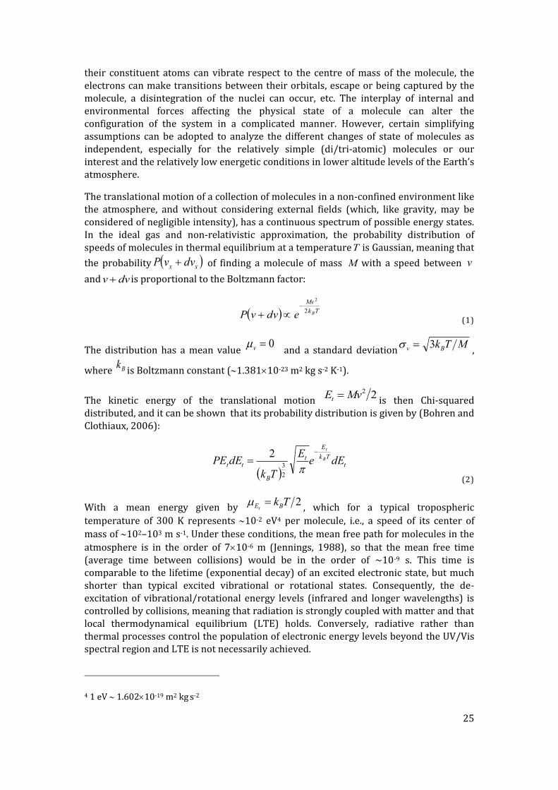
The translational motion of a collection of molecules in a non-confined environment like the atmosphere, and without considering external fields (which, like gravity, may be considered of negligible intensity), has a continuous spectrum of possible energy states. In the ideal gas and non-relativistic approximation, the probability distribution of speeds of molecules in thermal equilibrium at a temperatureT is Gaussian, meaning that
the probability xx dvvP of finding a molecule of mass M with a speed between v
and dvv is proportional to the Boltzmann factor:
Tk
Mv
BedvvP2
2
(1)
The distribution has a mean value 0v and a standard deviation
MTkBv 3,
where Bk is Boltzmann constant (1.38110-23 m2 kg s-2 K-1).
The kinetic energy of the translational motion 22MvEt is then Chi-squared
distributed, and it can be shown that its probability distribution is given by (Bohren and Clothiaux, 2006):
t
Tk
E
t
B
tt dEeE
Tk
dEPE B
t
2
3
2
(2)
With a mean energy given by 2TkBEt
, which for a typical tropospheric
temperature of 300 K represents 10-2 eV4 per molecule, i.e., a speed of its center of
mass of 102–103 m s-1. Under these conditions, the mean free path for molecules in the
atmosphere is in the order of 710-6 m (Jennings, 1988), so that the mean free time (average time between collisions) would be in the order of ~10-9 s. This time is comparable to the lifetime (exponential decay) of an excited electronic state, but much shorter than typical excited vibrational or rotational states. Consequently, the de-excitation of vibrational/rotational energy levels (infrared and longer wavelengths) is controlled by collisions, meaning that radiation is strongly coupled with matter and that local thermodynamical equilibrium (LTE) holds. Conversely, radiative rather than thermal processes control the population of electronic energy levels beyond the UV/Vis spectral region and LTE is not necessarily achieved.
4 1 eV 1.60210-19 m2 kg s-2

26
Due to the difference in mass between electrons and nucleons (protons, neutrons), the motion of the electrons can be considered independent of the motion of the nuclei (Born-Oppenheimer approximation). In this way the internal degrees of freedom correspond to the decoupled electronic, vibrational and rotational motions.
An “order of magnitude” estimate of the energy associated with each of these respective motions can be carried out considering the case of a diatomic molecule for which a
represents the average internuclear distance (Bransden and Joachain, 2003). In this
case, an electron of mass5 em will have a typical momentum of the order of a 6 and a
kinetic energy ee maE2
, where 2h . For a typical internuclear distance of 10-
10 m, this corresponds to a binding energy of the valence electrons of a molecule of 102 eV, i.e., energetic transitions lying in the ultraviolet to visible spectral region.
For the vibrational motion of the nuclei respect to the centre of mass, we can assume a
linear harmonic potential with a frequency N that corresponds to a vibrational energy
of the nuclei of mass NM equal to 222aME NNv , thus for a displacement
comparable to the dissociation radius a , the energy associated with a low mode of
vibration is eNeNv EMmE21
. Given that the ratio of electron to nuclei masses
is in the order of 10-3 to 10-5, the vibrational energy is typically about 2 orders of magnitude smaller than the electronic energy which corresponds to transitions in the
infrared region (1 eV).
A similar reasoning for a diatomic molecule leads to a typical low mode rotational energy around an axis passing by its centre of mass given
by eNer EMmMaE 22 , i.e., the energies associated with rotational transitions lie
in the far infrared to microwave spectral region (10-2–10-4 eV).
The combined effect of rotational, vibrational and electronic transitions constitutes a problem that doesn’t usually admit an analytical solution, and approximations dictated by the specific configuration of the studied system and invariance (symmetry) principles allow retrieving information of the structure and dynamics of molecules from their spectra. The state of the system then requires to be specified by a series of quantum numbers, for instance in Equation (3) below, a spectral “term” contains the contribution from electronical, vibrational and rotational levels represented by corresponding
quantum numbers ( ,...;2,1,0,...;2,1,0 Jv etc.):
)1(21 JJBvEEEEE eeerve (3)
Where eee BE . More complicated expressions including corrective terms are
necessary to account for the effect of “centrifugal distortion” of the rotation or “anharmonicity” in the vibration. An observable spectral line is calculated from the difference of the two terms involved in the transition, according to certain selection
5 1 em 9.10910-31 kg
6 From Heisenberg’s uncertainty relation: 222 papx

27
rules derived from e.g., conservation of angular momentum or change in the dipole moment. The development of this topic is beyond the scope of the work presented in this thesis, and the interested reader can find valuable sources of consultation elsewhere (Bransden and Joachain, 2003; Herzberg, 1950; Sakurai, 1967; Svanberg, 2003).
2.3.1 ELECTROMAGNETIC RADIATION
The external radiation field BE
, is described classically by the electromagnetic
potential A
, through the relations (in the absence of charge sources):
t
trAtrtrE
,,,
trAtrB ,,
(4)
Where E
represents the electric field, B
the magnetic field, the scalar potential, and
A
the vector potential, all of which are functions of space and time tr ,
. BE
, satisfy
the Maxwell equations and it can be shown that A
satisfies the wave equation (Waters, 1993):
0,1
,2
2
2
2
t
trA
ctrA
(5)
Which admits solutions of the form:
trki
eAtrA2
0 Re, (6)
Where ck 2
represents the wave or propagation vector, a frequency-dependent
real phase and
the polarisation vector. A
corresponds to a transverse monochromatic
wave 0
k propagating at the speed of light.
The rate of radiant energy E flow crossing a unit area s
is given by the Poynting vector
trBtrEctrS ,,, 2
0
, where 0 is the permittivity of vacuum (8.854×10⁻¹²
m−3s4kg−1A2). The magnitude of the Poynting vector averaged over one period for a
component of frequency is: 20
2
0
28 AcS
(for incoherent radiation, this
quantity includes the contributions from different waves at all polarizations7 for the
7 Electromagnetic waves are polarized, and the field is fully represented by the polarization matrix, composed of Stokes vectors that describe the total intensity, and the levels of horizontal, vertical and elliptical polarization. In this thesis we refer only to the total intensity, because our instruments are not polarization-sensitive and the radiation from sky is mostly not polarized.

28
different frequency components, which phases cancel out on average). This quantity is
also called spectral irradiance I (or intensity) and its quantum mechanical equivalent is
the photon fluxp , or number N of photons in a volume V that cross a unit of area per
unit of time, both quantities being related by:
pvV
cNhAcI
2
0
2
0
28 (7)
By considering specifically the directionality of the radiation, i.e., the spectral irradiance coming from a direction per unit solid angle , we arrive at the definition of spectral
radiance L or specific intensity, which can be considered as the elementary quantity
defining a radiation beam:
ddsdtd
Ed
d
dIL
coscos
4
(8)
2.3.2 INSTRUMENTAL CONSIDERATIONS
In a spectroscopic measurement setup, the observation intervals for time mt , spectral
resolution m 8, detector area ms , and solid angle m for radiation coming from
direction m with respect to the normal to the detector are pre-determined; thus, the
measurement is directly related to the amount of spectral radiant energy gathered by
the instrument mE :9
m m m mt sm ddsdtdLE
cos
(9)
However, the actual variable recorded by a digital electronic instrument or sensor is
usually a digital numberjiE ,* (for a detector i in band j ) which is connected to the
spectral radiant energy by an instrumental measurement equation of the type (Butler et al., 2005):
jimjiji ERE,,,* (10)
8 This resolution refers to the full-width-at-half-maximum (FWHM) of the response of the spectrometer to monochromatic radiation at the given frequency. A more appropriate factor to
quantify the resolution of a spectral apparatus is the resolving power, defined as for
radiation at wavelength and line separation .
9 For a system immersed in a medium with an index of refraction mn the so called étendue
mmmm sn cos2
is an invariant, and therefore the quantity 2
mnL is conserved in a non-
absorbing medium.

29
Where jiR ,represents the total responsitivity of the sensor which includes the effects of
detector spectral, spatial, temporal and polarization responsitivities, amplification and digitalization gains, transmittance or reflectance of optical elements, slit transmission function, etc. The measurement equation guides the characterization, calibration and uncertainty analysis of the measurements (Datla and Parr, 2005). For calibration purposes, for instance, a radiometric calibration implies the comparison of an unknown spectral radiance with a standard source, like a tunable laser source or an approximate
blackbody source, for which the spectral radiance BB
L at an equilibrium temperature
T is given by the expression:
1
122
3
Tk
h
B
BB
ec
hvTL
(11)
Although radiometric calibration is an important and sometimes necessary step for remote sensing applications, in some cases only relative measurements, where the ratio of two measured signals with unknown absolute spectral radiance is taken, is enough. This is the case considered in this work.
The frequency/wavelength scale should also be calibrated in a spectrometer, for which a source with known features is usually used, for example the so-called Fraunhofer lines in a solar spectrum or the emission lines of an inert gas like Hg or Xe, or a laser comb. For the UV spectrometers used in this work, a solar and a Hg-lamp methods were used for frequency calibration. For the IR interferometer, an internal laser source is used for precise frequency calibration.
The slit function represents the spectral resolution of a spectrometer, because it corresponds to the response of the spectrometer to a spectral feature that is narrower than the slit of a dispersive instrument. The same low pressure Hg-lamp spectrum used for frequency calibration of the UV spectrometers was used for characterizing the slit function at a wavelength of 302.1495 nm10, which lies close to the spectral region of interest for spectroscopy of SO2. This characterization makes the assumption that the same slit function applies to all wavelengths, but wavelength-invariance is not common because of the angular dependency of the dispersive mechanism of the spectrometers. For the FTIR method, the resolution is determined by factors like the entrance aperture and path-difference of the arms of the interferometer, which is considered in more detail in the respective section.
No measurement is exempt from noise either due to fundamental reasons (like quantum fluctuations) or due to effects introduced by each section of the instrument upon the incoming signal that can be reduced or characterized but usually not eliminated. If we limit the discussion of these effects to what happens at the detector itself, the most important sources of noise can be classified as those due to the incoming signal
10 Corresponding to a transition from the 44042.977 cm-1 (J=2) to the 77129.535 cm-1 (J=3)
electronic energy levels in air(Kurucz, R.L. and Bell, B., 1995. Atomic Line Data. Smithsonian
Astrophysical Laboratory.)

30
(photon/shot/background noise) and those debt to the electronics of photodetection (thermal/Johnson-Nyquist noise, amplification noise, read-out noise, digitalization noise). In the thermal infrared region the background signal is relatively important, while in the UV/Vis the photon noise is more significant. The ratio of the radiant power of the signal to be measured to the power measured when no external signal is present
defines the signal-to-noise ratio NS . When this ratio is equal to unity, the signal is
called the noise-equivalent-powerNEP , i.e., the power of a signal that equals 1 root-
mean-square (rms) of the fluctuating noise signal. For a detector with a quantum
efficiency of photoelectrons per incident photon, a signal of radiant power sP will
induce a current given by hePi ss , where e represents the electron’s charge11. In
this case, it can be shown (Kingston, 1995) that the mean square noise current is given
by inNBbsn RfTkhfPPei 42 22 , where the first term contains the
contribution from a signal dependent ( sP ) and background dependent ( bP ) noise, and
the second term the contribution of the equivalent noise temperature NT and input
resistance inR of the detector with electrical bandwidth f . Thus, the total NS can be
expressed as:
in
Nbs
s
R
fkT
e
hfhPfhP
P
N
S
4222
(12)
If a detector array is used, and additional detector noise term due to read-out should be added, which is proportional to the number of elements in the array.
Another important figure of merit of a detector is the specific
detectivity NEPfSD * , which introduces the effect of the size of the detector S in
the detectivity and it is therefore a useful quantity for comparison of different detectors.
2.3.3 ATMOSPHERIC MOLECULES AND RADIATION
The motion of the particles (nuclei and electrons) constituting a molecule is described
by the wavefunctions n
that depend on the coordinates of all the particles, and that
satisfy, in the non-relativistic case, the Schrödinger equation:
ii EH
ˆˆ (13)
Where ,...2,1i , VTH ˆˆˆ is the Hamiltonian (with kinetic T̂ and potential V̂ energy
operator terms) and tiE ˆ is the energy operator. The representation of the
system is done in terms of any appropriate observable quantity but not simultaneously
11 e 1.60210-19 C
31
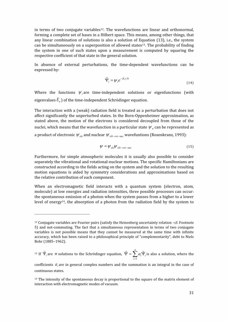
in terms of two conjugate variables12. The wavefunctions are linear and orthonormal, forming a complete set of bases in a Hilbert space. This means, among other things, that any linear combination of solutions is also a solution of Equation (13), i.e., the system can be simultaneously on a superposition of allowed states13. The probability of finding the system in one of such states upon a measurement is computed by squaring the respective coefficient of that state in the general solution.
In absence of external perturbations, the time-dependent wavefunctions can be expressed by:
tiE
iiie
(14)
Where the functions i are time-independent solutions or eigenfunctions (with
eigenvalues nE ) of the time-independent Schrödinger equation.
The interaction with a (weak) radiation field is treated as a perturbation that does not affect significantly the unperturbed states. In the Born-Oppenheimer approximation, as stated above, the motion of the electrons is considered decoupled from those of the
nuclei, which means that the wavefunction in a particular state n can be represented as
a product of electronic ele and nuclear nucrotvib wavefuntions (Rosenkranz, 1993):
nucrotvibele (15)
Furthermore, for simple atmospheric molecules it is usually also possible to consider separately the vibrational and rotational-nuclear motions. The specific Hamiltonians are constructed according to the fields acting on the system and the solution to the resulting motion equations is aided by symmetry considerations and approximations based on the relative contribution of each component.
When an electromagnetic field interacts with a quantum system (electron, atom, molecule) at low energies and radiation intensities, three possible processes can occur: the spontaneous emission of a photon when the system passes from a higher to a lower level of energy14, the absorption of a photon from the radiation field by the system to
12 Conjugate variables are Fourier pairs (satisfy the Heisenberg uncertainty relation –cf. Footnote 5) and not-commuting. The fact that a simultaneous representation in terms of two conjugate variables is not possible means that they cannot be measured at the same time with infinite accuracy, which has been raised to a philosophical principle of “complementarity”, debt to Niels Bohr (1885–1962).
13 If i
are n solutions to the Schrödinger equation, i
n
i
ia
1
is also a solution, where the
coefficients ia are in general complex numbers and the summation is an integral in the case of
continuous states.
14 The intensity of the spontaneous decay is proportional to the square of the matrix element of interaction with electromagnetic modes of vacuum.

32
make the transition from a lower to a higher level of energy and the stimulated emission of a photon by the system under the influence of the radiation field.
Following Waters (Waters, 1993), the probability per unit time of radiation within a solid angle 15 and frequency interval inducing a transition between two states
( 2E > 1E ) is proportional to its energy density (this is Einstein’s postulate that leads to
the coefficients for absorption and stimulated emission). In terms of the specific intensity, such probability is denoted:
tbLBPi 121221 , (16)
Whereas, the probability per unit time for a photon to be spontaneously emitted in time
t in direction within at a frequency is given by:
tbAPs 122112 ,4
1 (17)
Where 12B and 21A are the Einstein’s coefficients for absorption and stimulated
emission 212121 BgBg and spontaneous emission 213
3
21
8B
c
hA
, respectively; and,
12,b is the line-shape function for the transition, which expresses the fact that
monochromatic transitions cannot occur because of the nonzero probability of transitions given by Heinsenberg’s uncertainty relation, pressure broadening due to collisions with other molecules and atoms in the gas phase or phonons in the condensed phase, and thermal Doppler effect (Svanberg, 2003)16.
15 In direction , so that the factor cos is implied.
16 The resulting shape of the natural (uncertainty) and pressure broadening is Lorentzian:
4
222
0
b with a characteristic linewidth 2 , being the decay time;
whereas, for thermal broadening is Gaussian: with a
2
202ln4
2ln4Deb D
with
linewidth M
Tk
c
BD
2ln22 0

33
The net energy change 2,1
E in the radiation field within and in time t due to
the transition of a collection of 1n molecules per unit of volume in state 1 and 2n
molecules per unit of volume in state 2 within a volume V is given by17:
21122,1 EEE
VhPnPPn iis 21112122
VtL
2112
(18)
Where:
1221
212 ,412
bhA
LBn
12121 ,21
bhBn (19)
Using the definition of specific intensity, its rate of change with distance can be denoted:
Ldl
dL2112
12
(20)
Where the first term correspond to pure emission and the second to pure absorption of radiation. Equation (21) can also be expressed as:
LJdl
dL 2112
12
(21)
Which is the differential radiative transfer equation (DRTE)18, where:
12
21
12121
12 ,1 hvbgn
gnBn
(22)
Is the net absorption coefficient (absorption minus stimulated emission), and:
17 The mean number density of molecules ln in state l at thermal equilibrium is related to the
total number density n by: TQeg
nnTkE
ll
Bl
, where lg are the degeneracy of state l and
j
TkE
jBjegTQ is the partition function.
18 For more than two non-coherent possible transitions, the DRTE should include all the
contributions from individual transitions: ul
ulul LJdl
dL

34
112
21
1
21
gn
gn
eLJ
Tk
hv
B
BB (23)
Is the net emission coefficient or source function (equal to the blackbody function BB
L in
thermodynamic equilibrium).
Since the coefficient 12B corresponds to a probability of transition, it can be shown that
it is proportional to the square of the dipole operator
12M along direction . Thus, the
total absorption coefficient is given by19:
2
1212
12
21
3
0
,)(3
8
4
121 Mbeegg
ThcQn
TkETkE BB (24)
Defining the optical depth from distance l to L as:
L
ldllLl '', (25)
The DRTE becomes:
LJ
d
dL (26)
And after integration, the integral radiative transfer equation (IRTE) is:
deJeLLLL
LlL
,0
0
,,00
LLeJeL
,0,010
(27)
Where:
dedeJJL
LlL
Ll
,0
0
,,0
0
,.
In a typical absorption experiment, the difference between intensities at a spectral line
peak [ L,012 ] and at a nearby frequency [ 0
12L 0L ] where negligible absorption
occurs [ 0,0 L ] is calculated, leading to:
LeLJLLLLL,0
12
1212100
(28)
19 The last factor in Equation 24 can be extended to include besides electronic, also vibrational and rotational transition matrix elements, the so-called Franck-Condon (vibrational) and Hönl-London (rotational) factors, which represent the level of overlapping of vibrational or rotational wavefunctions of the states associated with the transition

35
If LL12 <0, the line is observed in absorption [ J < 0L ]; if LL
12 >0, the line is
observed in emission [ J > 0L ]; and, if 012
LL , the line is not observable
[ J = 0L ].
The optical depth of the transition can be readily calculated from Equation (28):
JLL
JLL
12
0ln,012 (29)
Equation (29) is a general expression for the so-called Bouguer-Beer-Lambert equation, which constitutes the basis for analysis by absorption spectroscopy.
Equation (27) was derived from microscopic considerations, but considering large scale radiation transport, density fluctuations add the effects of scattering (single, multiple and reflection in the surface). These are “source” terms that should be added to the RTE in plane-parallel (slab) geometry:
sfLdlLlp
lTlJllLl
dl
dL
'',,
4,
4
(30)
Where the first term on the right represents extinction characterized by the extinction
coefficient lll (the sum of scattering l and absorption l
coefficients); the second term represents thermal emission; the third term represents
multiple scattering, depending on the phase function ,lp , where is the scattering
angle; and the last term represents surface emission. To solve this equation, a given geometry, boundary conditions and the source function (thermal, scattering, reflection), should be specified and adjusted iteratively. Equation (30) does not include explicitly the contribution of “inelastic” Raman scattering, which is thought to be the cause of the so-called “Ring effect”, a filling-in of molecular absorption structures that can be as large as the typical absorption of trace gases, especially for large solar zenith angles ( sza )
The most important scattering processes in atmospheric spectroscopy in the optical region are debt to density fluctuations of particles much smaller than the wavelength of the radiation, as it is the case of molecules for optical wavelengths. This is called Rayleigh scattering. Another scattering process is debt to the interaction of radiation with particles comparable or bigger than the wavelengths, which is called Mie scattering for the case of spherical particles. These processes are conservative, in the sense that the radiation field does not transfer energy to the matter. Non-conservative processes also occur, as it is the case of Raman scattering20.
20 The term Rayleigh scattering sometimes includes the conservative component, called Cabannes line, and the series of higher or lower frequencies caused by rotational or vibrational scattering, called the Stokes and anti-Stokes lines (Young, A.T., 1982. Rayleigh scattering. Physics Today, 35(1): 42-48.)

36
The Mie scattering cross section are derived analytically by solving Maxwell equations in spherical coordinates through separation of variables, expanding the incident field in spherical harmonics and matching continuity in the boundary. For distances much larger than the wavelength of the radiation (i.e., in the far field), the Mie extinction
M and scattering M cross sections are given by:
1'
''2Re1'2
2
n
nnM bank
(31)
1'
2
'
2
'21'2
2
n
nnM bank
Where 2k is the radiation wavenumber and '' , nn ba are complex expressions
involving spherical functions of the parameter mka , being m the relative (complex)
refractive index (index of refraction and absorption coefficient of the particle relative to the index of the medium), and a the radius of the scatterer (Hansen and Travis, 1974).
In the limit kam << 1, i.e., for wavelengths much larger than the size of the scatterers,
the Rayleigh scattering cross section for molecules is obtained:
4 R
(32)
Equation (32) shows the strong dependency on frequency (wavelength) of the radiation. This is the reason why scattering is dominant in the shorter wavelengths producing effects like the blueness of the daylight or the redness of the twilight. By the same token, considering that the orientation of molecules plays a role in the coupling with the incident radiation field (polarizability), the effect of rotation or vibration alters the polarizability giving rise to the non-conservative Stokes and anti-Stokes lines of Raman scattering.
The dependency of the Mie scattering cross section M on frequency is complex but for
a collection of particles can be approximated by a polynomial of low order (i.e., 2,...,0 ,
explaining the whiteness of the clouds). The angular distribution of Mie scattering usually is characterized by a very peaked forward scattering component, whereas for Rayleigh scattering the angular scattering diagram is symmetric respect to the incident radiation (Bohren and Huffman, 1998; Thomas and Stammes, 1999). Although varying over a relatively large range, typical molecular cross sections for absorption in optical wavelengths are in the order of 10-18 cm2, whereas Rayleigh scattering cross sections are in the order of 10-26 cm2, Raman scattering in the order of 10-29 cm2, and Mie scattering in the order of 10-26-10-8 cm2 (Svanberg, 2003).

37
3 MEASUREMENT TECHNIQUES AND OBSERVATIONS
The work presented in this document has been done with two remote sensing techniques: Differential Optical Absorption Spectroscopy (DOAS) and Fourier Transform Infra-Red (FTIR) spectroscopy. The following sections describe these methods in more detail.
3.1 SPECTROSCOPIC REMOTE SENSING INVERSION
Every spectroscopic remote sensing measurement constitutes an inversion problem: the objective is to retrieve certain variables and parameters defining the physical state of the observed system from the observed effects. Thus, the inversion includes a forward model, reflecting the knowledge of the system (variables and parameters), and the errors present in the measurement. In the case of this work, the observed effect is the measured spectrum, and the variables to retrieve are the column densities of trace gases in the atmosphere. The retrieval procedure is iterative: from an initial guess of the variables and parameters, a model spectrum is calculated and compared with the measured spectrum. The comparison is done through a function and the iterations proceed to minimize such function by varying the values of the variables and parameters until an acceptable value is achieved. If the iteration converges, the retrieved values and the residual (difference between final modeled and measured spectra) determine the results of the measurement. The iterative or fitting function can be for instance a least-squares norm. The sum of squares of the normalized residuals should follow a Chi-square distribution if the residuals are effectively random, reflecting only the noise in the measurement. For non-linear minimizing functions, a common method is the Levenberg-Marquardt iterative algorithm (Levenberg, 1944; Marquardt, 1963), which is a combination of a gradient and a Gauss-Newton method. Another algorithm widely used in atmospheric sounding inversion is the Optimal Estimation Method, based on a Bayesian approach (Rodgers, 2000).
The whole process or passive remote sensing of molecules by spectroscopy can be described in the following steps (e.g., (Wenig et al., 2005)):
1) Radiation is emitted from a source. If this is the sun, it has emission characteristics that can be approximated by a blackbody source function at an effective temperature of 5778 K. The spectrum is not smooth, but has structures from absorption of atoms and molecules in the solar atmosphere, known as Fraunhofer lines. In the UV the spectrum has a variability of about 1%, and lower in the IR; the spectrum also varies along the radius of the solar disc, an effect known as “limb darkening”, due to the heterogeneous density distribution of the sun.
2) Radiation enters the atmosphere and it undergoes extinction, including both absorption by gases and Rayleigh, Mie or Raman scattering. These effects depend on the vertical and horizontal structure of the atmosphere in terms of composition, temperature, pressure and cloudiness. Any “polluting” cloud, like a volcanic plume also exerts an effect on the radiation transport.
3) The radiation is collected and analyzed by an instrument. In the front-end the transfer optics couples with the radiation field at a given direction (solid angle) and
38
transmits it to the spectral analyzing component, either a dispersive element like a prism, grating or beamsplitter, or a non-dispersive filter. The radiation is then detected by a sensor, amplified and digitalized. Co-adding several spectra in order to improve the
NS is usually performed in the instrument.
4) The digital spectrum is analyzed. This analysis usually corresponds to an inversion, as discussed before. Some correction measures, like offset/dark current subtraction, co-averaging of multiple spectra, or discarding over-attenuated or saturated spectra, are normally performed before the actual analysis. The forward model should include parameters that are known, e.g., instrumental characteristics, high-resolution spectra of absorbing molecules, and parameters to retrieve, like the slant column densities of gases, as well as irreducible errors. The results are obtained from the inversion procedure. These depend on the specific problem, but include both the retrieved parameters and their associated uncertainties.
The specific procedures for DOAS and FTIR are discussed in the next sections.

39
3.2 DOAS
Differential Optical Absorption Spectroscopy (Platt and Stutz, 2008) is a spectrometric analysis method for the quantification of trace gases concentrations based on the principles of absorption spectroscopy (Bouguer-Beer-Lambert law). A broad-band absorption spectrum can always be modeled as a signal that has “high frequency” and “low frequency” components, where the dividing criterion or cut-off frequency is determined by the characteristics of the spectrum itself and the spectral range and resolving power of the instrument. The high frequency or “differential” absorption signatures are related principally to the absorption structure of the spectra, whereas the lower frequency components typically correspond to broad-band absorption, scattering and instrumental effects (like the transmission of optical components).
According to the 4-step scheme presented above, a measured solar spectrum is the product of the following transformations:
1) The direct solar beam is not used in the passive DOAS method used in the field studies reported in this work. DOAS has been used in direct solar/lunar/star mode in other circumstances (Herman et al., 2009), and of course, active DOAS has been used with different sorts of sources like LEDs or Xe lamps (Kern et al., 2006; Platt and Stutz, 2008). The solar spectrum is however the “driving” source of the scattered spectrum that is measured and its known structure is caused of various effects, including the “I0-effect” (Platt and Stutz, 2008) of highly structured features that cannot be resolved by low-resolution spectrometers and that show up as pseudo absorbers in the DOAS methods; also the amount of “Ring-effect” (Chance and Spurr, 1997; Vountas et al., 1998) or filling-in of molecular absorption structures caused by rotational, and to a lower extent also vibrational, Raman scattering is scaled with the intensity of the solar beam. On the other hand, the known structure of the Fraunhofer lines can be used as a marker for self-calibration of the wavelength scale of the spectra (van Geffen and van Oss, 2003).

40
Figure 3. Section of the UV solar flux (irradiance) spectrum (Kurucz et al., 1984) between 296 and 440 nm.
The spectrum in gray was measured with a Fourier transform spectrometer at a resolving power of 5105 (at the central wavelength). The spectrum in red is a smoothed version at 1% resolution, similar to what would be measured by the UV spectrometers used for volcanic gas measurements. The structures in the
spectrum can be used as stable markers for wavelength calibration of the measurements
2) For diffuse radiation in the near UV spectral region, the leading terms in the RTE (Equation 30) correspond to extinction and multiple scattering, since emission is negligible at atmospheric temperatures and surface reflectivity is usually low for most soil types. The spectrum measured at surface then reduces to:
'',,4 4
dlLlpl
lLldl
dL
(33)
Which formal solution in terms of total optical depth L
ldllLl '', , single
scattering albedo llla and the factor cosu (correcting for vertical
component), can be represented by:
''
'',',''4
',0,
0
'
4d
u
edLp
aeLL
u
(34)

41
In fact, this radiance has a direct solar component sL and a diffuse component
dL . The
measurements we are interested in contain only the latter term, however, the direct component is inherently included in the scattering term. The measured radiance then can be expressed as:
0
''
4
''
0
'
''
0 4
''
'',','4
'
''
,'4
',0
''
'','',','4
',0
,
du
edLp
a
du
eeFp
aeL
du
edLLp
aeL
L
ud
uussud
udsud
d
s
(35)
Where sF is the extraterrestrial solar irradiance or flux. Equation (35) indicates that the radiance reaching the sensor at surface is the contribution from the diffuse radiance on top of the medium attenuated by extinction plus the direct solar radiance attenuated by extinction, single-scattered to the detector and further attenuated by extinction, plus the diffuse radiance multiply scattered and attenuated by extinction towards the sensor. If the single scattering albedo is small, the contribution from multiple scattering is minor
and may be neglected. Furthermore, the overlaying radiance ,0dL may be
considered null for a sensor at the surface in the single scattering approximation, since the scattering events that produce this term occur in the upwelling direction. Modeling of this radiation field from first principles require advanced computational programs that divides the atmosphere in layers with specific geometry and properties like composition, pressure, temperature, number density, scattering and absorption cross sections, single scattering albedo, the position of the sun with respect to the sensor, and polarization corrections (Hansen and Travis, 1974; Thomas and Stammes, 1999). The actual solution to the problem can be found by different approaches, for instance by Monte Carlo simulation of photonic trajectories (Kern et al., 2010).
For a single-scattering Rayleigh atmosphere, the incoming radiance reaching the surface is represented by:
uu
s
ss
R
s
x
d eeuu
up
aFL
s
4
,
(36)
This expression indicates that radiation detected at the surface is a function of solar zenith angle and observation angle and its origin is distributed along the line of sight at different altitudes. If an absorbing layer, like a volcanic plume, is present at certain altitude, only the radiation above the layer is further attenuated by the plume, whereas the radiation originated below the layer does not contain absorption features and therefore “dilutes” the effect of absorption. Representing the radiation above and below
the layer by abovedL , and below
dL , , respectively, the total radiance is expressed by:
,,, ,,,, belowbelow
damf
aboveaboved
x
d LeLL xv
(37)
42
Where VCDSCDvvndssnamfvs
xv
x )()( is the air-mass factor relating
the slant optical depth x
to the vertical optical depth xv , and which is equivalent to
the ratio of the slant column density SCD to the vertical column densityVCD when the
extinction inside the plume is independent on the optical path ( lxx ).
Note that from equation (37) the xVCD is equal to:
amf
LL
L
dvvnVCDx
belowbelowd
x
d
aboveaboved
vx
,,
,ln
,,
,,
(38)
If the radiation below the plume can be neglected, by combining two spectra from directions towards and outside ' the plume, the column is obtained from:
amf
L
L
VCDx
x
d
d
x
,
','ln
(39)
This approximation is not always accurate, since the component of foreground radiation may be significant at large instrument-plume distances.
3) The measured spectra are altered by the optics, spectral dispersion, detection, and digitalization. The optical elements usually modify the incident field by a slowly varying
transmission function n
i
iTT )( incorporating the functions of each optical
element.
The spectrometer response is characterized by the instrumental line-shape ( ILS )
function, which in the case of a grating spectrometer depends on the optical resolution given by the order of dispersion q and the number of lines illuminated in the grating z by
the relation qz1 , as well as on the line-spread-function (imperfect imaging of
the slit caused by the optics). The convolution of both functions defines the ILS which
on the spectrometers used for DOAS measurements depends on wavelength and it is determined by measuring the lines of a spectrum of a low-pressure Hg lamp, as represented in Figure 4.

43
Figure 4. Example of ILS used for calibration of DOAS instruments, corresponding to the
302.15 nm emission line of Hg at low pressure. The FWHM is about 0.6 nm
The detector of the UV spectrometers is a CCD array of 2048 elements for a typical spectral range of 150 nm (~270-420 nm). The detector is not inherently sensitive to UV radiation, but rather makes use of a shorter wavelength sensitive fluorescent coating. Coupled to the detector is the amplification, digitalization (12 bits for the spectrometers used) and linearity correction systems. It is noteworthy that for an array detector there
is an inter-pixel variation in responsitivity R . Furthermore, the effects of stray light,
detection, digitalization, etc. produce offset and dark current on top of the photon-
statistics noise. The noise is thus composed of systematic instrumental effects sN and
random photon noise rN . The spectrum upon these processes is a vector of discrete
spectral elements represented by:
rs
t s
t sNN
ddsdtd
ddsdtdILSLTRL
m m m m
m m m m
cos
cos
(40)
The relation between the pixel position and the wavelength spectral element is
established via calibration, by fitting a (quasi-linear) third order polynomial. In laboratory tests, a Hg lamp spectrum was also used for this purpose, but in the field, the position of the Fraunhofer lines in the solar spectrum can be used instead. This relation

44
may vary due to thermal stress or other causes, and therefore wavelength-pixel shift and squeeze operations are usually necessary to correct for these effects.
4) Once the spectrum has been recorded, the NS can be improved by averaging a
number of spectra, since this procedure will increase this ratio as the square-root of the number of averaged spectra. Noise reduction is then applied. The ultimate source of noise in the UV should be linked to the statistics of radiation detection (shot or photon noise which is a Poisson-like process), thus dark current and offset, as well as digitalization noise (due to truncation/round-off in the quantization), and inter-pixel variability should be properly subtracted. Dark current can be modeled by measuring a spectrum with the optics unexposed to external radiation, offset is usually taken from permanently blocked pixels in the spectrometer, the digitalization noise and inter-pixel variability can be measured in the laboratory. These effects are usually dependent on temperature and even the intensity of measured radiation. In the measurements here reported, a first order noise cancellation was performed by a simple subtraction of a dark spectrum taken under non-illuminated conditions. Inter-pixel variability and digitalization noise can be cancelled by taking the ratio of spectra taken under similar conditions and in close time proximity.
The next step consists in trying to reproduce the observed spectrum by a model and
from the comparison of the model ,,bxf with the measurement y
derive certain
unknown variables x
and a-priori parameters b
and errors
, most importantly; in this
case, the slant column densities SCDof atmospheric trace gases. The retrieved SCD are those that minimize an appropriate measure of the fitting, for instance the least squares norm:
2
,,min,,min
n
ii
iiii bxfybxfy
(41)
Where n represents the number of spectral elements or channels used in the fitting. The
DOAS inversion usually takes as the measurement the optical depth calculated from equation (38) and its model approximates the slowly varying part of the optical depth by a low order (usually 5) polynomial and the rapidly varying part by a weighted sum of absorption cross sections of the expected molecules present in the spectral range of analysis. The weights of the sum are the SCD . The implementation of this algorithm can
incorporate absolute or differential (high-pass filtered) cross sections. In the latter case, the same filter should be applied to the measured optical depth. The solution is found iteratively until a value under a threshold (e.g., 10-4) is reached for the norm or until a maximum number of iterations (e.g., 5000) have been performed. Once a solution is found, the residual (difference between measured and model functions) is scaled to absorption optical depth of the gas of interest to estimate the uncertainty of the retrieval. The minimizing function takes then the form:
2
10
2
,
'','lnminmin
n
ii
q
kikk
p
j
ij
ji
s
ixi
i
s
in
ii
ximodel
ximeas SCDc
NL
NL
(42)

45
It is important to emphasize that the ratio of two measured radiances cancels out most
of the common instrumental effects and that usually is
i
s NN ' . Moreover, the major
asset of DOAS consists in separating high and low frequency components of the optical depth. If the measurement is done under non-ideal conditions, the ratio of radiances taken at different directions would include a complicated function of different variables: the optical depths, single scattering albedoes, phase functions, and directions of observation and of solar position for both measurements. This ratio would not give directly the differential optical depth of the target cloud, but if the terms related to scattering have low variation with wavelength, the DOAS algorithm can effectively separate the effects of absorption from scattering.
For an ideal retrieval, the minimized function should converge to the variance 2 of the
measurement (related to the random error in measured radiance):
2
2
1minx
n
ii
ximodel
ximeas n
(43)
The uncertainty in the retrievedjVCD of a component j is calculated from:
jj
x
jVCDamf
(44)
Where denotes the plume extinction coefficient for absorption spectroscopy or the
plume (differential) absorption coefficient for differential absorption spectroscopy. An example of a DOAS evaluation for the measurement of BrO and SO2 from a volcanic plume is shown in Figure 5.

46
Figure 5. Example of a DOAS evaluation performed in the wavelength range of
330.6-352.75 nm, including BrO, SO2, O4, O3, NO2 and CH2O, Ring(2), offset, and DOAS polynomial. The red lines show the fit, the blue line the measurement data. A reference
spectrum and two Ring spectra were included in the DOAS fit. Every box in the figure shows the optical depth after successive subtraction of the retrieved optical depth of each of the species
included in the model (From Lûbcke et al., in preparation)

47
3.2.1 DOAS MEASUREMENTS OF VOLCANIC GAS EMISSION RATES
A particular DOAS measurement provides the VCD of the absorbers of interest in the
plume. The estimate of the total emission rate of the measured gas requires integrating these measurements and multiplying the product with the transport velocity of the fluid. This problem can be analyzed from the perspective of mass conservation in a box enclosing the volcano and surrounded by a surface defined by the scanning path of the DOAS sensor, as sketched in Figure 6.
Figure 6. Schematics representing mass conservation in a box to derive the emission rate of a volcanic gas from scanning DOAS measurements . The surface integral of the gas number density
multiplied by the normal wind speed, plus any accumulation in the volume, equal the volumetric source and sink strengths
According to the mass conservation equation, obtained as the zeroth velocity moment of the Boltzmann transport equation neglecting body forces (e.g., gravity), the total time
derivative of the mass density of a speciesj , equals the net rate of production per
volume of the species, i.e., the difference between volumetric rate sources jq and
sinksjp :
jjj
jjpqj
tdt
d
(45)
Where the current density dif
j
adv
jj jjj
is the sum of and advective term
jj
adv
j cj
( jc
is the advective transport velocity) and a diffusive term

48
jjj
dif
j DKj
(jK is the turbulent mass diffusion coefficient and
jD is the
molecular diffusion coefficient). Integrating this equation in a volume enclosing the source gives:
jy
jxjjjxjjjj
jjy
S
jjjz
jj
j
vjj
S
j
V
j
V
jj
PSDKdyVCDcmmQ
PQSdDKdydzct
m
dVpqSdjdVt
dVdt
d
dt
dm
(46)
Where the Stokes theorem has been used to transform volume V to surface S integrals
and a Cartesian system of coordinates has been used with x pointing in the
longitudinal, y in the transversal and z in the vertical directions. Equation (46) states
that the net rate of production or source strength of a gas species jQ is equal to the sum
of the rate of accumulation of the material inside the volume jm , the advective
y jxjj dyVCDcm and diffusive SDK jxjj fluxes across the surfaces of the
volume, and the net rate of destruction or sink strength of the speciesjP . Ground-based
remote sensing measures the advective term to estimate the source strength of volcanic emission, thus the approximation is better if diffusion, accumulation and sinks are either unimportant or properly accounted for.
The observation volume is naturally defined by the scanning planes of the instruments, which in some cases have complete azimuthal coverage of the volcanic plumes. From below the volume is bounded by the ground, and from above it may not be bounded (although conical scanning geometries may indeed enclose the sources also from above) but generally emissions at high, e.g., stratospheric altitudes, would not be accurately measured by typical instrumental DOAS networks. The advection is controlled by the local wind fields and determine one or more (in the case of crosswinds) prevalent directions. This term usually predominates over diffusion, and thus the main role of the diffusive flux is spreading the plume in the transverse directions. The source strength for a species like SO2 is generally dominated by crater plume emissions, since fumarolic and flank emissions are usually negligible in comparison, although flank emissions may be important for species like CO2 at some volcanoes (Allard et al., 1991). Another possible source of SO2 is chemical reactions, especially the oxidation chain of H2S. Accumulation inside the volume may be caused by processes like deposition or stagnant local wind fields. Different sink processes may be present, including chemical reactions, adsorption and solution in wet (e.g., sulfuric acid aerosols) or dry (e.g., tephra) surfaces, or dilution to a concentration below the limit of detection of the method. The presence and magnitude of each of these terms depends on various factors like the volcanic activity and composition of emissions, the local meteorological conditions, the surrounding topography, and the observation conditions (distance to crater, distance to plume, and scanning geometry).
The role of diffusive transport is important. In the longitudinal direction it tends to smooth out or spatially expand the heterogeneities in concentration and adds a component of transport that, under certain circumstances, can represent a considerable

49
fraction of the total mass transport. In the transversal direction, on the other hand, diffusion expands the plume dimensions and in this way dilutes the concentration, which affects the limit of detection. The lateral spread is determined by the magnitude of the gradient of concentration and the diffusivity, which in turn depends on atmospheric conditions. Naturally, the plume width increases by diffusion with distance from the source, and this effect can be used to estimate approximately the total transport speed if the diffusivity, which is dependent usually on altitude and atmospheric stability, is
properly constrained. The basic idea is that by measuring the width of the plume y at
its mean altitude z and by estimating the transport time ppp cdt of the plume (
pd is
the distance travelled from the source), the plume transport speed pc can be calculated
from values of the diffusivity at that altitude zK y:
2zy
dzKc
c
dzKtzKzy
py
p
p
p
ypy
(47)
3.2.2 SCANNING-DOAS
The introduction of the mini-DOAS instrument for volcanic gas studies arguably represented the most important innovation in remote sensing technology since the establishment of the COSPEC as a standard in this field (Galle et al., 2003). It also motivated the development of other techniques like the SO2 cameras and the refinement of spectroscopic analytical procedures that allow the identification of other species in volcanic plumes (Bobrowski et al., 2003) and the reduction of certain source of uncertainty in the measurements like radiation transport or plume velocity (Johansson et al., 2009).
The scanning DOAS is a double channel multi-axis (MAX) DOAS instrument (Hönninger et al., 2004). It consists of a flat or conical scanning UV telescope connected to a double grating spectrometer via two slightly off-focused optical fibres. Alternatively, a single-beam configuration has one channel and an in-focus optical fibre. The spectrometer and the driving, recording and transmitting electronics is housed at a distance from the scanning head for protection and versatility of installation. Time and position is determined with a GPS antenna and the temperature inside the box is measured by a small IC sensor. The spectral, GPS and thermal data is integrated and recorded in an internal memory or transmitted via a radio-link. Remote instrumental control and data analysis is done with the “NovacProgram” software. Details of the instrumentation and software can be found in (Galle et al., 2010; Johansson, 2009).
The scanner is common to the two channels, which are used for zenith-looking observations at slightly different directions along the plume axis. The obtained gas time series are similar but shifted in proportion to the plume speed in the direction of

50
observation21. The cross-correlation of the signals provides the best time shift, which combined with the spatial separation of the simultaneous sections of the plume seen by the two channels (dependent on the distance to the plume and the constant angular separation of the field of views), provides the mean transport speed along the observed axis. Figure 7 shows a sketch of the principle of measurement and data obtained from its application to a real volcanic plume.
02:10 02:15 02:20 02:25 02:30
0
100
200
300
400
Time lag = 86 s
Distance to plume = 4000 m
Angular separation = 80 mrad
Plume speed = 3.7 m s-1
SO
2 d
iffe
rential colu
mn d
ensity / p
pm
*m
Time UTC / hh:mm
Upwind
Downwind
Figure 7. The plume speed is measured by placing the instrument under the centre of the plume with one spectrometer looking further upwind than the other (Johansson et al., 2009). The plot shows a measurement at Karymsky volcano (Kamchatka) on 19 July 2012. The plume was at a
distance of about 4000 m, the angular separation of the two lines of sight was 80 mrad and the optimal time lag in the two series was 86 s. The retrieved plume speed was 3.7 m s -1
The calculation of the flux across a surface by scanning DOAS involves a series of steps on each scan:
1. A “clear background” or “sky” spectrum is measured, typically at zenith scanning position. All spectra in the same scan are divided by this spectrum to derive the differential column densities. If the target species is present in the sky spectrum, an
21 Assuming that non-periodical heterogeneities in the gas column densities are present. Such variations may be caused by inhomogeneous emission rates, eddies, meandering or fluctuations in wind speed. Typical variations in the observed column densities can be as large as 50%.

51
offset level is calculated from the measurements with lower (ideally null) gas column densities. Alternatively, a sky spectrum can be modeled or adapted from a measurement with the same or other instrument.
2. A “dark-offset” spectrum is measured, typically by pointing the scanner to the nadir position, which is shielded from incoming radiation. This spectrum is subtracted from each other spectrum in the same scan to give an approximate correction of dark current and electronic offset. Alternatively, the dark-offset spectrum can be modeled from independent measurements of dark current (no illumination at high exposure time, low number of co-additions) and electronic offset (no illumination al low exposure time, high number of co-additions), properly scaled to the exposure time and number of co-added spectra of each measurement.
3. A number of “scan” spectra are measured from horizon to horizon across a flat or conical surface intercepting the volcanic plume. The exposure time and number of co-averaged spectra are usually optimized for having high intensity at the spectral region of interest.
4. Slant gas column densities are retrieved by the DOAS method, incorporating reference cross sections of possible absorbents convoluted to the resolution of the spectrometer. Shift-squeeze of the spectral elements is usually necessary, which can be implemented by correlating the Fraunhofer structures in the measured spectra with those of a solar spectrum or by free fitting with the sky spectrum.
5. Vertical column densities are calculated from computation of respective air-mass-factors for each slant column density measurement.
6. Cross-section integration is performed based on the angular information and estimation or calculation of the plume height by triangulation of measurements from different locations.
7. The emission rate is estimated by multiplying the integral of column densities with the normal component of transport velocity.

52
3.2.3 UNCERTAINTY OF SCANNING-DOAS MEASUREMENTS
Each of the steps involved in the calculation of the gas emission rate by the scanning DOAS method involves some uncertainty. The most important ones are listed in Table 3, along with an estimate of their typical ranges.
Table 3. Sources of uncertainty related to measurements of volcanic gas emission rates by Scanning DOAS
Step Possible cause of
uncertainty
Presence of the problem
Estimated range of uncertainty
(310-325 nm, 0.8 nm res.,
1000 ppm*m SO2)
Possible reduction of uncertainty
Spectra
Dark current
Offset
Inter-pixel variability
Stray-light
Read-out noise
Shot-noise
Frequent
Frequent
Frequent
Frequent
Frequent
Frequent
<1% (Pinardi et al., 2007)
<1% (Pinardi et al., 2007)
<1% (Burton, pers. comm..)
<5% (van Roozendael et al., 2006)
<1% (Platt and Stutz, 2008)
1% (Platt and Stutz, 2008)
Lab characterization, thermal stabilization, measurement of dark
spectrum (calculation or measurement with blocked spectrometer)
Lab characterization, thermal stabilization, measurement of dark
spectrum (calculation or average of darkened pixels)
Lab characterization, division by sky spectrum
Use of optical filter, measurement of stray
light (average of low intensity pixels), fit of polynomial function, optimization of
spectral range Reduction of spectral range
Optimization of spectral range
Co-adding of spectra
Slant column densities
Limited resolution of
spectrometer
Absorption cross sections
errors
Shift-squeeze
Variation in line-shape
function
I0 effect
Ring effect
Frequent
Frequent
Frequent
Frequent
Frequent
Frequent
<5% (310-325 nm, <1000 ppm*m, 0.4 nm) (Kern,
2009)
2.4% (Vandaele et al.,
1994), 47% (Voigt et al., 2001)
5% (variable, for a typical
variation of ±10K) (Pinardi et al., 2007)
5% (variable) (Bobrowski,
2005)
<1%
10%
Optimization of spectral range Fraunhofer/simple calibration, thermal
stabilization
Deconvolution of solar spectrum, in-situ Hg-lamp calibration
Convolution with solar spectrum, optimization of shift-squeeze fitting
Reduction of spectral range, preparation of multiple reference spectra
Convolution with solar spectrum
Ring spectrum in evaluation
Vertical column densities
Multiple scattering
Errors in AMF calculation
Frequent
Occasional
Variable (-80%300%) (Kern et al., 2010)
Variable
Optimization of spectral range, estimation of dilution effect by various stations, RT
modeling, measurement of O4 column amounts
Optimization of spectral range, estimation
of dilution effect by various stations, RT modeling, measurement of O4 column
amounts

53
Plume cross section integral of VCDs
Incomplete coverage of
plume
Interpolation errors
Pointing errors
Geometrical
calculation errors
Occasional
Occasional
Occasional
Occasional
Variable
Variable
Variable
30% (Johansson, 2009)
Optimization of azimuthal coverage of plume
Estimation of scene overlapping
Regular tests of possible compensation
Neglect scan angles above 80 degrees
Plume transport speed
Variability and error in plume
speed
Frequent 30% (Galle et al., 2010) Dual-beam correlation measurement, transport modeling, meso-scale
meteorological modeling
Other sources
Plume bifurcation
Other sources
Occasional
Occasional
Variable Optimization of azimuthal coverage of plume
Multiple-station estimate Determination by field survey
Sinks Sinks
Chemical reactions
Adsorption in
liquids or solid particles
Dilution below
detection limits
Occasional
Occasional
Occasional
Variable
Variable
Variable
Estimation of longitudinal depletion
Identification of multiple scattering effects
Optimization of location of stations, estimation of longitudinal depletion,
transport modeling
Accumulation Deposition
Stagnant plume
Occasional
Occasional
Variable
Variable
Estimation of longitudinal depletion
Dual-beam measurements
From the Table above, it is evident that the range of uncertainty may be large (typically >30%) and highly variable, and thus, care must be taken in the interpretation and comparison of the measurements. However, the multiple-angle and multiple station approach of the scanning-DOAS method allows for identification and even reduction of the measurement uncertainty in various cases. Large part of the data analysis of the studies presented in this document corresponds to optimizing the quality of the data by reducing the error on them.
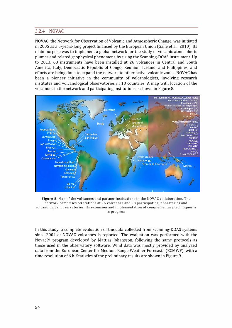
54
3.2.4 NOVAC
NOVAC, the Network for Observation of Volcanic and Atmospheric Change, was initiated in 2005 as a 5-years-long project financed by the European Union (Galle et al., 2010). Its main purpose was to implement a global network for the study of volcanic atmospheric plumes and related geophysical phenomena by using the Scanning-DOAS instrument. Up to 2013, 68 instruments have been installed at 26 volcanoes in Central and South America, Italy, Democratic Republic of Congo, Reunion, Iceland, and Philippines, and efforts are being done to expand the network to other active volcanic zones. NOVAC has been a pioneer initiative in the community of volcanologists, involving research institutes and volcanological observatories in 18 countries. A map with location of the volcanoes in the network and participating institutions is shown in Figure 8.
Figure 8. Map of the volcanoes and partner institutions in the NOVAC collaboration. The network comprises 68 stations at 26 volcanoes and 28 participating laboratories and
volcanological observatories. Its extension and implementation of complementary techniques is in progress
In this study, a complete evaluation of the data collected from scanning-DOAS systems since 2004 at NOVAC volcanoes is reported. The evaluation was performed with the NovacP3 program developed by Mattias Johansson, following the same protocols as those used in the observatory software. Wind data was mostly provided by analyzed data from the European Center for Medium-Range Weather Forecasts (ECMWF), with a time resolution of 6 h. Statistics of the preliminary results are shown in Figure 9.

55
Figure 9. Statistics of measurements of emission rate of SO2 from selected volcanoes of the NOVAC network during the period 2004-2013. The plot show box-chart distributions in logarithmic scale, with marks at the
minimum, the 1, 5, 25, 50, 75, 99, and 99% percentiles, and the maximum values, as well as the mean values. Notice the skewed distribution of emission rates observed at most volcanoes and the large variation
between different sources
NOVAC measurements represent a qualitative improvement in volcanic gas monitoring because about 40 flux measurements per station are typically obtained, the data is saved at a centralized server and can be exploited in the future, and it is obtained and evaluated in a standardized manner. For comparison, in the previous era of COSPEC, only a few volcanoes were monitored, in the best of the cases only 1 measurement of flux per week, the data was lost since there was no digital recording and the evaluations were not standardized and thus much more prompt to biases and errors.

56
3.2.5 STUDIES OF VOLCANIC DEGASSING WITH SCANNING-DOAS
3.2.5.1 KARYMSKY
We conducted ground-based remote measurements of volcanic plumes at Kamchatka during 5, 6 and 10-14 September 2011 by using scanning and mobile DOAS systems. The Rapid-Deployment System (RDS) is a scanning DOAS instrument similar to the Mark I system of the NOVAC project, but forming a single unit easy to transport and install in the field (Conde, 2011). It includes a back-pack/box containing the basic components: electronic box, spectrometer, timer, power regulator, and 12V battery; and the corresponding connectors for: tube-protected optical fiber, tripod-supported scanner, GPS antenna, foldable solar panel, and communication cables. Figure 10 shows photographs of the two instruments deployed at Karymsky volcano.
Figure 10. Left: Photograph of the Rapid-Deployment-System. Right and Large-Field-of-View- mobile-DOAS instrument used for the measurements at Kamchatka. The dashed lines represent the principle of scanning measurements (left) with a narrow FOV and pointing measur ements
(right) with a large FOV. Both strategies produce integral of slant column densities, which combined with transversal plume speed approximate the emission rate from the volcano
To correct for potential shifts in the pixel-wavelength relation of the spectrometers which occur mainly due to thermal stresses, the analysis of data included a calibration scheme that uses the known positions (wavelengths) of Fraunhofer structures in the solar spectrum to determine the optimal shift and applies it to all the spectra of each scan. Because the RDS incorporate a temperature sensor inside the box, it was possible to characterize the thermal dependence of this shift for the spectrometers. An example of such analysis is presented in Figure 11 below.

57
Figure 11. Linear dependence on temperature inside the box of the optimal shift for the pixel -wavelength mapping of the spectrometer D2J2356 (Shift = 2.82 – 0.152T). This relationship is obtained by finding the optimal shift to match the position of the solar lines in the measured
spectrum at a given temperature with those of a reference solar spectrum at the same resolution
In cooperation with the Institute of Volcanology and Seismology of the Far Eastern Division of the Russian Academy of Sciences (IVS FED RAS), our group conducted a campaign of remote sensing measurements of the SO2 gas emissions of Karymsky volcano during 10-14 September 2011. Karymsky is probably the most active volcano of Kamchatka and known for being the locus of persistent low-to-moderate explosive activity since its reactivation in 1996. Geophysical studies in the past have identified the main video-seismo-acoustic (Johnson and Lees, 1998; Johnson and Lees, 2000; Ozerov et al., 2001) and geochemical (Fischer et al., 2002) features of the explosions at Karymsky. The mechanisms responsible for these explosions seem to be related to the formation of temporal plugs in the vent which create a pressure buildup until a threshold is reached triggering an explosion. The emissions are occasionally rich in ash and lithics and continuous degassing usually followed after the explosive opening of the vent.
To better keep tracking of the gas emissions of Karymsky, we made a temporal installation of 2 scanning DOAS systems in flat and conical configurations oriented in order to intercept the plume as much perpendicular as possible. The stations were visited every day to download the saved data, clean the ash deposition, and check the

58
scanning directions and performance. No instrumental problems were detected during the measurement period. Additionally, mobile-DOAS measurements with 2 different systems were conducted from the Observatory of the RAS (located close to St. B) in different measurement modes. The positions and orientations of the RDSs are illustrated in Figure 12.
Figure 12. Image of Karymsky volcano showing the location (yellow marker) of the measurement stations and scanning directions (white dashed lines for flat and black dashed
lines for conical scanners) (Base image from Google Earth). The orientation of the scanners was established depending on the plume direction and varied, if needed, every day to maximize the
probabilities of intercepting the plume
The RDS collected a total of 432 scans during almost 4 days of operation. The close proximity to the plume (typically < 2 km) made possible to enclose the plume cross section most of the time (mean completeness indexes of 0.8 and 0.7 for stations A and B, respectively). As an example of a tandem observation of the plume by the 2 RDSs, Figure 13 shows scans taken on the 12th September.

59
Figure 13. Examples of scans obtained from stationary measurements at Karymsky volcano. the scan angle is the elevation angle measured clockwise from zenith. Station 1 (upper) was closer
to the plume than Station 2 (lower) and therefore produced a less skewed distribution of measured column densities. The combination of the 2 observations allows estimation of the
plume height and direction
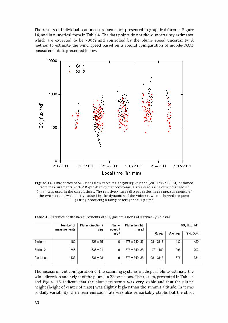
60
The results of individual scan measurements are presented in graphical form in Figure 14, and in numerical form in Table 4. The data points do not show uncertainty estimates, which are expected to be >30% and controlled by the plume speed uncertainty. A method to estimate the wind speed based on a special configuration of mobile-DOAS measurements is presented below.
Figure 14. Time series of SO2 mass flow rates for Karymsky volcano (2011/09/10-14) obtained from measurements with 2 Rapid-Deployment-Systems. A standard value of wind speed of
6 ms-1 was used in the calculations. The relatively large discrepancies in the measurements of the two stations was mostly caused by the dynamics of the volcano, which showed frequent
puffing producing a fairly heterogeneous plume
Table 4. Statistics of the measurements of SO 2 gas emissions of Karymsky volcano
Number of
measurements
Plume direction /
deg
Plume
speed /
ms-1
Plume height /
m a.s.l.
SO2 flux / td-1
Range Average Std. Dev.
Station 1 189 328 ± 35 6 1375 ± 340 (33) 28 – 3145 480 429
Station 2 243 333 ± 21 6 1375 ± 340 (33) 72 -1159 295 202
Combined 432 331 ± 28 6 1375 ± 340 (33) 28 – 3145 376 334
The measurement configuration of the scanning systems made possible to estimate the wind direction and height of the plume in 33 occasions. The results, presented in Table 4 and Figure 15, indicate that the plume transport was very stable and that the plume height (height of center of mass) was slightly higher than the summit altitude. In terms of daily variability, the mean emission rate was also remarkably stable, but the short

61
short-term variability was high due to a very dynamic degassing activity of the volcano (sealing-explosion processes). This variability had a temporal scale smaller than the temporal resolution of the scanning systems, therefore caused some discrepancies between the measurements of the two instruments.
Figure 15. Previous page: Wind-rose showing the distribution of plume directions (upwind) as measured from triangulation of the scanning systems. Above: Plume heights derived from the
same measurements

62
The main source of uncertainty in our measurements is the estimate of plume speed. For the measurements reported here, we have used values reported from external sources (visual or UV-camera observations, weather forecasts) and it is desirable to have concurrent measurements of this parameter. The dual-beam method was not performed due to logistical constraints to find a location below the centerline of the plume to do the measurements. For the case of Karymsky, visual estimates suggested that the plume transport speed was not very high at the section of the plume intercepted by the scanners. A report from NOAA (http://ready.arl.noaa.gov/READYamet.php), however, indicates wind-speed values at the summit of Karymsky that were unexpectedly high. We decided not to interpolate these values to report our flux measurements and instead used a constant value of 6 ms-1, which was a typical value obtained from Large-Field of View Mobile-DOAS measurements, as indicated in the following section.
3.2.5.1.1 LARGE FIELD-OF-VIEW MINI-DOAS MEASUREMENTS
The particular activity of frequent explosive emissions observed at Karymsky, led us to experiment a configuration of stationary measurements with the mobile-DOAS instrument in which we dispensed with the use of the telescope and point instead to the
plume with the large field of view (150 mrad) of the optical fiber. In this way, a considerable portion of the plume is observed at once in the field of view of the
instrument and acquisition can be done at a much higher frequency ( 1 Hz) than with a scanning method. The implementation of this methodology to volcanic studies is not new (Boichu et al., 2010; McGonigle et al., 2009), and Karymsky volcano was an ideal scenario to implement it.
We performed Large-Field of View mini-DOAS (LFOV-mini-DOAS) measurements at Karymsky during several hour-long periods on the 12, 13 and 14 September 2011 from the observatory. An extract of one of these periods is shown in Figure 16, in which the blue line represents the intensity of UV light in the region of SO2 absorption and the red line is the real-time column measurement. As expected from radiation extinction by the plume aerosols, there is a negative correlation between intensity and gas columns, which is exploited for the detection of volcanic plumes.

63
Figure 16. Time series of LFOV mini-DOAS measurements at Karymsky on 2011-09-12. The upper blue line represents UV intensity and the lower red line SO 2 column amounts. The shaded area corresponds to an interval used for estimation of the wind speed. Note the anti-correlation
between columns and intensity, thus intensity variations alone can be used for detecting the presence of a plume
A potential drawback of this method is the difficulty to determine how representative of the instantaneous emission is the snapshot of the plume observed by the instrument. Another limitation is the fact that inhomogeneities in gas concentration observed in the field of view might cause an underestimation that can be significant for optically thick regions of the plume, due to the non-linearity of the relation between radiation extinction and optical depth. On the other hand, the LFOV mini-DOAS method provides a reliable way to determine the plume transport speed for the type of activity of Karymsky. By tracking the time of occurrence of explosive events (by visual observation or acoustic signals), and controlling the geometry of the observation (distance to the plume and azimuth of observation respect to the vent direction), it is possible to quantify the time that takes for a given parcel of gas emitted in the explosion to be detected by the instrument. We mark the times of occurrence of explosions for a given period of observation in Figure 17 and observe the increase in the corresponding gas measurement after a certain period. In practice, we assume that the instrument detects the explosion before or right at the moment of a relative maximum in column amount, which is probably the time when the bulk of the emission of each event is covering the field of view of the instrument.

64
Figure 17. LFOV-mini-DOAS measurement on 2011-09-13, showing the times (green marks) of explosion events and increases in gas columns at Karymsky volcano. The correlation of the
peaks of the two series is used to estimate the plume speed
A concrete example of this method to estimate the plume speed is presented in Figure 18. The upper figure gives details for an individual measurement (in this case the time shift between the explosion and the beginning of the increase in the column series). The center figure shows the application of this method (with shifts until the position of the peak columns) to a longer data series, and the lower figure presents the results.
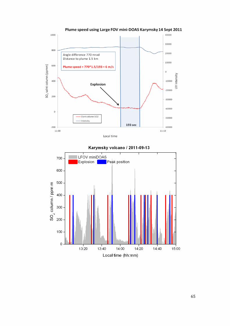
65

66
Figure 18. Application of the plume speed estimation method based on LFOV-mini-DOAS measurements. Previous page, above: Example of a single calculation showing positions of the
time lag and additional information used for the wind speed measurement. Previous page, below: Extension of the method to a larger dataset. Above: Results of the calculations for the
previous dataset, a mean value of 5.74±2.13 ms-1 (± 1) was obtained
The time series of SO2 emission rate measurements at Karymsky reveal two main degassing patterns:
- During 10-13 September, the volcano produced small Strombolian eruptions at a
typical rate of 3-20 explosions per hour. These were characterized by small-to-
moderate ash contents, variable audible intensity of explosions and
accompanying rumbling. At night, it was possible to distinguish incandescence
associated with some of the explosions with the naked eye. The gas emission
dropped to an undetectable level after the degassing events.
- On 14 September, the volcano produced bigger Vulcanian-type eruptions at a
typical rate of 1 per hour. These were characterized by variable amounts of ash,
strong audible signals and were followed by open degassing with variable
amounts of ash during each event. The gas emission did not cease between
events.
Such activity is typical of Karymsky since its reactivation in 1996 and the details of the shallow geophysical signals have been reported before (Fischer et al., 2002; Johnson and Lees, 1998). Our measurements constitute the first of its type during the last decade and confirm the permanency of Karymsky’s frequently-explosive activity.

67
3.2.5.2 NYIRAGONGO
Nyiragongo is a very active volcano located in eastern Congo, close to the border with Rwanda. The city of Goma, with about 1000 000 inhabitants, is located less than 20 km from the volcano. The area is politically unstable in recent times; with hundreds of thousands of refugees from a civil war in the area and in nearby Rwanda. In 2002 a flank eruption caused rapid lava flows that destroyed about 20% of the city. Besides the high direct threat of the volcano to the population, the volcano is one of the strongest sources of volcanic gases in the world with an SO2 emission of 5000-50000 ton/day. In addition, high amounts of HCl and HF are abundant in the plume. The population and vegetation downwind the volcano is strongly affected both directly by the toxic gases, and indirectly by acid rain and contaminated drinking water.
To help monitoring Nyiragongo, our group has installed 4 scanning-DOAS instruments since 2004 at distances between 9 and 14 km from the crater in the sites called Rusayo, Sake, Kunene and Buzi (Kunene station was later replaced by an instrument at Kingi). Due to difficulties to maintaining the stations, some gaps in the time series exist. About 70% of the valid measurements were done by the Rusayo station and most of the rest by the Sake instrument.
The evaluation of data was done according to the procedure described above and the most important results are depicted in Figure 19 below (cf. Paper 2).

68
Figure 19. Previous page: Time series of SO2 emission rate from Nyiragongo volcano measured with scanning-DOAS during 2004-2012 and detail of the period July-November 2012. Above:
Annual mean emission rates obtained from measurements performed by our group, extending the historical record of degassing monitoring at this volcano (See Paper 2)

69
3.3 FTIR
Fourier Transform Infra-Red spectrometry is a well-known analytical method for identification and measurement of chemical compounds. It has been developed for field operations and used in a variety of platforms (ground, ships, balloons, aircraft, and spacecraft). Its importance in Earth’s remote sensing lies on a number of advantages that FTIR usually has with respect to dispersive techniques such as grating spectrometry, like higher étendue (“Jacquinot advantage”), NS / , resolution, or
stability.
FTIR is a multiplex technique, which means that several spectral elements are sensed simultaneously by the same detector. This property, referred to as the “Fellgett advantage”, is achieved by interferometry: the measurement of an interference pattern of multiple radiation beams. The simplest and most common setup consists of the separation and posterior interference of two beams, as devised originally by A. Michelson for the accurate measurement of lengths in the end of the 1880s (famously used for the “Michelson-Morley” experiment of null absolute motion of Earth respect to hypothetical “ether”). Although the principle of interferometry can be applied to radiation of any wavelength, the technique has historically been developed mostly for infrared and longer wavelengths, where abundant information exists on molecular transitions and required materials and components, as well as sub-wavelength precision are available. In the Michelson configuration, which is the simplest but not always the most technically stable configuration, an incident beam is divided in two approximately equal beams by a beam-splitter/compensator and guided to travel two perpendicular, mirror-folded, counter–propagating paths to be then recombined (interfered) at the beamsplitter, deviating again half of the radiation to a detector and the other half to the entrance aperture. By controlling the difference in pathlength of the two beams, it is possible to relate the interference pattern to this difference, or equivalently, to time. This relation is called the interferogram (amplitude vs. path difference), from which the
spectrum (amplitude vs. frequency or wavenumber 1~ ) is obtained via a
mathematical operation known as the Fourier transformation, hence the name of this technique.
Expressed in mathematical form, the intensity as a function of path difference xI
formed from the interference of beams with monochromatic intensity as a function of
wavenumber ~F from a broad-band source is given by:
000
~~2cos~~~~~2cos1~ dxFdFdxFxI
(48)
Where the first term corresponds to the total energy incident on the system
CdF
~~ and the second term is the interferogram. The spectrum is obtained
from the Fourier transformation:
dxxxBCxIF ~2cos~
(49)
In which the boxcar function xB has been introduced to account for the limited
pathlength L of the system, while preserving the infinite limits of integration of the

70
transformation. The inclusion of the boxcar function is equivalent to a convolution of the
spectrum with a “sinc” function: LLF ~2~2sin~ , which represents the
nominal ILS of the FTIR with a resolution (FWHM) given by L6034.0~~ in cm-1.
Since this function presents unwanted periodic wings, it is common to include an “apodization” function like triangular, rectangular, Norton-Beer, Mertz, etc., at the cost of
degrading the spectral resolution. The ILS of a FTIR is wavelength invariant, a property
known as the “Connes advantage”. Precision in wavelength marking is also an asset of FTIR, which uses a very stable laser beam following the same optical path of the measurement to control de sampling. For instance, the FTIR employed in our measurements has a precision of 0.04 cm-1.
Limitations that degrade the resolution or produce spectral shifts include the effect of beam divergence, non-ideal modulation efficiency of the beamsplitter, pointing errors, and image motion (turbulence, jittering). The interested reader is referred to the extensive literature about the technique for more details (Beer, 1992; Davis et al., 2001; Griffiths and De Haseth, 2007).
3.3.1 FTIR MEASUREMENTS OF VOLCANIC PLUMES
The use of FTIR for volcanic gas studies in the field dates back to the 1990s. The first measurements were reported by Japanese researchers (Mori and Notsu, 1997; Notsu et al., 1993), who measured several species by employing the thermal emission from the hot volcanic rocks as the source for remote absorption measurements. Solar direct absorption and plume thermal emission measurements have also been reported (Francis et al., 1998; Love et al., 1998), as well as measurements with a lava fountain (Allard et al., 2005), lava lake (Sawyer et al., 2008), the moon (Burton et al., 2001), or explosively ejected material as sources of radiation (La Spina et al., 2013; Oppenheimer et al., 2006). Scanning image construction of the plume (Stremme et al., 2011) and active open-path FTIR measurements (Duffell et al., 2003) have also been carried out in volcanic environments. The range of trace gas species measured with FTIR is large, covering all the most abundant components (H2O, CO2, SO2, HCl, HF, CO, COS, SiF4), particularly when proximal (e.g., at the crater rim) observations and low temperature (e.g., terrestrial bodies, lamps) sources can be used.
Radiation transport in the infrared spectral region is complicated due to the fact that not only absorption of radiation from the source (sun/moon/lamp/rocks/plume) by the gas plume occurs, but also thermal radiation is emitted. Refraction, scattering and reflection are, on the other hand, usually negligible in this region. The information content of the spectrum makes possible in some cases to retrieve temperature/pressure conditions in the observed system as well as absolute concentrations of the absorbing species, however, this requires proper radiometric calibration. The situation is simpler if only ratios of column amounts/concentrations are needed, as explained below.
Infrared radiation is collected by a pointing/gathering radiation system, analyzed by the interferometer and detected by either a photovoltaic or photoconductive element or array of detectors. In direct solar configurations, the sun position has to be tracked with precision, especially for high resolution (<10-2 cm-1) measurements, because background source variations and pointing cause undesired shift or resolution
distortions. The most common detectors in the 1 to 12 m wavelength interval are

71
photovoltaic InSb and HgCdTe (MCT) detectors, which operate at low temperatures,
requiring contact with liquid N2 (77 K) or another cooling mechanism. The signal is then amplified, digitalized and recorded for further analysis.
Analysis consists first on the transformation from interferogram to spectrum (via a discrete Fourier transform, apodization, frequency-shift corrections). The spectral inversion then consists on trying to reconstruct the spectrum from a forward model, as for example explained by D. Griffith for the Multi-Layer-Atmospheric-Transmission (MALT) model (Griffith, 1996). This retrieval procedure consists on simulating the measured transmission by including spectral information (temperature/pressure dependence parameters for the line strengths of the molecules absorbing in the spectral interval of interest), pressure-temperature-composition of different atmospheric layers
depending on the measurement configuration, and instrumental parameters ( ILS ). A
non-linear Levenberg-Marquardt or another iterative fitting algorithm is performed to retrieve the variables of interest, particularly the gas column amounts of the absorbing molecules included in the model. Since the optical path is assumed to be the same for the plume molecules, the ratio of concentrations between different species can be obtained from a single spectrum.
3.3.2 SOLAR FTIR MEASUREMENTS OF VOLCANIC GAS MOLAR RATIOS
3.3.2.1 POPOCATÉPETL
With the aim of developing a Solar FTIR system for automatic volcanic plume measurements it was necessary to design and build a solar-tracking apparatus, which transfers the (moving) direct solar beam into the (stationary) interferometer. It was decided to build a simple stationary tracker based on two motorized rotating mirrors with the possibility of equatorial or horizontal setups22. Previous work in this line has been done by our group for stationary high-resolution FTIR measurements of atmospheric composition (Galle et al., 1999) and for mobile low-resolution FTIR measurements of industrial emissions by the Solar Occultation Flux (SOF) method (Kihlman, 2005), as well as for direct-sun DOAS measurements within the NOVAC collaboration (Sommer, 2008).
The solar tracker is mounted on a horizontal platform facing N. The solar tracking algorithm consists on first reading the time and position from a GPS sensor, then calculating the corresponding coordinates of the sun and moving the mirrors accordingly (Merlaud et al., 2012). Although the theoretical precision of the solar position calculation and of the stepper motors is high (0.001 deg, 0.004 deg respectively), misalignments are unavoidable, requiring an active fine-tuning of the signal based on the actual intensity at zero-path-difference (ZPD) of the interfering beams (centre of the interferogram). Spectral shifts caused by non-normal incidence of the beam can also be corrected for by adjusting the position of known features in the spectrum. The fine-tuning is done on a reduced interval of the spectrum and at low
22 An equatorial setup is particularly beneficial to preserve the orthogonality of the coordinates of solar motion at high solar zenith angles (close to noontime at low latitudes). Horizontal setups are prompt to such singularities.

72
resolution (8 cm-1) for speed. If the fine-tuning procedure fails at recognizing a high enough intensity due to, for instance, the presence of clouds, it proceeds to acquire interferograms based only on the calculated pointing direction. The acquisition of measurement interferograms is made at a highest possible resolution of the FTIR (0.5 cm-1). Photography of the solar tracker developed for volcanic plume measurements is presented in Figure 20.
Figure 20. Above: Schematics of the principle of Solar-FTIR measurements. Below: Photography of the solar tracker and FTIR system for measurements of volcanic plumes. The solar tracker
calculates the position of the sun and then performs a fine-tuning of the tracking based on the intensity
Solar-FTIR measurements were performed in 2 field campaigns at Popocatépetl volcano in Mexico during April 2010 within the project FIEL-VOLCÁN, and at Tungurahua volcano in Ecuador during July 2012 within an interim of the author of this thesis. At Popocatépetl, measurements were performed from 4 different sites at distances between 10 and 17 km from the crater. These observations were performed close to noon time, where it is easier to obtain the right geometry with the sun behind the plume. Examples of the spectral fit based on the MALT model are shown in Figure 21.

73
Figure 21. Upper: Spectral fit for SO2 based on the MALT model of a volcanic plume from Popocatépetl (Mexico) measured 17 km downwind the crater on 21 April 2010 by Solar FTIR.
Lower: Spectral fit for HCl. Other species including in the fit are H 2O, CH4 and N2O and a second order polynomial. The SO2/HCl molar ratio out of 21 measurements was 0.31 ± 0.29 (FIEL-
VOLCÁN Project Final Report 2011)
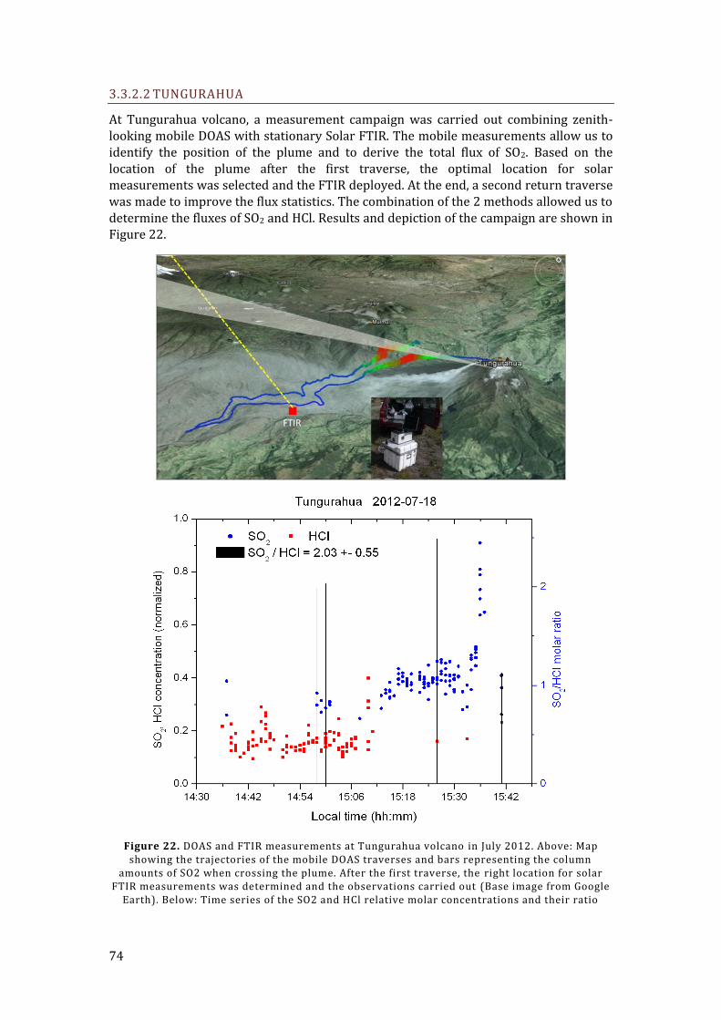
74
3.3.2.2 TUNGURAHUA
At Tungurahua volcano, a measurement campaign was carried out combining zenith-looking mobile DOAS with stationary Solar FTIR. The mobile measurements allow us to identify the position of the plume and to derive the total flux of SO2. Based on the location of the plume after the first traverse, the optimal location for solar measurements was selected and the FTIR deployed. At the end, a second return traverse was made to improve the flux statistics. The combination of the 2 methods allowed us to determine the fluxes of SO2 and HCl. Results and depiction of the campaign are shown in Figure 22.
Figure 22. DOAS and FTIR measurements at Tungurahua volcano in July 2012. Above: Map showing the trajectories of the mobile DOAS traverses and bars representing the column
amounts of SO2 when crossing the plume. After the first traverse, the right location for solar FTIR measurements was determined and the observations carried out (Base image from Google
Earth). Below: Time series of the SO2 and HCl relative molar concentrations and their ratio

75
3.3.3 OPEN-PATH FTIR MEASUREMENTS OF VOLCANIC GAS MOLAR RATIOS
3.3.3.1 FUEGO DE COLIMA
Open-path (OP) FTIR measurements of volcanic gases can be passive, using a hot body in the background of the plume, or active, when a IR lamp is used as source. Measurements in emission mode are also possible, but were not made during the work reported in this thesis.
The telescope used for this measurements was a simple Newtonian with a primary mirror of 30 cm diameter and focal length de 80 cm (f/2.7), and a flat secondary mirror, matching the entrance aperture of the interferometer. Schematic of the setup is shown in Figure 23.
Figure 23. Schematics of the Open-path FTIR system developed for volcanic gas measurements . Radiation is collected by a telescope and transferred to the FTIR for analysis. Acquired
interferograms are recorded in a computer for posterior analysis. The system is powered by batteries or AC power
OP-FTIR measurements were conducted in a field campaign at Fuego de Colima volcano in Mexico in February 2011 by B. Galle, V. Conde and Mexican colleagues. The system was deployed at a distance of 5.2 km from the crater dome, at the facilities of the volcanological observatory in Nevado de Colima. The telescope was pointed to the dome, where thermal radiation was intense enough to produce a signal above background. Unfortunately, the direction of the plume was most of the time in the opposite side, however, in certain occasions moved within the field of view of the instrument and volcanic species were measured. Figure 24 below shows examples of the fit of the spectra collected in this campaign.
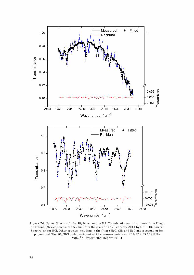
76
Figure 24. Upper: Spectral fit for SO2 based on the MALT model of a volcanic plume from Fuego de Colima (Mexico) measured 5.2 km from the crater on 17 February 2011 by OP-FTIR. Lower: Spectral fit for HCl. Other species including in the fit are H 2O, CH4 and N2O and a second order
polynomial. The SO2/HCl molar ratio out of 71 measurements was of 16.27 ± 85.65 (FIEL-VOLCÁN Project Final Report 2011)

77
More details about the Scanning-DOAS and FTIR techniques are given in the table below.
Table 5. Technical details of the Scanning-DOAS and FTIR techniques
Characteristic Scanning-DOAS Solar/OP FTIR
Spectral region (for SO2, HCl) 278– 425 (310–325) nm 1850–4000 (2470–2535, 2810–2870)
cm-1
Spectral resolution 0.6 nm 0.5 cm-1 (Maximum path difference of
1.8 cm)
Temporal resolution Approx. 5 min (per flux) Approx. 10 s (per spectrum)
Field of view 15 mrad 30 mrad (adjusted in fitting)
Source of radiation Diffuse solar radiation Direct solar radiation or hot lava dome
Transfer optics Flat/conical scanning refractor, VIS-filter, quartz
bundle optical fiber
Stationary solar tracker, flat, Au-coated
mirrors, Ge/Si filter
Spectral analyzer Crossed Czerny-Turner grating spectrometer “SolidRock” (pendulum) interferometer
with ZnSe covered KBr beamsplitter
Detector 2049-element linear Si CCD array, with UV-
fluorescent film
InSb, cooled by thermo-electrical
system or liquid N2
Typical acquisition parameters 15 co-added spectra, optimal integration time
(typically 100-1000 ms)
16 co-added scans
Species included in fitting SO2, O3, modeled Ring spectrum, polynomial of
5th order
SO2, HCl, CH4, N2O, H2O, polynomial of
2nd order
DOAS and FTIR
implementation
Dark/offset subtraction, ratio by sky spectrum,
HP-filter, NL-LS-fit
Multi-layer model (HITRAN), NL-LS-fit
(MALT)
Wavelength shift correction Fit to Fraunhofer solar spectrum Fit to modeled spectrum
Size Approx. 20 cm-3 Approx. 30 cm-3
Geometrical variables Plume height and velocity by correlation or
models
NA
Power consumption 5 W 40 W
Typical uncertainty Approx. 30% (per flux) Approx. 5% (per spectrum)

78

79
4 SUMMARY OF APPENDED PAPERS
4.1 Paper 1:
Arellano S., Hall M., Samaniego P., LePennec J.-L., Ruiz A., Molina I., Yepes H. (2008).
Degassing patterns of Tungurahua volcano (Ecuador) during the 1999-2006 eruptive period,
inferred from remote spectroscopic measurements of SO2 emissions.
J. Volcanol. Geotherm. Res., 176: 151-162.
In this paper, we report the results and analysis of scanning COSPEC and DOAS measurements of the SO2 plume of Tungurahua volcano (Ecuador) during the eruptive period 1999-2006, which includes both the initiation of a still ongoing eruptive process of this volcano (October 1999), and the most explosive phase culminated in a VEI 3 explosive eruption (July-August 2006). Data reduction incorporated novel approaches to assess the quality of the measurements, namely, the identification of scattering effects due to the presence of clouds determined by applying a simple single-scattering radiation transfer model, as well as quantitative and qualitative identification of the full error budget due to the measurement method and due to processes related to plume transport. The mean emission rate of SO2 was found to be about 1500 ± 2000 Mg d-1 with an uncertainty of the order of 13-36%. Based on the statistics of daily cumulative seismic energy released during explosions, a threshold energy level for explosive activity was found to categorize the activity as non-explosive or explosive. Based on this, it was found that non-explosive activity occurs about 95% of time and has a mean SO2 emission rate of about 1400 Mg d-1, which is 1.75 times lower than the emission rate associated with explosive activity. When the estimated gas output is compared with estimated tephra output, it was found that the dominant passive emission pattern is associated with a significant excess of gas (up to 2 orders of magnitude, assuming complete degassing of the erupted material) for a typical andesitic magma composition, whereas relatively good balance occurs for these observables during explosive activity. To explain the efficient degassing of this volcano two models are discussed: permeable (open) degassing through a stagnant magma column and closed degassing of magma in convection in the conduit. In particular, a quantitative 1-D dynamical model is applied for magma overturning, which is caused by densification of parcels of degassed magma. The model indicates that magma convection is a feasible mechanism for outgassing without tephra emission, as observed during the background passive activity of Tungurahua.
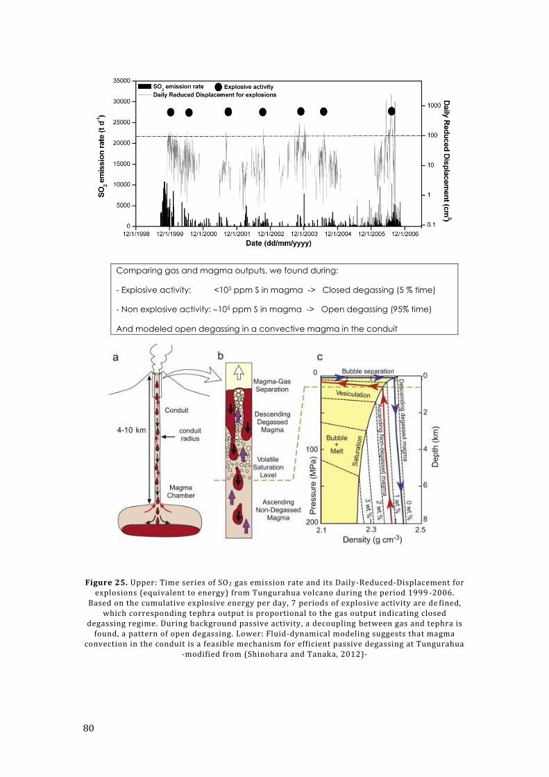
80
Comparing gas and magma outputs, we found during:
- Explosive activity: <103 ppm S in magma -> Closed degassing (5 % time)
- Non explosive activity: 105 ppm S in magma -> Open degassing (95% time)
And modeled open degassing in a convective magma in the conduit
Figure 25. Upper: Time series of SO2 gas emission rate and its Daily-Reduced-Displacement for explosions (equivalent to energy) from Tungurahua volcano during the period 1999 -2006.
Based on the cumulative explosive energy per day, 7 periods of explosive activity are de fined, which corresponding tephra output is proportional to the gas output indicating closed
degassing regime. During background passive activity, a decoupling between gas and tephra is found, a pattern of open degassing. Lower: Fluid-dynamical modeling suggests that magma
convection in the conduit is a feasible mechanism for efficient passive degassing at Tungurahua -modified from (Shinohara and Tanaka, 2012)-

81
4.2 Paper 2:
Arellano S., Yalire M., Galle B., Johansson M., Norman P., Bobrowski N., Magnitude, intensity and impact of SO2 gas emissions from Nyiragongo volcano during 2004-2012. In preparation for Bull. Volcanol.
In this paper, we present the record of measurements of the SO2 gas emission rate from
Nyiragongo volcano during the period 2004-2012 and analyzed it trends, statistics and
implications for understanding its recent state of activity. Nyiragongo hosts and active lava
lake for various decades and it is one of the strongest sources of volcanic species in the
atmosphere, as well as one of the most dangerous volcanoes due to its proximity to the city
of Goma, in the politically conflictive area close to the border of D.R. Congo with Rwanda.
The activity of Nyiragongo is characterized by permanent degassing, which intensity is
modulated by the rate of convection and altitude of the lava lake, whereas major outbursts
have been associated with tectonic rift activity or hydrothermal interactions. Measuring the
rate of degassing is therefore crucial to understand the state of the volcano. Although a few
sporadic campaigns have been done over the last decades and satellite sensors are able to
monitor large plumes, there has not been continuous surveillance of passive degassing until
the installation of permanent Scanning-DOAS instruments at four stations around
Nyiragongo between 2004 and 2007. Our measurements reveal the magnitude, intensity and
fate of the plumes of Nyiragongo, and show that, despite occasional and short term
variations, the bulk activity of this volcano in the studied period has been remarkably stable
and the emission events have magnitudes that are well approximated by a Lévy-distribution.
This suggests that the degassing process consists of independent and randomly distributed
batches of gas, which is compatible with the hypothesis of magma convection in the conduit,
supported by other lines of evidence found by other authors. Furthermore, the found
distribution opens up the possibility to identify anomalous emission events, which would not
follow the same pattern, since the degassing process itself may become non-markovian. Our
observations also indicate the altitude and direction of the plumes of Nyiragongo, which
together with the source strength constitute valuable information for assessing the impact
of the emissions downwind the vent, including their impact on human health.

82
Figure 26. Complementary Cumulative Distribution Function (CCDF) of daily mean SO2 emission rates from Nyiragongo volcano measured by scanning-DOAS in the period 2004-2012.
Black dots represent data and red and blue dash lines are Gaussian and Lorentzian fits to the CCDF. The CCDF lies in between both models, suggesting that degassing is a Lévy process and
that the time of a major emission can in principle be pred icted by deviations from the distribution of passive degassing events
83
5 CONCLUSIONS AND OUTLOOK
This document summarizes the work done mostly during the period 2008-2011 of my doctoral program. The main focus of this work was advancing the techniques used for remotely sensing volcanic gas emissions via spectroscopy of ultraviolet and infrared radiation, specifically by DOAS (scanning and mobile) and FTIR (solar and open-path).
On the instrumental side, the work led to the development of a sun-tracker for the solar-FTIR method, which was designed, built and finally tested in a field campaign in Mexico in April 2010. The system proved to work satisfactorily during the campaign, but needed of the presence of an operator due to a tendency to misalign after a few hours, when following the sun in passive (calculating the position) mode. The active (assessing the radiation intensity) mode worked fine, but could not be applied permanently due to the presence of clouds. The reason of the misalignments has to be found in the sensitivity of the design to small inaccuracies in the initial setup. For a permanent station, care should be taken to secure proper leveling and azimuthal orientation of the system and possibly add a diffuser to gain some freedom in the pointing accuracy. A second attempt of field use of the solar-tracker was done in Ecuador, during July 2012, but the system presented a failure in the electronic board, unfortunately. Further instrumental work was done on assembling a telescope for Open-Path FTIR measurements that was successfully used in a field campaign in Mexico in February 2012. Additional research was done on investigating the possibility of using a stationary setup for radiation-gathering without the need to have a dynamical tracking, making use of a hemispherical diffuser. Additionally, research on Gas-Filter-Correlation-Spectroscopy was carried out, but not reported in this thesis. More work should be done in these lines, which show great potential for remote sensing of volcanic plumes. Finally, the assembly of a number of Scanning-DOAS systems for the NOVAC network and other sites and field campaigns has been done throughout these years.
On the analytical side, the focus has been on evaluating data collected during the field campaigns and by the stations of the NOVAC network. For DOAS, these activities included a detailed analysis of uncertainty in the measurements and procedures to characterize it or reduce it. The quality assessment of data was applied to the several datasets from all volcanoes (26) of the NOVAC network and the volcanoes of Kamchatka (Mutnovsky, Gorely, Karymsky) and from the field campaigns in Mexico and Ecuador. FTIR evaluations were conducted with the MALT model and implemented operationally in Ecuador, where Solar-FTIR measurements are carried out frequently at Tungurahua.
After the work reported here, the main focus has been on analyzing the data from NOVAC and using the results for geophysical research on volcanoes, in collaboration with colleagues from the respective volcanological observatories. In specific, the time series of Nyiragongo and Nyamulagira (D.R. Congo), Nevado del Ruiz (Colombia), and Tungurahua (Ecuador) are being analyzed in their correlation with other geophysical parameters for volcanic risk assessment purposes. The analysis of uncertainty in Scanning-DOAS measurements has shown certain aspects in radiative transfer and plume transport amenable to modeling, which implementation has shown encouraging preliminary results. The comparison of the data generated with these methods for other purposes like satellite validation and plume deposition downwind the volcano, as well as the expansion of the NOVAC-type measurements to other species by using in-situ sensors, are other of the areas that have and will be investigated during the rest of this doctoral program.

84

85
6 REFERENCES
Afe, O.T., Richter, A., Sierk, B., Wittrock, F. and Burrows, J.P., 2004. BrO emission
from volcanoes: A survey using GOME and SCIAMACHY measurements.
Geophysical Research Letters, 31(24): L24113.
Allard, P., Burton, M. and Mure, F., 2005. Spectroscopic evidence for a lava fountain
driven by previously accumulated magmatic gas. Nature, 433(7024): 407-410.
Allard, P. et al., 1991. Eruptive and Diffuse Emissions of Co2 from Mount Etna.
Nature, 351(6325): 387-391.
Allègre, J.C., Staudacher, T. and Sarda, P., 1987. Rare gas systematics: formation of
the atmosphere, evolution and structure of the Earth's mantle. Earth and
Planetary Science Letters, 81: 127-150.
Andres, R.J. and Kasgnoc, A.D., 1998. A time-averaged inventory of subaerial
volcanic sulfur emissions. Journal of Geophysical Research D: Atmospheres,
103(D19): 25251-25261.
Beer, R., 1992. Remote Sensing by Fourier Transform Spectrometry. Chemical
Analysis. John Wiley & Sons, Inc., Toronto, 153 pp.
Bluth, G.J.S., Shannon, J.M., Watson, I.M., Prata, A.J. and Realmuto, V.J., 2007.
Development of an ultra-violet digital camera for volcanic SO2 imaging.
Journal of Volcanology and Geothermal Research, 161(1-2): 47-56.
Bobrowski, N., 2005. Volcanic Gas Studies by Multi Axis Differential Optical
Absorption Spectroscopy. PhD Thesis, University of Heidelberg, Heidelberg,
215 pp.
Bobrowski, N., Hönninger, G., Lohberger, F. and Platt, U., 2006. IDOAS: A new
monitoring technique to study the 2D distribution of volcanic gas emissions.
Journal of Volcanology and Geothermal Research, 150(4): 329-338.
Bobrowski, N., Hönninger, G., Platt, U. and Galle, B., 2003. Detection of bromine
monoxide in a volcanic plume. Nature, 423(6937): 273-276.
Bohren, C.F. and Clothiaux, E., 2006. Fundamentals of atmospheric radiation: an
introduction with 400 problems. Wiley-VCH, 472 pp.
Bohren, C.F. and Huffman, D.R., 1998. Absorption and Scattering of Light by Small
Particles. Wiley, 544 pp.
Boichu, M., Oppenheimer, C., Tsanev, V. and Kyle, P.R., 2010. High temporal
resolution SO2 flux measurements at Erebus volcano, Antarctica. Journal of
Volcanology and Geothermal Research, 190(3-4): 325-336.
Bourassa, A.E. et al., 2012. Large Volcanic Aerosol Load in the Stratosphere Linked
to Asian Monsoon Transport. Science, 337(6090): 78-81.
Bransden, B.H. and Joachain, C.J., 2003. Physics of Atoms and Molecules (2nd
Edition). Pearson education, Malaysia, 1114 pp.
Burton, M.R., Oppenheimer, C., Horrocks, L.A. and Francis, P.W., 2001. Diurnal
changes in volcanic plume chemistry observed by lunar and solar occultation
spectroscopy. Geophysical Research Letters, 28(5): 843-846.
Butler, J., Johnson, B.C. and Barnes, R.A., 2005. The Calibration and
Characterization of Earth Remote Sensing and Environmental Monitoring
Instruments, Optical Radiometry. Experimental Methods in the Physical
Sciences. Elsevier Academic Press, pp. 453-534.
Carn, S.A. et al., 2007. Extended observations of volcanic SO2 and sulfate aerosol in
the stratosphere. Atmospheric Chemistry and Physics Discussion, 7(1): 2857-
2871.

86
Chance, K.V. and Spurr, R.J.D., 1997. Ring effect studies: Rayleigh scattering,
including molecular parameters for rotational Raman scattering, and the
Fraunhofer spectrum. Applied Optics, 36(21): 5224-5230.
Clarisse, L. et al., 2008. Tracking and quantifying volcanic SO2 with IASI, the
September 2007 eruption at Jebel at Tair. Atmospheric Chemistry and Physics,
8(24): 7723-7734.
Conde, V., 2011. Development and implementation of a rapid deployment system for
volcanic gas emissions monitoring. Chalmers University of Technology.
Connor, C.B., Stoiber, R.E. and Malinconico, L.L., Jr., 1988. Variation in Sulfur
Dioxide Emissions Related to Earth Tides, Halemaumau Crater, Kilauea
Volcano, Hawaii. J. Geophys. Res., 93(B12): 14867-14871.
Datla, R.U. and Parr, A., 2005. Introduction to Optical Radiometry, Optical
Radiometry. Experimental Methods in the Physical Sciences. Elsevier
Academic Press, pp. 1-34.
Davis, S.P., Abrams, M.C. and Brault, J.W., 2001. Fourier Transform Spectrometry.
Elsevier Science, 262 pp.
Diaz, J.A., Giese, C.F. and Gentry, W.R., 2002. Mass spectrometry for in-situ
volcanic gas monitoring. TrAC Trends in Analytical Chemistry, 21(8): 498-
514.
Dingwell, D.B., 1996. Volcanic Dilemma--Flow or Blow? Science, 273(5278): 1054-
1055.
Duffell, H.J. et al., 2003. Changes in gas composition prior to a minor explosive
eruption at Masaya volcano, Nicaragua. Journal of Volcanology and
Geothermal Research, 126(3-4): 327-339.
Eisinger, M. and Burrows, J.P., 1998. Tropospheric sulfur dioxide observed by the
ERS-2 GOME instrument. Geophysical Research Letters, 25(22): 4177-4180.
Elachi, C. and Van Zyl, J., 2006. Introduction to the Physics and Techniques of
Remote Sensing (2nd Edition). John Wiley & Sons.
Fischer, T.P., Roggensack, K. and Kyle, P.R., 2002. Open and almost shut case for
explosive eruptions: Vent processes determined by SO2 emission rates at
Karymsky volcano, Kamchatka Geology, 30(12): 1059-1062.
Francis, P., Burton, M.R. and Oppenheimer, C., 1998. Remote measurements of
volcanic gas compositions by solar occultation spectroscopy. Nature,
396(6711): 567-570.
Galle, B. et al., 2010. Network for Observation of Volcanic and Atmospheric Change
(NOVAC): A global network for volcanic gas monitoring -Network layout and
instrument description. Journal of Geophysical Research, 115(D5): D05304.
Galle, B. et al., 1999. Ground based FTIR measurements of stratospheric species from
Harestua, Norway during SESAME and comparison with models. Journal of
Atmospheric Chemistry, 32(1): 147-164.
Galle, B. et al., 2003. A miniaturised ultraviolet spectrometer for remote sensing of
SO2 fluxes: a new tool for volcano surveillance. Journal of Volcanology and
Geothermal Research, 119(1-4): 241-254.
Gao, C., Robock, A. and Ammann, C., 2008. Volcanic forcing of climate over the past
1500 years: An improved ice core-based index for climate models. J. Geophys.
Res., 113(D23): D23111.
Gerlach, T.M., 2011. Volcanic versus anthropogenic carbon dioxide. Eos Trans.
AGU, 92(24): 201-202.
Gianfrani, L. and De Natale, P., 2000. Remote Measurements of Volcanic Gases With
a Diode-Laser-Based Spectrometer. Opt. Photon. News, 11(12): 44-44.

87
Gleckler, P.J. et al., 2006. Krakatoa lives: The effect of volcanic eruptions on ocean
heat content and thermal expansion. Geophys. Res. Lett., 33(17): L17702.
Gonnermann, H.M. and Manga, M., 2006. The Fluid Mechanics Inside a Volcano.
Annual Review of Fluid Mechanics, 39(1): 321-356.
Grainger, R.G. and Highwood, E.J., 2003. Changes in stratospheric composition,
chemistry, radiation and climate caused by volcanic eruptions. Geological
Society, London, Special Publications, 213(1): 329-347.
Grattan, J., Durand, M. and Taylor, S., 2003. Illness and elevated human mortality in
Europe coincident with the Laki Fissure eruption. Geological Society, London,
Special Publications, 213(1): 401-414.
Griffith, D., 1996. Synthetic calibration and quantitative analysis of gas-phase FT-IR
spectra. Applied Spectroscopy, 50(1): 59-70.
Griffiths, P. and De Haseth, J.A., 2007. Fourier Transform Infrared Spectrometry.
Chemical Analysis: A Series of Monographs on Analytical Chemistry and Its
Applications. John Wiley & Sons, 704 pp.
Hamilton, P.M., Varey, R.H. and Millan, M.M., 1978. Remote sensing of sulphur
dioxide. Atmospheric Environment, 12(1-3): 127-133.
Hansen, J.E. and Travis, L.D., 1974. Light-Scattering in Planetary Atmospheres.
Space Science Reviews, 16(4): 527-610.
Herman, J. et al., 2009. NO2 column amounts from ground-based Pandora and
MFDOAS spectrometers using the direct-sun DOAS technique:
Intercomparisons and application to OMI validation. Journal of Geophysical
Research-Atmospheres, 114.
Herzberg, G., 1950. Molecular spectra and molecular structure, 1-3. Van Nostrand,
New York.
Hönninger, G., von Friedeburg, C. and Platt, U., 2004. Multi axis differential optical
absorption spectroscopy (MAX-DOAS). Atmospheric Chemistry and Physics,
4(1): 231-254.
Jackson, M.G. et al., 2010. Evidence for the survival of the oldest terrestrial mantle
reservoir. Nature, 466(7308): 853-856.
Jaupart, C. and Allègre, C.J., 1991. Gas content, eruption rate and instabilities of
eruption regime in silicic volcanoes. Earth and Planetary Science Letters,
102(3-4): 413-429.
Jennings, S.G., 1988. The Mean Free-Path in Air. Journal of Aerosol Science, 19(2):
159-166.
Johansson, M., 2009. Application of Passive DOAS for Studies of Megacity Air
Pollution and Volcanic Gas Emissions, Chalmers University of Technology,
Gothenburg, 64 pp.
Johansson, M., Galle, B., Zhang, Y. and Rivera, C., 2009. The dual-beam mini-DOAS
technique—measurements of volcanic gas emission, plume height and plume
speed with a single instrument. Bulletin of Volcanology, 71(7): 747-751.
Johnson, J.B. and Lees, J.M., 1998. Degassing explosions at Karymsky volcano,
Kamchatka. Geophysical Research Letters, 25(21): 3999-4002.
Johnson, J.B. and Lees, J.M., 2000. Plugs and chugs: seismic and acoustic
observations of degassing explosions at Karymsky, Russia and Sangay,
Ecuador. Journal of Volcanology and Geothermal Research, 101(1): 67-82.
Kern, C., 2009. Spectroscopic Measurements of Volcanic Gas Emissions in the Ultra-
Violet Wavelength Region, University of Heidelberg, Heidelberg, 318 pp.

88
Kern, C. et al., 2010. Radiative transfer corrections for accurate spectroscopic
measurements of volcanic gas emissions. Bulletin of Volcanology, 72(2): 233-
247.
Kern, C., Trick, S., Rippel, B. and Platt, U., 2006. Applicability of light-emitting
diodes as light sources for active differential optical absorption spectroscopy
measurements. Appl. Opt., 45(9): 2077-2088.
Kihlman, M., 2005. Application of Solar FTIR Spectroscopy for Quantifying Gas
Emissions, Chalmers University of Technology, Gothenburg, 67 pp.
Kingston, R.H., 1995. Optical Sources, Detectors, and Systems: Fundamentals and
Applications. Optics and Photonics. Academic Press, London, 198 pp.
Krueger, A.J. et al., 1995. Volcanic sulfur dioxide measurements from the total ozone
mapping spectrometer instrument. Journal of Geophysical Research, 100(D7):
14057-14076.
Kurucz, R.L. and Bell, B., 1995. Atomic Line Data. Smithsonian Astrophysical
Laboratory.
Kurucz, R.L., Furenlid, I., Brault, J. and Testerman, L., 1984. Solar flux atlas from
296 nm to 1300 nm.
La Spina, A. et al., 2013. New insights into volcanic processes at Stromboli from
Cerberus, a remote-controlled open-path FTIR scanner system. Journal of
Volcanology and Geothermal Research, 249(0): 66-76.
Levenberg, K., 1944. A method for the solution of certain non-linear problems in least
squares. Quarterly of Applied Mathematics, 2: 164-168.
Love, S.P., Goff, F., Counce, D., Siebe, C. and Delgado, H., 1998. Passive infrared
spectroscopy of the eruption plume at Popocatepetl volcano, Mexico. Nature,
396(6711): 563-567.
Major, J. and Newhall, C., 1989. Snow and ice perturbation during historical volcanic
eruptions and the formation of lahars and floods. Bulletin of Volcanology,
52(1): 1-27.
Marquardt, D.W., 1963. An algorithm for least-squares estimation of nonlinear
parameters. Journal of the Society for Industrial and Applied Mathematics,
11(2): 431-441.
Massol, H. and Koyaguchi, T., 2005. The effect of magma flow on nucleation of gas
bubbles in a volcanic conduit. Journal of Volcanology and Geothermal
Research, 143(1-3): 69-88.
Matthews, A.J. et al., 2002. Rainfall-induced volcanic activity on Montserrat.
Geophys. Res. Lett., 29(13): 1644.
McGonigle, A.J.S., Aiuppa, A. and Ripepe, M., 2009. Spectroscopic capture of 1 Hz
volcanic SO2 fluxes and integration with volcano geophysical data.
Geophysical Research Letters, 36(21): doi:10.1029/2009GL040494.
Melnik, O., Barmin, A.A. and Sparks, R.S.J., 2005. Dynamics of magma flow inside
volcanic conduits with bubble overpressure buildup and gas loss through
permeable magma. Journal of Volcanology and Geothermal Research,
143(1/3): 53-68.
Merlaud, A., De Maziere, M., Hermans, C. and Cornet, A., 2012. Equations for Solar
Tracking. Sensors, 12(4): 4074-4090.
Miller, G.H. et al., 2011. Abrupt onset of the Little Ice Age triggered by volcanism
and sustained by sea-ice/ocean feedbacks. Geophysical Research Letters,
39(2): L02708.

89
Moffat, A.J. and Millan, M.M., 1971. The applications of optical correlation
techniques to the remote sensing of SO2 plumes using sky light. Atmospheric
Environment, 5(8): 677-690.
Mori, T. and Notsu, K., 1997. Remote CO, COS, CO2, SO2, HCI detection and
temperature estimation of volcanic gas. Geophysical Research Letters, 24(16):
2047-2050.
Neely, R.R. et al., 2013. Recent anthropogenic increases in SO2 from Asia have
minimal impact on stratospheric aerosol. Geophysical Research Letters, 40(5):
999-1004.
Notsu, K., Mori, T., Igarashi, G. and Tohjima, Y., 1993. Infrared spectral radiometer:
A new tool for remote measurement of SO2 of volcanic gas. Geochemical
Journal, 27: 361-366.
Oppenheimer, C., 2011. Eruptions that shook the world. Cambridge University Press,
408 pp.
Oppenheimer, C., Bani, P., Calkins, J.A., Burton, M.R. and Sawyer, G.M., 2006.
Rapid FTIR sensing of volcanic gases released by Strombolian explosions at
Yasur volcano, Vanuatu. Applied Physics B-Lasers and Optics, 85(2-3): 453-
460.
Ozerov, A., Ispolatov, I. and Lees, J., 2001. Modeling eruptions of Karymsky
volcano. Arxiv preprint physics/0106069.
Parfitt, E. and Wilson, L., 2008. Fundamentals of Physical Volcanology. John Wiley
& Sons, 256 pp.
Pinardi, G., van Roozendael, M. and Fayt, C., 2007. The influence of spectrometer
temperature variability on the data retrieval of SO2. 44-48.
Platt, U. and Stutz, J., 2008. Differential Optical Absorption Spectroscopy Principles
and Applications. Physics of Earth and Space Environments. Springer, 597 pp.
Prata, A.J. and Bernardo, C., 2007. Retrieval of volcanic SO2 column abundance from
Atmospheric Infrared Sounder data. Journal of Geophysical Research,
112(D20): D20204.
Prata, A.J. and Bernardo, C., 2009. Retrieval of volcanic ash particle size, mass and
optical depth from a ground-based thermal infrared camera. Journal of
Volcanology and Geothermal Research, 186(1-2): 91-107.
Prata, A.J. and Kerkmann, J., 2007. Simultaneous retrieval of volcanic ash and SO2
using MSG-SEVIRI measurements. Geophys. Res. Lett., 34(5): L05813.
Robock, A., 2000. Volcanic eruptions and climate. Reviews of Geophysics, 38(2):
191-219.
Robock, A., 2005. Cooling following large volcanic eruptions corrected for the effect
of diffuse radiation on tree rings. Geophys. Res. Lett., 32(6): L06702.
Robock, A. and Matson, M., 1983. Circumglobal transport of the El Chichon volcanic
dust cloud. Science, 221: 195-197.
Robock, A. and Oppenheimer, C., 2003. Volcanism and the Earth's Atmosphere.
Geophys. Monogr. Ser. AGU, Washington, DC, 360 pp.
Rodgers, C., 2000. Inverse Methods for Atmospheric Sounding : Theory and Practice.
Atmospheric Oceanic and Planetary Physics. World Scientific Pub Co Inc.
Rosenkranz, P.W., 1993. Absorption of microwaves by atmospheric gases. Chapter 2
in Atmospheric Remote Sensing By Microwave Radiometry, (edited by M.A.
Janssen). John Wiley & Sons, Inc. (New York).
Sakurai, J.J., 1967. Advanced quantum mechanics. Addison-Wesley series in
advanced physics. Addison-Wesley Pub. Co., Reading, Mass., 336 pp.

90
Sawyer, G.M., Carn, S.A., Tsanev, V.I., Oppenheimer, C. and Burton, M., 2008.
Investigation into magma degassing at Nyiragongo volcano, Democratic
Republic of the Congo. Geochemistry Geophysics Geosystems, 9(2).
Scarpa, R. and Tilling, R.I., 1996. Monitoring and Mitigation of Volcano Hazards.
Springer, 841 pp.
Seinfeld, J.H. and Pandis, S.N., 2006. Atmospheric Chemistry and Physics - From Air
Pollution to Climate Change (2nd Edition). John Wiley & Sons, 1225 pp.
Shinohara, H., 2005. A new technique to estimate volcanic gas composition: plume
measurements with a portable multi-sensor system. Journal of Volcanology
and Geothermal Research, 143(4): 319-333.
Shinohara, H. and Tanaka, H., 2012. Conduit magma convection of a rhyolitic
magma: Constraints from cosmic-ray muon radiography of Iwodake, Satsuma-
Iwojima volcano, Japan. Earth and Planetary Science Letters, 349-350(0): 87-
97.
Sigmundsson, F. et al., 2012. Intrusion triggering of the 2010 Eyjafjallajokull
explosive eruption. Nature, 468(7322): 426-430.
Simkin, T., 1993. Terrestrial Volcanism in Space and Time. Annual Review of Earth
and Planetary Sciences, 21: 427-452.
Simkin, T. and Siebert, L., 1984. Explosive Eruptions in Space and Time. Explosive
Volcanism Inception, Evolution and Hazards. National Academy Press,
Washington DC, 110-124 pp.
Simkin, T. and Siebert, L., 1999. Earth's Volcanoes and Eruptions: an Overview,
Encyclopedia of Volcanoes. Academic Press, pp. 249-261.
Slezin, Y.B., 2003. The mechanism of volcanic eruptions (a steady state approach).
Journal of Volcanology and Geothermal Research, 122(1): 7-50.
Sommer, T., 2008. Direct sun light measurements of trace gases in volcanic plumes
using differential optical absorption spectroscopy, Heidelberg University,
Heidelberg, 126 pp.
Sparks, R.S.J., 2003. Dynamics of magma degassing. Geological Society, London,
Special Publications, 213(1): 5-22.
Sparks, R.S.J., Biggs, J. and Neuberg, J.W., 2012. Monitoring Volcanoes. Science,
335(6074): 1310-1311.
Stix, J., Morrow, W.H., Nicholls, R. and Charland, A., 1996. Infrared remote sensing
of CO and COS gas emitted by the Galeras volcano, Colombia, January 8-10,
1993. Canadian Journal of Remote Sensing, 22(3): 297-304.
Stoiber, R.E. and Jepsen, A., 1973. Sulfur dioxide contributions to the atmosphere by
volcanoes. Science, 182(4112): 577-578.
Stoiber, R.E., Williams, S.N. and Huebert, B., 1987. Annual contribution of sulfur
dioxide to the atmosphere by volcanoes, Journal of Volcanology and
Geothermal Research, pp. 1-8.
Stremme, W., Ortega, I., Siebe, C. and Grutter, M., 2011. Gas composition of
Popocatepetl Volcano between 2007 and 2008: FTIR spectroscopic
measurements of an explosive event and during quiescent degassing. Earth and
Planetary Science Letters, 301(3-4): 502-510.
Svanberg, S., 2003. Atomic and Molecular Spectroscopy: Basic Aspects and Practical
Applications (Fourth edition). Springer Series on Atomic, Optical and Plasma
Physics. Springer, Germany, 588 pp.
Taran, Y.A., 2009. Geochemistry of volcanic and hydrothermal fluids and volatile
budget of the Kamchatka-Kuril subduction zone. Geochimica Et
Cosmochimica Acta, 73(4): 1067-1094.

91
Textor, C., Graf, H.F., Timmreck, C. and Robock, A., 2003. Emissions from
volcanoes. In: C. Granier, C. Reeves and P. Artaxo (Editors), Emissions of
Chemical Compounds and Aerosols in the Atmosphere. Kluwer, Dordrecht.
Thomas, G. and Stammes, K., 1999. Radiative Transfer in the Atmosphere and Ocean.
Atmospheric and Space Science Series. Cambridge University Press, 517 pp.
Urai, M., 2004. Sulfur dioxide flux estimation from volcanoes using Advanced
Spaceborne Thermal Emission and Reflection Radiometer: a case study of
Miyakejima volcano, Japan. Journal of Volcanology and Geothermal
Research, 134(1-2): 1-13.
van Geffen, J.H.G.M. and van Oss, R.F., 2003. Wavelength calibration of spectra
measured by the Global Ozone Monitoring Experiment by use of a high-
resolution reference spectrum. Applied Optics, 42(15): 2739-2753.
van Roozendael, M., Pinardi, G., Hermans, C., Fayt, C. and Merlaud, A., 2006.
MiniDOAS calibration issues. Second NOVAC retrieval workshop.
Vandaele, A.C., Simon, P.C., Guilmot, J.M., Carleer, M. and Colin, R., 1994. SO2
Absorption Cross-Section Measurement in the UV Using a Fourier-Transform
Spectrometer. Journal of Geophysical Research-Atmospheres, 99(D12):
25599-25605.
Voigt, S., Orphal, J., Bogumil, K. and Burrows, J.P., 2001. The temperature
dependence (203-293 K) of the absorption cross sections of O3 in the 230-850
nm region measured by Fourier-transform spectroscopy. Journal of
Photochemistry and Photobiology A: Chemistry, 143(1).
von Glasow, R., Bobrowski, N. and Kern, C., 2009. The effects of volcanic eruptions
on atmospheric chemistry. Chemical Geology, 263(1-4): 131-142.
Vountas, M., Rozanov, V.V. and Burrows, J.P., 1998. Ring effect: Impact of
rotational Raman scattering on radiative transfer in earth's atmosphere. Journal
of Quantitative Spectroscopy & Radiative Transfer, 60(6): 943-961.
Waters, J.W., 1993. Microwave limb sounding - Theoretical expressions. Chapter 8
in: Atmospheric Remote Sensing by Microwave Radiometry (edited by M.A.
Janssen). John Wiley & Sons, Inc. (New York).
Watson, I.M. et al., 2004. Thermal infrared remote sensing of volcanic emissions
using the moderate resolution imaging spectroradiometer. Journal of
Volcanology and Geothermal Research, 135(1-2): 75-89.
Weibring, P. et al., 2002. Optical monitoring of volcanic sulphur dioxide emissions -
comparison between four different remote-sensing spectroscopic techniques.
Optics and Lasers in Engineering, 37: 267-284.
Wenig, M., Jähne, B. and Platt, U., 2005. Operator representation as a new differential
optical absorption spectroscopy formalism. Appl. Opt., 44(16): 3246-3253.
Williams-Jones, G., Stix, J. and Hickson, C., 2008. The COSPEC Cookbook: making
SO2 measurements at active volcanoes. IAVCEI, Methods in Volcanology.
Wilson, L., 2009. Volcanism in the Solar System. Nature Geoscience, 2(6): 389-397.
Wilson, L., Sparks, R.S.J. and Walker, G.P.L., 1980. Explosive volcanic eruptions —
IV. The control of magma properties and conduit geometry on eruption
column behaviour. Geophysical Journal of the Royal Astronomical Society,
63(1): 117-148.
Wright, R. and Pilger, E., 2008. Radiant flux from Earth's subaerially erupting
volcanoes. International Journal of Remote Sensing, 29(22): 6443-6466.
Young, A.T., 1982. Rayleigh scattering. Physics Today, 35(1): 42-48.

92

93
Acknowledgements
I am grateful with many people who have been supportive during the time I have spent in Sweden for my doctoral degree, which progress is presented in this thesis.
Thanks to:
Bo Galle, my PhD advisor, for the guidance and freedom he has given me to pursue my own ideas and for his inspiring honesty and enthusiasm.
Johan Mellqvist, my second PhD advisor, as well as all the present and past members of the Optical Remote Sensing group: Claudia, Glenn, Johan, John, Jon, Jörg, Kent, Mattias, Niklas, Patrik, Pontus, and Vladimir for creating a nice work environment and for interesting discussions.
All people I have met from FluxSense: Bryan, Håkan, Jerker, Samuel, and Sini and to my “extended family” of colleagues in the Department of Earth and Space Sciences for contributing to make daily work an enjoyable experience. In particular, thanks to Donal, Gunnar, Katarina, Maria, Marita, and Monica for their great assistance with administrative issues.
My colleagues in Brussels, Goma, Heidelberg, Kiel, Manizales, Mexico DF, Petropavlovsk-Kamchatsky, and Quito for a rewarding scientific and logistic collaboration.
My dear mother and family, as well as my friends in and out of Sweden, for sharing with me so many important and life-enriching experiences.
And especial thanks to my loved wife Viviana and children Isaac and Carolina, for being always my firmest support and greatest motive.