eScholarship provides open access, scholarly publishingservices to the University of California and delivers a dynamicresearch platform to scholars worldwide.

University of California

Peer Reviewed

Title:Formation of seep bubble plumes in the Coal Oil Point seep field

Author:Leifer, Ira; Culling, Daniel

Publication Date:2010

Publication Info:Postprints, Multi-Campus

Permalink:http://escholarship.org/uc/item/4bp4j1k3

DOI:10.1007/s00367-010-0187-x

Abstract:The fate of marine seep gases (transport to the atmosphere or dissolution, and either bacterialoxidation or diffusion to the atmosphere) is intimately connected with bubble and bubble-plumeprocesses, which are strongly size-dependent. Based on measurements with a video bubblemeasurement system in the Coal Oil Point seep field in the Santa Barbara Channel, California,which recorded the bubble-emission size distribution (#) for a range of seep vents, three distinctplume types were identified, termed minor, major, and mixed. Minor plumes generally emittedbubbles with a lower emission flux, Q, and had narrow, peaked # that were well described by aGaussian function. Major plumes showed broad # spanning very small to very large bubbles, andwere well described by a power law function. Mixed plumes showed characteristics of both majorand minor plume classes, i.e., they were described by a combination of Gaussian and power lawfunctions, albeit poorly. To understand the underlying formation mechanism, laboratory bubbleplumes were created from fixed capillary tubes, and by percolating air through sediment beds offour different grain sizes for a range of Q. Capillary tubes produced a # that was Gaussian forlow Q. The peak radius of the Gaussian function describing # increased with capillary diameter.At high Q, they produced a broad distribution, which was primarily described by a power law.Sediment-bed bubble plumes were mixed plumes for low Q, and major plumes for high Q. For low-Q sediment-bed #, the peak radius decreased with increasing grain size. For high Q, sediment-bed # exhibited a decreased sensitivity to grain size, and # tended toward a power law, similarto that for major seep plumes.

ORIGINAL

Formation of seep bubble plumes in the Coal Oil Pointseep field

Ira Leifer & Daniel Culling

Received: 16 February 2009 /Accepted: 15 January 2010 /Published online: 27 February 2010# The Author(s) 2010. This article is published with open access at Springerlink.com

Abstract The fate of marine seep gases (transport to theatmosphere or dissolution, and either bacterial oxidation ordiffusion to the atmosphere) is intimately connected withbubble and bubble-plume processes, which are stronglysize-dependent. Based on measurements with a videobubble measurement system in the Coal Oil Point seepfield in the Santa Barbara Channel, California, whichrecorded the bubble-emission size distribution (Φ) for arange of seep vents, three distinct plume types wereidentified, termed minor, major, and mixed. Minor plumesgenerally emitted bubbles with a lower emission flux, Q,and had narrow, peaked Φ that were well described by aGaussian function. Major plumes showed broad Φ spanningvery small to very large bubbles, and were well described by apower law function. Mixed plumes showed characteristics ofboth major and minor plume classes, i.e., they were describedby a combination of Gaussian and power law functions, albeitpoorly. To understand the underlying formation mechanism,laboratory bubble plumes were created from fixed capillarytubes, and by percolating air through sediment beds of fourdifferent grain sizes for a range of Q. Capillary tubesproduced a Φ that was Gaussian for low Q. The peak radiusof the Gaussian function describing Φ increased withcapillary diameter. At high Q, they produced a broaddistribution, which was primarily described by a powerlaw. Sediment-bed bubble plumes were mixed plumes forlow Q, and major plumes for high Q. For low-Q sediment-bed Φ, the peak radius decreased with increasing grain size.For high Q, sediment-bed Φ exhibited a decreased sensitivityto grain size, and Φ tended toward a power law, similar tothat for major seep plumes.

Introduction

Marine seeps emit the important greenhouse gas methane(CH4), which is at least 20 times more potent than carbondioxide (Khalil and Rasmussen 1995), to the hydrosphereand atmosphere. The marine seep contribution has beenestimated at 10–30 Tg year−1 (Kvenvolden et al. 2001), of atotal natural source budget of 160–240 Tg year−1 (IPCC2001; Kvenvolden and Rogers 2005). Seep estimates arepoorly constrained because few quantitative seep emissionrates have been published (e.g., Hornafius et al. 1999), anddissolution (Leifer and Patro 2002) followed by microbialoxidation (Rehder et al. 1999) present a significant barrierto seabed CH4 transport to the atmosphere. Seep bubbledissolution and gas loss are strongly dependent on bubblesize, water depth (Leifer and Patro 2002), and plumeprocesses that can enhance significantly CH4 transport(Leifer et al. 2006a). Thus, the bubble size distribution(used to initialize a numerical bubble model) is key topredicting the fate of seep CH4. In this study, carried out inthe Coal Oil Point seep field in the Santa Barbara Channel,California, we explore the relationship between gas flux,bubble size distribution, and sediment substrate to betterunderstand the bubble-emission size distribution.

Published bubble-emission size distributions

Few seep bubble-emission size distributions, Φ, have beenpublished, where Φ is the number of bubbles per radiusincrement emitted per second (also see the Appendix fordefinitions of all terms used in this study). Leifer and Boles(2005) proposed classifying seep bubbles into major andminor bubble plumes. In general, major plumes have greaterflux (Q) than minor plumes, and their Φ are well describedby a power law, i.e., ∼r-s, where r is the radius, and s is thepower law exponent. In contrast, minor plumes have narrow,

I. Leifer (*) :D. CullingMarine Sciences Institute, University of California,Santa Barbara, CA 93106, USAe-mail: ira.leifer@bubbleology.com

Geo-Mar Lett (2010) 30:339–353DOI 10.1007/s00367-010-0187-x

peaked Φ. Leifer (2010) identified additional modification ofthe size distribution based on oil contamination.

Bubble size distributions have been reported for the Gulfof Mexico (Leifer and MacDonald 2003) from exposedhydrate at 550 m, which had a Φ for a minor vent with peakradius, RP, at 2,900 µm (RP is the equivalent spherical peakradius where the distribution is at its maximum). Also, amajor plume was observed with a weakly size-dependentΦ. Offshore Norway at the Håkon Mosby Mud Volcano,Sauter et al. (2006) reported a narrow Φ with Rp∼2,600 µmin ∼1,000 m of water. Likewise, Leifer and Judd (2002)identified a narrow, peaked sea-surface Φ for North Seaseep bubbles. Several marine seep bubble size distributionshave been reported for the Coal Oil Point (COP) seep fieldin the Santa Barbara Channel, including Φ for three minorplumes that exhibited narrow, sharp Φ, and a major plumewith a broad, shallow Φ (Leifer and Boles 2005; Leifer andTang 2007).

Methods

Field measurement system

Seep bubbles were observed with a video bubble measure-ment system (BMS; Fig. 1), which is reviewed in Leifer etal. (2003a), along with analysis approaches. The BMSmeasurement volume is backlit by two 300-W, wide-dispersion underwater lights (ML3010; DeepSea Power &Light, San Diego, CA), shining onto a translucent screen.Backlighting causes bubbles to appear (ideally) as darkrings surrounded by central bright spots, aiding computeranalysis. Side-lighting produces half-moon shapes, whichmay require manual outlining (Leifer and MacDonald2003). When bubbles are too close to the backlightingscreen, off-axis rays obscure the bubbles’ edges, decreasingcontrast and biasing r toward potentially significantunderestimation (Leifer et al. 2003b).

To ensure the bubbles have a defined size calibration,clear screens with size scale markings delineate the BMS’smeasurement volume in the axis along the camera viewdirection. Bubble blockers under the delineation screensin front and behind the measurement volume preventbubbles from rising into the camera’s field of view at anunknown distance (i.e., not in the measurement volume).Parallax errors are minimized through long focal length,i.e., high zoom settings. The underwater video camera(SuperCam 6500; DeepSea Power & Light, San Diego,CA) allowed complete remote control, including shutterspeed, which is set fast enough to prevent bubble blurring(Leifer et al. 2003a).

Although the ideal BMS would comprise long focal-length settings, and large distance between camera, mea-surement volume, and illumination screens, water turbidity,the need for a fast shutter speed, and illumination lossesrequire trade-offs. Thus, the BMS components are mountedon an aluminum tubing framework with linear bearings toallow easy component repositioning based on waterconditions and measurement requirements (i.e., spatialresolution, shutter speed, etc.).

All bolts are graphite lubricated to prevent seizing. Lightand video cables are secured to the frame (and boat) with astainless steel strain relief cable. The BMS is slightlynegatively buoyant, with buoys to maintain a verticalorientation. Cables and a buoy line are taped together intoa neutrally buoyant cable bundle. Video was recordedonboard with a mini digital video recorder (Sony VideoWalkman; Sony, Tokyo).

Laboratory measurement setup

Bubbles were created from fixed, upright, 0.159-, 0.318-,and 0.635-cm-diameter, stainless-steel capillary tubes andfrom sediment beds. In the sediment laboratory studies, arange of airflows were passed through a 10-cm-thicksediment bed for a range of grain sizes, and the bubble

Fig. 1 Bubble measurementsystem schematic for SCUBAdiver deployment (left) andsystem mounted on the Deltasubmarine (right)

340 Geo-Mar Lett (2010) 30:339–353

size distributions were measured. The sediment bed was aplastic, open–top cylinder, 13×10×12.5 cm deep, with aceramic air stone fixed to the bottom in its center. It wasfilled with sediment of a particular grain size purchasedfrom an aquarium supply store, creating a layer ∼10 cmthick. The sediment bed was located in a glass, 40-L fishtank (15×30×67.5 cm deep) filled with deionized water towhich salt was added to 35‰ salinity. The air stone wasconnected to a rotameter-controlled exterior air source(FL3804-ST; Omega, Stamford, CT) with three flows,QF1=6.4, QF2=6.9, and QF3=8.1 cm3s−1 at a constant andmeasured pressure. Q was determined from the fill time fora 1,000-mL inverted, submerged beaker, and was measuredbefore and after each test series for each Q.

Illumination was by two 500-W light bulbs, whichcould be adjusted with a variable transformer. Video wasrecorded from the BMS video camera, which waspositioned ∼42.5 cm from the measurement volume.Image quality was improved significantly by preventingoff-axis light rays (Leifer et al. 2003b). Specifically, theentire tank exterior was shrouded with flat-black plasticand particleboard with circular openings on the tank’sfront and rear that allowed for camera viewing andillumination. Light passed through two translucent whiteplastic sheets, which were sandwiched between theparticleboard and tank to provide homogeneous illumina-tion. Short video sequences were digitized and processedin the same manner as for the field data.

Sample sediment grains were digitally photographed(Coolpix 5400, Nikon, 12 megapixel), and analyzed usingthe photo imaging processing and analysis software, ImageJ(W. Rasband, 1997–2008, U.S. National Institutes ofHealth, Bethesda, MD, http://rsb.info.nih.gov/ij/). Imagedparticles were thresholded (i.e., made binary above andbelow an intensity value), a watershed filter (cf. segmen-tation filter that separates touching particles) was applied,and each particle’s area calculated. Then, a mean equivalentradius was calculated. Sediment dry density was determinedby weighing a sediment-filled, 1-L beaker, both dry and filledwith water. Based on the weight difference, the void volumeor porosity, �, was calculated, with the remaining volumecombined with the weight to yield the sediment graindensity. The relative density or packing efficiency, ζ, wasdefined as z ¼ 1� f=1; 000ð Þ.

Analysis

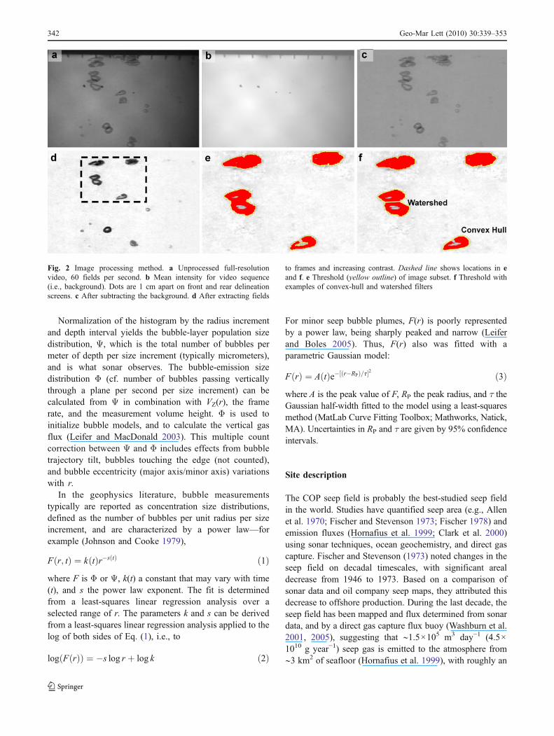
Video clips (Fig. 2a) were acquired at 8-bit, 60 fields persecond digital video resolution (720×240 pixels), andanalyzed using macros written in ImageJ. The macros(Leifer and MacDonald 2003; Leifer et al. 2003a; Leifer2010) extract the video to 60 frames per second by linearlyinterpolating the odd and even image rows on each frame

(Fig. 2d). Macros also removed background intensityvariations (Fig. 2c), decreased pixilation noise, filtered outblurry bubbles, and thresholded the image sequence(Fig. 2e).

Aided by macros that predict bubble location insubsequent frames, and to automatically track bubbleswhere possible, a significant fraction of bubbles weretracked between frames. For each bubble, the position,major and minor axes, angle, perimeter, area, circularity,and skew based on the thresholded outline, as well asframe number were recorded. Then, a convex-hulloutline was calculated and the bubble re-measured. Aconvex hull is the smallest polygon that can contain thebubble outline (also a rubber-band outline), and has theeffect of filling concavities where the bubble appears asa “half moon”, which can result from off-axis illumina-tion (Fig. 2f). Further analysis uses routines written inMatLab (Mathworks, Natick, MA).

Two measurements are available for each bubble, one withand one without a convex hull. In cases where the bubble ishalf moon-shaped, the convex-hull outline is used; otherwise,the non-convex-hull outline is used. Discrimination is basedon the circularity, C, defined as C=4π area/perimeter2.If C convex hullð Þ > C non�convex hullð Þ þ 15½ , then theconvex-hull measurement was used. For the bubbles labeledin Fig. 2f, C=0.238 and 0.781 for the non-convex-hull andconvex-hull outlines, respectively.

Then, for each tracked bubble, the mean bubble speedand equivalent spherical radius, r, from all measurementsduring its passage across the field of view, and the standarddeviations were determined. The bubble speed is correctedbased on the mean bubble trajectory to a vertical velocity,VZ. VZ allows conversion of the steady-state size distribu-tion (layer concentration) to the emission size distribution(flux passing through a horizontal plane), by accounting forthe number of repeat measurements of each bubble. Themean bubble rise trajectory is calculated from all the bubbletrajectories using a least-squares linear regression analysisof the positions of the tracked bubbles. The trajectory angleresults from camera tilt and currents. A polynomial fit of VZ

to r is used to derive a representative VZ(r). Then, outliersof more than one to two standard deviations are removedfrom the dataset (depending on the variability in VZ), andVZ(r) recalculated. VZ(r) includes the effects of buoyantrise, turbulence, oil, and bubble-induced upwelling flows.The upwelling flow is the vertical fluid motion driven bymomentum transfer from the rising bubbles.

All bubbles are r- and time (t)-segregated, and histo-grams N(r,t) were calculated. The histogram r-bin widthsare logarithmically spaced, and chosen so that a statisticallysignificant number of bubbles are counted in bins near thedistribution peak(s). The measurement uncertainty is N0.5,where N is the number of bubbles in each histogram bin.

Geo-Mar Lett (2010) 30:339–353 341

Normalization of the histogram by the radius incrementand depth interval yields the bubble-layer population sizedistribution, Ψ, which is the total number of bubbles permeter of depth per size increment (typically micrometers),and is what sonar observes. The bubble-emission sizedistribution Φ (cf. number of bubbles passing verticallythrough a plane per second per size increment) can becalculated from Ψ in combination with VZ(r), the framerate, and the measurement volume height. Φ is used toinitialize bubble models, and to calculate the vertical gasflux (Leifer and MacDonald 2003). This multiple countcorrection between Ψ and Φ includes effects from bubbletrajectory tilt, bubbles touching the edge (not counted),and bubble eccentricity (major axis/minor axis) variationswith r.

In the geophysics literature, bubble measurementstypically are reported as concentration size distributions,defined as the number of bubbles per unit radius per sizeincrement, and are characterized by a power law—forexample (Johnson and Cooke 1979),

F r; tð Þ ¼ kðtÞr�sðtÞ ð1Þwhere F is Φ or Ψ, k(t) a constant that may vary with time(t), and s the power law exponent. The fit is determinedfrom a least-squares linear regression analysis over aselected range of r. The parameters k and s can be derivedfrom a least-squares linear regression analysis applied to thelog of both sides of Eq. (1), i.e., to

log FðrÞð Þ ¼ �s log r þ log k ð2Þ

For minor seep bubble plumes, F(r) is poorly representedby a power law, being sharply peaked and narrow (Leiferand Boles 2005). Thus, F(r) also was fitted with aparametric Gaussian model:

FðrÞ ¼ AðtÞe� r�RPð Þ=t½ �2 ð3Þwhere A is the peak value of F, RP the peak radius, and τ theGaussian half-width fitted to the model using a least-squaresmethod (MatLab Curve Fitting Toolbox; Mathworks, Natick,MA). Uncertainties in RP and τ are given by 95% confidenceintervals.

Site description

The COP seep field is probably the best-studied seep fieldin the world. Studies have quantified seep area (e.g., Allenet al. 1970; Fischer and Stevenson 1973; Fischer 1978) andemission fluxes (Hornafius et al. 1999; Clark et al. 2000)using sonar techniques, ocean geochemistry, and direct gascapture. Fischer and Stevenson (1973) noted changes in theseep field on decadal timescales, with significant arealdecrease from 1946 to 1973. Based on a comparison ofsonar data and oil company seep maps, they attributed thisdecrease to offshore production. During the last decade, theseep field has been mapped and flux determined from sonardata, and by a direct gas capture flux buoy (Washburn et al.2001, 2005), suggesting that ∼1.5×105 m3 day−1 (4.5×1010 g year−1) seep gas is emitted to the atmosphere from∼3 km2 of seafloor (Hornafius et al. 1999), with roughly an

Fig. 2 Image processing method. a Unprocessed full-resolutionvideo, 60 fields per second. b Mean intensity for video sequence(i.e., background). Dots are 1 cm apart on front and rear delineationscreens. c After subtracting the background. d After extracting fields

to frames and increasing contrast. Dashed line shows locations in eand f. e Threshold (yellow outline) of image subset. f Threshold withexamples of convex-hull and watershed filters

342 Geo-Mar Lett (2010) 30:339–353

equal amount dissolved into the coastal ocean (Clark et al.2000). The seep field releases ∼80 barrels day−1, or 5×106 L year−1 (Clester et al. 1996), with oil slicks a commonchannel feature (Leifer et al. 2006b). Also, it has been notedthat oil emissions vary with tides (Mikolaj and Ampaya1973).

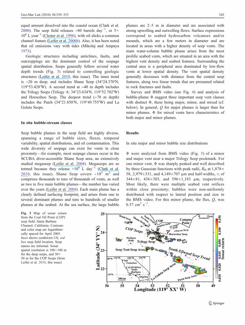
Geologic structures including anticlines, faults, andoutcroppings are the dominant control of the seepagespatial distribution. Seeps generally follow several waterdepth trends (Fig. 3) related to controlling geologicstructures (Leifer et al. 2010, this issue). The inner trendis ∼20 m deep, and includes Shane Seep (34°24.370′N,119°53.428′W). A second trend at ∼40 m depth includesthe Trilogy Seeps (Trilogy A: 34°23.634′N, 119°52.702′W)and Horseshoe Seep. The deepest trend (∼70 m depth)includes the Patch (34°21.850′N, 119°49.755′W) and LaGoleta Seeps.

In situ bubble-stream classes

Seep bubble plumes in the seep field are highly diverse,spanning a range of bubble sizes, fluxes, temporalvariability, spatial distributions, and oil contamination. Thiswide diversity of seepage can exist for vents in closeproximity—for example, most seepage classes occur in theSCUBA diver-accessible Shane Seep area, an extensivelystudied megaseep (Leifer et al. 2004). Megaseeps are sotermed because they release >106 L day−1 (Clark et al.2010, this issue). Shane Seep covers ∼103 m2 andcomprises thousands to tens of thousands of vents, as wellas two to five main bubble plumes—the number has variedover the years (Leifer et al. 2004). Each main plume has aclearly defined surfacing footprint, and arises from one toseveral dominant plumes and tens to hundreds of smallerplumes at the seabed. At the sea surface, the large bubble

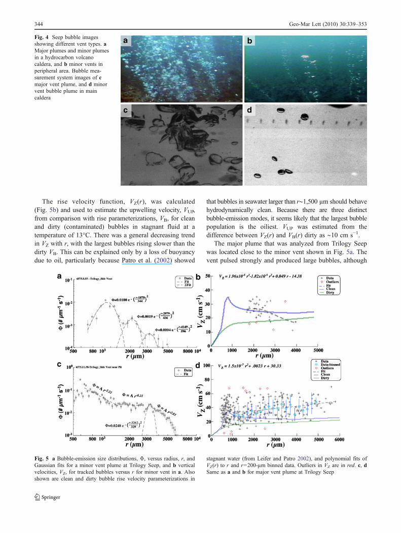
plumes are 2–5 m in diameter and are associated withstrong upwelling and outwelling flows. Surface expressionscorrespond to seabed hydrocarbon volcanoes and/ormounds, which are a few meters in diameter and arelocated in areas with a higher density of seep vents. Themain water-column bubble plume arises from the mostprolific seabed vents, which are situated in an area with thehighest vent density and seabed features. Surrounding thecentral area is a peripheral area dominated by low-flowvents at lower spatial density. The vent spatial densitygenerally decreases with distance from the central seepfeatures, along two linear trends that are presumed relatedto rock fractures and faults.

Survey and BMS video (see Fig. 4) and analysis ofbubble-plume Φ suggest three important seep vent classeswith distinct Φ, these being major, minor, and mixed (cf.below). In general, Q for major plumes is larger than forminor plumes. Φ for mixed vents have characteristics ofboth major and minor plumes.

Results

In situ major and minor bubble size distributions

Φ were analyzed from BMS video (Fig. 5) of a minorand major vent near a major Trilogy Seep pockmark. Forone minor vent, Φ was sharply peaked and well describedby three Gaussian functions with peak radii, RP, at 1,878±58, 2,979±331, and 4,149±707 µm and half-widths, τ, of344±81, 436±303, and 596±1,183 µm, respectively.Most likely, there were multiple seabed vent orificeswithin close proximity; bubbles were non-uniformlydistributed with respect to lateral position and size inthe BMS video. For this minor plume, the flux, Q, was0.57 cm3 s−1.

Fig. 3 Map of sonar returnfrom the Coal Oil Point (COP)seep field, Santa BarbaraChannel, California. Contoursand color map are logarithmi-cally spaced for April 2005.Inset shows southwest US, redbox seep field location. Seepnames are informal. Sonarspatial resolution is 100×100 mfor the deep seeps, and 50×50 m for the COP Seeps (fromLeifer et al. 2010, this issue)

Geo-Mar Lett (2010) 30:339–353 343

The rise velocity function, VZ(r), was calculated(Fig. 5b) and used to estimate the upwelling velocity, VUP,from comparison with rise parameterizations, VB, for cleanand dirty (contaminated) bubbles in stagnant fluid at atemperature of 13°C. There was a general decreasing trendin VZ with r, with the largest bubbles rising slower than thedirty VB. This can be explained only by a loss of buoyancydue to oil, particularly because Patro et al. (2002) showed

that bubbles in seawater larger than r∼1,500 µm should behavehydrodynamically clean. Because there are three distinctbubble-emission modes, it seems likely that the largest bubblepopulation is the oiliest. VUP was estimated from thedifference between VZ(r) and VB(r) dirty as ∼10 cm s−1.

The major plume that was analyzed from Trilogy Seepwas located close to the minor vent shown in Fig. 5a. Thevent pulsed strongly and produced large bubbles, although

Fig. 4 Seep bubble imagesshowing different vent types. aMajor plumes and minor plumesin a hydrocarbon volcanocaldera, and b minor vents inperipheral area. Bubble mea-surement system images of cmajor vent plume, and d minorvent bubble plume in maincaldera

Fig. 5 a Bubble-emission size distributions, Φ, versus radius, r, andGaussian fits for a minor vent plume at Trilogy Seep, and b verticalvelocities, VZ, for tracked bubbles versus r for minor vent in a. Alsoshown are clean and dirty bubble rise velocity parameterizations in

stagnant water (from Leifer and Patro 2002), and polynomial fits ofVZ(r) to r and r=200-µm binned data. Outliers in VZ are in red. c, dSame as a and b for major vent plume at Trilogy Seep

344 Geo-Mar Lett (2010) 30:339–353

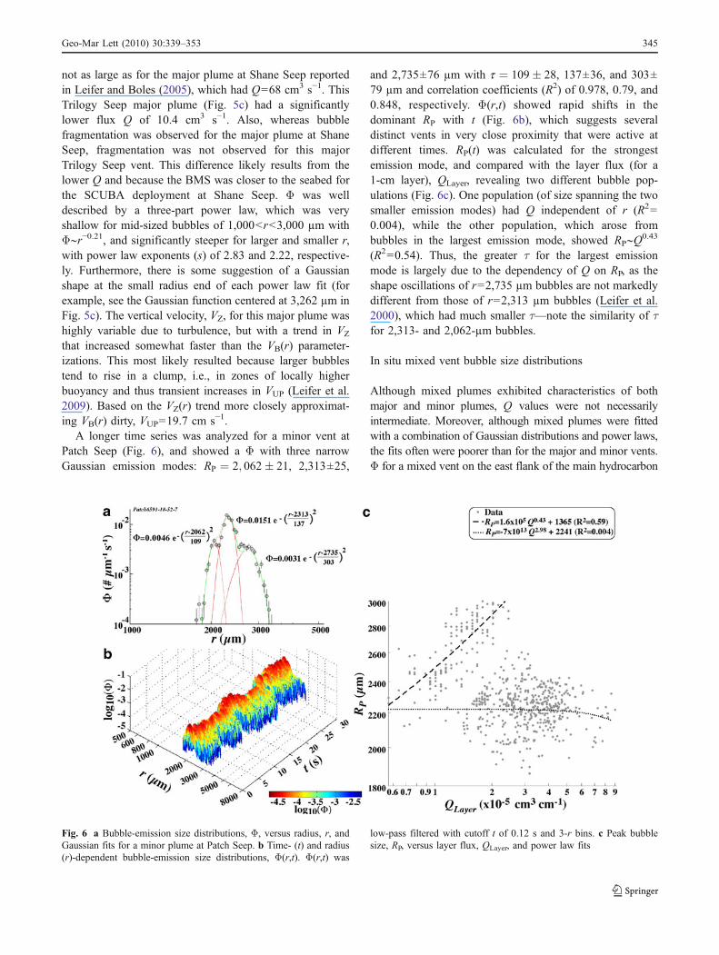
not as large as for the major plume at Shane Seep reportedin Leifer and Boles (2005), which had Q=68 cm3 s−1. ThisTrilogy Seep major plume (Fig. 5c) had a significantlylower flux Q of 10.4 cm3 s−1. Also, whereas bubblefragmentation was observed for the major plume at ShaneSeep, fragmentation was not observed for this majorTrilogy Seep vent. This difference likely results from thelower Q and because the BMS was closer to the seabed forthe SCUBA deployment at Shane Seep. Φ was welldescribed by a three-part power law, which was veryshallow for mid-sized bubbles of 1,000<r<3,000 µm withΦ∼r−0.21, and significantly steeper for larger and smaller r,with power law exponents (s) of 2.83 and 2.22, respective-ly. Furthermore, there is some suggestion of a Gaussianshape at the small radius end of each power law fit (forexample, see the Gaussian function centered at 3,262 µm inFig. 5c). The vertical velocity, VZ, for this major plume washighly variable due to turbulence, but with a trend in VZ

that increased somewhat faster than the VB(r) parameter-izations. This most likely resulted because larger bubblestend to rise in a clump, i.e., in zones of locally higherbuoyancy and thus transient increases in VUP (Leifer et al.2009). Based on the VZ(r) trend more closely approximat-ing VB(r) dirty, VUP=19.7 cm s−1.

A longer time series was analyzed for a minor vent atPatch Seep (Fig. 6), and showed a Φ with three narrowGaussian emission modes: RP ¼ 2; 062� 21, 2,313±25,

and 2,735±76 µm with t ¼ 109� 28, 137±36, and 303±79 µm and correlation coefficients (R2) of 0.978, 0.79, and0.848, respectively. Φ(r,t) showed rapid shifts in thedominant RP with t (Fig. 6b), which suggests severaldistinct vents in very close proximity that were active atdifferent times. RP(t) was calculated for the strongestemission mode, and compared with the layer flux (for a1-cm layer), QLayer, revealing two different bubble pop-ulations (Fig. 6c). One population (of size spanning the twosmaller emission modes) had Q independent of r (R2=0.004), while the other population, which arose frombubbles in the largest emission mode, showed RP∼Q0.43

(R2=0.54). Thus, the greater τ for the largest emissionmode is largely due to the dependency of Q on RP, as theshape oscillations of r=2,735 µm bubbles are not markedlydifferent from those of r=2,313 µm bubbles (Leifer et al.2000), which had much smaller τ—note the similarity of τfor 2,313- and 2,062-µm bubbles.

In situ mixed vent bubble size distributions

Although mixed plumes exhibited characteristics of bothmajor and minor plumes, Q values were not necessarilyintermediate. Moreover, although mixed plumes were fittedwith a combination of Gaussian distributions and power laws,the fits often were poorer than for the major and minor vents.Φ for a mixed vent on the east flank of the main hydrocarbon

Fig. 6 a Bubble-emission size distributions, Φ, versus radius, r, andGaussian fits for a minor plume at Patch Seep. b Time- (t) and radius(r)-dependent bubble-emission size distributions, Φ(r,t). Φ(r,t) was

low-pass filtered with cutoff t of 0.12 s and 3-r bins. c Peak bubblesize, RP, versus layer flux, QLayer, and power law fits

Geo-Mar Lett (2010) 30:339–353 345

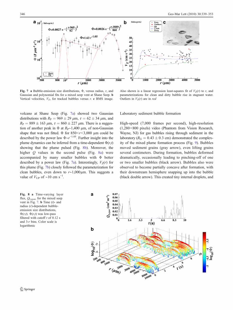
volcano at Shane Seep (Fig. 7a) showed two Gaussiandistributions with RP ¼ 969� 29 mm, t ¼ 62� 34 mm, andRP ¼ 889� 163 mm, t ¼ 860� 227 mm. There is a sugges-tion of another peak in Φ at RP∼1,400 µm, of non-Gaussianshape that was not fitted. Φ for 850<r<3,000 µm could bedescribed by the power law Φ∼r−1.05. Further insight into theplume dynamics can be inferred from a time-dependent Φ(r,t)showing that the plume pulsed (Fig. 8b). Moreover, thehigher Q values in the second pulse (Fig. 8a) wereaccompanied by many smaller bubbles with Φ betterdescribed by a power law (Fig. 7a). Interestingly, VZ(r) forthis plume (Fig. 7b) closely followed the parameterization forclean bubbles, even down to r∼1,000µm. This suggests avalue of VUP of ∼10 cm s−1.

Laboratory sediment bubble formation

High-speed (7,000 frames per second), high-resolution(1,280×800 pixels) video (Phantom from Vision Research,Wayne, NJ) for gas bubbles rising through sediment in thelaboratory (RG ¼ 0:43� 0:3 cm) demonstrated the complex-ity of the mixed plume formation process (Fig. 9). Bubblesmoved sediment grains (gray arrow), even lifting grainsseveral centimeters. During formation, bubbles deformeddramatically, occasionally leading to pinching-off of oneor two smaller bubbles (black arrow). Bubbles also wereobserved to become partially concave after formation, withtheir downstream hemisphere snapping up into the bubble(black double arrow). This created tiny internal droplets, and

Fig. 7 a Bubble-emission size distributions, Φ, versus radius, r, andGaussian and polynomial fits for a mixed seep vent at Shane Seep. bVertical velocities, VZ, for tracked bubbles versus r. c BMS image.

Also shown is a linear regression least-squares fit of VZ(r) to r, andparameterizations for clean and dirty bubble rise in stagnant water.Outliers in VZ(r) are in red

Fig. 8 a Time-varying layerflux, QLayer, for the mixed seepvent in Fig. 7. b Time (t)- andradius (r)-dependent bubble-emission size distributions,Φ(r,t). Φ(r,t) was low-passfiltered with cutoff t of 0.12 sand 3-r bins. Color scale islogarithmic

346 Geo-Mar Lett (2010) 30:339–353

in some cases led to the formation of very small bubbles.Finally, bubble coalescence was observed (white arrow).

Laboratory minor and major plumes

Airflow through capillary tubes for low Q produced asingle bubble chain. Gradually increasing Q, the bubblegeneration shifted to emission of two or three dominantsizes with sporadic small bubbles, and then for high Q to abroad size spectrum. Φ for low Q were sharply peaked andwell described by a Gaussian function (Fig. 10a).

A high-Q bubble plume from a 0.16-cm-diametercapillary tube was analyzed and showed Φ spanning abroad range, 200<r<4,000 µm (Fig. 10b), which could bedescribed, albeit poorly, by the power law Φ∼r−0.27. Finerstructure in Φ suggested that several portions of Φ werewell described by Gaussian functions; for example, there

were two peaks at peak radii (RP) of 600 and 1,030 µm andhalf-widths (τ) of 128 and 164 µm, with good R2 values of0.925 and 0.936, respectively. The broad peak at RP=2,900 µm, τ=549.2 µm was reasonably described by aGaussian function for r>RP, but not for r<RP (R2=0.783).Size segregation with t was observed at the measurementvolume, presumably because of the faster rise of largerbubbles—the tail of each bubble pulse comprised manysmaller bubbles.

Laboratory mixed bubble plumes

Bubble plumes generated by percolating bubbles through arange of sediment sizes in the laboratory showed a dominantpeak (RP) that varied inversely with grain size (RG)—forexample, RP=4,777, 2,947, 2,300, and 1,239 µm for RG=0.03, 0.43, 0.55, and 0.77 cm, respectively (Table 1). In all

Fig. 9 High-speed video image sequence of bubble formation from a gravel bed. The frame number is shown on each panel (0.14 ms per frame).Arrows identify bubbles undergoing different formation processes (see text for details)

Fig. 10 Bubble-emission sizedistribution, Φ, versus radius, r,for flux, Q, of a 2.10 cm3 s−1

from a capillary tube with0.64-cm orifice diameter, and b0.10 cm3 s−1 from a capillarytube with 0.16-cm orificediameter. Also shown are thecorresponding Gaussian andpower law function fits

Geo-Mar Lett (2010) 30:339–353 347

cases, Φ was described by a mixture of power law(s) and/orGaussian function(s). For sediment with RG=0.55 cm andfor the low QF1 (Fig. 11a), Φ for 1,550<r<3400 µm waswell described by a broad Gaussian distribution with RP ¼2; 157� 179 mm and t ¼ 671:9� 288 mm (R2=0.968); forRP<1550 and RP>2,200 µm, however, Φ was well describedby steep power laws with s=1.55 and 3.12 for the small andlarge r-ranges, respectively.

With increasing Q through a given sediment type, therewas a shift from Φ being a mixture of Gaussian and powerlaw functions to a single power law (Fig. 11c), with Φ forhigh Q being similar to Φ for major plumes (Fig. 5c). Forsediment with RG=0.55 cm, Φ for the low QF1 wasdescribed largely by two non-contiguous power laws withs=1.55 and 3.12 for the small and large size populations,respectively (Fig. 11a). For the highest QF3 (Fig. 11c), Φwas best described by a single, broad (585<r<5,020 µm),relatively shallow (s=1.29) power law. The intermediate ortransition QF2 produced a Φ similar to that for QF1, whichwas well described by bimodal non-contiguous power lawswith power law exponents s=2.33 and 2.47 for the ranges600<r<1,620 and 2,320<r<5,200 µm, respectively. Com-pared with Φ for QF1, the r ranges were larger and thevalues of s were intermediate (Fig. 11b), while the Gaussiantrends in Φ for QF1 had largely disappeared. Because itappears that QF2 is a transition between low- and high-Qbehaviors, a power law spanning the range 550<r<4,750 µm was calculated for QF2, and found s=2.33,steeper than for QF3. To summarize, with increasing Q the

troughs in Φ that separated the two distribution modes wereprogressively filled, while the range of these modesincreased between QF1 and QF2. Also, the r dependency ofΦ decreased, and the small Φ distribution was significantlyfilled from QF2 to QF3. Φ for QF3 was shallow and broad,consistent with the Φ associated with fragmentation.

Different behavior is expected for bubble formation fromsediments where bubble size and sediment grain size arecomparable—RP∼RG (e.g., Fig. 11), where sediment grainsize is much larger than bubble size—RP<<RG, and wheresediment grain size is much smaller than bubble size—RP>>RG. Where RP<<RG, the sediment should haveminimal impact on Φ; unfortunately, the sediment bed inthe laboratory was insufficiently thick to adequately studythis case. Where the two were comparable, high-speed video(Fig. 9) showed bubbles moving sediment during forma-tion. For the studied flow range, sediments 2–4 (Table 1) allhad RP<<RG and exhibited decreased bimodality for higherQ (e.g., Fig. 10c) than lower Q (e.g., Fig. 10a).

For RP>>RG (sediment #1, RG=300 µm), a differentbehavior is anticipated, because the bubbles cannot easilyslip through the pathways of the sediment without movingmany grains. Thus, elastic failure starts to become a keyprocess in bubble migration and formation (Boudreau et al.2005) for the smallest grain size that we studied, althoughthis sediment was non-cohesive, unlike clays. One result isthat bubble emissions tended to occur in transient pulsesseparated by times longer than the pulse length. For the lowQF1 (Fig. 12), Φ contained a broad (∼1,200<r<5,200 µm)

Fig. 11 Bubble-emission size distribution, Φ, versus radius, r, for laboratory flow, Q, of a 6.4, b 6.9, and c 8.1 cm3 s−1 through sediment withmean grain radius of 0.55 cm. Also shown are Gaussian and power law function fits

Table 1 Summary of laboratory sediment parametersa

Sediment DG (mm) RG (mm) dBD (gcm−3) � (cm3m−3) ζ Grain density (gcm−3) RP (µm)

Sediment 1 0.6 0.3 1.414 0.255 0.745 1.90 4,777

Sediment 2 8.6±7.0 4.3±3.5 1.576 0.191 0.809 1.95 2,947

Sediment 3 11.0±10. 5.5±5 1.425 0.339 0.661 2.16 2,300

Sediment 4 15.4±1.92 7.7±9.6 1.292 0.440 0.56 2.31 1,239

aDG mean grain size (diameter); RG mean grain radius; dBD dry bulk density; � porosity; ζ relative density; RP peak bubble size distributionradius

348 Geo-Mar Lett (2010) 30:339–353

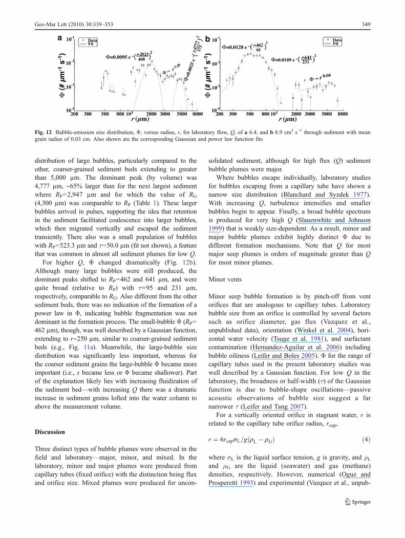
distribution of large bubbles, particularly compared to theother, coarser-grained sediment beds extending to greaterthan 5,000 µm. The dominant peak (by volume) was4,777 µm, ∼65% larger than for the next largest sedimentwhere RP=2,947 µm and for which the value of RG

(4,300 µm) was comparable to RP (Table 1). These largerbubbles arrived in pulses, supporting the idea that retentionin the sediment facilitated coalescence into larger bubbles,which then migrated vertically and escaped the sedimenttransiently. There also was a small population of bubbleswith RP=523.3 µm and τ=50.0 µm (fit not shown), a featurethat was common in almost all sediment plumes for low Q.

For higher Q, Φ changed dramatically (Fig. 12b).Although many large bubbles were still produced, thedominant peaks shifted to RP=462 and 641 µm, and werequite broad (relative to RP) with τ=95 and 231 µm,respectively, comparable to RG. Also different from the othersediment beds, there was no indication of the formation of apower law in Φ, indicating bubble fragmentation was notdominant in the formation process. The small-bubble Φ (RP=462 µm), though, was well described by a Gaussian function,extending to r∼250 µm, similar to coarser-grained sedimentbeds (e.g., Fig. 11a). Meanwhile, the large-bubble sizedistribution was significantly less important, whereas forthe coarser sediment grains the large-bubble Φ became moreimportant (i.e., s became less or Φ became shallower). Partof the explanation likely lies with increasing fluidization ofthe sediment bed—with increasing Q there was a dramaticincrease in sediment grains lofted into the water column toabove the measurement volume.

Discussion

Three distinct types of bubble plumes were observed in thefield and laboratory—major, minor, and mixed. In thelaboratory, minor and major plumes were produced fromcapillary tubes (fixed orifice) with the distinction being fluxand orifice size. Mixed plumes were produced for uncon-

solidated sediment, although for high flux (Q) sedimentbubble plumes were major.

Where bubbles escape individually, laboratory studiesfor bubbles escaping from a capillary tube have shown anarrow size distribution (Blanchard and Syzdek 1977).With increasing Q, turbulence intensifies and smallerbubbles begin to appear. Finally, a broad bubble spectrumis produced for very high Q (Slauenwhite and Johnson1999) that is weakly size-dependent. As a result, minor andmajor bubble plumes exhibit highly distinct Φ due todifferent formation mechanisms. Note that Q for mostmajor seep plumes is orders of magnitude greater than Qfor most minor plumes.

Minor vents

Minor seep bubble formation is by pinch-off from ventorifices that are analogous to capillary tubes. Laboratorybubble size from an orifice is controlled by several factorssuch as orifice diameter, gas flux (Vazquez et al.,unpublished data), orientation (Winkel et al. 2004), hori-zontal water velocity (Tsuge et al. 1981), and surfactantcontamination (Hernandez-Aguilar et al. 2006) includingbubble oiliness (Leifer and Boles 2005). Φ for the range ofcapillary tubes used in the present laboratory studies waswell described by a Gaussian function. For low Q in thelaboratory, the broadness or half-width (τ) of the Gaussianfunction is due to bubble-shape oscillations—passiveacoustic observations of bubble size suggest a farnarrower τ (Leifer and Tang 2007).

For a vertically oriented orifice in stagnant water, r isrelated to the capillary tube orifice radius, rcap,

r ¼ 6rcapsL=g rL � rGð Þ ð4Þ

where σL is the liquid surface tension, g is gravity, and ρLand ρG are the liquid (seawater) and gas (methane)densities, respectively. However, numerical (Oguz andProsperetti 1993) and experimental (Vazquez et al., unpub-

Fig. 12 Bubble-emission size distribution, Φ, versus radius, r, for laboratory flow, Q, of a 6.4, and b 6.9 cm3 s−1 through sediment with meangrain radius of 0.03 cm. Also shown are the corresponding Gaussian and power law function fits

Geo-Mar Lett (2010) 30:339–353 349

lished data) evidence suggests greater complexity with thebubble volume, varying as Q6/5 above a critical gas flowrate, QC. For Q<QC, an increase in Q causes the bubbleformation rate to increase, but not r, i.e., r is independent ofQ. Both of these behaviors were observed in the Patch Seepminor vent bubble population (Fig. 8), with r∼Q0.43 for onepopulation, in excellent agreement with theory. Thissuggests that there were three vents (or sediment pathways)with different characteristics that combined to produce theΦ shown in Fig. 8. This also demonstrates how τ increasedfor Q>QC, i.e., based on comparison with laboratory τ(RP),vents can be classified as Q>QC or Q<QC.

Multiple peaks were observed for a number of minorplumes and for laboratory sediment plumes. The mostcommon secondary peak was of very small bubbles even incases where a peak was not clearly resolved (Leifer 2010).These very small bubbles often were observed with Φdistinct from Φ for large bubbles (i.e., not fit with the samefunctional form). Based on the high-speed video, thesebubbles likely were created during bubble pinch-off (Fig. 9).For some vents, bubble peaks were for bubbles with integermultiple volumes (Fig. 5a) of the bubble volume. A bubblewith RP=2,979 µm has 3.99 times the volume of a bubblewith RP=1,878 µm. This suggests bubble formation with twomodes where either one or four bubbles are produced fromthe same Q. Bubbles from another, far lower probabilitypeak with RP=4,149 µm may have originated from aseparate vent. For most minor vents with multiple peaks,however, there was no clear relationship.

Major vents

Φ for major bubble plumes were primarily well describedby shallow power laws, suggesting bubble fragmentation asthe dominant formation mechanism. For the laboratorystudies, increasing Q from a capillary tube caused bubblesin the dominant peak (a minor plume at low Q) to visiblyfragment into smaller bubbles. For the laboratory capillarytube and QF3, the process was not complete, and adominant peak remained; however, RP for QF3 was smallerthan RP for low Q, suggesting that RP∼Q2/5 is inappropriateonce fragmentation becomes important. Apparently, RP∼Qk

where k is a constant less than 0.4. At higher Q, there nolonger is evidence of a preferential emission RP, i.e.,Gaussian peak. Because fragmentation occurs after the gasjet exits the orifice, it is unlikely to depend directly onorifice characteristics.

Mixed vents

Mixed vent Φ exhibited characteristics of both minor andmajor plumes, as well as different characteristics similar toneither of these types. Having characteristics of both

suggests incomplete fragmentation of a bubble size distri-bution Φ, which has a preferred size (Gaussian). Mixedplumes were not observed for capillary tubes, but werecreated for sediment-bed plumes. Thus, we propose thatsediment grain mobility plays a critical role in the mixedplume formation process.

Three sediment bubble formation regimes are proposedfor typical seep vents based on the grain size (RG) to peakradius (RP) ratio, leading to distinct Φ. Specifically, forRG>>RP bubble buoyancy is insufficient to move sedimentgrains, while pore sizes are large with low capillary forces;thus, we predict high permeability (rapid migration) and Φsimilar to capillary tube Φ. In this study, Φ measured forsediment grain size #5 (RG=2.35 cm) were similar to Φ forthe bubble fret—i.e., the sediment-bed layer was too thin,and no analysis was conducted (cf. not shown in Table 1).At the other extreme, RG<<RP (sediment grain size #1), allbubbles can easily shift and lift many grains; however,capillary forces are high and the bubbles are larger than thesediment voids; thus, permeability is low, enabling sedi-ment retention of bubbles. Here, migration bears similarityto elastic failure, because grains must shift to allow passageof a bubble, a process that was observed to occur veryunsteadily. For the sediments in this study, however,cohesion does not play a role. Thus, the regime whereelastic failure is truly dominant lies in even finer-grainedsediments than used in this study, like clays, which doexhibit cohesive forces. Buoyancy and pressure forces mustovercome cohesive forces and sediment compressibility toallow bubble migration. There exists extensive literature onbubble migration through fine-grained sediments (e.g., Sillsand Wheeler 1992; O’Hara et al. 1995; Boudreau et al.2005; Judd and Hovland 2007; Leighton and Robb 2008).From fine-grained cohesive muddy sediments, like afreshwater marsh, pulses of bubbles sporadically andinfrequently escape, spanning very large to small bubbles,a characteristic of only the finest sediments studied in thepresent laboratory work. Finally, bubbles with RG∼RP canmove and lift sediment grains during formation (Fig. 8).This leads to mobile sediment “orifices” and thus complexityin Φ, producing mixed bubble plumes. Q affects thesecategories: for higher Q, sediment with RG>RP couldbecome mobilized. Also, sediment grain characteristics atthe vent likely change as bubbles remove smaller grainsfrom the vent orifice, increasing RG until the remaininggrains are too large to lift. Finally, for fine-grained sedi-ments, the elastic failure mechanism is circumvented if thetime interval between bubbles in the migration pathway isshort, such that the sediment has sufficiently low relativedensity (high void space) to provide easy migration. In suchcases, the sediment acts more like a fluid, unable to retainbubbles. The high-Q case for the finest sediment in thisstudy likely was close to this behavior.

350 Geo-Mar Lett (2010) 30:339–353

Unfortunately, the seabed vents were not characterized;thus, the relationship between grain size and Q elucidatedin the laboratory requires further field studies for validation.Because of their greater buoyancy force, larger bubbles(correlating to higher Q; Leifer 2010) can be assumed to liftand displace larger sediment grains than smaller bubbles.Larger bubbles also generate stronger upwelling flows,which should lift larger grains (assuming the same graindensity) higher. Small grains were observed being upwelled(and then sinking) in some of the seep video. As a result,for constant vent flux, there should be a gradual removal ofsmall grains, with only grains too large to be movedremaining. Thus, there likely is a pattern of a shift frommobile to fixed orifice. Specifically, tar deposition, settlingof sand grains into locked positions, and bacterial mats allcould play a role in the evolution of the initial mixed Φvents to minor or major Φ vents. Reversion to a mixed ventwould occur if the migration pathway shifts (due toblockage of the vent or subsurface pathway), or after atransient or long-term increase in Q that remobilizessediments, or through deposition of new sediment.

Unsteady Q has been observed in many seep bubbleplumes. On 10-s timescales, wave-induced surge modulatesbubble formation (Leifer and Boles 2005); however, seepvents have been noted to exhibit unsteady flow on secondand sub-second timescales. Leifer and Boles (2005)observed a major plume that pulsed on sub-second time-scales; moreover, pulsing was observed for the major seepvent in Fig. 5c. This pulsing is not a measurement artifact;size segregation of the pulse due to different VZ of bubbles ofdifferent r are identified easily in the time- and size-resolvedΦ, with smaller bubbles arriving at the measurement volumelater than larger, faster rising bubbles (e.g., Fig. 8). In thelaboratory studies, pulsing was observed for sediment-bedplumes. This likely results from flow instabilities in thesediment bed, a process documented in fluid dynamicsstudies using magnetic resonance imaging of two-phasetrickle-bed flow (Sederman and Gladden 2005). Trickle bedsare used in chemical catalysis reactions, and for Q above athreshold exhibit rapid pulsing behavior. A different type ofpulsing was observed in the laboratory for relatively fine-grained, non-cohesive sediment (RP>>RG) related to elasticfailure migration, as discussed above. Pulsing was notobserved for high Q through sediments where RP∼RG, norfor low Q for capillary tubes. Similarly, low-Q minor seepvents did not significantly pulse. Finally, for major plumesfrom the capillary tube, rapid pulsing was observed at themeasurement volume on quarter- to half-second timescales.Because the gas escapes the orifice continuously, turbulenceprocesses must be responsible.

Although one would expect that with increasing grainsize, and hence space between grains, there would be anincrease in the dominant RP for low Q, laboratory

observations showed the opposite. This trend held not onlyfor sediments where RP∼RG, but also for the relatively fine-grained sediment where RP<<RG. This suggests that theprogressively decreasing ability of the sediment to retainbubbles is the underlying process, rather than pore size;finer sediments can more effectively trap bubbles prior toand during formation, because the capillary pressurerequired for a bubble to pass through pore spaces increasesfor smaller grain size. Sediment mobility also plays a role.High-speed video showed this process where during bubbleformation, sediment grains surrounding the bubble arepushed aside and then settle after pinch-off. With increas-ing RG, the sediment is less mobile because of packingleading to smaller pore throat and thus tending to decreasebubble size at formation. Also, the greater capillary forcewith decreasing grain size for a given buoyancy force (Q)will tend to decrease bubble size at formation.

Conclusions

The size-dependent flux distributions Φ for different seepvents were measured with a video bubble measurementsystem in the Santa Barbara Channel, California. Threedistinct plume types were identified—major, minor, andmixed. Minor plumes generally were of lower emission flux(Q), with narrow, peaked Φ that were well described byGaussian functions and were consistent with laboratoryobservations of capillary tube bubble formation at low Q.Major plumes showed a broad Φ spanning very small tovery large bubbles, and were well described by a powerlaw. Field observations of major plumes were consistentwith laboratory bubble plumes produced from capillarytubes for higher flows, where bubble fragmentation createdthe broad, shallow Φ. Examination of a long time record ofa minor plume vent showed that some vent bubblesincreased as RP∼Q0.43, in agreement with theory for Qgreater than a characteristic Q.

Mixed plumes showed characteristics of both minor andmajor plumes, which were very similar to those oflaboratory sediment-bed bubble plumes. This suggests thatunconsolidated sediment grains were key to mixed plumeformation. High-speed video showed significant interac-tions between bubbles and mobile sediment grains, withgrains being moved or lifted during the bubble formationand fragmentation process. Furthermore, the behavior ofbubbles from sediments with grain sizes smaller than thebubble size was quite different than the behavior observedwhere grain and bubble sizes were similar. It was concludedthat sediment retention ability was inversely related tosediment grain size over the range of (non-cohesive)sediment grain sizes studied here, and thus sediment grainsize was inversely related to the size of the dominant peak

Geo-Mar Lett (2010) 30:339–353 351

of Φ. For sediment with grains smaller than the bubble size,retention is efficient, creating pulsed emission separated byrelatively long intervals. This emission mode was a poormodel of field seep observations in the Coal Oil Point seepfield. We propose that vents cycle between mobilesediment-bed mixed emission, and fixed capillary-likemajor and minor vent activity through a range of processes.

Acknowledgements We would like to acknowledge the supportof the NOAA NURP, the U.S. Mineral Management Service,Agency #1435-01-00-CA-31063, Task #18211, and the Universityof California Energy Institute. Special thanks to the University ofCalifornia, Santa Barbara (UCSB) divers Shane Anderson, DaveFarrar, Dennis Divins, Christoph Pierre, and underwater videographerEric Hessel, as well as Tonya del Sontro for help collecting submersibleseep bubble video, and the crew of the Delta submersible. Thanks toLarry Vladic of Phantom Research for high-speed video of sedimentbubble formation. Views and conclusions in this document are those ofthe authors, and should not be interpreted as necessarily representing theofficial policies, either expressed or implied, of the U.S. government orUCSB.

Open Access This article is distributed under the terms of theCreative Commons Attribution Noncommercial License which per-mits any noncommercial use, distribution, and reproduction in anymedium, provided the original author(s) and source are credited.

Appendix

A (−) Peak value of F in Gaussian functional fitC (−) Circularity of bubble outline. Used in image

processingDG (mm) Equivalent spherical diameter of sediment

grainsF (#µm−1 m−1)

Function that represents either Φ or Ψ

N (−) Number of bubbles analyzedQ (L min−1) Flow (corrected to STP)QLayer (Lmin−1)

Layer flux (total volume of bubbles in alayer)

R2 (−) Correlation coefficientRG (mm) Equivalent spherical radius of sediment

grainsRP (µm) Radius of peak concentration in ΦVB (cm s−1) Bubble rise velocity in stagnant fluidVUP

(cm s−1)Upwelling velocity

VV (cm3) Porosity or sediment void volumeVZ (cm s−1) Bubble vertical velocitydBD(g cm−3)

Dry bulk density

g(m s−1 s−1)

Gravity

r (µm) Equivalent spherical bubble radiusrcap (µm) Capillary tube orifice radius opening

s (−) Power law exponent in Φt (s) Time�

(cm3 cm−3)Porosity

ζ (−) Relative densityρG (g cm−3) Bubble gas densityρL (g cm−3) Water densityτ (µm) Gaussian function half-widthΦ (#µm−1 s−1)

Bubble flux size distribution

Ψ (#µm−1 m−1)

Bubble-layer population size distribution

References

Allen AA, Schleuter RS, Mikolaj PG (1970) Natural oil seepage atCoal Oil Point, Santa Barbara, California. Science 170:974–977

Blanchard DC, Syzdek LD (1977) Production of air bubbles of aspecified size. Chem Eng Sci 32:1109–1112

Boudreau BP, Algar C, Johnson BD, Croudace I, Reed A, Furukawa Y,Dorgan KM, Jumars PA, Grader AS, Gardiner BS (2005) Bubblegrowth and rise in soft sediments. Geology 33(6):517–520

Clark JF, Washburn L, Hornafius JS, Luyendyk BP (2000) Naturalmarine hydrocarbon seep source of dissolved methane to Californiacoastal waters. J Geophys Res-Oceans 105:11509–511522

Clark JF, Washburn L, Schwager Emery K (2010) Variability of gascomposition and flux intensity in natural marine hydrocarbon seeps.In: Bohrmann G, Jørgensen BB (eds) Proc 9th Int Conf Gas inMarine Sediments, 5–19 September 2008, Bremen. Geo-Mar Lett SI30. doi:10.1007/s00367-009-0167-1

Clester SM, Hornafius JS, Scepan J, Estes JE (1996) Quantification ofthe relationship between natural gas seepage rates and surface oilvolume in the Santa Barbara Channel, (abstract). EOS AGUTrans 77:F419

Fischer PJ (1978) Oil and tar seeps, Santa Barbara basin, California.In: Fischer PJ (ed) California offshore gas, oil, and tar seeps.California State Lands Commission, Sacramento, pp 1–62

Fischer PJ, Stevenson AJ (1973) Natural hydrocarbon seeps, SantaBarbara basin. In: Fischer PJ (ed) Santa Barbara channel arearevisited field trip guidebook. American Association of PetroleumGeologists, Tulsa, pp 17–28

Hernandez-Aguilar JR, Cunningham R, Finch JA (2006) A test of theTate equation to predict bubble size at an orifice in the presenceof frother. Int J Min Process 79:89–97

Hornafius JS, Quigley DC, Luyendyk BP (1999) The world’s mostspectacular marine hydrocarbons seeps (Coal Oil Point, SantaBarbara Channel, California): quantification of emissions. JGeophys Res-Oceans 104:20703–20711

IPCC (2001) Climate change 2001—the scientific basis. CambridgeUniversity Press, Cambridge

Johnson BD, Cooke RC (1979) Bubble populations and spectra incoastal waters: a photographic approach. J Geophys Res 84(C7):3761–3766

Judd A, Hovland M (2007) Seabed fluid flow: the impact on geology,biology and the marine environment. Cambridge UniversityPress, Cambridge

Khalil MAK, Rasmussen RA (1995) The changing composition of theEarth’s atmosphere. In: Singh HB (ed) Composition, chemistry,and climate of the atmosphere. Van Nostrand Reinhold, NewYork, pp 50–87

352 Geo-Mar Lett (2010) 30:339–353

Kvenvolden KA, Rogers BW (2005) Gaia’s breath—global methaneexhalations. Mar Petrol Geol 22:579–590

Kvenvolden KA, Lorenson TD, Reeburgh WS (2001) Attentionturns to naturally occurring methane seepage. EOS AGU Trans82:457

Leifer I (2010) Characteristics and scaling of bubble plumes frommarine hydrocarbon seepage in the Coal Oil Point seep field. JGeophys Res. doi:10.1029/2009JC005844

Leifer I, Boles J (2005) Measurement of marine hydrocarbon seepflow through fractured rock and unconsolidated sediment. MarPetrol Geol 22:551–568

Leifer I, Judd AG (2002) Oceanic methane layers: a bubble depositionmechanism from marine hydrocarbon seepage. Terra Nova16:417–424

Leifer I, MacDonald IR (2003) Dynamics of the gas flux from shallowgas hydrate deposits: interaction between oily hydrate bubblesand the oceanic environment. Earth Planet Sci Lett 210:411–424

Leifer I, Patro RK (2002) The bubble mechanism for methanetransport from the shallow sea bed to the surface: a review andsensitivity study. Cont Shelf Res 22:2409–2428

Leifer I, Tang DJ (2007) The acoustic signature of marine seepbubbles. J Acoustical Soc Am 121:EL35–EL40

Leifer I, Patro RK, Bowyer P (2000) A study on the temperaturevariation of rise velocity for large clean bubbles. J AtmosOceanic Technol 17:1392–1402

Leifer I, de Leeuw G, Cohen LH (2003a) Optical measurement ofbubbles: system design and application. J Atmos OceanicTechnol 20:1317–1332

Leifer I, de Leeuw G, Kunz GH, Cohen L (2003b) Calibrating opticalbubble size by the displaced-mass method. Chem Eng Sci58:5211–5216

Leifer I, Boles JR, Luyendyk BP, Clark JF (2004) Transient dischargesfrom marine hydrocarbon seeps: spatial and temporal variability.Environ Geol 46:1038–1052

Leifer I, Luyendyk BP, Boles J, Clark JF (2006a) Natural marineseepage blowout: contribution to atmospheric methane. GlobalBiogeochem Cycles 20:GB3008. doi:10.1029/2005GB002668

Leifer I, Luyendyk B, Broderick K (2006b) Tracking an oil slick frommultiple natural sources, Coal Oil Point, California. Mar PetrolGeol 23:621–630

Leifer I, Jeuthe H, Gjøsund SH, Johansen V (2009) Engineered andnatural marine seep, bubble-driven buoyancy flows. J PhysOceanogr 39:3071–3090

Leifer I, Kamerling M, Luyendyk BP, Wilson D (2010) Geologiccontrol of natural marine seep hydrocarbon emissions, Coal OilPoint seep field, California. In: Bohrmann G, Jørgensen BB (eds)

Proc 9th Int Conf Gas in Marine Sediments, 5–19 September2008, Bremen. Geo-Mar Lett SI 30 (in press)

Leighton TG, Robb GBN (2008) Preliminary mapping of voidfractions and sound speeds in gassy marine sediments fromsubbottom profiles. J Acoustical Soc Am 124:EL313–EL320

Mikolaj PG, Ampaya JP (1973) Tidal effects on the activity of naturalsubmarine oil seeps. Mar Technol Soc J 7:25–28

Oguz HN, Prosperetti A (1993) Dynamics of bubble growth anddetachment from a needle. J Fluid Mech 257:111–145

O’Hara SCM, Dando PR, Schuster U, Bennis A, Boyle JD, Chui FTW,Hatherell TVJ, Niven SJ, Taylor LJ (1995) Gas seep inducedinterstitial water circulation: observations and environmentalimplications. Cont Shelf Res 15:931–948

Patro R, Leifer I, Bowyer P (2002) Better bubble process modeling:improved bubble hydrodynamics parameterisation. In: DonelanM, Drennan W, Salzman ES, Wanninkhof R (eds) Gas transferand water surfaces. American Geophysical Union, Washington,pp 315–320

Rehder G, Keir RS, Suess E, Rhein M (1999) Methane in the NorthernAtlantic controlled by microbial oxidation and atmospherichistory. Geophys Res Lett 26:587–590

Sauter EJ, Muyakshin SI, Charlou J-L, Schlüter M, Boetius A, JeroschK, Damm E, Foucher J-P, Klages M (2006) Methane dischargefrom a deep-sea submarine mud volcano into the upper watercolumn by gas hydrate-coated methane bubbles. Earth Planet SciLett 243:354–365

Sederman AJ, Gladden LF (2005) Transition to pulsing flow intrickle-bed reactors studied using MRI. AIChE J 51:615–621

Sills GC, Wheeler SJ (1992) The significance of gas for offshoreoperations. Cont Shelf Res 12:1239–1250

Slauenwhite DE, Johnson BD (1999) Bubble shattering: differences inbubble formation in fresh water and seawater. J Geophys Res104:3265–3275

Tsuge H, Hibino S, Nojima U (1981) Volume of a bubble formed at asingle submerged orifice in a flowing liquid. Int Chem Eng21:630–636

Washburn L, Johnson C, Gotschalk CG, Egland ET (2001) A gascapture buoy for measuring bubbling gas flux in oceans andlakes. J Atmos Oceanic Technol 18:1411–1420

Washburn L, Clark JF, Kyriakidis P (2005) The spatial scales,distribution, and intensity of natural marine hydrocarbon seepsnear Coal Oil Point, California. Mar Petrol Geol 22:569–578

Winkel ES, Ceccio SL, Dowling DR, Perlin M (2004) Bubble-sizedistributions produced by wall injection of air into flowingfreshwater, saltwater and surfactant solutions. Exp Fluids37:802–810

Geo-Mar Lett (2010) 30:339–353 353