
SPECTRAL ANALYSIS AND QUANTITATION IN MALDI-MS ...
326
SPECTRAL ANALYSIS AND QUANTITATION IN MALDI-MS IMAGING A THESIS SUBMITTED TO THE UNIVERSITY OF MANCHESTER FOR THE DEGREE OF DOCTOR OF PHILOSOPHY IN THE FACULTY OF BIOLOGY, MEDICINE AND HEALTH 2019 SOMRUDEE DEEPAISARN SCHOOL OF HEALTH SCIENCES DIVISION OF INFORMATICS, IMAGING AND DATA SCIENCES
-
Upload
khangminh22 -
Category
Documents
-
view
3 -
download
0
Transcript of SPECTRAL ANALYSIS AND QUANTITATION IN MALDI-MS ...

SPECTRAL ANALYSIS
AND QUANTITATION IN
MALDI-MS IMAGING
A THESIS SUBMITTED TO THE UNIVERSITY OF MANCHESTER
FOR THE DEGREE OF DOCTOR OF PHILOSOPHY
IN THE FACULTY OF BIOLOGY, MEDICINE AND HEALTH
2019
SOMRUDEE DEEPAISARN
SCHOOL OF HEALTH SCIENCES
DIVISION OF INFORMATICS, IMAGING AND DATA SCIENCES

2
‘Blank page’

3
Contents
Abstract ............................................................................................................. 22
Declaration ........................................................................................................ 23
Copyright Statement .......................................................................................... 24
Acknowledgement ............................................................................................. 25
Chapter 1 Introduction ..................................................................................... 26
1.1 Important Concepts ........................................................................................ 26
1.2 Aims and Objectives ....................................................................................... 31
1.3 Thesis Overview .............................................................................................. 32
1.4 List of Outputs ................................................................................................ 35
Chapter 2 Background I: Mass Spectrometry Instrumentation and Applications 37
2.1 Fundamentals of Mass Spectrometry ............................................................ 38
2.1.1 General Background ................................................................................. 39
2.1.2 Ionisation Techniques .............................................................................. 40
2.1.2.1 Electron Ionisation ............................................................................ 41
2.1.2.2 Chemical Ionisation ........................................................................... 41
2.1.2.3 Fast Atom Bombardment .................................................................. 42
2.1.2.4 Electrospray Ionisation ...................................................................... 43
2.1.3 Types of Mass Analysers .......................................................................... 44
2.1.3.1 Electric/Magnetic Sectors ................................................................. 44
2.1.3.2 Transmission Quadrupole ................................................................. 45
2.1.3.3 Orbitrap ............................................................................................. 46
2.1.3.4 Fourier Transform Ion Cyclotron Resonance .................................... 46
2.2 MALDI Mass Spectrometry ............................................................................. 47
2.2.1 Invention .................................................................................................. 47
2.2.2 MALDI Ionisation ...................................................................................... 50

4
2.2.3 Ion Acceleration ....................................................................................... 52
2.2.4 The Time-of-flight Mass Analyser ............................................................ 54
2.2.4.1 Linear Time-of-flight Mass Spectrometer ......................................... 54
2.2.4.2 Reflectron Time-of-flight Mass Spectrometer .................................. 56
2.2.4.3 Curved Field Reflectron Mass Spectrometer .................................... 57
2.2.5 Ion Detection ........................................................................................... 57
2.2.6 Mass Resolution ....................................................................................... 58
2.2.7 MALDI Matrices ....................................................................................... 59
2.2.8 Sample Preparation (Sample-matrix Depositions) .................................. 60
2.2.9 Tandem Mass Spectrometry .................................................................... 62
2.3 Lipidomics and the Application of MALDI-MS in Lipidomics .......................... 64
2.3.1 Lipid Types and Functions ........................................................................ 64
2.3.2 Cellular Lipids ........................................................................................... 65
2.3.3 Lipid Extraction Techniques ..................................................................... 67
2.3.4 Spectral Analysis (in Lipid Classification) ................................................. 68
2.3.5 Limitations and Challenges ...................................................................... 71
2.3.6 Lipids in the Brain .................................................................................... 72
2.4 Mass Spectrometry Imaging for Lipid Analysis .............................................. 74
2.4.1 General MS Imaging Instrumentation ..................................................... 74
2.4.2 Understanding the Mass Spectrometry Imaging Data Formats .............. 74
2.4.3 MALDI-MS Imaging of Lipids .................................................................... 76
2.4.4 Other Mass Spectrometry Imaging Techniques ...................................... 79
Chapter 3 Background II: Quantitative Mass Spectrometry ............................... 81
3.1 The Scope of Quantitative Mass Spectrometry ............................................. 82
3.1.1 Problems in MALDI-MS Quantitation ...................................................... 83
3.1.2 Uses of Standards .................................................................................... 85
3.1.2.1 Internal Standards ............................................................................. 85
3.1.2.2 External Standards ............................................................................ 87
3.1.3 Conventional Peak Analysis ..................................................................... 87
3.1.4 Supporting Software for Mass Spectrometry Data Analysis ................... 89
3.2 Computational Analysis Methods for MALDI-MS Data .................................. 90

5
3.2.1 Data Mining .............................................................................................. 91
3.2.2 Computational Approaches ..................................................................... 92
3.2.2.1 Support Vector Machine ................................................................... 92
3.2.2.2 Nearest Neighbours .......................................................................... 93
3.2.2.3 Random Forest .................................................................................. 93
3.2.2.4 Neural Networks ............................................................................... 94
3.2.2.5 Discussion and Comparison of Some Approaches to MALDI-MS Data
Analysis ............................................................................................................ 96
3.2.3 Understanding Signal and Noise and the Associated Analysis
Requirements.................................................................................................... 101
3.3 Pre-processing of Mass Spectra for LP-ICA................................................... 104
3.3.1 Windowing and Resolution Reduction .................................................. 105
3.3.2 Alignment ............................................................................................... 106
3.3.3 Baseline Correction ................................................................................ 106
3.3.4 Peak Detection and Integration ............................................................. 107
3.4 Linear Poisson Independent Component Analysis ....................................... 109
3.4.1 Correlation of Numerical Data ............................................................... 109
3.4.2 Standard PCA and ICA ............................................................................ 110
3.4.2.1 Principal Component Analysis (PCA) ............................................... 110
3.4.2.2 Independent Component Analysis (ICA) ......................................... 111
3.4.3 Distribution of Data: Gaussian vs. Poisson ............................................ 112
3.4.4 MALDI-MS Data Characteristics ............................................................. 115
3.4.5 Linear Poisson Independent Component Analysis (LP-ICA) Modelling . 116
3.4.6 Maximisation Separation (MAX SEP) ..................................................... 119
Chapter 4 Optimisation of Experimental Parameters ...................................... 122
4.1 Introduction .................................................................................................. 122
4.2 Instrumentation ............................................................................................ 124
4.2.1 The AXIMA.............................................................................................. 124
4.2.2 The 7090................................................................................................. 124
4.2.3 Standard Apparatus Settings ................................................................. 125
4.3 Sample Preparation ...................................................................................... 125

6
4.3.1 Materials ................................................................................................ 125
4.3.2 Preparation of Milk Samples ................................................................. 127
4.3.3 Preparation of Matrix Solution .............................................................. 127
4.3.4 Sample-matrix Deposition Method for MS Analysis of Milk Samples ... 128
4.3.5 Matrix Deposition Method for Imaging Samples .................................. 129
4.3.6 Calibration Standard .............................................................................. 130
4.4 Parameter Adjustment for Optimising Mass Spectrometry Data
Acquisitions .......................................................................................................... 130
4.4.1 Initial Tests of Instrumental and Technical Performance ...................... 130
4.4.2 Repeatability Tests of MS Spectra from Milk Samples .......................... 137
4.4.3 Matrix Coating and Signal Analysis ........................................................ 144
4.5 Conclusion .................................................................................................... 148
Chapter 5 Quantifying Binary Mixtures of Biological Samples ......................... 150
5.1 Introduction .................................................................................................. 150
5.2 Materials and Methods ................................................................................ 154
5.2.1 Materials ................................................................................................ 155
5.2.2 Sample Preparation ............................................................................... 156
5.2.2.1 Brain Dissection ............................................................................... 156
5.2.2.2 Tissue Homogenisation ................................................................... 157
5.2.2.3 Lipid Extraction ................................................................................ 157
5.2.2.4 Binary Mixture ................................................................................. 158
5.2.2.5 Matrix .............................................................................................. 159
5.2.2.6 MS Sample Preparation and Deposition ......................................... 159
5.2.3 MS Acquisition ....................................................................................... 159
5.3 Data Analysis Procedure ............................................................................... 160
5.3.1 Pre-processing ....................................................................................... 160
5.3.2 Peak Ratio Analysis ................................................................................ 165
5.3.3 Linear Poisson ICA Analysis .................................................................... 165
5.3.4 Mapping Components to Classes .......................................................... 167
5.3.5 Spectra Error Analysis ............................................................................ 169
5.3.6 Measurement Error Analysis ................................................................. 170

7
5.4 Results and Discussion .................................................................................. 171
5.4.1 Peak Ratio Analysis ................................................................................ 171
5.4.2 Linear Poisson ICA Analysis .................................................................... 173
5.4.3 Comparison of the Analysis Approach: Linear Poisson ICA vs. Peak Ratio
.......................................................................................................................... 177
5.4.4 Mean Prediction from Multiple Models ................................................ 180
5.4.5 Validation of the Poisson Assumption and Suitability of the LP-ICA in
Modelling MALDI-MS Data ............................................................................... 181
5.5 Conclusion..................................................................................................... 183
5.6 Overview: A Bridge to the Next Chapter ...................................................... 183
Chapter 6 MALDI-MS Imaging Analysis of Brain Tissue Section ........................ 186
6.1 Introduction .................................................................................................. 186
6.1.1 Outline of the Chapter ........................................................................... 186
6.1.2 The Importance of Quantitation and Error Analysis .............................. 189
6.1.3 LP-ICA vs. Other Approaches ................................................................. 190
6.2 Methods ........................................................................................................ 200
6.2.1 MALDI-MS Imaging Data Format ........................................................... 200
6.2.2 MALDI-MS Imaging Acquisition of a Rat Brain Tissue Section ............... 200
6.2.3 Pre-processing ........................................................................................ 201
6.2.4 Image Formation .................................................................................... 202
6.2.5 Image Normalisation .............................................................................. 203
6.2.6 Sodium Gradient Analysis ...................................................................... 205
6.2.7 Quality Assessment of the MS Image .................................................... 205
6.2.8 Peak Assessment on Individual ICA Component Spectra ...................... 206
6.2.9 Isotope Analysis ..................................................................................... 207
6.2.10 Tissue Compositions and Stroke Biomarkers ....................................... 208
6.2.11 Lipid Mapping on Anatomical Brain Atlas ............................................ 209
6.3 Results and Discussion .................................................................................. 209
6.3.1 Raw vs. Pre-processed Mass Spectra ..................................................... 209
6.3.2 Model Component Spectra and Images ................................................ 212
6.3.3 Sodium Gradient Analysis ...................................................................... 232

8
6.3.4 Isotope Analysis ..................................................................................... 236
6.3.5 Criteria for Differentiating Signal and Noise Components using Error
Distribution on Isotope Peak Measurements................................................... 238
6.3.6 Lipid Identification in Brain Tissue ......................................................... 248
6.3.7 Lipid Mapping on Brain Regions ............................................................ 252
6.3.8 Model Validation ................................................................................... 255
6.3.9 Tissue Phenotyping ................................................................................ 256
6.3.10 Compound Biomarker Discovery ......................................................... 259
6.4 Conclusion .................................................................................................... 260
Chapter 7 Summary ....................................................................................... 262
7.1 Overall Conclusions ...................................................................................... 263
7.2 Novelty of the Work ..................................................................................... 264
7.2.1 Achievements ........................................................................................ 265
7.2.2 Limitations ............................................................................................. 266
7.3 Future Work.................................................................................................. 267
References ...................................................................................................... 273
Appendix A: Extracted ICA Component Spectra of Binary Mixture Data Sets ... 297
Appendix B: Extracted ICA Components vs. Single Ion Distributions of the Image
Data Set .......................................................................................................... 308
B-1 Extracted ICA Components of the Image Data Set ...................................... 308
B-2 Single Ion Images ......................................................................................... 326
Word count: 63,901

9
List of Tables
Table 2.1 Main features for different types of optimised mass analysers ............... 44
Table 2.2 Laser sources for MALDI-MS ..................................................................... 50
Table 2.3 Comparison of mass spectrometry imaging techniques (Reproduced
from: Bodzon-Kulakowska and Suder (2016)) ........................................................... 79
Table 3.1 Example methods of data analysis that can be applied for classification of
mass spectrometry data ............................................................................................ 97
Table 3.2 Modelling options, with statistical and signal assumptions available for
varied data properties .............................................................................................. 114
Table 4.1 List of chemicals used in experiments .................................................... 126
Table 4.2 Summary of ANOVA for peak area ratios (m/z 760.5 vs. 734.5) resulting
from different sample-matrix deposition methods ................................................. 142
Table 5.1 Binary mixture proportions as measured by weight .............................. 158
Table 6.1 Comparison of typical properties of some available approaches to
analyse MS imaging data including the Linear Poisson ICA ..................................... 199
Table 6.2 List of m/z peaks used for the isotope analysis ...................................... 208
Table 6.3 List of peaks detected with the m/z value and the corresponding binning
index ......................................................................................................................... 211

10
Table 6.4 10 major peaks presented in each sub-spectral component of the 12-
component model .................................................................................................... 227
Table 6.5 10 major peaks presented in each sub-spectral component of the 20-
component model ........................................................................................... 228 - 229
Table 6.6 Comparison table for different ion forms of given molecular species of
phosphatidylcholine in brain tissues (Reproduced from: Sugiura and Setou (2009))
.................................................................................................................................. 234
Table 6.7 List of previously identified phosphatidylcholine species from literature
survey .............................................................................................................. 249 - 250
Table 6.8 Number of cells of main types within the sampling field of view .......... 252

11
List of Figures
Figure 1.1 Work flow chart: Outline of the experiments .......................................... 34
Figure 2.1 Taylor cone (Reproduced from: Wu et al., 2012) .................................... 43
Figure 2.2 Quadrupole mass analyser ...................................................................... 45
Figure 2.3 Orbitrap mass analyser (Reproduced from: Hu et al. (2005)) ................. 46
Figure 2.4 Desorption/ionisation process in MALDI (Adapted from: Lewis et al.
(2006)) ........................................................................................................................ 51
Figure 2.5 A simple diagram for orthogonal acceleration time-of-flight mass
spectrometer (Picture from: Fjeldsted (2003)) .......................................................... 55
Figure 2.6 Tandem TOF/TOF mass spectrometer combining linear and curved field
reflectron TOF mass analysers (Picture from: Cornish and Cotter (1993)) .............. 63
Figure 2.7 (a) A ω-3 fatty acid where N indicates a number of repeated CH2 (with
single bond C-C) (Adapted from: Berg et al. (2002)), (b) cis and trans structures, and
(c) DHA structure (from: www.sigmaaldrich.com) .................................................... 65
Figure 2.8 Lipid bilayer in cell membrane ................................................................. 65
Figure 2.9 Phosphatidylcholine structure ................................................................. 66
Figure 2.10 MALDI-MS spectrum of milk sample with an expanded view appearing
brominated C(36:1) and C(38:1) (Picture from: Picariello et al. (2007)) ................... 69
Figure 2.11 MALDI-MS spectrum for triacylglecerol (12:0/14:0/14:0) using positive
ion mode (Picture from: Al-Saad et al. (2003)) .......................................................... 70

12
Figure 2.12 MALDI-MS spectra of phospholipids samples (a) 1-palmitoyl-2-oleoyl-
sn-phosphatidylglycerol, (b) 1-palmitoyl-2-oleoyl-sn-phosphatidylethanoamine, (c)
1-palmitoyl-2-oleoyl-sn-phosphatidylcholine, and (d) mixture of equal fractions of
these 3 lipids with DHB matrix, acquired using positive ion mode (Picture from:
Fuchs et al. (2009)) ..................................................................................................... 71
Figure 2.13 Coronal section of Human vs. rat brains (Pictures from: Davis (1913)
and Bennett et al. (1964), respectively) .................................................................... 73
Figure 2.14 Diagram for mass spectrometry imaging data structure ...................... 76
Figure 2.15 MALDI-MS imaging steps (Diagram from: Murphy and Merrill (2011))
.................................................................................................................................... 77
Figure 2.16 A mass spectrometry image indicating potassiated PC(16:0a/16:0)
distributions for sagittal slice of mouse brain with labels of brain parts (Picture
from: Murphy et al. (2009)) ....................................................................................... 78
Figure 3.1 Main components of a mass spectrum (Picture from: Müller et al.
(2001)) ........................................................................................................................ 84
Figure 3.2 Calibration curve for insulin where the internal standard is des-
pentapeptide insulin (Graph from: Wilkinson et al. (1997)) ..................................... 86
Figure 3.3 Peak detected mass spectrum: A reference peak is selected for peak
analysis ....................................................................................................................... 87
Figure 3.4 Artificial neuron (left), and example of neural network with fully-
connected neurons and with an additional bias term indicated +1 in each layer
(right) (Diagrams from: http://ufldl.stanford.edu/tutorial/supervised/
MultiLayerNeuralNetworks/ (UFLDL Tutorial)) .......................................................... 95

13
Figure 3.5 (a) Decision tree characteristics where f1 and f2 are feature values of 2
different features at each node used as classification thresholds, and (b) plot of
data with decision boundaries being the feature values in the corresponding trees
(Adapted from: Hanselmann et al. (2009)) ................................................................ 99
Figure 3.6 Plot of data points on principal components showing clusters of human
serum samples using mass spectrometry where red and green spots represent data
from healthy and gastric cancer training sets, respectively, and the blue spots
represent data from testing sets (all from gastric cancer patients) (Adapted from:
Shao et al. (2012)) .................................................................................................... 101
Figure 3.7 (a) diagram and (b) graph showing Poisson vs. Gaussian noise behaviour
.................................................................................................................................. 108
Figure 3.8 Distribution of data on 2-dimensional contour plots of (a) uncorrelated
and (b) correlated variables ..................................................................................... 109
Figure 3.9 Simulated (a) Gaussian and (b) Poisson Bland-Altman plots ................. 113
Figure 4.1 Microscopic views of matrix top applications of cow’s milk samples with
different numbers of sample-matrix application layers (all at the same
magnification) .......................................................................................................... 131
Figure 4.2 Mass spectrum of the calibration standards with peaks m/z 609.7,
1046.5 and 1533.9 ................................................................................................... 133
Figure 4.3 Diagram of the metal sample plate indicating well positions (black
colour) where calibration standards were deposited for the dimensional variation
test. The diameter of a well is 2.8 mm. ................................................................... 134
Figure 4.4 Measured m/z values for the m/z 609.7, 1046.5 and 1533.9 calibration
peaks vs. (a) horizontal position and (b) vertical position on the metal target plate
.................................................................................................................................. 135

14
Figure 4.5 Microscopic views of sample-matrix materials deposited using different
techniques (all at the same magnification) ............................................................. 140
Figure 4.6 Examples of pure cow’s and goat’s milk mass spectra (acquired using
the pre-mixed deposition method) ......................................................................... 141
Figure 4.7 Microscopic views with same magnification of matrix coated onto glass
slides via (a) TLC Sprayer and (b) SunCollect ........................................................... 144
Figure 4.8 Peak area ratio (m/z 760.5 : 706.5) vs. cow’s milk concentration (% by
volume) using the TLC spraying method of deposition on a metal plate (blue) and a
glass slide (red) where error bars represent the standard deviations from the mean
of peak area ratios at each concentration from 4 repeated MS measurements from
the same sample deposited in 4 different wells – i.e. 1 measurement per well .... 146
Figure 4.9 Peak area ratio (m/z 760.5 : 734.5) vs. cow’s milk concentration (% by
volume) using the TLC spraying method of deposition on a metal plate (blue) and a
glass slide (red) where error bars represent the standard deviations from the mean
of peak area ratios at each concentration from 4 repeated MS measurements from
the same sample deposited in 4 different wells – i.e. 1 measurement per well .... 146
Figure 5.1 Lamb brain white and grey matter as shown in a coronal axis (Pérez et
al., 2013) .................................................................................................................. 157
Figure 5.2 Example of averaged raw and pre-processed spectrum before and after
peak detection (acquired from the lamb brain lipid extract) .................................. 161
Figure 5.3 Averaged peak detected spectra: (a) cow's and goat's milk, (b) brain and
liver tissue and (c) white and grey matter ...................................................... 162 - 164
Figure 5.4 Schematic diagram illustrating the linear Poisson ICA modelling method
.................................................................................................................................. 167
Figure 5.5 Linear fitting for conventional peak ratio analysis results: (a) cow’s and
goat’s milk, (b) brain and liver tissue and (c) white and grey matter ...................... 172

15
Figure 5.6 Bland-Altman plot showing behaviour of model residuals (y-axis) as a
function of peak intensity (x-axis). Each point represents a residual between an LP-
ICA modelled spectrum bin and actual spectrum. The fitted curves (power law of
Equation (5.4)) show ±1 standard deviation error as a function of peak intensity
consistent with Poisson statistics. ........................................................................... 173
Figure 5.7 Determination of model order for linear Poisson ICA models .............. 173
Figure 5.8 ICA component contributions per spectrum: (a) cow’s and goat’s milk,
(b) brain and liver tissue and (c) white and grey matter ......................................... 175
Figure 5.9 Linear fitting for linear Poisson ICA analysis results: (a) I. cow’s and
goat’s milk II. cow’s and goat’s milk with m/z 706.2 excluded, (b) brain and liver
tissue and (c) white and grey matter ....................................................................... 176
Figure 5.10 Pull distribution histograms: (a) I. cow’s and goat’s milk II. cow’s and
goat’s milk with m/z 706.2 excluded, (b) brain and liver tissue and (c) white and
grey matter, where pull distribution is defined as the actual differences between
ground truth and estimated value divided by the predicted error on measurements
(sample proportions) ............................................................................................... 177
Figure 5.11 Predictive ability of LP-ICA error theory, as measured using Pull
distributions (left). Measurement precision of peak ratio analysis versus LP-ICA
analysis. Values are 1 standard deviation relative errors, expressed as percentage of
quantity measurements (right). ............................................................................... 179
Figure 5.12 Model fitting performance assessed on averaged white:grey matter
models built with various number of components ................................................. 181
Figure 6.1 Pixels (blue) and sampling areas (yellow) .............................................. 187
Figure 6.2 Raw vs. Pre-processed mass spectrum (after peak detection) acquired at
a pixel of the image data set .................................................................................... 210

16
Figure 6.3 An example of single ion images plotted using m/z 782.6 – the dynamic
range has been set to maximise the contrast of the image (the darkest pixel has the
highest intensity value) ............................................................................................ 212
Figure 6.4 LP-ICA model selection curve for the brain MS image data .................. 213
Figure 6.5 12-component sub-spectra with 10 major peaks marked with green
arrows (their m/z values are listed in ascending order). The corresponding
component images are shown........................................................................ 214 - 217
Figure 6.6 20-component sub-spectra with 10 major peaks marked with green
arrows (their m/z values are listed in ascending order). The corresponding
component images are shown........................................................................ 219 - 225
Figure 6.7 Overlaid colour coded images constructed by merging three ICA
component images of the 20-component model .................................................... 231
Figure 6.8 Correlation plots of noise on a selected pair of component images
(component 7 vs. 12) of the 24-component LP-ICA model – estimated noise on one
image was plotted against the other on a pixel-to-pixel basis ................................ 232
Figure 6.9 Sodium gradient images and the corresponding plots showing the signal
intensity ratio of [M+Na]+ vs. [M+H]+ m/z peaks: (a) m/z 756.5 vs. 734.5, (b) m/z
782.6 vs. 760.6 and (c) m/z 810.6 vs. 788.6 at varied pixel positions – the position of
the line scan is shown on each image in red ........................................................... 235
Figure 6.10 Isotope ratio images of [M+1+Na]+ vs. [M+Na]+ m/z peaks: (a) m/z
757.5 vs. 756.5, (b) m/z 783.6 vs. 782.6 and (c) m/z 811.6 vs. 810.6, and the
corresponding plots showing their signal intensity ratio at varied pixel positions –
the position of the line scan is shown on each image in red ................................... 237
Figure 6.11 Isotope ratio images of [M+2+Na]+ vs. [M+Na]+ m/z peaks: (a) m/z
758.5 vs. 756.5, (b) m/z 784.6 vs. 782.6 and (c) m/z 812.6 vs. 810.6, and the
corresponding plots showing their signal intensity ratio at varied pixel positions –
the position of the line scan is shown on each image in red ................................... 238

17
Figure 6.12 Possible arrangements of isotope pattern of molecules that coincide at
the same m/z values ................................................................................................ 240
Figure 6.13 Predicted vs. measured deviations from expected ratio for selected
isotopic peaks at different model orders, plotted using original ratio (left) and
adjusted ratio with added fraction (right). Different symbols indicate the LP-ICA
components from which peaks were taken.................................................... 243 - 247
Figure 6.14 Colour coded component image (component 0 vs. 3 vs. 12 of the 20-
component model) with the overlaid Paxinos and Watson rat brain atlas
(approximate scaling) – see Paxinos and Watson (1986) for a full description of
functional rat brain regions...................................................................................... 253
Figure 6.15 Colour coded component image with the generalised rat brain regions
labelled (left), compared with microscopic anatomy (right; reproduced from:
Paxinos and Watsons (2006)) ................................................................................... 254
Figure 6.16 LP-ICA component images showing some large-scale structures and
associated spectra .................................................................................................... 258
Figure 6.17 LP-ICA component images showing some highly localised structures
and associated spectra ............................................................................................. 259
Figure A.1 Extracted ICA component spectra for the milk data set .............. 297 - 299
Figure A.2 Extracted ICA component spectra for the lamb brain:liver
data set ............................................................................................................ 300 - 303
Figure A.3 Extracted ICA component spectra for the white:grey matter
data set ............................................................................................................ 304 - 307
Figure B.1 Extracted ICA component spectra and images for the 8-component
model of the rat brain MALDI image data with 10 major peaks marked with green
arrows – their m/z values are listed in ascending order ................................. 309 - 311

18
Figure B.2 Extracted ICA component spectra and images for the 16-component
model of the rat brain MALDI image data with 10 major peaks marked with green
arrows – their m/z values are listed in ascending order ................................ 312 - 317
Figure B.3 Extracted ICA component spectra and images for the 24-component
model of the rat brain MALDI image data with 10 major peaks marked with green
arrows – their m/z values are listed in ascending order ................................ 318 - 325
Figure B.4 Single ion images of the rat brain MALDI image data for the top 20
strongest peaks detected – the dynamic range has been set to maximise the
contrast of each image where the darkest pixel has the highest intensity value ... 326

19
List of Abbreviations
ACN Acetonitrile
AD Alzheimer’s disease
ADC Apparent diffusion coefficient
ANOVA Analysis of variance
CFR Curved field reflectron
CHCA α-cyano-4-hydroxycinnamic acid
CI Chemical ionisation
CID Collision induced dissociation
CLASS Comprehensive lipidomics analysis by separation simplification
CNS Central nervous system
CSF Cerebrospinal fluid
DC Direct current
DESI Desorption electrospray ionisation
DHA Docosahexaenoic acid
DHB Dihydroxybenzoic acid
DI Desorption ionisation
EI Electron ionisation
EM Expectation maximisation
ESI Electrospray ionisation
FA Factor analysis
FAB Fast atom bombardment
FOV Field of view
FT-ICR Fourier transform ion cyclotron resonance
FWHM Full-width half maximum
HPLC High performance liquid chromatography
ICA Independent component analysis
iCAT Isotope-coded affinity tags
iid Independent, identically distributed
20
IR Infrared
ITO Indium tin oxide
iTRAQ Isobaric tag for relative and absolute quantification
LAESI Laser ablation electrospray ionisation
LD Laser desorption
LP-ICA Linear Poisson independent component analysis
LPM Linear Poisson modelling
LSIMS Liquid secondary ion mass spectrometry
m/z Mass-to-charge ratio
MALDI Matrix-assisted laser desorption/ionisation
MAX SEP Maximisation separation
MCP Microchannel plate
MRI Magnetic resonance imaging
MS Mass spectrometry
MS/MS or MSn Tandem mass spectrometry
MSI Mass spectrometry imaging
NMR Nuclear magnetic resonance spectroscopy
NNMF Non-negative matrix factorisation
PC Phosphatidylcholine
PCA Principal component analysis
PCoA Principal coordinate analysis
PD Plasma desorption
PE Phosphatidylethanolamine
PET Positron emission tomography
PG Phosphatidylglycerol
pLSA Probabilistic latent semantic analysis
PMF Probability mass function
PNA Paranitroaniline
PNS Peripheral nervous system
PSD Post-source decay
REIMS Rapid evaporative ionisation mass spectrometry

21
RF Radiofrequency
RGB Red-green-blue
RMS Root mean square
S/N Signal-to-noise ratio
SA Sinapinic acid
SALDI Surface-assisted laser desorption/ionisation
SILAC Stable isotope labelling of amino acids in cell culture
SIMS Secondary ion mass spectrometry
SM Sphingomyelin
SRM Selected reaction monitoring
SSIMS Static secondary ion mass spectrometry
SVM Support vector machine
t-SNE t-distributed stochastic neighbour embedding
TAG Triacylglycerol
TFA Trifluoroacetic acid
TIC Total ion count
TLC Thin layer chromatography
TOF Time-of-flight
UV Ultraviolet
YAG Yttrium aluminium garnet
YLF Yttrium lithium fluoride
22
Abstract
Name of University: The University of Manchester
Name of Candidate: Somrudee Deepaisarn
Degree Title: Doctor of Philosophy
Thesis Title: Spectral Analysis and Quantitation in MALDI-MS Imaging
Date: 9th April 2019
Matrix-assisted laser desorption/ionisation (MALDI) mass spectrometry is an
analytical technique used for identifying molecules on the basis of their mass-to-
charge ratio, facilitating the analyses of intact large biomolecules through soft
ionisation. The technique suits a wide range of biomedical applications, with
potential for biomarker discovery. However, quantitative MALDI analysis is very
difficult because of the complex variations introduced during sample preparation,
the ionisation process and data acquisition. An analysis method was therefore
developed based on linear Poisson independent component analysis (LP-ICA) that
appropriately addresses signal and noise statistical modelling. It was validated on real
MALDI mass spectra that have been pre-processed using in-house algorithms. LP-ICA
works by extracting independent components within the mass spectral data set,
describing underlying variations in the mass spectra.
In order to validate the LP-ICA approach, three data sets were acquired using
different binary mixtures of complex biological lipid samples, chosen to mimic the
complexity of different types of biological tissues that might be imaged by MALDI-
MS. These include cow and goat’s milk, lamb brain and liver, and lamb brain’s white
and grey matter, at varied relative concentrations to provide known “ground truth”
data sets for the analysis. The resulting quantitative analysis achieved twice the
accuracy of the conventional approach using a single mass-to-charge peak associated
with a particular biological sample composition. Moreover, it made use of
information from the entire mass spectrum, without bias.
The application of LP-ICA analysis was then extended to MALDI-MS imaging data,
where mass spectra are acquired at an array of locations across a thin tissue section.
Extraction of mass spectral components from a post-ischemic stroke rat brain tissue
cross-section image was successful, where the component images can distinguish
sub-types of brain tissue. The brain contains a number of different types of lipid-rich
tissue phenotypes which can be differentiated by biomolecules found to be specific
to distinct anatomical regions. LP-ICA is also shown to have potential for the
automatic identification and characterisation of healthy and diseased tissue regions.

23
Declaration
No portion of the work referred to in the thesis has been
submitted in support of an application for another degree
or qualification of this or any other university or other
institute of learning.

24
Copyright Statement
i. The author of this thesis (including any appendices and/or schedules to this
thesis) owns certain copyright or related rights in it (the “Copyright”) and s/he
has given The University of Manchester certain rights to use such Copyright,
including for administrative purposes.
ii. Copies of this thesis, either in full or in extracts and whether in hard or
electronic copy, may be made only in accordance with the Copyright, Designs
and Patents Act 1988 (as amended) and regulations issued under it or, where
appropriate, in accordance with licensing agreements which the University
has from time to time. This page must form part of any such copies made.
iii. The ownership of certain Copyright, patents, designs, trademarks and other
intellectual property (the “Intellectual Property”) and any reproductions of
copyright works in the thesis, for example graphs and tables
(“Reproductions”), which may be described in this thesis, may not be owned
by the author and may be owned by third parties. Such Intellectual Property
and Reproductions cannot and must not be made available for use without
the prior written permission of the owner(s) of the relevant Intellectual
Property and/or Reproductions.
iv. Further information on the conditions under which disclosure, publication and
commercialisation of this thesis, the Copyright and any Intellectual Property
and/or Reproductions described in it may take place is available in the
University IP Policy (see http://documents.manchester.ac.uk/DocuInfo.aspx?
DocID=24420), in any relevant Thesis restriction declarations deposited in the
University Library, The University Library’s regulations (see http://www.
library.manchester.ac.uk/about/regulations/) and in The University’s policy
on Presentation of Theses.

25
Acknowledgement I would like to extend my sincere appreciation to my supervisors, Dr Adam McMahon and Dr Neil Thacker, firstly for warmly welcoming me to the programme, PhD Medicine (Imaging), and most importantly, for always providing me with excellent supervision, academic support, professional/personal trainings, and kindness. A very special thank goes to Dr Paul Tar who developed the LP-ICA analysis tool used in this project, and who gave great contributions and advice on the project. The completion of this thesis would not have been possible without them.
My gratitude goes to Dr Fiona Henderson for training me to use the laboratory instrumentation, and for acquiring the rat brain MALDI-MS image data set that was analysed in Chapter 6. I feel thankful to Dr Herve Boutin who provided with the rat brain model and trained me to do the brain tissue dissection. I would also like to acknowledge Dr Ashley Seepujak, who took part in developing the mass spectral pre-processing tool and preparation of the lamb brain:liver mixtures. My heartfelt thanks are extended to my colleagues based at the Wolfson Molecular Imaging Centre (WMIC) and Stopford Building, University of Manchester, for their generosity and friendship, particularly Dr Jingduo Tian, who gave me occasional software support, and Dr Duncan Forster and Dr Roberto Paredes, who provided me with necessary equipment and related trainings.
Furthermore, I am indebted to Miss Amaia Carrascal Minino for always assisting me in the laboratory and giving fruitful advice on many aspects of my work, and Mr. Jaruphat Wongpanich for his useful discussions about some of the work contexts. I also appreciate best friendship from them, as well as from all my friends with whom I enjoyed spending time after work.
I would like to express my gratitude to the University of Manchester for educating me in the undergraduate and postgraduate levels; to all teachers who taught me in those years and in the past; the Royal Thai Government scholarship provided by the Development and Promotion of Science and Technology Talents Project (DPST) for the financial funding from secondary school until doctorate levels; Office of Educational Affairs, the Royal Thai Embassy, London, for taking good care of me throughout 9 years of my studies in the UK; Kratos (Shimadzu, Manchester) for granting me the opportunity to use the 7090 MALDI-TOF-MS instrument based at their company; and finally, TINA open source image analysis environment for the access to analysis tools which were essential to my work.
In addition, I have to thank all the examiners who assessed my work in the first year of the PhD programme and who assessed my final thesis in the viva voce, namely, Dr James Graham (first year), Professor Jamie Gilmour (first year and final thesis) and Professor Josephine Bunch (final thesis).
My deepest gratefulness goes to my beloved parents, Mr. Suroj Deepaisarn and Mrs. Somporn Deepaisarn, for their true love, care, endless support, and encouragement. I would also like to thank my family members for always being kind and supportive. Last but not least, I always remember my late grandfather, Mr. Kimsuang Sae-Bae, who inspired me to go study abroad.

26
Chapter 1
Introduction
1.1 Important Concepts
Mass spectrometry (MS) is an analytical tool for molecular characterisation by the
measurement of the mass-to-charge ratio (m/z) of gas-phase ions. MS technologies
have been actively developed throughout recent decades for higher performance,
including, mass resolution, precision and sample throughput. A variety of ionisation
methods coupled with appropriate mass analysers can be selected, to give optimal
performance, matched to the analytical application.
Matrix-assisted laser desorption/ionisation (MALDI) is a soft ionisation mass
spectrometry technique, invented by Karas and Hillenkamp (1988). Koichi Tanaka
and co-workers (1988) made key developments leading to intact ionisation of the
large proteins with masses above 30 kDa. Tanaka was later awarded a share in the
Nobel Prize in Chemistry in 2002, sharing with John Bennett Fenn who developed
electrospray ionisation (ESI) and Kurt Wüthrich who used nuclear magnetic
resonance spectroscopy for determining the three-dimensional structure of
biological macromolecules in solution. MALDI has particular usage in analysing
biomolecules, which are normally large and involatile. When a laser irradiates a
sample surface, the energy is preferentially absorbed by a matrix compound which
has been deposited and co-crystallised with the analytes in the sample. The matrix
assists in ionisation of analytes with which they have been co-crystallised. The use of

27
a matrix prevents unwanted damage to large molecular structures, yielding intact
ions of the analytes of interest. MALDI-TOF-MS is well-known for its ability to acquire
spectra across a wide mass range, and is a powerful qualitative analytical tool. The
technique is increasingly used in proteomics, lipidomics, metabolomics, and studies
of other large organic/inorganic molecules such as polymers, with a wide range of
applications, including medical, pharmaceutical, forensic, food and environmental
sciences (Fuh et al., 2017; Bonnel et al., 2018; Li et al., 2017; de Koster and Brul, 2016;
Avanzi et al., 2017). One of the strengths of MS is that it can determine the m/z ratio
for multiple analytes in a sample within the same acquisition. Thus, MS data is very
informative, containing many m/z peaks, which allows flexibility in targeting the
molecules to be investigated.
Biomolecules can be large, complex, and challenging to characterise. The advantages
of MALDI mass spectrometry outlined above, make the technique able to bridge the
gaps and/or complement other well-established in-vitro analysis techniques.
Immunohistochemistry, is a widely used imaging technique to detect an antigen-
antibody binding site for protein within cells or tissues, providing microscopic views
of biological samples. Note that more than one antibody is often required to target
a particular protein as one might not be specific enough to that protein. Other
standard analytic spectroscopy techniques such as nuclear magnetic resonance
(NMR) or infrared (IR) spectroscopy, are widely used too. Relative to MS, NMR is
considered a better method for structural identification, whereas IR, shows only the
functional groups of molecules within the sample but IR is also capable of direct
tissue imaging. However, NMR requires the analytes to be purified. Biomolecules are
unlike synthetic polymers, which are composed of identical serially repeated units
throughout their molecules. Instead, greater variation of monomers is observed
within large biomolecules of typically >1000 Da (Jacobsen, 2016). This usually reduces
the specificity of the NMR to determine molecules. For this reason, NMR typically
only works well when analysing smaller peptides of a few repeated amino units. On
the other hand, tandem MS or MSn with 𝑛 multiple MS stages, can provide structural
information for an analyte based on its fragmentation. Furthermore, MALDI-MS
together with other soft MS methods, e.g. desorption electrospray ionisation (DESI),

28
laser ablation electrospray ionisation (LAESI), secondary ion mass spectrometry
(SIMS), are capable of molecular imaging on thin tissue slices.
MS in medicine and biology has grown rapidly since the developments of MALDI and
ESI. Current research has major focuses in oncology and neurology (Liu et al., 2018;
Kaya et al., 2017), uncovering the biology/pathology that can guide treatment
directions for diseases. Given that MS techniques are sensitive to trace analytes
within small volumes of sample, it has potential for biomarker discovery,
toxicological studies, etc. Expanding the medical applications of MS from routine
clinical laboratories, to use during surgical operations, is also becoming a promising
possibility (Phelps et al., 2018). This approach could provide rapid and accurate
diagnoses, directing personalised medicine and influencing clinical decision making
in real time. Medical imaging using MALDI-MS, can give local information of chemical
compositions in tissue sections, and hence normal or abnormal regions can be
recognised. Combining results of mass spectrometry imaging (MSI) with other
medical imaging modalities, e.g. magnetic resonance imaging (MRI), positron
emission tomography (PET) is possible, when available, to study the biology
associated with stages of disease and understand the causes (Lohöfer et al., 2018;
Henderson et al., 2018). The complexity of the technical procedures used requires
experienced users to perform the experiments, and gain optimal outcomes – i.e.
from appropriate parameter adjustment.
However, analysis of MALDI-MS results is complicated by a number of sources of
variance produced before, during, and post-acquisition. These may come from
complex MALDI ionisation processes, contaminants, chemical noise, suppression
effects, and other uncontrollable parameters, such as a drift in the flight-time
measurement of same ion species. Sample preparation techniques can also introduce
significant variability. Typically, a time-of-flight (TOF) mass analyser is coupled to a
MALDI ion source, providing reasonably good mass resolution, which varies across
m/z values. For example the 7090 MALDI-TOF-MS (Shimadzu) can achieve a mass
resolution of 10,000 (full-width half maximum) at m/z 1200 (Shimadzu, 2013).
However, mass shift can be observed between acquisitions due to misalignment,
which happens to be within around 1 Da for simple instruments. All these factors

29
contribute to variation in the resultant mass spectra, causing problems for data
analysis, and especially quantification.
Scientific analyses can either be qualitative or quantitative. Qualitative analysis refers
to descriptive interpretations of data via observation of a process, which is therefore
considered subjective. On the other hand, quantitative analysis involves numerical
measurements, allowing for further investigation such as in-depth statistical
assessments and mathematical modelling. Quantitative or semi-quantitative
measurements are essential to some experiments, where numerical values are
required to confirm the basis of theory. In mass spectrometry experiments, the
measurements usually involve determination of how much of a substance or material
is present, in absolute or relative terms. Some indicators, generally a change in
amount of specific analyte detected relative to some form of standards, would
characterise and/or distinguish complex samples. Several approaches have been
described for quantitative analysis of MALDI-MS, including computational
multivariate analysis methods. However, the statistical properties of the data have
not normally been considered, despite the fact that appropriate assumptions about
the statistical properties of the data are necessary to form a mathematical solution
that matches the data behaviour. Also, as measurements cannot be exact, an
understanding of associated errors and uncertainties is particularly important, so
that the closest estimation/approximation is obtained when the right assumptions
are made. An analysis method should be testable by comparing predictions from a
hypothesis against the measured values from experiments. This topic is still open to
improvement.
The aim of this PhD project is therefore to develop a reliable method for quantifying
the relative signal contributions of the underlying components found in complex
biological mixtures measured by MALDI-MS, looking deeply into the nature of the
acquired mass spectra and their sources of variation, aiming for a more accurate
quantitative MS analysis. This can be related to the absolute concentration of the
component through the use of an internal or external reference standard. The
method should look for the source of mixture signal variability and extract
components (based upon the correlated set of signals) which best describe the

30
relative proportions of molecules present in the sample. This is a model of the
underlying material as a whole, not focusing only on an individual m/z peak. A mass
spectrum is normally recorded in the format of histogram, showing the frequency of
ion counts as a function of m/z. In the case of mass spectra produced on a MALDI-
MS instrument, they are confirmed to have a Poisson error distribution (Deepaisarn
et al., 2018), in contrast, many data analysis algorithms assume Gaussian errors for
convenience. Due to the complex characteristics of MALDI-MS, as described above,
with expected contamination and instability of signal detection, spectral pre-
processing is clearly needed prior to performing further analysis. In-house pre-
processing algorithms employed include resolution reduction, alignment, baseline
correction (background subtraction) and peak detection. The mass spectral data set
is not only huge and complex, but it is also high in dimensionality – i.e. each mass
peak represents the presence of one or a few molecules and thousands of molecules
may be present in a tissue sample. Spatial variations in signal intensity are also taken
into account in MS imaging. However, a commonly used approach to quantitative
analysis using MS data is based on a change in a single peak through multiple samples
of interest. Other approaches including principal component analysis (PCA) and
conventional independent component analysis (ICA) are very often used with the
assumption of Gaussian noise statistics of signal variability (errors of the
measurements) for the ease of calculation (Gut et al., 2015). If a robust error model
is to be established, this Gaussian assumption is found statistically inappropriate for
analysing MALDI-MS data which are expected to have a Poisson behaviour due to
their sampling process. Therefore, an in-house computational modelling method
called linear Poisson independent component analysis (LP-ICA) was applied to extract
the most information contained in the MS data set quantitatively, dealing
appropriately with the spectral signal and noise statistics. Available modelling
options are discussed in terms of assumptions on data properties as summarised in
Table 3.2 – see Section 3.4.3 of Chapter 3, showing the suitability of the LP-ICA
assumptions to mass spectral data. LP-ICA was initially developed for quantitative
analysis of planetary images, by Paul Tar (2013) (TINA vision). The method works for
quantitative analysis of histogram data in general (Tar and Thacker, 2014). It has
proven to be applicable to the analysis of the MRI parameter: apparent diffusion

31
coefficient (ADC) with applications in cancer imaging. The method was also applied
to time-of-flight mass spectrometry data, produced by the RELAX system (Gilmour et
al., 1994), which generates relatively simple mass spectra with only few peak of
xenon isotopes. This resulted in the quantitation accuracy being doubled in a
contaminated peak (Tar et al., 2017). On this basis, it was anticipated that the LP-ICA
method would be applicable for use with MALDI-TOF-MS data which has appropriate
signal and noise statistical behaviour. By fitting the model to the data, the noise
distribution shape was confirmed as matching the Poisson assumption via the Bland-
Altman plot (Figure 5.6 – see Section 5.4.2 of Chapter 5).
1.2 Aims and Objectives
The aims of the research project are;
To demonstrate that variability in the MALDI-MS data follows Poisson
statistics,
to develop and validate a quantitative approach for the analysis of MALDI-
TOF-MS / MSI data, using LP-ICA algorithms as a standard platform to obtain
numerical results and errors,
and to demonstrate the use of this approach in biomedical applications.
These aims break down into the following objectives:
Optimisation of the mass spectral signal-to-noise by improving preparation
protocols for the selected samples, and finding optimal acquisition
parameters for the MALDI-MS instrumentation used
Testing the statistical characteristics of MALDI mass spectra to confirm
agreement with the assumption on LP-ICA
Creation of the LP-ICA routine to model underlying sub-components within
MALDI mass spectra of biological mixtures (simulated concentrations of
known biological materials were used to mimic the complexity in real
biological systems)
32
Application of the LP-ICA to MALDI mass spectra of a real-world sample: MS
imaging data of biological tissues
Prediction of quantities of underlying sub-spectra which can be linearly
summed to have a biologically meaningful interpretation
Measurement of errors associated with the model’s quantity estimates,
minimising the errors using an automatic approach, and evaluating the
resultant model based on theoretical errors
Identifying classes of underlying variables in biological samples as modelled
by LP-ICA – i.e. the ability to classify extracted ICA components as belonging
to some specific tissue types, and comparing these results with the literature
1.3 Thesis Overview
The relevant background provided for this thesis includes mass spectrometry
instrumentation and applications (Chapter 2), and quantitative mass spectrometry
(Chapter 3). The experimental work was divided into 3 main parts, set out in Chapter
4, 5 and 6. At the end, the overall summary of the work is discussed with suggestions
for potential future work (Chapter 7).
Brief Experimental Description
Chapter 4: Sample preparation protocols and data acquisition parameters were
assessed for the Kratos AXIMA MALDI-TOF-MS instrument in order that the signal-
to-noise characterisation for mass spectra (for non-imaging, and some aspects
related to imaging) of selected lipid mass range were optimised. The ability to
quantify MALDI mass spectra was initially assessed. The general instrumental
specification of the AXIMA was compared with the superior Kratos 7090 MALDI-TOF-
MS used in acquiring the imaging data presented in Chapter 6.

33
Chapter 5: Binary mixtures of biological samples that varied in proportion, including
lipid extracts of cow and goat’s milk, of lamb brain and liver, and of lamb brain’s white
and grey matter, were selected as examples of complex lipid mixtures for generation
of mass spectral data sets. They are used as artificial samples of complex lipid
mixtures that mimic real-world variations that might be expected within tissue
samples but prepared with known relative quantities of underlying composition. The
analysis is therefore performed on a set of known samples and hence the errors can
be assessed accordingly. The in-house pre-processing steps were applied to the mass
spectral data sets prior to the LP-ICA analysis. From these data sets, the LP-ICA
method of modelling and quantifying variability within the mass spectra can be
tested and validated. A model was fitted using an extended maximum likelihood
estimation, based on an expectation maximisation algorithm. Weighted linear
combinations of certain components provided the quantity estimates for underlying
biological samples. The prediction accuracy using the model can be calculated and
assessed with respect to the ground truth.
Out of the three data sets, white and grey matter samples were considered the most
sophisticated choice of binary mixtures to test the capacity of the LP-ICA. Dissected
white and grey matter of lamb’s brain was expected to be more relevant to the goal
of imaging a brain section, and was used as a final test for the LP-ICA to justify sub-
spectral components of biologically similar samples.
Chapter 6: The LP-ICA analysis was applied to mass spectrometry imaging of a brain
tissue section taken from a rat model of ischemic stroke where mass spectra were
acquired on a grid of locations across the brain tissue section. As the brain contains
different types of lipid-rich tissue which can be differentiated by biomolecules
specific to anatomical regions, a set of component images showing sub-types of brain
tissue were extracted. If the identification and characterisation of various tissues in
brain regions can be automated, the application is likely to move on toward
identification of other tissue types.

34
Overview of the work done in this PhD thesis is summarised in the flow chart (Figure
1.1) below.
Figure 1.1 Work flow chart: Outline of the experiments

35
1.4 List of Outputs
The outputs from research reported in this thesis are listed here as journal
publications and international conference posters. Other relevant document
(internal reports, TINA memos: accessible via http://www.tina-vision.net/docs/
memos.php), including my first and second year PhD continuation reports, are also
listed. Note that some materials in this thesis, mainly in Chapter 5 and parts of
Chapter 6, are mostly covered in the published work. The contributions to these are
noted on the list of co-authors named below.
Chapter 4:
Deepaisarn, S., 'First year PhD continuation report: Spectral analysis and
quantitation in MALDI-MS imaging'; Internal report, TINA memos, 2015-016:
University of Manchester – Nov 2015
Chapter 5:
Deepaisarn S., Paul D. Tar, Neil A. Thacker, Ashley Seepujak and Adam W.
McMahon; ‘Quantifying biological samples using linear Poisson independent
component analysis for MALDI-TOF mass spectra’; Bioinformatics journal,
Oxford University Press – OCT 2017
Deepaisarn S., Adam W. McMahon, Neil A. Thacker, Paul D. Tar and Ashley
Seepujak; ‘Towards quantitative analysis of MALDI mass spectral data using
linear Poisson independent component analysis’; 65th ASMS Conference on
Mass Spectrometry and Allied Topics, American Society for Mass
Spectrometry (ASMS), Indiana, USA – JUN 2017

36
Deepaisarn S., Neil A. Thacker, Paul D. Tar, Ashley Seepujak and Adam W.
McMahon; ‘Quantitative MALDI mass spectrometry analysis of brain tissues
using linear Poisson ICA modelling’; 38th British Mass Spectrometry Society
Annual Meeting, Manchester, UK – SEP 2017
Deepaisarn S., Neil A. Thacker, Paul D. Tar, Ashley Seepujak, Adam W.
McMahon; ‘Quantitative MALDI mass spectrometry of biological mixtures
using linear Poisson independent component analysis’; 7th Asia-Oceania Mass
Spectrometry Conference, Singapore – DEC 2017
Deepaisarn, S., 'Second year PhD continuation report: Spectral analysis and
quantitation in MALDI-MS imaging'; Internal report, TINA memos, 2016-017:
University of Manchester – DEC 2016
Chapter 6:
Paul D. Tar, Neil A. Thacker, Deepaisarn S. and Adam W. McMahon; ‘A
reformulation of pLSA for mass spectra imaging, uncertainty estimation and
hypothesis testing’; Submitted to Bioinformatics journal, Oxford University
Press
Thacker, N. A., Deepaisarn, S. and McMahon, A.W. 2016; 'Estimating noise
models for arbitrary images', Internal report, TINA memos, 2016-009:
University of Manchester – APR 2016

37
Chapter 2
Background I:
Mass Spectrometry
Instrumentation and Applications
Generally, mass spectrometers comprise 4 main parts: an ion generator, an ion
accelerator, a mass analyser, and a detector. There are many combinations and
varieties of these components suitable for specific analyses. In Section 2.1, a broad
but brief overview of mass spectrometry is provided, including the types of ionisation
techniques and mass analysers. MALDI-MS, which is frequently combined with a TOF
mass analyser, will be discussed thoroughly in Section 2.2 because of its specific
relevance to this work. A basic introduction to lipidomics and the application of
MALDI-MS in lipidomics are reviewed in Section 2.3. Finally, the application of MS
imaging to lipid analysis, which is the focus of the experimental work in Chapter 6 of
this thesis, is introduced in Section 2.4.
38
2.1 Fundamentals of Mass Spectrometry
Mass spectrometry is an instrumental/analytical method for identifying and
quantifying a range of types of analyte. Mass spectrometry (MS), involves the
separation of charged molecules, in the gas phase, on the basis of their mass-to-
charge ratios. These data are presented as a mass spectrum; a plot of ion signal
intensity against mass-to-charge ratio.
The principles of mass spectrometry have developed from the work of Eugen
Goldstein (1886), a German Physicist in late 19th century who observed (positively
charged) “anode rays” in a gas discharge tube made from glass containing low-
pressured gas. The rays were accelerated along the direction of the applied electric
field. Wien (1897) investigated the deflection of anode rays when projected through
either electric or magnetic fields. He found that the degree of bending varied when
different types of gas were present. One of Wien’s experiments using parallel electric
and magnetic fields in a discharge tube had led towards the first mass spectrometer
constructed by J.J. Thomson (1907) and improved by Aston, which could record mass-
to-charge information in a mass photograph. J.J. Thomson reduced the pressure in
an observation tube so that it reduced scattering of the beam of charged particle
before reaching the detecting wall. Also, he improved sensitivity by using a Zn2SiO4
(Willemite) detector that could emit relatively intense visible radiation onto a
photograph compared to normal glass fluorescence (Münzenberg, 2013). This set-up
produced the mass spectrograph with the expected parabolic paths for a beam of
ionised hydrogen atoms (H+) and ionised hydrogen gas molecules (H2+) that were
deflected in electromagnetic fields, according to their mass-to-charge ratios
(Münzenberg, 2013). His invention of the mass spectrometer with the assistance of
Aston led to Thomson’s discovery of neon isotopes in 1913. Later, Aston (1919) found
that separate regions of electric and magnetic fields aligned at 90° was a preferred
design and managed to build the first quantitative mass spectrograph. The literature
reviews by Karl Wien (1999) and Münzenberg (2013) provide a detailed history of
mass spectrometry development in the early dates with clear explanations of those
early experiments.
39
Being an excellent tool for the study of isotopes is not the only advantage of mass
spectrometry. Today, it plays an important role in analytical chemistry with
applications in many branches of science such as biology, nuclear physics,
pharmacokinetics, forensic science, medical imaging, etc. Mass spectrometry
techniques continue to be developed since its invention. Many types of mass
spectrometer have been produced for research and also for commercial purposes.
2.1.1 General Background
The mass-to-charge ratio in mass spectrometry is typically represented by the
abbreviation m/z indicating a relative molecular mass per net charge number of an
ion – The unit is the Thomson (Th), 1 Th = 1.04 × 10⁻⁸ kg/C. Where the mass of an
atomic nucleon is equivalent to 1 Dalton (Da) (or 1.66 × 10⁻²⁷ kg), and the electronic
charge is 1.60 × 10⁻¹⁹ C.
The term ionisation describes a method to turn atoms or molecules into an ionic state
where they carry net positive or negative charge(s). In mass spectrometry, molecules
require enough energy to both vapourise and then ionise, perhaps in a vacuum,
which allows them to be accelerated in an electric field. The ionisation and
acceleration regions together comprise the ion source which generates an ion beam
that enters the mass analyser. The ionisation method should be matched with an
appropriate mass analyser. Selection of both ion source and mass analyser should
suit the applications and analyte types, taking into account the required level of
sensitivity and selectivity. The ions are separated according to their mass-to-charge
ratios and then passed to the ion detector separated in space and/or time. The ability
to distinguish the signals from different mass-to-charge ratio ions is expressed in
terms of mass resolution, or mass resolving power. The definition can vary as will be
mentioned in Section 2.2.6. The value of the mass resolution is affected by many
factors including ionisation method, ion energy distribution and the detection
system. All types of mass analysers have their relative strong and weak points.

40
Hard and soft ionisation refers to the amount of energy absorbed by the analyte
excess to that required for ionisation. Hard ionisation means that energy beyond the
ionisation threshold energy level is given to analyte molecules, where the excess
energy can pool to break the bonds within an ion, causing ion fragmentation (Sun,
2009). A widely used hard ionisation technique is the electron ionisation method,
where the fragmentation pattern aids in identification of the analyte. Soft ionisation
is a more gentle method that results in a higher yield of molecular ions. Such methods
include spray ionisation and desorption/ionisation methods. They also allow
ionisation of involatile molecules. In general, such ionisation processes involve cation
adduct formation transferring little energy to the analyte and causing little-
fragmentation, thereby allowing molecular weight determinations but giving no
structural details. Chemical structure can be studied by adding further dissociation
energy to ions of selected m/z through collisions, reactions or irradiation, and
operating in tandem mass spectrometry mode.
Scanning mass analysers detect a mass-filtered ion m/z value at a time. They are most
suitable for continuous ion sources. In contrast, time-of-flight mass analysers are
better suited to pulses of ions. Ion trap devices can store ions and enable scanned or
pulsed mass analysis from a continuous ion source (Dolnikowski et al., 1988).
2.1.2 Ionisation Techniques
There are a number of ionisation techniques available for use with mass
spectrometry. Each specific technique has its own characteristics and suits
appropriate applications. The principle and uses of some of the major ionisation
techniques, including, electron ionisation, chemical ionisation, fast atom
bombardment and electrospray ionisation are discussed in this section.

41
2.1.2.1 Electron Ionisation
Electron (impact) ionisation (EI) is classified as a hard ionisation method. A high
energy (70 eV) electron beam from a heated filament collides with gas-phase analyte
molecules. The collision allows energy transfer from the moving electron to a valance
electron of an analyte molecule. Given that the energy is greater than the first
ionisation energy, an electron of the analyte molecule is removed causing the
molecule to have a net positive charge. Multiply charged ions are also possible but
less common. The physical process is straightforward and its characteristics are
simple and almost fully-understood. Mass spectra generated from an EI source are
usually better for structural determination of the analyte using the typical 70 eV
electron beam where significant fragmentation takes place, whilst molecular weight
determination can be performed using a 20 eV electron beam where the molecular
ion is more likely to be observed (Dagan and Amirav, 1995). Many databases are
available for EI spectra, as they have been widely used in research. However, it is
limited to the formation of radical cation ions (Gross and Roepstorff, 2011) which are
not formed in large quantities during soft ionisation of biomolecules.
2.1.2.2 Chemical Ionisation
Tal’roze and Ljubimova (1952) introduced a softer method of ionisation called
chemical ionisation (CI) as seen in the republished paper (Tal’roze and Ljubimova,
1998). Detailed MS analysis of hydrocarbon compounds can be obtained in either
positive or negative ionisation modes, which is particularly useful for studying
biological materials (Harrison, 1980; 1992). This is classified as a soft ionisation
method in which a proton is transferred to the analyte molecule via a reagent gas,
leading to less fragmentation than using a direct EI process. Whilst typical energies
transferred in EI are greater than 10 eV, in CI they are less than 5 eV (Chapman, 1995).
CI involves electron impact ionisation of the reagent gas. Examples of such reagent
gases are methane, ammonia, isobutane, acetone, benzene, etc. (Gross, 2004). Then,
secondary reactions between gaseous reagent, ions and molecules create more ion
species. Analyte molecules subsequently participate in a chemical reaction with

42
these reagent gas ions to form analyte ions. Positive ions are produced by proton
transfer, anion abstraction, charge exchange, or electrophilic addition, whereas
negative ions can be created via electron capture or proton abstraction (Gross, 2004).
Collision rates can be increased with a combination of sufficiently high pressures, and
ion source residence time, which then give a sufficient ion yield (Field and Munson,
1965; Griffith and Gellene, 1993).
2.1.2.3 Fast Atom Bombardment
Fast atom bombardment (FAB) is a soft ionisation technique developed at the
University of Manchester by Barber and coworkers in 1981 to help ionise thermo-
labile and involatile biological molecules in mass spectrometry. A neutral particle
beam, normally a noble gas such as Ar, is directed onto the sample surface at the rate
of about 1010-1011 atoms∙s-1∙cm-2 (Barber et al., 1981). The sample is usually
dispersed in a glycerol matrix. The matrix is a host material which prevents instant
transfer of high energy from fast atoms to the analyte that could cause unnecessary
degradation. During ionisation, the ion chamber is under high vacuum. This ionisation
method does not require prior sample vapourisation, allowing the analysis of non-
volatile samples by mass spectrometry. The characteristics of the analyte ions are
defined by the nature of analyte and any added chemicals, such as the matrix
components. The technique is useful for molecular mass determination and possibly
structural analysis of high mass organic and inorganic molecules of up to 5.7 kDa and
25.8 kDa, respectively (Rinehart, 1982). However, high chemical background is a
significant problem to be avoided. The development of FAB ionisation paved the way
for the very similar, more sensitive and widely applicable, matrix-assisted laser
desorption/ionisation method which will be discussed in Section 2.2.1, to the point
that FAB-MS is now little used.

43
2.1.2.4 Electrospray Ionisation
Electrospray ionisation (ESI) is another soft ionisation technique where the ionisation
process differs considerably from the others. In 1914, Zeleny carried out an
experiment by applying positive electrical potential to ethanol in a glass capillary tube
and negative potential at a small distance from the tube. He observed positively
charged ethanol droplets released from the tube towards the negative electrode.
Electric field strength, sample flow rate, the tube’s diameter and gas pressure are
important factors, which affect the elongation of the charged sample at the end of
the tube. All of these influence the size of the droplets, that form from what is known
as Taylor cone as illustrated by the diagram in Figure 2.1 (Taylor, 1964). The fluid
droplets evaporate during their flight to the opposite electrode which makes charge
density increase, until the Coulombic repulsion forces overcome the cohesive surface
tension of the liquid as expected from Rayleigh’s limit estimation (Rayleigh, 1882).
The typical voltage applied is around 2 - 4 kV (Standford, 2013). As a result, the
smaller singly or multiple charged droplets are generated at atmospheric pressure.
This ionisation method produces a low chemical background. This allows the
application of electrospray as an ionisation process in mass spectrometry invented
by Yamashita and Fenn (1984) and the method is still widely used. However, it is
difficult to control the charge state of the ions formed. Also, the modality requires
many steps and is selective towards high-polarity analytes. A sample is often
introduced to the electrospray mass spectrometer via liquid chromatography.
Figure 2.1 Taylor cone (Reproduced from: Wu et al., 2012)

44
2.1.3 Types of Mass Analysers
The mass analyser is a core part of the mass spectrometer where separation of
different m/z ions take place. The main methods of mass analysis are
electric/magnetic sectors, transmission quadrupole, time-of-flight, and various types
of ion trap.
Table 2.1 below provides a summary of some features for the 5 types of mass
analysers. The overviews of principles of these different instruments are given in the
following parts of this section. However, the mass range and accuracy will depend on
the instrumental design. Typical values are provided here in the table based on
literature values.
Table 2.1 Main features for different types of optimised mass analysers
Mass analyser Detection
mode
Physical quantity
for ion separation
Upper mass
range (m/z)
Mass
accuracy
Sector Continuous Momentum/
kinetic energy 10,000 Sub-ppm
Quadrupole Continuous Path stability 10,000 20 ppm
Orbitrap Pulsed Axial frequency 6,000 2-5 ppm
Fourier
transform ion
cyclotron
resonance
Pulsed Orbital frequency
Varies with
trap size and
field strengths
Sub-ppm
Time-of-flight Pulsed Velocity Unlimited 2-5 ppm (Information from: Standford (2013); Marshall et al. (1998); Pedder et al. (1999); Hu et al. (2005))
2.1.3.1 Electric/Magnetic Sectors
Sector instruments are types of scanning mass analysers. In a magnetic sector
instrument, a magnetic field is applied perpendicular to the plane of ion motion so
that the ions experience centripetal force leading to circular motion. The 180°
magnetic sector design by Dempster (1918) is the simplest example. At a constant
magnetic field strength, the ion accelerating voltage is altered in order to scan
through different values of m/z (Pacey, 1976). In this way, it is possible to adjust ion
velocities which determine the flight path. In an electric sector instrument, ions with

45
different kinetic energies are dispersed in circular paths when experiencing a
centripetal force due to the static electric field in a cylindrically symmetric electrode
(Herbert and Johnstone, 2002). Ions with the same energy are focused together.
Much greater mass resolution is achieved using this combined electric and magnetic
sector design to filter the energy of an ion beam. Various combinations of electric
and magnetic sectors are possible.
2.1.3.2 Transmission Quadrupole
For this type of scanned mass analyser, instead of using a magnetic field to disperse
the ion beam according to mass-to-charge ratios of ions, ions are allowed to pass
through a quadrupole field (Paul and Steinwedel 1953; 1960). A quadrupole mass
analyser is composed of 4 parallel rods of monopoles at varying electrical potentials
(see the diagram presented in Figure 2.2). Opposite pairs of rods at sides have the
same polarity. They are electrically connected having direct current (DC) voltage and
radiofrequency (RF) alternating current voltage applied across the pairs of rods. This
results in an oscillating electric field which can be adjusted to allow only ions with a
selected mass-to-charge ratio to pass all the way through the gap between parallel
rods. Quadrupole instruments can apply ion trapping to temporally store ions at a
given mass-to-charge ratio with use of appropriate Mathieu’s equation parameters
(March et al., 1989; March, 1997).
Figure 2.2 Quadrupole mass analyser
RF+DC
RF-DC
Non-transmitted ion
Transmitted ion (goes to the detector)
Ions from
source

46
2.1.3.3 Orbitrap
The orbitrap is a modified Kingdon trap. The Kingdon trap is a cylindrical capacitor
which has a tungsten cathode wire, aligned on the central axis of the anode tube
made of molybdenum (Kingdon, 1923). The dynamic Kingdon trap has an alternating
voltage added across the capacitor to trap ions for longer period of time compared
to the original Kingdon trap which had only a static voltage applied (Blümel, 1995).
Knight (1981) adapted the shell of the electrodes to be spindle-like where direct
current voltage is applied such that the centripetal force due to electrostatic energy
balances the centrifugal force due to ion’s kinetic energy (Perry et al., 2008). This
induces ion orbits around the wire axis and harmonic oscillation in the longitudinal
direction. Ions are trapped and their m/z can be determined based upon Fourier
transform of the axial harmonic oscillation frequency of each ion detected in time
domain (Hu et al., 2005; Perry et al., 2008), see the diagram shown in Figure 2.3.
Figure 2.3 Orbitrap mass analyser (Reproduced from: Hu et al. (2005))
2.1.3.4 Fourier Transform Ion Cyclotron Resonance
Fourier transform ion cyclotron resonance (FT-ICR) can achieve the highest mass
resolution of all available types of mass analyser. The FT-ICR technique is suitable for
almost all ionisation methods. A cyclotron frequency is defined as the angular
frequency at which an ion orbits in a constant magnetic field. This quantity is a
function of magnetic field strength and ion mass-to-charge ratio. The kinetic energy
distribution does not influence the cyclotron frequencies. Therefore, high precision

47
and high resolution can be achieved without any energy focusing (Marshall and
Hendrickson, 2002). The ion cyclotron resonance is then excited by an RF voltage
pulse causing the charge particles in the detector to oscillate at the resonance
frequency. Ion image currents detected in the time domain can be converted into
the frequency domain spectra by a Fourier transform operation. The mass resolution
of FT-ICR spectra is mass-to-charge dependent. Exceptional resolution is achieved
using the multi-electrode ICR cell (Nagornov et al., 2014). However, FT-ICR MS is
relatively time consuming and expensive, as a superconducting device is required to
produce such a strong magnetic field. Also, the sensitivity is limited since its
measurements rely on image currents, not a multiplier detector.
2.2 MALDI Mass Spectrometry
This section aims to give an overview of MALDI mass spectrometry which was
developed to allow the ionisation of very large biological molecules. Understanding
MALDI-TOF-MS instrumentation is crucial to describing the nature of mass spectra
generated and to optimising experimental parameters. The mass spectra not only
contain useful information associated to analytes, but can also indicate the
performance of specific instrumental settings and experimental protocols via signals
and noise behaviour. Obtaining appropriate laboratory methods/conditions are key
to every analysis, especially in quantitative tasks, where reproducible results are
necessary. In what follows, the invention, instrumental design, mass resolution,
matrices and sample preparation of MALDI-MS will be reviewed, with discussion of
imaging aspect comes later in Section 2.4.
2.2.1 Invention
Matrix-assisted laser desorption/ionisation is one of the techniques in the desorption
ionisation family. Desorption ionisation (DI) techniques are classified as soft
ionisation techniques and include spray methods as well as laser desorption. The

48
processes involve quick transfer of energy to the sample by interactions between
incoming particles (charged or uncharged) or photons, and analyte molecules in the
sample, influencing molecular excitations and ionisation state (Busch, 1995).
Excitation, evaporation and ionisation are almost simultaneous. The desorption
ionisation techniques were developed specifically to enable vapourisation and
ionisation of molecules with low volatility that is not possible using EI or CI methods.
Also, typical methods to bring about sample volatilisation to initiate ionisation might
introduce too much internal energy to the analyte molecules causing unnecessary
fragmentation and/or rearrangement. In mass spectrometry applications, the softer
DI techniques tend to improve the ability to ionise large polymers especially
biological molecules.
FAB as discussed in Section 2.1.2.3, is a type of desorption ionisation technique which
uses fast-moving atoms, as an energetic incident beam. Similar sorts of ionisation
processes are involved, as for liquid secondary ion mass spectrometry (LSIMS) (Ross
and Colton, 1983) that was inspired by the previously-developed static secondary ion
mass spectrometry (SSIMS) (Benninghoven, 1969), except that incident ions are used
instead of neutral particles. In contrast, plasma desorption (PD) activates sample
ionisation using high energy ions derived from nuclear fission of the 252Cf isotope
(MacFarlane and Torgerson, 1976). A time-of-flight mass analyser measures the
mass-to-charge ratios of the produced sample ions. Typical PD energy is of the order
of MeV whereas FAB, SIMS and LSIMS use keV energies (Busch, 1995). Moreover,
primary collision events of the high energy ion beam with a sample molecule could
trigger secondary impulses with neighbouring molecules, thus increase the ionisation
and the variety of ion species. In FAB and LSIMS, a matrix material can be added or
dissolved in the sample solution. The sample-matrix could be removed from the
deposited area when exposed to the incident beam. Matrix molecules help to absorb
incident energy and impart the right amount of energy to the sample such that the
analyte molecules are ionised and separated from the rest of the solvent without
significant fragmentation.
Laser desorption (LD) is a distinct approach relative to other desorption ionisation
techniques where energy exchange is brought about by a beam of photons rather

49
than of particles. LD energy is adjustable and is controlled by choosing the
corresponding wavelength and fluence of the laser pulses. This method is generally
used with time-of-flight mass analysers. In mass spectrometry analysis of very large
biological molecules, a matrix is usually provided so as to mitigate degradation
problems. The two best-known techniques are matrix-assisted laser desorption/
ionisation (MALDI) and surface-assisted laser desorption/ionisation (SALDI) mass
spectrometry. However, the matrix-free approach is available for light molecules of
ideally less than 1 kDa (Peterson, 2007).
MALDI became an ionisation method for mass spectrometry analysis of larger
molecules, introduced in late 1980s following the interesting work of Japanese
(Tanaka et al., 1988) and also German (Karas and Hillenkamp, 1988) groups. They
added matrix substrate into the analyte in such a way that they would form a
solution. Suitable solvents were added as required. The selected matrix must co-
crystallise with the analytes after solvents are evaporated. Tanaka et al. (1988)
developed the “ultra-fine metal plus liquid matrix method”, where a mixture of fine
cobalt powder and glycerol is selected as a matrix in this experiment, which improved
the capability for producing ions of up to 25 kDa. Karas and Hillenkamp (1988)
reported the use of nicotinic acid solution as a matrix that enabled 67 kDa bovine
albumin to be measured. Nitrogen and neodimium-doped yttrium aluminium garnet
(Nd:YAG) ultraviolet lasers at wavelengths 337 nm and 266 nm were used in Tanaka’s
and Hillenkamp’s experiments, respectively. The photon-induced MALDI method
might be used for large polymers e.g. biomolecules with low volatility and usually
form closed-shell ions. (Li, 2009). The concept is that instead of giving a direct dose
of laser energy to ionise the analyte, the laser will increase the energy of the matrix
substance which can then be dissipated to the surrounding analytes in solution.
Firstly, an energetic fragment of sample-matrix crystal is removed from the sample
surface. Then, the matrix desorbs, causing itself to evaporate and induces electron-
proton transfers in the analyte molecules. This indirect absorption of laser energy by
the analyte reduces the damage caused to the molecular structure of analytes, and
hence, increases the number of useful ions and their stability. However, the
mechanism behind the MALDI ionisation process is not yet totally interpretable.

50
Typical MALDI-TOF instruments have a mass resolution of more or less 10,000
(Köfeler et al., 2012). It also tends to have limitations at very high mass due to the
sensitivity of ion detection systems (see Section 2.2.5) and the complex desorption
ionisation characteristics of sample-matrix crystals. Therefore, fundamental MALDI
research focuses on understanding and enhancing its mechanism and performance.
2.2.2 MALDI Ionisation
The energy source for ion generation in MALDI is the laser photons. Different laser
sources give different photon wavelengths ranging from the ultraviolet (UV) to
infrared (IR) regions of electromagnetic radiation. Examples of laser sources and their
characteristics are provided in Table 2.2.
Table 2.2 Laser sources for MALDI-MS
Laser type
Nitrogen
(gas
laser)
Neodymium:YAG (solid-state laser) Erbium:YAG
(solid-state
laser) Fundamental
Frequency-
tripled
Frequency-
quadrupled
Wavelength 337 nm 1.06 µm 355 nm 266 nm 2.94 µm
Pulse width Few ns Few ns Few tens ps (Information from: O’Connor and Hillenkamp (2007); Menzel et al. (2002); Soltwisch and Dreisewerd,
(2011))
A laser shot fired onto a small volume of matrix-analyte crystals on the sample
surface initiates evaporation and sudden plume expansion due to an increase in
temperature. This involves electronic, vibrational and kinetic energy excitations, with
exchange of energy over a short period of time. Energy propagation for MALDI has
to be completed within a period shorter than the sample’s thermal diffusion time to
promote proton transfer during the quasi-equilibrium state of the plume, and to
prevent ions from neutralisation (Knochenmuss, 2013). A pulsed laser generally has
higher fluence compared to a continuous laser design. It creates ion packets in pulses,
which works well with the time-of-flight analyser because it allows enough time for
a packet of ions ionised by a previous laser shot to reach the detector before the next
one comes. This makes the energy per pulse a more important consideration than

51
that of an individual photon. Therefore, not only the laser wavelength but also the
pulse width (duration of a pulse) and fluence are taken into account to evaluate the
energy available for ionisation in each laser pulse. The beam passes through focusing
optics, in order to generate a near-Gaussian or Top-Hat distribution of energy at the
surface, to filter out hot spots and to adjust the spot size of the beam on the sample.
The process of desorption/ionisation is illustrated by the diagram in Figure 2.4. When
a laser beam is fired at the sample-matrix mixture deposited on a target, some
fraction of energy is absorbed by the matrix and associated sample molecules. The
absorbed energy, 𝐸𝑎 in the irradiated sample volume, 𝑉 (determined by spot size and
penetration depth of beam into the sample), can be expressed in terms of laser
fluence as follows.
𝐸𝑎
𝑉 = 𝛼𝐻 (2.1)
Where laser fluence, 𝐻 which is defined as energy per unit area at depth, 𝑧 from
sample surface decays exponentially as a function of 𝑧 as shown in Equation (2.2)
(Hillenkamp et al., 2013).
𝐻 = 𝐻0𝑒−𝛼𝑧 (2.2)
With 𝐻0 being the fluence at 𝑧 = 0 and 𝛼 being absorption coefficient of sample-
matrix at a specific laser wavelength (Hillenkamp et al., 2013). Therefore, by
integrating Equation (2.2), Equation (2.1) is obtained.
Figure 2.4 Desorption/ionisation process in MALDI
(Adapted from: Lewis et al. (2006))

52
As a co-crystallised structure is formed, including molecules of the matrix and the
sample, energy absorbed by matrix molecules can be pooled in matrix clusters and
transferred to analyte molecules. Whilst escaping the sample surface, the matrix
molecules evaporate from sample, some forming matrix clusters, and which are
involved in ionisation of some of the sample molecules (analytes) as illustrated in
Figure 2.4. However, the majority of energetic sample molecules are non-ionised and
leave the sample source as neutrals. Following ionisation and acceleration, an Einzel
lens brings a divergent ion beam into focus. The ion beam experiences electric fields
whilst passing through a series of component lenses, causing the ion beam to diverge
and re-focus (Sise et al., 2005).
2.2.3 Ion Acceleration
The very first ion accelerator for TOF-MS applications dates back to a simple two-
plate capacitor (Stephens, 1946; Cameron and Eggers, 1948; Wolff and Stephens,
1953). Where a voltage is applied across the two parallel plates resulting in
acceleration of ions produced between the plates. The ion potential energy changes
when an electric field is applied. The sum of the potential energy and the initial
energy obtained from ionisation procedure (left hand side of Equation (2.3)) will be
fully converted into kinetic energy (right hand side of Equation (2.3)) after leaving an
exit grid of the accelerator into the mass analyser, following the law of conservation
of energy.
𝑞𝑉 + 𝑈0 = 1
2𝑚𝑣2 (2.3)
Where 𝑞 is ion charge, 𝑉 is electric potential difference at the ion source (typically 20
kV), 𝑚 is ion mass, 𝑣 is speed of ion when leaving electric field and 𝑈0 is an initial
energy after ionisation (translational energy).
However, individual molecules with identical mass-to-charge ratio are rarely ionised
at exactly the same time or distance, nor do they carry the same momenta. There
exists some shift in flight-time measurements from ion to ion even though their
masses are equal. Positional differences at which the ions are formed, transforms to

53
a kinetic energy distribution of ions in the mass analyser (drift) region which expands
the flight-time distribution (see more details in Section 2.2.4). Applying the Newton’s
second law of motion, Equation (2.4) determines a value for acceleration in the
accelerating region.
𝒂 = 𝑞𝑬
𝑚 (2.4)
Where 𝒂 is acceleration in the electric field direction and 𝑬 is electric field.
Accordingly, the time an ion takes to leave the acceleration region, 𝑡𝑎′ is given by
Equation (2.5) (Guilhaus, 1995). Assuming that sample molecules are ionised in the
same plane relative to the electric field direction.
𝑡𝑎′ = −
√2𝑚𝑈0
𝐸𝑞 ±
√2𝑚(𝑈0+𝐸𝑞𝑠)
𝐸𝑞 (2.5)
Where 𝑠 is a displacement of ion while being accelerated (only the displacement
along the axis of accelerating field is important). Given that the direction of
acceleration is positive, the sign of 𝑡𝑎′ indicates whether the direction of ion’s initial
velocity is the same as that of acceleration. In other words, positive valued 𝑡𝑎′ s refer
to ions that continue to travel in the same direction as their initial velocity. On the
other hand, those with negative values have initial velocities which oppose the
accelerating field. So they undergo deceleration prior to acceleration which results
in change in trajectory direction and some extra flight-time over the ones with same
initial energy which initially travelled downstream. In reality, the time an ion spends
in acceleration region, 𝑡𝑎 = |𝑡𝑎′ |. Where two times the first term of Equation (2.5) is
known as the turn-around time an opposing ion needs to catch up its original position
that often occurs in ionisation events (Guilhaus, 1995).
Space focus is arranged such that ions with different kinetic energies are spread over
the smallest possible displacement along the acceleration field. This removes the
spatial and energy shifts to some extent which leads to improvement of the overall
flight-time resolution. Furthermore, even better temporal resolutions can be
achieved via additional energy correction steps (see Section 2.2.6).

54
2.2.4 The Time-of-flight Mass Analyser
Ideally, a group of ions is generated starting from the same position at the same time
and ions are then accelerated to the same kinetic energy. Their transit time through
a field-free flight tube can then be measured. However, in reality, “the same
position”, “the same time” and “the same kinetic energy” are all approximations. The
relevant parameters and techniques to correct for each are discussed in this section.
MALDI-MS is usually coupled with a time-of-flight mass analyser. Other types of mass
analysers such as quadrupole, ion cyclotron resonance are also available but are less
commonly built for commercial purposes. The reasons which make time-of-flight
instrument a preferred mass analyser for MALDI-MS is that it is designed to detect
pulsed ions with ideally no limit in mass range, and no ions are wasted by scanning.
Also, TOF with a subsequent mass analyser of same or other types can be constructed
to perform multiple MS analysis. Therefore, in this instrumental design section, only
MALDI-TOF-MS instruments will be considered.
In time-of-flight instruments, flight-time is a parameter to be quantified and
converted into m/z information. The total flight-time can be expressed as the overall
time spent in acceleration region, 𝑡𝑎, drift region, 𝑡𝐷 and also any delayed time during
ionisation and detection processes.
The time-of-flight mass analyser is a simple yet effective tool for determining ion m/z.
Charged particles from the ion source are accelerated through an appropriate path
inside the mass spectrometer. The time taken to reach the detector called “time-of-
flight” or “flight-time” is the main parameter to be measured. Suitable detectors can
measure the flight-time of ion packets with different masses. This information is then
passed for computer processing to obtain mass spectra (plots of signal intensity vs.
m/z).
2.2.4.1 Linear Time-of-flight Mass Spectrometer
An ion enters the drift region of length, 𝐷 with a final velocity from the accelerator
that can be worked out from the equation of conservation of energy, Equation (2.3).

55
The ion exerts no force in the vacuum drift region. It therefore travels with the
constant velocity throughout the drift region. The time it takes to pass the drift
region, 𝑡𝐷 is derived in Equation (2.6).
𝑡𝐷 = 𝐷
2√
2𝑚
(𝑈0+𝑞𝐸𝑠) (2.6)
From Equations (2.5) and (2.6), the total flight-time, 𝑡 is directly proportional to the
square root of mass (𝑡 ∝ 𝑚1
2). Finally, the ion beam hits a detector device which
generates signals from the distribution of flight-times of the different ions in the
beam, and the mass-to-charge ratios of the ions are calculated. A diagram for this
type of mass spectrometer is shown in Figure 2.5.
Figure 2.5 A simple diagram for orthogonal acceleration time-of-flight
mass spectrometer (Picture from: Fjeldsted (2003))
In this simplest time-of-flight mass spectrometer, there is a limitation due to the fact
that ions are created in slightly different locations in space as mentioned earlier in
Section 2.2.3. The spatial variation in the position of ions in the direction of electric
field affects velocities and therefore the flight-time of ions of the same mass-to-
charge ratio leaving the exit plate of the capacitor. Each ion with the same mass and
carrying equal charge is accelerated at the same rate in the static electric field
between the capacitor plates, as described in Equation (2.4). The potential difference
Accelerating region Flight path distance (D)
Drift region Ion
optics
Ion source
Detector

56
in static electric field varies as a function of distance to be accelerated. Thus, the final
velocity of same ion varies as a function of distance being accelerated within the
capacitor as a result of differences in kinetic energy. This causes time-of-flight m/z
peaks in mass spectra to be broaden, influencing the mass resolution (see Section
2.2.6 for the definition of mass resolution). The uses of linear and curved field
reflectrons are approaches to overcome this distribution of flight-times.
2.2.4.2 Reflectron Time-of-flight Mass Spectrometer
The reflectron also known as the ion mirror, retards the incoming ions and causes
them to reverse their initial direction. This was first designed by Mamyrin et al.
(1973). It makes use of electrostatic lens components which create a retarding
electric field gradient.
Ions with identical mass-to-charge ratio in the drift region have a small kinetic energy
distribution caused mostly by initial energy when ions are formed. The longer the
flight path, the more significant shift in flight-time of these same ions would be
observed as a result of their variation in velocity. Higher velocity ions have a relatively
short flight-time in the drift region compared to lower velocity ions. To reduce the
flight-time shift, these ions must be introduced into a reflectron (Cornish and Cotter,
1993). The reflectron’s electric field decelerates the ions when they are travelling
inbound until they stop, then reaccelerates them in the outbound direction (Cornish
and Cotter, 1993). Faster ions (i.e. with greater than average kinetic energy) spend
more time in the reflectron region as they penetrate slightly deeper than slower
ones, this corrects for different time spent in the drift region. Also, a focus is made
at the point where the ion packet is most compressed (in time). This results in far
better mass resolving power than linear instruments with same drift length. It
therefore gives high performance without the need to build larger mass
spectrometers.
57
2.2.4.3 Curved Field Reflectron Mass Spectrometer
The curved field reflectron (CFR) is a subsequent generation of reflectron developed
by Cotter and Cornish (1993). This aims specifically to remove imperfections in
MS/MS time-of-flight mass analysis. When ions are fragmented via collision induced
dissociation (CID), the kinetic energy of product ions depend solely on their mass,
leading to separations of focal points associated with the depth travelled by ions into
a linear field reflectron as from SIMION trajectory simulations (Cornish and Cotter,
1993). In contrast, a curved field reflectron incrementally reduces the strength of the
electric field as it goes deeper into the reflectron. In other words, the potential used
to create the field goes down at a constant rate with the form of “the arc of a circle”
to satisfy conditions determined by SIMION simulations (Cornish and Cotter, 1993).
Thus, the focal points of different products (and their parent) ions are brought to
focus more tightly than with the linear field reflectron.
2.2.5 Ion Detection
The detection system includes the ion detector, signal amplifier and signal acquisition
electronics. The output of ion signal vs. mass-dependent flight-time variations of ions
is recorded and turned into a mass spectrum. A microchannel plate (MCP) detector
is often used as an ion detector in MALDI-TOF-MS instruments. An incident ion
collides with the detection surface and activates secondary electrons in parallel
electron multiplier tubes of few micrometres diameter in order to amplify signals.
The quality of mass measurements can be affected significantly by the design of the
detector (e.g. having a planar detector is useful for a time-of-flight mass analyser).
At a certain kinetic energy, ions with higher masses will travel with lower velocities
which might not be sufficient for secondary electron emission to occur and can result
in a decay of MCP detection sensitivity. For example, Liu et al. (2014) reported that
the detection of immunoglobulin G dimer whose mass is about 300 kDa can be more
than 10% less sensitive than the detection of the 1 kDa angiotensin ion. If ions are
accelerated with higher voltage, the kinetic energy and therefore velocity of all ions

58
increase and the sensitivity is then improved. On the other hand, detection of fast
moving, lower mass ions with high incident energy might be limited by the saturation
of the detector which can give rise to a poorer resolution. Temporal events can
currently be resolved down to the order of nanosecond or less (Li and Whittal, 2009).
In addition to the conventional approach, the ion conversion detector and
superconducting tunnel junction are attempts to overcome these sensitivity
limitations as velocity-dependence no longer applies (Wenzel et al., 2006). Higher
sensitivity can be attained by increasing detector voltage, however, would raise the
level of electrical background noise at the detector and lead to a corresponding
reduction of signal-to-noise (Wetzel et al., 2006).
2.2.6 Mass Resolution
The mass resolution is defined by Equation (2.7).
𝑚𝑎𝑠𝑠 𝑟𝑒𝑠𝑜𝑙𝑢𝑡𝑖𝑜𝑛 = 𝑚
∆𝑚 (2.7)
Where ∆𝑚 is the width of m/z peak centred at 𝑚 in a mass spectrum (width values
at full width half maximum or at 10% of the peak height may be used). ∆𝑚 represents
the extent to which the m/z measurements are distributed for that peak. Therefore,
the mass resolution represents an ability to tell apart different peaks in a mass
spectrum.
Mass resolution can be calculated from the flight-time resolution. For time-of-flight
instruments, flight-time is defined by the relationship 𝑡 ∝ 𝑚1
2 (see equation (2.6)),
given that flight-time is approximately equal to drift time providing that accelerating
time is much smaller than drift time (𝑡𝑎 ≪ 𝑡𝐷). Therefore, mass resolution can also
be derived using Equation (2.6) and its derivative with respect to 𝑚 and 𝑈0. In
addition, the kinetic energy resulting from accelerating an ion through the electric
field dominates the initial translational energy (𝑈0 ≪ 𝑞𝑉) such that 𝑈0 can be
ignored in the numerator of Equation (2.8). Therefore, the mass resolution for time-

59
of-flight mass spectrometer is estimated as in Equation (2.8) in terms of flight-time
and internal energy, respectively.
𝑚
∆𝑚=
𝑡
2∆𝑡=
𝑈0+𝑞𝑉
∆𝑈0 ≈
𝑞𝑉
∆𝑈0 (2.8)
Note that the electric field is in fact not perfectly uniform.
Further improvements of space focus in the acceleration region, include placing
another electric field next to the initial space focus field following an instrument
designed by Wiley and McLaren (1955), taking into account appropriate ratios of the
two electric field strengths and acceleration distances (Weinkauf et al., 1989; Karas,
1997). These designs eliminate up to the first and the second terms of Equation (2.9)
of Taylor’s expansion which express the inverse flight-time resolution as a function
of kinetic energy distribution, respectively (Weickhardt et al., 1996). The results
predict a much better mass resolution compared to the single field design (see
Section 2.2.3) without having to extend too far the space focus distance.
∆𝑡
𝑡= 𝑎
∆𝑈
𝑈+ 𝑏 (
∆𝑈
𝑈)
2
+ 𝑐 (∆𝑈
𝑈)
3
+ ⋯ (2.9)
Where 𝑡 is the overall flight-time, 𝑈 is the ion’s kinetic energy and 𝑎, 𝑏, 𝑐 are
constants.
The arrangements of linear and curved field reflectrons as discussed in Sections
2.2.4.2 and 2.2.4.3 that lead to better flight-time focus would offer similar
improvements in temporal resolution.
2.2.7 MALDI Matrices
The matrix is core to the process of MALDI as described in Sections 2.2.1 and 2.2.2. A
matrix is selected such that sample and matrix co-crystallise in an analyte-specific
manner, to suit a particular experiment. Key properties include the ability to
incorporate a chromophore to absorb the laser light and the ability to generate an
appropriate ionisation environment for the formation of positive or negative ions.
Standard matrices for MALDI-MS of biological molecules include α-cyano-4-

60
hydroxycinnamic acid (CHCA), dihydroxybenzoic acid (DHB) and sinapinic acid (SA).
They are able to absorb energy from ultraviolet frequency lasers. The structure of the
ions created from samples with the use of DHB matrix are more preserved compared
to ones with CHCA matrix which normally causes significant degradation (Hazama et
al., 2008). Therefore, CHCA matrix is well-suited for analytes of lower mass range
whereas DHB as well as SA can be used with higher mass range to avoid
fragmentations. In contrast, Luo et al. (2002) reported that greater internal energy
was observed in analytes ionised using DHB, where internal energy influences
fragmentation and stability of ion signals after shots of laser. However, this is highly
subject to the laser fluence and depends upon the analyte’s characteristics.
The more acidic a matrix is, the better positive ion yields are obtained (Schiller et al.,
2007; Dashtiev et al., 2007). Additional trifluoroacetic acid (TFA) could enhance
signal-to-noise ratios of mass spectra (Damnjanovic et al., 2011). DHB is used as a
matrix to prepare most lipid samples, especially the 2,5-DHB type which gives the
best quality mass spectra of all the isomers, as a result of relatively high positive ion
yield and small crystal size (which gives homogeneous preparation surface – good for
imaging in particular) relative to other available types, i.e. 2,3-DHB, 2,4-DHB, 2,6-
DHB, 3,4-DHB and 3,5-DHB (Schiller et al., 2007).
It is possible to make up a matrix compound of more than one component. For
example, DHB/CHCA as reported in Laugesen and Roepstorff (2003) could combine
the advantages of the two which accounted for a more complete set of analytes
within a sample, in a single acquisition.
2.2.8 Sample Preparation (Sample-matrix Depositions)
Appropriate matrix type and sample preparation methods are selected for each
analyte and sample type. The main consideration in matrix selection is to optimise
the signal-to-noise of the analyte signals. This requires increasing ionisation
efficiency without introducing background signals. Along with appropriate signal
intensity, the optimal mass accuracy, resolution and reproducibility are desired in

61
each MALDI-MS experiment. These can be achieved by optimising sample
preparation, together with adjusting instrumental parameters and calibration. In
general, a sample should be prepared in suitable conditions to form significant
numbers of analyte-containing matrix crystals. Such crystals should be distributed
homogeneously throughout the dried drop on the sample target with uniform shape
and size. Also, the target supporting the sample must be cleaned properly to
minimise impurities. Optional purification methods of hydration/recrystallisation or
sublimation/recrystallisation (Yang and Caprioli, 2011) can be used. Contaminants
that are highly soluble in water will be dissolved and can be removed, and then purer
crystals remain on the target plate. Solvents can be added to re-dissolve and
recrystallise which can purify the sample and change crystal morphology.
The original dried-droplet sample preparation method (Karas and Hillenkamp, 1988)
involves spotting a sample solution spotted onto the target surface and leaving it to
dry and then spotting the matrix solution on top of the sample spot. Another
approach is to make a mixture of saturated matrix and sample solutions, then a small
droplet of this is spotted onto a metal target. The dried-droplet technique results in
large crystal sizes. Therefore, useful spectra can be acquired repeatedly from the
large crystals at selected spatial locations. MALDI targets are usually designed to hold
an array of sample droplets that can be conveniently analysed in the same session.
The homogeneity of the MALDI sample surface depends in part on size of the crystals
being formed which is affected by the type of matrix and analyte concentrations, and
could be improved by selecting a solvent with high evaporation rate. When crystals
formed are small in size, better homogeneity of the preparation is achieved but fewer
ions (lower intensity mass spectra) are produced per crystal. To minimise this
disadvantage, the dried-droplet can be applied again on top of the preparation to
increase the crystal size for discrete (non-imaging) MALDI sample. Note that, for
imaging, a finer and consistent crystal size would be preferred for a uniform spread
on the prepared surface. This is achieved by appropriate preparation, choice of
matrix and matrix deposition parameters. Matrix deposition methods for MALDI-MS
imaging will be mentioned in Section 2.4.3.

62
2.2.9 Tandem Mass Spectrometry
A tandem mass spectrometry system refers to the use of two or more mass analysers
each subsequently perform mass spectrometry analysis – MSn where 𝑛 is the number
of MS stages. Usually 2 mass analysers are used, referred to as: MS/MS or MS2.
Between the 2 consecutive analysers, there can be a collision chamber containing
neutral gas, usually helium, argon and nitrogen. Collision with neutral gas molecules
can fragment a parent ion (Wells and McLuckey, 2005). The process is called collision
induced dissociation (CID), which can be used in TOF/TOF instruments. More
fragmentation occurs when target gas of heavier molecular weight is used, providing
higher centre-of-mass collision energy (Bordas-Nagy et al., 1992). The purpose of
tandem MS is to extract structural information from the analyte. First of all, the
analytes’ m/z(s) in the mixture (within a defined mass range) needs to be identified
in order to select the ion of interest. This can be achieved in a TOF instrument using
the ion mass spectrum resulting from the first mass analyser by gating a narrow mass
range that includes the mass peak of interest. Only ions with the selected mass range,
called precursor ions, undergo decomposition into product ions and suffer neutral
losses. These product ions then go on to the second mass analyser for further mass
analysis. The mass spectra of product ions provide the masses of component
fragments of the precursor (parent) ions. Alternatively, MS/MS spectra of the whole
mass range can be scanned to observe specific product ions resulting from CID and
metastable decays which could indicate the possible precursor. For increased
selectivity, selected reaction monitoring (SRM) is performed at specific precursor’s
and product’s m/z values (Lange et al., 2008). The other method called a neutral loss
scan is also applicable by observing for a specific interval between mass peaks, then
all possible products of a precursor can be determined and vice versa.
An early tandem MS instrument was the magnetic/electric sector. Ions pass the
magnetic sector component (constant field) followed by scanning field in the
electrostatic sector where the mass of product ions are determined based on their
kinetic energy (Beynon et al., 1973). This paved the way for generations of MS/MS
instruments. Triple quadrupole (Yost and Enke, 1979) and more accurate FT-ICR
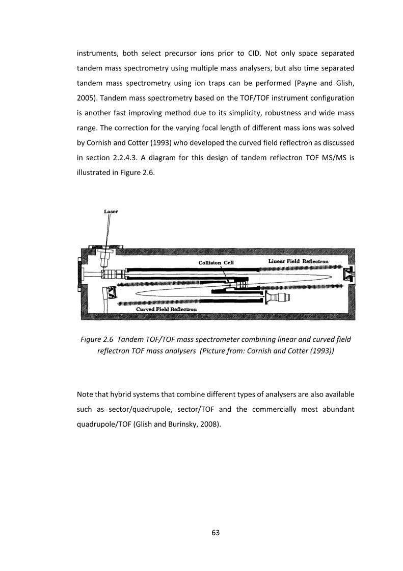
63
instruments, both select precursor ions prior to CID. Not only space separated
tandem mass spectrometry using multiple mass analysers, but also time separated
tandem mass spectrometry using ion traps can be performed (Payne and Glish,
2005). Tandem mass spectrometry based on the TOF/TOF instrument configuration
is another fast improving method due to its simplicity, robustness and wide mass
range. The correction for the varying focal length of different mass ions was solved
by Cornish and Cotter (1993) who developed the curved field reflectron as discussed
in section 2.2.4.3. A diagram for this design of tandem reflectron TOF MS/MS is
illustrated in Figure 2.6.
Figure 2.6 Tandem TOF/TOF mass spectrometer combining linear and curved field
reflectron TOF mass analysers (Picture from: Cornish and Cotter (1993))
Note that hybrid systems that combine different types of analysers are also available
such as sector/quadrupole, sector/TOF and the commercially most abundant
quadrupole/TOF (Glish and Burinsky, 2008).

64
2.3 Lipidomics and the Application of MALDI-
MS in Lipidomics
2.3.1 Lipid Types and Functions
Fahy et al. (2005) divided lipids into 8 main classes, “fatty acyls, glycerolipids,
glycerophospholipids, sphingolipids, sterol lipids, prenol lipids, saccharolipids, and
polyketides”. As a result of the diversity of lipid classes, their masses vary across a
wide range from few hundred daltons to kilodaltons. In general, lipids are organic
molecules that are present in biological systems and can be produced via
biosynthesis. Most lipids are highly soluble in organic and other low polarity solvents
as a result of highly hydrophobic components of these molecules, frequently having
an alkyl “tail”, see the structure of a fatty acid depicted in Figure 2.7 (a). Fatty acids
are the most fundamental lipids composed of carbon, hydrogen and oxygen atoms.
A fatty acid has the structure of carboxylic acid where a long chain hydrocarbon is
connected to a carboxyl group. They can be attached to functional groups to form
various head-tail structure of more complex lipid molecules. Fatty acid derivatives
also count as lipids (Adibhatla et al., 2006).
Lipids are involved in metabolic and other biological activities as energy storage,
vitamins, neurological signalling and can function as hormones. Phospholipids are
major structural components of cells, forming of cell membranes and protein binding
sites. Most biological cell membranes consist largely of phosphatidylcholine (PC).
Normal cells differ in the lipid components and distributions of specific organelles
and cell types (van Meer et al., 2008). Hence, lipid mass spectra might be good
indicators for tissue phenotypes and some pathological disorders. There have been
attempts to perform quantitative studies of lipids to possibly trace lipid metabolism
in cancer tissues that could identify cellular activities stated as hallmarks of cancers
(Hanahan and Weinberg, 2000; 2011; Santos and Schulze, 2012). As brain tissues are
lipid-rich, observing the correlations between lipid concentrations and brain
diseases, disorders and damage has become an interesting topic of research
(Adibhatla et al., 2006).

65
Figure 2.7 (a) A ω-3 fatty acid where N indicates a number of repeated CH2 (with
single bond C-C) (Adapted from: Berg et al. (2002)), (b) cis and trans structures, and
(c) DHA structure (from: www.sigmaaldrich.com)
2.3.2 Cellular Lipids
Figure 2.8 Lipid bilayer in cell membrane
Animal cells (eukaryote) are protected by the outer structure called membranes
which create the boundaries that separate the cell’s contents from its surrounding
environments. The membrane has a bilayer structure as seen in Figure 2.8 where two
layers of lipid are aligned such that the hydrophilic parts face inside of the bilayer
while the hydrophobic parts face outside. The major lipids found in membranes are
phosphatidylcholine whose structure is shown in Figure 2.9. Glycolipids and
H3C
CH2 H
H CH2
(CH2)N
COO-
a
H H
cis
b
H
H
trans
s
c
DHA structure

66
glycoproteins are strongly adhesive (via hydrogen bonds) to water part of the inner
and outer cell environments, assisting the cell structure to retain. Proteins are
attached to the bilayer and take part in several interactions – e.g. function as
channels for controlling transportation of molecules in and out of the cell, as
receptors for different enzymes. The polarity and electrical potential difference
across the membrane are designed to allow the exchange of ions through the cell.
Energy storage and cell communication are also fundamental roles of membrane
lipids. Some organelles within the cell are also surrounded by membrane, for
example, mitochondria (double-layer membrane with the internal layer responsible
for energy conversion and storage), lysosome (single-layer membrane with a
receptor at its surface for as binding site for specific proteins/nutrition/toxins/dead
cells which can then turn into small bag of phosphatidylcholine vesicles to be
digested by the associated enzymes). In neurons, the membrane at the axon can send
signals via electrical transmission to trigger neuronal activity and hence
communication between cells. Note that local lipids in the membranes are associated
with specific types of proteins that perform different tasks. Therefore, the lipid
contents could potentially be used to suggest main functionalities and types of
biological cell/tissue. Extracellular matrix also consists of various biological
molecules. In order to analyse all these complex biological components, mass
spectrometry can be employed.
Figure 2.9 Phosphatidylcholine structure
67
Phosphatidylcholines consist of 2 fatty acids structured as hydrocarbon chains
(hydrophobic tails) attached to the acyl groups. Both fatty acids are linked to the
glycerol backbone which links to a phosphate that carries the hydrophilic choline
head group. Each part of the phosphatidylcholine structure is marked in Figure 2.9
with different colours.
2.3.3 Lipid Extraction Techniques
An extraction method using chloroform and methanol has been widely used in
several applications due to its simplicity and robustness. Chloroform, methanol and
deionised water in an appropriate ratio can be added to a biological compound to
allow lipid extraction with no need to heat or evaporate the sample (Bligh and Dyer,
1959). Chloroform and lipids form a solution that sets itself apart from water,
methanol and other polar substances in the mixture which is seen as a separated top
layer. This extraction method requires only a small quantity of sample. In comparison
with the previous methods e.g. Dyer and Morton (1956), Folch et al. (1957), rapidity
of the procedure is maintained but the yield and purity of lipid extracts are
significantly improved. Chloroform can be added, followed by adding water to the
lipid extracts to repeat extractions until a satisfactory level of purification is achieved.
The use of water is to effectively wash the chloroform-based lipid extract, to remove
water soluble substances, such as salts. In tissue sample applications, the tissue
sample could be blended to facilitate extraction.
Thin layer chromatography (TLC) is a technique to separate components in the lipid
extracts based on their mass and polarity properties. Lipids move different distances
on a chromatography plate. Note that silica gel is often used as a stationary phase
and the chloroform-methanol mixture is a mobile phase solvent. Furthermore, liquid-
solid extraction can be applied by dissolving sample compound in different solvents
of varying polarity and pH. This allows filtering out the undissolved parts at each step,
and hence separation for different compound classes before introducing them into
analysis system.

68
2.3.4 Spectral Analysis (in Lipid Classification)
Mass spectrometry is widely used in proteomic studies, but can also be used for
lipidomics. In particular, MALDI is one of the soft ionisation methods that was shown
to generate useful ions for qualitative (and some quantitative) analysis of a wide
mass range of biological molecules. MALDI-TOF-MS analysis of phospholipids and
triacylglycerols by Emerson et al. (2010) requires as tiny portion as 1 µl of extracted
lipids from beef and egg yolk samples. Mass determination together with structural
information can be obtained by performing MS/MS (or MSn) which is very useful to
deal with complex lipid molecules.
Lipidomics covers the structural and functional study of lipids in living cells, and their
role in supporting metabolic processes, including interactions between lipids and
other fundamental biomolecules – i.e. generic and protein molecules contained in
the cells. There are 2 main aspects for lipid mass spectrometry analysis. The classical
one is when lipid extracts are separated through appropriate gas or liquid
chromatography before being introduced to a mass spectrometer. This is so-called
“comprehensive lipidomics analysis by separation simplification” (CLASS) allows
selected classes of lipids to be analysed by the mass spectrometer, one at a time
(Harkewicz and Dennis, 2011). Whereas another method called “shotgun lipidomics”
applies ESI mass spectrometry to the lipid extracts directly (Han and Gross, 2005).
The common shorthand notation for fatty acid (carboxylic acid) isomers can be
written as 𝐶 ∶ 𝐷 representing number of carbon atoms : number of double bonds in
the fatty acid components of the molecule. This reduces the complexity of writing
the lipid structure as a standard chemical formula. Molecular information about
complex lipids can be described by quoting each fatty acid component along with its
head group. To add clarity, if 𝐷 is non-zero in a fatty acid isomer, the symbol n-x or
𝜔-x is used with the x being the numerical order of the first double carbon-to-carbon
bond counting from its methyl end (Harwood and Scrimgeour, 2007), e.g. an essential
fatty acid, Docosahexaenoic acid (DHA) can be expressed as 22:6 (n-3) means that it
has 22 carbon atoms with 6 double bonds in the carbon chain, the first double bond
is at 𝜔-3 position – see the structure in Figure 2.7 (c). If there is a double (or triple)

69
bond between carbon atoms in the molecule, the fatty acid is said to be unsaturated;
otherwise, it is saturated. Metabolism rates in the organic tissue are thought to be
increased with the degree of phospholipid unsaturation in membrane (Hulbert and
Else, 1999). The conformation at each double bond could be either “trans” or “cis”
as illustrated in Figure 2.7 (b) which are reflected in the properties of lipid molecules
such as polarity, thermal stability. However, current mass spectrometers might not
provide enough information to distinguish between these two.
Typical lipids are saturated and have an even number of carbons, as shown in the
mass spectrum of lipids from a milk sample presented in Figure 2.10.
Figure 2.10 MALDI-MS spectrum of milk sample with an expanded view appearing
brominated C(36:1) and C(38:1) (Picture from: Picariello et al. (2007))
If the sample is treated with bromine, a brominated lipid would show up in a mass
spectrum as a shift in peak with an additional mass per double bond equal to
molecular mass of Br2 of approximately 160 Da and displaying a bromine isotope
pattern (Picariello et al., 2007). From the mass spectrum provided in Figure 2.10,
peaks for brominated C(36:1) and C(38:1) are well illustrated. A determination of
double bonds can be done by observing degrees of oxygenation as in a study of
unsaturated oils using MALDI-MS (van den Berg et al., 2004).

70
Figure 2.11 MALDI-MS spectrum for triacylglecerol (12:0/14:0/14:0) using positive
ion mode (Picture from: Al-Saad et al. (2003))
Loss of the different carboxylate groups during post-source decay (PSD) in a
triacylglycerol (TAG) is equally likely. The intensity ratio of the positive ion fragment
peaks agree with the stoichiometry of these carboxylate groups in the lipid – i.e. the
intensity of the remaining fragment from loss of C(14:0) is twice as much than loss of
C(12:0) following the spectrum in Figure 2.11, at m/z 467.4 and 495.4, respectively.
Therefore, the relative intensities of the fragments can be used to determine the
relative abundance of each carboxylate group contained in a molecule (Al-Saad et al.,
2003). Phospholipids have a phosphate head group attached to more than one
carboxylate tails. The phosphate groups are components of the polar part of
phospholipids. Al-Saad et al. (2003) also reported that only the fragmentations of
polar heads occurred with the protonated phospholipids whereas salted
phospholipids rather showed other fragmentations of the molecular structure as
well.

71
2.3.5 Limitations and Challenges
In phospholipids, the phospha-
tidylcholine (PC) head group can
cause severe signal suppression to
fragment ion signals of other head
groups, especially in phospha-
tidylethanolamine (PE) which is
also commonly present in bio-
logical compounds (Emerson et
al., 2010). The spectrum pre-
sented in Figure 2.12 (d) shows
the suppression effect of PCs
acting on PEs and phosphatidyl-
glycerols (PG) when the PC:PE:PG
lipid mixture mass spectrum was
acquired. This was compared to
each individual mass spectrum of
PGs, PEs and PCs in Figure 2.12 (a),
(b) and (c), respectively, in a
positive ion mode. For example,
all m/z peaks appeared in Figure
2.12 (a) and in Figure 2.12 (b)
apart from m/z 740.5 were not observed in the mixture mass spectrum. The negative
molecular ions of PC cannot be detected using MALDI-MS (Al-Saad et al., 2003). The
negative ion mode is then favored for a detection of PE and PG which is normally
suppressed by the PC in positive mode arrangements. Paranitroaniline (PNA) as a
matrix substance would give non-acidic environment that enhances the detection of
the negative molecular PE ions (Fuchs et al., 2009).
Matrix and analyte suppression effects occur in the presence of significant amounts
of salts as they also give rise to positive ions (Lou et al., 2009). In MALDI-MS
Figure 2.12 MALDI-MS spectra of phospholipids samples (a) 1-palmitoyl-2-oleoyl-
sn-phosphatidylglycerol, (b) 1-palmitoyl-2-oleoyl-sn-phosphatidylethanoamine, (c) 1-
palmitoyl-2-oleoyl-sn-phosphatidylcholine, and (d) mixture of equal fractions of these 3 lipids with DHB matrix, acquired using positive ion
mode (Picture from: Fuchs et al. (2009))
a
b
c
d

72
experiments, alkali metal salts of proteins can be washed after depositing samples
onto a target in order to minimise the chemical background noise they caused
(Smirnov et al., 2004). This might be applicable to remove lipid salts as well.
Nowadays, interest in lipidomics seems to be growing as lipid metabolism can
diagnose cellular dysfunction (Pirman et al., 2013). However, due to the complexity
of lipid analyses, there is relatively little research leading to a lower availability of
lipidomic databases compared to that of proteomics. There are many classes of lipid
occupying a wide mass range and the MS analysis is difficult to do at high masses.
However, mass spectrometry technology is continuously evolving. MS/MS analysis of
lipids with a mass resolution of greater than 30,000 can be achieved using a
quadrupole mass analyser to select lipids at an increment of 1 Da to pass to a CID
system and then proceed through a time-of-flight mass analyser for final mass
analysis (Simons et al., 2011). The “LIPID MAPS Lipidomic Gateway” website
(http://www.lipidmaps.org/) is a good resource for lipid identification whose
information is based on lipid classification studies as updated in 2009 by Fahy and
coworkers which provides a database of lipid structures and MS peaks of all lipid
classes. This has been reviewed every year. Nevertheless, numerous variations in
hydrocarbon chain length and bonding could cause a lot of confusion to mass spectral
analysis of large lipids (Fahy et al., 2005). Therefore, careful TLC or gas
chromatography separation methods are needed for full resolution.
2.3.6 Lipids in the Brain
As discussed earlier, a variety of lipids are found in biological cells as structural and
functional components. Brain tissues in general have very high lipid concentrations.
Lipid types and distributions should be consistent in normal brains in order to
perform their proper activities. Therefore, unusually distributed lipids in some parts
of the brain may link strongly to diseases, disorders and damage. Quantitative
imaging is therefore a powerful tool to investigate pathological changes giving

73
biochemical composition as well as anatomical information. Uses of MALDI imaging
will be discussed in Section 2.4.
There are similarities between human and rat brains that make a rat brain a
reasonable model for the study of brain disorders relevant to humans. Since the
1960s (Bayer et al., 1993), it was confirmed that human and rat brains show very
close correlation with processes of central nervous system (brain and spinal cord)
development since their embryonic stages. Where same developmental stage occurs
in the same order but at different time scales. They described details of brain
structure as a result of cells/neurons generations, tissue formations at different parts
of the brain. The appearance of human and rat brains have similarities as seen in the
pictures provided in Figure 2.13.
Human brain Rat brain
Figure 2.13 Coronal section of Human vs. rat brains (Pictures from: Davis (1913)
and Bennett et al. (1964), respectively)
From these correlations during early brain development, they are believed to show
comparable pathological and physical changes in response to brain diseases. Rat
brains can be modified to better mimic human brain diseases by altering parts of
brain either in terms of biochemical composition and/or physical degradation.

74
2.4 Mass Spectrometry Imaging for Lipid
Analysis
Mass spectrometry imaging (MSI) allows MS information to be represented as an
image, mapping distribution of analytes in each of its pixels in correspondence with
the spatial positions on the actual sample. Hence, applications can be in structural
observations of biological molecule distributions in tissues and their change due to
pathological conditions. MALDI-MS imaging is widely used to image drug and drug
metabolite distributions as well as peptides, proteins, and lipids which is the main
emphasis of this section, will be extensively discussed in Section 2.4.3.
2.4.1 General MS Imaging Instrumentation
A simple microprobe MSI controls the trajectory of the laser beam relative to spatial
coordinates of the plane of the sample either by moving the laser beam across the
sample area, or vice versa. A series of mass spectra is recorded at each point in space.
The size of the focusing beam influences the spatial precision (McDonnell and
Heeren, 2007). The number of scans per dimension determines the spatial resolution.
In contrast, microscope type MSI collects both MS and spatial coordinate data at a
position-sensitive detector. This allows measurement without the need to determine
the location at which each MS spectrum is acquired in the initial stage.
2.4.2 Understanding the Mass Spectrometry Imaging Data
Formats
All mass spectrometry images in this work were acquired using a Shimadzu 7090 TOF2
mass spectrometer (Kratos, Manchester). Each image data set was exported as two
separate files, with filename extensions: .imzML (hundreds of Mb) containing the
header information, and the accompanying .ibd (few Gb) which containing the
spectral information acquired at each pixel. This is one of the standard formats for
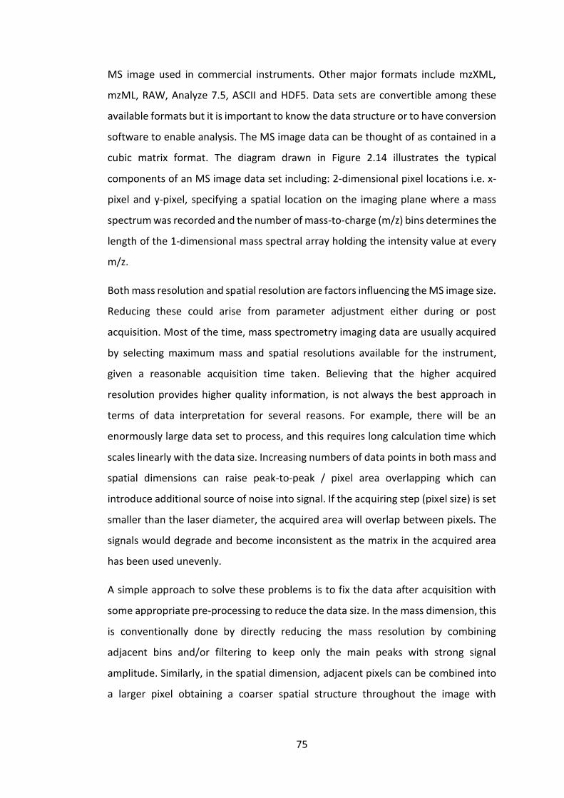
75
MS image used in commercial instruments. Other major formats include mzXML,
mzML, RAW, Analyze 7.5, ASCII and HDF5. Data sets are convertible among these
available formats but it is important to know the data structure or to have conversion
software to enable analysis. The MS image data can be thought of as contained in a
cubic matrix format. The diagram drawn in Figure 2.14 illustrates the typical
components of an MS image data set including: 2-dimensional pixel locations i.e. x-
pixel and y-pixel, specifying a spatial location on the imaging plane where a mass
spectrum was recorded and the number of mass-to-charge (m/z) bins determines the
length of the 1-dimensional mass spectral array holding the intensity value at every
m/z.
Both mass resolution and spatial resolution are factors influencing the MS image size.
Reducing these could arise from parameter adjustment either during or post
acquisition. Most of the time, mass spectrometry imaging data are usually acquired
by selecting maximum mass and spatial resolutions available for the instrument,
given a reasonable acquisition time taken. Believing that the higher acquired
resolution provides higher quality information, is not always the best approach in
terms of data interpretation for several reasons. For example, there will be an
enormously large data set to process, and this requires long calculation time which
scales linearly with the data size. Increasing numbers of data points in both mass and
spatial dimensions can raise peak-to-peak / pixel area overlapping which can
introduce additional source of noise into signal. If the acquiring step (pixel size) is set
smaller than the laser diameter, the acquired area will overlap between pixels. The
signals would degrade and become inconsistent as the matrix in the acquired area
has been used unevenly.
A simple approach to solve these problems is to fix the data after acquisition with
some appropriate pre-processing to reduce the data size. In the mass dimension, this
is conventionally done by directly reducing the mass resolution by combining
adjacent bins and/or filtering to keep only the main peaks with strong signal
amplitude. Similarly, in the spatial dimension, adjacent pixels can be combined into
a larger pixel obtaining a coarser spatial structure throughout the image with

76
improved signal quality at each pixel. Clearly, poorer spatial resolution is achieved
since pixels are combined.
Figure 2.14 Diagram for mass spectrometry imaging data structure
2.4.3 MALDI-MS Imaging of Lipids
Lipids are important in biological systems, and it makes more sense to observe lipid
distributions in tissue samples. This can be done by mass spectrometry imaging (MSI).
Using either microprobe or microscope methods (see Section 2.4.1), mass spectra at
particular spatial locations can be obtained. For each mass-to-charge ratio of
interest, a map of ion distribution within a tissue slice is acquired. A diagram outlining
the steps required to obtain MALDI-MS images of tissue samples at a specific m/z
values is shown in Figure 2.15. Results from all slices of tissue can be combined to
create a 3-dimentional MS image. Note that a tandem MS mode can be applied using
collision induced dissociation for more specified molecular information (Steven and
Bunch, 2013).

77
Figure 2.15 MALDI-MS imaging steps
(Diagram from: Murphy and Merrill (2011))
Matrix must be carefully applied such that it deposits uniformly with suitable
thickness over the thin section of sample. The application methods range from using
airbrushes (which are hand-held apparatus and therefore difficult to control uniform
spread of matrix solution), TLC sprayers, inkjet printers, oscillating capillary
nebulisers (which usually have a moving nozzle that enable automatic application of
matrix with selected parameters, e.g. rate of application, number of layers) or
sublimation methods (which give the most uniform and smallest matrix crystals)
(Zaima et al., 2010), or other purpose designed instrumentation.
Mouse brain contains significant lipid concentrations with the main types being
phospholipids, sphingolipids and glycerolipids (Murphy et al., 2009). Murphy et al.
(2009) observed concentrations of potassiated PC(16:0a/16:0) to vary from pixel to

78
pixel over the tissue section. The quantitative representation of the PC distribution
as the relative intensity level of each pixel in the MSI image at m/z 772.5 is seen in
Figure 2.16.
Figure 2.16 A mass spectrometry image indicating potassiated PC(16:0a/16:0)
distributions for sagittal slice of mouse brain with labels of brain parts
(Picture from: Murphy et al. (2009))
Deterioration of the brain can be involved in various diseases which decrease
capabilities to carry out normal lipid metabolism at specific brain regions (Adibhatla
et al., 2006). Lipid MSI analysis can be performed at a target brain region to trace for
the abnormalities. Alzheimer’s disease (AD) is a common brain diseases in the elderly
which can cause serious neurodegeneration. It induces abnormal lipid metabolism in
the central nervous system where a variety of lipids in the tissues are involved in
neurotransmission. Mass spectra hold molecular phenotyping information. If this
information was extracted, it could yield better understanding of the physiology and
pathology with respect to the anatomical structure, and help suggest disease stages.
However, the accuracy of the spatial mapping is subject to imaging resolution. Also,
sufficient concentrations of analyte must be present at a location to be detected by
MS imaging. Veloso et al. (2011) carried out research on real human brain samples
and studied particularly the lipid distributions of the central nervous system. The
hippocampus is a part in the central nervous system (located at the prosencephalon

79
of the brain) one of the primary sites attacked by Alzheimer’s (Mu and Gage, 2011).
For hippocampus MSI, to 100 µm imaging resolution was required due to the
complexity of the structure (Veloso et al., 2011).
2.4.4 Other Mass Spectrometry Imaging Techniques
The key mass spectrometry ionisation techniques used in tissue imaging beside
MALDI, include secondary ion mass spectrometry (SIMS), desorption electrospray
ionisation (DESI) and laser ablation electrospray ionisation (LAESI). The main features
and typical parameters of these techniques according to Bodzon-Kulakowska and
Suder (2016) are summarised in Table 2.3 below.
Table 2.3 Comparison of mass spectrometry imaging techniques (Reproduced
from: Bodzon-Kulakowska and Suder (2016))
Technique Ionisation
source
Soft/
hard Analytes
Spatial
resolution
(µm)
Upper
mass
range (Da)
SIMS Ion gun Hard
Elemental ions,
small molecules,
lipids
< 10 1,000
DESI Solvent spray Soft Small molecules,
lipids, peptides 100 2,000
LAESI
Mid-IR laser
beam,
solvent spray
Soft
Small molecules,
Lipids, peptides,
proteins
200 2,000
MALDI UV laser
beam Soft
Lipids, peptides,
proteins 20 100,000
SIMS has an advantage of spatial resolution over other techniques, allowing cell
imaging applications (Passarelli and Ewing, 2013). However, its hard ionisation due
to the energetic incident ion beam causes fragmentation to larger molecules, hence
the acquisition is limited to only some smaller analytes. In contrast, MALDI ionisation
is soft which specifically is good for ionising intact biomolecules up to a very high

80
mass, and can still preserve a reasonably good spatial resolution if coupled with a
laser source of small diameter.
DESI is an adaption of ESI used for imaging, works by introducing electrospray
droplets to carry away analytes from a sample surface (Takáts et al., 2004). It can
produce cleaner mass spectra compared to those acquired by MALDI because of the
expected greater stability of the technique (where there is no need to deal with the
variability due to matrix and laser). Another adaption to DESI called nano-DESI, which
uses two very thin separate capillaries, one for delivering the solvent to contact on
the sample surface, and immediately, another one for transportation and
electrospray ionisation of the analyte solution. This technique resulted in a factor of
10 - 20 improvement on the spatial resolution, e.g. Laskin et al. (2012). LAESI requires
two steps to allow ionisation; the mid-IR laser is fired locally onto a sample, allowing
extraction of analytes via evaporation of existing moisture on the sample, which then
undergoes ESI (Nemes and Vertes, 2007). Less precision in spatial location can be
achieved compared to DESI. With DESI, and LAESI, the main limitation is that multiply
charged ions are largely generated for molecules of higher mass as is normally seen
in ESI; therefore, the technique are efficient when observing smaller biomolecules.

81
Chapter 3
Background II:
Quantitative Mass Spectrometry
This chapter sets out the general scope of quantitative mass spectrometry, outlining
the challenges and conventional approaches used (see Section 3.1). Some common
computational methods (pattern recognition) are described in Section 3.2, with
examples of their uses in analysing mass spectrometry data discussed. The other
approaches of clustering and linear component decomposition specific to MS
imaging data analysis are discussed in Section 6.1.3 of Chapter 6. The background
specific to the analytical approach used in Chapters 5 and 6 of this thesis is described
in Section 3.3 and Section 3.4. Together, this demonstrates a new, alternative
approach to data analysis that comprises an error model that is especially important
for addressing a number of scientific questions.

82
3.1 The Scope of Quantitative Mass
Spectrometry
Mass spectrometry has been used by a range of scientific disciplines as a technique
to acquire information on a variety of molecules within a range of sample types. The
technical development of today’s spectrometers is based on research in a number of
fields, particularly, in chemistry and particle/atomic physics. The development of
mass spectrometry led to the discovery of isotopes – i.e. Francis William Aston
received a Nobel Prize in Chemistry in 1922, for the development of the mass
spectrograph (early mass spectrometer) which led to consequent discovery of many
isotopes. An example of MS use in biological sciences is the use of stable isotope
tracers such as 13C-enriched tracer. The investigation of isotope ratios, e.g.
207Pb/206Pb can help predicting the age of a planet, hence the application of MS to
geology. Many other applications lie in applied fields such as medical,
pharmaceutical, forensic, and food sciences. More routinely, the technique is often
used in industry for routine quality control and contaminant assessments.
Improvement of the method and the development of new techniques are ongoing.
In whatever application, the method of analysis, experimental protocol, and analysis
of results, must be optimised. Huge amounts of information are contained in a single
MS acquisition – i.e. ion counts at every mass-to-charge value within a selected mass
range are recorded. Therefore, it is important to extract as much relevant
information as possible from within a data set to get the most out of an experiment.
Mass spectrometry analysis may be divided into qualitative and quantitative
approaches. Qualitative analysis aims only on detecting the presence or absence of
analytes of interest whereas quantitative analysis provides also numerical quantities,
such as relative or absolute concentrations. For example, qualitative analysis could
answer the question like “Which drug metabolites can be observed in a sample?”
Quantitative analysis can answer questions like “Is the concentration high enough to
be toxic?” Quantitative analysis allows the estimation or prediction of some
mathematical model parameters. In addition, for completeness of scientific
interpretation, the errors associated with the measurement must be quoted to

83
determine the level of reliability of the data. Statistical analysis should then play an
important role in data interpretation. In order to meet these requirements, this
thesis presents a new approach to mass spectrometry data analysis called linear
Poisson independent component analysis (LP-ICA) which is demonstrated in Chapters
5 and 6. This approach is based on a quantity estimation of ions generated on mass
spectra, with a statistical error model (see Section 3.4). The results of quantitation
can then be extracted in terms of proportional quantities associated with the
underlying complex mixtures within samples of interest from either non-imaging or
imaging data sets. This can be applied in many quantitative problems, including
relative quantitation covered in this work and absolute quantitation which will be
discussed in the suggested future work, see Section 7.3 of Chapter 7.
3.1.1 Problems in MALDI-MS Quantitation
Quantitative analyses using MALDI-MS is difficult due to the high variability of ion
signals which causes uncertainties in measuring abundance of mass-to-charge
information in mass spectra. These variabilities are due to the availability of ions
formed in individual MS acquisitions which vary between different regions of the
deposited sample under what are apparently the same conditions, largely due to the
non-uniform spread of sample-matrix crystals, and even shot-to-shot changes at
exactly the same position (Duncan et al., 2008). Huge differences are also contributed
by different sample/matrix preparation and deposition methods, and the optimal
method ought to be carefully selected and defined in a protocol for each experiment,
as in Section 2.2.8. These significant influences limit repeatability and reproducibility
in MALDI-MS experiments. Mass spectrometrists have, for some time, been seeking
methods which could provide more meaningful quantitation in MALDI-MS analysis.
Approaches that yield significant improvement in MALDI-MS quantitation include
those that compensate for both physical and chemical variabilities in the various
processes and should overcome some of the systematic and random errors.
Techniques are being investigated based on approaches to sample preparation,

84
instrumentation, calibration using internal and external standards, and mathematical
approaches to data processing and analysis.
An effective plume temperature in the early stages of ionisation is one of the
parameters which influences ion yield (Bae et al., 2013). The ratio of the fraction of
protonated analyte yield to the fraction of protonated matrix yield, is known to
correspond to an early effective temperature of the plume. This is because the
positive charges from the protonated matrix are transferred in order to ionise the
neighbouring analyte molecules during the desorption/ionisation process.
Moreover, Bae et al. (2013) appeared to find that keeping the plume temperature
constant during the desorption/ionisation process improved the stability of the
ionisation rate.
The heterogeneity of crystal formation also influences the signal intensity variance.
This causes lower signal-to-noise values in regions where there are fewer crystals. In
contrast, the optimum signal intensity obtained from a crystalline region might result
in saturation of the mass spectrum. An automated system can be used to select only
the spectra with appropriate quality – i.e. spectra acquired from single laser shots
with satisfactory levels of signal-to-noise, but without saturation (Duncan et al.,
2008). A collection of these mass spectra that pass predefined thresholds are allowed
to proceed into the average or accumulative forms.
Figure 3.1 Main components of a mass spectrum (Picture from: Müller et al. (2001))
The diagram provided in Figure 3.1 illustrates the main components of a mass
spectrum. The peaks represent the associated m/z values that are detected on an MS
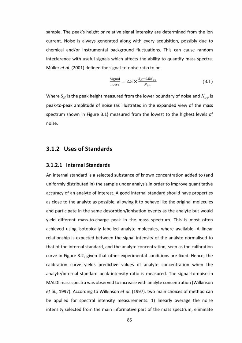
85
sample. The peak’s height or relative signal intensity are determined from the ion
current. Noise is always generated along with every acquisition, possibly due to
chemical and/or instrumental background fluctuations. This can cause random
interference with useful signals which affects the ability to quantify mass spectra.
Müller et al. (2001) defined the signal-to-noise ratio to be
Signal
noise= 2.5 ×
𝑆𝐻−0.5𝑁𝑝𝑝
𝑁𝑝𝑝 (3.1)
Where 𝑆𝐻 is the peak height measured from the lower boundary of noise and 𝑁𝑝𝑝 is
peak-to-peak amplitude of noise (as illustrated in the expanded view of the mass
spectrum shown in Figure 3.1) measured from the lowest to the highest levels of
noise.
3.1.2 Uses of Standards
3.1.2.1 Internal Standards
An internal standard is a selected substance of known concentration added to (and
uniformly distributed in) the sample under analysis in order to improve quantitative
accuracy of an analyte of interest. A good internal standard should have properties
as close to the analyte as possible, allowing it to behave like the original molecules
and participate in the same desorption/ionisation events as the analyte but would
yield different mass-to-charge peak in the mass spectrum. This is most often
achieved using isotopically labelled analyte molecules, where available. A linear
relationship is expected between the signal intensity of the analyte normalised to
that of the internal standard, and the analyte concentration, seen as the calibration
curve in Figure 3.2, given that other experimental conditions are fixed. Hence, the
calibration curve yields predictive values of analyte concentration when the
analyte/internal standard peak intensity ratio is measured. The signal-to-noise in
MALDI mass spectra was observed to increase with analyte concentration (Wilkinson
et al., 1997). According to Wilkinson et al. (1997), two main choices of method can
be applied for spectral intensity measurements: 1) linearly average the noise
intensity selected from the main informative part of the mass spectrum, eliminate

86
the averaged noise, and obtain peak intensity via integration, and 2) use the least
squares method to fit a local package of spectral peaks at each molecular mass,
including the protonated molecular ions, dehydrated molecular ions, and might
include metastable decay products and salted molecular ions.
Figure 3.2 Calibration curve for insulin where the internal standard is des-
pentapeptide insulin (Graph from: Wilkinson et al. (1997))
The use of isotopic labelling for internal standards works efficiently on lighter
molecules (<500 Da) where labels of ≥3 Da are ideally used (Duncan et al., 1993). This
should generate a distinctive peak outside the distribution of natural isotopes of the
original molecules. Available techniques such as isotope-coded affinity tags (iCAT),
stable isotope labelling of amino acids in cell culture (SILAC) and isobaric tag for
relative and absolute quantification (iTRAQ) are currently in use in quantitative
proteomic mass spectrometry research. The techniques could be used to generate
biomarkers for diagnosing and staging of diseases (Hultin-Rosenberg et al., 2013). For
example, iTRAQ is a technique to label the amino acid lysine by attaching an “isobaric
tag” to its amine functional group (Hultin-Rosenberg et al., 2013). Isobaric tags of
almost the same mass are added to different samples to label the same peptide, with
apparently the same MS characteristics for mixed sample, but will show distinct

87
features in MS/MS for low mass fragments (Unwin, 2010). During MS/MS, an isotope
“reporter” is fragmented from a labelled molecule of each isobaric species, resulting
in separate signals in the MS/MS spectra that allow for relative quantification of the
same peptide in each sample following the analysis described by Thompson et al.
(2003) and the absolute approach as explained in Ross et al. (2004).
3.1.2.2 External Standards
An external standard is a chemical with a m/z value selected to match an analyte of
interest within the analysing sample. The external standard is prepared at different
concentrations in the range that the concentration of the analyte of interest is
expected to be in the sample. To construct a calibration curve, the measured ion
current at the specific m/z is plotted against its known concentration for a linear least
square fitting. Then, the unknown concentration can be determined from its
correlation with the observed ion current at the m/z of interest. Note that a series of
m/z values can also be observed using the corresponding chemicals as external
standards for more robust control over a wide mass range.
3.1.3 Conventional Peak Analysis
Figure 3.3 Peak detected mass spectrum: A reference peak is selected
for peak analysis
Peak analysis methods have been used for quantitative spectroscopy analysis. The
method involves some sort of normalisation – i.e. against total spectral intensity or
Reference
Peak bin
Inte
nsi
ty

88
reference peak intensity. However, lack of signal-to-noise and repeatability problems
would result in inaccurate measurements, especially for MALDI mass spectra.
In this work, this single peak analysis approach is used as a conventional method to
compare with the linear Poisson ICA method. Where the intensity ratio of a single
peak bin to the reference peak is calculated in every mass spectrum in the data set
and will be used to quantify the components of the material analysed. Note that the
same pre-processing steps (Section 3.3) as for linear Poisson ICA were applied prior
to this analysis. Only strong signal peaks with intensities above the noise level will
remain in the spectral data set, as ensured by the peak detection (Section 3.3.4). A
diagram given in Figure 3.3 illustrates the peaks detected in the mass spectrum with
a reference peak selected for relative quantification.
A reference peak should be selected at a peak bin that appears consistent across all
spectra in the data set. The peak would be assessed to have relatively no correlation
between its signal intensity and the corresponding sample proportions. Usually, one
of the largest peaks would be chosen, firstly for stability of intensity values, and
secondly for reasonable ratio representation. For example, the appropriate
reference peak chosen for every MALDI-MS data sets in Chapter 5 was at m/z 760.5
[PC(16:0/18:1)+H]+ (Deepaisarn et al., 2018). An alternative strategy can be the use
of the integral over all data bins as a normalisation factor, e.g. in Chapter 6, which
should be a more consistent choice across a large data set, particularly for imaging.
Loss of generalisation is introduced by selecting the one peak, known to be most
correlated with the ground truth proportion of the underlying sample components
to represent the quantitation of the whole spectral set. In other words, the
conventional analysis only relies on a specific molecule.
One of the main problems in conventional MS peak analysis is that natural salt ions
(e.g. Na+, K+) exist in biological samples and there is no perfect way to purify such
samples, especially in imaging experiments. Hence, variation in mass spectral signal
intensity between sample deposits, or even between repeat measurements of same
sample deposit may be location dependent. The analysis of a single peak is therefore
not necessarily advisable when various salted species of the same molecule

89
contribute to the recorded signals, sharing the signal intensities between those peaks
with uncertain proportions.
3.1.4 Supporting Software for Mass Spectrometry Data
Analysis
The MALDI-TOF-MS instrument used at the Wolfson Molecular Imaging Centre
(WMIC), the University of Manchester is an AXIMA CFR+ TOF2 model from Kratos (a
Shimadzu group company). This instrument has been upgraded to have a 200 Hz
laser, effectively making it equivalent to the more recent “Performance” model of
instrument. The manufacturer’s “Launchpad” software allows selection of positive-
negative ion, linear-reflectron, MS, MS/MS, MSI modes with ranges of parameter
adjustments, including laser properties, mass range, data processing properties, etc.
These primary set-ups allow the users to perform a variety of experiments and to
acquire the optimised data with the selected sample-matrix types. However, both
experimental results and data analysis processes can be optimised with support of
other related software and the semi-automated enhancement of mass spectra is
possible with the aid of coding.
MATLAB is a widely used software for statistical and data analysis. As a high-level
programming language, it allows simple coding. Also, it is convenient and easy to use
for handling and accessing data. It can be designed to suit custom demands with the
ability to create graphical user interface format programmes. Moreover, MATLAB has
special sets of built-in algorithms called the “bioinformatics toolbox” which provides
several useful functions to improve spectral analysis such as baseline subtraction,
peak detection, etc., and the “image analysis toolbox” which can be applied for MS
imaging (http://uk.mathworks.com/products/bioinfo/; White et al., 2005).
In mass spectrometry imaging applications, mass spectral data match spatial voxels
to form graphical images of signal distribution throughout the sample (Parry et al.,
2013). Ranges of software designed for displaying, processing and analysing mass
spectrometry imaging data are available to users as open sources e.g. Biomap
(https://ms-imaging.org/wp/biomap/), MSiReader (Robichaud et al., 2013; Bokhart

90
et al., 2018), OpenMSI (https://openmsi.nersc.gov/), or commercially e.g. SCiLS Lab
(Bruker). Biomap allows basic interpretation of MS imaging data, including single ion
images, averaging of mass spectra in a region of interest. MSiReader (Robichaud et
al., 2013; Bokhart et al., 2018) is a Matlab based programme which features
conversion between image formats, pre-processing, pixel interpolation, etc.
However, the data uploading speed is slow and the computer memory can be a
problem for large data files since the data are loaded into a spreadsheet. OpenMSI
(Rübel et al., 2013) allows fast data management on a web-based interactive
environment, with an interactive view tool function which can represent distribution
of 3 different ions on RGB (red-green-blue) image at a time. There are vast number
of contributors globally. The commercial software, SCiLS Lab (Bruker) can perform
some more sophisticated functions including, correlation analysis, spectral analysis,
classification of data, etc.
Available software is easy to use but access to the algorithms that drive the tool is
limited. Therefore, it is very difficult to know exactly what the software does to
process the data and made worse by the many versions of updated software
released. Furthermore, quite often a Gaussian assumption of statistical errors is
made (without prior assessment of data). Frequently this is done for the sake of
algorithm simplification. There is still a gap that appears common to all available
tools, which is the statistical errors in quantitation are not provided. A statistically
appropriate chemometric analysis method would be required to solve this matter
properly.
3.2 Computational Analysis Methods for
MALDI-MS Data
This section gathers together some of the relevant computational methods for data
analysis that have been chosen by mass spectrometrists to analyse and report their
mass spectral data, particularly in imaging MS. A summary of the methods’ basic
descriptions and general applications are discussed.

91
3.2.1 Data Mining
Big data analysis has become one of the topics frequently talked about in the
information context including management and interpreting of data in the sciences
and social sciences. Currently in scientific research, real-world data generated by
state-of-the-art instruments tend to be provided at an increasing size and rate
promptly delivering the most relevant available information for studies. The data is
therefore ‘big’ in terms of the amounts and variations in data. This means a lot of
hidden information may be there to be extracted. Powerful tools are needed to deal
with this aspect properly, to identify useful components and properties of the data.
Modelling tasks for such big data are certainly difficult and require either huge or
complicated efforts to sort out specific problems. The techniques for organising data
systems and selecting methods to find the optimal solutions that satisfy the question
of study, are generically called ‘data mining’. Where modelling tasks range from
classification, regression, outlier detection, to correlation analysis, data mining can
be employed to build an appropriate method which allows multiple types of analysis
to uncover hidden information.
Unsupervised learning: By looking into unseen data, features (i.e. unique properties)
can be discovered that explain groups, clusters or trends contained in the data set,
without prior knowledge.
Supervised learning: A training data set of annotated samples is given. The training
data set will contain some associated values to train a computer to perform specific
tasks based on meaningful operations as justified in the training. For example, a data
set that is known to carry some number of categories and individual samples (already
determined as belonging to a particular category) can be utilised to train a classifier
that can then perform classification when applied to a new data set.

92
3.2.2 Computational Approaches
The following computational approaches can be categorised as pattern recognition
techniques, which are generally used in machine learning in various applications, e.g.
to handle multivariate problems, including MS data analysis. Basic descriptions of
these approaches including support vector machines, nearest neighbours, random
forests and neural networks are given below. Other machine learning methods,
particularly clustering approaches are important in terms of their application on
MALDI-MS imaging analysis – i.e. classification and subsequent segmentation. They
will be detailed in Section 6.1.3 at the introduction to the imaging experimental
Chapter 6 where data analysis approaches for MALDI-MS imaging are compared
specifically. Statistical multivariate analysis approaches that involve extraction of
linear spectral components (which allows spectral quantitation aimed in this work)
are also discussed in Section 6.3.1 with comments on data assumptions.
3.2.2.1 Support Vector Machine
The support vector machine (SVM) was developed as a classifying tool. The method
attempts to find the hyperplane that maximally separates the margin of classes in
the data in a multidimensional space, where the margin is defined as the
(perpendicular) distance from a hyperplane to the closest data point on each side of
that separating plane. For a data point, separation from the plane can be written as
the function 𝑔 defining a linear SVM in Equation (3.2).
𝑔𝒘,𝒃(𝒙) = 𝑦(𝒘𝑇𝒙 + 𝒃) (3.2)
Given that 𝑦′(𝒘𝑇𝒙 + 𝒃) ≥ 𝑔 for all other data points. The above equation can be
normalised by a factor of magnitude ‖𝒘‖ for vector 𝒘. This would give the distance
from the hyperplane in terms of a unit vector. Therefore, a minimum ‖𝒘‖ is needed
to represent the maximum distance and thus the optimal SVM classifier.
Corresponding values for each data point, 𝒙 can be calculated using 𝑦(𝒘𝑇𝒙 + 𝒃).
Note that 𝑦 indicates the positivity and negativity of a data point according to its side
of the hyperplane.

93
To analyse data with more complicated features (physical properties), a non-linear
transform of the linear expression above for each data point, 𝒙 can also be achieved
by multiplying an appropriate kernel of a higher-degree function by the first term in
𝑦 in order to define more precise boundaries between classes of data.
3.2.2.2 Nearest Neighbours
“k-nearest neighbours” is probably the simplest method amongst all the methods
which will be discussed in this section. When data are plotted in a vector space, data
might be expected to spatially cluster according to their common properties. A data
point of unknown class/value should be more likely to belong to the same class as its
nearest neighbour (the data point that is located closest to it). Considering some
number of nearest neighbours, 𝑘, greater than 1 reduces the effects of noise from
measurement. However, a large value for 𝑘 can lead to problem of regularisation
(when trying to fit a model to all data points) if non-relevant data points are taken
into account. In classification tasks, the unknown variables take the mode class of the
k-nearest neigbours. In regression tasks, the mean distance from an unknown point
to the k-nearest neighbours is normally observed, Euclidean distances are measured.
Although the method works with supervision, there is no need to model the data to
predict unknown variables. The only parameter that can be freely adjusted is 𝑘. This
ease of use can be a benefit, but also a problem, as the parametric optimisation is
too limited. Sometimes, when the distance relies mainly on a few variables, where
there are huge differences in the range of values, appropriate normalisation or
weighting techniques can be applied. This is rarely discussed in the literature and
there is no definition of the statistical principle involved in training the algorithm.
3.2.2.3 Random Forest
A random forest is a decision tree based method which is used to solve various
machine learning problems. A good decision tree should optimally separate samples
according to the distinctiveness of their features/variables. In supervised learning,

94
the method is validated by correctly identifying or estimating labelled samples in the
training set. Hence, the prediction in the testing data set is used to decide between
logical design choices. The algorithm is relatively fast to operate, therefore, many
individual decision trees can be constructed for randomly selected subsets of data to
achieve satisfying accuracy with the combined trees, or a “random forest”. The
method is very popular, particularly as a great tool for classification, because of its
flexibility. It applies little constraints on parametric assumptions of the data
compared to other methods, which could simply allow non-linear analysis without
adding much complexity to calculation. Random forests can also provide fair
solutions to regression problems but are quite limited, as they lack of some important
statistical assumptions and may introduce problems due to the model’s randomness.
For example, there may be a problem of overfitting the data, or that there is not
enough data to train an appropriate regressing estimation.
Random forests have a large application base, extended to dimensionality reduction
by ranking the features of data and discarding insignificant ones. Shi and Horvath
(2006) has also introduced a use of (semi-)unsupervised random forest where
Monte-Carlo sampling is used for training, providing unknown classes.
Random forests use votes and mean values to predict, discrete and continuous
variables, respectively. Whist clustering data samplings, optimal performance for
each decision tree is achieved when the minimal variance within a cluster, but
maximal variance between clusters are achieved. Significant tests used with the
method are based upon approaches such as chi-square, analysis of variance.
3.2.2.4 Neural Networks
The concept of the (artificial) neural network is to mimic the some aspects of
structure and connectivity of human brain, to learn based on information received
and to make decisions on unseen scenarios that comprise similar features. The
computer system aims to extract knowledge from training data, and can be used to
solve problems like classification, clustering or regression. In order to build a neural
network, a number of neurons are connected between layers and define processing

95
of the input variables with some form of activation function in order to generate
outputs – e.g. classified data. The diagrams presented in Figure 3.4 show the
structure of a single neuron and a multiple-layer neural network system. A classical
neural network equation is given below.
ℎ𝑾,𝒃(𝒙) = 𝑓 (∑ 𝑾𝑇𝒙 + 𝒃) (3.3)
Where an input vector 𝒙 mathematically expresses underlying feature elements of
the weighting factor 𝑾. As a result of the activation function 𝑓, the output ℎ from a
layer provides the inputs for the next layer’s “neurons”. The final outputs are
obtained after propagation of these “signals” through all layers in the neural
network. 𝒃 is a bias (intercept) term, allowing for flexibility of the model to fit the
data. Inputs and outputs take values of continuous variables.
Artificial neuron Artificial neural network
Figure 3.4 Artificial neuron (left), and example of neural network with fully-
connected neurons and with an additional bias term indicated +1 in each layer
(right) (Diagrams from: http://ufldl.stanford.edu/tutorial/supervised/
MultiLayerNeuralNetworks/ (UFLDL Tutorial))
Examples of non-linear functions, that are employed in the transformation Equation
(3.3), are Sigmoid functions, hyperbolic tangents (tanh) or other high-degree
functions. Neural networks seek the best innate features that need to be carried
through the functional network paths into final stage of fitting data. A convolutional
neural network, works by multiplying smaller kernels iteratively to different parts in
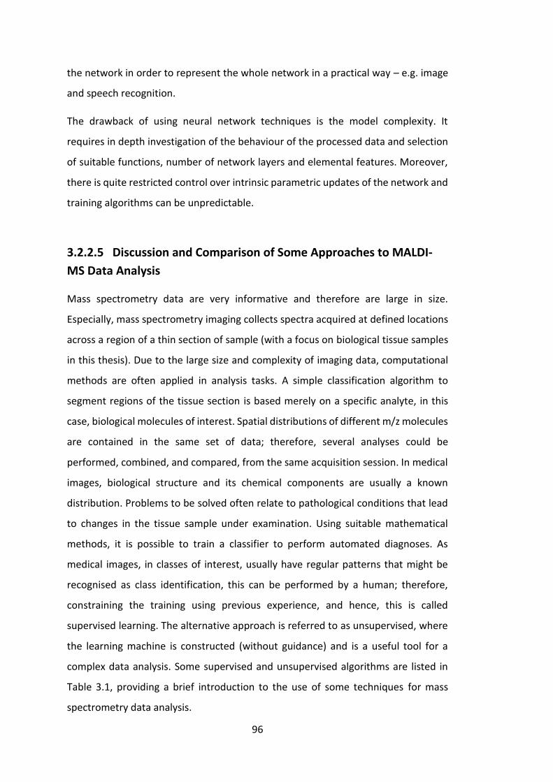
96
the network in order to represent the whole network in a practical way – e.g. image
and speech recognition.
The drawback of using neural network techniques is the model complexity. It
requires in depth investigation of the behaviour of the processed data and selection
of suitable functions, number of network layers and elemental features. Moreover,
there is quite restricted control over intrinsic parametric updates of the network and
training algorithms can be unpredictable.
3.2.2.5 Discussion and Comparison of Some Approaches to MALDI-
MS Data Analysis
Mass spectrometry data are very informative and therefore are large in size.
Especially, mass spectrometry imaging collects spectra acquired at defined locations
across a region of a thin section of sample (with a focus on biological tissue samples
in this thesis). Due to the large size and complexity of imaging data, computational
methods are often applied in analysis tasks. A simple classification algorithm to
segment regions of the tissue section is based merely on a specific analyte, in this
case, biological molecules of interest. Spatial distributions of different m/z molecules
are contained in the same set of data; therefore, several analyses could be
performed, combined, and compared, from the same acquisition session. In medical
images, biological structure and its chemical components are usually a known
distribution. Problems to be solved often relate to pathological conditions that lead
to changes in the tissue sample under examination. Using suitable mathematical
methods, it is possible to train a classifier to perform automated diagnoses. As
medical images, in classes of interest, usually have regular patterns that might be
recognised as class identification, this can be performed by a human; therefore,
constraining the training using previous experience, and hence, this is called
supervised learning. The alternative approach is referred to as unsupervised, where
the learning machine is constructed (without guidance) and is a useful tool for a
complex data analysis. Some supervised and unsupervised algorithms are listed in
Table 3.1, providing a brief introduction to the use of some techniques for mass
spectrometry data analysis.

97
Tab
le 3
.1 E
xam
ple
met
ho
ds
of
dat
a an
alys
is t
hat
can
be
app
lied
fo
r cl
assi
fica
tio
n o
f m
ass
spec
tro
met
ry d
ata
Ex
amp
le
Ap
plic
atio
n
Cla
ssif
yin
g se
rum
sam
ple
s fr
om
gas
tric
can
cer
pat
ien
ts a
nd
hea
lth
y co
ntr
ols
Pro
vid
ing
rep
rese
nta
tive
spec
tra
for
tum
ou
r ce
lls
and
oth
er c
ell t
ypes
,
allo
win
g ti
ssu
e
segm
enta
tio
n
Dif
fere
nti
atin
g ty
pes
of
bac
teri
a
Cla
ssif
icat
ion
of
bre
ast
can
cer
tiss
ues
an
d
dif
fere
nt
tum
ou
rs
Co
mp
arin
g an
d
det
erm
inin
g b
iom
arke
rs
for
bre
ast
can
cer
bas
ed
on
pro
teo
me
Re
fere
nce
Shao
et
al.
(20
12
)
Dei
nin
ger
et
al.
(20
12
)
AlM
aso
ud
et
al.
(20
14
)
Han
selm
ann
et a
l. (2
00
9)
San
der
s et
al.
(20
08
)
Pri
nci
ple
Red
uce
dim
ensi
on
alit
y o
f p
rin
cip
al c
om
po
nen
ts,
and
fin
d s
pec
tral
dis
trib
uti
on
s w
ith
op
tim
al
dif
fere
nce
bet
wee
n g
rou
ps.
Dis
trib
uti
on
s o
f d
iffe
ren
t ta
rget
bio
logi
cal c
ells
are
exp
ress
ed
by
pLS
A s
core
s w
hic
h w
ou
ld t
hen
det
erm
ine
mas
s sp
ectr
a o
f co
mp
on
ents
of
sele
cted
cel
l typ
es.
Bo
ots
trap
pin
g re
sam
plin
g m
eth
od
is u
sed
fo
r
trai
nin
g an
d t
esti
ng
the
SVM
wh
ere
the
mo
del
is
crea
ted
fro
m t
he
leas
t cr
oss
-val
idat
ion
err
or
trai
nin
g d
ata
set.
Cla
ssif
ier
incl
ud
es s
eri
es o
f tr
ee b
ran
ches
wit
h
dif
fere
nt
ran
do
m m
/z f
eat
ure
s.
The
Eucl
idea
n d
ista
nce
is m
easu
red
bet
wee
n t
he
feat
ure
s o
f a
test
ing
spec
tru
m a
nd
eve
ry t
rain
ing
spec
tru
m t
o d
ete
rmin
e th
e n
eare
st in
eac
h
com
par
iso
n a
nd
vo
te f
or
the
corr
ect
clas
s.
Sup
ervi
sed
/
Un
sup
ervi
sed
Un
sup
ervi
sed
Un
sup
ervi
sed
Sup
ervi
sed
Sup
ervi
sed
Sup
ervi
sed
Dat
a an
alys
is
me
tho
d
Pri
nci
pal
co
mp
on
ent
anal
ysis
(P
CA
)
Pro
bab
ilist
ic la
ten
t
sem
anti
c an
alys
is
(pLS
A)
Sup
po
rt v
ecto
r
mac
hin
e (S
VM
)
Ran
do
m f
ore
st
k-n
eare
st n
eigh
bo
urs

98
In the supervised approach, data points are annotated relative to their pixels in each
of the sample images which presumably contain the corresponding target tissue
components. Feature information contained in the data points is stored for the
purpose of training so that a classification model can be built across a series of sample
images via various algorithms such as the random forest method. In the work by
Hanselmann et al. (2009), random forest classifiers were generated for the
classification of breast cancer tissue for mass spectrometry images. This gave a true
positive rate for correct classification as high as about 90%. MSI data points
(characterised by mass spectra) amongst training samples of known classes are used
to build binary decision trees based on a hierarchy of randomly selected features.
Spectral information contained within each interval of the full spectrum (responsible
for these features) is used to categorise samples into two classes. The classifications
are trained sequentially, in a tree using different features until decision paths are
obtained that ultimately distinguish the sample between two different classes. The
diagram for structure of trees in Figure 3.5 (a) describes this algorithm. Where a
tree’s node represents a feature (member of a randomly selected subset of the whole
set of features) that optimises the separation of the classes with a feature value (e.g.
ion counts in a mass spectral interval) determining the class separation threshold
(Hanselmann et al., 2009) (See also the diagram in Figure 3.5 (b) for graphical
boundaries separating data into 2 distinct classes). The tree is grown by splitting each
node into 2 branches (representing the classes) starting from the root node. For
every child node, it undergoes the same procedure until satisfied at the leaf nodes,
where a final class decision is made. Then, a random forest classifier is formed
accordingly by combining series of these trees that have been trained randomly and
independently in order to achieve good generalisation (Criminisi and Shotton, 2013).
In testing, the same data point is classified through every individual decision tree in
the forest. In each tree, a decision is made at each node (starting from the root),
following an appropriate path until it reaches a leaf node, where a vote is generated
for the preferred class. The testing data are then classified as the class with the
maximum number of votes as a surrogate for the corresponding class probability.
Here, the classifier’s sensitivity can be derived from a comparison of the resulting
and true class of the test data. Note that the wavelet transform is widely used to

99
extract useful features with fewer dimensions and more efficient use of data, thus
giving better and faster classification performance (Liyen et al., 2013).
Figure 3.5 (a) Decision tree characteristics where f1 and f2 are feature values of 2
different features at each node used as classification thresholds, and (b) plot of data
with decision boundaries being the feature values in the corresponding trees
(Adapted from: Hanselmann et al. (2009))
Multivariate analysis allows many measured variables to be analysed simultaneously.
Data of high dimensionality are handled using matrix algebra for the convenience of
interpretation and computation of the multivariate data (Miller and Miller, 2010).
Approaches using linear decomposition of data components used in the mass
spectrometry imaging context, e.g. probabilistic latent semantic analysis (pLSA), are
discussed in Section 6.1.3. These approaches are usually unsupervised and allow
regression measurements. They can be powerful for analysing mass spectrometry

100
images in terms of dealing with variabilities in signal and noise, and are independent
of spatial locations. Therefore, they can also be applied for quantitative classification
purposes. For example, principal component analysis (PCA) is a statistical method of
handling and simplifying large data sets for further analysis where only the main
components of data variance are considered (see details in Section 3.4.2.1). A
principal component plot is a graph of data points in a coordinate space with the first
principal component axis indicating the direction of most data variance. The
complexity is reduced by rejecting the least significant principal components (least
variant) until left with fewer dimensions, where data points from a specific class are
distributed within certain deviations and can be distinguished from other classes.
Note that all principal component axes (the spectral shapes) are orthogonal, as a
result of the mathematical form of decompositions. In mass spectrometry, data
points are encoded by mass peaks in a set of MS spectra. A PCA algorithm was applied
to semi-quantitatively classify MALDI-MS data from different types of bacteria using
their relative mass peak intensities (AlMasoud et al., 2014). Classification accuracy of
90% was quoted for this specific data set using PCA, followed by further classification
using ‘support vector machines with a linear kernel’ (AlMasoud et al., 2014). They
also introduced an alternative qualitative approach using principal coordinate
analysis (PCoA) where only m/z signals greater than three times a baseline level were
considered as peaks (AlMasoud et al., 2014). Classification of MALDI-MS proteomic
data from serum of (gastric) cancerous and normal tissue samples in humans was
successfully performed by Shao et al. (2012) using the PCA method. Smaller MS data
sets were selected by the most useful proteomic peaks derived from PCA, plotted as
in Figure 3.6 with an accuracy in classifying samples in the patient group determined
by distribution to be 94.5% (Shao et al., 2012).
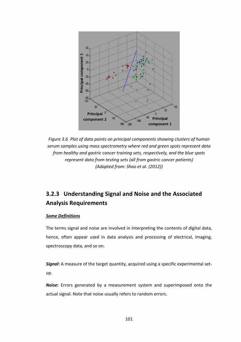
101
Figure 3.6 Plot of data points on principal components showing clusters of human
serum samples using mass spectrometry where red and green spots represent data
from healthy and gastric cancer training sets, respectively, and the blue spots
represent data from testing sets (all from gastric cancer patients)
(Adapted from: Shao et al. (2012))
3.2.3 Understanding Signal and Noise and the Associated
Analysis Requirements
Some Definitions
The terms signal and noise are involved in interpreting the contents of digital data,
hence, often appear used in data analysis and processing of electrical, imaging,
spectroscopy data, and so on.
Signal: A measure of the target quantity, acquired using a specific experimental set-
up.
Noise: Errors generated by a measurement system and superimposed onto the
actual signal. Note that noise usually refers to random errors.

102
Errors do exist in every measurement, in other words, recorded signals always
contain some sorts of error. Broadly speaking, errors are classed into 2 main types,
which are systematic and random errors. Both are expected to occur in several stages
of experiments, including instrumental, environmental and man-made errors. The
experimental procedure has to be adjusted to optimise the results such that these
errors are minimised, giving an accepted level of signal-to-noise ratio (S/N).
Systematic errors may be recovered by applying some form of function to the data –
e.g. constant shifting or scaling throughout the recorded signals. This can generally
be dealt with by calibration methods that suit the apparatus. Random errors are
determined by limitations of instrumental measuring stability (precision) which
causes statistically random variations. Pure signals can never be achieved, but
averaging the results from repeating measurements is a way to help getting rid of
random variations in many scientific problems. However, acquiring multiple
measurements may not be possible for some experiments. Attempts to use
computational techniques are therefore required at this point to address any serious
noise levels.
Identifying noise, and splitting separable noise from signal can improve the
interpretation and quantitation of the data, enhancing the S/N. It is important to
correctly describe the noise distribution on data as this determines how reliable it
can be in a prediction of the noise-free data, leading to appropriate analysis and
optimal solutions. Further discussion on Gaussian and Poisson noise characteristics
will be noted in Section 3.4.3. There is no explicit role for noise in support vector
machines, k-nearest neighbours, random forests, neural networks or clustering
approaches, even though it is clearly important for the valid interpretation of data.
Appropriate modelling using linear decomposition techniques with correct statistical
assumptions is required for a proper characterisation of signal and noise. This
therefore motivates the use of linear Poisson independent component analysis which
will be described in Section 3.4 and compared explicitly against other approaches for
analysis of MALDI-MS imaging in Section 6.1.3 of Chapter 6.

103
MALDI-MS: Where does the noise come from?
In the particular problem of the MALDI mass spectrometry context, noise comes from
many sources as discussed previously in Sections 2.2 and 3.1.1. There are number of
instrumental and experimental control parameters that can be optimised to enhance
S/N so that it satisfies the requirements for qualitative or quantitative analysis.
Instrumentation: laser power, number of laser shots per profile, pulsed extraction,
mass range of interest, pressure in flight tube, detector gain, electronics used for
amplification, etc.
Sample preparation: homogeneity of the sample and matrix on surface, the amount
and concentration of sample, the matrix type and its ratio to the sample, etc.
There are many other parameters that can also cause difficult concerns to MALDI-
MS measurements. For example, the non-planar nature of the sample surface,
especially with matrix added can contribute to variation of angles of the incident
laser beam. Temperature changes can affect chemical ionisation (heat from the laser
pulse raises the energy in the plume) and electrical parts of the machine (heat from
the laboratory/instrumental environment). Some uncontrollable fragmentation
introduced post ionisation can result in chemical noise that occurs in the mass
spectrum apparently at random. This is from matrix clusters and also analytes.
There are also some other instrumental and/or unintended signal variations and
systematic errors which interfere with the random noise. Analysis methods that treat
the data appropriately from a statistical perspective must be used to maintain the
integrity of both signal and noise characteristics so that they can be separated
correctly, e.g. via pre-processing, signal decomposition. The MS signals are in the
form of ion counts, which are peaks in the current above a certain threshold are
counted. These peaks come from ions, for a TOF-MS instrument, some ions arrive the
detector at the correct time for their m/z and some are not, hence the mass
resolution issues. In the event of two or more ions coinciding at the same m/z within
the range of mass resolution, the quantitation task will become even harder to
achieve given that a peak is composed of contributions of more than one ion. This is
not an issue of noise but the real signal that causes a problem when separate signals

104
cannot be discriminated (see Section 6.3.5, and the diagram in Figure 6.12 for the
analysis solution and discussion). If there is a non-ion induced event at the detector
e.g. when hit by a comic ray, or if the ion trajectory leads to a small signal below the
threshold for counting, etc., a non-predictable presence/absence of detected signals
is expected. However, the statistical assumptions on the data should still be
preserved.
All these represent contributions to systematic and random errors whose sources are
sometimes too complicated to be modelled, or controlled. The remaining factors that
have not been removed via experimental optimisation eventually add up and appear
as background noise in the mass spectral readings. Appropriate pre-processing and
statistical analysis methods, with suitable assumptions based on the data analysed,
can deal with the signal and noise behaviour in the calculation, allowing for a more
accurate quantitation of the final results (further quality control is usually required
given the complex nature of the MS data discussed above).
3.3 Pre-processing of Mass Spectra for LP-ICA
MALDI mass spectra obtained directly from acquisition are prone to noise and
variability. It is common for some pre-processing to be required before any
quantification work can be carried out. Pre-processing generally refers to steps of;
spectral alignment, background (or baseline) subtraction, and peak detection, prior
to analysis.
A complex biomolecule will generate a series of MS features, which undergo
correlated variations in intensity and position, depending upon equipment settings
and the local sample environment, e.g. Szájli et al. (2008), or even suppression effects
due to the influences of different molecules on ionisation. Aside from these
variations, MALDI mass spectra are approximately linear combinations of sub-spectra
from a sample’s constituent molecular components. Some sources of variation are
reduced through pre-processing. Baseline corrections can remove background by
subtracting a smooth function fitted beneath peaks, e.g. Williams et al. (2005).

105
Alignment can be achieved by shifting spectra, with various forms of interpolation
applied for sub-bin precision, e.g. Jeffries (2005). Peak detection and integration can
be achieved by thresholding, direct summation of m/z bins, or by the fitting of
Gaussians, e.g. Yang et al. (2009).
For a Linear Poisson Independent Component Analysis (LP-ICA) to be successful, MS
data must be presented in the form of a set of histograms composed from
(approximately) independent bins containing Poisson-distributed sample quantities.
For computational efficiency and convenience, it is desirable to have as few bins as
possible whilst maintaining the useful information from the original spectra. Each bin
should be well populated. Reducing the full mass resolution of the spectra (10 - 100
thousands of bins each spectrum) to a more manageable size can be achieved using
basic pre-processing steps. Additionally, several sources of MS variation can be
mitigated against during this pre-processing through some post-acquisition
calibration. The following steps are designed to: select an appropriate mass range
and resolution, correct misaligned peaks, correct spectral baselines, and integrate
significant peaks into individual histogram bins. Full descriptions are provided in
previous work, see Thacker et al. (2018) for the in-house pre-processing methods for
use where Poisson noise is dominant in peaks and Gaussian noise is dominant in
background.
An example MALDI mass spectrum before and after applying the following pre-
processing steps is shown in Figure 5.2 (see Chapter 5, Section 5.3.1).
3.3.1 Windowing and Resolution Reduction
Low mass peaks are noisy and imprecise, and matrix related ions contain little
information regarding the analyte content of samples. As such, the first pre-
processing step is to select a mass range containing the analytes of interest.
A basic analysis of correlation between bins is performed in the baseline correction
step (Section 3.3.3), the results of which determine the minimum down-sampling
required to improve the statistical independence of adjacent bins. Lower resolution
106
spectra are produced by combining whole bins thereby avoiding the need for
interpolation which can introduce aliasing artifacts.
3.3.2 Alignment
A peak alignment procedure, that has been validated for use on Poisson samples, is
applied to minimise unwanted shifting of peaks (e.g. due to changes in TOF due to
surface height differences, etc.). The algorithm is designed to conserve the pre- and
post-aligned integral of each spectrum and also maintain statistical independence of
adjacent bins.
A reference spectrum is first created by taking an average of all spectra. Each
spectrum is then aligned to this reference individually. A square-root (Anscombe,
1948) is applied to each bin to transform the Poisson quantities to approximately
Gaussian variables. Sub-bin alignment is then performed in the Fourier domain by
finding the phase shift in data which minimises a least-square difference of each
spectrum to the average. The same Fourier description is then used to interpret
shifted data.
3.3.3 Baseline Correction
Signal peaks are superposed on a non-uniform but smoothly-varying noisy
background. This means that there is no fixed baseline for ion counts across the range
of a spectrum. A baseline correction is required which estimates this background,
subtracts it, and performs some quality control upon the results. The algorithm
chosen to apply assumes that noise on the background is approximately independent
and Gaussian with zero mean. Each spectrum is iteratively baseline-corrected,
converging when a stable background is found. An initial attempt is made to identify
the location of peaks using hysteresis thresholding. A kernel is applied to the
identified background that estimates the smooth (noise-free) version and
interpolates beneath located peaks. The smooth background is subtracted from the

107
original spectrum and the root mean square (RMS) between the corrected baseline
and new background is computed. The RMS is used to update the hysteresis
thresholds, stopping when the RMS converges to a fixed value.
As an additional check, at the solution, the mean run-length – i.e. the mean value of
same-signed residuals is computed. This should be 2 if the baseline has been
successfully corrected and if adjacent spectral bins are independent. If this is larger
than 2, the original spectral resolution can be reduced to improve independence (see
Section 3.3.1).
3.3.4 Peak Detection and Integration
The final pre-processing step reduces spectra to a set of histograms containing as few
bins as possible, whilst attempting to maintain most of the useful information.
Spectral bins between peaks, and small peaks up to a few standard deviations above
the noise floor, contain little useful signal. These ranges are also dominated by
Gaussian noise (so-called ‘background’), whereas Poisson noise must be dominant in
signal variation for LP-ICAs to be applied. The peak detection and integration method
of Thacker et al. (2018) is used to perform this reduction. Significant peaks are
detected by applying hysteresis thresholding. Bins associated with each detected
peak are summed to give a measurement per peak. Unlike the baseline correction
step (which operates on a spectrum-by-spectrum basis) this thresholding is applied
to the sum of all spectra, as significant peaks may vary from one spectrum to another.
The result is a single common binning across all spectra. The resulting histograms are
fed through to a conventional analysis (Section 3.1.3) and the new LP-ICA analysis
(Section 3.4.5). As each bin represents a single peak, the terms bin and peak may be
used interchangeably from this point.
Once correlated effects have been removed, there are two main sources of random
noise that are expected to be present in mass spectra, superimposed on each other.
They differ in characteristics as seen in the diagram provided in Figure 3.7 (a). The
need for baseline correction is to correct for the background noise which is

108
introduced mainly by electrical effects of the instrument, which should be uniform
across all mass values and explainable as Gaussian noise. On the other hand, the ion
counts recorded are a Poisson sampling process, with the noise level proportional to
the square-root of signal. The following symbols are used in the rest of this thesis to
clearly state the distinction of the (signal variants) Poisson noise 𝜎𝑝, and the
(background) Gaussian noise 𝜎𝑔. The diagram provided in Figure 3.7 (b) and Equation
(3.4) show the effect of the two noise ground to the observed total noise, 𝜎𝑡𝑜𝑡.
𝜎𝑡𝑜𝑡 = √𝜎𝑔2 + 𝜎𝑝
2 (3.4)
a
b
Figure 3.7 (a) diagram and (b) graph showing Poisson vs. Gaussian noise behaviour
𝜎𝑔 is constant and independent of signal intensity, and is expected to be small in
comparison with 𝜎𝑝. Especially, after baseline correction, 𝜎𝑔 should be small.
Therefore, at higher signal intensity as a result of peak detection, the 𝜎𝑝 is dominant
in the observed total noise, 𝜎𝑡𝑜𝑡 – i.e. if 𝜎𝑔<<𝜎𝑝, 𝜎𝑡𝑜𝑡 is approximately 𝜎𝑝 (see Figure
3.7 (b) for the illustrating diagram).

109
3.4 Linear Poisson Independent Component
Analysis
3.4.1 Correlation of Numerical Data
This section explains the general correlation properties of numerical data
distributions. Note that correlation is an important concept in statistics for
description and interpretation of data. The diagram of an example data distribution
of two uncorrelated variables is presented as a 2-dimensional plot in Figure 3.8 (a).
The original horizontal and vertical axes of the plot indicate the two variables 𝑋1 and
𝑋2 which contribute to the data distribution about their means 𝜇1 and 𝜇2. An ellipse
indicates the confidence interval of the data points lie within it, with respect to the
value for standard deviation, 𝜎1 and 𝜎2. Here, the symmetry of the plot about 𝑋1 =
𝜇1 and 𝑋2 = 𝜇2 shows that the data distribution on one axis is not predictable using
the value on another axis, the data variables are theoretically uncorrelated – i.e.
independent. On the other hand, the data variables are said to be correlated if the
spread of data given one variable relies upon the value of the other variables. In the
plot presented in Figure 3.8 (b), 𝑋1′ and 𝑋2
′ are the direct rotational axes crossing the
mean values of the distribution of both variables at 𝜇1 and 𝜇2, and it can be seen that
the data lie within the corresponding ellipse are not independent.
a b
Figure 3.8 Distribution of data on 2-dimensional contour plots of (a) uncorrelated
and (b) correlated variables
𝑋1
𝑋2
𝜇2
𝜇1
𝑋2′′ 𝑋2
′ 𝑋1
′′
𝑋1′
𝛼

110
However, the data shown in Figure 3.8 (b) can be de-correlated mathematically by
rotating the axes by an angle, 𝛼, so that the new axes 𝑋1′′ and 𝑋2
′′ are aligned on the
most separable directions for the given data. The technique of finding most separable
directions in higher dimensional data is made useful in a well-known statistical
analysis: Principal Component Analysis (PCA).
The next sections will describe and compare the 2 types of multivariate data analysis
methods: Principal Component Analysis (PCA) and Independent Component Analysis
(ICA) which are often used for the analysis of scientific data.
3.4.2 Standard PCA and ICA
PCA and ICA have some commonalities in the basis of their principles, both aim at
simplifying multivariate data. The data are interpreted as a matrix of linear
combinations derived from the observed variations within data, following the
selected assumptions for each approach. Such methods involve dimensionality
reduction into a smaller number of components which best describe the original
data. Hence, further problems can be solved using fewer parameters.
3.4.2.1 Principal Component Analysis (PCA)
𝑋 is an 𝑀-dimensional vector of the underlying variables, each of which contributes
different amounts of variation into the data. 𝑌 is a vector representing the principal
components, where 𝑁 is the expected number of principal components to be
extracted. 𝑋 and 𝑌 are functions of some parameter 𝑡 that contain information about
the origin of variants.
𝑋 = [𝑥1(𝑡), 𝑥2(𝑡), … , 𝑥𝑀(𝑡)]𝑇 (3.5a)
𝑌 = [𝑦1(𝑡), 𝑦2(𝑡), … , 𝑦𝑁(𝑡)]𝑇 (3.5b)
In order to work out 𝑌 from 𝑋, a matrix, 𝐴𝑁×𝑀 containing eigenvalues 𝑎𝑛𝑚, needs to
be determined for the weighting of the linear combinations as in the following

111
Equation (3.6). Note that 𝑚 and 𝑛 are the indices for the original and the reduced
principal component dimensions, respectively.
𝑌 = 𝐴 𝑋 (3.6)
Orthogonality is assumed in PCA for convenience, as it simplifies the interpretation
and optimisation processes. Each element of vector 𝑋 of underlying parameters are
then separated onto orthogonal directions expressed in 𝑌 as principal components.
This means that a set of data composed of a number of underlying parameters can
be transformed into principal components, instead of looking for the variation in
each parameter individually. The ability to calculate a covariance matrix and rank the
principal components in accordance with their variance, makes PCA a useful method
for extraction of features of interest from a data set. However, physical data
generators are rarely orthogonal.
3.4.2.2 Independent Component Analysis (ICA)
ICA analysis is capable of modelling higher-order functions to describe underlying
variables according to the behaviour of the given data. Unlike PCA, ICA can attempt
to extract base compositions that were simultaneously produced within the
measured signal. Also, orthogonality of these components is not required in ICA.
The structure for elements of independent component analysis can now be
substituted in the linear formulation in Equation (3.6) where 𝑌 is the vector
containing the modelled independent components, and 𝑋 is the vector containing
underlying source signals, each comes with an associated weighting factor 𝑎𝑛𝑚 which
needs to be estimated. The original signals produced from individual sources
(generators) are seen as independent components. The measured signal, contains
the mixed characteristics of the source signals, which could be statistically
interdependent. A non-parametric assumption can be made for the distribution of
each of the source signals, which allows a more reliable modelling of real-world
problems. As the independent components are constructed from several signal
generators, they are often assumed to be Gaussian distributed and conventional ICA
is justified on the basis of the central limit theorem. When a single or too few

112
underlying variables exist in a component, the validity of this Gaussian assumption is
questionable.
ICA has important applications in signal processing/analysis. The early development
of the method was so-called “Blind Source Separation”. It was introduced and
interpreted by solving the “cocktail party problem” where a mixture of sound signals
(observed by the party goers) can be decomposed into its independent sources. The
problem was addressed in a speech recognition study by Cherry (1953) where
listeners had to try to distinguish 2 messages sent at the same time using one or both
ears. The development of the ICA method has brought interest in developing its
application in different fields, including the work done by Herault and Ans (1984) that
recorded neural activities and processed the signals using an unsupervised extraction
of linear parametric components within the acquired signal. Other later applications
are, for example, separating signal and noise in complex data from functional
magnetic resonance imaging data of brain activation (McKeown et.al., 2003),
electroencephalograms (Krishnaveni et.al., 2005), and planetary image analysis (Tar
et.al., 2015).
Note that many of experimental devices producing count signals can be described as
a Poisson sampling process. Neither conventional PCA nor ICA are based upon this
statistical model. However, the ICA algorithms may be adjusted using alternative cost
functions, to approximately suit these characteristics of the data. Hence, a wide
range of research that involves analysis of data containing multiple variables, has
made use of ICA, particularly in, chemometrics, bioinformatics, image analysis, and
speech recognition.
3.4.3 Distribution of Data: Gaussian vs. Poisson
The Gaussian distribution, also known as the normal distribution, is the most
common probabilistic distribution used to describe measurements of continuous
random variables, where the outcomes turn out symmetrical in variance with
maximum probability occurring at the mean of the distribution. The distribution of

113
the variance (mean square deviation from the mean of measurements) is uniform
and random throughout regardless of the measurement values. Although, a Gaussian
distribution is often assumed for convenience in solving statistical problems, based
on a central limit theorem justification, it is not always applicable for all data sets.
Hence, there is a need to ensure suitability of the data, especially before quantitative
analysis in experimental work.
Poisson noise, instead of being uniform, depends on the value of a particular
measurement. This type of probability distribution is typical for histogrammed
(count-based) data. Poisson processes include counting the number of occurrences
of some (random and independent) events within a definite space or time. Ideally,
the variance on a measurement is proportional (or equal) to the measurement value,
which indicates that more measurement variation is predicted for higher counts or
signals.
The plots provided in Figure 3.9 (a) and (b) show simulated error distributions for
Gaussian and Poisson types, presented as Bland-Altman plots (plot of model fitting
residual against signal intensity) which respectively have uniform error and power-
law error with regard to the measurement values.
a b
Figure 3.9 Simulated (a) Gaussian and (b) Poisson Bland-Altman plots
The formulations of standard PCA and ICA algorithms are based upon uniform
independent Gaussian errors, often conveniently leading to closed-form solutions.
However, MALDI may not be compatible with these assumptions. In particular,

114
Poisson statistics may better describe the counting of ions. Evidence of MALDI’s
Poisson nature has been highlighted in the literature, for example, Harn et al. (2015)
and Piehowski et al. (2009). A number of modifications of standard methods have
been made in order to allow for data suitability. Properties of data corresponding to
the choices of modelling method are shown in Table 3.2, and compared with the
expected MALDI data properties. These include the standard PCA (Jolliffe, 1986), the
standard ICA (Comon, 1994), PCA/ICA with square-root transform converting Poisson
noise into approximately Gaussian noise (Anscombe, 1948), Non-negative ICA
(Plumbley, 2003; Plumbley and Oja, 2004). And finally, the new Linear Poisson ICA
(LP-ICA) method was originally developed by Tar and Thacker (2014), where the ICA
method was derived for data with Poisson sampling characteristics: originally called
Linear Poisson Modelling (LPM). The method has been applied to planetary and
medical images (Tar et al., 2015; 2017; 2018). The method is also proposed as
appropriate for the analysis of MALDI data. The properties assessed are noise
characteristics (either independent, identically distributed (iid) Gaussian noise, or
Poisson noise), linearity of signal components 𝑥 with weighting factors 𝛼, component
orthogonality, and the coefficient (positive/negative) on extracted component
signals.
Table 3.2 Modelling options, with statistical and signal assumptions available for
varied data properties
Model Noise Signal Orthogonality Coefficients
PCA iid
Gaussian ∑ 𝛼𝑥 Yes +/-
PCA with
Anscombe Poisson ∑ 𝛼√𝑥 Yes +/-
ICA iid
Gaussian ∑ 𝛼𝑥 No +/-
ICA with
Anscombe Poisson ∑ 𝛼√𝑥 No +/-
Non-negative
ICA
iid
Gaussian ∑ 𝛼𝑥 No + only
Poisson ICA Poisson ∑ 𝛼𝑥 No + only
MALDI data ≈ Poisson ≈ ∑ 𝛼𝑥 No + only

115
3.4.4 MALDI-MS Data Characteristics
The time-of-flight measurement of ions in mass spectrometry is potentially a Poisson
process. Where ions of each specific mass-to-charge ratio (m/z) are grouped together
with near identical velocity. They drift apart in space from ions of other m/z values in
the time-of-flight tube before arriving at the detector a certain point in time. The
flight-time can be written in terms of square root of m/z, and the time intervals for
ions of specific m/z values to hit the detector can be converted into m/z bins on the
horizontal axis of a mass spectrum.
In principle, it is expected that a MALDI spectrum would have Poisson-like signal-to-
noise. That is the measurement error (spectral noise level) increases with signal
intensity by a power of ½. In reality, a MALDI mass spectrum consists of underlying
generators, each of which follows Poisson statistics (and the sum of Poisson’s is
Poisson). Therefore, the intention of this work was to create a model of mass spectra
based upon these signal generators (so-called components), assuming the model
parameters are consistent from spectrum to spectrum within a data set.
Furthermore, there are a number of complex processes involved in the MALDI-TOF-
MS signal generation that give rise to noise. For example, the signal could well be
contaminated by suppression effects, from chemical compounds of high proton
affinity, sample-matrix preparation, surface, or electrical noise generated within the
instrument, etc., not necessarily purely of Poisson type. Therefore, a well
approximated model is required – i.e. fits every spectrum, so that the noise
accompanied by each component can be interpreted by the Bland-Altman analysis
as described in Chapter 5, Section 5.3.5.
The MALDI-TOF mass spectral data has been assessed and found to follow Poisson
statistics by observing data distribution via Bland-Altman plot as seen in Figure 5.6
(Section 5.4.2 of Chapter 5). The generic nature of LP-ICA analysis method is detailed
in the next Section 3.4.5) and its numerical performance will be presented in later
chapters (Chapter 5 for discrete MS data and Chapter 6 for imaging MS data).
Taking appropriate account of the Poisson noise in data should maximise the
performance of the analysis of the MALDI mass spectra. In addition, the algorithm
116
can automate extraction of modelled components and can seek to identify any
components that have no association with true sample signals. These extra
components representing parts of signals that happened to appear in spectra,
without correlation to analyte quantities, are then called ‘background’. The
background components found in the spectra can then easily be rejected from the
spectral analysis.
3.4.5 Linear Poisson Independent Component Analysis
(LP-ICA) Modelling
The in-house Linear Poison Independent Component Analysis (LP-ICA) modelling
algorithm (see also LPM in TINA vision) has been designed specifically to quantify
histogram data which conforms to a Poisson distribution (Tar and Thacker, 2014; Tar
et al., 2015). While the standard Independent Component Analysis (ICA) algorithm
assumes Gaussian-distributed noise.
An LP-ICA modelling determines the necessary probability mass functions required
to describe the distribution of spectra. This process is a linear Poisson compatible
form of Independent Component Analysis. The training is achieved using Expectation
Maximisation (EM) to optimise the following Extended Maximum Likelihood (Barlow,
1989), see Equation (3.8).
Cost Function
A histogram, 𝐻 can be modelled by a LP-ICA probabilistic model, 𝑀, with 𝐾 linearly
independent components, indices 𝑘, with their associated component of quantities,
𝑞. Where 𝑖 is the histogram index and 𝑚 is the histogram bin. A probability mass
function, 𝑃(𝑚|𝑘) defines the underlying signal generator for a component to
contribute to each histogram bin. This probability is assumed common throughout
all histogram samplings of a data set.
𝐻𝑚𝑖 ≈ 𝑀𝑚𝑖 = ∑ 𝑃(𝑚|𝑘)𝑞𝑘𝑖 (3.7)
𝑘

117
When applied to mass spectra, 𝐻𝑚𝑖 is the histogram bin recording the frequency of
observed ions of mass 𝑚 within spectrum 𝑖; 𝑀𝑚𝑖 is the frequency predicted by the
LP-ICA model; 𝑘 is a label indicating an LP-ICA component (sub-spectrum); 𝑃(𝑚|𝑘) is
the probability of observing an ion of mass 𝑚 from source 𝑘 (note that there is no 𝑖
subscript here, as an LP-ICA model uses a common set of PMFs to describe multiple
histograms); and 𝑞𝑘𝑖 is the quantity of component 𝑘 contained in spectrum 𝑖. Given
a set of 𝑁 spectra, 𝑖 ∈ {1,2, … , 𝑁}, an LP-ICA model is used to provide Likelihood
estimates for the unknown terms: 𝑃(𝑚|𝑘) and 𝑞𝑘𝑖. Sub-spectra representing
different modes of variation are encoded as the probability mass functions, 𝑃(𝑚|𝑘),
with the amount of each present within each spectrum being determined by their
quantities, 𝑞𝑘𝑖.
A log likelihood, 𝑙𝑛𝓛 is maximised for this modelling scheme to find the best model
fit resulting from the additive sum of the quantities of the extracted components,
see Equation (3.8). The cost function required to be minimised is therefore the
negative log Likelihood, – 𝑙𝑛𝓛. This is based on the Extended Maximum Likelihood
which has a renormalisation term added to the standard Maximum Likelihood
formula to correct for the circumstance where a data quantity varies. In this case, the
data quantity varies according to the Poisson statistics (where the Poisson sampling
events are the counts on detected ions). Therefore, the likelihood estimation on data
is multiplied by the probability at which a certain number of Poisson events occur,
hence the second term in Equation (3.8) when the logarithm is applied.
𝑙𝑛𝓛 = ∑ ∑ 𝑙𝑛 [∑ 𝑃(𝑚|𝑘)𝑞𝑘𝑖
𝑘
] 𝐻𝑚𝑖
𝑚
−
𝑖
∑ 𝑞𝑘𝑖
𝑘
(3.8)
During training, this function is jointly optimised for a set of example histograms
giving a set of 𝑃(𝑚|𝑘) components (sub-spectra). The number of components
required to describe each class is determined by adding additional components until
the goodness-of-fit, 𝜒2 per degree of freedom (Equation (3.11)) between the model
and example histograms approaches a stable value (ideally unity).
In order to find the best linear trend for the underlying sample in the mass spectral
data, the model was finalised by putting in extra weighting factors, 𝑤𝑘 to the

118
extracted components. 𝑤𝑘 also models efficiencies, etc. which are needed to relate
measured values to sample quantities. This gives the following relationship for the
overall component contribution, 𝑄𝑇𝑖. Where 𝑇 contains a class of components that
contribute to describe an underlying sample proportion.
𝑄𝑇𝑖 = ∑ 𝑞𝑘𝑖𝑤𝑘
𝑘∈𝑇
(3.9)
Note that suitable 𝑤𝑘 values were initially obtained from linear regression optimising
the accuracy for some component combinations to predict concentrations of known
ground truth samples. (See the method of experimental Chapter 5)
Expected Poisson Error
Propagated error covariance calculated on the 𝑃(𝑚|𝑘) of model components is
expressed in the equation below, with 𝑎 and 𝑏 are different model components.
Where available, this can be compared with the measured error (the residual
between model prediction and ground truth values). (See the results of Chapters 5
and 6)
𝐶𝑎𝑏 = ∑ [(𝜕𝑞𝑎
𝜕𝐻𝑚) (
𝜕𝑞𝑏
𝜕𝐻𝑚) 𝜎𝐻𝑚
2 ]
𝑚
(3.10)
A chi-square per degree of freedom, 𝜒𝐷2 determines the goodness-of-fit. The degree
of freedom, 𝐷 takes values of total number of training histogram examples. The
adequacy of the model to describe the match score histograms is quantitatively
testable, unlike many alternative machine learning methods. The number of PMFs,
𝑘 ∈ {1,2, … , 𝐾}, required to sufficiently approximate the data (i.e. to accuracies
within the level of Poisson sampling) is determined to minimise 𝜒𝐷2 :
𝜒𝐷2 =
1
𝐷∑ ∑
(√𝐻𝑚𝑖 − √𝑀𝑚𝑖)2
𝜎𝑚𝑖2
𝑚𝑖
(3.11)
For a large spectral data set, particularly in imaging, the LP-ICA modelling process can
be time consuming and require heavy computational effort. Therefore, maximally
compressed data sets should be used. This was achieved by carefully selecting data

119
to keep only the most useful pieces of information, with less time and memory
consumed. The discussion of this topic is covered under pre-processing methods
(Section 3.3) designed specific for LP-ICA, and the background to the mass
spectrometry imaging data formats (Section 2.4.2).
3.4.6 Maximisation Separation (MAX SEP)
The Likelihood estimates of ICA components and weighting factors need not be
unique. Due to the possibility of linear degeneracies in the ∑ 𝑃(𝑚|𝑘)𝑞𝑘𝑖𝑘 terms,
there can be multiple equally good solutions, i.e. different sets of PMFs, which
combined in the right way can yield the same value for 𝑙𝑛𝓛 (and correspondingly
equivalent values for 𝜒𝐷2 ). It can be argued that, given a choice between multiple
equivalent Likelihood models, the better models are those which have better
physical meaning.
What constitutes physical meaning is dependent upon the system being modelled.
In the case of mass spectra, the components should map onto the correlated
appearance of different molecules associated with different types of biological
sample. If this is achieved then 𝑞𝑘𝑖 coefficients will be proportional to the quantities
of different materials present, i.e. amount of brain or liver. However, the data fitting
process guarantees only that the extracted linear model passes through a best fit
hyper-plane; the ICA components themselves are linearly degenerate. ICA
components may therefore be linear combinations of the underlying biological
samples. Typically, the components extracted might require modification (via
subtraction of a common structure) to remove unwanted components of the spectra.
In order to rectify this problem, it is reasonable to assume that certain molecules will
exist within some biological materials but not others. This should result in some m/z
values being zero in one sample and finite in another. Subtracting the maximum
amount of each ICA component from all others increases the chance of finding
unique stable solutions and makes model structure ‘simpler’. The criteria for defining

120
components with simple structure were first suggested in Thurstone (1947) with
respect to unit vector models in Factor Analysis (FA), the first three of which are that:
each row [data vector/histogram] contains at least one zero;
for each column [factor/component], there are at least as many zeros as there
are columns (i.e. number of factors kept);
for any pair of factors, there are some variables with zero loadings on one
factor and large loadings on the other factor;
are consistent without observation of mass spectral behaviour. The ‘loadings’ in unit-
vector models are equivalent to histogram bins found within LP-ICA models. The
‘factors’ are components, equivalent to probability mass functions in models. When
using unit-vector models, the above criteria can be achieved using rotations, e.g.
varimax (Kaiser, 1958). In the case of LP-ICA models of histograms, the criteria can
be achieved using MAX SEP.
The most popular rotation for unit vector-based linear models (e.g. PCA, FA) is
varimax, which maximises the sum of the variances of factors’ squared loadings. Such
an approach is inappropriate for LP-ICA modelling, as PMFs cannot be rotated in the
same way unit vectors can, due to the need to maintain positive only values. In
contrast, the MAX SEP algorithm attempts to achieve the ‘simple structure’ criteria
by maximising the differences between PMF components to make them as separate
and unique as possible. If a weighted amount of a PMF can be subtracted from
another unweighted PMF, such that no probability goes below zero, then a ‘new
PMF’, can be computed:
𝑃′(𝑚|𝑘) = 𝑃(𝑚|𝑘) − 𝛼𝑃(𝑚|𝑙) (3.12)
arg𝛼 max 𝑃′(𝑚|𝑘) ∶= {𝛼|∀𝑚 ∶ 𝑃(𝑚|𝑘) − 𝛼𝑃(𝑚|𝑙) ≥ 0} (3.13)
A renormalisation step, followed by further application of the model’s ICA EM loop
can converge upon the simplified components. Varimax solutions do not change the
linear space that can be reached by original unit vectors; they only provide
components that may be easier to attribute to physical measurements. MAX SEP,
however, not only provides components which may map better onto physically
meaningful measurements, it also widens the reach of the linear space available for

121
describing data with positive loadings. The introduction of a greater number of zero
bins (loadings) pushes back the origin for data on the hyperplane, permitting data
points to be reached that would otherwise require negative weights. It also makes
components more orthogonal (They can never be fully orthogonal when there is a
spectral overlap).
MAX SEP is expected to be especially useful for separating sub-spectra when a finite
quantity of each possible sub-spectrum exists within training data. If a finite amount
of each molecule is always present, it is more difficult to determine the location of
zero loadings needed to identify unique components. In these cases, there are no
Likelihood constraints to force extracted components to be capable of describing
compositions of data with zero amounts of some sub-spectra. Satisfying the ‘simple
structure’ criteria, via MAX SEP, should produce more repeatable components.

122
Chapter 4
Optimisation of
Experimental Parameters
4.1 Introduction
As shown in Section 2.2 of Chapter 2, it is clearly seen that MALDI mass spectra
comprise the signals of interest with a large number of underlying variables. Even
though there is no way of controlling all of the complex characteristics, nor
completely removing contamination in MALDI-MS experiments, adjustment of some
parameters is still possible in order to optimise MS data acquired from a specific
instrument in terms of the signal-to-noise.
The sources of the variability in mass spectra are mainly from the sample preparation
method and the mass spectral data acquisition. The former introduces chemical
contamination (something that is not interesting measuring), however, it might well
be deterministic to some extent and could consistently show up in every mass
spectrum. The latter is more complex to handle as variations may be introduced at
many stages of the MS process. Different ionised species appear in the mass spectra
with uncertain abundance, with suppression, unwanted fragmentation, matrix and
electrical effects all combining to add to signal variance. All these sources of
unwanted variability add up and appear as an inseparable combination of noise and
baseline in the measured mass spectra. This represents a significant challenge for the

123
quantitation of real variations in signal quantities. Therefore, when it comes to
quantifying the amount of a substance of interest using MALDI mass spectra,
approaches relying on the relative abundance of a single peak (see Section 3.1.3) are
often utilised. If the intensity of the strongest peaks are highly correlated with the
amount or concentration of an underlying substance in a sample, the unwanted
variability might be so negligible that it does not necessarily need to be removed. The
technique seems a good way to simplify quantitation by avoiding complicated pre-
processing. However, capturing only one or few peaks will never be good
representatives of the entire data set and will introduce bias and random errors to
the analysis. This work has developed an alternative method called the linear Poisson
ICA analysis in which all mass peaks are used (the method is applied in Chapter 5 and
6). A process of acquiring well-behaved mass spectra is still needed in order to allow
the linear Poisson ICA tool to detect real variations.
This chapter defines standard protocols to ensure that the quality of the entire mass
range of the mass spectra acquired is satisfactory for use in quantitative analysis,
which will be the basis for data acquisition in later chapters. The properties tested
include; signal intensity, signal-to-noise and mass resolution, to be optimised against
laser power. An appropriate amount of sample-matrix solution and a method of
deposition must be selected for the MS instrument used, in order to improve signal-
to-noise and repeatability of the measurements. The resultant mass spectral data
must be in an appropriate format suited to the requirements of the analysis tools
(linear Poisson ICA, TINA tool: Tar and Thacker (2014)). Note that the parameter
adjustments recommended in this chapter are general guidance for the process to
optimise conditions in MALDI mass spectral data acquisition. Another aspect of this
chapter is that it provides a better understanding of the performance of the
instrumentation and techniques used, including their quantitative capability. Slight
alterations were made in order to finalise the set of parameters for each particular
experiment in upcoming chapters.

124
4.2 Instrumentation
Two different MALDI mass spectrometer models, a Kratos AXIMA and Kratos 7090
were used in non-imaging and imaging experiments, respectively. The MALDI-TOF-
MS instrument used at the Wolfson Molecular Imaging Centre (WMIC), the University
of Manchester is an AXIMA CFR+ TOF2 model from Kratos (a Shimadzu group
company). The 7090 MALDI-TOF2-MS instrument is available at the Kratos Analytical
Laboratory based in Manchester. Both models are capable of imaging acquisition.
This section gives general specifications of both models and the standard parameter
settings used for acquiring lipid MS profiles in the remaining parts of this thesis.
4.2.1 The AXIMA
The AXIMA model was the instrument used to perform all non-imaging experiments.
The MALDI laser was a neodymium-doped yttrium lithium fluoride (Nd:YLF) laser,
frequency tripled to a wavelength 349 nm. This instrument can operate at 200 Hz
laser repetition rate, with beam diameter of about 100 µm. In each experiment, the
laser power was adjusted such that the signal to noise is optimised, and kept constant
throughout the experimental session. Note that only the AXIMA was used in this
chapter, since only non-imaging experiments were performed at this stage.
4.2.2 The 7090
The 7090 model was used to perform the MS imaging experiments (See later in
Chapter 6). It has a 2 kHz laser pulse rate (solid state UV laser, frequency tripled
Nd:YAG), wavelength 355 nm. It has tunable laser beam diameter which was set to
be 50 µm when acquired data in the experiment.

125
4.2.3 Standard Apparatus Settings
In lipid MS acquisition, the mass range 1 – 1500 Da was selected and pulsed
extraction was optimised at molecular mass of 750 Da. (mass range 1 – 2500 Da, and
pulse extraction optimised at 1250 Da for calibration)
4.3 Sample Preparation
4.3.1 Materials
Samples
Milk samples were used because they are examples of complex lipid mixtures and
were selected to set out protocols for MALDI-MS targeting of lipids that might also
be found in tissue sections. They are easily purchased and expected to have fewer
numbers of lipids present in mass spectra than in tissues. Strategies to obtain optimal
conditions and parameterisation for lipid MS experiments were justified. Note that
specific lipid identifications are not of particular interest here.

126
Chemicals
Table 4.1 List of chemicals used in experiments
Chemical Molecular
Formula Description Manufacturer
2,5-
Dihydroxybenzoic
acid (DHB)
C7H6OH Matrix
(recrystallised)
LASER Biolabs,
France
Acetonitrile (ACN) CH3CN Solvent Sigma-Aldrich, UK
Trifluoroacetic acid
(TFA) CF3CO2H Strong acid Sigma-Aldrich, UK
Methanol CH3OH Solvent Sigma-Aldrich, UK
Chloroform CHCl3 Solvent Sigma-Aldrich, UK
Ammonium acetate NH4C2H3O2 For washing
brain tissue Sigma-Aldrich, UK
Deionised water
(dH2O) H2O Solvent
PURELAB Ultra
ELGA, UK
Reserpine C33H40N2O9 Calibration
standard Sigma-Aldrich, UK
Angiotensin II C50H72N13O12 Calibration
standard Sigma-Aldrich, UK
ProteoMass™ P14R
MALDI-MS Standard
(P14R)
C76H112N18O16 Calibration
standard Sigma-Aldrich, UK
All chemicals are stored as recommended by manufacturers.
Equipment
Indium Tin Oxide (ITO) coated glass slides from Sigma-Aldrich (dimensions 25
× 75 × 1.0 mm)
Normal glass slides from Menzel:Gläser Superfrost Plus (dimensions 25 × 75
× 1.0 mm)
Metal targets (Fleximass target made of stainless steel, part number: TO-
483R00) from Shimadzu Kratos Analytical

127
4.3.2 Preparation of Milk Samples
Fresh cow’s milk (Sainsbury’s British Whole Milk) and fresh goat’s milk (St Helen’s
Whole Goats Milk) purchased from a local Sainsbury’s superstore were used in all
milk experiments. Milk samples were kept in -80ºC freezer for storage, and used
within 30 days from the date of purchase.
Fresh milk samples were ready to be prepared, or frozen milk samples were allowed
to defrost at room temperature for approximately 2 hours before preparation. The
same preparation steps for both milk types are as follows:
1.) Milk samples (250 µl) were mixed with methanol:chloroform (2:1) (935 µl)
and chloroform (620 µl) in a 2 ml Eppendorf tube.
2.) Vortex each tube containing a milk sample for 15 seconds until the sample
and solvents were visually mixed.
3.) Centrifuge all the samples at a frequency of 1,300 rpm, at 20 ºC, for 2
minutes. A Heraeus Biofuge Fresco centrifuge was used.
4.) For every milk sample, remove the top aqueous layer and discard the thin
solid disc, carefully collect the lipid extract solution present at the bottom layer and
transfer into another tube.
5.) Purify every lipid extract by adding 500 µl of water and follow step 2 to 4
6.) Repeat step 5 for a second time
Lipid extract solutions from individual milk samples are thus obtained.
4.3.3 Preparation of Matrix Solution
DHB matrix solution was prepared at a concentration of 10 mg/ml using
acetonitrile:water (1:1) as a solvent with the addition of 0.1% TFA.

128
4.3.4 Sample-matrix Deposition Method for MS Analysis of
Milk Samples
Small quantities of sample and matrix solutions (see below for each method) were
deposited in a well on a metal target plate and allowed to dry before MALDI-MS
analysis. The metal target used has 48 wells as shown in the diagram in Figure 4.3
(see Section 4.4.1), which allows measurements of multiple samples and/or repeats
at the same session. Three droplet spotting approaches, described as: matrix top,
sample top and pre-mixed methods are defined as follows.
Matrix top:
DHB matrix solution (1 µl) is spotted on top of lipid extract solution (1 µl) in a well.
Sample top:
Lipid extract solution (1 µl) is spotted on top of DHB matrix solution (1 µl) in a well.
Pre-mixed:
Lipid extract solution, DHB matrix solution and methanol were mixed in equal
volumes. (2 layers × 1.5 µl of this pre-mixed solution was deposited in a well for equal
sample-matrix deposited materials to the matrix top and sample top methods).
Note that extra layers were applied after a previous layer was completely dry.
In addition, an alternative approach using an automatic TLC sprayer (CAMAG
Automatic TLC Sampler 4) was tested, to apply more homogeneous sample-matrix
materials onto a metal plate and an indium tin oxide (ITO) coated glass slide, where
sample and matrix were mixed beforehand (lipid extract solution, DHB matrix
solution and methanol in a ratio 1:1:1.5). The device is a nebuliser that can be moved
across the sample at a programmable rate of dispense and movement in x and y
directions, similar to commercial nebulisers for matrix deposition. The spray builds
up thin layers of the sample-matrix solution, until the same amount of materials is
deposited as the above methods. This mimics the nature of samples containing
complex lipid mixtures, similar to tissue samples (that might be imaged) but where
matrix was mixed thoroughly with the sample. See also Section 4.3.5 for the TLC
sprayer apparatus details.

129
4.3.5 Matrix Deposition Method for Imaging Samples
Two different approaches for matrix deposition were tested by spraying matrix
solution onto a glass slide surface in order to observe the coating quality under a
microscope. The quantity of matrix material deposited on the glass slide was also
measured in order to ensure that the parameters used for both deposition
techniques resulted in comparable deposited quantities. This was done using high
performance liquid chromatography (HPLC) using a calibration curve of known
concentration matrix standards (for the detailed procedure, see Deepaisarn (2015),
in TINA memos, 2015-016: http://www.tina-vision.net/docs/memos/2015-016.pdf).
SunCollect
The SunCollect (SunChrom, Germany) is a commercial instrument built specifically
for use as a matrix applicator for MS imaging samples. The machine generates jet of
spray using a pneumatic nebulisation. The nozzle has x–y–z adjustable positioning
and spraying dimensions relative to the surface to be coated (where the z-axis is
perpendicular to the surface). The number of layers deposited can be programmed
and run consecutively.
TLC Sprayer
An instrument designed for TLC sample application (CAMAG Automatic TLC Sampler
4) was assessed as an alternative approach for matrix deposition on imaging samples.
The nozzle has x-y adjustable positioning at a fixed spraying distance to the coating
surface. It has the ability to vary the spray head temperature, and thereby adjust the
solvent content of the droplets. The number of layers can be programmed but the
syringe needs to be refilled every 5 successive layers.

130
4.3.6 Calibration Standard
The standard for mass calibration was a mixed solution of 3 peptides: reserpine,
angiotensin II and ProteoMass™ P14R MALDI-MS Standard (P14R), as recommended by
the manufacturer. The molecular weights for the three standards are 608.68,
1046.18 and 1532.86 Da, respectively.
4.4 Parameter Adjustment for Optimising Mass
Spectrometry Data Acquisitions
4.4.1 Initial Tests of Instrumental and Technical
Performance
This experiment was carried out using the lipids extracted from cow’s milk samples
and DHB matrix (see Sections 4.3.2 and 4.3.3 for preparing instructions). In each MS
measurement, 200 mass spectral profiles were accumulated with 5 laser shots per
profile, whilst the laser was moved at random within the region of interest (within a
well of 2.8 mm diameter). In general, very poor quality mass spectra can be visually
rejected. These are selected on the basis of poor signal-to-noise level and/or the
misalignment of main peaks by more than ± 1 Da. Poor signal-to-noise ratio (S/N) is
normally observed when the laser does not fire right on the “sweet spots” (dense
accumulation of crystals) of the sample-matrix mixture.
First of all, the standard method of sample-matrix deposition, the so-called “matrix
top” method as referred to Section 4.3.4 was used to test for an appropriate
thickness of sample-matrix depositions onto the metal surface in terms of
homogeneity of the deposited materials and the S/N obtained. Optimal thickness
was determined by varying the number of application layers. For a given thickness,
laser power was varied to observe S/N, signal intensity and mass resolution of a
specific peak, m/z 760.5, (N.B. the scale for laser power in the instrument is
uncalibrated and expressed in arbitrary units). This test was performed for each of

131
the matrix-sample application techniques, i.e. spotting (matrix top) and TLC spraying
on a metal plate and an ITO glass slide (see Section 4.3.4 for the application
methods). The laser power that gave the most appropriate results (see the discussion
below), was selected to be used throughout the repeatability tests in the following
experimental Section 4.4.2.
Mass spectra were acquired from calibration spots at various locations on the same
target plate to test for systematic errors in mass-to-charge measurements due to
plate misalignment or ion extraction field variations.
Thickness of Sample-matrix Materials
The images presented in Figure 4.1 show microscopic appearance of how sample-
matrix crystals formed in wells using the “matrix top” method of application with 1,
2 and 3 layers applied.
(a) 1 layer (b) 2 layers (c) 3 layers
Figure 4.1 Microscopic views of matrix top applications of cow’s milk samples with
different numbers of sample-matrix application layers
(all at the same magnification)
Higher energy was needed to generate a similar ion current when there was a thicker
layer coated on the metal surface of the target plate. 1-layer application formed a
thin layer of material onto the metal surface, allowing mass spectra to be acquired
1 mm

132
at the lowest threshold laser power. The mass spectra produced under these
conditions were relatively noisy, which may relate to the fact that not enough analyte
was deposited in the well. The image in Figure 4.1 (a) shows also that the crystal size
for the 1-layer application was relatively large and distributed unevenly. In
comparison, the image in Figure 4.1 (b) shows the 2-layer application to be a more
homogeneous distribution through the well as more analyte is present. 3-layer
deposition not only increases the chances of spilling of material outside the well, but
also generates a higher background noise level compared to the 2-layer method.
Thus, the 2-layer application method was selected for use in subsequent
experiments.
Laser Power
MS measurements were acquired across a range of laser powers from 90-180
(arbitrary units) for the different deposition techniques, including the “matrix top”
spotting on a metal plate, the TLC spraying on a metal plate and the TLC spraying on
an ITO glass slide. S/N, signal intensity, and mass resolution (see the definition for
FWHM mass resolution in Section 2.2.6) were observed (using Shimadzu Launchpad
software of AXIMA mass spectrometer) at varied laser power, for the MALDI-MS peak
at m/z 760.5 of milk samples. The influence of laser power on these parameters is
discussed below.
For all sample-matrix application methods, the measured signal intensity and S/N
increased with increasing laser power to a plateau at higher laser powers as observed
at a representative peak (m/z 760.5). In contrast, mass resolution decreased slightly
as a function of laser power. This decrease was usually observed approximately at
laser powers where S/N was greater than 200. Saturation of ion detection was
another factor of concern. On this basis, an appropriate laser power was selected
such that the detected signal would not exceed 100 mV. Such a laser power was
observed to prevent saturation for this instrument and still generate good S/N for
quantitation. The selected laser power of 135 for the “matrix top” method was also

133
used for all other spotting methods. Whereas those TLC spraying method (applied on
metal and glass plates) used a laser power of 137.
Calibration
Calibration standards gave an expected MALDI mass spectrum, allowing 500 mDa
tolerance for peak adjustment, as seen in the spectrum in Figure 4.2. This was
determined by the precision of the instrument.
The graphs presented in Figure 4.4 shows how the measured m/z of the calibration
peaks can vary with the position (see the diagram in Figure 4.3) of the calibration
standards deposited on the metal target.
Figure 4.2 Mass spectrum of the calibration standards with peaks m/z 609.7,
1046.5 and 1533.9
The m/z values of the three peaks were observed to vary as a function of horizontal
spatial location at which the laser was fired on the metal target plate, as summarised
by the graphs plotted in Figure 4.4 (a). Whereas no clear trends were observed by
varying position in the vertical direction as seen in the graphs plotted in Figure 4.4
(b), variations for the m/z 609.7 and 1046.5 peaks were within 1 Da (values fluctuate
within ± 0.5 Da from the accepted values). These may arise from the slide alignment

134
and/or the angle from which the laser beam was fired and/or from variations in the
local electric field during ion extraction.
Considering the MS lipid data set’s mass range of interest is below m/z 1000, the
safest range to allow for alignment of different acquisitions should be ± 1 Da (as this
applied to the calibration standard peaks in the same mass range).
Figure 4.3 Diagram of the metal sample plate indicating well positions (black
colour) where calibration standards were deposited for the dimensional variation
test. The diameter of a well is 2.8 mm.
25 mm
75 mm

135
a
b
Figure 4.4 Measured m/z values for the m/z 609.7, 1046.5 and 1533.9 calibration
peaks vs. (a) horizontal position and (b) vertical position on the metal target plate

136
Discussion
The fluence (laser energy per unit area) is an important parameter which is a function
of laser pulse power and laser spot size. It is not constant across the spot as the
intensity distribution is at best Gaussian and at worst very uneven, with hotspots.
Therefore, the averaged effect of these local (within spot) fluence variations were
seen. Varying the laser power alters the fraction of molecules ionised, and hence
leads to variation in ion signal intensities (as observed in mass spectra, recorded as
peak height at each m/z value). Relative quantification of peak ratios will be
considered reliable if the peaks have their S/N above some threshold. The absorption
and dissipation of energy in matrix-sample crystals and the resulting plume involve a
variety of possible mechanisms. The energy transfer rates at each step of the process
also depend on many factors, such as matrix type, temperature, photon penetration
depth. In the case of thick sample-matrix deposition, as with the 3-layer matrix top
application, higher laser power is required (the threshold for ion formation is higher),
as the laser fluence is known to exponentially decrease with depth (see Equation
(2.2)). The energy deposited may be enough to excite a large amount of matrix but
not enough to ionise the co-crystallised analytes resulting in a high matrix signal but
with poor analyte signal-to-noise (Knochenmuss, 2013). Reduction of ion signal
intensity for the analytes could also occur if the deposited materials are heated to
some extent, as some matrix might evaporate, especially in the vacuum, due to the
fact that DHB is quite volatile. The heat could come from irradiating at too high a
laser power or from the ambient temperature inside the instrument (of 45 ± 2 ºC for
the AXIMA).
It can be assumed that laser power was approximately of the order of 108 W/cm2 at
the threshold for signal detection of most organic molecules crystallised with DHB
(corresponding to a laser power of about 135 in the AXIMA instrument used in this
study) as this is usually the threshold for completion of the desorption and ionisation
processes (Morrical et al., 1998). The experiment on varying laser power has
illustrated that the signal intensity increases with the laser power, then levels off
possibly because of a saturation effect causing a high intensity to be recorded up to
a threshold value. Saturation must be avoided because it introduces non-linear

137
effects on mass spectral signals recorded – i.e. when only the higher intensity peaks
are saturated. Mass resolution is also worsened at higher laser power as discussed
earlier in this section. The laser power that provides just enough energy to give
reasonably good S/N but does not ruin the statistical characteristics of the spectra is
therefore preferred for quantitative purposes.
Most of the peaks from the calibration standard spectra at different plate locations
varied in mass within ± 0.5 Da from the accepted m/z values as shown in the graphs
plotted in Figure 4.4 which was expected from the tolerance limit of the instrument
(the figure of ± 0.6 Da was quoted in Yao et al. (2014)). Some major causes of the
observed mass shift could be due to the electric field inhomogeneity at the surface,
given that the sample is not in a perfect infinite parallel plate geometry. Rare cases
with greater uncertainty could come from other influences on mass accuracy. One
could be inhomogeneity of deposited surface thickness that was not taken into
account but can affect flight-time measurements of identical analyte. Another one
could be that measuring and detecting very low concentrations of standard at
specific points might give poor quality spectra, especially with a distorted distribution
of major isotopomer peaks of the calibration standards that may be more
concentrated in some deposited region can lead to a wrong peak being picked as an
expected calibration peak. It is suggested that mass spectra from a data set acquired
by this instrument are allowed up to a 1 Da range to align to account for the
fluctuation of up to ± 0.5 Da away from the true m/z values.
4.4.2 Repeatability Tests of MS Spectra from Milk Samples
In this experiment, solvent extracted lipids from cow’s milk sample and DHB matrix
were used. MS measurement were acquired in the same way as described in Section
4.4.1 (200 profiles of MS spectra, 5 laser shots per profiles). All sample-matrix
deposition methods described in Section 4.3.4 were compared. The following 2 sets
of MS measurements were considered for every sample-matrix deposition method.

138
1.) Between-well repeatability: A single MS measurement was acquired from
each of the 3 repeat depositions of same sample in separate wells. For every
MS measurement, laser was fired at random within a corresponding well.
2.) Within-well repeatability: 5 repeat MS measurements were acquired from
the same deposition of sample in a well. The laser was fired at series of
different positions within the well in order to yield good S/N.
Note that when the TLC sprayer approach was used for applying sample-matrix onto
an ITO glass slide, repeatability tests were conducted onto similarly-defined well
regions as with the metal plate – i.e. the regions on the glass slide, where each single
spectrum was recorded, were drawn with equal size and at the same positions as on
the metal plate.
Simple Pre-processing and Analysis Approach
This simple approach for baseline correction and the subsequent method to compute
peak area ratios were used in this chapter only.
A simple approach for mass spectral baseline correction was performed, where a
baseline was estimated by linear interpolation of the minima in each of the 30 data
point intervals (determined by the approximate width of a peak), throughout the full
range of every spectrum. Then, the estimated baseline was subtracted from the
original spectrum. Note that the same approach for baseline correction was also used
in the experiment to observe change in peak area ratios as a function of the relative
milk concentration (see Section 4.4.3). Integrating over the full-width half maximum
region of peaks at a specific m/z in a mass spectrum is used here to determine peak
area and hence peak area ratios in both the repeatability and concentration tests.
Mass spectra were recorded as the accumulated signals from all profiles acquired.
After pre-processing, the mass spectra of all sample-matrix deposition methods,
either the raw data or processed data using spline interpolation (using Matlab to
smooth the spectra), were compared to determine the variance of ratios between
peak areas of 2 selected ion peaks (see the result in Table 4.2). Where the peaks m/z

139
760.5 vs. 734.5 were selected from cow’s milk spectra because they were observed
as major peaks in every acquisition and also in the MSI spectra of rat brain tissue.
These peaks appear in the phospholipid mass range as stated in Veloso et al. (2011)
in a study of lipid distribution in human brain.
Variance Analysis
The appearance of extracted cow milk lipid samples deposited with DHB matrix into
wells on metal slides, using the different application techniques are shown in the
images provided in Figure 4.5. The “matrix top” approach produced large matrix-
analyte crystals with quite a uniform distribution in the well. In contrast, the “sample
top” approach deposition has poor uniformity with limited crystal formation.
Whereas the pre-mixed sample and matrix gave clear needle-like crystal shapes.
Because the sample and matrix are pre-mixed in the solvents, they were allowed to
interact more closely and co-crystallise more evenly on the slide. Spraying methods
where pre-mixed solution was applied onto both metal and ITO glass surfaces,
provided a highly uniform distribution of materials with relatively fine crystal sizes
since small amounts were deposited locally using the TLC sprayer with the constant
rate of application.
From these, it appeared that the “sample top” method generated visibly non-
uniformity of deposited materials relative to other methods. Also, when test
acquisitions were performed, it gave mass spectra of very poor repeatability with the
worst S/N compared to other deposition techniques. Therefore, the “sample top”
approach was rejected from this repeatability test.

140
(a) Matrix top (b) Sample top (c) Pre-mixed
(d) TLC spraying on metal surface (e) TLC spraying on ITO glass
surface
Figure 4.5 Microscopic views of sample-matrix materials deposited using different
techniques (all at the same magnification)
All other deposition methods were included in the within-well and between-well
repeatability assessments. From the recorded spectra (see examples of pure cow’s
and goat’s milk spectra in Figure 4.6 (a) and (b)), the ratio between m/z 760.5 and
734.5 peak areas (FWHM), was calculated to test for repeatability as the ratio was
expected to be constant for every acquisition of samples of the same concentration
across deposition positions. These were analysed through the analysis of variance
(ANOVA) calculation. The results are summarised in Table 4.2, giving two sets of
results which arose from the peak area (FWHM) ratios calculated from the raw data
and the interpolated data (smoothen between data points within mass spectral
peaks).
1 mm

141
a
b
Figure 4.6 Examples of pure cow’s and goat’s milk mass spectra
(acquired using the pre-mixed deposition method)

142
Tab
le 4
.2 S
um
mar
y o
f A
NO
VA
fo
r p
eak
area
rat
ios
(m/z
76
0.5
vs.
73
4.5
) re
sult
ing
fro
m d
iffe
ren
t sa
mp
le-m
atri
x
dep
osi
tio
n m
eth
od
s

143
The F-statistic values were determined by dividing between-well and within-well
variances. To test the null hypothesis that all wells are identical, the critical value for
F with degrees of freedom of 2 and 12 in the first and second sources of variation is
given as 3.885 (P=0.05) (Miller and Miller, 2010). Only the “matrix top” method
exceeds this value and leads to rejection of the null hypothesis. Whereas all other
methods give much lower F-values than the critical value which represent low
variations of MS measurements between wells compared to within the wells.
Discussion
It can be suggested that the “matrix top” approach produces quite a uniform spread
of sample with a large excess of solvent evaporated (chloroform and methanol)
before the application of matrix, making the sample and matrix mix and interact
reasonably well in the first sample-matrix application layer. Then, the second layer
of sample-matrix application may re-dissolve part of the first layer deposition, and
hence leads to more uniform re-crystallisation given a longer interaction between
sample and matrix. Different sample-matrix deposition methods led to significantly
different surface appearance as seen in the images in Figure 4.5. There appears to be
poor sample uniformity for the “sample top” approach – i.e. matrix-analyte crystals
were formed only in some places in the well and the acquired mass spectra were not
visually repeatable. The preferred crystal structure (needle-like) can be seen in the
pre-mixed sample and matrix. Firing laser onto locations with these crystals
encourages ionisation and produces a good level of signals. Very uniform deposition
was observed when using the spray-based methods to apply pre-mixed solution onto
both surface types, however, no clear sweet spot was visually observed due to
smaller crystals formed. This supports the observation in Section 4.4.1 where spray-
based deposition methods required a slightly higher laser power than spotting
deposition methods to give comparable signal levels.
The analysis of variance of the peak ratios (m/z 760.5 vs. 734.5), using the raw data
acquired from samples deposited by the pre-mixed spotting method (on metal
surface), and the spraying method on metal and glass surfaces have their F-values
equal to 0.54, 0.64 and 0.60, respectively. The conclusion was that the MS

144
measurements did not differ significantly from deposition to deposition when using
the same deposition method (P=0.05). Also, the spline interpolation method did not
make significant changes in the F-values, hence, only the raw data were used to
analyse the milk concentrations in the subsequent experiments. Note that the matrix
top method was found non-repeatable according to ANOVA with F-value of 6.94.
So far, it can be confirmed that using pre-mixed sample-matrix solution provides the
most repeatable results regardless of deposition method. However, the spraying
method is not practically convenient when dealing with large number of samples,
and also requires significant effort to prepare. Therefore, the most efficient method
for use in non-imaging experiments was the “pre-mixed droplet” deposition.
4.4.3 Matrix Coating and Signal Analysis
Comparison of Matrix Coating Techniques
The appearance of DHB matrix (10 mg/ml, see Section 4.3.3) coated onto normal
glass slides using different coating techniques was observed under a microscope as
illustrated in Figure 4.7, for the TLC sprayer and SunCollect methods of application
(see Section 4.3.5). The sizes and quantities of deposited crystals were comparable
in both techniques when the following parameters were set for each instrument.
TLC sprayer: 2 µl per layer, application area 15 x 15 mm
SunCollect: Flow rate 20 ml/min, medium nozzle speed
(a) TLC sprayer (b) SunCollect
Figure 4.7 Microscopic views with same magnification of matrix coated onto glass
slides via (a) TLC Sprayer and (b) SunCollect
100 µm

145
Nevertheless, there are a number of factors that prevent the TLC spraying technique
from being used as a substitute for the SunCollect. The major problem is the wait
time for refilling the syringe which can reduce the smoothness of the deposited
matrix as they are allowed to dry for different times between layers. In addition, the
speed at which the nozzle moves cannot be adjusted directly but is controlled by
setting the application area instead.
Quantifying Milk Concentrations
The pre-mixed sample-matrix solution can be deposited using the TLC sprayer, which
is proved to have a good between-well repeatability in Section 4.4.2. It is therefore
appropriate to use the TLC spraying approach to trial the quantitative measurement
using a similar method of deposition as for imaging (the SunCollect performance was
mimicked). Cow’s and goat’s milk samples were mixed at various concentrations
before solvent extraction at ratios 100:0, 75:25, 50:50, 25:75 and 0:100 (cow’s milk :
goat’s milk, by volume). Peak area ratios from each milk concentration were
calculated to find correlations with the relative concentration.
The simple quantitative analysis as described in Section 4.4.2 was assessed in this
experiment with deposition on both metal and ITO glass surfaces. The best linear
fittings of peak area ratio against the known cow’s milk concentration in the milk
mixtures, observed at peak ratios of m/z 760.5 versus 706.5, are plotted in Figure 4.8.
When using the TLC sprayer method on a metal plate,
𝑦 = (−0.036 ± 0.004)x + (5.439 ± 0.267)
When using the TLC spraying method on an ITO glass slide,
𝑦 = (−0.042 ± 0.006)𝑥 + (6.069 ± 0.373)
The m/z 760.5 and 734.5 peak area ratios are constant across all concentrations as
seen in the plot in Figure 4.9. Where mean ratios from metal plate and glass slide
experiments are 2.09 ± 0.16 and 2.11 ± 0.09, respectively – not significantly different.
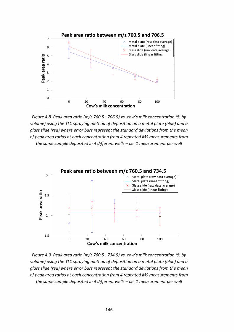
146
Figure 4.8 Peak area ratio (m/z 760.5 : 706.5) vs. cow’s milk concentration (% by
volume) using the TLC spraying method of deposition on a metal plate (blue) and a
glass slide (red) where error bars represent the standard deviations from the mean
of peak area ratios at each concentration from 4 repeated MS measurements from
the same sample deposited in 4 different wells – i.e. 1 measurement per well
Figure 4.9 Peak area ratio (m/z 760.5 : 734.5) vs. cow’s milk concentration (% by
volume) using the TLC spraying method of deposition on a metal plate (blue) and a
glass slide (red) where error bars represent the standard deviations from the mean
of peak area ratios at each concentration from 4 repeated MS measurements from
the same sample deposited in 4 different wells – i.e. 1 measurement per well

147
The quantitative analysis of milk concentrations that results from deposition on both
surface types agrees very well, suggesting the similarity of the mass peak
determination on either surface. The spraying device coated the surfaces with good
adhesion and uniformity. Without clearly seen sweet spots that normally give high
signals, the signal levels were nonetheless reasonably high and consistent
everywhere.
This strongly suggests that deposition by spraying will prepare samples appropriately
for imaging, with a good signal level, given the correct matrix-analyte proportion.
Discussion
The SunCollect apparatus has been shown to be able to generate small matrix crystal
sizes, with diameters of less than 50 µm and lead to a very homogeneous matrix layer
deposited onto the tissue surface (Römpp and Spengler, 2013). For a simple
quantitative milk experiment, TLC spraying parameters were adjusted to perform
similarly to the SunCollect system in terms of the amount of matrix applied per unit
area per layer. The mass spectra were repeatable as previously observed in Section
4.4.2 and the signals were also reasonably good. In real imaging sample preparation,
matrix application rate has an important influence on matrix-analyte interaction
while depositing. The sprayed matrix solution should not wet the sample too much
so that analytes are not displaced. With the SunCollect sprayer, appropriate distance
and the pressure of application can be achieved by adjusting positions of the spraying
nozzle and flow rate of the matrix solution, with multiple layers applied continuously,
such that the right amount of matrix is applied.
The AXIMA instrument requires long acquisition times, as it is limited by the data
transfer rates between the detector and analysis computer, to a sampling rate of
about 200 Hz. This affects its imaging capability because an imaging data set contains
thousands of mass spectra and therefore it can take a few hours to acquire,
depending on the image size and spatial resolution, and the sample should not be
left under a vacuum in the instrument for too long. The temperature inside the
instrument might cause some matrix evaporation and the vacuum can cause

148
shrinkage at the edge of the sample section. The superior 7090 instrument acquires
the same resolution imaging data set 10 times faster. It can also achieve higher
spatial resolution (up to 10 µm), better mass accuracy and the mass resolution (up
to 10,000 FWHM vs. 5,000 FWHM for the AXIMA), due to the longer flight path and
improvements in the pulsed extraction design.
A linear correlation was found between the specific peak area ratios (m/z 760.5 vs.
706.5) and the proportion of milk types. Thus, given appropriate sample preparation
and analysis, MALDI-MS data does allow quantitation of sample proportions. From
this basis, in the following chapters, the aim is to improve the analysis with more
advanced algorithms that utilise all the useful information contained in an MS data
set, and then progress to adapt the method to quantify mass spectrometry imaging
data.
4.5 Conclusion
This first experimental chapter addressed the basic aspects of sample preparation
and instrumentation used. The capabilities of the instrumentation and the important
parameters used to optimise performance have been identified and assessed.
MALDI-MS data acquisition can rely heavily on the experience of the user.
Consistency depends on optimising key parameters in each experimental step: from
sample washing/extraction, sample-matrix application, to laser power, diameter and
beam movement. Important findings that need to be embedded in protocols and
carried forward to next experimental chapters are;
Laser powers with optimal signal-to-noise ratios were determined, giving ion
signals of ≤100 mV, to achieve reasonable quantitative data analysis.
The instrument should be calibrated to an accuracy of ± 0.5 Da to allow for
the variation in spectral alignment of within 1 Da range across a data set.
Repeatability tests for each deposition method for the cow’s milk lipid extract
samples with DHB matrix were compared by variance analysis. The methods
where sample and matrix solutions were pre-mixed showed similar

149
repeatability regardless of the application techniques. The spotting technique
was preferable for analysing multiple (non-imaging) samples in the same
session.
There exists a linear relationship between the ratio of integrated areas of two
selected peaks and the concentration of milk mixture. Given that one of the
selected peak varies with the concentration and the other peak (normalising
peak in this case) is approximately constant throughout the data set.
Measurements taken after spraying materials including matrix on MALDI
target plates provided very consistent signal intensities from laser shot to
laser shot. This confirms the possibility of quantifying MALDI-MS data in both
non-imaging and imaging modes.

150
Chapter 5
Quantifying Binary Mixtures of
Biological Samples
5.1 Introduction
In mass spectrometry, the formation of gas phase ions from complex biomolecules
typically destroys structures of interest. John B. Fenn and Koichi Tanaka overcame
this problem, sharing the 2002 Nobel Prize in chemistry for matrix-assisted laser
desorption/ionisation (MALDI) and electrospray ionisation (ESI) (Hillenkamp and
Peter-Katalinić, 2007). MALDI co-crystallises complex samples within an easy to
ionise matrix. Samples and matrix are vapourised and ionised with a laser, giving a
pulsed source of ions ideal for TOF mass analysis. The ability to mass analyse large
molecules with high detection sensitivity makes MALDI attractive for biological
sample analysis, with applications ranging from milk adulteration detection, e.g.
Calvano et al. (2013), to cancer studies, e.g. Rodrigo et al. (2014). MALDI can also
form images by sampling across a 2D lattice (Fülöp et al., 2016), with mass peaks
forming pixel values. These data sets are massively rich, with hundreds of mass-
specific images able to be generated per acquisition. A method of data mining such
images would be a valuable enabling tool, allowing molecular correlations to be
identified and mapped upon biological structures. Such a system must quantitatively
model the complex variations and attribute them to classes of interest, e.g. tissue

151
types. This may be achieved using linear modelling approaches, such as Independent
Component Analysis (ICA), as in Gut et al. (2015). As a step towards a more general
data mining system, this work presents an ICA approach that is believed to match
well with the properties of MALDI data and therefore provides additional advantages
over traditional linear modelling methods, including the ability to build error models.
MALDI mass spectra (MS) are complex and highly variable. Careful preparation and
acquisition can mitigate against some factors, e.g. Seeley et al. (2008), but requires
training, practice and skill. Ideally, a homogeneous specimen might be expected to
produce spectra that are repeatable to levels of statistical sampling noise. However,
MS exhibits many other modes of variation:
Ionisation and detection vary depending upon local matrix density, chemistry,
laser intensity and duration of acquisition (Astigarraga et al., 2008).
Fragmentation is not a major process in MALDI. However, long chain
molecules can fragment by a number of mechanisms and also have isotopic
variations. Matrix molecules which absorb high energy can also fragment in
many ways. These would introduce background chemical noise.
Protonation is not the only process for cation formation. In fact, sodium and
potassium ionisation is often observed, even following attempts to wash
away soluble salts.
Suppression effects exist, where the presence of certain chemicals can mask
or change the appearance of others due to different affinities for attracting
charge.
Unwanted ions can contaminate mass spectra, including those from the
MALDI matrix.
There is a near-continuous ‘chemical noise’, from ungated post-source decay
processes and ion scattering, superimposed on any inherent instrumentation
noise.
The instrumentation and the detection process involve a series of electronic
components which contribute random signal fluctuations – i.e. electrical
noise.

152
A complex biomolecule will generate a series of MS features, which undergo
correlated variations in intensity and position, depending upon equipment settings
and local sample environment, e.g. Szájli et al. (2008). Aside from these variations,
MALDI mass spectra are approximately linear combinations of sub-spectra from a
sample’s constituent chemical components. Some sources of variation are reduced
through pre-processing. In previous work, pre-processing methods were developed
for use where Poisson noise, 𝜎𝑝 is dominant in peaks and Gaussian noise, 𝜎𝑔 is
dominant in background (Thacker et al., 2018). Section 3.3 of Chapter 3 provides a
description of these pre-processing methods and the definitions of notation used for
the two distinct types of noise are explained in the sub-section, Section 3.3.4.
A basic approach to MS analysis is to inspect single peaks that correlate maximally
with the parameters to be measured, e.g. Cahill et al. (2016). A peak can be
normalised to a second peak (or integral over a total ion current) in order to estimate
relative compositions. Peaks may also be artificially added to act as internal
standards, such as in Chumbley et al. (2016). Signals affected by high levels of
ambiguity or confounding variability are thus excluded, at the cost of discarding
potentially useful information. More efficient methods, such as Principal Component
Analysis (PCA) and Independent Component Analysis (ICA), extract correlated peak
variations. These approximate the data as weighted combinations of unit vectors,
each representing a correlated set of peaks. Comparisons between linear models can
be found in Gut et al. (2015) and Nicolaou et al. (2011), with evidence that ICA is most
beneficial. The formulations of standard PCA and ICA algorithms are based upon
uniform independent Gaussian errors, often conveniently leading to closed-form
solutions. However, MALDI may not be compatible with these assumptions. In
particular, Poisson statistics may better describe the counting of ions. Evidence of
Poisson nature of MALDI-MS data has been highlighted by others, e.g. Harn et al.
(2015) and Piehowski et al. (2009), with further investigation by this work.
The behaviour of noise can be assessed using Bland-Altman plots (Bland and Altman,
1986). These plot deviations from expected values as a function of signal strength.
Monte-Carlo generated Bland-Altman plots in Figure 3.9 (Section 3.4.3) illustrates

153
independent, identically distributed (iid) Gaussian noise, giving residuals with a fixed
spread, and also Poisson noise, where residuals grow with the square-root of the
signal. A square-root transform (Anscombe, 1948) can approximately convert
Poisson noise into iid Gaussian noise, but this invalidates any assumed linear model
of signal as a consequence. The main modelling options available and their key
properties are listed in Table 3.2 of Chapter 3, Section 3.4.3.
Using Bland-Altman analysis, there is evidence that a Gaussian noise assumption of
the error on measured signals is inappropriate for MALDI data and that a Poisson
noise, 𝜎𝑝 assumption is more realistic. In recent work, an ICA method for data with
Poisson sampling characteristics was derived (Tar and Thacker, 2014): Linear Poisson
Modelling (LPM). It has been applied to planetary and medical images (Tar et al.,
2015; 2017; 2018). This method is believed to provide the best match to the
properties of MALDI data (according to Table 3.2 of Section 3.4.3 (see the Poisson
ICA)) and is therefore evaluated here on the task of measuring mixtures of complex
lipid specimens. This method incorporates a Likelihood estimation procedure and a
predictive error theory capable of assessing the effects of Poisson noise, 𝜎𝑝 on
measurements. An extension, ‘MAX SEP’, is designed to reduce degeneracy inherent
in linear modelling, aiding interpretation of components allowing them to be
attributed to biologically meaningful MALDI sub-spectra. The aim of MAX SEP which
is to find a unique solution to the model, is similar to that of the varimax, quartimax
and equimax rotations, e.g. Kaiser (1958), but is appropriate for positive only data.
This current study uses mixtures of cow’s milk and goat’s milk; lamb brain and lamb
liver extracts; and lamb brain white matter and grey matter extracts, targeting mass
ranges associated with the samples’ lipid content. In addition to applying the new LP-
ICA method, single peak analyses on the same data were performed to corroborate
mixture measurements and to compare the attainable measurement precision. The
work-flow diagram (Figure 1.1) is provided earlier in Chapter 1, Section 1.3.

154
5.2 Materials and Methods
Section 3.4.3 previously discussed the noise distribution characteristics of data. The
Monte Carlo generated Bland-Altman plots showing behaviour of uniform
independent Gaussian noise and independent Poisson noise are compared in Figure
3.9. The modelling options: PCA (Jolliffe, 1986), ICA (Comon, 1994), Non negative ICA
(Plumbley and Oja, 2004; Plumbley, 2003), Poisson ICA (Tar and Thacker, 2014), etc.
are shown in Table 3.2 (Section 3.4.3) describing statistical and signal assumptions,
available for varied data properties. The selected method, linear Poisson ICA, is based
upon assumptions matching the properties of MALDI mass spectra. Given that MALDI
data has the properties noted in the same table which matches the proposed
method.
In this chapter, the use of the linear Poisson ICA is illustrated through application to
simple MALDI mass spectral data sets to ensure that the method is appropriate for
quantifying MALDI-MS data. These include the analysis of simpler lipid mixtures from
milk samples and biological tissue samples which give more complex lipid mixtures –
i.e. brain and liver tissues, and brain white and grey matter. Given that brain and liver
are two different organs that have very different functionalities, they would be
expected to have enough distinguishable characteristics for the algorithm to
differentiate. Finally, a more complicated problem was set by working on quantifying
mixtures of brain white and grey matter, which moved the study nearer to real
clinical questions – where the underlying samples in the mixtures have complex
spectra with many common characteristics, and fewer distinguishable mass peaks
are expected. The existence of background noise/contamination also blurs the
correlation of any mass peaks with the underlying sample proportion. Hence, it is a
challenge to confirm the suitability of the linear Poisson ICA method for use as a
quantitative tool for analysing MALDI-MS data.

155
5.2.1 Materials
Biological Samples
Fresh cow’s milk (Sainsbury’s British Whole Milk, UK)
Fresh goat’s milk (St Helen’s Whole Goats Milk, UK)
Fresh lamb brain (Worldwide Supermarket, Manchester, UK)
Fresh lamb liver (Worldwide Supermarket, Manchester, UK)
Chemicals
Recrystallised 2,5 dihydroxybenzoic acid (DHB)
Acetonitrile
Trifluoroacetic acid
Methanol
Chloroform
Deionised water
See Chapter 4, Section 4.3.1 for the manufacturer details, related descriptions and
calibration standards used.
Equipment
Stainless steel plate for MALDI-MS
Two pairs of curved forceps
Nylon filters of mesh size 40 µm (CorningTM, UK)
Instrumentation
AXIMA CFR+ TOF2 MALDI mass spectrometer
Power Gen 125 homogeniser (Fisher Scientific)
Heraeus Biofuge Fresco centrifuge
156
5.2.2 Sample Preparation
Binary mixtures in differing proportions (e.g. class A : class B) act as ground truth:
cow’s milk with goat’s milk mixtures, chloroform extracts of homogenised lamb brain
and liver, and chloroform extracts of lamb brain white matter and grey matter. For
each pair, mixtures of lipids were carefully prepared in 11 proportions ranging from
0% A (100% B) to 100% A (0% B), in increments of 10%, with proportions determined
by weight.
Milk mixtures were prepared prior to lipid extraction, whereas brain and liver lipids
were extracted first, then mixed afterwards. For milk samples, 1 ml at each
proportion underwent the lipid extraction procedure. For tissue samples, lipid
extraction was done separately using 2 g of homogenised tissue of each type (5
preparations per tissue type were repeated in order to get the amount needed to
create mixtures of varied proportions for the analysis – i.e. 5 x 2 g of each tissue type
were homogenised and extracted separately as the homogenisation worked well
with a small amount of tissue).
5.2.2.1 Brain Dissection
A fresh lamb brain was cut into smaller sections of around 1 cm thick along its coronal
axis. In each section, careful dissection for white and grey matter was performed
using two pairs of forceps to pull them apart. The brain must be placed on a glass
plate with ice beneath it during dissection to keep it in as fresh condition as possible.
There are nearly equal amounts of each of the two tissue types in a brain.
Approximately 30 g of each tissue type were obtained for the whole lamb brain used.
Where 10 g of each were required for this experiment.
The two tissue types are visually and spatially distinguishable. The image of a coronal
brain section is presented in Figure 5.1, with the identification of white and grey
matter regions labelled.

157
Figure 5.1 Lamb brain white and grey matter as shown in a coronal axis
(Pérez et al., 2013)
5.2.2.2 Tissue Homogenisation
10 g of each tissue type – i.e. brain / liver / dissected white matter / dissected grey
matter were homogenised prior to extraction of lipids. Note that the homogeniser
can only deal properly with a smaller portion of tissue: about 2 g were homogenised
at a time. The tissue container was placed in ice during homogenisation to minimise
heat building up in the sample.
5.2.2.3 Lipid Extraction
Lipids were extracted by adding 2:1 methanol:chloroform (4.5 ml), chloroform (2 ml)
and deionised water (1 ml) to the samples before mixing well. Samples were
centrifuged at 1,300 rpm for 2 min at 20 ºC. Levels of natural salts in the resulting
lipid extracts were reduced by the addition of 1 ml of deionised water before being
centrifuged again.
In the white and grey matter samples, nylon filters of mesh size 40 µm were used to
help remove fibrous tissue from the lipid extracts. However, emulsification occurred
in white matter, making the lipid extract hard to separate from the water and tissue.
The extracting solution of white matter was heated using boiling water to maximise
separation between lipid-tissue-water layers. Finally, chloroform was added into the
white matter lipid extract to compensate for evaporation.
White matter Grey matter

158
5.2.2.4 Binary Mixture
For each of the three mixtures mentioned at the beginning of this section, the
chloroform based lipid extracts of biological sample (class A : class B) were mixed into
11 different proportions. The binary mixture concentration was varied from pure
sample of class A to pure sample of class B, e.g. pure white matter to pure grey matter
lipid extracts, with increments of 10%. The Table 5.1 below indicates the exact
proportions for these class A : class B binary mixtures which determine the ground
truth used in the analysis. Mixtures were made volumetrically but checked for the
proportion gravimetrically to account for error associated with pipetting organic
solvent – i.e. the proportions of mixtures measured by weight, which are more
accurate than those by volume, are taken as actual values. The proportion was
calculated as class A concentration versus the total amount of class A and class B in
the sample – i.e. for milk, brain:liver and white:grey matter; class A are assigned to
be cow’s milk, brain, and white matter lipid extracts, respectively.
Table 5.1 Binary mixture proportions as measured by weight
Nominal concentration
by volume (Class A %)
Actual concentration by weight (Class A %)
Cow’s milk Brain White matter
0 0.00 0.00 0.00
10 10.74 11.00 8.95
20 19.36 22.41 20.66
30 30.61 32.73 29.12
40 40.11 41.53 38.26
50 49.97 52.34 50.66
60 59.46 63.34 58.73
70 69.35 73.45 71.21
80 80.07 81.94 80.16
90 90.34 91.28 89.54
100 100.00 100.00 100.00

159
5.2.2.5 Matrix
10 mg/ml of 2,5-dihydroxybenzoic acid (LaserBio Labs) in acetonitrile with addition
of 0.1% trifluoroacetic acid was prepared as a matrix solution.
5.2.2.6 MS Sample Preparation and Deposition
The matrix : sample solution was mixed with a ratio of 1:1 for the milk and 3:2 for the
tissue samples to form MALDI specimens. Double layers of a MALDI specimen, 1 µl
each layer, were deposited into a well of stainless steel MALDI target plate. 8 repeat
depositions were applied per mixture proportion to provide repeatability data. The
depositing locations of each proportion were randomly positioned on the target
plate to avoid correlations between the spatial organisation and the mixture
concentration.
5.2.3 MS Acquisition
An AXIMA (curved-field reflectron time-of-flight) mass spectrometer, manufactured
by Shimadzu Biotech, was used to acquire the MALDI-MS data. Where the MALDI
ionisation system of the instrument is a 349 nm neodymium-doped yttrium lithium
fluoride (Nd:YLF) laser of < 5 ns pulse width and approximately 200 Hz repetition rate.
Using the positive reflectron mode, an ion extraction energy of up to 24 kV was
allowed with an effective drift length of 2.0 m. Launchpad proprietary software was
used throughout all of the experiments for controlling acquisition. During acquisition,
default settings were adopted (i.e. 200 MS profiles, 5 shots per profile, pulsed
extraction 750 Da, mass range up to 1,500 Da). A total of 88 spectra were obtained
for each mixture type, one for each of the deposited targets.

160
5.3 Data Analysis Procedure
5.3.1 Pre-processing
Low m/z MS peaks (e.g. matrix-derived ions) contain little information regarding lipid
content. A mass window (m/z) between 650 and 850 was selected for milk mixtures;
a window between 690 and 890 for brain:liver mixtures and white:grey matter
mixtures. The total quantity of signal gathered per spectrum is difficult to control,
making it necessary to pre-filter poor data. Some spectra within this window were
rejected on grounds of low signal-to-noise. Spectra containing high signal were also
rejected to avoid saturated peaks. A combination of visual inspection and goodness-
of-fit tests determined which spectra were kept in order to build satisfactory models.
This left 66 milk mixtures, 80 brain:liver mixtures and 82 white:grey matter mixtures,
out of the original 88 per group. Pre-processing is performed to ensure that data
behaves as linearly additive histograms, with independent Poisson noise (𝜎𝑝), as is
required for LP-ICA modelling to operate correctly. The methods developed in
Thacker et al. (2018) satisfy this requirement, see Section 3.3 in Chapter 3. A peak
alignment procedure is applied to minimise unwanted shifting of peaks. A baseline
correction that assumes noise on the background is approximately Gaussian (𝜎𝑔) with
zero mean is applied. Finally, histograms are produced containing only bins for
significant peaks, with peaks integrated into each bin and inter-peak gaps removed.
A total of 102 peaks were retained in the milk spectra, 76 peaks were retained in the
brain:liver spectra and 67 peaks were retained in the white:grey matter spectra. The
appearance of an example raw spectrum, pre-processed spectrum (after alignment
and background/baseline correction), and pre-processed spectrum (after peak
detection) are provided in Figure 5.2.

161
Figure 5.2 Example of averaged raw and pre-processed spectrum before and after
peak detection (acquired from the lamb brain lipid extract)
Following pre-processing steps, the resulting (peak detected) spectra for each data
set are achieved. The averaged resulting spectra of pure samples are shown in Figure
5.3.

162
Fi
gu
re 5
.3 A
vera
ged
pea
k d
etec
ted
sp
ectr
a: (
a)
cow
's a
nd
go
at'
s m
ilk, (
b)
bra
in a
nd
live
r ti
ssu
e a
nd
(c)
wh
ite
an
d g
rey
ma
tter
(Pa
rt 1
of
3)

163
Fi
gu
re 5
.3 A
vera
ged
pea
k d
etec
ted
sp
ectr
a: (
a)
cow
's a
nd
go
at'
s m
ilk, (
b)
bra
in a
nd
live
r ti
ssu
e a
nd
(c)
wh
ite
an
d g
rey
ma
tter
(Pa
rt 2
of
3)

164
Fi
gu
re 5
.3 A
vera
ged
pea
k d
etec
ted
sp
ectr
a: (
a)
cow
's a
nd
go
at'
s m
ilk, (
b)
bra
in a
nd
live
r ti
ssu
e a
nd
(c)
wh
ite
an
d g
rey
ma
tter
(Pa
rt 3
of
3)

165
5.3.2 Peak Ratio Analysis
A simple peak ratio analysis is applied to estimate mixing proportions for the milk,
brain:liver and white:grey matter mixtures as a benchmark against which the new LP-
ICA analysis can be compared. Within the lipid window, the largest peak is used for
normalisation. This peak is at m/z 760.5 in all three mixture cases, corresponding to
a phosphotidylcholine. At each mixing proportion, all peaks are divided by the
reference peak, with results for each peak plotted against the known ground truth
proportions. A least-squares fit is computed for each peak, which should correlate
(or anti-correlate) well with the ground truth if there is useful information present.
The most informative peaks (providing smallest errors) were compared to the LP-ICA
results. These peaks were at m/z 706.2 for milk mixtures, m/z 786.5 for brain:liver
mixtures and m/z 734.5 for white:grey matter mixtures.
Sources of variability, including efficiency losses and possible contamination, make it
unlikely that a linear trend extracted from a single peak will have a slope and
intercept that exactly predicts ground truth. Rather, the fitted line is used to calibrate
a linear predictor that maps normalised peaks to ground truth proportions. The
standard deviation of predictions around the calibrated line is used as an estimate of
the measurement accuracy attainable from each peak.
5.3.3 Linear Poisson ICA Analysis
LP-ICA models describe the shape and variability of distributions found within
histograms using a linear combination of simpler fixed components, with Likelihood
estimates of parameters e.g. Barlow (1989) using Expectation Maximisation. Each
component can be viewed as a probability mass function (PMF) for a sub-spectrum,
representing some correlated set of peaks. Unlike other linear models, LP-ICA models
use mixtures of PMFs, rather than unit vectors. This permits positive-only
coefficients, appropriate for counting applications such as the ion counting in mass
spectra. The mixture of components, fitted on a spectrum-by-spectrum basis,

166
describes a spectrum as a weighted sum of sub-spectra – see Equation (5.1), adapted
from Equation (3.7) in Section 3.4.5 of Chapter 3. The method is illustrated on the
schematic diagram in Figure 5.4. An LP-ICA model must determine the necessary
PMFs (i.e. sub-spectra) required to describe the distribution of spectra. This process
is a Poisson compatible form of ICA, or LP-ICA, which maximises a Likelihood
formulation of the problem (Equation (3.8), see Section 3.4.5 of Chapter 3). The
number of components required to describe a set of spectra is determined through
a model selection process that aims to reach a satisfactory 𝜒𝐷2 goodness-of-fit
(Equation (3.11), see Section 3.4.5 of Chapter 3). Satisfactory fits are those that either
reach a minimum, or lie upon a plateau. In cases of a plateau, failing to achieving a
true minimum is compensated for in the error theory, as error covariances are scaled
by the final goodness-of-fit. Details of the full method and its validation in other
applications can be found in Tar and Thacker (2014) and Tar et al. (2015; 2017; 2018).
The Likelihood estimates of LP-ICA components and weighting factors need not be
unique. The models created are potentially degenerate, in the sense that different
weighted combination of different components could achieve equally good
likelihood solutions. The MAX SEP algorithm was therefore designed to reduce this
problem by manipulating components to increase their independence – i.e. subtracts
quantities of each component from others as far as possible, without generating
negative values. The linear components are maximally separated to match individual
physical meaning, in this case the correlated appearance of different chemicals
associated with different types of biological sample. See Section 3.4.6 for the
explanation of MAX SEP algorithm.

167
Figure 5.4 Schematic diagram illustrating the linear Poisson ICA modelling method
5.3.4 Mapping Components to Classes
The mixtures of two different biological materials (e.g. brain, liver) will be considered
to be composed of proportions from class A and class B. If spectra were stable to
within the limits of Poisson sampling and if all molecules within samples were
detected with 100% efficiency, there should be only 2 components extracted from
such mixtures, i.e. the spectrum for class A and the spectrum for class B. In practice,
the numerous sources of variation noted in Section 5.1 lead to multiple components
being required to describe spectra. Additionally, the ground truth measurements are
based upon the mass of the sample components, which is not, strictly, what is being
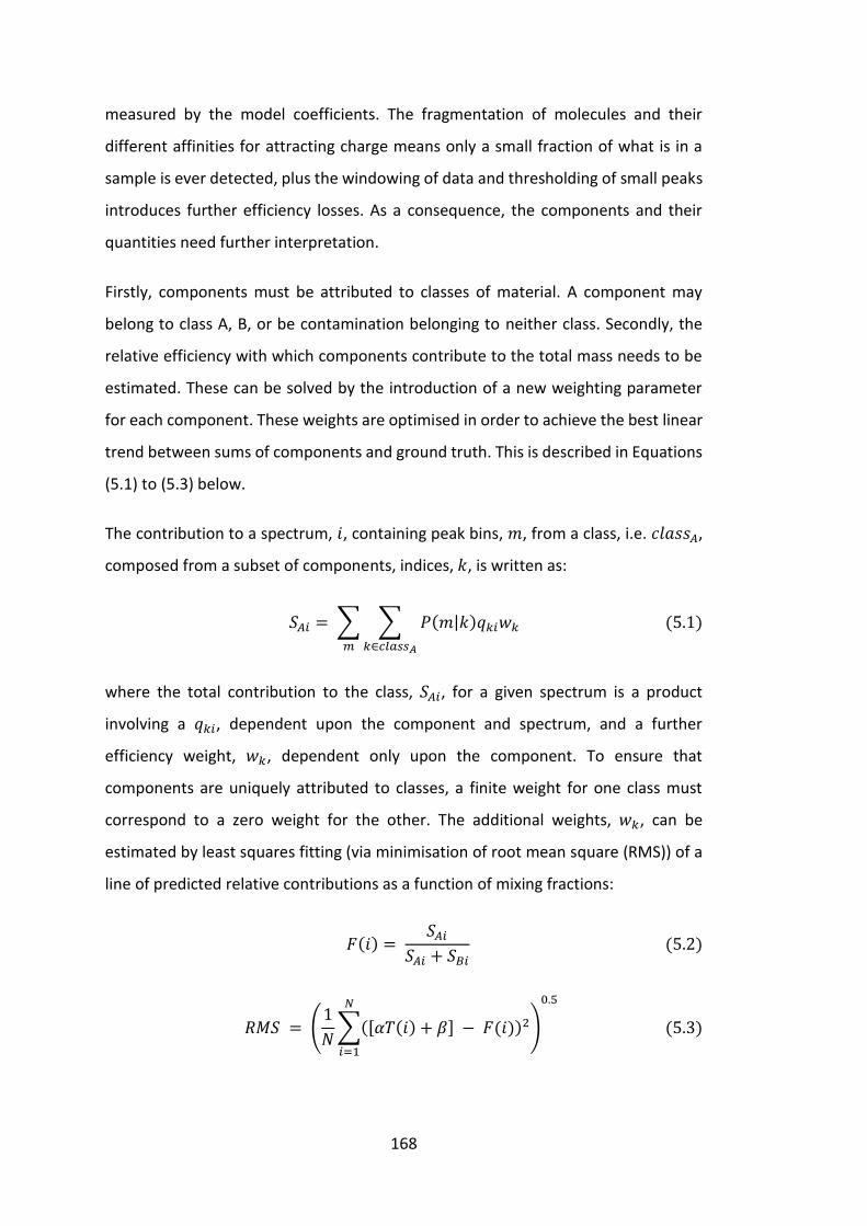
168
measured by the model coefficients. The fragmentation of molecules and their
different affinities for attracting charge means only a small fraction of what is in a
sample is ever detected, plus the windowing of data and thresholding of small peaks
introduces further efficiency losses. As a consequence, the components and their
quantities need further interpretation.
Firstly, components must be attributed to classes of material. A component may
belong to class A, B, or be contamination belonging to neither class. Secondly, the
relative efficiency with which components contribute to the total mass needs to be
estimated. These can be solved by the introduction of a new weighting parameter
for each component. These weights are optimised in order to achieve the best linear
trend between sums of components and ground truth. This is described in Equations
(5.1) to (5.3) below.
The contribution to a spectrum, 𝑖, containing peak bins, 𝑚, from a class, i.e. 𝑐𝑙𝑎𝑠𝑠𝐴,
composed from a subset of components, indices, 𝑘, is written as:
𝑆𝐴𝑖 = ∑ ∑ 𝑃(𝑚|𝑘)𝑞𝑘𝑖𝑤𝑘
𝑘∈𝑐𝑙𝑎𝑠𝑠𝐴𝑚
(5.1)
where the total contribution to the class, 𝑆𝐴𝑖, for a given spectrum is a product
involving a 𝑞𝑘𝑖, dependent upon the component and spectrum, and a further
efficiency weight, 𝑤𝑘, dependent only upon the component. To ensure that
components are uniquely attributed to classes, a finite weight for one class must
correspond to a zero weight for the other. The additional weights, 𝑤𝑘, can be
estimated by least squares fitting (via minimisation of root mean square (RMS)) of a
line of predicted relative contributions as a function of mixing fractions:
𝐹(𝑖) = 𝑆𝐴𝑖
𝑆𝐴𝑖 + 𝑆𝐵𝑖 (5.2)
𝑅𝑀𝑆 = (1
𝑁∑([𝛼𝑇(𝑖) + 𝛽] − 𝐹(𝑖))2
𝑁
𝑖=1
)
0.5
(5.3)

169
where 𝐹(𝑖) should linearly correlate well with ground truth fractions 𝑇(𝑖), given best
fitting 𝛼, 𝛽 and set of efficiency weights, 𝑤𝑘. Additionally, the RMS can be scaled to
the slope of this line, 𝑅𝑀𝑆
𝛼 to give an estimate of the predictive accuracy to ground
truth.
5.3.5 Spectra Error Analysis
The values recorded within mass spectral bins are expected to be Poisson in nature,
as peak heights are proportional to ion counts which are discrete events, occurring
in time, consistent with a Poisson process. However, there are additional sources of
noise, therefore the Poisson assumption must be checked. The residuals between
spectral models and original spectra can be used to assess the validity of the
assumption. If binned values are indeed Poisson in nature then the residuals should
grow proportionally to the square root of the bin quantity (the signal variance agrees
with the Poisson assumption, 𝜎𝑝). Any fixed scaling of the Poisson process should also
be revealed as a scaling factor on the square-root dependency.
Bland-Altman plots, i.e. Bland and Altman (1986), can be constructed and a power-
law error model fitted to assess both of these properties. Bland-Altman plots are
scatter plots which record expected bin values (i.e. expected peak intensity) on the
x-axis versus deviations away from the expected values on the y-axis. The linear
model predictions are used as estimates of expected bin values (x-axis), and residuals
between model and spectra are the observed deviations (y-axis). A power-law
function can be fitted to resulting plots to determine the behaviour. The following
function (Equation (5.4)) is fitted to Bland-Altman plots show differences in error
behaviour away from the Poisson assumption:
𝜎𝑀 = 𝑎 (𝐻𝑀
𝑎)
0.5𝑏
(5.4)
where 𝜎𝑀 is the standard deviation of model-data residuals; 𝑎 and 𝑏 should be unity
for non-scaled Poisson bins, and 𝑎 should be a variance scaling in cases where 𝑏 is

170
unity. This variance scaling, 𝑎, should also be close in value to the model’s goodness-
of-fit (𝜒𝐷2 ), which is an average scaling based upon a 𝜒2 per degree of freedom. This
Bland-Altman approach is a more stringent test than the goodness-of-fit. A value of
𝑏 deviating too far from unity would suggest that errors are not Poisson. The effects
of such a deviation can be evaluated via Monte Carlo if necessary (however, in
practice the power-law matches well with the Poisson assumption).
5.3.6 Measurement Error Analysis
Once established, the Poisson noise can be propagated to find its effect on measured
values. An error covariance matrix for model coefficients (i.e. estimated quantities,
𝑞𝑖) can be estimated as in Equation (3.10), see Section 3.4.5 of Chapter 3. Assuming
independent Poisson errors (𝜎𝑝), LP-ICA models provide estimates of quantity errors
by summing the effects of individual Poisson bins into quantity error covariances.
This is achieved using error propagation. The error covariance can be further scaled
by 𝜒𝐷2 (goodness-of-fit) computed from model-data residuals to boost errors to
better match actual distributions of true residuals, i.e. Poisson scaling factor.
Together, the Bland-Altman plots, goodness-of-fits and quantity error covariances
summarise the success (or otherwise) of the analysis without any need to refer to
ground truth.
Sampling errors in spectral histograms combine to give a level of uncertainty on the
estimated quantity measurements. In order to factor these uncertainties into final
mixture proportions they must be propagated through the EM algorithm using error
propagation, as described in Barlow (1989). This process uses derivative calculations
to assess how small changes in inputs (i.e. Poisson noise in data) affects small changes
in outputs (i.e. proportion measurements). Equations (3.10) and (5.5b) describe this
process.
In a mixture containing 2 sample classes, A and B, the proportion of quantity of class
A to the total quantity, 𝑝𝐴 = 𝐴
𝐴+𝐵 has the propagating error, 𝜎𝑝𝐴
.

171
𝜎𝑝𝐴2 = (
𝜕
𝜕𝐴(
𝐴
𝐴 + 𝐵))
2
𝜎𝐴2 + (
𝜕
𝜕𝐵(
𝐴
𝐴 + 𝐵))
2
𝜎𝐵2 (5.5𝑎)
Take square root on both side of the Equation (5.5a)
𝜎𝑝𝐴=
1
(𝐴 + 𝐵)2√𝐵2𝜎𝐴
2 + 𝐴2𝜎𝐵2 (5.5𝑏)
Where 𝜎𝐴 and 𝜎𝐵 are the standard deviations of estimating values for class A and
class B underlying sample, respectively. These final errors, 𝜎𝑝𝐴, can be compared to
actual accuracies computed using knowledge of ground truth values.
Predicted errors (𝜎𝑝) via this method can be compared to true measurement errors
(𝜎𝑡𝑜𝑡) by dividing the deviations of measured values from ground truth by the
predicted errors. These form a Pull distribution, which if unbiased should have a
mean of zero, and if precision is correctly predicted should have a width of unity.
In addition to the sampling errors, the Poisson ICA modelling processes is a numerical
optimisation method that utilises random initialisations leading to multiple local
optima. Local solutions are similar, but do add a level of variability to results. To
quantify this, multiple models (i.e. 50) are built to assess the spread of solutions.
5.4 Results and Discussion
5.4.1 Peak Ratio Analysis
The peak ratio approach found that the peak at m/z 706.2 correlated best with
changes in milk proportions, m/z 786.5 correlated best with changes in lamb
brain:liver tissue proportions, and m/z 734.5 correlated best with changes in
white:grey matter proportions. These peaks, for each data set, were normalised to
the largest and most stable peak throughout different proportions at m/z 760.5 and
the correlation with ground truth via peak ratio analysis is obtained (see the plots

172
presented in Figure 5.5). The x-axis shows the ground truth proportions. Each cross
(data point in the plots) is a peak ratio estimate from a different spectrum, with
repeatability data at each 10% increment. Deviations from the fitted line (least
square) show typical measurement accuracy. These peaks provide a relative
measurement precisions of ± 16%, ± 8% and ± 6%, respectively (see the plot in Figure
5.11 (right)).
a
b
c
Figure 5.5 Linear fitting for conventional peak ratio analysis results: (a) cow’s and
goat’s milk, (b) brain and liver tissue and (c) white and grey matter

173
5.4.2 Linear Poisson ICA Analysis
Figure 5.6 Bland-Altman plot showing behaviour of model residuals (y-axis) as a
function of peak intensity (x-axis). Each point represents a residual between
an LP-ICA modelled spectrum bin and actual spectrum. The fitted curves (power law
of Equation (5.4)) show ±1 standard deviation error as a function of peak intensity
consistent with Poisson statistics.
Bland-Altman analysis confirms that the pre-processed MALDI spectra are consistent
with Poisson statistics (see the Bland-Altman plot in Figure 5.6). The power-law
growth parameter (𝑏 in Equation (5.4)), was estimated as 1.04 ± 0.02, completely
consistent with Poisson style growth in residuals as a function of peak intensity. This
justifies the application of Linear Poisson Modelling to perform ICA and mixture
quantitation. The power-law scaling parameter (𝑎 in Equation (5.4)) was estimated
as 23.9 ± 1.4, consistent with the 𝜒𝐷2 goodness-of-fit, suggesting that each Poisson
event is equivalent to an increase of 5 units of signal intensity.
Figure 5.7 Determination of model order for linear Poisson ICA models

174
In the plot presented in Figure 5.7, the curves show the goodness-of-fit (Equation
3.11 of Section 3.4.5) of linear Poisson ICA models as a function of the number of
model components, where each component represents a sub-spectrum that is a
mode of correlated spectral variation. A total of six components were found to be
required to sufficiently model the milk spectra, at which point the goodness-of-fit
begins to plateau (see the plot in Figure 5.7). The lamb brain:liver spectra required
eight components and white:grey matter also required eight components. Extracted
ICA components (mass spectral components) for milk, lamb brain:liver and
white:grey matter mass spectra are presented in Appendix A (see sub-spectra in
Figure A.1, Figure A.2 and Figure A.3, respectively). Once attributed to sample
classes, one milk component, one brain:liver component and one white:grey
component were rejected as being uninformative (due to contamination or
ambiguity), with the remaining compositions showing a clear linear trend against
known mixtures (see the plots in Figure 5.8, showing composition of spectra in terms
of weighted contributions of extracted LP-ICA components). Each 10% increment is
shown as a step, where each step contains repeatability data for independent spectra
with the same mixing proportions. The black dots show the best fitted trend. Each
bar shows the relative proportion of each LP-ICA component present within a
spectrum. The error bars are the LP-ICA model predicted errors. The components
‘comp 1’, etc. are listed in the keys from top to bottom in the same order as they
appear in the figure. N.B. The results are also shown as scatter plots with linear fitted
line in Figure 5.9 in a comparable manner with the peak ratio analysis results in the
plots shown in Figure 5.5. These provided relative measurement precision of around
± 9%, ± 4% and ± 4%, up to approximately doubling that attained via peak ratio
analysis (see the plot in Figure 5.11 (right)). Even when the peak known to correlate
best with milk mixtures was removed from the LP-ICA analysis, a precision of ± 11%
could be achieved.
Pull distribution analysis (actual deviations from ground truth divided by predicted
deviations, see the histograms in Figure 5.10) show that LP-ICA model measurements
are unbiased (mean consistent with zero) and predicted errors (𝜎𝑝) successfully
describe the majority of measurement noise (𝜎𝑡𝑜𝑡), with true errors being 1.6, 1.6

175
and 1.4 times larger than predicted (plotted in Figure 5.11 (left)) in the analysis of
milk, brain:liver and white:grey matter data, respectively.
a
b
c
Figure 5.8 ICA component contributions per spectrum: (a) cow’s and goat’s milk,
(b) brain and liver tissue and (c) white and grey matter

176
a
I
II
b
c
Figure 5.9 Linear fitting for linear Poisson ICA analysis results: (a) I. cow’s and
goat’s milk II. cow’s and goat’s milk with m/z 706.2 excluded, (b) brain and liver
tissue and (c) white and grey matter
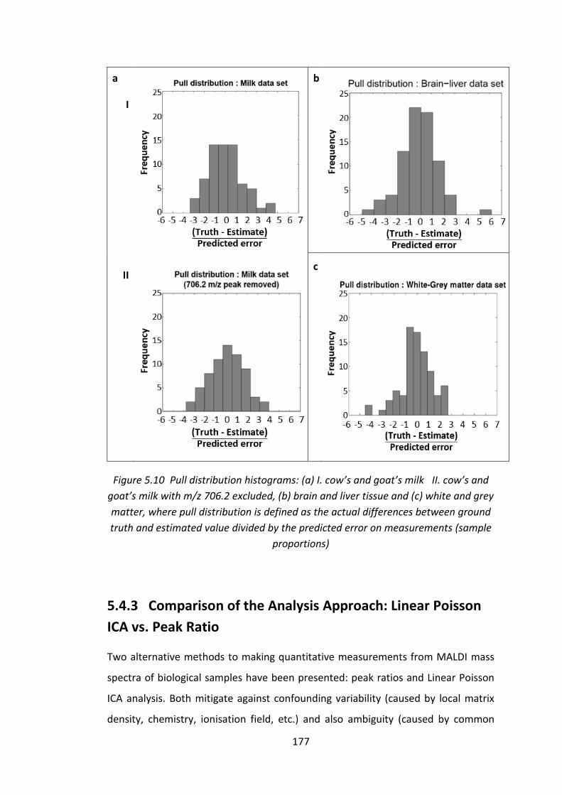
177
a
I
b
II
c
Figure 5.10 Pull distribution histograms: (a) I. cow’s and goat’s milk II. cow’s and
goat’s milk with m/z 706.2 excluded, (b) brain and liver tissue and (c) white and grey
matter, where pull distribution is defined as the actual differences between ground
truth and estimated value divided by the predicted error on measurements (sample
proportions)
5.4.3 Comparison of the Analysis Approach: Linear Poisson
ICA vs. Peak Ratio
Two alternative methods to making quantitative measurements from MALDI mass
spectra of biological samples have been presented: peak ratios and Linear Poisson
ICA analysis. Both mitigate against confounding variability (caused by local matrix
density, chemistry, ionisation field, etc.) and also ambiguity (caused by common

178
molecular constituents in different samples) using very different approaches. The
former avoids problems by simply discarding mass peaks which are adversely
affected, selecting those which empirically correlate best with sought
measurements. The latter is far more sophisticated, modelling sources of variability,
learning correlations between any number of peaks and attributing them to
meaningful classes of data. This latter method is far more efficient, as much more
signal is retained. The peak ratio method uses only 14% of the total signal available
in the pre-processed lamb spectra, whereas the LP-ICA approach uses 90%, which
immediately should provide an advantage through sample size alone. The LP-ICA
approach achieves levels of measurement precision double that attainable through
peak ratio analysis, with 1 standard deviation errors reducing from ± 16% and ± 8%
to as small as ± 9% and ± 4%, for milk and lamb tissue mixtures, respectively.
Achieving this increased precision using the peak ratios method would require at
least quadruple the quantity of data (assuming errors fall with the square-root of
sample size). White:grey matter measurement errors reduced from ± 6% to ± 4%,
suggesting that most information is already extracted from the single peak at m/z
734.5 (see the plot in Figure 5.11 (right) which illustrates that the LP-ICA method is
more precise than the peak ratio method in all experiments).
The efficient use of data is perhaps best illustrated by the LP-ICA method when the
most informative milk peak (m/z 706.2) is removed. Despite the ambiguity of
remaining peaks, measurements could still be made using the ICA method with errors
of ± 11%. If the inverse variance is used as a measure of information content, the LP-
ICA analysis precision using all milk peaks (± 9%) is consistent with combining the all-
but-one analysis (± 11%) with the conventional peak ratio results from the m/z 706.2
peak (± 16%).

179
Figure 5.11 Predictive ability of LP-ICA error theory, as measured using Pull
distributions (left). Measurement precision of peak ratio analysis versus LP-ICA
analysis. Values are 1 standard deviation relative errors, expressed as percentage of
quantity measurements (right).
In addition to the increased precision gained using the new method, the LP-ICA error
theory (Section 5.3.6) provides the capability to predict measurement errors on a
spectrum-by-spectrum basis. These predictions explain the majority of measurement
noise, as confirmed by Pull distributions which should have a mean of zero and width
(standard deviation) of unity if predicted errors (𝜎𝑝) match the observed errors (𝜎𝑡𝑜𝑡).
The plot presented in Figure 5.11 (left) shows that there is no bias (mean consistent
with zero) and that true errors (assessed against ground truth) are close to those
predicted. Error predictions within a factor of 2 are generally deemed sufficient for
scientific use, e.g. Barlow (1989) and Press et al. (2009). As these errors are
predictable from the input data, they do not require ground truth to be computed.
These predictive powers provide several advantages, permitting goodness-of-fits to
be constructed, such as 𝜒𝐷2 , and revealing data-specific errors (see variable-sized
error bars in the plots shown in Figure 5.8). In contrast, the peak ratio method uses
empiricism alone to determine measurement precision. This provides a single error
estimate, the use of which relies upon an assumption of uniform errors across all
spectra, which logically should not be the case due to differences in normalisation.
Furthermore, alternative analyses, such as PCA or conventional ICA do not provide
error predictions, and must also rely upon empiricism and ground truth.

180
Despite the success of the error predictions, observed errors were still larger than
expected. The additional sources of unpredictable error include: the spread of local
minima in the numerical ICA solutions; the Gaussian measurement noise superposed
upon the Poisson sampling process; non-linearity; the potential need for a greater
number of linear components; and imperfect pre-processing.
5.4.4 Mean Prediction from Multiple Models
The effect of local optima was assessed by building 50 ICA models. The typical
(median) precision attainable for milk mixtures was ± 9.77%, for brain:liver mixtures
was ± 4.59% and for white:grey matter was ± 5.15%. The best local solutions found
were ± 9.05%, ± 3.96%, and ± 3.98%, from milk, brain:liver and white:grey matter
respectively, which are the solutions used in the associated figures. Rather than
relying upon a single model (i.e. one local ICA solution) a mean linear mixing
prediction can be made from many local solutions, thereby reducing variability. The
mean predictions from the 50 model attempts provide precisions of ± 8.72% (milk),
± 3.77% (brain:liver tissue) and ± 4.19% (white:grey matter).
In addition, the mean prediction from multiple models can also help with selection
of suitable ICA component combination by comparing this value of models built using
different component combinations. Tested using the white:grey matter data set, the
plot in Figure 5.12 illustrates that certain number of components would be required
for achieving best proportion prediction accuracy. Modelling performance gets
improved and maximised with more components extracted before becomes plateau
thereafter. From the plot, better prediction accuracy was generally obtained via
models that only reject 1 component as contaminating background (i.e. amongst
models with the same numbers of extracted components, the RMS error values of
individual models that only reject 1 component tends to be smaller and closer in
values compared to those with multiple components rejected). However, this effect
evens out for the averaged models that account for some more variations in
predicting proportion values from individual models – i.e. higher model order.

181
Figure 5.12 Model fitting performance assessed on averaged white:grey matter
models built with various number of components
Note that ‘7/8’, as labelled on the horizontal axis of the plot in Figure 5.12, refers to
a component combination where 7 out of the total of 8 extracted components were
kept for the spectral model fitting and 1 component was rejected as a
background/noise component, etc. A small dip at 7/8 component combination is
seen in the plot. This confirm that it was a reasonable choice of model.
5.4.5 Validation of the Poisson Assumption and Suitability of
the LP-ICA in Modelling MALDI-MS Data
The Poisson sampling assumption was validated via Bland-Altman analysis (plotted
in Figure 5.6), showing that errors grow with the square-root of peak intensity (𝜎𝑝),
with an overall scaling factor of 24. The scaling factor measured is also consistent
with the 𝜒2 per degree of freedom of ICA models (i.e. 24 plateau reached in the
model selection curve provided in Figure 5.7). Alternative modelling approaches,
such as PCA, and other ICA methods, would be inappropriate due to their Gaussian
assumptions and lack of predictive error theories.
If the MS acquisition pipeline was ideal, there would only be two sources of
variability: changes in signal due to changing mixture proportions; and random

182
Poisson sampling noise (𝜎𝑝). Despite best efforts to homogenise mixtures, wash away
salts and perform basic pre-processing, resulting spectra still contain numerous
modes of variation. Six linear components were required to model milk and eight to
model lamb tissue. Within these components, one was rejected from each model on
account of its inability to provide information regarding mixture proportions.
Rejection was on the basis of linear regression applied to map components to classes,
Section 5.3.4, when the prediction improved with that component belonging to
neither classes. This could be due to either the component representing
contamination, or the component could contain common structure indistinguishable
between the sample classes. The remaining components are presumed to be
modelling those sources of variation noted in Section 5.1, i.e. fragmentation,
ionisation modes, isotopic variations, etc. The number of components required to
model the data could potentially be used as a measure of data quality. Preparation,
acquisition and pre-processing steps could be optimised to minimise the number of
required components.
Despite the numerous components required to describe the data, the MAX SEP
algorithm (see Section 3.4.6 of Chapter 3) provides the ability to attribute Poisson
sampled components physical meaning, allowing their quantities to be used for
measurement. The attribution of component quantities to classes of sample are only
valid if this physical meaning can be established. An alternative approach, based
upon PCA or factor rotations for example, would not have been appropriate due to
enforced orthogonality and non-physical negative weightings.
Finally, as a tool for future MALDI image data mining, the LP-ICA approach could
potentially improve the information content of images by replacing pixels based on
single m/z peaks with pixels based upon LP-ICA component weights. Such images are
expected to have better signal-to-noise, as pixels would incorporate information
from many peaks. They may also better correlate with tissue types, giving a higher-
level interpretation than simply being a map of specific chemicals. And finally,
through the LP-ICA error theory, pixel values are made quantitatively meaningful.

183
The ability to quantitatively assess correlated chemicals and map them onto
biological structures will be the focus of the next chapter.
5.5 Conclusion
LP-ICA modelling analysis of MALDI mass spectra has been shown to provide
improved quantitative accuracy for the measurement of proportions of biological
samples when compared to a conventional single peak approach. There are only a
relatively small number of peaks which are applicable to a single peak analysis, as
most are adversely affected by high levels of uncontrolled variability. LP-ICAs
successfully model this variability, permitting information in any number of peaks to
be included in measurement estimation. The accuracy of measuring the proportions
of milk, brain and liver mixtures were doubled using this new approach.
In addition, the modes of variation found within MALDI mass spectra, in terms of sub-
spectral combinations, can now be extracted and analysed providing physically
interpretable models with fewer parameters, marking a step improvement in related
ICA work in the field. The high levels of variability, sources of ambiguity and lack of
error predictions also suggests that simple single peak ratios are unlikely to be
quantitatively trustworthy. The approach demonstrated will be extended in Chapter
6 to data-mine MALDI images.
5.6 Overview: A Bridge to the Next Chapter
The brain is built up from many sub-types of tissues. It can be divided into white and
grey matter which are the two main tissue types of the brain that are readily
distinguished from one another. They are located in separate sites and are
responsible for different tasks but are highly associated and must properly co-
operate for the brain to perform normally.

184
The brain is an important organ in a body which is the main part in the central
nervous system (CNS) connected to the spinal cord. The CNS works in conjunction
with the peripheral nervous system (PNS) that controls autonomic and somatic
nervous systems. The brain gains and recognises information and consists of nerves,
in addition to spinal cord nerves, that receive sensation and deliver motor
commands.
White Matter
White matter has more variety of cell types, consists mainly of the tails of nerve cells,
axons and myelin, lipidic fibres that act as protecting pillow around axons. This is
what makes the white matter white/light pink and soft. Neuronal signals are
transmitted between nerve cells (neurons) through axons, allowing communication
within the complex neuronal network.
Grey Matter
Grey matter is located at the outer part of the brain. Folds of white matter branch
into grey matter region, the host for the neurons’ cell body, the receptor for neuronal
signals. This part of the brain requires most of blood and oxygen supply that comes
into the brain. Capillaries surrounded neuronal fibres make the region appear
grey/dark brown.
The brain stays shielded inside the skull and under layers of the brain’s membranes
called meninges. This is an important organ that must be protected as abnormalities
of the brain will cause potential risks and damage to other systems all over the body.
Degradation of brain tissues or changes in nervous system should be diagnosed
rapidly to avoid permanent damage. Detection of the concentration of molecular
species within tissues can be performed using mass spectrometry techniques. As with

185
the other biomolecules, MALDI-MS can detect lipids, which have relatively high
concentrations in brain tissue. Regional determination of detected molecules is also
capable with imaging MS. Making such analysis quantitative will enable a powerful
biomarker identification technique which can be extended to use for in vivo (e.g.
rapid evaporative ionisation mass spectrometry (REIMS) system for real-time analysis
by Phelps et al. (2018)) or in vitro diagnostics.
In this Chapter, a lamb brain which has many similarities to human brain has been
analysed. It has often been used to model the human brain in a variety of
study/demonstration contexts. It was therefore selected here for this experiment
where the sample proportions of white and grey matter present in the human brain
are mimicked. The white and grey matter were expected to show both shared and
differing mass spectral lipid profiles. Binary mixtures of the two allowed assessment
of the methods introduced for determining proportions within the mixture. As a
result of the analysis using the linear Poisson ICA method, all the underlying
variations were automatically modelled by extracting independent components that
contribute to the spectra, and hence providing accurate estimates of sample
proportions. This suggested that the linear Poisson ICA method also has the capability
for quantifying MALDI-MS image data, which is to be confirmed in the next chapter
using rat brain imaging example data. If so, the method could be seen as an
unsupervised approach that can provide quantitative information regarding the
spatial distribution of biomolecules of which cells and tissues are comprised. This
consequently can take a step closer towards an interpretation of the tissue’s
biological composition with potential applications in biomarker identification.

186
Chapter 6
MALDI-MS Imaging Analysis of
Brain Tissue Section
6.1 Introduction
6.1.1 Outline of the Chapter
A mass spectrometry imaging (MSI) data set is obtained by acquiring mass spectra
across a 2-dimensional array on thin layer of sample. An MSI data set is large in its
dimensions (mass bins and spatial locations) and therefore potentially extremely
informative. MALDI allows recording of imaging data as the laser moves (usually in
discrete steps) through these different spatial locations. However, extracting useful
information for quantitative analysis is not straightforward. This is partly caused by
the complex nature of the MALDI mass spectra. Moreover, a slight alteration in
sample preparation can significantly influence mass spectral behaviour. Unlike
normal, discrete sample MALDI-MS acquisition, the imaging approach limits the
number of laser shots fired onto a certain area of sample and can lead to fewer MS
profiles accumulated into one mass spectrum at a pixel. In order to boost the signal
intensity, signals acquired within a larger area may be averaged Chumbley et al.
(2016). This stabilises the spectra for further evaluation but reduces the spatial
resolution. The spatial resolution is determined by the pitch size (equal to pixel size),
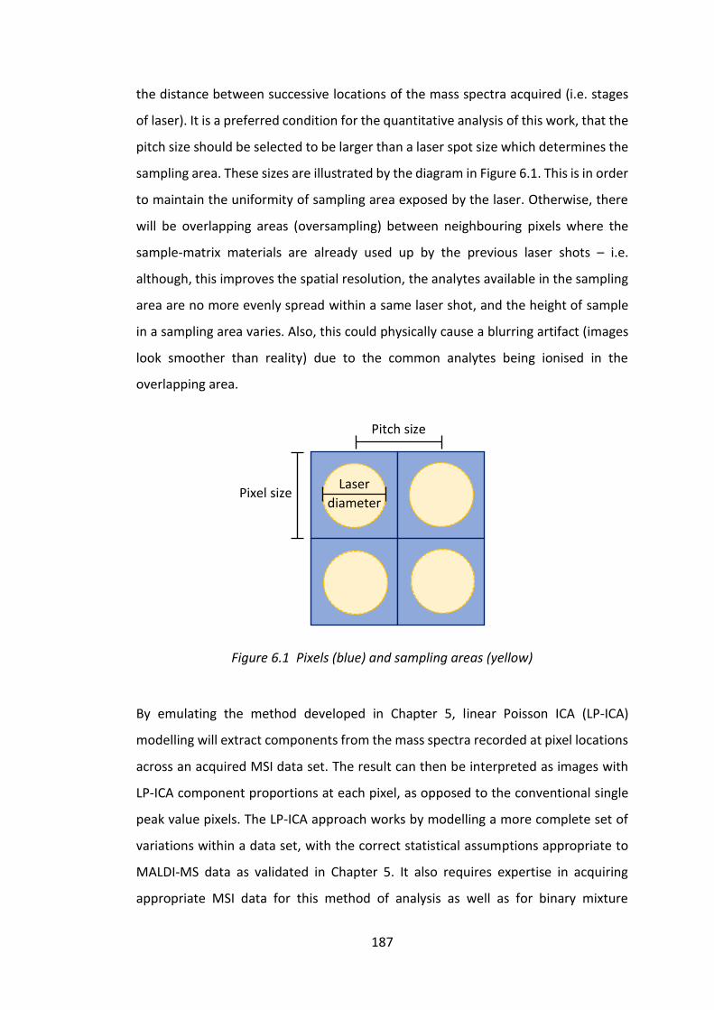
187
the distance between successive locations of the mass spectra acquired (i.e. stages
of laser). It is a preferred condition for the quantitative analysis of this work, that the
pitch size should be selected to be larger than a laser spot size which determines the
sampling area. These sizes are illustrated by the diagram in Figure 6.1. This is in order
to maintain the uniformity of sampling area exposed by the laser. Otherwise, there
will be overlapping areas (oversampling) between neighbouring pixels where the
sample-matrix materials are already used up by the previous laser shots – i.e.
although, this improves the spatial resolution, the analytes available in the sampling
area are no more evenly spread within a same laser shot, and the height of sample
in a sampling area varies. Also, this could physically cause a blurring artifact (images
look smoother than reality) due to the common analytes being ionised in the
overlapping area.
Figure 6.1 Pixels (blue) and sampling areas (yellow)
By emulating the method developed in Chapter 5, linear Poisson ICA (LP-ICA)
modelling will extract components from the mass spectra recorded at pixel locations
across an acquired MSI data set. The result can then be interpreted as images with
LP-ICA component proportions at each pixel, as opposed to the conventional single
peak value pixels. The LP-ICA approach works by modelling a more complete set of
variations within a data set, with the correct statistical assumptions appropriate to
MALDI-MS data as validated in Chapter 5. It also requires expertise in acquiring
appropriate MSI data for this method of analysis as well as for binary mixture
Pitch size
Pixel size Laser
diameter

188
experiments. An example MSI data set selected for this analysis is a rat brain section,
from a rat stroke model, prepared and acquired under the optimised conditions
(Henderson et al., 2018) which had been shown to give a good level of signal-to-noise
in the mass spectra. Images produced using selected single mass peaks should show
clear biological structure within the sample. Such images are used to define an image
quality baseline that the data set could produce. Nonetheless, it is expected that
more useful images would be formed using the LP-ICA method in terms of biological
interpretation due to the added uncertainty information produced by LP-ICA. In this
study, the ratios between those m/z peaks with relatively high intensity and their
carbon-isotope peaks were utilised as a quality control criteria to differentiate
between LP-ICA components that comprise useful signal or simply noise. Where the
accepted range of values (taking into consideration the presence of isobaric species)
for an isotope ratio can be found in the LIPID MAPS database (http://www.
lipidmaps.org/). Other effects including the variation in sodium concentrations
across the imaged brain tissue section were also observed. The proportion of
molecules ionised as a sodium adduct versus those in the protonated ion form were
compared.
At the end of this chapter, the aim is to map the variety of regional tissue types within
a brain section, suggesting a method for building a lipid atlas of the brain. A tissue
type will be defined by a series of mass peaks in a particular relative intensity ratio
that appears in an individual component. They are expected to be distributed across
anatomical regions with relative concentrations having biological meaning. These
depend on the type and proportion of cells that exist in each tissue at specific location
of the brain. The goal is to map all the variations automatically without prior targeting
of identified lipids of interest. Instead, the important lipids can be identified from the
m/z peaks that appear in the ICA components modelled. Recently, lipids in brain
tissues have been actively investigated using MALDI-MS. Given that brain tissues are
rich in lipids that perform various tasks, changes in lipid concentrations are often
hypothesised to indicate changes and even abnormalities in brain functions.
Examples of the earliest work to document the abundance of major lipid species
sorted by lipid head groups are the studies on lipids extracted from within specific

189
tissue types in human brains (O’Brien and Sampson, 1965) and from homogenised
regions of rat brains (Chavko and Nemoto, 1992). So far, Delvolve et al. (2011)
attempted to create complete anatomical segmentation of a rat brain section by
observing the concentrations of multiple lipids individually. A number of previous
papers (e.g. Astigarraga et al., 2008; Murphy et al, 2009; Delvolve et al., 2011;
Mohammadi et al., 2016), have listed the identification of important lipids, especially
of phosphatidylcholines which are the major species to appear in the imaging mass
spectra in this work. Therefore, these can be used as a reference to the data analysed
in this thesis.
In this chapter, the method of analysing the imaging MALDI-MS data is described
along with a critical discussion of the method and how it could possibly be improved.
6.1.2 The Importance of Quantitation and Error Analysis
Scientific quantitation/quantification is the process of determining the value of a
quantity based on experimental measurements or observations, with the ability to
quote an error on that value. Every measured value is just an estimate of the true
value. Without error estimates, the idea of precision or accuracy of the measurement
cannot be discussed meaningfully. Smaller errors on quantitative analysis contribute
to lower uncertainties (determined by standard deviations), and therefore greater
confidence on determination of the quantity of interest. Here, the quantity refers to
‘any quantity’ that possesses a value, not only include those with units of gram,
metre, or number of counts, etc., but also include ratios of quantities which can be
dimensionless. For example, in this work, the ratios of different components across
spatial locations are quantified, referring to the relative concentrations of the
underlying sub-tissues within the MALDI-MS imaging sample. In other words, the
extracted components along with their associated weighting quantities determine
the absolute amount of ion counts recorded as peaks in the mass spectrum at each
pixel. Because the ion counts come from only a fraction of molecules contained
within the sample that were ionised (ideally directly proportional to the amount of
that existing molecules), the quantities associated with the extracted components

190
must be calibrated in order to estimate the absolute concentrations of particular sets
of m/z peaks contained in the underlying sub-tissue types (see the future work
suggested in Section 7.3).
Segmentation (according to known anatomical structures) is only performed as a
general check, in terms of information that is supposed to be extracted as component
images, but is not the main purpose for doing this LP-ICA analysis. A quantitative
check of these measurements can be based on the error on a physical property, e.g.
the ratio of isotope peaks (see Section 6.3.5), where the accepted values are available
to compare with the results from the analysis. Therefore, the expected and the
measured errors on this quantity can be compared to validate the analysis.
6.1.3 LP-ICA vs. Other Approaches
The intention of this work was to develop a valid statistical method appropriate for
the characteristics of MALDI-MS data, to allow the construction of an error model.
The LP-ICA described in Chapter 5 was shown to improve the accuracy (over the
method that uses only single peak ratios) of measuring the proportions of samples in
man-made biological mixtures. In this chapter, the method was then proposed for
use in label-free quantitation of real-world MALDI-MS imaging data, where mass
spectral signals can be extracted as linear components. The measure of quantity
associated with these components can be thought of as the individual contributions
of the underlying samples that build up signals forming the imaging data. Each pixel
is therefore analogous to a simple mixture sample but with more than two
components. LP-ICA provides the spatial distributions of the underlying contributing
sources of component mass spectra. In this work, sub-tissue types within a brain
section were of interest. To emphasise this further, the usefulness of the approach
lies in its potential ability to identify the types of biological tissues (that correspond
to the independent components) that are quantified here, rather than the individual
lipids contained within each sample. Because tissues are complex mixtures and
combinations of biochemicals (such as lipids which are major constituents of brain
tissue), they comprise signatures of biological components or tissue types. The

191
regional structure associated with each component can be extracted, but the LP-
ICA’s value is not limited only to segmentation, but rather to indicating the relative
abundance of each component across the image.
Prior to building a useful algorithm for the analysis of MALDI mass spectrometry data,
appropriate assumptions about the input data should be satisfied in terms of their
physical/statistical properties. The important assumptions, that accord with MALDI-
MS data properties and the intended analysis, include:
1.) The mass spectral signals are in the form of positive counts only,
2.) The signal generation process is linear,
3.) The errors associated with the signal measurements obey Poisson
statistics,
4.) Any underlying components can be comprised of some of the same
molecules – i.e. the mass spectra of the underlying samples must be allowed to have
some signals at the same m/z bins, data correlation is thereby introduced and an
orthogonality assumption is not suitable.
Therefore, the LP-ICA method was designed to ensure that all the requirements listed
here are addressed. Some other approaches to analysis will be critically discussed
with comments in relation to the above assumptions.
There are a large number of existing analysis tools for quantification/classification of
mass spectral data. Most of these methods make use of dimensionality reduction in
a variety of alternative ways. Many of them are quite similar, with common core
principles but are given different names based on variations in the algorithms. These
methods may be divided into the following main categories. Note that depending on
the purpose of analysis (i.e. what is needed to be known from the analysis), an
appropriate method must be carefully selected.
1.) Linear component decomposition approaches, e.g. principal component
analysis (PCA), independent component analysis (ICA), non-negative matrix
factorisation (NNMF), probabilistic latent semantic analysis (pLSA), Linear
Poisson ICA

192
2.) Pattern recognition approaches, e.g. random forests, support vector
machines, k-nearest neighbours, neural-network based methods e.g. t-
distributed stochastic neighbour embedding (t-SNE)
3.) Clustering approaches, e.g. K-means, Fuzzy C-means
4.) Normalisation approaches, e.g. linear regression normalisation via peak ratio
calculation, total ion current normalisation, calibration using isotopically
labelled/internal/external standard (see Section 3.1.2 of Chapter 3), local
regression normalisation (Callister et al., 2006), quantile normalisation
(Callister et al., 2006), regional tissue extinction coefficient normalisation
(Hamm et al., 2012; Taylor et al., 2018)
The theoretical foundations of the methods listed in each category leads to
differences between them in terms of cost function and optimisation steps. These
are selected on the basis of the data characteristics. In mass spectral analysis,
statistical properties of data are often ignored and simplified without being
confirmed, and components and some properties of the data are therefore lost,
compromising appropriate error analysis. Generally speaking, machine learning
approaches do not use proper statistical models, rather they identify separable
features from the data set and perform arrangements that result in classification of
data in most cases. Neural networks are deemed to be the most sophisticated
method amongst the pattern recognition machine learning approaches listed and
discussed previously in Chapter 3, Section 3.2.2 because of the complexity of the
algorithm, involving a large number of connections and the processes of updating
parameters. They can perform classification and regression tasks – e.g. Fonville et al.
(2013) used a neural network-based approach (i.e. t-SNE) to segment anatomical
structures within MS images of biological tissues, or Thomas et al. (2017), used deep
neural networks as a tool for dimensionality reduction prior to performing other
classification techniques to increase their performance.
t-distributed stochastic neighbour embedding (t-SNE) has been used often in MS
image analysis, e.g. Abdelmoula et al. (2018). t-SNE can be applied to a variety of data
types because of its loose constraints on the properties of input data. It was not

193
designed specifically to suit the MALDI-MS data behaviour especially for quantitative
analysis. Its optimising cost function (e.g. the ‘Kullback-Leibler divergence’) is written
in a form similar to a standard likelihood function for assessing probability of the
extent of similarity between neighbouring spectral pixels. The result allows
assessment of the clustering and spread of data on a t-SNE scale and then the full
segmentation or soft class-labelling can be visualised (Fonville et al., 2013). The data
are assumed to have a t-distribution which is very close to a Gaussian distribution.
The analysis often applies to data of small sample size, e.g. reduced-dimensional
data, which makes this a rapid technique.
Neural networks adjust a set of hidden parameters during computation, whilst
learning from known data and can subsequently achieve reasonable classification
results when solving scientific questions with unseen data sets. The problem for this
type of method is that the separable features may not necessarily reveal the
underlying signal generators that give rise to the real variations in the data. These
underlying signal generators are of interest, because they are the biochemical tissue
components. Some form of additional statistical testing is required to guarantee the
suitability of these approaches for quantifying certain tissue/phenotype related
chemicals by MALDI-MS.
Clustering methods are relatively rapid approaches, generally used for identification
of distinct groups of data. In mass spectrometry, Frank et al. (2008) applied clustering
of tandem MS data where they grouped MS/MS spectra in the format of packets of
m/z peaks that occur as a result of redundant identical peptide spectral generation,
to create the representative spectrum, thereby reducing the size of the data set prior
to further analysis. This gave better stability with more complete information for
molecular identification when using an available database.
The K-means method works by associating a data point with the cluster that has the
minimum Euclidean distance between the data point to the centroid of a cluster,
where the centroid (centre of the cluster) is located at the mean of data points that
belong to the cluster. The position of the centroid can be updated iteratively after
adding a point to a cluster. A subsequent design in the clustering method family,
Fuzzy C-means, was adapted such that a data point is not restricted to one class.

194
Instead, it assesses how likely it is that a data point may be belong to different classes.
It uses the concept of Fuzzy logic which was introduced in computer science contexts
for approximating confidence levels – i.e. an alternative definition of uncertainty that
cannot be interpreted using standard statistical probability (Dunn, 1973). Therefore,
this is referred to as “soft K-means” as opposed to the K-means where the data are
hard-labelled into a specific class. Fuzzy C-means was applied to magnetic resonance
imaging data (MRI) where the algorithm was modified such that neighboring voxels
(3-dimensional pixels) take part in the classification of individual voxels (Ahmed et
al., 2002). This produces homogeneous segmentation of brain MRI images since
noise levels were reduced (Chuang et al., 2006). When applied to MS imaging of
myxofibrosarcoma (Jones et al., 2011), the Fuzzy C-means reveals superior
segmentation compared to PCA, non-negative matrix factorisation or pLSA.
Clustering performed well in classification. However, it is not based upon statistically
justifiable modelling assumptions and therefore is not appropriate for regression
purposes. Consequently, it is not useful in obtaining numerical quantitation. Also,
where initial clusters’ centroids are defined at the outset, quite significantly affects
the resulting classification – i.e. results are not unique.
Non-negative matrix factorisation (NNMF) and probabilistic latent semantic analysis
(pLSA) are approaches which are frequently mentioned in the MALDI-MS literature
as data analysis tools. The two algorithms have a very close relationship. In fact,
NNMF is a broader term describing methods of component decomposition with a
non-negative value constraint, and whose result is expressed as a linear matrix
equation via a singular value decomposition-like method. It uses an optimisation
function (i.e. cost function) to find a matrix of linearly separated factors
(components) within the data. The choice of a Poisson or Gaussian assumption can
be selected, depending upon the nature of the data (Brouwer, 2016). Therefore, by
definition, pLSA is a form of NNMF. pLSA was originally designed for text document
classification in linguistics research (Hofmann, 2001). The method was adapted for
use in mass spectrometry data analysis e.g. Hanselmann et al. (2008), and is also used
in commercial software e.g. SCiLS Lab (Bruker). It is not very clear whether there are
good links between text and mass spectral data characteristics.
195
A few options are available in NNMF to address different data types, including pLSA
as discussed, and Poisson matrix factorisation (Canny, 2004; Gopalan et al., 2014)
with similar assumptions, etc. NNMF has shown comparable segmentation results to
ICA in the analysis of a mouse brain MALDI-MS image data set, both perform better
than PCA (Siy et al., 2008). NNMF algorithms are generally unsupervised, however,
are modified in Leuschner et al. (2018) to be used as a supervised tool with a focus
on classification of tumour regions on MALDI-MS image. pLSA is the closest algorithm
to linear Poisson ICA in terms of the assumptions made (see Table 6.1 for analysing
data properties). Hanselmann et al. (2008) has shown use of Expectation
Maximisation (EM) in optimisation of a log-likelihood cost function for the pLSA
algorithm. This was drawn based on Poisson statistics which has be tested
appropriately for simulated data and real-world MALDI-MS imaging data. In addition,
the Akaike information criterion was used to calibrate model selection to determine
the suitable number of components to be extracted. This is equivalent to the plateau
reached in the model selection curved in Figure 6.4 of this chapter using the LP-ICA.
There are many more algorithms built with slight alterations but share core
principles, where the assumptions they make on the data analysed or algorithm
design are slightly different. Some of the variety is listed in Table 6.1 to compare their
main properties which reflect their suitability for use with MALDI-MS data. For
imaging tasks specifically, there is no ground truth to train the algorithm and the
ability to perform unsupervised tasks is therefore beneficial. A quantitative capability
is one of the main issues. Depending upon the objective of the research, a regression
or classification approach may be favoured. Regression approaches are required for
getting quantitative numerical results (specifying how much things vary between
different measurements). Whereas classification approaches aim at grouping the
most similar things together and separate dissimilar things (stating to which group
something belongs).
The concept of orthogonality applies mainly to the linear component decomposition
methods, and also in some other methods which produce equivalent forms of results.
In conventional PCA, the extracted (principal) components must be orthogonal. Note
that PCA is sometimes used to reduce a number of dimensions of data before

196
processing clustering methods. In the case of the prior positive only assumption on
component spectra (counts cannot be negative), having this orthogonality
assumption would mathematically force each and every component to include a
different sets of peaks, and therefore prevent components with any degree of
commonality from being extracted – i.e. orthogonality means the dot products
between components are zero. As discussed before, it is necessary to have non-
orthogonal components which means that the same m/z peaks are allowed to appear
in multiple components. This can then interpret underlying signals in a more
meaningful way. In particular, mass spectra of MALDI-MS imaging data of biological
tissues comprise the spectra of various biomolecular mixtures present in the
different sub-tissue types at each pixel location. Similar sub-tissue types of the same
organ are likely to contain some common biomolecules, but with varied proportions
depending on the functional characteristics of those regions. Conventional ICA and
its relevant methods e.g. LP-ICA satisfies this criterion. Conventional PCA vs. ICA
algorithms were discussed explicitly in Section 3.4.2.
Normalisation approaches are basic techniques of MS data analysis which work by
calculating a fraction (ratio) of the interested quantity against a defined reference
value. They are simple, with no complicated algorithm involved in the calculation.
The cumbersome tasks for normalisation are the additional sample preparation
procedures needed with external standards or the selection of appropriate internal
standards to suit the analysis (see Section 3.1.2). Individual ion peaks associated with
the variation in the sample must be found and validated; therefore, the
segmentation and/or quantitation based on this selection process is subjective. More
sophisticated normalisation methods, including quantile normalisation, central
tendency normalisation, linear regression/local regression normalisation, are
reviewed and evaluated in Callister et al. (2006).
Alternatively, Hamm et al. (2012) and Taylor et al. (2018) introduced region-specific
normalisation approaches using tissue extinction coefficients to scale mass spectra
of tissue regions, between organs and within an organ, respectively. The scaling
factors can be determined by the relative signal intensities between regions of a
specific molecule that was treated as a calibration standard. Note that spatial regions

197
based on the different tissue types have to be defined beforehand. The method
explained in Taylor et al. (2018) employed a clustering approach called ‘graph cut’ for
tissue segmentation. Applying this method can compensate for a problematic
inconsistency of ion signals throughout an MS image due to varied degrees of
suppression occurred at different tissues.
The common limitation for these normalisation approaches is mainly the potential
introduction of bias because the analysis relies only on a few pieces of information
contained in a data set, which are sometimes picked manually based on visualisation.
Nonetheless, a regression analysis can be constructed using these normalisation
approaches, for example, using the conventional peak analysis as demonstrated in
Chapter 5 Section 5.4.1. The analysis is very simple, does not require statistical
assumptions but errors cannot be predicted.
Although, the available approaches discussed above provide satisfactory results in a
number of research studies, they lack a statistical error theory where
predicted/expected errors can be estimated. With these methods (and without
further error modelling), the associated errors can be calculated only if the ground
truth exists for a specific data set. This ideal case is impossible in unseen MALDI-MS
imaging data. It is important in a scientific context to be able to estimate errors in
measurements because the predicted errors (from theory) and the measured errors
(deviation from ground truth) can then be compared and where signals differ, the
significance of that difference can be determined. This can test the whole analysis
methodology – i.e. the analysis is valid if the agreement or relationship between the
experimental error and that predicted by theory is observed, and assumptions used
in the algorithm are valid.
In this work, the component images that show reasonable segmentation according
to the anatomical structure can be seen as an independent check of the validity of
the analysis and are not the primary reason for using LP-ICA. The cost function is
derived from the likelihood (see Equation (3.8) of Section 3.4.5). The components
extracted by LP-ICA are the ratios of ion counts at a number of m/z peaks represented
by probability mass function vectors (of the same size, equal to the number of m/z
peaks contained) for each pixel. Associated quantities for components are indicated

198
per spectrum (at a specific pixel). The algorithm is similar to that of NNMF and pLSA
but is more readily formatted as vectors of mass spectrum instead of the matrix
format. The use of MAX SEP (see Section 3.4.6) is also another novel part of this work
which features maximal separation of components. Error covariances can be
calculated for the extracted components.
The algorithm used will automatically find mass spectral signatures that are common
to different parts of the brain. The model constructed by quantifying contents of
spectra will allow the relative contribution of these signatures (components at each
pixel) to be determined. What will be challenging is to relate each of these
signatures/components to biological features of the tissue shown by the spectral
model in specific ways. It is hypothesised that the components relate to biological
features of the tissue, for example, cell types, white matter, extracellular matrix, etc.
Referring back to Chapter 5 when binary mixtures of complex lipids were used, cow’s
milk would be one signature and goat’s milk would be another signature in the milk
mixture, and also for the brain:liver and the white:grey matter mixtures. Similarly, it
is expected that the nerve cells/sub-tissue features as mentioned before are a
number of signatures found differentiable in the brain MS image which comprise the
underlying tissue phenotypes. Determining the full biological meaning is beyond the
scope of the current work. Note that it is clear from the component images shown
later in Figures 6.5, 6.6, 6.16 and 6.17 that the spatial distribution correlates well with
the tissue anatomy.
The use of an algorithm must suit the purpose of the analysis. In this case, the LP-ICA
was selected to perform an appropriate quantitative analysis of the MALDI-MS image
data set as discussed. Table 6.1 below compares some available approaches for data
analysis that have been used with MALDI-MSI data, with abilities to perform
quantitation and/or segmentation. The lists of analysis properties compared include:
whether the analysis is supervised or unsupervised, performs classification or
regression, what parameter is measured, what typical statistical assumption involved
and error model availability. For decomposition methods, the positive/negative and
orthogonality constraints of the extracted components are also listed. The references
to examples of MS imaging application are also given.

199
Tab
le 6
.1 C
om
par
iso
n o
f ty
pic
al p
rop
erti
es o
f so
me
avai
lab
le a
pp
roac
he
s to
an
alys
e M
S im
agin
g d
ata
incl
ud
ing
the
Lin
ear
Po
isso
n IC
A

200
6.2 Methods
6.2.1 MALDI-MS Imaging Data Format
The original MALDI-MS imaging data are recorded as two separate files of type .imzml
and .ibd, which is a standard format for many MS imaging instrument outputs. These
are readable using commercial software compatible with the instrument used to
acquire data. Other software, for example, Matlab based MSiReader (Robichaud et
al., 2013; Bokhart et al., 2018) can convert between known MS file types. However,
it reads values form the imaging file and writes onto a spreadsheet, taking an
enormously long time and may reach the memory limits of the computer before
finishing. OpenMSI allows images produced at selected m/z peaks to be viewed
instantly on the running webpage, and three m/z peak images can be merged to see
the image structure more clearly in RGB colour scale (https://openmsi.nersc.gov/
openmsi/client/index.html). The original MS file formats can be converted into
H5/HDF5 Hierarchical Data Format (Askenazi et al., 2017) which is a way of
simplifying and retaining information from a multidimensional data set, resulting in
compression of file size by up to a factor of 8.
Given that .ibd file contains mass spectral information at every pixel of an image, and
.imzml file contains header information which directs these mass spectra to specified
pixel locations on the image, the image data were loaded into the in-house (TINA)
software and then saved in .csv format. This way it can be made certain that the data
for this analysis is as “raw” as possible – i.e. extracted as recorded in the original file
and has not been pre-processed in any way, as is often done in most instrumental
software. The data set in this format is easily manageable and small in size.
6.2.2 MALDI-MS Imaging Acquisition of a Rat Brain Tissue
Section
The MALDI-MS image was acquired by Fiona Henderson, PhD as part of her research
on post-ischemic stroke studies of a rat brain model comparing diseased and healthy

201
regions. MALDI-MS was used to image the distribution of lipids whereas PET was
used to image biological damage relevant to the disease three-months after the
stroke (Henderson et al. 2018). Her protocol for sample preparation and MALDI-MS
imaging data acquisition is outlined below, see Henderson et al. (2018) for the full
protocol.
The rat brain specimen with a stroke region was frozen in isopentane, and stored at
-80 °C before sectioning. Thin (12 µm) brain tissue sections were cut parallel to the
coronal axis. The sections were placed onto indium tin oxide (ITO) conductive glass
slides, washed using ammonium acetate solution (150 mM, aqueous). The matrix
solution contained 10 mg/ml DHB in methanol:water (70:30), with added 0.1% TFA.
30 successive layers of matrix solution were sprayed onto the thin brain tissue section
by the SunCollect matrix sprayer at a flow rate of 25 µl per minute, except the first
three layers which built up with lower flow rates in order to minimise the
displacement of lipids on tissues.
The data were acquired using the 7090 MALDI-TOF2-MS (Kratos, Manchester), see
instrument specifications in Section 4.2.2 of Chapter 4. The laser beam was adjusted
to a diameter of 50 µm. The distance between adjacent pixels, which determined
spatial resolution, was 80 µm. At each pixel, 100 laser shots were fired to accumulate
a mass spectrum.
6.2.3 Pre-processing
As a result of the white:grey matter experiment in the previous chapter, the same
mass range of m/z 690-890 was used for the imaging data set where the major
relevant lipid peaks were expected. Also, the narrow range of data was desirable for
computational efficiency during method development. Each mass spectrum has
15,539 original bins in the selected mass range. The size of the image was 219 x 118
pixels, comprising 25,842 mass spectra in the entire data set. The raw imaging mass
spectra underwent the same pre-processing process as previously used in the binary
mixture experiments, with parameters adjusted to suit the data set. Note that the

202
mass spectra of this imaging data set have double the number of original bins to that
of the binary mixture experiments as a consequence of using a different model of
mass spectrometer, but still a Kratos model MALDI-TOF2-MS. Therefore, the mass
spectra acquired should have consistent characteristics to the previous ones.
Initially, mass resolution reduction was performed by merging neighbouring bins of
the original mass spectra by a factor of one-sixth. Then, all mass spectra were allowed
to shift backward and forward by the maximum of 10 bins in order to get a well
aligned mass spectral data set. Next, the background was subtracted on a spectrum-
by-spectrum basis with mutual parameters: lower threshold, upper threshold and
the smoothing parameter, set appropriately according to the protocol for the
baseline correction as stated in Section 3.3.3. Finally, peak detection as described in
Section 3.3.4 was performed, grouping bins that were expected to contain a single
ion m/z peak and integrating them into a single bin, resulting in 67 peaks detected
throughout the selected 200 m/z range. Each of the detected peaks has an associated
m/z value. Descriptions of the pre-processing algorithm can be found in Section 3.3
of Chapter 3.
6.2.4 Image Formation
Conventional Single Ion Image
A conventional single ion image can be displayed as grey levels representing intensity
for each ion m/z in mass spectra, plotted at the corresponding pixel locations. In this
brain image data set, 67 different single peak images can be created. A series of single
ion images formed using the 20 largest peaks were created. These are used to
compare image quality to LP-ICA derived images and also show correspondence
between some tissue segmentations using hand-selected peaks verses the
automated alternatives.

203
LP-ICA Component Image
LP-ICA analysis was performed on the brain MS image data set (25,842 mass spectra)
– i.e. one per pixel location, with each mass spectrum having 67 bins. Models were
built for different numbers of ICA components: 8, 12, 16, 20 and 24. This had been
suggested by the model selection curve, see Figure 6.4, that the model fitting started
to be near optimal when 12 or more components were extracted. The LP-ICA
algorithm was based on an Expectation Maximisation (EM) algorithm with an EM
limit being the parameter to control the limit of optimisation divergent point,
empirically determined for a sufficiently consistent/accurate model fitting with a
reasonable speed, and with the MAX SEP mode applied for a maximal linear
separation of components within a model (detailed explanation of the algorithms can
be found in Sections 3.4.5 and 3.4.6 of Chapter 3). The use of the LP-ICA modelling
method was similar to that used in Chapter 5, which was for the extraction of spectral
components, however, the weighting combination scheme was not applied in this
experiment as the image data contains much more tissue-related underlying
variability. On average, it took 3.5 days to complete 5 attempts to find the best fitted
ICA model with this amount of data.
The extracted components are referred to as probability mass functions, which
describe a set of variations within the MS image data. Each component shows a mass
spectrum of multiple peaks. These peaks must have some degree of correlation in
order to appear in the same component. Therefore, better discriminative
information is expected using these component-specific mass spectra than using just
a single peak. A component image can be formed as a grey level image indicating the
variation in each component quantity at different spatial locations.
6.2.5 Image Normalisation
Normalisation is another key to constructing MS images, as well as the ordinary MS
data in most of the existing analysis routines. It is used to make all the mass spectra
in the whole set of data comparable in terms of the signal intensity scale. MALDI-MS

204
in particular is very sensitive to systematic artifacts produced, for example, by matrix
or contamination enhanced signals (Deininger et al., 2011). With normalisation, such
effects are expected to be evened out. However, MALDI mass spectra have a variety
of underlying complications.
The input data for the analysis needed to be raw (non-normalised) because any
normalisation would lead to the Poisson noise on signals, 𝜎𝑝 being scaled unevenly
across the image, as a result of varied normalisation factors from pixel to pixel – i.e.
because the signal integral would not be the same in every spectrum. Therefore, raw
signal quantities are required in the calculation to correctly optimise the log-
likelihood cost function and covariance (see Chapter 3 for Equations (3.8) and (3.10)).
As a consequence, normalisation can only be used here for the sake of image
presentation – i.e. images can be visually evaluated and compared. For the LP-ICA
component images, the mutual dynamic range was used through all the images
(ranges from 0 - 100%) so that the weighting for each component can be directly
compared with others.
In this chapter, the approaches to normalisation are described below, both for the
LP-ICA component images and the conventional single ion images. Each
normalisation process was performed on a spectrum-by-spectrum (pixel-by-pixel)
basis across the image.
Non-normalisation:
The raw measures of mass spectra in the data set (peak bin intensities as a result of
the peak detection) in every pixel were used for the input of MS image data into the
LP-ICA analysis tool.
Normalisation to the signal integral:
This is basically referred to as normalisation to the total ion count (TIC) in the
literature. The TIC in this case was calculated by integrating across all bins. That is:
205
For the conventional single ion images, the signal intensity of the peak of
interest in each bin was divided by the integral of total signals for that given
pixel.
For the LP-ICA component images, the signal quantity of the component of
interest was divided by the sum over all the component signal quantity in the
given model for that given pixel.
6.2.6 Sodium Gradient Analysis
Sodium is an alkali metal that naturally exists in biological tissues. In this specific brain
sample, the sodium was at a concentration that led the sodiated ion species [M+Na]+
to be majority for all main molecules in the observed lipid range, whilst the
protonated ion [M+H]+ species were the second largest in abundance.
As a first step towards understanding biases in quantitative analysis, the relative
sodium concentration across the imaged sample was measured. This was achieved
through measurement of sodiated-to-protonated ion peak intensity ratio – i.e.
[M+Na]+/ [M+H]+ for 3 major molecules, which are at m/z 756.5, 782.6 and 810.6
versus m/z 734.5, 760.6 and 788.6.
6.2.7 Quality Assessment of the MS Image
This section includes firstly an image segmentation test as an assessment of visual
quality of images, and secondly the noise correlation test as an assessment of
separation between component images. The following processes were repeated for
8-, 12-, 16-, 20- and 24-component models.
Image Segmentation Test
All LP-ICA component images of a model were computed. For every possible
combination of 3 component images, a colour coded image was generated where

206
intensity scale of three distinct colours: red, green and blue was given to each
component image, and then superimposed. This provided an indication of
segmentation quality based upon a subset of three images. Some of the colour coded
images that enhanced the subjective visualisation of tissue segmentation were
noted.
Noise Correlation Test
Some anti-correlation between noises in ICA component images might be evidence
of the need to add two or more components together to explain a single tissue type,
as was found in the analysis of the binary mixtures. In order to test this, first of all,
the noise on each of the component images created was estimated. A noise-free
image of a component was estimated through tangential smoothing, which predicts
each central pixel using its neighbouring pixels (http://www.tina-vision.net/docs/
memos/2016-009.pdf, Thacker et al. (2016)). Therefore, the noise estimate can be
obtained by subtracting the computed noise-free image from the modelled image of
a component.
A correlation plot was then generated for any given pair of the component noise
images, where noise on one image was plotted against the other on a pixel-to-pixel
basis. Noise correlation patterns were observed for every possible pair of the
component images.
6.2.8 Peak Assessment on Individual ICA Component Spectra
LP-ICA models a set of sub-spectra that can be linearly combined with appropriate
weighting factors (quantity associated to each component) to approximate the
original spectra of the data set. The extracted sub-spectra vary depending on the
number of components in a model. Even when the same number of components are
extracted, statistical variation leads to differences in those components each time
they are calculated, as in real-world data there can be multiple solutions (local
optima). The greater the number of components in the model, the more intimately
207
all the variations in the data are fitted. This is not necessarily a good thing, and when
there are too many components, the combination begins to model noise, a situation
known as “overfitting”. The opposite would be “underfitting” when too few
components extracted leads to failure of fitting enough variations. Continuing from
Section 6.2.4, the model selection curve estimated that the appropriate component
number was somewhere between 12 and 24 components – 8 components might still
be sufficient. Each of these was investigated whether it had modelled the level of
variation sufficiently, and that there was no obvious evidence of over- or under-
fitting by looking at the sub-spectra and the corresponding component images. This
was done as a primary quality control test.
For each of the 8-, 12-, 16-, 20- and 24-component models, individual sub-spectra
(component spectra) were examined for the 10 most intense peaks amongst the 67
ion peaks detected. All the m/z values corresponding to these top peaks were
labelled as they can potentially be used for further investigation of a link to biological
cause, e.g. Sections 6.2.10 and 6.2.11.
6.2.9 Isotope Analysis
The ratios between the different natural isotope permutations in molecules are well
known. An isotope peak at one mass unit higher than the monoisotopic peak (all 12C):
[M+1]+ for an organic molecule is due mainly to the presence of a single 13C in that
molecule replacing any one of the (most abundant) 12C atoms. A small contribution
is also due to the existence of 15N. 17O and deuterium can be considered negligible as
traced very small abundance in nature, however, they can be significant in larger
molecules. The larger the molecule, the higher chance finding these rarer isotopes.
The expected isotopic distribution of a molecule, knowing the distribution of the two
most abundance isotopes of each atomic type, should follow the general formula for
binomial expansion (𝑎 + 𝑏)𝑛. When 𝑎 and 𝑏 are the fractional natural abundance of
the two isotopes, and 𝑛 is the number of atoms in the molecule. The molecular
isotopic abundance can be derived by adding up distributions from each atomic

208
component. Similarly, the [M+2]+ isotope species incorporates two 13C atoms or an
18O within a molecule.
The isotope pattern is therefore a property that determines essential characteristics
of mass spectra. This property was used as a basis for assessing mass spectral
components extracted by the LP-ICA model – i.e. whether the isotope peak intensity
ratio at a selected m/z is consistent with the expected value. Then, any uncertainties
observed from the measured values were compared with the theoretical predicted
error, see Section 6.3.5. Isotope ratios were calculated from [M+Na]+ and [M+H]+ ion
forms of 3 molecules that appears major across every component, which are listed
in Table 6.2. Note that regardless of sodium concentration across pixel locations, the
isotope ratio is a conserved physical property. It is calculated from spectral
components which are derived on a per-pixel basis.
Table 6.2 List of m/z peaks used for the isotope analysis
m/z value
Ion form Molecular
type
Expected ratio [M+1+H]+/ [M+H]+ or [M+1+Na]+/ [M+Na]+
[M+2+H]+/ [M+H]+ or [M+2+Na]+/ [M+Na]+
734.5 [M+H]+ PC(16:0/16:0) 0.46 0.12
756.5 [M+Na]+
760.6 [M+H]+ PC(16:0/18:1) 0.49 0.13
782.6 [M+Na]+
788.6 [M+H]+ PC(18:0/18:1) 0.51 0.14
810.6 [M+Na]+ N.B. These expected isotope ratios were obtained via LIPID MAPS database for mass spectrometry
isotopic distribution
6.2.10 Tissue Compositions and Stroke Biomarkers
Component images show different component segments of brain anatomy.
Components that display specific regions or the stroke lesion were particularly of
interest. The component sub-spectra that relate to each of these were recorded.
There must be characteristic chemical (lipid) variations causing differentiation
between components which cause these specific tissues types to be separated.
Important differentiating molecules (determined by the 10 most intense peaks for

209
each component, following Section 6.2.8) were identified based on their m/z values
with reference to previously identification of those molecules in the similar sample
types reported in the literature and also the LIPID MAPS database online resource
(http://www.lipidmaps.org/).
6.2.11 Lipid Mapping on Anatomical Brain Atlas
An anatomical atlas of a brain section may be constructed based on chemical
labelling (of lipids in this case) at different spatial locations. The construction of
colour-coded component images as in Section 6.2.7 shows the segmentation of
different brain regions. Component images represents biochemical distributions
within the tissue. Tissue-specific functionalities depending on the lipid types
observed within the brain regions were explored. These were cross-compared to the
rat brain atlas of approximately the same cut of tissue section as presented in The
Rat Brain in Stereotaxic Coordinates by Paxinos and Watson (1986).
The list of top 10 major peaks in each component as assessed in Section 6.2.8 can be
used at this stage to help identify cell/tissue types according to their biochemical
compositions. Therefore, the underlying biology of the brain section can be
investigated, although a full biological functional analysis is beyond the scope of this
thesis.
6.3 Results and Discussion
6.3.1 Raw vs. Pre-processed Mass Spectra
For the rat stroke brain MS image data set, the mass range of m/z 690-890 was
selected for consistency with the previous white:grey matter binary mixture
experiment. More importantly, the method of preparation and acquisition favoured
phospholipids as the main lipid peaks shown on mass spectra, and they sit mostly
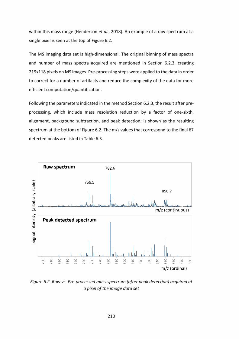
210
within this mass range (Henderson et al., 2018). An example of a raw spectrum at a
single pixel is seen at the top of Figure 6.2.
The MS imaging data set is high-dimensional. The original binning of mass spectra
and number of mass spectra acquired are mentioned in Section 6.2.3, creating
219x118 pixels on MS images. Pre-processing steps were applied to the data in order
to correct for a number of artifacts and reduce the complexity of the data for more
efficient computation/quantification.
Following the parameters indicated in the method Section 6.2.3, the result after pre-
processing, which include mass resolution reduction by a factor of one-sixth,
alignment, background subtraction, and peak detection; is shown as the resulting
spectrum at the bottom of Figure 6.2. The m/z values that correspond to the final 67
detected peaks are listed in Table 6.3.
Figure 6.2 Raw vs. Pre-processed mass spectrum (after peak detection) acquired at
a pixel of the image data set

211
Table 6.3 List of peaks detected with the m/z value and the corresponding binning
index
Index m/z value Index m/z value Index m/z value
0 697.98 23 778.66 46 814.60
1 699.12 24 782.56 47 820.66
2 699.97 25 783.53 48 822.73
3 719.39 26 784.66 49 823.66
4 734.50 27 785.56 50 824.66
5 735.45 28 786.46 51 828.60
6 745.50 29 788.49 52 830.67
7 746.46 30 789.62 53 832.69
8 747.41 31 790.53 54 833.69
9 750.49 32 791.58 55 834.62
10 753.65 33 792.57 56 835.63
11 754.47 34 794.61 57 836.64
12 756.53 35 796.64 58 837.65
13 757.64 36 798.69 59 838.57
14 758.60 37 804.61 60 848.78
15 760.67 38 805.60 61 849.71
16 761.48 39 806.59 62 850.73
17 762.51 40 808.65 63 851.75
18 768.60 41 809.49 64 852.68
19 769.57 42 810.63 65 856.60
20 772.46 43 811.62 66 864.70
21 773.51 44 812.46
22 774.48 45 813.61
Conventional Single Ion Image
Single ion images were formed using the 20 largest peaks from the peak detected
mass spectra. The full set of these single ion images are provided in Appendix B-2
(Figure B.4). The image presented in Figure 6.3 below shows an example of these
images plotted using m/z 782.6 which is the most intense peak of the image data set.
The tissue segmentations derived from these 20 single ion images are highly similar
because many molecules are present in common among different tissue regions. This
limits the ability of single ion images to represent tissue-specific characteristics.

212
Figure 6.3 An example of single ion images plotted using m/z 782.6 – the dynamic
range has been set to maximise the contrast of the image (the darkest pixel has the
highest intensity value)
6.3.2 Model Component Spectra and Images
Primary Model Selection
The primary model selection is assessed using the chi-square per degree of freedom
test, as a measure of how well the model fits to the data. A subset of 400 pre-
processed mass spectra was used to build models here to speed up computation
while preserving the nature of the data set by using mass spectra from 2 rows of
pixels horizontally across the middle of the tissue section, thereby typifying most of
the variations likely to be found in the sample. The number of ICA components
extracted was varied between 2 and 28. The model selection curve in Figure 6.4
demonstrates that the model fitting dramatically improves as component number
increases at a small number of components. This improvement starts to change
gradually until reaches a plateau. At about 12 components, the rate of improvement
of model fitting is considered to be approximately the point where the fitting value
begins to level off. This is taken to mean the model should be built with 12 or more
components. Given that this test only gives a lower limit on component number, this
value and a small set of component numbers beyond this value (12, 16, 20 and 24)
were selected for further examination for the rest of the analysis (a model with
slightly fewer component numbers (8) was also built for a sake of comparison).

213
Figure 6.4 LP-ICA model selection curve for the brain MS image data
Component Spectra
Mass spectral components (sub-spectra) extracted from the 12 and 20 component
ICA models are shown here in Figures 6.5 and 6.6, respectively, as representative
models built in the range of selected component numbers for the illustrative
purposes. Other models’ component sub-spectra are provided in Appendix B-1
(Figure B.1 to B.3). The peak bins were plotted in the index order and were scaled
here according to the m/z values for each component, making them directly
comparable with the format of the original mass spectra. For every spectral
component of both models (sub-spectra in Figures 6.5 and 6.6), the first 10 most
intense m/z peaks were labelled. They were compared against each other. The
unique relative concentrations of the major lipid molecules could be associated to
some sub-type of tissue (anatomical region). Some lipids were only observed in some
of the components and are not present in others. It is therefore of interest to
determine the identity of these lipids and then investigate the biological meaning of
their presence in that tissue. A comprehensive analysis is beyond the scope of this
thesis. For this purpose, individual component images of both models are provided
at the corner of the associated plots of component spectra (sub-spectra) in Figures
6.5 and 6.6. All component images were normalised to the integral intensity at each
pixel location. Areas outside tissue were masked off to improve visualisation. The
grey scale at the bottom of each image represents a relative weighting that each
component has to the total signal quantity as a result of normalisation for visualising
the LP-ICA component images as described in Section 6.2.5.

214
Figure 6.5 12-component sub-spectra with 10 major peaks marked with green arrows (their m/z values are listed in ascending order). The corresponding
component images are shown. (Part 1 of 4)

215
Figure 6.5 12-component sub-spectra with 10 major peaks marked with green
arrows (their m/z values are listed in ascending order). The corresponding
component images are shown. (Part 2 of 4)

216
Figure 6.5 12-component sub-spectra with 10 major peaks marked with green
arrows (their m/z values are listed in ascending order). The corresponding
component images are shown. (Part 3 of 4)
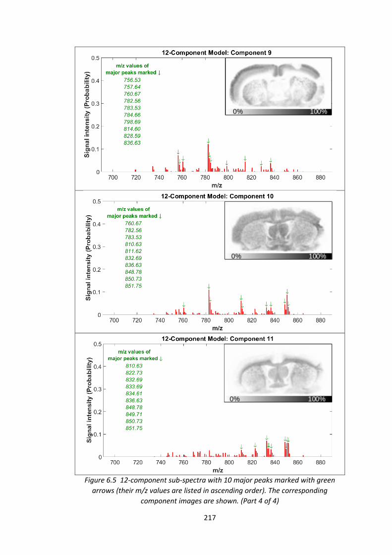
217
Figure 6.5 12-component sub-spectra with 10 major peaks marked with green
arrows (their m/z values are listed in ascending order). The corresponding
component images are shown. (Part 4 of 4)

218
LP-ICA component spectra estimated by the model can be used to generate a number
of 2-dimensional grey level plots for each of the extracted components. In a
component image, the grey level value at every pixel was determined by the
associated quantity of that component spectrum in the pixel which can potentially
be interpreted in terms of the common underlying biological variations distributed
across the image. The spectra varied slightly when the number of components was
altered. These component images show much clearer tissue-specific segmentations
compared to single ion images, which can benefit the determination of tissue
phenotypes and biomarkers (This will be discussed later in Sections 6.3.9 and 6.3.10).
The 20-component model showed better segmentation of brain tissue, compared to
the 12-component model. For example, the stroke region stands out individually in
the image corresponding to component number 8 of the 20-component model (see
the component image in Figure 6.6). This was not the case for the 12-component
model, where the stroke region was not discriminated from the ventricles (see the
image corresponding to component 6 in Figure 6.5).

219
Figure 6.6 20-component sub-spectra with 10 major peaks marked with green arrows (their m/z values are listed in ascending order). The corresponding
component images are shown. (Part 1 of 7)

220
Figure 6.6 20-component sub-spectra with 10 major peaks marked with green
arrows (their m/z values are listed in ascending order). The corresponding
component images are shown. (Part 2 of 7)

221
Figure 6.6 20-component sub-spectra with 10 major peaks marked with green
arrows (their m/z values are listed in ascending order). The corresponding
component images are shown. (Part 3 of 7)
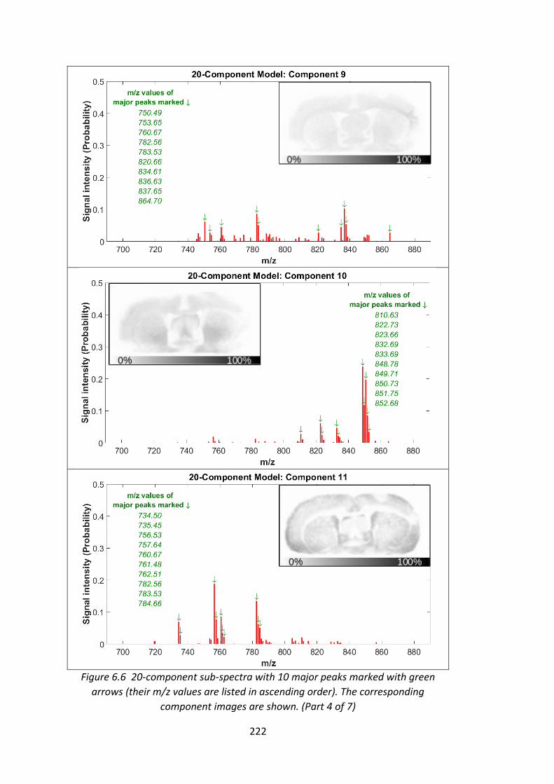
222
Figure 6.6 20-component sub-spectra with 10 major peaks marked with green
arrows (their m/z values are listed in ascending order). The corresponding
component images are shown. (Part 4 of 7)

223
Figure 6.6 20-component sub-spectra with 10 major peaks marked with green
arrows (their m/z values are listed in ascending order). The corresponding
component images are shown. (Part 5 of 7)

224
Figure 6.6 20-component sub-spectra with 10 major peaks marked with green
arrows (their m/z values are listed in ascending order). The corresponding
component images are shown. (Part 6 of 7)

225
Figure 6.6 20-component sub-spectra with 10 major peaks marked with green
arrows (their m/z values are listed in ascending order). The corresponding
component images are shown. (Part 7 of 7)

226
Major Peaks Listed by Component
The 10 most intense peaks observed in each component for the 12- and 20-
component models are listed in Tables 6.4 and 6.5, respectively, with bin indices and
the corresponding m/z values. A tick indicates the components for which each of
these peaks is detected. This information was used to guide identification of lipids of
interest. Note that the mass window selected for this analysis was in the
phospholipids range. There will very likely be important discriminating lipids outside
this range, such as sphingomyelin, cholesterol, etc. These should be included in
further work, but would have significantly slowed algorithm development in the
current project. Most cell membrane lipids are likely to remain in place when in
contact with solutions, whereas lipids of other class may be displaced on the
sectioned slice. Additionally, intact phospholipids have a phosphate group which
easily binds with a positive adduct, e.g. hydrogen or sodium ions. However, the mass
range chosen for this study clearly had sufficient peaks to test the analysis method
(as the analysis required a very long computational period: a few days per 5 attempts
of building models). When the method is validated, it can be extended to include
wider mass ranges – see the discussion on how the computational efficiency can be
improved in Section 7.3.

227
Table 6.4 10 major peaks presented in each sub-spectral component of the 12-
component model
Bin index m/z value Component index
0 1 2 3 4 5 6 7 8 9 10 11
0 697.98
1 699.12
2 699.97
3 719.39
4 734.50
10 753.65
12 756.53
13 757.64
14 758.60
15 760.67
17 762.51
24 782.56
25 783.53
26 784.66
29 788.49
31 790.53
36 798.69
37 804.61
38 805.60
42 810.63
43 811.62
44 812.46
45 813.61
46 814.60
48 822.73
49 823.66
51 828.60
53 832.69
54 833.69
55 834.62
57 836.64
58 837.65
60 848.78
61 849.71
62 850.73
63 851.75
64 852.68

228
Tab
le 6
.5 1
0 m
ajo
r p
eaks
pre
sen
ted
in e
ach
su
b-s
pec
tral
co
mp
on
ent
of
the
20-c
om
po
nen
t m
od
el (
Par
t 1
of
2)

229
Tab
le 6
.5 1
0 m
ajo
r p
eaks
pre
sen
ted
in e
ach
su
b-s
pec
tral
co
mp
on
ent
of
the
20-c
om
po
nen
t m
od
el (
Par
t 2
of
2)

230
61 bins have been identified as the major peaks in different components for the 20-
component model (Table 6.5) while only 37 bins were observed for the 12-
component model (Table 6.4) using the same criteria. This shows that the model
managed to extract more variations between components when more components
were allowed. For example, when there are fewer components than the underlying
variations within a data set, the peak bins that describe minor variations could be
hidden by other variations, resulting in peaks not being selected as major
contributors to the corresponding spectra. The component images acquired this way
would then be ambiguous. In other words, when the number of components is too
few, some spectral variations can be merged into a single component instead of
being appropriately separated. The peaks that appeared in the main peak list for the
20-component model but not the 12-component model are marked in blue in Table
6.5.
Therefore, the 20-component model was considered a reasonable model to
represent the data, providing sufficient unique components to be interpreted as
tissue-specific phenotypes. Table 6.7 lists the identified phosphatidylcholines (see
later in Section 6.3.6), at each m/z value based on previously reported literature for
brain tissues, using MS/MS analysis. These data can be used to determine which
molecules are associated with each LP-ICA component and their associated
anatomical features.
Overlaid Colour Coded Images
The image segmentation test described in Section 6.2.7 aimed to assess the overall
segmentation quality of the component images generated. Even though, some
distinguishable structures can be picked out from the grey scale component images
(see the images in Figure 6.6), the image constructed using an RGB (red-green-blue)
colour scheme to combine any 3 component images, provides visually clearer
segmentation and better contrast.
The overlaid colour coded images obtained from various groups of components are
presented in Figure 6.7 allowing enhanced visualisation of tissue segmentation. In

231
other words, this is a clear way of presenting the information seen in the image
results analysed using the LP-ICA method. These colour combination images
demonstrate how well the components anatomically segment the image into
relevant regions, which could support determination of the biological functions each
lipid plays.
Component 0 vs. 3 vs. 12 Component 4 vs. 5 vs. 17 Component 4 vs. 10 vs. 12
Figure 6.7 Overlaid colour coded images constructed by merging three ICA
component images of the 20-component model
Noise Correlation Plots
The technique of using linear combinations of components to describe an underlying
variation was previously suggested for binary mixture experiments. However, the
previous data sets were restricted to two underlying sample classes per mixture
whereas this parameter is completely unknown for the imaging data set. The noise
correlation test described in Section 6.2.7 was therefore established to look for pixel-
to-pixel cross-correlation of noise in all possible pairs of components. The reason for
doing this was to seek components whose noise value could have been counter-
correlated with one another – i.e. noise on a pair of components with different signs
of residuals shown on a correlation plot as negatively skew data points on the axes.
If that was the case, the chance would be these images have to be added together in
order to denoise; as evidence for the above component combination suggestion.
Unfortunately, no obvious anti-correlation was observed in any of the plots. An
example correlation plot of noise in image pair seen in Figure 6.8 was generated from
the 24-component model. They are instead considered (slightly) positively correlated
(i.e. when data are positively skew on the axes, resulted from same sign noise on a

232
pair of components) which means adding the two components together would cause
an overall increase in noise, as opposed to the anti-correlation. All other pairs of
component in every model built were tested in the same way. They showed more or
less similar characteristics. On this basis, it was concluded that components extracted
already represent independent variations; there was therefore no need to add
multiple components together to correct for evaluation and enhance the contents in
MALDI LP-ICA images (for modelling up to 24 components).
Note that tangential smoothing was available to compute an expected noise-free
image that could possibly give the closest approximation to this image type where
there are full of structural contents, e.g. the brain MS images (Thacker et al., 2016).
However, it is not an absolute ground truth and therefore leads to additional random
errors during the noise estimation.
Figure 6.8 Correlation plots of noise on a selected pair of component images
(component 7 vs. 12) of the 24-component LP-ICA model – estimated noise on one
image was plotted against the other on a pixel-to-pixel basis
6.3.3 Sodium Gradient Analysis
Na+ and K+ are common alkali metal ion adducts observed in the brain tissue spectra.
Therefore, a single lipid molecule may give rise to multiple peaks separated by known
mass differences – e.g. sodiated and potassiated ions, respectively, are placed 22 and
38 m/z units higher than the corresponding protonated ions. With this specific brain

233
tissue sample used, the Na+ adduct ion appears to be dominant over the protonated
or potassiated forms of same molecule. The distribution of sodiated ions across the
sample was therefore assessed.
This section examines whether there is any drift in sodium concentration across the
tissue sample. This might arise from the step of washing salts from the tissue section
during sample preparation. If so, it can cause problems regarding variations in the
model built e.g. an extra component related to sodiated ions may be needed to
describe a tissue type. On the other hand, if the sodium variation is only observed
from tissue to tissue but is uniform within a same tissue type, there should be no
gross change on the number of components due to sodiated ions. The ratio of
sodiated to protonated peaks, to be called ‘sodium gradient’, was calculated
throughout the image to look for this as a qualitative check for later model building.
In order to look for a sodium gradient in the brain tissue section, the pre-processed
spectra with 67 detected peaks were recorded at all the spatial locations. This rat
brain sample contained high levels of sodiated phospholipids in the mass range m/z
690-890. Sodium gradient analysis was performed on the three molecules that
appeared to produce major sodiated phosphatidylcholines (PC) in this range. This
follows an earlier study of complex lipids in rat brain myelin using liquid secondary
ion mass spectrometry (Fenselau et al., 1989). The findings also accorded with the
rat stroke model MSI data set that the signal strength of sodiated PCs were superior
to protonated PCs of the same molecular types. The identification of the pronated
form of these molecules is presented below. They were used here as a normalising
peak for their corresponding sodiated forms (given that these are the top 3 most
common molecular species across the mass spectra of this data set, also with
strongest signal intensities).
- m/z 734.5 was identified as [PC(16:0/16:0)+H]+ (Henderson et al., 2018;
Jackson et al., 2005)
- m/z 760.6 was identified as [PC(16:0/18:1) +H]+ (Henderson et al., 2018; Ma
and Kim, 1995)
- m/z 788.6 was identified as [PC(18:0/18:1) +H]+ (Sugiura and Setou, 2009)

234
Three images of the sodium gradient were created by computing the ratio of [M+Na]+
/ [M+H]+. Where [M+H]+ peaks were observed at m/z 734.5, 760.6 and 788.6, and
the [M+Na]+ peaks were 22 mass units higher, at: 756.6, 782.5, and 810.6,
respectively. The images were smoothed by applying a median filter once (to stabilise
the image with high fluctuation on local pixels, in this case, due to small intensity
values), followed by tangential smoothing (Thacker et al., 2016) twice. The images
for the sodium gradient calculated from each representative molecule are illustrated
in the left of Figure 6.9 (a), (b) and (c). Where the scan lines across the tissue area in
the images indicate selected pixels (arranged from left to right) that formed the
corresponding intensity ratio plots on the right of Figure 6.9 (a), (b) and (c) – N.B. the
same set of pixel locations was selected for all peak ratios.
Table 6.6 below shows the ion types for various PCs in brain tissues (from Sugiura
and Setou (2009)). It shows some common masses for different molecular species,
observed when cationisation changes. The m/z values highlighted with the same
colour are different ion forms that happened to have the same m/z. These indicate
that the sodiated and protonated peaks selected do not represent a single lipid
species. However, the selected peaks are of the dominant species. Therefore, the
characteristics for sodium gradient calculated from them should still be preserved.
Table 6.6 Comparison table for different ion forms of given molecular species of
phosphatidylcholine in brain tissues (Reproduced from: Sugiura and Setou (2009))

235
(a) m/z 756.5 vs. 734.5
(b) m/z 782.6 vs. 760.6
(c) m/z 810.6 vs. 788.6
Figure 6.9 Sodium gradient images and the corresponding plots showing the signal
intensity ratio of [M+Na]+ vs. [M+H]+ m/z peaks: (a) m/z 756.5 vs. 734.5, (b) m/z
782.6 vs. 760.6 and (c) m/z 810.6 vs. 788.6 at varied pixel positions – the position of
the line scan is shown on each image in red
The sodium concentration is region-specific as clearly observed by the three different
molecules. Higher sodium concentration regions include the CSF and the stroke scar.
The corpus callosum has also moderately high concentration relative to other
regions. These probably associate with parts of the brain that have high fluid content,
where sodium is more soluble. Conditions such as edema might occur post-stroke
where the tissue was damaged, leading to an excess of liquid in the affected site.
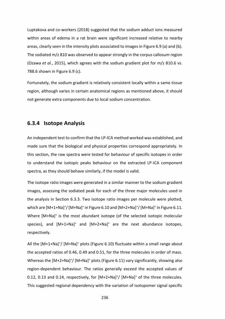
236
Luptakova and co-workers (2018) suggested that the sodium adduct ions measured
within areas of edema in a rat brain were significant increased relative to nearby
areas, clearly seen in the intensity plots associated to images in Figure 6.9 (a) and (b).
The sodiated m/z 810 was observed to appear strongly in the corpus callosum region
(Ozawa et al., 2015), which agrees with the sodium gradient plot for m/z 810.6 vs.
788.6 shown in Figure 6.9 (c).
Fortunately, the sodium gradient is relatively consistent locally within a same tissue
region, although varies in certain anatomical regions as mentioned above, it should
not generate extra components due to local sodium concentration.
6.3.4 Isotope Analysis
An independent test to confirm that the LP-ICA method worked was established, and
made sure that the biological and physical properties correspond appropriately. In
this section, the raw spectra were tested for behaviour of specific isotopes in order
to understand the isotopic peaks behaviour on the extracted LP-ICA component
spectra, as they should behave similarly, if the model is valid.
The isotope ratio images were generated in a similar manner to the sodium gradient
images, assessing the sodiated peak for each of the three major molecules used in
the analysis in Section 6.3.3. Two isotope ratio images per molecule were plotted,
which are [M+1+Na]+/ [M+Na]+ in Figure 6.10 and [M+2+Na]+/ [M+Na]+ in Figure 6.11.
Where [M+Na]+ is the most abundant isotope (of the selected isotopic molecular
species), and [M+1+Na]+ and [M+2+Na]+ are the next abundance isotopes,
respectively.
All the [M+1+Na]+/ [M+Na]+ plots (Figure 6.10) fluctuate within a small range about
the accepted ratios of 0.46, 0.49 and 0.51, for the three molecules in order of mass.
Whereas the [M+2+Na]+/ [M+Na]+ plots (Figure 6.11) vary significantly, showing also
region-dependent behaviour. The ratios generally exceed the accepted values of
0.12, 0.13 and 0.14, respectively, for [M+2+Na]+/ [M+Na]+ of the three molecules.
This suggested regional dependency with the variation of isotopomer signal specific

237
to location. Theoretically, there should be no variation at all. Although for low ion
counts, there might be larger influence by multiple variations, any significant spikes
that deviate from the expected ratios seen in the plots in Figures 6.10 and 6.11 are
likely due to isobaric interference in those regions which will be discussed later in
Section 6.3.5. Note that the reference values to the accepted isotope ratios were
obtained through http://www.lipidmaps.org/.
(a) m/z 757.5 vs. 756.5
(b) m/z 783.6 vs. 782.6
(c) m/z 811.6 vs. 810.6
Figure 6.10 Isotope ratio images of [M+1+Na]+ vs. [M+Na]+ m/z peaks:
(a) m/z 757.5 vs. 756.5, (b) m/z 783.6 vs. 782.6 and (c) m/z 811.6 vs. 810.6,
and the corresponding plots showing their signal intensity ratio at varied pixel
positions – the position of the line scan is shown on each image in red

238
(a) m/z 758.5 vs. 756.5
(b) m/z 784.6 vs. 782.6
(c) m/z 812.6 vs. 810.6
Figure 6.11 Isotope ratio images of [M+2+Na]+ vs. [M+Na]+ m/z peaks:
(a) m/z 758.5 vs. 756.5, (b) m/z 784.6 vs. 782.6 and (c) m/z 812.6 vs. 810.6,
and the corresponding plots showing their signal intensity ratio at varied pixel
positions – the position of the line scan is shown on each image in red
6.3.5 Criteria for Differentiating Signal and Noise
Components using Error Distribution on Isotope Peak
Measurements
Isobars are different molecules that have the same nominal molecular mass. In a
MALDI mass spectrum, peaks with a small mass difference might be seen as a single
peak given the limit of mass resolution – i.e. this could be distinguished only if MS/MS

239
was performed. If the most abundant isotope peaks of the isobaric molecules
coincide, then the other isotope peaks should still lie at the same mass positions with
more or less the same intensity ratios within errors. As shown in the previous section,
the [M+2+Na]+ isotope peaks, however, appear to be contaminated by some other
main isotope molecules, for example, at m/z 784.6 and 812.6, as their ratio to the
main isotope peaks deviated from the expected values stated in Table 6.2. Their
intensity ratios are much greater than their expected abundances and cannot be
used directly in the following analysis. Hence, only the ratio between the two most
abundant isotope peaks was of interest in this analysis. Furthermore, the three
different ion forms (sodiated > protonated > potassiated) also cause complicated
overlapping between peaks of different molecules, which affect values of isotope
ratios at the measuring m/z.
The following criteria were devised for differentiating between ICA components of
signal and noise based on the error pattern on the isotope ratio from 6 pairs of mass
peaks defined by [M+1+Na]+ / [M+Na]+ and [M+1+H]+ / [M+H]+ of 3 different
molecules quoted above. The simplest way for two molecules to have overlap can be
modelled as follows.
There are three common cases that might cause the measured value to be different
from the expected value of isotope ratio, see diagrams expressed in Figure 6.12.
Possible patterns of isobaric interference that give rise to measuring M1+1 / M1 ratio
are described in the list below.
1.) Upper diagram: M1 and M2 are isobars and the abundance of their isotopes
should be very close to identical, providing they are PC of similar molecular
masses. The ratio of M1+1 to M1 is conserved at the expected proportion.
2.) Middle diagram: M2 appears at the M1+1 position. Only M1+1 gets increased
in intensity. Therefore, the ratio of M1+1 to M1 is above the expected
proportion.
3.) Lower diagram: M2 appears at one mass unit below the M1+1 position,
adding a small fraction to both M1 and M1+1. The ratio of M1+1 to M1 is
slightly reduced but this should generally be insignificant, given the
measurement precision.

240
Therefore, in the majority of cases the isotope ratio between a large peak and its
neighbour should be preserved. When it does differ it can only be larger than
expected. This can be used as the basis for a test of ICA components. Such a test also
requires an understanding of measurement error.
Figure 6.12 Possible arrangements of isotope pattern of molecules that coincide at
the same m/z values

241
The Error Estimates on Peak Ratios of ICA Components
The errors on peak bins’ intensity of the ICA components were estimated by
computing error covariances through each pair of the probability mass functions
(PMF) that describe the component sub-spectra. The method is described in Tar and
Thacker (2018), where they corroborated the theory with simulated data
(http://www.tina-vision.net/docs/memos/2018-006.pdf). Then, the errors in isotope
ratios were calculated on this basis using error propagation.
The stability of each PMF bin, 𝑃(𝑚|𝑘), can be estimated using the minimum variance
bound applied to the LP-ICA Likelihood function (propagated to give the error
estimates on peak ratios). This gives an inverse co-variance between bin order 𝑚 in
component 𝑘 = 𝑘𝐴 and 𝑘 = 𝑘𝐵 as:
𝐶𝑃(𝑚|𝑘𝐴),𝑃(𝑚|𝑘𝐵)−1 ≈ ∑
𝑄𝑘𝐴𝑖𝑄𝑘𝐵𝑖
𝐻𝑚𝑖 (6.1)
𝑖
Where 𝑄 is the quantity of the corresponding component contained in spectrum 𝑖 at
a specific pixel, and 𝐻 is a histogram bin value (equivalent to the ion counts).
The Plots of Predicted vs. Measured Error Distribution of Isotope Ratios
The plots of predicted against measured error distribution of isotope ratios are
provided in Figure 6.13 (left). The x-axis in the plot is the measured error (difference
between the isotope ratio computed from the probabilistic model component and
the expected value as defined in the LIPID MAPS database). The y-axis is the error
estimate, defined by the model error covariance calculation, of the corresponding
isotope ratio. Adjusted ratio plots (Figure 6.13 (right)) are generated where a fraction
equal to some percentage of the main peaks M in an isotope pattern were added to
M and M+1 peaks to calculate the new isotope ratio, may compensate for a missing
fraction either from instrumentation off-set or from the background subtraction
failure, which was found to correct for some negative skew observed in the original
ratio plots. A small contribution may also occur when a peak (probably different
molecules with different adduct species) is found at a unit mass below the dominant

242
isotope peak, and hence fractions contribute for M and M+1 are different. In order
to define a suitable value of the fraction to be added back into peaks, the mean of
measured deviations from the expected ratios (the x-axis of the plot) should be
brought closer to zero, hence, the suitable correction – the percentage for these
correcting fractions is indicated in each plot (Figure 6.13 (right)).
A line can be drawn to separate noise and signal. For proportional errors, confidence
limit takes the form of V-shaped symmetrical lines around zero, where data points
that sit within the two lines are consistent with signal, and statistical significance can
then be quoted in terms of the p-value. However, a general conclusions can be drawn
for this type of plot by looking at the common cases of overlapping peaks illustrated
earlier in the diagrams in Figure 6.12. It is possible for a data point to be on the
positive side of the x-axis of plots in Figure 6.13. Data points that are too far away
from the x-axis in the negative direction should be suspected as modelling errors.
Therefore, this method can suggest the suitable number of components to build a
model, figure out contamination (background/noise) components, and/or
inappropriate parameter estimation (fit failure). Where the plot shows the expected
trend, it proved that the LP-ICA model built, according to the procedure and
parameters described in Section 6.2.4 e.g. EM, were adequate.
For the plots in Figure 6.13, a value on the vertical axis is proportional to the
minimum variance bound estimate of peak ratio error propagated from Equation
(6.1). The diagonal dotted lines (on all plots on the left of Figure 6.13, the original
ratio) have common slope as a visual aid to highlight the changes in the negative
skew of the distributions; these do not constitute error bounds or confidence
intervals and are for illustration only.

243
Fig
ure
6.1
3 P
red
icte
d v
s. m
easu
red
dev
iati
on
s fr
om
exp
ecte
d r
ati
o f
or
sele
cted
iso
top
ic p
eaks
at
dif
fere
nt
mo
del
ord
ers,
plo
tted
usi
ng
ori
gin
al
rati
o (
left
) a
nd
ad
just
ed r
ati
o w
ith
ad
ded
fra
ctio
n (
rig
ht)
. Dif
fere
nt
sym
bo
ls in
dic
ate
th
e LP
-IC
A c
om
po
nen
ts f
rom
wh
ich
pea
ks w
ere
take
n.
(Pa
rt 1
of
5)
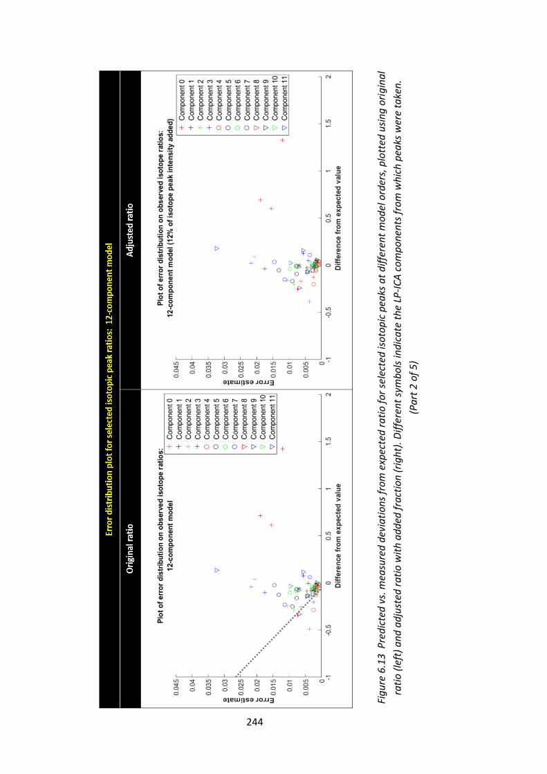
244
Fig
ure
6.1
3 P
red
icte
d v
s. m
easu
red
dev
iati
on
s fr
om
exp
ecte
d r
ati
o f
or
sele
cted
iso
top
ic p
eaks
at
dif
fere
nt
mo
del
ord
ers,
plo
tted
usi
ng
ori
gin
al
rati
o (
left
) a
nd
ad
just
ed r
ati
o w
ith
ad
ded
fra
ctio
n (
rig
ht)
. Dif
fere
nt
sym
bo
ls in
dic
ate
th
e LP
-IC
A c
om
po
nen
ts f
rom
wh
ich
pea
ks w
ere
take
n.
(Pa
rt 2
of
5)
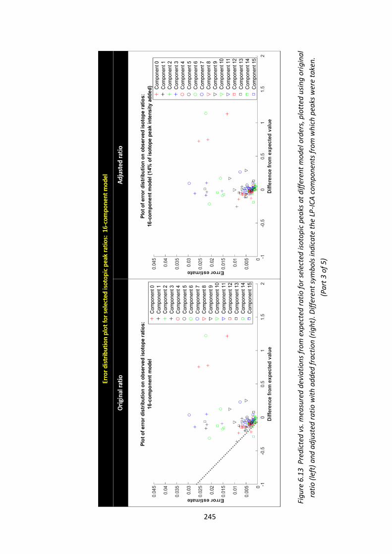
245
Fig
ure
6.1
3 P
red
icte
d v
s. m
easu
red
dev
iati
on
s fr
om
exp
ecte
d r
ati
o f
or
sele
cted
iso
top
ic p
eaks
at
dif
fere
nt
mo
del
ord
ers,
plo
tted
usi
ng
ori
gin
al
rati
o (
left
) a
nd
ad
just
ed r
ati
o w
ith
ad
ded
fra
ctio
n (
rig
ht)
. Dif
fere
nt
sym
bo
ls in
dic
ate
th
e LP
-IC
A c
om
po
nen
ts f
rom
wh
ich
pea
ks w
ere
take
n.
(Pa
rt 3
of
5)

246
Fig
ure
6.1
3 P
red
icte
d v
s. m
easu
red
dev
iati
on
s fr
om
exp
ecte
d r
ati
o f
or
sele
cted
iso
top
ic p
eaks
at
dif
fere
nt
mo
del
ord
ers,
plo
tted
usi
ng
ori
gin
al
rati
o (
left
) a
nd
ad
just
ed r
ati
o w
ith
ad
ded
fra
ctio
n (
rig
ht)
. Dif
fere
nt
sym
bo
ls in
dic
ate
th
e LP
-IC
A c
om
po
nen
ts f
rom
wh
ich
pea
ks w
ere
take
n.
(Pa
rt 4
of
5)
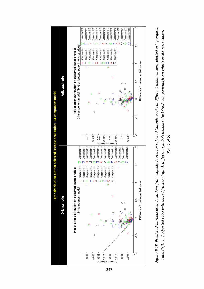
247
Fig
ure
6.1
3 P
red
icte
d v
s. m
easu
red
dev
iati
on
s fr
om
exp
ecte
d r
ati
o f
or
sele
cted
iso
top
ic p
eaks
at
dif
fere
nt
mo
del
ord
ers,
plo
tted
usi
ng
ori
gin
al
rati
o (
left
) a
nd
ad
just
ed r
ati
o w
ith
ad
ded
fra
ctio
n (
rig
ht)
. Dif
fere
nt
sym
bo
ls in
dic
ate
th
e LP
-IC
A c
om
po
nen
ts f
rom
wh
ich
pea
ks w
ere
take
n.
(Pa
rt 5
of
5)

248
Note that the percentage shown in each adjusted plot above came from the
optimally minimised accumulative distance of the x-axis values away from zero for
all data points in a reasonable signal range. These error plots could have been
improved by appointing appropriate weighting according to the estimated errors on
data points to determine the fraction added to peaks more precisely. – i.e. Currently
all points are equally weighted to get the optimal correction of peak intensity but
more accurate (smaller error) data points could be more strongly weighted in this
calculation.
6.3.6 Lipid Identification in Brain Tissue
Rat brains are often used in clinical research as models of pathology and treatment
procedures in mammalian brains. Therefore, there are number of available resources
for lipid identification from previous MALDI MS/MS studies. The following Table 6.7
gives a list of major lipid peaks found in the rat brain imaging data set that have
previously been identified in rat brain tissue, so that important differentiating
molecules e.g. the 10 most intense peaks for each component based on the 20-
component model (see Table 6.5), can be observed. The m/z values of the analysed
data were confirmed to match with the identified lipids within the mass tolerance of
± 0.3 Da based on the LIPID MAPS database (http://www.lipidmaps.org/).
As expected from the results of the ICA models, some of the peaks comprise multiple
molecular types. Without access to higher mass resolution, the only way to tell apart
those molecular species is to perform MS/MS and identify species based on their
fragmentation patterns. The proportion of each species can also be accessed if the
fragmentation pattern is known. However, the isotope ratios observed in ICA
component spectra can also be used to show the presence of unresolved isobars as
discussed in Sections 6.3.4 and 6.3.5.

249
Table 6.7 List of previously identified phosphatidylcholine species from literature
survey (Part 1 of 2)
m/z value Lipid identification Reference
697.98
699.12
699.97
719.39
734.50 [PC(16:0/16:0)+H]+ 1,2,5,9
735.45
745.50
746.46
[PC(15:0a/18:1)+H]+ [PC(16:0a/17:1)+H]+ [PC(18:1e/16:0)+H]+ [PC(16:0e/18:1)+H]+
5 5 5 5
747.41
750.49
753.65
754.47 [PC(14:0/18:1)+Na]+ 9
756.53 [PC(16:0/16:0)+Na]+ [PC(16:1a/18:2)+H]+ [PC(16:0a/18:3)+H]+
1,2,9 5 5
757.64
758.60 [PC(16:0a/18:2)+H]+ 5
760.67 [PC(16:0/18:1)+H]+ 1,3,5,9
761.48
762.51 [PC(16:0a/18:0)+H]+ 5,9
768.60
769.57
772.46 [PC(16:0/16:0)+K]+ *
773.51
774.48
778.66
782.56 [PC(16:0/18:1)+Na]+ [PC(16:0a/20:4)+H]+
1,3,9 5,9
783.53
784.66 [PC(18:1a/18:2)+H]+ [PC(16:0a/20:3)+H]+ [PC(16:0/18:0)+Na]+
5 5 9
785.56
786.46 [PC(18:1a/18:1)+H]+ 5
788.49 [PC(18:0/18:1)+H]+ 4,5,9
789.62
790.53 [PC(18:0p/18:0)+H]+ [PC(20:0a/16:0)+H]+ [PC(14:0a/22:0)+H]+
5 5 5
791.58
792.57
794.61
796.64
798.69 [PC(16:0/18:1)+K]+ 6
804.61 [PC(16:1a/22:6)+H]+
[PC(16:0a/20:4)+Na]+ 5 9
805.60

250
Table 6.7 List of previously identified phosphatidylcholine species from literature
survey (Part 2 of 2)
m/z value Lipid identification Reference
806.59 [PC(16:0a/22:6)+H]+
[PC(16:0a/20:3)+Na]+ [PC(18:1a/18:2)+Na]+
5,9 7,* *
808.65 [PC(16:0/22:5)+H]+ 9
809.49
810.63 [PC(18:0/18:1)+Na]+ [PC(18:0a/20:4)+H]+ [PC(16:0a/22:4)+H]+
4,9 5,9 5
811.62
812.46 [PC(C18:1/C20:2)+H] + [PC(C18:2/C20:1)+H] +
* *
813.61
814.60 [PC(18:0a/20:2)+H]+ 5
820.66
822.73
823.66
824.66
828.60 [PC(16:0/22:6)+Na]+ 9
830.67 [PC(16:0/22:5)+Na]+ 9
832.69 [PC(18:1a/22:6)+H]+
[PC(18:0a/20:4)+Na]+ [PC(16:0a/22:4)+Na]+
5 9 *
833.69
834.62 [PC(18:0a/22:6)+H]+
[PC(C18:1/C20:2)+Na] + [PC(C18:2/C20:1)+Na] +
5,9 * *
835.63
836.64 [PC(18:0a/20:2)+Na]+
[PC(18:0/22:5)+H]+ * 9
837.65
838.57
848.78 [PC(18:0a/20:4)+K]+ [PC(16:0a/22:4)+K]+
6
849.71
850.73 [PC(C18:1/C20:2)+K] + [PC(C18:2/C20:1)+K] +
8 8
851.75
852.68
856.60 [PC(18:0a/22:6)+Na]+ 9
864.70
N.B. References to the above table of lipid identification are 1.) Henderson et al., 2018; 2.) Jackson et
al., 2005; 3.) Ma and Kim, 1995; 4.) Sugiura and Setou, 2009; 5.) Delvolve et al., 2011; 6.) Delvolve and
Woods, 2011; 7.) Guo et al., 2017; 8.) Kruft, SCIEX online document; 9.) Löhmann et al., 2010. Where
* is noted, masses of other ion forms were related based on the identified lipids. The grey shadow
indicates the identified lipids from literature at m/z that were not picked up as major peaks as a result
of the 20-component model (the 10 most intense peaks for each component).

251
Lipids of the class sphingomyelin (SM) are important in signalling mechanisms
(Delvolve et al., 2011). The previous work of this stroke rat brain sample by
Henderson et al. (2018) reported a specific peak at m/z 725 which was identified
through tandem MALDI-MS analysis as SM (d18:1/16:0), to be a marker for the
stroke-damaged tissue. However, SM peaks in MALDI mass spectra are usually
relatively low in intensity in comparison with PCs. Therefore, it is difficult to find a
specific SM peak to analyse, especially when the background level is comparable with
small peaks. This situation is quite common in MALDI.
According to the above discussion, approaches for detecting this type of underlying
feature is restricted. In other words, small fluctuations might well be missed during
the procedure of thresholding and found to be statistically insignificant. The
alternative LP-ICA approach introduced here was designed to automatically select a
set of peaks that together correlate with the sample biology. This allows systematic
quantification even though one peak alone does not stand out as differentiating
between tissue regions. This would give molecular compositions for lipids at each
location which can then suggest the underlying cell/tissue types.
Davanlou and Smith (2004) performed a microscopic observation of Nissl-stained rat
brain sections to differentiate main types of cells in the cerebral cortex. They
determined three major cell types; neurons, glial cells and endothelial cells
accounting for 47%, 24% and 17% of the overall tissue volume. Endothelial cells had
the most distinct optical appearance with heavily stained elongate-shaped nuclei. It
was more ambiguous telling apart neurons and glial cells as sizes and staining
characteristics vary across their sub-types, ranging between few to tens of
micrometres. The study resulted in estimations of cell density by volume. The cell
densities quoted in the literature were adopted to proportionally calculate expected
number of cells of each type within a pixel’s sampling area (area irradiated by the
laser in a single pulse) of the rat brain MS image data as expressed in Table 6.8. For
this MS image data, the field of view (FOV) was defined by the sampling volume at a
spatial location to be 94.2×103 µm3 – i.e. a circular laser beam of 50 µm diameter was
fired onto sample tissue section of 12 µm thick.

252
Table 6.8 Number of cells of main types within the sampling field of view
Cell type Number of cells within a FOV(*)
Neuron (cell body) 15.11
Glia 11.02
Endothelial 5.75 * Values calculated proportionally from Davanlou and Smith (2004) where rat brain’s tissues in the
cerebral cortex were examined.
However, the dendrites and axons (myelinated) that connect one neuron to another
can branch further away from the cell body. Therefore, whole neurons were not
necessarily detected within a single pixel.
6.3.7 Lipid Mapping on Brain Regions
Bregma is a location where coronal and sagittal sutures which are main fibrous joints
of the skull/cranium meet at right angle. It is used as a point of origin on the rat brain
for referencing to which slice of the brain is referred in the rat brain atlas according
Paxinos and Watson (1986). The coronal section of rat brain in this experiment was
cut near the bregma. The colour coded image in Figure 6.14 shows regional
segmentation as a result of 3 ICA component images, in very good agreement with
the overlaid Paxinos and Watson functional brain atlas at the slice position -0.40 mm
away from the bregma. Where the atlas drawn (Wistar rats, 270 - 310 g) was stated
to have an approximate precision of 0.5 mm. Note that the brain size is a function of
age and weight of the rat, however, the atlas scaling should be sufficiently consistent
to compare with the acquired rat brain MALDI image (Wistar rat, 350 g).

253
Fig
ure
6.1
4 C
olo
ur
cod
ed c
om
po
nen
t im
ag
e (c
om
po
nen
t 0
vs.
3 v
s. 1
2 o
f th
e 20
-co
mp
on
ent
mo
del
) w
ith
th
e o
verl
aid
Pa
xin
os
an
d
Wa
tso
n r
at
bra
in a
tla
s (a
pp
roxi
ma
te s
calin
g)
– se
e P
axi
no
s a
nd
Wa
tso
n (
19
86
) fo
r a
fu
ll d
escr
ipti
on
of
fun
ctio
na
l ra
t b
rain
reg
ion
s

254
A more generalised brain atlas, indicating only the main anatomical regions with
different highlighted colours, is provided in Figure 6.15 (left). This specific coronal
cross-section of the rat brain shows the obvious structures of (cerebral) cortex,
corpus callosum, striatum, (lateral) ventricles, etc. The cortex is the outermost part
of the brain section. It is separated into discrete layers seen as fringes as labelled in
the generalised brain atlas in Figure 6.15 (left), due to the density (Skoglund et al.,
1996) length, size and arrangement of the myelinated nerve fibre that vary radially
in the region (Toga, 2015). The ventricles are filled with the ‘cerebrospinal fluid’ (CSF)
which also has pathways through the cranial cavity and spinal canal. Thus, biomarkers
can be derived from compositional abnormalities in CSF that report inflammation,
infection or disease in the central nervous system. External capsules are located next
to the corpus callosum, separating it from the cortex. Internal capsules are found
aligned beside the ventricles. The external and internal capsules are considered the
efferent projection fibres which means fibres projected from cerebral cortex into
other parts of the brain. Therefore, they are expected to have some biochemical
correlation with both cortex and their surrounding areas. In addition to the normal
structure, the stroke region is situated at the cortex of the right hemisphere of the
brain, and is expected to contain differentiable composition compared to the normal
tissue nearby.
Figure 6.15 Colour coded component image with the generalised rat brain regions
labelled (left), compared with microscopic anatomy (right; reproduced from:
Paxinos and Watsons (2006))
Cerebral cortex Corpus callosum External capsule Internal capsule Stroke region Striatum Lateral ventricle Fringes in the cortex

255
Detailed anatomical structures in the composite component images are consistent
with microscopic images in Figure 6.15 (right), especially for the fringes on the cortex
and the granularity of fibre tissues within the striatum areas. They are seen more
clearly in some component images. Examples are given in images corresponding to
components 4 and 12 of Figure 6.6 which is for the 20-component model. Note that
the missing area on the top right side of the cortex is due to a cutting artifact. (N.B.
it clearly behaves differently to the infarct region in this analysis).
Looking at grey-scale images created from individual components, the highlighted
spatial regions that refer to some specific anatomical structures only appear in
certain component(s). As in the 20-component model, a close component-by-
component investigation allows tissue segmentation along with information of lipid
constituents. The component 3 and 12 display the segmentation of the white matter,
whereas component 0, 4, 7 and 11 correspond to the grey matter.
6.3.8 Model Validation
Like all non-trivial analyses, the modelling approach demonstrated requires a level of
quality control to ensure results are trustworthy. Data must be pre-processed to
ensure statistical assumptions are met; an appropriate model order needs to be
selected; and linear degeneracies inherent in initial model builds must be addressed.
Failures in any of these areas can invalidate conclusions drawn from identified tissue
phenotypes. Quality has been assessed through a combination of Bland-Altman
analysis, goodness-of-fit testing and the checking of physical constraints upon
possible spectra. The Bland-Altman analysis shows that pre-processed MALDI spectra
exhibit Poisson sampling behaviour (see the plot in Figure 5.6 in Section 5.4.2). This
is an important result, as it confirms that an LP-ICA approach is appropriate. LP-ICA
relies heavily upon a Poisson sampling assumption, in both its Likelihood formulation
and its error theory. The errors on peak heights given by Equation (6.1), for instance,
is invalid for other distributions. Alternative linear modeling methods, such as PCA
and conventional ICA algorithms, make Gaussian noise assumptions (as discussed in
Section 3.4.2 of Chapter 3), rendering them less appropriate for this type of MALDI

256
data mining. In addition to the Bland-Altman results, the goodness-of-fit used during
model selection shows that the overall signal distribution successfully describes the
total spectra. On average, the sum of the extracted tissues matches the observed
spectrum at each pixel to the level of the Poisson sampling noise, 𝜎𝑝. Whilst the
overall model describes the total spectrum at each pixel, the individual model
components require further validation. Inspection of isotopic ratios in Figure 6.13
shows that at model order 20 the sub-spectra associated with all components are
consistent with the physical constraints expected due to the naturally occurring
12C:13C abundances. An ideal result should show a V-shaped distribution centred at
zero, with a positive skew permitted as discussed in Section 6.3.5. Those components
that fail these constraints at lower model orders give a negative skew due to poorly
described spectra, such as component numbers 0, 2, 4 for the 12-component model
and component numbers 0, 14 for the 16-component model. The improved
behaviour with higher model order is consistent with the model selection curve in
Figure 6.4, where 12- and 16-component models have not quite reached a goodness-
of-fit plateau, but the 20-component model has. For this reason, the 8-component
model deemed a poor fit to the data. There appears to be a net negative bias for all
model orders that can be explained by inappropriate thresholding of low signal
during acquisition (a low-level machine setting) and possible biases introduced
through pre-processing steps. Despite this, the isotope ratio test proves to be a good
quality control tool, giving more confidence that a model order of 20 is sufficient for
describing the rat brain data. Note that the 24-component model is considered too
complex (see the component sub-spectra and associated component images in
Figure B.3, Appendix B-1) and therefore some common biological features starts to
split out, and overfitting starts to be an issue.
6.3.9 Tissue Phenotyping
The spatial resolution in MALDI-MSI dictates that within each pixel there will be a
number of cells and probably a mixture of cell types. The functionality of each tissue
type will reflect its cellular composition. The cell types will include neurons, microglia,

257
astrocytes and oligodendrites and their various forms. Some of these cells, especially
the neurons have processes: the axons that can extend across many pixels and even
form a tissue type in their own right: white matter. As tissues are formed from a finite
number of these cellular building blocks, one might anticipate that this would be
represented in the components extracted. Certainly this is true of white matter.
The LP-ICA automatically extracts measurable correlations between biomolecules
that are related to the different tissues, providing soft-segmentations of both wide-
spread tissues (see component images and associated spectra in Figure 6.16) and
localised structures (see component images and associated spectra in Figure 6.17).
Of particular interest is component 8 (of the 20-component model), that highlights
the infarct region. In contrast to the LP-ICA 20-component model images, single ion
images for the most significant 20 peaks are shown in the Appendix B-2 (Figure B.4).
The integral of these peaks across all the data constitutes over 90% of the total
quantity, so they may be expected to reveal important information in regions of
interest – including the infarct. However, none clearly segment the infarct region,
even though these top 20 peaks make up 39% of the integral of component 8. A
comparison between images and spectra from different LP-ICA model orders shows
that there are some components that are sufficiently unique as to be easily identified
across multiple models. In particular, component 6, 12 and 14, respectively, of the
12-, 16-, and 20-component models, are almost identical. A consistent spectrum of
chemical noise is also identified in component 0, 0 and 15, respectively, of the 12-,
16-, and 20-component models. In contrast, certain features only become clear at
higher model orders. For example, the infarct region (see the associated image in
Figure 6.17) is most distinct when 20 components are extracted.

258
Figure 6.16 LP-ICA component images showing
some large-scale structures and associated spectra

259
Figure 6.17 LP-ICA component images showing
some highly localised structures and associated spectra
6.3.10 Compound Biomarker Discovery
For a single ion image to act as a useful biomarker it must correlate consistently with
a tissue or region of interest. It must also not appear in other regions, or only appear
in negligible quantities elsewhere. Given that there are many common chemicals
found in abundance, distributed throughout the brain and other organs, single-ions
that fulfill this criteria can be a minimal contribution to total spectra and thus be

260
difficult to find. Once found, it is reasonable to assume that the biomolecule
discovered plays an important function within the tissue or region of interest that
differentiates it from others. But if the biomarker is expressed in very small amounts
close to the noise-floor, or ‘in the grass’, then it may play only a minor role in local
biological and metabolic processes. Furthermore, it may only be a byproduct of local
processes or be correlated with, but not causally related to them. Whilst there are
many biomolecules that are common to multiple regions making them unsuitable as
individual biomarkers, they can appear together in unique ratios. A combination of
fixed ratios of multiple single ion images can be harnessed as a useful compound
biomarker. The LP-ICA components extracted during data mining can be interpreted
as such biomarkers. This style of marker has many advantages over single ion images.
Firstly, they make use of much more data, including more abundant biochemical with
better signal-to-noise. Secondly, a compound biomarker gives a more
comprehensive account of the regional chemical environment. The spectrum
associated with component 8 of the 20-component model, for example, shows a
number of biomolecules that appear in unique ratios (see relative m/z peak
intensities of the mass spectrum at the bottom of Figure 6.17), making them
candidates for use as naturally occurring biomarkers in stroke damaged tissue (see
the image with a highlighted infarct region at the bottom of Figure 6.17). A more
extensive study will be required to identify the extent of damage or possibly the
ingress of a particular cell type, generation of an astrocytic scar or ingress of CSF. This
may answer questions as to the function of this new tissue.
6.4 Conclusion
A MALDI image is a particularly specialised form of hyper-spectral image, as each
pixel corresponds to many thousands of masses that can all be visualised
simultaneously. Conventional approaches to reducing dimensionality are often
inapplicable, as they typically assume independent, identically distributed (iid)
Gaussian noise. LP-ICA modelling has been shown to effectively build low
dimensional models of orders 12 to 20, whilst appropriately taking into account the

261
Poisson nature of spectra and variable per-pixel signal-to-noise. The capability of the
method to predict errors associated with estimated quantities is useful for model
validation. Images constructed from LP-ICA weighting quantities correspond well
with biological structures and evidence from associated PMFs is consistent with the
discovery of meaningful tissue phenotypes. The discovery of a model component
highly correlated with stroke damaged tissue demonstrates the potential for the
method to be used in pathology. Through data mining, a new method for potential
biomarker discovery has been shown, along with detailed biomolecule correlation
analysis and spatial mapping validated using well-understood rat brain data. The
success provides confidence that the method may be applied in future work to less
well-understood images, including heterogeneous tumours.

262
Chapter 7
Summary
This final chapter summarises all the main findings of this thesis. Starting from the
knowledge that MALDI is a technique for biomolecular analysis widely used in many
research fields and industries but is poor at quantitation. The journey through this
PhD study was therefore seeking an alternative data analysis approach to quantify
MALDI-MS data both accurately and automatically. The experiments were designed
to find suitable solutions such that the aims and objectives of the thesis as outlined
in Section 1.2 of Chapter 1, were achieved. The detailed background in Chapter 2
explains the various processes, both instrumental and ionisation mechanisms, that
affect signal-to-noise in the resultant MALDI-MS spectra. The optimised parameters
in preparing samples for analysis and acquiring the mass spectral data with the
available instruments were described in Chapter 4. Chapter 2 also discusses the use
of MALDI-MS in lipidomics applications (especially the imaging aspect), which is
relevant to the samples used in Chapters 5 and 6. Attempts to apply computational
or multivariate analysis techniques to mass spectral data are discussed in Chapter 3,
which is then followed by the description of the preferred analysis method, namely
linear Poisson independent component analysis (LP-ICA), justified by the statistical
tests performed on the MALDI data (see the plot in Figure 5.6, Section 5.4.2 for Bland-
Altman analysis). The suitability of the method compared to other methods that have
been used to analyse MALDI-MS imaging data is discussed thoroughly in Section
6.1.3.

263
In what follows, the overall conclusions to the thesis will be summarised. This
discussion demonstrates the novelty of the work, including the achievements made
with the current experimental/analysis approach, and any limitations that have been
experienced. Finally, suggestions for future work are provided.
7.1 Overall Conclusions
For every MALDI-MS acquisition, the capabilities of the instrumentation and the
important parameters must be identified and assessed for optimal performance, and
are kept consistent throughout acquisition of the data set. A number of parameters
e.g. laser power, number of laser shots per spectrum, crystal sizes and homogeneity
of the prepared sample, affect signal-to-noise ratio and repeatability which are
particularly important in terms of getting quantitative analysis. Chapter 4 suggested
that a pre-mixed sample-matrix method is the most appropriate way to prepare
discrete MALDI samples so that the repeatability is maximised.
This PhD project has developed an analysis method which is capable of relative
quantification of underlying biological sub-samples within mixtures for discrete
samples, and within spatially located tissues for imaging tissue samples. This new
analysis approach is well-suited to the properties of MALDI mass spectra, based upon
an independent component analysis derived for Poisson sampled data – i.e. LP-ICA
as discussed in Section 3.4.5.
In chapter 5, the proposed analysis method was tested for validation. Lipid-rich
binary mixtures of cow’s and goat’s milk, lamb brain and liver, and also lamb brain
white and grey matter were made, and used as examples of complex biological
mixtures. These allow measurements of sample proportion and error predictions
using LP-ICA to be compared to a known “ground truth”. LP-ICA improved
quantitative accuracy by up to a factor of 2 for the measurement of these biological
samples, when compared to a conventional approach using only single peak ratios.
With the LP-ICA, the variations within MALDI mass spectra can be extracted in the

264
form of sub-spectra, which can be linearly combined to describe mass spectral
information of the underlying samples with a reduced set of parameters and lower
dimensionality. The results has validated the use of LP-ICA in MALDI-MS data and
imply that it can be applicable for larger scale analysis of real-world MALDI-MS data
– i.e. imaging.
The final analysis was the application of the LP-ICA method to data mine a MALDI-
MS image data set which is built up from thousands of mass spectra at an array of
pixel locations. Efficiently extracting the information contained within a large and
complex image data is more challenging than the previous binary mixture examples.
In Chapter 6, the LP-ICA was performed on a MALDI-MS image of a post-ischemic
stroke rat brain tissue cross-section. The results demonstrate an unsupervised
extraction of tissue phenotypes, and provide estimates of tissue quantities and
biochemical (i.e. lipid) distributions. Automated probabilistic segmentations reveal
anatomical structures and their associated mass spectra, which are data-driven,
requiring no human annotation or use of brain atlases. Results also include the
automatic identification of infarct region and potential associated biomarkers. A
range of LP-ICA models of different model order are assessed, with resulting
independent components being validated against predicted biological and physical
constraints, e.g. known lipids associated with tissues and patterns of adjacent peaks
driven by isotopic differences or sodium concentrations.
7.2 Novelty of the Work
Simple analyses have been limited to the use of a small number of mass peaks, via
peak ratios, which is known to be inefficient. Most of other peaks have high levels of
uncontrolled variability which is difficult to address using a single peak, and therefore
large volumes of information are left unused with this approach. Conventional PCA
and ICA methods have also been applied, which extract correlations between any
number of peaks, but these can be argued making inappropriate assumptions
regarding signal sampling noise, i.e. that it is both uniform and Gaussian. The LP-ICA

265
method successfully models underlying variability within a set of mass spectra,
permitting information in any number of peaks to be included in measurement
estimation.
7.2.1 Achievements
The statistical behaviour of the MALDI-MS data was shown to fit the assumptions
made for the LP-ICA modelling method. Firstly, the raw spectra were pre-processed
using the in-house algorithms listed in Section 3.3, assuming that Gaussian noise is
dominant in the background, 𝜎𝑔. The peak detected format of the spectra were
analysed using the LP-ICA, and the distribution of the residuals of the model fit
confirms that the Poisson noise of sampling process, 𝜎𝑝 was an appropriate
assumption. The quantitation using the LP-ICA method resulted in doubled
measurement accuracy for the binary mixture experiments. The ratio between
measured and predicted errors of modelling ranges 1.4 - 1.6 (see the Pull distribution
histograms in Figure 5.10, Section 5.4.2), meaning that most of the variability within
the data was successfully modelled. The automation of the method and ability of
making suitable error predictions, have made LP-ICA superior to the conventional
PCA, ICA, or single peak analysis. The modelled spectral components are unique and
refer to the correlated sets of molecular signals in the spectral data set. This provides
meaningful interpretations of what are contained in the underlying samples without
prior knowledge for both discrete and imaging data.
Tissue-specific mass spectral ‘fingerprints’ are commonly acquired by either
manually selecting regions of interest from an MS image, or through the mechanical
separation of tissues. Image region selection can be aided by the use of brain atlases,
but this method relies upon subjective expert judgments and can be limited to
coarsely shaped annotations designed to avoid contamination from neighboring
material. The alternative can involve challenging micro-dissections that necessarily
removes tissue from its spatial context. This can increase the complexity of an
analysis if both contextual imaging information and tissue-specific spectra are

266
needed. For certain classes of problem neither of these approaches may be
applicable. Atlases may be of limited use in pathological cases that do not follow
normal physiology. This includes stochastic structures, such as heterogeneous
tumors. Similarly, if the effects of drugs or injury are sought, image annotations or
dissections may be impractical due to a lack of knowledge of the spatial distribution
of effected regions – indeed, identifying such spatial distributions may be the
objective of a study. LP-ICA method for automated tissue phenotyping provides many
advantages over these conventional approaches. Primarily, it is a tool that removes
human subjectivity from tissue analyses, thus resulting in more objective data-driven
outputs. The model selection stage can be used to determine the complexity of the
data by identifying how many linear components exist within the spectra. Assuming
that non-linearities and chemical gradients are controlled, this number will be
indicative of the number of (detectable) unique tissue classes present. The LP-ICA
component images present the fractional tissue content of each pixel. Pixels at tissue
boundaries are therefore not forced to adopt hard labels and not subject to false-
positive or false-negative classifications that can otherwise contaminate spectra. This
approach therefore provides complete image coverage via ‘soft’ segmentations that
naturally address partial volume effects. Tissue-specific spectra can be extracted at
every location, in images of varying complexity, with no need for atlases or
dissections.
7.2.2 Limitations
Every attempt at modelling results in estimate values with some uncertainties. It is
almost impossible to capture every process present in the data. The limitations for
the current LP-ICA approach are noted here.
Due to the limited computational efficiency, the data sizes had to be reduced
by re-binning the peaks so that the analysis was done on a reasonable time
scale. This reduction in mass resolution benefits by evening out the
correlation between adjacent bins, but it can hide some finer information

267
between main peaks – i.e. smaller peaks might be merged into or split
between their neighbour peaks.
Some factors might partly destroy the linearity in the data assumptions made
for the LP-ICA modelling method. In reality, the combination of other
variability that builds up into signals e.g. the suppression of some ions,
(unintended) fragmentations which occur effectively at a random rate, would
affect the noise characteristics. However, this is relatively small compared
with the signal variability due to the Poisson sampling process, 𝜎𝑝. In imaging,
this problem will become important only if the effects do not occur globally.
Where a known ground truth does not exist for the imaging data, the ability
to test for measurement errors is limited. Although, they may be of
quantitative value.
7.3 Future Work
As was demonstrated in the binary mixture analysis in Chapter 5, predicted errors
can also be determined for each pixel (each spectrum) of the component images.
This allows the determination of the noise floor in the processed images, depending
on the signal generators. However, there is no definition of ground truth for real-
world MALDI-MS images; therefore, measurement accuracy is difficult to determine.
Using a simulated sample would be one of the ways to create a reliable ground truth
for the analysis. It is certainly not a simple task in imaging, considering the method
and amount of data taken compared with the non-imaging binary mixture approach.
A suggestion for the future work would therefore be growing cells (of different types
that are contained in an interested organ) in cultures, mixing them in varied
proportions, and then using methods such as inkjet printing to produce a simulated
sample. Biological materials extracted from separated parts of an organ or cell
mixtures can be 3-D printed into a model (Ma et al., 2018) with known spatial and
chemical distribution for subsequent analysis. This method has an advantage of
having full knowledge of input materials (ground truth). However, there is lack of

268
control over interactions which might occur during the processes after mixing
biological materials. This limitation might be overcome by acquiring mass
spectrometry data of these mixtures separately prior to forming a simulated sample
for comparison. Note that this problem could also exist in a real-world sample
environment where every tissue part naturally contains mixtures of various
cells/biochemicals as well (probably much more variety than simulated samples).
These simulated samples could help with understanding of the associated spectral
characteristics, the sources of background noise, and the appropriateness of
background subtraction algorithms in pre-processing or the relevance of the
background components in LP-ICA. The validity of the LP-ICA modelling method could
then be systematically tested. Primarily, these models would combine known
biological components and LP-ICA would be expected to re-extract these from the
mixture.
In the binary mixture analysis, a weighted combination of sub-spectra was needed to
describe a sample class. In contrast, single spectral components were used to explain
tissue types in the rat brain imaging analysis and there was evidence (based on the
error correlation between components, see the plot in Figure 6.8, explained in
Section 6.3.2 and segmentation seen in component images) that single sub-spectra
represent unique phenotypes for specific biological tissues. For completeness the
same criteria that were applied to the binary mixture experiments, should be applied
in the image analysis. The solution requires a mimic ground truth that could be
achieved through the use of Entropy and Mutual Information concepts (Bollenbeck
et al., 2009). These can determine the information content within the image created
from weighted component combinations compared to pixel intensities in an
independent target image – e.g. a single ion image, an immunohistochemistry image,
etc. This could lead to a model refinement, when there is a need for multiple
component images to be added together, for a more complete interpretation of the
underlying tissues.
A number of methods to extend the quantitative abilities of LP-ICA could be assessed.
The current LP-ICA provides an ‘absolute’ measure of the ion counts recorded across
the mass spectrum corresponding to each of the components. Alternatively, it can

269
be viewed as a ‘relative’ quantitation of the underlying sample quantities – i.e. it
quantifies the ratio of tissue sub-types contained in the tissue section expressed in
terms of the spectral components that are themselves comprised of mixtures of
underlying biochemicals. This enables sample to sample comparison, or between-
pixel measurements, in discrete and imaging samples, respectively. Separate steps
are required to quantify the things contained in tissue – i.e. to turn LP-ICA into an
imaging MS sample quantitation tool (as well as the binary mixtures in Chapter 5).
This is a primary step toward the absolute quantitation of samples. This will require
calibration with known standards. An internal standard of known concentration can
be added evenly across the sample surface (e.g. by spraying along with the matrix
solution). This would provide the calibration factor for the extracted components in
the absolute sense – i.e. as an approach to measuring the amount of a particular
biochemical in the sample. Once established, the calibration factor could then be
applied to a data set of same tissue type under the same conditions but without the
internal standard. If series of standards are applied to the imaging sample, LP-ICA
should be able to extract a component corresponding to these standard molecules.
Alternatively, peaks associated with matrix could potentially be used as calibration
standards. However, they must be very carefully selected as they are expected to be
quite unstable. This is because matrix is highly volatile, forms clusters that
subsequently fragment and sometimes bind with some other ions creating random
m/z peaks in a spectrum.
The mass spectral range used in this work was limited for the sake of computational
speed during development of the methods. It would be interesting to explore the use
of a wider mass range to cover a greater number of lipid species and determine
associated advantages in terms of overall signal to noise and the number of extracted
components. The method developed can also be applied to analyse other classes of
molecules, e.g. peptides, proteins, where appropriate for the sample of interest. A
LP-ICA component (sub-spectrum) identifies expected ratios between m/z peaks
from the associated sub-tissues which is an approach to characterising tissue types.
Identification of individual m/z peaks within each component (and therefore within
each tissue type) can then be checked with MS/MS.
270
Component images, as a result of the analysis, give soft segmentation (i.e. the
distribution) of the underlying sub-tissues, which could contain useful clinical
information (with more biologically interested and informative details than using
hard segmentation techniques with definite class labelling). Applications to
pathological problems such as identification of tumour sub-types and metabolically
distinct regions within tumours are therefore promising. A lipid atlas of the rat brain,
which was beyond the scope of this thesis, could potentially be produced.
Identification of lipids in specific tissue types corresponding to particular anatomical
regions requires collaboration with a range of expertise in biology, medicine and in
particular, lipidomics. This will be an extremely valuable resource for the
interpretation of MALDI-MS tissue images.
A comparison between the LP-ICA method and some of the other related approaches
discussed in Chapter 6 could also be considered for future work – i.e. to assess the
power of LP-ICA relative to the other methods in a range of applications, for
quantitation, segmentation and classification. However, as already discussed in
Section 6.1.3, the LP-ICA produces an error model (which is not available with other
approaches) along with the quantitative analysis using appropriate statistical
assumptions. The LP-ICA error model, which can be computed from Equation (3.10),
will allow error bars to be associated with all measurements (every pixel in an MS
imaging data set will have error bars determined on the quantities associated with
the extracted components and also on each individual ion count estimate on m/z
peak). Therefore, a statistical hypothesis test can be constructed using the
uncertainty information from LP-ICA to determine confidence when analysing real-
world MALDI-MSI data.
It is almost always possible to improve computational efficiency of every algorithm
including the LP-ICA. However, this requires effort and whether or not it is worth
doing depends on the objective of the work. The software for this analysis algorithm
was written in C. The structure of the algorithm at the moment is not necessary the
only way to obtain correct values. There is likely a better way to achieve the same
solution using a shorter computational pathway. In order to improve efficiency, it
requires a more in-depth analysis of the algorithm, for example, seeking a better

271
update function, initialising independent components closer to optimum points, etc.
Statistical validity was the main aim for this work. Therefore, it was most important
to make sure the method worked properly and obtained correct answers to the
question of the intended analysis, before considering speeding up the algorithm.
Alternative ways of speeding up the calculation is to increase the processing power.
This can be done with the help of hardware, using a faster computer and parallel
calculations. For example, the computer used to run the present analysis has 6-
physical (12-virtual) core processors. However, only one core processor was used,
which took a few days (i.e. 3.5 days on average) to complete 5 attempts of running
repeating analyses of the same model (equivalent to less than a day for individual
attempts). When all the virtual core processors are used in parallel, it can potentially
run 12 times faster immediately (reducing computation time to approximately 1.5
hours per attempt). Even with the current efficiency of this approach, the work
involved running analyses for multiple models simultaneously, and resulted in
multiple models (not only one model) built in a few days. Combining all of these
approaches of boosting the computational efficiency and processing power will
result in significantly higher analysis speed.
In summary, the issues to be addressed in the future work include:
Working out how to compute tissue quantities from spectral quantities, e.g.
using a calibration against a reference set of internal standards.
Creating a ground truth for MALDI-MS imaging to test for LP-ICA modelling
efficiency (e.g. using simulated samples), and observing noise distribution on
the extracted component images.
Applying the concept of mutual information to an independent target image
to find a suitable weighted combination of component images necessary to
describe a tissue type.
Including a wider mass range of spectra into the analysis.
Confirming ratios of m/z peaks in ICA components that relate to tissue
biochemistry. Note that unique m/z peaks can additionally be confirmed and
distinguished through MS/MS.

272
Extending applications to help answer biochemical questions and identify
region of interest, for example, tissue pathology.
Producing a lipid atlas of the rat brain.
Performing a statistical hypothesis test on an analysis of MS imaging data
using the error model available in LP-ICA.
Systematic testing of LP-ICA against other approaches for data analysis.
Improving computational efficiency.

273
References
Abdelmoula, Walid M., Nicola Pezzotti, Thomas Hölt, Jouke Dijkstra, Anna Vilanova,
Liam A. McDonnell, and Boudewijn P. F. Lelieveldt. 2018. 'Interactive Visual
Exploration of 3D Mass Spectrometry Imaging Data Using Hierarchical
Stochastic Neighbor Embedding Reveals Spatiomolecular Structures at Full
Data Resolution', Journal of proteome research, 17: 1054-64.
Adibhatla, Rao Muralikrishna, J. F. Hatcher, and R. J. Dempsey. 2006. 'Lipids and
lipidomics in brain injury and diseases', The AAPS Journal, 8: E314-E21.
Ahmed M. N., Yamany S. M., Mohamed N., Farag A. A., and Moriarty T. 2002. 'A
modified fuzzy c-means algorithm for bias field estimation and segmentation
of MRI data', IEEE Transactions on Medical Imaging, 21: 193-99.
Al-Saad, Khalid A., Vladimir Zabrouskov, William F. Siems, N. Richard Knowles,
Richard M. Hannan, and Herbert H. Hill. 2003. 'Matrix-assisted laser
desorption/ionization time-of-flight mass spectrometry of lipids: ionization
and prompt fragmentation patterns', Rapid Communications in Mass
Spectrometry, 17: 87-96.
AlMasoud, N., Y. Xu, N. Nicolaou, and R. Goodacre. 2014. 'Optimization of matrix
assisted desorption/ionization time of flight mass spectrometry (MALDI-TOF-
MS) for the characterization of Bacillus and Brevibacillus species', Analytica
Chimica Acta, 840: 49-57.
Anscombe, F. J. 1948. 'The Transformation of Poisson, Binomial and Negative-
Binomial Data', Biometrika, 35: 246-54.
Askenazi, Manor, Hisham Ben Hamidane, and Johannes Graumann. 2017. 'The arc of
Mass Spectrometry Exchange Formats is long, but it bends toward HDF5',
Mass Spectrometry Reviews, 36: 668-73.
Astigarraga, E., G. Barreda-Gomez, L. Lombardero, O. Fresnedo, F. Castano, M. T.
Giralt, B. Ochoa, R. Rodriguez-Puertas, and J. A. Fernandez. 2008. 'Profiling
and imaging of lipids on brain and liver tissue by matrix-assisted laser
desorption/ ionization mass spectrometry using 2-mercaptobenzothiazole as
a matrix', Anal Chem, 80: 9105-14.
274
Avanzi, I. R., L. H. Gracioso, M. D. Baltazar, B. Karolski, E. A. Perpetuo, and C. A. do
Nascimento. 2017. 'Rapid bacteria identification from environmental mining
samples using MALDI-TOF MS analysis', Environ Sci Pollut Res Int, 24: 3717-
26.
Bae, Y. J., J. C. Choe, J. H. Moon, and M. S. Kim. 2013. 'Why do the Abundances of
Ions Generated by MALDI Look Thermally Determined?', Journal of The
American Society for Mass Spectrometry, 24: 1807-15.
Barber, M., R. S. Bordoli, R. D. Sedgwick, and A. N. Tyler. 1981. 'Fast atom
bombardment of solids as an ion source in mass spectrometry', Nature, 293:
270-75.
Barlow, R.J. 1989. Statistics: A Guide to the Use of Statistical Methods in the Physical
Sciences (Wiley).
Bayer, S. A., J. Altman, R. J. Russo, and X. Zhang. 1993. 'Timetables of neurogenesis
in the human brain based on experimentally determined patterns in the rat',
Neurotoxicology, 14: 83-144.
Behrmann, Jens, Christian Etmann, Tobias Boskamp, Rita Casadonte, Jörg
Kriegsmann, and Peter Maaβ. 2018. 'Deep learning for tumor classification in
imaging mass spectrometry', Bioinformatics, 34: 1215-23.
Bennett, Edward L., Marian C. Diamond, David Krech, and Mark R. Rosenzweig. 1964.
'Chemical and Anatomical Plasticity of Brain', Science, 146: 610-19.
Benninghoven, A. 1969. 'Analysis of Submonolayers on Silver by Negative Secondary
Ion Emission', Physica Status Solidi, 34: K169-K171.
Berg, J.M., J.L. Tymoczko, and L. Stryer. 2002. 'Fatty Acids Are Key Constituents of
Lipids.' in, Biochemistry (W. H. Freeman and Company: New York).
Beynon, J. H., R. G. Cooks, J. W. Amy, Baitinge.We, and T. Y. Ridley. 1973. 'Design and
Performance of a Mass Analyzed Ion Kinetic-Energy (Mike) Spectrometer',
Analytical Chemistry, 45: 1023-31.
'Bioinformatics Toolbox'. The MathWorks, Inc.
http://uk.mathworks.com/products/bioinfo/ [Accessed: 06-09-2018].
'Biomap'. Novartis. https://ms-imaging.org/wp/biomap/ [Accessed: 06-09-2018].
Bland, J. M., and D. G. Altman. 1986. 'Statistical methods for assessing agreement
between two methods of clinical measurement', Lancet, 1: 307-10.

275
Bligh, E. G., and W. J. Dyer. 1959. 'A rapid method of total lipid extraction and
purification', Can J Biochem Physiol, 37: 911-7.
Blümel, R. 1995. 'The Dynamic Kingdon Trap - a Novel Design for the Storage and
Crystallization of Laser-Cooled Ions', Applied Physics B-Lasers and Optics, 60:
119-22.
Bodzon-Kulakowska, A., and P. Suder. 2016. 'Imaging mass spectrometry:
Instrumentation, applications, and combination with other visualization
techniques', Mass Spectrom Rev, 35: 147-69.
Bokhart, M. T., M. Nazari, K. P. Garrard, and D. C. Muddiman. 2018. 'MSiReader v1.0:
Evolving Open-Source Mass Spectrometry Imaging Software for Targeted and
Untargeted Analyses', J Am Soc Mass Spectrom, 29: 8-16.
Bollenbeck, Felix, Stephanie Kaspar, Hans-Peter Mock, Diana Weier, and Udo Seiffert.
2009. "Three-Dimensional Multimodality Modelling by Integration of High-
Resolution Interindividual Atlases and Functional MALDI-IMS Data." In
Bioinformatics and Computational Biology, edited by Sanguthevar
Rajasekaran, 126-38. Berlin, Heidelberg: Springer Berlin Heidelberg.
Bonnel, D., R. Legouffe, A. H. Eriksson, R. W. Mortensen, F. Pamelard, J. Stauber, and
K. T. Nielsen. 2018. 'MALDI imaging facilitates new topical drug development
process by determining quantitative skin distribution profiles', Anal Bioanal
Chem, 410: 2815-28.
Bordas-Nagy, Jozsef, Dominique Despeyroux, Keith R. Jennings, and Simon J. Gaskell.
1992. 'Experimental aspects of the collision-induced decomposition of ions in
a four-sector tandem mass spectrometer', Organic Mass Spectrometry, 27:
406-15.
Brouwer, T. A. 2016. "Probabilistic non-negative matrix factorisation and
extensions." In. https://www.semanticscholar.org/paper/Probabilistic-non-
negative-matrix-factorisation-and-Brouwer/6848045141f67facf171b456b4f
e3dd125fa0623 [Accessed: 06-03-2019]: Semantic Scholar.
Bruker. 2018. 'SCiLS lab - The advanced mass spectrometry imaging software
solution'. https://www.bruker.com/products/mass-spectrometry-and-
separations/ms-software/scils/overview.html [Accessed: 06-09-2018].

276
Busch, K. L. 1995. 'Desorption Ionization Mass-Spectrometry', Journal of Mass
Spectrometry, 30: 233-40.
Cahill, J. F., V. Kertesz, T. M. Weiskittel, M. Vavrek, C. Freddo, and G. J. Van Berkel.
2016. 'Online, Absolute Quantitation of Propranolol from Spatially Distinct
20- and 40-mum Dissections of Brain, Liver, and Kidney Thin Tissue Sections
by Laser Microdissection-Liquid Vortex Capture-Mass Spectrometry', Anal
Chem, 88: 6026-34.
Callister, Stephen J., Richard C. Barry, Joshua N. Adkins, Ethan T. Johnson, Wei-Jun
Qian, Bobbie-Jo M. Webb-Robertson, Richard D. Smith, and Mary S. Lipton.
2006. 'Normalization approaches for removing systematic biases associated
with mass spectrometry and label-free proteomics', Journal of proteome
research, 5: 277-86.
Calvano, C. D., C. De Ceglie, A. Aresta, L. A. Facchini, and C. G. Zambonin. 2013.
'MALDI-TOF mass spectrometric determination of intact phospholipids as
markers of illegal bovine milk adulteration of high-quality milk', Anal Bioanal
Chem, 405: 1641-9.
Cameron, A. E., and D. F. Eggers. 1948. 'An Ion Velocitron', Review of Scientific
Instruments, 19: 605-07.
Canny, J. 2004. "GaP: a factor model for discrete data." In Proceedings of the 27th
annual international ACM SIGIR conference on Research and development in
information retrieval, 122-29. Sheffield, United Kingdom: ACM.
Chapman, J. R. 1995. Practical Organic Mass Spectrometry: A Guide for Chemical and
Biochemical Analysis (Wiley).
Chavko, M., and E. M. Nemoto. 1992. 'Regional differences in rat brain lipids during
global ischemia', Stroke, 23: 1000-4.
Cherry, E. Colin. 1953. 'Some Experiments on the Recognition of Speech, with One
and with Two Ears', 25: 975-79.
Chuang, Keh-Shih, Hong-Long Tzeng, Sharon Chen, Jay Wu, and Tzong-Jer Chen.
2006. 'Fuzzy c-means clustering with spatial information for image
segmentation', Computerized Medical Imaging and Graphics, 30: 9-15.
Chumbley, C. W., M. L. Reyzer, J. L. Allen, G. A. Marriner, L. E. Via, C. E. Barry, 3rd,
and R. M. Caprioli. 2016. 'Correction to Absolute Quantitative MALDI Imaging

277
Mass Spectrometry: A Case of Rifampicin in Liver Tissues', Anal Chem, 88:
8920.
Comon, Pierre. 1994. 'Independent component analysis, A new concept?', Signal
Processing, 36: 287-314.
Cornish, T. J., and R. J. Cotter. 1993. 'A curved-field reflectron for improved energy
focusing of product ions in time-of-flight mass spectrometry', Rapid Commun
Mass Spectrom, 7: 1037-40.
Criminisi, A., and J. Shotton. 2013. 'Introduction: the abstract forest model.' in A.
Criminisi and J. Shotton (eds.), Decision forests for computer vision and
medical image analysis (Springer: London, UK).
Dagan, S., and A. Amirav. 1995. 'Electron-Impact Mass-Spectrometry of Alkanes in
Supersonic Molecular-Beams', Journal of The American Society for Mass
Spectrometry, 6: 120-31.
Damnjanovic, B., B. Petrovic, J. Dimitric-Markovic, and M. Petkovic. 2011.
'Comparison of MALDI-TOF mass spectra of [PdCl(dien)]Cl and [Ru(en)(2)Cl-
2]Cl acquired with different matrices', Journal of the Serbian Chemical Society,
76: 1687-701.
Dashtiev, M., E. Wafler, U. Rohling, M. Gorshkov, F. Hillenkamp, and R. Zenobi. 2007.
'Positive and negative analyte ion yield in matrix-assisted laser
desorption/ionization', International Journal of Mass Spectrometry, 268: 122-
30.
Davanlou, Maziar, and Donald F. Smith. 2004. 'Unbiased stereological estimation of
different cell types in rat cerebral cortex', Image Analysis & Stereology;
Vol 23, No 1: 1-11.
Davis, Gwilym G. 1913. Applied Anatomy: The Construction Of The Human Body (J. B.
Lippincott Company: Philadelphia&London).
de Koster, Chris G., and Stanley Brul. 2016. 'MALDI-TOF MS identification and tracking
of food spoilers and food-borne pathogens', Current Opinion in Food Science,
10: 76-84.
Deepaisarn, S. 2015. 'First year PhD continuation report: Spectral analysis and
quantitation in MALDI-MS imaging', Internal report, TINA memos, 2015-016:
University of Manchester.

278
Deepaisarn, S., P. D. Tar, N. A. Thacker, A. Seepujak, and A. W. McMahon. 2018.
'Quantifying biological samples using Linear Poisson Independent Component
Analysis for MALDI-TOF mass spectra', Bioinformatics, 34: 1001-08.
Deininger, S., K. Meyer, and A. Walch. 2012. 'Concise interpretation of MALDI imaging
data by probabilistic latent semantic analysis (pLSA)'.
Deininger, S. O., D. S. Cornett, R. Paape, M. Becker, C. Pineau, S. Rauser, A. Walch,
and E. Wolski. 2011. 'Normalization in MALDI-TOF imaging datasets of
proteins: practical considerations', Anal Bioanal Chem, 401: 167-81.
Delvolve, A. M., B. Colsch, and A. S. Woods. 2011. 'Highlighting anatomical sub-
structures in rat brain tissue using lipid imaging', Anal Methods, 3: 1729-36.
Delvolve, A. M., and A. S. Woods. 2011. 'Optimization of automated matrix
deposition for biomolecular mapping using a spotter', J Mass Spectrom, 46:
1046-50.
Dempster, A. J. 1918. 'A new Method of Positive Ray Analysis', Physical Review, 11:
316-25.
Dolnikowski, G. G., M. J. Kristo, C. G. Enke, and J. T. Watson. 1988. 'Ion-Trapping
Technique for Ion Molecule Reaction Studies in the Center Quadrupole of a
Triple Quadrupole Mass-Spectrometer', International Journal of Mass
Spectrometry and Ion Processes, 82: 1-15.
Duncan, M. W., H. Roder, and S. W. Hunsucker. 2008. 'Quantitative matrix-assisted
laser desorption/ionization mass spectrometry', Brief Funct Genomic
Proteomic, 7: 355-70.
Duncan, Mark W., Gabrijela Matanovic, and Anne Cerpa-Poljak. 1993. 'Quantitative
analysis of low molecular weight compounds of biological interest by matrix-
assisted laser desorption ionization', Rapid Communications in Mass
Spectrometry, 7: 1090-94.
Dunn, J. C. 1973. 'A Fuzzy Relative of the ISODATA Process and Its Use in Detecting
Compact Well-Separated Clusters', Journal of Cybernetics, 3: 32-57.
Dyer, W. J., and Margaret L. Morton. 1956. 'Storage of Frozen Plaice Fillets', Journal
of the Fisheries Research Board of Canada, 13: 129-34.
Emerson, Beth, Jennifer Gidden, Jackson O. Lay, and Bill Durham. 2010. 'A rapid
separation technique for overcoming suppression of triacylglycerols by

279
phosphatidylcholine using MALDI-TOF MS', Journal of Lipid Research, 51:
2428-34.
Fahy, Eoin, Shankar Subramaniam, H. Alex Brown, Christopher K. Glass, Alfred H.
Merrill, Robert C. Murphy, Christian R. H. Raetz, David W. Russell, Yousuke
Seyama, Walter Shaw, Takao Shimizu, Friedrich Spener, Gerrit van Meer,
Michael S. VanNieuwenhze, Stephen H. White, Joseph L. Witztum, and
Edward A. Dennis. 2005. 'A comprehensive classification system for lipids',
European Journal of Lipid Science and Technology, 107: 337-64.
Fahy, Eoin, Shankar Subramaniam, Robert C. Murphy, Masahiro Nishijima, Christian
R. H. Raetz, Takao Shimizu, Friedrich Spener, Gerrit van Meer, Michael J. O.
Wakelam, and Edward A. Dennis. 2009. 'Update of the LIPID MAPS
comprehensive classification system for lipids', Journal of Lipid Research, 50:
S9-S14.
Fenselau, C., D. N. Heller, J. K. Olthoff, R. J. Cotter, Y. Kishimoto, and O. M. Uy. 1989.
'Desorption of ions from rat membranes: selectivity of different ionization
techniques', Biomed Environ Mass Spectrom, 18: 1037-45.
Field, F. H., and M. S. B. Munson. 1965. 'Reactions of Gaseous Ions .14. Mass
Spectrometric Studies of Methane at Pressures to 2 Torr', Journal of the
American Chemical Society, 87: 3289-94.
Fjeldsted, J. 2003. 'Time-of-flight mass spectrometry: technical overview', Agilent
Technologies.
Folch, J., M. Lees, and G. H. Sloane Stanley. 1957. 'A simple method for the isolation
and purification of total lipides from animal tissues', J Biol Chem, 226: 497-
509.
Fonville, Judith M., Claire L. Carter, Luis Pizarro, Rory T. Steven, Andrew D. Palmer,
Rian L. Griffiths, Patricia F. Lalor, John C. Lindon, Jeremy K. Nicholson, Elaine
Holmes, and Josephine Bunch. 2013. 'Hyperspectral Visualization of Mass
Spectrometry Imaging Data', Analytical Chemistry, 85: 1415-23.
Frank, Ari M., Nuno Bandeira, Zhouxin Shen, Stephen Tanner, Steven P. Briggs,
Richard D. Smith, and Pavel A. Pevzner. 2008. 'Clustering Millions of Tandem
Mass Spectra', Journal of Proteome Research, 7: 113-22.

280
Fuchs, Beate, Ariane Nimptsch, Rosmarie Süß, and Jürgen Schiller. 2009. 'Capabilities
and Drawbacks of Phospholipid Analysis by MALDI-TOF Mass Spectrometry.'
in Donald Armstrong (ed.), Lipidomics (Humana Press).
Fuh, Manka M., Laura Heikaus, and Hartmut Schlüter. 2017. 'MALDI mass
spectrometry in medical research and diagnostic routine laboratories',
International Journal of Mass Spectrometry, 416: 96-109.
Fülöp, A., D. A. Sammour, K. Erich, J. von Gerichten, P. van Hoogevest, R. Sandhoff,
and C. Hopf. 2016. 'Molecular imaging of brain localization of liposomes in
mice using MALDI mass spectrometry', Sci Rep, 6: 33791.
Gilmour, J. D., I. C. Lyon, W. A. Johnston, and G. Turner. 1994. 'RELAX: An
ultrasensitive, resonance ionization mass spectrometer for xenon', 65: 617-
25.
Glish, G. L., and D. J. Burinsky. 2008. 'Hybrid mass spectrometers for tandem mass
Spectrometry', Journal of The American Society for Mass Spectrometry, 19:
161-72.
Gopalan, P., Charlin L., and Blei D. M. 2014. "Content-based recommendations with
Poisson factorization." In Proceedings of the 27th International Conference on
Neural Information Processing Systems, 2: 3176-84. Montreal, Canada: MIT
Press.
Griffith, K. S., and G. I. Gellene. 1993. 'Experimental and Theoretical Evidence for a
New Metastable Valence State of O2', Journal of Physical Chemistry, 97: 9882-
89.
Gross, J. H. 2004. Mass Spectrometry: A Textbook (Springer).
Gross, J. H., and P. Roepstorff. 2011. Mass Spectrometry: A Textbook (Springer).
Guilhaus, M. 1995. 'Principles and Instrumentation in Time-of-Flight Mass-
Spectrometry - Physical and Instrumental Concepts', Journal of Mass
Spectrometry, 30: 1519-32.
Guo, S., D. Zhou, M. Zhang, T. Li, Y. Liu, Y. Xu, T. Chen, and Z. Li. 2017. 'Monitoring
changes of docosahexaenoic acid-containing lipids during the recovery
process of traumatic brain injury in rat using mass spectrometry imaging', Sci
Rep, 7: 5054.

281
Gut, Y., M. Boiret, L. Bultel, T. Renaud, A. Chetouani, A. Hafiane, Y. M. Ginot, and R.
Jennane. 2015. 'Application of chemometric algorithms to MALDI mass
spectrometry imaging of pharmaceutical tablets', J Pharm Biomed Anal, 105:
91-100.
Hamm, Gregory, David Bonnel, Raphael Legouffe, Fabien Pamelard, Jean-Marie
Delbos, François Bouzom, and Jonathan Stauber. 2012. 'Quantitative mass
spectrometry imaging of propranolol and olanzapine using tissue extinction
calculation as normalization factor', Journal of Proteomics, 75: 4952-61.
Han, Xianlin, and Richard W. Gross. 2005. 'Shotgun lipidomics: Electrospray ionization
mass spectrometric analysis and quantitation of cellular lipidomes directly
from crude extracts of biological samples', Mass Spectrometry Reviews, 24:
367-412.
Hanahan, Douglas, and Robert A. Weinberg. 2000. 'The Hallmarks of Cancer', Cell,
100: 57-70.
Hanahan, Douglas, and Robert A Weinberg. 2011. 'Hallmarks of Cancer: The Next
Generation', Cell, 144: 646-74.
Hanselmann, Michael, Marc Kirchner, Bernhard Y. Renard, Erika R. Amstalden,
Kristine Glunde, Ron M. A. Heeren, and Fred A. Hamprecht. 2008. 'Concise
Representation of Mass Spectrometry Images by Probabilistic Latent
Semantic Analysis', Analytical Chemistry, 80: 9649-58.
Hanselmann, Michael, Ullrich Köthe, Marc Kirchner, Bernhard Y. Renard, Erika R.
Amstalden, Kristine Glunde, Ron M. A. Heeren, and Fred A. Hamprecht. 2009.
'Toward Digital Staining using Imaging Mass Spectrometry and Random
Forests', Journal of Proteome Research, 8: 3558-67.
Harkewicz, Richard, and Edward A. Dennis. 2011. 'Applications of Mass Spectrometry
to Lipids and Membranes', Annual review of biochemistry, 80: 301-25.
Harn, Y. C., M. J. Powers, E. A. Shank, and V. Jojic. 2015. 'Deconvolving molecular
signatures of interactions between microbial colonies', Bioinformatics, 31:
i142-50.
Harrison, A. G. 1992. Chemical Ionization Mass Spectrometry, Second Edition (Taylor
& Francis).

282
Harrison, AlexG. 1980. 'Chemical Ionization Mass Spectrometry of Hydrocarbons and
Halohydrocarbons.' in B. K. Afghan, D. Mackay, H. E. Braun, A. S. Y. Chau, J.
Lawrence, D. R. S. Lean, O. Meresz, J. R. W. Miles, R. C. Pierce, G. A. V. Rees,
R. E. White, D. M. Whittle and D. T. Williams (eds.), Hydrocarbons and
Halogenated Hydrocarbons in the Aquatic Environment (Springer US).
Harwood, J. L., and C. M. Scrimgeour. 2007. 'Fatty Acid and Lipid Structure.' in, The
Lipid Handbook with CD-ROM, Third Edition (CRC Press).
Hazama, Hisanao, Hirofumi Nagao, Ren Suzuki, Michisato Toyoda, Katsuyoshi
Masuda, Yasuhide Naito, and Kunio Awazu. 2008. 'Comparison of mass
spectra of peptides in different matrices using matrix-assisted laser
desorption/ionization and a multi-turn time-of-flight mass spectrometer,
MULTUM-IMG', Rapid Communications in Mass Spectrometry, 22: 1461-66.
Henderson, F., P. J. Hart, J. M. Pradillo, M. Kassiou, L. Christie, K. J. Williams, H. Boutin,
and A. McMahon. 2018. 'Multi-modal imaging of long-term recovery post-
stroke by positron emission tomography and matrix-assisted laser
desorption/ionisation mass spectrometry', Rapid Commun Mass Spectrom,
32: 721-29.
Herault, J., and B. Ans. 1984. '[Neuronal network with modifiable synapses: decoding
of composite sensory messages under unsupervised and permanent
learning]', C R Acad Sci III, 299: 525-8.
Herbert, C.G., and R.A.W. Johnstone. 2002. Mass Spectrometry Basics (CRC Press).
Hillenkamp, F., and J. Peter-Katalinic. 2007. Maldi MS: A Practical Guide to
Instrumentation, Methods and Applications (Wiley).
Hillenkamp, Franz, Thorsten W. Jaskolla, and Michael Karas. 2013. 'The MALDI
Process and Method.' in, MALDI MS (Wiley-VCH Verlag GmbH & Co. KGaA).
Hofmann, Thomas. 2001. 'Unsupervised Learning by Probabilistic Latent Semantic
Analysis', Machine Learning, 42: 177-96.
Hu, Q., R. J. Noll, H. Li, A. Makarov, M. Hardman, and R. Graham Cooks. 2005. 'The
Orbitrap: a new mass spectrometer', J Mass Spectrom, 40: 430-43.
Hulbert, A. J., and Paul Lewis Else. 1999. 'Membranes as Possible Pacemakers of
Metabolism', Journal of Theoretical Biology, 199: 257-74.

283
Hultin-Rosenberg, L., J. Forshed, R. M. M. Branca, J. Lehtio, and H. J. Johansson. 2013.
'Defining, Comparing, and Improving iTRAQ Quantification in Mass
Spectrometry Proteomics Data', Molecular & Cellular Proteomics, 12: 2021-
31.
Jackson, S. N., H. Y. Wang, and A. S. Woods. 2005. 'Direct profiling of lipid distribution
in brain tissue using MALDI-TOFMS', Anal Chem, 77: 4523-7.
Jacobsen, N.E. 2016. NMR Data Interpretation Explained: Understanding 1D and 2D
NMR Spectra of Organic Compounds and Natural Products (Wiley).
Jeffries, N. 2005. 'Algorithms for alignment of mass spectrometry proteomic data',
Bioinformatics, 21: 3066-73.
Jolliffe, I.T. 1986. Principal component analysis (Springer-Verlag).
Jones, Emrys A., Alexandra van Remoortere, René J. M. van Zeijl, Pancras C. W.
Hogendoorn, Judith V. M. G. Bovée, André M. Deelder, and Liam A.
McDonnell. 2011. 'Multiple statistical analysis techniques corroborate
intratumor heterogeneity in imaging mass spectrometry datasets of
myxofibrosarcoma', PloS one, 6: e24913-e13.
Kaiser, H.F. 1958. 'The varimax criterion for analytic rotation in factor analysis',
Psychometrika, 23: 187-200.
Karas, M. 1997. 'Time-of-flight mass spectrometer with improved resolution', Journal
of Mass Spectrometry, 32: 1-3.
Karas, M., and F. Hillenkamp. 1988. 'Laser desorption ionization of proteins with
molecular masses exceeding 10,000 daltons', Anal Chem, 60: 2299-301.
Kaya, I., D. Brinet, W. Michno, M. Baskurt, H. Zetterberg, K. Blenow, and J. Hanrieder.
2017. 'Novel Trimodal MALDI Imaging Mass Spectrometry (IMS3) at 10 mum
Reveals Spatial Lipid and Peptide Correlates Implicated in Abeta Plaque
Pathology in Alzheimer's Disease', ACS Chem Neurosci, 8: 2778-90.
Kingdon, K. H. 1923. 'A method for the neutralization of electron space charge by
positive ionization at very low gas pressures', Physical Review, 21: 408-18.
Knight, R. D. 1981. 'Storage of Ions from Laser-Produced Plasmas', Applied Physics
Letters, 38: 221-23.
Knochenmuss, R. 2013. 'MALDI and Related Methods: A Solved Problem or Still a
Mystery?', Mass Spectrom (Tokyo), 2: S0006.

284
Köfeler, H. C., A. Fauland, G. N. Rechberger, and M. Trotzmuller. 2012. 'Mass
spectrometry based lipidomics: an overview of technological platforms',
Metabolites, 2: 19-38.
Krishnaveni, V., Sanjini Jayaraman, Prof. Manoj Kumar, K. Shivakumar, and
Karthikeyan Ramadoss. 2005. "Comparison of Independent Component
Analysis Algorithms for Removal of Ocular Artifacts from
Electroencephalogram." In.
Kruft, V. 'MALDI Imaging: Applications to proteins, lipids and small molecules in MS
and MS/MS', SCIEX online document. http://www.mobi4health.ug.edu.pl/
wp-content/uploads/2014/10/2ndMSW-Volker-Kruft.pdf [Accessed: 23-08-
2018].
Lange, V., P. Picotti, B. Domon, and R. Aebersold. 2008. 'Selected reaction monitoring
for quantitative proteomics: a tutorial', Molecular Systems Biology, 4.
Laskin, J., B. S. Heath, P. J. Roach, L. Cazares, and O. J. Semmes. 2012. 'Tissue imaging
using nanospray desorption electrospray ionization mass spectrometry', Anal
Chem, 84: 141-8.
Laugesen, S., and P. Roepstorff. 2003. 'Combination of two matrices results in
improved performance of MALDI MS for peptide mass mapping and protein
analysis', J Am Soc Mass Spectrom, 14: 992-1002.
Leuschner, Johannes, Maximilian Schmidt, Pascal Fernsel, Delf Lachmund, Tobias
Boskamp, and Peter Maass. 2018. 'Supervised non-negative matrix
factorization methods for MALDI imaging applications', Bioinformatics.
Li, C., D. Ma, K. Deng, Y. Chen, P. Huang, and Z. Wang. 2017. 'Application of MALDI-
TOF MS for Estimating the Postmortem Interval in Rat Muscle Samples', J
Forensic Sci, 62: 1345-50.
Li, L. 2009. MALDI Mass Spectrometry for Synthetic Polymer Analysis (Wiley).
Li, Liang, and Randy M. Whittal. 2009. 'Time-of-Flight Mass Spectrometry for Polymer
Characterization.' in, Maldi Mass Spectrometry for Synthetic Polymer Analysis
(John Wiley & Sons, Inc.).
'LIPID Metabolites And Pathways Strategy (LIPID MAPS) Lipidomics Gateway'.
http://www.lipidmaps.org/ [Accessed: 06-09-2018].

285
Liu, R., Q. Li, and L. M. Smith. 2014. 'Detection of large ions in time-of-flight mass
spectrometry: effects of ion mass and acceleration voltage on microchannel
plate detector response', J Am Soc Mass Spectrom, 25: 1374-83.
Liu, S., L. Cheng, Y. Fu, B. F. Liu, and X. Liu. 2018. 'Characterization of IgG N-glycome
profile in colorectal cancer progression by MALDI-TOF-MS', J Proteomics, 181:
225-37.
Liyen, Wong, MaybinK Muyeba, JohnA Keane, Zhiguo Gong, and Valerie Edwards-
Jones. 2013. 'Classifying Mass Spectral Data Using SVM and Wavelet-Based
Feature Extraction.' in Tetsuya Yoshida, Gang Kou, Andrzej Skowron, Jiannong
Cao, Hakim Hacid and Ning Zhong (eds.), Active Media Technology (Springer
International Publishing).
Lohmann, C., E. Schachmann, T. Dandekar, C. Villmann, and C. M. Becker. 2010.
'Developmental profiling by mass spectrometry of phosphocholine containing
phospholipids in the rat nervous system reveals temporo-spatial gradients', J
Neurochem, 114: 1119-34.
Lohofer, F., L. Hoffmann, R. Buchholz, K. Huber, A. Glinzer, K. Kosanke, A. Feuchtinger,
M. Aichler, B. Feuerecker, G. Kaissis, E. J. Rummeny, C. Holtke, C. Faber, F.
Schilling, R. M. Botnar, A. K. Walch, U. Karst, and M. Wildgruber. 2018.
'Molecular imaging of myocardial infarction with Gadofluorine P - A combined
magnetic resonance and mass spectrometry imaging approach', Heliyon, 4:
e00606.
Lou, Xianwen, Joost L. J. van Dongen, Jef A. J. M. Vekemans, and E. W. Meijer. 2009.
'Matrix suppression and analyte suppression effects of quaternary
ammonium salts in matrix-assisted laser desorption/ionization time-of-flight
mass spectrometry: an investigation of suppression mechanism', Rapid
Communications in Mass Spectrometry, 23: 3077-82.
Luo, G., Marginean, L., and Vertes, A. 2002. 'Internal energy of ions generated by
matrix-assisted laser desorption/ionization', Anal Chem, 74: 6185-6190.
Luptakova, D., L. Baciak, T. Pluhacek, A. Skriba, B. Sediva, V. Havlicek, and I. Juranek.
2018. 'Membrane depolarization and aberrant lipid distributions in the
neonatal rat brain following hypoxic-ischaemic insult', Sci Rep, 8: 6952.

286
Ma, Jingyun, Yachen Wang, and Jing Liu. 2018. 'Bioprinting of 3D tissues/organs
combined with microfluidics', RSC Advances, 8: 21712-27.
Ma, Y. C., and H. Y. Kim. 1995. 'Development of the on-line high-performance liquid
chromatography/thermospray mass spectrometry method for the analysis of
phospholipid molecular species in rat brain', Anal Biochem, 226: 293-301.
Macfarlane, R. D., and D. F. Torgerson. 1976. 'Californium-252 Plasma Desorption
Mass-Spectroscopy', Science, 191: 920-25.
Mamyrin, B.A., Karataev, V.I., Shmikk,D.V. and Zagulin V.A. 1973. 'The mass-
reflectron, a new nonmagnetic time-of-flight mass spectrometer with high
resolution', Zh. Eksp. Teor. Fiz. (JETP), 64: 82-89.
March, R. E. 1997. 'An introduction to quadrupole ion trap mass spectrometry',
Journal of Mass Spectrometry, 32: 351-69.
March, R. E., R. J. Hughes, and J. F. J. Todd. 1989. Quadrupole Storage Mass
Spectrometry (Wiley).
Marshall, A. G., and C. L. Hendrickson. 2002. 'Fourier transform ion cyclotron
resonance detection: principles and experimental configurations',
International Journal of Mass Spectrometry, 215: 59-75.
Marshall, A. G., C. L. Hendrickson, and G. S. Jackson. 1998. 'Fourier transform ion
cyclotron resonance mass spectrometry: A primer', Mass Spectrometry
Reviews, 17: 1-35.
McCombie, Gregor, Dieter Staab, Markus Stoeckli, and Richard Knochenmuss. 2005.
'Spatial and Spectral Correlations in MALDI Mass Spectrometry Images by
Clustering and Multivariate Analysis', Analytical Chemistry, 77: 6118-24.
McDonnell, L. A., and R. M. Heeren. 2007. 'Imaging mass spectrometry', Mass
Spectrom Rev, 26: 606-43.
McKeown, Martin J., Lars Kai Hansen, and Terrence J. Sejnowski. 2003. 'Independent
component analysis of functional MRI: what is signal and what is noise?',
Current Opinion in Neurobiology, 13: 620-29.
Menzel, C., K. Dreisewerd, S. Berkenkamp, and F. Hillenkamp. 2002. 'The role of the
laser pulse duration in infrared matrix-assisted laser desorption/ionization
mass spectrometry', Journal of The American Society for Mass Spectrometry,
13: 975-84.
287
Miller, J.N., and J.C. Miller. 2010. Statistics and chemometrics for analitical chemistry
(Pearson).
Mohammadi, A. S., N. T. Phan, J. S. Fletcher, and A. G. Ewing. 2016. 'Intact lipid
imaging of mouse brain samples: MALDI, nanoparticle-laser desorption
ionization, and 40 keV argon cluster secondary ion mass spectrometry', Anal
Bioanal Chem, 408: 6857-68.
Morrical, B. D., D. P. Fergenson, and K. A. Prather. 1998. 'Coupling two-step laser
desorption/ionization with aerosol time-of-flight mass spectrometry for the
analysis of individual organic particles', Journal of The American Society for
Mass Spectrometry, 9: 1068-73.
Mu, Yangling, and Fred H. Gage. 2011. 'Adult hippocampal neurogenesis and its role
in Alzheimer's disease', Molecular Neurodegeneration, 6: 85-85.
Müller, Matthias, Jürgen Schiller, Marijana Petković, Wolf Oehrl, Regina Heinze,
Reinhard Wetzker, Klaus Arnold, and Jürgen Arnhold. 2001. 'Limits for the
detection of (poly-)phosphoinositides by matrix-assisted laser desorption and
ionization time-of-flight mass spectrometry (MALDI-TOF MS)', Chemistry and
Physics of Lipids, 110: 151-64.
Münzenberg, G. 2013. 'Development of mass spectrometers from Thomson and
Aston to present', International Journal of Mass Spectrometry, 349: 9-18.
Murphy, R. C., J. A. Hankin, and R. M. Barkley. 2009. 'Imaging of lipid species by MALDI
mass spectrometry', J Lipid Res, 50 Suppl: S317-22.
Murphy, Robert C., and Alfred H. Merrill Jr. 2011. 'Lipidomics and Imaging Mass
Spectrometry', Biochimica et Biophysica Acta (BBA) - Molecular and Cell
Biology of Lipids, 1811: 635-36.
Nagornov, K. O., M. V. Gorshkov, A. N. Kozhinov, and Y. O. Tsybin. 2014. 'High-
Resolution Fourier Transform Ion Cyclotron Resonance Mass Spectrometry
with Increased Throughput for Biomolecular Analysis', Analytical Chemistry,
86: 9020-28.
Nemes, P., and A. Vertes. 2007. 'Laser ablation electrospray ionization for
atmospheric pressure, in vivo, and imaging mass spectrometry', Anal Chem,
79: 8098-106.

288
Nicolaou, N., Y. Xu, and R. Goodacre. 2011. 'MALDI-MS and multivariate analysis for
the detection and quantification of different milk species', Anal Bioanal Chem,
399: 3491-502.
O'Brien, J. S., and E. L. Sampson. 1965. 'Lipid composition of the normal human brain:
gray matter, white matter, and myelin', J Lipid Res, 6: 537-44.
O'Connor, Peter B., and Franz Hillenkamp. 2007. 'MALDI Mass Spectrometry
Instrumentation.' in, MALDI MS (Wiley-VCH Verlag GmbH & Co. KGaA).
Ozawa, T., I. Osaka, T. Ihozaki, S. Hamada, Y. Kuroda, T. Murakami, A. Miyazato, H.
Kawasaki, and R. Arakawa. 2015. 'Simultaneous detection of
phosphatidylcholines and glycerolipids using matrix-enhanced surface-
assisted laser desorption/ionization-mass spectrometry with sputter-
deposited platinum film', J Mass Spectrom, 50: 1264-9.
Pacey, D.J. 1976. 'A simple linear scanning system for sector field mass
spectrometers', Journal of Physics E: Scientific Instruments, 9: 1050-51.
Parry, R. Mitchell, AsiriS Galhena, ChamindaM Gamage, RachelV Bennett, MayD
Wang, and FacundoM Fernández. 2013. 'OmniSpect: An Open MATLAB-Based
Tool for Visualization and Analysis of Matrix-Assisted Laser
Desorption/Ionization and Desorption Electrospray Ionization Mass
Spectrometry Images', Journal of The American Society for Mass
Spectrometry, 24: 646-49.
Passarelli, M. K., and A. G. Ewing. 2013. 'Single-cell imaging mass spectrometry', Curr
Opin Chem Biol, 17: 854-9.
Paul, W., and H. Steinwedel. 1953. 'A new mass spectrometer without a magnetic
field', Zeitschrift fuer Naturforschung (West Germany) Divided into Z.
Nautrforsch., A, and Z. Naturforsch., B: Anorg. Chem., Org. Chem., Biochem.,
Biophys., 8.
Paul, W., and H. Steinwedel. 1960. 'Apparatus for separating charged particles of
different specific charges', German patent, 944: 19-56.
Paxinos, G. and Watson, C. 1986. The rat brain in stereotaxic coordinates. 2nd edition
(Academic Press).
Paxinos, G., and Watson, C. 2006. The Rat Brain in Stereotaxic Coordinates: Hard
Cover Edition (Elsevier Science).

289
Payne, A. H., and G. L. Glish. 2005. 'Tandem mass spectrometry in quadrupole ion
trap and ion cyclotron resonance mass spectrometers', Methods Enzymol,
402: 109-48.
Pedder, Randall E., Dennis Lynch, and Jian Wei. 1999. 'Optimizing Quadrupole
Transmission for Wide Mass Range to 10,000 amu', Extrel CMS.
Perez, V., A. Suarez-Vega, M. Fuertes, J. Benavides, L. Delgado, M. C. Ferreras, and J.
J. Arranz. 2013. 'Hereditary lissencephaly and cerebellar hypoplasia in Churra
lambs', BMC Vet Res, 9: 156.
Perry, R. H., R. G. Cooks, and R. J. Noll. 2008. 'Orbitrap Mass Spectrometry:
Instrumentation, Ion Motion and Applications', Mass Spectrometry Reviews,
27: 661-99.
Peterson, D. S. 2007. 'Matrix-free methods for laser desorption/ionization mass
spectrometry', Mass Spectrom Rev, 26: 19-34.
Phelps, D. L., J. Balog, L. F. Gildea, Z. Bodai, A. Savage, M. A. El-Bahrawy, A. V. Speller,
F. Rosini, H. Kudo, J. S. McKenzie, R. Brown, Z. Takats, and S. Ghaem-
Maghami. 2018. 'The surgical intelligent knife distinguishes normal,
borderline and malignant gynaecological tissues using rapid evaporative
ionisation mass spectrometry (REIMS)', Br J Cancer, 118: 1349-58.
Picariello, Gianluca, Raffaele Sacchi, and Francesco Addeo. 2007. 'One-step
characterization of triacylglycerols from animal fat by MALDI-TOF MS',
European Journal of Lipid Science and Technology, 109: 511-24.
Piehowski, P. D., A. M. Davey, M. E. Kurczy, E. D. Sheets, N. Winograd, A. G. Ewing,
and M. L. Heien. 2009. 'Time-of-flight secondary ion mass spectrometry
imaging of subcellular lipid heterogeneity: Poisson counting and spatial
resolution', Anal Chem, 81: 5593-602.
Pirman, David A., Ekem Efuet, Xiao-Ping Ding, Yong Pan, Lin Tan, Susan M. Fischer,
Raymond N. DuBois, and Peiying Yang. 2013. 'Changes in Cancer Cell
Metabolism Revealed by Direct Sample Analysis with MALDI Mass
Spectrometry', PLoS ONE, 8: e61379.
Plumbley, M. D. 2003. 'Algorithms for nonnegative independent component
analysis', IEEE Trans Neural Netw, 14: 534-43.

290
Plumbley, M. D., and E. Oja. 2004. 'A "nonnegative PCA" algorithm for independent
component analysis', IEEE Trans Neural Netw, 15: 66-76.
Press, W.H., Teukolsky, S.A., Vetterling, W.T. and Flannery, B.P. 2009. Numerical
recipes in C (2nd ed.) (Cambridge University Press, New York, NY, USA, ).
Rayleigh, Lord. 1882. 'XX. On the equilibrium of liquid conducting masses charged
with electricity', Philosophical Magazine Series 5, 14: 184-86.
Rinehart, K. L. 1982. 'Fast Atom Bombardment Mass-Spectrometry', Science, 218:
254-60.
Robichaud, G., K. P. Garrard, J. A. Barry, and D. C. Muddiman. 2013. 'MSiReader: an
open-source interface to view and analyze high resolving power MS imaging
files on Matlab platform', J Am Soc Mass Spectrom, 24: 718-21.
Rompp, A., and B. Spengler. 2013. 'Mass spectrometry imaging with high resolution
in mass and space', Histochemistry and Cell Biology, 139: 759-83.
Ross, M. M., and R. J. Colton. 1983. 'Carbon as a Sample Substrate in Secondary Ion
Mass-Spectrometry', Analytical Chemistry, 55: 150-53.
Ross, P. L., Y. L. N. Huang, J. N. Marchese, B. Williamson, K. Parker, S. Hattan, N.
Khainovski, S. Pillai, S. Dey, S. Daniels, S. Purkayastha, P. Juhasz, S. Martin, M.
Bartlet-Jones, F. He, A. Jacobson, and D. J. Pappin. 2004. 'Multiplexed protein
quantitation in Saccharomyces cerevisiae using amine-reactive isobaric
tagging reagents', Molecular & Cellular Proteomics, 3: 1154-69.
Rübel, Oliver, Annette Greiner, Shreyas Cholia, Katherine Louie, E. Wes Bethel, Trent
R. Northen, and Benjamin P. Bowen. 2013. 'OpenMSI: A High-Performance
Web-Based Platform for Mass Spectrometry Imaging', Analytical Chemistry,
85: 10354-61.
Sanders, M. E., E. C. Dias, B. J. Xu, J. A. Mobley, D. Billheimer, H. Roder, J. Grigorieva,
M. Dowsett, C. L. Arteaga, and R. M. Caprioli. 2008. 'Differentiating proteomic
biomarkers in breast cancer by laser capture microdissection and MALDI MS',
J Proteome Res, 7: 1500-7.
Santos, Claudio R., and Almut Schulze. 2012. 'Lipid metabolism in cancer', FEBS
Journal, 279: 2610-23.
Schiller, J., R. Suss, B. Fuchs, M. Muller, M. Petkovic, O. Zschornig, and H. Waschipky.
2007. 'The suitability of different DHB isomers as matrices for the MALDI-TOF

291
MS analysis of phospholipids: which isomer for what purpose?', Eur Biophys
J, 36: 517-27.
Seeley, E. H., S. R. Oppenheimer, D. Mi, P. Chaurand, and R. M. Caprioli. 2008.
'Enhancement of protein sensitivity for MALDI imaging mass spectrometry
after chemical treatment of tissue sections', J Am Soc Mass Spectrom, 19:
1069-77.
Shao, Changli, Yaping Tian, Zhennan Dong, Jing Gao, Yanhong Gao, Xingwang Jia,
Guanghong Guo, Xinyu Wen, Chaoguang Jiang, and Xueji Zhang. 2012. 'The
Use of Principal Component Analysis in MALDI-TOF MS: a Powerful Tool for
Establishing a Mini-optimized Proteomic Profile', American journal of
biomedical sciences, 4: 85-101.
Shi, Tao, and Steve Horvath. 2006. 'Unsupervised Learning With Random Forest
Predictors', Journal of Computational and Graphical Statistics, 15: 118-38.
Shimadzu, Kratos Analytical Ltd. 2013. "MALDI Mass Spectrometer: MALDI-7090." In.
https://shimadzu.com.au/system/files/Brochure%20-%20MALDI-7090%20-
%20MO375.pdf [Accessed: 04-09-2018].
Sigma-Aldrich. 2018. "DHA structure." In.
https://www.sigmaaldrich.com/catalog/product/sigma/d2534?lang=en®
ion=GB [Accessed: 03-09-2018].
Simons, Brigitte, Eva Duchoslav, Lyle Burton, and Ron Bonner. 2011. 'Molecular
Characterization and Quantitation of Lipids with High Resolution Accurate
Mass Tandem MS Techniques', AB SCIEX, Framingham, MA.
Sise, O., M. Ulu, and M. Dogan. 2005. 'Multi-element cylindrical electrostatic lens
systems for focusing and controlling charged particles', Nuclear Instruments
& Methods in Physics Research Section a-Accelerators Spectrometers
Detectors and Associated Equipment, 554: 114-31.
Siy, Peter W., Richard A. Moffitt, R. Mitchell Parry, Yanfeng Chen, Ying Liu, M.
Cameron Sullards, Alfred H. Merrill, Jr., and May D. Wang. 2008. 'Matrix
Factorization Techniques for Analysis of Imaging Mass Spectrometry Data',
Proceedings. IEEE International Symposium on Bioinformatics and
Bioengineering, 2008: 10.1109/BIBE.2008.4696797.

292
Skoglund, T. S., R. Pascher, and C. H. Berthold. 1996. 'Heterogeneity in the columnar
number of neurons in different neocortical areas in the rat', Neurosci Lett,
208: 97-100.
Smirnov, I. P., X. Zhu, T. Taylor, Y. Huang, P. Ross, I. A. Papayanopoulos, S. A. Martin,
and D. J. Pappin. 2004. 'Suppression of α-Cyano-4-hydroxycinnamic Acid
Matrix Clusters and Reduction of Chemical Noise in MALDI-TOF Mass
Spectrometry', Analytical Chemistry, 76: 2958-65.
Soltwisch, J., and K. Dreisewerd. 2011. 'An ultraviolet/infrared matrix-assisted laser
desorption ionization sample stage integrating scanning knife-edge and slit
devices for laser beam analysis', Rapid Communications in Mass
Spectrometry, 25: 1266-70.
Standford, Michael F. 2013. 'Mass Analyzers and MS/MS Methods.' in Charles H. Wick
(ed.), Identifying Microbes by Mass Spectrometry Proteomics (CRC Press).
Stephens, W. E. 1946. 'A Pulsed Mass Spectrometer with Time Dispersion', Physical
Review, 69: 691-91.
Steven, RoryT, and Josephine Bunch. 2013. 'Repeat MALDI MS imaging of a single
tissue section using multiple matrices and tissue washes', Analytical and
Bioanalytical Chemistry, 405: 4719-28.
Sugiura, Y., and M. Setou. 2009. 'Selective imaging of positively charged polar and
nonpolar lipids by optimizing matrix solution composition', Rapid Commun
Mass Spectrom, 23: 3269-78.
Sun, Y. 2009. Field Detection Technologies for Explosives (ILM Publications).
Szajli, E., T. Feher, and K. F. Medzihradszky. 2008. 'Investigating the quantitative
nature of MALDI-TOF MS', Molecular & Cellular Proteomics, 7: 2410-8.
Takats, Z., J. M. Wiseman, B. Gologan, and R. G. Cooks. 2004. 'Mass spectrometry
sampling under ambient conditions with desorption electrospray ionization',
Science, 306: 471-3.
Tal'roze, V. L., and A. K. Ljubimova. 1998. 'Secondary Processes in the Ion Source of a
Mass Spectrometer (Presented by academician N.N. Semenov 27 VIII 1952)
(Reprinted from Report of the Soviet Academy of Sciences, vol 86, 1952)',
Journal of Mass Spectrometry, 33: 502-04.

293
Tanaka K., Waki H., Ido Y., Akita S., Yoshida Y. and Yoshida T. 1988. "Protein and
polymer analyses up to m/z 100 000 by laser ionization time-of-flight mass
spectrometry." In Rapid Communications in Mass Spectrometry, 3.
Tar, P., and Thacker, N. 2018. 'The stability of probability mass function estimation
for linear Poisson modelling', Internal report, TINA memos, 2018-006:
University of Manchester.
Tar, P. D., R. Bugiolacchi, N. A. Thacker, J. D. Gilmour, and Team MoonZoo. 2017.
'Estimating False Positive Contamination in Crater Annotations from Citizen
Science Data', Earth, Moon, and Planets, 119: 47-63.
Tar, P. D., N. A. Thacker, M. Babur, Y. Watson, S. Cheung, R. A. Little, R. G. Gieling, K.
J. Williams, and J. P. B. O'Connor. 2018. 'A new method for the high-precision
assessment of tumor changes in response to treatment', Bioinformatics, 34:
2625-33.
Tar, P. D., N. A. Thacker, J. D. Gilmour, and M. A. Jones. 2015. 'Automated
quantitative measurements and associated error covariances for planetary
image analysis', Advances in Space Research, 56: 92-105.
Tar, P.D. 2013. 'PhD thesis: Quantitative planetary image analysis via machine
learning', Internal report, TINA memos, 2013-008: University of Manchester.
Tar, P.D., and Thacker, N.A. 2014. 'Linear Poisson models: a pattern recognition
solution to the histogram composition problem', Ann. BMVA: 1-22.
Taylor, Adam J., Alex Dexter, and Josephine Bunch. 2018. 'Exploring Ion Suppression
in Mass Spectrometry Imaging of a Heterogeneous Tissue', Analytical
Chemistry, 90: 5637-45.
Taylor, Geoffrey. 1964. 'Disintegration of Water Drops in an Electric Field',
Proceedings of the Royal Society of London A: Mathematical, Physical and
Engineering Sciences, 280: 383-97.
Thacker, N. A., Deepaisarn, S., McMahon, A.W. 2016. 'Estimating noise models for
arbitrary images', Internal report, TINA memos, 2016-009: University of
Manchester.

294
Thacker, N. A., P. D. Tar, A. P. Seepujak, and J. D. Gilmour. 2018. 'The statistical
properties of raw and preprocessed TOF mass spectra', International Journal
of Mass Spectrometry, 428: 62-70.
Thomas S. A., Jin Y., Bunch J., and Gilmore I. S. 2017. "Enhancing classification of mass
spectrometry imaging data with deep neural networks." In 2017 IEEE
Symposium Series on Computational Intelligence (SSCI), 1-8.
Thompson, Andrew, Jürgen Schäfer, Karsten Kuhn, Stefan Kienle, Josef Schwarz,
Günter Schmidt, Thomas Neumann, and Christian Hamon. 2003. 'Tandem
Mass Tags: A Novel Quantification Strategy for Comparative Analysis of
Complex Protein Mixtures by MS/MS', Analytical Chemistry, 75: 1895-904.
Thurstone, L.L. 1947. Multiple-factor analysis (University of Chicago Press, Chicago,
USA).
Toga, A.W. 2015. Brain Mapping: An Encyclopedic Reference (Elsevier Science), p.138.
UFLDL, Tutorial. 'Multi-layer neural network'.
http://ufldl.stanford.edu/tutorial/supervised/MultiLayerNeuralNetworks/
[Accessed: 07-08-2018].
Unwin, R. D. 2010. 'Quantification of proteins by iTRAQ', Methods Mol Biol, 658: 205-
15.
van den Berg, Jorrit D. J., Nicoletta D. Vermist, Leslie Carlyle, Michal Holčapek, and
Jaap J. Boon. 2004. 'Effects of traditional processing methods of linseed oil on
the composition of its triacylglycerols', Journal of Separation Science, 27: 181-
99.
van Meer, Gerrit, Dennis R. Voelker, and Gerald W. Feigenson. 2008. 'Membrane
lipids: where they are and how they behave', Nature reviews. Molecular cell
biology, 9: 112-24.
Veloso, Antonio, Roberto Fernández, Egoitz Astigarraga, Gabriel Barreda-Gómez,
Iván Manuel, M. Teresa Giralt, Isidro Ferrer, Begoña Ochoa, Rafael Rodríguez-
Puertas, and JoséA Fernández. 2011. 'Distribution of lipids in human brain',
Analytical and Bioanalytical Chemistry, 401: 89-101.
Weickhardt, Christian, Friedrich Moritz, and Jürgen Grotemeyer. 1996. 'Time-of-flight
mass spectrometry: State-of the-art in chemical analysis and molecular
science', Mass Spectrometry Reviews, 15: 139-62.

295
Weinkauf, R., K. Walter, C. Weickhardt, U. Boesl, and E. W. Schlag. 1989. 'Laser
Tandem Mass-Spectrometry in a Time of Flight Instrument', Zeitschrift Fur
Naturforschung Section a-a Journal of Physical Sciences, 44: 1219-25.
Wells, J. M., and S. A. McLuckey. 2005. 'Collision-induced dissociation (CID) of
peptides and proteins', Methods Enzymol, 402: 148-85.
Wenzel, Ryan J., A. Nazabal, and Renato Zenobi. 2006. "Comparison of Sensitivity and
Saturation of MALDI-TOF Detectors for High-Mass Ions." In.
White, A. M., D. S. Daly, A. R. Willse, M. Protic, and D. P. Chandler. 2005. 'Automated
microarray image analysis toolbox for MATLAB', Bioinformatics, 21: 3578-79.
Wien, K. 1999. '100 years of ion beams: Willy Wien's canal rays', Brazilian Journal of
Physics, 29: 401-14.
Wiley, W. C., and I. H. McLaren. 1955. 'Time‐of‐Flight Mass Spectrometer with
Improved Resolution', 26: 1150-57.
Wilkinson, W. R., A. I. Gusev, A. Proctor, M. Houalla, and D. M. Hercules. 1997.
'Selection of internal standards for quantitative analysis by matrix assisted
laser desorption ionization (MALDI) time-of-flight mass spectrometry',
Fresenius Journal of Analytical Chemistry, 357: 241-48.
Williams, Betsy, Shannon Cornett, Benoit Dawant, Anna Crecelius, Bobby
Bodenheimer, and Richard Caprioli. 2005. "An algorithm for baseline
correction of MALDI mass spectra." In Proceedings of the 43rd annual
Southeast regional conference - Volume 1, 137-42. Kennesaw, Georgia: ACM.
Wolff, M. M., and W. E. Stephens. 1953. 'A Pulsed Mass Spectrometer with Time
Dispersion', Review of Scientific Instruments, 24: 616-17.
Wu, Xinyun, Richard D. Oleschuk, and Natalie M. Cann. 2012. 'Characterization of
microstructured fibre emitters: in pursuit of improved nano electrospray
ionization performance', Analyst, 137: 4150-61.
Yamashita, M., and J. B. Fenn. 1984. 'Electrospray Ion-Source - Another Variation on
the Free-Jet Theme', Journal of Physical Chemistry, 88: 4451-59.
Yang, C., Z. He, and W. Yu. 2009. 'Comparison of public peak detection algorithms for
MALDI mass spectrometry data analysis', BMC Bioinformatics, 10: 4.

296
Yang, J. H., and R. M. Caprioli. 2011. 'Matrix Sublimation/Recrystallization for Imaging
Proteins by Mass Spectrometry at High Spatial Resolution', Analytical
Chemistry, 83: 5728-34.
Yao, J., S. Utsunomiya, S. Kajihara, T. Tabata, K. Aoshima, Y. Oda, and K. Tanaka. 2014.
'Peptide Peak Detection for Low Resolution MALDI-TOF Mass Spectrometry',
Mass Spectrom (Tokyo), 3: A0030.
Yost, R. A., and C. G. Enke. 1979. 'Triple Quadrupole Mass-Spectrometry for Direct
Mixture Analysis and Structure Elucidation', Analytical Chemistry, 51: 1251-
1264.
Zaima, Nobuhiro, Takahiro Hayasaka, Naoko Goto-Inoue, and Mitsutoshi Setou.
2010. 'Matrix-Assisted Laser Desorption/Ionization Imaging Mass
Spectrometry', International Journal of Molecular Sciences, 11: 5040-55.
Zeleny, John. 1914. 'The Electrical Discharge from Liquid Points, and a Hydrostatic
Method of Measuring the Electric Intensity at Their Surfaces', Physical
Review, 3: 69-91.

297
Appendix A: Extracted ICA Component
Spectra of Binary Mixture Data Sets
Extracted ICA components (sub-spectra) for milk, lamb brain:liver and white:grey
matter data sets are presented in Figures A.1, A.2 and A.3, respectively. They are in
the form of probability mass functions which describe underlying signal generators
within the mass spectra. Each component is stated as having characteristics of either
of the underlying sample classes, e.g. of brain or liver for the brain:liver data set, etc.,
or contamination.
Figure A.1 Extracted ICA component spectra for the milk data set (Part 1 of 3)
Sign
al in
ten
sity
(pro
bab
ility
)
Sign
al in
ten
sity
(pro
bab
ility
)

298
Figure A.1 Extracted ICA component spectra for the milk data set (Part 2 of 3)
Sign
al in
ten
sity
(pro
bab
ility
)
Sign
al in
ten
sity
(pro
bab
ility
)

299
Figure A.1 Extracted ICA component spectra for the milk data set (Part 3 of 3)
Sign
al in
ten
sity
(pro
bab
ility
)
Sign
al in
ten
sity
(pro
bab
ility
)

300
Figure A.2 Extracted ICA component spectra for the lamb brain:liver data set
(Part 1 of 4)
Sign
al in
ten
sity
(pro
bab
ility
)
Sign
al in
ten
sity
(pro
bab
ility
)

301
Figure A.2 Extracted ICA component spectra for the lamb brain:liver data set
(Part 2 of 4)
Sign
al in
ten
sity
(pro
bab
ility
)
Sign
al in
ten
sity
(pro
bab
ility
)

302
Figure A.2 Extracted ICA component spectra for the lamb brain:liver data set
(Part 3 of 4)
Sign
al in
ten
sity
(pro
bab
ility
)
Sign
al in
ten
sity
(pro
bab
ility
)

303
Figure A.2 Extracted ICA component spectra for the lamb brain:liver data set
(Part 4 of 4)
Sign
al in
ten
sity
(pro
bab
ility
)
Sign
al in
ten
sity
(pro
bab
ility
)
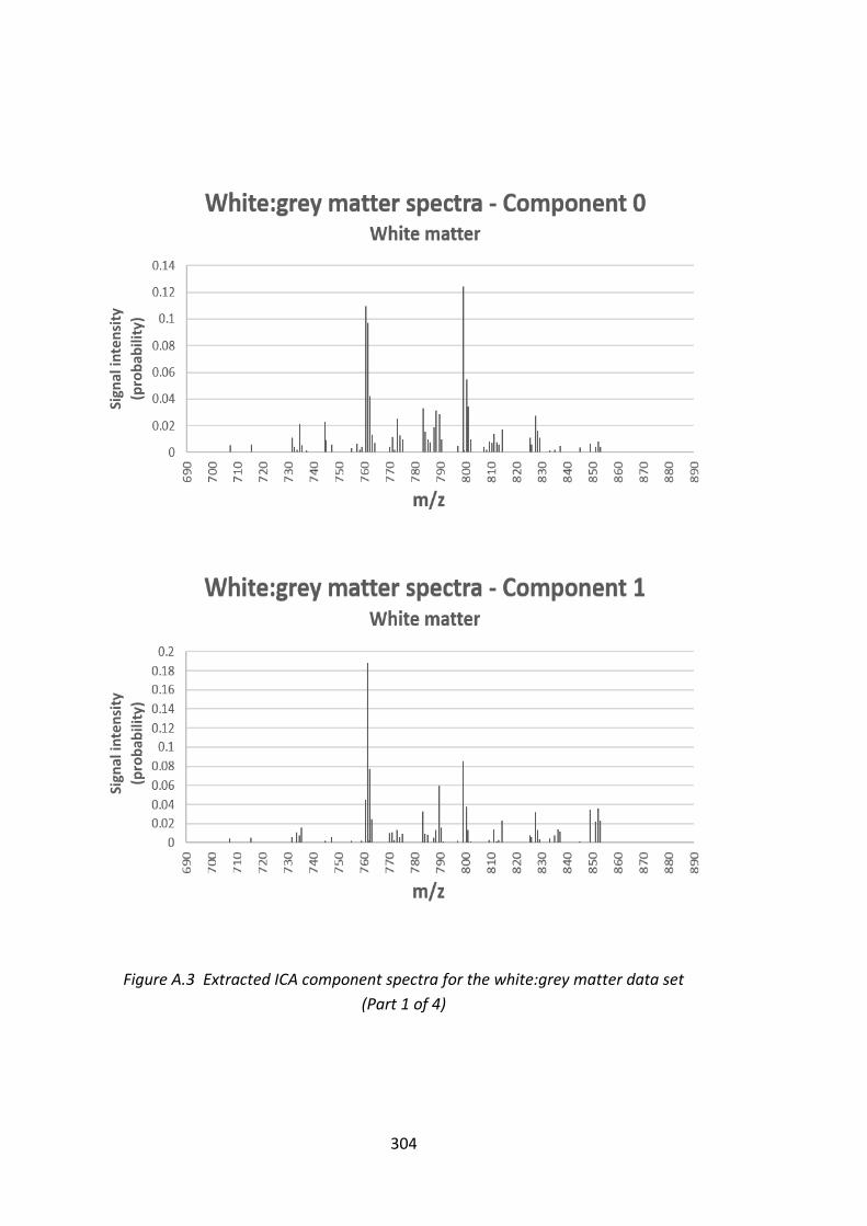
304
Figure A.3 Extracted ICA component spectra for the white:grey matter data set
(Part 1 of 4)
Sign
al in
ten
sity
(pro
bab
ility
)
Sign
al in
ten
sity
(pro
bab
ility
)

305
Figure A.3 Extracted ICA component spectra for the white:grey matter data set
(Part 2 of 4)
Sign
al in
ten
sity
(pro
bab
ility
)
Sign
al in
ten
sity
(pro
bab
ility
)

306
Figure A.3 Extracted ICA component spectra for the white:grey matter data set
(Part 3 of 4)
Sign
al in
ten
sity
(pro
bab
ility
)
Sign
al in
ten
sity
(pro
bab
ility
)

307
Figure A.3 Extracted ICA component spectra for the white:grey matter data set
(Part 4 of 4)
Sign
al in
ten
sity
(pro
bab
ility
)
Sign
al in
ten
sity
(pro
bab
ility
)

308
Appendix B: Extracted ICA Components vs.
Single Ion Distributions of the Image Data Set
B-1 Extracted ICA Components of the Image
Data Set
Extracted ICA components (sub-spectra) for the rat brain MALDI-MS images of 8-, 16-
and 24-component models are presented in Figures B.1, B.2 and B.3, respectively.
The corresponding component distribution images are also shown at a corner of each
component spectrum, plotted with a normalisation to the integral over all the
components in the given model. The grey scale at the bottom of each image
represents a relative weighting each component has to the total signal quantity. The
10 major peaks of each component spectrum are marked with green arrows, with
their m/z values listed in the figures.
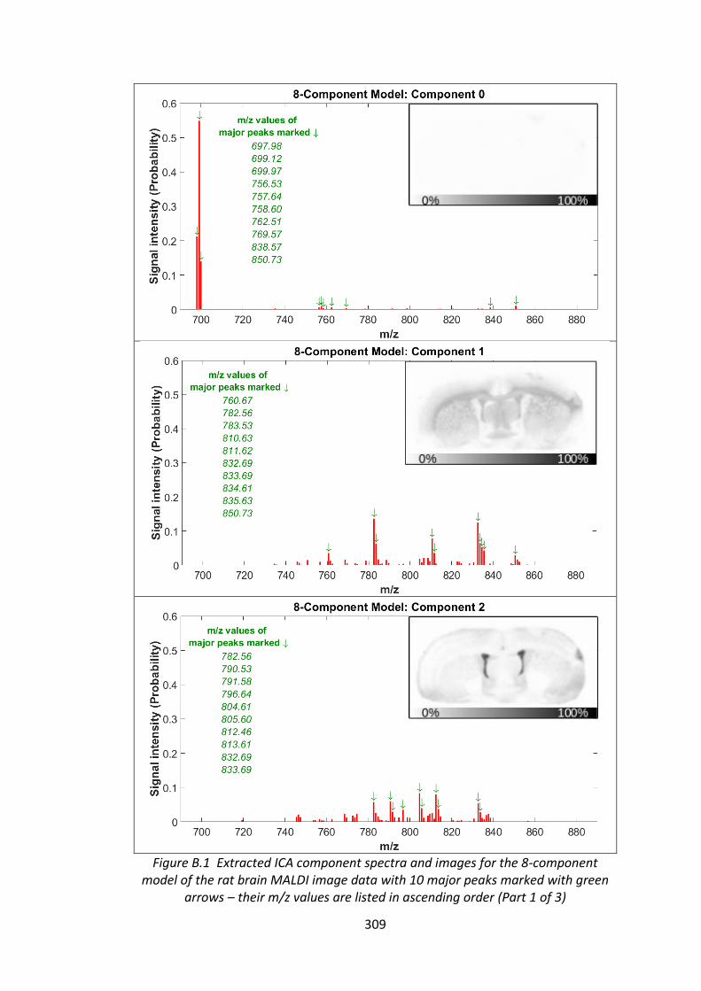
309
Figure B.1 Extracted ICA component spectra and images for the 8-component
model of the rat brain MALDI image data with 10 major peaks marked with green arrows – their m/z values are listed in ascending order (Part 1 of 3)

310
Figure B.1 Extracted ICA component spectra and images for the 8-component
model of the rat brain MALDI image data with 10 major peaks marked with green arrows – their m/z values are listed in ascending order (Part 2 of 3)

311
Figure B.1 Extracted ICA component spectra and images for the 8-component model of the rat brain MALDI image data with 10 major peaks marked with green
arrows – their m/z values are listed in ascending order (Part 3 of 3)

312
Figure B.2 Extracted ICA component spectra and images for the 16-component
model of the rat brain MALDI image data with 10 major peaks marked with green arrows – their m/z values are listed in ascending order (Part 1 of 6)

313
Figure B.2 Extracted ICA component spectra and images for the 16-component
model of the rat brain MALDI image data with 10 major peaks marked with green arrows – their m/z values are listed in ascending order (Part 2 of 6)

314
Figure B.2 Extracted ICA component spectra and images for the 16-component
model of the rat brain MALDI image data with 10 major peaks marked with green arrows – their m/z values are listed in ascending order (Part 3 of 6)

315
Figure B.2 Extracted ICA component spectra and images for the 16-component
model of the rat brain MALDI image data with 10 major peaks marked with green arrows – their m/z values are listed in ascending order (Part 4 of 6)

316
Figure B.2 Extracted ICA component spectra and images for the 16-component
model of the rat brain MALDI image data with 10 major peaks marked with green arrows – their m/z values are listed in ascending order (Part 5 of 6)

317
Figure B.2 Extracted ICA component spectra and images for the 16-component model of the rat brain MALDI image data with 10 major peaks marked with green
arrows – their m/z values are listed in ascending order (Part 6 of 6)

318
Figure B.3 Extracted ICA component spectra and images for the 24-component
model of the rat brain MALDI image data with 10 major peaks marked with green arrows – their m/z values are listed in ascending order (Part 1 of 8)

319
Figure B.3 Extracted ICA component spectra and images for the 24-component
model of the rat brain MALDI image data with 10 major peaks marked with green arrows – their m/z values are listed in ascending order (Part 2 of 8)

320
Figure B.3 Extracted ICA component spectra and images for the 24-component
model of the rat brain MALDI image data with 10 major peaks marked with green arrows – their m/z values are listed in ascending order (Part 3 of 8)
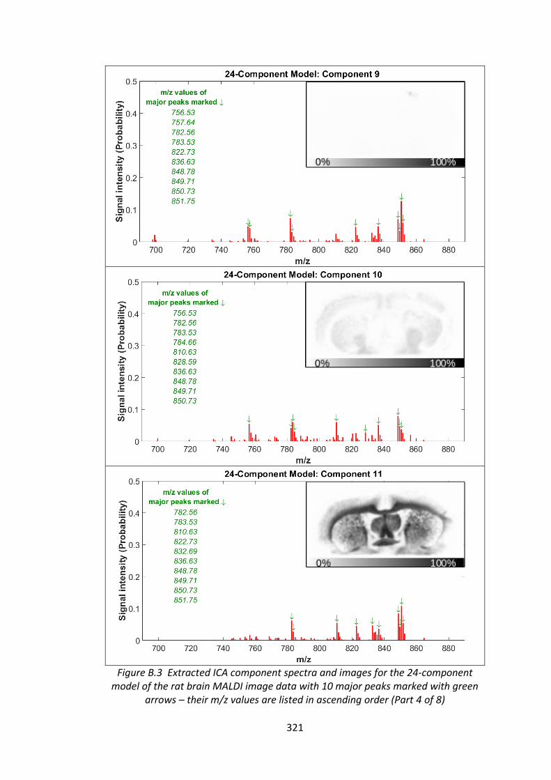
321
Figure B.3 Extracted ICA component spectra and images for the 24-component
model of the rat brain MALDI image data with 10 major peaks marked with green arrows – their m/z values are listed in ascending order (Part 4 of 8)

322
Figure B.3 Extracted ICA component spectra and images for the 24-component
model of the rat brain MALDI image data with 10 major peaks marked with green arrows – their m/z values are listed in ascending order (Part 5 of 8)

323
Figure B.3 Extracted ICA component spectra and images for the 24-component
model of the rat brain MALDI image data with 10 major peaks marked with green arrows – their m/z values are listed in ascending order (Part 6 of 8)

324
Figure B.3 Extracted ICA component spectra and images for the 24-component
model of the rat brain MALDI image data with 10 major peaks marked with green arrows – their m/z values are listed in ascending order (Part 7 of 8)

325
Figure B.3 Extracted ICA component spectra and images for the 24-component
model of the rat brain MALDI image data with 10 major peaks marked with green arrows – their m/z values are listed in ascending order (Part 8 of 8)

326
B-2 Single Ion Images
The single ion images created for the 20 largest peaks as a result of the peak detected
mass spectra of the rat brain MALDI image data set are provided in Figure B.4.
m/z 745.5 m/z 753.7 m/z 756.5 m/z 757.6
m/z 760.7 m/z 782.6 m/z 783.5 m/z 784.7
m/z 808.7 m/z 810.6 m/z 812.5 m/z 822.7
m/z 832.7 m/z 833.7 m/z 836.7 m/z 837.6
m/z 848.8 m/z 849.7 m/z 850.7 m/z 851.8
Figure B.4 Single ion images of the rat brain MALDI image data for the top 20
strongest peaks detected – the dynamic range has been set to maximise the
contrast of each image where the darkest pixel has the highest intensity value