Spatial Heterogeneity of Water Quality in a Highly Degraded Tropical Freshwater Ecosystem

Spatial Heterogeneity of Water Quality in a Highly DegradedTropical Freshwater Ecosystem

Luis Zambrano Æ Victoria Contreras ÆMarisa Mazari-Hiriart Æ Alba E. Zarco-Arista

Received: 5 October 2007 / Accepted: 9 September 2008 / Published online: 21 October 2008

� Springer Science+Business Media, LLC 2008

Abstract Awareness of environmental heterogeneity in

ecosystems is critical for management and conservation.

We used the Xochimilco freshwater system to describe the

relationship between heterogeneity and human activities.

This tropical aquatic ecosystem south of Mexico City is

comprised of a network of interconnected canals and lakes

that are influenced by agricultural and urban activities.

Environmental heterogeneity was characterized by spatially

extensive surveys within four regions of Xochimilco during

rainy and dry seasons over 2 years. These surveys revealed

a heterogeneous system that was shallow (1.1 m,

SD = 0.4 ), warm (17�C, SD = 2.9), well oxygenated

(5.0 mg l-1, SD = 3), turbid (45.7 NTU SD = 26.96), and

extremely nutrient-rich (NO3–N = 15.9 mg l-1, SD=13.7;

NH4–N = 2.88 mg l-1, SD = 4.24; and PO4–P = 8.3 mg

l-1, SD = 2.4). Most of the variables were not significantly

different between years, but did differ between seasons,

suggesting a dynamic system within a span of a year but

with a high resilience over longer periods of time. Maps

were produced using interpolations to describe distributions

of all variables. There was no correlation between indi-

vidual variables and land use. Consequently, we searched

for relationships using all variables together by generating a

combined water quality index. Significant differences in the

index were apparent among the four regions. Index values

also differed within individual region and individual water

bodies (e.g., within canals), indicating that Xochimilco has

high local heterogeneity. Using this index on a map helped

to relate water quality to human activities and provides a

simple and clear tool for managers and policymakers.

Keywords Interpolation � Land use � Urban lake �Shallow lake � Xochimilco � Water quality index �Wetlands

Environmental heterogeneity is closely related to ecosys-

tem pattern and function (George and others 2000; Guo and

others 2003). Recently, spatial heterogeneity has been

studied in aquatic systems to understand processes in riv-

ers, wetlands, and lakes (Dent and Grim 1999; Comin and

others 2001; Robinson and others 2002). Many aquatic

systems have spatial heterogeneity based on internal pro-

cesses (Comin and others 2001). For example, variability

in the depth of a lake or water velocity in a river can

produce local differences in sediment-water interactions

that create spatial heterogeneity in suspended solid and

nutrient concentrations.

High spatial heterogeneity increases habitat availability for

different organisms (Brown 2003; Dufour and others 2006;

Gundale and others 2006), as well as the overall resilience of

aquatic ecosystems. High heterogeneity fosters gradual rather

than catastrophic changes in zooplankton and phytoplankton

populations in response to perturbations (Scheffer and Rinaldi

2000). Managers consider high heterogeneity as a positive

attribute because it is directly related to species diversity

(Nienhuis and others 2002), although this is not always the

case for invertebrates (Brooks and others 2002).

Human activities are capable of modifying patterns in

spatial heterogeneity (UNESCO 2006) by changing the

L. Zambrano (&) � V. Contreras

Departamento de Zoologıa, Instituto de Biologıa, Universidad

Nacional Autonoma de Mexico, Tercer Circuito Exterior Ciudad

Universitaria, Coyoacan, Mexico, D.F. 04510, Mexico

e-mail: [email protected]

M. Mazari-Hiriart � A. E. Zarco-Arista

Departamento de Ecologıa de la Biodiversidad, Instituto de

Ecologıa, Universidad Nacional Autonoma de Mexico,

Tercer Circuito Exterior Ciudad Universitaria, Coyoacan,

Mexico, D.F. 04510, Mexico

123

Environmental Management (2009) 43:249–263

DOI 10.1007/s00267-008-9216-1

water quality of rivers or lakes (Harper 1992; Shivoga and

others 2006). For example, human settlements create patchy

eutrophication along a water system (Douterelo and others

2004; Kemka and others 2006). Consequently, these changes

can modify species distribution (Muhando and others 2002)

or sexual selection (Engstroem-Oest and Candolin 2007).

Therefore, it is necessary to understand how key ecological

variables change across the landscape, in response to both

natural complexity and changes in human land use. Ana-

lyzing spatial heterogeneity in water quality may help relate

the effects of human activities on those limnological vari-

ables that are critical for the survival of native organisms.

One of the difficulties in determining heterogeneity in a

system is that data collected from single point samples do

not explain the behavior of a particular variable in the area

surrounding that sampling point. Therefore, the nonsampled

areas do not provide information that could be relevant

regarding the variables’ spatial distribution within the entire

system. Interpolation techniques can help fill these gaps

between sampling points, which increase the information

obtained from specific sites (Matejicek and others 2006).

Once variables are interpolated, they can be overlapped,

generating a water quality index that may be capable of

describing the aquatic system health in a single map. Then it

may be possible to use this technique to analyze relation-

ships between spatial heterogeneity, based on a water quality

index, and land use (Tveito and others 2005).

The Xochimilco freshwater ecosystem is composed of

canals connecting small lakes and a wetland. It is located in

the southern portion of Mexico City, the second largest city in

the world, with a population of more than 18 million inhab-

itants (Fig. 1). This ecosystem still hosts 140 species of

migratory birds and native species such as the axolotl

(Ambystoma mexicanum) and crayfish (Cambarellus monte-

zumae), both of which are endemic and threatened. This

system is a tropical high-altitude water body which produces

distinct hydrological and ecological regimes. Water temper-

ature is normally lower and more inconsistent than in a

tropical system; thermal variability is due less to seasonal

dynamics (as in temperate systems) than to day-night cycles,

which can produce temperature fluctuations of [15�C

(Zambrano, unpublished data). The hydrological regime at

Xochimilco is marked by seasonal change, as the rainy season

results in substantial ecosystem expansion due to formation

of temporary wetlands that attach to permanent water bodies.

Anthropogenic perturbations have been imposed on

this dynamic hydrologic regime, as Xochimilco has

one of the longest histories of human management. The

contemporary aquatic system is the last remnant of the

original aquatic landscape composed of five lakes—

Xaltocan, Zumpango, Texcoco, Xochimilco, and Chalco—

which covered *920 km2 in the Basin of Mexico (DDF

1975). Historically, this ecosystem has been occupied by

traditional agriculture in portions of land known as chi-

nampas, using aquatic resources and lake sediments for

food production. However, 25 years ago, the decline in

water quality has caused a shift in agricultural activities to

more intensive production in greenhouses (Lopez and

others 2006; Mendez 2006). Nowadays Xochimilco is a

collage of land uses, ranging from completely urbanized

areas (mostly in the southern region) to rural areas (in the

central and northern regions), and it is currently threatened

by urban growth in the periphery of the Mexico City

Metropolitan Area. In 1989 the first attempt at management

and restoration of this system generated the Ecological

Park (Parque Ecologico de Xochimilco; PEX) in the

northern region. Also, the complete ecosystem has been

part of the UNESCO World Heritage List since 1987 and

the International Convention on Wetlands (known as

RAMSAR) list since 2004.

To maintain the biodiversity and ecosystem services

provided by this aquatic system, conservation and restora-

tion policies must be implemented which consider the high

heterogeneity in water quality produced by the regional

climate and contrasting land uses. Therefore, the aim of this

paper is to create a water quality index, using geographical

interpolations to spatially characterize the wetlands, lakes,

and channels in this system subject to multiple environ-

mental influences. The broad-scale information produced

by this index will help elucidate the spatial influences of

different land use types and highlight variation in limno-

logical processes in the whole ecosystem. Together, this

information is used to consider the persistence of key

aquatic species within this diverse aquatic setting.

Materials and Methods

Sampling

Two sets of samples were collected from a total of 29

canals and 8 lakes in 2000–2001 and 2004. During the

2000–2001 sampling season the whole system was divided

into 211 canal sections 250 m in length (Hill 1971). By a

simple randomization strategy, 19 sections were selected

and the midpoint of each section was georeferenced with a

GPS (Garmin GPS12XL) and served as the sampling site

for water chemistry. This sampling design provided a

representative area to evaluate the general environmental

conditions of the entire system. The same sites were

sampled twice: in the rainy season (from June to September

2000) and the dry season (from January to May 2001).

A second set of samples was obtained in June to Sep-

tember of 2004 with a different method of selecting sample

sites. This selection was based on finding those places

necessary to generate an interpolation map. This increased

250 Environmental Management (2009) 43:249–263

123

the number of sampling sites to 59, which included the

previous 19. Sites were again georeferenced. Although

both sets of samples had different numbers of sampling

points, they shared most of the canals and most of the data

collection techniques.

In both sets of samples, physicochemical measurements

(conductivity as microsvedbergs per centimeter, pH, tem-

perature as degrees centigrade, depth as meters, and

dissolved oxygen as milligrams per liter) were done in situ

with portable multiparametric equipment (YSI Model 6600).

Turbidity was included only in the second set of samples.

Nutrient concentration sampling methods varied for

each sampling set. In the first set of samples nitrate and

ammonium concentrations in water were analyzed using a

Corning electrode. In the second set of samples nutrient

concentrations were determined immediately after collec-

tion of the water samples with a LaMotte SMART

colorimeter. Nitrate was analyzed by zinc reduction,

ammonium was obtained by Nesslerization, and phosphate

was obtained following the ascorbic acid reduction method

(APHA 1998).

Bacteriological Analyses

Bacteriological analyses were conducted during 2001 to

characterize the distribution of fecal indicator bacteria.

Five hundred-milliliter samples were collected in sterile

polypropylene flasks. Water samples were analyzed fol-

lowing standard membrane filtration and incubation

procedures (APHA 1998) to enumerate two bacterial types:

fecal coliforms, as representative of gram-negative bacte-

ria; and fecal streptococci, as representative of gram-

positive bacteria. Membrane filters (0.45-lm cellulose

acetate; Millipore MF type HA) were placed on a pad with

M-FC for fecal coliforms and K-F agar for fecal strepto-

cocci (APHA 1998). For bacterial densities data were

normalized with Box-Cox transformations (Sokal and Ro-

hlf 1981). To ascertain the possible origins of

bacteriological contamination the index of Geldrich and

Kenner (1969) was used. Bacteriological samples were also

compared to regulations for water utilized for irrigation

purposes, which stipulate a maximum of 1000 CFU/100 ml

of fecal coliforms (DDF 1975; Blumenthal and others

Fig. 1 Map of Xochimilco (light gray) showing the study areas

Environmental Management (2009) 43:249–263 251

123

2000; DOF 2005). The Mexican water standards for con-

servation of freshwater aquatic life suggest the same levels

(DOF 2004). To analyze fecal contamination origin we

used the index of Toranzos and others (2007). A ratio [4 is

characteristic of human fecal contamination; between 2 and

4, predominantly of human origin; between 0.7 and 2,

predominantly of animal origin; \0.7, suggestive of animal

waste. This index has been questioned due to differential

die-off kinetics of the two bacterial groups, and the results

should be viewed with caution (Toranzos and others 2007).

However, it is useful in this case since it gives a general

idea of the origin of bacterial contamination.

Physicochemical variables gave information on the liv-

ing capabilities of organisms, while nutrient concentrations

helped to clarify the trophic status of the water system.

Finally, bacterial analysis gave information on water con-

tamination and its potential sources.

Interpolation

Interpolation is a technique that converts a unique sample

point value to a series of values that covers an area, using

information from neighboring stations. To create an inter-

polated map of water chemistry, it was first necessary to

build a polygon of the network morphology of Xochimilco.

This network constrained the influence between near sam-

pling points that were not interconnected by water (e.g., two

neighborhood sampling points separated by a piece of land).

The polygon was built from an aerial photograph (1:5,000

[Instituto de Geografia 2002]) with ESRI Arc View 3.2.

Interpolations were generated with data from the second set

of samples, using values of dissolved oxygen, turbidity,

conductivity, ammonium, nitrate, and phosphate concen-

trations. Water flow in canals is very slow (\4 m/h),

therefore we did not consider it in the interpolations.

Interpolations produced a value for each variable on every

pixel that represented canal areas within the aquatic system

using the inverse distance-weighted interpolation technique

with ESRI Arc Map 8.0. We assumed that the influence of

one station decreases linearly with the distance between

sampled points within 400 m (Dent and Grimm 1999). A

power of eight was used to obtain the influence of this

distance, giving higher weight to closer neighbors. The

power was chosen using smoothness as a decision criterion.

We considered relationships between land use variables

and water quality as a potential means of improving our

interpolations. Three land use variables were obtained from

INEGI (vegetation, human population densities, type of

soil). These data were converted in raster format to stan-

dardize pixel sizes with ESRI Arc View 3.2. A total of 21

Pearson correlations were performed for the seven physi-

cochemical parameters and three land use categories. Land

use variables that were significantly correlated with any of

the water quality variables were then considered in the

interpolation model.

Ranking from Interpolation Values

To picture which regions have better water quality using

data obtained from interpolations, it was necessary to

standardize all variables. Therefore, values obtained for

every pixel from the interpolations were placed in one of

three categories based on the effect of each variable on

water quality: (1) ‘‘suitable conditions,’’ in which values of

every variable were suitable for the survival and repro-

duction capacities of the native organisms (i.e., DO

concentration [3 mg l-1, nutrients at lower concentra-

tions, and turbidity values close to zero); (2) ‘‘nonsuitable

conditions,’’ in which variables can be suitable for some

organisms but not all of them (some of the native fish

species would need higher DO concentrations, but other

organisms such as amphibians would survive with these

concentrations); and (3) ‘‘bad conditions,’’ in which most

of the native organisms are not able to survive (i.e., toxic

concentrations or anoxic conditions). A simple division by

three was not always appropriate for categorizing all

variables. For instance, the lowest values of oxygen were

assigned the highest rank values, while the same category

was used for high concentrations of all nutrients and tur-

bidity (Table 1). Although this ranking system can be

considered subjective, it provides a broad regional view of

water quality within a complex system that is readily

understood by nonscientific stakeholders.

Ranking on turbidity was based on (1) clear water,

where vertebrates and invertebrate can forage properly; (2)

low turbidity, where visual predators experience reduced

capability of prey intake; and (3) high turbidity, where

visual predator foraging success is reduced almost to zero

(Reid and others 1999; De Robertis and others 2003).

Dissolved oxygen was divided into anoxic, hypoxic, and

sufficient oxygen conditions. Nitrate and ammonium ranks

were based on toxic concentrations of each variable (Cheng

and Chen 2002; Camargo and others 2004). Since the

lowest phosphate concentrations far exceeded any existing

trophic status classification system, a modal curve in his-

togram analysis with number of pixels per value was used

to define the ranking categories. This technique was also

used for electrical conductivity values, assuming a positive

relation between electrical conductivity and pollution

(Valsanen and others 1998).

Analysis of Seasons and Years

To compare differences among variables between seasons

and years, we standardized the data into two different sets of

samples. The information obtained from the second set of


123

samples was reduced to the 19 canals used in the first set of

samples by averaging all values within each canal. Infor-

mation obtained outside these canals was not used for this

analysis. Using each canal as a unit, a paired t-test was used

to identify differences between temporal changes (dry vs.

wet season and between years) from the two data sets. To

avoid Type I statistical error in making multiple comparisons

of canals in this test, we used the Bonferroni adjustment.

Analysis of Regions

We divided the sampled area into four regions according to

different human activities using satellite imagery and field

observations (Fig. 1).

A. The chinampera region has 10 canals and 1 lake. This

region supports traditional agricultural production in

small square islands called chinampas. Production is less

intensive and the area is not used for human settlement.

The Xochimilco Ecological Park (PEX) is located within

this region and contains an artificial wetland. Canals

situated in the northeast of the region receive water from

the rest of the system and sewage outflow toward the

deep drainage system of Mexico City.

B. The urban region has seven canals and four lakes.

This region has experienced legal and illegal urban

development and intensive cropping systems based on

greenhouses. Consequently, this region corresponds to

a transition state between urbanized chinampas and

modern agriculture, which relies on pesticides and

chemical fertilizers.

C. The tourist region has six canals and two lakes.

Economic activities of this region rely on tourism and

intensive cropping systems. This region has been

semiurbanized for a long time, but the rapid greenhouse

development has promoted human settlements without

any urban planning by the local or federal government.

D. The chinampera/urban region has six canals and one

lake. This region also maintains the chinampas

technique for production, but part of this region is

immersed in an urban matrix. The network of canals is

connected to the rest of the system by only one canal,

possibly working as a bottleneck, reducing the water

exchange with the other regions.

The first set of samples did not cover the complete study

area, and therefore we only used the second set of samples

to identify differences among the four regions. ANOVAs

were used to find differences among the regions using

interpolated data.

Results

General Description

Results demonstrate that Xochimilco is a heterogeneous

shallow (\2.2-m maximum depth) aquatic system (Table 2).

As a subtropical system [2200 meters above sea level

(masl), temperatures were slightly lower during the dry

season (but never below 11�C) compared to the rainy season

(never \16�C), and the maximum was close to 20�C in both

seasons. Turbidity varied from sites with virtually complete

transparency (Puente de Urrutia) to highly turbid canals

(Paso del Aguila). pH was circumneutral and slightly skewed

to basic (between 6.8 and 8). Although canals in general are

adequately oxygenated, anoxic conditions were present in

some areas. Bacteriological results obtained in the first set of

samples revealed contamination in 90% of the samples and

high bacteriological counts were attributable to human and

animal origin, as shown by the fecal coliforms/fecal

enterococci index (Table 3).

Differences Between Years and Seasons

Depth differences between years were observed (shallower

in the 2004 wet season compared to both seasons in 2001).

Dissolved oxygen showed limited seasonality, with lower

concentrations in the wet season, but it also differed

between years. Other variables that showed a seasonal

pattern included temperature and ammonium, with higher

values during the dry season; electrical conductivity, with

higher values in the wet season; and pH, with lower values

in the wet season. Nitrate did not differ between seasons or

years (Table 4).

Coliforms had significantly higher abundances in the dry

season, while enterococci did not show any significant dif-

ferences (Fig. 2). Bacteriological counts suggest a critical

Table 1 Values for categorization of physicochemical data (see Methods)

Category DO

(mg l-1)

Turbidity

(NTU)

Conductivity

(lS cm-1)

NO3–N

(mg l-1)

NH4–N

(mg l-1)

PO4–P

(mg l-1)

1 0–1 0–40 0–65 0–5 0–1 0–3

2 1.1–3 41–70 66–93 5.1–10 1.1–1.6 3.1–7

3 [3.1 [71 [94 [10.1 [1.7 [7.2

Note: DO, dissolved oxygen. Category levels: 1 = more suitable conditions; 2 = less suitable conditions; 3 = bad conditions


123

Table 2 Average values for the sampled channels in both seasons

Canal Depth (m) Temperature (�C) pH Dissolved oxygen (mg l-1)

2000–2001 2004 2000–2001 2004 2000–2001 2004 2000–2001 2004

Dry Wet Wet Dry Wet Wet Dry Wet Wet Dry Wet Wet

Almoloya 0.76 0.70 0.60 18.80 11.20 20.86 7.02 8.61 7.72 1.40 11.00 4.19

Apatlaco 1.83 1.45 0.90 21.40 15.50 20.66 7.53 7.66 8.21 7.00 7.80 7.32

Atizapa 1.44 1.08 0.60 21.80 16.00 21.80 7.52 8.21 7.52 4.60 9.47 5.17

Cerca Draga 0.80 2.05 1.20 19.80 18.40 21.68 6.91 7.18 7.40 4.00 5.80 4.10

Compuerta 2.10 1.90 1.60 19.70 17.60 21.11 6.74 7.77 7.33 3.40 2.40 2.14

Comunidad 1.20 0.50 0.50 19.25 12.80 20.25 7.21 8.01 7.75 2.15 7.50 5.39

Costetexpa 1.10 1.07 0.60 19.20 15.30 19.68 6.97 6.79 7.24 1.00 1.80 1.59

Cuemanco 1.70 1.10 0.70 20.60 18.10 21.63 8.80 8.99 8.42 7.40 9.60 9.30

El Bordo 1.03 1.60 0.90 19.80 12.40 22.24 7.73 8.89 9.37 4.60 7.40 5.45

Japon 1.32 1.50 1.30 20.90 13.00 22.85 7.62 8.65 8.57 7.60 11.00 9.78

Nativitas 1.44 1.10 1.50 18.60 18.90 20.61 7.33 7.32 7.23 2.00 5.40 1.91

Paso de Aguila 1.08 1.00 0.60 19.02 14.30 22.45 6.88 8.34 8.19 1.40 11.00 8.92

Pizocoxpa 1.70 1.80 0.70 21.65 16.45 20.59 6.91 7.47 7.34 3.10 3.00 2.79

San Diego 1.10 0.40 0.90 20.00 15.60 19.46 7.30 7.38 7.26 0.80 3.40 4.51

Seminario 1.30 1.10 1.40 19.90 15.30 20.66 7.00 7.25 7.34 3.80 2.40 3.11

Tezhuillo 1.15 1.00 0.70 19.70 15.30 22.38 6.91 7.36 8.51 3.20 4.20 9.96

Tlilac 1.20 0.70 0.60 21.40 13.30 21.38 7.51 8.10 7.62 5.20 9.80 4.47

Urrutia 1.87 1.82 1.00 20.20 16.30 16.17 7.38 8.18 6.97 0.60 3.20 0.07

Xaltocan 1.00 1.00 0.50 20.00 17.30 20.83 6.82 6.69 7.87 5.40 9.00 6.18

Average 1.32 1.20 0.88 20.09 15.42 20.91 7.27 7.83 7.78 3.61 6.59 5.07

SD 0.37 0.48 0.35 0.97 2.16 1.47 0.48 0.68 0.62 2.22 3.29 2.91

Conductivity (lS cm-1) NO3–N (mg l-1) NH4–N (mg l-1) Turbidity (NTU) PO4–P (mg l-1)

2000–2001 2004 2000–2001 2004 2000–2001 2004 2004 2004

Dry Wet Wet Dry Wet Wet Dry Wet Wet Wet Wet

Almoloya 939.0 713.0 704.0 29.12 0.62 5.76 4.57 5.73 2.32 50.30 10.20

Apatlaco 905.0 729.0 914.0 6.50 35.06 21.00 0.12 2.65 1.96 49.80 8.13

Atizapa 757.3 938.0 631.0 17.53 7.78 25.96 0.16 20.95 0.23 57.90 8.15

Cerca Draga 683.0 779.0 729.0 0.90 0.83 16.72 2.19 1.70 1.84 29.70 10.60

Compuerta 941.0 608.0 668.0 35.30 0.63 16.72 2.19 2.69 0.62 33.50 7.10

Comunidad 1360.5 715.0 693.0 14.52 13.74 2.77 2.43 3.16 0.31 52.40 10.20

Costetexpa 701.0 378.0 643.0 n.d n.d n.d n.d n.d n.d 24.70 n.d

Cuemanco 467.0 791.0 716.0 2.50 6.76 12.85 0.17 1.81 0.61 26.90 8.60

El Bordo 1077.0 762.0 535.0 4.05 15.74 2.51 0.45 1.24 0.22 78.20 1.08

Japon 1035.0 710.0 706.0 46.31 34.56 7.92 1.93 0.02 1.24 33.30 6.70

Nativitas 985.0 678.0 672.0 36.27 0.60 60.00 1.00 11.48 1.60 21.00 10.80

Paso de Aguila 989.0 702.0 784.0 32.70 20.46 6.20 2.53 12.31 2.50 68.00 10.10

Pizocoxpa 633.5 724.0 664.0 22.90 29.38 11.44 0.41 0.87 2.34 49.00 8.40

San Diego 797.0 627.0 655.0 17.09 43.65 12.67 0.65 0.03 1.79 14.30 8.90

Seminario 688.0 850.0 757.0 6.72 9.43 7.74 1.52 16.95 1.61 25.00 11.10

Tezhuillo 783.0 706.0 805.0 5.20 15.52 8.18 0.04 11.48 1.91 44.90 7.60

Tlilac 1189.0 738.0 677.0 9.90 44.93 5.06 0.09 5.73 0.53 103.00 6.30

Urrutia 1127.0 740.0 943.0 16.31 14.48 8.93 0.68 2.78 1.56 6.10 9.20

Xaltocan 638.0 745.0 757.0 15.72 4.21 11.35 1.00 7.55 1.27 101.00 6.20


123

period during the dry season, as 72% of the samples had

bacterial counts higher than the WHO and Mexican stan-

dards recommended for irrigation water. During the rainy

season, only 43% of the samples exceeded these standards,

and bacteria from human sources were reduced to 27% in all

samples, leaving higher proportions to animal origins.

Spatial Variation

There were no significant correlations between land use and

water quality, as the highest correlation coefficient (r)

was \0.43. Variable interpolations demonstrated variability

at relatively small spatial scales within canals (see the

Appendix). Turbidity values were generally higher in the

northern and western areas, while high-conductivity waters

were distributed in the western and central areas. Oxygen had

a relatively homogeneous distribution (values [3 mg l-1),

except in the southern and western areas, where canals were

anoxic. Phosphate concentration was higher in the central-

western region, ammonium was higher in the central and

western areas, and nitrate was highest in the southern region.

The chinampera region was significantly more turbid (75.7

NTU on average) than the other regions (urban = 40.5, tour-

ist = 47.2 and chinampera/urban = 46.0) (see Fig. 3).

Ammonium (average [avg] = 1.9 mg l-1) and bacterial counts

(avg = 10.3 tranformed Box-Cox) were significantly higher in

the urban region than in the other three regions (ammonium

avg—chinampera = 0.9 mg l-1, tourist = 1.5 mg l-1, and

chinampera/urban = 1.33 mg l-1; bacterial count avg—

chinampera = 2.8, tourist = 7.5, transformed Box-Cox). The

tourist region had the highest nitrate concentration

(avg = 22.2 mg l-1, vs chinampera = 7.7 mg l-1, urban =

10.0 mg l-1, and chinampera/urban = 6.9 mg l-1). Finally,

the chinampera/urban region had the highest conductivity

(avg = 1.0 lS cm-1) (Fig. 3). There were no significant

differences in DO (avg: chinampera = 6.8 mg l-1, urban =

5.8 mg l-1, tourist = 3.4 mg l-1, chinampera/urban =

3.9 mg l-1) and phosphate (avg: chinampera = 7.2 mg l-1,

urban = 9.3 mg l-1, tourist = 8.0 mg l-1, chinampera/

urban = 10.4 mg l-1) among regions.

Ranks of Physicochemical Variables

Categorical ranks of physicochemical data demonstrated

that most canals had intermediate water quality (lighter

areas in Fig. 4). Very few canals were in bad condition

Table 3 Percentage of contaminated samples by animal or human

origin, following Torranzos and others (2007)

Region Canals sampled Fecal contamination origin

Animal (%) Human (%)

Chinampera 30 87 13

Urban 25 68 32

Tourist 14 50 50

Chinampera/urban 2 50 50

Table 4 Paired t-test for sampled canal (see Table 2)

Variable Season/year t value P

Depth Dry 2001 vs. wet 2001 1.12 n.s.

Wet 2001 vs. wet 2004 4.70 \0.01

Dry 2001 vs. wet 2004 3.29 \0.01

Temperature Dry 2001 vs. wet 2001 8.79 \0.01

Wet 2001 vs. wet 2004 -2.11 n.s.

Dry 2001 vs. wet 2004 -8.46 \0.01

Conductivity Dry 2001 vs. wet 2001 2.74 n.s.

Wet 2001 vs. wet 2004 2.89 \0.01

Dry 2001 vs. wet 2004 -0.03 n.s.

Dissolved oxygen Dry 2001 vs. wet 2001 -4.34 \0.01

Wet 2001 vs. wet 2004 -2.60 n.s.

Dry 2001 vs. wet 2004 2.44 n.s.

pH Dry 2001 vs. wet 2001 -4.74 \0.01

Wet 2001 vs. wet 2004 -3.73 \0.01

Dry 2001 vs. wet 2004 0.36 n.s.

NO3–N Dry 2001 vs. wet 2001 0.25 n.s.

Wet 2001 vs. wet 2004 1.12 n.s.

Dry 2001 vs. wet 2004 0.57 n.s.

NH4–N Dry 2001 vs. wet 2001 -3.19 \0.01

Wet 2001 vs. wet 2004 -0.44 n.s.

Dry 2001 vs. wet 2004 3.17 \0.01

Note: n.s., not significant

Table 2 continued

Conductivity (lS cm-1) NO3–N (mg l-1) NH4–N (mg l-1) Turbidity (NTU) PO4–P (mg l-1)

2000–2001 2004 2000–2001 2004 2000–2001 2004 2004 2004

Dry Wet Wet Dry Wet Wet Dry Wet Wet Wet Wet

Average 878.7 717.5 718.6 17.75 16.58 13.54 1.23 6.06 1.36 45.74 8.30

SD 224.8 109.7 95.7 13.36 14.92 13.15 1.21 6.15 0.76 26.96 2.38

Note: Wet: samples obtained in wet season. Dry: samples obtained in dry season. Turbidity and PO4 were sampled only in the 2004 season


123

Fig. 2 Average bacteriological

densities for two seasons, using

a Box-Cox transformation.

Different numbers (1 and 2) in

region comparison indicate

significant differences in Tukey

multiple-comparison tests

Fig. 3 Average of the variables in the four regions with standard deviation (see Fig. 2). Letters over the variable indicate significant differences

in Tukey multiple-comparison tests. Chi, Chinampera; Ur, urban; To, tourist


123

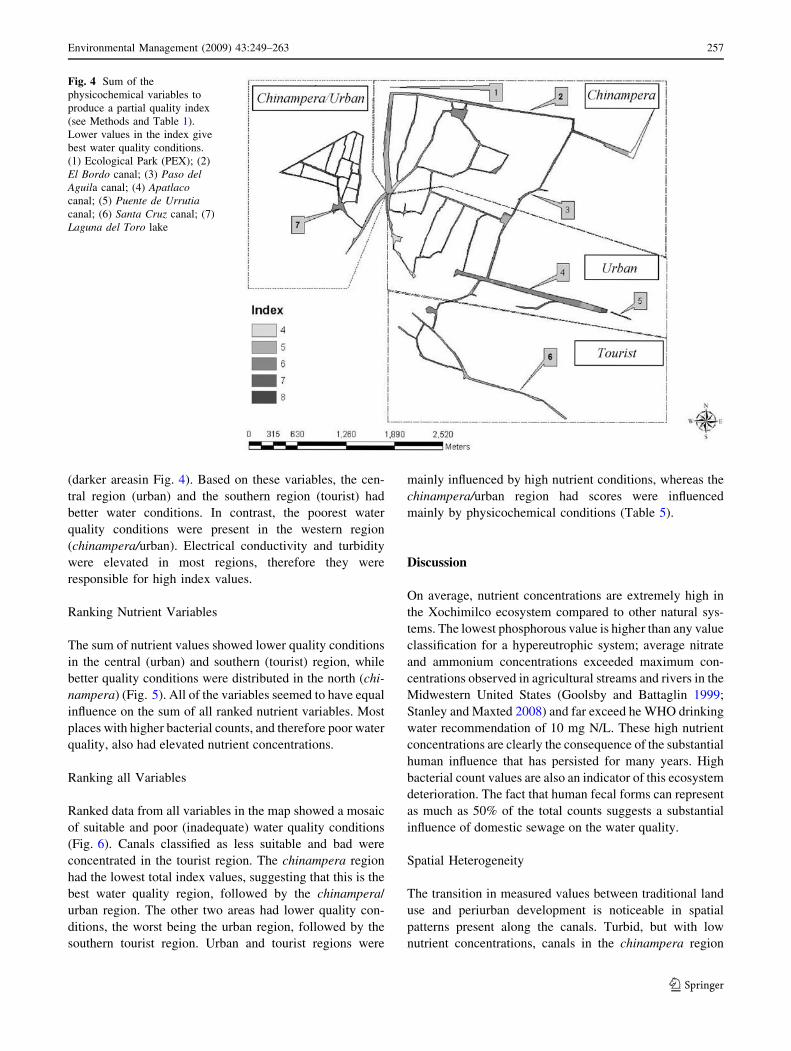
(darker areasin Fig. 4). Based on these variables, the cen-

tral region (urban) and the southern region (tourist) had

better water conditions. In contrast, the poorest water

quality conditions were present in the western region

(chinampera/urban). Electrical conductivity and turbidity

were elevated in most regions, therefore they were

responsible for high index values.

Ranking Nutrient Variables

The sum of nutrient values showed lower quality conditions

in the central (urban) and southern (tourist) region, while

better quality conditions were distributed in the north (chi-

nampera) (Fig. 5). All of the variables seemed to have equal

influence on the sum of all ranked nutrient variables. Most

places with higher bacterial counts, and therefore poor water

quality, also had elevated nutrient concentrations.

Ranking all Variables

Ranked data from all variables in the map showed a mosaic

of suitable and poor (inadequate) water quality conditions

(Fig. 6). Canals classified as less suitable and bad were

concentrated in the tourist region. The chinampera region

had the lowest total index values, suggesting that this is the

best water quality region, followed by the chinampera/

urban region. The other two areas had lower quality con-

ditions, the worst being the urban region, followed by the

southern tourist region. Urban and tourist regions were

mainly influenced by high nutrient conditions, whereas the

chinampera/urban region had scores were influenced

mainly by physicochemical conditions (Table 5).

Discussion

On average, nutrient concentrations are extremely high in

the Xochimilco ecosystem compared to other natural sys-

tems. The lowest phosphorous value is higher than any value

classification for a hypereutrophic system; average nitrate

and ammonium concentrations exceeded maximum con-

centrations observed in agricultural streams and rivers in the

Midwestern United States (Goolsby and Battaglin 1999;

Stanley and Maxted 2008) and far exceed he WHO drinking

water recommendation of 10 mg N/L. These high nutrient

concentrations are clearly the consequence of the substantial

human influence that has persisted for many years. High

bacterial count values are also an indicator of this ecosystem

deterioration. The fact that human fecal forms can represent

as much as 50% of the total counts suggests a substantial

influence of domestic sewage on the water quality.

Spatial Heterogeneity

The transition in measured values between traditional land

use and periurban development is noticeable in spatial

patterns present along the canals. Turbid, but with low

nutrient concentrations, canals in the chinampera region

Fig. 4 Sum of the

physicochemical variables to

produce a partial quality index

(see Methods and Table 1).

Lower values in the index give

best water quality conditions.

(1) Ecological Park (PEX); (2)

El Bordo canal; (3) Paso delAguila canal; (4) Apatlacocanal; (5) Puente de Urrutiacanal; (6) Santa Cruz canal; (7)

Laguna del Toro lake


123

contrast with those in the neighboring urban region,

which has a lower turbidity and higher nutrient concen-

trations. These variables maintained their values in the

two study seasons, suggesting that permanent factors such

as land use have a local influence on the water quality in

each region.

Land use is not the only possible cause of water quality

heterogeneity; physical barriers can play a role in this

variability. For example, in the chinampera/urban region,

substantial hydrologic isolation could determine its physi-

cochemical character of high conductivity and phosphate

concentration.

Fig. 5 Sum of the nutrient

variables to get the water quality

index (see Methods and

Table 1). Lower values in the

index give the best water quality

conditions. (1) Ecological Park

(PEX); (2) El Bordo canal; (3)

Paso del Aguila canal; (4)

Apatlaco canal; (5) Puente deUrrutia canal; (6) Santa Cruzcanal; (7) Laguna del Toro lake

Fig. 6 Sum of the nutrients and

physicochemical variables

together (see methods and

Table 1). Lower values in the

index gives best water quality

conditions. (1) Ecological Park

(PEX); (2) El Bordo canal; (3)

Paso del Aguila canal; (4)

Apatlaco canal; (5) Puente deUrrutia canal; (6) Santa Cruzcanal; (7) Laguna del Toro lake


123

High nutrient concentrations in a shallow system with an

average temperature close to 19�C throughout the year

(unpublished data) allow for high rates of primary pro-

duction. Such high productivity can be associated with a

variety of different biogeochemical and food web dynam-

ics (Mallin and others 2006), producing many paths of

energy flow within a small-scale area. For example, high

productivity increases water turbidity, which can modify

the food web reliance on benthic to pelagic organisms

within a few hundred meters (Zambrano and others 2008).

Therefore, an analysis based on point samples would create

difficulties in interpretation, and a broader-scale framework

is necessary for understanding the limnological dynamic

within this system.

Interpolation Technique

Interpolations helped to generate a two-dimensional picture

of water chemical dynamics in the Xochimilco freshwater

system. These interpolations can shed light on both pattern

and process in this intricate aquatic system. Different

interpolation methods were considered here. The lack of

relationship between physicochemical variables and land

use variables indicated the presence of other factors affect-

ing water quality at smaller spatial scales (e.g., heavy boat

traffic, nontreated sewage discharges, and strong localized

agriculture and urban influences). Therefore, it was not

possible to use extrapolation of land use variables to predict

water quality. Also, a Krigging method was tested but

required more data to produce reliable results (Kravchenko

2003). The inverse distance-weighted method used here is

simpler than others, but the interpolation method used was

based on the assumption that there is a linear relationship

among sampling points for all chemical variables, as shown

by Dent and Grimm (1999). Therefore, this method seems to

be accurate enough to achieve our goal of developing a

general pattern for this complicated system.

Water Quality Index

Generating an index based on environmental and biological

variables, such as the Index of Biological Integrity, has

been a common practice for evaluating ecosystem health

(Wang and others 2001). In a wider analysis, it is possible

to obtain information using all variables together to gen-

erate a composite value. This is particularly useful in

systems in which variables are not related and therefore

each individual variable cannot fully represent ecosystem

status. For example, high nutrient concentrations do not

necessarily result in large algal populations in shallow

systems (Zambrano and others 2001). Food web factors

such as top-down control (Carpenter and others 1985)

could generate a stable clear-water system with high

nutrient concentrations (Scheffer and others 2001). Con-

sequently, different variables apart from nutrient

concentrations must be considered to understand the tro-

phic status (Strobl and others 2007). In Xochimilco, the

oxygen concentration is sufficient to support resident biota

in the whole ecosystem, but there are regions in which

ammonium concentrations are often at levels considered

toxic for fish (Wetzel 2001). A single index value that

incorporates all these variables can be a simple, effective

means of providing qualitative information about overall

water suitability.

Because it is not possible to add data that have different

unit scales, ranking different variables allowed us to sum

the categories for each variable and derive a map of more

suitable, less suitable, and bad conditions. The categori-

zation also helps to simplify a description of the spatial

conditions. While the ranking reduces the opportunity to

understand the dynamics and processes driving each vari-

able, the information is easier to interpret and use for

resource managers and other stakeholders. Since the index

gives spatial information within a map, it is possible to

visualize specific activities in regions and relate them to

water quality. For instance, the effect of an industrial

corridor on water quality in the surrounding regions and its

consequences on organisms’ distribution or human health

in the neighborhood can easily be visualized using this

simple, spatially explicit index method.

We were able to use this index to describe the water

quality of a complex ecosystem such as Xochimilco and

relate it to human activities. The chinampera region has the

highest water quality values, but they are not homoge-

neous, improving in the northern part closer to the PEX and

being reduced along the urban region border. Index values

Table 5 Regional average (avg) for each variable using data obtained from the interpolation

Region DO (mg l-1) Turbidity (NTU) Conductivity (lS cm-1) NO3–N (mg l-1) NH4–N (mg l-1) PO4–P (mg l-1)

Avg SD Avg SD Avg SD Avg SD Avg SD Avg SD

Chinampera 6.78 2.30 68.90 29.79 0.70 0.08 6.97 3.67 0.77 0.50 6.32 3.00

Urban 7.13 2.99 45.58 21.72 0.85 0.10 9.64 3.67 1.97 0.31 8.84 1.03

Tourist 2.86 1.07 39.57 19.49 0.67 0.03 23.42 14.58 1.28 0.34 7.93 1.24

Chinampera/urban 3.72 1.21 49.49 14.24 1.02 0.13 3.03 4.50 1.22 0.27 10.04 0.90


123

can be related to its proximity to the artificial wetland in

the reserve area and to the traditional (low nutrient) agri-

culture activity. This is also complemented by measures of

low bacteriological density. The second-best-preserved

area, chinampera/urban, also includes the chinampas

farming technique, but the urban matrix in which it is

immersed possibly reduces its water quality index values,

which are higher in areas away from human settlements

such as Laguna del Toro. The second-worst conditions lie

in the tourist region, which has been urbanized, but has also

experienced rapid greenhouse development, which may

increase nutrient concentrations (mainly nitrate) (Lopez

and others 2006; Mendez 2006), in the northern area. The

urban region, with the lowest ranking values, has been

exposed to sewage going directly to canals (personal

observation), a product of intensive illegal urban devel-

opment and greenhouses that are spread throughout the

entire region. This results in homogeneous, low water

quality values in all the canals and lakes. It also may

explain the high ammonium values in most canals, which

are further exacerbated by added agrochemicals and man-

ure from cattle and pigs produced by nonregulated

agricultural activities. Higher bacterial densities in the

water also match this information.

The index also makes it possible to identify those

variables that have the greatest influence on water quality

within each region. By separating each standardized vari-

able on a map (see the Appendix), it is possible to weight

their contribution to the final results. In this case, the sum

of all nutrients seems to determine most of the areas with

higher index values. Within nutrient concentrations, it is

also possible to evaluate which elements produce spatial

heterogeneity. Here, even when phosphate caused high

index values in three of the four areas, ammonium and

nitrate were responsible for differences among regions in

the final calculation. Inverse patterns arise from the spatial

variation of these two nitrogen forms. While ammonium

was the major determinant of the sum ranks for the central

area, nitrate was the key variable in the southern area.

This index is also useful when analyzing species dis-

tribution patterns. The group of variables that we used to

form our water quality index is related to the survival

capacity of aquatic biota in the system. High heterogeneity

in water quality may produce local differences in the sur-

vival capacity of both native and exotic organisms

(Contreras 2006). A species’ distribution may be restricted

to isolated areas of suitable water quality (personal obser-

vation). Furthermore, food web structure may differ

dramatically among regions because of distinct biogeo-

chemical processes associated with contrasting water

quality (Zambrano and others 2008). Therefore, future

research must try to clarify the consequences of spatial

heterogeneity in water quality for native species in

Xochimilco. Such an analysis may suggest areas more

suitable for aquatic restoration and conservation of native

organisms such as the axolotl and native fish based on

increasing patch size and connectivity of areas with suffi-

cient water quality.

Conclusions

Human influence is capable of modifying the water quality

of freshwater environments in different regions, producing

aquatic ecosystems with pronounced small-scale spatial

heterogeneity. Such heterogeneity makes point-based data

more difficult to understand. The sum of the water quality

ranks index has been a useful approach for comparing

conditions among different regions within a complex,

interconnected ecosystem with many activities and variables

that influence its dynamics. These variables are related to

diverse ecological, economic, agricultural, and social issues,

and therefore there are multiple causes of water quality

changes in each region. An index representing the status of

the water quality spatially is intended to allow decision

makers to relate ecosystem health to human activities.

Despite the fact that Xochimilco is listed in RAMSAR

and UNESCO World Heritage, its water quality is

remarkably poor, and it clearly needs active management

to allow persistence of native species and human use of the

water. Information provided by this index can generate

possibilities for a better management strategy of the entire

water system. Some of these actions seem quite obvious,

such as prohibiting the discharge of wastewater without

adequate treatment. But other activities present more dif-

ficult management challenges, such as the influence of

agricultural nutrients on the aquatic ecosystem. Traditional

agriculture methods seem to be extremely efficient and

possibly have limited ecological effects on the system.

However, to increase the use of these agricultural practices,

they must be linked to economic incentives to make them

feasible. We hope that this type of approach will assist

decision makers in managing and sustaining the ecosystem.

Acknowledgments We thank PASPA and Posgrado de Ciencias

Biologicas de la UNAM. This project was supported by Instituto

Nacional de Ecologıa, SEMARNAT, and CONACYT (Project No.

32505-T, 1999/2001). We would also like to thank Pilar Islas, Rosa I.

Amieva, Josue Sandoval, Elsa Valiente, and Roberto Altamirano for

their help with the data gathering and lab work. We are grateful to

Emily Stanley for her invaluable suggestions about the manuscript.

Appendix

Geographical Interpolation of Each Abiotic Variable

Within Xochimilco Canals and Lakes Fig A1.


123

Fig. A1 Interpolations from physicochemical and nutrient variables,

using the index built based on more suitable to less suitable

categories. Higher values (darker regions on the map) give less

suitable conditions of the water quality based on each variable: (a)

dissolved oxygen; (b) turbidity; (c) electrical conductivity; (d) nitrate

concentration; (e) ammonium concentration; (f) phosphate concen-

tration. Numbers relate to the name of the canals or areas: (1)

ecological park (PEX); (2) El Bordo canal; (3) Paso del Aguila canal;

(4) Apatlaco canal; (5) Puente de Urrutia canal; (6) Santa Cruz canal;

(7) Laguna del Toro lake


123

References

APHA, American Water Works Association, Water Environment

Federation (1998) Standard methods for the examination of

water and wastewater, 20th edn. APHA, Washington, DC

Blumenthal UJ, Mara DD, Peasey A, Ruiz-Palacios G, Stott R

(2000) Guidelines for the microbiological quality of treated

wastewater used in agriculture: recommendations for revising

WHO guidelines. Bulletin of the World Health Organization

78:1104–1116

Brooks SS, Palmer MA, Cardinale BJ, Swan CM, Ribblett S (2002)

Assessing stream ecosystem rehabilitation: limitations of com-

munity structure data. Restoration Ecology 10:156–168

Brown BL (2003) Spatial heterogeneity reduces temporal variability

in stream insect communities. Ecology Letters 6:316–325

Camargo JA, Alonso A, Salamanca A (2004) Nitrate toxicity to aquatic

animals: a review with new data for freshwater invertebrates.

Chemosphere 58:1255–1267

Carpenter S, Kitchell J, Hodgson JR (1985) Cascading trophic

interactions in a lake productivity. Bioscience 35:634–639

Cheng S-Y, Chen J-C (2002) Study on the oxyhemocyanin, deoxy-

hemocyanin, oxygen affinity and acid-base balance of

Marsupenaeus japonicus following exposure to combined ele-

vated nitrite and nitrate. Aquatic Toxicology 61:181–193

Comin FA, Romero JA, Hernandez O, Menendez M (2001) Resto-

ration of wetlands from abandoned rice fields for nutrient

removal, and biological community and landscape diversity.

Restoration Ecology 9:201–208

Contreras REAV (2006) Distribucion potencial del Ambystomamexicanum en los canales de la zona chinampera de Xochimilco.

Universidad Nacional Autonoma de Mexico, Mexico, DF

DDF (Departamento del Distrito Federal) (1975) Memoria de las

obras del sistema de drenaje profundo del Distrito Federal.

Talleres Graficos de la Nacion

Dent CL, Grimm NB (1999) Spatial heterogeneity of streamwater

nutrient concentrations over successional time. Ecology 80:

2283–2298

De Robertis A, Ryer HC, Veloza A, Brodeur RD (2003) Differential

effects of turbidity on prey consumption of piscivorous and

planktivorous fish. Canadian Journal of Fisheries and Aquatic

Sciences 60:1517–1526

DOF (Departamento del Distrito Federal) (2004) Ley Federal de

Derechos. Disposiciones aplicables en materia de aguas nacio-

nales. GDF, Mexico

DOF (Departamento del Distrito Federal) (2005) Capitulo VIII Agua.

Ley Federal de Derechos, Mexico, DF, pp 183–190

Douterelo I, Perona E, Mateo P (2004) Use of cyanobacteria to assess

water quality in running waters. Environmental Pollution 127:

377–384

Dufour A, Gadallah F, Wagner HH, Guisan A, Buttler A (2006) Plant

species richness and environmental heterogeneity in a mountain

landscape: effects of variability and spatial configuration.

Ecography 29:573–584

Engstroem-Oest J, Candolin U (2007) Human-induced water turbidity

alters selection on sexual displays in sticklebacks. Behavioral

Ecology 18:393–398

Geldrich E, Kenner BA (1969) Comments on fecal streptococci in

stream pollution. Journal of Water Pollution Control Federation

41:336–341

George DG, Talling JF, Rigg E (2000) Factors influencing the

temporal coherence of five lakes in the English Lake District.

Freshwater Biology 43:449–461

Goolsby DA, Battaglin WA (1999) Long-term changes in the

concentration and flux of nitrogen in the Mississippi River

Basin, USA. Hydrological Processes 15:1209–1222

Gundale MJ, Metlen KL, Fiedler CE, DeLuca TH (2006) Nitrogen

spatial heterogeneity influences diversity following restoration in

a ponderosa pine forest, Montana. Ecological Applications

16:479–489

Guo Z, Li Y, Gan Y (2003) Spatial pattern of ecosystem function and

ecosystem conservation. Environmental Management 32:682–692

Harper D (1992) Eutrophication of freshwaters. Principles, problems

and restoration. Chapman and Hall, New York

Hill B (1971) Principles of medical statistics. Oxford University

Press, New York

Instituto de Geografia, Universidad Nacional Autonoma de Mexico

(2002) Fotomosaico escala 1:5000. Mexico

Kemka N, Njine T, Togouet SHZ, Menbohan SF, Nola M, Monkiedje

A, Niyitegeka D, Compere P (2006) Eutrophication of lakes in

urbanized areas: the case of Yaounde Municipal Lake in

Cameroon, Central Africa. Lakes & Reservoirs: Research and

Management 11:47–55

Kravchenko AN (2003) Influence of spatial structure on accuracy of

interpolation methods. Soil Science Society of American Journal

67:1564–1571

Lopez A, Guerrero M, Hernandez C, Aguilar A (2006) Rehabilitacion de

la zona chinampera. In: Carballo C (ed) Xochimilco. Un proceso de

gestion participativa. GDF-UNESCO, Mexico, pp 201–218

Mallin MA, Johnson VL, Ensign SH, MacPherson TA (2006) Factors

contributing to hypoxia in rivers, lakes, and streams. Limnology

and Oceanography 51:690–701

Matejicek L, Engst P, Janour Z (2006) A GIS-based approach to

spatio-temporal analysis of environmental pollution in urban

areas: a case study of Pragues environment extended by LIDAR

data. Ecological Modelling 199:261–277

Muhando CA, Kuguru BL, Wagner GM, Mbije NE, Oehman MC

(2002) Environmental effects on the distribution of Corallimor-

pharians in Tanzania. Ambio 31:558–561

Mendez A (2006) Rehabilitacion de la zona chinampera. In: Carballo

C (ed) Xochimilco. Un proceso de gestion participativa. GDF-

UNESCO, Mexico, pp 219–221

Nienhuis P, Bakker J, Grootjans A, Gulati R, de Jonge V (2002) The

state of the art of aquatic and semi-aquatic ecological restoration

projects in the Netherlands. Hydrobiologia 478:219–233

Reid SM, Fox M, Whillans T (1999) Influence of turbidity on

piscivory in largemouth bass (Microptherus salmoides). Cana-

dian Journal of Fisheries and Aquatic Sciences 56:1362–1369

Robinson CT, Tockner K, Ward JV (2002) The fauna of dynamic

riverine landscapes. Freshwater Biology 47:661–677

Scheffer M, Rinaldi S (2000) Minimal models of top-down control of

phytoplankton. Freshwater Biology 45:265–283

Scheffer M, Carpenter S, Foley RJA, Walker B (2001) Catastrophic

shifts in ecosystems. Nature 413:591–596

Shivoga WA, Muchiri M, Kibichi S, Odanga J, Miller SN, Baldyga

TJ, Maina-Gichaba C (2006) Impacts of upland land use on

downstream water quality in River Njoro Watershed, Kenya. In:

Proceedings of the 11th International Conference and the

Conservation and Management of Lakes, vol II, pp 472–476,

31 October to 4 November. Nairobi, Kenya

Sokal RR, Rohlf FJ (1981) Biometry. The principles and practice of

statistics in biological research. W.H. Freeman, New York

Strobl RO, Forte F, Pennetta L (2007) Application of artificial neural

networks for classifying lake eutrophication status. Lakes &

Reservoirs: Research and Management 12:15–25

Stanley E H, Maxted JT (2008) Changes in the dissolved nitrogen

pool across land cover gradients in Wisconsin streams. Ecolog-

ical Applications 18:1579–1590

Toranzos GA, McFeters GA, Borrego JJ, Savill AM (2007) Detection

of microorganisms in environmental freshwaters and drinking

waters. In: Hurst CJ, Crawford RL, Garland JL, Lipson DA,


123

Mills AL, Stetzenbach LD (eds) Manual of environmental

microbiology. ASM Press, Washington, DC, pp 249–264

Tveito OE, Bjorad I, Skjelvag AO, Une BA (2005) A GIS-base agro-

ecological decision system based on gridded climatology.

Meterological Application 12:57–68

UNESCO (2006) Water, a shared responsibility. Bergham Books,

New York

Valsanen U, Misund A, Chekushin V (1998) Ecogeochemical

investigation: stream water quality as an indicator of pollution

in the border areas of Finland, Norway and Russia. Water Air

and Soil Pollution 104:205–219

Wang LZ, Lyons J, Kanehl P (2001) Impacts of urbanization on

stream habitat and fish across multiple spatial scales. Environ-

mental Management 28:255–266

Wetzel R (2001) Limnology. Lake and river ecosystems. Academic

Press, San Diego, CA

Zambrano L, Scheffer M, Martinez-Ramos M (2001) Catastrophic

response of lakes to benthivorous fish introduction. Oikos 94:344–350

Zambrano L, Valiente E, Vander Zanden MJ (2008) Spatial variation

in food web structure of a highly heterogeneous freshwater

system: role of nutrient enrichment and species introductions

(submitted for publication)


123

Spatial Heterogeneity of Water Quality in a Highly Degraded Tropical Freshwater Ecosystem

Documents

Transcript of Spatial Heterogeneity of Water Quality in a Highly Degraded Tropical Freshwater Ecosystem