Software Challenges for Extreme Heterogeneity

Vivek Sarkar Professor, School of Computer Science

Stephen Fleming Chair for Telecommunications, College of Computing Georgia Institute of Technology

2

Habanero Extreme Scale Lab (as of Fall 2017)

§  Faculty §  Vivek Sarkar

§  Research Scientists §  Akihiro Hayashi, Jun Shirako,

Jisheng Zhao §  Postdoctoral Researchers

§  Tiago Cogumbreiro, Max Grossman, Farzad Khorasani

§  Graduate Students §  Kumud Bhandari, Prasanth

Chatarasi, Arghya Chatterjee, Sana Damani, Ankush Mandal, Sriraj Paul, Fangke Ye, Lechen Yu

§  Acknowledgments §  Research supported in part by

DARPA, DoD, DOE, NSF

3

Focus of our research is on software enablement of parallel algorithms on a wide range of extreme scale platforms

http://habanero.rice.edu Extreme Heterogeneity

Platforms

Parallel Algorithms Habanero

Programming Models

Habanero Compilers & Parallel IRs

Habanero Runtime Systems

Languages: DFGL, OpenMP extensions Libraries: Habanero-C/C++, Habanero-Java, Habanero-Scala

Structured-parallel execution model 1) Lightweight asynchronous tasks and data transfers §  Creation: async tasks, future tasks, data-driven tasks §  Termination: finish, future get, await §  Data Transfers: asyncPut, asyncGet 2) Locality control for task and data distribution §  Computation and Data Distributions: hierarchical places, global name space 3) Inter-task synchronization operations §  Mutual exclusion: isolated, actors §  Collective and point-to-point operations: phasers, accumulators

Compiler Extensions for explicit parallelism: Polyhedral+AST optimizers for C/C++ programs (src-to-src, LLVM), bytecode optimizers for Java Runtime Extensions for asynchronous tasks, data transfers, heterogeneity: Habanero-C++, Open Community Runtime (OCR), HC-MPI, HJlib cooperative runtime

4

Levels of Disruption in Moore’s Law End-Game and Post-Moore eras

36 C O M P U T E R W W W . C O M P U T E R . O R G / C O M P U T E R

OUTLOOK

to scale computer performance. How-ever, engineering software for the von Neumann architecture is itself a dif-ficult endeavor. Adding the need for explicit programming of parallelism is largely untenable to the software industry as a whole. Thus, the solution has been successful for HPC, a realm in which software rewriting is consid-ered an acceptable investment, and the result has been computer performance increases only for select applications.

Reaching the power wall has impli-cations for more than the PC industry. The PC–microprocessor ecosystem has driven down the cost of mainstream processors to an attractively low price fostered by the continual increase in logic IC volume. Consequently, these microprocessors and other ecosys-tem elements have migrated upward, affecting much more complex systems such as high-performance computers .

PROPOSED WAYS FORWARDAttendees at the RCI’s four past sum-mits reached consensus on the idea

that any solutions to extending com-puting performance and efficiency would have to radically depart from the straightforward interpretation of Moore’s law. As a 2015 IEEE Spectrum article put it,5

Today’s technology makes a 1-exaflops supercomputer capable of performing 1 million trillion floating-point operations per second almost inevitable. But pushing supercomputing beyond that point to 10 exaflops or more will require major changes in both computing technologies and computer architectures.

To address that requirement, the RCI meetings covered a range of solutions to the impending end of current com-puting paradigms, which can be char-acterized in terms of disruption to the computing stack, as Figure 2 shows.

Non−von Neumann computingThe most radical approaches rethink

computing from the ground up, and will require new algorithms, lan-guages, and so on. Chief among these is quantum computing, which uses properties of quantum mechanics to solve problems in optimization, search, and whole number theory. Although a quantum computer can be used as a universal computing plat-form, it will be no better than a con-ventional computer outside a limited set of problems. However, the quan-tum computer’s advantage is so large for some of those problems that it has the potential to shake the foundation of conventional scientific, engineer-ing, business, and security practices. For example, a working quantum com-puter could factor the product of two large primes in a nanosecond,6 which undermines asymmetric-key encryp-tion. This encryption standard, which is central to every facet of e-commerce and national security, is based on the notion that such factoring is computa-tionally intractable.

Another non−von Neumann ap-proach is neuromorphic computing, which leverages what is known about the human brain’s operation to create new computing technologies. Neuro-morphic computers do not attempt to replicate the brain, but rather draw from the neuroscientific aspects that enable humans to solve problems with great efficiency, such as recognizing and classifying patterns in text, au-dio, or images. Neuromorphic com-puters can be simulated on modern computers, but the true energy effi-ciencies come from specialized hard-ware built specifically for the task.

Neuromorphic algorithms differ greatly from traditional algorithms and overlap the important discipline of machine learning. The indus-try can now simulate neuromorphic

Algorithm

Language

API

Architecture

Instruction-setarchitecture

Microarchitecture

Function unit

Logic

Device More “Moore”

1

No disruption Total disruption

2 3 4

Hiddenchanges

Architecturalchanges

Non–von Neumann

computing

FIGURE 2. Four future computing approaches and the extent to which they disrupt the traditional computing stack (left). At the far right (level 4) are non−von Neumann archi-tectures, which completely disrupt all stack levels, from device to algorithm. At the least disruptive end (level 1) are more “Moore” approaches, such as new transistor technology and 3D circuits, which affect only the device and logic levels. Hidden changes are those of which the programmer is unaware.

Source: “Rebooting Computing: The Road Ahead”, T.M.Conte, E.P.DeBenedictis, P.A.Gargini, E.Track, IEEE Computer, 2017.

At the far right (level 4) are non−von Neumann architectures, which completely disrupt all stack levels, from device to algorithm. At the least disruptive end (level 1) are more “Moore” approaches, such as new transistor technology and 3D circuits, which affect only the device and logic levels. Hidden changes are those of which the programmer is unaware.

5

Range of Approaches (and disruptions!) for Memory-Centric Processing

6

Non-Von Neumann approaches promise even larger levels of disruption, e.g., use of Quantum Computing as an Accelerator

§ 6

20  mK

0.1  K

4  K

77KHost

Quantum  Substrate

Control  Processor

300  K

Memory(Cryo-­‐CMOS)

High  Density  Superconducting  Control  Wires

Low  density  metal  Interconnects

Source: Moin Qureshi, Georgia Tech

7

Another example of a possible analog accelerator …

Deep learning with coherent nanophotonic circuitsYichen Shen1*†, Nicholas C. Harris1*†, Scott Skirlo1, Mihika Prabhu1, Tom Baehr-Jones2,Michael Hochberg2, Xin Sun3, Shijie Zhao4, Hugo Larochelle5, Dirk Englund1 and Marin Soljačić1

Artificial neural networks are computational network models inspired by signal processing in the brain. These models havedramatically improved performance for many machine-learning tasks, including speech and image recognition. However,today’s computing hardware is inefficient at implementing neural networks, in large part because much of it was designedfor von Neumann computing schemes. Significant effort has been made towards developing electronic architectures tunedto implement artificial neural networks that exhibit improved computational speed and accuracy. Here, we propose a newarchitecture for a fully optical neural network that, in principle, could offer an enhancement in computational speed andpower efficiency over state-of-the-art electronics for conventional inference tasks. We experimentally demonstrate theessential part of the concept using a programmable nanophotonic processor featuring a cascaded array of 56 programmableMach–Zehnder interferometers in a silicon photonic integrated circuit and show its utility for vowel recognition.

Computers that can learn, combine and analyse vast amountsof information quickly, efficiently and without the need forexplicit instructions are emerging as a powerful tool for hand-

ling large data sets. ‘Deep learning’ algorithms have received anexplosion of interest in both academia and industry for theirutility in image recognition, language translation, decision-makingproblems and more1–4. Traditional central processing units(CPUs) are suboptimal for implementing these algorithms5, and agrowing effort in academia and industry has been directedtowards the development of new hardware architectures tailoredto applications in artificial neural networks (ANNs) and deep learn-ing6. Graphical processing units (GPUs), application-specific inte-grated circuits (ASICs) and field-programmable gate arrays(FPGAs)2,5,7–11, including IBM TrueNorth5 and Google TPU11,have improved both energy efficiency and speed enhancement forlearning tasks. In parallel, hybrid optical–electronic systems thatimplement spike processing12–14 and reservoir computing15–18 havebeen demonstrated.

Fully optical neural networks (ONNs) offer a promising alterna-tive approach to microelectronic and hybrid optical–electronicimplementations. ANNs are a promising fully optical computingparadigm for several reasons. (1) They rely heavily on fixedmatrix multiplications. Linear transformations (and certain non-linear transformations) can be performed at the speed of light anddetected at rates exceeding 100 GHz (ref. 19) in photonic networksand, in some cases, with minimal power consumption20,21. Forexample, it is well known that a common lens performs a Fouriertransform without any power consumption and that certainmatrix operations can also be performed optically without consum-ing power. (2) They have weak requirements on nonlinearities.Indeed, many inherent optical nonlinearities can be directly usedto implement nonlinear operations in ONNs. (3) Once a neuralnetwork is trained, the architecture can be passive, and computationon the optical signals will be performed without additional energyinput. These features could enable ONNs that are substantiallymore energy-efficient and faster than their electronic counterparts.However, implementing such transformations with bulk opticalcomponents (such as fibres and lenses) has been a major barrier

so far because of the need for phase stability and large neuroncounts22. Integrated photonics addresses this problem by providinga scalable solution to large, phase-stable optical transformations23.

Here, we begin with a theoretical proposal for a fully opticalarchitecture for implementing general deep neural network algor-ithms using nanophotonic circuits that process coherent light.The speed and power efficiency of our proposed architecture islargely enabled by coherent, fully optical matrix multiplication(a cornerstone of neural network algorithms). Under the assump-tion of practical, centimetre-scale silicon photonic die sizes andlow waveguide losses, we estimate that such an ONN wouldenable forward propagation that is at least two orders of magnitudefaster than state-of-the-art electronic or hybrid optical–electronicsystems, and with a power consumption that is nearly proportional(instead of quadratic, as in electronics) to the number of neurons(for more details see the discussion about scaling in the Methods).Next, we experimentally demonstrate the essential component ofour scheme by embedding our proposed optical interference unit(OIU) and diagonal matrix multiplication unit within a subset ofthe programmable nanophotonic processor (PNP), a photonic inte-grated circuit developed for applications in quantum information pro-cessing23. To test the practical performance of our theoreticalproposal, we benchmarked the PNP on a vowel recognitionproblem, which achieved an accuracy comparable to a conventional64-bit computer using a fully connected neural network algorithm.

ONN device architectureAn ANN1 consists of a set of input artificial neurons (representedas circles in Fig. 1a) connected to at least one hidden layer andthe output layer. In each layer (depicted in Fig. 1b), informationpropagates by a linear combination (for example, matrix multi-plication) followed by the application of a nonlinear activationfunction. ANNs can be trained by feeding training data into theinput layer and then computing the output by forward propa-gation; matrix entries (weights) are subsequently optimized usingback propagation24.

The ONN architecture is depicted in Fig. 1b,c. As shown inFig. 1c, the task (an image, a vowel or a sentence to be recognized)

1Research Laboratory of Electronics, Massachusetts Institute of Technology, Cambridge, Massachusetts 02139, USA. 2Elenion, 171 Madison Avenue, Suite1100, New York, New York 10016, USA. 3Department of Mathematics, Massachusetts Institute of Technology, Cambridge, Massachusetts 02139, USA.4Department of Biology, Massachusetts Institute of Technology, Cambridge, Massachusetts 02139, USA. 5Université de Sherbrooke, Administration, 2500Boulevard de l’Université, Sherbrooke, Quebec J1K 2R1, Canada. †These authors contributed equally to this work. *e-mail: ycshen@mit.edu; n_h@mit.edu

ARTICLESPUBLISHED ONLINE: 12 JUNE 2017 | DOI: 10.1038/NPHOTON.2017.93

NATURE PHOTONICS | VOL 11 | JULY 2017 | www.nature.com/naturephotonics 441

© 2017 Macmillan Publishers Limited, part of Springer Nature. All rights reserved.

is first preprocessed to a high-dimensional vector on a computerwith a standard algorithm (this step is computationally inexpensivecompared with inference). The preprocessed signals are thenencoded in the amplitude of optical pulses propagating in thephotonic integrated circuit, which implements a many-layerONN. Each layer of the ONN is composed of an OIU thatimplements optical matrix multiplication and an optical nonlinear-ity unit (ONU) that implements the nonlinear activation. In prin-ciple, the ONN can implement an ANN of arbitrary depth anddimensions fully in the optical domain.

To realize an OIU that can implement any real-valued matrix, wefirst note that a general, real-valued matrix (M) may be decomposedasM=UΣV† through singular value decomposition (SVD)25, whereU is an m ×m unitary matrix, Σ is an m × n rectangular diagonalmatrix with non-negative real numbers on the diagonal and V† isthe complex conjugate of the n × n unitary matrix V. It has beenshown theoretically that any unitary transformations U,V† can beimplemented with optical beamsplitters and phase shifters26,27.Finally, Σ can be implemented using optical attenuators—opticalamplification materials such as semiconductors or dyes could alsobe used28. Matrix multiplication with unitary matrices implementedin the manner above consumes, in principle, no power. The fact thata major proportion of ANN calculations involve matrix productsenables the extreme energy efficiency of the ONN architecturepresented here.

The ONU can be implemented using common optical non-linearities such as saturable absorption29–31 and bistability32–36,which have all been demonstrated previously in photonic circuits.For an input intensity Iin, the optical output intensity is given bya nonlinear function Iout = f(Iin)37. In this Article, we will consideran f that models the mathematical function associated with arealistic saturable absorber (such as a dye, semiconductor orgraphene saturable absorber or saturable amplifier) that could, infuture implementations, be directly integrated into waveguidesafter each OIU stage of the circuit. For example, graphene layersintegrated on nanophotonic waveguides have already been

demonstrated as saturable absorbers38. Saturable absorption is mod-elled as29 (Supplementary Section 2)

στsI0 =12ln (Tm/T0)1 − Tm

(1)

where σ is the absorption cross-section, τs is the radiative lifetime ofthe absorber material, T0 is the initial transmittance (a constant thatonly depends on the design of the saturable absorbers), I0 is the inci-dent intensity and Tm is the transmittance of the absorber. Given aninput intensity I0, one can solve for Tm(I0) from equation (1) andthe output intensity can be calculated as Iout = I0·Tm(I0). A plot ofthe saturable absorber’s response function Iout(Iin) is shown inSupplementary Section 2.

A schematic diagram of the proposed fully optical neuralnetwork is shown in Fig. 1d.

ExperimentWe evaluated the practicality of our proposal by experimentallyimplementing a two-layer neural network trained for vowel recog-nition. To prepare the training and testing data sets, we used 360data points, each consisting of four log area ratio coefficients39 ofone phoneme. The log area ratio coefficients, or feature vectors, rep-resent the power contained in different logarithmically spaced fre-quency bands and are derived by computing the Fouriertransform of the voice signal multiplied by a Hamming windowfunction. The 360 data points were generated by 90 differentpeople speaking four different vowel phonemes40. We used half ofthese data points for training and the remaining half to test the per-formance of the trained ONN. We trained the matrix parametersused in the ONN with the standard back-propagation algorithmusing a stochastic gradient descent method41 on a conventionalcomputer. Further details on the data set and back-propagation pro-cedure are included in Supplementary Section 3.

The OIU was implemented using a PNP23—a silicon photonicintegrated circuit fabricated in the OPSIS foundry42. This was

X1

X2

X3

X4

Y1

Y2

Y3

Y4

Z(1) = W0X h(i) = f (Z(i)) Y = Wnh(n)

Input layerHidden layers

Output layer

a b

c

d

Vowel X

M(1) = U(1) Σ(1) V(1) M(2) M(n−1) M(n)

fNL () fNL ()

Photonic integrated circuit

Layer i Layer n

Optical input Optical output

Layer 1X Y

xin xout

Waveguide

0

0

Optical interference unit Optical nonlinearity unit

0

0Σ(n)V(n) U(n) fNL

h1(1)

h2(1)

h3(1)

h4(1)

h1(i)

h2(i)

h3(i)

h4(i)

h1(n)

h2(n)

h3(n)

h4(n)

Figure 1 | General architecture of the ONN. a, General artificial neural network architecture composed of an input layer, a number of hidden layers and anoutput layer. b, Decomposition of the general neural network into individual layers. c, Optical interference and nonlinearity units that compose each layer ofthe artificial neural network. d, Proposal for an all-optical, fully integrated neural network.

ARTICLES NATURE PHOTONICS DOI: 10.1038/NPHOTON.2017.93

NATURE PHOTONICS | VOL 11 | JULY 2017 | www.nature.com/naturephotonics442

© 2017 Macmillan Publishers Limited, part of Springer Nature. All rights reserved.

8

Common themes: extreme heterogeneity, specialization, hybrid systems

Extreme Heterogeneity Workshop

– POC: Lucy Nowell(Lucy.Nowell@science.doe.gov)– Goal: Identify Priority Research Directions for

Computer Science needed to make future supercomputers usable, useful and secure for science applications in the 2025-2035 timeframe

– Primary focus on the software stack and programming models/environments

– 120 expected participants: DOE Labs, academia, & industry

– Observers from DOE and other federal agencies– Planning: Factual Status Document (FSD) is under

development, with outreach planned.• White papers to be solicited to contribute to the

FSD, identify potential participants, and help refine the agenda

• Report due early May 2018

46ASCAC Presentation 9/26/2017CP

U

Digital

GPU

FPGA

System SoftwareOS, Runtime

Quan

tum

Neur

omor

phic

Othe

rs

Compilers, Libraries, Debuggers

Applications

Non-Digital

Tentatively planned for Jan. 23-25, 2018, in D.C. area.

Heterogeneous Memories

Heterogeneous Interconnects

Increased diversity in – Processors and memory/storage technology – Workflows, including data-intensive analysis, interactive supercomputing, and near-real-time requirements – Volume, variety and velocity of data – User base, as increasing numbers of applications (e.g., deep learning) need high-performance computing

. . .

9

Opportunities for Order-of-Magnitude Improvements through Hardware-Software Customization (Old Example)

648 Mbits/sec ASM Pentium III [3] 41.4 W 0.015 (1/800)

Java [5] Emb. Sparc 450 bits/sec 120 mW 0.0000037 (1/3,000,000)

C Emb. Sparc [4] 133 Kbits/sec 0.0011 (1/10,000)

350 mW

Power

1.32 Gbit/sec FPGA [1]

11 (1/1) 3.84 Gbits/sec 0.18mm CMOS

Figure of Merit (Gb/s/W)

Throughput AES 128bit key 128bit data

490 mW 2.7 (1/4)

120 mW

ASM StrongARM [2] 240 mW 0.13 (1/85) 31 Mbit/sec

Source: P Schaumont and I Verbauwhede, "Domain specific codesign for embedded security," IEEE Computer 36(4), 2003 [1] Amphion CS5230 on Virtex2 + Xilinx Virtex2 Power Estimator [2] Dag Arne Osvik: 544 cycles AES – ECB on StrongArm SA-1110 [3] Helger Lipmaa PIII assembly handcoded + Intel Pentium III (1.13 GHz) Datasheet [4] gcc, 1 mW/MHz @ 120 Mhz Sparc – assumes 0.25 u CMOS [5] Java on KVM (Sun J2ME, non-JIT) on 1 mW/MHz @ 120 MHz Sparc – assumes 0.25 u CMOS

10

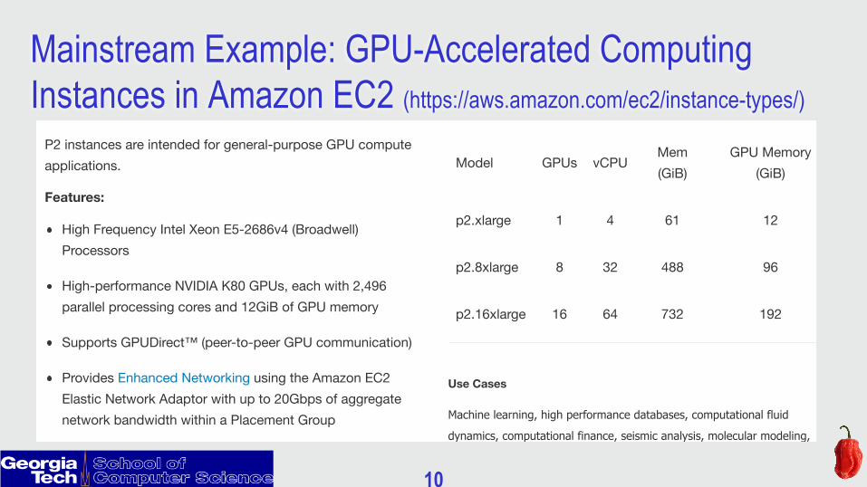
Mainstream Example: GPU-Accelerated Computing Instances in Amazon EC2 (https://aws.amazon.com/ec2/instance-types/)

∠

∠

∠

∠

∠

∠

∠

∠

Amazon EC2

Product Details

Instances

Pricing

Developer Resources

FAQs

Getting Started

Amazon EC2 Run Command

RELATED LINKS

Amazon EC2 Dedicated Hosts

Amazon EC2 Spot Instances

Amazon EC2 Reserved Instances

Amazon EC2 Dedicated Instances

Windows Instances

VM Import/Export

AWS Management Portal for vCenter

Management Console

Documentation

Release Notes

Discussion Forum

Amazon EC2 SLA

Run Command

Get Started for Free

Create Free Account

Accelerated Computing Instances

P2P2 instances are intended for general-purpose GPU compute

applications.

Features:

High Frequency Intel Xeon E5-2686v4 (Broadwell)

Processors

High-performance NVIDIA K80 GPUs, each with 2,496

parallel processing cores and 12GiB of GPU memory

Supports GPUDirect™ (peer-to-peer GPU communication)

Provides Enhanced Networking using the Amazon EC2

Elastic Network Adaptor with up to 20Gbps of aggregate

network bandwidth within a Placement Group

EBS-optimized by default at no additional cost

Model GPUs vCPUMem

(GiB)

GPU Memory

(GiB)

p2.xlarge 1 4 61 12

p2.8xlarge 8 32 488 96

p2.16xlarge 16 64 732 192

Use Cases

Machine learning, high performance databases, computational fluid

dynamics, computational finance, seismic analysis, molecular modeling,

genomics, rendering, and other server-side GPU compute workloads.

G2G2 instances are optimized for graphics-intensive applications.

Features:

High Frequency Intel Xeon E5-2670 (Sandy Bridge)

Processors

High-performance NVIDIA GPUs, each with 1,536 CUDA

cores and 4GB of video memory

Each GPU features an on-board hardware video encoder

designed to support up to eight real-time HD video streams

(720p@30fps) or up to four real-time full HD video streams

(1080p@30fps)

Support for low-latency frame capture and encoding for

either the full operating system or select render targets,

enabling high-quality interactive streaming experiences

Model GPUs vCPU Mem (GiB) SSD Storage (GB)

g2.2xlarge 1 8 15 1 x 60

g2.8xlarge 4 32 60 2 x 120

Use Cases

3D application streaming, video encoding, and other server-side graphics

workloads.

Storage Optimized

I2 – High I/O InstancesThis family includes the High Storage Instances that provide

very fast SSD-backed instance storage optimized for very high

random I/O performance, and provide high IOPS at a low cost.

Features:

High Frequency Intel Xeon E5-2670 v2 (Ivy Bridge)

Processors

SSD Storage

Support for TRIM

Support for Enhanced Networking

High Random I/O performance

Model vCPUMem

(GiB)Storage (GB)

i2.xlarge 4 30.5 1 x 800 SSD

i2.2xlarge 8 61 2 x 800 SSD

i2.4xlarge 16 122 4 x 800 SSD

i2.8xlarge 32 244 8 x 800 SSD

Use Cases

NoSQL databases like Cassandra and MongoDB, scale out

transactional databases, data warehousing, Hadoop, and

cluster file systems.

11

Mainstream Example: FPGA Computing Instances in Amazon EC2 (https://aws.amazon.com/ec2/instance-types/)

Source: https://aws.amazon.com/ec2/instance-types/f1

How it Works

DEVELOP

Develop custom

Amazon FPGA Images

(AFI) using the Hardware

Development Kit (HDK)

and full set of design

tools and simulators.

DEPLOY

Deploy your AFI directly

on F1 instances and

take advantage of all the

scalability, agility, and

security benefits of EC2.

OFFER

Offer AFIs you design on

the AWS Marketplace

for other customers.

PURCHASE

Purchase AFIs built and

listed on AWS

Marketplace to quickly

implement common

hardware accelerations.

12

Accelerators in Top500

§ 12

§  Lack of code portability is already a significant issue, and it is becoming worse. §  After years of effort, less than half of codes running on DOE supercomputers use GPUs and

still fewer use them effectively. §  Extreme Heterogeneity in computer architectures is relatively new, and not well understood

by the HPC community. Source: http://www.slideshare.net/top500/top500-list-november-2014?related=1

13

Heterogeneous Hardware leads to “Hybrid Programming” … 1.  for (int step = 0; step < nsteps; step++) {2.  stencil<<<grid, block, shared_size>>>(d_next, d_curr, ...);3.  if (rank < nprocs - 1) {4.  // copy up to the next rank and receive from it5.  cudaMemcpy(h_next + ..., d_next + ...);6.  MPI_Isend(h_next + ..., ...);7.  MPI_Irecv(h_next + ..., ...);8.  } 9.  . . .10.  if (rank < nprocs - 1) {11.  MPI_Wait(&high_send_request);12.  MPI_Wait(&high_recv_request);13.  cudaMemcpy(d_next + ..., h_next + ...);14.  } 15. }

14

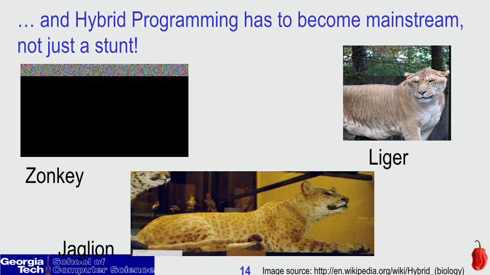
… and Hybrid Programming has to become mainstream, not just a stunt!

Zonkey Liger

Jaglion Image source: http://en.wikipedia.org/wiki/Hybrid_(biology)

15

Why is Hybrid Programming a hard problem? §  Each heterogeneous hardware component has its own

programming model and performance constraints §  e.g., multicore CPU, manycore CPU, GPU, DSP, FPGA, ASIC, …

§  Current approaches to integrating heterogeneous programming models can lead to challenging outcomes §  Unpredictable semantics, unpredictable performance, challenges

in functional and performance debugging, …

16

Our Approach: Hybrid by Design

§  If your starting point is a general unified execution model for extreme scale computing, then “hybridizations” can be viewed as orthogonal combinations of features, e.g., §  Accelerator parallelism + Multicore parallelism + Cluster parallelism §  Heterogeneous memories §  Distributed compute (includes near-memory computation) §  . . .

§  Key benefits: semantic guarantees, performance portability

17

Habanero Execution Model underlies all our software research 1) Lightweight asynchronous tasks and data transfers §  Creation: async tasks, future tasks, data-driven tasks §  Termination: finish, future get, await §  Data Transfers: asyncPut, asyncGet 2) Locality control for control and data distribution §  Computation and Data Distributions: hierarchical places, global name space 3) Inter-task synchronization operations §  Mutual exclusion: global/object-based isolation, actors §  Collective and point-to-point operations: phasers, accumulators Claim: these execution model primitives enable programmability, portability, performance, and debuggability for extreme scale software and hardware

18

Pedagogy using Habanero execution model §  Sophomore-level CS Course at Rice (http://comp322.rice.edu)

§  Approach: “Simple things should be simple, complex things should be possible” §  Introduce students to fundamentals of parallel programming

§  Primitive constructs for task creation & termination, collective & point-to-point synchronization, task and data distribution, and data parallelism

§  Parallel algorithms & data structures including lists, trees, graphs, matrices §  3-course introductory Coursera specialization on “Parallel, Concurrent and Distributed

Programming in Java” launched on 7/31/2017 (http://bit.ly/pcdpjava) §  Approach: use pedagogy from Rice COMP 322 course to target Java developers who

have never before taken a course on parallel programming §  Future plan: create online specialization on parallel programming in C++ based on

Habanero execution model, targeted to first-year graduate students (Masters & PhD)

19

Example: Habanero abstraction of a CUDA kernel invocation

async at(GPU1)

async at(GPU2)

forall(blockIdx)

forallPhased(threadIdx)

20

Target Platforms Habanero execution model is being mapped to a wide range of platforms §  Current/past systems

§  Multicore SMPs (IBM, Intel) §  Discrete GPUs (AMD, NVIDIA), Integrated GPUs (AMD, Intel) §  FPGA (Convey) §  HPC Clusters, Hadoop/Spark Clusters §  Embedded processors: TI Keystone

§  Future systems §  Members of “Rogues Gallery” in Georgia Tech’s Center for Research into Novel

Computing Hierarchies (CRNCH): Emu Chick, 3D Stacked Memories w/ FPGAs, Neuromorphic Hardware, …

21

3D Stacked Memories with FPGAs

§  Rogues Gallery includes traditional FPGA platforms (Arria 10, Ultrascale+) and stacked memory variants

§  Enables “near-memory” and memory-centric processing. §  FPGA platforms enable prototypes of non-traditional accelerators like

Automata, Sparse data engines, etc. §  Current work in CRNCH is supported in part by Micron hardware donation.

3D Stacked Memory and FPGAs

• Rogues Gallery includes traditional FPGA platforms (Arria

10, Ultrascale+) and stacked memory variants

• Enable “near-memory” and memory-centric processing.

• FPGA platforms enable prototypes of non-traditional

accelerators like Automata, sparse data engines, etc.

• Current work is supported in part by Micron hardware

donation.

CRNCH Rogues Gallery — 3 Nov 2017 9/16

22

Emu Chick

§  “Migratory Memory Side Processing” to exploit weak locality. §  Data for graph edge attributes, documents, etc. reside nearby even if

accessed irregularly. §  Moving threads to data on reads means all accesses are local, common

case needs to tolerate less latency.

Emu Chick

• “Migratory Memory Side Processing” to

exploit weak locality.

• Data for graph edge attributes, documents /

medical records, etc. reside nearby even if

accessed irregularly.

• Moving threads to data on reads means all

accesses are local, common case needs to

tolerate less latency.

Gossamer CPU

Memory

Gossamer CPU

Memory

Migrate on read

CRNCH Rogues Gallery — 3 Nov 2017 8/16

// Habanero abstraction of // remote read of location A at (HOME(A)) { continuation after reading A, . . . }

23

Outline for rest of talk

§  Type system & inference for place locality (Programming Model)

§  Optimized Two-Level Parallelization for GPUs (Compiler)

§  Hierarchical Place Tree for Locality, Heterogeneity, and Distribution (Runtime)

24

Place Types

Memory-Centric Programming with Places

HERE THERE

int xT f

T g

T p

p.xq = p.fr = p.gr.x

T q

T r

Type inference for locality analysis of distributed data structures. Satish Chandra, Vijay Saraswat, Vivek Sarkar, Ras Bodik. PPoPP 2008.

25 12/3/17

Memory-Centric Programming with Places

HERE THERE

int xT f

T g

T p

at (r) r.x

T q

T r

objects don’t migrate, so migrate the computation over there to read a value

26 12/3/17 12/3/17 Place Types

Memory-Centric Programming with Places

HERE THERE

int xT f

T g

T p

at (r) r.x

T q

T r

r.x

T q

T p

T r

at (r) q.xq.x

27

Example: Evenly Distributed Binary Tree

28

Example (contd.) 1.   class DarkNode { 2.   DarkNode@! left; 3.   DarkNode@! right;

4.   5.   int count () { 6.   return left.count() + 7.   right.count() + 1;

8.   } 9.   }

1.   class LightNode { 2.   Node@? left; 3.   Node@! right;

4.   5.   int count () { 6.   int l = at (left) left.count(); 7.   int r = right.count();

8.   return l + r + 1; 9.   } 10.  }

29

Summary of results §  Type system for places: in a distributed program with at

statements, ensure that all dereferences are local §  Based on an equality-based constraint system §  Therefore admits standard type inference machinery §  Includes support for distributed arrays

§  Algorithm for automatic inference of place types

30

Outline for rest of talk

§  Type system & inference for place locality (Programming Model)

§  Optimized Two-Level Parallelization for GPUs (Compiler)

§  Hierarchical Place Tree for Locality, Heterogeneity, and Distribution (Runtime)

31

§ Polyhedral model §  Algebraic framework for affine program optimizations

§  Unified view that captures arbitrary loop structures §  Generalized loop transformations as form of affine transform

§  Significant advancements over traditional AST-based transformations § Polyhedral compilation for GPUs (focus of this work) §  End-to-end frameworks

§  C-to-CUDA [M. Baskaran, et al., CC 2010] §  R-Stream [A. Leung, et al., GPGPU 2010] §  PPCG [S. Verdoolaege, et al., TACO 2013] §  This work [J. Shirako & V. Sarkar, CC 2017]

§  Input: Sequential C. Output: Optimized CUDA/OpenCL.

Polyhedral Compilation Frameworks

32

§  Two levels of parallelism within a GPU kernel §  Threads (inner level): inter-thread barriers supported within a block §  Blocks (outer level): limited inter-block synchronization

§  Memory hierarchy management §  Explicit data transfers between global and shared (local) memories

shared memory

block 0 Grid

global memory

threads with sync shared memory

block 1

threads with sync ... shared memory

block N-1

threads with sync

No synchronization supported among blocks

GPU Execution Model

33

Past work: PPCG Polyhedral Optimizer §  Coarse-grained parallelization policy [TACO 2013]

§  Compute polyhedral schedule (loop transformations) based on PLuTo algorithm developed for CPUs §  Map the outermost parallel loop in the schedule to both GPU blocks & threads // Input (variant of Jacobi-2d)for (t = 0; t < T; t++) { for (i = 1; i < N-1; i++) for (j = 1; j < N-1; j++) B[i][j] = (A[i][j] + A[i][j-1] + A[i][j+1]) / 3.0; for (i = 1; i < N-1; i++) for (j = 1; j < N-1; j++) A[i][j] = B[i][j];}

•  i-loop •  synchronization-free parallelism

•  j-loop •  cross-iteration dependence •  accesses inner array dimension

// Output of PPCG (CUDA kernel)b0 = blockIdx.x; // i-tile (block-x)t0 = threadIdx.x; // i (thread-x)for (c1 = 0; c1 <= T-1; c1+=32) for (c2 = 2 * c1; c2 <= ...; c2+=32) { if (...) for (c4 = ...; c4 <= ...; c4+=1) for (c5 = ...; c5 <= ...; c5+=1) { if (N + 2 * c1 + 2 * c4 >= c2 + c5 + 2) B[32*b0+t0][-2*c1+c2-2*c4+c5] = ...; if (g7+c3 >= 2*g5+2*c2+2) A[32*b0+t0][-2*g5+g7-2*c2+c3-1] = ...; } }

i-loop is mapped to blocks & threads j-loop is executed sequentially; no memory coalescing

// Output of PPCG (CUDA kernel)b0 = blockIdx.x; // i-tile (block-x)t0 = threadIdx.x; // i (thread-x)for (c1 = 0; c1 <= T-1; c1+=32) // t-tile for (c2 = 2 * c1; c2 <= ...; c2+=32) { // j-tile if (...) for (c4 = ...; c4 <= ...; c4+=1) // t for (c5 = ...; c5 <= ...; c5+=1) { // j if (N + 2 * c1 + 2 * c4 >= c2 + c5 + 2) B[32*b0+t0][-2*c1+c2-2*c4+c5] = ...; if (g7+c3 >= 2*g5+2*c2+2) A[32*b0+t0][-2*g5+g7-2*c2+c3-1] = ...; } }

34

Our Work: Optimized Two-level Parallelization for GPUs

§  Existing polyhedral approaches to GPUs §  Compute schedule — i.e., transformations — based on PLuTo algorithm §  Map the outermost parallelism in schedule to blocks & threads

§  Fundamentally same optimizations between block and thread §  Block-level : synchronization-free parallelism is mandatory §  Thread-level : can include barriers, important to coalesce memory accesses

•  Our approach: two-level parallelization for GPUs •  Compute two schedules with different optimization policies

•  Block-level : outermost synchronization-free parallelism •  Thread-level : parallelism with good coalescing + inter-thread synchronizations

•  Superposition to integrate block-level and thread-level schedules •  DL memory cost model to maximize coalesced memory access for threads

Optimized Two-Level Parallelization for GPU Accelerators using the Polyhedral Model. Jun Shirako, Akihiro Hayashi, Vivek Sarkar. CC 2017.

35 §

35

§  Polyhedral model §  Algebraic framework for affine program representations & transformations §  Unified view that captures arbitrary loop structures §  Generalize loop transformations as form of affine transform

§  Polyhedral representations (SCoP format) §  Domain 𝐷Si : set of statement instances for statement Si §  Access 𝑨Si : mapping an instance to array element(s) to be accessed §  Schedule 𝚯Si : mapping an instance to lexicographical time stamp (time mapping)

§  Extended in our work with a space mapping,

Polyhedral Compilation Framework

36 §

36

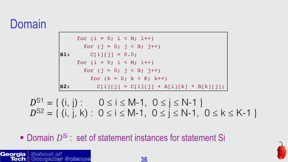
§ Domain 𝐷Si : set of statement instances for statement Si

for (i = 0; i < M; i++) for (j = 0; j < N; j++)S1: C[i][j] = 0.0; for (i = 0; i < M; i++) for (j = 0; j < N; j++) for (k = 0; k < K; k++)S2: C[i][j] = C[i][j] + A[i][k] * B[k][j];

𝐷S1 = { (i, j) : 0 ≤ i ≤ M-1, 0 ≤ j ≤ N-1 }"𝐷S2 = { (i, j, k) : 0 ≤ i ≤ M-1, 0 ≤ j ≤ N-1, 0 ≤ k ≤ K-1 }"

Domain

37

•  Schedule 𝚯Si(i): mapping statement instance i to "time stamp" vector •  Statement instances are executed in lexicographical order of schedules

•  Transformation = new schedule that optimizes performance while obeying dependences

Example of Schedule Transformation (Time Mapping)

§

37

for (i = 0; i < M; i++) for (j = 0; j < N; j++)S1: C[i][j] = 0.0; for (i = 0; i < M; i++) for (j = 0; j < N; j++) for (k = 0; k < K; k++)S2: C[i][j] = C[i][j]

+ A[i][k] * B[k][j];

𝚯S1(i, j) = (0, i, j)"𝚯S2(i, j, k) = (1, i, j, k)"

𝚯S1(i, j) = (0, i, j, 0)"𝚯S2(i, j, k) = (0, i, j, 1, k)"transformation"

for (i = 0; i < M; i++) { for (j = 0; j < N; j++) {S1: C[i][j] = 0.0; for (k = 0; k < K; k++)S2: C[i][j] = C[i][j] + A[i][k] * B[k][j]; } }

codegen"

38 §

38

§  Space-mapping 𝚯Si(i): mapping instance i to (logical) processor id §  Represents parallelism, no sequential ordering across processor ids

§  Time mapping can be used to order instances mapped to the same processor id

// high-level forall forall (i = 0; i < M; i++) forall (j = 0; j < N; j++)S1: C[i][j] = 0.0;

// CUDA threads in a block i = threadIdx.y; j = threadIdx.x;S1: C[i][j] = 0.0;

𝚯S1(i, j) = (iy, jx)"

Example of Schedule Transformation (Space Mapping)

39

Composition of Time- and Space-mapping

§

39

§  Scattering function §  In a multidimensional scattering function, some dimensions represent time-mappings while others

represent space-mappings §  Captures both sequential loop transformations and parallelization in a single

𝚯S1 = (t, 0, iy, jx)"𝚯S2 = (t, 1, iy, jx)"

// Jacobi-2d kernel (CUDA threads) for (t = 0; t < T; t++) { i = threadIdx.y + …; j = threadIdx.x + …;S1: B[i][j] = (A[i][j] + A[i][j-1] + A[i][j+1]) / 3.0; __syncthreads(); i = threadIdx.y + …; j = threadIdx.x + …;S2: A[i][j] = B[i][j]; __syncthreads(); }

Space-mapping dimensions are annotated with subscripts

// Jacobi-2d kernel (high-level forall) for (t = 0; t < T; t++) { forall (i = …; i < …; i++) forall (j = …; j < …; j++)S1: B[i][j] = (A[i][j] + A[i][j-1] + A[i][j+1]) / 3.0; barrier; forall (i = …; i < …; i++) forall (j = …; j < …; j++)S2: A[i][j] = B[i][j]; barrier; }

40 §

40

§  Transformations and parallelization §  Thread-level transformations

§  Extended memory cost model (DL model) to GPU memory warps §  Detect loop parallelism with good coalesced memory access; map to the innermost thread dimension

§  Block-level transformations (independent of thread-level transformations) §  Detect & map sync-free parallelism to block dimensions

§  Superposed into final scattering function §  Shared memory and register optimizations

1.  Individual tiles are identified after superposition 2.  Array elements to be used/modified within each tile are computed 3.  Insert data transfers to/from shared memory or registers

Overall Flow for our approach

41 §

41

§  Two scattering functions per statement §  Block-level scattering function, 𝚯Sout(i)

§  Many-to-one function to assign multiple instances i to same value

§  Must be fully permutable

§  Thread-level scattering function, 𝚯S(i) §  One-to-one function to assign each instance i to a unique value

§  Superposition as loop tiling §  Block-level: specify inter-tile schedule (individual tiles) §  Thread-level: specify intra-tile schedule (iterations within a tile)

Superposition

42

Schedule for original code:"𝚯S1 = (t, 0, i, j)"𝚯S2 = (t, 1, i, j)"

// Input (variant of Jacobi-2d)for (t = 0; t < T; t++) { for (i = 1; i < N-1; i++) for (j = 1; j < N-1; j++)S1: B[i][j] = (A[i][j] + A[i][j-1] + A[i][j+1]) / 3.0; for (i = 1; i < N-1; i++) for (j = 1; j < N-1; j++)S2: A[i][j] = B[i][j];}

Block scattering function:"𝚯S1 out = (ix)"𝚯S2 out = (ix)"

Thread scattering function:"𝚯S1 = (t, 0, iy, jx)"𝚯S2 = (t, 1, iy, jx)"

Superposed scattering function:"𝚯S1 = (⎣ix / 32⎦, t, 0, iy, jx)"𝚯S2 = (⎣ix / 32⎦, t, 1, iy, jx)"

(assumes tile size of 32)"

superposition"

// Superposed (final code)c1 = blockIdx.x; // i-tile (blk-x)for (c5 = 0; c5 <= T-1; c5++) { // t c3 = 32 * c1 + threadIdx.y; // i (thrd-y) if (c3 >= 1 && c3 <= N-2) { for (c7 = 0; c7 <= …; c7++) { // j-tile c9 = 32 * c7 + threadIdx.x; // j (thrd-x) if (c9 >= 1 && c9 <= N-2)S1: B[c3][c9] = … }} __syncthreads(); c3 = 32 * c1 + threadIdx.y; // i (thrd-y) if (c3 >= 1 && c3 <= N-2) { for (c7 = 0; c7 <= …; c7++) { // j-tile c9 = 32 * c7 + threadIdx.x; // j (thrd-x) if (c9 >= 1 && c9 <= 1998)S2: A[c3][c9] = B[c3][c9]; }} __syncthreads();}}} codegen"

Example of Superposition

43

Profitability Analysis via DL Memory Cost Function

§

43

§  Loop with best memory coalescing §  Partial derivative of memory cost w.r.t. Tk :

§  Reduction rate of memory cost when increasing Tk

§  Parallel loop with most negative value → most profitable loop for memory cost minimization → mapped to innermost thread dimension

§  Profitability of loop fusion §  Comparing mem_cost(T1, T2, ..., Td) before and after fusion

§  Memory cost decreased → fusion is profitable §  Other criteria, e.g., loss of parallelism, are also considered

∂mem_cost(T1, T2, ..., Td) ∂Tk

44 §

44

§  Platforms §  Intel Xeon X5660 + NVIDIA Tesla M2050 GPU (Fermi)

§  13SM x 32-core, total 448 CUDA Cores

§  IBM POWER8 + NVIDIA Tesla K80 GPU (Kepler) §  14SMX x 192-core, total 2496 CUDA Cores

§  Benchmarks (sequential C programs) §  PolyBench-C 3.2 §  SPEC Accel : 314.omriq and 357.sp (two kernels from x_solve)

§  Experimental variants §  Sequential : gcc -O3 on CPU §  PPCG : Polyhedral Parallel Code Generator from INRIA §  PolyAST+GPU : Two-level parallelization for GPUs (proposed)

Experimental Setup

45

Speedup vs. CPU sequential GCC (Fermi 448-core)

§  block-level : PolyAST+GPU has same schedule as PPCG §  thread-level : different schedules due to superposition and coalescing policy §  PPCG has more efficient code generation method (e.g., # threads can be ≤ block size) §  Geometric mean speedup : 44.8× by PPCG and 85.9× by PolyAST+GPU

§  Relative improvement of our work over PPCG ~ 1.8x

0.6

46

Speedup vs. CPU sequential GCC (Kepler 2496-core)

§  block-level : PolyAST+GPU has same schedule as PPCG §  thread-level : different schedules due to superposition and coalescing policy §  PPCG has more efficient code generation method (e.g., # threads can be ≤ block size) §  Geometric mean speedup : 45.6× by PPCG and 95.5× by PolyAST+GPU

§  Relative improvement of our work over PPCG ~ 2.1x

0.3 0.5

47

Outline for rest of talk

§  Type system & inference for place locality (Programming Model)

§  Optimized Two-Level Parallelization for GPUs (Compiler)

§  Hierarchical Place Tree for Locality, Heterogeneity, and Distribution (Runtime)

48

Load Balancing with Work-Stealing Schedulers

w1

pop tasks

push tasks

w2 w3 w4

steal tasks deque

tail

head

Core Core Core Core

Urgent need for extensions that support

locality with work-stealing

49

Locality-aware Scheduling for CPUs using the Hierarchical Place Tree (HPT) abstraction

§  Model target system as a tree/hierarchy §  Workers attached to leaf places §  Each place has a queue

§  async at(<pl>) <stmt>: push task on place pl’s queue §  Destination place can be determined by programmer, compiler or runtime

§  Current policy (can also be applied to distributed work-stealing) §  A worker executes tasks from ancestor places from bottom-up

§  W0 executes tasks from PL3, PL1, PL0 §  Tasks in a place queue can be executed by all workers in its subtree

§  Task in PL2 can be executed by workers W2 or W3

PL1 PL2

PL0

PL3

w0 PL4

w1

PL5

w2

PL6

w3

Hierarchical Place Trees: A Portable Abstraction for Task Parallelism and Date Movement. Yonghong Yan, Jisheng Zhao, Yi Guo, Vivek Sarkar. LCPC 2009.

50

……

Extending HPT with Tuning Tree for Temporal Locality

Affinity  Group  A     A,  1   A,2   A,3  

…Tuning Tree

(Staging area) Hierarchical Place Tree

(Execution Area)

w0

…

w1

w3

“Declarative Tuning for Locality in Parallel Programs.” Sanjay Chatterjee, Nick Vrvilo, Zoran Budimlic, Kathleen Knobe, Vivek Sarkar. ICPP 2016

51

A,  1  A,2   A,3  

……

w0 Tuning Tree

(Staging area) Hierarchical Place Tree

(Execution Area)

…

w1

w3

Group  A    

…

Use of HPT for Tuning Locality (contd)

52

w0 S,  1  S,2  

Tuning Tree (Staging area)

Hierarchical Place Tree (Execution Area)

……

…

w1

w3

…A,3  

Use of HPT for Tuning Locality (contd)

53

Distributed Work-Stealing

Intra-node steals

Inter-node steals

Inter-node steals are much costlier than intra-node steals

Optimized Distributed Work-Stealing. Vivek Kumar, Karthik Murthy, Vivek Sarkar and Yili Zheng. IA^3 2016

54

Our Approach

§  Use HabaneroUPC++ PGAS library for multicore cluster [Kumar et. al., PGAS 2014] §  Several asynchronous tasking APIs

§  Provide a programming model to express irregular computation §  Implement a high performance distributed work-stealing runtime that

completely removes all inter-node failed steal attempts

Nod

e_A

Nod

e_X

One process with a thread pool at each node

55

HabaneroUPC++ Programming Model

§  C++11 lambda-function based API §  Provides serial elision and improves productivity

asyncAny ( [=] {

irregular_computation();

}); //distributed work-stealing

56

Distributed Work-Stealing Runtime

§  Two different implementations in HabaneroUPC++ §  BaselineWS

§  Uses prior work + some optimizations §  SuccessOnlyWS

§  Extends BaselineWS by using a novel victim selection policy that complete removes all inter-node failed steals

§  See paper for details

§ Implementation

57

Extending the HPT abstraction for heterogeneous architectures & accelerators

PL0

PL1 PL2

PL3 PL4 PL5 PL6

PL7 PL8

W0 W1 W2 W3

W4 W5

§  Devices (GPU or FPGA) are represented as memory module places and agent workers

§  GPU memory configuration is fixed, while FPGA memory can be reconfigured at runtime

§  async at(P) S §  Creates new task to execute statement S at place P

PL

PL

PL

PL

Physical memory

Cache GPU memory

Reconfigurable FPGA Implicit data movement Explicit data movement

Wx CPU computation worker Wx Device agent worker

58

D1

R1

S1

…

D2

R2

S2

S2S1

R2R1

Instances of steps Dstolen by CPU or GPU

An instance of step R stolen by GPU

Steps of type S launched at a GPU place

CPU1

env

D2D1

CPU2 GPU FPGA

Steps of type R launched at a FPGA place

Steps D launched at a CPU place

Dedicated device queues

CPU only tasks

}  DFGL graph representation extended with affinity annotations: }  < C > :: ( D @CPU=20,GPU=10); }  < C > :: ( R @GPU=5, FPGA=10); }  < C > :: ( S @GPU=12);

}  [ IN : k-1 ] → ( D : k ) → [ IN2 : k+1 ]; }  [ IN2 : 2*k ] → ( R : k ) → [ IN3 : k/2 ]; }  [ IN3 : k ] → ( S : k ) → [ OUT : IN3[k] ];

}  env → [ IN : { 0 .. 9 } ], < C : { 0 .. 9 } >; }  [ OUT : 1 ] → env;

Adding Affinity Annotations for Heterogeneous Computing to CnC-inspired Dataflow Model

“Mapping a Data-Flow Programming Model onto Heterogeneous Platforms.” Alina Sbirlea, Yi Zou, Zoran Budimlic, Jason Cong, Vivek Sarkar. LCTES 2012

59

Hybrid Scheduling with Heterogeneous Work Stealing ♦  Steps are compiled for execution on CPU, GPU or FPGA

§  Aim for single-source multi-target compilation! ♦  Designate a CPU core as a proxy worker for heterogeneous device ♦  Device inbox is now a concurrent queue and tasks can be stolen by

CPU or other proxy workers

PL7 Continuations stolen by CPU workers

W4

tail head tail head

Device tasks stolen by CPU and other device workers

Device tasks created from CPU worker via

async at(gpl) IN() OUT() { … }

60

Intel® Xeon® Processor Intel®

Memory Controller Hub (MCH)

Intel® I/O Subsystem Memory Memory

Application Engine Hub (AEH)

Application Engines (AEs)

“Commodity” Intel Server Convey FPGA-based coprocessor

Standard Intel® x86-64 Server x86-64 Linux

Convey coprocessor FPGA-based Shared cache-coherent memory

Xeon Quad Core LV5408 40W TDP

Tesla C1060 100GB/s off-chip bandwidth 200W TDP

XC6vlx760 FPGAs 80GB/s off-chip bandwidth 94W Design Power

Convey HC-1ex Testbed

61

Static vs Dynamic Scheduling

§  Static Schedule

§  Dynamic Schedule

}  < C > :: ( D @CPU=20,GPU=10); }  < C > :: ( R @GPU=5, FPGA=10); }  < C > :: ( S @GPU=12);

62

Experimental Results for Medical Imaging Workload •  Execution times and active energy for dynamic vs.

static scheduling on heterogeneous processors

63

Conclusions §  Habanero execution model enables multiple levels of parallelism and

heterogeneity by bridging from programming models to extreme scale systems.

§  Well-designed execution model primitives can enable synergistic innovation across all levels of software+hardware stack

§  Habanero group is gearing up to address programming model, compiler and runtime system challenges in Georgia Tech’s Center for Novel Computer Hierarchies (CRNCH)