Iterative multiframe super-resolution algorithms for atmospheric turbulence-degraded imagery

978 J. Opt. Soc. Am. A/Vol. 15, No. 4 /April 1998 Sheppard et al.

Iterative multiframe superresolution algorithmsfor atmospheric-turbulence-degraded

imagery

David G. Sheppard, Bobby R. Hunt, and Michael W. Marcellin

Department of Electrical and Computer Engineering, University of Arizona, Tucson, Arizona 85721

Received May 28, 1997; revised manuscript received October 13, 1997; accepted October 27, 1997

The subject of interest is the superresolution of atmospheric-turbulence-degraded, short-exposure imagery,where superresolution refers to the removal of blur caused by a diffraction-limited optical system along withrecovery of some object spatial-frequency components outside the optical passband. Photon-limited space ob-ject images are of particular interest. Two strategies based on multiple exposures are explored. The first isknown as deconvolution from wave-front sensing, where estimates of the optical transfer function (OTF) asso-ciated with each exposure are derived from wave-front-sensor data. New multiframe superresolution algo-rithms are presented that are based on Bayesian maximum a posteriori and maximum-likelihood formulations.The second strategy is known as blind deconvolution, in which the OTF associated with each frame is unknownand must be estimated. A new multiframe blind deconvolution algorithm is presented that is based on aBayesian maximum-likelihood formulation with strict constraints incorporated by using nonlinear reparam-eterizations. Quantitative simulation of imaging through atmospheric turbulence and wave-front sensing areused to demonstrate the superresolution performance of the algorithms. © 1998 Optical Society of America[S0740-3232(98)01604-4]

OCIS codes: 010.7060, 010.0010, 100.0100.

1. INTRODUCTIONThe study of space objects (SO) such as satellites, orbitaldebris, and meteors is growing in importance as moreplatforms are sent into orbit. To avoid collisions withSO’s, it is necessary to observe and catalog them by usinghigh-resolution images so that their orbits can be deter-mined and used to predict future positions. Most, if notall, SO images are acquired by ground-based optical sys-tems that observe through the Earth’s atmosphere, andtherein lies the problem. Atmospheric-turbulence-induced optical distortions cause severe blurring and arean obstacle to obtaining high-resolution SO images.Diffraction-limited optical systems impose resolutionlimitations, as well, but the atmospheric distortion is theprimary resolution-limiting factor for large-aperture in-struments. Restoration of SO imagery involves the re-moval of both effects.1

The focus of this paper is on restoration of SO imagerywith superresolution. Superresolution algorithms pro-duce a restored image in which details too fine to be re-solved by the optical system are revealed, or superre-solved. Superresolution may be defined more formally asthe removal of blur caused by a diffraction-limited opticalsystem along with meaningful recovery of the object’sspatial-frequency components outside the optical system’spassband.2

In noise, full recovery of the original object is not pos-sible, and a solution must be defined as an element of aset of feasible solutions. Knowledge about the originalscene is used to constrain the solution and reduce the sizeof the feasible solution set. Typical examples of suchknowledge are (1) a limited region of support in which the

0740-3232/98/040978-15$15.00 ©

object of interest is smaller than the extent of the imageand (2) image positivity due the physical nature of light.The potent combination of support and positivity con-straints is the basis for most superresolution work. Animportant recent theoretical result in superresolution re-search provides a lower bound for accurate spatial-frequency recovery from this combination of constraints,where it is shown to be inversely proportional to the sizeof the object region of support and the noise level in theimage.2

There are many approaches to image restoration in theliterature, but not all can superresolve. For example, lin-ear, shift-invariant methods such as generalized inversefiltering and optimal Wiener filtering cannotsuperresolve.2 An example of a linear, shift-variant su-perresolution algorithm is the closed-form solution3 to theGerchberg–Papoulis algorithm,4 also known as a projec-tion onto convex sets (POCS) algorithm. However, mostsuperresolution algorithms are nonlinear and have beenderived from Bayesian maximum-likelihood5–7 and maxi-mum a posteriori (MAP) estimates8,9 to name a few. Formore information on superresolution history and back-ground, see the recent survey by Hunt.10

The superresolution algorithms presented below for SOimages are based on processing sequences of short-exposure images. There are two reasons for so doing.First, the atmospheric-turbulence distortions are notvarying during image acquisition. This curbs the loss ofinformation caused by averaging the time-varying distor-tion. Second, using sequences of images is an effectiveway to control the noise that is due to the low light levelsin short-exposure images.11 Processing such images is

1998 Optical Society of America

Sheppard et al. Vol. 15, No. 4 /April 1998 /J. Opt. Soc. Am. A 979

difficult because most restoration techniques requireknowledge of the distortions affecting each of the imagesin the sequence. Fortunately, this information can begained from an auxiliary measurement by using a wave-front sensor (WFS) system. These systems measure thedistortion of the optical wave front appearing in the tele-scope pupil. Restoration from WFS data is referred to asdeconvolution from wave-front sensing (DWFS) withinthe astronomical community.12 The restoration algo-rithms presented below are intended to address the re-quirement for advanced image restoration algorithms forDWFS. They are extensions of the Poisson MAPalgorithm8,9 to the multiframe problem.

In the absence of WFS data, one must turn to eitherspeckle interferometry with phase recovery or blind de-convolution. Within the astronomical community thereis growing interest in blind deconvolution, in which thedistortion affecting each image is unknown and must berecovered during the deconvolution process. That thismethod can be successful may sound too good to be true,but some surprisingly good results have been presentedrecently.13–17 The key to making these methods work isthe application of a priori knowledge about the nature ofthe degradations and the images. Using multiple differ-ently blurred frames is in itself a powerful constraint onthe restored original object image. The algorithms pre-sented below extend the work of Conan and Thiebaut17 tothe multiframe problem and are based on Bayes maxi-mum likelihood criteria for Poisson data.

The following sections provide an overview of the as-sumptions made concerning image formation through at-mospheric turbulence, a survey of image restoration in at-mospheric turbulence, presentation of the algorithms,and simulation results.

2. IMAGE FORMATION THROUGHATMOSPHERIC TURBULENCEA. Diffraction-Limited Image FormationThe process of image formation is central to the super-resolution problem. In this work, it is assumed thatquasi-monochromatic incoherent light energy propagatesfrom object plane sources through an intervening mediumand the telescope optical system, to an image plane. Theobject and image plane irradiance distributions will be de-noted by f(j, h) and g(x, y), respectively. The mediumand the optical system together constitute a mapping, de-noted by the operator L$ • %, between the object and im-age spaces.

A general statement of the process is given by

g~x, y ! 5 L$f~j, h!% ( n~x, y !, (1)

where ( n(x, y) refers to a point-by-point operationwith the noise process n(x, y). In the absence of a dis-ruptive medium, a rigorous expression for the operatorL$ • % can be derived from scalar diffraction theory.Diffraction-limited optical systems convert divergingspherical waves to spherical waves converging to a pointon the image plane, or, in other words, are in focus. Alinear, spatially shift-invariant relationship exists be-tween the object and image plane irradiance

distributions.18 The image formation process can there-fore be described as a convolution,

g~x, y ! 5 E2`

` E2`

`

h~x 2 j, y 2 h !f~j, h!djdh ( n~x, y !

5 ~h * f !~x, y ! ( n~x, y !, (2)

where the notation (h * f )(x, y) refers to the convolutionof f with the optical system point-spread function (PSF)h.

B. Modeling of Atmospheric-Turbulence EffectsThe atmosphere through which a telescope must view anobject possesses a stochastic index of refraction structurethat is a function of inhomogeneities in temperature andhumidity. In astronomy, a distinction is commonly madebetween short-exposure and long-exposure images. Dur-ing short-exposure image acquisition, the turbulencestructure of the atmosphere is effectively frozen, and theimage is distorted by the instantaneous turbulence struc-ture. Such images are generally referred to as speckleimages because of their modulated appearance. In spiteof the severity of the image degradation, there is spatial-frequency information about the object up to the diffrac-tion limit of the telescope encoded in the image.11,19

The relationship between resolution and turbulence isfairly complex and can be expressed in terms of the coher-ence function of the wave-front phase and Strehl’s crite-rion as originally derived by Fried.20 Fundamentally,resolution is limited by the telescope if the aperture diam-eter is smaller than the so-called Fried parameter r0 .And the resolution is limited by atmospheric distortionwhen the aperture is larger than r0 . The Fried param-eter is widely used to gauge the quality of the seeing atany given moment. Large values of r0 imply better see-ing. A value of 10 cm is considered canonical.

Atmospheric distortion effects can be incorporated intothe image formation model given by Eq. (2) by definingthe generalized exit-pupil function of the telescope as theproduct of the distorted wave front and the telescope exit-pupil function.21 The generalized incoherent PSF can befound by applying methods from Fourier optics. It is im-portant to note that the imaging system is spatially shiftinvariant only if the wave fronts from all points on thespace object acquire the same distortion. The angularextent for which this is true defines that portion of thefield of view referred to as the isoplanatic patch.11 Su-perresolution of anisoplanatic images is not addressed inthis paper.

3. IMAGE RESTORATION INATMOSPHERIC TURBULENCEA. Classical DeconvolutionEarly examples of image restoration in astronomy con-cern the treatment of long-exposure images. The natureof the long-exposure optical transfer function (OTF) hasbeen studied extensively, and good theoretical modelshave been available since the 1960’s. Many of these havebeen used for deconvolution.11 The short-exposure OTF,on the other hand, is a realization of the stochastic phasedistortion that appears across the telescope aperture and


must be measured by some means. Early results fromsimulations of short-exposure image restoration were bet-ter than those from long-exposure images and offeredsupport for the view that they do indeed contain morehigh-frequency information than long-exposure images.The short exposure time reduces the amount of light re-corded, dictating the use of long sequences of images toprovide robust recovery.11

With an estimate of the OTF, whether long or short ex-posure, a number of techniques are available to performthe deconvolution. Approaches such as inverse filteringand Wiener filtering are still in use,22 although they havelost ground to nonlinear algorithms based on maximumentropy and Bayesian estimation.23 The Richardson–Lucy (RL) algorithm for computing the maximum-likelihood estimate given Poisson image data is themethod of choice for deconvolution of astronomical imag-ery, with entropy-based methods following close behind.The RL algorithm was discovered in the West indepen-dently by Richardson in 19725 and by Lucy in 1974.6

Though the algorithm is nonlinear, it produces a photo-metrically linear restoration over a dynamic range of atleast six stellar magnitudes. This probably explains whyit has superseded the entropy-based methods, which areknown to have some problems in this regard.23,24 Manyother algorithms of note are used in the astronomicalcommunity, including POCS and the various CLEAN

algorithms.25–27

B. Speckle ImagingIn 1970 A. Labeyrie published a technique called stellarspeckle interferometry which revolutionized large-telescope astronomy.28 It was the first attempt toachieve diffraction-limited imaging with large telescopesobserving through the atmosphere. In this technique, alarge number of short-exposure images are acquired, andtheir power spectra are added together to form an esti-mate of the image power spectrum. This does not resultin the loss of high-spatial-frequency information causedby adding together short-exposure images. The expectedobject power spectrum can be recovered by inverse filter-ing. Although many factors can undermine the accuracyof the estimate in practice, speckle interferometry canprovide a good estimate of the object power spectrum upto the diffraction limit of the telescope. The problem isthat the phase spectrum is lost, and in general it is notpossible to recover a unique image of the object.21 Nu-merous methods have been proposed, of which theKnox–Thompson29 and bispectrum30 methods are com-monly employed.31 The combination of speckle interfer-ometry and phase recovery is referred to as speckle imag-ing.

C. Deconvolution from Wave-Front Sensing andAdaptive OpticsOf the many significant advances in astronomical imageprocessing since the invention of speckle interferometry,deconvolution from WFS and adaptive optics must be con-sidered one of the most important.32,33 In the usual con-figuration, the WFS system measures the wave-frontphase errors in the pupil of the telescope with use of a ref-erence star in the isoplanatic patch. These measure-

ments are mapped into control signals for the adaptiveoptics system, which changes the telescope’s optical char-acteristics in real time. The results can be impressive,yielding nearly diffraction-limited images. When a natu-ral reference star is not available, some systems havehigh-powered lasers that can provide an artificial refer-ence star by interacting with gases in the upperatmosphere.32,33 Postprocessing of adaptive-optics-compensated imagery has been proposed.34,35

However, building and maintaining adaptive opticssystems is quite expensive, and it is reasonable to seek al-ternatives. Moreover, it may not be feasible to retrofit anexisting large telescope with adaptive optics, thus high-lighting the need for a different solution in those cases.One strategy is to use a WFS to obtain estimates of theatmosphere/telescope OTF followed by postprocessing forimage recovery. This strategy is appealing for economicreasons but also because it may be possible to retrofit anolder telescope with a WFS at reasonable cost. Anotherstrategy, called the hybrid approach, is to build an adap-tive optics system that is capable of correcting some of theturbulence-induced errors. Measurements of the re-sidual phase error in the telescope pupil are then used forpostprocessing and image recovery.12,36 Constrainednonlinear algorithms for DWFS are presented below.

D. Blind DeconvolutionThe methods above rely on an estimate of the PSF thataffects the recorded image, usually from an auxiliarymeasurement but sometimes from a theoretical model.When such data are not available, one must turn to blinddeconvolution. This approach is inherently more difficultthan the techniques describe above simply because onehas less information. The key to the approaches re-viewed below is the incorporation of a priori information.Some of the recent work in this area is summarized be-low.

The seminal work was published in 1968 by Oppen-heim et al.37 and in 1975 by Stockham et al.38 Thesestudies were based on superposing signals in combinationwith homomorphic filtering. For Stockham et al. theproblem at hand was removal of the reverberation causedby the recording horn used on old phonograph recordings.It was shown that correction of the phase distortion of aone-dimensional signal is not possible without an en-semble of identically distorted signals. Lane and Bates39

subsequently demonstrated that correction was possiblefor higher-dimensional signals without ensembles. Theirresults showed that the Fourier transform of aK-dimensional function (K . 1) that had compact sup-port was zero on continuous surfaces called zero sheets.The sheets were of dimension 2K 2 2 and resided in aspace that had 2K dimensions. This information wasthen used to perform blind deconvolution with a singleimage, i.e., without using ensembles. Sensitivity to noisein the data was identified as the chief obstacle to successof the method. Others have since pursued this avenuewith some success.40,41

Ayers and Dainty42 spurred much of the current inter-est in blind deconvolution in the astronomical community.Their approach was based on POCS. The method provedto be promising in spite of stability problems in the pres-


ence of noise. Other researchers published improve-ments to the basic algorithm. For instance, Daveyet al.43 found improvements by incorporating the Wienerfilter into the iterations and using a support constraintfor the object estimate. The method was improvedfurther44 by use of the RL algorithm instead of the Wienerfilter.

Other researchers began to apply constrained nonlin-ear estimation procedures. Holmes45 employed the ex-pectation maximization approach for Poisson data and ar-rived at dual RL iterations for the object and the PSF. Inthis formulation, positivity constraints were implicit withassumption of positive initial estimates. To this wereadded constraints on the PSF such as radial symmetryand the band limit associated with the diffraction-limitedcutoff frequency of the optical system. Improvements toHolmes’s approach were presented by Schulz.14 Se-quences of turbulence-degraded images were brought to-gether in a maximum-likelihood estimate, with penaltyfunctions to steer the estimates away from trivial solu-tions. The problem of estimating the PSF was also refor-mulated directly in terms of the telescope pupil phase er-ror. Using multiple frames eliminated the case in whichthe object converged to the recorded image. Lane46 ap-proached the multiframe problem by using data consis-tency with a penalty function to enforce constraints.This method yielded more robust performance on simpleobjects than the Ayers and Dainty42 or Davey et al.43 al-gorithms. Jefferies and Christou15 and Christou et al.16

improved Lane’s algorithm by employing positivity, dataconsistency, support, band limit, multiple image, andFourier modulus constraints. They demonstrated super-resolution of simulated binary stars, star clusters, andrelatively simple extended objects. The Lane,46 Jefferiesand Christou,15 and Christou et al.16 approaches are char-acterized by their use of soft constraints that are notstrictly enforced.

Thiebaut and Conan17 improved on the above by reviv-ing Biraud’s approach to strictly enforced constraints.47

Their approach centered on a maximum-likelihood formu-lation with reparameterization of the PSF in terms oftelescope pupil phase errors. Constraints were enforcedby employing nonlinear reparameterizations of the objectand the PSF. The algorithms presented below extendtheir work to the multiframe case with different con-straint formulations.

4. ITERATIVE MULTIFRAMESUPERRESOLUTION ALGORITHMSIn this section iterative multiframe algorithms are de-rived for both deconvolution from WFS and blind decon-volution. The use of multiple frames is important forcontrolling the noise in short-exposure images and forachieving superresolution. Recall from the introductionthat spectral recovery outside the optical passband is afunction of the spatial extent of the object and the signal-to-noise ratio in the images.2 For the blind deconvolu-tion problem, using multiple frames has a regularizing ef-fect on the solutions in addition to noise control.14

A. Derivation of Multiframe Poisson Maximuma Posteriori Algorithms for Deconvolution fromWave-Front SensingGiven an object image f, let $gk%k51

K and $hk%k51K be a se-

quence of observed images and the sequence ofatmosphere/telescope PSF’s that correspond to them.Discrete-to-discrete image formation is assumed with theobject plane indexed by coordinates i and j and the imageplane indexed by coordinates x and y. Bayes’s rule pro-vides a complete description of the conditional probabilis-tic relationship between the object, f, and the sequence ofrecorded images:

p~f, $hk%u$gk%! 5p~$gk%uf, $hk%!p~f, $hk%!

p~$gk%!. (3)

There are two common estimates:

• the maximum-likelihood (ML) estimate,

f 5 arg maxf,h

p~$gk%uf, $hk%!, (4)

• and the MAP estimate,

f 5 arg maxf,h

p~$gk%uf, $hk%!p~f, $hk%!. (5)

A potential advantage of the MAP over the maximum-likelihood formulation is the inclusion of prior knowledgeabout the statistics of the object. In the following devel-opment it is assumed that PSF estimates have been pro-duced from WFS measurements. They will not betreated as statistical quantities as is possible in the gen-eral equations presented above. If we assume that theobserved images are statistically independent,1 the MAPestimate is given by

f 5 arg maxf

p~$gk%uf !p~f !

5 arg maxf

p~f !)k

p~gkuf ! (6)

5 arg maxf

(k

ln p~gkuf ! 1 ln pf ~f ! (7)

after the natural logarithm of the right-hand side of Eq.(6) is taken. (It is important to note that the assump-tions about statistical independence are acknowledged tobe generally incorrect. They are made solely for the pur-pose of mathematical tractability.) Solution of Eq. (7)can be obtained by noting that it is sufficient to solve thesystem of equations

(k

]

]fij@ln p~gkuf !#U

f

1]

]fij@ln p~f !#U

f

5 0. (8)

By assuming Poisson emission and observation modelsfor the object and image, respectively, one can derive themultiframe Poisson MAP (PMAP) algorithm given by

f ijn11 5 f ij

n)k

expH 1

K F S gk

~f n * hk!2 1 D * hk

1GijJ , (9)

where K is the number of data frames and the notationhk

1 refers to the adjoint of hk @(hk1) i, j 5 (hk)2i,2j* #. The


derivation is similar to that of the single-frame case8 andwill not be repeated in detail here. The object’s meanemission rate f ij is generally unknown, and implementa-tion of Eq. (9) is not possible without some additionalknowledge about the object. This term can be useful forincorporating models for the object in the form of Markovrandom fields.48 In the absence of such a model, it issimpler to adopt the heuristic approach that the latest es-timate embodies the best knowledge about the object’sprior distribution. Making the substitution f ij 5 fijyields the baseline multiframe Poisson MAP:

f ijn11 5 f ij

n)k

expX1K H F gk

~f n * hk!2 1G * hk

1JijC.

(10)

The computational requirements of this algorithm in-crease linearly with the number of frames. A more effi-cient algorithm, referred to as the incremental version,may be derived by using the single-frame PMAP algo-rithm with a different pair $gk , hk% at each iteration.These pairs may be drawn at random from the data set orin sequence. If the pairs are drawn in sequence, the al-gorithm can be written as

f ijn11 5 f ij

n expXH F g ~~n !!K

~f n * h ~~n !!K!

2 1G * h ~~n !!K

1 JijC, (11)

where ((n))K denotes the integer remainder of n dividedby K. Consequently, this algorithm has the same com-putational requirements as the single-frame versionwhile retaining the advantages of multiple observations.The incremental and baseline versions of the algorithmoffer nearly identical superresolution results. This sug-gests that the incremental algorithm is preferable in mostcircumstances. Appendix A shows the steps involved inthe multiframe PMAP algorithms.

B. Multiframe Maximum-Likelihood Algorithm forDeconvolution from Wave-front Sensing withStrict ConstraintsThe multiframe maximum-likelihood estimate can be re-formulated as a minimization problem,

f 5 arg minf

@2ln p~$gk%uf !#, (12)

and solved by any number of numerical optimization tech-niques. Such methods usually require a closed-form ex-pression for the gradient, although it is possible to com-pute it numerically at each iteration. This algorithm is acompanion to the blind deconvolution algorithm discussedlater in the paper. Once again, Poisson statistics are as-sumed for the observed image, yielding closed-form ex-pressions for the objective function and its gradient.Making the distributional substitution in Eq. (12) yields

J~f ! 5 2(k

(x,y

ln p~~gk!xyuf !

' 2(k

(x,y

$~gk!xy ln@~f * hk!xy# 2 ~f * hk!xy%.

(13)

An expression for the gradient can be found easily:

]J~f !

]fij5 2(

kH F gk

~f * hk!2 1G * hk

1Jij

, (14)

and a strict positivity constraint is imposed on fij by repa-rameterizing it as fij 5 f ij

2 , where f ij is free to take onany value. Enforcing constraints in this manner wasproposed by Biraud47 and was revived recently for blinddeconvolution of astronomical images by Thiebaut andConan.17 In comparing these types of formulation withpenalty functions, they found that results were signifi-cantly better with the strict formulations. This findingsupplied the impetus for using them in this work. Onecould suppose that the nonlinearity of the constraintreparameterization would make the objective functionmore difficult to solve because of an increase in the num-ber of local minima. However, this was not found to betroublesome in practice. Results produced by this formu-lation and the multiframe PMAP algorithms above werefound to be nearly identical for the DWFS problem.

The components of the gradient can be found in termsof f by applying the chain rule:

]J~f !

]f if5

]J~f !

]fij

]fij

]f ij

5 22f ij(k

H F gk

~f * hk!2 1G * hk

1Jij

. (15)

The conjugate-gradient method is becoming very popu-lar for solving inverse problems.49 It converges muchfaster than gradient-descent techniques or contractionmappings by employing line searching along so-calledconjugate-gradient directions. This avoids much of thebacktracking that takes place with gradient-descentmethods. The direction of descent at a particular itera-tion is a recursive function of previous search directions.For a good discussion of the details of the conjugate-gradient method, see the report by Shewchuk.50 The Nu-merical Recipes conjugate-gradient subroutines were usedto produce the results presented here.51 Appendix Bshows the steps involved in computing the multiframeconjugate-gradient maximum-likelihood DWFS algo-rithm.

C. Multiframe Maximum-Likelihood BlindDeconvolution Algorithm with Strict ConstraintsIn this section the work of Thiebaut and Conan is ex-tended to the multiframe case, with strict bandwidth con-straints for the PSF estimates. Poisson statistics are as-sumed for the recorded images. The objective functionand the object gradient components are given by Eqs. (13)and (15), respectively. It is necessary to compute thecomponents of the gradient that correspond to the PSF es-timates.

A threefold reparameterization of the PSF enforcespositivity, unit volume, and finite bandwidth simulta-neously. This is given by


~hk!ij 5~j * ck!ij

2

(i8, j8

~j * ck!i8j82

, (16)

where the ck are the free parameters and j is a low-passfilter designed to imposed a finite bandwidth on the PSF.The cutoff frequency of j should be set to half the opticcutoff frequency of the optical system, because squaringthe result of j * ck results in a doubling of the band-width. The gradient in terms of the ck parameters canbe found with the chain rule:

]J~f, $hk%!

]~ck!ij5 (

m,n

]J~f, $hk%!

]~hk!mn

]~hk!mn

]~ck!ij

5 2F 2

(i8, j8

~j * ck!i8j82 G

3 XH F ~j * ck!S gk

f * hk2 1 D * f 1G * j1J

ij

2 @~j * ck! * j1# ij (m,n

3 F S gk

f * hk2 1 D * f 1G

mn

~hk!mnC, (17)

where the dummy coordinates m and n index the objectplane. With closed-form expressions for the objectivefunction and its gradients, the problem may be solvedwith any number of gradient-descent-type methods. Themethod of conjugate gradients was also used to solve thisproblem. Appendix C shows the steps involved in themultiframe maximum-likelihood blind deconvolution al-gorithm.

5. QUANTITATIVE SIMULATION OFIMAGING THROUGH ATMOSPHERICTURBULENCE AND WAVE-FRONT SENSINGThere are two cases of interest: (1) restoration of uncom-pensated images from WFS data and (2) restoration of im-ages by blind deconvolution. In both cases, it is neces-sary to simulate distortion of the optical wave front by theatmosphere and the creation of short-exposure images.The former also requires simulation of the WFS systemfollowed by translation of the WFS data into an estimateof the atmospheric phase distortion and computation ofthe resulting atmosphere/telescope OTF. The methodol-ogy for quantitative simulation of imaging through turbu-lence and WFS is presented in this section.

A. Phase Screen Generation and Image FormationThe optical wave front after passage through the atmo-sphere is usually modeled as a two-dimensional Gaussianrandom field with a Kolmogorov power spectrum, referredto as the phase screen.12 A number of approaches to gen-erating such a field exist, but the most common consists ofapplying an inverse Karhunen–Loeve transformation to atwo-dimensional uncorrelated Gaussian random field.

The Karhunen–Loeve transform matrix is derived fromthe Kolmogorov power spectrum by use of the Wiener–Kinchine theorem to compute the correlation matrix thatcorresponds to the spectrum. This works quite well andis fairly simple to implement.12 After generation of thephase screen, two further steps are taken. The tilt, orlinear trend, of the phase screen is removed by subtract-ing a plane determined by the method of least squares ap-plied to the phase data. This results in the centering ofeach image. Wave-front piston error (nonzero mean) iscorrected by subtracting the mean. These basic steps arefollowed throughout the simulations presented below.

B. Wave-Front-Sensor SimulationA Hartman WFS system measures the spatial gradient ofthe phase screen at an array of sampling points. The keyparameters for this measurement are the number of sam-pling points and the accuracy of the measurements. Theaccuracy of the measurements is a function of the size ofthe subapertures in the WFS and the amount of lightgathered by each subaperture. The standard deviationof the phase difference across each subaperture (normal-izing by the subaperture diameter, lsa, yields the spatialphase gradient) is given by

s 5 50.86ph

A2n

lsar0

lsa . r0

0.74ph

A2nlsa < r0

, (18)

where n denotes the photon count in the subaperture andh denotes the efficiency factor of the Hartman WFS (avalue of 1.5 is assumed).52 It is important for the subap-ertures to be smaller than r0 to produce the best accuracy.Equation (18) is used to generate simulated phase-gradient measurements by introducing a normally dis-tributed measurement error, e ; N(0, s2). GaussianCCD read noise was not included in the WFS simulation.

C. Translation of Wave-Front-Sensing DataThe translation of WFS phase-gradient measurementsinto an estimate of the phase screen can be done by defin-ing a linear transformation of the phase-gradient mea-surements to weights in an eigenfunction expansion ofthe phase screen. If the phase-gradient measurementsfor the subapertures are collected together in a columnvector s, define the linear transformation matrix M suchthat c 5 Ms, where the vector c contains the weights forthe elementary function expansion. It is then necessaryto find the matrix M that minimizes the squared error,

E 5 Uc~u, v ! 2 (i51

N

ciei~u, v !U2

, (19)

where c(u, v) is the phase function in the aperture. Thegeneral solution is given by M 5 (HTH)21HT, where thematrix H is a Jacobian that contains the sensitivities ofthe slope measurements to changes in the elementary


function weights.12 Various elementary functions couldbe used here, but the Zernike polynomials were used inthis simulation. They are a set of radially symmetric, or-thonormal basis functions.53

6. SIMULATION RESULTSThe results presented in this section demonstrate the ca-pabilities of the algorithms derived above. The HYSIM3simulation software developed at the U.S. Air Force Insti-tute of Technology was used to generate the test data.The parameters of the simulated speckle images werechosen to create images similar to those that would be re-corded through the 1.6-m space-surveillance telescope lo-cated at the U.S. Air Force Maui Optical Station. For thesimulation each WFS subaperture corresponds to a 10-cm

subaperture in the telescope aperture. This provides fullcompensation capability for r0 > 10 cm. Figure 1 dis-plays the original OCNR5 satellite object image and sev-eral short-exposure images generated when the HYSIM3code was used. Figure 2 displays the corresponding spec-tra.

All images are of 256 3 256 resolution, and the opticalcutoff of the instrument corresponds to approximatelyhalf of the folding frequency. Because the data is over-sampled, no upsampling is carried out. In many practi-cal situations the recorded images are Nyquist sampled oreven undersampled. In such cases it is necessary to up-sample the restorations to avoid aliasing caused by thesuperresolution of the restored image.8 The main simu-lation variables are the Fried parameter r0 and thebrightness of the space object, as measured by its visualmagnitude mv . Results are presented for r0 5 10 cm.

Fig. 1. Original OCNR5 satellite object and sample tilt-corrected simulated short-exposure images for different visual magnitudes mv(r0 5 10 cm). Clockwise from upper left: OCNR5 object, mv 5 0-frame, mv 5 4-frame, mv 5 8-frame images.


Fig. 2. Spectra of images from Fig. 1. Clockwise from upper left: OCNR5 object spectrum, mv 5 0-frame spectrum, mv 5 4-framespectrum, mv 5 8-frame spectrum. All spectra are range compressed with log10(1 1 u • u2).

Three visual magnitudes are considered: an extremely-bright object of mv 5 0, a moderately bright object of mv5 4, and a fainter object of mv 5 8. These choices cor-respond to high, moderate, and low signal-to-noise-ratiocases. Table 1 contains the expected photon counts forimages acquired through the 1.6-m telescope as well thoseexpected in each subaperture of the Hartmann sensor.

Table 1. Expected Image and Subaperture PhotonCounts As a Function of Object Visual Magnitudea

mv Photons/Image Photons/Subaperture

0 65,590,000 600,3004 1,648,000 15,0838 41,390 378

a (1.6-m telescope with 10-cm subaps.)

A. Multiframe Poisson Maximum a posteriori ResultsTwo versions of the multiframe PMAP algorithm werepresented above: the baseline and incremental versions.From testing both of these algorithms, it was found thatthe results produced by the two were nearly identical inall cases. This is striking because the computational re-quirements are quite different. Many cases were consid-ered, and the near equivalence was uniform throughout.All of the results presented in this section for the PMAPalgorithm were produced by the incremental version.Figures 3 and 4 show the PMAP algorithm restorationsfrom uncompensated images for different numbers offrames. The algorithms were allowed to run for 1000 it-erations. In many cases this corresponds to early termi-nation of the algorithm’s progress. Clearly, using moreframes produces better restorations in all cases. Theother critical factor is the brightness of the object. Su-


perresolution is clearly evident in the spectra of the res-torations from mv 5 0 data (not shown) and for the 50-and 200-frame restorations from mv 5 4 data. Forfainter objects more frames are required for maintainingthe quality of the restoration. The restorations frommv 5 8 data (not shown) demonstrate that the algo-rithms are near the lower limits of acceptable perfor-mance and that 200 frames are required for a reasonablerestoration to be obtained. Both the signal-to-noise ratioof the data and the worsening performance of the WFSsystem are contributing factors in the decline of perfor-mance with decreasing object brightness. The originalobject image or its spectrum is included in all of the im-ages for direct comparison.

The best presentation of the restoration results seemsto be the restored image with a range-compressedFourier-transform magnitude image. Other possibilities

include the family of one-dimensional curves comparingthe restored image with the original in terms of phase er-ror, signal-to-noise ratio, correlation, or covariance versusradial distance from (fx , fy) 5 (0, 0). However, the su-perresolution details evident in the two-dimensionalrange-compressed spectra get lost in the data reductionprocess.

B. Multiframe Maximum-Likelihood Deconvolutionfrom a Wave-Front-Sensor with Strict ConstraintsAfter 40 iterations of the nonlinear conjugate-gradientmethod, the similarity to the output from the PMAP algo-rithms is striking. This is not too surprising in view ofthe prior work in which Bayesian algorithms are shown tobe related to minimum cross-entropy algorithms undercertain distributional assumptions, i.e., Poisson data.52

Fig. 3. Restoration of a simulated OCNR5 satellite object of visual magnitude mv 5 4 by use of the multiframe incremental PMAPalgorithm with varying number of frames (r0 5 10 cm). Clockwise from upper left: OCNR5 object, 10-frame restoration, 50-framerestoration, 200-frame restoration.


Fig. 4. Spectra of images from Fig. 3. Clockwise from upper left: OCNR5 object spectrum, 10-frame-restoration spectrum, 50-frame-restoration spectrum, 200-frame-restoration spectrum. All spectra are range compressed with log10(1 1 u • u2).

Due to the similarity of these results to those for PMAP,imagery is not included here for this method. Theconjugate-gradient technique offers a considerable accel-eration of the computation in terms of iterations, al-though total program execution time is on par with thatof the baseline PMAP because of the line search at eachiteration. A parallelized version of algorithm was alsoimplemented on the parallel IBM SP2 system.

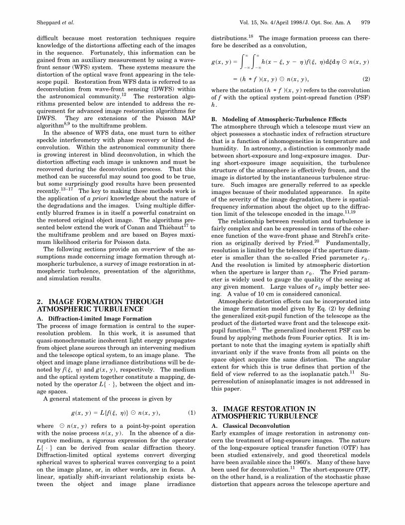
C. Multiframe Maximum-Likelihood BlindDeconvolution with Strict ConstraintsFigures 5 and 6 display sample output from the multi-frame maximum likelihood blind deconvolution algorithmfor a visual magnitude mv 5 4 OCNR5 satellite object.

Recall that strict constraints are employed for positivityon the object and strict positivity, unit volume, and band-width constraints on the PSF estimates. As expected,the results from the blind algorithm are not as free of ar-tifacts as the DWFS results. Many algorithms in the lit-erature do not perform well on extended objects. In lightof this, the results are encouraging. Superresolution isin evidence, although not to the same degree as in theDWFS results. An interesting subject for further studyis to determine whether a crossover exists for which theblind algorithm would outperform the DFWS approacheswith images acquired through a larger aperture. Also,an explicit support constraint was not used. Such a con-straint would improve the results even further. The al-


gorithm was implemented in C code on the parallel IBMSP2 system by using the message passing interface tomake the execution time manageable.

7. CONCLUSIONNew multiframe algorithms for constrained nonlinear de-convolution from wave-front sensing and blind deconvolu-tion were presented. In addition, superresolution of ex-tended space object images was demonstrated in both theDWFS and blind deconvolution cases with careful simu-lation of imaging through atmospheric turbulence. Theuse of multiple frames in the design of the algorithms wasinstrumental in controlling the noise present in photon-limited images and for regularizing the blind deconvolu-

tion process. The results indicate that postprocessing ofuncompensated images may be a viable alternative tobuilding fully compensated adaptive optics systems. Ret-rofitting existing large telescopes with wave-front-sensorsystems may also be the most effective way of bringingthem into the modern era of image recovery. It should bestressed that when real-time image recovery is critical,the approaches presented above do not provide a viablealternative to adaptive optics.

The results produced by blind deconvolution were notas good as those from wave-front sensing, which is notsurprising, given the inherent difficulty of the problem.However, they demonstrate that good image recovery ispossible in this mode of operation for extended satelliteobjects. It may be that a crossover point exists for whichblind deconvolution would outperform other techniques,

Fig. 5. Restoration of a simulated OCNR5 satellite object of visual magnitude mv 5 4 by use of the multiframe maximum-likelihoodblind deconvolution algorithm with varying number of frames (r0 5 10 cm). Clockwise from upper left: OCNR5 object, 10-frame res-toration, 50-frame restoration, 200-frame restoration.


Fig. 6. Spectra of images from Fig. 5. Clockwise from upper left: OCNR5 object spectrum, 10-frame-restoration spectrum, 50-frame-restoration spectrum, 200-frame-restoration spectrum. All spectra are range compressed with log10(1 1 u • u2).

given images acquired from a larger instrument. Theseand other questions will be addressed in future work.

APPENDIX A: STEPS INVOLVED IN THEMULTIFRAME POISSON MAXIMUMA POSTERIORI DECONVOLUTION FROMWAVE-FRONT SENSING ALGORITHMS

1. n 5 0.2. Compute initial estimate:

f 0 51

K (k51

K

gk

(positivity should be imposed on the elements of f 0).

3.

f ijn11 5 f ij

n11)k

expH 1

K F S gk

~f n * hk!2 1 D * hk

1GijJ

~baseline!

f ijn11 5 f ij

n expH F S g ~~n !!K

~f * h ~~n !!K!

2 1 D * h ~~n !!K

1 GijJ

~ incremental!.

4. n 5 n 1 1.5. If n 5 nmax , stop.6. Apply a suitable stopping criterion; i.e., if

if n11 2 f n i /i f ni , e, stop; else repeat step 3.


APPENDIX B: STEPS INVOLVED IN THEMULTIFRAME CONJUGATE-GRADIENTDECONVOLUTION WAVE-FRONT-SENSINGALGORITHM1. Equations for Objective Function J and Its Gradients

• J~fn! 5 2(k

(x,y

(~gk!xy ln$@~fn!2 * hk#xy%

2 @~fn!2 * hk#xy),

• J8~fn!uij 5]J~f n!

]f ijn 5

]J~f n!

]f ijn

]f ijn

]f ijn

5 22f ijn(

kXH gk

@~fn!2 * hk#2 1J * hk

1Cij

,

where the notation J8(fn) refers to the lexicographicallystacked vector of gradient values.

2. Outline of Nonlinear Conjugate-Gradient Method

1. Initialization:

n 5 0,

fn 5 Af n 5 A1K ( k51

k gk,

dn 5 rn 2 J8~fn!.

2. Line search:Find an that minimizes J(fn 1 andn) using the secantmethod.

3. Compute new estimate:

fn11 5 fn 1 andn.

4. Compute new conjugate-gradient direction:

rn11 5 2~J8fn11!bn11 5 maxH ~rn11!T~rn11 2 rn!

~rn!Trn , 0J(the Polak–Ribiere form),

dn11 5 rn11 1 bn11dn.

5. n 5 n 1 1.6. If n 5 nmax , then stop, else repeat step 2.

APPENDIX C: STEPS INVOLVED IN THEMULTIFRAME CONJUGATE-GRADIENTBLIND DECONVOLUTION ALGORITHM1. Equations for Objective Function J and Its Gradients

• J~fn, c1n , ..., ck

n!

5 2(k

(x,y X~gk!xy lnH F ~fn!2 *

~j * ckn!2

(i8, j8

~j * ckn!i8j8

2 Gxy

J2 F ~fn!2 *

~j * ckn!2

(i8j8

~j * ckn!i8j8

2 Gxy

C,

• J8~fn!uij 5]J~f n!

]f ijn 5

]J~f n!

]f ijn

]f ijn

]f ijn

5 22f ijn(

kXH gk

@~fn!2 * hk#2 1J * hk

1Cij

,

• J8~ckn!uij 5

]J~f, $hk%!

]~ck!ij

5 2 F 2

(i8, j8

~j * ck!i8j82 G

3 XH F ~j * ck!S gk

f * hk2 1 D * f 1G * j1J

ij

2 @~j * ck! * j1# ij

3 (mn

F S gk

f * hk2 1 D * f 1G

mn

~hk!mnCwhere the notation J8(fn : c1

n : ... : cKn ) refers to the

lexicographically stacked vector of gradient values.

2. Outline of Nonlinear Conjugate-Gradient Method

1. Initialization:

n 5 0,

fn 5 Af n 5 A1

K (k51

K

gk,

ckn 5 Ahk

n where the hkn are initially wide Gaussians,

dn 5 rn 5 2J8~fn:c1n : ...cK

n !.

2. Line search:Find a n that minimizes J(@fn : c1

n : ... : cKn #

1 andn) using the secant method.3. Compute new estimate:

@fn11 : c1n11 : ... : cK

n11# 5 @fn : c1n : ... : cK

n # 1 andn.

4. Compute new conjugate-gradient direction:

rn11 5 2J8~fn11 : c1n11 : ... : cK

n11!,

bn11 5 maxH ~rn11!T~rn11 2 rn!

~rn!Trn , 0J~the Polak–Ribiere form!,

dn11 5 rn11 1 bn11dn.


5. n 5 n 1 1.6. If n 5 nmax , then stop, else repeat step 2.

ACKNOWLEDGMENTSThe authors express their appreciation to Michael Rogge-man for providing the HYSIM3 software and for helpfuladvice regarding wave-front-sensing simulation. Thisresearch was supported by the U.S. Air Force under con-tract SC-92C-04-31.

REFERENCES1. H. C. Andrews and B. R. Hunt, Digital Image Restoration

(Prentice-Hall, Englewood Cliffs, N.J., 1977).2. P. J. Sementilli, B. R. Hunt, and M. S. Nadar, ‘‘Analysis of

the limit to superresolution in incoherent imaging,’’ J. Opt.Soc. Am. A 10, 2265–2276 (1993).

3. D. O. Walsh, P. A. Delaney, and M. W. Marcellin, ‘‘Non-iterative implementation of a class of iterative signal resto-ration algorithms,’’ in Proceedings of the International Con-ference on Speech, and Signal Processing (Institute ofElectrical and Electronics Engineers, Piscataway, N.J.,1996), pp. 1672–1675.

4. R. W. Gerchberg, ‘‘Superresolution through error energy re-duction,’’ Opt. Acta 21, 709–720 (1974).

5. W. H. Richardson, ‘‘Bayesian-based iterative method of im-age restoration,’’ J. Opt. Soc. Am. 62, 55–59 (1972).

6. L. B. Lucy, ‘‘An iterative technique for the rectification ofobserved distributions,’’ Astron. J. 79, 745–759 (1974).

7. T. J. Holmes, ‘‘Maximum likelihood image restorationadapted for noncoherent imaging,’’ J. Opt. Soc. Am. A 5,666–673 (1988).

8. B. R. Hunt and P. J. Sementilli, ‘‘Description of a Poissonimagery superresolution algorithm,’’ in Astronomical DataAnalysis Software and Systems I, D. Worral, C. Biemesder-fer, and J. Barnes, eds. (Astronomy Society of the Pacific,San Francisco, Calif., 1992), pp. 196–199.

9. E. S. Meinel, ‘‘Origins of linear and nonlinear recursive res-toration algorithms,’’ J. Opt. Soc. Am. A 3, 787–799 (1986).

10. B. R. Hunt, ‘‘Superresolution of images: algorithms, prin-ciples, performance,’’ Int. J. Imaging Syst. Technol. 6, 297–304 (1995).

11. F. Roddier, ‘‘The effects of atmospheric turbulence in opti-cal astronomy,’’ in Progress in Optics, E. Wolf, ed. (North-Holland, Amsterdam, 1981), Vol. XIX, pp. 281–376.

12. M. C. Roggeman and B. Welsh, Imaging Through Turbu-lence (CRC, New York, N.Y., 1996).

13. D. Kundur and D. Hatzinakos, ‘‘Blind image deconvolu-tion,’’ IEEE Signal Proc. Mag. 13, 43–64 (1996).

14. T. J. Schulz, ‘‘Multiframe blind deconvolution of astronomi-cal images,’’ J. Opt. Soc. Am. A 10, 1064–1073 (1993).

15. S. M. Jefferies and J. C. Christou, ‘‘Restoration of astro-nomical images by iterative blind deconvolution,’’ Astro-phys. J. 415, 862–874 (1993).

16. J. C. Christou, E. K. Hege, and S. M. Jefferies, ‘‘Speckle de-convolution imaging using an iterative algorithm,’’ in Ad-vanced Imaging Technologies and Commercial Applica-tions, N. Clark and J. D. Gonglewski, eds., Proc. SPIE 2566,134–143 (1995).

17. E. Thiebaut and J.-M. Conan, ‘‘Strict a priori constraintsfor maximum-likelihood blind deconvolution,’’ J. Opt. Soc.Am. A 12, 485–492 (1995).

18. J. W. Goodman, Introduction to Fourier Optics (McGraw-Hill, New York, 1968).

19. R. R. Beland, ‘‘Propagation through atmospheric opticalturbulence,’’ The Infrared and Electro-Optical Handbook.Vol. 2: Atmospheric Propagation of Radiation, F. G.Smith, ed. (SPIE Optical Engineering Press: Bellingham,Wash., 1993), pp. 157–232.

20. D. L. Fried, ‘‘Optical resolution through a randomly inho-mogeneous medium for very long and very short expo-sures,’’ J. Opt. Soc. Am. 56, 1372–1379 (1966).

21. J. C. Dainty, ‘‘Stellar speckle interferometry,’’ in LaserSpeckle and Related Phenomena, 2nd ed., J. C. Dainty, ed.(Springer-Verlag, Berlin, 1983), pp. 256–320.

22. P. A. Jansson, ‘‘Traditional linear deconvolution methods,’’in Deconvolution of Images and Spectra, P. A. Jansson, ed.(Academic, New York, 1997).

23. R. J. Hanisch and R. L. White, ‘‘HST image restoration:current capabilities and future prospects,’’ in Very High An-gular Resolution Imaging, J. G. Robertson and W. J. Tango,eds. (Kluwer, Dordrecht, The Netherlands, 1994), pp. 61–69.

24. R. J. Hanisch, R. L. White, and R. L. Gilliland, ‘‘Deconvolu-tion of Hubble Space Telescope images and spectra,’’ in De-convolution of Images and Spectra, P. A. Jansson, ed. (Aca-demic, New York, 1997).

25. H.-M. Adorf, R. N. Hook, and L. B. Lucy, ‘‘HST image res-toration developments at the ST-ECF,’’ Int. J. ImagingSyst. Technol. 6, 339–349 (1995).

26. H.-M. Adorf, ‘‘Hubble Space Telescope image restoration inits fourth year,’’ Inverse Probl. 11, 639–653 (1995).

27. P. A. Jansson, ‘‘Modern constrained nonlinear methods,’’ inDeconvolution of Images and Spectra, P. A. Jansson, ed.(Academic, New York, 1997).

28. A. Labeyrie, ‘‘Attainment of diffraction-limited resolution inlarge telescopes by Fourier analysing speckle patterns instar images,’’ Astron. Astrophys. 6, 85–87 (1970).

29. K. T. Knox and B. J. Thompson, ‘‘Recovery of images fromatmospherically degraded short exposure images,’’ Astro-phys. J. 193, L45–48 (1974).

30. A. W. Lohman, G. Weigelt, and B. Wirnitzer, ‘‘Specklemasking in astronomy: triple correlation theory and appli-cations,’’ Appl. Opt. 22, 4028–4037 (1983).

31. G. R. Ayers, M. J. Northcott, and J. C. Dainty, ‘‘Knox–Thompson and triple correlation imaging through atmo-spheric turbulence,’’ J. Opt. Soc. Am. A 5, 963–985 (1988).

32. L. A. Thompson, ‘‘Adaptive optics in astronomy,’’ Phys. To-day 47, 24–31 (1994).

33. T. E. Bell, ‘‘Electronics and the stars,’’ IEEE Spectr. 32,16–24 (1995).

34. J. C. Christou, ‘‘Blind deconvolution post-processing of im-ages corrected by adaptive optics,’’ in Adaptive Optical Sys-tems and Applications, R. K. Tyson and R. Q. Fugate, eds.,Proc. SPIE 2534, 226–234 (1995).

35. E. K. Hege, J. R. P. Angel, M. Cheselka, and M. Lloyd–Hart, ‘‘Simulation of aperture synthesis with the LargeBinocular Telescope,’’ in Advanced Imaging Technologiesand Commercial Applications, N. Clark and J. D. Gon-glewski, eds., Proc. SPIE 2566, 144–155 (1995).

36. J.-M. Conan, V. Michau, and G. Rousset, ‘‘Signal-to-noiseratio and bias of various deconvolution from wavefrontsensing estimators,’’ Image Propagation through the Atmo-sphere, L. R. Bissonnette and C. Dainty, eds., Proc. SPIE2828, 332–339 (1996).

37. A. V. Oppenheim, R. W. Schafer, and T. G. Stockham, ‘‘Non-linear filtering of multiplied and convolved signals,’’ Proc.IEEE 56, 1264–1291 (1968).

38. T. G. Stockham, Jr., T. M. Cannon, and R. B. Ingebretsen,‘‘Blind deconvolution through digital signal processing,’’Proc. IEEE 63, 678–692 (1975).

39. R. G. Lane and R. H. T. Bates, ‘‘Automatic multidimen-sional deconvolution,’’ J. Opt. Soc. Am. A 4, 180–188 (1987).

40. B. L. Satherly and P. J. Bones, ‘‘Zero tracks for blind decon-volution of blurred ensembles,’’ Appl. Opt. 33, 2197–2205(1994).

41. P. J. Bones, C. R. Parker, B. L. Satherly, and R. W. Watson,‘‘Deconvolution and phase retrieval with use of zero sheets,’’J. Opt. Soc. Am. A 12, 1842–1857 (1995).

42. G. R. Ayers and J. C. Dainty, ‘‘Iterative blind deconvolutionmethod and its applications,’’ Opt. Lett. 13, 547–549 (1988).

43. B. L. K. Davey, R. G. Lane, and R. H. T. Bates, ‘‘Blind de-convolution of noisy complex-valued image,’’ Opt. Commun.69, 353–356 (1989).

44. F. Tsumuraya, N. Miura, and N. Baba, ‘‘Iterative blind de-convolution method using Lucy’s algorithm,’’ Astron. Astro-phys. 282, 699–708 (1994).

45. T. J. Holmes, ‘‘Blind deconvolution of quantum-limited in-


coherent imagery: maximum-likelihood approach,’’ J. Opt.Soc. Am. A 9, 1052–1061 (1992).

46. R. G. Lane, ‘‘Blind deconvolution of speckle images,’’ J. Opt.Soc. Am. A 9, 1508–1514 (1992).

47. Y. Biraud, ‘‘A new approach for increasing the resolvingpower by data processing,’’ Astron. Astrophys. 1, 124–127(1969).

48. P. J. Sementilli, ‘‘Suppression of artifacts in super-resolvedimages,’’ Ph.D. dissertation (University of Arizona, Tucson,Ariz., 1993).

49. M. Hanke, Conjugate-Gradient Type Methods for Ill-PosedProblems (Wiley, New York, 1995).

50. J. R. Shewchuk, ‘‘An introduction to the conjugate-gradient

method without the agonizing pain,’’ Tech. Rep. CMU-CS-94-125 (Carnegie Mellon University, School of ComputerScience, Pittsburgh, Pa., 1994).

51. W. H. Press, B. P. Flannery, S. A. Teukolsky, and W. T.Vetterling, Numerical Recipes in C (Cambridge U. Press,Cambridge, 1988).

52. M. C. Roggeman, B. L. Ellerbroek, and T. A. Rhoadarmer,‘‘Widening the effective field of view of adaptive-optics tele-scopes by deconvolution from wave-front sensing: averageand signal-to-noise ratio performance,’’ Appl. Opt. 34,1432–1444 (1995).

53. R. J. Noll, ‘‘Zernike polynomials and atmospheric turbu-lence,’’ J. Opt. Soc. Am. A 66, 207–211 (1966).

Iterative multiframe super-resolution algorithms for atmospheric turbulence-degraded imagery

Documents

Transcript of Iterative multiframe super-resolution algorithms for atmospheric turbulence-degraded imagery