Spatial Exporter Dynamics∗

Fabrice Defever†, Benedikt Heid‡, Mario Larch§

April 23, 2010

—preliminary—not for circulation—comments welcome—

Abstract

Using Chinese customs data for estimating a discrete choice model between

potential export destinations, we present evidence for spatial export investment

decisions of exporters driven by search and learning processes in foreign markets.

We rationalize our empirical results by presenting a spatial learning by export-

ing model from which we derive our estimation equation. Our findings hint at a

positive correlation in unobserved firm profits across neighboring countries con-

trolling for previous export activities and firm productivity. These cross-border

spill-overs of export profitability are stronger for exports into regions where the

institutional environment is weak. Besides these cross-country spill-overs, we find

evidence for a substantial amount of spatial inter- and intra-product spill-overs

within multi-product firms.

∗We thank James E. Rauch and participants of the GEP conference on“Trade Costs, Infrastructureand Trade Development in Asia” for helpful comments on an earlier version of this paper. Fundingfrom the Leibniz-Gemeinschaft (WGL) under project“Pakt 2009 Globalisierungsnetzwerk”is gratefullyacknowledged.

†University of Nottingham, GEP and CEP, fabrice.defever@nottingham.ac.uk‡University of Bayreuth and ifo Institute, benedikt.heid@uni-bayreuth.de§University of Bayreuth, ifo Institute and CESifo, mario.larch@uni-bayreuth.de

1

1 Introduction

Globalization opens up new opportunities for firms to spread exports of their

different products in a wider range of destinations. The crucial need for local

information and trading partners may lead firms to concentrate their export mar-

kets close to each other. This implies a spatial expansion of export destinations

over time.

The recent integration of world markets did not only increase trade between

well established trade partners like the European countries but also saw the

emergence of new important net exporting countries like China. Underlying this

steady growth of aggregate trade flows at the country level is a large degree of

firm level fluctuation in both trade volumes and export destinations. For the year

2006 the Chinese customs report that 43% of all trade relationships are markets

a firm never exported to before. 50% of these firms did not export in previous

years at all, whereas all others already exported to another country previously.

From the firms that previously exported, 50% choose a new destination country

that is a neighboring country to a previous export destination.

Several learning mechanisms that explain the empirical importance of the

geographical spread of export destinations have been proposed in the literature.

First, if a firm does not know about its products’ appeal to foreign customers,

it can learn about it by exporting. For example, in the process of exporting to

Germany a Chinese firm does not only learn about the appeal of its product to

German customers but may also learn about profitable export opportunities in

nearby France. Furthermore, if tastes among nearby countries are correlated,

serving adjacent countries is informative about the product appeal of newly con-

sidered export markets (see for example Rauch and Watson (2003)). Second, an

exporting firm may gain access to a new export market via a multinational re-

tailer it already serves in a third country. Similar arguments are routinely made

in the literature on global production networks see, for example, Cheng and

Kierzkowski (2000) and McKendrick et al. (2000). As the network of subsidiaries

of wholesalers tends to expand spatially, this mechanism also implies a spread of

export destinations towards contiguous countries (see Head et al. (1995), Disdier

and Mayer (2004), Basker (2005)). A third mechanism is through networks of

typically ethnically-related firms, see for example Felbermayr et al. (2009). If

networks reduce search costs, a firm may learn about new export possibilities

from other firms in its ethnic community (Combes et al. (2005), Rauch (1999),

Rauch (2001)). Each of these mechanisms suggests that a firm’s export destina-

tion choice is determined in part by where it has exported to previously.

Even though there are several theoretical explanations of spatial exporter

dynamics, there is no systematic empirical evidence of how past exporting ex-

perience of firms impacts their future export destination choices. We set up a

2

dynamic model of firm destination choices which features correlation across ex-

port profitability of a firm induced by learning by exporting. From our model

we derive an estimation equation which enables us to study export destination

choices of firms accounting for cross-country spill-overs. We use our econometric

specification with Chinese firm level customs data which allow us to account for

inter- and intra-product spill-over effects of multi-product firms. In addition, we

take into account the possible simultaneous choice of new export destinations

of firms. With our proposed methodology we are able to quantify the spatial

cross-country information that a firm can capture from its past exporting expe-

rience. We find that learning from past exporting experience makes exporting to

a neighboring country 1.7 times more likely than exporting to a non-neighboring

country. We show that geographical as well as cultural proximity increase the

correlation of export profitability across potential export markets of firms.

In addition to the above-mentioned theoretical arguments, there is some em-

pirical work about export destination choices. Evenett and Venables (2002) pro-

vide first evidence of the gradual expansion of export destinations in bilateral

trade flows on the aggregate level. In contrast to their approach we derive our

empirical estimation equation from a theoretical model of forward looking firm

behavior in the presence of learning by exporting.

Eaton et al. (2008) provide stylized facts from Colombian firm-level customs

data about export dynamics of firms. They find that exporters tend to start

small in terms of revenue from exports, and only successful exporters start to

increase their export revenue over the following years. They present a search and

matching model in which firms learn about the appeal of their products from

previously arranged export contracts. When they update their beliefs about the

scope of their export profits, they adjust their export volumes, creating a dynamic

exporting behavior which is firm specific even under constant trade costs.

Albornoz et al. (2009) investigate the time pattern of the expansion of export

volumes for a firm which can export to two destinations. In their model, the firm

does only observe the profitability of an export market after having exported

once. If export profitability is correlated across those two markets, optimal firm

behavior is a sequential exporting strategy as the firm begins by exporting only a

small amount to a single market in order to get information about its profitability.

If it is high enough, it cranks up its export volumes and expands exports to the

other destination. Due to their restriction to two destinations, Albornoz et al.

(2009) cannot explore the question of spatial export destination choices in the

empirical part of their paper which is at the heart of our analysis.

The remainder of the paper is organized as follows: Section 2 presents a model

of spatial exporter dynamics, Section 3 derives an econometric specification of

the export destination choice from our model, and Section 4 describes the data

employed and discusses results. The last section concludes.

3

2 A Model of Spatial Exporter Dynamics

If a particular firm i exports a particular product k to destination market j at

time t we write yijkt = 1, while yijkt = 0 if firm i does not export product k to

country j at time t. For notational simplicity, let Yit = (yi11t, . . . , yijkt, . . . , yiJKt)

where J is the number of possible export destinations a firm may choose, and

K is the number of products the firm produces. Our model can also accomo-

date firm- and time-specific numbers of destinations and products Jit and Kit;

however, we suppress these subscripts for ease of notation. In a given year, the

decision to supply an export market depends on the revenue net of operating

costs that can be earned in the market, relative to the recurring fixed cost of

supplying the market. We denote the potential flow of expected operating profit

earned in destination market j at time t for firm i selling product k by E(rijkt),

and the one time fixed cost for entering the respective export market for a specific

product by fi. We therefore have,

yijkt =

1 if∞

∑

τ=t

βτ−tE(rijkτ ) − fi ≥ 0,

0 otherwise.

(1)

where β is the firm’s discount factor. Note that we model export destination

choice as a comparison of net present value benefits and costs, thereby taking

into account forward-looking behavior.

To characterize the firm’s profit flow, we assume that firm i produces good

k with a given efficiency ϕik. The associated cost is w/ϕik where w is the wage

in local currency. The exchange rate with country j is ej . Hence unit costs in

the foreign market are ejw/ϕik. Assuming that consumers have Dixit-Stiglitz

preferences with known demand elasticity σ, firm i receives the following price

for good k in country j1:

pijk =σ

σ − 1

ejw

ϕik(2)

Products differ in their appeal to consumers. This is summarized in a product

appeal index sijkt which consists of two components. The first component is

firm-product specific but time invariant for every possible export destination

country j, zijk, and the second component is firm-product-export-destination

idiosyncratic and time varying, εijkt.

We assume that exporting firms are able to observe all market-wide variables

like the current exchange rate and overall market size. However, the firm only

observes sijkt and cannot distinguish between the constant innate product appeal

zijk and the transitory shocks εijkt. Hence, sijkt serves as a noisy signal for

zijk. The firm can use its export volume to infer the associated demand shifter

1All produced goods are sold in the spot market.

4

sijkt = zijk + εijkt. In order to capture the search and learning processes by

exporting into foreign markets, product appeals are assumed to be correlated

across markets. Then, a firm can learn about the appeal of its product k by

experience gained in other export markets. Hence, cov(sijkt, sij′kt) 6= 0 for all

j 6= j′.

Product k sales of firm i to country j in period t are given by:

Xijkt = exp(zijk + εijkt)

(

pijk

Pj

)1−σ

Bj , (3)

where Bj represents spending levels of consumers in country j, and Pj is a price

index for all competing products of all firms selling in j.

The flow profits in home currency implied by (2) and (3) are:

Πijkt = rijkt − fi

=1

σ

Bj

ejPhexp(zijk + εijkt)

(

ejwσ/(σ − 1)

ϕikPj

)1−σ

− fi, (4)

where Ph is the price level in the home country.

Combining all the aggregate variables and constants capturing country char-

acteristics like market potential, distance and other country-specific trade costs

in Bj = 1σ

Bj

ejPh

(

ejwσ/(σ−1)Pj

)1−σ, net present value profits are given by

Πijkt =

∞∑

τ=t

βτ−t[

Bj exp(zijk + εijkτ )ϕσ−1ik

]

− fi. (5)

However, ex ante, i.e. before it has exported, the firm does not know its

product appeal sijkt. Therefore, the firm has to make its export destination

decision using its expectation about its net present value profits. We assume

that the firm forms its expectations using a Bayesian learning mechanism. More

precisely, before it has made sales to a specific foreign country, firm i ’s prior

beliefs concerning zijk are based on its market product appeal index for any

country j′ it serves via exports of any product k′, zij′k′ . The prior is assumed

to be a multivariate normal distribution (MV N) over destinations and products

with mean µ0 which we normalize to 0 for each firm implying an average product

appeal of 0. The prior beliefs are then distributed MV N(0,Σ) where Σ is the

covariance matrix of the firm’s prior beliefs.

However, each time a firm exports to a foreign country it updates its prior

beliefs by learning something about its products’ appeal to foreign consumers.

Let the time-varying idiosyncratic country-product-specific component of foreign

product appeal, εijkt, be distributed MV N(0,Θ). Hence, Sit ∼ MV N(Zi,Θ)

with

5

Sit = Zi + εit =

zi11

...

zijk

...

ziJK

+

εi11t

...

εijkt

...

εiJKt

, (6)

where Zi is a (JK × 1) vector. The firm updates its posterior belief based on its

prior and the information retrieved by previous export experience. The mecha-

nism of Bayesian updating reflects the learning by the exporting channel. Note

that this updating is a consequence of probability theory in the presence of infor-

mation asymmetries and does not require any ad hoc reasoning. It also justifies

another interpretation of the prior distribution as being based on information

about product appeals aquired from export decisions in previous periods. Note

that in the absence of any information concerning the product appeals from pre-

vious periods, the previous prior is considered as the equivalent of the previous

observed product appeal. For a similar interpretation, see Greenberg (2008),

page 25.

Accordingly, firm i’s posterior beliefs concerning Zi are distributed MV N(Zi,Ω),

where:

Zi = Ω(Θ−1Sit + Σ−1µ0), (7)

Ω = (Θ−1 + Σ−1)−1. (8)

Note that µ0 = 0. Hence we can simplify to

Zi = ΩΘ−1Sit, (9)

Ω = (Θ−1 + Σ−1)−1. (10)

As every country-specific product appeal of a firm is hit by time-varying shocks,

the firm never knows the actual value of zijk for sure in the short run. Therefore,

even though exporting to a new destination reveals new information about Zi,

the uncertainty does not disappear and hence the posterior does not collapse

into a single point.2 Note that through the cross-country correlation of product

appeals zijk, a typical element of the firm’s posterior belief about the appeal of

product k in country j, zijkt, is a function of all other product appeals of the

same or other products in other markets as well as other products in the same

market from the previous periods. This in turn highlights the fact that every

2Only in the long run steady state, the firm will get to know the true value of the product appeal,and there is no need for Bayesian learning any longer, as the belief distribution collapses into a singlepoint, the true value zijk.

6

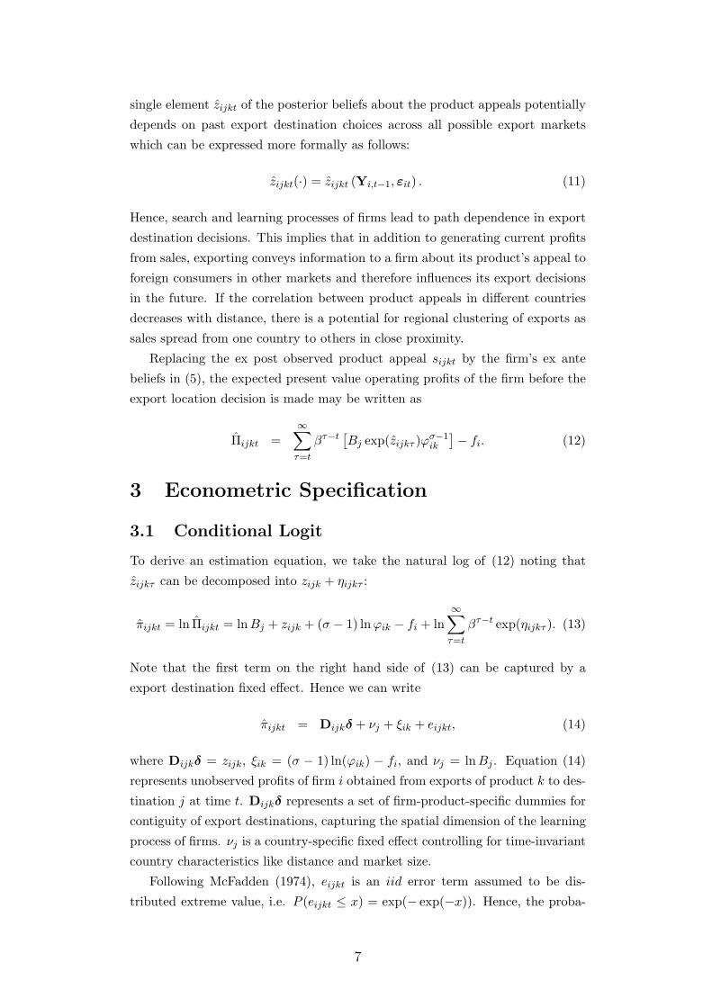
single element zijkt of the posterior beliefs about the product appeals potentially

depends on past export destination choices across all possible export markets

which can be expressed more formally as follows:

zijkt(·) = zijkt (Yi,t−1, εit) . (11)

Hence, search and learning processes of firms lead to path dependence in export

destination decisions. This implies that in addition to generating current profits

from sales, exporting conveys information to a firm about its product’s appeal to

foreign consumers in other markets and therefore influences its export decisions

in the future. If the correlation between product appeals in different countries

decreases with distance, there is a potential for regional clustering of exports as

sales spread from one country to others in close proximity.

Replacing the ex post observed product appeal sijkt by the firm’s ex ante

beliefs in (5), the expected present value operating profits of the firm before the

export location decision is made may be written as

Πijkt =

∞∑

τ=t

βτ−t[

Bj exp(zijkτ )ϕσ−1ik

]

− fi. (12)

3 Econometric Specification

3.1 Conditional Logit

To derive an estimation equation, we take the natural log of (12) noting that

zijkτ can be decomposed into zijk + ηijkτ :

πijkt = ln Πijkt = lnBj + zijk + (σ − 1) lnϕik − fi + ln∞

∑

τ=t

βτ−t exp(ηijkτ ). (13)

Note that the first term on the right hand side of (13) can be captured by a

export destination fixed effect. Hence we can write

πijkt = Dijkδ + νj + ξik + eijkt, (14)

where Dijkδ = zijk, ξik = (σ − 1) ln(ϕik) − fi, and νj = lnBj . Equation (14)

represents unobserved profits of firm i obtained from exports of product k to des-

tination j at time t. Dijkδ represents a set of firm-product-specific dummies for

contiguity of export destinations, capturing the spatial dimension of the learning

process of firms. νj is a country-specific fixed effect controlling for time-invariant

country characteristics like distance and market size.

Following McFadden (1974), eijkt is an iid error term assumed to be dis-

tributed extreme value, i.e. P (eijkt ≤ x) = exp(− exp(−x)). Hence, the proba-

7

bility that firm i chooses to export to destination j∗ ∈ Cik is then given by:

Pij∗ =exp(Dij∗kδ + νj∗ + ξik)

∑

j∈Cikexp(Dijkδ + νj + ξik)

=exp(Dij∗kδ + νj∗)

∑

j∈Cikexp(Dijkδ + νj)

for j∗ = 1, ..., Cik. (15)

Note that the set of possible export destinations Cik is firm-specific as well as

product-specific, depending on exports in previous periods, firms can choose

between a different number of new export destinations. Due to this specification

the firm-product specific productivity term ξik = (σ − 1) ln(ϕik) − fi, which is

constant across export destinations, does not affect the estimation of δ based on

relative probabilities. Note also that we drop the time subscript from now on as

our estimation looks at the export decision at one specific point in time.

The crucial assumption of the conditional logit is the independence of irrel-

evant alternatives (IIA). The iid assumption on the error terms precludes any

correlation in unobserved factors which influence the export destination choice

of the firm. Note at this point that even though at first glance IIA seems very

restrictive, it is more flexible as it may appear at first. Note especially that

unobserved firm heterogeneity in the sense of general productivity differences of

firms does not affect our estimates. If productivity levels apply generally across

product-specific export destinations, they do not interfere in the choice of one

export destination over the other as in a random utility maximization only differ-

ences in profit levels count but not the overall level. Here, productivity works just

as a level shifter of profits. Also, unobserved country characteristics do not pose

a problem for the IIA assumption as they are captured by the included country-

fixed effects. What is left is a correlation across export destinations induced

by destination×firm specific productivity differences which are unrelated to any

country characteristics. For example, a particular firm may be good at serving

country A, and equally good at serving country B due to historical reasons, e.g.

recent exports to both A and B. This export hysteresis effect is documented by

Eaton et al. (2008) and Das et al. (2007). In order to control for this, we include

firm-specific dummies which indicate former presence in the foreign market in the

preceding two years in our regressions. In principle, transaction level data would

also allow firm-destination specific fixed effects. However, the sheer volume of

data then prevents estimation of the model.

3.2 Multiple export destinations

In the conditional logit, firms are modeled as choosing one new export destination

which offers the highest expected profits. Empirically, however, we observe that

firms may choose to start to export to a multitude of new export destinations

simultaneously. In our data set, we observe that firms which choose to export

8

to new markets often do so in two or three markets (INCLUDE DESCRIPTIVE

STATISTICS HERE). In order to reflect this behavior in our estimation proce-

dure, we run a fixed effects logit due to Chamberlain (1980).3 Note that this

estimator models the probability of firm i choosing a set of mik export destina-

tions from Cik, the set of all possible new export destinations for the firm, given

the knowledge that the firm exports to a specific number of export destinations.

This probability is given by

Pi

(

j∗1 , . . . , j∗mik|mik

)

=exp

(

[∑Cik

j=1 yijk(D′

ijk + νj)]δ)

∑

di∈Bikexp

(

∑Cik

j=1 dijk(D′

ijk + νj)δ) (16)

as presented in Hamerle and Ronning (1995). Bik is the set of all possible

combinations of export destinations, given that the firm exports to mik desti-

nations in total. The number of elements in this set is equal to(

Cik

mik

)

. The

conditional likelihood is given by

lnL =n

∑

i=1

Cik∑

j=1

yijk(D′

ijk + νj)δ − ln fi(Cik, mik)

(17)

where fi(Cik, mik) =∑

di∈Bikexp

(

∑Cik

j=1 dijk(D′

ijk + νj)δ)

and dijk is equal to

0 or 1 with∑Ji

j=1 dijk = mik.

4 Data and Results

For our estimations, we investigate the export location decisions of the universe

of Chinese firms which exported in the years 2003 to 2005.4

Specifically, we investigate the choice of a firm’s new export destinations, irre-

spective of whether the firm has been an exporter in 2003 or 2004 at all (extensive

margin of exporting) or whether the firm chooses to increase its number of ex-

port destinations (intensive margin of exporting). Overall, there are about 70,000

firms in the data set exporting into 126 different export destinations. We exclude

all multinational firms in order to not capture effects from multinationals out-

sourcing parts of their production to China. Furthermore, we exclude all trading

companies, i.e. those firms which do not engage in production themselves but act

as an intermediary for Chinese producers who are not capable to export on their

own due to legal restrictions or actual incapability. These trading companies

represent about 21% of Chinese exports.

As the data are at the transaction level and separately for every SITC-4-digit

3For a succinct introduction, see Cameron and Trivedi (2005).4For a more detailed description of the data set used, see Manova and Zhang (2009).

9

product category, we aggregate to get annual values at the firm level.

We assume that contiguous countries have a higher correlation between expected

export profits than non-contiguous countries. Our concept of contiguity is a

broad one, i.e. we do not only consider geographic contiguity between export

destinations but also cultural closeness measures as shared language between ex-

port destinations as well as a common colonizer of export destination countries.

Note that all these contiguity measures are firm-specific. The geographic conti-

guity dummy is equal to 1 when a possible export destination for firm i in 2005

is contiguous to one of the previous export destinations of i in 2003 and 2004. As

the set of the previous export destinations is firm-specific, so is the geographic

contiguity dummy.

As proxies for cultural contiguity, we include a dummy which indicates whether

a new possible export destination was colonized by one of the countries to which

the firm exported to in previous periods. For example, consider a firm having

exported to France in 2004. Then, the colony dummy is 1 e.g. for Algeria (DLZ).

If this firm had not exported to France in 2004 (or 2003), then the dummy would

be 0.

Analogously, we construct a dummy indicating common language between an

export destination in 2003 or 2004 and potential export destinations in 2005. All

the contiguity dummies are constructed using CEPII data.5

As we estimate a conditional fixed effects logit, coefficients can be interpreted as

odds ratios according to the formula:

P (yir = 1|Dir = 1)

P (yij = 1|Dij = 0)=

eδDir

eδDij= exp[(Dir − Dij)δ] = exp(δ)

Hence, the exponentiated coefficient of the firm specific dummy Dir gives the

relative probability of a firm exporting to a country which is contiguous to a

previous export destination compared to the probability of a firm exporting to a

country which is not a neighboring country to the firm’s previous export desti-

nations.

Finally, in all our regressions we exclude the direct neighbors of China. This is

due to the fact that with China having such a vast territory, it shares a common

border with many countries, which are again very large countries like India and

Russia. By dropping these neighbors, we prevent to get estimates which are un-

duly influenced by these outliers. If our conditional logit specification is correct,

there arises no problem from estimating the model parameters from a subsample

of the possible export destination choices as we assume the unobserved errors

to be iid. Hence, dropping some countries only affects the efficiency of our esti-

mates.

5The geographical contiguity definition from CEPII is a broad one, e.g. Russia is consideredcontiguous to Poland.

10

As a first step, we estimate our model for four different world regions separately.

As just pointed out, this only affects the efficiency of our estimates and hence

works as a natural consistency check for our model specification.

In Table 1, we report estimates of the conditional logit for the regions Asia/

Oceania/ Middle East, Europe, Africa, and America. For every region, we re-

port two columns: Specification (I) gives the estimate for a choice between all

possible export destinations, including the countries to which the firm exported

in 2003 or 2004. Specification (II) gives the estimates for the choice between all

possible additional export destinations, i.e. excluding the destinations to which

the firm exported already in 2003 or 2004. Overall, the geographical contiguity

dummy turns out to be highly significant across all specifications and the sepa-

rate world regions. It ranges between 0.244 for Europe in specification (I) and

0.557 for Africa in specification (I). These coefficients imply, in turn, an odds ra-

tio of 1.28 and 1.75, i.e. the probability of a firm to export to a country which is

contiguous to a previous export destination of this firm is between a quarter and

three quarters higher than the probability to export to a non-contiguous country.

We find the highest contiguity effects for both Africa and Asia/ Oceania/ Middle

East. This is as expected, as in these regions, markets are highly diverse and the

political environment is rather unstable. This translates into higher insecurity

about expected profit possibilities across possible export destinations and high-

lights the importance of firm-specific networks and knowledge. Obviously, firms

opt for erecting a bridgehead from which they spread spatially towards other

export destinations as time evolves. In Europe, this effect is less pronounced due

to the relatively homogeneous culture and political system. This implies that

once a firm has entered the European market, it is still more likely to go from,

say France to Germany than to Portugal, but this effect is less pronounced than

in Africa. America lies in between these more extreme estimates which hints at

a medium heterogeneity in tastes and culture on the continent.

Furthermore, we find that the probability of exporting to a country is more than

17 times6 as large when the firm already has exported into the market the year

before. Estimates of these coefficients are in the same range across all specifi-

cations. In Table 2, where we repeat the estimations but differentiate between

exports to the country in 2003 and 2004 with separate dummies, we find that this

export hysteresis effect quickly dwindles down after two years to a probability

which is about three times higher compared to the probability of exporting to a

country the firm has not exported to in the previous two years. This is in line

with descriptive statistics as presented in Eaton et al. (2008). As we additionally

control for country effects and our estimation approach is insensitive to differ-

6exp(2.848) = 17.25 for Asia/ Oceania/ Middle East in Table 1, specification (I).

11

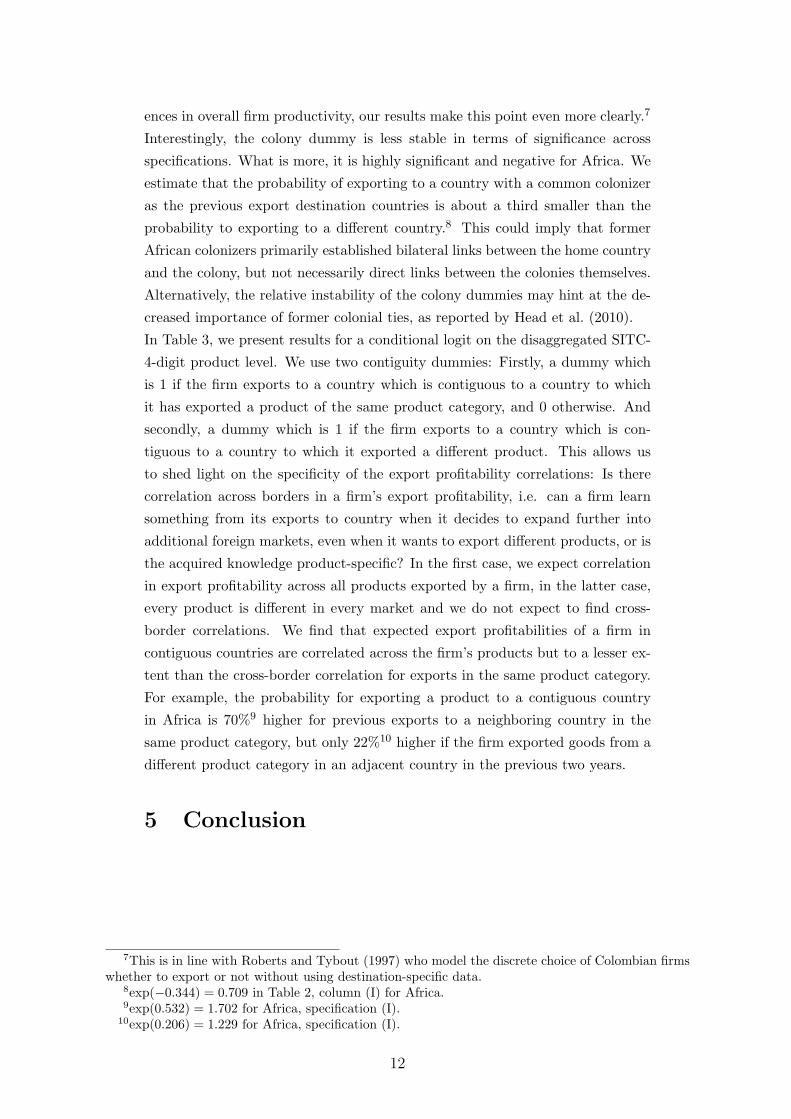
ences in overall firm productivity, our results make this point even more clearly.7

Interestingly, the colony dummy is less stable in terms of significance across

specifications. What is more, it is highly significant and negative for Africa. We

estimate that the probability of exporting to a country with a common colonizer

as the previous export destination countries is about a third smaller than the

probability to exporting to a different country.8 This could imply that former

African colonizers primarily established bilateral links between the home country

and the colony, but not necessarily direct links between the colonies themselves.

Alternatively, the relative instability of the colony dummies may hint at the de-

creased importance of former colonial ties, as reported by Head et al. (2010).

In Table 3, we present results for a conditional logit on the disaggregated SITC-

4-digit product level. We use two contiguity dummies: Firstly, a dummy which

is 1 if the firm exports to a country which is contiguous to a country to which

it has exported a product of the same product category, and 0 otherwise. And

secondly, a dummy which is 1 if the firm exports to a country which is con-

tiguous to a country to which it exported a different product. This allows us

to shed light on the specificity of the export profitability correlations: Is there

correlation across borders in a firm’s export profitability, i.e. can a firm learn

something from its exports to country when it decides to expand further into

additional foreign markets, even when it wants to export different products, or is

the acquired knowledge product-specific? In the first case, we expect correlation

in export profitability across all products exported by a firm, in the latter case,

every product is different in every market and we do not expect to find cross-

border correlations. We find that expected export profitabilities of a firm in

contiguous countries are correlated across the firm’s products but to a lesser ex-

tent than the cross-border correlation for exports in the same product category.

For example, the probability for exporting a product to a contiguous country

in Africa is 70%9 higher for previous exports to a neighboring country in the

same product category, but only 22%10 higher if the firm exported goods from a

different product category in an adjacent country in the previous two years.

5 Conclusion

7This is in line with Roberts and Tybout (1997) who model the discrete choice of Colombian firmswhether to export or not without using destination-specific data.

8exp(−0.344) = 0.709 in Table 2, column (I) for Africa.9exp(0.532) = 1.702 for Africa, specification (I).

10exp(0.206) = 1.229 for Africa, specification (I).

12

References

Albornoz, F., Pardo, H. F. C., Corcos, G., and Ornelas, E. (2009). Sequential

exporting. unpublished working paper.

Basker, E. (2005). Job creation or destruction? Labor market effects of Wal-Mart

expansion. The Review of Economics and Statistics, 87:174–183.

Cameron, A. C. and Trivedi, P. K. (2005). Microeconometrics. Methods and

Applications. Cambridge: Cambridge University Press.

Chamberlain, G. (1980). Analysis of covariance with qualitative data. Review of

Economic Studies, 47:225–238.

Cheng, L. K. and Kierzkowski, H., editors (2000). Global Production and Trade

in East Asia. Kluwer Academic Publishers.

Combes, P.-P., Lafourcade, M., and Mayer, T. (2005). The trade-creating effects

of business and social networks: evidence from France. Journal of International

Economics, 66(1):1–29.

Das, S., Roberts, M. J., and Tybout, J. R. (2007). Market entry costs, producer

heterogeneity, and export dynamics. Econometrica, 75(3):837–873.

Disdier, A.-C. and Mayer, T. (2004). How different is Eastern Europe? Structure

and determinants of location choices by French firms in Eastern and Western

Europe. Journal of Comparative Economics, 32:280–296.

Eaton, J., Eslava, M., Krizan, C., Kugler, M., and Tybout, J. (2008). A search

and learning model of export dynamics. unpublished working paper.

Evenett, S. J. and Venables, A. J. (2002). Export growth in developing countries:

Market entry and bilateral trade flows. unpublished working paper.

Felbermayr, G., Jung, B., and Toubal, F. (2009). Ethnic networks, information

and international trade: revisiting the evidence. unpuplished working paper.

Greenberg, E. (2008). Introduction to Bayesian Econometrics. cambridge: Cam-

bridge University Press.

Hamerle, A. and Ronning, G. (1995). Panel analysis for qualitative variables. In

Arminger, G., Clogg, C. C., and Sobel, M. E., editors, Handbook of Statistical

Modeling for the Social and Behavioral Sciences, pages 401–451. New York:

Plenum.

Head, K., Mayer, T., and Ries, J. (2010). The erosion of colonial trade linkages

after independence (forthcoming). Journal of International Economics.

13

Head, K., Ries, J., and Swenson, D. (1995). Agglomeration benefits and loca-

tion choice: Evidence from Japanese manufacturing investments in the United

States. Journal of International Economics, 38(3-4):223–247.

Manova, K. and Zhang, Z. (2009). China’s exporters and importers: Firms,

products and trade partners. unpuplished working paper.

McFadden, D. (1974). Conditional logit analysis of qualitative choice analysis.

In Zarembka, P., editor, Frontiers in Econometrics, chapter 4, pages 105–142.

New York: Academic Press.

McKendrick, D. G., Donder, R. F., and Haggard, S. (2000). From Silicon Valley

to Singapore: Location and Competitive Advantage in the Hard Disk Drive

Industry. Stanford: Stanford University Press.

Rauch, J. and Watson, J. (2003). Starting small in an unfamiliar environment.

International Journal of Industrial Organization, 21:1021–1042.

Rauch, J. E. (1999). Networks versus markets in international trade. Journal of

International Economics, 48:7–35.

Rauch, J. E. (2001). Business and social networks in international trade. Journal

of Economic Literature, 39:1177–1203.

Roberts, M. and Tybout, J. (1997). The decision to export in colombia: An em-

pirical model of entry with sunk costs. American Economic Review, 87(4):545–

564.

14

Table 1: Conditional logit with country fixed effects: previous export status I

Asia, Oceania,

Middle East

Europe Africa America

(I) (II) (I) (II) (I) (II) (I) (II)

Contiguous to a country withexport in t-1 or t-2

0.483A 0.554A 0.244A 0.266A 0.557A 0.537A 0.339A 0.373A

0.012 0.016 0.012 0.015 0.025 0.032 0.016 0.021

Export in t-1 or t-22.848A 2.418A 2.641A 2.530A

0.009 0.010 0.021 0.016

Export in a colony in t-1 or t-20.041A 0.044B 0.080A 0.044B −0.307A −0.471A

0.014 0.020 0.016 0.022 0.061 0.080Export in a country with thesame language in t-1 or t-2

0.128A 0.253A 0.051A 0.088A −0.045C 0.141A −0.051B 0.192A

0.011 0.015 0.014 0.019 0.024 0.031 0.024 0.033

Country FE Yes Yes Yes Yes Yes Yes Yes Yes# of countries 28 up to 28 39 up to 39 35 up to 35 24 up to 24# of firms 58638 37852 40696 30837 17376 12377 41434 26464Log-Likelihood -274935 -193147 -241608 -176418 -67736 -52862 -110266 -80887R

2 0.36 0.18 0.4 0.28 0.39 0.26 0.53 0.38

Coefficient estimates of conditional logit; dependent variable: export status in 2005;A: significant at 1%, B: significant at 5%, C : significant at 10%Specification (I) gives the estimate for a choice between all possible export destinations, including the country to which the firm exportedin 2003 or 2004. Specification (II) gives the estimates for the choice between all possible additional export destinations, i.e. excludingthe destinations to which the firm exported already in 2003 or 2004.

15

Table 2: Conditional logit with country fixed effects: previous export status II

Asia, Oceania,

Middle East

Europe Africa America

(I) (II) (I) (II) (I) (II) (I) (II)

Contiguous to a country withexport in t-1

0.465A 0.527A 0.230A 0.246A 0.484A 0.466A 0.336A 0.380A

0.014 0.019 0.013 0.016 0.028 0.035 0.018 0.022Contiguous to a country withexport in t-2

0.103A 0.147A 0.042A 0.096A 0.276A 0.305A −0.006 0.062B

0.018 0.025 0.015 0.020 0.035 0.045 0.022 0.030

Export in t-12.604A 2.312A 2.502A 2.423A

0.010 0.011 0.023 0.017

Export in t-21.164A 0.925A 1.096A 0.919A

0.013 0.015 0.031 0.022

Export in a colony in t-1 or t-2−0.009 0.039C 0.103A 0.046B −0.344A −0.498A

0.015 0.020 0.017 0.022 0.062 0.080Export in a country with the samelanguage in t-1 or t-2

0.118A 0.256A 0.013 0.079A −0.067A 0.147A −0.047C 0.194A

0.011 0.015 0.015 0.019 0.025 0.031 0.024 0.033

Country FE Yes Yes Yes Yes Yes Yes Yes Yes# of countries 28 up to 28 39 up to 39 35 up to 35 24 up to 24# of firms 58638 37852 40696 30837 17376 12377 41434 26464Log-Likelihood -267774 -193133 -237370 -176404 -66848 -52847 -108436 -80866R2 0.38 0.18 0.41 0.27 0.4 0.26 0.54 0.38

Coefficient estimates of conditional logit; dependent variable: export status in 2005;A: significant at 1%, B: significant at 5%, C : significant at 10%Specification (I) gives the estimate for a choice between all possible export destinations, including the country to which the firm exported in 2003or 2004. Specification (II) gives the estimates for the choice between all possible additional export destinations, i.e. excluding the destinations towhich the firm exported already in 2003 or 2004.

16

Table 3: Conditional Logit with country fixed effects: product level evidence

Asia, Oceania,

Middle East

Europe Africa America

(I) (II) (I) (II) (I) (II) (I) (II)

Contiguous to acountry with export int-1 or t-2. . .

. . . of a different product0.089A 0.198A 0.156A 0.166A 0.206A 0.287A 0.110C 0.1050.015 0.029 0.016 0.027 0.035 0.056 0.062 0.102

. . . of the same product 0.406A 0.459A 0.264A 0.374A 0.532A 0.575A 0.218A 0.412A

0.017 0.032 0.017 0.028 0.038 0.059 0.062 0.101

Export in t-1 or t-22.230A 1.942A 2.301A 2.047A

0.012 0.014 0.028 0.053Export in a colony in t-1 ort-2

0.065A 0.021 0.074A 0.112A −0.171A −0.376A

0.014 0.029 0.016 0.032 0.056 0.108Export in a country withsame language in t-1 or t-2

0.057A 0.201A 0.071A 0.085A −0.009 0.277A 0.134C 0.1720.013 0.020 0.015 0.027 0.031 0.042 0.079 0.117

Country FE Yes Yes Yes Yes Yes Yes Yes Yes# of countries 28 up to 28 39 up to 39 35 up to 35 24 up to 24Log-Likelihood -188869 -108363 -142006 -81107 -40253 -28741 -8932 -5399R2 0.31 0.19 0.38 0.3 0.36 0.25 0.64 0.53

Coefficient estimates of conditional logit; dependent variable: export status in 2005; same product dummy is defined as previous exports in thesame SITC 4-digit product category;A: significant at 1%, B: significant at 5%, C : significant at 10%Specification (I) gives the estimate for a choice between all possible export destinations, including the country to which the firm exported in 2003or 2004. Specification (II) gives the estimates for the choice between all possible additional export destinations, i.e. excluding the destinations towhich the firm exported already in 2003 or 2004.

17