�����������������

Citation: Wang, X.; Wang, H.; Zhao,

J.; Xu, C.; Luo, Z.; Han, Q.

Rigid-Flexible Coupling Dynamics

Modeling of Spatial Crank-Slider

Mechanism Based on Absolute Node

Coordinate Formulation. Mathematics

2022, 10, 881. https://doi.org/

10.3390/math10060881

Academic Editor: António M. Lopes

Received: 8 February 2022

Accepted: 4 March 2022

Published: 10 March 2022

Publisher’s Note: MDPI stays neutral

with regard to jurisdictional claims in

published maps and institutional affil-

iations.

Copyright: © 2022 by the authors.

Licensee MDPI, Basel, Switzerland.

This article is an open access article

distributed under the terms and

conditions of the Creative Commons

Attribution (CC BY) license (https://

creativecommons.org/licenses/by/

4.0/).

mathematics

Article

Rigid-Flexible Coupling Dynamics Modeling of SpatialCrank-Slider Mechanism Based on Absolute NodeCoordinate FormulationXiaoyu Wang 1,*, Haofeng Wang 1, Jingchao Zhao 1, Chunyang Xu 2, Zhong Luo 1 and Qingkai Han 1

1 School of Mechanical Engineering and Automation, Northeastern University, Shenyang 110819, China;2170237@stu.neu.edu.cn (H.W.); 2170293@stu.neu.edu.cn (J.Z.); zhluo@mail.neu.edu.cn (Z.L.);qhan@mail.neu.edu.cn (Q.H.)

2 AECC Shenyang Engine Research Institute, Shenyang 110015, China; xucy11@126.com* Correspondence: wangxy@me.neu.edu.cn

Abstract: In order to study the influence of compliance parts on spatial multibody systems, a rigid-flexible coupling dynamic equation of a spatial crank-slider mechanism is established based on thefinite element method. Specifically, absolute node coordinate formulation (ANCF) is used to formulatea three-dimensional, two-node flexible cable element. The rigid-flexible coupling dynamic equationof the mechanism is derived by the Lagrange multiplier method and solved by the generalizedα method and Newton–Raphson iteration method combined. Comparison of the kinematics anddynamics response between rigid-flexible coupling system and pure rigid system implies that theflexible part causes a certain degree of nonlinearity and reduces the reaction forces of joints. Theelastic modulus of the flexible part is also important to the dynamics of the rigid-flexible multibodysystem. With smaller elastic modulus, the motion accuracy and reaction forces become lower.

Keywords: spatial crank-slider mechanism; absolute node coordinate formulation; Lagrange multipliermethod; rigid-flexible coupling dynamics

MSC: 37M05

1. Introduction

Multibody systems are composed of several rigid or flexible objects interconnectedby joints, which are applied in various fields, such as aviation, robots and vehicle systems.With the development of industry, more and more mechanical systems demand spatialmovement [1,2], which requires further analysis of spatial multibody systems.

The fundamental problem of multibody system dynamics is modeling and compu-tation. Since the 1960s, many scholars have studied multibody systems. Wittburg [3]published research work on multibody system dynamics, which laid the foundation for theLagrange method for multibody system dynamics. Nikravesh [4] focused on computer-aided analysis of multibody systems and discussed the modeling and calculation of multi-body systems in detail. Haug and Habana [5,6] put forward the Cartesian method ofmodeling multi-rigid-body systems. Computational multibody system dynamics researchcan be divided into rigid multibody systems, flexible multibody systems and rigid-flexiblecoupling multibody systems according to the mechanical characteristics of objects existingin the system. The term multi-rigid body system refers to a system in which all objects arerigid and elastic deformation can be ignored. The term flexible multibody system refersto the large-scale elastic deformation of objects during the movement of the system. Arigid-flexible coupling system is a rigid multibody system with some flexible parts [7–10].

Rigid-flexible coupling multibody dynamics is becoming more and more important es-pecially for spacecraft structures, and the deformation of flexible bodies can cause complex

Mathematics 2022, 10, 881. https://doi.org/10.3390/math10060881 https://www.mdpi.com/journal/mathematics

Mathematics 2022, 10, 881 2 of 13

nonlinear mechanical behaviors to the multibody system [11–13]. Traditionally, machinesare assumed to be rigid bodies for multibody dynamics analysis. However, with the grow-ing demand of higher precision and resolution it is necessary to consider the influence ofcomponent deformation. In fact, each component of a mechanical system has deformationunder loading. In order to simplify the calculation and modeling, some components withtiny deformations of the mechanical system can be regarded as rigid bodies. The rigid-flexible coupling system takes into account the deformation of flexible bodies, and alsoconsiders calculation efficiency and simplicity [13–19].

The crank-slider system, as a basic mechanism, is widely used in various fields. Forthose mechanisms running at high speed and large scale, the influence of the flexibility can-not be ignored, otherwise it would reduce the precision of the system, and make dynamicscharacteristics seriously different from real system [20,21]. Different modeling methods tostudy the kinematics and dynamics of the crank-slider system have been proposed. Liu [22]established the slider-crank mechanism model and studied the kinematics and dynamics ofoffset slider-crank mechanism. Li et al. [23] studied the dynamics of the crank-connectingrod system with clearance and flexible rod, and discussed the influence of flexible con-necting rod on the mechanism. Qian et al. [24] analyzed the kinematics and dynamics ofthe crank-slider mechanism based on Simulink in MATLAB. Ma et al. [25–27] simulatedthe dynamics of the planetary gear train based on the virtual prototype technology. Wuet al. [28,29] conducted simulation research on multibody dynamics mechanisms of a crankconnecting rod mechanism based on Adams, and provided a simulation idea of multibodydynamics. The above-mentioned research is basically for rigid planar crank-slider mecha-nisms, while research on spatial crank-slider mechanisms with flexible component is rare.In this paper, the spatial crank-slider mechanism is formulated, and the flexible rod is estab-lished based on the absolute node coordinate formulation, and the rigid-flexible couplingdynamic equation of spatial crank-slider mechanism is derived by the Lagrange multiplierequation to analyze the influence of flexible rod on spatial crank-slider mechanism.

2. Cable Model Based on ANCF Method2.1. ANCF Cable Element Model

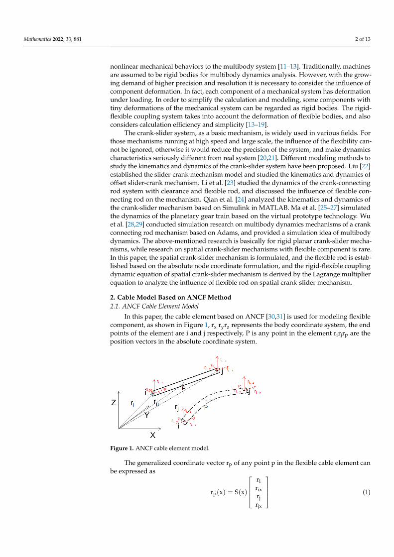
In this paper, the cable element based on ANCF [30,31] is used for modeling flexiblecomponent, as shown in Figure 1, rx ryrz represents the body coordinate system, the endpoints of the element are i and j respectively, P is any point in the element rirjrp are theposition vectors in the absolute coordinate system.

Mathematics 2022, 10, x FOR PEER REVIEW 2 of 13

Rigid-flexible coupling multibody dynamics is becoming more and more important especially for spacecraft structures, and the deformation of flexible bodies can cause com-plex nonlinear mechanical behaviors to the multibody system [11–13]. Traditionally, ma-chines are assumed to be rigid bodies for multibody dynamics analysis. However, with the growing demand of higher precision and resolution it is necessary to consider the in-fluence of component deformation. In fact, each component of a mechanical system has deformation under loading. In order to simplify the calculation and modeling, some com-ponents with tiny deformations of the mechanical system can be regarded as rigid bodies. The rigid-flexible coupling system takes into account the deformation of flexible bodies, and also considers calculation efficiency and simplicity [13–19].

The crank-slider system, as a basic mechanism, is widely used in various fields. For those mechanisms running at high speed and large scale, the influence of the flexibility cannot be ignored, otherwise it would reduce the precision of the system, and make dy-namics characteristics seriously different from real system [20,21]. Different modeling methods to study the kinematics and dynamics of the crank-slider system have been pro-posed. Liu [22] established the slider-crank mechanism model and studied the kinematics and dynamics of offset slider-crank mechanism. Li et al. [23] studied the dynamics of the crank-connecting rod system with clearance and flexible rod, and discussed the influence of flexible connecting rod on the mechanism. Qian et al. [24] analyzed the kinematics and dynamics of the crank-slider mechanism based on Simulink in MATLAB. Ma et al. [25–27] simulated the dynamics of the planetary gear train based on the virtual prototype technology. Wu et al. [28,29] conducted simulation research on multibody dynamics mechanisms of a crank connecting rod mechanism based on Adams, and provided a sim-ulation idea of multibody dynamics. The above-mentioned research is basically for rigid planar crank-slider mechanisms, while research on spatial crank-slider mechanisms with flexible component is rare. In this paper, the spatial crank-slider mechanism is formulated, and the flexible rod is established based on the absolute node coordinate formulation, and the rigid-flexible coupling dynamic equation of spatial crank-slider mechanism is derived by the Lagrange multiplier equation to analyze the influence of flexible rod on spatial crank-slider mechanism.

2. Cable Model Based on ANCF Method 2.1. ANCF Cable Element Model

In this paper, the cable element based on ANCF [30,31] is used for modeling flexible component, as shown in Figure 1, r r r represents the body coordinate system, the end points of the element are i and j respectively, P is any point in the element r r r are the position vectors in the absolute coordinate system.

Figure 1. ANCF cable element model.

The generalized coordinate vector r of any point p in the flexible cable element can be expressed as

Figure 1. ANCF cable element model.

The generalized coordinate vector rp of any point p in the flexible cable element canbe expressed as

rp(x) = S(x)

ririxrjrjx

(1)

Mathematics 2022, 10, 881 3 of 13

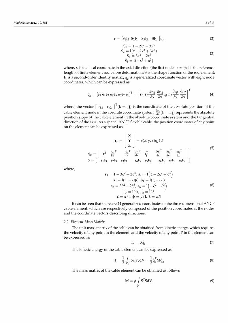
r =[S1I2 S2I2 S3I2 SI2

]qe (2)

S1 = 1− 2x2 + 3x3

S2 = l(x− 2x2 + 3x3)

S3 = 3x2 − 2x3

S4 = l(−x2 + x3) (3)

where, x is the local coordinate in the axial direction (the first node i x = 0); l is the referencelength of finite element rod before deformation; S is the shape function of the rod element;I2 is a second-order identity matrix; qe is a generalized coordinate vector with eight nodecoordinates, which can be expressed as

qe = [e1 e2e3 e4e5 e6e7 e8]T =

[ri1 ri2

∂ri1

∂x∂ri2

∂xrj1 rj2

∂rj1

∂x∂rj2

∂x

]T

(4)

where, the vector[

rk1 rk2]T(k = i, j) is the coordinate of the absolute position of the

cable element node in the absolute coordinate system; ∂rk∂x (k = i, j) represents the absolute

position slope of the cable element in the absolute coordinate system and the tangentialdirection of the axis. As a spatial ANCF flexible cable, the position coordinates of any pointon the element can be expressed as

rp =

XYZ

= S(x, y, z)qe(t)

qe =

[rT

i∂ri∂x

T ∂ri∂y

T ∂ri∂z

TrT

j∂rj∂x

T ∂rj∂y

T ∂rj∂z

T]T

S =[

s1I3 s2I3 s3I3 s4I3 s5I3 s6I3 s7I3 s8I3]

(5)

where,s1 = 1− 3ζ2 + 2ζ3, s2 = l

(ζ− 2ζ2 + ζ3

)s3 = l(ψ− ζψ), s4 = l(ξ− ζξ)

s5 = 3ζ2 − 2ζ3, s6 = l(−ζ2 + ζ3

)s7 = lζψ, s8 = lζξ

ζ = x/l, ψ = y/l, ξ = z/l

(6)

It can be seen that there are 24 generalized coordinates of the three-dimensional ANCFcable element, which are respectively composed of the position coordinates at the nodesand the coordinate vectors describing directions.

2.2. Element Mass Matrix

The unit mass matrix of the cable can be obtained from kinetic energy, which requiresthe velocity of any point in the element, and the velocity of any point P in the element canbe expressed as

rx = S.

qe (7)

The kinetic energy of the cable element can be expressed as

T =12

∫VρrT

x rxdV =12

.qT

e M.qe (8)

The mass matrix of the cable element can be obtained as follows

M = ρ

∫V

STSdV. (9)

Mathematics 2022, 10, 881 4 of 13

where v is the volume of the element; ρ is the density of material; M is the element massmatrix. rx = ∂ r

∂x =.r and rxx = ∂2r

∂x2 .

2.3. Generalized Elastic Force of Element

u is the displacement vector of any point along the axis and the deformation gradientJ is

J =∂u∂v

(10)

where r is the position vector in the element body coordinate system.

U =12

∫ l

0

(EAε2

x + EIκ2)

dx (11)

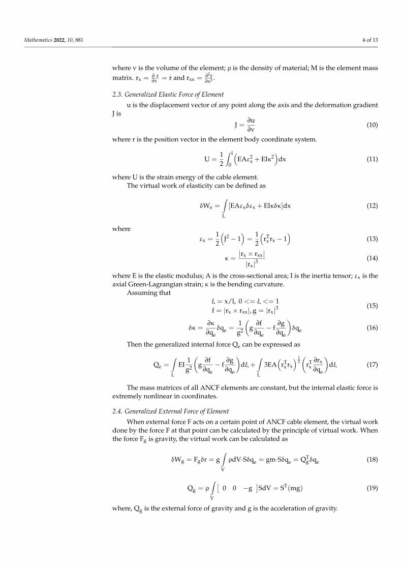
where U is the strain energy of the cable element.The virtual work of elasticity can be defined as

δWe =∫L

[EAεxδεx + EIκδκ]dx (12)

whereεx =

12

(J2 − 1

)=

12

(rT

x rx − 1)

(13)

κ =|rx × rxx||rx|3

(14)

where E is the elastic modulus; A is the cross-sectional area; I is the inertia tensor; εx is theaxial Green-Lagrangian strain; κ is the bending curvature.

Assuming thatξ = x/l, 0 <= ξ <= 1f = |rx × rxx|, g = |rx|3

(15)

δκ =∂κ

∂qeδqe =

1g2

(g

∂f∂qe− f

∂g∂qe

)δqe (16)

Then the generalized internal force Qe can be expressed as

Qe =∫L

EI1g2

(g

∂f∂qe− f

∂g∂qe

)dξ+

∫L

3EA(

rTx rx

) 12(

rTx

∂rx

∂qe

)dξ (17)

The mass matrices of all ANCF elements are constant, but the internal elastic force isextremely nonlinear in coordinates.

2.4. Generalized External Force of Element

When external force F acts on a certain point of ANCF cable element, the virtual workdone by the force F at that point can be calculated by the principle of virtual work. Whenthe force Fg is gravity, the virtual work can be calculated as

δWg = Fgδr = g∫V

ρdV·Sδqe = gm·Sδqe = QTgδqe (18)

Qg = ρ

∫V

[0 0 −g

]SdV = ST(mg) (19)

where, Qg is the external force of gravity and g is the acceleration of gravity.

Mathematics 2022, 10, 881 5 of 13

The dynamics formula is derived as follows

M..qe = Qg + Qe (20)

3. Rigid-Flexible Coupling Dynamic Model3.1. Mechanism Analysis

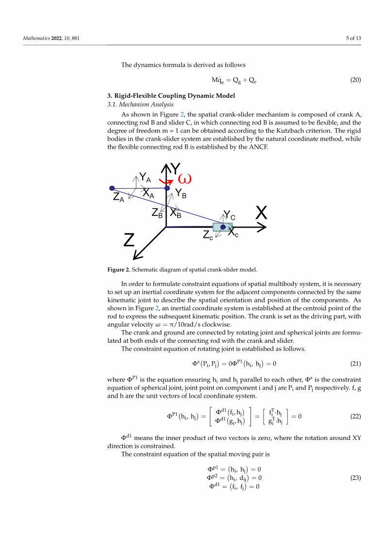
As shown in Figure 2, the spatial crank-slider mechanism is composed of crank A,connecting rod B and slider C, in which connecting rod B is assumed to be flexible, and thedegree of freedom m = 1 can be obtained according to the Kutzbach criterion. The rigidbodies in the crank-slider system are established by the natural coordinate method, whilethe flexible connecting rod B is established by the ANCF.

Mathematics 2022, 10, x FOR PEER REVIEW 5 of 13

δW = F δr = g ρ dV ∙ Sδq = gm ∙ Sδq = Q δq (18)

Q = ρ 0 0 −g S dV = S (mg) (19)

where, Q is the external force of gravity and g is the acceleration of gravity. The dynamics formula is derived as follows Mq = Q + Q (20)

3. Rigid-Flexible Coupling Dynamic Model 3.1. Mechanism Analysis

As shown in Figure 2, the spatial crank-slider mechanism is composed of crank A, connecting rod B and slider C, in which connecting rod B is assumed to be flexible, and the degree of freedom m = 1 can be obtained according to the Kutzbach criterion. The rigid bodies in the crank-slider system are established by the natural coordinate method, while the flexible connecting rod B is established by the ANCF.

In order to formulate constraint equations of spatial multibody system, it is necessary to set up an inertial coordinate system for the adjacent components connected by the same kinematic joint to describe the spatial orientation and position of the components. As shown in Figure 2, an inertial coordinate system is established at the centroid point of the rod to express the subsequent kinematic position. The crank is set as the driving part, with angular velocity ω = π/10rad/s clockwise.

Figure 2. Schematic diagram of spatial crank-slider model.

The crank and ground are connected by rotating joint and spherical joints are formu-lated at both ends of the connecting rod with the crank and slider.

The constraint equation of rotating joint is established as follows. Φ P , P = 0Φ h ，h = 0 (21)

where Φ is the equation ensuring hi and hj parallel to each other, Φ is the constraint equation of spherical joint, joint point on component i and j areP and P respectively. f, g and h are the unit vectors of local coordinate system.

Figure 2. Schematic diagram of spatial crank-slider model.

In order to formulate constraint equations of spatial multibody system, it is necessaryto set up an inertial coordinate system for the adjacent components connected by the samekinematic joint to describe the spatial orientation and position of the components. Asshown in Figure 2, an inertial coordinate system is established at the centroid point of therod to express the subsequent kinematic position. The crank is set as the driving part, withangular velocityω = π/10rad/s clockwise.

The crank and ground are connected by rotating joint and spherical joints are formu-lated at both ends of the connecting rod with the crank and slider.

The constraint equation of rotating joint is established as follows.

Φs(Pi, Pj)= 0ΦP1(hi, hj

)= 0 (21)

where ΦP1 is the equation ensuring hi and hj parallel to each other, Φs is the constraintequation of spherical joint, joint point on component i and j are Pi and Pj respectively. f, gand h are the unit vectors of local coordinate system.

ΦP1(hi, hj)=

[Φd1(fi, hj

)Φd1(gi, hj

) ] =

[fTi ·hj

gTi ·hj

]= 0 (22)

Φd1 means the inner product of two vectors is zero, where the rotation around XYdirection is constrained.

The constraint equation of the spatial moving pair is

Φp1 =(hi, hj

)= 0

Φp2 =(hi, dij

)= 0

Φd1 =(fi, fj

)= 0

(23)

Mathematics 2022, 10, 881 6 of 13

where dij = rPi − rP

j , rPi and rP

j are the absolute coordinate vectors of P point on i and jcomponent respectively. The constraint equations keep the slider move along the x-axis

For rigid bodies, unknown Cartesian coordinate q and constraint equations can beestablished as follows

qi =

[ripi

](24)

Φ(q, t) ≡

ΦK(q)ΦD(q, t)

Φp(q)

= 0 (25)

where, ΦK(q) is the kinematic constraint. ΦD(q, t) is the driving constraint. Φp(q) is Eulerparameter constraint. ri is the position vector of inertia coordinate of each component. pi isthe Euler parameter of the inertia coordinate of each component.

The Jacobian of the constraint equation is

Φq =

ΦKq

ΦDq

ΦPq

(26)

Φq∆q(j) = −Φ(

q(j), t)

q(j+1) = q(j) + ∆q(j) (27)

Given an estimated initial value q(0), q can be calculated by Newton-Raphson iterationFormula (26). The constraint equation between rigid components and flexible component isformulated as below, where r0 and rn are the node position vectors of the flexible component,while rB1 and rB2 are node position vectors of the rigid component.

Φ1 =

[r(0) − rB1r(n) − rB2

]= 0 (28)

3.2. Rigid-Flexible Coupling Dynamic Equation

The rigid-flexible coupling dynamic equation of space crank-slider is constructed.The mass matrix of flexible components formulated by ANCF is constant, so there isno centrifugal force or Coriolis force. Mass matrix of rigid components Mr and flexiblecomponents Mf are formulated as below,

Mr = diag(mi, mi, mi, Iix, Iiy, Iiz

)(29)

Mf = ρ

∫V

STSdV (30)

The spatial rigid-flexible coupling dynamic equation is obtained as follows, which canbe solved by generalized αmethod and Euler implicit method combined.{

MΣ..q + ΦT

qλ = Q + QeΦ(q, t) = 0

(31)

MΣ =

[Mr 00 Mf

], q =

[qrqf

](32)

4. Numerical Simulation and Analysis4.1. Simulation Process and Parameters

The fully rigid spatial slider-crank mechanism and rigid-flexible coupling spatialslider-crank mechanism are analyzed respectively. The related parameters are shownin Table 1.

Mathematics 2022, 10, 881 7 of 13

Table 1. Mechanism parameter.

Component Crank A Connecting Rod B Slider C

Ix/kg·m2 0.005 0.005 0.05Iy/kg·m2 0.1 0.1 0.05Iz/kg·m2 0.1 0.1 0.05Mass/kg 1 0.5 1

Length/m 2√

17 0.4Section Diameter/m / 0.03 /Young’s Modulus/Pa / 5 × 109 /Number of Elements / 9 /

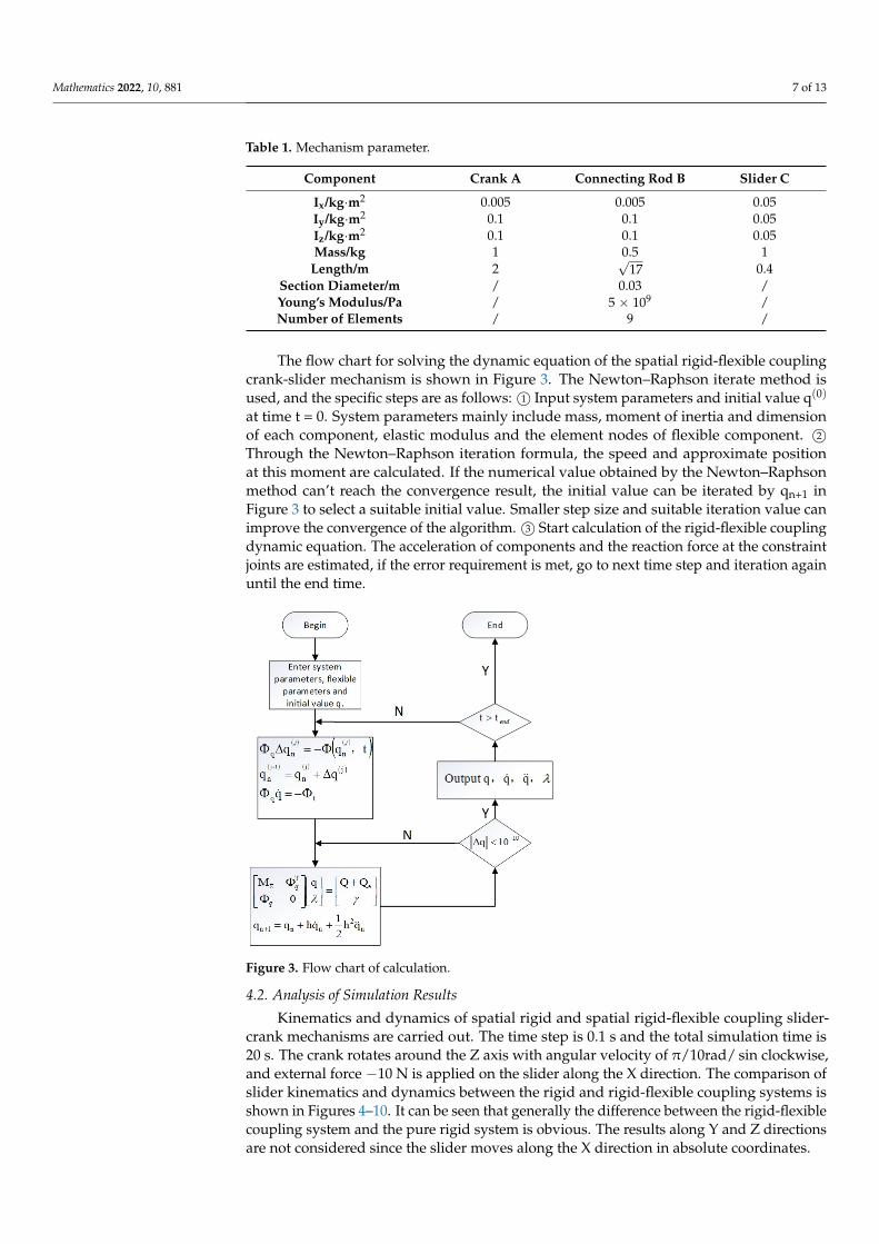
The flow chart for solving the dynamic equation of the spatial rigid-flexible couplingcrank-slider mechanism is shown in Figure 3. The Newton–Raphson iterate method isused, and the specific steps are as follows: 1© Input system parameters and initial value q(0)

at time t = 0. System parameters mainly include mass, moment of inertia and dimensionof each component, elastic modulus and the element nodes of flexible component. 2©Through the Newton–Raphson iteration formula, the speed and approximate positionat this moment are calculated. If the numerical value obtained by the Newton–Raphsonmethod can’t reach the convergence result, the initial value can be iterated by qn+1 inFigure 3 to select a suitable initial value. Smaller step size and suitable iteration value canimprove the convergence of the algorithm. 3© Start calculation of the rigid-flexible couplingdynamic equation. The acceleration of components and the reaction force at the constraintjoints are estimated, if the error requirement is met, go to next time step and iteration againuntil the end time.

Mathematics 2022, 10, x FOR PEER REVIEW 8 of 13

Figure 3. Flow chart of calculation.

4.2. Analysis of Simulation Results Kinematics and dynamics of spatial rigid and spatial rigid-flexible coupling slider-

crank mechanisms are carried out. The time step is 0.1 s and the total simulation time is 20 s. The crank rotates around the Z axis with angular velocity of π/10rad/sin clockwise, and external force −10 N is applied on the slider along the X direction. The comparison of slider kinematics and dynamics between the rigid and rigid-flexible coupling systems is shown in Figures 4–10. It can be seen that generally the difference between the rigid-flex-ible coupling system and the pure rigid system is obvious. The results along Y and Z di-rections are not considered since the slider moves along the X direction in absolute coor-dinates.

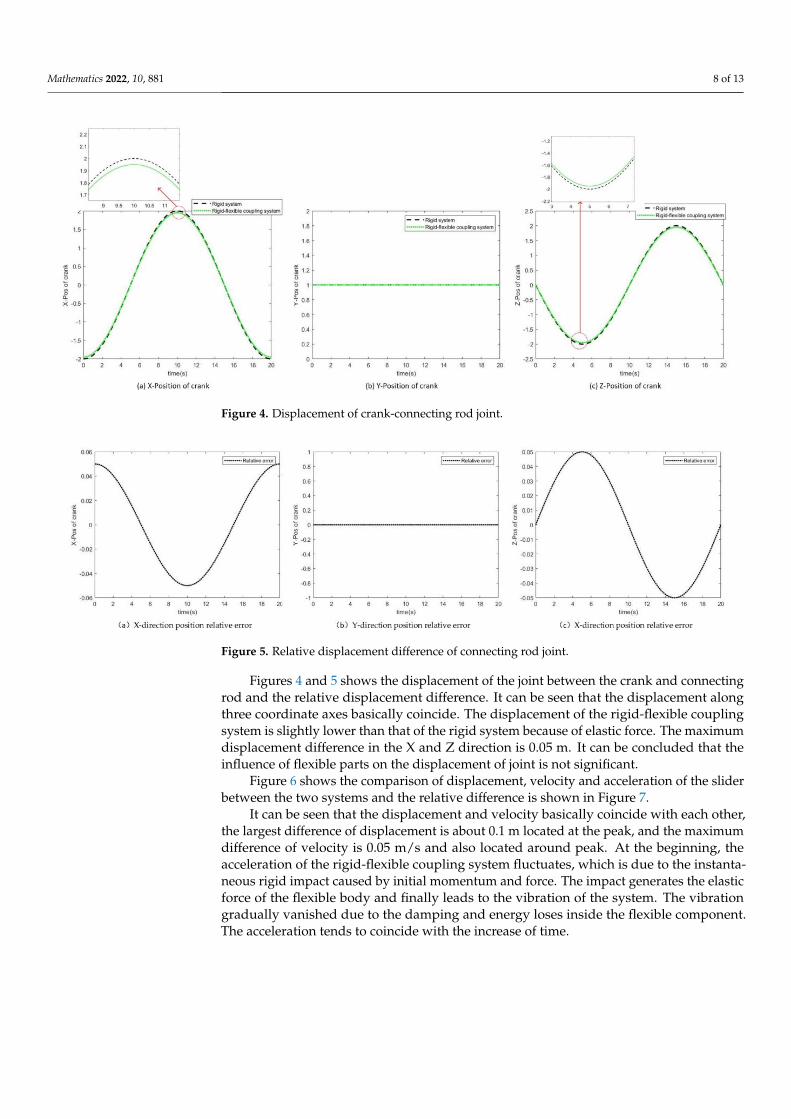
Figures 4 and 5 shows the displacement of the joint between the crank and connecting rod and the relative displacement difference. It can be seen that the displacement along three coordinate axes basically coincide. The displacement of the rigid-flexible coupling system is slightly lower than that of the rigid system because of elastic force. The maxi-mum displacement difference in the X and Z direction is 0.05 m. It can be concluded that the influence of flexible parts on the displacement of joint is not significant.

Figure 4. Displacement of crank-connecting rod joint.

Figure 3. Flow chart of calculation.

4.2. Analysis of Simulation Results

Kinematics and dynamics of spatial rigid and spatial rigid-flexible coupling slider-crank mechanisms are carried out. The time step is 0.1 s and the total simulation time is20 s. The crank rotates around the Z axis with angular velocity of π/10rad/ sin clockwise,and external force −10 N is applied on the slider along the X direction. The comparison ofslider kinematics and dynamics between the rigid and rigid-flexible coupling systems isshown in Figures 4–10. It can be seen that generally the difference between the rigid-flexiblecoupling system and the pure rigid system is obvious. The results along Y and Z directionsare not considered since the slider moves along the X direction in absolute coordinates.

Mathematics 2022, 10, 881 8 of 13

Mathematics 2022, 10, x FOR PEER REVIEW 8 of 13

Figure 3. Flow chart of calculation.

4.2. Analysis of Simulation Results Kinematics and dynamics of spatial rigid and spatial rigid-flexible coupling slider-

crank mechanisms are carried out. The time step is 0.1 s and the total simulation time is 20 s. The crank rotates around the Z axis with angular velocity of π/10rad/sin clockwise, and external force −10 N is applied on the slider along the X direction. The comparison of slider kinematics and dynamics between the rigid and rigid-flexible coupling systems is shown in Figures 4–10. It can be seen that generally the difference between the rigid-flex-ible coupling system and the pure rigid system is obvious. The results along Y and Z di-rections are not considered since the slider moves along the X direction in absolute coor-dinates.

Figures 4 and 5 shows the displacement of the joint between the crank and connecting rod and the relative displacement difference. It can be seen that the displacement along three coordinate axes basically coincide. The displacement of the rigid-flexible coupling system is slightly lower than that of the rigid system because of elastic force. The maxi-mum displacement difference in the X and Z direction is 0.05 m. It can be concluded that the influence of flexible parts on the displacement of joint is not significant.

Figure 4. Displacement of crank-connecting rod joint. Figure 4. Displacement of crank-connecting rod joint.

Mathematics 2022, 10, x FOR PEER REVIEW 9 of 13

Figure 5. Relative displacement difference of connecting rod joint.

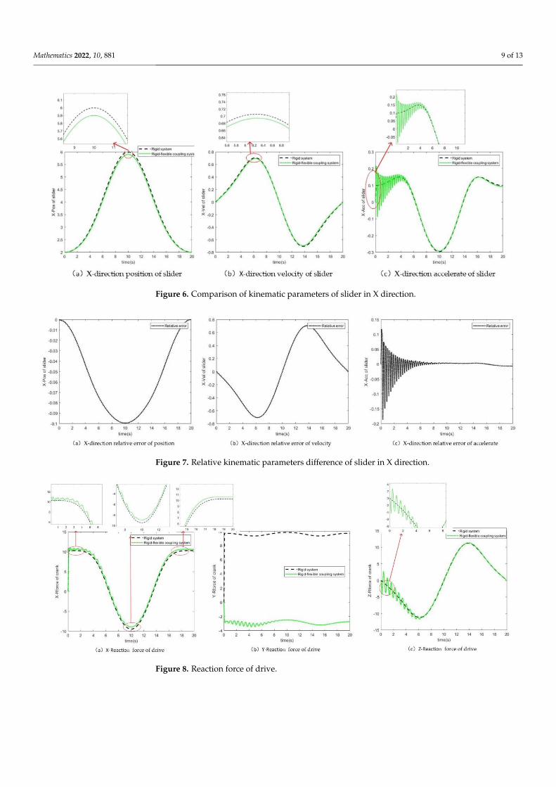
Figure 6 shows the comparison of displacement, velocity and acceleration of the slider between the two systems and the relative difference is shown in Figure 7.

It can be seen that the displacement and velocity basically coincide with each other, the largest difference of displacement is about 0.1 m located at the peak, and the maximum difference of velocity is 0.05 m/s and also located around peak. At the beginning, the ac-celeration of the rigid-flexible coupling system fluctuates, which is due to the instantane-ous rigid impact caused by initial momentum and force. The impact generates the elastic force of the flexible body and finally leads to the vibration of the system. The vibration gradually vanished due to the damping and energy loses inside the flexible component. The acceleration tends to coincide with the increase of time.

Figure 6. Comparison of kinematic parameters of slider in X direction.

Figure 7. Relative kinematic parameters difference of slider in X direction.

Reaction forces of the crank drive and the relative difference are shown in Figures 8 and 9. The maximum difference in the X direction is about 1 N accompanied by fluctuation. The relative difference of the amplitude gradually decreases. The difference of the driving reaction force in the Y direction of the two system is about 12 N, which is due to the

Figure 5. Relative displacement difference of connecting rod joint.

Figures 4 and 5 shows the displacement of the joint between the crank and connectingrod and the relative displacement difference. It can be seen that the displacement alongthree coordinate axes basically coincide. The displacement of the rigid-flexible couplingsystem is slightly lower than that of the rigid system because of elastic force. The maximumdisplacement difference in the X and Z direction is 0.05 m. It can be concluded that theinfluence of flexible parts on the displacement of joint is not significant.

Figure 6 shows the comparison of displacement, velocity and acceleration of the sliderbetween the two systems and the relative difference is shown in Figure 7.

It can be seen that the displacement and velocity basically coincide with each other,the largest difference of displacement is about 0.1 m located at the peak, and the maximumdifference of velocity is 0.05 m/s and also located around peak. At the beginning, theacceleration of the rigid-flexible coupling system fluctuates, which is due to the instanta-neous rigid impact caused by initial momentum and force. The impact generates the elasticforce of the flexible body and finally leads to the vibration of the system. The vibrationgradually vanished due to the damping and energy loses inside the flexible component.The acceleration tends to coincide with the increase of time.

Mathematics 2022, 10, 881 9 of 13

Mathematics 2022, 10, x FOR PEER REVIEW 9 of 13

Figure 5. Relative displacement difference of connecting rod joint.

Figure 6 shows the comparison of displacement, velocity and acceleration of the slider between the two systems and the relative difference is shown in Figure 7.

It can be seen that the displacement and velocity basically coincide with each other, the largest difference of displacement is about 0.1 m located at the peak, and the maximum difference of velocity is 0.05 m/s and also located around peak. At the beginning, the ac-celeration of the rigid-flexible coupling system fluctuates, which is due to the instantane-ous rigid impact caused by initial momentum and force. The impact generates the elastic force of the flexible body and finally leads to the vibration of the system. The vibration gradually vanished due to the damping and energy loses inside the flexible component. The acceleration tends to coincide with the increase of time.

Figure 6. Comparison of kinematic parameters of slider in X direction.

Figure 7. Relative kinematic parameters difference of slider in X direction.

Reaction forces of the crank drive and the relative difference are shown in Figures 8 and 9. The maximum difference in the X direction is about 1 N accompanied by fluctuation. The relative difference of the amplitude gradually decreases. The difference of the driving reaction force in the Y direction of the two system is about 12 N, which is due to the

Figure 6. Comparison of kinematic parameters of slider in X direction.

Mathematics 2022, 10, x FOR PEER REVIEW 9 of 13

Figure 5. Relative displacement difference of connecting rod joint.

Figure 6 shows the comparison of displacement, velocity and acceleration of the slider between the two systems and the relative difference is shown in Figure 7.

It can be seen that the displacement and velocity basically coincide with each other, the largest difference of displacement is about 0.1 m located at the peak, and the maximum difference of velocity is 0.05 m/s and also located around peak. At the beginning, the ac-celeration of the rigid-flexible coupling system fluctuates, which is due to the instantane-ous rigid impact caused by initial momentum and force. The impact generates the elastic force of the flexible body and finally leads to the vibration of the system. The vibration gradually vanished due to the damping and energy loses inside the flexible component. The acceleration tends to coincide with the increase of time.

Figure 6. Comparison of kinematic parameters of slider in X direction.

Figure 7. Relative kinematic parameters difference of slider in X direction.

Reaction forces of the crank drive and the relative difference are shown in Figures 8 and 9. The maximum difference in the X direction is about 1 N accompanied by fluctuation. The relative difference of the amplitude gradually decreases. The difference of the driving reaction force in the Y direction of the two system is about 12 N, which is due to the

Figure 7. Relative kinematic parameters difference of slider in X direction.

Mathematics 2022, 10, x FOR PEER REVIEW 10 of 13

stretching action of the flexible part. The fluctuation of reaction forces at the initial period comes from the elastic forces of the flexible part resisting the driving impact. The maxi-mum difference of the reaction force in the Z direction is about 4 N.

Figure 8. Reaction force of drive.

Figure 9. Relative reaction force difference of drive.

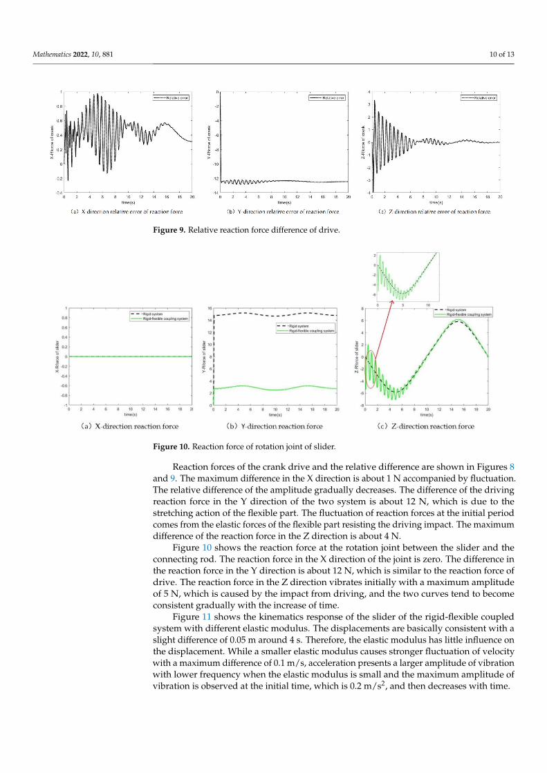
Figure 10 shows the reaction force at the rotation joint between the slider and the connecting rod. The reaction force in the X direction of the joint is zero. The difference in the reaction force in the Y direction is about 12 N, which is similar to the reaction force of drive. The reaction force in the Z direction vibrates initially with a maximum amplitude of 5 N, which is caused by the impact from driving, and the two curves tend to become consistent gradually with the increase of time.

Figure 10. Reaction force of rotation joint of slider.

Figure 8. Reaction force of drive.

Mathematics 2022, 10, 881 10 of 13

Mathematics 2022, 10, x FOR PEER REVIEW 10 of 13

stretching action of the flexible part. The fluctuation of reaction forces at the initial period comes from the elastic forces of the flexible part resisting the driving impact. The maxi-mum difference of the reaction force in the Z direction is about 4 N.

Figure 8. Reaction force of drive.

Figure 9. Relative reaction force difference of drive.

Figure 10 shows the reaction force at the rotation joint between the slider and the connecting rod. The reaction force in the X direction of the joint is zero. The difference in the reaction force in the Y direction is about 12 N, which is similar to the reaction force of drive. The reaction force in the Z direction vibrates initially with a maximum amplitude of 5 N, which is caused by the impact from driving, and the two curves tend to become consistent gradually with the increase of time.

Figure 10. Reaction force of rotation joint of slider.

Figure 9. Relative reaction force difference of drive.

Mathematics 2022, 10, x FOR PEER REVIEW 10 of 13

stretching action of the flexible part. The fluctuation of reaction forces at the initial period comes from the elastic forces of the flexible part resisting the driving impact. The maxi-mum difference of the reaction force in the Z direction is about 4 N.

Figure 8. Reaction force of drive.

Figure 9. Relative reaction force difference of drive.

Figure 10 shows the reaction force at the rotation joint between the slider and the connecting rod. The reaction force in the X direction of the joint is zero. The difference in the reaction force in the Y direction is about 12 N, which is similar to the reaction force of drive. The reaction force in the Z direction vibrates initially with a maximum amplitude of 5 N, which is caused by the impact from driving, and the two curves tend to become consistent gradually with the increase of time.

Figure 10. Reaction force of rotation joint of slider. Figure 10. Reaction force of rotation joint of slider.

Reaction forces of the crank drive and the relative difference are shown in Figures 8and 9. The maximum difference in the X direction is about 1 N accompanied by fluctuation.The relative difference of the amplitude gradually decreases. The difference of the drivingreaction force in the Y direction of the two system is about 12 N, which is due to thestretching action of the flexible part. The fluctuation of reaction forces at the initial periodcomes from the elastic forces of the flexible part resisting the driving impact. The maximumdifference of the reaction force in the Z direction is about 4 N.

Figure 10 shows the reaction force at the rotation joint between the slider and theconnecting rod. The reaction force in the X direction of the joint is zero. The difference inthe reaction force in the Y direction is about 12 N, which is similar to the reaction force ofdrive. The reaction force in the Z direction vibrates initially with a maximum amplitudeof 5 N, which is caused by the impact from driving, and the two curves tend to becomeconsistent gradually with the increase of time.

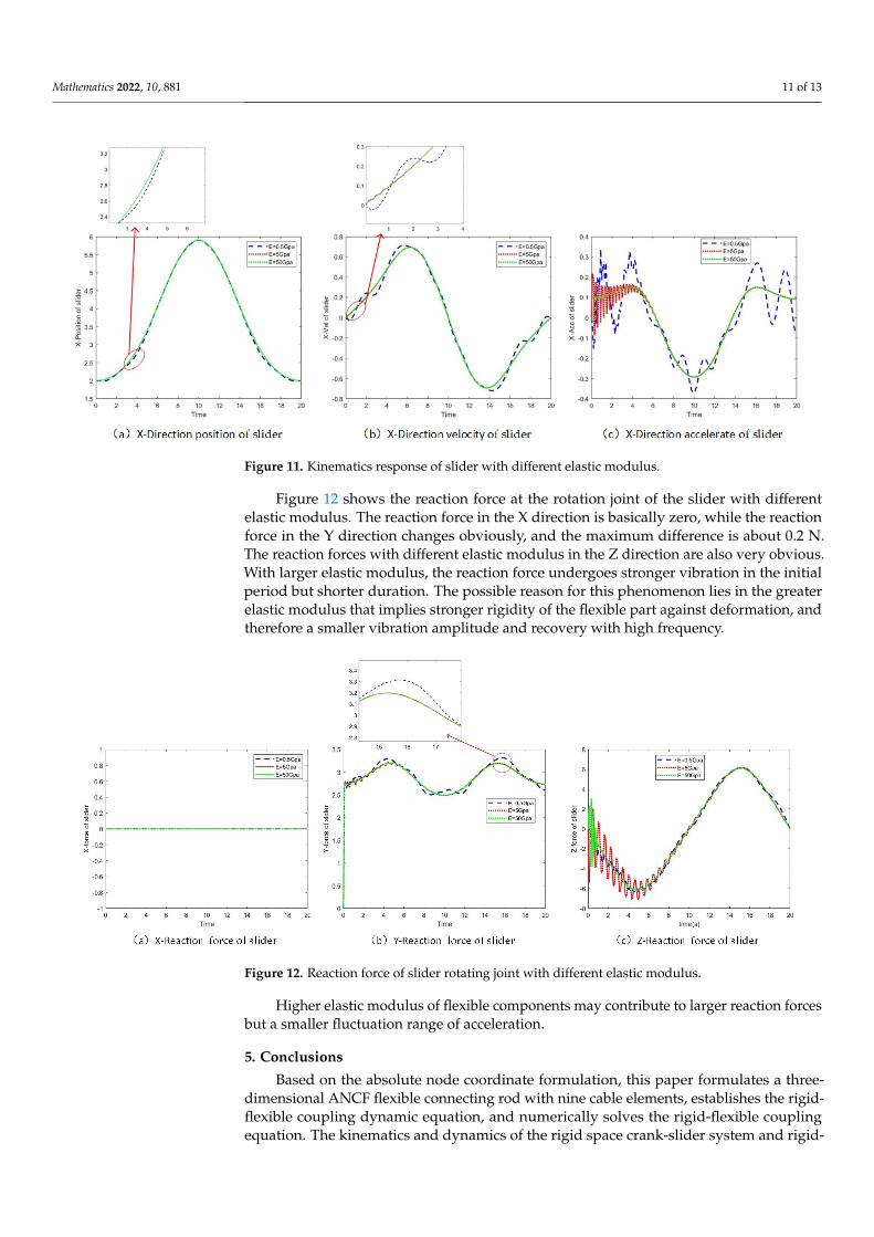
Figure 11 shows the kinematics response of the slider of the rigid-flexible coupledsystem with different elastic modulus. The displacements are basically consistent with aslight difference of 0.05 m around 4 s. Therefore, the elastic modulus has little influence onthe displacement. While a smaller elastic modulus causes stronger fluctuation of velocitywith a maximum difference of 0.1 m/s, acceleration presents a larger amplitude of vibrationwith lower frequency when the elastic modulus is small and the maximum amplitude ofvibration is observed at the initial time, which is 0.2 m/s2, and then decreases with time.

Mathematics 2022, 10, 881 11 of 13

Mathematics 2022, 10, x FOR PEER REVIEW 11 of 13

Figure 11 shows the kinematics response of the slider of the rigid-flexible coupled system with different elastic modulus. The displacements are basically consistent with a slight difference of 0.05 m around 4 s. Therefore, the elastic modulus has little influence on the displacement. While a smaller elastic modulus causes stronger fluctuation of ve-locity with a maximum difference of 0.1 m/s, acceleration presents a larger amplitude of vibration with lower frequency when the elastic modulus is small and the maximum am-plitude of vibration is observed at the initial time, which is 0.2 m/s2, and then decreases with time.

Figure 11. Kinematics response of slider with different elastic modulus.

Figure 12 shows the reaction force at the rotation joint of the slider with different elastic modulus. The reaction force in the X direction is basically zero, while the reaction force in the Y direction changes obviously, and the maximum difference is about 0.2 N. The reaction forces with different elastic modulus in the Z direction are also very obvious. With larger elastic modulus, the reaction force undergoes stronger vibration in the initial period but shorter duration. The possible reason for this phenomenon lies in the greater elastic modulus that implies stronger rigidity of the flexible part against deformation, and therefore a smaller vibration amplitude and recovery with high frequency.

Figure 12. Reaction force of slider rotating joint with different elastic modulus.

Higher elastic modulus of flexible components may contribute to larger reaction forces but a smaller fluctuation range of acceleration.

5. Conclusions Based on the absolute node coordinate formulation, this paper formulates a three-

dimensional ANCF flexible connecting rod with nine cable elements, establishes the rigid-

Figure 11. Kinematics response of slider with different elastic modulus.

Figure 12 shows the reaction force at the rotation joint of the slider with differentelastic modulus. The reaction force in the X direction is basically zero, while the reactionforce in the Y direction changes obviously, and the maximum difference is about 0.2 N.The reaction forces with different elastic modulus in the Z direction are also very obvious.With larger elastic modulus, the reaction force undergoes stronger vibration in the initialperiod but shorter duration. The possible reason for this phenomenon lies in the greaterelastic modulus that implies stronger rigidity of the flexible part against deformation, andtherefore a smaller vibration amplitude and recovery with high frequency.

Mathematics 2022, 10, x FOR PEER REVIEW 11 of 13

Figure 11 shows the kinematics response of the slider of the rigid-flexible coupled system with different elastic modulus. The displacements are basically consistent with a slight difference of 0.05 m around 4 s. Therefore, the elastic modulus has little influence on the displacement. While a smaller elastic modulus causes stronger fluctuation of ve-locity with a maximum difference of 0.1 m/s, acceleration presents a larger amplitude of vibration with lower frequency when the elastic modulus is small and the maximum am-plitude of vibration is observed at the initial time, which is 0.2 m/s2, and then decreases with time.

Figure 11. Kinematics response of slider with different elastic modulus.

Figure 12 shows the reaction force at the rotation joint of the slider with different elastic modulus. The reaction force in the X direction is basically zero, while the reaction force in the Y direction changes obviously, and the maximum difference is about 0.2 N. The reaction forces with different elastic modulus in the Z direction are also very obvious. With larger elastic modulus, the reaction force undergoes stronger vibration in the initial period but shorter duration. The possible reason for this phenomenon lies in the greater elastic modulus that implies stronger rigidity of the flexible part against deformation, and therefore a smaller vibration amplitude and recovery with high frequency.

Figure 12. Reaction force of slider rotating joint with different elastic modulus.

Higher elastic modulus of flexible components may contribute to larger reaction forces but a smaller fluctuation range of acceleration.

5. Conclusions Based on the absolute node coordinate formulation, this paper formulates a three-

dimensional ANCF flexible connecting rod with nine cable elements, establishes the rigid-

Figure 12. Reaction force of slider rotating joint with different elastic modulus.

Higher elastic modulus of flexible components may contribute to larger reaction forcesbut a smaller fluctuation range of acceleration.

5. Conclusions

Based on the absolute node coordinate formulation, this paper formulates a three-dimensional ANCF flexible connecting rod with nine cable elements, establishes the rigid-flexible coupling dynamic equation, and numerically solves the rigid-flexible couplingequation. The kinematics and dynamics of the rigid space crank-slider system and rigid-

Mathematics 2022, 10, 881 12 of 13

flexible coupling space crank-slider system are compared, and the influence of the flexiblecomponent on motion accuracy and reaction forces is obtained. It can be inferred that theexistence of an internal elastic force causes the rigid-flexible coupling system to fluctuategreatly. Finally, the kinematic and dynamic responses of the rigid-flexible coupled systemwith different elastic modulus are analyzed. The results show that a smaller elastic modulushas a greater influence on motion accuracy and reaction forces.

Spatial deficient ANCF beam formulation coupled with spatial rigid body dynamicsproposed in this paper represents and advance for rigid-flexible multibody dynamics,which are mostly focused on planar mechanisms. The analysis of the influence of differentelastic coefficients on system dynamics has significance for flexible component design.

Author Contributions: Conceptualization, X.W.; data curation, H.W.; formal analysis, H.W.; fundingacquisition, C.X.; methodology, X.W.; project administration, Z.L.; resources, X.W. and C.X.; software,X.W.; supervision, Z.L. and Q.H.; visualization, H.W. and J.Z.; writing–original draft, H.W.; writing–review & editing, X.W. All authors have read and agreed to the published version of the manuscript.

Funding: This work was supported by the National Natural Science Foundation of China (52005088)and the Natural Science Foundation of Liaoning Province (2020-MS-076) and National Science andTechnology Major Project (J2019-IV-0002-0069).

Institutional Review Board Statement: Not applicable.

Informed Consent Statement: Not applicable.

Data Availability Statement: No reported data.

Conflicts of Interest: The authors declare no conflict of interest.

References1. Dias, J.; Pereira, M.S. Sensitivity Analysis of Rigid-Flexible Multibody Systems. Multibody Syst. Dyn. 1997, 1, 303–322. [CrossRef]2. Youwu, L. Application of multi-body dynamics in mechanical engineering. China Mech. Eng. 2000, 11, 6.3. Wittenburg, J.; Likins, P. Dynamics of Systems of Rigid Bodies. J. Appl. Mech. 1977, 45, 458. [CrossRef]4. Nikravesh, P.E.; Chung, I.S. Application of Euler Parameters to the Dynamic Analysis of Three-Dimensional Constrained

Mechanical Systems. J. Mech. Des. 1982, 104, 785–791. [CrossRef]5. Haug, E.J.; Wu, S.C.; Yang, S.M. Dynamics of mechanical systems with Coulomb friction, stiction, impact and constraint

addition-deletion—III Spatial systems. Mech. Mach. Theory 1986, 21, 401–406. [CrossRef]6. Shabana, A.A. Definition of the Slopes and the Finite Element Absolute Nodal Coordinate Formulation. Multi-Body Syst. Dyn.

1997, 1, 339–348. [CrossRef]7. Garcia-Vallejo, D.; Mayo, J.; Escalona, J.L.; Domínguez, J. Three-dimensional formulation of rigid-flexible multibody systems with

flexible beam elements. Multibody Syst. Dyn. 2008, 20, 1–28. [CrossRef]8. Zhang, C. Mechanical Dynamics, 2nd ed.; Higher Education Press: Beijing, China, 2008.9. Jiazhen, H.; Chaolan, Y. Research progress of rigid-flexible coupling system dynamics. J. Dyn. Control. 2004, 2, 6.10. Jiazhen, H.; Zhuyong, L. Modeling method of rigid-flexible coupling dynamics. J. Shanghai Jiaotong Univ. 2008, 42, 5.11. Jiazhen, H.; Lizhong, J. Rigid-flexible coupling dynamics of flexible multi-body system. Mech. Prog. 2000, 30, 6.12. Likins, P.W. Finite element appendage equations for hybrid coordinate dynamic analysis. Int. J. Solids Struct. 1972, 8, 709–731.

[CrossRef]13. Bakr, E.M.; Shabana, A.A. Geometrically nonlinear analysis of multi-body systems. Comput. Struct. 1986, 23, 739–751. [CrossRef]14. Lin, B.; Xie, C. Dynamics of Flexible multi-body Systems. Acta Mech. Sin. 1989, 4, 469–478.15. Yigi, S.A. The Effect of Flexibility on the Impact Response of a Two-Link Rigid-Flexible Manipulator. J. Sound Vib. 1994, 177,

349–361. [CrossRef]16. Choura, S.; Yigit, A.S. Control of a Two-Link Rigid–Flexible Manipulator with a Moving Payload Mass. J. Sound Vib. 2001, 243,

883–897. [CrossRef]17. Williams, D.; Fredrickson, G.H. Cylindrical Micelles in Rigid-Flexible Diblock Copolymers. MRS Online Proc. Libr. 1991, 248,

3561–3568. [CrossRef]18. Duan, Y.C.; Zhang, D.G. Rigid-Flexible Coupling Dynamics of a Flexible Robot with Impact. Adv. Mater. Res. 2011, 199, 243–250.

[CrossRef]19. Zhao, F.; Liu, J.; Hong, J. Nonlinear dynamic analysis on rigid-flexible coupling system of an elastic beam. Theor. Appl. Mech. Lett.

2012, 2, 023001. [CrossRef]20. Bai, Z.F.; Zhao, Y.; Tian, H. Study on collision dynamics of flexible multibody system. J. Vib. Shock. 2009, 28, 75–78+195–196.21. Wang, J.M.; Hong, J.Z. Experimental Study on Flexible Multibody Dynamics. J. Astronaut. 1999, 2, 108–112.

Mathematics 2022, 10, 881 13 of 13

22. Mo, L. Kinematics and dynamics analysis of crank-slider mechanism based on MATLAB. Automot. Pract. Technol. 2019, 23,135–137. [CrossRef]

23. Li, T.T.; Zhang, Z.S.; Cui, G.H.; Guan, L.Z. Dynamic analysis of crank-connecting rod mechanism with coupling hinge clearanceand flexibility. Mech. Transm. 2021, 45, 116–122. [CrossRef]

24. Qian, Y.; Cao, Y.; Liu, Y.W.; Zhou, H. Forward Kinematics Simulation Analysis of Slider-Crank Mechanism. Adv. Mater. Res. 2011,308–310, 1855–1859. [CrossRef]

25. Ma, X.G.; Lu, Y.; You, X.M. Multi-body dynamics simulation analysis of planetary gear train based on multi-body dynamicstechnology. China Mech. Eng. 2009, 20, 1956–1959+1964.

26. Liu, Y.H.; Miu, B.Q. Theoretical basis and functional analysis of multi-body dynamics simulation software ADAMS. Electron.Packag. 2005, 5, 5.

27. Shi, Z.X.; Fung, E.; Lie, Y.C. Dynamic modelling of a rigid-flexible manipulator for constrained motion task control. Appl. Math.Model. 1999, 23, 509–525. [CrossRef]

28. Wu, M.Q.; Mei, H.F.; Zhang, Z.Q. Multi-body dynamics simulation of linkage mechanism based on ADAMS. J. Eng. Des. 2005, 12, 4.29. Fan, B.L.; Yang, G.H.; Zhu, X.Y. Research and practice teaching of crank-connecting rod mechanism based on multi-body

dynamics simulation. Met. World 2021, 1, 71–75.30. Sugiyama, H.; Escalona, J.L.; Shabana, A.A. Formulation of Three-Dimensional Joint Constraints Using the Absolute Nodal

Coordinates. Nonlinear Dyn. 2003, 31, 167–195. [CrossRef]31. Shabana, A.A. Computational Continuum Mechanics; Cambridge University Press: Cambridge, UK, 2012.