Flexible multibody dynamics approach for tire dynamics ...

-

Flexible multibody dynamics approach for tiredynamics simulationYamashita, Hirokihttps://iro.uiowa.edu/discovery/delivery/01IOWA_INST:ResearchRepository/12730541150002771?l#13730793160002771

Yamashita. (2016). Flexible multibody dynamics approach for tire dynamics simulation [University ofIowa]. https://doi.org/10.17077/etd.gfixb2od

Downloaded on 2022/07/10 05:13:02 -0500Copyright © 2016 Hiroki YamashitaFree to read and downloadhttps://iro.uiowa.edu

-

FLEXIBLE MULTIBODY DYNAMICS APPROACH

FOR TIRE DYNAMICS SIMULATION

by

Hiroki Yamashita

A thesis submitted in partial fulfillment of the requirements for the Doctor of

Philosophy degree in Mechanical Engineering in the Graduate College of

The University of Iowa

December 2016

Thesis Supervisor: Associate Professor Hiroyuki Sugiyama

Graduate College The University of Iowa

Iowa City, Iowa

CERTIFICATE OF APPROVAL

_______________________

PH.D. THESIS

_______________

This is to certify that the Ph.D. thesis of

Hiroki Yamashita

has been approved by the Examining Committee for the thesis requirement for the Doctor of Philosophy degree in Mechanical Engineering at the December 2016 graduation.

Thesis Committee: ___________________________________ Hiroyuki Sugiyama, Thesis Supervisor

___________________________________ Kyung K. Choi

___________________________________ Paramsothy Jayakumar

___________________________________ Jia Lu

___________________________________ Shaoping Xiao

ii

ACKNOWLEDGMENTS

I would like to express my deepest gratitude to my advisor Professor Hiroyuki

Sugiyama for giving me not only invaluable guidance on my PhD research, but also

continuous support for my study at the University of Iowa. I could not have kept pursuing

my PhD research without his support. I would also like to thank Dr. Paramsothy

Jayakumar from US Army TARDEC for providing me with constructive suggestions and

various advice to my research. I would also like to thank Dr. Ryoji Hanada from

Yokohama Rubber Co., Ltd. for giving me invaluable technical advice on developing the

high-fidelity tire model. I would like to thank Professors Kyung K. Choi, Jia Lu, and

Shaoping Xiao for serving on my thesis defense committee. I wish to thank all my friends

and colleagues who have encouraged me and provided insight into my research. In

particular, I would like to thank my labmates, Huaxia Lee, Chris Feldmeier, Bryan

Peterson, and Xiangkang Chen.

This research was supported by the Automotive Research Center (ARC) in

accordance with Cooperative Agreement W56HZV-04-2-0001 U.S. Army Tank

Automotive Research, Development and Engineering Center (TARDEC) and Yokohama

Rubber Co., Ltd. These financial supports are greatly acknowledged.

iii

ABSTRACT

The objective of this study is to develop a high-fidelity physics-based flexible tire

model that can be fully integrated into multibody dynamics computer algorithms for use

in on-road and off-road vehicle dynamics simulation without ad-hoc co-simulation

techniques. Despite the fact detailed finite element tire models using explicit finite

element software have been widely utilized for structural design of tires by tire

manufactures, it is recognized in the tire industry that existing state-of-the-art explicit

finite element tire models are not capable of predicting the transient tire force

characteristics accurately under severe vehicle maneuvering conditions due to the

numerical instability that is essentially inevitable for explicit finite element procedures

for severe loading scenarios and the lack of transient (dynamic) tire friction model suited

for FE tire models. Furthermore, to integrate the deformable tire models into multibody

full vehicle simulation, co-simulation technique could be an option for commercial

software. However, there exist various challenges in co-simulation for the transient

vehicle maneuvering simulation in terms of numerical stability and computational

efficiency. The transient tire dynamics involves rapid changes in contact forces due to the

abrupt braking and steering input, thus use of co-simulation requires very small step size

to ensure the numerical stability and energy balance between two separate simulation

using different solvers.

In order to address these essential and challenging issues on the high-fidelity

flexible tire model suited for multibody vehicle dynamics simulation, a physics-based tire

model using the flexible multibody dynamics approach is proposed in this study. To this

end, a continuum mechanics based shear deformable laminated composite shell element

is developed based on the finite element absolute nodal coordinate formulation for

modeling the complex fiber reinforced rubber tire structure. The assumed natural strain

(ANS) and enhanced assumed strain (EAS) approaches are introduced for alleviating

element lockings exhibited in the element. Use of the concept of the absolute nodal

coordinate formulation leads to various advantages for tire dynamics simulation in that

(1) constant mass matrix can be obtained for fully nonlinear dynamics simulation; (2)

exact modeling of rigid body motion is ensured when strains are zero; and (3) non-

iv

incremental solution procedure utilized in the general multibody dynamics computer

algorithm can be directly applied without specialized updating schemes for finite

rotations. Using the proposed shear deformable laminated composite shell element, a

physics-based flexible tire model is developed. To account for the transient tire friction

characteristics including the friction-induced hysteresis that appears in severe

maneuvering conditions, the distributed parameter LuGre tire friction model is integrated

into the flexible tire model. To this end, the contact patch predicted by the structural tire

model is discretized into small strips across the tire width, and then each strip is further

discretized into small elements to convert the partial differential equations of the LuGre

tire friction model to the set of first-order ordinary differential equations. By doing so, the

structural deformation of the flexible tire model and the LuGre tire friction force model

are dynamically coupled in the final form of the equations, and these equations are

integrated simultaneously forward in time at every time step.

Furthermore, a systematic and automated procedure for parameter identification

of LuGre tire friction model is developed. Since several fitting parameters are introduced

to account for the nonlinear friction characteristics, the correlation of the model

parameters with physical quantities are not clear, making the parameter identification of

the LuGre tire friction model difficult. In the procedure developed in this study, friction

parameters in terms of slip-dependent friction characteristics and adhesion parameter are

estimated separately, and then all the parameters are identified using the nonlinear least

squares fitting. Furthermore, the modified friction characteristic curve function is

proposed for wet road conditions, in which the linear decay in friction is exhibited in the

large slip velocity range. It is shown that use of the proposed numerical procedure leads

to an accurate prediction of the LuGre model parameters for measured tire force

characteristics under various loading and speed conditions. Furthermore, the fundamental

tire properties including the load-deflection curve, the contact patch lengths, contact

pressure distributions, and natural frequencies are validated against the test data. Several

numerical examples for hard braking and cornering simulation are presented to

demonstrate capabilities of the physics-based flexible tire model developed in this study.

Finally, the physics-based flexible tire model is further extended for application to

off-road mobility simulation. To this end, a locking-free 9-node brick element with the

v

curvature coordinates at the center node is developed and justified for use in modeling a

continuum soil with the capped Drucker-Prager failure criterion. Multiplicative finite

strain plasticity theory is utilized to consider the large soil deformation exhibited in the

tire/soil interaction simulation. In order to identify soil parameters including cohesion and

friction angle, the triaxial soil test is conducted. Using the soil parameters identified

including the plastic hardening parameters by the compression soil test, the continuum

soil model developed is validated against the test data. Use of the high-fidelity physics-

based tire/soil simulation model in off-road mobility simulation, however, leads to a very

large computational model to consider a wide area of terrains. Thus, the computational

cost dramatically increases as the size of the soil model increases. To address this issue,

the component soil model is proposed such that soil elements far behind the tire can be

removed from the equations of motion sequentially, and then new soil elements are added

to the portion that the tire is heading to. That is, the soil behavior only in the vicinity of

the rolling tire is solved in order to reduce the overall model dimensionality associated

with the finite element soil model. It is shown that use of the component soil model leads

to a significant reduction in computational time while ensuring the accuracy, making the

use of the physics-based deformable tire/soil simulation capability feasible in off-road

mobility simulation.

vi

PUBLIC ABSTRACT

This study aims to develop a high-fidelity physics-based tire model that can be

fully integrated into multibody dynamics computer algorithms for the transient on-road

and off-road vehicle dynamics simulation. Due to the essential difference in formulations

and solution procedures traditionally used in multibody dynamics and classical finite

element approaches, integration of existing finite element tire models into multibody

vehicle dynamics simulation is not straightforward and requires special treatments

including co-simulation techniques.

In the tire model proposed in this study, the detailed tire structure considering the

fiber-reinforced rubber material is modeled by the shear deformable laminated composite

shell element using the flexible multibody dynamics approach. To account for the

dynamic coupling of the structural tire deformation and the transient tire friction

behavior, spatially discretized LuGre tire friction model is integrated into the flexible tire

model. The tire model developed is validated against the test data, and numerical

examples are presented in order to demonstrate the use of the flexible tire model for the

transient braking and cornering analysis. The tire model is further extended for

application to off-road mobility simulation. The continuum soil model using the capped

Drucker-Prager failure criterion based on the multiplicative plasticity theory is developed

and validated against the triaxial soil test data. To reduce the computational time, the soil

behavior only in the vicinity of the rolling tire is solved and the moving soil patch is

updated sequentially. This allows for the use of the physics-based deformable tire/soil

simulation capability feasible for off-road mobility simulation.

vii

TABLE OF CONTENTS

LIST OF TABLES ...............................................................................................................x

LIST OF FIGURES ........................................................................................................... xi

CHAPTER 1 INTRODUCTION .........................................................................................1 1.1 Background and Motivation .......................................................................2

1.1.1 Tire Dynamics Simulation ................................................................2 1.1.2 Off-Road Mobility Simulation .........................................................3 1.1.3 Needs for Flexible Multibody Dynamics Approach for Tire

Dynamics Simulation .......................................................................5 1.1.4 Finite Element Absolute Nodal Coordinate Formulation .................7

1.2 Objectives of the Study .............................................................................10 1.3 Organization of Thesis ..............................................................................10

CHAPTER 2 DEVELOPMENT OF SHEAR DEFORMABLE LAMINATED COMPOSITE SHELL ELEMENT ............................................................12

2.1 Introduction ...............................................................................................12 2.2 Kinematics of Bi-linear Shear Deformable Shell Element .......................12 2.3 Generalized Elastic Forces .......................................................................14

2.3.1 Generalized Elastic Forces with Continuum Mechancis Approach ........................................................................................14

2.3.2 Element Locking for Transverse Shear and In-Plane Shear/Normal Strains .....................................................................16

2.3.3 Thickness Locking ..........................................................................18 2.4 Generalization to Laminated Composite Shell Element ...........................20 2.5 Equations of Motion and Solution Procedires ..........................................23

CHAPTER 3 ELEMENT PERFORMANCE TEST..........................................................26 3.1 Numerical Examples of Locking Remedy ................................................26

3.1.1 Cantilevered Plate and Shell Subjected to a Point Force ...............26 3.1.2 Pinched Semi-Cylindrical Shell .....................................................30 3.1.3 Slit Annular Plate Subjected to Lifting Force ................................31

3.2 Numerical Examples for Composite Laminated Shell Element ..............33 3.2.1 Extension and In-Plane Shear Coupling of Fiber Reinforced

Plate Subjected to Uniaxial Tensile Load ......................................33 3.2.2 Warpage of Two-Layer Laminated Composite Plate

Subjected to Uniaxial Tensile Load ...............................................35 3.2.3 Cantilevered Two-Layer Composite Shell Subjected to a

Point Load ......................................................................................36 3.2.4 Natural Frequencied of Laminatd Composite Plate .......................39 3.2.5 Quarter Cylinder Pendulum with Laminated Composite

Material ..........................................................................................40

viii

CHAPTER 4 PHYSICS-BASED FLEXIBLE TIRE MODEL FOR TRANSIENT BRAKING AND CORNERING ANALYSIS ............................................43

4.1 Introduction ...............................................................................................43 4.2 Structural Tire Model Using Laminated Composite Shell Element .........43

4.2.1 Modeling of Tire Structure with Cord-Rubber Composite Material ..........................................................................................43

4.2.2 Modeling of Air Pressure ...............................................................45 4.2.3 Assembly of Flexible Tire and Rigid Rim .....................................46

4.3 LuGre Tire Friction Model .......................................................................49 4.3.1 LuGre Tire Friction Model for Combined Slip ..............................49 4.3.2 Steady-State LuGre Tire Friction Model ........................................51 4.3.3 Slip Dependent Characteristics for Wet Condition ........................52

4.4 Integration of LuGre Tire Friction Model into Deformable Tire Model ........................................................................................................53

CHAPTER 5 PARAMETER IDENTIFICATION AND TIRE DYANMICS SIMULATION ............................................................................................59

5.1 Introduction ...............................................................................................59 5.2 Parameter Identification Procedure of LuGre Tire Friction Model ..........59 5.3 Parameter Identification Results of LuGre Tire Friction Model ..............65

5.3.1 Pure Slip .........................................................................................65 5.3.2 Combined ......................................................................................69

5.4 Tire Dynamics Simulation ........................................................................71 5.4.1 Structural Tire Characteristics and Validation ..............................71 5.4.2 Transient Braking Simulation ........................................................77 5.4.3 Antilock Braking System (ABS) Simulation ................................79 5.4.4 Transient Cornering Simulation ....................................................83

CHAPTER 6 CONTINUUM BASED SOIL MODEL AND VALIDATION .................87 6.1 Introduction ...............................................................................................87 6.2 Brick Elements for Modeling Continuum Soil .........................................87

6.2.1 Tri-linear 8-Node Brick Element (Brick24) ...................................87 6.2.2 Tri-cubic 8-Node ANCF Brick Element (Brick96) .......................90 6.2.3 9-Node Brick Element with Curvature Coordinates (Brick33) ......94 6.2.4 Comparison of Brick Element Performance ...................................96

6.3 Soil Model Using Multiplicative Plasticity Theory ...............................101 6.3.1 Finite Strain Plasticity Theory ......................................................101 6.3.2 Drucker-Prager Failure Model and Return Mapping

Algorithm ....................................................................................103 6.3.3 Capped Drucker-Prager Failure Model and Return Mapping

Algorithm ....................................................................................107 6.3.4 Plate Sinkage Test of Soil ............................................................113

6.4 Triaxial Compression Test and Soil Validation .....................................117 6.4.1 Triaxial Compression Test of Soil ...............................................117 6.4.2 Triaxial Compression Test Simulation ........................................122

ix

CHAPTER 7 CONTINUUM BASED TIRE/SOIL INTERACTION SIMULATION CAPABILITY FOR OFF-ROAD MOBILITY SIMULATION .........................................................................................124

7.1 Introduction .............................................................................................124 7.2 Modeling of Tire/Soil Interaction ...........................................................124

7.2.1 Contact Model between Deformable Tire and Soil .....................124 7.2.2 Component Soil Approach ..........................................................127

7.3 Numerical Examples ..............................................................................129 7.3.1 Off-Road Tire Model ....................................................................129 7.3.2 Tire/Soil Interaction Simulation ..................................................133

CHAPTER 8 CONCLUSIONS AND FUTURE WORK ................................................140 8.1 Summary and Conclusions .....................................................................140 8.2 Future Work ............................................................................................143

APPENDIX .....................................................................................................................146

REFERENCES ................................................................................................................153

x

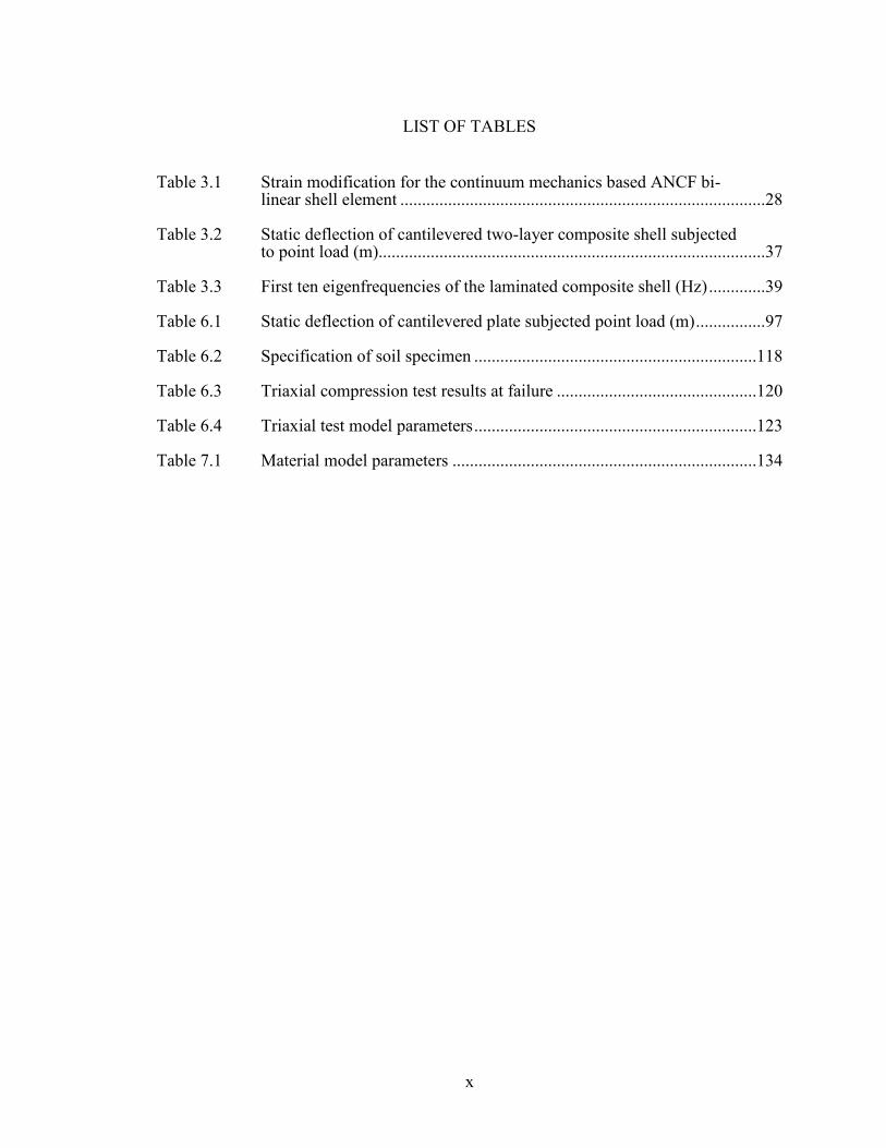
LIST OF TABLES

Table 3.1 Strain modification for the continuum mechanics based ANCF bi-linear shell element ....................................................................................28

Table 3.2 Static deflection of cantilevered two-layer composite shell subjected to point load (m).........................................................................................37

Table 3.3 First ten eigenfrequencies of the laminated composite shell (Hz) .............39

Table 6.1 Static deflection of cantilevered plate subjected point load (m) ................97

Table 6.2 Specification of soil specimen .................................................................118

Table 6.3 Triaxial compression test results at failure ..............................................120

Table 6.4 Triaxial test model parameters .................................................................123

Table 7.1 Material model parameters ......................................................................134

xi

LIST OF FIGURES

Figure 2.1 Kinematics of bi-linear shear deformable laminated composite shell element .......................................................................................................13

Figure 2.2 Sampling points for assumed natural strain ...............................................16

Figure 3.1 Deformed shape of a cantilevered plate subjected to a tip force ...............27

Figure 3.2 Numerical convergence of ANCF shell solutions: cantilevered plate subjected to a tip force with large deformation. ........................................27

Figure 3.3 Deformed shape of a quarter cylinder subjected to a tip force ..................29

Figure 3.4 Numerical convergence of ANCF shell solutions: quarter cylinder subjected to a tip force. ..............................................................................30

Figure 3.5 Deformed shape of pinched semi-cylindrical shell ....................................31

Figure 3.6 Load-deflection curve of pinched semi-cylindrical shell. ..........................31

Figure 3.7 Deformed shape of slit annular plate subjected to lift force ......................32

Figure 3.8 Load-deflection curve of slit annular plate subjected to lifting force ........32

Figure 3.9 Uniaxial tensile test models .......................................................................34

Figure 3.10 In-plane shear strain of one layer orthotropic plate ...................................34

Figure 3.11 Twisting angle and in-plane shear strain of two-layer laminated composite plate subjected to uniaxial tensile load .....................................36

Figure 3.12 Deformed shape of cantilevered two-layer composite shell subjected to point load ...............................................................................................38

Figure 3.13 Numerical convergence of finite element solutions ...................................38

Figure 3.14 Vibration mode shapes of two-layer laminated composite shell ...............40

Figure 3.15 Deformed shapes ........................................................................................41

Figure 3.16 Global X-position at the tip point ..............................................................41

Figure 3.17 Global Y-position at the tip point ..............................................................42

Figure 3.18 Global Z-position at the tip point ...............................................................42

Figure 4.1 Tire model creation procedure ...................................................................44

Figure 4.2 Physics-based tire model using the laminated composite shell element .......................................................................................................45

xii

Figure 4.3 Assembly of flexible tire and rigid rim ......................................................46

Figure 4.4 LuGre tire friction model ...........................................................................50

Figure 4.5 Longitudinal tire force on wet surface .......................................................52

Figure 4.6 Integration of LuGre tire friction model in flexible tire model .................55

Figure 5.1 Slip-dependent friction coefficient ............................................................62

Figure 5.2 Slip-dependent friction coefficient modeled by existing and modified ( )rg v -function ...........................................................................66

Figure 5.3 Longitudinal tire force with exiting and modified ( )rg v -function ...........67

Figure 5.4 Friction testing of tread rubber ..................................................................67

Figure 5.5 Tangential force coefficients for 4 kgf .......................................................68



Figure 5.8 Tire force characteristics under combined slip condition ..........................70

Figure 5.9 Tangential force coefficient under combined slip condition .....................70

Figure 5.10 Deformed shape of tire cross section .........................................................71

Figure 5.11 Lateral deflection of tire for various wheel loads ......................................72

Figure 5.12 Vertical deflection of tire for various wheel loads .....................................72

Figure 5.13 Longitudinal contact patch length for various wheel loads .......................73

Figure 5.14 Lateral contact patch length for various wheel loads.................................73

Figure 5.15 Normal contact pressure distribution in the longitudinal direction ...........74

Figure 5.16 Normal contact pressure distribution in the lateral direction .....................74

Figure 5.17 Normal contact pressure distribution considering tread pattern ................75

Figure 5.18 Comparison of normal contact pressure distribution with LS-DYNA FE tire model..............................................................................................76

Figure 5.19 In-plane and out-of-plane natural frequencies ...........................................77

Figure 5.20 Transient braking analysis results ..............................................................78

Figure 5.21 Shear contact stress distribution in the transient braking analysis .............79

Figure 5.22 Simplified slip-based ABS control algorithm ............................................81

xiii

Figure 5.23 Forward and circumferential velocities of tire with and without ABS control ........................................................................................................82

Figure 5.24 µ-slip curve with and without ABS control ...............................................82

Figure 5.25 Cornering force responses to oscillatory steering input .............................83

Figure 5.26 Cornering force responses and phase lag ...................................................84

Figure 5.27 Transient cornering analysis results ...........................................................85

Figure 5.28 Shear contact stress distribution in the transient cornering analysis ..........86

Figure 6.1 Kinematics of 8-node tri-linear brick element (Brick24) ..........................88

Figure 6.2 Kinematics of 8-node tri-cubic ANCF brick element (Brick96) ...............91

Figure 6.3 Kinematics of 9-node brick element with curvature coordinates (Brick33) ....................................................................................................95

Figure 6.4 Deformed shape of a cantilevered plate subjected to a tip force ...............96

Figure 6.5 Convergence of brick element solutions ....................................................98

Figure 6.6 Deformed shapes ........................................................................................99

Figure 6.7 Global Z-position at the tip point (Brick24: 8-node tri-linear brick element)......................................................................................................99

Figure 6.8 Global Z-position at the tip point (Brick96: 8-node tri-cubic brick element)....................................................................................................100

Figure 6.9 Global Z-position at the tip point (Brick33: 9-node brick element) ........100

Figure 6.10 CPU time to achieve the convergent solutions ........................................101

Figure 6.11 Multiplicative decomposition of displacement gradient ..........................102

Figure 6.12 Drucker-Prager failure model ..................................................................104

Figure 6.13 Capped Drucker-Prager failure model .....................................................108

Figure 6.14 Flow chart for the return mapping of capped Drucker-Prager model ......110

Figure 6.15 Plate sinkage test model ...........................................................................115

Figure 6.16 Deformed shape of soil at plate sinkage of 0.1 m (Drucker-Prager model) ......................................................................................................115

Figure 6.17 Pressure-sinkage relationship (comparison with ABAQUS model) ........116

Figure 6.18 Deformed shape of soil at plate sinkage of 0.1 m (capped Drucker-Prager model) ...........................................................................................116

xiv

Figure 6.19 Pressure-sinkage relationship using capped Drucker-Prager model (comparison with ABAQUS model) ........................................................117

Figure 6.20 Triaxial soil test........................................................................................118

Figure 6.21 Deviator stress vs axial strain curves .......................................................119

Figure 6.22 Deviator stress vs mean effective stress at failure ...................................120

Figure 6.23 Void ratio vs vertical stress obtained by one-dimensional compression test .......................................................................................121

Figure 6.24 Triaxial test model ...................................................................................122

Figure 6.25 Stress-strain result of triaxial test model (200kPa Confining pressure) ...................................................................................................123

Figure 7.1 Modeling tread geometry using contact nodes ........................................126

Figure 7.2 Contact force model for tire soil interaction ............................................126

Figure 7.3 Updates of component soil model............................................................128

Figure 7.4 Physics-based off-road tire model using the laminated composite shell element ............................................................................................130

Figure 7.5 Deformed shape of off-road tire cross section .........................................130

Figure 7.6 Normal contact pressure in a longitudinal direction (4kN) .....................131

Figure 7.7 Normal contact pressure in a lateral direction (4kN) ...............................131

Figure 7.8 Load-longitudinal contact patch length for off-road tire model ..............132

Figure 7.9 Load-lateral contact patch length for off-road tire model ........................132

Figure 7.10 Load-vertical deflection curve for off-road tire model ............................133

Figure 7.11 Tire/soil interaction model .......................................................................134

Figure 7.12 Tire/soil interaction model using component soil approach ....................135

Figure 7.13 Tire sinkage and rolling resistance with 0.8 m long (64x40x6) ..............136

Figure 7.14 Tire sinkage and rolling resistance with 1.0m long (80x40x6) ...............137

Figure 7.15 Tire sinkage and rolling resistance with 1.2m long (96x40x6) ...............137

Figure 7.16 Tire sinkage and rolling resistance for various wheel loads ....................138

Figure 7.17 CPU time comparison between long soil model and component soil model........................................................................................................139

1

CHAPTER 1

INTRODUCTION

This study is aimed to develop a high-fidelity physics-based tire model that can be

fully integrated into multibody dynamics computer algorithms for the transient on-road

and off-road vehicle dynamics simulation. While detailed finite element tire models using

explicit finite element software have been widely used for structural design of tires by tire

manufactures, they are not suited for the analysis of transient tire dynamics under severe

vehicle maneuvers, in which the transient tire force characteristics and the interaction

with deformable terrains for off-road vehicles play a crucial role in predicting the overall

vehicle performance. Furthermore, due to the essential difference in formulations and

solution procedures traditionally used in multibody dynamics and classical finite element

approaches, integration of existing finite element tire models into multibody vehicle

dynamics simulation is not straightforward and requires special treatments including a

reliance on co-simulation techniques. Use of the co-simulation, however, leads to very

small step size to ensure the numerical stability and energy balance between two separate

simulation (i.e., finite element tire simulation and multibody vehicle simulation) in severe

vehicle maneuvering conditions. In the tire model proposed in this study, the detailed tire

structure consisting of the fiber-reinforced rubber material is modeled by the shear

deformable laminated composite shell element based on the absolute nodal coordinate

formulation developed in this study. The shell element developed allows for the use of

non-incremental solution procedures suited for general multibody dynamics computer

algorithms. Furthermore, to account for the transient tire friction characteristics including

the friction-induced hysteresis that appears in severe braking and cornering conditions,

the distributed parameter LuGre tire friction model is integrated into the flexible tire

model. By doing so, the structural deformation of the flexible tire model and the LuGre

tire friction force model are dynamically coupled in the final form of the equations.

Furthermore, using the tire model based on the flexible multibody dynamics approach, a

physics-based tire/soil interaction simulation capability is developed for prediction of off-

road mobility in various terrain condition without resorting to ad-hoc co-simulation

procedures.

2

1.1 Background and Motivation

1.1.1 Tire Dynamics Simulation

Tire models play an essential role in virtual prototyping of ground vehicles and

they are classified according to the frequency range to be considered in the analysis [1].

The rigid ring tire model accounts for the frequency range up to approximately 80 Hz

associated with the tire sidewall stiffness, while the tire belt flexibility is assumed to be

negligible [2]. Because of the rigid tire belt assumption, the contact pressure distribution

is assumed by a prescribed function, preventing the consideration of the dynamic change

in the contact pressure distribution in the analysis. To account for more detailed

deformation modes of the complex tire structure, high-fidelity finite-element (FE) tire

models are constructed and used for design and analysis of tires [3,4]. In particular, an

accurate modeling of the complex tire geometry and the anisotropic material properties of

the tire structure is essential to the tire performance evaluation including the tire contact

pressure and the braking/traction and cornering forces. Since a tire consists of layers of

plies and steel belts embedded in rubber, the tire structure needs to be modeled by cord-

rubber composite materials and various fiber-reinforced rubber material models are

proposed for use in detailed finite element tire models. Since Young’s modulus of the

steel cord is significantly higher than that of the rubber material, mechanical property of

the fiber-reinforced rubber is highly nonlinear [5]. Furthermore, the tire cross-section

geometry and stiffness distribution are of significant importance in characterizing the

normal contact pressure distribution, and the in-plane shear deformation of the carcass

contributes to the cornering stiffness of tires. For this reason, high-fidelity finite element

tire models that account for the tire geometric and material nonlinearities have been

developed and used extensively in automotive and aerospace industry [6-9]. It is,

however, known that these computational tire models encounter difficulties in predicting

the transient tire force characteristics under severe vehicle maneuvering conditions such

as braking with antilock braking control due to the numerical instability that could occur

in the time-domain analysis and the lack of transient tire friction model fully integrated

into finite element tire models. In such transient vehicle maneuvering conditions,

structural tire deformation due to the large load transfer causes an abrupt change in

normal contact pressure and slip distribution in the contact patch, and it has a dominant

3

effect on characterizing the transient braking and cornering forces including the history-

dependent friction-induced hysteresis effect. Furthermore, co-simulation techniques,

which are widely used to incorporate finite element tire models into multibody vehicle

simulation, could require very small step size to ensure the numerical stability in the

severe transient tire dynamics simulation, involving rapid changes in normal and

tangential contact forces due to the abrupt braking and steering input.

To overcome these fundamental and essential issues in the tire dynamics

simulation, various types of flexible tire models have been proposed for use in vehicle

dynamics simulation. Among others, FTire [10], CDTire [11], RMOD-K [12] are widely

used and they have an interface to various multibody dynamics software. In the FTire

model, the flexible belt is modeled using a large number of rigid segments that are

connected together by springs and dampers. Such a modeling procedure for a flexible

body is often called finite segment method in multibody dynamics community [13]. 80-

200 segments are usually used for the discretization of a flexible belt [10], and this leads

to a large number of degrees of freedom even for a single tire modeling. CDTire and

RMOD-K tire models, on the other hand, use a finite element description for modeling

the tire structure and these models are integrated into vehicle dynamics simulation

framework via co-simulation techniques. Recently, a shell element based tire model was

proposed by Roller, et al. using the geometrically exact shell formulation with

inextensible directors for multibody vehicle dynamics simulation [14,15]. The

inextensibility conditions of the directors are imposed on the nodal points to ensure zero

through-thickness strain by introducing constraint equations, and the unilateral frictional

contact model is employed in the contact patch [15].

1.1.2 Off-Road Mobility Simulation

The vehicle-terrain interaction model is essential to demonstrate vehicle mobility

capability on deformable terrains in various scenarios, and the overall vehicle

performance on sand and rough dirt roads needs to be carefully evaluated at various

design stages, including drawbar pull, tire sinkage, and rolling resistance. Over the past

decades, empirical models, analytical models based on terramechanics [16,17], and

numerical simulation models using finite element and discrete element methods [18-26]

have been proposed and utilized for modeling the vehicle and deformable terrain

4

interaction. Empirical terramechanics models, for which model parameters are based on

experimental results such as the cone index to characterize the soil properties, allows for

a quick prediction of off-road mobility performance. Among others, a NATO Reference

Mobility Model (NRMM) has been used for various military scenarios. Analytical and

semi-empirical models, on the other hand, were developed by Bekker [16] and Wong

[17] to better understand the tire/soil interaction mechanics and the principles behind, and

those models are developed based on terramechanics theories. However, it is known that

empirical and analytical terramechanics models do not capture many of the soil

deformation modes that can be captured by numerical models [18].

For this reason, physics-based numerical models have been utilized to understand

more details on the tire soil interaction behavior quantitatively and many different models

with different level of fidelity have been proposed. The high-fidelity computational soil

models are classified into continuum-based finite element (FE) models and discrete

element (DE) models. In the finite element soil model, a soil is assumed to be ideal

continuum and the soil behavior is modeled by the elasto-plasticity model such as Mohr-

Coulomb or capped Drucker-Prager models. The contact between deformable tires and

soil models is defined on continuous surfaces and, therefore, the normal and tangential

contact forces can be modeled accurately using computational contact mechanics theories

[19]. Shoop [20] developed the computational model for predicting the vehicle mobility

on snow using the standard finite element approach, and the results were validated

against the test data. Xia, et al. used the tire/soil interaction model to predict the soil

compaction using finite element models [19]. Furthermore, to circumvent the fine mesh

due to the large element distortion in the Lagrangian approach, Arbitrary Lagrangian

Eulerian (ALE) approach is applied to the tire/soil interaction model [21], where the

wheel is formulated in the Lagrangian description, while the soil is formulated in the

Eulerian description to allow for relatively coarse mesh for soil. On the other hand, a

discrete element method (DEM) has been also investigated extensively using high-

performance computing (HPC) techniques. In the DEM, soil is modeled by many

particles contacting each other. The contact between particles is modeled by either the

penalty approach [22] or constraint approach [23]. Use of the penalty approach

introduces high frequencies to the equations of motion due to the multiple elastic impacts

5

of particles, requiring small stepsize in the time integration. On the other hand, rigid

contact is assumed between particles in the constraint contact approach, allowing for

large stepsize in the time integration due to the elimination of high frequencies arising

from impacts of particles. This approach, however, requires more computationally

intensive solution procedures to solve nonlinear complementary contact problems, and

use of GPU computing has been investigated in the context of multibody dynamics

problem in the literature [23,24]. A rigid tire model is integrated into the DEM

computational framework in a straightforward manner since all the bodies (particles) are

rigid [22,23]. Integration of DEM approach with a finite element flexible tire model

requires addressing a challenging numerical issue. This is due to the fact that implicit

time integrators are suited for the finite element equations (FE tire models), while the

discrete element equations can be solved efficiently by an explicit time integration.

Nakashima et al. developed the two-dimensional coupled discrete and finite element

tire/soil contact model [25]. In addition, smooth particle hydrodynamics (SPH) method,

which is a meshless approach, is applied to model large soil deformation together with

the finite element tire model [26]. Most existing approaches rely on co-simulation

techniques which could lead to computationally intensive procedures to ensure the

accuracy and numerical stability. For this reason, a new high-fidelity physics-based

tire/soil interaction simulation capability that can be fully integrated into multibody

dynamics computer algorithms are pursued in this study without ad-hoc co-simulation

techniques.

1.1.3 Needs for Flexible Multibody Dynamics Approach

for Tire Dynamics Simulation

Tire dynamics simulation calls for addressing many challenging issues in the flexible

body dynamics. A tire rotates at high speed, thus the gyroscopic nonlinear inertia effects

arising from the large reference motion need to be precisely described in the model. This

is not a trivial issue when existing structural finite elements based on the incremental

solution procedure are used [27] since the flexible body kinematics are either linearized

or simplified when the reference configuration, from which motion of the flexible body is

described, is updated every time step. In other words, exact modeling of the rigid body

dynamics cannot be ensured due to the approximation utilized in the finite element

6

updating scheme for structural elements. For this reason, in the multibody dynamics

simulation, a method called the floating frame of reference formulation has been widely

used for modelling flexible bodies in multibody dynamics simulation [28]. In this

approach, deformation of a flexible body is defined with respect to the body coordinate

system using the local elastic coordinates and the assumed mode method is used to

reduce the overall model dimensionality. The general motion description utilized in the

floating frame of reference formulation allows for the integration with the general

multibody dynamics simulation algorithm without resorting to the updating scheme of the

reference configuration at every time step, and the exact modeling of the rigid body

dynamics is ensured when strains are zero. However, despite the successful integration of

the finite element models into the multibody dynamics simulation, strains are limited to

small in this formulation and complex local deformation modes resulting from contact

events (i.e., the rolling contact in the case of tires) cannot be efficiently described.

Furthermore, the material behavior is limited to the linear strain range.

As a solution to overcome these difficulties in the flexible multibody dynamics

simulation, the absolute nodal coordinate formulation (ANCF) has been proposed and

proven to be successful in solving many challenging engineering problems that involve

large deformable bodies in complex multibody systems [28,29]. This finite element

procedure is developed for the nonlinear dynamics simulation of large deformable bodies.

In the structural elements such as a beam and shell developed with the absolute nodal

coordinate formulation, the finite rotation and deformation of the element are

parameterized by the global position vector gradients, rather than the rotational nodal

coordinates such as Euler angles. This parameterization leads to a constant mass matrix

for fully nonlinear dynamics problems while ensuring the exact modeling of the rigid

body reference motion. Since it is known that the displacement gradient tensor can be

decomposed into the orthogonal rotation matrix and the stretch tensor that describes the

most general six deformation modes using the polar decomposition theorem, it can be

proved that use of the position vector gradient coordinates allows for describing the

rotation and deformation within the element, thereby circumventing the complex

nonlinear coupling of the rotation and deformation coordinates that appears in the inertia

terms of flexible body models with rotational parameterization. The constant mass matrix

7

of large deformable bodies not only leads to efficient solutions in nonlinear dynamics

simulation, but also allows for the use of the non-incremental solution procedures utilized

in general multibody dynamics computer algorithms. Using these important features and

general motion description employed in the absolute nodal coordinate formulation, the

structural beam and shell elements for modelling the detailed tire structures can be

directly integrated into general multibody dynamics computer algorithms without

resorting to ad hoc co-simulation procedures, and the flexible tire model based on the

absolute nodal coordinate formulation was developed for multibody vehicle dynamics

simulation by Sugiyama and Suda [31]. This in-plane tire model was further extended by

Yamashita, et al. for transient longitudinal tire dynamics simulation by integrating the

with LuGre tire friction model that allows for capturing the friction-induced hysteresis for

an in-plane longitudinal tire dynamics problem [32]. This ANCF-LuGre tire model

considers the nonlinear coupling between the dynamic structural deformation of the tire

and its transient tire friction behavior in the contact patch, and the tire model is

implemented directly in general multibody dynamics computer algorithms without

resorting to ad hoc co-simulation techniques. It was shown that the ANCF-LuGre tire

model has the potential of providing a better understanding of how structural deformation

of tires under severe maneuvering conditions influences the transient tire force

characteristics. This concept is further extended in this study to the three-dimensional

high-fidelity flexible tire model as will be discussed in Chapter 4.

1.1.4 Finite Element Absolute Nodal Coordinate Formulation

The absolute nodal coordinate formulation (ANCF) has been widely used in the large

deformation analysis of flexible multibody systems [28,29] due to following advantages

for use in multibody dynamics simulation:

(1) Constant mass matrix can be obtained for fully nonlinear dynamics simulation

(2) Exact rigid body motion can be obtained when strains are zero

(3) Non-incremental solution procedure utilized in the general multibody dynamics

computer algorithms can be directly applied without specialized updating schemes

for finite rotations, thereby allowing for incorporating detailed finite element models

into existing multibody dynamics simulation algorithms in a straightforward manner

8

Shell elements of the absolute nodal coordinate formulation can be classified into the

fully parameterized shear deformable element [30,33] and the gradient deficient thin plate

element [34,35]. While the fully parameterized element leads to a general motion

description that accounts for complex coupled deformation modes of the plate/shell

element, use of higher order polynomials and the coupled deformation modes exhibited

in this type of element causes severe element locking and special care needs to be

exercised to alleviate the locking [36]. The gradient deficient thin plate element, on the

other hand, is developed by removing the position vector gradients along the thickness

( / z∂ ∂r ). The global displacement field in the middle surface can be uniquely

parameterized by the global position vector and the two gradient vectors ( / x∂ ∂r and

/ y∂ ∂r ) which are both tangent to the surface. By doing so, the cross section is assumed

to be rigid and the elastic forces are derived using a plane stress assumption with

Kirchhoff-Love plate theory. This leads to the non-conforming plate element in which the

inter-element continuity is not guaranteed, while the conforming thin plate element can

be obtained by introducing the additional nodal coordinates 2 / x y∂ ∂ ∂r with bi-cubic

Hermite polynomials [34]. Despite the fact that the gradient deficient thin ANCF plate

elements have proven to be successful in solving challenging engineering problems that

involve large deformable thin plate and shell structures, consideration of general

nonlinear material models requires special formulations and implementation due to the

plane stress assumption.

Due to the severe element lockings and computational inefficiency of the fully

parameterized ANCF elements utilizing three sets of gradient nodal coordinates ( / x∂ ∂r ,

/ y∂ ∂r , and / z∂ ∂r ), an ANCF parameterization which does not include the position

vector gradients tangent to the beam centerline and the middle surface are investigated

for shear deformable ANCF beam and plate elements. For beam problems, it is shown in

the literature [37] that the elimination of the tangential slope vector along the beam

centerline leads to an accurate elastic force description due to weaker polynomial

coupling between the position and gradient fields, and use of the general continuum

mechanics approach for the elastic forces calculation allows for modeling curved beam

structures in a straightforward manner. The assumed displacement field on the beam

centerline does not involve any gradient coordinates, while the transverse gradient

9

coordinates are employed to parameterize the orientation and deformation of the beam

cross section. For plate elements, on the other hand, the position vector gradient along the

thickness can be used to describe the transverse shearing and the thickness stretch of the

plate element, and this parameterization leads to a shear deformable shell element. That is,

use of such an element parameterization leads to shear deformable plate/shell elements

while reducing the number of coordinates per node as discussed in the literature [38]. For

the shear deformable shell element, there are two approaches to formulate the elastic

forces, elastic middle surface approach and continuum mechanics approach. In the

former method, the six strain components are evaluated in the middle surface using

Green-Lagrange strains and the approximated curvature expression is used to define the

bending and twisting deformation of the shell. In other words, the strain distribution

along the thickness is assumed to be constant in this approach based on the plane stress

assumption, allowing for the evaluation of the elastic forces as an area element. Use of

this element is limited to moderately thick plate problems and it requires special

formulation and implementation to incorporate nonlinear material models. On the other

hand, in the latter approach based on the continuum mechanics theory, the elastic forces

of the shell element are evaluated as a continuum volume and various nonlinear material

models can be considered in a way same as a solid element. This is an important

requirement for shell elements utilized for tire models since cord-reinforced rubber

material indispensable for modeling highly nonlinear material behavior of tires needs to

be incorporated into the shell formulation.

It is also important to notice that there are a wide variety of continuum-based

rotation-free shell elements proposed in the finite element community that have similar

features to ANCF shell elements including the constant mass matrix and use of three-

dimensional material laws without special modifications. Among others, solid shell

elements [39-43] and shell elements utilizing extensible directors [44-46] can fall into

this category. The configuration update schemes for the continuum-based shell elements

were pursued in the literature to interface with incremental solution procedures of

nonlinear finite element computer algorithms, including the updating scheme of

extensible directors at every load step. On the other hand, the non-incremental solution

procedure is adopted in the absolute nodal coordinate formulation to enable the

10

straightforward implementation of elements in general multibody dynamics computer

algorithms. Furthermore, various joint constraint formulations have been proposed

specialized for ANCF elements to facilitate the integration with multibody dynamics

software [47,48]. These important features of the absolute nodal coordinate formulation

are utilized in this study for modeling the tire structure using the shear deformable shell

element. In addition, the element locking remedy for the shear deformable ANCF shell

element is addressed in Chapter 2 using the assumed natural strain (ANS) and the

enhanced assumed strain (EAS) approaches to alleviate the transverse shear locking,

thickness locking, Poisson’s locking, and the in-plain normal/shear locking.

1.2 Objective of the Study

This study is aimed to develop a high-fidelity physics-based tire/soil interaction

simulation capability using flexible multibody dynamics techniques based on the finite

element absolute nodal coordinate formulation. To this end, the following issues are

addressed in this thesis:

(1) Development of a locking-free shear deformable laminated composite shell element

based on the finite element absolute nodal coordinate formulation for modeling the

complex fiber reinforced rubber tire structure

(2) Development and validation of a physics-based structural tire model that can be

integrated into multibody dynamics computer algorithm

(3) Integration of the distributed parameter LuGre dynamic tire friction model into the

physics-based structural tire model for transient braking and cornering simulation

(4) Development and validation of the continuum soil model based on the capped

Drucker-Prager yield criterion using the multiplicative finite strain plasticity theory

for multibody off-road vehicle dynamics simulation

(5) Development of a physics-based tire/soil interaction simulation capability for off-road

mobility simulation

1.3 Organization of Thesis

This thesis is organized as follows: In Chapter 2, a new shear deformable

laminated composite shell element based on the finite element absolute nodal coordinate

formulation is developed for modeling the fiber reinforced rubber tire structure.

11

Numerical examples and accuracy of the shear deformable laminated composite shell

element developed are demonstrated with several benchmark problems in Chapter 3. In

Chapter 4, a high-fidelity physics-based flexible tire model is developed using the shear

deformable laminated composite shell element and validated against test data. The

distributed parameter LuGre tire friction model is integrated into the deformable tire

model to capture the transient tire force characteristics for severe vehicle maneuvering

scenarios. In Chapter 5, the parameter identification procedure for the LuGre tire friction

model and numerical results of the transient tire dynamics simulation including hard

braking and cornering scenarios are presented. A new brick element for modeling the

continuum soil behavior using the capped Drucker-Prager yield criterion is developed

based on multiplicative finite strain plasticity theory in Chapter 6. In this Chapter, the

triaxial soil test results are also presented and those results are used to identify the

parameters of the capped Drucker-Prager soil model. Furthermore, the continuum soil

model developed is validated against the test results. In Chapter 7, the continuum based

deformable tire/soil interaction simulation model is developed for multibody off-road

mobility simulation, and the component soil model using the moving soil patch is

introduced to reduce the computational time for use in the off-road mobility simulation.

Summary, conclusions and the future works are provided in Chapter 8.

12

CHAPTER 2

DEVELOPMENT OF SHEAR DEFORMABLE LAMINATED

COMPOSITE SHELL ELEMENT

2.1 Introduction

In this chapter, a continuum mechanics based shear deformable shell element is

developed based on the absolute nodal coordinate formulation for use in the modeling of

fiber-reinforced rubber structure of the physics-based tire model. The element consists of

four nodes, each of which has the global position coordinates and the transverse gradient

coordinates along the thickness introduced to describe the orientation and deformation of

the cross section of the shell element. The global position field on the middle surface and

the position vector gradient at a material point in the element are interpolated by the bi-

linear polynomial. The continuum mechanics approach is used to formulate the

generalized elastic forces, allowing for the consideration of nonlinear constitutive models

in a straightforward manner. The element locking exhibited in the element can be

eliminated using the assumed natural strain (ANS) and enhanced assumed strain (EAS)

approaches. In particular, the combined ANS and EAS approach is introduced to alleviate

both curvature and Poisson’s thickness lockings arising from the erroneous transverse

normal strain distribution [49].

2.2 Kinematics of Bi-linear Shear Deformable Shell Element

As shown in Fig. 2.1, the global position vector ir of a material point T[ ]i i i ix y z=x in shell element i is defined as

( , ) ( , )i

i i i i i i im ix y z x y

z∂

= +∂rr r (2.1)

where ( , )i i im x yr is the global position vector in the middle surface and ( , )i i i ix y z∂ ∂r is

the transverse gradient vector used to describe the orientation and deformation of the

infinitesimal volume in the element. The preceding global displacement field is

interpolated using the bi-linear polynomials as follows:

0 1 2 3 4 5 6 7( )i i i i i i i i i ir a a x a y a x y z a a x a y a x y= + + + + + + + (2.2)

13

from which, one can interpolate both position vector in the middle surface and the

transverse gradient vector using the same bi-linear shape function matrix imS as follows:

( , ) ( , ) , ( , ) ( , )i

i i i i i i i i i i i i im m p m gix y x y x y x y

z∂

= =∂rr S e S e (2.3)

where 1 2 3 4i i i i im S S S S = S I I I I and

( )( ) ( )( )

( )( ) ( )( )

1 2

3 4

1 11 1 , 1 1 ,4 41 11 1 , 1 14 4

i i i i i i

i i i i i i

S S

S S

ξ η ξ η

ξ η ξ η

= − − = + −

= + + = − + (2.4)

where 2 /i i ixξ = and 2 /i i iy wη = . i and iw are lengths along the element ix and iy

axes, respectively. In Eq. 2.3, the vectors ipe and i

ge represent the element nodal

coordinates associated with the global position vector in the middle surface and the

transverse gradient vector. That is, for node k of element i, one has ik ikp =e r and

ik ik ig z= ∂ ∂e r . It is important to notice here that the assumed displacement field i

mr

defined in the middle surface does not involve any gradient coordinates, while the

orientation and deformation of the infinitesimal volume at the material point is

parameterized by the transverse gradient coordinates only. Substitution of Eq. 2.3 into

Eq. 2.1 leads to the following general expression for the global position vector used for

the absolute nodal coordinate formulation:

Figure 2.1 Kinematics of bi-linear shear deformable laminated composite

shell element

14

( , , ) ( , , )i i i i i i i i ix y z x y z=r S e (2.5)

where the shape function matrix iS and the element nodal coordinate vector ie are,

respectively, defined as

, [( ) ( ) ]i i i i i i T i T Tm m p gz = = S S S e e e (2.6)

It is important to notice here that the element parameterization and the assumed global

displacement field defined in the ANCF shell element are essentially different from those

of the degenerated shell elements [50]. For more details on the difference between the

ANCF and degenerated shell elements, one can refer to the literature [51], in which a

fully parameterized ANCF shell element [30] is used for comparison. The difference

between the fully parameterized shell element [30] and the gradient deficient shear

deformable bi-linear shell element considered in this study lies in the order of

polynomials introduced to the global position field of the middle surface. The transverse

position gradient vector is interpolated with the same bi-linear polynomial in the fully

parameterized shell element, while the global position vector in the middle surface is

interpolated by an incomplete bi-cubic polynomial.

2.3 Generalized Elastic Forces

2.3.1 Generalized Elastic Forces with Continuum Mechanics Approach

In the continuum mechanics approach, the elastic forces of the shell element are

evaluated as a continuum volume and the Green-Lagrange strain tensor E at an arbitrary

material point in element i is defined as follows:

( )1 ( )2

i i T i= −E F F I (2.7)

where iF is the global position vector gradient tensor defined by 1

1( )i i i

i i ii i i

−

− ∂ ∂ ∂= = = ∂ ∂ ∂

r r XF J JX x x

(2.8)

In the preceding equation, i i i= ∂ ∂J r x and i i i= ∂ ∂J X x , where the vector iX

represents the global position vector of element i at an arbitrary reference configuration.

Substitution of Eq. 2.8 into Eq. 2.7 leads to 1( ) ( )i i T i i− −=E J E J (2.9)

15

where iE is the covariant strain tensor defined by

( )1 ( ) ( )2

i i T i i T i= −E J J J J (2.10)

The transformation (push-forward operation) of the covariant strain tensor iE given by

Eq. 2.10 can be re-expressed in a vector form by introducing the engineering covariant

strain vector iε as

( )i i T i−=ε T ε (2.11)

where the vector ε in Eq. 2.11 is the engineering strain vector at the deformed

configuration defined as

[ ]i i i i i i i Txx yy xy zz xz yzε ε γ ε γ γ=ε (2.12)

and the engineering covariant strain vector is defined as


The transformation matrix iT in Eq. 2.11 can be expressed explicitly as 2 2 2

11 12 11 12 13 11 13 12 132 2 2

21 22 21 22 23 21 23 22 23

11 21 12 22 11 22 12 21 13 23 11 23 13 21 12 23 13 222 2

31 32 31 32 3

( ) ( ) 2 ( ) 2 2( ) ( ) 2 ( ) 2 2

( ) ( ) 2 (

i i i i i i i i i

i i i i i i i i i

i i i i i i i i i i i i i i i i i ii

i i i i

J J J J J J J J JJ J J J J J J J J

J J J J J J J J J J J J J J J J J JJ J J J J

+ + +=T 2

3 31 33 32 33

11 31 12 32 11 32 12 31 13 33 11 33 13 31 12 33 13 32

21 31 22 32 21 32 22 31 23 33 21 33 23 31 22 33 23 32

) 2 2i i i i i

i i i i i i i i i i i i i i i i i i


J J J JJ J J J J J J J J J J J J J J J J JJ J J J J J J J J J J J J J J J J J

+ + +

+ + +

(2.14)

and iabJ is the element in the a-th column and b-th row of matrix iJ which is constant in

time. The generalized elastic forces can then be obtained using the virtual work as

follows:

00i

Tii i ik iV

dV ∂

= ∂ ∫

εQ σe

(2.15)

where iσ is a vector of the second Piola–Kirchhoff stresses and 0idV is the infinitesimal

volume at the reference configuration of element i. It is important to notice here that the

element elastic forces are evaluated as a continuum volume, and the stress vector for the

shell element can be obtained with various nonlinear material models for large

deformation problems without ad hoc procedures.

16

2.3.2 Element Locking for Transverse Shear and

In-Plane Shear/Normal Strains

As it has been addressed in literature of shell element formulations

[41,42,44,45,52-57], the bi-linear quadrilateral shell element suffers from the transverse

shear and the in-plane shear/normal lockings. The transverse shear locking can be

eliminated using the assumed natural strain (ANS) approach proposed by Bathe and

Dvorkin [55,56]. In this approach, the covariant transverse shear strains are interpolated

using those evaluated at the sampling points A, B, C and D shown in Fig. 2.2 as follows:

( ) ( )

( ) ( )

1 11 12 21 11 12 2

ANS C Dxz xz xz

ANS A Byz yz yz

γ η γ η γ

γ ξ γ ξ γ

= − + + = − + +

(2.16)

where Cxzγ , D

xzγ , Ayzγ and B

yzγ are compatible covariant transverse shear strains at the

sampling points.

The parasitic in-plane shear under pure bending loads is a typical locking problem

exhibited in the bi-linear quadrilateral element [58], and the compatible in-plane strains

( xxε , yyε and xyγ ) obtained by the assumed displacement field can be enhanced by

introducing the enhanced assumed strains (EAS) EASε as [44,54] c EAS= +ε ε ε (2.17)

Figure 2.2 Sampling points for assumed natural strain

17

where cε indicates the compatible strain vector and the strain vector EASε is defined by

( ) ( )EAS =ε ξ G ξ α (2.18)

In the preceding equation, α is a vector of internal parameters introduced to define the

enhanced in-plane strain field and the matrix ( )G ξ can be defined as [44,54]

0 T0( ) ( )

( )−=

JG ξ T N ξ

J ξ (2.19)

where ( )J ξ and 0J are the global position vector gradient matrices at the reference

configuration evaluated at the Gaussian integration point ξ and at the center of element

( =ξ 0 ), respectively. ξ is a vector of the element coordinates in the parametric domain

and 0T is the constant transformation matrix evaluated at the center of element as shown

in Eq. 2.19. The matrix ( )N ξ defines polynomials for the enhancement of the in-plane

strain field in the parametric domain. For example, consideration of the linear distribution

of in-plane strains ( xxε , yyε and xyγ ) requires introducing the following interpolation

matrix ( )N ξ :

0 0 00 0 00 0

( )0 0 0 00 0 0 00 0 0 0

ξη

ξ η

=

N ξ (2.20)

where the additional four internal EAS parameters are introduced in this model. Using Eq.

2.14, the enhanced covariant strains are then pushed forward to those at the deformed

configuration in the physical domain. It is important to notice here that the matrix ( )N ξ

needs to satisfy the following condition [44]:

( )d =∫ N ξ ξ 0 (2.21)

such that the orthogonality condition between the assumed stress and strain is satisfied as

00 0EAS

VdV⋅ =∫ σ ε (2.22)

18

Using the preceding condition, the unknown assumed stress term that appears in Hu-

Washizu mixed variational principle vanishes and one can obtain the generalized elastic

force vector as follows [44]:

00

( )i

Tc i c EASi ik i iV

W dV ∂ ∂ +

= − ∂ ∂ ∫

ε ε εQe ε

(2.23)

where W is an elastic energy function. For example, the elastic energy function W of the

compressible neo-Hookean material model is defined as follows [59]:

( ) ( )2tr( ) 3 ln ln2 2

W J Jµ λµ= − − +C (2.24)

where µ and λ are the Lamé constants; T=C F F is the right Cauchy-Green deformation

tensor; and det( ) det( )J = =F C . It is important to notice here that the right Cauchy-

Green deformation tensor that accounts for the enhanced assumed strain modification is

defined as follows:

2( )c EAS= + +C E E I (2.25)

2.3.3 Thickness Locking

Use of the transverse gradients in the shell element introduces the thickness

stretch and the locking associated with the transverse normal strain is exhibited in the bi-

linear shear deformable shell element. That is, the transverse gradient vectors can be

erroneously elongated when the shell element is subjected to bending and twisting

deformation. This phenomenon is called curvature thickness locking. The solid shell

elements which consists of layers of translational nodal coordinates at the top and bottom

surfaces of the element [41,42,52,53] and shell elements parameterized by extensible

directors for capturing the transverse shearing and the thickness stretch [45,46,57] suffer

from the similar thickness locking resulting from the erroneous transverse normal strain

distribution. Use of the assumed natural strain (ANS) approach is proposed in the

literature [45] to alleviate the curvature thickness locking of the shell element modeled by

extensible directors and the transverse normal strain at a material point in the element is

approximated as follows: 1 2 3 4

1 2 3 4ANS ANS ANS ANS ANSzz zz zz zz zzS S S Sε ε ε ε ε= + + + (2.26)

19

where kzzε indicates the compatible transverse normal strain at node k as shown in Fig.

2.2 and ANSkS is the shape function associated with it. This approach is applied to the bi-

linear shear deformable shell element based on the elastic middle surface approach shown

in Appendix to alleviate the thickness locking problem. Since the strain distribution along

the thickness is assumed to be constant and the stress is evaluated in the middle surface,

use of the assumed natural strain approach can successfully alleviate the thickness

locking if the compatible transverse normal strains at four corners are accurate.

In addition to the curvature thickness locking, use of a linear interpolation of the

global position field along the shell thickness leads to locking called Poisson´s thickness

locking because it is the Poisson´s ratio that introduces the coupling of the in-plane

strains to the transverse normal strain. In the case of pure bending, the axial strains due to

bending are linearly distributed along the thickness and it leads to the linearly varying

transverse normal strain due to the coupling induced by Poisson’s ratio. However, the use

of the linear interpolation along the thickness leads to constant thickness strains which

make the element behave overly stiff since the thickness strain does not vanish on the

neutral axis. It has been shown that the use of the enhanced assumed strain (EAS)

approach alleviates the Poisson’s thickness locking effectively [41,46]. That is, the

additional internal EAS parameters associated with the enhanced transverse normal strain

are added to consider the linear distribution of the transverse normal strain along the

thickness coordinate iz . The interpolation matrix ( )N ξ introduced for the in-plane

normal/shear lockings in Eq. 2.20 is modified as

0 0 0 00 0 0 00 0 0

( )0 0 0 00 0 0 0 00 0 0 0 0

ξη

ξ ηζ

=

N ξ (2.27)

where 2 /z hζ = . It is important to notice here that there are no strain enhancement terms

associated with the transverse shear strains xzγ and yzγ defined in the fifth and sixth rows.

In the literature [46], the transformation matrix ( )G ξ associated with the enhanced in-

20

plane and thickness strain terms are assumed to be decoupled and the approximated

transformation matrix is used. In this investigation, the exact transformation matrix

defined for the general three-dimensional stress state is considered.

Accordingly, the compatible transverse normal strain is replaced by the assumed

natural strain defined by Eq. 2.26 to alleviate both curvature thickness locking and

Poisson’s thickness lockings as follows: ANS EAS

zz zz zzε ε ε= + (2.28)

The similar approach is employed for solid shell elements in literature [41]. In this

investigation, the combined ANS and EAS approach for the thickness locking is applied

to the bi-linear shear deformable shell element. With this approach, the transverse normal

strain improved by the ANS approach for the curvature thickness locking is further

modified by the enhanced assumed strain approach to eliminate the Poisson’s locking.

For application of this approach to the continuum mechanics based ANCF shell element,

the covariant strain components of the transverse shear and transverse normal strains are

interpolated in the natural coordinate domain first and then the covariant strain vector

given in Eq. 2.13 is replaced by the following strain vector: TANS ANS ANS

xx yy xy zz xz yzε ε γ ε γ γ = ε (2.29)

and then the strain field can be defined as follows:

T EAS−= +ε T ε ε (2.30)

In the preceding equation, the enhanced assumed strain vector is defined as

0 0TEAS EAS EAS EAS EAS

xx yy xy zzε ε γ ε = ε (2.31)

This leads to a systematic derivation of the generalized elastic forces of the locking-free

continuum mechanics based shear deformable shell element.

2.4 Generalization to Laminated Composite Shell Element

In fiber-reinforced composite materials that are widely used in many engineering

applications, laminae having different fiber angles are bonded together to produce desired

material properties. Since many laminae are stacked at different fiber angles, the complex

deformation coupling between the extension, shearing, bending and twisting occurs, and

21

such a deformation coupling characterizes the mechanical behavior of fiber-reinforced

composite materials [60]. To account for the laminated composite materials in shell

elements, various formulations are proposed and one can refer to review articles on this

topic [61,62]. The shell element used in this study is formulated as a continuum solid that

accounts for the three-dimensional stress state, thus the complex deformation coupling

exhibited in laminates can be automatically considered without specialized formulations

for shell elements. That is, the generalized elastic force of the laminated composite shell

element that consists of N layers can be defined as follows:

00

1

( )ik

Tik ik ikNi iks i ikV

k

W dV=

∂ ∂= − ∂ ∂

∑∫ε εQe ε

(2.32)

In the preceding equation, the integration interval for the k-th layer in the thickness

direction is from 1kz − to kz . In other words, the element generalized elastic forces are

evaluated layer by layer, and the resulting generalized elastic forces of each layer are

added together to define the elastic force vector of the laminated composite shell. Two

Gaussian integration points are used along the thickness when the elastic forces of each

layer are evaluated. It is important to notice here that there is no restriction in material

models considered in each lamina, despite the fact that the orthotropic material law is the

most popular material model used for reinforced composite materials.

For an orthotropic Saint-Venant-Kirchhoff material, the stress and strain relation

is defined in the fiber coordinate system as [41] ab abcd

cdS C E= (2.33)

where the material moduli abcdC is defined in the fiber coordinate system as 1111 1122 1133

1122 2222 2233

1212

1133 2233 3333

2323

1313

0 0 00 0 0

0 0 0 0 0[ ]

0 0 00 0 0 0 00 0 0 0 0

ijkl

C C CC C C

CC

C C CC

C

=

(2.34)

where

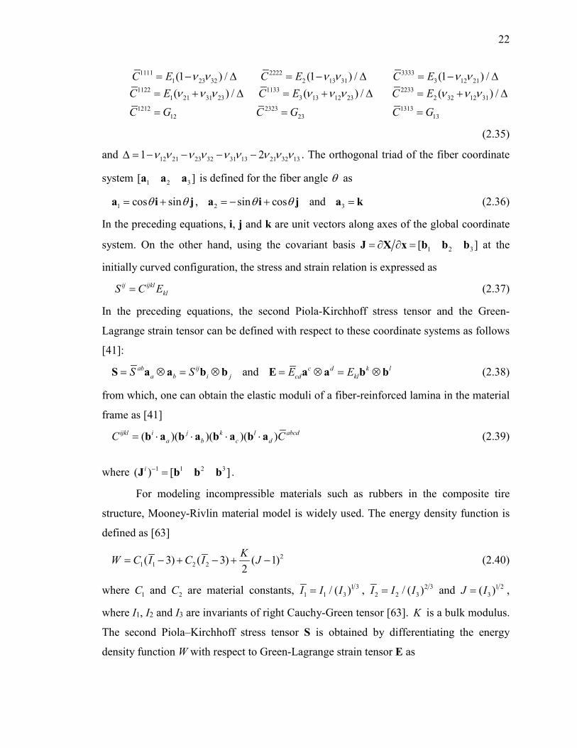
22

1111 2222 33331 23 32 2 13 31 3 12 21

1122 1133 22331 21 31 23 3 13 12 23 2 32 12 31

1212 2323 131312 23 13

(1 ) / (1 ) / (1 ) /( ) / ( ) / ( ) /

C E C E C EC E C E C EC G C G C G

ν ν ν ν ν νν ν ν ν ν ν ν ν ν

= − ∆ = − ∆ = − ∆= + ∆ = + ∆ = + ∆

= = =

(2.35)

and 12 21 23 32 31 13 21 32 131 2ν ν ν ν ν ν ν ν ν∆ = − − − − . The orthogonal triad of the fiber coordinate

system 1 2 3[ ]a a a is defined for the fiber angle θ as

1 cos sinθ θ= +a i j , 2 sin cosθ θ= − +a i j and 3 =a k (2.36)

In the preceding equations, i, j and k are unit vectors along axes of the global coordinate

system. On the other hand, using the covariant basis 1 2 3[ ]= ∂ ∂ =J X x b b b at the

initially curved configuration, the stress and strain relation is expressed as ij ijkl

klS C E= (2.37)

In the preceding equations, the second Piola-Kirchhoff stress tensor and the Green-

Lagrange strain tensor can be defined with respect to these coordinate systems as follows

[41]: ab ij

a b i jS S= ⊗ = ⊗S a a b b and c d k lcd klE E= ⊗ = ⊗E a a b b (2.38)

from which, one can obtain the elastic moduli of a fiber-reinforced lamina in the material

frame as [41]

( )( )( )( )ijkl i j k l abcda b c dC C= ⋅ ⋅ ⋅ ⋅b a b a b a b a (2.39)

where 1 1 2 3( ) [ ]i − =J b b b .

For modeling incompressible materials such as rubbers in the composite tire

structure, Mooney-Rivlin material model is widely used. The energy density function is

defined as [63]

21 1 2 2( 3) ( 3) ( 1)

2KW C I C I J= − + − + − (2.40)

where 1C and 2C are material constants, 1 31 1 3/ ( )I I I= , 2 3

2 2 3/ ( )I I I= and 1 23( )J I= ,

where I1, I2 and I3 are invariants of right Cauchy-Green tensor [63]. K is a bulk modulus.

The second Piola–Kirchhoff stress tensor S is obtained by differentiating the energy

density function W with respect to Green-Lagrange strain tensor E as

23

( ) ( )1 3 2 31 1 11 3 1 2 3 1 2

1 22 2 (J 1)3 3

W C I I C I I I KJ− −− − −∂ = = − + − − + − ∂ S I C I C C C

E (2.41)

2.5 Equations of Motion and Solution Procedures

Using the principle of virtual work in dynamics, the equations of motion of the

shear deformable laminated composite shell element i can be expressed as

( , ) ( , , )i i i i i i i i is e ct= + +M e Q e α Q e e Q (2.42)

where the vectors ikQ , i

eQ and icQ are respectively, vectors of the element elastic forces,

external forces and constraint forces associated with connection to adjacent elements; and

the matrix iM is the constant element mass matrix defined by

00 0

1( )

ik

Ni ik i T i ik

Vk

dVρ=

= ∑∫M S S (2.43)

where 0ikρ is the material density of k-th layer at the reference configuration.

It is important to notice here that the generalized elastic forces are defined as a

function of the nodal coordinates and the internal EAS parameters iα . The parameter iα

are determined by solving the following equation for each element:

00

( )( , )i

TEAS i c EASi i i i

i iV

W dV ∂ ∂ +

= = ∂ ∂ ∫

ε ε εh e α 0α ε

(2.44)

The nodal coordinates ie and the EAS internal parameters iα are determined at every

time step such that both Eqs. 2.42 and 2.43 are satisfied. Using the time integration

scheme in Newmark-β family, the nodal acceleration and velocity vectors at time step

1nt + are discretized in time as

1 12

1 1

1 1 1( ) ( 1)2

( ) ( 1) ( 1)2

n n n n n

n n n n n

h h

hh

β β βγ γ γ

β β β

+ +

+ +

= − − − − = − − − − −

e e e e e

e e e e e

(2.45)

where h is the step size; and β and γ are integration coefficients. Using the preceding

equations, the equations of motion given by Eq. 2.42 can be expressed as a function of

the unknown system nodal coordinates 1n+e and EAS parameters 1n+α for all the elements

as follows:

24

1 1( , )n n+ + =f e α 0 (2.46)

In other words, one needs to seek solutions to the following equations at time step 1nt + :

1 11 1

1 1

( , )( , )

( , )n n

n nn n

+ ++ +

+ +

= =

f e αg e α 0

h e α (2.47)

Using Newton-Raphson method, Newton difference for 1n+e and 1n+α can be obtained by

solving the following matrix equation:

1

1

n n n n

n n n n

+

+

∂ ∂ ∂ ∂ ∆ = − ∂ ∂ ∂ ∂ ∆

f e f α e fh e h α α h

(2.48)

By eliminating 1n+∆α from the preceding equation, 1n+∆e can be obtained as a solution to

the following equation: 1 1

1n n n n n n

n n nn n n n n n

− −

+

∂ ∂ ∂ ∂ ∂ ∂ − ∆ = − + ∂ ∂ ∂ ∂ ∂ ∂

f f h h f he f he α α e α α

(2.49)

The system nodal coordinates can then be updated by 1 1n n n+ += + ∆e e e , while the EAS

parameters are updated as follows: 1

1 1n n

n n n nn n

−

+ +

∂ ∂= − + ∆ ∂ ∂

h hα α h eα e

(2.50)

It is important to recall that the EAS parameters are introduced to each element and can

be determined at the element level as internal variables. That is, for given element nodal

coordinates 1in+e for element i obtained from the updated system nodal coordinates 1n+e

(Eq. 2.49), the EAS parameters 1in+α for element i can then be determined at the element

level using Eq. 2.42 with the following updating scheme: ( 1) ( ) 1 ( )

1 1 1 1( ) ( , )i k i k i i i i kn n n n

+ −+ + + += −α α H h e α (2.51)

where (0)1

i in n+ =α α and Jacobian matrix iH in the preceding equation is defined by

0

2

02( )( )

i

i i c EASi i T i i

i iV

W dV∂ ∂ += =

∂ ∂∫

h ε εH G Gα ε

(2.52)

where the matrix iG is defined by Eq. 2.19. The term 2 2/W∂ ∂ε leads to a material

moduli matrix obtained by the second derivative of the elastic energy function. That is,

for a linear Hookean material model, this matrix is constant. However, for general

25

nonlinear material models, the material moduli matrix is no longer constant and the

iterative solution procedure is required to determine the internal EAS parameters iα for

each element. Using this procedure, the dimension of the governing equations remains

the same as the number of the system nodal coordinates, while the EAS parameters can

be determined element by element without solving the augmented large dimensional

governing equations. This also allows for implementing the shell element formulated

with the EAS approach in a straightforward manner without significant modifications of

existing algorithms developed for ANCF elements.

26

CHAPTER 3

SHELL ELEMENT PERFORMANCE TEST

3.1 Benchmark Problems

In this chapter, several numerical examples are presented in order to demonstrate

the accuracy and the rate of convergence of numerical solutions obtained by the

continuum mechanics based shear deformable shell element developed in this

investigation. The effect of the assumed natural strain (ANS) and enhanced assumed

strain (EAS) approaches on the element accuracy is also discussed.

3.1.1 Cantilevered Plate and Shell Subjected to a Point Force

In the first problem, a rectangular cantilevered plate subjected to a vertical point

force at one of the corners of the plate is considered as shown in Fig. 3.1 The length,

width and thickness of the plate are assumed to be 1.0 m, 1.0 m and 0.01 m. The Young’s

modulus and Poisson’s ratio are assumed to be 82.1 10× Pa and 0.3, respectively. The

vertical point force zF defined at the corner is assumed to be 50 N. As shown in Fig. 3.1,

the plate is subjected to large deformation at the static equilibrium state. The six models

with different strain modifications discussed in Chapter 2 are considered to demonstrate

the effect of the EAS and ANS approaches on the element convergence and accuracy.

These models are summarized in Table 3.1. In Model-1, no strain modifications are made,

while Model-2 is used to demonstrate the effect of the ANS approach to alleviate the

transverse shear locking for the shell element. A comparison between Model-3 and 4

explains the effect of the in-plane shear/normal lockings alleviated by the EAS approach,

while a comparison between Model-4, 5 and 6 explains the use of the three different

approaches for elimination of the thickness locking, i.e., the ANS (Model-4), the EAS

(Model-5), and the combined ANS and EAS (Model-6) approaches as discussed in

Section 2.2.

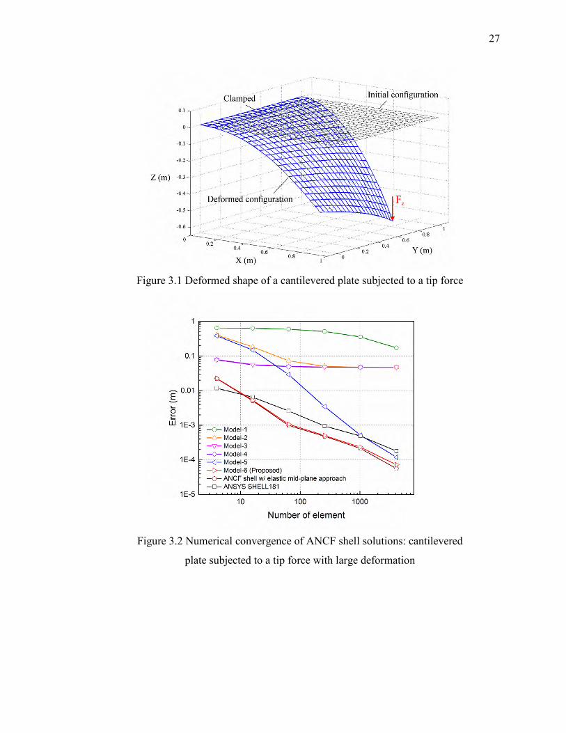
27

Figure 3.1 Deformed shape of a cantilevered plate subjected to a tip force

Figure 3.2 Numerical convergence of ANCF shell solutions: cantilevered

plate subjected to a tip force with large deformation

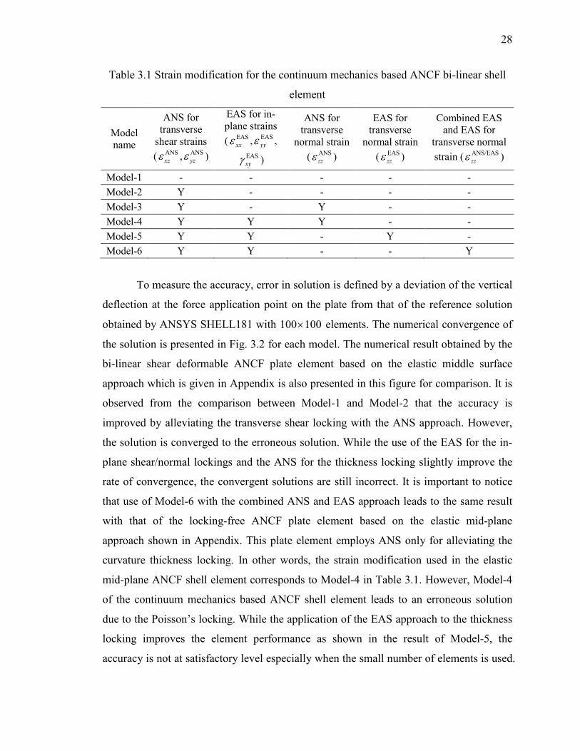
28

Table 3.1 Strain modification for the continuum mechanics based ANCF bi-linear shell

element

Model name

ANS for transverse

shear strains ( ANS

xzε , ANSyzε )

EAS for in-plane strains ( EAS

xxε , EASyyε ,

EASxyγ )

ANS for transverse

normal strain ( ANS

zzε )

EAS for transverse

normal strain ( EAS

zzε )

Combined EAS and EAS for

transverse normal strain ( ANS/EAS

zzε )

Model-1 - - - - - Model-2 Y - - - - Model-3 Y - Y - - Model-4 Y Y Y - - Model-5 Y Y - Y - Model-6 Y Y - - Y

To measure the accuracy, error in solution is defined by a deviation of the vertical

deflection at the force application point on the plate from that of the reference solution

obtained by ANSYS SHELL181 with 100 100× elements. The numerical convergence of

the solution is presented in Fig. 3.2 for each model. The numerical result obtained by the

bi-linear shear deformable ANCF plate element based on the elastic middle surface

approach which is given in Appendix is also presented in this figure for comparison. It is

observed from the comparison between Model-1 and Model-2 that the accuracy is

improved by alleviating the transverse shear locking with the ANS approach. However,

the solution is converged to the erroneous solution. While the use of the EAS for the in-

plane shear/normal lockings and the ANS for the thickness locking slightly improve the

rate of convergence, the convergent solutions are still incorrect. It is important to notice

that use of Model-6 with the combined ANS and EAS approach leads to the same result

with that of the locking-free ANCF plate element based on the elastic mid-plane

approach shown in Appendix. This plate element employs ANS only for alleviating the

curvature thickness locking. In other words, the strain modification used in the elastic

mid-plane ANCF shell element corresponds to Model-4 in Table 3.1. However, Model-4

of the continuum mechanics based ANCF shell element leads to an erroneous solution

due to the Poisson’s locking. While the application of the EAS approach to the thickness

locking improves the element performance as shown in the result of Model-5, the

accuracy is not at satisfactory level especially when the small number of elements is used.

29

This result clearly indicates severity of the Poisson’s locking exhibited in the continuum

mechanics based shear deformable ANCF shell element and the locking for the

continuum mechanics based ANCF shell element needs to be eliminated using the

combined EAS and ANS approach as demonstrated by the result of Model-6.

In the second problem, the flat plate is replaced with the quarter cylinder modeled

by the continuum mechanics based bi-linear ANCF shell elements as shown in Fig. 3.3,

and the radius of curvature is assumed to be 1.0 m. The material properties, tip load,

width and height are the same as the previous example. The deformed shape at the static

equilibrium state is shown in Fig. 3.3 and the large deformation is exhibited in this

problem. As in the previous example, error in solution is defined by a deviation of the

vertical deflection at the force application point from that of the reference solution

obtained by ANSYS SHELL181 with 100 100× elements. The numerical convergence in

solution is presented in Fig. 3.4 for Models 1 to 6 and ANSYS SHELL181 for

comparison. Furthermore, the numerical result obtained by the bi-linear shear deformable

ANCF plate element based on the elastic middle surface approach is also presented in Fig.

3.3 for comparison. The overall trend of the numerical convergence of solutions obtained

by different models is similar to that observed for the flat plate problem. The result

clearly indicates that use of the combined EAS and ANS approach is necessarily to

ensure the ideal rate of convergence and accuracy for the proposed shell element.

Figure 3.3 Deformed shape of a quarter cylinder subjected to a tip force

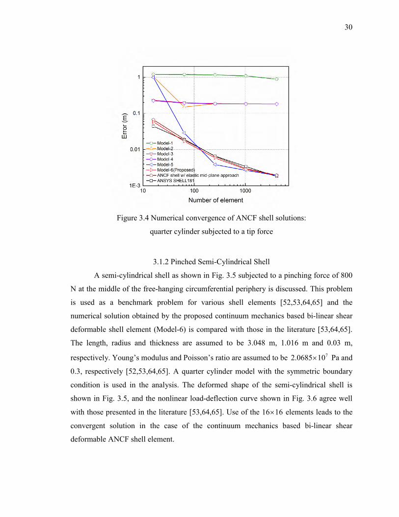
30

Figure 3.4 Numerical convergence of ANCF shell solutions:

quarter cylinder subjected to a tip force

3.1.2 Pinched Semi-Cylindrical Shell

A semi-cylindrical shell as shown in Fig. 3.5 subjected to a pinching force of 800

N at the middle of the free-hanging circumferential periphery is discussed. This problem

is used as a benchmark problem for various shell elements [52,53,64,65] and the

numerical solution obtained by the proposed continuum mechanics based bi-linear shear

deformable shell element (Model-6) is compared with those in the literature [53,64,65].

The length, radius and thickness are assumed to be 3.048 m, 1.016 m and 0.03 m,

respectively. Young’s modulus and Poisson’s ratio are assumed to be 72.0685 10× Pa and

0.3, respectively [52,53,64,65]. A quarter cylinder model with the symmetric boundary

condition is used in the analysis. The deformed shape of the semi-cylindrical shell is

shown in Fig. 3.5, and the nonlinear load-deflection curve shown in Fig. 3.6 agree well

with those presented in the literature [53,64,65]. Use of the 16 16× elements leads to the

convergent solution in the case of the continuum mechanics based bi-linear shear

deformable ANCF shell element.

31

Figure 3.5 Deformed shape of pinched semi-cylindrical shell

Figure 3.6 Load-deflection curve of pinched semi-cylindrical shell

3.1.3 Slit Annular Plate Subjected to Lifting Force

In the next example, a slit annular plate subjected to a lifting line force is

considered as shown in Fig. 3.7. This problem is also widely used as a benchmark

problem for shell elements [52]. The inside and outside radii of the annular plate are

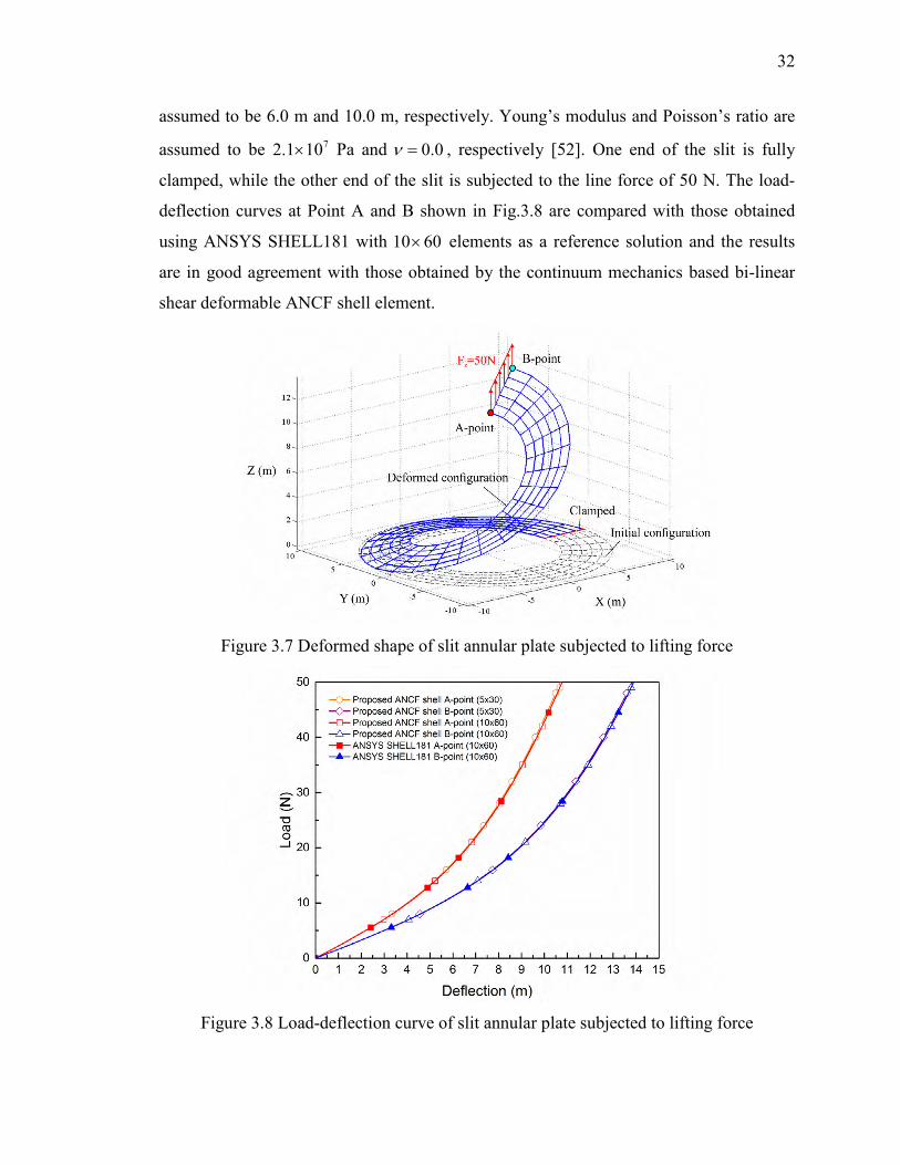
32

assumed to be 6.0 m and 10.0 m, respectively. Young’s modulus and Poisson’s ratio are

assumed to be 72.1 10× Pa and 0.0ν = , respectively [52]. One end of the slit is fully

clamped, while the other end of the slit is subjected to the line force of 50 N. The load-

deflection curves at Point A and B shown in Fig.3.8 are compared with those obtained

using ANSYS SHELL181 with 10 60× elements as a reference solution and the results

are in good agreement with those obtained by the continuum mechanics based bi-linear

shear deformable ANCF shell element.

Figure 3.7 Deformed shape of slit annular plate subjected to lifting force

Figure 3.8 Load-deflection curve of slit annular plate subjected to lifting force

33

3.2 Numerical Examples of Laminated Composite Shell Element

In this section, the element accuracy of the shear deformable laminated composite

shell element is discussed.

3.2.1 Extension and In-Plane Shear Coupling of Fiber-

Reinforced Plate Subjected to Uniaxial Tensile Load

To discuss the extension and in-plane shear coupling of a fiber-reinforced rubber

material, a uniaxial tension test as shown in Fig. 3.9 (a) is considered using the shear

deformable ANCF shell element. The length, width and thickness of the plate are 2.0 m,

1.0 m, and 0.01 m, respectively. Young’s modulus of the fiber and those of the matrix are,

respectively, assumed to be 111.8 10xE = × Pa and 71.3333 10y zE E= = × Pa. The shear

modulus of rigidity and Poisson’s ratio are assumed to be 6G G 3.33333 10 Paxy xz yzG = = = × and 0.4xy xz yzν ν ν= = = , respectively. The tensile

distributed uniaxial load of 5000 N/m is applied in the X direction. The in-plane shear

strain of the plate is presented in Fig. 3.10 as a function of the fiber angle θ . In this

figure, the in-plane shear strain obtained by the composite shell element is compared with

the analytical solution given by [5]

2 212

1 2 1 12

2cos sin 1 1sin 2 cos 22xy xE E E G

νθ θγ θ θ σ

= − + − (3.1)

It is observed from the preceding equation that the change in the shear strain is nonlinear

in the fiber angle θ . The sign of the shear strain changes at 54.7θ = degrees [5] as

shown by the magnified deformed shapes at 20θ = , 54.7 and 70 degrees in Fig. 3.10.

The results obtained by the ANCF shell element agree well with the analytical solution

based on the assumption of Kirchhoff plate theory with infinitesimal deformation.

Furthermore, using Eq. 3.1 the inflection points of the in-plane shear strain are obtained

at 25.5θ = and 71.3 degrees, and they are also well predicted using the composite shell

element discussed in this study.

34

Figure 3.10 In-plane shear strain of one-layer orthotropic plate

Figure 3.9 Uniaxial tensile test models

35

3.2.2 Warpage of Two-Layer Laminated Composite Plate

Subjected to Uniaxial Tensile Load

In the next example, a uniaxial tensile test of a two-layer laminate at / θ+ − fiber

angles is considered as shown in Fig. 3.9 (b) [60]. The length, width and thickness of the

plate are same as the previous example in Section 3.1. The thicknesses of each layer is

0.005 m. The fiber angles of the upper and lower layers are same in magnitude, but

opposite in direction as shown in Fig. 3.9 (b). The material properties of each layer are

also same as the previous example in Section 3.2.1. The tensile distributed uniaxial load

of 500 N/m is applied in the X direction. In this problem, the extension and

bending/twisting coupling occurs in this laminate, and it causes the warpage (twisting)

under the uniaxial tensile loading [60]. While the extension and shear coupling occurs in

each lamina, shear deformation of the upper and lower layers caused by the uniaxial

tensile load are same in magnitude, but opposite in direction. Thus, the shear

deformations of both layers are canceled out and no in-plane shearing occurs in the

laminated composite. To demonstrate this fundamental coupling behavior of the

laminated composite material, the twisting angle and the in-plane shear strain of the two-

layer laminated composite plate are presented in Fig. 3.11 as a function of the fiber angle

θ . In this figure, results obtained by the laminated composite shell element are compared

with the analytical model based on the classical lamination theory. In the analytical

model, the warpage is defined by [60]

( )2 212 x y xyw x y xyκ κ κ= − + + (3.2)

where the curvatures are determined by solving equilibrium equations of the force and

moment resultants of fiber-reinforced composite [60]. It is observed from Fig. 3.11 that

the twisting angles agree well with those based on the classical lamination theory, and the

warpage developed by the uniaxial tensile load applied to the two-layer laminated

composite plate is well predicted. The sign of the twisting angle of the composite plate

changes at the fiber angle of 54.7θ = degrees [5], and this important fiber angle is also

correctly predicted. Furthermore, zero in-plane shear strain is ensured in the results

regardless of the fiber angle, and this result agrees with that of the analytical model based

on the classical lamination theory.

36

Figure 3.11 Twisting angle and in-plane shear strain of two-layer laminated

composite plate subjected to uniaxial tensile load

3.2.3 Cantilevered Two-Layer Composite Shell Subjected

to a Point Load

To demonstrate the accuracy of the composite shell element for large deformation

problem of initially curved shell structures, a cantilevered quarter cylinder modeled by

/ θ+ − two-layer composite shell is considered as shown in Fig. 3.12. The initial shape

and the location of a subjected point load is the same as Section 3.1.1 shown in Fig. 3.3.

The fiber angle of each layer is assumed to be 20° . The radius of curvature is assumed to

be 1.0 m. The width and height are assumed to be 1.0 m and 0.01 m (i.e., 0.005 m

thickness for each layer). Young’s modulus of the fiber and those of the matrix are,

respectively, assumed to be 82.0 10xE = × Pa and 81.0 10y zE E= = × Pa. The shear

modus of rigidity and Poisson’s ratio are assumed to be 7G G 3.84615 10xy xz yzG = = = ×

Pa and 0.3xy xz yzν ν ν= = = , respectively. The vertical point load of 10 N is applied to the

corner of the shell as shown in Fig. 3.12. The deformed shape at the static equilibrium

37

state is shown in Fig. 3.12, in which the large deformation is exhibited. The static

deflections of the load application point obtained by the laminated composite shell

element are compared with those of the shear deformable composite shell element of

ANSYS (SHELL181) [63] in Table 3.2 for different number of elements. It is

demonstrated in this Table that good agreements in solution are obtained with the MITC

shell formulation [63] implemented in ANSYS. The numerical convergence of the finite

element solutions are presented in Fig. 3.13 for errors defined by the deviation from the

reference solution, where the reference solution of -0.80517 m is obtained by 100 100×

elements using the ANSYS SHELL181 composite shell element. It is observed from this

figure that the ideal linear rate of convergence is ensured in both models for the large

deformation problem and it indicates that element lockings are properly eliminated in the

ANCF laminated composite shell element discussed in this study. On the other hand, the

fully parameterized ANCF shell element utilizing the bi-cubic polynomial does not

converge to the reference solution, despite the fact that higher order polynomials are used

due to the element lockings exhibited. Furthermore, the number of integration points for

the elastic force calculation of each layer is 8 ( 2 2 2× × ) in the bi-linear shell element

having 24 nodal coordinates per element, while 32 ( 4 4 2× × ) integration points are used

in the bi-cubic fully parameterized shell element with 48 nodal coordinates per element.

This has a significant impact on the computational efficiency for large scale problems

including tire simulation.

Table 3.2 Static deflection of cantilevered two-layer composite

shell subjected to point load (m)

Number of elements

ANCF composite shell

ANSYS composite shell (SHELL181)

4 4× -0.77157 -0.78262 8 8× -0.79931 -0.79786

16 16× -0.80310 -0.80220 32 32× -0.80414 -0.80619 50 50× -0.80452 -0.80473 64 64× -0.80469 -0.80493

38

Figure 3.12 Deformed shape of cantilevered two-layer composite

shell subjected to point load

Figure 3.13 Numerical convergence of finite element solutions

39

3.2.4 Natural Frequencies of Laminated Composite Plate

The eigenfrequency analysis of the / θ+ − two-layer composite plate is

considered in this example. The fiber angle of each layer is assumed to be 20° . A free

boundary condition is assumed. The length, width and thickness of the plate are 1.0 m,

1.0 m, and 0.01 m (i.e., 0.005 m thickness for each layer), respectively. Young’s

modulus of the fiber and those of the matrix are, respectively, assumed to be 76.0 10xE = × Pa and 73.0 10y zE E= = × Pa. The shear modus of rigidity and Poisson’s

ratio are assumed to be 7G G 1.1538 10xy xz yzG = = = × Pa and 0.3xy xz yzν ν ν= = = ,

respectively. The material density is assumed to be 500 kg/m3. The first ten

eigenfrequencies and their mode shapes are shown in Table 3.3 and Fig. 3.14,

respectively. The eignfrequencies are compared with the reference solutions obtained by

the 100 100× elements using the ANSYS SHELL181 composite shell element. The

eigenfrequencies are also in good agreement with the reference solutions. Use of the

proposed low-order continuum mechanics based shear deformable shell element leads to

better rate of convergence than the higher-order fully parameterized ANCF element

presented in literature [30].

Table 3.3 First ten eigenfrequencies of the laminated composite shell (Hz)

ANCF composite

shell 2 2×

ANCF composite

shell 4 4×

ANCF composite

shell 8 8×

ANCF composite

shell 16 16×

ANCF composite

shell 32 32×

ANSYS composite

shell (SHELL181)

100 100× 1.8168 1.7705 1.7385 1.7291 1.7295 1.7175 2.9444 2.6214 2.4887 2.4518 2.4296 2.4424 4.3411 3.7085 3.4579 3.3853 3.3642 3.3700 4.8487 4.6450 4.4097 4.3355 4.3088 4.2951 5.4240 5.0939 4.8413 4.7605 4.7412 4.7220 9.1235 9.3139 7.7790 7.2886 7.1604 7.1146

116.4075 9.7130 8.5528 8.3152 8.2496 8.2005 127.6218 10.7920 9.2868 8.8343 8.7120 8.6442 133.0542 12.3383 9.8813 9.2463 9.0973 9.0559 141.4632 14.1086 11.5408 10.8417 10.6750 10.6080

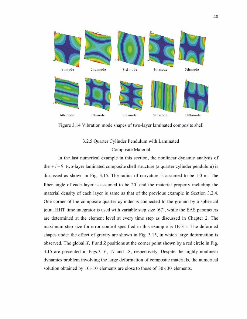
40

Figure 3.14 Vibration mode shapes of two-layer laminated composite shell

3.2.5 Quarter Cylinder Pendulum with Laminated

Composite Material

In the last numerical example in this section, the nonlinear dynamic analysis of

the / θ+ − two-layer laminated composite shell structure (a quarter cylinder pendulum) is

discussed as shown in Fig. 3.15. The radius of curvature is assumed to be 1.0 m. The

fiber angle of each layer is assumed to be 20° and the material property including the

material density of each layer is same as that of the previous example in Section 3.2.4.

One corner of the composite quarter cylinder is connected to the ground by a spherical

joint. HHT time integrator is used with variable step size [67], while the EAS parameters

are determined at the element level at every time step as discussed in Chapter 2. The

maximum step size for error control specified in this example is 1E-3 s. The deformed

shapes under the effect of gravity are shown in Fig. 3.15, in which large deformation is

observed. The global X, Y and Z positions at the corner point shown by a red circle in Fig.

3.15 are presented in Figs.3.16, 17 and 18, respectively. Despite the highly nonlinear

dynamics problem involving the large deformation of composite materials, the numerical

solution obtained by 10 10× elements are close to those of 30 30× elements.

41

Figure 3.15 Deformed shapes

Figure 3.16 Global X-position at the tip point

42

Figure 3.17 Global Y-position at the tip point

Figure 3.18 Global Z-position at the tip point

43

CHAPTER 4

PHYSICS-BASED FLEXIBLE TIRE MODEL FOR TRANSIENT

BRAKING AND CORNERING ANALYSIS

4.1 Introduction

In this chapter, a high fidelity physics-based finite element tire model is

developed using the shear deformable laminated composite shell element based on the

absolute nodal coordinate formulation discussed in Chapter 2 and 3 for use in the

transient braking and cornering analysis of multibody vehicle systems [66]. To account

for the transient tire force characteristics, the distributed parameter LuGre tire friction

model is introduced and then integrated into the physics-based flexible tire model. Using

the LuGre tire friction model, the dynamic friction effect is modeled by the first order

partial differential equation in terms of an internal friction parameter and, therefore, the

history-dependent friction-induced hysteresis can be considered [68,69]. It is shown that

the nonlinear structural tire deformation due a large load transfer in the severe maneuvers

and the transient tire force characteristics are fully coupled in the final form of the

governing equations. Furthermore, a modified friction characteristic curve function is

proposed for wet road conditions, in which the linear decay in friction is exhibited in the

large slip velocity range.

4.2 Structural Tire Model Using Laminated Composite Shell

Element

4.2.1 Modeling of Tire Structure with Cord-Rubber Composite Materials

A tire has a complex structure that consists of layers of plies and steel belts that

are embedded in rubber, thus an accurate modeling of the complex tire geometry and the

anisotropic material properties is essential to the tire performance evaluation including

the tire contact pressure and the braking/traction and cornering forces. While the in-plane

tire belt deformation can be modeled by an equivalent material model [31,32], such a

simplified material model cannot be used for predicting the overall tire structural

deformation in the three-dimensional analysis. This is attributed to the fact that the tire

44

section property in both geometry and material is of crucial importance in characterizing

the contact pressure distribution.

In order to develop a physics-based flexible tire model, the tire cross section

geometry is imported from the tire cut section and data points are interpolated by a cubic

smoothing spline to extract the nodal position and slope coordinates. As shown in Fig.

4.1, the tire cross-section is divided into the tread, sidewall, and bead sections. The

number of layers, cord angles, thickness, and material properties, which vary through the

tire structure, are provided in each section to create the tire model data as shown in Fig.

4.1. The tread section consists of a carcass ply, two steel belts, a belt cover, and tread

blocks. The carcass ply and steel belt are modeled as an orthotropic material with

polyester and steel cords embedded in rubber, respectively. A rubber layer is considered

between the upper and lower steel belts and between the carcass ply and the lower steel

belt, and these rubber layers are modeled by Mooney-Rivlin material in the laminated

composite shell element. The sidewall section is modeled by two carcass ply layers and a

rubber layer that lies in between. The bead section is modeled by two carcass ply layers, a

steel belt, and a rubber layer as shown in Fig. 4.2. Having created the cross-section

geometry and material properties, the three-dimensional tire model data including the

nodal position and slope coordinates is generated by rotating the tire section model as

summarized in Fig. 4.1.

Figure 4.1 Tire model creation procedure

45

Figure 4.2 Physics-based tire model using the laminated composite shell element

4.2.2 Modeling of Air Pressure

The internal air pressure is modeled by the distributed load acting in the direction

normal to the deformable inner tire surface, and the generalized force vector of element i

for the air pressure is defined as

( )i i T i ip pa

da= ∫Q S F (4.1)

where iS is the shape function of the shell element introduced in Section 2, da is the

infinitesimal area at the current configuration, and i ip pf=F n (4.2)

In the preceding equation, pf defines the air pressure and the unit normal is defined as

/ // /

i i i ii

i i i i

x yx y

∂ ∂ ×∂ ∂=

∂ ∂ ×∂ ∂r rnr r

(4.3)

Gaussian integration is used for the spatial integral of Eq 4.1. It is important to note here

that the integral over the current area ida is converted to that over the area at the

reference configuration idA using Nanson’s formula ( )det ( ) ( )i i i T i i T i ida dA= J n J J n ,

where iJ is the position vector gradient tensor at the reference configuration. If the

deformation is small, one can assume i ida dA≈ .

46

Figure 4.3 Assembly of flexible tire and rigid rim

4.2.3 Assembly of Flexible Tire and Rigid Rim

The bead part of the finite element tire model is connected to the rigid rim by

multiple spring and damper elements as shown in Fig. 4.3. For a spring and damper

element defined at point ilP on the finite element i of the deformable tire model, the

global position vector is defined by ( , , )i i i i i il l l lx y z=r S e and the nodal point can also be

selected as the force definition point. This point is connected to point jlP on the rigid rim

j and the global position vector of this point on the rigid rim is written by j j j j

l l= +r R A u , where jR is the global position vector of the origin of the body

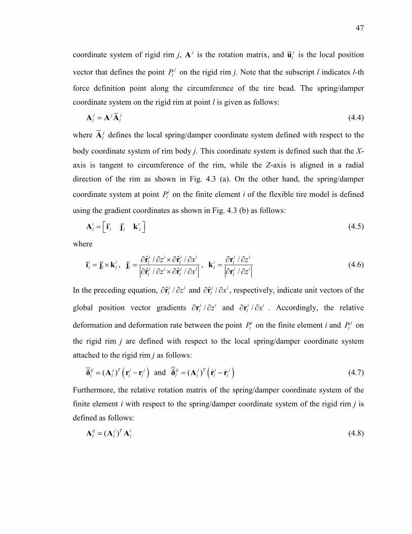
47

coordinate system of rigid rim j, jA is the rotation matrix, and jlu is the local position

vector that defines the point jlP on the rigid rim j. Note that the subscript l indicates l-th

force definition point along the circumference of the tire bead. The spring/damper

coordinate system on the rigid rim at point l is given as follows: j j jl l=A A A (4.4)

where jlA defines the local spring/damper coordinate system defined with respect to the

body coordinate system of rim body j. This coordinate system is defined such that the X-

axis is tangent to circumference of the rim, while the Z-axis is aligned in a radial

direction of the rim as shown in Fig. 4.3 (a). On the other hand, the spring/damper

coordinate system at point ilP on the finite element i of the flexible tire model is defined

using the gradient coordinates as shown in Fig. 4.3 (b) as follows: i i i il l l l = A i j k (4.5)

where

i i il l l= ×i j k ,

ˆ ˆ/ /ˆ ˆ/ /

i i i ii l ll i i i i

l l

z xz x

∂ ∂ ×∂ ∂=

∂ ∂ ×∂ ∂r rjr r

, //

i ii ll i i

l

zz

∂ ∂=

∂ ∂rkr

(4.6)

In the preceding equation, ˆ /i il z∂ ∂r and ˆ /i i

l x∂ ∂r , respectively, indicate unit vectors of the

global position vector gradients /i il z∂ ∂r and /i i

l x∂ ∂r . Accordingly, the relative

deformation and deformation rate between the point ilP on the finite element i and j

lP on

the rigid rim j are defined with respect to the local spring/damper coordinate system

attached to the rigid rim j as follows:

( )( )ij j T i jl l l l= −δ A r r and ( )( )ij j T i j

l l l l= −δ A r r (4.7)

Furthermore, the relative rotation matrix of the spring/damper coordinate system of the

finite element i with respect to the spring/damper coordinate system of the rigid rim j is

defined as follows:

( )ij j T il l l=A A A (4.8)

48

From which, relative rotation angles Tij ij ij ij

l x y zθ θ θ = θ about the three axes can be

extracted from the relative rotation matrix ijlA and used for defining the restoring torque

about each axis. Rotational deformation rate can be defined as

( )( )ij j T i jl l l= −ω A ω ω (4.9)

where ilω and jω are the angular velocity vectors of the force application point l on the

shell element i and rigid rim j, respectively. It is important to notice here that ilω can be

obtained from the skew-symmetric matrix ( )i i i Tl l l=ω A A . It is important to notice here

that ilω can be obtained from the skew-symmetric matrix

( )i i i Tl l l=ω A A (4.10)

where the time derivative of the tangent frame is given as i i i il l l l = A i j k (4.11)

In the preceding equation, one has

( ) ( )

( ) ( )2

1

1 cosˆ ˆ ˆ ˆ ˆ ˆsin sin

1 T T

T

i i i i il l l l l

i i i i i i il z x z x z x

i i i i i il z z z z z

i iz z

α αα α

−

= × + × = × + × − × = −

i j k j k

j r r r r r r

k I r r r r rr r

(4.12)

where /i i iz z= ∂ ∂r r ; /i i i

x x= ∂ ∂r r ; ( ) ( )i i i iz z x xα α α= ∂ ∂ ⋅ + ∂ ∂ ⋅r r r r ; ˆ ˆcos

Ti iz xα = r r ;

ˆ( 1 sin ) ( )Ti i i i

z x z zα α∂ ∂ = − ∂ ∂r r r r ; and ˆ( 1 sin ) ( )Ti i i i

x z x xα α∂ ∂ = − ∂ ∂r r r r .

Using the deformation and deformation rate at the spring and damper definition

point, the spring and damping forces and torques defined with respect to the local spring

and damper coordinate system are defined as follows:

ij ij ijl r l r l= − −F K δ C δ and 0( )ij ij ij ij

l l l lθ θ= − − −N K θ θ C ω (4.13)

where rK and θK are the translational and rotational spring constant matrices, while rC

and θC are translational and rotational damping coefficient matrices, respectively. 0ijlθ is

the initial relative rotation angle vector of the spring/damper coordinate systems at ilP

49

and jlP . The preceding force and torque vectors are defined with respect to the global

coordinate system as ij j ijl l lij j ijl l l

=

F A FN A N

(4.14)

and then the generalized forces can be obtained for both element i and rigid rim j using

the virtual work.

4.3 LuGre Tire Friction Model

4.3.1 LuGre Tire Friction Model for Combined Slip

In existing deformable tire models, the steady-state tire friction model are widely

used and the tire frictional force is defined by the product of the friction coefficient and

the normal contact force at discretized points in the contact patch. The friction coefficient

is defined in many cases as a multi-variable function of the contact pressure, slip velocity,

temperature, etc. While such a frictional contact model leads to a straightforward

implementation, it requires a large set of test data prepared a priori to define the multi-

variable friction function. Furthermore, it does not account for the history-dependent

dynamic friction effect needed for the severe transient maneuver simulation due to the

steady-state assumption made. For this reason, to account for the transient tire friction

effect for severe braking and cornering analysis, the distributed parameter LuGre tire

friction model [68,69] is introduced in this study and a numerical procedure to integrate

the LuGre tire friction model into the finite-element based deformable tire model is

proposed.

In the LuGre tire force model originally proposed for rigid-body based tire models,

the state of friction between a tire tread and road is described by internal friction

parameters ( , )xz tζ and ( , )yz tζ defined in time and space, where ζ is a spatial

coordinate defined along the contact patch longitudinal axis ( 0 Lζ≤ ≤ ) as shown in Fig.

4.4. The longitudinal and lateral tire forces are then defined using the following equations

[68,69]:

50

Figure 4.4 LuGre tire friction model

2

0 1 20 2

2

0 1 20 2

( , ) ( , ) ( )

( , ) ( , ) ( )

L W xx x x x x rx nW

L W yy y y y y ry nW

zF z t t v p d dtz

F z t t v p d dt

σ ζ σ ζ σ ζ η ζ

σ ζ σ ζ σ ζ η ζ

−

−

∂ = + + ∂ ∂ = + + ∂

∫ ∫

∫ ∫ (4.15)

where L and W are, respectively, the length and width of the contact patch, and

/ 2 / 2W Wη− ≤ ≤ . rkv ( ,k x y= ) is the slip velocity in the longitudinal ( k x= ) and

lateral ( k y= ) directions, respectively; 0kσ and 1kσ are, respectively, coefficients

associated with kz and kz , where ,k x y= ; and 2kσ ( ,k x y= ) is a coefficient describing

viscous friction effect between the tread and road. ( )np ζ is the normal contact pressure

in the contact patch. The internal friction parameter ( , )xz tζ and ( , )yz tζ are given as

solution to the following partial differential equations [68,69]:

0

0

( , ) ( , )( , )( )

( , ) ( , )( , )

( )

x rxx xrx x

x rx

y ryy yry y

y ry

vz t z tv z t rt g v

vz t z tv z t r

t g v

σζ ζζ ωζ

σζ ζζ ω

ζ

∂ ∂= − − ∂ ∂

∂ ∂ = − − ∂ ∂

(4.16)

where rω is the circumferential velocity; and ( )x rxg v and ( )y ryg v are functions that

define the longitudinal and lateral slip-dependent friction coefficient characteristics. In

this study, the friction characteristics are identified at pure braking conditions, and then

friction curves for the longitudinal and lateral frictions under combined slip conditions

are defined as follows [69]:

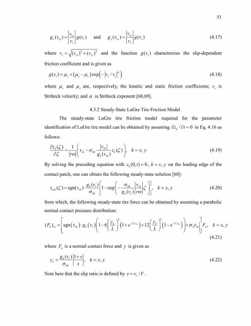
51

( ) ( )rxx rx r

r

vg v g vv

= and ( ) ( )ryy ry r

r

vg v g v

v= (4.17)

where 2 2( ) ( )r rx ryv v v= + and the function ( )rg v characterizes the slip-dependent

friction coefficient and is given as

( ) ( )( ) exp /r c s c r sg v v v αµ µ µ= + − − (4.18)

where cµ and sµ are, respectively, the kinetic and static friction coefficients; sv is

Stribeck velocity; and α is Stribeck exponent [68,69].

4.3.2 Steady-State LuGre Tire Friction Model

The steady-state LuGre tire friction model required for the parameter

identification of LuGre tire model can be obtained by assuming / 0kz t∂ ∂ = in Eq. 4.16 as

follows:

0( ) 1 ( ) , ,

( )rkk

rk k kk rk

vz v z k x yr g v

ζ σ ζζ ω

∂= − = ∂

(4.19)

By solving the preceding equation with (0, ) 0kz t = , ,k x y= on the leading edge of the

contact patch, one can obtain the following steady-state solution [68]:

0

0

( )( ) sgn( ) 1 exp , ,( )

k r k rkssk rk

k k r

g v vz v k x yg v rσζ ζ

σ ω

= ⋅ − − =

(4.20)

from which, the following steady-state tire force can be obtained by assuming a parabolic

normal contact pressure distribution:

( ) ( ) ( ) ( )2 3

/ /2( ) sgn 1 6 1 12 1 , ,k kL Lk k

k ss rk k r rk nF v g v e e v F k x yL L

γ γγ γ σ− − = ⋅ − + + − + =

(4.21)

where nF is a normal contact force and γ is given as

0

( ) 1 , ,k rk

k

g v s k x ys

γσ

+= = (4.22)

Note here that the slip ratio is defined by /rs v V= .

52

4.3.3 Slip Dependent Characteristics for Wet Condition

The longitudinal tire force measured by a tire test rig on a wet condition is shown

in Fig. 4.5. The forward velocity is assumed to be 100 km/h (27.8 m/s) and the tire size is

195/65/R15. It is observed from this figure that the tire force builds up as the slip ratio

increases and then it drops after it reaches the maximum point, which is the typical

braking force characteristic on wet road conditions. Furthermore, it is important to note

here that the tire force decreases linearly as the slip ratio increases in the large slip ratio

regime. Such a linear decay in the tire force in the large slip ratio range is also observed

in the literature [70] for the measured tire forces on wet road conditions. However, since

the slip-dependent friction characteristics given in Eq. 4.18 are approximated by an

exponential function, the linear decay of the tire force in the large slip ratio range cannot

be described. In order to account for the linear decay of the friction coefficient in the

large slip ratio range, the function ( )rg v is modified in this investigation as follows:

( )( ) ( ) ( ( )) exp /r r s r r sg v h v h v v v αµ= + − − (4.23)

where the linear change in the friction coefficient is modeled by the following function

( )rh v as

Figure 4.5 Longitudinal tire force on wet surface

53

( ) rr

s

vh vv ββ µ= − + (4.24)

where β and βµ are the model parameters that need to be identified. Using the

preceding equations, the friction coefficient can decrease exponentially in small slip

range, while in the large slip range, the friction coefficient decreases linearly as defined

by the function ( )rh v . Since the exponential function that appears in the second term of

Eq. 4.23. approaches to zero as the slip velocity increases, the function ( )rh v has a

dominant effect in the large slip range, allowing for the accurate modeling of the slip-

dependent friction coefficient characteristics which involve the linear decay in the large

slip range. It is important to notice here that the original function proposed in the

literature [68] can be recovered if β in Eq. 4.24 is equal to zero.

4.4 Integration of LuGre Tire Friction Model into Deformable Tire Model

In most literature that discuss the LuGre tire friction model using rigid-body

based tire models, the tangential tire force distribution across the contact patch width is

assumed to be constant and the spatial distribution of the friction parameter ( , )z tζ is

approximated by a single mean friction parameter ( )z t such that the tire force can be

determined as a solution to the ordinary differential equation in terms of the single

friction variable ( )z t [68,69]. This leads to a straightforward implementation of the

LuGre tire friction model in rigid-body based tire models. However, the shear contact

stress distribution over the contact patch cannot be evaluated and the slip velocity is

approximated at a single contact point. For this reason, to account for the effect of the

change in the normal contact pressure and slip distributions over the contact patch

predicted by the flexible tire model, spatially discretized form of the LuGre tire friction

model is derived and integrated into the flexible tire model developed in this study. Since

the state of friction is dependent on the longitudinal and transverse coordinates as

( , , )kz tζ η , one has

, ,k k k kdz z z z k x ydt t t t

ζ ηζ η

∂ ∂ ∂∂ ∂= + + =

∂ ∂ ∂ ∂ ∂ (4.25)

54

In rolling contact problems, / tζ∂ ∂ term defines the velocity of the contact patch

coordinate system in the rolling direction ζ . However, the lateral velocity of the contact

patch coordinate system represented by / tη∂ ∂ in the second term is assumed to be small

enough as compared to / tζ∂ ∂ and /kz t∂ ∂ describing the transient effect of the friction

parameter in rolling contact problems. Thus, one can assume / 0tη∂ ∂ ≈ as in the original

LuGre tire friction model. However, this does not mean that distribution of the friction

parameters xz and yz in the width direction is neglected since the contact pressure and

slip velocity distributions obtained from the finite element tire model are defined as a

function of ζ and η in this study, i.e., ( , )np ζ η and ( , )rv ζ η . For this reason, the

contact patch predicted by the flexible tire model is discretized into strips across the tire

width first to account for the shear contact stress distribution along the transverse axis of

the contact patch, and then shear contact stresses are evaluated strip by strip as shown in

Fig. 4.6. This strip is called “LuGre strip” in this study. For each LuGre strip j defined at jη η= shown in Fig. 4.6, the state of friction is defined by the following partial

differential equations in terms of the two parameters jxz and j

yz associated with the

longitudinal and lateral shear stresses:

0

0

, 1, ,( )

, 1, ,( )

jj jx rxj j j jx x

rx xj jx rx

jj jy ryy yj j j j

ry yj jy ry

vz zv z r j mt g v

vz zv z r j m

t g v

σω

ζ

σω

ζ

∂ ∂= − − =

∂ ∂

∂ ∂ = − − = ∂ ∂

(4.26)

where the superscript j indicates the quantity on the j-th LuGre strip along the

longitudinal axis of the contact patch. In order to solve the preceding partial differential

equations of the LuGre tire friction model, Eq. 4.26 is spatially discretized as 1,/ ( ) /j j ij i j ijz z z Lζ −∂ ∂ = − ∆ and then converted to the set of first-order ordinary

differential equations as follows:

55

( )

( )

01,

01,

, 1, , ; 1, ,

, 1, , ; 1, ,

ij ij ij ij ijijx rxij i j ijx

rx x xij ijijx rx

ij ij ij ij ijijy ryy ij i j ij

ry y yij ijijy ry

r v rdz v z z i n j mdt L Lg v

r v rdzv z z i n j m

dt L Lg v

ω σ ω

ω σ ω

−

−

= + − + = =

∆ ∆

= + − + = = ∆ ∆

(4.27)

where the superscript i and j, respectively, indicate the i-th discretized element

( 1, ,i n= ) in the j-th LuGre strip ( 1, ,j m= ). ijL∆ is the length of the LuGre element

ij shown in Fig. 4.6. 0 0 0j jx yz z= = is assumed on the leading edge. The preceding

Figure 4.6 Integration of LuGre tire friction model in flexible tire model

56

equations are expressed in the following matrix form for all the discretized LuGre

elements in the contact patch:

= +z A z b (4.28)

where the vector z contains all the LuGre friction variables ijxz and ij

yz for 1, ,i n= and

1, ,j m= . A is the square matrix of mn mn× and b is the vector of slip velocities ijrxv

and ijryv defined in the discretized element ij. Accordingly, the longitudinal and lateral

shear contact stresses in the LuGre element ij are defined as

( )( )

0 1 2

0 1 2

ij ij ij ij ijx x x x x x rx n

ij ij ij ij ijy y y y y y ry n

p z z v p

p z z v p

σ σ σ

σ σ σ

= + +

= + +

(4.29)

where ijnp is the normal contact pressure acting on the LuGre element ij. From which, the

longitudinal and lateral contact forces defined in the LuGre element ij can be obtained as

,ij ij ij ij ij ij ij ijx x y yF p L b F p L b= ∆ ∆ = ∆ ∆ (4.30)

where ijb∆ is the width of LuGre element ij. It is important to notice here that the finite

element nodes in contact and LuGre elements in the contact patch do no coincide as

shown in Fig. 4.6, and finer LuGre mesh is required to obtained accurate shear contact

stress distribution. For this reason, the contact pressure and slip velocity predicted at each

finite element node in contact are spatially interpolated to evaluate those at discretized

LuGre elements to construct the set of ordinary differential equations associated with the

dynamic tire friction for each LuGre element defined by Eq. 4.27. On the other hand, to

define the nodal tangential contact forces applied to the flexible tire model, the shear

contact stresses evaluated at the discretized LuGre elements are then interpolated to

define the LuGre tangential tire forces acting on each finite element node in the contact

patch as shown in Fig. 4.6. These nodal tangential contact forces are added to the right

hand side of the equations of motion of the flexible tire model. By doing so, the structural

deformation of the flexible tire model can be dynamically coupled with the LuGre tire

friction model in the final form of the equations as follows:

( , ) ( , , , )( ) ( )

s e= + = +

Me Q e α Q e e z zz A e z b e

(4.31)

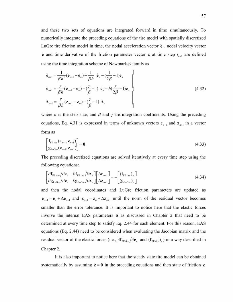
57

and these two sets of equations are integrated forward in time simultaneously. To

numerically integrate the preceding equations of the tire model with spatially discretized

LuGre tire friction model in time, the nodal acceleration vector e , nodal velocity vector

e and time derivative of the friction parameter vector z at time step 1nt + are defined

using the time integration scheme of Newmark-β family as

1 12

1 1

1 1

1 1 1( ) ( 1)2

( ) ( 1) ( 1)2

( ) ( 1)

n n n n n

n n n n n

n n n n

h h

hh

h

β β βγ γ γ

β β βγ γ

β β

+ +

+ +

+ +

= − − − − = − − − − −

= − − −

e e e e e

e e e e e

z z z z

(4.32)

where h is the step size; and β and γ are integration coefficients. Using the preceding

equations, Eq. 4.31 is expressed in terms of unknown vectors 1n+e and 1n+z in a vector

form as

FE tire 1 1

LuGre 1 1

( , )( , )

n n

n n

+ +

+ +

=

f e z0

g e z (4.33)

The preceding discretized equations are solved iteratively at every time step using the

following equations:

FE tire FE tire 1 FE tire

LuGre LuGre 1 LuGre

( )( )

n n n n

n n n n

+

+

∂ ∂ ∂ ∂ ∆ = − ∂ ∂ ∂ ∂ ∆

f e f z e fg e g z z g

(4.34)

and then the nodal coordinates and LuGre friction parameters are updated as

1 1n n n+ += + ∆e e e and 1 1n n n+ += + ∆z z z until the norm of the residual vector becomes

smaller than the error tolerance. It is important to notice here that the elastic forces

involve the internal EAS parameters α as discussed in Chapter 2 that need to be

determined at every time step to satisfy Eq. 2.44 for each element. For this reason, EAS

equations (Eq. 2.44) need to be considered when evaluating the Jacobian matrix and the

residual vector of the elastic forces (i.e., FE tire n∂ ∂f e and FE tire( )nf ) in a way described in

Chapter 2.

It is also important to notice here that the steady state tire model can be obtained

systematically by assuming =z 0 in the preceding equations and then state of friction z

58

can be uniquely determined by solving the linear algebraic equations ( ) ( )+ =A e z b e 0 if

the transient tire friction effect is considered negligible for some simulation scenarios.

That is, the steady-state model of the spatially discretized LuGre tire friction can be

obtained by assuming that the transient term of the friction parameters equal zero, i.e.,

/ / 0ij ijx ydz dt dz dt= = in Eq. 4.27. This assumption leads to the following equations:

( )

( )

0 1,

0 1,

, 1, , ; 1, ,

, 1, , ; 1, ,

ij ij ij ij ijx rx ij ij i j

x rx xij ijijx rx

ij ij ij ij ijy ry ij ij i j

y ry yij ijijy ry

v r rz v z i n j m

L Lg v

v r rz v z i n j m

L Lg v

σ ω ω

σ ω ω

−

−

+ = + = =

∆ ∆

+ = + = = ∆ ∆

(4.35)

It is important to notice here that the preceding equations can be solved for ijxz and ij

yz

without any time-integration procedures from the leading edge ( 1i = ) to the trailing edge

( i n= ) recursively for each LuGre strip j with the boundary condition 0 0 0j jx yz z= = on

the leading edge. This indicates that the leading edge of the contact patch is in adhesion.

The shear contact stresses can then be defined by Eq. 4.29. Since the state of shear

contact stress distribution over the contact patch is defined by algebraic equations,

friction parameters are no longer treated as system coordinates, resulting in a smaller

number of equations being solved. The steady-state tire friction model is, however,

unable to incorporate the history-dependent friction-induced hysteresis since friction state

can be uniquely determined without the state at previous time step through time

integration.

59

CHAPTER 5

PARAMETER IDENTIFICATION AND TIRE DYNAMICS

SIMULATION

5.1 Introduction

For use of LuGre tire friction model, the parameter identification is crucial to

accurate and reliable prediction of transient tire forces under various driving conditions

[70]. Since governing equations of LuGre tire friction model are highly nonlinear and

several fitting parameters are introduced to account for the nonlinear friction

characteristics, the correlation of the model parameters with physical quantities are not

clear, making the parameter identification of the LuGre tire friction model difficult [70].

That is, inappropriate initial estimates may lead to parameters that have nothing to do

with physical quantities even though the LuGre model are fitted well with measured tire

force curves. For this reason, a systematic and automated procedure for parameter

identification of LuGre tire friction model is developed in this chapter. Furthermore, the

fundamental tire characteristics including the normal contact pressure distribution and

load-deflection curve of the physics-based flexible tire model discussed in Chapter 4 are

validated against the tire test data, and then the nonlinear tire dynamic simulation under

abrupt braking and cornering scenarios on a rigid ground are presented to demonstrate the

tire model capability for transient maneuvering scenarios developed in this study.

5.2 Parameter Identification Procedure of LuGre Tire Friction Model

Since the basic tire force characteristics are, in most cases, evaluated using tire

test rigs in the steady state condition, the steady state model given by Eq. 4.21 is

introduced for the purpose of the parameter identification of the LuGre tire friction model.

The parameters identified in the steady state condition are then introduced to the transient

LuGre tire friction model in the time-domain analysis. It is important to notice here that

the steady-state model is derived as a special case of the general transient model, thus all

the LuGre model parameters for describing the tire tread friction characteristics are, in

principle, consistent in both models to ensure that the steady state tire force

characteristics can be recovered from the transient tire force model.

60

In the steady-state LuGre tire friction model given by Eq. 4.21 with the modified

function ( )rg v (Eqs. 4.23 and 4.24), the following 7 parameters need to be identified

using the measurement data:

0 0[ ]Tx y s svβσ σ µ µ β α=p (5.1)

While the first two parameters 0xσ and 0 yσ are identified in the longitudinal and lateral

directions separately, the rest of the friction parameters are determined in a pure slip

condition and then slip-dependent friction curves in the longitudinal and lateral directions

are assumed by Eq. 4.17. In this study, the steady-state friction-slip curve for the

longitudinal tire force is used to identify the tire friction characteristics. For example,

using Eq. 4.21, the tangential force coefficient (ratio of tire force to normal force) at the

steady state condition can be obtained by assuming that the viscous friction effect is

negligibly small as follows:

( ) ( ) ( ) ( )2 3

/ /1 6 1 12 1x xL LLG ssx x xx x r

n

F g v e eF L L

γ γγ γµ − − = = − + + −

p (5.2)

where 0

( ) 1rx

x

g v ss

γσ

+= since ( ) ( )x rx rg v g v= at the pure slip state. In the preceding

equation, the unknown LuGre parameter vector 0[ ]Tx x s c svσ µ µ β α=p is

identified such that an error function defined by the difference between the tangential

force coefficient obtained by Eq. 5.2 and the measurement data can be minimized in the

entire slip range. That is,

( ) ( ) ( )( )2

1

1 min2

LG EXPnsk x k

x xEXPk k

J Jµ µ

µ=

−= →

∑

pp p (5.3)

where ns is the number of data points used for the parameter identification, and all the

components of the vector xp need to be positive. In order to solve the preceding

nonlinear optimization problem, iterative solution procedures are employed. Since there

are many local minima in the error function, appropriate initial estimates for iterative

solution procedures are crucial to accurate and reliable identification of the LuGre tire

friction model parameters. Although the model curve can be fitted to the measurement

data, it is not guaranteed that the model parameters identified are physically consistent.

61

Furthermore, all the LuGre model parameters are not necessarily correlated to

measureable physical quantities, making the determination of the initial estimates for the

nonlinear parameter identification difficult. For this reason, initial estimates provided for

solving Eq. 5.2 need to be accurately predicted first, and it allows for developing a

systematic and automated procedure for estimating parameters of the LuGre tire friction

model. The proposed slip-dependent friction coefficient given by function ( )rg v is

defined by the five parameters sµ , βµ , β , sv and α . Since these parameters can be

identified solely by the measured slip-dependent friction characteristics, they can be

estimated first and then adhesion parameters 0xσ and 0 yσ are identified by the

traction/braking and cornering stiffness extracted from the measured data. Since one has

( )r sg v µ= for 0rv = using Eq. 4.23, sµ can be estimated by finding the point of

intersection between the function ( )rg v and its ordinate axis. To find the point of

intersection, the friction coefficient of the measured data denoted by ( )EXPrg v in the

small slip velocity range is approximated by a linear function as shown at the top left

corner of Fig. 5.1 (also denoted as (A)) using the least square method, and then the point

of intersection with the ordinate axis that defines sµ can be obtained as

2

1 1 1 10 2

2

1 1

( ) ( )s s s s

s s

N N N NEXP EXP

r k r k r k r k r kk k k k

s N N

s r k r kk k

v g v v g v v

N v v

µ = = = =

= =

−=

−

∑ ∑ ∑ ∑

∑ ∑ (5.4)

where sN is the number of data points used for defining a linear function around the left

end of the ( )EXPr kg v and r kv ( 1, , sk N= ) indicates the slip velocity at data point k.

In the next step, βµ and β are estimated by approximating EXPg in the large slip

velocity range as a linear function as shown at the bottom right corner of Fig. 5.1 (also

denoted as (B)). As a result, the intercept βµ and the slope / svβ of the function

( ) /r r sh v v v ββ µ= − + can be estimated by the linear regression as follow:

62

Figure 5.1 Slip-dependent friction coefficient

2

1 1 1 10 2

2

1 1

( ) ( )N N N N

EXP EXPr k r k r k r k r k

k k k k

N N

r k r kk k

v g v v g v v

N v v

β β β β

β ββ

β

µ = = = =

= =

−=

−

∑ ∑ ∑ ∑

∑ ∑ (5.5)

and

0 1 1 12

0 2

1 1

( ) ( )N N N

EXP EXPr k r k r k r k

k k k

N Ns

r k r kk k

N v g v v g v

vN v v

β β β

β β

β

β

β = = =

= =

−= −

−

∑ ∑ ∑

∑ ∑ (5.6)

An additional equation needs to be introduced to uniquely determine 0β and 0sv using

Eq. 4.23. To this end, the 1 2/L L ratio as shown in Fig. 5.1 is defined as follows:

1

2

(0) ( )( ) ( )

s

s s

g g vLL g v h v

−=

− (5.7)

where

(0) sg µ= , ( )( ) ( )e

s ss s

h vg v h v µ −= + and ( )sh v ββ µ= − + (5.8)

63

Substituting the preceding equations into the right hand side in Eq. 5.7, one can prove the

following identity:

1

2

e 1 constantLL

= − = (5.9)

The preceding equation indicates that the 1 2/L L ratio defined by Fig. 5.1 is always

constant if the slip-dependent friction characteristics is approximated by Eqs. 4.23 and

4.24. In other words, Stribeck velocity sv can be found such that Eq. 5.9 is satisfied.

Since the initial estimate for sµ is given by 0sµ (Eq. 5.4), one has 0(0) sg µ= .

Furthermore, using Eq. 5.6, 0( )sh v can be defined as a function of 0sv as

0 0 0( )s sh v c v βµ= − + , where c is the right-hand side of Eq. 5.6 evaluated with the

measurement data. Consequently, the initial estimate for the Stribeck velocity 0sv can be

defined such that the following equation is satisfied:

0 01

2 0 0 0

( ) e 1( )

EXPs s

EXPs s

g vLL g v c v β

µµ

−≡ = −

+ − (5.10)

where 0( )EXPsg v indicates the measured g-function evaluated at the slip velocity of 0sv

(see (C) in Fig. 5.1). The Stribeck velocity 0sv can be determined such that the difference

of the both sides of the preceding equation can be minimized.

To determine the parameter α , the function ( )rg v is differentiated with respect to

the slip velocity rv and one can obtain

( ) ( ) ( )1( ) ( ) ( ) exp / ( ) / exp /r r r r s s r r s r ss

g v h v h v v v h v v v v vv

α α ααµ −′ ′ ′= − − − − − (5.11)

where ( ) ( ) / /r r r sh v dh v dv vβ′ = = − . By evaluating the preceding equation at r sv v= , one

can obtain the following equation:

( 1) ( )( ) s

ss

eg v

evββ α µ µ β− + − +

′ = − (5.12)

Since all the estimated parameters on the right hand side of Eq. 5.12 are already given

except for α , the parameter α can be uniquely determined as follows:

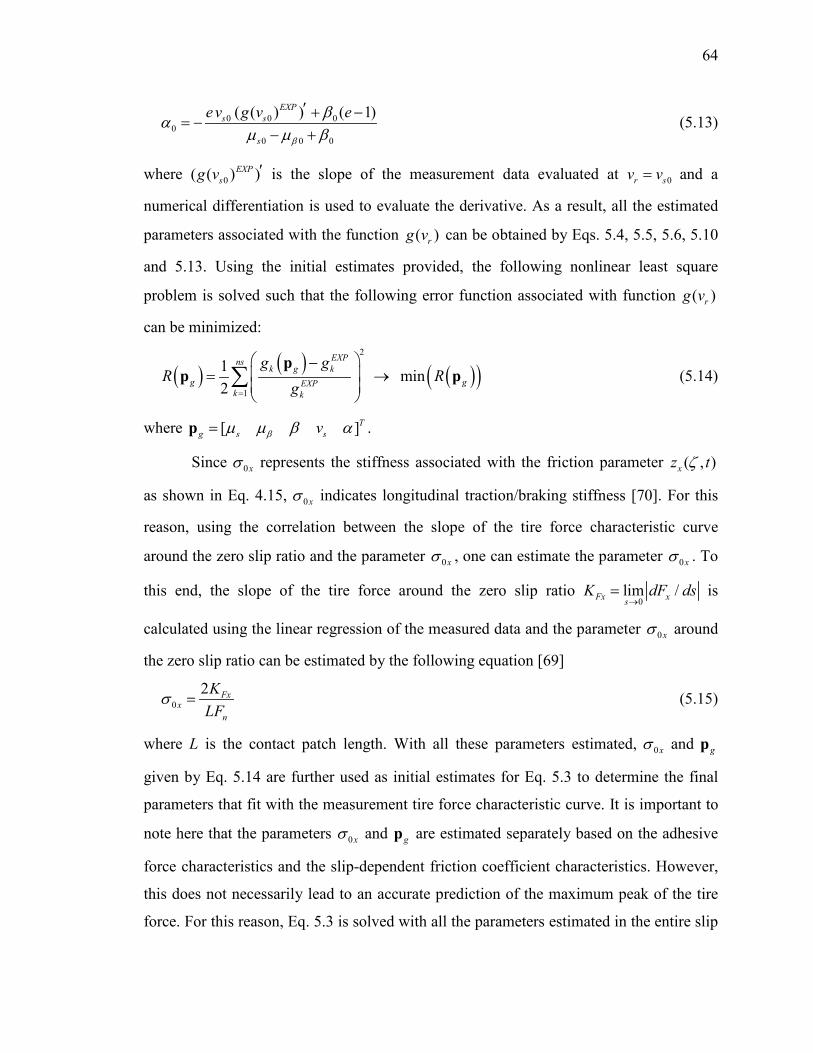
64

0 0 00

0 0 0

( ( ) ) ( 1)EXPs s

s

e v g v e

β

βαµ µ β

′ + −= −

− + (5.13)

where 0( ( ) )EXPsg v ′ is the slope of the measurement data evaluated at 0r sv v= and a

numerical differentiation is used to evaluate the derivative. As a result, all the estimated

parameters associated with the function ( )rg v can be obtained by Eqs. 5.4, 5.5, 5.6, 5.10

and 5.13. Using the initial estimates provided, the following nonlinear least square

problem is solved such that the following error function associated with function ( )rg v

can be minimized:

( ) ( ) ( )( )2

1

1 min2

EXPnsk g k

g gEXPk k

g gR R

g=

− = →

∑p

p p (5.14)

where [ ]Tg s svβµ µ β α=p .

Since 0xσ represents the stiffness associated with the friction parameter ( , )xz tζ

as shown in Eq. 4.15, 0xσ indicates longitudinal traction/braking stiffness [70]. For this

reason, using the correlation between the slope of the tire force characteristic curve

around the zero slip ratio and the parameter 0xσ , one can estimate the parameter 0xσ . To

this end, the slope of the tire force around the zero slip ratio 0

lim /Fx xsK dF ds

→= is

calculated using the linear regression of the measured data and the parameter 0xσ around

the zero slip ratio can be estimated by the following equation [69]

02 Fx

xn

KLF

σ = (5.15)

where L is the contact patch length. With all these parameters estimated, 0xσ and gp

given by Eq. 5.14 are further used as initial estimates for Eq. 5.3 to determine the final

parameters that fit with the measurement tire force characteristic curve. It is important to

note here that the parameters 0xσ and gp are estimated separately based on the adhesive

force characteristics and the slip-dependent friction coefficient characteristics. However,

this does not necessarily lead to an accurate prediction of the maximum peak of the tire

force. For this reason, Eq. 5.3 is solved with all the parameters estimated in the entire slip

65

range such that the maximum peak also agrees with the measurement data. In the same

way, the rest of unknown LuGre parameter 0 yσ which represents the cornering stiffness

is determined as

0

2 Fyy

n

KLF

σ = (5.16)

where the slope of the cornering force around the zero slip ratio 0

lim /Fy ysK dF ds

→= is

calculated using the linear regression of the measured data. Using the procedure proposed

in this chapter, all the LuGre parameters can be systematically estimated by exploiting

important mathematical features of the functions used in the LuGre tire friction model

and correlating them to the measured data. Furthermore, providing proper initial

estimates improves the numerical convergence of iterative solution procedures for the

nonlinear least square problem.

5.3 Parameter Identification Results of LuGre Tire Friction Model

5.3.1 Pure Slip

The measurement data of a tire for passenger cars as previously shown in Fig. 4.5

on a wet road condition is used to demonstrate the use of the parameter identification

procedure proposed in this study. The slip-dependent friction coefficient (i.e., tangential

force coefficient) is shown as a function of the slip velocity in Fig. 5.2, while the

longitudinal tire force is shown as a function of slip ratio in Fig. 5.3. The nonlinear least

square problems given by Eqs. 5.3 and 5.14 are solved by lsqnonlin function in

MATLABTM. In these figures, numerical results obtained using the original function

( )rg v given by Eq. 4.18 (i.e., 0β = in Eq. 4.23) and the proposed one given by Eq. 4.23

are compared. It is observed from these figures that use of the modified g-function leads

to good agreement with the one obtained by measurement. In the use of the original g-

function, noticeable difference from the measurement data is exhibited. Since the change

in the tangential force coefficient in the entire slip velocity range needs to be described

by an exponential function, the tangential force coefficient that linearly decays with the

slip velocity cannot be accurately described with the original function. As a result, the

model does not agree well with the measurement data in both small and large slip

66

velocity regimes since the overall errors in the entire slip velocity range are minimized in

the optimization process. Furthermore, it is observed from Fig. 5.3 that use of the original

g-function also leads to noticeable difference in the maximum peak of the tire force,

which leads to less accurate prediction of the traction and braking performance of tires.

On the other hand, using the modified g-function along with the parameter estimation

procedure for LuGre tire friction model, the model curve is well fitted to the measured

tire force characteristic curve.

In order to demonstrate the use of the proposed parameter identification procedure

for LuGre tire friction model with the modified g-function for a wide variety of loading

and forward speed conditions, friction characteristic curves of a tread rubber are

measured in a wet road condition and used for demonstrating the accuracy of the

proposed parameter identification procedure. As shown in Fig. 5.4, a tread rubber is

glued on a small rigid wheel and the friction characteristics of a tread rubber are

measured by changing the slip ratio. This testing allows to measure the pure tangential

Figure 5.2 Slip-dependent friction coefficient modeled by exiting and

modified ( )rg v -function

67

force characteristics for the tread rubber under consideration. The wheel is pressed on a

drum and the slip ratio is quasi-statically changed by controlling the brake torque of the

wheel. The outside diameter of the wheel is 70 mm and the forward velocities are 20

km/h (5.6 m/s), 30 km/h (8.3 m/s) and 40 km/h (11.1 m/s), while the vertical loads are

changed to 4 kgf (39.2 N), 5 kgf (49.1 N) and 6 kgf (58.9 N). The tangential force

coefficients in different wheel load conditions are shown in Figs. 5.5, 5.6 and 5.7. In each

figure, results obtained for different forward velocities are presented. It is observed from

Figure 5.3 Longitudinal tire force with exiting and modified ( )rg v -function

Figure 5.4 Friction testing of tread rubber

68

these figures that the linear decay in the tangential force in the large slip range is

exhibited due to the wet road condition and the tangential forces are well described using

the LuGre tire friction model with model parameters identified regardless of the load and

speed condition.

Figure 5.5 Tangential force coefficients for 4 kgf


69


5.3.2 Combined Slip

The longitudinal and lateral tire forces are presented for slip angles of 1, 3, 5 and

7 degrees and compared with those obtained by the tire test in Fig. 5.8, showing good

agreement with the tire test results. It is important to notice here that tire force

characteristics differ in traction ( xF− ) and braking ( xF+ ) in the test result, while

numerical results in this figure are obtained using parameters identified for braking

conditions. For the slip angle of 1 degree, the longitudinal and cornering tangential force

coefficients under combined slips (i.e., longitudinal and lateral slips occur

simultaneously) are compared with the test results in Fig. 5.9 for vertical load of 4 kN.

The longitudinal and lateral tire forces characteristics are well predicted using the LuGre

tire friction model with the parameters identified.

70

Figure 5.8 Tire force characteristics under combined slip condition

Figure 5.9 Tangential force coefficient under combined slip condition

71

5.4 Tire Dynamics Simulation

5.4.1 Structural Tire Characteristics and Validation

The tire considered in the numerical example is 215/45R17. The air pressure of

220 kPa is considered by distributed pressure loads applied normal to the inner surface of

the tire. The penalty approach is used to define the normal contact forces in the contact

patch. The load-deflection curve is used to validate fundamental structural properties of

tires. The lateral and vertical deflections of the tire model shown in Fig. 5.10 are

compared with the test results in Figs. 5.11 and 5.12. It is observed from these figures

that the lateral and vertical tire deflections are in good agreement with test results for the

various wheel loads. Furthermore, the lengths of the contact patch in the longitudinal and

lateral axes also agree well with those of the test results as shown in Fig. 5.13 and 5.14.

The two-dimensional normal contact pressure distribution defined along the longitudinal

and lateral axes of the contact patch coordinate system are also compared with those of

the test data for the vertical load of 4 kN in Figs. 5.15 and 5.16.

Figure 5.10 Deformed shape of tire cross section

72

Figure 5.11 Lateral deflection of tire for various wheel loads

Figure 5.12 Vertical deflection of tire for various wheel loads

73

Figure 5.13 Longitudinal contact patch length for various wheel loads

Figure 5.14 Lateral contact patch length for various wheel loads

74

Figure 5.15 Normal contact pressure distribution in the longitudinal direction

Figure 5.16 Normal contact pressure distribution in the lateral direction

75

In Fig. 5.17, the contour plot of the normal contact pressure is presented considering the

tread patter of tire as shown in Fig. 5.18 for a static wheel load of 3 kN. Furthermore, the

normal contact pressure distribution is compared with high-fidelity LS-DYNA FE tire

model validated and used in tire design by a tire manufacture in Fig. 5.18. It is observed

from this figure that a good agreement is obtained between both models and effect of the

tread pattern is captured using the tire model developed in this study.

Figure 5.17 Normal contact pressure distribution considering tread pattern

76

Figure 5.18 Comparison of normal contact pressure distribution

with LS-DYNA FE tire model

To validate the vibration characteristics of the tire model, natural frequencies and

associated mode shapes are identified by the experimental modal analysis in the free

boundary condition and then the first three in-plane and out-of-plane elastic deformation

modes are compared with those obtained by the tire model developed in this study as

shown in Fig. 5.19. It is observed from this figure that good agreements are obtained for

both in-plane and out-of-plane natural frequencies.

77

Figure 5.19 In-plane and out-of-plane natural frequencies

5.4.2 Transient Braking Simulation

To demonstrate the shear contact stresses under hard braking maneuvers using the

flexible tire model with the distributed parameter LuGre tire friction model, the transient

braking analysis is carried out. The constant traveling velocity of 22.6 m/s is prescribed

and then external braking torque is applied to the rigid rim to completely lock the rotation

of the rigid rim. The circumferential velocity and braking force predicted by the proposed

tire model is presented in Fig. 5.20. As shown in this figure, the braking force builds up

right after the braking torque is applied to the rim at t = 0.1 s and increases until it

exceeds the maximum peak around t = 0.4 s. The braking force then drops when it goes

beyond the peak, which is a typical behavior of the braking force of tires. The tire rim is

finally locked completely around t = 0.47 s and the tire is skidding at the prescribed

78

constant speed of 22.6 m/s. In this simulation, HHT time integration scheme is used with

variable step size control. CPU time for this hard braking simulation was 8175 seconds

using single processor (Intel Core i7-3770, 3.4GHz). The shear contact stresses acting on

the tire in this transient braking scenario are shown in Fig. 5.21 at various instants of time.

In each figure, the longitudinal (braking) components of the mean shear contact stresses

are also plotted along the longitudinal axis of the contact patch. In the steady state rolling,

the shear contact stresses around the center of the contact patch is small, while large

contact stresses occur around the shoulder of the tire due to larger slips. The similar shear

contact stress distribution is obtained using the detailed finite element tire model as

presented in the literature [8] at the steady state rolling condition. After the braking toque

is applied to the rim, the trailing contact zone starts sliding and the shear contact stresses

increase, while contact stresses in the leading region are small since it is still in adhesion.

For example, as shown in the result at t = 0.22 s, the shear contact stress increases

linearly from the leading edge until it reaches the friction bound, and then sliding region

appears. Finally, all the contact regions become sliding zone and the shear contact stress

arrows get aligned, pointing to the direction opposite to the traveling direction (i.e.,

braking direction). It is also important to notice here that the shear contact stress at this

Figure 5.20 Transient braking analysis results

79

state (t = 0.48 s) is smaller than that at t = 0.39 s, at which the maximum peak of the

braking force occurs. Furthermore, it is observed that the contact patch is pulled

backward due to the tire deformation after the braking torque is applied.

5.4.3 Antilock Braking System (ABS) Simulation

To further discuss the simulation capability of the flexible tire model proposed in

this study, an antilock braking system (ABS) control is considered. Using the ABS

control, the braking torque is controlled to prevent a tire from being locked completely

and the tire force around the peak friction can be generated during braking to minimize

Figure 5.21 Shear contact stress distribution in the transient braking analysis

80

the braking distance. While there are various ABS control algorithms proposed in the past,

a simplified slip-based on/off control algorithm is used in this study to focus on the tire

model simulation capability under the severe braking scenario. In the numerical example,

it is assumed that the braking torque T is defined as follows:

1 1 21

1 1 2

1 1 11

1 1 1

If ( ) ( )

( ) if ( )( )

( ) if ( )If ( ) ( )

( ) if ( )( )

( ) if ( )

n up n

up n nn

down n n

n down n

down n nn

up n n

T t T t

T t s t sT t

T t s t sT t T t

T t s t sT t

T t s t s

+ ++

+ +

+ ++

+ +

=

<= ≥

=

>= ≤

(5.17)

where s1=0.08 and s2=0.14 such that the braking force is kept in that target slip range

during braking and the target slip range is selected around the peak friction in the µ-slip

curve. In the preceding equation, ( )upT t and ( )downT t are assumed to be a linear function

having the positive and negative slopes, respectively. In Fig. 5.22, the slip ratio, the

tangential force coefficient, and braking torque under the ABS control are shown as a

function of time. It is observed from this figure that the slip ratio lies in the target range

( 0.08 0.14s≤ ≤ ) during the braking, while the tire completely locks if the ABS control is

off (i.e., the slip ratio becomes one), as shown in the dotted line. Furthermore, the braking

torque changes up and down according to the change in the slip ratio by following the

ABS control algorithm defined by Eq. 5.17. Furthermore, the change in the tangential

force coefficient follows the change in the braking torque.

The forward velocity at the rim center and the circumferential velocity of the rim

are presented in Fig. 5.23 for cases with and without ABS control. As shown in this figure,

rotation of the rim is locked at t = 0.47 s if ABS is off and the tire continues skidding

until it stops as presented in this figure. On the other hand, the tangential velocity in the

case of ABS control decreases almost linearly to zero, indicating that a nearly constant

braking force is ideally generated to stop the tire. This results in a shorter braking

distance as demonstrated in Fig. 5.23. It is important to notice here that the

circumferential velocity of the tire changes very frequently due the frequent switching of

braking torque based on the ABS control. That is, as observed in Fig. 5.23, when the

deviation of the circumferential velocity from the forward velocity gets larger due to the

81

increase in slip, the braking torque decreases until the circumferential velocity gets closer

to the forward velocity. This process is repeated in order for the slip ratio to always lie in

the target slip range. The µ-slip curve obtained using this time-domain ABS analysis is

presented in Fig. 5.24. It is clearly observed from this figure that the tangential force

coefficient (µ) lies in the target slip range if ABS control is used and it changes back and

forth to keep generating the peak braking force during braking. If the ABS control is off,

the tangential force coefficient sharply drops beyond the peak point and continue to

decreases to the kinetic friction as discussed in the previous braking simulation scenario.

It is also important to notice here that the tangential force coefficient gradually increases

during the operation of the ABS control. Since the coefficient of friction increases as an

Figure 5.22 Simplified slip-based ABS control algorithm

82

increases in the slip velocity, the tangential force coefficient increase as the tire speed

decreases. It is known that this friction behavior is observed in braking tests, and this

typical friction behavior is captured in this physics-based tire dynamics simulation. As it

is demonstrated in this ABS transient tire dynamics simulation that is challenging for

existing finite element based tire models, the flexible tire model developed in this study is

computationally robust and is capable of predicting the transient tire dynamics behavior.

Figure 5.23 Forward and circumferential velocities of tire with and without ABS control

Figure 5.24 µ-slip curve with and without ABS control

83

5.4.4 Transient Cornering Simulation

To evaluate the transient cornering force characteristics, frequency response of a

cornering force to an oscillatory steering input is evaluated. The cornering force

responses for different steering (slip) angle path frequencies are shown in Fig. 5.25. The

path frequency is defined by a frequency of the slip angle input divided by the forward

velocity and its unit is cycle/m. The steering (slip) angle is assumed to be 1 degree in

both directions. It is observed from this figure that the cornering force amplitude

decreases and the phase lag increases as the path frequency increases. To validate the

cornering force response, the cornering force gain and phase lag are presented in Fig.

Figure 5.25 Cornering force responses to oscillatory steering input

84

5.26 as a function of the input path frequency. It is observed from these figures that very

good agreements are obtained in the cornering force gain and the phase lag for a wide

range of path frequency using the physics-based flexible tire model developed in this

study.

Figure 5.26 Cornering force responses and phase lag

85

In the last example, a hard cornering maneuver is considered as shown in Fig.

5.27, where the slip angle changes from zero to one degree in 0.2 seconds. CPU time for

this transient cornering simulation was 8427 seconds using single processor (Intel Core

i7-3770, 3.4GHz). It is observed from the shear contact stresses shown in Fig. 5.28 that

the shear contact stresses are pointing to the cornering direction (right to the direction of

travel) as the slip angle increases. Furthermore, the shear contact stresses increase on the

right side of the contact patch due to the increase in the normal contact pressure in this

region for the steering input.

Figure 5.27 Transient cornering analysis results

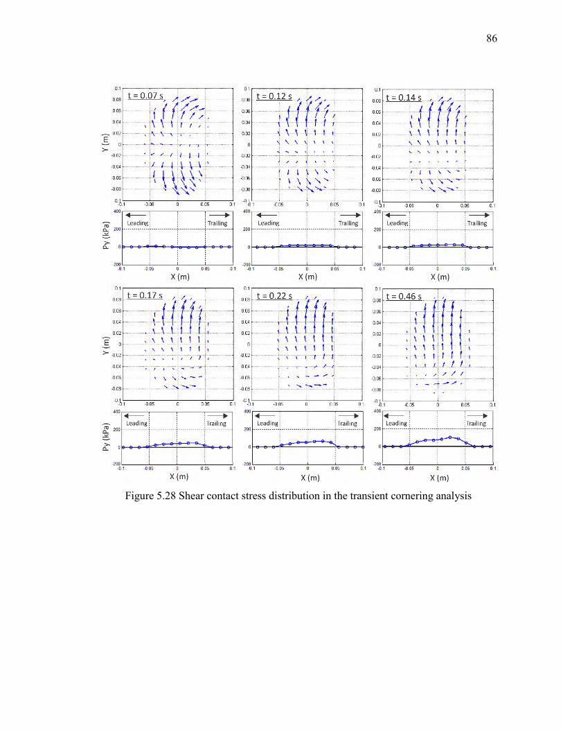
86

Figure 5.28 Shear contact stress distribution in the transient cornering analysis

87

CHAPTER 6

CONTINUUM BASED SOIL MODEL AND VALIDATION

6.1 Introduction

In this chapter, a continuum based finite element soil model is developed for use

in off-road mobility simulation using the physics-based flexible tire model discussed in

previous chapters. For modeling deformable soil, a 9-node brick element is proposed by

introducing the additional curvature coordinates at the center node to the standard tri-

linear 8-node brick element. It is shown that the 9-node brick element does not suffer

from the element lockings exhibited in the standard 8-node tri-linear brick element

caused by the incapability of describing the linear stress and strain distribution over the

volume, thereby making the implementation of the plasticity material model

straightforward for soil model. The capped Drucker-Prager failure material model based

on the multiplicative finite strain plasticity theory is applied to the 9-node brick element

to develop the large deformable continuum soil model for off-road mobility simulation.

Using the triaxial soil test data, parameters of the capped Drucker-Prager model are

identified and used for validating the soil behavior under the triaxial test condition.

6.2 Brick Elements for Modeling Continuum Soil

6.2.1 Tri-linear 8-Node Brick Element (Brick24)

The global position vector of the standard 8-node 24-DOF brick element is

defined using the tri-linear polynomial as

0 1 2 3 4 5 6 7r a a a a a a a aξ η ζ ξη ξζ ηζ ξηζ= + + + + + + + (6.1)

Each corner node has three degrees of freedom describing the global position at the node

as shown in Fig. 6.1, thus only C0 continuity is ensured at nodal points. Using the

preceding polynomial, the global position vector is defined as

( , , ) ( , , )i i i i i i i i iξ η ζ ξ η ζ=r S e (6.2)

where ie is the element nodal coordinate vector and each nodal coordinate at node k

( 1, ,8k = ) include three position coordinates only as ik ik=e r . The matrix iS is the

shape function matrix given by

88

Figure 6.1 Kinematics of 8-node tri-linear brick element

(Brick24)

1 2 3 4 5 6 7 8i i i i i i i i iS S S S S S S S = S I I I I I I I I (6.3)

and

1 2

3 4

5 6

7 8

1 1(1 )(1 )(1 ), (1 )(1 )(1 )8 81 1(1 )(1 )(1 ), (1 )(1 )(1 )8 81 1(1 )(1 )(1 ), (1 )(1 )(1 )8 81 1(1 )(1 )(1 ), (1 )(1 )(1 )8 8

i i i i i i i i

i i i i i i i i

i i i i i i i i

i i i i i i i i

S S

S S

S S

S S

ξ η ζ ξ η ζ

ξ η ζ ξ η ζ

ξ η ζ ξ η ζ

ξ η ζ ξ η ζ

= − − − = + − −

= + + − = − + −

= − − + = + − +

= + + + = − + +

(6.4)

The elastic forces of the brick element are evaluated using the continuum

mechanics approach and the Green-Lagrange strain tensor at an arbitrary material point in

element i is defined as follows:

( )1 ( )2

i i T i= −E F F I (6.5)

where iF is the global position vector gradient tensor defined by 1

1( )i i i

i i ii i i

−

− ∂ ∂ ∂= = = ∂ ∂ ∂

r r XF J JX x x

(6.6)

89

In the preceding equation, i i i= ∂ ∂J r x and i i i= ∂ ∂J X x , where the vector iX

represents the global position vector of element i at an arbitrary reference configuration.

Strain tensor iE can be re-expressed in a vector form as

( )i i T i−=ε T ε (6.7)

where the vectors of the Green-Lagrange strains and covariant strains are, respectively,

given as


and


The transformation matrix iT in Eq. 6.7 is be expressed as 2 2 2

11 12 11 12 13 11 13 12 132 2 2

21 22 21 22 23 21 23 22 23

11 21 12 22 11 22 12 21 13 23 11 23 13 21 12 23 13 222 2

31 32 31 32 3

( ) ( ) 2 ( ) 2 2( ) ( ) 2 ( ) 2 2

( ) ( ) 2 (

i i i i i i i i i

i i i i i i i i i

i i i i i i i i i i i i i i i i i ii

i i i i

J J J J J J J J JJ J J J J J J J J

J J J J J J J J J J J J J J J J J JJ J J J J

+ + +=T 2

3 31 33 32 33

11 31 12 32 11 32 12 31 13 33 11 33 13 31 12 33 13 32

21 31 22 32 21 32 22 31 23 33 21 33 23 31 22 33 23 32

) 2 2i i i i i



J J J JJ J J J J J J J J J J J J J J J J JJ J J J J J J J J J J J J J J J J J

+ + +

+ + +

(6.10)

and iabJ is the element in the a-th column and b-th row of matrix iJ which is constant in

time. The generalized elastic forces can then be obtained using the virtual work as

follows:

00i

Ti ii ik i iV

W dV ∂ ∂

= − ∂ ∂ ∫

εQe ε

(6.11)

where W is an elastic energy function and 0idV is the infinitesimal volume at the

reference configuration of element i. It is important to notice here that, because of the tri-

linear polynomial utilized, the strains are constant over the volume, causing the element

lockings. To alleviate the locking, the 9-parameter enhanced assumed strain (EAS) are

introduced as follows: c EAS= +ε ε ε (6.12)

where cε indicates the compatible strain vector and one has

( ) ( )EAS =ε ξ G ξ α (6.13)

90

In the preceding equation, α is a vector of internal parameters introduced to define the

enhanced strain field of the brick element and the matrix ( )G ξ can be defined as [54,73]

0 T0( ) ( )

( )−=

JG ξ T N ξ

J ξ (6.14)

where ( )J ξ and 0J are the global position vector gradient matrices at the reference

configuration evaluated at the Gaussian integration point ξ and at the center of element

( =ξ 0 ), respectively. ξ is a vector of the element coordinates in the parametric domain

and 0T is the constant transformation matrix evaluated at the center of element. The

matrix ( )N ξ defines polynomials for the enhancement of the strain field in the parametric

domain as follows:

0 0 0 0 0 0 0 00 0 0 0 0 0 0 00 0 0 0 0 0 0

( )0 0 0 0 0 0 0 00 0 0 0 0 0 00 0 0 0 0 0 0

ξη

ξ ηζ

ξ ζη ζ

=

N ξ (6.15)

6.2.2 Tri-cubic 8-Node ANCF Brick Element (Brick96)

The concept of the fully parameterized beam and shell elements of the absolute

nodal coordinate formulation utilizing the three sets of the global position vector

gradients along the element x, y and z coordinates can be extended to the 8-node brick

element [74]. In other words, the three sets of gradient vector coordinates, / x∂ ∂r ,

/ y∂ ∂r and / z∂ ∂r are introduced to the nodal coordinates of each node as shown in Fig.

6.2, thus C1 continuity is automatically ensured due to the use of position vector gradient

at all the nodal points. This leads to the 8-node 96-DOF brick element using the

following polynomial: 2 2 2

0 1 2 3 4 5 6 7 8 9 102 2 2 2 2 2 3 3 3

11 12 13 14 15 16 17 18 193 3 3 3 3 3 2 2

20 21 22 23 24 25 26 273 3 2

28 29 30 31

r a a a a a a a a a a aa a a a a a a a aa a a a a a a aa a a a

ξ η ζ ξη ξζ ηζ ξηζ ξ η ζ

ξη ξ η ηζ η ζ ζξ ξζ ξ η ζ

ξ η ξη ζ η η ζ ζ ξ ξ ζ ξ ηζ ξη ζ

ξ ηζ ξη ζ ζ ηξ ζ

= + + + + + + + + + +

+ + + + + + + + +

+ + + + + + + +

+ + + + 3ηξ

(6.16)

Using the preceding polynomial, the global position vector is defined as

91

Figure 6.2 Kinematics of 8-node tri-cubic ANCF brick

element (Brick96)


where ie is the element nodal coordinate vector and each nodal coordinate at node k

( 1, ,8k = ) is defined as

[( ) ( ) ( ) ( ) ]ik ik T ik i T ik i T ik i T Tx y z= ∂ ∂ ∂ ∂ ∂ ∂e r r r r (6.18)

The shape function matrix iS in Eq. 6.17 is given by

1 2 31 32i i i i iS S S S = S I I I I (6.19)

where

92

( )( )( )( )

( ) ( )( )( )

( ) ( )( )( )

( ) ( )( )( )

( )( )( )( )

( ) ( )( )( )

( ) ( )( )( )

( ) ( )( )( )

( )( )

2 2 21

22

23

24

2 2 25

26

27

28

9

1 1 1 1 2161 1 1 1 1321 1 1 1 1321 1 1 1 132

1 1 1 1 216

1 1 1 1 132

1 1 1 1 1321 1 1 1 1321 1 1

16

S

S a

S b

S c

S

S a

S b

S c

S

ξ η ζ ξ η ζ ξ η ζ

ξ ξ η ζ

η ξ η ζ

ζ ξ η ζ


ξ ξ η ζ

η ξ η ζ

ζ ξ η ζ

ξ η ζ

= − − − + + + + + −

= − + − −

= − − + −

= − − − +

= − + − − + + − + + −

= + − − −

= − − + + −

= − − + − +

= − − + −( )( )

( ) ( )( )( )

( ) ( )( )( )

( ) ( )( )( )

( )( )( )( )

( ) ( )( )( )

( ) ( )( )( )

( ) ( )( )( )

2 2 2

210

211

212

2 2 213

214

215

216

1 2

1 1 1 1 132

1 1 1 1 132

1 1 1 1 132

1 1 1 1 216

1 1 1 1 1321 1 1 1 132

1 1 1 1 132

S a

S b

S c

S

S a

S b

S c

ξ η ζ ξ η ζ

ξ ξ η ζ

η ξ η ζ

ζ ξ η ζ


ξ ξ η ζ

η ξ η ζ

ζ ξ η ζ

+ + + − + −

= − − + + −

= + − − −

= − − − + +

= + + − + + − − + −

= − + − + −

= − + + − −

= − + + +

(6.20a)

93

( )( )( )( )

( ) ( )( )( )

( ) ( )( )( )

( ) ( )( )( )

( )( )( )( )

( ) ( )( )( )

( ) ( )( )( )

( ) ( )( )( )

2 2 217

218

219

220

2 2 221

222

223

224

25

1 1 1 1 2161 1 1 1 1321 1 1 1 132

1 1 1 1 1321 1 1 1 2

161 1 1 1 132

1 1 1 1 132

1 1 1 1 132

1

S

S a

S b

S c

S

S a

S b

S c

S


ξ ξ η ζ

η ξ η ζ

ζ ξ η ζ


ξ ξ η ζ

η ξ η ζ

ζ ξ η ζ

= − − − + + + + + − −

= − − + − +

= − − − + +

= + − − −

= + − + + + − + − −

= − + − − +

= − + + +

= − + + − −

= ( )( )( )( )

( ) ( )( )( )

( ) ( )( )( )

( ) ( )( )( )

( )( )( )( )

( ) ( )( )( )

( ) ( )( )( )

( ) ( )( )( )

2 2 2

226

227

228

2 2 229

230

231

232

1 1 1 2161 1 1 1 132

1 1 1 1 1321 1 1 1 1321 1 1 1 2

161 1 1 1 1321 1 1 1 1321 1 1 1 132

S a

S b

S c

S

S a

S b

S c


ξ ξ η ζ

η ξ η ζ

ζ ξ η ζ


ξ ξ η ζ

η ξ η ζ

ζ ξ η ζ

− + + + + + − − −

= − + + +

= − + − − +

= − + − + −

= − + + + + + − − − −

= + − + +

= + + − +

= + + + −

(6.20b)

where 2( 2) /x a aξ = − , 2( 2) /y b bη = − , and 2( 2) /z c cζ = − . The generalized

elastic forces can then be obtained using the virtual work as follows:

00i

Ti ii ik i iV

W dV ∂ ∂

= − ∂ ∂ ∫

εQe ε

(6.21)

94


reference configuration of element i.

6.2.3 9-Node Brick Element with Curvature Coordinates (Brick33)

Despite the C1 continuity ensured for the 96-DOF ANCF brick element (Brick96),

the element has large degrees of freedom, thereby making the element force calculation

computationally intensive. On the other hand, the standard 8-node 24-DOF brick element

(Brick24) requires use of locking remedies such as the enhanced assumed strain method

to describe the linear stress and strain distribution over the volume. In other words, nine

internal parameters are introduced to improve the compatible strain field to describe the

accurate stress distribution while keeping the same number of degrees of freedom. This,

however, requires additional iterative solution procedure to determine the internal EAS

parameters at element level at every time step, and use of plasticity material model for

modeling soil makes the solution procedure more computationally intensive. For this

reason, in this study, the 8-node 24DOF brick element is extended to capture the

quadratic terms in ξ, η and ζ, and the polynomial of the global position vector is re-

defined as follows: 2 2 2

0 1 2 3 4 5 6 7 8 9 10r a a a a a a a a a a aξ η ζ ξη ξζ ηζ ξηζ ξ η ζ= + + + + + + + + + + (6.22)

To consider the quadric terms in the preceding polynomial, an additional node defining

the second derivative of the position coordinate 9 2 9 2 2 9 2 2 9 2[ ( ) ( ) ( ) ]i i i i i i i Tx y z= ∂ ∂ ∂ ∂ ∂ ∂e r r r is introduced to the center of the brick

element as shown in Fig. 6.3. Accordingly, the global position vector is defined as


where ie is the element nodal coordinate vector and each nodal coordinate at node k (k =

1 to 9) is defined as

9 2 9 2 2 9 2 2 9 2

( ) , 1, ,8[ ( ) ( ) ( ) ]

ik ik T

i i i i i i i T

kx y z

= =

= ∂ ∂ ∂ ∂ ∂ ∂

e re r r r

(6.24)

The shape function matrix iS in Eq. 6.23 is given by

1 2 3 4 5 6 7 8 9 10 11S S S S S S S S S S S = S I I I I I I I I I I I (6.25)

where

95

Figure 6.3 Kinematics of 9-node brick element with

curvature coordinates (Brick33)

1 2

3 4

5 6

7 8

9

1 1(1 )(1 )(1 ), (1 )(1 )(1 )8 81 1(1 )(1 )(1 ), (1 )(1 )(1 )8 81 1(1 )(1 )(1 ), (1 )(1 )(1 )8 81 1(1 )(1 )(1 ), (1 )(1 )(1 )8 8

i i i i i i i i

i i i i i i i i

i i i i i i i i

i i i i i i i i

i

S S

S S

S S

S S

S

ξ η ζ ξ η ζ

ξ η ζ ξ η ζ

ξ η ζ ξ η ζ

ξ η ζ ξ η ζ

= − − − = + − −

= + + − = − + −

= − − + = + − +

= + + + = − + +

= 2 2 210 11

1 1 1(( ) 1), (( ) 1), (( ) 1)2 2 2

i i i i iS Sξ η ζ

− = − = −

(6.26)

It is important to notice here that the introduction of the quadratic terms allows for

describing the linear distribution of the strain field, thus the locking exhibited in 8-node

24-DOF brick element can be alleviated without introducing the enhanced assumed strain

approach. The similar approach such as a bubble function to add incompatible modes is

employed for brick elements in literature [75]. This makes the implementation of the

complex plasticity failure models such as Drucker-Prager yield criterion for deformable

soil straightforward. The generalized elastic forces can then be obtained using the virtual

work as follows:

00i

Ti ii ik i iV

W dV ∂ ∂

= − ∂ ∂ ∫

εQe ε

(6.27)

96


reference configuration of element i.

6.2.4 Comparison of Brick Element Performance

To demonstrate the accuracy and computational efficiency of the three brick

elements introduced in this section, numerical results of nonlinear static and dynamic

analysis are presented. In the first example, a cantilever plate subjected to a point load is

considered as shown in Fig. 6.4. The length, width and thickness of the plate are assumed

to be 1.0 m, 1.0 m and 0.01 m. Young’s modulus and Poisson’s ratio 82.1 10× Pa and 0.3,

respectively. The vertical point force zF defined at the corner node is assumed to be 50 N.

The rate of convergence of the numerical solution obtained using the three different brick

elements are presented in Table 6.1 and Fig. 6.5. In those results, the reference solution is

obtained by ANSYS Solid185 element with 100 100 1× × elements. The result of ANSYS

Solid185 that is the tri-linear brick element with locking remedies is also presented in Fig.

6.5 for comparison, indicating the linear rate of convergence. It is observed from Fig. 6.5

Figure 6.4 Deformed shape of a cantilevered plate subjected to a tip force

97

that the tri-linear 8-node brick element ensures the linear rate of convergence if the

enhanced assumed strain is used (Brick24 w/ EAS), while 9-node brick element archives

the linear rate of convergence without introducing any locking remedies (Brick33 w/o

EAS). While the nine internal parameters are introduced to describe the linear

distribution of stresses and strains over the volume in Brick24, additional nine curvature

coordinates for 2 2x∂ ∂r , 2 2y∂ ∂r , and 2 2z∂ ∂r are introduced to Brick33 for defining

the quadratic displacement field, allowing for the linear distribution of stresses and

strains over the volume. In other words, both brick elements are essentially equivalent in

a sense that the linear strain distribution is enabled by the nine internal enhanced assumed

strain parameters in Brick24 and by the nine additional curvature nodal coordinates in

Brick33. It is also important to notice here that the tri-cubic ANCF brick element

(Brick96) does not ensure the ideal cubic rate of convergence of solutions, indicating that

element lockings occur, despite the fact that higher order polynomials and the larger

degrees of freedom are introduced per element.

In the second numerical example, a nonlinear dynamics problem is considered. A

flat plate is pinned to the ground at one of the corners as shown in Fig. 6.6 and numerical

solutions of the flexible plate pendulum under the effect of gravity is discussed. The

length, width and thickness of the plate are assumed to be 1.0 m, 1.0 m and 0.01 m. HHT

time integrator is used with variable step size. The Young’s modulus and Poisson’s ratio

are assumed to be 72.1 10× Pa and 0.3 respectively. The material density is assumed to be

Table 6.1. Static deflection of cantilevered plate subjected point load (m)

Brick24 Brick24 Brick33 Brick96 ANSYS

(SOLID185)

w/o EAS w/ EAS w/o EAS w/o EAS w/ EAS

2x2x1 -0.00402 -0.21767 -0.21407 -0.59117 -0.18381 4x4x1 -0.01604 -0.46600 -0.44784 -0.64519 -0.40824 8x8x1 -0.05705 -0.61744 -0.61124 -0.65331 -0.60228

16x16x1 -0.13902 -0.64965 -0.64902 -0.65410 -0.64769 32x32x1 -0.29807 -0.65360 -0.65356 -0.65436 -0.65356

100x100x1 -0.65426

98

1,000 kg/m3. Large deformation is observed as shown in Fig. 6.6. The global vertical

positions at the tip of the plate are presented in Figs. 6.7 to 6.9 for the three brick

elements (Brick24 w/ EAS, Brick33, and Brick96) under consideration for different mesh

sizes. It is important to notice here that the number of Gaussian integration points for

Brick24 and Brick33 is 8 ( 2 2 2× × ), while that of ANCF Brick96 requires at least 27

( 3 3 3× × ) due to the use of higher order polynomials. For the minimum number of

elements that reaches the convergent solutions for the three types of brick elements, the

normalized CPU time is compared in Fig. 6.10. CPU time of Brick33 is used as a

reference and is slightly less than that of Brick24 w/ EAS, however the higher order

ANCF Brick96 element leads to computationally inefficient solutions for the nonlinear

dynamics problem considered in his study. For this reason, in this study, the 9-node brick

element (Brick33) is applied to the modeling of continuum deformable soil for the

tire/soil interaction simulation.

Figure 6.5 Convergence of brick element solutions

99

Figure 6.7 Global Z-position at the tip point (Brick24: 8-node

tri-linear brick element)

Figure 6.6 Deformed shapes

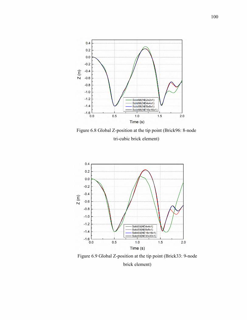
100


tri-cubic brick element)


brick element)

101

Figure 6.10 CPU time to achieve the convergent solutions

6.3 Soil Model Using Multiplicative Plasticity Theory

6.3.1 Finite Strain Plasticity Theory

To model soil behavior undergoing large plastic deformations, the multiplicative

finite strain plasticity theory is utilized in this study. In large deformation problems,

identification of the plastic strain involves more than just kinematic considerations [76]

and elastic and plastic deformations are coupled. Lee and Liu [77] proposed that the

displacement gradient tensor can be decomposed into elastic and plastic components and

the intermediate stress free configuration is introduced such that the plastic state can be

conceptually recovered by an elastic unloading from a current configuration. The

multiplicative plasticity formulation was then applied to finite element computational

framework by Simo [78] using the principle of the plastic maximum dissipation and has

gained acceptance for modeling finite strain plasticity [79-84]. Since the elastic response

can be described by the hyperelasticity constitutive model, this approach naturally

bypasses drawbacks of hypo-plasticity formulation including erroneous dissipated elastic

responses and the possible lack of objectivity of incremental constitutive equations [81-

83]. Furthermore, it is shown that use of the logarithmic (Hencky) strain measure for

102

multiplicative plasticity formulation allows for the use of the classical return mapping

scheme developed for the infinitesimal plasticity model [80].

As shown in Fig. 6.11, the position vector gradient tensor F is decomposed into

the elastic and plastic components as follows [77]: e p=F F F (6.28)

where subscripts e and p indicate the elastic and plastic parts, respectively. To define the

elastic strain, the left Cauchy-Green tensor of the elastic strain eB is defined as 1( ) ( )e e e T p T−= =B F F F C F (6.29)

where pC is the right Cauchy-Green tensor of the plastic strain given as

( )p p T p=C F F (6.30)

from which, the elastic logarithmic strain tensor can be defined using the spectral

decomposition of the left Cauchy-Green tensor eB as 3

1

1 ln( ) ln( )2

e eL i i i

iλ

=

= = ⊗∑ε B e e (6.31)

In the preceding equation, one has 3

2

1( )e

i i ii

λ=

= ⊗∑B e e (6.32)

where iλ ( 1, 2,3i = ) is the i-th eigenvalue of spatial stretch tensor eV defined by the

polar decomposition e e=F V R and the rotation tensor R . The vector ie defines the

/= ∂ ∂F r X

eF

pF

Intermediate stress-free configuration

Current configuration

Reference configuration

Figure 6.11 Multiplicative decomposition of displacement gradient

103

direction of the principal stretch. Using the logarithmic strain measure, Kirchhoff stress

tensor is defined for an isotropic material as

: eL=τ E ε (6.33)

Using the Kirchhoff stress tensor, the generalized elasto-plastic force vector is defined as

[85] T

e VdV∂ = ∂ ∫

DQ τe

(6.34)

where D is the rate of deformation tensor given by

1 ( )2

T= +D L L (6.35)

and L is the velocity gradient tensor as given by 1−=L FF .

6.3.2 Drucker-Prager Failure Model and Return Mapping Algorithm

There are many failure models proposed for modeling soil behavior [18]. Among

others, Drucker-Prager model has been widely used to describe the fundamental soil

behavior for tire/soil interaction simulation. The yield function of Drucker-Prager model

with an assumption of isotropic hardening is given as [79]

2 ( )J p dη ξΦ = + −s (6.36)

where 21( ) :2

J =s s s ; ( )s τ is the deviatoric stress of the Kirchhoff stress tensor defined

by ( ) ( )p= −s τ τ τ I ; and ( )p τ is the hydrostatic pressure (mean effective stress) given by

( ) ( ) 3p tr=τ τ . The parameters η and ξ are defined using the friction angle β as

follows:

1 tan3

η β= and 13

ξ = (6.37)

Furthermore, the cohesion d in Eq. 6.36 is expressed as a function of the equivalent

plastic strain plε , and for the linear hardening case, one has

0pld d Hε= + (6.38)

104

where 0d is the initial cohesion and H is the slope of the plastic hardening. The

Drucker-Prager yield cone is illustrated in Fig. 6.12(a). The incremental plastic strain is

defined as [79] pLδ γ= ∆ε N (6.39)

and the plastic flow vector N is defined by

(a) Drucker-Prager yield surface

(b) Drucker-Prager return mapping process on p-q plane

Figure 6.12 Drucker-Prager failure model

105

2

132 ( )Jη∂Ψ

≡ = +∂

N s Iτ s

(6.40)

where Ψ is the flow potential given by

2 ( )J pηΨ ≡ +s (6.41)

and tan / 3η ϕ= with the dilatancy angle ϕ . In the associative plastic flow, the friction

angle and the dilatancy angle are assumed to be equal, and one has / /= ∂Ψ ∂ = ∂Φ ∂N τ τ .

However, in the non-associative flow rule which is common for soils, the dilatancy angle

used in the flow potential is not equal to the friction angle. The use of non-associated law

can avoid the excessive dilatancy exhibited in the associative rule [79].

To find the plastic strains at every time step, the return mapping algorithm for the

multiplicative finite strain plasticity model is developed. As shown in Fig. 6.12(b), an

elastic trial step is taken first (i.e. 1 0nγ +∆ = ) to check if the plastic loading occurs or not.

To this end, the trial elastic left Cauchy-Green tensor at 1nt t += is evaluated using the

accumulated plastic strains up to the previous time step nt t= as

trial 11 1 1( ) ( )e p T

n n n n−

+ + +=B F C F (6.42)

where the plastic strains are stored using the right Cauchy-Green tensor pnC . Using the

trial elastic left Cauchy-Green tensor, the trial logarithmic elastic strain tensor and

Kirchhoff stress tensor are evaluated using Eqs. 6.31 and 6.33, respectively. The yield

function given by Eq. 6.36 is then evaluated to determine if the Gaussian integration

point under consideration is subjected to plastic loading at the current step. That is, if trial trial

1 1( , ) 0pln n nε+ +Φ <τ , an elastic loading occurs and then update the Kirchhoff stress tensor,

the inverse of the plastic right Cauchy-Green tensor, and the hardening parameter as

follows: trial 1 1

1 1 1 1, ( ) ( ) ,e p p pl pln n n n n nε ε− −

+ + + += = =τ τ C C (6.43)

If trial trial1 1( , ) 0pl

n n nε+ +Φ >τ , the plastic loading occurs, thus the plastic strain tensor is

determined using the return mapping algorithm. In the Drucker-Prager yield criterion, the

stress state lies on either the yield cone surface or the apex of the cone as shown in Fig.

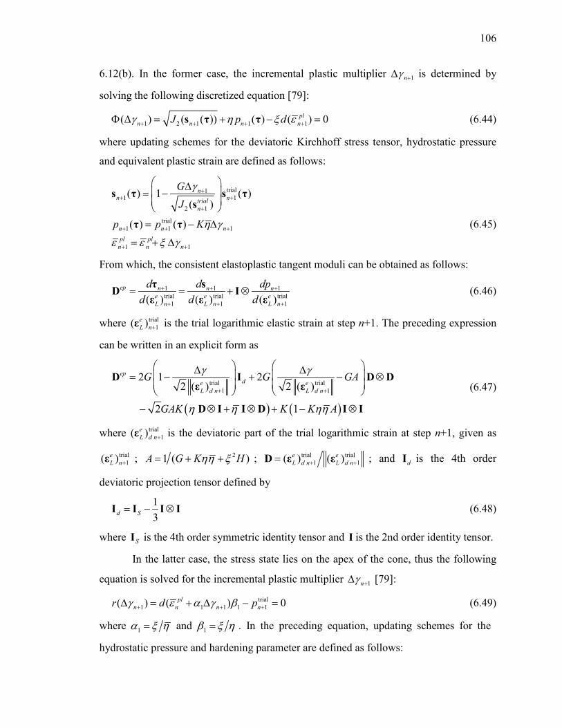
106

6.12(b). In the former case, the incremental plastic multiplier 1nγ +∆ is determined by

solving the following discretized equation [79]:

1 2 1 1 1( ) ( ( )) ( ) ( ) 0pln n n nJ p dγ η ξ ε+ + + +Φ ∆ = + − =s τ τ (6.44)

where updating schemes for the deviatoric Kirchhoff stress tensor, hydrostatic pressure

and equivalent plastic strain are defined as follows:

trial11 1

2 1

trial1 1 1

1 1

( ) 1 ( )( )

( ) ( )

nn ntrial

n

n n npl pl

n n n

GJ

p p K

γ

η γ

ε ε ξ γ

++ +

+

+ + +

+ +

∆ = −

= − ∆

= + ∆

s τ s τs

τ τ (6.45)

From which, the consistent elastoplastic tangent moduli can be obtained as follows:

1 1 1trial trial trial

1 1 1( ) ( ) ( )ep n n n

e e eL n L n L n

d d dpd d d

+ + +

+ + +

= = + ⊗τ sD Iε ε ε

(6.46)

where trial1( )e

L n+ε is the trial logarithmic elastic strain at step n+1. The preceding expression

can be written in an explicit form as

( ) ( )

trial trial1 1

2 1 22 ( ) 2 ( )

2 1

epde e

L d n L d n

G G GA

GAK K K A

γ γ

η η ηη

+ +

∆ ∆ = − + − ⊗

− ⊗ + ⊗ + − ⊗

D I D Dε ε

D I I D I I

(6.47)

where trial1( )e

L d n+ε is the deviatoric part of the trial logarithmic strain at step n+1, given as

trial1( )e

L n+ε ; 21 ( )A G K Hηη ξ= + + ; trial trial1 1( ) ( )e e

L d n L d n+ +=D ε ε ; and dI is the 4th order

deviatoric projection tensor defined by

13d S= − ⊗I I I I (6.48)

where SI is the 4th order symmetric identity tensor and I is the 2nd order identity tensor.

In the latter case, the stress state lies on the apex of the cone, thus the following

equation is solved for the incremental plastic multiplier 1nγ +∆ [79]:

trial1 1 1 1 1( ) ( ) 0pl

n n n nr d pγ ε α γ β+ + +∆ = + ∆ − = (6.49)

where 1α ξ η= and 1β ξ η= . In the preceding equation, updating schemes for the

hydrostatic pressure and hardening parameter are defined as follows:

107

rial1 1 1

1 1 1

( ) ( )tn n npl pl

n n n

p p K γ

ε ε α γ+ + +

+ +

= − ∆

= + ∆

τ τ (6.50)

Thus, the expression of consistent tangent moduli for the apex return mapping can be

derived from Eq. 6.44 and expressed as follows:

1 1

1ep KKK Hα β

= − ⊗ +

D I I (6.51)

It is important to notice here that one seeks the solution on the cone yield surface first. If

the solution meets trial2 1 1( ) 0n nJ G γ+ +− ∆ ≥s , then the stress state lies on the cone surface as

shown in Fig. 6.12(b). If it is not met, the solution on the cone apex needs to be sought.

Having determined the plastic multiplier, the total elastic strain tensor is updated as [79]:

11 1

1( )2 3

e nL n n

pG K

++ += +ε s I (6.52)

and then the elastic left Cauchy-Green tensor at current step is updated as

( )3

1 11

exp (2( ) )e en L n i i i

i+ +

=

= ⊗∑B ε e e (6.53)

where 1(( ) )eL n i+ε indicates i-th principal logarithmic strain. Using Eq. 6.42, the inverse of

the plastic right Cauchy-Green tensor at 1nt t += is updated as

1 11 1 1 1( )p e T

n n n n− − −

+ + + +=C F B F (6.54)

In other words, the cumulative plastic strains are saved using the inverse of the plastic

right Cauchy-Green tensor 11( )p

n−

+C . Finally, the Kirchhoff stress tensor at the current step

is updated by 1 1 1n n np+ + += +τ s I and then the generalized elasto-plasitc force vector is

evaluated using Eq. 6.34.

6.3.3 Capped Drucker-Prager Failure Model and Return Mapping Algorithm

Geomaterials undergo plastic deformations under compressive hydrostatic

pressure observed as a soil compaction. However, the Drucker-Prager failure model

discussed in Section 6.3.2 is unable to capture this effect, and the soil compaction

behavior (compressive plastic flow) under compressive hydrostatic pressures is usually

considered by introducing an elliptical cap surface to the original Drucker-Prager failure

108

model. The yield functions of the capped Drucker-Prager model with an assumption of

isotropic hardening are given as [79]:

[ ]

2

22 2

2

( )

1 ( )

a

bt

J p d

qp p a ab M

η ξ Φ = + − Φ = − + + −

s

s (6.55)

where aΦ is the original Drucker-Prager yield function presented in Section 6.3.2, while

(a) Capped Drucker-Prager yield surface

(b) Capped Drucker-Prager return mapping process

Figure 6.13 Capped Drucker-Prager failure model

109

bΦ defines the elliptical cap yield function based on a modified Cam-Clay yield criterion

as illustrated in Fig. 6.13(b) [79]. ( )tp dξ η= is the tensile yield pressure; b is the

parameter that defines the cap shape; 3M η= ; and ( )q s is the deviator stress defined by

2( ) 3 ( )q J=s s . The yield surface is illustrated in Fig. 6.13(a). It is important to notice

here that the linear hardening used in Section 6.3.2 is no longer applied to the capped

Drucker-Prager model. In other words, the cohesion d remains constant ( 0d d= with

0H = in Eq. 6.38), and the size of Drucker-Prager yield surface does not change even if

plastic deformation occurs. On the other hand, the hardening behavior of soil can be

modeled by the movement of the elliptical cap surface. The parameter ( )a a α= is a

function of a hardening variable α defining the compressive positive volumetric plastic

strain as pvα ε≡ − . The hardening parameter a is then defined as follows:

( )( )1

c tp pab

αα +=

+ (6.56)

where ( )cp α is the compaction pressure (i.e., the yield mean effective stress). It is noted

that the relationship between the compaction pressure cp and the plastic volumetric

strain pvε (= α ) can be determined experimentally by the compression test as will be

discussed in more detail in Section 6.4.

The return mapping algorithms for the capped Drucker-Prager model consists of

four different stages as shown in Fig 6.13(b). That is,

(1) Return mapping to the smoothed Drucker-Prager yield surface

(2) Return mapping to the apex of the Drucker-Prager cone

(3) Return mapping to the cap surface

(4) Return mapping to the intersection between the Drucker-Prager yield surface and

the cap surface

These four return mappings are considered to determine the stress state at every time step

at all the Gaussian integration points. The return mapping algorithm is summarized in Fig

6.14. It is important to notice here that the elasto-plastic tangent moduli have to be

evaluated according to the current yield surface or point that the stress lies on.

110

(1) The return mapping algorithm for Drucker-Prager smoothed surface

If 0aΦ > , the return mapping algorithm for the Drucker-Prager yield surface is

considered first. This algorithm is essentially the same as the original Drucker Prager

model shown in Section 6.3.2 except for the hardening parameter being zero. In other

words, the cohesion remains constant under a plastic loading. Thus, the same algorithm is

utilized as the capped Drucker-Prager model discussed in Section 6.3.2 at this first step.

(2) The return mapping algorithm to apex of the Drucker-Prager cone

If the stress does not lie on the smoothed cone yield surface (i.e., Step 1 fails) as shown in

Fig.6.14, the return mapping algorithm to the apex of the Drucker-Prager yield cone is

considered next. This step is also same as the original Drucker-Prager model discussed in

6.3.2.

Figure 6.14 Flow chart for the return mapping of capped Drucker-Prager model

111

(3) The return mapping algorithm to the cap surface

If the stress does not lie on the apex (i.e., Step 2 also fails), the return mapping to the cap

surface is sought considering the plastic hardening behavior by ( )a α . To this end, the

incremental plastic strain is defined as [79] p b bLδ γ= ∆ε N (6.57)

and the plastic flow vector bN is defined as

( )2 2

3 2bb

tp p aM b

∂Φ≡ = + − +

∂N s I

τ (6.58)

The associative plastic flow is usually selected for the return mapping to the elliptical cap

surface. Here, the residual vectors for return mapping to the cap surface are defined as

[ ]

[ ]

22 2

1 1 121

1

1 1 12

1 ( )( ) ( ) ( )

2 ( ) ( )

b

n t n n

bn n n t n

qp p a aR b MR

p p ab

γα α α

α α γ α α

+ + +

+ + +

∆− + + − = =

− + ∆ − +

0 (6.59)

It is important to notice here that there are two variables to be determined. One is bγ∆

defined in Eq. 6.58 and another is 1nα + which characterizes the hardening behavior

1( )na α + . Equation 6.59 is a nonlinear vector equation, thus iterative Newton-Raphson

method is used to determine those two variables. The Newton differences are written as 12

2 21

21

2 2

12 2 ( ) 26

2 21 ( )

b b

bn

G q p K H aH Rd M G M bRd p K H

b b

γ γα γ

−

+

− + − ∆ + ∆ = − ∆ + +

(6.60)

where 1 1( ) ( )n t np p p aα α+ += − + and ( )H a α α= ∂ ∂ defining a slope of hardening

behavior. The two variables are updated by b b bdγ γ γ∆ = ∆ + ∆ and 1 1 1n n ndα α α+ + += +

until the residuals become less than the tolerances. The update schemes for the deviatoric

Kirchhoff stress tensor and hydrostatic pressure are, respectively, defined as follows:

( )

2trial

1 12

trial1 1 1

( ) ( )6

( ) ( )

n nb

n n n n

MM G

p p Kγ

α α

+ +

+ + +

=+ ∆

= + −

s τ s τ

τ τ (6.61)

112

The consistent tangent for the cap yield surface can be obtained from Eq. 6.46 and is

written as follows:

( )

( )( ) ( )

2 221

1122 2

2 21

12 21 2222

12 ( )26 6

12 ( )1

6

e trialL d nep

db b

e trialL d n

b

G MGM CM G M G

G MC KC K KC

M G

γ γ

γ

+

+

= − ⊗ + ∆ + ∆ − ⊗ + ⊗ + + ⊗ + ∆

εD I D D

εD I I D I I

(6.61)

where, 11 12 21 22, , ,C C C C are scalars. The cumulative plastic strains are saved using the

inverse of the plastic right Cauchy-Green tensor 11( )p

n−

+C and then the hardening variable

1nα + is also stored for use in the next time step. Finally, Kirchhoff stress tensor at the

current step is updated by 1 1 1n n np+ + += +τ s I and then the generalized elasto-plasitc force

vector is evaluated using Eq. 6.34.

(4) Return mapping to the intersection between DP yield surface and Cap surface

If the stress does not lie on the cap yield surface (i.e., Step 3 also fails), the stress must lie

on the intersection between Drucker-Prager yield surface and the cap surface. The

incremental plastic strain is then defined by combining two flow vectors as [79] p a a b bLδ γ γ= ∆ + ∆ε N N (6.62)

and the plastic flow vector aN and bN are defined as

22

1 3,32 ( )

a b bd MJ

η= + = =N s I N N s

s (6.63)

It is noted that aN is the flow vector for Drucker-Prager yield surface, while bN is the

flow vector of the deviatoric part for the cap surface as shown in Fig. 6.13(b). The

residual vectors are defined as follows:

[ ]

21 2

2 21 1 1 12

( )

1 ( )( ) ( ) ( )

anbn n t n n

J p d

qp p a ab M

η ξ

γα α α+

+ + + +

+ − Φ

= = ∆ Φ − + + −

s0 (6.64)

To find aγ∆ and bγ∆ , the Newton differences of these variables are given as

113

12 2

2 2 2

2 2 2

2 2 2 2 3

2 3 ( 3 )6 ( 6 )

2 3 ( 3 ) 2 12 ( 3 )( 6 ) ( 6 )

a trial

b ba a

b ba trial a trial

b b

GM GM G qKM G M Gd

d GM G q K p GM G qM G b M G

γηηγ γγ

γ γ η γγ γ

− ∆ −

− − + ∆ + ∆ ∆ Φ = − ∆ Φ∆ − ∆ − −+ ∆ + ∆

(6.65)

where tp p p a= − + . The two variables are updated by a a adγ γ γ∆ = ∆ + ∆ and

b b bdγ γ γ∆ = ∆ + ∆ . Having determined the plastic multipliers, the deviatoric stress, the

hydrostatic stress and the hardening parameter are updated as follows:

2trial

1 122 1

trial1 1

1

( ) 1 ( )6

( ) ( )

a

n nb trialn

an n

an n

M GM G J

p p K

γγ

η γ

α α η γ

+ +

+

+ +

+

∆ = − + ∆ = − ∆

= − ∆

s τ s τ

τ τ (6.66)

The consistent tangent for the intersection between the Drucker-Prager yield surface and

the cap surface is written as follows:

( )

2 2

2 211

2 2 211 21

12 2 2

2 2 212 22

2 2 2

22 16 6 ( )2 ( )

2 12 ( ) 26 ( 6 )

2 12 ( )6 ( 6 )

b aep

db b e triale trialL d nL d n

e trial aL d nb b

eL db b

M GMGM G M G

GM C G M C GM G M G

GM C G M CM G M G

γ γγ γ

γγ γ

γ γ

++

+

∆ ∆ = − + ⊗ + ∆ + ∆

+ − − − ∆ ⊗ + ∆ + ∆

+ − −+ ∆ + ∆

D I D Dεε

ε D D

ε( )( )

1

11 12

2

1

trial an G

K C K C

γ

η η

+

− ∆ ⊗

− ⊗ + − ⊗

D I

I D I I

(6.67)

where 11 12 21 22, , ,C C C C are scalars. The cumulative plastic strains are saved and then the

generalized elasto-plasitc force vector is evaluated using Eq. 6.34.

6.3.4 Plate Sinkage Test of Soil

To demonstrate the use of the continuum soil model developed using the 9-node

brick element with capped and uncapped Drucker-Prager failure criteria and the

multiplicative finite strain plasticity theory, a plate sinkage test of soil is carried out and

numerical results are compared with ABAQUS models. A square plate

( 0.25 0.25 0.01× × m) on the soil in a square box ( 0.8 0.8 0.6× × m) is pressed vertically as

114

shown in Fig. 6.15 to obtain the pressure-sinkage relationship. A quarter model is used by

imposing the symmetric boundary condition as shown in Fig. 6.15. In the ABAQUS

model for comparison, the tri-linear brick element using the reduced integration with

hourglass control (C3D8R) is used together with capped and uncapped Drucker-Prager

yield criteria.

In the first example, uncapped Drucker-Prager failure model is considered. The

Young’s modulus, Poisson’s ratio, material density are 71.379 10× Pa, 0.3, and 200 kg/m3,

respectively. The initial cohesion is assumed to be zero (i.e., 20 0.0 N md = ) and linear

hardening is assumed with a coefficient of 5 21.0 10 N mH = × . The friction angle β is

assumed to be 10 degrees. The dilatancy angle is assume to be zero for non-associative

flow model, while 10 degree angle is assumed for the associative model. The deformed

shape of the soil at the plate sinkage of 0.1 m obtained using the soil model developed in

this study is compared with the ABAQUS soil model. It is observed from Fig. 6.16 that

the large plastic soil deformation occurs and the deformed shapes of both models agree

well. Furthermore, the pressure and sinkage relationship is presented in Fig. 6.17 for both

present and ABAQUS models. It is shown in this figure that use of 10 10 8× × elements

leads to a convergent solution obtained using 16 16 12× × elements, and the results

obtained using the soil model developed in this study agree well with those of ABAQUS

model for both associative and non-associative plastic flow models. Furthermore, due to

the soil dilatancy, the associative flow model leads to higher pressure for the same

sinkage as expected.

In the second example, the capped Drucker-Prager failure model is tested. The

Young’s modulus, Poisson’s ratio, material density are 54.1 MPa, 0.293, and 2,149

kg/m3, respectively. The number of element is the same as the first example. The

deformed shapes at 0.1m sinkage using the capped Drucker-Prager failure model are

compared with the ABAQUS model using the capped Drucker-Prager failure model in

Fig. 6.18. The results agree well in shape and magnitude. The pressure and sinkage

relationship are also in good agreement with the ABAQUS reference solution as shown

in Fig. 6.19.

115

Figure 6.15 Plate sinkage test model

Figure 6.16 Deformed shape of soil at plate sinkage of 0.1 m

(Drucker-Prager model)

116

Figure 6.17 Pressure-sinkage relationship (comparison with

ABAQUS model)

Figure 6.18 Deformed shape of soil at plate sinkage of 0.1 m

(capped Drucker-Prager model)

117

Figure 6.19 Pressure-sinkage relationship using capped Drucker-Prager

model (comparison with ABAQUS model)

6.4 Triaxial Compression Test and Soil Validation

6.4.1 Triaxial Compression Test of Soil

The triaxial compression test is used to determine the strength and the stress-strain

behavior of soil under uniform confining pressures [89]. The triaxial compression test is

conducted by Delta Geotechnics. As shown in Fig. 6.20, the cylindrical soil specimen

subjected to a uniform confining pressure is vertically compressed until failure. To this

end, the soil specimen is fully saturated first by supplying water from the bottom tube

shown in Fig. 6.20. The water circulates through the soil and is drained from the top tube.

After that, a uniform confining pressure ( 3σ ) is applied to consolidate the cylindrical soil

specimen and excessive water is drained from both tubes. The deviator stress

( 1 3dσ σ σ= − ) is applied vertically such that the stress element in the soil is subjected to

the major principal stress 1σ in the vertical direction. In this process, both drain valves

are open and the volume of the drained water is measured to calculate the volume change

118

of the soil specimen during loading (i.e., consolidated-drained (CD) test). The three

confining pressures (25, 50 and 200 kPa) are considered in this test to identify parameters

of the continuum soil model with the capped Drucker-Prager failure criterion including

the Young’s modulus, shear modulus of rigidity, friction angle, cohesion. The

specification of the soil specimen is summarized in Table 6.2.

Figure 6.20 Triaxial soil test

Table 6.2 Specification of soil specimen

Specimen diameter 71.10 mm

Specimen height 142.27 mm

Water content 11.20%

Initial area 39.70 cm2

Initial volume 564.86 cm3

Density 2.149 g/cm3

Dry density 1.933 g/cm3

Confining pressure 25 kPa, 50 kPa, and 200 kPa

119

Figure 6.21 Deviator stress vs axial strain curves

The deviator stress versus the axial strain relationship for the three different confining

pressures are presented in Fig. 6.21. It is observed from this figure that the yield strength

increases as the confining pressure increases due to the increase in soil consolidation.

Furthermore, since the soil is partially saturated for the low confining pressure case,

difference in the strength for 25 and 50 kPa confining pressures is small. To identify the

cohesion and friction angle at failure, the deviator stress, principal stress and mean

effective stress at failure are summarized for the three confining pressures in Table 6.3.

Using this result, the deviator stress and the mean effective stress at failure are plotted,

and the linear regression is carried out to identify the cohesion from the intercept and the

friction angle from the slope as shown in Fig. 6.22. The cohesion and friction angle are,

respectively, identified as 0 211 (kPa)d = and 51.8β = . The Young’s modulus and shear

modus of rigidity are also identified using the slope of the stress-strain curve.

120

Table 6.3 Triaxial compression test results at failure

Confining pressure

Deviator stress at failure

Major principal stress at failure

Mean effective stress at failure

σ3 kPa q = σ 1 - σ 3 kPa σ1 kPa p = (σ 1 +2 σ 3 )/3 kPa

Test 1 25 444.4 469.4 173.1

Test 2 50 450.0 500.0 200.0

Test 3 200 808.6 1008.6 469.5

Figure 6.22 Deviator stress vs mean effective stress at failure

121

In order to identify the strain hardening curve, the plastic volumetric strain pvε is

approximated as a function of the mean effective stress p as [89]

0 0

ln2.3(1 )

p c sv

C C pe p

ε −=

+ (6.68)

where Cc and Cs are identified experimentally using the compression test of the soil,

while e0 and p0 are, respectively, the void ratio and the mean effective stress at the initial

state. The change in the void ratio obtained using the one-dimensional compression test

of the same soil specimen is plotted as a function of the mean effective stress in Fig. 6.23.

This test result is obtained by Delta Geotechnics. In this figure, the loading stage is

shown as black rectangular symbols, while the unloading stage is shown as red circular

symbols. Using this test result, the linear regression is performed to determine the slopes

at the loading and unloading stages that correspond to Cc and Cs, respectively, as shown

in Fig. 6.23. Using this one-dimensional compression test result, Cc and Cs, are identified

as 0.2035 and 0.00268.

Figure 6.23 Void ratio vs vertical stress obtained by one-

dimensional compression test

122

6.4.2 Triaxial Compression Test Simulation

Using all the parameters identified by the triaxial compression test as well as the

one-dimensional compression test for the soil hardening characteristics, the triaxial

compression test model is developed using the 9-node brick soil element with the capped

Drucker-Prager failure criterion as shown in Fig. 6.24 for validating the soil model

simulation capability. The model parameters identified for this soil specimen are

summarized in Table 6.4. The deviator stress and axial stress strain relationship obtained

using the 9-node brick soil element with the capped Drucker-Prager failure model is

presented in Fig. 6.25 and is compared with the test data at 200 kPa confining pressure. It

is observed from this figure that the nonlinear plastic and hardening behavior of the soil

under triaxial compression test condition is well captured using the soil model developed

and implemented in this study, and the result agrees reasonably well with the test result.

Figure 6.24 Triaxial test model

123

Table 6.4 Triaxial test model parameters

General Density ρ 2,149 kg/m3

Elastic Young’s modulus E 54.1 MPa

Poisson’s ratio ν 0.293

Capped DP Plasticity Cohesion d 210.926 kPa

Friction angle β 51.7848 deg

Compression index cC 0.20351

Swelling index sC 0.00268

Initial void ratio 0e 0.424

Initial mean effective stress 0p 0.358 MPa

Figure 6.25 Stress-strain result of triaxial test model (200kPa

confining pressure)

124

CHAPTER 7

CONTINUUM BASED TIRE/SOIL INTERACTION SIMULATION

CAPABILITY FOR OFF-ROAD MOBILITY SIMULATION

7.1 Introduction

In this chapter, a physics-based tire/soil interaction simulation capability is

proposed using the deformable tire and soil models developed in this study for use in off-

road mobility simulation on deformable terrains. To define the frictional contact forces

between the deformable tire and soil models, contact nodes are defined on the shell

element to define the tire tread block geometry and on the soil element surface. The

penalty approach is then utilized to define normal contact forces. Use of the high-fidelity

physics-based tire/soil simulation model in off-road mobility simulation, however, leads

to a large computational model to account for a wide area of terrains, and it makes the use

of the high-fidelity tire/soil simulation model less attractive due to high computational

costs resulting from the large dimensional deformable soil model. To address this issue, a

numerical procedure is developed such that only soil behavior in the vicinity of the

rolling tire is solved to reduce the overall computational soil model dimensionality

without loss of generality. This approach is called a component soil model in this study.

It is shown that use of the component soil model leads to a significant reduction in

computational time while ensuring the accuracy.

7.2 Modeling of Tire/Soil Interaction

7.2.1 Contact Model between Deformable Tire and Soil

To model the contact with deformable soil, the outer surface of the finite-element

tire model is discretized into numerous contact nodes defined on the shell element surface

as shown in Fig. 7.1. These contact nodes are different from the finite element nodes and

they are used to define the tire tread geometry and contact forces with soil elements.

Using this approach, a detailed tread pattern required for off-road tire simulation can be

described without increasing the number of elements for the tire model. The same

procedure is used to define the contact nodes on the soil element contact surface. To

detect contact points, an interpenetration between the contact nodes on the tire tread and

125

on the soil surfaces is evaluated. As shown in Fig. 7.2, for contact node i on the tire tread

surface, the nearest contact node j on the soil is detected, and then the distance ijδ normal

to the soil surface at contact node j is evaluated as

( )ij i j jδ = − ⋅r r n (7.1)

where jn is a unit normal to the surface at contact node j. If the sign of the distance

function is negative (i.e., ( ) 1ijsgn δ = − ), two contact nodes are in contact and the normal

contact force nF is defined as a compliant force function as follows:

( )ij ij jn k cδ δ= +F n (7.2)

where ( )ij i j jδ = − ⋅r r n , k is a spring contact, and c is a damper coefficient. The

tangential forces at the contact point can be calculated based on either LuGre friction

force model or simplified slip-dependent kinetic friction force model. In the latter case,

one has

( ) tt t t n

t

µ= −vF v Fv

(7.3)

where the tangential slip velocity vector is defined by ( )ij ij j jt = − ⋅v r r n n as shown in

Fig. 7.2. The coefficient of friction is assumed as a function of slip velocity tv as [12]

1( ) tan ( )t tµ α β−=v v (7.4)

where the parameters α and β are determined by the curve fitting. In this study, α is

assumed as 02α µ π= for the kinetic friction coefficient 0µ , and β is determined by

the slope around zero slip. The total contact force vector can then be defined as

t n= +F F F using Eqs. 7.2 and 7.3, and then the generalized contact force vectors for tire

and soil elements are defined using the principle of virtual work.

126

FE node of the laminated composite shell elements

Contact node(tread geometry)

Contact force

FE node

Element

Internal contact nodeGrid line

(b) Contact nodes(a) Tread block geometry using contact nodes

Figure 7.1 Modeling tread geometry using contact nodes

Figure 7.2 Contact force model for tire soil interaction

127

7.2.2 Component Soil Approach

Use of the high-fidelity physics-based tire/soil simulation model in off-road

mobility simulation leads to a very large computational model to consider a wide area of

terrains. Thus, the computational cost dramatically increases as the size of the soil model

increases. In addition to the parallel computing utilized in this study to improve the

computational efficiency, the large computational cost inherent to the tire/soil interaction

simulation needs to be improved from a modeling perspective as well. When the rolling

tire comes into contact with deformable soil, the soil undergoes plastic deformation

around the contact region and the permanent soil deformation propagates as the tire

travels. Since the large plastic soil deformation introduces energy dissipation, the

propagation of the plastic soil deformation stops around the contact region and the soil far

from the contact region has no contribution to the tire/soil interaction behavior. In other

words, one can solve the soil behavior only in the vicinity of the rolling tire in order to

reduce the overall computational soil model dimensionality. That is, soil elements far

behind the tire can be removed from the equations of motion after the tire passes, and

then new soil elements are added to the portion that the tire is heading to. The similar

idea was applied to the discrete element (DE) soil model by Wasfy, et al. to reduce the

overall computational cost of the tire/soil interaction simulation [90]. Having removed

the soil elements behind from the equations of motion, the nodal coordinates and plastic

strains of the removed soil elements are saved such that the previous soil state can be

recovered any time when the other tire comes and rolls over this soil portion. In other

words, the soil element freezes temporary and then defreezes if the other tire comes

closer and travels over this soil element. This allows for considering multiple pass

scenarios on deformable terrains without loss of generality.

To utilize this procedure, the moving soil patch size (length and width) around the

rolling tire needs to be predetermined, and this localized soil patch is called a

“component soil model” in this study. On the cut section of the component soil model,

the symmetric boundary condition is imposed. In order for the tire to always lie around

the center of the component soil surface, the component soil model needs to be updated

as the tire travels. To this end, the minimum horizontal distance from the center of the tire

rim to the edges of the component soil model is monitored. If the minimum horizontal

128

distance becomes less than a threshold, the component soil model is updated by removing

soil elements behind and adding new elements to the portion that the tire is heading to, as

illustrated in Fig. 7.3. By doing so, the number of degrees of freedom of the soil model

remains small and constant throughout the simulation regardless the overall area of soil

considered in the off-road mobility simulation. This leads to a significant saving of

memory usage and reduction of the computational time as will be discussed in Section

7.3.2.

Figure 7.3 Updates of component soil model

129

7.3 Numerical Examples

7.3.1 Off-Road Tire Model

For the tire soil interaction simulation, an off-road tire model is developed using the

laminated composite shell element in a way discussed in Section 5.4.1. The off-road tire

considered in this study is 235/75R15. The tire geometry, the cross-section geometry, and

the layer property are shown in Fig. 7.4. As shown in Fig. 7.4, the tire cross-section is

divided into the tread, shoulder, sidewall, and bead sections. The number of layers, cord

angles, thickness, and material properties, which vary through the tire structure, are

specified in each section. The tread section consists of a carcass ply, two steel belts, a belt

cover, and tread blocks. The carcass ply and steel belt are modeled as an orthotropic

material with polyester and steel cords embedded in rubber, respectively. A rubber layer

is considered between the upper and lower steel belts and between the carcass ply and the

lower steel belt. The shoulder section is modeled by a carcass ply layer and rubber layer.

The sidewall section is modeled by a carcass ply layer. The bead section is modeled by

two carcass ply layers and a rubber layer as shown in Fig. 7.4. The deformed cross

section is shown in Fig. 7.5. For comparison with test results, the air pressure is set to 180

and 230 kPa. The normal contact pressure distribution in the longitudinal and lateral

direction at 4 kN wheel load are shown in Figs. 7.6 and 7.7 and compared with the test

results. The tire model results agree well with the test results in magnitude and shape.

Furthermore, the contact patch lengths along the longitudinal and lateral axes are

compared with the test results for various wheel loads and various air pressure in Figs.

7.8 and 7.9 respectively. It is observed from these figures that the results agree well with

the test results for different loads in both directions and the nonlinear effect is also

captured for large wheel loads using the present tire model for both air pressures (i.e., 230

and 180 kPa). The vertical load and deflection relationship is presented in Fig. 7.10 for

various wheel loads under various air pressures and they are compared with test results.

The result matches reasonably well with the test data. For modeling the tread pattern of

off-road tire, the tread location is measured and the tread block geometry is created using

the contact nodes as explained in Section 7.2.1. This off-road tire model is used in the

following examples to demonstrate the use of the tire and soil simulation capability.

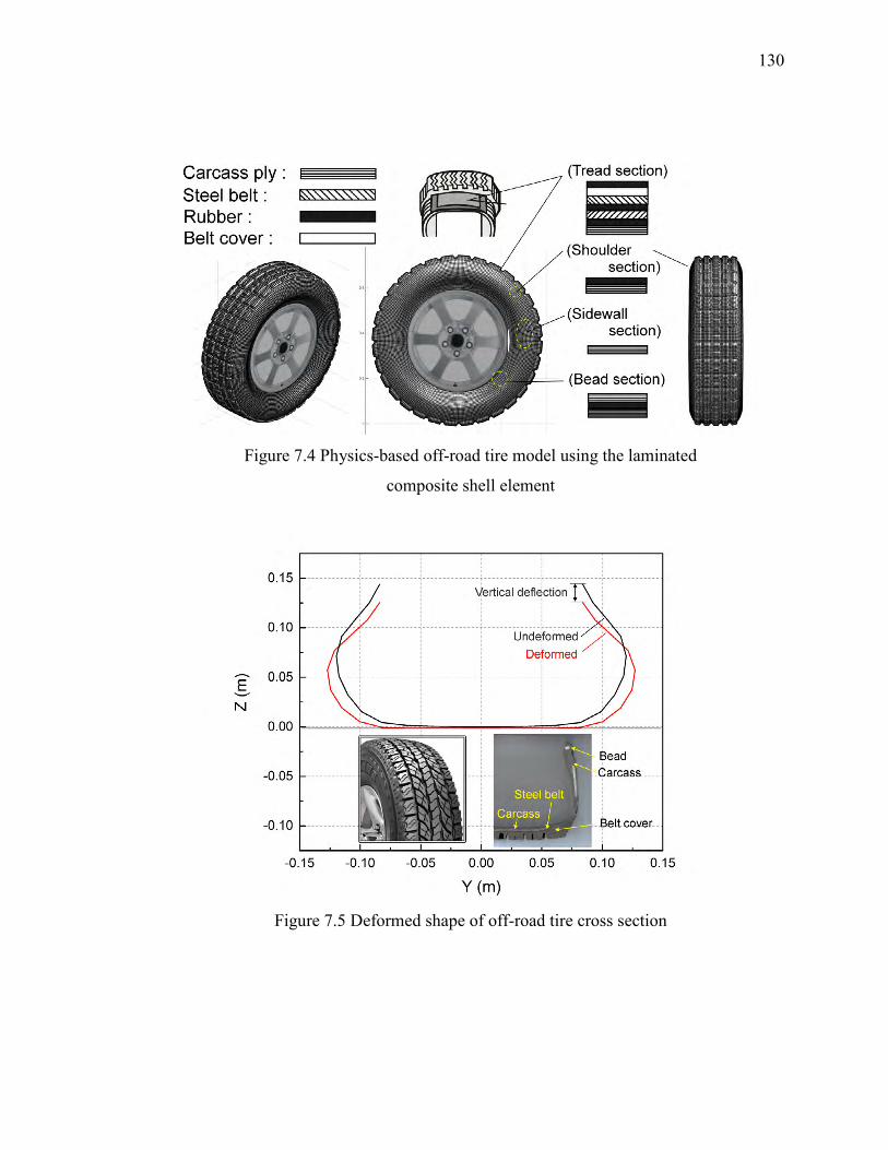
130

Figure 7.4 Physics-based off-road tire model using the laminated

composite shell element

Figure 7.5 Deformed shape of off-road tire cross section

131

Figure 7.6 Normal contact pressure in a longitudinal direction (4kN)

Figure 7.7 Normal contact pressure in a lateral direction (4kN)

132

Figure 7.8 Load-longitudinal contact patch length for off-road tire model

Figure 7.9 Load-lateral contact patch length for off-road tire model

133

Figure 7.10 Load-vertical deflection curve for off-road tire model

7.3.2 Tire/Soil Interaction Simulation

In this subsection, several numerical examples are presented in order to

demonstrate the use of the physics-based tire/soil interaction simulation capability

developed in this study. The off-road tire model discussed in Section 7.3.2 is used and a

constant traveling speed of 5 m/s is assumed. The air pressure and normal load are

assumed to be 230 kPa and 4 kN, respectively. The coefficient of friction is assumed to

be 0.3. The parameters of the deformable terrain model are summarized in Table 7.1 [86].

The width and height of the soil model are assumed to be 0.4 m and 0.4 m, respectively.

40 elements are used in the width direction, while 6 elements are used in the height

direction. In the longitudinal (traveling) direction, 80 elements are used for 1 meter long

soil. That is, the soil element is 12.5 mm in length and 10 mm in width to capture the

tread pattern geometry on the soil footprint as shown in Fig. 7.11.

134

In Fig. 7.12, the tire and soil deformation using the component soil model

approach is presented. It is shown that the moving soil patch is updated as the tire travels.

In order to discuss the effect of length in the component soil model on accuracy, 0.8 m,

1.0 m and 1.2 m long component soil models are considered and compared with the

complete soil model. The soil element size (i.e., 12.5 mm in length and 10 mm in width)

are kept constant for all the models and symmetric boundary condition is imposed on the

cut section of the component soil model. The tire rim vertical position and the rolling

Table 7.1 Material model parameters

Initial cohesion 0d (Pa) 5000

Yield surface coefficient η 0.0

Yield surface coefficient ξ 1.155

Young’s modulus E (MPa) 13.79

Poisson’s ratio ν 0.3

Density ρ (kg/m3) 200

Figure 7.11 Tire/soil interaction model

135

resistance defined by the ratio of the longitudinal tire force to the vertical ( /x zF F ) for

the traveled distance of 1 m are shown in Figs. 7.13, 7.14 and 7.15 for the three

component soil models, and they are compared with the complete soil model as the

reference solution. In this simulation, 2 m long soil bin is considered and the tire is

dropped on the soil at the initial configuration, resulting in approximately 0.05 m sinkage

of the vertical position of the tire rim from the initial position as observed between time t

= 0 and 0.2 seconds. The rolling resistance at the steady state rolling is approximately

0.26, which is close to the coefficient of friction assumed in this model. It is observed

from Figs. 7.13, 7.14 and 7.15 that use of 0.8 m long component soil model leads to

noticeable deviations in the vertical position and the rolling resistance from the reference

solutions obtained using the complete soil model, while use of 1.2 m long component soil

model leads to identical solutions to the complete soil model. The computational time for

the three models are, respectively, 28.0, 39.0 and 42.8 hours. The use of longer

component soil model leads to longer computational time as expected, while in this

simulation scenario, the 1.0 m long soil model also predicts the overall tire and soil

behavior well, despite the small deviation as shown in Fig. 7.14. The selection of the

Figure 7.12 Tire/soil interaction model using component soil approach

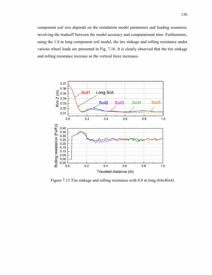
136

component soil size depends on the simulation model parameters and loading scenarios,

involving the tradeoff between the model accuracy and computational time. Furthermore,

using the 1.0 m long component soil model, the tire sinkage and rolling resistance under

various wheel loads are presented in Fig. 7.16. It is clearly observed that the tire sinkage

and rolling resistance increase as the vertical force increases.

Figure 7.13 Tire sinkage and rolling resistance with 0.8 m long (64x40x6)

137

Figure 7.14 Tire sinkage and rolling resistance with 1.0m long (80x40x6)

Figure 7.15 Tire sinkage and rolling resistance with 1.2m long (96x40x6)

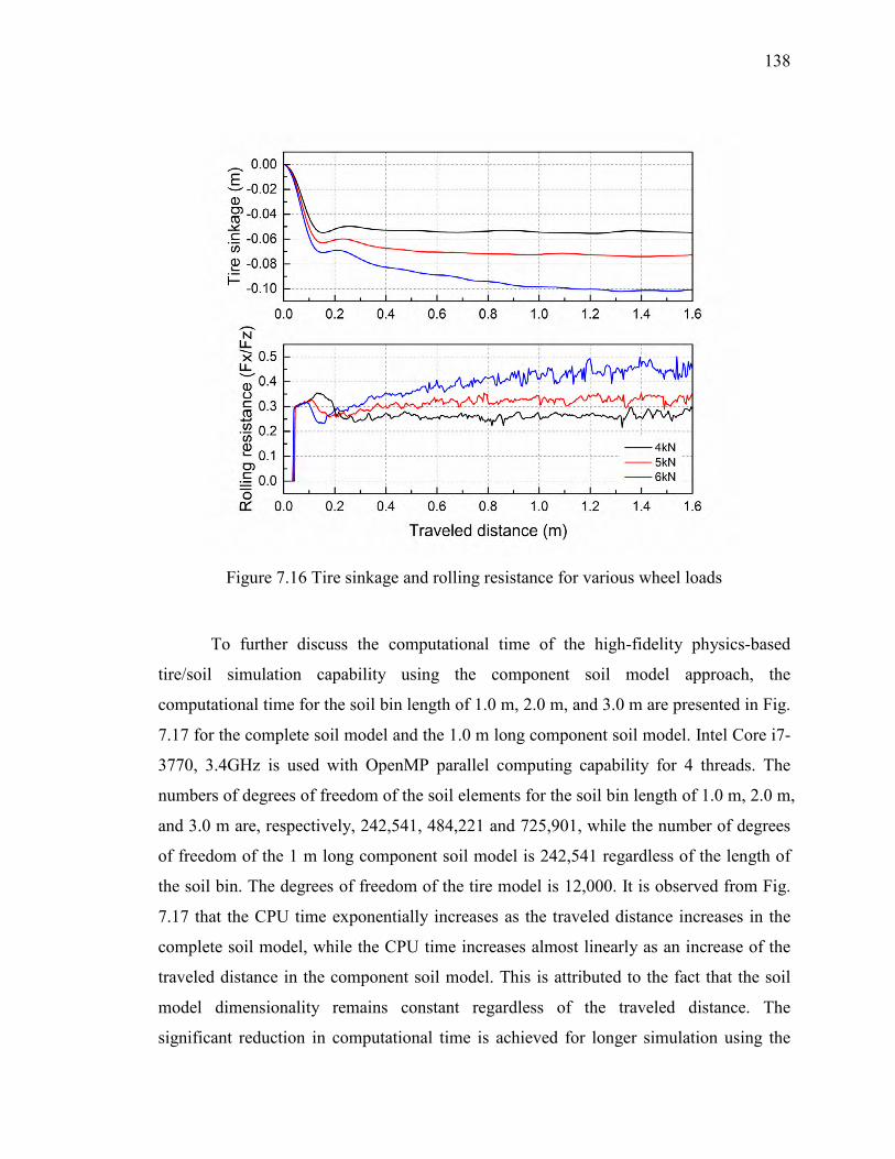
138

To further discuss the computational time of the high-fidelity physics-based

tire/soil simulation capability using the component soil model approach, the

computational time for the soil bin length of 1.0 m, 2.0 m, and 3.0 m are presented in Fig.

7.17 for the complete soil model and the 1.0 m long component soil model. Intel Core i7-

3770, 3.4GHz is used with OpenMP parallel computing capability for 4 threads. The

numbers of degrees of freedom of the soil elements for the soil bin length of 1.0 m, 2.0 m,

and 3.0 m are, respectively, 242,541, 484,221 and 725,901, while the number of degrees

of freedom of the 1 m long component soil model is 242,541 regardless of the length of

the soil bin. The degrees of freedom of the tire model is 12,000. It is observed from Fig.

7.17 that the CPU time exponentially increases as the traveled distance increases in the

complete soil model, while the CPU time increases almost linearly as an increase of the

traveled distance in the component soil model. This is attributed to the fact that the soil

model dimensionality remains constant regardless of the traveled distance. The

significant reduction in computational time is achieved for longer simulation using the

Figure 7.16 Tire sinkage and rolling resistance for various wheel loads

139

component soil model as demonstrated in this example, and it enables the use of the high-

fidelity physics-based tire/soil interaction simulation model in the large-scale off-road


Figure 7.17 CPU time comparison between long soil model and

component soil model

140

CHAPTER 8

CONCLUSIONS AND FUTURE WORK

8.1 Summary and Conclusions

Despite the fact detailed finite element tire models using explicit finite element

software have been widely utilized for structural design of tires by tire manufactures, it is

recognized in the tire industry that existing state-of-the-art explicit finite element tire

models are not capable of predicting the transient tire force characteristics accurately

under severe vehicle maneuvering conditions due to the numerical instability that is

essentially inevitable for explicit finite element procedures for severe loading scenarios

and the lack of transient (dynamic) tire friction model suited for FE tire models.

Furthermore, to integrate the deformable tire models into multibody full vehicle

simulation, co-simulation technique could be an option for commercial software.

However, there exit various challenges in co-simulation for the transient vehicle

maneuvering simulation in terms of numerical stability and computational efficiency. The

transient tire dynamics involves rapid changes in contact forces due to the abrupt braking

and steering input, thus use of co-simulation requires very small step size to ensure the

numerical stability and energy balance between two separate simulation using different

solvers. For this reason, a high-fidelity physics-based tire model that can be fully

integrated into multibody dynamics computer algorithms is developed in this study for

vehicle dynamics simulation without resorting to ad-hoc co-simulation procedures.

To this end, a continuum mechanics based shear deformable laminated composite

shell element is developed based on the finite element absolute nodal coordinate

formulation for modeling the complex fiber reinforced rubber tire structure in Chapter 2.

The element consists of four nodes, each of which has the global position coordinates and

the transverse gradient coordinates along the thickness introduced for describing the

orientation and deformation of the cross section of the shell element. The global position

field on the middle surface and the position vector gradient at a material point in the

element are interpolated by bi-linear polynomials. The continuum mechanics approach is

used to formulate the generalized elastic forces, allowing for the consideration of

nonlinear constitutive models in a straightforward manner. The element locking exhibited

141

in the element can be eliminated using the assumed natural strain (ANS) and enhanced

assumed strain (EAS) approaches. In particular, the combined ANS and EAS approach is

introduced to alleviate both curvature and Poisson’s thickness lockings arising from the

erroneous transverse normal strain distribution. The shell element developed is further

generalized to a laminated composite shell element for application to the modeling of

fiber-reinforced rubber (FRR) structure of the physics-based flexible tire model. The

complex deformation coupling exhibited in fiber-reinforced composite materials can be

automatically considered in the shear deformable laminated composite shell element

using the continuum mechanics approach, and the element lockings are systematically

eliminated by ANS and EAS approaches, thereby leading to a locking-free shear

deformable composite shell element. Furthermore, various nonlinear material models can

be considered for each layer in a way same as solid elements. Several numerical

examples are presented in Chapter 3 in order to demonstrate the accuracy and the rate of

convergence of numerical solutions obtained by the continuum mechanics based bi-linear

shear deformable shell element proposed in this study. In particular, the effect of locking

remedy and the element performance including the rate of convergence of the finite

element solutions are compared with those of ANSYS for nonlinear problems and

analytical solutions for linear problems for various benchmark problems.

Using the shear deformable laminated composite shell element based on the

absolute nodal coordinate formulation, a physics-based flexible tire model for the

transient braking and cornering analysis is developed for use in multibody vehicle

dynamics simulation in Chapter 4. To account for the transient tire friction characteristics

including the friction-induced hysteresis that appears in severe maneuvering conditions,

the distributed parameter LuGre tire friction model is integrated into the flexible tire

model. To this end, the contact patch predicted by the structural tire model is discretized

into small strips across the tire width, and then each strip is further discretized into small

elements to convert the partial differential equations of the LuGre tire friction model to

the set of first-order ordinary differential equations. By doing so, the structural

deformation of the flexible tire model and the LuGre tire friction force model are

dynamically coupled in the final form of the equations, and these equations are integrated

simultaneously forward in time at every time step.

142

In Chapter 5, a systematic and automated procedure for parameter identification

of LuGre tire friction model introduced in Chapter 4 is developed for accurate and

reliable prediction of transient tire forces. Since several fitting parameters are introduced

to account for the nonlinear friction characteristics, the correlation of the model

parameters with physical quantities are not clear, making the parameter identification of

the LuGre tire friction model difficult. That is, inappropriate initial estimates may lead to

parameters that have nothing to do with physical quantities even though the LuGre model

are fitted well with measured tire force curves. To this end, friction parameters used in

the LuGre tire force model are estimated using the measured slip-dependent friction

characteristics first and used for the nonlinear least square fitting. The adhesion

parameter is then estimated using the slope around the zero slip ratio. The nonlinear least

square fitting is used to identify all the parameters for the entire slip range such that the

maximum tire force peak can agree with the measurement data. Furthermore, the

modified friction characteristic curve function is proposed for wet road conditions, in

which the linear decay in friction is exhibited in the large slip velocity range. It is shown

that use of the proposed numerical procedure leads to an accurate prediction of the LuGre

model parameters for measured tire force characteristics under various loading and speed

conditions. Furthermore, the fundamental tire properties including the load-deflection

curve, the contact patch lengths, contact pressure distributions, and natural frequencies

are validated against the test data. Several numerical examples for the hard braking and

cornering simulation including the antilock braking control are presented to demonstrate

the robust simulation capability of the physics-based flexible tire model developed in this

study.

The physics-based flexible tire model is further extended for application to off-

road mobility simulation in Chapters 6 and 7. In Chapter 6, a locking-free 9-node 33-

DOF brick element is developed with the curvature coordinates at the center node for

modeling a continuum soil using the capped Drucker-Prager failure criterion.

Introduction of the curvature coordinates allows for considering the quadratic terms in the

polynomial for the assumed displacement field, thus the linear distribution of the stresses

and strains, which cannot be captured in the standard tri-linear 8-node 24-DOF brick

element, can be considered. This eliminates the reliance on the enhanced assumed strain

143

method to alleviate the element lockings exhibited in the standard tri-linear 8-node brick

element, thereby making the formulation and implementation of the continuum soil

model straightforward. Several benchmark test results are presented to demonstrate the

use of the 9-node brick element with curvature coordinates. Furthermore, the

multiplicative finite strain plasticity theory is utilized to consider the large soil

deformation exhibited in the tire/soil interaction simulation using the capped Drucker-

Prager failure criterion. The implementation of the capped Drucker-Prager failure is

verified by comparison with the soil elements in ABAQUS for the plate sinkage

benchmark test of soil. In order to identify soil parameters including cohesion and friction

angle, the triaxial soil test is carried out. Using the soil parameters identified including

the plastic hardening parameters by the compression soil test, the continuum soil model

developed is validated against the test data for the triaxial compression test condition.

The stress-strain curve agrees well with the triaxial soil test result.

In Chapter 7, using the physics-based deformable tire and soil models, the tire/soil

interaction simulation capability is developed and implemented in the general multibody

dynamics computer algorithm. Use of the high-fidelity physics-based tire/soil simulation

model in off-road mobility simulation, however, leads to a very large computational

model to consider a wide area of terrains. Thus, the computational cost dramatically

increases as the size of the soil model increases. To address this issue, the component soil

model is proposed such that soil elements far behind the tire can be removed from the

equations of motion sequentially, and then new soil elements are added to the portion that

the tire is heading to. That is, the soil behavior only in the vicinity of the rolling tire is

solved in order to reduce the overall model dimensionality associated with the finite

element soil model. It is shown that use of the component soil model leads to a

significant reduction in computational time while ensuring the accuracy, making the use

of the physics-based deformable tire/soil simulation capability feasible in off-road


8.2 Future Work

While the physics-based tire and soil models developed in this study are tested

and validated extensively against the test results using the test facility for the tire and soil

144

individually, validation of the tire/soil interaction simulation model has not be completed

yet. This involves more extensive tests using the mobility soil bin test facility to measure

the tire sinkage and rolling resistance on deformable terrains for various test conditions.

For validating the computational model, the mobility soil bin test will be carried out

using the off-road tire introduced in Section 7.3 and the soil used in the triaxial soil test

presented in Section 6.4. These computational models are validated against the test data

individually as discussed in Section 6.4 and 7.3, and their model parameters are also

identified. The soil bin test involves measuring the static wheel load and tire sinkage

curve for various tire air pressures; and the rolling resistance of the tire on soil in various

wheel load and air pressure conditions. Tire forces are measured by force transducers

embedded in the instrumented rim.

In addition, the integration of the physics-based flexible tire model developed in

this study in a high-performance computing (HPC) off-road mobility simulation

framework is crucial to enable the evaluation of overall vehicle performance and mobility

capability in various terrain conditions. While use of the component soil model leads to

significant reduction in the computational time, use of the physics-based tire/soil

simulation capability for full vehicle simulation including four tires and detailed

suspension models still requires significant computational power. For this reason, the tire

and soil models developed in this study are currently implemented into the physics-based

HPC off-road mobility simulation software called Chrono such that deformable tire and

soil interaction simulation capability can be utilized in multibody full vehicle simulation

in a single computational framework. Furthermore, the integration with Chrono software

allows for the use of discrete element (DE) soil models consisting of millions of particles

and DE soil models are needed for severe vehicle maneuvering scenarios involving high

slippages.

Development of a systematic parameter identification and validation procedure

for the physics-based tire/soil simulation model developed in this study is also needed. A

145

tire has a complex structure and various model parameters need to be identified to create

the physics-based tire model. In addition, soil parameters are stochastic in nature and

spatially distributed. Furthermore, an uncertainty quantification of terrains requires

extensive measurement, thus in most cases, only limited number of test data under

limited test conditions is available, and uncertainties of the tire and soil model parameters

make the validation process of the tire/soil interaction simulation very difficult and

challenging. This issue, however, has not been thoroughly addressed in the field of study,

and is of crucial importance in use of the physics-based tire and soil simulation model.

146

APPENDIX

ELASTIC MIDDLE SURFACE APPROACH FOR SHEAR

DEFORMABLE SHELL ELEMENT

A.1 Introduction

In Appendix, the elastic middle surface approach used for formulating the elastic

forces of the shear deformable shell element discussed in Chapter 2 is presented with a

plane stress assumption [87]. While the continuum mechanics approach is utilized to

consider fiber reinforced rubber (FRR) material which is indispensable for tire modeling,

the elastic middle surface approach discussed below can be applied to the thin to

moderately thick shell structures. For some applications, this shell formulation would be

suited from computational standpoint since the integration along the thickness can be

performed analytically and Poisson’s locking can be automatically eliminated by the

plane stress assumption. However, this formulation requires a special formulation to

consider nonlinear material models.

A.2 Elastic Middle Surface Approach

Using Green-Lagrange strain tensor, the six strain components in the middle

surface of the shell element i can be defined as follows:

( )1ˆ ( , ,0) ( )2

i i i i T im m mx y = −E F F I (A.1)

where imF is the global position vector gradient tensor at a material point in the middle

surface of the shell element i and is given as

1( , ,0) ( )i

i i i i imm m mix y −∂

= =∂

rF J JX

(A.2)

where ( , ,0) ( , )i i i i i i i i im m px y x y= =r S e S e . i

mJ and imJ are covariant base tensors of the

material point in the middle surface at the deformed and reference configurations,

respectively. These tensors are defined as

1 2 3

ii i i imm i

∂ = = ∂rJ g g gx

(A.3)

where 1 2 3/ , / , /i i i i i i i i im m mx y z= ∂ ∂ = ∂ ∂ = ∂ ∂g r g r g r and

147

1 2 3

ii i i imm i

∂ = = ∂XJ G G Gx

(A.4)

where the vector imX represents the global position vector of element i at the reference

configuration in the middle surface and is given by 0( , ,0)i i i i im x y=X S e with the initial

element nodal coordinates 0ie . Furthermore, one can define

1 2/ , /i i i i i im mx y= ∂ ∂ = ∂ ∂G X G X and 3 /i i i

m z= ∂ ∂G X . Substituting Eq. A.2 into Eq. A.1,

one can obtain 1ˆ ( , ,0) ( ) ( )i i i i T i i

m m m mx y − −=E J E J (A.5)

where

( )1( , ,0) ( ) ( )2

i i i i T i i T im m m m mx y = −E J J J J (A.6)

The Green-Lagrange strains given by Eq. A.5 are transformed to those defined with

respect to the orthogonal frame imA defined at the reference configuration as follows:

1( , ,0) ( ) ( ) , ,s , ,i i i i T i i im m m m rsx y r x y zε− −= ≡ =E B E B (A.7)

where

( ) , ,s 1, 2,3i i T i im m m rsB r= ≡ =B A J (A.8)

The tensor transformation given by Eq. A.7 can be re-expressed in terms of the

engineering strain vector imε and the covariant strain vector i

mε as:

( )i i T im m m

−=ε T ε (A.9)

where imT is a 6 by 6 matrix is defined as

2 2 211 12 11 12 13 11 13 12 13

2 2 221 22 21 22 23 21 23 22 23

11 21 12 22 11 22 12 21 13 23 11 23 13 21 12 23 13 222 2

31 32 31 32

( ) ( ) 2 ( ) 2 2( ) ( ) 2 ( ) 2 2

( ) ( ) 2 (

i i i i i i i i i

i i i i i i i i i

i i i i i i i i i i i i i i i i i iim i i i i

B B B B B B B B BB B B B B B B B B

B J B B B B B B B B B B B B B B B BB B B B B

+ + +=T 2

33 31 33 32 33

11 31 12 32 11 32 12 31 13 33 11 33 13 31 12 33 13 32

21 31 22 32 21 32 22 31 23 33 21 33 23 31 22 33 23 32

) 2 2i i i i i



B B B BB B B B B B B B B B B B B B B B B BB B B B B B B B B B B B B B B B B B

+ + +

+ + +

(A.10)

The orthogonal frame imA is defined using the cross-section frame [47]. In the cross-

148

section frame, the unit vector along the Z-axis of the orthogonal frame imA is parallel to

the third covariant base vector 3iG , thus the orthogonal frame describes the orientation of

the cross-section of the shell. That is, the unit vector isk along the Z-axis of the cross-

section frame is defined as

3

3

iis i

=GkG

(A.11)

Two other axes are defined using Gram-Schmidt orthogonalization procedure as follows:

2 2

2 2

(( ) )(( ) )

i i T i ii s ss i i T i i

s s

−=

−G G k kjG G k k

and i i is s s= ×i j k (A.12)

from which, one has i i i im s s s = A i j k (A.13)

Since the orthogonal frame imA is defined at the reference configuration, the orientation

matrix is an identity matrix if the element is initially flat.

Since the six strain components are defined in the middle surface, the bending and

twisting deformations of the shell element need to be introduced. To this end, the three

curvature components with respect to the orthogonal frame imA are defined as

1( , ,0) ( ) ( ) , ,s ,i i i i T i i im m m m rsx y r x yκ− −= ≡ =Κ C Κ C (A.14)

where imC is a 2 by 2 matrix that can be extracted from the matrix i

mB and is defined by

i i im rs rsC B≡ =C for ,s 1,2r = . In the preceding equation, the matrix i

mΚ is defined as

0 0

0 0

i i i ixx xx xy xyi

m i i i ixy xy yy yy

κ κ κ κκ κ κ κ

− −= − −

Κ

(A.15)

where

,

12

T Ti i i ii im m m mxx yyi i i i i i

T Ti i i ii m m m mxy i i i i i i

x z x y z y

x z y y z x

κ κ

κ

∂ ∂ ∂ ∂∂ ∂ = − = − ∂ ∂ ∂ ∂ ∂ ∂ ∂ ∂ ∂ ∂∂ ∂ = − − ∂ ∂ ∂ ∂ ∂ ∂

r r r r

r r r r

(A.16)

and

149

0 0

0

,

12

T Ti i i ii im m m mxx yyi i i i i i

T Ti i i ii m m m mxy i i i i i i

x z x y z y

x z y y z x

κ κ

κ

∂ ∂ ∂ ∂∂ ∂ = − = − ∂ ∂ ∂ ∂ ∂ ∂ ∂ ∂ ∂ ∂∂ ∂ = − − ∂ ∂ ∂ ∂ ∂ ∂

X X X X

X X X X

(A.17)

A.3 Locking Remedy

In the shear deformable bi-linear shell element based on continuum mechanics

approach, the following lockings are exhibited as discussed in Chapter 2: (1) in-plane

normal/shear locking, (2) transverse shear locking, (3) Poisson’s thickness locking and

(4) curvature thickness locking. In this section, the locking remedy for the shell element

based on the elastic middle surface approach is discussed.

A.3.1 In-Plane Normal/Shear Locking

As in the continuum mechanics approach, in-plain normal/shear locking can be

alleviated by the enhanced assumed strain (EAS) approach. The compatible in-plane

strains in the middle surface i cpε obtained by differentiating the assumed global position

vector is modified as follows as follows: EASi i c i

p p p= +ε ε ε (A.18)

where EASipε is the enhanced assumed strain vector defined by

EAS( ) ( )i i i i ip =ε ξ G ξ α (A.19)

In the preceding equation iα is the vector of internal parameters that define the assumed

strain field of element and the matrix ( )i iG ξ is defined as:

00( ) ( ) ( )

( )

ii i i T i i

mpi i−=

JG ξ T N ξ

J ξ (A.20)

where ( )i iJ ξ and 0iJ are, respectively, the position vector gradient tensor at the reference

configuration evaluated at the Gauss integration point iξ and that evaluated at the center

of the element ( i =ξ 0 ). 0impT is the 3 by 3 transformation matrix defined by the sub-

matrix of the 6 by 6 transformation matrix given by Eq. A.10 associated with the in-plane

150

strain vector ipε , and this matrix has to be evaluated at the center of the element [44,54,88

]. The explicit form of the transformation matrix is given as follows: 2 2

11 12 11 122 2

0 21 22 21 22

11 21 12 22 11 22 12 21

( ) ( ) 2( ) ( ) 2

i i i i

i i i i imp

i i i i i i i i

B B B BB B B B

B B B B B B B B=

= + ξ 0

T (A.21)

where ( ) (( ) ) , ,s 1, 2i i i T irs m rs m m rsB r= = =B A J as defined by Eq. A.8. The matrix ( )i iN ξ

consists of polynomial terms of the enhanced strain field in parametric domain. The

simplest enhancement which introduces four internal parameters iα is given as follows:

0 0 0( ) 0 0 0

0 0

i

i i i

i i

ξη

ξ η

=

N ξ (A.22)

The effect of the number of internal parameters on the elastic force accuracy is discussed

in literature [54]. It is important to notice here that the matrix ( )i iN ξ should fulfill the

following condition

( )i i id =∫ N ξ ξ 0 (A.23)

such that the assumed stress vanishes over the reference volume of the element and it

passes the patch test [44].

A.3.2 Transverse Shear Locking

The transverse shear locking can be removed by the assumed natural strain (ANS)

approach. The covariant strains evaluated at Barlow points where the strain field terms

are correct are tied to assumed natural strain interpolation points through the use of

Lagrange interpolation. The assumed covariant natural transverse shear strain field can

re-expressed as follows:

( ) ( )

( ) ( )

ANS

ANS

1 11 12 21 11 12 2

i i iC i iDxz xz xz

i i iA i iByz yz yz

γ η γ η γ

γ ξ γ ξ γ

= − + + = − + +

(A.24)

where iCxzγ , iD

xzγ , iAyzγ and iB

yzγ are the covariant transverse shear strains at the tying points.

151

A.3.3 Poisson’s Thickness Locking

Poisson’s thickness locking is not essentially exhibited in case of elastic middle

surface approach since in-plane strains and the transverse normal strain are decoupled

due to the plane strain assumption. It is known that Poisson’s thickness locking occurs

when Poisson ratio has some value, which introduces the coupling of the in-plane strains

to the transverse normal strain. For instance, in the case of pure bending, the axial strains

due to bending are linearly distributed along the thickness, and it leads to the linearly

varying transverse normal strain due to the coupling induced by Poisson’s ratio. However,

the use of the linear interpolation along the thickness leads to constant thickness strains

which make the element behave overly stiff since the thickness strain does not vanish on

the neutral axis. Continuum mechanics-based shear deformable element with EAS allows

for incorporating the linearly varying transverse normal strain to alleviate Poisson’s

thickness locking effectively as discussed in Section 2.2. On the other hand, due to the

plane stress assumption made in the shell element, the in-plane strains and the transverse

normal strain are decoupled, thus the Poisson’s thickness locking is not essentially

exhibited. This is one of the most economical ways of treating the Poisson´s locking for

applications where the plane stress assumption is fulfilled. For thick shell structures with

nonlinear material models, this assumption is no longer valid and the continuum

mechanics approach needs to be used.

A.3.4 Curvature Thickness Locking

Curvature thickness locking is also exhibited in case of initially curved

configuration as the same as continuum mechanics approach. The transverse gradient

vectors can be erroneously elongated when the shell element is subjected to bending and

twisting deformation. The assumed natural strain (ANS) method is applied, the covariant

transverse normal strains at the four nodal points are interpolated by the Lagrange

polynomial as follows: ANS ANS 1 ANS 2 ANS 3 ANS 4

1 2 3 4i i i i i i i i izz zz zz zz zzS S S Sε ε ε ε ε= + + + (A.25)

where kzzε indicates the compatible transverse normal strain at node k and ANS

kS is the

shape function associated with it.

152

A.4 Equation of Motion

Using Eqs. A.9 and A.15, the generalized elastic forces ikQ for the initially curved

shell element can be defined using the virtual work as follows:

0 0

0 0

( ) ( )

( )

( )

i i i T i i i i T i ip p p t t

i i i i i T i izz zz

i T ik

W h dA h dA

h E dA dA

γ

κ

δ δ δ

δε ε δ

δ

= − −

− −

=

∫ ∫∫ ∫

ε D ε γ D γ

κ D κ

e Q

(A.26)

where 0iA is the infinitesimal area of element in the reference configuration and the

following engineering strain and curvature vectors are defined:

[ 2 ]i i i i Tp xx yy xyε ε ε=ε , [2 2 ]i i i T

t xz yzε ε=γ , [ 2 ]i i i i Txx yy xyκ κ κ=κ (A.27)

where ipε represents the vector of the in-plane strains, i

tγ the vector of transverse shear

strains and iκ the vector of curvatures. For a linear Hookean material model in plane

stress condition with constant shell thickness h, the following matrices of elasticity are

defined:

2

1 01 0

10 0 (1 ) / 2

pE

νν

νν

= − −

D , 0

02(1 )xz

yz

cEcγ ν

= +

D , 3

12 ph

κ =D D (A.28)

where E is Young’s modulus; ν Poisson´s ratio; xzc and yzc the transverse shear strain

distribution correction factors. The integration is performed over the middle surface of

the element and the stress distribution along the thickness of the shell is assumed constant

in this model. This assumption can be considered as a reasonable approximation for thin

shell structures with linear Hookean material model. It is also important to notice that

since the elastic forces are evaluated only in the middle surface, the total number of

integration points is less than that of the continuum mechanics based shell element.

Several numerical examples of the use of elastic middle surface approach are

demonstrated in Section 3.1, showing that element lockings are eliminated by the

approaches discussed in this Appendix.

153

REFERENCES

1. Lugner, P., Pacejka, H. and Plochl, M., 2005, "Recent Advances in Tyre Models and Testing Procedures", Vehicle System Dynamics, vol. 43, no. 6-7, pp. 413-436.

2. Pacejka, H. B., 2002, Tire and Vehicle Dynamics, Society of Automotive Engineers (SAE), Warrendale, PA.

3. Gruber, P., Sharp, R. S. and Crocombe, A. D., 2012, "Normal and Shear Forces in the Contact Patch of a Braked Racing Tyre. Part 1: Results from a Finite-Element Model", Vehicle System Dynamics, vol. 50, pp. 323–337

4. Gruber, P., Sharp, R. S. and Crocombe, A. D., 2012, "Normal and Shear Forces in the Contact Patch of a Braked Racing Tyre. Part 2: development of a physical tyre model", Vehicle System Dynamics, vol. 50, pp. 339–356

5. Clark, S. K. (ed.), Mechanics of Pneumatic Tires, 1981, US DOT HS805 952 NHTSA.

6. Lee, C.R., Kim, J.W., Hallquist, J.O., Zhang, Y. and Farahani, A.D., 1997, "Validation of a FEA Tire Model for Vehicle Dynamic Analysis and Full Vehicle Real Time Proving Ground Simulations", SAE Technical Paper 971100

7. Koishi, M., Kabe, K. and Shiratori, M., 1998, "Tire Cornering Simulation Using an Explicit Finite Element Analysis Code", Tire Science and Technology, vol. 26, pp. 109-119

8. Gruber, P., Sharp, R. S. and Crocombe, A. D., 2012, "Shear Forces in the Contact Patch of a Braked Racing Tyre", Vehicle System Dynamics, vol. 50, pp. 1761-1778

9. Tanner, J.A., 1996, "Computational Methods for Frictional Contact with Applications to the Space Shuttle Orbiter Nose-Gear Tire", NASA Technical Report 3573, pp. 1-52

10. Gipser, M., 2005, "FTire: A Physically Based Application-Oriented Tyre Model for Use with Detailed MBS and Finite-Element Suspension Models", Vehicle System Dynamics, vol. 43, pp. 76-91

11. Gallrein, A. and Baecker, M., "CDTire: A Tire Model for Comfort and Durability Applications", Vehicle System Dynamics, vol. 45, Supplement, 2007, pp. 69-77

12. Oertel, C. and Fandre, A., 1999, "Ride Comfort Simulations and Step Towards Life Time Calculations: RMOD-K and ADAMS", Proceedings of International ADAMS conference, Berlin, Germany

13. Huston, R. L. Multibody Dynamics, 1990 (Butterworth Heinemann, Stonham).

14. Roller, M., Betsch, P., Gallrein A. and Linn, J., 2014, "On the Use of Geometrically Exact Shells for Dynamic Tyre Simulation", Ch. 9 in Multibody Dynamics, Computational Methods in Applied Sciences 35, Terze, Z., (ed.), pp. 205-236, Springer-Verlag

154

15. Roller, M., Betsch, P., Gallrein, A. and Linn, J., 2015, "An Enhanced Tire Model for Dynamic Simulation Based on Geometrically Exact Shells", Proceedings of ECCOMAS Thematic Conference on Multibody Dynamics, June 29-July 2, Barcelona, Spain

16. Bekker, M. G. 1969, Introduction to Terrain-Vehicle Systems, The University of Michigan Press, Ann Arbor.

17. Wong, J. Y. 2008, Theory of Ground Vehicle. 4th ed. Hoboken, NJ: John Wiley & Sons.

18. Contreras, U. Li, G., Foster, C.D. Shabana,A.A. Jayakumar, P. and Letherwood, M.D., 2013, “Soil Models and Vehicle System Dynamics”, Applied Mechanics Reviews, vol. 65, 040802-1.

19. Xia, K., 2011, “Finite Element Modeling of Tire/Terrain Interaction: Application to Predicting Soil Compaction and Tire Mobility”, Journal of Terramechanics, vol. 48, pp.113-123.

20. Shoop S.A., Richmond,P.W., Lacombe, J., 2006, “Overview of Cold Regions Mobility Modeling at CRREL”, Journal of Terramechanics, vol. 43, pp. 1-26.

21. Varghese, A.G., Turner, J.L., Way,T.R., Johnson,C.E., Dorfi, H.R., 2012, “Traction prediction of a smooth rigid wheel in soil using coupled Eulerian-Lagrangian analysis”, Proceedings of 2012 SIMULIA Community Conference, pp. 1-15.

22. Wasfy, T.M., Wasfy.H.M., Peters, J.M., 2014, “Coupled Multibody Dynamics and Discrete Element Modeling of Vehicle Mobility on Cohesive Granular Terrains”, Proceedings of the ASME 2014 IDETC & CIE Conference, Buffalo, DETC2014-35146.

23. Negrut, D.,Serban, R., Mazhar, H., Heyn, T., 2014, “Parallel Computing in Multibody System Dynamics: Why, When and How”, ASME Journal of Computational and Nonlinear Dynamics, 9:041007-1.

24. Heyn, T., Anitescu, M., Tasora. A, Negrut, D., 2013, “Using Krylov subspace and spectral methods for solving complementarity problems in many-body contact dynamics simulation”, International Journal for Numerical Methods in Engineering, vol. 95, pp. 541-561.

25. Nakashima, H., and Oida, A., 2004, “Algorithm and Implementation of Soil-Tire Contact Analysis Code Based on Dynamic FE-DE Method”, Journal of Terramechanics, vol. 41, pp. 127-137.

26. El-Gindy, M., Lescoe, R., Oljer, F., Jojansson, I., Trlvedl, M., 2011, “Soil Modeling Using FEA and SPH Techniques for a Tire-Soil Interaction”, Proceedings of the ASME 2011 IDETC & CIE Conference, Washington, DETC2011-47104

27. Belytschko, T., Liu, W.K., Moran, B., 2000, Nonlinear Finite Elements for Continua and Structures, Wiley

28. Shabana, A. A., Dynamics of Multibody Systems, 2005, Cambridge University Press, New York.

155

29. Gerstmayr, J., Sugiyama, H. and Mikkola, A., 2013, “Review on the Absolute Nodal Coordinate Formulation for Large Deformation Analysis of Multibody Systems”, ASME Journal of Computational and Nonlinear Dynamics, vol. 8, pp. 031016-1-12.

30. Mikkola, A. M. and Shabana, A. A., 2003, "A Non-Incremental Finite Element Procedure for the Analysis of Large Deformation of Plates and Shells in Mechanical System Applications", Multibody System Dynamics, vol. 9, pp.283-309.

31. Sugiyama, H. and Suda, Y., 2009, "Nonlinear Elastic Ring Tire Model Using the Absolute Nodal Coordinate Formulation", IMechE Journal of Multi-Body Dynamics, vol. 223, pp. 211-219

32. Yamashita, H., Matsutani, Y. and Sugiyama, H., 2015, "Longitudinal Tire Dynamics Model for Transient Braking Analysis: ANCF-LuGre Tire Model", ASME Journal of Computational and Nonlinear Dynamics, vol. 10, pp. 031003-1-11

33. Mikkola, A.M.; Matikainen, M.K., 2006, “Development of Elastic Forces for a Large Deformation Plate Element Based on the Absolute Nodal Coordinate Formulation”. ASME Journal of Computational and Nonlinear Dynamics, vol. 1, pp. 103-108, 2006

34. Dmitrochenko, O. and Pogorelov, D. Y., 2003, "Generalization of Plate Finite Elements for Absolute Nodal Coordinate Formulation", Multibody System Dynamics, vol. 10, pp. 17-43

35. Dufva, K., and Shabana, A. A., 2005, “Analysis of Thin Plate Structures Using The Absolute Nodal Coordinate Formulation”, IMechE Journal of Multi-body Dynamics, vol. 219, pp. 345-355.

36. Schwab, A. L., Gerstmayr, J., and Meijaard, J. P., 2007, “Comparison of Three-Dimensional Flexible Thin Plate Elements for Multibody Dynamic Analysis: Finite Element Formulation and Absolute Nodal Coordinate Formulation”, Proceedings of the ASME 2007 International Design Engineering Technical Conferences & Computers and Information in Engineering Conference, Las Vegas, Nevada, USA

37. Nachbagauer, K., Gruber, P., and Gerestmayr, J., 2013, “Structural and Continuum Mechanics Approaches for a 3D shear Deformable ANCF Beam Finite Element: Application to Static and Linearized Dynamic Examples”, ASME Journal of Computational and Nonlinear Dynamics, vol. 8, pp.021004-1-7

38. Dmitrochenko, O., Matikainen, M., and Mikkola, A., 2012, “The Simplest 3- and 4-Noded Fully Parameterized ANCF Plate Elements”, Proceedings of the ASME 2012 International Design Engineering Technical Conferences & Computers and Information in Engineering Conference, Chicago, IL, USA

39. Hauptmann, R., Doll, S., Harnau, M., Schweizerhof, K., 1998, "A Systematic Development of ‘Solid-Shell’ Element Formulations for Linear and Non-Linear Analyses Employing Only Displacement Degrees of Freedom", International Journal for Numerical Methods in Engineering, vol. 42, pp. 49–69

40. Hauptmann, R., Doll, S., Harnau, M., Schweizerhof, K., 2001, "Solid-Shell Elements with Linear and Quadratic Shape Functions at Large Deformations with Nearly Incompressible Materials", Computers & Structures, vol. 79, pp. 1671-1685

156

41. Vu-Quoc, L., and Tan, X. G., 2003, "Optimal Solid Shells for Non-Linear Analyses of Multilayer Composites I. Statics", Computer Methods in Applied Mechanics and Engineering, vol. 192, pp. 975-1016

42. Vu-Quoc, L., and Tan, X.G., 2003, "Optimal Solid Shells for Non-Linear Analyses of Multilayer Composites. II. Dynamics", Computer Methods in Applied Mechanics and Engineering, vol. 192, pp. 1017-1059

43. Tan, X.G., and Vu-Quoc, L., 2005, "Efficient and Accurate Multilayer Solid-Shell Element: Nonlinear Materials at Finite Strain'', International Journal for Numerical Methods in Engineering, vol. 63, pp. 2124-2170

44. Simo, J. C., and Rifai, M. S. and Fox, D.D., 1990, "On a Stress Resultant Geometrically Exact Shell Model. Part IV: Variable Thickness Shells with Through-the-Thickness Stretching", International Journal for Numerical Methods in Engineering, vol. 81, pp. 91-126

45. Betsch, P., and Stein, E., 1995, "An Assumed Strain Approach Avoiding Artificial Thickness Straining for A Non-Linear 4-Node Shell Element", Communications in Numerical Methods in Engineering, vol. 11, pp. 899-909

46. Betsch, P., and Stein, E., 1996, "A Nonlinear Extensible 4-Node Shell Element Based on Continuum Theory and Assumed Strain Interpolations", Journal of Nonlinear Science, vol. 6, pp. 169-199

47. Sugiyama, H., Escalona, J. L. and Shabana, A. A., 2003, "Formulation of Three-Dimensional Joint Constraints Using the Absolute Nodal Coordinates", Nonlinear Dynamics, vol. 31, pp. 167-195

48. Sugiyama, H. and Yamashita, H., 2011, "Spatial Joint Constraints for the Absolute Nodal Coordinate Formulation using the Non-Generalized Intermediate Coordinates", Multibody System Dynamics, vol. 26, pp. 15-36

49. Yamashita, H., Valkeapää, A., Jayakumar, P., Sugiyama, H. and 2015, "Continuum Mechanics Based Bilinear Shear Deformable Shell Element Using Absolute Nodal Coordinate Formulation", ASME Journal of Computational and Nonlinear Dynamics, vol. 10, 051012-1-9.

50. Ahmad, S., Irons, B. M., Zienkiewicz O. C., 1970, “Analysis of Thick and Thin Shell Structures by Curved Finite Elements”. International Journal for Numerical Methods in Engineering. vol. 2, pp. 419–451

51. Shabana, A. A., Mikkola, A. M., 2003, “On the Use of the Degenerate Plate and the Absolute Nodal Coordinate Formulations in Multibody System Applications”, Journal of Sound and Vibration. vol. 259, pp. 481–489.

52. Sze, K. Y., 2002, “Three-Dimensional Continuum Finite Element Models for Plate/Shell Analysis”, Progress in Structural Engineering and Materials, vol. 4, pp. 400-407

53. Mostafa, M., Sivaselvan, M. V. and Felippa, C. A., 2013, “A Solid-Shell Corotational Element Based on ANDES, ANS and EAS for Geometrically Nonlinear Structural Analysis”, International Journal for Numerical Methods in Engineering, vol. 95, pp. 145-180

157

54. Andelfinger, U., and Ramm, E., 1993, “EAS-Elements for Two-Dimensional, Three-Dimensional, Plate and Shell Structures and Their Equivalence to HR-Elements”, International Journal for Numerical Methods in Engineering, vol. 36, pp. 1311-1337

55. Dvorkin, E. N., and Bathe, K. J., 1984, “A Continuum Mechanics Based Four-Node Shell Element for General Non-Linear Analysis”, Engineering Computations, vol. 1, pp. 77-88

56. Bathe, K. J. and Dvorkin, E. N., 1986, “A Formulation of General Shell Elements - The Use of Mixed Interpolation of Tensorial Components”, International Journal for Numerical Methods in Engineering, vol. 22, pp. 697-722

57. Bischoff, M., Ramm, E., 1997, “Shear Deformable Shell Elements for Large Strains and Rotations”, International Journal for Numerical Methods in Engineering, vol. 40, pp. 4427-4449

58. Cook, R. D., Malkus, D. S., Plesha, M. E., and Witt, R. J., 2002, Concepts and Applications of Finite Element Analysis Fourth Edition, Wiley

59. Bonet, J., and Wood, D. R., 1997, Nonlinear Continuum Mechanics for Finite Element Analysis, Cambridge University Press

60. Jones, R. M., 1999, Mechanics of Composite Materials, Taylor and Francis

61. Noor, A.K. and Burton, W.S., 1989, "Assessment of Shear Deformation Theories for Multilayered Composite Plates", Applied Mechanics Review, vol. 42, pp. 1-13

62. Noor, A.K. and Burton, W.S., 1990, "Assessment of Computational Models for Multilayered Composite Shells", Applied Mechanics Review, vol. 43, pp. 67-97

63. Bathe, K.J., Finite Element Procedures, 1996, Prentice Hall

64. Stander, N., Matzenmiller, A., Ramm, E, 1988, “An Assessment of Assumed Strain Methods in Finite Rotation Shell Analysis”, Engineering Computations, vol. 6, pp.58-66

65. Matikainen, M.K., Valkeapää, A. I., Mikkola, A. M., and Schwab, A. L., 2013, “A Study of Moderately Thick Quadrilateral Plate Elements Based on the Absolute Nodal Coordinate Formulation”, Multibody System Dynamics, pp. 1–30

66. Yamashita, H., Jayakumar, P., Sugiyama, H., 2016, “Physics-Based Flexible Tire Model Integrated With LuGre Tire Friction For Transient Braking and Cornering Analysis”, ASME Journal of Computational and Nonlinear Dynamics, vol. 11, 031017-1-17

67. Hilber, H. M., Hughes, T. J. R., and Taylor, R. L., 1977, "Improved Numerical Dissipation for Time Integration Algorithms in Structural Dynamics", Earthquake Engineering and Structural Dynamic, vol. 5, pp. 265–284

68. Canudas-de-Wit, C., Tsiotras, P., Velenis, E., Basset, M. and Gissinger, G., 2003, "Dynamic Friction Models for Road/Tire Longitudinal Interaction", Vehicle System Dynamics, vol. 39, pp. 189-226.

158

69. Deur, J., Asgari, J., Hrovat, D., 2004, "A 3D Brush-Type Dynamic Tire Friction Model", Vehicle System Dynamics, vol. 42, pp. 133-173

70. Rajapakshe, M. P., Gunaratne, M., and Kaw, A. K., 2010, "Evaluation of LuGre Tire Friction Model with Measured Data on Multiple Pavement Surfaces", Tire Science and Technology, vol. 38, pp. 213-227

71. Deur, J., Ivanović, V., Troulis, M., Miano, C., Hrovat, D. and Asgari, J., 2005, "Extensions of the LuGre Tyre Friction Model Related to Variable Slip Speed along the Contact Patch Length", Vehicle System Dynamics, vol. 43, pp. 508-524

72. Deur, J., Ivanović, V., Pavković, D., Hrovat, D., Asgari, J., Troulis, M. and Miano, C., 2005, "Experimental Analysis and Modelling of Longitudinal Tyre Friction Dynamics for Abrupt Transients", Vehicle System Dynamics, vol. 43, pp. 525-539

73. Simo, J. C., and Rifai, M. S., 1990, “A Class of Mixed Assumed Strain Methods and The Method of Incompatible Modes”, International Journal for Numerical Methods in Engineering, vol. 29, pp. 1595-1638

74. Olshevskiy, A., Dmitrochenko, O., Kim, C.W., 2014,”Three-Dimensional Solid Brick Element Using Slopes in the Absolute Nodal Coordinate Formulation”, ASME Journal of Computational and Nonlinear Dynamics. vol. 9, pp. 021001

75. Wilson, E. L., Taylor, R. L., Doherty, W. P. Ghabussi, T., 1973, “Incompatible Displacement Models”, Numerical and Computer Methods in Structural Mechanics, pp. 43-57

76. Naghdi, P. M., 1990, "A Critical Review of the State of Finite Plasticity", Journal of Applied Mathematics and Physics (ZAMP), vol. 41, pp. 315-394

77. Lee, E. H. and Liu, D. T., 1967, "Finite Strain Elastic-Plastic Theory Particularly for Plane Wave Analysis", Journal of Applied Physics, vol. 38, pp. 19-27

78. Simo, J. C., 1988, "A Framework for Finite Strain Elastoplasticity Based on Maximum Plastic Dissipation and the Multiplicative Decomposition: Part I Continuum Formulation", Computer Methods in Applied Mechanics and Engineering, vol. 66, pp. 199-219

79. de Souza Neto, E. A., Peric, D. and Owen, D. R. J., 2008, Computational Methods for Plasticity: Theory and Applications, Wiley

80. Simo, J. C., 1992, "Algorithms for Static and Dynamic Multiplicative Plasticity That Preserve the Classical Return Mapping Schemes of the Infinitesimal Theory", Computer Methods in Applied Mechanics and Engineering, vol. 99, pp. 61-112.

81. Nagtegaal, J. C. and De Jong, J. E., 1982, "Some Aspects of Non-Isotropic Work Hardening in Finite Strain Plasticity", Plasticity of Metal at Finite Strain, Stanford University Press, pp. 65-102

82. Nemat-Nasser, S., 1982, "On Finite Deformation Elasto-Plasticity", International Journal of Solids and Structures, vol. 18, pp. 857-872

159

83. Nagtegaal, J. C., 1982, "On the Implementation of Inelastic Constitutive Equations with Special Reference to Large Deformation Problems", Computer Methods in Applied Mechanics and Engineering, vol. 33, pp. 469-484

84. Simo, J. C. and Hughes, T. J. R., 1998, Computational Inelasticity, Springer

85. Crisfield, M. A., 1996, Non-Linear Finite Element Analysis of Solids and Structures, Volume 2, Wiley

86. Shoop, S. A. 2001, “Finite Element Modeling of Tire-Terrain Interaction”, ERDC/CRREL TR-01-16, US. Army Corps of Engineers, Engineer Research and Development Center

87. Valkeapää, A., Yamashita, H., Jayakumar, P. and Sugiyama, H., 2015, "On the Use of Elastic Middle Surface Approach in the Large Deformation Analysis of Moderately Thick Shell Structures using Absolute Nodal Coordinate Formulation", Nonlinear Dynamics, vol. 80, pp. 1133-1146

88. Simo, J. C. and Armero, F., 1992, “Geometrically Non-Linear Enhanced Strain Mixed Methods and the Method of Incompatible Modes.” International Journal for Numerical Methods in Engineering. vol. 33, pp. 1413–1449.

89. Helwany, S., 2007, Applied Soil Mechanics with ABAQUS Applications, John Wiley and Sons, New York.

90. Wasfy, M. T., Jayakumar, P., Mechergui, D. and Sanikommu, S., 2016, “Prediction of Vehicle Mobility on Large-Scale Soft-Soil Terrain Maps Using Physics-Based Simulation”, Proceeding to 2016 NDIA Ground Vehicle Systems Engineering and Technology Symposium.

Flexible multibody dynamics approach for tire dynamics ...

Documents

Transcript of Flexible multibody dynamics approach for tire dynamics ...