arX

iv:1

207.

1791

v5 [

phys

ics.

soc-

ph]

27

Nov

201

2

Spatial effects in real networks: measures, null models, and applications

Franco Ruzzenenti∗

Center for the Study of Complex Systems, University of di Siena, Via Roma 56, 53100 Siena (Italy) andDepartment of Chemistry, University of di Siena, Via Aldo Moro 1, 53100 Siena (Italy)

Francesco PiccioloDepartment of Chemistry, University of di Siena, Via Aldo Moro 1, 53100 Siena (Italy)

Riccardo BasosiDepartment of Chemistry, University of di Siena, Via Aldo Moro 1, 53100 Siena (Italy) and

Center for the Study of Complex Systems, University of di Siena, Via Roma 56, 53100 Siena (Italy)

Diego GarlaschelliInstituut-Lorentz for Theoretical Physics, Leiden Institute of Physics,

University of Leiden, Niels Bohrweg 2, 2333 CA Leiden (The Netherlands)(Dated: November 28, 2012)

Spatially embedded networks are shaped by a combination of purely topological (space-independent) and space-dependent formation rules. While it is quite easy to artificially generatenetworks where the relative importance of these two factors can be varied arbitrarily, it is muchmore difficult to disentangle these two architectural effects in real networks. Here we propose asolution to the problem by introducing global and local measures of spatial effects that, through acomparison with adequate null models, effectively filter out the spurious contribution of non-spatialconstraints. Our filtering allows us to consistently compare different embedded networks or differenthistorical snapshots of the same network. As a challenging application we analyse the World TradeWeb, whose topology is expected to depend on geographic distances but is also strongly determinedby non-spatial constraints (degree sequence or GDP). Remarkably, we are able to detect weak butsignificant spatial effects both locally and globally in the network, showing that our method suc-ceeds in retrieving spatial information even when non-spatial factors dominate. We finally relateour results to the economic literature on gravity models and trade globalization.

PACS numbers: 89.65.Gh; 89.70.Cf; 89.75.-k; 02.70.Rr

I. INTRODUCTION

The growth of interest towards complex networks dur-ing the last decade was mainly determined by the un-expected structural and dynamical consequences of thelack of spatial constraints in many real-world networks.For instance, the emergence of a scale-free topology [1]and unconventional percolation properties [2] is impos-sible in networks (such as regular lattices) that are en-tirely shaped by geometric constraints. However, manyreal networks are in general the result of a combinationof spatial and non-spatial effects. So, even if not en-tirely, spatial constraints still partially and substantiallyaffect network topology [3]. A remarkable example isthat of transportation networks, that offer an insightfulapproach to some prominent and apparently unrelatedscientific questions concerning the size and form of re-current structures in Nature [4–9]. The ubiquitous al-lometric scaling laws characterizing the shape of living(e.g. vascular networks [10]) and non-living (e.g. rivernetworks [11]) systems have been demonstrated to bethe result of efficient and optimized transportation pro-

∗ ruzzenenti@unisi.it

cesses, crucially dependent on the dimension of the em-bedding space [10–15]. Even more generally, when theembedding space is abstract rather than physical (as inecological networks [16, 17] and food webs [18, 19]), ef-fective pseudo-spatial constraints (such as interspecificcompetition) allow to treat the network as an efficienttransportation system [18]. In all these examples, the op-timized character of many real transportation networkshighlights the interplay between spatial (geometric con-straints) and non-spatial (evolution towards efficiency)effects.

Thanks to the important results in graph theory andnetwork science [1, 2], it is now relatively easy to gen-erate artificial networks with any desired combination ofspatial and non-spatial effects [3, 20, 21]. However, dis-entangling these two factors in real networks is still diffi-cult, for at least two reasons. Firstly, one needs to spec-ify a model incorporating spatial information and fit themodel to real data. This immediately poses the problemof the (arbitrary) choice of the model’s functional depen-dence on empirical spatial quantities. Secondly, one alsoneeds to appropriately filter out a spurious component ofspatial dependence which might be simply due to othernon-spatial factors shaping the network. For instance, inscale-free networks where many vertices with small de-gree (number of neighbours) coexist with a few vertices

2

(hubs) with very large degree, the spatial position of thehubs will be the destination of many links, irrespectiveor the positions of the source vertices. This will inducean apparent spatial independence (hubs appear to haveno preference to connect over short or long distances)even if the topology was instead generated by a space-dependent process. Conversely, since any two hubs arevery likely to be connected (and also very intensely con-nected if the network is weighted), the distance betweenthem would set an apparent spatial scale for connectiv-ity, even if the network formation process was insteadspace-independent. In general, the entity of the spuriousmixture of spatial and non-spatial effects will depend onthe detailed spatial distribution of vertices, and on thecorrelation between positions and topological properties.

In this article, we propose a solution to the above prob-lem by jointly introducing meaures of spatial effects andadequate null models. Null models are meant to con-trol for important topological properties, treated as non-spatial constraints, while being neutral with respect tospatial factors. The most important null models are thosethat control for local topological properties which have animmediate structural effect, i.e. the degree sequence (theset of the degrees of all vertices in binary networks) orthe strength sequence (the set of the sum of edge weightsof all vertices in weighted networks). We show that, be-sides filtering out spurious spatial effects, null models alsosuggest a natural and simple choice for the definition of(both global and local) spatial measures. This enables usto analyse both binary and weighted networks in a sim-ilar manner. Taken together, measures and null modelsallow us to effectively disentangle spatial and non-spatialeffects in real networks.

In order to illustrate our approach, we apply it to theWorld Trade Web (WTW), the network of internationalimport/export trade relationships among world countries[22–24]. The choice of this particular network arises fromthe fact that the WTW is an excellent example of a net-work where spatial effects are expected but weak, andin some sense dominated by stronger non-spatial ones.On one hand, well-known results in the economic litera-ture show that international trade depends significantlyon the geographic distances among countries. In partic-ular, the so-called Gravity Models [25, 26] are able toreproduce quite well the intensity of trade between twocountries as a function of their Gross Domestic Product(GDP) and their geographic distances. Including dis-tances improves the fit significantly. On the other hand,as has been recently found [27], when such models areadjusted in order to predict the existence of a link alongwith its weight (thus, when the binary topology of thenetwork is also concerned), they perform very badly. Atthe binary level, the topology of the WTW can instead beexcellently reproduced by the specification of local non-spatial constraints (the degree sequence in its more andmore detailed forms: undirected [22, 23], directed [23],or reciprocated [28]). This means that, once the degreesequence is specified, the topology of the entire network

can be reproduced almost exactly (in other words, thedegree sequence is highly informative about the topologyof the whole network). If the GDP of world countriesis used as an alternative constraint replacing the degree,the same results are obtained [22, 29]. Again, the GDPis a non-spatial constraint.

Taken together, the above results appear to indicatethat the influence of distances on the structure of theWTW becomes smaller as the focus is shifted from non-zero weights to the network as a whole. As a result,we expect distances to play a significant but weaker rolethan the degree sequence. This makes the WTW a chal-lenging benchmark for our method. We therefore useour approach in order to look for the residual spatialdependence of the WTW, once the degree sequence iscontrolled for. We also perform an analogous analysisin the weighted case, by controlling for the strength se-quence. We find that our method is indeed capable tofilter out the strong non-spatial effects and uncover sig-nificant spatial dependencies, despite the weakness of thelatter. This makes us confident that our approach can besuccessfully applied to any network, irrespective of thestrength of spatial effects.

II. BINARY ANALYSIS

We start by considering binary graphs. The extensionto weighted networks will be presented in section III. Forgenerality, we assume that the graph is directed, evenif our discussion can be applied to undirected graphs aswell, by treating each undirected link as a pair of di-rected ones pointing in opposite direction. A binary di-rected graph with N vertices is specified by a N × Nadjacency matrix A. The entries aij of A are equal to 1if a directed link from vertex i to vertex j exists, and 0otherwise. The number of links in the network is givenby L =

∑

i

∑

j 6=i aij . If the nodes of the network are em-bedded in a metric space, we can also define a symmetricdistance matrix D, whose entries dij are the distancesbetween nodes i and j. This matrix is symmetric, i.e.dij = dji ∀i, j, and additionally dii = 0 ∀i. For futureconvenience, we also consider the list of all (off-diagonal)distances ordered from the smallest to the largest, and

denote it by V ↑ = (d↑1, . . . , d↑n, . . . , d

↑

N(N−1)), where d↑n ≤

d↑n+1. Similarly, we consider the inverse ordering fromthe largest to the smallest distances, and denote it by

V ↓ = (d↓1, . . . , d↓n, . . . , d

↓

N(N−1)), where d↓n ≥ d↓n+1. Note

that, since dij = dji, the distance between each pair ofvertices (dyad) appears twice in both lists.

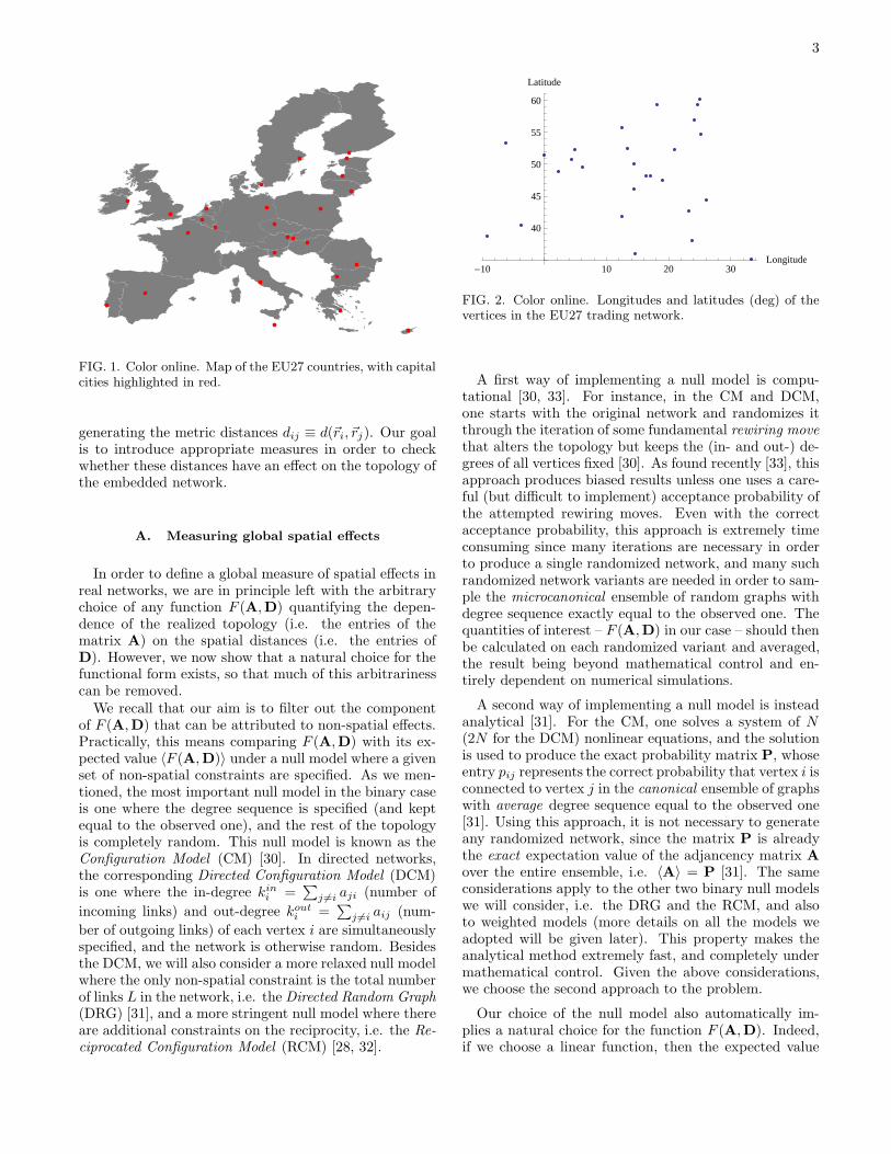
Just to visualize a concrete example, imagine the sub-set of the World Trade Web (graph of the whole WTWwould be confusing), whose vertices are the 27 countriesbelonging to the European Union (EU27). The embed-ding space for this network is shown in Fig. 1, wherevertices are located at capital cities. Figure 2 shows thecities’ coordinates ~ri = (xi, yi) (longitudes and latitudes)

3

FIG. 1. Color online. Map of the EU27 countries, with capitalcities highlighted in red.

generating the metric distances dij ≡ d(~ri, ~rj). Our goalis to introduce appropriate measures in order to checkwhether these distances have an effect on the topology ofthe embedded network.

A. Measuring global spatial effects

In order to define a global measure of spatial effects inreal networks, we are in principle left with the arbitrarychoice of any function F (A,D) quantifying the depen-dence of the realized topology (i.e. the entries of thematrix A) on the spatial distances (i.e. the entries ofD). However, we now show that a natural choice for thefunctional form exists, so that much of this arbitrarinesscan be removed.We recall that our aim is to filter out the component

of F (A,D) that can be attributed to non-spatial effects.Practically, this means comparing F (A,D) with its ex-pected value 〈F (A,D)〉 under a null model where a givenset of non-spatial constraints are specified. As we men-tioned, the most important null model in the binary caseis one where the degree sequence is specified (and keptequal to the observed one), and the rest of the topologyis completely random. This null model is known as theConfiguration Model (CM) [30]. In directed networks,the corresponding Directed Configuration Model (DCM)is one where the in-degree kini =

∑

j 6=i aji (number of

incoming links) and out-degree kouti =∑

j 6=i aij (num-

ber of outgoing links) of each vertex i are simultaneouslyspecified, and the network is otherwise random. Besidesthe DCM, we will also consider a more relaxed null modelwhere the only non-spatial constraint is the total numberof links L in the network, i.e. the Directed Random Graph

(DRG) [31], and a more stringent null model where thereare additional constraints on the reciprocity, i.e. the Re-

ciprocated Configuration Model (RCM) [28, 32].

-10 10 20 30Longitude

40

45

50

55

60

Latitude

FIG. 2. Color online. Longitudes and latitudes (deg) of thevertices in the EU27 trading network.

A first way of implementing a null model is compu-tational [30, 33]. For instance, in the CM and DCM,one starts with the original network and randomizes itthrough the iteration of some fundamental rewiring move

that alters the topology but keeps the (in- and out-) de-grees of all vertices fixed [30]. As found recently [33], thisapproach produces biased results unless one uses a care-ful (but difficult to implement) acceptance probability ofthe attempted rewiring moves. Even with the correctacceptance probability, this approach is extremely timeconsuming since many iterations are necessary in orderto produce a single randomized network, and many suchrandomized network variants are needed in order to sam-ple the microcanonical ensemble of random graphs withdegree sequence exactly equal to the observed one. Thequantities of interest – F (A,D) in our case – should thenbe calculated on each randomized variant and averaged,the result being beyond mathematical control and en-tirely dependent on numerical simulations.

A second way of implementing a null model is insteadanalytical [31]. For the CM, one solves a system of N(2N for the DCM) nonlinear equations, and the solutionis used to produce the exact probability matrix P, whoseentry pij represents the correct probability that vertex i isconnected to vertex j in the canonical ensemble of graphswith average degree sequence equal to the observed one[31]. Using this approach, it is not necessary to generateany randomized network, since the matrix P is alreadythe exact expectation value of the adjancency matrix A

over the entire ensemble, i.e. 〈A〉 = P [31]. The sameconsiderations apply to the other two binary null modelswe will consider, i.e. the DRG and the RCM, and alsoto weighted models (more details on all the models weadopted will be given later). This property makes theanalytical method extremely fast, and completely undermathematical control. Given the above considerations,we choose the second approach to the problem.

Our choice of the null model also automatically im-plies a natural choice for the function F (A,D). Indeed,if we choose a linear function, then the expected value

4

FIG. 3. Color online. Maximally shrunk configuration forthe EU27 trading network with a constraint on the numberof links: f = 0 (N = 27, L = 27).

〈F (A,D)〉 can be calculated exactly as

〈F (A,D)〉 = F (〈A〉,D) = F (P,D) (1)

which only requires the probability matrix P (note thatthe distance matrix D is constant and unaffected by thenull model). The simplest linear choice for a global mea-sure that exploits the entire topological and spatial in-formation (i.e. relevant to all pairs of vertices) is

F ≡N∑

i=1

∑

j 6=i

aijdij (2)

(where we have dropped the dependence on A and D tosimplify the notation), whose expected value reads

〈F 〉 =

N∑

i=1

∑

j 6=i

pijdij (3)

Due to the exact knowledge of P, 〈F 〉 can be computedin a time as short as that required to compute F on thereal network, with no need to generate any realization ofthe null model.Although not fundamentally different, we consider a

slightly more complicated definition, for the unique pur-pose of having a normalized quantity between 0 and 1:

f ≡

∑

i

∑

j 6=i aijdij − Fmin

Fmax − Fmin(4)

where Fmin and Fmax are the minimum and maximumvalues that F can take, given the distance matrix D

and the total number of links L. Explicitly, in termsof the two lists V ↑ and V ↓ introduced above, the maxi-

mum and minimum values for F read Fmin =∑L

n=1 d↑n

and Fmax =∑L

n=1 d↓n. The former extreme (f = 0)

represents the case where the L links are placed amongthe closest couples of nodes (maximally shrunk network).The latter extreme (f = 1) instead represents the casewhere the L links are placed among the most distant

FIG. 4. Color online.Maximally stretched configuration forthe EU27 trading network with a constraint on the numberof links: f = 1 (N = 27, L = 27).

couples of nodes (maximally stretched network). For ourprevious example of the EU27 trading network, thesetwo extremes are shown in Figs. 3 and 4 respectively,where for visualization purposes we have actually chosena value of L equal to N = 27, much less than the realvalue (which would fill the plot with links). This wouldhave been the case, for instance, if in the original networkeach vertex had exactly one outgoing link. Networks inbetween the two extrema would have a value 0 < f < 1.As intuitively rendered by the figures, a larger value of fimplies a more pronounced filling of the available space.Therefore we denote f as the (spatial) filling of the net-work represented by the matrix A.The above choice of the normalization for f is practi-

cal but somewhat arbitrary. For instance, while networksgenerated under the DRG model will achieve the two ex-tremes, networks generated under the DCM (where theconstraints are stricter than just the number of links) willin general do not. For instance, Fig. 5 shows the max-imally shrunk configuration available by imposing thateach vertex has one outgoing link (for simplicity, with-out constraints on the number of incoming links). Thisproduces a filling f = 0.06 > 0. Similarly, in Fig. 6 weshow the maximally stretched configuration under thesame constraints (f = 0.87 < 1). In Fig. 5 the outgoinglink of each vertex is directed towards the closest node,while in Fig. 6 it is directed towards the most distantone.In principle, depending on the null model or on the

type of analysis, one could choose alternative and moreconvenient values for the constants Fmin and Fmax, suchthat f can indeed achieve the extreme values 0 and 1.However, we are interested not in the value of f itself,but rather on its comparison with the expected value

〈f〉 =

∑

i

∑

j 6=i pijdij − Fmin

Fmax − Fmin(5)

under the null model adopted. This makes the choice ofthe constants Fmin and Fmax irrelevant, so we can stickto the option which is easiest to calculate (we will keep

5

FIG. 5. Color online. Maximally shrunk configuration for theEU27 trading network with a constraint on the out-degrees:f = 0.06 (N = 27, kout

i = 1 ∀i).

the one based on the total number of links, i.e. the onenaturally associated with the DRG). Therefore, we willfocus on the following rescaled quantity, which we denoteas the filtered filling:

φ ≡f − 〈f〉

1− 〈f〉(6)

The above quantity is equal to zero whenever the ob-served filling (f or F ) coincides with the expected fill-ing (〈f〉 or 〈F 〉) under the specified model. Positive(negative) values of φ indicate a network which is morestretched (shrunk) than expected. The above definitionfilters out the non-spatial effects encapsulated into thenull model considered, i.e. the random value 〈f〉 thatwould be produced, given the spatial configuration ofvertices, even in a network generated irrespective of thedistances, and only determined by the topological con-straints enforced. Being a rescaled quantity, it also al-lows us to compare the degree of filling in networks withdifferent numbers of vertices and links, or with differentdegree sequences. This also means that we can consis-tently compare different snapshots of the same network,even if the topological properties of the latter change overtime.

B. Local spatial effects

The above considerations also suggest a natural (lin-ear) choice for the definition of local measures of spatialeffects. The two possible building blocks for any linearquantity locally defined around vertex i, in analogy witheq.(2), are the local sums

F outi ≡

∑

j 6=i

aijdij F ini ≡

∑

j 6=i

ajidij (7)

(note that dij = dji), whose expected values under thenull model are

〈F outi 〉 =

∑

j 6=i

pijdij 〈F ini 〉 =

∑

j 6=i

pjidij (8)

FIG. 6. Color online. Maximally stretched configurationfor the EU27 trading network with a constraint on the out-degrees: f = 0.87 (N = 27, kout

i = 1 ∀i).

Again, although this is not strictly necessary, we canrescale F out

i and define the local outward filling as

louti ≡

∑

j 6=i aijdij − (F outi )min

(F outi )max − (F out

i )min(9)

where (F outi )max and (F out

i )min are the two extremevalues of F out

i achieved in a maximally stretched andmaximally shrunk network respectively, for some con-venient reference situation. For consistency with theglobal case, we choose the reference associated withthe DRG, i.e. one where all vertices have on aver-age the same out- and in-degree kout = kin = L/N .

In this case we can write (F outi )min =

∑L/Nn=1 d↑i,n and

(F outi )max =

∑L/Nn=1 d↓i,n, where d

↑i,n and d↓i,n are elements

of the two ordered lists V ↑i = (d↑i,1, . . . , d↑i,n, . . . , d

↑i,N−1)

and V ↓i = (d↓i,1, . . . , d↓i,n, . . . , d

↓i,N−1) of local distances

from vertex i to the other N − 1 vertices (where d↑i,n ≤

d↑i,n+1 and d↓i,n ≥ d↓i,n+1). Note that the above extremesare those achieved by the typical realizations of the DRGwhere all degrees are close to their expected value. Theactual extremes would be either the empty graph andthe complete graph (in the canonical DRG), or the max-imally shrunk and maximally stretched configuration asin the examples of Figs. 3 and 4 (in the microcanonicalDRG). However, in both cases these extreme configura-tions, along with all the other non-typical ones wherethe degrees are far from their expected values, are pro-duced with very small probability. As for the global case,the above choice of (F out

i )max and (F outi )min is arbitrary

(and additionally, in this case louti can be even larger than1 for vertices with large out-degree in the real network).However, this limitation is not essential, since our aim isthe comparison of eq.(9) with its expected value

〈louti 〉 =

∑

j 6=i pijdij − (F outi )min

(F outi )max − (F out

i )min(10)

where (F outi )max and (F out

i )min will be treated as con-

6

stants.In complete analogy with eq.(9), we can also define the

local inward filling as

lini ≡

∑

j 6=i ajidij − (F ini )min

(F ini )max − (F in

i )min(11)

whose expected value is

〈lini 〉 =

∑

j 6=i pjidij − (F ini )min

(F ini )max − (F in

i )min(12)

Note that, due to the symmetry of the distances,(F in

i )min = (F outi )min and (F in

i )max = (F outi )max un-

der the same reference as above. In principle, as for theglobal filling f , we can combine the measured and ex-pected values into a single filtered quantity analogousto eq.(6). However, in this case it is also instructive tocompare louti and lini (which combine local spatial andtopological information) with the out-degree kouti and in-degree kini (which only embody topological information).Therefore we will avoid the introduction of additionalquantities, and simply discuss the impact of spatial andnon-spatical effects by directly comparing measured andexpected values as a function of the degree.We finally introduce a higher-order property which

probes the effects of correlations between vertices.(Dis)assortativity is the (reduced) tendency of verticeswith determined common topological properties to con-nect with each other [1]. A way to measure assortativitylocally is comparing the degree of a vertex with the av-erage degree of its neighbours. We adapt this definitionin order to take into account spatial effects as well, andintroduce the following measures of outward and inward

assortativity:

Aouti ≡

∑

j 6=i aij loutj

kouti

Aini ≡

∑

j 6=i ajilinj

kini(13)

We can approximate the expected values of the abovequantities with

〈Aouti 〉 =

∑

j 6=i pij〈loutj 〉

〈kouti 〉〈Ain

i 〉 =

∑

j 6=i pji〈linj 〉

〈kini 〉(14)

Under the DCM and RCM, 〈kini 〉 = kini and 〈kouti 〉 = kouti

so the above expectations become particularly simple.Moreover, expected and observed values can be comparedby plotting both quantities as a function of the degree ofvertices.

C. Binary null models

Before presenting our results, we describe a bit more indetail the set of null models we adopt in our analysis, inorder to highlight our motivations and also to clarify theinterpretations we can get from the analysis we presentimmediately after.

The method we use is the analytical one proposed bySquartini and Garlaschelli [31]. The method is basedon the class of Exponential Random Graphs (ERGs) [34]that mathematically represent maximum-entropy ensem-bles of networks with specified constraints, and uses theMaximum-Likelihood Principle (MLP) [29] to fit ERGsto real networks. A constraint is a given topological prop-erty (e.g. the number of links), which can be evaluated onany graph G. Different choices of the constraints specifydifferent models in the family of ERGs. For a particularchoice of constraints, the model is specified by a graph

Hamiltonian H(G) which is a linear combination of theconstraints, and hence a function of the particular graphG on which it is evaluated. For binary graphs, one canthink of G as the adjacency matrix (G = A), while forweighted graphs one can think of G as the weight matrix(G = W), where wij is the weight of the link from vertexi to vertex j. In the Hamiltonian, each of the constraintsis coupled to a free parameter acting as a Lagrange mul-tiplier. H(G) uniquely determines the occurrence prob-

ability P (G) = e−H(G)/∑

G′ e−H(G′) of each graph G

in the ensemble. The free parameters are then chosen insuch a way that the likelihood P (G∗) to generate the ob-served network G

∗ is maximum. This parameter choiceautomatically ensures that the expected value of each ofthe constraints is exactly equal to the observed value [29].The fitted parameters are finally used to produce, amongother quantities, the expected values of G under the nullmodel, i.e. the probability matrix P = 〈A〉 = 〈G〉 orthe matrix of expected weights 〈W〉 = 〈G〉 [31]. In thepresent article, we use three null models for binary net-works and two null models for weighted networks.

The first binary null model is the DRG where, as wementioned, the only constraint is the total number oflinks L. In terms of ERGs, the DRG is therefore definedby the following Hamiltonian [34]:

HDRG(G) = θL(G) (15)

Following the general method [31], we fit this model toa real network according to the MLP and obtain the re-sulting parameter value θ∗. The latter is used to producethe probability matrix P, which in this simple case hasall entries equal to pij = e−θ

∗

/(1+ e−θ∗

) = L/N(N − 1).When used to obtain the expected values of the space-dependent quantities we have defined in sections IIA andII B, the DRG filters out the non-spatial effects due tothe overall density of the network, i.e. the spurious spa-tial dependencies only due by chance when on averageL links are placed among vertices with a given spatialconfiguration. Although such overall density effects areimportant, the number of links does not represent a suf-ficiently informative property of real networks. There-fore the non-spatial effects embodied by the DRG arenot highly informative as well. For this reason, we alsoconsider more stringent models.

The second binary null model is the DCM, where the

7

constraints are the in- and out-degree sequence [34–36]:

HDCM (G) =

N∑

i=1

[

θini kini (G) + θouti kouti (G)]

(16)

The MLP yields in this case a more complicated, but stillexact, probability matrix P whose entries are functionsof the fitted values of θini and θouti . The DCM filters outnot only the overall density effects, but also the spuriousspatial dependencies due to the different intrinsic connec-tivities of the vertices of the network. Since the strikingheterogeneity of the degrees of vertices is one of the keyproperties of real networks, the DCM is a very importantnull model. The non-spatial effects filtered out by it arevery informative and robust. For the particular case ofthe WTW, it was shown that the degree sequence is ex-tremely informative, as the DCM very closely reproducesmany higher-order topological properties such as the de-gree correlations and the clustering coefficients [23]. Inour analysis, by filtering out the effects induced by thedegree sequence, the DCM will filter out a significantamount of non-spatial effects present in the WTW.The third and most stringent binary model is the

RCM, where the constraint are the three reciprocated de-

grees of all vertices [28, 31, 32]. The out-degree kouti canbe split in two contributions k→i and k↔i , representingthe number of non-reciprocated outgoing links and thenumber of reciprocated (thus both outgoing and incom-ing) links of vertex i. Similarly, the in-degree kini can besplit in k←i and k↔i , where k←i represents the number ofnon-reciprocated incoming links of vertex i. If we specifythese three degrees separately for each vertex, we obtainthe Hamiltonian for the RCM:

HRCM (G) =

N∑

i=1

[θ←i k←i (G) + θ→i k→i (G) + θ↔i k↔i (G)]

(17)Again, the MLP yields a precise expression [28, 31] forthe exact probability matrix P, which now involves thefitted values of the three sets of parameters θ←i , θ→i , andθ↔i . The RCM controls for the non-spatial effects dueto the different connectivities of vertices, including theirdifferent intrinsic tendency to reciprocate links. The reci-procity is another robust property of real directed net-works [28, 37, 38]. As a consequence, the RCM is a fur-ther improvement with respect to the DCM in cotrollingfor systematic topological effects. In the particular caseof the WTW, is was shown that, unlike the DCM, theRCM almost perfectly reproduces the occurrence of tri-adic motifs [28]. More in general, we note that, in spa-tially embedded networks, both distance-dependence andreciprocity will tend to produce symmetric networks. Forinstance, as shown in Figs. 3 and 4, the two extremes of amaximally shrunk and maximally stretched network arestrongly symmetric (and perfectly symmetric if the num-ber of links is even and the matrix of distances is non-degenerate). In those examples, this effect is entirely dueto the strong dependence on the (necessarily symmetric)

æ

æææ

æ

æ

æ

ææ

æ

ææ

ææ

æææææææ

æ

ææ ææ

æ

æ

ææææææææææ

æ

æ

ææææ

æ

æ

ææææ

à

à

àà

à

à

ààà

à

àà

àà

ààààààà

à

àààà

à

à

àààààààààà

àà

à

àààà

à

àààààà

ì

ì

ìì

ìì

ìì

ì

ìì

ì

ìì

ììì

ì

ì

ìì

ì

ì

ì

ìì

ì

ì

ììì

ììì

ì

ìì

ìì

ìì

ì

ì

ì

ì

ììì

ìììì

1950 1960 1970 1980 1990 2000

-0.24

-0.22

-0.20

-0.18

-0.16

-0.14

-0.12

Year

Φ

FIG. 7. Color online. Filtered binary filling in the WTWfrom 1948 to 2000. Non-spatial effects have been removedusing the Random Graph model (red/rhombus), the Di-rected Configuration Model (blue/cirlces), and the Recip-rocated Configuration Model (yellow/squares).

distances, and not to any reciprocity effect. However, thesame topology would be induced in the opposite situa-tion of maximal reciprocity and no distance dependence.Therefore it is very important, for the specific problem ofassessing spatial effects, to filter out the impact of reci-procity on real networks. The RCM will accurately filterout such strong and systematic topological effects.

D. Spatial effects in the binary WTW

Having clarified our approach in the binary case,we can finally apply it to the topology of the WTW,which represents a challenging and instructive bench-mark wherein spatial effects are expected but weak, as wehave already discussed. We use the database prepared byGleditsch [39] from year 1948 to 2000. During this timespan, the network exhibits an increase in its sizeNt (num-ber of world countries) and connectance ct (link density),from N1948 = 86 and c1948 = 0.39 to N2000 = 187 andc2000 = 0.57. Despite the increase of Nt (mainly dueto the creation of new countries from former Europeancolonies and the Soviet Union), the mean inter-countrydistance µt and variance σ2

t have been remarkably stable,going from µ1948 = 7516 Km and σ2

1948 = 2.3 ∗ 107 Km2

to µ2000 = 7550 Km and σ22000 = 1.9 ∗ 107 Km2. This is

not surprising, since the embedding space of the WTW(the Earth’s surface) is bounded. However, as we nowshow, spatial effects have not remained constant.In Fig. 7 we plot the temporal evolution of the fil-

tered filling corresponding to all null models, i.e. thethree quantities φDRG(t), φDCM (t) and φRCM (t). As ageneral observation, it should be noted that the negativevalues of φ always indicate that the WTW is more spa-tially shrunk than expected on the basis of topologicalconstraints. This means that our method indeed suc-ceeds in uncovering spatial effects that were expected inthe WTW, but that could not detected by previous anal-

8

100 150ki

out

0.01

0.02

0.05

0.10

0.20

0.50

1.00

2.00

liout

FIG. 8. Color online. Local outward filling louti versus out-degree kout

i in the binary WTW (year 2000): observed (blue)and predicted under the DCM (yellow).

yses where non-spatial properties of the real network werecompared with the expectations of the above null models[22–24, 28]. Moreover, the entity of the spatial effects ismoderate (i.e. the values of φ range between −0.10 and−0.25, far from the extreme value −1). This confirmsquantitatively the qualitative expectation that distancesshould play an appreciable but weak role.It is also instructive to inspect the nontrivial tempo-

ral behaviour of the filtered spatial effects. We startby comparing the results obtained under the DRG andthe DCM. Interestingly, apart from the first decade,the trends of φDRG and φDCM are almost perfectly in-verted. Roughly from 1960 to the mid 1970s, φDRG

fluctuated around an increasing trend, while φDCM de-creased steadily. Conversely, from the late 1970s to 2000,φDRG decreased markedly while φDCM increased. Thisresult highlights the importance of the choice of topolog-ical constraints in null models. As we discussed, whilethe number of links used by the DRG is not informativeabout the entire topology of the WTW, the degree se-quence is, to a great extent [23]. Thus, by successfullyreproducing the structure of the WTW, the DCM effec-tively filters out strong topological effects. The net resultis a surprising inversion of the trend generated under theDRG.It should be noted that the rise of φDCM partly over-

laps with the period during which the reciprocity alsostrongly increased in the WTW, i.e. from the late 1980sonward [36]. It therefore becomes important to furthercontrol (using the RCM) for the strong reciprocity which,as we discussed, might have the same apparent impact ofdistance-dependence by enhancing the symmetry of thenetwork. Using the RCM is important in general, as itcontrols for more stringent topological constraints andachieves a better fit to any real directed network (includ-ing the WTW [28]), thus filtering out non-spatial effectseven more accurately than the DCM. As shown in thefigure, we find that the RCM yields almost exactly thesame results as the DCM.We can therefore conlude that, even after disentangling

100 150ki

in0.02

0.05

0.10

0.20

0.50

1.00

2.00

Aiin

FIG. 9. Color online. Local inward filling lini versus in-degreekin

i in the binary WTW (year 2000): observed (blue) andpredicted under the DCM (yellow).

distance and reciprocity effects, global spatial dependen-cies are present throughout the evolution of the WTW,with varying intensity. In particular, the WTW experi-enced a phase of spatial shrinking from 1960 to the mid1970s, followed by a phase of spatial stretching until 2000.The latter trend is probably the result of the economicglobalization. In any case, note that for a network start-ing from a shrunk configuration (i.e. with φ < 0), theevolution towards a more stretched configuration meansthat distances play a smaller and smaller role (i.e. φ get-ting closer to zero). This means that, if the above trendwill persist in time, spatial effects will become less andless important in the WTW.

We deepen our analysis of the binary WTW by study-ing the local spatial quantities defined in eqs. (9)-(14).This is important in order to understand whether indi-vidual vertices contribute uniformly to the global spa-tial effects we characterized above, or whether system-atic heterogeneities are instead present. In Figs. 8 and9 we show the local outward filling louti versus the out-degree kouti and the local inward filling lini versus thein-degree kini , both for the WTW in year 2000 (we ob-served similar results for all snapshots). Along with theobserved quantities, we also plot the expectations underthe DCM. Note that, due to the approximate symmetryof the WTW topology and the exact symmetry of geo-graphic distances, the inward and outward quantities arevery similar. For brevity, given the similarity of the re-sults generated by the DCM and RCM as shown above,we discard the RCM in what follows (this approach isjustified for the specific case of the WTW, but is not arecipe to be followed in general). We find that louti andlini are strongly dependent, but nonlinearly, on kini andkouti respectively. Moreover, for vertices with small andintermediate degree, the observed local (inward and out-ward) filling is significantly smaller than expected underthe DCM. This difference gradually reduces as the degreeincreases, and for vertices with large degree the observedand expected values coincide. This means that poorly

9

50 100 150ki

out

0.5

1.0

1.5

Aiout

FIG. 10. Color online. Outward assortativity Aout

i versusout-degree kout

i in the binary WTW (year 2000): observed(blue) and predicted under the DCM (yellow).

connected countries tend to trade more locally (i.e. togeographically closer countries) than expected only onthe basis of the different numbers of trade partners of allcountries. By contrast, highly connected countries areless limited by distances, as clear in the extreme case of acountry trading with all other countries, an ‘unavoidable’space-neutral configuration which coincides with the nullmodel’s prediction, irrespective of spatial dependencies.It is interesting to notice that, since the number of tradepartners (degree) is strongly correlated with the GDP[22], the above results can be rephrased in terms of thedifferent resistance to trade that geographic distances im-pose on poor (strong resistance) and rich (weak or no re-sistance) countries. We therefore find that the global spa-tial effects captured by φ arise from the combination ofheterogeneous contributions from different vertices, andare not representative of the more diverse local patterns.We finally study the distance-induced correlation pro-

files by plotting, in Figs. 10 and 11, the outward andinward assortativity (Aout

i and Aini ) versus the out- and

in-degree (kouti and kini ), again for the WTW in year2000. We find clearly decreasing trends, indicating thatcountries with large degree trade with countries that areembedded in a more spatially shrunk trade neighbor-hood, while countries with few connections trade withcountries that have a more spatially stretched neighbor-hood (where by ‘neighborhood’ of a vertex we mean theset of vertices topologically connected to that vertex viaa link, and not the set of geographically close vertices).However, the expected values are also decreasing, even ifsystematically larger than the observed ones. This meansthat the negative correlation between the degree of a ver-tex and the average filling of its neighbours is simply in-terpretable as a negative correlation between the degreesof neighboring vertices imposed by the specific degree se-quence (well documented in the WTW [22, 23]), throughthe relation between degree and filling already shown inFigs. 8 and 9. Therefore we find that the mere decreaseof the trend is not informative per se about spatial effects.Rather, it is the comparison with the null model that con-

50 100 150ki

in

0.2

0.4

0.6

0.8

1.0

1.2

1.4

Aiin

FIG. 11. Color online. Inward assortativity Ain

i versus in-degree kin

i in the binary WTW (year 2000): observed (blue)and predicted under the DCM (yellow).

veys information: the systematic difference between theobserved and expected value of the assortativity showsthat, irrespective of their degree, all countries tend totrade with countries that are embedded in a more spa-tially shrunk trade neighborhood than expected on thebasis of topological constraints. This confirms that ourmethod successfully disentangles spatial and non-spatialeffects, even when both produce similar patterns.

III. WEIGHTED ANALYSIS

In this section we extend our formalism to weightednetworks. As we mentioned, a weighted graph G is de-scribed by a weight matrixW whose entries wij representthe intensity of the link from vertex i to vertex j (includ-ing wij = 0 if no link is there). As for binary networks,we assume no self-loops, i.e. wii = 0 ∀i. In weighted net-works, the analogue of the degree is the strength. For adirected network, the out-strength souti =

∑

j 6=i wij is thetotal weight of the outgoing links of vertex i, and simi-larly the in-strength sini =

∑

j 6=i wji is the total weightof the incoming links of vertex i. The total weight of anetwork is the sum of the weights of all directed links,

i.e. W =∑N

i=1

∑

j 6=i wij =∑N

i=1 souti =

∑Ni=1 s

ini .

A. Generalizing the binary approach

For weighted networks, in order to filter out non-spatialeffects encoded in structural constraints, we will use twonull models generated according to the same analyticalmethod [31] we used so far.The first null model is the Weighted Random Graph

Model (WRG) [31, 40], which is the analogue of the DRG.In this model, the only constraint is the total weight W ,so its Hamiltonian reads

HWRG(G) = θW (G) (18)

10

The WRG filters out the non-spatial effects due to theoverall intensity of connections in a real network. In theWRG, every vertex has on average the same out- and in-strength sout = sin = W/N . The out- and in-strengths ofvertices follow a negative binomial distribution with theabove mean value, and link weights follow a geometricdistribution with mean W/N(N − 1) [40].The second null model we consider is the Weighted

Configuration Model (WCM) [31], which is the analogueof the DCM. The constraints are the out-strength andin-strength of all vertices:

HWCM (G) =

N∑

i=1

[

θini sini (G) + θouti souti (G)]

(19)

The WCM controls for non-spatial effects due to the dif-ferent intrinsic sizes or capacities of vertices. As theDCM, the WCM is very important in order to filter outapparent spatial dependencies that are only due to theheterogeneity of the weights induced by the strength ofvertices. As we discuss later, in the particular case of theWTW this model is particularly appropriate as it indi-rectly controls for the heterogeneity of the GDP of worldcountries.For simplicity, in the weighted case we do not con-

sider the equivalent of the RCM, i.e. a weighted modelthat controls for reciprocated and non-reciprocated in-teractions separately. In fact, we expect that, as in thebinary case, such a model would be indistinguishable (asfar as spatial effects are considered) from the WCM. Forthe interested reader, a detailed description of the recip-rocated weighted configuration model is provided in ref.[38]. What follows can be directly extended in order toinclude that model as well.Following the general method [31], both the WRG and

the WCM can be fitted to the real network to gener-ate the exact matrix 〈W〉 of expected weights. Again,this suggests that a natural choice for any functionF (W,D) aimed at measuring the effects of distances onthe weighted structure of a network is the linear one, sothat the expectation value can be obtained exactly as〈F (W,D)〉 = F (〈W〉,D). Therefore it is easy to gener-alize the linear binary quantities we introduced in sectionII to the weighted case. Starting from the quantity

F ≡

N∑

i=1

∑

j 6=i

wijdij (20)

we introduce the rescaled global filling, in analogy witheq. (4), as

f ≡

∑

i

∑

j 6=i wijdij − Fmin

Fmax − Fmin(21)

where now Fmin and Fmax are chosen as the two extremevalues that F can take in a network with the same totalweight W as the original network, i.e. Fmin = Wd↑1 and

Fmax = Wd↓1 (d↑1 and d↓1 are the smallest and largest

distance between vertices respectively). This referencecorresponds to the WRG, and is analogous to the choiceof the DRG we made in the binary case.The filtered filling that properly controls for non-

spatial effects embodied in a null model is again

φ ≡f − 〈f〉

1− 〈f〉(22)

where 〈f〉 is now obtained by replacing wij with 〈wij〉in eq. (21). Positive (negative) values of φ indicate anetwork which is more stretched (shrunk) than expected.For a space-independent network, φ = 0.For the local weighted quantities, from the sums

F outi ≡

∑

j 6=i

wijdij F ini ≡

∑

j 6=i

wjidij (23)

we define the local outward filling as

louti ≡

∑

j 6=i wijdij − (F outi )min

(F outi )max − (F out

i )min(24)

and the local inward filling as

lini ≡

∑

j 6=i wjidij − (F ini )min

(F ini )max − (F in

i )min(25)

Consistently with the global case and in analogy with thebinary one, we choose the extreme values to correspondto the maximally stretched and maximally shrunk con-figuration achieved by a typical realization of the WRG(where all strengths are close to their expected value

W/N), i.e. (F outi )max = (F in

i )max = Wd↓i,1/N and

(F outi )min = (F in

i )min = Wd↑i,1/N . The expected val-ues of the above quantities are

〈louti 〉 =

∑

j 6=i〈wij〉dij − (F outi )min

(F outi )max − (F out

i )min(26)

〈lini 〉 =

∑

j 6=i〈wji〉dij − (F ini )min

(F ini )max − (F in

i )min(27)

Finally, we define the local outward assortativity andthe local inward assortativity as

Aouti ≡

∑

j 6=i wij loutj

souti

Aini ≡

∑

j 6=i wjilinj

sini(28)

The expected values can be approximated as

〈Aouti 〉 =

∑

j 6=i〈wij〉〈loutj 〉

〈souti 〉〈Ain

i 〉 =

∑

j 6=i〈wji〉〈linj 〉

〈sini 〉(29)

For the WCM, since 〈sini 〉 = sini and 〈souti 〉 = souti , theobserved and expected assortativities can be comparedby plotting both quantities as functions of the strengthof vertices.

11

æ

æ

æ

æææææææææ

æææææææææææ

ææ æææææææ

ææææææææææ

ææ

æææææ

æææ

à

à

à

à

àà

àààààà

àà

ààààààààààà

àààà

ààà

ààààà

àààà

à

àà

à

ààà

àààà

1950 1960 1970 1980 1990 2000

-0.30

-0.25

-0.20

-0.15

-0.10

Year

Φ

FIG. 12. Color online. Filtered weighted filling in the WTWfrom 1948 to 2000. Non-spatial effects have been removedusing the Weighted Random Graph model (yellow) and theWeighted Configuration Model (blue).

B. Spatial effects in the weighted WTW

We now employ the quantities defined above in orderto perform a weighted analysis of the WTW. The evolu-tion of φWRG and φWCM is shown in Fig. 12. The trendsare the weighted counterparts of those shown previouslyin Fig. 7. Both quantities are always negative, indicat-ing that, even after taking into account the intensity oftrade flows, the WTW is still found to be more spatiallyshrunk than expected under non-spatial models. Thisconfirms the general lesson learnt from gravity models inthe economic literature [25, 26], but with a big difference:while gravity models only take into account the observednon-zero flows, and completely disregard missing links[27], here we are combining the weighted information ofnonzero flows with the topological information of missinglinks, as our quantities exploit the full matrix W. Theend result is that spatial effects are significant but weak,as the values of φ (especially under the WCM) are small.

At this point it is worth observing that the WCM, by

107 108 109si

out

0.001

0.01

0.1

1

10

liout

FIG. 13. Color online. Weighted outward filling louti versusout-strength souti in the weighted WTW (year 2000): observed(blue) and predicted under the WCM (yellow).

controlling for the strengths of vertices (total exports andtotal imports of all countries), automatically controls forthe GDP, since the linear correlation between the latterand the total exports (or imports) of a country is ex-tremely high. This important aspect of the WCM is simi-lar to the GDP-dependence in gravity models, and makesthe WCM a more accurate and economically meaningfulnull model than the WRG. In any case, unlike gravitymodels, our approach is not intended to provide a spa-tial model of trade, but only to single out statisticallyrobust space-dependencies that can be used in the futureto develop an improved spatially explicit model.

As for the binary case, we find that different null mod-els provide a very different filtering of non-spatial effects,even over time. Apart from the first snapshot, φWCM

first increases, then remains almost constant (during the1970s) and finally decreases, approximately following aninverted U shape with small fluctuations. By contrast,φWRG first decreases and then displays large fluctuationsaround an approximately constant trend. Quite surpris-ingly, these trends are almost opposite to the correspond-ing binary trends, and in particular φWCM appears toindicate an unexpected spatial shrinking of the networkfrom 1980 onwards, depite the economic globalization.However, it should be noted that while the DCM repro-duces the higher-order properties of the binary WTWwith good accuracy [23], the WCM does not satisfacto-rily reproduce the observed weighted WTW [24]. There-fore, even if the WCM accurately controls for the totalimport and exports (hence the GDP) of world countries,it does not entirely filter out other non-spatial effects, atleast not as stringently as its binary counterpart.

We finally consider the local spatial effects in theweighted WTW. Figures 13-16 show the quantities de-fined in Eqs. (24)-(29), where the null model used isthe WCM. The increasing trends mean that rich con-tries have a more spatially stretched trade neighborhoodthan poor countries. However, as opposed to the binaryresults, here we find that the observed and expected val-

107 108 109si

in

0.001

0.01

0.1

1

10

liin

FIG. 14. Color online. Weighted inward filling lini versusin-strength sini in the weighted WTW (year 2000): observed(blue) and predicted under the WCM (yellow).

12

105 107 109si

out5´10-5

1´10-4

5´10-4

0.001

0.005

Aiout

FIG. 15. Color online. Weighted outward assortativity Aout

i

versus out-strength souti in the weighted WTW (year 2000):observed (blue) and predicted under the WCM (yellow).

ues of the local filling (louti and lini ) are almost always inclose agreement, except for minor differences in the scat-tered values of vertices with small strength (Figs. 13 and14). This means that the global spatial effects detectedby φ are due to the combination of local effects involv-ing only vertices with very small values of the strength,i.e. the poorest countries with small GDP and small im-port/export values. Interestingly, the richest countriesappear not to be affected by distances at all, in bothimports and exports.By contrast, the observed assortativities are system-

atically larger than the expectations of the WCM (Figs.15 and 16). However, looking at the definition in Eq.(29), we find that the cause of this divergence must bethe difference between wij and 〈wij〉, and not the tinydisagreement between the observed and expected valuesof louti and lini shown above (of course, the expected andobserved strengths are identical by construction). Thestrong difference between wij and 〈wij〉 under the WCMhas already been well documented in ref. [24]. This con-firms the different interpretations we can get from thebinary and weighted analysis of the WTW. While the re-markable agreement between the DCM and the observedtopology of the WTW [23] ensures that the DCM accu-rately controls for non-spatial effects, the disagreementbetween the WCM and the real WTW [24] implies thatthe final differences are partly due to the disagreementitself (i.e. differences between observed and expectedquantities, irrespective of spatial effects). Still, as far asthe problem of controlling for the intrinsic heterogeneityof vertices (in terms of import, exports, and indirectlyGDP), the WCM yields the correct answer.

IV. CONCLUSIONS

In this paper we have introduced a simple frameworkto detect spatial effects in geometrically embedded net-works. We have proposed global and local measures ofspace dependence for both binary and weighted networks.

104 105 106 107 108 109 1010si

in

1´10-4

2´10-4

5´10-4

0.001

0.002

0.005

Aiin

FIG. 16. Color online. Weighted inward assortativity Ain

i

versus in-strength sini in the weighted WTW (year 2000): ob-served (blue) and predicted under the WCM (yellow).

Our approach makes intense use of null models intendedto preserve non-spatial constraints that strongly and un-avoidably affect the structure of any network, irrespec-tive of any spatial arrangement. This allowed us to filterout, from the measured spatial effects, a spurious com-ponent due either to the overall density and intensity ofconnections (as in the DRG and WRG), or to the intrin-sic heterogeneity of vertices (as in the DCM, RCM andWCM).We tested our approach on the WTW, which is affected

by both non-spatial constraints [22–24] and geographicdistances [25, 26]. The dependence of the weightedWTWon distances is well documented by gravity models, how-ever the latter are generally fitted to the observed non-zero weights of the network, and hence disregard theeffects of distances on the creation of links, and henceon the binary topology [27]. By constrast, our weightedanalysis of the WTW takes into account both zero andnon-zero weights, as it exploits the full matrix W. A re-cent study employed a more sophisticated class of GravityModels (the so-called ‘Zero-Inflated’ models) [27] whichcan also incorporate zero flows, thus aiming at reproduc-ing topology and weights simultaneously. The importantresult of this study is that even these generalized modelsfail in reproducing the properties of the WTW. In otherwords, unless the topology is pre-specified, Gravity Mod-els perform not satisfactorily. These results show that,if the binary topology is taken into account, the WTWis less clearly affected by geographic distances than ordi-narily thought. At the same time, it has been shown thatthe binary structure of the WTW is strongly dependenton the degree-sequence [23] and indirectly on the GDP[22].Taken together, the above results imply that spatial

effects in the binary WTW, if present, are expected tobe weak. This makes the WTW an ideal candidate fortesting our method, due to the challenge of disentanglingspatial dependencies and strong topological constraints.Indeed, we showed that our method is able to detect weakspatial effects even in a network which is dominated by

13

non-spatial constraints. Our results confirm the impor-tance of the use of null models in the analysis of real-world networks, including spatially embedded ones.

ACKNOWLEDGMENTS

FR acknowledges the University of Siena for the fi-nancial support and the Instituut-Lorentz for Theoreti-

cal Physics of Leiden for the logistic, scientific and moralsupport received during the visit. DG acknowledges sup-port from the Dutch Econophysics Foundation (Sticht-ing Econophysics, Leiden, Netherlands) with funds frombeneficiaries of Duyfken Trading Knowledge BV, Amster-dam, The Netherlands. RB acknowledges support fromthe FESSUD project on “Financialisation, economy, so-ciety and sustainable development”, Seventh FrameworkProgramme, EU. Authors warmly thank Tiziano Squar-tini for his kind and insightful comments that helped usimprove a previous version of this paper.

[1] G. Caldarelli, Scale-Free Networks: Complex Webs inNature and Technology (Oxford University Press, Ox-ford, 2007).

[2] A. Barrat, M. Barthelemy, and A. Vespignani, Dynami-cal Processes on Complex Networks (Cambridge Univer-sity Press, 2008).

[3] M. Barthelemy, Physics Reports 499, 1 (2011).[4] G. B. West, J. H. Brown, and B. J. Enquist, Science

284, 1677 (1999).[5] G. B. West, J. H. Brown, and B. J. Enquist, Nature 413,

628 (2001).[6] L. M. A. Bettencourt, J. Lobo, D. Helbing, C. Kuhnert,

and G. B. West, PNAS 104, 7301 (2007).[7] A. Bejan and S. Lorente, Philosophical Transactions

of the Royal Society B: Biological Sciences 365, 1335(2010).

[8] O. Woolley-Meza, C. Thiemann, D. Grady, J. Lee,H. Seebens, B. Blasius, and D. Brockmann, The Euro-pean Physical Journal B - Condensed Matter and Com-plex Systems , 1 (2011).

[9] P. Kaluza, A. Kolzsch, M. T. Gastner, and B. Blasius,Journal of The Royal Society Interface 7, 1093 (2010).

[10] G. B. West, J. H. Brown, and B. J. Enquist, Science276, 122 (1997).

[11] J. R. Banavar, A. Maritan, and A. Rinaldo, Nature 399,130 (1999).

[12] D. Queiros-Conde, J. Bonjour, W. Wechsatol, and A. Be-jan, Physica A: Statistical Mechanics and its Applica-tions 384, 719 (2007).

[13] L. Rocha, E. Lorenzini, and C. Biserni, InternationalCommunications in Heat and Mass Transfer 32, 1281(2005).

[14] D. P. Bebber, J. Hynes, P. R. Darrah, L. Boddy, andM. D. Fricker, Proc. R. Soc. B 274, 2307 (2007).

[15] A. Tero, S. Takagi, T. Saigusa, K. Ito, D. P. Bebber,M. D. Fricker, K. Yumiki, R. Kobayashi, and T. Naka-gaki, Science 327, 439 (2010).

[16] R. E. Ulanowicz, Growth and Development: EcosystemsPhenomenology (iUniverse, 2000).

[17] B. D. Fath, B. C. Patten, and J. S. Choi, Journal ofTheoretical Biology 208, 493 (2001).

[18] D. Garlaschelli, G. Caldarelli, and L. Pietronero, Nature423, 165 (2003).

[19] J. Zhang and L. Guo, Journal of Theoretical Biology 264,760 (2010).

[20] M. Barthelemy, EPL (Europhysics Letters) 63, 915(2003).

[21] S. Bradde, F. Caccioli, L. Dall’Asta, and G. Bianconi,Phys. Rev. Lett. 104, 218701 (2010).

[22] D. Garlaschelli and M. I. Loffredo, Phys. Rev. Lett. 93,188701 (2004).

[23] T. Squartini, G. Fagiolo, and D. Garlaschelli, PhysicalReview E 84, 046117 (2011).

[24] T. Squartini, G. Fagiolo, and D. Garlaschelli, PhysicalReview E 84, 046118 (2011).

[25] R. C. Feenstra, J. R. Markusen, and A. K. Rose, TheCanadian Journal of Economics / Revue Canadienned’Economique 34, 430 (2001).

[26] J. E. Anderson and Y. V. Yotov, Gold Standard Grav-ity, Working Paper 17835 (National Bureau of EconomicResearch, 2012).

[27] M. Duenas and G. Fagiolo, Modeling the International-Trade Network: A Gravity Approach, LEM Papers Se-ries 2011/25 (Laboratory of Economics and Management(LEM), Sant’Anna School of Advanced Studies, Pisa,Italy, 2011).

[28] T. Squartini and D. Garlaschelli, in Self-Organizing Sys-tems, Lecture Notes in Computer Science, Vol. 7166,edited by F. Kuipers and P. Heegaard (Springer Berlin /Heidelberg, 2012) pp. 24–35.

[29] D. Garlaschelli and M. I. Loffredo, Phys. Rev. E 78,015101 (2008).

[30] S. Maslov and K. Sneppen, Science 296, 910 (2002).[31] T. Squartini and D. Garlaschelli, New Journal of Physics

13, 083001 (2011).[32] D. Garlaschelli and M. I. Loffredo, Phys. Rev. E 73,

015101 (2006).[33] E. S. Roberts and A. C. C. Coolen, Phys. Rev. E 85,

046103 (2012).[34] J. Park and M. E. J. Newman, Phys. Rev. E 70, 066117

(2004).[35] D. Garlaschelli, F. Ruzzenenti, and R. Basosi, Symmetry

2, 1683 (2010).[36] F. Ruzzenenti, D. Garlaschelli, and R. Basosi, Symmetry

2, 1710 (2010).[37] D. Garlaschelli and M. I. Loffredo, Phys. Rev. Lett. 93,

268701 (2004).[38] T. Squartini, F. Picciolo, F. Ruzzenenti, and D. Gar-

laschelli, ArXiv e-prints (2012), arXiv:1208.4208.[39] K. S. Gleditsch, Journal of Conflict Resolution 46, 712

(2002).[40] D. Garlaschelli, New Journal of Physics 11, 073005

(2009).