arX

iv:n

lin/0

1090

23v1

[nl

in.C

D]

18

Sep

2001 On the performance of different

synchronization measures in real data: a case

study on EEG signals

R. Quian Quiroga†∗, A. Kraskov†, T. Kreuz†‡, and P. Grassberger†

†John von Neumann Institute for Computing,

Forschungszentrum Julich GmbH,

D - 52425 Julich, Germany

‡Department of Epileptology, University of Bonn,

Sigmund-Freud Str. 25,

D - 53105 Bonn, Germany

February 4, 2008

PACS numbers: 05.45.Tp; 87.90.+y; 87.19.Nn 05.45.Xt

∗ corresponding author

1

Abstract

We study the synchronization between left and right hemisphere

rat EEG channels by using various synchronization measures, namely

non-linear interdependences, phase-synchronizations, mutual informa-

tion, cross-correlation and the coherence function. In passing we show

a close relation between two recently proposed phase synchronization

measures and we extend the definition of one of them. In three typical

examples we observe that except mutual information, all these mea-

sures give a useful quantification that is hard to be guessed beforehand

from the raw data. Despite their differences, results are qualitatively

the same. Therefore, we claim that the applied measures are valuable

for the study of synchronization in real data. Moreover, in the partic-

ular case of EEG signals their use as complementary variables could

be of clinical relevance.

2

1 Introduction

The concept of synchronization goes back to the observation of interactions

between two pendulum clocks by Huygens. Synchronization of oscillatory

systems has been widely studied but it was not until recently that synchro-

nization between chaotic motions received attention. A first push in this

direction was the observation of identical synchronization of chaotic systems

[1, 2, 3, 4]. But more interesting has been the idea of a “generalized syn-

chronization” relationship as a mapping between non-identical systems, and

the further proposal by Rulkov et al. [5] of a topological method to quantify

it. The work of Rulkov and coworkers indeed triggered a number of studies

applying the concept of generalized synchronization to real data. One of

these applications is to the study of electroencephalographic (EEG) signals,

where synchronization phenomena have been increasingly recognized as a key

feature for establishing the communication between different regions of the

brain [6], and pathological synchronization as a main mechanism responsible

of an epileptic seizure [7]. Since many features of EEG signals cannot be

generated by linear models, it is generally argued that non-linear measures

are likely to give more information than the one obtained with conventional

linear approaches.

In a first study dealing with EEG signals, Schiff and coworkers [8] applied

a synchronization measure similar to the one defined in [5] to the study

of data from motoneurons within a spinal cord pool. More recently, non-

linear synchronization measures were used for the analysis of EEG data from

epileptic patients with the main goal of localizing the epileptogenic zone and

of predicting the seizure onset[9, 10, 11]. These results, of course, have a clear

clinical relevance. Arnhold and coworkers [11] proposed a robust measure (S),

1

a variant of which (H), already mentioned by these authors, has been studied

in detail in [12]. These last two measures of interdependence, together with

a new measure (N) to be defined, will be further studied in this paper.

The previous papers give convincing arguments in favor of using non-

linear interdependences, which in most cases were illustrated with examples

using chaotic toy models. However, it still remains an open question whether

this also holds true for real data. In this paper we therefore address the point

of whether non-linear measures give a relevant contribution to the study of

synchronization in electroencephalographic (EEG) signals [13]. In particular,

we will show with three typical EEG examples (see Fig. 1) how non-linear

interdependence measures can disclose information difficult to obtain by vi-

sual inspection. Although the data are EEG recordings from rats, their main

features are common to human EEG. Moreover, results should not be re-

stricted to EEG data and should also be valuable to study synchronization

of other signals. For comparison purposes, we will also study phase synchro-

nization measures as defined from the Hilbert transform [14] and from the

Wavelet transform [15], which had been recently applied to the study of EEG

signals [16, 18, 19]. Moreover, we will also compare these results with the

ones obtained with more conventional measures of synchronization, such as

the cross-correlation, the coherence function and the mutual information.

The paper is organized as follows: In section 2 we define the synchroniza-

tion measures to be used. In particular, in section 2.1 we define the linear

cross-correlation and the coherence function, while in section 2.2 we describe

three recently proposed measures of non-linear interdependence. The mutual

information is defined in section 2.3, whereas section 2.4 is dedicated to the

description of phase synchronization measures with the phases defined from

a Hilbert transform. Very close to these last measures are the ones described

2

in section 2.5 but in this case the phases are defined from the Wavelet trans-

form. Finally in section 2.6 we show the relation between these two phase

synchronization approaches. Details of the data sets to be analyzed are dis-

closed in section 3. In section 4 we describe the results obtained by applying

the different synchronization measures to these data sets. Finally in section

5 we present the conclusions.

2 Synchronization measures

In the following, unless when further specified, we shall use the notion of

synchronization in a very loose sense. Thus it is more or less synonymous

with interdependence or (strong) correlation.

2.1 Linear measures of synchronization

Let us suppose we have two simultaneously measured discrete univariate time

series xn and yn, n = 1, . . . , N . The most commonly used measure of their

synchronization is the cross-correlation function defined as:

cxy(τ) =1

N − τ

N−τ∑

i=1

(xi − x

σx) · (

yi+τ − y

σy) (1)

where x and σx denote mean and variance, and τ is a time lag. The cross-

correlation gives a measure of the linear synchronization between x and y.

Its absolute value ranges from zero (no synchronization) to one (maximum

synchronization) and it is symmetric: cxy(τ) = cyx(τ).

The sample cross-spectrum is defined as the Fourier transform of the

cross-correlation or, via the Wiener-Khinchin theorem, as:

Cxy(ω) = (Fx)(ω) · (Fy)∗(ω) (2)

3

where (Fx) is the Fourier transform of x, ω are the discrete frequencies

( −N/2 < ω < N/2) and ∗ means complex conjugation. For details of the

implementation, see sec. 4.1. The cross-spectrum is a complex number whose

normalized amplitude

Γxy(ω) =|Cxy(ω)|

√

Cxx(ω) ·√

Cyy(ω), (3)

is called the coherence function and gives a measure of the linear synchro-

nization between x and y as a function of the frequency ω. This measure

is very useful when synchronization is limited to some particular frequency

band, as it is usually the case in EEG signals (see [20] for a review).

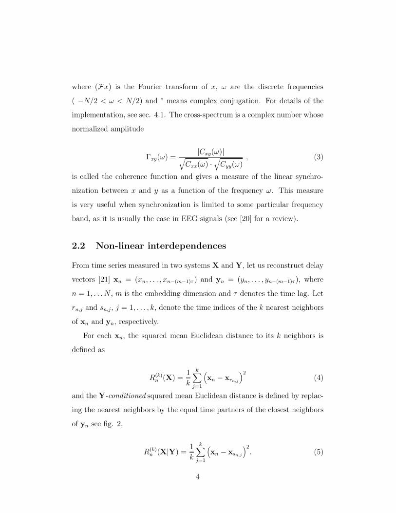
2.2 Non-linear interdependences

From time series measured in two systems X and Y, let us reconstruct delay

vectors [21] xn = (xn, . . . , xn−(m−1)τ ) and yn = (yn, . . . , yn−(m−1)τ ), where

n = 1, . . . N , m is the embedding dimension and τ denotes the time lag. Let

rn,j and sn,j, j = 1, . . . , k, denote the time indices of the k nearest neighbors

of xn and yn, respectively.

For each xn, the squared mean Euclidean distance to its k neighbors is

defined as

R(k)n (X) =

1

k

k∑

j=1

(

xn − xrn,j

)2(4)

and the Y-conditioned squared mean Euclidean distance is defined by replac-

ing the nearest neighbors by the equal time partners of the closest neighbors

of yn see fig. 2,

R(k)n (X|Y) =

1

k

k∑

j=1

(

xn − xsn,j

)2. (5)

4

If the point cloud {xn} has an average squared radius R(X) = 1N

∑Nn=1 R(N−1)

n (X),

then R(k)n (X|Y) ≈ R(k)

n (X) ≪ R(X) if the systems are strongly correlated,

while R(k)n (X|Y) ≈ R(X) ≫ R(k)(X) if they are independent. Accordingly,

we can define an interdependence measure S(k)(X|Y) [11] as

S(k)(X|Y) =1

N

N∑

n=1

R(k)n (X)

R(k)n (X|Y)

. (6)

Since R(k)n (X|Y) ≥ R(k)

n (X) by construction, we have

0 < S(k)(X|Y) ≤ 1. (7)

Low values of S(k)(X|Y) indicate independence between X and Y, while high

values indicate synchronization (reaching maximum when S(k)(X|Y) → 1).

Following ref.[11, 12] we define another non-linear interdependence mea-

sure H(k)(X|Y) as

H(k)(X|Y) =1

N

N∑

n=1

logRn(X)

R(k)n (X|Y)

(8)

This is zero if X and Y are completely independent, while it is positive if

nearness in Y implies also nearness in X for equal time partners. It would be

negative if close pairs in Y would correspond mainly to distant pairs in X.

This is very unlikely but not impossible. Therefore, H(k)(X|Y) = 0 suggests

that X and Y are independent, but does not prove it. This is one main

difference between H(k)(X|Y) and the mutual information, to be defined in

sec. 2.3. The latter is strictly positive whenever X and Y are not completely

independent. As a consequence, mutual information is quadratic in the cor-

relation P (X,Y)−P (X)P (Y) for weak correlations (P are here probability

distributions), while H(k)(X|Y) is linear. Thus H(k)(X|Y) is more sensitive

to weak dependences which might make it useful in applications. Also, it

should be easier to estimate than mutual informations which are notoriously

hard to estimate reliably as we will see later.

5

In a previous study with coupled chaotic systems [12], H was more robust

against noise and easier to interpret than S, but with the drawback that it

is not normalized. Therefore, we propose a new measure N(X|Y) using also

a different way of averaging,

N (k)(X|Y) =1

N

N∑

n=1

Rn(X) − R(k)n (X|Y)

Rn(X)(9)

which is normalized (but as in the case of H , it can be slightly negative) and

in principle more robust than S.

The opposite interdependences S(Y|X), H(Y|X) and N(Y|X) are de-

fined in complete analogy and they are in general not equal to S(X|Y),

H(X|Y) and N(Y|X), respectively. The asymmetry of S, H and N is

the main advantage over other non-linear measures such as the mutual in-

formation and the phase synchronizations defined in sections 2.4 and 2.5.

This asymmetry can give information about driver-response relationships

[11, 12, 22], but can also reflect the different dynamical properties of each

data [11, 12]. To address this point we will compare results with synchro-

nization values obtained from time shifted signals used as surrogates.

Figure 2 illustrates the idea of how the non-linear interdependence mea-

sures work. Let us consider a Lorenz and a Roessler system that are in-

dependent (upper case, no coupling) and a second case with the Roessler

driving the Lorenz via a strong coupling (lower plot). For a detailed study of

synchronization between these systems refer to [12]. Given a neighborhood

in one of the attractors, we see how this neighborhood maps in the other.

If the point cloud is still a small neighborhood (lower plot), the systems are

synchronized. On the other hand, if the points are spread over the attractor

(upper plot), the systems are independent. The three measures described S,

H and N , are just different ways of normalizing these ratio of distances.

6

2.3 Mutual Information

The previous measures of synchronization were based on similarities in the

time and frequency domain (sec. 2.1) or on similarities in a phase space (sec.

2.2). In this section we describe an approach to measure synchronization by

means of information-theoretic concepts. Let us suppose we have a discrete

random variable X with M possible outcomes X1, . . . , XM , obtained e.g. by a

partition of X into M bins. Each outcome has a probability pi, i = 1, . . . , M ,

with pi ≥ 0 ∀i and∑

pi = 1. A first estimate is to consider pi = ni/N ,

where ni is the number of occurrences of Xi after N samples. From this set

of probabilities the Shannon entropy is defined as:

I(X) = −M∑

i=1

pi log pi (10)

The Shannon entropy is positive and measures the information content of

X, in bits, if the logarithm is taken with base 2. When finite samples N are

considered, the naive definition pi = ni/N may not be appropriate. Grass-

berger [23] introduced a series of correction terms, which are asymptotic in

1/N . The first and most important term essentially gives

I(X) ≈∑

i

ni

N(log N − Ψ(ni)) (11)

with Ψ(x) = d log Γ(x)/dx ≈ log x − 1/2x for large x.

Let us now suppose we have a second discrete random variable Y , whose

degree of synchronization with X we want to measure. The joint entropy is

defined as:

I(X, Y ) = −∑

i,j

pXYij log pXY

ij (12)

7

where pXYij is the joint probability of X = Xi and Y = Yj. If the systems

are independent we have pXYij = pX

i · pYj and then, I(X, Y ) = I(X) + I(Y ).

Thus, the mutual information between X and Y is defined as

MI(X, Y ) = I(X) + I(Y ) − I(X, Y ) (13)

which indicates the amount of information of X we obtain by knowing Y

and vice versa. If X and Y are independent, MI(X, Y ) = 0 and otherwise,

it will take positive values with a maximum of MI(X, X) = I(X) for iden-

tical signals. Note also that MI is symmetric, i.e. MI(X, Y ) = MI(Y, X).

Schreiber extended the concept of MI and defined a transfer entropy [24],

which has the main advantage of being asymmetric and can in principle dis-

tinguish driver-response relationships. Another asymmetric measure based

on the MI has been proposed by Palus [25].

Mutual information can also be regarded as a Kullback-Leibler entropy

[26, 27], which is an entropy measure of the similarity between two probability

distributions. To illustrate this, we rewrite eq.(13) in the form

MI(X, Y ) =∑

pXYij log

pXYij

pXi · pY

j

(14)

Then, considering a probability distribution qXYij = pX

i · pYj (which is the

correct probability distribution if the systems are independent), eq. (14) is a

Kullback-Leibler entropy and measures the difference between the probability

distributions pXYij and qXY

ij [28]. In other words, MI(X, Y ) measures how

different is the true joint probability distribution pXYij from another in which

independence between X and Y is assumed.

We previously mentioned that each pi can be obtained by a partition of

X. In our case, X is the space of time-delay vectors xn as in section 2.2. In

8

principle, we can calculate pi by box counting. But it was shown in [29, 30]

that the Shannon entropies (eq. (10)) can be calculated from the first order

correlation integral C1(X, δ), which gives more accurate results [30, 28, 31].

Thus, instead of calculating probabilities within boxes of a fixed grid with

sidelength δ, we compute probabilities within neighborhoods of a certain

radius δ/2 around each point [30]. Therefore we have:

I(X; δ) = −1

N

N∑

i=1

log pi (15)

with pi ≃ni

N, ni =

∑

j Θ(δ/2 − ‖xi − xj‖) and N the number of embedding

vectors. In this case, we can also introduce finite sample corrections which

give [23]

I(X; δ) = −1

N

N∑

i=1

(Ψ(ni + 1) − log N) (16)

2.4 Phase synchronization from the Hilbert Transform

Given a univariate measurement x(t) (with continuous t) we first define the

analytic signal Zx(t) = x(t) + i x(t) = AHx (t)eiφH

x (t), where x(t) is the Hilbert

Transform of x(t) [14],

x(t) ≡ (Hx)(t) =1

πP.V.

∫ +∞

−∞

x(t′)

t − t′dt′ , (17)

(P.V. means Cauchy principal value). Analogously, we define AHy and φH

y

from y(t)1. We say that the x and y are n : m synchronized, if the (n, m)

phase difference of their analytic signals, φHxy(t) ≡ nφH

x (t) − mφHy (t), with

1In the actual implementation, where x(t) and y(t) are only known at discrete times,

we calculate xn from the Fourier transform, as described in [14].

9

n, m some integers, remains bounded for all t. Thus, we define a phase

synchronization index as [32, 18]

γH ≡ |〈eiφHxy(t)〉t| =

√

〈cosφHxy(t)〉

2t + 〈sin φH

xy(t)〉2t (18)

(brackets denote average over time). By construction, γH will be zero if the

phases are not synchronized at all and will be one when the phase difference

is constant (perfect synchronization). The key feature of γH is that it is only

sensitive to phases, irrespective of the amplitude of each signal. This feature

has been illustrated in [14] and following papers (see [32]) with bidirection-

ally coupled Rossler systems. Another important feature of γH is that it is

parameter free. However, if the signals to be analyzed have a broadband or

a multimodal spectrum, then the definition of the phase can be troublesome

and pre-filtering of the signals might be necessary. Of course, it should be

checked that the filter to be used does not introduce phase distortions.

Tass and coworkers [16] defined another phase synchronization measure

from the Shannon entropy of the distribution of φHxy(t). The range of φ′ =

φHxy(mod, 2π) is first divided into M bins. Let pk be the probability that φ′

is in the bin k at any random time. Then,

γH−Sh =Smax − S

Smax, S = −

M∑

k=1

pk · ln pk (19)

and Smax = ln M . It ranges from zero for an uniform distribution of φHxy, to

one if the distribution is a delta function. The advantage over γH is that γH

can underestimate phase synchronizations when the distribution of φHxy has

more than one peak. This corresponds to the case where the phase difference

remains fairly stable but occasionally “jumps” between different values[17].

Although the signals are synchronized (except at the times of the jumps),

10

the phases φHxy(t) can cancel in the time average of eq.(18), thus giving a

low γH2. We also calculated another quantification proposed in [16] defined

from conditional probabilities between φHx (t) and φH

y (t), but results were very

similar to those obtained with γH and will be not further reported.

2.5 Phase synchronization from the Wavelet Trans-

form

Another phase synchronization measure defined from the Wavelet Transform

(γW) has been recently introduced by Lachaux et al.[15, 34]. It is very similar

to γH, with the only difference that the phases are calculated by convolving

each signal with a complex wavelet function Ψ(t) [33]

Ψ(t) = (eiω0t − e−ω20σ2/2) · e−t2/2σ2

, (20)

where w0 is the center frequency of the wavelet and σ determines its rate of

decay (and by the uncertainty principle, its frequency span)3.

The convolution of x(t) and y(t) with Ψ(t) gives two complex time series

of wavelet coefficients

Wx(t) = (Ψ ◦ x)(t) =∫

Ψ(t′) x(t′ − t) dt′ = AWx (t) · eiφW

x (t) , (21)

2 A multimodal distribution of the phases can also appear if we look e.g. for a 1 : 1

synchronization but the real relationship is 1 : 2.3Instead of eq.(20), the authors of [15, 34] used a Morlet wavelet i.e. Ψ(t) = eiω0t ·

e−t2/2σ2

, which satisfies the zero mean admissibility condition of a wavelet only for large

σ. Since in our case we will use a low σ (i.e. a Ψ with few significant oscillations, see

sect.2.5), an additional negative term is introduced. When σ is small, disregarding this

term can introduce spurious effects, especially if the signal to be analyzed has non-zero

mean or low frequency components. We do not need a normalization term in eq. (20)

because we will be interested only in phases.

11

(Wy(t) is defined in the same way from y(t)) from which we can again cal-

culate the phase differences φWxy(t) ≡ φW

x (t) − φWy (t) and define a phase syn-

chronization factor (γW) as in eq. (18), or from the Shannon entropy of the

distribution of φWxy(t) (γW−Sh) as in eq.(19).

The main difference with the measures defined by using the Hilbert trans-

form is that a central frequency ω0 and a width σ for the wavelet function

should be chosen, and therefore γW and γW−Sh will be sensitive only to phase

synchronizations in a certain frequency band. In particular, DeShazer et.

al. [35] recently analyzed phase synchronization in coupled laser systems

defining the phases both from a Gabor (similar to eq.(20)) and a Hilbert

transform. In the first case they distinguished a phase synchronization at

140 Hz, something not seen when using the Hilbert transform. The differ-

ence between both approaches, of course, does not imply that one measure

is superior to the other. There are cases in which one would like to restrict

the analysis to a certain frequency band and other cases in which one would

prefer to have a method that is parameter free, as γH. In fact, in section 2.6

we will show that there is a close relation between both methods.

2.6 Relation between the phase synchronization mea-

sures

In sections 2.4 we already mentioned that in some cases it might be nec-

essary to pre-filter the signals before applying the Hilbert Transform, while

for the Wavelet Transform a center frequency (and frequency width) should

be chosen beforehand. In fact, the phases defined by the complex wavelet

transform φWx and by the Hilbert transform φH

x are closely related. Indeed,

the real part of Wx(t) can be considered as a band-pass filtered signal. From

12

it, we can form the Hilbert transform

Wx(t) = (H Re[Wx] )(t) , (22)

and a phase by

Re[Wx](t) + i Wx(t) = AHRe[Wx](t) · e

iφHRe[Wx]

(t). (23)

Let us now recall the definition of analytic signals. A complex function g(t)

is an analytic signal if it satisfies (Fg)(ω) = 0 ∀ ω < 0 [36]. If g is analytic,

then Im[g(t)] = g(t) ≡ (H Re[g])(t). If a wavelet function Ψ is analytic,

then Wx(t) = (Ψ ◦ x)(t) is also analytic4. In this case Wx(t) ≡ Im[Wx(t)]

and φHRe[Wx](t) ≡ φW

x (t), as defined in eq.(21). Since the corrected Morlet

wavelet of eq.(20) is approximately analytic5 we have φHRe[Wx](t)

∼= φWx (t) to

very good approximation. Since as we mentioned, Wx(t) acts as a band pass

filter of x(t), then φHx (t) ∼= φW

x (t) as long as for the first one the signal is

pre-filtered with the same wavelet function used for calculating the latter.

It is important to remark that the previous result is not limited to com-

plex Morlet wavelets and can be extended to other wavelet functions. In

particular, from a real wavelet function Ψ(t) we can construct an analytic

signal by using the Hilbert transform, i.e. Ψ′(t) ≡ Ψ(t) + i (HΨ)(t), which

satisfies that Wx(t) = (Ψ′ ◦ x)(t) is analytic. Then, from Wx(t) we can de-

fine a phase and e.g. study the phase synchronization with another signal

y(t). The important advantage is that we have the freedom of defining the

phase from a particular wavelet function, chosen from a dictionary of avail-

able wavelets according to the signal to be studied. This can be interesting

4 Taking the Fourier Transform we get (F Wx)(ω) = (F (Ψ ◦ x)(t))(ω) = (FΨ)(ω) ·

(Fx)(ω) = 0 ∀ ω < 0, where we used the Fourier convolution theorem and that Ψ is

analytic.5 The Morlet wavelet tends to the analytic signal for large ω0 and low σ [36].

13

in cases in which defining a phase from the Hilbert transform is troublesome

or if conventional filters are not well suited.

3 Details of the data

We will analyze the synchronization between two EEG channels in three

different data sets [13]. The EEG signals were obtained from electrodes

placed on the left and right frontal cortex of male adult WAG/Rij rats (a

genetic model for human absence epilepsy) [37]. Both signals were referenced

to an electrode placed at the cerebellum, they were filtered between 1-100

Hz and digitized at 200 Hz.

In a previous study [39], the main objective of this set up was to study

changes in synchronization after unilateral lesions with ibothenic acid in the

rostral pole of the reticular thalamic nucleus. To achieve this, synchroniza-

tion was first assessed visually by looking for the simultaneous appearance

of spike discharges6 and then it was further quantified by calculating both

a linear cross-correlation and the non-linear interdependence measure H de-

fined in the previous section. For the quantitative analysis, for each rat and

condition, 10 data segments pre- and 10 segments post-lesion were analyzed,

five of these segments corresponding to normal EEGs and the other five con-

taining spike discharges. The length of each data segment was 5 seconds

(i.e. 1000 data points), this being the largest length in which the signals con-

taining spikes could be visually judged as stationary. In all 7 rats studied,

it was found that synchronization significantly decreased after the lesions in

the reticular thalamic nucleus [39]. Moreover, changes shown with the non-

6More properly, “spike-wave discharges” but for simplicity we will call them spikes in

the remaining of the paper.

14

linear synchronization H were more pronounced than those found with the

cross-correlation. In the following section we will analyze in detail three of

these EEG segments.

4 Synchronization in the EEG data

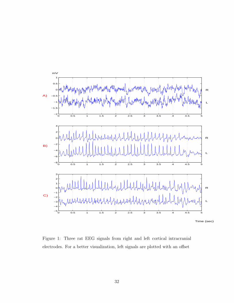
In Fig.1 we show the right and left channels of three of the (pre-lesion)

EEG signals described in the previous section. The first case (example A)

corresponds to a normal EEG, and in the remaining two cases the signals have

spike discharges (examples B and C). Spikes usually appear due to a local

synchronization of neurons in the neighborhood of the electrode at which

they are recorded. Since epilepsy is related to an abnormal synchronization

in the brain, spikes are usually considered as a landmark of epileptic activity.

A localized appearance of spikes can delimit a zone with abnormal discharges

(but this will not necessarily be the epileptic focus). On the contrary, if spikes

are observed over the whole set of electrodes, abnormal synchronization is

said to be global. This concept seems to be obvious, but it has some subtleties

as we will see in the following. Let us analyze examples B and C. In both

cases we see spikes at the left and right electrodes. As we said, this will point

towards a global synchronization behavior. However, a more detailed analysis

shows that the spikes of example B are well synchronized and in example C

they are not. Indeed, in example C the spikes have slightly different time lags

between the right and left channels. This is of course not easily seen in a first

sight. For making clear this point, we picked up the spikes of examples B and

C and we noted the times of their maximum for the right and left channels.

We then calculated the lag between the spikes in the two channels and its

standard deviation with time. For the case B, the lag was very small and

15

stable, mainly between -5 to 5 ms (i.e. of the order of the sampling rate) and

the standard deviation was of 4.7 ms. For the case C, the lag was much more

unstable and covered a larger range (between -20 to 50ms). In this last case

the standard deviation was of 14.9 ms. This shows that in example B the

simultaneous appearance of spikes is correlated with a global synchronization,

while in example C bilateral spikes are not synchronized (i.e. we have local

synchronization for both channels, but no global synchronization). In the

case of example A, due to its random-like appearance it is difficult to estimate

the level of synchronization by visual inspection. However, we can already

observe some patterns appearing simultaneously in both the left and right

channels, thus showing some degree of interdependence.

Summarizing, we may say that example B seems the most “ordered”

and synchronized. Among the other two examples, A looks definitely more

disordered than C, but a closer look raises doubts and a formal analysis is

asked for.

4.1 Linear measures

The second column of Table 1 shows the zero lag cross-correlation values

for the three examples. As stated in eq.(1), the calculation of the cross-

correlation requires a normalization of the data. We note that the tendency is

in agreement with what we expect from the arguments of the previous section

(i.e. B > A > C). However, the difference between cases A and B is relatively

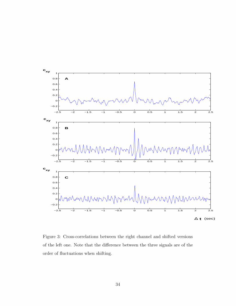
small. To get more insight, in Fig.3 we plot the cross-correlation as a function

of time shifts between the two channels. For the shifted versions, we used

periodic boundary conditions. For large enough shifts, the synchronization

will in principle be lost and the values obtained will give an estimation of

the zero synchronization level, which we will call background level, and its

16

fluctuation (i.e. we use the shifted versions as surrogates). We observe that

the synchronization drops to a background level for shifts larger than 50 data

points (i.e. 250ms). The average of this background level is zero, but the

fluctuations are quite large. Taking these fluctuations as an estimation of

the error, we see that cross-correlation does not distinguish between cases A

and B.

We also note that the cross-correlation shows oscillations when shifting,

most clearly in case B. These oscillations have the same period of the spikes

and might put into doubt the idea of considering the shifted signals as sur-

rogates. We therefore re-calculated the cross-correlation but taking the left

channel signals from other data segments of the same rat (for each rat we

had 5 segments with spikes and 5 of normal EEG before the lesions in the

thalamus) and corresponding to the same condition (pre-lesion, normal EEG

for example A and EEG with spikes for examples B and C). In all cases,

the background level and its fluctuations were of the order of those shown in

fig.3. This indicates that shifted signals can be used as surrogates in spite of

the oscillations.

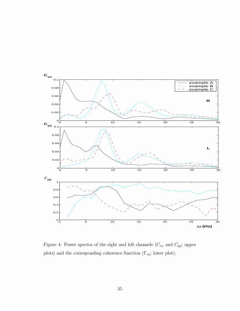
Figure 4 shows the spectral estimates for the three examples. The two

upper plots correspond to the power spectra of the right and left channels and

the lower plot to the corresponding coherence function (3). Each spectrum

(Cxx, Cyy and Cxy) was estimated using the Welch technique7, i.e. the data is

divided into M segments and then Cxx =∑M

i=1 Cxx,i. We used half overlapped

segments of 128 data points tapered with a Hamming window. Example

A has both in the right and left channels a power spectrum resembling a

power law distribution, with its main activity concentrated between 1 −

7without this segmentation technique, the coherence function (eq.(3)) would be always

equal to one.

17

10Hz. The coherence function shows a significant interaction for this range

of frequencies. Examples B and C show a more localized distribution in

the power spectrum. In both examples and for both channels there is a

peak between 7 − 10Hz and a harmonic at about 15Hz. In agreement with

previously reported results [38], these peaks correspond to the spikes observed

in Fig.1. We can already see from the power spectra that the matching

between right and left channels in example B is much clearer than in example

C. This is correlated with the larger coherence values of example B, showing

a significant synchronization for almost the whole frequency range. On the

other hand, the coherence is much lower for example C and it seems to be

significant only for low frequencies (up to 6Hz). As in the case of the cross-

correlation, the coherence function for ω ≤ 11Hz does not distinguish well

between examples A and B. There is only a difference for frequencies larger

than 11Hz, but this just reflects the lack of activity in this frequency range

for example A, whereas in example B it corresponds to the synchronization

between the high frequency harmonics of the spikes. In the third column of

Table 1 we summarize the results obtained with the coherence function. The

values shown correspond to a frequency of 9Hz, the main frequency of the

spikes in examples B and C.

4.2 Non-linear interdependences

For calculating the non-linear interdependence measures S, H and N between

left and right electrodes we first reconstruct the state spaces of each signal

using a time lag τ = 2 and an embedding dimension m = 10. We chose

this time lag in order to focus on frequencies lower than 50Hz (i.e. half the

Nyquist frequency) and the choice of the embedding dimension was in order

to have the length of the embedding vectors about the length of the spikes.

18

We further chose k = 10 nearest neighbors and a Theiler correction for tem-

poral correlations [40] of T = 50. These parameters were chosen heuristically

in order to maximize the sensitivity to the underlying synchronizations, but

results were robust against changes of them. Table 1 summarizes the re-

sults for the three examples. We will first discuss results with the non-linear

measures H and N . For both measures, example B has the highest synchro-

nization due to the presence of phase-locked spike discharges and example

C has a much smaller value. The synchronization of example A is between

these values. Again, it is interesting to remark that the non-linear interde-

pendence measures show the random looking signal of example A to be more

synchronized than the one with spikes of example C but less than the one in

B, something surprising at a first sight, and not clearly following from the

cross-correlation or the coherence as shown in section 4.1.

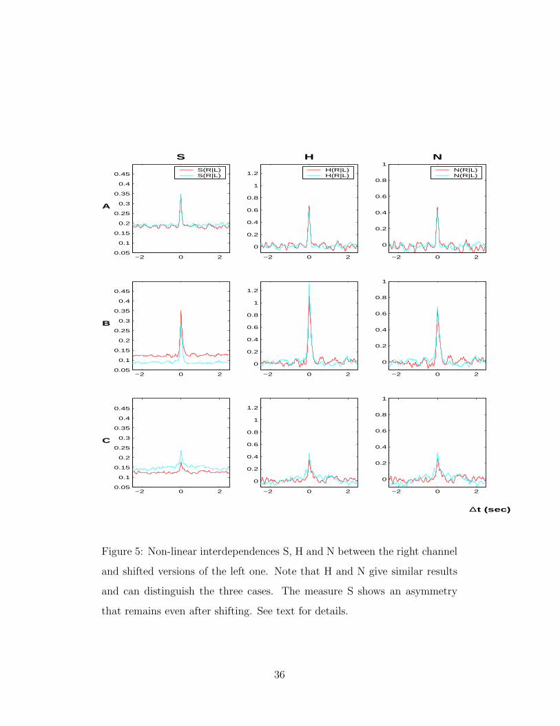
As done for the cross-correlation, in Fig.5 we also plot the two non-linear

synchronizations H(R|L), N(R|L) and H(L|R), N(L|R) as a function of

time shifts between the two channels. Again, the synchronization drops to a

background level for shifts larger than 50 data points (i.e. 250ms) and the

background level is about zero. But in the case of H and N we observe that

the fluctuations are much smaller than those for the cross-correlation. In

fact, with H and N the synchronization levels of the three cases are clearly

separated, while the cross-correlation does not distinguish between cases A

and B. However, even though we expect example B to be the most ordered

and synchronized of all (see sec. 4), we do not have objective means for

claiming that the difference between examples A and B is significant. So, the

fact that non-linear measures are able to separate the three examples might

imply a higher sensitivity of these measures in comparison with the linear

measures, but it does not prove it. We also observe some asymmetries in

19

H and N , most pronounced in case C. This might suggest that one of the

signals drives the other (i.e. the focus is on one side). However, in all cases

this is of the order of the asymmetries seen with the shifted signals, thus not

significant.

The case for the synchronization measure S is quite different. As seen in

Fig.5, for examples B and C there is a clear asymmetry between right and

left channels. In contrary to H and N , this asymmetry remains even for large

time shifts between the two channels. Moreover, the background level for the

three examples is between 0.1−0.2 and not zero as with H . Thus, the asym-

metries observed in examples B and C reflect more the individual properties

of each channel rather than a synchronization phenomenon8. Nevertheless,

H and N were clearly more robust in this respect.

Again, in order to check for the validity of the shifted signals as surrogates,

we re-calculated H , N and S but taking the left channel signals from other

data segments. As in the case of the cross-correlation, the background level

and its fluctuations were of the order of those shown in fig.5.

4.3 Hilbert phase synchronization

Prior to the estimation of the phase synchronization measures, each set of

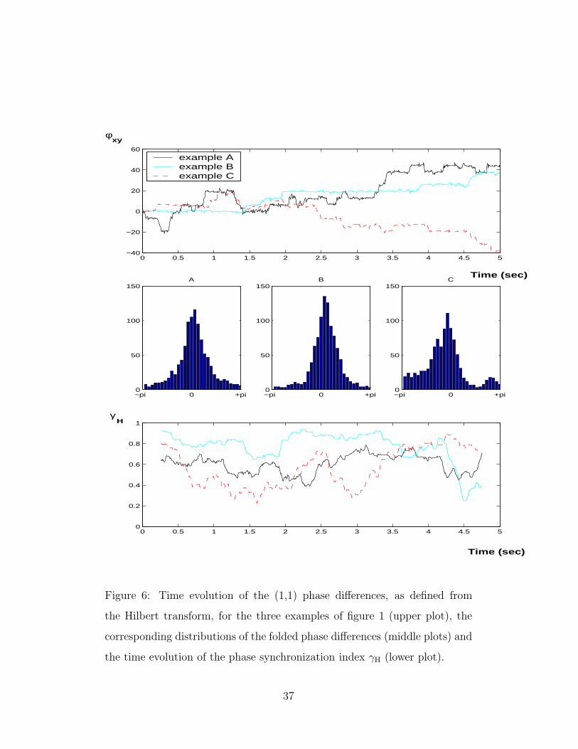
data was de-meaned. No further filtering was applied. Figure 6 shows the

time evolution of the phases (upper plot) and their distribution (middle plots)

for the three examples. From the time evolution of the phases we can already

see that the phase of example B is clearly more stable than the other two

examples (except in the last half second, as we will detail later). Examples

8As pointed out in [11], precisely such an asymmetry is expected if otherwise equal

systems are coupled asymmetrically. Thus, if we expect both subsystems a priori to have

the same complexity, the asymmetry of S is a hint to an asymmetric coupling.

20

A and C are not so easily differentiated, but in the middle plots we see that

the phase distribution of A is more localized than the one of C. The values

of γH , indicated in Table 1, are in agreement with these observations and

with the general tendency observed with the other synchronization measures

(B > A > C). The phase synchronization index defined from the Shannon

entropy (γH−Sh, defined in eq.(19)) shows qualitatively similar results (see

Table 1).

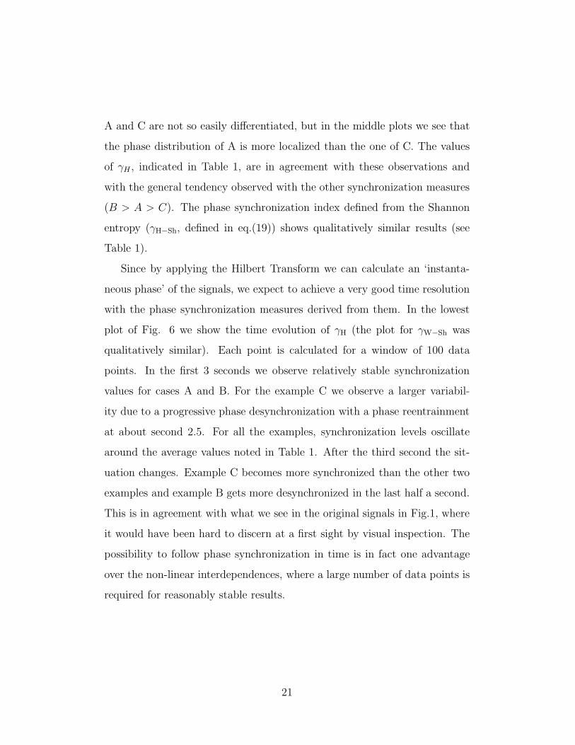
Since by applying the Hilbert Transform we can calculate an ‘instanta-

neous phase’ of the signals, we expect to achieve a very good time resolution

with the phase synchronization measures derived from them. In the lowest

plot of Fig. 6 we show the time evolution of γH (the plot for γW−Sh was

qualitatively similar). Each point is calculated for a window of 100 data

points. In the first 3 seconds we observe relatively stable synchronization

values for cases A and B. For the example C we observe a larger variabil-

ity due to a progressive phase desynchronization with a phase reentrainment

at about second 2.5. For all the examples, synchronization levels oscillate

around the average values noted in Table 1. After the third second the sit-

uation changes. Example C becomes more synchronized than the other two

examples and example B gets more desynchronized in the last half a second.

This is in agreement with what we see in the original signals in Fig.1, where

it would have been hard to discern at a first sight by visual inspection. The

possibility to follow phase synchronization in time is in fact one advantage

over the non-linear interdependences, where a large number of data points is

required for reasonably stable results.

21

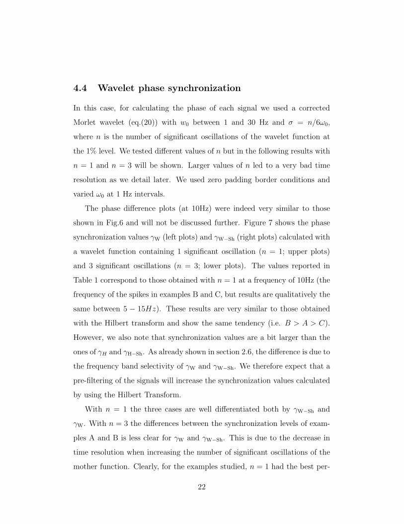
4.4 Wavelet phase synchronization

In this case, for calculating the phase of each signal we used a corrected

Morlet wavelet (eq.(20)) with w0 between 1 and 30 Hz and σ = n/6ω0,

where n is the number of significant oscillations of the wavelet function at

the 1% level. We tested different values of n but in the following results with

n = 1 and n = 3 will be shown. Larger values of n led to a very bad time

resolution as we detail later. We used zero padding border conditions and

varied ω0 at 1 Hz intervals.

The phase difference plots (at 10Hz) were indeed very similar to those

shown in Fig.6 and will not be discussed further. Figure 7 shows the phase

synchronization values γW (left plots) and γW−Sh (right plots) calculated with

a wavelet function containing 1 significant oscillation (n = 1; upper plots)

and 3 significant oscillations (n = 3; lower plots). The values reported in

Table 1 correspond to those obtained with n = 1 at a frequency of 10Hz (the

frequency of the spikes in examples B and C, but results are qualitatively the

same between 5 − 15Hz). These results are very similar to those obtained

with the Hilbert transform and show the same tendency (i.e. B > A > C).

However, we also note that synchronization values are a bit larger than the

ones of γH and γH−Sh. As already shown in section 2.6, the difference is due to

the frequency band selectivity of γW and γW−Sh. We therefore expect that a

pre-filtering of the signals will increase the synchronization values calculated

by using the Hilbert Transform.

With n = 1 the three cases are well differentiated both by γW−Sh and

γW. With n = 3 the differences between the synchronization levels of exam-

ples A and B is less clear for γW and γW−Sh. This is due to the decrease in

time resolution when increasing the number of significant oscillations of the

mother function. Clearly, for the examples studied, n = 1 had the best per-

22

formance (for n > 3 results get worse than for n = 3). Notice the similarity

between the lower plots for n = 3, i.e. the ones with less resolution, with the

coherence plots shown in Fig. 4. This supports the usefulness of the phase

synchronization measures defined from the Wavelet Transform in comparison

with traditional approaches. Finally, we should also remark that, as shown

in section 2.6, we are not limited to use Morlet wavelets, but we can rather

choose between several wavelet functions depending on the application.

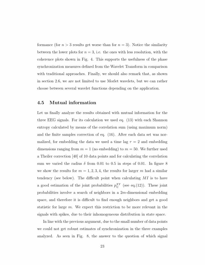
4.5 Mutual information

Let us finally analyze the results obtained with mutual information for the

three EEG signals. For its calculation we used eq. (13) with each Shannon

entropy calculated by means of the correlation sum (using maximum norm)

and the finite samples correction of eq. (16). After each data set was nor-

malized, for embedding the data we used a time lag τ = 2 and embedding

dimensions ranging from m = 1 (no embedding) to m = 50. We further used

a Theiler correction [40] of 10 data points and for calculating the correlation

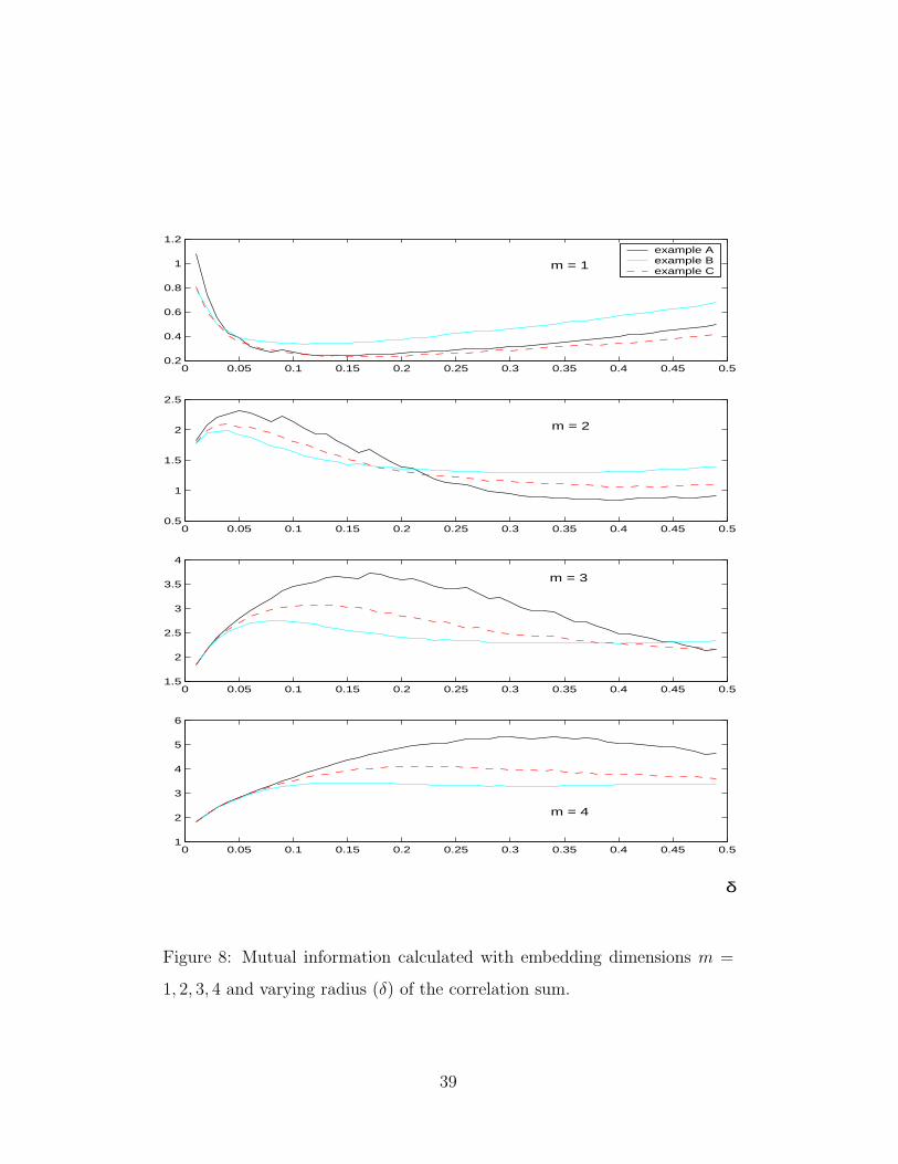
sum we varied the radius δ from 0.01 to 0.5 in steps of 0.01. In figure 8

we show the results for m = 1, 2, 3, 4, the results for larger m had a similar

tendency (see below). The difficult point when calculating MI is to have

a good estimation of the joint probabilities pXYij (see eq.(12)). These joint

probabilities involve a search of neighbors in a 2m-dimensional embedding

space, and therefore it is difficult to find enough neighbors and get a good

statistic for large m. We expect this restriction to be more relevant in the

signals with spikes, due to their inhomogeneous distribution in state space.

In line with the previous argument, due to the small number of data points

we could not get robust estimates of synchronization in the three examples

analyzed. As seen in Fig. 8, the answer to the question of which signal

23

is more and which is less synchronized dramatically depends on the choice

of m and δ. We observe the same tendency as with the previous measures

(B > A > C) only for m = 1 and δ > 0.15.

All previous analysis done in this paper show clear evidence that example

B has the highest synchronization. For m = 1 this is the case for δ > 0.05,

for m = 2 it occurs for δ > 0.2, for m = 3 at δ > 0.45 and for m = 4 it

does not occur for the range of δ shown. In fact, there is a crossing between

the synchronization values of examples A and B, that takes place at larger

δ for larger m. This simply reflects the impossibility of finding neighbors in

the 2m-dimensional state space for small δ and/or large m. As mentioned

before, we expect this effect to be less restrictive for the homogeneous distri-

bution of example A. This explains why example A always shows the highest

synchronization for small δ.

5 Conclusions

We applied several linear and non-linear measures of synchronization to three

typical EEG signals. Besides mutual information, which was not robust

due to the low number of data points, all these measures gave a similar

tendency in the synchronization levels. A similar analysis would have been

impossible by visual inspection. Moreover, in one case with bilateral spikes,

synchronization was much lower than expected at a first sight. Therefore,

we claim that the quantification of synchronization between different EEG

signals can complement the conventional visual analysis and can even be of

clinical value. In particular, this is very important for the study of epilepsy

[9, 10, 11, 18] and for the study of brain processes involving a synchronous

activation of different areas or structures in the brain.

24

In the last years, mainly two types of non-linear synchronization mea-

sures were proposed, namely, the ones based on phase relationships (phase

synchronization) and the ones based on non-linear interdependences (gener-

alized synchronization). It is interesting to remark that in our study with

real data these measures gave similar results, despite their different defini-

tions and their sensitivity to different characteristics of the signals. We also

show a close similarity between phase synchronization measures based on the

Hilbert and on the Wavelet Transform. In the particular case of the last one,

we generalize its definition to different wavelet functions that will be more

or less suitable according to the problem under investigation.

We validated the results obtained with the new non-linear measures by

comparing them with those obtained with traditional methods. All measures

ranked the synchronization levels of the three examples in the same way.

However the separation between them was more pronounced with non-linear

measures. Although we do not have objective means for claiming that the

difference between the synchronization of the signals is significant, this might

suggest a higher sensitivity of non-linear measures.

Although these results should not be automatically extended to other sig-

nals and problems, they also support the value of non-linear synchronization

measures in real data analysis.

25

Acknowledgments

We are very thankful to Dr. Giles van Luijtelaar and to Joyce Welting from

NICI - University of Nijmegen, for the data used in this paper. We are also

indebt to Dr. Klaus Lehnertz, Florian Mormann and Giles van Luijtelaar for

useful discussions and comments. One of us (A.K.) acknowledges support

from the US civilian research development foundation for the independent

states of the former Soviet Union, Award nr: REC-006.

26

References

[1] H. Fujisaka and T. Yamada, Prog. Theor. Phys. 69, 32 (1983); 76, 582

(1986)

[2] T. Yamada and H. Fujisaka, Prog. Theor. Phys. 70, 1240 (1984); 72,

885 (1985)

[3] A. Pikovsky, Z. Physik B 55, 149 (1984).

[4] L.M. Pecora and T.L. Carroll, Phys. Rev. Lett. 64, 821 (1990).

[5] N.F. Rulkov, M.M. Sushchik, L.S. Tsimring, and H.D.I. Abarbanel.

Phys. Rev. E 51, 980 (1995).

[6] C. Gray, P. Koenig, A. Engel and W. Singer, Nature 338, 335 (1989).

[7] E. Niedermeyer. Epileptic seizure disorders in Electroencephalography:

Basic Principles, Clinical Applications and Related Fields, edited by E.

Niedermeyer and F. H. Lopes da Silva (Baltimore, Williams and Wilkins

3rd ed., 1993), pp 1097.

[8] S.J. Schiff, P. So, T. Chang, R.E. Burke and T. Sauer. Phys. Rev. E 54,

6708 (1996).

[9] M. Le Van Quyen, C. Adam, M. Baulac, J. Martinerie, and F.J. Varela,

Brain Research 792, 24 (1998).

[10] M. Le Van Quyen, J. Martinerie, C. Adam, and F.J. Varela, Physica D

127, 250 (1999).

[11] J. Arnhold, P. Grassberger, K. Lehnertz, and C.E. Elger, Physica D

134, 419 (1999).

27

[12] R. Quian Quiroga, J. Arnhold and P. Grassberger. Phys. Rev. E, 61,

5142 (2000).

[13] The three EEG signals to be studied can be downloaded from

www.physio.mu-luebeck.de/user/rq/data.htm

[14] M. Rosenblum, A. Pikovsky and J. Kurths. Phys. Rev. Lett, 76, 1804

(1996).

[15] J. Lachaux, E. Rodriguez, J. Martinerie and F. Varela. Human Brain

Mapping, 8, 194 (1999).

[16] P. Tass, M. Rosenblum, J. Weule, J. Kurths, A. Pikovsky, J. Volkmann,

A. Schitzler and H. Freund. Phys. Rev. Lett, 81, 3291 (1998).

[17] M. Zaks, E. Park, M. Rosenblum and J. Kurths. Phys. Rev. Lett. 82,

4228, 1999.

[18] F. Mormann, K. Lehnertz, P. David and C.E. Elger. Physica D, 144,

358 (2000).

[19] E. Rodriguez, N. George, J. Lachaux, J. Martinerie, B. Renault and F.

Varela. Nature, 397, 430 (1999).

[20] F.H. Lopes da Silva, in Electroencephalography: Basic Principles, Clin-

ical Applications and Related Fields, edited by E. Niedermeyer and F.

H. Lopes da Silva (Baltimore, Williams and Wilkins 3rd ed., 1993), pp

1097.

[21] F. Takens, in D.A. Rand and L.S. Young, eds., Lecture Notes in Math-

ematics 898, page 366 (Springer, Berlin etc., 1981).

[22] A. Schmitz. Phys. Rev. E, 62, 7508 (2000).

28

[23] P. Grassberger. Phys. Lett. A, 128, 369, 1988.

[24] T. Schreiber. Phys. Rev. Lett. 85, 461, 2000.

[25] M. Palus. Phys. Lett., submitted.

[26] R. Gray. Entropy and information theory. New York, Springer Verlag,

1990.

[27] R. Quian Quiroga, J. Arnhold, K. Lehnertz and P. Grassberger. Phys.

Rev. E, 62, 8380, 2000.

[28] P. Grassberger, T. Schreiber and C. Schaffrath. Int.J. of Bifurcation and

Chaos, 1, 521, 1991.

[29] P. Grassberger. Phys. Lett. A 97, 224, 1983.

[30] K. Pawelzik and H.G. Schuster. Phys. Rev. A, 35, 481, 1987.

[31] D. Pritchard and J. Theiler. Physica D 84, 476, 1995.

[32] M.G. Rosenblum, A.S. Pikovsky, C. Schafer, P. Tass, and J. Kurths. In:

Handbook of Biological Physics; Vol. 4, Neuro-informatics (F. Moss and

S. Gielen eds.), Elsevier Science, pp. 279-321, 2000.

[33] A. Grossmann, R. Kronland-Martinet and J. Morlet. In: (Combes et

al. eds.) Wavelets: Time-Frequency methods and phase space. Berlin,

Springer (1989).

[34] J. Lachaux, E. Rodriguez, M. Le van Quyen, A. Lutz, J. Martinerie and

F. Varela. Int. J. Bifurcation and Chaos, 10, 2429 (2000).

[35] D. DeShazer, R. Breban, E. Ott and R. Roy. Phys. Rev. Lett, in press.

29

[36] L. Cohen. Time-frequency analysis. Prentice Hall, New Jersey (1995).

[37] G. van Luijtelaar and A. Coenen (eds.). The WAG/Rij rat model of ab-

sence epilepsy: Ten years of research. Nijmegen University Press, 1997.

[38] WHIM Drinkenburg, G. van Luijtelaar, WJ van Schaijk and A Coenen.

Physiol. Behav. 54, 779, 1993.

[39] G. van Luijtelaar, J. Welting and R. Quian Quiroga. In: van Bemmel

et al. (eds.) Sleep-wake research in the Netherlands, vol 11, pp:86-95.

Dutch Society for Sleep-Wake Research, 2000.

[40] J. Theiler. Phys. Rev. A, 34, 2427 (1986).

30

Example cxy Γxy S(R|L) S(L|R) H(R|L) H(L|R) N(R|L) N(L|R) γH γH−Sh γW γW−Sh

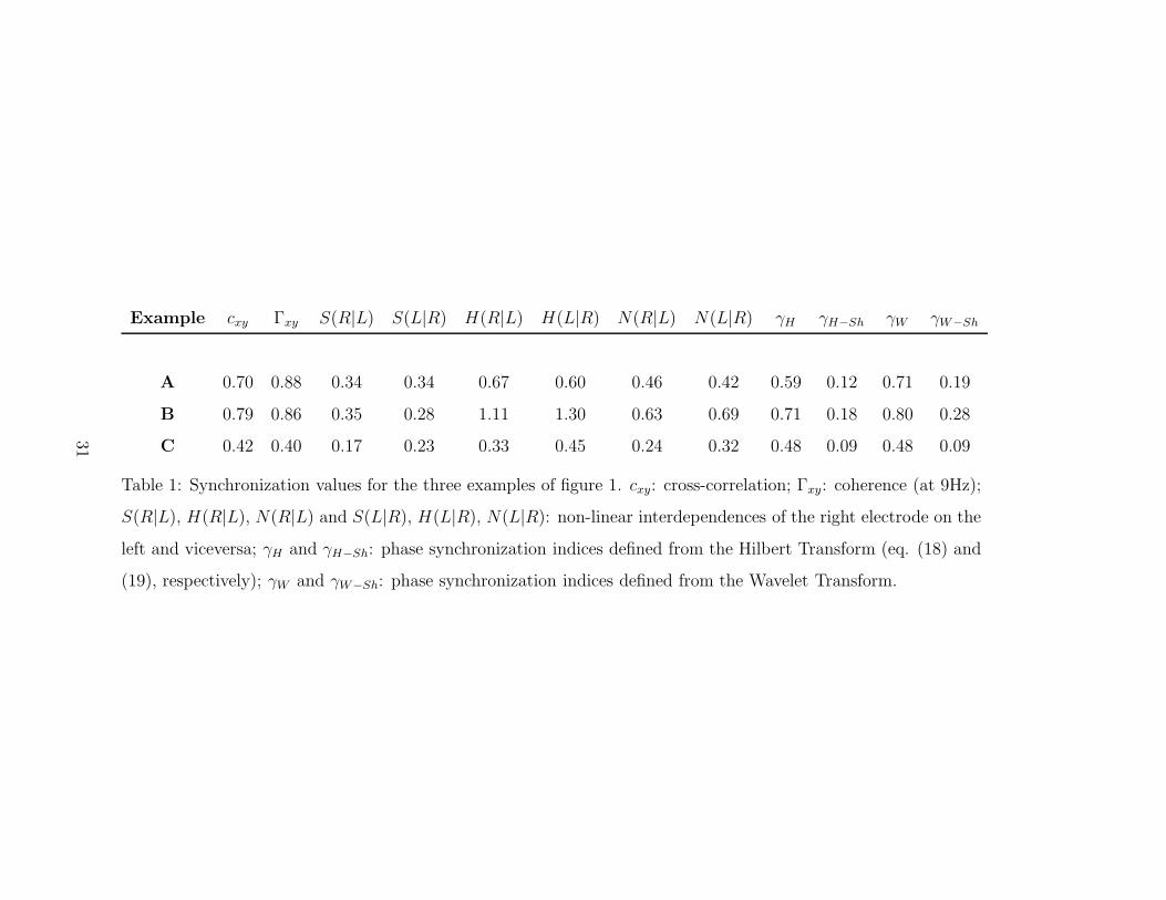
A 0.70 0.88 0.34 0.34 0.67 0.60 0.46 0.42 0.59 0.12 0.71 0.19

B 0.79 0.86 0.35 0.28 1.11 1.30 0.63 0.69 0.71 0.18 0.80 0.28

C 0.42 0.40 0.17 0.23 0.33 0.45 0.24 0.32 0.48 0.09 0.48 0.09

Table 1: Synchronization values for the three examples of figure 1. cxy: cross-correlation; Γxy: coherence (at 9Hz);

S(R|L), H(R|L), N(R|L) and S(L|R), H(L|R), N(L|R): non-linear interdependences of the right electrode on the

left and viceversa; γH and γH−Sh: phase synchronization indices defined from the Hilbert Transform (eq. (18) and

(19), respectively); γW and γW−Sh: phase synchronization indices defined from the Wavelet Transform.

31

0 0.5 1 1.5 2 2.5 3 3.5 4 4.5 5−2

−1.5

−1

−0.5

0

0.5

1

0 0.5 1 1.5 2 2.5 3 3.5 4 4.5 5−8

−6

−4

−2

0

2

4

0 0.5 1 1.5 2 2.5 3 3.5 4 4.5 5−5

−4

−3

−2

−1

0

1

2

3

mV

A)

B)

C)

Time (sec)

R

L

L

R

L

R

Figure 1: Three rat EEG signals from right and left cortical intracranial

electrodes. For a better visualization, left signals are plotted with an offset

32

No coupling

Strong coupling

Roessler

Lorenz

S(Y|X) = 0.001H(Y|X) = 0.056N(Y|X) = 0.003

S(Y|X) = 0.275 H(Y|X) = 3.694 N(Y|X) = 0.935

X Y

Figure 2: Basic idea of the non-linear interdependence measures. The size

of the neighborhood in one of the systems, say X, is compared with the

size of its mapping in the other system. The example shows a Lorenz system

driven by a Roessler with zero coupling (upper case) and with strong coupling

(lower case). Below each attractor, the corresponding time series is shown.

The (X|Y ) interdependences are calculated in the same way, starting with a

neighborhood in Y . For details see ref. [11, 12].

33

−2.5 −2 −1.5 −1 −0.5 0 0.5 1 1.5 2 2.5

−0.2

0

0.2

0.4

0.6

0.8

1

A

−2.5 −2 −1.5 −1 −0.5 0 0.5 1 1.5 2 2.5

−0.2

0

0.2

0.4

0.6

0.8

1

B

−2.5 −2 −1.5 −1 −0.5 0 0.5 1 1.5 2 2.5

−0.2

0

0.2

0.4

0.6

0.8

1

C

(sec) ∆ t

cxy

cxy

cxy

Figure 3: Cross-correlations between the right channel and shifted versions

of the left one. Note that the difference between the three signals are of the

order of fluctuations when shifting.

34

0 5 10 15 20 25 300

0.02

0.04

0.06

0.08

0.1

example Aexample Bexample C

0 5 10 15 20 25 300

0.02

0.04

0.06

0.08

0.1

0 5 10 15 20 25 300

0.2

0.4

0.6

0.8

1

R

L

ω (Hz)

Cxx

Cyy

xy

Γ

Figure 4: Power spectra of the right and left channels (Cxx and Cyy; upper

plots) and the corresponding coherence function (Γxy; lower plot).

35

−2 0 20.05

0.1

0.15

0.2

0.25

0.3

0.35

0.4

0.45

S

A

S(R|L)S(R|L)

−2 0 20.05

0.1

0.15

0.2

0.25

0.3

0.35

0.4

0.45

B

−2 0 20.05

0.1

0.15

0.2

0.25

0.3

0.35

0.4

0.45

C

−2 0 2

0

0.2

0.4

0.6

0.8

1

1.2

H

H(R|L)H(R|L)

−2 0 2

0

0.2

0.4

0.6

0.8

1

1.2

−2 0 2

0

0.2

0.4

0.6

0.8

1

1.2

−2 0 2

0

0.2

0.4

0.6

0.8

1N

N(R|L)N(R|L)

−2 0 2

0

0.2

0.4

0.6

0.8

1

−2 0 2

0

0.2

0.4

0.6

0.8

1

t (sec) ∆

Figure 5: Non-linear interdependences S, H and N between the right channel

and shifted versions of the left one. Note that H and N give similar results

and can distinguish the three cases. The measure S shows an asymmetry

that remains even after shifting. See text for details.

36

0 0.5 1 1.5 2 2.5 3 3.5 4 4.5 5−40

−20

0

20

40

60

example Aexample Bexample C

−pi 0 +pi0

50

100

150A

−pi 0 +pi0

50

100

150B

−pi 0 +pi0

50

100

150C

0 0.5 1 1.5 2 2.5 3 3.5 4 4.5 50

0.2

0.4

0.6

0.8

1

xy

φ

H γ

Time (sec)

Time (sec)

Figure 6: Time evolution of the (1,1) phase differences, as defined from

the Hilbert transform, for the three examples of figure 1 (upper plot), the

corresponding distributions of the folded phase differences (middle plots) and

the time evolution of the phase synchronization index γH (lower plot).

37

0 10 20 300

0.1

0.2

0.3

0.4

0.5

0.6

0.7

0.8

0.9

1

n = 1

example Aexample Bexample C

0 10 20 300

0.1

0.2

0.3

0.4

0.5

0.6

0.7

0.8

0.9

1

n = 3

0 10 20 300

0.1

0.2

0.3

0.4

0.5

0.6

0.7

0.8

0.9

1

n = 1

0 10 20 300

0.1

0.2

0.3

0.4

0.5

0.6

0.7

0.8

0.9

1

n = 3

ω (Hz)

(Hz) ω

γ W

γ W

γ W−Sh

γ W−Sh

ω (Hz)

ω (Hz)

Figure 7: Phase synchronization indices γW and γW−Sh defined from the

Wavelet Transform for two different wavelet functions (n = 1 and n = 3).

38

0 0.05 0.1 0.15 0.2 0.25 0.3 0.35 0.4 0.45 0.50.2

0.4

0.6

0.8

1

1.2example Aexample Bexample C

0 0.05 0.1 0.15 0.2 0.25 0.3 0.35 0.4 0.45 0.50.5

1

1.5

2

2.5

0 0.05 0.1 0.15 0.2 0.25 0.3 0.35 0.4 0.45 0.51.5

2

2.5

3

3.5

4

0 0.05 0.1 0.15 0.2 0.25 0.3 0.35 0.4 0.45 0.51

2

3

4

5

6

δ

m = 1

m = 2

m = 3

m = 4

Figure 8: Mutual information calculated with embedding dimensions m =

1, 2, 3, 4 and varying radius (δ) of the correlation sum.

39