0

Performing Periodic Tasks: On-LineLearning, Adaptation and Synchronization

with External Signals

Andrej Gams, Tadej Petric, Aleš Ude and Leon ŽlajpahJožef Stefan Institute, Ljubljana

Slovenia

1. Introduction

One of the central issues in robotics and animal motor control is the problem of trajectorygeneration and modulation. Since in many cases trajectories have to be modified on-linewhen goals are changed, obstacles are encountered, or when external perturbations occur,the notions of trajectory generation and trajectory modulation are tightly coupled.This chapter addresses some of the issues related to trajectory generation and modulation,including the supervised learning of periodic trajectories, and with an emphasis on thelearning of the frequency and achieving and maintaining synchronization to external signals.Other addressed issues include robust movement execution despite external perturbations,modulation of the trajectory to reuse it under modified conditions and adaptation of thelearned trajectory based on measured force information. Different experimental scenarios onvarious robotic platforms are described.For the learning of a periodic trajectory without specifying the period and without usingtraditional off-line signal processing methods, our approach suggests splitting the task intotwo sub-tasks: (1) frequency extraction, and (2) the supervised learning of the waveform.This is done using two ingredients: nonlinear oscillators, also combined with an adaptiveFourier waveform for the frequency adaptation, and nonparametric regression 1 techniquesfor shaping the attractor landscapes according to the demonstrated trajectories. The systemsare designed such that after having learned the trajectory, simple changes of parametersallow modulations in terms of, for instance, frequency, amplitude and oscillation offset, whilekeeping the general features of the original trajectory, or maintaining synchronization with anexternal signal.The system we propose in this paper is based on the motion imitation approach describedin (Ijspeert et al., 2002; Schaal et al., 2007). That approach uses two dynamical systems likethe system presented here, but with a simple nonlinear oscillator to generate the phase andthe amplitude of the periodic movements. A major drawback of that approach is that itrequires the frequency of the demonstration signal to be explicitly specified. This meansthat the frequency has to be either known or extracted from the recorded signal by signal

1 The term “nonparametric” is to indicate that the data to be modeled stem from very large families ofdistributions which cannot be indexed by a finite dimensional parameter vector in a natural way. Itdoes not mean that there are no parameters.

1

2 Will-be-set-by-IN-TECH

processing methods, e.g. Fourier analysis. The main difference of our new approach isthat we use an adaptive frequency oscillator (Buchli & Ijspeert, 2004; Righetti & Ijspeert,2006), which has the process of frequency extraction and adaptation totally embedded intoits dynamics. The frequency does not need to be known or extracted, nor do we need toperform any transformations (Righetti et al., 2006). This simplifies the process of teachinga new task/trajectory to the robot. Additionally, the system can work incrementally inon-line settings. We use two different approaches. One uses several frequency oscillatorsto approximate the input signal, and thus demands a logical algorithm to extract the basicfrequency of the input signal. The other uses only one oscillator and higher harmonics of theextracted frequency. It also includes an adaptive fourier series.Our approach is loosely inspired from dynamical systems observed in vertebrate centralnervous systems, in particular central pattern generators (Ijspeert, 2008a). Additionally, ourwork fits in the view that biological movements are constructed out of the combination of“motor primitives” (Mataric, 1998; Schaal, 1999), and the system we develop could be used asblocks or motor primitives for generating more complex trajectories.

1.1 Overview of the research fieldOne of the most notable advantages of the proposed system is the ability to synchronize withan external signal, which can effectively be used in control of rhythmic periodic task where thedynamic behavior and response of the actuated device are critical. Such robotic tasks includeswinging of different pendulums (Furuta, 2003; Spong, 1995), playing with different toys, i.e.the yo-yo (Hashimoto & Noritsugu, 1996; Jin et al., 2009; Jin & Zacksenhouse, 2003; Žlajpah,2006) or a gyroscopic device called the Powerball (Cafuta & Curk, 2008; Gams et al., 2007;Heyda, 2002; Petric et al., 2010), juggling (Buehler et al., 1994; Ronsse et al., 2007; Schaal &Atkeson, 1993; Williamson, 1999) and locomotion (Ijspeert, 2008b; Ilg et al., 1999; Morimotoet al., 2008). Rhythmic tasks are also handshaking (Jindai & Watanabe, 2007; Kasuga &Hashimoto, 2005; Sato et al., 2007) and even handwriting (Gangadhar et al., 2007; Hollerbach,1981). Performing these tasks with robots requires appropriate trajectory generation andforemost precise frequency tuning by determining the basic frequency. We denote the lowestfrequency relevant for performing a given task, with the term "basic frequency".Different approaches that adjust the rhythm and behavior of the robot, in order to achievesynchronization, have been proposed in the past. For example, a feedback loop that locksonto the phase of the incoming signal. Closed-loop model-based control (An et al., 1988), as avery common control of robotic systems, was applied for juggling (Buehler et al., 1994; Schaal& Atkeson, 1993), playing the yo-yo (Jin & Zackenhouse, 2002; Žlajpah, 2006) and also for thecontrol of quadruped (Fukuoka et al., 2003) and in biped locomotion (Sentis et al., 2010; Spong& Bullo, 2005). Here the basic strategy is to plan a reference trajectory for the robot, whichis based on the dynamic behavior of the actuated device. Standard methods for referencetrajectory tracking often assume that a correct and exhaustive dynamic model of the object isavailable (Jin & Zackenhouse, 2002), and their performance may degrade substantially if theaccuracy of the model is poor.An alternative approach to controlling rhythmic tasks is with the use of nonlinearoscillators. Oscillators and systems of coupled oscillators are known as powerful modelingtools (Pikovsky et al., 2002) and are widely used in physics and biology to modelphenomena as diverse as neuronal signalling, circadian rhythms (Strogatz, 1986), inter-limbcoordination (Haken et al., 1985), heart beating (Mirollo et al., 1990), etc. Their properties,which include robust limit cycle behavior, online frequency adaptation (Williamson, 1998)

4 The Future of Humanoid Robots – Research and Applications

Performing Periodic Tasks: On-Line Learning, Adaptation and Synchronization with External Signals 3

and self-sustained limit cycle generation on the absence of cyclic input (Bailey, 2004), to namejust a few, make them suitable for controlling rhythmic tasks.Different kinds of oscillators exist and have been used for control of robotic tasks. The van derPol non-linear oscillator (van der Pol, 1934) has successfully been used for skill entrainment ona swinging robot (Veskos & Demiris, 2005) or gait generation using coupled oscillator circuits,e.g. (Jalics et al., 1997; Liu et al., 2009; Tsuda et al., 2007). Gait generation has also been studiedusing the Rayleigh oscillator (Filho et al., 2005). Among the extensively used oscillators isalso the Matsuoka neural oscillator (Matsuoka, 1985), which models two mutually inhibitingneurons. Publications by Williamson (Williamson, 1999; 1998) show the use of the Matsuokaoscillator for different rhythmic tasks, such as resonance tuning, crank turning and playingthe slinky toy. Other robotic tasks using the Matsuoka oscillator include control of giantswing problem (Matsuoka et al., 2005), dish spinning (Matsuoka & Ooshima, 2007) andgait generation in combination with central pattern generators (CPGs) and phase-lockedloops (Inoue et al., 2004; Kimura et al., 1999; Kun & Miller, 1996).On-line frequency adaptation, as one of the properties of non-linear oscillators (Williamson,1998) is a viable alternative to signal processing methods, such as fast Fourier transform (FFT),for determining the basic frequency of the task. On the other hand, when there is no inputinto the oscillator, it will oscillate at its own frequency (Bailey, 2004). Righetti et al. haveintroduced adaptive frequency oscillators (Righetti et al., 2006), which preserve the learnedfrequency even if the input signal has been cut. The authors modify non-linear oscillatorsor pseudo-oscillators with a learning rule, which allows the modified oscillators to learn thefrequency of the input signal. The approach works for different oscillators, from a simplephase oscillator (Gams et al., 2009), the Hopf oscillator, the Fitzhugh-Nagumo oscillator,etc. (Righetti et al., 2006). Combining several adaptive frequency oscillators in a feedbackloop allows extraction of several frequency components (Buchli et al., 2008; Gams et al., 2009).Applications vary from bipedal walking (Righetti & Ijspeert, 2006) to frequency tuning of ahopping robot (Buchli et al., 2005). Such feedback structures can be used as a whole imitationsystem that both extracts the frequency and learns the waveform of the input signal.Not many approaches exist that combine both frequency extraction and waveform learningin imitation systems (Gams et al., 2009; Ijspeert, 2008b). One of them is a two-layeredimitation system, which can be used for extracting the frequency of the input signal in thefirst layer and learning its waveform in the second layer, which is the basis for this chapter.Separate frequency extraction and waveform learning have advantages, since it is possible toindependently modulate temporal and spatial features, e.g. phase modulation, amplitudemodulation, etc. Additionally a complex waveform can be anchored to the input signal.Compact waveform encoding, such as splines (Miyamoto et al., 1996; Thompson & Patel,1987; Ude et al., 2000), dynamic movement primitives (DMP) (Schaal et al., 2007), or Gaussianmixture models (GMM) (Calinon et al., 2007), reduce computational complexity of the process.In the next sections we first give details on the two-layered movement imitation system andthen give the properties. Finally, we propose possible applications.

2. Two-layered movement imitation system

In this chapter we give details and properties of both sub-systems that make the two-layeredmovement imitation system . We also give alternative possibilities for the canonical dynamicalsystem.

5Performing Periodic Tasks: On-Line Learning, Adaptation and Synchronization with External Signals

4 Will-be-set-by-IN-TECH

... Q

... Q

Ω1..Q

y1...Q

w1...Q

canonicaldynamical system

outputdynamical

system

ydemo

two-layered system

Φ1..Q

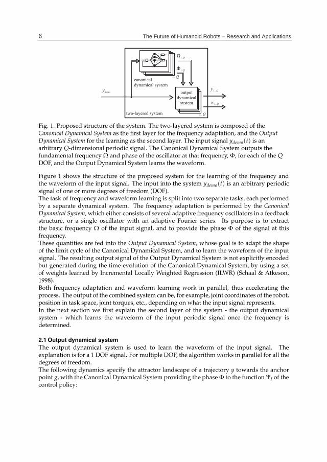
Fig. 1. Proposed structure of the system. The two-layered system is composed of theCanonical Dynamical System as the first layer for the frequency adaptation, and the OutputDynamical System for the learning as the second layer. The input signal ydemo(t) is anarbitrary Q-dimensional periodic signal. The Canonical Dynamical System outputs thefundamental frequency Ω and phase of the oscillator at that frequency, Φ, for each of the QDOF, and the Output Dynamical System learns the waveform.

Figure 1 shows the structure of the proposed system for the learning of the frequency andthe waveform of the input signal. The input into the system ydemo(t) is an arbitrary periodicsignal of one or more degrees of freedom (DOF).The task of frequency and waveform learning is split into two separate tasks, each performedby a separate dynamical system. The frequency adaptation is performed by the CanonicalDynamical System, which either consists of several adaptive frequency oscillators in a feedbackstructure, or a single oscillator with an adaptive Fourier series. Its purpose is to extractthe basic frequency Ω of the input signal, and to provide the phase Φ of the signal at thisfrequency.These quantities are fed into the Output Dynamical System, whose goal is to adapt the shapeof the limit cycle of the Canonical Dynamical System, and to learn the waveform of the inputsignal. The resulting output signal of the Output Dynamical System is not explicitly encodedbut generated during the time evolution of the Canonical Dynamical System, by using a setof weights learned by Incremental Locally Weighted Regression (ILWR) (Schaal & Atkeson,1998).Both frequency adaptation and waveform learning work in parallel, thus accelerating theprocess. The output of the combined system can be, for example, joint coordinates of the robot,position in task space, joint torques, etc., depending on what the input signal represents.In the next section we first explain the second layer of the system - the output dynamicalsystem - which learns the waveform of the input periodic signal once the frequency isdetermined.

2.1 Output dynamical systemThe output dynamical system is used to learn the waveform of the input signal. Theexplanation is for a 1 DOF signal. For multiple DOF, the algorithm works in parallel for all thedegrees of freedom.The following dynamics specify the attractor landscape of a trajectory y towards the anchorpoint g, with the Canonical Dynamical System providing the phase Φ to the function Ψi of thecontrol policy:

6 The Future of Humanoid Robots – Research and Applications

Performing Periodic Tasks: On-Line Learning, Adaptation and Synchronization with External Signals 5

z = Ω

(αz (βz (g− y)− z) +

∑Ni=1 Ψiwir

∑N

i=1 Ψi

)(1)

y = Ωz (2)

Ψi = exp (h (cos (Φ− ci)− 1)) (3)

Here Ω (chosen amongst the ωi) is the frequency given by canonical dynamical system, Eq.(10), αZ and βz are positive constants, set to αz = 8 and βz = 2 for all the results; the ratio 4:1ensures critical damping so that the system monotonically varies to the trajectory oscillatingaround g - an anchor point for the oscillatory trajectory. N is the number of Gaussian-likeperiodic kernel functions Ψi, which are given by Eq. (3). wi is the learned weight parameterand r is the amplitude control parameter, maintaining the amplitude of the demonstrationsignal with r = 1. The system given by Eq. (1) without the nonlinear term is a second-orderlinear system with a unique globally stable point attractor (Ijspeert et al., 2002). But, because ofthe periodic nonlinear term, this system produces stable periodic trajectories whose frequencyis Ω and whose waveform is determined by the weight parameters wi.In Eq. (3), which determines the Gaussian-like kernel functions Ψi, h determines their width,which is set to h = 2.5N for all the results presented in the paper unless stated otherwise, andci are equally spaced between 0 and 2π in N steps.As the input into the learning algorithm we use triplets of position, velocity and accelerationydemo(t), ydemo(t), and ydemo(t) with demo marking the input or demonstration trajectory weare trying to learn. With this Eq. (1) can be rewritten as

1Ω

z− αz (βz (g− y)− z) =∑N

i=1 Ψiwir

∑N

i=1 Ψi(4)

and formulated as a supervised learning problem with on the right hand side a set of localmodels wir that are weighted by the kernel functions Ψi, and on the left hand side the target

function ftarg given by ftarg = 1Ω2 ydemo − αz

(βz (g− ydemo)− 1

Ω ydemo

), which is obtained by

matching y to ydemo, z to ydemoΩ , and z to ydemo

Ω .Locally weighted regression corresponds to finding, for each kernel function Ψi, the weightvector wi, which minimizes the quadratic error criterion 2

Ji =

P

∑t=1

Ψi(t)(

ftarg(t)− wir(t))2

(5)

where t is an index corresponding to discrete time steps (of the integration). The regressioncan be performed as a batch regression, or alternatively, we can perform the minimization ofthe Ji cost function incrementally, while the target data points ftarg(t) arrive. As we wantcontinuous learning of the demonstration signal, we use the latter. Incremental regression isdone with the use of recursive least squares with a forgetting factor of λ, to determine theparameters (or weights) wi. Given the target data ftarg(t) and r(t), wi is updated by

wi(t + 1) = wi(t) + ΨiPi(t + 1)r(t)er(t) (6)

2 LWR is derived from a piecewise linear function approximation approach (Schaal & Atkeson, 1998),which decouples a nonlinear least-squares learning problem into several locally linear learningproblems, each characterized by the local cost function Ji . These local problems can be solved withstandard weighted least squares approaches.

7Performing Periodic Tasks: On-Line Learning, Adaptation and Synchronization with External Signals

6 Will-be-set-by-IN-TECH

10 10.5 11 11.5 12−2

−1

0

1

2y

10 10.5 11 11.5 12−400

−200

0

200

400

y10 10.5 11 11.5 12

−20

−10

0

10

20

y

10 10.5 11 11.5 120

0.5

1

Ψi

10 10.5 11 11.5 120

0.5

1

1.5

2

r

t [s]10 10.5 11 11.5 12

0

2

4

6mod(Φ

,2π)

t [s]20 20.2 20.4 20.6 20.8 21 21.2 21.4 21.6 21.8 22

−0.2

0

0.2

0.4

0.6

t [s]

|y dem

o−

y learned|2 N = 10

N = 25N = 50

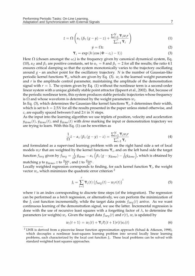
Fig. 2. Left: The result of Output Dynamical System with a constant frequency input and withcontinuous learning of the weights. In all the plots the input signal is the dash-dot line whilethe learned signal is the solid line. In the middle-right plot we can see the evolution of thekernel functions. The kernel functions are a function of Φ and do not necessarily changeuniformly (see also Fig. 7). In the bottom right plot the phase of the oscillator is shown. Theamplitude is here r = 1, as shown bottom-left. Right: The error of learning decreases with theincrease of the number of Gaussian-like kernel functions. The error, which is quite small, ismainly due to a very slight (one or two sample times) delay of the learned signal.

Pi(t + 1) =1λ

(Pi(t)− Pi(t)2r(t)2

λΨi

+ Pi(t)r(t)2

)(7)

er(t) = ftarg(t)− wi(t)r(t). (8)

P, in general, is the inverse covariance matrix (Ljung & Söderström, 1986). The recursion isstarted with wi = 0 and Pi = 1. Batch and incremental learning regressions provide identicalweights wi for the same training sets when the forgetting factor λ is set to one. Differencesappear when the forgetting factor is less than one, in which case the incremental regressiongives more weight to recent data (i.e. tends to forget older ones). The error of weight learninger (Eq. (8)) is not “related” to e when extracting frequency components (Eq. (11)). This allowsfor complete separation of frequency adaptation and waveform learning.Figure 2 left shows the time evolution of the Output Dynamical System anchored to aCanonical Dynamical System with the frequency set at Ω = 2π rad/s, and the weightparameters wi adjusted to fit the trajectory ydemo(t) = sin (2πt) + cos (4πt) + 0.4sin(6πt). Aswe can see in the top-left plot, the input signal and the reconstructed signal match closely. Thematching between the reconstructed signal and the input signal can be improved by increasingthe number of Gaussian-like functions.

Parameters of the Output Dynamical SystemWhen tuning the parameters of the Output Dynamical System, we have to determine thenumber of Gaussian-like Kernel functions N, and specially the forgetting factor λ. The numberN of Gaussian-like kernel functions could be set automatically if we used the locally weightedlearning (Schaal & Atkeson, 1998), but for simplicity it was here set by hand. Increasing thenumber increases the accuracy of the reconstructed signal, but at the same time also increasesthe computational cost. Note that LWR does not suffer from problems of overfitting when the

8 The Future of Humanoid Robots – Research and Applications

Performing Periodic Tasks: On-Line Learning, Adaptation and Synchronization with External Signals 7

number of kernel functions is increased.3 Figure 2 right shows the error of learning er whenusing N = 10, N = 25, and N = 50 on a signal ydemo(t) = 0.65sin (2πt) + 1.5cos (4πt) +0.3sin (6πt). Throughout the paper, unless specified otherwise, N = 25.The forgetting factor λ ∈ [0, 1] plays a key role in the behavior of the system. If it is sethigh, the system never forgets any input values and learns an average of the waveform overmultiple periods. If it is set too low, it forgets all, basically training all the weights to the lastvalue. We set it to λ = 0.995.

2.2 Canonical dynamical systemThe task of the Canonical Dynamical System is two-fold. Firstly, it has to extract thefundamental frequency Ω of the input signal, and secondly, it has to exhibit stable limit cyclebehavior in order to provide a phase signal Φ, that is used to anchor the waveform of theoutput signal. Two approaches are possible, either with a pool of oscillators (PO), or with anadaptive Fourier Series (AF).

2.2.1 Using a pool of oscillatorsAs the basis of our canonical dynamical system we use a set of phase oscillators, see e.g.(Buchli et al., 2006), to which we apply the adaptive frequency learning rule as introducedin (Buchli & Ijspeert, 2004) and (Righetti & Ijspeert, 2006), and combine it with a feedbackstructure (Righetti et al., 2006) shown in Figure 3. The basic idea of the structure is that each ofthe oscillators will adapt its frequency to one of the frequency components of the input signal,essentially “populating” the frequency spectrum.We use several oscillators, but are interested only in the fundamental or lowest non-zerofrequency of the input signal, denoted by Ω, and the phase of the oscillator at this frequency,denoted by Φ. Therefore the feedback structure is followed by a small logical block, whichchooses the correct, lowest non-zero, frequency. Determining Ω and Φ is important becausewith them we can formulate a supervised learning problem in the second stage - the OutputDynamical System, and learn the waveform of the full period of the input signal.

ydemo eΣαi icos( )ɸ

-+

ω1 1( ),t ɸ

ω2 2( ),t ɸ

ω3 3( ),t ɸ

ωM M( ),t ɸ

lowest

non-zero

Ω,Φ

y^

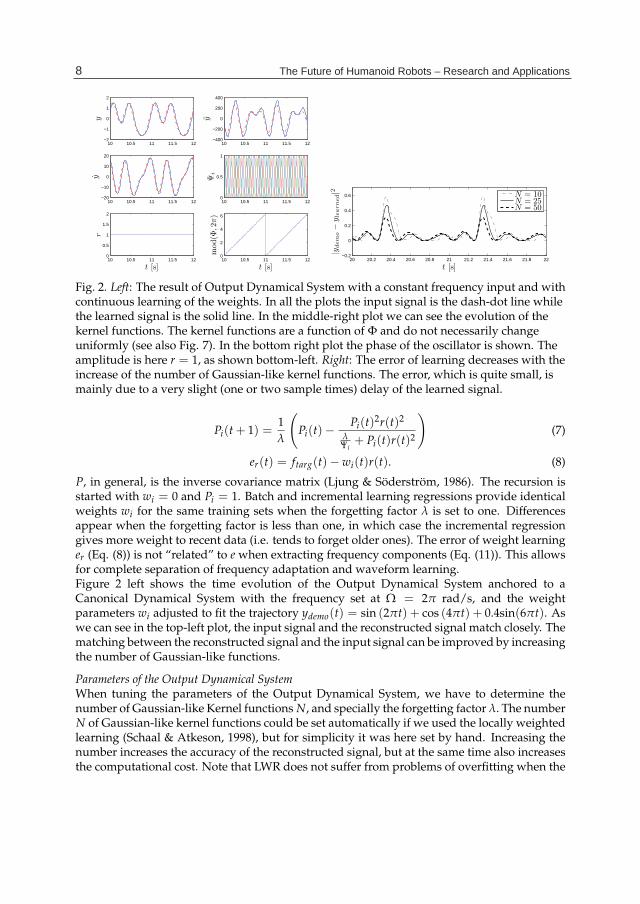
Fig. 3. Feedback structure of a network of adaptive frequency phase oscillators, that form theCanonical Dynamical System. All oscillators receive the same input and have to be atdifferent starting frequencies to converge to different final frequencies. Refer also to text andEqs. (9-13).

The feedback structure of M adaptive frequency phase oscillators is governed by the followingequations:

3 This property is due to solving the bias-variance dilemma of function approximation locally with aclosed form solution to leave-one-out cross-validation (Schaal & Atkeson, 1998).

9Performing Periodic Tasks: On-Line Learning, Adaptation and Synchronization with External Signals

8 Will-be-set-by-IN-TECH

φi = ωi − Ke sin(φi) (9)

ωi = −Ke sin(φi) (10)

e = ydemo − y (11)

y =

M

∑i=1

αi cos(φi) (12)

αi = η cos(φi)e (13)

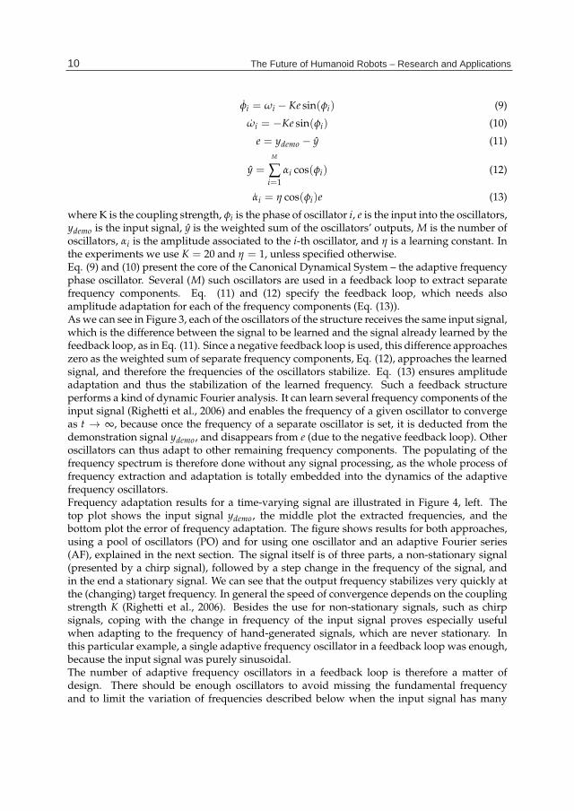
where K is the coupling strength, φi is the phase of oscillator i, e is the input into the oscillators,ydemo is the input signal, y is the weighted sum of the oscillators’ outputs, M is the number ofoscillators, αi is the amplitude associated to the i-th oscillator, and η is a learning constant. Inthe experiments we use K = 20 and η = 1, unless specified otherwise.Eq. (9) and (10) present the core of the Canonical Dynamical System – the adaptive frequencyphase oscillator. Several (M) such oscillators are used in a feedback loop to extract separatefrequency components. Eq. (11) and (12) specify the feedback loop, which needs alsoamplitude adaptation for each of the frequency components (Eq. (13)).As we can see in Figure 3, each of the oscillators of the structure receives the same input signal,which is the difference between the signal to be learned and the signal already learned by thefeedback loop, as in Eq. (11). Since a negative feedback loop is used, this difference approacheszero as the weighted sum of separate frequency components, Eq. (12), approaches the learnedsignal, and therefore the frequencies of the oscillators stabilize. Eq. (13) ensures amplitudeadaptation and thus the stabilization of the learned frequency. Such a feedback structureperforms a kind of dynamic Fourier analysis. It can learn several frequency components of theinput signal (Righetti et al., 2006) and enables the frequency of a given oscillator to convergeas t → ∞, because once the frequency of a separate oscillator is set, it is deducted from thedemonstration signal ydemo, and disappears from e (due to the negative feedback loop). Otheroscillators can thus adapt to other remaining frequency components. The populating of thefrequency spectrum is therefore done without any signal processing, as the whole process offrequency extraction and adaptation is totally embedded into the dynamics of the adaptivefrequency oscillators.Frequency adaptation results for a time-varying signal are illustrated in Figure 4, left. Thetop plot shows the input signal ydemo, the middle plot the extracted frequencies, and thebottom plot the error of frequency adaptation. The figure shows results for both approaches,using a pool of oscillators (PO) and for using one oscillator and an adaptive Fourier series(AF), explained in the next section. The signal itself is of three parts, a non-stationary signal(presented by a chirp signal), followed by a step change in the frequency of the signal, andin the end a stationary signal. We can see that the output frequency stabilizes very quickly atthe (changing) target frequency. In general the speed of convergence depends on the couplingstrength K (Righetti et al., 2006). Besides the use for non-stationary signals, such as chirpsignals, coping with the change in frequency of the input signal proves especially usefulwhen adapting to the frequency of hand-generated signals, which are never stationary. Inthis particular example, a single adaptive frequency oscillator in a feedback loop was enough,because the input signal was purely sinusoidal.The number of adaptive frequency oscillators in a feedback loop is therefore a matter ofdesign. There should be enough oscillators to avoid missing the fundamental frequencyand to limit the variation of frequencies described below when the input signal has many

10 The Future of Humanoid Robots – Research and Applications

Performing Periodic Tasks: On-Line Learning, Adaptation and Synchronization with External Signals 9

−1

0

1

y demo

5

10

15

20

Ω[rad]

ωt ΩAF ΩPO

0 10 20 30 40 50 600

200

Error

t [s]

0

20

40

ΩPO

[rad]

0 100 200 300 400 500

6

8

ΩAF

[rad]

−0.5

0

0.5

y

20 20.5 210

0.04error

150 150.5 151t [s]

350 350.5 351

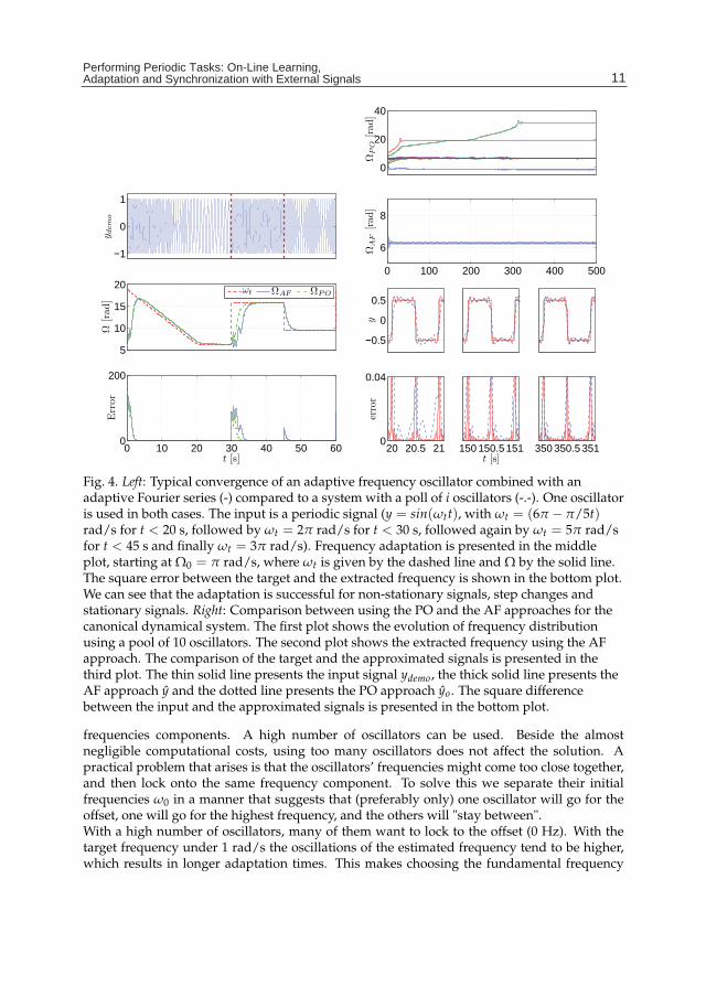
Fig. 4. Left: Typical convergence of an adaptive frequency oscillator combined with anadaptive Fourier series (-) compared to a system with a poll of i oscillators (-.-). One oscillatoris used in both cases. The input is a periodic signal (y = sin(ωtt), with ωt = (6π − π/5t)rad/s for t < 20 s, followed by ωt = 2π rad/s for t < 30 s, followed again by ωt = 5π rad/sfor t < 45 s and finally ωt = 3π rad/s). Frequency adaptation is presented in the middleplot, starting at Ω0 = π rad/s, where ωt is given by the dashed line and Ω by the solid line.The square error between the target and the extracted frequency is shown in the bottom plot.We can see that the adaptation is successful for non-stationary signals, step changes andstationary signals. Right: Comparison between using the PO and the AF approaches for thecanonical dynamical system. The first plot shows the evolution of frequency distributionusing a pool of 10 oscillators. The second plot shows the extracted frequency using the AFapproach. The comparison of the target and the approximated signals is presented in thethird plot. The thin solid line presents the input signal ydemo, the thick solid line presents theAF approach y and the dotted line presents the PO approach yo. The square differencebetween the input and the approximated signals is presented in the bottom plot.

frequencies components. A high number of oscillators can be used. Beside the almostnegligible computational costs, using too many oscillators does not affect the solution. Apractical problem that arises is that the oscillators’ frequencies might come too close together,and then lock onto the same frequency component. To solve this we separate their initialfrequencies ω0 in a manner that suggests that (preferably only) one oscillator will go for theoffset, one will go for the highest frequency, and the others will "stay between".With a high number of oscillators, many of them want to lock to the offset (0 Hz). With thetarget frequency under 1 rad/s the oscillations of the estimated frequency tend to be higher,which results in longer adaptation times. This makes choosing the fundamental frequency

11Performing Periodic Tasks: On-Line Learning, Adaptation and Synchronization with External Signals

10 Will-be-set-by-IN-TECH

without introducing complex decision-making logic difficult. Results of frequency adaptationfor a complex waveform are presented in Fig. 4, where results for both PO and AF approachare presented.Besides learning, we can also use the system to repeat already learned signals. It this case, wecut feedback to the adaptive frequency oscillators by setting e(t) = 0. This way the oscillatorscontinue to oscillate at the frequency to which they adapted. We are only interested in thefundamental frequency, determined by

Φ = Ω (14)

Ω = 0 (15)

which is derived from Eqs. (9 and 10). This is also the equation of a normal phase oscillator.

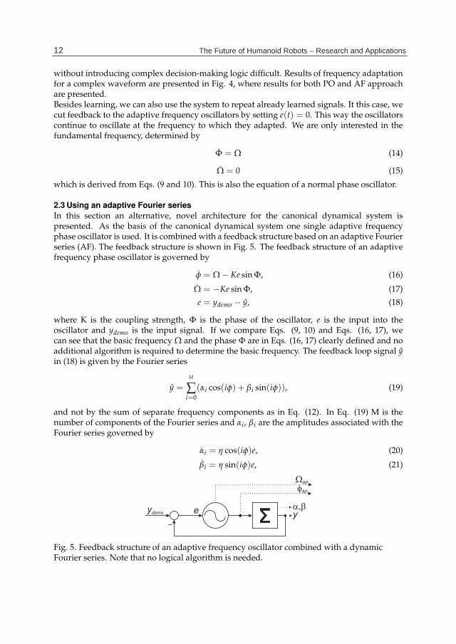
2.3 Using an adaptive Fourier seriesIn this section an alternative, novel architecture for the canonical dynamical system ispresented. As the basis of the canonical dynamical system one single adaptive frequencyphase oscillator is used. It is combined with a feedback structure based on an adaptive Fourierseries (AF). The feedback structure is shown in Fig. 5. The feedback structure of an adaptivefrequency phase oscillator is governed by

φ = Ω− Ke sin Φ, (16)

Ω = −Ke sin Φ, (17)

e = ydemo − y, (18)

where K is the coupling strength, Φ is the phase of the oscillator, e is the input into theoscillator and ydemo is the input signal. If we compare Eqs. (9, 10) and Eqs. (16, 17), wecan see that the basic frequency Ω and the phase Φ are in Eqs. (16, 17) clearly defined and noadditional algorithm is required to determine the basic frequency. The feedback loop signal yin (18) is given by the Fourier series

y =

M

∑i=0

(αi cos(iφ) + βi sin(iφ)), (19)

and not by the sum of separate frequency components as in Eq. (12). In Eq. (19) M is thenumber of components of the Fourier series and αi, βi are the amplitudes associated with theFourier series governed by

αi = η cos(iφ)e, (20)

βi = η sin(iφ)e, (21)

ydemo

�AF

�AF

���e y

Fig. 5. Feedback structure of an adaptive frequency oscillator combined with a dynamicFourier series. Note that no logical algorithm is needed.

12 The Future of Humanoid Robots – Research and Applications

Performing Periodic Tasks: On-Line Learning, Adaptation and Synchronization with External Signals 11

where η is the learning constant and i = 0...M. As shown in Fig. 5, the oscillator inputis the difference between the input signal ydemo and the Fourier series y. Since a negativefeedback loop is used, the difference approaches zero when the Fourier series representation yapproaches the input signal y. Such a feedback structure performs a kind of adaptive Fourieranalysis. Formally, it performs only a Fourier series approximation, because input signalsmay drift in frequency and phase. General convergence remains an open issue. The numberof harmonic frequency components it can extract depends on how many terms of the Fourierseries are used.As it is able to learn different periodic signals, the new architecture of the canonical dynamicalsystem can also be used as an imitation system by itself. Once e is stable (zero), the periodicsignal stays encoded in the Fourier series, with an accuracy that depends on the number ofelements used in Fourier series. The learning process is embedded and is done in real-time.There is no need for any external optimization process or other learning algorithm.It is important to point out that the convergence of the frequency adaptation (i.e. the behaviorof Ω) should not be confused with locking behavior (Buchli et al., 2008) (i.e. the classicphase locking behavior, or synchronization, as documented in the literature (Pikovsky et al.,2002)). The frequency adaptation process is an extension of the common oscillator with a fixedintrinsic frequency. First, the adaptation process changes the intrinsic frequency and not onlythe resulting frequency. Second, the adaptation has an infinite basin of attraction (see (Buchliet al., 2008)), third the frequency stays encoded in the system when the input is removed (e.g.set to zero or e ≈ 0). Our purpose is to show how to apply the approach for control of rhythmicrobotic task. For details on analyzing interaction of multiple oscillators see e.g. (Kralemannet al., 2008).Augmenting the system with an output dynamical system makes it possible to synchronizethe movement of the robot to a measurable periodic quantity of the desired task. Namely,the waveform and the frequency of the measured signal are encoded in the Fourier series andthe desired robot trajectory is encoded in the output dynamical system. Since the adaptationof the frequency and learning of the desired trajectory can be done simultaneously, all ofthe system time-delays, e.g. delays in communication, sensor measurements delays, etc., areautomatically included. Furthermore, when a predefined motion pattern for the trajectory isused, the phase between the input signal and output signal can be adjusted with a phase lagparameter φl (see Fig. 9). This enables us to either predefine the desired motion or to teach therobot how to preform the desired rhythmic task online.Even though the canonical dynamical system by itself can reproduce the demonstrationsignal, using the output dynamical system allows for easier modulation in both amplitudeand frequency, learning of complex patterns without extracting all frequency componentsand acts as a sort of a filter. Moreover, when multiple output signals are needed, only onecanonical system can be used with several output systems which assure that the waveformsof the different degrees-of-freedom are realized appropriately.

3. On-line learning and modulation

3.1 On-line modulationsThe output dynamical system allows easy modulation of amplitude, frequency and center ofoscillations. Once the robot is performing the learned trajectory, we can change all of these bychanging just one parameter for each. The system is designed to permit on-line modulationsof the originally learned trajectories. This is one of the important motivations behind the useof dynamical systems to encode trajectories.

13Performing Periodic Tasks: On-Line Learning, Adaptation and Synchronization with External Signals

12 Will-be-set-by-IN-TECH

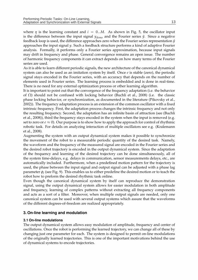
Changing the parameter g corresponds to a modulation of the baseline of the rhythmicmovement. This will smoothly shift the oscillation without modifying the signal shape. Theresults are presented in the second plot in Figure 6 left. Modifying Ω and r correspondsto the changing of the frequency and the amplitude of the oscillations, respectively. Sinceour differential equations are of second order, these abrupt changes of parameters result insmooth variations of the trajectory y. This is particularly useful when controlling articulatedrobots, which require trajectories with limited jerks. Changing of the parameter Ω only comesinto consideration when one wants to repeat the learned signal at a desired frequency thatis different from the one we adapted to with our Canonical Dynamical System. Results ofchanging the frequency Ω are presented in the third plot of Figure 6 left. Results of modulatingthe amplitude parameter r are presented in the bottom plot of Figure 6 left.

3.2 Perturbations and modified feedback3.2.1 Dealing with perturbationsThe Output Dynamical System is inherently robust against perturbations. Figure 6 rightillustrates the time evolution of the system repeating a learned trajectory at the frequencyof 1 Hz, when the state variables y, z and Φ are randomly changed at time t = 30 s. From theresults we can see that the output of the system reverts smoothly to the learned trajectory. Thisis an important feature of the approach: the system essentially represents a whole landscapein the space of state variables which not only encode the learned trajectory but also determinehow the states return to it after a perturbation.

3.2.2 Slow-down feedbackWhen controlling the robot, we have to take into account perturbations due to the interactionwith the environment. Our system provides desired states to the robot, i.e. desired joint anglesor torques, and its state variables are therefore not affected by the actual states of the robot,unless feedback terms are added to the control scheme. For instance, it might happen that, dueto external forces, significant differences arise between the actual position y and the desiredposition y. Depending on the task, this error can be fed back to the system in order to modifyon-line the generated trajectories.

23 23.5 24 24.5 25 25.5 26 26.5 27 27.5 28−10

0

10

y out

23 23.5 24 24.5 25 25.5 26 26.5 27 27.5 28−10

0

10

y out

23 23.5 24 24.5 25 25.5 26 26.5 27 27.5 28−10

0

10

y out

23 23.5 24 24.5 25 25.5 26 26.5 27 27.5 28

−10

0

10

y out

t [s]28 29 30 31 32

−10

−5

0

5

10

t [s]

y

28 29 30 31 320

2

4

6

Φ[rad]

t [s]

Fig. 6. Left: Modulations of the learned signal. The learned signal (top), modulating thebaseline for oscillations g (second from top), doubling the frequency Ω (third from top),doubling the amplitude r (bottom). Right: Dealing with perturbations – reacting to a randomperturbation of the state variables y, z and Φ at t = 30 s.

14 The Future of Humanoid Robots – Research and Applications

Performing Periodic Tasks: On-Line Learning, Adaptation and Synchronization with External Signals 13

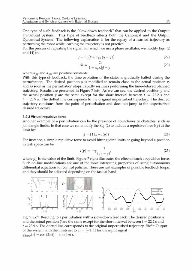
One type of such feedback is the “slow-down-feedback” that can be applied to the OutputDynamical System. This type of feedback affects both the Canonical and the OutputDynamical System. The following explanation is for the replay of a learned trajectory asperturbing the robot while learning the trajectory is not practical.For the process of repeating the signal, for which we use a phase oscillator, we modify Eqs. (2and 14) to:

y = Ω(z + αpy (y− y)

)(22)

Φ =Ω

1 + αpΦ|y− y| (23)

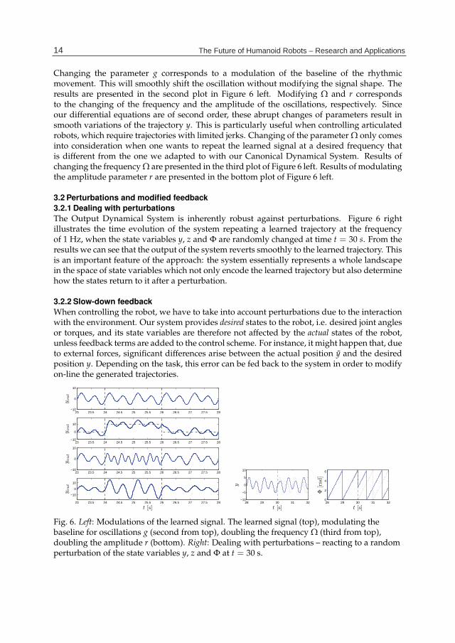
where αpy and αpΦ are positive constants.With this type of feedback, the time evolution of the states is gradually halted during theperturbation. The desired position y is modified to remain close to the actual position y,and as soon as the perturbation stops, rapidly resumes performing the time-delayed plannedtrajectory. Results are presented in Figure 7 left. As we can see, the desired position y andthe actual position y are the same except for the short interval between t = 22.2 s andt = 23.9 s. The dotted line corresponds to the original unperturbed trajectory. The desiredtrajectory continues from the point of perturbation and does not jump to the unperturbeddesired trajectory.

3.2.3 Virtual repulsive forceAnother example of a perturbation can be the presence of boundaries or obstacles, such asjoint angle limits. In that case we can modify the Eq. (2) to include a repulsive force l(y) at thelimit by:

y = Ω (z + l(y)) (24)

For instance, a simple repulsive force to avoid hitting joint limits or going beyond a positionin task space can be

l(y) = −γ1

(yL − y)3 (25)

where yL is the value of the limit. Figure 7 right illustrates the effect of such a repulsive force.Such on-line modifications are one of the most interesting properties of using autonomousdifferential equations for control policies. These are just examples of possible feedback loops,and they should be adjusted depending on the task at hand.

21 22 23 24 25 26−2

−1

0

1

2

y

21 22 23 24 25 260

0.5

1

Ψi

21 22 23 24 25 260

1

2

3

4

5

|y−

y|2

t [s]21 22 23 24 25 26

0

2

4

6

mod(Φ

,2π)

t [s]10 10.2 10.4 10.6 10.8 11 11.2 11.4 11.6 11.8 12

−2

−1

0

1

2

y

t [s]

InputOutputlimit

Fig. 7. Left: Reacting to a perturbation with a slow-down feedback. The desired position yand the actual position y are the same except for the short interval between t = 22.2 s andt = 23.9 s. The dotted line corresponds to the original unperturbed trajectory. Right: Outputof the system with the limits set to yl = [−1, 1] for the input signalydemo(t) = cos (2πt) + sin (4πt).

15Performing Periodic Tasks: On-Line Learning, Adaptation and Synchronization with External Signals

14 Will-be-set-by-IN-TECH

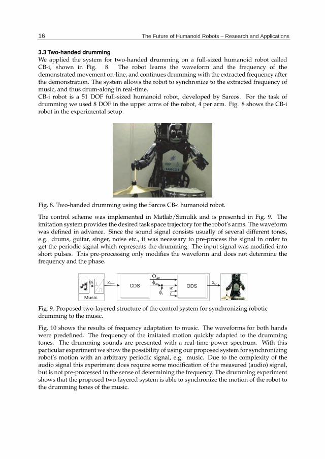
3.3 Two-handed drummingWe applied the system for two-handed drumming on a full-sized humanoid robot calledCB-i, shown in Fig. 8. The robot learns the waveform and the frequency of thedemonstrated movement on-line, and continues drumming with the extracted frequency afterthe demonstration. The system allows the robot to synchronize to the extracted frequency ofmusic, and thus drum-along in real-time.CB-i robot is a 51 DOF full-sized humanoid robot, developed by Sarcos. For the task ofdrumming we used 8 DOF in the upper arms of the robot, 4 per arm. Fig. 8 shows the CB-irobot in the experimental setup.

Fig. 8. Two-handed drumming using the Sarcos CB-i humanoid robot.

The control scheme was implemented in Matlab/Simulik and is presented in Fig. 9. Theimitation system provides the desired task space trajectory for the robot’s arms. The waveformwas defined in advance. Since the sound signal consists usually of several different tones,e.g. drums, guitar, singer, noise etc., it was necessary to pre-process the signal in order toget the periodic signal which represents the drumming. The input signal was modified intoshort pulses. This pre-processing only modifies the waveform and does not determine thefrequency and the phase.

ydemo

CDS ODSwi

rMusic

�AF

�AF

�l

xl,r

Fig. 9. Proposed two-layered structure of the control system for synchronizing roboticdrumming to the music.

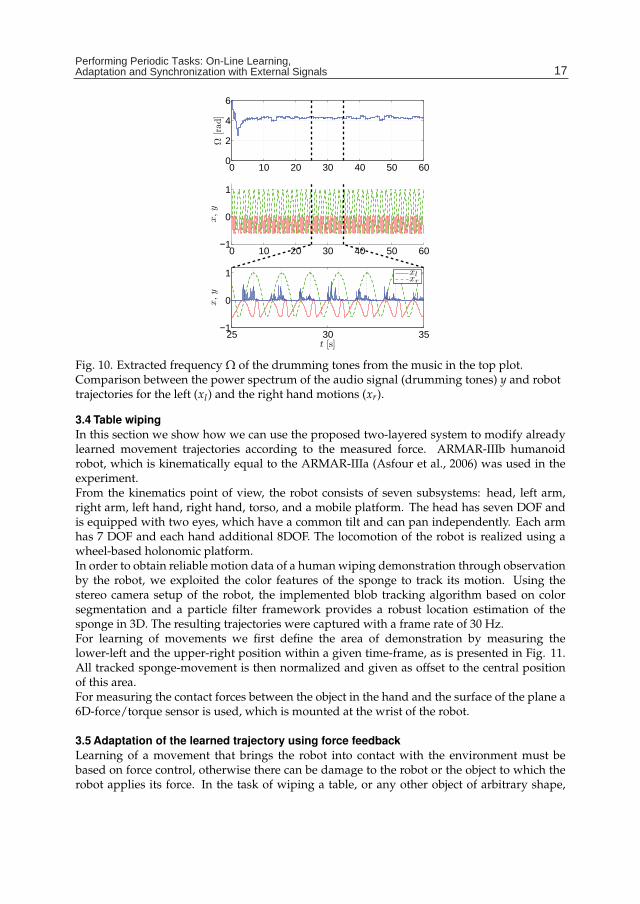
Fig. 10 shows the results of frequency adaptation to music. The waveforms for both handswere predefined. The frequency of the imitated motion quickly adapted to the drummingtones. The drumming sounds are presented with a real-time power spectrum. With thisparticular experiment we show the possibility of using our proposed system for synchronizingrobot’s motion with an arbitrary periodic signal, e.g. music. Due to the complexity of theaudio signal this experiment does require some modification of the measured (audio) signal,but is not pre-processed in the sense of determining the frequency. The drumming experimentshows that the proposed two-layered system is able to synchronize the motion of the robot tothe drumming tones of the music.

16 The Future of Humanoid Robots – Research and Applications

Performing Periodic Tasks: On-Line Learning, Adaptation and Synchronization with External Signals 15

0 10 20 30 40 50 600

2

4

6

Ω[rad]

0 10 20 30 40 50 60−1

0

1

x,y

25 30 35−1

0

1

t [s]

x,y

xlxr

Fig. 10. Extracted frequency Ω of the drumming tones from the music in the top plot.Comparison between the power spectrum of the audio signal (drumming tones) y and robottrajectories for the left (xl) and the right hand motions (xr).

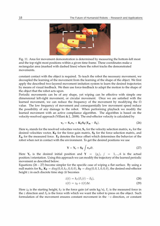
3.4 Table wipingIn this section we show how we can use the proposed two-layered system to modify alreadylearned movement trajectories according to the measured force. ARMAR-IIIb humanoidrobot, which is kinematically equal to the ARMAR-IIIa (Asfour et al., 2006) was used in theexperiment.From the kinematics point of view, the robot consists of seven subsystems: head, left arm,right arm, left hand, right hand, torso, and a mobile platform. The head has seven DOF andis equipped with two eyes, which have a common tilt and can pan independently. Each armhas 7 DOF and each hand additional 8DOF. The locomotion of the robot is realized using awheel-based holonomic platform.In order to obtain reliable motion data of a human wiping demonstration through observationby the robot, we exploited the color features of the sponge to track its motion. Using thestereo camera setup of the robot, the implemented blob tracking algorithm based on colorsegmentation and a particle filter framework provides a robust location estimation of thesponge in 3D. The resulting trajectories were captured with a frame rate of 30 Hz.For learning of movements we first define the area of demonstration by measuring thelower-left and the upper-right position within a given time-frame, as is presented in Fig. 11.All tracked sponge-movement is then normalized and given as offset to the central positionof this area.For measuring the contact forces between the object in the hand and the surface of the plane a6D-force/torque sensor is used, which is mounted at the wrist of the robot.

3.5 Adaptation of the learned trajectory using force feedbackLearning of a movement that brings the robot into contact with the environment must bebased on force control, otherwise there can be damage to the robot or the object to which therobot applies its force. In the task of wiping a table, or any other object of arbitrary shape,

17Performing Periodic Tasks: On-Line Learning, Adaptation and Synchronization with External Signals

16 Will-be-set-by-IN-TECH

Fig. 11. Area for movement demonstration is determined by measuring the bottom-left mostand the top-right most positions within a given time frame. These coordinates make arectangular area (marked with dashed lines) where the robot tracks the demonstratedmovements.

constant contact with the object is required. To teach the robot the necessary movement, wedecoupled the learning of the movement from the learning of the shape of the object. We firstapply the described two-layered movement imitation system to learn the desired trajectoriesby means of visual feedback. We then use force-feedback to adapt the motion to the shape ofthe object that the robot acts upon.Periodic movements can be of any shape, yet wiping can be effective with simple onedimensional left-right movement, or circular movement. Once we are satisfied with thelearned movement, we can reduce the frequency of the movement by modifying the Ωvalue. The low frequency of movement and consequentially low movement speed reducethe possibility of any damage to the robot. When performing playback we modify thelearned movement with an active compliance algorithm. The algorithm is based on thevelocity-resolved approach (Villani & J., 2008). The end-effector velocity is calculated by

vr = Svvv + KFSF(Fm − F0). (26)

Here vr stands for the resolved velocities vector, Sv for the velocity selection matrix, vv for thedesired velocities vector, KF for the force gain matrix, SF for the force selection matrix, andFm for the measured force. F0 denotes the force offset which determines the behavior of therobot when not in contact with the environment. To get the desired positions we use

Y = Yr + SF

∫vrdt. (27)

Here Yr is the desired initial position and Y = (yj), j = 1, ..., 6 is the actualposition/orientation. Using this approach we can modify the trajectory of the learned periodicmovement as described below.Equations (26 – 27) become simpler for the specific case of wiping a flat surface. By using anull matrix for Sv, KF = diag(0, 0, kF, 0, 0, 0), SF = diag(0, 0, 1, 0, 0, 0), the desired end-effectorheight z in each discrete time step Δt becomes

z(t) = kF(Fz(t)− F0), (28)

z(t) = z0 + z(t)Δt. (29)

Here z0 is the starting height, kF is the force gain (of units kg/s), Fz is the measured force inthe z direction and F0 is the force with which we want the robot to press on the object. Suchformulation of the movement ensures constant movement in the −z direction, or constant

18 The Future of Humanoid Robots – Research and Applications

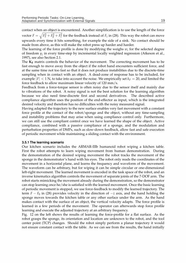
Performing Periodic Tasks: On-Line Learning, Adaptation and Synchronization with External Signals 17

contact when an object is encountered. Another simplification is to use the length of the force

vector F =√

F2x + F2

y + F2z for the feedback instead of Fz in (28). This way the robot can move

upwards every time it hits something, for example the side of a sink. No contact should bemade from above, as this will make the robot press up harder and harder.The learning of the force profile is done by modifying the weighs wi for the selected degreeof freedom yj in every time-step by incremental locally weighted regression (Atkeson et al.,1997), see also Section 2.1.The KF matrix controls the behavior of the movement. The correcting movement has to befast enough to move away from the object if the robot hand encounters sufficient force, andat the same time not too fast so that it does not produce instabilities due to the discrete-timesampling when in contact with an object. A dead-zone of response has to be included, forexample |F| < 1 N, to take into account the noise. We empirically set kF = 20, and limited theforce feedback to allow maximum linear velocity of 120 mm/s.Feedback from a force-torque sensor is often noisy due to the sensor itself and mainly dueto vibrations of the robot. A noisy signal is not the best solution for the learning algorithmbecause we also need time-discrete first and second derivatives. The described activecompliance algorithm uses the position of the end-effector as input, which is the integrateddesired velocity and therefore has no difficulties with the noisy measured signal.Having adapted the trajectory to the new surface enables very fast movement with a constantforce profile at the contact of the robot/sponge and the object, without any time-samplingand instability problems that may arise when using compliance control only. Furthermore,we can still use the compliant control once we have learned the shape of the object. Activecompliance, combined with a passive compliance of a sponge, and the modulation andperturbation properties of DMPs, such as slow-down feedback, allow fast and safe executionof periodic movement while maintaining a sliding contact with the environment.

3.5.1 The learning scenarioOur kitchen scenario includes the ARMAR-IIIb humanoid robot wiping a kitchen table.First the robot attempts to learn wiping movement from human demonstration. Duringthe demonstration of the desired wiping movement the robot tracks the movement of thesponge in the demonstrator’s hand with his eyes. The robot only reads the coordinates of themovement in a horizontal plane, and learns the frequency and waveform of the movement.The waveform can be arbitrary, but for wiping it can be simple circular or one-dimensionalleft-right movement. The learned movement is encoded in the task space of the robot, and aninverse kinematics algorithm controls the movement of separate joints of the 7-DOF arm. Therobot starts mimicking the movement already during the demonstration, so the demonstratorcan stop learning once he/she is satisfied with the learned movement. Once the basic learningof periodic movement is stopped, we use force-feedback to modify the learned trajectory. Theterm F − F0 in (28) provides velocity in the direction of −z axis, and the hand holding thesponge moves towards the kitchen table or any other surface under the arm. As the handmakes contact with the surface of an object, the vertical velocity adapts. The force profile islearned in a few periods of the movement. The operator can afterwards stop force profilelearning and execute the adjusted trajectory at an arbitrary frequency.Fig. 12 on the left shows the results of learning the force-profile for a flat surface. As therobot grasps the sponge, its orientation and location are unknown to the robot, and the toolcenter point (TCP) changes. Should the robot simply perform a planar trajectory it wouldnot ensure constant contact with the table. As we can see from the results, the hand initially

19Performing Periodic Tasks: On-Line Learning, Adaptation and Synchronization with External Signals

18 Will-be-set-by-IN-TECH

0 5 10 15 20 25 30 35 40−400

−350

−300

−250

z[m

m]

0 5 10 15 20 25 30 35 40−2

0

2

4

6

8

|F|[N]

t [s]

0 20 40 60 80 100−400

−350

−300

−250

z[m

m]

0 20 40 60 80 100−2

0

2

4

6

8

|F|[N]

t [s]

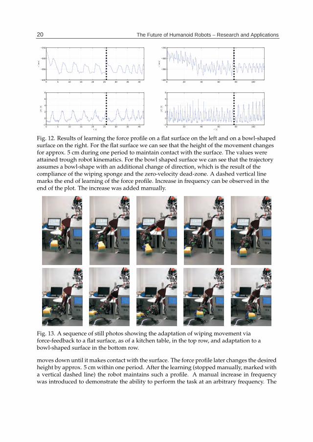
Fig. 12. Results of learning the force profile on a flat surface on the left and on a bowl-shapedsurface on the right. For the flat surface we can see that the height of the movement changesfor approx. 5 cm during one period to maintain contact with the surface. The values wereattained trough robot kinematics. For the bowl shaped surface we can see that the trajectoryassumes a bowl-shape with an additional change of direction, which is the result of thecompliance of the wiping sponge and the zero-velocity dead-zone. A dashed vertical linemarks the end of learning of the force profile. Increase in frequency can be observed in theend of the plot. The increase was added manually.

Fig. 13. A sequence of still photos showing the adaptation of wiping movement viaforce-feedback to a flat surface, as of a kitchen table, in the top row, and adaptation to abowl-shaped surface in the bottom row.

moves down until it makes contact with the surface. The force profile later changes the desiredheight by approx. 5 cm within one period. After the learning (stopped manually, marked witha vertical dashed line) the robot maintains such a profile. A manual increase in frequencywas introduced to demonstrate the ability to perform the task at an arbitrary frequency. The

20 The Future of Humanoid Robots – Research and Applications

Performing Periodic Tasks: On-Line Learning, Adaptation and Synchronization with External Signals 19

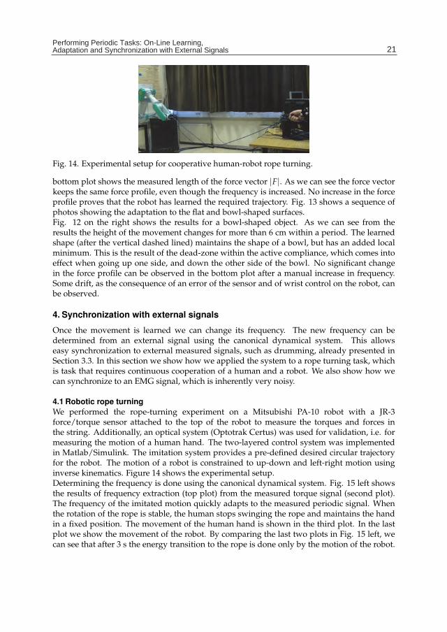
Fig. 14. Experimental setup for cooperative human-robot rope turning.

bottom plot shows the measured length of the force vector |F|. As we can see the force vectorkeeps the same force profile, even though the frequency is increased. No increase in the forceprofile proves that the robot has learned the required trajectory. Fig. 13 shows a sequence ofphotos showing the adaptation to the flat and bowl-shaped surfaces.Fig. 12 on the right shows the results for a bowl-shaped object. As we can see from theresults the height of the movement changes for more than 6 cm within a period. The learnedshape (after the vertical dashed lined) maintains the shape of a bowl, but has an added localminimum. This is the result of the dead-zone within the active compliance, which comes intoeffect when going up one side, and down the other side of the bowl. No significant changein the force profile can be observed in the bottom plot after a manual increase in frequency.Some drift, as the consequence of an error of the sensor and of wrist control on the robot, canbe observed.

4. Synchronization with external signals

Once the movement is learned we can change its frequency. The new frequency can bedetermined from an external signal using the canonical dynamical system. This allowseasy synchronization to external measured signals, such as drumming, already presented inSection 3.3. In this section we show how we applied the system to a rope turning task, whichis task that requires continuous cooperation of a human and a robot. We also show how wecan synchronize to an EMG signal, which is inherently very noisy.

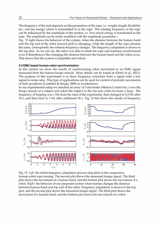
4.1 Robotic rope turningWe performed the rope-turning experiment on a Mitsubishi PA-10 robot with a JR-3force/torque sensor attached to the top of the robot to measure the torques and forces inthe string. Additionally, an optical system (Optotrak Certus) was used for validation, i.e. formeasuring the motion of a human hand. The two-layered control system was implementedin Matlab/Simulink. The imitation system provides a pre-defined desired circular trajectoryfor the robot. The motion of a robot is constrained to up-down and left-right motion usinginverse kinematics. Figure 14 shows the experimental setup.Determining the frequency is done using the canonical dynamical system. Fig. 15 left showsthe results of frequency extraction (top plot) from the measured torque signal (second plot).The frequency of the imitated motion quickly adapts to the measured periodic signal. Whenthe rotation of the rope is stable, the human stops swinging the rope and maintains the handin a fixed position. The movement of the human hand is shown in the third plot. In the lastplot we show the movement of the robot. By comparing the last two plots in Fig. 15 left, wecan see that after 3 s the energy transition to the rope is done only by the motion of the robot.

21Performing Periodic Tasks: On-Line Learning, Adaptation and Synchronization with External Signals

20 Will-be-set-by-IN-TECH

The frequency of the task depends on the parameters of the rope, i.e. weight, length, flexibilityetc., and the energy which is transmitted in to the rope. The rotating frequency of the ropecan be influenced by the amplitude of the motion, i.e. how much energy is transmitted to therope. The amplitude can be easily modified with the amplitude parameter r.Fig. 15 right shows the behavior of the system, when the distance between the human handand the top end of the robot (second plot) is changing, while the length of the rope remainsthe same, consequently the rotation frequency changes. The frequency adaptation is shown inthe top plot. As we can see, the robot was able to rotate the rope and maintain synchronizedeven if disturbances like changing the distance between the human hand and the robot occur.This shows that the system is adaptable and robust.

4.2 EMG based human-robot synchronizationIn this section we show the results of synchronizing robot movement to an EMG signalmeasured from the human biceps muscle. More details can be found at (Petric et al., 2011).The purpose of this experiment is to show frequency extraction from a signal with a lowsignal-to-noise ratio. This type of applications can be used for control of periodic movementsof limb prosthesis (Castellini & Smagt, 2009) or exoskeletons.In our experimental setup we attached an array of 3 electrodes (Motion Control Inc.) over thebiceps muscle of a subject and asked the subject to flex his arm when he hears a beep. Thefrequency of beeping was 1 Hz from the start of the experiment, then changed to 0.5 Hz after30 s, and then back to 1 Hz after additional 30 s. Fig. 16 left shows the results of frequency

81012141618

Ω[rad/s]

−1

0

1

y x,y

[Nm]

−0.2

0

0.2

hx,y

[m]

0 1 2 3 4 5 6 7

−0.1

0

0.1

xx,y

[m]

t [s]

81012141618

Ω[rad/s]

0.81

1.21.41.6

hz[m

]

−0.2

0

0.2

hx,y

[m]

0 10 20 30 40

−0.1

0

0.1

xx,y

[m]

t [s]

Fig. 15. Left: the initial frequency adaptation process (top plot) of the cooperativehuman-robot rope turning. The second plot shows the measured torque signal. The thirdplot shows the movement of a human hand, and the bottom plot shows the movement of arobot. Right: the behavior of our proposed system when human changes the distancebetween human hand and top end of the robot. Frequency adaptation is shown in the topplot, and the second plot shows the measured torque signal. The third plot shows themovement of a human hand, and the bottom plot shows the movement of a robot.

22 The Future of Humanoid Robots – Research and Applications

Performing Periodic Tasks: On-Line Learning, Adaptation and Synchronization with External Signals 21

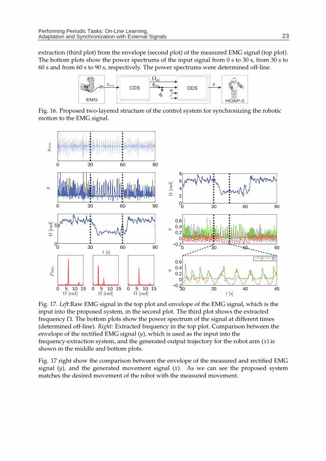
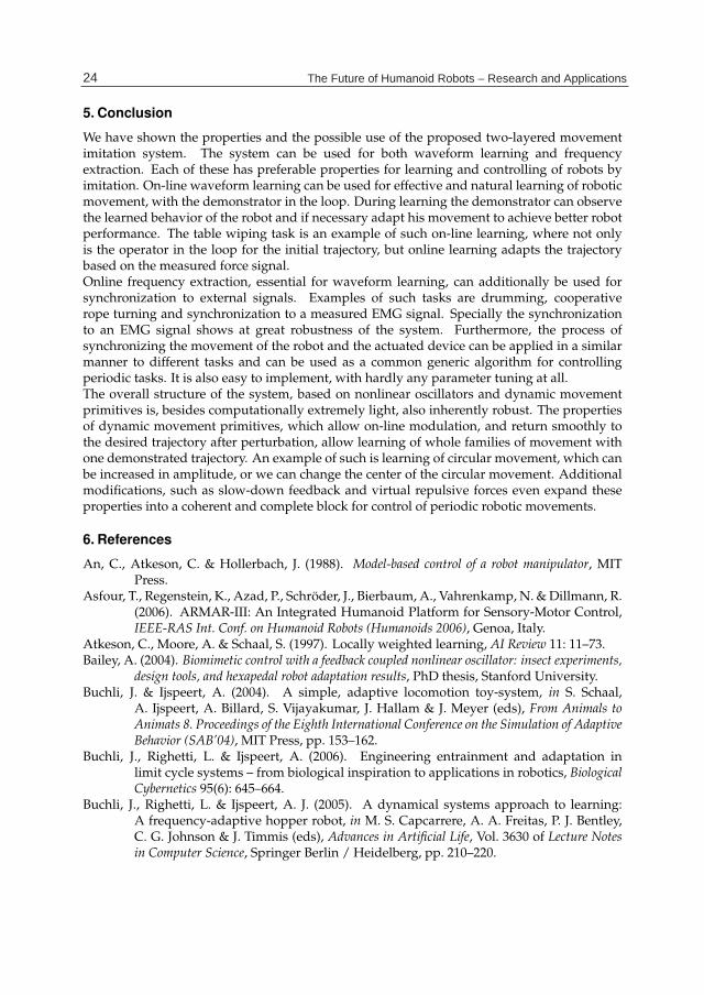
extraction (third plot) from the envelope (second plot) of the measured EMG signal (top plot).The bottom plots show the power spectrums of the input signal from 0 s to 30 s, from 30 s to60 s and from 60 s to 90 s, respectively. The power spectrums were determined off-line.

HOAP-3EMG

ydemo

CDS ODSwi

r

�AF

�AF

�l

x

Fig. 16. Proposed two-layered structure of the control system for synchronizing the roboticmotion to the EMG signal.

0 30 60 90

y raw

0 30 60 90

y

0 30 60 900

5

t [s]

Ω[rad]

0 5 10 15

Pow

.

Ω [rad]0 5 10 15

Ω [rad]0 5 10 15

Ω [rad]

0 30 60 9002468

Ω[rad]

0 30 60 90−0.2

00.20.40.6

y

30 35 40 45−0.2

00.20.40.6

t [s]

y

x y

Fig. 17. Left:Raw EMG signal in the top plot and envelope of the EMG signal, which is theinput into the proposed system, in the second plot. The third plot shows the extractedfrequency Ω. The bottom plots show the power spectrum of the signal at different times(determined off-line). Right: Extracted frequency in the top plot. Comparison between theenvelope of the rectified EMG signal (y), which is used as the input into thefrequency-extraction system, and the generated output trajectory for the robot arm (x) isshown in the middle and bottom plots.

Fig. 17 right show the comparison between the envelope of the measured and rectified EMGsignal (y), and the generated movement signal (x). As we can see the proposed systemmatches the desired movement of the robot with the measured movement.

23Performing Periodic Tasks: On-Line Learning, Adaptation and Synchronization with External Signals

22 Will-be-set-by-IN-TECH

5. Conclusion

We have shown the properties and the possible use of the proposed two-layered movementimitation system. The system can be used for both waveform learning and frequencyextraction. Each of these has preferable properties for learning and controlling of robots byimitation. On-line waveform learning can be used for effective and natural learning of roboticmovement, with the demonstrator in the loop. During learning the demonstrator can observethe learned behavior of the robot and if necessary adapt his movement to achieve better robotperformance. The table wiping task is an example of such on-line learning, where not onlyis the operator in the loop for the initial trajectory, but online learning adapts the trajectorybased on the measured force signal.Online frequency extraction, essential for waveform learning, can additionally be used forsynchronization to external signals. Examples of such tasks are drumming, cooperativerope turning and synchronization to a measured EMG signal. Specially the synchronizationto an EMG signal shows at great robustness of the system. Furthermore, the process ofsynchronizing the movement of the robot and the actuated device can be applied in a similarmanner to different tasks and can be used as a common generic algorithm for controllingperiodic tasks. It is also easy to implement, with hardly any parameter tuning at all.The overall structure of the system, based on nonlinear oscillators and dynamic movementprimitives is, besides computationally extremely light, also inherently robust. The propertiesof dynamic movement primitives, which allow on-line modulation, and return smoothly tothe desired trajectory after perturbation, allow learning of whole families of movement withone demonstrated trajectory. An example of such is learning of circular movement, which canbe increased in amplitude, or we can change the center of the circular movement. Additionalmodifications, such as slow-down feedback and virtual repulsive forces even expand theseproperties into a coherent and complete block for control of periodic robotic movements.

6. References

An, C., Atkeson, C. & Hollerbach, J. (1988). Model-based control of a robot manipulator, MITPress.

Asfour, T., Regenstein, K., Azad, P., Schröder, J., Bierbaum, A., Vahrenkamp, N. & Dillmann, R.(2006). ARMAR-III: An Integrated Humanoid Platform for Sensory-Motor Control,IEEE-RAS Int. Conf. on Humanoid Robots (Humanoids 2006), Genoa, Italy.

Atkeson, C., Moore, A. & Schaal, S. (1997). Locally weighted learning, AI Review 11: 11–73.Bailey, A. (2004). Biomimetic control with a feedback coupled nonlinear oscillator: insect experiments,

design tools, and hexapedal robot adaptation results, PhD thesis, Stanford University.Buchli, J. & Ijspeert, A. (2004). A simple, adaptive locomotion toy-system, in S. Schaal,

A. Ijspeert, A. Billard, S. Vijayakumar, J. Hallam & J. Meyer (eds), From Animals toAnimats 8. Proceedings of the Eighth International Conference on the Simulation of AdaptiveBehavior (SAB’04), MIT Press, pp. 153–162.

Buchli, J., Righetti, L. & Ijspeert, A. (2006). Engineering entrainment and adaptation inlimit cycle systems – from biological inspiration to applications in robotics, BiologicalCybernetics 95(6): 645–664.

Buchli, J., Righetti, L. & Ijspeert, A. J. (2005). A dynamical systems approach to learning:A frequency-adaptive hopper robot, in M. S. Capcarrere, A. A. Freitas, P. J. Bentley,C. G. Johnson & J. Timmis (eds), Advances in Artificial Life, Vol. 3630 of Lecture Notesin Computer Science, Springer Berlin / Heidelberg, pp. 210–220.

24 The Future of Humanoid Robots – Research and Applications

Performing Periodic Tasks: On-Line Learning, Adaptation and Synchronization with External Signals 23

Buchli, J., Righetti, L. & Ijspeert, A. J. (2008). Frequency Analysis with coupled nonlinearOscillators, Physica D: Nonlinear Phenomena 237: 1705–1718.

Buehler, M., Koditschek, D. & Kindlmann, P. (1994). Planning and Control of Robotic Jugglingand Catching Tasks, The International Journal of Robotics Research 13(2): 101–118.

Cafuta, P. & Curk, B. (2008). Control of nonholonomic robotic load, Advanced Motion Control,2008. AMC ’08. 10th IEEE International Workshop on, pp. 631 –636.

Calinon, S., Guenter, F. & Billard, A. (2007). On learning, representing, and generalizing atask in a humanoid robot, Systems, Man, and Cybernetics, Part B: Cybernetics, IEEETransactions on 37(2): 286 –298.

Castellini, C. & Smagt, P. v. d. (2009). Surface emg in advanced hand prosthetics, BiologicalCybernetics 100(1): 35–47.

Filho, A. C. d. P., Dutra, M. S. & Raptopoulos, L. S. C. (2005). Modeling of a bipedalrobot using mutually coupled rayleigh oscillators, Biological Cybernetics 92: 1–7.10.1007/s00422-004-0531-1.

Fukuoka, Y., Kimura, H. & Cohen, A. H. (2003). Adaptive Dynamic Walking of a QuadrupedRobot on Irregular Terrain Based on Biological Concepts, The International Journal ofRobotics Research 22(3-4): 187–202.

Furuta, K. (2003). Control of pendulum: from super mechano-system to human adaptivemechatronics, Decision and Control, 2003. Proceedings. 42nd IEEE Conference on, Vol. 2,pp. 1498 – 1507 Vol.2.

Gams, A., Ijspeert, A. J., Schaal, S. & Lenarcic, J. (2009). On-line learning and modulation ofperiodic movements with nonlinear dynamical systems, Auton. Robots 27(1): 3–23.

Gams, A., Žlajpah, L. & Lenarcic, J. (2007). Imitating human acceleration of a gyroscopicdevice, Robotica 25(4): 501–509.

Gangadhar, G., Joseph, D. & Chakravarthy, V. (2007). An oscillatory neuromotor model ofhandwriting generation, International Journal on Document Analysis and Recognition10: 69–84. 10.1007/s10032-007-0046-0.

Haken, H., Kelso, J. A. S. & Bunz, H. (1985). A theoretical model of phase transitions in humanhand movements, Biological Cybernetics 51: 347–356. 10.1007/BF00336922.

Hashimoto, K. & Noritsugu, T. (1996). Modeling and control of robotic yo-yo withvisual feedback, Robotics and Automation, 1996. Proceedings., 1996 IEEE InternationalConference on, Vol. 3, pp. 2650 –2655 vol.3.

Heyda, P. G. (2002). Roller ball dynamics revisited, American Journal of Physics70(10): 1049–1051.

Hollerbach, J. M. (1981). An oscillation theory of handwriting, Biological Cybernetics39: 139–156. 10.1007/BF00336740.

Ijspeert, A. J. (2008a). Central pattern generators for locomotion control in animals and robots:a review, Neural Networks 21(4): 642–653.

Ijspeert, A. J. (2008b). Central pattern generators for locomotion control in animals and robots:A review, Neural Networks 21(4): 642 – 653. Robotics and Neuroscience.

Ijspeert, A. J., Nakanishi, J. & Schaal, S. (2002). Movement imitation with nonlineardynamical systems in humanoid robots, Proc. IEEE Int. Conf. Robotics and Automation,pp. 1398–1403.

Ilg, W., Albiez, J., Jedele, H., Berns, K. & Dillmann, R. (1999). Adaptive periodic movementcontrol for the four legged walking machine bisam, Robotics and Automation, 1999.Proceedings. 1999 IEEE International Conference on, Vol. 3, pp. 2354 –2359 vol.3.

25Performing Periodic Tasks: On-Line Learning, Adaptation and Synchronization with External Signals

24 Will-be-set-by-IN-TECH

Inoue, K., Ma, S. & Jin, C. (2004). Neural oscillator network-based controller for meanderinglocomotion of snake-like robots, Robotics and Automation, 2004. Proceedings. ICRA ’04.2004 IEEE International Conference on, Vol. 5, pp. 5064 – 5069 Vol.5.

Jalics, L., Hemami, H. & Zheng, Y. (1997). Pattern generation using coupled oscillators forrobotic and biorobotic adaptive periodic movement, Robotics and Automation, 1997.Proceedings., 1997 IEEE International Conference on, Vol. 1, pp. 179 –184 vol.1.

Jin, H.-L., Ye, Q. & Zacksenhouse, M. (2009). Return maps, parameterization, and cycle-wiseplanning of yo-yo playing, Trans. Rob. 25(2): 438–445.

Jin, H.-L. & Zackenhouse, M. (2002). Yoyo dynamics: Sequence of collisions capturedby a restitution effect, Journal of Dynamic Systems, Measurement, and Control124(3): 390–397.

Jin, H.-L. & Zacksenhouse, M. (2003). Oscillatory neural networks for robotic yo-yo control,Neural Networks, IEEE Transactions on 14(2): 317 – 325.

Jindai, M. & Watanabe, T. (2007). Development of a handshake robot system based ona handshake approaching motion model, Advanced intelligent mechatronics, 2007IEEE/ASME international conference on, pp. 1 –6.

Kasuga, T. & Hashimoto, M. (2005). Human-robot handshaking using neural oscillators,Robotics and Automation, 2005. ICRA 2005. Proceedings of the 2005 IEEE InternationalConference on, pp. 3802 – 3807.

Kimura, H., Akiyama, S. & Sakurama, K. (1999). Realization of dynamic walking andrunning of the quadruped using neural oscillator, Autonomous Robots 7: 247–258.10.1023/A:1008924521542.

Kralemann, B., Cimponeriu, L., Rosenblum, M., Pikovsky, A. & Mrowka, R. (2008). Phasedynamics of coupled oscillators reconstructed from data, Phys. Rev. E 77(6): 066205.

Kun, A. & Miller, W.T., I. (1996). Adaptive dynamic balance of a biped robot usingneural networks, Robotics and Automation, 1996. Proceedings., 1996 IEEE InternationalConference on, Vol. 1, pp. 240 –245 vol.1.

Liu, C., Chen, Q. & Zhang, J. (2009). Coupled van der pol oscillators utilised as central patterngenerators for quadruped locomotion, Control and Decision Conference, 2009. CCDC’09. Chinese, pp. 3677 –3682.

Ljung, L. & Söderström, T. (1986). Theory and Practice of Recursive Identification, MIT Press.Mataric, M. (1998). Behavior-based robotics as a tool for synthesis of artificial behavior and

analysis of natural behavior, Trends in Cognitive Science 2(3): 82–87.Matsuoka, K. (1985). Sustained oscillations generated by mutually inhibiting neurons with

adaptation, Biological Cybernetics 52: 367–376. 10.1007/BF00449593.Matsuoka, K., Ohyama, N., Watanabe, A. & Ooshima, M. (2005). Control of a giant swing

robot using a neural oscillator, ICNC (2), pp. 274–282.Matsuoka, K. & Ooshima, M. (2007). A dish-spinning robot using a neural oscillator,

International Congress Series 1301: 218 – 221.Mirollo, R. E., Steven & Strogatz, H. (1990). Synchronization of pulse-coupled biological

oscillators, SIAM J. Appl. Math 50: 1645–1662.Miyamoto, H., Schaal, S., Gandolfo, F., Gomi, H., Koike, Y., Osu, R., Nakano, E., Wada, Y. &

Kawato, M. (1996). A kendama learning robot based on bi-directional theory, NeuralNetworks 9(8): 1281–1302.

Morimoto, J., Endo, G., Nakanishi, J. & Cheng, G. (2008). A biologically inspired bipedlocomotion strategy for humanoid robots: Modulation of sinusoidal patterns by acoupled oscillator model, Robotics, IEEE Transactions on 24(1): 185 –191.

26 The Future of Humanoid Robots – Research and Applications

Performing Periodic Tasks: On-Line Learning, Adaptation and Synchronization with External Signals 25

Petric, T., Curk, B., Cafuta, P. & Žlajpah, L. (2010). Modeling of the robotic powerball: anonholonomic, underactuated, and variable structure-type system, Mathematical andComputer Modelling of Dynamical Systems . 10.1080/13873954.2010.484237.

Petric, T., Gams, A., Tomšic, M. & Žlajpah, L. (2011). Control of rhythmic robotic movementsthrough synchronization with human muscle activity, 2011 IEEE InternationalConference on Robotics and Automation, ICRA 2011, May 9-13, 2011, Shanghai, China,Proceedings, IEEE.

Pikovsky, A., Author, Rosenblum, M., Author, Kurths, J., Author, Hilborn, R. C. & Reviewer(2002). Synchronization: A universal concept in nonlinear science, American Journalof Physics 70(6): 655–655.

Righetti, L., Buchli, J. & Ijspeert, A. (2006). Dynamic hebbian learning in adaptive frequencyoscillators, Physica D 216(2): 269–281.

Righetti, L. & Ijspeert, A. J. (2006). Programmable Central Pattern Generators: an applicationto biped locomotion control, Proceedings of the 2006 IEEE International Conference onRobotics and Automation.

Ronsse, R., Lefevre, P. & Sepulchre, R. (2007). Rhythmic feedback control of a blind planarjuggler, Robotics, IEEE Transactions on 23(4): 790 –802.

Sato, T., Hashimoto, M. & Tsukahara, M. (2007). Synchronization based control using onlinedesign of dynamics and its application to human-robot interaction, Robotics andBiomimetics, 2007. ROBIO 2007. IEEE International Conference on, pp. 652 –657.

Schaal, S. (1999). Is imitation learning the route to humanoid robots?, Trends in cognitive sciences(3): 233–242.

Schaal, S. & Atkeson, C. (1993). Open loop stable control strategies for robot juggling, Roboticsand Automation, 1993. Proceedings., 1993 IEEE International Conference on, pp. 913–918.

Schaal, S. & Atkeson, C. (1998). Constructive incremental learning from only localinformation, Neural Computation 10: 2047–2084.

Schaal, S., Mohajerian, P. & Ijspeert, A. (2007). Dynamics systems vs. optimal control –a unifying view, Vol. 165 of Progress in Brain Research, Elsevier, pp. 425 – 445.10.1016/S0079-6123(06)65027-9.

Sentis, L., Park, J. & Khatib, O. (2010). Compliant control of multicontact and center-of-massbehaviors in humanoid robots, Robotics, IEEE Transactions on 26(3): 483 –501.

Spong, M. (1995). The swing up control problem for the acrobot, Control Systems Magazine,IEEE 15(1): 49 –55.

Spong, M. & Bullo, F. (2005). Controlled symmetries and passive walking, Automatic Control,IEEE Transactions on 50(7): 1025 – 1031.

Strogatz, S. H. (1986). The mathematical structure of the human sleep-wake cycle, Springer-VerlagNew York, Inc., New York, NY, USA.

Thompson, S. E. & Patel, R. V. (1987). Formulation of joint trajectories for industrial robotsusing b-splines, Industrial Electronics, IEEE Transactions on IE-34(2): 192 –199.

Tsuda, S., Zauner, K.-P. & Gunji, Y.-P. (2007). Robot control with biological cells,Biosystems 87(2-3): 215 – 223. Papers presented at the Sixth International Workshopon Information Processing in Cells and Tissues, York, UK, 2005 - IPCAT 2005,Information Processing in Cells and Tissues.

Ude, A., Atkeson, C. G. & Riley, M. (2000). Planning of joint trajectories for humanoid robotsusing b-spline wavelets, ICRA, pp. 2223–2228.

van der Pol, B. (1934). The nonlinear theory of electric oscillations, Proceedings of the Instituteof Radio Engineers 22(9): 1051 –1086.

27Performing Periodic Tasks: On-Line Learning, Adaptation and Synchronization with External Signals

26 Will-be-set-by-IN-TECH

Veskos, P. & Demiris, Y. (2005). Developmental acquisition of entrainment skills in robotswinging using van der pol oscillators, Vol. 123, Lund University Cognitive Studies,pp. 87–93.

Villani, L. & J., D. S. (2008). Handbook of Robotics, Springer, chapter Force Control.Žlajpah, L. (2006). Robotic yo-yo: modelling and control strategies, Robotica 24(2): 211–220.Williamson, M. (1999). Designing rhythmic motions using neural oscillators, Intelligent Robots

and Systems, 1999. IROS ’99. Proceedings. 1999 IEEE/RSJ International Conference on,Vol. 1, pp. 494 –500 vol.1.

Williamson, M. M. (1998). Neural control of rhythmic arm movements, Neural Networks11(7-8): 1379 – 1394.

28 The Future of Humanoid Robots – Research and Applications