NHST Debate p. 1

The Null Hypothesis Significance Testing Debate and Its Implications for Personality Research

R. Chris Fraley and Michael J. Marks

University of Illinois at Urbana-Champaign

Fraley, R. C., & Marks, M. J. (2007). The null hypothesis significance testing debate and its

implications for personality research. In R. W. Robins, R. C. Fraley, & R. F. Krueger (Eds.),

Handbook of research methods in personality psychology (pp. 149-169). New York: Guilford.

Note: This version might not be identical to the copy-edited published version.

NHST Debate p. 2

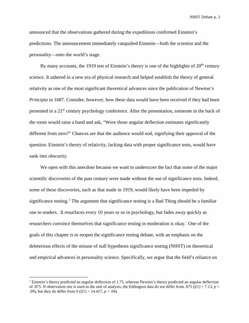
In 1915 Einstein published his now classic treatise on the theory of general relativity. According

to his theory, gravity, as it had been traditionally conceived, was not a force per se, but an artifact

of the warping of space and time resulting from the mass or energy of objects. Although

Einstein’s theory made many predictions, one that captured a lot of empirical attention was that

light should bend to a specific degree when it passes by a massive object due to the distortions in

space created by that object. Experimental physicists reasoned that, if an object’s mass is truly

capable of warping space, then the light passing by a sufficiently massive object should not

follow a straight line, but rather a curved trajectory. For example, if one were to observe a distant

star during conditions in which its light waves had to pass near the Sun, the star would appear to

be in a slightly different location than it would under other conditions.

Scientists had a challenging time testing this prediction, however, because the ambient light

emitted by the Sun made it difficult to observe the positioning of stars accurately. Fortunately,

copies of Einstein’s papers made it to Cambridge where they were read by the astrophysicist,

Arthur Stanley Eddington. Eddington realized that it would be possible to test Einstein’s

prediction by observing stars during a total eclipse. With the Sun’s light being momentarily

blocked, the positioning of stars could be recorded more accurately than would be possible

during normal viewing conditions. If Einstein’s theory was correct, the angular deflection of the

stars’ light would be 1.75 seconds of an arc—twice that predicted by the then dominant theory of

Sir Isaac Newton. Eddington was able to obtain funding to organize expeditions to Sobral, Brazil

and the island of Principe off the West African coast to take photographs of the sky during the

eclipse. The expeditions, while not going as smoothly as Eddington had hoped, were productive

nonetheless. The Sobral group obtained an angular deflection estimate of 1.98; the Principe

group obtained an estimate of 1.61 (Kaku, 2004). In November of 1919 the Royal Society

NHST Debate p. 3

announced that the observations gathered during the expeditions confirmed Einstein’s

predictions. The announcement immediately catapulted Einstein—both the scientist and the

personality—onto the world’s stage.

By many accounts, the 1919 test of Einstein’s theory is one of the highlights of 20th century

science. It ushered in a new era of physical research and helped establish the theory of general

relativity as one of the most significant theoretical advances since the publication of Newton’s

Principia in 1687. Consider, however, how these data would have been received if they had been

presented in a 21st century psychology conference. After the presentation, someone in the back of

the room would raise a hand and ask, “Were those angular deflection estimates significantly

different from zero?” Chances are that the audience would nod, signifying their approval of the

question. Einstein’s theory of relativity, lacking data with proper significance tests, would have

sank into obscurity.

We open with this anecdote because we want to underscore the fact that some of the major

scientific discoveries of the past century were made without the use of significance tests. Indeed,

some of these discoveries, such as that made in 1919, would likely have been impeded by

significance testing.1 The argument that significance testing is a Bad Thing should be a familiar

one to readers. It resurfaces every 10 years or so in psychology, but fades away quickly as

researchers convince themselves that significance testing in moderation is okay. One of the

goals of this chapter is to reopen the significance testing debate, with an emphasis on the

deleterious effects of the misuse of null hypothesis significance testing (NHST) on theoretical

and empirical advances in personality science. Specifically, we argue that the field’s reliance on

1 Einstein’s theory predicted an angular deflection of 1.75, whereas Newton’s theory predicted an angular deflection of .875. If observation site is used as the unit of analysis, the Eddington data do not differ from .875 (t[1] = 7.13, p = .09), but they do differ from 0 (t[1] = 14.417, p = .04).

NHST Debate p. 4

significance testing has led to numerous misinterpretations of data, a biased research literature,

and has hampered our ability to develop sophisticated models of personality processes.

We begin by reviewing the basics of significance tests (i.e., how they work, how they are

used). Next, we discuss some common misinterpretations of NHST as well as some of the

criticisms that have been leveled at NHST even when understood properly. Finally, we make

some recommendations on how personality psychologists can avoid some of the pitfalls that tend

to be accompanied by the use of significance tests. It is our hope that this chapter will help

facilitate discussion of what we view as a crucial methodological issue for the field, while

offering some constructive recommendations.

What is a Significance Test?

Before discussing the significance testing debate in greater detail, it will be useful to first

review what a significance test is. Let us begin with a hypothetical, but realistic, research

scenario. Suppose our theory suggests that there should be a positive association between two

variables, such as attachment security and relationship quality. To test this hypothesis, we obtain

a sample of 20 secure and 20 insecure people in dating and marital relationships and administer

questionnaires designed to assess relationship quality.

Let us assume that we find that secure people score 2 points higher than insecure people on

our measure of relationship quality. Does this finding corroborate our hypothesis? At face value,

the answer is “yes”: We predicted and found a positive difference. As statisticians will remind

us, however, even if there is no real association between security and relationship quality, we are

likely to observe some difference between groups due to sampling error – the inevitable

statistical noise that results when researchers study a subset of cases from a larger population.

Thus, to determine whether the empirical difference corroborates our hypothesis, we first need to

NHST Debate p. 5

determine the probability of observing a difference of 2 points or higher under the hypothesis

that there is no association between these constructs in the population. According to this null

hypothesis, the population difference is zero and any deviation from this value observed in our

sample is due to sampling error.

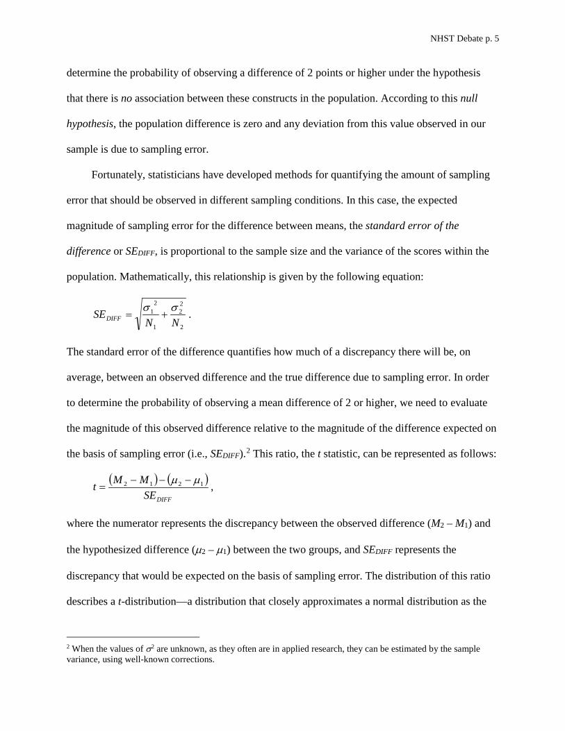
Fortunately, statisticians have developed methods for quantifying the amount of sampling

error that should be observed in different sampling conditions. In this case, the expected

magnitude of sampling error for the difference between means, the standard error of the

difference or SEDIFF, is proportional to the sample size and the variance of the scores within the

population. Mathematically, this relationship is given by the following equation:

2

22

1

21

NNSEDIFF

σσ+= .

The standard error of the difference quantifies how much of a discrepancy there will be, on

average, between an observed difference and the true difference due to sampling error. In order

to determine the probability of observing a mean difference of 2 or higher, we need to evaluate

the magnitude of this observed difference relative to the magnitude of the difference expected on

the basis of sampling error (i.e., SEDIFF).2 This ratio, the t statistic, can be represented as follows:

( ) ( )DIFFSE

MMt 1212 µµ −−−= ,

where the numerator represents the discrepancy between the observed difference (M2 – M1) and

the hypothesized difference (µ2 – µ1) between the two groups, and SEDIFF represents the

discrepancy that would be expected on the basis of sampling error. The distribution of this ratio

describes a t-distribution—a distribution that closely approximates a normal distribution as the

2 When the values of σ2 are unknown, as they often are in applied research, they can be estimated by the sample variance, using well-known corrections.

NHST Debate p. 6

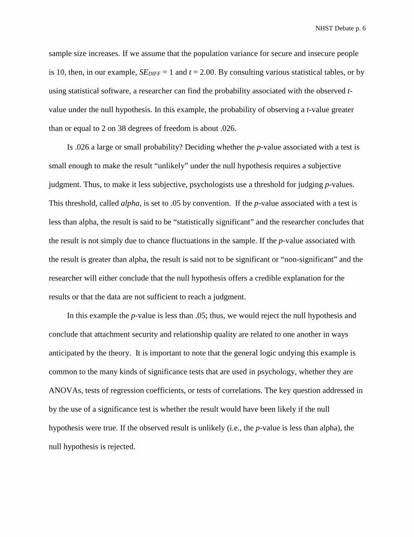
sample size increases. If we assume that the population variance for secure and insecure people

is 10, then, in our example, SEDIFF = 1 and t = 2.00. By consulting various statistical tables, or by

using statistical software, a researcher can find the probability associated with the observed t-

value under the null hypothesis. In this example, the probability of observing a t-value greater

than or equal to 2 on 38 degrees of freedom is about .026.

Is .026 a large or small probability? Deciding whether the p-value associated with a test is

small enough to make the result “unlikely” under the null hypothesis requires a subjective

judgment. Thus, to make it less subjective, psychologists use a threshold for judging p-values.

This threshold, called alpha, is set to .05 by convention. If the p-value associated with a test is

less than alpha, the result is said to be “statistically significant” and the researcher concludes that

the result is not simply due to chance fluctuations in the sample. If the p-value associated with

the result is greater than alpha, the result is said not to be significant or “non-significant” and the

researcher will either conclude that the null hypothesis offers a credible explanation for the

results or that the data are not sufficient to reach a judgment.

In this example the p-value is less than .05; thus, we would reject the null hypothesis and

conclude that attachment security and relationship quality are related to one another in ways

anticipated by the theory. It is important to note that the general logic undying this example is

common to the many kinds of significance tests that are used in psychology, whether they are

ANOVAs, tests of regression coefficients, or tests of correlations. The key question addressed in

by the use of a significance test is whether the result would have been likely if the null

hypothesis were true. If the observed result is unlikely (i.e., the p-value is less than alpha), the

null hypothesis is rejected.

NHST Debate p. 7

Some Common Misinterpretations of Significance Tests and P-values

Significance testing is widely used in personality psychology, despite the fact that

methodologists have critiqued those tests for several decades. One of the many claims that critics

of NHST have made is that many researchers hold mistaken assumptions about what significance

tests can and cannot tell us about our data. In this section we review some of the common

misconceptions that researchers have concerning the meaning of p-values. Once we have

clarified what p-values do and do not tell us about our data and hypotheses, we turn to the more

controversial question of whether significance tests, even when properly understood, are a help

or a hindrance in the scientific enterprise.

Statistically Significant = Substantively Significant

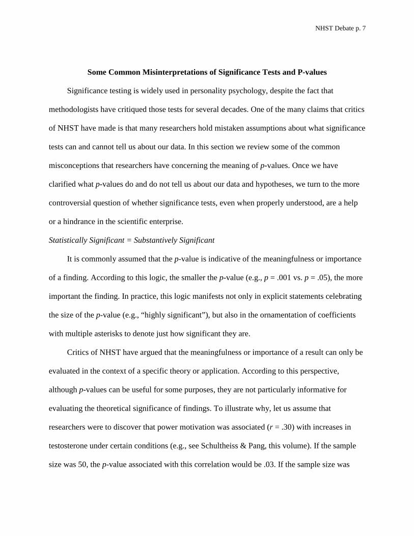
It is commonly assumed that the p-value is indicative of the meaningfulness or importance

of a finding. According to this logic, the smaller the p-value (e.g., p = .001 vs. p = .05), the more

important the finding. In practice, this logic manifests not only in explicit statements celebrating

the size of the p-value (e.g., “highly significant”), but also in the ornamentation of coefficients

with multiple asterisks to denote just how significant they are.

Critics of NHST have argued that the meaningfulness or importance of a result can only be

evaluated in the context of a specific theory or application. According to this perspective,

although p-values can be useful for some purposes, they are not particularly informative for

evaluating the theoretical significance of findings. To illustrate why, let us assume that

researchers were to discover that power motivation was associated (r = .30) with increases in

testosterone under certain conditions (e.g., see Schultheiss & Pang, this volume). If the sample

size was 50, the p-value associated with this correlation would be .03. If the sample size was

NHST Debate p. 8

1000, however, the p-value associated with the correlation would be <.001. One association is

clearly more statistically significant than the other, but is one more important than the other? No.

The actual magnitude of the correlations is the same in both cases; therefore, the two studies

have identical implications for the theory in question. It is true that one finding is based on a

larger sample size than the other and, thus, produces a smaller standard error. However, it would

be better to conclude that one correlation estimates the true correlation with more precision than

the other (i.e., one study is better designed than the other because it draws upon a larger sample

size) than to conclude that one correlation is more substantively important than the other.

The key point here is that the way in which a finding is interpreted should depend not on

the p-value but on the magnitude of the finding itself—the effect size or parameter value under

consideration. Meehl (1990) argued that one reason researchers tend to look to p-values rather

than effect sizes for theoretical understanding is that statistical training in psychology encourages

students to equate “hypothesis testing” with NHST. When NHST is equated with hypothesis

testing, it is only natural to assume that the size of the p-value has a direct relationship to the

theoretical significance of the findings. But, in Meehl’s view, this subtle equation has led

psychologists to conflate two very distinct roles that mathematics and statistics play in science

(see Figure 1). One function of mathematics is for the formalization of theories and the

derivation of quantitative predictions that can be tested empirically. For example, if one works

through the mathematics underlying Einstein’s theory of General Relativity, one can derive the

angular deflection of light as it passes by an object of a given mass. The theoretical model can

then be tested by comparing the theoretical values with the empirical ones. The other function of

mathematics is for quantifying sampling error and estimating the degree to which empirical

values deviate from population values. This latter function, which is more familiar to

NHST Debate p. 9

psychologists and statisticians, is useful for deriving the expected magnitude of sampling errors

in different research situations, but it is not directly relevant for testing psychological theories.

Given Meehl’s (1990) distinction between hypothesis tests (i.e., the comparison of

theoretical values to observed ones) and inferential statistics (i.e., the study of sampling

distributions), why do psychologists assume that evaluating sampling error is the same thing as

testing a substantive hypothesis? It is hard to say for sure, but both Meehl (1990) and Gigerenzer

(1993) have speculated that is has something to do with the artificial sense of rigor that comes

along with using the machinery of NHST.

To demonstrate just how ingrained this sense is in psychologists, Meehl (1990) challenged

his readers to imagine how hypothesis testing would proceed if the sample values were the

population values, thereby making sampling error and NHST irrelevant. In such a situation,

theory testing would be relatively straight-forward in most areas of psychology. If a theory

predicts a positive correlation and, empirically, the correlation turns out to be positive, then the

hypothesis would pass the test. Most psychologists would admit that this seems like a flimsy

state of affairs. Indeed, from Meehl’s (1990) perspective, it is not only flimsy, but it poses a huge

problem for the philosophy of theory testing in psychology. Meehl (1978) argued that when a

directional prediction is made, the hypothesis has a 50-50 chance of being confirmed, even if it is

false. In his view, a test would be much more rigorous if it predicted a point value (i.e., a specific

numerical value, such as a correlation of .50 or a ratio among parameters) or a narrow range of

values. In such a case, the empirical test would be a much more risky one and the empirical

results would carry more interpretive weight.

Meehl argues that researchers have created an artificial sense of rigor and objectivity by

using NHST because the test statistic associated with NHST must fall in a narrow region to allow

NHST Debate p. 10

the researcher to reject the null hypothesis. The difficulty in obtaining a statistic in such a small

probability region, coupled with the tendency of psychologists to make directional predictions, is

one reason why researchers celebrate significant results and attach substantive interpretations to

p-values rather than the effects of interest. (As will be discussed in a subsequent section,

obtaining a significant result can be challenging not because of the rigor of the test, but due to

the relative lack of attention psychologists pay to statistical power.)

Statistically Significant = The Null Hypothesis Provides an Unlikely Explanation for the Data

Another problematic assumption that researchers hold is that the p-value is indicative of the

likelihood that the results were due to chance. Specifically, if p is less than .05, it is assumed that

the null hypothesis is unlikely to offer a viable account for the findings. According to critics of

NHST, this misunderstanding stems from the conflation of two distinct interpretations of

probability: relative frequency and subjective probability. A relative frequency interpretation of

probability equates probability with the long-run outcome of an event. For example, if we were

to toss a fair coin and claim that the chances that the coin will land on heads is .50, the “.50”

technically refers to what we would expect to observe over the long-run if we were to repeat the

procedure across an infinite number of trials. Importantly, “.50” does not refer to any specific

toss, nor does it reference the likelihood that the coin is a fair one. From a relative frequency

perspective, the language of probability applies only to long-run outcomes, not to specific trials

or hypotheses. A subjective interpretation of probability, in contrast, treats probabilities as

quantitative assessments concerning the likelihood of an outcome or the likelihood that a certain

claim is correct. Subjective probabilities are ubiquitous in everyday life. For example, when

someone says “I think there is an 80% chance that it will rain today,” he or she is essentially

claiming to be highly confident that it will rain. When a researcher concludes that the null

NHST Debate p. 11

hypothesis offers an unlikely account for the data, he or she is relying upon subjective

interpretations of probability.

The familiar p-value produced by NHST is a relative frequency probability, not a

subjective probability. As described previously, it reflects the proportion of time that a test

statistic (i.e., a t-value) would be observed if the same study were to be carried out ad infinitum

and if the null hypothesis were true. It is also noteworthy that, because it specifies the probability

(P) of an outcome (D) given a particular state of affairs (i.e., that the null hypothesis is true: H0),

the familiar p-value is a conditional probability and can be written as P(D|H0). Importantly, this

probability does not indicate whether a specific outcome (D) is due to chance nor does it indicate

the likelihood that the null hypothesis is true (H0). In other words, P(D|H0) does not quantify

what researchers think it does, namely the probability that null hypothesis is true given the data

(i.e., P(H0|D)).

Bayes’ theorem provides a useful means to explicate the relationship between these two

kinds of probability statements (see Salsburg, 2001). According to Bayes’ theorem,

( ) ( ) ( )( ) ( ) ( ) ( )1100

000 ||

||HDPHPHDPHP

HDPHPDHP×+×

×= .

In other words, if a researcher wishes to evaluate the probability that his or her findings are due

to chance, he or she would need to know the a priori probability that the null hypothesis is true,

P(H0), in addition to other probabilities (i.e., the probability that the alternative hypothesis is

true, P(H1), and the probability of the data under the alternative hypothesis, P(D|H1)).3 Because

these first two probabilities are not relative frequency probabilities (i.e., probabilities based on

long-run frequencies) but are subjective probabilities (see Oakes, 1986), they can be selected

3 When there are multiple hypotheses, the term P(D|H1) is expanded accordingly. In this example, we assume that the research hypothesis, H1, is inclusive of all values other than 0.00 (i.e., a non-directional prediction).

NHST Debate p. 12

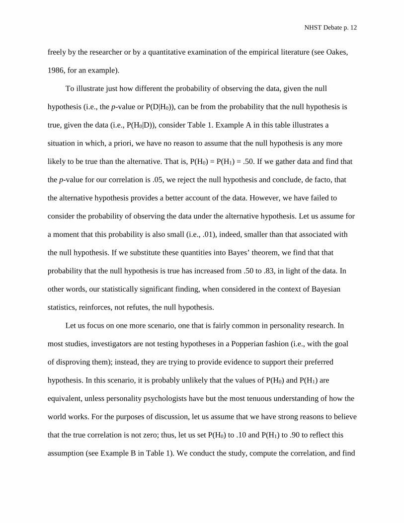
freely by the researcher or by a quantitative examination of the empirical literature (see Oakes,

1986, for an example).

To illustrate just how different the probability of observing the data, given the null

hypothesis (i.e., the p-value or P(D|H0)), can be from the probability that the null hypothesis is

true, given the data (i.e., P(H0|D)), consider Table 1. Example A in this table illustrates a

situation in which, a priori, we have no reason to assume that the null hypothesis is any more

likely to be true than the alternative. That is, P(H0) = P(H1) = .50. If we gather data and find that

the p-value for our correlation is .05, we reject the null hypothesis and conclude, de facto, that

the alternative hypothesis provides a better account of the data. However, we have failed to

consider the probability of observing the data under the alternative hypothesis. Let us assume for

a moment that this probability is also small (i.e., .01), indeed, smaller than that associated with

the null hypothesis. If we substitute these quantities into Bayes’ theorem, we find that that

probability that the null hypothesis is true has increased from .50 to .83, in light of the data. In

other words, our statistically significant finding, when considered in the context of Bayesian

statistics, reinforces, not refutes, the null hypothesis.

Let us focus on one more scenario, one that is fairly common in personality research. In

most studies, investigators are not testing hypotheses in a Popperian fashion (i.e., with the goal

of disproving them); instead, they are trying to provide evidence to support their preferred

hypothesis. In this scenario, it is probably unlikely that the values of P(H0) and P(H1) are

equivalent, unless personality psychologists have but the most tenuous understanding of how the

world works. For the purposes of discussion, let us assume that we have strong reasons to believe

that the true correlation is not zero; thus, let us set P(H0) to .10 and P(H1) to .90 to reflect this

assumption (see Example B in Table 1). We conduct the study, compute the correlation, and find

NHST Debate p. 13

a p-value of .15. The result is not statistically significant; thus, standard NHST procedures would

lead us to “fail to reject” the null hypothesis. Does this mean that the null hypothesis is likely to

be correct? If we assume that the data are equivocal with respect to the research hypothesis (i.e.,

P(D|H1)), the probability of the null hypothesis being true, given the data, is actually .03. Thus,

although the empirical result was not statistically significant, the revised likelihood estimate

(which Bayesians call the posterior probability) that the null hypothesis is correct has dropped

from .10 to .03. These data, in fact, undermine the null hypothesis, despite the fact that standard

NHST procedures would lead us to not reject it.

Table 1 illustrates these and some alternative situations, including one in which the p-value

is equal to the inverse probability (see Example C). The important thing to note is that, in most

circumstances, these two quantities will not be identical. In other words, a small p-value does not

necessarily mean that the null hypothesis is true, nor does a nonsignificant finding indicate that

the null hypothesis should be retained. Within a Bayesian framework, evaluating the null

hypothesis requires attention to more than just one probability. If researchers are truly interested

in evaluating the likelihood that their results are due to chance (i.e., P(H0|D)), it is necessary to

make assumptions about other quantities and use the empirical p-value in combination with these

quantities to estimate P(H0|D). Without doing so, one could argue that there are little grounds for

assuming that a small p-value provides evidence against the null hypothesis.

Before closing this section, we should note that when researchers learn about subjective

probabilities and Bayesian statistics, they sometimes respond that there is no place for subjective

assessments in an objective science. Bayesians have two rejoinders to this point. First, some

advocates of Bayesian statistics have argued that subjective probability is the only meaningful

way to discuss probability. According to this perspective, when lay people and scientists use

NHST Debate p. 14

probability statements they are often concerned with the assessment of specific outcomes or

hypotheses; they are not truly concerned with what will happen in a hypothetical universe of

long-run experiments. No one really cares how often it would rain in Urbana, Illinois on

September 8, 2005, for example, if that date were to be repeated over and over again in a

hypothetical world. When researchers conduct a study on the association between security and

relationship quality or any other variables of interest, they are concerned with assessing the

likelihood that the null hypothesis is true in light of the data. This likelihood cannot be directly

quantified through long run frequency definitions of probability, but, if the various quantities are

taken seriously and combined via Bayes’ Theorem, it is possible to attach a rationally justified

probability statement to the null hypothesis. This brings us to the second rejoinder: Subjective

assessments play an inevitable role in science, even for those who like to conceptualize science

as an objective enterprise. Bayesian advocates argue that, so long as subjective appraisals are

used in psychology, it is most defensible (i.e., more objective) to formalize those appraisals in a

manner that is public and rational than to allow them to seep into the scientific process through

more idiosyncratic, and potentially insidious, channels. In other words, the use of subjective

probabilities, when combined with Bayesian analyses, facilitates an objective and rational means

for evaluating scientific hypotheses.

In summary, researchers often assume that a small p-value indicates that the null

hypothesis is unlikely to be true (and vice versa: a non-significant results implies that the null

hypothesis may provide a viable explanation for the data). In other words, researchers often

assume that the p-value can be used to evaluate the likelihood that their data are due to chance.

Bayesian considerations, however, show this assumption to be false. The p-value, which

provides information about the probability of the data, given that the null hypothesis is true, does

NHST Debate p. 15

not indicate the probability that chance events can explain the data. Researchers who are

interested in evaluating the probability that chance explains the data can do so by combining the

p-value with other kinds of probabilities via Bayes’ Theorem.

Statistically Significant = A Reliable Finding

Replication is one of the cornerstones of the science. The most straightforward way to

demonstrate the reliability of an empirical result is to conduct a replication study to see whether

or not the result can be found again. The more common approach, however, is to conduct a null

hypothesis significance test. According to this tradition, if a researcher can show that the p-value

associated with a test statistic is very low (less than 5%), the researcher can be reasonably

confident that, if he or she were to do the study again, the results would be significant.

The belief that the p-value of a significance test is indicative of a result’s reliability is

widespread (see Sohn, 1998, pp. 292-293, for examples). Indeed, authors often write about

statistically significant findings as if the results are “reliable.” However, as recent writers have

explained, researchers hold many misconceptions about what p-values can tell us about the

reliability of findings (Meehl, 1990; Oakes, 1986; Schmidt, 1996; Sohn, 1998). Oakes (1986),

for example, surveyed 70 academic psychologists and found that 60% of them erroneously

believed that a p-value of .01 implied that a replication study would have a 99% chance of

yielding significant results (see Oakes, 1986, for a discussion of why this assumption is

incorrect). While recent advocates of significance tests have concurred that the probability of

replicating a significant effect is not literally equal to 1 minus the p-value, they have defended

researchers’ intuition that p-values indicate something about the replicability of a finding (Harris,

1997; Krueger, 2001; Scarr, 1997).

NHST Debate p. 16

Is this intuition correct? To address this question, we must first discuss which factors

determine whether a finding is replicable. The likelihood of replicating an empirical result is

directly related to the statistical power of the research design. Statistical power refers to the

probability that the statistical test will lead to a significant result, given that the null hypothesis is

false (Cohen, 1992). Statistical power is a function of 3 major factors: (a) the alpha level used for

the statistical test (set to .05, by convention), (b) the true effect size or population parameter, and

(c) the sample size. Thus, to determine whether a significant finding can be replicated, one needs

to know the statistical power of the replication study. It is important to note that, because the

statistical power is determined by the population effect size and that that effect is unknown

(indeed, it is the key quantity to be inferred from an estimation perspective), one can never know

the statistical power of a test in any unambiguous sense. Instead, one must make an assumption

about the population effect size (based on theory, experience, or previous research), and, given

the sample size and alpha level, compute the statistical power of the test.

For the sake of discussion, let us assume that we are interested in studying the correlation

between security and relationship quality and that the population correlation is .30. Now, let us

draw a sample of 100 people from the population, assess both variables, and compute the

correlation between them. Let us assume that the correlation we observe in our initial study is .20

and that the associated p-value is .04. Does this p-value tell us anything about the likelihood that,

if we were to conduct an exact replication study (i.e., another study in which we drew 100 people

from the same population), we would get a significant result?

No. To understand why, it is necessary to keep in mind the way in which sampling

distributions work and which factors influence statistical power. If we define the probability of

replication as the statistical power of the test, the first thing to note is that, in a series of

NHST Debate p. 17

replication studies, the key factors that influence the power of the test (i.e., alpha, N, and the

population effect size) are constants, not variables. Thus, if the true correlation is .30 and the

sample size used is 100, the power of the test is .80 in Study 1, .80 in Study 2, .80 in Study 3, and

so on regardless of the p-value associated with any one test. In other words, the p-value from

any one replication study is irrelevant for the power of the test. More importantly, the p-value in

any one study is statistically independent of the others because the only factor influencing

variation in the observed correlations (upon which the p-value is calculated) is random sampling

error. Thus, the p-value observed in an initial study is unrelated to the likelihood that an exact

replication study will yield a significant result.

There is one exception to this conclusion. Namely, if researchers are examining a large

number of correlations (e.g., correlations between 10 distinct variables) in one sample, the

correlations with the smaller p-values are more likely to be replicable than those with larger p-

values (see Greenwald, Gonzalez, Harris, & Guthrie, 1996). This is the case because the larger

correlations will have smaller p-values and larger correlations are more likely to reflect larger

population correlations than smaller ones. Although one could argue that the p-values for the

various correlations is associated with the replicability of those correlations (see Greenwald et

al., 1996; Krueger, 2001), it would be inaccurate to assume that the p-value itself is responsible.

It would be more appropriate to conclude that, holding sample size constant, it is easier to

replicate findings when the population correlations are large as opposed to small. Larger effects

are easier to detect for a given sample size.

The Potential Problems of Using Significance Tests in Personality Research

Although some of the major criticisms of NHSTs concern misinterpretations of p-values,

several writers have argued that, even if properly interpreted, p-values and significance tests

NHST Debate p. 18

would be of limited use in psychological science. In this section we discuss some of these

arguments, with attention focused on their implications for research in personality psychology.

The Asymmetric Nature of Significance Tests

Significance tests are used to evaluate the probability of observing data of a certain

magnitude, assuming that the null hypothesis is true. When the test statistic falls within the

critical region of a sampling distribution, the null hypothesis is rejected; if it does not, the null

hypothesis is retained. When students first learn this logic, they are often confused by the fact

that the null hypothesis is being tested rather than the research hypothesis. It would seem more

intuitive to determine whether the data are unlikely under the research hypothesis and, if so,

reject the research hypothesis. Indeed, according to Meehl (1967), significance tests are used in

this way in some areas of science, but this usage is rare in psychology.

When students query instructors on this apparent paradox, the common response is that,

yes, it does seem odd to test the null hypothesis instead of the research hypothesis, but, as it turns

out, testing the research hypothesis is impossible. (This is not an answer that most students find

assuring.) When the research hypothesis leads to a directional prediction (i.e., the correlation will

be greater than zero, one group will score higher on average than the other), there are an infinite

number of population values that are compatible with it (e.g., r = .01, r = .10, r = .43, r = .44). It

would not be practical to generate a sampling distribution for each possibility. Doing so would

lead to the uninteresting (but valid) conclusion that the correlation observed is most likely in a

case in which the population value is equal to the observed correlation.

The fact that only one hypothesis is tested in the traditional application of NHST makes

significance tests inherently asymmetrical (see Rozeboom, 1960). In other words, depending on

the statistical power of the test, the test will be biased either in favor of or against the null

NHST Debate p. 19

hypothesis. Consider the following example. Let us assume that the true correlation is equal to

.30. If a researcher were to draw a sample of 40 cases from the population and obtain a

correlation of .25 (p = .12), he or she would not reject the null hypothesis, thereby concluding

that the null hypothesis offers a viable account of the data. If one were to generate a sampling

distribution around the true correlation of .30, however, one would see that a value of .25 is, in

fact, relatively likely under the true hypothesis. In other words, in this situation we cannot reject

the null hypothesis, but, if we compared our data against the “true” sampling distribution instead

of a null one, we would find that we cannot reject the research hypothesis either.

The important point here is that basic statistical theory demonstrates that the sample

statistic (in some cases, following adjustment, as with the standard deviation) is the best estimate

of the population parameter. Thus, in the absence of any other information, researchers would be

best off to conclude that the population value is equal to the value observed in the sample

regardless of the p-value associated with sample value. When significance tests are emphasized,

focus shifts away from estimation and towards answering the question of whether the null

hypothesis provides the most parsimonious account for the data. The use of a significance test

implicitly gives the null hypothesis greater weight than is warranted in light of the fundamentals

of sampling theory. If researchers want to give the null hypothesis greater credence than the

alternatives a priori, it may be useful to use Bayesian statistics so that a priori weights can be

explicitly taken into account in evaluating hypotheses.

Low Statistical Power

Statistical power refers to the probability that the significance test will produce a

significant result when, in fact, the null hypothesis is false. (The Type II error is the complement

of power; it is the probability of incorrectly accepting the null hypothesis when it is false.) As

NHST Debate p. 20

noted previously, the power of a test is a function of three key ingredients: the alpha level (i.e,

the probability threshold for what counts as significant, such as .05), the sample size, and the true

effect size. In an ideal world, researchers would make some assumptions when designing their

studies about what the effect size might be (e.g., r = .30) and select a sample size that would

ensure that, say, 80% of the time they will be able to reject the null hypothesis. In actuality, it is

extremely rare for psychologists to consider statistical power when planning their research

designs. Surveys of the literature by Cohen (1962) and others (e.g., Sedlmeier & Gigerenzer,

1989) have demonstrated that the statistical power to detect a medium-sized effect (e.g., a

correlation of .24) in published research is about 50%. In other words, the power to detect a true

effect in a typical study in psychology is not any better than a coin toss.

The significance of this point is easily overlooked, so let us spell it out explicitly. If most

studies conducted in psychology have only a 50-50 chance of leading researchers to the correct

conclusion (assuming the null hypothesis is, in fact, false), we could fund psychological science

for the mere cost of a coin. In other words, by flipping a penny to decide whether a hypothesis is

correct or not, on average, psychologists would be right just as often as they would be if they

conducted empirical research to test their hypotheses. (The upside, of course, is that the federal

government would save millions of dollars in research funding by contributing one penny to each

investigator.)

Is statistical power a problem in personality psychology? To address this issue, we

surveyed articles from the 2004 volumes of the Journal of Personality and Social Psychology:

Personality Processes and Individual Differences (JPSP:PPID) and the Journal of Personality

(JP) and recorded the sample sizes used in each study, as well as some other information that we

summarize in a subsequent section. The results of our survey are reported in Table 2. Given that

NHST Debate p. 21

a typical study in personality psychology has an N of 120, it follows that a typical study in

personality psychology has a power of 19% to detect a correlation of size .10 (what Cohen

[1992] calls a “small” effect), 59% to detect a correlation of .20 (a small to medium effect), 75%

to detect a correlation of .24 (what Cohen calls a “medium” effect), and 98% to detect a

correlation of .37 (what Cohen calls a “large” effect). This suggests that, for simple bivariate

analyses, personality researchers are doing okay with detecting medium to large effects, but

poorly for detecting small to medium ones.

It has long been recognized that attention to statistical power is one of the easiest ways to

improve the quality of data analysis in psychology (e.g., Cohen, 1962). Nonetheless, many

psychologists are reluctant to use power analysis in the research design phase for two reasons.

First, some researchers are uncomfortable speculating about what the effect size may be for the

research question at hand. We have two recommendations that should make this process easier.

One approach is to consider the general history of effects that have been found in the literature of

interest. The data we summarized in Table 2, for example, imply that the typical correlation

uncovered in personality research is about .21. Thus, it would be prudent to use .21 as an initial

guess as to what the correlation might be if the research hypothesis is true and select a sample

size that will enable the desired level of statistical power (e.g., 80%) to detect that sized

correlation. To facilitate this process, we have reported in Table 3 the sample sizes needed for a

variety of correlations in order to have statistical power of 80%. As can be seen, if one wants to

detect a correlation of .21 with high power, one needs a sample size of approximately 200

people.

Another way to handle the power issue is to ask oneself how large the correlation would

need to be either to warrant theoretical explanation or to count as corroboration for the theory in

NHST Debate p. 22

question. Doing so may feel overly subjective, but, we have found it to be a useful exercise for

some psychologists. For example, if one determines that the correlation between

conscientiousness and physical health outcomes is only worth theorizing about if it is .10 or

higher, then one could select a sample size (in this case, an N of 618) that would enable a fair test

of the research hypothesis. We call this the “choose your power to detect effects of interest”

strategy and we tend to rely upon it in our own work when the existing literature does not

provide any guidance on what kinds of effects to expect.

The bottom line is that, if power is not taken into consideration in the research design

phase, one’s labor is likely to be in vain. In situations in which researchers cannot obtain the

power they need for a specific research question (e.g., perhaps researchers are studying a limited

access population), we recommend revising the alpha level (e.g., using an alpha threshold of .10

instead of .05) for the significance test so that the power is not compromised.

Many researchers are uncomfortable with adjusting alpha to balance the theoretical Type I

and Type II error rates of a research design, claiming that, if researchers were free to choose their

own alpha levels, everyone would be publishing “significant findings.” We have two rejoinders

to this argument. First, we believe that it only makes sense to adjust alpha before the data are

collected. If alpha is adjusted after the data are collected to make a finding “significant,” then,

yes, the process of adjusting alpha would be biased. Second, and more important, allowing

researchers to choose their alpha levels a priori is no more subjective than allowing researchers

to choose their own sample sizes a priori. Current convention dictates that alpha be set to .05, but

also allows researchers the freedom to choose any sample size they desire. As a consequence,

some researchers simply run research subjects until they get the effects they are seeking. If any

conventions are warranted, we argue that it would be better for the field if researchers were

NHST Debate p. 23

expected to design studies with .80 power rather than holding researchers to an alpha of .05

while allowing power to vary whimsically. Such a convention would lower the Type II error rate

of research in our field which, according to the estimates in Table 2, is fairly high for effects in

the small to medium range. In short, we recommend that researchers design studies with .80

power to detect the effects hypothesized and select their samples sizes (or alpha rates, when N is

beyond the researcher’s control for logistic or financial reasons) accordingly. Such a practice

would help to improve the quality of research design in personality psychology without making

it impossible for researchers to study populations to which they have limited access.

Perhaps the real fear that psychologists have is that, by allowing researchers to choose their

own alpha levels to decrease the Type II error rate in psychological research, a number of Type I

errors (i.e., findings that are statistically significant when in actuality the null hypothesis is true)

would be published. Type I errors are made when researchers obtain a significant result, but, in

fact, the true effect is zero. Are Type I errors worth worrying about in personality psychology? It

depends on how likely it is that the null hypothesis is credible in personality research, a topic we

turn to in the next section.

We close this section with a final thought, one that we have not seen articulated before. The

impetus for using NHST is the recognition that sampling error makes it difficult to evaluate the

meaning of empirical results. Sampling error is most problematic when sample sizes are small

and, thus, when statistical power is low. When statistical power and sample sizes are high,

however, sampling error is less of a problem. The irony is that researchers use significance tests

in precisely the conditions under which they are most likely to lead to inferential errors (namely,

Type II errors). When the Type II error rate is reduced by increasing sample size, sampling error

is no longer a big problem. Defenders of NHST often claim that significance tests should not be

NHST Debate p. 24

faulted simply because the researchers who use them fail to appreciate the limitations of low

power studies. What defenders of NHST fail to recognize, however, is that there would be little

need for significance tests if power was taken seriously.

The Null Hypothesis is Almost Always False in Psychological Research

Recall that the primary reason for conducting a significance test is to test the null

hypothesis—to determine how likely the data would be under the assumption that the effect does

not really exist. Thus, in principle, the test is necessary only if the null hypothesis has a priori

credibility. Given the prevalence of significance testing in personality research, a disinterested

observer might conclude that the null hypothesis is a serious contender in many domains in our

field.

But, is the null hypothesis really a credible explanation for the data we collect? According

to Lykken (1991) and Meehl (1990) everything is correlated with everything else to some non-

zero degree in the real world. If this is the case, then, technically, the null hypothesis is unlikely

to be true in virtually every research situation in personality psychology. Because significance

tests are used to test the hypothesis of zero difference or zero association, any test conducted will

produce a significant result so long as its statistical power is sufficiently high. Of course, because

power is typically modest in personality research (see the previous section), not all tests will lead

to significant results, thereby fostering the illusion that the null hypothesis might be correct most

of the time.

To provide a less speculative analysis of the credibility of the null hypothesis in personality

research, we again turned to our sample of coefficients from the 2004 volumes of the JPSP and

JP. We recorded all correlations that were intended to represent associations between distinct

variables (i.e., cases in which two variables were thought to load on the same factor were not

NHST Debate p. 25

recorded). A summary of these correlations is reported in Table 2. According to these data, the

average correlation in personality research is .24 (SD = .17; Mdn = .21). Indeed, if we break

down the effects into discrete ranges (e.g., .00 to .05, .06 to .10, .11 to .15), the proportion of

correlations that fall between .00 and .05 is only 14%. (The proportion of correlations that are

0.00, as implied by the null hypothesis, is 1%.) In summary, a study of a broad cross-section of

the effects reported in the leading journals in the field of personality suggests that correlations

are rarely so small as to suggest that the null hypothesis offers a credible explanation in any area

of personality research. It really does seem that, in personality psychology, everything is

correlated with everything else (at least 99% of the time).

It could be argued that this conclusion is premature because our analysis only highlights

studies that “worked”—studies in which the null hypothesis was rejected. Our first response to

this point is that, yes, the sample is a biased one. However, the reason it is biased not because we

drew a biased sample from the literature, but because the empirical literature itself is biased. We

view this as an enormous problem for the field and discuss it—and the role that NHST has

played in creating it—in more depth in the sections that follow. Our second response is that only

some of the correlations we studied were focal ones (i.e., correlations relevant to a favored

prediction on the part of the authors). Some of the correlations were auxiliary ones (i.e., relevant

to the issues at hand, but the value of which was not of interest to the investigators) or

discriminant validity correlations (i.e., correlations that, in the mind of the investors, should have

been small). Although this is unlikely to solve any biasing problems, it does make the results less

biased than might be assumed otherwise.

Assuming for now that our conclusions are sound, why is it the case that most variables

studied in personality psychology are correlated with one another? According to Lykken (1991),

NHST Debate p. 26

many of these associations exist due to indirect causal effects. For example, two seemingly

unrelated variables, such as political affiliation and preferences for the color blue, might be

weakly correlated because members of a certain political group may be more likely to wear red,

white, and blue ties, which, in turn, leads those colors to become more familiar and, hence,

preferable. There is no causal effect of political orientation and color preferences, obviously, but

the variety of complex, indirect, and, ultimately uninteresting pathways are sufficient to produce

a non-zero correlation between the variables.4

In summary, the null hypothesis of zero correlation is unlikely to be true in personality

research. As such, personality researchers who use significance tests should relax their concerns

about Type I errors, which can only occur if the null hypothesis is true, and focus more on

minimizing Type II errors. Better yet, a case could be made for ceasing significance testing

altogether. If the null hypothesis is unlikely to be true, testing it is unlikely to advance our

knowledge.

The Paradox of Using NHST as a “Hypothesis Test”

Textbook authors often write about significance tests as if they are “hypothesis tests.” This

terminology is unfortunate because it leads researchers to believe that significance tests provide a

way to test theoretical, as opposed to statistical, hypotheses. As we mentioned previously, the

link between theoretical hypotheses, statistical hypotheses, and data, however, does not receive

much attention in psychology (see Meehl, 1990). In fact, explicit training on translating

theoretical hypotheses into statistical ones is absent in most graduate programs. The only

mathematical training that students typically receive is concerned with the relation between

4 This problem is less severe in experimental research because, when people are randomly assigned to conditions, the correlations between nuisance variables and the independent variable approaches zero as the sample size increases.

NHST Debate p. 27

statistical hypotheses and data—the most trivial part of the equation, from a scientific and

philosophical perspective (Meehl, 1990).

One limitation of significance tests is that the null hypothesis will always be rejected as

sample size approaches infinity because no statistical model (including the null model) is

accurate to a large number of decimal places. This fact leads to an interesting paradox, originally

articulated by Meehl (1967): In cases in which the null hypothesis is the hypothesis of interest

(e.g., in some domains of physics or in psychological applications of structural equation models),

the theory is subjected to a more stringent test as sample size and measurement precision

increase. In cases in which the null hypothesis is the straw man (e.g., in most personality

research), the theory is subjected to a weaker test as sample size and precision increase.

According to Meehl, a theoretical model that is good, but not perfect, should have a greater

chance of being rejected as the research design becomes more rigorous (i.e., as more

observations are collected and with greater fidelity). As precision increases, researchers are able

to ignore the problem of how sample values relate to population values (i.e., the right-hand side

of Figure 1) and focus more on the implication of those values for the theoretical predictions

under consideration (i.e., the left-hand side of Figure 1). Because psychologists equate the

significance test with the test of the theoretical hypothesis, however, the process flows in the

opposite direction in psychology. Our studies bode well for the research hypothesis, whether it is

right or not, as our sample sizes increase because the probability of rejecting the null approaches

1.00.

NHST Has Distorted the Scientific Nature of our Literature

Although any single study in personality psychology is likely to meet the key criteria for

being scientific (i.e., based on systematic empirical observation), the literature is unlikely to do

NHST Debate p. 28

so. Because researchers are selective in which studies they choose to submit for publication, the

research published in the leading journals represents a biased sample of the data actually

collected by psychologists.

Research by Cooper, DeNeve, and Charlton (1997) indicates that this bias creeps into the

scientific publication process at multiple levels. For example, based on a survey of researchers

who submitted studies for review to the Internal Review Board (IRB) at the University of

Missouri, Cooper and his colleagues found that, of the 155 studies that were approved and

started, only 121 were carried forward to the data analysis stage. Among those studies, only 105

led to a written document and only 55 of those were submitted as articles or book chapters. The

reasons investigators cited for not drafting written reports included design problems,

uninteresting findings, and the lack of significant results. Importantly, 74% of studies with

significant results were submitted for publication whereas only 4% of studies with nonsignificant

results were submitted, indicating a strong reporting bias due to the use of significance tests (see

also Sterling, Rosenbaum, & Weinkam, 1995).

Many researchers are aware of the publication bias problem in the literature. Nonetheless,

they operate as if the bias is unidirectional: The bias works against decent studies that do not get

published, but, what does get published is valid. However, one of the artifacts of the NHST

publication bias is that the published findings are actually likely to be inaccurate. Schmidt (1996)

has illustrated this problem nicely. Assume that a researcher is interested in the effect of a

specific treatment on an outcome and that the true effect size is equal to a standardized mean

difference of .50. Using a sample size of 15 per cell, the researcher conducts a significance test to

determine whether the observed difference allows him or her to reject the null hypothesis.

Because the null hypothesis is false in this scenario, the Type I error rate is undefined. As a

NHST Debate p. 29

consequence, the only error that can be made is a Type II error (the failure to reject the null when

it is false). In Schmidt’s example, the power to do so is 37%, indicating that the researcher has

only a 37% chance of coming to the correct conclusion. The point of this example, however, is

not to revisit the problems of low power in psychological research. The crucial point is that, due

to power problems, the researcher must observe a standardized mean difference of .62 to obtain a

significant result—a difference that is larger than the actual effect size. Thus, the only way for

the researcher to correctly reject the null hypothesis it to make an error in the direction of

overestimating the effect by capitalizing on sampling variability. More troubling, if multiple

studies were conducted and only the significant effects were published, the published literature

would lead to a meta-analytic estimate of .89—a value that is 78% higher than the true difference

of .50 (Schmidt, 1996).

Let us assume for a moment that some of the non-significant results were published and

that a psychologist were to peruse the empirical literature. The reviewer would notice that the

treatment worked in some studies, but failed to work in others. This raises the question: Why?

The most common answer to this question would be that there is a moderator that explains why

the effect emerges in some cases but not in others. However, as Schmidt (1996) notes, the

variation in effect size estimates across the studies in this example is due entirely to sampling

errors. According to Schmidt (1996), it is probably the case that many of the moderator variables

that have been proposed in the literature are based on false leads. Namely, given the current

statistical power problems in psychological research, the most plausible explanation for why an

effect emerges in one study but not in the next is low power, not the existence of moderators.

We share one final observation on how significance testing can distort the answers

psychologists obtain. Because power considerations are rare, many researchers, instead of

NHST Debate p. 30

designing a study and running a predetermined number of participants, run the study until they

get significant results (or until they run out of patience). This leads to two problems. First, if the

null hypothesis is true, this practice leads to an inflated Type I error rate. We will not elaborate

upon this point here because we do not think Type I errors are a real problem in personality

research, although we suspect they are a problem in experimental social psychology (see

Greenwald, 1975). Second, and related to Schmidt’s (1996) point, this practice leads to

overestimates of effect sizes because, for a study to produce a significant result, the association

that is required may be larger than the true association. Thus, when sampling variability produces

a deviation from the true value that favors a significant result, it will always be in the direction of

overestimating the association rather than underestimating it (Berger & Berry, 1988). Indeed, in

the coefficients we studied in our literature review, the correlation between the magnitude of

correlations and the sample size from which they came was -.24. In other words, studies with

smaller Ns tended to produce larger effects or, more accurately, larger effects were necessary in

order to detect significant differences with small sample sizes.

In summary, one of the criticisms of the use of NHST, especially when coupled with

inattention to power considerations, is that it can lead to the wrong answers. Specifically, the

habits and traditions that govern the use of NHST can result in (a) a biased literature and (b)

inflated effect sizes. In the rare case in which the null hypothesis is true, these same traditions

lead to inflated Type I error rates.

What are the Alternatives to Significance Testing? Recommendations and Considerations

In this final section we make some recommendations on what researchers can do to break

NHST habits. We emphasize at the outset that there are no magical alternatives to NHST. From

our point of view, the best solution is to simply stop using significance tests. We realize,

NHST Debate p. 31

however, that this solution is too radical to lead to constructive change in the field. Thus, in the

meantime we advocate that, if significance tests are used, they be used in an educated and

judicious way. We believe the first step in this process is to follow Meehl’s (1990)

recommendation: Always ask yourself, “If there was no sampling error present (i.e., if the

sample statistics were the population values), what would these data mean and does the general

method provide a strong test of my theory?” If one feels uncomfortable confronting this

question, then one is probably relying on significance testing for the wrong reasons. If one can

answer this question confidently, then the use of significance tests will probably do little harm.

Distinguish Parameter Estimation from Theory Testing

Our first recommendation is that researchers make a sharper distinction between two

distinct functions of empirical research: To describe the world and to test theoretical models. In

our opinion, most of the research that is conducted in social and personality psychology is best

construed as descriptive, parameter-estimation research. Just about any research question posed

in psychology can be spun as one of parameter estimation. For example, an article that states that

the research was conducted to “test the hypothesis” that two variables are related in a specific

manner can just as easily be framed as being conducted to “determine the correlation” between

those variables because the value of that correlation has important implications for the theory or

theories under consideration.

Once researchers recognize that most of their research questions are really ones of

parameter estimation, the appeal of statistical tests will wane. Specifically, researchers will find

it much more important to report estimates of parameters and effect sizes, to report error bands

associated with those estimates (e.g., standard errors or confidence intervals), and to discuss in

greater detail the sampling process (e.g., whether a convenience sample was used, how attrition

NHST Debate p. 32

might impact estimates, how the reliability of measures might compromise the estimate of the

population parameter).

We also think that once researchers begin to equate inferential statistics with estimation,

they will be less inclined to confuse “hypothesis testing” as it is discussed in the philosophy of

science with “significance testing.” Specifically, without NHST, hypothesis testing will become

much more rigorous and informative because researchers will need to find creative ways to test

hypotheses without relying on p-values.

Don’t Test the Null Hypothesis When it is Known to Be False

One of the absurdities of significance testing is that it encourages researchers to test the

hypothesis of “no difference” or “zero correlation” even in situations in which previous research

has shown the null hypothesis to be false. In our experience in reviewing manuscripts, we have

repeatedly seen cases in which a specific association is examined across a handful of samples

and the association was significant in one sample but not significant in the other. Even when the

effect sizes are identical in the two studies, researchers speculate on possible moderator effects

that may have led to the effect in one situation and not the next.

In such cases, does it make sense to test the null hypothesis of 0.00 in the second study?

We do not see a reason to do so. In fact, it might be best to combine the different estimates to

create a single estimate that takes into account the information gleaned from the two samples.

Regardless of how researchers choose to handle this kind of situation, we recommend against

concluding that there is an effect in one sample and not in the other when the effect sizes are in

the same general ballpark. Without considering issues of power, sampling variability, and effect

sizes, there is little grounds for assuming that a non-significant result in one study is

incompatible with a significant result from a previous study.

NHST Debate p. 33

Take Steps to Remove the Bias in the Literature

One of the key points we made previously was that the existing literature in psychology is

not as scientific as it could be. If researchers and editors are selecting which data get published

based primarily on study outcome rather than study design, they are ensuring that significant

effects will be overrepresented in the literature. How can this problem be fixed? One solution is

to make the publishing process more similar to that used by granting agencies. In other words,

manuscripts should be evaluated and accepted based solely on the potential importance of the

questions being addressed and the soundness of the methods proposed to answer those questions.

If reviewers appreciate the significance of the questions and have confidence in the methods used

to address them, then the research will, by definition, make a contribution to knowledge—even if

that contribution is the documentation of a so-called “null effect.”

Another potential advantage of such a publishing system is that it would encourage

researchers to focus on strengthening their research designs. The current publishing system

appears to reward significant findings at the expense of the quality of research design. For

example, it is possible for a researcher with a carefully designed longitudinal study to have a

manuscript rejected because his or her key results fail to reach statistical significance whereas a

researcher with a cross-sectional study and a significant result might have his or her manuscript

accepted. If researchers were competing for journal space on the basis of research design rather

than the statistical significance of findings, researchers would likely pay more attention to

measurement and design issues and their role in advancing knowledge.

Perhaps the take home message here is that “knowledge” is more than just knowing what

variables are associated with one another; knowledge is also about knowing which variables are

not associated with one another. Our publication system currently encourages investigators to

NHST Debate p. 34

function like detectives who devote their time poking around for clues to indict any suspect,

while never attempting to gather the kind of information needed to rule out suspects.

Do Not Fall into the Trap of Assuming that the Bigger the Effect, the Better the Theory

In many research circles (although not necessarily in personality psychology), the concept

of effect size is relatively new. For example, in experimental social psychology, researchers have

traditionally omitted standard deviations from their empirical reports, thereby giving readers

nothing to judge except the p-value associated with an effect. Fortunately, psychologists are now

starting to emphasize effect sizes and parameter estimates more in their research (Wilkinson et

al., 1999). The recent emphasis on the reporting of effect sizes, however, has raised a second and

equally precarious problem. Namely, there appears to be a “bigger the better” heuristic that has

evolved in psychology, such that larger effect sizes are treated as being more important than

smaller ones.

Why are researchers impressed with large effect sizes—even when those effects are

estimated with little precision? The answer might have to do with limitations in the way in which

psychologists derive predictions from theories, coupled with a dash of insecurity. Specifically,

many quantitative predictions in personality psychology are ordinal ones, making claims about

directions of effects (e.g., positive or negative) rather than the specific values of parameters or

the ratios among them. When an ordinal prediction is made, testing it without NHST is fairly

straightforward: The correlation is either the right sign (i.e., positive or negative) or it is not.

There simply is no way to impose a stiffer hurdle on a directional prediction other than by

demanding larger effects.

Emphasizing the size of effects is not a wise strategy if one is genuinely interested in

understanding the true relationships among variables in the natural world. Without an accurate

NHST Debate p. 35

map of how the psychological world is organized, there is no foundation for theory construction

and theory testing. For example, if a researcher is interested in knowing the relationship between

neuroticism and mortality (e.g., Mroczek & Spiro, 2005), there are good reasons for wanting to

get the answer right, at least for the neurotic among us. If the true relationship is equal to a

coefficient of .15, an empirical result is “better” if it estimates this particular quantity with

precision rather than overestimating it as .30.

We should make it clear that the tendency to equate bigger with better does not typically

emerge when researchers make point instead of ordinal predictions. A point prediction is a

specific quantitative value or ratio implied by a theory. For example, according to the commonly

used additive genetic (ACE) model in behavior genetics, the correlation between phenotypes for

DZ twins is expected to be half that of the MZ correlation. Thus, if the DZ correlation is much

higher than the predicted value (i.e., and even more statistically significant), such a finding

would be problematic for researchers testing hypotheses concerning additive genetic effects.

We mentioned previously that part of the “bigger = better” mentality might stem from

insecurity. The field of personality psychology has often been accused of concerning itself with

small effects. Should personality psychologists harbor these insecurities? There are two points

that researchers should bear in mind when considering this matter. First, one should never

expect the association between any two variables in the natural world to be too large due to the

phenomenon of multiple causation (see Ahadi & Diener, 1989). To the extent to which multiple

factors play a role in shaping individual differences in a domain, the association between any one

factor and that outcome will necessarily be limited. For example, if 80% of the variance in an

outcome is due to 8 independent variables with identical weights, the maximum value of the

correlation between any one of those variables and the outcome will be .32. One should only

NHST Debate p. 36

expect high correlations in situations in which a researcher is trying to assess the same variable

in distinct ways or in cases in which variation in the outcome of interest is, in reality, only

affected by a small number of variables.

The second critical point is that the so-called “small” associations typically observed in

personality research are on par with those observed in other areas of scientific inquiry. Several

decades ago personality psychology got a bad rap because the correlations reported in the

literature rarely peaked above .30, a value that came to be known as the “personality coefficient”

(Mischel, 1968). What critics of the field failed to appreciate, however, is that most effects,

when expressed in a standard effect size metric, such as the correlation coefficient, rarely cross

the .30 barrier. As Funder and Ozer (1983) cogently observed, the classic studies in experimental

social psychology, when expressed in a standard effect size metric, are no larger than those

commonly observed in personality research. In an extraordinarily valuable article, Meyer and

his colleagues (2001) summarized via meta-analysis the effect sizes associated with various

treatments and tests. We have summarized some of their findings in Table 4, but highlight a few

noteworthy ones here. For example, the effect of chemotherapy on surviving breast caner is

equivalent to a correlation of .03, while the effect of psychotherapy on well being is equal to a

correlation of .30.

Before closing this section, we wish to make a final point. Namely, psychologists in

general do not have a well honed intuition for judging effect sizes. In other words, researchers

often label correlations in the .10 range as “small” because, implicitly, they are comparing the

value of the correlation against its theoretical maximum—1.00. To see why this can be a

problem, let us consider a concrete example. No one would doubt that shooting someone in the

knee caps would severely impair that person’s ability to walk without a limp. In fact, when

NHST Debate p. 37

asked what the phi correlation should be between (a) being shot in the kneecaps and (b) walking

with a limp, most people we have queried have indicated that it is likely .80 or higher. For the

sake of discussion, let us throw some hypothetical numbers at the problem and see how they pan

out. Let us imagine that we have a sample of 20 people who were shot in the kneecaps, 18 of

whom were walking with a limp shortly after the incident. Let us also assume that 3000 people in

our sample have not been shot in the kneecaps and 500 of these 3000 are walking with a limp. In

this scenario, the phi correlation between being shot in the knee and walking with a limp is only

.16. Nonetheless, there is certainly a powerful effect underlying these data. Consider the fact

that 90% of people who were shot in the kneecaps exhibited a limp. (Some did not, simply

because they were too busy running away from the shooter.) This intuitively powerful effect

appears weak in a correlational metric for two reasons. Most importantly, the base rate of being

shot in the kneecaps is low, occurring in less than 1% of the population. Second, there is a lot of

variability in gait among those who were not shot in the kneecaps. Some are walking briskly,

but some are limping for a variety of reasons (e.g., they suffer from arthritis, they pulled a leg

muscle during a soccer game, they have a ball and chain attached to their left ankle). Because the

correlation takes into account the relative rates of gait across the two situations, the natural

variability that exists in one situation works to diminish the overall comparison. In order for the

effect to emerge as a strong one in a correlational metric, it would not only have to be the case

that being shot in the knees impairs gait, but that people who have not been shot are able to walk

briskly. In short, sometimes powerful effects appear small when expressed in correlational

metrics. As such, researchers should avoid rushing to judgment too quickly.

In summary, we recommend that psychologists avoid the trap of assuming that bigger

effect sizes are better. The size of an effect is often contingent not only on the relationship

NHST Debate p. 38

between the two variables in question, but upon all of the variables involved in the causal system

in which they exist. Without understanding the broader system, there is no context in which to

evaluate the size of an effect. It is also important to note that personality psychologists should

not feel insecure about so-called small correlations. The effects typically observed in personality

psychology are no smaller than those observed in other sciences, including other domains of

psychology as well as medicine (Meyer et al., 2001) and the physical sciences (Hedges, 1987).

Indeed, by some standards, personality psychologists are accomplishing many of their goals

(e.g., predicting job performance) with better success than other scientific disciplines (Meyer et

al., 2001).

Generating Point Predictions and Model-Data Bootstrapping

It is our belief that the use of NHST has impeded the development of more sophisticated

models in personality psychology—models that either make point predictions or place severe

constraints on the range of plausible empirical values. But, how can researchers move beyond

directional predictions? In this section we make some modest recommendations on steps that

researchers can take to derive more precise predictions from their theoretical assumptions.

Our first recommendation is that researchers move beyond bivariate associations and focus

instead on multivariate patterns. For example, in path analysis, the focus is typically on

explaining the pattern of associations among variables rather than the specific value of any one

association. Indeed, in path analysis the model-implied correlation or covariance matrix is tested,

not necessarily the value of any one path. To illustrate, take a simple theoretical model in which

certain kinds of appraisals lead to the experience of negative emotions which, in turn, lead

people to behave in a less supportive way towards their romantic partners (see Figure 2).

Importantly, the theory that inspired this model makes no assumptions about the specific values

NHST Debate p. 39

of causal paths a and b; nonetheless, the range of possible correlations matrices among the three

variables is tightly constrained. Using covariance algebra it can be shown that the correlation

between appraisals and affect is equal to a, the correlation between appraisals and support is

equal to a × b, and the correlation between affect and support is equal to b. Thus, although the

model is fairly vague in the predictions it makes about the precise value of specific causal paths,

it is specific in the predictions it makes about the pattern of associations among variables.

This point leads to our second recommendation: Researchers should use model-data

bootstrapping to derive quantitative predictions. Once a model (such as the one articulated

above) is specified—and once certain parameters are estimated—severe constraints are placed on

kinds of empirical values that should be observed if the model is correct. In the previous

example, if researchers already had data on (a) the correlation between appraisals and negative

affect and (b) the correlation between negative affect and supportive behavior, it would be

possible to estimate paths a and b and then derive the expected correlation between appraisals

and supportive behavior—a correlation that has yet to be empirically observed. If a and b are

estimated as .50, then the expected correlation between appraisals and supportive behavior is a ×

b or .25. It would now be possible for researchers to collect empirical data on the correlation

between appraisals and supportive behavior to test this prediction. Without model-data

bootstrapping, researchers could only predict a positive association between these two variables.

With model-data bootstrapping, however, it is possible to specify a specific value (i.e., r = .25)

that should be observed if the theory is correct.

We will offer one more example of this process from our own work as a means of driving

the point home. There have been debates in recent years about the stability of individual

differences in basic personality traits, such as neuroticism, attachment security, and subjective

NHST Debate p. 40

well being. Although the debate has focused largely on the mechanisms of stability and change,

the predictions that are tested are fairly vague. One camp might argue that the test-retest

correlation over a long span of time will be small whereas the others might argue that the

correlation should be large. To illustrate how it is possible to go beyond vague directional

predictions in this situation, let us consider a simple autoregressive model of stability and

change. According to this model, a person’s trait score at time T will be a function of his or her

trait score at time T – 1 plus any other factors that lead to trait change (see Fraley & Roberts,

2005). When this model is formalized, it predicts that the test-retest correlation over interval T

will equal aT, where a is the path leading from the trait at time T to time T + 1. If we knew based

on previous research that the test-retest coefficient for a personality trait over 1 week was .90,

then it is possible to substitute that parameter into the model to generate point predictions about

other values that might be observed. Substituting .90 in to the previous equation leads to the

prediction that, over 5 weeks, the test-retest correlation will be .59 and that, over 10 weeks, the

correlation will be .35. The bottom line is that, if one has a theoretical model of the process in

question, estimating one or two parameters can sometimes be sufficient to squeeze more precise

predictions from the model. Those point predictions, in turn, can then be tested in a more

rigorous fashion.5 We should note that, in the absence of such bootstrapping, researchers would

simply predict a positive correlation between measurements of a trait across different occasions,

a prediction that is not only loose, but, as Fraley and Roberts (2005) explained, perfectly

compatible with theoretical perspectives that are incompatible with one another.

Our final recommendation is that researchers experiment with “thinking backwards”

regarding the relationship between theory and data. When researchers study complex causal

5 For the record, a simple autoregressive model of continuity and change in personality traits does not fare well in empirical tests (Fraley & Roberts, 2005).

NHST Debate p. 41

models, they often begin by collecting data and then attempt to fit those data to one or more

theoretical models. In other words, researchers often treat modeling as a “data analysis” strategy

rather than a theoretical exercise, as is revealed in the use of phrases such as “running a model”

or “fitting the data.” There is a lot to be learned by moving in the other direction. By beginning

with several theoretical models, formalizing them, and exploring their unique implications for

the data, it is possible to understand the constraints of a model better and to identify exactly

which kinds of data are necessary to test alternative theoretical assumptions (see Roberts &

Pashler, 2000). In our own theoretical work on stability and change, we have sometimes

discovered that by simply formalizing a set of assumptions and exploring their implications

mathematically, the predictions implied by the model can be surprisingly different that what

might be expected otherwise (Fraley, 2002). There is a lot that can be learned by exploring

formal models without actually doing any data analyses. Such explorations can help clarify the

predictions of theories, the precise points of convergence and divergence between theoretical

models, and, most importantly, point the way to the crucial tests that are needed to allow two

theoretical models to be distinguished.

Use Confidence Intervals, but not as Replacements for NHST

It is sometimes suggested that researchers abandon significance tests in favor of confidence

intervals. Those who favor this proposal often diverge in exactly how it should be implemented.

Some researchers recommend the use of confidence intervals as a useful way to quantify the

amount of sampling variability that is associated with a sample estimate. Others argue that

confidence intervals should be used because, in addition to providing a more straight-forward

means for quantifying sampling variability, they can be used for significance testing if desired.

For example, if a 95% confidence interval around a correlation overlaps with 0.00, then,

NHST Debate p. 42

conceptually, one might argue that 0.00 offers a plausible account of the data. (This claim,

however, is debatable without the use of Bayesian confidence or “credible” intervals. See

Salsburg, 2001, for further discussion.) We strongly encourage researchers who wish to use

confidence intervals not to fall into the trap of using them as if they were significance tests.

Granted, using them as such would still be more informative than using p-values, but replacing

NHST with another kind of significance test does not solve the problems that accompany the

field’s reliance on NHST.

Adopt a Do It Yourself (DIY) Attitude

There tends to be a generational lag in the scientific process (Sulloway 1996). Thus,

although the significance testing debate has waged for some time, it will probably take another

generation until researchers can confront the issues in a less contentious way and evaluate the

pros and cons of significance testing rationally. In the meantime, it will be necessary for

researchers who want to think outside the NHST box to adopt a DIY attitude. If you think you

would benefit from learning more about formalizing theoretical models (i.e., the left-hand side of

Figure 1), you will have to start reading more books on philosophy and mathematics, “sitting in”

on courses in other areas of science, and looking for good examples of non-NHST research to

emulate. Unless there is a revolution on the horizon, this kind of training will not come to you;

you will have to hunt it down—or, if you are a graduate student, demand it from your graduate

program.

To facilitate this process, we recommend that you start learning how to use mathematical

software packages other than SPSS. There is an increasing trend toward “click and point” data

analysis in mainstream statistical packages. This trend will constrain, not liberate, your ability to

explore new approaches to theory testing and data analysis. R, S-Plus, Mathematica, Matlab and

NHST Debate p. 43

other packages exist that allow you to do things your own way. We would strongly encourage

you to explore these packages. The learning curve is a bit steep at first, but keep in mind, most

people do not master SPSS in a day either.

Nature does not present itself as an ANOVA problem. If you chose to explore theoretical

modeling techniques, chances are that the models you develop for psychological phenomena will

not conform to those available in the SPSS tool chest. You will need to be able to build, explore,

and test these models via alternative means.

Conclusions

Cohen (1994) opened his well-cited article on the significance testing debate by stating “I

make no pretense of the originality of my remarks in this article . . . If [the criticism] was hardly

original in 1966, it can hardly be original now” (p. 997). Many of the points we have made in

this chapter overlap considerably with those that have been made in the past. Yet, it seems

prudent to revisit the key ideas behind the significance debate again, given that a new generation

of researchers have come of age since the debate was last waged. In this chapter we have

summarized some of the core ideas, but we have also tried to contextualize the discussion to

make it clear how significance testing may impact the study of personality and how we might be

able to move beyond significance tests. It is our hope that this chapter will help stimulate

discussion of these matters and encourage some personality psychologists to reconsider the role

of significance testing in their research.

NHST Debate p. 44

References

Ahadi, S., & Diener, E. (1989). Multiple determinants and effect size. Journal of Personality and

Social Psychology, 56, 398-406.

Bakan, D. (1966). The test of significance in psychological research. Psychological Bulletin, 66,

423-437.

Berger, J. O. & Berry, D. A. (1988). Statistical analysis and illusion of objectivity. American

Scientist, 76, 159-165.

Cohen, J. (1962). The statistical power of abnormal-social psychological research: A review.

Journal of Abnormal and Social Psychology, 65, 145-153.

Cohen, J. (1992). A power primer. Psychological Bulletin, 112, 155-159.

Cohen, J. (1994). The earth is round (p < .05). American Psychologist, 49, 997-1003.

Cooper, H., DeNeve, K., & Charlton, K. (1997). Finding the missing science: The fate of studies

submitted for review by a human subjects committee. Psychological Methods, 2, 447-452.

Fraley, R. C. (2002). Attachment stability from infancy to adulthood: Meta-analysis and dynamic

modeling of developmental mechanisms. Personality and Social Psychology Review, 6,

123-151.

Fraley, R. C., & Roberts, B. W. (2005). Patterns of continuity: A dynamic model for

conceptualizing the stability of individual differences in psychological constructs across the

life course. Psychological Review, 112, 60-74.

Funder, D. C., & Ozer, D. J. (1983) Behavior as a function of the situation. Journal of

Personality and Social Psychology, 44, 107-112.

Harris, R. J. (1997). Significance tests have their place. Psychological Science, 8, 8-11.

NHST Debate p. 45

Hedges, L. V. (1987). How hard is hard science, how soft is soft science?: The empirical

cumulativeness of research. American Psychologist, 42, 443-455.

Gigerenzer, G. (1993). The superego, the ego, and the id in statistical reasoning. In G. Keren &

C. Lewis (Eds.), A handbook for data analysis in the behavioral sciences: Methodological

issues (pp. 311-339). Hillsdale, NJ: Lawrence Erlbaum Associates.

Greenwald, A. G. (1975). Consequences of prejudice against the null hypothesis. Psychological

Bulletin, 82, 1-20.

Greenwald, A. G., Gonzalez, R., Harris, R. J., & Guthrie, D. (1996). Effect sizes and p values:

What should be reported and what should be replicated? Psychophysiology, 33, 175-183.

Kaku, M. (2004). Einstein’s cosmos. New York: Atlas Books.

Krueger, J. (2001). Null hypothesis significance testing: On the survival of a flawed method.

American Psychologist, 56, 16-26.

Lyken, D. L. (1991). What’s wrong with psychology? In D. Cicchetti & W.M. Grove (eds.),

Thinking Clearly about Psychology, vol. 1: Matters of Public Interest, Essays in honor of

Paul E. Meehl (pp. 3 – 39). Minneapolis, MN: University of Minnesota Press.

Meehl, P. E. (1967). Theory-testing in psychology and physics: A methodological paradox.

Philosophy of Science, 34, 103-115.

Meehl, P. E. (1978). Theoretical risks and tabular asterisks: Sir Karl, Sir Ronald, and the slow

progress of soft psychology. Journal of Consulting and Clinical Psychology, 46, 806-834.

Meehl, P. E. (1990). Appraising and amending theories: The strategy of Lakatosian defense and

two principles that warrant it. Psychological Inquiry, 1, 108-141.

Meyer et al. (2001). Psychological testing and psychological assessment: A review of evidence

and issues. American Psychologist, 56, 128-165.

NHST Debate p. 46

Mischel, W. (1968). Personality and assessment. New York: Wiley.

Mroczek & Spiro 2005

Oakes, M. (1986). Statistical inference: A commentary for the social and behavioral sciences.

New York: Wiley.

Roberts, S. & Pashler, H. (2000). How persuasive is a good fit? A comment on theory testing.

Psychological Review, 107, 358-367.

Rozeboom, W. W. (1960). The fallacy of the null hypothesis significance test. Psychological

Bulletin, 57, 416-428.

Salsburg, D. (2001). The lady tasting tea: How statistics revolutionized science in the twentieth

century. New York: W. H. Freeman.

Schmidt, F. L. (1996). Statistical significance testing and cumulative knowledge in psychology:

Implications for training of researchers. Psychological Methods, 1, 115-129.

Schmidt, F. L. & Hunter, J. E. (1997). Eight common but false objections to the discontinuation

of significance testing in the analysis of research data. In Lisa A. Harlow, Stanley A.

Mulaik, and James H. Steiger (Eds.) What if there were no significance tests? (pp. 37-64).

Mahwah, NJ: Lawrence Erlbaum Associates.

Sedlmeier, P., & Gigerenzer, G. (1989). Do studies of statistical power have an effect on the

power of studies? Psychological Bulletin, 105, 309-316.

Scarr, S. (1997). Rules of evidence: A larger context for the statistical debate. Psychological

Science, 8, 16-17.

Sohn, D. (1998). Statistical significance and replicability: Why the former does not presage the

latter. Theory and Psychology, 8, 291-311.

NHST Debate p. 47

Sulloway, F. J. (1996). Born to rebel: Birth order, family dynamics, and creative lives

(hardcover edition). New York: Pantheon.

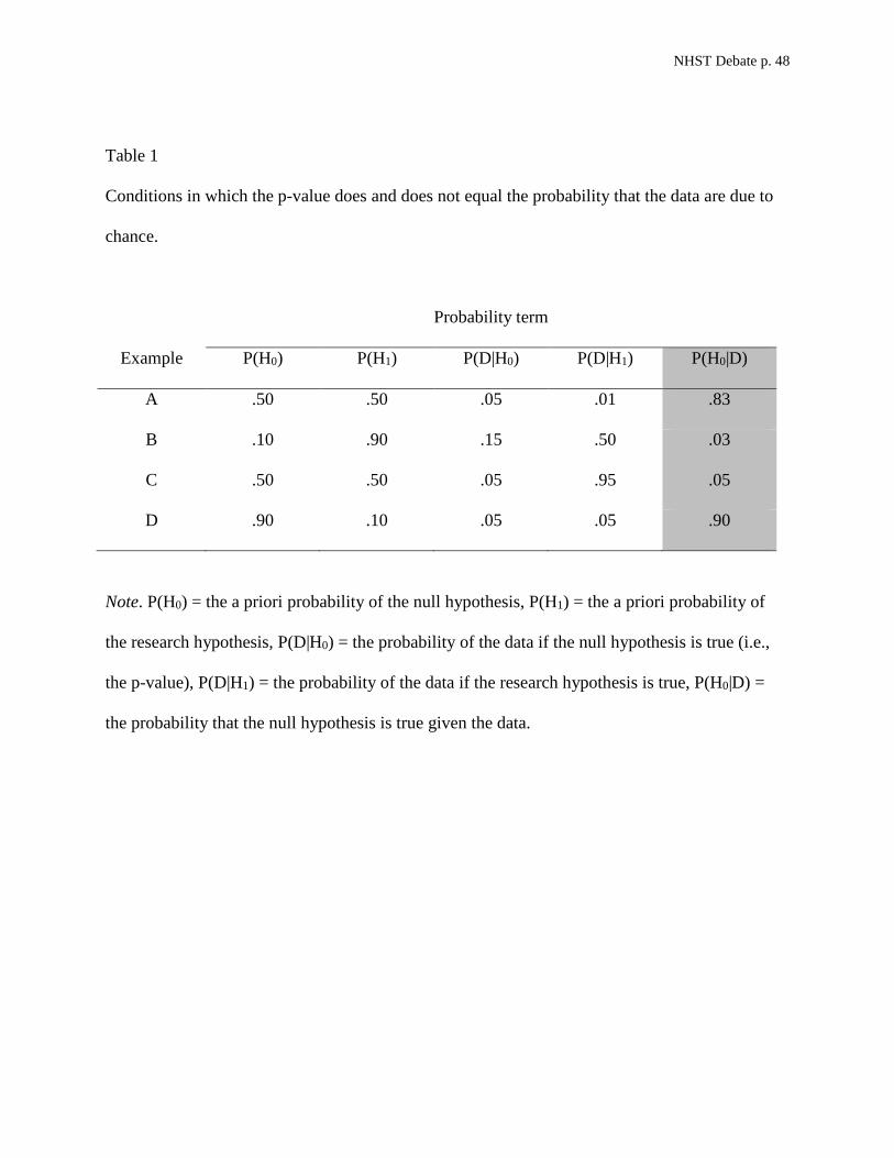
NHST Debate p. 48

Table 1

Conditions in which the p-value does and does not equal the probability that the data are due to

chance.

Probability term

Example P(H0) P(H1) P(D|H0) P(D|H1) P(H0|D)

A .50 .50 .05 .01 .83

B .10 .90 .15 .50 .03

C .50 .50 .05 .95 .05

D .90 .10 .05 .05 .90

Note. P(H0) = the a priori probability of the null hypothesis, P(H1) = the a priori probability of

the research hypothesis, P(D|H0) = the probability of the data if the null hypothesis is true (i.e.,

the p-value), P(D|H1) = the probability of the data if the research hypothesis is true, P(H0|D) =

the probability that the null hypothesis is true given the data.

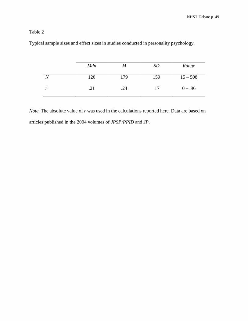
NHST Debate p. 49

Table 2

Typical sample sizes and effect sizes in studies conducted in personality psychology.

Mdn M SD Range

N 120 179 159 15 – 508

r .21 .24 .17 0 – .96

Note. The absolute value of r was used in the calculations reported here. Data are based on

articles published in the 2004 volumes of JPSP:PPID and JP.

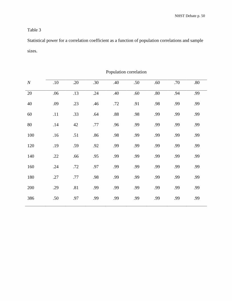
NHST Debate p. 50

Table 3

Statistical power for a correlation coefficient as a function of population correlations and sample

sizes.

Population correlation

N .10 .20 .30 .40 .50 .60 .70 .80

20 .06 .13 .24 .40 .60 .80 .94 .99

40 .09 .23 .46 .72 .91 .98 .99 .99

60 .11 .33 .64 .88 .98 .99 .99 .99

80 .14 42 .77 .96 .99 .99 .99 .99

100 .16 .51 .86 .98 .99 .99 .99 .99

120 .19 .59 .92 .99 .99 .99 .99 .99

140 .22 .66 .95 .99 .99 .99 .99 .99

160 .24 .72 .97 .99 .99 .99 .99 .99

180 .27 .77 .98 .99 .99 .99 .99 .99

200 .29 .81 .99 .99 .99 .99 .99 .99

386 .50 .97 .99 .99 .99 .99 .99 .99

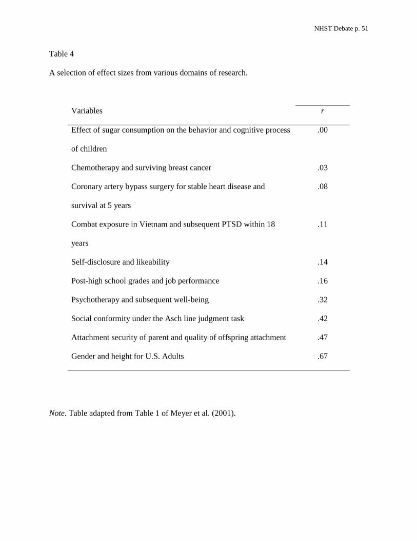
NHST Debate p. 51

Table 4

A selection of effect sizes from various domains of research.

Variables r

Effect of sugar consumption on the behavior and cognitive process

of children

.00

Chemotherapy and surviving breast cancer .03

Coronary artery bypass surgery for stable heart disease and

survival at 5 years

.08

Combat exposure in Vietnam and subsequent PTSD within 18

years

.11

Self-disclosure and likeability .14

Post-high school grades and job performance .16

Psychotherapy and subsequent well-being .32

Social conformity under the Asch line judgment task .42

Attachment security of parent and quality of offspring attachment .47

Gender and height for U.S. Adults .67

Note. Table adapted from Table 1 of Meyer et al. (2001).

NHST Debate p. 52

Recommended Readings

Meehl, P. E. (1978). Theoretical risks and tabular asterisks: Sir Karl, Sir Ronald, and the slow

progress of soft psychology. Journal of Consulting and Clinical Psychology, 46, 806-834.

Meehl, P. E. (1990). Appraising and amending theories: The strategy of Lakatosian defense and

two principles that warrant it. Psychological Inquiry, 1, 108-141.

Meyer et al. (2001). Psychological testing and psychological assessment: A review of evidence

and issues. American Psychologist, 56, 128-165.

Oakes, M. (1986). Statistical inference: A commentary for the social and behavioral sciences.

New York: Wiley.

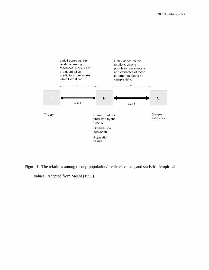
NHST Debate p. 53

Figure 1. The relations among theory, population/predicted values, and statistical/empirical

values. Adapted from Meehl (1990).

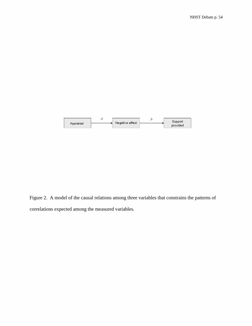
NHST Debate p. 54

Figure 2. A model of the causal relations among three variables that constrains the patterns of

correlations expected among the measured variables.