Consumption and the Permanent Income Hypothesis

Consumption and the Permanent Income Hypothesis

Cooper Allton, Kabira Namit, Michael Thibert WWS 512C - Macroeconomic Analysis

Roadmap

1. Keynesian Consumption Function

2. Permanent Income Hypothesis

3. 2001 and 2008 Tax Rebate Studies

4. 2009 Making Work Pay Tax Credit

5. Empirical Application in Developing Countries

J.M.K.

Keynes’s Assumptions

The main determinant of consumption is income

0 < Marginal Propensity to Consume < 1

Average propensity to consume (APC) declines with an increase in income

APC = C/Y

C

Y

1

c

C

c = MPC = slope of the

consumption function

The Keynesian consumption function

C C cY= +

Criticisms of the Keynesian Consumption Function

Assumes that people are myopic

Their only basis of current consumption is current income

They ignores future streams of revenue, impending retirement, redundancy etc.

Milton Friedman

The Permanent Income Hypothesis

Y = Y P + Y

T

where

Y = current income

Y P = permanent income

- average expected income over a lifetime

Y T = transitory income

- fluctuations in income above or below your permanent income


Consumers smooth their consumption by borrowing in times of need and saving in times of plenty.

The PIH consumption function

C = λ Y P

where λ is the proportion of permanent income that people consume every year.


As soon as you hear that your income will change in the future (maybe due to a policy change), you will factor that into your expected permanent income

Anticipated changes in income (like a tax rebate) will not alter your expected permanent income or consumption

A stimulus during a recession will lead an individual (who is indifferent between present and future consumption) to use a fraction of his windfall for present consumption

How do tax rebates impact expenditure?

Economic Growth and Tax Relief Reconciliation Act of 2001

(Johnson, D. et, al. Household Expenditure and the Income Tax Rebates of 2001: 2006.)

Economic Stimulus Act (ESA) of 2008

(Johnson, D. et, al. Consumer Spending and the Economic Stimulus Payments of 2008: 2011)

Key Facts

Rebate amount: (most) $300 or $600 per person.

Mailing dates: Rebate checks mailed according to last two digits of social security number (effectively random).

Comparison of 2001 and 2008 studies

Similarities:

1. Authors the same for both studies.

2. Same data source.

3. Methodology nearly identical.

Some differences:

1. 2008 study looked at differences between electronic rebates and paper check rebates. 2001 study looked only at paper check rebates.

2. 2008 study looked at home ownership as a measurement of liquidity constraints (in addition to age, income, liquid assets). 2001 study only looked at age, income and liquid assets as measures of liquidity constraints.

The Data

Characteristics

Random sample of U.S. Households.

Of large household surveys in U.S. CES has most comprehensive data on consumer expenditure.

Households interviewed 5 times. Introductory interview + up to 4 more at 3 month intervals.

In 2nd and 5th interviews report expenditures during preceding three month reference period.

New households added every month.

Data Source: Consumer Expenditure Survey (CES). Authors worked with Bureau of Labor Statistics (BLS) to add module to CES on timing and amount of the rebate check.

Regression Specification

Ri,t+1 = Key rebate variables:

1. Dollar amount received by household i in period t + 1 (Rebatei,t+1)

2. Dummy variable indicating whether any rebate was received in t + 1 (I(Rebatei,t+1>0)

3. Distributed lag of (Rebatei,t+1) or (I(Rebatei,t+1>0)

C = consumption expenditures (or their log)

Month = complete set of indicator variables for every period in the sample (absorb seasonal effects).

X = control variables (age, changes in family composition) included to absorb some of the

preference-driven differences in the growth rate of consumption expenditures across households.

Key Coefficient B2: Measure of the average causal effect of rebate receipt on expenditure.

Dollar Change in expenditures (per dollar of rebate)Food

Strictly Nondurable Goods

Nondurable Goods

.109* .239** .373**

Percent change in spending (Rebate>0)Food Strictly Nondurable

GoodsNondurable Goods

2.72** 1.76* 3.16**

Results: Expenditure estimates

* = significant at .10 level, ** = significant at .05 level

Key finding for testing PIH: On average, people spent 11% of the amount of their rebate on food, 24% on strictly nondurable goods and 37% on nondurable goods in the three months after receiving their check.

2008: Dollar Change in expenditures (per dollar of rebate)

FoodStrictly

Nondurable Goods

Nondurable Goods

Total Spending

.016 .079* .121** .516**


Dollar Change in expenditures (per dollar of rebate): Households receiving only on-‐time rebates

Strictly nondurable Goods

Nondurable Goods Total Spending

0.188** 0.214** .590**


Food Strictly nondurable Goods

Nondurable Goods

.109* .239** .373**

2008 2001

2001: Dollar Change in expenditures (per dollar of rebate): Households receiving only on-‐time rebates

Strictly nondurable Goods Nondurable Goods

0.152 0.247

Takeaway: Estimates for change in expenditure are higher for the 2001 study than for the 2008 study. Estimates in the restricted models are more similar, but those in the 2001 study are not statistically significant.

A Comparison: Expenditure Estimates



Rebatet+1 0.248** 0.386**

Rebatet -‐0.156* -‐0.082

Implied cumulative fraction (6 months) 0.340* 0.691**



Rebatet+1 0.247** 0.386**

Rebatet -‐0.172* -‐0.099

Rebatet-‐1 -‐0.034 -‐0.123

Implied cumulative fraction (6 months) 0.362 0.838**


Results: Time Lag (2001)

Implications: Spending increased significantly when people received their rebate checks and declined over

the next two periods. Inconsistent with income smoothing and “news” principles of PIH.

Implications for evaluating the PIH

What PIH predicts:

1. Coefficient on “Rebate” should be close to zero.

2. Any wealth effect should have begun when people learned about the rebates (“news” principle).

3. After people found out about the rebates, they should have smoothed their consumption over subsequent periods.

What we find:

1. Coefficient on “Rebate” is significantly greater than zero.

2. Spending spiked when people received their rebate checks.

3. Post-news spending did not follow a smooth path.

Did they just kill PIH?

No, not really…

Key assumption of the PIH:

“We assume well-functioning capital markets, where consumers can borrow and lend at the same interest rate r.”

Lecture notes: “Consumption and Savings – Part I: Households”

Implication: PIH predictions may not match reality if significant liquidity constraints exist.

2008: Propensity to Spend (Interaction = Income) Low: <$32,000 | High: >$74,677

Percent change in:Strictly

nondurable Goods

Nondurable Goods

Total spending

Low Group 0.096 0.024 0.715

2008: Propensity to Spend (Interaction = Liquid Assets) Low: <$500 | High: >$7,000

Dollar change in: Strictly nondurable

Goods

Nondurable Goods

Total spending

Low Group -‐0.181 -‐0.253 -‐0.844

2001: Propensity to Spend (Interaction = Income) Low: <$34,298 | High: >$69,000

Percent change in:Strictly nondurable

GoodsNondurable Goods

Low Group .319 .672**

2001: Propensity to Spend (Interaction = Liquid Assets) Low: <$1,000 | High: >$8,000

Dollar change in: Strictly nondurable Goods

Nondurable Goods

Low Group .569** .876**

2008 2001

Takeaway: The 2001 study found higher propensity to spend among people likely to face liquidity constraints. The 2008 study found the same result for the low-income group, but the results were not statistically significant. Authors suggest the lack of statistical significance may be due to sampling error.

A Comparison: Tests of Liquidity Constraints

Car purchases: Another possible indicator of liquidity constraints (2008 study)

“Keeping in mind the degree of statistical significance, our finding of a large spending response on new cars is suggestive of an important role for liquidity constraints. The ESPs may have provided otherwise unavailable down payments for debt-financed purchases of cars.”

(Johnson, D. et, al. 2011: page 23)

American Recovery and Reinvestment

Act of 2009Signed into law February 17, 2009 with subsequent fiscal measures to extend effects

About half of the jobs measures were tax cuts ($237 billion in tax cuts for individuals)

From: ERP 2014 Chapter 3: The Economic Impact of the American Recovery and Reinvestment Act Five Years Later.

Making Work Pay Tax Credit

$116 billion towards new payroll tax credit

$400 per worker and $800 per couple in 2009 and 2010

Phaseout begins at $75,000 for individuals and $150,000 for joint filers

Difference: Employers decreased tax withholdings throughout the year, leading to an increase in monthly inome (Not a one-time payment)

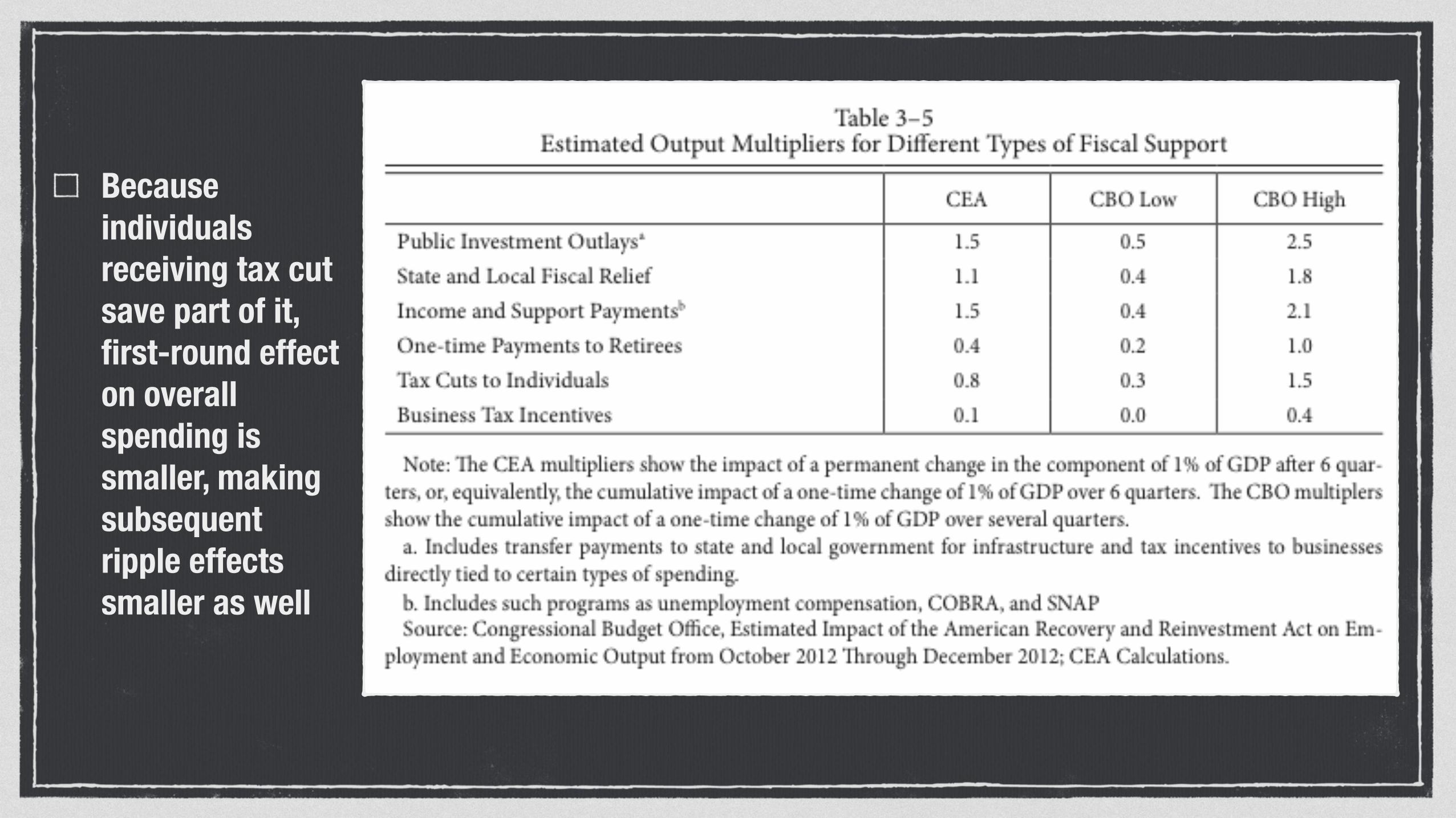
Because individuals receiving tax cut save part of it, first-round effect on overall spending is smaller, making subsequent ripple effects smaller as well

Quickly raised GDP in first half of 2009

2 to 2.5% increase between 4Q 2009 and 2Q 2011

Impact wound down in 2012

Difficult to disaggregate the effects of individual policy elements

110 | Chapter 3

0.0

0.5

1.0

1.5

2.0

2.5

3.0

3.5

2009:Q2 2010:Q2 2011:Q2 2012:Q2

Figure 3-7Quarterly Effect of the Recovery Act and Subsequent

Fiscal Measures on GDP, 2009–2012Percent of GDP

ARRA

Other FiscalMeasures

2012:Q4

Source: Bureau of Economic Analysis, National Income and Product Accounts; Congressional Budget Office; CEA calculations.

0.0

0.5

1.0

1.5

2.0

2.5

3.0

3.5

2009:Q2 2010:Q2 2011:Q2 2012:Q2

Figure 3-8Quarterly Effect of the Recovery Act and Subsequent

Fiscal Measures on Employment, 2009–2012Millions

ARRA

Other FiscalMeasures

2012:Q4

Source: Bureau of Economic Analysis, National Income and Product Accounts; Congressional Budget Office; CEA calculations.

Stimulus acts allowed US and Germany to outperform other nations following recession

Germany passed own €50 billion stimulus package in 2009

Contrast with austerity in EU

Locate and enroll participants from poor communities for one-time cash transfers

Average $1,000 (about 1 year’s budget for a typical household)

Condition-free

Households both credit- and savings-constrained

Kenya

Give Directly RCT Results

Increase in average monthly consumption from USD 157 to USD 194 four months after the transfer ended

Implied elasticities for food, medical and education expenditures range between 0.84 and 1.47, while the point estimates are negative for alcohol and tobacco

Compared with monthly transfers, recipients of lump sum transfers are…

Significantly more likely to invest in durables (such as metal roofs)

Less likely to improve food security

From: Haushofer, J. and Shapiro, J. Household Response to Income Changes: Evidence from an Unconditional Cash Transfer Program in Kenya (2013). Princeton University.

Liquidity Constraints

People with lack of access to credit or savings

Will increase consumption more than PIH would predict

Purchases of large durable goods require substantial one-time payment in the absence of credit

Low liquid wealth or income leads to violations of the Permanent Income Hypothesis

The Allton - Namit - Thibert Hypothesis (Permanent Income Hypothesis Revised)

Liquidity affects the behavior of consumers

Little change in consumption as a result of the announcement of future one-time gains in income

Affects of one-time income increases on consumption differs by context

Both the Keynesian Consumption Function and the PIH are useful in understanding consumer behavior. But the degree of applicability will depend upon context.

Consumption and the Permanent Income Hypothesis

Documents

Transcript of Consumption and the Permanent Income Hypothesis