Source/Sink Patterns of Disturbance and Cross-Scale Mismatches in a Panarchy of Social-Ecological...

Copyright © 2008 by the author(s). Published here under license by the Resilience Alliance.Zaccarelli, N., I. Petrosillo, G. Zurlini, and K. Hans Riitters 2008. Source/sink patterns of disturbance andcross-scale mismatches in a panarchy of social-ecological landscapes. Ecology and Society 13(1): 26.[online] URL: http://www.ecologyandsociety.org/vol13/iss1/art26/

ResearchSource/Sink Patterns of Disturbance and Cross-Scale Mismatches in aPanarchy of Social-Ecological Landscapes

Nicola Zaccarelli 1, Irene Petrosillo 1, Giovanni Zurlini 1, and Kurt Hans Riitters 2

ABSTRACT. Land-use change is one of the major factors affecting global environmental change andrepresents a primary human effect on natural systems. Taking into account the scales and patterns of humanland uses as source/sink disturbance systems, we describe a framework to characterize and interpret thespatial patterns of disturbances along a continuum of scales in a panarchy of nested jurisdictional social-ecological landscapes (SELs) like region, provinces, and counties. We detect and quantify those scalesthrough the patterns of disturbance relative to land use/land cover exhibited on satellite imagery over a 4-yr period in the Apulia region, South Italy. By using moving windows to measure composition (amount)and spatial configuration (contagion) of disturbance, we identify multiscale disturbance source/sinktrajectories in the pattern metric space defined by composition and configuration of disturbance. We groupdisturbance trajectories along a continuum of scales for each location (pixel) according to broad land-useclasses for each SEL level in the panarchy to identify spatial scales and geographical regions wheredisturbance is more or less concentrated in space indicating disturbance sources, sinks, and mismatches.We also group locations by clustering, and results are compared in the same pattern space and interpretedwith respect to disturbance trajectories derived from random, multifractal and hierarchical neutral models.We show that in the real geographical world spatial mismatches of disturbances can occur at particularscale ranges because of cross scale disparities in land uses for the amount and contagion of disturbance,leading to more or less exacerbation of contrasting source/sink systems along certain scale domains. Allcross-scale source/sink issues can produce both negative and positive effects on the scales above and belowtheir levels, i.e., cross-scale effects. Through the framework outlined in our examples, managers, as wellas stakeholders belonging to SELs in the panarchy, can be aware of specific scale ranges of disturbancewhere mismatches might occur and that will help them to value where and how to intervene in the panarchyof SELs to enhance the benefits and to minimize negative effects.

Key Words: disturbance mismatches; disturbance source/sink; multiscale disturbance patterns; panarchy;social-ecological landscapes.

INTRODUCTION

Land-use change is one of the major factorsaffecting global environmental change andrepresents a primary human effect on naturalsystems, and underlying fragmentation and habitatloss, which are the greatest threats to biodiversity(Alcamo and Bennett 2003). Since human land useis a major force in driving landscape change,landscape dynamics can be better understood in thecontext of complex adaptive socioeconomic andecological systems (e.g., Berkes and Folke 1998),integrating phenomena across multiple scales ofspace, time and organizational complexity. In the

real geographic world such systems can be betterdefined as social-ecological landscapes (SELs),taking into account the scales and patterns of humanland use as ecosystem disturbances.

During recent decades, worldwide losses ofbiodiversity have occurred on an unprecedentedscale and agricultural intensification has beenindicated as a major driver of this global change (e.g., Matson et al. 1997, Donald et al. 2001, Tilmanet al. 2002, Stokstad 2006). Agriculturalintensification is determined by practices on bothlocal and landscape scales (e.g., Matson et al. 1997,Tilman et al. 2002). On a local scale, it is due to

1Landscape Ecology Laboratory, University of Salento, Lecce, Italy, 2U.S. Forest Service

http://www.ecologyandsociety.org/vol13/iss1/art26/

mailto:[email protected]




Ecology and Society 13(1): 26http://www.ecologyandsociety.org/vol13/iss1/art26/

shorter crop rotation cycles, decreased cropdiversity, increased input of mineral fertilizers andpesticides, winter sowing of cereals, implementationof genetically modified (GM) crops, andmonoculture, increased field size, and machine-driven farming. On a landscape scale, intensificationoccurs owing to conversion of perennial habitat intoarable fields, destruction of hedgerows, fragmentationof natural habitat, the loss of low-intensity land-usemanagement, reallocation of land to increased fieldsize, loss of set-aside fallows, cultivation offormerly abandoned areas, and farmer specializationin one or few crop types.

Land-use intensification has disrupted ecologicalprocesses such as biological pest control (e.g.,Matson et al. 1997, Tylianakis et al. 2004) and croppollination (e.g., Stokstad 2006). Increasedfertilizer inputs can reduce water quality (e.g.,Vitousek et al. 1997), decrease the richness of plantspecies (e.g., Mitchell et al. 2004) and increase theoccurrence of plant diseases (e.g., Vickery et al.2001). Local landscape intensification may affectgrassland production (e.g., Loreau and Hector2001), and resistance to plant invasion (e.g.,Kennedy et al. 2002). Recent agriculturalintensification also includes GM crops, which offernew opportunities for increased yields in the comingdecades, but also risk side-effects (Hails 2002). Alsothe dynamic spatial configuration of land use inSELs resulting from human appropriation can havea variety of ecological effects at a landscape scale.Fields have been merged and enlarged to enhancefarming efficiency resulting in homogeneouslyfarmed landscapes. New land-cover types can bejuxtaposed within increasingly fragmented nativeland-cover types, modifying nutrient transport(Peterjohn and Correll 1984), affecting speciespersistence and biodiversity (Tilman et al. 2002,Benton et al. 2003), and nurturing invasive species(With 2002).

Disturbances are deemed as any relatively discreteevent in space and time that disrupts ecosystem,community, or population structure and changesresources, substrates, or the physical environment(Pickett and White 1985). In this study land-useintensification is deemed as a disturbance from alandscape perspective which is justifiable in thecontext of SELs, since observed land-use/land-cover changes demonstrate that agricultural fieldsare more dynamic than other types of land-usesystems (e.g., Young and Harris 2005). Thisstandpoint is different from classical land-cover

mapping that would ignore, for instance, apparentdisturbances from crop rotation because agriculturalfields can be fallow one year and planted the next,and still be labeled as agricultural fields. In addition,drawing on the notion of source and sink coined formetapopulation by Levins (1969), agriculturalfields with their widespread practices might act asa source or a sink as to the potential spread ofdisturbance agents like fire, pesticides, fertilizers,pests, diseases, and alien species to neighboringnonagricultural areas, along with a variety ofpotential associated ecological effects at thelandscape scale. In summary, the effects of land-useintensity on local biodiversity and ecologicalfunctioning in SELs depend on spatial scales muchlarger than a single field or land use. This demandsa landscape perspective, which takes into accountthe spatial arrangement of surrounding land-usetypes at multiple scales (Turner and Gardner 1991,Ricketts 2001).

Anthropogenic disturbances are determined by thesocial component of SELs organized in a panarchyof nested jurisdictional levels defined as clearlybounded and organized social-political units, e.g.,household, village, county, province, region, andnation (Cash et al. 2006). This draws on the notionof hierarchies of influences between embeddedscales, and how these linked scales influence eachother and cross-scale effects can take place(Gunderson and Holling 2002). In social-ecologicallandscapes (Berkes and Folke 1998) such cross-scale mismatches become so critical that spatialeffects are expected when the spatial scales ofmanagement and the spatial scales of ecosystemprocesses do not align properly leading toinefficiencies, and/or loss of important componentsof the ecological system and, ultimately, todisruptions of SELs (Cash et al. 2006). In Europe,social and ecological systems are so interlinked thatany SEL is bound to be anyhow disturbed to somedegree (Reidsma et al. 2006). Then if disturbancepatterns originating from various land-usemanagements do not follow the same pathwayacross scales, scale mismatches can take placeowing to disparities of disturbance among land usesacross scales in the landscape that can exacerbateor mitigate the contrast between disturbance sourcesand sinks at particular scale ranges.

Although social-ecological systems and panarchyare becoming a popular topic of inquiry in ecology(Carpenter and Turner 2001), it is surprising thatlittle theoretical or practical work has explicitly



addressed frameworks able to indicate the scalingbehavior of human disturbances in a real panarchyof SELs. In this study, rooted in previous results onboth real disturbance patterns (Zurlini et al. 2006)and simulated neutral landscape pattern maps(Zurlini et al. 2007), we develop a conceptualframework and apply it through the state space ofthe disturbance pattern, i.e., composition andconfiguration, for both simulated and reallandscapes in a panarchy of SELs, i.e., region,provinces, counties, in Apulia, southern Italy.Unlike our previous studies, we set few broad land-use/land-cover categories with their relevantdisturbances as the thematic base level for the wholepanarchy of SELs. Our intention is to analyze andinterpret SELs along a continuum of scales throughpatterns of disturbance trajectories relative to land-use/land-cover to indicate spatial pattern domainsof disturbances and mismatches. To this purpose,we produce a disturbance map based on satelliteimagery of Apulia, and employ moving windows(Milne 1992) to measure composition (amount) andconfiguration (contagion) of disturbance patterns.We obtain disturbance trajectories at multiple scalesfor each location (pixel), and we group locationsaccording to broad classes of land-use andmembership for each subregion in the panarchy. Wealso group locations by clustering, and results arecompared in the same state space, identified bycomposition and configuration of disturbance, to theclustering from simulated random, multifractal andhierarchical neutral maps. We then indicate thespatial scales and SELs where disturbance is moreor less concentrated in space along the panarchyindicating disturbance sources, sinks, andmismatches.

MATERIALS AND METHODS

In order to better communicate our methods, wehave constructed an Appendix as a tutorial for thereader on satellite imagery and processing,normalized difference vegetation index (NDVI),change detection, moving windows and neutrallandscape models (NLMs), as well as further detailswhich have received thorough treatment elsewhere(Zurlini et al. 2006, 2007).

Study area

Apulia is an administrative region of 1,936,000 hain southern Italy, inhabited for thousands of years,mostly karstic with a typical semi-aridMediterranean climate with hot and dry summersand moderately cold and rainy winter seasons (Vieland Zurlini 1986). For our purposes, Apulia can bevisualized as a panarchy of nested jurisdictionallevels of social-ecological landscapes (region,provinces, and counties) embodying different setsof political, social, economic, and cultural features(Fig. 1). All hierarchical levels can be described interms of their unique social-ecological landscapes(SELs) based on the composition of land-use.

Overall, more than 82% of Apulia contains agro-ecosystems (see the Appendix for further details).To provide a realistic interpretation of spatialproperties of Apulia landscapes, we reclassified theoriginal Corine land-cover map of Apulia (APAT2005; Fig. 1) into four broad land-use/land-covercategories (Table 1), namely arable land,heterogeneous agricultural areas, permanentcultivations, which are mostly olive groves, andnatural areas including forests and shrub and/orherbaceous associations. We consider only land-use/land-cover classes of the terrestrial surface,which total 100% (Table 1), excluding seawater,lagoons, wetlands, and urban and industrial areas.

Change detection and what is meant bydisturbance

We use satellite change detection to produce a mapof disturbance as input to the analysis of disturbancepatterns. Six cloud-free Landsat Thematic Mapper5 (TM) and two Enhanced Thematic Mapper Plus(ETM+) images with a 30-m pixel resolution in thesame period of vegetation phenological cycles intwo different years, i.e. June 1997 and June 2001,have been processed to describe the pattern ofchange in Apulia (see the Appendix). As changeresponse variable, we use changes over time inNDVI, defined as the difference between the visible(red) and near-infrared (nir) bands, over their sum(Goward et al. 1991). NDVI has been validated asa robust indicator of vegetation photosynthesis, withbuilt-in relationships to social-ecological processessuch as habitat conversion or crop rotation, andrelated to a number of vegetation indicators andcharacteristics (see Young and Harris 2005, and



Fig. 1. Panarchy of nested jurisdictional levels defined as clearly bounded and organized jurisdictionalunits in Apulia, an administrative region of 1,936,000 ha in south Italy. Three main jurisdictional levelscan be identified (region, province, county): one unit for the region, five units for the province level, and258 units for the county level. The entire region or each sub-unit in the panarchy can be described interms of their unique social-ecological landscapes (SEL) based on land-use composition. Six broad land-use/land-cover classes (top) and a simplified example of Corine land-cover map for one county (down)are presented. The original Corine land-cover map (1:100.000) updated at 1999 has a global accuracy of88.1% and a Cohen's K coefficient of 0.84 (APAT 2005). Our use of broader land-use/land-covercategories improves upon that classification accuracy.



Table 1. Broad land-use/land-cover categories of Apulia and its five nested administrative provinces, basedon the aggregation of Corine classes from 1999 land-use/land-cover map (see text). Percentages sum upto 100% and are calculated only for terrestrial surface by excluding seawater, lagoons, wetlands and urbanfabrics (adapted from Zurlini et al. 2006).

Percentage composition

Category Apulia Bari Brindisi Foggia Lecce Taranto

Arable lands 41.7 30.9 28.6 59.2 35.0 30.2

Permanent cultivations 30.2 40.7 53.5 11.7 48.0 25.5

Heterogeneous agricultural areas 13.8 16.9 15.3 7.3 13.3 26.4

Natural areas 14.2 11.5 2.5 21.8 3.8 17.9

references therein). In addition to this evidence, wewanted to substantiate the sensitivity of NDVI tovegetation changes for the Apulia region, before itwas used further for change detection (see theAppendix).

Since landscape mosaic is mostly defined byvegetation cover, we operationally measuredisturbance by any detectable alteration in landcover reflecting significant and relatively frequentNDVI changes, mainly assignable to fast human-driven disturbances (CEC 1999), as captured by anarrow four-year time window (see the Appendix).We focus on land cover dynamics including bothNDVI gains and losses, so that disturbances aremostly associated with agricultural expansion andintensification, conversion of perennial habitats andvineyards to field cultivation and new olive grovetillage, farming practices such as fire and croprotation, and urban sprawl. It is worth noting that,in this context, disturbance might also be due toafforestation, which is the conversion of open landinto a forest by planting seeds or trees as it widelyoccurs in Apulia for new olive grove tillagepromoted by EU subsidies. Large disturbances fromwindstorms, floods, and fires are extremely rare inthe region and did not occur within the temporalwindow of this study.

In summary, taking into account the differentsources of error, we believe that it is possible by thisprocedure to capture most of the significant real

human-driven disturbances detectable at theresolution of Landsat imagery. However, theremight be cases where occasionally NDVI does notcapture disturbance when it is in fact there, forexample in agricultural fields which went from onecrop to the same or another crop but retained exactlythe same NDVI. On the contrary, it would be veryunlikely that this procedure captures disturbancewhen it is not there.

The conceptual framework of disturbancepatterns at multiple scales

To analyze spatial patterns it has been suggestedthat it is best to focus on a few key measures (Li andReynolds 1994, Riitters et al. 1995) and, forcategorical map data, on the two fundamentalcomponents of a pattern, namely composition, i.e.,the quantities of various entities, and configuration,i.e., their spatial arrangements (Li and Reynolds1994, Fortin et al. 2003). In our case, the entity isdefined as disturbance and we therefore characterizelandscape patterns in terms of the amount and spatialarrangement of disturbance.

Consider a binary map showing pixels of disturbedand undisturbed locations. Multi-scale disturbancepatterns can be measured and mapped using anoverlapping pixel-level moving window wherebyscale is varied by changing the size of the window(Milne 1992, Kerkhoff et al. 2000). Within a given



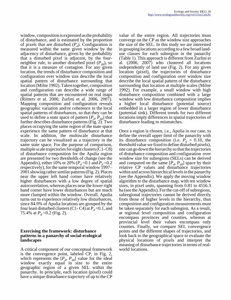
window, composition is expressed as the probabilityof disturbance, and is estimated by the proportionof pixels that are disturbed (Pd). Configuration ismeasured within the same given window by theadjacency of disturbance, given by the probabilitythat a disturbed pixel is adjacent, by the four-neighbor rule, to another disturbed pixel (Pdd), sothat it is a measure of contagion. For any givenlocation, the trends of disturbance composition andconfiguration over window size describe the localspatial pattern of disturbance surrounding thatlocation (Milne 1992). Taken together, compositionand configuration can describe a wide range ofspatial patterns that are encountered on real maps(Riitters et al. 2000, Zurlini et al. 2006, 2007).Mapping composition and configuration revealsgeographic variation and/or coherence in the localspatial patterns of disturbances, so that they can beused to define a state space of pattern [Pd, Pdd] thatfurther describes disturbance patterns (Fig. 2). Twoplaces occupying the same region of the state spaceexperience the same pattern of disturbance at thatscale. In addition, the multiscale disturbancetrajectory can be visualized as a trajectory in thesame state space. For the purpose of comparison,multiple scale trajectories for eight clusters (C1- C8)of disturbance composition for the Apulia regionare presented for two thresholds of change (see theAppendix), either 10% or 20% (Pd =0.1 and Pd =0.2respectively), for the same temporal window 1997–2001 showing rather similar patterns (Fig. 2). Placesnear the upper left hand corner have relativelyhigher disturbances with a low degree of spatialautocorrelation, whereas places near the lower righthand corner have lower disturbances but are muchmore clumped within the window. Overall, Apuliaturns out to experience relatively low disturbances,since 84.9% of Apulia locations are grouped by thefour least disturbed clusters (C1- C4) at Pd =0.1, and75.4% at Pd =0.2 (Fig. 2).

Exercising the framework: disturbancepatterns in a panarchy of social-ecologicallandscapes

A critical component of our conceptual frameworkis the convergence point, labeled CP, in Fig. 2,which represents the [Pd, Pdd] value for the idealwindow exactly equal in size to the entiregeographic region of a given SEL within thepanarchy. In principle, each location (pixel) couldhave a unique disturbance trajectory of up to the CP

value of the entire region. All trajectories mustconverge on the CP as the window size approachesthe size of the SEL. In this study we are interestedin grouping locations according to a few broad land-use classes for each subregion in the panarchy(Table 1). This approach is different from Zurlini etal. (2006, 2007) who clustered all locationsindependently of land use (Fig. 2). For any givenlocation (pixel), the trajectories of disturbancecomposition and configuration over window sizedescribe the local spatial pattern of the disturbancesurrounding that location at multiple scales (Milne1992). For example, a small window with highdisturbance composition combined with a largewindow with low disturbance composition impliesa higher local disturbance (potential source)embedded in a larger region of lower disturbance(potential sink). Different trends for two differentlocations imply differences in spatial trajectories ofdisturbance leading to mismatches.

Once a region is chosen, i.e., Apulia in our case, todefine the overall upper limit of the panarchy withits disturbance composition (i.e. Pd = 0.10, thethreshold value we fixed to define disturbed pixels),one can go down the hierarchy so that the trajectoriesof disturbance composition and configuration overwindow size for subregions (SELs) can be derivedand compared on the same [Pd, Pdd] space by theirrelative CP values and disturbance trajectorieswithin and across hierarchical levels in the panarchy(see the Appendix). We apply the moving windowalgorithm to the disturbance map, with ten windowsizes, in pixel units, spanning from 0.81 to 4556.3ha (see the Appendix). For the cut-off of subregions,subregional trajectories cannot be derived directlyfrom those of higher levels in the hierarchy, thuscomposition and configuration measurements mustbe taken separately for each subregion. As a result,at regional level composition and configurationencompass provinces and counties, whereas atprovincial level their values encompass onlycounties. Finally, we compare SEL convergencepoints and the different shapes of trajectories, andlook back to the geographical space to evaluate thephysical locations of pixels and interpret themeaning of disturbance trajectories in terms of real-world locations.



Fig. 2. Pattern state space [Pd, Pdd] defined by composition (Pd) and configuration (Pdd) and disturbancetrajectories at multiple scales (10 window sizes) for eight clusters (C1-C8) representing disturbancepatterns in Apulia in the period 1997–2001. On top, the two figures correspond to an overall Pd = 0.10, i.e., disturbance of 10% (left), and Pd = 0.20, i.e., disturbance of 20% (right) respectively, with Pdd in bothcases about 0.41. The percentage of pixels belonging to each cluster is given in the legend. Alltrajectories converge from the finest to the coarsest scale, i.e., from smallest to largest window size, on aregional point called convergence point (CP). Below, the single trajectories of Pd and Pdd vs. scale (10window sizes) are shown (see text; adapted from Zurlini et al. 2006, 2007).

Disturbance sources or sinks

Any region in the panarchy is characterized by thespatial composition (what and how much is there)and configuration (how is it spatially arranged) oflandscape elements like land use/land cover. Anylandscape element, in turn, contributes to the overallproportion of disturbed pixels (Pd) in the region,through its composition of disturbed locations(pixels). In rural landscapes, elements with higherland cover dynamics (disturbance) like fields

characterized by widespread agricultural practices,might act as a source of the potential spread ofdisturbance agents like fire, pesticides, fertilizers,pests, diseases, and alien species to neighboringnonagricultural areas (sink). Such interplay ofexchange of disturbance agents among land uses orregions in the panarchy can conveniently draw onthe notions of source and sink adopted by Levins(1969) to describe a model of metapopulationdynamics of insect pests in agricultural fields. Thusa landscape perspective of disturbance source-sink



patterns is ultimately required to evaluate howchanges in landscape structure, e.g., habitatfragmentation, may affect the potential spread ofdisturbance agents.

Disturbance trajectories at multiple scales on the[Pd, Pdd] state space, indicate whether and whereland-use disturbances might act as a potential sourceor as a sink. If a mean trajectory is always largerthan the CP of reference and tends downwards tothe CP, then land-use disturbances act as a sourcebecause there is a locally high rate of disturbanceembedded in a larger region of fewer disturbances.Otherwise, land-use disturbance acts as a sinkbecause there is a locally low rate of disturbanceembedded in a larger region of heavy disturbances.Disturbance source effects are expected to begreater not only in terms of higher composition ofdisturbance (Pd) but also in terms of higherconfiguration of disturbance (Pdd).

To compare CPs by their disturbance composition(Pd) and configuration (Pdd) (proportions) we uselog-odds ratios (Agresti 1996) (see the Appendix).The larger the log-odds, the greater will be thedifference. When proportions are respectivelyequal, the log-odds ratio is 0 otherwise, they can bepositive or negative. If they are positive, e.g. fordisturbance composition, SEL acts in general as asource of disturbance respect of the SEL ofreference, on the contrary SEL acts as a sink.

Generating neutral landscape patterns

Simulated, neutral landscape models have evolvedfrom simple random landscape maps (Gardner et al.1987) to maps with hierarchical structure (O’Neillet al. 1992, Lavorel et al. 1993). To comparedisturbance trajectories from clustering (Fig. 2) toNLMs, we generated simulated random, multifractaland hierarchical landscape pattern maps. Details ofprocedures and results are given in the Appendix.

RESULTS

Upper jurisdictional level (region)

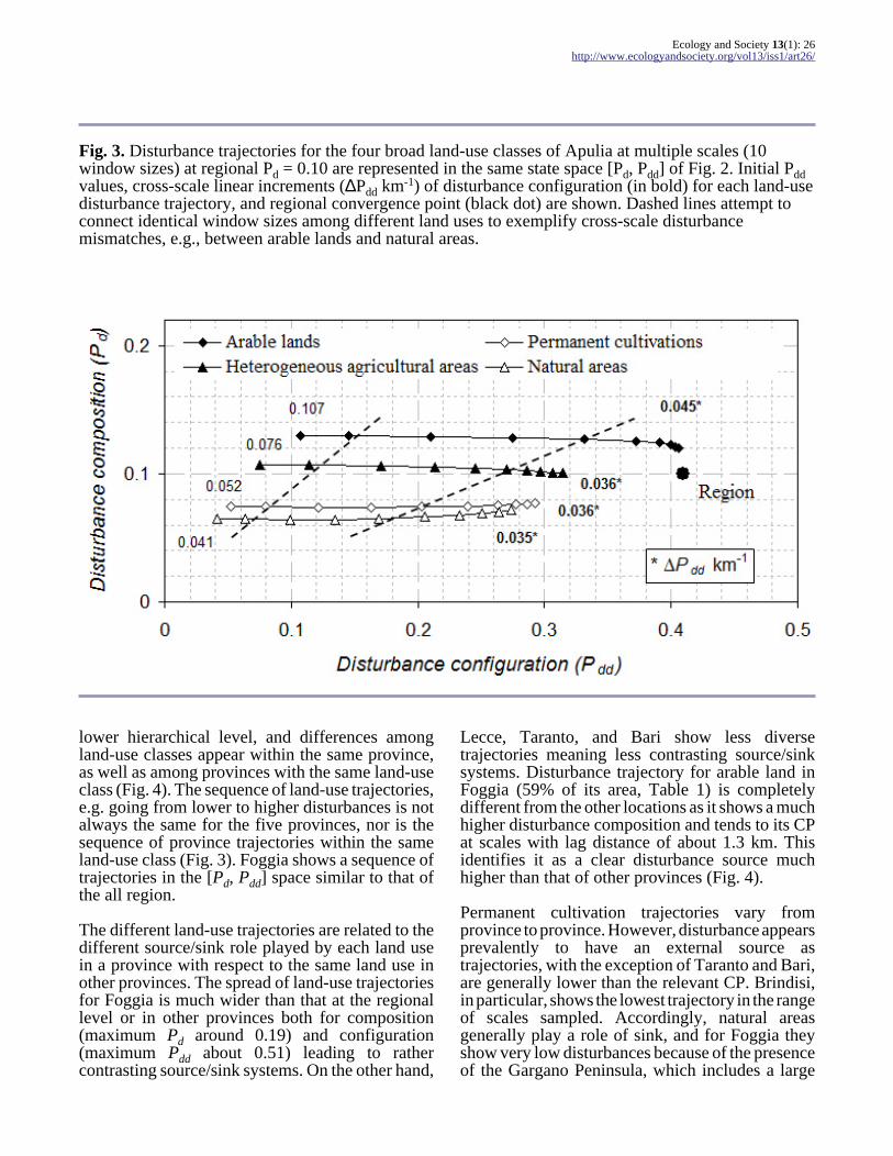
In the [Pd, Pdd] space defined by composition andconfiguration of disturbance, land-use trajectoriesfor the regional level have been found to be almostaligned along the configuration axis (Pdd) andremain largely unvaried as to composition (Pd)

across the ten window sizes (scales) converging tothe regional CP only at the largest windows (Fig.3). They appear ordered according to increasingdisturbance composition in a precise sequence.Thus, arable land (41.7% of Apulia in Table 1) canact as a disturbance source in the range of scalesconsidered, showing composition and configurationlevels higher than those of other land uses.Heterogeneous agricultural areas (13.8%) show anintermediate trajectory at about the samedisturbance level of regional CP, with a very finetexture, followed by permanent cultivations(30.2%) and natural areas (14.2%) with the twolowest trajectories indicating their possible sinkrole. Initial disturbance configurations oftrajectories show an increase from natural areas toarable lands. Arable land trajectory very nearlyconverges with the CP (Pdd = 0.417), whereas forother land uses there are gaps between the highestwindow size (6.75 km lag distance) and the regionalCP. Gaps depend on both the initial configurationvalue and cross-scale increase of configurationcomprised within the ten windows. The differencesbetween the final and initial disturbanceconfigurations (∆Pdd), over the highest spatial(linear) lag distance (6.75 km) provide a measureof the average linear rate of increase of disturbanceconfiguration across scales for each land use (Fig.3). Taking into account the fact that initialdisturbance configuration (Pdd) level for arablelands is more than twice that of natural areas, arablelands show relatively higher cross-scale linearincrements with an outstanding average increment(∆Pdd km-1) of =0.127 in the first 2.25 km of lagdistance (75×75 window size in pixel units),whereas other land uses show similar but lower andmore equally distributed increments. Suchdifferences give an indication of spatial cross-scalemismatches among land uses as to theiraccumulative rate of disturbance clumping acrossscales.

First nested jurisdictional levels (provinces)

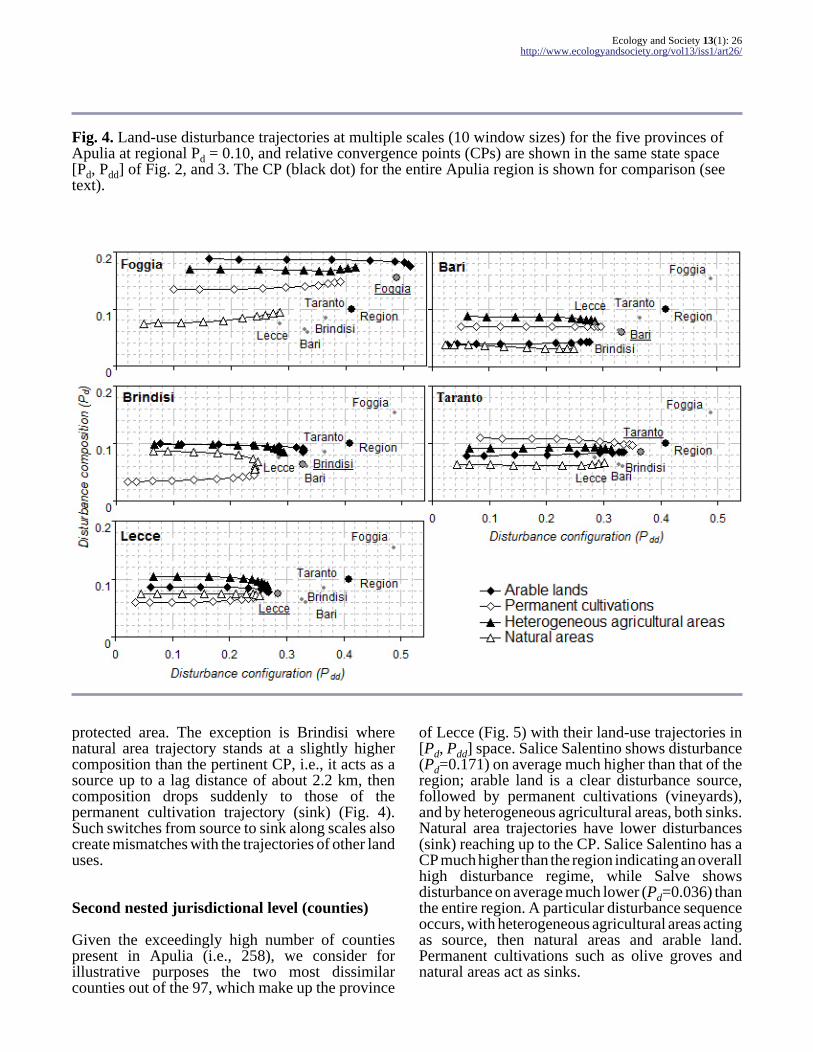
In the same [Pd, Pdd] space of Fig. 3, disturbancetrajectories of the different land uses in differentprovinces again align mainly along the Pdd axis (Fig.4), while the relevant CPs of social-ecologicallandscapes (SELs) in space show a clear sequenceat increasing Pdd from Lecce (bottom left) to Foggia(upper left, Fig. 4). Diversity among processes andregimes of disturbance emerge more clearly at this



Fig. 3. Disturbance trajectories for the four broad land-use classes of Apulia at multiple scales (10window sizes) at regional Pd = 0.10 are represented in the same state space [Pd, Pdd] of Fig. 2. Initial Pdd values, cross-scale linear increments (∆Pdd km-1) of disturbance configuration (in bold) for each land-usedisturbance trajectory, and regional convergence point (black dot) are shown. Dashed lines attempt toconnect identical window sizes among different land uses to exemplify cross-scale disturbancemismatches, e.g., between arable lands and natural areas.

lower hierarchical level, and differences amongland-use classes appear within the same province,as well as among provinces with the same land-useclass (Fig. 4). The sequence of land-use trajectories,e.g. going from lower to higher disturbances is notalways the same for the five provinces, nor is thesequence of province trajectories within the sameland-use class (Fig. 3). Foggia shows a sequence oftrajectories in the [Pd, Pdd] space similar to that ofthe all region.

The different land-use trajectories are related to thedifferent source/sink role played by each land usein a province with respect to the same land use inother provinces. The spread of land-use trajectoriesfor Foggia is much wider than that at the regionallevel or in other provinces both for composition(maximum Pd around 0.19) and configuration(maximum Pdd about 0.51) leading to rathercontrasting source/sink systems. On the other hand,

Lecce, Taranto, and Bari show less diversetrajectories meaning less contrasting source/sinksystems. Disturbance trajectory for arable land inFoggia (59% of its area, Table 1) is completelydifferent from the other locations as it shows a muchhigher disturbance composition and tends to its CPat scales with lag distance of about 1.3 km. Thisidentifies it as a clear disturbance source muchhigher than that of other provinces (Fig. 4).

Permanent cultivation trajectories vary fromprovince to province. However, disturbance appearsprevalently to have an external source astrajectories, with the exception of Taranto and Bari,are generally lower than the relevant CP. Brindisi,in particular, shows the lowest trajectory in the rangeof scales sampled. Accordingly, natural areasgenerally play a role of sink, and for Foggia theyshow very low disturbances because of the presenceof the Gargano Peninsula, which includes a large



Fig. 4. Land-use disturbance trajectories at multiple scales (10 window sizes) for the five provinces ofApulia at regional Pd = 0.10, and relative convergence points (CPs) are shown in the same state space[Pd, Pdd] of Fig. 2, and 3. The CP (black dot) for the entire Apulia region is shown for comparison (seetext).

protected area. The exception is Brindisi wherenatural area trajectory stands at a slightly highercomposition than the pertinent CP, i.e., it acts as asource up to a lag distance of about 2.2 km, thencomposition drops suddenly to those of thepermanent cultivation trajectory (sink) (Fig. 4).Such switches from source to sink along scales alsocreate mismatches with the trajectories of other landuses.

Second nested jurisdictional level (counties)

Given the exceedingly high number of countiespresent in Apulia (i.e., 258), we consider forillustrative purposes the two most dissimilarcounties out of the 97, which make up the province

of Lecce (Fig. 5) with their land-use trajectories in[Pd, Pdd] space. Salice Salentino shows disturbance(Pd=0.171) on average much higher than that of theregion; arable land is a clear disturbance source,followed by permanent cultivations (vineyards),and by heterogeneous agricultural areas, both sinks.Natural area trajectories have lower disturbances(sink) reaching up to the CP. Salice Salentino has aCP much higher than the region indicating an overallhigh disturbance regime, while Salve showsdisturbance on average much lower (Pd=0.036) thanthe entire region. A particular disturbance sequenceoccurs, with heterogeneous agricultural areas actingas source, then natural areas and arable land.Permanent cultivations such as olive groves andnatural areas act as sinks.



Fig. 5. Land-use disturbance trajectories at multiple scales (10 window sizes) for two counties (secondnested jurisdictional level) of Apulia at regional Pd = 0.10, i.e., Salice Salentino and Salve in theprovince of Lecce (small map in the center). On top, maps of land use with disturbed locations in black.Land-use percentage composition (bottom left), and disturbance trajectories for land-uses (bottom right)in the same state space [Pd, Pdd] of Figg. 2, 3, and 4, with the pertinent CPs and the CPs of the upperhierarchical levels of the panarchy, i.e., Lecce province and region (see text).

Within and cross-scale comparisons of social-ecological landscape convergence points

The location of the convergence point (CP) of anySEL in the same [Pd, Pdd] space is a measure ofintensity of the disturbance pattern over the entireSEL. Were disturbance composition (Pd) orconfiguration (Pdd) distributed spatially at randomamong subsystems in the panarchy, CP valueswould be correspondingly similar to that of theentire region and among different subsystems,otherwise land-use composition and relative

disturbance of subsystems would be responsible forthe deviations observed.

All log-odds for both composition and configurationare significantly different (Table 2), thusdisturbance composition (Pd) and configuration(Pdd) are not distributed randomly among provincesbut rather there is a geographical pattern ofdisturbance among provinces with some subsystemscontributing, more or less, disproportionately to theregional CP. Among provinces, Bari has thesmallest negative log-odds in the region as regards



composition, whereas Lecce has the smallestnegative log-odds in the region as regardsconfiguration (Table 2). Therefore, Bari generallyacts as a sink and Lecce has a disturbance much lessclumped than the region overall (Fig. 4). Foggia hasthe highest positive log-odds for both compositionand configuration with reference to the region,meaning that it acts as a disturbance source, withdisturbance greater and much more clumped thanthe average in the region. Log-odds for counties areagain significantly different (Table 2). SaliceSalentino has the highest positive log-odds (source)with reference to its province (Lecce), whereasSalve has the smallest negative log-odds (sink) withreference to the same province.

Simulated neutral landscape pattern

Results on simulated neutral landscape patterns aregiven in detail in the Appendix. As expected for arandom pattern, every place on the random mapexperiences the same disturbance pattern for asufficiently large window, thus the random mapexhibits a convergence to the CP at a relatively smallwindow size (Fig. A2). The random pattern exhibitsan almost even distribution of pixels among clusters,and simulated CPs at various Pd values are alwayslocated above the main diagonal of [Pd, Pdd] (Fig.A2, insert). The other real and simulated maps donot exhibit such an early convergence withincreasing window size, which generally indicatesnon-random multi-scale trajectories, nor is there aneven distribution of pixels among clusters, and noCP is ever found above the diagonal of patternmetric space [Pd, Pdd] (Figs 2, A3, A4). Multifractalmaps exhibit the slowest convergence and none ofthe trajectories reaches the CP, whereas thehierarchical maps do exhibit a convergence forwindow sizes larger than for the random map (FigsA3, A4).

The trajectories of hierarchical maps look likestrings of a frayed rope that start from differentregions at local scales and then quickly aggregatealong the scale to form a common rope given byvariations in disturbance composition but withconfiguration almost constant showing a remarkablecross-scale mismatch (Fig. A4). Cluster trajectoriesappear as strings that approach the rope fromdifferent regions and join the rope at different levelsof composition with high cross-scale increments ofconfiguration. For multifractal maps, clustertrajectories do not show any convergence to a

common rope because, by definition, a multifractalis constructed to have the higher moments growincreasingly with scale, making for nonstationaryparameters, which implies that cluster strings willnot converge to a rope except asymptotically.

DISCUSSION

Overall, results not only agree with what we knowabout the complex patterns of land-use dynamics inApulia, but they also provide a novel insight intothe disturbance heterogeneity of social-ecologicallandscapes (SELs) in the region. We used a singlepattern metric space [Pd, Pdd] with the embeddedconvergence point (CP) for standardizingcomparisons among disturbance cluster trajectoriesand land-use disturbance trajectories of the diverseSELs in the panarchy. Trajectories of land-usedisturbance located near the lower left hand corner(e.g., Fig. 3) show a minor spread in the [Pd, Pdd]space in comparison to trajectories of real orsimulated disturbance clusters (e.g., Figs 2, A2, A3,A4), and a different disturbance configuration alongwith a certain invariance of disturbance compositionacross scales. It has already been mentioned thatApulia is mainly affected by low disturbance levelsoverall. So, while disturbance cluster trajectoriesemphasize differences among locations inmultiscale composition and pattern, by confining,for instance, extreme highly disturbed locations inclusters like C8 and C7 (5.8%–8.8%) (Fig. 2), land-use disturbance trajectories gather varioussituations of disturbance composition, which mustnecessarily reflect the most recurrent lowdisturbance level of the region (Fig. 3).

Land uses are not the only factor determiningdisturbance cluster trajectories, and there is nocompelling evidence of a high correlation betweenland use and disturbance trajectory (Zurlini et al.2006,; 2007). The exceptions are natural parks,forests and olive groves contributing most of C1,and intensive agricultural land contributing most ofC8 (Fig. 2). Prevailing land uses contribute indifferent ways to the disturbance gradient atmultiple scales for different SELs, as land usesresulted from other types of biophysical and socialcontrols shaping the region. Disturbance processesand frequencies at work are not always the same forthe same land use, but rather they are linked to boththe nature and composition of SEL mosaics and thedifferent management practices of the same land use(Figs 3, 4, and 5).



Table 2. Disturbance composition Pd and configuration Pdd values defining convergence points (CPs) ofSELs like provinces and counties in the panarchy of Apulia (Fig. 1) with regional Pd = 0.10. Log-oddsratios and approximate confidence limits are given for Pd and Pdd. Log-odds ratios for provinces refer tothe regional CP, whereas log-odds ratios for counties refer to the CP of Lecce province (see text).

Pd Pdd

Odds ratio log-odds ratio Conf. Limits§ Odds ratio log-odds ratio Conf. Limits§SELs in the nestedpanarchy

Bari 0.564 -0.572 [-0.576; -0.568] 0.707 -0.347 [-0.352; -0.343]

Brindisi 0.615 -0.486 [-0.491; -0.480] 0.691 -0.370 [-0.377; -0.363]

Foggia 1.638 0.494 [0.491; 0.496] 1.355 0.303 [0.301; 0.306]

Lecce 0.719 -0.330 [-0.334; -0.325] 0.564 -0.572 [-0.578; -0.567]

Taranto 0.836 -0.179 [-0.184; -0.175] 0.817 -0.202 [-0.207; -0.197]

Salve 0.467 -0.761 [-0.818; -0.704] 0.453 -0.791 [-0.876; -0.707]

Salice salentino 2.581 0.948 [0.927; 0.969] 2.449 0.896 [0.872; 0.919]

§ Approximate 95% confidence limits for the log-odds ratios

Comparisons of real and simulated disturbancepatterns derived by clustering indicate thatdisturbances at multiple scales for the region are notrandom, but might exhibit a mixture of hierarchicaland multifractal patterns although they look verysimilar to multifractal (Figs 2, A2, A3, A4). Themixture of hierarchical and multifractal patternsfrom clustering appears to be related to the interplayof disturbance patterns linked to specific land uses(Zurlini et al. 2007).

The geographical pattern of disturbance amongprovincial SELs is confirmed by log-odds ratios(Table 2). The interplay among land-usedisturbance trajectories suggest roles, i.e., source orsink, played across scales by different SELs andland uses in the panarchy as to the potential spreadof disturbance agents to neighboring areas. Landuses in SELs show distinct disturbance trajectoriesat multiple scales with paths mostly aligned up tothe CP value of the entire region, and with increasingdisturbance composition generally ranging fromnatural areas to arable land. Arable land playsmainly a role of source (Figs 3 and 4), whereas

natural areas and permanent cultivations, given byolive groves or vineyards, a role of sink. Themismatch in role, e.g. between arable land (source)and natural areas (sink), is not the same acrossscales, which would imply a certain parallelismbetween dashed lines in Fig. 3. The way disturbanceconfiguration increases with scale is morepronounced for arable lands at the regional level (e.g., Fig. 3) due to intensification of agriculture bywhich fields have been merged and enlarged toenhance farming efficiency, resulting in almosthomogeneously farmed landscapes (e.g., Foggia,Fig. 1). Interestingly, some land uses can alsoapparently change their role from source to sinkacross scales as they do in Brindisi (Fig. 4). In thiscase, scale mismatch occurs because in this provincenatural areas are perforated at local scale by anumber of heterogeneous agricultural cultivations.

Because disturbances may be inflicted at multiplescales, both native and invasive species as well ashabitats could be differentially affected bydisturbance in the same place on different scales,and to look at how disturbances are patterned in



space at multiple scales is a potentially useful wayto appreciate these differences. Fragmentation ofremaining natural habitat due to expandedagriculture is a major cause of extinction offragmented, small and isolated populations (Tilmanet al. 2002, Benton et al. 2003), on the other hand,habitat patches connected by corridors retain morenative plant species than do isolated patchessupporting the use of corridors in biodiversityconservation (Damschen et al 2006). As to invasivespecies, percolation theory (Stauffer 1985)indicates that the critical level of disturbance atwhich invasive spread occurs on random maps is Pd ≥ 0.59, and the effective region in [Pd, Pdd] space isdefined by the portion of a cluster or land usetrajectory that lies above that threshold level (Figs2, A2, A3, A4). Invasive spread occurring at lowerlevels of disturbance, when disturbances are largeor clumped in distribution on the landscape (With2004), corresponds to portions of trajectories withvery high Pdd values in [Pd, Pdd] space (e.g., Fig. 2).This is particularly central to the dispersal of alienspecies and therefore to the spatial distribution ofrisk of competition from alien species. Ideally, poordispersers could spread more in landscapes in whichdisturbances are concentrated in space (contagiousdisturbance), whereas good dispersers could spreadmore in landscapes where disturbances are smalland dispersed, i.e., fragmented disturbance (With2004). In the rope area of a hierarchical pattern ofdisturbance (e.g., Fig. A4) different disturbanceclusters aggregate into a large geographic regionwhere invasive species might experience, for aspecific scale range of disturbance composition, alarge undisturbed matrix perforated by patches ofdisturbance with the same configuration.

Although agricultural landscapes are oftenconsidered homogenous matrices, in practice thereis a large heterogeneity in farming systems, as wellas in land-use management practices. Compared torather homogeneous and highly contagious input-intensive systems like broad agricultural areas (e.g.,Foggia, Fig. 1), less contagious heterogeneous rurallandscapes (e.g., Lecce, Fig. 1) tend to include moreplant species in the seed rain and create marginaleffects (Harris 1988). Seed-eating birds, particularlythose dependent on cereal grain or annual weedseeds, occur in higher numbers in pastoral areascontaining small areas of arable land occurring inpure grassland landscapes (Robinson andSutherland 2002), the diversity of generalist insectsin crops increases with habitat diversity (Jonsen andFahrig 1997), and habitat diversity enables source

populations to repeatedly seed sink populationswithin intensively managed fields (Sunderland andSamu 2000).

Holling et al. (1996) suggested that contagiousdisturbance processes are examples of keystoneprocesses producing discrete ecological patterns. Inour examples, typical contagious disturbanceprocesses are related to land use or land cover andreflect changes associated with agriculturalexpansion and intensification, land conversion,farming practices and urban sprawl. Unlike otherdisturbances such as storms or hurricanes, the extentand duration of contagious disturbance events inApulia are dynamically determined by theinteraction of the disturbance with the landscapeconfiguration. Although land-use intensification isaddressed here as source of disturbances,agriculture is not always detrimental to biodiversity,since the high nutrient status of the ecosystem canoccasionally enhance the biodiversity of a varietyof organisms (e.g., Tscharntke et al. 2005).

CONCLUDING REMARKS

This study clarifies the potential roles of naturalareas and permanent cultivations (olive groves andvineyards) in buffering landscape dynamics anddisturbances across scales in South Italy. Theirfunction has consequences for regional biodiversitymanagement since their particular interactions inspace and time may govern if and how disturbancesassociated with land-use intensification (sources)will trigger changes affecting regional biodiversity.Taking into account the footprint of agriculture(Butler et al. 2007), disturbance sources and sinkscould be properly arranged deliberately by plannersand managers in the landscape to match somedesirable spatial and temporal pattern so thatecological disruptions only occur across a limitedrange of scales, which would allow persistence ofecological functions operating on unaffected scales.These considerations are similar to those involvedin assessing the risk of invasive spread acrossfragmented landscapes (With 2004), which requiresconsideration of the effects of landscape structuresand scales on processes like land-use intensificationcontributing to invasive spread with successfulcolonization.

In summary, we show that in the real geographicworld, spatial scale mismatches of disturbance canoccur at particular scale ranges because of cross-



scale disparities in land uses for the amount ofdisturbance and/or the lag distance of disturbanceconfiguration, leading to more or less exacerbationof contrasting source/sink systems along certainscale domains. All cross-scale source/sink issuescan produce both negative and positive effects onthe scales above and below their levels, i.e., cross-scale effects. The challenge then, is to developadaptive management strategies for social-ecological landscapes (SELs) with social norms thatfoster cooperative responses across scales andjurisdictional levels to enhance the benefits andminimize the negative effects (e.g., Folke et al.2005, Levin 2006). Because stakeholders are facingcomplex and uncertain management situations, theyhave to learn about their social-ecologicalenvironment in order to act in more sustainableways. Public participation resulting in sociallearning processes can create the conditions forthese changes to happen (Steyaert and Ollivier2007). This is not an easy matter, but at least,through the framework outlined in our examples,managers, as well as stakeholders belonging toSELs in the panarchy, can be aware of specific scaleranges of disturbance where mismatches mightoccur and that will help them to understand whereand how to intervene in the panarchy of SELs toenhance long-term sustainability.

Responses to this article can be read online at:http://www.ecologyandsociety.org/vol13/iss1/art26/responses/

Acknowledgments:

Anonymous referees are gratefully acknowledgedfor helpful comments on early drafts of the paper.Thanks to Bruce Milne for advice on theinterpretation of neutral multifractal models.

LITERATURE CITED

Agresti, A. 1996. An Introduction to CategoricalData Analysis, Wiley and Sons, New York, NewYork, USA.

Alcamo, J., and E. M. Bennett. 2003. Ecosystemsand human well-being. Millennium EcosystemAssessment (MA). Island Press, Washington, D.C.,USA.

Agenzia per la protezione dell'ambiente e per iservizi tecnici (APAT). 2005. La realizzazione inItalia del progetto europeo Corine Land Cover2000. Technical report Number 36, Rome.Available online at: http://www.sinanet.apat.it.

Barnes, W. L., X. Xiong, and V. V. Salomonson. 2003. Status of terra MODIS and aqua MODIS.Advances in Space Research 32(11):2099-2106.

Benton, T. G., J. A. Vickery, and J. D. Wilson. 2003. Farmland biodiversity:is habitat heterogeneitythe key? Trends in Ecology and Evolution 18:182-188.

Berkes, F., and C. Folke, editors. 1998. Linkingsocial and ecological systems: managementpractices and social mechanisms for buildingresilience. Cambridge University Press. Cambridge,UK.

Butler, S. J., J. A. Vickery, and K. Norris. 2007.Farmland biodiversity and the footprint ofagriculture. Science 315:381-384.

Carpenter, S. R., and M. G. Turner. 2001.Editorial. Panarchy 101. Ecosystems 4:389.

Cash, D. W., W. Adger, F. Berkes, P. Garden, L.Lebel, P. Olsson, L. Pritchard, and O. Young.2006. Scale and cross-scale dynamics:governanceand information in a multilevel world. Ecology andSociety 11(2):8. [online] URL: http://www.ecologyandsociety.org/vol11/iss2/art8/.

Chavez, P. S., Jr. 1988. An improved dark-objectsubtraction technique for atmospheric scatteringcorrection of multispectral data. Remote Sensing ofEnvironment 24:459-479.

Commission of the European Communities(CEC). 1999. Agriculture, environment, ruraldevelopment: facts and figures. Office for OfficialPublications of the European Communities,Luxembourg.

Damschen, E. I., N. M. Haddad, J. L. Orrock, J.J. Tewksbury, and J. D. Levey. 2006. Corridorsincrease plant species richness at large scales. Science 313(5791):1284-1286.

Donald, R. F., R. E. Green, and M. F. Heath. 2001.Agricultural intensification and the collapse ofEurope’s farmland bird populations. Proceedings ofthe Royal Society, London B 268:25-29.


http://www.ecologyandsociety.org/vol13/iss1/art26/responses/

http://www.sinanet.apat.it




Folke, C., T. Hahn, P. Olsson, and J. Norberg. 2005. Adaptive governance of social-ecologicalsystems. Annual Review of Environment andResources 30:441-473.

Fortin, M-J., B Boots, F. Csillag, and T.K.Remmel. 2003. On the role of spatial stochasticmodels in understanding landscape indices.Oikos 102:203-212.

Gardner, R. H. 1999. RULE: Map generation anda spatial analysis program. Pages 43-62 in J. M.Klopatek and R. H. Gardner, editors. Landscapeecological analysis issues and applications. Springer, New York, New York, USA.

Gardner, R. H., B. T. Milne, M. G. Turner, andR. V. O’Neill. 1987. Neutral models for the analysisof broad-scale landscape pattern. LandscapeEcology 1:19-28.

Goward, S. N., B. Markham, D. Dye, W. Dulaney,and J. Yang. 1991. Normalized differencevegetation index measurements from the AdvancedVery High Resolution Radiometer. Remote Sensingof Environment 35:257-277.

Gunderson, L H., and C. S. Holling, editors. 2002.Panarchy: understanding transformations in humanand natural systems. Island Press, Washington, D.C., USA.

Hails, R. S. 2002. Assessing the risks associatedwith new agricultural practices. Nature 418:685-688.

Harris, L. D. 1988. Edge effects and conservationof biotic diversity. Conservation Biology 2:330-332.

Holling, C. S., G. Peterson, P. Marples, J.Sendzimir, K. Redford, L. Gunderson, and D.Lambert. 1996. Self-organization in ecosystems:lumpy geometries, periodicities, and morphologies.Pages 346-384 in B. H. Walker and W. L. Steffen,editors. Global change and terrestrial ecosystems.Cambridge University Press, Cambridge, UK.

Jonsen, I. D., and L. Fahrig. 1997. Response ofgeneralist and specialist insect herbivores tolandscape spatial structure. Landscape Ecology 12:185-197.

Kennedy, T. A., S. Naeem, K. M. Howe, J. M. H.Knops, D. Tilman, and P. Reich. 2002.Biodiversity as a barrier to ecological invasion.Nature 417:636-638.

Kerkhoff, A. J., B. T. Milne, and D. S. Maehr. 2000. Toward a panther-centered view of the forestsof South Florida. Conservation Ecology 4(1):1.[online] URL: http://www.consecol.org/vol4/iss1/art1/.

Lavorel, S., R. H. Gardner, and R. V. O’Neill. 1993. Analysis of patterns in hierarchicallystructured landscapes. Oikos 67:521-528.

Legendre, P., and L. Legendre. 1998. NumericalEcology. Second English edition. Elsevier ScienceBV, Amsterdam, The Netherlands.

Levin, S. A. 2006. Learning to live in a globalcommons:socioeconomic challenges for a sustainableenvironment. Ecological Research 21:328-333.

Levins, R. 1969. Some demographic and geneticconsequences of environmental heterogeneity forbiological control. Bulletin of the EntomologySociety of America 71:237-240.

Li, H., and J. F. Reynolds. 1994. A simulationexperiment to quantify spatial heterogeneity incategorical maps. Ecology 75:2446-2455.

Loreau, M., and A. Hector. 2001. Partitioningselection and complementarity in biodiversityexperiments. Nature 412:72-76.

Matson, P. A., W. J. Parton, A. G. Power, and M.J. Swift. 1997. Agricultural intensification andecosystem properties. Science 277:504-509.

Milne, B. T. 1992. Spatial aggregation and neutralmodels in fractal landscapes. American Naturalist 139:32-57.

Mitchell, R. J., M. A. Sutton, A. M. Truscott, I.D. Leith, J. N. Cape, C. E. R. Pitcairn, and N. vanDijk. 2004. Growth and tissue nitrogen of epiphyticAtlantic bryophytes:effects of increased anddecreased atmospheric N deposition. FunctionalEcology 18:322-329.

National Aeronautics and Space Administration(NASA). 2007. MODIS 32-day composite


http://www.consecol.org/vol4/iss1/art1


MOD44C, Collection 3. The Global Land CoverFacility, University of Maryland, College Park,Maryland, USA. Available online at: http://glcf.umiacs.umd.edu/data/modis/.

O’Neill, R. V., R. H. Gardner, and M. G. Turner. 1992. A hierarchical neutral model for landscapeanalysis. Landscape Ecology 7:55-61.

Parmesan, C., and G. A. Yohe. 2003. Globallycoherent fingerprint of climate change impactsacross natural systems. Nature 421:37-42.

Peterjohn, W. T., and D. L. Correll. 1984. Nutrientdynamics in an agricultural watershed. Observationson the roles of a riparian forest. Ecology 65:1466-1475.

Pickett, S. T. A., and P. S. White, editors. 1985.The ecology of natural disturbance and patchdynamics. Academic Press, Orlando, Florida, USA.

Reidsma, P., T. Tekelenburg, M. van den Berg,and R. Alkemade. 2006. Impacts of land-usechange on biodiversity:An assessment ofagricultural biodiversity in the European Union.Agriculture, Ecosystems and Environment 114:86-102.

Ricketts, T. H. 2001. The matrix matters: effectiveisolation in fragmented landscapes. AmericanNaturalist 158:87-99.

Riitters, K. H., O'Neill, R. V., Hunsaker, C. T.,Wickham, J. D., Yankee, D. H., Timmins, S.,Jones, K. B., and B. L. Jackson. 1995. A factoranalysis of landscape pattern and structure metrics.Landscape Ecology 10:23-39.

Riitters, K. H., J. D. Wickham, R. V. O’Neill, K.B. Jones, and E. R. Smith. 2000. Global-scalepatterns of forest fragmentation. ConservationEcology 4(3). [online] URL: http://www.ecologyandsociety.org/vol4/iss2/art3/.

Robinson, R. A., and W. J. Sutherland. 2002.Post-war changes in arable farming and biodiversityin Great Britain. Journal of Applied Ecology 39:157-176.

Stauffer, D., editor. 1985. Introduction topercolation theory. Taylor and Francis, Philadelphia,Pennsylvania, USA.

Steyaert, P., and G. Ollivier. 2007. The EuropeanWater Framework Directive: how ecological

assumptions frame technical and social change.Ecology and Society 12(1):25. [online] URL: http://www.ecologyandsociety.org/vol12/iss1/art25/.

Stokstad, E. 2006. Pollinator diversity declining inEurope. Science 313(5785):286.

Sunderland, K., and F. Samu. 2000. Effects ofagricultural diversification on the abundance,distribution, and pest control potential of spiders: areview. Entomologia Experimentalis et Applicata 95:1-13.

Tilman, D., K. G. Cassman, P. A. Matson, R.Naylor, and S. Polasky. 2002. Agriculturalsustainability and intensive production practices.Nature 418:671-677.

Tscharntke T, A. M. Klein, A. Kruess, I. Steffan-Dewenter, and C. Thies. 2005. Landscapeperspectives on agricultural intensification andbiodiversity: ecosystem service management.Ecology Letters 8:857-874.

Turner, M. G., and R. H. Gardner, editors. 1991.Quantitative methods in landscape ecology.Springer-Verlag, New York, New York, USA.

Tylianakis, J. M., R. K. Didham, and S. D.Wratten. 2004. Improved fitness of aphidparasitoids receiving resource subsidies. Ecology 85:658-666.

Vickery, J. A., J. R. Tallowin, R. E. Feber, E. J.Asteraki, P. W. Atkinson, R. J. Fuller, and V. K.Brown. 2001. The management of lowland neutralgrasslands in Britain: effects of agriculturalpractices on birds and their food resources. Journalof Applied Ecology 38:647-664.

Viel, M., and G. Zurlini, editors. 1986. Indagineambientale del sistema marino costiero dellaregione Puglia. Elementi per la definizione delpiano delle coste. ENEA, Direzione CentraleRelazioni, Rome, Italy.

Vitousek, P. M., J. Aber, R. W. Howarth, E. G.Likens, P. A. Matson, D. W. Schindler, W. H.Schlesinger, and D. Tilman. 1997. Humanalteration of the global nitrogen cycle:causes andconsequences. Ecological Applications 7:737-750.

Walther, G.-R., E. Post, P. Convey, A. Menzel, C.Parmesan, T. J. C. Beebee, J.-M. Fromentin, O.Hoegh-Guldberg, and F. Bairlein. 2002.


http://glcf.umiacs.umd.edu/data/modis/

http://glcf.umiacs.umd.edu/data/modis/






Ecological responses to recent climate change.Nature 416:389-395.

With, K. A. 2002. The landscape ecology ofinvasive spread. Conservation Biology 16:1192-1203.

With, K. A. 2004. Assessing the risk of invasivespread in fragmented landscapes. Risk Analysis 24:803-815.

Young, S. S., and R. Harris. 2005. Changingpatterns of global-scale vegetation photosynthesis,1982–1999. International Journal of RemoteSensing 26(20):4537-63.

Zurlini, G., K. H. Riitters, N. Zaccarelli, and I.Petrosillo. 2007. Patterns of disturbance at multiplescales in real and simulated landscapes. LandscapeEcology 22:705-721.

Zurlini, G., K. H. Riitters, N. Zaccarelli, I.Petrosillo, K. B. Jones, and L. Rossi. 2006.Disturbance patterns in a socioecological system atmultiple scales. Ecological Complexity 3:119-128.



Appendix 1. Satellite imagery and processing, normalized difference vegetation index (NDVI), changedetection, moving windows and neutral landscape models.

Please click here to download file ‘appendix1.pdf’.


http://www.ecologyandsociety.org/2416/appendix1.pdf

Source/Sink Patterns of Disturbance and Cross-Scale Mismatches in a Panarchy of Social-Ecological...

Documents

Transcript of Source/Sink Patterns of Disturbance and Cross-Scale Mismatches in a Panarchy of Social-Ecological...