Movie-maps of low-latitude magnetic storm disturbance

ClickHere

for

FullArticle

Movie‐maps of low‐latitude magneticstorm disturbance

Jeffrey J. Love1 and Jennifer L. Gannon1

Received 14 August 2009; revised 10 December 2009; accepted 6 February 2010; published 5 June 2010.

[1] We present 29 movie‐maps of low‐latitude horizontal‐intensity magnetic disturbance for the years1999–2006: 28 recording magnetic storms and 1 magnetically quiescent period. The movie‐maps arederived from magnetic vector time series data collected at up to 25 ground‐based observatories. Using atechnique similar to that used in the calculation of Dst, a quiet time baseline is subtracted from the timeseries from each observatory. The remaining disturbance time series are shown in a polar coordinatesystem that accommodates both Earth rotation and the universal time dependence of magnetosphericdisturbance. Each magnetic storm recorded in the movie‐maps is different. While some standardinterpretations about the storm time equatorial ring current appear to apply to certain moments andcertain phases of some storms, the movie‐maps also show substantial variety in the local timedistribution of low‐latitude magnetic disturbance, especially during storm commencements and stormmain phases. All movie‐maps are available at the U.S. Geological Survey Geomagnetism Program Website (http://geomag.usgs.gov).

Citation: Love, J. J., and J. L. Gannon (2010), Movie‐maps of low‐latitude magnetic storm disturbance, Space Weather,8, S06001, doi:10.1029/2009SW000518.

1. Introduction[2] Magnetic field data produced by ground‐based mag-

netic observatories are rich with information. The data areuseful for a wide variety of applications, including mea-suring the intensity of magnetic storms and mapping theirtime‐dependent evolution. Of particular importance formonitoring space weather conditions is the storm timedisturbance index Dst, defined by a weighted average ofdisturbance data from a sparse longitudinal distributionof 4 low‐latitude magnetic observatories [Sugiura, 1964;Sugiura and Kamei, 1991]. Dst is usually interpreted interms of the energy of an equivalent magnetospheric ringcurrent that flows westward in the equatorial plane [Singer,1957; Dessler and Parker, 1959; Sckopke, 1966], and as such,the index is a fundamental measure of the intensity of amagnetic storm. However, Dst does not, in any way,measure the local time shape of low‐latitude magneticdisturbance. But with the present operation of numerouslow‐latitude observatories, each producing high‐qualitymagnetometer data, we can make maps of the local timefunctional dependence of storm time disturbance. Withthese maps we can obtain a better understanding of theformation and decay of the storm time ring current, and,more generally, illuminate the complex storm time coupling

that exists between the ionosphere, the magnetosphere,and the interplanetary magnetic field. All of this can helpin mitigating the hazardous impacts that magnetic stormscan have on the activities and infrastructure of ourmodern,technologically based society [e.g., Baker et al., 2009].[3] A schematic depiction of a typical storm time Dst

time series is shown in Figure 1. Storms often commencewith a “sudden impulse,” an abrupt and positive increasein Dst. Chapman and Ferraro [1930] hypothesized that thisis due to a pressure impulse in the solar wind that com-presses the dayside of the magnetosphere, bringing themagnetopause closer to theEarth’s surface and intensifyingits eastward directed electric currents. This produces apositive perturbation in the horizontal magnetic field asmeasured at low‐latitude magnetic observatories and,correspondingly, a positive perturbation in Dst. If theenhancement of solar wind pressure persists for a notice-able duration of time, then the initial impulse leads into an“initial phase,” where Dst is positive and relatively steady.Initial phases can last for only a few minutes or they canpersistent for several hours [e.g., Akasofu and Chapman,1972].[4] While sudden impulses and initial phases are impor-

tant geomagnetic phenomena, in the modern vocabularyof space weather, magnetic storms are usually defined interms of a “main phase” and subsequent “recovery” [e.g.,Gonzalez et al., 1994]. As the energy of the ring currentintensifies, Dst becomes negative relative to its zero‐value1U.S. Geological Survey, Denver, Colorado, USA.

SPACE WEATHER, VOL. 8, S06001, doi:10.1029/2009SW000518, 2010

S06001This paper is not subject to U.S. copyright.Published in 2010 by the American Geophysical Union.

1 of 21

http://dx.doi.org/10.1029/2009SW000518

quiet time baseline. This energy is correlated with theorientation of the interplanetary magnetic field [Rostokerand Fälthammar, 1967; Russell et al., 1974]. When it issouthward directed, dayside magnetic reconnection isfacilitated [Dungey, 1961; Cowley, 1995]. This opens themagnetosphere to interplanetary space, driving magne-tospheric convection [e.g., Kennel, 1995]. The process canbe highly dynamic, with occasional substorm collapse ofthe tail current [McPherron, 1997; Kamide et al., 1998b], theinjection of ions into the ring current from the tail [Kozyraand Liemohn, 2003], and the upflow of ions from the ion-osphere [Daglis et al., 1999].[5] During storm main phase, low‐latitude magnetic

disturbance is often observed to be asymmetric in localtime. This is interpreted in terms of partial ring currents[e.g., Fukushima and Kamide, 1973], with part of the ringcurrent making a complete circuit around the Earth, partconnected onto field‐aligned currents with circuit closurethrough the ionosphere, and part simply flowing fromthe magnetotail into the inner magnetosphere and thenout to the magnetopause. With a turning of the inter-planetary magnetic field northward, ring current energyinjection is damped, and with ion‐electron charge recom-bination the ring current decays. During storm recovery,low‐latitude magnetic disturbance is typically relativelysymmetric in local time, and, finally, Dst slowly returns toits near‐zero quiet time baseline.[6] To enable quantitative analysis of storm time mag-

netic disturbance, and to facilitate comparisons of obser-vatory data with theories, numerical simulations, andsatellite data, we seek to map time‐dependent low‐latitudemagnetic disturbance in a magnetospheric reference frame.Of course, geomagnetic observatories produce time seriesfrom fixed geographic sites. We bridge this reference framedifference by adopting a plotting convention that accom-modates both Earth rotation and the universal time depen-dence of magnetospheric disturbance. Our work here isinspired by that of others who investigated the phaserelationship between universal and local time dependenceof magnetic disturbance [Zaitzev and Boström, 1971; Clauerand McPherron, 1974; Clauer et al., 2003; Søraas et al., 2006].But rather than display results in static form, as wouldbe normal in a journal article, we exploit the relativeease with which dynamic images can now be constructed

and viewed on computers; our results are presented asmovie‐maps.

2. Observatory Data[7] In making our movie‐maps, minute‐mean mag-

netometer data from a longitudinal necklace of low‐latitude observatories are used. Magnetic observatoriesare specially designed and carefully operated facilitiesthat provide accurate data over long periods of time [e.g.,Jankowski and Sucksdorff, 1996; Love, 2008]. Since 1991 theINTERMAGNET consortium has set standards for obser-vatory operation, and the organization has validated andpublished 1 min resolution digital data from the observa-tories of member institutes [e.g., Kerridge, 2001; Rasson,2007]. For each INTERMAGNET observatory, raw 1 minvariational data, usually collected from a fluxgate sensor, arecombined through data processing with calibration mea-surements to produce magnetic vector time series havinglong‐term stability and accuracy, usually much better than5 nT. The data are reported on the INTERMAGNET Website as definitive data in either Cartesian components(X north, Y east, Z down) or horizontal polar components(H horizontal intensity, D declination, Z down). Conversionbetween the two coordinate systems is simple. Time stampshave been consistently assigned on the top of the universaltime minute (HR:MN:SC, 00:00:00, 00:01:00, etc.).[8] Following Sugiura [1964], we choose observatories

(Table 1 and Figure 2) whose data can be reasonablyinterpreted in terms of an equatorial ring current. Thechosen observatories must not be located at latitudes thatare so high (low) that they have storm time disturbancefields that are dominated by the auroral zone (equatorial)electrojet; the highest (lowest) magnetic latitude observa-tory considered here is San Pablo–Toledo (SPT) (Alibag(ABG)) at 42.78°N (10.19°N). Of course, there do not existdistinct latitude boundaries for avoiding the electrojets,but we have checked that the data used give relativelyconsistent results across a range of observatory latitudesand for storms of various intensities.[9] From the chosen observatories, and consistent with

the standard calculation of Dst, we only use the horizontal‐intensity H component. For observatories on low magneticlatitudes, H is the vector component most affected by thering current. Storm time induced currents in the litho-sphere and mantle contribute a substantial signal to thevertical vector component Z, and so it is almost never usedfor ring current studies. For each storm that we map, wevisually inspect the H data from each candidate observa-tory for overall fidelity, checking for obvious problems.For the most part, the data are of very high quality, butin a few cases, we choose not to use parts of some of theavailable time series. A subset of the acceptable data areselected for each year from observatories having relativelygood uniformity in site longitudes and a variety of sitelatitudes. For movie‐maps for the years 1999–2006 (solarcycle 23), we use data from between 20 and 25 observatories

Figure 1. Schematic representation of a typical Dsttime series having four different and distinct phases.

LOVE AND GANNON: MOVIE‐MAPS OF MAGNETIC STORMS S06001S06001

2 of 21

for each storm. This number is comparable to the numberof observatory time series used by Clauer et al. [2003] (formagnetic latitudes < 43°), and it is considerably moreobservatories than the 6 used by Søraas et al. [2006].

3. Satellite Data[10] We use solar wind density n, velocity V, and inter-

planetary magnetic field vector data expressed in geocen-tric solar magnetospheric (GSM) coordinates (magneticdusk By, magnetic north Bz) collected by the AdvancedComposition Explorer (ACE) [Stone et al., 1999], GEOTAIL[Nishida, 1994], and WIND [Russell, 1995] spacecraft. Withthese data, we can calculate solar wind pressure P on themagnetosphere. Since 1997, ACE has orbited outside themagnetosphere and in front of the bow shock at the L1Lagrange point, about 1.5 million km from the Earth andtoward the Sun on the Sun‐Earth line. Since the solar wind

advances outward from the Sun, ACE measures the inter-planetary medium prior to its arrival at the Earth. Thismakes the ACE data extremely valuable for predictingthe imminent occurrence of a magnetic storm some 20 or30 min in advance. Unfortunately, the ACE data timeseries are rather frequently discontinuous. In particular,solar wind sensors often do not properly operate duringperiods of strong enhancement of solar wind, a problemcaused by the penetration of MeV protons through theshielding of the solar wind sensors. For this reason, andwhen ever possible, we fill in gaps in the ACE data withdata from the other satellites. Since 1992, GEOTAIL hasorbited the Earth and Moon in a highly elliptical orbitwhich, as the satellite’s name implies, is usually in themagnetotail; on the occasions when it is outside of the bowshock, GEOTAIL data are useful for monitoring ambientinterplanetary conditions. Since 1994, WIND has orbitedthe Earth and the L1 and L2 Lagrange points. It is usually

Table 1. Summary of Magnetic Observatories Providing Data for the Movie‐Maps

Observatory Code

Geographic Magnetic

Supporting InstituteslG (°N) �G (°E) lB (°N) �B (°E)

Alma Ata AAA 43.25 76.92 34.29 152.74 Institute of the Ionosphere, KazakhstanAlibag ABG 18.64 72.87 10.19 146.16 Indian Institute of GeomagnetismApia API −13.81 188.22 −15.36 262.65 Samoa Meteorology Division and

Institute of Geological and Nuclear Sciences, New ZealandBeijing Ming Tombs BMT 40.30 116.20 30.13 187.04 Chinese Academy of SciencesStennis BSL 30.35 270.37 40.05 339.79 U.S. Geological SurveyCharters Towers CTA −20.09 146.26 −28.01 220.97 Geoscience AustraliaDel Rio DLR 29.49 259.08 38.30 327.31 U.S. Geological SurveyZhaoqing GZH 23.09 113.34 12.88 184.84 China Earthquake AdministrationHartebeesthoek HBK −25.88 27.71 −27.13 94.40 National Research Foundation, South AfricaHermanus HER −34.42 19.22 −33.98 84.02 National Research Foundation, South AfricaHonolulu HON 21.32 202.00 21.64 269.74 U.S. Geological SurveyKakioka KAK 36.23 140.19 27.37 208.75 Japan Meteorological AgencyKakadu KDU −12.69 132.47 −21.99 205.61 Geoscience AustraliaKanoya KNY 31.42 130.88 21.89 200.75 Japan Meteorological AgencyKourou KOU 5.21 307.27 14.89 19.66 Institut de Physique du Globe de Paris, FranceLunping LNP 25.00 121.17 14.99 192.14 Directorate General of Communication, TaiwanLearmonth LRM −22.22 114.10 −32.42 186.46 Geoscience AustraliaLanzhou LZH 36.09 103.84 25.86 176.08 China Earthquake Administration and

Institut de Physique du Globe de Paris, FranceM’Bour MBO 14.38 343.03 20.11 57.47 Institut de Recherche pour le Développement, FranceMidway MID 28.21 182.62 25.02 249.50 U.S. Geological SurveyMemambetsu MMB 43.91 144.19 35.35 211.26 Japan Meteorological AgencyPhu Thuy PHU 21.03 105.96 10.78 177.85 Vietnamese Academy of Science and

Institut de Physique du Globe de Paris, FrancePamatai PPT −17.57 210.43 −15.14 285.14 Institut de Physique du Globe de Paris, FranceQsaybeh QSB 33.87 35.64 30.27 113.47 National Council for Scientific Research, Lebanon

Institut de Physique du Globe de Paris, FranceSan Fernando SFS 36.46 353.79 40.09 73.18 Real Observatorio de la Armada, SpainSan Juan SJG 18.11 293.85 28.31 6.08 U.S. Geological SurveySan Pablo–Toledo SPT 39.55 355.65 42.78 75.98 Instituto Geografico Nacional, SpainTamanrasset TAM 22.79 5.53 24.66 81.76 Centre de Recherche en Astronomie, Astrophysique et Geophysique,

Algeria, and Institut de Physique du Globe de Paris, FranceAntananarivo TAN −18.92 47.55 −23.67 115.78 University of Antananarivo, Madagascar

Ecole et Observatoire des Sciences de la Terre, FranceTeoloyucan TEO 19.75 260.81 28.77 330.38 Universidad Nacional Autonoma de MéxicoTrelew TRW −43.25 294.68 −33.05 5.62 Universidad Nacional de la Plata, Argentina, and

Institut Royal Météorologique, BelgiumTucson TUC 32.17 249.27 39.88 316.11 U.S. Geological SurveyVassouras VSS −22.40 316.35 −13.29 26.61 Observatorio Nacional, Brazil


3 of 21

outside the bow shock, and so WIND data are also usefulfor monitoring ambient interplanetary conditions. For allthree satellites, we use “contributed” (Level 3) 1 min aver-age data obtained from NASA’s OmniWeb. These datahave been ballistically propagated forward in time so thatthey correspond to proxy measurements made at the bowshock nose.[11] We use magnetometer data from the geostationary

GOES satellites [Singer et al., 1996]. Depending on the year(1991–2006) data from the GOES 9, 10, 11 (225°E) and 8, 12(285°E) are used. The data are reported in geographicallyfixed spacecraft coordinates, and we use only the northgeographic component Bz. The GOES satellites, with theirorbital radii of about 6.65 R�, are usually within the mag-netosphere and in the midst of the ring current. On occa-sion, however, during periods of highly enhanced solarwind pressure, the magnetopause is pushed in sufficientlyfar toward the Earth so that when the GOES satellites areon the dayside they can be within the magnetopauseboundary layer. Most of the GOES data were obtainedfrom NASA’s CDAWeb, but a large gap in those holdings(May 2005 to September 2005) was filled with data pro-

vided by P. T. M. Loto’Aniu (NOAA, personal communi-cation, 2009).

4. Extraction of the Disturbance Field[12] Observatory horizontal‐intensity time series contain

several superimposed signals in time t :

H tð Þ ¼ C þ SV þ Sqþ SC þ Dist; ð1Þ

compare with Sugiura [1964, equation (1)]. C is permanentcrustal magnetization; SV is the main field and its secularvariation generated by the dynamo in the Earth’s core;Sq is solar quiet variation that has its primary source inionospheric electric currents, but where magnetosphericand induced telluric currents contribute as well; and SCis any long‐term, cyclical or secular variation associatedwith the solar cycle. The disturbance time series Dist isdominated by magnetic storms and it is the focus of ourmapping project here. In terms of mathematical adjectives,the Dist field is transient, nonstationary magnetic variationthat is very distinct from the steady C field, the long‐term

Figure 2. Map in geomagnetic coordinates showing the geographic distribution of magnetic obser-vatories contributing data used in the movie‐maps.


4 of 21

decadal SV and SC fields, and the shorter‐term, but sta-tionary, harmonic Sq field.[13] These qualitative differences facilitate a separation

of the constituent parts of H and the isolation of the Distfield; we use a time and frequency domain filteringmethodthat is inspired by standard methods used to prepareobservatory data for the calculation of Dst [Sugiura, 1964;Sugiura and Kamei, 1991]. In detail, our method is almostidentical to that given by Love and Gannon [2009] andGannon and Love [2010], modified slightly for application toshorter time series. We briefly summarize here. We workwith 1 year units of observatory minute data. Magneticsignals that are much longer in time scale than magneticstorms, and longer in time scale than 1 year,

L tð Þ ¼ C þ SV þ SC; ð2Þ

arewellmodeled over a finite time domainwith a truncatedChebyshev polynomial. This polynomial is fitted to quiet‐day data using a least squares algorithm, and it is sub-tracted from each horizontal intensity data, denoted withthe subscript i, leaving an external‐field combination ofsolar quiet and disturbance variation:

Hi � L tið Þ ¼ Ei ¼ Sqi þ Disti: ð3Þ

Next, large magnetic storms are identified in the E timeseries with a simple algorithm that searches for periods ofunusual negative (or, even, positive) disturbance. Thesestormy periods are removed and, along with any data gaps,filled with interpolated values that mimic simple diurnalvariation of Sq; we call this time series Q because it closelyapproximates the Sq time series.[14] The model solar quiet time series is constructed by

cleaning Q in the frequency domain: we apply a Fouriertransform

F Qið Þ ! q�; ð4Þ

see the power spectra given in Figure 3. We band‐passfilter the Fourier coefficients corresponding to diurnalvariation,

B � q� ¼ sq�: ð5Þ

We do not filter for monthly and annual solar quietharmonics, as Love and Gannon [2009, equations (11) and(12)] did, because those harmonics cannot be well resolvedwith the relatively short 1 year time periods consideredhere. Upon inverse Fourier transformation back into thetime domain, we obtain the model solar quiet variation

F�1 sq�ð Þ ! Sqi: ð6Þ

When this is subtracted from the external field E, we are leftwith the sought‐after disturbance field,

Disti ¼ Ei � Sqi: ð7Þ

[15] And, finally, each disturbance datum from eachdisturbance time series is weighted by 1/cos lB, where lBis the observatory site’s magnetic latitude (Table 1). Thistransforms observatory–local horizontal disturbance datainto the equivalent of disturbance data measured on themagnetic equator under the assumption of a uniformcylindrical‐solenoidal‐current source. For reasons out-lined by Love and Gannon [2009], our method for removingSq resolves certain small biases in the corresponding“standard” method defined by Sugiura [1964] and Sugiuraand Kamei [1991]. Our method is also very different fromthat used, for example, by Clauer et al. [2003].

5. Plotting Conventions[16] Example horizontal‐intensity disturbance time series,

Dist, from 24 observatories recording the Halloween stormof October 2003 are shown in Figure 4. To first order, themagnetograms from different observatory site longitudesare similar. Good correlation is seen over time scales ofhours and longer, an observation that supports the gen-eral belief that data from just a few stations can be used toobtain an accurate estimate of average low‐latitude mag-netic disturbance (Dst). But close inspection of Figure 3also shows important differences over short time scales.Note, for example, the first 1.5 hours of the storm. Atsome local times, disturbance is positive, while at otherlocal times it is negative. Other differences in detail, whichclearly have local time dependence, can be seen in thestorm’s two main phases.[17] From these and other observations of the rich com-

plexity of storm time magnetograms, it is evidently non-trivial to use a simple stack plot of magnetograms to relatelocal time differences in disturbance to processes occurringin a magnetospheric reference frame and over universaltime. One way of obtaining a panoramic view of the datais to make contour plots of magnetic disturbance across adomain of local time and universal time [Zaitzev andBoström, 1971; Clauer and McPherron, 1974; Clauer et al.,2003; Søraas et al., 2006]. We will use such plots, but wealso appreciate the utility of plotting data in a geometrythat bears a resemblance to the physical system of interest,especially, if the plotting scheme permits detailed inspec-tion of the data, their variation in time and their variance inspace.[18] Toward that end, we use a slightly unusual polar

coordinate system to display storm time disturbance; see,for example, Figure 5, which represents a snapshot in timefrom one of our movie‐maps (see caption for details). Eachinstantaneous disturbance value Disti from each obser-vatory is plotted radially (Figure 5f), where the zero value ison a circle centered at the origin. This permits unambig-uous plotting of disturbance data that are positive (insidethe zero‐value circle) and negative (outside the circle). Theazimuthal angle used for plotting each Disti value is thelocal magnetic time for the observatory. The disturbance


5 of 21

data for each universal time minute are fitted in local timewith a truncated Fourier series

Dist �mð Þ ¼ DstþP3i¼1

aci cos2�i�m1440

� �þP3

i¼1asi sin

2�i�m1440

� �;

ð8Þ

where �m is local magnetic time measured in decimalminutes of day. The first term in the Fourier expansion is anazimuthally independent radial offset. This represents thelocal time (longitudinal) average of the disturbance curve,and it can be interpreted as an accurate estimate of Dst as

extracted from all of the observatory data. The modelparameters (Dst, ai

c, ais) are obtained with a least squares

algorithm, and the smooth curveDist(�m) is plotted in polarcoordinates. Our choice, here, of a decomposition in termsof Fourier terms is obviously motivated by a need for acomplete basis set that is periodic in local time. Our choicefor truncating the Fourier expansion, at degree 3, is thesame as that of Clauer and McPherron [1974].[19] In Figure 5, the Dst time series is plotted twice, once

at the top (a) as a 7 day panoramic view of each storm’slocal time average disturbance and once (b) as a detailed1 day close‐up centered on the given instantaneous time.

Figure 3. Relative power spectra for horizontal‐intensity data from Alibag (ABG) for 2003. Shownare spectra for (a) periods of 0.08–400 days and (b) periods in the neighborhood of 1 day, in eachcase for the external‐field E time series, the disturbance‐interpolated time series Q, the solar quietvariation Sq, and the residual disturbance time series Dist. Labels show spectral peakscorresponding to diurnal (d) harmonics.


6 of 21

Figure 4. Stack plot of horizontal‐intensity disturbance time series, Dist, from a longitudinal neck-lace of observatories recording the Halloween storm: 28 October to 1 November 2003.


7 of 21

Figure 5


8 of 21

In both (a) and (b) we also plot the local time maximumand minimum value of Dist(�m). With respect to the ACE/GEOTAIL/WIND magnetic field data, in (c) the By and Bzcomponents (dusk and north in GSM coordinates) areplotted as time series and, also, as an instantaneousvalue in polar coordinates which makes the clock angle,tan−1(By/Bz), visually clear. In (d) we plot solar windproton number density n, velocity V, and the calculatedsolar wind pressure P. In (e) we plot the GOES (east andwest) north Bz magnetic component time series. And,finally, in (g) we plot the instantaneous subsolar mag-netopause distance as determined by a simple balancebetween solar wind pressure and the magnetic pressureof the Earth’s dipole and its image outside the magne-topause [e.g., Chapman and Ferraro, 1930; Prölss, 2004]. Asalready mentioned, all solar wind parameters used herehave been propagated forward in time so that their timestamps correspond very nearly to those of the magneticobservatory data.[20] Movie‐maps are made by first generating a sequence

of still plots of the format shown in Figure 5, one for eachminute over a duration of time that encompasses most orall of the evolution in time of a chosen period of magneticdisturbance. There are, of course, many ways to generatestill plots; we use a Fortran code that generates distur-bance time series and a large number of format andcommand files. We then apply a simple plotting programthat gives postscript output. These are converted into pdffiles, useful for detailed inspection, and gif images that areconcatenated into a movie. We use Apple Inc.’s Quick-Time Pro (a trademark of Apple Inc., registered in theU.S. and other countries) for constructing mov‐formatmovies which can be displayed with controls using normalQuickTime software (www.apple.com).

6. Results[21] In Table 2 we list 29 movie‐maps, each of which are

freely available at the USGS Geomagnetism ProgramWebsite (http://geomag.usgs.gov). The collection of movie‐maps encompasses most of the large storms that occurredduring solar cycle 23, including the great storm ofNovember 2003 which had a maximum −DstM of 561 nT.Also included in the collection is a movie‐map of an

unusual period of magnetic quiescence. In one importantcase, for the storm of 2000:04:06 (YEAR:MN:DY), generat-ing a movie‐map was problematic because critical obser-vatories were either temporarily not in operation or thedata are defective in some way, so no movie‐map for thisstorm is reported here. Still, this is more the exception thanthe rule, since the observatories typically deliver data withhigh fidelity and good continuity. Occasional operationalproblems were more of an issue for the interplanetarymonitoring satellites. The most unfortunate example ofthis is the lack of high‐resolution (1 min) solar wind datafrom ACE and WIND recording the Halloween storm ofOctober 2003; GEOTAIL provided a small amount of data,but not during the critical early phases of this importantstorm. For some other storms, we use GEOTAIL or WINDin place of missing ACE data, for example, the Bastille Daystorm of July 2000.[22] Other than the unusual quiet time recorded in

the movie‐map (1999:05:11), all of the other movie‐mapsrecord one or more storms, each having the requisitemain and recovery phases. Many of the movie‐maps alsorecord sudden impulses and initial phases as well.Watching the movie‐maps makes it clear that each largemagnetic storm has its own personality. Some stormshave a rapid and complicated time dependence in termsof Dst and low‐latitude magnetic disturbance asymmetry.Other storms are relatively slow and simple. Although wehave chosen, in this analysis, to use data from observa-tories that should record the signal of the magnetosphericequatorial ring current, it is important to recognize thatthe Dist time series is a superposition of magnetic signals,including those originating from currents in the magne-topause, the magnetotail, and the ionosphere. In thecontinuum that is the reality of the Earth’s space envi-ronment, all of these currents are, to some degree, cou-pled together. It is not, therefore, surprising that ourmovie‐maps show magnetic disturbance having a widevariety of temporal and spatial complexity.[23] Still, the movie‐maps show a reasonably coherent

storm time signal. This is true, despite the fact that eachobservatory time series has been separately processed bystaff from each supporting institution. Each time serieshas had a different time‐dependent quiet time baselineremoved, and each has been weighted according to the

Figure 5. Format used for movie‐maps (example still from the great November 2003 storm). Time is indicated atthe top in YR:MN:DY:HR:MN format and in terms of decimal day of year. Dst and maximum and minimum Dist asdetermined by equation (8). The Dst and Dist time series (a) for 7 days of time and (b) for 1 day of time centered onthe time stamp given at the top. (c) ACE/GEOTAIL/WIND interplanetary magnetic field, By and Bz. (d) ACE/GEOTAIL/WIND solar wind ion density n, velocity V, and pressure P. (e) GOES east and west magnetic field, Bz.(f) Polar coordinate plot showing horizontal‐field disturbance Dist(�m) (equation (8)). We also plot the individualinstantaneous disturbance values, Disti, according to the observatory’s local magnetic time, and each value islabeled with the standard IAGA three‐letter code. A red (blue) dot denotes an observatory in the magnetic northern(southern) hemisphere. Geographic longitudes (0°E, 90°E, 180°E, and 270°E) are shown. For the years 1999–2006 andfor low latitudes, a geographic longitude can be reasonably accurately translated into geomagnetic longitudes bysubtracting 72.07°. The GOES east and west longitudes are indicated. (g) Estimated magnetopause distance;geostationary distance is labeled.


9 of 21

observatory’s magnetic latitude. The fact that observatoriesfrom northern and southern hemispheres often showsimilar storm time disturbance variation, tells us that thedata we are using are of high quality, that we are treatingthe datamore or less correctly, and that interpretations thatwe and others might make in terms of large‐scale magne-tospheric current systems are probably reasonable. Occa-sionally, however, this coherence breaks down, as it does, tosome degree, during some brief moments of very rapidfield change, when the data sometimes show substantialscatter about the curve given by equation (8). This mightbe evidence for the existence of substantial, but transient,superposition of magnetic fields from different sourceregions. And when this happens, it is, of course, of interest.[24] We give, now, a summary of some straightforward

observations we have taken from the movie‐maps; begin-ning with a discussion of the Halloween storm, followedby a general discussion of different storm phases fromother storms together with some comparisons with theHalloween storm, and closing with a discussion of a periodof magnetic quiescence. For this discussion we will use asimplified version of the format given in Figure 5; moredetailed inspection requires viewing of the movie‐maps.

6.1. Halloween Storm 2003:10:30[25] The Halloween storm of October 2003 [e.g., Balch et

al., 2004; Gopalswamy et al., 2005] was well recorded by

magnetic observatories, but the solar wind was not wellrecorded by any of the monitoring satellites consideredhere. The ACE solar wind monitor was almost over-whelmed, but Skoug et al. [2004] have managed to processthe affected data (maximum V > 2240 km/s), but theirtime series has half‐hour resolution, very course comparedto the minute‐mean observatory data considered here.Still, this storm was of unusual dimension and complexity,and it is, therefore, worthy of special examination.[26] The storm begins with a sudden impulse, Figure 6

(a, DY:HR:MN, 29:06:13), which, in the first few minutes ofthe storm is marked a positive Dst of 31 nT. At this point,low‐latitude disturbance is asymmetric; positive distur-bance of about 150 nT is seen on the nightside, but verylittle disturbance, positive or negative, is seen on thedayside. Over the next hour or so (b), and as the stormenters its main phase, the asymmetry grows; at 29:06:57we estimate −Dst = 79 nT and a local time range, Max Dist −Min Dist, of an enormous 867 nT. At this time there issignificant scatter in the individual observatory distur-bance fields at about 09:00 local time, and GOES 10 and12 appear to indicate some degree of nightside dipolariza-tion. At the end of this dynamic early phase (c, 29:07:39),−Dst = 126 and low‐latitude disturbance becomes moresymmetrical. This is followed by a complex period lastingabout 11 hours when there is prominent dayside ultralow‐

Table 2. Summary of Movie‐Mapsa

Year Month Day −DstMNumber of

Observatories Solar Wind Data Comments

1999 4 17 121 21 ACE Simple, almost linear piecewise evolution of Dst1999 5 11 — 20 ACE The day the solar wind disappeared1999 9 22 198 20 ACE1999 10 22 236 20 ACE2000 7 16 397 24 ACE and GEOTAIL Isolated initial phase, Bastille Day storm2000 8 12 244 23 ACE2000 9 17 244 24 ACE2000 10 5 192 24 ACE2000 11 6 175 23 ACE2001 3 20 166 22 ACE Storm, followed by activity, no KOU, VSS data2001 3 31 398 24 ACE Isolated initial phase, large but brief sudden impulses, then large storm2001 4 11 310 23 ACE Isolated initial phases, storm with very asymmetric early main phase2001 10 3 191 24 ACE2001 10 21 212 24 ACE2001 10 28 139 23 ACE Two medium size storms2001 11 6 298 23 Large sudden impulse, large storm, but no solar wind data2001 11 24 233 24 GEOTAIL Interesting large asymmetries, no ABG data2002 4 20 154 22 ACE2002 9 8 180 23 ACE2002 10 1 173 21 ACE No ABG data2003 10 30 429 24 Spectacular Halloween storm, two steps, no 1 min solar wind data2003 11 20 561 24 ACE Largest storm in movie‐map collection2004 7 27 222 24 ACE Long duration of activity, or three storms2004 11 8 348 23 ACE Long complex, two‐step storm with all phases represented2005 5 15 283 25 ACE Distinctive initial phase, no API data2005 5 30 125 23 ACE No API, MBO data2005 8 24 193 23 GEOTAIL Very asymmetric, no API data2005 9 11 129 24 WIND No solar wind data during storm maximum2006 12 15 172 25 ACE

a−DstM, maximum storm intensity. Largest storms are highlighted in bold font.


10 of 21

Figure 6. Simplified stills from the movie‐map 2003:10:30 recording the Halloween storm. Thisstorm is of great complexity, and many of the features seen in these stills and in the movie‐mapare seen in other storms as well.


11 of 21

Figure 6. (continued)


12 of 21

frequency (ULF) variation with periods of a few minutes [e.g., Panasyuk et al., 2004] (see movie‐map).[27] The storm enters (d, 29:19:38) the first of two main

phase “steps” (in the vocabulary of Kamide et al. [1998a]),when disturbance shows substantial local time asymmetry;there is an almost complete collapse at dawn of magneticdisturbance as measured at observatories across a widerange of latitudes: China (BMT, GZH, LZH), Japan (KAK),and Australia (CTA, KDU). A brief duration of solar winddata from the GEOTAIL satellite is available at this time;the pressure is not unusually high, but the interplanetarymagnetic field is essentially directed southward, with anintensity of about 25 nT (see movie‐map), a situation whichis well known to promote magnetospheric convection. Afirst‐step maximum follows (e, 29:23:35), −DstM = 373 nT.After a subsequent period of asymmetry (f), storm partialrecovery commences (g) with typically more symmetricaldisturbance. The storm’s second step commences withalternating periods of symmetry and asymmetry (again,see movie‐map). The storm attains its overall maximum(h, 30:22:55) with −DstM = 429 nT. Prominent ULF varia-tion occurs during the second‐step recovery phase [Potapovet al., 2006].

6.2. Initial Phases[28] The Halloween storm does not have a distinctive

initial phase, such as those shown in Figure 7 for otherstorms. In Figure 7a the initial phase is essentially an iso-lated event, maximum Dst = 84 nT, although some 2 dayslater, after a period of magnetic quiescence, it is followedby the Bastille Day storm (2000:07:16). Consistent withthe theory of Chapman and Ferraro [1930], the movie‐mapfor this storm makes it clear that the onset of the isolatedinitial phase is caused by an enhancement of solar windpressure. This pushes the magnetopause in toward theEarth and intensifies the eastward electric currents of themagnetopause. By Ampère’s law, the magnetopause cur-rents generate a northward magnetic disturbance, andsince the dimension of the magnetopause is much largerthan the diameter of the Earth, positive magnetic distur-bance is seen more or less uniformly at all local times; thecurve fitted to the disturbance data is relatively symmet-rical. Over the course of the next 5–7 hours, however, thedisturbance of this initial phase becomes more asym-metrical, possibly in response to mild magnetosphericconvection commencing with intermittent Bz south andconnection of the interplanetary magnetic field onto thegeomagnetic field.[29] The main phase of the great storm of March 2001

was preceded by a large sudden impulse (Figure 7b,31:01:00), maximum Dst = 146 nT, corresponding to thearrival of a sharp pressure pulse of about 100 nPa. Russellet al. [1992] estimate that an increase of 1 (nPa)1/2 in thesquare root of solar wind pressure on the magnetopauseproduces a positive perturbation in Dst of 16.5 nT, andthis matches well with the data for this sudden impulse.Note that the impulse is also prominently seen in theGOES data. The positive magnetic disturbance seen at all

local times in Figure 7b is not especially consistent withstatements offered by Skoug et al. [2003, section 2.3]. Theinitial phases seen for the November 2004 storm arenoteworthy for their tidy superposition, one arriving atabout 07:03:05 and one subsequently arriving at 07:11:00,each associated with an increase in solar wind pressure(see movie‐map). These initial phases eventually diminish,and, then, hours later, with the arrival of yet anotherincrease in solar wind pressure, a new and substantialinitial phase is supported (Figure 7c, 07:19:24). The May2005 storm commences with a very prominent initialphase (Figure 7d, 15:02:53), one that persists at a more orless constant level for about 3.5 hours; as expected, it iscorrelated with an increase in solar wind pressure. In ouropinion, there is very little that is controversial about theseobservations concerning storm initial phases.

6.3. Early Positive Asymmetry[30] In Figure 8 we show four example maps of early

storm time asymmetry in low‐latitude disturbance. In (a),after a sudden impulse and before the storm’s main phase,positive disturbance is seen on the dayside, but, otherwise,disturbance is nearly zero; in (b), after a sudden impulseand before main phase, positive on the dawnside; in (c),after an initial phase and before main phase, positiveon the nightside; in (d), in the middle of an initial phase,positive on the nightside. Although a variety of earlystorm asymmetry is certainly possible, on the basis ofthese simple observations, we can safely say that theearly positive asymmetries seen in the Halloween storm(Figure 6a) and a similar asymmetry reported by Clauer etal. [2001] for the September 1998 storm, are not particu-larly unusual.[31] As for an explanation for the early positive asym-

metries shown in Figure 8, drawing general conclusionsabout disturbance asymmetry and interplanetary magneticfield orientation would require the examination of farmore than just four specific moments in time from fourindependent storms. And we see no obvious correlation.Still, it is worth noting that for each case shown in Figure 8,solar wind pressure is enhanced to about 10 nPa, aboutan order of magnitude above normal quiet levels. Whenthe movie‐maps are viewed, it becomes clear that (a, b, c)are just instantaneous snapshots taken from continuousmagnetic field evolution progressing from a symmetricinitial phase, produced by enhanced solar wind pressure,toward a typically asymmetrical main phase, with a ringcurrent that is possibly energized through particle injec-tion in a limited range of local times. When described inthese terms, it is not surprising that the first moments ofsome, and probably most, magnetic storms can exhibitoccasional positive asymmetry.

6.4. Positive‐Negative Asymmetry[32] We next examine some instances of storm time

asymmetry having a mixture of positive and negative dis-turbance across a range of local time, Figure 9. In (a)positive (negative) on the night (day) side, interplanetary


13 of 21

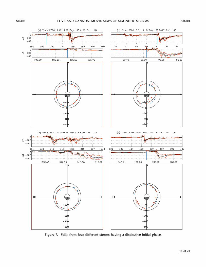
Figure 7. Stills from four different storms having a distinctive initial phase.


14 of 21

Figure 8. Stills from four different storms showing early positive asymmetry.


15 of 21

Figure 9. Stills from four different storms showing positive‐negative asymmetry.


16 of 21

Bz < 0 (see movie‐map); in (b) positive (negative) on theday (night) side, interplanetary Bz > 0; in (c) positive(negative) on the night (day) side, interplanetary Bz < 0;note that this instance is a subsequent snapshot of thestorm shown in Figure 8c; in Figure 9d positive (negative)on the day (night) side, no reliable solar wind data. Hereagain, with only a limited number of examples, we do notfeel we can draw general conclusions about disturbanceasymmetry and the orientation of the interplanetary mag-netic field. We note, however, that solar wind pressure in(a, b, c) is enhanced, especially for (b, 2001:11:24) when itapproaches 100 nPa.[33] We believe that Figures 8 and 9 are showing a

superposition of disturbance sustained by magnetopausecurrents, supported by solar wind pressure, and partialring currents (and, even, field‐aligned currents) [Siscoe,2006]. The later can be realized at just about any localtime, especially during highly dynamic storm evolution,but which might be rather often centered on the daysideduring periods of enhanced solar wind pressure andBz < 0, but, again, we are cautious about conclusions that

over reach. If this is true, then it might also explain theextreme asymmetry seen during the early main phase ofthe Halloween storm (Figure 6b). Shi et al. [2005] suggestthat when interplanetary Bz < 0 (Bz > 0) solar wind pres-sure enhances (has little effect) on low‐latitude magneticdisturbance. In light of their work, the storm (2001:11:24),with its extremely variable asymmetry under conditionsof high solar wind pressure, might be a good candidatefor a similar detailed study.

6.5. Extreme Negative Asymmetry[34] In Figure 10 we show two examples of asymmetric

disturbance that is extremely negative at about 09:00 localtime. In Figure 10a during a rough initial phase of theBastille Day storm, solar wind pressure has abruptlyincreased and interplanetary Bz has turned north (seemovie‐map). In Figure 10b the situation is seemingly verydifferent, during early main phase, with solar wind pres-sure enhanced, but with Bz < 0. That these two independentinstances of disturbance are visually so similar is rathersurprising. The extreme negative asymmetry seen during

Figure 10. Stills from two different storms showing extreme negative asymmetry.

Figure 11. For three different storms. (a, d, g) The Dst and maximum and minimum Dist time series for 7 days oftime. (b, e, h) Contour plots of horizontal‐field disturbance Dist over the local time and universal time domain, con-tour interval 100 nT. (c, f, i) Contour plots of the asymmetric part of the disturbance field Asym(�m) = Dist(�m) − Dst,contour interval 50 nT. Note the prominent dawn−dusk asymmetry in main phase disturbance.


17 of 21

Figure 11


18 of 21

the early main phase development of the Halloweenstorm, Figure 6b, also at about 09:00 local time, mighthave some physical similarity to the disturbance shown inFigure 10b.

6.6. Main Phase Dawn‐Dusk Asymmetry[35] One of the clearest patterns seen in observatory

storm time disturbance data is transient diurnal variation[Sabine, 1856; Moos, 1910a, 1910b], with greatest (least)negative storm disturbance seen in individual observatorytime series at dusk (dawn) local time [Chapman and Bartels,1962, chapters 6.8 and 9.3; Cummings, 1966]. This patternis distinct from stationary diurnal solar quiet variation,but to resolve the dawn‐dusk asymmetry in observatorydata, it is important that the Sq signal be carefully removedbefore proceeding with an analysis of the Dist field. A Dst‐scalable map of dawn‐dusk asymmetry, based on 50 yearsof observatory disturbance time series, is given by Love andGannon [2009, Figure 12]. The cause of the asymmetry is acombination of forces due to magnetic field gradients andconvective electric fields. This results in a concentration(reduction) of ion drift lines of trajectory in the dusk (dawn)magnetosphere [e.g., Takahashi et al., 1990; Liemohn et al.,2001], or, equivalently, a dusk‐centered partial ring current.[36] These observations are not obviously consistent

with the standard picture of substorms and associatedabrupt collapses of current in the magnetotail [e.g.,McPherron, 1991; Kamide et al., 1998b], which should givepositive midnight‐centered disturbance. Nor are theyobviously consistent with various types of satellite data,which tend to show a midnight‐centered partial ringcurrent [e.g., C:son Brandt et al., 2002; Le et al., 2004] thatwould give a negative midnight‐centered disturbance. Thediscrepancy has been explained as a “shielding effect”related to field‐aligned currents [Harel et al., 1981; Crookerand Siscoe, 1981; Wolf et al., 2007], but additional investi-gation is worthwhile.[37] Dawn‐dusk asymmetry in low‐latitude magnetic

disturbance is seen during the November 2003 storm(Figure 5) and during the October 2003 storm (Figure 6d).In contrast, the great storm of March 2001 shows a patternof negative magnetic disturbance that is greatest (least) atmidnight (noon) local time [Skoug et al., 2003]. This isunusual. The overwhelming pattern seen in the movie‐maps is one of dawn‐dusk asymmetry. To emphasize thisfact, in Figure 11 we show Dst time series, contour plotsof magnetic disturbance, Dist(�m) from equation (8), andthe asymmetric component of magnetic disturbance,Asym(�m) = Dist(�m) − Dst, over the local time and uni-versal time domains. In (a–c) for the Halloween storm, in(d–f) for three medium‐size storms that occurred in quicksuccession in July 2004, and in (g–i) for the November2004 storm. In each of these cases, and in most othercases for storms of various sizes, dawn‐dusk asymmetryis prominent during storm main phase; relative symmetryis seen during most periods of storm recovery.

6.7. Geographically Fixed Asymmetry[38] In Figure 11c, days 303.5–304.0 (see, also, movie‐

map 2003:10:30), a transient asymmetry that is roughlyfixed in geographic coordinates is seen (diagonal featuresin the contour plot). Similar transient asymmetry is seen,for example, in the work by Clauer and McPherron [1974,Figure 2] and in the work by Clauer [2006, Figure 2],although those authors do not comment upon the phe-nomenon. We suspect that this asymmetry is caused bythe tilt of the geomagnetic dipole relative to the Earth’srotational axis, causing a diurnal modulation in stormtime magnetic disturbance. As such, geographically fixedasymmetry might be a manifestation of the well‐knownsemiannual diurnal variation, explained by either theRussell‐McPherron [1973] hypothesis or the equinoctial[Bartels, 1925] hypothesis. Again, additional investigation iscertainly worthwhile.

6.8. Day the Solar Wind Disappeared[39] The days of 10–11 May 1999 saw the solar wind

pressure, as measured by the ACE satellite, drop toanomalously low levels (∼0.01 nPA) [Smith et al., 2001]. Notsurprisingly, global magnetic conditions were very quiet;the Kp index briefly dropped to 0. This unusual periodof time serves as a test of our algorithms for isolatingmagnetic disturbance and estimating a stable baselineagainst which disturbance is measured. The movie‐map(1999:05.11) includes a 3 day duration of magnetic quies-cence, during which time very little happens. Indeed, themost interesting thing about this movie‐map is that it isboring. The final day of the movie‐map, however, recordsa small storm, and that is about as exciting as this movie‐map gets. We can confidently say that features seen in theother movie‐maps recording magnetic storms are notartifacts of unremoved solar quiet variation.

7. Conclusion[40] In constructing our movie‐maps, we have become

very well acquainted with some of the time‐dependentevolutionary details of individual storms. And we recog-nize that the movie‐maps contain so much informationthat it is impossible to summarize it all at once. As always,there is much that remains to be done. We plan on inves-tigating a similar movie‐map display of magnetic obser-vatory declination data, which should reveal patterns infield‐aligned currents. In the mean time, our hope is thatthe movie‐maps of horizontal‐intensity disturbance pre-sented here will be useful for other research scientists.

[41] Acknowledgments. We thank the many institutes listed inTable 1 for their support of magnetic observatory operations. Weacknowledge INTERMAGNET (www.intermagnet.org) for its role inpromoting high standards of magnetic observatory practice. Wethank the ACE, GEOTAIL, WIND, and GOES science centers forcollecting solar wind and interplanetary magnetic field data; wethank NASA’s OmniWeb and CDAWeb teams for making dataeasily available. We thank W. J. Burke, J. E. Caldwell, C. A. Finn,


19 of 21

J. P. McCollough, and two anonymous referees for reviewing a draftmanuscript. We thank C. R. Clauer, J. C. Green, T. Iyemori, R. L.McPherron, K. Mursula, T. G. Onsager, H. J. Singer, B. T. Tsurutani,and G. R. Wilson for useful conversations. The USGS GeomagnetismProgram has supported this work, the present operation of theHonolulu, San Juan, Stennis, and Tucson observatories, and the pastoperation of the Del Rio and Midway observatories.

ReferencesAkasofu, S. I., and S. Chapman (1972), Solar‐Terrestrial Physics, OxfordUniv. Press, Oxford, U. K.

Baker, D. N., et al. (2009), Severe Space Weather Events: UnderstandingSocietal and Economic Impacts, Natl. Acad. Press, Washington, D. C.

Balch, C., B. Murtagh, D. Zezula, L. Combs, G. Nelson, K. Tegnell,M. Crown, and B. McGehan (2004), Intense space weather stormsOctober 19–November 07, 2003, service assessment, NOAA, U.S.Dep. of Commerce, Silver Spring, Md.

Bartels, J. (1925), Eine universelle Tagesperiode der erdmagnetischenAktivität, Meteorol. Z., 42, 147–152.

Chapman, S., and J. Bartels (1962), Geomagnetism, Oxford Univ. Press,London.

Chapman, S., and V. C. A. Ferraro (1930), A new theory of magneticstorms, Nature, 126, 129–130.

Clauer, C. R. (2006), The geomagnetic storm‐time response to differentsolar wind driving conditions, in The Solar Influence on the Heliosphereand Earth’s Environment: Recent Progress and Prospects—Proceedings ofthe ILWSWorkshop, edited byN. Gopalswamy andA. Bhattacharyya,pp. 332–339, Quest, Birmingham, Ala.

Clauer, C. R., and R. L. McPherron (1974), Mapping local time–universal time development of magnetospheric substorms usingmid‐latitude magnetic observations, J. Geophys. Res., 79, 2811–2820.

Clauer, C. R., I. I. Alexeev, E. S. Belenkaya, and J. B. Baker (2001), Spe-cial features of the September 24–27, 1998 storm during high solarwind dynamic pressure and northward interplanetary magneticfield, J. Geophys. Res., 106, 25,695–25,711.

Clauer, C. R., M. W. Liemohn, J. U. Kozyra, and M. L. Reno (2003),The relationship of storms and substorms determined from mid‐latitude ground‐based magnetic maps, in Disturbances in Geospace:The Storm‐Substorm Relationship, Geophys. Monogr. Ser., vol. 142, edi-ted by A. S. Sharma, Y. Kamide, and G. S. Lakhina, pp. 143–157,AGU, Washington, D. C.

Cowley, S. W. H. (1995), The Earth’s magnetosphere: A brief begin-ner’s guide, Eos Trans. AGU, 76(51), 525.

Crooker, N. U., and G. L. Siscoe (1981), Birkeland currents as thecause of the low‐latitude asymmetric disturbance field, J. Geophys.Res., 86, 11,201–11,210.

C:son Brandt, P., S. Ohtani, D. G. Mitchell, M.‐C. Fok, E. C. Roelof,and R. Demajistre (2002), Global ENA observations of the stormmainphase ring current: Implications for skewed electric fields inthe inner magnetosphere, Geophys. Res. Lett., 29(20), 1954,doi:10.1029/2002GL015160.

Cummings, W. D. (1966), Asymmetric ring currents and the low‐latitude disturbance daily variation, J. Geophys. Res., 71, 4495–4503.

Daglis, I. A., R. M. Thorne, W. Baumjohann, and S. Orsini (1999), Theterrestrial ring current: Origin, formation, and decay, Rev. Geophys.,37, 407–438.

Dessler, A. J., and E. N. Parker (1959), Hydromagnetic theory of geo-magnetic storms, J. Geophys. Res., 64, 2239–2252.

Dungey, J. W. (1961), Interplanetary magnetic field and the auroralzones, Phys. Rev. Lett., 6, 47–48.

Fukushima, N., and Y. Kamide (1973), Partial ring current models forworldwide geomagnetic disturbances, Rev. Geophys., 11, 795–853.

Gannon, J. L., and J. J. Love (2010), USGS 1‐min Dst index, J. Atmos.Sol. Terr. Phys., in press.

Gonzalez, W. D., J. A. Joselyn, Y. Kamide, H. W. Kroehl, G. Rostoker,B. T. Tsurutani, and V. M. Vasyliunas (1994), What is a geomagneticstorm?, J. Geophys. Res., 99, 5771–5792.

Gopalswamy, N., L. Barbieri, E. W. Cliver, G. Lu, S. P. Plunkett, andR. M. Skoug (2005), Introduction to violent Sun‐Earth connectionevents of October–November 2003, J. Geophys. Res., 110, A09S00,doi:10.1029/2005JA011268.

Harel, M., R. A. Wolf, R. W. Spiro, P. H. Reiff, C. K. Chen, W. J. Burke,F. J. Rich, and M. Smiddy (1981), Quantitative simulation of amagnetospheric substorm: 2. Comparison with observations,J. Geophys. Res., 86, 2242–2260.

Jankowski, J., and C. Sucksdorff (1996), Guide for Magnetic Measure-ments and Observatory Practice, Int. Assoc. of Geomagn. and Aeron.,Warsaw.

Kamide, Y., N. Yokoyama, W. Gonzalez, B. T. Tsurutani, I. A. Daglis,A. Brekke, and S. Masuda (1998a), Two‐step development of geo-magnetic storms, J. Geophys. Res., 103, 6917–6921.

Kamide, Y., et al. (1998b), Current understanding of magnetic storms:Storm‐substorm relationships, J. Geophys. Res., 103, 17,705–17,728.

Kennel, C. F. (1995), Convection and Substorms: Paradigms of Magneto-spheric Phenomenology, Oxford Univ. Press, Oxford, U. K.

Kerridge, D. J. (2001), INTERMAGNET: Worldwide near realtimegeomagnetic observatory data, paper presented at ESA SpaceWeatherWorkshop, Eur. Space Res. and Technol. Cent., Noordwijk,Netherlands. (Available at http://www.esa‐spaceweather.net/spweather/workshops/workshops.html.)

Kozyra, J. U., and M. W. Liemohn (2003), Ring current energy inputand decay, Space Sci. Rev., 109, 105–131.

Le, G., C. T. Russell, and K. Takahashi (2004), Morphology of the ringcurrent derived from magnetic field observations, Ann. Geophys.,22, 1267–1295, sref:1432‐0576/ag/2004‐22‐1267.

Liemohn, M. W., J. U. Kozyra, M. F. Thomsen, J. L. Roeder, G. Lu,J. E. Borovsky, and T. E. Cayton (2001), Dominant role of the asym-metric ring current in producing the stormtime Dst*, J. Geophys.Res., 106, 10,883–10,904.

Love, J. J. (2008), Magnetic monitoring of Earth and space, Phys.Today, 61, 31–37.

Love, J. J., and J. L. Gannon (2009), Revised Dst and the epicycles ofmagnetic disturbance: 1958–2007, Ann. Geophys., 27, 3101–3131.

McPherron, R. L. (1991), Physical processes producing magneto-spheric substorms and magnetic storms, in Geomagnetism, vol. 4,edited by J. A. Jacobs, pp. 593–739, Academic, London.

McPherron, R. L. (1997), The role of substorms in the generation ofmagnetic storms, in Magnetic Storms, Geophys. Monogr. Ser., vol. 98,edited by B. T. Tsurutani et al., pp. 131–147, AGU,Washington, D. C.

Moos, N. A. F. (1910a), Colaba Magnetic Data, 1846 to 1905: Part I—Magnetic Data and Instruments, Gov. Cent. Press, Bombay, India.

Moos, N. A. F. (1910b), Colaba Magnetic Data, 1846 to 1905: Part II—ThePhenomenon and its Discussion, Gov. Cent. Press, Bombay, India.

Nishida, A. (1994), Foward of GEOTAIL special issue, J. Geomagn.Geoelectr., 46, 3–5.

Panasyuk, M. I., et al. (2004), Magnetic storms in October 2003, CosmicRes., 42, 489–534.

Potapov, A., A. Guglielmi, B. Tsegmed, and J. Kultima (2006), GlobalPC5 event during 29–31 October 2003 magnetic storm, Adv. SpaceRes., 38, 1582–1586.

Prölss, G. W. (2004), Physics of the Earth’s Space Environment, Springer,Berlin.

Rasson, J. L. (2007), INTERMAGNET, in Encyclopedia of Geomagnetismand Paleomagnetism, edited by D. Gubbins and E. Herrero‐Bervera,pp. 715–717, Springer, New York.

Rostoker, G., and C. G. Fälthammar (1967), Relationship betweenchanges in the interplanetary magnetic field and variations in themagnetic field at the Earth’s surface, J. Geophys. Res., 72, 5853–5863.

Russell, C. T. (1995), Foward of WIND special issue, Space Sci. Rev.,71, 1–4.

Russell, C. T., and R. L. McPherron (1973), Semiannual variation ofgeomagnetic activity, J. Geophys. Res., 78, 92–108.

Russell, C. T., R. L. McPherron, and R. K. Burton (1974), On the causeof geomagnetic storms, J. Geophys. Res., 79, 1105–1109.

Russell, C. T., M. Ginskey, S. Petrinec, and G. Le (1992), The effect ofsolar wind dynamic pressure changes on low and mid‐latitudemagnetic records, Geophys. Res. Lett., 19, 1227–1230.

Sabine, E. (1856), On periodical laws discoverable in the mean effectsof the larger magnetic disturbances. No. III, Philos. Trans. R. Soc.London, 146, 357–374.

Sckopke, N. (1966), A general relation between the energy of trappedparticles and the disturbance field over the Earth, J. Geophys. Res., 71,3125–3130.

Shi, Y., E. Zesta, L. R. Lyons, A. Boudouridis, K. Yumoto, andK. Kitamura (2005), Effect of solar wind pressure enhancements


20 of 21

on storm time ring current asymmetry, J. Geophys. Res., 110, A10205,doi:10.1029/2005JA011019.

Singer, H., L. Matheson, R. Grubb, A. Newman, and D. Bouwer(1996), Monitoring space weather with the GOES magnetometers,in GOES‐8 and Beyond, vol. 2812, edited by E. R. Washwell,pp. 299–308, Soc. of Photo‐Optical Instrum. Eng., Bellingham,Wash.

Singer, S. F. (1957), A new model of magnetic storms and aurorae, EosTrans. AGU, 38, 175–190.

Siscoe, G. L. (2006), Global force balance of region 1 current system,J. Atmos. Sol. Terr. Phys., 68, 2119–2126.

Skoug, R.M., et al. (2003), Tail‐dominated stormmain phase: 31March2001, J. Geophys. Res., 108(A6), 1259, doi:10.1029/2002JA009705.

Skoug, R.M., J. T. Gosling, J. T. Steinberg, D. J. McComas, C.W. Smith,N. F. Ness, Q. Hu, and L. F. Burlaga (2004), Extremely high speedsolar wind: 29–30 October 2003, J. Geophys. Res., 109, A09102,doi:10.1029/2004JA010494.

Smith, C. W., D. J. Mullan, N. F. Ness, R. M. Skoug, and J. Steinberg(2001), Day the solar wind almost disappeared: Magnetic field fluc-tuations, wave refraction and dissipation, J. Geophys. Res., 106,18,625–18,634.

Søraas, F., M. Sørbø, K. Aarsnes, and D. S. Evans (2006), Ring currentbehavior inferred from ground magnetic and space observations, inRecurrent Magnetic Storms: Corotating Solar Wind Streams, Geophys.

Monogr. Ser., vol. 167, edited by B. T. Tsurutani et al., pp. 85–95,AGU, Washington, D. C.

Stone, E. C., A. M. Frandsen, R. A. Mewaldt, E. R. Christian,D. Margolies, J. F. Ormes, and F. Snow (1999), The Advanced Com-position Explorer, Space Sci. Rev., 86, 1–22.

Sugiura, M. (1964), Hourly values of equatorial Dst for the IGY, Ann.Int. Geophys. Year, 35, 9–45.

Sugiura, M., and T. Kamei (1991), Equatorial Dst index 1957–1986,IAGA Bull. 40, Int. Serv. Geomagn. Indices Publ. Off., Saint‐Maur‐des‐Fossés, France.

Takahashi, S., T. Iyemori, and M. Takeda (1990), A simulation of thestorm‐time ring current, Planet. Space Sci., 38, 1133–1141.

Wolf, R. A., R.W. Spiro, S. Sazykin, and F. R. Toffoletto (2007), How theEarth’s inner magnetosphere works: An evolving picture, J. Atmos.Sol. Terr. Phys., 69, 288–302.

Zaitzev, A. N., and R. Boström (1971), On methods of graphicaldisplaying of polar magnetic disturbances, Planet. Space Sci., 19,643–649.

J. L. Gannon and J. J. Love, Geomagnetism Program, U.S.Geological Survey, Box 25046, MS 966, DFC, Denver, CO 80225,USA. ([email protected])


21 of 21

Movie-maps of low-latitude magnetic storm disturbance

Documents

Transcript of Movie-maps of low-latitude magnetic storm disturbance