Optimized Thermoelectric Module-Heat Sink ... - Tufts Digital Library
129
Optimized Thermoelectric Module-Heat Sink Assemblies for Precision Temperature Control Submitted by Rui Zhang IN PARTIAL FULFILLMENT OF THE REQUIREMENTS FOR THE DEGREE OF MASTERS OF SCIENCE IN MECHANICAL ENGINEERING School of Engineering Tufts University Medford, Massachusetts Aug. 2011 Author: Certified By: Rui Zhang Associate Professor Marc Hodes Department of Mechanical Engineering Department of Mechanical Engineering Tufts University Tufts University Committee: Committee: Professor Vincent P. Manno Ross Wilcoxon Department of Mechanical Engineering Rockwell Collins, Inc. Tufts University Cedar Rapids, IA
-
Upload
khangminh22 -
Category
Documents
-
view
4 -
download
0
Transcript of Optimized Thermoelectric Module-Heat Sink ... - Tufts Digital Library
Optimized Thermoelectric Module-Heat SinkAssemblies for Precision Temperature Control
Submitted byRui Zhang
IN PARTIAL FULFILLMENT OF THE REQUIREMENTS FOR THE DEGREE OF
MASTERS OF SCIENCE IN MECHANICAL ENGINEERING
School of EngineeringTufts University
Medford, Massachusetts
Aug. 2011
Author: Certified By:Rui Zhang Associate Professor Marc HodesDepartment of Mechanical Engineering Department of Mechanical EngineeringTufts University Tufts University
Committee: Committee:Professor Vincent P. Manno Ross WilcoxonDepartment of Mechanical Engineering Rockwell Collins, Inc.Tufts University Cedar Rapids, IA
ABSTRACT
Optimized Thermoelectric Module-Heat Sink Assemblies for Precision Temperature Control
by
Rui Zhang
Chair: Marc Hodes
Robust precision temperature control of heat-dissipating photonics components is achieved
by mounting them on thermoelectric modules (TEMs) which are in turn mounted on heat
sinks. However, the power consumption of such TEMs is high. Indeed, it may exceed that
of the component. This problem is exacerbated when the ambient temperature surrounding
a TEM and/or component heat load that it accommodates vary. In the usual packaging
configuration a TEM is mounted on an air-cooled heat sink of specified thermal resistance.
However, heat sinks of negligible thermal resistance minimize TEM power for sufficiently
high ambient temperatures and/or heat loads. Conversely, a relatively high thermal resis-
tance heat sink minimizes TEM power for sufficiently low ambient temperature and heat
load. In the problem considered, total footprint of thermoelectric material in a TEM, ther-
moelectric material properties, component operating temperature, relevant component-side
thermal resistances and ambient temperature range are prescribed. Moreover, the minimum
and maximum rates of heat dissipation by the component are zero and a prescribed value,
respectively. Provided is an algorithm to compute the combination of the height of the pel-
lets in a TEM and the thermal resistance of the heat sink attached to it which minimizes the
maximum sum of the component and TEM powers for permissible operating conditions. It
ii

is further shown that the maximum value of this sum asymptotically decreases as the total
footprint of thermoelectric material in a TEM increases. Implementation of the algorithm
maximizes the fraction of the power budget in an optoelectronics circuit pack available for
other uses. Use of the algorithm is demonstrated through an example for a typical set of
conditions.
iii

Acknowledgements
This thesis would not have been possible without the guidance and the help of several
individuals who in one way or another contributed and extended their valuable assistance in
the development and completion of this research.
First and foremost, my utmost gratitude to my advisor, Dr. Marc Hodes, who has
supported me thoughout my thesis with his patience, encouragement and knowledge whilst
allowing me the room to work in my own way for the last two years. Without him, this
thesis would not have been completed or written. His ideas and passions in science inspire
and enrich my growth as a student. One could not wish for a better or friendlier advisor
and I am indebted to him more than he knows.
I gratefully acknowledge my thesis committee members, Professor Vincent Manno and
Ross Wilcoxon for their advice, insight, encouragement and assistance. Special thank to
Ross for offering me a visit of the thermal lab at Rockwell Collins which was incredibly
valuable to me.
Many thanks to Dave Brooks, a fellow graduate student, and Martin Cleary, a post-
doctoral fellow, for their generous help and collaboration in the completion of this thesis
and the design and construction of the thermocouple calibration apparatus. Thanks are also
extended to Drew Mills, a fellow graduate student, for his help on LabVIEW and Latex and
Gennady Ziskind, a visiting professor, for his help and insight in apparatus design.
Finally, I would like to thank the Wittich Energy Sustainability Research Initiation Fund
for supporting this research.
iv
TABLE OF CONTENTS
ABSTRACT . . . . . . . . . . . . . . . . . . . . . . . . . . . . . . . . . . . . . . . ii
ACKNOWLEDGEMENTS . . . . . . . . . . . . . . . . . . . . . . . . . . . . . . iv
LIST OF FIGURES . . . . . . . . . . . . . . . . . . . . . . . . . . . . . . . . . . . vii
LIST OF APPENDICES . . . . . . . . . . . . . . . . . . . . . . . . . . . . . . . . xii
NOMENCLATURE . . . . . . . . . . . . . . . . . . . . . . . . . . . . . . . . . . . xiv
CHAPTER
I. Introduction And Background . . . . . . . . . . . . . . . . . . . . . . . 1
1.1 Thermoelectric Effects . . . . . . . . . . . . . . . . . . . . . . . . . . 11.2 Thermoelectric Modules . . . . . . . . . . . . . . . . . . . . . . . . . 21.3 Problem Statement . . . . . . . . . . . . . . . . . . . . . . . . . . . 31.4 Previous Work . . . . . . . . . . . . . . . . . . . . . . . . . . . . . . 41.5 Outline of Thesis . . . . . . . . . . . . . . . . . . . . . . . . . . . . . 5
II. Methodology . . . . . . . . . . . . . . . . . . . . . . . . . . . . . . . . . . 7
2.1 Governing Equations . . . . . . . . . . . . . . . . . . . . . . . . . . . 72.1.1 Expressions for General Case . . . . . . . . . . . . . . . . . 92.1.2 Expressions for Simplified Case . . . . . . . . . . . . . . . . 11
2.2 Prescribed, Independent and Dependent Variables . . . . . . . . . . 112.3 Analysis . . . . . . . . . . . . . . . . . . . . . . . . . . . . . . . . . . 13
2.3.1 The case when qcp = qcp,max . . . . . . . . . . . . . . . . . . 132.3.2 The case when qcp = 0 . . . . . . . . . . . . . . . . . . . . 182.3.3 Role of φAsub . . . . . . . . . . . . . . . . . . . . . . . . . 20
2.4 Algorithm . . . . . . . . . . . . . . . . . . . . . . . . . . . . . . . . . 202.5 Dependence of TEM Operating Mode on T∞, H and Ru−∞ . . . . . 21
III. Implementation of Algorithm . . . . . . . . . . . . . . . . . . . . . . . . 25
v

3.1 Fixed Pellet Height . . . . . . . . . . . . . . . . . . . . . . . . . . . 263.2 Arbitrary Pellet Height . . . . . . . . . . . . . . . . . . . . . . . . . 27
IV. Conclusion and Future Work . . . . . . . . . . . . . . . . . . . . . . . . 33
BIBLIOGRAPHY . . . . . . . . . . . . . . . . . . . . . . . . . . . . . . . . . . . . 34
APPENDICES . . . . . . . . . . . . . . . . . . . . . . . . . . . . . . . . . . . . . . 36
vi

LIST OF FIGURES
Figure
1.1 Cutaway view of a single stage TEM [1]. . . . . . . . . . . . . . . . . . . . 3
2.1 Schematic of a TEM embedded in a thermal resistance network. . . . . . . 8
2.2 Ru−∞,max as a function of H at T∞,min and T∞,max. . . . . . . . . . . . . . 14
2.3 Wt as a function of H at T∞,min and T∞,max when Ru−∞ = 0 and Ru−∞,max. 14
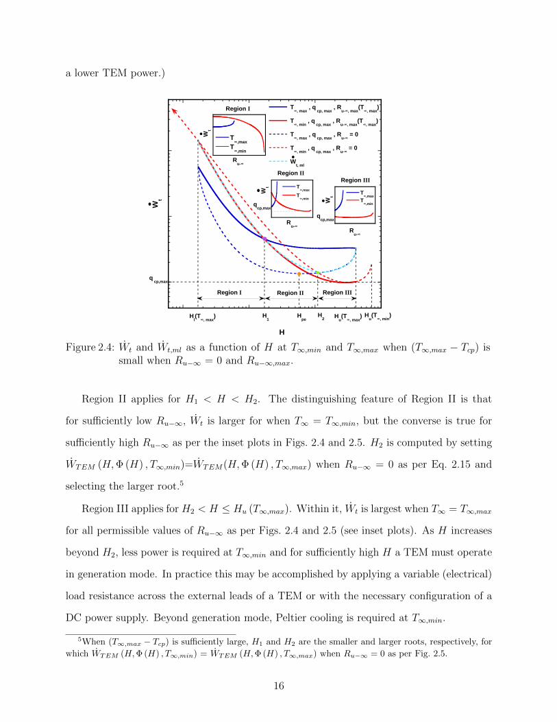
2.4 Wt and Wt,ml as a function of H at T∞,min and T∞,max when (T∞,max − Tcp)is small when Ru−∞ = 0 and Ru−∞,max. . . . . . . . . . . . . . . . . . . . . 16
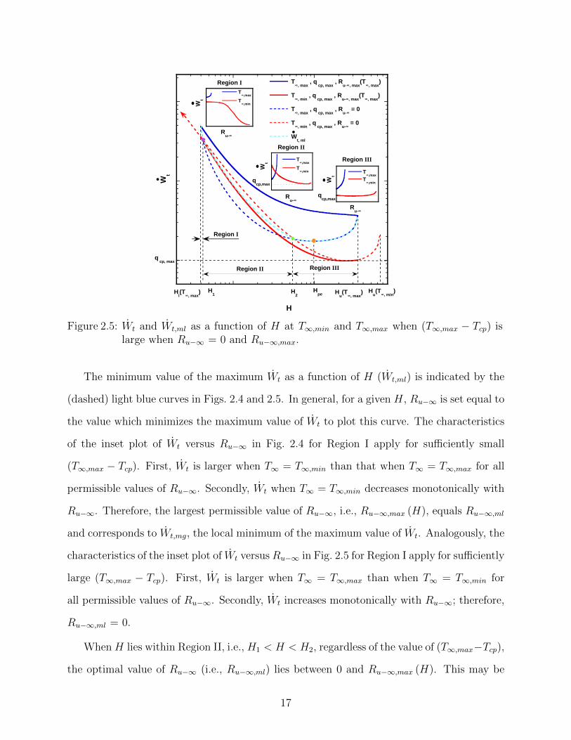
2.5 Wt and Wt,ml as a function of H at T∞,min and T∞,max when (T∞,max − Tcp)is large when Ru−∞ = 0 and Ru−∞,max. . . . . . . . . . . . . . . . . . . . . 17
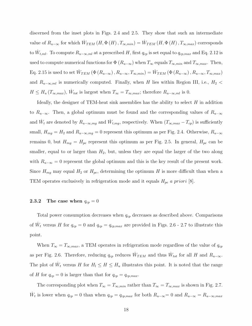
2.6 Wt as a function of H at T∞,max when qcp = 0 and qcp,max when Ru−∞ = 0and Ru−∞,max. . . . . . . . . . . . . . . . . . . . . . . . . . . . . . . . . . . 19
2.7 Wt as a function of H at T∞,min when qcp = 0 and qcp,max when Ru−∞ = 0and Ru−∞,max. . . . . . . . . . . . . . . . . . . . . . . . . . . . . . . . . . . 19
2.8 Wt,mg as a function (φAsub)1/2. . . . . . . . . . . . . . . . . . . . . . . . . . 20
2.9 Delineation of TEM operating modes as a function of H and Ru−∞ whenT∞ = T∞,min < Tcp. . . . . . . . . . . . . . . . . . . . . . . . . . . . . . . . 23
2.10 Delineation of TEM operating modes as a function of H and Ru−∞ whenT∞ = T∞,min < Tcp. . . . . . . . . . . . . . . . . . . . . . . . . . . . . . . . 23
3.1 WTEM as a function of Ru−∞ (Tcp = 55 C). . . . . . . . . . . . . . . . . . 27
3.2 qcp,TEM,max as a function of H at T∞,min and T∞,max for Ru−∞ = 0. . . . . 28
vii

3.3 Ru−∞,max as a function H at T∞,min and T∞,max. . . . . . . . . . . . . . . . 29
3.4 Wt and Wt,ml as a function of H at Tcp = 55 C when Ru−∞ = 0 and Ru−∞,max. 29
3.5 Wt as a function of Ru−∞ at Hmg at T∞,min and T∞,max. . . . . . . . . . . . 30
3.6 Wt,mg as a function of (φAsub)1/2. . . . . . . . . . . . . . . . . . . . . . . . 30
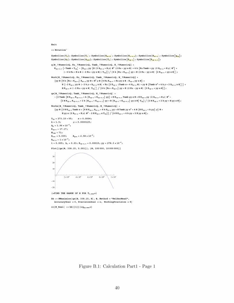
A.1 Mathematica Codes for Eqs. 2.12 - 2.15 . . . . . . . . . . . . . . . . . . . . 38
B.1 Calculation Part1 - Page 1 . . . . . . . . . . . . . . . . . . . . . . . . . . . 40
B.2 Calculation Part1 - Page 2 . . . . . . . . . . . . . . . . . . . . . . . . . . . 41
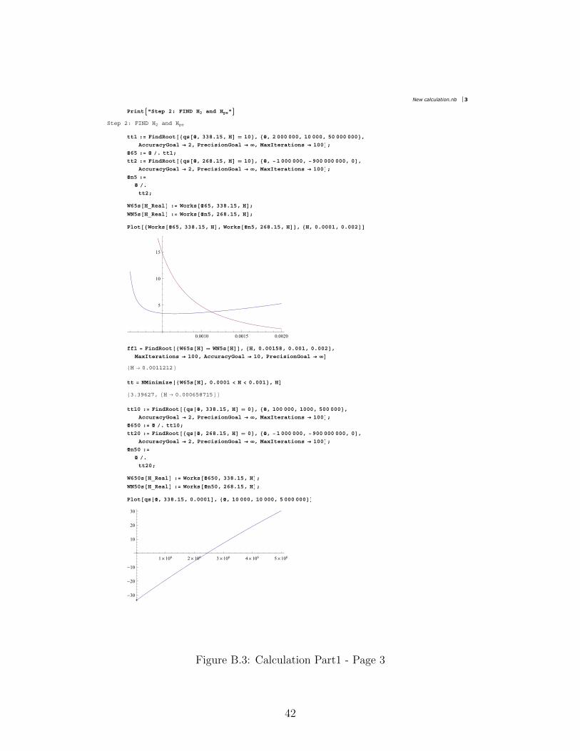
B.3 Calculation Part1 - Page 3 . . . . . . . . . . . . . . . . . . . . . . . . . . . 42
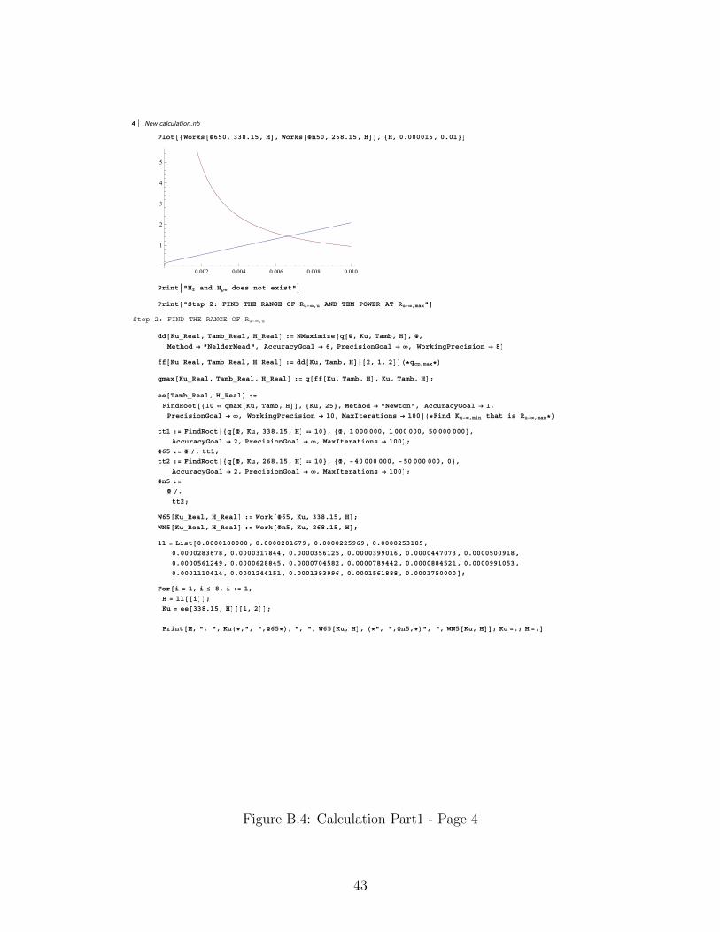
B.4 Calculation Part1 - Page 4 . . . . . . . . . . . . . . . . . . . . . . . . . . . 43
B.5 Calculation Part1 - Page 5 . . . . . . . . . . . . . . . . . . . . . . . . . . . 44
B.6 Calculation Part1 - Page 6 . . . . . . . . . . . . . . . . . . . . . . . . . . . 45
B.7 Calculation Part1 - Page 7 . . . . . . . . . . . . . . . . . . . . . . . . . . . 46
B.8 Calculation Part1 - Page 8 . . . . . . . . . . . . . . . . . . . . . . . . . . . 47
B.9 Calculation Part1 - Page 9 . . . . . . . . . . . . . . . . . . . . . . . . . . . 48
B.10 Calculation Part2 - Page 1 . . . . . . . . . . . . . . . . . . . . . . . . . . . 50
B.11 Calculation Part2 - Page 2 . . . . . . . . . . . . . . . . . . . . . . . . . . . 51
B.12 Calculation Part2 - Page 3 . . . . . . . . . . . . . . . . . . . . . . . . . . . 52
B.13 Calculation Part2 - Page 4 . . . . . . . . . . . . . . . . . . . . . . . . . . . 53
B.14 Calculation Part2 - Page 5 . . . . . . . . . . . . . . . . . . . . . . . . . . . 54
B.15 Calculation Part2 - Page 6 . . . . . . . . . . . . . . . . . . . . . . . . . . . 55
B.16 Calculation Part2 - Page 7 . . . . . . . . . . . . . . . . . . . . . . . . . . . 56
B.17 Calculation Part3 - Page 1 . . . . . . . . . . . . . . . . . . . . . . . . . . . 58
B.18 Calculation Part3 - Page 2 . . . . . . . . . . . . . . . . . . . . . . . . . . . 59
viii
B.19 Calculation Part3 - Page 3 . . . . . . . . . . . . . . . . . . . . . . . . . . . 60
B.20 Calculation Part3 - Page 4 . . . . . . . . . . . . . . . . . . . . . . . . . . . 61
C.1 Type-T thermocouple measurement circuit. . . . . . . . . . . . . . . . . . . 64
C.2 Tigtech 116 SRL Thermocouple welder. . . . . . . . . . . . . . . . . . . . . 66
C.3 Handheld thermal wire strippers. . . . . . . . . . . . . . . . . . . . . . . . 66
C.4 Magnifying lens. . . . . . . . . . . . . . . . . . . . . . . . . . . . . . . . . . 67
C.5 Schematic of thermocouple calibration rig. . . . . . . . . . . . . . . . . . . 69
C.6 Copper annulus assembly design for measurement junction . . . . . . . . . 71
C.7 Teflon cover drawings for reference junction (Dimensions are in inches). . . 72
C.8 Teflon cover drawings for measurement junction (Dimensions are in inches). 73
C.9 Copper enclosure drawing (Dimensions are in inches). . . . . . . . . . . . . 74
C.10 Copper bottom cover drawing (Dimensions are in inches). . . . . . . . . . . 75
C.11 Copper rod drawing for reference junction (Dimensions are in inches). . . . 76
C.12 Copper rod drawing for measurement junction (Dimensions are in inches). . 77
C.13 Fluke 5610 thermistor probe. . . . . . . . . . . . . . . . . . . . . . . . . . . 78
C.14 Black stack overview. . . . . . . . . . . . . . . . . . . . . . . . . . . . . . . 79
C.15 2182A Nanovoltmeter. . . . . . . . . . . . . . . . . . . . . . . . . . . . . . 80
C.16 2182A Nanovoltmeter voltage specifications. . . . . . . . . . . . . . . . . . 80
C.17 7001 Switch system front panel. . . . . . . . . . . . . . . . . . . . . . . . . 81
C.18 7001 Switch system back panel. . . . . . . . . . . . . . . . . . . . . . . . . 81
C.19 7011-S Switch card with thermocouples attached. . . . . . . . . . . . . . . 81
C.20 LabView VI front panel for thermocouple calibration. . . . . . . . . . . . . 83
ix
C.21 LabView VI block diagram for thermocouple calibration. . . . . . . . . . . 84
C.22 Thermocouple Junctions Attached to the Copper Rod Example. . . . . . . 84
C.23 Calibration readouts of thermocouples and thermistors. . . . . . . . . . . . 86
C.24 Calibration results after reference junction compensation. . . . . . . . . . . 87
C.25 Experimental data, Least-squares Fit data and data from reference tables(ITS-90) for thermocouple 1, 11, 21 and 31 . . . . . . . . . . . . . . . . . . 88
C.26 Comparison of experimental data, least-squares fit data and that in referencerables for thermocouple 1. . . . . . . . . . . . . . . . . . . . . . . . . . . . 89
C.27 Comparison of experimental data, least-squares fit data and that in referencerables for thermocouple 11. . . . . . . . . . . . . . . . . . . . . . . . . . . . 89
C.28 Comparison of experimental data, least-squares fit data and that in referencerables for thermocouple 21. . . . . . . . . . . . . . . . . . . . . . . . . . . . 90
C.29 Comparison of experimental data, least-squares fit data and that in referencerables for thermocouple 31. . . . . . . . . . . . . . . . . . . . . . . . . . . . 90
C.30 Absolute errors versus temperatures in voltage for thermocouple 1. . . . . . 91
C.31 Absolute errors versus temperatures in temperature for thermocouple 1. . . 91
C.32 Calibration report of reference thermistor probe (Serial Number: B072717)page 1. . . . . . . . . . . . . . . . . . . . . . . . . . . . . . . . . . . . . . . 93
C.33 Calibration report of reference thermistor probe (Serial Number: B072717)page 2. . . . . . . . . . . . . . . . . . . . . . . . . . . . . . . . . . . . . . . 94
C.34 Calibration report of reference thermistor probe (Serial Number: B072717)page 3. . . . . . . . . . . . . . . . . . . . . . . . . . . . . . . . . . . . . . . 95
C.35 Calibration report of reference thermistor probe (Serial Number: B072717)page 4. . . . . . . . . . . . . . . . . . . . . . . . . . . . . . . . . . . . . . . 96
C.36 Calibration report of reference thermistor probe (Serial Number: B072717)page 5. . . . . . . . . . . . . . . . . . . . . . . . . . . . . . . . . . . . . . . 97
C.37 Calibration report of reference thermistor probe (Serial Number: B072717)page 6. . . . . . . . . . . . . . . . . . . . . . . . . . . . . . . . . . . . . . . 98
x

C.38 Calibration report of reference thermistor probe (Serial Number: B072717)page 7. . . . . . . . . . . . . . . . . . . . . . . . . . . . . . . . . . . . . . . 99
C.39 Calibration report of reference thermistor probe (Serial Number: B072717)page 8. . . . . . . . . . . . . . . . . . . . . . . . . . . . . . . . . . . . . . . 100
C.40 Calibration report of reference thermistor probe (Serial Number: B072717)page 9. . . . . . . . . . . . . . . . . . . . . . . . . . . . . . . . . . . . . . . 101
C.41 Calibration report of measurement thermistor probe (Serial Number: B072719)page 1. . . . . . . . . . . . . . . . . . . . . . . . . . . . . . . . . . . . . . . 102
C.42 Calibration report of measurement thermistor probe (Serial Number: B072719)page 2. . . . . . . . . . . . . . . . . . . . . . . . . . . . . . . . . . . . . . . 103
C.43 Calibration report of measurement thermistor probe (Serial Number: B072719)page 3. . . . . . . . . . . . . . . . . . . . . . . . . . . . . . . . . . . . . . . 104
C.44 Calibration report of measurement thermistor probe (Serial Number: B072719)page 4. . . . . . . . . . . . . . . . . . . . . . . . . . . . . . . . . . . . . . . 105
C.45 Calibration report of measurement thermistor probe (Serial Number: B072719)page 5. . . . . . . . . . . . . . . . . . . . . . . . . . . . . . . . . . . . . . . 106
C.46 Calibration report of measurement thermistor probe (Serial Number: B072719)page 6. . . . . . . . . . . . . . . . . . . . . . . . . . . . . . . . . . . . . . . 107
C.47 Calibration report of measurement thermistor probe (Serial Number: B072719)page 7. . . . . . . . . . . . . . . . . . . . . . . . . . . . . . . . . . . . . . . 108
C.48 Calibration report of measurement thermistor probe (Serial Number: B072719)page 8. . . . . . . . . . . . . . . . . . . . . . . . . . . . . . . . . . . . . . . 109
C.49 Calibration report of Black Stack page 1. . . . . . . . . . . . . . . . . . . . 110
C.50 Calibration report of Black Stack page 2. . . . . . . . . . . . . . . . . . . . 111
C.51 Calibration report of Black Stack page 3. . . . . . . . . . . . . . . . . . . . 112
C.52 Mathematica Code for Least-squares Fit and Reference Tables page 1. . . . 113
C.53 Mathematica Code for Least-squares Fit and Reference Tables page 2. . . . 114
C.54 Mathematica Code for Least-squares Fit and Reference Tables page 3. . . . 115
xi
LIST OF APPENDICES
Appendix
A. Mathematica Codes for Eqs. 2.12 - 2.15 . . . . . . . . . . . . . . . . . . . . . 37
B. Mathematica Codes for Example Calculation . . . . . . . . . . . . . . . . . . 39
C. Thermocouple Welding and Calibration . . . . . . . . . . . . . . . . . . . . . 63
xii

Nomenclature
AP Pellet cross-sectional area [m2]
Asub Footprint of TEM substrates [m2]
k Thermal conductivity [W/(mK)]
K Thermal conductance [W/C]
H Pellet height [m]
H1 H corresponding to Region I-II transition [m]
H2 H corresponding to Region II-III transition [m]
Hl Lower limit of H [m]
Hu Upper limit of H [m]
I Current [A]
Ki−j Thermal conductance from node i to node j [W/C]
N Number of thermocouples
q Heat transfer rate [W]
R Ohmic resistance [Ω]
Rec−ρ Electrical contact resistivity [Ωm2]
Rec−R Electrical contact resistance [Ω]
Ri−j Thermal resistance from node i to node j [C/W]
T Temperature [K]
V Voltage [V]
W Electrical power [W]
Greek Symbols
α Seebeck coefficient [V/K]
xiii
φ Pellet packing density
Φ Current flux [A/m2]
ρ Electrical resistivity [Ωm]
Subscripts
∞ Ambient
c Controlled side
cp Control plane
cp-c Control plane to controlled side
cp-∞ Control plane to ambient
csi Controlled-side interface
max Maximum
mg Global minimum maximum quantity
min Minimum
ml Local minimum maximum quantity
n n-type
open Open circuit mode
p Peltier effect
p p-type or pellet
pe Quantity when efficiency maximized
p, n p-n (as in difference in Seebeck coefficients)
sh Short circuit mode
u Uncontrolled side
u-∞ Uncontrolled side to ambient
TEM Thermoelectric module
t Total power consumption
xiv

CHAPTER I
Introduction And Background
1.1 Thermoelectric Effects
Thermal energy may be reversibly converted into electrical energy and vice versa in
electrically conducting materials by three thermoelectric effects [2]. The Seebeck effect occurs
when a conductor subjected to a temperature gradient generates an electric potential gradient
under open circuit conditions. It is described by
dV = αdT (1.1)
where V is voltage, α is the Seebeck coefficient of a conductor (or semiconductor) and T
is temperature. The Seebeck coefficient may be positive or negative and depends upon the
scattering properties of a conductor.
When current, I, flows through the interface between conductors, heat is absorbed or
rejected by the Peltier effect due to varying levels of electrical energy associated with current
flow in different conductors. The rate of heat absorption, qp, is
qp = I(αB − αA)T (1.2)
when the direction of current (i.e., flow of positive charge carriers) is from conductor A to
1
conductor B.
When current flows through a conducting material in the presence of a temperature gra-
dient, heat is also absorbed or evolved due to the Thomson (bulk) effect [3]. The irreversible
effects of bulk and interfacial Ohmic heating and heat conduction must also be considered
in the analysis of thermoelectric circuits.
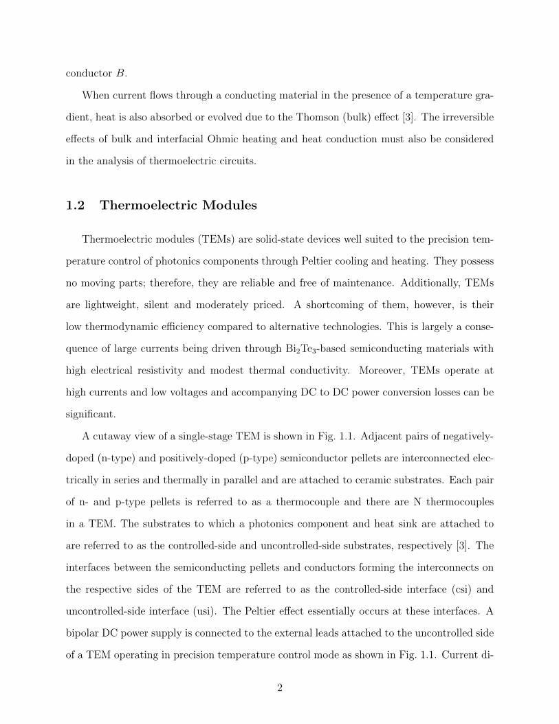
1.2 Thermoelectric Modules
Thermoelectric modules (TEMs) are solid-state devices well suited to the precision tem-
perature control of photonics components through Peltier cooling and heating. They possess
no moving parts; therefore, they are reliable and free of maintenance. Additionally, TEMs
are lightweight, silent and moderately priced. A shortcoming of them, however, is their
low thermodynamic efficiency compared to alternative technologies. This is largely a conse-
quence of large currents being driven through Bi2Te3-based semiconducting materials with
high electrical resistivity and modest thermal conductivity. Moreover, TEMs operate at
high currents and low voltages and accompanying DC to DC power conversion losses can be
significant.
A cutaway view of a single-stage TEM is shown in Fig. 1.1. Adjacent pairs of negatively-
doped (n-type) and positively-doped (p-type) semiconductor pellets are interconnected elec-
trically in series and thermally in parallel and are attached to ceramic substrates. Each pair
of n- and p-type pellets is referred to as a thermocouple and there are N thermocouples
in a TEM. The substrates to which a photonics component and heat sink are attached to
are referred to as the controlled-side and uncontrolled-side substrates, respectively [3]. The
interfaces between the semiconducting pellets and conductors forming the interconnects on
the respective sides of the TEM are referred to as the controlled-side interface (csi) and
uncontrolled-side interface (usi). The Peltier effect essentially occurs at these interfaces. A
bipolar DC power supply is connected to the external leads attached to the uncontrolled side
of a TEM operating in precision temperature control mode as shown in Fig. 1.1. Current di-
2
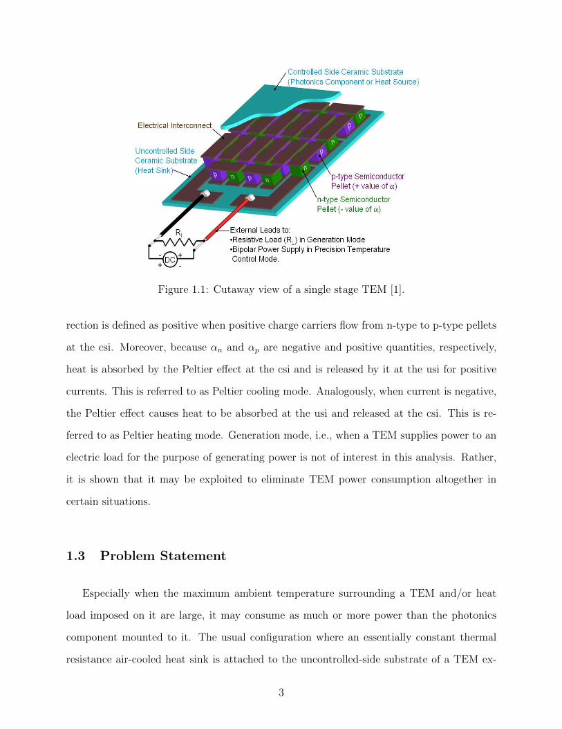
Figure 1.1: Cutaway view of a single stage TEM [1].
rection is defined as positive when positive charge carriers flow from n-type to p-type pellets
at the csi. Moreover, because αn and αp are negative and positive quantities, respectively,
heat is absorbed by the Peltier effect at the csi and is released by it at the usi for positive
currents. This is referred to as Peltier cooling mode. Analogously, when current is negative,
the Peltier effect causes heat to be absorbed at the usi and released at the csi. This is re-
ferred to as Peltier heating mode. Generation mode, i.e., when a TEM supplies power to an
electric load for the purpose of generating power is not of interest in this analysis. Rather,
it is shown that it may be exploited to eliminate TEM power consumption altogether in
certain situations.
1.3 Problem Statement
Especially when the maximum ambient temperature surrounding a TEM and/or heat
load imposed on it are large, it may consume as much or more power than the photonics
component mounted to it. The usual configuration where an essentially constant thermal
resistance air-cooled heat sink is attached to the uncontrolled-side substrate of a TEM ex-
3
acerbates this problem. Indeed, a heat sink of negligible thermal resistance minimizes TEM
power for sufficiently high ambient temperature and/or heat load, but a relatively high
thermal resistance one minimizes it for sufficiently low ambient temperature and heat load.
Optimized TEM-heat sink assemblies reduce the severity of this problem.
The primary purpose of this thesis is provision of an algorithm to compute the combina-
tion of the height of the pellets in a TEM and the thermal resistance of a heat sink attached
to it which minimizes the maximum sum of the component and TEM powers for permissible
operating conditions. In the problem considered, total footprint of thermoelectric material
in a TEM, thermoelectric material properties, component operating temperature, relevant
component-side thermal resistances and ambient temperature range are prescribed. The
minimum ambient temperature is assumed to be less than or equal to the component oper-
ating temperature. Moreover, the minimum and maximum rates of heat dissipation by the
component are zero and a prescribed value, respectively.1 (When a fraction of the power
supplied to a photonics component is converted to light rather than heat this should be
considered.) Further insight into the design problem is provided by considering the impact
of increasing the total footprint of thermoelectric material on decreasing the minimum max-
imum sum of component and TEM powers. Finally, the TEM operating modes relevant to
the optimization are discussed in some depth.
1.4 Previous Work
Hodes [4] presented a means to compute the optimal value of heat sink thermal resistance
for the problem at hand when all other parameters are prescribed. Elsewhere, the premise
that the ability to adjust heat sink thermal resistance is beneficial because as the ambient
temperature changes different values of heat sink thermal resistance minimize TEM power
has been addressed. This has been discussed in the context of TEM-finned variable conduc-
1The latter two assumptions imply TEM operation in refrigeration mode is necessary at some, if not all,permissible operating conditions.
4

tance heat pipe assemblies [5] and moving shrouds which slide along a heat sink to vary the
number of fins exposed to air [6]. Moreover, Wilcoxon et al. [7] proposed utilizing a liquid
metal substrate to separate the uncontrolled side of a TEM from a low thermal resistance
heat sink. Then the dominant thermal resistance between the uncontrolled-side interface
and ambient is the caloric thermal resistance of the liquid metal, which may be controlled
by varying its mass flow rate. Another approach is to implement a variable speed fan to
vary the thermal resistance of a conventional air-cooled heat sink. However, this is typically
not viable as the airflow supplied to optoelectronic circuit packs is provided by shelf-level
fans running at a fixed speed. Finally, it is noted that the height of the pellets which mini-
mizes the power of a TEM operating in refrigeration mode is relevant and calculable for an
arbitrary heat sink thermal resistance [8]. However, this is not necessarily the optimal pellet
height for the problem at hand as discussed in the analysis section below.
1.5 Outline of Thesis
The governing equations for the optimization problem are presented next. Then, the
algorithm is developed and, where appropriate, TEM operating modes are discussed. Lastly,
application of the algorithm is illustrated by an example for a typical set of operating con-
ditions. Further power savings achievable by increasing the total footprint of thermoelectric
material in a TEM are quantified in the example.
5

6
CHAPTER II
Methodology
2.1 Governing Equations
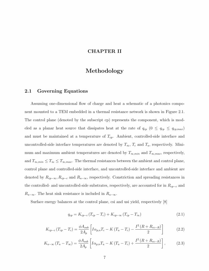
Assuming one-dimensional flow of charge and heat a schematic of a photonics compo-
nent mounted to a TEM embedded in a thermal resistance network is shown in Figure 2.1.
The control plane (denoted by the subscript cp) represents the component, which is mod-
eled as a planar heat source that dissipates heat at the rate of qcp (0 ≤ qcp ≤ qcp,max)
and must be maintained at a temperature of Tcp. Ambient, controlled-side interface and
uncontrolled-side interface temperatures are denoted by T∞, Tc and Tu, respectively. Mini-
mum and maximum ambient temperatures are denoted by T∞,min and T∞,max, respectively,
and T∞,min ≤ T∞ ≤ T∞,max. The thermal resistances between the ambient and control plane,
control plane and controlled-side interface, and uncontrolled-side interface and ambient are
denoted by Rcp−∞, Rcp−c and Ru−∞, respectively. Constriction and spreading resistances in
the controlled- and uncontrolled-side substrates, respectively, are accounted for in Rcp−c and
Ru−∞. The heat sink resistance is included in Ru−∞.
Surface energy balances at the control plane, csi and usi yield, respectively [8]
qcp = Kcp−c (Tcp − Tc) +Kcp−∞ (Tcp − T∞) (2.1)
Kcp−c (Tcp − Tc) =φAsub2Ap
[Iαp,nTc −K (Tu − Tc)−
I2 (R +Rec−R)
2
](2.2)
Ku−∞ (Tu − T∞) =φAsub2Ap
[Iαp,nTu −K (Tu − Tc) +
I2 (R +Rec−R)
2
], (2.3)
7
Figure 2.1: Schematic of a TEM embedded in a thermal resistance network.
where αp,n = αp−αn and thermal conductances (Ki−j) are the inverse of thermal resistances.
The pellet packing density(φ), bulk electrical resistance of a thermocouple (R), thermal
conductance of a thermocouple (K) and electrical contact resistance associated with the
four pellet-interconnect interfaces in a thermocouple (Rec−R) are, respectively
φ =2NApAsub
(2.4)
R =2ρH
Ap(2.5)
K =2kApH
(2.6)
Rec−R =4Rec−R
Ap, (2.7)
where ρ,H, k and AP are the electrical resistivity, height, thermal conductivity and cross-
sectional area of a pellet, respectively, and Rec−ρ is the electrical contact resistivity at the
8
interface between a pellet and an interconnect. Finally, Asub is the footprint of a TEM such
that φAsub is the total footprint of thermoelectric material.
Based on the definitions of φ, R, K and Rec−ρ and , the surface energy balances at the
csi and usi become, respectively,
Kcp−c (Tcp − Tc) = φAsub
[Φαp,nTc
2− k (Tu − Tc)
H− Φ2
(ρH
2+Rec−ρ
)](2.8)
Ku−∞ (Tu − T∞) = φAsub
[Φαp,nTu
2− k (Tu − Tc)
H+ Φ2
(ρH
2+Rec−ρ
)](2.9)
where the flux of current through the pellets (Φ) is
Φ =I
Ap. (2.10)
The electrical power consumed by a TEM, WTEM , is [8]
WTEM =φAsubΦ
2[αp,n (Tu − Tc) + Φ (2ρH + 4Rec−ρ)] . (2.11)
WTEM is positive when DC power is supplied to a TEM and negative when it operates in
generation mode.
Equations 2.8, 2.9 and 2.11 show that the current flux through the pellets in a TEM
is the relevant variable rather than the individual values of I and AP . Based on Eq. 2.1,
Eqs. 2.8 - 2.9 and Eq. 2.11, expressions for qcp and WTEM for a general case and a simplified
case are provided as follows. The Mathematica codes for these expressions are provided in
Appendix A.
2.1.1 Expressions for General Case
Tc and Tu are computed as a function of Φ, H and Ku−∞ from the csi and usi surface
energy balances (Eqs 2.8 and 2.9). Then, as per Eqs 2.1 and 2.11, expressions for qcp and
9
WTEM , respectively, which are independent of Tc and Tu are
qcp = Kcp−∞ (−T∞ + Tcp)−AsubKcp−cφ
[HΦ2 (2Rec−ρ +Hρ)
(2Ku−∞ − Asubαp,nφΦ)
+ 4k(Ku−∞T∞ + Asub (2Rec−ρ +Hρ)φΦ2
)− (4kKu−∞ +Hαp,nΦ (2Ku−∞ − Asubαp,nφΦ))Tcp] /
[4Asubk (Kcp−c +Ku−∞)φ
+ H (2Ku−∞ − Asubαp,nφΦ) (2Kcp−c + Asubαp,nφΦ)] (2.12)
WTEM = AsubφΦ [8Asubk (Kcp−c +Ku−∞)Rec−ρφΦ
+H2ρΦ (4Kcp−cKu−∞ − AsubKcp−cαp,nφΦ + AsubKu−∞αp,nφΦ)
+H(AsubKu−∞φΦ
(T∞α
2p,n + 4kρ+ 2Rec−ραp,nΦ
)+ 2Kcp−c(Ku−∞(T∞αp,n + 4Rec−ρΦ)
+ AsubφΦ (2kρ−Rec−ραp,nΦ)))
− HKcp−cαp,n (2Ku−∞ − Asubαp,nφΦ)Tcp] /
[4Asubk (Kcp−c +Ku−∞)φ
+ H (2Ku−∞ − Asubαp,nφΦ) (2Kcp−c + Asubαp,nφΦ)] . (2.13)
10
2.1.2 Expressions for Simplified Case
Assuming that Ku−∞ → ∞ implies that Tu = T∞. Then the surface energy balance at
the usi is unnecessary and qcp and WTEM are, respectively1
qcp = −2T∞ [HKcp−cKcp−∞ + Asubk (Kcp−c +Kcp−∞)φ]
+ AsubHKcp−∞T∞αp,nφΦ
+ AsubHKcp−cφΦ2 (2Rec−ρ +Hρ)
− [2HKcp−cKcp−∞ + 2Asubk (Kcp−c +Kcp−∞)φ
+ AsubH (Kcp−c +Kcp−∞)αp,nφΦ] /
(2HKcp−c + 2Asubkφ+ AsubHαp,nφΦ) (2.14)
WTEM = AsubφΦ [2HKcp−cT∞αp,n + (4HKcp−c (2Rec−ρ +Hρ)
+ Asub(8KRec−ρ +HT∞α
2p,n + 4Hkρ
)φ)
Φ
+ AsubHαp,n (2Rec−ρ + hρ)φΦ2 − 2HKcp−cαp,nTcp]/
(4HKcp−c + 4Asubkφ+ 2AsubHαp,nφΦ) (2.15)
2.2 Prescribed, Independent and Dependent Variables
The relevant properties of the pellets, i.e., ρ, k, αn (a negative quantity), αp (a positive
quantity assumed equal in magnitude to αn) and the electrical contact resistivity at the
interconnects in a TEM, Rec−ρ, are prescribed constants. Tcp, Kcp−∞, Kcp−c, and φAsub
are also prescribed constants.2 A range of ambient temperatures, subject to the constraint
that T∞,min ≤ T∞ ≤ T∞,max is specified. This constraint, a typical, albeit not universal,
condition for photonics components utilized in telecommunications circuit packs, implies
1These expressions are necessary to determine the permissible range of H and H2 and Hpe in the nextsection.
2The benefit of increasing φAsub is considered below.
11

that the optimal value of Ru−∞ = 0 when T∞ = T∞,max. It is noted that (T∞,max−Tcp) may
not exceed a maximum value as discussed below. A procedure to compute the minimum
value of Tcp and thus the maximum value of (T∞,max − Tcp) when all variables aside from
H are prescribed is given by Hodes [8]. (See Section V.A.2 of this reference). It should be
invoked for the limiting case when Ru−∞ = 0 and qcp = qcp,max. If the result is that T∞,max is
too large, the limiting case when Ru−∞ = 0 and qcp = 0 may be checked as this corresponds
to a TEM of infinite footprint. If the result is favorable then the required TEM footprint
should be computed. Otherwise, the problem at hand may not be accommodated by the
prescribed thermoelectric material properties and/or component-side thermal resistances.
Finally, qcp ranges from zero to a prescribed maximum value, qcp,max. However, total power
consumption Wt, that is (WTEM + qcp), decreases when qcp drops below qcp,max. Therefore,
only qcp,max need be considered in the algorithm as discussed in the next section.
Pellet height (H) and the thermal resistance between the uncontrolled-side interface and
ambient (Ru−∞) are the independent variables optimized to minimize the maximum total
power consumption (Wt). It is noted that qcp,max is a prescribed constant and minimizing
Wt is equivalent to minimizing WTEM .3 For the sake of generality we assume that H and
Ru−∞ may assume arbitrary values larger than 0. (The optimal H does not approach 0 in
practice. However, unless H is constrained to be a sub-optimal value, the optimal value of
Ru−∞ equals 0 and it should be made as low as possible.)
The current flux through a TEM (Φ), the controlled-side interface temperature (Tc) and
the uncontrolled-side interface temperature (Tu) are dependent variables that assume the
necessary values to maintain Tcp over the range of ambient temperatures and heat loads for
permissible combinations of H and Ru−∞. WTEM , itself a dependent variable, follows from
Eq. 2.11 once the other dependent variables have been computed. Recall, the objective here
is minimization of the maximum value of WTEM (or, equivalently, Wt) over all permissible
combinations of qcp and T∞. The corresponding value of WTEM or Wt is subsequently denoted
3The ordinate of (most of) the log-log plots below is Wt rather than WTEM . Otherwise, negative valuesof WTEM arising when generation mode is encountered may not be displayed.
12

by the subscript “ml” or “mg” as are the corresponding values of H and Ru−∞,ml or those of
Hmg and Ru−∞,mg. The subscripts “ml” and “mg” denote local minimums (at a prescribed
H) and global minimums (for all H), respectively. Permissible combinations of H and Ru−∞
are determined by the existence of an H and Ru−∞-dependent maximum (and positive) value
of the temperature difference between the ambient and the control plane as described above.
2.3 Analysis
2.3.1 The case when qcp = qcp,max
The range of permissible pellet heights (Hl ≤ H ≤ Hu) in a TEM is determined by
setting qcp = qcp,max and T∞ = T∞,max. At the minimum and maximum pellet heights, a
TEM operates in Peltier cooling mode as a refrigerator; therefore, the corresponding usi-to-
ambient thermal resistance equals zero. (Smaller values of Hl and larger values of Hu are
permitted when T∞ < T∞,max and/or qcp < qcp,max).
Hl and Hu are determined following the (numerical) procedure given by Hodes [8]. First,
differentiating the expression for qcp when Ru−∞ = 0 (Eq. 2.14) with respect to Φ and setting
the result equal to zero determines a numerical function for the current flux (Φmax (H))
which maximizes qcp as a function of H. The corresponding values of qcp are denoted by
qcp,TEM,max(H). Next, setting qcp,TEM,max (H) = qcp,max, Hl and Hu may be computed. The
maximum value of Ru−∞, for Hl ≤ H ≤ Hu is denoted by Ru−∞,max (H) and, moreover,
it is finite for Hl < H < Hu. It is determined by differentiating qcp with respect to Φ
and defining a numerical function Φmax (Ru−∞, H) as the corresponding root. Then, by
inserting this result into the expression for qcp and setting qcp = qcp,max, Ru−∞,max (H) may
be computed. Representative results are shown in Fig. 2.2. for conditions corresponding to
T∞,min and T∞,max. Smaller values of Ru−∞,max (H), are permissible when T∞ = T∞,max and
thus dictate the maximum value of Ru−∞,max for a given H.
When T∞ = T∞,max, qcp = qcp,max and Hl (T∞,max) ≤ H ≤ Hu (T∞,max), Wt corresponding
13

T∞, max
, qcp, max
T∞, min
, qcp, max
Impermissible Region
H
Hl(T
∞, max) H
u(T
∞, max)
0
Hu(T
∞, min)
Ru
-∞,
max
Figure 2.2: Ru−∞,max as a function of H at T∞,min and T∞,max.
T∞, max
, qcp, max
, Ru-∞, max
(T∞, max
)
T∞, min
, qcp, max
, Ru-∞, max
(T∞, max
)
T∞, max
, qcp, max
, Ru-∞
= 0
T∞, min
, qcp, max
, Ru-∞
= 0
Wt
H2
Hl(T
∞, max) H
u(T
∞, max)H
pe
H
H1
Hu(T
∞, min)
qcp,max
Region I Region II Region III
Figure 2.3: Wt as a function of H at T∞,min and T∞,max when Ru−∞ = 0 and Ru−∞,max.
14
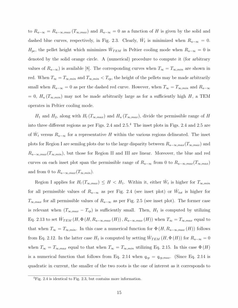
to Ru−∞ = Ru−∞,max (T∞,max) and Ru−∞ = 0 as a function of H is given by the solid and
dashed blue curves, respectively, in Fig. 2.3. Clearly, Wt is minimized when Ru−∞ = 0.
Hpe, the pellet height which minimizes WTEM in Peltier cooling mode when Ru−∞ = 0 is
denoted by the solid orange circle. A (numerical) procedure to compute it (for arbitrary
values of Ru−∞) is available [8]. The corresponding curves when T∞ = T∞,min are shown in
red. When T∞ = T∞,min and T∞,min < Tcp, the height of the pellets may be made arbitrarily
small when Ru−∞ = 0 as per the dashed red curve. However, when T∞ = T∞,min and Ru−∞
= 0, Hu (T∞,min) may not be made arbitrarily large as for a sufficiently high H, a TEM
operates in Peltier cooling mode.
H1 and H2, along with Hl (T∞,max) and Hu (T∞,max), divide the permissible range of H
into three different regions as per Figs. 2.4 and 2.5.4 The inset plots in Figs. 2.4 and 2.5 are
of Wt versus Ru−∞ for a representative H within the various regions delineated. The inset
plots for Region I are semilog plots due to the large disparity between Ru−∞,max(T∞,max) and
Ru−∞,max(T∞,min), but those for Region II and III are linear. Moreover, the blue and red
curves on each inset plot span the permissible range of Ru−∞ from 0 to Ru−∞,max(T∞,max)
and from 0 to Ru−∞,max(T∞,min).
Region I applies for Hl (T∞,max) ≤ H < H1. Within it, either Wt is higher for T∞,min
for all permissible values of Ru−∞ as per Fig. 2.4 (see inset plot) or Wtot is higher for
T∞,max for all permissible values of Ru−∞ as per Fig. 2.5 (see inset plot). The former case
is relevant when (T∞,max − Tcp) is sufficiently small. Then, H1 is computed by utilizing
Eq. 2.13 to set WTEM (H,Φ (H,Ru−∞,max (H)) , Ru−∞,max (H)) when T∞ = T∞,max equal to
that when T∞ = T∞,min. In this case a numerical function for Φ (H,Ru−∞,max (H)) follows
from Eq. 2.12. In the latter case H1 is computed by setting WTEM (H,Φ (H)) for Ru−∞ = 0
when T∞ = T∞,max equal to that when T∞ = T∞,min utilizing Eq. 2.15. In this case Φ (H)
is a numerical function that follows from Eq. 2.14 when qcp = qcp,max. (Since Eq. 2.14 is
quadratic in current, the smaller of the two roots is the one of interest as it corresponds to
4Fig. 2.4 is identical to Fig. 2.3, but contains more information.
15
a lower TEM power.)
T∞, max
, qcp, max
, Ru-∞, max
(T∞, max
)
T∞, min
, qcp, max
, Ru-∞, max
(T∞, max
)
T∞, max
, qcp, max
, Ru-∞
= 0
T∞, min
, qcp, max
, Ru-∞
= 0
Wt, ml
Wt
H2
Hl(T
∞, max) H
u(T
∞, max)H
pe
H
H1
Hu(T
∞, min)
qcp,max
T∞,max
T∞,min
Ru-∞
Ru-∞
Wt
Wt
Region I Region II Region III
Region I
Region II
qcp,max
T∞,max
T∞,min
Ru-∞
Wt
Region III
qcp,max
T∞,max
T∞,min
Figure 2.4: Wt and Wt,ml as a function of H at T∞,min and T∞,max when (T∞,max − Tcp) issmall when Ru−∞ = 0 and Ru−∞,max.
Region II applies for H1 < H < H2. The distinguishing feature of Region II is that
for sufficiently low Ru−∞, Wt is larger for when T∞ = T∞,min, but the converse is true for
sufficiently high Ru−∞ as per the inset plots in Figs. 2.4 and 2.5. H2 is computed by setting
WTEM (H,Φ (H) , T∞,min)=WTEM(H,Φ (H) , T∞,max) when Ru−∞ = 0 as per Eq. 2.15 and
selecting the larger root.5
Region III applies for H2 < H ≤ Hu (T∞,max). Within it, Wt is largest when T∞ = T∞,max
for all permissible values of Ru−∞ as per Figs. 2.4 and 2.5 (see inset plots). As H increases
beyond H2, less power is required at T∞,min and for sufficiently high H a TEM must operate
in generation mode. In practice this may be accomplished by applying a variable (electrical)
load resistance across the external leads of a TEM or with the necessary configuration of a
DC power supply. Beyond generation mode, Peltier cooling is required at T∞,min.
5When (T∞,max − Tcp) is sufficiently large, H1 and H2 are the smaller and larger roots, respectively, for
which WTEM (H,Φ (H) , T∞,min) = WTEM (H,Φ (H) , T∞,max) when Ru−∞ = 0 as per Fig. 2.5.
16
T∞, max
, qcp, max
, Ru-∞, max
(T∞, max
)
T∞, min
, qcp, max
, Ru-∞, max
(T∞, max
)
T∞, max
, qcp, max
, Ru-∞
= 0
T∞, min
, qcp, max
, Ru-∞
= 0
Wt, ml
H2
Hl(T
∞, max) H
u(T
∞, max)H
peH
u(T
∞, min)
Wt
qcp, max
H1
H
T∞,max
T∞,min T
∞,max
T∞,min
Ru-∞
Ru-∞
Wt
Wt
qcp,max
qcp,max
Wt
Ru-∞
Region I
Region I
Region II Region III
T∞,max
T∞,min
Region II
Region III
Figure 2.5: Wt and Wt,ml as a function of H at T∞,min and T∞,max when (T∞,max − Tcp) islarge when Ru−∞ = 0 and Ru−∞,max.
The minimum value of the maximum Wt as a function of H (Wt,ml) is indicated by the
(dashed) light blue curves in Figs. 2.4 and 2.5. In general, for a given H, Ru−∞ is set equal to
the value which minimizes the maximum value of Wt to plot this curve. The characteristics
of the inset plot of Wt versus Ru−∞ in Fig. 2.4 for Region I apply for sufficiently small
(T∞,max − Tcp). First, Wt is larger when T∞ = T∞,min than that when T∞ = T∞,max for all
permissible values of Ru−∞. Secondly, Wt when T∞ = T∞,min decreases monotonically with
Ru−∞. Therefore, the largest permissible value of Ru−∞, i.e., Ru−∞,max (H), equals Ru−∞,ml
and corresponds to Wt,mg, the local minimum of the maximum value of Wt. Analogously, the
characteristics of the inset plot of Wt versusRu−∞ in Fig. 2.5 for Region I apply for sufficiently
large (T∞,max − Tcp). First, Wt is larger when T∞ = T∞,max than when T∞ = T∞,min for
all permissible values of Ru−∞. Secondly, Wt increases monotonically with Ru−∞; therefore,
Ru−∞,ml = 0.
When H lies within Region II, i.e., H1 < H < H2, regardless of the value of (T∞,max−Tcp),
the optimal value of Ru−∞ (i.e., Ru−∞,ml) lies between 0 and Ru−∞,max (H). This may be
17
discerned from the inset plots in Figs. 2.4 and 2.5. They show that such an intermediate
value of Ru−∞ for which WTEM (H,Φ (H) , T∞,min) = WTEM (H,Φ (H) , T∞,max) corresponds
to Wt,ml. To compute Ru−∞,ml at a prescribed H, first qcp is set equal to qcp,max and Eq. 2.12 is
used to compute numerical functions for Φ (Ru−∞) when T∞ equals T∞,min and T∞,max. Then,
Eq. 2.15 is used to set WTEM (Φ (Ru−∞) , Ru−∞, T∞,min) = WTEM (Φ (Ru−∞) , Ru−∞, T∞,max)
and Ru−∞,ml is numerically computed. Finally, when H lies within Region III, i.e., H2 <
H ≤ Hu (T∞,max), Wtot is largest when T∞ = T∞,max; therefore Ru−∞,ml is 0.
Ideally, the designer of TEM-heat sink assemblies has the ability to select H in addition
to Ru−∞. Then, a global optimum must be found and the corresponding values of Ru−∞
and Wt are denoted by Ru−∞,mg and Wt,mg, respectively. When (T∞,max−Tcp) is sufficiently
small, Hmg = H2 and Ru−∞,mg = 0 represent this optimum as per Fig. 2.4. Otherwise, Ru−∞
remains 0, but Hmg = Hpe represent this optimum as per Fig. 2.5. In general, Hpe can be
smaller, equal to or larger than H2, but, unless they are equal the larger of the two along
with Ru−∞ = 0 represent the global optimum and this is the key result of the present work.
Since Hmg may equal H2 or Hpe, determining the optimum H is more difficult than when a
TEM operates exclusively in refrigeration mode and it equals Hpe a priori [8].
2.3.2 The case when qcp = 0
Total power consumption decreases when qcp decreases as described above. Comparisons
of Wt versus H for qcp = 0 and qcp = qcp,max are provided in Figs. 2.6 - 2.7 to illustrate this
point.
When T∞ = T∞,max, a TEM operates in refrigeration mode regardless of the value of qcp
as per Fig. 2.6. Therefore, reducing qcp reduces WTEM and thus Wtot for all H and Ru−∞.
The plot of Wt versus H for Hl ≤ H ≤ Hu illustrates this point. It is noted that the range
of H for qcp = 0 is larger than that for qcp = qcp,max.
The corresponding plot when T∞ = T∞,min rather than T∞ = T∞,max is shown in Fig. 2.7.
Wt is lower when qcp = 0 than when qcp = qcp,max for both Ru−∞= 0 and Ru−∞ = Ru−∞,max
18
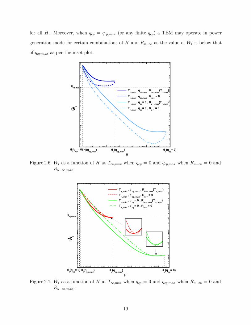
for all H. Moreover, when qcp = qcp,max (or any finite qcp) a TEM may operate in power
generation mode for certain combinations of H and Ru−∞ as the value of Wt is below that
of qcp,max as per the inset plot.
T∞,max
, qcp,max
, Ru-∞,max
(T∞,max
)
T∞,max
, qcp,max
, Ru-∞
= 0
T∞,max
, qcp
= 0 , Ru-∞,max
(T∞,max
)
T∞,max
, qcp
= 0 , Ru-∞
= 0
Hl(q
cp,max) H
u(q
cp,max)H
l(q
cp= 0) H
u(q
cp= 0)
Wt
H
qcp,max
Figure 2.6: Wt as a function of H at T∞,max when qcp = 0 and qcp,max when Ru−∞ = 0 andRu−∞,max.
T∞, min
, qcp, max
, Ru-∞, max
(T∞, max
)
T∞, min
, qcp, max
, Ru-∞
= 0
T∞, min
, qcp
= 0 , Ru-∞, max
(T∞, max
)
T∞, min
, qcp
= 0 , Ru-∞
= 0
Hl(q
cp,max) H
u(q
cp,max)H
l(q
cp= 0) H
u(q
cp= 0)
Wt
qcp,max
H
Figure 2.7: Wt as a function of H at T∞,min when qcp = 0 and qcp,max when Ru−∞ = 0 andRu−∞,max.
19
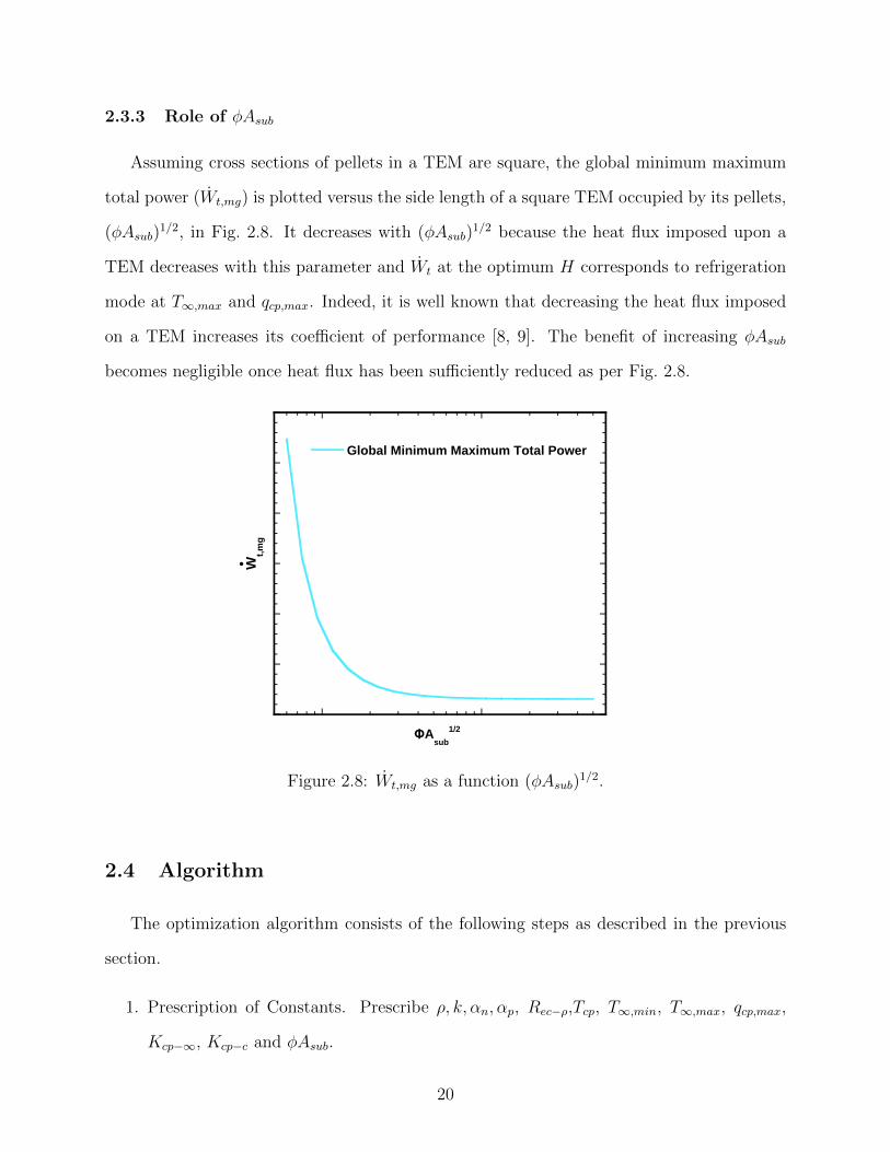
2.3.3 Role of φAsub
Assuming cross sections of pellets in a TEM are square, the global minimum maximum
total power (Wt,mg) is plotted versus the side length of a square TEM occupied by its pellets,
(φAsub)1/2, in Fig. 2.8. It decreases with (φAsub)
1/2 because the heat flux imposed upon a
TEM decreases with this parameter and Wt at the optimum H corresponds to refrigeration
mode at T∞,max and qcp,max. Indeed, it is well known that decreasing the heat flux imposed
on a TEM increases its coefficient of performance [8, 9]. The benefit of increasing φAsub
becomes negligible once heat flux has been sufficiently reduced as per Fig. 2.8.
Global Minimum Maximum Total Power
ΦAsub
1/2
Wt,
mg
Figure 2.8: Wt,mg as a function (φAsub)1/2.
2.4 Algorithm
The optimization algorithm consists of the following steps as described in the previous
section.
1. Prescription of Constants. Prescribe ρ, k, αn, αp, Rec−ρ,Tcp, T∞,min, T∞,max, qcp,max,
Kcp−∞, Kcp−c and φAsub.
20
2. Determine the permissible Range of H. Use the smallest range as determined by T∞,max
and qcp,max.
3. Compute Ru−∞,max (H). Use the smallest value at a given H as determined by T∞,max
and qcp,max.
4. Plot Wt versus H as in Figs. 2.4 and 2.5. Delineate Regions I-III in the permissible
range of H and whether H2, if it exists, or Hpe corresponds to the global optimal total
power.
5. Determining the Optimal Combination of H and Ru−∞. The larger of H2 or Hpe is the
global optimal (Hmg) along with Ru−∞ = 0 based on the plot in Step 4. If Step 4 is
skipped, both H2 and Hpe must be computed and compared to determine which one
corresponds to the global optimal total power (Wt,mg). However, it is suggested that
Wt versus H be plotted as per Step 4 rather than proceeding directly to Step 5. This is
because although Hpe or H2 has been shown to be the optimum value of H in all cases
considered in this thesis, proof that this is universally true for arbitrary combinations
of the prescribed constants is not obvious.
6. Plot Wt,mg versus (φAsub)1/2. If the value of (φAsub)
1/2 used in Steps 1-5 is below that
corresponding to saturation, increase it to one nearer saturation to the extent that
packaging constraints permit.
2.5 Dependence of TEM Operating Mode on T∞, H and Ru−∞
Dependent upon the values of T∞, H and Ru−∞, a TEM operates in one of 5 different
modes. Peltier cooling, Peltier heating and generation modes were defined above. Open
circuit and short circuit modes correspond to disconnected and shorted external leads of
a TEM.6 The uncontrolled-side to ambient thermal resistances corresponding to them are
6See Hodes [3] for further discussion on TEM operating modes, albeit using not an entirely consistent setof definitions.
21

denoted by Ru−∞,open (H) and Ru−∞,sh (H), respectively.
The case discussed here assumes T∞,min ≤ Tcp ≤ T∞,max. In Fig. 2.9, Ru−∞,open (H),
Ru−∞,sh (H) and Ru−∞,max are plotted versus H for T∞,min. When T∞ = T∞,min and for
sufficiently low H, as Ru−∞ is increased from 0 to Ru−∞,max (H) the operating modes tra-
versed are Peltier heating, open circuit, generation, short circuit and Peltier cooling modes,
successively.
Peltier heating is required when H and Ru−∞ are sufficiently low in order to maintain Tcp
above T∞,min as per the region under the blue curve in Fig. 2.9. When Ru−∞ = Ru−∞,open (H),
the conduction resistance of the TEM is precisely that required to maintain the component
at its operating temperature. When Ru−∞,open < Ru−∞ < Ru−∞,sh, a TEM must operate
in generation mode. Essentially as Ru−∞ increases from Ru−∞,open (H) to Ru−∞,sh (H) the
requisite electrical resistance of a load across a TEM decreases from∞ to 0. It is noted that
Peltier cooling occurs at the csi when a TEM operates in generation mode and, moreover, the
current and thus the rate of Peltier cooling increases as Ru−∞ increases from Ru−∞,open (H)
to Ru−∞,sh (H). Therefore, larger values of Ru−∞ may be accommodated as load resistance
decreases. When Ru−∞,sh < Ru−∞ ≤ Ru−∞,max, a TEM must operate in cooling mode to
overcome the insulative nature of the attached heat sink. Finally, when Ru−∞ > Ru−∞,max,
operation is impermissible as the insulation of the attached heat sink surpasses the Peltier
cooling ability of a TEM.
In the case of T∞,max, Ru−∞,open (H) and Ru−∞,sh (H) do not exist, and Ru−∞,max is
plotted versus H in Fig. 2.10. For an arbitrary H, a TEM operates in Peltier cooling mode
at T∞,max as T∞,max > Tcp. Note that, when H is sufficiently high, only cooling mode is
permissible regardless of the value of T∞ as per Figs. 2.9 and 2.10.
22

Ru-∞,max
at T∞,min
Ru-∞,open
at T∞,min
Ru-∞,sh
at T∞,min
Peltier Cooling Mode
Generation Mode
Peltier Heating Mode
Ru
-∞
H
Impermissible Region
Open Circuit Mode
Short Circuit Mode
Figure 2.9: Delineation of TEM operating modes as a function of H and Ru−∞ when T∞ =T∞,min < Tcp.
Ru-∞,max
at T∞,max
Peltier Cooling Mode
Impermissible Region
Ru
-∞
H0
Hl
Hu
Figure 2.10: Delineation of TEM operating modes as a function of H and Ru−∞ when T∞= T∞,min < Tcp.
23

24
CHAPTER III
Implementation of Algorithm
Examples are provided to illustrate the use of the optimization algorithm and its implica-
tions and the corresponding Mathematica codes are provided in Appendix B. Thermoelectric
material properties used are those typical of Bi2Te3-based TEMs operating near 300 K such
that the Seebeck coefficient of a thermocouple (αp,n) is 4.0 × 10⁻⁴ V/K, pellet thermal con-
ductivity (k) is 1.5 W/(mK) and pellet electrical resistivity (ρ) is 1.25 × 10⁻⁵ Ωm [10]. The
electrical contact resistivity at the interconnects (Rec−ρ) is 1 × 10⁻⁹ Ωm2, representative of a
typical TEM [11]. The footprint of the TEM (Asub) is 30 mm × 30 mm. The corresponding
total footprint of thermoelectric material in the TEM (φAsub) is 278.3 mm2.1 The maximum
rate of heat dissipation of the component mounted to the control plane is qcp,max = 10 W
and its operating temperature is Tcp = 55 C. The prescribed ambient temperature range
is T∞,min = -5 C ≤ T∞ ≤ T∞,max = 65 C. The conductance between the control plane
and csi (Kcp−c) is set equal to 17.17 W/C. This is based on a typical thermal contact resis-
tance between a component and TEM substrate with three-dimensional conduction through
an alumina substrate [8]. The conductance between the control plane and controlled-side
ambient (Kcp−∞) is set equal to 0.00015 W/C as the control plane is assumed to be well
insulated from the ambient. A list of the prescribed variables is provided in Table 3.1. In the
first set of calculations pellet height is assumed to equal 1 mm, a pellet height in Region II,
and usi-to-ambient thermal resistance is optimized. Then pellet height and usi-to-ambient
1The number of the thermocouples (N) affects the operating voltage and spreading/constriction resis-tances in the substrates; however, none of these paremeters are required to perform the optimization.
25

thermal resistance are simultaneously optimized. Finally, the effect of increasing φAsub is
considered.
Table 3.1: List of prescribed variables.
Prescribed Variables Prescribed Values
αp,n 4.0 × 10⁻⁴ V/K
k 1.5 W/(mK)
ρ 1.25 × 10⁻⁵ Ωm
Rec−ρ 1 × 10⁻⁹ Ωm2
Asub 30 mm × 30 mm
φAsub 278.3 mm2
qcp,max 10 W
Tcp 55 C
T∞,min -5 C
T∞,max 65 C
Kcp−c 17.17 W/C
Kcp−∞ 0.00015 W/C
3.1 Fixed Pellet Height
When H = 1 mm, TEM power is plotted versus the usi-to-ambient thermal resistance
(Ru−∞) when T∞ equals T∞,min and T∞,max, in Fig. 3.1.2 WTEM increases with Ru−∞ when
T∞ = T∞,max as the TEM operates in Peltier cooling mode. Ru−∞,max (T∞,max) = 1.07
C/W and Ru−∞ = 0 C/W minimizes WTEM when T∞ = T∞,max. When T∞ = T∞,min, the
TEM maintains the control plane temperature substantially (i.e., 60 C) above the ambient
temperature. Then Ru−∞,max (T∞,min) = 5.44 C/W as, the lower the ambient temperature,
the higher the value of Ru−∞,max. The permissible range of Ru−∞ is 0 C/W to 1.07 C/W,
which corresponds to Ru−∞,max when T∞ = 65 C. It is noted that when T∞ = -5 C, a
2TEM power (WTEM ) rather than total power (Wt) is plotted to clearly show the range of Ru−∞ forwhich the TEM operates in generation mode.
26

TEM operates in Peltier heating mode when 0 C/W ≤ Ru−∞ <3.65 C/W, in open circuit
mode at Ru−∞ = 3.65 C/W, in generation mode when 3.65 C/W < Ru−∞ < 4.68 C/W,
in short circuit mode at Ru−∞ = 4.68 C/W and in Peltier cooling mode when 4.68 C/W
< Ru−∞ ≤ 5.36 C/W. The minimum maximum value of WTEM occurs when Ru−∞ = 0.17
C/W as per Fig. 3.1 and corresponds to 4.25 W.
-5
0
5
10
15
20
25
0 1 2 3 4 5 6
T∞,max
= 65 °C
T∞,min
= -5 °C
WT
EM
[W]
Ru-∞
[°C/W]
-0.1
-0.05
0
0.05
0.1
3.62 3.99 4.35 4.71
Ru-∞,max
(65 °C) Ru-∞,max
(- 5°C)
Ru-∞,open
Ru-∞,sh
Figure 3.1: WTEM as a function of Ru−∞ (Tcp = 55 C).
3.2 Arbitrary Pellet Height
When H is not prescribed, Step 2 of the algorithm is followed to compute the permissible
range of H. The maximum heat rate that may be dissipated from the control plane is plotted
versus TEM pellet height when Ru−∞ = 0 and T∞ = T∞,max (blue curve) and T∞,min (red
curve) in Fig. 3.2. The horizontal dashed line corresponding to qcp,max = 10 W intersects the
Peltier cooling mode curve at Hl (T∞,max) and Hu (T∞,max). When H is within this range
(0.017 mm ≤ H ≤ 4.158 mm), the TEM may maintain Tcp = 55 C when qcp ≤ 10 W. Values
of H outside of this range are impermissible. It is noted that the permissible range of H
determined confirms that the initial pellet height of 1 mm used above is a valid one.
27
0
200
400
600
800
10-2
10-1
100
101
T∞,max
= 65°C
T∞,min
= -5°C
qcp
= 10W
qcp
,TE
M,m
ax
[W]
H [mm]
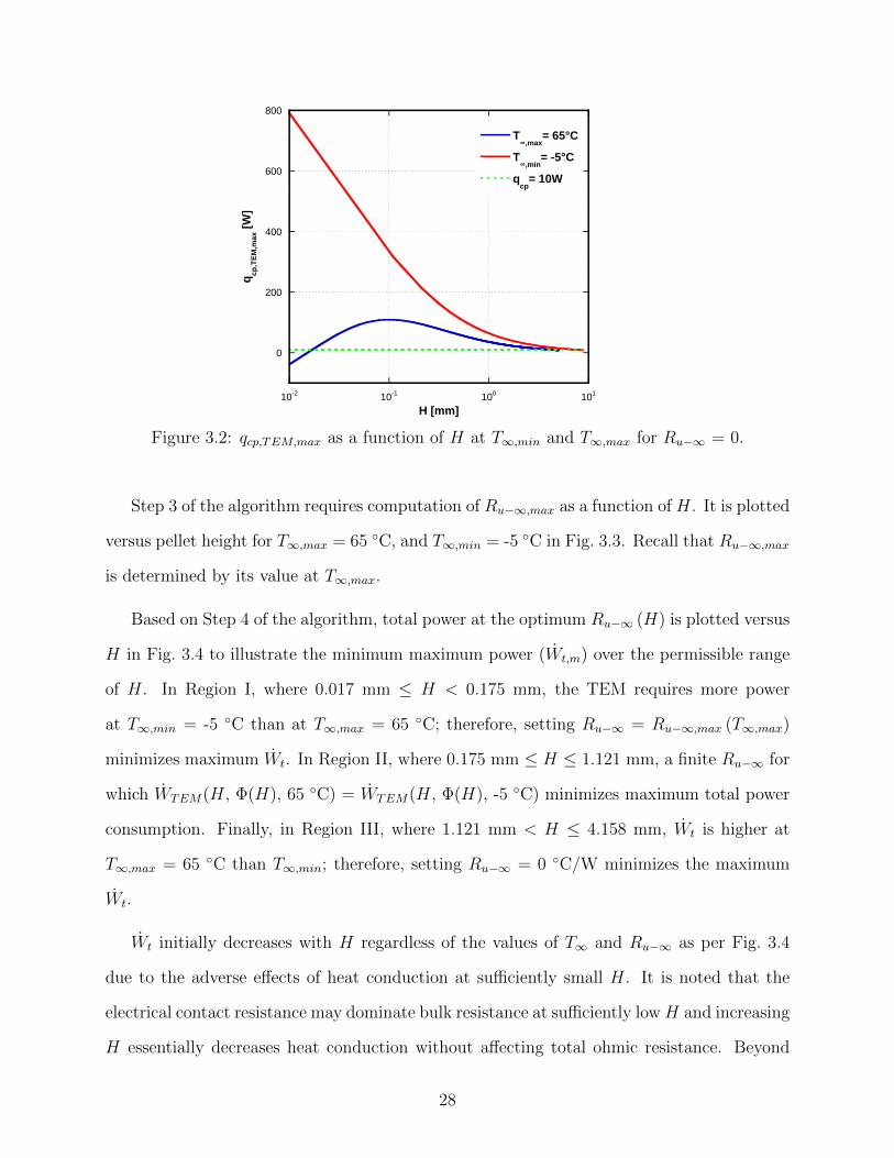
Figure 3.2: qcp,TEM,max as a function of H at T∞,min and T∞,max for Ru−∞ = 0.
Step 3 of the algorithm requires computation of Ru−∞,max as a function of H. It is plotted
versus pellet height for T∞,max = 65 C, and T∞,min = -5 C in Fig. 3.3. Recall that Ru−∞,max
is determined by its value at T∞,max.
Based on Step 4 of the algorithm, total power at the optimum Ru−∞ (H) is plotted versus
H in Fig. 3.4 to illustrate the minimum maximum power (Wt,m) over the permissible range
of H. In Region I, where 0.017 mm ≤ H < 0.175 mm, the TEM requires more power
at T∞,min = -5 C than at T∞,max = 65 C; therefore, setting Ru−∞ = Ru−∞,max (T∞,max)
minimizes maximum Wt. In Region II, where 0.175 mm ≤ H ≤ 1.121 mm, a finite Ru−∞ for
which WTEM(H, Φ(H), 65 C) = WTEM(H, Φ(H), -5 C) minimizes maximum total power
consumption. Finally, in Region III, where 1.121 mm < H ≤ 4.158 mm, Wt is higher at
T∞,max = 65 C than T∞,min; therefore, setting Ru−∞ = 0 C/W minimizes the maximum
Wt.
Wt initially decreases with H regardless of the values of T∞ and Ru−∞ as per Fig. 3.4
due to the adverse effects of heat conduction at sufficiently small H. It is noted that the
electrical contact resistance may dominate bulk resistance at sufficiently lowH and increasing
H essentially decreases heat conduction without affecting total ohmic resistance. Beyond
28

0
1
2
3
4
5
6
7
10-3
10-2
10-1
100
101
T∞,max
= 65 °C
T∞,min
= - 5 °C
Ru
-∞,m
ax
[°C
/W]
H [mm]
Figure 3.3: Ru−∞,max as a function H at T∞,min and T∞,max.
10
100
1000
T∞,max
= 65°C , qcp
= 10W , Ru-∞,max
(65°C)
T∞,min
= - 5°C , qcp
= 10W , Ru-∞,max
(65°C)
T∞,max
= 65°C , qcp
= 10W , Ru-∞
= 0
T∞,min
= - 5°C , qcp
= 10W , Ru-∞
= 0
Wt,ml
H [mm]
Wt[W
]
1.1210.017 0.6590.175 7.1604.158
Region I Region II Region III
Figure 3.4: Wt and Wt,ml as a function of H at Tcp = 55 C when Ru−∞ = 0 and Ru−∞,max.
Hpe (0.659 mm) Wt increases with H when qcp = qcp,max (10 W) and T∞ = T∞,max(65 C).
However, increasing H from Hpe to H2 (1.121 mm) is of benefit because of the accompanying
reduction in Wt when T∞ = T∞,min despite the increase in Wt when T∞ = T∞,max. The global
minimum maximum total power (Wt,mg = 13.75 W) occurs at H = 1.121 mm and Ru−∞ =
0 C/W. Typical TEM heights are between 1 mm and 3 mm and when Ru−∞ is optimized
29
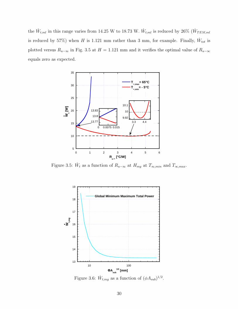
the Wt,ml in this range varies from 14.25 W to 18.73 W. Wt,ml is reduced by 26% (WTEM,ml
is reduced by 57%) when H is 1.121 mm rather than 3 mm, for example. Finally, Wtot is
plotted versus Ru−∞ in Fig. 3.5 at H = 1.121 mm and it verifies the optimal value of Ru−∞
equals zero as expected.
5
10
15
20
25
30
35
0 1 2 3 4 5 6
T∞,max
= 65°C
T∞,min
= - 5°C
Wt[W
]
Ru-∞
[°C/W]
13.77
13.8
13.83
0 0.0075 0.015
9.92
10
10.1
3.3 4.4
Figure 3.5: Wt as a function of Ru−∞ at Hmg at T∞,min and T∞,max.
Global Minimum Maximum Total Power
13
14
15
16
17
18
19
10 100
ΦAsub
1/2[mm]
Wt,
mg
Figure 3.6: Wt,mg as a function of (φAsub)1/2.
30

Wt,mg versus (φAsub)1/2 is plotted in Fig. 3.6. Wt,mg may be reduced to 13.3 W for
sufficiently high (φAsub)1/2. In practice, the footprint of a TEM is constrained to about 50
mm x 50 mm, but arbitrarily large footprint arrays of them may be used. However, the “real
estate” in optoelectronics circuit packs is limited and thus φAsub is too.
31

32
CHAPTER IV
Conclusion and Future Work
An algorithm to find the unique value of pellet height and uncontrolled-side interface to
ambient thermal resistance to minimize maximum total power utilized for precision tempera-
ture control of photonics components has been provided. This algorithm is confined to steady
state conditions and assumes that the total power consumption during transients does not
exceed the maximum one predicted by this algorithm because of the thermal capacitance of
the system. However, further investigation on transient phenomena is required to verify this.
Prescribed paremeters are total footprint of thermoelectric material, thermoelectric material
properties, heat load, component operating temperature, relevant component-side thermal
resistances and ambient temperature range. “Blindly” choosing an off-the-shelf TEM for a
particular precision temperature control problem may henceforth be avoided. The algorithm
has been invoked to show through example calculations the benefit of the optimization.
It was shown that considerable power savings can be achieved, a significant result for op-
toelectronics circuit packs in telecommunications hardware with specified power budgets.
Moreover, additional power savings can be accomplished by varying the total footprint of
thermoelectric material. The physics of the algorithm have been interpreted in the context
of TEM operating modes.
Although the results presented here have demonstrated that implementation of the algo-
rithm provided in this thesis maximizes the fraction of the power budget in an optoelectronics
circuit pack available for other uses, experimental verification of the algorithm is suggested.
Because precise temperature measurement is very important in such experiments, the first
33

step in the future work is calibrating the thermocouples. An apparatus and a procedure to
calibrate thermocouples with a high accuracy is provided in Appendix C.
34

BIBLIOGRAPHY
[1] M. Hodes. Thermoelectric Modules: Principles and Research. Notes from short coursepresented at ITHERM 2010, Las Vegas, NV.
[2] C. L. Foiles. Thermoelectric effects. New York: McGraw-Hill, 2nd edition, 2005.
[3] M. Hodes. On one-dimensional anaysis of thermoelectric modules(TEMs). IEEE Tran.Compon. Packag. TEchnol., 28(2):218–229, 2005.
[4] M. Hodes. Precision temperature control of an optical router. New York: McGraw-Hill,2005.
[5] C. Melnick, M. Hodes, G. Ziskind, M. Cleary, and V. P. Manno. Thermoelectric module-variable conductance heat pipe assemblies for reduced power temperature control. IEEETran. Compon. Packag. TEchnol., 2010. to appear.
[6] Temperature Control of Thermooptic Devices, 2007.
[7] R. Wilcoxon, N. Lower, and D. Dlouhy. A compliant thermal spreader with internalliquid metal cooling channels. In in Proc. 25th IEEE SEMI-THERM Symposium, SantaClara, CA, February 2010.
[8] M. Hodes. Optimal design of thermoelectric refrigerators embedded in a thermal resis-tance network. IEEE Tran. Compon. Packag. Technol., 2011. to appear.
[9] M. Hodes. Optimal pellet geometries for thermoelectric refrigeration. IEEE Tran.Compon. Packag. Technol., 30(1), 2007.
[10] Melcor thermal solutions, 2002.
[11] L. W. da Silva and M. Kaviany. Micro-thermoelectric cooler: Interfacial effects onthermal and electrical transport. Int. J. Heat Mass Tran., 47, 2004.
[12] National Institute of Standards, Technology (US), C. Croarkin, P. Tobias, C. Zey, andInternational SEMATECH. Engineering statistics handbook. The Institute, 2001.
[13] American Society for Testing and Materials. Annual book of astm standards. AmericanSociety for Testing and Materials, 1992.
[14] JV Nicholas and D.R. White. Traceable temperatures: an introduction to temperaturemeasurement and calibration. John Wiley & Sons Inc, 2001.
35
[15] Hart Scientific. A fluke company catalog., 2010.
[16] Hart Scientific. Black Stack 1560 Thermometer Readout User’s Guide., 2010.
[17] Keithley Instruments Inc. Models 2182 and 2182A Nanovoltmeter User’s Manual., 2004.
[18] Keithley Instruments Inc. Model 7001 Switch System Instruction Manual Rev. H, 1991.
[19] Keithley Instruments Inc. Models 7011-S and 7011-C Instruction Manual, 1991.
[20] G.W. Burns, MG Scroger, GF Strouse, MC Croarkin, and WF Guthrie. Temperature-electromotive force reference functions and tables for the letter-designated thermocoupletypes based on the its-90. NASA STI/Recon Technical Report N, 93:31214, 1993.
36

APPENDIX A
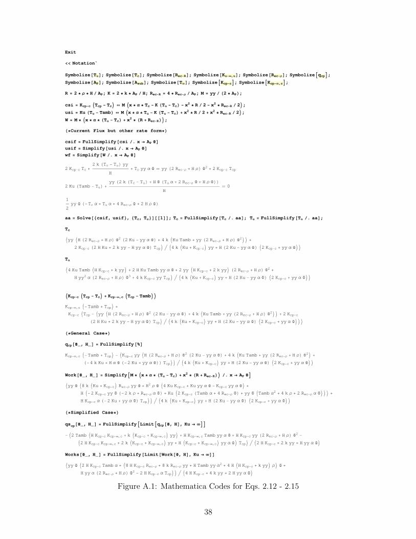
Mathematica Codes for Eqs. 2.12 - 2.15
Mathematica Codes for Eqs. 2.12 - 2.15
37
Exit
<< Notation`
Symbolize@TuD; Symbolize@TcD; Symbolize@Rec-RD; Symbolize@Ku-¥,uD; Symbolize@Rec-ΡD; SymbolizeAqcpE;Symbolize@APD; Symbolize@AsubD; Symbolize@T¥D; SymbolizeAKcp-cE; SymbolizeAKcp-¥,cE;
R = 2 * Ρ * H AP; K = 2 * k * AP H; Rec-R = 4 * Rec-Ρ AP; M = yy H2 * APL;
csi = Kcp-c ITcp - TcM M Ix * Α * Tc - K HTu - TcL - x2 * R 2 - x2 * Rec-R 2M;usi = Ku HTu - TambL M Ix * Α * Tu - K HTu - TcL + x2 * R 2 + x2 * Rec-R 2M;W = M * Ix * Α * HTu - TcL + x2 * HR + Rec-RLM;
H*Current Flux but other rate form*L
csif = FullSimplify@csi . x ® AP FDusif = Simplify@usi . x ® AP FDwf = Simplify@W . x ® AP FD
2 Kcp-c Tc +2 k HTc - TuL yy
H+ Tc yy Α F yy H2 Rec-Ρ + H ΡL F
2+ 2 Kcp-c Tcp
2 Ku HTamb - TuL +yy H2 k HTc - TuL + H F HTu Α + 2 Rec-Ρ F + H Ρ FLL
H 0
1
2yy F H-Tc Α + Tu Α + 4 Rec-Ρ F + 2 H Ρ FL
aa = Solve@8csif, usif<, 8Tc, Tu<D@@1DD; Tc = FullSimplify@Tc . aaD; Tu = FullSimplify@Tu . aaD;
Tc
Iyy IH H2 Rec-Ρ + H ΡL F2 H2 Ku - yy Α FL + 4 k IKu Tamb + yy H2 Rec-Ρ + H ΡL F
2MM +
2 Kcp-c H2 H Ku + 2 k yy - H yy Α FL TcpM I4 k IKu + Kcp-cM yy + H H2 Ku - yy Α FL I2 Kcp-c + yy Α FMM
Tu
I4 Ku Tamb IH Kcp-c + k yyM + 2 H Ku Tamb yy Α F + 2 yy IH Kcp-c + 2 k yyM H2 Rec-Ρ + H ΡL F2
+
H yy2 Α H2 Rec-Ρ + H ΡL F3
+ 4 k Kcp-c yy TcpM I4 k IKu + Kcp-cM yy + H H2 Ku - yy Α FL I2 Kcp-c + yy Α FMM
IKcp-c ITcp - TcM + Kcp-¥,c ITcp - TambMM
Kcp-¥,c I-Tamb + TcpM +
Kcp-c ITcp - Iyy IH H2 Rec-Ρ + H ΡL F2 H2 Ku - yy Α FL + 4 k IKu Tamb + yy H2 Rec-Ρ + H ΡL F
2MM + 2 Kcp-c
H2 H Ku + 2 k yy - H yy Α FL TcpM I4 k IKu + Kcp-cM yy + H H2 Ku - yy Α FL I2 Kcp-c + yy Α FMMM
H*General Case*L
qcp@F_, H_D = FullSimplify@%D
Kcp-¥,c I-Tamb + TcpM - IKcp-c yy IH H2 Rec-Ρ + H ΡL F2 H2 Ku - yy Α FL + 4 k IKu Tamb + yy H2 Rec-Ρ + H ΡL F
2M +
H-4 k Ku + H Α F H-2 Ku + yy Α FLL TcpMM I4 k IKu + Kcp-cM yy + H H2 Ku - yy Α FL I2 Kcp-c + yy Α FMM
Work@F_, H_D = SimplifyAM * Ix * Α * HTu - TcL + x2 * HR + Rec-RLM . x ® AP FE
Iyy F I8 k IKu + Kcp-cM Rec-Ρ yy F + H2 Ρ F I4 Ku Kcp-c + Ku yy Α F - Kcp-c yy Α FM +
H I-2 Kcp-c yy F H-2 k Ρ + Rec-Ρ Α FL + Ku I2 Kcp-c HTamb Α + 4 Rec-Ρ FL + yy F ITamb Α2
+ 4 k Ρ + 2 Rec-Ρ Α FMMM +
H Kcp-c Α H-2 Ku + yy Α FL TcpMM I4 k IKu + Kcp-cM yy + H H2 Ku - yy Α FL I2 Kcp-c + yy Α FMM
H*Simplified Case*L
qscp@F_, H_D = FullSimplifyALimitAqcp@F, HD, Ku ® ¥EE
-I2 Tamb IH Kcp-c Kcp-¥,c + k IKcp-c + Kcp-¥,cM yyM + H Kcp-¥,c Tamb yy Α F + H Kcp-c yy H2 Rec-Ρ + H ΡL F2
-
I2 H Kcp-c Kcp-¥,c + 2 k IKcp-c + Kcp-¥,cM yy + H IKcp-c + Kcp-¥,cM yy Α FM TcpM I2 H Kcp-c + 2 k yy + H yy Α FM
Works@F_, H_D = FullSimplify@Limit@Work@F, HD, Ku ® ¥DD
Iyy F I2 H Kcp-c Tamb Α + I8 H Kcp-c Rec-Ρ + 8 k Rec-Ρ yy + H Tamb yy Α2
+ 4 H IH Kcp-c + k yyM ΡM F +
H yy Α H2 Rec-Ρ + H ΡL F2
- 2 H Kcp-c Α TcpMM I4 H Kcp-c + 4 k yy + 2 H yy Α FM
Figure A.1: Mathematica Codes for Eqs. 2.12 - 2.15
38

APPENDIX B
Mathematica Codes for Example Calculation
Calculation Part 1
39
Û¨·¬
ää Ò±¬¿¬·±²À
ͧ³¾±´·¦» Ì« å ͧ³¾±´·¦» ̽ å ͧ³¾±´·¦» λ½óÎ å ͧ³¾±´·¦» Õ«óô« å ͧ³¾±´·¦» λ½ó® å ͧ³¾±´·¦» ¯½° å
ͧ³¾±´·¦» ßÐ å ͧ³¾±´·¦» ß«¾ å ͧ³¾±´·¦» Ì å ͧ³¾±´·¦» Õ½°ó½ å ͧ³¾±´·¦» Õ½°óô½ å
¯ ÚÁáÒ«³»®·½Ïô Õ«Á áÒ«³»®·½Ïô Ì¿³¾Á áÒ«³»®·½Ïô ØÁ áÒ«³»®·½Ï ã
Õ½°óô½ óÌ¿³¾ õ ̽° ó Õ½°ó½ §§ Ø î λ½ó® õ Ø ® Úî î Õ« ó §§ ¿ Ú õ ì µ Õ« Ì¿³¾ õ §§ î λ½ó® õ Ø ® Úî õ
óì µ Õ« õ Ø ¿ Ú óî Õ« õ §§ ¿ Ú Ì½° ì µ Õ« õ Õ½°ó½ §§ õ Ø î Õ« ó §§ ¿ Ú î Õ½°ó½ õ §§ ¿ Ú å
ɱ®µ ÚÁáÒ«³»®·½Ïô Õ«Á áÒ«³»®·½Ïô Ì¿³¾Á áÒ«³»®·½Ïô ØÁ áÒ«³»®·½Ï ã
§§ Ú è µ Õ« õ Õ½°ó½ λ½ó® §§ Ú õ Øî ® Ú ì Õ« Õ½°ó½ õ Õ« §§ ¿ Ú ó Õ½°ó½ §§ ¿ Ú õ
Ø óî Õ½°ó½ §§ Ú óî µ ® õ λ½ó® ¿ Ú õ Õ« î Õ½°ó½ Ì¿³¾ ¿ õ ì λ½ó® Ú õ §§ Ú Ì¿³¾ ¿î õ ì µ ® õ î λ½ó® ¿ Ú õ
Ø Õ½°ó½ ¿ óî Õ« õ §§ ¿ Ú Ì½° ì µ Õ« õ Õ½°ó½ §§ õ Ø î Õ« ó §§ ¿ Ú î Õ½°ó½ õ §§ ¿ Ú å
¯ ÚÁáÒ«³»®·½Ïô Ì¿³¾Á áÒ«³»®·½Ïô ØÁáÒ«³»®·½Ï ã
ó î Ì¿³¾ Ø Õ½°ó½ Õ½°óô½ õ µ Õ½°ó½ õ Õ½°óô½ §§ õ Ø Õ½°óô½ Ì¿³¾ §§ ¿ Ú õ Ø Õ½°ó½ §§ î λ½ó® õ Ø ® Úî ó
î Ø Õ½°ó½ Õ½°óô½ õ î µ Õ½°ó½ õ Õ½°óô½ §§ õ Ø Õ½°ó½ õ Õ½°óô½ §§ ¿ Ú Ì½° î Ø Õ½°ó½ õ î µ §§ õ Ø §§ ¿ Ú å
ɱ®µ ÚÁáÒ«³»®·½Ïô Ì¿³¾Á áÒ«³»®·½Ïô ØÁáÒ«³»®·½Ï ã
§§ Ú î Ø Õ½°ó½ Ì¿³¾ ¿ õ è Ø Õ½°ó½ λ½ó® õ è µ λ½ó® §§ õ Ø Ì¿³¾ §§ ¿î õ ì Ø Ø Õ½°ó½ õ µ §§ ® Ú õ
Ø §§ ¿ î λ½ó® õ Ø ® Úî ó î Ø Õ½°ó½ ¿ ̽° ì Ø Õ½°ó½ õ ì µ §§ õ î Ø §§ ¿ Ú å
̽° ã îéíòïë õ ëëå ¿ ã ðòðððìå
µ ã ïòëå ® ã ðòððððïîëå
ß° ã ïòçê ö ïðóêå
Õ½°ó½ ã ïéòïéå
Ò¬»³ ã éïå
ν»® ã ðòðíçå ι®» ã îòëè ö ïðóëå
λ½ó® ã ï ö ïðóçå
¬ ã ðòððëå µ½ ã ðòðíå Õ½°óô½ ã ðòðððïëå §§ ã îéèòí ö ïðóêå
䱬 ¯ Úô ííèòïëô ðòððï ô Úô ïðð ðððô ïð ððð ððð
î l ïðê ì l ïðê ê l ïðê è l ïðê ï l ïðé
óîð
óïð
ïð
îð
íð
öÚ×ÒÜ ÌØÛ ÎßÒÙÛ ÑÚ Ø ÚÑÎ Ìô³¿¨ö
¾¾ æã ÒÓ¿¨·³·¦» ¯ Úô ííèòïëô Ø ô Úô Ó»¬¸±¼ r þÒ»´¼»®Ó»¿¼þô
ß½½«®¿½§Ù±¿´ r êô Ю»½··±²Ù±¿´ r ô ɱ®µ·²¹Ð®»½··±² r è
½½ ØÁλ¿´ æã ¾¾ ï ö¯½°ô³¿¨ö
Figure B.1: Calculation Part1 - Page 1
40

䱬 ½½ Ø ô Øô ðòððððïô ðòððï
ðòðððî ðòðððì ðòðððê ðòðððè ðòððïð
óìð
óîð
îð
ìð
êð
èð
ïðð
Ю·²¬ þͬ»° ïæ Ú×ÒÜ ÌØÛ ÎßÒÙÛ ÑÚ Øþ
ͬ»° ïæ Ú×ÒÜ ÌØÛ ÎßÒÙÛ ÑÚ Ø
ö¯½°ãïðÉ Ú·²¼ Ø´ ¿²¼ Ø«ö
Ú·²¼Î±±¬ ½½ Ø ïðô Øô ðòðððî öØ« ¿¬ ¯½° ã ïðÉö
Ø r ðòððìïëèìê
Ú·²¼Î±±¬ ½½ Ø ïðô Øô ðòððððï öØ´ ¿¬ ¯½° ã ïðÉö
Ø r ðòððððïêççìé
ö¯½°ã ðÉ Ú·²¼ Ø´ ¿²¼ Ø«ö
Ú·²¼Î±±¬ ½½ Ø ðô Øô ðòðððî öØ« ¿¬ ¯½° ã ðÉö
Ø r îçòïèîé
Ú·²¼Î±±¬ ½½ Ø ðô Øô ðòððððï öØ´ ¿¬ ¯½° ã ðÉö
Ø r ðòððððïëîëèë
öÚ×ÒÜ ÌØÛ ÎßÒÙÛ ÑÚ Ø ÚÑÎ Ìô³·²ö
¾¾ æã ÒÓ¿¨·³·¦» ¯ Úô îêèòïëô Ø ô Úô Ó»¬¸±¼ r þÒ»´¼»®Ó»¿¼þô
ß½½«®¿½§Ù±¿´ r êô Ю»½··±²Ù±¿´ r ô ɱ®µ·²¹Ð®»½··±² r è
½½ ØÁλ¿´ æã ¾¾ ï ö¯½°ô³¿¨ö
䱬 ½½ Ø ô Øô ðòððððïô ðòððï
ðòðððî ðòðððì ðòðððê ðòðððè ðòððïð
ïëð
îðð
îëð
íðð
íëð
ìðð
ö¯½°ãïðÉ Ú·²¼ Ø´ ¿²¼ Ø«ö
Ú·²¼Î±±¬ ½½ Ø ïðô Øô ðòðððî öØ« ¿¬ ¯½° ã ïðÉö
Ø r ðòððéïêðíî
2 New calculation.nb
Figure B.2: Calculation Part1 - Page 2
41
Ю·²¬ þͬ»° îæ Ú×ÒÜ Øî ¿²¼ Ø°»þ
ͬ»° îæ Ú×ÒÜ Øî ¿²¼ Ø°»
¬¬ï æã Ú·²¼Î±±¬ ¯ Úô ííèòïëô Ø ïð ô Úô î ððð ðððô ïð ðððô ëð ððð ððð ô
ß½½«®¿½§Ù±¿´ r îô Ю»½··±²Ù±¿´ r ô Ó¿¨×¬»®¿¬·±² r ïðð å
Úêë æã Ú ò ¬¬ïå
¬¬î æã Ú·²¼Î±±¬ ¯ Úô îêèòïëô Ø ïð ô Úô óï ððð ðððô óçðð ððð ðððô ð ô
ß½½«®¿½§Ù±¿´ r îô Ю»½··±²Ù±¿´ r ô Ó¿¨×¬»®¿¬·±² r ïðð å
Ú²ë æã
Ú ò
¬¬îå
Éêë ØÁλ¿´ æã ɱ®µ Úêëô ííèòïëô Ø å
ÉÒë ØÁλ¿´ æã ɱ®µ Ú²ëô îêèòïëô Ø å
䱬 ɱ®µ Úêëô ííèòïëô Ø ô ɱ®µ Ú²ëô îêèòïëô Ø ô Øô ðòðððïô ðòððî
ðòððïð ðòððïë ðòððîð
ë
ïð
ïë
ººï ã Ú·²¼Î±±¬ Éêë Ø ÉÒë Ø ô Øô ðòððïëèô ðòððïô ðòððî ô
Ó¿¨×¬»®¿¬·±² r ïððô ß½½«®¿½§Ù±¿´ r ïðô Ю»½··±²Ù±¿´ r
Ø r ðòððïïîïî
¬¬ ã ÒÓ·²·³·¦» Éêë Ø ô ðòðððï ä Ø ä ðòððï ô Ø
íòíçêîéô Ø r ðòðððêëèéïë
¬¬ïð æã Ú·²¼Î±±¬ ¯ Úô ííèòïëô Ø ð ô Úô ïðð ðððô ïðððô ëðð ððð ô
ß½½«®¿½§Ù±¿´ r îô Ю»½··±²Ù±¿´ r ô Ó¿¨×¬»®¿¬·±² r ïðð å
Úêëð æã Ú ò ¬¬ïðå
¬¬îð æã Ú·²¼Î±±¬ ¯ Úô îêèòïëô Ø ð ô Úô óï ððð ðððô óçðð ððð ðððô ð ô
ß½½«®¿½§Ù±¿´ r îô Ю»½··±²Ù±¿´ r ô Ó¿¨×¬»®¿¬·±² r ïðð å
Ú²ëð æã
Ú ò
¬¬îðå
Éêëð ØÁλ¿´ æã ɱ®µ Úêëðô ííèòïëô Ø å
ÉÒëð ØÁλ¿´ æã ɱ®µ Ú²ëðô îêèòïëô Ø å
䱬 ¯ Úô ííèòïëô ðòðððï ô Úô ïð ðððô ïð ðððô ë ððð ððð
ï l ïðê î l ïðê í l ïðê ì l ïðê ë l ïðê
óíð
óîð
óïð
ïð
îð
íð
New calculation.nb 3
Figure B.3: Calculation Part1 - Page 3
42
䱬 ɱ®µ Úêëðô ííèòïëô Ø ô ɱ®µ Ú²ëðô îêèòïëô Ø ô Øô ðòððððïêô ðòðï
ðòððî ðòððì ðòððê ðòððè ðòðïð
ï
î
í
ì
ë
Ю·²¬ þØî ¿²¼ Ø°» ¼±» ²±¬ »¨·¬þ
Ю·²¬ þͬ»° îæ Ú×ÒÜ ÌØÛ ÎßÒÙÛ ÑÚ Î«óô« ßÒÜ ÌÛÓ ÐÑÉÛÎ ßÌ Î«óô³¿¨þ
ͬ»° îæ Ú×ÒÜ ÌØÛ ÎßÒÙÛ ÑÚ Î«óô«
¼¼ Õ«Áλ¿´ô Ì¿³¾Áλ¿´ô ØÁλ¿´ æã ÒÓ¿¨·³·¦» ¯ Úô Õ«ô Ì¿³¾ô Ø ô Úô
Ó»¬¸±¼ r þÒ»´¼»®Ó»¿¼þô ß½½«®¿½§Ù±¿´ r êô Ю»½··±²Ù±¿´ r ô ɱ®µ·²¹Ð®»½··±² r è
ºº Õ«Áλ¿´ô Ì¿³¾Áλ¿´ô ØÁλ¿´ æã ¼¼ Õ«ô Ì¿³¾ô Ø îô ïô î ö¯½°ô³¿¨ö
¯³¿¨ Õ«Áλ¿´ô Ì¿³¾Áλ¿´ô ØÁλ¿´ æã ¯ ºº Õ«ô Ì¿³¾ô Ø ô Õ«ô Ì¿³¾ô Ø å
»» Ì¿³¾Áλ¿´ô ØÁλ¿´ æã
Ú·²¼Î±±¬ ï𠯳¿¨ Õ«ô Ì¿³¾ô Ø ô Õ«ô îë ô Ó»¬¸±¼ r þÒ»©¬±²þô ß½½«®¿½§Ù±¿´ r ïô
Ю»½··±²Ù±¿´ r ô ɱ®µ·²¹Ð®»½··±² r ïðô Ó¿¨×¬»®¿¬·±² r ïðð öÚ·²¼ Õ«óô³·² ¬¸¿¬ · Ϋóô³¿¨ö
¬¬ï æã Ú·²¼Î±±¬ ¯ Úô Õ«ô ííèòïëô Ø ïð ô Úô ï ððð ðððô ï ððð ðððô ëð ððð ððð ô
ß½½«®¿½§Ù±¿´ r îô Ю»½··±²Ù±¿´ r ô Ó¿¨×¬»®¿¬·±² r ïðð å
Úêë æã Ú ò ¬¬ïå
¬¬î æã Ú·²¼Î±±¬ ¯ Úô Õ«ô îêèòïëô Ø ïð ô Úô óìð ððð ðððô óëð ððð ðððô ð ô
ß½½«®¿½§Ù±¿´ r îô Ю»½··±²Ù±¿´ r ô Ó¿¨×¬»®¿¬·±² r ïðð å
Ú²ë æã
Ú ò
¬¬îå
Éêë Õ«Áλ¿´ô ØÁλ¿´ æã ɱ®µ Úêëô Õ«ô ííèòïëô Ø å
ÉÒë Õ«Áλ¿´ô ØÁλ¿´ æã ɱ®µ Ú²ëô Õ«ô îêèòïëô Ø å
´´ ã Ô·¬ ðòððððïèððððô ðòððððîðïêéçô ðòððððîîëçêçô ðòððððîëíïèëô
ðòððððîèíêéèô ðòððððíïéèììô ðòððððíëêïîëô ðòððððíççðïêô ðòððððììéðéíô ðòððððëððçïèô
ðòððððëêïîìçô ðòððððêîèèìëô ðòððððéðìëèîô ðòððððéèçììîô ðòððððèèìëîïô ðòððððççïðëíô
ðòðððïïïðìïìô ðòðððïîììïëïô ðòðððïíçíççêô ðòðððïëêïèèèô ðòðððïéëðððð å
Ú±® · ã ïô · èô · õã ïô
Ø ã ´´ · å
Õ« ã »» ííèòïëô Ø ïô î å
Ю·²¬ Øô þô þô Õ« öôþô þôÚêëö ô þô þô Éêë Õ«ô Ø ô öþô þôÚ²ëôö þô þô ÉÒë Õ«ô Ø å Õ« ãòå Ø ãò
4 New calculation.nb
Figure B.4: Calculation Part1 - Page 4
43
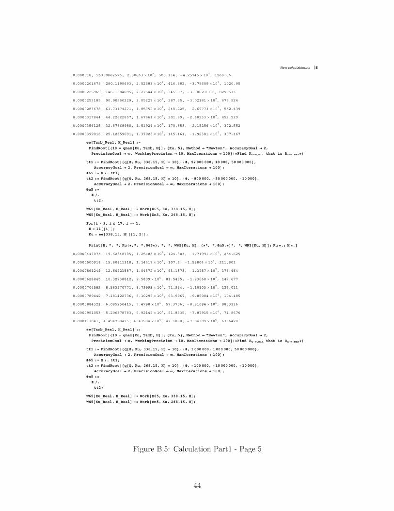
ðòððððïèô çêíòðèêîëéêô îòèðêêí l ïðéô ëðëòïíìô óìòîëéìë l ïðéô ïîêðòðê
ðòððððîðïêéçô îèðòïïççêçíô îòëîëèí l ïðéô ìïêòèèîô óíòéçêðç l ïðéô ïðîðòçë
ðòððððîîëçêçô ïìêòïíèìðçëô îòîéëìì l ïðéô íìëòíéô óíòíèêî l ïðéô èîçòëïí
ðòððððîëíïèëô çðòçðèêðîîçô îòðëîîé l ïðéô îèéòíëô óíòðîïèï l ïðéô êéëòçîì
ðòððððîèíêéèô êïòéíïéìîéïô ïòèëíëî l ïðéô îìðòîîëô óîòêçééí l ïðéô ëëîòìíç
ðòððððíïéèììô ììòîîêîîèëéô ïòêéêêï l ïðéô îðïòèçô óîòìðçíí l ïðéô ìëîòçîç
ðòððððíëêïîëô íîòèéêêèçèðô ïòëïçîì l ïðéô ïéðòêëèô óîòïëîëê l ïðéô íéîòëëî
ðòððððíççðïêô îëòïîíëçðçïô ïòíéçîè l ïðéô ïìëòïêïô óïòçîíèï l ïðéô íðéòìêé
»» Ì¿³¾Áλ¿´ô ØÁλ¿´ æã
Ú·²¼Î±±¬ ï𠯳¿¨ Õ«ô Ì¿³¾ô Ø ô Õ«ô ë ô Ó»¬¸±¼ r þÒ»©¬±²þô ß½½«®¿½§Ù±¿´ r îô
Ю»½··±²Ù±¿´ r ô ɱ®µ·²¹Ð®»½··±² r ïðô Ó¿¨×¬»®¿¬·±² r ïðð öÚ·²¼ Õ«óô³·² ¬¸¿¬ · Ϋóô³¿¨ö
¬¬ï æã Ú·²¼Î±±¬ ¯ Úô Õ«ô ííèòïëô Ø ïð ô Úô îî ððð ðððô ïð ðððô ëð ððð ððð ô
ß½½«®¿½§Ù±¿´ r îô Ю»½··±²Ù±¿´ r ô Ó¿¨×¬»®¿¬·±² r ïðð å
Úêë æã Ú ò ¬¬ïå
¬¬î æã Ú·²¼Î±±¬ ¯ Úô Õ«ô îêèòïëô Ø ïð ô Úô óèðð ðððô óëð ððð ðððô óïð ððð ô
ß½½«®¿½§Ù±¿´ r îô Ю»½··±²Ù±¿´ r ô Ó¿¨×¬»®¿¬·±² r ïðð å
Ú²ë æã
Ú ò
¬¬îå
Éêë Õ«Áλ¿´ô ØÁλ¿´ æã ɱ®µ Úêëô Õ«ô ííèòïëô Ø å
ÉÒë Õ«Áλ¿´ô ØÁλ¿´ æã ɱ®µ Ú²ëô Õ«ô îêèòïëô Ø å
Ú±® · ã çô · ïéô · õã ïô
Ø ã ´´ · å
Õ« ã »» ííèòïëô Ø ïô î å
Ю·²¬ Øô þô þô Õ« öôþô þôÚêëö ô þô þô Éêë Õ«ô Ø ô öþô þôÚ²ëôö þô þô ÉÒë Õ«ô Ø å Õ« ãòå Ø ãò
ðòððððììéðéíô ïçòêîíìèéðëô ïòîëìèí l ïðéô ïîìòíðíô óïòéïççï l ïðéô îëìòêîë
ðòððððëððçïèô ïëòêðèïïíïèô ïòïììïé l ïðéô ïðéòîô óïòëíèðì l ïðéô îïïòêðï
ðòððððëêïîìçô ïîòêðçîïëèéô ïòðìëéî l ïðéô çíòïíéèô óïòíéëé l ïðéô ïéêòìêì
ðòððððêîèèìëô ïðòíîéíèèïîô çòëèðç l ïðêô èïòëìíëô óïòîíðêè l ïðéô ïìéòêéé
ðòððððéðìëèîô èòëêíëéðééïô èòéçççí l ïðêô éïòçëìô óïòïðïðí l ïðéô ïîìòðïï
ðòððððéèçììîô éòïèïìîîéíêô èòïðîçë l ïðêô êíòççêéô óçòèëððì l ïðêô ïðìòìèë
ðòððððèèìëîïô êòðèëîëðìïëô éòìéçè l ïðêô ëéòíéðêô óèòèïðèì l ïðêô èèòíïíê
ðòððððççïðëíô ëòîðêíéèéèíô êòçîïìë l ïðêô ëïòèííëô óéòèéçïë l ïðêô éìòèêéê
ðòðððïïïðìïô ìòìçìéëèìéëô êòìïççì l ïðêô ìéòïèçèô óéòðìíðç l ïðêô êíòêìîè
»» Ì¿³¾Áλ¿´ô ØÁλ¿´ æã
Ú·²¼Î±±¬ ï𠯳¿¨ Õ«ô Ì¿³¾ô Ø ô Õ«ô ë ô Ó»¬¸±¼ r þÒ»©¬±²þô ß½½«®¿½§Ù±¿´ r îô
Ю»½··±²Ù±¿´ r ô ɱ®µ·²¹Ð®»½··±² r ïðô Ó¿¨×¬»®¿¬·±² r ïðð öÚ·²¼ Õ«óô³·² ¬¸¿¬ · Ϋóô³¿¨ö
¬¬ï æã Ú·²¼Î±±¬ ¯ Úô Õ«ô ííèòïëô Ø ïð ô Úô ï ððð ðððô ï ððð ðððô ëð ððð ððð ô
ß½½«®¿½§Ù±¿´ r îô Ю»½··±²Ù±¿´ r ô Ó¿¨×¬»®¿¬·±² r ïðð å
Úêë æã Ú ò ¬¬ïå
¬¬î æã Ú·²¼Î±±¬ ¯ Úô Õ«ô îêèòïëô Ø ïð ô Úô óïðð ðððô óïð ððð ðððô óïð ððð ô
ß½½«®¿½§Ù±¿´ r îô Ю»½··±²Ù±¿´ r ô Ó¿¨×¬»®¿¬·±² r ïðð å
Ú²ë æã
Ú ò
¬¬îå
Éêë Õ«Áλ¿´ô ØÁλ¿´ æã ɱ®µ Úêëô Õ«ô ííèòïëô Ø å
ÉÒë Õ«Áλ¿´ô ØÁλ¿´ æã ɱ®µ Ú²ëô Õ«ô îêèòïëô Ø å
New calculation.nb 5
Figure B.5: Calculation Part1 - Page 5
44
Ú±® · ã ïéô · îïô · õã ïô
Ø ã ´´ · å
Õ« ã »» ííèòïëô Ø ïô î å
Ю·²¬ Øô þô þô Õ« öôþô þôÚêëö ô þô þô Éêë Õ«ô Ø ô öþô þôÚ²ëôö þô þô ÉÒë Õ«ô Ø å Õ« ãòå Ø ãò
ðòðððïïïðìïô ìòìçìéëèìéëô êòìïççì l ïðêô ìéòïèçèô óéòðìíðç l ïðêô êíòêìîè
ðòðððïîììïëô íòçïíîçíîììô ëòçêèîë l ïðêô ìíòîèïîô óêòîçîïé l ïðêô ëìòîííè
ðòðððïíçìô íòìíìïêëîéêô ëòëêðîë l ïðêô íçòçéççô óëòêïéïì l ïðêô ìêòíïíç
ðòðððïëêïèçô íòðíêîéíïîèô ëòïçðêî l ïðêô íéòïèîíô óëòððçç l ïðêô íçòêîðï
ðòðððïéëô îòéðíììïðïìô ìòèëìéì l ïðêô íìòèðìíô óìòìêíîé l ïðêô ííòçíçì
´´î ã Ô·¬ ðòðððïçîðíðëô ðòðððîïðéïèìô ðòðððîíïîîëðô ðòðððîëíéîéîô
ðòðððîéèìïçíô ðòðððíðëëïìíô ðòðððííëîìêîô ðòðððíêéèéïìô ðòðððìðíêéïéô
ðòðððììîçëêðô ðòðððìèêðêííô ðòðððëíííêëéô ðòðððëèëîéïìô ðòðððêìîîîèëô ðòðððéðìéîèëô
ðòðððééííïðèô ðòðððèìèëêéìô ðòðððçíïïìééô ðòððïðîïéêìêô ðòððïïîïîððð å
»» Ì¿³¾Áλ¿´ô ØÁλ¿´ æã
Ú·²¼Î±±¬ ï𠯳¿¨ Õ«ô Ì¿³¾ô Ø ô Õ«ô î ô Ó»¬¸±¼ r þÒ»©¬±²þô ß½½«®¿½§Ù±¿´ r îô
Ю»½··±²Ù±¿´ r ô ɱ®µ·²¹Ð®»½··±² r ïðô Ó¿¨×¬»®¿¬·±² r ïðð öÚ·²¼ Õ«óô³·² ¬¸¿¬ · Ϋóô³¿¨ö
¬¬ï æã Ú·²¼Î±±¬ ¯ Úô Õ«ô ííèòïëô Ø ïð ô Úô î ððð ðððô ïðð ðððô ë ððð ððð ô
ß½½«®¿½§Ù±¿´ r îô Ю»½··±²Ù±¿´ r ô Ó¿¨×¬»®¿¬·±² r ïðð å
Úêë æã Ú ò ¬¬ïå
¬¬î æã Ú·²¼Î±±¬ ¯ Úô Õ«ô îêèòïëô Ø ïð ô Úô óïð ðððô óïð ððð ðððô óïð ððð ô
ß½½«®¿½§Ù±¿´ r îô Ю»½··±²Ù±¿´ r ô Ó¿¨×¬»®¿¬·±² r ïðð å
Ú²ë æã
Ú ò
¬¬îå
Éêë Õ«Áλ¿´ô ØÁλ¿´ æã ɱ®µ Úêëô Õ«ô ííèòïëô Ø å
ÉÒë Õ«Áλ¿´ô ØÁλ¿´ æã ɱ®µ Ú²ëô Õ«ô îêèòïëô Ø å
Ú±® · ã ïô · çô · õã ïô
Ø ã ´´î · å
Õ« ã »» ííèòïëô Ø ïô î å
Ю·²¬ Øô þô þô Õ« öôþô þôÚêëö ô þô þô Éêë Õ«ô Ø ô öþô þôÚ²ëôö þô þô ÉÒë Õ«ô Ø å Õ« ãòå Ø ãò
ðòðððïçîðíïô îòìéïðèçðëíô ìòêðîêç l ïðêô ííòïîëêô óìòðëéì l ïðêô îçòçíðê
ðòðððîïðéïèô îòîêèíïðïëëô ìòíêèëè l ïðêô íïòêëðïô óíòêèìêì l ïðêô îêòìðìî
ðòðððîíïîîëô îòðçðêëêèéêô ìòïëðéí l ïðêô íðòíëïèô óíòíìîîî l ïðêô îíòîçìí
ðòðððîëíéîéô ïòçíììêìíèëô íòçìéêé l ïðêô îçòîðèëô óíòðîéëç l ïðêô îðòëìëì
ðòðððîéèìïçô ïòéçêêçéîèçô íòéëèðç l ïðêô îèòîðïíô óîòéíèìê l ïðêô ïèòïïðï
ðòðððíðëëïìô ïòêéìèííìèèô íòëèðèî l ïðêô îéòíïìíô óîòìéîéì l ïðêô ïëòçìèï
ðòðððííëîìêô ïòëêêééîëêêô íòìïìèí l ïðêô îêòëííêô óîòîîèëí l ïðêô ïìòðîëï
ðòðððíêéèéïô ïòìéðéëìëçëô íòîëçîï l ïðêô îëòèìéçô óîòððìðç l ïðêô ïîòíïïè
ðòðððìðíêéîô ïòíèëíðééðêô íòïïíïë l ïðêô îëòîìêèô óïòéçéèï l ïðêô ïðòéèí
¬¬ï æã Ú·²¼Î±±¬ ¯ Úô Õ«ô ííèòïëô Ø ïð ô Úô î ìîð ðððô çðð ðððô ì ððð ððð ô
ß½½«®¿½§Ù±¿´ r îô Ю»½··±²Ù±¿´ r ô Ó¿¨×¬»®¿¬·±² r ïðð å
Úêë æã Ú ò ¬¬ïå
¬¬î æã Ú·²¼Î±±¬ ¯ Úô Õ«ô îêèòïëô Ø ïð ô Úô óîð ðððô óïð ððð ðððô óïð ððð ô
ß½½«®¿½§Ù±¿´ r îô Ю»½··±²Ù±¿´ r ô Ó¿¨×¬»®¿¬·±² r ïðð å
Ú²ë æã
Ú ò
¬¬îå
Éêë Õ«Áλ¿´ô ØÁλ¿´ æã ɱ®µ Úêëô Õ«ô ííèòïëô Ø å
ÉÒë Õ«Áλ¿´ô ØÁλ¿´ æã ɱ®µ Ú²ëô Õ«ô îêèòïëô Ø å
6 New calculation.nb
Figure B.6: Calculation Part1 - Page 6
45
Ú±® · ã çô · îðô · õã ïô
Ø ã ´´î · å
Õ« ã »» ííèòïëô Ø ïô î å
Ю·²¬ Øô þô þô Õ« öôþô þôÚêëö ô þô þô Éêë Õ«ô Ø ô öþô þôÚ²ëôö þô þô ÉÒë Õ«ô Ø å Õ« ãòå Ø ãò
ðòðððìðíêéîô ïòíèëíðééðêô íòïïíïë l ïðêô îëòîìêèô óïòéçéèï l ïðêô ïðòéèí
ðòðððììîçëêô ïòíðçïçèïêíô îòçéëçï l ïðêô îìòéîïçô óïòêðèîë l ïðêô çòìïéðì
ðòðððìèêðêíô ïòîìïíçîíçîô îòèìêèë l ïðêô îìòîêëèô óïòìíìðé l ïðêô èòïçëìê
ðòðððëíííêêô ïòïèïðîêçðêô îòéîëíè l ïðêô îíòèéîïô óïòîéìðî l ïðêô éòïðîîî
ðòðððëèëîéïô ïòïîéíèìééíô îòêïðçé l ïðêô îíòëíëîô óïòïîé l ïðêô êòïîíëí
ðòðððêìîîîçô ïòðéçèéêíéëô îòëðíïî l ïðêô îíòîëðíô óççï çììòô ëòîìéìí
ðòðððéðìéîçô ïòðíèðîìèïîô îòìðïìï l ïðêô îíòðïíô óèêé çðéòô ìòìêíêï
ðòðððééííïïô ïòððïëððíðëô îòíðëìé l ïðêô îîòèîðêô óéëì ðïëòô íòéêíîî
ðòðððèìèëêéô ðòçêçççêðèîîô îòîïìèé l ïðêô îîòêêèëô óêìç ììïòô íòïíèíè
ðòðððçíïïìèô ðòçìííêçéèðëô îòïîçí l ïðêô îîòëëìîô óëëí ììîòô îòëèîìí
ðòððïðîïéêô ðòçîïëéîçéìèô îòðìèìî l ïðêô îîòìéìêô óìêë íîëòô îòðèçëè
ðòððïïîïîô ðòçðìêèîêïïïô ïòçéïçë l ïðêô îîòìîéíô óíèì ìëêòô ïòêëìéè
´´í ã Ô·¬ ðòððïïëèëìëêô ðòððïïçéïíëïô ðòððïîíéðïððô ðòððïîéèîïíðô
ðòððïíîðéèèëô ðòððïíêìéèîðô ðòððïìïðîìïðô ðòððïìëéîïìïô ðòððïëðëéëïèô ðòððïëëëçðêíô
ðòððïêðééíïíô ðòððïêêïîèîêô ðòððïéïêêïéëô ðòððïééíéçëêô ðòððïèíîèéèîô ðòððïèçíçîèèô
ðòððïçëéðïîçô ðòððîðîîïçèîô ðòððîðèçëëìéô ðòððîïëçïëìèô ðòððîîíïðéíîô ðòððîíðëíèéïô
ðòððîíèîïéêíô ðòððîìêïëîíîô ðòððîëìíëïíðô ðòððîêîèîííèô ðòððîéïëééêëô ðòððîèðêîíëîô
ðòððîèççéðêçô ðòððîççêîçîðô ðòððíðçêðçìîô ðòððíïççîîðéô ðòððííðëéèîîô ðòððíìïëèçíïô
ðòððíëîçêéïéô ðòððíêìéîìððô ðòððíéêèéîììô ðòððíèçìîëëíô ðòððìðîíçêéìô ðòððìïëèðððð å
»» Ì¿³¾Áλ¿´ô ØÁλ¿´ æã
Ú·²¼Î±±¬ ï𠯳¿¨ Õ«ô Ì¿³¾ô Ø ô Õ«ô ðòè ô Ó»¬¸±¼ r þÒ»©¬±²þô ß½½«®¿½§Ù±¿´ r îô
Ю»½··±²Ù±¿´ r ô ɱ®µ·²¹Ð®»½··±² r ïðô Ó¿¨×¬»®¿¬·±² r ïðð öÚ·²¼ Õ«óô³·² ¬¸¿¬ · Ϋóô³¿¨ö
¬¬ï æã Ú·²¼Î±±¬ ¯ Úô Õ«ô ííèòïëô Ø ïð ô Úô çç çççô ðô ì ððð ððð ô
ß½½«®¿½§Ù±¿´ r îô Ю»½··±²Ù±¿´ r ô Ó¿¨×¬»®¿¬·±² r ïðð å
Úêë æã Ú ò ¬¬ïå
¬¬î æã Ú·²¼Î±±¬ ¯ Úô Õ«ô îêèòïëô Ø ïð ô
Úô óçç çççô óçç ççç çççô ð ô ß½½«®¿½§Ù±¿´ r îô Ю»½··±²Ù±¿´ r ô Ó¿¨×¬»®¿¬·±² r ïðð å
Ú²ë æã
Ú ò
¬¬îå
Éêë Õ«Áλ¿´ô ØÁλ¿´ æã ɱ®µ Úêëô Õ«ô ííèòïëô Ø å
ÉÒë Õ«Áλ¿´ô ØÁλ¿´ æã ɱ®µ Ú²ëô Õ«ô îêèòïëô Ø å
Ú±® · ã ïô · ïîô · õã ïô
Ø ã ´´í · å
Õ« ã »» ííèòïëô Ø ïô î å
Ю·²¬ Øô þô þô Õ« öôþô þôÚêëö ô þô þô Éêë Õ«ô Ø ô öþô þôÚ²ëôö þô þô ÉÒë Õ«ô Ø å Õ« ãòå Ø ãò
New calculation.nb 7
Figure B.7: Calculation Part1 - Page 7
46
ðòððïïëèëëô ðòèçççíïêìëíô ïòçìëçê l ïðêô îîòìïéêô óíëé ëìîòô ïòëïììï
ðòððïïçéïìô ðòèçëèííîéìèô ïòçîðìè l ïðêô îîòìïïêô óííï ìíîòô ïòíèðëë
ðòððïîíéðïô ðòèçîìðêððêèô ïòèçëìç l ïðêô îîòìðçô óíðê ïðîòô ïòîëíðì
ðòððïîéèîïô ðòèèçêéïçìíìô ïòèéðçé l ïðêô îîòìðçéô óîèï ëíðòô ïòïíïéî
ðòððïíîðéçô ðòèèéêëéîïèîô ïòèìêçî l ïðêô îîòìïíêô óîëé êçíòô ïòðïêìê
ðòððïíêìéèô ðòèèêíçîëìççô ïòèîííí l ïðêô îîòìîðëô óîíì ëéðòô ðòçðéïïï
ðòððïìïðîìô ðòèèëçïíèîðêô ïòèððïè l ïðêô îîòìíðíô óîïî ïíçòô ðòèðíëìê
ðòððïìëéîïô ðòèèêîêîèíêíô ïòéééìê l ïðêô îîòììîçô óïçð íèðòô ðòéðëêìí
ðòððïëðëéëô ðòèèéìèèïçðíô ïòéëëïê l ïðêô îîòìëèïô óïêç îéíòô ðòêïíîèë
ðòððïëëëçïô ðòèèçêìêííìïô ïòéííîè l ïðêô îîòìéëèô óïìè éççòô ðòëîêíêë
ðòððïêðééíô ðòèçîèðîèìëêô ïòéïïéç l ïðêô îîòìçëèô óïîè çíçòô ðòìììééç
ðòððïêêïîèô ðòèçéðíìðïèïô ïòêçðé l ïðêô îîòëïéçô óïðç êéëòô ðòíêèìíï
»» Ì¿³¾Áλ¿´ô ØÁλ¿´ æã
Ú·²¼Î±±¬ ï𠯳¿¨ Õ«ô Ì¿³¾ô Ø ô Õ«ô ïòî ô Ó»¬¸±¼ r þÒ»©¬±²þô ß½½«®¿½§Ù±¿´ r îô
Ю»½··±²Ù±¿´ r ô ɱ®µ·²¹Ð®»½··±² r ïðô Ó¿¨×¬»®¿¬·±² r ïðð öÚ·²¼ Õ«óô³·² ¬¸¿¬ · Ϋóô³¿¨ö
¬¬ï æã Ú·²¼Î±±¬ ¯ Úô Õ«ô ííèòïëô Ø ïð ô Úô ççç çççô ðô ì ððð ððð ô
ß½½«®¿½§Ù±¿´ r îô Ю»½··±²Ù±¿´ r ô Ó¿¨×¬»®¿¬·±² r ïðð å
Úêë æã Ú ò ¬¬ïå
¬¬î æã Ú·²¼Î±±¬ ¯ Úô Õ«ô îêèòïëô Ø ïð ô Úô îçç çççô óçç ççç çççô ïð ððð ððð ô
ß½½«®¿½§Ù±¿´ r îô Ю»½··±²Ù±¿´ r ô Ó¿¨×¬»®¿¬·±² r ïðð å
Ú²ë æã Ú ò ¬¬îå
Éêë Õ«Áλ¿´ô ØÁλ¿´ æã ɱ®µ Úêëô Õ«ô ííèòïëô Ø å
ÉÒë Õ«Áλ¿´ô ØÁλ¿´ æã ɱ®µ Ú²ëô Õ«ô îêèòïëô Ø å
Ú±® · ã ïíô · ìðô · õã ïô
Ø ã ´´í · å
Õ« ã »» ííèòïëô Ø ïô î å
Ю·²¬ Øô þô þô Õ« öôþô þôÚêëö ô þô þô Éêë Õ«ô Ø ô öþô þôÚ²ëôö þô þô ÉÒë Õ«ô Ø å Õ« ãòå Ø ãò
8 New calculation.nb
Figure B.8: Calculation Part1 - Page 8
47
ðòððïéïêêîô ðòçðîìîèéíîêô ïòêêççé l ïðêô îîòëìïèô óçð çèçòíô ðòîçéîíï
ðòððïééíèô ðòçðçðçðèéêçô ïòêìçêî l ïðêô îîòëêéêô óéî èêìòéô ðòîíïðçî
ðòððïèíîèèô ðòçïéïìîîïêêô ïòêîçêí l ïðêô îîòëçìçô óëë îèìòéô ðòïêççíê
ðòððïèçíçíô ðòçîêéîêïðëíô ïòêðççç l ïðêô îîòêîíêô óíè îííòìô ðòïïíêèé
ðòððïçëéðïô ðòçíèðïîðéêçô ïòëçðêè l ïðêô îîòêëíìô óîï êçëòïô ðòðêîîéìë
ðòððîðîîîô ðòçëïîðïéëïêô ïòëéïêç l ïðêô îîòêèìô óëêëìòèçô ðòðïëêííë
ðòððîðèçëëô ðòçêêëíêìîïçô ïòëëíðî l ïðêô îîòéïëíô ççðïòèîô óðòðîêîçèï
ðòððîïëçïëô ðòçèìíðêçïèëô ïòëíìêê l ïðêô îîòéìéô îì çèçòïô óðòðêíëéèî
ðòððîîíïðéô ïòððìèêêëíèô ïòëïêëç l ïðêô îîòééèêô íç êîðòêô óðòðçêîêïî
ðòððîíðëíçô ïòðîèêìèíëçô ïòìçèè l ïðêô îîòèïðïô ëí èðçòíô óðòïîìíçè
ðòððîíèîïèô ïòðëêïèèêëêô ïòìèïîç l ïðêô îîòèìðçô êé ëêèòô óðòïìèðíè
ðòððîìêïëîô ïòðèèïëçðìðô ïòìêìðí l ïðêô îîòèéðèô èð çðèòèô óðòïêéîîé
ðòððîëìíëïô ïòïîëìïïëëéô ïòììéðî l ïðêô îîòèççíô çí èìíòìô óðòïèîððç
ðòððîêîèîíô ïòïêçðìíðìçô ïòìíðîë l ïðêô îîòçîêíô ïðê íèíòô óðòïçîìîè
ðòððîéïëéèô ïòîîðìèçïîìô ïòìïíéï l ïðêô îîòçëïïô ïïè ëíçòô óðòïçèëîí
ðòððîèðêîìô ïòîèïêêëíèêô ïòíçéíè l ïðêô îîòçéíîô ïíð íîïòô óðòîððííè
ðòððîèççéïô ïòíëëïèëïçëô ïòíèïîë l ïðêô îîòççîëô ïìï éíçòô óðòïçéçïì
ðòððîççêîçô ïòìììéðèêéíô ïòíêëíï l ïðêô îíòððèïô ïëî èðíòô óðòïçïîçí
ðòððíðçêðçô ïòëëëëîíéêíô ïòíìçëê l ïðêô îíòðïçêô ïêí ëîïòô óðòïèðëïç
ðòððíïççîîô ïòêçëëêíîïêô ïòíííçé l ïðêô îíòðîêéô ïéí çðîòô óðòïêëêíé
ðòððííðëéèô ïòèééîçîëêìô ïòíïèëí l ïðêô îíòðîèëô ïèí çëëòô óðòïìêêçç
ðòððíìïëèçô îòïîïìèëííðô ïòíðíîí l ïðêô îíòðîììô ïçí êèëòô óðòïîíéëé
ðòððíëîçêéô îòìêëëîëëíçô ïòîèèðê l ïðêô îíòðïìô îðí ïðïòô óðòðçêèêçë
ðòððíêìéîìô îòçèìïëïêèìô ïòîéíðï l ïðêô îîòççêêô îïî îïðòô óðòðêêïðîë
ðòððíéêèéîô íòèëïêìêèîéô ïòîëèðê l ïðêô îîòçéïìô îîï ðïêòô óðòðíïëîèí
ðòððíèçìîêô ëòëçðîéîìèïô ïòîìíî l ïðêô îîòçíéçô îîç ëîêòô ðòððêééïëé
ðòððìðîíçéô ïðòèðìîëèëëô ïòîîèìï l ïðêô îîòèçëîô îíé éììòô ðòðìèéðëì
ðòððìïëèô íðèîòíèîèîëô ïòîïíêç l ïðêô îîòèìîéô îìë êéëòô ðòðçìïêçë
New calculation.nb 9
Figure B.9: Calculation Part1 - Page 9
48

Calculation Part 2
49

Û¨·¬
ää Ò±¬¿¬·±²À
ͧ³¾±´·¦» Ì« å ͧ³¾±´·¦» ̽ å ͧ³¾±´·¦» λ½óÎ å ͧ³¾±´·¦» Õ«óô« å ͧ³¾±´·¦» λ½ó® å ͧ³¾±´·¦» ¯½° å
ͧ³¾±´·¦» ßÐ å ͧ³¾±´·¦» ß«¾ å ͧ³¾±´·¦» Ì å ͧ³¾±´·¦» Õ½°ó½ å ͧ³¾±´·¦» Õ½°óô½ å
¯ ÚÁáÒ«³»®·½Ïô Õ«Á áÒ«³»®·½Ïô Ì¿³¾Á áÒ«³»®·½Ïô ØÁ áÒ«³»®·½Ï ã
Õ½°óô½ óÌ¿³¾ õ ̽° ó Õ½°ó½ §§ Ø î λ½ó® õ Ø ® Úî î Õ« ó §§ ¿ Ú õ ì µ Õ« Ì¿³¾ õ §§ î λ½ó® õ Ø ® Úî õ
óì µ Õ« õ Ø ¿ Ú óî Õ« õ §§ ¿ Ú Ì½° ì µ Õ« õ Õ½°ó½ §§ õ Ø î Õ« ó §§ ¿ Ú î Õ½°ó½ õ §§ ¿ Ú å
ɱ®µ ÚÁáÒ«³»®·½Ïô Õ«Á áÒ«³»®·½Ïô Ì¿³¾Á áÒ«³»®·½Ïô ØÁ áÒ«³»®·½Ï ã
§§ Ú è µ Õ« õ Õ½°ó½ λ½ó® §§ Ú õ Øî ® Ú ì Õ« Õ½°ó½ õ Õ« §§ ¿ Ú ó Õ½°ó½ §§ ¿ Ú õ
Ø óî Õ½°ó½ §§ Ú óî µ ® õ λ½ó® ¿ Ú õ Õ« î Õ½°ó½ Ì¿³¾ ¿ õ ì λ½ó® Ú õ §§ Ú Ì¿³¾ ¿î õ ì µ ® õ î λ½ó® ¿ Ú õ
Ø Õ½°ó½ ¿ óî Õ« õ §§ ¿ Ú Ì½° ì µ Õ« õ Õ½°ó½ §§ õ Ø î Õ« ó §§ ¿ Ú î Õ½°ó½ õ §§ ¿ Ú å
¯ ÚÁáÒ«³»®·½Ïô Ì¿³¾Á áÒ«³»®·½Ïô ØÁáÒ«³»®·½Ï ã
ó î Ì¿³¾ Ø Õ½°ó½ Õ½°óô½ õ µ Õ½°ó½ õ Õ½°óô½ §§ õ Ø Õ½°óô½ Ì¿³¾ §§ ¿ Ú õ Ø Õ½°ó½ §§ î λ½ó® õ Ø ® Úî ó
î Ø Õ½°ó½ Õ½°óô½ õ î µ Õ½°ó½ õ Õ½°óô½ §§ õ Ø Õ½°ó½ õ Õ½°óô½ §§ ¿ Ú Ì½° î Ø Õ½°ó½ õ î µ §§ õ Ø §§ ¿ Ú å
ɱ®µ ÚÁáÒ«³»®·½Ïô Ì¿³¾Á áÒ«³»®·½Ïô ØÁáÒ«³»®·½Ï ã
§§ Ú î Ø Õ½°ó½ Ì¿³¾ ¿ õ è Ø Õ½°ó½ λ½ó® õ è µ λ½ó® §§ õ Ø Ì¿³¾ §§ ¿î õ ì Ø Ø Õ½°ó½ õ µ §§ ® Ú õ
Ø §§ ¿ î λ½ó® õ Ø ® Úî ó î Ø Õ½°ó½ ¿ ̽° ì Ø Õ½°ó½ õ ì µ §§ õ î Ø §§ ¿ Ú å
̽° ã îéíòïë õ ëëå ¿ ã ðòðððìå
µ ã ïòëå ® ã ðòððððïîëå
ß° ã ïòçê ö ïðóêå
Õ½°ó½ ã ïéòïéå
Ò¬»³ ã éïå
ν»® ã ðòðíçå ι®» ã îòëè ö ïðóëå
λ½ó® ã ï ö ïðóçå
¬ ã ðòððëå µ½ ã ðòðíå Õ½°óô½ ã ðòðððïëå §§ ã îéèòí ö ïðóêå
䱬 ¯ Úô ííèòïëô ðòððï ô Úô ïðð ðððô ïð ððð ððð
î l ïðê ì l ïðê ê l ïðê è l ïðê ï l ïðé
óîð
óïð
ïð
îð
íð
öÚ×ÒÜ ÌØÛ ÎßÒÙÛ ÑÚ Ø ÚÑÎ Ìô³¿¨ö
¾¾ æã ÒÓ¿¨·³·¦» ¯ Úô ííèòïëô Ø ô Úô Ó»¬¸±¼ r þÒ»´¼»®Ó»¿¼þô
ß½½«®¿½§Ù±¿´ r êô Ю»½··±²Ù±¿´ r ô ɱ®µ·²¹Ð®»½··±² r è
½½ ØÁλ¿´ æã ¾¾ ï ö¯½°ô³¿¨ö
Figure B.10: Calculation Part2 - Page 1
50
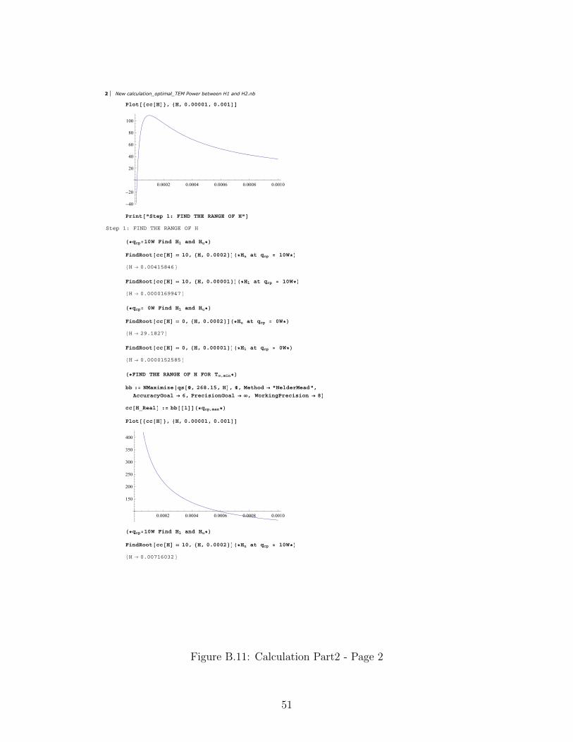
䱬 ½½ Ø ô Øô ðòððððïô ðòððï
ðòðððî ðòðððì ðòðððê ðòðððè ðòððïð
óìð
óîð
îð
ìð
êð
èð
ïðð
Ю·²¬ þͬ»° ïæ Ú×ÒÜ ÌØÛ ÎßÒÙÛ ÑÚ Øþ
ͬ»° ïæ Ú×ÒÜ ÌØÛ ÎßÒÙÛ ÑÚ Ø
ö¯½°ãïðÉ Ú·²¼ Ø´ ¿²¼ Ø«ö
Ú·²¼Î±±¬ ½½ Ø ïðô Øô ðòðððî öØ« ¿¬ ¯½° ã ïðÉö
Ø r ðòððìïëèìê
Ú·²¼Î±±¬ ½½ Ø ïðô Øô ðòððððï öØ´ ¿¬ ¯½° ã ïðÉö
Ø r ðòððððïêççìé
ö¯½°ã ðÉ Ú·²¼ Ø´ ¿²¼ Ø«ö
Ú·²¼Î±±¬ ½½ Ø ðô Øô ðòðððî öØ« ¿¬ ¯½° ã ðÉö
Ø r îçòïèîé
Ú·²¼Î±±¬ ½½ Ø ðô Øô ðòððððï öØ´ ¿¬ ¯½° ã ðÉö
Ø r ðòððððïëîëèë
öÚ×ÒÜ ÌØÛ ÎßÒÙÛ ÑÚ Ø ÚÑÎ Ìô³·²ö
¾¾ æã ÒÓ¿¨·³·¦» ¯ Úô îêèòïëô Ø ô Úô Ó»¬¸±¼ r þÒ»´¼»®Ó»¿¼þô
ß½½«®¿½§Ù±¿´ r êô Ю»½··±²Ù±¿´ r ô ɱ®µ·²¹Ð®»½··±² r è
½½ ØÁλ¿´ æã ¾¾ ï ö¯½°ô³¿¨ö
䱬 ½½ Ø ô Øô ðòððððïô ðòððï
ðòðððî ðòðððì ðòðððê ðòðððè ðòððïð
ïëð
îðð
îëð
íðð
íëð
ìðð
ö¯½°ãïðÉ Ú·²¼ Ø´ ¿²¼ Ø«ö
Ú·²¼Î±±¬ ½½ Ø ïðô Øô ðòðððî öØ« ¿¬ ¯½° ã ïðÉö
Ø r ðòððéïêðíî
2 New calculation_optimal_TEM Power between H1 and H2.nb
Figure B.11: Calculation Part2 - Page 2
51
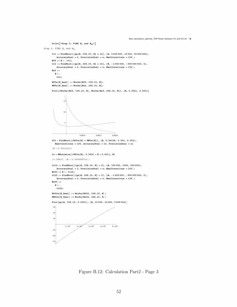
Ю·²¬ þͬ»° îæ Ú×ÒÜ Øî ¿²¼ Ø°»þ
ͬ»° îæ Ú×ÒÜ Øî ¿²¼ Ø°»
¬¬ï æã Ú·²¼Î±±¬ ¯ Úô ííèòïëô Ø ïð ô Úô î ððð ðððô ïð ðððô ëð ððð ððð ô
ß½½«®¿½§Ù±¿´ r îô Ю»½··±²Ù±¿´ r ô Ó¿¨×¬»®¿¬·±² r ïðð å
Úêë æã Ú ò ¬¬ïå
¬¬î æã Ú·²¼Î±±¬ ¯ Úô îêèòïëô Ø ïð ô Úô óï ððð ðððô óçðð ððð ðððô ð ô
ß½½«®¿½§Ù±¿´ r îô Ю»½··±²Ù±¿´ r ô Ó¿¨×¬»®¿¬·±² r ïðð å
Ú²ë æã
Ú ò
¬¬îå
Éêë ØÁλ¿´ æã ɱ®µ Úêëô ííèòïëô Ø å
ÉÒë ØÁλ¿´ æã ɱ®µ Ú²ëô îêèòïëô Ø å
䱬 ɱ®µ Úêëô ííèòïëô Ø ô ɱ®µ Ú²ëô îêèòïëô Ø ô Øô ðòðððïô ðòððî
ðòððïð ðòððïë ðòððîð
ë
ïð
ïë
ººï ã Ú·²¼Î±±¬ Éêë Ø ÉÒë Ø ô Øô ðòððïëèô ðòððïô ðòððî ô
Ó¿¨×¬»®¿¬·±² r ïððô ß½½«®¿½§Ù±¿´ r ïðô Ю»½··±²Ù±¿´ r
Ø r ðòððïïîïî
¬¬ ã ÒÓ·²·³·¦» Éêë Ø ô ðòðððï ä Ø ä ðòððï ô Ø
íòíçêîéô Ø r ðòðððêëèéïë
¬¬ïð æã Ú·²¼Î±±¬ ¯ Úô ííèòïëô Ø ð ô Úô ïðð ðððô ïðððô ëðð ððð ô
ß½½«®¿½§Ù±¿´ r îô Ю»½··±²Ù±¿´ r ô Ó¿¨×¬»®¿¬·±² r ïðð å
Úêëð æã Ú ò ¬¬ïðå
¬¬îð æã Ú·²¼Î±±¬ ¯ Úô îêèòïëô Ø ð ô Úô óï ððð ðððô óçðð ððð ðððô ð ô
ß½½«®¿½§Ù±¿´ r îô Ю»½··±²Ù±¿´ r ô Ó¿¨×¬»®¿¬·±² r ïðð å
Ú²ëð æã
Ú ò
¬¬îðå
Éêëð ØÁλ¿´ æã ɱ®µ Úêëðô ííèòïëô Ø å
ÉÒëð ØÁλ¿´ æã ɱ®µ Ú²ëðô îêèòïëô Ø å
䱬 ¯ Úô ííèòïëô ðòðððï ô Úô ïð ðððô ïð ðððô ë ððð ððð
ï l ïðê î l ïðê í l ïðê ì l ïðê ë l ïðê
óíð
óîð
óïð
ïð
îð
íð
New calculation_optimal_TEM Power between H1 and H2.nb 3
Figure B.12: Calculation Part2 - Page 3
52

䱬 ɱ®µ Úêëðô ííèòïëô Ø ô ɱ®µ Ú²ëðô îêèòïëô Ø ô Øô ðòððïêô ðòðï
ðòððì ðòððê ðòððè ðòðïð
ï
î
í
ì
ë
ê
Ю·²¬ þØî ¿²¼ Ø°» ¼±» ²±¬ »¨·¬þ
Øî ¿²¼ Ø°» ¼±» ²±¬ »¨·¬
Ю·²¬ þͬ»° îæ Ú×ÒÜ ÌØÛ ÎßÒÙÛ ÑÚ Î«óô« ßÒÜ ÌÛÓ ÐÑÉÛÎ ßÌ Î«óô³¿¨þ
ͬ»° îæ Ú×ÒÜ ÌØÛ ÎßÒÙÛ ÑÚ Î«óô« ßÒÜ ÌÛÓ ÐÑÉÛÎ ßÌ Î«óô³¿¨
¼¼ Õ«Áλ¿´ô Ì¿³¾Áλ¿´ô ØÁλ¿´ æã ÒÓ¿¨·³·¦» ¯ Úô Õ«ô Ì¿³¾ô Ø ô Úô
Ó»¬¸±¼ r þÒ»´¼»®Ó»¿¼þô ß½½«®¿½§Ù±¿´ r êô Ю»½··±²Ù±¿´ r ô ɱ®µ·²¹Ð®»½··±² r è
ºº Õ«Áλ¿´ô Ì¿³¾Áλ¿´ô ØÁλ¿´ æã ¼¼ Õ«ô Ì¿³¾ô Ø îô ïô î ö¯½°ô³¿¨ö
¯³¿¨ Õ«Áλ¿´ô Ì¿³¾Áλ¿´ô ØÁλ¿´ æã ¯ ºº Õ«ô Ì¿³¾ô Ø ô Õ«ô Ì¿³¾ô Ø å
»» Ì¿³¾Áλ¿´ô ØÁλ¿´ æã
Ú·²¼Î±±¬ ï𠯳¿¨ Õ«ô Ì¿³¾ô Ø ô Õ«ô îë ô Ó»¬¸±¼ r þÒ»©¬±²þô ß½½«®¿½§Ù±¿´ r ïô
Ю»½··±²Ù±¿´ r ô ɱ®µ·²¹Ð®»½··±² r ïðô Ó¿¨×¬»®¿¬·±² r ïðð öÚ·²¼ Õ«óô³·² ¬¸¿¬ · Ϋóô³¿¨ö
¬¬ï æã Ú·²¼Î±±¬ ¯ Úô Õ«ô ííèòïëô Ø ïð ô Úô ï ððð ðððô ï ððð ðððô ëð ððð ððð ô
ß½½«®¿½§Ù±¿´ r îô Ю»½··±²Ù±¿´ r ô Ó¿¨×¬»®¿¬·±² r ïðð å
Úêë æã Ú ò ¬¬ïå
¬¬î æã Ú·²¼Î±±¬ ¯ Úô Õ«ô îêèòïëô Ø ïð ô Úô óìð ððð ðððô óëð ððð ðððô ð ô
ß½½«®¿½§Ù±¿´ r îô Ю»½··±²Ù±¿´ r ô Ó¿¨×¬»®¿¬·±² r ïðð å
Ú²ë æã
Ú ò
¬¬îå
Éêë Õ«Áλ¿´ô ØÁλ¿´ æã ɱ®µ Úêëô Õ«ô ííèòïëô Ø å
ÉÒë Õ«Áλ¿´ô ØÁλ¿´ æã ɱ®µ Ú²ëô Õ«ô îêèòïëô Ø å
´´ ã Ô·¬ ðòððððïèððððô ðòððððîðïêéçô ðòððððîîëçêçô ðòððððîëíïèëô
ðòððððîèíêéèô ðòððððíïéèììô ðòððððíëêïîëô ðòððððíççðïêô ðòððððììéðéíô ðòððððëððçïèô
ðòððððëêïîìçô ðòððððêîèèìëô ðòððððéðìëèîô ðòððððéèçììîô ðòððððèèìëîïô ðòððððççïðëíô
ðòðððïïïðìïìô ðòðððïîììïëïô ðòðððïíçíççêô ðòðððïëêïèèèô ðòðððïéëðððð å
Ú±® · ã ïô · èô · õã ïô
Ø ã ´´ · å
Õ« ã »» ííèòïëô Ø ïô î å
Ю·²¬ Øô þô þô Õ« öôþô þôÚêëö ô þô þô Éêë Õ«ô Ø ô öþô þôÚ²ëôö þô þô ÉÒë Õ«ô Ø å Õ« ãòå Ø ãò
4 New calculation_optimal_TEM Power between H1 and H2.nb
Figure B.13: Calculation Part2 - Page 4
53
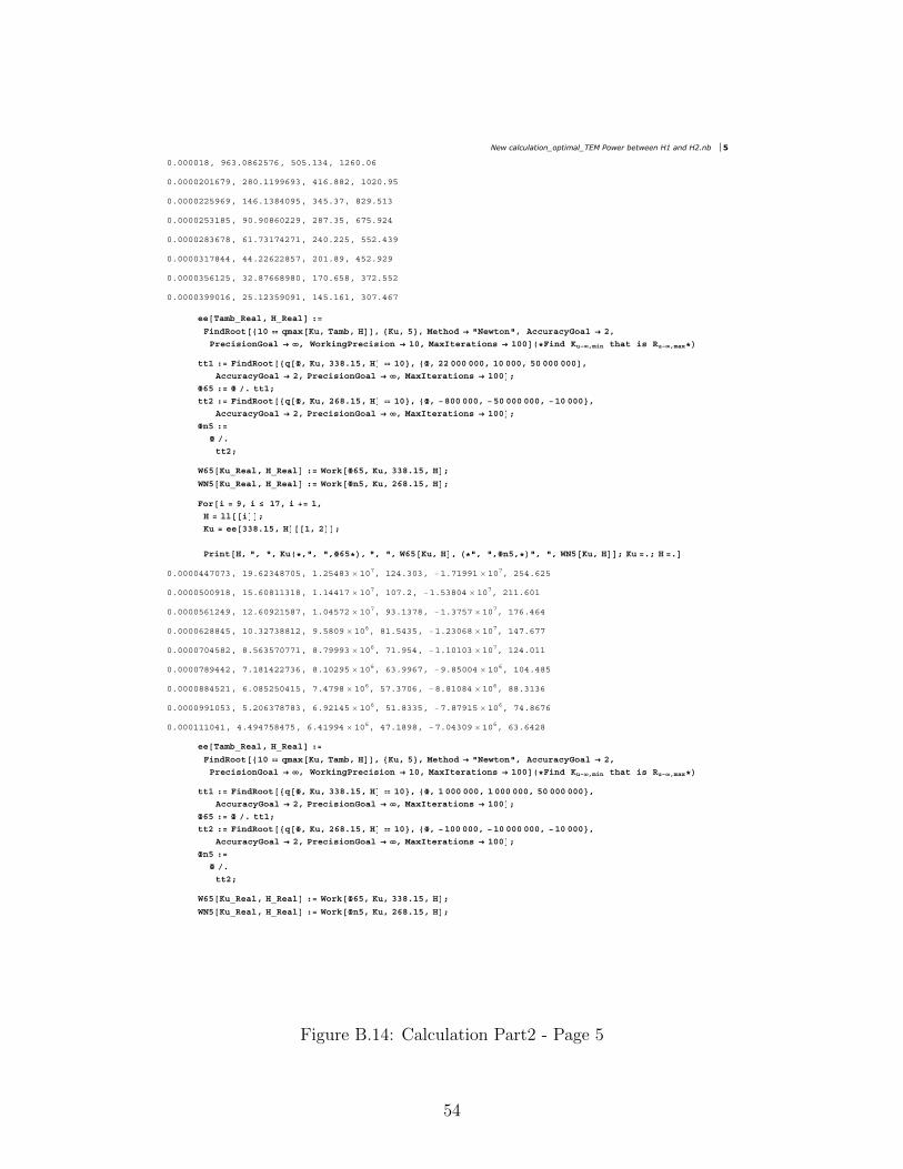
ðòððððïèô çêíòðèêîëéêô ëðëòïíìô ïîêðòðê
ðòððððîðïêéçô îèðòïïççêçíô ìïêòèèîô ïðîðòçë
ðòððððîîëçêçô ïìêòïíèìðçëô íìëòíéô èîçòëïí
ðòððððîëíïèëô çðòçðèêðîîçô îèéòíëô êéëòçîì
ðòððððîèíêéèô êïòéíïéìîéïô îìðòîîëô ëëîòìíç
ðòððððíïéèììô ììòîîêîîèëéô îðïòèçô ìëîòçîç
ðòððððíëêïîëô íîòèéêêèçèðô ïéðòêëèô íéîòëëî
ðòððððíççðïêô îëòïîíëçðçïô ïìëòïêïô íðéòìêé
»» Ì¿³¾Áλ¿´ô ØÁλ¿´ æã
Ú·²¼Î±±¬ ï𠯳¿¨ Õ«ô Ì¿³¾ô Ø ô Õ«ô ë ô Ó»¬¸±¼ r þÒ»©¬±²þô ß½½«®¿½§Ù±¿´ r îô
Ю»½··±²Ù±¿´ r ô ɱ®µ·²¹Ð®»½··±² r ïðô Ó¿¨×¬»®¿¬·±² r ïðð öÚ·²¼ Õ«óô³·² ¬¸¿¬ · Ϋóô³¿¨ö
¬¬ï æã Ú·²¼Î±±¬ ¯ Úô Õ«ô ííèòïëô Ø ïð ô Úô îî ððð ðððô ïð ðððô ëð ððð ððð ô
ß½½«®¿½§Ù±¿´ r îô Ю»½··±²Ù±¿´ r ô Ó¿¨×¬»®¿¬·±² r ïðð å
Úêë æã Ú ò ¬¬ïå
¬¬î æã Ú·²¼Î±±¬ ¯ Úô Õ«ô îêèòïëô Ø ïð ô Úô óèðð ðððô óëð ððð ðððô óïð ððð ô
ß½½«®¿½§Ù±¿´ r îô Ю»½··±²Ù±¿´ r ô Ó¿¨×¬»®¿¬·±² r ïðð å
Ú²ë æã
Ú ò
¬¬îå
Éêë Õ«Áλ¿´ô ØÁλ¿´ æã ɱ®µ Úêëô Õ«ô ííèòïëô Ø å
ÉÒë Õ«Áλ¿´ô ØÁλ¿´ æã ɱ®µ Ú²ëô Õ«ô îêèòïëô Ø å
Ú±® · ã çô · ïéô · õã ïô
Ø ã ´´ · å
Õ« ã »» ííèòïëô Ø ïô î å
Ю·²¬ Øô þô þô Õ« öôþô þôÚêëö ô þô þô Éêë Õ«ô Ø ô öþô þôÚ²ëôö þô þô ÉÒë Õ«ô Ø å Õ« ãòå Ø ãò
ðòððððììéðéíô ïçòêîíìèéðëô ïòîëìèí l ïðéô ïîìòíðíô óïòéïççï l ïðéô îëìòêîë
ðòððððëððçïèô ïëòêðèïïíïèô ïòïììïé l ïðéô ïðéòîô óïòëíèðì l ïðéô îïïòêðï
ðòððððëêïîìçô ïîòêðçîïëèéô ïòðìëéî l ïðéô çíòïíéèô óïòíéëé l ïðéô ïéêòìêì
ðòððððêîèèìëô ïðòíîéíèèïîô çòëèðç l ïðêô èïòëìíëô óïòîíðêè l ïðéô ïìéòêéé
ðòððððéðìëèîô èòëêíëéðééïô èòéçççí l ïðêô éïòçëìô óïòïðïðí l ïðéô ïîìòðïï
ðòððððéèçììîô éòïèïìîîéíêô èòïðîçë l ïðêô êíòççêéô óçòèëððì l ïðêô ïðìòìèë
ðòððððèèìëîïô êòðèëîëðìïëô éòìéçè l ïðêô ëéòíéðêô óèòèïðèì l ïðêô èèòíïíê
ðòððððççïðëíô ëòîðêíéèéèíô êòçîïìë l ïðêô ëïòèííëô óéòèéçïë l ïðêô éìòèêéê
ðòðððïïïðìïô ìòìçìéëèìéëô êòìïççì l ïðêô ìéòïèçèô óéòðìíðç l ïðêô êíòêìîè
»» Ì¿³¾Áλ¿´ô ØÁλ¿´ æã
Ú·²¼Î±±¬ ï𠯳¿¨ Õ«ô Ì¿³¾ô Ø ô Õ«ô ë ô Ó»¬¸±¼ r þÒ»©¬±²þô ß½½«®¿½§Ù±¿´ r îô
Ю»½··±²Ù±¿´ r ô ɱ®µ·²¹Ð®»½··±² r ïðô Ó¿¨×¬»®¿¬·±² r ïðð öÚ·²¼ Õ«óô³·² ¬¸¿¬ · Ϋóô³¿¨ö
¬¬ï æã Ú·²¼Î±±¬ ¯ Úô Õ«ô ííèòïëô Ø ïð ô Úô ï ððð ðððô ï ððð ðððô ëð ððð ððð ô
ß½½«®¿½§Ù±¿´ r îô Ю»½··±²Ù±¿´ r ô Ó¿¨×¬»®¿¬·±² r ïðð å
Úêë æã Ú ò ¬¬ïå
¬¬î æã Ú·²¼Î±±¬ ¯ Úô Õ«ô îêèòïëô Ø ïð ô Úô óïðð ðððô óïð ððð ðððô óïð ððð ô
ß½½«®¿½§Ù±¿´ r îô Ю»½··±²Ù±¿´ r ô Ó¿¨×¬»®¿¬·±² r ïðð å
Ú²ë æã
Ú ò
¬¬îå
Éêë Õ«Áλ¿´ô ØÁλ¿´ æã ɱ®µ Úêëô Õ«ô ííèòïëô Ø å
ÉÒë Õ«Áλ¿´ô ØÁλ¿´ æã ɱ®µ Ú²ëô Õ«ô îêèòïëô Ø å
New calculation_optimal_TEM Power between H1 and H2.nb 5
Figure B.14: Calculation Part2 - Page 5
54
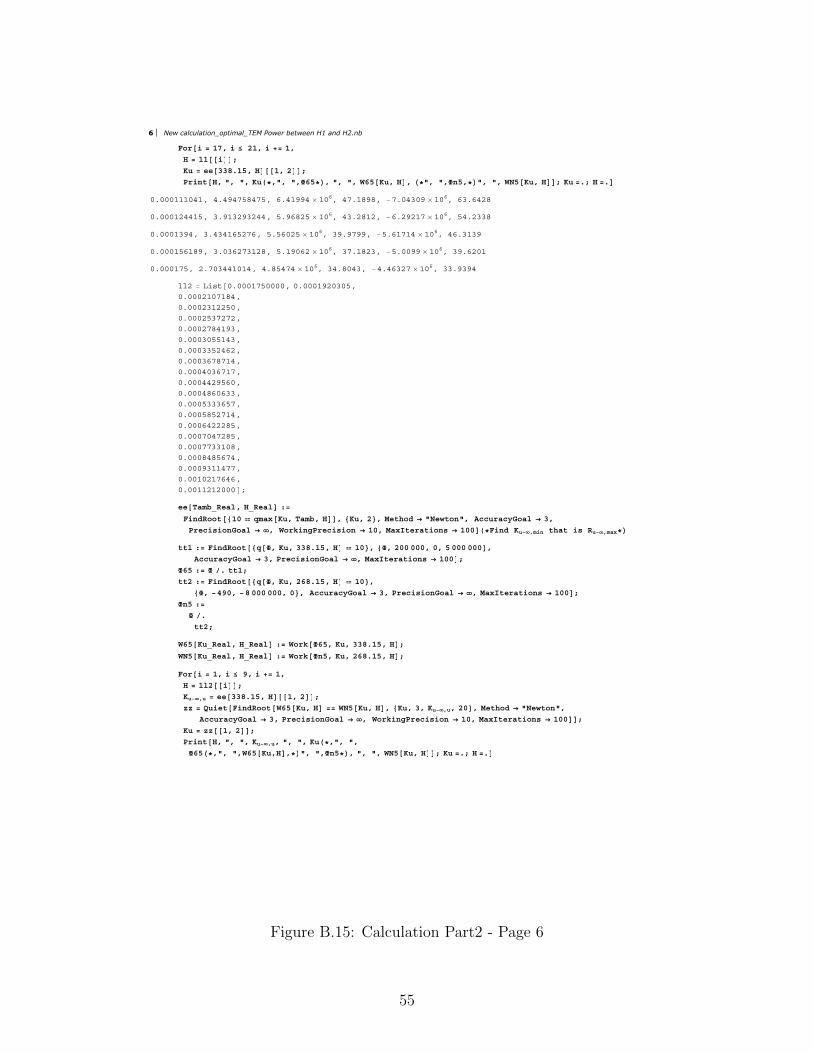
Ú±® · ã ïéô · îïô · õã ïô
Ø ã ´´ · å
Õ« ã »» ííèòïëô Ø ïô î å
Ю·²¬ Øô þô þô Õ« öôþô þôÚêëö ô þô þô Éêë Õ«ô Ø ô öþô þôÚ²ëôö þô þô ÉÒë Õ«ô Ø å Õ« ãòå Ø ãò
ðòðððïïïðìïô ìòìçìéëèìéëô êòìïççì l ïðêô ìéòïèçèô óéòðìíðç l ïðêô êíòêìîè
ðòðððïîììïëô íòçïíîçíîììô ëòçêèîë l ïðêô ìíòîèïîô óêòîçîïé l ïðêô ëìòîííè
ðòðððïíçìô íòìíìïêëîéêô ëòëêðîë l ïðêô íçòçéççô óëòêïéïì l ïðêô ìêòíïíç
ðòðððïëêïèçô íòðíêîéíïîèô ëòïçðêî l ïðêô íéòïèîíô óëòððçç l ïðêô íçòêîðï
ðòðððïéëô îòéðíììïðïìô ìòèëìéì l ïðêô íìòèðìíô óìòìêíîé l ïðêô ííòçíçì
´´î ã Ô·¬ ðòðððïéëððððô ðòðððïçîðíðëô
ðòðððîïðéïèìô
ðòðððîíïîîëðô
ðòðððîëíéîéîô
ðòðððîéèìïçíô
ðòðððíðëëïìíô
ðòðððííëîìêîô
ðòðððíêéèéïìô
ðòðððìðíêéïéô
ðòðððììîçëêðô
ðòðððìèêðêííô
ðòðððëíííêëéô
ðòðððëèëîéïìô
ðòðððêìîîîèëô
ðòðððéðìéîèëô
ðòðððééííïðèô
ðòðððèìèëêéìô
ðòðððçíïïìééô
ðòððïðîïéêìêô
ðòððïïîïîððð å
»» Ì¿³¾Áλ¿´ô ØÁλ¿´ æã
Ú·²¼Î±±¬ ï𠯳¿¨ Õ«ô Ì¿³¾ô Ø ô Õ«ô î ô Ó»¬¸±¼ r þÒ»©¬±²þô ß½½«®¿½§Ù±¿´ r íô
Ю»½··±²Ù±¿´ r ô ɱ®µ·²¹Ð®»½··±² r ïðô Ó¿¨×¬»®¿¬·±² r ïðð öÚ·²¼ Õ«óô³·² ¬¸¿¬ · Ϋóô³¿¨ö
¬¬ï æã Ú·²¼Î±±¬ ¯ Úô Õ«ô ííèòïëô Ø ïð ô Úô îðð ðððô ðô ë ððð ððð ô
ß½½«®¿½§Ù±¿´ r íô Ю»½··±²Ù±¿´ r ô Ó¿¨×¬»®¿¬·±² r ïðð å
Úêë æã Ú ò ¬¬ïå
¬¬î æã Ú·²¼Î±±¬ ¯ Úô Õ«ô îêèòïëô Ø ïð ô
Úô óìçðô óè ððð ðððô ð ô ß½½«®¿½§Ù±¿´ r íô Ю»½··±²Ù±¿´ r ô Ó¿¨×¬»®¿¬·±² r ïðð å
Ú²ë æã
Ú ò
¬¬îå
Éêë Õ«Áλ¿´ô ØÁλ¿´ æã ɱ®µ Úêëô Õ«ô ííèòïëô Ø å
ÉÒë Õ«Áλ¿´ô ØÁλ¿´ æã ɱ®µ Ú²ëô Õ«ô îêèòïëô Ø å
Ú±® · ã ïô · çô · õã ïô
Ø ã ´´î · å
Õ«óô« ã »» ííèòïëô Ø ïô î å
¦¦ ã Ï«·»¬ Ú·²¼Î±±¬ Éêë Õ«ô Ø ãã ÉÒë Õ«ô Ø ô Õ«ô íô Õ«óô«ô îð ô Ó»¬¸±¼ r þÒ»©¬±²þô
ß½½«®¿½§Ù±¿´ r íô Ю»½··±²Ù±¿´ r ô ɱ®µ·²¹Ð®»½··±² r ïðô Ó¿¨×¬»®¿¬·±² r ïðð å
Õ« ã ¦¦ ïô î å
Ю·²¬ Øô þô þô Õ«óô«ô þô þô Õ« öôþô þô
Úêë öôþô þôÉêë Õ«ôØ ôö þô þôÚ²ëö ô þô þô ÉÒë Õ«ô Ø å Õ« ãòå Ø ãò
6 New calculation_optimal_TEM Power between H1 and H2.nb
Figure B.15: Calculation Part2 - Page 6
55
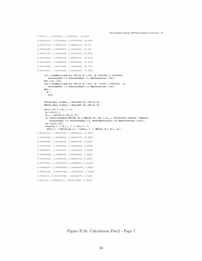
ðòðððïéëô îòéðíììïðîïô îòéðíçðçïîïô ííòçìîî
ðòðððïçîðíïô îòìéïðèçîçîô îòìééçëïéèìô îçòçéðí
ðòðððîïðéïèô îòîêèíïðïëëô îòîèèîïêïéíô îêòëïê
ðòðððîíïîîëô îòðçðêëêèéêô îòïîçìçíèìîô îíòëðë
ðòðððîëíéîéô ïòçíììêìíèëô ïòççéêééëîïô îðòèéìë
ðòðððîéèìïçô ïòéçêêçéíìðô ïòèèçëçéêéïô ïèòëéïì
ðòðððíðëëïìô ïòêéìèíììèïô ïòèðîçððîçíô ïêòëëðì
ðòðððííëîìêô ïòëêêééîëêêô ïòéíëçèìðèëô ïìòééíï
ðòðððíêéèéïô ïòìéðéëìëçëô ïòêèéçççëðéô ïíòîðêç
¬¬ï æã Ú·²¼Î±±¬ ¯ Úô Õ«ô ííèòïëô Ø ïð ô Úô î ìîð ðððô ðô ì ððð ððð ô
ß½½«®¿½§Ù±¿´ r îô Ю»½··±²Ù±¿´ r ô Ó¿¨×¬»®¿¬·±² r ïðð å
Úêë æã Ú ò ¬¬ïå
¬¬î æã Ú·²¼Î±±¬ ¯ Úô Õ«ô îêèòïëô Ø ïð ô Úô óîð ðððô óïð ððð ðððô óð ô
ß½½«®¿½§Ù±¿´ r îô Ю»½··±²Ù±¿´ r ô Ó¿¨×¬»®¿¬·±² r ïðð å
Ú²ë æã
Ú ò
¬¬îå
Éêë Õ«Áλ¿´ô ØÁλ¿´ æã ɱ®µ Úêëô Õ«ô ííèòïëô Ø å
ÉÒë Õ«Áλ¿´ô ØÁλ¿´ æã ɱ®µ Ú²ëô Õ«ô îêèòïëô Ø å
Ú±® · ã ïðô · îïô · õã ïô
Ø ã ´´î · å
Õ«óô« ã »» ííèòïëô Ø ïô î å
¦¦ ã Ï«·»¬ Ú·²¼Î±±¬ Éêë Õ«ô Ø ãã ÉÒë Õ«ô Ø ô Õ«ô ëô Õ«óô«ô çðð ððð ððð ô Ó»¬¸±¼ r þÒ»©¬±²þô
ß½½«®¿½§Ù±¿´ r ëô Ю»½··±²Ù±¿´ r ô ɱ®µ·²¹Ð®»½··±² r ïðô Ó¿¨×¬»®¿¬·±² r ïðð å
Õ« ã ¦¦ ïô î å
Ю·²¬ Øô þô þô Õ«óô«ô þô þô Õ« öôþô þô
Úêë öôþô þôÉêë Õ«ôØ ôö þô þôÚ²ëö ô þô þô ÉÒë Õ«ô Ø å Õ« ãòå Ø ãò
ðòðððìðíêéîô ïòíèëíðééðêô ïòêëèçðìêíðô ïïòèîíè
ðòðððììîçëêô ïòíðçïçèïêíô ïòêìçêìééçðô ïðòëççç
ðòðððìèêðêíô ïòîìïíçîíçîô ïòêêîìçéëçîô çòëïìèí
ðòðððëíííêêô ïòïèïðîéîðêô ïòéðïêèîêììô èòëëðèè
ðòðððëèëîéïô ïòïîéíèêïîîô ïòééìêïçîíðô éòêçîçê
ðòðððêìîîîçô ïòðéçèèïìêçô ïòèçììðêìèðô êòçîèðï
ðòðððéðìéîçô ïòðíèðìïîêìô îòðèëíëïéêìô êòîììéï
ðòðððééííïïô ïòððïëððíðëô îòíçêèîîèïìô ëòêííîè
ðòðððèìèëêéô ðòçêçççêðèîîô îòçììèìíðçëô ëòðèëîï
ðòðððçíïïìèô ðòçìííêçéèðëô ìòðéèëïíìçîô ìòëçíðè
ðòððïðîïéêô ðòçîïëéîçéìèô éòëìëðîêðéðô ìòïëðìî
ðòððïïîïîô ðòçðìêèîêïïïô ïèë èéíòèèìíô íòéëïëë
New calculation_optimal_TEM Power between H1 and H2.nb 7
Figure B.16: Calculation Part2 - Page 7
56

Calculation Part 3
57
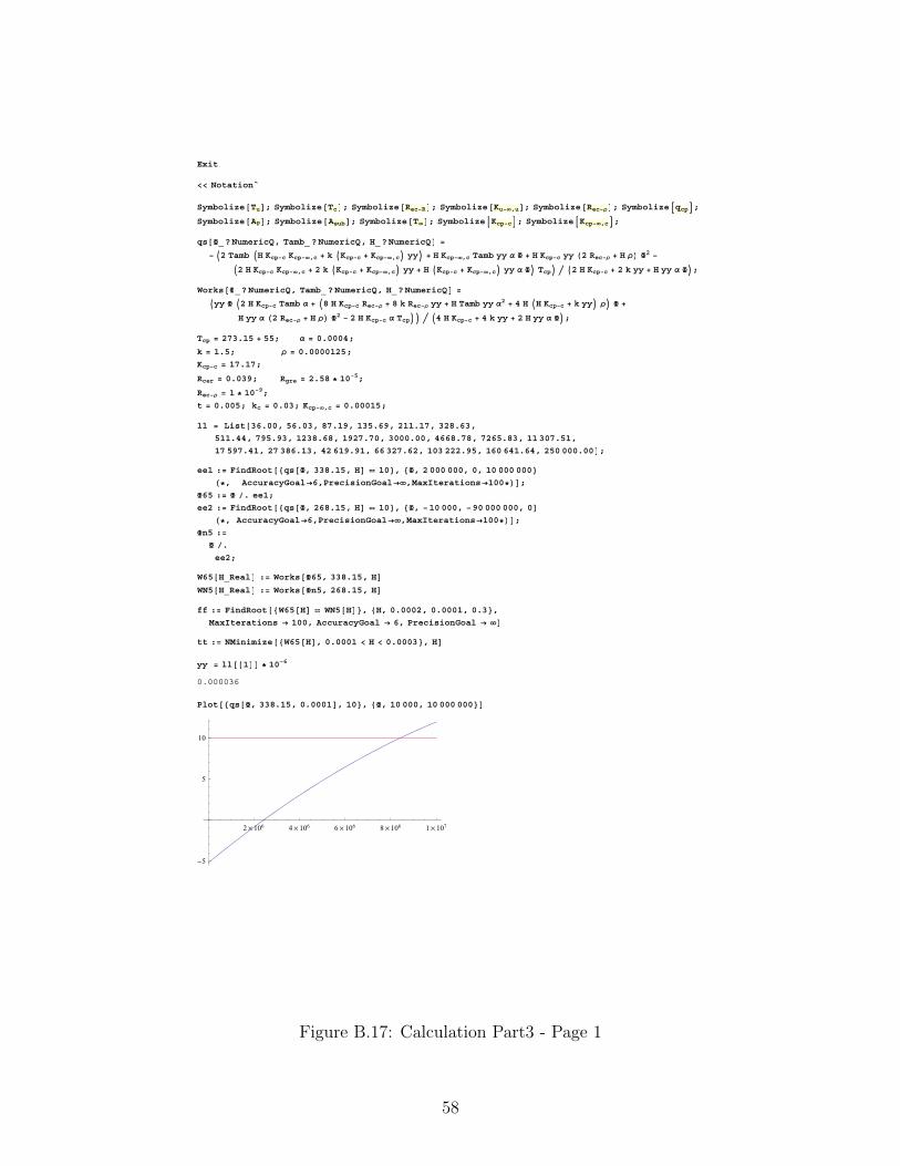
Û¨·¬
ää Ò±¬¿¬·±²À
ͧ³¾±´·¦» Ì« å ͧ³¾±´·¦» ̽ å ͧ³¾±´·¦» λ½óÎ å ͧ³¾±´·¦» Õ«óô« å ͧ³¾±´·¦» λ½ó® å ͧ³¾±´·¦» ¯½° å
ͧ³¾±´·¦» ßÐ å ͧ³¾±´·¦» ß«¾ å ͧ³¾±´·¦» Ì å ͧ³¾±´·¦» Õ½°ó½ å ͧ³¾±´·¦» Õ½°óô½ å
¯ ÚÁáÒ«³»®·½Ïô Ì¿³¾Á áÒ«³»®·½Ïô ØÁáÒ«³»®·½Ï ã
ó î Ì¿³¾ Ø Õ½°ó½ Õ½°óô½ õ µ Õ½°ó½ õ Õ½°óô½ §§ õ Ø Õ½°óô½ Ì¿³¾ §§ ¿ Ú õ Ø Õ½°ó½ §§ î λ½ó® õ Ø ® Úî ó
î Ø Õ½°ó½ Õ½°óô½ õ î µ Õ½°ó½ õ Õ½°óô½ §§ õ Ø Õ½°ó½ õ Õ½°óô½ §§ ¿ Ú Ì½° î Ø Õ½°ó½ õ î µ §§ õ Ø §§ ¿ Ú å
ɱ®µ ÚÁáÒ«³»®·½Ïô Ì¿³¾Á áÒ«³»®·½Ïô ØÁáÒ«³»®·½Ï ã
§§ Ú î Ø Õ½°ó½ Ì¿³¾ ¿ õ è Ø Õ½°ó½ λ½ó® õ è µ λ½ó® §§ õ Ø Ì¿³¾ §§ ¿î õ ì Ø Ø Õ½°ó½ õ µ §§ ® Ú õ
Ø §§ ¿ î λ½ó® õ Ø ® Úî ó î Ø Õ½°ó½ ¿ ̽° ì Ø Õ½°ó½ õ ì µ §§ õ î Ø §§ ¿ Ú å
̽° ã îéíòïë õ ëëå ¿ ã ðòðððìå
µ ã ïòëå ® ã ðòððððïîëå
Õ½°ó½ ã ïéòïéå
ν»® ã ðòðíçå ι®» ã îòëè ö ïðóëå
λ½ó® ã ï ö ïðóçå
¬ ã ðòððëå µ½ ã ðòðíå Õ½°óô½ ã ðòðððïëå
´´ ã Ô·¬ íêòððô ëêòðíô èéòïçô ïíëòêçô îïïòïéô íîèòêíô
ëïïòììô éçëòçíô ïîíèòêèô ïçîéòéðô íðððòððô ìêêèòéèô éîêëòèíô ïï íðéòëïô
ïé ëçéòìïô îé íèêòïíô ìî êïçòçïô êê íîéòêîô ïðí îîîòçëô ïêð êìïòêìô îëð ðððòðð å
»»ï æã Ú·²¼Î±±¬ ¯ Úô ííèòïëô Ø ïð ô Úô î ððð ðððô ðô ïð ððð ððð
öô ß½½«®¿½§Ù±¿´rêôЮ»½··±²Ù±¿´rôÓ¿¨×¬»®¿¬·±²rïððö å
Úêë æã Ú ò »»ïå
»»î æã Ú·²¼Î±±¬ ¯ Úô îêèòïëô Ø ïð ô Úô óïð ðððô óçð ððð ðððô ð
öô ß½½«®¿½§Ù±¿´rêôЮ»½··±²Ù±¿´rôÓ¿¨×¬»®¿¬·±²rïððö å
Ú²ë æã
Ú ò
»»îå
Éêë ØÁλ¿´ æã ɱ®µ Úêëô ííèòïëô Ø
ÉÒë ØÁλ¿´ æã ɱ®µ Ú²ëô îêèòïëô Ø
ºº æã Ú·²¼Î±±¬ Éêë Ø ÉÒë Ø ô Øô ðòðððîô ðòðððïô ðòí ô
Ó¿¨×¬»®¿¬·±² r ïððô ß½½«®¿½§Ù±¿´ r êô Ю»½··±²Ù±¿´ r
¬¬ æã ÒÓ·²·³·¦» Éêë Ø ô ðòðððï ä Ø ä ðòðððí ô Ø
§§ ã ´´ ï ö ïðóê
ðòððððíê
䱬 ¯ Úô ííèòïëô ðòðððï ô ïð ô Úô ïð ðððô ïð ððð ððð
î l ïðê ì l ïðê ê l ïðê è l ïðê ï l ïðé
óë
ë
ïð
Figure B.17: Calculation Part3 - Page 1
58

䱬 ɱ®µ Úêëô ííèòïëô Ø ô ɱ®µ Ú²ëô îêèòïëô Ø ô Øô ðòðððïô ðòðððí
ðòðððïë ðòðððîð ðòðððîë ðòðððíð
î
ì
ê
è
ïð
ïî
ºº
Ø r ðòðððïïðîêç
¬¬
èòìêèçíô Ø r ðòðððïíèçêê
»»ï æã Ú·²¼Î±±¬ ¯ Úô ííèòïëô Ø ïð ô Úô î ððð ðððô ðô ïð ððð ððð
öô ß½½«®¿½§Ù±¿´rêôЮ»½··±²Ù±¿´rôÓ¿¨×¬»®¿¬·±²rïððö å
Úêë æã Ú ò »»ïå
»»î æã Ú·²¼Î±±¬ ¯ Úô îêèòïëô Ø ïð ô Úô óï ððð ðððô óçðð ððð ðððô ð
öô ß½½«®¿½§Ù±¿´rêôЮ»½··±²Ù±¿´rôÓ¿¨×¬»®¿¬·±²rïððö å
Ú²ë æã
Ú ò
»»îå
Éêë ØÁλ¿´ æã ɱ®µ Úêëô ííèòïëô Ø
ÉÒë ØÁλ¿´ æã ɱ®µ Ú²ëô îêèòïëô Ø
ºº æã Ú·²¼Î±±¬ Éêë Ø ÉÒë Ø ô Øô ðòðððîô ðòðððïô ðòðï
öôÓ¿¨×¬»®¿¬·±²rïððôß½½«®¿½§Ù±¿´rêôЮ»½··±²Ù±¿´rö
¬¬ æã ÒÓ·²·³·¦» Éêë Ø ô ðòðððï ä Ø ä ðòððï ô Ø
Ï«·»¬ Ú±® · ã ïô · êô · õã ïô
§§ ã ´´ · ö ïðóêå
Ø ã ºº ïô î å
Éï ã ɱ®µ Úêëô ííèòïëô Ø å
Ø ãòå
Ю·²¬ ºº ïô î ô þ ôþô Éïô þ ôþô ¬¬ îô ïô î ô þ ôþô ¬¬ ï å §§ ãò
2 WTEM verses phiAsub_list plot.nb
Figure B.18: Calculation Part3 - Page 2
59
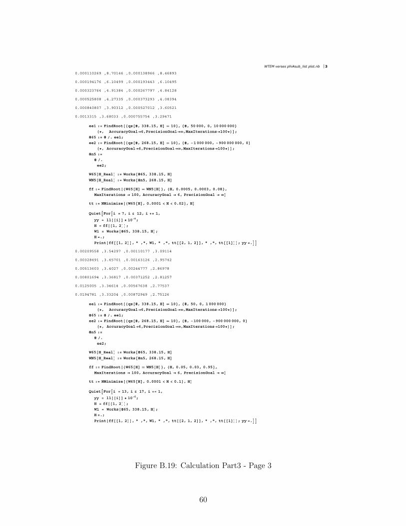
ðòðððïïðîêç ôèòéðïìê ôðòðððïíèçêê ôèòìêèçí
ðòðððïçìïéê ôêòïðìçç ôðòðððïçíììí ôêòïðìçë
ðòðððíîíéêì ôìòçïíèì ôðòðððîêééçé ôìòèìïîè
ðòðððëîëèðè ôìòîéííë ôðòðððíéíîçí ôìòðèíçì
ðòðððèìðèðé ôíòçðíïî ôðòðððëîéðïî ôíòêðëîï
ðòððïííïë ôíòêèðíí ôðòðððéëëéëì ôíòîçìéï
»»ï æã Ú·²¼Î±±¬ ¯ Úô ííèòïëô Ø ïð ô Úô ëð ðððô ðô ïð ððð ððð
öô ß½½«®¿½§Ù±¿´rêôЮ»½··±²Ù±¿´rôÓ¿¨×¬»®¿¬·±²rïððö å
Úêë æã Ú ò »»ïå
»»î æã Ú·²¼Î±±¬ ¯ Úô îêèòïëô Ø ïð ô Úô óï ððð ðððô óçðð ððð ðððô ð
öô ß½½«®¿½§Ù±¿´rêôЮ»½··±²Ù±¿´rôÓ¿¨×¬»®¿¬·±²rïððö å
Ú²ë æã
Ú ò
»»îå
Éêë ØÁλ¿´ æã ɱ®µ Úêëô ííèòïëô Ø
ÉÒë ØÁλ¿´ æã ɱ®µ Ú²ëô îêèòïëô Ø
ºº æã Ú·²¼Î±±¬ Éêë Ø ÉÒë Ø ô Øô ðòðððëô ðòðððíô ðòðè ô
Ó¿¨×¬»®¿¬·±² r ïððô ß½½«®¿½§Ù±¿´ r êô Ю»½··±²Ù±¿´ r
¬¬ æã ÒÓ·²·³·¦» Éêë Ø ô ðòðððï ä Ø ä ðòðî ô Ø
Ï«·»¬ Ú±® · ã éô · ïîô · õã ïô
§§ ã ´´ · ö ïðóêå
Ø ã ºº ïô î å
Éï ã ɱ®µ Úêëô ííèòïëô Ø å
Ø ãòå
Ю·²¬ ºº ïô î ô þ ôþô Éïô þ ôþô ¬¬ îô ïô î ô þ ôþô ¬¬ ï å §§ ãò
ðòððîðçëëè ôíòëìîçé ôðòððïïðïéé ôíòðçïïì
ðòððíîèìçï ôíòìëéðï ôðòððïêíïîê ôîòçëéìî
ðòððëïíêðí ôíòìðîé ôðòððîììééé ôîòèêçéè
ðòððèðïêçì ôíòíêèïé ôðòððíéïîëî ôîòèïîëé
ðòðïîëððë ôíòíìêïì ôðòððëêéêíè ôîòééëíé
ðòðïçìéèï ôíòííîðì ôðòððèéîçìç ôîòéëïîê
»»ï æã Ú·²¼Î±±¬ ¯ Úô ííèòïëô Ø ïð ô Úô ëðô ðô ï ððð ððð
öô ß½½«®¿½§Ù±¿´rêôЮ»½··±²Ù±¿´rôÓ¿¨×¬»®¿¬·±²rïððö å
Úêë æã Ú ò »»ïå
»»î æã Ú·²¼Î±±¬ ¯ Úô îêèòïëô Ø ïð ô Úô óïðð ðððô óçðð ððð ðððô ð
öô ß½½«®¿½§Ù±¿´rêôЮ»½··±²Ù±¿´rôÓ¿¨×¬»®¿¬·±²rïððö å
Ú²ë æã
Ú ò
»»îå
Éêë ØÁλ¿´ æã ɱ®µ Úêëô ííèòïëô Ø
ÉÒë ØÁλ¿´ æã ɱ®µ Ú²ëô îêèòïëô Ø
ºº æã Ú·²¼Î±±¬ Éêë Ø ÉÒë Ø ô Øô ðòðëô ðòðíô ðòçë ô
Ó¿¨×¬»®¿¬·±² r ïððô ß½½«®¿½§Ù±¿´ r êô Ю»½··±²Ù±¿´ r
¬¬ æã ÒÓ·²·³·¦» Éêë Ø ô ðòðððï ä Ø ä ðòï ô Ø
Ï«·»¬ Ú±® · ã ïíô · ïéô · õã ïô
§§ ã ´´ · ö ïðóêå
Ø ã ºº ïô î å
Éï ã ɱ®µ Úêëô ííèòïëô Ø å
Ø ãòå
Ю·²¬ ºº ïô î ô þ ôþô Éïô þ ôþô ¬¬ îô ïô î ô þ ôþô ¬¬ ï å §§ ãò
WTEM verses phiAsub_list plot.nb 3
Figure B.19: Calculation Part3 - Page 3
60

ðòðíðííéï ôíòíîíðï ôðòðïíìéèé ôîòéíëêç
ðòðìéîíêë ôíòíïéîî ôðòðîðèêèí ôîòéîëêì
ðòðéíëíêí ôíòíïíëï ôðòðíîíêéì ôîòéïçïê
ðòïïììêê ôíòíïïïî ôðòðëðîêîí ôîòéïë
ðòïéèïêí ôíòíðçëç ôðòðéèïïïï ôîòéïîíî
ºº æã Ú·²¼Î±±¬ Éêë Ø ÉÒë Ø ô Øô ðòðëô ðòðíô ëòçë ô
Ó¿¨×¬»®¿¬·±² r ïððô ß½½«®¿½§Ù±¿´ r êô Ю»½··±²Ù±¿´ r
¬¬ æã ÒÓ·²·³·¦» Éêë Ø ô ðòðððï ä Ø ä ðòê ô Ø
Ï«·»¬ Ú±® · ã ïèô · îïô · õã ïô
§§ ã ´´ · ö ïðóêå
Ø ã ºº ïô î å
Éï ã ɱ®µ Úêëô ííèòïëô Ø å
Ø ãòå
Ю·²¬ ºº ïô î ô þ ôþô Éïô þ ôþô ¬¬ îô ïô î ô þ ôþô ¬¬ ï å §§ ãò
ðòîééîçï ôíòíðèê ôðòïîïìëï ôîòéïðê
ðòìíïëêï ôíòíðéçé ôðòïèèèçè ôîòéðçìç
ðòêéïêìë ôíòíðéëê ôðòîçíèêì ôîòéðèéè
ïòðìëîè ôíòíðéí ôðòìëéîïé ôîòéðèíî
4 WTEM verses phiAsub_list plot.nb
Figure B.20: Calculation Part3 - Page 4
61

APPENDIX C
Thermocouple Welding and Calibration
Temperature measurement is very important in experimental heat transfer as temper-
ature is a key variable in any heat transfer problem. Depending on the media, operating
range and application, temperature can be measured by many different methods. Thermo-
couples are the most widely used of all temperature sensors due to their reliability and low
cost. As high accuracy thermocouples are required in the future experimental work, numer-
ous thermocouples were made and calibrated against NIST-traceable thermistor probes in a
custom-built laboratory apparatus.
Introduction and Background
Theory of Thermocouples
Thermocouples consist essentially of two dissimilar conductors electrically joined together
at one end. The other ends of the conductors are connected directly to a temperature-
compensated voltmeter or to an intermediate reference junction at a precisely controlled
temperature. In any case, in order to use a thermocouple to measure temperature, one end
must be maintained at a known temperature, the so-called reference temperature, TR. The
other junction, which is placed in contact with the body or fluid of interest of unknown
temperature, is called the measurement junction, T j, as in Fig. C.1. The electromotive force
63
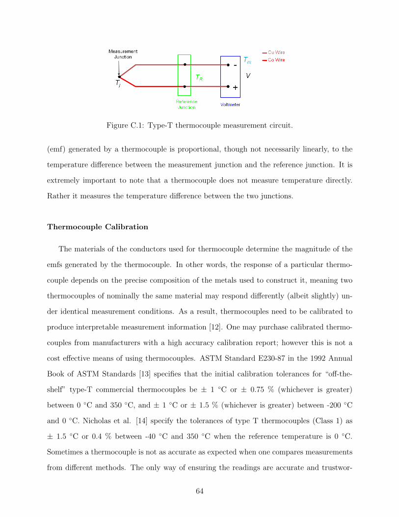
Figure C.1: Type-T thermocouple measurement circuit.
(emf) generated by a thermocouple is proportional, though not necessarily linearly, to the
temperature difference between the measurement junction and the reference junction. It is
extremely important to note that a thermocouple does not measure temperature directly.
Rather it measures the temperature difference between the two junctions.
Thermocouple Calibration
The materials of the conductors used for thermocouple determine the magnitude of the
emfs generated by the thermocouple. In other words, the response of a particular thermo-
couple depends on the precise composition of the metals used to construct it, meaning two
thermocouples of nominally the same material may respond differently (albeit slightly) un-
der identical measurement conditions. As a result, thermocouples need to be calibrated to
produce interpretable measurement information [12]. One may purchase calibrated thermo-
couples from manufacturers with a high accuracy calibration report; however this is not a
cost effective means of using thermocouples. ASTM Standard E230-87 in the 1992 Annual
Book of ASTM Standards [13] specifies that the initial calibration tolerances for “off-the-
shelf” type-T commercial thermocouples be ± 1 C or ± 0.75 % (whichever is greater)
between 0 C and 350 C, and ± 1 C or ± 1.5 % (whichever is greater) between -200 C
and 0 C. Nicholas et al. [14] specify the tolerances of type T thermocouples (Class 1) as
± 1.5 C or 0.4 % between -40 C and 350 C when the reference temperature is 0 C.
Sometimes a thermocouple is not as accurate as expected when one compares measurements
from different methods. The only way of ensuring the readings are accurate and trustwor-
64
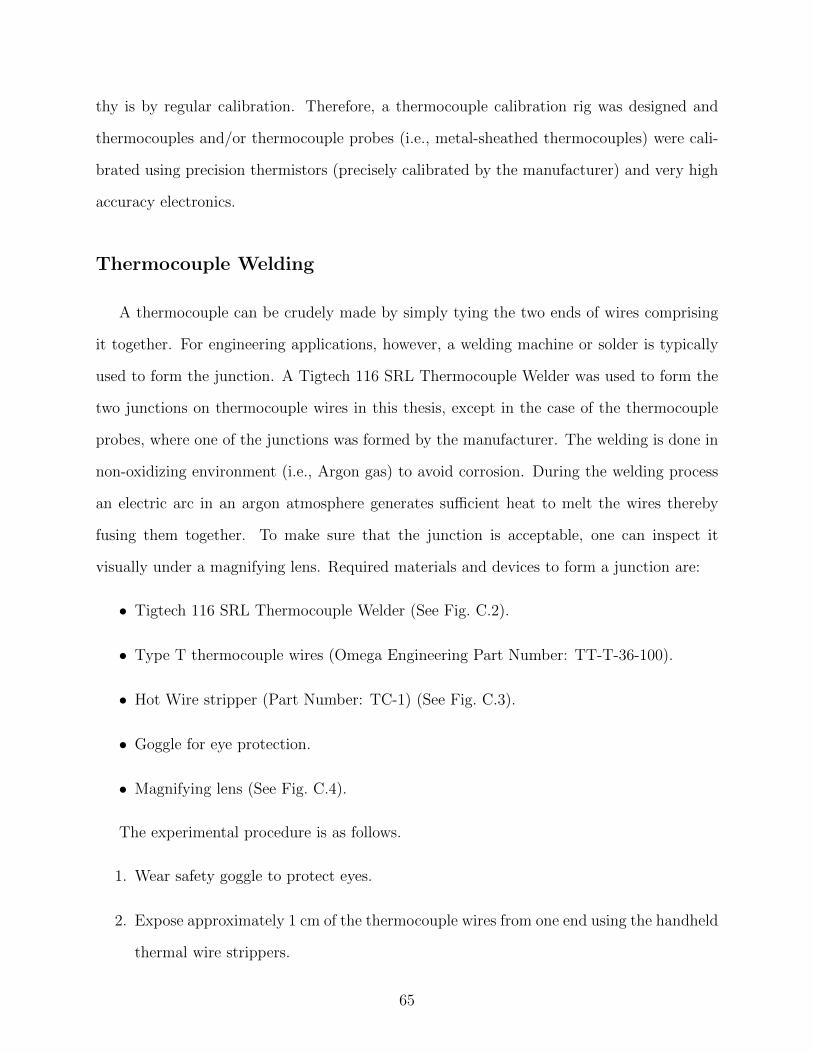
thy is by regular calibration. Therefore, a thermocouple calibration rig was designed and
thermocouples and/or thermocouple probes (i.e., metal-sheathed thermocouples) were cali-
brated using precision thermistors (precisely calibrated by the manufacturer) and very high
accuracy electronics.
Thermocouple Welding
A thermocouple can be crudely made by simply tying the two ends of wires comprising
it together. For engineering applications, however, a welding machine or solder is typically
used to form the junction. A Tigtech 116 SRL Thermocouple Welder was used to form the
two junctions on thermocouple wires in this thesis, except in the case of the thermocouple
probes, where one of the junctions was formed by the manufacturer. The welding is done in
non-oxidizing environment (i.e., Argon gas) to avoid corrosion. During the welding process
an electric arc in an argon atmosphere generates sufficient heat to melt the wires thereby
fusing them together. To make sure that the junction is acceptable, one can inspect it
visually under a magnifying lens. Required materials and devices to form a junction are:
• Tigtech 116 SRL Thermocouple Welder (See Fig. C.2).
• Type T thermocouple wires (Omega Engineering Part Number: TT-T-36-100).
• Hot Wire stripper (Part Number: TC-1) (See Fig. C.3).
• Goggle for eye protection.
• Magnifying lens (See Fig. C.4).
The experimental procedure is as follows.
1. Wear safety goggle to protect eyes.
2. Expose approximately 1 cm of the thermocouple wires from one end using the handheld
thermal wire strippers.
65

Figure C.2: Tigtech 116 SRL Thermocouple welder.
Figure C.3: Handheld thermal wire strippers.
66
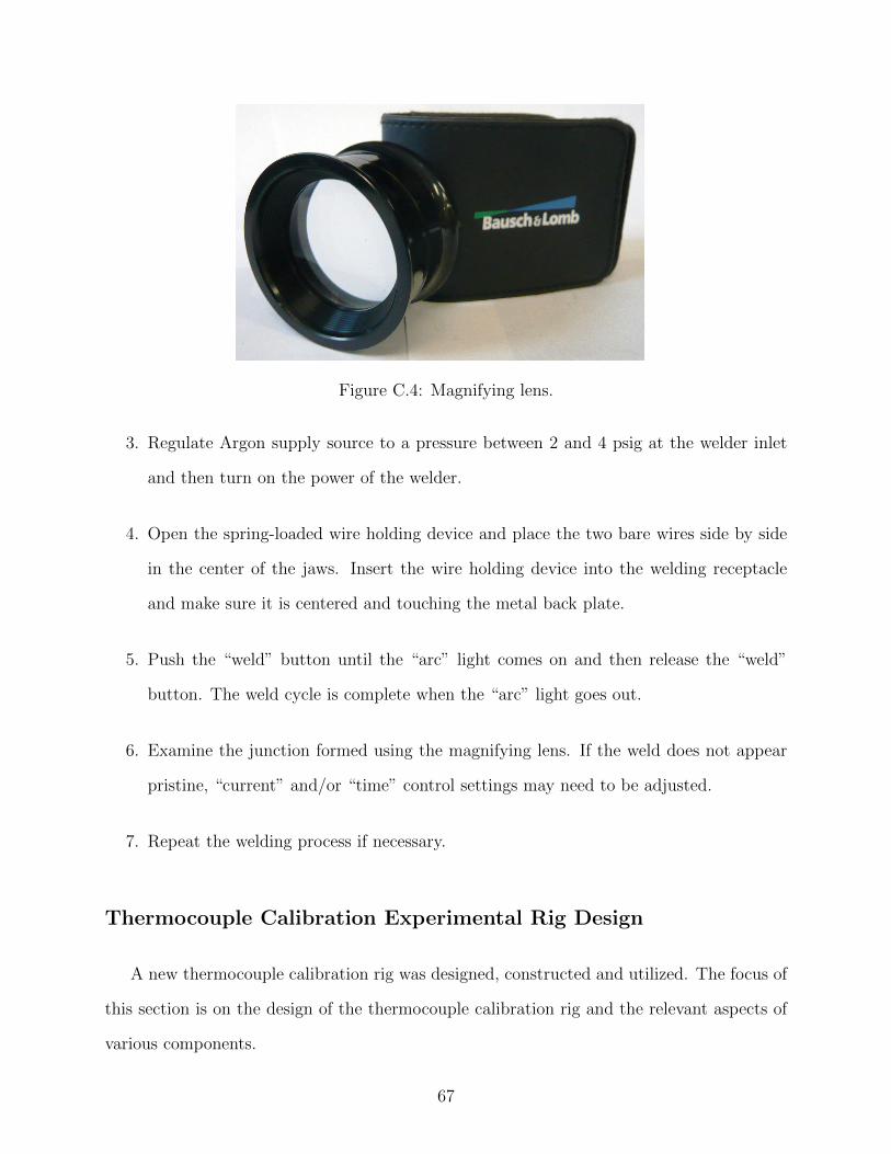
Figure C.4: Magnifying lens.
3. Regulate Argon supply source to a pressure between 2 and 4 psig at the welder inlet
and then turn on the power of the welder.
4. Open the spring-loaded wire holding device and place the two bare wires side by side
in the center of the jaws. Insert the wire holding device into the welding receptacle
and make sure it is centered and touching the metal back plate.
5. Push the “weld” button until the “arc” light comes on and then release the “weld”
button. The weld cycle is complete when the “arc” light goes out.
6. Examine the junction formed using the magnifying lens. If the weld does not appear
pristine, “current” and/or “time” control settings may need to be adjusted.
7. Repeat the welding process if necessary.
Thermocouple Calibration Experimental Rig Design
A new thermocouple calibration rig was designed, constructed and utilized. The focus of
this section is on the design of the thermocouple calibration rig and the relevant aspects of
various components.
67

Design Requirements
The first step in the design of the thermocouple calibration rig was to identify the key
design requirements that the system must meet. They were as follows.
• Measurement Junction Temperature. The measurement junction temperature should
be able to be stabilized for a certain length of time at any required temperature as per
control by a constant temperature bath or other sources. The measurement junction
should be isothermal and its temperature should not be affected by a temperature
gradient along the thermocouples wires.
• Reference Junction Temperature. The reference junction must be maintained at a
constant chosen temperature and it should be controlled to be a higher accuracy than
that expected from the thermocouple calibration.
• Readout Instruments. The resolution and accuracy of the voltmeters for reading the
voltages produced by thermocouples must produce a very small uncertainty in the
temperature measurement.
• Wiring Connection to Readout Instruments. Copper wires should be used between the
reference junction and readout instruments.
• Calibration Range and Interval. Calibration temperature range is from -10 C to 90 C.
Thermocouples need to be calibrated in sufficiently small temperature intervals such
that linear interpolation is valid between adjacent calibration points on the calibration
curve.
Experiment Rig Schematic
A schematic of the experimental rig is shown in Fig. C.5. The use of an ice bath (mixture
of melting shaved ice and water) to enclose the reference junction has the advantage of
simplicity in that its temperature is (i.e., 0 C) is precisely known. Ice baths are also cost
68
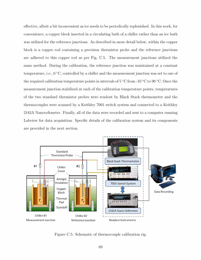
effective, albeit a bit inconvenient as ice needs to be periodically replenished. In this work, for
convenience, a copper block inserted in a circulating bath of a chiller rather than an ice bath
was utilized for the reference junctions. As described in more detail below, within the copper
block is a copper rod containing a precision thermistor probe and the reference junctions
are adhered to this copper rod as per Fig. C.5. The measurement junctions utilized the
same method. During the calibration, the reference junction was maintained at a constant
temperature, i.e., 0 C, controlled by a chiller and the measurement junction was set to one of
the required calibration temperature points in intervals of 5 C from -10 C to 90 C. Once the
measurement junction stabilized at each of the calibration temperature points, temperatures
of the two standard thermistor probes were readout by Black Stack thermometer and the
thermocouples were scanned by a Keithley 7001 switch system and connected to a Keithley
2182A Nanovoltmeter. Finally, all of the data were recorded and sent to a computer running
Labview for data acquisition. Specific details of the calibration system and its components
are provided in the next section.
Figure C.5: Schematic of thermocouple calibration rig.
69
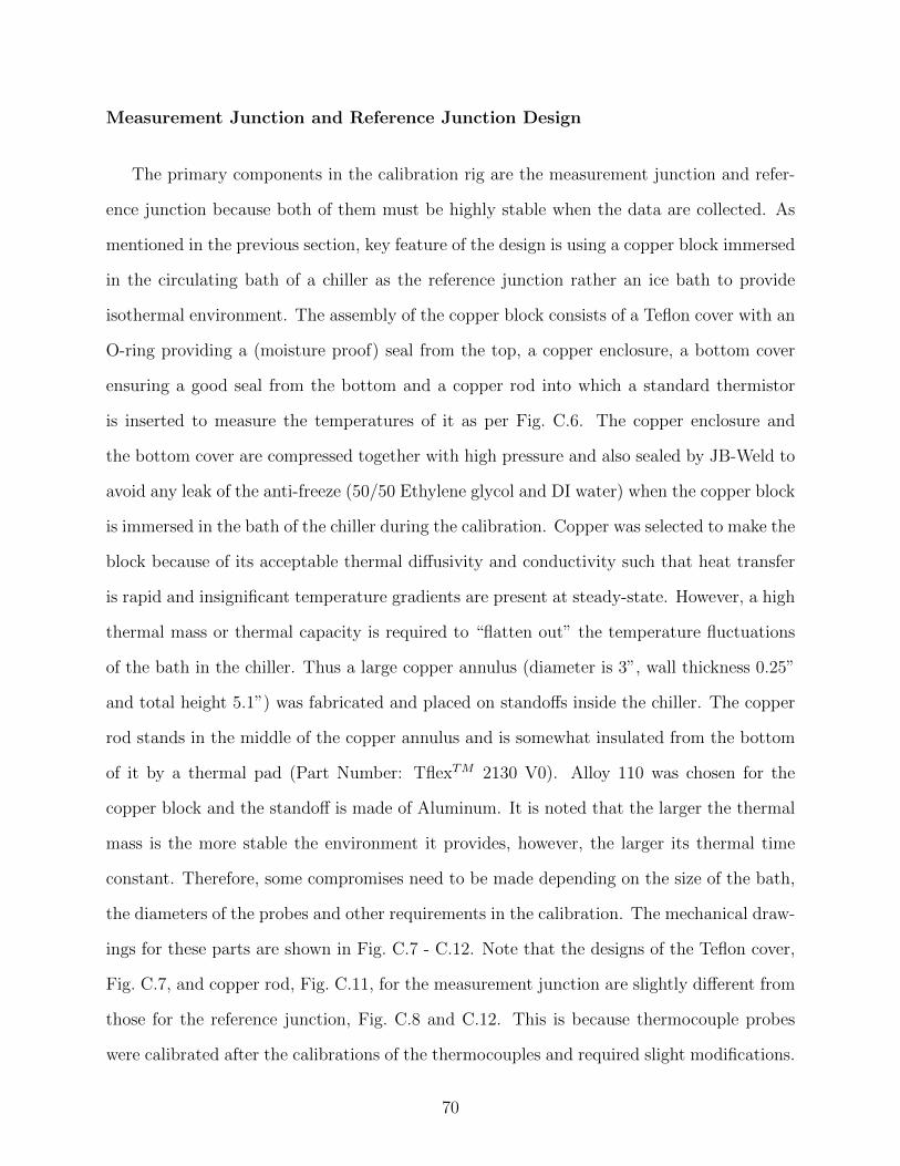
Measurement Junction and Reference Junction Design
The primary components in the calibration rig are the measurement junction and refer-
ence junction because both of them must be highly stable when the data are collected. As
mentioned in the previous section, key feature of the design is using a copper block immersed
in the circulating bath of a chiller as the reference junction rather an ice bath to provide
isothermal environment. The assembly of the copper block consists of a Teflon cover with an
O-ring providing a (moisture proof) seal from the top, a copper enclosure, a bottom cover
ensuring a good seal from the bottom and a copper rod into which a standard thermistor
is inserted to measure the temperatures of it as per Fig. C.6. The copper enclosure and
the bottom cover are compressed together with high pressure and also sealed by JB-Weld to
avoid any leak of the anti-freeze (50/50 Ethylene glycol and DI water) when the copper block
is immersed in the bath of the chiller during the calibration. Copper was selected to make the
block because of its acceptable thermal diffusivity and conductivity such that heat transfer
is rapid and insignificant temperature gradients are present at steady-state. However, a high
thermal mass or thermal capacity is required to “flatten out” the temperature fluctuations
of the bath in the chiller. Thus a large copper annulus (diameter is 3”, wall thickness 0.25”
and total height 5.1”) was fabricated and placed on standoffs inside the chiller. The copper
rod stands in the middle of the copper annulus and is somewhat insulated from the bottom
of it by a thermal pad (Part Number: TflexTM 2130 V0). Alloy 110 was chosen for the
copper block and the standoff is made of Aluminum. It is noted that the larger the thermal
mass is the more stable the environment it provides, however, the larger its thermal time
constant. Therefore, some compromises need to be made depending on the size of the bath,
the diameters of the probes and other requirements in the calibration. The mechanical draw-
ings for these parts are shown in Fig. C.7 - C.12. Note that the designs of the Teflon cover,
Fig. C.7, and copper rod, Fig. C.11, for the measurement junction are slightly different from
those for the reference junction, Fig. C.8 and C.12. This is because thermocouple probes
were calibrated after the calibrations of the thermocouples and required slight modifications.
70

Figure C.6: Copper annulus assembly design for measurement junction
In Fig. C.12, extra holes with different diameters were drilled for the thermocouple probe
calibration. Finally, the temperatures of these two junctions are controlled by two chillers,
NESLab Model RTE7, which can operate from -24 C to 150 C with an accuracy of ± 0.1
C.
71
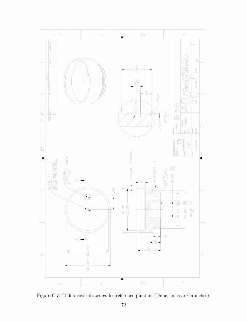
Figure C.7: Teflon cover drawings for reference junction (Dimensions are in inches).
72
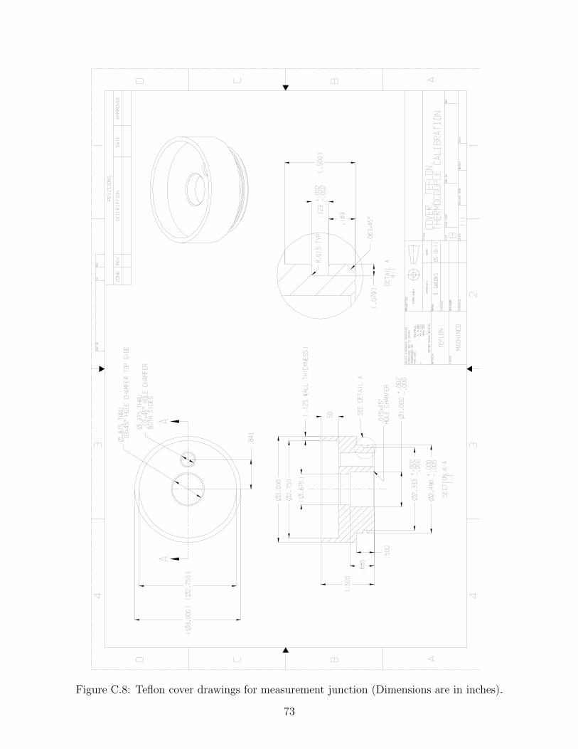
Figure C.8: Teflon cover drawings for measurement junction (Dimensions are in inches).
73
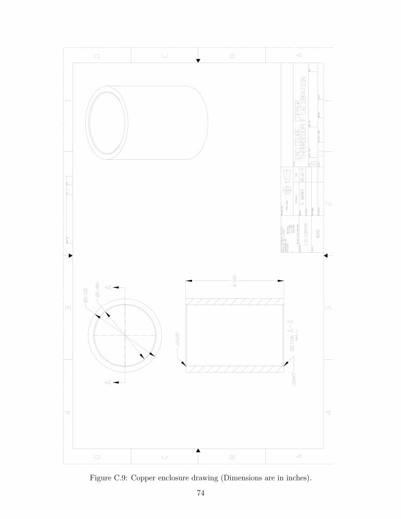
Figure C.9: Copper enclosure drawing (Dimensions are in inches).
74
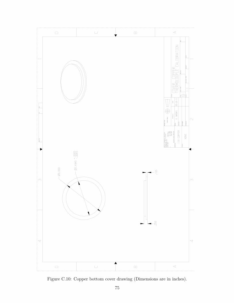
Figure C.10: Copper bottom cover drawing (Dimensions are in inches).
75
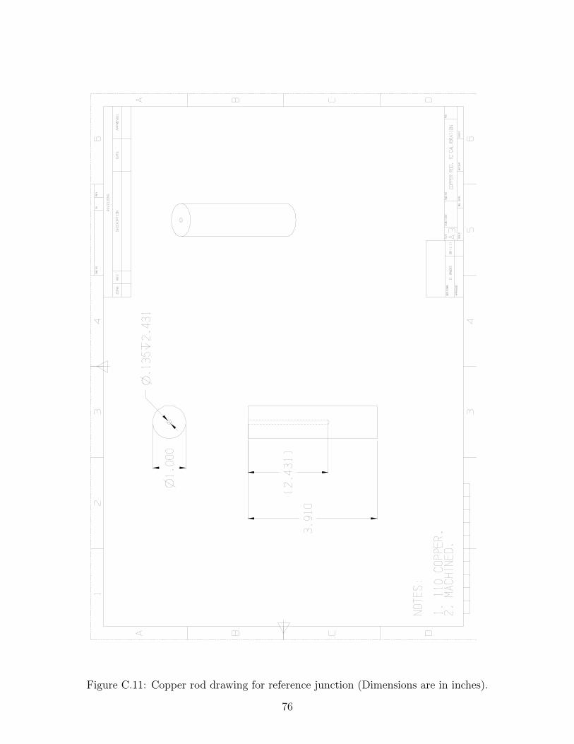
Figure C.11: Copper rod drawing for reference junction (Dimensions are in inches).
76

Figure C.12: Copper rod drawing for measurement junction (Dimensions are in inches).
77
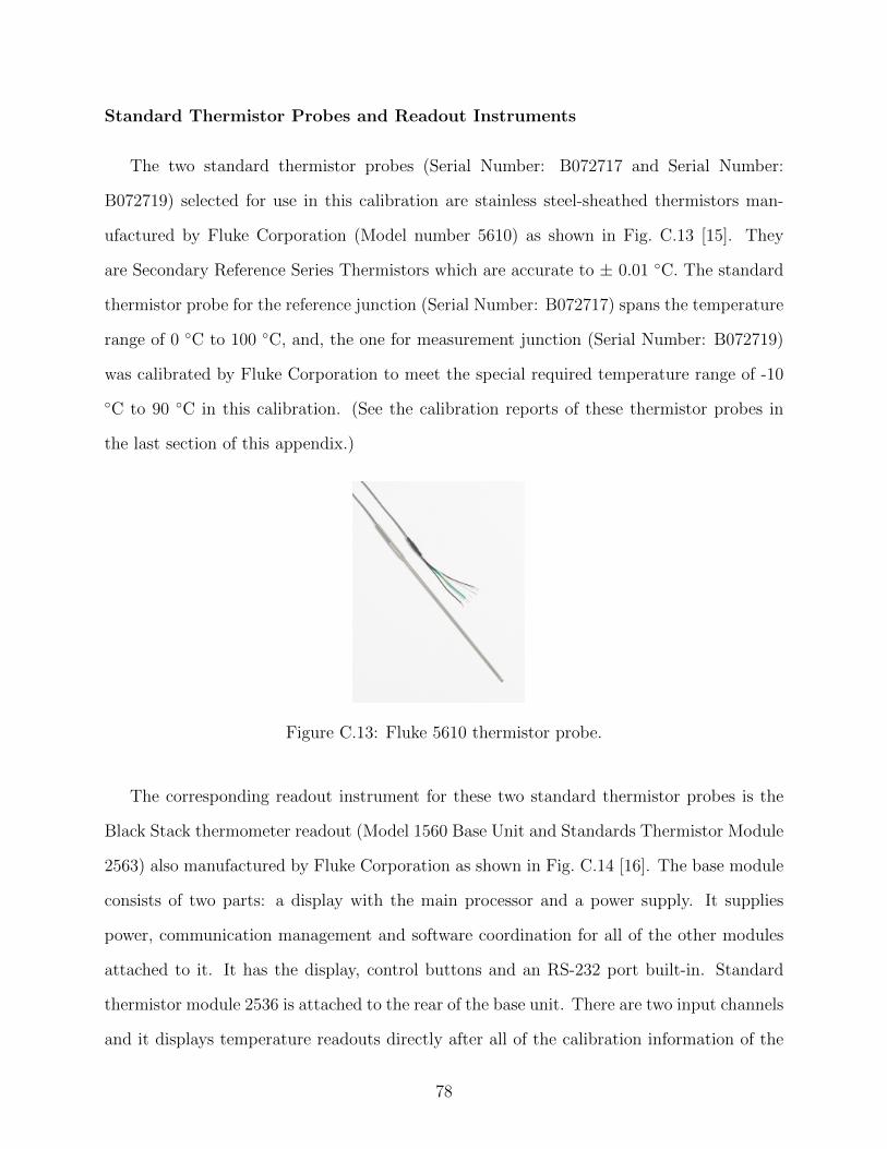
Standard Thermistor Probes and Readout Instruments
The two standard thermistor probes (Serial Number: B072717 and Serial Number:
B072719) selected for use in this calibration are stainless steel-sheathed thermistors man-
ufactured by Fluke Corporation (Model number 5610) as shown in Fig. C.13 [15]. They
are Secondary Reference Series Thermistors which are accurate to ± 0.01 C. The standard
thermistor probe for the reference junction (Serial Number: B072717) spans the temperature
range of 0 C to 100 C, and, the one for measurement junction (Serial Number: B072719)
was calibrated by Fluke Corporation to meet the special required temperature range of -10
C to 90 C in this calibration. (See the calibration reports of these thermistor probes in
the last section of this appendix.)
Figure C.13: Fluke 5610 thermistor probe.
The corresponding readout instrument for these two standard thermistor probes is the
Black Stack thermometer readout (Model 1560 Base Unit and Standards Thermistor Module
2563) also manufactured by Fluke Corporation as shown in Fig. C.14 [16]. The base module
consists of two parts: a display with the main processor and a power supply. It supplies
power, communication management and software coordination for all of the other modules
attached to it. It has the display, control buttons and an RS-232 port built-in. Standard
thermistor module 2536 is attached to the rear of the base unit. There are two input channels
and it displays temperature readouts directly after all of the calibration information of the
78

Figure C.14: Black stack overview.
thermistors are entered into it. The Black Stack readout has a temperature accuracy of ±
0.0013 C at 0 C and ± 0.0015 C at 75 C with a resolution of 0.0001 C. The report of
calibration is provided in the last section of this appendix. The combined accuracy of the
Black Stack in combination with the thermistor probes is ± 0.0113 C at 0 C and ± 0.0115
C at 75 C.1
The key readout instrument for the thermocouples selected is a nanovoltmeter (Model
2182A) made by Keithley as shown in Fig. C.15. It combines the accuracy of a digital
multimeter with low noise at high speeds for high-precision metrology applications. Its low
noise, high signal observation time, fast measurement rates, and 2 ppm (ppm = parts per
million) accuracy provide the most cost-effective meter available today. Voltage specifications
of it are shown in Fig. C.16. A range of 10 mV in Channel 1 with a resolution of 1 nV was
utilized. The accuracy for 2 years in voltage is ± 0.040 µV at 0 V and ± 0.192 µV at 3.134
mV and the corresponding accuracy in temperature is 0.0010 C at 0 C and 0.00432 C at
75 C. The combined accuracy of the Black Stack in combination with the thermistor probes
and the Keithley Naonovoltmeter is 0.0123 C at 0 C and 0.01582 C at 75 C. Because
40 thermocouples were calibrated at the same time, a switch system (Model 7011) with a
1The accuracy is conservatively estimated here and next in the total combination accuracy because it isalready high enough for the purpose of this thermocouple calibration.
79
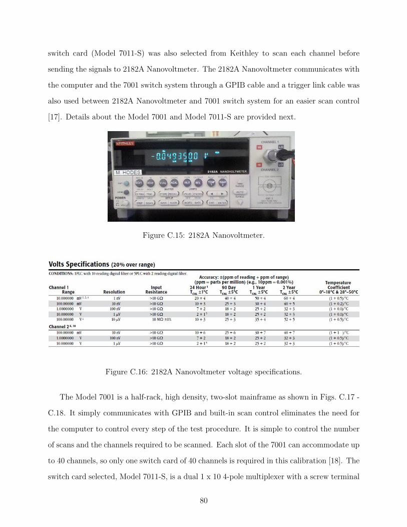
switch card (Model 7011-S) was also selected from Keithley to scan each channel before
sending the signals to 2182A Nanovoltmeter. The 2182A Nanovoltmeter communicates with
the computer and the 7001 switch system through a GPIB cable and a trigger link cable was
also used between 2182A Nanovoltmeter and 7001 switch system for an easier scan control
[17]. Details about the Model 7001 and Model 7011-S are provided next.
Figure C.15: 2182A Nanovoltmeter.
Figure C.16: 2182A Nanovoltmeter voltage specifications.
The Model 7001 is a half-rack, high density, two-slot mainframe as shown in Figs. C.17 -
C.18. It simply communicates with GPIB and built-in scan control eliminates the need for
the computer to control every step of the test procedure. It is simple to control the number
of scans and the channels required to be scanned. Each slot of the 7001 can accommodate up
to 40 channels, so only one switch card of 40 channels is required in this calibration [18]. The
switch card selected, Model 7011-S, is a dual 1 x 10 4-pole multiplexer with a screw terminal
80
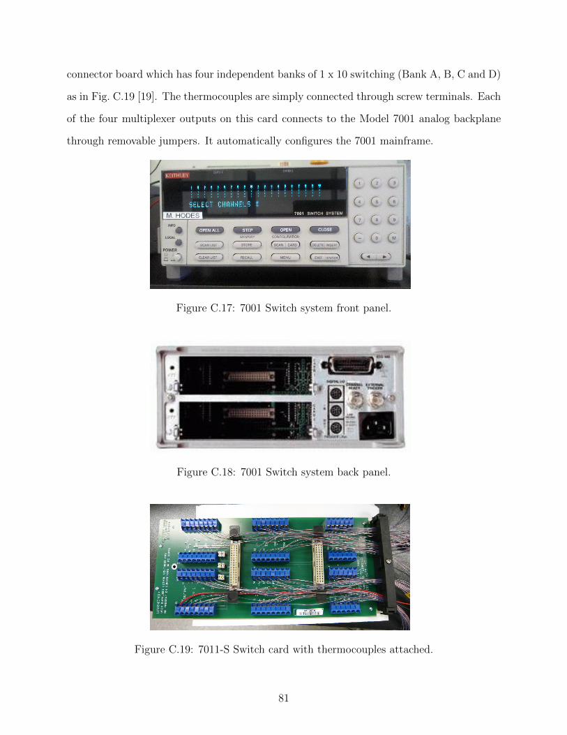
connector board which has four independent banks of 1 x 10 switching (Bank A, B, C and D)
as in Fig. C.19 [19]. The thermocouples are simply connected through screw terminals. Each
of the four multiplexer outputs on this card connects to the Model 7001 analog backplane
through removable jumpers. It automatically configures the 7001 mainframe.
Figure C.17: 7001 Switch system front panel.
Figure C.18: 7001 Switch system back panel.
Figure C.19: 7011-S Switch card with thermocouples attached.
81
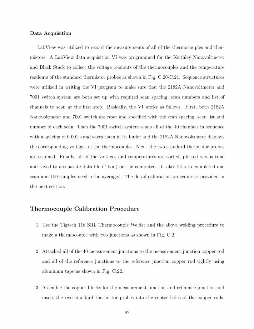
Data Acquisition
LabView was utilized to record the measurements of all of the thermocouples and ther-
mistors. A LabView data acquisition VI was programmed for the Keithley Nanovoltmeter
and Black Stack to collect the voltage readouts of the thermocouples and the temperature
readouts of the standard thermistor probes as shown in Fig. C.20-C.21. Sequence structures
were utilized in writing the VI program to make sure that the 2182A Nanovoltmeter and
7001 switch system are both set up with required scan spacing, scan numbers and list of
channels to scan at the first step. Basically, the VI works as follows. First, both 2182A
Nanovoltmeter and 7001 switch are reset and specified with the scan spacing, scan list and
number of each scan. Then the 7001 switch system scans all of the 40 channels in sequence
with a spacing of 0.001 s and saves them in its buffer and the 2182A Nanovoltmeter displays
the corresponding voltages of the thermocouples. Next, the two standard thermistor probes
are scanned. Finally, all of the voltages and temperatures are sorted, plotted versus time
and saved to a separate data file (*.lvm) on the computer. It takes 24 s to completed one
scan and 100 samples need to be averaged. The detail calibration procedure is provided in
the next section.
Thermocouple Calibration Procedure
1. Use the Tigtech 116 SRL Thermocouple Welder and the above welding procedure to
make a thermocouple with two junctions as shown in Fig. C.2.
2. Attached all of the 40 measurement junctions to the measurement junction copper rod
and all of the reference junctions to the reference junction copper rod tightly using
aluminum tape as shown in Fig. C.22.
3. Assemble the copper blocks for the measurement junction and reference junction and
insert the two standard thermistor probes into the center holes of the copper rods.
82

Figure C.20: LabView VI front panel for thermocouple calibration.
Note that probe # B072717 is for the reference junction and probe # B072719 is for
the measurement junction.
4. Immerse the two copper blocks in the two NESLab RTE7 circulating chiller baths as
shown in Fig. C.5.
5. Connect the other two ends of the thermocouples into the 7011-S switch cards using
the screw terminals as shown in Fig. C.22 to measure the generated emf of the ther-
mocouples and connect the four leads of the thermistor probes to the terminals of the
Black Stack according to its manual.
6. Adjust the reference chiller temperature to get a constant reference temperature. Usu-
ally, by setting the chiller temperature at -0.7 C a reference temperature around 0.0018
C is obtained. Note that setting reference around 0 C was not ideal in this calibration
because the temperature range of the standard thermistor probe is from 0 to 100 C,
83
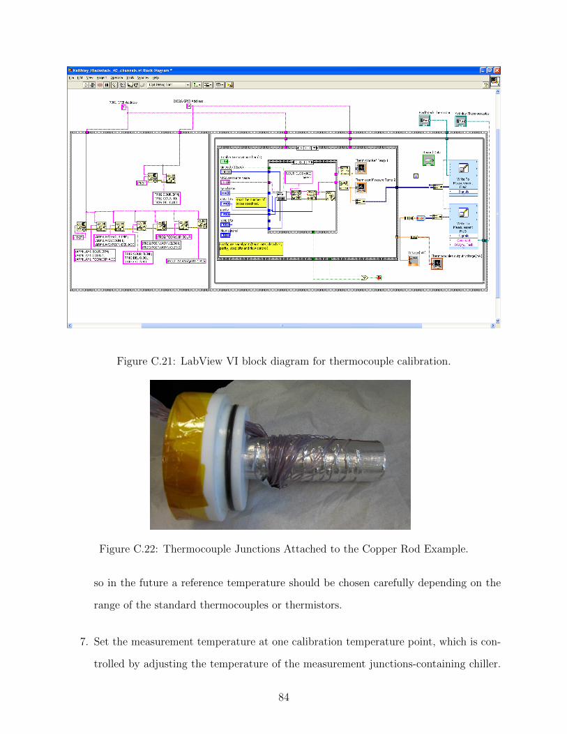
Figure C.21: LabView VI block diagram for thermocouple calibration.
Figure C.22: Thermocouple Junctions Attached to the Copper Rod Example.
so in the future a reference temperature should be chosen carefully depending on the
range of the standard thermocouples or thermistors.
7. Set the measurement temperature at one calibration temperature point, which is con-
trolled by adjusting the temperature of the measurement junctions-containing chiller.
84

Usually set the chiller temperature slightly lower than the required measurement tem-
perature when it is lower than the ambient temperature but slightly higher when it
is higher than the ambient temperature. For example, setting chiller temperature at
-5.5 C results in a measurement junction temperature of about -5.18 C, however, to
obtain a temperature of 45 C for the measurement junction, the chiller needs to be
set at about 45.3 C.
8. Run the LabView VI for the calibration and acquire the thermistor temperatures and
thermocouple voltages. Wait until the curves are flat, which implies that steady-state
conditions have been reached.
9. Record the voltages generated from the thermocouples which are in the a scale of
millivolts (i.e., -0.3 to 4 mV) and the temperatures of the standard thermistor probes
at the same time by clicking the “Record Data” button in the VI’s front panel. Wait
until 100 samples are obtained for each thermocouple and then click the “Stop” button
to stop recording, which usually takes 40 minutes. Voltages of 40 thermocouples and
temperatures of two thermistor probes will be saved in two difference data files (*.lvm)
on the computer.
10. Set the measurement temperature at the next calibration temperature point and repeat
steps 8 and 9. The calibration temperature points are obtained by increasing the
measurement junction from the lowest to the highest temperature, i.e., from -10 C to
90 C by a step of 5 C.
Data Analysis
Calibration results for thermocouple 1, 11, 21 and 31 were used as examples in the analysis
as per Fig. C.23. The first column is the reference junction temperature and the second
column is the measurement junction temperature. Reference temperature was controlled by
the chiller which was set at - 0.6 C and adjusted by ± 0.1 C depending on the ambient
85

temperature. Note that thermocouples were calibrated from -8.7 C to 87.6 C, because the
standard thermistors cover the range of 0 C and 100 C and setting the reference junction
temperature at the lowest or the highest temperature can not ensure the required accuracy.
After the cold junction compensations, the new data are provided in Fig. C.24. The Seebeck
coefficient of type T thermocouples at 0 C selected in the cold junction compensation is
38.748 µV/K [20].
Figure C.23: Calibration readouts of thermocouples and thermistors.
A “Least-squares Fit” was used to find a polynomial expression of the voltage of a
thermocouple as a function of the temperature using Mathematica which is provided at the
end of this appendix. Experiment data of thermocouples 1, 11, 21 and 31, Least-squares Fit
data and data from reference tables (ITS-90) [20] are provided in Fig. C.25. Comparisons of
these data are provided as in Fig. C.26 - C.29. It shows that the experimental data matches
the data in thermocouple reference tables for type-T thermocouple very well and the least-
squares fit method data also agrees very well with the experimental data. The absolute
error of experimental data comparing to the reference table data and that of least-squares
fit data corresponding to the experimental data are shown in Fig. C.30 - C.31. It is shown
86
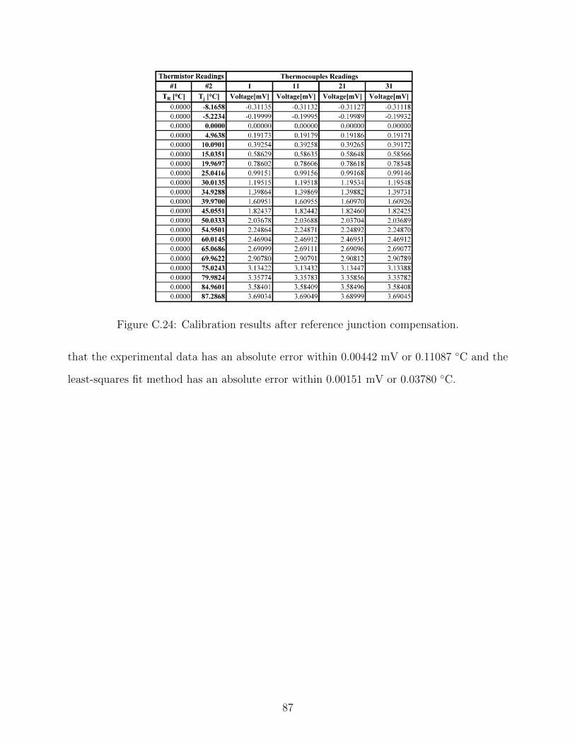
Figure C.24: Calibration results after reference junction compensation.
that the experimental data has an absolute error within 0.00442 mV or 0.11087 C and the
least-squares fit method has an absolute error within 0.00151 mV or 0.03780 C.
87
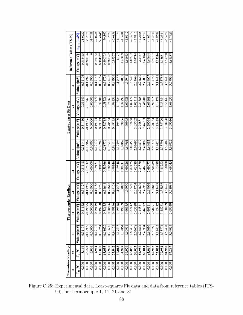
Figure C.25: Experimental data, Least-squares Fit data and data from reference tables (ITS-90) for thermocouple 1, 11, 21 and 31
88
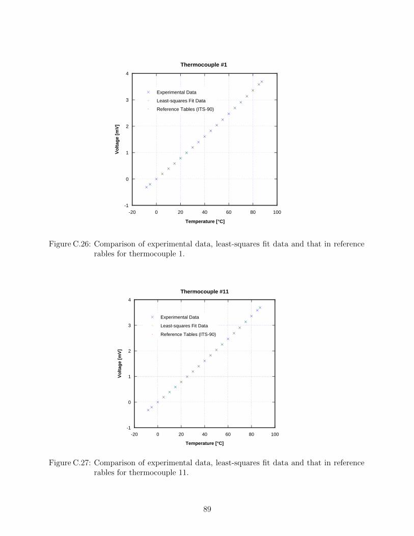
-1
0
1
2
3
4
-20 0 20 40 60 80 100
Experimental Data
Least-squares Fit Data
Reference Tables (ITS-90)
Vo
ltag
e[m
V]
Temperature [°C]
Thermocouple #1
Figure C.26: Comparison of experimental data, least-squares fit data and that in referencerables for thermocouple 1.
-1
0
1
2
3
4
-20 0 20 40 60 80 100
Thermocouple #11
Experimental Data
Least-squares Fit Data
Reference Tables (ITS-90)
Vo
ltag
e[m
V]
Temperature [°C]
Figure C.27: Comparison of experimental data, least-squares fit data and that in referencerables for thermocouple 11.
89

-1
0
1
2
3
4
-20 0 20 40 60 80 100
Thermocouple #21
Experimental Data
Least-squares Fit Data
Reference Tables (ITS-90)
Vo
ltag
e[m
V]
Temperature [°C]
Figure C.28: Comparison of experimental data, least-squares fit data and that in referencerables for thermocouple 21.
-1
0
1
2
3
4
-20 0 20 40 60 80 100
Thermocouple #31
Experimental Data
Least-squares Fit Data
Reference Tables (ITS-90)
Vo
ltag
e[m
V]
Temperature [°C]
Figure C.29: Comparison of experimental data, least-squares fit data and that in referencerables for thermocouple 31.
90

-0.001
0
0.001
0.002
0.003
0.004
0.005
0.006
-20 0 20 40 60 80 100
|Experimental Data - Reference Table Data|
|Experimental Data - Least-squares Fit Data|
Ab
so
lute
Err
or
of
Vo
ltag
e[m
V]
Temperature [°C]
Figure C.30: Absolute errors versus temperatures in voltage for thermocouple 1.
-0.02
0
0.02
0.04
0.06
0.08
0.1
0.12
0.14
-20 0 20 40 60 80 100
|Experimental Data - Reference Table Data|
|Experimental Data - Least-squares Fit Data|
Ab
so
lute
Err
or
of
Tem
pera
ture
[°C
]
Temperature [°C]
Figure C.31: Absolute errors versus temperatures in temperature for thermocouple 1.
91

Calibration Reports and Mathematica Code for Data Analysis
92

Figure C.32: Calibration report of reference thermistor probe (Serial Number: B072717)page 1.
93

Figure C.33: Calibration report of reference thermistor probe (Serial Number: B072717)page 2.
94
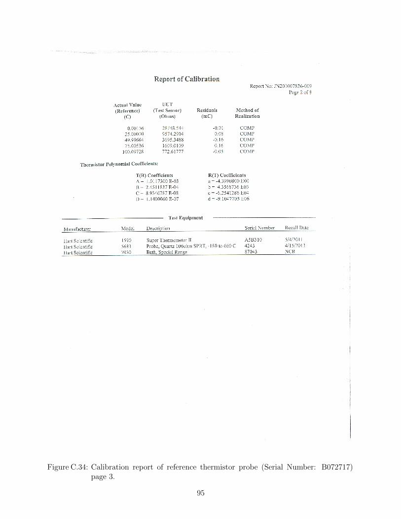
Figure C.34: Calibration report of reference thermistor probe (Serial Number: B072717)page 3.
95
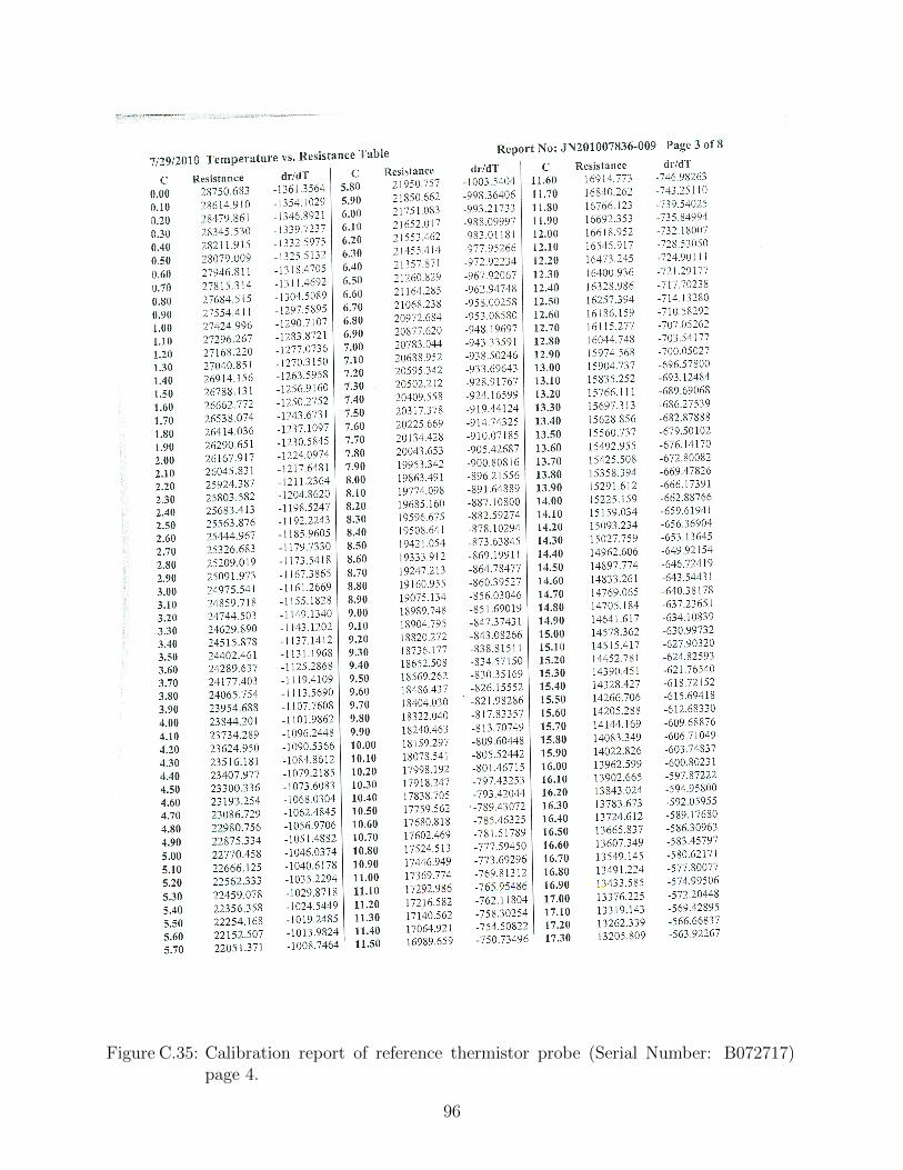
Figure C.35: Calibration report of reference thermistor probe (Serial Number: B072717)page 4.
96
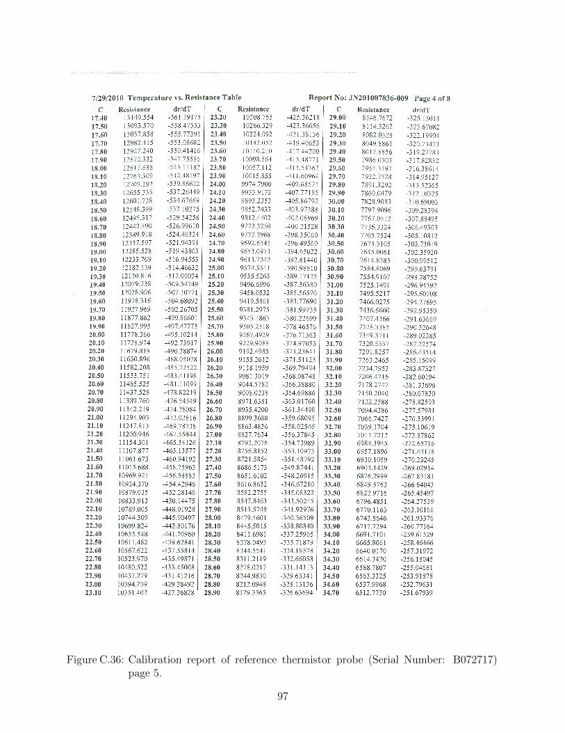
Figure C.36: Calibration report of reference thermistor probe (Serial Number: B072717)page 5.
97
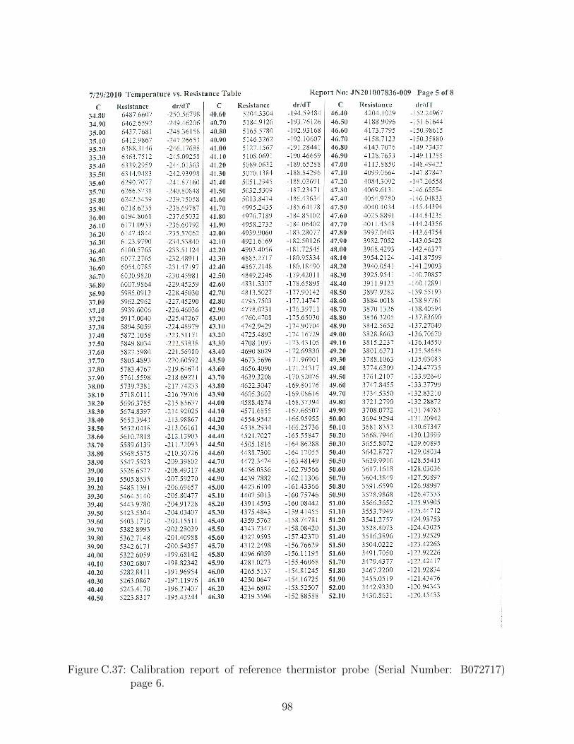
Figure C.37: Calibration report of reference thermistor probe (Serial Number: B072717)page 6.
98
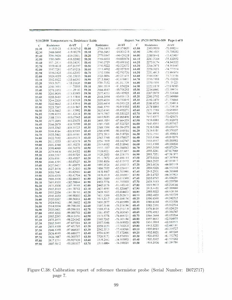
Figure C.38: Calibration report of reference thermistor probe (Serial Number: B072717)page 7.
99

Figure C.39: Calibration report of reference thermistor probe (Serial Number: B072717)page 8.
100
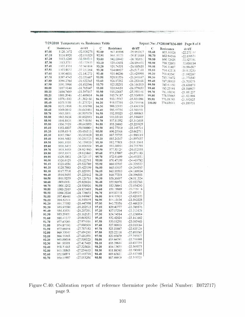
Figure C.40: Calibration report of reference thermistor probe (Serial Number: B072717)page 9.
101

Figure C.41: Calibration report of measurement thermistor probe (Serial Number: B072719)page 1.
102

Figure C.42: Calibration report of measurement thermistor probe (Serial Number: B072719)page 2.
103
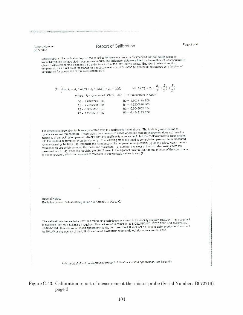
Figure C.43: Calibration report of measurement thermistor probe (Serial Number: B072719)page 3.
104
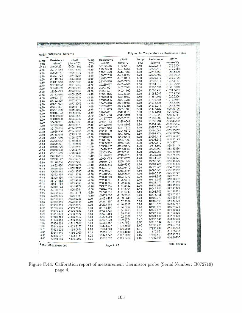
Figure C.44: Calibration report of measurement thermistor probe (Serial Number: B072719)page 4.
105
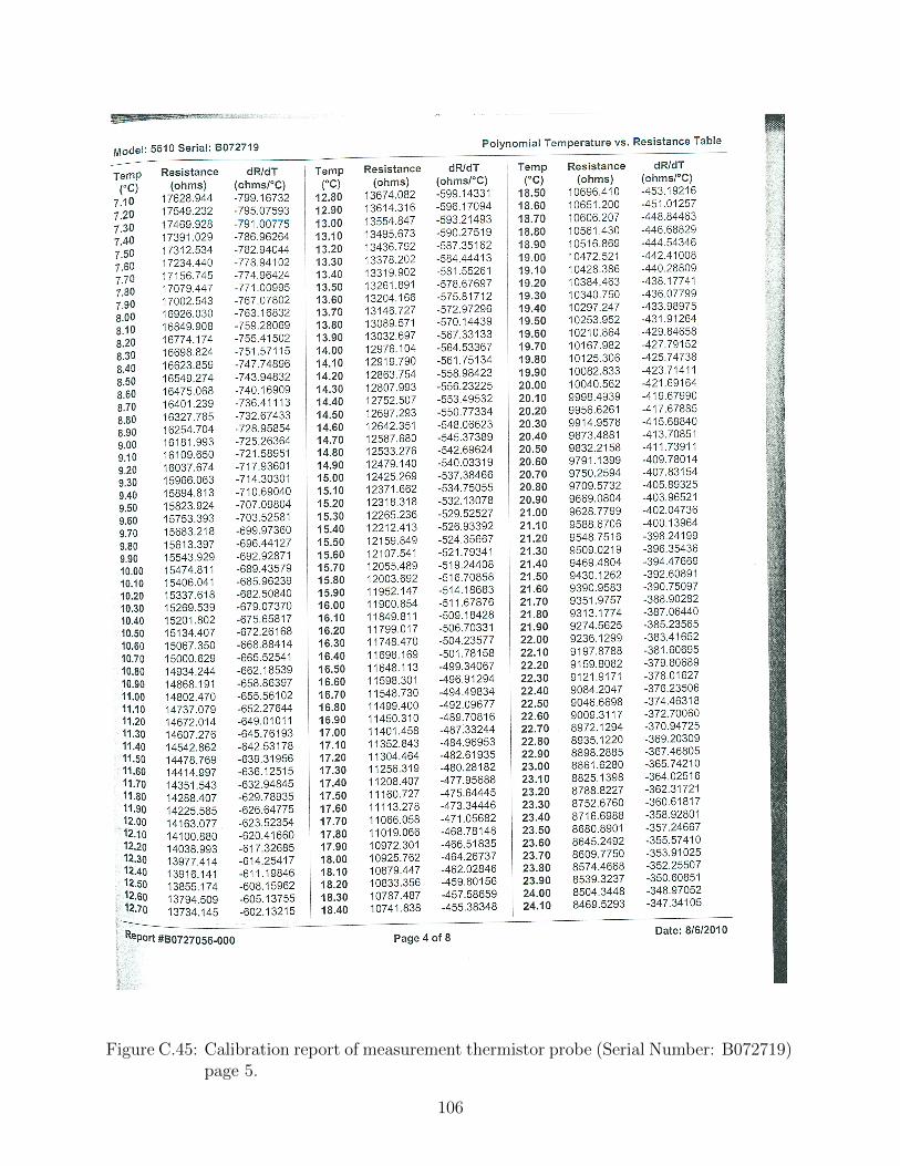
Figure C.45: Calibration report of measurement thermistor probe (Serial Number: B072719)page 5.
106
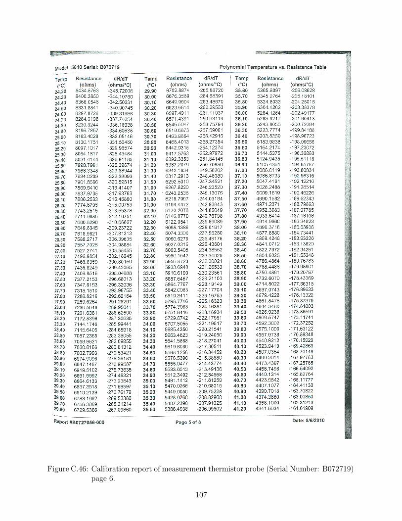
Figure C.46: Calibration report of measurement thermistor probe (Serial Number: B072719)page 6.
107
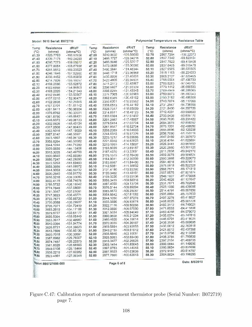
Figure C.47: Calibration report of measurement thermistor probe (Serial Number: B072719)page 7.
108
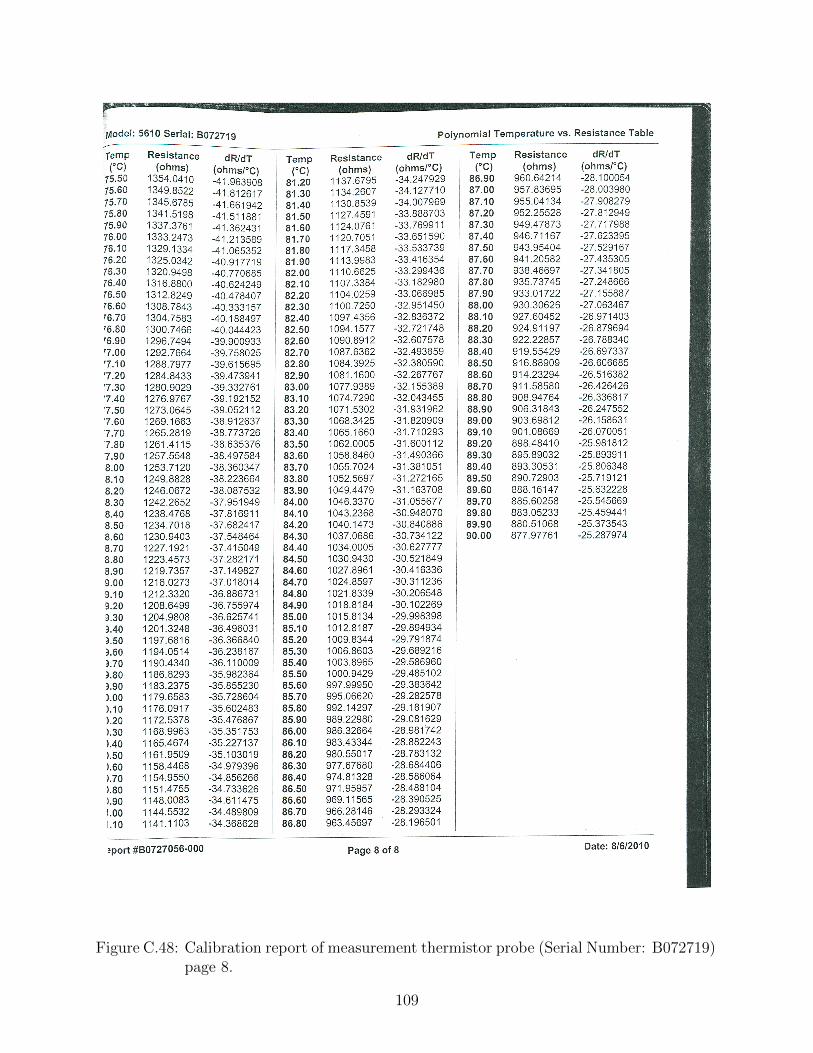
Figure C.48: Calibration report of measurement thermistor probe (Serial Number: B072719)page 8.
109
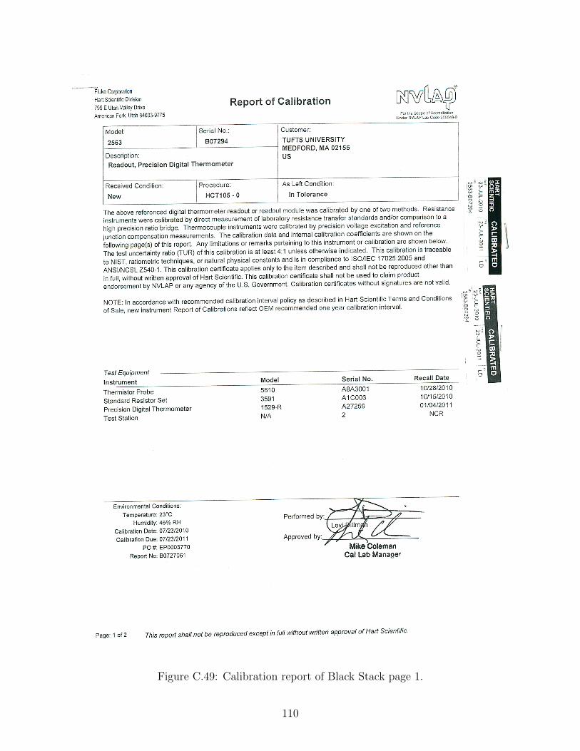
Figure C.49: Calibration report of Black Stack page 1.
110
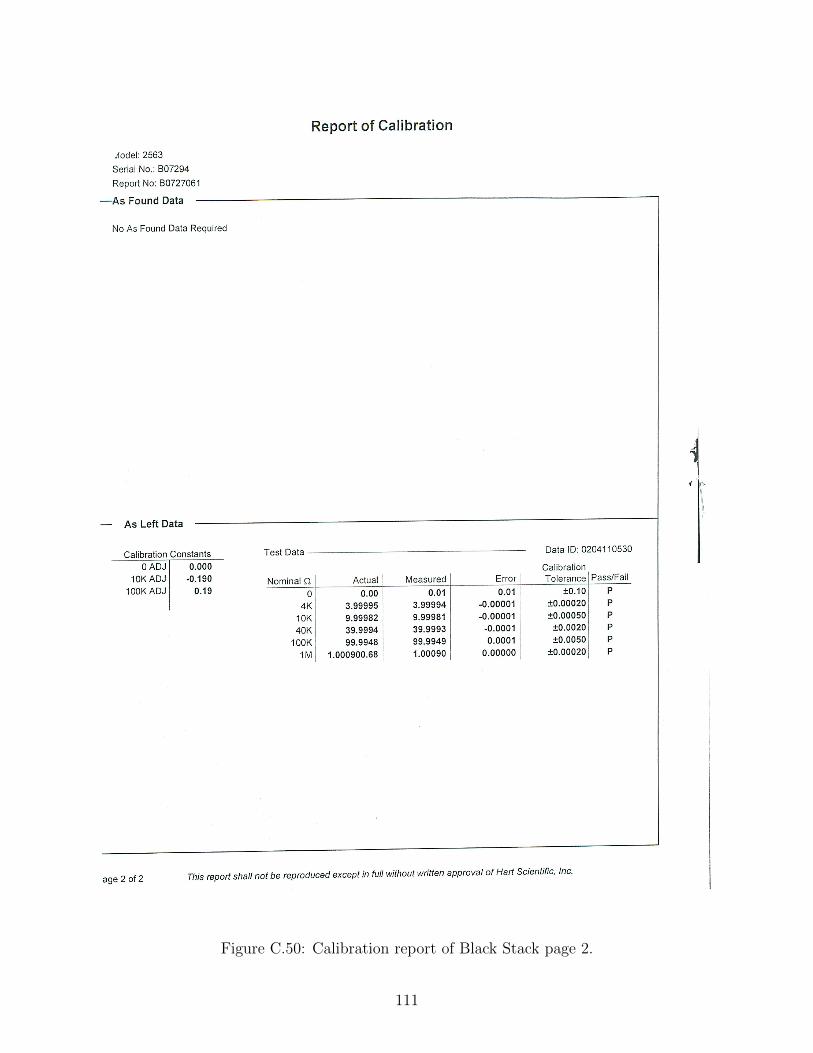
Figure C.50: Calibration report of Black Stack page 2.
111
Figure C.51: Calibration report of Black Stack page 3.
112
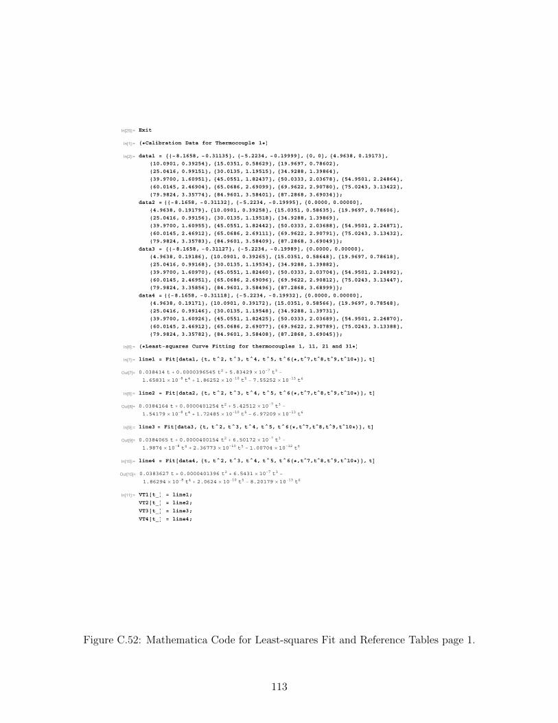
ײÅîëÃæã Û¨·¬
ײÅïÃæã öÝ¿´·¾®¿¬·±² Ü¿¬¿ º±® ̸»®³±½±«°´» ïö
ײÅîÃæã ¼¿¬¿ï ã óèòïêëèô óðòíïïíë ô óëòîîíìô óðòïçççç ô ðô ð ô ìòçêíèô ðòïçïéí ô
ïðòðçðïô ðòíçîëì ô ïëòðíëïô ðòëèêîç ô ïçòçêçéô ðòéèêðî ô
îëòðìïêô ðòççïëï ô íðòðïíëô ïòïçëïë ô íìòçîèèô ïòíçèêì ô
íçòçéððô ïòêðçëï ô ìëòðëëïô ïòèîìíé ô ëðòðíííô îòðíêéè ô ëìòçëðïô îòîìèêì ô
êðòðïìëô îòìêçðì ô êëòðêèêô îòêçðçç ô êçòçêîîô îòçðéèð ô éëòðîìíô íòïíìîî ô
éçòçèîìô íòíëééì ô èìòçêðïô íòëèìðï ô èéòîèêèô íòêçðíì å
¼¿¬¿î ã óèòïêëèô óðòíïïíî ô óëòîîíìô óðòïçççë ô ðòððððô ðòððððð ô
ìòçêíèô ðòïçïéç ô ïðòðçðïô ðòíçîëè ô ïëòðíëïô ðòëèêíë ô ïçòçêçéô ðòéèêðê ô
îëòðìïêô ðòççïëê ô íðòðïíëô ïòïçëïè ô íìòçîèèô ïòíçèêç ô
íçòçéððô ïòêðçëë ô ìëòðëëïô ïòèîììî ô ëðòðíííô îòðíêèè ô ëìòçëðïô îòîìèéï ô
êðòðïìëô îòìêçïî ô êëòðêèêô îòêçïïï ô êçòçêîîô îòçðéçï ô éëòðîìíô íòïíìíî ô
éçòçèîìô íòíëéèí ô èìòçêðïô íòëèìðç ô èéòîèêèô íòêçðìç å
¼¿¬¿í ã óèòïêëèô óðòíïïîé ô óëòîîíìô óðòïççèç ô ðòððððô ðòððððð ô
ìòçêíèô ðòïçïèê ô ïðòðçðïô ðòíçîêë ô ïëòðíëïô ðòëèêìè ô ïçòçêçéô ðòéèêïè ô
îëòðìïêô ðòççïêè ô íðòðïíëô ïòïçëíì ô íìòçîèèô ïòíçèèî ô
íçòçéððô ïòêðçéð ô ìëòðëëïô ïòèîìêð ô ëðòðíííô îòðíéðì ô ëìòçëðïô îòîìèçî ô
êðòðïìëô îòìêçëï ô êëòðêèêô îòêçðçê ô êçòçêîîô îòçðèïî ô éëòðîìíô íòïíììé ô
éçòçèîìô íòíëèëê ô èìòçêðïô íòëèìçê ô èéòîèêèô íòêèççç å
¼¿¬¿ì ã óèòïêëèô óðòíïïïè ô óëòîîíìô óðòïççíî ô ðòððððô ðòððððð ô
ìòçêíèô ðòïçïéï ô ïðòðçðïô ðòíçïéî ô ïëòðíëïô ðòëèëêê ô ïçòçêçéô ðòéèëìè ô
îëòðìïêô ðòççïìê ô íðòðïíëô ïòïçëìè ô íìòçîèèô ïòíçéíï ô
íçòçéððô ïòêðçîê ô ìëòðëëïô ïòèîìîë ô ëðòðíííô îòðíêèç ô ëìòçëðïô îòîìèéð ô
êðòðïìëô îòìêçïî ô êëòðêèêô îòêçðéé ô êçòçêîîô îòçðéèç ô éëòðîìíô íòïííèè ô
éçòçèîìô íòíëéèî ô èìòçêðïô íòëèìðè ô èéòîèêèô íòêçðìë å
ײÅêÃæã öÔ»¿¬ó¯«¿®» Ý«®ª» Ú·¬¬·²¹ º±® ¬¸»®³±½±«°´» ïô ïïô îï ¿²¼ íïö
ײÅéÃæã ´·²»ï ã Ú·¬ ¼¿¬¿ïô ¬ô ¬Âîô ¬Âíô ¬Âìô ¬Âëô ¬Âê öô¬Âéô¬Âèô¬Âçô¬Âïðö ô ¬
Ñ«¬ÅéÃã ðòðíèìïì ¬ õ ðòððððíçêëìë ¬î õ ëòèíìîç l ïðóé ¬í ó
ïòêëèíï l ïðóè ¬ì õ ïòèêîëî l ïðóïð ¬ë ó éòëëîëî l ïðóïí ¬ê
ײÅèÃæã ´·²»î ã Ú·¬ ¼¿¬¿îô ¬ô ¬Âîô ¬Âíô ¬Âìô ¬Âëô ¬Âê öô¬Âéô¬Âèô¬Âçô¬Âïðö ô ¬
Ñ«¬ÅèÃã ðòðíèìïêì ¬ õ ðòððððìðïîëì ¬î õ ëòìîëïî l ïðóé ¬í ó
ïòëìïéç l ïðóè ¬ì õ ïòéîìèë l ïðóïð ¬ë ó êòçéîðç l ïðóïí ¬ê
ײÅçÃæã ´·²»í ã Ú·¬ ¼¿¬¿íô ¬ô ¬Âîô ¬Âíô ¬Âìô ¬Âëô ¬Âê öô¬Âéô¬Âèô¬Âçô¬Âïðö ô ¬
Ñ«¬ÅçÃã ðòðíèìðêë ¬ õ ðòððððìððïëì ¬î õ êòëðïéî l ïðóé ¬í ó
ïòçèéì l ïðóè ¬ì õ îòíêééí l ïðóïð ¬ë ó ïòððéðì l ïðóïî ¬ê
ײÅïðÃæã ´·²»ì ã Ú·¬ ¼¿¬¿ìô ¬ô ¬Âîô ¬Âíô ¬Âìô ¬Âëô ¬Âê öô¬Âéô¬Âèô¬Âçô¬Âïðö ô ¬
Ñ«¬ÅïðÃã ðòðíèíêîé ¬ õ ðòððððìðïíçê ¬î õ êòëìíï l ïðóé ¬í ó
ïòèêîçì l ïðóè ¬ì õ îòðêîì l ïðóïð ¬ë ó èòîðïéç l ïðóïí ¬ê
ײÅïïÃæã ÊÌï ¬Á ã ´·²»ïå
ÊÌî ¬Á ã ´·²»îå
ÊÌí ¬Á ã ´·²»íå
ÊÌì ¬Á ã ´·²»ìå
Figure C.52: Mathematica Code for Least-squares Fit and Reference Tables page 1.
113
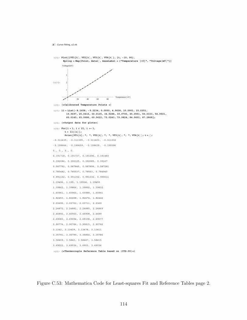
ײÅïëÃæã 䱬 ÊÌï ¬ ô ÊÌî ¬ ô ÊÌí ¬ ô ÊÌì ¬ ô ¬ô óïðô çð ô
Û°·´±¹ r Ó¿° б·²¬ô ¼¿¬¿ï ô ߨ»Ô¿¾»´ r þÌ»³°»®¿¬«®» 7Ý þô þʱ´¬¿¹» ³Ê þ
Ñ«¬ÅïëÃã
îð ìð êð èðÌ»³°»®¿¬«®» à7ÝÜ
ï
î
í
ʱ´¬¿¹»à³ÊÜ
ײÅïêÃæã öÝ¿´·¾®¿¬»¼ Ì»³°»®¿¬«®» б·²¬ ö
ײÅïéÃæã ´´ ã Ô·¬ óèòïêëèô óëòîîíìô ðòððððô ìòçêíèô ïðòðçðïô ïëòðíëïô
ïçòçêçéô îëòðìïêô íðòðïíëô íìòçîèèô íçòçéððô ìëòðëëïô ëðòðíííô ëìòçëðïô
êðòðïìëô êëòðêèêô êçòçêîîô éëòðîìíô éçòçèîìô èìòçêðïô èéòîèêè å
ײÅïèÃæã öÑ«¬°«¬ ¼¿¬¿ º±® °´±¬ö
ײÅïçÃæã Ú±® · ã ïô · îïô · õã ïô
¬ ã ´´ · å
Ю·²¬ ÊÌï ¬ ô þô þô ÊÌî ¬ ô þô þô ÊÌí ¬ ô þô þô ÊÌì ¬ å ¬ ãò å
óðòíïïìíëô óðòíïïíçëô óðòíïïìðíô óðòíïïðíî
óðòïççêêêô óðòïççêëçô óðòïççêîçô óðòïççíçê
ðòô ðòô ðòô ðò
ðòïçïéïèô ðòïçïéíéô ðòïçïêçêô ðòïçïìèí
ðòíçîðèìô ðòíçîïîëô ðòíçîðèëô ðòíçïêé
ðòëèééçîô ðòëèéèìëô ðòëèéèëêô ðòëèéîèï
ðòéèëìèîô ðòéèëëíéô ðòéèëêíô ðòéèìçìç
ðòççïïðîô ðòççïïëîô ðòççïííîô ðòççðêïï
ïòïçìçêô ïòïçëô ïòïçëîìô ïòïçìëë
ïòíçèêîô ïòíçèêêô ïòíçèçîô ïòíçèíî
ïòêðçêïô ïòêðçêëô ïòêðçèèô ïòêðçìï
ïòèîìëíô ïòèîìëèô ïòèîìéìô ïòèîììî
îòðíêçëô îòðíéðîô îòðíéïïô îòðíêç
îòîìèéîô îòîìèèïô îòîìèèëô îòîìèêç
îòìêèçîô îòìêçðíô îòìêçðèô îòìêèç
îòêçðèíô îòêçðçìô îòêçïðèô îòêçðéé
îòçðééìô îòçðéèìô îòçðèïëô îòçðéêê
íòïíìîô íòïíìîçô íòïíìéèô íòïíìïï
íòíëéçïô íòíëéççô íòíëèëìô íòíëéèê
íòëèìðçô íòëèìîô íòëèììéô íòëèìïë
íòêçðîîô íòêçðíêô íòêçðíô íòêçðíê
ײÅîðÃæã ö̸»®³±½±«°´» λº»®»²½» Ì¿¾´» ¾¿»¼ ±² ×ÌÍóçð ö
2 Curve Fitting_v2.nb
Figure C.53: Mathematica Code for Least-squares Fit and Reference Tables page 2.
114

ײÅîïÃæã ÍÊï ¬Á ã íèòéìèïðêíêì ö ¬ õ ìòìïçììíìíìé ö ïðÂóî ö ¬Âî õ ïòïèììíîíïðë ö ïðÂóì ö ¬Âí õ
îòððíîçéíëëì ö ïðÂóë ö ¬Âì õ çòðïíèðïçëëç ö ïðÂóé ö ¬Âë õ îòîêëïïëêëçí ö ïðÂóè ö ¬Âê õ
íòêðéïïëìîðë ö ïðÂóïð ö ¬Âé õ íòèìçíçíçèèí ö ïðÂóïî ö ¬Âè õ îòèîïíëîïçîë ö ïðÂóïì ö ¬Âç õ
ïòìîëïëçìééç ö ïðÂóïê ö ¬Âïð õ ìòèéêèêêîîèê ö ïðÂóïç ö ¬Âïï õ
ïòðéçëëíçîéð ö ïðÂóîï ö ¬Âïî õ ïòíçìëðîéðêî ö ïðÂóîì ö ¬Âïí õ éòçéçëïëíçîé ö ïðÂóîê ö ¬Âïì
Ñ«¬ÅîïÃã íèòéìèï ¬ õ ðòðììïçìì ¬î õ ðòðððïïèììí ¬í õ ðòððððîððíí ¬ì õ çòðïíè l ïðóé ¬ë õ îòîêëïî l ïðóè ¬ê õ
íòêðéïî l ïðóïð ¬é õ íòèìçíç l ïðóïî ¬è õ îòèîïíë l ïðóïì ¬ç õ ïòìîëïê l ïðóïê ¬ïð õ
ìòèéêèé l ïðóïç ¬ïï õ ïòðéçëë l ïðóîï ¬ïî õ ïòíçìë l ïðóîì ¬ïí õ éòçéçëî l ïðóîê ¬ïì
ײÅîîÃæã ÍÊî ¬Á ã íèòéìèïðêíêì ö ¬ õ íòíîçîîîéèèð ö ïðÂóî ö ¬Âî õ
îòðêïèîìíìðì ö ïðÂóì ö ¬Âí ó îòïèèîîëêèìê ö ïðÂóê ö ¬Âì õ ïòðççêèèðçîè ö ïðÂóè ö ¬Âë ó
íòðèïëéëèééî ö ïðÂóïï ö ¬Âê õ ìòëìéçïíëîçð ö ïðÂóïì ö ¬Âé ó îòéëïîçðïêéí ö ïðÂóïê ö ¬Âè
Ñ«¬ÅîîÃã íèòéìèï ¬ õ ðòðííîçîî ¬î õ ðòðððîðêïèî ¬í ó îòïèèîí l ïðóê ¬ì õ
ïòðççêç l ïðóè ¬ë ó íòðèïëè l ïðóïï ¬ê õ ìòëìéçï l ïðóïì ¬é ó îòéëïîç l ïðóïê ¬è
ײÅîíÃæã öÑ«¬°«¬ Ü¿¬¿ º±® °´±¬ö
ײÅîìÃæã Ú±® · ã ïô · îô · õã ïô
¬ ã ´´ · å
Ю·²¬ ÍÊï ¬ å ¬ ãò å
óíïíòìêë
óîðïòïçê
ײÅîëÃæã Ú±® · ã íô · îïô · õã ïô
¬ ã ´´ · å
Ю·²¬ ÍÊî ¬ å ¬ ãò å
ðò
ïçíòïèî
íçìòëëî
ëçðòéðë
éèèòíçî
ççíòêé
ïïçéò
ïìððòðç
ïêïðòëí
ïèîëòðî
îðíéòïì
îîìèòé
îìêèòéì
îêçðòìì
îçðéòðé
íïííòïê
ííëêòëï
íëèîòëè
íêèèòèé
Curve Fitting_v2.nb 3
Figure C.54: Mathematica Code for Least-squares Fit and Reference Tables page 3.
115