Journal of the Association of Arab Universities for Basic and Applied Sciences (2014) xxx, xxx–xxx

University of Bahrain

Journal of the Association of Arab Universities for

Basic and Applied Scienceswww.elsevier.com/locate/jaaubas

www.sciencedirect.com

ORIGINAL ARTICLE

Some new modifications of Kibria’s and Dorugade’s

methods: An application to Turkish GDP data

* Corresponding author.

Peer review under responsibility of University of Bahrain.

http://dx.doi.org/10.1016/j.jaubas.2014.08.005

1815-3852 ª 2014 Production and hosting by Elsevier B.V. on behalf of University of Bahrain.

Please cite this article in press as: Karaibrahimoglu, A. et al., Some new modifications of Kibria’s and Dorugade’s methods: An application to Turkish GDJournal of the Association of Arab Universities for Basic and Applied Sciences (2014), http://dx.doi.org/10.1016/j.jaubas.2014.08.005

Adnan Karaibrahimoglu a, Yasin Asar b,*, As�ır Genc c

a Meram Faculty of Medicine, Medical Education and Informatics Department, Biostatistics Unit, Necmettin ErbakanUniversity, Konya, Turkeyb Department of Mathematics-Computer Sciences, Faculty of Science, Necmettin Erbakan University, Konya, Turkeyc Department of Statistics, Faculty of Science, Selcuk University, Konya, Turkey

Received 19 May 2014; revised 11 August 2014; accepted 31 August 2014

KEYWORDS

Multicollinearity;

Multiple linear regression;

Ridge regression;

Ridge estimator;

Monte Carlo simulation

Abstract In multiple linear regression analysis, multicollinearity is an important problem. Ridge

regression is one of the most commonly used methods to overcome this problem. There are many

proposed ridge parameters in the literature. In this paper, we propose some new modifications to

choose the ridge parameter. A Monte Carlo simulation is used to evaluate parameters. Also, biases

of the estimators are considered. The mean squared error is used to compare the performance of the

proposed estimators with others in the literature. According to the results, all the proposed estima-

tors are superior to ordinary least squared estimator (OLS).ª 2014 Production and hosting by Elsevier B.V. on behalf of University of Bahrain.

1. Introduction

Consider the following standard linear regression model

Y ¼ Xbþ e ð1:1Þ

where Y is an n · 1 vector of dependent variable, X is a designmatrix of order n · p where p is the number of explanatoryvariables, b is a p · 1 vector of coefficients and e is the error

vector of order n · 1 distributed as N(0, r2In). Ordinary leastsquared (OLS) method is the most common method of esti-mating b and the OLS estimator of b is given as follows

b ¼ ðX0XÞ�1X0Y ð1:2Þ

In some situations, the matrix X0X has almost zero eigenvaluesmeaning the explanatory variables are correlated. This leads to

a large variance and so large mean squared error (MSE). Thusone may not reach a reliable solution for b. This is the com-

monly faced problem called multicollinearity. There are vari-ous methods to solve this problem. The ridge regression isone of the most popular methods proposed by Hoerl and

Kennard (1970a,b).In ridge regression, adding a small positive number

k(k> 0) called ridge parameter to the diagonal elements ofthe matrix X0X, we obtain the following ridge estimator

bRR ¼ ðX0Xþ kIpÞ�1X0Y; k > 0 ð1:3Þ

The MSEs of the OLS estimator and the ridge estimator bRR

are as follows respectively,

MSEðbÞ ¼ r2Xpi¼1

1

ki

ð1:4Þ

P data.

2 A. Karaibrahimoglu et al.

MSE bRR

� �¼ Var bRR

� �þ BiasðbRRÞh i2

¼ r2Xpi¼1

ki

ðki þ kÞ2þ k2b0ðX0Xþ kIpÞ�2b ð1:5Þ

where ki ’s are eigenvalues of the matrix X0X and r2 is the errorvariance.

Hoerl and Kennard, 1970b showed the properties of thisfunction in detail. They concluded that the total variance

decreases and the squared bias increases as k increases. Thevariance function is monotonically decreasing and the squaredbias function is monotonically increasing. Thus, there is the

probability that some k exists such that the MSE for bRR is lessthan MSE for the usual b (Hoerl and Kennard, 1970ab).

We know that k is estimated from the observed data. There

are many papers proposing different ridge parameters in theliterature. In recent papers, these parameters have been com-pared with the one proposed by Hoerl et al., 1975 and eachother. After Hoerl and Kennard, 1970b, many researchers

studied this area and proposed different estimates of the ridgeparameter. Some of them are McDonald and Galarneau(1975), Lawless and Wang (1976), Saleh and Kibria (1993),

Liu and Gao (2011), Kibria (2003), Khalaf and Shukur(2005), Alkhamisi et al. (2006), Adnan et al. (2006), Yan(2008), Yan and Zhao (2009), Muniz and Kibria (2009),

Mansson et al. (2010), Al-Hassan (2010), Muniz et al.(2012), Asar et al. (2014) and Dorugade (2014).

The purpose of this article is to study much of the param-

eters in the literature and propose some new ones and alsomake a comparison between them by conducting a Monte Car-lo experiment. The comparison criterion is based on the meansquared properties.

The article is organized as follows. In Section 2, we presentthe methodology of different estimators and give some newestimators. A Monte Carlo simulation has been provided in

Section 3. Results of the simulation are discussed in Section 4.In Section 5, an application of the estimators is given. Finally,we give a summary and conclusion.

2. Model and estimators

Firstly we write the general model (1.1) in canonical form.

Suppose that there exits an orthogonal matrix D we apply atransformation such that

DðX0XÞD0 ¼ K ¼ diag k1; k2; . . . ; kp

� �ð2:1Þ

where D is a p · p orthogonal matrix and k1 P k2 P � � �P kp.If we substitute Z= XD and a = D’b in the model (1.1), thenthe model may be rewritten as

Y ¼ Zaþ e ð2:2Þ

where Z0Z= K.Thus, the ridge estimator of a becomes

aRR ¼ ðZ0Zþ kIpÞ�1Z0Y. It is stated in Hoerl and Kennard,1970a that the value of k minimizing the MSEðaRRÞ is

ki ¼r2

a2i

: ð2:3Þ

As seen in the formula (2.3), k depends on the unknownparameters r2 and a. Hence we use the estimators r2 and adue to Hoerl and Kennard, 1970b and get

Please cite this article in press as: Karaibrahimoglu, A. et al., Some new modificatioJournal of the Association of Arab Universities for Basic and Applied Sciences (201

ki ¼r2

a2i

: ð2:4Þ

2.1. Proposed estimators

In this section, we review some of the ridge estimators sug-gested earlier and propose some new ones. The list of estima-tors with which we will compare ours is given below:

ð1Þ k1 ¼ kHK ¼r2

a2max

Hoerl&Kennard; 1970að Þ ð2:5Þ

where amax is the maximum element of a.

ð2Þ k2 ¼pr2Ppi¼1kia2

i

; i ¼ 1; 2; . . . ; p ðLawless&Wang; 1976Þ

ð2:6Þ

which is proposed from the Bayesian point of view.

ð3Þ k3 ¼ medianr2

a2i

� �; i ¼ 1; 2; . . . ; p ðKibria; 2003Þ ð2:7Þ

which is the median of ki ¼ r2

a2i

.

ð4Þ k4 ¼2r2

kmax

Qa2ið Þ1=p

; i ¼ 1; 2; . . . ; p ðDorugade; 2014Þ

ð2:8Þ

which is the geometric mean of ki ¼ 2r2

kmax a2i:

ð5Þ k5 ¼2p

kmax

r2Ppi¼1a

2i

; i ¼ 1; 2; . . . ; p ðDorugade; 2014Þ ð2:9Þ

which is the harmonic mean of ki ¼ 2r2

kmax a2i:

A sufficient condition that MSEðaRRÞ <MSEðaÞ is given byHoerl and Kennard (1970a,b) such that k < kHK ¼ r2

a2max. A

quick survey shows us that some of the existing ridge parame-ters are smaller than kHK. However, if we try the estimatorslarger than kHK, we observe that one can also have better esti-mators in sense of MSE.

In the figure given by Hoerl and Kennard (1970a,b), it isobvious that the first derivative of the function MSEðaRRÞ isnegative when the value of kHK is used as the biasing parame-

ter. Therefore, any estimator satisfying 0<k<kHK gives us anegative derivative. However, if we examine the intersectionpoint of the variance and the squared bias functions, we see

that it is absolutely greater than kHK. Thus, one can find esti-mators such that the first derivative of the MSEðaRRÞ functionis positive and being greater than kHK. There are greater esti-

mators than kHK in the literature, for example see Alkhamisiand Shukur, 2007 for the estimators kNAS and kAS.

It should also be pointed out that the optimal selection pro-cess of the parameter k in ridge regression cannot be truly pro-

vided from the theoretical point of view. Actually, this is anopen problem to researchers. Thus we suggest some estimators

which are modifications of kK ¼ 1p

Ppi¼1

r2

a2i

proposed in Kibria,

2003 kD ¼ 2pkmax

r2Pp

i¼1a2i

and kD ¼ 2pkmax

r2Pp

i¼1a2i

proposed in

Dorugade, 2014. We apply some transformations and we fol-low Khalaf and Shukur (2005) and Alkhamisi and Shukur

(2007) in order to get some estimators being greater thankHK and having better performances. The first two estimatorsare smaller than kHK and others are greater than it.

ns of Kibria’s and Dorugade’s methods: An application to Turkish GDP data.4), http://dx.doi.org/10.1016/j.jaubas.2014.08.005

Table 1 The AMSE as a function of r2.

n 20 50 100

p= 4, q = 0.75

r2 0.1 0.5 1.0 5.0 0.1 0.5 1.0 5.0 0.1 0.5 1.0 5.0

k1 0.8018 4.3489 7.5183 39.0185 0.7438 3.7920 6.8246 27.9983 0.7029 2.9245 6.1673 23.5762

k2 0.7727 4.7676 8.3778 44.2431 0.7133 4.0857 7.4317 28.0331 0.6664 3.0179 6.4671 23.1509

k3 0.7846 5.0495 9.1799 48.9552 0.7428 4.3901 8.1411 31.7462 0.6884 3.3637 7.1451 27.2164

k4 0.7167 4.4135 8.1842 44.2272 0.6709 3.9050 7.2784 28.5271 0.6226 3.0754 6.3872 25.1134

k5 0.7088 3.6649 6.0314 29.9480 0.6477 3.2296 5.5757 22.1414 0.6069 2.4728 5.0739 18.7134

kN1 0.6910 3.6451 6.0659 30.2548 0.6325 3.2132 5.5900 22.0714 0.5918 2.4698 5.0680 18.7983

kN2 0.7298 3.7024 6.0289 29.7302 0.6691 3.2641 5.5984 22.4143 0.6299 2.5016 5.1228 18.8006

kN3 0.7245 3.6846 6.0369 29.7471 0.6706 3.2559 5.6112 22.5370 0.6343 2.5223 5.1435 19.0303

kN4 0.6862 4.3086 7.3445 36.7735 0.6309 3.7810 6.7037 25.8954 0.5828 2.8875 5.9905 22.0626

OLS 1.4625 8.6222 14.2958 71.7297 1.2800 7.3098 12.6382 50.2923 1.1755 5.4638 11.4942 42.1464

p= 4, q = 0.85

r2 0.1 0.5 1.0 5.0 0.1 0.5 1.0 5.0 0.1 0.5 1.0 5.0

k1 2.5925 7.9881 12.6128 102.2997 1.4107 5.3567 11.8893 79.6890 1.2014 4.4455 10.2231 60.0734

k2 2.8936 10.1650 15.3204 137.0792 1.4823 6.1005 14.3277 103.9478 1.2273 4.8987 11.7653 74.9186

k3 2.9571 10.6945 15.7596 137.3515 1.5931 6.3183 14.4882 98.3121 1.2976 5.1854 12.1973 76.2568

k4 2.6016 9.4165 13.5265 121.9175 1.4319 5.4256 12.2743 84.8187 1.1766 4.5210 10.4937 66.7519

k5 2.2860 6.0829 9.6697 72.4183 1.2541 4.4396 9.4002 60.2166 1.0848 3.6822 7.9935 45.1846

kN1 2.2572 6.1846 9.7280 73.4788 1.2377 4.4184 9.3862 59.9767 1.0650 3.6675 7.9889 45.3840

kN2 2.2968 5.9923 9.6551 71.7758 1.2685 4.4704 9.4386 60.4528 1.1005 3.7128 8.0291 45.1771

kN3 2.2387 6.0057 9.6579 72.5659 1.2449 4.4367 9.3929 59.9748 1.0752 3.6966 8.0014 45.1750

kN4 2.6230 7.9527 12.1402 96.0898 1.4050 5.3006 11.4860 73.5664 1.1539 4.3835 9.7517 56.7623

OLS 5.3294 14.4634 23.1875 178.5352 2.7670 10.1480 21.6767 139.8967 2.2929 8.1819 18.1937 104.3610

p= 4, q = 0.95

r2 0.1 0.5 1.0 5.0 0.1 0.5 1.0 5.0 0.1 0.5 1.0 5.0

k1 4.4843 17.6719 43.2137 285.2298 3.6713 15.2385 39.8144 211.9142 3.0023 13.8284 27.6675 187.9357

k2 5.4332 24.3150 62.0304 428.1496 4.3521 20.3761 57.6365 317.5391 3.5398 18.2148 37.9291 276.4823

k3 5.2084 21.7618 53.5358 369.9291 4.2803 18.1883 51.3576 277.0999 3.6190 16.7532 34.8457 241.7900

k4 4.4122 17.5500 43.9138 326.1944 3.6350 14.6845 42.0855 242.7515 3.1331 13.6560 28.8147 212.4845

k5 3.8087 13.6617 32.3764 205.8630 3.1348 11.9416 29.4144 153.8375 2.5679 10.7092 20.8151 137.6582

kN1 3.7673 13.5906 32.2286 206.1835 3.1006 11.8395 29.4070 153.9551 2.5506 10.6571 20.7991 137.6976

kN2 3.8173 13.6882 32.4253 205.9081 3.1437 11.9751 29.4385 153.9099 2.5752 10.7345 20.8414 137.7477

kN3 3.7398 13.6022 32.3259 209.1952 3.0774 11.7948 29.6282 155.4830 2.5457 10.6581 20.8693 138.7788

kN4 4.4834 16.7420 39.8726 263.3648 3.6897 14.3511 37.4322 196.8083 3.0924 13.1481 26.1427 174.9628

OLS 9.0396 32.5136 78.5206 514.2492 7.1454 27.9423 68.4895 361.1289 5.7255 24.6632 48.0141 321.5286

p= 8, q = 0.75

r2 0.1 0.5 1.0 5.0 0.1 0.5 1.0 5.0 0.1 0.5 1.0 5.0

k1 2.2324 7.9806 20.7148 98.3940 1.7880 7.4095 15.8289 89.4041 1.7462 7.2615 13.0052 82.4673

k2 2.2673 8.1524 25.6294 122.2006 1.8878 7.8641 18.0645 108.6631 1.7441 7.6161 13.9494 97.8043

k3 2.6692 8.7870 27.0009 125.1359 2.2413 8.5847 19.2593 111.2952 1.9512 8.2726 15.0922 100.5385

k4 2.3364 7.6846 23.7623 107.8760 2.0024 7.5203 16.8049 96.3113 1.7414 7.3143 13.2117 86.9273

k5 2.1026 7.7269 17.9763 85.8827 1.6169 7.0094 14.4084 79.5819 1.6307 6.8876 12.0654 74.4692

kN1 2.0667 7.5343 17.9416 84.9353 1.6063 6.8763 14.2413 78.6360 1.6036 6.7574 11.8623 73.4395

kN2 2.0581 7.4499 17.9446 84.9656 1.6090 6.8610 14.2226 78.3751 1.5976 6.7238 11.8579 73.1182

kN3 2.1998 8.1117 18.5642 90.3647 1.6988 7.4657 15.0726 82.3965 1.7116 7.2623 12.8917 77.3164

kN4 2.3118 7.9974 22.2105 101.7014 1.8764 7.6855 16.6246 92.7855 1.7125 7.4613 13.3351 85.0792

OLS 4.2967 15.5416 38.8491 185.4425 3.1334 13.8163 28.8404 159.1808 2.9932 13.1563 23.3809 145.3175

p= 8, q = 0.85

r2 0.1 0.5 1.0 5.0 0.1 0.5 1.0 5.0 0.1 0.5 1.0 5.0

k1 3.1444 21.4056 54.3085 202.0053 2.5682 17.7387 36.0596 156.8762 2.4620 10.8207 25.1449 119.7675

k2 3.3571 28.3796 75.8952 284.6723 2.6303 22.1753 47.4561 211.9725 2.5101 12.2457 30.9778 154.2272

k3 3.8979 29.1936 72.4889 275.8329 2.9825 22.5715 46.6600 201.8615 2.7762 12.8455 31.2573 150.6953

k4 3.3834 25.8376 59.1447 238.7088 2.6130 19.3626 39.2020 172.1409 2.4645 11.0033 26.5278 128.3152

k5 2.9414 17.5096 47.5644 170.9078 2.4781 15.6459 31.5818 139.3364 2.3925 10.2494 22.8063 108.1431

kN1 2.8966 17.6051 46.9861 170.3857 2.4293 15.5167 31.2769 137.6626 2.3448 10.0590 22.5121 106.6644

kN2 2.8683 17.6876 46.4738 170.4134 2.3926 15.4309 31.0563 136.3521 2.3049 9.9242 22.3054 105.6248

kN3 2.9750 17.4701 46.9108 171.0634 2.5064 15.6132 31.4888 139.1297 2.4100 10.4023 22.9707 109.0800

kN4 3.3558 23.5494 57.9280 219.3679 2.6441 19.0878 38.4865 165.6201 2.4915 11.3337 26.5494 125.2557

OLS 6.0621 39.0492 101.3570 375.4153 4.6611 31.7765 63.3548 279.4298 4.3699 19.6167 44.6007 209.6424

(continued on next page)

Modifications of Kibria’s and Dorugade’s methods 3

Please cite this article in press as: Karaibrahimoglu, A. et al., Some new modifications of Kibria’s and Dorugade’s methods: An application to Turkish GDP data.Journal of the Association of Arab Universities for Basic and Applied Sciences (2014), http://dx.doi.org/10.1016/j.jaubas.2014.08.005

Table 1 (continued)

n 20 50 100

p= 8, q = 0.95

r2 0.1 0.5 1.0 5.0 0.1 0.5 1.0 5.0 0.1 0.5 1.0 5.0

k1 10.1517 62.3589 256.3495 510.1337 8.3145 43.598 114.5677 443.13 7.0777 38.516 72.2927 441.6436

k2 12.4626 91.64 394.4763 797.0015 10.055 61.718 175.5814 679.2201 8.1842 53.2412 104.6281 677.2535

k3 12.9914 84.9505 367.1545 668.6289 10.5799 55.2194 150.651 586.6407 8.6537 50.1042 92.8478 598.2785

k4 10.7853 69.2146 320.9709 554.7026 9.163 44.3726 122.6003 497.4623 7.4245 41.7137 76.8874 516.3498

k5 9.3234 53.168 195.5032 464.0262 7.4015 40.5554 103.2034 388.1869 6.6582 33.5896 65.7234 376.9323

kN1 9.1688 52.6306 196.4644 455.3866 7.3301 39.7718 101.5887 383.3861 6.5494 33.2534 64.7785 374.3269

kN2 8.9755 52.1332 199.8805 443.7877 7.2614 38.6766 99.4564 378.0306 6.4089 32.921 63.6095 372.6178

kN3 8.9577 52.1043 201.9508 441.7225 7.2644 38.5061 98.9504 377.8803 6.4152 32.9412 63.6302 372.6184

kN4 10.9554 67.0785 283.3606 534.8243 9.0699 45.7474 121.9183 472.5697 7.5963 41.3113 76.988 481.2463

4 A. Karaibrahimoglu et al.

The following are our proposed estimators:

ð1Þ kN1 ¼ffiffiffi5p

p

kmax

r2Ppi¼1a

2i

ð2:10Þ

We suggest the modification by multiplying kmaxffiffi5p to the denom-

inator of (2.4). Thus the suggested estimator isffiffi5p

r2

kmax a2i. This is an

estimator having a denominator greater than that of Hoerl and

Kennard, 1970a. Thus, we can write a2

a2 Pffiffi5p

r2

kmax a2i; i ¼ 1; 2; . . . ; p.

Finally, we use harmonic mean function and get the new esti-mator given in Eq. (2.10).

ð2Þ kN2 ¼pffiffiffiffiffiffiffiffiffikmax

p r2Ppi¼1a

2i

ð2:11Þ

Similar to the above discussion, we multiply the denominator

of (2.4) by kmax and we get r2

kmax a2i: Again, we have r2

a2i

P r2

kmax a2i

showing that this new estimator is clearly smaller than (2.4).Taking the harmonic mean, we finally get the new estimatorgiven in (2.11).

ð3Þ kN3 ¼2pPp

i¼1 k1=4i

� � r2Xp

i¼1ai2

ð2:12Þ

ð4Þ kN4 ¼2pffiffiffiffiffiffiffiffiffiffiffiffiffiffiPpi¼1ki

p r2Ppi¼1a

2i

ð2:13Þ

We havePp

i¼ki > p because the matrix X0X is in the correla-tion form. Thus, the new proposed estimators kN3 and kN4

are definitely greater than kHK. All the above parameters willbe compared by a Monte Carlo simulation and the whole pro-cess is explained in Section 3.

3. The Monte Carlo simulation

In this section, a Monte Carlo simulation has been conducted

to compare the performances of the estimators. There are twocriteria used to design a good Monte Carlo simulation. One ofthem is to specify what factors are expected to affect the prop-erties of the estimators and the other is to determine the crite-

rion of judgment. We decided that the effective factors are thedata size n, the number of explanatory variables p, the correla-tion between the explanatory variables q and the variance of

error terms r2. Mean squared error (MSE) will be the criterion

Please cite this article in press as: Karaibrahimoglu, A. et al., Some new modificatioJournal of the Association of Arab Universities for Basic and Applied Sciences (201

to compare the performances of the estimators. In the simula-tion, we examined the average MSE (AMSE) of the ridge

parameters. Now, we give details of the study.The mean squared error of the ridge estimator bR is

MSE bR

� �¼ Var bR

� �þ BiasðbRÞh i2

¼ r2Xpi¼1

ki

ðki þ kÞ2þ k2

Xpi¼1

a2i

ðki þ kÞ2ð3:1Þ

Although we reviewed 41 different estimators for estimating

the ridge parameter k, we finally consider k1, k2, k3, k4, k5 fromthe literature and new proposed kN1, kN2, kN3 and kN4 of them.

The true model Y= Xb + e is considered with indepen-dent e � N(0, r2) and b is chosen such that b0b = 1 since

Newhouse and Oman, 1971 stated that if b is taken to be theeigenvector of the largest eigenvalue of the matrix X0X thenthe MSE is minimized.

To generate the explanatory variables, we used the follow-ing commonly used process:

xji = (1 � q2)1/2zji + qzjp, j= 1, 2, . . ., n and i = 1, 2, . . ., pwhere q2 represents the correlation between the explanatoryvariables and zij ’s are independent, random numbers followingthe standard normal distribution. Also, the dependent variable

Y is generated byYj = b1xj1 + b2xj2 + . . . + bpxjp + ej, j= 1, 2, . . ., n

where ej ’s are independent normal pseudorandom numberswith zero mean and variance r2.

Here, we consider the cases n = 20, 50, 100; q = 0.75, 0.85,0.95; p= 4, 8 and r2 = 0.1, 0.5, 1.0, 5.0. After generating theexplanatory variables X and the dependent variable Y, we

standardized both of them so that X0X and X’Y are in the cor-

relation form.For the values of n, p, q and r2, the experiment was

repeated 10.000 times by generating the error terms in theEq. (1.1). After this procedure, for each replicate MSEOLS,MSERR and the average mean squared error (AMSE) for each

estimator are calculated for each of the values (n, p, q, r2) suchthat

AMSEðaÞ ¼ 1

10000

X10000

r¼1MSEðaÞ ð3:2Þ

and results are given in Tables 1–3. We also computed biasesof the ridge parameters and reported results in Figs. 1–12.

ns of Kibria’s and Dorugade’s methods: An application to Turkish GDP data.4), http://dx.doi.org/10.1016/j.jaubas.2014.08.005

Table 2 The AMSE as a function of q.

r2 0.1 0.5 1.0 5.0

n= 20, p= 4

q 0.75 0.85 0.95 0.75 0.75 0.85 0.95 0.75 0.75 0.85 0.95 0.75

k1 0.8018 2.5925 4.4843 4.3489 7.9881 17.6719 7.5183 12.6128 43.2137 39.0185 102.2997 285.2298

k2 0.7727 2.8936 5.4332 4.7676 10.1650 24.3150 8.3778 15.3204 62.0304 44.2431 137.0792 428.1496

k3 0.7846 2.9571 5.2084 5.0495 10.6945 21.7618 9.1799 15.7596 53.5358 48.9552 137.3515 369.9291

k4 0.7167 2.6016 4.4122 4.4135 9.4165 17.5500 8.1842 13.5265 43.9138 44.2272 121.9175 326.1944

k5 0.7088 2.2860 3.8087 3.6649 6.0829 13.6617 6.0314 9.6697 32.3764 29.9480 72.4183 205.8630

kN1 0.6910 2.2572 3.7673 3.6451 6.1846 13.5906 6.0659 9.7280 32.2286 30.2548 73.4788 206.1835

kN2 0.7298 2.2968 3.8173 3.7024 5.9923 13.6882 6.0289 9.6551 32.4253 29.7302 71.7758 205.9081

kN3 0.7245 2.2387 3.7398 3.6846 6.0057 13.6022 6.0369 9.6579 32.3259 29.7471 72.5659 209.1952

kN4 0.6862 2.6230 4.4834 4.3086 7.9527 16.7420 7.3445 12.1402 39.8726 36.7735 96.0898 263.3648

OLS 1.4625 5.3294 9.0396 8.6222 14.4634 32.5136 14.2958 23.1875 78.5206 71.7297 178.5352 514.2492

n= 50, p= 4

q 0.75 0.85 0.95 0.75 0.75 0.85 0.95 0.75 0.75 0.85 0.95 0.75

k1 0.7438 1.4107 3.6713 3.7920 5.3567 15.2385 6.8246 11.8893 39.8144 27.9983 79.6890 211.9142

k2 0.7133 1.4823 4.3521 4.0857 6.1005 20.3761 7.4317 14.3277 57.6365 28.0331 103.9478 317.5391

k3 0.7428 1.5931 4.2803 4.3901 6.3183 18.1883 8.1411 14.4882 51.3576 31.7462 98.3121 277.0999

k4 0.6709 1.4319 3.6350 3.9050 5.4256 14.6845 7.2784 12.2743 42.0855 28.5271 84.8187 242.7515

k5 0.6477 1.2541 3.1348 3.2296 4.4396 11.9416 5.5757 9.4002 29.4144 22.1414 60.2166 153.8375

kN1 0.6325 1.2377 3.1006 3.2132 4.4184 11.8395 5.5900 9.3862 29.4070 22.0714 59.9767 153.9551

kN2 0.6691 1.2685 3.1437 3.2641 4.4704 11.9751 5.5984 9.4386 29.4385 22.4143 60.4528 153.9099

kN3 0.6706 1.2449 3.0774 3.2559 4.4367 11.7948 5.6112 9.3929 29.6282 22.5370 59.9748 155.4830

kN4 0.6309 1.4050 3.6897 3.7810 5.3006 14.3511 6.7037 11.4860 37.4322 25.8954 73.5664 196.8083

OLS 1.2800 2.7670 7.1454 7.3098 10.1480 27.9423 12.6382 21.6767 68.4895 50.2923 139.8967 361.1289

n= 100, p= 4

q 0.75 0.85 0.95 0.75 0.75 0.85 0.95 0.75 0.75 0.85 0.95 0.75

k1 0.7029 1.2014 3.0023 2.9245 4.4455 13.8284 6.1673 10.2231 27.6675 23.5762 60.0734 187.9357

k2 0.6664 1.2273 3.5398 3.0179 4.8987 18.2148 6.4671 11.7653 37.9291 23.1509 74.9186 276.4823

k3 0.6884 1.2976 3.6190 3.3637 5.1854 16.7532 7.1451 12.1973 34.8457 27.2164 76.2568 241.7900

k4 0.6226 1.1766 3.1331 3.0754 4.5210 13.6560 6.3872 10.4937 28.8147 25.1134 66.7519 212.4845

k5 0.6069 1.0848 2.5679 2.4728 3.6822 10.7092 5.0739 7.9935 20.8151 18.7134 45.1846 137.6582

kN1 0.5918 1.0650 2.5506 2.4698 3.6675 10.6571 5.0680 7.9889 20.7991 18.7983 45.3840 137.6976

kN2 0.6299 1.1005 2.5752 2.5016 3.7128 10.7345 5.1228 8.0291 20.8414 18.8006 45.1771 137.7477

kN3 0.6343 1.0752 2.5457 2.5223 3.6966 10.6581 5.1435 8.0014 20.8693 19.0303 45.1750 138.7788

kN4 0.5828 1.1539 3.0924 2.8875 4.3835 13.1481 5.9905 9.7517 26.1427 22.0626 56.7623 174.9628

OLS 1.1755 2.2929 5.7255 5.4638 8.1819 24.6632 11.4942 18.1937 48.0141 42.1464 104.3610 321.5286

n= 20, p= 8

q 0.75 0.85 0.95 0.75 0.85 0.95 0.75 0.85 0.95 0.75 0.85 0.95

k1 2.2324 3.1444 10.1517 7.9806 21.4056 62.3589 20.7148 54.3085 256.3495 98.3940 202.0053 510.1337

k2 2.2673 3.3571 12.4626 8.1524 28.3796 91.6400 25.6294 75.8952 394.4763 122.2006 284.6723 797.0015

k3 2.6692 3.8979 12.9914 8.7870 29.1936 84.9505 27.0009 72.4889 367.1545 125.1359 275.8329 668.6289

k4 2.3364 3.3834 10.7853 7.6846 25.8376 69.2146 23.7623 59.1447 320.9709 107.8760 238.7088 554.7026

k5 2.1026 2.9414 9.3234 7.7269 17.5096 53.1680 17.9763 47.5644 195.5032 85.8827 170.9078 464.0262

kN1 2.0667 2.8966 9.1688 7.5343 17.6051 52.6306 17.9416 46.9861 196.4644 84.9353 170.3857 455.3866

kN2 2.0581 2.8683 8.9755 7.4499 17.6876 52.1332 17.9446 46.4738 199.8805 84.9656 170.4134 443.7877

kN3 2.1998 2.9750 8.9577 8.1117 17.4701 52.1043 18.5642 46.9108 201.9508 90.3647 171.0634 441.7225

kN4 2.3118 3.3558 10.9554 7.9974 23.5494 67.0785 22.2105 57.9280 283.3606 101.7014 219.3679 534.8243

OLS 4.2967 6.0621 19.5364 15.5416 39.0492 116.0329 38.8491 101.3570 453.3480 185.4425 375.4153 961.3745

n= 50, p= 8

q 0.75 0.85 0.95 0.75 0.75 0.85 0.95 0.75 0.75 0.85 0.95 0.75

k1 1.7880 2.5682 8.3145 7.4095 17.7387 43.5980 15.8289 36.0596 114.5677 89.4041 156.8762 443.1300

k2 1.8878 2.6303 10.0550 7.8641 22.1753 61.7180 18.0645 47.4561 175.5814 108.6631 211.9725 679.2201

k3 2.2413 2.9825 10.5799 8.5847 22.5715 55.2194 19.2593 46.6600 150.6510 111.2952 201.8615 586.6407

k4 2.0024 2.6130 9.1630 7.5203 19.3626 44.3726 16.8049 39.2020 122.6003 96.3113 172.1409 497.4623

k5 1.6169 2.4781 7.4015 7.0094 15.6459 40.5554 14.4084 31.5818 103.2034 79.5819 139.3364 388.1869

kN1 1.6063 2.4293 7.3301 6.8763 15.5167 39.7718 14.2413 31.2769 101.5887 78.6360 137.6626 383.3861

kN2 1.6090 2.3926 7.2614 6.8610 15.4309 38.6766 14.2226 31.0563 99.4564 78.3751 136.3521 378.0306

kN3 1.6988 2.5064 7.2644 7.4657 15.6132 38.5061 15.0726 31.4888 98.9504 82.3965 139.1297 377.8803

kN4 1.8764 2.6441 9.0699 7.6855 19.0878 45.7474 16.6246 38.4865 121.9183 92.7855 165.6201 472.5697

OLS 3.1334 4.6611 14.9055 13.8163 31.7765 78.4528 28.8404 63.3548 201.7302 159.1808 279.4298 780.6791

(continued on next page)

Modifications of Kibria’s and Dorugade’s methods 5

Please cite this article in press as: Karaibrahimoglu, A. et al., Some new modifications of Kibria’s and Dorugade’s methods: An application to Turkish GDP data.Journal of the Association of Arab Universities for Basic and Applied Sciences (2014), http://dx.doi.org/10.1016/j.jaubas.2014.08.005

Table 2 (continued)

r2 0.1 0.5 1.0 5.0

n= 100, p= 8

q 0.75 0.85 0.95 0.75 0.75 0.85 0.95 0.75 0.75 0.85 0.95 0.75

k1 1.7462 2.4620 7.0777 7.2615 10.8207 38.5160 13.0052 25.1449 72.2927 82.4673 119.7675 441.6436

k2 1.7441 2.5101 8.1842 7.6161 12.2457 53.2412 13.9494 30.9778 104.6281 97.8043 154.2272 677.2535

k3 1.9512 2.7762 8.6537 8.2726 12.8455 50.1042 15.0922 31.2573 92.8478 100.5385 150.6953 598.2785

k4 1.7414 2.4645 7.4245 7.3143 11.0033 41.7137 13.2117 26.5278 76.8874 86.9273 128.3152 516.3498

k5 1.6307 2.3925 6.6582 6.8876 10.2494 33.5896 12.0654 22.8063 65.7234 74.4692 108.1431 376.9323

kN1 1.6036 2.3448 6.5494 6.7574 10.0590 33.2534 11.8623 22.5121 64.7785 73.4395 106.6644 374.3269

kN2 1.5976 2.3049 6.4089 6.7238 9.9242 32.9210 11.8579 22.3054 63.6095 73.1182 105.6248 372.6178

kN3 1.7116 2.4100 6.4152 7.2623 10.4023 32.9412 12.8917 22.9707 63.6302 77.3164 109.0800 372.6184

kN4 1.7125 2.4915 7.5963 7.4613 11.3337 41.3113 13.3351 26.5494 76.9880 85.0792 125.2557 481.2463

OLS 2.9932 4.3699 12.6329 13.1563 19.6167 66.3018 23.3809 44.6007 127.7137 145.3175 209.6424 758.4431

6 A. Karaibrahimoglu et al.

4. Results of the simulation

According to the results of the simulation, we get the following

Tables 1–3 which show the average mean squared error(AMSE) values for different numbers of observation, numberof explanatory variables, variances and the correlation values.

We also give some of our important findings in terms of figuresespecially for some of the cases in which n or q changes whenthe others are fixed. Additionally, we give the comparison ofbiases in terms of figures for similar consideration. We did

not give the tables of biases since they are too large.

4.1. Comparison of the estimators according to the AMSEs

4.1.1. Comparison according to the variances r2

In Table 1, we have given the average mean squared error val-

ues of the estimators as a function of the variances. We can seethe change of AMSEs according to the variances of the errors(r2). It is obvious that when r2 increases, the AMSE of the esti-

mators increases. For all of the cases, AMSE of the OLS esti-mator is larger than the AMSE of the new proposed ridgeestimators. In most of the cases, the estimators kN1, kN2, kN3,kN4 dominate the estimators k1, k2 and k3. However, the per-

formance of the proposed estimators kN2, kN3 and kN4 (at leastone of them) are the best in all cases.

For given values n = 20, p = 4, q = 0.75 and n= 20,

p= 8, q = 0.75, the performances of the estimators are givenin Figs. 1 and 2 respectively. We can see from these figures thatas r2 changes from 0.1 to 5.0, the AMSE values of the estima-

tors increase. The number of explanatory variables p has agreat effect on multicollinearity. If there are more variablescorrelated in the model, the effect of collinearity increases. Inthese figures, there is a change in the number of explanatory

variables. In the case of p= 8, the AMSEs are larger thanthe former case. Actually, changing p = 4 to p = 8, fixingn,r2 and q , we see that there is an increase in the AMSEs in

all cases.

4.1.2. Comparison according to the correlation q

In Table 2, we have given the AMSE values as a function of

the correlation q. If we fix n and p, we generally see that theAMSE values increase when the correlation increases. The per-formances of the estimators kN1, kN2, kN3 and kN4 are better

than the other estimators. For given values n = 20, p= 4,

Please cite this article in press as: Karaibrahimoglu, A. et al., Some new modificatioJournal of the Association of Arab Universities for Basic and Applied Sciences (201

r2 = 0.1 and n = 20, p = 4, r2 = 5.0, performances of theestimators are given in Figs. 3 and 4 respectively.

According to these figures, for smaller values of r2, thechange in the correlation gives a small increase in the AMSEvalues. For each combination of the sample size n and the

number of variables p, the smaller the correlation, the smallerthe AMSE values. However, the change in the correlation givesa large increase in AMSE values when jumping from r2 = 0.1

to r2 = 5.0. In all situations the OLS estimator has a largerAMSE compared to all the ridge estimators.

4.1.3. Comparison according to the sample size n

In Table 3, we have given the AMSE values of the estimatorsas a function of the sample size n. If p and q are fixed, we gen-erally see that the AMSE values decrease when the data size nincreases. The performances of the estimators kN1, kN2, kN3 are

again better than the rest of the estimators. Sometimes k5 dom-inates one of kN1, kN2, kN3 but not all of them. For given valuesp= 8 and q = 0.85 the performances of the estimators for

r2 = 0.1 and r2 = 1.0 are given in Figs. 5 and 6 respectively.We can say that there is a big amount of increase in the AMSEwhen jumping from r2 = 0.1 to r2 = 1.0. We did not include

the line of AMSE values of the OLS estimator in the graphbecause if it is included, the scale becomes very large so thatthe difference between the estimators could not be seen from

the figures.It is obvious from Figs. 5 and 6 that kN3 is the best estima-

tor for the given case and the AMSE decreases when the sam-ple size increases. In general, when p = 4, kN1 has the best

performance and if p= 8, then kN3 has the best performancefor all cases.

4.2. Comparison of the estimators according to the biases

In this simulation study, we also considered biases of estima-tors. We know that some of the researchers need small biased

estimators while the others only need estimators having smallMSE. In this section, we compare biases of some selected esti-mators having least biases in the simulation. We only provide

some graphs and make our comments using them.

4.2.1. Comparison according to the variance r2

In the previous section, we see that an increase in the variance

of the errors r2 makes an increase in the mean squared error.

ns of Kibria’s and Dorugade’s methods: An application to Turkish GDP data.4), http://dx.doi.org/10.1016/j.jaubas.2014.08.005

Table 3 The AMSE as a function of n.

r2 0.1 0.5 1.0 5.0

q = 0.75, p= 4

n 20 50 100 20 50 100 20 50 100 20 50 100

k1 0.8018 0.7438 0.7029 4.3489 3.7920 2.9245 7.5183 6.8246 6.1673 39.0185 27.9983 23.5762

k2 0.7727 0.7133 0.6664 4.7676 4.0857 3.0179 8.3778 7.4317 6.4671 44.2431 28.0331 23.1509

k3 0.7846 0.7428 0.6884 5.0495 4.3901 3.3637 9.1799 8.1411 7.1451 48.9552 31.7462 27.2164

k4 0.7167 0.6709 0.6226 4.4135 3.9050 3.0754 8.1842 7.2784 6.3872 44.2272 28.5271 25.1134

k5 0.7088 0.6477 0.6069 3.6649 3.2296 2.4728 6.0314 5.5757 5.0739 29.9480 22.1414 18.7134

kN1 0.6910 0.6325 0.5918 3.6451 3.2132 2.4698 6.0659 5.5900 5.0680 30.2548 22.0714 18.7983

kN2 0.7298 0.6691 0.6299 3.7024 3.2641 2.5016 6.0289 5.5984 5.1228 29.7302 22.4143 18.8006

kN3 0.7245 0.6706 0.6343 3.6846 3.2559 2.5223 6.0369 5.6112 5.1435 29.7471 22.5370 19.0303

kN4 0.6862 0.6309 0.5828 4.3086 3.7810 2.8875 7.3445 6.7037 5.9905 36.7735 25.8954 22.0626

OLS 1.4625 1.2800 1.1755 8.6222 7.3098 5.4638 14.2958 12.6382 11.4942 71.7297 50.2923 42.1464

q = 0.85, p= 4

n 20 50 100 20 50 100 20 50 100 20 50 100

k1 2.5925 1.4107 1.2014 7.9881 5.3567 4.4455 12.6128 11.8893 10.2231 102.2997 79.6890 60.0734

k2 2.8936 1.4823 1.2273 10.1650 6.1005 4.8987 15.3204 14.3277 11.7653 137.0792 103.9478 74.9186

k3 2.9571 1.5931 1.2976 10.6945 6.3183 5.1854 15.7596 14.4882 12.1973 137.3515 98.3121 76.2568

k4 2.6016 1.4319 1.1766 9.4165 5.4256 4.5210 13.5265 12.2743 10.4937 121.9175 84.8187 66.7519

k5 2.2860 1.2541 1.0848 6.0829 4.4396 3.6822 9.6697 9.4002 7.9935 72.4183 60.2166 45.1846

kN1 2.2572 1.2377 1.0650 6.1846 4.4184 3.6675 9.7280 9.3862 7.9889 73.4788 59.9767 45.3840

kN2 2.2968 1.2685 1.1005 5.9923 4.4704 3.7128 9.6551 9.4386 8.0291 71.7758 60.4528 45.1771

kN3 2.2387 1.2449 1.0752 6.0057 4.4367 3.6966 9.6579 9.3929 8.0014 72.5659 59.9748 45.1750

kN4 2.6230 1.4050 1.1539 7.9527 5.3006 4.3835 12.1402 11.4860 9.7517 96.0898 73.5664 56.7623

OLS 5.3294 2.7670 2.2929 14.4634 10.1480 8.1819 23.1875 21.6767 18.1937 178.5352 139.8967 104.3610

q = 0.95, p= 4

n 20 50 100 20 50 100 20 50 100 20 50 100

k1 4.4843 3.6713 3.0023 17.6719 15.2385 13.8284 43.2137 39.8144 27.6675 285.2298 211.9142 187.9357

k2 5.4332 4.3521 3.5398 24.3150 20.3761 18.2148 62.0304 57.6365 37.9291 428.1496 317.5391 276.4823

k3 5.2084 4.2803 3.6190 21.7618 18.1883 16.7532 53.5358 51.3576 34.8457 369.9291 277.0999 241.7900

k4 4.4122 3.6350 3.1331 17.5500 14.6845 13.6560 43.9138 42.0855 28.8147 326.1944 242.7515 212.4845

k5 3.8087 3.1348 2.5679 13.6617 11.9416 10.7092 32.3764 29.4144 20.8151 205.8630 153.8375 137.6582

kN1 3.7673 3.1006 2.5506 13.5906 11.8395 10.6571 32.2286 29.4070 20.7991 206.1835 153.9551 137.6976

kN2 3.8173 3.1437 2.5752 13.6882 11.9751 10.7345 32.4253 29.4385 20.8414 205.9081 153.9099 137.7477

kN3 3.7398 3.0774 2.5457 13.6022 11.7948 10.6581 32.3259 29.6282 20.8693 209.1952 155.4830 138.7788

kN4 4.4834 3.6897 3.0924 16.7420 14.3511 13.1481 39.8726 37.4322 26.1427 263.3648 196.8083 174.9628

OLS 9.0396 7.1454 5.7255 32.5136 27.9423 24.6632 78.5206 68.4895 48.0141 514.2492 361.1289 321.5286

q = 0.75, p= 8

n 20 50 100 20 50 100 20 50 100 20 50 100

k1 2.2324 1.7880 1.7462 7.9806 7.4095 7.2615 20.7148 15.8289 13.0052 98.3940 89.4041 82.4673

k2 2.2673 1.8878 1.7441 8.1524 7.8641 7.6161 25.6294 18.0645 13.9494 122.2006 108.6631 97.8043

k3 2.6692 2.2413 1.9512 8.7870 8.5847 8.2726 27.0009 19.2593 15.0922 125.1359 111.2952 100.5385

k4 2.3364 2.0024 1.7414 7.6846 7.5203 7.3143 23.7623 16.8049 13.2117 107.8760 96.3113 86.9273

k5 2.1026 1.6169 1.6307 7.7269 7.0094 6.8876 17.9763 14.4084 12.0654 85.8827 79.5819 74.4692

kN1 2.0667 1.6063 1.6036 7.5343 6.8763 6.7574 17.9416 14.2413 11.8623 84.9353 78.6360 73.4395

kN2 2.0581 1.6090 1.5976 7.4499 6.8610 6.7238 17.9446 14.2226 11.8579 84.9656 78.3751 73.1182

kN3 2.1998 1.6988 1.7116 8.1117 7.4657 7.2623 18.5642 15.0726 12.8917 90.3647 82.3965 77.3164

kN4 2.3118 1.8764 1.7125 7.9974 7.6855 7.4613 22.2105 16.6246 13.3351 101.7014 92.7855 85.0792

OLS 4.2967 3.1334 2.9932 15.5416 13.8163 13.1563 38.8491 28.8404 23.3809 185.4425 159.1808 145.3175

q = 0.85, p= 8

n 20 50 100 20 50 100 20 50 100 20 50 100

k1 3.1444 2.5682 2.4620 21.4056 17.7387 10.8207 54.3085 36.0596 25.1449 202.0053 156.8762 119.7675

k2 3.3571 2.6303 2.5101 28.3796 22.1753 12.2457 75.8952 47.4561 30.9778 284.6723 211.9725 154.2272

k3 3.8979 2.9825 2.7762 29.1936 22.5715 12.8455 72.4889 46.6600 31.2573 275.8329 201.8615 150.6953

k4 3.3834 2.6130 2.4645 25.8376 19.3626 11.0033 59.1447 39.2020 26.5278 238.7088 172.1409 128.3152

k5 2.9414 2.4781 2.3925 17.5096 15.6459 10.2494 47.5644 31.5818 22.8063 170.9078 139.3364 108.1431

kN1 2.8966 2.4293 2.3448 17.6051 15.5167 10.0590 46.9861 31.2769 22.5121 170.3857 137.6626 106.6644

kN2 2.8683 2.3926 2.3049 17.6876 15.4309 9.9242 46.4738 31.0563 22.3054 170.4134 136.3521 105.6248

kN3 2.9750 2.5064 2.4100 17.4701 15.6132 10.4023 46.9108 31.4888 22.9707 171.0634 139.1297 109.0800

kN4 3.3558 2.6441 2.4915 23.5494 19.0878 11.3337 57.9280 38.4865 26.5494 219.3679 165.6201 125.2557

OLS 6.0621 4.6611 4.3699 39.0492 31.7765 19.6167 101.3570 63.3548 44.6007 375.4153 279.4298 209.6424

(continued on next page)

Modifications of Kibria’s and Dorugade’s methods 7

Please cite this article in press as: Karaibrahimoglu, A. et al., Some new modifications of Kibria’s and Dorugade’s methods: An application to Turkish GDP data.Journal of the Association of Arab Universities for Basic and Applied Sciences (2014), http://dx.doi.org/10.1016/j.jaubas.2014.08.005

Figure 1 n= 20, p= 4, q = 0.75.

Figure 2 n= 20, p= 8, q = 0.75.

Figure 3 n= 20, p= 4, r2 = 0.1.

Table 3 (continued)

r2 0.1 0.5 1.0 5.0

q = 0.95, p= 8

n 20 50 100 20 50 100 20 50 100 20 50 100

k1 10.1517 8.3145 7.0777 62.3589 43.5980 38.5160 256.3495 114.5677 72.2927 510.1337 443.1300 441.6436

k2 12.4626 10.0550 8.1842 91.6400 61.7180 53.2412 394.4763 175.5814 104.6281 797.0015 679.2201 677.2535

k3 12.9914 10.5799 8.6537 84.9505 55.2194 50.1042 367.1545 150.6510 92.8478 668.6289 586.6407 598.2785

k4 10.7853 9.1630 7.4245 69.2146 44.3726 41.7137 320.9709 122.6003 76.8874 554.7026 497.4623 516.3498

k5 9.3234 7.4015 6.6582 53.1680 40.5554 33.5896 195.5032 103.2034 65.7234 464.0262 388.1869 376.9323

kN1 9.1688 7.3301 6.5494 52.6306 39.7718 33.2534 196.4644 101.5887 64.7785 455.3866 383.3861 374.3269

kN2 8.9755 7.2614 6.4089 52.1332 38.6766 32.9210 199.8805 99.4564 63.6095 443.7877 378.0306 372.6178

kN3 8.9577 7.2644 6.4152 52.1043 38.5061 32.9412 201.9508 98.9504 63.6302 441.7225 377.8803 372.6184

kN4 10.9554 9.0699 7.5963 67.0785 45.7474 41.3113 283.3606 121.9183 76.9880 534.8243 472.5697 481.2463

OLS 19.5364 14.9055 12.6329 116.0329 78.4528 66.3018 453.3480 201.7302 127.7137 961.3745 780.6791 758.4431

Figure 4 n= 20, p= 4, r2 = 5.0.

8 A. Karaibrahimoglu et al.

Similarly, there is an increase in biases when we increase thevariances of errors. k1, k5, kN1 and kN3 are the selected estima-

tors to be compared. For given cases n= 20, p = 4, q = 0.75and n= 20, p = 8, q = 0.75, biases of the selected estimatorsare given in Figs. 7 and 8 respectively.

From these figures, we see that increasing the variance givesan increase in biases. kN1 has a better performance i.e. it has asmall bias among the estimators k1, k5, kN1 and kN3 for the

given cases. It is obvious that if we increase the number of

Please cite this article in press as: Karaibrahimoglu, A. et al., Some new modificatioJournal of the Association of Arab Universities for Basic and Applied Sciences (201

variable p from 4 to 8, then there is a small increase in the bias

values fixing n and q. This is valid for all similar cases.

4.2.2. Comparison according to the correlation q

When the correlation q increases, biases of estimators increase.

In most cases, the estimators kN1 and kN3 have the least biases.Especially when p = 8, k5 is better than kN3 but kN1 is againthe best estimator. For given values n = 20, p= 4, r2 = 0.1

and n = 20, p= 4, r2 = 5, biases of the estimators are pro-vided in Figs. 9 and 10. It is obvious from these figures that

ns of Kibria’s and Dorugade’s methods: An application to Turkish GDP data.4), http://dx.doi.org/10.1016/j.jaubas.2014.08.005

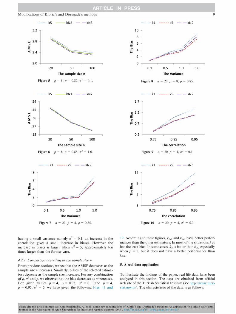
Figure 5 p= 8, q = 0.85, r2 = 0.1.

Figure 6 p= 8, q = 0.85, r2 = 1.0.

Figure 8 n= 20, p= 8, q = 0.85.

Figure 9 n= 20, p= 4, r2 = 0.1.

Figure 7 n= 20, p= 4, q = 0.85. Figure 10 n= 20, p= 4, r2 = 5.0.

Modifications of Kibria’s and Dorugade’s methods 9

having a small variance namely r2 = 0.1, an increase in thecorrelation gives a small increase in biases. However theincrease in biases is larger when r2 = 5, approximately ten

times larger than the former case.

4.2.3. Comparison according to the sample size n

From previous sections, we see that the AMSE decreases as the

sample size n increases. Similarly, biases of the selected estima-tors decrease as the sample size increases. For any combinationof q, r2 and p, we observe that the bias decreases as n increases.

For given values p = 4, q = 0.95, r2 = 0.1 and p = 4,q = 0.95, r2 = 5, we have given the following Figs. 11 and

Please cite this article in press as: Karaibrahimoglu, A. et al., Some new modificatioJournal of the Association of Arab Universities for Basic and Applied Sciences (201

12. According to these figures, kN1 and kN3 have better perfor-

mances than the other estimators. In most of the situations kN1

has the least bias. In some cases, k5 is better than kN3 especiallywhen p = 8, but it does not have a better performance than

kN1.

5. A real data application

To illustrate the findings of the paper, real life data have beenanalyzed in this section. The data are obtained from officialweb site of the Turkish Statistical Institute (see http://www.turk-stat.gov.tr/). The characteristic of the data is as follows:

ns of Kibria’s and Dorugade’s methods: An application to Turkish GDP data.4), http://dx.doi.org/10.1016/j.jaubas.2014.08.005

Figure 11 p= 4, q = 0.95, r2 = 0.1.

Figure 12 p= 8, q = 0.85, r2 = 5.0.

Table 5 MSE values of the estimators in the application.

k k values MSE Variance Sq. Bias R2 PRESS

k1 0.0022 0.1551 0.0804 0.0747 0.9880 0.0137

k2 0.0023 0.1564 0.0785 0.0780 0.9879 0.0137

k3 0.0098 0.2726 0.0230 0.2496 0.9816 0.0146

k4 0.0026 0.1615 0.0723 0.0892 0.9876 0.0137

k5 0.0008 0.1495 0.1312 0.0184 0.9895 0.0134

kN1 0.0009 0.1480 0.1262 0.0219 0.9894 0.0135

kN2 0.0011 0.1464 0.1178 0.0285 0.9892 0.0135

kN3 0.0010 0.1471 0.1224 0.0247 0.9893 0.0135

kN4 0.0018 0.1498 0.0902 0.0596 0.9884 0.0136

OLS 0.0000 0.1916 0.1916 0.0000 0.9906 0.0134

10 A. Karaibrahimoglu et al.

Wide lands and underground sources are not the onlywealth of countries. Some indicators are calculated to putforth the exact power of countries. In order to compare the

wealth of nations, one of the most important indicators isthe Gross Domestic Products (GDP). We have modeledGDP by cost components (at 1987 and 1998 prices) between

the years 1968 and 2008, closely concerning the economy ofTurkey in parallel to the growth and trends in the world. Wehave explained GDP using some parameters in the axes of for-

eign trade and production by multiple linear regression.The dependent variable is the GDP of Turkey. The eight

explanatory variables are the following respectively: X1:export, X2: import, X3: energy production, X4: number of

establishments in manufacturing industry, X5: number ofemployees in manufacturing industry, X6: wheat production,X7: milk production and finally X8: meat production.

Table 4 The correlation matrix of the GDP data.

Xi X1 X2 X3 X4

X1 1.0000 0.9971 0.8961 0.9

X2 0.9971 1.0000 0.8978 0.8

X3 0.8961 0.8978 1.0000 0.8

X4 0.9063 0.8977 0.8199 1.0

X5 0.9456 0.9399 0.8902 0.9

X6 0.4113 0.4201 0.5373 0.3

X7 0.6804 0.6793 0.7435 0.5

X8 0.4468 0.4437 0.4946 0.2

Please cite this article in press as: Karaibrahimoglu, A. et al., Some new modificatioJournal of the Association of Arab Universities for Basic and Applied Sciences (201

We have seen that the model has a multicollinearity prob-

lem since the condition number is j ¼ffiffiffiffiffiffiffikmax

kmin

q¼ 49:1128 > 30

which shows severe multicollinearity. We have given the corre-lation matrix of the GDP data in Table 4. One can see from

that table that there are high correlations among the explana-tory variables. The MSE values of the given estimators areprovided in Table 5. It can be seen from Table 5 that kN1,

kN2 and kN3 have less MSE than the others, especially kN2

which has the best performance in the sense of MSE. More-over, if we look at the determination coefficients and PRESSstatistics of each model, it can be said that using these biased

estimators makes no significant change in the model predict-ability. Thus, we advise to use the new defined estimatorsrather than the others.

6. Conclusion

In this paper, we reviewed some new modified ridge parame-

ters and the ones proposed earlier. At first, we explained themulticollinearity and gave necessary information about meth-odology of the ridge regression. We introduced, secondly, ten

ridge estimators half of which were proposed earlier and theother half were our proposals. Then, we compared the param-eters according to their performance evaluating the average

mean squared errors and also biases. The simulation studywas performed for different combinations of the variances ofthe error terms (r2), the numbers of explanatory variables(p), the numbers of observations (n) and different correlation

coefficients between the predictors (q). We found that our pro-posals are better than the ones proposed by k1: Hoerl andKennard (1970a), k2: Lawless and Wang (1976), k3: Kibria

(2003), k4 and k5: Dorugade (2014) according to their AMSEand bias performance. Finally, we conclude that our estima-

X5 X6 X7 X8

063 0.9456 0.4113 0.6804 0.4468

977 0.9399 0.4201 0.6793 0.4437

199 0.8902 0.5373 0.7435 0.4946

000 0.9643 0.3249 0.5092 0.2572

643 1.0000 0.5201 0.6869 0.4622

249 0.5201 1.0000 0.7583 0.6950

092 0.6869 0.7583 1.0000 0.8756

572 0.4622 0.6950 0.8756 1.0000

ns of Kibria’s and Dorugade’s methods: An application to Turkish GDP data.4), http://dx.doi.org/10.1016/j.jaubas.2014.08.005

Modifications of Kibria’s and Dorugade’s methods 11

tors are satisfactory over the multicollinearity problem andamong our estimators kN4 has the best performance. The esti-mator kN1 has the least bias in most situations. However deal-

ing with real data, the case may differ. Therefore we highlyrecommend researchers not to use just one ridge estimator toovercome their problem and not to decide without further

study.

References

Adnan, N., Ahmad, M.H., Adnan, R., 2006. A comparative study on

some methods for handling multicollinearity problems. Matemati-

ka 22 (2), 109–119.

Al-Hassan, Y.M., 2010. Performance of a new ridge regression

estimator. J. Assoc. Arab Univ. Basic Appl. Sci. 9 (1), 23–26.

Alkhamisi, M.A., Khalaf, G., Shukur, G., 2006. Some modifications

for choosing ridge parameters. Commun. Stat. Theory Methods 35

(11), 2005–2020.

Alkhamisi, M.A., Shukur, G., 2007. A Monte Carlo study of recent

ridge parameters. Commun. Stat. Simul. Comput. 36 (3), 535–547.

Asar, Y., Karaibrahimoglu, A., Genc, A., 2014. Modified ridge

regression parameters: a comparative Monte Carlo study. Hacet-

tepe J. Math. Stat. 42 (accepted).

Dorugade, A.V., 2014. New ridge parameters for ridge regression. J.

Assoc. Arab Univ. Basic Appl. Sci. 15, 94–99.

Hoerl, A.E., Kannard, R.W., Baldwin, K.F., 1975. Ridge regression:

some simulations. Commun. Stat. Theory Methods 4 (2), 105–123.

Hoerl, A.E., Kennard, R.W., 1970a. Ridge regression: applications to

nonorthogonal problems. Technometrics 12 (1), 69–82.

Hoerl, A.E., Kennard, R.W., 1970b. Ridge regression: biased estima-

tion for nonorthogonal problems. Technometrics 12 (1), 55–67.

Please cite this article in press as: Karaibrahimoglu, A. et al., Some new modificatioJournal of the Association of Arab Universities for Basic and Applied Sciences (201

Khalaf, G., Shukur, G. (2005). Choosing ridge parameter for

regression problems.

Kibria, B.M.G., 2003. Performance of some new ridge regression

estimators. Commun. Stat. Simul. Comput. 32 (2), 419–435.

Lawless, J.F., Wang, P., 1976. A simulation study of ridge and other

regression estimators. Commun. Stat. Theory Methods 5 (4).

Liu, X.-Q., Gao, F., 2011. Linearized ridge regression estimator in

linear regression. Commun. Stat. Theory Methods 40 (12), 2182–

2192.

Mansson, K., Shukur, G., Kibria, B.G., 2010. On some ridge

regression estimators: a Monte Carlo simulation study under

different error variances. J. Stat. 17 (1), 1–22.

McDonald, G.C., Galarneau, D.I., 1975. A Monte Carlo evaluation of

some ridge-type estimators. J. Am. Stat. Assoc. 70 (350), 407–416.

Muniz, G., Kibria, B.G., 2009. On some ridge regression estimators:

An empirical comparisons. Commun. Stat. Simul. Comput. 38 (3),

621–630.

Muniz, G., Kibria, B.G., Mansson, K., Shukur, G., 2012. On

developing ridge regression parameters: a graphical investigation.

Sort Stat. Oper. Res. Trans. 36 (2), 115–138.

Newhouse, J.P., Oman, S.D., 1971. An evaluation of ridge estimators,

Technical report R-716-PR. Rand Corporation, Santa Monica.

Saleh, A.M., Kibria, B.M.G., 1993. Performance of some new

preliminary test ridge regression estimators and their properties.

Commun. Stat. Theory Methods 22 (10), 2747–2764.

Yan, X., 2008. Modified nonlinear generalized ridge regression and its

application to develop naphtha cut point soft sensor. Comput.

Chem. Eng. 32 (3), 608–621.

Yan, X., Zhao, W., 2009. 4-CBA concentration soft sensor based on

modified back propagation algorithm embedded with ridge regres-

sion. Intell. Automation Soft Comput. 15 (1), 41–51.

ns of Kibria’s and Dorugade’s methods: An application to Turkish GDP data.4), http://dx.doi.org/10.1016/j.jaubas.2014.08.005